Finance and Economics Discussion SeriesDivisions of Research & Statistics and Monetary Affairs

Federal Reserve Board, Washington, D.C.

Effective Lower Bound Risk

Timothy S. Hills, Taisuke Nakata, and Sebastian Schmidt

2019-077

Please cite this paper as:Hills, Timothy S., Taisuke Nakata, and Sebastian Schmidt (2019). “Effective Lower BoundRisk,” Finance and Economics Discussion Series 2019-077. Washington: Board of Governorsof the Federal Reserve System, https://doi.org/10.17016/FEDS.2019.077.

NOTE: Staff working papers in the Finance and Economics Discussion Series (FEDS) are preliminarymaterials circulated to stimulate discussion and critical comment. The analysis and conclusions set forthare those of the authors and do not indicate concurrence by other members of the research staff or theBoard of Governors. References in publications to the Finance and Economics Discussion Series (other thanacknowledgement) should be cleared with the author(s) to protect the tentative character of these papers.

Effective Lower Bound Risk∗

Timothy Hills†

New York University

Taisuke Nakata‡

Federal Reserve Board

Sebastian Schmidt§

European Central Bank

First Draft: February 2016

This Draft: September 2019

Abstract

Even when the policy rate is currently not constrained by its effective lower bound (ELB), the

possibility that the policy rate will become constrained in the future lowers today’s inflation

by creating tail risk in future inflation and thus reducing expected inflation. In an empirically

rich model calibrated to match key features of the U.S. economy, we find that the tail risk

induced by the ELB causes inflation to undershoot the target rate of 2 percent by as much

as 50 basis points at the economy’s risky steady state. Our model suggests that achieving

the inflation target may be more difficult now than before the Great Recession, if the likely

decline in long-run neutral rates has led households and firms to revise up their estimate of

the frequency of future ELB events.

JEL: E32, E52

Keywords: Deflationary Bias, Disinflation, Inflation Targeting, Risky Steady State, Tail Risk,

Effective Lower Bound.

∗We would like to thank participants at 5th New York University Alumni Conference, 20th Conference“Theories and Methods in Macroeconomics” at Bank of France, Bank of Japan, Board of Governors of theFederal Reserve System, Hitotsubashi University, Japan Center for Economic Research, Keio University, KyotoUniversity, Miami University, Osaka University, Texas Tech University, University of Tokyo, “Inflation: Driversand Dynamics” Conference at Federal Reserve Bank of Cleveland, Waseda University, and Workshop on“Monetary Policy When Heterogeneity Matters” at l’EHESS for useful comments. We also thank the editorFlorin Bilbiie and two anonymous referees for constructive suggestions. Philip Coyle, Paul Yoo, and MarkWilkinson provided excellent research assistance. This paper supersedes two older papers: “The Risky SteadyState and the Interest Rate Lower Bound” (Hills, Nakata, and Schmidt, 2016) and “The Risk-AdjustedMonetary Policy Rule” (Nakata and Schmidt, 2016). The views expressed in this paper, as well as all errorsand omissions, should be regarded as those solely of the authors and are not necessarily those of the FederalReserve Board of Governors, the Federal Reserve System, or the European Central Bank.†Stern School of Business, New York University, 44 West 4th Street New York, NY 10012; Email:

hills.timoteo@gmail.com‡Division of Research and Statistics, Federal Reserve Board, 20th Street and Constitution Avenue NW

Washington, DC 20551; Email: taisuke.nakata@frb.gov§European Central Bank, Monetary Policy Research Division, 60640 Frankfurt, Germany; Email: sebas-

tian.schmidt@ecb.int.

1

1 Introduction

It is well known that when the effective lower bound (ELB) constraint on the policy rate

is binding, it becomes more difficult for the central bank to stabilize inflation at its objective,

as it cannot lower its policy rate further in response to adverse shocks. However, even when

the current policy rate is not constrained by the ELB, the possibility that the policy rate may

be constrained by the ELB in the future—which we will refer to as the ELB risk—can pose

a challenge for the central bank’s stabilization policy. Such a challenge can arise because, if

the private sector agents are forward-looking, they may factor in the ELB risk when making

economic decisions today.

This paper examines the implications of such ELB risk for the task of the central bank

to meet its inflation objective. We do so by contrasting the risky steady state with the

deterministic steady state in an empirically rich sticky-price model with an occasionally

binding ELB constraint on nominal interest rates. The risky steady state is the “point where

agents choose to stay at a given date if they expect future risk and if the realization of

shocks is 0 at this date” (Coeurdacier, Rey, and Winant, 2011). The risky steady state is

an important object in dynamic macroeconomic models: This is the point around which the

economy fluctuates, the point where the economy eventually converges to when all headwinds

and tailwinds dissipate. Thus, a wedge between the rate of inflation in the risky steady state

and the rate of inflation in the deterministic steady state—the latter corresponds to the

inflation target in the policy rule—can be seen as a failure of central banks to meet their

inflation objective.

We first use a stylized New Keynesian model to illustrate how, and why, the risky steady

state differs from the deterministic steady state. Monetary policy is assumed to be governed

by a simple interest-rate feedback rule of the type widely used by central banks to help them

gauge the appropriate policy stance (Yellen, 2017; Powell, 2018). We show that, under this

standard policy rule, inflation and the policy rate are lower, and output is higher, at the

risky steady state than at the deterministic steady state. This result obtains because the

lower bound constraint on interest rates makes the distribution of firm’s marginal costs of

production asymmetric; the decline in marginal costs caused by a large negative shock is

larger than the increase caused by a positive shock of the same magnitude. As a result, the

ELB constraint reduces expected marginal costs for forward-looking firms, leading them to

lower their prices even when the policy rate is not currently constrained.1 Reflecting the

lower inflation rate at the risky steady state, the policy rate is lower at the risky steady

state than at the deterministic one. In equilibrium, the ex-ante real interest rate is lower

at the risky steady than at the deterministic steady state, and the output gap is positive

as a result. These qualitative results are consistent with those in Adam and Billi (2007)

and Nakov (2008) on how the ELB risk affects the economy near the ELB constraint under

1ELB risk ceteris paribus also reduces expected consumption of forward-looking households, leading themto lower their consumption expenditures.

2

optimal discretionary policy.

We then turn to the main exercise of our paper, which is to explore the quantitative

importance of the wedge between the risky and deterministic steady states in an empirically

rich DSGE model calibrated to match key features of the U.S. economy. We find that,

under the standard monetary policy rule, the wedge between the deterministic and risky

steady states is nontrivial in our calibrated empirical model. Inflation is a bit more than

30 basis points lower than the target rate of 2 percent at the risky steady state, with about

25 basis points attributable to the ELB constraint as opposed to other nonlinear features

of the model. Output is 0.3 percentage points higher at the risky steady state than at the

deterministic steady state. The risky steady state policy rate is 2.9 percent—about 80 basis

points lower than the deterministic steady state policy rate—and is broadly in line with the

median projection of the long-run federal funds rate in the latest Summary of Economic

Projections by FOMC participants. The magnitude of the wedge depends importantly on

the frequency of hitting the ELB, which in turn depends importantly on the level of the long-

run equilibrium policy rate. Under an alternative plausible assumption about the long-run

level of the policy rate, then the inflation wedge between the deterministic and risky steady

states can exceed 60 basis points, with the ELB risk contributing about 50 basis points to

the overall inflation wedge.

The observation that inflation falls below the inflation target in the policy rule at the

risky steady state is different from the well known fact that the average rate of inflation falls

below the target rate in the model with the ELB constraint. The decline in inflation arising

from a contractionary shock can be exacerbated when the policy rate is at the ELB, while the

rise in inflation arising from an expansionary shock is tempered by a corresponding increase

in the policy rate. As a result, the distribution of inflation is negatively skewed and the

average inflation falls below the median. This fact is intuitive and has been well recognized

in the profession for a long time (Coenen, Orphanides, and Wieland, 2004; Reifschneider

and Williams, 2000). The risky steady state inflation is different from the average inflation;

it is the rate of inflation that would prevail at the economy’s steady state when agents are

aware of risks. It is worth mentioning that the average inflation falls below the target even

in perfect foresight models or backward-looking models where the inflation rate eventually

converges to its target. On the other hand, for the risky steady state inflation to fall below

the inflation target, it is crucial that price-setters are forward-looking and take tail risk in

future marginal costs into account in their pricing decisions.

In the final part of the paper, we explore some implications of ELB risk for the design of

monetary policy rules. Specifically, we show that one way to eliminate the wedge between the

deterministic and risky steady states of inflation is to lower the intercept term of the interest-

rate feedback rule. We refer to this augmented rule as the risk-adjusted policy rule. In our

empirical model, the intercept of the standard policy rule is 3.75 percent while the intercept

of the risk-adjusted policy rule that allows the central bank to achieve its 2 percent inflation

3

target in the risky steady state is only 3.24 percent.2 While our risk-adjusted monetary

policy rule is mathematically equivalent to assigning a value different from the central bank’s

inflation objective to the inflation targeting parameter in the standard monetary policy rule,

we argue that our proposed policy rule has the benefit that the inflation target parameter in

our rule retains the structural interpretation as the central bank’s inflation objective.3

The policy rates in some advanced economies are still at the ELB, and whether inflation

rates will eventually return to the central bank’s inflation objective after liftoff remains to be

seen. The first part of our analysis can be read as a cautionary tale of a potential systematic

policy mistake central banks could make if they do not appropriately adjust their strategies

in light of ELB risk. In the United States, inflation was stubbornly below the target rate

of 2 percent for at least two years after the policy rate liftoff in December 2015. At the

same time, the unemployment rate moved below most estimates of its natural rate. Hence,

initial economic dynamics after the liftoff seem to be consistent with the model featuring

the standard policy rule. However, more recently, the rate of inflation has moved close to

the target rate. Thus, current inflation dynamics in the U.S. economy seems to be more

consistent with the model with the risk-adjusted monetary policy rule.

Throughout the paper, we focus on a rational expectations equilibrium where the economy

fluctuates around a positive level of nominal interest rates so that if all uncertainty were

permanently resolved the economy would converge to a deterministic steady state where the

ELB constraint is not binding and inflation is at target. It is well known that accounting

for the ELB can give rise to two deterministic steady states and equilibrium multiplicity

(Benhabib, Schmitt-Grohe, and Uribe, 2001). In particular, rational expectations equilibria

may exist where the ELB constraint is binding either permanently or at least in most states

of nature (Armenter, 2018). It is also possible to construct sunspot equilibria where a sunspot

shock can move the economy from a regime with an occasionally binding ELB constraint to

one with a binding ELB constraint in most states of nature. The effects of policy interventions

and changes in policy regimes on macroeconomic outcomes in these sunspot equilibria may

differ from those in the fundamental equilibrium that is at the core of our analysis (see, e.g.

Mertens and Ravn, 2014; Bilbiie, 2018; Coyle and Nakata, 2019; Nakata and Schmidt, 2019b).

Our choice of equilibrium is supported by some empirical evidence. Aruoba, Cuba-Borda,

and Schorfheide (2018) estimate a New Keynesian model with a lower bound, a set of fun-

damental shocks, and a sunspot shock that captures shifts from a regime where the economy

fluctuates around a strictly positive nominal interest rate to a regime where the lower bound

constraint is binding in most states. For the United States, they do not find evidence that she

moved to the latter regime in the aftermath of the Great Recession. Since our quantitative

2While we focus on the risky steady state, the risk-adjusted monetary policy rule also mitigates thedeviations of inflation from target in other states. For alternative approaches to mitigate the deflationary biasproblem, please see Nakata and Schmidt (2019a) and Bianchi, Melosi, and Rottner (2019).

3In section 4.5, we also consider two unconventional monetary policies—“lower-for-longer” forward guid-ance and negative interest rate policy.

4

analysis focuses on the U.S. economy, we align our choice of equilibrium with the empirical

results in Aruoba, Cuba-Borda, and Schorfheide (2018). Nevertheless, we document analyt-

ically the possibility of equilibrium multiplicity for a variant of our stylized model. For this

model, we show that in any equilibrium with an occasionally binding ELB constraint—that

is, with ELB risk—the risky steady state of inflation is below the inflation target.

The question of how the possibility of returning to the ELB affects the economy has

remained largely unexplored. The majority of the literature adopts the assumption that the

economy will eventually return to an absorbing state where the policy rate is permanently

away from the ELB constraint, and analyzes the dynamics of the economy, and the effects

of various policies, when the policy rate is at the ELB (Eggertsson and Woodford, 2003;

Christiano, Eichenbaum, and Rebelo, 2011). While an increasing number of studies have

recently departed from the assumption of an absorbing state, the focus of these studies is

mostly on how differently the economy behaves at the ELB versus away from the ELB,

instead of how the ELB risk affects the economy away from the ELB.4,5 With the longer-run

equilibrium real rates expected to stay lower going forward, the question of how the possibility

of returning to the ELB affects the economy is as relevant as ever.6

Our paper builds on the work by Adam and Billi (2007), Nakov (2008), and Evans,

Fisher, Gourio, and Krane (2015) who noted that the possibility of returning to the ELB has

consequences for the economy even when the policy rate is currently away from the ELB.

Our work differs from these papers in two substantive ways. First, while they pointed out

the anticipation effect of returning to the ELB on the economy when the policy rate is near

the ELB and the economy is away from the steady state, our work shows that the possibility

of returning to the ELB has consequences for the economy even when the policy rate is well

above the ELB and the economy is at the steady state. Second, while they studied the effects

of the ELB risk in a stylized model, we quantify the magnitude of the effects of the ELB risk

in an empirically rich, calibrated model.

Our paper is closely related to Nakata and Schmidt (2019a) and Seneca (2018). Nakata

and Schmidt (2019a) analytically show that ELB risk confronts discretionary central banks

with a trade-off between inflation and output gap stabilization when the ELB constraint

is not binding that manifests itself in a systematic undershooting of the inflation target.

This so-called deflationary bias can be reduced and welfare be improved by appointing an

inflation-conservative central banker. Unlike Nakata and Schmidt (2019a), we are silent

4For example, Gavin, Keen, Richter, and Throckmorton (2015) and Keen, Richter, and Throckmorton(2016) ask how differently technology and anticipated monetary policy shocks affect the economy when thepolicy rate is constrained than when it is not, respectively. Schmidt (2013) and Nakata (2016) ask howdifferently the government should conduct fiscal policy when the policy rate is at the ELB than when it is not.

5As discussed in Section 4, in many existing models with an occasionally binding ELB constraint, theprobability of being at the ELB is small, typically comfortably below 10 percent—often below 5 percent. Asa result, the anticipation effects described in these papers are weak.

6According to the Federal Reserve Bank of New Yorks Survey of Primary Dealers from July 2019, themedian respondent attached a 35 percent probability to the event that the federal funds rate returns to theELB between July 2019 and the end of 2021.

5

about normative implications of the ELB risk. Instead, the main goal of our paper is to

document the quantitative relevance of ELB risk using an empirically rich model. Like our

paper, Seneca (2018) highlights the importance of ELB risk for the dynamics of the economy

when the policy rate is currently not constrained. We examine the quantitative importance of

ELB risk in an empirically rich model, whereas he examines the consequences of time-varying

ELB risk—induced by exogenous time-variations in the variance of the demand shock—in a

stylized model.

Our paper shares the same spirit with Kiley and Roberts (2017) in that both papers aim

to understand the implications of the ELB constraint for the dynamics of the economy and

monetary policy. However, our paper differs from Kiley and Roberts (2017) in a fundamental

way: we focus on the anticipation effects of hitting the ELB in the future on the steady state

allocations—and how large those might be in an empirically rich model—whereas Kiley and

Roberts (2017) abstract from the anticipation effects of the ELB risk by solving the model

with the perfect-foresight assumption. In particular, in the model of Kiley and Roberts

(2017), there is no undershooting of the inflation target at the steady state, even though the

distribution of inflation is asymmetric and average inflation is below the 2 percent target.

In our model, the distribution of inflation is asymmetric and average inflation is below the

target as in their model. However, unlike in their model, inflation in our model fluctuates

around a steady state below the 2 percent target.

This seemingly subtle difference—our focus on the steady state inflation and the focus

on the average inflation by Kiley and Roberts (2017)—is relevant in thinking about inflation

dynamics when the policy rate is away from the ELB. Perfect-foresight models, like the model

of Kiley and Roberts (2017), can explain why inflation averages below 2 percent over a long

period of time including the period in which the ELB constraint binds. However, it cannot

explain why inflation persistently falls below the 2 percent objective when the policy rate

is away from the ELB, the situation the U.S. economy has found itself in over the past few

years. Almost all estimates of the ELB frequency we are aware of suggest that the probability

of being at the ELB is less than half. That is, the economy spends more than half of the

time away from the ELB. Thus, understanding the dynamics of the economy away from the

ELB—and how that might be affected by the possibility of returning to the ELB in the

future—is of first-order importance.

Our focus on the anticipation effects of the ELB also differentiates our work from papers

examining different aspects of the model with the ELB in perfect-foresight environment se-

tups, including Coibion, Gorodnichenko, and Wieland (2012)—who focus on the implication

of the ELB for optimal inflation target—and Guerrieri and Iacoviello (2017)—who estimate

a model with a borrowing constraint and the ELB constraint—among others.

Finally, our paper is related to other papers which also work with models with the ELB

without abstracting from uncertainty—especially those which work with empirically rich mod-

els with ELB (Gust, Herbst, Lopez-Salido, and Smith (2017), Plante, Richter, and Throck-

6

morton (2018), Hirose and Sunakawa (2016), among others). Our paper differs from these

papers in two important ways. First, we focus on the anticipation effect of the ELB risk when

the policy rate is away from the ELB, whereas the existing papers focus on other aspects of

the model (for example, Gust, Herbst, Lopez-Salido, and Smith (2017) on the dynamics of the

economy at the ELB; Plante, Richter, and Throckmorton (2018) on endogenous uncertainty

at the ELB, Hirose and Sunakawa (2017) on the natural rate of interest at the ELB).

Second, the existing models in this category—those papers working with fully nonlinear

models with uncertainty—typically predict low probabilities of being at the ELB because

these models are intended to fit the data including the 1980s and 1990s when the long-run

equilibrium interest rate was higher than it is now and it is expected to be in the future.7

We calibrate our model using the data starting in the mid 1990s and the baseline ELB

probability is 16 percent. We consider parameter values under which the probability is even

higher. Thus, our calibration is suited for understanding how large the anticipation effect

of ELB risk might be in the future. All in all, we see our empirical model as a valuable

complement to the existing fully-nonlinear DSGE models with uncertainty.

The rest of the paper is organized as follows. After a brief review of the concept of

the risky steady state in Section 2, Section 3 analyzes the risky steady state in a stylized

New Keynesian economy. Section 4 quantifies the wedge between the deterministic and risky

steady states in an empirically rich DSGE model. Section 5 discusses a simple modification to

the monetary policy rule to achieve the inflation objective at the risky steady state. Section 6

discusses empirical relevance of our main results, whereas Section 7 discusses some additional

thoughts and results. Section 8 concludes.

2 The Risky Steady State: Definition

The risky steady state is defined generically as follows.

Let Γt and St denote vectors of endogenous and exogenous variables, respectively, in the

model under investigation. Let f(·, ·) denote a vector of policy functions mapping the values

of endogenous variables in the previous period and today’s realizations of exogenous variables

into the values of endogenous variables today.8 That is,

Γt = f(Γt−1, St) (1)

The risky steady state of the economy, ΓRSS , is given by a vector satisfying the following

7For example, about 4 percent for Gust, Herbst, Lopez-Salido, and Smith (2017), about 5 percent inRichter and Throckmorton (2016) and 9.7 percent for Hirose and Sunakawa (2016). As discussed in Richterand Throckmorton (2015), when the shock variance is too high, the equilibrium ceases to exist once uncertaintyis correctly accounted for in solving these models, making it difficult to achieve a high ELB frequency.

8Note that the policy function does not need to depend on the entire set of the endogenous variables inthe prior period. It may not depend on any endogenous variables in the prior period at all, as in the stylizedmodel presented in the next section.

7

condition.

ΓRSS = f(ΓRSS , SSS) (2)

where SSS denotes the steady state of St.9 That is, the risky steady state is where the

economy will eventually converge as the exogenous variables settle at their steady state. In

this risky steady state, the agents are aware that shocks to the exogenous variables can occur,

but the current realizations of those shocks are zero. On the other hand, the deterministic

steady state of the economy, ΓDSS , is defined as follows:

ΓDSS = fPF (ΓDSS , SSS) (3)

where fPF (·, ·) denotes the vector of policy functions obtained under the perfect foresight

assumption.

In principle, the deterministic steady state does not have to be unique. Indeed, as dis-

cussed in Section 1, it is well known that accounting for the ELB constraint can induce

multiplicity of steady state equilibria in models that would otherwise have a unique deter-

ministic steady state. In the next section, we show that such multiplicity can also arise in

the context of the risky steady state.

3 The Risky Steady State in a Stylized Model with the ELB

3.1 Model

We start by characterizing the risky steady state in a stylized New Keynesian model.

Since the model is standard, we only present its equilibrium conditions here. The details of

the model are described in Appendix A.

C−χct = βδtRtEtC−χct+1 Π−1

t+1, (4)

wt = Nχnt Cχct , (5)

YtCχct

[ϕ (Πt − 1) Πt − (1− θ)− θwt] = βδtEtYt+1

Cχct+1

ϕ (Πt+1 − 1) Πt+1, (6)

Yt = Ct +ϕ

2[Πt − 1]2 Yt, (7)

Yt = Nt, (8)

Rt = max

[RELB,

Πtarg

β

(Πt

Πtarg

)φπ], (9)

(δt − 1) = ρδ(δt−1 − 1) + εδ,t, (10)

Ct, Nt, Yt, wt, Πt, and Rt are consumption, labor supply, output, real wage, inflation, and

9There is no distinction between deterministic and risky steady states for St because St is exogenous.

8

the policy rate, respectively. δt is an exogenous shock to the household’s discount rate, and

follows an AR(1) process with mean one, as shown in equation (10). The innovation to the

discount rate shock process, εδ,t, is normally distributed with a standard deviation of σε.

Equation (4) is the consumption Euler equation, equation (5) is the intratemporal optimality

condition of the household, Equation (6) is the optimality condition of the intermediate good

producing firms relating today’s inflation to real marginal cost today and expected inflation

tomorrow (forward-looking Phillips Curve), equation (7) is the aggregate resource constraint

capturing the resource cost of price adjustment, and equation (8) is the aggregate production

function. Equation (9) is the interest-rate feedback rule where RELB is the lower bound on

the gross nominal interest rate and Πtarg is the inflation target parameter.

A recursive equilibrium of this stylized economy is given by a set of policy functions for

{C(·), N(·), Y (·), w(·), Π(·), R(·)} satisfying the equilibrium conditions described above.

As discussed in Section 1, we focus on a rational expectations equilibrium that fluctuates

around a strictly positive nominal interest rate level. The model is solved with a global

solution method described in detail in Appendix B. Table 1 lists the parameter values used

for this exercise.

Table 1: Parameter Values for the Stylized Model

Parameter Description Parameter Value

β Discount rate 11+0.004365

χc Inverse intertemporal elasticity of substitution for Ct 1χn Inverse labor supply elasticity 1θ Elasticity of substitution among intermediate goods 6ϕ Price adjustment cost 200400(Πtarg − 1) (Annualized) target rate of inflation 2φπ Coefficient on inflation in the Taylor rule 1.5RELB Effective lower bound 1ρ AR(1) coefficient for the discount factor shock 0.8σδ Standard deviation of shocks to the discount factor 0.38

100*Implied prob. that the policy rate is at the lower bound 20%

3.2 Dynamics and the risky steady state

Before analyzing the risky steady state of the model, it is useful first to look at the

dynamics of the model. Solid black lines in Figure 1 show the policy functions for the policy

rate, inflation, output, and the expected real interest rate. Dashed black lines show the policy

function of the model obtained under the assumption of perfect foresight. Under the perfect

foresight case, the agents in the model attach zero probability to the event that the policy

rate will return to the ELB when the policy rate is currently away from the ELB. Under both

versions of the model, an increase in the discount rate makes households want to save more

for tomorrow and spend less today. Thus, as δ increases, output, inflation, and the policy

rate decline. When δ is large and the policy rate is at the ELB, an additional increase in the

discount rate leads to larger declines in inflation and output than when δ is small and the

9

policy rate is not at the ELB, as the adverse effects of the increase in δ are not countered by

a corresponding reduction in the policy rate.

Figure 1: Policy Functions from the Stylized Model

1 1.003 1.006 1.009 1.012 1.015

δ

0

1

2

3

4

Annualiz

ed %

Nominal Interest Rate

Deterministic St.St.

Risky St.St.

1 1.003 1.006 1.009 1.012 1.015

δ

-4

-2

0

2

Annualiz

ed %

Inflation

Deterministic St.St.

Risky St.St.

1 1.003 1.006 1.009 1.012 1.015

δ

-6

-4

-2

0

% D

evia

tion fro

m

the D

et. S

teady S

tate

Output

Deterministic St.St.

Risky St.St.

1 1.003 1.006 1.009 1.012 1.015

δ

-10

-5

0

Annualiz

ed %

Real Wage

Deterministic St.St.

Risky St.St.

1 1.003 1.006 1.009 1.012 1.015

δ

0

1

2

3

Annualiz

ed %

Exp. Real Rate

With uncertainty

Without uncertainty

*The dashed black lines (“Without uncertainty” case) show policy functions obtained under the perfect foresight as-sumption (i.e., σε = 0).

When the policy rate is at the ELB, the presence of uncertainty reduces inflation and

output. This is captured by the fact that the solid lines are below the dashed lines for

inflation and output in the figure. The non-neutrality of uncertainty is driven by the ELB

constraint. If the economy is buffeted by a sufficiently large expansionary shock, then the

policy rate will adjust to offset some of the resulting increase in real wages. If the economy is

hit by a contractionary shock, regardless of the size of the shock, the policy rate will stay at

the ELB and the resulting decline in real wages will not be tempered. Due to this asymmetry,

an increase in uncertainty reduces the expected real wage, which in turn reduces inflation as

price-setters are forward-looking and thus inflation today depends on the expected real wage.

With the policy rate constrained at the ELB, a reduction in inflation leads to an increase in

the expected real rate, pushing down consumption and output today. These adverse effects

of uncertainty at the ELB are studied in detail in Nakata (2017).

When the policy rate is away from the ELB, the presence of uncertainty reduces inflation

and the policy rate, but increases output. If the economy is hit by a sufficiently large con-

tractionary shock, the policy rate will hit the ELB and the resulting decline in real wages will

not be tempered. If the economy is hit by an expansionary shock, regardless of the size of the

shock, the policy rate will adjust to partially offset the resulting increase in real wages. Thus,

the presence of uncertainty, by generating the possibility that the policy rate will return to

10

the ELB, reduces the expected real wage and thus today’s inflation. When the policy rate is

away from the ELB, its movement is governed by the Taylor rule. Since the Taylor principle

is satisfied (i.e., the coefficient of inflation is larger than one), the reduction in inflation comes

with a larger reduction in the policy rate. As a result, the expected real rate is lower, and

thus consumption and output are higher, with uncertainty than without uncertainty.

Table 2: The Risky Steady State in the Stylized Model

Inflation Output∗ Policy rate

Deterministic steady state 2 0 3.75Risky steady state 1.59 0.15 2.93

(Wedge) (−0.41) (0.15) (−0.82)

Risky steady state w/o the ELB 1.98 −0.04 3.71(Wedge) (−0.02) (−0.04) (−0.04)

*Output is expressed as a percentage deviation from the determistic steady state.

While these effects are stronger the closer the policy rate is to the ELB, they remain

nontrivial even at the economy’s risky steady state. In the stylized model of this section, in

which the policy functions do not depend on any of the model’s endogenous variables from

the previous period, the risky steady state is given by the vector of the policy functions

evaluated at δ = 1. That is, inflation, output, and the policy rate at the risky steady state

are given by the intersection of the policy functions for these variables and the left vertical

axes. As shown in Table 2, inflation and output are 41 basis points lower and 0.15 percentage

points higher at the risky steady state than at the deterministic steady state, respectively.

The risky steady state policy rate is 82 basis points lower than its deterministic counterpart.

In our model, the ELB constraint is not the only source of nonlinearity. Our specifications

of the utility function and the price adjustment cost also make the model nonlinear, and thus

explain some of the wedge between the deterministic and risky steady states. To understand

the extent to which these other nonlinear features matter, Table 2 also reports the risky

steady state in the version of the model without the ELB constraint. Overall, the differences

between the deterministic and risky steady states would be small were it not for the ELB

constraint. Inflation and the policy rate at the risky steady state are only 2 and 4 basis

points below those at the deterministic steady state, respectively. Output at the risky steady

state is about 4 basis points below that at the deterministic steady state. Thus, the majority

of the overall wedge between the deterministic and risky steady states is attributed to the

nonlinearity induced by the ELB constraint, as opposed to other nonlinear features of the

model.

3.3 The risky steady state and the average

It is important to recognize that the risky steady state is different from the average.

Let’s take inflation as an example. The risky steady state inflation is the point around

which inflation fluctuates and coincides with the median of its unconditional distribution

11

in the model without any endogenous state variables like the one analyzed here. On the

other hand, the average inflation depends on the inflation rate in all states of the economy.

Provided that the probability of being at the ELB is sufficiently large, the unconditional

distribution of inflation is negatively skewed and therefore the risky steady state inflation is

higher than the average inflation, as depicted in Figure 2. The observation that the ELB

constraint pushes down the average inflation below the median by making the distribution of

inflation negatively skewed is intuitive and has been well recongnized for a long time (Coenen,

Orphanides, and Wieland, 2004; Reifschneider and Williams, 2000). This observation holds

true even when price-setters form expectations in a backward-looking manner and thus there

is no anticipation effect due to the ELB risk. The result that the ELB risk lowers the

median of the distribution below the target is less intuitive and requires that price-setters

are forward-looking in forming their expectations.

Figure 2: Unconditional Distribution of Inflation in the Stylized Model

-6 -4 -2 0 2 4 6 8

Skewness: -0.3380

ELB Binds

Inflation Target: 2

RSS Inflation: 1.59

Average Inflation: 1.45

1.2 1.4 1.6 1.8 2 2.2

*RSS stands for the risky steady state.

3.4 The risk-adjusted Fisher relation

One way to understand the discrepancy between deterministic and risky steady states is

to examine the effect of the ELB risk on the Fisher relation. Let RDSS and ΠDSS be the

deterministic steady state policy rate and inflation. In the deterministic environment, the

consumption Euler equation evaluated at the steady state becomes

RDSS =ΠDSS

β(11)

after dropping the expectation operator from the consumption Euler equation and eliminating

the deterministic steady-state consumption from both sides of the equation. This relation is

12

often referred to as the Fisher relation.

In the stochastic environment, the consumption Euler equation evaluated at the (risky)

steady state can be written as

RRSS =ΠRSS

β· 1

ERSS [(CRSSCt+1

)χc ΠRSSΠt+1

](12)

where RRSS , ΠRSS , and CRSS are the risky steady-state policy rate, inflation, and consump-

tion. ERSS [·] is the conditional expectation operator when the economy is at the risky steady

state today. In the stylized model with one shock and without any endogenous state vari-

ables, ERSS [·] := Et[·|δt = 1]. We will refer to Equation (12) as the risk-adjusted Fisher

relation. Relative to the standard Fisher relation, there is an adjustment term that reflects

the discrepancy between today’s economic conditions and the expected economic conditions

next period. This term captures the effect of the tail risk in future economic conditions

induced by the ELB constraint on household expectations. Notice that the adjustment term

is less than one,1

ERSS [(CRSSCt+1

)χc ΠRSSΠt+1

]< 1, (13)

because of the fat tail on the lower end of the distributions of future inflation and consumption

induced by the ELB constraint.

Figure 3 plots the standard Fisher relation (11), the risk-adjusted Fisher relation (12),

and the Taylor rule (9). Consider, first, the deterministic case. Deterministic steady state

equilibria are represented by the intersections of the standard Fisher relation and the Taylor

rule. Due to the kink in the Taylor rule induced by the lower bound constraint there exist

two deterministic steady state equilibria: One where the lower bound constraint is slack

and inflation is at target and another one where the lower bound constraint is binding and

inflation is below target.

Now consider the stochastic case. In equilibrium, The risky steady state of a rational-

expectations equilibrium is given by the intersection of the line representing the risk-adjusted

Fisher relation and the line representing the Taylor rule. Since the risk-adjustment term is

less than one, the risk-adjusted Fisher relation is flatter than the standard Fisher relation.

There are two intersections with the Taylor rule: One where the lower bound constraint is

binding and one where the lower bound constraint is slack. The two risky steady states are

associated with two distinct rational expectations equilibria. As discussed before, we focus

on the equilibrium where the policy rate is above the lower bound in the risky steady state.10

10The intersection of the standard Fisher relation and the Taylor-rule equation in a region where theTaylor-rule equation is flat at the ELB is the deflationary steady state explored by Benhabib, Schmitt-Grohe,and Uribe (2001). Comparing that intersection with the intersection of the risk-adjusted Fisher relation andthe Taylor-rule equation in the ELB region indicates that, in a deflationary rational expectations equilibrium,inflation is higher at the risky steady state than at the deterministic steady state. We have confirmed thevalidity of this feature in a semi-loglinear model with a three-state discount rate shock. This property of the

13

In the region where the policy rate is positive, the line representing the risk-adjusted Fisher

relation crosses the line representing the Taylor rule at a point below the line for the standard

Fisher relation crosses it., as shown in Figure 3. Thus, inflation and the policy rate are lower

at the risky steady state than at the deterministic steady state.

Figure 3: The Risk-Adjusted Fisher Relation and the Taylor Rule

1

RSS

DSS

Π

R

Risk−AdjustedFisher Relation

StandardFisher Relation

Taylor Rule

†DSS stands for “deterministic steady state,” and RSS stands for “risky steady state.”

3.5 An analytical example

Even though the model we have used so far is stylized, we still had to rely on numerical

analysis to expose the discrepancy between deterministic and risky steady states that is

induced by ELB risk. We close this section by providing some analytical results on the

deflationary bias at the risky steady state in a semi-loglinearized version of the model.

Aggregate private sector behavior and monetary policy of the semi-loglinearized model

are described by the following three equations

πt = βEtπt+1 + κyt (14)

yt = Etyt+1 −1

χc(it − Etπt+1 − rnt ) (15)

it = max[0, rn + πtarg + φπ

(πt − πtarg

)], (16)

where πt and yt denote the rate of inflation and output expressed in percentage deviations

from the deterministic steady state with stable prices, respectively, it denotes the level of

the policy rate, and rnt denotes the natural real rate of interest which is a function of the

discount factor shock. To be able to obtain analytical results, we assume that rnt is uniformly

deflationary equilibrium is further explored in Coyle, Nakata, and Schmidt (2019).

14

distributed, rnt ∼ U(rn − ε, rn + ε), with rn = 1β − 1, and ε ≥ 0. The slope of the log-

linearized Phillips curve is a function of the structural model parameters κ = θ(χc+χn)ϕ .

Finally, we assume that the monetary policy parameters satisfy φπ > 1 and πtarg ≥ 0. Note

that this model has two deterministic steady state equilibria. In the intended steady state

equilibrium, πDSS = πtarg and the lower bound constraint is slack. In the unintended steady

state equilibrium, πDSS = −rn and the lower bound constraint is binding.

We now proceed in two steps. We first show that in any equilibrium of the stochastic

model where the lower bound is an occasionally binding constraint, unconditional expected

inflation is below the inflation target. We then show that the inflation rate at the risky steady

state of any such equilibrium is below the inflation target, and, therefore, below the intended

deterministic steady state of inflation.11

Using (14) to substitute out (expected) output in (15), we obtain

πt = (1 + κχ−1c )Eπt+1 − κχ−1

c (it − rnt ), (17)

where we made use of the fact that Etπt+1 = Eπt+1. Next, substituting (17) into (16), one

obtains an equation that relates the policy rate to expected inflation and the natural real

rate shock

it = max

[0,

rn

1 + κχ−1c φπ

+κχ−1

c φπ

1 + κχ−1c φπ

rnt +1− φπ

1 + κχ−1c φπ

πtarg +φπ(1 + κχ−1

c )

1 + κχ−1c φπ

Eπt+1

](18)

From (17) and (18), it follows that

πt =

(1 + κχ−1c )Eπt+1 + κχ−1

c rnt ,

if rnt < − rn

κχ−1c φπ

− 1+κχ−1c

κχ−1c

Eπt+1 − 1−φπκχ−1

c φππtarg

1+κχ−1c

1+κχ−1c φπ

Eπt+1 + κχ−1c

1+κχ−1c φπ

(rnt − rn)− κχ−1c (1−φπ)

1+κχ−1c φπ

πtarg,

if rnt ≥ − rn

κχ−1c φπ

− 1+κχ−1c

κχ−1c

Eπt+1 − 1−φπκχ−1

c φππtarg.

Let µt be the probability that the lower bound constraint is binding in period t. Then,

µt =

1, if − 1+κχ−1c φπ

κχ−1c φπ

rn − 1+κχ−1c

κχ−1c

Eπt+1 − 1−φπκχ−1

c φππtarg ≥ ε

12ε

(ε− 1+κχ−1

c φπκχ−1

c φπrn − 1+κχ−1

c

κχ−1c

Eπt+1 − 1−φπκχ−1

c φππtarg

),

if − ε < −1+κχ−1c φπ

κχ−1c φπ

rn − 1+κχ−1c

κχ−1c

Eπt+1 − 1−φπκχ−1

c φππtarg < ε

0, if − 1+κχ−1c φπ

κχ−1c φπ

rn − 1+κχ−1c

κχ−1c

Eπt+1 − 1−φπκχ−1

c φππtarg ≤ −ε.

Taking unconditional expectations of πt, we have

11Mertens and Williams (2018) show how to solve for expected inflation in a log-linearized New Keynesianmodel with a lower bound on nominal interest rates and a uniformly distributed price markup shock. Wefollow their approach to solve for expected inflation. Unlike us, they consider an optimizing central bank witha zero inflation target acting under discretion, and they do not characterize the risky steady state.

15

Eπt =

(1 + κχ−1

c

)Eπt+1 + κχ−1

c rn, if µt = 1

− 14ε

(κχ−1c )2φπ

1+κχ−1c φπ

(ε− 1+κχ−1

c φπκχ−1

c φπrn − 1+κχ−1

c

κχ−1c

Eπt+1 − 1−φπκχ−1

c φππtarg

)2

+ 1+κχ−1c

1+κχ−1c φπ

Eπt+1 − κχ−1c (1−φπ)

1+κχ−1c φπ

πtarg, if 0 < µt < 1

1+κχ−1c

1+κχ−1c φπ

Eπt+1 − κχ−1c (1−φπ)

1+κχ−1c φπ

πtarg, if µt = 0.

In equilibrium, Eπt = Eπt+1. In any equilibrium in which the probability of a binding

lower bound constraint is one, Eπ = −rn. That is, expected inflation is equal to the unin-

tended deterministic steady state. In any equilibrium, in which the probability of a binding

lower bound constraint is zero, Eπ = πtarg. That is, expected inflation is equal to the in-

tended deterministic steady state. In both cases, actual inflation fluctuates symmetrically

around the respective deterministic steady state. We are, however, interested in equilibria

where the lower bound constraint is occasionally binding. For the remainder, we thus focus

on equilibria where 0 < µt < 1. According to the above functional relationship between

Eπt+1 and Eπt, there can be up to two such equilibria. Rearranging terms, in these equilibria

κχ−1c (φπ − 1) (Eπ − πtarg) = − 1

4ε(κχ−1

c )2φπ

(ε− 1 + κχ−1

c φπ

κχ−1c φπ

rn − 1 + κχ−1c

κχ−1c

Eπ − 1− φπκχ−1

c φππtarg

)2

Hence, given φπ > 1, any equilibrium where the lower bound constraint is occasionally

binding features below-target unconditional inflation expectations, Eπ < πtarg.12 If two such

equilibria exist, unconditional inflation expectations in one of them will be strictly higher

than in the other. This is the one that we focus on in our quantitative analysis.

We can now proceed with the second step and show that in any equilibrium where the

lower bound constraint is occasionally binding, the risky steady state of inflation is below the

inflation target, and, therefore, below the intended deterministic steady state of inflation. At

the risky steady state, the policy rate is given by

iRSS = max

[0, rn +

1− φπ1 + κχ−1

c φππtarg +

φπ(1 + κχ−1c )

1 + κχ−1c φπ

Eπ

](19)

Substituting (19) into (17), evaluated at the risky steady state, one obtains

πRSS =

(1 + κχ−1

c

)Eπ + κχ−1

c rn, if Eπ ≤ − 1+κχ−1c φπ

φπ(1+κχ−1c )

rn − 1−φπφπ(1+κχ−1

c )πtarg

1+κχ−1c

1+κχ−1c φπ

Eπ + κχ−1c (φπ−1)

1+κχ−1c φπ

πtarg, if Eπ > − 1+κχ−1c φπ

φπ(1+κχ−1c )

rn − 1−φπφπ(1+κχ−1

c )πtarg.

(20)

Consider, first, the case where the lower bound constraint is binding in the risky steady

state

12The closed-form solutions for expected inflation and inflation are rather complicated and not of particularinterest for what follows.

16

πRSS =(1 + κχ−1

c

)Eπ + κχ−1

c rn

<− 1

φπrn − 1− φπ

φππtarg,

and, hence, φπ(πRSS − πtarg

)< −(rn+πtarg) < 0. That is, the risky steady state of inflation

is below the target. Next, consider the case where the lower bound constraint is not binding

in the risky steady state. Rearranging terms, we have

πRSS − πtarg =1 + κχ−1

c

1 + κχ−1c φπ

(Eπ − πtarg

)From Eπ < πtarg follows πRSS < πtarg. Hence, even when the policy rate is not constrained

by the lower bound at the risky steady state, risky steady state inflation will be below its

target.

4 The Risky Steady State in an Empirical Model with the

ELB

We now quantify the magnitude of the wedge between the deterministic and risky steady

states in an empirically rich model calibrated to match key features of the U.S. economy.

4.1 Model

Our empirical model adds four additional features as well as two additional shocks on top

of the stylized New Keynesian model of the previous section. The four additional features are

(i) a non-stationary productivity process, (ii) consumption habits, (iii) sticky wages, and (iv)

an interest rate smoothing term in the interest-rate feedback rule. The two additional shocks

are a productivity shock and a monetary policy shock. Since these features are standard,

we relegate the detailed description of them to Appendix C and only show the equilibrium

conditions of the model here. Let Yt = YtAt

, Ct = CtAt

, wt = wtAt

, and λt = λtA−χct

be the stationary

representations of output, consumption, real wage, and marginal utility of consumption,

respectively, where At is a non-stationary productivity path. The stationary equilibrium is

characterized by the following system of equations:

λt =β

aχcδtRtEtλt+1

(Πpt+1

)−1exp(−χcat+1), (21)

λt = (Ct −ζ

aCt−1exp(−at))−χc , (22)

17

Ntwt

λ−1t

[ϕw

(Πwt

Πw− 1

)Πwt

Πw− (1− θw)− θwN

χnt

λtwt

]=

βϕwaχc−1

δtEtNt+1wt+1

λ−1t+1

(Πwt+1

Πw− 1

)Πwt+1

Πwexp ((1− χc) at+1) ,

(23)

Πwt =

wtwt−1

Πpt exp (at) , (24)

Yt

λ−1t

[ϕp

(Πpt

Πp− 1

)Πpt

Πp− (1− θp)− θpwt

]=

βϕpaχc−1

δtEtYt+1

λ−1t+1

(Πpt+1

Πp− 1

)Πpt+1

Πpexp ((1− χc) at+1) ,

(25)

Yt = Ct +ϕp2

[Πpt

Πp− 1

]2

Yt +ϕw2

[Πwt

Πw− 1

]2

wtNt, (26)

Yt = Nt, (27)

and

Rt = max [RELB, R∗t ] , (28)

where

R∗t = R

(R∗t−1

R

)ρR ( Πpt

Πtarg

)(1−ρr)φπ(YtY

)(1−ρr)φy

exp (εR,t) , (29)

and the following process for the discount rate and the technology growth:

(δt − 1) = ρδ(δt−1 − 1) + εδ,t, (30)

ln(At) = ln(a) + ln(At−1) + at, (31)

at = ρaat−1 + εa,t. (32)

εδ,t, εa,t, and εR,t are normally distributed with mean zero and standard deviation of σε,δ,

σε,a, and σε,R, respectively. While the discount rate shock and the technology shock follow

AR(1) processes, the monetary policy shock is i.i.d., a common assumption in the literature.

ζ is the degree of consumption habits in the household’s utility function and a is the trend

growth rate of productivity. ϕp and ϕw are the price and wage adjustment costs. ρR is the

weight on the lagged shadow policy rate in the truncated interest-rate feedback rule. Πp and

Πw are price and wage inflation rates in the determistic steady state, and they are equal to

Πtarg. In the truncated interest-rate feedback rule, R is the intercept of the policy rule and

is given by the deterministic steady state policy rate. That is,

R =aχcΠtarg

β(33)

This specification of the intercept term of the policy rule is universal in the literature on

18

New Keynesian DSGE models. In Section 5, we consider an alternative specification of the

intercept term that allows the central bank to achieve its inflation objective at the risky

steady state. Y is the level of output (normalized by At) at the deterministic steady state

and is a function of the structural parameters. Yt/Y is the deviation of the stationarized

output from its deterministic steady state and will be referred to as the output gap in this

paper.

4.2 Calibration

We calibrate our model to match key features of the output gap, inflation, and the policy

rate in the U.S. since the mid 1990s, which are shown in Figure 4. We focus on this relatively

recent past for two reasons. First, long-run inflation expectations were low and stable during

this period. As shown in Figure 5, the median of CPI inflation forecasts 5-10 years ahead

in the Survey of Professional Forecasters, a commonly used measure of long-run inflation

expectations, declined to 2.5 percent in the second half of the 1990s and has been relatively

stable since then, except for recent small declines during the ELB episode.13 Second, the

ELB was either a concern or a binding constraint to the Federal Reserve during this period.

The concern for the ELB surged in the U.S. in the second half of the 1990s when the Bank of

Japan lowered the policy rate to the lower bound for the first time in the Post WWII history

among major advanced economies.14

We set the time discount rate to 0.99875 so that the contribution of the discount rate to

the deterministic steady state real rate is 50 basis points. We set the target rate of inflation

in the interest-rate feedback rule to 2 percent as this is the FOMC’s official target rate of

inflation. In our baseline calibration, we set the trend growth rate of productivity to 1.25

percent so that the policy rate is 3.75 percent at the economy’s deterministic steady state.

Later in this section, we will consider alternative values for this productivity parameter,

which imply alternative policy rates at the deterministic steady state.

In the household utility function, the degree of consumption habits, the inverse Frisch

labor elasticity, and the inverse intertemporal elasticity of substitution are set to 0.5, 1 and 1,

respectively. These are all within the range of standard values found the literature. Following

Erceg and Linde (2014), the parameters governing the steady-state markups for intermediate

goods and the intermediate labor inputs are set to 11 and 4 and the parameters governing

the price adjustment costs for prices and wages to 1000 and 300. In a hypothetical log-linear

environment, these values would correspond to 90 and 85 percent probabilities that prices

and wages cannot adjust each quarter in the Calvo version of the model, respectively. High

13The long-run inflation expectations measured by PCE inflation are available only from 2007. The averagedifferential between CPI and PCE inflation rates over the past two decades is about 50 basis points. Thus,the stability of CPI inflation expectations at 2.5 percent can be interpreted as the stability of PCE inflationexpectations at 2 percent.

14Some of the earliest research on the ELB were initiated within the Federal Reserve System in this period.See, for example, Clouse, Henderson, Orphanides, Small, and Tinsley (2003), Reifschneider and Williams(2000), and Wolman (1998).

19

Figure 4: Policy Rate, Inflation, and Output Gap†

1996 2000 2004 2008 2012 2016

Year

0

1

2

3

4

5

6

7

8Policy Rate (Annualized %)

1996 2000 2004 2008 2012 2016

Year

-1

-0.5

0

0.5

1

1.5

2

2.5

3Inflation (Annualized %)

1996 2000 2004 2008 2012 2016

Year

-10

-7.5

-5

-2.5

0

2.5

5Output Gap (%)

†The measure of the output gap is based on the public version of the FRB/US model. The inflation rate is computed asthe annualized quarterly percentage change (log difference) in the personal consumption expenditure core price index(St. Louis Fed’s FRED). The quarterly average of the (annualized) federal funds rate is used as the measure for thepolicy rate (St. Louis Fed’s FRED). Dashed vertical lines mark the beginning and the end of the ELB era. Horizontallines represent target values for the respective variables.

Figure 5: Long-Run Inflation Expectations†

1992 1996 2000 2004 2008 2012 2016

Year

1.5

2

2.5

3

3.5

4

†Source: Federal Reserve Board, Survey of Professional Forecasters, accessed August 2019,https://www.philadelphiafed.org/research-and-data/real-time-center/survey-of-professional-forecasters/. Dashed

vertical lines mark the beginning and the end of the ELB era.

degrees of stickiness in prices and wages help the model to capture the moderate decline in

inflation in the data while the federal funds rate was constrained at the ELB.

The coefficients on inflation and the output gap in the interest-rate feedback rule are set

to 3 and 0.25. The coefficient on the output gap, 0.25, is standard. The coefficient on inflation

is a bit higher compared to the values commonly used in the literature. A higher coefficient

serves two purposes. First, it reduces the volatility of inflation relative to the volatility of

the output gap. Second, a higher value makes the existence of the equilibrium more likely.15

15Richter and Throckmorton (2015) show that the model with occasionally binding ELB constraints maynot have minimum-state-variable solutions when this coefficient is low even if the Taylor principle is satisfied.

20

Table 3: Parameter Values for the Empirical Model

Parameter Description Parameter Value

β Discount rate 0.99875a Trend growth rate of productivity 1.25

400ζ Degree of consumption habits 0.5χc Inverse intertemporal elasticity of substitution for Ct 1χn Inverse labor supply elasticity 1θp Elasticity of substitution among intermediate goods 11θw Elasticity of substitution among intermediate labor inputs 4ϕp Price adjustment cost 1000ϕw Wage adjustment cost 300Interest-rate feedback rule400(Πtarg − 1) (Annualized) target rate of inflation 2ρR Interest-rate smoothing parameter in the Taylor rule 0.8φπ Coefficient on inflation in the Taylor rule 3φy Coefficient on the output gap in the Taylor rule 0.25400(RELB − 1) (Annualized) effective lower bound 0.13Shocksρd AR(1) coefficient for the discount factor shock 0.85σε,δ Standard deviation of shocks to the discount factor 0.62

100ρa AR(1) coefficient for the technology shock 0.9σε,a Standard deviation of innovations to the technology shock 0.1

100σε,r Standard deviation of the monetary policy shock 0.19

100

Erceg and Linde (2014) argue that an inflation coefficient of this magnitude is consistent

with an IV-type regression estimate of this coefficient based on a recent sample. The interest

rate smoothing parameter for the policy rule is set to 0.8. This high degree of interest rate

smoothing helps in increasing the expected duration of the lower bound episodes, improving

the model’s implication in this dimension. The ELB on the policy rate is set to 0.13 percent,

the average of the annualized federal funds rate during the recent ELB episode (from 2009:Q1

to 2015:Q4).

The persistence parameters of the discount rate shock and the technology shock are set

to 0.85 and 0.9, respectively. As discussed earlier, the monetary policy shock is assumed to

be i.i.d. The standard deviation of the monetary policy shock is set to the standard deviation

of the residuals in the interest-rate feedback rule computed using the U.S. data before the

federal funds rate hit the ELB (σr = 0.19100 ). The standard deviations of the discount factor

shock and the technology shock are chosen so that (i) the volatility of the policy rate from

the model is consistent with that in the data and (ii) the TFP shock accounts for about 10

percent of the standard deviation of output.

Table 4 shows the key statistics for the output gap, inflation and the policy rate in the

model and in the data. The measure of the output gap is based on the estimate of potential

output from the FRB/US model. As for the measure of inflation, we use core PCE Price

Index inflation.

The standard deviation of the output gap in the model is 2.7, which is the same as

21

Table 4: Key Moments

Moment Variable ModelData†

(1996Q1–2019Q2)

St.Dev.(·)Output gap 2.7 2.7

Inflation 0.4 0.5

Policy rate 2.3 2.2

E(X|ELB)Output gap −2.7 −3.6

Inflation 1.2 1.5

Policy rate 0.13 0.13

ELBFrequency 16.0% 30.0%

Expected/Actual Duration 5.7 quarters 28 quarters

†The measure of the output gap is based on the public version of the FRB/US model. Inflation rate is computed as theannualized quarterly percentage change (log difference) in the personal consumption expenditure core price index. Thequarterly average of the (annualized) federal funds rate is used as the measure for the policy rate.

the sample standard deviation from the data. The conditional mean of the output gap at

the ELB in the model is -2.7 percent, which is is a bit higher than the estimate from the

data. The standard deviation of inflation in the model is 0.4 percent, which is in line with

what’s observed in the data, while the ELB conditional mean of inflation in the model is

1.2 percent, which is somewhat lower than what’s observed in the data. The model-implied

unconditional probability of being at the ELB and the expected ELB duration are 16.0 percent

and 5.7 quarters, respectively. While these numbers are substantially higher than those in

other existing models with occasionally binding ELB constraints, they are substantially lower

than the empirical counterparts over the past two decades in the U.S.16,17 In particular, the

duration of the recent ELB experience is seen by the model as surprisingly long. Consistent

with this interpretation, the data on liftoff expectations shows that market participants have

underestimated how long the policy rate will be kept at the ELB throughout the recent ELB

episode, as described in Appendix E.

16In most existing models with an occasionally binding ELB constraint, the probability of being at theELB is comfortably less than 10 percent—often less than 5 percent—and the expected ELB duration is lessthan one year. A few exceptions are Nakata (2017) and Hirose and Sunakawa (2017). In Nakata (2017), theprobability of being at the ELB is 14.1 percent and the expected ELB duration is 8.6 quarters. In Hirose andSunakawa (2017), they are 11.8 percent and 4.3 quarters.

17More generally, since we have only one ELB episode in the U.S. recently, the probability of being at theELB in the data is very sensitive to the starting date of the sample period considered. In particular, the earlierthe starting date, the lower the frequency. While the choice of our reference sample can be justified by thefact that it focuses on an episode where long-run inflation expectations and long-run real interest rates havebecome markedly lower than has previously been the case, there is arguably some arbitrariness in this choice.We report the ELB frequency for this sample in the table just as a reference, without insisting that the valueis a reasonable approximation to the “true” frequency in the U.S. economy. Also, note that because of thelikely decline in the long-run neutral rate in recent years, the ELB is likely to be binding more frequently inthe future than in the past.

22

4.3 Main results

Table 5 shows the risky and deterministic steady state values of inflation, the output

gap, and the policy rate from our empirical model. For this model, the risky steady state

is computed by simulating the model for a long period while setting the realization of the

exogenous disturbances to zero. All (stationarized) endogenous variables eventually converge

in that simulation, and that point of convergence is the risky state of the economy. By

construction, the deterministic steady state of inflation is given by the target rate of inflation

and the output gap is zero at the deterministic steady state. As explained earlier, parameter

values (β, χc and a) are chosen so that the deterministic steady state of the policy rate is

3.75 percent.

Table 5: The Risky Steady State in the Empirical Model

Inflation Output gap Policy rate

Deterministic steady state 2 0 3.75Risky steady state 1.66 0.29 2.94

(Wedge) (−0.34) (0.29) (−0.81)

Risky steady state w/o the ELB 1.91 0.01 3.48(Wedge) (−0.09) (0.01) (−0.27)

Consistent with our earlier analyses based on a stylized model, inflation and the policy

rate are lower, and the output gap is higher, at the risky steady state than at the deterministic

steady state. Inflation falls 34 basis points below the target rate of inflation at the risky steady

state. This is large given the small standard deviation of inflation. The policy rate at the

risky steady state falls 81 basis points below its deterministic counterpart and is 2.94 percent.

The risky steady state policy rate of 2.94 percent is in line with the average of the median

projections of the long-run federal funds rate in the Summary of Economic Projections over

the past few years. Finally, the output wedge between the deterministic and risky steady

states is small, with the output gap standing at 0.29 percentage point at the risky steady

state.

As explained in the previous section, the discrepancy between the deterministic and risky

steady states is not only driven by the lower bound constraint on policy rates, but is also

affected by other nonlinear features of the model. To isolate the effects of the lower bound

constraint, the fourth line of Table 5 shows the risky steady state of the model without the

lower bound constraint. Inflation, the output gap, and the policy rate are 1.91, 0.01, and 3.48

percent, respectively. Thus, most of the wedge between the deterministic and risky steady

states in the model with the ELB constraint is attributed to the nonlinearity associated with

the ELB constraint, as opposed to other nonlinear features of the model. For inflation, the

ELB risk accounts for 25 basis points of the overall steady state deflationary bias.

To visualize the difference between the deterministic and risk steady state in our economy,

Figure 6 contrasts the paths of the model’s key variables from our empirical model (shown

23

Figure 6: The Effect of the ELB Risk: A Recession Scenario

0 10 20 30 40

Quarter

0

1

2

3

4Policy Rate (Annualized %)

0 10 20 30 40

Quarter

0.5

1

1.5

2Inflation (Annualized %)

0 10 20 30 40

Quarter

-10

-8

-6

-4

-2

0

2Output Gap (%)

With Uncertainty

Without Uncertainty

by solid black lines) to those from a perfect foresight version of our model that abstracts

from uncertainty (shown by dashed black lines). In each version of the model, the size of the

initial shock is set so that the inflation rate and the output gap at time 1 are 0.5 percent

and -7 percent, respectively. Under the perfect foresight version of the model, the model’s

endogenous variables eventually converge to the determistic steady state. The policy rate

leaves the ELB after 10 quarters and gradually returns to its deterministic steady state of 3.75

percent. Inflation increases monotonically and converges to 2 percent, whereas the output gap

converges to zero. In our model that correctly takes into account the effect of uncertainty

on the private sector’s decision making, the policy rate leaves the ELB after 15 quarters

and eventually converges to its risky steady state of 2.94 percent. Inflation monotonically

increases, but never reaches the central bank’s inflation objective of 2 percent, whereas the

output gap eventually converges to a small positive value.

4.4 Long-run interest rates

There are substantial uncertainties surrounding the level of the long-run real equilibrium

interest rate on short-term risk free assets. Many economists recently have argued that various

structural factors—including a lower trend growth rate of productivity, demographic trends,

and global factors—have contributed to a persistent downward trend in long-run equilibrium

interest rates of risk free assets.18 A lower long-run equilibrium interest rate means that the

probability of hitting the ELB is higher, which ceteris paribus increases the magnitude of the

undershooting of the inflation target at the risky steady state.

The high degree of uncertainty regarding the long-run equilibrium interest rate in the

United States is rflected in U.S. policymakers’ long-run projections for the federal funds rate

in the Summary of Economic Projections (SEPs) released four times a year. According to

Figure 7, at any given point in time, there is a wide range of views regarding the long-run

18See, for example, Hamilton, Harris, Hatzius, and West (2015) and Rachel and Smith (2015).

24

level of the federal funds rate. In the June-2019 SEPs, the lowest and highest projections are

2.38 percent and 3.25 percent, respectively. The projected rates have come down quite a bit

over the past six years since the beginning of SEPs. The median projection was 4.25 percent

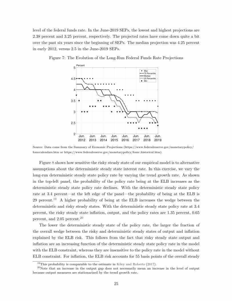
in early 2012, versus 2.5 in the June-2019 SEPs.

Figure 7: The Evolution of the Long-Run Federal Funds Rate Projections

2

2.5

3

3.5

4

4.5

5Percent

Jun.

2012

Jun.

2013

Jun.

2014

Jun.

2015

Jun.

2016

Jun.

2017

Jun.

2018

Jun.

2019

Max

75 Percentile

Median

25 Percentile

Min

Source: Data come from the Summary of Economic Projections (https://www.federalreserve.gov/monetarypolicy/

fomccalendars.htm or https://www.federalreserve.gov/monetarypolicy/fomc historical.htm).

Figure 8 shows how sensitive the risky steady state of our empirical model is to alternative

assumptions about the deterministic steady state interest rate. In this exercise, we vary the

long-run deterministic steady state policy rate by varying the trend growth rate. As shown

in the top-left panel, the probability of the policy rate being at the ELB increases as the

deterministic steady state policy rate declines. With the deterministic steady state policy

rate at 3.4 percent—at the left edge of the panel—the probability of being at the ELB is

29 percent.19 A higher probability of being at the ELB increases the wedge between the

deterministic and risky steady states. With the deterministic steady state policy rate at 3.4

percent, the risky steady state inflation, output, and the policy rates are 1.35 percent, 0.65

percent, and 2.05 percent.20

The lower the deterministic steady state of the policy rate, the larger the fraction of

the overall wedge between the risky and deterministic steady states of output and inflation

explained by the ELB risk. This follows from the fact that risky steady state output and

inflation are an increasing function of the deterministic steady state policy rate in the model

with the ELB constraint, whereas they are insensitive to the policy rate in the model without

ELB constraint. For inflation, the ELB risk accounts for 55 basis points of the overall steady

19This probability is comparable to the estimate in Kiley and Roberts (2017).20Note that an increase in the output gap does not necessarily mean an increase in the level of output

because output measures are stationarized by the trend growth rate.

25

state deflationary bias of 65 basis points when the deterministic steady state policy rate is

3.4 percent.21

Figure 8: Long-Run Interest Rates and the Risky Steady State†

3.4 3.5 3.75 4 4.25

DSS Policy Rate

0

5

10

15

20

25

30Probability of being at the ELB

3.4 3.5 3.75 4 4.25

DSS Policy Rate

1.2

1.4

1.6

1.8

2RSS Inflation

With ELB Constraint

Without ELB Constraint

3.4 3.5 3.75 4 4.25

DSS Policy Rate

0

0.2

0.4

0.6

0.8RSS Output Gap

3.4 3.5 3.75 4 4.25

DSS Policy Rate

2

2.5

3

3.5

4RSS Policy Rate

†DSS stands for “deterministic steady state,” and RSS stands for “risky steady state.” Solid vertical lines mark thedeterministic steady state policy rate in the baseline calibration (3.75 percent).

4.5 Unconventional monetary policies

In this subsection, we analyze how our quantitative results are affected by two unconven-

tional monetary policies that have been used by several central banks in the aftermath of

the Global Financial Crisis. The first is forward guidance to keep the policy rate lower for

longer than would be warranted by future economic conditions alone. The second is negative

interest rate policy.

4.5.1 “Lower-for-longer” forward guidance

In our model, “lower-for-longer” forward guidance is captured by the policy inertia pa-

rameter, ρR. Unlike an interest-rate feedback rule that responds to the lagged actual policy

rate, our policy rule responds to the lagged shadow policy rate—see equation (29)—and thus

makes the period for which the policy rate is kept at the ELB beyond the point in time

21Hamilton, Harris, Hatzius, and West (2015) argue that any value between 0 and 2 percent is a plausiblevalue for the long-run real rate. Thus, the long-run nominal rate of 2.05 percent—or equivalently, the long-runreal rate of 0.05 percent—in this example is within their plausible range.

26

where current economic conditions would call for an increase in the policy rate depend on

the severity of the previous economic downturn.22

In Figure 9, we show the dynamics of the economy in the recession scenario considered

in Figure 6 for three alternative values of ρR—0.85, 0.9 and 0.95—as well as those under the

baseline value of 0.8. According to the figure, a higher value of the policy inertia parameter is

associated with higher inflation and output at the ELB as well as a shorter ELB duration.23

Even though a higher policy inertia parameter would lead to a longer ELB duration if the

path of inflation and output were unchanged, a longer ELB duration mitigates the declines

in inflation and output at the ELB through expectations, which puts downward pressure on

the ELB duration. In equilibrium, the ELB duration is shorter with a higher policy inertia

parameter. It is interesting to note that, if the policy inertia parameter is sufficiently high,

inflation is above 2 percent even when the policy rate is at the ELB.

Figure 9: A Recession Scenario with Forward Guidance

0 10 20 30 40

Quarter

0

1

2

3

4Policy Rate (Ann. %)

0 10 20 30 40

Quarter

0.5

1

1.5

2

2.5Inflation (Ann. %)

0 10 20 30 40

Quarter

-9

-6

-3

0

3Output Gap (%)

R = 0.8

R = 0.85

R = 0.9

R = 0.95

Figure 10 shows how the risky steady state inflation, the probability of being at the

ELB, and welfare depend on the policy inertia parameter. The risky steady state inflation is

higher with a higher policy inertia. The probability of being at the ELB is lower because a

higher risky steady state inflation is associated with a higher risky steady state policy rate

and also because a higher policy inertia lowers the volatility of the policy rate. With better

stabilization outcomes both at and away from the ELB, welfare is higher with a higher policy

inertia parameter, but only up to a point, as shown in the right panel of Figure 10. If the

policy inertia is sufficiently high, the economy suffers from too high inflation, and a further

increase in the policy inertia parameter lowers welfare.

22See Gust, Herbst, Lopez-Salido, and Smith (2017), Hills and Nakata (2018), and Nakata and Schmidt(2019c) for more details.

23Bilbiie (2018) shows that when the policy rate is temporary at the ELB due to a confidence shock,“lower-for-longer” forward guidance reduces output and inflation at the ELB.

27

Figure 10: The Risky Steady State Inflation, Probability of Being at the ELB, and Welfare:Forward Guidance

0.725 0.8 0.85 0.9 0.95

R

1

1.5

2RSS Inflation

0.725 0.8 0.85 0.9 0.95

R

0

10

20

30

Pr(Rt=R

ELB)

0.725 0.8 0.85 0.9 0.95

R

-0.6

-0.3

0

0.3Welfare

4.5.2 Negative interest rate policy

In our baseline calibration, we imposed a lower bound of 0.13 (annualized) percent based

on the mid-point of the target range for the federal funds rate in place from December 2008 to

December 2015 in the U.S. However, other central banks lowered the policy rate into negative

territory.

Figure 11: A Recession Scenario with Negative Interest Rate Policy

0 10 20 30 40

Quarter

-2

0

2

4Policy Rate (Ann. %)

0 10 20 30 40

Quarter

0.5

1

1.5

2Inflation (Ann. %)

0 10 20 30 40

Quarter

-10

-8

-6

-4

-2

0

2Output Gap (%)

RELB

= -1

RELB

= -0.5

RELB

= 0

RELB

= 0.13

Figure 11 shows the dynamics of the economy in the same recession scenario considered

earlier under three alternative values of the lower bound—0, -0.5 and -1—as well as under

the baseline value. Not surprisingly, the declines in output and inflation at the ELB are

smaller the lower the ELB, because there is more scope for the central bank to lower the

policy rate if the ELB is lower.24 The better stabilization outcomes at the ELB mitigate the

deflationary bias problem away from the ELB through expectations. As shown in the left

panel of Figure 12, the risky steady state inflation is higher if the ELB is lower. Consistent

24Cuba-Borda and Singh (2019) shows that when the policy rate is at the ELB due to a confidence shock,lowering the ELB reduces output and inflation at the ELB.

28

with higher risky steady state inflation, the probability of being at the ELB is lower when

the ELB is lower. Finally, a lower ELB is associated with higher welfare because a lower

ELB improves allocations both at and away from the ELB. In our model, there is no cost of

lowering the policy rate into negative territory. As a result, welfare monotonically increases

as we decrease the ELB.25 This feature is in stark contrast to “lower-for-longer” forward

guidance policy in which a further increase in the policy inertia parameter lowers welfare

when the policy inertia parameter is sufficiently high.

Figure 12: The Risky Steady State Inflation, Probability of Being at the ELB, and Welfare:Negative Interest Rate Policy

-1 -0.5 0 0.4

RELB

1

1.5

2RSS Inflation

-1 -0.5 0 0.4

RELB

0

10

20

30

Pr(Rt=R

ELB)

-1 -0.5 0 0.4

RELB

-0.6

-0.3

0

0.3Welfare

Note: The horizontal axis is expressed in the unit of annualized percent.

5 The risk-adjusted monetary policy rule

If the ELB risk makes the task of the central bank in meeting its inflation objective more

difficult, a natural question is what, if anything, the central bank can do to counteract the

ELB risk. In the previous section, we have shown that unconventional monetary policies—

“lower-for-longer” forward guidance and negative interest rate policy—that improve stabi-

lization outcomes at the ELB can mitigate the deflationary bias away from the ELB through

expectations. These two policies improve welfare, but fall short of achieving 2 percent in-

flation at the risky steady state. In this section, we propose a simple modification of the

standard interest rate rule (28)-(29)—the risk-adjusted monetary policy rule—that allows

the central bank to achieve its inflation objective at the risky steady state.26

25As recently argued by Brunnermeier and Koby (2019) and Eggertsson, Juelsrud, Summers, and Wold(2019), if the lower bound is sufficiently negative, a further reduction in the policy rate can be contractionary.Because our model abstracts from any costs a negative policy rate may have on the economy, the effect oflowering the ELB in our model can be seen as the upper bound of what the central bank can actually achieveby lowering the policy rate into negative territory in reality.

26We interpret the central bank’s inflation objective as specifying the desired rate of inflation at the riskysteady state, as opposed to the desired unconditional average rate of inflation. See Appendix F for an extensivediscussion on this interpretation.

29

5.1 The proposed rule

Let the intercept-adjusted monetary policy rule be given by (28) and

R∗t = SRaχcΠtarg

β

(R∗t−1

SRaχcΠtarg

β

)ρR (Πpt

Πtarg

)(1−ρR)φπ(YtY

)(1−ρR)φy

, (34)

where SR that appears in front of aχcΠtarg

β is the intercept adjustment term and SRaχcΠtarg

β

is the adjusted intercept. We call SR an intercept-adjustment term because this term would

show up as the intercept in the linearized version of the policy rule.

A key feature of equation (34) is that the presence of the intercept-adjustment parameter

breaks the standard link between the intercept and the model’s structural parameters. When

the standard monetary policy rule is specified in the context of structural models, the inter-

cept is a function of the model’s structural parameters—a, β, χc, and Πtarg in our model—as

seen in equation (33). Thus, under the standard monetary policy rule, one needs to adjust

at least one of the structural parameters of the model to change the intercept. Under the

intercept-adjusted policy rule, the intercept is a free parameter of the model.

Our proposal is to use the intercept-adjusted policy rule with the value for SR chosen so

that the risky steady state inflation and the inflation target parameter coincide. We will refer

to the intercept-adjusted policy rule with SR so chosen as the risk-adjusted policy rule. The

size of the intercept adjustment that equates the risky steady state of inflation to the inflation

target parameter depends on the specifics of the model and needs to be found numerically.

The left panel in Figure 13 shows how the risky steady state of inflation changes with

the adjusted intercept in the empirical model of the previous section. Since the risky steady

state of inflation is below 2 percent under the standard policy rule, the necessary adjustment

would be to lower the intercept, as a lower intercept implies, all else being equal, a more

accommodative policy stance, generating upward pressures on inflation. According to the

panel, lowering the intercept by about 50 basis point (from 3.75 percent to 3.26 percent)

leads to the risky steady state inflation of 2 percent.

Table 6 reports the risky steady state of the empirical model under the risk-adjusted

monetary policy rule. By construction, under the risk-adjusted policy rule, the risky steady

state of inflation is 2 percent. Even though the intercept in the policy rule is lower in the

risk-adjusted policy rule than in the standard policy rule, the risky steady state policy rate

is higher—3.45 percent (versus 2.94 percent in the model with the standard monetary policy

rule)—reflecting a higher risky steady state inflation.27

The risky steady state output gap is positive, but it is a bit lower under the risk-adjusted

policy rule than under the standard policy rule. The lower risky steady state output gap is

explained by the lower frequency of being at the ELB (11.8 percent under the risk-adjusted

27If the long-run natural rate of interest is interpreted as the level of the policy rate that is consistent withthe achievement of the central bank’s inflation objective, then the ELB risk can be seen as pushing down thelong-run natural rate of interest.

30

Figure 13: The Risky Steady State Inflation, Probability of Being at the ELB, and Welfare:The Risk-Adjusted Monetary Policy Rule

2 3 3.26 4

Adjusted Intercept

1

2

3RSS Inflation

(SR

RDSS

)

2 3 4

SR

RDSS

5

10

15

20

Pr(Rt=R

ELB)

2 3 4

SR

RDSS

-0.2

-0.1

0

0.1

0.2Welfare

Notes: The figure shows how the risky steady state inflation varies with the adjusted intercept. Both the riskysteady state inflation and the adjusted intercept are expressed in annualized percent.

rule versus 16.2 percent under the standard rule), which in turn is explained by the higher

risky steady state policy rate. This positive relationship between the intercept adjustment

term and the probability of being at the ELB can be also seen in the middle panel of Figure 13.

Note that the risky steady state policy rate is higher than the intercept of the policy rule

(3.45 percent versus 3.26 percent) because inflation is at the target and the output gap is

positive at the risky steady state.

Table 6: The Risky Steady State with the Risk-Adjusted Monetary Policy Rule

Inflation Output Gap Policy Rate

Risky steady state 2 0.19 3.45Adjusted Intercept 3.26Prob(Rt = RELB) 11.8%

Figure 14 shows the dynamics of the economy in the same recession scenario as in the pre-

vious section under three alternative values of the intercept (SRRDSS = (2.5, 3.26, 3.75)) to

understand the implications of adopting the risk-adjusted monetary policy rule at the ELB.

According to the figure, the higher inflation away from the ELB associated with a lower inter-

cept adjustment term mitigates the declines in output and inflation through expectations.28

The smaller declines in inflation and output at the ELB in turn are associated with a shorter

ELB duration.28As discussed shortly, lowering the intercept of the policy rule is mathematically equivalent to increasing

the inflation target parameter. As discussed in Cuba-Borda and Singh (2019), an increase in the inflationtarget does not affect the allocations in the deflationary equilibrium, provided that there is no possibility ofswitching to the target regime. If there is a positive probability of switching to the target regime, Nakata andSchmidt (2019b) and Coyle and Nakata (2019) show that an increase in the inflation target worsens allocationsat the ELB.

31

Figure 14: A Recession Scenario with the Risk-Adjusted Monetary Policy Rule

0 10 20 30 40

Quarter

0

1

2

3

4Policy Rate (Ann. %)

0 10 20 30 40

Quarter

0.5

1

1.5

2

2.5Inflation (Ann. %)

0 10 20 30 40

Quarter

-9

-6

-3

0

3Output Gap (%)

SR

RDSS

= 2.5

SR

RDSS

= 3.26

SR

RDSS

= 3.75

Turning to the right panel of Figure 13, welfare increases as we lower the intercept of

the policy rule from the baseline value—indicated by the thin vertical line. However, if the

intercept is sufficiently low, a further decrease in the intercept lowers welfare. As discussed

in the next subsection, lowering the intercept of the policy rule is mathematically equivalent

to increasing the inflation target. As a result, in terms of welfare, lowering the intercept

involves involves costs and benefits similar to those associated with increasing the inflation

target. On the one hand, a lower intercept is associated with more inefficient outcomes in

normal times because inflation is too high. On the other hand, a lower intercept is associated

with a lower ELB frequency and better stabilization outcomes at the ELB. The intercept

adjustment that maximizes welfare is lower than the level that induces the risky steady state

inflation of 2 percent, which is 3.26 percent.

To better understand how our proposed policy rule works, it is useful to graphically

illustrate how the intercept adjustment affects the risky steady state of inflation and the

policy rate. Figure 15 plots the standard Fisher relation, the risk-adjusted Fisher relation,

the standard policy rule, and the risk-adjusted policy rule. The risky (deterministic) steady

state of the model with the standard policy rule is given by the intersection of the risk-

adjusted (standard) Fisher relation and the standard policy rule. The risky steady state of

the model with the risk-adjusted policy rule is given by the intersection of the risk-adjusted

Fisher relation and the risk-adjusted policy rule. According to the figure, and as discussed

in Section 3.4, the presence of risk lowers the line representing the Fisher relation, pushing

down the steady state inflation rate in the absence of an adjustment in the policy rule. The

risk adjustment in the policy rule lowers the level of the policy rate corresponding to a given

inflation rate, pushing up the risky steady state inflation back to the level consistent with

the inflation target parameter.

32

Figure 15: The Risk-Adjusted Fisher Relation and the Risk-Adjusted Monetary Policy Rule

2

1

RSS

DSS

RSS*

Π

R

Risk−AdjustedFisher Relation

StandardFisher Relation

StandardTaylor Rule

Risk−AdjustedTaylor Rule

†DSS stands for “deterministic steady state,” and RSS stands for “risky steady state.”

5.2 Comparison with the inflation target parameter adjustment

The intercept adjustment in equation (34) is mathematically equivalent to an adjustment

in the value assigned to the inflation target parameter in the standard policy rule. Let ΠCB be

the value of the central bank’s inflation objective. The standard policy rule with an adjusted

value for the inflation target parameter is given by

R∗t =aχcSΠΠCB

β

(R∗t−1

aχcSΠΠCB

β

)ρR (Πpt

SΠΠCB

)(1−ρR)φπ(YtY

)(1−ρR)φy

,

where SΠ is the inflation target adjustment term and SΠΠCB is the adjusted value assigned

to the inflation target parameter. This approach has a precedent. With the interpretation

that the model’s unconditional average of inflation corresponds to the central bank’s inflation

objective, Reifschneider and Williams (2000) proposed an upward adjustment in the value

assigned to the inflation target parameter in the standard policy rule so that the model’s

unconditional average of inflation is 2 percent, which is the Federal Reserve’s inflation objec-

tive.

To see the equivalence between the intercept-adjusted policy rule with Πtarg = ΠCB

and the standard policy rule with an adjusted value assigned to the inflation target param-

eter (Πtarg = SΠΠCB), notice that there is a one-to-one mapping between the intercept-

adjustment term and the inflation target adjustment term:

SR = S1−φπΠ . (35)

When the Taylor principle is satisfied (i.e., φπ > 1), this relationship implies that an adjust-

ment to lower the intercept (i.e., a lower SR) is equivalent to an adjustment to increase the

33

inflation target parameter (i.e., a higher SΠ). Figure 16 shows this mapping between the

adjusted intercept and the adjusted inflation target parameter in our model.

Figure 16: Mapping Between the Adjusted Intercept and the Adjusted Inflation TargetParameter

3 3.5 3.75 4

Adjusted Intercept (SR

RDSS

)

1.8

1.9

2

2.1

2.2

2.3

2.4

Ad

juste

d I

nfla

tio

n T

arg

et

(SC

B)

2.25

3.26

Note: The figure shows the mapping between the adjusted intercept and the adjusted inflation target param-eter. Both the adjusted intercept and the adjusted inflation target parameter are expressed in annualizedpercent.

An advantage of the risk-adjusted policy rule over the standard policy rule with an ad-

justed value assigned to the inflation target parameter is that the former allows for a simple

structural interpretation of the inflation target parameter. In the risk-adjusted policy rule,

the inflation target parameter can be naturally interpreted as the central bank’s inflation

objective because the risky steady state of inflation coincides with the value of the inflation

target parameter. In the standard policy rule, the risky steady state of inflation is different

from the value assigned to the inflation target parameter unless the model is linear, compli-

cating the interpretation of the inflation target parameter. In our model, assigning the value

of 2.25 percent to the inflation target parameter achieves the risky steady state inflation of

2 percent, as seen in Figure 16. However, in this setup, the value assigned to the inflation

target parameter is simply a number that allows the model to generate the risky steady state

of inflation so that it is consistent with the central bank’s inflation objective, and does not

have any structural interpretation.

The desirability of being able to interpret the inflation target parameter as the central

bank’s inflation objective depends on the purpose of the analysis. In many estimation exer-

cises using U.S. data, the estimated value for the inflation target parameter can substantially

differ from 2 percent, depending on the sample used for estimation. The discrepancy between

the estimated value and the Federal Reserve’s target rate of 2 percent may not pose any issue

if the goal of estimation is only to fit the data and understand the past.

However, if the goal of the analysis is to think about the implications of alternative policy

rules for the economic outlook and if such analyses are used to inform policymakers, it is typi-

34

cally useful—from the perspective of communication between modelers and policymakers—if

the inflation target parameter in the policy rule can be simply interpreted as the central

bank’s inflation objective. For example, in the EDO Model—short for Estimated Dynamic

Optimization-based Model—which is used at the Board of Governors of the Federal Reserve

System for various policy analyses, the inflation target parameter in the policy rule is set

to 2 percent, the Federal Reserve’s target rate of inflation, to allow for a simple interpre-

tation of the inflation target parameter (Chung, Kiley, and Laforte, 2010).29 Similarly, in

the New Area-Wide Model of the Euro Area, the DSGE model used for policy analyses at

the European Central Bank, the inflation target parameter is interpreted as the monetary

authority’s long-run inflation objective and is set to 1.9 percent, which is “consistent with

the ECB’s quantitative definition of price stability of inflation below, but close to 2 percent”

(Christoffel, Coenen, and Warne, 2008).30

6 Empirical relevance

In this section, we discuss why the steady-state undershooting of the inflation target

arising from the anticipation effects of the ELB risk in our model might be empirically

relevant. Our main result on the deflationary bias depends on a number of assumptions, in

particular that (i) that firms attach a positive probability to the event that the ELB will

bind again in the future, (ii) that this ELB risk lowers their inflation expectations, and (iii)

that lower inflation expectations lead firms to lower their prices today. We are not aware

of any direct evidence on each of these three assumptions. However, available measures of

ELB risk and long-run inflation expectations are supportive for the first two assumptions.

There is little evidence regarding the third assumption. Finally, we demonstrate that U.S.

policymakers are concerned about the possibility that long-run inflation expectations might

be slipping down.

6.1 On the ELB frequency

Figure 17 shows the evolution of subjective measures of the medium-term ELB risk—

defined as the probability of returning to the ELB at least once over the next 3 years or

so—in the Survey of Primary Dealers (SPD) and the Survey of Market Participants (SMD).

29Chung, Kiley, and Laforte (2010) explain their calibration choice by saying, “some important determinantsof steady-state behavior were calibrated to yield growth rates of GDP and associated price indexes thatcorresponded to “conventional” wisdom in policy circles, even though slight deviations from such values wouldhave been preferred (in a “statistically significant” way) to our calibrated values.”

30These models are used for policy analyses in the context of the ELB on nominal interest rates (see,for instance, Chung, Laforte, Reifschneider, and Williams (2012) and Coenen and Warne (2014)). Due tothe computational difficulty of globally solving large-scale DSGE models, the models are currently solvedand simulated using solution methods that rely on the assumption that certainty equivalence holds (“perfectforesight” assumption). As a result of this assumption, the risky steady state coincides with the deterministicsteady state in these applications.

35

Figure 17: Medium-term ELB Risk

2016 2017 2018 2019

Year

0

10

20

30

40

Pro

babili

tyPrimary Dealers

25th Percentile

Median

75th Percentile

2016 2017 2018 2019

Year

0

10

20

30

40

Pro

babili

ty

Market Participants

25th Percentile

Median

75th Percentile

Note: Data come from the Survey of Primary Dealers (https://www.newyorkfed.org/markets/primarydealer survey questions)and the Survey of Market Participants (https://www.newyorkfed.org/markets/survey market participants).

According to the figure, the respondents in these surveys have attached non-trivial prob-

abilities of returning to the ELB since the liftoff that occurred in December 2015. Right after

the liftoff, the probabilities were high, reflecting the fact that the federal funds rate was only

slightly above the ELB. The SPD measure of ELB risk came down to 20 percent in early

2017, stayed at that level until mid 2018. The SMD measure of ELB risk hovered around

20 percent in 2017 and 2018. Both measures have edged up a bit since later 2018. As of

July 2019, the median probabilities for the SPD and the SMD are 35 percent and 30 percent,

respectively.

What matters in our model is the probability that firms attach to the event of returning

to the ELB in the future. Unfortunately, we are not aware of any survey asking firms about

their subjective assessment of the probability of returning to the ELB constraint in the future.

Nonetheless, the very high probabilities that financial market participants attach to the event

of returning to the ELB are supportive of the general idea that economic agents are cognizant

of the fact that the ELB constraint can bind again.

6.2 On long-run inflation expectations

Figure 18 shows various measures of long-run inflation expectations in the recent past.

Top-left and top-right panels show the evolution of long-run CPI inflation expectations from

the Survey of Professional Forecasters (SPF), the SPD, and the Livingston Survey. Middle-

left and middle-right panels show the evolution of long-run PCE inflation expectations from

the SPF and the SPD. The bottom-left panel shows the inflation expectations over the next

three years from the Survey of Consumer Expectations as well as the inflation expectations

over the next 5-10 years from the University of Michigan’s Survey of Consumers. Finally, the

bottom-right panel shows two measures of breakeven inflation rates.

36

Figure 18: Long-Run Inflation Expectations

2005 2010 2015

Year

2

2.25

2.5

2.75

3CPI Next 10 Years

SPF

Livingston Survey

2005 2010 2015

Year

2

2.25

2.5

2.75

3CPI Forward Expectations

SPF, 6-10

Primary Dealers, 5-10

2007 2009 2011 2013 2015 2017 2019

Year

1.8

2

2.2

2.4

2.6PCE Next 10 Years

SPF

2007 2009 2011 2013 2015 2017 2019

Year

1.8

2

2.2

2.4

2.6PCE Forward Expectations

SPF, 6-10 years

Primary Dealers, Longer run

2005 2010 2015

Year

2

2.5

3

3.5

4Survey of Consumers

FRBNY, 3 years ahead

Michigan, next 5-10 years

2005 2010 2015

Year

0

1

2

3Breakeven Inflation

5-year, 5-year Forward

10-year Breakeven

Source: The Survey of Professional Forecasters (SPF) data come from FRB Philadelphia(https://www.philadelphiafed.org/research-and-data/real-time-center/survey-of-professional-forecasters), asdoes the Livingston Survey (https://www.philadelphiafed.org/research-and-data/real-time-center/livingston-survey/historical-data). The primary dealer series are taken from FRB New York’s Survey of PrimaryDealers (https://www.newyorkfed.org/markets/primarydealer˙survey˙questions). The FRB New York seriesfor inflation expectations three years ahead comes from the FRB NY Survey of Consumer Expectations(https://www.newyorkfed.org/microeconomics/sce). The series from the University of Michigan Survey of Con-sumers is available here (http://www.sca.isr.umich.edu/). The breakeven inflation data come from FRED. All sourcesaccessed on August 15, 2019.

According to the figure, over the last several years, many—albeit not all—measures have

drifted down and they are currently at the lower ends of their historical ranges. The declines

in these measures coincided with the decline in the estimates of the long-run equilibrium real

rate, as shown earlier in Figure 7. This pattern is consistent with our model’s prediction

because a lower long-run equilibrium real rate implies a higher ELB frequency, as shown in

Figure 8.

The extent to which lower long-run inflation expectations are pulling down inflation is an

empirical question. To our knowledge, there are few research papers investigating the causal

relationship between inflation expectations and firm’s pricing decisions and the evidence is

mixed. Using a survey of Italian firms, Coibion, Gorodnichenko, and Ropele (2019) show that

higher inflation expectations lead firms to raise their prices. Using a survey of New Zealand

37

firms, Coibion, Gorodnichenko, and Kumar (2018) show that higher inflation expectations

do not necessarily lead them to change prices in a statistically or economically significant

way.31 Also, even if inflation expectations affect the behavior of households and firms, the

effects may not be as strong as standard rational-expectations models suggest.

6.3 Policymakers’ concerns

While there is uncertainty about whether long-run inflation expectations are currently

below 2 percent, and if so, whether below-target inflation expectations are pushing downward

pressure on inflation today, these possibilities have been real concerns for U.S. monetary

policymakers who have been struggling to raise inflation to their objective of 2 percent.

While there are many hypotheses about the cause of the persistent inflation undershoot,

some policymakers have stated that a higher ELB risk might be causing long-run inflation

expectations to be below 2 percent and that such below-target long-run inflation expectations

in turn are causing inflation to stay below the target, sometimes citing the previous version

of our paper.32 For example, Williams (2019) states:

“Even in times when policy is not constrained, the expectation of below-target in-

flation in the future affects current decisions, putting additional downward pres-

sure on inflation. In other words, monetary policy is always swimming upstream,

fighting a current of too-low inflation expectations that interferes with achieving

the target inflation rate.”

Our paper directly speaks to this concern by U.S. policymakers on the inflation un-

dershooting by showing that a moderate degree of ELB risk can quantitatively explain a

nontrivial degree of the inflation undershoot when the federal funds rate is away from the

ELB.

7 Additional results and discussion

7.1 On the importance of other nonlinear features

As we saw in Section 4, the effect of nonlinearities unrelated to the ELB on the risky

steady state inflation can be nontrivial.

Even before the ELB literature blossomed, many papers studied the implication of various

nonlinearities on the dynamics of the economy using New Keynesian models (for example,

31There are more research papers analyzing whether inflation expectations affect the behaviors of house-holds, but the evidence is mixed here as well. See, for example, Ichiue and Nishiguchi (2015), D’Acunto,Hoang, and Weber (2018), Malmendier and Nagel (2016), Armantier, de Bruin, Topa, Klaauw, and Zafar(2015), Abe and Ueno (2015), Coibion, Gorodnichenko, Kumar, and Pedemonte (2018), and Duca, Kenny,and Reuter (2018) for papers finding that inflation expectations affect the behaviors of households. See Bach-mann, Berg, and Sims (2015) and Burke and Ozdagli (2013) for papers finding that inflation expectations donot affect the behaviors of households.

32See, for example, Brainard (2018), Evans (2019), and Williams (2019).

38

downward nominal wage rigidities by Kim and Ruge-Murcia (2011), stochastic volatilities

by Fernandez-Villaverde, Guerron-Quintana, Kuester, and Rubio-Ramırez (2015), and an

Epstein-Zin preference with a high risk-aversion by Rudebusch and Swanson (2012), among

many others). These papers typically use higher-order perturbation methods to solve the

model, which can capture the steady-state implication of uncertainty. Nonetheless, to our

knowledge, no one has pointed out that the risky steady state inflation can nontrivially differ

from the inflation target, likely because these papers are focused on the implications of various

nonlinearities for other aspects of the model, as opposed to the risky steady state inflation

(Kim and Ruge-Murcia (2011) on asymmetric economic dynamics, Fernandez-Villaverde,

Guerron-Quintana, Kuester, and Rubio-Ramırez (2015) on the effect of fiscal volatility shock,

Rudebusch and Swanson (2012) on term-premiums implications).

While our paper focuses on the implication of the ELB constraint for the risky steady

state, it would be useful to study how these other realistic sources of nonlinearity affect the

risky steady state inflation.

7.2 Output growth in the interest-rate rule

Figure 19: Coefficient on Output Growth and the Risky Steady State

0 0.25 0.5

Coefficient on Output Growth

15

20

25Probability of being at the ELB

0 0.25 0.5

Coefficient on Output Growth

1.4

1.5

1.6

1.7RSS Inflation

0 0.25 0.5

Coefficient on Output Growth

0.2

0.4

0.6RSS Output Gap

0 0.25 0.5

Coefficient on Output Growth

2.5

2.75

3RSS Policy Rate

In this section, we analyze the implication of introducing an output growth term to the

interest-rate feedback rule, a common feature of many estimated DSGE models (see, for

example, Smets and Wouters (2007) and Gust, Herbst, Lopez-Salido, and Smith (2017)).

Figure 19 shows how the risky steady state inflation and output gap—as well as the ELB

39

frequency—depend on the coefficient on the output growth term. According to the figure,

the larger the coefficient, the lower (higher) the risky steady state inflation (output gap).

This in turn is driven by the fact that a higher coefficient leads to worse allocations at the

ELB.

This result is consistent with Nakata, Schmidt, and Yoo (2018), who show speed-limit

policies (policies in which the policy rate reacts positively to output growth) worsen alloca-

tions at and away from the ELB in the context of the optimal discretionary policymaker. In

the aftermath of a deep recession, a speed-limit policy prescribes a higher policy rate path,

because output growth is positive when the economy is recovering. However, such a higher

policy rate path—the opposite of what the optimal commitment policy prescribes—lowers

output and inflation at the ELB through expectations. And, lower inflation at the ELB

exacerbates the deflationary bias away from the ELB through expectations.

8 Conclusion

In this paper, we have examined the implications of ELB risk—the possibility that the

policy rate will be constrained by ELB in the future—for the economy when the policy rate is

currently not constrained. Using an empirically rich DSGE model calibrated to capture key

features of the U.S. economy since the mid 1990s, we have shown that the ELB risk causes

inflation to fall below the target rate of 2 percent by about 25 basis points at the risky steady

state. This deflationary bias induced by ELB risk at the risky steady state can be as much as

50 basis points under alternative plausible assumptions about the long-run growth rate of the

economy. Our analysis suggests that achieving the inflation target may be more difficult now

than before the Great Recession, if the recent recognition of lower long-run equilibrium real

rates has led households and firms to increase their assessment of future ELB risk: prescribing

policies that accommodate or adjust to such risk may therefore be the natural step moving

forward.

References

Abe, N., and Y. Ueno (2015): “Measuring Inflation Expectations: Consumers’ Heterogeneity and

Nonlinearity,” RCESR Discussion Paper Series 15-5, Hitotsubashi University.

Adam, K., and R. Billi (2007): “Discretionary Monetary Policy and the Zero Lower Bound on

Nominal Interest Rates,” Journal of Monetary Economics, 54(3), 728–752.

Armantier, O., W. B. de Bruin, G. Topa, W. Klaauw, and B. Zafar (2015): “Inflation Ex-

pectations And Behavior: Do Survey Respondents Act On Their Beliefs?,” International Economic

Review, 56, 505–536.

Armenter, R. (2018): “The Perils of Nominal Targets,” Review of Economic Studies, 85(1), 50–86.

40

Aruoba, B. S., P. Cuba-Borda, and F. Schorfheide (2018): “Macroeconomic Dynamics Near

the ZLB: a Tale of Two Countries,” Review of Economic Studies, 85(1), 87–118.

Bachmann, R., T. O. Berg, and E. R. Sims (2015): “Inflation Expectations and Readiness to

Spend: Cross-Sectional Evidence,” American Economic Journal: Economic Policy, 7(1), 1–35.

Benhabib, J., S. Schmitt-Grohe, and M. Uribe (2001): “The Perils of Taylor Rules,” Journal

of Economic Theory, 96(1-2), 40–69.

Bianchi, F., L. Melosi, and M. Rottner (2019): “Hitting the Elusive Inflation Target,” Working

Paper Series 2019-07, Federal Reserve Bank of Chicago.

Bilbiie, F. O. (2018): “Neo-Fisherian Policies and Liquidity Traps,” Mimeo.

Brainard, L. (2018): “Sustaining Full Employment and Inflation around Target,” Remarks at the

Forecasters Club of New York, New York, New York.

Brunnermeier, M. K., and Y. Koby (2019): “The Reversal Interest Rate,” Mimeo.

Burke, M. A., and A. K. Ozdagli (2013): “Household Inflation Expectations and Consumer

Spending: Evidence from Panel Data,” Working Paper Series 13-25, Federal Reserve Bank of

Boston.

Christiano, L., M. Eichenbaum, and S. Rebelo (2011): “When Is the Government Spending

Multiplier Large?,” Journal of Political Economy, 119(1), 78–121.

Christiano, L. J., and J. D. M. Fisher (2000): “Algorithms for Solving Dynamic Models with

Occasionally Binding Constraints,” Journal of Economic Dynamics and Control, 24(8), 1179–1232.

Christoffel, K., G. Coenen, and A. Warne (2008): “The New Area-Wide Model of the Euro

Area: A Micro-Founded Open-Economy Model for Forecasting and Policy Analysis,” ECB Working

Paper Series 944, European Central Bank.

Chung, H., M. Kiley, and J.-P. Laforte (2010): “Documentation of the Estimated, Dynamic,

Optimization-based (EDO) Model of the U.S. Economy: 2010 Version,” Finance and economics

discussion series, Board of Governors of the Federal Reserve System (U.S.).

Chung, H., J.-P. Laforte, D. Reifschneider, and J. C. Williams (2012): “Have We Under-

estimated the Likelihood and Severity of Zero Lower Bound Events?,” Journal of Money, Credit

and Banking, 44(s1), 47–82.

Clouse, J., D. Henderson, A. Orphanides, D. H. Small, and P. A. Tinsley (2003): “Mone-

tary Policy When the Nominal Short-Term Interest Rate is Zero,” The B.E. Journal of Macroeco-

nomics, 3(1), 1–65.

Coenen, G., A. Orphanides, and V. Wieland (2004): “Price Stability and Monetary Policy

Effectiveness when Nominal Interest Rates are Bounded at Zero,” B.E. Journal of Macroeconomics:

Advances in Macroeconomics, 4(1), 1–25.

Coenen, G., and A. Warne (2014): “Risks to Price Stability, the Zero Lower Bound and Forward

Guidance: A Real-Time Assessment,” International Journal of Central Banking, 10(2), 7–54.

41

Coeurdacier, N., H. Rey, and P. Winant (2011): “The Risky Steady State,” American Economic

Review, 101(3), 398–401.

Coibion, O., Y. Gorodnichenko, and S. Kumar (2018): “How Do Firms Form Their Expecta-

tions? New Survey Evidence,” American Economic Review, 108(9), 2671–2713.

Coibion, O., Y. Gorodnichenko, S. Kumar, and M. Pedemonte (2018): “Inflation Expec-

tations as a Policy Tool?,” NBER Working Paper Series 24788, National Bureau of Economic

Research.

Coibion, O., Y. Gorodnichenko, and T. Ropele (2019): “Inflation Expectations and Firm

Decisions: New Causal Evidence,” Mimeo.

Coibion, O., Y. Gorodnichenko, and J. Wieland (2012): “The Optimal Inflation Rate in New

Keynesian Models: Should Central Banks Raise Their Inflation Targets in Light of the ZLB?,”

Review of Economic Studies, 79(4), 1371–1406.

Coyle, P., and T. Nakata (2019): “Optimal Inflation Target with Expectations-Driven Liquidity

Traps,” Finance and Economics Discussion Series 2016-036, Board of Governors of the Federal

Reserve System (U.S.).

Coyle, P., T. Nakata, and S. Schmidt (2019): “Deflationary Equilibrium under Uncertainty,”

Mimeo.

Cuba-Borda, P., and S. Singh (2019): “Understanding Persistent Stagnation,” International Fi-

nance Discussion Papers 1243, Board of Governors of the Federal Reserve System (U.S.).

D’Acunto, F., D. Hoang, and M. Weber (2018): “Unconventional Fiscal Policy,” NBER Working

Paper Series 24244, National Bureau of Economic Research.

Draghi, M. (2016): “Delivering a Symmetric Mandate with Asymmetric Tools: Monetary Policy in

a Context of Low Interest Rates,” Remarks at the Ceremony to Mark the 200th Anniversary of the

Oesterreichische Nationalbank, Vienna.

Duca, I. A., G. Kenny, and A. Reuter (2018): “Inflation Expectations, Consumption and the

Lower Bound: Micor Evidence from a Large Euro Area Survey,” Working Paper Series 2196,

European Central Bank.

Eggertsson, G., and M. Woodford (2003): “The Zero Bound on Interest Rates and Optimal

Monetary Policy,” Brookings Papers on Economic Activity, 34(1), 139–235.

Eggertsson, G. B., R. Juelsrud, L. H. Summers, and E. G. Wold (2019): “Negative Nominal

Interest Rates and the Bank Lending Channel,” NBER Working Paper Series 25416, National

Bureau of Economic Research.

Erceg, C. J., and J. Linde (2014): “Is There a Fiscal Free Lunch in a Liquidity Trap?,” Journal

of the European Economic Association, 12(1), 73–107.

Evans, C. (2019): “On Risk and Credibility in Monetary Policy,” Remarks at the National Associa-

tion for Business Economics (NABE) and Sveriges Riksbank conference, Global Economies at the

Crossroads: Growing Together While Growing Apart?, in Stockholm, Sweden.

42

Evans, C., J. Fisher, F. Gourio, and S. Krane (2015): “Risk Management for Monetary Policy

Near the Zero Lower Bound,” Brookings Papers on Economic Activity, Spring.

Fernandez-Villaverde, J., G. Gordon, P. A. Guerron-Quintana, and J. Rubio-Ramırez

(2015): “Nonlinear Adventures at the Zero Lower Bound,” Journal of Economic Dynamics and

Control, 57, 182–204.

Fernandez-Villaverde, J., P. Guerron-Quintana, K. Kuester, and J. Rubio-Ramırez

(2015): “Fiscal Volatility Shocks and Economic Activity,” American Economic Review, 105(11),

3352–84.

Gavin, W. T., B. D. Keen, A. W. Richter, and N. A. Throckmorton (2015): “The Zero

Lower Bound, the Dual Mandate, and Unconventional Dynamics,” Journal of Economic Dynamics

and Control, 55, 14–38.

Guerrieri, L., and M. Iacoviello (2017): “Collateral Constraints and Macroeconomic Asymme-

tries,” Journal of Monetary Economics, 90, 28–49.

Gust, C., E. Herbst, D. Lopez-Salido, and M. Smith (2017): “The Empirical Implications of

the Interest-Rate Lower Bound,” American Economic Review, 107(7)(1), 1971–2006.

Hamilton, J. D., E. Harris, J. Hatzius, and K. D. West (2015): “The Equilibrium Real Funds

Rate: Past, Present and Future,” Working Paper.

Hills, T. S., and T. Nakata (2018): “Fiscal Multipliers at the Zero Lower Bound: The Role of

Policy Inertia,” Journal of Money, Credit and Banking, 50(1), 155–172.

Hills, T. S., T. Nakata, and S. Schmidt (2016): “The Risky Steady State and the Interest

Rate Lower Bound,” Finance and Economics Discussion Series 2016-009, Board of Governors of the

Federal Reserve System (U.S.).

Hirose, Y., and T. Sunakawa (2016): “Parameter Bias in an Estimated DSGE Model: Does

Nonlinearity Matter?,” Mimeo.

(2017): “The Natural Rate of Interest in a Nonlinear DSGE Model,” Mimeo.

Ichiue, H., and S. Nishiguchi (2015): “Inflation Expectations and Consumer Spending at the Zero

Bound: Micro Evidence,” Economic Inquiry, 53(2), 1086–1107.

Keen, B. D., A. W. Richter, and N. A. Throckmorton (2016): “Forward Guidance and the

State of the Economy,” Economic Inquiry, 55(4), 1593–1624.

Kiley, M., and J. Roberts (2017): “Monetary Policy in a Low Interest Rate World,” Brookings

Papers on Economic Activity.

Kim, J., and F. J. Ruge-Murcia (2011): “Monetary Policy When Wages are Downwardly Rigid:

Friedman Meets Tobin,” Journal of Economic Dynamics and Control, 35, 2064–2077.

Maliar, L., and S. Maliar (2015): “Merging Simulation and Projection Approaches to Solve High-

Dimensional Problems with an Application to a New Keynesian Model,” Quantitative Economics,

6(1), 1–47.

43

Malmendier, U., and S. Nagel (2016): “Learning from Inflation Experiences,” The Quarterly

Journal of Economics, 131(1), 53–87.

Mertens, K., and M. Ravn (2014): “Fiscal Policy in an Expectations Driven Liquidity Trap,”

Mimeo.

Mertens, T. M., and J. C. Williams (2018): “What to expect from the lower bound on interest

rates: evidence from derivatives prices,” Staff Reports 865, Federal Reserve Bank of New York.

Nakata, T. (2016): “Optimal Fiscal and Monetary Policy With Occasionally Binding Zero Bound

Constraints,” Journal of Economic Dynamics and Control, 73, 220–240.

(2017): “Uncertainty at the Zero Lower Bound,” American Economic Journal: Macroeco-

nomics, 9(3), 186–221.

Nakata, T., and S. Schmidt (2016): “The Risk-Adjusted Monetary Policy Rule,” Finance and

Economics Discussion Series 2016-061, Board of Governors of the Federal Reserve System (U.S.).

(2019a): “Conservatism and Liquidity Traps,” Journal of Monetary Economics, 104.

(2019b): “Expectations-Driven Liquidity Traps: Implications for Monetary and Fiscal Pol-

icy,” Finance and Economics Discussion Series 2019-053, Board of Governors of the Federal Reserve

System (U.S.).

(2019c): “Gradualism and Liquidity Traps,” Review of Economic Dynamics, 31.

Nakata, T., S. Schmidt, and P. Yoo (2018): “Speed Limit Policy and Liquidity Traps,” Finance

and Economics Discussion Series 2018-050, Board of Governors of the Federal Reserve System

(U.S.).

Nakov, A. (2008): “Optimal and Simple Monetary Policy Rules with Zero Floor on the Nominal

Interest Rate,” International Journal of Central Banking, 4(2), 73–127.

Plante, M., A. Richter, and N. Throckmorton (2018): “The Zero Lower Bound and Endoge-

nous Uncertainty,” Economic Journal, 128(611), 1730–1757.

Powell, J. H. (2018): “Semiannual Monetary Policy Report to the Congress,” Testimony before the

Committee on Banking, Housing, and Urban Affairs, U.S. Senate, Washington, D.C.

Rachel, L., and T. D. Smith (2015): “Secular Drivers of the Global Real Interest Rate,” Staff

Working Paper 571, Bank of England.

Reifschneider, D., and J. C. Williams (2000): “Three Lessons for Monetary Policy in a Low-

Inflation Era,” Journal of Money, Credit and Banking, 32(4), 936–966.

Richter, A. W., and N. A. Throckmorton (2015): “The Zero Lower Bound: Frequency, Du-

ration, and Numerical Convergence,” B.E. Journal of Macroeconomics: Contributions, 15(1), 157–

182.

(2016): “Is Rotemberg Pricing Justified by Macro Data?,” Economics Letters, 149, 44–48.

44

Rudebusch, G. D., and E. T. Swanson (2012): “The Bond Premium in a DSGE Model with

Long-Run Real and Nominal Risks,” American Economic Journal: Macroeconomics, 4, 105–143.

Schmidt, S. (2013): “Optimal Monetary and Fiscal Policy with a Zero Bound on Nominal Interest

Rates,” Journal of Money, Credit and Banking, 45(7), 1335–1350.

Seneca, M. (2018): “Risk Shocks and Monetary Policy in the New Normal,” Working paper.

Smets, F., and R. Wouters (2007): “Shocks and Frictions in US Business Cycles: A Bayesian

DSGE Approach,” American Economic Review, 97(3), 586–606.

Williams, J. C. (2019): “Living Life Near the ZLB,” Remarks at 2019 Annual Meeting of the Central

Bank Research Association (CEBRA), New York City.

Wolman, A. L. (1998): “Staggered Price Setting and the Zero Bound on Nominal Interest Rates,”

Federal Reserve Bank of Richmond Economic Quarterly, 84(4), 1–24.

Yellen, J. (2017): “The Economic Outlook and the Conduct of Monetary Policy,” Remarks at

Stanford Institute for Economic Policy Research, Stanford University, 19 January.

45

For Online Publication: Technical Appendix

A Details of the Stylized Model

This section describes a stylized DSGE model with a representative household, a final goodproducer, a continuum of intermediate goods producers with unit measure, and governmentpolicies.

A.1 Household

The representative household chooses its consumption level, amount of labor, and bondholdings so as to maximize the expected discounted sum of utility in future periods. As iscommon in the literature, the household enjoys consumption and dislikes labor. Assumingthat period utility is separable, the household problem can be defined by

maxCt,Nt,Bt

E1

∞∑t=1

βt−1[ t−1∏s=0

δs

][C1−χct

1− χc− N1+χn

t

1 + χn

](A.1)

subject to the budget constraint

PtCt +R−1t Bt ≤WtNt +Bt−1 + PtΦt (A.2)

or equivalently

Ct +BtRtPt

≤ wtNt +Bt−1

Pt+ Φt (A.3)

where Ct is consumption, Nt is the labor supply, Pt is the price of the consumption good, Wt

(wt) is the nominal (real) wage, Φt is the profit share (dividends) of the household from theintermediate goods producers, Bt is a one-period risk free bond that pays one unit of moneyat period t+1, and R−1

t is the price of the bond.

The discount rate at time t is given by βδt where δt is the discount factor shock alteringthe weight of future utility at time t+1 relative to the period utility at time t. This shockfollows an AR(1) process:

δt − 1 = ρ(δt−1 − 1) + εt, εt ∼ N(0, σε) (A.4)

This increase in δt is a preference imposed by the household to increase the relative valuationof future utility flows, resulting in decreased consumption today (when considered in theabsence of changes in the nominal interest rate).

A.2 Firms

There is a final good producer and a continuum of intermediate goods producers indexedby i ∈ [0, 1]. The final good producer purchases the intermediate goods Yi,t at the intermedi-ate price Pi,t and aggregates them using CES technology to produce and sell the final good

46

Yt to the household and government at price Pt. Its problem is then summarized as

maxYi,t,i∈[0,1]

PtYt −∫ 1

0Pi,tYi,tdi (A.5)

subject to the CES production function

Yt =[ ∫ 1

0Y

θ−1θ

i,t di] θθ−1

. (A.6)

Intermediate goods producers use labor to produce the imperfectly substitutable intermedi-ate goods according to a linear production function (Yi,t = Ni,t) and then sell the product tothe final good producer. Each firm maximizes its expected discounted sum of future profits33

by setting the price of its own good. We can assume that each firm receives a productionsubsidy τ so that the economy is fully efficient in the steady state.34 In our baseline, however,we set τ = 0. Price changes are subject to quadratic adjustment costs.

maxPi,t

E1

∞∑t=1

βt−1[ t−1∏s=0

δs

]λt

[Pi,tYi,t − (1− τ)WtNi,t − Pt

ϕ

2[Pi,tPi,t−1

− 1]2Yt

](A.7)

such that

Yi,t =

[Pi,tPt

]−θYt.

35 (A.8)

λt is the Lagrange multiplier on the household’s budget constraint at time t and βt−1[∏t−1

s=0 δs

]λt

is the marginal value of an additional profit to the household. The positive time zero priceis the same across firms (i.e. Pi,0 = P0 > 0).

A.3 Government policies

It is assumed that the monetary authority determines nominal interest rates according toa Taylor rule

Rt = max

[RELB,

Πtarg

β

(Πt

Πtarg

)φπ](A.9)

where Πt = PtPt−1

. This equation will be modified in order to do an extensive sensitivityanalysis of policy inertia and other rule specifications.

33Each period, as it is written below, is in nominal terms. However, we want each period’s profits in realterms so the profits in each period must be divided by that period’s price level Pt which we take care of furtheralong in the document.

34(θ− 1) = (1 − τ)θ which implies zero profits in the zero inflation steady state. In a welfare analysis, thiswould extract any inflation bias from the second-order approximated objective welfare function. τ thereforerepresents the size of a steady state distortion (see Chapter 5 Appendix, Galı (2008)).

35This expression is derived from the profit maximizing input demand schedule when solving for the finalgood producer’s problem above. Plugging this expression back into the CES production function implies that

the final good producer will set the price of the final good Pt =[ ∫ 1

0P 1−θi,t di

] 11−θ

.

47

A.4 Market clearing conditions

The market clearing conditions for the final good, labor and government bond are givenby

Yt = Ct +

∫ 1

0

ϕ

2

[ Pi,tPi,t−1

− 1]2Ytdi (A.10)

Nt =

∫ 1

0Ni,tdi (A.11)

andBt = 0. (A.12)

A.5 Recursive equilibrium

Given P0 and a two-state Markov shock process establishing δt and γt, an equilibriumconsists of allocations {Ct, Nt, Ni,t, Yt, Yi,t, Gt}∞t=1, prices {Wt, Pt, Pi,t}∞t=1, and a policy in-strument {Rt}∞t=1 such that (i) given the determined prices and policies, allocations solve theproblem of the household, (ii) Pi,t solves the problem of firm i, (iii) Rt follows a specifiedrule, and (iv) all markets clear.

Combining all of the results from (i)-(v), a symmetric equilibrium can be characterizedrecursively by {Ct, Nt, Yt, wt,Πt, Rt}∞t=1 satisfying the following equilibrium conditions:

C−χct = βδtRtEtC−χct+1 Π−1

t+1 (A.13)

wt = Nχnt Cχct (A.14)

YtCχct

[ϕ (Πt − 1) Πt − (1− θ)− θ(1− τ)wt] = βδtEtYt+1

Cχct+1

ϕ (Πt+1 − 1) Πt+1 (A.15)

Yt = Ct +ϕ

2[Πt − 1]2 Yt (A.16)

Yt = Nt (A.17)

Rt = max

[RELB,

Πtarg

β

(Πt

Πtarg

)φπ](A.18)

Equation A.13 is the consumption Euler equation, Equation A.14 is the intratemporal op-timality condition of the household, Equation A.15 is the optimal condition of the inter-mediate good producing firms (forward-looking Phillips Curve) relating today’s inflation toreal marginal cost today and expected inflation tomorrow, Equation A.16 is the aggregateresource constraint capturing the resource cost of price adjustment, and Equation A.17 is theaggregate production function. Equation A.18 is the interest-rate feedback rule.

B Solution Method

We describe our solution method using the stylized model analyzed in the main text. Theextension of the method to the empirical model is straightforward.

The problem is to find a set of policy functions, {C(·), N(·), Y (·), w(·), Π(·), R(·)}, that

48

solves the following system of functional equations.

C(δt)−χc = βδtR(δt)EtC(δt+1)−χcΠ(δt+1)−1 (B.1)

w(δt) = N(δt)χnC(δt)

χc (B.2)

N(δt)

C(δt)χc

[ϕ(

Π(δt)− 1)

Π(δt)− (1− θ)− θw(δt)]

= βδtEtN(δt+1)

C(δt+1)χcϕ(

Π(δt+1)− 1)

Π(δt+1) (B.3)

Y (δt) = C(δt) +ϕ

2

[Π(δt)− 1

]2Y (δt) (B.4)

Y (δt) = N(δt) (B.5)

R(δt) = max

[RELB,

Πtarg

β

[Π(δt)

Πtarg

]φπ](B.6)

Substituting out w(·) and N(·) using equations (B.2) and (B.5), this system can be reducedto a system of four functional equations for C(·), Y (·), Π(·), and R(·).

C(δt)−χc = βδtR(δt)EtC(δt+1)−χcΠ(δt+1)−1 (B.7)

Y (δt)

C(δt)χc

[ϕ(

Π(δt)− 1)

Π(δt)− (1− θ)− θY (δt)χnC(δt)

χc]

= βδtEtY (δt+1)

C(δt+1)χcϕ(

Π(δt+1)− 1)

Π(δt+1) (B.8)

Y (δt) = C(δt) +ϕ

2

[Π(δt)− 1

]2Y (δt) (B.9)

R(δt) = max

[RELB,

Πtarg

β

[Π(δt)

Πtarg

]φπ](B.10)

Following the idea of Christiano and Fisher (2000), we decompose these policy functionsinto two parts using an indicator function: One in which the policy rate is allowed to be lessthan zero, and the other in which the policy rate is assumed to be zero. That is, for anyvariable Z,

Z(·) = I{R(·)≥1}Zunc(·) + (1− I{R(·)≥1})ZELB(·). (B.11)

The problem then becomes finding a set of a pair of policy functions, {[Cunc(·), CELB(·)],[Yunc(·), YELB(·)], [Πunc(·), ΠELB(·)], [Runc(·), RELB(·)]} that solves the system of functionalequations above. This method can achieve a given level of accuracy with a considerable lessnumber of grid points relative to the standard approach.

The time-iteration method starts by specifying a guess for the values policy functionstake on a finite number of grid points. The values of the policy function that are not onany of the grid points are interpolate or extrapolated linearly. Let X(·) be a vector of policyfunctions that solves the functional equations above and let X(0) be the initial guess of suchpolicy functions.36 At the s-th iteration and at each point of the state space, we solve thesystem of nonlinear equations given by equations (B.7)-(B.10) to find today’s consumption,

36For all models and all variables, we use flat functions at the deterministic steady-state values as the initialguess.

49

output, inflation, and the policy rate, given that X(s−1)(·) is in place for the next period.In solving the system of nonlinear equations, we use Gaussian quadrature to evaluate theexpectation terms in the consumption Euler equation and the Phillips curve, and the valueof future variables not on the grid points are evaluated with linear interpolation. The systemis solved numerically by using a nonlinear equation solver, dneqnf, provided by the IMSLFortran Numerical Library. If the updated policy functions are sufficiently close to theguessed policy functions, then the algorithm ends. Otherwise, using the updated policyfunctions just obtained as the guess for the next period’s policy functions, we iterate on thisprocess until the difference between the guessed and updated policy functions is sufficientlysmall (

∥∥vec(Xs(δ)−Xs−1(δ))∥∥∞ < 1e-11 is used as the convergence criteria). The solution

method can be extended to models with multiple exogenous shocks and endogenous statevariables in a straightforward way.

For the stylized model, we used equally spaced 201 grid points on the interval between[1−4σδ, 1 + 4σδ]. For the empirical model, we used 15 grid points for the discount rate shockon the interval between [1 − 4.5σδ, 1 + 4.5σδ], 8 grid points for the technology shock on theinterval between [1 − 4.5σA, 1 + 4.5σA], and 8 grid points for the monetary policy shock onthe interval between [1 − 3σR, 1 + 3σR]. We used 9 grid points for the lagged consumptionon the interval between -12 and 8 percent from the steady state (normalized) consumption,9 grid points for the lagged real wage on the interval between -2.5 and 2 percent from thesteady state (normalized) real wage, and 9 grid points on the lagged shadow policy rate onthe interval between -8 and 10 annualized percent.

C Details of the Empirical Model

This section describes an extension of the stylized model with a representative household,a final good producer, a continuum of intermediate goods producers with unit measure, andthe government.

C.1 Household markets

C.1.1 Labor packer

The labor packer buys labor Nh,t from households at their monopolistic wage Wh,t andresells the packaged labor Nt to intermediate goods producers at Wt. The problem can bewritten as

maxNh,t,h∈[0,1]

WtNt −∫ 1

0Wh,tNh,tdf (C.1)

subject to the following CES technology

Nt =

[∫ 1

0N

θw−1θw

h,t dh

] θw

θw−1

. (C.2)

The first order condition implies a labor demand schedule

Nh,t =

[Wh,t

Wt

]−θwNt.

37 (C.3)

37This implies that the labor packer will set the wage of the packaged labor to Wt =[∫ 1

0W 1−θwh,t dh

] 11−θw

.

50

θw is the wage markup parameter.

C.1.2 Household

The representative household chooses its consumption level, amount of labor, and bondholdings so as to maximize the expected discounted sum of utility in future periods. As iscommon in the literature, the household enjoys consumption and dislikes labor. Assumingthat period utility is separable, the household problem can be defined by

maxCh,t,wh,t,Bh,t

E1

∞∑t=1

βt−1

[t−1∏s=0

δs

][(Ch,t − ζCat−1)1−χc

1− χc−A1−χc

t

N1+χnh,t

1 + χn

](C.4)

subject to the budget constraint

PtCh,t+R−1t Bh,t ≤Wh,tNh,t−Wt

ϕw2

[Wh,t

aWh,t−1

(Πw)1−ιw (Πw

t−1

)ιw − 1

]2

Nt+Bh,t−1+PtΦt−PtTt

(C.5)or equivalently

Ch,t+Bh,tRtPt

≤ wh,tNh,t−wtϕw2

[wh,t

awh,t−1

Πpt(

Πw)1−ιw (Πw

t−1

)ιw − 1

]2

Nt+Bh,t−1

Pt+Φt−Tt (C.6)

and subject to the labor demand schedule

Nh,t =

[Wh,t

Wt

]−θwNt. (C.7)

–or equivalently

Nh,t =

[wh,twt

]−θwNt. (C.8)

where Ch,t is the household’s consumption, Nh,t is the labor supplied by the household, Pt isthe price of the consumption good, Wh,t (wh,t) is the nominal (real) wage set by the house-hold, Wt (wt) is the market nominal (real) wage, Φt is the profit share (dividends) of thehousehold from the intermediate goods producers, Bh,t is a one-period risk free bond thatpays one unit of money at period t+1, Tt are lump-sum taxes or transfers, and R−1

t is theprice of the bond. Cat−1 represents the aggregate consumption level from the previous periodthat the household takes as given. The parameter 0 ≤ ζ < 1 measures how important theseexternal habits are to the household. Because we are including wage indexation, measured bythe parameter ιw, we assume the household takes as given the previous period wage inflation,Πwt−1, where Πw

t = WtaWt−1

= wtPtawt−1Pt−1

= wtawt−1

Πpt .

The discount rate at time t is given by βδt where δt is the discount factor shock alteringthe weight of future utility at time t+1 relative to the period utility at time t. δt is assumedto follow an AR(1) process

(δt − 1) = ρδ(δt−1 − 1) + εδ,t ∀t ≥ 2 (C.9)

51

and δ1 is given. The innovation εδ,t is normally distributed with mean zero and standarddeviation σδ. It may therefore be interpreted that an increase in δt is a preference imposedby the household to increase the relative valuation of the future utility flows, resulting indecreased consumption today (when considered in the absence of changes in the nominalinterest rate).

At is a non-stationary total factor productivity shock that also augments labor in the utilityfunction in order to accommodate the necessary stationarization of the model later on. Seethe next section for more details on this process.

C.2 Producers

C.2.1 Final good producer

The final good producer purchases the intermediate goods Yf,t at the intermediate pricePf,t and aggregates them using CES technology to produce and sell the final good Yt to thehousehold and government at price Pt. Its problem is then summarized as

maxYf,t,f∈[0,1]

PtYt −∫ 1

0Pf,tYf,tdi (C.10)

subject to the CES production function

Yt =

[∫ 1

0Y

θp−1θp

f,t di

] θp

θp−1

. (C.11)

θp is the price markup parameter.

C.2.2 Intermediate goods producers

There is a continuum of intermediate goods producers indexed by f ∈ [0, 1]. Intermediategoods producers use labor to produce the imperfectly substitutable intermediate goods ac-cording to a linear production function (Yf,t = AtNf,t) and then sell the product to the finalgood producer. Each firm maximizes its expected discounted sum of future profits38 by set-ting the price of its own good. Any price changes are subject to quadratic adjustment costs.ϕp will represent an obstruction of price adjustment, the firm indexes for prices—measuredby ιp—and takes as given previous period inflation Πp

t−1, and Πp represents the monetaryauthority’s inflation target.

maxPf,t

E1

∞∑t=1

βt−1

[t−1∏s=0

δs

]λt

[Pf,tYf,t −WtNf,t − Pt

ϕp2

[Pf,t(

Πp)1−ιp (Πp

t−1

)ιp Pf,t−1

− 1]2Yt

](C.12)

such that

Yf,t =

[Pf,tPt

]−θpYt.

39 (C.13)

38NOTE: Each period, as it is written below, is in nominal terms. However, we want each period’s profitsin real terms so the profits in each period must be divided by that period’s price level Pt which we take careof further along in the document.

39This expression is derived from the profit maximizing input demand schedule when solving for the finalgood producer’s problem above. Plugging this expression back into the CES production function implies that

52

λt is the Lagrange multiplier on the household’s budget constraint at time t and βt−1[∏t−1

s=0 δs

]λt

is the marginal value of an additional profit to the household. The positive time zero priceis the same across firms (i.e. Pi,0 = P0 > 0).

At represents total factor productivity which follows a random walk with drift:

ln(At) = ln(a) + ln(At−1) + at. (C.14)

a is the unconditional rate of growth of productivity. at is a productivity shock following anAR(1) process:

at = ρaat−1 + εa,t. (C.15)

where εa,t is normally distributed with mean zero and standard deviation σA. This growthfactor will imply that some of the variables will acquire a unit root, meaning the model willhave to be stationarized. Monetary policy will also have to accommodate this growth factoras well.

C.3 Government policies

It is assumed that the monetary authority determines nominal interest rates according toa truncated notional inertial Taylor rule augmented by a speed limit component.

Rt = max [RELB, R∗t ] (C.16)

whereR∗tR

=

(R∗t−1

R

)ρR (Πpt

Πp

)(1−ρr)φπ ( YtAtY

)(1−ρr)φyexp(εR,t) (C.17)

where Πpt = Pt

Pt−1is the inflation rate between periods t− 1 and t, R = Πpaχc

β (see the section

on stationarization to see why), and εR,t represents white noise monetary policy shocks withmean zero and standard deviation σR.

C.4 Market clearing conditions

The market clearing conditions for the final good, labor and government bond are given by

Yt = Ct +

∫ 1

0

ϕp2

[Pf,t(

Πp)1−ιp (Πp

t−1

)ιp Pf,t−1

− 1

]2

Ytdf + ...

...+

∫ 1

0wtϕw2

[wh,t

awh,t−1

Πpt(

Πw)1−ιw (Πw

t−1

)ιw − 1

]2

Ntdh

(C.18)

Nt =

∫ 1

0Nf,tdi (C.19)

Cat = Ct =

∫ 1

0Ch,tdh (C.20)

the final good producer will set the price of the final good Pt =[∫ 1

0P 1−θpf,t di

] 11−θp

.

53

and

Bt =

∫ 1

0Bh,tdh = 0. (C.21)

C.5 An equilibrium

Given P0 and stochastic processes for δt, an equilibrium consists of allocations {Ct, Nt,Nf,t, Yt, Yf,t, Gt}∞t=1, prices {Wt, Pt, Pf,t}∞t=1, and a policy instrument {Rt}∞t=1 such that

(i) allocations solve the problem of the household given prices and policies

∂Ch,t : (Ch,t − ζCat−1)−χc − λt = 0 (C.22)

∂wh,t : θwA1−χct

N1+χnt

wt

(wh,twt

)−θw(1+χn)−1

+(1− θw)λt

(wh,twt

)−θwNt

−λtwtϕw

(wh,t

awh,t−1

Πpt(

Πw)1−ιw (Πw

t−1

)ιw − 1

)Nt

Πpt

awh,t−1

(Πw)1−ιw (Πw

t−1

)ιw+βδtEtλt+1wt+1ϕw

(wh,t+1

awh,t

Πpt+1(

Πw)1−ιw (Πw

t )ιw− 1

)Nt+1

wh,t+1

aw2h,t

Πpt+1(

Πw)1−ιw (Πw

t )ιw= 0

(C.23)

∂Bh,t : − λtRtPt

+ βδtEtλt+1

Pt+1= 0 (C.24)

(ii) Pf,t solves the problem of firm i

By making the appropriate substitution (the intermediate goods producer’s constraints inplace of Yf,t and subsequently in for Nf,t) and by dividing each period’s profits by that pe-riod’s price level Pt so as to put profits in real terms (and thus make profits across periodscomparable) we get the following:

∂Pf,t : λtYtPt

[ Pt(Πp)1−ιp (Πp

t−1

)ιp Pf,t−1

ϕp

(Pf,t(

Πp)1−ιp (Πp

t−1

)ιp Pf,t−1

− 1

)− (1− θp)

(Pf,tPt

)−θp

−θpwtAt

(PtPf,t

)1+θp ]= βδtEt

λt+1Yt+1

Pt+1

[Pt+1ϕp

(Pf,t+1(

Πp)1−ιp (Πp

t )ιp Pf,t

− 1

)Pf,t+1(

Πp)1−ιp (Πp

t )ιp P 2

f,t

](C.25)

(iii) Pf,t = Pj,t ∀i 6= j

Yt

λ−1t

[ϕp

(Πpt(

Πp)1−ιp (Πp

t−1

)ιp − 1

)Πpt(

Πp)1−ιp (Πp

t−1

)ιp − (1− θp)− θpwtAt

]= ...

... = βδtEtYt+1

λ−1t+1

ϕp

(Πpt+1(

Πp)1−ιp (Πp

t )ιp− 1

)Πpt+1(

Πp)1−ιp (Πp

t )ιp

(C.26)

(iv) Rt follows a specified rule

54

and

(v) all markets clear.

Combining all of the results derived from the conditions and exercises in (i)-(v), a sym-metric equilibrium can be characterized recursively by {Ct, Nt, Yt, wt,Π

pt , Rt}∞t=1 satisfying

the following equilibrium conditions:

λt = βδtRtEtλt+1

(Πpt+1

)−1(C.27)

λt = (Ct − ζCt−1)−χc (C.28)

Nt

λ−1t

[ϕw

(Πwt(

Πw)1−ιw (Πw

t−1

)ιw − 1

)Πwt(

Πw)1−ιw (Πw

t−1

)ιw − (1− θw)− θwA1−χct Nχn

t

λtwt

]= ...

... = βδtEtNt+1

λ−1t+1

ϕw

(Πwt+1(

Πw)1−ιw (Πw

t )ιw− 1

)Πwt+1(

Πw)1−ιw (Πw

t )ιwwt+1

wt

(C.29)

Πwt =

wtawt−1

Πpt (C.30)

Yt

λ−1t

[ϕp

(Πpt(

Πp)1−ιp (Πp

t−1

)ιp − 1

)Πpt(

Πp)1−ιp (Πp

t−1

)ιp − (1− θp)− θpwtAt

]= ...

... = βδtEtYt+1

λ−1t+1

ϕp

(Πpt+1(

Πp)1−ιp (Πp

t )ιp− 1

)Πpt+1(

Πp)1−ιp (Πp

t )ιp

(C.31)

Yt = Ct +ϕp2

[Πpt(

Πp)1−ιp (Πp

t−1

)ιp − 1

]2

Yt +ϕw2

[Πwt(

Πw)1−ιw (Πw

t−1

)ιw − 1

]2

wtNt (C.32)

Yt = AtNt (C.33)

Rt = max [RELB, R∗t ] (C.34)

whereR∗tR

=

(R∗t−1

R

)ρR (Πpt

Πp

)(1−ρr)φπ ( YtAtY

)(1−ρr)φyexp(εR,t) (C.35)

and given the following processes (∀t ≥ 2):

(δt − 1) = ρδ(δt−1 − 1) + εδ,t (C.36)

andln(At) = ln(a) + ln(At−1) + at. (C.37)

at = ρaat−1 + εa,t. (C.38)

C.6 A stationary equilibrium

Let Yt = YtAt

, Ct = CtAt

, wt = wtAt

, and λt = λtA−χct

be the stationary representations of output,

consumption, real wage, and marginal utility of consumption respectively. The stationary

55

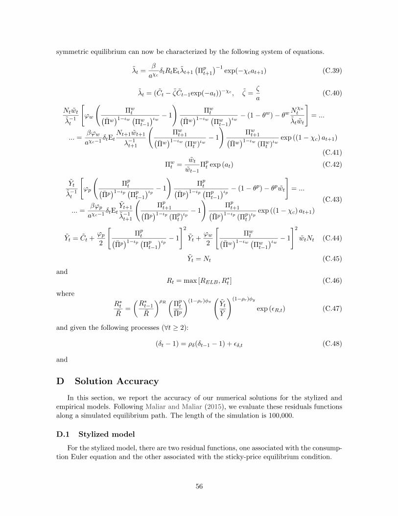
symmetric equilibrium can now be characterized by the following system of equations.

λt =β

aχcδtRtEtλt+1

(Πpt+1

)−1exp(−χcat+1) (C.39)

λt = (Ct − ζCt−1exp(−at))−χc , ζ =ζ

a(C.40)

Ntwt

λ−1t

[ϕw

(Πwt(

Πw)1−ιw (Πw

t−1

)ιw − 1

)Πwt(

Πw)1−ιw (Πw

t−1

)ιw − (1− θw)− θwNχnt

λtwt

]= ...

... =βϕwaχc−1

δtEtNt+1wt+1

λ−1t+1

(Πwt+1(

Πw)1−ιw (Πw

t )ιw− 1

)Πwt+1(

Πw)1−ιw (Πw

t )ιwexp ((1− χc) at+1)

(C.41)

Πwt =

wtwt−1

Πpt exp (at) (C.42)

Yt

λ−1t

[ϕp

(Πpt(

Πp)1−ιp (Πp

t−1

)ιp − 1

)Πpt(

Πp)1−ιp (Πp

t−1

)ιp − (1− θp)− θpwt

]= ...

... =βϕpaχc−1

δtEtYt+1

λ−1t+1

(Πpt+1(

Πp)1−ιp (Πp

t )ιp− 1

)Πpt+1(

Πp)1−ιp (Πp

t )ιp

exp ((1− χc) at+1)

(C.43)

Yt = Ct +ϕp2

[Πpt(

Πp)1−ιp (Πp

t−1

)ιp − 1

]2

Yt +ϕw2

[Πwt(

Πw)1−ιw (Πw

t−1

)ιw − 1

]2

wtNt (C.44)

Yt = Nt (C.45)

andRt = max [RELB, R

∗t ] (C.46)

where

R∗tR

=

(R∗t−1

R

)ρR (Πpt

Πp

)(1−ρr)φπ(YtY

)(1−ρr)φy

exp (εR,t) (C.47)

and given the following processes (∀t ≥ 2):

(δt − 1) = ρδ(δt−1 − 1) + εδ,t (C.48)

and

D Solution Accuracy

In this section, we report the accuracy of our numerical solutions for the stylized andempirical models. Following Maliar and Maliar (2015), we evaluate these residuals functionsalong a simulated equilibrium path. The length of the simulation is 100,000.

D.1 Stylized model

For the stylized model, there are two residual functions, one associated with the consump-tion Euler equation and the other associated with the sticky-price equilibrium condition.

56

R1,t =∣∣∣1− Cχct βδtRtEtC

−χct+1 Π−1

t+1

∣∣∣ (D.1)

R2,t =

∣∣∣∣(Πt − 1) Πt −[(1− θ) + θ(1− τ)wt

ϕ− Cχct

YtβδtEt

Yt+1

Cχct+1

(Πt+1 − 1) Πt+1

]∣∣∣∣ (D.2)

With our log-utility specification, the residual R1,t measures the difference between thechosen consumption today and today’s consumption consistent with the optimization behav-ior of the household, as a percentage of the chosen consumption. The residual R2,t is givenby the difference between (Πt − 1)Πt and the sum of the term involving today’s real wagesand the term involving the expectations. Given that the standard deviation of Πt is about[0.001] (∼= [40] basis points), Πt is always close to one and thus the (Πt − 1)Πt is roughlyequal to (Πt−1). (Πt−1) is the deviation of inflation from the target rate of inflation. Thus,the difference between this term and the sum of the term involving today’s real wages andthe term involving the expectations measures how much the chosen inflation rate differs fromthe inflation rate consistent with the optimization behavior of firms.

Table D.1: Solution Accuracy

Mean[log10(Rk,t)] 95th-percentile of [log10(Rk,t)]Stylized Model

k = 1: Euler equation error −8.5 −7.2k = 2: Sticky-price equation error −9.2 −8.1

Empirical Model

k = 1: Euler equation error −4.0 −3.2k = 2: Sticky-price equation error −5.5 −5.1k = 3: Sticky-wage equation error −5.4 −4.7

Reflecting the large number of grid points used to solve the stylized model, the approxima-tion errors are very small. The average errors on the consumption Euler equation is 0.3∗10−7

percent (= 10−8.5) with the 95th percentile being 6.3 ∗ 10−6 percent (= 100 ∗ 10−7.2). Theaverage errors on the sticky price equation is 2.5 ∗ 10−5 basis points (= 400 ∗ 100 ∗ 10−9.2)with the 95th percentile being 0.0003 basis points ([= 400 ∗ 100 ∗ 10−8.1]).

D.2 Empirical Model

For the empirical model, there are three residual functions of interest. As in the stylizedmodel, the first and second residual functions are associated with the consumption Eulerequation and the sticky-price equilibrium condition, respectively. The third residual functionis associated with the sticky-price and sticky-wage equilibrium conditions.

R1,t =

∣∣∣∣1− β

aχc λtδtRtEtλt+1

(Πpt+1

)−1∣∣∣∣ (D.3)

R2,t =

∣∣∣∣∣(

Πwt

Πw− 1

)Πwt

Πw−[1− θw

ϕw+θw

ϕw

Nχnt

λtwt+

λ−1t

Ntwt

β

aχc−1δtEt

Nt+1wt+1

λ−1t+1

(Πwt+1

Πw− 1

)Πwt+1

Πw

]∣∣∣∣∣(D.4)

57

R3,t =

∣∣∣∣∣(

Πpt

Πp− 1

)Πpt

Πp−[(1− θp) + θpwt

ϕp+λ−1t

Yt

β

aχc−1δtEt

Yt+1

λ−1t+1

(Πpt+1

Πp− 1

)Πpt+1

Πp

]∣∣∣∣∣ (D.5)

Table D.1 shows the average and the 95th percentile of the residuals for the three equilib-rium conditions. The average size of the Euler equation errors is [0.008] percent ([= 10−4.1])with the 95th percentile of the errors being [0.06] percent ([= 10−3.2]). These are larger thanthose in the stylized model, reflecting the coarser grid used in the solution of the empiricalmodel. However, this degree of accuracy fares well in comparison with what’s reported inother studies such as Fernandez-Villaverde, Gordon, Guerron-Quintana, and Rubio-Ramırez(2015) and Maliar and Maliar (2015).

The average size of the sticky-price equation errors is 0.1 basis points (= 400∗100∗10−5.7)with the 95th percentile being 0.2 basis points (= 400 ∗ 100 ∗ 10−5.3). These are againlarger than those in the stylized model, reflecting the coarser grid used in the solution of theempirical model. The sticky-wage equation errors are somewhat larger than the sticky-priceequation errors. The average size is [0.3] basis points ([= 400 ∗ 100 ∗ 10−5.1]) with the 95thpercentile being 0.8 basis points (= 400 ∗ 100 ∗ 10−4.7).

E Expected Time Until the Liftoff

In this section, we present the survey-based measures of the expected time until the liftoffto support the claim that the market participants consistently underestimated the durationof the lower bound episode since the federal funds rate hit the lower bound in late 2008. Thesurveys we examine are (i) the Blue Chip Surveys, (ii) the Survey of Professional Forecasters,and (iii) the Primary Dealers Survey.

The evidence from all three surveys is consistent with the claim that the market partici-pants have consistently underestimated the duration of the lower bound episode. In particu-lar, for the first two years of the lower bound episode, the market participants expected thatthe federal funds rate to stay at the ELB only for additional few quarters.40

E.1 Blue Chip Surveys

The Blue Chip Surveys consists of two monthly surveys, the Blue Chip Economic Indi-cators Survey and the Blue Chip Financial Forecasts Survey. These two surveys ask theirparticipants (about 50 financial institutions for each survey) their forecast paths of variousmacroeconomic variables, including the 3-month Treasury Bill rate in the Economic Indi-cators Survey and the federal funds rate in the Financial Forecasts Survey. The near-termforecast horizon is up until the end of next calendar year and the frequency of the projectionis quarterly. Thus, the forecast path of the Treasury rate or the federal funds rate can tellus the expected time until the liftoff when the participants expect the first liftoff to occurwithin two years.

Twice a year, the surveys ask longer-run projections of certain variables in the specialquestion section (March and October for the Economic Indicators and June and Decemberfor the Financial Forecasts). The longer-run forecasts are in annual frequency for next 5 to 6years. Towards the end of the lower bound episode, the Surveys also asked the participantsto provide the expected liftoff date in the special questions section.

40While not shown, the expected duration of the lower bound episode based on the expected policy pathimplied by the federal funds rate futures is also consistent with this claim.

58

For each survey, we combine these various pieces of information in the following wayto construct a series for the expected period until the liftoff. First, we use the averageprobability distribution over the timing of the liftoff to compute the expected time until theliftoff whenever that information is available. Second, if the probability distribution is notavailable, we use the information from the near-term forecasts. The time of liftoff is definedto be the first quarter when the median federal funds rate forecast exceeds 37.5 basis points.Finally, when the policy rate is projected to stay at the ELB until the end of the near-termforecast horizon, we use the information from the long-run projections if the Survey has thatinformation and leave the series blank when the Long-Range section is not available.

Figure E.1: Expected Time Until Liftoff†

2009 2010 2011 2012 2013 2014 2015 2016

Year

0

2

4

6

8

10

12

Du

ratio

n (

in q

ua

rte

rs)

Blue Chip Economic Indicators

2009 2010 2011 2012 2013 2014 2015 2016

Year

0

2

4

6

8

10

12

Du

ratio

n (

in q

ua

rte

rs)

Blue Chip Financial Forecasts

2009 2010 2011 2012 2013 2014 2015 2016

Year

0

2

4

6

8

10

12

Du

ratio

n (

in q

ua

rte

rs)

Primary Dealers Survey

2009 2010 2011 2012 2013 2014 2015 2016

Year

0

2

4

6

8

10

12

Du

ratio

n (

in q

ua

rte

rs)

Survey of Professional Forecasters

† Data sourced from: Blue Chip Economic Indicators Survey (from January 2009 to August 2015); Blue Chip FinancialForecasts Survey (from January 2009 to August 2015); Federal Reserve Bank of New York, Primary Dealer Survey,accessed September 2015, https://www.newyorkfed.org/markets/primarydealer˙survey˙questions.html; Federal ReserveBoard, Survey of Professional Forecasters, accessed September 2015, https://www.philadelphiafed.org/research-and-data/real-time-center/survey-of-professional-forecasters/

The top two panels in Figure E.1 show the evolutions of the expected period until liftoffbased on the Blue Chip Economic Indicators Survey and the Blue Chip Financial ForecastsSurvey. According to both panels, the market participants expected the lower bound episodeto be transitory in the early stage of the lower bound episode. The expectation shifted inthe second half of 2011, with the expectated duration of staying at the ELB exceeding 2years. Starting in late 2012 or early 2013, the survey respondents gradually reduced theirexpectation for the additional duration of the lower bound episode.

59

E.2 Primary Dealers Survey

The Primary Dealers Survey (the PD Survey in the remainder of the text), conducted bythe Federal Reserve Bank of New York, asks primary dealers about their policy expectationseight times a year. The survey asks its participants their probability distribution over theliftoff timing (quarter or FOMC meeting). We compute the expected time until the liftoffusing the average probability distribution over the liftoff timing. The results of the PD Surveyare publicly available since January 2011.

The bottom-left panel of Figure E.1 shows the evolution of the expected period until theliftoff based on the PD Survey. Consistent with the measures based on the Blue Chip survey,the expected duration of the additional period of the lower bound episode increase markedlyin the second half of 2011. The expected duration hovers around 10 quarters during 2012,and has declined steadily since then.

E.3 Survey of Professional Forecasters

The Survey of Professional Forecasters (SPF) is a quarterly survey of about 40 individ-uals in academia, financial industries, and policy institutions, administered by the FederalReserve Bank of Philadelphia. Like the Blue Chip Surveys, the SPF asks its participantstheir projections of various macroeconomic variables, including the 3-month Treasury rate.For the near-term projection that extends to the end of the next calendar year, the forecastsare available in quarterly frequency. For the longer horizon, the forecast is available in annualfrequency.

The bottom-right panel of Figure E.1 shows the evolution of the expected period untilliftoff based on the SPF. Consistent with the Blue Chip Surveys and the Primary DealersSurvey, the SPF shows that the market anticipated the lower bound episode to last for onlyabout one additional year until the second half of 2011. The expected duration averagesabout 9 quarters in 2012 and 2013. The expected duration started declining in the secondhalf of 2013 and has come down to 2 quarters in February 2015.

F Further discussion on the risk-adjusted monetary policyrule

F.1 Interpreting the central bank’s inflation objective

Throughout the paper, we interpret the central bank’s inflation objective as specifyingthe desired level of the risky steady state inflation. Under this interpretation, the dynamicsof inflation are consistent with the central bank’s inflation objective of x percent if the riskysteady state of inflation is x percent. Accordingly, our focus in Section 5 was on how tomodify the policy rule to eliminate the wedge between the risky steady state inflation andthe central bank’s inflation objective. However, some have interpreted the central bank’sinflation objective as specifying the average rate of inflation over a long period of time. Underthis alternative interpretation, the dynamics of inflation are consistent with the central bank’sinflation objective of x percent if the unconditional average of inflation is x percent. The paperby Reifschneider and Williams (2000) is a prominent example adopting this interpretation.In our model, the unconditional average of inflation is also below the target rate of 2 percent,as shown in Table 5. Thus, the need for adjusting the policy rule can also arise under thisalternative interpretation of the central bank’s inflation objective.

60

Our intercept-adjustment procedure can be easily modified if modelers take this alterna-tive interpretation and want to set the unconditional average of inflation, as opposed to therisky steady state of inflation, to the central bank’s inflation objective. Specifically, modelerswould need to search for the size of the intercept adjustment such that the unconditionalaverage of inflation, instead of the risky steady state inflation, equals the central bank’s in-flation objective. In our example, the intercept that achieves the unconditional average ofinflation of 2 percent is lower than the intercept that achieves the risky steady state inflationof 2 percent, because the unconditional average of inflation is lower than the risky steadystate inflation in the model with the standard policy rule, as shown in Table 5.

While our intercept-adjustment procedure is useful regardless of the interpretation of thecentral bank’s inflation objective adopted by modelers, it is perhaps appropriate to explainwhy it is more plausible to interpret the central bank’s inflation objective as specifying thedesired level of the risky steady state inflation than as specifying the desired unconditionalaverage of inflation.

The interpretation that the central bank’s inflation objective specifies the desired uncon-ditional average of inflation is inconsistent with the inflation projections by U.S. policymakersin the following sense. In the United States, both core and overall PCE inflation rates aver-aged non-trivially below 2 percent over the last decade or so. Thus, to achieve the averageinflation rate of 2 percent over a long period of time, policymakers will need to overshootthe target rate non-trivially and persistently in the future. However, according to recentreleases of the Summary of Economic Projections (SEP), U.S. policymakers expect inflationto return to 2 percent in the long-run without any overshooting.41 In the aftermath of a re-cession, the inflation projection from the model with the risk-adjusted monetary policy rulemonotonically increases with forecast horizon and eventually converges to the risky steadystate inflation. Thus, the eventual return of the inflation projection to 2 percent without anyovershooting in the SPE is consistent with the interpretation that the central bank’s inflationobjective specifies the desired level of the risky steady state inflation.42

In a similar vein, Draghi (2016) states that “In the ECB’s case, our aim is to keep inflationbelow but close to 2 percent over the medium term. Today, this means raising inflation backtowards 2 percent.” Thus, even though inflation in the euro area, as measured by the HICP,averaged below 2 percent over recent years, ECB policymakers do not seem to interpret theirmandate to be consistent with aiming for a transitory overshooting of inflation rates close to2 percent.

The issue described in this section has not received much attention because linear mone-tary DSGE models have been predominant tools for model-based analyses of monetary policyuntil recently. In linear monetary DSGE models, the inflation target parameter in the pol-icy rule coincides with the risky steady state of inflation and the unconditional average ofinflation. Researchers typically set the inflation target parameter to the central bank’s infla-tion objective, and because of this coincidence, there is less need to think about conceptualdifferences among these objects. Our analysis highlights the importance and difficulty ofunderstanding conceptual differences among the central bank’s objective, the inflation targetparameter, and the risky steady state and the unconditional average of inflation, as nonlinearmodels become more widely used in the analyses of monetary policy.

41See, for example, the Summary of Economic Projections released on June 15, 2016 (available at www.

federalreserve.gov/monetarypolicy/files/fomcprojtabl20160615.pdf).42Note that, if the central bank tries to achieve an inflation objective at the unconditional mean, that

policy is better characterized as a price level targeting.

61

F.2 Other applications

As discussed in the main text, the difference between the deterministic steady state andrisky steady state are nontrivial in our empirical model even without the ELB constraint. Thedifference between the deterministic steady state and risky steady state caused by nonlinear-ities that are unrelated to ELB can be quite large depending on specifications of other partsof the model. Thus, our proposed intercept-adjustment will be useful in such applicationseven if the model abstracts from the ELB constraint.

In addition to the ELB constraint on nominal interest rates, researchers are increasinglyinterested in the implications of other inequality constraints in macroeconomic models. Forexample, since the Great Recession, the literature on financial frictions has been developingrapidly, examining the implications of occasionally binding borrowing constraints on thehousehold or leverage constraints on banks. Our risk-adjusted policy rule is likely to beuseful in models featuring these other inequality constraints.

62