
e Dissertation
85
CHAPTER ONE 1.0 INTRODUCTION Nigeria is facing the twin problem of underdevelopment and stagnant growth rate despite its natural position as a green area with huge resource endowment. It manifests most of the attribut es of sub-Sa haran Africa which has about the large st absolute increase of 72 million people in the last decade. About 70 percent of Nigerians live on less than N100 / day (US$ 0.7/da y), while youth unemployment is close to 90 percent (EZE,2003 ). The country has a large informal sector in which a substantial number of the unemployed take up employment (CBN, 2000a). The poverty syndrome is a bit difficult to understand with Nigeria being the sixth world highest producer of crude oil and earning upwards of US$ 15 billion annually (CBN, 2000b). Regrettably in 2002 alone, 80 percent of the national earning accruing from oil exportation was spent on maintaining the government, leaving only 20 percent for economic development. This partly explains the nature of budgetary 1
Transcript of e Dissertation

8/8/2019 e Dissertation
http://slidepdf.com/reader/full/e-dissertation 1/84
CHAPTER ONE
1.0 INTRODUCTION
Nigeria is facing the twin problem of underdevelopment and stagnant growth rate despite
its natural position as a green area with huge resource endowment. It manifests most of
the attributes of sub-Saharan Africa which has about the largest absolute increase of 72
million people in the last decade. About 70 percent of Nigerians live on less than N100 /
day (US$ 0.7/day), while youth unemployment is close to 90 percent (EZE,2003 ). The
country has a large informal sector in which a substantial number of the unemployed take
up employment (CBN, 2000a). The poverty syndrome is a bit difficult to understand with
Nigeria being the sixth world highest producer of crude oil and earning upwards of US$
15 billion annually (CBN, 2000b). Regrettably in 2002 alone, 80 percent of the national
earning accruing from oil exportation was spent on maintaining the government, leaving
only 20 percent for economic development. This partly explains the nature of budgetary
1

8/8/2019 e Dissertation
http://slidepdf.com/reader/full/e-dissertation 2/84
problems facing the nation. The question then is, what intervention option besides the oil
sector, does the nation have for sustainable growth?
Nigeria’s overall economic performance since Independence in 1960 has been decidedly
unimpressive. According to World Bank data, the average annual growth rate of Gross
Domestic Product (GDP) between 1960 and 2000 was less than 4 percent. Thus, despite
the availability and expenditure of colossal amounts of foreign exchange obtained mainly
from its oil and gas resources, Nigeria’s economic growth has been weak and the
incidence of poverty has increased. It is estimated that Nigeria received over US$228
billion from oil export receipts between 1981 and 1999 (Udeh, 2000). Yet the number of
Nigerians living in abject poverty- that is, on less than US$1 a day – more than doubled
between 1970 and 2000, and the proportion of the population living in poverty rose from
36% in 1970 to 70% in 2000. Nigeria’s per capita income of US$260 in 2000 is much
less than, indeed it is only one-third of its level, US$780, in 1980, World Bank (2003).
Nigeria faces the challenge of meeting the macroeconomic targets of growth rate and
development. Nigeria is among the world’s 27 poorest countries, according to the United
Nations Development Programme (UNDP 2001). The country has had lost decades of
development due to negative and slow growth and has been one of the weakest growing
economy in the world on a per capita basis especially for the period between 1981- 2000.
In analysing the major macroeconomic targets of growth rate we will be looking at the
aggregate GDP, the manufacturing sector, agricultural sector, the service sector which are
basically the non-oil sector for this particular study. The level of economic development
and growth rate over the decades has been disappointing. The real sector is dominated by
the primary sectors of the economy which has always been the crude oil sector. The
agricultural sector is a predominating sector with a low and declining productivity. This
sector has stagnated and failed to keep pace with the needs of the rapidly growing
population in Nigeria. The crude oil sector is categorised to fall under the primary sector
for which the resources from this particular sector has not been diversified to other
sectors of the economy to enhance growth and development in other sectors. Using a
poverty frontier of US$2 per day, Collier and Dollar (1999:33) reports that 60% of
Nigeria’s population was below the poverty line in 1996. A recent report issued by the
2

8/8/2019 e Dissertation
http://slidepdf.com/reader/full/e-dissertation 3/84
Federal Government of Nigeria confirms that the problem of poverty is acute. According
to the report titled “Poverty alleviation policy”. With a per capita income of about
US$300 and a human development index of 0.4, Nigeria is a poor country despite the
abundance of human, material and natural resources. Recent studies show that at least
50% of the population is poor while another 30% may be regarded as moderately poor.
The majority of the poor, over 70%, are located in the rural areas where most of the
people and national resources are located. The paradox of this is that she is ranked the 6th
largest producer of petroleum in the world. Nigeria nevertheless has one of the lowest
GDP per capita incomes: $970 in purchasing power parity-adjusted U.S. dollars.
The secondary sector deals with the manufacturing sector, and the service sector. Themanufacturing sector is one sector of the economy that has classified Nigeria as the least
industrialized countries in Africa. This sector of the economy has been stale and entails
about 5 - 7% of GDP, according to NEEDS report (2004, p.20). In the industrial sector, it
is the role of the manufacturing sector that appears to be the strategic factor in modern
economic growth. ‘Solow stated that development cannot occur without growth (Hall,
1983:19). Thus, the objective of this paper is to analyse the impact of the major various
sectors contributions to economic growth and development, laying more emphasis on the
manufacturing sector, agricultural sector, and the service sector. The Global Research
Project, ‘Explaining Growth’ is an attempt to compile the most comprehensive
assessment of growth in developing and transition countries. Yuba and Suman (2002
p.1). This research work on growth consists of three phases. Phase one of the study
comprises the progression of growth. The current dilemma in understanding economic
development and growth is not just about understanding the process by which an
economy raises its savings rate and boosting the rate of physical capital accumulation, but
'something else’, which captures the differences in economic growth and economic
development, TFP is usually ascribed to as the 'something else', which contributes to the
differential growth rates.
1.1 JUSTIFICATION OF STUDY
3

8/8/2019 e Dissertation
http://slidepdf.com/reader/full/e-dissertation 4/84
By the time Nigeria became politically independent in October 1960, the agricultural
sector was known to be the dominant sector of the economy, contributing almost 70% of
the Gross Domestic Product (GDP). But today, the development of this sector tends to be
neglected. In as much as the government has been trying to provide stable growth rate in
the core sectors, the truth still remains that there are lack of distribution of resources for
the development of these non-oil sectors.The major sector contributions to economic
growth in Nigeria, for the purpose of this study will be the economic indicators which are
basically the Consumption expenditure, gross fixed capital formation (GFCF) this will
serve as the gross investments , government expenditure, net exports and lagged variables
of GDP. Over the years, too much attention has been allocated to indicators that do not
have significant impact on GDP in Nigeria. The country’s decade of development plans
has not led to increase growth rate in the non-oil sectors which consist of the
manufacturing industry, service sector and the agriculture industry in country. High
productivity in the non-oil sectors like the industrial, agricultural and the service sectors
are essential for rapid economic growth and development in Nigeria. Transformation in
the relative significance of agriculture, service and industry has been recognized as the
core sectors for the process of growth. In the industrial sector, it is the role of
manufacturing sector that seem to be the significant factor in modern economic growth.
Barro (1990) concludes that the role of public service (infrastructure) creates positive
linkage between government and growth. Barro's work established that there is a negative
correlation between growth in government expenditure and economic growth, as well as
savings rates for governments whose expenditures provide consumption services only.
The role of government in development is a controversial one. Datta-Chandhuri (1990)
notes "the success of Keynesian activism in fighting the great depressions in the western
countries, the success of the Marshall Plan in engineering the quick reconstruction of the
war-damaged economies of western Europe, and the achievements of the Soviet
industrialization drive in the 1930s had created a virtual intellectual consensus in the
world on the power of the "visible hand. There is no doubt that the state has a role to play
in the economic development of a country. The importance of the study therefore lies
4
8/8/2019 e Dissertation
http://slidepdf.com/reader/full/e-dissertation 5/84
with the fact that government should pay attention and devote economic resources to the
growth of non-oil sectors. The Nigerian economy should be concerned about policy
implementation that tends to hamper its efforts in development. If the implementation
problem is to be alleviated, it is of paramount significance that the nature of the existing
measures maybe taken.
1.2 AIMS AND OBJECTIVES OF THE STUDY
This dissertation examines Nigeria’s economic growth in three steps. First, it conducts a
straightforward examination of past economic growth trends by looking at the
contributions of the major economic sectors in Nigeria to the GDP which includes the
manufacturing sector, the agricultural sector and the service sector from 1970 to 2005.
Secondly it presents an in-depth literature on economic growth which explains the
determinants of growth. The review takes into consideration both theoretical and
empirical literature on growth which are considered as important determinants of growth.
Thirdly it also aims at identifying which components of growth is the most important
determinant of economic growth in Nigeria by regressing the GDP of Nigeria against the
following independent variables: Consumption expenditure, gross fixed capital formation
(GFCF) this will serve as the gross investments , government expenditure, net exports
and lagged variables of GDP. The statistical aggregate of GFCF is a measure of the net
investment by enterprises in the domestic economy. This usually comes in as fixed
capital assets during an accounting. Due to data availability GFCF is used in place of
gross investment, this is due to the fact that GFCF time series is often used to analyse the
trends in investment activity over time. These variables are considered because they are
readily available and form the core components in econometric studies of this kind. This
research therefore reveals how important the traditional determinants of growth
(consumption expenditure, gross fixed capital formation, government expenditure and net
exports) as used in the study and variables on how investments on the GDP dependent
variable will greatly influence or impact economic growth rate in Nigeria. The GDP of
Nigeria is used as a proxy for economic growth. This study is carried out econometrically
using both univariate and multivariate regression techniques. GDP (the dependent
5
8/8/2019 e Dissertation
http://slidepdf.com/reader/full/e-dissertation 6/84
variable) is regressed on all the independent variables indicated above for the period 1970
to 2005.
1.3 SIGNIFICANCE OF THE STUDY
This study is significant for various reasons; firstly the study provides an insight into the
determinants of economic growth and development which enriches the existing literature
on the topic by exploring some of the most recent literatures on economic growth and
applying it to the Nigerian economy. Secondly the study on the sectoral contribution to
economic growth in Nigeria will give an insight of which sectors of the Nigeria economy
will dominate in attracting economic growth and development. The results obtained from
this agenda can assist the Nigeria government in the country’s economic policy to
attracting growth and development and as well help in addressing what measures can be
taken in boosting economic growth and development.
1.4 ORGANISATION OF THE STUDY
Chapter two reviews the relevant literature on the subject under study. This chapter looks
at the determinants of growth, outlines and explains the factors that attract growth to a
country. Chapter three comprises the research methodology as well as the econometric
model to be used in the empirical analysis. Chapter four gives an overview of the overall
assessment of the Nigeria economy. This chapter outlines the economic performance of
the Nigeria economy. In chapter five the actual test is conducted and the results
discussed. Chapter six concludes the study and tenders some policy implication for
boosting growth in Nigeria.
6
8/8/2019 e Dissertation
http://slidepdf.com/reader/full/e-dissertation 7/84
CHAPTER TWO
LITERATURE REVIEW
2.0 INTRODUCTION
The literature on the analysis and contributions of economic growth and development is
vast and inconclusive. Many economists and other social scientists would say that drives
to develop are present but are masked by current political structures and organisation
barriers. Many theories have been developed by economist over the years to explain
economic growth and development. These usually try to identify what the determining
factors that contribute to growth and development are. Nevertheless this literature
remains one of the most researched with respect to development and growth. The
importance of the economic growth and development can hardly be over-emphasized.
The likes of Hamilton (1995) were of the opinion that economic growth is unsustainable,
if the elasticity of substitution between exhaustible resources and reproducible capital is
7
8/8/2019 e Dissertation
http://slidepdf.com/reader/full/e-dissertation 8/84
less than unity. Growth can be regarded as one of the mainstays of a modern economy. It
is challenging for any researcher to point at a particular set of theory or determinants
which contributes to economic growth and development. In this chapter an extensive
review of the literature relating to the application of economic growth and development,
sources of economic growth by explaining the use of GDP in Nigeria as a proxy for
economic growth which accounts for national income in an open economy such as that of
Nigeria, sectoral contributions and their impacts to GDP is reviewed. This dissertation
empirically assesses conflicting views that retards various factors to economic growth.
The approach complements the growth literature, which examines the relationship
between the level of development and economic growth. This study adds to a large
policy-oriented literature on the relationship between economic development and growth.
This paper highlights some policy approach that will boost the Nigerian economic
performance.
2.1 DETERMINANTS OF ECONOMIC GROWTH
Understanding the growth process is central in the context of development economics;
while theory is useful to streamline guidance for identifying, analysing and interpreting
the determinants of growth. Most of the empirical literature is actually based on cross-
country growth regressions, which are seen as being useful in identifying those factors
that most consistently appear to be important determinants. The existing studies of
determinants of growth can be grouped into several categories, there are studies which
focused on the explanation of Output growth of an economy can be attributed to many
reasons. Technological progress, capital accumulation, employment growth and
institutional change are attributed to be driving forces of economic growth. Levine and
Renelt (1992) and Sala-i-Martin (1997) identify investment as a key determinant. High
investment ratios do not necessarily lead to rapid economic growth; the quality of
investment, its productivity, existence of appropriate policy, political, and social
8
8/8/2019 e Dissertation
http://slidepdf.com/reader/full/e-dissertation 9/84
infrastructure are all determinants of the effectiveness of investment (Hall and Jones,
1999; Fafchamps, 2000; Artadi and Sala-i-Martin, 2003). Investment in general is
often seen as the engine that drives a country’s economy; Investment can be classified
into public and private investment. Public investment provides the necessary
infrastructure that is need for the economy while private investment is the driving force
that spins the economy. Public investment can affect growth either directly, through
productivity, or indirectly through the effect on private investment. Public investment in
human capital, law and order, research and development, and social and economic
infrastructure leads to creation of positive externalities which in turn improve the
productivity of private investment. One of the principal determinants of growth necessary
for any takeoff is the mobilization of domestic and foreign saving in order to generate
sufficient investment to accelerate economic growth. The growth mechanism by which
more investment leads to more economic growth can be described in terms of the Harrod-
Domar growth model. Every economy should be able to save certain proportion of its
national income in order to be able to replace worn out or impaired capital goods.
However in order to grow, new investments representing net additions to the capital stock
are considered important. Every good economy’s growth rate should greatly depend on
the level of savings, the savings ratio and as well the productivity of investment. Thus,
one would expect a positive relationship between public investment and economic
growth (Barro, 1991, 1996, 2003; Artadi and Sala-i-Martin, 2003). Conventional
macroeconomic policies such as government investment can greatly affect the level of
per-capita income but they have no effect on the long run growth rate of the economy
Barro (1991), Mankiw et al. (1992) and Barro and Sala-i-Martin (1992).
Kaipornsak (1995) studied the source of economic growth and found that spending on
R&D, especially government expenditure, and the degree of openness with the emphasis
on FDI were major factors.
Another factor that is related to investment is foreign aid. In theory, foreign aid could
relax any or all of three constraints on investment (Bacha, 1990). The constraint on
savings give rises to low-income countries, domestic savings are not sufficient to meet
the requirements of the general investment as a whole. There are constraint which
9
8/8/2019 e Dissertation
http://slidepdf.com/reader/full/e-dissertation 10/84
captures the possibility that government reactions can affect private savings and public
investment and this can affect investment. Chenery and Strout (1966) also posit a
knowledge gap in developing countries and foreign aid in the form of technical assistance
can relax this constraint (and increase productivity). If foreign aid is used to relax these
constraints it is expected to be positively correlated with investment and growth
(Hjertholm et al, 2000). Elbadawi (1999) argues that the African foreign aid causes
exchange rate appreciation thereby dampening growth of exports and thus economic
growth. Foreign trade is one major variable that influences private investment and
ultimately economic growth.
According to neoclassical thinking, openness to trade has many advantages such as
efficiency gains that come with specialisation and competition from international trade;
embodied technological transfer through imported inputs; scale economies arising from
expanded markets, and diffusion of ideas through global interaction (Piazolo, 1995;
Zhang and Zou, 1995; Harrison, 1996; Frankel and Romer, 1999). The literature on
trade and growth tends to mainly pay attention on exports, there are two justifications for
concentrating on imports – they represent imported technology, capital, and intermediate
goods and to some extent they can be used directly for investment. Michaely (1977)
tested the hypothesis "that a rapid growth of exports accelerates the economy's growth of
a country." Balassa (1985) concluded that "trade orientation has been an important factor
contributing to inter-country differences in the growth of output. Dornbusch and
Reynoso (1988) concluded that there was no evidence to attribute rapid development of a
country to financial liberalization alone. Tyler (1981) argues that the dramatic economic
success of some countries pursuing export oriented policies, along with the equally
dramatic failures of those countries pursuing autarkist policies, has provided examples
necessitating a reexamination of the role of international trade in the development of poor
countries. Thus, he concluded that countries which neglect their export sectors through
discriminatory economic policies are likely to have to settle for lower rates of economic
growth as a result.
2.2 A BRIEF HISTORY OF GROWTH THEORIES AND EMPIRICS
10

8/8/2019 e Dissertation
http://slidepdf.com/reader/full/e-dissertation 11/84
Studies conducted on growth theories draws back to Adam Smith’s (1776) An Inquiry
into the Nature and Causes of the Wealth of Nations may be seen as a suitable starting
point for economic growth theories. In Smith (1776), not only capital accumulation but
also technological progress and institutional and social factors play a crucial role in the
economic development process of a country (Kibritcioglu, 1997). Smith distinguished
between three different stages of economic growth. In his own view, some nations were
at “a low level equilibrium trap” because of “bad-governance” and an insufficiency in
maintaining common human rights and freedoms or “property rights” in modern
parlance. This, stated was due to cultural and institutional backwardness of these
countries.
Developed nations in his time were England and North America but they were only at the
second stage of development. They were still in a “natural freedom” environment, and
therefore, in an ongoing economic growth process. Smith believed that no country in the
18th century was rated at the third stage of economic growth. According to his view, the
natural environment limits economic growth beyond a certain level. Falling profit rates
along with the growth path of an economy gives way to changes in the relative factor
scarcity and decreases in profitable investment opportunities all play a role in
constraining economic growth. Thus, every developing economy had to slow down and
stop at an upper limit of development. The notion of an upper limit to growth is perhaps
related to the agrarian based economy of Smith’s age. As a corollary of the model,
government policies can affect the long-run growth rate of real output in an economy.
The standard neoclassical growth model implies that the steady state growth rate, aside
from exogenous technological progress, is zero.
In this case our focus is to find the statistically significant relationship between GDP and
some economic indicators in Nigeria. Theories of growth are highly aggregated usually
featuring only one or two types of output and a limited number of inputs. Exogenous
growth models that have focused primarily on the role of factor accumulation in the
growth process, as well as endogenous growth models given examples from Romer
1990, Grossman and Helpman 1991, and Aghion and Howitt 1992 have devoted their
11
8/8/2019 e Dissertation
http://slidepdf.com/reader/full/e-dissertation 12/84
attention to the role of endogenous technological progress in the process of development,
were designed to capture the main characteristics of the Modern Growth Regime. These
models are however not consistent with the pattern of development that had characterized
economies over most of human existence. Most endogenous and exogenous growth
models are not consistent with the changes in the demographic regime along the process
of development.
2.3 FACTORS THAT ATTRACTS GROWTH TO A COUNTRY
The kind of factors which attracts any form of growth and development to a country
differs. To disentangle the sources of economic growth one needs an analytical
framework to assess the contribution of various factors to growth. This involves the
formulation of theories, models and hypotheses on the role of accumulation, productivity
and technology. In the last decades this has been the concern of economists and economic
historians; however there is no consensus on what emphasis that should be given to the
key factors behind growth. The significance of economic growth involves as follows; the
role of investment as a form of foreign investment, technological progress and financial
development.
One of the factor economists anticipate is that financial integration will lead to more
investment with a progress on more efficient allocation of capital. Increase in investment
is expected because of financial integrated markets. Financial integration is not an end in
itself but rather a means to achieve higher economic growth. Greater investment and its
more efficient allocation are the two principal channels through which financial
integration will lead to growth. The prevailing view in economics is that financial
development contributes greatly to growth in various ways. Economists have found
empirical evidence that countries with developed financial systems tend to grow faster
and rapidly. King and Levine (1993) pointed out that early literature tried to explain that
growth is positively related to the level of financial development. Given evidence from
80 countries from 1960 to 1989, they show that the relative size of the financial sector in
1960 is positively correlated with economic growth over the period. However, positive
12

8/8/2019 e Dissertation
http://slidepdf.com/reader/full/e-dissertation 13/84
correlation may simply reflect the fact that faster and rapidly growing countries have
larger financial sectors because of the increase in the number of financial transactions
conducted. Subsequent work using statistical techniques to control for the endogenous
effect of economic growth on financial development as well as for country-specific
factors that are not explicitly considered, and using both time series and cross-sectional
data to extract more information from the data, has analyzed this information more
efficiently. In addition, once a project has started, they can better monitor its managers to
the effect of financial development is robust (Levine, Loayza, and Beck 2000,
Benhabib and Spiegel 2000).
2.4 EVIDENCE FROM SOME SELECTED EMPIRICAL STUDIES
Studies on the contribution to economic growth have been studied differently in past
research. These studies have been conducted at inter country level. Inter country studies
gives an insight on the pattern of growth varies across nations in terms of their different
characteristics. In this section we review briefly some of the findings conducted on
growth rate simply because this study is interested in estimating the determinants of
growth of which sectoral investment is likely to have a positive effect on GDP growth.
The benefit of these studies is that it helps developing countries to formulate good
policies which help to attract growth and development.
The pioneer work in this regard is the work of Lucas (1988) which explained that the
growth rate of human capital is also dependent on the amount of time, allocated by
individuals to acquire skills found out that time investment positively the growth rate of
human capital. Rebelo (1991) using the time investment as a proxy for growth rate
human capital yielded the same result but later extended the model by introducing
physical capital as an additional input in the human capital accumulation function.
However, the model of endogenous growth by Romer (1990) assumes that the creation
of new ideas is a direct function of human capital, which manifests in the form of
knowledge. As a result investment in human capital led to growth in physical capital
which in turn leads to economic growth. Other studies that supported the human capital
accumulation as a source of economic growth include (Barro and Lee, 1993; Romer,
13

8/8/2019 e Dissertation
http://slidepdf.com/reader/full/e-dissertation 14/84
1991; Benhabib and Spiegel, 1994). Some studies have examined different ways
through human capital can affect economic growth, however recent studies on growth
factors such as human growth accumulation influence the determinants of growth have
been diverse from one research to the other. Gupta and Chakraborty (2004) developed
an endogenous growth model of a dual economy where human capital accumulation is
the source of economic growth. Bratti et al (2004) estimated a model of economic
growth and human capital accumulation based on a sample of countries at a different
stage of development. Based on this identification of structural constraints to growth and
development, it is not surprising that a major part of colonial economic policies was
devoted to tackling some of these, even if in obviously inadequate terms. It was that need
to reduce the fragility of the economy and hasten structural change that informed early
post-independence development strategy (World Bank 1993). Although the techniques
employed in past studies seem to be accurate, one cannot concretely point at what
particular factors that determines economic growth and development in a country. At best
these studies give a general idea of what determines economic growth and development.
CHAPTER THREE
NIGERIAN ECONOMY: AN OVERALL ASSESSMENT
3.0 INTRODUCTION
This chapter is aimed at presenting an overview of the economic performance of the
Nigeria economy from 1970 to 2005. This chapter provides a brief overview of Nigeria’s
key development challenges in order to provide a basis for assessing contributions to the
nation’s development priorities during this period (1970-2005). Nigeria is a relatively
large nation of considerable wealth, it has a rich natural resource endowment and
relatively high levels of human and social capital. Notwithstanding its wealth and
considerable economic potential, Nigeria has not as yet succeeded in effectively
translating its potential into economic growth, human development and overall social
14

8/8/2019 e Dissertation
http://slidepdf.com/reader/full/e-dissertation 15/84
transformation. This chapter reviews the Nigerian economy by focusing on the
contributions of the major sectors to GDP.
3.1 THE STRUCTURE OF THE ECONOMY
An analysis of the structure of the Nigerian economy is fundamental for comprehending
the predominance of poor economic growth and development in the country. During the
period of independence in 1960, the backbone of the national economy relied primarily
on agricultural sector. The agricultural sector accounted for more than half of its national
output between 1950 and 1960. The attraction drawn to the agricultural sector was later
diverted to the oil sector, which became a major source of revenue. The oil boom
transformed the economy drastically. The economy became absolutely dependent on the
oil sector, which accounted for more than 98 per cent of export earnings. From table 3.1
below, the manufacturing sector has experienced rather sluggish growth since around
1970, while the services sector appears to have had persistent growth interrupted only by
the economic recession of the 1980s. The agricultural sector has experienced a general
improvement in a portion of GDP since 1985, over the incessant increase from 26.6 to
about 40.8 in 1990. Over the same period, oil and mining fell to about 14 per cent of
GDP, while infrastructure and services appear to stabilize at lower levels of about 9 per
cent and 28 per cent, respectively, between 1987 and 1990.
Table 3.1 Distribution of gross domestic product in Nigeria for selected years (%)
(1960-1990)
Sector 1960 1965 1970 1975 1980 1985 1987* 1990
Agriculture 64.1 55.4 44.7 26.5 21.1 26.6 40.2 40.8
Mining 1.2 4.7 11.9 23.9 24.1 19.8 13.4 13.8
Manufacturing 4.8 7.0 7.5 4.5 8.9 9.3 9.7 8.5
Infrastructure 8.9 10.4 9.1 15.4 17.6 12.8 8.0 8.6
Services 21.0 22.5 26.8 29.7 28.3 31.5 28.7 28.3
Total 100 100 100 100 100 100 100 100
Value (Nm) 2 493.4 3 146.8 4 219.0 26 283.3 30 808.3 26 159.0 79 270.0 89 100.0
15
8/8/2019 e Dissertation
http://slidepdf.com/reader/full/e-dissertation 16/84
Source: Central Bank of Nigeria. Annual Report and Statement of Accounts,
Various Issues
Analysing one the recent work of the Central Bank of Nigeria (CBN, 2000) highlights
most of the structural issues in perspective, with supporting data as evidence. Agriculture
dominates the Gross Domestic Product (GDP), but its contribution has reduced gradually
over the years since the accomplishment of political independence in 1960. This ratio
drastically dropped from 64.1% in 1960 to 28.35% in 2002, this is detailed in the table
above. An economy that experiences rapid and sustained growth that is not less than 6–
10% per annum at the end of the present Administration’s tenure, the creation of a
national economy that is highly competitive, responsive to incentives, private sector–led,
broad-based, diversified, and market-oriented and open, but based on internal momentumfor its growth is the aim. (Nigeria, Ministry of Finance 2000c, pp. 8–9)
3.2 GENERAL PERFORMANCE OF THE ECONOMY
The Nigerian economy has had a truncated history. Between the period of 1960 and 1970,
the Gross Domestic Product (GDP) recorded was 3.1 per cent growth annually. During
the oil boom era, which was in the period of 1970 to 1978, GDP grew positively by 6.2
per cent annually; this signified a remarkable growth. In the period of 1980s, the growth
rate of GDP dropped negatively. Between the periods of 1988 to 1997, the GDP
responded positively at a rate of 4.0, this period was a period there was economic
adjustment policy which is known as the structural adjustment and economic
liberalization. After independence, the industry and manufacturing sector had a slowly
positive growth rate given exception for the period of 1980 to 1988, during this time
frame of the two periods, the industry and manufacturing sector grew negatively by 3.2
per cent and 2.9 per cent respectively. The growth rate for the agricultural sector for the
periods 1960 to 1970 and 1970 to 1978 was unsatisfactory. In the early 1960s, the
agricultural sector declined in low commodity prices while the oil boom contributed to
the negative growth of agricultural sector in the 1970s. The services sector includes
wholesale and retail trade, real estate, government services, transportation, financial,
16

8/8/2019 e Dissertation
http://slidepdf.com/reader/full/e-dissertation 17/84
communication, hotels and restaurant services. According to Nigeria Bureau of Public
Enterprise (BPE 2000) the three highest contributors to Nigeria’s GDP are agriculture
(34.62%), oil (33.44%) and Service (12.45%).
3.3 AN OVERVIEW OF THE AGRICULTURAL SECTOR
Agriculture is the backbone of the rural economy, generating more than 30 percent of
gross domestic product (GDP) and so far has provided the largest source of rural
employment. Before the outbreak of the Second World War, the Nigerian economy was
still largely dominated by peasant agriculture (Helleiner, 1966) albeit with a small and
active export enclave. It was an open economy (Kilby, 1969); exporting agricultural
products and importing manufactured ones.
The empirical work will attempt to improve on the recent results on the sources of
economic growth in Nigeria reported by Iyoha (2000b).
Growth in Nigeria’s agricultural sector, seen as attaining better than the growth achieved
in many other African countries, has fallen short of expectations. Value added per capita
in agriculture has accelerated by less than 1 percent per year for the past 20 years, from
analysis states in past years, food production supply have not kept pace with population
growth, this is as a result in increase of food imports and a decline rate of national food
self-sufficiency. Blessed with abundant land, natural resources and water resources,
Nigeria’s agricultural sector has a high potential for growth, but this potential is not been
actualized. Productivity is very low and basically stagnant. Most of the agricultural
policies that have established have been ineffective, either because they have been
misguided, or for a reason that their impacts have been swamped by macro policies
affecting inflation, exchange rates, and the cost of capital. The rapid expansion of the oil
sector has also played so much eroding the competitiveness of agriculture, due to the fact
that successive governments have chosen the easy path of depending heavily on earnings
from oil exports rather than making the investments needed to diversify the economy by
maintaining productivity growth in agriculture and other non-oil sectors. The largely
subsistence agricultural sector has not kept up with the rapid population growth in recent
times. Nigeria once a big net exporter of food has now become an importer of food.
17

8/8/2019 e Dissertation
http://slidepdf.com/reader/full/e-dissertation 18/84
Agriculture was the backbone of the economy at the time of independence in 1960s.
Nevertheless, due to over-dependence on oil, its contribution to national revenue declined
from 64.1 per cent in 1960 from table 4.1 to 28.35 per cent in 2002 from table 4.2 below.
This was known to be the economy’s booming sector and people’s main source of
livelihood along with its contribution to GDP. Agriculture, if given direct attention and
improved on will remain the major contributor to GDP.
There are several major reasons which are defined for the declines in production of
agricultural products in the agricultural sector are noted as follows:
• Deterioration in rural infrastructure.
• Lack of working capital for agricultural boost.
• Low rate of adoption of high technology.
• Poor post-harvest technology.
• Environmental degradation.
• Premature liberalisation and deregulation.
• Lack of proactive pro-farmer food pricing.
• High cost of farm inputs.
• Poor distribution of fertilizer.
• High population growth.
3.3.1 CONSTRAINTS TO INADEQUATE AGRICULTURAL PRODUCTION IN
NIGERIA
There is inadequate empirical analysis of the real problems situations facing agricultural
production in Nigeria. Problem identification will be beneficial to agricultural policy
makers, the extension agents, the researchers and the peasant farmers. Basic
understanding of these problems and the ability to plan in advance will help immensely to
accelerate agricultural production and pave the way for effective management of both
agricultural inputs and outputs in Nigeria.
According to Nwosu (1980:143), Ogunfiditime (1996), the major constraints on
agricultural production in Nigeria include:
18

8/8/2019 e Dissertation
http://slidepdf.com/reader/full/e-dissertation 19/84
A. Shortage of capital which includes shortage of credit facilities, farm
infrastructure, transport services, and high cost of production etc;
B. Shortage of qualified manpower in key areas
C. Inadequate supplies of agricultural inputs
D. Inadequate or lack of effective supporting services such as farm credit
to genuine farmers, marketing facilities, etc
E. The poor condition of feeder roads and other transport facilities
F. Management oriented problems such as the problem of land ownership, land and
water management, crop management, energy management problem, inadequate
farming systems, etc. Our land tenure system inhibits investment, expansion,
effective utilization and increased food production. There is need to allow small
farmers to have more access to land in order to boast their output;
G. The problem posed by increasing labour shortage in the rural areas in
consequence of rural urban migration;
H. The problem of diseases and pest control
I. Nature oriented problems like drought, desert encroachment, as lack of
dependable water resources constitutes an obstacle to agricultural productivity.
J. Problem of Technology. There is need to develop and encourage appropriate
technology for rapid development of the agricultural sector.
K. Inappropriate policies by government. There is need for sustainable policy
towards favourable conditions for farmers.
L. Neglect of irrigated agriculture
M. The instability in the price of agricultural products discourages farmers.
At the micro-economic level, Nigerian agricultural policy in the 1970s can be criticized
for its deficiencies in three key areas: (i) failure to encourage private price-setting and
marketing channels, (ii) failure to ensure a workable agricultural credit system, and (iii)
failure to provide necessary infrastructure and thus an enabling economic environment to
support provision of key services like machinery maintenance, repair and spare parts to
farmers.
Iyoha and Oriakhi (2002)
19

8/8/2019 e Dissertation
http://slidepdf.com/reader/full/e-dissertation 20/84
3.4 OIL SECTOR
The Nigerian oil sector can be categorized into three main sub-sectors, namely, upstream,
downstream and gas. The most uncertain over the years has been the downstream sector,
which demonstrates the distribution arm and association with final consumers of refined
petroleum products in the domestic economy.
According to Vincent Nwanma and Norval Scott Dow Jones Newswires (2004).
Nigeria is raking in the cash from the high prices of its crude-oil exports. But the country
is in a bind: Because of inadequate refining capacity, it has to import gasoline which it
sells at subsidized prices. Now, it faces rising bills to cover the costs. Although it is the
fifth-largest supplier of crude oil to the U.S. and the 12th largest world-wide, Nigeria is
saddled with a dilapidated infrastructure and little economic development outside the oil
sector. Its four refineries, with a total capacity of 438,750 barrels a day, have lasted for
the past 30 years old. Because of their age and poor maintenance, it operates at around
100,000 barrels a day. This embraces less than half of Nigeria's gasoline requirement of
around 250,000 barrels a day meaning it has to rely on imports. According to a journal
by Bureau of Public Enterprises Oil and Gas Investments in Nigeria Conference
(2002 p 4-7). Oil accounts for 40% of GDP, 70% of Government revenue and 95% of
foreign exchange earnings. Production level is about 2.2million bpd and 2 billion cubic
feet per day
TABLE 3.2 NIGERIA GAS SECTOR AND GDP
OPPORTUNITIES AND BARRIERS
THE POTENTIAL
● World’s 7th largest gas reserves=
184 TCF
● Significant gas reserves upside
5 BARRIERS
● Pricing
● Fiscal Terms
20

8/8/2019 e Dissertation
http://slidepdf.com/reader/full/e-dissertation 21/84
● No dedicated gas exploration to
date
● High grade gas quality – 0%
Sulphur; rich in liquids
● Institutional/Infrastructural
Arrangements
● Legal and Regulatory Framework
● Financing
Source: Nigeria National Petroleum Corporation, (NNPC) 2006
3.5 SERVICE SECTOR
The Service sector is a wide sector and can be classified as part of the Nigerian economy
which embrace most informal and many formal enterprises. In analysing the Nigerian
various sectors, services account for 24 percent of the GDP. The informal service sector
consists of small-scale enterprises that rely on family labour, including traders,
hairdressers, entertainers, porters, tailors, auto mechanics, restaurants, hotels, retail trade
and wholesales. Other services are provided by formal-sector entrepreneurs that include,
law offices, banks, and travel agencies, financial intermediaries, real estate, renting and
business activities, transport, storage, communication, government and other services.
High productivity in industrial, agricultural, oil and the service sectors are essential for
rapid economic growth and development in Nigeria. Transformation in the relative
significance of agriculture, service and industry has been recognized as the core of the
process of growth.
3.6 INDUSTRIAL SECTOR
The increased revenue from oil aided to speed up the rate of industrial development, but
the fall in the global price of oil in the mid-1980s created a shortage of the foreign
exchange needed to acquire raw materials. The industrial sector has performed dismally
in the last century. In the industrial sector, it is the role of manufacturing sector that seem
to be the significant factor in modern economic growth. The manufacturing sector
21
8/8/2019 e Dissertation
http://slidepdf.com/reader/full/e-dissertation 22/84
compose a range of goods that included milled grain, vegetable oil, meat products, dairy
products, sugar refined, soft drinks, beer, cigarettes, textiles, footwear, wood, paper
products, soap, paint, pharmaceutical goods, ceramics, chemical products, tires, tubes,
plastics, cement, glass, bricks, tiles, metal goods, agricultural machinery, household
electrical appliances, radios, motor vehicles, and jewelleries.
Between 1982 and 1986, Nigeria's value added in manufacturing fell 25 percent, this is
due to the effect of inefficient resource allocation caused by distorted prices most
importantly for exports and import substitutes and prohibitive import restrictions. Often,
the manufacturing sector is characterized by increasing returns to scale and positive
externalities. A decrease of the manufacturing sector further decreases the productivity
and profitability of investments, accelerating the decrease in investments (Sachs and
Warner 1995, 1999a, Gillis et.al 1996, Gylfason 2000, 2001a). Other reasons for the
poor performance of manufacturing enterprises include poor investment phase
preparation, (inadequate feasibility), lack of adequate techno managerial skills for
investments production and maintenance, misuses of monopoly powers, poor
capitalization resulting in inadequate working capital, defective capital structures
resulting in heavy dependence on government for the operation, bureaucracy in their
relations with supervising ministries, mismanagement, corruption and nepotism.
(Oyelaran-Oyeyinka et al, 1997). The following reasons account for the fall in the
performance of the manufacturing sector:
• Low capacity utilisation.
• A collapse in the world market price of oil, creating shortages of the foreign
currency required for importing raw materials and capital goods.
• Obsolete equipment and machinery.
• Inadequate infrastructure.
• Implementation of inappropriate economic policies, such as high interest-rate regimes and inflationary financing.
• Liberalisation and deregulation of the economy.
3.6.1 PERFORMANCE OF THE MANUFACTURING SECTOR
22

8/8/2019 e Dissertation
http://slidepdf.com/reader/full/e-dissertation 23/84
The performance of the manufacturing sector was unprepossessing, even appalling,
within the sub-period, exclusively between 1995 and 2000. This weak performance was
perhaps has not expectedly given the unclear macroeconomic and policy environment in
Nigeria. During the 1996-2000 periods, overall growth of real gross domestic product
(GDP) was unimpressive, ranging between 2.4% and 3.8%. See Table 3.2 below for
selected macroeconomic indicators. The early period of independence till the mid-1970s
brought about a rapid growth of industrial capacity along side with output, as this denotes
the contribution of the manufacturing sector to GDP which rose from 4.8% to 8.2%. This
structure was altered when crude oil suddenly became imperative and important to the
world economy through its supply-price nexus, as shown in the table below
Table 3.3 NIGERIA: SECTORAL CONTRIBUTION TO GROSS DOMESTIC
PRODUCT (GDP)
SECTOR 1960 1970 1980 1990 2000 2002
Agriculture 64.1% 47.6% 30.8% 39.0% 35.7% 28.35%
Manufacturing 4.8% 8.2% 8.1% 8.2% 3.4% 5.5%
Crude Oil 0.3% 7.1% 22.0% 12.8% 47.5% 40.6%
Others 30.8% 37.1% 39.1% 40.0% 13.4% 25.55%
Source: Central Bank of Nigeria, Changing Structure of the Nigerian Economy (2000)
and Annual Report & Statement of Accounts (2002).
As manufacturers are required to invest huge capital funds to provide alternative
infrastructural facilities for their operations, domestic industries carry high cost/price
structure which results in loss of competitiveness for their products in both the domestic
and foreign markets. Hence, manufacturing capacity utilization rate has fallen from an
23
8/8/2019 e Dissertation
http://slidepdf.com/reader/full/e-dissertation 24/84
average of over 70.0 percent for the period 1975-80 to about 30.0 percent during 1996-
1998, owing to infrastructural failures and other
endemic problems of the economy, CBN (2000, p. 46).
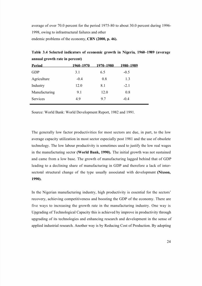
Table 3.4 Selected indicators of economic growth in Nigeria, 1960–1989 (average
annual growth rate in percent)
Period 1960–1970 1970–1980 1980–1989
GDP 3.1 6.5 -0.5
Agriculture -0.4 0.8 1.3
Industry 12.0 8.1 -2.1
Manufacturing 9.1 12.0 0.8
Services 4.9 9.7 -0.4
Source: World Bank: World Development Report, 1982 and 1991.
The generally low factor productivities for most sectors are due, in part, to the low
average capacity utilization in most sector especially post 1981 and the use of obsolete
technology. The low labour productivity is sometimes used to justify the low real wages
in the manufacturing sector (World Bank, 1990). The initial growth was not sustained
and came from a low base. The growth of manufacturing lagged behind that of GDP
leading to a declining share of manufacturing in GDP and therefore a lack of inter-
sectoral structural change of the type usually associated with development (Nixson,
1990).
In the Nigerian manufacturing industry, high productivity is essential for the sectors’
recovery, achieving competitiveness and boosting the GDP of the economy. There are
five ways to increasing the growth rate in the manufacturing industry. One way is
Upgrading of Technological Capacity this is achieved by improve in productivity through
upgrading of its technologies and enhancing research and development in the sense of
applied industrial research. Another way is by Reducing Cost of Production. By adopting
24

8/8/2019 e Dissertation
http://slidepdf.com/reader/full/e-dissertation 25/84
strategic planning is one way of minimising costs and boosting productivity in the
manufacturing sector. The third way is by Increasing Investments. Increase in
investments will yield a high growth rate and high productivity in the manufacturing
sector. The fourth method is by Reducing Dependence on Imports. Reducing dependence
on imports for industrial goods will contribute a lot in reducing cost in the long-run and
boosting productivity in the manufacturing sector. Finally there should be Rehabilitation
and Development of Infrastructural Facilities. The Government should give priority
facilities that will contribute or facilitate industrial operations, such as
telecommunication, transportation services, Power supply and water supply. Good
working framework increases productivity in the manufacturing sector and reduces
production costs.
3.6.2 PRODUCTIVITY IN THE NIGERIAN MANUFACTURING INDUSTRY
Perhaps owing to the complexities involved in constructing productivity index, there is
little or no data on productivity levels in the Nigerian economy in general and the
manufacturing sector in particular. Ad hoc studies conducted during 1989 indicated that,
on the average, there was little rise in productivity (Enisan and Akinlo, 1996). Oshoba
(1989) study on food and basic metal industries, only 30 per cent of respondents
indicated they had rising productivity. About 11 per cent recorded no growth, while more
than half, 57 per cent, recorded declining productivity levels. The Manufacturers
Association of Nigeria (MAN) acknowledged the general trend in productivity in the
industrial sector was proved negative in 1989. Since then it’s been indicated that the
situation has been worsened ever since then. Growth rate in the Industrial was relatively
high in the period 1960-70 at an annual average of 12.0 per cent. This demonstrated the
significance at which the government attributed to manufacturing activities and the
adoption of import substitution industralisation strategy from independence which was as
a result in the establishment of many consumer goods industries, including soft drinks,
cement, paints, soap and detergents. However, the manufacturing output growth cut down
drastically to an annual average of about -2.1 per cent during the period 1980-89. This
negative trend in the performance of manufacturing production indicates falling
productivity in the sub-sector.
25

8/8/2019 e Dissertation
http://slidepdf.com/reader/full/e-dissertation 26/84
3.6.3 INCESSANT PROBLEMS IN THE MANUFACTURING SECTOR
High productivity in the Nigerian manufacturing sector has been accountable to many
factors which include the following:
(a) Low Level of Technology: This is considered to be the greatest impediment
constraining productivity in the sub-sector as advancement in technology and innovations
are the fundamental forces propelling industrialization in recent times. Technology has
brought about easy processes and procedures of carrying out jobs and automation have
revolutionalised the manufacturing industry. Industries in Nigeria cannot secure the use
of modern machines in order to reduce processes. Most machineries used especially for
textiles, cement, bakery, leather, paper production and many others are all being
produced with machineries procured in the 1960s and 1970s, giving rise to frequent
breakdown and reduction in capacity utilization rates. Low technology is accountable for
the inadequacy for local industry to be able to produce capital goods such as raw
materials, spare parts and machinery, the bulk of which are imported.
(b) Low Level of Investments: The level of inadequacy of funds makes it difficult for
firms to invest in modern machines, information technology and human resources
development which are vital for reducing production costs, raising productivity and
improving competitiveness. The level of low investments has been traced immensely to
the financial sector mainly the indisposition to make credits available to manufacturers.
Nevertheless, banks acknowledge manufacturing as a high risk venture in the Nigerian
environment, hence banks prefer to lend to low-risk ventures, such as commerce, that
have high returns.
(c) High Cost of Production: Since the introduction of Structural Adjustment
Programme SAP (of which its major objectives were, to; restructure and diversify the
productive base of the economy so as to reduce dependency on the oil sector and imports;
achieve fiscal and balance of payments viability over the medium term; and to promote
non-inflationary economic growth), high and increasing cost of production has been
recorded by most firms as a main constraint on their operations. High cost are traced
largely to poor performing infrastructural facilities, high interest and exchange rates and
diseconomies of scale, which has developed into increased unit price of manufactures,
26

8/8/2019 e Dissertation
http://slidepdf.com/reader/full/e-dissertation 27/84
low effective demand for goods, liquidity squeeze and fallen capacity utilization rates.
(d) Inflation: This can be described as persistent increase in the general price level. It
creates a disincentive to for future saving use and also retards investments and growth. It
also encourages speculative activities thereby diverting resources from productive
ventures.
(e) Poor Performing Infrastructure: Poor performance of infrastructural facilities, are
characterized by frequent interruption in power supply, water supplies and inconsistency
in telecommunication systems and transportation systems. These poor performances have
a negative effect on productivity.
3.7 WHY THE PAST FAILURES?
According to Professor Kilby, who suggested great majority of underdeveloped countries
will have to place major emphasis upon import replacement if they wish to increase the
extent of their industrialization, Bauer (1991, p.133). The government used the old
development models of import substitution industrialization and this postulated the
government as the dictator, producer and controller in the economy which had affected
abnormal incentives, inefficiencies and waste. There was an inappropriate development
framework, poor and frequently changing policies and programmes, lack of clear
development vision and commitment to the Nigerian project. Nigeria's vast oil wealth,
was bankrupt by corrupt rulers in the past, is now unable to payoff foreign debts and
rebuilds the country. According to Gordon (1992), Nigeria has a national debt of $32
billion, compared with a Gross Domestic Product of $21 billion. The Nigerian debt came
when the price of oil crashed in the 1980's. Nigeria is depended on oil exports for 95% of
its foreign exchange. The price of oil escalated in the 1970's where the economy boomed
and afterwards the price of oil fell. There was a neglect of the agricultural sector by mid
1980s and this contributed to the origin of our economic problem. Bauer(1991, p.122)
analysed that industrialization in the sense of state support for manufacturing activity has
been a major plank of development policy and planning in many less developed
countries’ Manufacturing is a subset within the industrialization matrix and the
manufacturing sector in Nigeria has been facing many problems over the years. All these
contributed to the major causes of Nigeria’s failed past. In Nigeria the history of
27
8/8/2019 e Dissertation
http://slidepdf.com/reader/full/e-dissertation 28/84
industrial and manufacturing development is a classic illustration of how a country could
neglect a vital sector through policy inconsistencies. The neglect of the agricultural sector
has further denied manufacturers and industries their basic source of raw material and
this has to a shortage in locally sourced inputs which attributes to low industrialization.
There are certain constraints that drawn in this sector which include, Low patronage,
dumping of cheap products, unfair tariff regime, inadequate infrastructure, ineffective
regulatory agencies, high interest rates, unpredictable government policies, non-
implementation of existing policies. It is now accepted in the development conformity
that good policies matters and can bring about development. Nigeria has practised poor
policies and there have been policy inconsistencies.
3.8 SOUND ECONOMIC POLICIES
Economic growth is an integrated concept which includes increasing income and
productivity, generation of employment, and economic diversification. The type of
policies that drive economic growth include those on service, agricultural, and industrial
sector; in many poor countries agriculture is especially important. Growth generates
resources which are potentially available for development. A convenient way to approach
the complex is issues of appropriate trade policies for development is to set specific
policies in the context of a broader LDC strategy of looking inward. According to
Todaro (2000), Inward-looking development strategy stresses the need for LDCs to
evolve their own styles of development and control their own destiny. This means
policies to encourage indigenous “learning by doing” in manufacturing and the
development of indigenous technologies appropriate to a country’s resource endowments.
The last two centuries, countries rich in natural resources, e.g. Russia, Nigeria and
Venezuela, experienced growth of comparatively low or mediocre magnitude, Sachs and
Warner (1995) claim that this is a historically common pattern. According to the Fourth
National Development Plan, the overriding aim of development effort in Nigeria was to
bring about an improvement in the living conditions of the people. In addition to the three
policy objectives inherited from the Third National Development Plan namely; economic
growth and development and development, price stability and social equity, the fiscal
28

8/8/2019 e Dissertation
http://slidepdf.com/reader/full/e-dissertation 29/84
policy in the Fourth National Development Plan was specifically directed at raising
additional revenue (Mbanefoh 1992).
Herrick and Kindleberger (1988) stated that countries that aspire to economic
development must face international issues squarely if they are to be successful. In order
to rekindle economic growth, the authorities need to formulate and implement sound
macroeconomic policies that promote growth through;
• Sustenance of high but broad –based non-oil GDP growth rate consistent with poverty
reduction and employment generation.
• Diversification of the production structure away from oil/mineral resources.
• Ensuring international competitiveness.
• Systematic reduction of the role of government in direct production of goods and
strengthening its facilitation and regulatory roles
• Pursuit of private sector/export led growth
• Empowering the people through gainful employment and creating safety nets for
vulnerable groups.
3.8.1 EXPLAINING NIGERIA’S SLOW GROWTH
In the development orthodoxy it is accepted that good policies matters and can bring
about development. Nevertheless, Nigeria has been on the track of poor policies and this
brings about policy inconsistencies, policy reversals and often a lack of policy coherence.
In providing solution to the question of why Nigeria has failed to develop, adopting a
recently approach used by Taiwo (2001; 30-32) in attempting to explain Nigeria’s
economic stagnation. According to him, there are remote (long-term) and immediate
causes for this economic stagnation. The remote causes are based on weak production
base arising largely from a poor technological base. Taiwo(2001; 31-32) adds that these
remote causes are manifested in many immediate causes such as: (i) the high cost of
doing business arising mainly from inadequate infrastructure; (ii) the non-
competitiveness of the domestic producers; (iii) a falling investment-GDP ratio (which
had reached 6% during the 1995- 99 period), leading to continued de-industrialization;
(iv) a poor planning and data base, and incomprehensible delays in capital releases for
29
8/8/2019 e Dissertation
http://slidepdf.com/reader/full/e-dissertation 30/84
public sector projects coupled with inadequate capacity for executing large-scale projects;
and (v) political instability, insecurity of life and property, and social and ethnic
disharmony.
3.8.2 POLICIES TO REKINDLE ECONOMIC GROWTH IN NIGERIA
Between 1960 and 2000, the annual ratio of investment to income averaged 16.75%. This
is low compared with the standards of both developing and industrialized countries.
Following the presentation drawn on the discussion from Iyoha (1999b), the following
were identified as the major macroeconomic issues in the attempt to rekindle investment
and sustain it in Nigeria: “the macroeconomic policy environment; appropriate
macroeconomic policies; strategies, policies and measures to deal with uncertainty; the
debt overhang problem; achieving a deregulated financial environment; increasing
economic and financial openness; promotion of foreign private investment; and improved
political stability.” Macroeconomic policy instruments fall within the realm of major
macroeconomics policy. These economic policies should refer to the actions in which
government controls the economic field.
CHAPTER FOUR
METHODOLOGY
4.0 Introduction
This section discusses the methodology used in conducting our empirical studies. As
discussed briefly we employed most of the traditional variables that are considered as the
determinants for economic growth. These variables include private consumption,
government expenditure, gross fixed capital formation as a proxy for gross investment,
net exports which is the difference between exports and imports and lagged variables of
GDP. GDP which is set as the dependent variable in our empirical study is also used as a
proxy for economic growth. This chapter begins by explaining how these variables are
measured. Hence in section 4.1, we explain the variables used, in section 4.2 we specify
our model. Subsequently, section 4.3 expatiates on how the estimations are conducted
this includes how to test for the existence of a unit root, the generation of residuals and
30
8/8/2019 e Dissertation
http://slidepdf.com/reader/full/e-dissertation 31/84
the application of an Error correction model in conducting our regression for the
determinants of economic growth.
4.1 VARIABLES USED AND THEIR MEASUREMENT
The literature on the determinants of growth is replete in economic literature. Although
there exist a large volume of text on the subject of economic growth most of the literature
relies on the use of a cobb-douglas function which involves two variables such as labour
and capital which owning to data problems are not employed in this study. Economic
growth can be achieved at least theoretically through a high inflow of both domestic and
foreign capital, in a politically stable economy and in a country in which the rule of law is
enforced. However for the purposes of this study we only limit our study to the use of the
variables discussed in the introduction of this chapter.
4.1.1 GROSS DOMESTIC PRODUCT
This is one of the major ways of measuring the size of the economy. This is the actual
monetary value of all finished goods and services produced in a country within a specific
period of time. It is also the sum of value which is added up at every stage of production
of all final goods and services produced within a country in a specific period of time
(McGuckin, Van Ark and Barrington, 2000). As an economy grows it is expected that
the growth rate in GDP increases. Thus changes in the economic growth are captured by
changes in GDP. As a result we use the GDP in Nigeria as a proxy for economic growth.
Going by the expenditure approach in accounting for national income in an open
economy such as that of Nigeria. This will be based on the Keynesian model, aggregate
demand (AD) equals C + I + G + NX. Macroeconomic equilibrium in the short-run
Keynesian model occurs when aggregate output equals aggregate demand. This is
represented below by the following equation;
GDP = C + G + I + NX
Where
GDP = is a measure of economic growth from year to year
31

8/8/2019 e Dissertation
http://slidepdf.com/reader/full/e-dissertation 32/84
C – Equal to all private consumption, or consumer spending in a nation’s
economy.
G – is the sum of government spending
I – the sum of all the country’s businesses spending on capital
NX – the nation’s total net exports, calculated as total exports minus total imports.(NX =
Exports – Imports)
We therefore modify the above equation to ascertain the effectiveness of each of the
variables serve as the most important determinants of economic growth in Nigeria.
Due to the difficulty associated in obtaining annual data for gross investment in the
economy we use gross fixed capital formation as a proxy for gross investment in the
economy, variables such as gross fixed capital formation
net export, government expenditure and lagged variables of GDP are used.
4.2 MODEL SPECIFICATION
Given time and resource constraints this study relied mostly on secondary data. Data was
collected on those variables originating from the appendix review as being relevant to the
indicators of economic growth. Methods require form to be developed in order to find
statistically significant relationship between the traditional determinants of growth
(consumption expenditure, gross fixed capital formation, government expenditure and net
exports) and GDP. To allow for sustained growth GDP equation is employed. Gross
investment is assumed to be a fraction of GDP. Genuine saving is intended to indicate the
difference between sustainable net national product and consumption, where sustainable
net national product means the maximum amount that could be consumed without
reducing the present value of national welfare along the optimum path (Hamilton, 2001).
The main idea behind this assumption is that the higher the output or national income, the
more the economy can afford to invest. In this growth model, the larger the fraction of
GDP devoted to investment at the expense of consumption, the higher the rate of capital
32
8/8/2019 e Dissertation
http://slidepdf.com/reader/full/e-dissertation 33/84
formation and hence the higher the rate of GDP growth. The model of national income
determination in the short run is based on the forces of aggregate demand. By way of the
national income identity, national output can be decomposed into expenditure by the
consumers C, on investment I, by government G, and on net exports NX (exports minus
imports) and this is represented by
Y = C + I + G + NX……………………………………………………………..(1)
The modelling approach controls and measures variables we employ which are chosen to
be consistent with the prior high quality of national economic growth by economists
(Barro, 1991). We use ordinary least squares (OLS) regression to model economic
growth. Economic growth studied for about 35 years is employed for this research work.
This lag allows sufficient time for independent variables such as investment, private
consumption, net exports, and government expenditure to have an impact on national
economic performance.
We specify the econometric model used in the study as;
GDPt = αt + Σ β1Ct + Σ β2 It + Σ β3Gt + Σ β4NXt + Σ β5GDPt-1 + εt ...………………..
(2)
WHERE; OUR DEPENDENT VARIABLE
GDP=Gross domestic product
EXPLANATORY VARIABLES ARE
α = Constant factor
Σ = Summation of a variable from t=year 1 to 35 (i.e. 1970-2005)
C = Consumption
G = Government Expenditures
I= Gross fixed capital formation
NX = Net Exports = (X- M)
GDPt-1=lagged variables of GDP
33

8/8/2019 e Dissertation
http://slidepdf.com/reader/full/e-dissertation 34/84
Where
X = Exports
M = Imports
ε = the random error term to compensate for errors in data
4.3 ECONOMETRIC METHODOLOGIES: BASIC REGRESSION
SPECIFICATIONS
Recent developments in econometric studies suggests that caution is necessary in
applying the ordinary least square (OLS) method in time series analysis of this nature.
The reason is because most times series data are usually non- stationary. Non-stationarity
in the level of a time series can always be tested in an applied econometric research.
Stationarity results as the mean and variance of a time series data remains constant
overtime, whilst the value of the covariance between two specified periods depends only
on the gap between the periods and not the actual time at which the covariance is
considered and any violation in the conditions above results in the non-stationarity of the
process (Tsikata et al, 2000:49).
When a time series is non-stationary it is most likely for one to obtain regression results
with promising diagnostic test statistics given the when the reason of estimation isspurious Charemza & Deadman (1992),. In order to then avoid having a spurious result
we employ the Dickey – Fuller (DF) and Augmented Dickey – Fuller (ADF) test using
Microfit4.1 software package to test for the stationarity of the time series data. A time
series data is stationary when it is integrated to order zero I (0) and non-stationary when it
is integrated to a higher order I (n) where n is a higher order. When the ADF test statistic
(t-ratio) is greater than the DF critical value in absolute terms as reported by Microfit, we
reject the null hypothesis of a unit root and conclude that the variables are stationary
(Koop, 2005:154).
In order to test for the existence of stationarity or non stationarity among the variables,
we set the following hypothesis:
Ho: ρ =1 variables are non stationary and has a unit root
Hı: / ρ / <1 variables are stationary and has a deterministic trend.
34

8/8/2019 e Dissertation
http://slidepdf.com/reader/full/e-dissertation 35/84
Yt = β0 + ρYt-1+ et (3) by subtract Yt-1 from both sides of….… (3),
we obtain equation (4) below,
Yt -Yt-1 = β0 + ρYt-1 - Yt-1 + et………………………………… (4),
Re-arranging (4) we express the equation above as
Yt -Yt-1 = β0 + (ρ – 1)Yt-1+ et ………………………………….(5),
but ∆ Yt = Yt -Yt-1 hence
∆ Yt = β0 + (ρ – 1)Yt-1+
et…………………………………………………………………. (6),
when ρ=1, then the time series data is stationary and has a unit root. Let λ = (ρ – 1)
this simply implies that
∆ Yt = β0 + λYt-1+ et………………………………………………(7),
hence if ρ=1, then λ =0 and this gives the general condition for non-stationarity
or unit root for a time series data (i.e. -1< ρ <1 which is equivalent to -2< λ < 0). Thus
when ρ=1 the times series data is non-stationary.
In (time series) econometrics, a time series that has a unit root is known as a random walk
(time series). And a random walk is an example of a non-stationarity time series. When
the time series data is non stationary, it can be made stationary by running the regressionin their first differences as long as their first differences are stationary. Nevertheless, such
estimations will only cover in the short run which response to the variables by the given
result, an error correction term that ties in the short – run behaviour of the dependent
variables with its long- run value will be added. In order to do this we estimate equation
two by OLS to determine the variables are well co-integrated. This is achieved by
generating the residuals in equation two and performing a unit root test on the residuals to
ascertain if it is stationary [integrated to order zero I (0)] . When the residuals is
stationary I (0), the equation two is then co-integrated and there will then be the
performance of our final analysis by adding lagged variables of the residual term to the
first difference of equation two. The coefficient of the lagged residual measures the
extent of adjustment in a given period to deviations from the long-run equilibrium (Koop,
2005:160-175).
35

8/8/2019 e Dissertation
http://slidepdf.com/reader/full/e-dissertation 36/84
∆ GDPt = αt + Σ β1∆ Ct + Σ β2∆ It + Σ β3∆ Gt + Σ β4∆ NXt + Σ β5∆ LAGGDPt +
λ LAGRES εt ……………………………………………………………………………………………………………………………………..
(8)
Where
∆ Yt = Yt -Yt-1
and
∆ Yt = the first difference of a time series data
and
Yt-1 = lagged variable of Y by one period.
4.4 UNIT ROOT TEST FOR RESIDUAL
There are two basic steps to follow in order to perform a unit root test on the residuals
(1) To regress the dependent variable in equation two this is GDP, on the set of
independent variables and then generates the residuals.
(2) To conduct a unit root test on the residuals using the Dickey – Fuller (DF) and
Augmented Dickey – Fuller (ADF). The results stated from these tests are based on
regression estimates with intercept but without a trend. This occurs if the errors or
residuals trends with the variables the errors produced in the estimation will be growing
steadily and this will violate the principles of cointegration (Koop, 2005:168).
When the ADF test statistic (t-ratio) is greater than the DF critical value in absolute terms
as reported by Microfit, we reject the null hypothesis of a unit root and come to a
conclusion that the variables are cointegrated. However, if we accept the null hypothesis
then cointegration does not exist and we will end up with spurious regression which
renders the obtained results from the regression meaningless. We use an Error Correction
Model or Approach to carry out our estimation.
4.5 Error Correction Model
36

8/8/2019 e Dissertation
http://slidepdf.com/reader/full/e-dissertation 37/84
Drawing from our analysis above the Error Correction Model (ECM) is applied only
when the variables are cointegrated. If the variables are not stationary, then the first
difference of equation two will be,
∆ GDPt = αt + Σ β1∆ Ct + Σ β2∆ It + Σ β3∆ Gt + Σ β4∆ NXt + Σ β5∆ GDPt-1 + εt ...
……..(9)
Recalling from equation (8)
∆ GDPt = αt + Σ β1∆ Ct +Σ β2∆ It + Σ β3∆ Gt + Σ β4∆ NXt + Σ β5∆ GDPt-1 +
λ LAGRES + εt
The first difference of this equation is tested for stationarity. Nevertheless, it is possible
that the first differences are not stationary, this is usually the case in some time series
variables. Hence we test their second difference for a unit root. The second difference is
given in equation (10) below. Most data become stationary at their second difference. We
also generate the residuals from equation (9) and test for cointegration. The seconddifference of the time series is stated below.
∆2GDPt = αt + Σ β1∆
2Ct + Σ β2∆2It + Σ β3∆
2Gt + Σ β4∆2NXt + Σ β5∆
2GDPt-1 + εt
(10)
After testing for cointegration and stationarity in the residuals from (9), and established
the existence of cointegration, we then will add the residuals to equation (10) to form our
ECM and we estimate our determinants using equation (11) below.
∆2GDPt = αt + Σ β1∆
2Ct + Σ β2∆2It + Σ β3∆
2Gt + Σ β4∆2NXt + Σ β5∆
2GDPt-1 +
δLAGRES1 + εt .………………………………………………..……….…………..(11)
37

8/8/2019 e Dissertation
http://slidepdf.com/reader/full/e-dissertation 38/84
δ = the coefficient of the lagged residual term or error correction term which has
both short-run and long-run properties.
LagRES1= the lagged values of the residual generated by OLS in equation 9.
∆2= Second difference. (i.e. ∆ 2 2Xt = ∆ 2Xt - ∆ 2Xt-1)
Coefficient of lagged values of the residual δ measures the extent of adjustment in a
given period to derivations in the long run equilibrium (Tsikata et al, 2000). Bound
cointegration techniques also involves the use of the logs in the data transformation and
because the data has got some variables, we cannot work with logs. However, the Bounds
cointegration method relies extensively on using logs of variables included in the model
and when one has negative values whose
logs can not be calculated as in this research, Bounds cointegration technique crashes
(Frimpong & Oteng-Abayie, 2006).
Equation (11) is tested for autocorrelation and heteroskedasticity. It is very likely that
heteroskedastic problems may not exist but autocorrelations may pertain and this iseliminated using Cochrane-Orcutt procedure with Microfit. Hence we report the Durbin-
Waston (DW) Statistic, functional form statistic and heteroskedastic statistic in our table
of results. Whereby the DW statistic is numerically further away from two or above two,
then we can then say serial correlation exists and when its closer to two (i.e 1.22< dw
stat < 2.0) then serial correlation or autocorrelation is eliminated and the resulting
estimates forms the core components of the model (Halicioglu, 2005).
A CUSUM (cumulative sum) and CUSUMSQ (cumulative sum of squares) test is
conducted on the final model to finally determine if the determinants of GDP growth rate
are stable in the long run. The CUSUM test plots the recursive residuals against the break
points and the CUSUMQ test plots the squared recursive residuals against the break
38
8/8/2019 e Dissertation
http://slidepdf.com/reader/full/e-dissertation 39/84
points. The estimated regression coefficients are stable and correctly specified when both
plots stay within the five percent significance level (Brown et al, 1975).
4.6 SOURCES OF DATA
The principle data source of Nigeria in this paper is drawn from the CBN, statistical
bulletin, various issues. The data set starts from 1970 to 2005 by time series data on the
focus variables for the study were obtained from the IMF statistical yearbooks and the
official website of the Central Bank of Nigeria. Gujarati (1995:23) describes a time
series as ‘a set of observations on the values that a variable takes at different times’. The
time frame usually is at regular intervals, in this instance the data relate to yearly
intervals. The data was taken for all variables on a yearly basis from 1970 to 2005
obtained from the official website of the Central Bank of Nigeria (CBN). Other
complementary data were obtained from the Internet based databanks of the World Bank,
The International Monetary Fund, and The United Nations Development Program. In
Nigeria, while the Federal Office of Statistics (FOS), an agency under the National
Planning Commission (NPC) is responsible for the production of macroeconomic data
while the Central Bank of Nigeria (CBN) needs these statistics for analyses of economic
and financial developments and the formulation implementation and monitoring of
economic and financial policy measures.
4.7 SCOPE AND LIMITATIONS OF THE STUDY
The literature search will aim to be comprehensive and broad in scope, but restricted
access to primary literature, for example due to the remote location of material sought,
and collection of adequate data for this study. The period for making this research is
limited due to the restrictions of time to complete the project and resources to support it.
Due mainly to data constraints, the present study suffers from the following limitations:
1 a) One major limitation is lack of reliable data on the major macro-economic
variables under consideration for economic growth rate over a period of 35 years.
2 b) Further, it has been widely believed that one major reason for the poor growth
performance of Nigeria’s economy is lack of good governance. However, no
39

8/8/2019 e Dissertation
http://slidepdf.com/reader/full/e-dissertation 40/84
satisfactory indicator is readily available at the moment to account for the
governance variable over the years.
c) Similarly, another data constraint relates to lack of adequate and reliable
information on economic growth rate for various sectors over the years.
CHAPTER FIVE
ESTIMATION, RESULTS AND INTERPRETATION
5.0 Introduction
The empirical estimates of our econometric models are presented in this chapter. Most
time series econometric analysis are normally done by performing a correlation test
among the stationary variables and explore the time series properties of our data to
ascertain the optimal lag structure of our models as stated in the methodology. This is
mainly done to avoid spurious regression results which are the basic characteristic of time
series variables and they are non stationary. The results on the unit root test for all
variables and regression results are reported and explained in Section 5.1 and Section 5.2
tests our hypotheses and model stability.
40

8/8/2019 e Dissertation
http://slidepdf.com/reader/full/e-dissertation 41/84
5.1 UNIT ROOT TESTS
We test for the existence of a unit root in equation two and therefore we present the table
below which gives a summary of the results. We test the usual hypotheses for a unit root.
Ho: ρ =1 variables are non stationary and has a unit root
Hı: / ρ / <1 variables are stationary and has a deterministic trend.
TABLE 5(a): ADF Unit root Tests results with trends
VARIABLES ADF (TEST
STATISTICS)
LAG
LENGTH
DF CRITICAL
VALUE
GDP -1.445 5 -3.5671
C -2.4372 5 -3.5671
G -1.4904 3 -3.5671
I -2.1770 2 -3.5671
NX -2.2034 1 -3.5671
LAGGDP -1.7469 5 -3.5671
Notes: Critical values for the augmented Dickey-Fuller statistics are at 5% level. The
order of the lag length is selected using the Akaike Information Criterion (AIC).
Table 5(a) indicates that all the variables have a unit root since all the ADF test statistics
is less than the DF critical value. Therefore we cannot reject the null hypothesis Ho hence
concluding that all the variables have a unit root. To ensure all non stationary variables
stationary, we evaluated the first difference of equation two and tested if they were
stationary. The first difference of equation two is given below;
∆ GDPt = αt + Σ β1∆ Ct + Σ β2∆ It + Σ β3∆ Gt + Σ β4∆ NXt + Σ β5∆ LAGGDPt + εt
Where ∆ Xt = Xt - Xt-1
. TABLE 5(b): ADF Unit root Tests results with trends
VARIABLES ADF (TEST LAG DF CRITICAL
41

8/8/2019 e Dissertation
http://slidepdf.com/reader/full/e-dissertation 42/84
STATISTICS) LENGTH VALUE
DGDP -2.4240 5 -3.5731
DC -2.8925 5 -3.5731
DG -2.2520 3 -3.5731
D I -3.2516 5 -3.5731
DNX -2.8097 5 -3.5731DLAGGDP -2.4531 5 -3.5731
Notes: Critical values for the augmented Dickey-Fuller statistics are at 5% level. The
order of the lag length is selected using the Akaike Information Criterion (AIC). D
represents ∆ in microfit
Table 5(b) above shows that none of the variables are stationary. As a result we cannot
run a regression of non-stationary variables hence we estimate the second difference for
stationarity. The second difference shows that all the variables are stationary hence we
estimate the determinants by using the second difference with an
error correction approach. Table 5(c), below shows a summary of the unit root test (See
appendix).
TABLE 5(c): ADF Unit root Tests results with trends
VARIABLES ADF (TEST
STATISTICS)
LAG
LENGTH
DF CRITICAL
VALUE
DDGDP -7.2919 1 -3.5796
DDC -7.8985 1 -3.5796
DDG -7.1271 1 -3.5796
DD I -4.5091 3 -3.5796
DDNX -3.8143 4 -3.5796
DDLAGGDP -5.0199 3 -3.5796
Notes: Critical values for the augmented Dickey-Fuller statistics are at 5% level. The
order of the lag length is selected using the Akaike Information Criterion (AIC). DD
represents ∆ 2 in microfit
It is clearly noted that the second difference of all estimated variables are stationary. In
order to use the error correction model we first and foremost generate the residuals from
42

8/8/2019 e Dissertation
http://slidepdf.com/reader/full/e-dissertation 43/84
the first difference of equation (9) and then conduct a unit root test on the residuals
(lagged by one period) to ascertain if the dependent variable is cointegrated with the
independent variables. This signifies that the result is affirmative and that cointegration
exists. Table 5(d) below reports the results obtained from the unit root test of the
residuals.
TABLE 5(d): ADF Unit root Tests results with residuals in equation eight without
trends
VARIABLES ADF (TEST
STATISTICS)
LAG
LENGTH
DF CRITICAL
VALUELAGRES1 -4.2398 1 -2.9665
Notes: Critical values for the augmented Dickey-Fuller statistics are at 5% level. The
order of the lag length is selected using the Akaike Information Criterion (AIC). DD
represents ∆ 2 in microfit
Given that the ADF test statistic is greater than the DF critical value we reject the null
hypothesis of a unit root and arrive at a conclusion that the variables of the second
difference are cointegrated and stationary. Hence the determinants of GDP are carried out
in their second difference. Table 5(e) presents a summary of the regression estimates as
carried out in their second difference. A full report of the regression results is stated in
the appendix
∆2GDPt = αt + Σ β1∆
2Ct + Σ β2∆2It + Σ β3∆
2Gt + Σ β4∆2NXt + Σ β5∆
2GDPt-1 +
δLAGRES1 + εt
Initial results from our regression indicate that we have a low DW-statistic; this is
reported in column one. A low dw value normally suggests that autocorrelation is present
in our estimation. Hence, we adopt Cochrane Orcutt’s measures with the aid of microfit
to eliminate it. The DW statistic improves drastically and therefore the most appropriate
estimates are reported in column 2. The results indicate that approximately 98% of the
43

8/8/2019 e Dissertation
http://slidepdf.com/reader/full/e-dissertation 44/84
dependent variable (GDP) is explained variations in the explanatory variables. The
intercept (INPT) is statistically significant at 5% significance level therefore we find it
statistically appropriate to employ it in subsequent analysis and subsequent results are
reported in column 2 and 3.
Table 5(e)
Ordinary Least Squares Estimation Dependent Variables in DDGDP
33 Observations used for estimation from 1973 to 2005
1 2 3
INPT 458.9880.093859
787.1377.61882
397.3705.081260
DDC .83920
5.1406
1.0058
10.9997
.90822
6.1360
DDG 1.3888
1.7824
1.6592
4.3962
1.3980
1.7942
DDI -.077210
-.162337
.63292
2.8505
-.14592
-.31010
DDNX .73014
6.3107
.93681
16.1161
.78659
7.78341DDLAGGDP -.081365
-1.0018
-.010145
-.29129
-
LAGRES1
-1.0908
-5.1047
-.20906
-1.3820
-1.1443
-5.5297
Diagnostic Tests
R 2
.90214 .98890 .89836
R BAR SQUARE .87955 .98391 .87954
DW STATISTIC 1.2287 2.3898 1.2135
Autocorrelation[X2(1)] .019 - .171
Heteroskedasticity[X2(1)] .507 - .547
Functional Form [X2(1)] .067 - .198
Notes: Significant at 5% **Significant at 5% after the elimination of serial
autocorrelation with COCHRANE-ORCUTT. [T-RATIOS ARE IN BRACKTS] *** DD
44

8/8/2019 e Dissertation
http://slidepdf.com/reader/full/e-dissertation 45/84
represents ∆ 2 in microfit
Upon the elimination of serial correlation from the results obtained in column 1, it is
obvious that at a 5% significance level past values of gdp (ddlaggdp) is not statistically
significant. Similarly, the constant is represented by INPT is also statistically
insignificant. In order to ascertain the most significant contributors or determinants of
economic growth we drop the lagged values of gdp from our model and carry out a third
regression which is reported in column 3 of the table above. From column three we can
see that apart from the gross fixed capital formation which has a negative sign all of the
other variables have the correct signs. In addition changes in consumption and changes in
net export appear to be the most statistically significant since they have t-ratios which are
greater than two in absolute terms. The diagnostic tests also indicate that the functional
form of our estimated model is correct and there is no problem with autocorrelation nor
heteroskedasticity. Again our results indicate that approximately 89.9% of the variations
in the dependent variable (i.e gdp or economic growth ) are accounted for by changes in
the explanatory variables.
Comparing the coefficients of the respective variables we can deduce that among thestatitistically significant variables, private consumption in Nigeria happen to be the most
important determinant of growth according to our study. Thus were as a 1% change in
private consumption will cause economic growth or GDP to change by approximately
one naira whereas the same proportionate change in net export will causes GDP or
economic growth to change by approximately 80 kobo. Thus it indicates that there is a
statitistically significant positive relationship between economic growth and net exports
as well as private consumption. The former may be attributed to the high level of oil
export by Nigeria considering that is the sixth leading exporter of oil in the world.
The result of not obtaining a significant relationship between government investment
expenditure and economic growth is not really surprising considering the high level of
corruption in the government and government also having to spend a huge chunk of
45

8/8/2019 e Dissertation
http://slidepdf.com/reader/full/e-dissertation 46/84
revenues accruing from the exportation of oil to service its self because of its size. For a
meaningful and sustained economic growth it will be appropriate government channels
more of state revenue to put up infrastructure which is a sine qua non for economic
growth since the availability of much need infrastructure tends to attract foreign
investment ceteris paribus,
In addition to the above a plausible explanation as to why net export and Private
consumption happen to be the only statistically significant variables are that: population
growth in Nigeria is extremely high and in actual fact high population growth leads to
increase in private consumption which boosts economic growth as it practically promotes
production due to constant demand and constant supply. Government expenditure is
statistically insignificant and this could be due to misplacement of priorities or this could
be an increase in corruption rate.
In conclusion private net exports and private consumption are significant determinants of
GDP inflow to Nigeria. However, this result is consistent with many other researches on
GDP to developing and middle income countries. An example is the works of Taylor
(2000). Other measures used in measuring the openness variable in this work such as the
ratio of imports plus exports to GDP did not change our result hence it wasn’t reported.
The model is found to be stable and therefore has predictive ability since both plots lie
between the 5% critical boundaries. See fig 1 and 2 below.
46
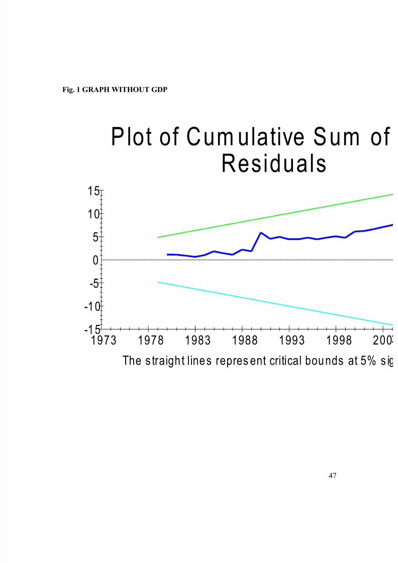
8/8/2019 e Dissertation
http://slidepdf.com/reader/full/e-dissertation 47/84
Fig. 1 GRAPH WITHOUT GDP
Plot of Cum ulative Sum Residuals
The s traigh t l ines repres ent critical bounds at 5%
-5
-10
-15
0
5
10
15
1973 1978 1983 1988 1993 1998
47

8/8/2019 e Dissertation
http://slidepdf.com/reader/full/e-dissertation 48/84
P lo t o f C u m u la t ivR e c u rs ive R
T h e s tra ig h t l in e s re p re s e n t c r i ti
-0 .5
0 .0
0 .5
1 .0
1 .5
1 9 7 3 1 9 7 8 1 9 8 3 1 9 8 8 1 9 9 3
48

8/8/2019 e Dissertation
http://slidepdf.com/reader/full/e-dissertation 49/84
Fig. 2 GRAPH WITH GDP
P lo t o f C u m u l a t ive SR e s i d u a l s
T h e s tra i g h t l in e s re p r e s e n t c r i ti c a l b o u n
-5
-1 0
-1 5
0
5
1 0
1 5
1 9 7 3 1 9 7 8 1 9 8 3 1 9 8 8 1 9 9 3 1 9 9 8 2 0
49
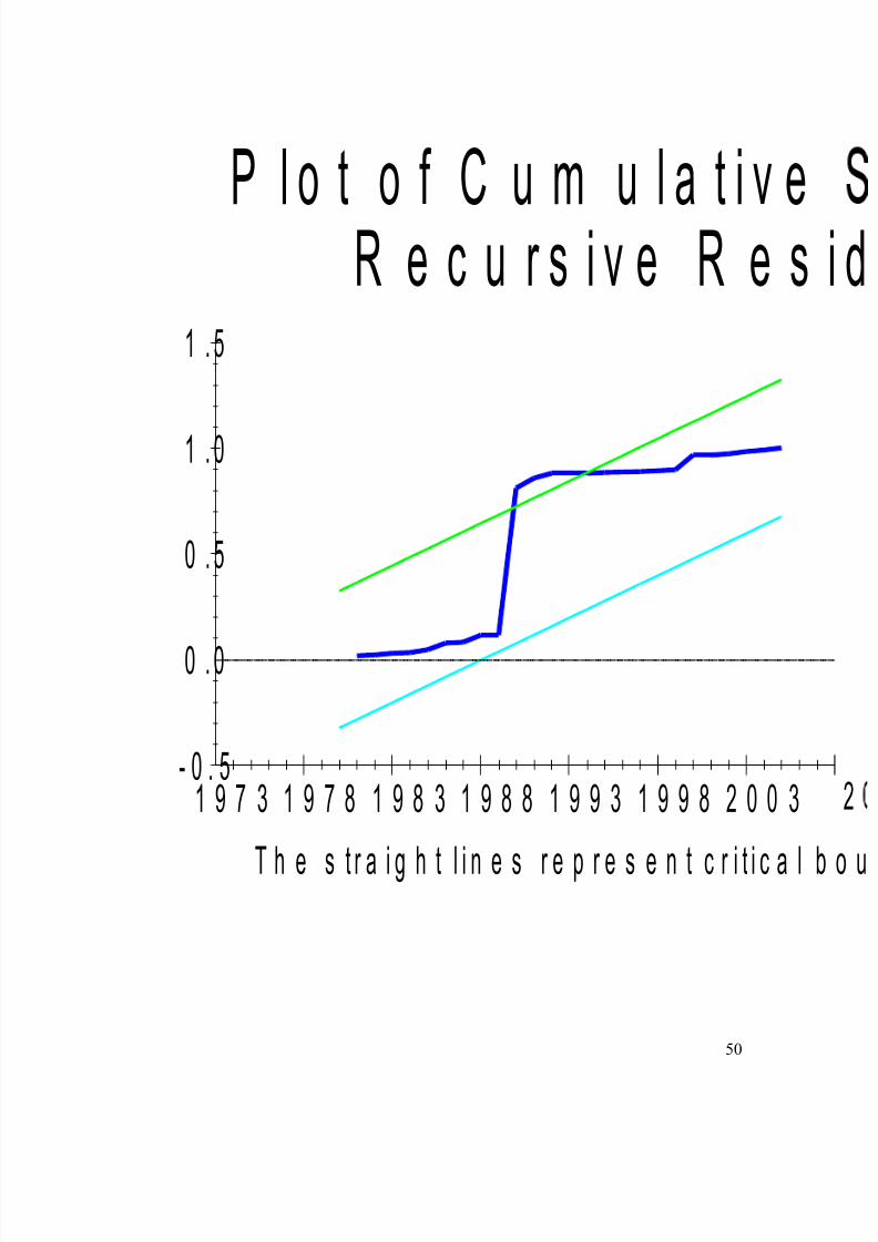
8/8/2019 e Dissertation
http://slidepdf.com/reader/full/e-dissertation 50/84
P l o t o f C u m u l a t i v eR e c u r s i v e R e s
T h e s t r a i g h t l i n e s r e p r e s e n t c r i t i c a l
- 0 . 5
0 . 0
0 . 5
1 . 0
1 . 5
1 9 7 3 1 9 7 8 1 9 8 3 1 9 8 8 1 9 9 3 1 9 9 8 2 0 0 3
50

8/8/2019 e Dissertation
http://slidepdf.com/reader/full/e-dissertation 51/84
CHAPTER SIX
SUMMARY, CONCLUSION AND RECOMMENDATION
6.0 SUMMARY AND CONCLUSION
This chapter covers the entire research and draws a conclusion based on the empirical test
conducted on the determinants of GDP and economic growth in Nigeria The study begun
by identifying what the determinants of Economic growth are by relying on cross- section
or panel analysis of most researchers on developing countries. This is because most
developing countries have contrasting the characteristics of underdevelopment hence
encountering instability of economic growth which are not taken into cognisance in such
studies. We therefore employed some of the controversial results arising from the
determinants economic growth in developing countries and as well developed countries
which are yet to be tested on the Nigerian economy to ascertain their significance as
determinants of economic growth in Nigeria
.The study presented a literature review on how important the traditional determinants of
growth (consumption expenditure, gross fixed capital formation, government expenditureand net exports) as used in the study and variables on how investments on the GDP
explanatory variables will greatly influence or impact economic growth rate in Nigeria.
The GDP of Nigeria is used as a proxy for economic growth in this study which suggest
that hhigh investment ratios do not necessarily lead to rapid economic growth; the quality
of investment, its productivity, existence of appropriate policy, political, and social
infrastructure are all determinants of the effectiveness of investment (Hall and Jones,
1999; Fafchamps, 2000; Artadi and Sala-i-Martin, 2003). We adapted univariate and
multivariate regression. The results indicated that private consumption and net exports in
Nigeria were significant determinants of GDP growth rate over the period of study. They
were positively related. However, net exports was the most significant factor. Previous
study on GDP growth rate indicated that the variable for government expenditure was
insignificant which were not cognisance in some empirical studies. Kaipornsak (1995)
51

8/8/2019 e Dissertation
http://slidepdf.com/reader/full/e-dissertation 52/84
studied the source of economic growth and found that spending on R&D, especially
government expenditure, and the degree of openness with the emphasis on FDI were
major factors.
6.1 RECOMMENDATIONS
To boost economic growth in Nigeria, this research recommends among others that
Government bodies in charge of promoting economic growth should assist
foreign investors some basic fundamentals like acquiring land, and for local investors in
acquiring loans and ways in encouraging new businesses to grow, which according to
United Nations Survey Report (2003), has been a subject of concern to potential
investors to the country. The resources and time should be channelled towards economic
growth by increasing investment to the country and increasing government expenditures.
This study tends to highlight some recommendations for future research which will be
important if studies are conducted on what granger causes growth in Nigeria whether it is
private consumption or net exports. It also will be important if one can ascertain the
impart of investments into various sectors of the Nigerian economy to economic growth.
52

8/8/2019 e Dissertation
http://slidepdf.com/reader/full/e-dissertation 53/84
REFERENCE
Banji Oyelaran-Oyeyinka et al (1997), The management of Technology and Technical
Change in: Ailing Public Enterprises: Technological Project Failures and Prospects for
Industrial Renewal in Nigeria),. Raw Material Research and Development Council,
Abuja, Nigeria.
Barro, R. J. (1991), Economic Growth in a Cross Section of Countries. Quarterly Journal
of Economics, Accounting.
Barro, R. J. and X. Sala-i-Martin (1992), Convergence. Journal of Political Economy.
Benhabib, Jess, and Mark M. Spiegel.(2000), The Role of Financial Development in
Growth and Investment . Journal of Economic Growth.
Brown, N. (1991), Apocalypse and/or Metamorphosis, Berkeley: University of
California Press.
Brown, R. L., Durbin, J. & Evans, J. M. (1975), Techniques for Testing the Constancy
of Regression Relations over Time. Journal of the Royal Statistical Society, (volume) 37:
(pages) 149-192.
Bureau of Public Enterprises (2002), Strengthening Nigeria’s Refinery Sector : Oil and
Gas Investments in Nigeria Conference. 3rd May 2002.
Gujarati D. N., (1995), ‘Basic Econometrics’ Third Edition McGraw-Hill Book
Company.
Barro, R. J. (1990), Economic Growth in a Cross Section of Countries. Quarterly
Journal of Economics, Accounting.
53

8/8/2019 e Dissertation
http://slidepdf.com/reader/full/e-dissertation 54/84
Barro, R.J. (1991), Economic Growth in a Cross-Section of Countries, Quarterly Journal
of
Economics, 106 (2): 407-443.
CBN, (2002 a), Annual Report and Statement of Account, December p 53
Chenery, H.B. and Strout, A.M. (1966), Foreign Assistance and Economic Development.
American Economic Review, 56 (4): 679 – 731.
Eze J.C. (2003), Key Issues Affecting Nigeria’s Development . Paper Presented at
Workshop Private Company Chief Executives, Awka. 4 – 5 Oct
Fafchamps, Marcel (2000), Engines of Growth and Africa’s Economic Performance.
mimeo, Centre for the Study of African Economies, University of Oxford.
Frankel, J.A. and Romer, D. (1999), Does Trade Cause Growth?. American Economic
Review, 89 (3): 379-399.
Gillis, Malcom., Perkins, Dwight H., Roemer, Michael, and Snodgrass, Donald R.(1996),
Economics of Development, New York: Norton.
Gylfason Thorvaldur,(2001), “Natural Resources, Education, and Economic
Development.” European Economy. 847-859, May 2001a.
Gujarati D. N., (1995), Basic Econometrics. Third Edition McGraw-Hill Book
Company.
Hall, R.E. and Jones, C.I. (1999), Why Do Some Countries Produce So Much Output per
Worker than others?. Quarterly Journal of Economics, 114 (1): 83-116.
Halicioglu, R. F, (2005), Applied Quantitative Skills , The University of Greenwich,
Department of Economics. London: Unpublished
54
8/8/2019 e Dissertation
http://slidepdf.com/reader/full/e-dissertation 55/84
Hamilton, K., (1995), Sustainable development , the Hartwick rule and optimal growth.
Environ.
Hamilton, Kirk (2001), The Sustainability of Extractive Economies, Ch. 3 in Auty.
Harrison, Ann (1996), Openness and Growth: A Time-Series, Cross-Country Analysis for
Developing Countries. Journal of Development Economics, 48: 419-447.
Kaipornsak, P. (1995), Source of economic growth in Thailand : Ph.D. dissertation,
Australian National University.
King, Robert G., and Ross Levine. (1993). Finance and Growth: Schumpeter Might Be
Right . Quarterly Journal of Economics.
Koop, G. (2005), Analysis of Economic Data, Chichester, John Wiley & Sons Ltd.
Levine, Ross, Norman Loayza, and Thorsten Beck. (2000), Financial Intermediation
and Growth: Causality and Causes. Journal of Monetary Economics.
Levine, R. and Renelt, D. (1992), A sensitivity Analysis of Cross-country regressions.
American Economic Review, 82 (4): 942-963.
Mankiw, N. G., D. Romer and D. N. Weil (1992), A Contribution to the Empirics of
Economic Growth. Quarterly Journal of Economics, 107 (2), 407-437.
McGuckin, R.H., B. van Ark and L. Barrington (2000), Perspectives on a Global
Economy: Are PoorNations Closing the Gap in Living Standards?, Report Number 1263-
00-RR, The Conference Board.
Nigeria National Petroleum Corporation, (2006), Nigeria and the Future Global Market.
Baker Institute Energy Forum. May
55
8/8/2019 e Dissertation
http://slidepdf.com/reader/full/e-dissertation 56/84
Nigeria, Ministry of Finance (2000), Journal of International Development pp. 8–9
Nixson, F. (1990), “Industrialization and Structural Change in Developing Countries”,
Journal of International Development , Vol.20 No.3, 310-33.
Romer, Paul, (1991), Idea Gaps and Object Gaps in Economic Development , Journal of
Monetary Economics, 1991, pp. 543-573.
Romer, Paul M., (1990), Endogenous Technological Change, Journal of Political
Economy, October.
Sachs, Jeffrey D.,and Warner, Andrew M., (1995), Natural Resource Abundance and Economic Growth, NBER Working Paper No 5398, Cambridge, Massachusetts, National
Bureau of Economic Research, Dec.
Sachs, Jeffrey D., and Warner, Andrew M.,(1997), Fundamental Sources of Long-Run
Growth.” Amer. Econ. Rev., 87, 2:184-188, May.
Sachs, Jeffrey D., and Warner, Andrew M., (1999), The Big Push, Natural Resource
Booms
and Growth. J. Dev. Econ. 59, 1:43-76, June.
Taylor, C. T. (2000), The Impact of Host Country Government Policy on US
Multinational Investment Decisions, World Economy (volume/number ) 23(5): (pages)
635–647.
Tsikata, G. K, Asante, Y. & Gyasi, E.M. (2000), Determinants of Foreign Direct
Investment in Ghana . London: Overseas Development Institute.
56

8/8/2019 e Dissertation
http://slidepdf.com/reader/full/e-dissertation 57/84
Udeh, J. 2000. Petroleum revenue management: The Nigerian perspective. Paper
Presented at World Bank/IFC Petroleum Revenue Management Workshop, Washington,
D.C., U.S.A., Oct. 23 – 24.
UNDP (United Nations Development Programme). (2001). Human Development Report:
Nigeria 2000/2001 Millennium Edition. Lagos.
United Nations Development Program (2003) Country Evaluation: Assessment of
Development Results: Nigeria, United Nations Development Program Evaluation Office.
United Nations Statistical Division (2006), [online]. Available from: http:// www.
unsdcommondatabase.htm, [Accessed: 10 March 2007].
Vincent Nwanma and Norval Scott Dow Jones Newswires (2004), Nigeria Has Oil, but
It's Low on Gas. Dow Jones & Company, Inc.
World Bank (1990), Nigeria: Industrial Sector Report: Restructuring Policies for
Competitiveness and Export Growth. Volume II: Marc Report No. 8868 - UNI.
World Bank. (2005), World Development Indicators CD-ROM 2005. Washington,D.C.:
The World Bank.
57
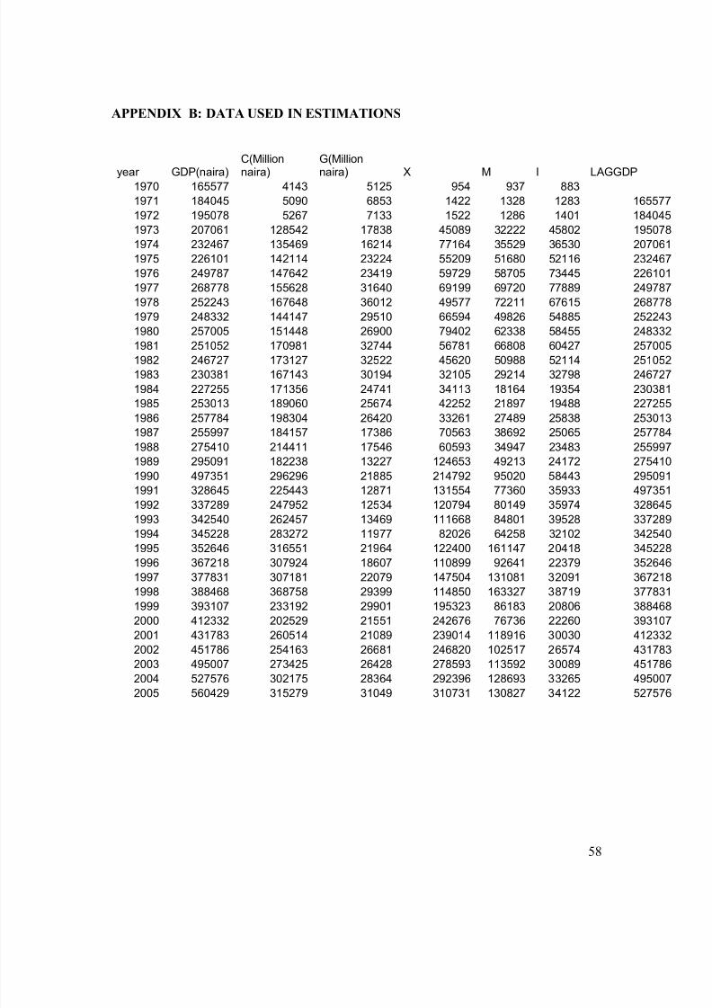
8/8/2019 e Dissertation
http://slidepdf.com/reader/full/e-dissertation 58/84
APPENDIX B: DATA USED IN ESTIMATIONS
year GDP(naira)
C(Million
naira)
G(Million
naira) X M I LAGGDP1970 165577 4143 5125 954 937 883
1971 184045 5090 6853 1422 1328 1283 16557
1972 195078 5267 7133 1522 1286 1401 18404
1973 207061 128542 17838 45089 32222 45802 19507
1974 232467 135469 16214 77164 35529 36530 20706
1975 226101 142114 23224 55209 51680 52116 23246
1976 249787 147642 23419 59729 58705 73445 22610
1977 268778 155628 31640 69199 69720 77889 24978
1978 252243 167648 36012 49577 72211 67615 26877
1979 248332 144147 29510 66594 49826 54885 25224
1980 257005 151448 26900 79402 62338 58455 24833
1981 251052 170981 32744 56781 66808 60427 257001982 246727 173127 32522 45620 50988 52114 25105
1983 230381 167143 30194 32105 29214 32798 24672
1984 227255 171356 24741 34113 18164 19354 23038
1985 253013 189060 25674 42252 21897 19488 22725
1986 257784 198304 26420 33261 27489 25838 25301
1987 255997 184157 17386 70563 38692 25065 25778
1988 275410 214411 17546 60593 34947 23483 25599
1989 295091 182238 13227 124653 49213 24172 27541
1990 497351 296296 21885 214792 95020 58443 29509
1991 328645 225443 12871 131554 77360 35933 49735
1992 337289 247952 12534 120794 80149 35974 32864
1993 342540 262457 13469 111668 84801 39528 337281994 345228 283272 11977 82026 64258 32102 34254
1995 352646 316551 21964 122400 161147 20418 34522
1996 367218 307924 18607 110899 92641 22379 35264
1997 377831 307181 22079 147504 131081 32091 36721
1998 388468 368758 29399 114850 163327 38719 37783
1999 393107 233192 29901 195323 86183 20806 38846
2000 412332 202529 21551 242676 76736 22260 39310
2001 431783 260514 21089 239014 118916 30030 41233
2002 451786 254163 26681 246820 102517 26574 43178
2003 495007 273425 26428 278593 113592 30089 45178
2004 527576 302175 28364 292396 128693 33265 49500
2005 560429 315279 31049 310731 130827 34122 52757
58
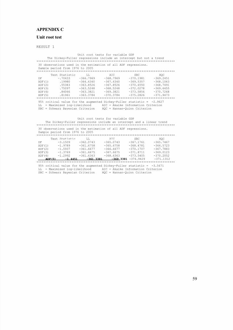
8/8/2019 e Dissertation
http://slidepdf.com/reader/full/e-dissertation 59/84
APPENDIX C
Unit root test
RESULT 1
Unit root tests for variable GDP
The Dickey-Fuller regressions include an intercept but not a trend
*******************************************************************************
30 observations used in the estimation of all ADF regressions.
Sample period from 1976 to 2005
*******************************************************************************
Test Statistic LL AIC SBC HQC
DF -.70433 -366.7969 -368.7969 -370.1981 -369.2451
ADF(1) .19980 -364.4340 -367.4340 -369.5357 -368.1063
ADF(2) .55383 -363.8526 -367.8526 -370.6550 -368.7491
ADF(3) .75097 -363.5248 -368.5248 -372.0278 -369.6455
ADF(4) .84066 -363.3821 -369.3821 -373.5856 -370.7268
ADF(5) .81961 -363.3784 -370.3784 -375.2826 -371.9473
*******************************************************************************
95% critical value for the augmented Dickey-Fuller statistic = -2.9627
LL = Maximized log-likelihood AIC = Akaike Information Criterion
SBC = Schwarz Bayesian Criterion HQC = Hannan-Quinn Criterion
Unit root tests for variable GDP
The Dickey-Fuller regressions include an intercept and a linear trend
*******************************************************************************
30 observations used in the estimation of all ADF regressions.
Sample period from 1976 to 2005
*******************************************************************************
Test Statistic LL AIC SBC HQC
DF -3.1509 -362.0743 -365.0743 -367.1761 -365.7467
ADF(1) -1.9789 -361.6758 -365.6758 -368.4781 -366.5723
ADF(2) -1.5937 -361.6677 -366.6677 -370.1707 -367.7883
ADF(3) -1.3769 -361.6675 -367.6675 -371.8711 -369.0123
ADF(4) -1.2992 -361.6363 -368.6363 -373.5405 -370.2052
ADF(5) -1.4451 -361.3381 -369.3381 -374.9429 -371.1312
*******************************************************************************
95% critical value for the augmented Dickey-Fuller statistic = -3.5671
LL = Maximized log-likelihood AIC = Akaike Information CriterionSBC = Schwarz Bayesian Criterion HQC = Hannan-Quinn Criterion
59
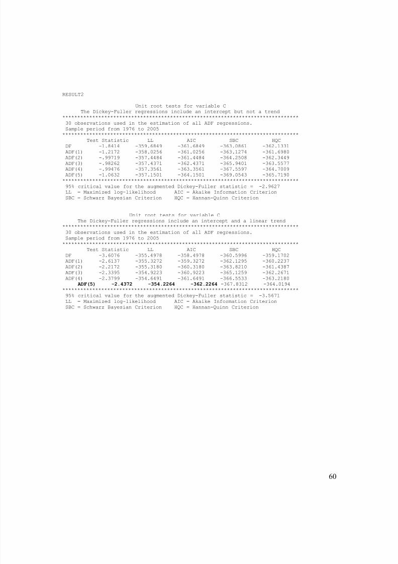
8/8/2019 e Dissertation
http://slidepdf.com/reader/full/e-dissertation 60/84
RESULT2
Unit root tests for variable C
The Dickey-Fuller regressions include an intercept but not a trend
*******************************************************************************
30 observations used in the estimation of all ADF regressions.
Sample period from 1976 to 2005
*******************************************************************************
Test Statistic LL AIC SBC HQC
DF -1.8414 -359.6849 -361.6849 -363.0861 -362.1331
ADF(1) -1.2172 -358.0256 -361.0256 -363.1274 -361.6980
ADF(2) -.99719 -357.4484 -361.4484 -364.2508 -362.3449
ADF(3) -.98262 -357.4371 -362.4371 -365.9401 -363.5577
ADF(4) -.99476 -357.3561 -363.3561 -367.5597 -364.7009
ADF(5) -1.0632 -357.1501 -364.1501 -369.0543 -365.7190
*******************************************************************************
95% critical value for the augmented Dickey-Fuller statistic = -2.9627
LL = Maximized log-likelihood AIC = Akaike Information CriterionSBC = Schwarz Bayesian Criterion HQC = Hannan-Quinn Criterion
Unit root tests for variable C
The Dickey-Fuller regressions include an intercept and a linear trend
*******************************************************************************
30 observations used in the estimation of all ADF regressions.
Sample period from 1976 to 2005
*******************************************************************************
Test Statistic LL AIC SBC HQC
DF -3.6076 -355.4978 -358.4978 -360.5996 -359.1702
ADF(1) -2.6137 -355.3272 -359.3272 -362.1295 -360.2237
ADF(2) -2.2172 -355.3180 -360.3180 -363.8210 -361.4387
ADF(3) -2.3395 -354.9223 -360.9223 -365.1259 -362.2671
ADF(4) -2.3799 -354.6491 -361.6491 -366.5533 -363.2180
ADF(5) -2.4372 -354.2264 -362.2264 -367.8312 -364.0194
*******************************************************************************95% critical value for the augmented Dickey-Fuller statistic = -3.5671
LL = Maximized log-likelihood AIC = Akaike Information Criterion
SBC = Schwarz Bayesian Criterion HQC = Hannan-Quinn Criterion
60
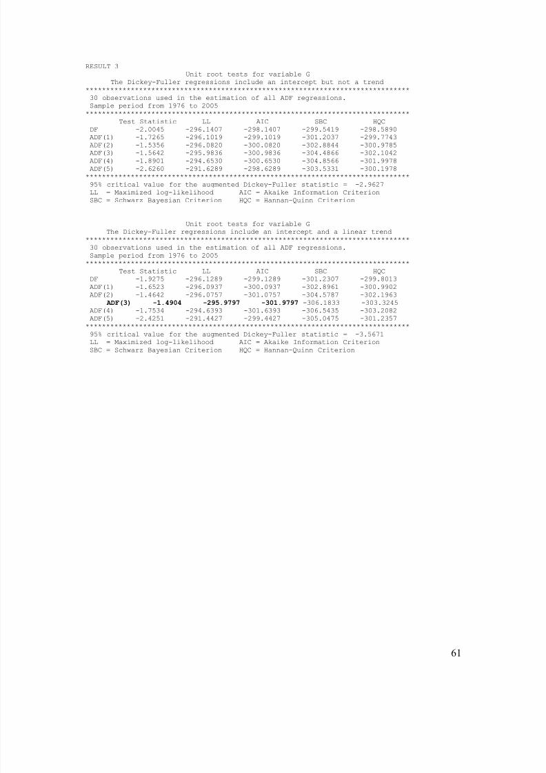
8/8/2019 e Dissertation
http://slidepdf.com/reader/full/e-dissertation 61/84
RESULT 3
Unit root tests for variable G
The Dickey-Fuller regressions include an intercept but not a trend
*******************************************************************************
30 observations used in the estimation of all ADF regressions.
Sample period from 1976 to 2005
*******************************************************************************
Test Statistic LL AIC SBC HQC
DF -2.0045 -296.1407 -298.1407 -299.5419 -298.5890
ADF(1) -1.7265 -296.1019 -299.1019 -301.2037 -299.7743
ADF(2) -1.5356 -296.0820 -300.0820 -302.8844 -300.9785
ADF(3) -1.5642 -295.9836 -300.9836 -304.4866 -302.1042
ADF(4) -1.8901 -294.6530 -300.6530 -304.8566 -301.9978
ADF(5) -2.6260 -291.6289 -298.6289 -303.5331 -300.1978
*******************************************************************************
95% critical value for the augmented Dickey-Fuller statistic = -2.9627
LL = Maximized log-likelihood AIC = Akaike Information Criterion
SBC = Schwarz Bayesian Criterion HQC = Hannan-Quinn Criterion
Unit root tests for variable G
The Dickey-Fuller regressions include an intercept and a linear trend
*******************************************************************************
30 observations used in the estimation of all ADF regressions.
Sample period from 1976 to 2005
*******************************************************************************Test Statistic LL AIC SBC HQC
DF -1.9275 -296.1289 -299.1289 -301.2307 -299.8013
ADF(1) -1.6523 -296.0937 -300.0937 -302.8961 -300.9902
ADF(2) -1.4642 -296.0757 -301.0757 -304.5787 -302.1963
ADF(3) -1.4904 -295.9797 -301.9797 -306.1833 -303.3245
ADF(4) -1.7534 -294.6393 -301.6393 -306.5435 -303.2082
ADF(5) -2.4251 -291.4427 -299.4427 -305.0475 -301.2357
*******************************************************************************
95% critical value for the augmented Dickey-Fuller statistic = -3.5671
LL = Maximized log-likelihood AIC = Akaike Information Criterion
SBC = Schwarz Bayesian Criterion HQC = Hannan-Quinn Criterion
61

8/8/2019 e Dissertation
http://slidepdf.com/reader/full/e-dissertation 62/84
RESULT 4
Unit root tests for variable NX
The Dickey-Fuller regressions include an intercept but not a trend
*******************************************************************************
30 observations used in the estimation of all ADF regressions.
Sample period from 1976 to 2005
*******************************************************************************
Test Statistic LL AIC SBC HQC
DF -1.3296 -361.3902 -363.3902 -364.7914 -363.8384
ADF(1) -1.0204 -361.3338 -364.3338 -366.4356 -365.0062
ADF(2) -.13757 -359.8158 -363.8158 -366.6182 -364.7123
ADF(3) -.98120 -357.8319 -362.8319 -366.3349 -363.9525
ADF(4) -.66378 -357.7541 -363.7541 -367.9577 -365.0988
ADF(5) -.71345 -357.6774 -364.6774 -369.5816 -366.2463
*******************************************************************************
95% critical value for the augmented Dickey-Fuller statistic = -2.9627
LL = Maximized log-likelihood AIC = Akaike Information Criterion
SBC = Schwarz Bayesian Criterion HQC = Hannan-Quinn Criterion
Unit root tests for variable NX
The Dickey-Fuller regressions include an intercept and a linear trend
*******************************************************************************
30 observations used in the estimation of all ADF regressions.
Sample period from 1976 to 2005
*******************************************************************************Test Statistic LL AIC SBC HQC
DF -2.4956 -358.9484 -361.9484 -364.0502 -362.6208
ADF(1) -2.2034 -358.9461 -362.9461 -365.7485 -363.8426
ADF(2) -1.3174 -357.9014 -362.9014 -366.4044 -364.0220
ADF(3) -2.1981 -355.1140 -361.1140 -365.3176 -362.4588
ADF(4) -1.9397 -355.0768 -362.0768 -366.9810 -363.6457
ADF(5) -2.2767 -354.0445 -362.0445 -367.6493 -363.8375
*******************************************************************************
95% critical value for the augmented Dickey-Fuller statistic = -3.5671
LL = Maximized log-likelihood AIC = Akaike Information Criterion
SBC = Schwarz Bayesian Criterion HQC = Hannan-Quinn Criterion
62
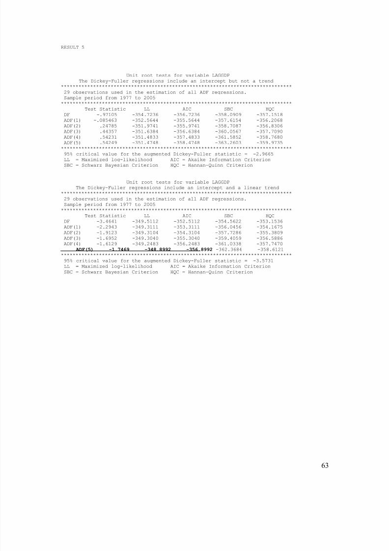
8/8/2019 e Dissertation
http://slidepdf.com/reader/full/e-dissertation 63/84
RESULT 5
Unit root tests for variable LAGGDP
The Dickey-Fuller regressions include an intercept but not a trend
*******************************************************************************
29 observations used in the estimation of all ADF regressions.
Sample period from 1977 to 2005
*******************************************************************************
Test Statistic LL AIC SBC HQC
DF -.97105 -354.7236 -356.7236 -358.0909 -357.1518
ADF(1) -.085463 -352.5644 -355.5644 -357.6154 -356.2068
ADF(2) .24785 -351.9741 -355.9741 -358.7087 -356.8306
ADF(3) .44357 -351.6384 -356.6384 -360.0567 -357.7090
ADF(4) .54231 -351.4833 -357.4833 -361.5852 -358.7680
ADF(5) .54249 -351.4748 -358.4748 -363.2603 -359.9735
*******************************************************************************
95% critical value for the augmented Dickey-Fuller statistic = -2.9665
LL = Maximized log-likelihood AIC = Akaike Information Criterion
SBC = Schwarz Bayesian Criterion HQC = Hannan-Quinn Criterion
Unit root tests for variable LAGGDP
The Dickey-Fuller regressions include an intercept and a linear trend*******************************************************************************
29 observations used in the estimation of all ADF regressions.
Sample period from 1977 to 2005
*******************************************************************************
Test Statistic LL AIC SBC HQC
DF -3.4641 -349.5112 -352.5112 -354.5622 -353.1536
ADF(1) -2.2943 -349.3111 -353.3111 -356.0456 -354.1675
ADF(2) -1.9123 -349.3104 -354.3104 -357.7286 -355.3809
ADF(3) -1.6952 -349.3040 -355.3040 -359.4059 -356.5886
ADF(4) -1.6129 -349.2483 -356.2483 -361.0338 -357.7470
ADF(5) -1.7469 -348.8992 -356.8992 -362.3684 -358.6121
*******************************************************************************
95% critical value for the augmented Dickey-Fuller statistic = -3.5731
LL = Maximized log-likelihood AIC = Akaike Information Criterion
SBC = Schwarz Bayesian Criterion HQC = Hannan-Quinn Criterion
63

8/8/2019 e Dissertation
http://slidepdf.com/reader/full/e-dissertation 64/84
RESULT 6
Unit root tests for variable I
The Dickey-Fuller regressions include an intercept but not a trend
*******************************************************************************
30 observations used in the estimation of all ADF regressions.
Sample period from 1976 to 2005
*******************************************************************************
Test Statistic LL AIC SBC HQC
DF -1.9808 -320.6962 -322.6962 -324.0974 -323.1445
ADF(1) -2.1456 -320.2953 -323.2953 -325.3971 -323.9677
ADF(2) -1.6769 -319.8951 -323.8951 -326.6975 -324.7916
ADF(3) -1.9993 -319.0050 -324.0050 -327.5080 -325.1256
ADF(4) -2.6933 -316.7590 -322.7590 -326.9626 -324.1038
ADF(5) -3.0929 -315.4974 -322.4974 -327.4016 -324.0663
*******************************************************************************
95% critical value for the augmented Dickey-Fuller statistic = -2.9627
LL = Maximized log-likelihood AIC = Akaike Information Criterion
SBC = Schwarz Bayesian Criterion HQC = Hannan-Quinn Criterion
Unit root tests for variable I
The Dickey-Fuller regressions include an intercept and a linear trend
*******************************************************************************
30 observations used in the estimation of all ADF regressions.
Sample period from 1976 to 2005
*******************************************************************************Test Statistic LL AIC SBC HQC
DF -2.3782 -319.7681 -322.7681 -324.8699 -323.4404
ADF(1) -2.7259 -318.8423 -322.8423 -325.6447 -323.7388
ADF(2) -2.1770 -318.7874 -323.7874 -327.2904 -324.9080
ADF(3) -2.4759 -317.7212 -323.7212 -327.9248 -325.0660
ADF(4) -3.2831 -314.7369 -321.7369 -326.6411 -323.3058
ADF(5) -3.9498 -312.4611 -320.4611 -326.0658 -322.2541
*******************************************************************************
95% critical value for the augmented Dickey-Fuller statistic = -3.5671
LL = Maximized log-likelihood AIC = Akaike Information Criterion
SBC = Schwarz Bayesian Criterion HQC = Hannan-Quinn Criterion
64
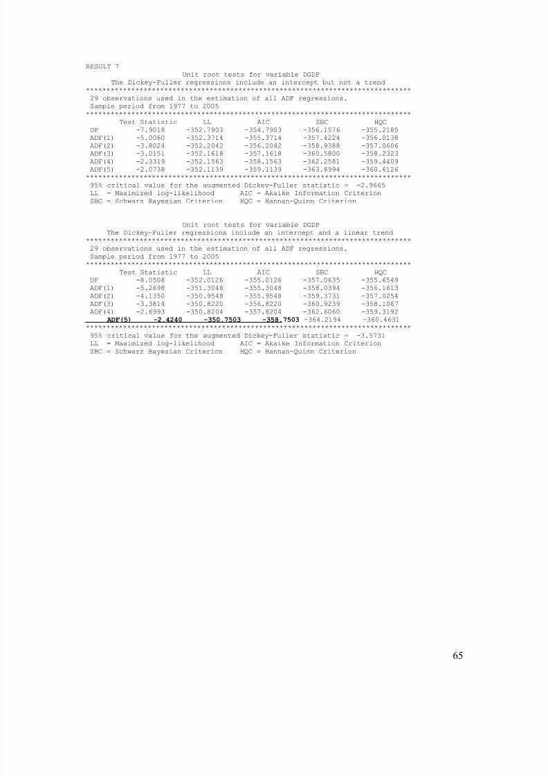
8/8/2019 e Dissertation
http://slidepdf.com/reader/full/e-dissertation 65/84
RESULT 7
Unit root tests for variable DGDP
The Dickey-Fuller regressions include an intercept but not a trend
*******************************************************************************
29 observations used in the estimation of all ADF regressions.
Sample period from 1977 to 2005
*******************************************************************************
Test Statistic LL AIC SBC HQC
DF -7.9018 -352.7903 -354.7903 -356.1576 -355.2185
ADF(1) -5.0060 -352.3714 -355.3714 -357.4224 -356.0138
ADF(2) -3.8024 -352.2042 -356.2042 -358.9388 -357.0606
ADF(3) -3.0151 -352.1618 -357.1618 -360.5800 -358.2323
ADF(4) -2.3319 -352.1563 -358.1563 -362.2581 -359.4409
ADF(5) -2.0738 -352.1139 -359.1139 -363.8994 -360.6126
*******************************************************************************
95% critical value for the augmented Dickey-Fuller statistic = -2.9665
LL = Maximized log-likelihood AIC = Akaike Information Criterion
SBC = Schwarz Bayesian Criterion HQC = Hannan-Quinn Criterion
Unit root tests for variable DGDP
The Dickey-Fuller regressions include an intercept and a linear trend
*******************************************************************************
29 observations used in the estimation of all ADF regressions.
Sample period from 1977 to 2005
*******************************************************************************Test Statistic LL AIC SBC HQC
DF -8.0508 -352.0126 -355.0126 -357.0635 -355.6549
ADF(1) -5.2698 -351.3048 -355.3048 -358.0394 -356.1613
ADF(2) -4.1350 -350.9548 -355.9548 -359.3731 -357.0254
ADF(3) -3.3814 -350.8220 -356.8220 -360.9239 -358.1067
ADF(4) -2.6993 -350.8204 -357.8204 -362.6060 -359.3192
ADF(5) -2.4240 -350.7503 -358.7503 -364.2194 -360.4631
*******************************************************************************
95% critical value for the augmented Dickey-Fuller statistic = -3.5731
LL = Maximized log-likelihood AIC = Akaike Information Criterion
SBC = Schwarz Bayesian Criterion HQC = Hannan-Quinn Criterion
65
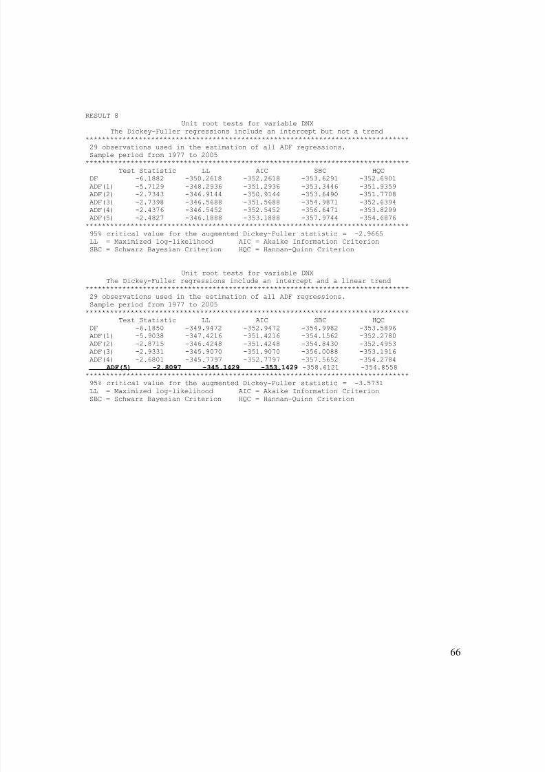
8/8/2019 e Dissertation
http://slidepdf.com/reader/full/e-dissertation 66/84
RESULT 8
Unit root tests for variable DNX
The Dickey-Fuller regressions include an intercept but not a trend*******************************************************************************
29 observations used in the estimation of all ADF regressions.
Sample period from 1977 to 2005
*******************************************************************************
Test Statistic LL AIC SBC HQC
DF -6.1882 -350.2618 -352.2618 -353.6291 -352.6901
ADF(1) -5.7129 -348.2936 -351.2936 -353.3446 -351.9359
ADF(2) -2.7343 -346.9144 -350.9144 -353.6490 -351.7708
ADF(3) -2.7398 -346.5688 -351.5688 -354.9871 -352.6394
ADF(4) -2.4376 -346.5452 -352.5452 -356.6471 -353.8299
ADF(5) -2.4827 -346.1888 -353.1888 -357.9744 -354.6876
*******************************************************************************
95% critical value for the augmented Dickey-Fuller statistic = -2.9665
LL = Maximized log-likelihood AIC = Akaike Information Criterion
SBC = Schwarz Bayesian Criterion HQC = Hannan-Quinn Criterion
Unit root tests for variable DNX
The Dickey-Fuller regressions include an intercept and a linear trend
*******************************************************************************
29 observations used in the estimation of all ADF regressions.
Sample period from 1977 to 2005
*******************************************************************************
Test Statistic LL AIC SBC HQC
DF -6.1850 -349.9472 -352.9472 -354.9982 -353.5896
ADF(1) -5.9038 -347.4216 -351.4216 -354.1562 -352.2780
ADF(2) -2.8715 -346.4248 -351.4248 -354.8430 -352.4953
ADF(3) -2.9331 -345.9070 -351.9070 -356.0088 -353.1916
ADF(4) -2.6801 -345.7797 -352.7797 -357.5652 -354.2784
ADF(5) -2.8097 -345.1429 -353.1429 -358.6121 -354.8558
*******************************************************************************
95% critical value for the augmented Dickey-Fuller statistic = -3.5731
LL = Maximized log-likelihood AIC = Akaike Information Criterion
SBC = Schwarz Bayesian Criterion HQC = Hannan-Quinn Criterion
66

8/8/2019 e Dissertation
http://slidepdf.com/reader/full/e-dissertation 67/84
RESULT 9 Unit root tests for variable DI
The Dickey-Fuller regressions include an intercept but not a trend
*******************************************************************************
29 observations used in the estimation of all ADF regressions.
Sample period from 1977 to 2005
*******************************************************************************
Test Statistic LL AIC SBC HQC
DF -5.9753 -310.3165 -312.3165 -313.6838 -312.7447
ADF(1) -5.2896 -309.3920 -312.3920 -314.4429 -313.0343
ADF(2) -4.2085 -309.1780 -313.1780 -315.9126 -314.0344
ADF(3) -3.4691 -308.5915 -313.5915 -317.0097 -314.6620
ADF(4) -3.2744 -308.5863 -314.5863 -318.6882 -315.8709
ADF(5) -3.5749 -307.4551 -314.4551 -319.2407 -315.9539
*******************************************************************************
95% critical value for the augmented Dickey-Fuller statistic = -2.9665
LL = Maximized log-likelihood AIC = Akaike Information Criterion
SBC = Schwarz Bayesian Criterion HQC = Hannan-Quinn Criterion
Unit root tests for variable DI
The Dickey-Fuller regressions include an intercept and a linear trend
*******************************************************************************
29 observations used in the estimation of all ADF regressions.
Sample period from 1977 to 2005
*******************************************************************************Test Statistic LL AIC SBC HQC
DF -6.0134 -309.7817 -312.7817 -314.8326 -313.4240
ADF(1) -5.2747 -308.8973 -312.8973 -315.6319 -313.7537
ADF(2) -4.1835 -308.6857 -313.6857 -317.1040 -314.7563
ADF(3) -3.3698 -307.7816 -313.7816 -317.8835 -315.0663
ADF(4) -3.0601 -307.7558 -314.7558 -319.5413 -316.2546
ADF(5) -3.2516 -306.9849 -314.9849 -320.4540 -316.6977
*******************************************************************************
95% critical value for the augmented Dickey-Fuller statistic = -3.5731
LL = Maximized log-likelihood AIC = Akaike Information Criterion
SBC = Schwarz Bayesian Criterion HQC = Hannan-Quinn Criterion
67

8/8/2019 e Dissertation
http://slidepdf.com/reader/full/e-dissertation 68/84
RESULT 10
Unit root tests for variable DLAGGDP
The Dickey-Fuller regressions include an intercept but not a trend
*******************************************************************************
28 observations used in the estimation of all ADF regressions.
Sample period from 1978 to 2005
*******************************************************************************
Test Statistic LL AIC SBC HQC
DF -7.8438 -340.8908 -342.8908 -344.2230 -343.2980
ADF(1) -5.0380 -340.3427 -343.3427 -345.3410 -343.9536
ADF(2) -3.8911 -340.0919 -344.0919 -346.7563 -344.9064
ADF(3) -3.1422 -340.0019 -345.0019 -348.3324 -346.0201
ADF(4) -2.4825 -340.0014 -346.0014 -349.9980 -347.2232
ADF(5) -2.2331 -339.9378 -346.9378 -351.6005 -348.3632
*******************************************************************************
95% critical value for the augmented Dickey-Fuller statistic = -2.9706
LL = Maximized log-likelihood AIC = Akaike Information Criterion
SBC = Schwarz Bayesian Criterion HQC = Hannan-Quinn Criterion
Unit root tests for variable DLAGGDP
The Dickey-Fuller regressions include an intercept and a linear trend
*******************************************************************************
28 observations used in the estimation of all ADF regressions.
Sample period from 1978 to 2005
*******************************************************************************Test Statistic LL AIC SBC HQC
DF -7.9141 -340.3147 -343.3147 -345.3130 -343.9256
ADF(1) -5.1984 -339.5633 -343.5633 -346.2277 -344.3778
ADF(2) -4.1038 -339.1734 -344.1734 -347.5039 -345.1916
ADF(3) -3.3793 -339.0088 -345.0088 -349.0054 -346.2306
ADF(4) -2.7174 -339.0002 -346.0002 -350.6629 -347.4257
ADF(5) -2.4531 -338.9170 -346.9170 -352.2458 -348.5461
*******************************************************************************
95% critical value for the augmented Dickey-Fuller statistic = -3.5796
LL = Maximized log-likelihood AIC = Akaike Information Criterion
SBC = Schwarz Bayesian Criterion HQC = Hannan-Quinn Criterion
68
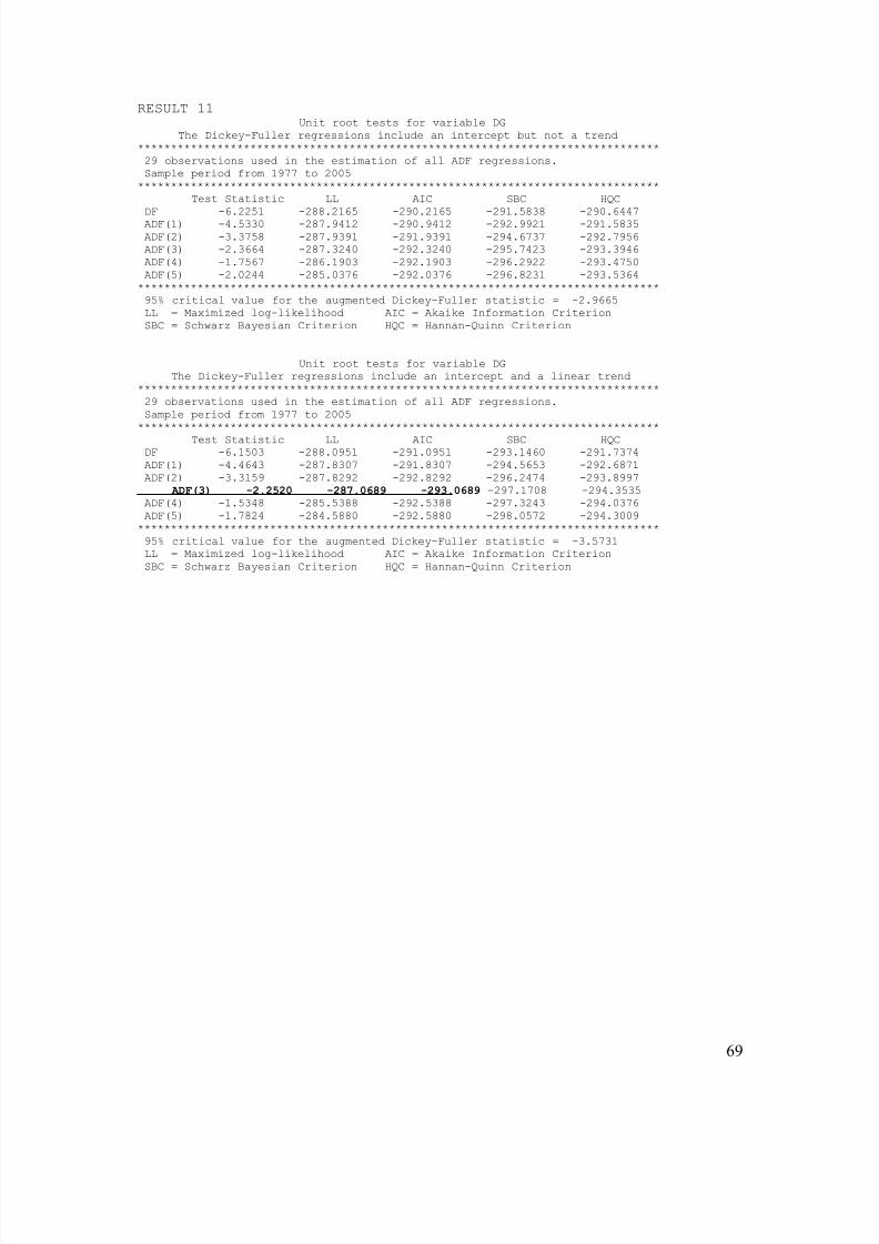
8/8/2019 e Dissertation
http://slidepdf.com/reader/full/e-dissertation 69/84
RESULT 11Unit root tests for variable DG
The Dickey-Fuller regressions include an intercept but not a trend
*******************************************************************************
29 observations used in the estimation of all ADF regressions.
Sample period from 1977 to 2005
*******************************************************************************
Test Statistic LL AIC SBC HQC
DF -6.2251 -288.2165 -290.2165 -291.5838 -290.6447ADF(1) -4.5330 -287.9412 -290.9412 -292.9921 -291.5835
ADF(2) -3.3758 -287.9391 -291.9391 -294.6737 -292.7956
ADF(3) -2.3664 -287.3240 -292.3240 -295.7423 -293.3946
ADF(4) -1.7567 -286.1903 -292.1903 -296.2922 -293.4750
ADF(5) -2.0244 -285.0376 -292.0376 -296.8231 -293.5364
*******************************************************************************
95% critical value for the augmented Dickey-Fuller statistic = -2.9665
LL = Maximized log-likelihood AIC = Akaike Information Criterion
SBC = Schwarz Bayesian Criterion HQC = Hannan-Quinn Criterion
Unit root tests for variable DG
The Dickey-Fuller regressions include an intercept and a linear trend
*******************************************************************************
29 observations used in the estimation of all ADF regressions.
Sample period from 1977 to 2005
*******************************************************************************Test Statistic LL AIC SBC HQC
DF -6.1503 -288.0951 -291.0951 -293.1460 -291.7374
ADF(1) -4.4643 -287.8307 -291.8307 -294.5653 -292.6871
ADF(2) -3.3159 -287.8292 -292.8292 -296.2474 -293.8997
ADF(3) -2.2520 -287.0689 -293.0689 -297.1708 -294.3535
ADF(4) -1.5348 -285.5388 -292.5388 -297.3243 -294.0376
ADF(5) -1.7824 -284.5880 -292.5880 -298.0572 -294.3009
*******************************************************************************
95% critical value for the augmented Dickey-Fuller statistic = -3.5731
LL = Maximized log-likelihood AIC = Akaike Information Criterion
SBC = Schwarz Bayesian Criterion HQC = Hannan-Quinn Criterion
69
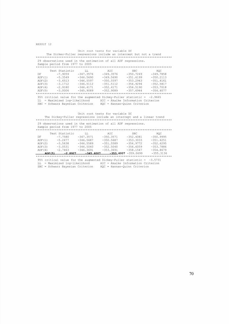
8/8/2019 e Dissertation
http://slidepdf.com/reader/full/e-dissertation 70/84
RESULT 12
Unit root tests for variable DC
The Dickey-Fuller regressions include an intercept but not a trend
*******************************************************************************
29 observations used in the estimation of all ADF regressions.
Sample period from 1977 to 2005
*******************************************************************************
Test Statistic LL AIC SBC HQC
DF -7.9059 -347.3576 -349.3576 -350.7249 -349.7858
ADF(1) -5.3549 -346.5690 -349.5690 -351.6199 -350.2113
ADF(2) -3.6513 -346.5597 -350.5597 -353.2943 -351.4161
ADF(3) -3.1712 -346.5112 -351.5112 -354.9294 -352.5817
ADF(4) -2.9180 -346.4171 -352.4171 -356.5190 -353.7018
ADF(5) -3.0006 -345.9089 -352.9089 -357.6944 -354.4077
*******************************************************************************
95% critical value for the augmented Dickey-Fuller statistic = -2.9665
LL = Maximized log-likelihood AIC = Akaike Information Criterion
SBC = Schwarz Bayesian Criterion HQC = Hannan-Quinn Criterion
Unit root tests for variable DC
The Dickey-Fuller regressions include an intercept and a linear trend
*******************************************************************************
29 observations used in the estimation of all ADF regressions.
Sample period from 1977 to 2005
*******************************************************************************
Test Statistic LL AIC SBC HQC
DF -7.7580 -347.3571 -350.3571 -352.4081 -350.9995
ADF(1) -5.2477 -346.5687 -350.5687 -353.3033 -351.4251
ADF(2) -3.5638 -346.5589 -351.5589 -354.9772 -352.6295
ADF(3) -3.0531 -346.5040 -352.5040 -356.6059 -353.7886
ADF(4) -2.7463 -346.3691 -353.3691 -358.1547 -354.8679
ADF(5) -2.8927 -345.6007 -353.6007 -359.0699 -355.3136
*******************************************************************************
95% critical value for the augmented Dickey-Fuller statistic = -3.5731
LL = Maximized log-likelihood AIC = Akaike Information Criterion
SBC = Schwarz Bayesian Criterion HQC = Hannan-Quinn Criterion
70

8/8/2019 e Dissertation
http://slidepdf.com/reader/full/e-dissertation 71/84
RESULTS 13
Unit root tests for variable DDGDP
The Dickey-Fuller regressions include an intercept but not a trend
*******************************************************************************
28 observations used in the estimation of all ADF regressions.
Sample period from 1978 to 2005
*******************************************************************************
Test Statistic LL AIC SBC HQC
DF -11.1070 -350.1379 -352.1379 -353.4701 -352.5452
ADF(1) -7.4078 -346.9311 -349.9311 -351.9294 -350.5420
ADF(2) -5.9121 -345.0002 -349.0002 -351.6646 -349.8147
ADF(3) -5.1520 -343.4686 -348.4686 -351.7991 -349.4868
ADF(4) -4.1488 -342.9589 -348.9589 -352.9555 -350.1807
ADF(5) -3.3200 -342.8293 -349.8293 -354.4920 -351.2547
*******************************************************************************
95% critical value for the augmented Dickey-Fuller statistic = -2.9706
LL = Maximized log-likelihood AIC = Akaike Information Criterion
SBC = Schwarz Bayesian Criterion HQC = Hannan-Quinn Criterion
Unit root tests for variable DDGDP
The Dickey-Fuller regressions include an intercept and a linear trend
*******************************************************************************
28 observations used in the estimation of all ADF regressions.
Sample period from 1978 to 2005
*******************************************************************************Test Statistic LL AIC SBC HQC
DF -10.9096 -350.0991 -353.0991 -355.0974 -353.7100
ADF(1) -7.2919 -346.8414 -350.8414 -353.5058 -351.6559
ADF(2) -5.8495 -344.8225 -349.8225 -353.1530 -350.8406
ADF(3) -5.1440 -343.1535 -349.1535 -353.1501 -350.3753
*******************************************************************************
95% critical value for the augmented Dickey-Fuller statistic = -3.5796
LL = Maximized log-likelihood AIC = Akaike Information Criterion
SBC = Schwarz Bayesian Criterion HQC = Hannan-Quinn Criterion
71
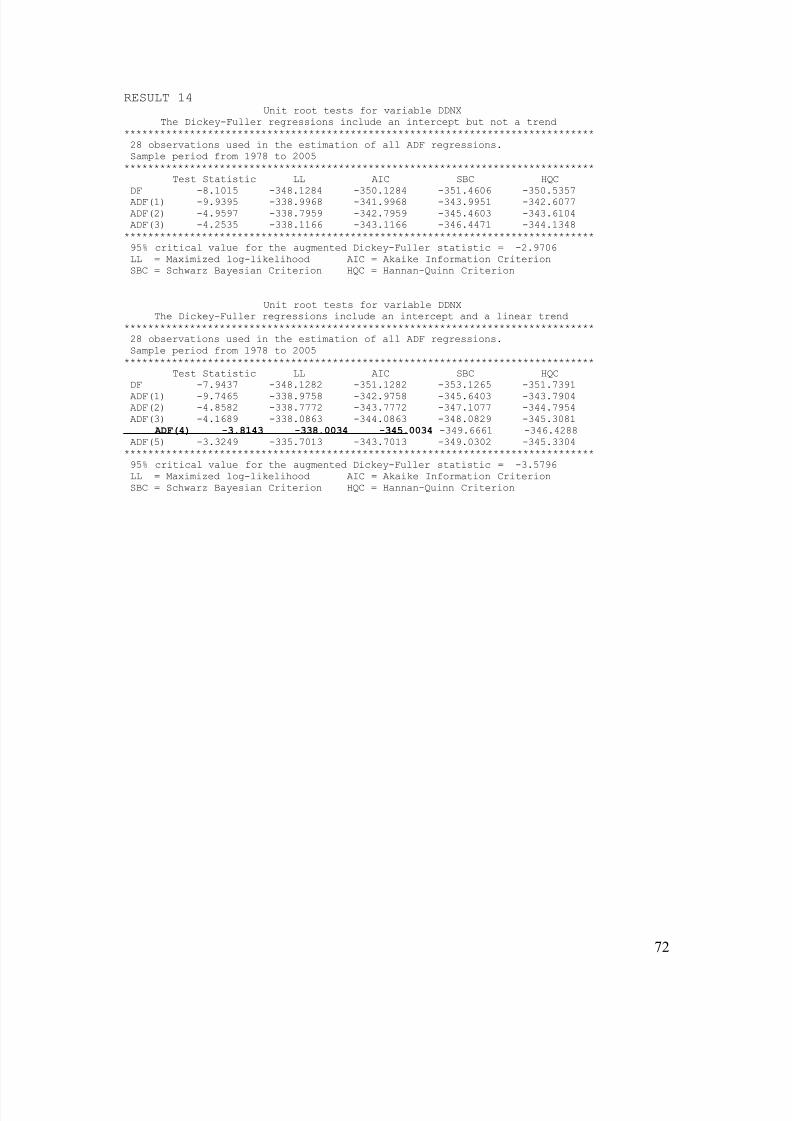
8/8/2019 e Dissertation
http://slidepdf.com/reader/full/e-dissertation 72/84
RESULT 14Unit root tests for variable DDNX
The Dickey-Fuller regressions include an intercept but not a trend
*******************************************************************************
28 observations used in the estimation of all ADF regressions.
Sample period from 1978 to 2005
*******************************************************************************
Test Statistic LL AIC SBC HQC
DF -8.1015 -348.1284 -350.1284 -351.4606 -350.5357ADF(1) -9.9395 -338.9968 -341.9968 -343.9951 -342.6077
ADF(2) -4.9597 -338.7959 -342.7959 -345.4603 -343.6104
ADF(3) -4.2535 -338.1166 -343.1166 -346.4471 -344.1348
*******************************************************************************
95% critical value for the augmented Dickey-Fuller statistic = -2.9706
LL = Maximized log-likelihood AIC = Akaike Information Criterion
SBC = Schwarz Bayesian Criterion HQC = Hannan-Quinn Criterion
Unit root tests for variable DDNX
The Dickey-Fuller regressions include an intercept and a linear trend
*******************************************************************************
28 observations used in the estimation of all ADF regressions.
Sample period from 1978 to 2005
*******************************************************************************
Test Statistic LL AIC SBC HQC
DF -7.9437 -348.1282 -351.1282 -353.1265 -351.7391ADF(1) -9.7465 -338.9758 -342.9758 -345.6403 -343.7904
ADF(2) -4.8582 -338.7772 -343.7772 -347.1077 -344.7954
ADF(3) -4.1689 -338.0863 -344.0863 -348.0829 -345.3081
ADF(4) -3.8143 -338.0034 -345.0034 -349.6661 -346.4288
ADF(5) -3.3249 -335.7013 -343.7013 -349.0302 -345.3304
*******************************************************************************
95% critical value for the augmented Dickey-Fuller statistic = -3.5796
LL = Maximized log-likelihood AIC = Akaike Information Criterion
SBC = Schwarz Bayesian Criterion HQC = Hannan-Quinn Criterion
72

8/8/2019 e Dissertation
http://slidepdf.com/reader/full/e-dissertation 73/84
RESULT 15
Unit root tests for variable DDI
The Dickey-Fuller regressions include an intercept but not a trend
*******************************************************************************
28 observations used in the estimation of all ADF regressions.
Sample period from 1978 to 2005
*******************************************************************************
Test Statistic LL AIC SBC HQC
DF -7.8527 -309.0149 -311.0149 -312.3471 -311.4222
ADF(1) -6.4785 -306.4838 -309.4838 -311.4821 -310.0947
ADF(2) -6.3342 -303.3101 -307.3101 -309.9745 -308.1246
ADF(3) -4.3653 -303.1508 -308.1508 -311.4813 -309.1690
*******************************************************************************
95% critical value for the augmented Dickey-Fuller statistic = -2.9706
LL = Maximized log-likelihood AIC = Akaike Information Criterion
SBC = Schwarz Bayesian Criterion HQC = Hannan-Quinn Criterion
Unit root tests for variable DDI
The Dickey-Fuller regressions include an intercept and a linear trend
*******************************************************************************
28 observations used in the estimation of all ADF regressions.
Sample period from 1978 to 2005
*******************************************************************************
Test Statistic LL AIC SBC HQC
DF -7.7238 -308.9307 -311.9307 -313.9290 -312.5416ADF(1) -6.4428 -306.1983 -310.1983 -312.8627 -311.0129
ADF(2) -6.3746 -302.8210 -307.8210 -311.1515 -308.8391
ADF(3) -4.5091 -302.3952 -308.3952 -312.3918 -309.6170
*******************************************************************************
95% critical value for the augmented Dickey-Fuller statistic = -3.5796
LL = Maximized log-likelihood AIC = Akaike Information Criterion
SBC = Schwarz Bayesian Criterion HQC = Hannan-Quinn Criterion
73
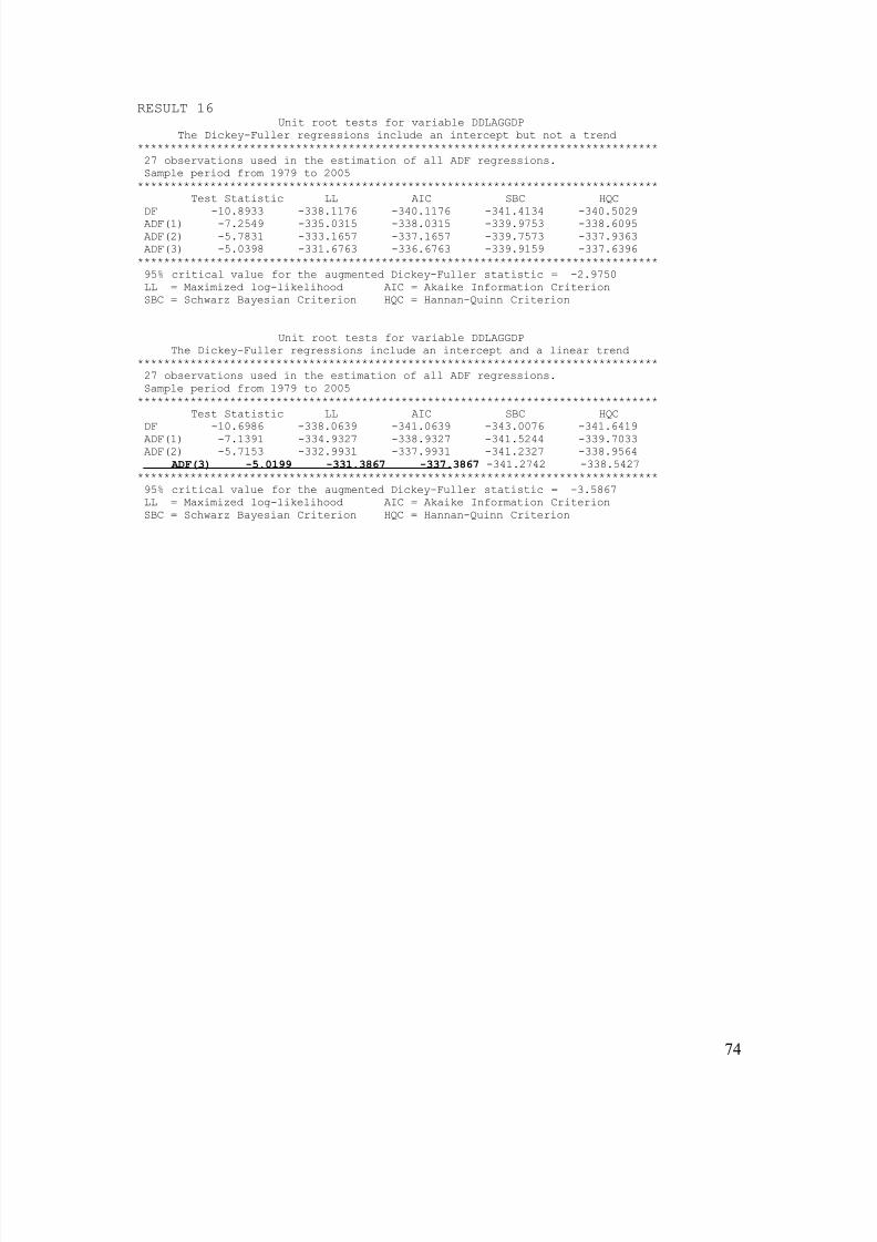
8/8/2019 e Dissertation
http://slidepdf.com/reader/full/e-dissertation 74/84
RESULT 16Unit root tests for variable DDLAGGDP
The Dickey-Fuller regressions include an intercept but not a trend
*******************************************************************************
27 observations used in the estimation of all ADF regressions.
Sample period from 1979 to 2005
*******************************************************************************
Test Statistic LL AIC SBC HQC
DF -10.8933 -338.1176 -340.1176 -341.4134 -340.5029ADF(1) -7.2549 -335.0315 -338.0315 -339.9753 -338.6095
ADF(2) -5.7831 -333.1657 -337.1657 -339.7573 -337.9363
ADF(3) -5.0398 -331.6763 -336.6763 -339.9159 -337.6396
*******************************************************************************
95% critical value for the augmented Dickey-Fuller statistic = -2.9750
LL = Maximized log-likelihood AIC = Akaike Information Criterion
SBC = Schwarz Bayesian Criterion HQC = Hannan-Quinn Criterion
Unit root tests for variable DDLAGGDP
The Dickey-Fuller regressions include an intercept and a linear trend
*******************************************************************************
27 observations used in the estimation of all ADF regressions.
Sample period from 1979 to 2005
*******************************************************************************
Test Statistic LL AIC SBC HQC
DF -10.6986 -338.0639 -341.0639 -343.0076 -341.6419ADF(1) -7.1391 -334.9327 -338.9327 -341.5244 -339.7033
ADF(2) -5.7153 -332.9931 -337.9931 -341.2327 -338.9564
ADF(3) -5.0199 -331.3867 -337.3867 -341.2742 -338.5427
*******************************************************************************
95% critical value for the augmented Dickey-Fuller statistic = -3.5867
LL = Maximized log-likelihood AIC = Akaike Information Criterion
SBC = Schwarz Bayesian Criterion HQC = Hannan-Quinn Criterion
74
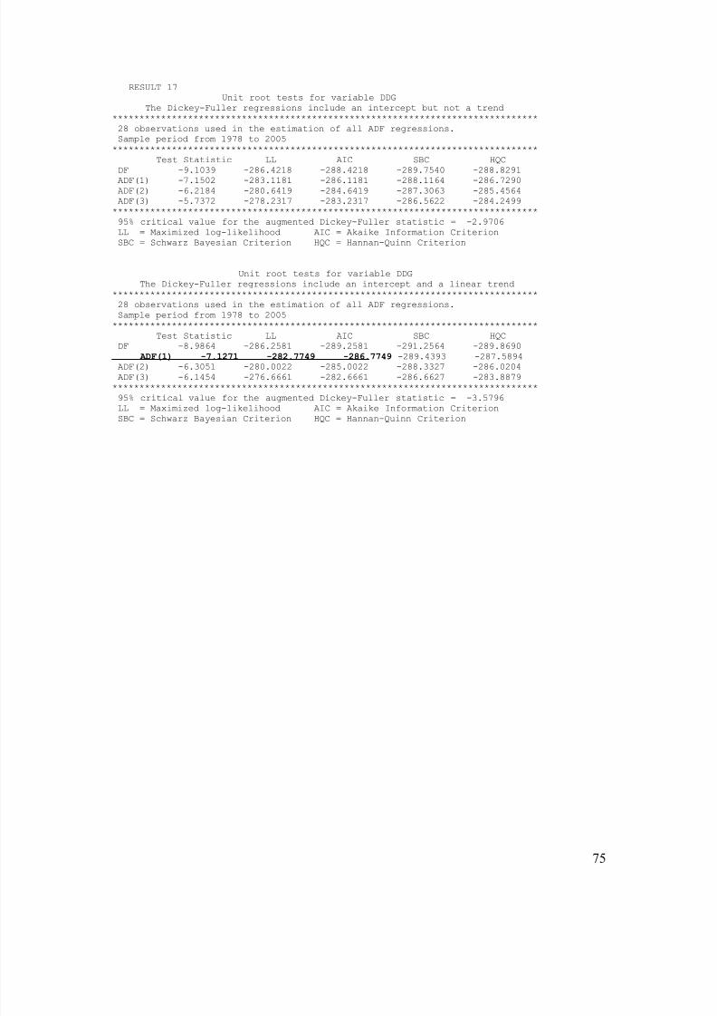
8/8/2019 e Dissertation
http://slidepdf.com/reader/full/e-dissertation 75/84
RESULT 17
Unit root tests for variable DDG
The Dickey-Fuller regressions include an intercept but not a trend
*******************************************************************************
28 observations used in the estimation of all ADF regressions.
Sample period from 1978 to 2005
*******************************************************************************
Test Statistic LL AIC SBC HQC
DF -9.1039 -286.4218 -288.4218 -289.7540 -288.8291
ADF(1) -7.1502 -283.1181 -286.1181 -288.1164 -286.7290
ADF(2) -6.2184 -280.6419 -284.6419 -287.3063 -285.4564
ADF(3) -5.7372 -278.2317 -283.2317 -286.5622 -284.2499
*******************************************************************************
95% critical value for the augmented Dickey-Fuller statistic = -2.9706
LL = Maximized log-likelihood AIC = Akaike Information Criterion
SBC = Schwarz Bayesian Criterion HQC = Hannan-Quinn Criterion
Unit root tests for variable DDG
The Dickey-Fuller regressions include an intercept and a linear trend
*******************************************************************************
28 observations used in the estimation of all ADF regressions.
Sample period from 1978 to 2005
*******************************************************************************
Test Statistic LL AIC SBC HQC
DF -8.9864 -286.2581 -289.2581 -291.2564 -289.8690 ADF(1) -7.1271 -282.7749 -286.7749 -289.4393 -287.5894
ADF(2) -6.3051 -280.0022 -285.0022 -288.3327 -286.0204
ADF(3) -6.1454 -276.6661 -282.6661 -286.6627 -283.8879
*******************************************************************************
95% critical value for the augmented Dickey-Fuller statistic = -3.5796
LL = Maximized log-likelihood AIC = Akaike Information Criterion
SBC = Schwarz Bayesian Criterion HQC = Hannan-Quinn Criterion
75
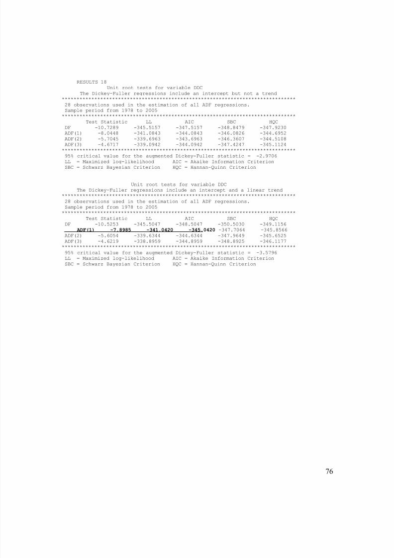
8/8/2019 e Dissertation
http://slidepdf.com/reader/full/e-dissertation 76/84
RESULTS 18
Unit root tests for variable DDC
The Dickey-Fuller regressions include an intercept but not a trend
*******************************************************************************
28 observations used in the estimation of all ADF regressions.
Sample period from 1978 to 2005
*******************************************************************************
Test Statistic LL AIC SBC HQC
DF -10.7289 -345.5157 -347.5157 -348.8479 -347.9230
ADF(1) -8.0448 -341.0843 -344.0843 -346.0826 -344.6952
ADF(2) -5.7045 -339.6963 -343.6963 -346.3607 -344.5108
ADF(3) -4.6717 -339.0942 -344.0942 -347.4247 -345.1124
*******************************************************************************
95% critical value for the augmented Dickey-Fuller statistic = -2.9706
LL = Maximized log-likelihood AIC = Akaike Information Criterion
SBC = Schwarz Bayesian Criterion HQC = Hannan-Quinn Criterion
Unit root tests for variable DDC
The Dickey-Fuller regressions include an intercept and a linear trend*******************************************************************************
28 observations used in the estimation of all ADF regressions.
Sample period from 1978 to 2005
*******************************************************************************
Test Statistic LL AIC SBC HQC
DF -10.5253 -345.5047 -348.5047 -350.5030 -349.1156
ADF(1) -7.8985 -341.0420 -345.0420 -347.7064 -345.8566
ADF(2) -5.6054 -339.6344 -344.6344 -347.9649 -345.6525
ADF(3) -4.6219 -338.8959 -344.8959 -348.8925 -346.1177
*******************************************************************************
95% critical value for the augmented Dickey-Fuller statistic = -3.5796
LL = Maximized log-likelihood AIC = Akaike Information Criterion
SBC = Schwarz Bayesian Criterion HQC = Hannan-Quinn Criterion
76
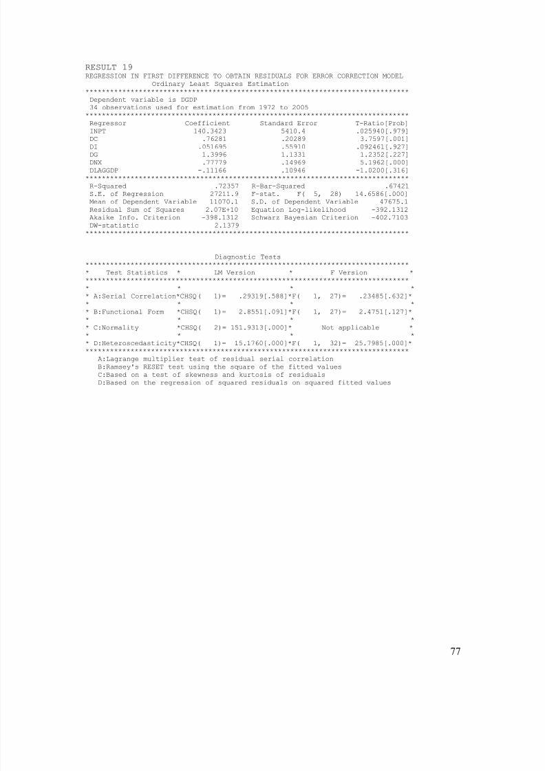
8/8/2019 e Dissertation
http://slidepdf.com/reader/full/e-dissertation 77/84
RESULT 19REGRESSION IN FIRST DIFFERENCE TO OBTAIN RESIDUALS FOR ERROR CORRECTION MODEL
Ordinary Least Squares Estimation
*******************************************************************************
Dependent variable is DGDP
34 observations used for estimation from 1972 to 2005
*******************************************************************************
Regressor Coefficient Standard Error T-Ratio[Prob]
INPT 140.3423 5410.4 .025940[.979]DC .76281 .20289 3.7597[.001]
DI .051695 .55910 .092461[.927]
DG 1.3996 1.1331 1.2352[.227]
DNX .77779 .14969 5.1962[.000]
DLAGGDP -.11166 .10946 -1.0200[.316]
*******************************************************************************
R-Squared .72357 R-Bar-Squared .67421
S.E. of Regression 27211.9 F-stat. F( 5, 28) 14.6586[.000]
Mean of Dependent Variable 11070.1 S.D. of Dependent Variable 47675.1
Residual Sum of Squares 2.07E+10 Equation Log-likelihood -392.1312
Akaike Info. Criterion -398.1312 Schwarz Bayesian Criterion -402.7103
DW-statistic 2.1379
*******************************************************************************
Diagnostic Tests
******************************************************************************** Test Statistics * LM Version * F Version *
*******************************************************************************
* * * *
* A:Serial Correlation*CHSQ( 1)= .29319[.588]*F( 1, 27)= .23485[.632]*
* * * *
* B:Functional Form *CHSQ( 1)= 2.8551[.091]*F( 1, 27)= 2.4751[.127]*
* * * *
* C:Normality *CHSQ( 2)= 151.9313[.000]* Not applicable *
* * * *
* D:Heteroscedasticity*CHSQ( 1)= 15.1760[.000]*F( 1, 32)= 25.7985[.000]*
*******************************************************************************
A:Lagrange multiplier test of residual serial correlation
B:Ramsey's RESET test using the square of the fitted values
C:Based on a test of skewness and kurtosis of residuals
D:Based on the regression of squared residuals on squared fitted values
77

8/8/2019 e Dissertation
http://slidepdf.com/reader/full/e-dissertation 78/84
RESULTS 20
RESIDUALS FOR REGRESSION
Residuals and Fitted Values of Regression
*******************************************************************************
Based on OLS regression of DGDP on:
INPT DC DI DG DNX
DLAGGDP
34 observations used for estimation from 1972 to 2005
*******************************************************************************
Observation Actual Fitted Residual
1972 11033.0 -1278.3 12311.3
1973 11983.0 120045.6 -108062.6
1974 25406.0 23709.8 1696.2
1975 -6366.0 -16649.5 10283.5
1976 23686.0 4495.1 19190.9
1977 18991.0 14121.3 4869.7
1978 -16535.0 -4422.8 -12112.2
1979 -3911.0 4948.5 -8859.51980 8673.0 2908.2 5764.8
1981 -5953.0 1281.6 -7234.6
1982 -4325.0 5325.3 -9650.3
1983 -16346.0 -1774.3 -14571.7
1984 -3126.0 7008.8 -10134.8
1985 25758.0 18733.8 7024.2
1986 4771.0 -5654.5 10425.5
1987 -1787.0 -3567.7 1780.7
1988 19413.0 18718.3 694.7419
1989 19681.0 6151.4 13529.6
1990 202260.0 133317.5 68942.5
1991 -168706.0 -141275.8 -27430.2
1992 8644.0 25139.4 -16495.4
1993 5251.0 1015.6 4235.4
1994 2688.0 5882.7 -3194.7
1995 7418.0 -5358.0 12776.0
1996 14572.0 32472.6 -17900.61997 10613.0 1880.6 8732.4
1998 10637.0 6035.3 4601.7
1999 4639.0 17912.0 -13273.0
2000 19225.0 8800.0 10425.0
2001 19451.0 6324.6 13126.4
2002 20003.0 19598.1 404.8650
2003 43221.0 28526.5 14694.5
2004 32569.0 19109.4 13459.6
2005 32853.0 22902.9 9950.1
*******************************************************************************
78

8/8/2019 e Dissertation
http://slidepdf.com/reader/full/e-dissertation 79/84
Result 21
Unit root tests for variable LAGRES
The Dickey-Fuller regressions include an intercept but not a trend
*******************************************************************************
29 observations used in the estimation of all ADF regressions.
Sample period from 1977 to 2005
*******************************************************************************
Test Statistic LL AIC SBC HQC
DF -5.2615 -323.5796 -325.5796 -326.9469 -326.0078
ADF(1) -4.2398 -323.1836 -326.1836 -328.2345 -326.8259
ADF(2) -4.0480 -322.8184 -326.8184 -329.5530 -327.6748
ADF(3) -3.2692 -322.8167 -327.8167 -331.2349 -328.8873
*******************************************************************************
95% critical value for the augmented Dickey-Fuller statistic = -2.9665
LL = Maximized log-likelihood AIC = Akaike Information Criterion
SBC = Schwarz Bayesian Criterion HQC = Hannan-Quinn Criterion
Unit root tests for variable LAGRES
The Dickey-Fuller regressions include an intercept and a linear trend
*******************************************************************************
29 observations used in the estimation of all ADF regressions.
Sample period from 1977 to 2005
*******************************************************************************
Test Statistic LL AIC SBC HQCDF -5.3630 -322.9861 -325.9861 -328.0371 -326.6284
ADF(1) -4.3963 -322.4498 -326.4498 -329.1843 -327.3062
ADF(2) -4.4304 -321.4588 -326.4588 -329.8771 -327.5294
ADF(3) -3.7346 -321.2744 -327.2744 -331.3762 -328.5590
*******************************************************************************
95% critical value for the augmented Dickey-Fuller statistic = -3.5731
LL = Maximized log-likelihood AIC = Akaike Information Criterion
SBC = Schwarz Bayesian Criterion HQC = Hannan-Quinn Criterion
SINCE THE TEST STATISTIC IS GREATER THAN THE CRITICAL VALUE THE
RESIDUALS ARE FIRST STATIONARY AND THIS SUGGESTS THAT THERE IS A
COINTEGRATION BETWEEN OUR DEPENDENT VARIABLE AND THE INDEPENDENT
VARIABLES USED IN THIS STUDY
79

8/8/2019 e Dissertation
http://slidepdf.com/reader/full/e-dissertation 80/84
RESULT 22
ERROR CORRECTION MODELOrdinary Least Squares Estimation
******************************************************************************* Dependent variable is DDGDP33 observations used for estimation from 1973 to 2005
*******************************************************************************
Regressor Coefficient Standard Error T-Ratio[Prob]
INPT 458.9880 4890.2 .093859[.926]
DDC .83920 .16325 5.1406[.000]
DDG 1.3888 .77917 1.7824[.086]
DDI -.077210 .47550 -.16237[.872]
DDNX .73014 .11570 6.3107[.000]
DDLAGGDP -.081365 .081218 -1.0018[.326]
LAGRES -1.0908 .21369 -5.1047[.000]
*******************************************************************************
R-Squared .90214 R-Bar-Squared .87955
S.E. of Regression 28074.4 F-stat. F( 6, 26) 39.9458[.000]
Mean of Dependent Variable 661.2121 S.D. of Dependent Variable 80892.9
Residual Sum of Squares 2.05E+10 Equation Log-likelihood -380.8974
Akaike Info. Criterion -387.8974 Schwarz Bayesian Criterion -393.1352DW-statistic 1.2287
*******************************************************************************
Diagnostic Tests
*******************************************************************************
* Test Statistics * LM Version * F Version *
*******************************************************************************
* * * *
* A:Serial Correlation*CHSQ( 1)= 5.4855[.019]*F( 1, 25)= 4.9842[.035]*
* * * *
* B:Functional Form *CHSQ( 1)= 3.3486[.067]*F( 1, 25)= 2.8233[.105]*
* * * *
* C:Normality *CHSQ( 2)= 159.6786[.000]* Not applicable *
* * * *
* D:Heteroscedasticity*CHSQ( 1)= .44035[.507]*F( 1, 31)= .41925[.522]*
*******************************************************************************
A:Lagrange multiplier test of residual serial correlation
B:Ramsey's RESET test using the square of the fitted values
C:Based on a test of skewness and kurtosis of residuals
D:Based on the regression of squared residuals on squared fitted values
80

8/8/2019 e Dissertation
http://slidepdf.com/reader/full/e-dissertation 81/84
RESULT 23Cochrane-Orcutt Method AR(3) converged after 6 iterations
*******************************************************************************
Dependent variable is DDGDP
33 observations used for estimation from 1973 to 2005
*******************************************************************************
Regressor Coefficient Standard Error T-Ratio[Prob]
INPT 787.1377 1272.0 .61882[.541]
DDC 1.0058 .091435 10.9997[.000]
DDG 1.6592 .37742 4.3962[.000]
DDI .63292 .22204 2.8505[.008]
DDNX .93681 .058129 16.1161[.000]
DDLAGGDP -.010145 .034829 -.29129[.773]
LAGRES -.20906 .15128 -1.3820[.179]
*******************************************************************************
R-Squared .98890 R-Bar-Squared .98391
S.E. of Regression 10748.1 F-stat. F( 9, 20) 197.9979[.000]
Mean of Dependent Variable 661.2121 S.D. of Dependent Variable 80892.9
Residual Sum of Squares 2.31E+09 Equation Log-likelihood -314.9608
Akaike Info. Criterion -324.9608 Schwarz Bayesian Criterion -332.4434
DW-statistic 2.3898
*******************************************************************************
Parameters of the Autoregressive Error Specification
*******************************************************************************
U= -.59852*U(-1)+ -.040191*U(-2)+ -.047504*U(-3)+E
( -2.7444)[.012] ( -.34163)[.736] ( -.62598)[.537]
T-ratio(s) based on asymptotic standard errors in brackets
*******************************************************************************
81

8/8/2019 e Dissertation
http://slidepdf.com/reader/full/e-dissertation 82/84
RESULT 24
Ordinary Least Squares Estimation
*******************************************************************************
Dependent variable is DDGDP
33 observations used for estimation from 1973 to 2005
*******************************************************************************
Regressor Coefficient Standard Error T-Ratio[Prob]
INPT 397.3705 4890.1 .081260[.936]
DDC .90822 .14801 6.1360[.000]
DDG 1.3980 .77917 1.7942[.084]
DDI -.14592 .47056 -.31010[.759]
DDNX .78659 .10106 7.7834[.000]
LAGRES -1.1443 .20694 -5.5297[.000]
*******************************************************************************
R-Squared .89836 R-Bar-Squared .87954
S.E. of Regression 28076.3 F-stat. F( 5, 27) 47.7278[.000]
Mean of Dependent Variable 661.2121 S.D. of Dependent Variable 80892.9
Residual Sum of Squares 2.13E+10 Equation Log-likelihood -381.5223
Akaike Info. Criterion -387.5223 Schwarz Bayesian Criterion -392.0119
DW-statistic 1.2135
*******************************************************************************
Diagnostic Tests
*******************************************************************************
* Test Statistics * LM Version * F Version ********************************************************************************
* * * *
* A:Serial Correlation*CHSQ( 1)= 1.8741[.171]*F( 1, 26)= 1.5654[.222]*
* * * *
* B:Functional Form *CHSQ( 1)= 1.6542[.198]*F( 1, 26)= 1.3721[.252]*
* * * *
* C:Normality *CHSQ( 2)= 188.0652[.000]* Not applicable *
* * * *
* D:Heteroscedasticity*CHSQ( 1)= .36241[.547]*F( 1, 31)= .34422[.562]*
*******************************************************************************
A:Lagrange multiplier test of residual serial correlation
B:Ramsey's RESET test using the square of the fitted values
C:Based on a test of skewness and kurtosis of residuals
D:Based on the regression of squared residuals on squared fitted values
82
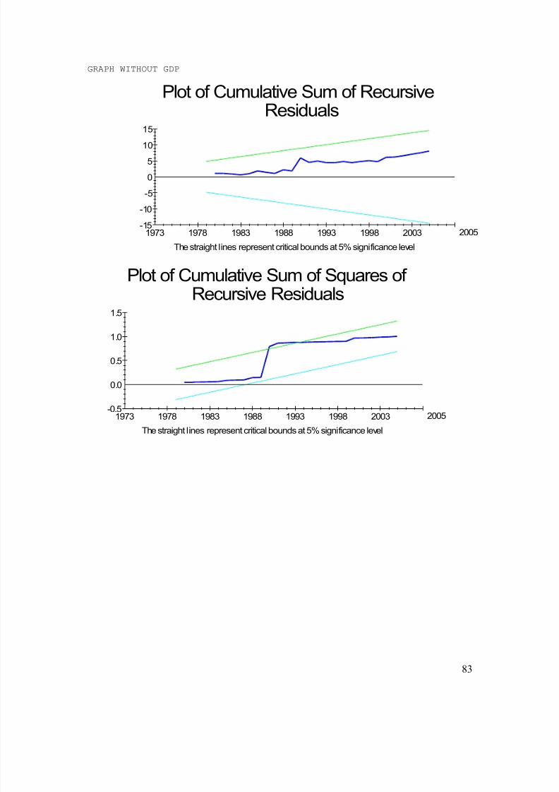
8/8/2019 e Dissertation
http://slidepdf.com/reader/full/e-dissertation 83/84
GRAPH WITHOUT GDP
Plot of Cumulative Sum of RecursiveResiduals
The straight lines represent critical bounds at 5% significance level
-5
-10
-15
0
5
10
15
1973 1978 1983 1988 1993 1998 2003 2005
Plot of Cumulative Sum of Squares of Recursive Residuals
The straight lines represent critical bounds at 5% significance level
-0.5
0.0
0.5
1.0
1.5
1973 1978 1983 1988 1993 1998 2003 2005
83

8/8/2019 e Dissertation
http://slidepdf.com/reader/full/e-dissertation 84/84
GRAPH WITH GDP
Plot of Cumulative Sum of Recursive
Residuals
The straight lines represent critical bounds at 5% significance level
-5
-10
-15
0
5
10
15
1973 1978 1983 1988 1993 1998 2003 2005
Plot of Cumulative Sum of Squares of Recursive Residuals
The straight lines represent critical bounds at 5% significance level
-0.5
0.0
0.5
1.0
1.5
1973 1978 1983 1988 1993 1998 2003 2005


![Dissertation on Dmitry Shostakovich's Harmonic Language... · 2019-11-27 · [MUSIC] January 1, 2014 I . B . M u s i c E x t e n d e d E s s a y Page 1 Dissertation on Dmitry Shostakovich’s](https://static.fdocuments.in/doc/165x107/5e5cc36f1832ee2a0f5f244f/dissertation-on-dmitry-shostakovichs-harmonic-language-2019-11-27-music.jpg)