Finance and Economics Discussion SeriesDivisions of Research & Statistics and Monetary Affairs

Federal Reserve Board, Washington, D.C.

Efficient Mismatch

David M. Arseneau and Brendan Epstein

2018-037

Please cite this paper as:Arseneau, David M., and Brendan Epstein (2018). “Efficient Mismatch,” Finance andEconomics Discussion Series 2018-037. Washington: Board of Governors of the FederalReserve System, https://doi.org/10.17016/FEDS.2018.037.

NOTE: Staff working papers in the Finance and Economics Discussion Series (FEDS) are preliminarymaterials circulated to stimulate discussion and critical comment. The analysis and conclusions set forthare those of the authors and do not indicate concurrence by other members of the research staff or theBoard of Governors. References in publications to the Finance and Economics Discussion Series (other thanacknowledgement) should be cleared with the author(s) to protect the tentative character of these papers.

Efficient Mismatch∗

David M. Arseneau†

Federal Reserve BoardBrendan Epstein‡

University of Massachusettsat Lowell

May 15, 2018

Abstract

This paper presents a model in which mismatch employment arises in a constrainedefficient equilibrium. In the decentralized economy, however, mismatch gives rise to acongestion externality whereby heterogeneous job seekers fail to internalize how theirindividual actions affect the labor market outcomes of competitors in a common un-employment pool. We provide an analytic characterization of this distortion, assessthe distributional nature of the associated welfare effects, and relate it to the relativeproductivity of low- and high-skilled workers competing for similar jobs.

Keywords: Labor market frictions, crowding in/out, skill-mismatch,competitivesearch equilibrium

JEL Classification: E24, J31, J64

∗The views expressed here are solely those of the authors and should not be interpreted as reflecting theviews of the Board of Governors of the Federal Reserve System or of any other person associated with theFederal Reserve System.

†Corresponding Author. Board of Governors of the Federal Reserve System; 20th St. and ConstitutionAve. NW; Washington, D.C. 20551; Phone: 202-452-2534. Email address: david.m.arseneau@frb.gov.

‡University of Massachusetts at Lowell, Department of Economics, Falmouth Hall, Suite 302l; One Uni-versity Ave., Lowell, MA 01854; Phone: 978-934-2789. Email address: brendan epstein@uml.edu.

1

1 Introduction

Empirical evidence suggests that labor market mismatch may help to explain recent U.S.

unemployment dynamics. Sahin, Song, Topa, and Violante (2014), for example, estimate

that an increase in sectoral mismatch between vacant jobs and unemployed workers con-

tributed as much as one-third of the rise in the U.S. unemployment rate after the 2007-’08

global financial crisis. Beyond labor market dynamics, mismatch may also have important

distributional implications as idle workers shift job seeking behavior across different sectors,

industries, and occupations within the labor market.

This paper develops a tractable theoretical framework to understand the welfare im-

plications of skill-mismatch employment. Our starting point is to build a model in which

mismatch is a feature of the constrained efficient equilibrium. The notion of mismatch con-

sidered in this paper is one in which an unemployed worker with a college degree chooses

to accept a lower paying job that does not necessarily require post-secondary education to

perform (i.e., an engineer can chose to work as a waiter). The alternative is to search instead

for a high-tech job that requires post-secondary education and, hence, cannot be performed

by a low-skilled worker (a college degree is required to get a job as an engineer).

A key contribution of the paper is to show that efficient mismatch does not generally

emerge in the decentralized equilibrium. In the private economy, mismatch generates a

distortion owing to competition amongst heterogeneous job seekers searching for low-skilled

employment in a common unemployment pool. While our model of mismatch is stylized, a

virtue is that it is tractable. This tractability allows for a complete analytic characterization

of all the distortions operating in the model as well as a clear understanding of how they are

shaped by the underlying structure of the labor market.

Our framework builds on the body of literature that embeds Diamond-Mortensen-Pissarides

style labor search and matching frictions (Diamond, 1982; Mortensen and Pissarides, 1994;

and Pissarides, 2000) into a general equilibrium setting. We deviate from the standard

setup by introducing two-sided heterogeneity and segmented labor markets. 1 Low-skilled

1Examples of papers that focus on heterogeneity in job matching include, among others, Pissarides (1994),Mortensen and Pissarides (1999), Albrecht and Vroman (2002), Gautier (2002), Shi (2002), and Pries (2008).More recently this literature has expanded to include on-the-job search; some examples include Barlevy(2002), Krause and Lubick (2006), Dolado et al. (2009), Menzio and Shi (2010), and Lise and Marc Robin

2

individuals are assumed to only be qualified to work in the low-tech sector while high-skilled

individuals can work in either the low- or high-tech sector. Hence, in our setup low- and

high-skilled job seekers are forced to compete in a common unemployment pool for job op-

portunities with a low-tech firm. Skill-mismatch employment (henceforth, mismatch) is a

situation in which a high-skilled worker endogenously chooses to enter into an employment

relationship with the low-tech firm.

Employment relationships are formed in one of two segmented labor markets, both of

which are characterized by search and matching frictions. The high-tech job market is a

standard search market with high-tech firms posting costly vacancies in order to match with

high-skilled job seekers. In contrast, the low-tech job market assumes that low- and high-

skilled job seekers compete in order to match with a given vacancy posted by the low-tech

firm. Once a vacancy is matched with an anonymous searching worker, there is random

assignment to worker type. That is, a vacant low-tech job is filled with either a low-skilled

worker or a high-skilled worker seeking mismatch employment with some probability. This

probability is an endogenous variable which depends on the labor force participation decisions

of low- and high-skilled households, respectively.

Our setup assumes only one type of low-tech job and does not consider the case in

which differentiated vacancies can be posted for low-skilled and mismatched workers. These

assumptions seem justified for two reasons. First, allowing for differentiated vacancies for

low-tech jobs implies a level of labor market segmentation which seems unrealistic. Second,

in our view, competition amongst different types of workers for a given job is at the heart of

the welfare relevance of mismatch employment. This competition is captured in our model

by the endogenous probability that a vacant low-tech job is filled with either a low-skilled or

mismatched worker. Under what circumstances does this competition result in an efficient

allocation of resources? Under what circumstances does it generate externalities? Who gains

and who losses from these externalities? Our framework allows us to answer these questions

by modeling job market competition explicitly through a common matching function for

low-tech jobs. In this sense, search and matching frictions are essential to our analysis.

(2017). Shimer (2007) presents a model of a mismatch with heterogeneous labor markets. Finally, somerecent contributions that study mismatch from an empirical standpoint include Sahin et al. (2014) andBarnichon and Figura (2015).

3

We show that in the constrained efficient equilibrium, a planner that takes as given the

search frictions internalizes the competition for low-tech jobs by choosing the socially optimal

skill-composition of the unemployment pool. The resulting efficient level of mismatch equates

the productivity differential between low-skilled and mismatched workers employed in low-

tech jobs to the differential in the marginal rate of substitution between consumption and

leisure across the two types of households. The planner can achieve this outcome because

labor allocations are chosen from the perspective of a socially optimal value of leisure.

Heterogeneous households do not necessarily share this value of leisure; hence, the level

of mismatch that obtains in the decentralized economy is generally inefficient. This result

is established in a series of propositions which, taken together, provide a complete analytic

characterization of the distortions in the model. Intuitively, the mismatch distortion arises

because high-skilled workers searching for mismatch jobs in the low-tech job market do

not internalize the effect their search activity has on the labor market outcomes of low-

skilled workers. By the same token, low-skilled workers do not internalize the effect their

search activity has on high-skilled job seekers looking for mismatch employment. As long

as individual households make participation decisions based on their own heterogeneous

private valuation of leisure, the socially optimal skill-composition of the unemployment pool

for low-tech jobs will not obtain.

Ultimately, the welfare implications across households are determined by relative pro-

ductivity. When high-skilled workers are more productive in mismatch employment relative

to their low-skilled colleagues, their participation in the market for low-tech jobs is ineffi-

ciently low. There is too little search activity and mismatch job creation is too low relative

to the constrained efficient equilibrium. In contrast, low-skilled participation is inefficiently

high. The resulting welfare effects are distributional in that high-skilled households experi-

ence welfare gains that come entirely at the expense of low-skilled households. The opposite

intuition holds when low-skilled workers are relatively more productive.

Efficient mismatch only emerges in the private economy when low-skilled and mismatched

workers are equally productive. In this knife-edge case, both types independently share

a common view of the private value of leisure which happens to coincide with the social

optimum. The lack of any true heterogeneity across households means that private objective

4

functions coincide and there is no scope for competition to distort the labor market.

Our main results are derived under a labor market structure characterized by wage bar-

gaining. It should be clear, however, that this distortion generalizes to any environment in

which wages are determined by a time-invariant surplus sharing rule, regardless of the wage

setting protocol that delivers that rule. Moreover, we show that while it is theoretically pos-

sible to decentralize efficient mismatch using a market-based method of wage determination,

doing so requires a strong assumption regarding the ability of the firm to post wages. In

order to obtain efficient mismatch in a competitive search equilibrium a la Moen (1997), the

low-tech firm needs to be able to post differentiated wages in a way that allows competing

job seekers to trade off their individual labor compensation against type-specific job finding

probabilities. Effectively, this implies the firm has an ability to segment the low-tech labor

market in a way that eliminates job competition. In this sense, it is not surprising that wage

posting removes the mismatch distortion.

We close the paper by doing some simple quantitative exercises using a calibrated version

of the model to illustrate the distributional effects of the mismatch distortion. The calibrated

model is also used to help gauge the size of the mismatch distortion relative to more well

known distortions in the search and matching literature (i.e., those created through inefficient

bargaining and/or the presence of unemployment benefits).

Our paper is related to a broader literature that focuses on different notions of mismatch

unemployment as well as heterogeneity in job matching. Within this strand, our work

focuses more narrowly on matching efficiency. Similar papers include Albrecht, Navarro,

and Vroman (2010) and Gravel (2011), both of which show that inefficiencies arise in models

with endogenous participation and heterogeneity in the productivity of matches. Gavrel

(2012) shows inefficiencies in a model with two-sided heterogeneity where firms can rank their

applicants. In each of these papers, the inefficiency operates through the production function

as the firm does not internalize how its vacancy posting decision affects average match quality.

In our paper, average match quality is also distorted, but the source of the inefficiency comes

from job competition amongst heterogeneous job seekers. Gautier, Teulings, and van Vuuren

(2010) develop a model of mismatch with two-sided heterogeneity where, absent on-the-job

search, efficiency obtains with a constant returns matching technology, provided congestion

5

externalities are absent. They show introducing on-the-job search generates a distortion that

can be removed by wage posting with commitment. Menzio and Shi (2011) develop a model

with heterogeneous quality in job matches and on-the-job search where, upon meeting, a

worker and a firm observe a potentially imperfect signal regarding the productivity of the

potential match. In their framework, the unique decentralized equilibrium is efficient. Our

paper differs from both of these in that we show mismatch itself generates a distortion which

is unrelated to on-the-job search.

The remainder of the paper is organized as follows. The next section presents the model.

Section 3 describes decentralized equilibrium with wages determined via bargaining. The

main results are presented in Section 4 in a series of propositions. Section 5 presents results

in the competitive search equilibrium. Section 6 uses a parameterized version of the model

to illustrate some quantitative points. Finally, Section 7 concludes.

2 The Model

The model introduces two-sided heterogeneity for both workers and firms into the general

equilibrium labor search framework of Arseneau and Chugh (2012). This framework offers a

convenient benchmark for understanding the efficient equilibrium and the distortions associ-

ated with the decentralized search equilibrium. Note also that our model does not allow for

mismatched workers to transit to high-tech employment through on-the-job search. We have

shown in other work that on-the-job search only serves to amplify the mismatch distortion,

but does so at the expense of notably complicating the model.

2.1 Production

Production is divided into two sectors: a final goods sector and an intermediate goods sector.

The intermediate goods sector consists of two types of firms called high-tech and low-tech

firms, respectively. Regardless of firm type, labor is the only input into production. In order

to hire a unit of labor, intermediate goods producing firms must engage in costly search and

matching in order to form a long-lasting employment relationship.

Firm type is differentiated by the skill set required to do the job. High-tech intermediate

6

goods, denoted yH(nHt ) where the production function yH(.) is increasing and concave, can

only be produced by high-skilled workers, nHt . In contrast, low-tech intermediate goods,

denoted yLt (nL

t , nMt ) where yL(.) is increasing and weakly concave in both its arguments, can

be produced using either low- or high-skilled workers. In our notation, nLt denotes a low-

skilled worker employed by the low-tech firm and nMt denotes a high-skilled worker engaged

in mismatch employment in the low-tech production sector.

The final goods producer simply aggregates the intermediate goods into a single final

product, which is sold to, and ultimately consumed by, households, so Yt = F (yLt , yH

t ). It is

helpful to differentiate between three distinct cases depending on the relative productivity

of low-skilled versus mismatched workers in the production of low-tech goods. Letting yLi

denote the derivative of with respect to the ith input in the production function for the

low-tech intermediate good, the cases we focus on are:

(Case i.) yL1 (nL

t , nMt ) < yL

2 (nLt , nM

t );

(Case ii.) yL1 (nL

t , nMt ) > yL

2 (nLt , nM

t );

(Case iii.) yL1 (nL

t , nMt ) = yL

2 (nLt , nM

t ).

As will become clear later in the paper, assumptions regarding the precise nature of

mismatch employment turn out to play a critical role in shaping our main results.

2.2 The Labor Market

The labor market is segmented into two distinct markets for low- and high-tech employment,

respectively, both of which are subject to search and matching frictions.

The search market for high-tech jobs is standard. Existing high-tech employment rela-

tionships exogenously terminate with probability ρH . Replenishing the stock of high-skilled

jobs requires costly effort on the part of workers and firms. High-skilled households spend

time searching, sHt , for employment opportunities while high-tech firms must pay a fixed

cost, γH , to post vacancies in the high-tech market, vHt , in order to attract workers. There

is free entry in high-tech vacancy postings. New high-tech jobs are formed according to

a matching technology, m(sHt , vH

t ), which is constant returns to scale and increasing and

concave in both vHt and sH

t .

7

The stock of high-tech jobs evolves according to

nHt = (1 − ρH)nH

t−1 + m(sHt , vH

t ) (1)

The market for low-tech jobs is non-standard due to the introduction of mismatch em-

ployment. Low-tech jobs expire at exogenous rate, ρL, and low-tech firms must pay a fixed

cost, γL, in order to post a vacancy, vLt , to attract workers into employment in the low-tech

industry. As above, there is free entry in low-tech vacancy postings. However, a key differ-

ence is that, in contrast with high-tech jobs, low-tech production can be done using labor

supplied by both types of households. Let et = sLt + sM

t denote total search effort in the

market for low-tech jobs, where sL denotes search by low-skilled households for low-tech jobs

and sM denotes search by high-skilled households for mismatched jobs.

New matches are formed according to a matching technology, m(et, vLt ), which is constant

returns to scale and increasing and concave in both et and vLt . However, because the pool of

searching workers in the low-tech job market contains both low- and high-skilled job seekers,

we assume random assignment regarding whether a given low-tech vacancy matches with a

low- or a high-skilled worker.2 Let ηt = sLt /et denote the share of low-skilled job seekers in

the market for low-tech jobs and 1 − ηt denote the share of high-skilled workers searching

for mismatched jobs.

Under these assumptions, new low-tech jobs form according to ηtm(et, vLt ), so the stock

of low-tech labor evolves according to

nLt = (1 − ρL)nL

t−1 + ηtm(et, vLt ) (2)

and the stock of mismatch labor evolves according to

nMt = (1 − ρL)nM

t−1 + (1 − ηt)m(et, vLt ). (3)

Assuming that both low- and high-skilled individuals obtain low-tech jobs through a

2Random assignment reflects an assumption that the market for low-skilled jobs is not further segmentedand that low-tech firms cannot rank applicants by skill level in the job matching process.

8

common matching technology captures the idea that mismatch creates spillovers across het-

erogeneous workers through competition in a common unemployment pool for these types

of jobs.

Finally, in terms of notation, let fHt = m(sH

t , vHt )/sH

t ; fLt = m(et, v

Lt )/et; qH

t = m(sHt , vH

t )/vHt ;

qLt = m(et, v

Lt )/vL

t . Also, define θHt ≡ vH

t /sHt as market tightness in the high-tech sector and

θLt ≡ vL

t /et as market tightness in the low-tech sector.

2.3 The Social Welfare Problem

The economy is inhabited by a unit mass of individuals, a fraction κ of which are low-skilled

while the remaining 1 − κ are high-skilled. Individuals are aggregated into two separate

households, differentiated by type. For the sake of convenience, we assume there is aggregate

risk sharing across individuals within a given household type.3

Regardless of type, households allocate their time between labor market activity (i.e.,

working or actively searching for employment) and leisure. In terms of notation, let the

mass of low-skill individuals participating in the labor force be given by lfpLt = nL

t + sLt −

ηtm(e, vLt ).4 Similarly, the mass of high-skill individuals participating in the labor force is

given by lfpHt + lfpM

t , where: lfpHt = nH

t + sHt − m(sH

t , vHt ) denotes participation in the

market for high-tech jobs and lfpMt = nM

t + sMt − (1 − ηt)m(e, vL

t ) denotes participation in

the low-tech job market for mismatched jobs.

Household preferences are defined over consumption of the final good, denoted cLt and

cHt for low- and high-skilled households, respectively, and the disutility of labor market

participation. Any given household derives utility from consumption per the function u,

with ∂u∂c

= uc > 0 and ∂2u∂c2

< 0. In addition, any given household derives disutility from labor

force participation per the function h, with ∂h∂lfp

= h′ > 0 and ∂2h∂lfp2 < 0.

The planner chooses allocations subject to the search frictions—so that the concept of

efficiency is one of constrained efficiency, or the “second best”—but internalizes the random

3The risk sharing assumption is common in search-theoretic general equilibrium models of the labormarket following Merz (1995) and Andolfatto(1996).

4Note that the timing of the model is such that successful search within the period, given by ηtm(e, vLt )

for low-skilled individuals searching in the low-tech job market, is counted as part of the employment stock,so it must be netted out to avoid double counting.

9

assignment of low-tech jobs between low-skilled and mismatched workers. It does this by

directly choosing the skill composition of the pool of unemployed workers seeking employment

in the low-tech industry.

The social welfare problem involves choosing a sequence of allocations, {cLt , cH

t , nLt ,

nMt , nH

t , sLt , sM

t , sHt , vH

t , vLt , ηL

t }, to maximize an equally-weighted sum of the utility of

low- and high-skilled households whose discounted lifetime expected value is denoted by U .

Specifically, the planner’s problem is

max U = Et

∞∑

t=0

βt{u(cLt ) − hL

(nL

t + sLt − ηL

t m(eL, vLt ))

(4)

+u(cHt ) − hH

(nH

t + sHt − m(sH , vH

t ))− hM

(nM

t + sMt −

(1 − ηL

t

)m(eL, vL

t ))}

where: Et is the expectation operator; β ∈ (0, 1) is the subjective discount factor.

The planner faces a resource constraint

Yt = cLt + cH

t + γLvLt + γHvH

t (5)

as well as the three different laws of motion for the respective stocks of employment given

by equations (1) through (3), and the definitions et = sLt + sM

t and ηt = sLt /et.

2.4 Social Efficiency

The constrained efficient equilibrium is characterized by a set of six efficiency conditions

combined with the economy-wide resource constraint, the three laws of motion for the re-

spective labor stocks, and the definition of the share of low-skilled searchers in the market for

low-tech employment. All details regarding the derivation of these conditions are relegated

to a supplementary online appendix for expositional purposes.

The planner chooses allocations to equate the the marginal utility of consumption across

both households, so consumption risk sharing extends across as well as within households.

uLc,t = uH

c,t = uc,t (6)

10

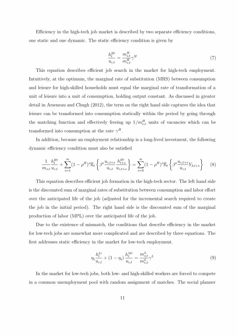
Efficiency in the high-tech job market is described by two separate efficiency conditions,

one static and one dynamic. The static efficiency condition is given by

hH′t

uc,t

=mH

s,t

mHv,t

γH (7)

This equation describes efficient job search in the market for high-tech employment.

Intuitively, at the optimum, the marginal rate of substitution (MRS) between consumption

and leisure for high-skilled households must equal the marginal rate of transformation of a

unit of leisure into a unit of consumption, holding output constant. As discussed in greater

detail in Arseneau and Chugh (2012), the term on the right hand side captures the idea that

leisure can be transformed into consumption statically within the period by going through

the matching function and effectively freeing up 1/mHv,t units of vacancies which can be

transformed into consumption at the rate γH .

In addition, because an employment relationship is a long-lived investment, the following

dynamic efficiency condition must also be satisfied

1

ms,t

hH′t

uc,t

+∞∑

s=1

(1 − ρH)sEt

{

βs uc,t+s

uc,t

hH′t+s

uc,t+s

}

=∞∑

s=0

(1 − ρH)sEt

{

βs uc,t+s

uc,t

Y3,t+s

}

(8)

This equation describes efficient job formation in the high-tech sector. The left hand side

is the discounted sum of marginal rates of substitution between consumption and labor effort

over the anticipated life of the job (adjusted for the incremental search required to create

the job in the initial period). The right hand side is the discounted sum of the marginal

production of labor (MPL) over the anticipated life of the job.

Due to the existence of mismatch, the conditions that describe efficiency in the market

for low-tech jobs are somewhat more complicated and are described by three equations. The

first addresses static efficiency in the market for low-tech employment.

ηt

hL′t

uc,t

+ (1 − ηt)hM ′

t

uc,t

=mL

s,t

mLv,t

γL (9)

In the market for low-tech jobs, both low- and high-skilled workers are forced to compete

in a common unemployment pool with random assignment of matches. The social planner

11

internalizes this by equating a probability weighted average of the marginal rates of substitu-

tion for low- and high-skilled job seekers, respectively, to the marginal rate of transformation

of a generic unit of leisure into consumption. In other words, the equation highlights the fact

that the social planner has in mind a specific notion of the socially optimal value of leisure

when it internalizes the composition of the low-skilled labor pool.

There are two separate dynamic efficiency conditions that govern the evolution of the

stock of low-tech and mismatched jobs in the economy, respectively, given by

1

mLs,t

(

ηt

hL′t

uc,t

+ (1 − ηt)hM ′

t

uc,t

)

−1 − ηt

fLt

(hM ′

t

uc,t

−hL′

t

uc,t

)

(10)

+∞∑

s=1

(1 − ρL)sEt

{

βs uc,t+s

uc,t

hL′t+s

uc,t+s

}

=∞∑

s=0

(1 − ρL)sEt

{

βs uc,t+s

uc,t

Y1,t+s

}

and

1

mLs,t

(

ηt

hL′t

uc,t

+ (1 − ηt)hM ′

t

uc,t

)

+ηt

fLt

(hM ′

t

uc,t

−hL′

t

uc,t

)

(11)

+∞∑

s=1

(1 − ρL)sEt

{

βs uc,t+s

uc,t

hM ′t+s

uc,t+s

}

=∞∑

s=0

(1 − ρL)sEt

{

βs uc,t+s

uc,t

Y2,t+s

}

The general intuition for both expressions, which describe socially optimal low-tech and

mismatch job creation, respectively, is generally similar to that for equation (8) above.

Indeed, the second line of each equation equates the discounted sum of the MRS between

consumption and leisure to the discounted sum of the MPL over the life of the job. But,

equations (10) and (11) differ from equation (8) in two key respects. First, as with the static

efficiency condition, the planner has in mind a particular notion of the socially optimal value

of leisure given the nature of matching in the low-tech market. This is captured by the first

term in the top line of each equation, familiar from equation (9) above. In addition, the

second term on the top line of each equation captures the relative cost of shifting job search

activity for low-tech jobs between the low-skilled and high-skilled household.

The interpretation is more clear if we take the difference between equations (10) and (11)

12

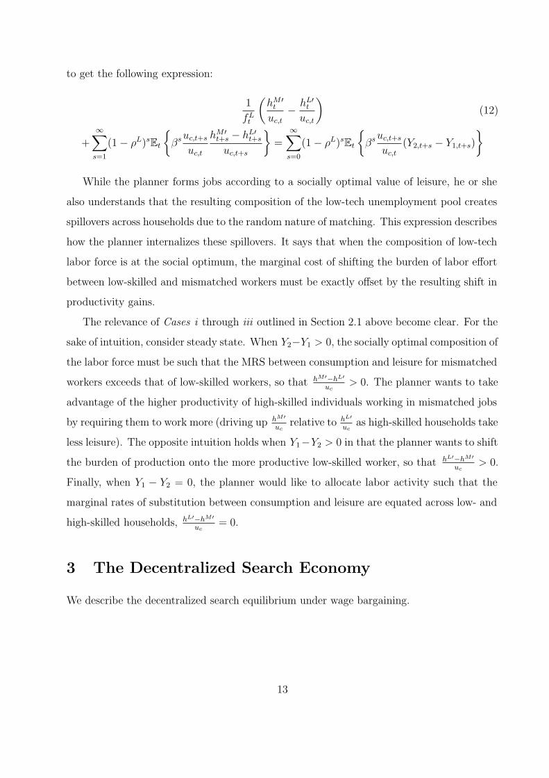
to get the following expression:

1

fLt

(hM ′

t

uc,t

−hL′

t

uc,t

)

(12)

+∞∑

s=1

(1 − ρL)sEt

{

βs uc,t+s

uc,t

hM ′t+s − hL′

t+s

uc,t+s

}

=∞∑

s=0

(1 − ρL)sEt

{

βs uc,t+s

uc,t

(Y2,t+s − Y1,t+s)

}

While the planner forms jobs according to a socially optimal value of leisure, he or she

also understands that the resulting composition of the low-tech unemployment pool creates

spillovers across households due to the random nature of matching. This expression describes

how the planner internalizes these spillovers. It says that when the composition of low-tech

labor force is at the social optimum, the marginal cost of shifting the burden of labor effort

between low-skilled and mismatched workers must be exactly offset by the resulting shift in

productivity gains.

The relevance of Cases i through iii outlined in Section 2.1 above become clear. For the

sake of intuition, consider steady state. When Y2−Y1 > 0, the socially optimal composition of

the labor force must be such that the MRS between consumption and leisure for mismatched

workers exceeds that of low-skilled workers, so that hM ′−hL′

uc> 0. The planner wants to take

advantage of the higher productivity of high-skilled individuals working in mismatched jobs

by requiring them to work more (driving up hM′

ucrelative to hL′

ucas high-skilled households take

less leisure). The opposite intuition holds when Y1−Y2 > 0 in that the planner wants to shift

the burden of production onto the more productive low-skilled worker, so that hL′−hM′

uc> 0.

Finally, when Y1 − Y2 = 0, the planner would like to allocate labor activity such that the

marginal rates of substitution between consumption and leisure are equated across low- and

high-skilled households, hL′−hM ′

uc= 0.

3 The Decentralized Search Economy

We describe the decentralized search equilibrium under wage bargaining.

13

3.1 Households

Individuals in the economy are separated into low- and high-skilled households.

3.1.1 Low-Skilled Households

The low-skilled household chooses sequences of consumption, cLt , real non state-contingent

bond, BLt , and search activity to achieve a desired low-tech employment stock in order

to maximize discounted lifetime utility UL = Et

∑∞t=0 βt(u(cL

t ) − h(lfpL

t

)). Low-skilled

households face the following budget constraint:

cLt + BL

t = wLt nL

t + χL(1 − fLt )sL

t + RtBLt−1 + κ(ΠL

t + ΠHt ) − TL

t

where: wLt is the wage received by a low-skilled individual employed in a low-tech job; χL

is an exogenous unemployment benefit; the real non state-contingent bond pays an interest

rate of Rt; ΠLt and ΠH

t denote the profits of intermediate low- and high-tech goods producing

firms paid to the household in the form of a dividend, and TLt is a lump sum tax levied by a

government to finance the unemployment benefit. We assume that households pay the lump

sum tax and receive a dividend from firm ownership in proportion to their share of the total

population.

In addition to the budget constraint, the household also faces a constraint on the perceived

law of motion for the stock of employment given by:

nLt = (1 − ρL)nL

t−1 + fLt sL

t

The first order conditions for cLt and BL

t can be manipulated into a standard bond Euler

equation:

1 = Et

{βuL

c,t+1

uLc,t

Rt+1

}

, (13)

which defines the stochastic discount factor for pricing the one-period, risk-free government

bond, Ξt+1|t ≡ βuLc,t+1/u

Lc,t.

We can also use the first order conditions on sLt and nL

t to obtain the optimal labor-force

14

participation condition for low-skilled individuals:

hL′t

uLc,t

= (1 − fLt )χL + fL

t

[

wLt + (1 − ρL)EtΞt+1|t

{1 − fL

t+1

fLt+1

(hL′

t+1

uLc,t+1

− χL

)}]

(14)

which says that the low-skilled household will search for low-tech employment up until the

point at which the probability-weighted cost of doing so, the disutility of search effort net

of the outside option, χL, is exactly offset by the probability weighted expected benefit of

getting a low-tech job. The expected benefit of low-tech employment is the wage plus the

continuation value of the long-lived employment relationship.

3.1.2 High-Skilled Households

High-skilled households choose sequences of consumption, cHt , non state-contingent bond

holdings, BHt , and search activity in both the market for low- and high-tech jobs, given by

sMt and sH

t , in order to achieve a desired stock of mismatch and high-tech employment, given

by nMt and nH

t , respectively. These quantities are chosen in order to maximize discounted

lifetime utility, UH = Et

∑∞t=0 βt(u(cH

t ) − h(lfpH

t , lfpMt

)).

The high-skilled household faces the following budget constraint:

cHt + BH

t = wHt nH

t + wMt nM

t + χH[(1 − fL

t )sMt + (1 − fH

t )sHt

]

+RtBHt−1 + (1 − κ) (ΠL

t + ΠHt ) − TH

t ,

and perceived laws of motion for the stocks of mismatch and high-tech employment:

nMt = (1 − ρL)nM

t−1 + fLt sM

t ,

and

nHt = (1 − ρH)nH

t−1 + fHt sH

t ,

where: wHt and wM

t are the wages received by high-skilled individuals employed in high-tech

and mismatch jobs, respectively; χH is an exogenous unemployment benefit paid to high-skill

workers who searched for jobs but did not find one, and THt is a lump sum tax.

The first-order conditions over cHt and BH

t can be combined to yield a standard consump-

tion Euler equation:

1 = Et

{βuH

c,t+1

uHc,t

Rt+1

}

. (15)

Noting that trade of the non-contingent real bond equates the marginal utility of con-

15

sumption across the low- and high-skilled household, so that βuLc,t+1/u

Lc,t = βuH

c,t+1/uHc,t =

Ξt+1|t, we can use the first order condition for nHt to write the optimal participation condition

in the market for high tech employment as:

hH′t

uHc,t

= (1 − fHt )χH + fH

t

[

wHt + (1 − ρH)EtΞt+1|t

{1 − fH

t+1

fHt+1

(hH′

t+1

uHc,t+1

− χH

)}]

, (16)

Finally, the condition governing optimal participation for high-skilled individuals in the

market for low-tech jobs can be written as:

hM ′t

uHc,t

=(1 − fL

t

)χH + fL

t

[

wMt + (1 − ρL)EtΞt+1|t

{1 − fL

t+1

fLt+1

(hM ′

t+1

uHc,t+1

− χH

)}]

(17)

Intuitively, the interpretation of equations (16) and (17) are very similar to that of equa-

tion (14) above for the low-skilled household.

The tradeoff faced by the high-skilled household when deciding how to allocate search

activity across the two segmented labor markets can be highlighted by comparing equations

(16) and (17) in the steady state. For simplicity, assume no unemployment benefits, χH = 0,

and that employment relationships form in the presence of search frictions, so fL < 1

and fH < 1, but they only last for a single period, so ρL = ρH = 1. In this case, the

high-skilled household allocates search activity so that the marginal rate of substitution

between participation in the high-tech and mismatch labor markets is equal to the probability

adjusted wage ratio across the two markets:

hH′

hM ′=

fH

fL

wH

wM.

Holding hH′/hM ′ constant, a larger wage premium for working in high-tech employment

(higher wH/wM) must be compensated by improved job finding prospects in the market for

mismatch employment (lower fH/fL). In this sense, our model captures the idea that high-

skilled individuals are willing to accept a lower quality job to move out of unemployment

more quickly, but doing so comes at the cost of accepting a lower wage.

16

3.2 Production

Production is divided into a final goods and an intermediate goods sector.

3.2.1 Final Goods Production

The representative final goods producer purchases both low- and high-tech intermediate

inputs and aggregates them into a final good using the technology, Y (yLt ,yH

t ). This final

good is then sold to households in a perfectly competitive market. The final goods producer

chooses intermediate inputs to solve the following problem:

max Et

∞∑

t=0

Ξt+1|t

[Y (yL

t , yHt ) − pL

t yLt − pH

t yHt

],

where: pLt and pH

t are the prices of the low- and high-tech intermediate inputs, respectively,

relative to the final good. The demand for each intermediate input equates the marginal

product to the price, so that YL,t = pLt and YH,t = pH

t .

3.2.2 Intermediate Goods Production

Two types of firms engage in the production of intermediate goods. Each operates separately

in either the low- or the high-tech sector.

Low-tech Firms. For a given low-tech vacancy, the low-tech firm can match with and

hire either a low- or a high-skilled worker. Accordingly, the low-tech firm chooses the desired

stock of low-skill employees, nLt , the desired stock of high-skill employees, nM

t , and vacancies,

vLt , to solve:

max Et

∑

t

Ξt+1|t

[pL

t yL(nLt , nM

t ) − wLt nL

t − wMt nM

t − γLvLt

],

subject to the perceived laws of motion for low-skill and mismatch employment stocks,

respectively:

nLt = (1 − ρL)nL

t−1 + ηLt qL

t vLt ,

andnM

t = (1 − ρL)nMt−1 +

(1 − ηL

t

)qLt vL

t ,

where: qLt is the probability that a given vacancy posted in the market for low-tech jobs

is successful in finding a worker, regardless of whether the worker is low- or high-skill.

17

Furthermore, the fraction of low-skill workers in the total pool of individuals searching for

low-skill jobs is given by ηLt ≡ sL

t /(sLt + sM

t ). With this notation, the per period probability

that a low-tech vacancy turns into an employment match with a low-skill worker is ηtqLt and

the probability that a low-tech vacancy turns into a mismatch employment relationship with

a high-skill worker is (1 − ηt)qLt .

The optimal vacancy posting condition is given by:

γL

qLt

= ηLt J

Lt +

(1 − ηL

t

)JM

t , (18)

where: JLt and JM

t are defined by the Lagrangian multipliers on the perceived laws of motion

for low-tech and mismatch employment, respectively. Free entry implies that low-tech firm

posts vacancies up until the point at which the cost, γL, is exactly offset by the expected

gain from making a match. The expected gain is the probability that a match is made in

the low-tech market, qLt , times a probability weighted average of the value of a match with

a low-tech worker, ηLt J

Lt , and a (mismatched) high-tech worker, (1 – ηL

t )JMt . Note that free

entry implies that it is always optimal for the low-tech firm to fill an open position with

any type of worker it encounters as long as the surplus associated with the employment

relationship is positive.

The job creation conditions for low-skill and mismatch employment are given by:

JLt = pL

t yL1,t − wL

t +(1 − ρL

)Et

{Ξt+1|tJ

Lt+1

}, (19)

andJM

t = pLt yL

2,t − wMt +

(1 − ρL

)Et

{Ξt+1|tJ

Mt+1

}. (20)

Both equate the value of a (low-skilled or mismatched, respectively) employee working in

the low-tech job to the present discounted value of the stream of marginal revenues that the

job produces, net of the wage, over the expected duration of the employment relationship.

High-tech Firms. High-tech firms can only employ high-skilled workers because they are

the only ones qualified to do the work. The high-tech firm chooses the stock of high-skill

employees, nHt , and vacancies, vH

t , to solves the following profit maximization problem:

max Et

∑

t

Ξt+1|t

[pH

t yH(nHt ) − wH

t nHt − γHvH

t

],

subject to the perceived law of motion for high-tech employment:

nHt = (1 − ρH)nH

t−1 + qHt vH

t ,

18

where: qHt is the probability that a given vacancy posted in the market for high-tech jobs is

successful in finding a worker.

The optimal vacancy posting condition is given by:

γH/qHt = JH

t , (21)

where: JHt is the Lagrangian multiplier on the law of motion for high-tech employment.

The job creation condition for high-skill employment is given by:

JHt = pH

t yH1,t − wH

t +(1 − ρH

)Et

{Ξt+1|tJ

Ht+1

}. (22)

3.3 The Labor Market

In order to close the model, we need to address matching and wage determination in each

of the two segmented labor markets.

3.3.1 Matching

Labor market matches are formed according to the same constant returns matching tech-

nologies described in Section 2 for low-tech, mismatched, and high-tech jobs, respectively.

3.3.2 Wage Determination

Wages are determined through Nash bargaining. Let ψi ∈ (0, 1) for i ∈ (L,H) denote the

exogenous bargaining power of workers. Nash bargaining we well known in the literature, so

for the sake of brevity we present only the wage solution, leaving the details to the Appendix.

The wage for a low-skilled worker employed in a low-tech job is given by:

wLt = ψLpL

t yL1,t +

(1 − ψL

)χL + ψL(1 − ρL)Et

{Ξt+1|tf

Lt+1J

Lt+1

}. (23)

The wage paid by low-tech firms to low-skilled workers is a weighted average of the

present discounted value of the stream of marginal revenue that accrues to the low-tech firm

from hiring the additional employee and the outside option that accrues to the worker, given

by the unemployment benefit.

19

The mismatch wage is given by the expression:

wMt = ψHpL

t yL2,t +

(1 − ψH

)χH + ψH(1 − ρL)Et

{Ξt+1|tf

Lt+1J

Mt+1

}. (24)

Finally, the wage for a high-skilled worker employed in a high-tech job is given by:

wHt = ψHpH

t yH1,t +

(1 − ψH

)χH + ψH(1 − ρH)Et

[Ξt+1|t

(fH

t+1JHt+1

)]. (25)

Note that because free entry into vacancy postings drives JHt+1 = γH/qH

t+1, the continua-

tion value in equation (25) can also be expressed as Et{Ξt+1|t(fHt+1/q

Ht+1)γ

H ].

3.4 Search Equilibrium

The equilibrium of the system is a sequence of allocations and prices {cLt , cH

t , Rt, nLt , nM

t ,

nHt , sL

t , sMt , sH

t , vLt , vH

t , JLt , JM

t , JHt , wL

t , wMt , wH

t , pLt , pH

t , BHt , BL

t , T Lt , T H

t } that solves

the optimality conditions for: low-skilled households, summarized by equations (13) through

(14); high-skilled households, summarized be equations (15) through (17); low-tech interme-

diate goods producers, summarized by equations (18) through (20); high-tech intermediate

goods producers, summarized by equations (21) and (22).

We also have the demand for the low- and high-tech intermediate input, given by YL,t =

pLt /Zt and YH,t = pH

t /Zt, respectively; the laws of motion for respective employment stocks,

equations (1) through (3); the wages are pinned down by equations (23) through (25).

The bond market clearing condition is given by BLt + BH

t = 0. There is a government

budget constraint that must be satisfied in order to finance the unemployment benefit,

κT Lt + (1 − κ)TH

t = χL(1 − fLt )sL

t + χH[(1 − fL

t )sMt + (1 − fH

t )sHt

]. The household budget

constraint pins down the level of bond holdings.

Finally, the economy-wide resource constraint is given by:

Yt = cLt + cH

t + γLvLt + γHvH

t (26)

20

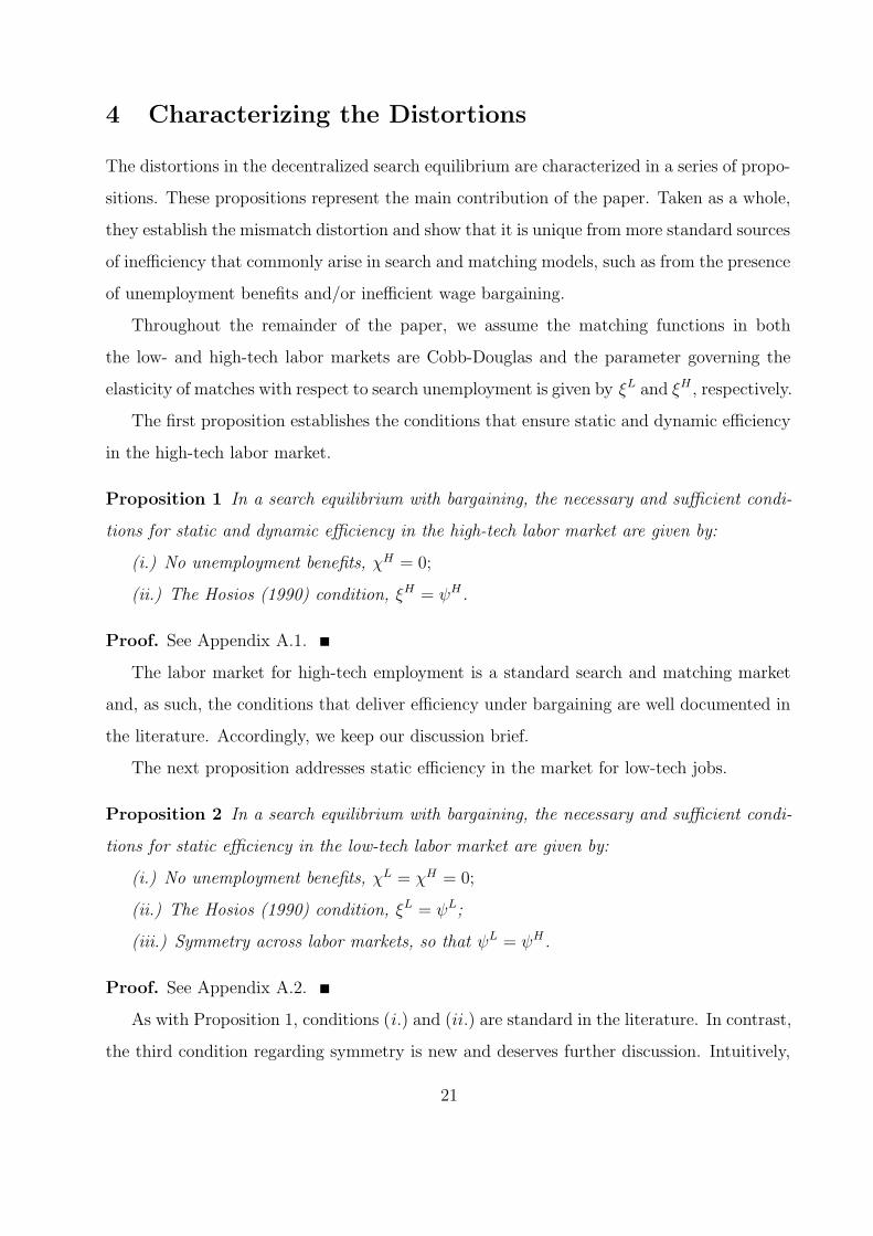
4 Characterizing the Distortions

The distortions in the decentralized search equilibrium are characterized in a series of propo-

sitions. These propositions represent the main contribution of the paper. Taken as a whole,

they establish the mismatch distortion and show that it is unique from more standard sources

of inefficiency that commonly arise in search and matching models, such as from the presence

of unemployment benefits and/or inefficient wage bargaining.

Throughout the remainder of the paper, we assume the matching functions in both

the low- and high-tech labor markets are Cobb-Douglas and the parameter governing the

elasticity of matches with respect to search unemployment is given by ξL and ξH , respectively.

The first proposition establishes the conditions that ensure static and dynamic efficiency

in the high-tech labor market.

Proposition 1 In a search equilibrium with bargaining, the necessary and sufficient condi-

tions for static and dynamic efficiency in the high-tech labor market are given by:

(i.) No unemployment benefits, χH = 0;

(ii.) The Hosios (1990) condition, ξH = ψH .

Proof. See Appendix A.1.

The labor market for high-tech employment is a standard search and matching market

and, as such, the conditions that deliver efficiency under bargaining are well documented in

the literature. Accordingly, we keep our discussion brief.

The next proposition addresses static efficiency in the market for low-tech jobs.

Proposition 2 In a search equilibrium with bargaining, the necessary and sufficient condi-

tions for static efficiency in the low-tech labor market are given by:

(i.) No unemployment benefits, χL = χH = 0;

(ii.) The Hosios (1990) condition, ξL = ψL;

(iii.) Symmetry across labor markets, so that ψL = ψH .

Proof. See Appendix A.2.

As with Proposition 1, conditions (i.) and (ii.) are standard in the literature. In contrast,

the third condition regarding symmetry is new and deserves further discussion. Intuitively,

21

condition (ii.) delivers the efficient wage for low-skilled workers endowed with bargaining

power, ψL, while condition (iii.) delivers the efficient wage for mismatched workers endowed

with bargaining power, ψH . Given that the elasticity of the matching function with respect

to search unemployment, ξL, is common for both types of jobs (i.e., they are formed through

a common matching function), it must be that efficiency requires ψL = ψH = ξL. In this

sense, the symmetry condition is nothing more than an additional constraint that is required

to ensure bargaining efficiency across both types of jobs. When taken in conjunction with

Proposition 1, it highlights the fact that asymmetries in labor market institutions (i.e.,

ψL 6= ψH and/or ξL 6= ξH) can lead to distortions that spill over across segmented labor

markets. This is true even in the case where ψL = ξL and ψH = ξH holds for each market

individually.

The next proposition establishes the unique instance in which the decentralized economy

is able to achieve the constrained efficient outcome.

Proposition 3 The search equilibrium with bargaining achieves the constrained efficient

equilibrium if and only if yLnL(nL

t , nMt ) = yL

nM (nLt , nM

t ) and Propositions 1 and 2 both hold.

Proof. See Appendix A.3.

The following corollary is a direct result of Proposition 3 and establishes a link between

productivity differentials and dynamic efficiency in low-tech and mismatch employment.

This is the mismatch distortion, which is a key result of the paper.

Corollary 1 In a search equilibrium with bargaining, productivity differential in low-tech

production (i.e., yL1 (nL

t , nMt ) 6= yL

2 (nLt , nM

t )) violate dynamic efficiency for both low-tech and

mismatch employment. In this case, the private equilibrium is not constrained efficient,

regardless of whether or not Proposition 1 and 2 both hold.

The mismatch distortion is a form of congestion externality that arises because low- and

high-skilled workers compete to match with a fixed number of low-tech vacancies. This

competition is distortionary as long as there is heterogeneity in the private valuation of

leisure. This heterogeneity only occurs when there is a productivity gap between the two

22

labor inputs. In this case, high-skilled workers searching for mismatched jobs do not in-

ternalize the fact that increasing search effort can crowd in or crowd out the job finding

prospects of low-skilled workers who are looking to match with the same set of vacancies.

Similarly, low-skilled workers do not internalize the fact that their search behavior affects

the job finding prospects of high-skilled workers looking for mismatch employment. Neither

agent participates in the labor market in a way that is consistent with the planner’s view of

the social valuation of leisure.

When there is no productivity gap low- and high-skilled workers value leisure symmetri-

cally in a way that aligns with the social value of leisure. Accordingly, the intuition behind

Proposition 3 is straightforward: the mismatch distortion is eliminated due to the lack of

any meaningful heterogeneity in the objective functions of the two types of households.

5 Competitive Search Equilibrium

The mismatch distortion is derived assuming wages are determined via bargaining. This

raises the question of whether it is robust to other wage determination protocols.

In this section, we show that while it is technically feasible to decentralize the efficient

set of wages, doing so requires an extreme—an we think unreasonable—assumption about

the ability of the firm to effectively segment the low-skilled labor market.

We consider wage posting in a competitive search equilibrium (CSE) as described in

Moen (1997). The firm understands there is a tradeoff between the wage that it posts in a

given que and the number of workers that will join that que in order to try to match with

that particular posting. While posting a lower wage may increase the value of a potential

match to the firm, doing so makes that same match harder to fill because the lower wage is

less attractive to searching workers.

In order to implement wage posting, the high-tech firm chooses wHt and θH

t to maximize

the value of a high-tech vacancy, given by equation (21), subject to optimal participation

condition for high-skilled households, equation (16). The resulting surplus sharing rule is

WHt − UH

t

JHt

=ξH

1 − ξH(27)

23

where: WHt − UH

t =hH′

t −χHuHc,t

fHt uH

c,tis the value of a high-tech job to a high-skilled worker as

defined by equation (16). This equation implicitly determines the high-tech wage.

The low-tech firm chooses differentiated wages, wLt and wM

t , as well as the effective que

lengths for each type of worker, by choosing θLt and ηt, in order to maximize the expected

value of a low-tech vacancy, given by equation (18), subject to the participation constraints

for low-tech and mismatch search activity, given by equations (14) and (17), respectively.

The solution to this problem gives rise to two conditions which, together, implicitly pin

down the wages for low-skilled and mismatch jobs. The first condition states that the firm

posts wages in a way that equates the value of low-skilled and mismatch workers.

JLt = JM

t (28)

The second condition gives rise to the following surplus sharing rule:

ηt(WLt − UL

t ) + (1 − ηt)(WMt − UM

t )

ηtJLt + (1 − ηt)J

Mt

=ξL

1 − ξL(29)

where: WLt −UL

t =hL′

t −χLuLc,t

fLt uL

c,tis the value of a low-tech job to a low-skilled worker as defined

by equation (14) and WMt −UH

t =hM ′

t −χHuHc,t

fLt uM

c,tis the value of a low-tech job to a high-skilled

worker as defined by equation (17).

In order to solve for the CSE, we replace equations (23) through (25), which determine

wages in the search equilibrium with bargaining, with equations (27) through (29), which

determine the posted wages.

The results are summarized by the following proposition.

Proposition 4 As long as χL = χH = 0, the competitive search equilibrium with wage

posting gives rise to a constrained efficient equilibrium. This is true regardless of the relative

productivity of low-skilled and mismatch workers.

Proof. See Appendix A.4.

The proposition establishes that, in absence of an unemployment benefit, it is technically

feasible decentralize the constrained efficient equilibrium. Intuitively, the low-tech firm’s

24

objective is to post differentiated wages that maximize the expected value of a match. In

solving this problem, the firm internalizes the distortion stemming from job competition and

posts wages in a way that elicits optimal search on the part of heterogeneous job seekers.

One reaction might be that Proposition 4 implies the mismatch distortion is nothing

more than an artifact of an arbitrary assumption regarding the structure of the frictional

labor market (i.e., it reflects wage bargaining). In other words, as long as wages are posted

in a competitive search equilibrium, the novelty of the result disappears.

This reaction is warranted provided the assumptions underlying the firm’s ability to post

wages in the CSE are reasonable. We argue they are not. In particular, implementing the

CSE requires the firm to post wages in a way that allows competing job seekers to trade off

their individual labor compensation against type-specific job finding probabilities.5 Effec-

tively, this amounts to giving the firm the ability to segment the low-tech labor market. It is

not at all surprising that this resolves the mismatch distortion. Ultimately, the inefficiency

due to mismatch depends on job competition and segmentation eliminates this competition.

While Proposition 4 establishes that it is technically feasible to decentralize the efficient

equilibrium, doing so requires what we view as an unrealistic assumption with regard to

the power the firm has in posting wages. Viewed this way, it is more difficult to dismiss the

distortion as imply a function of the bargaining assumption. Indeed, the mismatch distortion

extends to any equilibrium in which wages are determined by a time invariant surplus sharing

rule, be it the solution of a bargaining problem or otherwise.

6 Quantitative Results

A calibrated version of the model is used to illustrate how the mismatch distortion affects

the labor market outcomes and welfare of low- and high-skilled households.

5Specifically, it does this by choosing not only wLt and wM

t , but also the type-specific labor markettightness through its simultaneous choice of θL

t and ηt.

25

6.1 The Benchmark Economy

The benchmark economy is socially efficient. There are no unemployment benefits, a sym-

metric Hosios condition is imposed across both labor markets, and low-skilled and mis-

matched workers are equally productive, so there is no mismatch distortion.

6.1.1 Parameterization

Our calibration, summarized in Table 1, is at the weekly frequency. We use data on educa-

tional attainment to calibrate worker heterogeneity and data on employment by occupation

to calibrate firm heterogeneity. Where applicable, we also use aggregate labor market data.

The empirical counterparts to our low- and high-tech sectors correspond to routine and

non-routine occupations, respectively, as per BLS occupational classifications. With this

dichotomy, we use the BLS occupational outlook handbook to obtain educational attainment

requirements for entry-level positions by occupation. Only 14 percent of routine jobs require

at least some post-secondary education, while the same is true for roughly 82 percent of

non-routine jobs. Accordingly, we interpret low-skill workers as those with at most a high

school degree and high-skill workers as those with at least some post-secondary education.

Moreover, data from the BLS shows that about one-half the U.S. population has at most a

high school degree, so we set κ = 0.5.

With regard to preferences, because we assume that the time period is equal to one week

we set the discount factor β = 0.999, which is consistent with an annual interest rate of

5 percent. We assume a standard functional form for the sub-utility over consumption for

both low- and high-skilled individuals:

u(cit) =

1

1 − σ

(cit

)1−σfor i ∈ (H,L).

and set σ = 1 for i ∈ (H,L).

The sub-utilities over labor activity for low- and high-skilled individuals, respectively are:

h(lfpLt ) =

φL

1 + 1/ε

(nL

t + (1 − fLt )sL

t

)1+1/ε,

and

h(lfpH

t

)+ h

(lfpM

t

)=

[φH

1+1/ε

(nH

t + (1 − fHt )sH

t

)1+1/ε

+ φM

1+1/ε

(nM

t + (1 − fLt )sM

t

)1+1/ε

]

,

26

where: φi > 0, for i ∈ (H,L), and ε > 1 are parameters.

In parameterizing preferences over labor market activity, quadratic labor disutility (so

that ε = 1) implies that aggregate labor force participation rate is highly inelastic with

respect to output per worker, which is in line with the data.6 The average labor force par-

ticipation rate in the U.S. is 0.631. Moreover, BLS data show that the average participation

rate of individuals with at least some post-secondary education is 1 .33 times higher than the

participation rate of individuals with at most a high school education. We calibrate the scal-

ing parameters, φL and φH , to target these participation rates. The scaling parameter for the

disutility of mismatch employment for high-skilled individuals, φM , is calibrated to target a

steady-state ratio of total employment in high- to low-tech jobs of nH/(nL + nM ) = 1.11,

which is the average ratio of employment in non-routine to routine occupations in the U.S.

Table 1: Baseline parameterization

Preference parameters

Discount factor, β 0.999Utility curvature, σ 1Elasticity of participation, ε 1Scaling for disutility of low-skill participation, φL 9.592Scaling for disutility of mismatch participation, φM 79.732Scaling for disutility of high-skill participation, φH 11.091

Production parameters

Aggregate technology, Z 0.278Input-specific technologies, zH = zM = zL 1High-skill share in final goods, % 0.582Final goods input substitutability, ω 0.400

Labor market parameters

Fraction of low-skill population, κ 0.500Vacancy flow costs, γH = γL 0.200Low-tech job destruction probability, ρL 0.012High-tech job destruction probability, ρH 0.007Low-tech matching efficiency, AL 0.185High-tech matching efficiency, AH 0.158Matching function elasticity, ξL = ξH 0.500Worker bargaining power, ψH = ψL 0.500Unemployment benefits, χL = χH 0

For production, we assume that output of final goods is a CES aggregate of the low- and

high-tech intermediate good, so that:

Yt = Zt

(%(yH

t

)ω+ (1 − %)

(yL

t

)ωF)1/ω

,

where: Zt is aggregate productivity; % ∈ (0,1) is the share of the high-tech intermediate input

6Our assessment of this elasticity comes from using quarterly data on real GDP from the Bureau ofEconomic Analysis and data on aggregate employment and the aggregate labor force participation rate fromthe BLS.

27

in final goods production; and ω governs the degree of substitutability between the high- and

low-tech goods in final goods production. In turn, production of the high-tech good is given

by yHt = zH

t nHt , where: zH is an input-specific technology parameter. Similarly, production

of the low tech good is linear in low-skill and mismatch employment relationships; in other

words, this good can be produced with only low-skill labor, only mismatch labor, or both:

yLt = zL

t nLt + zM

t nMt ,

where: zLt and zM

t are input-specific technology parameters. The steady state values of zH ,

zL, and zM are normalized to 1. In contrast, the value of Z is chosen to normalize steady

state aggregate output so that at quarterly frequency Y = 1.

The remainder of the production parameters are either chosen based on the existing

literature or calibrated to match empirically observed wage differentials. For final output

we follow Krusell, Ohanian, Rios-Rull, and Violante (2000) and set ω equal to 0.4. Setting

zL = zM equates the mismatch and low-skill wage and eliminates the mismatch distortion

(zH = 1 is a normalization). For the share parameter in the final goods aggregator % we

draw on occupational wage data from the BLS. The employment-weighted median wages of

individuals employed in nonroutine occupations is 1 .35 times that of employment-weighted

median wages of individuals employed in routine occupations. Accordingly, we choose % so

that wH/W L = 1.35, where WL = (wLt nL

t + wMt nM

t )/(nLt + nM

t ).

Turning to the labor market, we assume that both the low- and high-tech job markets

are characterized by a standard Cobb-Douglas matching function:

mit = Ai

(ei

t

)ξi (vi

t

)1−ξi

, for i ∈ {L,H},

where: Ai is matching efficiency; and ξi is the elasticity of the matching function with respect

to total search search activity in a market, which we denote by ei. We set ξi = 0.5 for i ∈ {L,

H}, which is broadly in line with Petrongolo and Pissarides (2001).

The matching efficiency parameters, AL and AH , are jointly calibrated to hit empirical

targets that we obtain from both aggregate and sector-specific data on job finding probabil-

ities. Starting with the aggregate data and following the methodology in Elsby, Michaels,

and Solon (2009) and Shimer (2012), monthly data on unemployment since 1951 reveal that

the probability that an average unemployed individual matches with a job within a week is

28

0.132. Thus, one calibrating target for the two matching efficiency parameters is the steady-

state value mH+ mL

sL + sM + sH = 0.132. Moving to the sector-specific data, we find that since 2000

the average job-finding probability of individuals last employed in routine occupations is

0.99 times that of individuals last employed in nonroutine occupations. Assuming that an

individual’s last occupation is roughly indicative of their skill level, our second calibrating

target for the matching efficiency parameters is the steady-state value: mL/(sL + sM )mH/sH = 0.99.

The exogenous job destruction probabilities ρL and ρH are calibrated using BLS data on

aggregate and occupation-specific unemployment rates. These data show that the average

U.S. unemployment rate since 1951 is 0.058, so one of the job destruction rates is pinned

down by targeting the steady-state ratio (uL + uH)/(lfpL + lfpH) = 0.058. In addition,

these data also show that the average unemployment rate of individuals last employed in

nonroutine occupations is about 1.62 times as high as that of individuals last employed in

nonroutine occupations. So, we pin down the second job destruction rate by targeting the

steady-state ratio uL

lfpL / uH

lfpH = 1.62.

We assume symmetry in the vacancy posting costs, γH = γL, and calibrate these costs

to target the ratio of aggregate vacancies to aggregate unemployment: vL + vH

(1 – fL)sL + (1 + fH)sH

= 0.68. The target for this ratio results from using data on aggregate job openings from the

BLS Job Openings and Labor Turnover Survey since 2000 (when first available) combined

with the Conference Board’s Help-Wanted Index from 1951 through 2000 together with time

series for aggregate U.S. unemployment.

Unemployment benefits are set to zero, χL = χH = 0, to ensure that the private equilib-

rium in the benchmark economy is efficient. Similarly, we assume symmetry in bargaining

power, so that ψH = ψL = 0.5. This parameterization has the virtue that, absent any other

distortion in the model, ψH = ψL = ξH = ξL delivers both an efficient split of match surplus

(see Hosios (1990)) as well as cross-market efficiency.

6.1.2 Allocations in the Efficient Equilibrium

Table 2 presents allocations in the baseline economy in which the private equilibrium coin-

cides with the socially efficient equilibrium (that is, Case iii. in Section 2.1).

29

Table 2: Benchmark Economy (Quarterly Frequency)

Efficient Private EquilibriumLow-skilled Household High-skilled Household

Aggregate Variables

1. cL, cH 0.358 0.3582. LFP rate (L,H) 0.542 0.719

Labor Market Variables

3. nL, nH 0.251 0.313nM – 0.030

4. sL, sH 0.023 0.016sM – 0.003

5. vL, vH 0.013 0.0126. θL, θH 0.509 0.7107. fL, fH 0.748 0.7828. qL, qH 0.989 0.9379. Unemp. rate (L,H) 0.075 0.04610. η 0.893 –

Consumption is equal across the two households. Accordingly, all of the heterogeneity is

forced into the labor market with the participation rate for low-skilled households at 54 .2%

as opposed to 71.9% for high-skilled households. Vacancy postings are broadly similar across

the two segmented labor markets, but there is a notable difference in labor market tightness

reflecting relatively more job seeking activity in the market for low-tech jobs. The last line

of the table shows that low-skilled workers constitute only 89 .3% of the unemployment pool

for low-tech jobs, with high-skilled workers seeking mismatch jobs making up the rest. High-

skilled participation in the low-tech labor market pushes down the effective job finding rate

for low-skilled workers. This (efficient) crowding out in the unemployment pool results in a

notable difference in the unemployment rate across the two types of workers, which stands

at 7.5% for the low-skilled household and 4.6% for the high-skilled household.

6.2 The Mismatch Distortion

We turn now to a quantitative illustration of the mismatch distortion, for which we focus

on steady states. The exercises that follow focus on how private allocations change as the

productivity of mismatched workers is altered relative to low-skilled workers, spanning the

three cases highlighted in Section 2.1.

Table 3 shows selected allocations in the presence of the mismatch distortion under two

different assumptions regarding relative productivity. Panel A presents the case where mis-

30

match workers are 10% more productive than low-skilled counterparts in low-tech employ-

ment (that is, zM/zL = 1.1, corresponding to Case i. in Section 2.1). The first two columns

of Panel A present the efficient allocations while the second two show the allocations in the

private economy. When mismatched workers have comparative advantage in the production

of the low-tech good, the high-skilled household experiences a welfare gain on the order of

0.9% of steady state consumption. (Welfare differentials are measured in terms of consump-

tion equivalence: see table footnote for details.) This welfare gain comes almost entirely at

the expense of the low-skilled household, which suffers a cost of roughly equal magnitude

implying the distributional nature of the mismatch distortion washes out in aggregate.

The remaining rows in Panel A show the loss in consumption is negligible and shared

evenly across households. In contrast, the mismatch distortion operates largely through

differences in labor market activity. Participation for the (more productive) high-skilled

household is inefficiently low in the private equilibrium and for the low-skilled household it

is inefficiently high. Accordingly, the skill-composition of the low-tech unemployment pool

shifts in such a way that there are too many low-skilled workers. A social planner would like

to increase the participation of high-skilled households in mismatch job activity.

The distributional nature of the welfare effects stems from the fact that, on the one hand,

both households share the welfare costs associated with lower consumption in the private

equilibrium. But, at the same time, the high-skilled worker is able to exploit of his/her

comparative advantage in productivity by enjoying leisure and shifting an inefficiently high

burden of production onto the low-skilled worker.

Panel B presents the case where low-skilled workers are 10% more productive than mis-

matched workers (zM/zL = 0.9, corresponding to Case ii. in Section 2.1). The results are

somewhat similar quantitatively but, in this case, low-skilled households gain 0 .8% percent

of steady state consumption at the expense of the high-skilled households.

Figures 1 through 5 shed additional light on the distributional nature of the welfare

effects. In all of the figures, we report differences in steady state allocations between the

efficient and the private equilibrium (either in levels or in percent, as noted) for zM/zL ∈

[0.2, 1.4]. This range for relative productivity includes the baseline economy (Case iii. pre-

sented in Table 2), which is denoted by the solid dots in each panel, as well as Cases i and

31

ii (as presented in Panels A and B of Table 3), denoted by the hollow dots to the right and

the left, respectively, of the solid dot in each panel.

Table 3: Allocations under the mismatch distortion (Quarterly Frequency)

Panel A. Panel B.yL1 (nL

t , nMt ) < yL

2 (nLt , nM

t ) yL1 (nL

t , nMt ) > yL

2 (nLt , nM

t )Efficient Private Efficient Private

Equilibrium Equilibrium Equilibrium EquilibriumLow High Low High Low High Low High

Welfare Costs

1. Hh. welfare −− −− 0.896 −0.885 −− −− −0.768 0.7772. Agg welfare −− 0.002 −− 0.002

Aggregate and Labor Market Variables

3. cL, cH 0.360 0.360 0.360 0.360 0.357 0.357 0.357 0.3574. LFP rate (L,H) 0.476 0.761 0.484 0.754 0.486 0.750 0.480 0.7575. Unemp. rate (L,H) 0.091 0.052 0.091 0.052 0.092 0.051 0.092 0.0526. ηL 0.882 – 0.895 – 0.903 – 0.891 –

Notes: Welfare costs (gains) are calculated as percent of steady state consumption required to give to (take awayfrom) each household (low-and high-skilled, separately) in the private equilibrium to make them as well off as in thesocially efficient equilibrium. Aggregate welfare costs are an equally weighted sum of the costs to low- and high-skilledhouseholds. Positive numbers indicate welfare costs and negative numbers indicate gains.

Figure 1 shows how the change in zM/zL affects the marginal product of labor for low-

skilled, mismatch, and high-skilled workers (left panel) as well as relative wages (right panel).

In the baseline economy, the MPL of low-skilled and mismatched workers is equal and the

corresponding wage ratio is given by wM/wL = 1. At the same time, the wage premium for

high-tech employment is wH/wM = 1.6. Moving to the right of the baseline, an increase in

zM/zL pushes up the wage premium for mismatch over low-skilled workers, so wM/wL > 1

while the high-tech premium declines getting closer to 1 as zM/zL approaches the upper

bound of its range in the exercise. Moving to the left of the baseline, as zM/zL decreases

low-skilled workers command a wage premium over mismatched workers, so that wM/wL < 1,

and the high-tech wage premium increases sharply.

Components of the utility function are shown in Figure 2. Private consumption, in the left

panel, is equal across households and is inefficiently low for any point other than the baseline.

In contrast, the right panel shows heterogeneity in the response of labor force participation.

When mismatch workers have a comparative advantage in low-tech production participation

for high-skilled households is inefficiently low in the market for low-tech jobs. In contrast,

participation for low-skilled agents is inefficiently high. The opposite is true when low-skilled

workers have a comparative advantage.

32

Figure 3 shows the distributional welfare effects. Low-skilled household suffer welfare

costs from mismatch when they are relatively less productive in low-tech production. When

low-skilled workers are relatively more productive they gain at the expense of mismatch

workers. That said, the dotted grey line in the center shows that these costs and benefits wash

out at the aggregate level suggesting that the mismatch distortion is largely distributional.

The implications for labor market tightness and unemployment rates are shown in the

bottom two panels of Figure 4. Market tightness is always inefficiently low in the low-

tech sector, which translates into excess unemployment for low-skilled workers. For the

high-skilled household, whether or not unemployment is too high or too low relative to the

constrained efficient equilibrium depends on relative productivity in the low-tech market.

Finally, Figure 5 shows that any deviation in the efficient composition of the low-tech

labor pool (right panel) shows up in the form of inefficiently low average match quality in

the low-tech firm (left panel). Together, the two panels suggest the planner’s objective is to

manage the composition of the low-tech labor pool to maximize expected match quality.

6.3 Wage Differentials: Bargaining vs. CSE

The differential between the bargained wage and the posted wage under the competitive

search equilibrium is shown in Figure 6 for each of the three job types as relative productivity

varies over the interval zM/zL ∈ [0.75, 1.25]. The high-tech wage differential, shown by the

solid line, is flat at zero because there is no distortion in the high-tech labor market, hence

under this parameterization the Nash wage and the efficient competitive wage coincide. In

the case of the low-tech labor market, the wage differential for low-skilled and mismatch jobs

both cross zero at zM/zL = 1, where the mismatch distortion is eliminated. To the right

of this point, where zM/zL > 1, the Nash wage is too high relative to the efficient wage for

low-skilled workers and it is too low relative to the efficient wage for mismatched workers.

The opposite is true for zM/zL < 1.

One way to interpret the wage differentials is that they implicitly reveal something about

how optimal labor market policy would operate in the model. For example, it is feasible to

introduce a set of proportional wage taxes/subsidies that would allow the bargained wages

to replicate their efficient counterpart in the CSE. For cases in which zM/zL > 1, it is

33

clear that the optimal tax policy would call for a tax on the low-skilled wage (to reduce

inefficiently high participation of the low-skilled household) and a subsidy on the mismatch

wage (to increase inefficiently low participation of the high-skilled household in the low-tech

labor market).7 Note that, in order to restore efficiency, an optimizing fiscal authority would

need the power to levy differentiated taxes/subsidies on the two types of labor. This type

of distributional fiscal policy might not be feasible to implement.

6.4 The Size of the Mismatch Distortion

As a final exercise, we measure the welfare costs associated with each of the three different

sources of inefficiency in the model in order to gauge their relative size. For this section, let

χH = χL = χ and ψH = ψL = ψ.

Table 4: Welfare costs associated with distortions in the model

Parameterizationχ = 0; ψ = 0.5 χ = 0; ψ = 0.55 χ = 0.05; ψ = 0.5

Panel A: zM/zL = 1Low-skilled Hh. 0 1.7 30High-skilled Hh. 0 0.2 2.4

Panel B : zM/zL = 0.9Low-skilled Hh. 0.9 1.0 28.8High-skilled Hh. -0.9 0.9 3.8

Panel C : zM/zL = 1.1Low-skilled Hh. -0.8 2.6 31.3High-skilled Hh. 0.8 -0.6 0.9

Notes: Welfare costs (gains) are calculated as percent of steady state consumption required to give to (take awayfrom) each household (low- and high-skilled, separately) in the private equilibrium to make them as well off as in thesocially efficient equilibrium. Positive numbers indicate welfare costs and negative numbers indicate gains.

Results are presented in Table 4. In the top panel, where zM/zL = 1, the first column

shows that welfare costs are zero in the efficient equilibrium with χ = 0 and ψ = 0.5. Moving

to the second column, keeping the unemployment benefit at zero, χ = 0, and introducing

the bargaining distortion in isolation, ψ = 0.55 > ξ results in a roughly 2% welfare cost

for the low-skilled household, while the effect on the high-skilled household is more muted.

Finally, the third column shows the case in which the bargaining distortion is zeroed out, so

7Typically, optimal fiscal policy in a general equilibrium labor search model has the result that a pro-portional labor tax and a vacancy subsidy are redundant tax instruments (i.e., both appear simultaneouslyin the same efficiency conditions). It is interesting to note that this redundancy breaks down in this model.Though its beyond the scope of the paper, it is clear that optimal labor market policy here calls for twoseparate instruments to elicit optimal search from firms as well as heterogeneous job seekers.

34

that ψ = ξ, and only the distortion from the unemployment benefit operate, χ = 0.05. The

welfare costs are considerably larger for both types of households. Panels B and C present

the same set of results varying relative productivity to zM/zL = 0.9 and zM/zL = 1.1,

respectively. The size of the mismatch distortion is similar in magnitude to the bargaining

distortion.

Finally, Figure 7 shows there is an important nonlinear interaction between the three

distortions. For the case in which zM/zL = 1, the welfare costs for both types of agents blow

up as χ gets larger and as ξ gets farther away from its efficient parameterization.

7 Conclusion

A model is presented in which mismatch employment exists in a constrained efficient equi-

librium. However, in the private economy the presence of mismatch employment creates

a form of congestion externality. We provide an analytic characterization of the mismatch

distortion, assess the distributional nature of the associated welfare effects, and relate it to

the relative productivity of low- and high-skilled workers competing for similar jobs.

Our model emphasizes tractability. The assumptions that deliver this tractability nat-

urally open the door for a number of possible extensions. To keep the model simple, we

employ two-by-two heterogeneity in households and firms. It might be interesting to incor-

porate richer heterogeneity. A natural extension would be to allow firms to rank applicants

and select the ones most suitable for a job. Finally, it is also interesting to allow for on-the-

job search, which we examine in Arseneau and Epstein (2014), as well as the potential for

lock-in to mismatch employment due to skill deterioration in the spirit of Pissarides (1994).

35

References

[1] Albrecht, J., and S. Vroman. 2002. “A Matching Model with Endogenous Skill Require-ments,” International Economic Review, 43, pp. 283-305.

[2] Albrecht, J., L. Navarro, and S. Vroman. 2010. “Efficiency in a Search and MatchingModel with Endogenous Participation,” Economic Letters, 106(1), pp. 48-50.

[3] Andolfatto, D. 1996. “Business Cycles and Labor-Market Search,” American EconomicReview, 86, pp. 112-132.

[4] Arseneau, D.M. and B. Epstein. 2014. “The Welfare Costs of Skill Mismatch Employ-ment,” Finance and Economics Discussion Series 2014-42. Board of Governors of theFederal Reserve System (U.S.).

[5] Arseneau, D.M. and S. K. Chugh. 2012. “Tax Smoothing in Frictional Labor Markets,”Journal of Political Economy 120(5), pp. 926-985.

[6] Barlevy, G. 2002. “The Sullying Effect of Recessions,” Review of Economic Studies, 69,pp. 65-96.

[7] Barnichon, R. and A. Figura. 2015. “Labor Market Heterogeneity and the AggregateMatching Function,” American Economic Journal: Macroeconomics, 7(4), pp. 222-249.

[8] Diamond, Peter A. 1982. “Wage Determination and Efficiency in Search Equilibrium,”The Review of Economic Studies, 49(2), pp. 217-227.

[9] Dolado, J.J., M. Jansen, and J.F. Jimeno. 2009. “On-the-job Search in a MatchingModel with Heterogeneous Jobs and Workers”, The Economic Journal, 119, pp. 200-228.

[10] Elsby, M., R. Michaels, and G. Solon. 2009. “The Ins and Outs of Cyclical Unemploy-ment,” American Economic Journal: Macroeconomics, 1(1), pp. 84-110.

[11] Gautier, P.A. 2002. “Unemployment and Search Externalities in a Model with Hetero-geneous Jobs and Workers,” Economica, 69. pp. 21-40.

[12] Gautier, P.A., C.N. Tuelings, and A. Van Vuuren. 2010. “On-the-Job Search, Mismatch,and Efficiency,” Review of Economic Studies, 77. pp. 245-272.

[13] Gavrel, F. 2011. “On the Efficiency of Participation with Vertically Differentiated Work-ers,” Economics Letters, 112(1), pp. 100-102.

[14] Gavrel, F. 2012. “On the Inefficiency of Matching Models of Unemployment with Het-erogeneous Workers and Jobs when Firms Rank their Applicants,” European EconomicReview, 56(8), pp. 1746-1758.

[15] Hosios, A. 1990. “On the Efficiency of Matching and Related Models of Search andUnemployment,” Review of Economic Studies, 57(2), pp. 279-298.

36

[16] Krause, M. and T. Lubik. 2006. “The Cyclical Upgrading of Labor and On-the-JobSearch,” Labour Economics, 13(4), 459-477.

[17] Krusell, P., Ohanian, L. E., Rıos-Rull, J. V., and G.L. Violante. 2000. “Capital-skillComplementarity and Inequality: A Macroeconomic Analysis,” Econometrica, 68(5),pp. 1029-1053.

[18] Lise J., and Robin J-M. 2017. “The Macrodynamics of Sorting between Workers andFirms,” American Economic Review, 107(4), pp. 1104-1135.

[19] Menzio, G., and S. Shi. 2011. “Efficient Search on the Job and the Business Cycle,”Journal of Political Economy, 119(3), pp. 468-510.

[20] Merz, M. 1995. “Search in the Labor Market and the Real Business Cycle,” Journal ofMonetary Economics, 36, pp. 269-300.

[21] Moen, E. 1997. “Competitive Search Equilibrium”, Journal of Political Economy,105(2), pp. 385-411.

[22] Mortensen, D., and C. Pissarides. 1994. “Job Creation and Job Destruction in theTheory of Unemployment,” Review of Economic Studies, 61(3), pp. 397-415.

[23] Mortensen, D., and C. Pissarides. 1999. “Unemployment Responses to “Skill-Biased”Technology Shocks: The Role of Labor Market Policy,” Economic Journal, 109(455),pp. 242-265.

[24] Petrongolo, B. and C. Pissarides. 2001. “Looking into the Black Box: A Survey of theMatching Function,” Journal of Economic Literature, 39, pp. 390-431.

[25] Pissarides, C. 1994. “Search Unemployment with On-the-job Search,” Review of Eco-nomic Studies, 61(3), pp. 457-475.

[26] Pissarides, C. 2000. Equilibrium Unemployment Theory. Cambridge, MA: MIT Press.

[27] Pries, M. 2008. “Worker Heterogeneity and Labor Market Volatility in Matching Mod-els,” Review of Economic Dynamics, 11(3), pp. 664-678.

[28] Sahin, A., J. Song, G. Topa, and G. Violante. 2014. “Mismatch Unemployment,” Amer-ican Economic Review, 104(11), pp. 3529-3564.

[29] Shi, S. 2002. “A Directed Search Model of Inequality with Heterogeneous Skills andSkill-Biased Technology”, Review of Economic Studies, 69(2), pp. 467-491.

[30] Shimer, R. 2007. “Mismatch,” American Economic Review, 97(4), pp. 1074-1101.

[31] Shimer, R. 2012. “Reassessing the Ins and Outs of Unemployment,” Review of EconomicDynamics, 15(2), pp. 127-148.

37

A Proofs

The general approach for all proofs involves deriving a set of efficiency conditions in thedecentralized equilibrium and then comparing them to their socially efficient counterparts.We sketch the derivation for both sets of efficiency conditions and relegate the algebraicdetails to an online appendix. The proofs then amount to simply establishing the conditionsunder which the private and social efficiency conditions coincide.

A.1 Proof of Proposition 1

To establish the necessary and sufficient conditions for efficiency in the high-tech labormarket, we need to show the conditions under which the both the static and dynamic privateefficiency conditions coincide with their socially optimal counterparts.

We begin by establishing static efficiency in high-tech job search. Combine the planner’sfirst order conditions for vH

t and sHt to get the following expression:

γHmH

s,t

mHv,t

=hH′

t

uHc,t

(A.1.1)

which is equation (7) in the paper.Deriving the privately optimal counterpart involves combining the high-tech firm’s first

order conditions for vHt and sH

t along with the expression for the Nash wage, making use ofthe fact that the high-skilled household’s optimal participation condition defines the valueof a high-tech job, WH

t − UHt . The resulting expression yields:

γHmH

s,t

mHv,t

=1 − ψH

ψH

ξH

1 − ξH

(hH′

t

uHc,t

− χH

)

(A.1.2)

Comparing (A.1.1) and (A.1.2), it is clear that static efficiency requires χH = 0 andψH = ξH for the two to coincide, which are conditions (i.) and (ii.) in the proposition.

All we have left to do is to show that these same two conditions also deliver dynamicefficiency. Start by combining the planner’s first order conditions for nH

t and vHt to get:

γH

mHv,t

= Y3,t +(1 − ρH

)EtΞt+1

[γH

mHv,t+1

−hH′

t+1

uHc,t+1

]

(A.1.3)

Note that using A.1.1 to substitute in for γH/mHv,t on the left hand side and iterating the

resulting expression ahead recursively gives equation (8) in the paper.The privately optimal analog is derived by combining the firm’s first order conditions for

vHt and sH

t into a single job creation condition and then substituting the Nash wage intothe resulting expression. Finally, the last step involves substituting in equation (A.1.2) andrearranging terms to get:

γH

mHv,t

=1 − ψH

1 − ξH

(Y3,t − χH

)+(1 − ρH

)EtΞt+1|t

[γH

mHv,t+1

−1 − ψH

1 − ξH

(hH′

t

uHc,t

− χH

)]

(A.1.4)

38

Comparing equation (A.1.3) and (A.1.4), it is clear that χH = 0 and ψH = ξH arenecessary and sufficient conditions for efficiency along both the static and dynamic high-tech margins.

A.2 Proof of Proposition 2

We establish the necessary and sufficient conditions for static efficiency in the low-tech jobmarket following a similar approach as above. In the socially optimal equilibrium, combinethe planner’s first order conditions on sL

t , sMt , et, and vL

t to get the following expression:

γLmL

s,t

mLv,t

= ηLt

hL′t

uLc,t

+(1 − ηL

t

) hM ′t

uHc,t

, (A.2.1)

which is equation (9) in the paper.Deriving the private analog to equation (A.2.1) is a multi-step process. First, combine the

first order condition for vLt with the low-skilled household’s participation condition, which

defines WLt −UL

t . Next, substitute in the Nash wage paid to low-skilled workers and multiplythe resulting expression by the weight, ηt. In the second step, we do the same thing withthe high-skilled household’s optimal participation condition, which defines WM

t − UHt , and

apply the Nash wage for mismatched workers. Multiply the resulting expression by 1 − ηt

and add it to the expression obtained in the first step.The result is the static efficiency condition for search activity in the low-tech job market

in the private equilibrium:

γLmL

s,t

mLv,t

=ξL

1 − ξL

[ηL

t

(hL′

t

uLc,t

− χL)

1−ψL

ψL +(1 − ηL

t

) (hM ′t

uHc,t

− χH)

1−ψH

ψH

](A.2.2)

Equations (A.2.1) and (A.2.2) coincide only when χL = χH = 0, ξL = ψL, and ψL = ψH ,which are conditions (i.), (ii.), and (iii.) in the proposition.

A.3 Proof of Proposition 3

Dynamic efficiency in the low-tech job market is characterized by the social planner’s jobcreation conditions for low-skilled and mismatched jobs, separately.

Substitute the planner’s first order condition for vLt into the first order condition for nL

t

and then substitute in the first order conditions for sMt , eL

t , and ηt. After rearranging andmaking use of the static efficiency condition, equation (A.2.1), the result is the followingefficient condition for low-skilled job creation:

γL

mLv,t

−(1 − ηL

t

)ΓL

t = Y1,t +(1 − ρL

)EtΞt+1

{γL

mLv,t+1

−hL′

t+1

uLc,t+1

−(1 − ηL

t+1

)ΓL

t+1

}

(A.3.1)

The derivation of the planner’s efficiency condition for mismatch job creation follows ananalogous approach starting with the first order conditions for vL

t and nMt and ultimately

39

results in the following:

γL

mLv,t

+ ηLt ΓL

t = Y2,t +(1 − ρL

)EtΞt+1

{γL

mLv,t+1

−hM ′

t+1

uLc,t+1

−(1 − ηL

t+1

)ΓL

t+1

}

, (A.3.2)

In both equations (A.3.1) and (A.3.2), define ΓLt ≡ (1/ηL

t fLt )(hM ′

t /uHc,t − γLmL

s,t/mLv,t

).

Note that substituting in the static efficiency condition on the left side of either expressionand iterating forward gives equations (10) and (11) in the main text.

Deriving the analogous private efficiency conditions requires substituting the appropriateNash wage expression into the firm’s first order condition for nL

t and nMt , respectively, and

combine the two using the firm’s first order condition for vLt . The resulting expression can

be simplified using the Nash bargaining solution and ultimately gives:

γL

mLv,t

= ηLt

1 − ψL

1 − ξL

(Y1,t − χL

)+(1 − ηL

t

) 1 − ψH

1 − ξL

(Y2,t − χH

)

+ηLt (1 − ρL)Et

[

Ξt+1|t

(

1 −ψL

ξLmL

s,t+1

)1 − ψL

1 − ξL

ξL

ψL

1

mLs,t+1

(hL′

t+1

uLc,t+1

− χL

)]

+(1 − ηL

t

) (1 − ρL

)Et

[Ξt+1|t

(1 − ψH

ξL mLs,t+1

)1−ψH

1−ξLξL

ψH1

mLs,t+1

(hM ′

t+1

uHc,t+1

− χH) ]

Apply the conditions in Proposition 1 and 2, so that χL = χH = 0, ξL = ψL, andψL = ψH allowing us to write the privately optimal low-tech job creation condition as:

γL

mLv,t

= ηLt Y1,t +

(1 − ηL

t

)Y2,t + ηL

t (1 − ρL)Et

[Ξt+1|t

(1 − mL

s,t+1

)1

mLs,t+1

hL′t+1

uLc,t+1

](A.3.3)

+(1 − ηL

t

) (1 − ρL

)Et

[Ξt+1|t

(1 − mL

s,t+1

)1

mLs,t+1

hM ′t+1

uHc,t+1

]

As long as 0 < ηt < 1, the only way in which equation (A.3.3) jointly coincides with bothequations (A.3.1) and (A.3.2) is when Y1,t = Y2,t ≡ YL,t.

A.4 Proof of Proposition 4

Establishing efficiency in the competitive search equilibrium requires showing the conditionsunder which the static and dynamic private efficiency conditions for both the high- andlow-tech labor markets coincide with their socially optimal counterparts.

Static and Dynamic Efficiency in the High-tech Labor Market. Equation(27) implicity pins down the competitive wage. Substituting in the definitions of JH

t andWH

t − UHt and solving the resulting expression for wH

t reveals that the posted wage in theCSE is equivalent to the Nash wage under the restriction ψH = ξH . As such, the proofto Proposition 1 applies directly. As long as χH = 0, both the static and dynamic privateefficiency conditions coincide with their socially efficient counterparts.

Static Efficiency in the Low-tech Labor Market. We first show that equation(29) is equivalent to the static efficiency condition in the social planner’s problem given by

equation (9). Use the fact that with a CRTS matching function, me,t

mv,t

qLt

fLt

= ξH

1−ξH , to substitute

40

this in on the right side of equation (29) and rearrange to get the following

fLt

[ηt(W

Lt − UL

t ) + (1 − ηt)(WMt − UM

t )]

=me,t

mv,t

qLt

[ηtJ

Lt + (1 − ηt)J

Mt

]

We can then use the free entry condition, given by equation (18), to write this as

fLt

[ηt(W

Lt − UL

t ) + (1 − ηt)(WMt − UM

t )]

=me,t

mv,t

γL

Finally, using the definition of WLt − UL

t and WMt − UH

t , we have

ηLt

(hL′

t

uLc,t

− χL

)

+(1 − ηL

t

)(

hM ′t

uHc,t

− χH

)

= γLmL

s,t

mLv,t

(A.4.1)

The private static efficiency condition coincides with its socially efficient counterpart aslong as χL = χH = 0.

Dynamic Efficiency in the Low-tech Labor Market. Next, we need to showthat as long as the static efficiency condition holds, equation (28) implies that the dynamicefficiency conditions given by equations (10) and (11) must also be satisfied.

In the competitive search equilibrium, free entry implies JLt = JM

t = γL

qLt. We can use

this, and the fact that qLt = 1

1−ξmv,t to rewrite equation (19) as

(1 − ξ)γL

mv,t

= Y L1,t − wL

t + (1 − ρL)Et

(

Ξt+1|t(1 − ξ)γL

mv,t+1

)

Use equation (A.4.1) to plug in for γL

mv,ton both sides of the above equation to get

(1 − ξ)1

ms,t

(

ηLt

(hL′

t

uLc,t

− χL

)

+(1 − ηL

t

)(

hM ′t

uHc,t

− χH

))

= Y L1,t − wL

t

+(1 − ρL)Et

[

Ξt+1|t(1 − ξ)1

ms,t+1

(

ηLt+1

(hL′

t+1

uLc,t+1

− χL

)

+(1 − ηL

t+1

)(

hM ′t+1

uHc,t+1

− χH

))]

Next, solve the low-skilled household’s optimal participation condition, equation (14), forthe low-tech wage, wL

t , and substitute the resulting expression in above to get

(1 − ξ)1

ms,t

(

ηLt

(hL′

t

uLc,t

− χL

)

+(1 − ηL

t

)(

hM ′t

uHc,t

− χH

))

= Y L1,t + χL

−1

fLt

(hL′

t

uLc,t

− χL

)

− (1 − ρL)Et

[

Ξt+1|t1 − fL

t+1

fLt+1

(hL′

t+1

uLc,t+1

− χL

)]

+(1 − ρL)Et

[

Ξt+1|t(1 − ξ)1

ms,t+1

(

ηLt+1

(hL′

t+1

uLc,t+1

− χL

)

+(1 − ηL

t+1

)(

hM ′t+1

uHc,t+1

− χH

))]

Using the fact that ms,t = ξfLt , we can simplify and rearrange to get

41

1

ms,t

(

ηLt

(hL′

t

uLc,t

− χL

)

+(1 − ηL

t

)(

hM ′t

uHc,t

− χH

))

− (1 − ηt)1

fLt

(hL′

t

uLc,t

− χL −hM ′

t

uHc,t

+ χH

)

=

Y L1,t + χL + (1 − ρL)Et

(

Ξt+1|t

(hL′

t+1

uLc,t+1

− χL

))

+(1 − ρL)Et

(

Ξt+1|t1

ms,t+1

(

ηLt+1

(hL′

t+1

uLc,t+1

− χL

)

+(1 − ηL

t+1

)(

hM ′t+1

uHc,t+1

− χH

)))

−(1 − ρL)Et

(

Ξt+1|t(1 − ηt+1)1

fLt+1

(hL′

t+1

uLc,t+1

− χL −hM ′

t+1

uHc,t+1

+ χH

))

As long as χL = χH = 0, we can iterate this expression forward to get

1

mLs,t

(

ηt

hL′t

uc,t

+ (1 − ηt)hM ′

t

uc,t

)

−1 − ηt

fLt

(hM ′

t

uc,t

−hL′

t

uc,t

)

+∞∑

s=1

(1 − ρL)sEt

{

βs uc,t+s

uc,t

hL′t+s

uc,t+s

}

=∞∑

s=0

(1 − ρL)sEt

{

βs uc,t+s

uc,t

Y1,t+s

}

which is equation (10), proving dynamic efficiency for low-skill jobs.An identical approach is used to establish dynamic efficiency of mismatch jobs starting

with equation (20). After plugging in the expression for the mismatch wage, wMt , derived

from the high-skilled household’s optimal participation condition, equation (17), we get

(1 − ξ)1

ms,t

(

ηLt

(hL′

t

uLc,t

− χL

)

+(1 − ηL

t

)(

hM ′t

uHc,t

− χH

))

= Y L2,t + χH

−1

fLt

(hM ′

t

uHc,t

− χH

)

− (1 − ρL)Et

[

Ξt+1|t1 − fL

t+1

fLt+1

(hM ′

t+1

uHc,t+1

− χH

)]

+(1 − ρL)Et

[

Ξt+1|t(1 − ξ)1

ms,t+1

(

ηLt+1

(hL′

t+1

uLc,t+1

− χL

)

+(1 − ηL

t+1

)(

hM ′t+1

uHc,t+1

− χH

))]

Using the fact that ms,t = ξfLt , simplifying and rearranging gives side, gives

1

ms,t

(

ηLt

(hL′

t

uLc,t

− χL

)

+(1 − ηL

t

)(

hM ′t

uHc,t

− χH

))

+ηt

fLt

(hL′

t

uLc,t

− χL −hM ′

t

uHc,t

+ χH

)

=

Y L2,t + χH + (1 − ρL)Et

(

Ξt+1|t

(hM ′

t+1

uHc,t+1

− χH

))

+(1 − ρL)Et

(

Ξt+1|t1

ms,t+1

(

ηLt+1

(hL′

t+1

uLc,t+1

− χL

)

+(1 − ηL

t+1

)(

hM ′t+1

uHc,t+1

− χH

)))

+(1 − ρL)Et

(

Ξt+1|tηt+1

fLt+1

(hL′

t+1

uLc,t+1

− χL −hM ′

t+1

uHc,t+1

+ χH

))

42

As long as χL = χH = 0, we can iterate this expression forward to obtain

1

mLs,t

(

ηt

hL′t

uc,t

+ (1 − ηt)hM ′

t

uc,t

)

+ηt

fLt

(hM ′

t

uc,t

−hL′

t

uc,t

)

+∞∑

s=1

(1 − ρL)sEt

{

βs uc,t+s

uc,t

hM ′t+s

uc,t+s

}

=∞∑

s=0

(1 − ρL)sEt

{

βs uc,t+s

uc,t

Y2,t+s

}

which is equation (11), proving dynamic efficiency for mismatch jobs.

43

Figure 1: Marginal product of labor and wage ratios, by relative productivity (zM/zL)

Figure 2: Consumption and labor force participation, by relative productivity (zM/zL)

Notes: In each panel, a solid dot denotes private outcomes in the benchmark efficient calibration reported

in Table 2. The hollow dots denote outcomes in reported in Panels A and B of Table 3. In all cases,

ψH = ψL = ξH = ξL and χL = χH = 0.

44

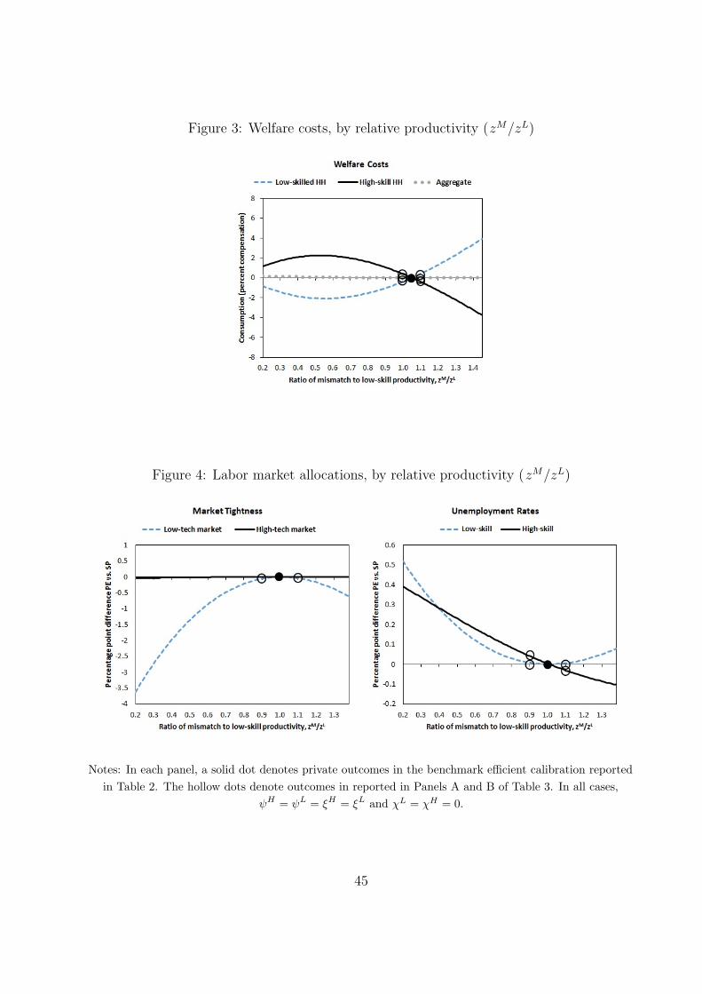
Figure 3: Welfare costs, by relative productivity (zM/zL)

Figure 4: Labor market allocations, by relative productivity (zM/zL)

Notes: In each panel, a solid dot denotes private outcomes in the benchmark efficient calibration reported

in Table 2. The hollow dots denote outcomes in reported in Panels A and B of Table 3. In all cases,

ψH = ψL = ξH = ξL and χL = χH = 0.

45

Figure 5: Match quality and composition of labor pool, by relative productivity (zM/zL)

Notes: In each panel, a solid dot denotes private outcomes in the benchmark efficient calibration reported

in Table 2. The hollow dots denote outcomes in reported in Panels A and B of Table 3. In all cases,

ψH = ψL = ξH = ξL and χL = χH = 0.

Figure 6: Match quality and composition of labor pool, by relative productivity (zM/zL)

Notes: In each panel, a solid dot denotes private outcomes in the benchmark efficient calibration reported

in Table 2. The hollow dots denote outcomes in reported in Panels A and B of Table 3. In all cases,

ψH = ψL = ξH = ξL and χL = χH = 0.

46

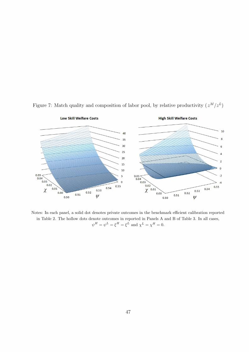
Figure 7: Match quality and composition of labor pool, by relative productivity (zM/zL)

Notes: In each panel, a solid dot denotes private outcomes in the benchmark efficient calibration reported

in Table 2. The hollow dots denote outcomes in reported in Panels A and B of Table 3. In all cases,

ψH = ψL = ξH = ξL and χL = χH = 0.

47