Efficiency and Equity Impacts of Energy Subsidies

Robert Hahn and Robert D. Metcalfe∗

January 14, 2021

Abstract

Economic theory suggests that energy subsidies can lead to excessive consumption and envi-

ronmental degradation. However, the precise impact of energy subsidies is not well understood.

We analyze a large energy subsidy: the California Alternate Rates for Energy (CARE). CARE

provides a price reduction for low-income consumers of natural gas and electricity. Using a natu-

ral field experiment, we estimate the price elasticity of demand for natural gas to be about -0.35

for CARE customers. An economic model of this subsidy yields three results. First, the natural

gas subsidy appears to reduce welfare. Second, the economic impact of various policies, such

as cap-and-trade, depends on whether prices for various customers move closer to the marginal

social cost. Third, benefits to CARE customers need to increase by 6% to offset the costs of the

program.

Keywords: energy; subsidy; natural field experiment; demand elasticity; benefit-cost analysis;

efficiency; equity.

JEL: D1, D04, D60, Q40.

∗Robert Hahn: University of Oxford, and the Technology Policy Institute bob.hahn@gmail.com; Robert D. Metcalfe: BostonUniversity, University of Southern Califronia, and NBER, rdmetc@gmail.com. Acknowledgements: We are extremely gratefulto David Baron and Ted Humphrey at Southern California Gas for partnering with us on this research. Liran Einav providedexcellent editorial comments that allowed us to sharpen and improve the paper, and co-editor Thomas Lemieux and three refereesalso offered astute comments that improved the manuscript. We thank Hunt Allcott, Soren Anderson, Severin Borenstein, MarkEllis, Ed Fong, Ken Gillingham, Michael Greenstone, Steve Levitt, John List, Al McGartland, Michael Price, and Eddy Tamfor constructive comments. We also thank Jackie Flores, Ken Parris, and Andrew Tung for their assistance in design and datacollection, and Senan Hogan Hennessy, Manuel Monti-Nussbaum, Florian Rundhammer and Nick Zhao for their excellent researchassistance. The views expressed in this article are those of the authors and should not be attributed to Southern California Gasor any other institutions. The research was approved by Boston University IRB, 5821X. AEA Registry: AEARCTR-0006999.

1 Introduction

Energy is subsidized in many countries around the world. Global energy subsidies were pro-

jected to be $5 trillion after tax in 2015 (roughly 7% of worldwide GDP) (Coady et al., 2019).

Motivations for using energy subsidies include reducing inequality, lifting households out of fuel

poverty, and gaining political support. Economic theory suggests that these subsidies distort

market prices, leading to excessive energy consumption and environmental degradation.

Several government and academic studies have attempted to quantify the economic and en-

vironmental impacts of energy subsidies (Aldy, 2013; Davis, 2014; International Energy Agency,

2014; Coady et al., 2015; Parry et al., 2014; United Nations Environment Program, 2008). These

studies suggest that the environmental consequences of energy subsidies could be significant. For

example, Clements et al. (2013) and Coady et al. (2019) suggest that eliminating energy subsi-

dies could reduce worldwide annual carbon dioxide (CO2) emissions by about 20-30% and reduce

fossil fuel air pollution deaths by 46 percent.

In general, these studies do not rely on clean causal econometric models for price elasticities

because such estimates do not exist for the subsidized population under investigation. We intro-

duce a novel approach for deriving and identifying natural gas price elasticity estimates using a

large natural field experiment in California. We then use this estimate to assess the economic

and environmental impacts of the price subsidy, and estimate the conditions under which price

subsidies lead to a reduction in welfare.

We analyze a subsidy that is a marginal energy price reduction for low-income customers

in California. It is called the California Alternate Rates for Energy (CARE) program, which

provides a 20% reduction in the marginal price of natural gas and a 30-35% reduction in the

marginal price of electricity for low-income customers throughout the state (California Public

Utilities Commission, 2016). In 2015, approximately 4.85 million households qualified for this

program in California, and approximately 1.5 million households qualified in the Los Angeles

region served by Southern California Gas (SoCalGas).

Our field experiment had two primary objectives. First, we wanted to obtain a causal estimate

of the price elasticity of demand for natural gas. There are relatively few good estimates of the

price elasticity of gas demand that account for endogeneity in pricing. There is a large historical

literature in applied econometrics on energy demand (e.g., Houthakker and Taylor, 1970). Some

of the earlier work analyzed cross-sectional or panel data (Krichene, 2002; Alberini et al., 2011).

Some used panel studies with instrumental variables (IV) (Davis and Muehlegger, 2010; Hausman

and Kellogg, 2015). More recent work by Auffhammer and Rubin (2018) uses a supply-shifting

IV approach to estimate natural gas elasticities across California. The authors provide point

estimates for natural gas price elasticities of 0.24 for CARE consumers and 0.14 for the rest

of the population who are not on CARE. We use the latter elasticity for a part of our welfare

estimates.1 Overall, this literature suggests a wide price elasticity of natural gas demand between

-0.1 and -0.6. The dearth of causal studies estimating the price elasticity of demand for natural

1Their elasticity estimates are different from ours in that they measure their CARE elasticity after people enroll onto CAREand spend several years on the pricing subsidy. We are primarily interested in the quantity response that results from a 20% pricedecrease when people sign up for CARE.

1

gas is surprising given that natural gas is: (i) currently used by around half of U.S. residential

consumers to heat their home (U.S. Energy Information Administration, 2016); and (ii) the fuel

that will probably be used more in the future as it is a relatively clean fossil fuel with desirable

cost characteristics (Levine et al., 2014).

Second, we wanted to understand the welfare impacts and equity-tradeoffs associated with the

price subsidy. This included the welfare impacts of introducing the subsidy, and the impacts of

modifying the price subsidy in a number of ways that might increase economic welfare. Examples

include moving prices toward the marginal social cost (MSC), introducing a cap-and-trade or tax

regime, and implementing a voucher program for low-income households. To address equity, we

examine the implied weight that policy makers put on the subsidy in order for costs of the subsidy

to just equal benefits.2

To help achieve these objectives, we implemented a natural field experiment with over 70,000

households over two years with SoCalGas, resulting in around one million monthly energy use

observations. We randomized a fraction of the customers who were potentially eligible to be on

the price subsidy to receive a letter. The letter noted their eligibility and encouraged them to

sign up for the CARE price subsidy. It is important to note that our encouragement treatment

is the business-as-usual treatment, so the selection we have into the price subsidy is as natural

as one could achieve. The control group did not receive the encouragement letters although they

were free to enroll if they wanted to by finding out about the program online or through other

means. Our randomized design allowed us to estimate a local average treatment effect (LATE)

of enrolling onto the CARE price subsidy on gas consumption. Once we estimate the change in

quantity demanded from the price subsidy, we then calculate the impact of the price subsidy on

economic welfare for those who received the subsidy and society more generally.

The field experiment had three main results. First, our encouragement design worked well,

which allowed us to estimate gas price elasticities. Our first-stage letters resulted in an 8 to

10 percentage point increase in the number of people who enrolled onto CARE over the non-

encouraged control group. Using this randomized first-stage, we estimated the LATE of the

price subsidy on consumption. Over the course of 12 to 18 months, the 20% price subsidy led

to around an 8.5% increase in natural gas demand. We find price elasticity estimates between

-0.29 and -0.35 for our CARE sample over 12 to 18 months, and about -0.35 for a representative

CARE customer. Second, the poorer the household, the more price elastic they are. Third, we

find no causal evidence of a difference in the elasticity of those already randomized in to a gas

conservation program and those not in the conservation program. The conservation program

is the Opower (Oracle) Home Energy Report (HER), which provides social information on how

customers compare to their neighbors in gas use and provides other information on conservation

(Allcott, 2011b; Allcott, 2015). This evidence demonstrates that nudges, such as social norms,

may not change the consumer’s price elasticity of demand.

Using these findings, we construct a structural model that allows us to estimate the change

in total economic welfare resulting from this price subsidy. The model includes a regulated en-

2See Borenstein and Davis (2012) for an estimation of the distributional impact of a transition to marginal cost pricing in gasmarkets. For related research in other markets on the economic impacts of low-income price subsidies, see Attanasio et al. (2011)for education, Cohen et al. (2015) Dupas (2014) and Decarolis (2015) for health, and Duflo et al. (2011) for employment.

2

ergy sector with two prices: one for CARE customers and one for non-CARE customers. Our

model provides a simple way of recovering the counterfactual price before CARE is introduced.

The model may have general applicability for regulated entities that offer low-income customers

subsidized prices, as is often the case with gas, electricity, water, telecommunications, and trans-

portation.

There are three main results associated with the welfare model. First, the overall impact of

the subsidy appears to reduce economic welfare. This result is not obvious because the subsidy

involves a good where there is a significant externality and prices are set above the marginal

private cost (MPC). In the base case, there is a net increase in energy use and emissions that

results in an estimated total welfare loss of about $4.8 million. The consumer surplus gain for

CARE customers is about $76 million, due to the price reduction; but the consumer surplus loss

for non-CARE customers is about $87 million, due to the price increase.

We calculate the optimal subsidy for California is zero. There is no level of the price subsidy

that would lead to increases in total welfare. We also consider the economic impact of removing

the natural gas subsidy instead of supporting current energy efficiency investments for natural

gas in California. We find that removing the subsidy could be a cost-effective way of reducing

CO2 emissions (saving about $130 per ton reduced), and is much more cost-effective than some

energy efficiency investments in California. Furthermore, the CO2 emissions reduced by removing

the subsidy would be comparable in quantity to the current CO2 emissions reduced from energy

efficiency investments in California.

Second, the impact of CARE on welfare depends on whether particular policy experiments

move the prices customers face closer to the marginal social cost. Following convention, the

marginal social cost is defined to be equal to the marginal private cost plus the marginal external

cost. If prices are set equal the marginal social cost, we measure the increase in efficiency.

In some cases, the efficiency impacts of a policy intervention can differ for CARE and non-

CARE customers. For example, introducing a CO2 allowance price of $13/ton (similar to the

California price during the period of study) on top of existing prices makes the new gas price

closer to the MSC for CARE customers, but further away for non-CARE customers. The resulting

net loss in social welfare is about $7.4 million. Furthermore, any cap-and-trade scheme will not

be efficient because the prices faced by CARE and non-CARE customers will still differ because

there is only one policy instrument and two regulated prices.3

We also estimate the welfare effects of a CARE voucher scheme, as opposed to a price subsidy.

Our analysis of vouchers is similar to the welfare analyses described above, with one important

wrinkle: we allow for vouchers to have a behavioral component whereby CARE customers may

consume more of the good than a standard neoclassical model might predict. We find that the

total welfare with vouchers can be positive or negative compared with a subsidy, depending on

the assumed value of the social cost of carbon (SCC).

The third result of the welfare model relates to efficiency-equity tradeoffs. We estimate the

implied welfare weight a decisionmaker would have to put on benefits of the subsidy to CARE

3Regulators may want to take such price differences into account in designing more efficient approaches to addressing exter-nalities.

3

customers for it to just balance other net costs to others. In the base case, with a SCC of $40/ton

(Greenstone et al., 2013), benefits need to be increased by 6% to offset costs. The result is

sensitive to the SCC. At $100/ton, for example, (Cai and Lontzek, 2019), benefits need to be

increased by 16% to offset costs because environmental damages from introducing the subsidy

are larger.

Our results address two important areas in economics. The first is research estimating con-

sumer price elasticities in the energy domain. Natural field experiments may shed new light on

the price responsiveness of customers, which may not agree with prior estimates that use different

econometric methods or identification strategies. Our price elasticities of demand for natural gas

are also important for other policy reasons, such as estimating the impacts that a carbon tax

would have on the economy.

The second relates to the political economy of regulation and mechanism design. It has long

been suggested that price subsidies could be replaced by more efficient transfers such as vouchers

or a lump sum tax, resulting in a potential Pareto improvement (Steuerle, 2000).4 Our analysis

helps to define conditions under which vouchers increase economic efficiency. In addition, we

show that, lump sum taxes may not be efficient compared with an ad valorem tax. The intuition

is that an ad valorem tax can actually move prices closer to the marginal social cost, and thus

may be preferred in some situations.

2 Background and Design

2.1 The CARE Price Subsidy

The California Alternate Rates for Energy (CARE) is a subsidy program that offers a discount for

natural gas and electricity for all low-income qualified energy utility customers in California for

the last two decades. CARE was established in 1989 by the California Public Utility Commission

(CPUC) under the name Low-Income Rate Assistance program, and was expanded during the

2001 California energy crisis (Dimetrosky et al., 2003). The program offers a 20% price discount

on marginal gas prices and a 30 to 35% price discount on marginal electricity prices. CARE gas

customers face a two-tiered pricing system. The first tier has an average marginal price of $0.71

per therm up to 51 therms in the winter (December to April), 15 therms in the summer (June

to October), and 30 therms for spring (May and October). The second tier has a marginal price

of $0.91 for any additional therms consumed in the respective seasons. In our data, over 80% of

the customers consume only in tier 1. In our data, the average price per therm of gas without

CARE is around $0.93 and the average price per therm enrolled on CARE is around $0.73 (All

dollar numbers are in 2014 dollars.)

The eligibility for CARE varies by income and household size. Table A1 shows who is eligible

based on income household size. A two-person household, for example, must earn less than

$31,860 (2015-2016) to qualify. A household is also eligible if a person in the household receives

4There is also a large literature on the impact of income subsidies on household outcomes, such as the U.S. Earned IncomeTax Credit (see Dahl and Lochner, 2012; Meyer and Rosenbaum, 2001; Eissa and Liebman, 1996; Hoynes et al., 2015; Hoynesand Patel, 2015).

4

Medicaid, Head Start, CalFresh (Food Stamps), Low Income Home Energy Assistance Program,

or Supplemental Security Income. To qualify for CARE, a household must officially enroll by

sending an application form to the utility stating how they are eligible.

In total, CARE expenditures exceeded $1 billion in 2015 in California for natural gas and

electricity. Table A2 provides estimates of the number of households that are enrolled in CARE

and eligible for CARE for SoCalGas (our population), Southern California Edison (SCE), Pacific

Gas and Electric (PG&E), and San Diego Gas and Electric (SDG&E). The table shows that

SoCalGas has the largest number of households eligible for CARE, but expenditures on CARE

are largest for PG&E. Of the $109 million spent by SoCalGas in 2015, 91% was used for subsidies.

The rest was spent on administration and advertising.

2.2 Experimental Design

To estimate the price elasticity of energy demand, we analyzed an encouragement design in a

natural field experimental setting to calculate the local average treatment effect. The key idea

is to model the decision to participate in the CARE program as a function of whether or not an

individual was randomly selected to be in a treatment encouragement letter group that motivated

enrollment into the price subsidy. Under plausible assumptions, this approach allows us to derive

an unbiased estimate of the impact of the 20% price reduction in natural gas on consumption for

those individuals who enrolled in the program. We compute the price elasticity by estimating the

percentage change in quantity and dividing by the percentage change in price.5

Our experimental approach differs from earlier research on estimating energy elasticities in two

important ways. First, the traditional discrete/continuous choice approaches to estimating energy

elasticities (see Reiss and White, 2005) impose strong and perhaps unrealistic assumptions on the

energy behavior of the customer (Borenstein, 2012). These assumptions appear to be violated

in practice (Burgess and Nye, 2008; Bushnell and Mansur, 2005; Costanzo et al., 1986; Ito,

2014; Kahn and Wolak, 2013; Shaffer, 2020; Shin, 1985). Our approach does not rely on any

of these assumptions. Second, our approach extends the previous research on field experiments

in the energy area by using a natural field experiment instead of a framed field experiment.

Much research on estimating electricity price elasticities have used framed field experiments, in

which participants opt-in to the experiment (i.e., randomization and treatment) (Battalio et al.,

1979; Caves and Christensen, 1980; Caves et al., 1984; Faruqui and George 2005; Wolak, 2006;

Allcott, 2011a; Jessoe and Rapson, 2014). Bias may arise in framed field experiments because

of: (i) selection into the experiment; (ii) consumers knowing that they are being watched and

monitored; (iii) experimenter demand effects; and (iv) consumers knowing that they are being

randomized into a new price group or the control group (Harrison and List, 2004; Al-Ubaydli and

List, 2015). In this setting, natural field experiments are superior from an internal and external

validity perspective to framed field experiments. We employ a natural field experiment to reduce

these sources of bias.

We had to focus our experimental design on CARE customers that failed to re-enroll in time

for CARE before falling off the price subsidy. This population represents about 10% of the overall

5This is a standard arc price elasticity calculation as we only have two points on the demand curve.

5

CARE population. In our estimation, we impose the assumption that those who failed to re-enroll

initially, but who enrolled with our encouragement, had the same local average treatment effect,

and hence price elasticity, as those who were already on the CARE subsidy. It is possible that

these individuals may have less elastic demand than the general population of CARE customers,

because they dropped out of the program and might value the subsidy less. We will address the

external validity of estimates after the results section.

In our design, we had different waves of letters sent to the customers (for logistical reasons).

SoCalGas processed the letters in batches. As soon as each successful application was processed,

a letter was sent to the customer notifying them that the CARE discount applies automatically

to their current billing period (which is monthly). For wave 1 in 2014, most of the customers who

signed up for CARE were enrolled by mid-September 2014. The majority of customers in waves

2 to 5 were enrolled in CARE by early October 2015.6

Within each wave, we randomized slightly different letters based on findings from the behav-

ioral literature on motivating take-up of social programs (e.g., Bhargava and Manoli, 2015). This

also relates to the growing literature on motivating enrollment and screening citizens into fed-

eral programs, such as Manoli and Turner (2016), Armour (2018), Finkelstein and Notowidigdo

(2019), and Deshpande and Li (forthcoming). See the overview of the design in Table 1. For

2014, the treatment 1 letter was SoCalGas’ conventional business as usual letter, which it had

used for many years before this experiment. The treatment 2 letter added basic information on

how much each customer actually saved on their gas bill over the last two years by being on

CARE. This saving was personalized to customers’ actual accounts and linked to their previous

two years consumption, so the letter had the actual subsidy given to them over the last two years.7

The treatment 3 letter was the same as the treatment 2 letter, but was couched in terms of a loss

framing. The letter said that by not enrolling in CARE, the customer will lose a specified amont

over two years. The loss framing, which stems from prospect theory (Kahneman and Tversky,

1979), has been shown to be successful in increasing the productivity of workers (Hossain and

List, 2012), the adoption of energy efficiency reward programs (List et al., 2016), and the adop-

tion of water efficiency landscape rebates (Hahn et al., 2016). The treatment 4 letter was based

on literature that suggests that social information can affect household energy behavior (Allcott,

2011b) and payment compliance (Hallsworth et al., 2014). The letter told customers in this group

that “over 200,000 households like them enrolled in CARE over the last year.”

For the 2015 waves (2-5), we used slightly different letters based on the results from the

first experiment. Again, we had a no-letter control group, and treatment letter 1 was the loss

framing letter from experiment 1. Treatment letter 2 tried to leverage reciprocity by using the

6Each household was only assigned to one wave. They were assigned to the wave 1 if they fell off CARE between January andMarch 2014 and waves 2, 3, 4, and 5, if they fell off CARE in May, June, July, or August 2015 respectively. The timeline for ourexperiment is shown in Table A3. There were five distinct waves of mailings from 2014 to 2015. These waves corresponded tostandard SoCalGas mailing operations for enrollment on CARE. In 2014, subjects received a re-enrollment letter for three to fivemonths after coming off CARE (see Wave 1). In 2015, subjects received re-enrollment letter one month after coming off CARE.However, in 2015, we sent four separate and distinct mailings (see Waves 2-5). The month when households came off CAREdetermined the wave number for each household. Encouragement letters were the same across each of waves 2 to 5.

7This information on the actual subsidy could increase or decrease enrollment. The ambiguity stems from the fact that wedo not know whether customers thought their CARE subsidy was less than, greater than, or equal to the actual amount. If, forexample, they thought the subsidy was lower than the actual amount, then this might provide motivation to re-enroll in CARE.We did not measure these beliefs ex ante.

6

letter header: “Thank you for being a SoCalGas customer,” and treatment letter 3 provided more

information on gas consumption in an attempt to fully inform the customer of the benefits and

costs of their gas consumption. Samples of the letters in English are in Figures ??, A2, and A1

(the letters were also sent to consumers in Spanish). All letter versions are available from the

authors.

The summary statistics for natural gas demand for the different groups of both experiment 1

and experiment 2 are presented in Table A5. The units reported are therms, where one therm

equals 29.3 kilowatt-hours. Tables A5 and A6 test differences in means in gas consumption across

the various groups across both experiments, and illustrate that these differences are not statisti-

cally significant at conventional levels. We conclude that the various treatments are balanced on

pre-experimental gas usage within the two experiments. Figure A3 shows these 70,000 customers

distributed across the SoCalGas districts. For simplicity, we will pool all of the waves together

when estimating the LATE of gas prices on demand.

2.3 Estimation Strategy

We estimate the local average treatment effect (LATE), which provides a causal estimate of a

change in the gas price on gas demand for our population of interest. Below, we will describe our

LATE estimation strategy from the design of our natural field experiment and the variables that

we use for implementing this strategy.

SoCalGas sent the letters to the randomized encouragement groups after the 70,784 households

were randomized into the control and letter encouragement groups (i.e., treatments). To enroll,

the household had to provide evidence of low income or evidence of being enrolled on a current

government welfare program. SoCalGas checked the accuracy of this information and then notified

the household immediately if they have been enrolled in the CARE program. While customers

in the treatment groups are encouraged to apply for the subsidy, customers in the control group

could also apply (i.e., they would be classified as the always takers if they enroll).

The underlying assumptions for our estimation strategy using the LATE are that: (a) the

change in participation in CARE (from no participation (0) to participation (1)) is induced by the

randomized encouragement and not by any other variables; and (b) that this change is orthogonal

to any factors that impact on gas consumption (G). We use the monthly consumption data coming

directly from the smart meter. In our experiment, the encouragement (Ti) is randomly assigned,

so that GCAREi, CAREi(Ti) ⊥ Ti. This means that the encouragement is assigned independent

of possible outcomes of the individual household. As a result, the LATE in our example is

simply LATE = GTi=1−GTi=0¯CARE1− ¯CARE0

, which is the difference in average gas consumption of those who

received an encouragement letter and those who did not, divided by the difference between those

who enrolled onto CARE and those who did not.8

8While our experiment satisfies the condition that the encouragement is randomly assigned to households, our LATE estimatorembeds the monotonicity/uniformity assumption. In our context, this assumption states that if a control group household iparticipated in CARE when not encouraged, i will participate when encouraged. We do not observe the latter, and so our LATEestimator is the ATE of a subpopulation whose choice is impacted by the random variation in the encouragement. It is impossibleto know the counterfactual of those who are likely to gain on CARE and therefore the types of households that come on to CAREthrough the encouragement (Heckman and Vytlacil, 2005). We can, however, provide correlates of what types of households seemto value CARE more through the encouragement design. Our encouragement is binary so we cannot estimate marginal treatment

7

A key question when using the LATE is how our subpopulation of takers through the encour-

agement relates to the more general population already on CARE. When we estimate the price

elasticity of demand for those encouraged on CARE, we are going to assume it is the same as those

already on CARE, although we cannot estimate the latter within our context. The households in

our experiment, who dropped out of the CARE program, may have less elastic demand than the

general population of CARE customers. We explore this issue by considering what happens to

general economic welfare and the welfare for CARE customers when the elasticity of demand for

CARE customers changes. In section 3.4, we show that our estimated elasticities are externally

valid.

The first-stage regression models the decision to take up CARE, and estimates whether the

encouragement had a significant impact on take up. If the encouragement had a significant

positive impact on take up of the price subsidy, we can then use the random assignment to the

encouragement letter treatment groups as an instrumental variable for being on CARE.

In a first stage, we use OLS to estimate:

1(CARE)imt = ϕTimt + θmGbim + πm + γj + µimt (1)

where the indicator dependent variable 1(CARE)imt is a dummy variable indicating whether the

household i in month m and year t enrolls onto CARE (1 = yes and 0 = no). The indicator

variable Timt is set to zero for all households prior to the encouragement treatment intervention.

After the letters have been sent out to those in the encouragement groups, this indicator switches

to 1 for these households. Gbim measures gas consumption of household i in the same month m for

the previous years of consumption data (i.e., before the experiment). We include month-by-year

fixed effects, πm, to control for time-varying decisions to apply for CARE. We also include wave

fixed effects, γj , which control for the letter wave the customer belonged to in the natural field

experiment.

Our second specification is the intention-to-treat (ITT) analysis. We use an OLS regression

to understand the marginal impact of being in the treatment group on gas consumption following

the delivery of the encouragement letters to each individual household i. We estimate an OLS

equation designed to control for the effects of observable factors that affect energy consumption

levels for households that apply for CARE (irrespective of group):

Gimt = βTimt + θmGbim + πm + γj + εimt (2)

Gim measures gas consumption of household i in month m and year t. The T indicator variable

switches from zero to one in the month after a household receives the CARE application letter.

We include month-by-year controls for baseline usage, denoted θmGbim, where Gb

im is household

i’s average gas usage in the same calendar month during the baseline period. This accounts for

permanent differences in a household’s energy consumption across months. Again, we include

month-by-year fixed effects, πm, to control for the average effects of time-varying factors (e.g.,

winter temperature) that generates variation in average consumption across all households, and

effects (Heckman and Vytlacil, 2005) and all of our sample have been compliers in the past.

8

wave fixed effects, γj . The seasonality in the gas consumption data arises because gas heating

accounted for 46 percent of all residential gas consumption in California in 2012. Water heating,

including that for clothes washers and dishwashers, consumes the second largest portion at 42

percent. Cooking accounts for 7%, clothes dryers use 4%, and pools and spas use 2% (California

Energy Commission, 2016). In this regression, the standard errors are clustered at the individual

household level (Bertrand et al., 2004).

Our LATE specification is estimated using a two stage least squares (2SLS), where being in

a treatment group (in equation (1)) will be the instrument used in the second stage to analyze

the impact that being on CARE has on gas consumption. The parameter of interest is β, which

measures the mean difference in gas consumption between being in the CARE enrolled group

versus the non-enrolled group, after adjustment for the fixed effects. In this instrumental variables

(IV) framework, β is identified using the exogenous variation in CARE participation that is

generated via the random assignment of the encouragement letters; this is the estimation of

the LATE. As a result, β provides us with the change in gas demand associated with the 20%

reduction in the price of gas.

Once we have estimated the general price elasticity (from the LATE) for the whole experi-

mental sample, we then estimate price elasticities for observable sub-populations in our sample.

First, we examine the effects of the price subsidy on the very low-income households versus those

slightly better off. Previous literature has sought to estimate different elasticities for different

income groups (e.g., Reiss and White, 2005), and we denote very low income through detailed

PRIZM data on each individual household.9 Second, we examine whether there is a differential

response from high and low gas users using over two years of pre-experimental data. Third, we

compare the price responsiveness of customers who have been randomized into the Opower energy

conservation program (i.e., Home Energy Report (HER)) with those who do not receive the re-

port. We crossed our experimental groups with the Opower conservation experiment taking place

in SoCalGas to estimate the impact of their HER, which has been shown to significantly reduce

household gas consumption by around 1-1.5% around the U.S. (Allcott, 2011b; 2015; Brandon et

al., 2017). The HER uses social comparisons and tips on energy conservation to motivate people

to reduce their household energy use. It is an open question as to whether nudges, in the form

of the Opower HER, change the slope of the demand curve and/or shift the demand curve. We

analyze whether there are any changes in the slope of the demand curve between Opower HER

treatment group households and control households.

Finally, we examine whether customers who do not receive paper bills respond differently than

those who do. While there is likely to be selection into paperless billing by the customer, there

could be good reasons that those who receive bills online or have bills paid automatically might

be less responsive to price changes and use more energy (Sexton, 2015).

The summary statistics of our sample are shown in Table A7. 25% of our households are very

low-income households, 9% are in the Opower HER treatment group, and 29% are on paperless

billing. Randomization blocked on initial gas use and balanced on all other variables, so there

9PRIZM codes combine demographic, consumer behavior, and geographic data to help marketers describe and engage withtheir customers. Many utilities around the world use such data to know who to target low-income subsidy to, or to who to offerenergy-efficient technology rebates to

9

are no significant differences in the observable variables jointly across waves.

3 Results

3.1 CARE Enrollment

We first show the impact of the encouragement treatment on enrollment rates for CARE. The

general story is that receiving a letter increases enrollment rates significantly, on the order of 10

percentage points, and these increases are statistically significant relative to not receiving a letter.

The particular behavioral content of the letter does not seem to dramatically affect enrollment

rates. This is true for all letters, including ones that contain social norm information or loss

framing the benefits.

Figure 1 shows the enrollment rates for the five experimental groups in experiment 1. The

enrollment rate for customers not receiving a letter (control) is around 4.3%. Enrollment rates

for the treatment groups that received a letter (1-4) had significantly higher enrollment rates

averaging 14% across. Figure 2 is identical to Figure 1, but presents the enrollment data for

experiment 2. The enrollment rate for customers not receiving a letter (control) is just over 2%.

Enrollment rates for the treatment groups that received a letter (1-3) had significantly higher

enrollment rates averaging 13.5% across.

Table 2 provides linear probability models on the impact of the treatment letters on enrollment

in CARE, which allows us to formally test for statistical differences in response rates across the

control and treatment groups (results using logit regressions provide very similar effects). Column

(1) provides the analysis of the first experiment. It is clear that all of the letters had a significantly

larger impact on enrollment than the no letter control. The business as usual treatment 1 letter

increases enrollment by around 9 percentage points (p<0.01). Treatment letters 2-4 increase

enrollment by around 10.1 to 10.3 percentage points (p<0.01). There are no significant differences

between the gain and the loss framings (treatment 2 and treatment 3). We do find a significant

1.35 percentage point difference between treatment 1 (conventional letter) and treatment 3 (loss

framing letter) (p<0.05). That is the only statistically significant difference between the letters.

Columns (2) and (3) present the logit regression for experiment 2, where the latter includes

wave fixed effects. The letters had between a 10.9 and 11.1 percentage point increase in enrollment

for CARE (p<0.01), and there were no significant differences between the letters. These three

regressions show the encouragement effect, in the form of a letter, is pronounced. In the first

experiment, our treatment enrollment is around three times the control enrollment, and in the

second experiment, our treatment enrollment is almost five times the control enrollment.

Table A8 examines specific factors affecting a household’s decision to enroll in CARE, in

addition to receiving a letter. This table examines the four different background variables we

have for most households - whether they are very low-income, a high gas user, receive an Opower

treatment, and are enrolled onto paperless billing. We find that: (i) low-income households

are more likely to enroll in CARE and that the low-income households are 0.9% more likely

to enroll in CARE through the encouragement letter compared with the non low-income types

10

(column 1); those who enroll onto CARE have no significant differences in pre-existing gas use,

but the encouragement letter increases enrollment into CARE by 1% high gas users (column 2);

households that are part of the randomized Opower HER treatment group do not make households

more likely to enroll on CARE and the encouragement letter does not change this result (column

3); paperless customers are 0.7% less likely to enroll into CARE, and the encouragement design

makes those on paperless 1.3% less likely to enroll onto CARE in comparison to those customers

not on paperless. Column (4) jointly examines these variables in the same regression. Some of

these results hold and some change. For example, it seems the very low-income types are not more

encouraged to sign up for CARE from the letters. Taken together, these results suggest that there

are some very small differences between those who come onto CARE with the encouragement

letters and those do do not receive the encouragement letters. We examine this in detail in

appendix section A.2.

3.2 Impact of the CARE pricing subsidy on Gas Use

We observe monthly natural gas usage for all households in three discrete time periods: time

period (1) when they are on CARE before they fall off the subsidy; time period (2) when they fall

off the CARE subsidy; and time period (3) when they (may) enroll again onto the CARE subsidy.

This timeline is outlined in Table A3. For our econometric specifications, we use pre-re-enrollment

gas usage averages to control for gas usage before (when on CARE previously). Table 3 uses all

post-re-enrollment data (i.e., periods 2 and 3) but Table 4 uses post-re-enrollment data and does

not include observations of take-up households between falling off and re-enrolling onto CARE

(i.e., only includes period 3 but not period 2). We also include usage controls in the specifications

as randomization was based on pre-enrollment usage. We estimate the impact of CARE on gas use

using the post-treatment time period only, rather than a difference-in-difference, following Allcott

and Rogers (2014) and Fowlie et al. (2018). We believe given the particular experimental design

and the different time periods for re-enrollment across all waves, this approach is appropriate.

The reason is that with the month-of-sample and wave fixed effects, we allow general patterns

of energy behavior to differ by wave that seems plausible given the different timing and slightly

different populations. For example, the off-CARE period or what we call the intermediate period

is in different time frames for each wave; so is the treatment period. For our experiment, we

know the exact date when households fell off CARE and did not initially renew. These dates are

crucial for the estimation as they differ for each household.

For our LATE estimation, we pool all of the waves together. In Table 3 we present the

consumption results for up to six months after enrollment onto CARE in both years, and in

Table 4 we include data up to 18 months after enrollment onto CARE for those in the first wave

but not the second to fifth waves.10 For both tables, we present four different specifications.

The first provides the first-stage (FS) regression of the impact of the encouragement treatment

on the enrollment of the CARE subsidy, so the dependent variable is take-up of CARE and not

10We do not have consumption data beyond 2015 for either sample. As a result, (i) only includes months later in the yearbecause the treatment was administered in June, July, August, or September. Because the waves have different characteristics, itis important to have wave fixed effects included in these specifications.

11

consumption. The second specification provides the ITT regression of the impact of simply being

in the treatment encouragement groups on gas consumption. The third specification estimates

the LATE with the IV from the FS specification.11

Column (1) in Table 3 presents the first stage regression across the five waves. We find

that the first-stage demonstrates a 7.7% increase in take-up of CARE; this is an extra 6,158

households signing up to CARE until the end of the calendar year for each wave.12 The F -

statistic in this first-stage is >2000 suggesting that our instrument is not weak. Column (2)

presents the ITT specification on gas consumption. From this specification, we observe that

those in the encouragement letter groups consumed 0.15 therms more per month (p<0.05) than

those in the control group (no letter) – the baseline consumption for this period is around 21

therms a month. This is equivalent to a 0.7% increase in gas consumption for the approximately

54,000 customers in the treatment group. Column (3) presents the LATE from the first stage

regression for Enrolling in CARE. We find that this Enrolling in CARE coefficient from the main

specification is 1.91 therms per month for the two to six months after taking up the CARE

discount (p<0.05). Given the control group’s consumption in the post-enrollment period is 21

therms per month, we estimate the increase in gas consumption is around 9.1%. This estimate

provides us with a price elasticity of around -0.35.13

Columns (4) to (6) replicate columns (1) to (3), but we also include the entire year of 2015 for

experiment 1; this extra data extends the consumption period for an extra year for experiment

1 - the baseline consumption for this period is around 23 therms a month. We do not have 2016

data for either experiment, so we do not have longer-term consumption for waves 2-5 households.

Column (4) shows that over a longer time period the encouragement treatment had a 9.2% effect

- given take up rates in the control group were around 3%, we had a 300% treatment effect of

the letters. Column (5) includes the ITT analysis, and we show that the letters group had a

0.162 therms increase per month (p<0.05) - not significantly different from the ITT effect in

specification (2). Specification (6) shows the LATE, and this estimate is around a 1.66 therms

increase per month (p<0.05) for those who signed up for the CARE discount. This estimate is not

significantly different than the LATE estimate in specification (3), which has fewer observations

due to a shorter time period. This is a 7.2% increase in gas consumption for those enrolled onto

CARE, and the elasticity is around -0.29.

Table 4 presents the specifications where we include the consumption observations when all

customers fell off CARE and before they were offered to return onto CARE through the encour-

agement treatment letters. As a result this table includes more consumption data; however, the

data may contain more noise, as customers might have been more uncertain about eligibility and

status of enrollment in this time period. Column (1) in Table 4 presents the first stage regression

and shows that take-up increases by 8% with the CARE discount; this is an extra 6,158 house-

holds signing up to CARE. Column (2) presents the ITT specification on gas consumption. From

11We have a small fraction of households who re-enroll in the control condition - the always takers. If we removed thesehouseholds from the analysis, we then estimate the treatment on the treated, which yields very similar estimates to our LATE.

12This effect is smaller than those presented in Table 2 because here we estimate a CARE take-up equation where we only use12 months of data, and also not everyone signs up on the first month after receiving the encouragement.

13In contrast to some other estimates in the literature, we estimate an arc elasticity. The formula is: Egas =22.91−21

(21+22.91)/20.9−0.7

(0.7+0.9)/2

= −0.35.

12

this specification, we observe that those in the treatment groups consumed 0.15 therms more

(p<0.05) than those in the control group (no letter). This is equivalent to a 0.7% increase in gas

consumption for the approximately 54,000 customers in the treatment group.

Column (3) presents the LATE from the first stage regression (1) for Post-Take-up. We

find that this Post-Take-up coefficient from the main specification is 1.78 therms per month for

the average of five months after taking up CARE. This is equivalent to a 7.7% increase in gas

consumption. The elasticity estimate from these specifications is -0.32. Column (4) shows that

over a longer time period the encouragement treatment had a 9.4% effect, with an F-statistic of

>2000. Column (5) has the ITT analysis, and we show that the letters group had a 0.169 therms

increase per month (p < 0.05); not significantly different from the ITT effect in specification (2).

Specification (6) shows the LATE, and this estimate is around a 1.71 therm increase per month

(p < 0.05) for those who sign up for the CARE discount. This estimate is not significantly different

than the LATE estimate in specification (3). There was a 7.4% increase in gas consumption for

those enrolled on CARE, with an elasticity around -0.29.

Our field experiment enrolled people into CARE during the summer months of 2014 and 2015.

We can compare the LATE for summer and winter months, but we did not randomize whether

people were encouraged in the summer or winter months. This makes comparison between the

two seasons difficult since people’s price change might have been more salient in the first few

months of enrolling, which is in the summer. Nonetheless, table A10 examines the impact of

CARE on consumption by summer and winter months. We find that for the summer months,

the LATE is 1.84 therms extra per month (10.7%), and for the winter months, it is 2.23 therms

extra per month (7.8%). We cannot reject that these two coefficients are equal to each other at

a conventional statistical significance level.

An important robustness check for the LATE estimation is how receiving a letter might affect

gas consumption. In particular, we examine whether households who received the business as

usual encouragement letter, but did not take up the CARE subsidy, cut their gas usage. This

would offset the elasticity of those who did take up the subsidy and bias the LATE upwards. We

want to compare the consumption of this group with the entire control group. The specification

in Table A9 replicates the specification of our main Table 3, except we add a dummy variable

that takes on the value one if the household was in the encouragement group and did not take

up the CARE subsidy. It shows that those in the encouragement group who do not take-up the

CARE subsidy increase their gas use by 0.092 therms, but this is not significantly different from

zero at the ten per cent level.

3.3 Heterogeneity in Price Elasticities

In this section we examine how estimated elasticities in the previous section differ for different

“types” of households in our sample. These types of households include very low-income house-

holds, high-gas using households, Opower conservation treatment group households, and paperless

billing households. We estimate separate regressions for each background variable, present the

separate elasticities, and then use t-tests to understand any differences.

For example, the row in Table 5 computes the LATE for the very low-income households as

13

defined from the Prizm codes, and compares it with the LATE for those households that are

not very low income. The LATE for those who are very low-income is 2.92 therms per month

(p < 0.01). This is larger than for those who are not low income, who consume 1.31 therms per

month (p < 0.05) as a result of being on CARE. The elasticities are -0.52 and -0.24 respectively.

This difference in the LATE estimates provides evidence that low-income households are more

responsive to the price changes than those not from low-income households. Row (2) examines

the changes in consumption for those who are high gas users and compares that with low gas

users. The LATE for the high gas users is larger than for those low gas users (define as below

the mean consumption levels for the previous twelve months) (p < 0.05). The elasticities are

-0.41 and -0.13 respectively. These estimates indicate that high-usage households are more price

sensitive than low-usage households.

Row (3) examines the changes in consumption for those who are part of the Opower Home

Energy Report (HER) treatment group versus those not in the HER group (control group and

those not in the HER control group). The table shows that the LATE for the HER households

is not different from those not part of the HER group. The elasticities are -0.35 and -0.34

respectively. This suggests that the HER does not change the elasticity for those households who

are part of the Opower HER treatment group in comparison to all other households in a way that

is economically important. This result supports the theory that social norms are similar to a lump

sum moral tax (Levitt and List, 2007). The result suggests a nudge that yields a reduction in

quantity at a given price would need to be accompanied by a less steeply sloped demand curve at

that point. This evidence provides some support for the finding that technology adoption might

drive the energy efficiency savings from the HER by shifting the demand curve (Brandon et al.,

2017).

Finally, row (4) examines the changes in consumption for those who signed up to paperless

billing versus those who had not. It is clear here that the LATE for the paperless billing house-

holds is lower than those who are not on paperless billing. The elasticities are -0.25 and -0.31

respectively. This suggests that the paperless billing households are slightly less elastic than those

who are not on paperless. In summary, we find that the very low-income households and those

who are high-gas using households are the households who seem to change their behavior more

with the 20% price subsidy (i.e., they have a statistically significant larger price elasticity of gas

demand).

3.4 External Validity

Before we assess the welfare associated with introducing the CARE subsidy using our price

elasticities of demand, we will examine the external validity of the estimated elasticities. We are

interested in the question of whether the CARE population we sample is representative of the

general CARE population that SoCalGas serves. In table A11, we show that the experimental

population is broadly similar to the rest of the CARE population, with some minor differences in

household income. We see no major selection into CARE based on previous gas use. We reweight

our LATE on the observable variables of the the entire CARE population and show that the range

for unweighted elasticities is -0.29 to -0.35 and the range for weighted elasticities is -0.31 to -0.43

14

(see Table A12). In the welfare section we use a baseline elasticity of -0.35 (which represents the

mid-point of the weighted and unweighted range).

4 The Welfare Effect of the CARE Price Subsidy

In this section, we present the economic model used to estimate the welfare impacts of CARE.

We consider three measures of welfare:

1. a measure of the consumer surplus gain that CARE customers receive as a result of the

CARE discount;

2. a measure of the consumer surplus loss that non-CARE customers incur as a result of the

price increase they pay with CARE; and

3. the change in total welfare from introducing CARE.

The first two measures do not include the impact on producer surplus, or the impact on

society from a change in the level of the global externality resulting from changes in energy usage.

The third includes the net change in consumer and producer surplus after taking full account of

the environmental externality and the administration costs. Our measure of the change in total

welfare depends on whether prices for CARE or non-CARE customers move toward the marginal

social cost (MSC). A key intuitive feature that drives the results of our model is that economic

welfare improves (decreases) as prices resulting from introducing CARE move toward (away from)

the marginal social cost for a particular group of customers.

Suppose, for illustrative purposes, that the initial price that both CARE and non-CARE

customers pay is just equal to the MSC of energy. Then, introducing the CARE price subsidy

means CARE customers pay a price below the MSC, and non-CARE customers pay a price above

the MSC. Because both price changes represent departures from the MSC, the overall quantities

consumed by each group are different from the efficient amount, and overall welfare decreases in

this special case.

While our main interest in this section is in examining the welfare effects of these price changes

(section 4.1), one could alternatively ask whether the implicit tax structure associated with CARE

is efficient. We discuss this issue later in section 4.1, building on the seminal work of Ramsey

(1927).

We analyze the welfare impacts of introducing the CARE price subsidy for SoCalGas cus-

tomers, and then extend this analysis to other California customers in 4.1. In section 4.2, we

analyze the welfare impacts of: (1) introducing a cap-and trade program such as the one now in

place in California (California Air Resources Board, 2014); and (2) introducing a voucher pro-

gram instead of a price subsidy for CARE customers. Finally, in section 4.3, we use this welfare

analysis to identify the implied equity weight that decision makers place on CARE households

in order to render the program worthwhile from a social point of view. By implied, we mean the

weight that would just equate the benefits that CARE customers received with the costs of the

subsidy.

15

4.1 The welfare model and results for introducing the CARE

program

We use a partial equilibrium analysis to model welfare changes.14 In our model, CARE households,

C, receive a subsidy, and this subsidy is paid for by non-CARE households, N , through an increase

in their variable rates. Furthermore, the energy utility provides both CARE and non-CARE

households with the natural gas they demand at a regulated price. The change in energy demand

from introducing the CARE subsidy affects the surplus of CARE users and non-CARE users, and

overall energy use. Energy use, in turn, affects carbon dioxide emissions, which affects society

more broadly.

Our structural model is tied to what we can observe. We observe the natural gas price for a

CARE household, P1c, and the price for a non-CARE household, P1n. We assume that there is

a representative CARE household, c, and a representative non-CARE household, n. The model

allows us to estimate the price that would have prevailed before introduction of the subsidy, so

we can construct a counterfactual price for a world without the CARE subsidy. Comparing the

counterfactual with the new prices after CARE is introduced allows us to estimate the welfare

impacts of CARE under various assumptions. We first do this for Southern California Gas, and

then extend the welfare analysis to California. In appendix section B.2, we explore a number

of theoretical features of our model in more detail. These include: showing that setting prices

equal to MSC is first best; defining conditions under which the subsidy can increase or decrease

welfare; the comparative statics of a change in elasticity on welfare; and the comparative statics

of a change in the allowance price on welfare.

For simplicity, we assume that demand curves are linear for CARE households and non-CARE

households. We can observe a point on the demand curve for c and n. This point, along with the

elasticity, gives us the slope of the demand curve at that point. Elasticities for C are based on

our natural field experiment and elasticities for N are based on the literature.

4.1.1 Welfare analysis

We assume for now that the initial price of energy, P0, is known, and we show below in section

4.1.2 how to derive it. The loss in welfare for non-CARE customers is simply the consumer

surplus loss due to the price increase that these customers incur with the introduction of CARE.

Similarly, the gain in welfare for for non-CARE customers is the consumer surplus gain that these

customers enjoy as a result of the price subsidy.

To calculate the total welfare change, we measure the net social benefits from the changes

in output for CARE and non-CARE households and subtract the administrative costs. Consis-

tent with standard benefit-cost analysis, we assume that the net impact of transfers, say from

consumers to the state, is zero.

14We call this a partial equilibrium analysis because we focus on one part of the energy sector. With a suitable reframing,however, this analysis can be interpreted as a general equilibrium formulation that follows in the spirit of Chetty (2009) andJacobsen et al. (2020). If utility functions for CARE and non-CARE households are quasilinear, and there is one numeraire good,then the welfare analysis for assessing the impact of changing prices is very similar to their analysis. Indeed, equation (3) belowis analogous to equation (6) in Jacobsen et al. (2020), which provides a general expression for welfare loss compared with optimaltaxes. These welfare issues are explored in more detail in Hahn et al. (2020).

16

Define Pn = Pn(Q) as the inverse demand curve for n, and P c = P c(Q) as the inverse demand

curve for c. Let n’s consumption before the introduction of CARE be Q0n, and n’s consumption

after the introduction of CARE be Q1n. Similarly, define c’s consumption before the introduction

of CARE as Q0c, and c’s consumption after the introduction of CARE as Q1c. The net change

in welfare is given by:

Nn

∫ Q1n

Q0n

(Pn(Q)−MSC)dQ+Nc

∫ Q1c

Q0c

(P c(Q)−MSC)dQ−A (3)

The first two terms in equation (3) include the change in direct consumer surplus for CARE

and non-CARE customers, the change in producer surplus, and the change in environmental

benefits. The third term represents administrative costs, A, which are assumed to be a fixed cost.

This equation governs the results in the welfare analysis, and also governs the various extensions

of the model in section 4.2.

4.1.2 Identifying the counterfactual

An intriguing aspect of our problem is that we cannot directly observe the counterfactual –

prices and quantities that would have been in place before CARE. However, we can derive the

counterfactual price, P0, and this in turn allows us to compute Q0c and Q0n from the demand

curves for c and n (see appendix section B.2.1).

We can derive P0 by assuming that the transfer from non-CARE customers just equals the

sum of the transfer to CARE customers plus any administrative costs, A, associated with the

program (this assumption is justified by actual regulator behavior). This means:

Nn(P1n − P0)Q1n = Nc(P0 − P1c)Q1c +A (4)

The term on the left-hand side is the transfer from N and the term on the right hand side is the

transfer to C plus administrative costs. Solving (4) for P0 yields:

P0 =NnP1nQ1n +NcP1cQ1c −A

NcQ1c +NnQ1n(5)

The quantities on the right-hand side are known at the initial point (P0, Q0n). We construct

the linear demand curve as the line going through the initial point with the slope dQn/dP . The

same analysis holds for deriving Qc(P ), with c substituting for n.

An alternative way of recovering the initial price is to assume that utility profits remain the

same before and after the introduction of CARE. We implemented this counterfactual as well to

compare it with our approach. Compared with the base case used here, it changed the welfare

results by about 12% (from -$4.81 million to -$4.24 million) and the counterfactual price by less

than 1% (from $0.904 to $0.909).15 We use equation (5) in the simulations that follow because it

more accurately reflects the pricing policy used with CARE.16

15We are grateful to an anonymous referee for suggesting this approach. See appendix section B.3.4 for details on the calculation.16See California Public Utilities Commission (2012: 13) which provides a formula for the surcharge for non-CARE customers.

That surcharge requires that non-CARE customers pay for the subsidy and administrative expenses on a per therm basis, which

17

4.1.3 Estimated welfare impacts from introducing CARE

The two main results from our model for introducing CARE for SoCalGas customers are that: (1)

the impact of the subsidy on total surplus is generally negative for plausible values of the CARE

demand elasticity; and (2) net energy use and emissions increase, and, thus, pollution damages

increase. Also, the direct impacts of the subsidy increase welfare for CARE customers and reduce

welfare for non-CARE customers.

We examine welfare results for SoCalGas customers here and extend the analysis to the main

gas utilities in California in the next subsection. We show our main results in Figure 3 for the base

case and the case in which we vary the elasticity for C from -0.2 to -0.5. as part of a sensitivity

analysis.17.

The results for the base case are shown along the vertical line in Figure 3, which uses our

best estimate of elasticity based on our field experiment (-0.35), a price elasticity for non-CARE

households of -0.14 (taken from Auffhammer and Rubin (2018)). and a social cost of carbon of

$40/ton.18 In the base case, the consumer surplus loss for N is about $87 million. This loss is

associated with a price increase of about $0.05 per therm from a base price of $0.90 per therm.

The consumer surplus gain for C is about $76 million, associated with a price decrease of about

$0.15 per therm. The overall welfare change for society is about -$4.8 million. This welfare

change also includes the change in utility surplus, and the benefits of reduced emissions. We

discuss sensitivities in appendix section B.3.2.

The reason for the negative total welfare result is the relatively high administrative costs

of the program, which exceed the net gains from implementing the subsidy. In the base case,

administrative costs are $7 million, the social loss from a reduction in output for non-CARE

customers is $3.1 million, and the social gain for an increase in output for CARE customers is

$5.3 million. Combining these numbers yields a $4.8 million total loss. We show in appendix

section B.2.3 that when N ’s demand is sufficiently inelastic or C’s demand is sufficiently elastic,

introducing CARE has a positive impact on social welfare in this case. This result is similar to

Ramsey’s inverse elasticity rule, where the good with the more inelastic demand should be taxed

more heavily (Baumol and Bradford, 1970).

Further insight can be gained into the total welfare result in this case if we assume administra-

tive costs are zero. In this case, the social loss from N is around -$2.9 million, and the social gain

from C is around $5.5 million, leading to a net welfare gain of about $2.5 million. This example

shows that the administrative costs of the program are important in determining whether the

overall welfare impact of introducing CARE is positive or negative.

Figure 3 also shows what happens with changes in the elasticity of demand for CARE users

from -0.50 to -0.20. This range includes the best point estimate of the CARE elasticity from

our natural field experiment, the recent estimate using non-experimental variation (Auffhammer

serves as the basis for equation (4).17The baseline parameters are presented in the appendix section B.1. In this example the MSC ($0.68/therm) is less than P1c

($0.74/therm), P0 ($0.9/therm), and P1n ($0.95/therm).18We use the middle estimate (using a 3% discount rate) from Greenstone et al. (2013) adjusted for inflation to 2014 dollars.

As sensitivities, we use the lower and upper bounds of $5/ton ($6/ton in 2014) and $65/ton ($74/ton in 2014) from Greenstoneet al (2013) rounded to the nearest dollar. The word ‘ton’ is used here to refer to metric ton.

18

and Rubin, 2018), and also our reweighted estimate of the CARE elasticity for the entire CARE

population. We model this elasticity change as a rotation of the linearized demand curve for

CARE customers through their observed point of consumption, Q1c.

The welfare for C is affected because the baseline level of consumption Q0c changes with a

rotation of its demand curve even though the new consumption level Q1c is fixed. The rotation

of c’s demand curve has no direct effect on the welfare of non-CARE customers because they are

still being asked to supply the same level of subsidy (i.e., the welfare rectangle representing the

transfer remains the same ). Thus, the welfare for N is unaffected (see the horizontal dashed line

labelled ”Consumer Surplus (N)” in Figure 3). The key to understanding the qualitative results

on changes in the elasticity of C is to note that the baseline level of consumption changes based

on the elasticity, but the new level of consumption for C, Q1c, does not. We do the analysis this

way because we can observe the new quantity Q1c, but must construct the counterfactual, Q0c,

based on the elasticity and the initial price without CARE.

The welfare benefit for CARE customers increases slightly as their demand becomes more

inelastic (see the top curve in Figure 3). To understand why, consider the extreme case where

demand is perfectly inelastic. In this case, C would capture all the rents from the price sub-

sidy, because there is no change in quantity. A more inelastic demand at Q0c means CARE

customers are capturing more of the subsidy in pure rents because they have a smaller increase

in consumption.19

The overall welfare impact decreases as the demand by C becomes more inelastic, but it still

remains negative.20 When the elasticity for C is -0.50, the total welfare loss is about $2.5 million,

as noted above; when the elasticity is -0.20, the total welfare loss is about $7.1 million. This

effect is shown in Figure 3 as the line labeled “Total welfare”. Appendix section B.3.2 provides a

sensitivity analysis for changing the elasticity of N .21 We find that overall welfare for the CARE

program is negative for a wide range of assumptions.

The preceding welfare analysis takes the taxation system as given, so that CARE households

pay for the subsidy through an ad valorem tax. It is of some interest to explore whether there are

more efficient taxation systems that could achieve the same objective, and we do so by comparing

a lump sum tax with the CARE subsidy in appendix section B.2.5. A full investigation of the

taxation issue is beyond the scope of this paper, but we wish to make one point: intuitions regard-

ing optimal taxation may need to be modified when current prices do not reflect marginal social

cost (Ramsey, 1927; Sandmo, 1975; Oum and Tretheway, 1988; Reguant, 2019). In particular,

we show that lump sum taxes are not always more efficient than ad valorem taxes (see appendix

section B.2.5).

19Because there is a smaller increase in consumption (relative to the benchmark Q0c) as demand becomes more inelastic, thereis a smaller increase in overall gas use. The smaller increase in consumption with more inelastic demand means a smaller increasein CO2 emissions, which means pollution damages decrease (in absolute value) as demand become more inelastic.

20This results depends on MSC, P0 and P1c. See appendix section B.2.4 for a more detailed economic analysis.21We also investigated the issue of tiered pricing at the suggestion of a referee. The model presented here is based on a single

tier, but in actuality pricing is based on two tiers, with customers facing a higher price on the second tier, when quantity consumedexceeds a certain amount. We considered three cases: one in which the unit surcharge paid by N is the same on both tiers; asecond in which the unit subsidy received by C is the same on both tiers; and a third case that minimizes the squared sum of thetax difference and the subsidy difference across tiers. In all three cases, there was an overall loss in welfare: -$5.6 million for thefirst case; -$3.3 million in the second case; and -$4.5 million in the third case. See appendix section B.3.4.

19

4.1.4 Aggregate welfare results for California

We use a similar approach to extend our analysis to the two other large investor-owned utilities

that supply gas in California. We make two additional assumptions: first, we assume that the

citygate price of natural gas that we use of $0.47 per therm applies to all three utilities. Second,

we assume that the elasticities for all three utilities are the same as in our base case for SoCalGas.

Together, the three utilities cover 80 percent of California households. A rough estimate for

the all households in the state could be obtained by scaling our numbers 1.25. From public data,

we know Q1c, Q1n, P1c, P1n, Nn, Nc, and A for the two other large utilities in California: Pacific

Gas & Electric and San Diego Gas & Electric (see appendix Table A14 for a full breakdown

of these parameters for each utility). We use our model to derive Q0c, Q0n, P0c, P0n for each

utility. For the baseline model, the total welfare loss from introducing the CARE subsidy is $3

million. Using the average citygate price from 2000-2015 of $.59/therm, the total welfare loss

from introducing the CARE subsidy is -$8.2 million. Scaling by a factor of 1.25 yields estimated

welfare losses of $3.8 to $10.3 million.22

The state of California spends a considerable resources on abating CO2 emissions. Using

our welfare model and analysis, we can calculate the average cost effectiveness of removing the

subsidy and compare it with other abatement activities, such as energy efficiency investments in

natural gas. To do that, we need to know the emissions reduced and the cost associated with

those emissions reduced. CARE results in an increase in overall gas consumption of about 240,000

tons of CO2 per year in the base case (see section B.3.1.)

The costs of CO2 abatement in this case represent cost savings. They are calculated as the sum

of the private cost savings from reducing natural gas use (the marginal private cost multiplied by

the quantity reduced) and the administrative cost savings of the CARE program. These amount

to $21.4 million and $11.0 million, which add to $32.4 million. This yields a cost effectiveness of

-$130 per ton of CO2 removed (the negative number means there are cost savings associated with

removing the subsidy).

This cost effectiveness can be compared with energy efficiency investments in California aimed

at reducing natural gas consumption. The average cost-effectiveness of these investments is rela-

tively poor. According to the CPUC for the years 2010-2012, California spent $4.2 billion, which

resulted in a 5.3 million ton reduction of CO2 over those three years (CPUC, 2016b).23 This

results in an average cost per ton of CO2 removed of about $800 (4.2 billion/5.3 million).

The bottom line is that removing the subsidy could be a cost-effective way of reducing CO2

and is less expensive than some energy efficiency investments. Furthermore, the reduction in

energy use from removing the subsidy is comparable to the reduction in energy use associated

with state-sponsored energy efficiency investments.24

22The results differ across utilities because of differences in administrative costs and pricing. See equation (3). Also see thediscussion in appendix section B.2.3.

23The costs include direct costs of buying the technology, installation costs, administrative costs, and marketing costs. Theydo not include all consumer and producer surplus changes because those data are unavailable.

24The CPUC noted that it saved around 57 million therms in natural gas per year in this time period. For the CARE program,we estimate gas consumption in California increases by around 46 million therms per year.

20

4.2 Extensions to the model

We briefly discuss the welfare impacts for three policy-relevant cases: (1) the introduction of a cap-

and-trade program in addition to the CARE program; (2) the introduction of CARE implemented

as a voucher scheme and not a price subsidy and (3) the setting of an optimal subsidy. In the

first two cases, the baseline for comparison is the welfare associated with existing prices P1c and

P1n. The analysis shows that the welfare change depends critically on whether the quantities

consumed after the price change are closer to the optimal quantities associated with the MSC.25

We find that the cap-and-trade policy moves the price of gas for N and C further away from the

MSC for SCC values ranging from $6/ton to $74/ton. Its introduction, thus, has a negative impact

on welfare. Only when the value of the SCC exceeds $79 per ton does welfare become positive

with an allowance price of $13/ton. Note that within a standard cap-and-trade framework, the

allowance price cannot be set so that the price equals MSC for both N and C. That is because C

is subsidized by about 20% initially, so C’s price is below N’s by about $0.20/therm. This means

that we must consider a second-best result in the maximization where the price for N is above

the MSC and the price for C is below the MSC.

For standard and behavioral vouchers, the analysis depends on whether the price for CARE

customers moves closer to the MSC, and depends on what is assumed about the SCC. The value

of the SCC where vouchers become positive is $72 per ton for standard vouchers.

Finally, we calculate the optimal CARE subsidy that would maximize net benefits (see ap-

pendix section B.3.9). We show that this subsidy is zero for both SoCalGas and SDG&E, resulting

in no change in welfare. If the state of California could select only one subsidy level that max-

imizes net benefits, it would be zero. For PG&E, we show the optimal CARE subsidy is a 23

percent price decrease for natural gas CARE customers from P0, with a social welfare increase of

$2.4 million. A key point is that the optimal subsidy may differ across utilities.

4.3 Implicit equity-efficiency trade-off

We can use our welfare analysis, which uses standard measures of producer and consumer surplus,

to better understand equity-efficiency tradeoffs. Specifically, we estimate the implied welfare

weight that decision makers may place on the transfer to low income households, and show how

this weight can vary dramatically depending on the decision-maker’s utility function. Using such

distributional weights extends back to Dasgupta et al. (1972) and Little and Mirrless (1974).

The rationale for these weights is based on differences in the social marginal utility of income

(Harberger, 1978). The key point is that the elasticity numbers we estimate are useful not only

for standard welfare analysis, but also for understanding equity-efficiency tradeoffs.

We define the implied weight that is placed on benefits to CARE households relative to cost

to others (e.g., the utility, non-CARE customers, and environmental costs). Define BC as the

benefits to CARE households and C0 as the net costs to others. Then, we have (1+κ)BC−C0 = 0

25See appendix section B.3.5 and appendix B.3.8 for further analysis of the welfare effects of CARE under a cap-and-tradescheme and a voucher scheme respectively. Appendix B.3.7 and B.3.6 also provides an analysis of the welfare consequences ofmoving prices to the marginal private cost and the marginal social cost.

21

or κ = C0BC− 1, and thus 100× κ represents the percent by which benefits to CARE households,

BC , would need to increase to just offset net cost to others.

Consider this calculation for the base case in which CARE is introduced, where BC is about

$77 million for CARE households. In this case benefits would need to increase by about 6.3% to

offset costs. Using an MPC of $0.59/therm, which is the average citygate price from 2000-2015,

yields a value of 10.1%. In sensitivity analyses, we varied the SCC and elasticities for CARE and

Non-CARE customers. We found that the value of κ ranged from about 1% to 12%.

5 Conclusion

Energy subsidies are pervasive around the world but we know little about their causal impacts on

demand and welfare. Our analysis of the CARE price subsidy for customers in Southern California

has made several contributions to this debate. First, we showed that encouragement letters could

increase enrollment of natural gas customers eligible for the price subsidy. Second, we showed

how a natural field experiment could be used to provide an estimate of the demand elasticity for

natural gas. Third, we developed and implemented a structural model that allowed us to estimate

the welfare benefits of CARE, and various policy instruments such as cap-and-trade, taxes, and

vouchers.

Implementation of the model resulted in three main findings. First, introducing CARE appears

to have a negative impact on total welfare. Second, the impact of changing existing prices as a

result of policy interventions on total welfare will depend on the SCC. Specifically, we showed that

policy interventions, such as cap-and-trade and vouchers, may not increase welfare for relatively

low values of the SCC, but can improve welfare at higher values. Third, equity-efficiency tradeoffs

can vary significantly, depending on which costs are included. We find that benefits to CARE

customers may need to be increased by about 6% in order to offset the costs of the CARE program

when environmental costs are included.

Our research also has implications for policies that could improve economic welfare. We

suggested that one promising approach for improving economic welfare and reducing emissions

may be to eliminate or reduce energy subsidies. While our recommendation is in line with

suggestions of previous authors (Aldy, 2013; Davis, 2015; Coady et al., 2015, 2019; Parry et al.,

2014), our analysis defines more precise conditions under which such subsidy removal could be

welfare enhancing. The main point is that if subsidies move prices away from marginal social

costs, then they are likely to reduce efficiency. Another approach to improving welfare could be

to revisit the pricing structure for utilities. It may, for example, be possible to set prices equal

to the marginal social cost, and use fixed charges to address the revenue requirements of utilities

and transfers to lower income groups. A key design challenge is to develop a relatively simple

pricing scheme that achieves both equity and efficiency objectives.

This paper began by noting that energy subsidies are ubiquitous. Yet, there have been few

rigorous studies that attempt to causally tease out both the direct and indirect economic impact

of these subsidies. We hope the research presented here makes at least a small contribution toward

deepening our understanding of how to evaluate subsidies.

22

6 References

Alberini, Anna, Will Gans, Daniel Velez-Lopez (2011). Residential consumption of gas and electricity in

the U.S.: The role of prices and income. Energy Economics 33 (5): 870–881.

Aldy, Joe (2013). Eliminating Fossil Fuel Subsidies. In The Hamilton Project: 15 Ways to Rethink the Federal

Budget, edited by Michael Greenstone et al., 31–5. Washington, DC: The Brookings Institution.

Allcott, Hunt (2011a). Rethinking Real-time Electricity Pricing. Resource and Energy Economics, 33(4): 820–

842.

Allcott, Hunt (2011b). Social Norms and Energy Conservation. Journal of Public Economics, 95: 1087–1095.

Allcott, Hunt (2015). Site Selection Bias in Program Evaluation. Quarterly Journal of Economics, 1117–1165.

Allcott, Hunt, Todd Rogers (2014). The Short-Run and Long-Run Effects of Behavioral Interventions: Exper-

imental Evidence from Energy Conservation. American Economic Review, 104(10): 3003–3037.

Allcott, Hunt, Dmitry Taubinsky (2015). Evaluating behaviorally motivated policy: Experimental evidence

from the lightbulb market. American Economic Review, 105 (8): 2501-38.

Al-Ubaydli, Omar, John A. List (2015). On the Generalizability of Experimental Results in Economics. In

Handbook of Experimental Economic Methodology, Guillaume R. Frechette and Andrew Schotter (eds.), Oxford

University Press.

Angrist, Joshua D., Guido W. Imbens, Donald B. Rubin (1996) Identification of causal effects using

instrumental variables. Journal of the American Statistical Association 91.434: 444-455.

Armour, Philip (2018). The Role of Information in Disability Insurance Application: An Analysis of the Social

Security Statement Phase-In. American Economic Journal: Economic Policy, 10: 1-41.

Attanasio, Orazio, Adriana Kugler, Costas Meghir (2011). Subsidizing Vocational Training for Disadvan-

taged Youth in Colombia: Evidence from a Randomized Trial. American Economic Journal: Applied Economics,

3 (3): 188-220.

Auffhammer, Maximilian, Edward Anton Rubin (2018). Natural Gas Price Elasticities and Optimal Cost

Recovery Under Consumer Heterogeneity: Evidence from 300 million natural gas bills. NBER Working Paper

24295.

Battalio, Raymond C., John H. Kagel, Robin C. Winkler, Richard A. Winett (1979). Residential

Electricity Demand: An Experimental Study. Review of Economics and Statistics, 61 (2): 180-189

Baumol, William J., and David F. Bradford (1970). Optimal departures from marginal cost pricing. Amer-

ican Economic Review 60 (3): 265-283.

Baumol, William J., Wallace E. Oates (1998). The Theory of Environmental Policy. Cambridge University

Press.

Bertanha, Marinho, Guido W. Imbens (2019). External validity in fuzzy regression discontinuity designs.

Journal of Business & Economic Statistics, 1-39.

Bertrand, Marianne, Esther Duflo, Sendhil Mullainathan (2004). How Much Should We Trust Differences-

in-Differences Estimates? Quarterly Journal of Economics, 119 (1): 249–75.

Bhargava, Saurabh, Day Manoli (2015). Psychological Frictions and the Incomplete Take-Up of Social Benefits:

Evidence from an IRS Field Experiment. American Economic Review, Vol. 105 (11): 3489–3529.

Borenstein, Severin (2012). The Redistributional Impact of Nonlinear Electricity Pricing. American Economic

Journal: Economic Policy, 4(3): 56–90.

Borenstein, Severin, James Bushnell (2019). Do Two Electricity Pricing Wrongs Make a Right? Cost Recov-

ery, Externalities, and Efficiency. Energy Institute at Haas Working Paper No. 274R.

Borenstein, Severin, Lucas W. Davis (2012). The Equity and Efficiency of Two-Part Tariffs in U.S. Natural

Gas Markets. Journal of Law and Economics, 55 (1): 75–128.

Borenstein, Severin, James Bushnell, Frank A. Wolak, Matthew Zaragoza-Watkins (2019). Expecting

the Unexpected: Emissions Uncertainty and Environmental Market Design. American Economic Review, 109 (11):

3953-77.

Bradford, David F., Daniel N. Shaviro (2000). The Economics of Vouchers. In Vouchers and the Provision

of Public Services (Eds. C. Eugene Steuerle, Van Doorn Ooms, George Peterson and Robert D. Reischauer),

Brookings Institution Press.

23

Brandon, Alec, Paul J. Ferraro, John A. List, Robert D. Metcalfe, Michael K. Price, Florian Rund-

hammer (2017). Do the effects of social nudges persist? Theory and evidence from 38 natural field experiments.

National Bureau of Economic Research, No. w23277.

Burgess, Jacquelin, Michael Nye (2008). Re-materialising energy use through transparent monitoring systems.

Energy Policy, 36 (12): 4454-4459.

Bushnell, James, Erin T. Mansur (2005). Consumption Under Noisy Price Signals: A Study of Electricity

Retail Rate Deregulation in San Diego. Journal of Industrial Economics, 53 (4): 493-513

Cai, Yongyang, Thomas S. Lontzek (2019). The Social Cost of Carbon with Economic and Climate Risks.

Journal of Political Economy, 127(6): 2684-2734.

California Air Resources Board (2014) ‘Assembly Bill 32 Overview’. https://ww3.arb.ca.gov/cc/ab32/ab32.htm,

(accessed 20 April 2019).

California Energy Commission (2016). 2016 Building Energy Efficiency Standards.

California Public Utilities Commission (2012). Assembly Bill 1002 Establishing a natural gas surcharge.

California Public Utilities Commission (2016a). http://consumers.

cpuc.ca.gov/lowincomerates/ site accessed 5.16.16

California Public Utilities Commission (2016b). Regulating Energy Efficiency: A Primer on the CPUC’s

Energy Efficiency Programs.

Caves, Douglas W., Laurits R. Christensen (1980). Residential Substitution of Off-peak for Peak Electricity

Usage under Time-of-Use Pricing. The Energy Journal, 1 (2).

Caves, Douglas, Christensen, Laurits, Joseph Herriges (1984). Consistency of Residential Customer Re-

sponse in Time-of-use Electricity Pricing Experiments. Journal of Econometrics, 26(1–2): 179–203.

Chetty, Raj (2009). Sufficient Statistics for Welfare Analysis: A Bridge Between Structural and Reduced-Form

Methods. Annual Review of Economics, 1: 451-488.

Chetty, Raj (2015). Behavioral economics and public policy: A pragmatic perspective. American Economic

Review, 105 (5): 1-33.

Chetty, Raj, Adam Looney, and Kory Kroft (2009). Salience and taxation: Theory and evidence. American

Economic Review, 99 (4): 1145-77.

Clements, Benedict, David Coady, Stefania Fabrizio, Sanjeev Gupta, Trevor Alleyne, Carlo Sdrale-

vich (2013). Case Studies on Energy Subsidy Reform: Lessons and Implications. IMF Paper.

Coady, David, Ian Parry, Louis Sears, Baoping Shang (2015). How Large Are Global Energy Subsidies?

IMF Working Paper 15/105.

Coady, David, Ian Parry, Nghia-Piotr Le, Baoping Shang (2019). Global Fossil Fuel Subsidies Remain

Large: An Update Based on Country-Level Estimates. IMF Working Paper 19/89.

Cohen, Jessica, Pascaline Dupas, Simone Schaner (2015). Price Subsidies, Diagnostic Tests, and Targeting of

Malaria Treatment: Evidence from a Randomized Controlled Trial. American Economic Review, 105 (2): 609-645.

Costanzo, Mark; Dane Archer, Elliot Aronson, Thomas Pettigrew (1986). Energy conservation behavior:

The difficult path from information to action. American Psychologist, 41 (5): 521-528.

Dahl, Gordon B., Lance Lochner (2012). The Impact of Family Income on Child Achievement: Evidence from

the Earned Income Tax Credit. American Economic Review, 102(5): 1927-56.

Dasgupta, Partha, Stephen A. Marglin, Amartya Sen (1972). Guidelines for Project Evaluation. United

National Industrial Development: Vienna.

Davis, Lucas W. (2014). The Economic Cost of Global Fuel Subsidies. American Economic Review: Papers and

Proceedings, 104 (5): 581-585.

Davis, Lucas W., Muehlegger, Eric. (2010). Do Americans consume too little natural gas? An empirical test

of marginal cost pricing. RAND Journal of Economics, 41(4): 791–810.

Decarolis, Francesco (2015). Medicare Part D: Are Insurers Gaming the Low Income Subsidy Design? American

Economic Review, 105 (4): 1547-1580.

Deshpande, Manasi, Yue Li (forthcoming). Who Is Screened Out? Application Costs and the Targeting of

Disability Programs. American Economic Journal: Economic Policy.

Dimetrosky, Scott, M. Sami Khawaja, Sharon Baggett (2003). Evaluation of California Alternate Rates

for Energy (CARE) Program’s Outreach and Administrative Practices. Quantec.

24

Duflo, Esther, Michael Kremer, Jonathan Robinson (2011). Nudging Farmers to Use Fertilizer: Theory

and Experimental Evidence from Kenya. American Economic Review, 101 (6): 2350-90

Dupas, Pascaline (2014). Short-Run Subsidies and Long-Run Adoption of New Health Products: Evidence From

a Field Experiment. Econometrica, 82 (1): 197-228.

Einav, Liran, Amy Finkelstein, Mark R. Cullen (2010). Estimating welfare in insurance markets using

variation in prices. Quarterly Journal of Economics 125 (3): 877-921.

Eissa, Nada, Jeffrey B. Liebman (1996). Labor Supply Response to the Earned Income Tax Credit. Quarterly

Journal of Economics, May.

Faruqui, Ahmad., Stephen George (2005). Quantifying Customer Response to Dynamic Pricing. The Elec-

tricity Journal, 18 (4): 53–63.

Finkelstein, Amy, Matthew J. Notowidigdo (2019). Take-Up and Targeting: Experimental Evidence from

SNAP. Quarterly Journal of Economics, 134 (3): 1505-1556.

Fowlie, Meredith, Michael Greenstone, Catherine Wolfram (2018). Do Energy Efficiency Investments De-

liver? Evidence from the Weatherization Assistance Program. Quarterly Journal of Economics, 133 (3): 1597–1644.

Greenstone, Michael, Elizabeth Kopits, Ann Wolverton (2013). Developing a Social Cost of Carbon for US

Regulatory Analysis: A Methodology and Interpretation. Review of Environmental Economics and Policy, 7(1):

23–46,

Hahn, Robert, Robert D. Metcalfe, David Novordosky, Michael K. Price (2016) The Behavioralist as

Policy Designer: The Need to Test Multiple Treatments to Meet Multiple Targets. Working paper.

Hahn, Robert, Robert D. Metcalfe, Eddy Tam (2020). Measuring Welfare in Regulated Markets. Working

Paper.

Harberger, Arnold C. (1978). On the Use of Distributional Weights in Social Cost-Benefit Analysis. Journal of

Political Economy, 86 (2): S87-S120.

Harrison, Glenn, John A. List (2004). Field Experiments. Journal of Economic Literature, 42 (4): 1009-1055.

Hastings, Justine, Jesse M. Shapiro (2018). How are SNAP benefits spent? Evidence from a retail panel.

American Economic Review, 108 (12): 3493-3540.

Hausman, Catherine, Ryan Kellogg (2015). Welfare and Distributional Implications of Shale Gas. Brookings

Papers on Economic Activity, Spring: 71–125.

Heckman James J., Edward Vytlacil (2005). Structural Equations, Treatment Effects, and Econometric Policy

Evaluation. Econometrica, 73 (3): 669-738.

Hossain, Tamjin, John A. List (2012). The Behavioralist Visits the Factory: Increasing Productivity Using

Simple Framing Manipulations. Management Science, 58 (12): 2151-2167.

Houthakker, Hendrik S., Lester D. Taylor (1970). Consumer Demand in the United States 1929-1970.

Harvard University, Cambridge.

Hoynes, Hilary, Doug Miller, David Simon (2015). Income, the Earned Income Tax Credit, and Infant

Health. American Economic Journal: Economic Policy, 7 (1): 172–211.

Hoynes, Hilary W., Ankur J. Patel (2015). Effective Policy for Reducing Inequality? The Earned Income Tax

Credit and the Distribution of Income. NBER Working Paper No. 21340.

Hoynes, Hilary W., Diane Whitmore Schanzenbach (2009). Consumption responses to in-kind transfers:

Evidence from the introduction of the food stamp program. American Economic Journal: Applied Economics, 1

(4): 109-39.

International Energy Agency (2014). World Energy Outlook. Paris: International Energy Agency.

Ito, Koichiro (2014). Do Consumers Respond to Marginal or Average Price? Evidence from Nonlinear Electricity

Pricing. American Economic Review, 104(2): 537-563.

Jacobsen, Mark R., Christopher R. Knittel, James M. Sallee, Arthur A. van Benthem (2020). The

Use of Regression Statistics to Analyze Imperfect Pricing Policies. Journal of Political Economy, 128(5), 1826-1876.

Jessoe, Katrina, David Rapson (2014). Knowledge Is (Less) Power: Experimental Evidence from Residential

Energy Use. American Economic Review, 104(4), pp. 1–42.

Kahn, Matthew E., Wolak, Frank A. (2013). Using information to improve the effectiveness of nonlinear

pricing: Evidence from a field experiment. Working paper.

25

Kahneman, Daniel, Amos Tversky (1979). Prospect Theory: An Analysis of Decision under Risk. Economet-

rica, 47 (2): 263-292.

Kowalski, Amanda E. (2016). Doing More When You’re Running LATE: Applying Marginal Treatment Effect

Methods to Examine Treatment Effect Heterogeneity in Experiments. NBER Working Paper No. 22363.

Krichene, Noureddine (2002). World crude oil and natural gas: a demand and supply model. Energy Economics,

24 (6): 557-576.

Levine, Steven, Paul Carpenter, Anul Thapa (2014). Understanding natural gas markets. Brattle Group

Report for the American Petroleum Institute.

Levitt, Steven D., John A. List (2007). What Do Laboratory Experiments Measuring Social Preferences Reveal

About the Real World? Journal of Economic Perspectives, 21 (2), 153–174.

Little, Ian M.D., James A. Mirrlees (1974). Project Appraisal and Planning for Developing Countries. Heine-

mann: London.

Mabli, James, Rosalie Malsberger (2013). Recent trends in spending patterns of Supplemental Nutrition

Assistance Program participants and other low-income Americans. Monthly Labor Review, 136: 1.

Manoli, Dayand, Nicholas Turner (2016). Nudges and Learning: Evidence from Informational Interventions

for Low-Income Taxpayers. NBER Working Paper 20718.

Meyer, Bruce D., Dan T. Rosenbaum (2001). Welfare, The Earned Income Tax Credit, and the Labor Supply

of Single Mothers. Quarterly Journal of Economics, 116(3): 1063-2014.

Mogstad, Magne, Andres Santos, Alexander Torgovitsky (2018). Using instrumental variables for inference

about policy relevant treatment parameters. Econometrica, 86 (5): 1589-1619.

Oum, T. H., & Tretheway, M. W. (1988). Ramsey pricing in the presence of externality costs. Journal of

Transport Economics and Policy, 307-317.

Parry, Ian W.H., Dirk Heine, Eliza Lis, Shanjin Li (2014). Getting Energy Prices Right: From Principle to

Practice. IMF. Washington DC.

Ramsey, Frank P. (1927). A Contribution to the Theory of Taxation. Economic Journal, 37: 47–61.

Reguant, M. (2019). The efficiency and sectoral distributional impacts of large-scale renewable energy policies.

Journal of the Association of Environmental and Resource Economists, 6(S1), S129-S168.

Reiss, Peter C., Matthew W. White (2005). Household Electricity Demand, Revisited. Review of Economic

Studies, 72 (3): 853-883.

Sandmo, Agnar (1975). Optimal Taxation in the Presence of Externalities. The Swedish Journal of Economics,

77 (1): 86-98.

Sexton, Steven (2015). Automatic Bill Payment and Salience Effects: Evidence from Electricity Consumption.

Review of Economics and Statistics, 97(2): 229-241.

Shaffer, Blake (2020). Misunderstanding Nonlinear Prices: Evidence from a Natural Experiment on Residential

Electricity Demand. American Economic Journal: Economic Policy.

Shin, Jeong-Shik (1985). Perception of Price When Price Information is Costly: Evidence from Residential

Electricity Demand. Review of Economics and Statistics, 67: 591–598

Steuerle, C. Eugene (2000). Common Issues for Voucher Programs.

Stuart, Elizabeth A., Stephen R. Cole, Catherine P. Bradshaw, Philip J. Leaf (2011). The use of

propensity scores to assess the generalizability of results from randomized trials. Journal of the Royal Statistical

Society: Series A (Statistics in Society), 174 (2): 369-386.

United Nations Environment Programme (2008). Reforming Energy Subsidies: Opportunities to Contribute

to the Climate Change Agenda. Division of Technology, Industry and Economics, Paris.

U.S. Energy Information Administration (2016). Electric Power Monthly - Net Generation by Energy Source:

Total (All Sectors), 2006-May 2016.

Willig, Robert D. (1976). Consumer’s Surplus Without Apology. American Economic Review 66 (4): 589-597.

Wolak, Frank A. (2006). Residential customer response to real-time pricing: The Anaheim critical peak pricing

experiment. Working paper.

26

Table 1: Experimental Groups and Detail

Group Detail Sample sizeExperiment 1 (2014)T0 (Control) No letter 7,366T1 Business as usual letter asking to enrol in CARE 7,329T2 T1 + Personalized information on benefits 7,363T3 T2 + loss framing on benefits 7,368T4 T3 + Social norms 7,370Experiment 2 (2015)T0 (Control) No letter 8,496T1 Rebranded letter 8,499T2 T1 + Thank you for being a customer 8,496T3 T1 + More information on gas efficiency 8,497

Table 2: Overview of Enrollment Behavior: Linear Probability Model

(1) (2) (3)Enrollment Exp 1 Enrollment Exp 2 Enrollment Exp 2

Treatment 1 0.0895*** 0.1114*** 0.1114***(0.0046) (0.004) (0.004)

Treatment 2 0.1008*** 0.1091*** 0.1091***(0.0047) (0.004) (0.004)

Treatment 3 0.1031*** 0.1109*** 0.1109***(0.0047) (0.004) (0.004)

Treatment 4 0.1011***(0.0047)

Constant 0.0430*** 0.0232*** 0.0406***(0.0024) (0.0016) (0.0035)

Wave FE No No YesR2 0.015 0.024 0.025N 36,796 33,988 33,988

Notes: Column (1) contains results for Experiment 1, the other columns for Experiment 2.

27

Table 3: ITT and LATE estimates of CARE [all data]

(1) (2) (3)(FS) (ITT) (LATE)

Take-up CARE Gas consumption Gas consumption

Receive encouragement0.0772***(0.0014)

0.1513**(0.0729)

Monthly usage control0.0001***(0.0000)

0.7110***(0.0145)

0.7108***(0.0145)

Enrolling in CARE1.9090**(0.9198)

Control usage (Therms) 21 21 21F-stat in first-stage 14412015 data for wave 1R2 0.063 0.53 0.464N 515,017 499,274 499,274

(4) (5) (6)(FS) (ITT) (LATE)

Take-up CARE Gas consumption Gas consumption

Receive encouragement0.0924***(0.0020)

0.1615**(0.0711)

Monthly usage control0.0001***(0.0000)

0.6902***(0.0107)

0.6902***(0.0107)

Enrolling in CARE1.6624**(0.7322)

Control usage (Therms) 23 23 23F-stat in first-stage 10202015 data for wave 1 x x xR2 0.046 0.591 0.591N 942,309 860,644 860,644

Notes: Dependent variable is household-level monthly natural gas usage in therms for columns (2), (3), (5), and (6), and a binary indicatorfor household program take-up in columns (1) and (4). The analysis is restricted to the post-recertification period only, i.e. the period afterhouseholds got off the CARE rates initially. Columns (1)-(3) only utilize observations from the year of the experiment (2014 for experiment1 and 2015 for experiment 2), columns (4)-(6) also utilize 2015 observations for experiment 1. Receive Encouragement is an indicator equalto one in the month of treatment letters and thereafter for all households assigned to a treatment group. Enrolling in CARE is an indicatorequal to one in the month of take-up and thereafter for households who re-sign successfully for CARE. Columns (2) and (5) present theITT, Columns (1) and (4) the first-stage, and Columns (3) and (6) the LATE estimates where we instrument for program take-up(Enrolling in CARE) with random assignment to treatment (Receive Encouragement). Month-of-sample and wave fixed effects are includedin all specifications. Monthly Usage Control is a variable capturing the average usage in the same month-of-year prior to the year of theexperiment (2012 and 2013 for experiment 1, 2012 to 2014 for experiment 2). Standard errors are clustered at the household level. ***denotes significance at the 1 percent level, ** at the 5 percent level, and * at the 10 percent level.

28

Table 4: ITT and LATE estimates of CARE [excluding data in the intermediate period wherehouseholds fell off CARE]

(1) (2) (3)(FS) (ITT) (LATE)

Take-up CARE Gas consumption Gas consumption

Receive encouragement0.0800***(0.0015)

0.1461**(0.0741)

Monthly usage control0.0001***(0.0000)

0.7118***(0.0151)

0.7116***(0.0151)

Enrolling in CARE1.7768**(0.9010)

Control usage (Therms) 21 21 21F-stat in first-stage 14482015 data for wave 1R2 0.061 0.531 0.531N 484,021 468,385 468,385

(4) (5) (6)(FS) (ITT) (LATE)

Take-up CARE Gas consumption Gas consumption

Receive encouragement0.0937***(0.0021)

0.1692**(0.0719)

Monthly usage control0.0001***(0.0000)

0.6902***(0.0109)

0.6901***(0.0109)

Enrolling in CARE1.7139**(0.7289)

Control usage (Therms) 23 23 23F-stat in first-stage 10152015 data for wave 1 x x xR2 0.043 0.592 0.592N 911,313 829,755 829,755

Notes: Dependent variable is household-level monthly natural gas usage in therms for columns (2), (3), (5), and (6), and a binary indicatorfor household program take-up in columns (1) and (4). The analysis is restricted to the post-recertification period only, i.e. the period afterhouseholds got off the CARE rates initially. Columns (1)-(3) only utilize observations from the year of the experiment (2014 for experiment1 and 2015 for experiment 2), columns (4)-(6) also utilize 2015 observations for experiment 1. Receive Encouragement is an indicator equalto one in the month of treatment letters and thereafter for all households assigned to a treatment group. Enrolling in CARE is an indicatorequal to one in the month of take-up and thereafter for households who re-sign successfully for CARE. Columns (2) and (5) present theITT, Columns (1) and (4) the first-stage, and Columns (3) and (6) the LATE estimates where we instrument for program take-up(Enrolling in CARE) with random assignment to treatment (Receive Encouragement). Month-of-sample and wave fixed effects are includedin all specifications. Monthly Usage Control is a variable capturing the average usage in the same month-of-year prior to the year of theexperiment (2012 and 2013 for experiment 1, 2012 to 2014 for experiment 2). Standard errors are clustered at the household level. ***denotes significance at the 1 percent level, ** at the 5 percent level, and * at the 10 percent level.

29

Table 5: Heterogeneous Treatment Effects and Elasticities

LATE Elasticities(1) (2) (3) (4)

Yes (1) tocharacteristic

No (0) tocharacteristic

Yes (1) tocharacteristic

No (0) tocharacteristic

(1) Low-income household 2.918** 1.31 0.52 0.24N 219693 640951(2) High gas user 2.2731* 0.6794 0.41 0.13N 435854 424790(3) Opower treatment group 1.917 1.889** 0.35 0.34N 89181 771463(4) Paperless billing 1.329 1.718** 0.25 0.31N 235467 625177

Notes: The full specifications are available from the author. We define low-income household as being in the bottom groups of the Prizmsegmentation codes. We define high gas user as being in the upper half of the sample for our overall dataset. Opower treatment grouphouseholds are defined as those who have been randomly paced in the Opower Home Energy Report treatment group. Paperless billing arethose households who receive their bill online and not delivered to their home address. Month-of-sample and wave fixed effects are includedin all specifications. Monthly Usage Control is a variable capturing the average usage in the same month-of-year prior to the year of theexperiment (2012 and 2013 for experiment 1, 2012 to 2014 for experiment 2). Standard errors are clustered at the household level. ***denotes significance at the 1 percent level, ** at the 5 percent level, and * at the 10 percent level. Baseline consumption used here is 23therms a month.

0.00

0.02

0.04

0.06

0.08

0.10

0.12

0.14

0.16

Control Treatment 1 Treatment 2 Treatment 3 Treatment 4

Enrollment rate

Figure 1: Enrollment rates for Experiment 1.

Notes: Control has no encouragement letter. Treatment 1 has the usual SoCalGas letter, Treatment 2 has the personalized CARE

subsidy on the first paragraph, Treatment 3 has the personalization in a loss frame, and Treatment 4 has the personalization in

a loss frame plus a social norm.

30

0.00

0.02

0.04

0.06

0.08

0.10

0.12

0.14

0.16

Control Treatment 1 Treatment 2 Treatment 3

Enrollment rate

Figure 2: Enrollment rates for Experiment 2.

Notes: Control has no encouragement letter. Treatment 1 has the new branded letter - copying the language in treatment 4 in

Experiment 1. Treatment 2 has the thank you framing, and treatment 3 has the extra information on gas efficiency for SoCalGas.

31

Figure 3: Effect of Varying CARE Household Elasticity on Welfare Associated with IntroducingCARE

Notes: The figure shows the welfare effects of varying the elasticity for SoCalGas CARE customers. Total welfare is negative

over the range of elasticities and decreases slightly as the demand by CARE customers becomes more inelastic. The base case

results in a welfare loss of about $4.8 million.

32

Efficiency and Equity Impacts of Energy

Subsidies

Robert Hahn and Robert Metcalfe

Online Appendix

1

A External Validity

Appendix A consists of three parts:

• A.1 presents the representativeness of our experimental sample in comparison to the

whole CARE population;

• A.2 presents the examination of selection into CARE within our experimental sample;

and

• A.3 presents a reweighting analysis to match the demographic composition of the

general population of CARE customers to our experimental sample.

A.1 Representativeness of our sample

Despite our treatments being business as usual (and the control group not receiving BAU),

it could be argued that the experimental sample is different from the rest of the CARE

population because the sample is based on those customers that failed to recertify for CARE

after receiving a notification from SoCalGas. Given our sample did not respond to one letter

sent to their home address, it could be argued that they might be less price responsive

than the average CARE customer. Table A11 shows the observable characteristics of those

in our experimental sample compared to the rest of the CARE population in SoCalGas

and the non-CARE population in SoCalGas. We do not find any meaningful economic

differences between our sample and the rest of the CARE population with respect to pre-

experiment gas use in both the summer and winter months, geographical location, use of

other voluntary utility programs such as paperless billing, and in the Opower conservation

program. We do find that the experimental sample has slightly higher incomes (as defined

by the PRIZM codes) than the rest of the CARE population in SoCalGas. We will examine

this difference when reweighting elasticities based on the observable characteristic of the

full population (see section A.2 below).26

A.2 Heterogeneous Selection in the LATE

We examine selection into CARE within our experimental sample. In particular, we analyze

whether encouragement letters selected a different type of gas user into enrolling into CARE

as compared to those who did not select into CARE. We use the untreated outcome test

(see, e.g., Kowalski 2018). In accord with Angrist et al. (1996), we define three categories:

always takers – who are measured by the fraction of people in the control group who reenroll

into CARE without an encouragement; never takers, who are measured by the fraction of

people in the treatment and control groups who do not reenroll onto CARE; and compliers,

26The CARE customers are different than the non-CARE customers, in that the non-CARE customers consume more gas inthe summer and winter months, are less likely to have very low incomes (as defined by the PRIZM codes), more likely to be apaperless billing customer, and more likely to reside in the greater LA area.

2

who represent the difference between these two categories. As has been shown in previous

research by Einav et al. (2010), Kowalski (2016), Mogstad et al. (2018), Bertanha and

Imbens (2019), if the difference in average untreated outcomes between compliers and never

takers is statistically different from zero, then we reject the hypothesis there is homogeneous

selection into CARE.

We begin by defining the percentage of customers in each category – always takers,

never takers, and compliers – which is is 3%, 87%, and 10% respectively. Then, we test for

selection heterogeneity (positive selection) by comparing the untreated outcome of never

takers and the untreated outcome of compliers. Our analysis shows that the difference in

the pre-treated gas use of compliers versus never takers is not statistically different from

zero (and economically it is very small; the coefficient is -0.04 therms and the p-value

is 0.9). This result suggests that our encouragement design and the LATE within our

selected sample are externally valid. It may also have implications for overall selection into

the experiment, in that if there are no differences in selection after a second letter, it might

be very conceivable that there is no selection bias associated with the first letter (which

we do not observe).

A.3 Reweighting the LATE

Despite very little heterogenous selection into CARE through our encouragement (section

A.2), we do have some small differences in our CARE sample versus the entire CARE

population in SoCalGas (section A.1). As a result, we will examine whether our estimated

LATE from the field experiment is driven by the demographic composition of the study

sample. We test the sensitivity of the results by reweighting the study sample to match

the demographic composition of the general population of CARE customers. We have

two types of households,–experimental households and other households on CARE (see

table A11). We reweight the experimental sample so that they it looks like the population

households, and that implies a reweighted LATE.

To implement the reweighting, we conduct the following five steps (similar to Stuart

et al., 2001). First, we determine the household demographics we use to reweight. We

choose all of the observable variables that were provided to us by the utility: socioeconomic

status (whether household is underprivileged or not); previous consumption above or below

the median (whether household consumption in the previous year exceeded that of the

median user in the study sample in the year prior to the experiment period);27 paperless

status (whether they receive paperless billing or not); and Los Angeles residency (whether

they live in Los Angeles or not). Second, we calculate the probability that each ‘type’

of household (i.e., each permutation in the vector of household demographics) is in the

27As a robustness check we also use different distributions of previous consumption than above or below the median (e.g.,quartiles and quintiles) and it does not significantly change our estimates.

3

general population, we call this P . Third, we then calculate the probability of each ‘type’

of household being in the study sample, we call this p. Fourth, we generate a weight, w,

so that p × w = P , for each ‘type’ of household, and lastly, estimate the LATE of CARE

using the weight w we generated as a population weight.

We do this reweighting for our two major specifications (tables 3 and 4 in the main

analysis). In Table A12, we show that there is a slight increase in the LATE in both

the specification that uses only observations from the first year of the study as well as

the specification that also includes observations from the second year (experiment 1 only).

In the first specification (only the first year), the LATE goes from 1.86 to 2.19. In the

second specification (year one and two), the LATE goes from 1.64 to 1.72. The range for

unweighted elasticities is -0.29 to -0.35 and the range for weighted elasticities is -0.31 to

-0.43. In the welfare section we use a baseline elasticity of -0.35 (which represents the

mid-point of the weighted and unweighted range). We also conduct sensitivity analyses for

the elasticity for CARE households ranging from -0.2 to -0.5.

4

B Welfare Extensions

Appendix B consists of four parts:

• B.1 presents the key parameter values in the base case;

• B.2 presents some theory related to the model and its implementation;

• B.3 presents a further discussion of empirical results; and

• B.4 summarizes the programs used in the analysis that are available online.

B.1 Base case assumptions

The table below presents the values used in the base case of the welfare model discussed

in body of the paper. This table’s numbers have been rounded to two significant digits.28

Term Description Value in Base CaseEc Price elasticity of C -0.35En Price elasticity of N -0.14SCC Social cost of carbon/ton of CO2 ($) 40MEC Marginal external cost/therm ($) 0.21MPC Marginal private cost/therm ($) 0.47MSC Marginal social cost/therm ($) 0.68Nc Sample of C 1,600,000Nn Sample of N 3,850,000P0 Price of Therm before CARE ($) 0.90P1c Price of Therm after CARE for C ($) 0.75P1n Price of Therm after CARE for N ($) 0.95Q0c Therms before CARE for C 290Q0n Therms before CARE for N 500Q1c Therms after CARE for C 310Q1n Therms after CARE for N 490A Administrative cost ($) 7,000,000

Notes: Parameters P0, Q0c, and Q0n are estimated using our model.

B.2 Results on Theory and Model Implementation

B.2.1 Derivation of the demand curve for CARE and non-CARE households

We use the point-slope formula for a line to derive the demand curves for n and c. Consider

the case of Qn = Qn(P ). We know P1n, Q1n, and the elasticity of demand for n, En. We

wish to solve for dQdP

, the slope of the demand curve, and this is sufficient with the point

we observe on the demand curve to construct the entire linear demand curve through

28More detail is provided in the programs online.

5

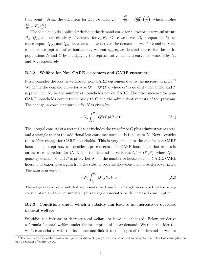
that point. Using the definition for En, we have, En =dQQdPP

=(dQdP

) (PQ

), which implies

dQdP

= En

(QP

).

The same analysis applies for deriving the demand curve for c, except now we substitute

P1c, Q1c, and the elasticity of demand for c, Ec. Once we derive P0 in equation (5), we

can compute Q0n, and Q0c, because we have derived the demand curves for c and n. Since

c and n are representative households, we can aggregate demand curves for the entire

populations N and C by multiplying the representative demand curve for n and c by Nn

and Nc, respectively.

B.2.2 Welfare for Non-CARE customers and CARE customers

First, consider the loss in welfare for non-CARE customers due to the increase in price.29

We define the demand curve for n as Qn = Qn(P ), where Qn is quantity demanded and P

is price. Let Nn be the number of households not on CARE. The price increase for non-

CARE households covers the subsidy to C and the administrative costs of the program.

The change in consumer surplus for N is given by:

−Nn

∫ P1n

P0

Qn(P )dP < 0 (A1)

The integral consists of a rectangle that includes the transfer to C plus administrative costs,

and a triangle that is the additional lost consumer surplus. It is a loss to N . Next, consider

the welfare change for CARE households. This is very similar to the one for non-CARE

households, except now we consider a price decrease for CARE households that results in

an increase in welfare for C. Define the demand curve forcas Qc = Qc(P ), where Qc is

quantity demanded and P is price. Let Nc be the number of households on CARE. CARE

households experience a gain from the subsidy because they consume more at a lower price.

The gain is given by:

−Nc

∫ P1c

P0

Qc(P )dP > 0 (A2)

The integral is a trapezoid that represents the transfer rectangle associated with existing

consumption and the consumer surplus triangle associated with increased consumption.

B.2.3 Conditions under which a subsidy can lead to an increase or decrease

in total welfare.

Subsidies can increase or decrease total welfare, or leave it unchanged. Below, we derive

a formula for total welfare under the assumption of linear demand. We then consider the

welfare associated with the base case and link it to the slopes of the demand curves for

29For now, we treat welfare losses and gains for different groups with the same welfare weights. We relax this assumption inour discussion of equity below.

6

CARE and non-CARE customers. We then discuss how this analysis relates to the optimal

taxation problem defined by Ramsey (1927). Finally, we identify some special cases where

welfare increases or decreases with the introduction of a subsidy.

The net change in total welfare for introducing CARE is as follows:

∆W = Nn

∫ Q1n

Q0n

(P n(Q)−MSC)dQ + Nc

∫ Q1c

Q0c

(P c(Q)−MSC)dQ− A (A3)

where ∆W is the net change in welfare. For simplicity, we consider the case where admin-

istrative costs are zero (i.e. A = 0).30 Because the demand curve is linear, we can simplify

the integrands in (A3). Consider the first term with Nn, but drop Nn for simplicity. With

linear demand, this yields:

1

2(Q1n −Q0n)(P0 + P1n)− (Q1n −Q0n)MSC = (Q0n −Q1n)[MSC− 1

2(P0 + P1n)]

Applying this same logic to C, and assuming A = 0, yields a total welfare change of:

∆W = Nn(Q0n −Q1n)[MSC− 1

2(P0 + P1n) + Nc(Q0c −Q1c)[MSC− 1

2(P0 + P1c) (A4)

We can express the change in quantities in terms of a change in prices because the demand

curves are linear. We know, for example, that (Q0n −Q1n) = (dQn

dP)(P0 − P1n), and that a

similar result obtains for c.31 We can simplify the integrand for n as follows:

(Q0n −Q1n)[MSC− 1

2(P0 + P1n)] =

(dQn

dP)(P0 − P1n)[MSC− 1

2(P0 + P1n)]

Substituting into ∆W in equation (A4) above yields:

∆W = [Nn(dQn

dP)][P0−P1n][MSC− 1

2(P0 +P1n)]+[Nc(

dQc

dP)][P0−P1c][MSC−(

1

2)(P0 +P1c)]

(A5)

Equation (A5) consists of two terms, each of which has three “sub-terms” within square

brackets. The sign pattern for the first and second terms are (−)(−)(?) and (−)(+)(?).

Neither of these two terms can be signed without further assumptions, and thus, the effect

of introducing the subsidy on total welfare can be positive, negative or zero.

Consider now the problem of understanding the impact on total welfare of introducing

CARE in the base case . A feature of this problem is that [MSC − 12(P0 + P1n)] < 0 and

[MSC − (12)(P0 + P1c)] < 0. This means the first term of (A5) is negative and the second

term is positive. For this case, (A5) says that there is a social welfare loss associated with

30Results below can be easily modified with constant administrative costs.31( dQn

dP) refers to the derivative of quantity for n, with respect to change in the price for n, and similarly for c. The subscript

on price is not used in the interest of simplicity.

7

N ’s reduction in quantity consumed and a social welfare gain associated with C’s increase

in quantity consumed. Total welfare will increase on net if the second effect dominates

the first. Ceteris paribus, total welfare will increase if (dQn

dP) increases toward zero. In the

extreme, if n’s demand curve is perfectly inelastic, i.e., (dQn

dP) = 0, then n does not change

consumption with the subsidy and there a gain in total welfare for society. A similar

analysis holds for c. If c’s demand becomes more elastic, so (dQn

dP) decreases further below

zero, then total welfare increases.

This model is related to, but not the same as, Ramsey’s optimal taxation problem.

It is related in the sense that elasticities matter for computing CARE’s impact on total

welfare, but so do other parameters. Our analysis differs from Ramsey’s in that we are

not trying to identify optimal tax levels or markups, though that would be possible to do.

Instead, we are comparing two pricing regimes, both of which deviate from the MSC and

the MPC. Whether or not the new pricing regime improves welfare over the old regime

depends on demand characteristics and the relationship between the MSC and new and old

prices (see equation (A5)). For the base case analyzed above, under the assumption that

administrative costs are zero, taxing the inelastic good (n’s consumption) and subsidizing

the elastic good (c’s consumption) improves welfare, but that will not always be the case.

Below, we examine some special cases in which total welfare improves. The two sub-

terms, [MSC− (12)(P0 +P1n)] and [MSC− (1

2)(P0 +P1c)], can be useful for signing equation

(A5). We consider three cases below for each of these expressions.

Case A1: [MSC− (12)(P0 + P1n)] > 0

The first term in (A5) has the following sign pattern: (+)(+)(+) = (+). The second term

has the following sign pattern: (+)(-)(?) = (?). Thus, we cannot sign (A5) without further

assumptions. But if the first term is bigger in absolute value than the second term, we

could ensure that the subsidy has a positive welfare effect. Inspection of (A5) yields the

following observation:

Lemma 1: As dQc

dPapproaches 0, the second term gets sufficiently small and this will

ensure that the subsidy has a positive impact on welfare.

Case A2: [MSC− (12)(P0 + P1c)] > 0

The first term has the following sign pattern: (−)(−)(?) = (?). The second term has

the following sign pattern: (−)(+)(+) = (+). Thus, we cannot sign (A5) without further

assumptions, similar to the ones in Case A1.

Case A3: [MSC− (12)(P0 + P1n)] = 0

Assume further that P1c < P1n, which is true for CARE. The first term has the fol-

lowing sign pattern: (−)(−)(0) = (0). The second term has the following sign pattern:

(−)(+)(+) = (−).

Case A4: [MSC− (12)(P0 + P1c)] = 0

The first term has the following sign pattern: (−)(−)(−) = (−). The second term has the

following sign pattern: (−)(+)(0) = (0). Together, case A3 and case A4 yield the following

8

result:

Lemma 2: If [MSC− (12)(P0 +P1n)] = 0 or [MSC− (1

2)(P0 +P1c)] = 0, then the welfare

change is negative with the introduction of the subsidy.

Case A5: [MSC− (12)(P0 + P1n)] < 0

The first term has the following sign pattern: (−)(−)(−) = (−). The second term has the

following sign pattern: (−)(+)(?) = (?). If we further assume that MSC > (12)(P0 + P1c),

then the second term can be signed as (−)(+)(+) = (−). In this case, the welfare change

is negative with the introduction of the subsidy. We could also follow the method used in

Case A1 to sign this expression.

Case A6: [MSC− (12)(P0 + P1c)] < 0

The first term has the following sign pattern: (−)(−)(−) = (−). The second term has the

following sign pattern: (−)(+)(−) = (+). In this case the sign is indeterminate. We could

also follow the method used in Case A1 to sign this as positive or negative. For example, asdQn

dPapproaches 0, the first term gets sufficiently small and this will ensure that the subsidy

has a positive impact on welfare.

In summary, we have identified cases where the subsidy could have a positive or negative

effect on welfare. For our parameter choices, the CARE subsidy often has a negative impact

on welfare.

B.2.4 Comparative statics associated with introducing CARE when there is

a change in the demand elasticity.

We examine what happens if the demand curve for n or c changes. We consider the changes

in welfare with a change in elasticity. Given the demand curves are straight lines, a change

in elasticity is modeled as a rotation of the demand curve around a specific point, which

means that the slope is changing.

We wish to show:

d∆W

dEc

>=< 0 if and only if [MSC− 1

2(P0 + P1c)] >=< 0 (A6)

Andd∆W

dEn

>=< 0 if and only if [MSC− 1

2(P0 + P1n)] <=> 0 (A7)

Consider the effect of a change in Ec on ∆W . Inspection of equation (A4) reveals that

the only parameter that Ec affects is Q0c, giving:

d∆W

dEc

= (dQ0c

dEc

)Nc[MSC− 1

2(P0 + P1c)] (A8)

We can write:dQ0c

dEc

=dQ0c

dE= (

dQ0c

dm)(dm

dE) (A9)

9

where E is substituted for Ec in the first equality and the second equality introduces the

slope of c’s demand curve, so m = dQdP

. Writing the demand curve in point slope form,

we have: (Q0c − Q1c) = m(P0 − P1c). Rearranging yields: Q0c = m(P0 − P1c) + Q1c.

Thus,dQ0c

dm= P0 − P1c.

We can compute the elasticity as follows: Ec = E = ( P1c

Q1c)(dQ

dP) = km, where k = ( P1c

Q1c).

Note that (dmdE

) = 1k. Substituting into equation (A9) gives:

dQ0c

dEc

=dQ0c

dE= (

dQ0c

dm)(dm

dE) =

P0 − P1c

k=

(P0 − P1c)Q1c

P1c

> 0 (A10)

Equation (A10) is positive so long as P0 > P1c, which is assumed (i.e., the CARE subsidy

is lower than the original price). The first and second terms in equation (A10) are positive.

This yields the desired result in equation (A6) .

Reasoning by analogy for n, we have (assuming P1n > P0):

dQ0n

dEn

=(P0 − P1n)Q1n

P1n

< 0

Similar reasoning for n yields the general expression:

d∆W

dEn

= (dQ0n

dEn

)Nc[MSC− (1

2)(P0 + P1n)] (A11)

The first term is negative and the second, Nc, is positive. This yields the desired result in

equation (A7).

We can develop some intuition for this result on elasticity through a graphical analysis.

The first thing to note is that the change in elasticity is similar to a change in slope around

the point (Q1c, P1c). We consider the precise situation for c in a graph, but suppress the c

subscript for simplicity. A similar analysis will apply to n.

We are comparing two situations: (1) the change in welfare associated with introducing

the CARE subsidy in the new situation (∆WB), which is depicted in Panel 1 in Figure

A4 when demand is less elastic; and (2) the change in welfare associated with introducing

the CARE subsidy in the old situation (∆WA), which is depicted in Panel 2 of Figure A4

when demand is more elastic. Note that the demand curve rotates around the point in the

diagram (Q1, P1), from DA to DB. We define ∆∆W∆E

as the change in the change in welfare

from introducing CARE as demand becomes more inelastic, in this case for c. We wish

to compute: ∆∆W∆E

= ∆WB − ∆WA. Note in the limit ∆∆W∆E

approaches d∆WdE

for c. We

are asking what happens to the change in welfare associated with introducing CARE as

demand becomes more inelastic for c.

When MSC = 12(P0 + P1), it is clear from the geometry that ∆WB = 0 and ∆WA=0,

In both of these cases for demand, half of the increase in demand has willingness to pay

(WTP) above MSC, and half of the increase in demand has WTP below MSC. In Figure

10

A4 the two welfare triangles are congruent in each panel (triangles Y and Z, and W and

X), and cancel each other out. This shows the net welfare change is zero in both cases

from introducing CARE. The preceding analysis provides the intuition for

d∆W

dEc

= 0 if and only if [MSC− 1

2(P0 + P1c)] = 0

To provide the intuition for the greater than result in equation (A6), we must consider

what happens to benefits and costs. Because the demand curves do not change, benefits

to c are the same as the situation just analyzed. Consider what happens to cost if MSC

increases, so that MSC = 12(P0 + P1) + k, where k > 0. MSC increases by k for each

additional unit that is consumed from introducing the subsidy. For the new situation,

MSC increases by (Q1−QB)k, and for the old situation, costs increase by (Q1−QA)k. In

this case: ∆WB = −(Q1−QB)k and ∆WA = −(Q1−QA)k, and thus ∆W∆E

= ∆WB −∆WA

= (QB−QA)k > 0. The greater than inequality follows because QB > QA (see Figure A4).

The preceding graphical analysis provides the intuition for greater than result in equa-

tion (A6). A similar analysis provides the intuition for the less than result in equation

(A6). In that case, cost decreases by more in the old situation than the new situation, so

on net, welfare decreases. An analogous graphical result can be constructed for n with the

signs reversed in equation (A6) (see equation (A7)). In that case, the new price exceeds

the old price.

We can use this analysis to explain the slope for the welfare change from making demand

more inelastic in our base case for both n and c. The base case has MSC < P1c < P0 < P1n.

Equation (A6) implies d∆WdEc

< 0 (because MSC −12(P0 +P1c) < 0) which is shown in figure

3; equation (A7) implies d∆WdEn

> 0 (i.e., MSC −12(P0 + P1n) < 0) which is shown in figure

A6.

For further intuition, consider the case of n. Start with a situation where n’s demand

is perfectly inelastic. There is no change in n’s quantity demanded with the introduction

of CARE, and thus the first term in (3) becomes zero in the limit.32 Now, suppose n’s

demand curve has some elasticity less than 0. In this case, there is a change in n’s quantity

demanded with the introduction of CARE and the first term becomes negative (the other

two terms in (3) remain the same). This shows welfare increases as the demand curve for

N rotates from being downward sloping to becoming perfectly inelastic.

A similar argument applies for c, except the first and third terms in equation (3) do

not change, and the second term becomes positive if c’s demand is downward sloping

(it approaches zero when c’s demand becomes perfectly inelastic). This shows welfare

decreases as the demand curve for C rotates from being downward sloping to becoming

perfectly inelastic.

32We say in the limit because the willingness to pay is technically not defined for perfectly inelastic demand; but as the demandcurve becomes perfectly inelastic, the value of the first term approaches zero.

11

B.2.5 Lump sum taxes and economic efficiency

A lump sum tax is generally an efficient form of taxation when prices reflect marginal

cost. This will not always be the case when prices do not equal marginal cost, or marginal

social cost when there is an externality. The intuition is that an ad valorem tax can actually

move prices closer to the MSC, and thus may be preferred in some “second-best” situations.

Below we will refine this intuition in our model and show the following: a lump sum tax

increases (reduces) economic welfare if the resulting price for energy is closer to (or further

away) from the MSC than the price that prevailed with an ad valorem tax.

We do this for non-CARE customers, N . We wish to compare economic welfare under

a lump sum tax and an ad valorem tax for non-CARE customers. This is equivalent to

identifying conditions under which a price move from P1n to P0 for n increases economic

welfare. That is because with an ad valorem tax, N faces a price of P1n; and with a lump

sum tax, N faces a price of P0. The expression for the change in welfare in moving from

an ad valorem tax to a lump sum tax is:

∆W = Nn

∫ Q0n

Q1n

(P n(Q)−MSC)dQ

which follows from (A3).33 We consider a representative consumer n without loss of gen-

erality for our welfare calculation. The welfare expression for n is

∆W =

∫ Q0n

Q1n

(P n(Q)−MSC)dQ

Following the logic in equation (A5), the welfare change for n becomes:

∆W =dQn

dP(P1n − P0)[MSC− 1

2P0 + P1n)]

The first term, (dQn

dP), is negative because demand is downward sloping; the second

term, (P1n − P0), is positive because this represents the ad valorem tax that n pays for

subsidizing C. This yields the following lemma on welfare:

Lemma 3: ∆W >=< 0 if and only if [MSC− 12(P0 + P1n)] <=> 0

The reasoning can be seen graphically. Consider panel 2 in Figure A4, and reverse the

subscripts for P and Q, so that P1 > P0, and P1 = P1n in this case. If MSC = 12(P0 +P1n),

welfare does not change in moving from an ad valorem tax to a lump sum tax to an ad

(i.e., the area of triangle X equals the area of triangle W ). If MSC increases so that

MSC − 12(P0 + P1n) > 0, the benefits to n stay the same, but the social costs go up,

which implies the benefits of introducing a lump sum tax are negative (the lump sum tax

results in a price that is further away from the MSC). Conversely, if MSC decreases so that

33This is true if administrative costs are the same with a lump sum tax and an ad valorem tax.

12

MSC − 12(P0 + P1n) < 0, the benefits to n stay the same, but the social costs go down,

which implies the benefits of introducing a lump sum tax are positive (the lump sum tax

results in a price that is closer to the MSC.

This framework can also be applied to a case when there is not a lump sum tax, but

a tax whose deadweight loss can be measured. Define T as the transfer from N that pays

for CARE, which includes administrative costs (A) and the transfer to CARE customers

(see equation (4)) Let kT be the welfare costs associated with T (typically k ≥ 0).

Then the expression for ∆W for n becomes:

∆W =dQn

dP(P1n − P0)[MSC− 1

2(P0 + P1n)]− kT

Nn

Note that the last term in this equation, − kTNn

is added to reflect the fact that we are

considering the tax cost for a representative non-CARE household, n. We would need to

multiply the preceding equation by Nn to get the social welfare loss. If there were these

deadweight costs associated with the tax, Lemma 3 would need to be revised to take them

into account. For example, when MSC = 12(P0 +P1n), the welfare would be lower under the

alternative tax by kT than with the ad valorem tax. Thus, the existing tax on non-CARE

customers would be preferred in this case.

In short, we have developed closed form expressions that allow us to compare the welfare

effects of different tax regimes when prices depart from marginal social costs. We could

also explore how the results here are affected by a change in demand elasticity.34

B.2.6 Some additional information on the welfare impacts of vouchers

We will assume there are three instruments: a standard subsidy, a standard voucher, and

a behavioral voucher. The amount of the voucher is set equal to the subsidy. We wish to

know whether vouchers will be better or worse for C and for social welfare compared with

the subsidy.

For C, a standard voucher is generally preferred to a subsidy. The reason is that a

representative CARE household could consume the same bundle she consumed with the

subsidy. Under our assumptions of downward sloping demand, she chooses a different

bundle, and is therefore better off using a revealed preference argument.

Figure A5 shows why standard vouchers are preferred to a subsidy. At the subsidized

price P1, c chooses Q1 on demand curve D. At the unsubsidized price P0 with the voucher,

c chooses Q0. c has a net welfare gain of triangle ABC for the standard voucher over the

subsidy. She receives the voucher equal to rectangle P0P1CB, but loses the trapezoid in

consumer surplus given by P0P1CA, so the remaining gain is triangle ABC.

For the behavioral voucher, we assume that c’s “true” demand is given by D, but that

34The formal analysis is similar to the previous analysis of demand elasticity.

13

she does not demand A at P0. In general, her demand with a voucher will exceed Q0. If she

chooses a point on the interior of this segment AC, then she is better off than she would

have been with the subsidy (again using a revealed preference argument). In this case, she

is not as well off as if she would be with the standard voucher because she consumes some

units beyond Q0 that reduce her surplus.35 However, it is possible that the behavioral

voucher could lead c to consume more than Q1, say Q2, in which case she would be worse

off than with the subsidy. If she chose Q2, her welfare loss would be AEF relative to the

standard voucher, and her loss would exceed that of the subsidy relative to the standard

voucher (ABC).

Thus, a standard voucher, as defined here, will always be preferred by C to a behavioral

voucher or a subsidy under the assumptions of this model. In contrast, C’s preference for

a behavioral voucher is ambiguous in general. If voucher expenditures do not result in

a quantity that exceeds that selected under the subsidy, CARE households prefer the

standard voucher to the behavioral voucher to the subsidy.

As noted in the text, a more interesting question from a social perspective is whether

these vouchers increase or decrease economic welfare compared with the subsidy. For a

given MSC, the welfare associated with N ’s choices do not change because N picks the

same quantity.

However, c’s quantity choices will be affected by standard and behavioral vouchers. For

c, the change in total social welfare in moving from a subsidy to a voucher is given by:∫ QI

Q1c

(P c(Q)−MSC)dQ (A12)

where Q1c = Qc(P1c), and QI is the quantity selected under intervention, I. For the

subsidy QI = Q1c, so there is no change in welfare. For standard vouchers, QI = Qc(P0).

In words, equation (A12) says that the welfare change for standard vouchers is defined

by the difference between the benefit tocand the marginal social cost for the reduction

in quantity demanded as prices increase from the subsidized price, P1c, to the original

price, P0.36. This welfare change per household is then multiplied by the total number of

households to obtain the total welfare change.

For behavioral vouchers, c selects QB (using B for behavioral) at P0. Let QB = Qc(P0)

plus the additional quantity demanded as a result of the bias. That additional quantity is

defined by marginal propensity to consume from the voucher (between 0 and 1) multiplied

by the cash value of the vouchers thatcreceives, and then divided by P0.

To estimate welfare benefits, we will define the “true” demand curve for c as Qc(P ).37

35If the behavioral voucher resulted in spending more than the voucher on the commodity, c would be worse off with the voucherthan the subsidy. We think this case is unlikely. Also, if the behavioral voucher resulted in consumption that was far below Q0,c could be worse off with the voucher than the subsidy. Again, we think this case is unlikely.

36In the case of linear demand, the integral is given by 12[(MSC − P1c) + (MSC − P0)](Q1c −Q0c)

37Our demand curve may not be the “true” one for a variety of reasons, including the possibility that some consumers may not

14

With behavioral vouchers, c selects a point on her observed demand curve. We take that

the quantity QB and associate it with a price on the true demand curve Qc(P ).38 That

price will be lower than P0 if the voucher results in additional consumption. We then carry

out the welfare analysis using equation (A12), with the upper limit of integration set to

QB.

There is another way to rank the welfare of the subsidy and voucher policies that

allows for a simpler comparison of quantities. Equation (A12) ranks vouchers and subsidies

relative to the welfare associated with the subsidy. We could also have chosen a different

reference point. One such point is the optimal level of output for c or Qc(MSC). In this

case the best policy would be the one that has the lowest social cost compared with this

optimal policy.39 This is given by the following formula: −12(Q(MSC))−QI)

2 dPdQ

.40

The formula shows that the closer the quantity selected, QI , is to the optimal quantity,

Q(MSC), the smaller the welfare gain in moving to the optimal quantity. Hence, quantities

closer to the optimal quantity have a higher level of economic welfare associated with them.

Thus, if the standard voucher or behavioral voucher results in a quantity that is closer in

distance to the optimal quantity than the subsidy, then society enjoys a higher level of

economic welfare than with the subsidy. In the special case where the initial price is equal

to the MSC, and the agent spends some of the voucher on gas, then the economic welfare

for the standard voucher is higher than economic welfare for the behavioral voucher.

Under certain assumptions, we can show that the welfare associated with behavioral

vouchers may actually exceed standard vouchers or a price subsidy. This may be viewed

as unusual, because, by definition, the observed response to behavioral vouchers may be

viewed as not consistent with theory. The result is again driven by the fact that such a

response could bring the quantity demanded closer to the optimal quantity, Q(MSC), and

thus improve welfare. For an example of behavioral vouchers being preferred to vouchers,

assume that the voucher price P0 > MSC, so Q(P0) < Q(MSC). Define the additional

fraction of each dollar spent from the voucher as the “bias,” or b.41 If the bias is sufficiently

small, then the welfare of behavioral vouchers exceeds that of standard vouchers because

the quantity selected with behavioral vouchers is closer to Q(MSC). To show that the

welfare of behavioral vouchers may exceed that of a subsidy, assume that P0 = MSC, so

that the voucher price is optimal. In this case, the welfare of standard vouchers exceeds

that of the subsidy. Again, if the bias is sufficiency small, the welfare associated with

behavioral vouchers exceeds that of the subsidy.

appreciate the nature of the subsidy.38Our analysis is similar to Figure 4, p. 1172 in Chetty et al. (2009), except we are considering an overstatement in the observed

demand. See also Chetty (2015), Figure 9.39Strictly speaking, this is not the first-best policy, because n’s quantity is not optimal.40This formula can be derived as follows. In (A12) , substitute Q1 as the lower limit of integration and Q(MSC) as the upper

limit of integration. Then noting that Pc(Q) is linear and MSC is a constant, integrating the function yields this result.41By additional, we mean beyond what might be spent with an equivalent cash transfer. See Allcott and Taubinsky (2015) for

an insightful treatment of the bias issue in the context of energy efficiency.

15

B.3 Further Discussion of Empirical Results

This section includes several subsections on topics of empirical interest. They include:

• B.3.1 - Extrapolating the welfare results to California;

• B.3.2 - Impact of introducing CARE;

• B.3.3 - Impact of using a different counterfactual for CARE price;

• B.3.4 - Welfare analysis with two-tiered pricing;

• B.3.5 - Welfare analysis when adding cap-and-trade;

• B.3.6 - Welfare analysis when prices are set equal to the marginal social cost;

• B.3.7 - Welfare analysis when prices are set equal to the marginal private cost;

• B.3.8 - Comparing the welfare impact of CARE vouchers with a CARE price subsidy;

and

• B.3.9 - Computing an “optimal” subsidy.

B.3.1 Extrapolating the welfare results to California

We outline our approach for extrapolating our results to California. We do this by consid-

ering two other utilities that supply natural gas, Pacific Gas and Electric and San Diego

Gas and Electric. Together, the three utilities represent about 80% of the gas supply in

California. We use the same elasticities we used for SoCalGas as well as the same SCC

values. However, prices, quantities, and administrative costs differ. The values we use are

shown in Table A14 below along with the welfare and environmental results.

The key results are that net welfare decreases overall, and emissions increase for all the

three utilities. The total welfare loss is about $3 million and the emissions increase is about

240,000 tons of CO2. SoCalGas is responsible for the largest share of welfare losses and

emissions.

B.3.2 Impact of introducing CARE

We consider two sensitivities in this subsection: varying the elasticity for non-CARE cus-

tomers and varying the SCC.

In the base case, we assume that CARE customers have demand elasticities that are

at least as elastic as non-CARE customers because they have lower incomes. Figure A6

shows how welfare changes with changes in the elasticity of N moving from -0.35 to 0. As

non-CARE household demand becomes more inelastic, there is a small increase in total

welfare for these households. The reasoning is similar to that for CARE customers. In this

case, the reduction in consumption for N is smaller as demand becomes more inelastic, and

thus the welfare loss for N is smaller. The utility increases its profits as the demand by

16

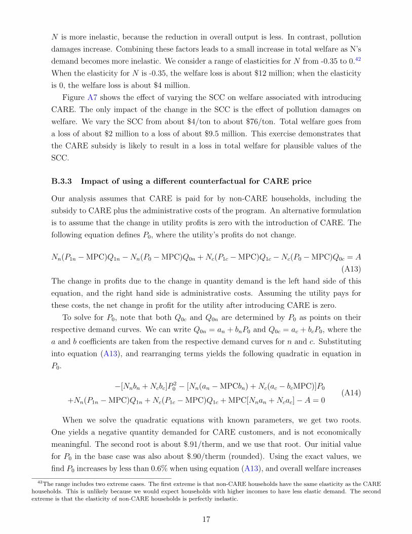
N is more inelastic, because the reduction in overall output is less. In contrast, pollution

damages increase. Combining these factors leads to a small increase in total welfare as N’s

demand becomes more inelastic. We consider a range of elasticities for N from -0.35 to 0.42

When the elasticity for N is -0.35, the welfare loss is about $12 million; when the elasticity

is 0, the welfare loss is about $4 million.

Figure A7 shows the effect of varying the SCC on welfare associated with introducing

CARE. The only impact of the change in the SCC is the effect of pollution damages on

welfare. We vary the SCC from about $4/ton to about $76/ton. Total welfare goes from

a loss of about $2 million to a loss of about $9.5 million. This exercise demonstrates that

the CARE subsidy is likely to result in a loss in total welfare for plausible values of the

SCC.

B.3.3 Impact of using a different counterfactual for CARE price

Our analysis assumes that CARE is paid for by non-CARE households, including the

subsidy to CARE plus the administrative costs of the program. An alternative formulation

is to assume that the change in utility profits is zero with the introduction of CARE. The

following equation defines P0, where the utility’s profits do not change.

Nn(P1n −MPC)Q1n −Nn(P0 −MPC)Q0n + Nc(P1c −MPC)Q1c −Nc(P0 −MPC)Q0c = A

(A13)

The change in profits due to the change in quantity demand is the left hand side of this

equation, and the right hand side is administrative costs. Assuming the utility pays for

these costs, the net change in profit for the utility after introducing CARE is zero.

To solve for P0, note that both Q0c and Q0n are determined by P0 as points on their

respective demand curves. We can write Q0n = an + bnP0 and Q0c = ac + bcP0, where the

a and b coefficients are taken from the respective demand curves for n and c. Substituting

into equation (A13), and rearranging terms yields the following quadratic in equation in

P0.

−[Nnbn + Ncbc]P20 − [Nn(an −MPCbn) + Nc(ac − bcMPC)]P0

+Nn(P1n −MPC)Q1n + Nc(P1c −MPC)Q1c + MPC[Nnan + Ncac]− A = 0(A14)

When we solve the quadratic equations with known parameters, we get two roots.

One yields a negative quantity demanded for CARE customers, and is not economically

meaningful. The second root is about $.91/therm, and we use that root. Our initial value

for P0 in the base case was also about $.90/therm (rounded). Using the exact values, we

find P0 increases by less than 0.6% when using equation (A13), and overall welfare increases

42The range includes two extreme cases. The first extreme is that non-CARE households have the same elasticity as the CAREhouseholds. This is unlikely because we would expect households with higher incomes to have less elastic demand. The secondextreme is that the elasticity of non-CARE households is perfectly inelastic.

17

by about 12%, yielding a total welfare loss of -$4 million.

B.3.4 Welfare analysis with two-tiered pricing

Our calculations assumed that CARE and Non-CARE households face a single price. In

actuality, there is two-tiered pricing for both CARE and non-CARE. This means households

that demand more than a certain amount face a higher price at the margin.

This two-tiered system can be modelled by considering a representative consumer on

each price tier for both CARE households and non-CARE households. We will denote the

number of CARE households on tier one by Nc1, tier two by Nc2, and the same for Non-

CARE households by Nn1, Nn2. As before, we can derive the counterfactual, prices P01 and

P02 for the respective tiers, by adjusting equation (4) (shown below as (A15)) so that the

transfer from non-CARE customers on both price tiers equals the sum of the transfer to

CARE customers on both price tiers plus administrative costs.

Nn(P1n − P0)Q1n = Nc(P0 − P1c)Q1c + A (A15)

So that original equation (A15) becomes equation (A16) below.

Nn1(P1n1 − P01)Q1n1 + Nn2[(P1n2 − P02)(Q1n2 − Q) + (P1n1 − P01)Q]

= Nc1(P01 − P1c1)Q1c1 + Nc2[(P02 − P1c2)(Q1c2 − Q) + (P01 − P1c1)Q] + A(A16)

P1n1, P1n2, P1c1, P1c2 are observed prices after CARE is introduced. Q1c1, Q1c2 are cal-

culated from data for consumers on CARE above and below our the maximum quantity

in the first tier, Q. We do not observe the distribution of non-CARE customers or their

consumption, but we know their total population and the mean annual consumption. To

address this, we extrapolate from CARE consumption, using a normal distribution. We

use this distribution around the mean of non-CARE consumption to produce estimates of

Nn1, Nn2 and Q1n1, Q1n2.

The counterfactual prices P01, P02 are no longer uniquely identified in equation (A16)

because there is 1 equation and 2 unknowns, so we consider two solutions:

1. The utility equalizes the tax difference between tiers, P1n1 − P01 = P1n2 − P02

2. The utility equalizes subsidy difference between tiers, P01 − P1c1 = P02 − P1c2

Both conditions are plausible for the utility, yet imposing both concurrently leads to an

over-determined system in (A16). We present the welfare analysis under these two solu-

tions, as well as a third case that minimizes the squared sum of the tax difference and the

subsidy difference across tiers.

Finally, the demand curves for each tier are calculated to be linear curves that sum

point-wise to the aggregate demand of that group in the original demand system (see

18

sections 4.1.1 and B.2.1). These yield values for Q0n1, Q0c1 corresponding to P01, and

Q0n2, Q0c2 corresponding to P02.

The first case for counterfactual prices leads to P01, P02 values of $0.87, $1.08/therm for

the two tiers, and an overall welfare decrease of 1% compared with the original simulation.

The second case leads to P01, P02 values $0.86, $1.12/therm for the two tiers and an overall

welfare increase of 32% in comparison to our base case. The third case yields values

between the previous two scenarios. In all cases, the change in welfare is still negative

with the introduction of the CARE subsidy, as was the case in our original analysis. More

detailed parameter estimates are summarized in the table A13.

B.3.5 Welfare analysis when adding cap-and-trade regime

Cap-and-trade is modeled as an exogenous price on CO2 emissions determined by the

market. There are two key points of the analysis of cap-and-trade. First, a single policy

instrument will not achieve the first best outcome because of the different prices faced

by CARE and non-CARE consumers. Given the subsidy for CARE customers, at least

one of the prices will be different from marginal social cost with cap-and-trade. The sub-

optimal nature of this policy is a necessary consequence of the CARE subsidy. This means

that we must consider a second-best result in the maximization. The second result is an

empirical finding. Welfare is generally negative upon introducing a cap-and-trade scheme

for SoCalGas customers. In this particular case, both the natural gas price for CARE and

non-CARE customers start above the MSC. Adding cap-and-trade leads to welfare losses

as prices depart further from the MSC.

The change in overall welfare for introducing cap-and-trade is given by:

Nn

∫ Q2n

Q1n

(P n(Q)−MSC)dQ + Nc

∫ Q2c

Q1c

(P c(Q)−MSC)dQ (A17)

The initial quantities Q1n and Q1c are determined by the introduction of CARE. The new

quantities are determined by adding an allowance price, t, to P1n and P1c, yielding the new

quantities Q2n and Q2c.43 44 Note that equation (A17) has the same structure as equation

(3), but without additional administrative costs.45

We can also apply equation (A17) to replacing the subsidy with vouchers. In this

case, there is no welfare change for N because non-CARE customers do not change their

43With no uncertainty, perfect information and a competitive market, the tax and the allowance scheme can be shown to beequivalent in terms of their impact on pollution (Baumol and Oates, 1988).

44For the scenario in which the price for n moves from P1n to the MSC, the upper limit of integration is defined by the quantitydemanded by n at the MSC. For the scenario in which the price for n moves from P1n to the MPC, the upper limit of integrationis defined by the quantity demanded by n at the MPC. We consider these cases in the appendix, along with the same pricemovements for c.

45We assume that administrative costs of the program are a sunk cost, and thus they do not enter into (A17), as they did withthe introduction of the CARE program. If the administrative costs change in these scenarios, this cost would need to be includedin the welfare analysis.

19

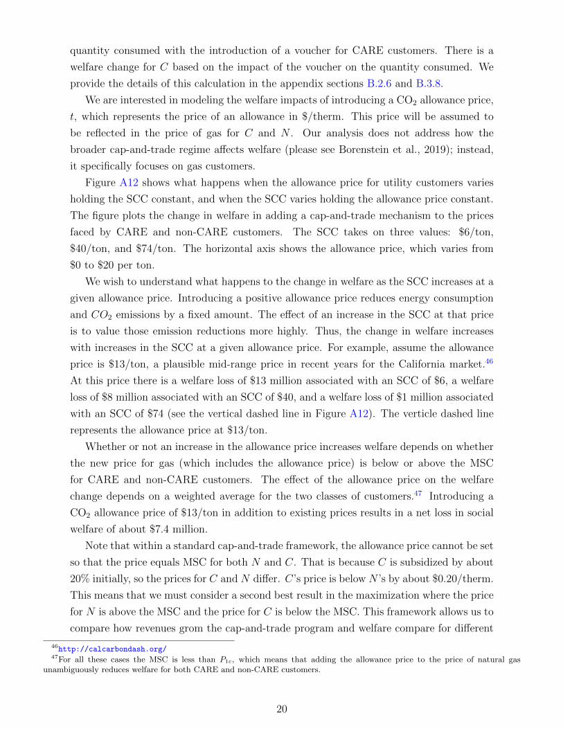
quantity consumed with the introduction of a voucher for CARE customers. There is a

welfare change for C based on the impact of the voucher on the quantity consumed. We

provide the details of this calculation in the appendix sections B.2.6 and B.3.8.

We are interested in modeling the welfare impacts of introducing a CO2 allowance price,

t, which represents the price of an allowance in $/therm. This price will be assumed to

be reflected in the price of gas for C and N . Our analysis does not address how the

broader cap-and-trade regime affects welfare (please see Borenstein et al., 2019); instead,

it specifically focuses on gas customers.

Figure A12 shows what happens when the allowance price for utility customers varies

holding the SCC constant, and when the SCC varies holding the allowance price constant.

The figure plots the change in welfare in adding a cap-and-trade mechanism to the prices

faced by CARE and non-CARE customers. The SCC takes on three values: $6/ton,

$40/ton, and $74/ton. The horizontal axis shows the allowance price, which varies from

$0 to $20 per ton.

We wish to understand what happens to the change in welfare as the SCC increases at a

given allowance price. Introducing a positive allowance price reduces energy consumption

and CO2 emissions by a fixed amount. The effect of an increase in the SCC at that price

is to value those emission reductions more highly. Thus, the change in welfare increases

with increases in the SCC at a given allowance price. For example, assume the allowance

price is $13/ton, a plausible mid-range price in recent years for the California market.46

At this price there is a welfare loss of $13 million associated with an SCC of $6, a welfare

loss of $8 million associated with an SCC of $40, and a welfare loss of $1 million associated

with an SCC of $74 (see the vertical dashed line in Figure A12). The verticle dashed line

represents the allowance price at $13/ton.

Whether or not an increase in the allowance price increases welfare depends on whether

the new price for gas (which includes the allowance price) is below or above the MSC

for CARE and non-CARE customers. The effect of the allowance price on the welfare

change depends on a weighted average for the two classes of customers.47 Introducing a

CO2 allowance price of $13/ton in addition to existing prices results in a net loss in social

welfare of about $7.4 million.

Note that within a standard cap-and-trade framework, the allowance price cannot be set

so that the price equals MSC for both N and C. That is because C is subsidized by about

20% initially, so the prices for C and N differ. C’s price is below N ’s by about $0.20/therm.

This means that we must consider a second best result in the maximization where the price

for N is above the MSC and the price for C is below the MSC. This framework allows us to

compare how revenues grom the cap-and-trade program and welfare compare for different

46http://calcarbondash.org/47For all these cases the MSC is less than P1c, which means that adding the allowance price to the price of natural gas

unambiguously reduces welfare for both CARE and non-CARE customers.

20

values of the allowance price. Figure A8 reproduces the high SCC curve for the welfare

associated when moving to a cap-and-trade when the SCC is $74/ton. The other curve in

the figure is the value of allowances as a function of the allowance price. The figure shows

that there is an increasing gap between the value of allowances and the welfare change as

the allowance price increases. The gap is even more pronounced if the low or medium value

for the SCC is used.

We can also formally derive how welfare from introducing a cap-and-trade scheme

changes with a change in the allowance price. This derivation will show conditions un-

der which welfare increases or decreases, and it will depend on the relationship of MSC to

prices.

The effect of a change in the allowance price on a change in welfare can be derived from

equation (A17):

Consider the first integrand in this equation. The analytical expression for the welfare

change is given by:

1

2(Q2n −Q1n)(P1n + P2n)−MSC(Q2n −Q1n) (A18)

The first term represents the consumer surplus loss for n with the change in price, and

the second term represents the change in social costs associated with the change in quantity.

Note that the first term is negative and the second term is positive. The expression shows

that as the MSC increases, the change in welfare from introducing cap and trade increases.

This is true for the SCC as well because the SCC and MSC are linearly related.

Now consider the point slope form for the demand curve for n: (Q2n − Q1n) = (P2n −P1n)dQ

n

dP. Substituting into (A3) and simplifying yields:

1

2(P2n − P1n)(

dQn

dP)(P1n + P2n)−MSC(P2n − P1n)(

dQn

dP) =

(dQn

dP)[

1

2(P2n − P1n)(P1n + P2n)−MSC(P2n − P1n)]

Substituting: P2n = P1n + t gives:

(dQn

dP)[

1

2t(2P1n + t)− t MSC] = (

dQn

dP)(tP1n +

1

2t2 − t MSC)

Note that this expression for welfare is quadratic in t. Differentiating the previous expres-

sion with respect to t yields:

(dQn

dP)(P1n + t−MSC) (A19)

Equation (A19) will be negative if P1n + t−MSC > 0, since the demand curve is downward

sloping. Furthermore, the second derivative with respect to t is (dQn

dP) < 0. The formulas

21

for c and n are analogous with c substituted for n in (A19), so the general formula for the

first derivative is:

(d∆W

dt) = Nn(

dQn

dP)(P1n + t−MSC) + Nc(

dQc

dP)(P1c + t−MSC) (A20)

In general the sign of (A19) will depend on (P1n + t−MSC) and (P1c + t−MSC). If, for

example, (P1c + t−MSC) > 0, welfare will decrease with an increase in the allowance price

(recall P1n > P1c, which implies (P1n + t−MSC) > 0. In this case, new prices for c and n

both exceed the MSC, and raising the price moves prices away from the MSC, which reduces

welfare. A similar argument shows that welfare will increase when (P1n + t −MSC) > 0.

The second derivative is always constant and negative. It is given by the formula:

(d2∆W

dt2) = Nn(

dQn

dP) + Nc(

dQc

dP) < 0

This explains the concavity of the curves for SCC values of $6, $40 and $74 in Figure A12.

B.3.6 Welfare analysis when prices are set equal to the marginal social cost

We know that as price moves toward the marginal social cost, welfare increases. The intu-

ition is that if price is below (above) MSC, then a household should consume less (more).

That is because society puts a higher (lower) value on the marginal unit of consumption

than the household does if the price is < (>) MSC. We estimate the quantitative impact

of moving existing prices to the marginal social cost. This could be accomplished in a

number of ways, including adjusting variable costs and fixed costs for different customer

classes (e.g., Borenstein and Bushnell, 2019).

The amount of the welfare increase will depend on the deviation between the current

price and the marginal social cost. This deviation will differ for N and C for a given MSC

because CARE customers are subsidized, so the two groups face different prices.

To compute the welfare change for moving prices to the MSC, we start with equation

(A17) and redefine the upper limits of integration. Specifically, define Q2n = Q2n(MSC) as

the upper limit for n and Q2c = Q2c(MSC) as the upper limit for c.

Figure A9 shows the welfare change for various assumed values of the MSC ranging

from $0.50/therm to $0.86/therm (corresponding to an SCC of $6/ton and $74/ton, re-

spectively). The figure has three curves: the welfare gains associated with moving from

the current price N faces to the MSC for N ; analogous welfare gains for C; and the total

welfare gains. Total welfare gains represent the vertical sum of the gains for N and C

at a given MSC. We use the price for CARE households (P1c = 0.75) and the price for

non-CARE households (P1n = 0.95) as the benchmark for making welfare comparisons (see

equation (A17)). Welfare gains are 0 for C when the MSC = P1c = 0.75 and welfare gains

are 0 for N when MSC = P1n = 0.95 (which is beyond the range of values used for the

22

SCC).

The gains associated with N , C, and total welfare are parabolas as a function of the

MSC. The key message of this figure is that welfare gains will always be positive as prices are

moved to the MSC, but exhibit substantial variation depending on which MSC is selected.

The differences in the welfare gains can be explained by the extent to which existing prices

deviate from the assumed MSC.The actual MSC (and SCC) is uncertain. To illustrate

plausible potential gains, we consider three simulations associated with SCC’s of $6, $40,

and $74 per ton (in 2014 dollars).48 These numbers correspond to the SCC calculated with

discount rates of 2.5%, 3%, and 5%, respectively (Greenstone et al., 2013). The welfare

gains of setting a price equal to MSC for an SCC equal to $6/ton are about $35 million;

for a price associated with an SCC of $40/ton, they drop to about $10 million; and for a

price associated with an SCC of $74/ton they decrease to about $3 million. The analysis

shows that the potential gains from setting price equal to the MSC will vary dramatically

depending on the precise value of the SCC.

B.3.7 Welfare analysis when prices are set equal to the marginal private cost

The CARE and non-CARE prices appear to be above the marginal private cost, and may

be substantially above the MPC. We consider two issues: the effect of varying the MPC on

the change in welfare associated with introducing CARE; and the welfare impact of setting

prices equal to the MPC for CARE and non-CARE customers.

Figure A11 shows the effect of varying the MPC on the welfare associated with in-

troducing CARE. The figure varies MPC from 0 percent to over 100% of the price that

non-CARE households face, or from $0/therm to $0.95/therm. The lower bound of 0 is

obviously an extreme case. We include it to show the breakeven point for total welfare in

the figure. At an MPC of $0.27/therm, total welfare declines to $0. Above that MPC, total

welfare is negative. This analysis further supports the finding that welfare impacts of the

subsidy are likely to be negative under reasonable assumptions about the MPC. Adjusting

current CARE and non-CARE prices to include a social cost of carbon (SCC) of $40/ton

results in a gain of $5.9 million.

To compute the welfare change for moving prices to the MPC, we start with equation

(A17) and redefine the upper limits of integration. Specifically, define Q2n = Q2n(MPC)

as the upper limit for n and Q2c = Q2c(MPC) as the upper limit for c.49

As equation (A17) suggests, this will depend on the relationship between existing prices

for N and C, the marginal private cost and marginal social cost.

Figure A10 shows the welfare effects of moving prices for CARE and non-CARE house-

holds to the marginal private cost of $0.47/therm used in the base case. This would amount

48For these values of the SCC, the MSC is $0.50, $0.68, and $0.86 per therm respectively.49Note that the counterfactual here is the welfare associated with existing prices, $0.75/therm for C and $0.95/therm for N ,

with the subsidy in place.

23

to a reduction in the price for N of $0.48/therm and a reduction in the price for C of about

$0.28/therm.

Figure A10 presents three curves, the welfare gains associated with N , the welfare gains

associated with C, and the total welfare gains, which represents the vertical sum of the

gains for N and C at a given MSC. The benchmark for the welfare comparison is the

welfare associated with the current prices offered to CARE and non-CARE households.

The welfare change is a function of the distance of the specified MSC from both the

MPC and the existing prices for CARE and non-CARE households. If the MSC is at the

low end of the range ($0.50/therm in the base case), then there is a gain in moving prices

to the MPC of about $36 million in total welfare (about $6 million associated with CARE

households and about $30 million associated with non-CARE households). The welfare

change associated with C households just equals zero when the MSC is precisely halfway

between the MPC and the current price for C households (an MSC value of $0.61/therm).

In contrast if the MSC equals the current price for C ($0.75/therm), moving prices to the

MPC for C households results in a $17 million welfare loss.

Total welfare declines as the MSC moves toward existing prices and away from the

MPC. The welfare decline is linear because the welfare function is a linear function of the

MSC. The key message of the figure is that welfare gains will not necessarily be positive

in moving prices to the MPC.

B.3.8 Comparing the welfare impact of CARE vouchers with a CARE price

subsidy

An alternative approach to a subsidy would be to provide vouchers to low-income customers

for natural gas purchases instead of CARE price subsidies. Vouchers are of interest because

they are sometimes viewed as a mechanism that will not distort consumption patterns. In

this sense, they may yield greater benefits than price subsidies if prices were initially set

optimally to reflect marginal social costs.

We wish to compare the welfare effects of vouchers for the purchase of natural gas

versus a price subsidy when the amount of the voucher is set equal to the subsidy that a

representative CARE customer receives.50 We will distinguish between two types of agents

in how they respond to vouchers. The case of standard vouchers will refer to a situation

when the agent follows standard neoclassical assumptions in reacting to a voucher.51 The

case of behavioral vouchers will refer to a situation in which the agent consumes more or

less than a standard neoclassical agent would with a voucher.52 We introduce behavioral

vouchers because there is evidence that vouchers may change an individual’s observed

50We thank the editors Liran Einav and Thomas Lemieux for encouraging us to conduct this analysis.51We analyze the case in which the cash value of vouchers received does not exceed the total expenditures on natural gas for

the CARE customer when price equals P0. This case is the relevant one in our empirical estimation.52We will assume the agent consumes more, in line with empirical work discussed below. For an instructive review of some of

the economic issues with using vouchers see Bradford and Shaviro (2000).

24

demand curve. Hastings and Shapiro (2018) find, for example, that vouchers used in a food

program – SNAP (Supplemental Nutrition Assistance Program) – increase consumption

compared with cash transfers. If a similar phenomenon arises in the case of energy, this

raises the question of how to assess the welfare implications.

We will assume there are three instruments: a standard price subsidy, a standard

voucher, and a behavioral voucher. We wish to know whether vouchers will be better

or worse for C and for social welfare compared with the price subsidy. The benchmark for

comparison is a situation in which CARE customers do not receive any subsidy. For C, a

standard voucher is generally preferred to a price subsidy. The reason is that a represen-

tative CARE household could consume the same bundle she consumed with the subsidy.

Under our assumptions of downward sloping demand, she chooses a different bundle, and

is therefore better off using a revealed preference argument. A standard voucher is also

preferred to a behavioral voucher if C does not choose a utility maximizing bundle with a

behavioral voucher.53

A more interesting question from a social perspective is whether these vouchers increase

or decrease total economic welfare compared with the CARE price subsidy. For a given

MSC, the welfare associated with N ’s choices do not change because N picks the same

quantity. For C, the three policy instruments affect the quantity selected differently. In

general, the relationship between the total welfare associated with standard vouchers, be-

havioral vouchers, and the price subsidy is ambiguous.54 This underscores the need for

empirical work to assess the welfare implications of vouchers.55

To estimate the quantitative impact of vouchers, we will assume that the true willingness

to pay is given by the demand curve we have estimated for c. To carry out the analysis,

we need an estimate of the how much vouchers change consumption, beyond that of an

equivalent cash transfer. We will use a crude approach to estimating this bias. Hastings and

Shapiro suggest that the marginal propensity to consume using vouchers for SNAP is in the

neighborhood of 0.5-0.6 and for cash it was much less – on the order of 0.1 (see also Hoynes

and Schanzenbach, 2009). This yields an upper bound estimate of bias of 0.5 (0.6-0.1) for

additional expenditures out of each voucher dollar on food. Expenditure on food at home

represented about 18% of total expenditures for this group (Mabli and Malsberger, 2013).

In contrast, the natural gas customers enrolled on CARE spend about 2% percent of their

income on natural gas.56 Assuming the extra expenditure on gas vouchers is proportionate

to income, we multiply the 0.5 estimate by (2/18) to get about 0.06 for the amount of bias.

53See appendix section B.2.6 for a more in-depth comparison of standard and behavioral vouchers.54See appendix section B.3 for a more in-depth analysis that links this instrument choice comparison to the marginal social

cost.55In principle, we can apply this welfare analysis to any policy intervention, provided that we know the true demand and the

observed demand (Chetty et al., 2009).56Gas expenditures are about $350 per year and the cut-off for CARE income for a two-person household is about $30,000,

yielding 1%. If the average income were half that for CARE households, this would imply that 2% of expenditures were made onnatural gas.

25

In the sensitivity analysis below, we vary the bias over the range 0 to 0.2.

Figure A13 shows the impact of replacing the CARE price subsidy with vouchers, and

also shows the impact of varying the degree of bias for SoCalGas customers for three

values of the SCC: $6/ton, $40/ton, and $74/ton. The figure shows that the welfare effect

of standard vouchers and behavioral vouchers can be positive or negative compared with

the subsidy. This is shown by noting that the SCC = 6 and the SCC = 40 curves have

a negative value when bias equal zero – the standard voucher case. In contrast, the SCC

= 74 curve has a positive value when bias equals 0. Similar results obtain when bias is

positive – the behavioral voucher case. The impact of vouchers on welfare compared with

a subsidy depends on whether the quantity chosen by CARE customers under vouchers is

closer to or further away from the optimal quantity.57

B.3.9 Computing an “optimal” subsidy

This section describes how we compute the subsidy that maximizes net benefits as defined

by equation (3), which we call the optimal subsidy. We define this subsidy as the percentage

decrease from P0. We consider all percentage decreases from P0, including zero, that result

in a positive price for CARE customers. We assume that P0 is given by our base case

assumptions, and is the same across the three utilities. We also assume that non-CARE

customers pay for both the subsidy and administrative costs.

We consider values for P1n and P1c that satisfy equation (4) for each of the three

utilities. Note that Q1n and Q1c must also lie on the demand curves for non-CARE and

CARE customers, respectively.

Consider the three utilities: SoCalGas, SDG&E and PG&E. Figure A14 shows how

welfare varies with the subsidy for these three utilities, and California as a whole. The

figure also shows that the welfare values are always negative for the subsidy for SoCalGas

and SDG&E. We conclude that welfare would be maximized by having no subsidy for

CARE customers for these two utilities (i.e., a corner solution). This solution would avoid

the administrative costs of CARE for SoCalGas and SDG&E, which total $ 8 million. For

PG&E, the optimal CARE subsidy is 23 percent, with a social welfare increase of $2.4

million. See the curve labeled PG&E in the figure. The curve labeled California sums the

three curves for the utilities and multiplies by 1.25 to reflect that these utilities represent

about 80 percent of the natural gas supply. The California curve shows that net benefits

would be maximized with a zero subsidy (a corner solution), because that would result in

a welfare change of zero as opposed to the negative values shown in the figure.

The results are summarized in Table A15. This analysis shows that the socially optimal

CARE subsidy may differ across utilities, and policy makers may want to take this into

account.

57For the cases in which the SCC is $6/ton and $40/ton, the MSC is less than P1c, which means that increasing the the priceof natural gas to P0 unambiguously reduces welfare for CARE customers because it represents a movement away from the MSC.

26

B.4 Programs used to implement welfare models

This section summarizes the programs that implement the formulas in the text. The six

different programs and the sensitivities we run are outlined below. The programs can be

found in the online appendix. See README.md for related file names.

B.4.1 Welfare results for introducing CARE

This program calculates welfare changes when moving to a CARE subsidy for low-income

households. Welfare changes are aggregated across different sectors (welfare associated

with non-CARE households, CARE households, and administrative costs), presented at an

aggregate level. The file defines the base welfare calculation, creating a table of parameters

and model results used in section B.3.2.

B.4.2 Welfare results for introducing CARE: Sensitivities

This program takes the welfare calculation defined in program B.4.1 and performs a number

of sensitivities for different parameter values used in the model, which include: simulations

for a range of Ec from -0.2 to -0.5 in Figure 3; simulations for a range of En from -0.35 to

0 in figure A6; simulations for a range of SCC values from $6/ton to $74/ton in A7, and

simulations for a range of MPC from $0/therm to $1/therm in Figure A11.

B.4.3 Welfare analysis across California

This program takes the welfare calculation defined in program B.4.1 and extends the model

to the three largest natural gas utilities in California, representing 80% of natural gas

consumption. It then creates the table of the individual and total results of our model in

section B.3.1.

B.4.4 Welfare analysis when moving to a cap-and-trade regime

This program calculates changes in welfare for CARE and non-CARE agents when moving

from CARE pricing to a scenario where all customers have to pay the allowance price for

a cap and trade scheme. Welfare changes are disaggregated by changes that are associated

with CARE households and changes that are associated with non-CARE households. The

sum of both values represents the total changes in welfare. The file simulates the model

across a range of allowance prices from $0 to $20, generating Figures A12 and A8.

B.4.5 Welfare analysis when moving to a voucher system

This program calculates changes in welfare associated with CARE households when moving

from CARE pricing to a scenario where CARE households receive a voucher instead of the

subsidy and pay the pre-CARE price. Welfare changes are shown as changes that are

27

associated with CARE households. These are calculated using equations (A17) and (A3).

The file contains simulations for a range of bias from 0 to 0.3 for three different values

of MSC: $0.50/therm, $0.68/therm, and $0.86/therm (corresponding to the bounds and

mid-point of the SCCs values we consider), creating Figure A13.

B.4.6 Welfare analysis when prices are moved to MPC and MSC

This program calculates changes in welfare when moving from CARE pricing to a scenario

where all customers pay a price equal to either the MPC, or MSC. Welfare changes are

disaggregated by changes that are associated with CARE households and changes that

are associated with non-CARE households. The aggregation of both values represents the

total changes in welfare. The file generates Figures A10 and A9, simulations of setting

price to the MPC and MSC, respectively, across a range of MSC values (corresponding to

SCC values from $6 to $74/ton).

B.4.7 Computing an “optimal” subsidy

This program estimates the optimal CARE discount from P0 that maximizes total welfare

for the three utilities in our sample, as well for the state of California.

B.4.8 Welfare analysis

This program takes the welfare calculation defined in program B.4.1 and calculates the

percent by which benefits to CARE households, BC , would need to increase to just offset

net cost to others. It concisiders a range of elasticities for CARE and non-CARE households

and a range of values for the SCC.

28

C Appendix: Additional Tables and Figures

Table A1: The Income Eligibility for CARE for 2015-2016

CARE Income GuidelinesHousehold Size Income Eligibility Upper Limit

1-2 $31,8603 $40,1804 $48,5005 $56,8206 $65,1407 $73,4608 $81,780

Each Additional Person $8,320Effective June 1, 2015 to May 31, 2016

Notes: This is publicly available information from both Southern California Gas (SoCalGas) and the CPUC.

Table A2: Eligibility and Expenditures for the 2015 CARE Program

Expected Eligible Households Actual Households Expected Cost Actual Cost(million) (million) (million) (million)

SoCalGas 1.9 1.557 $147 $109SCE 1.499 1.282 $424 $377PG&E 1.636 1.424 $622 $573SDG&E 0.37 0.271 $89 $82Total 5.405 4.534 $1,282 $1,141

Notes: Southern California Gas (SoCalGas) customers receive a subsidy of 20% for gas consumption, Southern CaliforniaEdision (SCE) customers only receive a subsidy of 35% for electricity consumption, and both Pacific Gas and Electric (PGE)and San Diego Gas and Electric (SDGE) customers receive a 20% subsidy for gas and a 35% subsidy for electricity. The eligiblehouseholds column is estimated by each utility. Source: CPUC (2016).

29

Table A3: Timeline of the Experiment for the Five Different Waves

Wave 1 Wave 2 Wave 3 Wave 4 Wave 5(1) Consumption data started Jan-12 Jan-14 Jan-14 Jan-14 Jan-14(2) Customers came off CARE Feb-Apr-14 May-15 Jun-15 Jul-15 Aug-15(3) Randomized letter encouragedre-certifying for CARE sent out

May-14 Jun-15 Jul-15 Aug-15 Sep-15

(4) CARE letters processed and customersfirst notified of being on CARE

Aug-14 Aug-15 Sep-15 Oct-15 Nov-15

(5) Consumption data ended Dec-15 Dec-15 Dec-15 Dec-15 Dec-15

Table A4: Baseline Usage of the Experimental Population

Experiment 1 Experiment 2Pre-Experiment Usage Pre-Experiment Usage

Treatment NMean Use(therms)

NMean Use(therms)

0 7,366 29.04 8,496 26.301 7,329 29.03 8,499 26.442 7,363 28.95 8,496 26.313 7,368 28.92 8,497 26.204 7,370 29.14

Notes: We present summary statistics by experiment. N describes the number of households in a given treatment cell.

Table A5: Balance for Pre-experimental Gas Use in Experiment 1

t-tests [p-value]Treatment Average Use 0 1 2 3

0 29.04 -1 29.03 0.97 -2 28.95 0.75 0.79 -3 28.92 0.67 0.71 0.92 -4 29.14 0.72 0.70 0.52 0.44

Notes: Average use is defined as average number of therms per month before the letters were sent to households.

Table A6: Balance for Pre-experimental Gas Use in Experiment 2

t-tests [p-value]Treatment Average Use 0 1 2

0 26.30 -1 26.44 0.59 -2 26.31 0.97 0.61 -3 26.20 0.67 0.34 0.65

Notes: Average use is defined as average number of therms per month before the letters were sent to households.

30

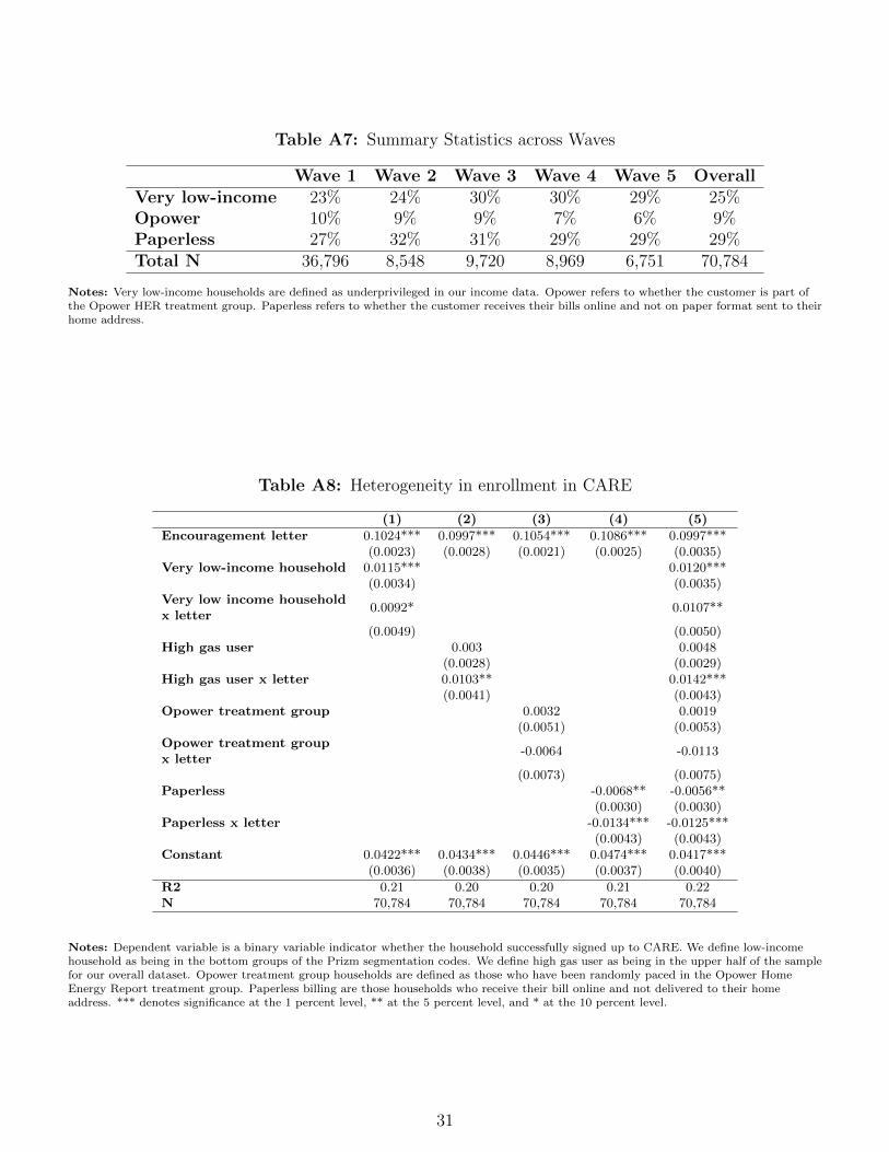
Table A7: Summary Statistics across Waves

Wave 1 Wave 2 Wave 3 Wave 4 Wave 5 OverallVery low-income 23% 24% 30% 30% 29% 25%Opower 10% 9% 9% 7% 6% 9%Paperless 27% 32% 31% 29% 29% 29%Total N 36,796 8,548 9,720 8,969 6,751 70,784

Notes: Very low-income households are defined as underprivileged in our income data. Opower refers to whether the customer is part ofthe Opower HER treatment group. Paperless refers to whether the customer receives their bills online and not on paper format sent to theirhome address.

Table A8: Heterogeneity in enrollment in CARE

(1) (2) (3) (4) (5)

Encouragement letter 0.1024*** 0.0997*** 0.1054*** 0.1086*** 0.0997***(0.0023) (0.0028) (0.0021) (0.0025) (0.0035)

Very low-income household 0.0115*** 0.0120***(0.0034) (0.0035)

Very low income householdx letter

0.0092* 0.0107**

(0.0049) (0.0050)High gas user 0.003 0.0048

(0.0028) (0.0029)High gas user x letter 0.0103** 0.0142***

(0.0041) (0.0043)Opower treatment group 0.0032 0.0019

(0.0051) (0.0053)Opower treatment groupx letter

-0.0064 -0.0113

(0.0073) (0.0075)Paperless -0.0068** -0.0056**

(0.0030) (0.0030)Paperless x letter -0.0134*** -0.0125***

(0.0043) (0.0043)Constant 0.0422*** 0.0434*** 0.0446*** 0.0474*** 0.0417***

(0.0036) (0.0038) (0.0035) (0.0037) (0.0040)

R2 0.21 0.20 0.20 0.21 0.22N 70,784 70,784 70,784 70,784 70,784

Notes: Dependent variable is a binary variable indicator whether the household successfully signed up to CARE. We define low-incomehousehold as being in the bottom groups of the Prizm segmentation codes. We define high gas user as being in the upper half of the samplefor our overall dataset. Opower treatment group households are defined as those who have been randomly paced in the Opower HomeEnergy Report treatment group. Paperless billing are those households who receive their bill online and not delivered to their homeaddress. *** denotes significance at the 1 percent level, ** at the 5 percent level, and * at the 10 percent level.

31

Table A9: Comparison of Nonparticipants in the Control and Encouragement Groups

(1)Gas use

Receive encouragement0.092

(0.077)

Monthly usage control0.709***(0.016)

Control usage (therms) 21.11R2 0.53N 440,615

Notes: Dependent variable is household-level monthly natural gas usage in therms. The analysis is restricted to the post-recertificationperiod only, i.e. the period after households got off the CARE rates initially. The regression utilizes observations from the year of theexperiment (2014 for experiment 1 and 2015 for experiment 2). Receive Encouragement is an indicator equal to one in the month oftreatment letters for all of those who are in the encouragement group but do not take-up the CARE subsidy. Month-of-sample and wavefixed effects are included in all specifications. Monthly Usage Control is a variable capturing the average usage in the same month-of-yearprior to the year of the experiment (2012 and 2013 for experiment 1, 2012 to 2014 for experiment 2). Standard errors are clustered at thehousehold level. *** denotes significance at the 1 percent level, ** at the 5 percent level, and * at the 10 percent level.

32

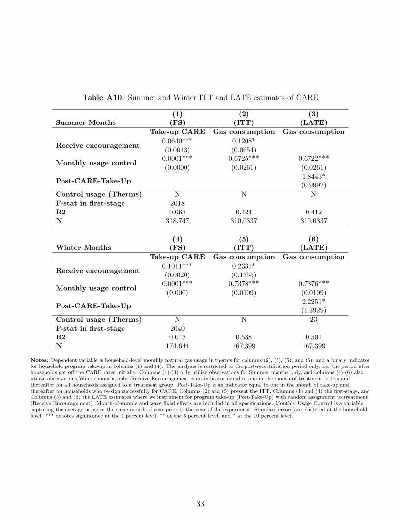
Table A10: Summer and Winter ITT and LATE estimates of CARE

(1) (2) (3)Summer Months (FS) (ITT) (LATE)

Take-up CARE Gas consumption Gas consumption

Receive encouragement0.0640***(0.0013)

0.1208*(0.0654)

Monthly usage control0.0001***(0.0000)

0.6725***(0.0261)

0.6722***(0.0261)

Post-CARE-Take-Up1.8443*(0.9992)

Control usage (Therms) N N NF-stat in first-stage 2018R2 0.063 0.424 0.412N 318,747 310,0337 310,0337

(4) (5) (6)Winter Months (FS) (ITT) (LATE)

Take-up CARE Gas consumption Gas consumption

Receive encouragement0.1011***(0.0020)

0.2331*(0.1355)

Monthly usage control0.0001***

(0.000)0.7378***(0.0109)

0.7376***(0.0109)

Post-CARE-Take-Up2.2251*(1.2929)

Control usage (Therms) N N 23F-stat in first-stage 2040R2 0.043 0.538 0.501N 174,644 167,399 167,399

Notes: Dependent variable is household-level monthly natural gas usage in therms for columns (2), (3), (5), and (6), and a binary indicatorfor household program take-up in columns (1) and (4). The analysis is restricted to the post-recertification period only, i.e. the period afterhouseholds got off the CARE rates initially. Columns (1)-(3) only utilize observations for Summer months only, and columns (4)-(6) alsoutilize observations Winter months only. Receive Encouragement is an indicator equal to one in the month of treatment letters andthereafter for all households assigned to a treatment group. Post-Take-Up is an indicator equal to one in the month of take-up andthereafter for households who re-sign successfully for CARE. Columns (2) and (5) present the ITT, Columns (1) and (4) the first-stage, andColumns (3) and (6) the LATE estimates where we instrument for program take-up (Post-Take-Up) with random assignment to treatment(Receive Encouragement). Month-of-sample and wave fixed effects are included in all specifications. Monthly Usage Control is a variablecapturing the average usage in the same month-of-year prior to the year of the experiment. Standard errors are clustered at the householdlevel. *** denotes significance at the 1 percent level, ** at the 5 percent level, and * at the 10 percent level.

33

Table A11: Comparison of our sample with the rest of the CARE and non-CARE populations

Field ExperimentalSample

Rest of CAREin SCG

Non-CARE inSCG

Overall monthly gas use pre-experiment 26.67 26.46 41Summer months gas use pre-experiment 18.97 18.26 25Winter months gas use pre-experiment 34.15 34.65 56Very low income 0.25 0.49 0.10Paperless 0.29 0.25 0.35Opower 0.09 0.09 0.09LA area 0.17 0.17 0.24Total number of households 70,784 1,198,191* 3,843,707

Notes: The gas use variables (first three rows) are average therms per month. The very low income, paperless, Opower, and LA variablesare in fractions. The data for the Non-CARE in SCG sample comes from SCG. The Opower nummber in the second column comes fromthe utility. The sample size is those who were on CARE for twelve months before the experiment started and so is lower than the 1.5million customers who are on CARE on any given month.

34

Table A12: Reweighted ITT and LATE estimates of CARE

(1) (2) (3)(FS) (ITT) (LATE)

Take-up CARE Gas consumption Gas consumption

Receive encouragement0.0810***(0.0018)

0.1789**(0.0717)

Monthly usage control0.0002***(0.0000)

0.7343***(0.0097)

0.7340***(0.0097)

Post-CARE-Take-Up2.1688**(0.8693)

Control usage (Therms) 19 19 19F-stat in first-stage 10842015 data for wave 1R2 0.063 0.56 0.51N 493,391 477,736 477,736

(4) (5) (6)(FS) (ITT) (LATE)

Take-up CARE Gas consumption Gas consumption

Receive encouragement0.0960***(0.0025)

0.1707**(0.0708)

Monthly usage control0.0001***

(0.000)0.7096***(0.0071)

0.7094***(0.0071)

Post-CARE-Take-Up1.7151**(0.7122)

Control usage (Therms) 21 21 21F-stat in first-stage 7732015 data for wave 1 x x xR2 0.046 0.610 0.541N 920,683 839,106 839,106

Notes: Dependent variable is household-level monthly natural gas usage in therms for columns (2), (3), (5), and (6), and a binary indicatorfor household program take-up in columns (1) and (4). The analysis is restricted to the post-recertification period only, i.e. the period afterhouseholds got off the CARE rates initially. Columns (1)-(3) only utilize observations from the year of the experiment (2014 for experiment1 and 2015 for experiment 2), columns (4)-(6) also utilize 2015 observations for experiment 1. Receive Encouragement is an indicator equalto one in the month of treatment letters and thereafter for all households assigned to a treatment group. Post-Take-Up is an indicator equalto one in the month of take-up and thereafter for households who re-sign successfully for CARE. Columns (2) and (5) present the ITT,Columns (1) and (4) the first-stage, and Columns (3) and (6) the LATE estimates where we instrument for program take-up(Post-Take-Up) with random assignment to treatment (Receive Encouragement). Month-of-sample and wave fixed effects are included in allspecifications. Monthly Usage Control is a variable capturing the average usage in the same month-of-year prior to the year of theexperiment (2012 and 2013 for experiment 1, 2012 to 2014 for experiment 2). Standard errors are clustered at the household level. ***denotes significance at the 1 percent level, ** at the 5 percent level, and * at the 10 percent level.

35

Table A13: Welfare estimates under different counterfactual price determinants

Price determinant Tax difference Subsidy difference Minimizationequal equal exercise

across tiers across tiers

Welfare change (millions $):Total -5.3 -3.2 -4.3Total in base case -4.8 -4.8 -4.8% change, compared to base 0.10 -0.34 -0.11

Notes: Parameters are taken from the base case: Nc is 1600000, Nn is 3850000 and A is $7001307.52. Percent on tier 2, C isestimated as 0.27, N as 0.72. P1c1 is observed as 0.69, P1n1 as 0.86, P1c2 as 0.90, P1n2 is 1.12. The bottom line is that thisanalysis suggests that introducing the assumption of two-tiered pricing still yields a loss in welfare when CARE is introduced.

36

Table A14: Extrapolating the welfare results to California

SoCalGas PG&E SDG&E TotalEc -0.35 -0.35 -0.35En -0.14 -0.14 -0.14SCC 39.95 39.95 39.95MEC 0.21 0.21 0.21MPC 0.47 0.47 0.47MSC 0.68 0.68 0.68Nc 1,600,000 1,076,000 176,000Nn 3,850,000 3,124,000 1,024,000P0 0.9 1.10 1.22P1c 0.75 0.91 1.0P1n 0.95 1.14 1.25Q0c 289.51 338.82 222.34Q0n 495.31 576.96 380.44Q1c 312.84 364.96 241.17Q1n 492.0 573.97 379.29A 7,000,000.00 3,000,000.0 1,000,000.00Welfare estimates:∆W , total welfare change ($ mill) -4.8 2.0 -0.23 -3.0CO2, extra emissions tons 130,000 99,000 11,000 241,000

Sources: Authors calculations and the California Public Utilities Commission (CPUC).

37

Table A15: Optimal CARE subsidy for the three California utilities and the State of California

SoCalGas PG&E SDG&E California% change in subsidy 0% 22% 0% 0%Welfare change $0 $2.4M $0 $0

Notes: With a subsidy of zero percent, we assume that there are no administrative costs of CARE. The table shows that the optimalsubsidy is zero for two of the three utilities, as well as for California as a whole. See the text for details.

38

Figure A1: Application page (in English).

39

Figure A2: Letter from Experiment 2 (in English).

40

Figure A3: Heat map of customers in the Southern California Gas districts.

Notes: This heat map demonstrates the density of households in our experiment in each five-digit zip code. The heat intensity

is divided by deciles of the frequency by zip. The declie cut-offs are: 9, 21, 37, 57, 77, 106, 152, 210, 303, 751. The data for this

map comes from the utility.

41

Panel 1: New situation

Panel 2: Old Situation

Figure A4: Effect of Varying the Elasticity with Introducing CARE

42

Q1 Q0

P1

P0 A

D

B

C

E

F

Q2

Figure A5: Explanation for Standard and Behavioral voucher welfare analysis for the group receivingthe subsidy.

Notes: This figure compares the welfare for CARE households of a subsidy with standard vouchers and behavioral vouchers.

With the subsidy the CARE household chooses C at the subsidized price P1. With the voucher, she chooses A. She prefers a

standard voucher to a subsidy by a revealed preference argument. A behavioral voucher may or may not be preferred to a subsidy

or a standard voucher from the perspective of a CARE household.

43

Figure A6: Effect of Varying Elasticity of non-CARE households on Welfare Associated with Intro-ducing CARE

Notes: The figure shows the welfare effects of varying the elasticity for SoCalGas non-CARE customers. Total welfare is negative

over the range of elasticities and increases slightly as the demand by non-CARE customers becomes more inelastic.

44

Figure A7: Effect of Varying the SCC on Welfare Associated with Introducing CARE

Notes: Total welfare from introducing CARE is negative when the SCC is $6/ton and continues to decrease as the SCC increases.

The only impact of the change in the SCC on welfare is the effect of pollution damages, shown as the Environment curve in the

figure.

45

Figure A8: The Value of Allowances with Varying the Allowance Price

Notes: The figure shows that there is an increasing gap between the value of allowances and the welfare change with a high value

for the SCC as the allowance price increases.

46

Figure A9: The Impact of Varying the Social Cost of Carbon on the Welfare Increase associatedwith setting Energy Prices equal to Marginal Social Cost

Notes: The figure shows the welfare effects of moving prices for CARE and non-CARE households to the marginal social cost

(the two dashed curves). The total welfare change is the solid curve. The key message of this figure is that welfare gains will

always be positive as prices are moved to the MSC, but gains exhibit substantial variation depending on which MSC is selected.

The differences in the welfare gains can be explained by the extent to which existing prices deviate from the assumed MSC.

47

Figure A10: Welfare Impacts of setting prices equal to the MPC with different values of the MarginalSocial Cost.

Notes: The figure shows the welfare effects of moving prices for CARE and non-CARE households to the marginal private cost

(the two dashed lines) for different values of the marginal social cost. The total welfare change is the solid line. The welfare

change associated with a change in the price for C and the welfare change with a change in the price for N are dashed lines. The

change in welfare declines as the MSC increases (for plausible values of the SCC). The total welfare change can be positive or

negative.

48

Figure A11: Effect of Varying the MPC on Welfare Associated with Introducing CARE

Notes: The figure shows the effect of varying the MPC on the welfare associated with introducing CARE for SoCalGas customers.

In general, as the MPC increases, utility profits decline, and overall welfare decreases.

49

Figure A12: How the Welfare Impacts of a Cap-and-Trade Policy Vary with the SCC

Notes: This figure shows how the change in welfare from introducing cap-and trade varies with the allowance price and the level

of the SCC for SoCalGas customers. The welfare change from introducing cap-and-trade is negative for the values of the SCC

considered here.

50

Figure A13: Change in economic welfare compared with subsidy for standard vouchers and behavioralvouchers

Notes: This figure shows the impact of varying the degree of bias for three values of the SCC for SoCalGas customers. The

figure shows that the welfare effect of standard vouchers and behavioral vouchers can be positive or negative compared with the

subsidy. This is shown by noting that the SCC=6 and SCC=40 curves have a negative value when the bias equal zero – the

standard voucher case; in contrast, the SCC=74 curve has a positive value when bias equals 0. Similar results obtain when bias is

positive – the behavioral voucher case. The general point for policy makers is that the welfare associated with a voucher is quite

sensitive to what is assumed about the degree of bias and the SCC.

51

Figure A14: Optimal CARE subsidy for the three California utilities and the State of California

Notes: All of the points in these four curves include administrative costs. If the subsidy is zero, these costs could be avoided.

See discussion in the text for details.

52