E�cient Bulk-Loading of Grid�les �

Scott T. Leutenegger

Institute for Computer Applications in Science and Engineering

Mail Stop 132c, NASA Langley Research Center

Hampton, VA 23681-0001

leut@icase.edu

David M. Nicol

Dept. of Computer Science

College of William and Mary

Williamsburg, VA 23187-8795

Abstract

This paper considers the problem of bulk-loading large data sets for for the

grid�le multi-attribute indexing technique. We propose a rectilinear parti-

tioning algorithm that heuristically seeks to minimize the size of the grid�le

needed to ensure no bucket over ows. Empirical studies on both synthetic

data sets and on data sets drawn from computational uid dynamics appli-

cations demonstrate that our algorithm is very e�cient, and is able to handle

large data sets. In addition, we present an algorithm for bulk-loading data

sets too large to �t in main memory. Utilizing a sort of the entire data set

it creates a grid�le without incurring any over ows.

�This research was supported by the National Aeronautics and Space Administration under NASA contract NAS1-19480

while the authors were in residence at the Institute for Computer Applications in Science and Engineering (ICASE), NASA

Langley Research Center, Hampton, VA 23681-0001. Nicol's work was also supported in part by NSF grant CCR-9210372

and NASA grant NAG-1-1132.

i

1 Introduction

We are developing a scienti�c database to support retrieval of subsets of Computational Fluid Dynamics

(CFD) data sets. Retrieval of subsets is required for visualization and data exploration. All of our data

is two or three-dimensional and thus requires multiattribute indexing. We are speci�cally interested in

partially quali�ed, fully quali�ed, and point queries. Grid�les are a well known multi-attribute indexing

technique [5]. The basic idea is to partition each attribute range into subranges, thereby inducing a

multi-dimensional rectilinear partitioning on the entire multi-attribute space. Enough partitions are

chosen to ensure that all tuples sharing the same subrange in each dimension will �t on a disk page.

Any point query can be then be satis�ed with two disk accesses, one to fetch a pointer to the data page,

and one to fetch the data page itself.

The data we wish to store is contained in �les created by CFD simulations. Both the size of the data

sets and anticipated extensive use of the data sets require that we provide fast organization of new data,

and fast retrivial of existing data. Our two dimensional data is typically a large set of tuples of the form:

(X;Y; f loat1; f loat2; : : : f loatN )

Current data sets measure only tens of megabytes, but are projected to be 2-3 orders of magnitude

larger soon. Although we are speci�cally concerned with CFD data sets, large physically oriented data

sets are common outputs to a wide spectrum of scienti�c computations.

In this paper we show how to quickly load entire data �les into a grid�le indexing structure. This

is termed bulk loading. Note similar functionality is required from relational databases for reloading

relations when changing platforms, during recovery, or during reorganization. In a relational database

the relation is analogous to the data set in our work.

The main contributions of this paper are:

1. A partitioning algorithm which requires up to two to four orders of magnitude less CPU time

than the only known algorithm for partitioning data into grid�le blocks. We provide experimental

results for our partitioning algorithm.

2. An e�cient algorithm to aggregate under-utilized logical grid-buckets to achieve better disk uti-

lization. We provide expermental results which demonstrate the utility of the aggregation phase.

3. A complete algorithm for bulk-loading of large data sets (signi�cantly larger than main memory)

that guarantees no bucket over ows.

The rest of this paper is organized as follows: In the next section we relate our work to prior

e�orts. In section 3 we present the general problem in more detail and provide an example. In section

4 we present the existing partitioning algorithm, our new algorithm, and our aggregation algorithm. In

section 5 we experimentally compare the execution times of the two algorithms, on a variety of data

sets including highly skewed CFD data sets. We also demonstrate the e�ectiveness of our aggregation

technique. In section 6 we present our two phase bulk-loading algorithm. We end with our conclusions

and plans for future work.

1

2 Previous Work

Bulk-loading of B+ trees [6] has been investigated, but only recently have bulk-loaded grid �les been

considered. The single paper on this of which we are aware is that of Li, Rotem, and Srivastava [2].

Their main emphasis is bulk-loading of Parallel Grid Files, i.e. grid �les that are distributed across

multiple sites in a shared nothing environment. They de�ne logical partitioning as that of the grid�le

among the sites in the database system, and physical partitioning as that of the portion of a grid�le

located at one site, into the buckets that compose that portion of the grid�le. Their solution is based on

dynamic programming, for both the logical partitioning and physical partitioning of parallel grid�les.

For physical partitioning their objective function is to minimize bucket over ow. We are concerned only

with physical partitioning at a single site, although a modi�ed version of our algorithm could be used

for logical partitioning. The Li et al. algorithm optimally partitions one dimension, given a speci�c

number of partitions and a �xed partitioning in the other dimension (which is likely equally spaced,

but details on this �xed partition are lacking the the Li et al. paper). Our algorithm dynamically �nds

the number of partitions, �nds a partitioning much more quickly, and directly addresses the issue of

selecting the �xed partition. For uniformly distributed data it may be su�cient to assume an equally

spaced partitioning, but this is not the case when data is skewed.

We show that the dynamic programming approach is too ine�cient to be considered for large

grid �les. Li et al. recognize this problem themselves, and suggest sampling [7, 8] to accelerate their

algorithm. However, sampling may introduce over ows, the handling of which may be signi�cant. For

each bucket that over ows an additional bucket must be created and the grid directory split. If the

number of over ows within a bucket is larger than the bucket capacity, multiple new buckets will need

to be created and the grid directory will be split multiple times. The earlier work inadequately assesses

the risks of sampling, focusing as it does on the probability that some block over ows rather than, say,

the average number of blocks which over ow and the average total number of over ow tuples.

For the problem speci�cation given in Li et al. , i.e. given a �xed partitioning and �xed number

of partitions, the dynamic programming formulation is an excellent approach, but we propose that it

is better to reformulate the problem and �nd the smallest number of partitions for which the total

over ow is zero. The freedom introduced by allowing an arbitrary number of partitions enables us to

use a fast heuristic algorithm instead of an expensive dynamic programming algorithm. The possibly

larger number of buckets resulting from an increased number of partitions is reduced via a low cost

aggregation algorithm. Thus, our partitioning algorithm is capable of handling much larger grid �les

and still guarantee no over ows while achieving good bucket utilization, although if the data set is too

large to �t into main memory the data must �rst be sorted. Furthermore, we consider more extensive

data sets than the earlier work, to better understand the e�ects of positionally skewed and clustered

data which is typical of CFD data sets.

Our partitioning algorithm is a modi�cation of the rectilinear partitioning algorithm developed

by Nicol[4] for the purposes of load-balancing irregular data-parallel computations. The two principle

di�erences between our algorithm and this earlier one are that the number of subranges in each dimension

are not considered �xed in the present context, and that there is an upper limit on the number of tuples

in a bucket.

2

3 General Problem Description

Before considering algorithmic issues, let us �rst examine the general problem. Our exposition is of the

two-dimensional case; all the algorithms generalize immediately to higher dimensions. We also assume

that each attributed range is partitioned into the same number of subranges. This is not rigorously

necessary, but we have not addressed how one would choose the desired relationship between number

of subranges in each dimension.

Let S be a set of tuples (a1; a2; q[]) where attributes a1 and a2 are the indexed attributes and q[] is

the rest of the tuple. In our speci�c data sets a1 and a2 are x and y coordinates, and q[] is an array of

3-5 oating point values representing physical quantities such as pressure, density, directional derivative

information, chemical composition, and so on. For ease of exposition assume the domain of both a1 and

a2 are integers 2 1; : : : ; n; the algorithms extend in a straightforward fashion to real-valued attributes

and generalized ranges. The empirical results we report are based on these extensions. Let F be a n�n

frequency matrix which for each entry contains the number of tuples with that coordinate, i. e.

fi;j = jj ftjt 2 S; a1 = i; a2 = jg jj; 1 � i; j � n

We use the following notation:

T = the number of tuples in data set S,

P = the number of partitions in each dimension,

B = the maximum number of tuples a bucket can hold,

Ui = the number of unique coordinate values in dimension i,

Umax = max fUig,

Ci = (ci;1; ci;2; : : : ; ci;P�1) is the vector of cuts in dimension i, speci�cally C1 is the vector of

horizontal cuts and C2 is the vector of vertical cuts,

[Oi;j] = the P � P occupancy matrix resulting from applying the cut vectors C1 and C2 to S,

total over ow =PP

i=1

PPj=1maxfOi;j � B; 0g.

We seek a pair (C1; C2) whose total over ow equals zero, and whose number of cuts is minimized.

To make these concepts more intuitive, in the left hand side of �gure 1 we have the partitioned

data set for S = f(1; 1)(1; 3)(1; 4)(2; 2)(2; 8)(3; 9)(4; 2)(4; 3)(5; 1)(5; 3)(7; 2)(7; 4)(8; 8); (9; 3)g ; P = 3, C1

(the horizontal cuts) = (2,7), and C2 = (2,6). The partitioning (C1; C2) divides the domain of S into

9 bins. Note, the dashed lines of (C1; C2) are slightly o�set to clearly show the occupancy of the bins.

In this case bin 1 contains points (1,1) and (2,2); bin 2 contains (1,3) and (1,4); bin 3 contains (2,8);

bin 4 contains (4,2), (5,1) and (7,2); bin 5 contains (4,3), (5,3), and (7,4); bin 6 contains (3,9); bin 7 is

empty; bin 8 contains (9,3); and bin 9 contains (8,8). Thus, the occupancy matrix, [Oi;j], is:

2 2 1

3 3 1

0 1 1

3

2 6

2

7

2

2

6

6

Figure 1: Partitioning Example; Left: total over ow equals 1; Right: total over ow equals 0

If we assume B = 2, then the total over ow for this partitioning is 2 because bins 4 and 5 each

contain 3 points. If we move the position of the second cut of C1 to position 6, i. e. let C1 = (2,6), as

shown in the right hand side of �gure 1, then the total over ow would be zero.

4 Algorithm Descriptions

We now describe the algorithm of Li et. al., and our own. Our implementation of the earlier algorithm

is presented in 4.1 in some detail. We provide the detail because it is lacking in the Li et. al paper,

and we wish to show that we've made every e�ort to optimize the performance of their dynamic pro-

gramming solution. Section 4.2 gives our own partitioning algorithm, while 4.3 describes our method

for aggregating under-utilized buckets.

4.1 Dynamic Programming Solution

The dynamic programming equation to be described is precisely the one given in Li et al. [2]. We reword

that formulation and describe speci�cs of an optimized algorithm for solving that equation.

It is assumed that S is already partitioned in the horizontal dimension, i.e. C1 is �xed. Our task

is to �nd a vector C2 that minimizes the total over ow. Let R(i; j) be the n� (j � i+ 1) submatrix of

F obtained by restricting a2, i � a2 � j. Now consider the column of bins resulting from partitioning

R(i; j) horizontally by C1. Let OV1(i; j) be the sum, over each member of this column, of the bin

over ow. For example, with B = 2 and the matrix on the left of �gure 1, OV1(2; 3) equals 2 since the

middle bin has 4 tuples, and no over ow is observed in the other two bins. To reduce over ows we

might consider partitioning R(i; j) vertically with l� 1 cuts, thereby creating a P � l submatrix of bins

with an attendant total over ow value. There may be many ways of partitioning columns i through j

of R(i; j) with l � 1 cuts; let TOV1(i; j; l) be the minimum possible total over ow cost among all these

4

possibilities. The principle of optimality [1] then asserts that

TOV1(1; j; l) =

8><>:

Mini=l�1;:::;j�1 fTOV1(1; i; l � 1) +OV1(i+ 1; j)g ; 1 < l � j;

OV1(1; j); l = 1

(1)

Of particular interest is the value TOV1(1; T; P ), and the partition that achieves this cost.

Solution of this equation is aided by precomputing values from which each OV1(i; j) can be derived

in O(P ) time, as follows. C1 partitions F into P submatrices, S1; � � � ; SP . For each Sk and column

index j de�ne rk(1; j) to be the sum of entries in Si between column indices 1 and j, inclusive. Then,

for any pair of column indices i and j we have rk(i; j) = rk(1; j) � rk(1; i� 1). Now

OV1(i; j) =PX

k=1

maxfrk(i; j) �B; 0g:

Since rk(i; j) is computed with a single subtraction, OV1(i; j) is computed in O(P ) time. The set of all

rk(1; j) values can be computed in time proportional to n log(P ). With only slightly more computation

(a sort in each dimension) we can accommodate tuple sets that are sparse relative to n�n. We project

the data set onto each coordinate axis and sort it, essentially working with a T � T array containing

only T non-zeros. The indices we describe in this paper may be thought of as the ordinal positions

of the data projections on each axis. We take advantage of the sparse structure and still compute all

rk(1; j) values time proportional to T log(P ).

The dynamic programming equation expresses a recursion in both column index j, and number of

cuts, l. Our approach is to unravel the recursion with j being the inner index, and l the outer one.

Speci�cally, we start by solving TOV1(1; j; 1) for all j; given these we solve TOV1(1; j; 2) for all j, and so

on. For l > 1, when solving TOV1(1; j; l) we must make up to j� l comparisons (actually, we must make

one comparison for every non-zero column of F between columns l�1 and j�1). If the tuple sets are not

sparse relative to n�n, the complexity of the inner loop of the recursion is O(P n2), and the outer loop is

executed giving a complexity of O(P 2 n2). In addition, the complexity of the initial precalculation of the

rk(1; j) is O(T log(P )), thus the total complexity is O(P 2 n2 + T log(P )). If the data sets are sparse

relative to n�n, then the complexity can be reduced to O(P 2 U22 + U2 log(P ) + T log(T )), where U2

is the number of unique attribute values in dimension 2, and the additional T log(T ) is for sorting the

tuples which is needed to maintain the sparse representation. In the rest of this paper we will assume

the data sets are sparse relative to n� n. Sparse data sets are especially relevant since the coordinates

of our unstructured CFD data sets are reals. The asymptotic complexity is O(maxfP 2U22 ; T log Tg).

We will henceforth call this algorithm the DP algorithm.

The speed of the algorithm can be further increased by precalculating and storing all the values

OV1(i; j) 8i;8j. The complexity is then O(P U22 + U2 log(P ) + T log(T )). The precalculation of

the OV1(i; j) requires time proportional to O(P U22 ), and is thus included in that term. This storage

cost can be very signi�cant and hence limits the applicability of this optimization. For example, if U2 is

5000, the space required for storing the OV1(i; j) is 95 megabytes. We will henceforth call this algorithm

the DP2 algorithm.

We have now described how to calculate the optimal over ow cost and partitioning of S given �xed

partitioning C1. So far the only di�erence from our work and that of Li et al. is that we have provided

5

the details of our implementation of the dynamic programming problem. We now come to the �rst

contribution of this paper, how to determine the �xed partitionings and how to determine the number

of partitions.

We assume that the number of partitions in each dimension is the same, thus resulting in square

grid�le directories. We presume the existence of an algorithm which, given a �xed set of cuts in one

dimension �nds a \good" set of cuts in the other dimension. The paper by Li et al. provides one such,

but neglects to specify the origin of the �xed cut set. We follow Nicol [4] by using such an algorithm

as the basis for an iterative method: Given �xed cuts in one dimension, �nd good cuts in the other.

Treat the new cuts as �xed, and �nd better ones in the previously �xed dimension. The iterations are

maintained until some termination mechanism triggers. The initial �xed cut is uniformly spaced. In

the grid�le application of this idea, each application of the cut-�nding algorithm attempts to �nd cuts

that yield zero over ow at all buckets. Termination of such a partitioning session is de�ned when either

an over ow-free cut-set is discovered, or after some speci�ed number of iterations (we use 20) no such

cut-set is discovered. The sole parameter to a partitioning session is the number of partitions, P , in each

dimension. A partitioning session may be viewed as a probe that determines whether we can quickly

discovered an over ow-free partitioning using P � 1 cuts in each dimension. Our overall strategy is to

do an intelligent search on P to �nd the smallest value for which we can quickly determine a desirable

partitioning.

Any cut assignment might be used in the approach above. The results we later report use both

the dynamic programming solution of Li et al., and our own algorithm (to be reported) within this

same framework. For skewed data sets it may be advantageous to have the number of partitions in

each dimension di�er, but our aggregation phase described later minimizes the poor e�ciency of using

square regions. In the future we intend to investigate non-square regions. Given a square region, strict

lower and upper bounds on the number of partitions needed in each dimension are:

lowerBound = (bT=Bc)0:5

upperBound = T

We thus can do a binary search to �nd the minimal number of partitions P , lowerBound � P �

upperBound, for which the total over ow is equal to zero. In practice, we have found it is faster start

with the number of partitions equal to 2� lowerBound. Then, while the total over ow is greater than

zero keep doubling the number of partitions. Once a partition value has been found for which the total

over ow is zero, conduct a binary search with that value as the upper bound, and the previous value

as the lower bound.

4.2 Rectilinear Partitioning

We now come to the second contribution of our work, an alternative rectilinear partitioning algorithm.

Like that of Li et al., it optimizes the cuts in one dimension given a �xed set of cuts in the other. In

the discussion to follow we take C1 as �xed.

At each step of the algorithm we seek to de�ne a column of buckets whose width is as wide as

possible without any bucket in the column being assigned more than B tuples. To de�ne the �rst column

6

we seek the largest index j for which OV1(1; j) = 0; call this index j1. Since OV1(1; j) is monotone

non-decreasing in j, we may identify j1 with a binary search. Using the precalculated rk(i; j), each

candidate j requires O(P ) time to compute OV1(1; j), hence O(P logU2) time is required to de�ne the

�rst column. The second column is computed exactly as the �rst, only taking index j1 + 1 as the

starting point, i.e., identify the largest j2 for which OV1(j1 + 1; j2) = 0. This process continues until

either P or fewer adjacent over ow-free columns are discovered, or all P � 1 cuts are placed and the

last column su�ers over ow. In the former case the partitioning session terminates; in the latter case

we may freeze the newly discovered cuts and choose new cuts in the other dimension. The complexity

of one partitioning session has several components. First there is an O(T log T ) cost for sorting the

tuples in each dimension. Now for each time we optimize in one dimension we �rst compute new

rk(1; j) values, which takes O(T log(P )) time. This is followed by a O(P 2 logU2) cost for allocating

cuts. Since any partitioning session iterates a bounded number of times, the asymptotic complexity is

O(maxfP 2 logU2; T log Tg).

The original rectilinear application [4] was shown to converge to unchanging cut sets (given su�-

ciently many iterations). Our algorithm too would converge, but we have found it more prudent to back

away to a larger number of partitions when a small number of iterations fails to �nd a suitable partition.

The original rectilinear partitioning problem was shown to be NP-hard in three dimensions; the same

proof su�ces to show the intractability of �nding minimal P for which a square over ow-free partition

exists. The tractability of the rectilinear partitioning problem in two dimensions is still unknown.

It is informative to consider an essential di�erence between our partitioning algorithm and that

of Li et al. We are uninterested in any partition that has over ow, and so expend no computational

energy on minimizing non-zero over ows. If, given C1 it is possible to �nd C2 yielding an over ow-free

partition, our algorithm will �nd it. If none exists, our algorithm determines that quickly. By contrast,

the previous algorithm seeks to �nd C2 that minimizes over ow. We are uninterested in whether the

minimal over ow is two or three, only whether it is zero or non-zero. This distinction permits us to �nd

over ow-free partitions with substantially less work than the previous algorithm, as will be seen in the

empirical results.

4.3 Aggregation

Our third contribution is an algorithm for aggregating adjacent buckets with low utilization. After the

partitioning phase some of the buckets may have low utilization. If two adjacent buckets both have 50%

utilization or smaller we may combine them into a single bucket (even though the grid�le directory will

contain two pointers|they will be identical). Following partitioning, we apply an aggregation scheme

based on this observation.

Let B equal the bucket capacity. First assume the grid directory is of size 2i�2i, and view it as four

equal sized 2i�1�2i�1 quadrants labeled NW,NE,SE,SW . De�ne a procedure CanMerge(A;B; j) that

returns logical true if neither A nor B has already been merged into some group at level j and their sum

of utilization is less than 100%. De�ne procedure Merge(A;B; j) to merge A and B into one bucket

at level j. Using CanMerge and Merge we de�ne a recursive function function Aggregate(A; j) as

follows.

7

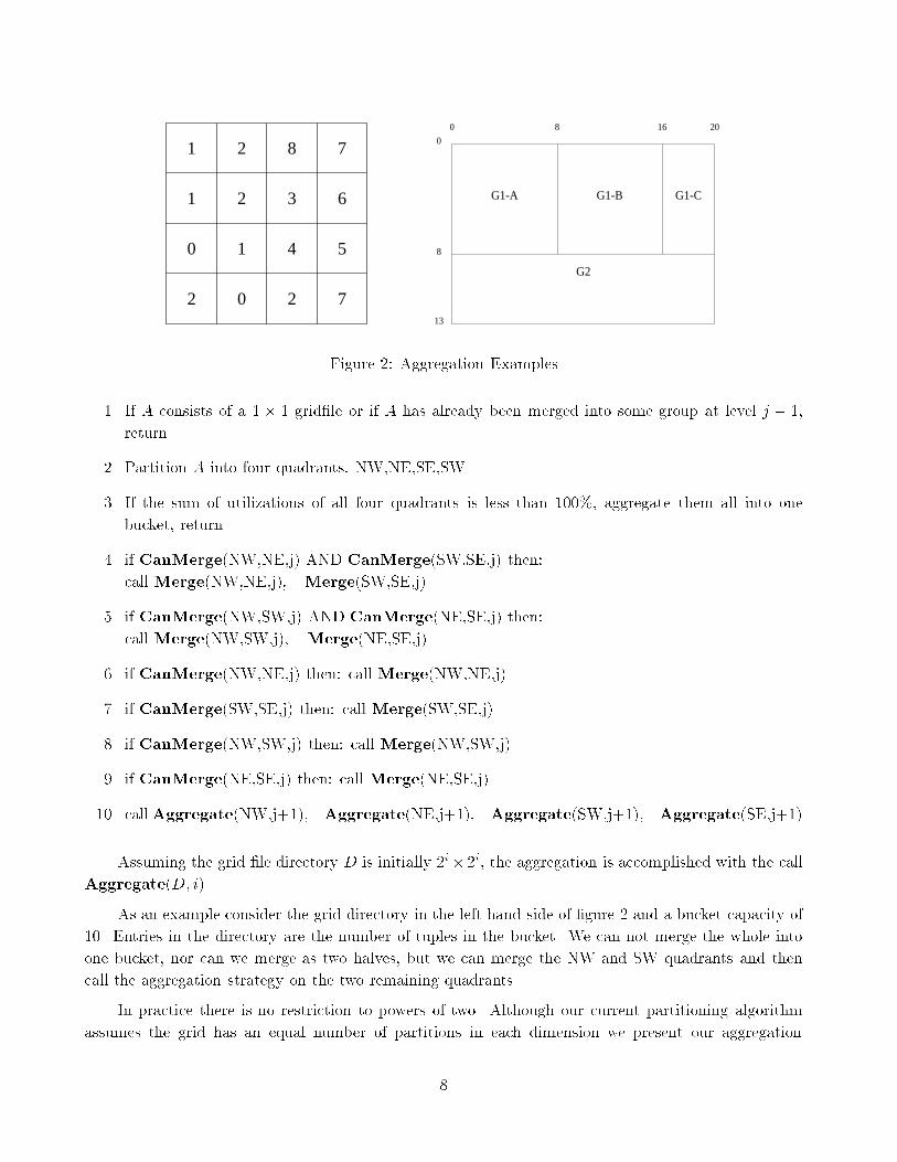
1 2 8 7

1 2 3 6

0 1 4 5

2 0 2 7

G1-A G1-C

G2

G1-B

0 8 16 20

8

13

0

Figure 2: Aggregation Examples

1. If A consists of a 1 � 1 grid�le or if A has already been merged into some group at level j � 1,

return.

2. Partition A into four quadrants, NW,NE,SE,SW.

3. If the sum of utilizations of all four quadrants is less than 100%, aggregate them all into one

bucket, return.

4. if CanMerge(NW,NE,j) AND CanMerge(SW,SE,j) then:

call Merge(NW,NE,j), Merge(SW,SE,j)

5. if CanMerge(NW,SW,j) AND CanMerge(NE,SE,j) then:

call Merge(NW,SW,j), Merge(NE,SE,j)

6. if CanMerge(NW,NE,j) then: call Merge(NW,NE,j)

7. if CanMerge(SW,SE,j) then: call Merge(SW,SE,j)

8. if CanMerge(NW,SW,j) then: call Merge(NW,SW,j)

9. if CanMerge(NE,SE,j) then: call Merge(NE,SE,j)

10. callAggregate(NW,j+1), Aggregate(NE,j+1), Aggregate(SW,j+1), Aggregate(SE,j+1)

Assuming the grid �le directory D is initially 2i� 2i, the aggregation is accomplished with the call

Aggregate(D; i).

As an example consider the grid directory in the left hand side of �gure 2 and a bucket capacity of

10. Entries in the directory are the number of tuples in the bucket. We can not merge the whole into

one bucket, nor can we merge as two halves, but we can merge the NW and SW quadrants and then

call the aggregation strategy on the two remaining quadrants.

In practice there is no restriction to powers of two. Although our current partitioning algorithm

assumes the grid has an equal number of partitions in each dimension we present our aggregation

8

algorithm in the most general case. Without loss of generality assume the shape of the grid directory

is N rows by M columns, where N < M . We �nd the largest i such that 2i < N . Let G1 be the

2i �M subdirectory of the grid directory composed of the �rst 2i rows, and let G2 be the N � 2i �M

subdirectory composed of the complement of the original directory. We �rst aggregate G1. Let j =

M div N , this is the number of square 2i � 2i subdirectories that can �t in G1. For each one of these

j square subdirectories we apply the square region aggregation algorithm above. We are then left with

a 2i � (M � j � 2i) subdirectory and G2. We apply the algorithm recursively on these two regions.

In the right hand side of �gure 2 we show an example for a 13 � 20 grid directory. Subdirectory G1

is composed of G1-A, G1-B, and G1-C. The square power of two region aggregation policy above is

applied to G1-A and G1-B, while the entire aggregation policy is called recursively on G1-C and G2.

This algorithm could be improved to yield slightly better bucket utilizations, but is very fast and has

proved to su�cient for our needs so far.

Depending on the use of the grid�le, di�erent aggregation strategies can be used. If the grid�le

is read only, as in our CFD database, then the buddy-system pairing approach needed to facilitate

splits for future insertion of tuples is not necessary. In this case regions of aggregated buckets need

not be rectangular and hence could allow for more aggregation resulting in improved bucket utilization.

We have not yet developed any algorithms to calculate this aggregation since the above algorithm has

been su�cient for our needs to date. On the other hand, if the grid�le is being used in a transaction

processing environment and tuples might later be inserted, the buddy pairing must be preserved.

5 Experimental Comparison

In this section we present experimental results for the two partitioning algorithms. We present both

run times and bucket utilization results. In all of our experiments we do not make any attempt to get

smooth curves or collect con�dence intervals. The �gures are the result of one experimental run and

thus often have some noise, presumably from use of the workstation by other jobs. All experiments

were run on a Sparc 10 workstation.

Sanity checks on the code were made by running both algorithms through a pro�ler to make sure

time was being spent in sections of the code where expected. The run time of the RP algorithm is

dominated by the startup costs of creating the pre-calculated rk(1; j) and sorting the records. For most

of the data sets in this paper over 40% of the run time is spent creating the rk(1; j) and over 20% of

the time sorting the data points. Note that even with this high cost of creating rk(1; j), the overall

algorithm signi�cantly faster than when the rk(1; j) are not precalculated. In contrast, the run time of

the DP algorithm is dominated by the actually partitioning since it is O(P 2 U2max).

In section 5.1 we present results for a single partitioning given a �xed partitioning in the other

dimension. In the following sections we present results assuming the number of partions and the

initial partitioning is not known. In section 5.2 we present results when the from uniformly distributed

synthetic data sets, while in section 5.3 we present results for highly skewed CFD data sets. In section

5.4 we present the bucket utilization results from our experiments and demonstrate the utility of the

aggregation phase.

9

5.1 Fixed Partitioning Given

We �rst compare the DP, DP2, and RP algorithms assuming that a �xed partitioning exists in one

dimension. We conduct these experiments since this is the exact scenario for which Li et al. proposed

their algorithm. Note again that how this �xed partitioning is obtained is not speci�ed in Li et al. [2].

We consider a data set of 5,000 tuples where the x and y coordinates of each tuple are each chosen

from a uniform distribution from 1 to 2000. We obtain the initial horizontal partitioning by equally

spacing the cuts within the domain. In table 1 we present results for the number of partitions in each

dimension varied from 12 to 5 assuming a bucket capacity of 50 tuples. The columns headed \seconds"

record the amount of CPU time used for the partitioning, columns headed \over ow" are the total

number of tuples that did not �t within the bucket capacity, and the columns headed \BlocksOver"

are the number of blocks which over owed. The over ow and BlocksOver numbers are identical for the

DP and DP2 algorithms since the algorithms �nd the exact same partitioning and only di�er in run

time. First note that the RP algorithm is one to two orders of magnitude faster than the DP and DP2

algorithms for all values of P. Conversely, the dynamic programming algorithms minimize total over ow

better when there is a large number of partitions. Thus, for the speci�c problem and objective function

as formulated by Li et al. the dynamic programming algorithm proposed satis�es the objective function

better than our rectilinear partitioning algorithm, but at the expense of signi�cantly more computation.

A premise of our work is that it is better to partition with a su�ciently large number of partitions to

ensure no over ows.

Note that although the DP algorithm does have a smaller number of tuples over owed, it results

in a larger number of buckets which over ow when the number of partitions is less than 11. The blocks

which over ow when the RP algorithm is used are all in the last column of the partitioning, whereas

when the DP algorithm is used the over ow blocks are spread out in the partitioning space. Consider

the case where the number of partitions is 10. When the RP algorithm is used there are 10 over ow

blocks. These 10 blocks have 106, 106, 101, 111, 94, 94, 108, 112, 113, and 106 tuples allocated to them.

Since only 50 tuples �t per block 18 new blocks will need to be created. One the other hand, when the

DP algorithm is used there are 40 over ow blocks, each of which has at most 68 tuples, requiring 40 new

blocks to be created. Hence, total over ow is not a good indicator of the optimality of a partitioning.

We propose that a better metric would be the number of new blocks needed to hold the over ows. We

will continue to use total tuple over ow in this paper since our algorithms dynamically �nd the number

of partitions needed to make the over ow zero.

5.2 Number of Partitions Not Given: Uniformly Distributed Data

We now assume that the number of partitions is not known and that no initial �xed partitioning is

given. We �rst consider the run time of the algorithm for uniformly distributed data. The x and y

coordinates of each tuple are each chosen from a uniform distribution from 1 to N, where N depends

on the experiment. In all reported experiments we do not allow any duplicate data set points since our

CFD data does not have any duplicate points. We have veri�ed that inclusion of duplicates results in

similar relative performance. We �rst consider the relative performance of the algorithms as the number

of tuples is varied.

10

RP Algorithm DP DP2

P seconds over ow BlocksOver seconds seconds over ow BlocksOver

12 6.50e-01 0 0 2.47e+02 1.36e+02 0 0

11 6.30e-01 98 9 2.19e+02 1.27e+02 14 5

10 6.70e-01 1051 10 1.80e+02 1.23e+02 239 40

9 6.20e-01 1672 9 1.59e+02 1.13e+02 950 76

8 6.50e-01 2321 8 1.97e+02 9.87e+01 1800 56

7 6.30e-01 2958 7 1.22e+02 8.94e+01 2550 43

6 6.20e-01 3465 6 9.54e+01 8.02e+01 3200 31

5 6.80e-01 3940 5 7.43e+01 7.07e+01 3750 20

Table 1: CPU Times and Over ow, Fixed Partitioning Given

In �gures 3 and 4 we plot the computation time in seconds versus the number of tuples in the

relation assuming coordinate values are uniformly distributed from 1 to 2000. Note that the y-axis is

logarithmic. From top to bottom we plot the computation time of the DP, DP2, and RP algorithms.

Remember that the DP2 algorithm is the same as the DP algorithm except it precomputes and stores

the OV1(i; j)8i 8j. The plot in �gure 3 assumes 50 tuples �t per page, the plot in �gure 4 assumes 300

tuples per page. If page size is 8192 bytes then tuples size would be 164 and 27 bytes respectively. A

tuple size of 164 bytes may be a typical size for transaction processing systems, and tuples in our data

sets are usually around 24-32 bytes. As the number of tuples increases the run time of the DP algorithm

becomes too long to be of practical use. A relation of 40,000 164 byte tuples is only 6.4 mega-bytes, for

32 byte tuples this is only 1.2 mega-bytes, hence it is reasonable to expect there to be su�cient memory

to partition data sets of at least 40,000 tuples.

For 40,000 164 byte tuples, �gure 3, the DP algorithm requires 26600 seconds (about 7.4 hours),

and 100,000 tuples require 77200 seconds (21.4 hours). These times are clearly prohibitive. The DP2

algorithm requires 3000 seconds (50 minutes) and 6070 seconds (101 minutes) for 40,000 and 100,000

tuples respectively, but it requires 15 mega-bytes of space to hold the precomputed OV1(i; j). The RP

algorithm only requires 12 and 40 seconds for 40,000 and 100,000 tuples respectively. Thus, the RP

algorithm is a practical algorithm. The RP algorithm is about 2000 (250) times faster than the DP (DP2)

algorithm for 40,000 tuples. The di�erence in solution times is not unexpected given the complexities

of the DP, DP2, and RP algorithms which are O(maxfP 2U22 ; T log Tg), O(maxfPU2

2 ; T log Tg), and

O(maxfP 2 logU2; T log Tg) respectively.

We now consider how the number of unique attribute values in the data set impacts the relative

performance of the policies. In �gure 5 we plot the computation time in seconds versus the maximum

of the attribute domain for a data set with 40,000 tuples and assuming 300 tuples �t per page. Note

that the y-axis is logarithmic. The curves from top to bottom are for the DP, DP2, and RP algorithms.

We did not run the DP2 algorithm when the storage space for the precalculated OV (i; j) exceeded 80

mega-bytes, thus there are no points plotted for maximum domain values of 5,000 and higher. Increasing

the maximum domain value increases the number of unique attribute values in the data set. The DP

and DP2 algorithms are highly sensitive to the number of unique values in the data set. Conversely,

the RP algorithm is relatively insensitive to the number of unique values. When the maximum domain

value is 2,000, the RP algorithm is 450 (110) times faster than the DP (DP2) algorithm. When the

11

maximum domain value is 10,000, the RP algorithm is 17,000 times faster than the DP algorithm. All

other experiments in this section assume a maximum domain value of 2000. For many of our CFD data

sets the number of unique values is almost equal to the number of tuples, thus even 10,000 is a very

small value.

We now consider how the tuple size e�ects the relative performance of the two algorithms. In �gure

6 we plot the computation time in seconds versus the number of tuples per page assuming 40,000 tuples

with an attribute domain maximum of 2000. Once again the y-axis is logarithmic. As the number

of tuples per page decreases, hence the tuple size increases, the DP algorithms requires signi�cantly

more computation. Conversely, the RP algorithm is relatively insensitive to the size of the tuples.

Thus, the RP algorithm remains a viable algorithm for a wide range of tuple sizes. The degradation

of the DP algorithm as tuple size increases is easy to predict from the complexity of the algorithm:

O(P 2(Umax)2 + (Umax)log(P )). As tuple size increases the number of tuples per bucket decreases

and hence the number of partitions, P , increases. We would expect the runtime of the RP algorithm

to increase also since the complexity of the RP algorithm is O(P 2 log(Umax)), but the majority of the

run time of the RP algorithm is spent sorting the tuples and creating the rk(1; j), thus obscuring the

sensitivity to tuple size.

In �gure 7 we plot the ratios of the computation time of the DP and DP2 algorithms relative to

the RP algorithm. As the tuple size increases the ratio increases.

5.3 Number of Partitions Not Given: Unstructured CFD Data

We now consider the run time of the algorithm for highly skewed data. We use actual data sets from

unstructured grid CFD simulations. Here the term grid is used to describe the way the coordinates in

the data set are connected. The data set is composed of x,y real-valued coordinates. The data sets

are from computational models of cross sections of air ows around aircraft wings [3]. In �gure 8 we

plot the data set for a set with 1034 points where x 2 (�10 : : : 10), y 2 (�12 : : : 12), and restrict the

range plotted since the majority of the data is in the central region and plotting the whole range would

make it di�cult to distinguish the points in areas of high concentration. Only 94 of the 1034 points are

not plotted. The vertical and horizontal lines are the partitioning lines resulting from running the RP

algorithm on the data set. Note, there is one vertical line at x = 6.09 which is not included in the plot.

As can be seen from the partitioning, a �xed equal space partitioning would be a bad choice.

In �gure 9 we plot the partitioning computation time versus the number of tuples for three di�erent

data sets. For the smallest data set, 1034 tuples, the DP (DP2) algorithm required 2370 (650) times

more computation than the RP algorithm for partitioning. For the data set with 3959 tuples, the DP

(DP2) algorithm required 38,817 (5629) times more computation than the RP algorithm. Thus, the DP

algorithm is especially impractical for highly skewed data. Since the DP algorithm required 42 hours

for the 3959 tuples data set we did not run the 15895 tuple data set. The RP algorithm required 66

seconds to partition a 15,895 tuple data set.

The four orders of magnitude di�erence in computation time is not surprising in light of the results

from the experiment plotted in �gure 5. For unstructure grid data sets the number of unique attribute

values is almost equal to the number of tuples, hence as the number of tuples in the set increases not

12

RP Algorithm DP Algorithm

Bucket Utilization Bucket Utilization

n Partitions pre-aggregation post-aggregation Partitions pre-aggregation post-aggregation

1000 5 8.00e-01 8.70e-01 5 8.00e-01 8.00e-01

5000 12 6.94e-01 7.94e-01 12 6.94e-01 7.81e-01

10000 16 7.81e-01 7.84e-01 16 7.81e-01 8.06e-01

20000 24 6.94e-01 7.43e-01 23 7.56e-01 7.60e-01

40000 33 7.35e-01 7.47e-01 33 7.35e-01 7.45e-01

60000 41 7.14e-01 7.27e-01 40 7.50e-01 7.54e-01

80000 48 6.94e-01 7.31e-01 47 7.24e-01 7.37e-01

100000 53 7.12e-01 7.27e-01 52 7.40e-01 7.43e-01

Table 2: Average Bucket Utilizations, Number of Tuples Varied

only does the number of partitions needed increase, but so does the number of unique attribute values.

The RP algorithm does not experience as much of an increase in computation time as the data sets get

larger since the majority of its time is spent in the precalculation of the rk(1; j) and the initial sort of

the data.

5.4 Bucket Utilizations and Aggregation E�ectiveness

We now present the average bucket utilizations for some of the previous experiments both before and

after our aggregation phase is completed. In table 2 we present the utilizations for the uniformly

distributed data experiment in �gure 3. The column label \Partitions" is the number of partitions in

each direction. This was the smallest number for which the algorithm returned a total over ow of zero.

Overall the average bucket utilization is quite good, about the same as would result from inserting the

tuples one at a time. There is little di�erence between the utilization for the DP and RP algorithms. In

addition, the aggregation phase does not signi�cantly improve the bucket utilization. This is because

the bucket utilization is already good. For most experiments, the run time of the aggregation phase is

minimal, less than 2% of the RP runtime, hence it is worth aggregating even for a modest improvement.

In table 3 we present the utilizations for the uniformly distributed data experiment in �gure 6.

Once again there is little di�erence in bucket utilization for the two algorithms. The average bucket

utilization tends to decrease as the number of tuples per page decreases. When only 5 tuples �t per

page the bucket utilization is only 28%, but after the aggregation it is better than 70%. Thus, the

aggregation phase can considerably improve the utilization for cases where the utilization is poor. The

runtime of the DP algorithm for 5 and 10 tuples per page was excessive and hence we do not present

aggregation results for those parameters.

For skewed data the aggregation phase results in substantial savings of disk space. In table 4 we

present the utilizations for the unstructured grid CFD data set for three di�erent grids. The average

bucket utilization without aggregation is very poor but improves signi�cantly with aggregation. Thus,

for highly skewed data aggregation is essential for achieving good bucket utilizations. Note, there is no

15,896 tuple data for the DP algorithm since its computation time on the 3959 tuple data set required

42 hours.

13

RP Algorithm DP Algorithm

Tuples Bucket Utilization Bucket Utilization

per-page Partitions pre-aggregation post-aggregation Partitions pre-aggregation post-aggregation

300 13 7.89e-01 8.33e-01 12 9.26e-01 9.26e-01

200 15 8.89e-01 8.89e-01 15 8.89e-01 8.89e-01

100 22 8.26e-01 8.26e-01 22 8.26e-01 8.26e-01

50 33 7.35e-01 7.47e-01 33 7.35e-01 7.45e-01

25 51 6.15e-01 6.93e-01 49 6.66e-01 7.14e-01

10 94 4.53e-01 7.10e-01

5 169 2.80e-01 7.05e-01

Table 3: Average Bucket Utilizations, Tuples Per Page Varied

RP Algorithm DP Algorithm

Bucket Utilization Bucket Utilization

t Partitions pre-aggregation post-aggregation Partitions pre-aggregation post-aggregation

1034 10 2.07e-01 6.27e-01 10 2.07e-01 7.95e-01

3959 34 6.85-02 7.61-01 29 9.41e-02 5.87e-01

15896 131 1.85e-02 5.76e-01

Table 4: Average Bucket Utilizations, Unstructured Grid CFD Data

6 Two-Phase Bulk Loading Algorithm Description

In this section we describe a two phase algorithm for bulk loading of data sets signi�cantly larger than

available bu�er space. Suppose the data set contains S tuples, and suppose that a maximum of A

tuples can be contained in memory at a time when applying the RP algorithm. Our approach has two

steps. First we partition the set into groups of size A or fewer. Each set will contain all points within

a rectangle in the x-y plane; however the collection of sets need not be rectilinear. In the second step

we apply RP to each individual set, and merge the individual grid �les created. These steps are now

elaborated upon.

Given S and A we �nd the smallest perfect square integer R such that R > SA. We will partition

the data set into R groups, as follows. By sorting the data set on the x-coordinate value we may easily

divide the set intopR groups of

pR successive elements in the sorted order. This serves to partition

the data set along the x-axis into \strips" of tuples. Each such strip may be sorted along the y-axis,

after which its points may be separated into groups of successive SApoints. This e�ectual divides a strip

into rectangles, with no rectangle containing more than the permitted number of points.

It remains to apply RP to each group, and write the buckets of data to disk. One possibility is

to partition each group separately, and de�ne the �nal grid �le as the union of all separately de�ned

grid�les. Recognizing that a cut which is de�ned for a group on one side of the data domain must

propagate throughpR-1 other groups (and cause splitting of grid directories in each) we consider a

di�erent approach. As the groups are partitioned we build up a global grid �le, initially empty. Upon

reading in a group we identify the set of cuts in the global grid �le which a�ect this group, treat them

as immutable, and seek to �nd the minimum number of additional cuts needed to avoid over ow. This

requires a simple modi�cation to the RP algorithm.

14

Another optimization is to �rst strip the attributes being indexed from the data set. Then the

two phase algorithm is applied to the coordinates without requiring I/O of the whole tuple. After

partitioning the set of coordinates and creating the overall grid directory, the buckets could be �lled by

making a second pass over the data set. This may result in a faster load time if the tuple size is large.

If the data set (and hence the grid directory) is extremely large, another optimization uses a two

level directory scheme as suggested in [5] where the top level directory has one entry for each of the R

sub-directories. Note, this would mean that a point access could require three disk accesses instead of

two.

7 Conclusions and Future Work

We have proposed and implemented a new rectilinear partitioning (RP) algorithm for physical par-

titioning of grid�les. Our proposed RP algorithm is signi�cantly faster than the recently proposed

dynamic partitioning (DP) algorithm of Li et al. [2]. The number of over ows RP permits is necessarily

larger than the DP algorithm (which minimizes them), however we argue that minimizing the number

of additional blocks created due to over ow is actually a better measure, and is one for which the RP

algorithm �nds better solutions that the DP algorithm.

We considered the use of our greedy algorithm and the DP algorithm as kernels in a loop that

seeks to minimize the size of the grid �le needed to achieve no over ows. For synthetic data sets of

uniformly distributed integers the RP algorithm is two to three orders of magnitude faster than the DP

algorithm. For actual CFD data sets, whose indexed attributes are highly skewed reals, the RP-based

algorithm is three to four orders of magnitude faster than the DP-based algorithm.

We have also developed an e�cient aggregation algorithm for improving bucket utilizations of grid-

�les resulting from bulk loading using the RP or DP partitioning algorithms. The algorithm has minimal

overhead, and can yield substantial improvements in bucket utilization when the bucket utilization after

partitioning is poor. This aggregation phase is necessary to achieve reasonable bucket utilizations when

the indexed data is highly skewed.

We have also proposed a two phase bulk load algorithm and several optimizations for loading

data sets that are signi�cantly larger then the available bu�er space. This algorithm guarantees no

bucket over ows and is proposed as a possible alternative to sampling based methods. We have yet not

investigated the performance of the algorithm.

In the future we plan to experimentally compare our two phase algorithm with inserting one tuple

at a time and sampling based methods. We also intend to consider more sophisticated aggregation

techniques and partitioning with di�ering numbers of partitions for each attribute.

References

[1] T.H. Horowitz, S. Sahni, Fundamentals of Computer Algorithms, Computer Science Press,

1978.

15

[2] Li, J., Rotem, D., Srivastave, J., "Algorithms for Loading Parallel Grid Files," Proceedings of ACM

SIGMOD 1993, p. 347-356, Washington D.C., 1993.

[3] D.J. Mavriplis, "Algebraic Turbulence Modeling for Unstructured and Adaptive Meshes," American

Institute of Aeronautics and Astronautics (AIAA) Journal vol. 29, no. 12, p. 2086-2093, December1991.

[4] Nicol, D.M., "Rectilinear Partitioning of Irregular Data Parallel Computations," ICASE Report

91-55, NASA Contractor Report #187601, July 1991, to appear in the Journal of Parallel andDistributed Computation.

[5] Nievergelt, J., Hinterberger, H., Sevcik, K.C., "The Grid File: An Adaptable, Symetric Multikey

File Structure," ACM Transactions on Database Systems, vol. 9, no. 1, March 1984, p. 38-71.

[6] Rosenberg, A.L., Snyder, L., "Time and Space Optimality in B-Trees," ACM Trasactions on Dat-base Systems, vol. 6, no. 1, March 1981.

[7] Seshadri, S., "Probalistic Method in Query Processing,", Ph. D. thesis, Department of Computer

Science, University of Wisconsin-Madison, 1992.

[8] Seshadri, S., Naughton, J.F., "Sampling Issues in Parallel Database Systems," Proceeding of the3rd International Conf. on Extending Database Technology, Vienna, Austria, March 1992.

16

0.1

1

10

100

1000

10000

100000

0 10000 20000 30000 40000 50000 60000 70000 80000 90000 100000

Computation Time in Seconds

Number of Tuples

DPDP2RP

Figure 3: Number of Tuples Varied, 50 tuples per page, Domain Maximum = 2000

17

0.1

1

10

100

1000

10000

0 10000 20000 30000 40000 50000 60000 70000 80000 90000 100000

Computation Time in Seconds

Number of Tuples

DPDP2RP

Figure 4: Number of Tuples Varied, 300 tuples per page, Domain Maximum = 2000

18

1

10

100

1000

10000

100000

1e+06

0 1000 2000 3000 4000 5000 6000 7000 8000 9000 10000

Computation Time in Seconds

Cardinality of Attribute Domain

DPDP2RP

Figure 5: Maximum of Attribute Domain Varied; 40,000 Tuples, 300 tuples per page

19

1

10

100

1000

10000

100000

0 50 100 150 200 250 300

Computation Time in Seconds

Number of Tuples Per Page

DPDP2RP

Figure 6: Size of Tuples Varied; 40,000 Tuples, Range of attribute = 1 .. 2000

20

100

1000

10000

0 50 100 150 200 250 300

Ratio of Computation Time Relative to RP

Number of Tuples Per Page

DPDP2

Figure 7: Size of Tuples Varied; 40,000 Tuples, Range of attribute = 1 .. 2000

21

-0.6

-0.4

-0.2

0

0.2

0.4

0.6

-1 -0.5 0 0.5 1 1.5 2

Figure 8: Plot of Unstructured Grid CFD Data Set

22

0.1

1

10

100

1000

10000

100000

1e+06

0 2000 4000 6000 8000 10000 12000 14000 16000

Computation Time in Seconds

Number of Tuples

DPDP2RP

Figure 9: Partitioning Time for Unstructured Grid CFD Data Sets

23