E-bike Impacts: Quantifying the Energy Use and Lifecycle Emissions in Response to Real World Driving Conditions

by

Daniel Clancy

B.Eng, University of Victoria, 2015

A Thesis Submitted in Partial Fulfillment of the Requirements for the Degree of

MASTER OF APPLIED SCIENCE

in the Department of Mechanical Engineering

© Daniel Clancy, 2020

University of Victoria

All rights reserved. This thesis may not be reproduced in whole or in part, by photocopy

or other means, without the permission of the author.

ii

Supervisory Committee

E-bike Impacts: Quantifying the Energy Use and Lifecycle Emissions in Response to

Real World Driving Conditions

by

Daniel Clancy

B.Eng, University of Victoria, 2015

Supervisory Committee

Dr. Curran Crawford, Department of Mechanical Engineering

Co-Supervisor

Dr.Nedjib Djilali, Department of Mechanical Engineering

Co-Supervisor

iii

Abstract

E-bikes can significantly enhance adoption of cycling as an urban transportation mode

and have the advantage of low space requirements, very small operational GHG

emissions, and a negligible contribution to infrastructure degradation. This work explores

some key environmental and physical performance features of E-bikes in real world

settings in order to systematically determine the capabilities of E-bikes for greater

adoption. This includes analysis on the lifecycle emissions associated with E-bikes and

comparisons with other major urban modes. Empirical data was collected about the

performance of a third-party electric motor technology that could improve energy

efficiency. The ability of this technology to offer improvements under real world

conditions was verified and showed promise with recommendations for further

development. A trial of E-bikes deployed in a corporate fleet, with 17 riders and over 600

km of trip data was completed and used for several additional analyses. This include

validating a mathematical model of an E-bike, as well as extending the boundaries of

previous lifecycle research to include upstream dietary emissions associated with human

supplied mechanical power while riding an E-bike. The results in this thesis show both

the strengths of E-bikes as used for corporate and personal transportation, as well as the

barriers that still remain for greater adoption.

iv

Table of Contents

Supervisory Committee ...................................................................................................... ii Abstract .............................................................................................................................. iii

Table of Contents ............................................................................................................... iv List of Tables ..................................................................................................................... vi List of Figures ................................................................................................................... vii Acknowledgments.............................................................................................................. ix 1. Introduction ................................................................................................................. 1

1.1. E-bike Technology Overview ............................................................................. 2 1.2. Literature Review................................................................................................ 5

1.2.1. Driving Factors for Change in Urban Transportation ................................. 5

1.2.2. E-bike Research .......................................................................................... 8 1.3. Objectives and Contributions ............................................................................ 10 1.4. Thesis Structure ................................................................................................ 11

2. Experimental Data Collection ................................................................................... 13 2.1. Exro Motor Performance Characterisation ....................................................... 13

2.1.1. Experimental Set-up.................................................................................. 13

2.1.2. First Testing Method ................................................................................. 16 2.1.3. Second Testing Method ............................................................................ 21

2.1.4. Exro Project Summary Results ................................................................. 26 2.2. CRD E-bike Trial .............................................................................................. 27

2.2.1. Experimental Set-up.................................................................................. 27

2.2.2. CRD Summary .......................................................................................... 28

2.3. Experimental Conclusions ............................................................................ 31 3. E-bike Emissions and Energy Use ............................................................................ 33

3.1. Introduction ....................................................................................................... 33

3.2. Referenced Life-Cycle Emissions ..................................................................... 35 3.3. Dietary and Grid Emission Intensities .............................................................. 37

3.4. Energy Use While Cycling ............................................................................... 40 3.5. Potential GHG Emissions from the Use Phase of E-bikes and Bicycles .......... 45 3.6. Conclusions ....................................................................................................... 49

4. E-bike Energy-Based Model ..................................................................................... 51 4.1. Model Derivation .............................................................................................. 52

4.2. Model Variables ................................................................................................ 55 4.3. Model Accuracy Assessment ............................................................................ 58 4.3.1. Simple and Dynamic Model Assessment ..................................................... 60

4.4. Conclusions ....................................................................................................... 66 5. Analysis..................................................................................................................... 68

5.1. Human Energy Contributions ........................................................................... 68 5.2. Exro Duty Cycle Response ............................................................................... 71

5.3. CRD E-bike fleet impacts ................................................................................. 75 5.4. Cargo Bike Assessment .................................................................................... 78 5.5. Analysis Conclusions ........................................................................................ 84

6. Conclusions ............................................................................................................... 86 6.1. Summary of Work............................................................................................. 86

v

6.2. Results ............................................................................................................... 87 Exro Data Collection and Performance Analysis ..................................................... 87

CRD Data Collection ................................................................................................ 88 Emissions and Energy Use........................................................................................ 88 Mathematical Model ................................................................................................. 89

6.3. Future Research ................................................................................................ 89 ‘Bibliography .................................................................................................................... 91

vi

List of Tables

Table 1: Estimated land area requirements of various modes of transport [6]. .................. 6 Table 2: Embodied Energy of various transport modes divided among passenger load

[19] ...................................................................................................................................... 8 Table 3: Summary of Initial Exro Project Test Equipment .............................................. 14 Table 4: Summary of Final Expo Project Test Equipment ............................................... 15 Table 5: Quality of fit parameters for surface fit to first testing method data. ................. 20 Table 6: Quality of fit parameters for surface fit to second testing method data. ............. 24

Table 7: CRD Project data collection summary. .............................................................. 28 Table 8: Average energy and power for total recorded data ............................................. 29 Table 9: Dietary Emissions from a range of UK and USA diet types [46], [47] .............. 38 Table 10:Summary of electrical grid emission intensities for UK and USA for 2017 [48],

[49] .................................................................................................................................... 39 Table 11: Energy use of bicycles in urban commuting [52], [53]. Rider EE reported as

human caloric expenditure, other energy values reported as output at pedals. ................. 41 Table 12: E-bike system efficiency estimates ................................................................... 42 Table 13: E-bike primary energy intensity as determined from CRD project data. ......... 43

Table 14: Chung method drag area and rolling resistance values. ................................... 57 Table 15: Model constant values along with source and measured or estimated

uncertainty......................................................................................................................... 57 Table 16: Simply and Dynamic trip power prediction uncertainty contributions from each

variable. Mean power uncertainty (Mean Ci) as well as percentage of average predicted

power (Ci/P0) shown. ........................................................................................................ 63 Table 17: Comparison of model prediction error for Simple trip with and without grade,

dynamic trip, and the results from Dahmen et al’s work. ................................................. 64 Table 18: Well-to-wheel emission intensity along with typical urban pace for E-bikes,

fossil fuel and electric cars, and walking. Values marked with an asterisk (*) come from

Weiss et al’s 2015 study. Pace includes average of all recorded data, including zero

speeds [41], [72], [73]. ...................................................................................................... 75 Table 19: CRD Project well-to-wheel emissions for E-bikes compared to CRD ICE and

BEV sedans. A total of 607 km were logged during the CRD project. ............................ 76 Table 20: E-bike, fossil fuel and electric car capital and operational costs per vehicle

representing ownership over 5 years [74]–[76]. ............................................................... 77 Table 21: Modified model input variables for assessing E-bike cargo performance. ...... 79 Table 22: Cargo E-bike motor energy requirements for varying loads ............................ 79

vii

List of Figures

Figure 1: On the left, a typical Mid-Drive, geared motor E-bike, the Norco VLT as used

in CRD E-bike Trial. On the right, a hub-located direct-drive e-bike. Images from

www.norco.com and www.publicbikes.com ...................................................................... 3 Figure 2: Example of initial test results for a fixed braking force as the Bionx system is

accelerated from rest to maximum speed. ......................................................................... 17 Figure 3: Entire range of achieved torque-RPM states for two rounds of testing using the

first method and equipment. A) first round of testing, b) second round of testing ........... 18

Figure 4: Polynomial surface fits to A) round 1 and B) round 2 state data of first testing

method. Contours show system efficiency. ...................................................................... 19 Figure 5: Absolute difference between the two efficiency surface fits of Figure 4 .......... 19 Figure 6: Distribution of residuals for surface fit to a) round 1 and b) round 2 data using

the first testing method. Mean and standard deviation of error from surface fit shown for

each round of testing. ........................................................................................................ 20

Figure 7: Achieved torque-RPM states for two rounds of testing using the second method

for both parallel and series wiring configurations. a) and b) are parallel tests, c) and d) are

series tests. ........................................................................................................................ 22

Figure 8: Polynomial surface fits to second method results. a) and b) use parallel test

data, c) and d) use series test data. .................................................................................... 23

Figure 9: Absolute difference between round and 2 efficiency maps for second testing

method. a) parallel and b) series wiring configurations. ................................................... 24 Figure 10: Distribution of residuals for surface fit to round 1 and 2 results using second

testing method. a) Parallel round 1, b) parallel round 2, c) series round 1, d) series round

2......................................................................................................................................... 25

Figure 11: Efficiency maps for both rounds combined. a) parallel combined efficiency

map, b) series combined efficiency map, c) parallel individual efficiency data points, d)

series individual efficiency data points. ............................................................................ 26 Figure 12: Per-trip energy use (top), average per-trip power (middle), and trip distance

(bottom), as recorded during the CRD project. ................................................................. 30 Figure 13: E-bike travel speed for various grades. ........................................................... 31 Figure 14: Summary of life-cycle GHG emissions from referenced studies. Source is

listed on left axis, and emissions reported per-passenger-kilometre travelled [14], [39]–

[44]. ................................................................................................................................... 36 Figure 15: Primary energy source emission intensity as delivered to the bicycle/E-bike

and rider ............................................................................................................................ 39 Figure 16: Primary energy intensity comparison of bicycles and E-bikes. [52], [53] ...... 44 Figure 17: Life-cycle Emission Scenario comparisons of bicycle and E-bikes................ 46

Figure 18: Full range of potential life-cycle emissions for bicycles and E-bikes compared

to other modes of urban transport. .................................................................................... 47

Figure 19: Free body diagram for E-bike and rider as used to develop the model. Image

comes from www.sustrans.org.uk ..................................................................................... 53 Figure 20: Chung method iterative output for drag-area coefficient estimation. Top is first

guess, bottom is final iteration of method showing CDA and CRR values. ....................... 56 Figure 21: Simple trip elevation and speed profile. 1 Hz sample rate, no data filtering. . 60

viii

Figure 22: Dynamic trip elevation and speed profile. 1 Hz sample rate, no data filtering.

........................................................................................................................................... 61

Figure 23: Model power predictions for simple trip. Top shows prediction for recorded

grade, bottom shows prediction for grade artifically entered as zero for simple trip. Right

side shows distribution of predicted power error. ............................................................. 63 Figure 24: Example of discrepancy between recorded power and predicted power for

dynamic trip behaviour between 1095 and 1110 seconds. ............................................... 66

Figure 25: Human power contributions using Equation 5.1 and CRD trip data for a

variety of assist factors...................................................................................................... 69 Figure 26: Human power contributions using Equation 5.1 and CRD trip data for a

variety of assist factors with impact of grade removed. ................................................... 70 Figure 27: Surface fit and scattered data of all recorded CRD trip power plotted against

the speed of the E-bike and the decimal % grade of the roadway. ................................... 71

Figure 28: Typical efficiency savings when using switching method compared to baseline

for a representative duty cycle. ......................................................................................... 72

Figure 29: Histogram of relative efficiency savings per-trip provided by switching

method relative to baseline. Each figure shows different assist factor. ............................ 73 Figure 30: Absolute efficiency savings per-trip between baseline and switching methods

for differing assist factors. Trips sorted by length. ........................................................... 74

Figure 31: Histogram of mean motor-power per trip for all trips and for varied cargo load.

Each count represents one trip from the CRD data. Red bars represent nominal motor

power limit of 500 W according to BC regulations. ......................................................... 80 Figure 32:Histogram of instantaneous motor-power for all data points at various loads.

Each count represents one second of data from the CRD data set. Red bars represent

nominal motor power limit of 500 W according to BC regulations. ................................ 81

Figure 33:Time-series human and motor power demands from model for an individual

trip recorded from CRD data. ........................................................................................... 82

ix

Acknowledgments

I would like to thank:

My wife for her boundless love and support through this long and time-consuming process.

Dr. Ned Djilali, and Dr. Curran Crawford, for their unique insights, experience, and patience.

Pacific Institute for Climate Solutions for funding my research.

and last but not least, Coffee, for without your support I could never make it through the

endless nights and long days.

We live in this culture of endless extraction and disposal: extraction

from the earth, extraction from people’s bodies, from communities, as

if there’s no limit, as if there’s no consequence to how we’re taking and

disposing, and as if it can go on endlessly. We are reaching the

breaking point on multiple levels. Communities are breaking, the

planet is breaking, people’s bodies are breaking. We are taking too

much.

Naomi Klein

1. Introduction

Transportation systems, particularly in urban environments, are having to be adapted to

increasingly restrictive constraints. From mandatory reductions in GHG emissions, to

increased concern about land requirements, infrastructure degradation, and human health

impacts, transportation systems are having to change, and personal conveyance choices

are one of the primary aspects through which these problems can be solved. While

electric cars can reduce GHG emissions, they still as require a high level of energy per

passenger kilometre as well as exacerbating land use constraints in dense urban

environments. Improved mass transit solutions can reduce land constraints and address

energy use, but often still cause significant infrastructure degradation over time due to

large vehicle mass and can have large costs associated with them.

All of the major modes of urban transport struggle with one or more of these

challenges. As an alternative, E-bikes represent a personal conveyance technology that

can tackle many of these issues at once in urban environments: they have small space

requirements per user, typically have very small operational GHG emissions, and have a

negligible contribution to infrastructure degradation.

Currently, E-bikes for personal transport are considered cost prohibitive when

compared to traditional bicycles. Entry level E-bikes are an order of magnitude more

expensive than entry level bicycles. Cost is only part of the underlying cause of a low

adoption rate for E-bikes in North America; the perceived value of E-bikes prior to using

them is also a barrier. It appears that there is confusion among the general population as

to the value inherent in E-bikes because of a lack of understanding as to their physical

capabilities and what their optimal role is in transportation systems.

Additionally, from a commercial perspective, the lack of well-defined capabilities of E-

bikes for cargo delivery is also problematic. Fleet operators need well defined metrics

2

showing the utility of a particular vehicle (cargo capacity, energy requirements, pace, etc)

in order to integrate it successfully into a well managed commercial fleet.

From a government and policy perspective, the full environmental life-cycle costs of E-

bikes are unclear. While some Life Cycle Analysis (LCA) work has been done to date,

none has explored the upstream emissions associated with human powered mechanical

work that would be of concern to a national level government whose domain covers a

vast array of GHG emission sources.

This lack of knowledge surrounding the capabilities and costs of E-bikes for a variety

of roles is holding back their greater adoption as an environmentally and logistically

effective mode of transport in urban environments. As with many other technologies used

for transportation, understanding the demands placed on the technology with higher

fidelity will allow for more intelligent design decisions to be made, thus improving their

performance and reducing their cost, and inform policy developments that can take

advantage of evolving technology.

The work in this thesis forms part of a larger project funded by the Pacific Institute for

Climate Solutions (PICS) investigating solutions to transportation-based climate issues in

the province of British Columbia.

The remainder of the introductory section is intended as a primer on 'E-bike'

technology, along with a discussion of relevant problems facing urban transportation

systems, followed by an overview of the current state of research surrounding 'E-bikes'.

The introduction section ends with an explanation of the specific objectives and

contributions, and an overview of the structure of the thesis.

1.1. E-bike Technology Overview

E-bikes as considered in this thesis fall into a category that is most common among

Western markets [1]. Built upon a traditional style bicycle frame, with none of the plastic

3

fairing that is typically included with Chinese scooter-style E-bikes. Two typical

configurations are shown in Figure 1. On the left is a mid-drive style E-bike where the

motor is integrated into the bottom bracket of the bicycle (the pedal location), and on the

right is a hub-drive E-bike with the motor integrated into the hub of one of the wheels.

Most common among current large brands in western markets are E-bikes operated only

in a pedal-assist or power-assist mode where the motor-system only supplies power while

the rider pedals. Throttle style E-bikes can still be purchased but they are becoming less

common due to regulatory limitations in the European Union that forbid the use of

independent throttle E-bikes on public paths and roadways.

Figure 1: On the left, a typical Mid-Drive, geared motor E-bike, the Norco VLT as used in

CRD E-bike Trial. On the right, a hub-located direct-drive e-bike. Images from

www.norco.com and www.publicbikes.com

In addition to the position, E-bike motors can also be internally geared or direct drive.

Geared motors are more common among large commercial brands but both types are still

readily available. Direct drive tends be heavier relative to the nominal power rating when

compared to a geared motor. This is partially due to direct drive motors being hub

mounted, and that the rotational speeds for the motor are relatively low from an electric

motor standpoint (approximately 250 RPM). Direct drive hub-motors are always

mechanically engaged, which means that they can benefit from regenerative braking, but

also that the internal resistance of the stator and rotor must be overcome when pedalling

without assist (although this rarely happens). Geared motors contrast the direct drive in

that they tend to be smaller, spin at higher RPMs due to internal gearing, and often have

more efficient torque output than a comparable direct drive motor.

4

Historically, E-bikes started mostly as an enthusiast project where conversion kits

would be used on standard bicycles. They typically took the form of rear-wheel or front-

wheel hub kits along with a battery mounted on the rear rack of the bicycle. OEM E-

bikes didn't gain market relevance until the past decade and only started dominating the

E-bike market in the past few years. With this shift, the retrofit market has shrunk

significantly, with one of the major suppliers of retrofit kits going into receivership in the

past year [2]. Fully integrated E-bikes are now the dominant form. These fully integrated

E-bikes have also supported the use of frame-integrated mid-drive motors (which require

a custom frame to fit the motor in place of a typical bicycle bottom-bracket).

Practically every E-bike sold in western markets uses lithium battery technology,

which offers the best balance of lifetime cycle count, energy density, and cost for the

application of E-bikes. While the exact chemistry of each brand's battery pack isn't easily

distinguished, the primary two chemistries appear to be lithium iron-phosphate, and

lithium cobalt manganese. The benefits of one chemistry compared to another are mostly

due to differences in energy density, current limits, safety, cost, and life time cycle limits.

Aside from the variation in physical design of E-bikes, there is also a variety of

regulatory constraints placed on the use of E-bikes on public roadways. In Canada, E-

bikes are regulated through the Canada Motor Vehicle Safety Regulations (MVSR) to

have no more than a 500 watt nominal power rating on the motor, to supply no electric

assist past 32 kph, and to have fully operable pedals. E-bikes fitting within these

constraints do not require a license or registration to be operated (similar to a bicycle). In

Europe, the motor power is restricted to less than 250 Watts, and a maximum speed while

under assistive motor power of 25 kph. There are some region-specific variations in

Europe. Denmark allows 'speed' pedal assist E-bikes able to achieve motor-assisted

speeds of up to 45 km/hr but only on designated cycle paths. In the United States of

America, federal regulations limit E-bike motors to no more than 750 watts of power, and

a top speed when assisted by the motor of 32 km/hr. As long as the E-bike meets these

regulations, no registration, insurance, or driver's license is required to use one on public

5

trails and roadways. There are E-bikes on the market not subject to these regulations, but

they are restricted to off-road applications such as mountain biking.

1.2. Literature Review

This section provides an overview of the state of E-bike use, along with the current

state of E-bike related research. Background information on issues facing urban

transportation systems (specifically automobile dominated urban transportation), is

followed by a review of research progress. Later sections will provide more targeted

literature reviews addressing the subject at hand (i.e. modelling, GHG emissions, etc.).

The following areas are outside the scope in this thesis:

• human physiological response to cycling and e-bikes,

• human psychology of e-bike and bicycle use,

• civil infrastructure considerations,

• detailed electric motor design,

• detailed battery chemistry or mechanical e-bike configurations.

1.2.1. Driving Factors for Change in Urban Transportation

Urban transportation networks are under an unprecedented set of challenges with a

wide variety of causes. Land constraints, GHG emissions, air quality, and energy limits

are causing the way society looks at transportation in urban environments to change. How

these challenges will be dealt with over the coming decade is still to be determined but it

is likely to be through greater emphasis on multi-modal transportation system design. In

order to understand how E-bikes can be a solution, a better understanding of how other

personal conveyance choices contribute to these problems is required.

Land constraints are a major driving force in urban environments. With the share of

urban populations nearly doubling over the last 50 years [3], the demand placed on each

square metre has increased. Many North American cities have responded to this increased

demand for space by encouraging urban sprawl through the development of sub-urban

zones. One major impact is an increasing reliance on cars to perform all trips; the farther

people live from urban centres, the more time they spend travelling in personal

automobiles [4]. This increasing reliance on cars requires vast amounts of urban space,

6

with some major urban centres, such as Tokyo, New York, and Paris, having as much as

25% of their total urban land dedicated to roadways [5].

As urban populations continue to grow, and with cities running low on available land

for development, the various transportation options available for use in urban

environments can play a large role in either exacerbating this problem or offering relief.

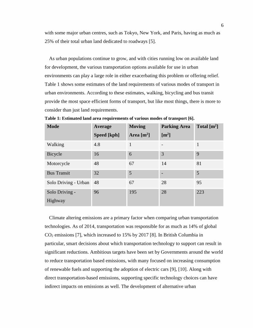
Table 1 shows some estimates of the land requirements of various modes of transport in

urban environments. According to these estimates, walking, bicycling and bus transit

provide the most space efficient forms of transport, but like most things, there is more to

consider than just land requirements.

Table 1: Estimated land area requirements of various modes of transport [6].

Mode Average

Speed [kph]

Moving

Area [m2]

Parking Area

[m2]

Total [m2]

Walking 4.8 1 - 1

Bicycle 16 6 3 9

Motorcycle 48 67 14 81

Bus Transit 32 5 - 5

Solo Driving - Urban 48 67 28 95

Solo Driving -

Highway

96 195 28 223

Climate altering emissions are a primary factor when comparing urban transportation

technologies. As of 2014, transportation was responsible for as much as 14% of global

CO2 emissions [7], which increased to 15% by 2017 [8]. In British Columbia in

particular, smart decisions about which transportation technology to support can result in

significant reductions. Ambitious targets have been set by Governments around the world

to reduce transportation based emissions, with many focused on increasing consumption

of renewable fuels and supporting the adoption of electric cars [9], [10]. Along with

direct transportation-based emissions, supporting specific technology choices can have

indirect impacts on emissions as well. The development of alternative urban

7

transportation infrastructure (bike lanes, rapid light rail, etc.) fosters increased urban

density, thus reducing total per-capita energy and emission intensities [11].

Fossil fuel-based transportation is a major contributor of climate changing emissions,

but electric cars can also have a significant contribution if their electrical energy supply is

fossil fuel based. Electric cars address tail-pipe emissions but not necessarily well-to-

wheel (WTW) emissions associated with the production of the fuel or energy required to

move the vehicle. For countries relying heavily on fossil fuels for electricity generation,

electric vehicles have the potential to increase total GHG emissions when replacing fossil

fuel-based cars, contrary to initial expectations [12]. The choice of energy carrier

(hydrogen, fossil fuel, biofuel, etc) and battery production are found to be the primary

drivers of well-to-wheel emissions in vehicles, therefore choosing to support vehicles that

use renewable sources of energy can make dramatic reductions in associated well-to-

wheel emissions [13]. Although well-to-wheel emissions can be reduced with renewable

energy sources, the use of electric cars, whether hybrid drive-trains or fully electric, have

significantly increased GHG emissions associated with their production when compared

to traditional ICE cars [14], [15].

Urban air quality can also have a significant impact on the health of city-dwellers with

fossil fuel vehicles responsible for 25% of global urban ambient air pollution [16]. Within

large North American cities, 30-45% of the population lives within areas considered

highly affected by traffic emissions [17]. Urban air quality concerns are driving change

through targeted improvements in transportation infrastructure, improved fuel quality,

and alternative transportation technologies [18].

Though alternative fuel cars (biogas, natural gas, electric) can reduce climate changing

emissions and urban air pollution, they don't necessarily address the issue of energy

intensity of transport. A 1200kg vehicle, whether electric or fossil fuel powered, still

requires large amounts of energy to transport a single occupant. Table 2. shows the

energy intensity per passenger kilometre of several modes of transportation with

occupant values typical for Dublin, Ireland, where the study was based.

8

Table 2: Embodied Energy of various transport modes divided among passenger load [19]

Mode Embodied

Energy

[MJ/km]

Occupancy Embodied

Energy

[MJ/pkm]

Bicycle 0.11 1 0.11

City Bus 1.37 25 0.05

Private Car 0.73 1.4 0.52

SUV 1.44 1.4 1.03

Light Rail 5.92 428 0.01

As electrification is often touted as a solution for replacing most consumption of fossil

fuels (building heating and cooling, transportation, industrial processes, etc.), the demand

placed on the future electrical grid is going to be enormous. Heating alone is predicted to

require almost a 30% increase in future grid capacity in California, a relatively warm

location [20]. From a global perspective, transportation is responsible for nearly 30% of

total global energy consumption, of which approximately 92% is fossil fuel based [21].

Electrification of transportation will place enormous demands on National grid

infrastructure, with the UK predicting that it may require up to a 30% increase in energy

generation to handle the electrification of its entire fleet [22].

A shift from cars to E-bikes as a major urban transportation mode would result in a

dramatic reduction in land-use requirements, GHG emissions, negative urban air quality

impacts, and energy use. Some of these impacts have been researched previously (land-

use requirements, urban air quality impacts) but others such as GHG emissions and

energy use are not as clearly understood in academic literature. The next section explores

the existing literature surrounding E-bike use in Western societies.

1.2.2. E-bike Research

E-bike research to-date has covered a wide range of topics, with a particular focus on

safety, behaviours, demographics, and environmental performance. While there are many

engineering-based papers focusing on the electrical sub-systems of E-bikes, they are

9

considered outside the scope of this thesis. A large number of papers focusing on E-bike

issues in China are not considered within this thesis for two primary reasons: a large

portion of Chinese E-bikes are of the scooter style with large plastic fairings and lead-

acid batteries [23], and this thesis focuses primarily on western issues facing E-bikes. The

research discussed below is intended to provide the reader with context regarding the

current use of E-bikes in western society while highlighting the lack of information on

the energy use, emissions, and physical capabilities of E-bikes for transport.

Age and female gender appear to be negatively associated with perceived safety while

riding an E-bike when compared to a regular bicycle in Denmark [24]. A common

perception of the cause of accidents is other road-users underestimating the speed of E-

bikes [24]. Perceptions are different than actual risk, as another study found no

correlation between age and actual accident rates but did find that elderly riders and

women were more likely to be severely injured when crashing [25]. While E-bikes tend

to travel faster than regular bicycles, another study showed that there is no significant

difference in the overall traffic conflict risk between bicycles and E-bikes, although

according to this research, E-bikes have a dramatically higher risk of accident at

intersections due to the increased average speed [26].

A study out of the Netherlands showed no significant difference between riders of E-

bikes and riders of bicycles with respect to rider safety behaviour; E-bikes most often

travelled at faster speeds with the exception of E-bikes travelling slower than bicycles on

shared pathways, and traffic safety violations were comparable between e-bike and

bicycle riders [27]. While traffic safety violation rates in the Netherlands are quite similar

for both bicycle and E-bike riders, other research has shown that typical usage cases for

the two vehicles can differ. E-bikes are more often used for running errands and

commuting when compared to regular bicycles [28]. The same research also shows that

the reason for using an E-bike differed between young and old, with Generation X and

Millennials choosing E-bikes to save time and reduce environmental impacts, while most

other people chose it to increase health outcomes [28], [29]. Typically, as people age,

10

they cycle less frequently but E-bikes have been shown to reverse this trend, as well as

increasing self-reported cycling distances when compared to regular bicycles [30]–[32]

A review of many studies found that most of the increase in E-bike use comes at the

cost of decreased bicycle use, and while the exact environmental cost of this switch isn't

known in the literature, E-bike adoption still has noticeable impacts in reducing car use

[33]. While the reduction of bicycle use isn't ideal, once switched, E-bike owners use cars

noticeably less frequently than bicycle users [33]. The exact nature of mode substitution

is very context specific and varies from region to region depending on technology

availability and infrastructure support [33]. Research has shown that in North America at

least, most e-bike users rode a traditional bicycle prior to using an e-bike [32]. A

comprehensive study out of the United States in 2014 showed that the majority of E-bike

users were male (85%) and white (90%) [32].

Research shows E-bikes safety metrics are similar to bicycles. If the infrastructure is in

place, accidents are rare. Current E-bike users tend to be male, college educated, and

white; and the reasons they use E-bikes are either altruistic in their attempts to address

environmental problems or motivated by health benefits of bicycles while physical

capabilities diminish with age. With this understanding, the objectives and contributions

of this thesis are presented.

1.3. Objectives and Contributions

This thesis addresses the following question: "How does electric assist alter the

environmental impact and physical performance of bicycles, and what are the optimal

roles for electric assist bicycles?"

The primary research question will be answered through the following specific

objectives:

• Create and validate a high-fidelity energy-based bicycle/E-bike model;

• Characterise urban bicycle/E-bike trips with respect to the demands of

instantaneous power expenditure;

11

• Analyze contributions of human supplied mechanical work and electrically

supplied work to the motion of E-bikes;

• Quantify GHG emissions associated with human supplied mechanical work and

compare with emissions from electrically supplied work;

• Quantify physical response of E-bikes + Rider with respect to variation in

loading, human power contributions, motor power contributions, and

geographic topology.

This work is intended to provide a comprehensive overview of the capabilities and

impacts of E-bikes in a variety of scenarios. The primary contributions are to provide a

quantitative assessment to inform decisions regarding the applicability of E-bikes for

commercial fleets and personal use. With a more detailed understanding of the

relationship between human power, electric power, and trip characteristics, further

progress can be made with respect to motor design, control systems, commercial fleet

deployment, and policy decisions.

1.4. Thesis Structure

The remainder of the work contained in this thesis consists of four primary projects that

are detailed in chapters 2 through 4, and are then combined for several sets of analysis in

Chapter 5. The content of each chapter is detailed below:

Chapter 2 covers the experimental data collection campaigns that represent the

original data used in this thesis and represents the preliminary results. The two

experimental campaigns are presented as subsections, detailing the methodology,

analysis, and preliminary results. The first subsection is an analysis of an electric motor

with two internal wiring configurations offering distinct performance profiles. The

second is an E-bike trial involving 17 participants and several months of urban E-bike

trip data.

Chapter 3 shows the investigation of the life-cycle environmental performance of E-

bikes and bicycles relative to other primary modes of urban transportation. This chapter

also includes analysis to quantify the upstream emissions that occur from accounting for

12

the food-based energy supplied to produce human-mechanical work for E-bikes and

bicycles.

Chapter 4 covers the development of a mathematical model to predict the energy use

that occurs while riding a bicycle and an E-bike. A brief literature review is presented

followed by the derivation and validation of the model.

Chapter 5 documents the several different sets of analysis performed with the

experimental data, the environmental data from the LCA, and the mathematical model.

This includes an assessment of the human power contributions during the CRD trial, an

performance assessment of a novel electric motor configuration, quantification of the

performance of E-bikes deployed in a municipal urban fleet, and finally an investigation

into the energy demands of E-bikes used for urban cargo delivery.

Chapter 6 offers a discussion of the results in this thesis, final conclusions that can be

drawn from this work, as well as recommendations for future work.

13

2. Experimental Data Collection

This section of the thesis summarises the two major data collection campaigns

conducted as part of this research. The first comprises a series of E-bike electric motor

performance characterisation tests captured in a laboratory setting. The second captures

trip characteristics and human riding behaviour through the deployment of E-bikes in a

commercial fleet. This chapter summarises the data collection methods, the data, some

preliminary analysis and summary results. In-depth analysis and predictive modelling

using the data presented here occurs in Chapters 3 and 5.

2.1. Exro Motor Performance Characterisation

The Exro Project was a partnership between myself, my academic supervisors Dr.’s

Ned Djilali and Curran Crawford, and Exro Technologies. The project was funded with a

National Science and Engineering Research Council (NSERC) Engage grant designed to

foster relationships between academia and industry such that Canadian based innovative

research can be improved. The purpose of the research from Exro’s perspective was to

quantify the effect of Exro’s switching technology as applied to E-bikes. From my

perspective, I had the added goal of obtaining empirical data detailing the efficiency of a

commercial E-bike motor within the range of typical urban-use duty-cycles.

Two approaches are used to achieve these goals: the first is to quantify the performance

of a typical commercial E-bike motor for both its off-the-shelf operation and with Exro’s

switching technology, and the second is to cross compare this laboratory performance

with real-world urban E-bike duty cycle data from the CRD project (detailed in section

2.2).

2.1.1. Experimental Set-up

Multiple experiment configurations were used over the course of the project, with any

opportunism for improvement in data collection and analysis applied. The initial

configuration is listed in Table 3. A Bionx P350 motor was used for all tests.

14

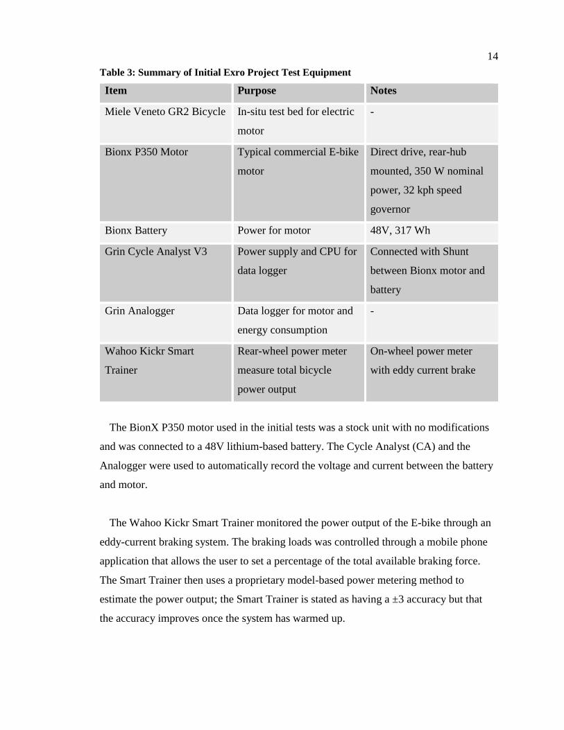
Table 3: Summary of Initial Exro Project Test Equipment

Item Purpose Notes

Miele Veneto GR2 Bicycle In-situ test bed for electric

motor

-

Bionx P350 Motor Typical commercial E-bike

motor

Direct drive, rear-hub

mounted, 350 W nominal

power, 32 kph speed

governor

Bionx Battery Power for motor 48V, 317 Wh

Grin Cycle Analyst V3 Power supply and CPU for

data logger

Connected with Shunt

between Bionx motor and

battery

Grin Analogger Data logger for motor and

energy consumption

-

Wahoo Kickr Smart

Trainer

Rear-wheel power meter

measure total bicycle

power output

On-wheel power meter

with eddy current brake

The BionX P350 motor used in the initial tests was a stock unit with no modifications

and was connected to a 48V lithium-based battery. The Cycle Analyst (CA) and the

Analogger were used to automatically record the voltage and current between the battery

and motor.

The Wahoo Kickr Smart Trainer monitored the power output of the E-bike through an

eddy-current braking system. The braking loads was controlled through a mobile phone

application that allows the user to set a percentage of the total available braking force.

The Smart Trainer then uses a proprietary model-based power metering method to

estimate the power output; the Smart Trainer is stated as having a ±3 accuracy but that

the accuracy improves once the system has warmed up.

15

The second round of tests had a modified equipment set-up that accounted for issues

that arose during the first round of testing. In addition to improving the testing methods,

the Bionx P350 was opened and rewired internally to allow for the coils to be run either

in a parallel configuration (same as stock) or a series configuration. The rewiring,

completed by Exro staff, required the removal of the Bionx speed controller, which was

housed inside the Bionx motor casing, in order to accommodate the space required by the

additional motor wires. An external third party speed controller was used in place of the

Bionx controller. Additionally, a dedicated DC power supply was used to remove and

state of charge (SOC) issues. Table 4 shows the equipment used for the second round of

testing.

Table 4: Summary of Final Expo Project Test Equipment

Item Purpose Notes

Toba Edison Bicycle In-situ test bed for electric

motor

-

Bionx P350 Motor Typical commercial E-bike

motor

Direct drive, rear-hub

mounted, 350 watt nominal

power, rewired and speed

control removed

Volteq HY502EX DC Power for motor 50V, 20A max

Fluke 289 Multimeter Monitor DC supply voltage -

Fluke 325 Clap meter Monitor DC supply current -

Wahoo Kickr Smart

Trainer

Rear-wheel power meter

measure total bicycle

power output

On-wheel power meter

with eddy current brake

Speed controller RPM based motor

controller

Restricts maximum current

and power demands of the

motor relative to first

round testing.

16

2.1.2. First Testing Method

The first testing method used the equipment listed in Table 3 to generate a series of

RPM and torque states for the Bionx motor and bicycle system. The states covered the

range of typical bicycle duty cycles, with up to approximately 270 RPM (32 kph) and up

to approximately 30 N of torque. At each recorded state, the power input and output of

the motor was measured, and the efficiency of the E-bike system was calculated. The

efficiency values included the losses across the motor, through the contact between the

wheel and the roller based smart trainer (vibration, friction, contact resistance), and losses

due to the inertia of the bicycle wheel and the smart trainer flywheel. All data points were

not steady state during this testing method.

The first testing method consisted of mounting the E-bike on the smart trainer, setting

the smart trainer eddy current brake resistance, and applying a throttle signal to the Bionx

system to steadily accelerate to the maximum speed (32 kph) under load. This process

was then repeated for successively larger braking loads (increased eddy current brake

resistance) until the maximum achievable torque output was reached.

Figure 2 shows the response of the system to the human controlled throttle input for an

individual test and is intended to show the variability in the system response to the human

controlled throttle. Since the power was recorded in a dynamic state, the variations in

sample rates between the input power monitoring and the output power monitoring

caused negative impacts on the fidelity of the resulting calculations. An increase in power

input did not always temporally match the power output.

17

Figure 2: Example of initial test results for a fixed braking force as the Bionx system is

accelerated from rest to maximum speed.

Figure 2 shows in a few spots that an increase in power input was followed several

seconds later by an increase in power output. This temporal offset caused issues in

calculating efficiency at each time step in the recorded. Also, since the throttle control

was very sensitive, it was difficult to achieve slow and steady accelerations to minimize

the temporal effects. This could not be remedied by simply shifting the data sets, as the

temporal discrepancies were not consistent throughout a given test.

The input power data (recorded as voltage and current by the CA shunted between the

Bionx battery and Bionx motor), and the output power data (recorded as a single power

metric from the smart trainer) were in two different data files with different sample rates

and different relative time-stamps. An attempted remedy was to align the two signals

using the point of maximum cross-correlation between the two signals1.

1 MATLAB’s built in ‘xcorr.m’ function was used to measure the similarity of the two signals with the

maximum of the output of ‘xcorr.m’ being used as a delay to align the two signals.

18

The individual test of Figure 2 was repeated for the whole range of available braking

forces. The recorded power output was converted to a torque value using equation 1, with

the resulting torque-RPM state data for two full rounds of testing shown in Figure 3. At

each state, the current and voltage input to the motor was recorded, as well as the speed

and power output of the motor. This entire process was repeated several times to

determine whether the results were consistent across multiple trials using the same

method.

𝜏 = 𝑃𝑜𝑤𝑒𝑟

2 𝜋𝑅𝑃𝑀

60

(1)

Figure 3: Entire range of achieved torque-RPM states for two rounds of testing using the

first method and equipment. A) first round of testing, b) second round of testing

Efficiency maps using the recorded state data are shown in Figure 4. The maps were

generated by applying a polynomial fit2 to the scattered data which consists of the

hundreds of torque-RPM states recorded during testing. The efficiency at each recorded

state was calculated using the ratio of power input from the battery to the motor, and

power output of the motor at the wheel-cycle trainer interface. These two surface fits

show fairly significant differences in the estimated efficiency for a given torque-RPM

state.

2 The polynomial fit was generated using the MATLAB function ‘fit.m’ with the ‘poly32’ fit type option, and

the experimental data input as a scattered data set.

19

Figure 4: Polynomial surface fits to A) round 1 and B) round 2 state data of first testing

method. Contours show system efficiency.

The absolute difference in efficiency between the two rounds of testing is shown in

Figure 5. Up to a 20% difference can be seen between the two surfaces. This is especially

prevalent in what will later be shown to be the primary operating states for typical urban

duty-cycles.

Figure 5: Absolute difference between the two efficiency surface fits of Figure 4

A brief analysis of the surface fit was done to ensure that fitting was not one of the

major causes of the discrepancies between the multiple rounds of testing. The residuals of

20

the surface fit for both rounds of testing are shown in Figure 6 along with an assessment

of how well the error is distributed. One metric of a good fit is to show a random

distribution of the error centred around zero, which can be seen in both cases of Figure 6.

Additional goodness of fit metrics for each surface are shown in Table 5: the RMSE for

both is relatively small compared to the scale of the dependent variable (efficiency from

0% to 100%); the R-squared value is not great, showing that the modeled surface fit only

accounts for 79% and 60% of the variability of the experimental data for round 1 and 2

respectively. Other surface fit types were using within the MATLAB toolbox with the

method used in this thesis found to be the most accurate.

Figure 6: Distribution of residuals for surface fit to a) round 1 and b) round 2 data using

the first testing method. Mean and standard deviation of error from surface fit shown for

each round of testing.

Table 5: Quality of fit parameters for surface fit to first testing method data.

Parameter Round 1 Round 2

SSE 2119 3584

RMSE 5.40 4.43

21

R Square 0.79 0.60

Ultimately, it was felt that the test results were too heavily impacted by the battery

SOC, the variability in the temperature of the smart trainer eddy current brake, the

sensitivity of the throttle signal, and the apparent temporal difference between recorded

powers. Attempts were made to minimize these issues by starting with a full SOC and

working through the tests in the same order for each round but due to the difficulty of

controlling the throttle signal, the SOC was not the same from one round to the next.

Significant changes were made to the experimental set-up in an attempt to counter these

issues, which form the basis of the next section.

2.1.3. Second Testing Method

The second testing method used the equipment shown in Table 4. A third-party RPM

based speed controller was used to remove any of the human throttle control issues, and

the DC power supply was used to remove any of the SOC issues. Before data was

collected, the smart trainer was warmed up by setting a braking load and allowing the

system to run for 20 minutes in an attempt to reach a relatively stable thermal state. All

further tests were run by setting a fixed braking load with the smart trainer, setting a

target RPM, allowing the system to reach a steady state, and then recording all of the data

points at the steady state (power supply voltage, power supply current, motor power

output, and motor RPM). This process was repeated for the entire range of achievable

RPM and for successively increasing braking loads.

For the second testing method, rather than capturing a continuous run of data as in the

first method, steady state data was captured at a range of states that span as similar a

domain as possible to real-world duty-cycle states. This second method removed the

temporal misalignment between input and output power that was present in the firs

testing method. The only remaining obstacle was that the speed controller used in the

second testing method had internal electrical limits that restricted the upper range of

torque values achievable. The states obtained using the second testing method are shown

in Figure 7.

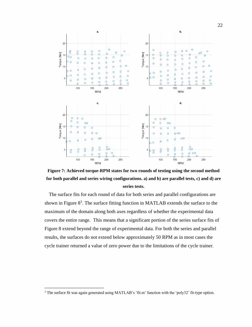
22

Figure 7: Achieved torque-RPM states for two rounds of testing using the second method

for both parallel and series wiring configurations. a) and b) are parallel tests, c) and d) are

series tests.

The surface fits for each round of data for both series and parallel configurations are

shown in Figure 83. The surface fitting function in MATLAB extends the surface to the

maximum of the domain along both axes regardless of whether the experimental data

covers the entire range. This means that a significant portion of the series surface fits of

Figure 8 extend beyond the range of experimental data. For both the series and parallel

results, the surfaces do not extend below approximately 50 RPM as in most cases the

cycle trainer returned a value of zero power due to the limitations of the cycle trainer.

3 The surface fit was again generated using MATLAB’s ‘fit.m’ function with the ‘poly32’ fit-type option.

23

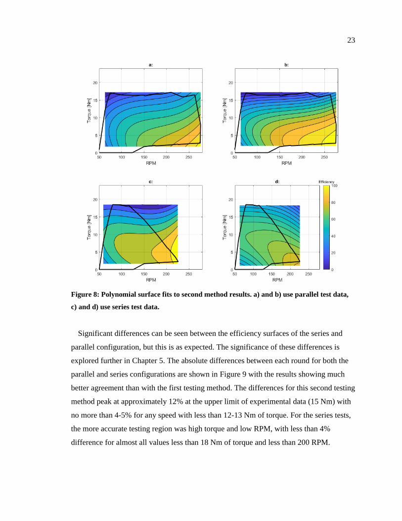
Figure 8: Polynomial surface fits to second method results. a) and b) use parallel test data,

c) and d) use series test data.

Significant differences can be seen between the efficiency surfaces of the series and

parallel configuration, but this is as expected. The significance of these differences is

explored further in Chapter 5. The absolute differences between each round for both the

parallel and series configurations are shown in Figure 9 with the results showing much

better agreement than with the first testing method. The differences for this second testing

method peak at approximately 12% at the upper limit of experimental data (15 Nm) with

no more than 4-5% for any speed with less than 12-13 Nm of torque. For the series tests,

the more accurate testing region was high torque and low RPM, with less than 4%

difference for almost all values less than 18 Nm of torque and less than 200 RPM.

24

Figure 9: Absolute difference between round and 2 efficiency maps for second testing

method. a) parallel and b) series wiring configurations.

The quality of fit for each surface is examined to understand what contributions they

might have on the error between tests. As in the previous section, the distribution of the

residuals and the other quality of fit metrics are presented in Figure 10 and Table 6.

Table 6: Quality of fit parameters for surface fit to second testing method data.

Parameter Parallel

Round 1

Parallel

Round 2

Series Round

1

Series Round

2

SSE 795 2071 261 840

RMSE 3.47 5.65 2.66 4.7

R Square 0.94 0.92 0.93 0.84

25

Figure 10: Distribution of residuals for surface fit to round 1 and 2 results using second

testing method. a) Parallel round 1, b) parallel round 2, c) series round 1, d) series round 2.

The second testing method produces significantly smaller SSE and RMSE as well as an

increased R-squared value when compared to the results of the first testing method in

Table 5. This is very likely due to the steady state nature of the recorded data. By

recording data at steady state, the temporal noise discussed in the previous section, along

with the throttle sensitivity issues, were effectively removed. The removal of the SOC

impacts improved the repeatability and reliability of the tests, although further analysis

using the second method efficiency maps of Figure 8 requires the caveat that it assumes

all operation is at full battery SOC.

26

2.1.4. Exro Project Summary Results

The tests for each configuration are combined to generate a final efficiency map for

both the series and parallel configuration. These efficiency maps are presented in. These

efficiency maps were generated by combining the raw data points from both rounds of

testing prior to surface fitting. Figure 11 shows the clear difference in performance

offered by the series and parallel wiring configurations. The series configuration offers

better efficiency at medium to high levels of torque and low RPM while the parallel

configuration contrasts this with higher efficiency at high RPM and low to medium

torque values.

Figure 11: Efficiency maps for both rounds combined. a) parallel combined efficiency map,

b) series combined efficiency map, c) parallel individual efficiency data points, d) series

individual efficiency data points.

27

2.2. CRD E-bike Trial

The CRD Project is a joint project between myself and my supervisors, Dr.’s Ned

Djilali and Curran Crawford as members of IESVIC, and the Capital Regional District

(CRD), that is funded by a grant from the Green Municipal Fund. The CRD is a local

governmental organization that oversees the region-wide management of services that

can be shared between the thirteen municipalities of Greater Victoria. The E-bike project

forms one part of a larger FCM funded transportation program that focuses on reducing

the transportation-based emissions of the CRD while incorporating academic research.

The specific goals of the CRD E-bike Trial are:

• To characterize the energy use and physical capabilities of E-bikes for urban trips

• To quantify the reduction in GHG emissions of the CRD fleet through the

substitution of E-bikes for car trips.

The results of the pursuing the first goal are reported in this Chapter, while the

substitution impacts are reported in Chapter 5.

2.2.1. Experimental Set-up

Both goals were achieved through the deployment of three E-bikes outfitted with

sensors that logged performance metrics during each trip. The sensor package installed

on each E-bike consisted of a Garmin Edge 520 cycle computer, a Garmin ANT+

protocol speed sensor mounted on the front wheel hub, and a PowerTap Ant+ protocol

hub-based power meter built into the rear wheel. Due to the location of the power meter,

only total power output of the E-bike with no explicit differentiation between the rider

and the electric motor is recorded. Later analysis will break down the results into human

and motor contributions.

Each of these sensors was connected to a Norco VLT R1 E-bike, synced to the Garmin

Edge 520, with the data collected from the Edge on a weekly basis. The CRD staff

involved in the project could reserve and E-bike through the CRD’s internal online

vehicle booking system. Each time they rode the E-bike, they would simply press a

button on the Edge to initiate data logging and press the same button to end the ride and

28

save the data. Seventeen users were recruited into the project, with each rider’s trip data

anonymized to meet CRD privacy concerns.

By the end of data collection, the CRD project resulted in a large number of trips

representing over 4 months of data. There was a significant amount of non-compliance

when it came to recording data. The E-bike odometers showed a total of nearly 1200 km

with the actively recorded data, summarized in Table 7 showing only approximately 600

km. While data logging was optional for CRD staff, this missed data did likely impact the

fidelity of the results as many trips were missed.

Table 7: CRD Project data collection summary.

Metric Value

Total kilometres travelled 607 km

Number of trips 92

Average speed 20.3 ± 5.9 kph

Average trip length 6.6 ± 5.8 km

Average trip time 25.9 ± 25.2 min

By capturing both speed and grade, the CRD data can then be assumed to represent an

estimate of typical urban trips, although with comparative data from other regions or

fleets, it is difficult to say how transferrable the results are to other jurisdictions.

Conversely, since the E-bike speed limiter is almost universal among e-bikes in Canada

as governing speed to a maximum of 32 kph, and the motor power rating is also

regulated, it can be assumed that the typical speed profiles would have a relatively

consistent

2.2.2. CRD Summary

The energy values were recorded using the PowerTap G3 power meter and are reported

in two different forms in this thesis: either as primary energy use (dietary and electrical)

or as the total energy use required to overcome air resistance, rolling resistance, and to

make the mass of the E-bike+rider system accelerate. In this chapter, only the total

29

energy use is reported, with primary energy use detailed in Chapter 3. The power data,

along with the other ride characteristics (speed, location, grade) are used to understand

how and when energy was expended during the trip. The energy use also allows for

determination of the GHG emissions that occur from using the E-bike, as detailed in

chapters 3 and 5.

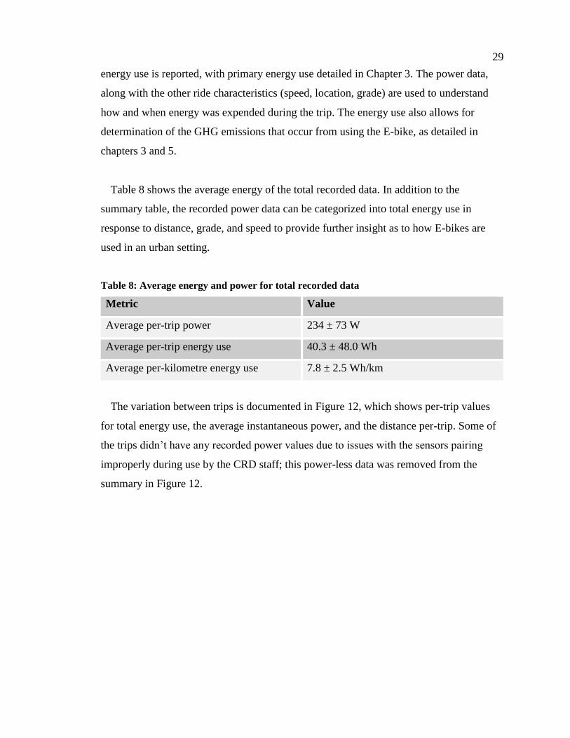
Table 8 shows the average energy of the total recorded data. In addition to the

summary table, the recorded power data can be categorized into total energy use in

response to distance, grade, and speed to provide further insight as to how E-bikes are

used in an urban setting.

Table 8: Average energy and power for total recorded data

Metric Value

Average per-trip power 234 ± 73 W

Average per-trip energy use 40.3 ± 48.0 Wh

Average per-kilometre energy use 7.8 ± 2.5 Wh/km

The variation between trips is documented in Figure 12, which shows per-trip values

for total energy use, the average instantaneous power, and the distance per-trip. Some of

the trips didn’t have any recorded power values due to issues with the sensors pairing

improperly during use by the CRD staff; this power-less data was removed from the

summary in Figure 12.

30

Figure 12: Per-trip energy use (top), average per-trip power (middle), and trip distance

(bottom), as recorded during the CRD project.

31

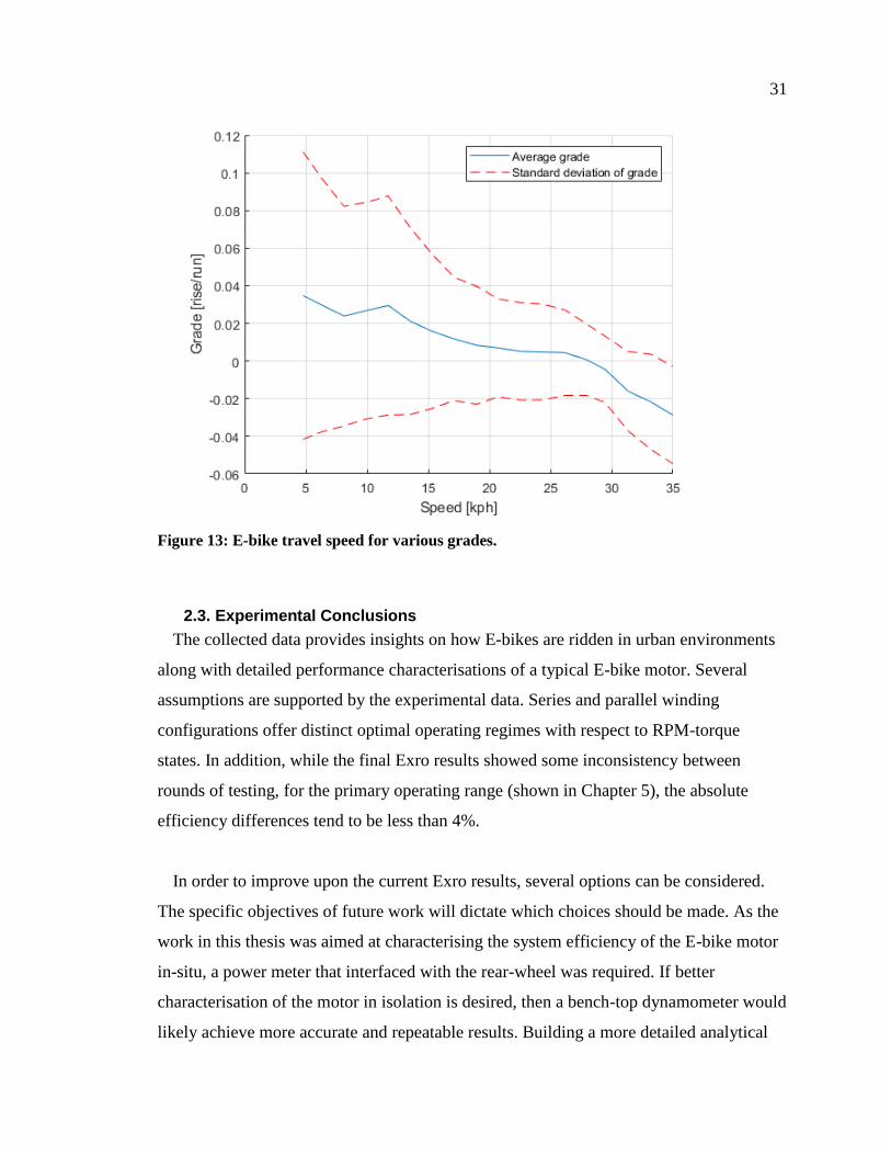
Figure 13: E-bike travel speed for various grades.

2.3. Experimental Conclusions

The collected data provides insights on how E-bikes are ridden in urban environments

along with detailed performance characterisations of a typical E-bike motor. Several

assumptions are supported by the experimental data. Series and parallel winding

configurations offer distinct optimal operating regimes with respect to RPM-torque

states. In addition, while the final Exro results showed some inconsistency between

rounds of testing, for the primary operating range (shown in Chapter 5), the absolute

efficiency differences tend to be less than 4%.

In order to improve upon the current Exro results, several options can be considered.

The specific objectives of future work will dictate which choices should be made. As the

work in this thesis was aimed at characterising the system efficiency of the E-bike motor

in-situ, a power meter that interfaced with the rear-wheel was required. If better

characterisation of the motor in isolation is desired, then a bench-top dynamometer would

likely achieve more accurate and repeatable results. Building a more detailed analytical

32

model of the bicycle that accounted for efficiency losses through the wheel could be

combined with the bench-top dynamometer results to allow a simulated total E-bike

system efficiency.

For the CRD data, we can surmise that from a fleet operations standpoint, users appear

to have no problem maintaining total motive power output for trips up to at least 10

kilometres total. Average power across all trips was relatively consistent with the

standard deviation representing only approximately 30% of mean power. When queried,

most participants stated they used a variety of assist levels, meaning that even with the

assist factor in the data sets changing from 0.5 to 2.75, the average instantaneous power

did not vary greatly. From a fleet managers perspective, this data shows that E-bikes can

fill a niche without human endurance limiting E-bike success.

There are several avenues to improve upon the findings from the CRD campaign. The

first, which was considered and rejected due to the added burden it would place on the

CRD participants, was the addition of a second power meter in the pedals that would

record the human power output during all trips. This would have required a second cycle

computer, and since the user compliance rate for the CRD was relatively low (only

approximately 50% of all trips were recorded), this would likely have led to even lower

levels of recorded data. Second, a similar trial with a bicycle without electric assist would

have given more detailed data about un-assisted human power for comparison purposes

later in this thesis. Finally, a comprehensive survey of CRD participants would have

given further insight as to a range of factors that would influence the power meter

readings: user fitness, experience with bicycles, aversion to rain, purpose of trips, etc.

Employer confidentially issues and academic ethics study procedures were too onerous to

include a survey of this type during the CRD project.

33

3. E-bike Emissions and Energy Use

This chapter is a partial reproduction of a paper in-review with the International

Journal of Sustainable Transportation. The reproduction here omits some parts in favour

of keeping them in Chapter 2, where they fit better within this thesis. The paper here

synthesizes the results of several lifecycle analysis studies, builds a range of dietary and

grid emission intensities, and then determines the primary energy-use of E-bikes and

bicycles using data from the CRD project. All of these parts are combined to determine

what is proposed as a higher fidelity estimate of the potential whole lifecycle emissions

that come from the use of bicycles and E-bikes.

This chapter is developed to answer the environmental aspect of the thesis question:

How does electric assist augment (or detriment) the environmental performance of

bicycles when considering the full life cycle and fuel/energy sources.

3.1. Introduction

As of 2014, fossil fuel based transportation is responsible for 14% of total global CO2

emissions [34]. With these significant emissions and air quality issues facing urban

transportation systems the benefits of a shift to cycling would appear obvious. Municipal

authorities from around the world are significantly expanding cycling infrastructure in the

hopes of stimulating mode switching. Decades of infrastructure investment in locations

such as Amsterdam and Copenhagen have helped achieve cycling mode shares in the

range of 17-41% [35], [36]. Along with the growth in traditional bicycle mode share,

many European cities are also seeing a large growth in the adoption of electric bicycles

(E-bikes) as costs and performance have improved and availability increased [37]. E-

bikes as considered in our study, vs. E-scooters, still require human pedal input power but

augment that power proportionally with an electric motor.

Survey results of early adopters of E-bikes found that they were more likely to switch

from driving to cycling with an E-bike as opposed to a traditional bicycle, and that they

made more trips with an E-bike than with a bicycle before having access to the E-bike

[38]. An increase in willingness to use a bicycle once it is electrified is attributed to the

34

rider's perception of a decrease in the significance of hills and overall exertion required to

reach a destination: E-bikes make cycling feasible for a broader population and over a

broader range of routes. If E-bikes can address some of the shortcomings of the

traditional bicycle, then what are the challenges facing E-bikes? It is relatively straight

forward to surmise that adding an electric motor and battery to a bicycle will increase its

environmental impact during the production phase, but an open question is how this

might impact the use phase and its relative share of life-cycle emissions. Seldom

acknowledged in the current body of research on environmental performance of bicycles

is the fact that their power source is a food-fuelled human body [39]–[41]. Food

production is generally an energy intensive process and its environmental performance

when compared to electricity as a method for powering transportation has yet to be

thoroughly explored in the realm of bicycles.

The motivation of this paper is to explore the range of possible upstream GHG

emissions due to the caloric intake required to balance the human mechanical work used

for riding bicycles and E-bikes, as well as the range of grid emissions associated with

powering the electric assist. While this work references several published LCA, and

expands upon them with empirical e-bike trip data, it does not offer clarity on the impacts

of long term changes in energy intake (increased food consumption) in response to

increased in energy expenditure (exercise). An LCA that truly accounts for the impacts of

active transportation on increased caloric intake would be quite difficult due to the long

time required for equilibrium between energy expenditure and energy intake (on the order

of several months) with the introduction of increased exercise. This work is meant to

show a broad range of possible emissions scenarios that should catch within its

boundaries the reality.

Additionally, this work is intended to show an estimate of the energy required by both

the human provided power and that provided by the electric assist. A dearth of

longitudinal physiological studies fully examining the interplay of diet and increased

regular exercise, along with the obesity range of the population, requires bounding the

caloric input impacts.

35

Establishing the range of possible emissions from E-bike and bicycle use can help

determine the extent to which dietary and grid-linked emissions bound the relative GHG

benefits of bicycles and E-bikes.

A rational approach to account for and compare emissions associated with human

power for bicycles and E-bikes is to perform a seed-to-wheel life-cycle analysis that

parallels well-to-wheel analyses used for plug-in vehicles. In the first stage of analysis, a

review and aggregation of several Life-Cycle Analyses (LCA) studies is performed to

create a baseline for several primary urban transportation modes. Building on this

baseline, further analysis considers the GHG emissions intensities of both human power

and electric power. The human-supplied mechanical work is assessed by accounting for

energy expenditures of commuter cyclists from both third-party research and the results

of an experimental campaign conducted by the authors, which are then combined with

dietary emission intensities of typical Western diets. The electrical power analysis is

performed using electrical grid emission intensities corresponding to the location of the

cited dietary emission intensities. In order to provide greater context to the E-bike and

bicycle emissions results, other primary modes of urban transport are also considered in

the comparative analysis: cars, buses, and electric cars (BEV). The GHG emissions

associated with buses, cars, and electric cars are aggregated from previous studies along

with a brief review of the assumptions and limitations from each study. Finally, the paper

concludes with the insights and further questions gleaned from the study.

3.2. Referenced Life-Cycle Emissions

Seven distinct LCA studies that modelled the impacts of bicycles, E-bikes, traditional

internal combustion cars, battery electric cars, and buses are used as input to our analysis.

These particular studies were chosen because within each study, they covered a range of

transportation options and employed self-consistent methodologies. Intra-study

methodology variations were inevitable and were used to generate an associated while

capturing a wider range of potential attributable emissions within each mode.

36

The results from each of the referenced studies are shown in Figure 14. They are

separated into production phase emissions and use-phase emissions (where delineated),

otherwise only the total life-cycle GHG emissions were reported. The functional unit of

most of the results in this paper are presented as kilograms of carbon dioxide equivalent

emissions per-passenger kilometre travelled. This metric accounts for the varying

passenger loads of each mode of transport, variations in assumed functional lifetime, and

total kilometres travelled over that lifetime. Within the referenced bicycle and E-bike

LCA, the studies did account for embodied emissions associated with infrastructure for

the use of the vehicles, as well as the production of batteries, motors, and other electronic

components. This puts the E-bike and bicycle LCA boundaries in a similar position to

those of buses, battery electric cars, cars.

Figure 14: Summary of life-cycle GHG emissions from referenced studies. Source is listed

on left axis, and emissions reported per-passenger-kilometre travelled [14], [39]–[44].

The variation among the bicycle and E-bike results in Figure 14 are primarily due

to differences in operational lifetime, average speed (and thus energy use), and battery

37

chemistry. The operational lifetime among the bicycle and E-bike LCA varies from 10

years [40] to 15 years [42]. Not all the studies list the average speed assumed for

bicycles, but those that do show a range of 16 km/hr to 22 km/hr. Most of the studies

appear to simply have an average speed and an average trip length with no variation (no

acceleration), unlike in the case of cars which use standardised drive-cycles that include

changes in elevation, acceleration, and other drive cycle inputs (e.g. HFET, US06). The

inclusion of the CRD study results used in this chapter allows for the results to capture

the impact of urban riding conditions (varying acceleration and topology) which puts the

results into a more even comparison with those of traditional modes of transportation

cited.

The impact of human supplied mechanical work was limited to only include either

CO2 exhaled from the rider as in Dave and Walsh [40], [42], or have no associated use

phase emissions as in Cherry, Weiss, and Del Duce [39], [41], [45]. These assumptions

completely neglect the potential upstream GHG emissions of food consumption required

to power such modes of transport.

For E-bikes, each referenced LCA assumed no contributions due to food

consumption but did include the emission intensity of grid supplied electrical energy

from different regions to power the E-bikes. The results include Chinese, Continental

European, and American grid emission intensities. Likely because Weiss and Cherry

include the lead acid type E-bike in their modelling, it can be seen in Figure 14 that their

results show a larger GHG per kilometre travelled then the results of Del Duce and Dave

who only model lithium type batteries. The latter are the only commercially relevant type

in North American and EU markets.

3.3. Dietary and Grid Emission Intensities

The emission intensity per unit energy consumed while riding E-bikes and bicycles

can be traced back to both dietary emission intensity and electrical grid emission

intensities. The dietary emission intensity data comes from the UK and the USA. The

study out of the UK reported dietary emission intensities by recording daily dietary

patterns of 65,000 people using a validated food frequency questionnaire and using LCA

38

analysis of the reported food types [46]. The study out of the USA had a sample size of

73,000 people, and recorded food intake using a validated food frequency questionnaire.

The American example consistently reports lower specific (not total) associated GHG

emissions per calorie than its UK counterpart; both studies normalize the results to a

recommended 2000 kcal per-day diet with no other major differences identified between

the studies other than the different geographical regions in which the analyses focused. It

was not explicitly mentioned in either study, but it could be that one of the studies uses a

source-based emission accounting method and the other uses a destination-based

accounting method such that the source-based emissions include food-waste in

production to generate 2000 kcal at the consumers table while the other doesn't not

include waste generated.

Table 9 summarises the two studies. Both regions have different values for the

amount and source of protein for a given diet classification such that the 'meat light' in

the UK and 'semi-vegetarian' in the US are not directly comparable diet types. With that

caveat, the two studies cited are intended to show the range of typical diet types for each

region and thus are still representative of actual impacts.

Table 9: Dietary Emissions from a range of UK and USA diet types [46], [47]

Diet Type UK [kg CO2e/Cal] USA [kg CO2e/Cal]

Meat Heavy 0.0036 -

Meat moderate / Non-

vegetarian

0.0028 0.0015

eat light / Semi-vegetarian 0.0023 0.0012

Fish based 0.0020 -

Vegetarian based 0.0020 0.0011

Vegan 0.0014 -

The grid emission intensities were sourced from regions that corresponded to

those of the dietary emission studies (the U.K and the U.S.A.). The grid referenced

emission intensities are listed in Table 10 as the high, average, and low emission

intensities averaged over each region for an entire year.

39

Table 10:Summary of electrical grid emission intensities for UK and USA for 2017 [48], [49]

Kg CO2e/kWh UK USA

High 0.494 0.803

Avg. 0.433 0.524

Low 0.352 0.165

Figure 15 was created from Table 9 and Table 10 and shows the energy-emission

intensity of the primary energy delivered to both the rider (dietary) and the E-bike

(electrical).

Figure 15: Primary energy source emission intensity as delivered to the bicycle/E-bike and

rider

It can be clearly seen that dietary based energy has quite significant potential

emissions associated with it. What is not accounted for yet is the losses that occur when

converting dietary energy into human supplied mechanical work, as well as the electrical

40

system losses that occur in the E-bike. These will be added in the next section as we

account for the energy use that occurs while cycling.

3.4. Energy Use While Cycling

The relationship between daily energy expenditure (EE) and calories consumed

(energy intake, EI) by an individual in response to the added exercise of daily cycling

may not be exactly proportional but when viewed through the lens of the first law of

thermodynamics, if the added energy expenditure is not balanced by caloric intake over

the long term, then loss of body mass will occur. Blundell et al have pointed out the

“growing evidence that it takes considerable time for EI to adjust to elevations of EE”

and showed in their analysis of short (1-2 days) and medium term (7-16 days) data that

the immediate effect of taking up exercise is weight loss, but subsequently (7-16 days)

food intake begins to increase in order to provide compensation for about 30% of the

energy expended in activity [50]. In a recent systematic review related to weight loss

from exercise-induced energy deficits, Riou et al found that for longer duration (about 80

weeks), the energy compensation approached 84% and concluded that “lower energy

compensation occurs with short-term exercise, and a much higher level of energy

compensation accompanies long-term exercise interventions” [51]. All of this seems to

indicate that the relationship between EE and EI changes over time until it approaches

some new equilibrium; what this equilibrium is, is not known.

When comparing human energy use while riding bicycles and E-bikes one must

consider that E-bikes can cause riders to travel farther and faster than they otherwise

would on a traditional bicycle [52]. The exact impacts this has on total energy

expenditure is not clearly defined in the literature. In order to compare the use-phase

emissions of E-bikes and bicycles along with other modes of transport, the energy

consumption for a rider and the electric motor must be more clearly identified. Third

party references are compared to experimentally obtained data from a campaign run by

the authors. In addition, it should be noted that this work doesn’t explore the impacts of

increased energy expenditure that might occur from the use of cars, BEVs, and buses

above the average BMR of a user. This means that there could potentially be an increase

41

in up-stream emissions due to increased dietary consumption for cars, buses, and BEVs

that isn’t accounted for in this work.

The third-party source for energy use while cycling was referenced from two distinct

studies. The first study measured 18 untrained healthy males for caloric expenditure

while riding a bicycle, once at the beginning of the study, and then again after commuting

to work via bicycle at least twice a week over a 24 week period [53]. Caloric expenditure

while cycling was determined using a maximal exercise test that recorded the rider's heart

rate and maximal oxygen consumption as well as a data logger that recorded kilometres

travelled. The results showed that on average, a healthy untrained adult commuting via

bicycle has a total energy use of 540 kcal/hr, which results in 470 kcal/hr net energy use

once the basal metabolic rate has been subtracted. The study results also showed that the

average of their sample travelled at approximately 17.8 km/hr, and covered a one way

distance of 8.3 km [53]. The second study cited, used similar data logging methods and

had 17 participants complete a 4.43 kilometre route by bicycle, E-bike, and walking [52].

The results summarized in Table 11 show the Energy Expenditure (EE) rate of the

bicycle riders before a human mechanical work conversion efficiency is applied

(𝜂ℎ𝑢𝑚𝑎𝑛) [54]. This cited work includes variations in speed and topology, which in the

absence of a standardized drive-cycle, should capture some of the dynamic behaviour that

occurs when E-bikes are used for commuting in urban environments.

Table 11: Energy use of bicycles in urban commuting [52], [53]. Rider EE reported as

human caloric expenditure, other energy values reported as output at pedals.

Metric De Geus Langford

Rider EE [kcal/hr] 470 442

Average speed [km/hr] 17.8 14.9

Trip length [km] 8.3 4.3

Average power at pedals [W] 109 103

42

Per-trip energy use [Wh] 50.9 29.7

Per-kilometre energy use [Wh/km] 6.14 6.90

The results of E-bike energy and power from Table 8 are now further assessed to

determine the human and electric motor contributions. Bosch E-bikes have a torque-

based assist that applies motor power at an amount proportional to the torque input of the

rider. The minimum and maximum assist factors are 50% and 275% respectively and are

accounted for at the output shaft after the internal gearing of the Bosch motor. By using

the assist levels and an energy balance applied at the centre hub of the rear wheel, the

power contribution of the human and motor can be estimated using equation 3.1:

�̇�𝑟𝑒𝑐 = 𝜂𝐷𝑇 × (�̇�ℎ + �̇�𝑚) (3.1)

𝜂𝐷𝑇 represents the drive train efficiency from pedal crank/E-motor output to

wheel (i.e. geared), �̇�ℎ is the power required of the human measured at the pedals, �̇�𝑚 is

the power required of the motor at the motor output shaft, and �̇�𝑟𝑒𝑐 is the recorded power

output from the experimental campaign. Since the motor and the human are peddling on

the same shaft, the angular speed of the pedals and that of the motor output are the same

(𝜔ℎ = 𝜔𝑚), which allows us to model the assist using power instead of torque. To relate

this energy balance back to the primary energy supply emission intensities of Figure 15,

several efficiency losses must be added to the motor energy use. The electrical efficiency

losses that occur are due to charger losses (due to the power electronics in the charger),

charging losses (the ratio of the input energy to the battery to the output energy from the

battery), and the motor/controller efficiency (due to the losses required to convert

electrical energy to mechanical). These losses are summarized in Table 12.

Table 12: E-bike system efficiency estimates

Charger efficiency 0.95

Charging efficiency 0.85

43

Motor efficiency 0.90

Total electrical system efficiency 0.73

Human energy conversion efficiency 0.20

Drive train efficiency 0.96

In order to relate the power required at the motor output shaft (�̇�𝑚) and the power

required at the pedals (�̇�ℎ) to the energy consumed in relation to the primary energy

supply emission intensity (�̇�𝑚,𝑒 and �̇�ℎ,𝑒), the electrical system efficiency and human

energy conversion efficiency must be applied using equations 3.2 and 3.3

�̇�𝑚 = �̇�𝑚,𝑒 × 𝜂𝐸𝑙𝑒𝑐 (3.2)

𝐸ℎ̇ = �̇�ℎ,𝑒 × 𝜂𝐻𝑢𝑚𝑎𝑛 (3.3)

Equations 3.2 and 3.3 are now substituted into equation 3.1 to show how the

recorded power from the experimental trial is related back to the primary energy emission

intensities.

�̇�𝑚,𝑒 = �̇�𝑟𝑒𝑐

𝜂𝐸𝑙𝑒𝑐 × 𝜂𝐷𝑇 (1𝐴 + 1)

(3.4)

𝐸ℎ,𝑒̇ =

�̇�𝑟𝑒𝑐

𝜂𝐷𝑖𝑒𝑡 × 𝜂𝐷𝑇(𝐴 + 1) (3.5)

𝐴 represents the electric assist factor that models the variation in torque-based

assist supplied by the e-bike motor. Equations 3.4 and 3.5 can now be used alongside the

experimental campaign results to estimate the range of potential human and electrical

energy intensities for E-bike use in urban environments. Table 13 was generated to show

the minimum and maximum human and motor energy intensities that occurred while

riding an E-bike during the trial based on variations in the assist level 𝐴.

Table 13: E-bike primary energy intensity as determined from CRD project data.

Assist = 0.5 Assist = 2.75

Dietary energy intensity

[Wh/km]

27.3±8.1 11.1±3.2

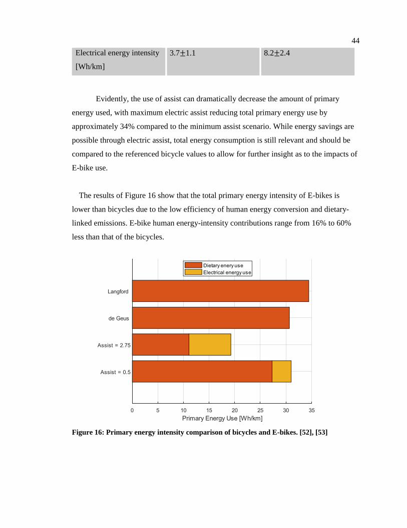
44

Electrical energy intensity

[Wh/km]

3.7±1.1 8.2±2.4

Evidently, the use of assist can dramatically decrease the amount of primary

energy used, with maximum electric assist reducing total primary energy use by

approximately 34% compared to the minimum assist scenario. While energy savings are

possible through electric assist, total energy consumption is still relevant and should be

compared to the referenced bicycle values to allow for further insight as to the impacts of

E-bike use.

The results of Figure 16 show that the total primary energy intensity of E-bikes is

lower than bicycles due to the low efficiency of human energy conversion and dietary-

linked emissions. E-bike human energy-intensity contributions range from 16% to 60%

less than that of the bicycles.

Figure 16: Primary energy intensity comparison of bicycles and E-bikes. [52], [53]

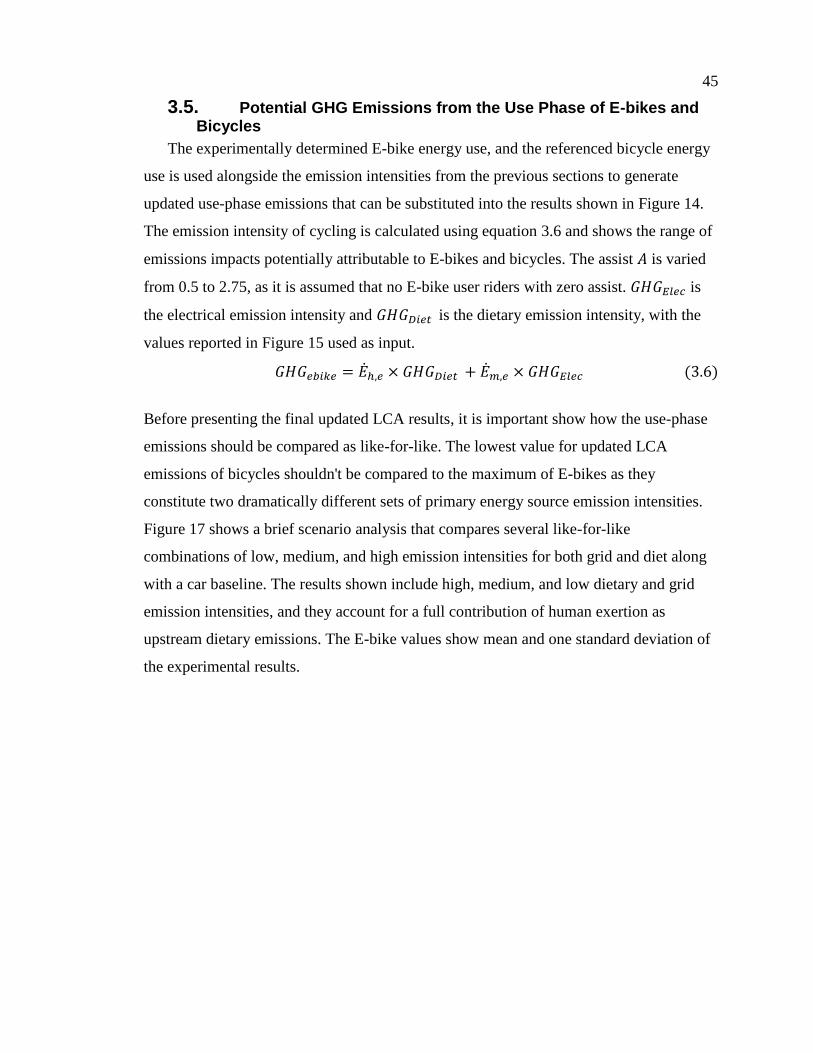
45

3.5. Potential GHG Emissions from the Use Phase of E-bikes and Bicycles

The experimentally determined E-bike energy use, and the referenced bicycle energy

use is used alongside the emission intensities from the previous sections to generate

updated use-phase emissions that can be substituted into the results shown in Figure 14.

The emission intensity of cycling is calculated using equation 3.6 and shows the range of

emissions impacts potentially attributable to E-bikes and bicycles. The assist 𝐴 is varied

from 0.5 to 2.75, as it is assumed that no E-bike user riders with zero assist. 𝐺𝐻𝐺𝐸𝑙𝑒𝑐 is

the electrical emission intensity and 𝐺𝐻𝐺𝐷𝑖𝑒𝑡 is the dietary emission intensity, with the

values reported in Figure 15 used as input.

𝐺𝐻𝐺𝑒𝑏𝑖𝑘𝑒 = �̇�ℎ,𝑒 × 𝐺𝐻𝐺𝐷𝑖𝑒𝑡 + �̇�𝑚,𝑒 × 𝐺𝐻𝐺𝐸𝑙𝑒𝑐 (3.6)

Before presenting the final updated LCA results, it is important show how the use-phase

emissions should be compared as like-for-like. The lowest value for updated LCA

emissions of bicycles shouldn't be compared to the maximum of E-bikes as they

constitute two dramatically different sets of primary energy source emission intensities.

Figure 17 shows a brief scenario analysis that compares several like-for-like

combinations of low, medium, and high emission intensities for both grid and diet along

with a car baseline. The results shown include high, medium, and low dietary and grid

emission intensities, and they account for a full contribution of human exertion as

upstream dietary emissions. The E-bike values show mean and one standard deviation of

the experimental results.

46

Figure 17: Life-cycle Emission Scenario comparisons of bicycle and E-bikes.

When the upstream emissions related to human energy expenditure are accounted for,

substituting grid supplied electrical energy can have a significant potential impact on

LCA emissions for bicycles and E-bikes. As seen in Figure 17, when using the same

dietary and electrical intensity for bicycles and E-bikes and an assist factor of 1.75,

switching from bicycle to E-bike has the potential to reduce the total life-cycle

transportation emission intensity by as much as 50%. With higher levels of assist

emissions reductions could be increased but the trade-off would be reducing the ability of

E-bikes to make meaningful contributions towards daily recommended exercise goals.

Further work is required to determine the exact nature of the relationship between E-bike

assist levels and daily recommended exercise goals.

Figure 18 shows the updated upper and lower bounds for bicycles and E-bikes based on

the use-phase emissions calculated using the dietary and electrical emission intensities

listed in Table 9 and Table 10, as well as the life-cycle emissions for cars, buses, and

BEVs as determined from the range of LCA studies cited in this thesis.

47

Figure 18: Full range of potential life-cycle emissions for bicycles and E-bikes compared to

other modes of urban transport.

The results of Figure 18 are meant to convey the total range of possible GHG emissions

that could be attributable to both bicycles and E-bikes due to food consumption: from no

emissions associated with dietary-supplied human mechanical work, to total attribution

with high dietary emission intensity. The car, bus, and BEV values are a summary of the

range of results from the LCA studies referenced in the current paper. If dietary

emissions are ignored (shown by the lowest point of the bicycle and E-bike emissions in

Figure 18), bicycles and E-bikes have the lowest per kilometre emissions of any of the

forms of transportation considered in this paper. Alternatively, if the full impact of

dietary emissions are included from a meat-heavy, UK-based diet, then bicycles can

potentially be a poor choice of transportation based on GHG emissions alone. The truth

likely lies somewhere in between, with some of the energy expenditure of riders on

48

bicycles and E-bikes being directly attributable to that form of transport rather than a

sunk GHG cost that is the same among all forms of transportation.

While the results in Figure 15 through Figure 18 seem to show that all of human

effort should be replaced by electrically supplied power, it is important to note that the

scope for this analysis is limited to only GHG emissions associated with the life-cycle of

the vehicle. In the case of high levels of dietary emissions and full attribution of human

mechanical work to dietary emissions, then perhaps BEVs become a more

environmentally friendly option but in the real world, there is always more to assess than

just emissions when considering each mode of transportation.

Public health is a major factor to consider when it comes to transportation options.

A study by the Transportation Department of Minnesota found that regular cycling use

(2-3 times week) was linked with a 32% reduction in obesity and prevented 12-61 deaths

per year [55]. Research has also shown that commuter cycling regularly meets the

recommended duration and intensity required to improve physical health and fitness as

put forth by the American College of Sports Medicine and the Centre for Disease Control

and that the use of E-bikes for commuting can also meet recommended daily exercise

targets [52], [53]. With many European and North American communities suffering from

chronic health impacts due to sedentary lifestyles [56], bicycles and E-bikes represent a

highly valuable tool to combat this epidemic.

Infrastructure degradation is also of major importance with respect to

transportation. E-bikes, much like bicycles, are considered to have negligible impacts in

regards to infrastructure degradation [57]. According to a report by the Government

Accountability Office out of the USA, a 5 axle 18 wheel tractor trailer does as much

damage to roadways as approximately 9600 cars, primarily based on the dynamic axle

loads placed upon the road way [58]. That study assumes a weight increase of 20 times

between a car and a tractor trailer, which is about the same again as the weight reduction

from a car to a bicycle (2000 kg car to 100 kg bicycle and rider), this implies that E-bikes

49

and bicycles are potentially thousands of times less destructive to road infrastructure than

cars and buses.

When comparing bicycles and E-bikes to mass transport, it can be seen in Figure

18 that in some cases a bus can have lower CO2 equivalent emissions per kilometre than

bicycles or E-bikes for short trips but the hidden information in the figure is that lowest

bus GHG emission estimates are based on an assumed passenger load of 50 people,

where as the actual amount can vary dramatically from city to city. A bus has the

potential to emit the least amount of CO2 equivalents per passenger kilometre but is

highly dependent on the operating environment and the passenger load.

The inclusion of dietary based emissions for human supplied mechanical power is

not without criticism. On an individual basis, research is not definitive as to how exactly

the introduction of regular exercise impacts that individual's dietary demands over the

long term, although it appears that increases in daily EE correlate to increases in EI [51].

In addition, the trade off for bicycles and E-bikes between the food-based emissions of

human supplied mechanical power and the health benefits of exercise are not easily

measured. Replacing human supplied mechanical power reduces emissions but also

reduces the benefits of regular exercise to individuals and societies. To counter that

argument, there are studies that show individuals are more likely to take an active form of

transport if it has some form of electric assist to ease the amount of effort involved, thus

potentially increasing the society wide amount of exercise obtained by lowering the

barrier to entry [38]. If a holistic view is taken when examining bicycles and E-bikes and

an attempt is made to give them the same environmental examination as cars that

includes a well-to-wheel examination, the data in Figure 18 shows that bicycles and E-

bikes are still better environmental performers than cars and in most cases buses and

BEVs.

3.6. Conclusions

This paper shows that with the policies aimed at growing bicycle mode-share, E-bikes not

only offer similar or better environmental performance but are also addressing one of the

primary barriers to people considering active transport: ease of use. The primary

50

environmental trade-off between E-bikes and bicycles stems from the high environmental

costs of food production and the low levels of efficiency in converting food energy into

human supplied mechanical power. By substituting some human mechanical power with

electrical power while still maintaining most of the environmental benefits that bicycles

have over cars, allows the E-bike to excel in the realm of environmental performance. In

the context of current food and electricity production methods - whether coal, nuclear, or

hydro - substituting mechanical human power with electrical can still be environmentally

beneficial. If a much more GHG efficient food production method were to be developed,

bicycle emissions would also benefit.

These results offer support to the conclusion that E-bikes should be better

supported to allow them to increase total bicycle mode-share in urban environments. In

particular, the extensive subsidies to electric personal vehicles in-place in many

jurisdictions should be examined relative to potential rebates or other incentives for E-

bikes. This policy analysis should include the total magnitude of mode switch possible,

and the mode being switched from. Personal vehicle purchase incentives that create a

mode switch from a car (average of 0.21 kg CO2e/km Figure 18) to BEV (average of 0.1

kg CO2e/km Figure 18) should be evaluated to determine the monetary cost per kg of

CO2e saved. An end user rebate of $5000 to mode switch from a car to a BEV is a

$45,000/kg CO2e/km government GHG abatement costs. Giving the same consumer a

$2000 rebate to negate the E-bike vs. bike cost would be $12,000/kg CO2e/km reduction

over a car, a 4 times improvement in GHG abatement cost, not considering the lowered

medical and traffic congestion costs to society.

Opportunities for future work include gathering data to define route variability and to

better understand how electric assist impacts trip characteristics such as speed and

distance travelled. By improving fidelity of the demands placed on E-bikes and bicycles

during the use-phase more planning can be made as to the optimal usage scenarios for E-

bikes and bicycles in urban environments. Additionally, understanding long-term dietary

intake impacts in response to regular exercise would also allow for increased

understanding as to the impacts of greater adoption of bicycles and E-bikes.

51

4. E-bike Energy-Based Model

The model used in this thesis is an energy-based model of a bicycle and rider in

motion. For the E-bike portion of the model, the underlying equations remain the same

but with the total power required being modelled as having two components: the electric

motor and the human rider (using equations 3.4 and 3.5).

This type of approach to modelling a bicycle has been done many times in academic

research but so far has not been investigated for E-bikes. The first time the model was

seen in academic literature was in an article by James Martin published in the Journal of

Applied Biomechanics, that has subsequently been cited nearly 300 times [59]. Martin’s

goal was to determine if a mathematical mode could accurately predict power during road

cycling. The model was validated using an ergometer in a laboratory as well as an in-situ

power meter during outdoor riding. The mode was validated over a range of steady-state

velocities with the ultimate conclusion being that the model was accurate with a

difference of only 2.7 W between modelled and measured power at steady state.

A number of later papers used the model to investigate how various system changes

(mass, aerodynamics coefficients, etc.) can change power requirements for various

speeds, or for comparing various in-situ power meters [60]–[63]. In most cases, it appears

the subsequent work tended to use the coefficients from Martin et al’s original work. The

aerodynamic coefficient was measured using a wind-tunnel in Martin et al’s work, which

is the most accurate method but also the most expensive. Work by Atkinson et al used

Martin’s model but with variable gradients and wind velocities to determine their effect

on rider power for maintaining constant speed under these conditions [64].

Only one instance of the model being applied to E-bikes was found and it involved

using the model to create a utility based bicycle speed choice model [65]. While this

work included pedal-assist type E-bikes, its focus was on steady-state cruising for various

assist levels and energy outputs.

52

The model as formed in this thesis closely follows the model as developed in a 2011

paper by Dahmen et al which in turn builds on the work of Martin et al. In the case of

Dahmen et al’s work the model was validated by using recorded power data from riding

through a course in the Swiss Alps multiple times at either a fixed speed or fixed power.

The elevation profile of the track was measured using a differential-GPS device which

allowed for greater accuracy of the model’s predictions than was achieved using a

standard consumer GPS device in the CRD project. Ultimately, Dahmen et al found the

model to be highly accurate at predicting rider power under fixed speeds, or rider speed

under fixed power as long as high fidelity input data is used [66].

The primary difference between this model and all other known variations of it, is that

in this thesis, the model is attempting to predict either dynamic power or dynamic speed

behaviour. Previous models have focused on either constant speed or constant power with

no stopping. Because of this change, it is expected that the model will be less accurate

than the other reported instances of its use due to the difficulty of capturing dynamic

power fluctuations that occur with starting and stopping.

The remainder of this chapter covers the development of the governing equation, along

with the input variables, followed by an analysis of the accuracy of the model for

dynamic behaviour and its sensitivity to slight fluctuations in each variable.

4.1. Model Derivation

The derivation of an equation to predict the power required to move the E-bike starts

with basic engineering and physics principals; overcoming static and dynamic forces to

achieve changes in velocity. In this thesis, the rider and the motor can be viewed

equivalently as sources of mechanical power to move the E-bike. From this source of

power, the model can be developed by introducing each factor that acts to inhibit or

retard the motion of the bicycle in response to the power input by the rider.

These factors include aerodynamic drag, rolling resistance, friction from the wheel

bearings, and the rate o change in potential and kinetic energy in response to variations in

53

altitude and speed. Figure 19 lists the factors that control the motion of the system. The

E-bike and rider are both considered within the system boundaries so that the masses of

each impact the motion.

Figure 19: Free body diagram for E-bike and rider as used to develop the model. Image

comes from www.sustrans.org.uk

Equation 4.1 is arrived at by applying an energy balance to the E-bike system, where

the input power from the rider and motor (Ph and Pm) are balanced by the loss terms (Pair,

Pbear, Proll, and DT ) and the conservative terms (Pkin and Ppot).

𝑃𝑝𝑜𝑡 + 𝑃𝑘𝑖𝑛 + 𝑃𝑎𝑖𝑟 + 𝑃𝑏𝑒𝑎𝑟 + 𝑃𝑟𝑜𝑙𝑙 = 𝜂𝐷𝑇(𝑃ℎ + 𝑃𝑚) (4.1)

Ppot represents the change in energy that occurs due to variations in elevation while

riding, Pkin is the term corresponding to changes in velocity, Pair represents the

aerodynamic drag losses, Pbear represents the losses due to friction in the wheel bearings,

Proll represents the losses due to the rolling resistance of the wheels, and Ph and Pm

represent the human and motor power contributions respectively. DT represents the

efficiency losses that occur while transmitting power from the motor/pedals ti the rear

wheel of the E-bike (where the data is recorded in the CRD project), referred to as the

drive train efficiency and represents an additional loss mechanism.

54

From equation 4.1, each individual term will be presented base on the underlying

physical principles, beginning with the potential energy term. The rider/motor has to

supply power (Ppot ) in proportion to the rate of change of the elevation (𝑑𝑦

𝑑𝑥) experienced

by the E-bike system, referred to as grade. The amount of power required is also

proportional to the mass of the E-bike and rider (mT), the gravitational acceleration (g)

and the velocity of the E-bike (𝑑𝑥

𝑑𝑡).

𝑃𝑝𝑜𝑡 = 𝑚𝑇𝑔 𝑑𝑥

𝑑𝑡sin (𝑎𝑟𝑐𝑡𝑎𝑛 (

𝑑𝑦

𝑑𝑥)) (4.2)

The kinetic term (Pkin) is due to the energy required to change the velocity (𝑑𝑥

𝑑𝑡) of the

mass of the rider and E-bike (𝑚𝑇). The kinetic term also includes the energy required to

rotate the wheels, given by the mass moment of inertia of the wheels (Itotal) multiplied by

the angular velocity of the wheels (𝑑𝑥

𝑑𝑡/𝑟𝑤

2).

𝑃𝑘𝑖𝑛 = (𝑚𝑇 + 𝐼𝑡𝑜𝑡𝑎𝑙

𝑟𝑤2

)𝑑𝑥

𝑑𝑡

𝑑2𝑥

𝑑𝑡2(4.3)

Next, the air resistance term is the result of the rider’s surface area (A), the coefficient of

drag (CD), and the density of the air (𝜌), multiplied by the relative wind-velocity opposite

the motion of the E-bike. For this work, the wind-speed is assumed to be zero and thus

the relative airspeed is simply the speed of the E-bike (𝑑𝑥

𝑑𝑡).

𝑃𝑎𝑖𝑟 = 0.5 𝜌𝐶𝐷𝐴 (𝑑𝑥

𝑑𝑡)

3

(4.4)

The bearing resistance term relies on measured constants (Β0 and Β1) that act as a force

of friction to counter the velocity of the E-bike system.

𝑃𝑏𝑒𝑎𝑟 = Β0 + Β1

𝑑𝑥

𝑑𝑡 (4.5)

The rolling resistance losses occur due to tire deformations and irregular surface contact

between the tires and the road surface. The losses from rolling resistance is calculated

using a rolling resistance coefficient (CRR) that represents the interactions between the

road surface and the tires, multiplied by the grade of the path of travel, the mass of the

rider and E-bike, and the speed.

𝑃𝑟𝑜𝑙𝑙 = 𝐶𝑅𝑅𝑚𝑇𝑔 cos (arctan (𝑑𝑦

𝑑𝑥))

𝑑𝑥

𝑑𝑡(4.6)

55

Both the input power terms (Ph and Pm) can be either outputs or inputs to the model

depending on the formulate of the final governing equation. The final governing equation

is shown below in equation 4.7.

𝑃𝑡𝑜𝑡𝑎𝑙 = 𝜂𝐷𝑇(𝑃ℎ + 𝑃𝑚) = 𝑚𝑇𝑔𝑑𝑥

𝑑𝑡𝑠𝑖𝑛 (arctan (

𝑑𝑦

𝑑𝑥)) + (𝑚𝑇 +

𝐼𝑡𝑜𝑡𝑎𝑙

𝑟𝑤2

)𝑑𝑥

𝑑𝑡

𝑑2𝑥

𝑑𝑡2+

0.5𝜌𝐶𝐷𝐴 (𝑑𝑥

𝑑𝑡)

3

+ (Β0 + Β1

𝑑𝑥

𝑑𝑡)

𝑑𝑥

𝑑𝑡+ 𝐶𝑅𝑅𝑚𝑇𝑔𝑐𝑜𝑠 (arctan (

𝑑𝑦

𝑑𝑥))

𝑑𝑥

𝑑𝑡(4.7)

4.2. Model Variables

The variables used in this implementation of the model have been obtained from a

variety of sources. Some come from Dahmen et al’s 2011 paper, while others are

measured from the CRD E-bike project.

The most difficult metric to obtain was the drag-area of the rider and E-bike. For this

thesis it was obtained using the Chung Method [67]. This method works by recording the

power while riding the E-bike under several specific conditions. The method must be

repeated over the same route multiple times so that each lap can be compared. The route

should not be flat, and it is expected that speed and power will not be constant due to

realistic riding conditions. Ambient wind speed should be as close to zero as possible and

there is to be no braking during each lap. Rider position should also be kept constant.

Equation 4.7 is solved for the grade term 𝑑𝑦

𝑑𝑥, with small angle assumptions applied to

linearize the trigonometric terms, as shown in equation 4.8. This method works by re-

arranging the governing equation for elevation change as a function of speed. This means

that if there are any changes in power not accounted for in the governing equation, then

these can impact the elevation estimates. Therefore, the testing was conducted with

minimal wind velocity and with no braking.

𝑑𝑦

𝑑𝑥=

1

𝑚𝑇𝑔[

𝑃𝑡𝑜𝑡𝑎𝑙

𝑑𝑥𝑑𝑡

− 𝐶𝑅𝑅𝑚𝑇𝑔 − (𝑚𝑇 +𝐼𝑡𝑜𝑡𝑎𝑙

𝑟𝑤2

)𝑑𝑥

𝑑𝑡− 0.5𝐶𝐷𝐴𝜌 (

𝑑𝑥

𝑑𝑡)

2

− (Β0 + Β1

𝑑𝑥

𝑑𝑡)] (4.8)

To start the Chung Method, several laps were run on a quiet street near UVic, with

power, speed, and elevation recorded. The recorded power and speed were then

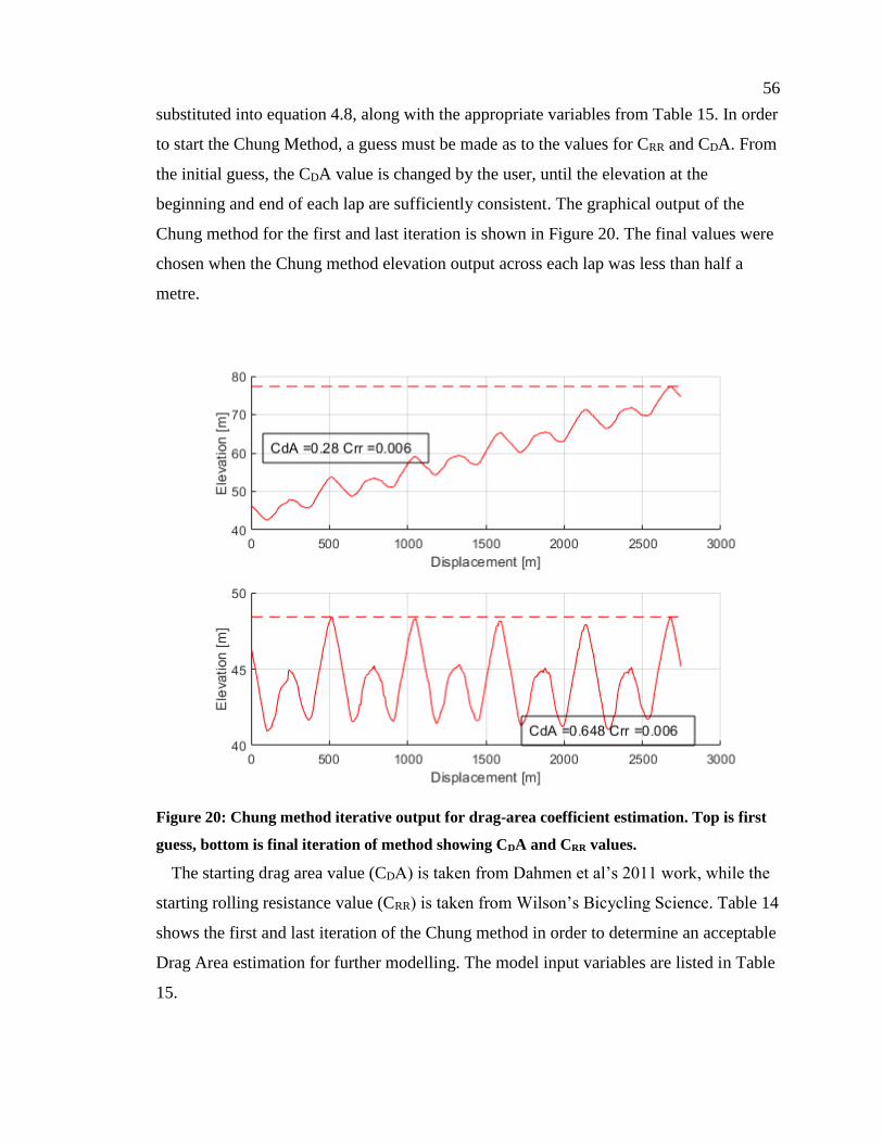
56

substituted into equation 4.8, along with the appropriate variables from Table 15. In order

to start the Chung Method, a guess must be made as to the values for CRR and CDA. From

the initial guess, the CDA value is changed by the user, until the elevation at the

beginning and end of each lap are sufficiently consistent. The graphical output of the

Chung method for the first and last iteration is shown in Figure 20. The final values were

chosen when the Chung method elevation output across each lap was less than half a

metre.

Figure 20: Chung method iterative output for drag-area coefficient estimation. Top is first

guess, bottom is final iteration of method showing CDA and CRR values.

The starting drag area value (CDA) is taken from Dahmen et al’s 2011 work, while the

starting rolling resistance value (CRR) is taken from Wilson’s Bicycling Science. Table 14

shows the first and last iteration of the Chung method in order to determine an acceptable

Drag Area estimation for further modelling. The model input variables are listed in Table

15.

57

Table 14: Chung method drag area and rolling resistance values.

Iteration CDA CRR

1 0.28 0.006

- - -

13 0.648 0.006

The caveats that are inherent with the drag area estimation method is that the actual

value can shift with the rider simply changing their position on the E-bike, or by riding

with a hooded sweater, or any other number of slight changes. The value chosen for this

thesis is meant to approximate a typical drag area for an urban commuter rather than a

constantly varying term for each use-case that might occur.

Table 15: Model constant values along with source and measured or estimated uncertainty.

E-bike system metric Symbol Units Value Uncertainty Source

Rider mass mr kg 73.5 2.5 measured

E-bike mass me kg 25 2.5 measured

Wheel Radius rw m 0.358 - measured

Front wheel mass mwf kg 2.13 - measured

Rear wheel mass mwr kg 2.56 - measured

Bearing Coefficient B0 N 0.091 0.009 [66]

Bearing Coefficient B1 Ns/m 0.0087 0.0009 [66]

Rolling resistance coefficient CRR - 0.006 0.001 [54]

Air density kg/m3 1.204 - [68]

Gravitational acceleration g m/s2 9.81 - [68]

Moment of Inertia Itotal kgm2 0.61 0.16 calculated

Drag Area CDA m2 0.648 0.098 calculated

Grade 𝑑𝑥

𝑑𝑦 - - 0.25 calculated

Velocity 𝑑𝑥

𝑑𝑡 m/s - 0.11 [69]

The last major concern with the model input variables is that some of the uncertainties

are estimated rather than taken from an official source or a measurement. The grade

uncertainty is partially based on the barometric pressure-based elevation uncertainty from

the Garmin device, which is ±3m [70]. Since the model requires the change in elevation,

58

the fidelity of the absolute elevation isn’t as important. If the elevation uncertainty of

±3m is used in the model, then equation 4.9 which predicts the grade uncertainty as a

function of vertical and horizontal measurement uncertainties, results in a final predicted

power uncertainty of up to 2000 watts in some of the trips detailed in the next section.

Instead of the ±3m elevation uncertainty, a delta-elevation uncertainty of 0.25m is used

which results in a more realistic potential power uncertainty, as detailed in the next

section. The delta-elevation uncertainty was chosen to correspond in magnitude with

smallest step size observed in the recorded grade data (approximately 0.2m).

𝜖𝑔𝑟𝑎𝑑𝑒 = |𝑔𝑟𝑎𝑑𝑒|√

(𝜖Δ𝑥

Δ𝑥)

2

+ (𝜖Δ𝑦

Δ𝑦)

2 (4.9)

4.3. Model Accuracy Assessment

The accuracy assessment of the model uses as input a set of time-series velocity and

grade data, recorded with the E-bike described in Section 2.2.1, to then predict the power

use of an E-bike. This prediction is then compared to the actual recorded power demands

of the E-bike to quantify the model’s accuracy. It is also important to remember that the

measured power values come from a rear-wheel hub-based power meter, whereas the

power predictions of the model attempts to predict both positive and negative power

values. The measured power from the hub-based power meter also has inherent errors in

accounting for both the electrical motor output and the human power output. The

accuracy is assessed with two primary methods. The first is an uncertainty analysis of the

model, and the second is a more direct prediction error assessment.

The uncertainty of the model in response to each of the input variables is tested

using a computerized uncertainty analysis [71], with the following steps:

1. Determine the predicted power for a given trip using all baseline values for the

variables listed in Table 15,

2. For each variable (xi) listed in Table 15, increase the variable value by its uncertainty

(𝜖𝑥𝑖), and calculate the resultant power (Pi+). Once more alter the variable value by

decreasing it by the uncertainty from the nominal value and calculate the resultant

59

power (Pi-). This is done for each variable in turn with all other variables held at their

baseline value.

3. The difference is then calculated for both altered powers, 𝐶𝑖+ = 𝑃𝑖+ − 𝑃𝑝𝑟𝑒𝑑𝑖𝑐𝑡𝑒𝑑, and

𝐶𝑖− = 𝑃𝑖− − 𝑃𝑝𝑟𝑒𝑑𝑖𝑐𝑡𝑒𝑑, then the average of the absolute value of the two

contributions is stored for each variable as 𝐶𝑖 = 𝑚𝑒𝑎𝑛(|𝐶𝑖−|, |𝐶𝑖+|),

4. The uncertainty in the final power prediction is the root-sum-square of all the Ci

The direct prediction error is assessed using the following measures between the two

signals:

Correlation coefficient: defined by equation 4.10, where A and B represent the two

power signals (recorded and predicted), N is the number of observations of power in the

given trip, and µ and are the mean and standard deviation of power in either data set:

𝜌(𝐴, 𝐵) = 1

𝑁 − 1∑ [(

𝐴𝑖 − 𝜇𝐴

𝜎𝐴) (

𝐵𝑖 − 𝜇𝐵

𝜎𝐵)]

𝑁

𝑖=1

(4.10)

Mean Prediction Error defined by equation 4.11, where 𝑃𝜖,𝑖 = 𝑃𝑝𝑟𝑒𝑑𝑖𝑐𝑡𝑒𝑑,𝑖 −

𝑃𝑟𝑒𝑐𝑜𝑟𝑑𝑒𝑑,𝑖 is referred to as the prediction error:

𝜇𝜖 =1

𝑁∑ 𝑃𝜖,𝑖

𝑁

𝑖=1

(4.11)

Standard Deviation of the Prediction Error defined by equation 4.12:

𝜎𝜖 = √1

𝑁 − 1∑ 𝑃𝜖,𝑖

𝑁

𝑖=1

(4.12)

Signal to Noise Ration defined by equation 4.13, where 𝑀𝑆𝑃 = 1

𝑁∑ 𝑃𝑟𝑒𝑐𝑜𝑟𝑑𝑒𝑑,𝑖

2𝑁𝑖=1 is

the mean squared power, and 𝑀𝑆𝐸 = 1

𝑁∑ 𝑃𝜖,𝑖

2𝑁𝑖=1 is the mean squared error:

𝑆𝑁𝑅 = 10 log10

𝑀𝑆𝑃

𝑀𝑆𝐸𝑑𝐵 (4.13)

Percentage of Recorded Variation Explained by Prediction is defined by equation

4.14:

𝑝 = 100 (1 −𝑀𝑆𝐸

𝑀𝑆𝑃) (4.14)

60

Relative Error of Total Energy Prediction is defined by equation 4.15 and shows the

error in total cumulative energy prediction over the course of the trip:

𝐸𝜖 =∑ 𝑃𝑝𝑟𝑒𝑑𝑖𝑐𝑡𝑒𝑑,𝑖

𝑁𝑖=1 − ∑ 𝑃𝑟𝑒𝑐𝑜𝑟𝑑𝑒𝑑,𝑖

𝑁𝑖=1

∑ 𝑃𝑟𝑒𝑐𝑜𝑟𝑑𝑒𝑑,𝑖𝑁𝑖=1

(4.15)

This two-pronged approach to assessing the accuracy of the model is repeated twice,

once for a short simple trip with relatively constant grade and power, and then again for a

dynamic trip with varying speed, power, and grade.

4.3.1. Simple and Dynamic Model Assessment

One of the many primary difficulties when attempting to predict the recorded power

using the model output was the lack of fidelity in the recorded elevation profile from each

trip. Even for trips around a level running track, the recorded elevation at the same point

(beginning and end of one lap) showed a variation of 1.2 metres with significant

fluctuation throughout. Figure 21 shows the Simple Trip along with the recorded changes

in elevation on what should be a level track.

Figure 21: Simple trip elevation and speed profile. 1 Hz sample rate, no data filtering.

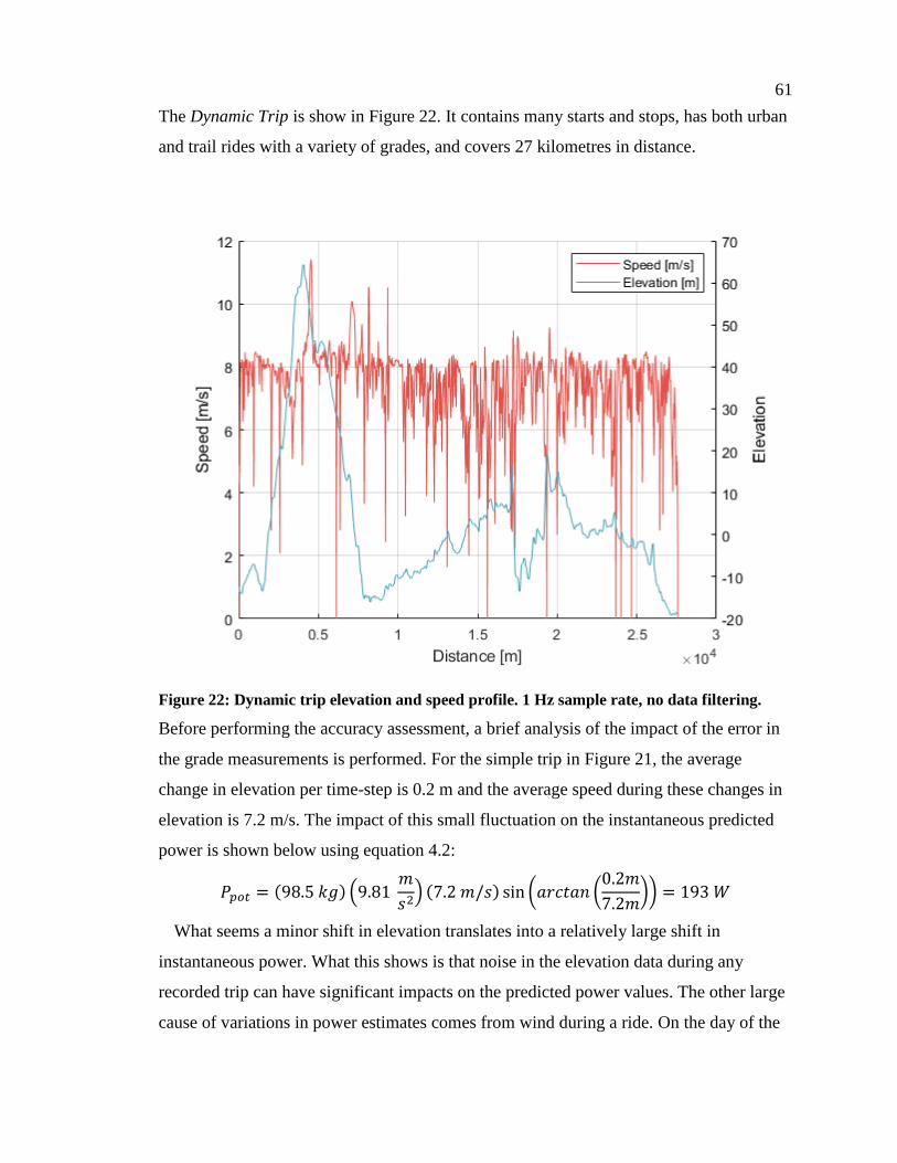
61

The Dynamic Trip is show in Figure 22. It contains many starts and stops, has both urban

and trail rides with a variety of grades, and covers 27 kilometres in distance.

Figure 22: Dynamic trip elevation and speed profile. 1 Hz sample rate, no data filtering.

Before performing the accuracy assessment, a brief analysis of the impact of the error in

the grade measurements is performed. For the simple trip in Figure 21, the average

change in elevation per time-step is 0.2 m and the average speed during these changes in

elevation is 7.2 m/s. The impact of this small fluctuation on the instantaneous predicted

power is shown below using equation 4.2:

𝑃𝑝𝑜𝑡 = (98.5 𝑘𝑔) (9.81 𝑚

𝑠2) (7.2 𝑚/𝑠) sin (𝑎𝑟𝑐𝑡𝑎𝑛 (

0.2𝑚

7.2𝑚)) = 193 𝑊

What seems a minor shift in elevation translates into a relatively large shift in

instantaneous power. What this shows is that noise in the elevation data during any

recorded trip can have significant impacts on the predicted power values. The other large

cause of variations in power estimates comes from wind during a ride. On the day of the

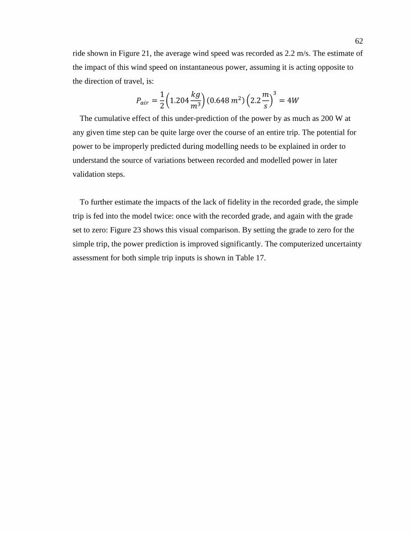
62

ride shown in Figure 21, the average wind speed was recorded as 2.2 m/s. The estimate of

the impact of this wind speed on instantaneous power, assuming it is acting opposite to

the direction of travel, is:

𝑃𝑎𝑖𝑟 =1

2(1.204

𝑘𝑔

𝑚3) (0.648 𝑚2) (2.2

𝑚

𝑠)

3

= 4𝑊

The cumulative effect of this under-prediction of the power by as much as 200 W at

any given time step can be quite large over the course of an entire trip. The potential for

power to be improperly predicted during modelling needs to be explained in order to

understand the source of variations between recorded and modelled power in later

validation steps.

To further estimate the impacts of the lack of fidelity in the recorded grade, the simple

trip is fed into the model twice: once with the recorded grade, and again with the grade

set to zero: Figure 23 shows this visual comparison. By setting the grade to zero for the

simple trip, the power prediction is improved significantly. The computerized uncertainty

assessment for both simple trip inputs is shown in Table 17.

63

Figure 23: Model power predictions for simple trip. Top shows prediction for recorded

grade, bottom shows prediction for grade artifically entered as zero for simple trip. Right

side shows distribution of predicted power error.

The dynamic trip is also run through the model with the same computerized uncertainty

analysis applied with the results reported in Table 16. For the simple trip, drag and

acceleration dominate, with the impacts of drag decreased due to the dynamic speed. For

the dynamic trip, the recorded power is within the total uncertainty boundaries for 84% of

all data points. For the simple trip with grade set to zero, the recorded power is within the

total uncertainty boundaries for 99% of all data points.

Table 16: Simply and Dynamic trip power prediction uncertainty contributions from each

variable. Mean power uncertainty (Mean Ci) as well as percentage of average predicted

power (Ci/P0) shown.

Variable Symbol Simple Dynamic

Mean Ci

[W]

Ci/P0 Mean Ci

[W]

Ci/P0

Total mass mT 2.83 1.52 % 10.0 4.80 %

Bearing Coef. B0 0.06 0.03 % 0.06 0.03 %

Bearing Coef. B1 0.05 0.02 % 0.05 0.02 %

64

Rolling Resistance

Coef.

CRR 6.80 3.66 % 6.91 3.40 %

Moment of Inertia Itotal 0.39 0.21 % 1.60 0.78 %

Drag Area CDA 21.10 11.3 % 23.9 11.70 %

Grade 𝑑𝑥𝑑𝑦⁄ 0.00 0.00 % 189 92.0 %

Velocity 𝑑𝑥𝑑𝑡⁄ 7.43 4.00 % 8.37 4.10 %

Acceleration 𝑑2𝑥𝑑𝑡2⁄ 113.04 60.8% 115 56.2 %

The acceleration has such a significant impact on the power uncertainty because it is

the product of several uncertainty terms (as seen in equation 4.7); the uncertainty from

velocity, from mass, from moment of inertia, are all multiplied to determine a final

uncertainty. This large uncertainty means that each time the E-bike starts and stops, the

power requirements associated with that are likely to have relatively low fidelity.

Next the prediction errors of the simple trip, with and without the recorded grade, along

with the dynamic trip, and the results of Dahmen et al’s use of the model, are displayed in

Table 17. There are several items to discuss regarding the discrepancy in model fidelity

between the work in this thesis and that of Dahmen et al’s work.

Table 17: Comparison of model prediction error for Simple trip with and without grade,

dynamic trip, and the results from Dahmen et al’s work.

Metric Simple Dynamic Dahmen et al

w/ grade w/o grade

Correlation coef. 0.50 0.71 0.63 0.98

Mean prediction error 28.4 W 21.6 W -15.0 W 4.9 W

STD prediction error 54.2 W 46.8 W 166.4 W 20.0 W

SNR 11.0 dB 12.5 dB 4.2 dB 19.7 dB

Percentage variation

explained

92.1% 98.9 % 62.4 % 98.9 %

Relative error of total

energy prediction

13.2 % 10.2 % -7.7 % -

The dynamic behaviour of the trips recorded, and the 1 Hz data sample rate of the

Garmin sensors means that some of the ride behaviour is likely not adequately

65

represented in the recorded data. Thus, when comparing the model to the actual ride,

there are gaps in the predicted power. Aside from the impacts of wind gusts, the

governing equation realistically describes all of the major factors that could impact power

requirements and so any major discrepancies between the two have to come to either

model variables not being accurate (drag area, rolling resistance, mass, etc.) or the time

series data not adequately capturing the true behaviour of the E-bike trips such that the

model can’t reproduce them.

Additional issues were noticed in dynamic rides between expected and recorded power

values. Figure 24 shows two instances of these power discrepancies. The first occurs

between 1095 and 1100 seconds; the E-bike sensors record an increase in speed, and

records a very minor positive grade, but also records no power output, whereas the model

predicts a large spike in required power to increase speed on what is recorded as

essentially level ground. The second discrepancy occurs between 1105 and 1115, where a

positive power is recorded by the sensor along with decreasing speed and decreasing

grade. The model for this second interval predicts no power required for what is

essentially someone slowing down while travelling downhill. These discrepancies happen

multiple times throughout most trips recorded during this project.

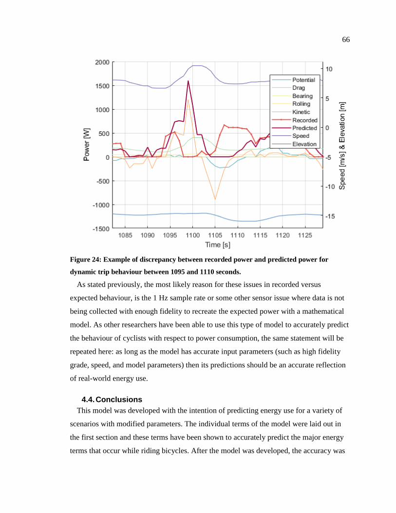
66

Figure 24: Example of discrepancy between recorded power and predicted power for

dynamic trip behaviour between 1095 and 1110 seconds.

As stated previously, the most likely reason for these issues in recorded versus

expected behaviour, is the 1 Hz sample rate or some other sensor issue where data is not

being collected with enough fidelity to recreate the expected power with a mathematical

model. As other researchers have been able to use this type of model to accurately predict

the behaviour of cyclists with respect to power consumption, the same statement will be

repeated here: as long as the model has accurate input parameters (such as high fidelity

grade, speed, and model parameters) then its predictions should be an accurate reflection

of real-world energy use.

4.4. Conclusions

This model was developed with the intention of predicting energy use for a variety of

scenarios with modified parameters. The individual terms of the model were laid out in

the first section and these terms have been shown to accurately predict the major energy

terms that occur while riding bicycles. After the model was developed, the accuracy was

67

assessed using data recorded from the CRD project. What this analysis showed was that

there is significant uncertainty in the predictions, primarily due to the uncertainty in the

recorded grade, as well as in the uncertainty in the mass and velocity as they impact the

acceleration term.

For the long dynamic trip, the recorded power was within the predicted uncertainty

boundaries for 84% of all data points. The correlation coefficient is low compared to the

work of Dahmen et al, (0.63 compared to 0.98 for Dahmen’s work), and the same holds

for the other comparative error metrics. Future predictions using the model are to be used

to quantify the impacts of Exro’s intellectual property, and to quantify the energy use of

E-bikes in response to variations in loading, human power contributions, motor power

contributions, and geographic topology. The model itself isn’t inherently flawed but

rather the use of data recorded during the CRD trial has limitations. For later use of the

model in this thesis, the caveat must be attached that the model can predict the energy use

an E-bike with high fidelity as long as it is assumed that the input data is truthful.

For future work, it would benefit any modelling efforts to have a higher resolution of

recorded data if dynamic power modelling is required. A 1 Hz sample rate can still miss

out on important behaviour under dynamic riding conditions. Recording grade with

higher fidelity would also have a significant impact on the ability of the model to

accurately predict the E-bike behaviour. The Garmin device used in this study measured

changes in grade with a barometric pressure sensor which has a relatively high

uncertainty. This was chosen over more accurate sensor options for two primary reasons:

the actual magnitude of the grade uncertainty of consumer grade Garmin cycling

computers is not published anywhere so the magnitude of the uncertainty was not known

prior to deployment, additionally, more accurate options for grade measurement were not

consumer/end-user friendly and so were removed from consideration by CRD staff. In

hindsight, a more accurate sensor with a known uncertainty should have been purchased

for laboratory data collection sessions and for quantification of the Garmin Edge 520

grade uncertainty.

68

5. Analysis

This section contains several independent analysis subsections that use the riding data

from Chapter 2 as well as the bike drivetrain model from Chapter 4. The first set of

analysis and results presented in Section 5.1 details the extraction of typical human

energy contributions while riding an E-bike from the CRD Project. Section 5.2 explores

the impacts of Exro’s technology for reducing energy use in response to real-world duty

cycles taken from the CRD project. Section 5.3 quantifies the emissions and costs of the

CRD project so that fleet managers or other commercial organizations can better

understand the capabilities and optimal role for E-bikes in their fleet. Section 5.4

quantifies the energy use that occurs when E-bikes are used for urban delivery of cargo

by combining the CRD trip data with the mathematical model.

5.1. Human Energy Contributions

The typical human energy contributions that occur while riding an E-bike are important

because they allow for later analysis to model larger motors while still maintaining

expected human behaviour. This section estimates the human power contributions that

occurred during the CRD project by using the governing equation (equation 4.7)

presented in Chapter 4, along with Equation 5.1 which shows the relationship between

human power (�̇�ℎ) and motor power (�̇�𝑚) as a function of assist level (A = [0.5, 1.20,

1.90, 2.75]).

�̇�𝑚 = 𝐴�̇�ℎ (5.1)

This analysis follows a similar format to that of Chapter 3 but without any human or

electrical energy conversion efficiencies as the analysis is not interested in emissions,

only in the energy or power output by the rider at the pedals or from the motor and not

from a wall outlet or in terms of calories consumed. Drive train efficiency losses are

included as the modelled power is located at the output of the rear wheel.

Figure 25 shows the range of human power contributions during the CRD data as they

vary with speed and different assist levels. This figure was created by sorting the time

series recorded power data from the CRD project into speed bins. Within each speed bin,

the power was averaged (not including zero values). The assist varies from a factor of A

= 0.5 up to 2.75, matching the capabilities of the Norco E-bike used in the CRD Project.

69

Figure 25: Human power contributions using Equation 5.1 and CRD trip data for a variety

of assist factors.

The removal of assist as the rider approaches 32 kph was modelled by using a linear

decrease of the assist level starting at 27 kph and decreasing linearly to A = 0 at 32 kph.

The Bosch E-bike system was observed to decrease assist as the rider approached max

speed rather than maintain assist right up to the maximum speed and then drop off

suddenly. In reality, as the limited speed is approached, the assist factor drops to zero and

motion relies only on human power. When CRD staff were queried during the data

collection phase regarding which level of assist they most often used, the majority of the

17 participants responded that they most often ride on maximum assist (A = 2.75). Figure

25 supports this: if the riders weren’t using maximum assist, the level of human power

output for the other levels of assist (A = 0.5, 1.20, 1.90) wouldn’t be likely to decrease as

dramatically when passing the cut-off speed.

This binning process was repeated to generate Figure 26 but now only with the power

data that was recorded with a grade between negative 2% and positive 2%. The results of

70

this process are used to compare with the results of an external study: Langford et al

recorded an average human power contribution of 62 W at approximately 20 kph while

on level ground while using a maximum level of assist on an E-bike. The assist level in

the Langford et al research is not known but the results are very similar to the value

shown in Figure 26 at 20 kph, which is approximately 60 W at maximum assist and

relatively level ground.

Figure 26: Human power contributions using Equation 5.1 and CRD trip data for a variety

of assist factors with impact of grade removed.

The next stage of analysis was an attempt to investigate whether human power could be

modelled as a function of speed and grade. This was initially investigated by modelling a

surface fit to the aggregated power recorded during all of the CRD trips. This surface fit,

along with the individual data points is shown in Figure 27. While some initial trends can

be seen, such as speed decreasing as grade increases, the corresponding power did not

show any such consistency. The lack of clear correlations while plotting the data, seemed

to hint at other data points not recorded during the empirical campaign that may have

71

allowed for more in-depth investigation of these connections. The surface fit doesn’t

reflect the large variations in power observed at any given grade and speed; as much as

300 watts variation is regularly seen at any given grade and speed state. In addition, there

is little to no data in the high-speed high-torque region provide more uncertainty to

determining the relationship between variables.

Figure 27: Surface fit and scattered data of all recorded CRD trip power plotted against the

speed of the E-bike and the decimal % grade of the roadway.

5.2. Exro Duty Cycle Response

This section outlines the methods and results of applying the Exro efficiency maps to

the CRD duty cycle data. The analysis is completed by stepping through the time series

CRD data, and at each time-step, comparing the series and parallel efficiency in response

to the current time-step RPM and torque state. This process is repeated for the four

different electric assist factors: A = 0.5, 1.20, 1.90, 2.75. Where the motor power

demands are determined using the relationship between human, motor, and total power:

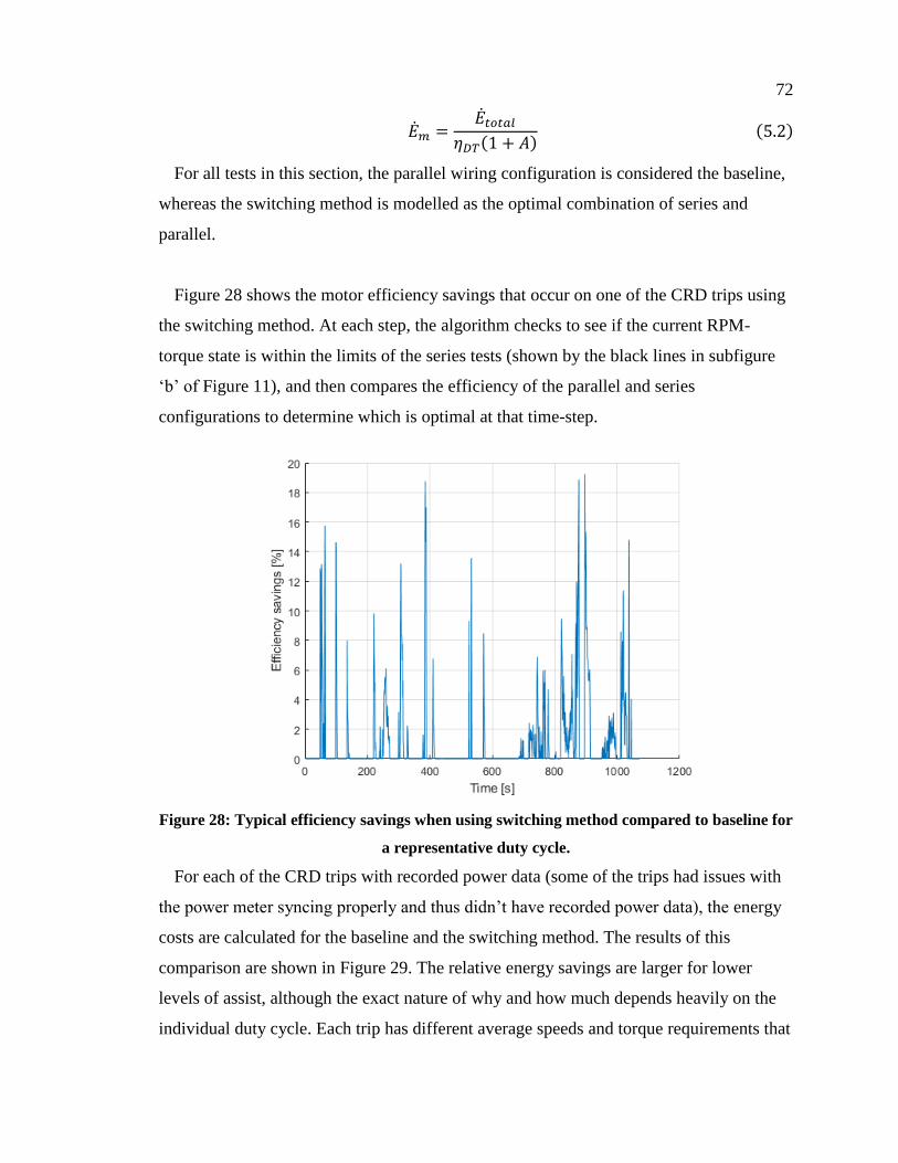
72

�̇�𝑚 =�̇�𝑡𝑜𝑡𝑎𝑙

𝜂𝐷𝑇(1 + 𝐴) (5.2)

For all tests in this section, the parallel wiring configuration is considered the baseline,

whereas the switching method is modelled as the optimal combination of series and

parallel.

Figure 28 shows the motor efficiency savings that occur on one of the CRD trips using

the switching method. At each step, the algorithm checks to see if the current RPM-

torque state is within the limits of the series tests (shown by the black lines in subfigure

‘b’ of Figure 11), and then compares the efficiency of the parallel and series

configurations to determine which is optimal at that time-step.

Figure 28: Typical efficiency savings when using switching method compared to baseline for

a representative duty cycle.

For each of the CRD trips with recorded power data (some of the trips had issues with

the power meter syncing properly and thus didn’t have recorded power data), the energy

costs are calculated for the baseline and the switching method. The results of this

comparison are shown in Figure 29. The relative energy savings are larger for lower

levels of assist, although the exact nature of why and how much depends heavily on the

individual duty cycle. Each trip has different average speeds and torque requirements that

73

alter the effectiveness of the switching method. In some cases, relative energy use can be

reduced by as much as 8% but this was typically restricted to shorter trips.

Figure 29: Histogram of relative efficiency savings per-trip provided by switching method

relative to baseline. Each figure shows different assist factor.

For most of the trips, the majority of the energy use occurs at high speeds (see section

2.2.1). As the assist factor is increased, the torque required from the motor also increases,

which causes the average optimal operating state to more strongly favour the parallel

configuration. Since the parallel configuration is the baseline, this means that higher

assist factors don’t result in very significant energy savings when using the switching

method.

The absolute energy savings are summarized in Figure 30. This gives further clarity as

to the fact that each trip’s exact torque and RPM demands vary, such that trip distance

isn’t directly indicative of total energy savings. The energy savings are determined by the

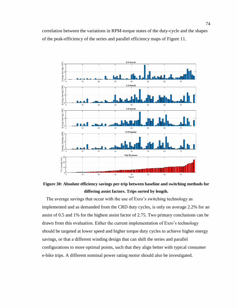
74

correlation between the variations in RPM-torque states of the duty-cycle and the shapes

of the peak-efficiency of the series and parallel efficiency maps of Figure 11.

Figure 30: Absolute efficiency savings per-trip between baseline and switching methods for

differing assist factors. Trips sorted by length.

The average savings that occur with the use of Exro’s switching technology as

implemented and as demanded from the CRD duty cycles, is only on average 2.2% for an

assist of 0.5 and 1% for the highest assist factor of 2.75. Two primary conclusions can be

drawn from this evaluation. Either the current implementation of Exro’s technology

should be targeted at lower speed and higher torque duty cycles to achieve higher energy

savings, or that a different winding design that can shift the series and parallel

configurations to more optimal points, such that they align better with typical consumer

e-bike trips. A different nominal power rating motor should also be investigated.

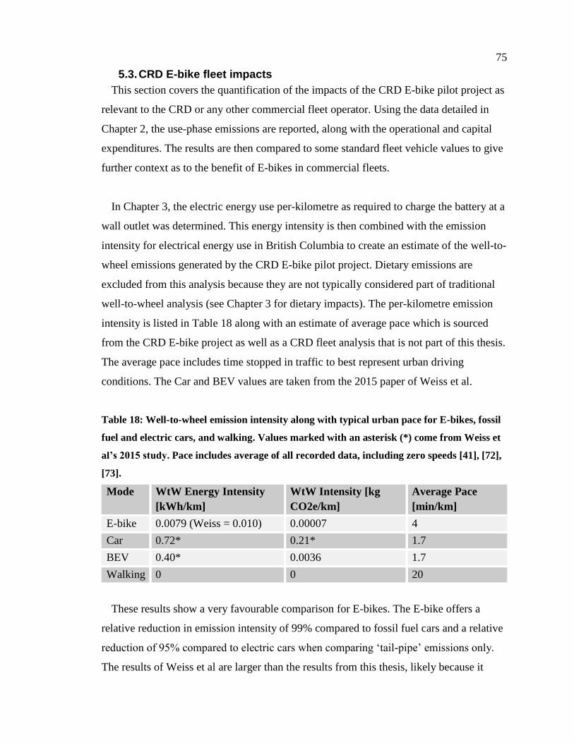
75

5.3. CRD E-bike fleet impacts

This section covers the quantification of the impacts of the CRD E-bike pilot project as

relevant to the CRD or any other commercial fleet operator. Using the data detailed in

Chapter 2, the use-phase emissions are reported, along with the operational and capital

expenditures. The results are then compared to some standard fleet vehicle values to give

further context as to the benefit of E-bikes in commercial fleets.

In Chapter 3, the electric energy use per-kilometre as required to charge the battery at a

wall outlet was determined. This energy intensity is then combined with the emission

intensity for electrical energy use in British Columbia to create an estimate of the well-to-

wheel emissions generated by the CRD E-bike pilot project. Dietary emissions are

excluded from this analysis because they are not typically considered part of traditional

well-to-wheel analysis (see Chapter 3 for dietary impacts). The per-kilometre emission

intensity is listed in Table 18 along with an estimate of average pace which is sourced

from the CRD E-bike project as well as a CRD fleet analysis that is not part of this thesis.

The average pace includes time stopped in traffic to best represent urban driving

conditions. The Car and BEV values are taken from the 2015 paper of Weiss et al.

Table 18: Well-to-wheel emission intensity along with typical urban pace for E-bikes, fossil

fuel and electric cars, and walking. Values marked with an asterisk (*) come from Weiss et

al’s 2015 study. Pace includes average of all recorded data, including zero speeds [41], [72],

[73].

Mode WtW Energy Intensity

[kWh/km]

WtW Intensity [kg

CO2e/km]

Average Pace

[min/km]

E-bike 0.0079 (Weiss = 0.010) 0.00007 4

Car 0.72* 0.21* 1.7

BEV 0.40* 0.0036 1.7

Walking 0 0 20

These results show a very favourable comparison for E-bikes. The E-bike offers a

relative reduction in emission intensity of 99% compared to fossil fuel cars and a relative

reduction of 95% compared to electric cars when comparing ‘tail-pipe’ emissions only.

The results of Weiss et al are larger than the results from this thesis, likely because it

76

appears the work of Weiss et al includes Chinese lead-acid battery type E-bikes but they

are still relatively close in magnitude. The near complete reduction in use-phase

emissions observed in the CRD project only comes at the cost of being two times slower

than a car during travel. This doesn’t account for the time required to find parking in an

urban environment which could shift the accounting more in favour of E-bikes because of

the simplicity and availability of bicycle parking. Walking reduces emissions over E-

bikes, but E-bikes already represent a tiny fraction of the emissions of fossil fuel and

electric cars such that the trade-offs between pace and emissions aren’t as worth-while.

Using the total kilometres logged during the CRD E-bike project (607 km), an estimate

of the total use-phase emissions from the E-bikes is accounted for and presented in Table

19, along with an estimate of the same distance covered by the car and BEV detailed in

Table 18.

Table 19: CRD Project well-to-wheel emissions for E-bikes compared to CRD ICE and BEV

sedans. A total of 607 km were logged during the CRD project.

Mode CRD Project Emissions

[kg CO2e]

E-bike 0.08

Car 127

BEV 4.2

The other metric of importance is the financial costs for each of these modes. While

electric cars reduce tailpipe emissions versus the traditional fossil fuel car by nearly 95%,

they cost significantly more than E-bikes. The financial costs of the E-bikes were detailed

by the CRD staff and are summarized in Table 20. E-bike values were sourced from the

CRD project and includes safety equipment for users added security features and added

storage such as panniers and baskets on the E-bike. The operation costs also include

regularly schedule maintenance and a estimate of annual parts replacement costs (tires,

drivetrain, etc.). It does not include training costs for users or parking requirements for

the E-bikes (such as secured storage, charging infrastructure, etc.) as these can vary quite

widely from one organization to the next and are not included in the car ownership costs.

77

Table 20: E-bike, fossil fuel and electric car capital and operational costs per vehicle

representing ownership over 5 years [74]–[76].

The vehicle values assume annual travel of 10,000 km, which is a low value for a

commercial fleet but is meant to make it more comparable to the E-bike with respect to

short urban trips. It includes maintenance, license and registration fees, insurance costs,

and upfront vehicle cost. Vehicle capital costs are sourced from brand websites, and the

operating costs are sourced from the CAA online car costs calculator.

A brief analysis of the savings potential of using E-bikes over ICE light-duty vehicles

is done by investigating the impacts of switching 1% of trips within the CRD LDV fleet

over to E-bikes. If the assumption continues, that each LDV in the CRD fleet travels an

average of 10,000 km per year, and the emission factors from Table 18 are used for each

respective mode, then the emission reductions per one percent of annual kilometres

travelled can be estimated. This is done by multiplying the average annual distance

(10,000km) by the number of LDV vehicles in the CRD fleet (158) and by the emission

intensity of the average LDV:

𝐴𝑛𝑛𝑢𝑎𝑙 𝐿𝐷𝑉 𝑒𝑚𝑖𝑠𝑠𝑖𝑜𝑛𝑠 = 158 𝐿𝐷𝑉 × 𝑃𝑒𝑟 𝐴𝑛𝑛𝑢𝑚 𝑘𝑚 × 0.21 𝑘𝑔𝐶𝑂2𝑒

𝑘𝑚= 330 𝑡 𝐶𝑂2𝑒

Using E-bikes for one percent of total annual kilometres would result in each vehicle

being replaced by an E-bike for 100 km of its total annual use. This in turn would result

in a fleet wide savings of 3 t CO2e compared to the total fleet emissions estimate of 33 t

Mode Capital Costs

[$CAD]

Operational Costs

[$CAD]

Total

[$CAD]

E-bike 4,400 1,730 6130

Chevrolet

Malibu

22,295 14,000 36295

Kia Soul EV 35,895 8,300 44195

78

CO2e. The emission reduction would occur alongside a total cost of ownership reduction

of approximately $30,000 when replacing an ICE sedan.

While the type of trips the E-bikes are typically used for (detailed in Section 2.2.2) do

not cover the entire range of trip distances covered by traditional cars, for a smart fleet

planner, E-bikes open up a new category of technology that is optimal for short urban

single occupancy trips. Larger vehicles will still be needed but when appropriate, E-bikes

offer a virtual elimination of use-phase emissions as accounted for by the fleet, as well as

an 83% and 86% cost reduction over a five-year operating period when compared to a

typical CRD fleet car and electric car respectively.

5.4. Cargo Bike Assessment

This section details the methods and results of varying the mass of the governing

equation to simulate cargo scenarios for an E-bike. Most commercially available cargo

style bicycles are rated to carry up to 200kg in addition to the rider’s weight. The analysis

is performed by altering the total vehicle mass and the drag area value to simulate a cargo

style E-bike, and then running through all of the CRD trips to determine averaged energy

intensity, motor size recommendations, and other metrics.

When the analysis explores the increased energy requirements under high loads, the

impact that these increased loads and motor power capabilities have on trip

characteristics (speed, acceleration) are not accounted for in this work. In the real-world,

cargo trip characteristics would likely be very different. The typical speeds a rider would

choose to travel at while hauling heavy loads is not explicitly known in this work since

the CRD project covers only the rider and E-bike at much lighter loads (load mass of

around 0-10kg in addition to the rider). While this lack of info could cause problems, it is

claimed that under ideal conditions, the power supplied by the human would remain

similar between both cases with the motor supplied power making up the difference to

allow for similar travel speeds. This claim is made because when considering urban E-

79

bike cargo travel, being able to travel at maximum speeds would allow for the optimal

use of these vehicles.

Table 21: Modified model input variables for assessing E-bike cargo performance.

Variable Value

E-bike mass 45 kg

Load mass range 50-200 kg

Drag Area (CDA) 0.712 m2

The model governing equation (equation 4.7) along with the motor assist relationship

of equation 5.1 are used with a load mass of 0 kg to determine the baseline human power

contributions for all recorded trips using the CRD data.

The governing equation is then run again using a range of mass values from Table 21

(m = 50kg, 100kg, 150kg, 200kg) to determine total system power requirements. The

drag area of the cargo E-bike is assumed to be 10% more than that of a standard E-bike to

reflect the bluntness of a typical cargo box. The final motor power requirements are then

determined by subtracting the baseline human power contributions from the total system

requirements.

This process is repeated for each time-series trip recorded during the CRD project. The

impacts on energy are summarized in Table 22.

Table 22: Cargo E-bike motor energy requirements for varying loads

Load 0 kg 50kg 100kg 150kg 200kg

Motor Energy Intensity [Wh/km] 6.7 8.7 10.7 12.9 15.0

Range with 500 Wh battery [km] 65 50 40 34 29

System mass increase over no load [%] 0 42 84 126 168

Increase in energy intensity relative to

baseline [%]

0 30 60 93 124

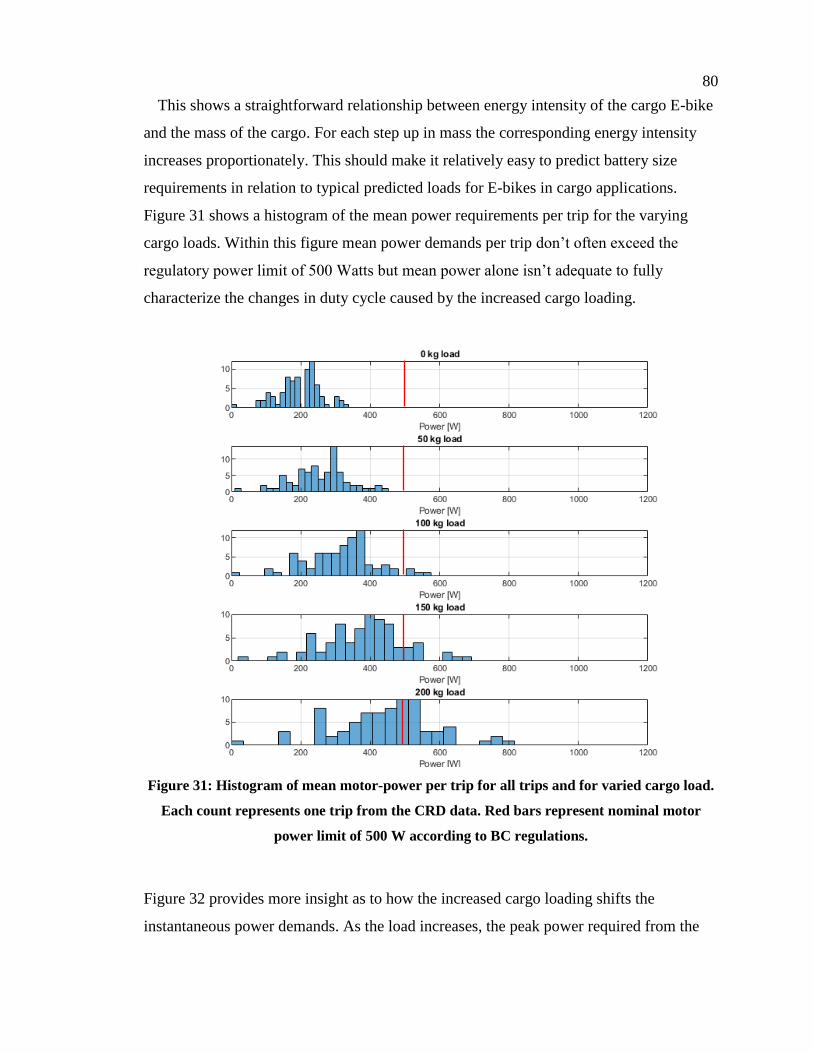
80

This shows a straightforward relationship between energy intensity of the cargo E-bike

and the mass of the cargo. For each step up in mass the corresponding energy intensity

increases proportionately. This should make it relatively easy to predict battery size

requirements in relation to typical predicted loads for E-bikes in cargo applications.

Figure 31 shows a histogram of the mean power requirements per trip for the varying

cargo loads. Within this figure mean power demands per trip don’t often exceed the

regulatory power limit of 500 Watts but mean power alone isn’t adequate to fully

characterize the changes in duty cycle caused by the increased cargo loading.

Figure 31: Histogram of mean motor-power per trip for all trips and for varied cargo load.

Each count represents one trip from the CRD data. Red bars represent nominal motor

power limit of 500 W according to BC regulations.

Figure 32 provides more insight as to how the increased cargo loading shifts the

instantaneous power demands. As the load increases, the peak power required from the

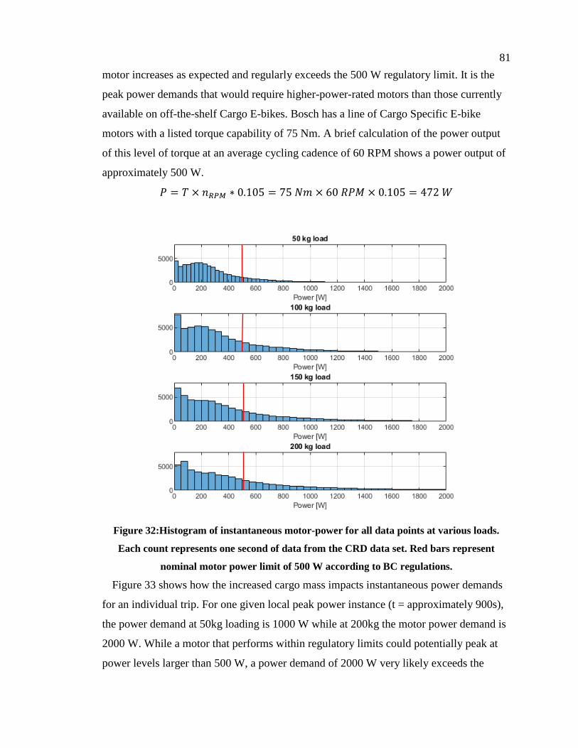
81

motor increases as expected and regularly exceeds the 500 W regulatory limit. It is the

peak power demands that would require higher-power-rated motors than those currently

available on off-the-shelf Cargo E-bikes. Bosch has a line of Cargo Specific E-bike

motors with a listed torque capability of 75 Nm. A brief calculation of the power output

of this level of torque at an average cycling cadence of 60 RPM shows a power output of

approximately 500 W.

𝑃 = 𝑇 × 𝑛𝑅𝑃𝑀 ∗ 0.105 = 75 𝑁𝑚 × 60 𝑅𝑃𝑀 × 0.105 = 472 𝑊

Figure 32:Histogram of instantaneous motor-power for all data points at various loads.

Each count represents one second of data from the CRD data set. Red bars represent

nominal motor power limit of 500 W according to BC regulations.

Figure 33 shows how the increased cargo mass impacts instantaneous power demands

for an individual trip. For one given local peak power instance (t = approximately 900s),

the power demand at 50kg loading is 1000 W while at 200kg the motor power demand is

2000 W. While a motor that performs within regulatory limits could potentially peak at

power levels larger than 500 W, a power demand of 2000 W very likely exceeds the

82

capabilities of any E-bike motor that meets regulatory guidelines of 500 W nominal

power. Figure 31 through Figure 33 show the nature of motor power demands, and that in

order to increase cargo loads simply adding a larger battery with existing motor power

levels (500 W nominal) would require either a significant increased human power

contribution or increased travel time due to decreased speeds.

Figure 33:Time-series human and motor power demands from model for an individual trip

recorded from CRD data.

The British Columbia Motor Assisted Cycle Regulation dictates that E-bike electric

motors must have continuous power output ratings that in total do not exceed 500 watts.

83

This contrasts with how existing E-bike motors are marketed based on power and torque.

The current line up of Bosch branded E-bike motors, show capabilities of up to 75 Nm of

torque and over 120 RPM. This would equate to power peak power outputs of nearly

1000 watts which is well over the ‘continuous power’ output rating of the BC Act, but

still falls short of the peak power demands seen under modelling scenarios as shown in

Figure 33. In the USA, E-bike motors are regulated to have a continuous power output of

no more than 750 watts while the European Union limits most E-bikes to 250 watts

continuous rated power. With the European market being dominant in terms of sales, the

EU regulations appear to be driving a large share of big brand E-bike retailers to limit

their motor power outputs to the lower end of the range of international regulations. Since

continuous power output of an electric motor isn’t currently tested by regulators on a

large scale, nor is “continuous rated power output” defined explicitly within regulations,

most E-bike manufacturers appear to use their motors across multiple markets with only

the speed governor adjusted to match local regulations.

Due to the relatively small cost per unit of E-bikes (as compared to cars) and the large

volume of sales, audits to ensure they meet power and speed restrictions would be

difficult to accomplish without significant cost and administrative burden. This could

have the impact of increasing the barrier to entry in the market for small to medium

enterprises attempting to sell E-bikes. End-users of cargo E-bikes are also feeling the

impact of inadequate regulation. For example, UPS has currently deployed custom made

E-bikes for cargo transport in Toronto but is limited to a specific campus as they operate

outside existing regulations due to their power ratings [77]. UPS and other logistics and

delivery companies are seeing the benefit of this type of mobility for urban delivery but

are currently facing regulatory challenges that are severely limiting their potential.

To properly support E-bikes for cargo hauling, Provincial regulators should adjust

current power limitations and clearly define average power versus peak power within the

regulations. Any power limits should be based on some defensible rationale arising from

safety or other concerns, which requires further research to avoid arbitrary limits

impacting the positive rollout of E-bikes for various applications. The limitation on

84

maximum assisted speed of 32 kph does not seem to have a significant impact on the

pace of E-bikes in urban environments. As shown in Table 18, the average pace of E-

bikes isn’t dramatically less than cars, and in addition, cargo delivery via E-bike is likely

to improve the comparison because of the ease with which bikes and E-bikes can park in

dense urban environments.

5.5. Analysis Conclusions

The analysis in this chapter was done to answer some aspects of the thesis questions as

set out in Chapter 1, namely, how does electric assist augment the physical performance

of bicycles and what are the optimal roles for an electric assist bicycle. The results of

Section 5.1 shows that electric assist allows riders to travel at relatively high speeds for a

bicycle without putting in significant human power. In addition, the impact of grade on

human power contributions appears to be quite small when using an E-bike; the

difference between maximum assist power in Figure 25 and Figure 26 is approximately

10 W over all speeds.

The ability of Exro’s technology, as assessed in Section 5.2, shows promise in

improving the performance of E-bikes as implemented, but would be better suited to the

demands of cargo E-bikes rather than typical commuter E-bikes due to the higher torque

demands of cargo hauling applications. The series configuration peak efficiency as

currently implemented is outside of most of the CRD trip typical RPM and torque states.

The most favourable results show the switching method saving up to 8% of energy use.

Section 5.3 showed significant environmental and cost savings when E-bikes are used

in commercial fleets for urban trips. Previous chapters detailed the specific duty-cycle

characteristics (Section 2.2.2) and while the sample size and restriction of data to the

Victoria region will restrict the transferability of the results, it is argued that the results

still represent a sample of typical urban e-bike trips and so can be relied on as an initial

assessment of this type of transportation. This Chapter showed that E-bikes can reduce

corporate fleet emissions practically to zero. When compared to a typical sedan as seen in

the CRD fleet, the E-bikes are also able to reduce the capital and operating costs over a

five-year period by nearly 80%. The typical pace of urban trips for both E-bikes and cars,

85

as listed in Table 18, shows that E-bikes can compete with cars over short trips in urban

environments in terms of travel time.

The application of E-bikes for cargo use is currently limited by Federal regulations that

restrict continuous motor power to 500 W. Existing Federal and Provincial regulations

also restrict cargo e-bikes to “not have more than three wheels in continuous contact with

the ground” which presents further barriers to the role of cargo E-bikes. In order to

achieve optimal speeds with an E-bike for cargo, motor power limits should be increased

while still keeping existing speed limits in place.

Electric assist augments the performance of E-bikes, allowing riders to travel faster and

with less work than on a comparable bicycle. Grade doesn’t appear to have a significant

impact on the speed of E-bikes. The dominant factor that appears to be affecting E-bike

speed is the cut-off speed at which the motor stops applying assistive power: 32 kph.

After this point all power comes from the human rider. The optimal role for E-bikes is

urban trips where traffic and parking are restricting effective car use and where

organizations which to reduce emissions and costs associated with fleet vehicle use.

86

6. Conclusions

6.1. Summary of Work

This thesis set out to determine how electric assist alters the environmental impacts and

physical performance of bicycles, as well as attempting to determine some of the optimal

roles for E-bikes. All analysis in this thesis was performed using MATLAB alongside

custom functions written by the author.

The first stage of this research was a characterisation of the baseline environmental

performance of E-bikes and comparative performance of other major modes of urban

transportation (car, BEV, bus, bicycle). This was achieved by synthesizing existing

literature to form a baseline, which was then expanded to include the upstream emissions

associated with human supplied mechanical power. The upstream emissions were

integrated into the results of existing LCA analysis to determine new estimates on the

range of life cycle emissions that could occur under a variety of scenarios based on

dietary variation (low to high meat consumption in two regions) and grid emission

intensity.

The estimate of human power contributions during E-bike use was derived from

empirical data obtained during the CRD E-bike trial that consisted of 17 participants and

over 600km of recorded data. This data was collected over the course of four months and

in partnership with the CRD staff as part of their Zero Emission Fleet Initiative and

captured dynamic trip characteristics due to topology and speed. This data was also used

to develop and calibrate a mathematical model that can estimate power requirements of

an E-bike or bicycle when given road grade and speed time-series data.

Once the empirical data was collected and the model calibrated, several sets of analyses

were performed. The first was an attempt to derive further insight into the human power

contributions that occurred during the CRD trial. This involved applying the range of

assist factors available to the E-bike riders during the trial, and cross comparing the

instantaneous human power to the recorded grade and speed to see if there were any

obvious correlations between these metrics.

The next was the cross comparison of the Exro switching technology efficiency maps

with the CRD data. This was an attempt to see if the current iteration of Exro’s

87

technology showed benefits in response to the typical duty cycles observed within the

CRD data. Each recorded trip in the CRD data set, was fed assessed using the Exro

efficiency maps, assuming that the two Exro motor configurations could be switched

between on-demand.

An assessment of the CRD trial was performed. This included an environmental

assessment using earlier determined emissions intensities. It also looked at the total cost

expenditures associated with the use of E-bikes in the CRD fleet over a five-year time

period, as mentioned as the expected lifetime of the E-bikes in the CRD fleet.

The final analysis combined the mathematical model with the CRD speed and route

topology to predict energy and power requirements of a Cargo E-bike if it were used

during the CRD trips. The load was varied for several rounds of analysis from a baseline

of no load up to 200 kg.

6.2. Results

All of these steps of analysis and evaluation have presented a fulsome

characterisation of E-bikes in urban settings under a variety of applications.

Exro Data Collection and Performance Analysis

The performance characterisation of an E-bike with and without Exro Technology’s

‘switching’ technology showed promise as a means of improving energy efficiency of

rear-hub E-bike motors. By altering the wiring configuration of an E-bike motor on the

fly, Exro’s technology has the potential to reduce energy use by offering different

efficiency profiles across RPM and torque states. While in the series wiring

configuration, the motor is able to improve efficiency in low RPM states, while the

parallel wiring configuration has optimal efficiency in high RPM states. While the

absolute efficiency differences between the two configurations was on average 4%, the

technology shows promise and as currently implemented would likely best be suited to

operations that have high torque during low RPM states, such as cargo E-bikes where

loads can be up to 200kg.

Exro’s technology also showed measurable, but small, efficiency improvements when

applied to the CRD trip data. In contrast to the efficiency savings of Exro’s technology

occurring most prominently at low speeds, the majority of energy use during bicycle trips

88

occurs at high speeds. Improvements to Exro’s technology could be to either design new

wiring configurations that more effectively target high RPM efficiency improvements or

to use the existing configuration for low speed applications such as cargo hauling.

CRD Data Collection

The CRD E-bike trial provided a more in-depth insight into the energy and power

characteristics of urban E-bike use than previous studies. From this data, the power

results showed that the riders appeared to have no issues with achieving trips of at least

10km with no significant reductions in total power output (rider + motor). Across all 17

riders, and all trips, average power was relatively consistent with the standard deviation

representing only 30% of the mean. The average power output across all trips was

approximately 240 W and the average trip energy intensity was 7.8 Wh/km. This is an

increase of approximately 20-30% more energy than traditional bicycles under similar

urban conditions.

Additional analysis of the CRD data showed that E-bikes offered significant

improvements in total ownership costs, on the order of tens of thousands of dollars, when

trips can be appropriately substituted by E-bikes. The correct trips would be those in

urban environments with a distance of approximately 10 km or less. The CRD E-bike

deployment was also able to avoid approximately 120 kg of CO2 equivalent emissions

through reducing car use. This reduction in costs also compares favourably to BEVs: the

cost per kg of CO2e abated for E-bikes is dramatically decreased when compared to BEVs

even though both offer similar emission reductions to corporate fleets. In addition, the E-

bikes don’t require expensive charging infrastructure as E-bikes can be charged at any

standard wall outlet.

Emissions and Energy Use

Chapter 3 of this thesis showed how the GHG emissions associated with the use of E-

bikes can vary when increasing the scope of a typical LCA to include upstream emission

associated with human supplied mechanical power. The impact was dependent on the

level of direct attribution between energy expenditure (EE) while cycling and energy

intake (EI) in the form of food; if a rider maintains constant mass, and it is assumed the

89

rider does not reduce other physical activities to conserve total energy, then the rider

must consume more food to balance their energy expenditure and energy intake. Chapter

3 details more of the arguments surrounding this point, and the results show the full range

of attribution: from zero increase in EI in response to an increase in EE, to a full

attribution of EI equaling EE. Under a full attribution scenario, with a meat-like diet and

clean electricity, E-bikes can offer a 50% reduction in emission intensity compared to

bicycles. This is in addition to the multitude of other benefits presented by E-bikes in the

literature review of Chapter 1. While E-bikes reduce the level of physical exertion,

typical assist levels have been shown to still provide daily recommended levels of

physical activity.

Mathematical Model

The work in this thesis reinforced the importance of high-fidelity road grade data when

using this mathematical model of bicycle energy use. Slight variations in recorded road

grade resulted in large variations in predicted power output by the model. The model

struggled to accurately predict the power requirements of most CRD trips. This was due

to lack of fidelity in the grade recordings. When used to predict the power of rides on a

level surface, the model showed estimates that were in-line with the use of the model in

other work.

The model was used to predict energy requirements for cargo E-bikes using the trips

recorded during the CRD campaign. The results showed that existing E-bike regulations

(in BC, the USA and EU) would likely restrict the effective use of E-bikes for heavy

cargo applications of around 200 kg. While average power requirements from the

modelling showed as being roughly in line with regulatory limits, it was the peak power

demands that dramatically exceeded what would be capable on E-bikes within existing

regulations. The recommendations from this modelling are that regulations be reviewed

to allow for increased power limits while still maintaining speed controls.

6.3. Future Research

Future work base on this thesis could be directed in a number of different directions.

The first would be to compare the CRD E-bike data with a more fulsome data set

containing typical car and BEV duty cycles and usage rates. This would allow for a better

90

understanding as to what proportion of trips within a corporate fleet are able to be

substituted by E-bikes. This type of comparative analysis would be more beneficial to

fleet managers when trying to plan future fleet vehicle acquisitions.

The second major action would be to set up E-bike trials that includes both a rear-hub

power meter as well as a pedal-based power meter. This would provide full quantification

of human power and motor power contributions while riding in a variety of cases.

Additionally, a higher fidelity road grade sensor would make a large difference in

validating the abilities of the mathematical model to predict power requirements. With a

more detailed data set and calibrated experimental data, additional rationalized

recommendations for updating Provincial and Federal regulations for E-bikes, and E-

cargo bikes in particular, could be formulated.

An additional line of work could look into safety and health impacts of E-bikes.

Quantification of health benefits alongside GHG emissions could buttress the financial

arguments in favour of E-bikes, mitigated by studies into associated crash risk. Along the

same lines, an investigation of the safety ramifications of the 3 wheel Federal and

Provincial limit, relative to allowing 4 wheeled electric assisted cycles, would be

informative for the E-cargo bike space for carrying heavier loads through a range of road

and weather conditions.

91

‘Bibliography

[1] E. Fishman and C. Cherry, “E-Bikes in the Mainstream: Reviewing a Decade of

Research,” Transp. Rev., vol. 36, no. 1, pp. 72–91, Jan. 2016.

[2] BionX Canada Sells off Parts of Its Business. .

[3] World Urbanization Prospects - Population Division - United Nations. .

[4] Table 1 The More Suburban the Neighbourhood, the More Time People Spent in a

Car on the Reference Day. .

[5] E. A. de Vasconcellos, Urban Transport, Environment, and Equity: The Case for

Developing Countries. Earthscan Publications, 2001.

[6] T. Litman, “Transportation Land Valuation: Evaluating Policies and Practices That

Affect the Amount of Land Devoted to Transportation Facilities.,” Victoria

Transport Policy Institute, Jan. 2012.

[7] “Climate Change 2014 - Synthesis Report,” Intergovernmental Panel on Climate

Change, 2014.

[8] CAIT Climate Data Explorer. .

[9] E. and C. C. C. Government of Canada, ARCHIVED - Environment and Climate

Change Canada - Sustainable Development - Addressing Climate Change and Air

Quality, Goal 1: Reducing Greenhouse Gas Emissions, Reducing Canada’s

Greenhouse Gas Emissions. 2012.

[10] Anonymous, Transport Emissions. 2016.

[11] J. Hong, “Non-Linear Influences of the Built Environment on Transportation

Emissions: Focusing on Densities,” J. Transp. Land Use, vol. 10, no. 1, pp. 229–

240, 2017.

[12] J. Woo, H. Choi, and J. Ahn, “Well-to-Wheel Analysis of Greenhouse Gas

Emissions for Electric Vehicles Based on Electricity Generation Mix: A Global

Perspective,” Transp. Res. Part Transp. Environ., vol. 51, pp. 340–350, Mar. 2017.

[13] M. Yazdanie, F. Noembrini, S. Heinen, A. Espinel, and K. Boulouchos, “Well-to-

Wheel Costs, Primary Energy Demand, and Greenhouse Gas Emissions for the

Production and Operation of Conventional and Alternative Vehicles,” Transp. Res.

Part Transp. Environ., vol. 48, pp. 63–84, Oct. 2016.

[14] A. D. Duce, “Life Cycle Assessment of Conventional and Electric Bicycles,” in

Eurobike 2011, 2011.

[15] A. Del Duce, M. Gauch, and H.-J. Althaus, “Electric Passenger Car Transport and

Passenger Car Life Cycle Inventories in Ecoinvent Version 3,” Int. J. Life Cycle

Assess., vol. 21, no. 9, pp. 1314–1326, Sep. 2016.

[16] F. Karagulian et al., “Contributions to Cities’ Ambient Particulate Matter (PM): A

Systematic Review of Local Source Contributions at Global Level,” Atmos.

Environ., vol. 120, pp. 475–483, Nov. 2015.

[17] Traffic-Related Air Pollution: A Critical Review of the Literature on Emissions,

Exposure, and Health Effects. 2010.

[18] N. Nazarian, A. Martilli, L. Norford, and J. Kleissl, “Impacts of Realistic Urban

Heating. Part II: Air Quality and City Breathability,” Bound.-Layer Meteorol., vol.

168, no. 2, pp. 321–341, Aug. 2018.

92

[19] C. Walsh, P. Jakeman, R. Moles, and B. O’Regan, “A Comparison of Carbon

Dioxide Emissions Associated with Motorised Transport Modes and Cycling in

Ireland,” Transp. Res. Part Transp. Environ., vol. 13, no. 6, pp. 392–399, 2008.

[20] B. Tarroja et al., “Translating Climate Change and Heating System Electrification

Impacts on Building Energy Use to Future Greenhouse Gas Emissions and Electric

Grid Capacity Requirements in California,” Appl. Energy, vol. 225, pp. 522–534,

Sep. 2018.

[21] IEA Statistics, Energy Balance Flows, Global. 2015.

[22] C. Crozier, D. Apostolopoulou, and M. McCulloch, “Mitigating the Impact of

Personal Vehicle Electrification: A Power Generation Perspective,” Energy Policy,

vol. 118, pp. 474–481, Jul. 2018.

[23] X. Yan, J. He, M. King, W. Hang, and B. Zhou, “Electric Bicycle Cost Calculation

Models and Analysis Based on the Social Perspective in China,” Environ. Sci.

Pollut. Res., vol. 25, no. 20, pp. 20193–20205, Jul. 2018.

[24] S. Haustein and M. Møller, “E-Bike Safety: Individual-Level Factors and Incident

Characteristics,” J. Transp. Health, vol. 3, no. 3, pp. 386–394, Sep. 2016.

[25] P. Hertach, A. Uhr, S. Niemann, and M. Cavegn, “Characteristics of Single-Vehicle

Crashes with e-Bikes in Switzerland,” Accid. Anal. Prev., vol. 117, pp. 232–238,

Aug. 2018.

[26] T. Petzoldt, K. Schleinitz, S. Heilmann, and T. Gehlert, “Traffic Conflicts and Their

Contextual Factors When Riding Conventional vs. Electric Bicycles,” Transp. Res.

Part F Traffic Psychol. Behav., vol. 46, pp. 477–490, Apr. 2017.

[27] B. C. Langford, J. Chen, and C. R. Cherry, “Risky Riding: Naturalistic Methods

Comparing Safety Behavior from Conventional Bicycle Riders and Electric Bike

Riders,” Accid. Anal. Prev., vol. 82, pp. 220–226, Sep. 2015.

[28] Z. Ling, C. R. Cherry, J. H. MacArthur, and J. X. Weinert, “Differences of Cycling

Experiences and Perceptions between E-Bike and Bicycle Users in the United

States,” Sustainability, vol. 9, no. 9, p. 1662, Sep. 2017.

[29] A. Wolf and S. Seebauer, “Technology Adoption of Electric Bicycles: A Survey

among Early Adopters,” Transp. Res. Part Policy Pract., vol. 69, pp. 196–211, Nov.

2014.

[30] S. Haustein and M. Møller, “Age and Attitude: Changes in Cycling Patterns of

Different e-Bike User Segments,” Int. J. Sustain. Transp., vol. 10, no. 9, pp. 836–

846, Oct. 2016.

[31] T. Jones, L. Harms, and E. Heinen, “Motives, Perceptions and Experiences of

Electric Bicycle Owners and Implications for Health, Wellbeing and Mobility,” J.

Transp. Geogr., vol. 53, pp. 41–49, May 2016.

[32] J. MacArthur, J. Dill, and M. Person, “Electric Bikes in North America: Results of

an Online Survey,” Transp. Res. Rec., vol. 2468, no. 1, pp. 123–130, Jan. 2014.

[33] M. Kroesen, “To What Extent Do E-Bikes Substitute Travel by Other Modes?

Evidence from the Netherlands,” Transp. Res. Part Transp. Environ., vol. 53, pp.

377–387, Jun. 2017.

[34] “Climate Change 2014 - Synthesis Report,” Intergovernmental Panel on Climate

Change, 2014.

[35] A. Cathcart-Keays, “Two-Wheel Takeover: Bikes Outnumber Cars for the First

Time in Copenhagen,” The Guardian, Nov. 2016.

93

[36] C. of Amsterdam, Cycling Facts and Figures. 2017.

[37] “European Bicycle Market and Industry Profile - 2013 Edition,” COLIBI, Brussels,

Techreport, 2013.

[38] J. MacArthur, N. Kobel, J. Dill, and Z. Mumuni, “Evaluation of an Electric Bike

Pilot Project at Three Employment Campuses in Portland, OR,” National Institute

for Transportation and Communities (NITC), Mar. 2017.

[39] C. R. Cherry, J. X. Weinert, and Y. Xinmiao, “Comparative Environmental Impacts

of Electric Bikes in China,” Transp. Res. Part Transp. Environ., vol. 14, no. 5, pp.

281–290, 2009.

[40] C. Walsh, P. Jakeman, R. Moles, and B. O’Regan, “A Comparison of Carbon

Dioxide Emissions Associated with Motorised Transport Modes and Cycling in

Ireland,” Transp. Res. Part Transp. Environ., vol. 13, no. 6, pp. 392–399, 2008.

[41] M. Weiss, P. Dekker, A. Moro, H. Scholz, and M. K. Patel, “On the Electrification

of Road Transportation. A Review of the Environmental, Economic, and Social

Performance of Electric Two-Wheelers,” Transp. Res. Part Transp. Environ., vol.

41, pp. 348–366, 2015.

[42] S. Dave, “Life Cycle Assessment of Transportation Options for Commuters,”

Massachusets Institute of Technology, 2010.

[43] K. Aguirre et al., “Lifecycle Analysis Comparison of a Battery Electric Vehicle and

a Conventional Gasoline Vehicle,” University of California, Los Angeles, 2012.

[44] H. Ma, F. Balthasar, N. Tait, X. Riera-Palou, and A. Harrison, “A New Comparison

between the Life Cycle Greenhouse Gas Emissions of Battery Electric Vehicles and

Internal Combustion Vehicles,” Energy Policy, vol. 44, pp. 160–173, May 2012.

[45] A. D. Duce, “Life Cycle Assessment of Conventional and Electric Bicycles,” Sep-

2011.

[46] P. Scarborough et al., “Dietary Greenhouse Gas Emissions of Meat-Eaters, Fish-

Eaters, Vegetarians and Vegans in the UK,” Clim. Change, vol. 125, no. 2, pp. 179–

192, 2014.

[47] S. Soret, A. Mejia, M. Batech, K. Jaceldo-Sielf, H. Harwatt, and J. Sabate, “Climate

Change Mitigation and Health Effects of Varied Dietary Patterns in Real-Life

Settings throughout North America,” Am. J. Clin. Nutr., May 2017.

[48] E. P. Agency, Emissions & Generation Resource Integrated Database (eGRID). .

[49] E. & I. S. Department for Business, “Greenhouse Gas Reporting: Conversion

Factors 2017.”

[50] J. E. Blundell and N. A. King, “Physical Activity and Regulation of Food Intake:

Current Evidence,” Med. Sci. Sports Exerc., vol. 31, p. S573.

[51] M.-È. Riou, S. Jomphe-Tremblay, G. Lamothe, D. Stacey, A. Szczotka, and E.

Doucet, “Predictors of Energy Compensation during Exercise Interventions: A

Systematic REview,” Nutrients, 2015.

[52] B. C. Langford, C. R. Cherry, D. R. Bassett, E. C. Fitzhugh, and N. Dhakal,

“Comparing Physical Activity of Pedal-Assist Electric Bikes with Walking and

Conventional Bicycles,” J. Transp. Health, 2017.

[53] B. de Geus, S. De Smet, J. Nijs, and R. Meeusen, “Determining the Intensity and

Energy Expenditure during Commuter Cycling,” Br. J. Sports Med., vol. 41, no. 1,

pp. 8–12, 2006.

94

[54] D. G. Wilson, J. Papadopoulos, and F. R. Whitt, Bicycling Science, 3rd ed.

Cambridge, Mass: MIT Press, 2004.

[55] xinyi Qian et al., Assessing the Economic Impact and Health Effects of Bicycling in

Minnesota. Minnesota Department of Transportation, 2016.

[56] K. N. Lopez and J. D. Knudson, “Obesity: From the Agricultural Revolution to the

Contemporary Pediatric Epidemic,” Congenit. Heart Dis., vol. 7, no. 2, pp. 189–

199, 2012.

[57] M. V. Chester, “Life-Cycle Environmental Inventory of Passenger Transportation in

the United States,” PhD Thesis, Institution of Transportation Studies, 2017.

[58] “Excessive Truck Weight: An Expensive Burden We Can No Longer Support,”

Government Accountability Office, Apr. 2017.

[59] J. C. Martin, D. L. Milliken, J. E. Cobb, K. L. McFadden, and A. R. Coggan,

“Validation of a Mathematical Model for Road Cycling Power,” J. Appl. Biomech.,

vol. 14, no. 3, pp. 276–291, Aug. 1998.

[60] C. D. Paton and W. G. Hopkins, “Tests of Cycling Performance,” Sports Med., vol.

31, no. 7, pp. 489–496, Jun. 2001.

[61] A. E. Jeukendrup and J. Martin, “Improving Cycling Performance,” Sports Med.,

vol. 31, no. 7, pp. 559–569, Jun. 2001.

[62] A. S. Gardner, S. Stephens, D. T. Martin, E. Lawton, H. Lee, and D. Jenkins,

“Accuracy of SRM and Power Tap Power Monitoring Systems for Bicycling:,”

Med. Sci. Sports Exerc., vol. 36, no. 7, pp. 1252–1258, Jul. 2004.

[63] A. E. Jeukendrup, N. P. Craig, and J. A. Hawley, “The Bioenergetics of World

Class Cycling,” J. Sci. Med. Sport, vol. 3, no. 4, pp. 414–433, Dec. 2000.

[64] G. Atkinson, O. Peacock, and L. Passfield, “Variable versus Constant Power

Strategies during Cycling Time-Trials: Prediction of Time Savings Using an up-to-

Date Mathematical Model,” J. Sports Sci., vol. 25, no. 9, pp. 1001–1009, Jul. 2007.

[65] A. Bigazzi and R. Lindsey, “A Utility-Based Bicycle Speed Choice Model with

Time and Energy Factors,” Transportation, Jul. 2018.

[66] T. Dahmen, R. Byshko, D. Saupe, M. Roder, and S. Mantler, “Validation of a

Model and Simulator for Road Cycling on Real Tracks,” Sports Eng., 2011.

[67] R. Chung, “Estimating CdA with a Power Meter,” p. 112, 2012.

[68] Air - Density, Specific Weight and Thermal Expansion Coefficient at Varying

Temperature and Constant Pressures. .

[69] Bike Speed Sensor Accuracy | Bike Speed Sensor and Cadence Sensor | Garmin

Support. .

[70] Barometric Altimeter Accuracy on a Compatible Edge Device | Garmin Support. .

[71] R. J. Moffat, “Describing the Uncertainties in Experimental Results,” Exp. Therm.

Fluid Sci., vol. 1, no. 1, pp. 3–17, Jan. 1988.

[72] “2016 B.C. Best Practices Methodology for Quantifying Greenhouse Gas

Emissions,” British Columbia Ministry of Environment, 2016.

[73] T. Litman, “Transportation Cost and Benefit Analysis II- Travel Time Costs,”

Victoria Transport Policy Institute.

[74] K. Canada, Kia Build & Price | Kia Canada. .

[75] 2018 Chevrolet Malibu | Mid-Size Car | Chevrolet Canada. .

[76] CAA Driving Costs Calculator. .

[77] UPS Launches Cargo Bike in Canada : UPS - Canada. .