Effective and Equitable Supply of Gasoline to Impacted Areas in

the Aftermath of a Natural Disaster

Xiaoping Li, Rajan BattaDepartment of Industrial and Systems EngineeringUniversity at Buffalo(State University of New York)

Buffalo,NY,14260,USA

Changhyun KwonDepartment of Industrial and Management Systems Engineering

University of South FloridaTampa,FL,USA

January 2016

Abstract

The focus of this research is on supplying gasoline after a natural disaster. There are twoaspects for this work: determination of which gas stations should be provided with generators(among those that do not have electric power) and determination of a delivery scheme thataccounts for increased demand due to lack of public transportation and considerations such asequity. We develop an MIP for this situation. Two case studies based on Hurricane Sandy inNew Jersey are developed and solved in CPLEX.

Keywords: humanitarian logistics,disaster operations management,location, allocation, disas-ter logistics

1 Introduction and Literature Review

In the past few years there have been an increasing number of high-impact events that involved

both a natural disaster and man-made hazardous materials; we call these events “nahaz” events.

Our purpose is to develop models and algorithms for safe transportation and equitable supply

of commodities like gasoline in the aftermath of a disaster, and to provide insights on disaster

recovery planning in the face of disruptions. With the continuously rising population and our

reliance on hazardous material (hazmat) goods like gasoline, the likelihood of these “nahaz” events

has two dimensions: (a) Impact of Hazmat Accidents - After a natural disaster, with damaged

infrastructure, the probability of hazmat spill increases significantly, hence hazmat transportation

can potentially lead to a catastrophic environmental disaster; (b) Disruption in Hazmat Supply-

Limited, inappropriate and inequitable supply of hazmat commodities in the aftermath of a natural

disaster can delay the recovery considerably. Due to these potentially devastating impacts, there is

an increasing need for research on this topic. This research specifically aims to innovate logistical

techniques employed to alleviate the potential impacts of these “nahaz” events.

Dependence on hazardous materials (hazmat), especially petroleum products, is a necessary

evil in industrialized societies and, indeed, our society uses thousands of different hazmat today

(PHMSA, 2013). Unfortunately, natural diasters such as hurricanes and earthquakes often cause

supply chain disruptions of hazmat goods due to lack of available supply, lack of ability to deliver

the items to the customer, and damage to the transportation infrastructure. Another key aspect is

that the requirements for the hazmat in question can change significantly as a result of a natural

disaster. These supply chain disruptions can severely impede the natural diaster recovery process

as seen during the mindboggling gasoline shortage after 2012’s Superstorm Sandy; aggravate an

existing food shortage as seen after the 2010 Chilean Earthquake; and raise hazmat prices as

seen after the 2008 China winter storm. These are only a few of the negative impacts that can

result from a supply chain disruption of hazmat commodities after a natural disaster. Secondary

disruptions are likely due to the shortage of hazmat energy products such as oil, diesel fuel and

gasoline. Important examples of such secondary disruptions include the inability of people to go

to work and the difficulty with securing basic supplies due to lack of transportation. Clearly, oil,

diesel fuel and gasoline are the three hazmats with the highest probability of being involved in a

1

transportation-related accident after a natural disaster. For example, out of 170 cases of hazmat

accidents triggered by flooding reported by the European Directive on dangerous substances, 142

of them were oil, diesel fuel and gasoline (Cozzani et al., 2010).

Supply chain disruptions of hazmat commodities, such as gasoline shortages, resulted in a

multitude of problems. For example, after Superstorm Sandy, drivers in the New York City area

and parts of New Jersey were waiting for hours in line for the chance to buy gasoline before it

ran out. This gasoline shortage impeded relief and recovery efforts and prolonged the time-period

for business operations to return to normalcy. The government took many steps to tone down the

problem, such as lifting of restrictions banning certain methods of transporting gasoline by the

federal and state government as well as gasoline rationing. Even so, the severe gasoline problem

lingered for weeks. Palph Bombardiere, head of the New York State Association of Service Stations

and Repair Shops believes “Once the gasoline starts to flow, we’ll go back to the same old habits.”

Gongloff and Chun Argued potential solutions to reduce vulnerability to this type of event “could

be costly, politically unfeasible or both” (Huffington Post, 2010).

In this paper, we will see the gasoline supply problem as an emergency supply chain management

problem that involves hazmat. In this section, we review the related work mainly focus on disaster

operations management and emergency logistics. Disaster operations management has four phases:

mitigation, preparedness, response, and recovery (Altay and Green, 2006; Caunhye et al., (2012);

Galindo and Batta, 2013).

Several research studies in the disaster management literature concentrate on the disaster re-

sponse phase. Haghani and Oh (1996) propose a multi-commodity multi-modal network flow model

to determine the transportation of emergency supplies and relief personnel. Barbarosoglu and Arda

(2004) investigate a two-stage stochastic programming model for the transportation planning of vi-

tal first-aid commodities. Ozdamar et al. (2004) propose a dynamic time-dependent transportation

model, a hybrid model combining the multi-commodity network flow and vehicle routing problems,

for emergency logistics planning. Gong and Batta (2007) formulate a model to locate and allocate

ambulance in a post of disaster. Sheu (2007) provides a hybrid fuzzy clustering-optimization ap-

proach for efficient emergency logistics distribution. Sheu (2010) proposes a dynamic relief-demand

management methodology, which involves data fusion, fuzzy clustering, and the Technique for Or-

der of Preference by Similarity to Ideal Solution (TOPSIS), for emergency logistics operations.

2

Caunhye et al. (2015) focus on casualty response planning for catastrophic radiological incidents

and propose a location-allocation model to locate alternative care facilities and allocate casualties

for triage and treatment.

Some recent research studies consider combining disaster preparedness and disaster response

decisions. Mete and Zabinsky (2010) propose a two-stage stochastic programming model for storing

and distributing medical supplies and a mixed integer linear program for subsequent vehicle loading

and routing for each scenario realization. Rawls and Turnquist (2010) propose a two-stage stochas-

tic mixed integer program for prepositioning and distributing emergency supplies. Lodree et al.

(2012) provide a two-stage stochastic programming model for managing disaster relief inventories.

Rawls and Turnquist (2012) extend Rawls and Turnquist (2010) to incorporate dynamic deliv-

ery planning. Galindo and Batta (2013) propose an integer programming model for prepositioning

emergency supplies for hurricane situations. Rennemo et al. (2014) provide a three-stage stochastic

mixed integer programming model for locating distribution centers and distributing aid. Pacheco

and Batta (2016) incorporate periodic forecast updates for predictable hurricanes and propose a

forecast-driven dynamic model for prepositioning relief supplies. Caunhye et al. (2016) propose a

stochastic location-routing model for prepositioning and distributing emergency supplies.

In the context of gasoline supply disruption after a natural disaster, the response phase is

most relevant. The response actions involve many emergency logistics problems that do not occur

in normal daily operations, and include providing food, clothes, and other critical supplies for

evacuees and impacted people. These supply problems to help disaster relief operations are often

called humanitarian logistics problems (Van Wassenhove, 2005).

The humanitarian logistics literature that addresses the critical notion of equity is limited

(Huang et al., 2012). Relevant models include a max-min approach for customer satisfaction (Tzeng

et al., 2007), a min-max approach for unsatisfied demand (Balcik et al., 2007), a multi-objective

approach that minimizes unsatisfied demand along with other costs (Lin et al., 2009), a min-max

approach for waiting time (Campbell et al., 2008), and multi-objective approach that minimizes

the maximum pairwise difference in delivery times (Huang et al., 2012).

3

2 Modeling

In the aftermath of a natural disaster, especially when supply chain infrastructures were largely

destroyed, supply chain disruption occurs. Therefore, the gasoline delivery was highly impacted and

limited since there are number of refineries, terminals etc are out of operation. Given the situations

that with limited gasoline resource and generators available, effective and equitable gasoline delivery

and generators allocation will highly impact on the recovery and rebuild of the community. As

illustrated in Figure 1, a typical gasoline supply chain consists of four stages: producing/importing

crude oil or, refining into gasoline, blending gasoline with ethanol, and retailing and transportation

between them. A disruption by a natural disaster can happen in any stage (U.S. EIA, 2013).

Let’s take Hurricane Sandy as an example. After Sandy’s arrival, a total of 9 refineries in the

area were shut down and a total of 57 petroleum terminals were either shut down or were running

with reduced capacity (Benfield, 2013). Motivated by such a scenario, we will try to maximize the

total gasoline sale of all gasoline stations across the regions, and at the same time incorporate the

requirement of equity delivery across the regions. Since it is very important to fulfill the gasoline

demands of the communities to have a speedy recovery from disaster, in our model we will not

consider any cost or profit factors, instead we aim at moving the gasoline delivery fast and efficient.

By putting this into the objective, we will consider all the related constraints, e.g. gas station

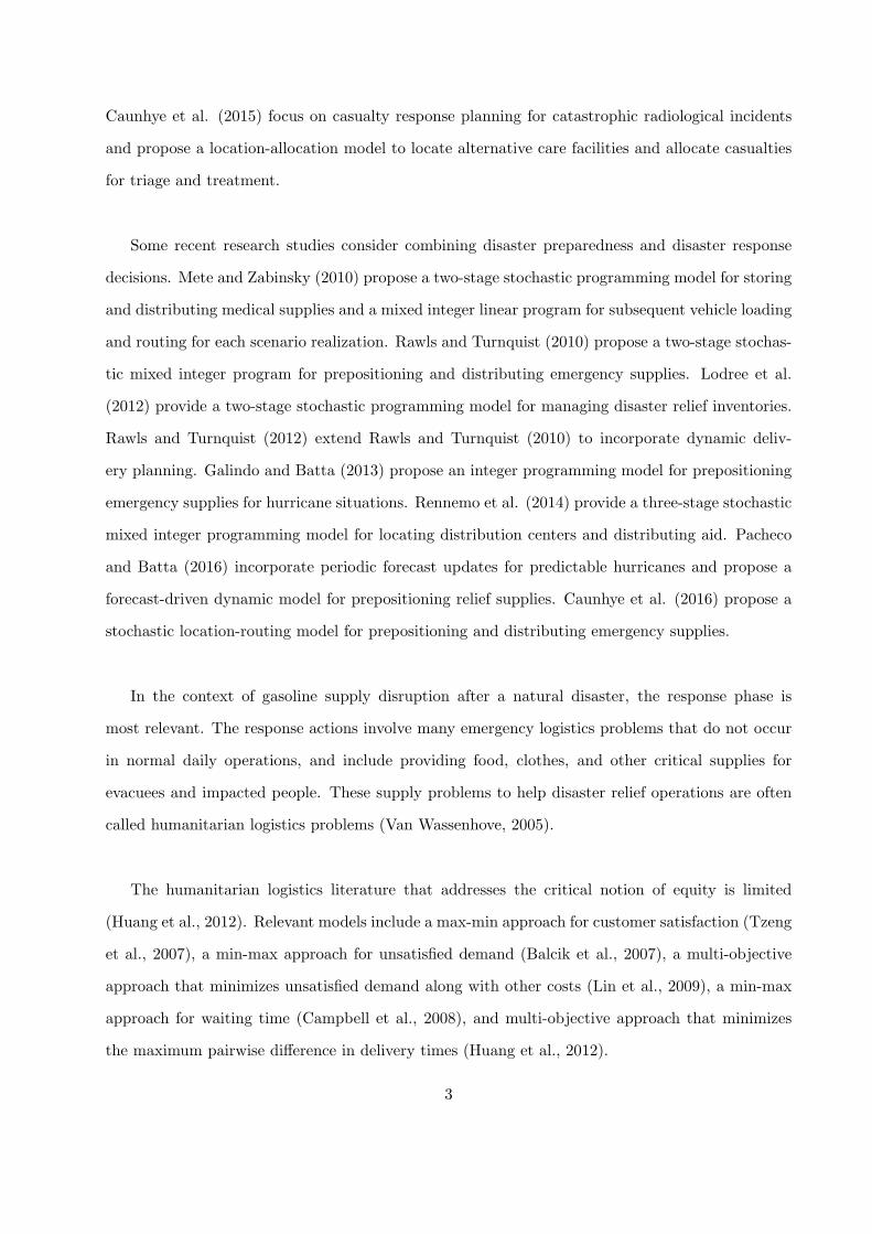
capacity. We also consider each gas station will have a gasoline sale cap, which is usually not the

case to be considered in regular gas station operation. But after Superstorm Sandy, as figure 2

shows, people and cars are waiting in a line to fill gas for their home electric generators and cars.

We thus have limited gasoline pumps to fulfill the demands of the community.

Based on the fact that lots of refineries and petroleum terminal were shut down in the aftermath

of hurricane Sandy, in this paper we assume that we have a single depot for available gasoline

resource and delivery trucks. We further assume that this depot will only supply gasoline to the

affected regions. There is very limited gasoline resource available in this single depot. And because

of that, we will also assume each gas station in the affected regions will only demand gasoline. Of

course these gas stations will have reserve capacity and sale capacity limitations. After Hurricane

Sandy, New Jersey and New York city both ordered a mandatory ration to regulate access to gas

stations for a few weeks. So we consider our model with a limited time period, this time period can

4

Figure 1: Gasoline Supply Chain Overview (Source: U.S. EIA, 2013)

be short as a day or longer as a few weeks according to the severity of the aftermath of a natural

diaster. Since gasoline is one of type of hazmat, we will assume each delivery truck will deliver on

a full truck load to one single gasoline station and we can’t partially deliver gasoline out. We can

also deliver a few truck loads to a single gas station if one single deliver of gasoline truck would

not satisfy the demand. In the aftermath of Hurricane Sandy, lots of gasoline stations were out of

power even though these stations still had gasoline in stock. To address this we assume a pool of

available generators that can be assigned to the gas stations which are out of power. Then, based

on the assigned generators, we will assign trucks to deliver full truck load gasoline to those gasoline

stations. We assume that there is a set of regions I, indexed by i. Let J be the set of all gas

stations in all regions, indexed by j. J = J1 ∪ J2 where J1 is the set of gas stations with power

aftermath, and J2 is the set of gas stations which are out of power. We assume T as the number of

time periods. Let Gi be the set of gas stations in region i. For each gasoline station, let Wj be the

storage capacity at gas station j, Oj be the maximum output at gas station j, and Vj be the initial

storage inventory at gas station j. Now let us assume there is a set of available generators B. For

the simplification of the modeling and at the same time without loss of generality, we assume that

there are two types of gasoline delivery trucks available, type 1 truck and type 2 truck. Each truck

tank only contains a single compartment (which makes sense after a natural disaster since high

demand quantities at gas stations will be highly likely). For the two types of trucks parameters,

the total number of available type 1 delivery truck is denoted by A1, while the total number of

5

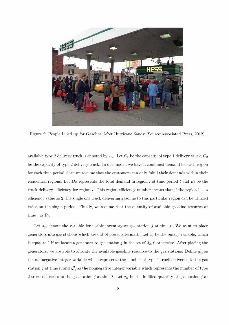
Figure 2: People Lined up for Gasoline After Hurricane Sandy (Source:Associated Press, 2012).

available type 2 delivery truck is denoted by A2. Let C1 be the capacity of type 1 delivery truck, C2

be the capacity of type 2 delivery truck. In our model, we have a combined demand for each region

for each time period since we assume that the customers can only fulfill their demands within their

residential regions. Let Dit represents the total demand in region i at time period t and Ei be the

truck delivery efficiency for region i. This region efficiency number means that if the region has a

efficiency value as 2, the single one truck delivering gasoline to this particular region can be utilized

twice on the single period. Finally, we assume that the quantity of available gasoline resource at

time t is Rt.

Let sjt denote the variable for usable inventory at gas station j at time t. We want to place

generators into gas stations which are out of power aftermath. Let xj be the binary variable, which

is equal to 1 if we locate a generater to gas station j in the set of J2, 0 otherwise. After placing the

generators, we are able to allocate the available gasoline resource to the gas stations. Define y1jt as

the nonnegative integer variable which represents the number of type 1 truck deliveries to the gas

station j at time t, and y2jt as the nonnegative integer variable which represents the number of type

2 truck deliveries to the gas station j at time t. Let qjt be the fulfilled quantity at gas station j at

6

Table 1: The complete list of notations

Symbol Description

I The set of regions, indexed by i

J1 The set of gas stations which still operate aftermath

J2 The set of gas stations which run out of power aftermath

J The set of all gas stations, indexed by j. J = J1 ∪ J2

Gi The set of gas stations in region i

T Time period indexed by t

Wj The storage capacity at gas station j

Oj The maximum output at gas station j

Vj The initial inventory at gas station j

B Total number of generators available

A1 Total number of type 1 trucks available

A2 Total number of type 2 trucks available

C1 The capacity of type 1 trucks

C2 The capacity of type 2 trucks

Ei Efficiency of truck delivery for region i

Dit The total demand of region i at time period t

Rt The total available gasoline resource at time period t

λ The parameter for equity variable

sjt The usable inventory variable for gas station j at time period t

xj binary variable equal to 1 if a generator is located at gas station j, 0 otherwise

y1jt The integer variables for the number of type 1 truck deliveries to gas station j at time t

y2jt The integer variables for the number of type 2 truck deliveries to gas station j at time t

qjt The output of gas station j at time period t

z The equity variable

time t. Last, define z as the equity variable with parameter λ. Here we maximize the minimum of

the equity value cross all regions in all time periods.

We have formulated the following linear binary integer program model:

The objective function (1) is to maximize the total fulfilled gasoline outputs plus equity. Con-

straint (2) makes sure that the number of generators that we will locate in the set of J2 are less

than or equal to the total number of available generators. Constraint (3) assigns initial inventory

in the set J1. Constraint (4) assigns initial inventory in the set of J2 since only inventories in those

gas stations located with generators are countable. Constraint (5) sets next day usable inventory

7

[Obj] max∑T

t=1

∑j∈J qjt + λz (1)

s.t.∑

j∈J2 xj ≤ B, (2)

sj,0 = Vj , ∀j ∈ J1, (3)

sj,0 = xjVj , ∀j ∈ J2, (4)

sj,t = sj,t−1 + C1y1j,t + C2y

2j,t − qj,t, ∀j ∈ J, for t = 1, 2, ..., T, (5)

qjt ≤ Oj , ∀j ∈ J, for t = 1, 2, ..., T, (6)

C1y1jt ≤ Wjxj , ∀j ∈ J2, for t = 1, 2, ..., T, (7)

C2y2jt ≤ Wjxj , ∀j ∈ J2, for t = 1, 2, ..., T, (8)

sj,t−1 + C1y1jt + C2y

2jt ≤ Wj , ∀j ∈ J, for t = 1, 2, ..., T, (9)

qjt ≤ sj,t−1 + C1y1j,t + C2y

2j,t, ∀j ∈ J, for t = 1, 2, ..., T, (10)∑

j∈Giqjt ≤ Dit, ∀i ∈ I, for t = 1, 2, ..., T, (11)∑

i∈I∑

j∈Gi(1/Ei)y

1jt ≤ A1, for t = 1, 2, ..., T, (12)∑

i∈I∑

j∈Gi(1/Ei)y

2jt ≤ A2, for t = 1, 2, ..., T, (13)∑

j∈J(C1y1jt + C2y

2jt) ≤ Rt, for t = 1, 2, ..., T, (14)

z ≤∑

j∈Giqjt

Dit, ∀i ∈ I, for t = 1, 2, ..., T, (15)

xj ∈ {0, 1}, ∀j ∈ J, (16)

sjt ≥ 0, ∀j ∈ J, for t = 1, 2, ..., T, (17)

qjt ≥ 0, ∀j ∈ J, for t = 1, 2, ..., T, (18)

y1jt, y2jt ∈ I+, ∀j ∈ J, for t = 1, 2, ..., T, (19)

z ≥ 0. (20)

for each gas station at time period t. Constraint (6) ensures that the fulfilled gasoline quantity at

each gas station is less or equal to the maximum output of the gas station at time period t. Con-

straints (7, 8) ensure that only gas stations located with generators in the set J2 can have gasoline

deliveries. Constraint (9) makes sure that the usable inventory is less than the capacity of the gas

station. Constraint (10) ensures the fulfilled gasoline output is less than or equal to the usable

inventory of the gas station at time period t. Constraint (11) makes sure that the total output

quantity in each region is less than or equal to the regional demand at time t. Constraints (12, 13)

ensure that the number of utilized trucks does not exceed the total number of available trucks of

each type. Constraint (14) makes sure the total allocated gasoline resource could not exceed the

available resource at time t. Constraint (15) is the equity constraint, here we set our equity as the

maximum of the minimum ration of total output quantities over the region’s demands. Constraint

(16) is the binary constraint to place generators. Constraints (17, 18, 20) are the nonnegative

8

constraints since we can’t sell any gasoline if our inventory stock is negative. Constraint (19) is the

nonnegative integer constraint which means that we could deliver multiple truck loads of gasoline to

one single gas station based upon the appropriate situation e.g. the gas station is the only station

that still open within the region.

3 Numerical Example

We now provide a numerical example to explain the model. For problem simplicity, we will only

consider four small regions with gas stations. Figure 3 shows the regions, along with a gasoline

station diagram where gas stations with/without power are indicated. In order to simplify the

display, we will just assume that the single depot is located in the center of four region. We test

different efficiency parameters for different regions. If the efficiency parameter is 2, it means that

each single truck can transport two truck loads to the region. Thus the utilization of each type of

trucks assigned to those regions with efficiency parameter 2 will be doubled. Table 2 lists all the

parameters and their values.

Figure 3: An Illustrative Example.

We tested three values of λ: 0, 100 and 200 for different equatability scenarios to gain a

perspective on the impact on the performance of parameter λ. We run this model using IBM Ilog

9

Table 2: Parameter Values

Parameter Description ValueI Set of regions {1, 2, 3, 4}J1 Set of gasoline stations which still operate aftermath {2, 5, 9, 10, 11}J2 Set of gasoline stations which run out of power aftermath {1, 3, 4, 6, 7, 8, 12}J The set of all gas stations, indexed by j. J = J1 ∪ J2 {1, 2, 3, 4, 5, 6, 7, 8, 9, 10, 11, 12}Wj The storage capacity at gas station j 20,10,8,24,30,26,12,18,20,24,30,26 for station 1..12Oj The maximum output at gas station j 10,5,4,12,15,14,6,9,10,12,15,13 for station 1..12Vj The initial inventory at gas station j 12,2,3,20,4,19,6,12,0,12,5,18 for station 1..12T Time period indexed by t 1,2,3,4,5B Total number of generators available 2A1 Total number of type 1 trucks available 3A2 Total number of type 2 trucks available 6C1 The capacity of type 1 trucks 10C2 The capacity of type 2 trucks 6Dit The total demand of region i at time period t 200 for each region at period tRt The total available gasoline resource at time period t 30 for each period tEi Efficiency of truck delivery for region i E1=3, E2=2, E3=2,E4=3λ The parameter for equity variable 0,100,200

Cplex for a total of three scenarios. All these scenarios utilize the same parameter data set as listed

in table 2. For scenario 1, we set parameter λ for equatability z as 0, scenario 2 with the values

of λ as 100, and scenario 3 with the values of λ as 200. Figure 4 shows us the result where we are

going to place the generators.

Figure 4: Generator Placement for Illustrative Example.

We can see that, for scenario 1 where the values of λ is zero, we tend to place the only 2 available

generators to the gas stations 4 and 6 with the objective value as 212. This makes intuitive sense,

since when equity factor λ is zero, we simply try to maximize the total gasoline sale since those

two gas stations have the largest initial gasoline inventory. Consider scenario 2. In this case, we

will still place the two available generators to gas station 4 and gas station 6, but since we slightly

increase the weight of the equity factor λ to 100, we obtain the objective value as 216.67 with the

10

equity value z=0.0467. So when we increase the weight of equity factor λ but not big enough to

overcome the impact of big initial inventories, we will still place our available generators to the gas

station with large initial inventory. Now let’s look at scenario 3 where values of λ is equal to 200.

In this case, we place the two generators at gas station 1 and gas station 6 which will produce the

objective value as 224 while generating the largest equity value z as 0.1 across these three cases.

We note that the first two scenarios only produce equity value as 0 and 0.0467 instead.

Figure 5: Truck Assignments for Scenario 3.

Figure 6: Truck Assignments for Scenario 3 (continued).

In our numerical study we test 5 periods. Figures 5 and 6 provide us detailed information

regarding truck assignments for each period. The case that we show in Figures 5 and 6 is for

11

scenario 3 where we use the equity factor λ as 200. From figure 5, we can see that for period 1,

we will assignment one type 2 truck to gas stations 2, 5, 6 and two type 2 trucks to gas station

9 since gas station 9 has power but with zero initial inventory available. As for period 2, we will

assign one type 1 truck to gas stations 1, 5 and 10. In period 3 we will continue to assign two type

1 trucks to gas station 5 and one type 1 truck to gas station 6. We then assign one type 2 truck

to gas stations 1 ,2 6, 9 and 11 in period 4. Finally, in period 5, one type 1 truck is assigned to

gas stations 1, 5 and 6. The total sale value is 204 for all periods with 42, 40, 40, 41 and 41 for

each period respectively. As we mentioned earlier, for scenario 3 we have equity factor λ as 200

and an equity variable value as 0.1. Our finally objective is 224, including the total sale quantity

and equity weight. From this numerical case study we can see that our model is quite flexible and

sensitive when we want to maximize sale quantity with the equity weight considered. We can see

that as the value of parameter λ increases, the equatability variable z gets larger, and the objective

value gets bigger. When we consider just maximizing the outputs of all gasoline stations, we tend

to place generators to the stations with large initial inventories. When we increase the importance

of equatability, we tends to evenly distributed generators to regions so as to improve the equity

value.

4 Case Study for Two Counties in the State of New Jersey

In this paper, we will consider Superstorm Sandy as the case that we want to study. In the late

October of 2012, hurricane Sandy hit the Eastern Coastal areas of the United States, the total

loss or damage by Superstrom Sandy was roughly about 72 billion dollars (comfort etc. 2013).

Among them, the state of New Jersey and New York City were badly hit by Sandy (Aon Benfield,

2013). In this case study, we utilize gasoline station data we obtained from the New Jersey Office

of GIS Open Data source online to apply our model (New Jersey Office of GIS Open Data). After

Superstorm Sandy, most of the refineries and terminals are shut down due to the damage of the

storm, the state of New Jersey encountered gasoline shortage and trucks are waiting in the line

to fill gas. Houses, cars and trucks etc were out of power, and the need of gasoline dramatically

increased. As we see from the Figure 2, trucks and individuals are lined up in the queue to wait

for gas fulfillment.

Among counties in the state of New Jersey, we will pick Monmouth and Ocean Counties for

12

Figure 7: Gas Station Map for Monmouth and Ocean Counties in New Jersey

our case study since these two counties are the most hit counties across New Jersey state. Figure

7 provides a glance at the gas station map in these two counties. After Superstorm Sandy, about

of 40 percent of gasoline stations in New Jersey closed either because of power loss or gasoline

shortage (CNN, 2012). In this case study, we will consider the case with 40 percent of gas stations

out of power. In order to reflect the fact of the gasoline demand crisis, we will assume our demand

is three times of maximum gasoline outputs for all gasoline stations within the region. The gasoline

stations within the same region will share the demand of the region. We also assume customers

within the region will be only serviced by the gasoline stations in the region.

Since we only have the gas station location information, it is impossible to get all the parameters

for each single gas stations. So we randomly generate parameters such as Wj the storage capacity

at gas station j, Oj the maximum output at gas station j, Vj the initial inventory at gas station j.

We randomly generate the storage capacity of gas stations with the range of 8000 gallons to 35000

gallons, and generate initial inventory Vj of each gas station j randomly with the range of 0 gallon

to Wj the storage capacity at gas station j. Then we assume the maximum output of each gas

13

station j is half of their respective storage capacity. Based on this same set of gas station parameter

data, we construct 12 cases in two groups. For each of the 12 cases, we generate 30 replications

based on the fact that 40 percent of gasoline stations out of power. So for each replication, we

randomly select gas stations and set these stations with power. These 30 replications are shared

by each individual case so that we can conduct valid comparisons on the same data set. All 12

cases are developed based on the factors of truck numbers, truck capacities, number of available

generators, equity parameter λ, available resource and region efficiencies. We run our cases by

IBM Ilog Cplex (version 12.6.1) with computer processor as Intel(R) Xeon(R) CPU e5-2630 v3

@2.4GHz, 32GM installed memory(RAM). In order to speed up the case study all cases are run

with 5 percentage of tolerance gap from optimal.

As we said previously, we conduct these 12 cases in two different groups. One group consists of

8 cases, all these 8 cases are generated by differentiating trucks parameters while keeping the same

total delivery capacities. Table 3 provides detailed information regarding each individual case. The

objective value, equity z, total delivery and CPU time are average values of the 30 replications for

each single case. From table 3, we can see that, with the same total delivery capacity, the size and

numbers of each type of trucks affects our result quite significant. We see that when we have more

trucks with smaller capacities for both type of trucks, e.g. cases 3, 4, 6 and 7, our objective value,

total delivery quantities and equity variable can all achieve better result while the CPU solving

time tends to take a much longer. While in the cases where we have large capacities of trucks, e.g.

cases 1, 5 and 8, our solution solving time improved dramatically without sacrificing the objective

value and equity much. As for case 2, we see that if we have really unbalanced number of types of

vehicles and the truck capacity is relatively large, the total delivery quantity wasn’t affected much,

we actually improve the solution solving time but with sacrifice on equity and objective value.

For group 2, we pick one of the cases in the previous group (case 8), then we fix the trucks

parameters such as number of available trucks, capacity of each different size of trucks. We simply

change one parameter for each case as listed in table 4. Similar to group 1, We run each of 30

replications again for these 5 cases. The results are listed in table 4. Again, the objective value,

equity z, total delivery and CPU time are average cross 30 replications for each case. Case 8 serves

as the baseline for this group. We see that if we decrease the equity factor Λ, we will still achieve

similar total delivery quantity, but the equity value was hardly affected although the solution solving

14

Tab

le3:

8Cases

withSameDeliveryCapacity

Case

1Case

2Case

3Case

4Case

5Case

6Case

7Case

8Number

ofReg

ions

72

72

72

72

72

72

72

72

Number

ofGasStations

453

453

453

453

453

453

453

453

Number

ofPeriods

12

12

12

12

12

12

12

12

Number

ofType1Tru

ck50

236

59

71

59

71

34

Capacity

ofType1Tru

ck15,000

14,000

13,000

12,000

11,000

10,000

9,000

15,000

Number

ofType2Tru

ck50

132

124

68

41

80

88

80

Capacity

ofType2Tru

ck8,000

8,500

5,500

6,500

9,000

7,000

5,500

8,000

Number

ofGen

erators

30

30

30

30

30

30

30

30

Weightofeq

uity(λ

)200,000,000

200,000,000

200,000,000

200,000,000

200,000,000

200,000,000

200,000,000

200,000,000

Resourceatt(R

t)

1,000,000

1,000,000

1,000,000

1,000,000

1,000,000

1,000,000

1,000,000

1,000,000

Reg

ionEfficien

cy2

22

22

22

2ObjectiveValue

26,911,776

15,356,380

29,859,632

29,779,899

15,317,239

29,798,549

29,824,764

26,835,218

Equityz

0.0628939

0.005,151,8

0.077,981,5

0.077,505,6

0.005,197,8

0.077,609,9

0.077,793,4

0.062,386

TotalDeliveryGallons

14,332,996

14,326,020

14,263,329

14,278,779

14,277,688

14,276,568

14,266,089

14,358,023

CPU

time(byreplica

tion)

11.72(s)

2.12(s)

360.11(s)

397.88(s)

5.79(s)

303.27(s)

234.72(s)

9.91(s)

15

time improves much. As for case 10, here we decrease the number of available generators. Usually

generators are very expensive and stakeholder of the relative parties (e.g. New Jersey government)

would not have lots of generators on hand. So the result of case 10 shows us that the equity will

drop significantly even though we only reduced 20 generators. The total delivery drops not much in

the fact that we have very limited resource while solving time increases quite a bit. Case 11 is quite

obvious since we doubled our available resource. In this case, the objective value, equity value and

total delivery quantity increase significantly while solution solving time just increases a little bit.

In case 12, we simply change all the region efficiency value from 2 to 1, it means that, each type of

truck can only be utilized once for each single periods, while in other cases, each type of trucks can

by utilized twice in each period. This implies that we have affectively reduced the total number

of available trucks. We see that the solution time time is reduced but other values e.g. objective

value, equity and total delivery actually do not change much. In this case, it is because we have

very limited resource and the number of available trucks are enough to carry on the delivery job.

Table 4: Five Cases with Fixed Truck ParametersCase 8 Case 9 Case 10 Case 11 Case 12

Number of Regions 72 72 72 72 72Number of Gas Stations 453 453 453 453 453Number of Periods 12 12 12 12 12Number of Type 1 Truck 34 34 34 34 34Capacity of Type 1 Truck 15,000 15,000 15,000 15,000 15,000Number of Type 2 Truck 80 80 80 80 80Capacity of Type 2 Truck 8,000 8,000 8,000 8,000 8,000Number of Generators 30 30 10 30 30Weight of equity(λ) 200,000,000 200 200,000,000 200,000,000 200,000,000Resource at t(Rt) 1,000,000 1,000,000 1,000,000 2,000,000 1,000,000Region Efficiency 2 2 2 2 1Objective Value 26,835,218 14,256,237 14,834,092 38,364,007 26,851,117Equity z 0.062,386 0 0.003,912,8 0.064,960,4 0.062,514,6Total Delivery (Gallons) 14,358,023 14,256,237 14,051,529 25,371,920 14,348,197CPU time(by replication) 9.91(s) 0.83(s) 65.93(s) 12.15(s) 6.29(s)

5 Case Study for All Counties in the State of New Jersey

We follow the same process as the previous case study to utilize gasoline station data which we

obtain from the New Jersey Office of GIS Open Data source online to apply to our model (New

Jersey Office of GIS Open Data). We still consider the case with 40 percent of gas stations out

of power. Same with the previous case study, we will assume our demand is three times of the

maximum gasoline outputs for all gasoline stations within each region. The gasoline stations within

16

the same region will share the demand of the region. Customers within the region will be only

serviced by the gasoline stations in the region. We also randomly generate gas stations parameters

such as Wj , Oj and Vj . The storage capacity of gas stations will also be generated with the range

of 8,000 gallons to 35,000 gallons, and initial inventory Vj of each gas station j randomly with the

range of 0 gallon to Wj . The maximum output of each gas station j is half of their respective

storage capacity. Based on this same set of gas station parameter data, we construct 8 cases. For

all these cases, we will only generate one replication based on the fact that 40 percent of gasoline

stations out of power. And all these cases will share this same data set. Again we run these 9 cases

by IBM Ilog Cplex (version 12.6.1) on the same pc as the previous case study. All cases are run with

5 percentage of tolerance gap from optimal since the data set is really large e.g. there are a total of

3,387 gas stations in the state of New Jersey. Table 5 provides us detailed information regards to

each individual case. Since the data set is large when we consider all gas stations in NJ, the region

efficiency parameters are set to 2 for some regions close to the depot and 1 for the rest of regions.

Cases 1 , 2 and 3 in the table shows us that once we increase number of available generators, we can

obtain much better equity value while decreasing the solution solving time significantly. Now let us

compare cases 4, 5 and 2 since in these cases, we simply change the equity weight parameter value

from 0 as in case 4, 20,000 as in case 5 and 200,000,000 in case 2. We see that for the large data

set, in order to achieve a better equity value, we have to use a very large value for equity weight

parameter. Now compare case 6 with case 2. We see that if we change all the region efficiency

parameter to 1, in this case, the change didn’t affect the results much. The reason for this is because

we have enough trucks available. Last let us compare cases 2, 7 and 8. We see that the available

resource affects our objective value very much. When we get more available gasoline resource, our

objective value and total delivery increased. The solution solving time for smaller resource value

as in case 8 is significantly longer when we try to achieve a better equity value and total delivery.

From this large case study, we conclude that our model is effective and efficient.

6 Conclusions and Future Work

In the aftermath of a natural disaster, gasoline supply chain may be disrupted. Gasoline shortage

may become a key factor to the recovery of the community. In our model, we consider a single

depot and two types of delivery trucks with limited gasoline resource in a limited time period. We

17

Tab

le5:NineCases

forAllGasStatio

nsin

New

Jersey

Case

1Case

2Case

3Case

4Case

5Case

6Case

7Case

8Number

ofReg

ions

489

489

489

489

489

489

489

489

Number

ofGasStatio

ns

3387

3387

3387

3387

3387

3387

3387

3387

Number

ofPerio

ds

12

12

12

12

12

12

12

12

Number

ofType1Tru

ck400

400

400

400

400

400

400

400

Capacity

ofType1Tru

ck15,000

15,000

15,000

15,000

15,000

15,000

15,000

15,000

Number

ofType2Tru

ck500

500

500

500

500

500

500

500

Capacity

ofType2Tru

ck8,000

8,000

8,000

8,000

8,000

8,000

8,000

8,000

Number

ofGen

erators

50

150

300

150

150

150

150

150

Weig

htofeq

uity

(λ)

200,000,000

200,000,000

200,000,000

020,000

200,000,000

200,000,000

200,000,000

Reso

urce

att(R

t )9,000,000

9,000,000

9,000,000

9,000,000

9,000,000

9,000,000

12,000,000

5,000,000

Reg

ionEfficien

cy2,1

2,1

2,1

2,1

2,1

12,1

2,1

Objectiv

eValue

114,932,000

124,232,295

127,852,956

117,742,400

117,704,400

126,248,192

154,249,049

80,356,812

Equity

z0

0.045

0.040,3

00

0.050,8

0.043,9

0.040,8

TotalDeliv

eryGallo

ns

114,932,000

115,162,000

119,797,400

117,742,400

117,704,400

116,078,700

145,469,900

72,205,900

CPU

time

3871.96(s)

395.68(s)

338.23(s)

318.48(s)

318.60(s)

319.21(s)

715.62(s)

8,124.81(s)

18

utilize the limited back up generators and optimize the generators assignment and truck deliveries

to the gas stations to achieve maximum gasoline delivery, and at the same time incorporate equity

factor across the different regions. Our numerical example validates our model and proves that

our model works effectively to locate generators to gas stations and assign delivery trucks to gas

stations. With different equity parameters λ, we can achieve the desirable level of equity. In the

two county case study we found out that different combinations of two types of trucks can affect the

performance quite a bit. Different input parameters, e.g. available resource, number of generators,

equity parameter affect the deliverable results. From the large case study we conclude that our

model is quite efficient and useful to manage gasoline delivery in the aftermath of a natural disaster.

To evaluate the true impact of our model we need to understand how individuals seek gas in a gas

shortage situation. Analytical models based on queueing and simulation model would be useful in

this regard. The development of such models and their interaction with the basic model proposed

in this paper can be treated as future work.

References

Altay, N., Green, W.G.(2006). OR/MS Research in Disaster Operations Management. European Journal ofOperational Research, 175(1), 475-493.doi:10.1016/j.ejor.2005.05.016

Benfield, A.(2013). Hurricane Sandy Event Recap Report http://thoughtleadership.aonbenfield.

com/Documents/20130514_if_hurricane_sandy_event_recap.pdf

Barbarosoglu, G., Arda, Y.(2004). A Two-Stage Stochastic Programming Framework for Transporta-tion Planning in Disaster Response, Journal of the Operational Research Society, 55(1): 43-53.

Campbell, A.M., Vandenbussche, D., Hermann,W.(2008). Routing for Relief Efforts. TransportationScience,42(2),127-145.doi:10.1287/trsc.1070.0209.

Caunhye, A.M., Nie, X., Pokharel, S.(2012). Optimization Models in Emergency Logistics: A Litera-ture Review, Socio-Economic Planning Sciences, 46(1): 4-13.

Caunhye, A.M., Li, M., Nie, X.(2015). A Location-Allocation Model for Casualty Response Planningduring Catastrophic Radiological Incidents, Socio-Economic Planning Sciences, 50: 32-44.

Caunhye, A.M., Zhang, Y., Li, M., Nie, X.(2016). A Location-Routing Model for Prepositioning andDistributing Emergency Supplies, to appear in Transportation Research Part E: Logistics and TransportationReview.

Cozzani, V., Campedel, M., Renni, E., & Krausmann, E.(2010). Industrial Accidents Triggered byFlood Events: Analysis of Past Accidents, Journal of Hazardous Materials, 175(1-3),501-509.

CNN (2012). Gas shortage continues in areas hit by Sandy http://money.cnn.com/2012/11/02/news/

economy/gas-shortage-sandy/

Huffington Post (2012). Hurricane Sandy Gasoline Shortage: Dry Pumps Could Last For Days. Retrieved

19

September, 2013 http://www.huffingtonpost.com/2012/11/01/sandy-gasoline-shortage_n_2059651.html

PHMSA (Pipeline and Hazardous Materials Safety Administration, U.S. Department of Transportation)(2013). Hazardous Materials Table (HMT), Title 49 CFR 172. 101 Table (List of Hazardous Materials).Retrieved September, 2013 (http://www.phmsa.dot.gov/hazmat/library).

Galindo, G., Batta, R. (2013). Review of Recent Developments in OR/MS Research in Disaster Opera-tions Management. European Journal of Operational Research, 230(2), 201-211. doi:10.1016/j.ejor.2013.01.039

Galindo, G., Batta, R. (2013). Prepositioning of Supplies in Preparation for a Hurricane under Poten-tial Destruction of Prepositioned Supplies, Socio-Economic Planning Sciences, 47(1): 20-37.

Gong, Q., Batta R. (2007). ”Allocation and Reallocation of Ambulances to Casualty Clusters in a Dis-aster Relief Operation.” IIE Transactions 39.1: 27-39.

Haghani, A., Oh, S.C. (1996). Formulation and Solution of a Multi-Commodity. Multi-Modal NetworkFlow Model for Disaster Relief Operations, Transportation Research Part A: Policy and Practice, 30(3):231-250.

Huang, M., Smilowits, K., Balcik, B.(2012). Models for Relief Routing: Equity,Efficiency and Efficacy.Transporation Research Part E: Logistics and Transportation Review, 48(1),2-18.doi:10.1016/j.tre.2011.05.004

Lodree, E.J., Ballard, K.N., Song, C.H. (2012). Pre-Positioning Hurricane Supplies in a CommercialSupply Chain, Socio-Economic Planning Sciences, 46(4): 291-305.

Maskrey, A. (1989). Disaster mitigation: A Community Based Approach. Oxfam Professional, Oxford, England.

Mete, H.O., Zabinsky, Z.B. (2010). Stochastic Optimization of Medical Supply Location and Distribu-tion in Disaster Management, International Journal of Production Economics, 126(1):76-84.

New Jersey Office of GIS Open Data http://njogis.newjersey.opendata.arcgis.com/datasets/

d511b06f89cb48dc903e59cf4f346dda_2

Ozdamar, L., Ekinci, E., Kucukyazici, B. (2004). Emergency Logistics Planning in Natural Disasters,Annals of Operations Research, 129(1-4): 217-45.

Pacheco, G.G., Batta, R. (2016). Forecast-driven Model for Prepositioning Supplies in Preparation fora Foreseen Hurricane, Journal of the Operational Research Society, 67(1): 98-113.

Rawls, C.G., Turnquist, M.A. (2010). Pre-Positioning of Emergency Supplies for Disaster Response,Transportation Research Part B: Methodological, 44(4): 521-534.

Rawls, C.G., Turnquist, M.A. (2012). Pre-Positioning and Dynamic Delivery Planning for Short-TermResponse Following a Natural Disaster, Socio-Economic Planning Sciences, 46(1): 46-54.

Rennemo, S.J., Ro, K.F., Hvattum, L.M., Tirado, G. (2014). A Three-Stage Stochastic Facility Rout-ing Model for Disaster Response Planning, Transportation Research Part E: Logistics and TransportationReview, 62(2): 116-135.

Sheu, J.B. (2007). An Emergency Logistics Distribution Approach for Quick Response to Urgent ReliefDemand in Disasters, Transportation Research Part E: Logistics and Transportation Review, 43(6): 687-709.

Sheu, J.B. (2010). Dynamic Relief-Demand Management for Emergency Logistics Operations underLarge-Scale Disasters, Transportation Research Part E: Logistics and Transportation Review, 46(1): 1-17.

Van Wassenhove, L.N. (2005). Humanitarian Aid Logistics: Supply Chain Managment in High Gear.Journal of the Operational Research Society, 57(5),475-489.

20