Dynamics of Water Accounting Balance for Assessing Water ...
46
Dynamics of Water Accounting Balance for Assessing Water Stress Vulnerability Considering Social Aspects Elham Ebrahimi University of Tehran Mohammad Karamouz ( [email protected] ) University of Tehran https://orcid.org/0000-0001-7574-3763 Research Article Keywords: Vulnerability, System Dynamics, Productivity, Water Stress, Principal Component Analysis Posted Date: November 9th, 2021 DOI: https://doi.org/10.21203/rs.3.rs-1054348/v1 License: This work is licensed under a Creative Commons Attribution 4.0 International License. Read Full License
Transcript of Dynamics of Water Accounting Balance for Assessing Water ...

Dynamics of Water Accounting Balance forAssessing Water Stress Vulnerability ConsideringSocial AspectsElham Ebrahimi
University of TehranMohammad Karamouz ( [email protected] )
University of Tehran https://orcid.org/0000-0001-7574-3763
Research Article
Keywords: Vulnerability, System Dynamics, Productivity, Water Stress, Principal Component Analysis
Posted Date: November 9th, 2021
DOI: https://doi.org/10.21203/rs.3.rs-1054348/v1
License: This work is licensed under a Creative Commons Attribution 4.0 International License. Read Full License

1
Dynamics of Water accounting balance for assessing water stress vulnerability
considering social aspects
Elham Ebrahimi Sarindizaj 1, Mohammad Karamouz 2
1 Ph.D. Candidate, School of Civil Engineering, University of Tehran, Tehran, Iran, [email protected]
2 Professor, School of Civil Engineering, University of Tehran, Tehran, Iran, [email protected]
Abstract
To advance proper planning, water accounting (WA) could provide the possibility of linking physical
and operational data to their interdisciplinary attributes. In its new form, WA, combined with a
dynamic model considering socio-economic aspects, is a valuable tool for rectifying today's water
issues. The social water-accounting-based system dynamics (SWA-SD) provides a feedback-based
platform to better support flexible decision-making. Analyzing the indicators that correspond to water
security in the context of DPSIR (driving force-pressure-state-impact-response) and SWA-SD
combined with principal component analysis (PCA) for identifying data patterns is applied to a
generic study area suffering from water stress to assess the environmental, economic, and social
vulnerabilities. The water accounting has to be based on water balance data (called water accounting
balance). As a practical solution to generate water balance data, a time series by the use of basic
climatic and hydrologic data is synthesized. According to the results, the water stress and
urbanization index were increased by a factor of 43% and 64% in 2020 during a 20-year time horizon,
respectively, which is alarming for the region. Moreover, the economic and social water resources
vulnerability shows an upward trend, and the environmental component shows many highs (as much
as 2.24) and lows (as low as 0.73) due to different supply measures responded to the increasing
demands. This study provides a basis that can be replicated for other developing regions to quantify
this type of important planning information and for implementing different socially sensitive triggers
and technically feasible to measure water vulnerabilities.
Keywords: Vulnerability, System Dynamics, Productivity, Water Stress, Principal Component
Analysis.

2
1. Introduction
In order to quantify a water system’s balance, a comprehensive understanding of variables affecting
the state of water supply and demand, performance indicators, and their interdependencies is needed.
Among the widely used performance criteria are resiliency, and vulnerability. Vulnerability is the
extent at which the environment, the economy, or the social system (the responder) are prone to
damage/degradation by a hazard or stressor (IPCC, 2014). The critical parameter of water resources
vulnerability (WRV) is the water stress which is exposed to a system (Adger, 2006). In the traditional
hazard-centric view of vulnerability, the focus was on hazard impacts assessment (Dwyer et al.,
2004). However, vulnerability is not a product of a single factor and results from interactions of
socio-economic attributes (Rajesh et al., 2018). The vulnerability components include environmental,
economic, and social aspects of anthropogenic activities (Wei et al., 2020). Resiliency, as the system
capacity to adapt to any stressed situation (Karamouz and Movahhed, 2021), is widely by quantifying
the rapidity, robustness, resourcefulness, and redundancy (4 Rs) dimensions proposed by Bruneau et
al. (2003). Water stress refers to having sufficient water for socio-economic development and
addressing poor management's adverse effects. Based on the different related indicators, it is defined
as when the annual water withdrawal divided by the annual water availability is higher than 0.4
(Kiguchi et al., 2015). Water security generally emphasizes risk management and vulnerability
reduction in the water resources arena when encountering shocks from water-related disasters such
as droughts (van Beek and Arriens, 2014) and water supply-demand management (Cook and Bakker,
2012). Due to increasing water use, water resources are progressively concerned with sustainable
development. For describing water use, water accounting suggests a tool for economic analysis of
water-related issues based on a systematic approach (Dutta, 2017). Water accounting is the process
of communicating water-resources-related information and the services generated from consumptive
use in a domain (Wateraccounting.org). IWMI (International Water Management Institute) (Molden,
1997), Water Footprint Accounting (Hoekstra and Chapagain, 2006), General Purpose Water
Accounting (United Nations, 2009), and SEEA-W (System of Environmental and Economic

3
Accounts for Water) (UNSD, 2012) and Water Accounts Plus (WA+) (Karimi et al., 2013 a,b) are a
few examples of water accounting frameworks. The WA+ includes explicit spatial information on
water depletion and net withdrawal processes in complex river basins and is dependent on satellite
data. Its application in the regions with qualified remote sensing data is stated, which is focused on
hydrological aspects of water resources (Karimi et al., 2013 a). However, it does not consider any
social variable compared to SEEA-W used in this study.
SEEA-W provides physical water data based on socio-economic aspects instead of focusing on water
balance (Esen and Hein., 2020). It suggests the possibility of utilizing policies in an informed and
integrated manner. This framework includes physical, hybrid (a combination of physical accounts
and financial data), and asset accounts tables (UNSD, 2012). SEEA-W should be customized for
applications based on the concerning attributes in each specific case and data availability.
DPSIR (Driver-Pressure-State-Impact-Response) provides the basic structure of conceptual modeling
and helps capture the problem's primary components. Analytical frameworks could establish
interdependencies among governing indicators to bring water's effect on environmental, economic,
and social aspects into the light. The DPSIR, as an analytical framework, supports problem scoping
and structuring in the system dynamics (SD) modeling process (Zare et al., 2019). The scope and uses
of SD methodology have expanded in a variety of water and environmental problems. As the
transparent interaction of the components on a system, the feedback loops are the main advantages of
SD, among other simulation methods (Ekinci et al., 2020). SD is increasingly used to conceptualize
and simulate complex water systems and offers new opportunities to develop dynamic alternatives to
the decision support systems (Jin et al., 2009). A SD model can accurately describe system behavior
under a given range of conditions and incorporate them to find acceptable solutions (Hjorth and
Bagheri, 2006). Thus, coupling water accounting tables with simulation models results in describing
the system and analyzing the effects of potential scenarios (Mahdavi et al., 2019). Hence, developing
indicators and integrated sets of conceptual and analytical frameworks, as mentioned, would be
worthwhile. Different studies have been carried out in the context of water accounting (WA)

4
applications. Contreras and Hunink (2015) proposed a SEEA-W framework for the Segura River Basin
in Spain from 2000 to 2010. The indicators regarding the use and availability of water under normal
and extreme climate conditions were analyzed. Borrego-Marín et al. (2016) utilized WA for the
drought impact assessment on agricultural water productivity in the Guadalquivir River basin in Spain.
In the context of investigating the indicators of water resources systems, Gasco et al. (2005) utilized
an accounting physical input-output table (PIOT) to evaluate the water resources management in
Spain. Karamouz et al. (2021) proposed a hybrid index named PI-Plus (P for Paydari as it is an
indigenous term for sustainability). They also performed an uncertainty analysis to assess the random
nature of variables in estimating water balance and quantifying water sustainability. This index
consisted of available water, efficient water delivery, water supply reliability, aquifer storage, and river
streamflow requirements. The Nash bargaining theory was utilized to capture the satisfaction of water
users. Long and Ji (2019) assessed China's economic growth, environmental sustainability, and social
welfare from 1997 to 2016. Among strategies aimed at agricultural water use management, reducing
irrigated areas, and increasing irrigation efficiency have been investigated as among the most effective
practices (Ebrahimi Sarindizaj and Zarghami 2019; Karamouz et al. 2021). Besides, deficit irrigation
(DI) is widely used as a water-saving irrigation strategy in which irrigation water is applied at amounts
less than full crop water requirements, thereby increases water use efficiency (Morison et al., 2008).
Dealing with numerous indicators, principal component analysis (PCA) is used for exploratory data
analysis. It is recently being used in water resources studies due to its ability to simplify correlated
multivariate data into a few key dimensions.
Water accounting (WA) based on true and synthesized water balance data and causal modeling have
not been widely used and coupled in previous studies. The WA so-called tables are often included five
components with only some social attributes. A standalone table for social issues has not been
developed. In addition, while previous studies have assessed the water resources vulnerabilities, less
attention has been given to the estimation of the socio-economic and environmental aspects of the
vulnerabilities. Water balance data (entails far more details of water supply and demand/allocation

5
than basic climatic and hydrologic data), which is the core of water accounting, is not widely available
(is even scarce) in developing and even developed regions. See Karamouz et al. (2021) for more
details.
In this study, these shortcomings have been realized. A separate table has been added to the WA
structure. Vulnerabilities have been accounted for to see meaningful socio-economic indicators using
a principal component analysis platform. This study investigates the application of social-based water
accounting system dynamics (SWA-SD) for synthesizing system dynamics model outcomes in water
resources vulnerability assessment. A combination of DPSIR and conceptual modeling techniques
(cause and effect loops) is incorporated into a SWA-SD model to assess water resource vulnerabilities
in the environmental, economic, and social sectors. Water resource vulnerabilities are estimated by
employing a set of indicators that correspond to water stress. The dynamics of demographic changes,
unemployment, and variation of income and water use in different sectors are addressed. Besides, the
proposed algorithm considers the water, labor (employment) productivity of the agricultural,
industrial, and urban/services sectors which are defined based on the income produced. A new water
resources vulnerability index in three sub-indicators (water/environment, economic, social) are
discussed based on the principal components. The needed water balance data are generated to offset
the limited official data available by utilizing and extending the platform Karamouz et al. (2021)
provided before. The case study is designed to be generic so that it can be applied to other geographic
settings. However, the information for the components is based on the actual data of Tashk-Bakhtegan
basin in the central part of Iran.
In the remainder of the paper, the methodology section consists of the DPSIR framework's details and
derived indicators in environmental, economic, and social dimensions. The water resources system
vulnerability is provided by water accounting tables followed by the system dynamics approach. The
following section is the case study and the results and discussion. Finally, a summary and conclusion
is given.
2. Materials and methods

6
A flowchart of the methodology for dynamic assessing a water system's vulnerability (SWA-SD) on a
basin-scale is presented in Figure 1. Up to date water balance data is essential for the regions in which
the official data is released after 5-10 years and is scarce in many developing and even developed
regions. Therefore, assumptions and correlations are taken into account based on a platform developed
by Karamouz et al. (2021) to synthesize a 20-year water balance data time series with the same
attributes of official water balance data. Then, the DPSIR framework is utilized to configure the
primary cause and effect relations in a water resource in line with vulnerability. Next, the SEEA-W is
implemented to organize the hydrological-economic-social data. The SEEA-W framework is often
included physical, hybrid (a combination of physical accounts and financial data), and assets categories
with only some social attributes. This paper has developed a standalone table of social issues, and
social water accounting is tabulated. Estimating water accounting tables with social inclusion can
improve the combination of the economy and the environment. The social water accounting table
focuses on population, employment, education, and social welfare.
The SWA-SD model simulates the feedback loops and stock-flow diagrams in the Vensim software
(Ventana Systems, 2004). Different scenarios are assessed to simulate the system's behavior based on
the SD model. In the next step, based on the water accounting tables' organized information,
performance indicators are utilized to evaluate water security regarding water availability. The PCA
method is used to reduce many variables into a smaller number of relevant principal components,
making it possible to determine a more focused description of the data. Based on Fussel (2007),
vulnerability assessment is performed by considering four components: system, threat, time reference,
and the attribute of concern. The vulnerabilities are assessed in the water resources system. The threat
is the water stress, and the time reference is annual. The attribute of concern is water security. Finally,
environmental, economic, and social indices are assessed water resources vulnerability.

7
Figure 1. A framework of social water accounting based system dynamics model for assessing water
resources vulnerabilities
2.1. DPSIR (driving force-pressure-state-impact-response) framework
Assessing the cause-and-effect relationships could offer a better insight into evaluating water resources
sustainability and developing indicators. Unlike many previous studies on water resources causal
analysis, a platform is developed to fine-tune governing elements and components assessment on a
watershed scale (Figure 2). This analysis allows for refining supply-demand balance, better assessing
socio-economic aspects, environmental issues, and system performance. Using this framework

8
resulted in clarification of human activities' impact (as 'driving forces'). These activities impose
'pressures' on the system, leading to changes in environmental conditions (the 'state'). Accordingly,
society reacts to these changes and the corresponding 'impact' through environmental and economic
policies responding to actions or feedbacks processes. Many pressure components make the system
unsustainable; however, the system's 'response' is geared toward mitigating the pressures, providing
necessary resistance against changes, and strengthening sustainability. DPSIR framework is utilized
to system feedback identification and developing the feedback-based nonlinear relationship between
the variables in the context of causal loop diagrams (CLDs) in the system dynamics methodology.
Supply and demand-side management
Response
Pressure
Water availability
Water demand
Land use change
Human activities
Structural development
(Dam, irrigation network,
Driving force
Climate change
Temperature and percipitation
Drought
Regional and national characteristics
Population
Demands (Water, food, employment)
Topographic characteristics
State
Surface water
quantity
Groundwater level
Water productivity
Labor productivity
Impact
Resources degradation
Agricultural production
Income in water related
activities
Social challenges (immigration,
unemployment,
Water stress
Dam construction, Deficit irrigation, Modern irrigation technology expansion such as drip systems,
Regional/local policies
Input data
System s Identification & Casual Loop
Diagram (CLD) Specification
Figure 2. A flow work of the DPSIR framework for the development of causal loops
Generally, regional and national policies affect the population, demands, development plans, emerging
technologies, and a system's topographic characteristics. Besides, temperature and precipitation
variations and droughts are among the driving forces imposed by climate change as an external force.
The pressure element includes the main categories of water demand, water and soil resources,
9
economic change, and environmental issues, which cause changes to the water system. Changes in the
water usage and variations of available water should reflect the imposed pressure on resources and
water supply and demand as the major components. Regarding the socio-economic part, costs and
benefits related to human activities in different sectors (agriculture, industry, urban/services) are
considered.
The state element refers to the water system's state under the pressure variables and describes the water
system's physical characteristics. It consists of four main categories: surface water and groundwater
resources, Labor productivity, and water productivity.
Impacts include water resources degradation, economic, and social challenges as follows:
1- Water resources degradation: Increasing water demand as the primary pressure component
drives water users to exploit water resources further. Because of the water withdrawal
increase, available water resources are affected. Water stress occurs when water demand
exceeds the available amount, implying water resource scarcity due to the pressures and supply
variability.
2- Economic challenges: Water-related activities are affected by water availability. As water
withdrawals increase, the benefits resulting from these activities decrease due to the higher
water supply costs. Besides, considering yield in the farmers' agriculture sector and profit,
benefits can be investigated. The volatile price of agricultural products and the cost of
consumed water impose pressure on farmers. They try to increase the actual yield and
irrigation efficiency to maximize their profit.
3- Social challenges: Changes in water resources and food security affect the social state
regarding unemployment and low labor productivity. The mentioned social challenges have
associations with the environmental and economic aspects. Water stress results in low income,
and low income as a significant economic problem leads to more severe environmental
subsequences. Attempts to exploit more water increase conflicts.

10
Responses refer to measures adopted during the water resources development and utilization to
guarantee higher efficiency and sustainability; however, this may lead to the rebound effect. These
actions try to decrease the pressures and are principally composed of demand and supply-side
management to have more available water and improve water productivity, including dam
construction, deficit irrigation, modern irrigation technology expansion such as drip systems.
As shown in Figure 2, water quantity variations are attributed to water withdrawal increase and
structural development (dam, irrigation network, etc.). Pressures such as sewage volume changes
affect water quality. From an economic perspective, water productivity changes under pressure
imposed by human activities, so-called driving forces. The tendency to gain higher productivity leads
to more cultivation and technology usage, such as modern irrigation systems. Such systems can save
water due to their higher efficiencies; however, this may lead to increased cultivated areas and the use
of the saved water for irrigating newly added areas, known as the rebound effect. Furthermore, social
welfare is affected by water availability. Mismanagement may result in challenges such as immigration
and unemployment.
Among the major application of the DPSIR framework is facilitating the system identification and
helping with recognizing or developing the most suitable indicators related to the effective variables
of the system (Table 1). Besides, the relationship of the different variables and components in the
DPSIR framework (which is often linear) helps identify the possible interdependencies. The basic
information on the nonlinear relationship between the variables might be gained from the DPSIR;
however, it can be considered the basis of analyzing the system's dynamics. DPSIR framework is
utilized to identify and develop CLDs as the primary steps of system dynamics.
2.2. Water accounting framework
The SEEA-W framework is used to derive indicators for assessing the concerning attributes of the
study area as a vulnerable system (Figure 3). Physical water supply and use, hybrid and economic,
asset, and social accounts are the water accounts associated with SEEA-W. The social water
accounting table is as essential as the physical, hybrid, and asset accounting tables, as shown in Figure

11
3. The physical supply and use tables show the water exchange between the environment and the
economy. While the hybrid accounts indicate the costs and revenues of various water uses, the asset
account elaborates the water storage variation. Due to the importance of social aspects in water
resources planning and management, a separate table for social issues has been developed. It seems
that the social water accounting table is the missing category of the SEEA-W. However, estimating
water accounting tables with social inclusion can improve the efforts to integrate the economy and the
environment. A social water account table is proposed to investigate the accounts based on population,
employment, education, financial status, and social welfare.
Da
ta c
oll
ecti
on
:
Fin
anci
al D
ata,
Phy
sica
l D
ata
(Res
ourc
es,
Acti
vit
ies)
Ind
ica
tors
Physical Tables
Use
Cost
Supply
Income
Hybrid Tables
Use
Cost
Abstraction
Supply
Income
Returns
Assets
Water Stock
Input
Output
Stock Changes
Social
Population
Employement
Income
Asset Owners
Figure 3. The components of the modified SEEA-W framework for assessing the concerning attributes of a
vulnerable system
The water accounts are usually compiled every five years and are estimated on a basin scale. Based on
data availability, the past temporal reference on the study area's compiled water accounts is 2006 and
2011. Wheat, barley, rice, corn, apple, grape, and pomegranate are the selected crops.
2.3. Simulation model
As an efficient approach to conceptualizing the behavior of systems, SD deals with their internal
feedback loops. Starting from the DPSIR framework, the feedback-based relationships of variables are
investigated. A positive link indicates parallel behavior of variables: in the case of an increase
(decrease) in the causative variable, the other variable also increases (decreases). In contrast, a negative
link indicates an inverse linkage between the variables. A Causal Loop Diagram (CLD), as a

12
qualitative technique to investigate the problem's scope and structure, including variables'
interrelationships, feedback loops, and delays (Mirchi et al., 2012). is proposed based on closed loops.
Closed circles or loops may be either reinforcing (R) or balancing (B) loops. A reinforcing loop is a
cycle in which the effect of any variable's variation propagates and reinforces the variable. In contrast,
in a balancing loop, it is vice versa (Inam et al., 2015).
Based on CLDs and the SEEA-W framework, a SWA-SD model is built to study the system's behavior
during a 20-year timeframe, from 2001 to 2020. In the proposed model, system components are
regarded as stocks and flows. Vensim, as the SD tool platform, provided a flexible environment for
conceptualization, simulation, and analysis of the dynamic system.
Taking agriculture as the primary sector of development in the study area, scenarios are defined based
on water management in the agricultural sector as the primary water user (Iran ministry of energy,
2020). Then, the effectiveness of scenarios is tested by assessing the indicator’s variation under
different scenarios.
Selected indicators based on the water accounting tables, DPSIR, and SD model's associated variables
to assess the system's water stress vulnerability from the environmental, economic, and social points
of view are illustrated in Table 1. Among those are relative water stress (water withdrawals from the
resources), water productivity (income of water use), agricultural water use efficiency (economic
efficiency of delivered water), labor productivity (income of labor employment), and urbanization
index. Most of the proposed indicators are simple. They are the primary governing factors in water
resources planning and management literature. They have been chosen to provide a more perceptible
understanding of the systems' vulnerabilities.
Table 1: Seventeen indicators derived from the WA and DPSIR frameworks
A: Water/Environmental resources dimension
Indicator description Equation Variables
(1) Dependency on Groundwater** 𝐷𝐺 = 𝑊𝑊𝐺𝑤𝑇𝑊𝑊𝐺𝑤+𝑆𝑤
WWGw: Water withdrawal from groundwater
(MCM), TWWGw+Sw: Water withdrawal from
groundwater and surface water (MCM).

13
(2) Relative water stress 𝑅𝑊𝑆𝐼 = 𝐷 + 𝐼 + 𝐴𝐼𝑅𝑒𝑛
D: Water withdrawal for urban/ services
(MCM), I: Water withdrawal for industry
(MCM), A: Water withdrawal for agriculture
(MCM), 𝐼𝑅𝑒𝑛: Renewable water resources
(runoff and infiltration) (MCM).
(3) Water use index 𝑊𝐶𝐼 = 𝑊𝐶𝑇𝐼𝑅𝑒𝑛
𝑊𝐶𝑇: Water use in agriculture, industry,
urban/services (MCM), 𝐼𝑅𝑒𝑛: Renewable water
resources volume (runoff and infiltration)
(MCM)
(4)
Agriculture impact on water
balance (Mahdavi et al. 2019)
𝑅𝐼𝐵𝐴 = 𝑊𝑊𝑤,𝐴𝐼𝑅𝑒𝑛
𝑊𝑊𝑤,𝐴: Water withdrawal in the agriculture
(MCM), 𝐼𝑅𝑒𝑛: Renewable water resources
(MCM)
B: Economic dimension
(5) Agricultural water productivity 𝑊𝐸𝑃𝐴 = 𝐼𝑤,𝐴𝑊𝑊𝑤,𝐴
𝐼𝑤,𝐴: The income of the agriculture (USD), 𝑊𝑊𝑤,𝐴: Water withdrawal in the agriculture
(MCM)
(6) Industrial water productivity 𝑊𝐸𝑃𝐼 = 𝐼𝑤,𝐼𝑊𝑊𝑤,𝐼
𝐼𝑤,𝐼: The income of the industry (USD), 𝑊𝑊𝑤,𝐼: Water withdrawal in the industry
(MCM)
(7) Urban/services water productivity 𝑊𝐸𝑃𝑈 = 𝐼𝑤,𝑈 𝑊𝑊𝑤,𝑈
𝐼𝑤,𝑈: The income of urban/ services (USD), 𝑊𝑊𝑤,𝑈: Water withdrawal in the
urban/services (MCM)
Total water productivity
(Sum of indicators 5-7)
𝑊𝐸𝑃𝑇 = 𝑊𝐸𝑃𝐴 + 𝑊𝐸𝑃𝐼 + 𝑊𝐸𝑃𝑈
𝑊𝐸𝑃𝐴: Agricultural water productivity
(USD/MCM), 𝑊𝐸𝑃𝐼: Industrial water
productivity (USD/MCM), 𝑊𝐸𝑃𝑈:
Urban/services water productivity
(USD/MCM)
(8)
Agriculture economic impact
(Mahdavi et al. 2019)
𝑅𝐼𝐸𝐴 = 𝐼𝑤,𝐴𝐼𝑤
𝐼𝑤,𝐴𝑔𝑟: The income of the agriculture (USD), 𝐼𝑤: The agriculture, industry, urban/ services
income (USD)
(9) Agricultural water use efficiency
(Karamouz et al. 2021)
𝑊𝑈𝐸𝐴 = 𝐴 × 𝑌 × 𝑃𝐶𝑊𝑈 × 𝐼𝐸 × 𝑃𝑤
𝐴 : Cultivated area (ha), Y: Yield (kg/ha), 𝑃𝐶:
Crop price (USD/kg), 𝑃𝑤: Water price

14
(USD/m3), 𝑊𝑈: Water allocated to agriculture, 𝐼𝐸 : Irrigation efficiency.
C: Social dimension
(10) Agricultural labor productivity 𝐿𝑃𝐴 = 𝐼𝑤,𝐴Emp𝐴
𝐼𝑤,𝐴: The income in agriculture (USD), Emp 𝐴:
The employee in agriculture (Person)
(11) Industrial labor productivity 𝐿𝑃𝐼 = 𝐼𝑤,𝐼Emp𝐼 𝐼𝑤,𝐼𝑛𝑑: The income in the industry (USD), Emp 𝐼: The employee in the industry (Person)
(12) Urban/services labor productivity 𝐿𝑃𝑈 = 𝐼𝑤,𝑈Emp𝑈
𝐼𝑤,𝑈: The income in urban/ services (USD), Emp 𝐴: The employee in urban/services
(Person)
Total labor productivity
(Sum of indicators 10-12)
𝐿𝑃𝑇 = 𝐿𝑃𝐴 + 𝐿𝑃𝐼 + 𝐿𝑃𝑈
𝐿𝑃𝐴: Agricultural labor productivity
(USD/Person), 𝐿𝑃𝐼: Industrial labor
productivity (USD/Person), 𝐿𝑃𝑈:
Urban/services labor productivity
(USD/Person)
(13)
Agricultural employment
productivity
𝐸𝑃𝐴 = 𝐸𝑚𝑝𝐴𝑊𝑤,𝐴
Emp 𝐴: The employee in the agriculture
(Person), 𝑊𝑤,𝐴: The water uses in agriculture
(m3)
(14)
Industrial employment
productivity
𝐸𝑃𝐼 = 𝐸𝑚𝑝𝐼𝑊𝑤,𝐼
Emp 𝐼: The employee in the industry (Person), 𝑊𝑤,𝐼: The water uses in the industry (m3)
(15)
Urban/services employment
productivity
𝐸𝑃𝑈 = 𝐸𝑚𝑝𝑈𝑊𝑤,𝑈 Emp 𝑈: The employee in the urban/services
(Person), 𝑊𝑤,𝑈: The volume of water used in
urban/ services (m3)
Total employment productivity
(Sum of indicators 13-15)
𝐸𝑃𝑇 = 𝐸𝑃𝐴 + 𝐸𝑃𝐼 + 𝐸𝑃𝑈
𝐿𝑃𝐴: Agricultural employment productivity
(Person/m3), 𝐿𝑃𝐼: Industrial employment
productivity (Person/m3), 𝐿𝑃𝑈: Urban/services
employment productivity (Person/ m3)
(16)
Urbanization index (Li et al.
2019) 𝑈𝐼 = 𝑃𝑢𝑃
𝑃𝑢: Urban population (Person), 𝑃: total
Population (Person)

15
(17)
Housing index (da Silva et al.
2020) 𝐻𝐼 = 𝐴𝑅𝑒𝑠𝑃
𝐴𝑅𝑒𝑠: Residential area (m2), 𝑃: Population
(Person)
** From UNSD (2012) indicators unless otherwise stated
2.4. Water resources vulnerability index
As a performance metric, the water resources vulnerability index (WRV) is developed. Principal
component analysis (PCA) is employed to evaluate the indicators listed in Table 1, in the practical
aspects of the vulnerability assessment based on developing a set of uncorrelated principal
components. PCA is a multivariate method and converts many potentially correlated variables (here
indicators) into a set of uncorrelated components that capture the variabilities. PCA finds the accurate
data representation to reduce the dimensionality of the dataset without significant loss of information
(Haak and Pagilla, 2020).
As for the application of the principal components in this study, the values of the variables included
in the indicators are derived by combining the SWA-SD model and the environment and human
activities in the study area to characterize the region's ability to cope with water stress. After selecting
the effective components, water resources vulnerabilities (WRV) are categorized in terms of
environmental (VWat/Env), economic (VEco), and social (VSoc) components. In the PCA procedure, first,
assuming that matrix X presents the indicators, the original indicators of matrix X are standardized to
produce matrix C through the standard score method (Cao et al., 2020). Based on the data's average
and variance, this step ensures that differences in the scale are compatible by standardizing different
indicators. Second, the correlation coefficient matrix (R) is calculated as below:
𝑅 = [𝑟11 ⋯ 𝑟1𝑝⋮ ⋱ ⋮𝑟𝑝1 ⋯ 𝑟𝑝𝑝] (1)
where rii represents the variance of Ci and rij represents the covariance of Ci and Cj. In this study, R
is a 4×4 matrix for water/environment and 6×6 and 10×10 matrices for economic and social attributes.
Then, the eigenvalues of the correlation matrix R (here, we have three matrices as mentioned in the
previous sentence) are calculated to determine the principal component. The eigenvalues are ranked

16
as 𝜆1> 𝜆2>⋯ >𝜆i> 0, and the corresponding unit eigenvectors can be written as αi = α1i, α2i, …, αpi,
in which i = 1, 2, …, p (the number of indicators, here totally 20 indicators). The basis of selecting
principal components is that the first principal component represents the most significant variance in
the data (Zhou et al., 2017). Each principal component is summarized as a linear combination of the
essential indicators, using the indicator scores for weighting (Eigen value-based weights). The
principal component PCi can be written as: 𝑃𝐶𝑖 = 𝛼1𝑖𝐶1𝑖 + 𝛼2𝑖𝐶2𝑖 + ⋯ + 𝛼𝑝𝑖𝐶𝑝𝑖 (2)
where PCi is the indicator's aggregate score for the ith principal component and 𝐶𝑝𝑖 are the elements
of matrix C (standardized indicators). For example, PC1 represents the first principal component (a
combination of indicators); PC2 represents the second principal component. Therefore, we have a
principal component for each of water/environment, economic and social attributes. In order to
develop these principal components, in the next step, the cumulative contribution rate (E) is
determined by Eq. 3 (Wei et al., 2020). The higher values of E show that the proposed principal
component has a large cover of the initial inputs. If the E is acceptable, the remaining components
can be ignored.
𝐸 = 𝜆𝑖/ ∑ 𝜆𝑖𝑝𝑖=1 (3)
Finally, based on the eigenvectors, the PC is calculated. Therefore, we have three principal
components, namely (VWat/Env), economic (VEco), and social (VSoc); considering these components,
the vulnerability index is estimated as follows:
𝑊𝑅𝑉𝐴 = ∑ 𝜆𝑖𝑃𝐶𝑖 𝑖∑ 𝜆𝑖 𝑖 (4)
where A represents the attributes of environmental, economic, and social. PCi is the indicator's
aggregate score for the ith principal component. The eigenvalues (λi) are the weights assigned to each
component, as determined through PCA analysis. Finally, total water resources' vulnerability (WRV)
is estimated based on the weighted average of three vulnerability components.

17
3. Study area
A generic watershed is assumed with some basic information from a real watershed, having most of
the components of a catchment (Figure 4). Although the methodology is applied to a generic study
area, the data of the Tashk-Bakhtegan basin (Figure 9, Appendix A), as the second-largest lake in
Iran, located in the southwest of Fars province, is utilized in this study. The main water supplies of
the basin area are Kor and Sivand rivers (River 1 and 2 in Figure 4, respectively), with 50-year
average flow rates of about 21.3 and 3.7 m3/sec, and precipitation. The annual average rainfall is
about 320 mm, and the average pan evaporation is 1763.1-2849.4 mm/yr (Iran ministry of energy,
2020). The basin includes large agricultural areas with intensive irrigation; about 60% of the irrigated
area is dependent on groundwater resources (Delavar et al., 2020). This study area has dealt with
water scarcity in the recent decade; several reservoirs have been built to alleviate water stress.
AQ1
Station1
Dam1Dam2
AQ3
Station3
AQ4
Dam3
Station4
AQ5
AQ6
AQ2
Station2
Lake
IN1
IN2
IN3
IN4
IN5
Urban Demand
Point
Industrial Demand Point
River1
River2
Urban Demand
Point
Aquifer
Dam
Hydrometric station
River
IN: Irrigation Network
Industrial Demand Point
Urban Demand Point
Lake
Figure 4. The developed generic schematic of the case study and the water resources sub-system for
better adaptation to other regions
There are four hydrometric stations and three dams in the study area. The reservoir capacity of Dam1
(Mollasadra dam) is 440 MCM, and for Dam2 and Dam3 (Sivand and Doroudzan dams) are 225 and
993 MCM, respectively. In addition to rivers, dams, rainfall, and hydrometric stations (Dehkadeh
sefid, Tangbolaghi, Pole Khan, and Kharameh), there are different demand points for urban/service
and industrial sectors. Furthermore, five irrigation networks as the agricultural demand points are
demonstrated in Figure 4. The demands are supplied with surface and groundwater. With the

18
significant reduction in the surface water volume, a considerable part of the demand is supplied from
the aquifers (Aspas, Namdan, Marvdasht, Arsanjan, Abadeh, and Neiriz).
3.1. Data Preparation
In order to implement the proposed algorithm, three data categories are used: hydrological, economic, and social
data. The population is about 1.2 million in 2020 in Tashk-Bakhtegan. In the context of the land-use
change, the agricultural area is approximately tripled from 1956 (223594 hectares) to 2020 (604700
hectares). Some other information, such as the water withdrawal from surface and groundwater
resources, are shown in Table 2.
Table 2: Water resources usage and land-use changes in the study area (1956-2006)
2006 1956
1487 1331 Surface water use (MCM)
3108 259 Groundwater use (MCM)
Among the variables of the water balance, the up to dated precipitation and evaporation have been
reported in the synoptic stations, however, variables such as water withdrawals from groundwater and
surface water and water demands in different sectors (agriculture, industry, and urban/services) have
not been reported in any yearly official documents in most regions. The official reports are usually
released every five years. Water balance data are not available on an annual basis in many developing,
and even developed regions. The official data is published every five years or even longer, resulting
in a drawback in watershed management. Therefore, the need for up-to-date water balance data should
be responded to practically, satisfying the statistical acceptability measures. The data of Tashk-
Bakhtegan basin is used as the basis of the data used for generating water balance data for the case
study. This basin has only three formal reports of the water balance data for the years 2001, 2006, and
2011. Therefore, a model developed by Karamouz et al. (2021) is extended and applied to the basic
data (precipitation, evaporation, etc.) of the case study to generate water balance data for the entire
twenty years duration of the study (2001-2020). This is a practical exercise with the same reasonable
assumptions and engineering judgments used by localities for preparing the official water balance (see

19
Karamouz et al., 2021). Certain details of synthesizing water balance data procedures are presented in
Table B2 of Appendix B. The first part of this table is the equations of demands in agricultural,
industrial, and urban/service sectors. Then the surface water and groundwater sections are presented.
All these mentioned variables are vital in every research related to water resources water balance. The
demands in each sector correspond to the water withdrawals, and the surface and groundwater
resources volume represent water availability. Therefore, having these synthesized water balance data
helps analyze and plan the water resources with up-to-date data. However, this approach is associated
with some uncertainties due to the assumptions and estimations; it may significantly contribute to
synthesizing water balance data, system's analysis, and planning and management.
4. Results and discussion
In this paper, water accounting tables are developed for 2006, 2011, and 2020. The proposed social
table (Tables 3) expanded the social dimensions of the accounting framework. Table 3 shows
demographic changes time series in the study area, and the values for 2006, 2011 official, and 2020
synthesized data are included. For the basin's organized data on physical supply and use, hybrid supply
and use, and asset account tables using the SEEA-W framework, please refer to Tables A1-A3 in the
Appendix, which corresponds to the mentioned data. As can be inferred from the tables in the
Appendix, the abstraction for agricultural, industrial, and urban/services sectors are 3807, 49, and 112
MCM, respectively. Water consumption in agricultural, industrial, and urban/services sectors are
1728, 49, and 12.5 MCM, respectively, showing that the water consumption in the agricultural sector
is much higher than in other sectors. In developing a social table, social and demographic changes in
rural and urban sectors, are considered. Besides, the unemployment and employment divisions are
included in the social table. The population classification follows the guidelines of the Iran Statistical
Center (2020). The income in the different sectors and total water use/demand are included in Table 3
for the dynamic presentation of time series (2001- 2020) and values of the data in for 2006, 2011 and
2020 (based on synthesized data) are considered.
Table 3. The dynamics of social table time series in the study area (2001-2020).

20
Average 2001-2003 2004-2006 2007-2009 2010-2012 2013-2015 2016-2018 2019-2020
Population (× 103)
Total 750.6 769.9 770.7 775.0 791.3 801.8 823.4
Unemployment (%)
Unemployment
(%) 12.9 11.0 10.9 12.6 10.7 12.2 11.0
Employment change (%)
Agriculture 21.2 9.3 13.3 18.8 4.7 3.8 2.4
Industry 47.7 7.8 12.1 21.8 5.3 2.8 2.4
Urban/ Services 67.1 12.4 15.3 21.7 5.2 3.8 1.5
Income (Million USD)
Total 716.5 742.9 784.8 887.7 943.1 951.7 995.9
Income change (%)
Agriculture 8.1 8.6 -16.4 -9.2 1.7 3.1 5.6
Industry 2.0 7.0 6.2 5.1 4.8 3.8 8.0
Urban/ Services 20.1 4.3 26.5 10.7 0.4 5.1 2.5
Total supply/demand of water (MCM)
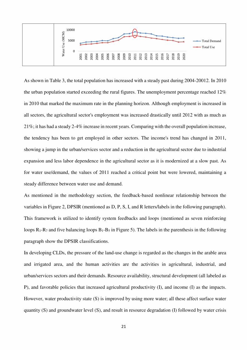
Demand 4128.4 4837.8 6828.6 8678.9 7908.1 6710.3 6133.9
Use 3229.3 3863.2 5522.0 7117.5 6227.1 5240.6 4406.4
Water use change (%)
Industry 34.6 47.4 37.6 28.2 32.8 38.7 43.5
Urban/ Services 99.4 109.5 102.6 103.1 105.1 102.0 99.3
0.0
500.0
1000.0
Pop
ula
tion
(×
10
3)
Total
Urban
Rural
0.03.06.09.0
12.015.0
Un
emp
loym
ent
(%)
0.0
200.0
400.0
600.0
800.0
1000.0
1200.0
Inco
me
(Mil
lion
US
D)
Total
Urban/ Services
Industry
Agriculture
21
As shown in Table 3, the total population has increased with a steady past during 2004-20012. In 2010
the urban population started exceeding the rural figures. The unemployment percentage reached 12%
in 2010 that marked the maximum rate in the planning horizon. Although employment is increased in
all sectors, the agricultural sector's employment was increased drastically until 2012 with as much as
21%; it has had a steady 2-4% increase in recent years. Comparing with the overall population increase,
the tendency has been to get employed in other sectors. The income's trend has changed in 2011,
showing a jump in the urban/services sector and a reduction in the agricultural sector due to industrial
expansion and less labor dependence in the agricultural sector as it is modernized at a slow past. As
for water use/demand, the values of 2011 reached a critical point but were lowered, maintaining a
steady difference between water use and demand.
As mentioned in the methodology section, the feedback-based nonlinear relationship between the
variables in Figure 2, DPSIR (mentioned as D, P, S, I, and R letters/labels in the following paragraph).
This framework is utilized to identify system feedbacks and loops (mentioned as seven reinforcing
loops R1-R7 and five balancing loops B1-B5 in Figure 5). The labels in the parenthesis in the following
paragraph show the DPSIR classifications.
In developing CLDs, the pressure of the land-use change is regarded as the changes in the arable area
and irrigated area, and the human activities are the activities in agricultural, industrial, and
urban/services sectors and their demands. Resource availability, structural development (all labeled as
P), and favorable policies that increased agricultural productivity (I), and income (I) as the impacts.
However, water productivity state (S) is improved by using more water; all these affect surface water
quantity (S) and groundwater level (S), and result in resource degradation (I) followed by water crisis
0
5000
10000
20
01
20
02
20
03
20
04
20
05
20
06
20
07
20
08
20
09
20
10
20
11
20
12
20
13
20
14
20
15
20
16
20
17
20
18
20
19
20
20
Wat
er U
se (
MC
M)
Total Demand
Total Use

22
(water stress (I)). Labor productivity state (S) changes in the different sectors and non-uniform
distribution of income and productivity may cause social challenges (I). Different supply and demand-
side management measures are considered as responses for these conditions; among those are
irrigation network expansions (R).
This results in the reduction of water resources availability and resource degradation, resulting in a
water crisis. As shown in Figure 5, gaining more income motivated farmers to cultivate more (R4),
improve water extraction potential (R6), and increase water withdrawals (R5). On the other hand,
employment in labor productivity increased with more developed agriculture and higher production
(R1 reinforcing loop). It should be noted that these loops and feedbacks might result in some social
challenges, including unbalanced employment development and, in some cases, immigration (rural to
urban); all these result in higher agricultural income. Expanded cultivated areas decreased available
water. Thus, some measures are employed to exploit more water, causing an increase in the cultivated
area and increased water demand (B3 balancing loop). Finally, agricultural development is prevented
by limited available cultivation areas (B1 and B2). As agricultural water demand increases, developing
irrigation technologies for increasing efficiency attracts more attention (R2), resulting in higher
efficiency and decreased water use affecting water productivity. However, cultivating new areas may
be inevitable due to the rebound effect (R3). By withdrawing more water, available water levels are
reduced (B4) since the supply is developed regardless of water shortage (B5), which results in more
water demand (R7). Different supply and demand-side management measures such as irrigation
network expansions and increasing agricultural area to gain more benefit are the measures (temporary
solutions) in recent years. For characterizing the behavior and processes of the system, the SFD (Stock
Flow Diagram) is developed based on the CLDs (Figure 6).

23
Figure 5. Causal loop diagrams of Agro-economic attributes of a system
IrrigationEfficiency
Irrigation TechnologiesDevelopment Potential
Non-agriculturalLand Arable Land
Current Cultivated Area
New CultivatedArea
Maximum Arable Area
AgriculturalProduction
Job Demand
AgriculturalEmployment Agricultural Water
Demand
Water Shoratage
Supply DevelopmentPotential
Water ResourcesExtraction Capacity
Available Water
Water Resources(GW & SW)
AgriculturalIncome
Total Income (Industry,Agriculture, Urban/Services)
Supply
Water Demand
Water CrisisDenial
Water Demand inDevelopment
Human Activities
Social Challenges
Water Productivity
Labor Productivity Water Stress
Total Employement (Indusry,Agriculture, Urban/Services)
+
+
+
+ -
+
++
+
+
+
+
+
-
+
+
+
+
+
+
+
+
+
+
+
+
+
+
+
+
-
-
+
+
+
+
+
B1 B2
R3
R2
R1
R4
R5
R6
B3 B4
B5
R7
+
ResourceDegradation
+
+
.

24
Figure 6. Stock-flow diagram (SD model) of socio-economic attributes of the water system in the study area
Surface water resourcesSurface water
inflow
Surface water
outflow
Agricultural water
withdrawal (SW)
Domestic water
withdrawal (SW) Industrial water
withdrawal (SW)
SW inflow from
other basins
Groundwater resourcesGroundwater
recharge
Groundwater
discharge
Agricultural water
withrawal (GW)
Domestic water
withdrawal (GW)
Industrial water
withdrawal (GW)
Returnflow to GW
Agricultural
returnflow to GW
Industrial
returnflow to GW
Domestic returnflow
to GW
Infiltration
Agricultural area Arable area
Decreasing area
Increasing area
Desired
agricultural area
Differnce between
current and desired area
Water based
agricultural areaIncome based
agricultural area
Agricultural
income
Percipitation
Runoff
Runoff coef
PopulationGrowth rate
Water balance
Supply Demand
Agricultural
demand
Urban demand
Per capita demand
Gross supplyLoss
Water withdrawal
Water shortage
Lake inflow coef.
<Time>
<Time>
SW withdrawal
GW withdrawal
<Time>
<Time>Water req.
Percipitation coef
Available water
Ind. GW coef
<Time>
Agr. GWDom. GW
Dom. SWAgr. SW
Ind. SW
Efficiency
<TIME STEP>
<TIME STEP>
<TIME STEP>
<TIME STEP>
Income-Area func
<Time>
Lake inf.
Evaporation
Evaporation coef
Income-area coef
Evapo
Active population Retried population
R1R2
Agr. emp
Ind. empUrb and services emp
Inc. ind.
empInc. ser.
emp
Inc. agr.
emp
Dec. ind.emp Dec. ser.
emp
Dec. agr.
emp<Agricultural
income>
Ind.
income
Urb and services
income
Difference between urb-service
emp and expected urb-service emp
Expected
urb-service emp
Expected
ind emp
Expected agr emp
Difference between ind.
emp and expected ind. emp
Difference between agr. emp
and expected agr. emp
<TIME STEP>
<TIME STEP><TIME STEP>
Ratio of urb-service mp
per urb-services income
Ratio of ind emp per
ind income
Ratio of agr emp per
agr income
Ind inc ratio
Urb inc ratio
<Time>
Crop price
A ratio
Agr tot with
<Agricultural water
withrawal (GW)>
<Agr tot with>
Crop p
Ind unit ratio
Ind units
Industrial demand
<Ind units>

25
As shown in Figure 6, the model consists of two parts as follows:
1. Social-Economy: including population, urban and services, industries and mines, agriculture, and
the employment (corresponded to the R1 loop in Figure 5) corresponding to each economic sector;
2. Water/Environment: including hydrological cycle’s variables (precipitation, evaporation, etc.),
water resource (inland water resource), water supply and demand, and return flows (corresponded
to the B3, B4, B5 and R5, R6 loop in Figure 5).
The key variables to develop a SD model in the agricultural sector are water withdrawal (MCM),
irrigation efficiency, water requirement (MCM), production (kg), and yield (kg/ha). The two stocks
in this sector are agricultural area (hectare per month), arable area (hectare per month). Two
income-based and water-based agricultural areas are modeled to estimate the desired agricultural
area (Table 4). Considering these stocks and flows, in the context of the causal loop diagrams
(CLDs), the agricultural systems' dynamics corresponded to the B1, B2, and R3, R4, and R5 loops
in Figure 5. The arable area and agricultural area stocks are in a closed-loop by the variables of
increasing and decreasing area. There is another loop between these two stocks with the difference
between current and desired agricultural areas. More details on the equations of functional
relationships considered in the SD model are shown in Table 4.
Table 4. Functional relationships of the SD model
Description Equation Variable
AW: Available Water (MCM), P: Population
(Person), Awc: Agricultural Water Allocation
(MCM), TAw: Total Agricultural Water Need
(MCM), T: Time Step (Year)
Ac = If Then Else (AW>0: &:P>0: &: Awc>0,
MIN ((TAw /T), Awc), 0)
Agricultural water use (Ac)
AI: Agricultural Income (IRR), A: Agricultural area
(km2) AIncome-Based= Lookup Function AI and A(AI)
Income-Based Agriculture
Area (AIncome-Based)
AW: Available Water (MCM), PW: Product Water
Need (cms/ km2), T: Time Step (Year)
AWater-Based = If Then Else (AW >0, (AW ×T)/
PW, 0)
Water-Based Agriculture
Area (AWater-Based)
AIncome-Based: Income-Based Agriculture Area (km2),
AWater-Based: Water-Based Agriculture Area (km2)
AAD = MIN ("AIncome-Based", "AWater-Based")
Desired Agriculture Area
(AAD)

26
CAA: Current Agriculture Crop Area (km2), AAD:
Desired Agriculture Area (km2) DAA = (CAA- AAD)
Difference Between Current
& Desired agricultural Area
(DAA)
DAA: Difference Between Current and Desired
Agriculture Area (ha), T: Time Step (Year), P:
Population (Person)
IA = If Then Else (DAA /T <=0: or: P<=0,
MIN(ABS(DAA), AA)/T, 0)
Increasing agricultural Area
(IA)
DAA: Difference Between Current and Desired
Agriculture Area (km2), P: Population (Person), T:
Time Step (Year)
DA = If Then Else (DAA >0: or: P<=0,
(DAA)/T, 0)
Decreasing agricultural Area
(DA)
DA: Decreasing Area (km2), IA: Increasing Area
(km2) AA = Ʃ (DA - IA) Arable Area (AA)
A: Agricultural area (ha)
Y: Yield (kg/ha)
PrA = A×Y Production (PrA)
a: Irrigation efficiency (dimensionless), h: Applied
agricultural water (m3/ha), Y: Yield (kg/ha) Y=5069.82+811.17(a×h)-0.092(a×h)2 Yield (Y)
CP: Crop price (IRR/kg), A: Agricultural area (km2),
Awc: Applied Agricultural Water (MCM)
AI = 0.062 CP - 0.53 A + 0.65 Awc + 2079.1 Agricultural Income (AI)
In this table, agricultural income as an important variable in estimating the irrigated area, which
alters the variables mentioned above, is developed based on crop price, agricultural area, and
agricultural water use. Agricultural crop production is assumed to have a quadratic relationship
with water input (Caswell and Zilberman 1986). More effective water use leads to higher yields.
However, after reaching the maximum yield, the crop yield decreases with additional effective
water use (Karamouz et al., 2021). The indicators mentioned above (Table 1) are estimated based
on the model's output values. The model is verified by the behavior reproduction tests based on the
data of 2001- 2020.
Behavior-Reproduction Test is one of the critical tests that are conducted before using the model
(Sterman, 2000). Comparing the model's output to historical data ensures that the model's structure

27
and behavior can be reproduced satisfactorily. Observed vs. estimated values for the variables are
shown in Figure 7. As a statistical measure, the coefficient of determination (R2) is used (Eq. 6).
𝑅2 = { ∑ (𝑄𝑖−�̅�)(�̈�𝑡−�̃�)𝑛𝑖=1√∑ (𝑄𝑖−�̅�)2 ∑ (�̈�𝑡−�̃�)2𝑛𝑖=1𝑛𝑖=1 }2 (6)
where 𝑄𝑖 is the estimated value, �̅� is the average of estimated value, �̈�𝑡 is the observed value and �̃� is the average observed value. N is the period of the evaluation. The value of R2 is obtained as
0.84 and 0.68 for agricultural income and area, respectively.
(a) Agricultural income (b) Agricultural area
Figure 7. Observed and modeled variables in the SD model
After the model verification (acceptable R2s estimated by Eq. 6), indicators in environmental,
economic, and social dimensions (derived from the SWA-SD model) are estimated. Table 5 shows
the indicator values in 2001-2020, in three years intervals.
Table 5. Indicator values in 2001-2020 (derived from the SWA-SD model) with 3-year sequence
Indicator 2001 2004 2007 2010 2013 2016 2019 2020
DG 0.60 0.57 0.57 0.62 0.52 0.51 0.63 0.66
RWSI 0.44 0.33 0.51 0.64 0.46 0.58 0.53 0.63
WC 0.66 0.49 1.42 1.84 1.27 1.73 1.45 1.77
RIB A 0.63 0.47 0.79 1.03 0.71 0.97 0.80 0.98
WEP T 4.74 4.54 5.32 7.65 6.98 7.74 10.23 10.70
WEP A 0.67 0.58 0.59 0.71 0.72 0.78 0.96 0.95
0
1000
2000
3000
4000
5000
6000
2000 2010 2020
Agri
cult
ura
l ar
ea (
km
2)
Time
Observed
Modelled
0
1,000
2,000
3,000
4,000
5,000
6,000
2000 2010 2020Agri
cult
ura
l in
com
e (b
IR
R)
Time
Modelled
Observed

28
WEP I 94.71 100.47 86.73 127.03 101.09 89.35 79.04 75.89
WEP U 218.46 284.24 343.40 394.25 424.03 445.76 465.24 471.30
RIE A 0.14 0.13 0.11 0.09 0.10 0.10 0.09 0.09
WUE A 0.08 0.13 0.14 0.14 0.26 0.48 0.61 0.50
LP T 0.18 0.22 0.27 0.29 0.27 0.25 0.24 0.23
LP A 0.12 0.13 0.13 0.13 0.18 0.17 0.17 0.16
LP I 0.60 0.55 0.36 0.39 0.24 0.19 0.16 0.15
LP U 0.17 0.24 0.29 0.32 0.32 0.29 0.27 0.27
EP T 26.63 20.45 20.03 26.56 25.88 30.69 43.00 45.94
EP A 5.55 4.54 4.46 5.37 4.03 4.57 5.63 5.78
EP I 156.93 184.06 242.80 327.99 423.34 462.32 496.81 506.92
Ep U 1257.72 1202.91 1177.03 1216.76 1310.84 1520.67 1708.82 1767.28
UI 0.38 0.42 0.46 0.50 0.57 0.65 0.63 0.63
HI 19.50 23.54 27.63 32.43 36.22 38.55 46.43 47.20
*DG: Dependency on groundwater (MCM/MCM); RWSI: Relative water stress (MCM/MCM); WC: Consumption Index
(MCM/MCM); RIB: Agriculture importance in local water balance (MCM/MCM); WEP: Water productivity (IRR/MCM); RIE:
Agriculture economic importance (Dimensionless); WUE: Agricultural water use efficiency (Dimensionless); LP: Labor
productivity (IRR/cap); EP: Employment productivity (cap/m3); UI: Urbanization index (cap/cap); HI: Housing index (m2/cap).
The values of the relative water stress index (RWSI) demonstrate that this basin faces water stress
and the deficiency (RWSI>0.4) due to high water withdrawals. RWSI was 0.44 in 2001 and became
0.63 in 2020, indicating the worsening situation. Based on Table 5, the agricultural sector's impact
on water balance grew significantly over time (from 0.63 to 0.98). Although the agricultural sector's
water use results higher stress levels, it did not show remarkable water productivity. As for WEP
(Water productivity), the value is increased from 94.71 (in 2000) to 127.03 (in 2010). It is decreased
to 75.89 in 2020. The reason behind this reduction may be related to the fact that the significant
proportion of the industrial sector in the case study are food industry and the variations in crop
production results in variation in the industry sector. For agriculture economic importance (RIE),
a reduction trend is shown, implying that the proportion of agricultural income to total gained

29
income, is reduced by the time. As for labor productivity, the values are increased for the
urban/services sector, while a reduction is shown in industrial sector. As labor productivity is the
value that each employed person creates per unit of his or her input, it implies a growth in income
and output in the urban/services sector. Increases in labor productivity are driven by technological
change, efficiency improvements, quality of labor, and capital deepening (when more capital is
added to a given amount of labor). Therefore, the reduction in industrial labor productivity may be
the result of poor labor education and investments.
PCA is utilized to recognize the most critical variables and evaluate the main components.
According to Eq. 3, the number of components is evaluated based on the eigenvalues (Eq.7 and Eq.
8). In the water/environment attribute, the maximum Eigenvalue is 2.98 out of 4 and has a
contribution of 74. The maximum Eigenvalue is 4.415 and 6.063 for the economic and social
attributes, respectively. Total Eigenvalues are 6 and 10 for economic and social attributes,
respectively. Based on the eigenvalues and the indicators standardized matrix, the eigenvectors are
calculated. The eigenvectors show the coefficients of chosen indicators in principal components.
The values of E (cumulative contribution rate) are estimated as 74, 74, and 61% for environmental,
economic, and social aspects, respectively. Here, there is only one principal component in each
attribute (three components in total). 𝑊𝑅𝑉 = 𝑤1𝑉𝐸𝑛𝑣 + 𝑤2𝑉𝐸𝑐𝑜 + 𝑤3𝑉𝑆𝑜𝑐 (7) VEnv, VEco, and VSoc show the vulnerability in environmental, economic, and social attributes based
on the principal components in each group, respectively. The w1, w2, and w3 are the weights of
these components, respectively. Then, utilizing the SWA-SD and selected indicators, the
environmental, economic, and social principal components are evaluated to estimate water
resources vulnerabilities (WRV). The weights of these components are assumed to be equal. The
values of the coefficients in Eq. 8 are estimated based on the eigenvalues and Eqs. 3, 4, and 5. These
coefficients' signs may vary based on their nature and effect on the estimated principal component.
Each component of WRV consists of certain indicators. The RWSI, WC, and RIBA in

30
water/environmental attribute WEPT, WEPU, WUEA, RIEA, and WUEA in economic attribute, and
EPI, UI, LPI, EPT, EPU, and LPA, in the social attribute are chosen based on principal component
analysis. The WRV principal components are shown as follows:
{𝑉𝑊𝑎𝑡/𝐸𝑛𝑣 = 0.58𝑅𝑊𝑆𝐼 + 0.57𝑊𝐶 + 0.55𝑅𝐼𝐵𝐴 𝑉𝐸𝑐𝑜 = 0.47𝑊𝐸𝑃𝑇 + 0.45𝑊𝐸𝑃𝑈 + 0.45𝑊𝐸𝑃𝐴 − 0.42𝑅𝐼𝐸𝐴 + 0.4𝑊𝑈𝐸𝐴𝑉𝑆𝑜𝑐 = 0.4𝐸𝑃𝐼 + 0.39𝑈𝐼 + 0.32𝐿𝑃𝐴 + 0.36𝐸𝑃𝑇 + 0.35𝐸𝑃𝑈 + 0.33𝐿𝑃𝐴 (8)
The results of estimating different components of water resources vulnerability using Eq. 7 and
Eq. 8 are shown in Figure 8.
Figure 8. Water resources vulnerability in environmental, economic, and social aspects in the study area
(2001-2020)
Agricultural water concerns have also been accompanied by social concerns, including food
security, migration from rural to urban areas, unemployment in rural areas, decreased social
equality, etc. Applying some measures for improving employments in rural areas or increasing
agricultural water productivity might reduce the social vulnerability.
However, the VWat/Env decreased over some years, which could be attributed to the more water
supply. It is demonstrated that increasing demands are responded to with different water-supply
measures, which is why VWat/Env has so many highs and lows. It lays in the range of 0.73-2.24. the
maximum value corresponds to 2008. This water resource vulnerability component has increased
in recent years, as the demands are not met. On the other hand, economic water resources
vulnerability (VEco) with the range of 0.82-1.90 and social water resources vulnerability (VSoc)
0.00
0.50
1.00
1.50
2.00
2.50
3.00
2000 2005 2010 2015 2020
Vu
lner
ab
ilit
y I
nd
icie
s
Year
V-Env
V-Eco
V-Soc
V-Total

31
with the range of 0.89-2.34 follow an upward trend. The maximum values for VEco and VSoc
correspond to 2019 and 2020, respectively. WRV is estimated based on the average values of the
three vulnerability attributes and has a range of 0.89 - 2.04, implying the 20-year period
vulnerability in the case study. Also, it can be stated that increasing trends may result in higher
vulnerabilities if the limiting measures or policies are not considered in local and national policy
and decision making. Considering the results of the vulnerability index, it may be implied that
there was a period of using better technologies, enabling farmers to use water without the
limitation concerns of the supply side. Water systems dynamic evolve hydrological and socio-
economic processes. Therefore, for better system identification, the ability of socio-economic
systems to withstand under certain conditions may be estimated in the context of resiliency.
In the context of better system identification, the scenario assessment is defined based on the
practical measures in the agricultural drought management, including changing the irrigation
efficiency, reducing cultivated area, and applying deficit irrigation (DI) (Table 6). However,
increasing efficiency reduces the return flow and the GW resources in long-term periods; the
rebound effect is another challenge in applying this scenario. Usually, DI decreases agricultural
production based on the water use reduction in the production function mentioned in Table 4;
however, applying DI can reduce water use.
Table 6. Different scenarios based on agricultural drought management
Policies Description
Agricultural drought management
Scenario 1: Reducing cultivated area by 25%
Scenario 2: Changing gravity irrigation to drip irrigation system (Increasing
the irrigation efficiency by 40%)
Scenario 3: Deficit irrigation by 50% for 50% of irrigated area.
Then the scenarios' effectiveness is evaluated based on the SD model during the study period. The
values correspond to the different vulnerability indices are shown in Table 7.

32
Table 7. The scenarios' effectiveness on the system vulnerability in the year 2020 (percentage).
Vulnerability indices Scenario 1 Scenario 2 Scenario 3
VWat/Env 28 45 48
VEco 21 34 41
VSoc 13 22 30
WVR 21 34 40
As shown in Table 7, the third scenario is the most effective scenario. The effect of applying this
scenario (deficit irrigation) is in line with the study by Goli et al. (2019). DI provides lower water
use with acceptable yield (based on the production function); however, it results in some return
flow reduction which is not significant. The second scenario is ranked second, implying that
increasing irrigation efficiency is a good and practical measure in most cases if the rebound effect
is neglected. Changing irrigation systems to drip systems (increasing irrigation efficiency by 40%)
results in approximately zero return flow affecting the GW resources recharge. It may result in
increasing the soil salt content.
5. Summary and conclusion
A framework for water resources systems assessment considering physical water resources and
socio-economic aspects was presented. The methodology consisted of conceptual modeling
methods (i.e., CLD, DPSIR), SEEA-W, and SFD to model the water system through the
development of the SWA-SD (social water-accounting-based system dynamics). The analytical
frameworks such as DPSIR and WA are utilized to evaluating the most effective variables in water
resources performance. A water balance-based extension of the SEEA-W is developed
considering the social accounts. The form of indicators representing the basin's characteristics is
provided based on these frameworks. The feedback-based relationships are identified by causal
loops, and the dynamic interaction of all variables is assessed in the system dynamics environment
33
(SWA-SD model). Without the SD framework, the interaction of the important variables in water
balance and system’s performance could not be evaluated.
The methodology is tested on a generic system that resembles Tashk-Bakhtegan basin in Iran and
the real data of that basin was used. In addition, a practical approach is taken into account to
estimate water balance components for 20 years based on the basic hydrological and water use
data and limited available official water balance data.
As there is no social table in the list of tables of the SEEA-W framework, a dynamic social table
based on the “heart bit” of time series of social data including the demographical changes,
unemployment, migration (urban vs rural population changes), income, water use disparity
compared with the water demand as an indicative of water system welfare.
Based on the relative water stress index values (RWSI>0.4), the water stress and deficiency in the case
study show the supply and demand management requirement of available water resources.
Agriculture's impact on the water balance was increased from 0.47 to 1.28. It implied that water
use in the agricultural sector led to higher water stress and did not produce remarkable water
productivity. Urban/services water productivity was improved by the coefficient of 2.16, with
32% more water use in 20 years. It may be a result of local policies and measures in the case study.
Principal components were evaluated to identify those with a more significant contribution to
variabilities within that component. The principal component analysis (PCA) method was utilized
to divide indicators into three environmental, economic, and social attributes. Then utilizing the
results of the SWA-SD and selected indicators, the environmental (VWat/Env), economic (VEco), and
social (VSoc) components were evaluated to quantify water resources vulnerabilities (WRV). Based
on the results, as increasing demands were supplied with different measures, VWate/Env had many
ups and downs. The economic and social water resources vulnerability (VEco and VSoc) followed an
increasing trend. The effect of applying this scenario (deficit irrigation) it is in line with previous
similar studies (Goli et al., 2019). DI provides about 40% effect of the vulnerability indices.
However, lower agricultural water use, with acceptable yield, results in return flow reduction.

34
Although changing irrigation system to drip systems (increasing irrigation efficiency) affects the
GW resources recharge, it may be the most practical solution of effective water use.
Utilizing the analytical frameworks for evaluating the most effective variables, a water balance-
based extension of the SEEA-W framework is developed considering the social dynamics
accounts. Based on the identified feedback-based relationships, the dynamic interaction of the
variables is assessed by a system dynamics approach. As for utilizing the PCA method, it helps
to reduce some interdependent indicators into a manageable number of components to quantify
water stress vulnerabilities. The result shows the significant value of utilizing water balance data
in the development and practical application of seventeen indicators representing different
water/environment, economic and social attributes of a water supply and demands system. The
proposed methodology could be utilized as a tool for system analysts and decision-making in
water systems with social and economic volatility in different developing geographic settings.
Declarations
Conflict of interest
The authors declare that there is no conflict of interest.
Ethical Approval
Not applicable.
Consent to Participate
Not applicable.
Consent to Publish
Not applicable.
Authors Contributions
E. Ebrahimi: Conceptualization; Data acquisition and preparation; Materials and Methods;
Modeling setup; Analysis and presentation, Manuscript preparation.
M. Karamouz: Development of the original concepts and scope of the work; Materials and
Methods; Validation; Manuscript preparation; Review and editing.

35
Funding
Not applicable.
Competing interests
The authors declare no competing interests.
Availability of data and materials
All input data used in this research can be found from the publicly available domains Ministry of
Energy (http://www.moe.gov.ir/), Ministry of Agriculture (https://www.maj.ir/), Ministry of
Industry, Mining, and Trade (http://en.mimt.gov.ir/), and Statistical Center
(https://www.amar.org.ir/). Nevertheless, all data, models, or codes that support the findings of
this study are available from
the corresponding author upon request.
References
Adger, W. N. (2006). Vulnerability. Global environmental change, 16(3), 268-281.
Borrego-Marín, M. M., Gutiérrez-Martín, C., & Berbel, J. (2016). Water productivity under drought
conditions estimated using SEEA-Water. Water, 8(4), 138.
Bruneau, M., Chang, S.E., Eguchi, R.T., Lee, G.C., O' Rourke, T.D., Reinhorn, A.M., Shinozuka,
M., Tierney, K., Wallace, W.A. and Von Winterfeldt, D., (2003). A framework to
quantitatively assess and enhance the seismic resilience of communities. Earthquake
spectra, 19(4), pp.733-752.
Caswell, M. F., and D. Zilberman. (1986). “The effects of well depth and land quality on the choice
of irrigation technology.” Am. J. Agric. Econ. 68 (4): 798–811.
Contreras, S., & Hunink, J. E. (2015). Water Accounting at the Basin Scale: Water Use and Supply
(2000–2010) in the Segura River Basin Using the SEEA Framework. FutureWater:
Cartagena, Spain.
Cook, C., & Bakker, K. (2012). Water security: Debating an emerging paradigm. Global
environmental change, 22(1), 94-102.

36
da Silva, J., Fernandes, V., Limont, M., Dziedzic, M., Andreoli, C. V., & Rauen, W. B. (2020).
Water sustainability assessment from the perspective of sustainable development capitals:
Conceptual model and index based on literature review. Journal of environmental
management, 254, 109750.
Delavar, M., Morid, S., Morid, R., Farokhnia, A., Babaeian, F., Srinivasan, R., & Karimi, P. (2020).
Basin-wide water accounting based on modified SWAT model and WA+ framework for
better policy making. Journal of Hydrology, 124762.
Dutta, D., Vaze, J., Kim, S., Hughes, J., Yang, A., Teng, J., & Lerat, J. (2017). Development and
application of a large scale river system model for National Water Accounting in
Australia. Journal of Hydrology, 547, 124-142.
Dwyer, A., Zoppou, C., Nielsen, O., Day, S., & Roberts, S. (2004). Quantifying social vulnerability:
a methodology for identifying those at risk to natural hazards.
Ebrahimi, S. E., & Zarghami, M. (2019). Sustainability assessment of restoration plans under
climate change using system dynamics: application on Urmia Lake, Iran. Journal of Water
and Climate Change, 10(4), 938-952.
Ekinci, E., Kazancoglu, Y., Mangla, S (2020). Using system dynamics to assess the environmental
management of cement industry in streaming data context. Science of The Total
Environment, (715), 136948.
Esen, S; Hein, L (2020). Development of SEEA water accounts with a hydrological model. Science
of The Total Environment, (737), 140168.
Fussel, H.M. (2007). Vulnerability: a generally applicable conceptual framework for climate
change research. Global Environ. Change 17 (2), 155–167.
Gasco, G., D. Hermosilla, A. Gasco, and J. M. Naredo. (2005). “Application of a physical input–
output table to evaluate the development and sustainability of continental water resources
in Spain.” Environ. Manage. 36 (1): 59–72.

37
Haak, L., & Pagilla, K. (2020). The water-economy nexus: a composite index approach to evaluate
urban water vulnerability. Water Resources Management, 34(1), 409-423.
Hjorth, P., Bagheri, A. (2006). Navigating towards sustainable development: A system dynamics
approach. Futures 38 (2006) 74–92
Hoekstra, A.Y., Chapagain, A.K. (2006). Water footprints of nations: water use by people as a
function of their consumption pattern. In: Integrated Assessment of Water Resources and
Global Change. Springer, Dordrecht, pp. 35–48.
IPCC, 2014: Summary for policymakers. In: Climate Change 2014: Impacts, Adaptation, and
Vulnerability. Part A: Global and Sectoral Aspects. Contribution of Working Group II to
the Fifth Assessment Report of the Intergovernmental Panel on Climate Change [Field, CB,
V.R. Barros, D.J. Dokken, K.J. Mach, MD. Mastrandrea, T.E. Bilir, M. Chatterjee, K.L.
Ebi, Y.O. Estrada, R.C. Genova, B. Girma, E.S. Kissel, A.N. Levy, S. MacCracken, P.R.
Mastrandrea, and L.L. White (eds.)]. Cambridge University Press, Cambridge, United
Kingdom and New York, NY, USA, pp. 1-32.
Inam, A., Adamowski, J., Halbe, J., & Prasher, S. (2015). Using causal loop diagrams for the
initialization of stakeholder engagement in soil salinity management in agricultural
watersheds in developing countries: A case study in the Rechna Doab watershed,
Pakistan. Journal of environmental management, 152, 251-267.
Iran Ministry of Energy. (2020). http://www.moe .gov.ir/.
Iran Statistical Center. (2020). https://www.amar.org.ir/.
Jin, W., Xu, L., & Yang, Z. (2009). Modeling a policy making framework for urban sustainability:
Incorporating system dynamics into the Ecological Footprint. Ecological
Economics, 68(12), 2938-2949.
Karamouz, M., Barkhordari, H., & Ebrahimi, E. (2021). Dynamics of Water Allocation: Tradeoffs
between Allocator's and Farmers' Benefits of Irrigation Practices. Journal of Irrigation and
Drainage Engineering, 147(6), 04021017.

38
Karamouz M. and Movahhed, M. (2021). Asset management based flood resiliency of water
infrastructure. Proceedings of Virtual World Environmental and Water Resources Congress
2021, Milwaukee, WS, June 7–11.
Karamouz, M., Rahimi, R., & Ebrahimi, E. (2021). Uncertain water balance-based sustainability
index of supply and demand. Journal of Water Resources Planning and Management,
147(5), 04021015.
Karimi, P., Bastiaanssen, W. G., & Molden, D. (2013). Water Accounting Plus (WA+)–a water
accounting procedure for complex river basins based on satellite measurements. Hydrology
and Earth System Sciences, 17(7), 2459-2472.
Karimi, P., Bastiaanssen, W. G., Molden, D., & Cheema, M. J. M. (2013). Basin-wide water
accounting based on remote sensing data: an application for the Indus Basin. Hydrology and
Earth System Sciences, 17(7), 2473-2486.
Kiguchi, M., Shen, Y., Kanae, S., & Oki, T. (2015). Re-evaluation of future water stress due to
socio-economic and climate factors under a warming climate. Hydrological Sciences
Journal, 60(1), 14-29.
Li, H., Cohen, A., Li, Z., & Zhang, M. (2019). The impacts of socio-economic development on
rural drinking water safety in China: a provincial-level comparative analysis. Sustainability,
11(1), 85.
Long, X., Ji, X., (2019). Economic Growth Quality, Environmental Sustainability, and Social
Welfare in China - Provincial Assessment Based on Genuine Progress Indicator (GPI).
Ecological economics, 159, 157-176.
Mahdavi, T., Bagheri, A., & Hosseini, S. A. (2019). Applying the System of Environmental and
Economic Accounts for Water (SEEA-Water) for integrated assessment of water security in
an aquifer scale-Case study: Azarshahr aquifer, Iran. Groundwater for Sustainable
Development, 9, 100261.
39
Mirchi, A., Madani, K., Watkins, D., & Ahmad, S. (2012). Synthesis of system dynamics tools for
holistic conceptualization of water resources problems. Water resources management,
26(9), 2421-2442.
Molden, D. (1997). Accounting for Water Use and productivity (No. 42). IWMI.Colombo, Sri
Lanka.
Rajesh, S., Jain, S., & Sharma, P. (2018). Inherent vulnerability assessment of rural households
based on socio-economic indicators using categorical principal component analysis: A case
study of Kimsar region, Uttarakhand. Ecological indicators, 85, 93-104.
Sterman, J.D., 2000. Business Dynamics: Systems Thinking and Modeling for a Complex World.
UNSD, United Nations Statistical Division (2012). London group on environmental accounting.
Subgroup on water accounting. In: System of Environmental-Economic Accounting for
Water, vol. 100, United Nations Publications.
United Nations (2009). System of National Accounts 2008. UN, New York.
van Beek, E., & Arriens, W. L. (2014). Water security: putting the concept into practice (p. 55).
Stockholm: Global Water Partnership.
Ventana Systems, (2004). Vensim 5 User's Guide. Ventana Systems Inc., Harvard, MA, USA.
Wateraccounting.org
Wei, W., Shi, S., Zhang, X., Zhou, L., Xie, B., Zhou, J., & Li, C. (2020). Regional-scale assessment
of environmental vulnerability in an arid inland basin. Ecological Indicators, 109, 105792.
Zare, F., Elsawah, S., Bagheri, A., Nabavi, E., & Jakeman, A. J. (2019). Improved integrated water
resource modeling by combining DPSIR and system dynamics conceptual modeling
techniques. Journal of environmental management, 246, 27-41.

40
Appendix A
The basin's data are organized using the SEEA-W framework water account tables (Tables A1, A2, and A3). In the agricultural sector, different crops are
selected based on the cultivated areas of the five subareas of the Tashk-Bakhtegan basin (Figure 9) (UNSD, 2012).
Table A1. Water accounting table in the study area based on the 2006 data.
Agriculture
Industry
Urban/
Services
Total
Rice Barely Maize Wheat Apple Grapes Pomegranate Total
Total abstraction (MCM) 703.9 221.8 104.8 2281.9 249.7 90.9 153.7 3806.7 49.1 111.7 3967.5
Surface water (MCM) 166.5 43.3 24.8 471.2 58.8 64.7 2.9 832.2 4.9 27.9 865
Groundwater (MCM) 536.8 139.5 80 1519.4 190.9 6.1 0 2472.7 44.2 83.8 2600.7
Soil water (MCM) 0 38.8 0 274.2 1.1 6.1 2.9 323.1 0 0 323.1
Total returns (MCM) 385.8 121.7 57.4 1260 136.9 49.8 84.2 2095.8 0 29.7 2125.5
Total output (1000 USD) 216.7 11.9 4.8 1614.3 0.0 321.4 9.5 2178.6 51471.4 509047.6 562697.6
Total use (1000 USD) 62595.2 3695.2 1073.8 467797.6 23.8 92973.8 2481.0 630640.5 29173.8 386876.2 1046690.5
Evapotranspiration (MCM) 6204.4

41
As shown in Table A1, for the year 2006, about 96% of the total water use is corresponded to the agricultural sector. About 22% of the total abstraction is
from surface water resources. As for the year 2011 (Table A2), the agricultural sector's proportion of total water abstraction is about 0.97%, with about 10%
share of surface water. Showing the highest dependency on groundwater in 2011 due to the highest demand for water in that year.
Table A2. Water accounting table in the study area based on the 2011 data of the official record.
Agriculture
Industry
Urban/
Services
Total
Rice Barely Maize Wheat Apple Grapes Pomegranate Total
Total abstraction (MCM) 505.8 1992.2 575.1 3376 374.7 278.4 216.9 7319.1 27 108.3 7454.4
Surface water (MCM) 72.9 101 114.8 233.2 74.5 35.8 42.5 674.7 1.9 22.3 698.9
Groundwater (MCM) 404.2 291.7 459.3 932.7 298.2 143.2 170.2 2699.5 24.3 86 2809.8
Soil water (MCM) 0 1626.2 0 2199.2 1.6 99.3 4 3930.4 0 0 3930.4
Total returns (MCM) 278 102.2 315.8 1856.3 205.5 152.7 119 4019.5 18.6 21.7 4059.8
Total output (1000 USD) 178.6 52.4 38.1 876.2 0.0 9.5 9.5 1164.3 57111.9 713450.0 771726.2
Total use (1000 USD) 98433.3 28119.0 21364.3 479709.5 90.5 4819.0 5066.7 637604.8 39978.6 189778.6 867361.9
Evapotranspiration (MCM) 9691
As shown in Table A3, for the year 2020, the agricultural sector's proportion of total water use is about 0.98%, with about 14% share of surface water. Total
economic output is increased by 11% from 2011 to 2020. Water abstraction for the industrial sector was increased after the lowest experienced in 2011.

42
Table A3. Water accounting table in the study area, synthesized for 2020 data, based on the framework proposed by Karamouz et al. (2021).
Agriculture
Industry
Urban/
Services
Total
Rice Barely Maize Wheat Apple Grapes Pomegranate Total
Total abstraction (MCM) 668.6 200.1 197.8 2400.3 412.6 205.1 242.5 4327 44.5 98.8 4470.3
Surface water (MCM) 77.3 96.9 83.5 208.6 81.3 33.6 50.3 631.5 9.9 24.2 665.6
Groundwater (MCM) 591.3 103.2 114.3 2191.7 331.3 171.5 192.2 3695.5 34.5 74.5 3804.5
Total returns (MCM) 308.1 131.5 98.8 1396.7 248.4 164.2 156.2 2503.9 26.7 69.2 2599.8
Total output (103 USD) 223.8 45.2 40.5 1271.4 0.0 240.5 11.9 1833.3 63504.8 788104.8 853442.9
Total use (103 USD) 148866.7 46404.8 26192.9 505842.9 121.4 6514.3 6045.2 739988.1 47559.5 314526.2 1102073.8
Evapotranspiration (MCM)
Figure 9. The location of the water resources sub-system based on the Tashk-Bakhtegan basin
Irrigation Network 1- Namdan Irrigation Network 1- Aspas
Irrigation Network 1- Doroudzan
Irrigation Network 1- Marvdasht
Irrigation Network 1- Neiriz
Surface water
Groundwater

43
Appendix B (Water Balance Estimation)
Table B1 shows the source of available data that are used for estimating water balance variables.
The variables, relationships, assumptions, and the framework of technical information to generate
water balance data are listed in Table B2.
Table B1. Time series of climatic and hydrologic data for generating water balance variables
Data Source
Rainfall Regional Water Authority (RWA)
Precipitation/Evaporation RWA
Population Iran statistical center
Irrigated area Dept. of Agriculture
In Table B2, there are three parts. The first part is the equations of water demand in different sectors
(agricultural, industrial, and urban/services). A regression equation is developed based on the
income, irrigated area, population, and industrial units. The next parts correspond to the
groundwater and surface water. Variables such as inflow, infiltration, and drainage are included in
synthesizing groundwater resources balance data. The main components of surface water balance
data that are not stated in official reports are the irrigation and non-irrigation backflows. The values
of all these variables are synthesized based on official reports, time series of the basic hydrologic
cycle variables (precipitation etc.), and judgment. See Karamouz et al. (2021) for more details.

44
Table B2. Water balance data technical framework - variables, relations, assumptions, (2001-
2020)
Variable Relationship Assumptions Note
Agricultural 𝐷𝑒𝑚𝑎𝑛𝑑𝑎𝑔𝑟𝑖 = 0.12 × 𝐼 + 1.35 × 𝐴 − 1340.9 It is proportional to the
cultivated area and income
𝐼 = 𝐼𝑛𝑐𝑜𝑚𝑒 𝐴 = 𝐴𝑟𝑒𝑎 𝑜𝑓irrigation network
Domestic 𝐷𝑒𝑚𝑎𝑛𝑑𝑑𝑜𝑚 = 0.05 × 𝑃 + 47.49 It is proportional to the
population 𝑃 = 𝑃𝑜𝑝𝑢𝑙𝑎𝑡𝑖𝑜𝑛
Industrial 𝐷𝑒𝑚𝑎𝑛𝑑𝑖𝑛𝑑 = 0.02 × 𝑛 + 17.17 It is proportional to the
number of industrial units 𝑛 = 𝑛𝑢𝑚𝑏𝑒𝑟 𝑜𝑓 𝑖𝑛𝑑𝑢𝑠𝑡𝑟𝑖𝑎𝑙 𝑢𝑛𝑖𝑡𝑠
Groundwater variables
Variable Relationship Assumptions Note
Inflow to the
aquifer Qin = Inf + RF
Inf= infiltration
RF= Return flow
Infiltration from
precipitation
Estimated according to the rate of infiltration
from precipitation (reported in the formal
reports)
16% of the precipitation Time series for rainfall of available
stations
Infiltration from
surface water
Estimated according to the rate of infiltration
from runoff (reported in the formal reports) 12% of the precipitation
Time series for rainfall of available
stations
Infiltration from
irrigation backflow 𝐼𝑛𝑓𝑎𝑔𝑟𝑖 = 0.12(0.12 × 𝐼 + 1.35 × 𝐴 − 1340.9)
12% of the agricultural
water demand
Estimated according to the official
reports
Infiltration from
non-irrigation
backflow
𝐼𝑛𝑓𝑖𝑛𝑑 = 0.7[(0.05 × 𝑃 + 47.49) + (0.02 × 𝑛+ 17.17)] 70% of the domestic water
demand
Estimated according to the official
reports
Drainage to
surface water 𝑀𝑎𝑥 (0.01 × 𝐺𝑊 𝑠𝑡𝑜𝑟𝑎𝑔𝑒 𝑎𝑛𝑑 370)
Estimated according to the official
reports
Surface water variables
Variable Relationship Assumptions Note
Inflow from out of
the basin 0
According to the topography of the
basin, there is no Inflow from the
outside of the basin
Non-irrigation
backflow
𝑏𝑎𝑐𝑘𝑓𝑙𝑜𝑤𝑑𝑜𝑚 = 0.3[(0.05 × 𝑃 + 47.49)+ (0.02 × 𝑛 + 17.17)] 30% of the domestic water
demand
Estimated according to the official
reports
Irrigation
backflow
𝑏𝑎𝑐𝑘𝑓𝑙𝑜𝑤𝑎𝑔𝑟𝑖 = 0.3(0.12 × 𝐼 + 1.35 × 𝐴− 1340.9)
30% of the agricultural
water demand
Estimated according to the official
reports

45
Table B3 shows the values for available water (AW) in the last two years of official record (2006
and 2011) and the synthesized water balance data. The synthesized data closely follows the official
record shown by the absolute error (%).
Table B3. Available water (AW) values from official and Synthesized data
Absolute Error (%) AW ** (MCM) AW* (MCM) Year
3.9 5084 5292 2006
0.5 4912 4937 2011
*/**: based on official/synthesized water balance data