Dynamics of disordered systems - LPTHE
43
Dynamics of disordered systems Leticia F. Cugliandolo Sorbonne Universités, Université Pierre et Marie Curie Laboratoire de Physique Théorique et Hautes Energies Institut Universitaire de France [email protected] www.lpthe.jussieu.fr/ ˜ leticia/seminars Boulder, Colorado, USA, 2017
Transcript of Dynamics of disordered systems - LPTHE

Dynamics of disordered systems
Leticia F. Cugliandolo
Sorbonne Universités, Université Pierre et Marie Curie
Laboratoire de Physique Théorique et Hautes Energies
Institut Universitaire de France
www.lpthe.jussieu.fr/ leticia/seminars
Boulder, Colorado, USA, 2017
1

Plan of Lectures
1. Introduction
2. Coarsening processes
3. Formalism
4. Dynamics of disordered spin models
2
Plan of 3rd Lecture
1. Langevin equation
(derivation, time-scales)
2. Stochastic calculus
(discretisation, chain-rule, Fokker-Planck, drift-force)
3. Generating functional formalism
(Onsager-Machlup, Martin-Siggia-Rose)
4. Time-reversal symmetry
(fluctuation-dissipation theorem, fluctuation theorems)
3

Formalism
4

Dissipative systemsAim
Interest in describing the statics and dynamics of a classical or quan-
tum physical system coupled to a classical or quantum environment.
The Hamiltonian of the ensemble is
H = Hsyst +Henv +Hint
Environment
System
Interaction
The dynamics of all variables are given by Newton or Heisenberg rules, depen-
ding on the variables being classical or quantum.
The total energy is conserved,E = ct, but each contribution is not, in particular,
Esyst 6= ct, and we’ll take Esyst � Eenv .
5

Reduced systemModel the environment and the interaction
E.g., an ensemble of harmonic oscillators and a linear in qa and non-linear in x,
via the function V(x), coupling :
Henv +Hint =N∑α=1
[p2α
2mα
+mαω
2α
2q2α
]+N∑α=1
cαqαV(x)
Equilibrium. Imagine the whole system in contact with a bath at inverse tempe-
rature β. Compute the reduced classical partition function or quantum density
matrix by tracing away the bath degrees of freedom.
Dynamics. Classically (coupled Newton equations) and quantum (easier in a
path-integral formalism) to get rid of the bath variables.
In all cases one can integrate out the oscillator variables as they appear only
quadratically.
6

Reduced systemStatistics of a classical system
Imagine the coupled system in canonical equilibrium with a megabath
Zsyst + env =∑
env, syst
e−βH
Integrating out the environmental (oscillator) variables
Zredsyst =∑syst
e−β(Hsyst− 1
2
∑a
c2amaω2
a[V(x)]2
)6= Zsyst =
∑syst
e−βHsyst
One possibility : assume weak interactions and drop the new term.
Trick : add Hcounter to the initial coupled Hamiltonian, and choose it in such a
way to cancel the quadratic term in V(x) to recover
Zredsyst = Zsyst
i.e., the partition function of the system of interest.
7

Reduced systemDynamics of a classical system : general Langevin equations
The system, p, x, coupled to an equilibrium environment evolves according
to the multiplicative noise non-Markov Langevin equation
Inertia friction︷ ︸︸ ︷mx(t) +V ′(x(t))
︷ ︸︸ ︷∫ ∞t0
dt′ γ(t− t′)x(t′)V ′(x(t′)) =
−δV (x)
δx(t)︸ ︷︷ ︸+V ′(x(t)) ξ(t)︸︷︷︸deterministic force noise
The friction kernel is γ(t− t′) = Γ(t− t′)θ(t− t′)The noise has zero mean and correlation 〈 ξ(t)ξ(t′) 〉 = kBT Γ(t− t′) with
T the temperature of the bath and kB the Boltzmann constant.
8

Reduced systemDynamics of a classical system : general Langevin equations
The system, p, x, coupled to an equilibrium environment evolves according
to the multiplicative noise non-Markov Langevin equation
Inertia friction︷ ︸︸ ︷mx(t) +V ′(x(t))
︷ ︸︸ ︷∫ ∞t0
dt′ γ(t− t′)x(t′)V ′(x(t′)) =
−δV (x)
δx(t)︸ ︷︷ ︸+V ′(x(t)) ξ(t)︸︷︷︸deterministic force noise
Important Noise arises from lack of knowledge on bath ; noise can be mul-
tiplicative ; memory kernel generated ; equilibrium assumption on bath va-
riables implies detailed balance between friction and noise
9

Separation of time-scalesAdditive white noise
In classical systems one usually takes a bath kernel with the smallest
relaxation time, tenv � tall other time scales.
The bath is approximated by the white form Γ(t− t′) = 2γδ(t− t′)
Moreover, one assumes the coupling is bi-linear, Hint =∑
a caqax.
The Langevin equation becomes
mx(t) + γx(t) = − δV (x)δx(t)
+ ξ(t)
with 〈ξ(t)〉 = 0 and 〈ξ(t)ξ(t′)〉 = 2kBTγ δ(t− t′).
10

Separation of time-scalesVelocities and coordinates
For t� τv = m/γ one expects the velocities to equilibrate to the
Maxwell distribution P ({~v}) =∏i
P (~vi) ∝∏i
e−βmv2i /2
In this limit, one can drop mvai and work with the
overdamped equation γrai = −V ({~ri})δrai
+ ξai .
The positions can have highly non-trivial dynamics, see examples.
Message : be very careful when trying to prove equilibration.
Different variables could behave very differently.
11

Stochastic calculusTwo ways of writing the multiplicative noise equation
The physical eq. that comes from integrating away the bath (oscillators)
(V ′[x(t)])2dtx(t) = F [x(t)] + V ′[x(t)]ξ(t)
and the equation usually found in the mathematics literature
dtx(t) = f [x(t)] + g[x(t)]ξ(t)
are equivalent after identification
g[x(t)] =1
V ′[x(t)]
f [x(t)] =1
(V ′[x(t)])2F (x(t)) = (g[x(t)])2 F [x(t)]
12

Stochastic calculusDiscretization prescriptions
dtx(t) = f [x(t)] + g[x(t)] ξ(t)
with 〈ξ(t)〉 = 0 and 〈ξ(t)ξ(t′)〉 = 2D δ(t− t′) means
x(t+ dt) = x(t) + f [x(t)] dt+ g[x(t)] ξ(t)dt
withx(t) = αx(t+ dt) + (1− α)x(t)
and 0 ≤ α ≤ 1. Particular cases are α = 0 Ito ; α = 1/2 Stratonovich.
Stratonovich 67, Gardiner 96, Øksendal 00, van Kampen 07
13

Stochastic calculusOrders of magnitude & different stochastic processes
ξk ≡ ξ(tk) = O(dt−1/2) because of the Dirac-delta correlations
dx ≡ x(tk+1)− x(tk) = O(dt1/2) Variable increment
What is the difference between the two terms in the right-hand-side when
they are evaluated using different discretisation schemes?
f [xα(tk)]− f [xα(tk)] = O(dt1/2) vanishes for dt→ 0
g[xα(tk)]ξ(tk)− g[xα(tk)]ξ(tk) = O(dt0) remains finite for dt→ 0
For multiplicative noise processes the discretisation matters:
different α yields different stochastic processes.
14

Stochastic calculusDiscretization prescriptions
dtx(t) = f [x(t)] + g[x(t)] ξ(t)
with 〈ξ(t)〉 = 0 and 〈ξ(t)ξ(t′)〉 = 2D δ(t− t′) means
x(tk+1) = x(tk) + f [x(tk)] dt+ g[x(tk)] ξ(tk)dt
withx(tk) = αx(tk+1) + (1− α)x(tk)
The chain rule for the time-derivative is (just from Taylor expansion)
dtY (x) = dtx dxY (x) +D(1− 2α) g2(x) d2xY (x)
Only for α = 1/2 (Stratonovich) one recovers the usual expression.
Not even for additive noise the chain rule is the usual one if α 6= 1/2
15
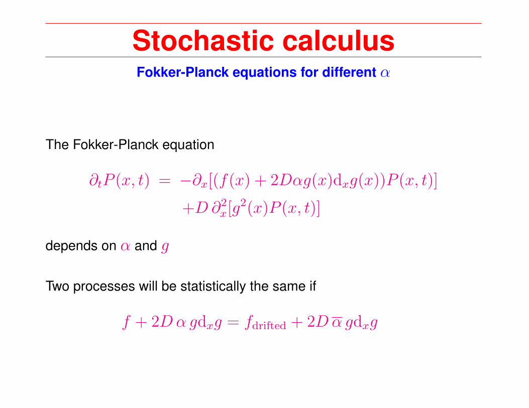
Stochastic calculusFokker-Planck equations for different α
The Fokker-Planck equation
∂tP (x, t) = −∂x[(f(x) + 2Dαg(x)dxg(x))P (x, t)]
+D∂2x[g
2(x)P (x, t)]
depends on α and g
Two processes will be statistically the same if
f + 2Dαgdxg = fdrifted + 2Dαgdxg
16
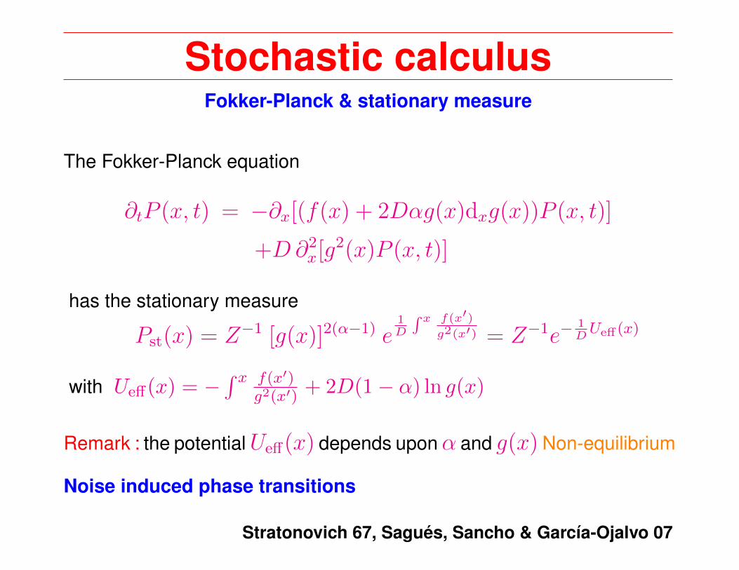
Stochastic calculusFokker-Planck & stationary measure
The Fokker-Planck equation
∂tP (x, t) = −∂x[(f(x) + 2Dαg(x)dxg(x))P (x, t)]
+D∂2x[g
2(x)P (x, t)]
has the stationary measure
Pst(x) = Z−1 [g(x)]2(α−1) e1D
∫ x f(x′)g2(x′) = Z−1e−
1DUeff(x)
with Ueff(x) = −∫ x f(x′)
g2(x′) + 2D(1− α) ln g(x)
Remark : the potentialUeff(x) depends uponα and g(x) Non-equilibrium
Noise induced phase transitions
Stratonovich 67, Sagués, Sancho & García-Ojalvo 07
17

Stochastic calculusFokker-Planck & stationary measure
e.g. f = −g2U and Ueff = U + 2D(1− α) ln g
x2 + 2D(1− α) lnx x2 + 2D(1− α) ln (1− x2)
g(x) = x g(x) = (1− x2)
U(x) = x2 U(x) = x2
18

Stochastic calculusDrift
The Gibbs-Boltzmann equilibrium
PGB(x) = Z−1 e−βU(x)
is approached if (recall the physical writing of the equation)
f(x) 7→ −g2(x)dxU(x)︸ ︷︷ ︸+ 2D(1− α)g(x)dxg(x)︸ ︷︷ ︸Potential drift
Remark: the drift is also needed for the Stratonovich mid-point scheme.
Important choice : if one wants the dynamics to approach thermal equi-
librium independently of α and g the drift term has to be added.
19
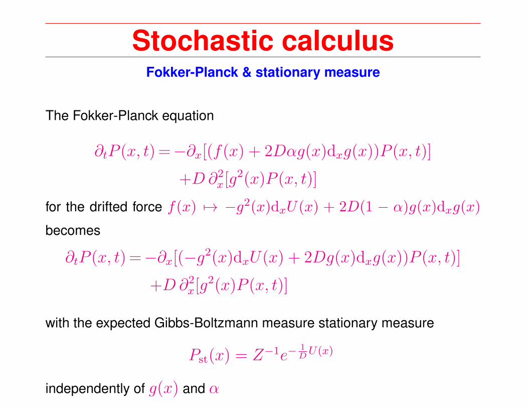
Stochastic calculusFokker-Planck & stationary measure
The Fokker-Planck equation
∂tP (x, t) =−∂x[(f(x) + 2Dαg(x)dxg(x))P (x, t)]
+D∂2x[g
2(x)P (x, t)]
for the drifted force f(x) 7→ −g2(x)dxU(x) + 2D(1 − α)g(x)dxg(x)
becomes
∂tP (x, t) =−∂x[(−g2(x)dxU(x) + 2Dg(x)dxg(x))P (x, t)]
+D∂2x[g
2(x)P (x, t)]
with the expected Gibbs-Boltzmann measure stationary measure
Pst(x) = Z−1e−1DU(x)
independently of g(x) and α
20

Why care aboutmultiplicative noise ?
21
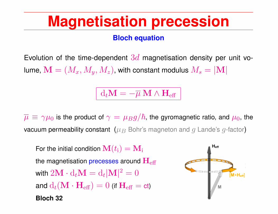
Magnetisation precessionBloch equation
Evolution of the time-dependent 3d magnetisation density per unit vo-
lume, M = (Mx,My,Mz), with constant modulus Ms = |M|
dtM = −µM ∧Heff
µ ≡ γµ0 is the product of γ = µBg/~, the gyromagnetic ratio, and µ0, the
vacuum permeability constant (µB Bohr’s magneton and g Lande’s g-factor)
For the initial condition M(ti) = Mi
the magnetisation precesses around Heff
with 2M · dtM = dt|M|2 = 0
and dt(M ·Heff) = 0 (if Heff = ct)
Bloch 32
22

Dissipative effectsLandau-Lifshitz & Gilbert equations
dtM = − µ
1 + γ20µ
2 M ∧[Heff +
γ0µ
Ms(M ∧Heff)
]Landau &
Lifshitz 35
dtM = −µM ∧(Heff −
γ0
MsdtM
)Gilbert 55
2nd terms in RHS : dissipative mechanisms slow
down the precession and push M towards Heff
with 2M · dtM = dt|M|2 = 0
and dt(M ·Heff) > 0
23

Thermal fluctuationsÀ la Langevin in Gilbert’s formulation
dtM = −µM ∧(Heff + H− γ0
Ms
dtM
)
H is a white random noise, with zero mean 〈Hi(t)〉 = 0 and correlations
〈Hi(t)Hj(t′)〉 = 2Dδijδ(t− t′)
The (diffusion) parameter D is proportional to kBT Brown 63
The noise H multiplies the magnetic moment M and one cannot always write
2M · dtM = dtM2 (only if the Stratonovich calculus is used)
This is the Markov stochastic Landau-Lifshitz-Gilbert-Brown (sLLGB) multi-
plicative white noise stochastic differential equation.
Subtleties of Markov multiplicative noise processes are now posed.
24

Thermal fluctuationsÀ la Langevin in Gilbert’s formulation
dtM = −µM ∧(Heff + H− γ0
Ms
dtM
)− 2D(1− 2α)µ2
1 + µ2γ20
M
H is a white random noise, with correlations 〈Hi(t)Hj(t′)〉 = 2Dδijδ(t− t′)
The (diffusion) parameter D is proportional to kBT Brown 63
The modulus of the magnetic moment is now conserved dtM2 = 0 for all α
One also proves that the dynamics approaches the asymptotic Gibbs-Boltzmann
distribution
PGB(M) ∝ e−1DM·Heff
25

MethodsDynamic generating functional
• Glassy models with and without disorder:
The "order parameter" is a composite object depending on two-times.
It’s handy to use functional methods to write a dynamic generating
functional as a path-integral
Onsager-Machlup & Martin-Siggia-Rose-Janssen-deDominicis formalisms
Similar to Feynman path-integral
The construction will follow LFC & Lecomte, “Rules of calculus in the path integralrepresentation of white noise Langevin equations : the Onsager-Machlup approach”,arXiv :1704.03501, J. Phys. A (to appear) where special care of discretisation effectswas taken.
26
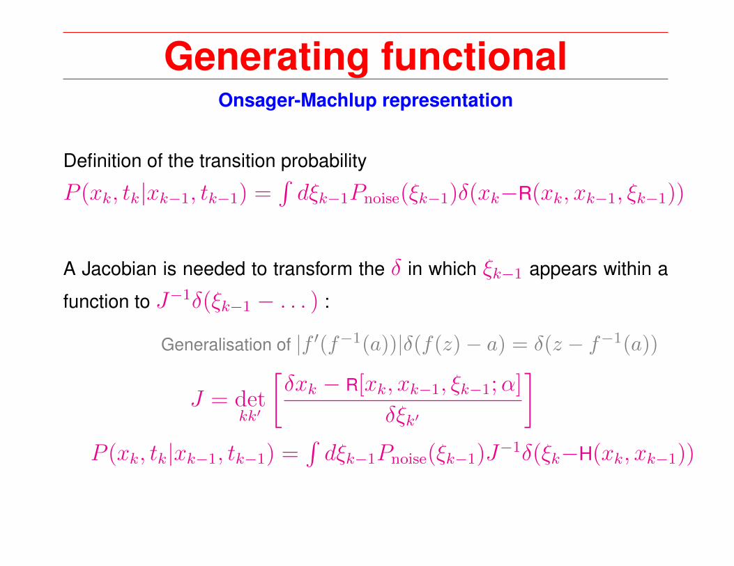
Generating functionalOnsager-Machlup representation
Definition of the transition probability
P (xk, tk|xk−1, tk−1) =∫dξk−1Pnoise(ξk−1)δ(xk−R(xk, xk−1, ξk−1))
A Jacobian is needed to transform the δ in which ξk−1 appears within a
function to J−1δ(ξk−1 − . . . ) :
Generalisation of |f ′(f−1(a))|δ(f(z)− a) = δ(z − f−1(a))
J = detkk′
[δxk − R[xk, xk−1, ξk−1;α]
δξk′
]P (xk, tk|xk−1, tk−1) =
∫dξk−1Pnoise(ξk−1)J−1δ(ξk−H(xk, xk−1))
27

Generating functionalOnsager-Machlup representation
The transition probability now reads
P (xk, tk|xk−1, tk−1) =
√1
4πkBTdt
1
|g(xk−1)|eSOM[xk,xk−1;α]
For dtx(t) = f(x(t)) + g(x(t))ξ(t), the Onsager-Machlup action is
SOM[xk, xk−1;α] ≡ lnPi(x−T )
− dt
4kBT
[1
g2(xk−1)
((xk − xk−1)
dt− f(xk−1)
+2Dαg(xk−1)g′(xk−1)︸ ︷︷ ︸)2
−αf ′(xk−1)︸ ︷︷ ︸]
From the integration over the noise Jacobian
28
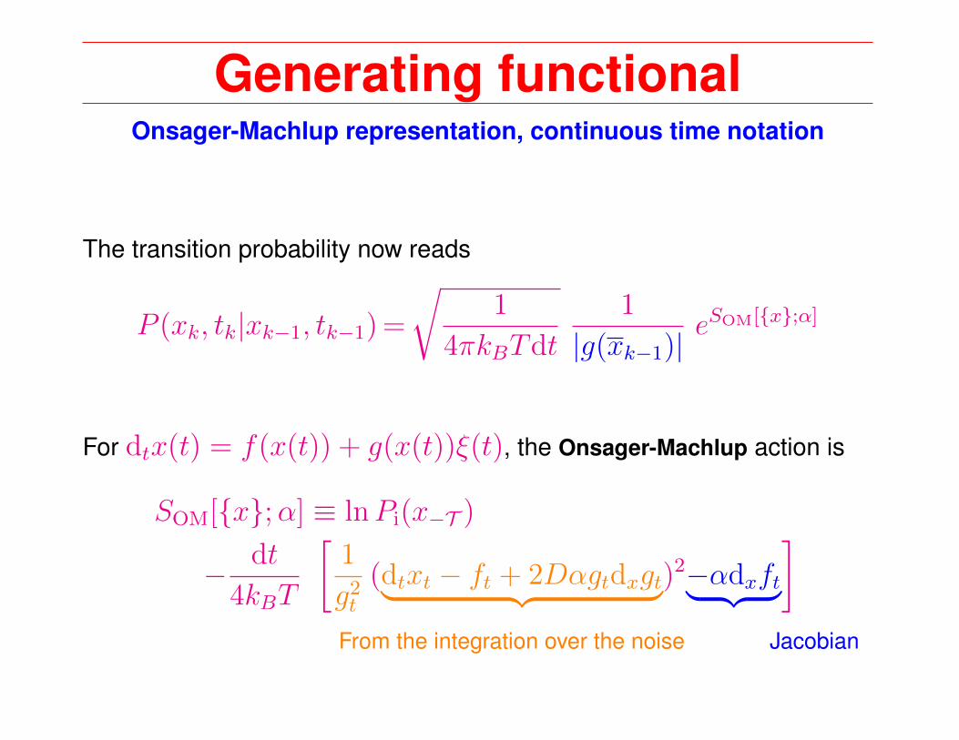
Generating functionalOnsager-Machlup representation, continuous time notation
The transition probability now reads
P (xk, tk|xk−1, tk−1) =
√1
4πkBTdt
1
|g(xk−1)|eSOM[{x};α]
For dtx(t) = f(x(t)) + g(x(t))ξ(t), the Onsager-Machlup action is
SOM[{x};α] ≡ lnPi(x−T )
− dt
4kBT
[1
g2t
(dtxt − ft + 2Dαgtdxgt︸ ︷︷ ︸)2−αdxft︸ ︷︷ ︸]
From the integration over the noise Jacobian
29

Generating functionalMSR path-integral representation
The initial state at time−T is drawn from a probability distributionPi(x−T ).
The noise generates random trajectories with probability density
P ({x};α) = 〈∏N
k=1 δ(xk − xsolk )〉Pi(x−T )
where the angular brackets represent an average over the noise {ξ}weighted with its probability distribution.
xsolk is the (possibly implicit) solution to the Langevin equation
0 = Eqnt[xk, xk−1, ξk−1;α]
The integral over the noise can be computed if one inverts to write ξk−1 =
L(xk, xk−1;α) and imposes this constraint with a delta function.
30

Generating functionalMSR path-integral representation
A Jacobian is needed to transform the δ in which ξk−1 appears within a
function to J−1δ(ξk−1 − . . . ) :
Generalisation of |f ′(f−1(a))|δ(f(z)− a) = δ(z − f−1(a))
J = detkk′
[δEqnt[xk, xk−1, ξk−1;α]
δξk′
]The path-probability now reads
P ({x};α) = 〈∏N
k=1 J−1δ(ξk−1 − L(xk, xk−1;α))〉Pi(x−T )
where the angular brackets still represent an average over the noise {ξ}weighted with its probability distribution.
This Jacobian is simple for additive noise but not so simple to compute
for multiplicative noise.
31

Generating functionalMSR path-integral representation
A Jacobian is needed to transform the δ in which ξk−1 appears within a
function to J−1δ(ξk−1 − . . . ) :
Generalisation of |f ′(f−1(a))|δ(f(z)− a) = δ(z − f−1(a))
J = detkk′
[δEqnt[xk, xk−1, ξk−1;α]
δξk′
]The path-probability now reads
P ({x};α) = 〈∏N
k=1 J−1δ(ξk−1 − L(xk, xk−1;α))〉Pi(x−T )
where the angular brackets still represent an average over the noise {ξ}weighted with its probability distribution.
This Jacobian is simple for additive noise but not so simple to compute
for multiplicative noise.
32

Generating functionalMSR path-integral representation
Using now the exponential representation of the delta δ(y) ∝∫dy e±iyy,
the integral over the noise is now a Gaussian that can be computed and
POM({x};α) =
∫D{x}
N−1∏k=0
(4πkBTdtg2(xk))−1/2 eSMSR[{x},{ix};α]
and the Martin-Siggia-Rose-Janssen 79 action is
SMSR[{x}, i{x};α] ≡ lnPi(x−T )
+
∫ [±ixt(dtxt︸︷︷︸− ft + 2Dαgtdxgt) +D(ixt)
2g2t︸ ︷︷ ︸−αdxft︸ ︷︷ ︸
]proportional to γ0 (not written) Jacobian
where we have also transformed the auxiliary field ixt 7→ ixtgt
33

Generating functionalPath-integral representation
POM({x};λ, α) ∝∫D{x} PMSR({x}, {ix};λ, α)
=
∫D{x}
N−1∏k=0
(4πkBTdtg2(xk))−1/2 eSMSR[{x},{ix};λ,α]
SMSR[{x}, {ix};λ, α] ≡ lnPi(x−T , λ−T )
+
∫ [±ixt(dtxt − ft + 2Dαgtdxgt) +D(ixt)
2g2t − αdxft
]λt is a time-dependent parameter, for example, a parameter in the poten-
tial that one can tune in time. The action depends on α and g.
Observable averages can now be calculated as
〈A(xt, ixt′)〉 =
∫D{x}D{x} PMSR({x}, {ix};λ, α) A(xt, ixt′)
34

Generating functionalPath-integral representation
For the drifted force ft = −g2dxVt + 2D(1− α)gtdxgt
SMSR({x}, {ix};λ, α) ≡ lnPi(x−T , λ−T )
+
∫ [±ixt(dtxt + g2
t dxVt − 2D(1− 2α)gtdxgt)
+D(ixt)2g2t − αdxft
]Remark: The action depends on α and g.
Observable averages can now be calculated as
〈A(xt, ixt′)〉 =
∫D{x}D{x} PMSR({x}, {ix};α, λ) A(xt, ixt′)
and do not depend on α
35

Stochastic calculusPath-integral representation for additive noise
For g = 1 and the force ft = −dxVt the action is
SMSR[{x}, {ix};α] ≡ lnPi(x−T )
+
∫ [±ixt(dtxt + dxVt) +D(ixt)
2 + αd2xVt]
Observable averages can now be calculated as
〈A(xt, ixt′)〉 =
∫D{x}D{x} PMSR({x}, {ix};λ, α) A(xt, ixt′)
and do not depend on α
36

MethodsDynamical symmetry & exact results
The functional path-integral formalism allows one to obtain exact iden-
tities (fluctuation-dissipation theorem, fluctuation theorems) as conse-
quences of a dynamic symmetry and its symmetry breaking.
Details in :
“Symmetries of generating functionals of Langevin processes with colored multiplicativenoise” Aron, Biroli & LFC, J. Stat. Mech. P11018 (2010) ; “Dynamical symmetries ofMarkov processes with multiplicative white noise”, Aron, Barci, LFC, González Arenas& Lozano, J. Stat. Mech. 053207 (2016)
Possible (though not easy) to extend to quantum system.
“(Non) equilibrium dynamics : a (broken) symmetry of the Keldysh generating functional”
Aron, Biroli & LFC, arXiv:1705.10800
37
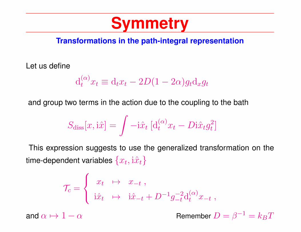
SymmetryTransformations in the path-integral representation
Let us define
d(α)t xt ≡ dtxt − 2D(1− 2α)gtdxgt
and group two terms in the action due to the coupling to the bath
Sdiss[x, ix] =
∫−ixt [d
(α)t xt −Dixtg
2t ]
This expression suggests to use the generalized transformation on the
time-dependent variables {xt, ixt}
Tc =
xt 7→ x−t ,
ixt 7→ ix−t +D−1g−2−t d
(α)t x−t ,
and α 7→ 1−α Remember D = β−1 = kBT
38
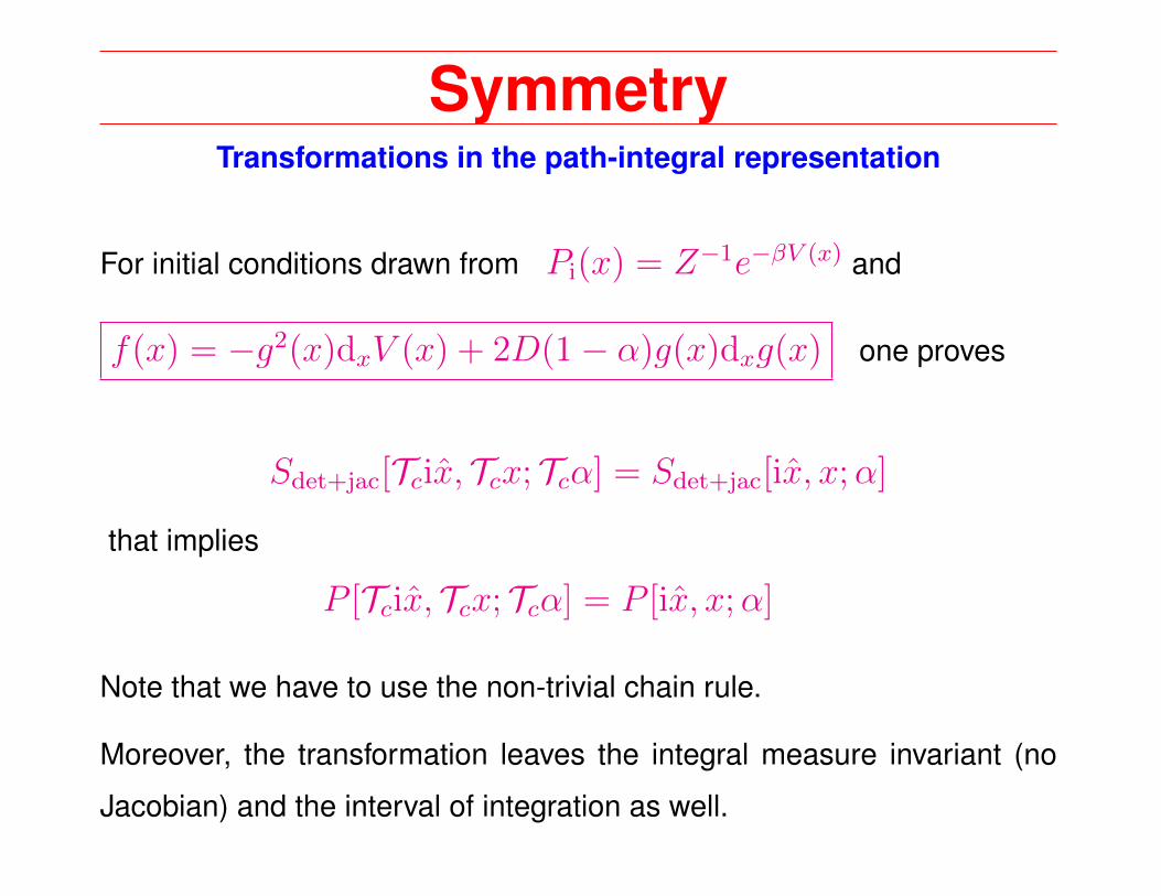
SymmetryTransformations in the path-integral representation
For initial conditions drawn from Pi(x) = Z−1e−βV (x) and
f(x) = −g2(x)dxV (x) + 2D(1− α)g(x)dxg(x) one proves
Sdet+jac[Tcix, Tcx; Tcα] = Sdet+jac[ix, x;α]
that implies
P [Tcix, Tcx; Tcα] = P [ix, x;α]
Note that we have to use the non-trivial chain rule.
Moreover, the transformation leaves the integral measure invariant (no
Jacobian) and the interval of integration as well.
39

SymmetryConsequences of the transformation: FDT
From this result we can prove exact equilibrium relations such as the
fluctuation-dissipation theorem linking the (causal) linear response to
a field that changes the force as ft 7→ ft + ht
R(t, t′) =δ〈x(t)〉δh(t′)
∣∣∣∣h=0
∝ θ(t− t′)
and the correlation function in a model independent way :
R(t, t′)−R(−t,−t′) = β ∂t′〈x(−t)x(−t′)〉
that for a stationary problem (in equilibrium) becomes
R(t− t′)−R(t′ − t) = β ∂t′C(t′ − t) = β ∂t′C(t− t′)
40
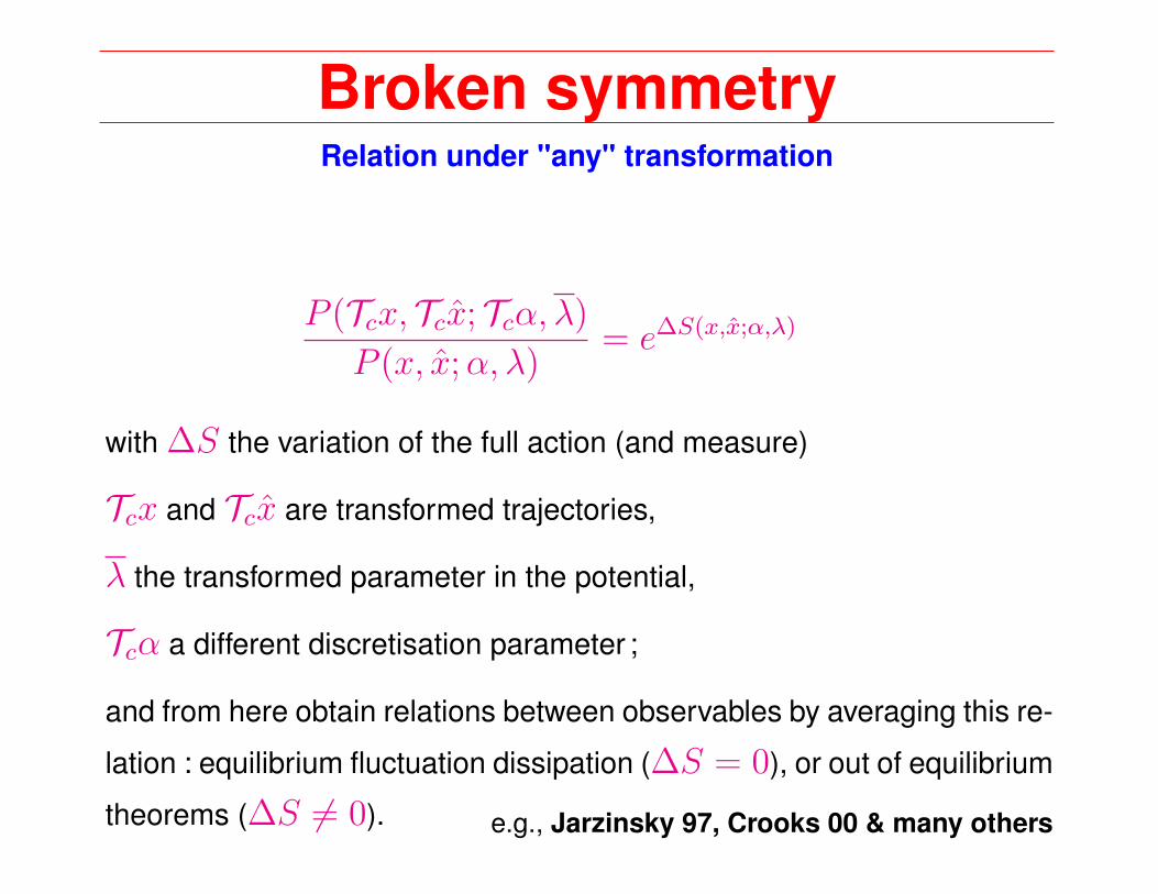
Broken symmetryRelation under "any" transformation
P (Tcx, Tcx; Tcα, λ)
P (x, x;α, λ)= e∆S(x,x;α,λ)
with ∆S the variation of the full action (and measure)
Tcx and Tcx are transformed trajectories,
λ the transformed parameter in the potential,
Tcα a different discretisation parameter ;
and from here obtain relations between observables by averaging this re-
lation : equilibrium fluctuation dissipation (∆S = 0), or out of equilibrium
theorems (∆S 6= 0). e.g., Jarzinsky 97, Crooks 00 & many others
41
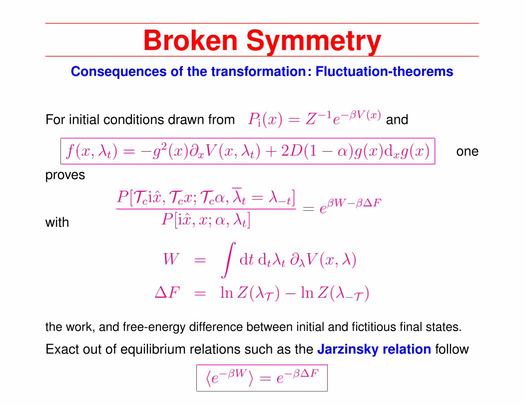
Broken SymmetryConsequences of the transformation: Fluctuation-theorems
For initial conditions drawn from Pi(x) = Z−1e−βV (x) and
f(x, λt) = −g2(x)∂xV (x, λt) + 2D(1− α)g(x)dxg(x) one
proves
P [Tcix, Tcx; Tcα, λt = λ−t]
P [ix, x;α, λt]= eβW−β∆F
with
W =
∫dt dtλt ∂λV (x, λ)
∆F = lnZ(λT )− lnZ(λ−T )
the work, and free-energy difference between initial and fictitious final states.
Exact out of equilibrium relations such as the Jarzinsky relation follow
〈e−βW 〉 = e−β∆F
42

Coloured noiseLangevin equation & generating functional
The generic Langevin equation for a particle in 1d is
mx(t) + V ′[x(t)]
∫ t
−Tdt′ Γ(t− t′)V ′[x(t′)]x(t′) = F (t) + ξ(t)M ′[x(t)]
with the coloured noise 〈ξ(t)ξ(t′)〉 = kBT Γ(t− t′)
The dynamic generating functional is a path-integral
Zdyn[η] =
∫dx−T dx−T
∫DxDx e−S[x,ix;η]
with ix(t) the ‘response’ variable.
x−T and x−T are the initial conditions at time−T .
Martin-Siggia-Rose-Jenssen-deDominicis formalism
43