The Dissertation Committee for Yao You Certifies that this is the approved version of the following:

Dynamics of dilative slope failure

Committee:

David Mohrig, Supervisor

Peter Flemings, Co-Supervisor

Omar Ghattas

John T. Germaine

Marc Hesse

Dynamics of dilative slope failure

by

Yao You, B.S.; M.S.

Dissertation

Presented to the Faculty of the Graduate School of

The University of Texas at Austin

in Partial Fulfillment

of the Requirements

for the Degree of

Doctor of Philosophy

The University of Texas at Austin

December 2013

iii

Acknowledgements

I would like to thank my co-advisors, Peter Flemings and David Mohrig, for their

strong support and guidance; they pushed me forward when I stuck and they pick me up

when I lost confidence. I also want to thank them for their great patience in helping me to

present scientific work better, both in presentations and in writing. Both Peter and

David’s passion for science inspires me to keep exploring and thinking. I would also like

to thank my other dissertation committee members, Jack Germaine, Marc Hesse, and

Omar Ghattas, for helpful discussions on the research. I also want to thank Jack

Germaine for his guidance in properly running geotechnical tests.

This work is based on experiments and I owe it to the lab assistants and managers.

I thank David Brown for assisting in designing, preparing, and running the experiments;

Mark Andrews for building the data collection system for pore pressure measurements

and helping with geotechnical tests; Polito and Donnie Brooks for assisting geotechnical

tests; Jim Buttles for his assistance in building the flumes and running the flume

experiments; Mauricio Perillo for his assistance on using the ultrasonic transceiver. I

would also like to thank Brandon Minton, Tian Dong, Trevor Hutton, and Stephen Heron

for their assistance in running the flume experiments.

I thank other faculty members, postdocs, and my colleagues for their assistance in

running experiments, helpful discussions, comments on writings, and support for my

work. I would especially thank John Shaw for the brain storming we had; a lot of the

ideas we discussed may seem silly now but those discussions pushed this work forward

tremendously. I also thank Derek Sawyer, Kuldeep Chaudhary, Kristopher Darnel,

Audrey Sawyer, Travis Swanson, Aymeric Peyret, Luc Lavier, Ravindra Duddu, Jake

iv

Jordan, Kiran Sathaye, Anjali Fernandes, Julia Reece, Athma Bhandari, Maria-Katerina

Nikolinakou, Katie Delbecq, Virginia Smith, Wayne Wagner, Wen Deng, and Nicolas

Huerta.

I thank the staff members in Jackson School of Geosciences for their support on

everything happens in the background of this work. I especially thank Mark Wiederspahn

for maintaining the computing systems at the Institute for Geophysics, where all my

numerical models ran and all my data is saved; Tessa Green for keeping the GeoFluids

research group running smoothly; Philip Guerrero for assistance on the administrative

aspects of graduate student life; Elsa Jimenez for assistance with financial quests.

I thank my partner Justin Stigall, for his support, patience, and love that carried

me through.

Financial support for this work comes from GeoFluids consortium at the

University of Texas at Austin (www.beg.utexas.edu/geofluids/index, supported by 11

energy companies), the Ewing Worzel fellowship from the University of Texas Institute

for Geophysics, National Science Foundation funded National Center for Earth-surface

Dynamics, and RioMAR Industry Consortium.

v

Dynamics of dilative slope failure

Yao You, Ph.D.

The University of Texas at Austin, 2013

Supervisors: Peter Flemings and David Mohrig

Submarine slope failure releases sediments; it is an important mechanism that

changes the Earth surface morphology and builds sedimentary records. I study the

mechanics of submarine slope failure in sediment that dilates under shear (dilative slope

failure). Dilation drops pore pressure and increases the strength of the deposit during

slope failure. Dilation should be common in the clean sand and silty sand deposits on the

continental shelf, making it an important mechanism in transferring sand and silt into

deep sea. Flume experiments show there are two types of dilative slope failure: pure

breaching and dual-mode slope failure. Pure breaching is a style of retrogressive

subaqueous slope failure characterized by a relatively slow (mm/s) and steady retreat of a

near vertical failure front. The retreating rate, or the erosion rate, of breaching is

proportional to the coefficient of consolidation of the deposit due to an equilibrium

between pore pressure drop from erosion and pore pressure dissipation. The equilibrium

creates a steady state pore pressure that is less than hydrostatic and is able to keep the

deposit stable during pure breaching. Dual-mode slope failure is a combination of

breaching and episodic sliding; during sliding a triangular wedge of sediment falls and

causes the failure front to step back at a speed much faster than that from the breaching

period. The pore pressure fluctuates periodically in dual-mode slope failure. Pore

pressure rises during breaching period, weakens the deposit and leads to sliding when the

vi

deposit is unstable. Sliding drops the pore pressure, stabilizes the deposit and resumes

breaching. The frequency of sliding is proportional to the coefficient of consolidation of

the deposit because dissipation of pore pressure causes sliding. Numerical model results

show that more dilation or higher friction angle in the deposit leads to pure breaching

while less dilation or lower friction angle leads to dual-mode slope failure. As a

consequence, pure breaching is limited to thinner deposits and deposits have higher

relative density.

vii

Table of Contents

List of Tables ...........................................................................................................x

List of Figures ........................................................................................................ xi

Chapter 1: Introduction .........................................................................................1

Chapter 2: 1D analytical model for steady state breaching ..................................5

2.1 Introduction ...............................................................................................5

2.2 Experimental observation .........................................................................7

2.3 1D steady-state breaching model ............................................................11

2.4 Equilibrium between the slope failure and pore pressure dissipation.....14

2.5 Characteristics of the steady state pore pressure solution .......................17

2.6 Breaching condition ................................................................................21

2.7 Conclusions .............................................................................................23

Chapter 3: 2D numerical model for steady state breaching ................................25

3.1 Introduction .............................................................................................25

3.2 2D pore pressure model for steady state breaching ................................28

3.3 Empirical model for dilation potential ....................................................31

3.4 Numerical model solutions .....................................................................39

3.4.1 Approach .....................................................................................39

3.4.2 Pore pressure results ...................................................................42

3.4.3 Stress path of the sediments during breaching ............................46

3.4.4 Sensitivity study ..........................................................................49

3.7 Variation of erosion rate in the vertical direction ...................................54

3.8 Conclusions and discussion ....................................................................57

Chapter 4: Dual-mode slope failure ....................................................................61

4.1 Introduction .............................................................................................61

4.2 Experiment setup ....................................................................................63

4.3 Dual-Mode failure ...................................................................................66

4.4 Pore pressure measurements ...................................................................70

viii

4.5 2D transient pore pressure model ...........................................................75

4.6 Stability analysis .....................................................................................79

4.7 Mechanics of dual-mode slope failure ....................................................82

4.8 Conditions for dual-mode slope failure to occur ....................................87

4.9 Potential field sites for dilative slope failure ..........................................89

4.10 Conclusions and discussion ..................................................................93

Chapter 5: Conclusions .......................................................................................95

Chapter 6: Future Research .................................................................................98

6.1 Study dilative slope failure with centrifuge models ...............................98

6.2 Varying Cv ...........................................................................................100

6.3 Develop better models for material properties ......................................101

6.4 Experiment with different initial slope angles ......................................102

6.5 Study how common dilation is in the field ...........................................103

Appendix A: Supplementary material for Chapter 2 ........................................105

A.1 Pore pressure measurements from all 9 locations ................................105

A.2 Estimate the modeling parameter η and s0 .......................................105

A.3 Estimate the dilation potential of sand at Scripps Canyon from published simple shear test results .....................................................................106

Appendix B: Additional steps in processing triaxial test data ..........................110

Appendix C: Procedure for measuring pore pressure in the flume ...................113

C.1 Install tube fittings ................................................................................114

C.1.1 Tube fitting attached to the transducer .....................................114

C.1.2 Tubing system attached to the inner flume ..............................116

C.2 Installing tubes .....................................................................................116

C.3 flush the tubing system .........................................................................117

C.4 Calibration of the transducers ..............................................................118

Appendix D: Procedure for setting up flume ....................................................122

D.1 Setup of the experiment .......................................................................122

D.2 Running the experiment .......................................................................123

ix

References ............................................................................................................126

x

List of Tables

Table 3.1: List of modeling parameter symbols, explanation, values (if it is a model

input), and units. ...............................................................................41

Table 3.2: Estimated relative density (ID) of clean sand deposits in published

literature. Larger values of ID means the deposit has smaller

porosity/void ratio. ID > 1 means the in situ porosity is smaller than the

estimated minimum value and ID < 0 means the in situ porosity is

larger than the estimated maximum value. Assuming the deposits are

less than 10m thick, the condition for the deposit to dilate is ID > 0.2

according to Bolton (1986). ..............................................................60

Table 4.1. Size of the 4 sliding wedges compared to the associated magnitude of

pore pressure drop. The number of the sliding events is according to the

order they occur in time (Figure 4.4). ...............................................86

xi

List of Figures

Figure 2.1: Morphodynamic evolution and pore pressure response during breaching.

Initial dimensions of sediment: ~30 cm tall, 40 cm wide. The pore

pressure is monitored at nine locations and I show two of them here for

simplicity (for measurements from all sensors see Figure A.1 in

Appendix A). A: After 10 s, sediments are falling from vertical face

(breaching front) and forming turbidity current (light gray). B: After 80

s, erosion has shifted breaching front to right and it is approaching blue

pressure sensor. Turbidity currents have deposited sediment in front of

breaching front. C: Removal of retaining wall results in abrupt drop in

pore pressure at both sensors (0–22 s, dark gray region). As breaching

front approaches each pressure sensor, there is second pressure drop and

then rise to hydrostatic pressure (light gray zones at 80 s and 130 s for

blue and red sensors, respectively). Final pore pressure is lower than

initial pore pressure due to drop of water table, which is caused by

removal of restraining plate. Chaotic pore pressure signal recorded

between 10 s and 40 s by all sensors is due to transient slumping of

sediments connected to removal of restraining plate; this is not part of

steady-state breaching process I focus on in this study. .....................6

Figure 2.2: Grain size distributions of the silty sand (solid line) and well-sorted fine

sand (dashed line) used in the study. ..................................................8

Figure 2.3: Traces of the breaching front during one experiment, the trace lines are

separated by 20s. The dashed line represents the location where I

measure the erosion rate (shown in Figure 2.4). .................................9

xii

Figure 2.4: Erosion rate v estimated from the trace of breaching front (Figure 2.3)

against time. v at time t represents the average velocity between

t-20s and t; it is calculated as the distance the breaching front travels

along the dashed line in Figure 2.3 during this period divided by 20s.

The error bars represents the uncertainty in time (± 1s). This uncertainty

is too small compared to the time scale of the experiment (horizontal

axis) therefore only its influence on the erosion rate (vertical axis) is

plotted here..........................................................................................9

Figure 2.5: Excess pore pressure 10 s (diamonds), 80 s (squares), 140 s (triangles),

and 190 s (dashed line) after onset of breaching, plotted with distance

from breaching front (Lagrangian coordinates). At each time, there is

minimum in pore pressure ~5 cm behind breaching front. Pore pressure

at 140 s is almost identical to pore pressure at 190 s in Lagrangian

coordinates, suggesting that pore pressure is at steady state. Solid line is

excess pore pressure predicted by Equation 4. .................................11

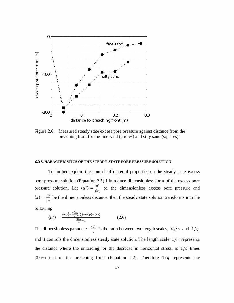
Figure 2.6: Measured steady state excess pore pressure against distance from the

breaching front for the fine sand (circles) and silty sand (squares). .17

Figure 2.7: A: The dimensionless distance to the minimum dimensionless excess

pore pressure (or maximum pore pressure drop) xm against the

controlling parameter ξ for the dimensionless excess pore pressure

solution. B: the minimum dimensionless excess pore pressure um

against the controlling parameter ξ. The circle symbol in both sub

figures marks the ξ for fine sand and the square symbol in both sub

figures marks the ξ for silty sand. ...................................................19

xiii

Figure 2.8: A: dimensionless excess pore pressure u*

βs0 against dimensionless

distance xvCv

from measurements in silty sand (squares) and in fine sand

(circiles), and the steady state solution (solid lines, Equation 2.6). The

controlling parameter ξ is 24 for the fine sand and 1.5 for the silty sand.

B: zoom in of the boxed area in A. Dimensionless excess pore pressure u*

βs0 against dimensionless distance xv

Cv from measurements (circles and

dashed line) and the steady state solution (solid line, Equation 2.6) for

the fine sand. The scales of the axes of the two plots are different. .20

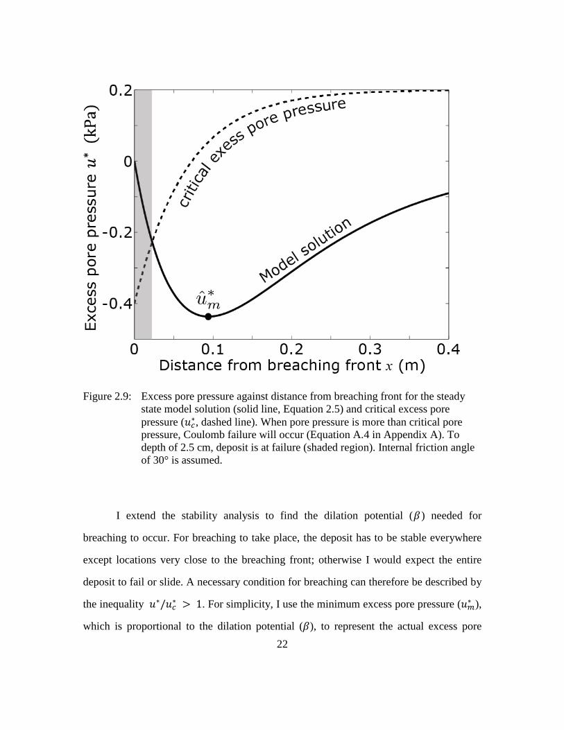
Figure 2.9: Excess p pore pressure against distance from breaching front for the

steady state model solution (solid line, Equation 2.5) and critical excess

pore pressure (uc* , dashed line). When pore pressure is more than critical

pore pressure, Coulomb failure will occur (Equation A.4 in Appendix

A). To depth of 2.5 cm, deposit is at failure (shaded region). Internal

friction angle of 30° is assumed. .......................................................22

Figure 2.10: Ratio of minimum excess pore pressure (um* , Figure 2.9) to critical

excess pore pressure (uc*) increases linearly with dilation potential �β = 1

2+ mq

2mu�. When um

*

uc*< 1, sliding and slumping will occur and

breaching will not proceed. When β ≥ 4, um*

uc*> 1 and breaching can

proceed. Three silty sand samples from Scripps Canyon (squares) have

dilation potential β = 4.1, 8.6, and 25.4 (not plotted), indicating that

they are in regime where breaching can proceed. .............................24

xiv

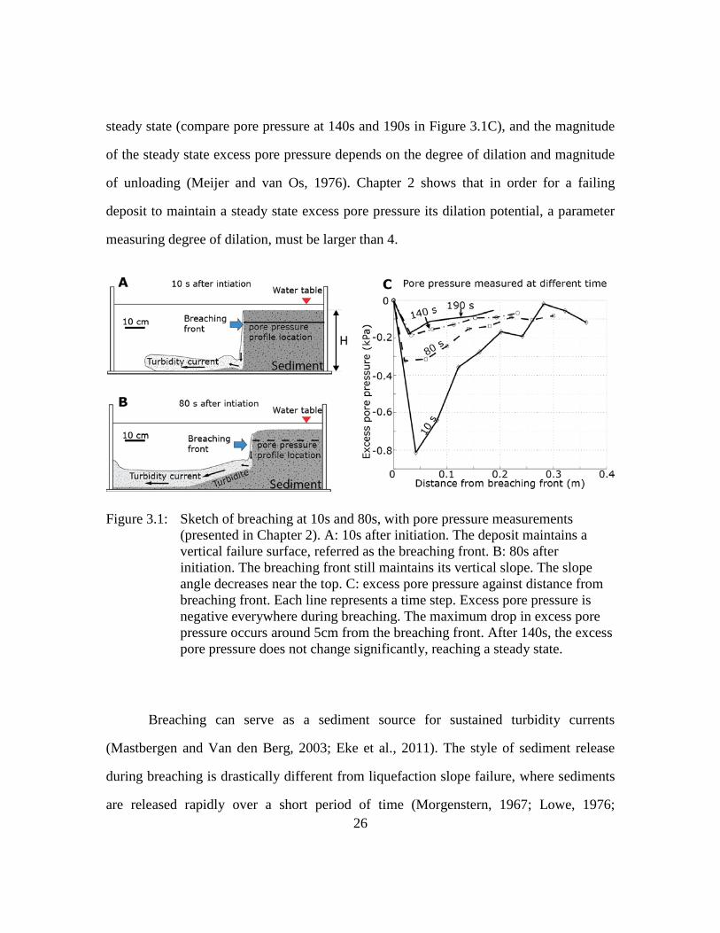
Figure 3.1: Sketch of breaching at 10s and 80s, with pore pressure measurements

(presented in Chapter 2). A: 10s after initiation. The deposit maintains a

vertical failure surface, referred as the breaching front. B: 80s after

initiation. The breaching front still maintains its vertical slope. The slope

angle decreases near the top. C: excess pore pressure against distance

from breaching front. Each line represents a time step. Excess pore

pressure is negative everywhere during breaching. The maximum drop

in excess pore pressure occurs around 5cm from the breaching front.

After 140s, the excess pore pressure does not change significantly,

reaching a steady state. .....................................................................26

Figure 3.2: Sketch of the triaxial shearing device. The specimen is wrapped in a

layer of water tight membrane so that it is hydraulically separated from

the water chamber. The cell pump and pore pump controls the pressure

in the water chamber and specimen respectively. The pore pump also

measures the changes in the specimen volume (δV). Pore pressure (up)

is measured from both the top and bottom end of the specimen. A load

sensor located on the piston measures the amount of force acting on the

specimen in the vertical direction (Fv). The chamber water pressure (uc)

is measured at the base. The specimens have an averaged diameter of

5cm and an averaged height of 10cm. ..............................................32

xv

Figure 3.3: Measurements of the isotropic unloading compressibility mu (squares)

and absolute value of reloading compressibility |mc| (circles) at

different mean effective stress p' on the fine sand used in Chapter 2.

The relationship between p' and mu is the same as the relationship

between p' and |mc|, and both are best fit with a logarithmic equation

(dashed line, R2 = 0.92). .................................................................33

Figure 3.4: A: volumetric strain against differential stress q measured from one

drained vertical compression test on the fine sand, with an initial mean

effective stress p0' of 14kPa. The solid line represents the total

volumetric strain εv, from both shear dilation and isotropic loading. The

dashed line represents the volumetric strain from shear dilation only.

The parameters mt and mq are defined as the local slopes on the total

volumetric strain curve and the volumetric strain from shear curve

respectively. B: mt against effective stress ratio R' for the same test.

Both R' and mt reaches their maximum value at the same point

(Rm' , Mt), represented by the filled circle. ........................................36

Figure 3.5: Relationship between normalized mt (defined in Figure 3.4A) and the

normalized effective stress ratio R'. Each solid grey ling represents

results from one drained vertical compression test. The deposit reaches its critical state when R'

Rm'= 1. I use a power-law relationship to fit all

experimental results (dashed line, R2 = 0.87). ...............................38

Figure 3.6: Relationship between the maximum value for mt (denoted as Mt,

defined in Figure 3.4B) and the initial mean effective stress p0' from 6

different tests. The relationship between Mt and 1/p0' is best fit with a

linear function (R2 = 0.85). .............................................................39

xvi

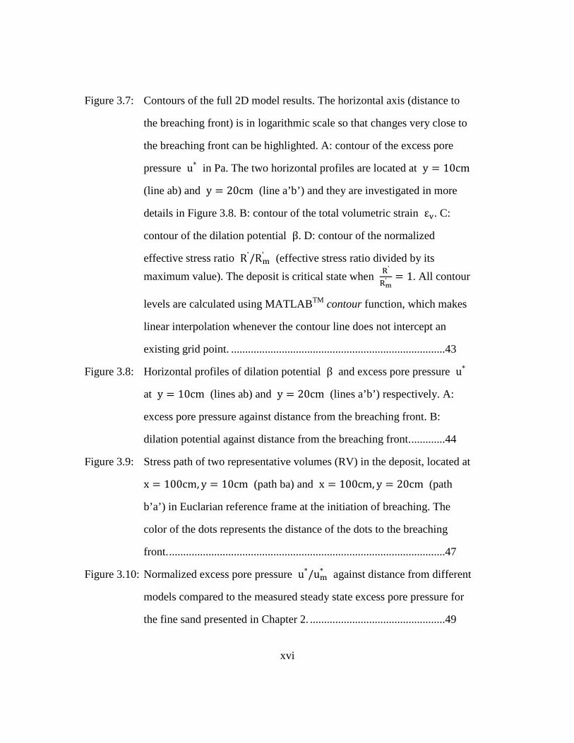
Figure 3.7: Contours of the full 2D model results. The horizontal axis (distance to

the breaching front) is in logarithmic scale so that changes very close to

the breaching front can be highlighted. A: contour of the excess pore

pressure u* in Pa. The two horizontal profiles are located at y = 10cm

(line ab) and y = 20cm (line a’b’) and they are investigated in more

details in Figure 3.8. B: contour of the total volumetric strain εv. C:

contour of the dilation potential β. D: contour of the normalized

effective stress ratio R'/Rm' (effective stress ratio divided by its

maximum value). The deposit is critical state when R'

Rm'= 1. All contour

levels are calculated using MATLABTM contour function, which makes

linear interpolation whenever the contour line does not intercept an

existing grid point. ............................................................................43

Figure 3.8: Horizontal profiles of dilation potential β and excess pore pressure u*

at y = 10cm (lines ab) and y = 20cm (lines a’b’) respectively. A:

excess pore pressure against distance from the breaching front. B:

dilation potential against distance from the breaching front. ............44

Figure 3.9: Stress path of two representative volumes (RV) in the deposit, located at

x = 100cm, y = 10cm (path ba) and x = 100cm, y = 20cm (path

b’a’) in Euclarian reference frame at the initiation of breaching. The

color of the dots represents the distance of the dots to the breaching

front. ..................................................................................................47

Figure 3.10: Normalized excess pore pressure u*/um* against distance from different

models compared to the measured steady state excess pore pressure for

the fine sand presented in Chapter 2. ................................................49

xvii

Figure 3.11: Dimensionless minimum excess pore pressure um* (y)/um* (y0) for the

full 2D model (solid line) and uniform 2D model (dash-dotted line) and

dimensionless magnitude of unloading ∂σ3∂x�

(0,y)�∂σ3∂x�

(0,y0)�

-1 (dashed

line) against dimensionless depth y/y0, where the reference depth

y0 = 10cm (solid line). The slopes of the solid line represent the rate of

increase in pore pressure drop in the full 2D model with depth. The

slopes of the dash-dotted line represent the rate of increase in pore

pressure drop in the uniform 2D model with depth. The dashed line,

representing the increase in the magnitude of unloading with depth, has

a constant slope of 1 because unloading increases linearly with depth.

...........................................................................................................52

Figure 3.12: Contour of normalized effective stress ratio R'/Rm' for the uniform 2D

model: a 2D model with uniform dilation potential β. ....................53

Figure 3.13: Modeled erosion rate, or velocity of the breaching front, v against

depth. Dilation potential is a function of stresses in this model (Equation

14). ....................................................................................................57

Figure 4.1: Side view of the setup of the experiment. .........................................65

xviii

Figure 4.2: Dual-mode slope failure captured by video and sonar. A: sketch of

breaching mode slope failure. B: sketch of the sliding mode slope failure

as the wedge starts to slide down slope. The sliding wedge is thicker

near its top therefore as it slides down the location of the failure front

could temporary prograde instead of retreat (e.g., circled area in

subfigure C). C: ultrasound image showing the retreating of the failure

front with time. The gray scale represents the amplitude of the reflected

acoustic wave; the white color represents largest amplitudes, i.e.,

strongest reflectors. The coordinates of the brightest reflectors (e.g.,

point a) represent the distance the failure front has retreated (horizontal

axis, d) at a given time t (vertical axis). ........................................68

Figure 4.3: Measured excess pore pressure u* in the deposit. A: measured excess

pore pressure at the 4 locations closest to the initial gate (labeled in

different colors) against time t. The grey color shaded area contains

measurements made before releasing the gate. The yellow color shaded

area indicates the duration of initiation (pulling gate out). B: measured

excess pore pressure from all the sensors (squares) against distance from

failure front (x) at 3 different time: 10s (dash dotted line), 18s (dashed

line), and 20s (solid line). x = 0 is the failure front. ......................72

Figure 4.4: Excess pore pressure measurements for all the sensors against time (top

figure) compared to the position of the slope failure surface against time

(bottom figure, it is Figure 4.2C viewed in a different orientation). The

two time series are aligned at the moment the gate starts to slide (t = 0).

The red dashed lines mark the time when the excess pore pressure (u*)

suddenly drops in the top figure........................................................74

xix

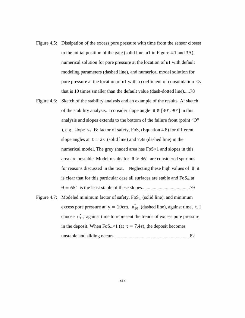
Figure 4.5: Dissipation of the excess pore pressure with time from the sensor closest

to the initial position of the gate (solid line, u1 in Figure 4.1 and 3A),

numerical solution for pore pressure at the location of u1 with default

modeling parameters (dashed line), and numerical model solution for

pore pressure at the location of u1 with a coefficient of consolidation Cv

that is 10 times smaller than the default value (dash-dotted line). ....78

Figure 4.6: Sketch of the stability analysis and an example of the results. A: sketch

of the stability analysis. I consider slope angle θ ∈ [30∘, 90∘] in this

analysis and slopes extends to the bottom of the failure front (point “O”

), e.g., slope s1. B: factor of safety, FoS, (Equation 4.8) for different

slope angles at t = 2s (solid line) and 7.4s (dashed line) in the

numerical model. The grey shaded area has FoS<1 and slopes in this

area are unstable. Model results for θ > 86∘ are considered spurious

for reasons discussed in the text. Neglecting these high values of θ it

is clear that for this particular case all surfaces are stable and FoSm at

θ = 65∘ is the least stable of these slopes........................................79

Figure 4.7: Modeled minimum factor of safety, FoSm (solid line), and minimum

excess pore pressure at y = 10cm, u10* (dashed line), against time, t. I

choose u10* against time to represent the trends of excess pore pressure

in the deposit. When FoSm<1 (at t = 7.4s), the deposit becomes

unstable and sliding occurs. ..............................................................82

xx

Figure 4.8: Minimum factor of safety against the minimum excess pore pressure at

y = 10cm, which represents the pore pressure in the deposit. The solid

line with circle at the right end marks the model for the deposit in the

experiment, referred as the base model. The dashed dotted line with

square in the right end (most of the line covered by the solid line) marks

a model that is the same as the base model except the dilation potential

is increased by 2 times. The dashed line with star in the right end marks

a model with 0.5m thickness, same dilation potential as base model, and

higher friction angle than the base model. ........................................88

Figure 4.9: Summary sketch of the evolution and possible styles of dilative slope

failure. ...............................................................................................92

Figure 4.10: Sketch of how a storm could generate dilative slope failure. The top

figures are cross sections from the locations marked as dashed lines on

the associated regional maps positioned underneath each section. 1. pre-

storm. 2. storm enhanced or generated currents (arrows) cut into the

deposit. 3. the cut initiates slope failure and the failure front retreats

toward the right-hand side of the figure. ...........................................93

Figure A.1: Excess pore pressure measured at 9 locations during one breaching

experiment. The two lines colored blue and red are the two sensors

presented in Chapter 2. ...................................................................108

Figure A.2: StressMohr circle for the testing specimen at critical state. Measured

normal stress σN is OB, measured shear stress τ is BC. The mean

stress p is OA, and the differential stress q is AC. Line OC is the

failure envelope and the angle AOC is the internal friction angle ϕ

.....................................................................................................…109

xxi

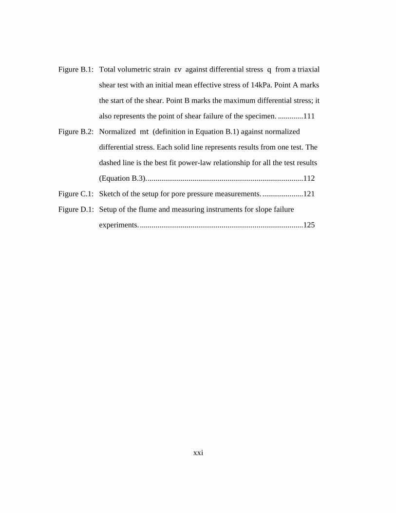
Figure B.1: Total volumetric strain εv against differential stress q from a triaxial

shear test with an initial mean effective stress of 14kPa. Point A marks

the start of the shear. Point B marks the maximum differential stress; it

also represents the point of shear failure of the specimen. .............111

Figure B.2: Normalized mt (definition in Equation B.1) against normalized

differential stress. Each solid line represents results from one test. The

dashed line is the best fit power-law relationship for all the test results

(Equation B.3). ................................................................................112

Figure C.1: Sketch of the setup for pore pressure measurements. .....................121

Figure D.1: Setup of the flume and measuring instruments for slope failure

experiments. ....................................................................................125

1

Chapter 1: Introduction

The purpose of this study is to expand our knowledge on the mechanics of

submarine slope failure and how sediments are released from submarine slope failure

events. Submarine slope failure is an important mechanism that releases sediments stored

on the continental shelf into the deep sea (Hampton et al., 1996; Van den Berg et al.,

2002; Piper and Normark, 2009). Accurate interpretation of the sedimentary records in

subsurface and the morphological changes on the surface of the sea floor requires a

complete understanding of submarine slope failure. First, we need to understand the

mechanics of submarine slope failure to be able to predict what conditions could lead to

slope failure under sea level. Second, we need to understand how sediment is released

from slope failure to accurately describe how slope failure redistributes sediments.

Previous studies identify two end members of submarine slope failure. One end

member is the liquefaction slope failure that is usually associated with clay rich deposits

(Terzaghi, 1956; Morgenstern, 1967; Hampton et al., 1996; McAdoo et al., 2000). During

liquefaction large amounts of sediments are released as a slide or slump. The other end

member is breaching that occurs in densely packed sand (de Koning, 1970; Van den Berg

et al., 2002; Eke et al., 2011). Breaching is characterized by slow release of sand grains

over a near-vertical failure surface; the failure surface retreats at a constant rate. Studies

suggest that the differences in sediment release between those two end members are due

to different types of shear deformation and different excess pore pressure (defined as the

difference between the pore pressure and the hydrostatic pore pressure) in the sediment.

During liquefaction the sediment contracts under shear, which increases the excess pore

pressure (Terzaghi, 1951; Hampton et al., 1996; Flemings et al., 2008). The increase in

excess pore pressure decreases the effective stress between sediment grains and weakens

2

the deposit (Terzaghi, 1951; Wood, 1990). During breaching the sediment dilates, which

decreases the excess pore pressure (Meijer and van Os, 1976; Van Rhee and Bezuijen,

1998). The drop in excess pore pressure increases the effective stress between the

sediment grains and strengthens the deposit (Wood, 1990). In summary, excess pore

pressure controls the slope failure by changing the effective stress. On the other hand,

slope failure generates excess pore pressure. Slope failure release sediments from the

deposit, which changes the stresses in the deposit. Changes in stress can generate excess

pore pressure in the deposit (Skempton, 1954; Gibson, 1958; Meijer and van Os, 1976).

Previous studies suggest that the excess pore pressure and the slope failure are

coupled (Terzaghi, 1951; Meijer and van Os, 1976; Hampton et al., 1996; Van Rhee and

Bezuijen, 1998; Flemings et al., 2008). However, studies on the mechanics of submarine

slope failure so far separate the excess pore pressure and the slope failure. For example,

Meijer and van Os (1976) built a 2D model to show that breaching slope failure generates

negative excess pore pressure. However, they assume the rate of sediment release, or

erosion rate, is a constant and treat it as an input variable in the model. Because the

coupling is missing from those studies they cannot explain why the erosion rate is

constant or other features that rely on the interaction between the slope failure and the

excess pore pressure. Studies on the interaction between slope failure and excess pore

pressure can help us to setup a framework to study the mechanics of slope failure,

especially how sediments are released from slope failure. Iverson et al (2000) adopted

this approach in studying subarial slope failures. Iverson et al (2000) combines

measurements of displacement and pore pressure in subarial slope failure experiments

and find that dilative sediment and contractive sediment are associated with different

styles of slope failure. Here I apply a similar approach in studying submarine slope

failures in sediment that dilates.

3

In this study, I investigate the coupling of excess pore pressure and slope failure

in two different types of slope failure: breaching and a new type of slope failure that I call

the dual-mode slope failure. Both types of slope failure occur in sediments that dilate

under shear. I develop a dimensionless parameter called “dilation potential” to quantify

the degree of dilation in the sediments and show that this parameter controls the

mechanics of dilative slope failure. I also show that the release of sediments in dilative

slope failure is controlled by the pore pressure dissipation in the deposit.

In chapter 2, I study the mechanics of pure breaching. I present pore pressure

measurements made during breaching, as well as an analytical model that shows how the

pore pressure field within the failing deposit is connected to the erosion rate associated

with the failure surface. I show that breaching occurs in sediments with dilative potential

larger than 4.3. This condition could be common on the continental shelf, making

breaching an important mechanism in transferring sediment into the deep ocean. I use the

analytical model to show that a dynamic equilibrium exists between the slope failure and

the pore pressure dissipation during breaching. This equilibrium leads to a way to

estimate the rate of sediment release from breaching using a simple material property, the

coefficient of consolidation. Contrary to previous work, I find that the erosion rate is

independent of the dilation of the deposit due to the coupling between erosion and pore

pressure dissipation. The equilibrium between the erosion and pore pressure dissipation

decouples the steady-state pore pressure field from the permeability of the deposit; this is

the first time this behavior has been recognized in sediment failures.

In chapter 3, I study the mechanics of breaching in more details with a 2D

numerical model. In this model I show how spatial distribution of the dilation potential

affects the excess pore pressure and the release of sediments during breaching. I develop

an empirical model for dilation potential based on geotechnical test results from the lab.

4

Test results show that the dilation potential increases when the deposit is closer to shear

failure. As a result, the majority of dilation as well as the interaction between slope

failure and pore pressure occurs close to the failure surface. The experiment results also

show that dilation decreases with increasing overburden, as a result, the deposit becomes

weaker with increasing depth. I solve for the erosion rate with the 2D numerical model

and show that erosion can be treated as being uniform in the vertical direction except for

the portion close to the top boundary. Dissipation of pore pressure in the vertical

direction accelerates the erosion near the top of the deposit.

In chapter 4, I present a new type of submarine slope failure, the dual-mode slope

failure, with experiments. The slope failure is characterized by a periodic switch between

breaching and sliding. During breaching mode the sediment is released at a constant rate

over a near vertical failure surface. The failure surface retreats at 2.5mm/s for a period of

16s before sliding occurs. During sliding a triangular wedge of sediment slides down

along a basal slope of 80∘. The deposit becomes stable after the sliding and sediment

release is switched back to breaching mode. I present pore pressure measurements and

numerical model results to show that the evolution of excess pore pressure switches the

slope failure between those two modes. The negative excess pore pressure dissipates

towards its steady state during breaching mode; dissipation of the negative excess pore

pressure weakens the deposit. The slope failure switches to sliding mode when the

magnitude of negative excess pore pressure is too small to keep the deposit stable. This is

different from the pure breaching slope failure where the deposit is stable even after the

pore pressure reaches its steady state. Sliding increases the magnitude of the negative

excess pore pressure; this strengthens the deposit and switches the slope failure back to

breaching mode. I show that dilative sediments with smaller dilation potential or smaller

friction angle tend to generate dual-mode slope failure instead of breaching slope failure.

5

Chapter 2: 1D analytical model for steady state breaching

2.1 INTRODUCTION

Accurate interpretation of Earth-surface morphology and environmental records

preserved in sediment accumulations requires a complete understanding of the processes

governing the storage and release of sediment on this interface. Breaching is one such

process; it is a style of retrogressive subaqueous slope failure that occurs in densely

packed sand and is characterized by nearly vertical failure angles, slow and steady

retrogressive erosion rates, and production of sustained turbidity currents (Figure 2.1)

(Van den Berg et al., 2002; Mastbergen and Van den Berg, 2003; Eke et al., 2011).

Retrogressive slope failures are controlled by the responses of sedimentary

deposit to shear. Most granular material either contracts or dilates when subject to shear;

the best studied cases are associated with contraction, increased pore pressures, and

subsequent liquefaction (Terzaghi, 1951; Hampton et al., 1996; Iverson, 2005). On the

other hand, dilation and the development of negative excess pore pressure near the failure

surface lead to breaching (Meijer and van Os, 1976; Van Rhee and Bezuijen, 1998). This

breaching can be initiated by scour from focused channel flow, or an initial liquefaction

slope failure (Van den Berg et al., 2002). Mastbergen and Van den Berg (2003) and Eke

et al. (2011) proposed that breaching may be one of the processes by which sands are

released into turbidity currents and transported down Scripps Canyon (offshore southern

California). Because breaching produces sustained turbidity currents, the sands delivered

downslope may build thick uniform turbidites (Van den Berg et al., 2002). Previous

studies associate breaching with fine-grained sand (de Koning, 1970; Meijer and van Os,

1976; Van Rhee and Bezuijen, 1998; Van den Berg et al., 2002); however, Houthuys

6

(2011) speculated that breaching could also be the mechanism that contributes to building

coarse sand turbidites. An understanding of the mechanism of breaching is important to

correctly interpret these turbidites.

Figure 2.1: Morphodynamic evolution and pore pressure response during breaching. Initial dimensions of sediment: ~30 cm tall, 40 cm wide. The pore pressure is monitored at nine locations and I show two of them here for simplicity (for measurements from all sensors see Figure A.1 in Appendix A). A: After 10 s, sediments are falling from vertical face (breaching front) and forming turbidity current (light gray). B: After 80 s, erosion has shifted breaching front to right and it is approaching blue pressure sensor. Turbidity currents have deposited sediment in front of breaching front. C: Removal of retaining wall results in abrupt drop in pore pressure at both sensors (0–22 s, dark gray region). As breaching front approaches each pressure sensor, there is second pressure drop and then rise to hydrostatic pressure (light gray zones at 80 s and 130 s for blue and red sensors, respectively). Final pore pressure is lower than initial pore pressure due to drop of water table, which is caused by removal of restraining plate. Chaotic pore pressure signal recorded between 10 s and 40 s by all sensors is due to transient slumping of sediments connected to removal of restraining plate; this is not part of steady-state breaching process I focus on in this study.

7

The increase in porosity during breaching is a result of both unloading and shear

dilation as the deposit undergoes slow retrogressive failure (Meijer and van Os, 1976;

Van Rhee and Bezuijen, 1998). Shear dilation is the dominant mechanism generating the

negative excess pore pressure, or underpressure (Meijer and van Os, 1976). As the pore

pressure drops, the effective stress increases and stabilizes the deposit. Dissipation of this

underpressure must occur for slope failure to continue (Van Rhee and Bezuijen, 1998;

Van Rhee, 2007). This dissipation is focused at the failure surface, releasing one grain

layer at a time (Van Rhee, 2007). Shear dilation and unloading associated with these

failing grains continuously generates underpressure that strengthens the remaining

deposit. Here I study the interaction between the pore pressure field and the erosion rate

of the failing surface during breaching. I build a physical model that treats the pore

pressure field and the erosion rate as coupled variables, rather as variables that do not

directly affect one another (Meijer and van Os, 1976; Van Rhee and Bezuijen, 1998; Van

Rhee, 2007). I show how this coupling leads to a coevolution of values for the erosion

rate and the pore pressure field that could not be otherwise predicted. I also present a

model that describes what material properties are necessary for breaching.

2.2 EXPERIMENTAL OBSERVATION

I deposit silty sand (median diameter, D50 = 0.14 mm, grain size is presented in

Figure 2.2) into one end of a flume filled with water, and restrain the sediment with a

vertical mesh plate. The mesh plate allows water to flow through but holds the sediment

in place, creating a submerged water-saturated deposit. The plate is removed quickly

from the tank to initiate breaching (Figure 2.1A). The deposit does not collapse after the

release of the gate and the breaching front starts to retreat. The breaching front maintains

8

a slope that is larger than 90∘ except for the portion near the top of the deposit, where

the slope reduces to 0∘ at the top surface. The height of the breaching front decreases

with time but its shape is similar at different time (Figure 2.3). The breaching front

retrogrades slowly and steadily as the sediment on the vertical face erodes (Figure 2.4)

and forms turbidity currents. The average speed of the breaching front, also referred as

the erosion rate, is 0.14 cm/s. These observations are consistent with field examples (Van

den Berg et al., 2002) and previous flume studies (Van Rhee and Bezuijen, 1998; Eke et

al., 2011).

Figure 2.2: Grain size distributions of the silty sand (solid line) and well-sorted fine sand (dashed line) used in the study.

9

Figure 2.3: Traces of the breaching front during one experiment, the trace lines are separated by 20s. The dashed line represents the location where I measure the erosion rate (shown in Figure 2.4).

Figure 2.4: Erosion rate 𝑣 estimated from the trace of breaching front (Figure 2.3) against time. 𝑣 at time 𝑡 represents the average velocity between 𝑡 − 20𝑠 and 𝑡; it is calculated as the distance the breaching front travels along the dashed line in Figure 2.3 during this period divided by 20s. The error bars represents the uncertainty in time (± 1s). This uncertainty is too small compared to the time scale of the experiment (horizontal axis) therefore only its influence on the erosion rate (vertical axis) is plotted here.

10

The pore pressure is monitored with pressure sensors plumbed to the sediment by

thin stainless steel tubes. Two distinct pore pressure drops are recorded by each sensor.

The first drop occurs immediately after the plate is removed (Figure 2.1C). I interpret this

drop to be the result of unloading and shear dilation of the deposit caused by removal of

the confining vertical plate (Casagrande, 1936; Skempton, 1954; Iverson et al., 2000).

The second drop is recorded by a sensor as the breaching front approaches its location in

the sedimentary deposit (Figure 2.1C). In the experiment the pore pressure begins to drop

when the horizontal distance separating the breaching front and the sensor is about 3 cm.

Just before the breaching front passes the sensor location, the pore pressure abruptly rises

to hydrostatic pressure over a period of about 10 s (Figure 2.1C). I interpret this second

style of pore pressure decline to be caused by a local unloading and shear dilation of the

sediment deposit in the vicinity of the breaching front (Meijer and van Os, 1976; Van den

Berg et al., 2002). This pore pressure signal is similar to the one created during the

initiation of breaching, only with smaller magnitude. As a result, this pore pressure signal

is recorded by the nearest sensor only (Figure 2.1C).

The spatial variation in pore pressure response can be viewed from a Lagrangian

reference frame that follows the breaching front (Figure 2.5). In this reference frame the

minimum pore pressure always occurs about 3 cm in front of the breaching surface, and

pore pressure rises toward hydrostatic pressure with greater distance into the deposit

(Figure 2.5). This spatial pattern for pore pressure was noted in previous studies of

breaching (Meijer and van Os, 1976; Van Rhee and Bezuijen, 1998). The experiment in

this study shows that the general pattern of pore pressure is maintained through time,

converging onto a steady-state profile after 140 s (cf. pore pressure at 140 s and 190 s in

Figure 2.5).

11

Figure 2.5: Excess pore pressure 10 s (diamonds), 80 s (squares), 140 s (triangles), and 190 s (dashed line) after onset of breaching, plotted with distance from breaching front (Lagrangian coordinates). At each time, there is minimum in pore pressure ~5 cm behind breaching front. Pore pressure at 140 s is almost identical to pore pressure at 190 s in Lagrangian coordinates, suggesting that pore pressure is at steady state. Solid line is excess pore pressure predicted by Equation 4.

2.3 1D STEADY-STATE BREACHING MODEL

The existence of a steady-state pore pressure profile suggests that a balance exists

between the pore pressure dissipation, which triggers slope failure, and the continuous

dilation, which produces negative pore pressure. I describe this balance in a one-

dimensional steady-state model. Consider a sediment volume with constant material

properties moving with the breaching front at steady erosion rate v; the pore pressure in

the Lagrangian reference frame can be written as

12

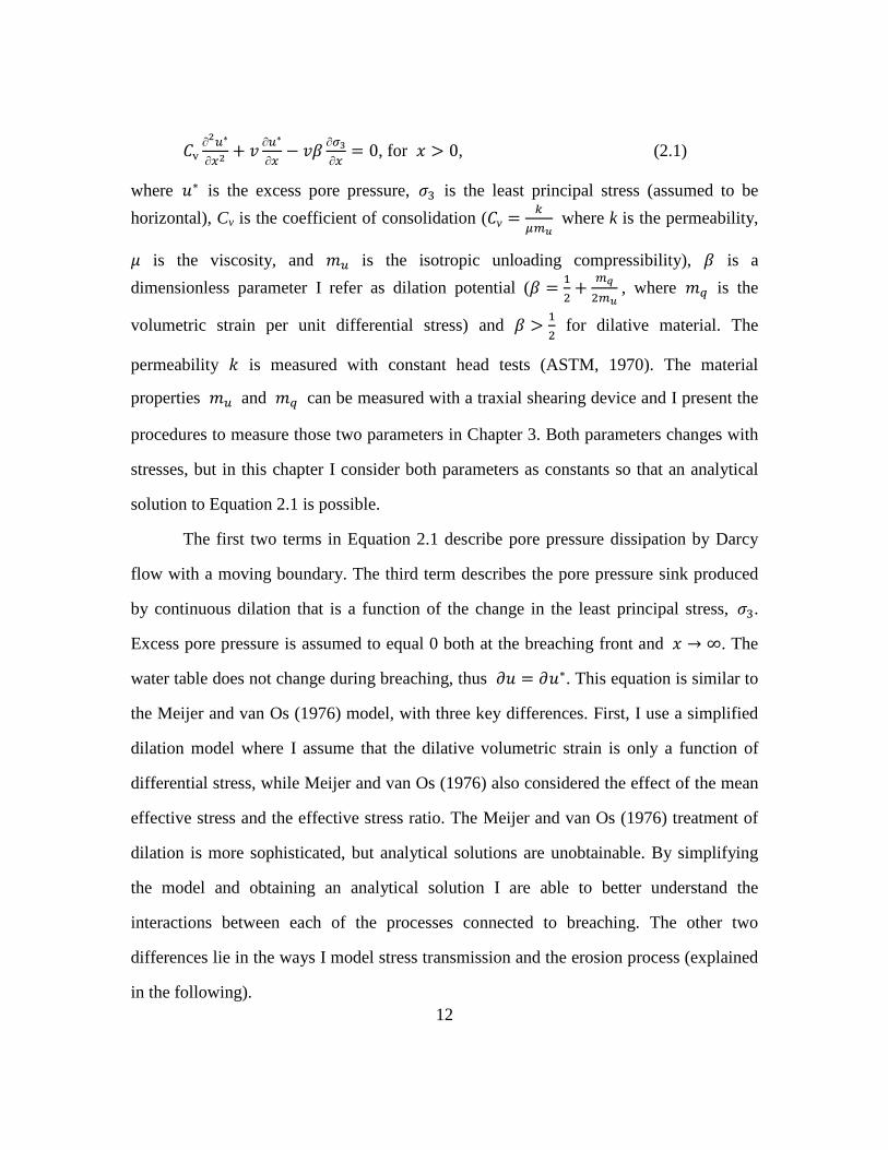
𝐶v∂2𝑢∗

∂𝑥2+ 𝑣 ∂𝑢

∗

∂𝑥− 𝑣𝛽 ∂𝜎3

∂𝑥= 0, for 𝑥 > 0, (2.1)

where 𝑢∗ is the excess pore pressure, 𝜎3 is the least principal stress (assumed to be horizontal), Cv is the coefficient of consolidation (𝐶v = 𝑘

𝜇𝑚𝑢 where k is the permeability,

𝜇 is the viscosity, and 𝑚𝑢 is the isotropic unloading compressibility), 𝛽 is a dimensionless parameter I refer as dilation potential (𝛽 = 1

2+ 𝑚𝑞

2𝑚𝑢 , where 𝑚𝑞 is the

volumetric strain per unit differential stress) and 𝛽 > 12

for dilative material. The

permeability 𝑘 is measured with constant head tests (ASTM, 1970). The material

properties 𝑚𝑢 and 𝑚𝑞 can be measured with a traxial shearing device and I present the

procedures to measure those two parameters in Chapter 3. Both parameters changes with

stresses, but in this chapter I consider both parameters as constants so that an analytical

solution to Equation 2.1 is possible.

The first two terms in Equation 2.1 describe pore pressure dissipation by Darcy

flow with a moving boundary. The third term describes the pore pressure sink produced

by continuous dilation that is a function of the change in the least principal stress, 𝜎3.

Excess pore pressure is assumed to equal 0 both at the breaching front and 𝑥 → ∞. The

water table does not change during breaching, thus 𝜕𝑢 = 𝜕𝑢∗. This equation is similar to

the Meijer and van Os (1976) model, with three key differences. First, I use a simplified

dilation model where I assume that the dilative volumetric strain is only a function of

differential stress, while Meijer and van Os (1976) also considered the effect of the mean

effective stress and the effective stress ratio. The Meijer and van Os (1976) treatment of

dilation is more sophisticated, but analytical solutions are unobtainable. By simplifying

the model and obtaining an analytical solution I are able to better understand the

interactions between each of the processes connected to breaching. The other two

differences lie in the ways I model stress transmission and the erosion process (explained

in the following).

13

I assume that the change in least principal stress, the source for continuous

dilation, declines exponentially with distance from the breaching front: 𝜕𝜎3𝜕𝑥

= 𝜂𝑠0𝑒−η𝑥, for 𝑥 > 0, (2.2)

where s0 is the value of least principal stress as 𝑥 → ∞, and 𝜂 is a constant that defines

the rate of stress decay with distance. Equation 2.2 is consistent with our measured initial

pore pressure profile at 10 s (Figure 2.5); it also explains the localized pore pressure

signal produced by the continuous dilation (Figure 2.1C). Previous studies have shown

similar behavior in dry granular material undergoing localized unloading (Balmforth and

Kerswell, 2005; Lube et al., 2005; Siavoshi and Kudrolli, 2005) and when subjected to a

stress pulse (Hostler, 2004). This model is different from the linear elastic model used by

Meijer and van Os (Meijer and van Os, 1976) and it results in more dilation close to the

breaching front.

The drop in pore pressure caused by dilation creates a pore pressure gradient

(Figure 2.5A) that drains water into the deposit through the breaching front. As a

consequence, the pore pressure near the front increases and the effective stress decreases,

which results in failure and erosion. The volumetric strain (𝜀𝑣) times the erosion rate (v),

which is the change in volume per time, must equal the flux of water per unit area (𝑄)

into the deposit, 𝜀𝑣𝑣 = 𝑄. I assume that the volumetric strain is proportional to the

minimum pore pressure, 𝜀𝑣 = 𝐸0𝑢m, where E0 is a function of the friction angle of the

deposit and the stress level prior to breaching. Hence, 𝑣 = 𝑄

𝐸0𝑢𝑚∗= − 𝑘

𝐸0𝑢𝑚∗∂𝑢∗

∂𝑥�𝑥=0

. (2.3)

Solutions for Equations 2.1, 2.2, and 2.3 yield

𝑣 = 𝛿𝜂𝐶v , (2.4)

𝑢∗ = 𝛿𝜂𝑠0𝛿−1

�𝑒−𝜂𝑥 − 𝑒−𝑣𝐶v𝑥� , (2.5)

14

where 𝛿 =𝑊�𝑚𝑢

𝐸0log�𝑚𝑢

𝐸0��

log�𝑚𝑢𝐸0

� and W(x) is the Lambert W-function (Polya and Szegö, 1970).

2.4 EQUILIBRIUM BETWEEN THE SLOPE FAILURE AND PORE PRESSURE DISSIPATION

The erosion rate (v) is proportional to the coefficient of consolidation (Cv)

(Equation 2.4). Thus during breaching, more rapid dissipation (high Cv) is balanced by

more rapid erosion, as has been shown by previous studies (Van Rhee and Bezuijen,

1998; Van Rhee, 2007). An interesting result from the solution (Equation 2.4) is that the

erosion rate is independent of the dilation potential (𝛽). A larger 𝛽 generates a larger

change in porosity, which requires a greater volume of water to flow into the dilated

material. However, the larger dilation potential also generates more underpressure,

resulting in a larger flow rate. These two effects compensate for each other to produce an

erosion rate that is independent of the dilation potential. This result conflicts with the

prediction of Van Rhee (2007), who suggested that the erosion rate is lower for greater

dilation potential; however, Van Rhee (2007) did not couple the pore pressure field with

the erosion process and therefore did not include the feedback that produces an erosion

rate that is independent of dilation potential.

There is a dynamic equilibrium between pressure dissipation and continuous

dilation. At steady state, the slope failure triggered by the pore pressure dissipation

always produces a dilative strain in the remaining deposit that returns the pore pressure

back to its original level. This is because the magnitude of dilation is proportional to the

erosion rate (Equation 2.1), and the erosion rate is proportional to the coefficient of

consolidation (Equation 2.4). This feedback keeps the pore pressure profile at steady state

in the Lagrangian reference frame. One consequence of this dynamic equilibrium is that

the steady-state pore pressure is independent of the permeability k. This can be shown

15

mathematically by substituting Equation 2.4 into Equation 2.5, which removes Cv

(= 𝑘/𝜇𝐸) from the pore pressure solution.

I use a group of parameters (Cv = 1.4 ×10-4 m2 s–1, 𝛽 = 4.5, mv = 3.5 ×10-7 Pa–1,

𝜂 = 15, s0 = 400 Pa) measured from the lab and fit E0 = 1.4 × 10-6 Pa–1 to the measured

erosion rate in order to predict the steady-state pore pressure field connected with our

experiment. The modeled pressure distribution is similar in shape to the observed

pressure (140 s in Figure 2.5); confirming the form of the analytical solution. However,

the magnitude of the pore pressure drop predicted by the model is twice the observed

values (Figure 2.5). This discrepancy may result from our assumption of constant

material properties. For example, if the coefficient of consolidation (Cv) increases as

sediment dilates, then the pore pressure minimum will be closer to hydrostatic pressure

than the modeled example. In addition, I do not include vertical draining in the 1D

model; the draining of pore pressure in the vertical direction could reduce the magnitude

of the underpressure.

To explore the control of material properties on breaching I carry out experiments

using two types of sediments, silty sand and well sorted fine sand (grain sizes are

presented in Figure 2.2). During breaching, the erosion rate of the fine sand is 4 times

that of the silty sand, and the excess pore pressure profiles at steady state are identical

(Figure 2.6). Geotechnical analysis shows that the compressibility of the two materials

are similar but the permeability of the fine sand is 65 times that of the silty sand, which

means the 𝐶𝑣 for the fine sand should be 65 times that of the silty sand (Equation 2.1).

Equation 2.4 and 2.5 predict that materials of similar compressibility have similar pore

pressure profiles, as is observed. However, Equation 2.4 also predicts that the erosion rate

for the fine sand should be 65 times larger than the silty sand (i.e., proportional to Cv)

whereas I only observe a 4 times difference. The discrepancies can be explained an

16

overestimation of the coefficient of consolidation 𝐶𝑣 for the fine sand or an

underestimation of the coefficient of consolidation for the silty sand.

There are two possible sources for the mismatch of 𝐶𝑣 and I use the silty sand as

an example. First, the underestimation of the 𝐶𝑣 for the silty sand could due to an

underestimation of the permeability 𝑘 from the lab. I measure permeability 𝑘 in the

direction the sediments are deposited. However, the 1D model considers the pore water

flow, therefore the permeability, in the direction perpendicular to the direction the

sediments are deposited. The difference in the direction of the permeability could cause

and underestimation its value, especially in a silty sand deposit where stratification due to

sorting can occur in the direction of sedimentation (Freeze and Cherry, 1977). Second,

the underestimation of 𝐶𝑣 for the silty sand could due to an overestimation of 𝑚𝑢 from

the lab. I measure the values for 𝑚𝑢 with isotropic stress condition, i.e., the major and

minor principal stresses are the same. However, the deposit in the experiment experience

anisotropic stress conditions; the vertical stress is larger than the horizontal stress due to

removal of the horizontal support. The different stress conditions alters the fabric of the

deposit (Oda, 1972; Oda et al., 1980) and could change the values for 𝑚𝑢, thus 𝐶𝑣. More

research on how to properly model the compressibility is required to resolve this

discrepancy. Further discussion on this topic is presented in Chapter 6: Future Research.

17

Figure 2.6: Measured steady state excess pore pressure against distance from the breaching front for the fine sand (circles) and silty sand (squares).

2.5 CHARACTERISTICS OF THE STEADY STATE PORE PRESSURE SOLUTION

To further explore the control of material properties on the steady state excess

pore pressure solution (Equation 2.5) I introduce dimensionless form of the excess pore pressure solution. Let ⟨𝑢∗⟩ = 𝑢∗

𝛽𝑠0 be the dimensionless excess pore pressure and

⟨𝑥⟩ = 𝑥𝑣𝐶𝑣

be the dimensionless distance, then the steady state solution transforms into the

following

⟨𝑢∗⟩ =exp�−𝜂𝐶𝑣𝑣 ⟨𝑥⟩�−exp(−⟨𝑥⟩)

𝜂𝐶𝑣𝑣 −1

(2.6)

The dimensionless parameter 𝜂𝐶𝑣𝑣

is the ratio between two length scales, 𝐶𝑣/𝑣 and 1/𝜂,

and it controls the dimensionless steady state solution. The length scale 1/𝜂 represents

the distance where the unloading, or the decrease in horizontal stress, is 1/𝑒 times

(37%) that of the breaching front (Equation 2.2). Therefore 1/𝜂 represents the

18

characteristic distance for changes in stress and the source for excess pore pressure. The

length scale 𝐶𝑣𝑣

represents the changes of pore pressure due to advection (through the

moving boundary) and diffusion (through pore water flow). To illustrate its physical

meaning, I setup a boundary condition problem similar to Equations 2.1 with two

changes. First, there is no source term in this problem. Second, the excess pore pressure

at breaching front equals to a finite non-zero value 𝑢0. Therefore, 𝑑2𝑢∗

𝑑𝑥2+ 𝑣 𝑑𝑢∗

𝑑𝑥= 0 (2.7)

𝑢∗(0) = 𝑢0 (2.8)

lim𝑥→∞ 𝑢∗(𝑥) = 0 (2.9)

This set of equations describes the changes of pore pressure due to advection and

diffusion, without the influence of a source. The solution to this problem is 𝑢∗ = 𝑢0 exp �− 𝑣

𝐶𝑣𝑥� (2.10)

The solution shows that the length 𝐶𝑣/𝑣 is the distance where the excess pore pressure

is 1/𝑒 times (37%) that of the boundary value.

In summary the parameter 𝜂𝐶𝑣𝑣

combines all the factors that control the spatial

variation in pore pressure: 1/𝜂 controls the changes in source of pore pressure and

𝐶𝑣/𝑣 controls the changes in pore pressure due to advection and diffusion. I denote

𝜉 = 𝜂𝐶𝑣𝑣

, (2.11)

as the controlling parameter for dimensionless excess pore pressure ⟨𝑢∗⟩. The location and value of the minimum for ⟨𝑢∗⟩ are both functions of 𝜉. The location ⟨𝑥𝑚⟩ = log𝜉

𝜉−1,

i.e., the dimensionless distance to the minimum ⟨𝑢∗⟩ decreases as 𝜉 increases (Figure

2.7A). The value of the minimum dimensionless excess pore pressure, ⟨𝑢𝑚⟩, is −𝜉−𝜉

𝜉−1.

⟨𝑢𝑚⟩ increases in value (becomes less negative and closer to hydrostatic pore pressure)

as 𝜉 increases in value (Figure 2.7B).

19

Figure 2.7: A: The dimensionless distance to the minimum dimensionless excess pore pressure (or maximum pore pressure drop) ⟨𝑥𝑚⟩ against the controlling parameter 𝜉 for the dimensionless excess pore pressure solution. B: the minimum dimensionless excess pore pressure ⟨𝑢𝑚⟩ against the controlling parameter 𝜉. The circle symbol in both sub figures marks the 𝜉 for fine sand and the square symbol in both sub figures marks the 𝜉 for silty sand.

I use two the silty sand and fine sand experiment results (Figure 2.6) to test the

dimensionless solution. The controlling parameter 𝜉 is 24 for the fine sand and 1.5 for

the silty sand, a 16 fold difference. The two types of sediment have very different

dimensionless pore pressure ⟨𝑢∗⟩ profile, even though the actual pore pressure profile

are very similar (Figures 2.6 and 2.8). The modeled ⟨𝑢∗⟩ roughly fits the measured ⟨𝑢∗⟩

for the silty sand (Figure 2.8A) but does not fit very well for the fine sand (Figure 2.8B).

The model overestimates ⟨𝑥𝑚⟩ for both types of deposit but fits much better for the silty

sand case. The overestimation of ⟨𝑥𝑚⟩ could due to the assumption that dilation

potential is a constant. In the next Chapter I show that in a model with spatial variations

of dilation potential, the location for minimum excess pore pressure is closer to the

breaching front (i.e., ⟨𝑥𝑚⟩ is smaller) than a model with constant dilation potential.

(Section 3.4.4, Figure 2.10)

20

Figure 2.8: A: dimensionless excess pore pressure 𝑢∗

𝛽𝑠0 against dimensionless distance

𝑥𝑣𝐶𝑣

from measurements in silty sand (squares) and in fine sand (circiles), and the steady state solution (solid lines, Equation 2.6). The controlling parameter 𝜉 is 24 for the fine sand and 1.5 for the silty sand. B: zoom in of the boxed area in A. Dimensionless excess pore pressure 𝑢∗

𝛽𝑠0 against

dimensionless distance 𝑥𝑣𝐶𝑣

from measurements (circles and dashed line) and the steady state solution (solid line, Equation 2.6) for the fine sand. The scales of the axes of the two plots are different.

21

The model overestimates the value for maximum dimensionless pore pressure

drop |⟨𝑢𝑚⟩| for the silty sand while underestimates the value for |⟨𝑢𝑚⟩| for the fine

sand (Figure 2.8). Because the absolute value of ⟨𝑢𝑚⟩ increases (becomes more

negative) as 𝜉 decreases (Figure 2.7B), an overestimation of |⟨𝑢𝑚⟩| for the silty sand

suggests that I underestimated the controlling parameter 𝜉 for the silty sand. By

definition of 𝜉 (Equation 2.11), this means I underestimated the value for the coefficient

of consolidation 𝐶𝑣 for the silty sand in the model. With similar reason, the

underestimation of |⟨𝑢𝑚⟩| for the fine sand suggests that I overestimated the value of 𝐶𝑣

for the fine sand. Possible sources for the error in 𝐶𝑣 are explained at the end of last

section; a possible solution to this error is to find a better model for the compressibility of

the deposit (further discussions are presented in Chapter 6).

2.6 BREACHING CONDITION

I determine the zone of shear instability near the breaching front for our model by

solving for the critical underpressure (𝑢𝑐∗ < 0) necessary for failure using the Mohr-

Coulomb criterion (Figure 2.9); failure will occur where underpressure are higher than

this critical value (𝑢∗ > 𝑢c∗, or 𝑢∗/𝑢𝑐∗ < 1 since 𝑢𝑐∗ < 0). In our example this zone

extends from the breaching front to a depth of 2.5 cm, indicating that this region is prone

to failure (Figure 2.9, shaded region).

22

Figure 2.9: Excess pore pressure against distance from breaching front for the steady state model solution (solid line, Equation 2.5) and critical excess pore pressure (𝑢𝑐∗, dashed line). When pore pressure is more than critical pore pressure, Coulomb failure will occur (Equation A.4 in Appendix A). To depth of 2.5 cm, deposit is at failure (shaded region). Internal friction angle of 30° is assumed.

I extend the stability analysis to find the dilation potential (𝛽) needed for

breaching to occur. For breaching to take place, the deposit has to be stable everywhere

except locations very close to the breaching front; otherwise I would expect the entire

deposit to fail or slide. A necessary condition for breaching can therefore be described by

the inequality 𝑢∗/𝑢𝑐∗ > 1. For simplicity, I use the minimum excess pore pressure (𝑢𝑚∗ ),

which is proportional to the dilation potential (𝛽), to represent the actual excess pore

23

pressure and I consider the stress conditions at the breaching front. I find that material

with a dilation potential greater than 4 can breach (Figure 2.10); the deposit must be

sufficiently densely packed so that unloading produces a significant increase in pore

volume per unit differential stress.

I can estimate the dilation potential for the sand samples collected at the head of

Scripps Canyon from shear test results (Dill, 1964, for details see Appendix A). I find

that 𝛽 is larger than the critical value of 4 for most of the samples (Figure 2.10),

satisfying the derived condition. In general, sediments deposited on the continental shelf

that are subject to shaking from waves and shearing by gravity (Dill, 1969) are candidates

to have dense packing (Rutgers, 1962; Scott et al., 1964; Visscher and Bolsterl.M, 1972)

and high dilation potential (Bolton, 1986), consistent with breaching. More field

observations and in situ measurements of 𝛽 are clearly needed to accurately determine

the role of breaching in slope failures on the continental shelf.

2.7 CONCLUSIONS

In conclusion, I find that coupling of the pore pressure field with the erosion rate

of breaching has a significant impact on the calculated values for both variables. The

model developed in this study shows that breaching can occur in any granular material

with sufficient dilation potential. My work also provides a framework and motivation for

considering the occurrence of breaching on the surfaces of other planets and moons

(Dromart et al., 2007; Metz et al., 2009) where liquid and granular materials exist.

24

Figure 2.10: Ratio of minimum excess pore pressure (𝑢𝑚∗ , Figure 2.9) to critical excess pore pressure (𝑢𝑐∗) increases linearly with dilation potential �𝛽 = 1

2+ 𝑚𝑞

2𝑚𝑢�.

When 𝑢𝑚∗

𝑢𝑐∗< 1, sliding and slumping will occur and breaching will not

proceed. When 𝛽 ≥ 4, 𝑢𝑚∗

𝑢𝑐∗> 1 and breaching can proceed. Three silty

sand samples from Scripps Canyon (squares) have dilation potential 𝛽 = 4.1, 8.6, and 25.4 (not plotted), indicating that they are in regime where breaching can proceed.

25

Chapter 3: 2D numerical model for steady state breaching

3.1 INTRODUCTION

Submarine slope failures act to release sediments stored on the continental shelf.

Understanding the mechanics of slope failure is therefore crucial to understanding where

slope failures occur and how sediments are released during slope failure events. Past

studies identified two end members of slope failure: liquefaction and breaching.

Liquefaction slope failure is usually associated with clay-rich deposits; increase in shear

stress in the deposit drives the elevation of pore pressures until the deposit liquefies and

releases large volumes of sediments all in once (Terzaghi, 1956; Morgenstern, 1967;

Lowe, 1976; Hampton et al., 1996). Breaching occurs in clean sand and silty sand, and is

a type of retrogressive slope failure during which shear failure drives a drop in pore

pressures so that sediments are slowly and steadily released from a near vertical failure

surface that is referred as the breaching front (Figure 3.1A and B) (Van Rhee and

Bezuijen, 1998; Van den Berg et al., 2002; Eke, 2008). The velocity of the breaching

front is on the order of mm/s and the retreating of the breaching front can last for periods

up to days (Van Rhee and Bezuijen, 1998; Eke, 2008).

During breaching the release of sediments increases the shear stress on the

deposit, especially close to the breaching front (Meijer and van Os, 1976; Van Rhee and

Bezuijen, 1998). The increase in shear stress causes dilation in densely packed sediments

(Casagrande, 1936; Bolton, 1986). Dilation generates negative excess pore pressure (i.e.,

the pore pressure drops below the hydrostatic pressure), which increases the effective

stress and strength of the deposit so that it maintains a near-vertical slope (Meijer and van

Os, 1976; Van Rhee and Bezuijen, 1998). The negative excess pore pressure can reach a

26

steady state (compare pore pressure at 140s and 190s in Figure 3.1C), and the magnitude

of the steady state excess pore pressure depends on the degree of dilation and magnitude

of unloading (Meijer and van Os, 1976). Chapter 2 shows that in order for a failing

deposit to maintain a steady state excess pore pressure its dilation potential, a parameter

measuring degree of dilation, must be larger than 4.

Figure 3.1: Sketch of breaching at 10s and 80s, with pore pressure measurements (presented in Chapter 2). A: 10s after initiation. The deposit maintains a vertical failure surface, referred as the breaching front. B: 80s after initiation. The breaching front still maintains its vertical slope. The slope angle decreases near the top. C: excess pore pressure against distance from breaching front. Each line represents a time step. Excess pore pressure is negative everywhere during breaching. The maximum drop in excess pore pressure occurs around 5cm from the breaching front. After 140s, the excess pore pressure does not change significantly, reaching a steady state.

Breaching can serve as a sediment source for sustained turbidity currents

(Mastbergen and Van den Berg, 2003; Eke et al., 2011). The style of sediment release

during breaching is drastically different from liquefaction slope failure, where sediments

are released rapidly over a short period of time (Morgenstern, 1967; Lowe, 1976;

27

Hampton et al., 1996). Sustained turbidity currents can be generated by other

mechanisms such as hyperpycnal flow, where sediment laden river water associated with

flooding plunges to the sea floor and continues to travel down slope as a bottom current

(Kneller and Branney, 1995; Mulder et al., 2003; Lamb and Mohrig, 2009). Accurate

interpretation of sedimentary records constructed by sustained turbidity currents requires

us to understand how sediments are released during breaching. Chapter 2 and past studies

find that the retreating velocity of the breaching front, also referred as the erosion rate, is

proportional to the coefficient of consolidation for the deposit (Van Rhee, 2007). This is

because pore pressure generation from release of sediments is balanced by the dissipation

of pore pressure from water flow; this equilibrium creates a steady state pore pressure and

erosion rate for breaching.

Previous studies provide a foundation for us to understand the mechanics of

breaching. However, all of them fail to include the vertical dimension or thickness of the

deposit in their analyses of breaching mechanics. Vertical variations of stresses, pore

pressure, and material properties are missing in 1D models. While Meijer and van Os’s

study (Meijer and van Os, 1976) is based on a 2D model, they did not use the model to

systematically analyze changes in slope failure and pore pressure distribution as a

function of burial depth. These vertical variations of stress, pore pressure, and material

properties can change the distribution of excess pore pressure in the deposit, which in

turn can affect the mechanics of the slope failure. Variations in material properties could

also allow the erosion rate to change in the vertical direction. Understanding how erosion

rate varies in the vertical direction is not only required for us to accurately predict how

sediments are released by breaching, it is also crucial to understanding how breaching

slope failure evolves. Breaching requires the maintenance of a relatively stable slope

angle for the breaching front. Breaching will cease when this slope angle drops down to

28

the angle of repose; steepening of this slope would lead to overhanging and ultimately

collapse of sediments.

In this chapter I study the pore pressure distribution in the deposit and the erosion

rate of breaching using 2D numerical models. I build a 2D pore pressure model similar to

that of Meijer and van Os (1976) with one important difference, I model the stress in the

deposit using laboratory-defined values of the material properties rather than by simply

imposing a linear elastic behavior. I model dilation as a function of both the stress ratio

and mean effective stress using geotechnical test results. I compare this stress dependent

dilation model to a model where dilation is uniform and to the 1D steady state model

presented in Chapter 2. These comparisons show that the majority of the excess pore

pressure drop is focused close to the breaching front due to the decrease of dilation with

distance into the stable deposit. It also shows that the deposit becomes weaker with

increasing thickness due to a decrease in dilation with depth. I model the erosion rate of

breaching in 2D for the first time. I couple this erosion rate model to the 2D pore pressure

model. The coupled model illustrates that while the erosion rate can be accurately

considered a constant in the vertical direction, the boundary conditions at the top of the

2D model do affect the erosion rates observed very close to this boundary.

.

3.2 2D PORE PRESSURE MODEL FOR STEADY STATE BREACHING

I model the excess pore pressure in two dimensions by conserving the volume of

pore water. Because the excess pore pressure (𝑢∗) at steady state is constant in time, the

pore volume change due to pore water flow must be compensating the pore volume

change due to changes in the mean effective stress 𝑝′ and differential stress 𝑞 (Meijer

29

and van Os, 1976). I assume incompressible flow, then in the Lagrangian reference frame

that moves with the breaching front we have, 𝜕𝑄𝑥𝜕𝑥

+ 𝜕𝑄𝑦𝜕𝑦

= 𝑣 �𝑚𝑢𝜕𝑝′

𝜕𝑥+ 𝑚𝑞

𝜕𝑞𝜕𝑥� (3.1)

𝑝′ = 𝜎1+𝜎32

− 𝑢∗ (3.2)

𝑞 = 𝜎1−𝜎32

(3.3)

where 𝑄𝑥 (ms-1) and 𝑄𝑦 (ms-1) are the pore water volumetric fluxes per unit area in the

horizontal (𝑥) and vertical (𝑦) directions, 𝑣 is the velocity of the breaching front, 𝑚𝑢

(Pa−1) is the volumetric strain per unit decrease in mean effective stress (referred as the

isotropic unloading compressibility), 𝑚𝑞 (Pa−1 ) is the volumetric strain per unit

increase in differential stress, 𝜎1 is the major principal stress, and 𝜎3 is the minor

principal stress. The horizontal coordinate 𝑥 is defined as the distance to the breaching

front.

I simplify the model (Equation 3.1) using a few assumptions. First, I assume the

flow of pore water obeys Darcy’s law so that the water fluxes are proportional to

gradients in excess pore pressure, 𝑢∗. Second, I assume that the minimum principal

stress σ3 is the horizontal stress and changes with distance to the breaching front, 𝑥,

following Chapter 2. Third, I assume that the vertical stress is the major principal stress

σ1 and it is a constant. Last, I assume that the breaching front is a straight vertical wall

and the erosion rate 𝑣 is uniform (I relax this assumption later in this chapter).

Consequently the model domain is a rectangle with a vertical height equal to the height of

the breaching front. I apply these assumptions to the Equations 3.1-3.3 and obtain 𝐶𝑣𝑥

𝜕2𝑢∗

𝜕𝑥2+ 𝐶𝑣𝑦

𝜕2𝑢∗

𝜕𝑦2+ 𝑣 𝜕𝑢∗

𝜕𝑥− 𝑣𝛽 𝜕𝜎3

𝜕𝑥= 0, for 0 < x < L and 0 < y < H (3.4)

𝛽 = 12

+ 𝑚𝑞

2𝑚𝑢 (3.5)

𝑢∗(0,𝑦) = 0, 𝑢∗(𝑥, 0) = 0 (3.6) 𝜕𝑢∗ 𝜕𝑥

|(𝐿,𝑦) = 0, 𝜕𝑢∗

𝜕𝑦|(𝑥,𝐻) = 0 (3.7)

30

where 𝐶𝑣𝑥 and 𝐶𝑣𝑦 are the coefficients of consolidation for the deposit in the horizontal

(𝑥) and vertical (𝑦) directions, L is the total length of the domain, H is the total height

(Figure 3.1), and 𝛽 is the dilation potential. The coefficient of consolidation 𝑐𝑣 is

defined as 𝑘(𝑚𝑢𝜇)−1, where 𝑘 is the permeability of the deposit and 𝜇 is the viscosity

of water. I choose a large value for L so that the pore pressure is hydrostatic far from the

breaching front, near 𝑥 = L. The last term on the left hand side of Equation 3.4 is the

source for pore pressure changes and it is the changes in minimum principal stress

multiplied by the dilation potential 𝛽.

The change of the minimum principal stress, assumed to be the horizontal stress,

is (following Chapter 2), 𝜕𝜎3𝜕𝑥

= 𝑘0𝜌𝑠𝑔𝑦𝑒−𝜂𝑥 (3.8)

where 𝑘0 is the ratio between the horizontal and vertical stress in the far field, 𝜌𝑠 is the

density of the submerged sediment, 𝑔 is acceleration by gravity, and 𝜂 is a constant

that describes the decay of unloading with distance away from the breaching front. This

model is different from the linear elastic model in Meijer and van Os (1976); the model in

this study predicts a much great gradient in stress with distance 𝑥 near the breaching

front. Studies suggest linear elastic model may not be appropriate for sand because sand

does not have tensile strength and the grain to grain deformation is nonlinear at low mean

effective stresses (Hostler, 2004). A detailed discussion of the granular physics is beyond

the scope of this study; here I adopt the empirical model for its simplicity and its good fit

with pore pressure measurements shown in Chapter 2.

Dilation potential β determines how the pore pressure responds to the changes in

stress. When β = 0, 𝑚𝑞 = −𝑚𝑢 and there is no pore pressure in response to unloading.

The volume changes that results from the increase in differential stress 𝑞 is equal and

opposite to the volume change that results from decreases in mean effective stress 𝑝′,

31

resulting no change in the pore volume and pore pressure. The deposit is contractive in

this case, i.e., volume decreases with increasing differential stress. When β > 0.5,

𝑚𝑞 > 0 and the material is dilative (i.e., increases in volume with increasing differential

stress). In this case, the pore pressure drops due to both increase in 𝑞 and decreases in

𝑝′ during lateral unloading. In other words, dilation amplifies the pore pressure drop

during breaching and dilation potential β quantifies how large the amplifications are.

Larger values of β mean there is more dilation and more pore pressure drop during

breaching. In this study, I model 𝛽 as a function of the effective stresses. As a result, 𝛽

depends on the excess pore pressure, 𝑢∗ , making Equation 3.4 nonlinear. In the

following section I present the experimental procedures used to determine the

relationship between 𝛽 and the effective stresses.

3.3 EMPIRICAL MODEL FOR DILATION POTENTIAL

The dilation potential 𝛽 is a function of 𝑚𝑢 and 𝑚𝑞 (Equation 3.5). In order to

determine these functions, I first find the relationship between 𝑚𝑢 and effective stresses

and then the relationship between 𝑚𝑞 and effective stresses. After separately

determining these two relationships I combine them to obtain the relationship between 𝛽

and effective stresses. I use a Trautwein triaxial shearing device (Figure 3.2) to measure

𝑚𝑢 and 𝑚𝑞. The procedures used to prepare a specimen for the two tests are the same

and are described in detail in geotechnical testing guides (ASTM, 2006); the effects of

the membrane that encases the specimen (Figure 3.2) are ignored when interpreting the

testing results. I collected measurements on the fine sand (D50=0.19mm, very well

sorted) used in Chapter 2. The deposits I study are subaqueous clean sand with no

overburden other than their own weight; therefore the mean effective stress 𝑝′ in the

32

deposit can be less than 7kPa, the lowest stress I can achieve in the shearing device. As a

result, I must extrapolate values produced using the triaxial shearing device into lower 𝑝′

conditions considered when using the numerical model.

Figure 3.2: Sketch of the triaxial shearing device. The specimen is wrapped in a layer of water tight membrane so that it is hydraulically separated from the water chamber. The cell pump and pore pump controls the pressure in the water chamber and specimen respectively. The pore pump also measures the changes in the specimen volume (𝛿𝑉). Pore pressure (up) is measured from both the top and bottom end of the specimen. A load sensor located on the piston measures the amount of force acting on the specimen in the vertical direction (𝐹𝑣). The chamber water pressure (uc) is measured at the base. The specimens have an averaged diameter of 5cm and an averaged height of 10cm.

33

The isotropic unloading compressibility 𝑚𝑢 is the volumetric strain per unit

decrease in mean effective stress (Equation 3.1). I measure 𝑚𝑢 with an isotropic

unloading test. In this test, I decrease the vertical and horizontal stresses from their initial

value 𝑝0′ by the same amount (𝛿𝑝′) and record the corresponding changes in the

specimen volume δV. I calculate the volumetric strain 𝜀𝑣 of the specimen as δV/V0,

where V0 is the initial volume of the specimen (positive 𝜀𝑣 means increase in volume).

By definition, 𝑚𝑢 equals to δV/V0𝑝′ at mean effective stress 𝑝0′ . By repeating this

procedure I obtain 𝑚𝑢 at progressively smaller mean effective stresses (at 𝑝0′ − 𝛿𝑝′,

𝑝0′ − 2𝛿𝑝′, etc). The value of 𝑚𝑢 increases as the mean effective stress decreases

(Figure 3.3). This relationship is best fit by the logarithmic function,

𝑚𝑢 = 𝑎0 + 𝑎1log10 𝑝′ , (3.9)

where a0 = 8.7 × 10−7 Pa−1, a1 = −1.8 × 10−7 Pa−1 are constants.

Figure 3.3: Measurements of the isotropic unloading compressibility 𝑚𝑢 (squares) and absolute value of reloading compressibility |𝑚𝑐| (circles) at different mean effective stress 𝑝′ on the fine sand used in Chapter 2. The relationship between 𝑝′ and 𝑚𝑢 is the same as the relationship between 𝑝′ and |𝑚𝑐|, and both are best fit with a logarithmic equation (dashed line, 𝑅2 = 0.92).

34

I find 𝑚𝑞, the volumetric strain per unit increase in differential stress, with

drained vertical compression tests. In these tests, the horizontal stresses on the specimen

are held constant while the vertical stress is increased; the specimen is being sheared

during the test. As a result both the mean effective stress 𝑝′ and the differential stress 𝑞

increases at the same rate on the specimen. The resulting volume change is a combination

of volume changes from increases in mean effective stress 𝑝′ and increases in the differential stress 𝑞, 𝜀𝑣 = 𝛿𝑉

𝑉0= 𝑚𝑐𝛿𝑝′ + 𝑚𝑞𝛿𝑞 = (𝑚𝑞 + 𝑚𝑐)𝛿𝑞. Simplified as

𝑚𝑞 + 𝑚𝑐 = 𝛿𝑉𝑉0𝛿𝑞

(3.10)

where 𝑚𝑐 is the volumetric strain per unit increase in 𝑝′, under the condition that the

current 𝑝′ is smaller than the maximum 𝑝′ the specimen has ever experienced (96kPa,

this number is also referred as the pre-consolidation stress in civil engineer literatures). I

define

𝑚𝑡 = 𝑚𝑞 + 𝑚𝑐. (3.11)

𝑚𝑡 represents the total volumetric strain, from both dilation and compression, from

increases in the vertical stress in the drained vertical compression test. 𝑚𝑐 is not

measured in the drained vertical compression test. As a result, 𝑚𝑞 cannot be directly

obtained from just the drained vertical compression test. Instead, I determine the values

for 𝑚𝑡 from the shear test and 𝑚𝑐 from another test independently then combine the

results to calculate the value for 𝑚𝑞 as 𝑚𝑡 −𝑚𝑐.

I use similar procedures I used to measure 𝑚𝑢 to measure 𝑚𝑐. In this test I

increase 𝑝′ and calculate 𝑚𝑐 as δV/V0δp′. The absolute value of mc increases as the

mean effective stress decreases and this relationship is the same as Equation 3.9. But 𝑚𝑐

represents decrease in volume while 𝑚𝑢 represents increase in volume, therefore

𝑚𝑐 = −𝑚𝑢. (3.12)

I assume both 𝑚𝑢 and 𝑚𝑐 are independent of the differential stress 𝑞.

35

The value for 𝑚𝑡 is calculated from direct measurements from the drained vertical compression test as the slope between volumetric strain (𝜀𝑣 = 𝛿𝑉

𝑉0) and the

differential stress 𝑞 (Equations 3.10, Figure 3.4A). Test results show that 𝑚𝑡 is a function of the effective stress ratio 𝑅′ = 𝜎1′

𝜎3′. For example, the test with an initial mean

effective stress 𝑝0′ = 14𝑘𝑃𝑎 (i.e., 𝑝′ prior to shear) shows that 𝑚𝑡 increases as 𝑅′

increases, i.e., when the specimen is closer to shear failure (Figure 3.4B). 𝑚𝑡 reaches its

maximum value 𝑀𝑡 when 𝑅′ reaches its maximum value 𝑅𝑚′ , i.e., when the specimen

fails. Because that 𝑚𝑡 is on the order of 10-6Pa-1 while 𝑚𝑐 is on the order of 10-7Pa-1,

volumetric strain from the isotropic compression is small compared to the total

volumetric strain (Figure 3.4A).

36

Figure 3.4: A: volumetric strain against differential stress 𝑞 measured from one drained vertical compression test on the fine sand, with an initial mean effective stress 𝑝0′ of 14kPa. The solid line represents the total volumetric strain 𝜀𝑣, from both shear dilation and isotropic loading. The dashed line represents the volumetric strain from shear dilation only. The parameters 𝑚𝑡 and 𝑚𝑞 are defined as the local slopes on the total volumetric strain curve and the volumetric strain from shear curve respectively. B: 𝑚𝑡 against effective stress ratio 𝑅′ for the same test. Both 𝑅′ and 𝑚𝑡 reaches their maximum value at the same point (𝑅𝑚′ ,𝑀𝑡), represented by the filled circle.

37

I run 6 such drained tests with 5 different initial mean effective stress 𝑝0′ at 7kPa,

14kPa (includes a duplicated test, one of them shown in Figure 3.4), 21kPa, 28kPa, and

56kPa. Test results show the relationship between mt and the effective stress ratio 𝑅′ is

independent of 𝑝0′ (each test is represented by a single gray line in Figure 3.5). The

relationship between mt and R’ for all the test data is best fit with the power-law

function

𝑚𝑡 = 𝑀𝑡(𝑅′/𝑅′𝑚)𝑏0 (3.13)

where b0 = 4.8 is a constant.

Test results from experiments with different initial mean effective stress 𝑝0′ show

that the value of 𝑀𝑡 decreases as the initial mean effective stress p′0 increases (Figure

3.6). The relationship between Mt and p′0 is best fit with the function 𝑀𝑡 = 𝑏1

𝑝0′+ 𝑏2 (3.14)

where 𝑏1 = 0.042 (dimensionless) and 𝑏2 = 8.3 × 10−7Pa−1 are constants. From

Equations 3.5 and 3.10-3.14 we can model dilation potential β with

𝛽 = 1 + 12𝑚𝑢

�𝑏1𝑝0′

+ 𝑏2� �𝑅′

𝑅𝑚′�𝑏0

(3.15)

The model shows that dilation potential increases with increasing normalized effective

stress ratio 𝑅′/𝑅𝑚′ , i.e., when the material is closer to shear failure. Because the deposit

near the breaching front is closer to failure, Equation 3.15 suggests that there is more

dilation near the breaching front. The model also suggests that dilation potential is larger

with increasing depth, where the initial mean effective stress is larger.

38

Figure 3.5: Relationship between normalized 𝑚𝑡 (defined in Figure 3.4A) and the normalized effective stress ratio 𝑅′. Each solid grey ling represents results from one drained vertical compression test. The deposit reaches its critical state when 𝑅′

𝑅𝑚′= 1. I use a power-law relationship to fit all experimental

results (dashed line, 𝑅2 = 0.87).

39

Figure 3.6: Relationship between the maximum value for 𝑚𝑡 (denoted as 𝑀𝑡, defined in Figure 3.4B) and the initial mean effective stress 𝑝0′ from 6 different tests. The relationship between 𝑀𝑡 and 1/𝑝0′ is best fit with a linear function (𝑅2 = 0.85).

3.4 NUMERICAL MODEL SOLUTIONS

3.4.1 Approach

I solve for the excess pore pressure 𝑢∗ and the dilation potential 𝛽 with finite

difference methods. Because 𝑢∗ and 𝛽 are interdependent, the governing equation

(Equation 3.4) is nonlinear. In addition, the power law relationship between dilation

potential 𝛽 is very sensitive to the effective stress ratio 𝑅′ (which is a function of 𝑢∗)

40

due to the large index 4.8 in Equation 3.15. As a result of these two challenges, I could

not find a converging numerical solution for 𝑢∗ and 𝛽 of Equation 3.4 and 3.15 using

an iterative method. To overcome this problem I use a transient solution to approximate

the steady state solution. Equation 3.4 is rewritten as a transient problem as follows, 𝜕𝑢∗

𝜕𝑡= 𝐶𝑣𝑥

𝜕2𝑢∗

𝜕𝑥2+ 𝐶𝑣𝑦

𝜕2𝑢∗

𝜕𝑦2+ 𝑣 𝜕𝑢∗

𝜕𝑥− 𝑣𝛽 𝜕𝜎3

𝜕𝑥 (3.16)

with the initial condition 𝑢∗(𝑡 = 0) = 𝑦𝑢0

ℎ0 (3.17)

where 𝑢0 is the measured excess pore pressure immediately after initiation (experiments

presented in Chapter 2) and ℎ0 = 8𝑐𝑚 is the depth at which the measurements are

made. I assume the principal stresses (𝜎1 and 𝜎3) do not change with time in the

Lagrangian reference frame; as a result the dilation potential 𝛽 is only a function of the

excess pore pressure 𝑢∗. Therefore, when 𝑢∗ converges 𝛽 also converges. The deposit

is assumed to have a height of 50cm and a length of 100cm. I use the single point

iterative method at each time step to solve for both the dilation potential 𝛽 and excess

pore pressure 𝑢∗. I start with excess pore pressure from the last time step as an initial

guess, calculate 𝛽 with Equation 3.15, substitute the results into Equation 3.16 and solve

for an updated𝑢∗ ; I repeat these steps until the relative difference between two

consecutive pressure solutions is less than 1%. I use the fully implicit method for time

discretization. The spatial grid has a size of 1cm, or 50 times the mean grain size of the

deposit. The time step size is 0.1s. I set the erosion rate 𝑣 equal to the one observed in

the experiment, 4 𝑚𝑚/𝑠. Values for other model parameters are the same as the ones

used in Chapter 2 and they are listed in Table 3.1. The value for 𝑘0 is chosen by using

Jaky (1944), where 𝑘0 = 1 − sin𝜙′ with 𝜙′ being the friction angle at critical state.

Assuming 𝜙′ = 30∘,𝑘0 = 0.5 . I use the SuperLU solver in this numerical model

(Demmel et al., 1999; Li et al., 1999).

41

Parameter symbol

Explanation Value, if it is an input

Unit

𝛽 Dilation potential, Equation 5 𝜀𝑣 Volumetric strain 𝜂 Stress exponent, Equation 8 15 𝑚−1 𝜇 Viscosity of water 1 × 10−3 𝑃𝑎 𝑠 𝜌𝑠 Density of submerged sediment 1.1 × 103 𝑘𝑔 𝑚−3 𝜎1 Major principal stress 𝑃𝑎 𝜎3 Minor principal stress 𝑃𝑎 𝐶𝑣𝑥 Horizontal coefficient of consolidation 𝑚2𝑠−1 𝐶𝑣𝑦 Vertical coefficient of consolidation 𝑚2𝑠−1 𝐸0 Fitting parameter for erosion rate model,

Equation 17 3 × 10−6 𝑃𝑎−1

𝑔 Gravitational acceleration 9.8 𝑚2𝑠−1 𝑘0 Ratio between the horizontal and the

vertical stress 0.5

𝑘𝑥 Horizontal permeability 1 × 10−12 𝑚2 𝑘𝑦 Vertical permeability 1 × 10−12 𝑚2 𝑚𝑞 Volumetric strain per unit increase in

differential stress, Equation 1 𝑃𝑎−1

𝑚𝑢 Volumetric strain per unit decrease in mean effective stress, Equation 1

𝑃𝑎−1

𝑚𝑐 Volumetric strain per unit increase in mean effective stress before the mean effective stress reaches its previous maximum value

𝑃𝑎−1

𝑝′ Mean effective stress 𝑃𝑎 𝑞 Differential stress 𝑃𝑎 𝑅′ Effective stress ratio 𝑢∗ Excess pore pressure 𝑃𝑎 𝑢𝑚∗ Maximum pore pressure drop 𝑃𝑎 𝑣 Velocity of the breaching front 4 × 10−3 𝑚𝑠−1 𝑥𝑚 Location for maximum pore pressure drop 𝑐𝑚

Table 3.1: List of modeling parameter symbols, explanation, values (if it is a model input), and units.

I use the solution at 200s to approximate the steady state solution. The selection

of this time scale is supported by Chapter 2 using similar sediment and deposit sizes that

42

show pore pressures reaching steady state after 140s (Figure 3.1C). The results show that

at 200s the relative changes in excess pore pressure with time is insignificant, on the

order of 10−5s−1, therefore the solution for the transient model at 200s can indeed be

used to approximate the steady state solution.

3.4.2 Pore pressure results

Numerical solutions for the excess pore pressure 𝑢∗ at 200s show that the excess

pore pressure changes greatly in both the horizontal and vertical direction (Figure 3.7A).

At a given depth 𝑦, 𝑢∗ drops from hydrostatic, i.e., 𝑢∗ = 0, to its minimum value 𝑢𝑚∗

at a distance 𝑥 ≈ 5𝑐𝑚 (Figure 3.8A). Then the value of 𝑢∗ rises to hydrostatic as the

distance increases. The changes of pore pressure between the breaching front and the

location for the minimum excess pore pressure (also referred as the maximum pore

pressure drop in this paper) 𝑥𝑚 is much greater than the changes of pore pressure

beyond 𝑥𝑚. At a given distance from the breaching front 𝑥, the drops in 𝑢∗ increases

with increasing depth 𝑦.

43

Figure 3.7: Contours of the full 2D model results. The horizontal axis (distance to the breaching front) is in logarithmic scale so that changes very close to the breaching front can be highlighted. A: contour of the excess pore pressure 𝑢∗ in Pa. The two horizontal profiles are located at 𝑦 = 10𝑐𝑚 (line ab) and 𝑦 = 20𝑐𝑚 (line a’b’) and they are investigated in more details in Figure 3.8. B: contour of the total volumetric strain 𝜀𝑣. C: contour of the dilation potential 𝛽. D: contour of the normalized effective stress ratio 𝑅′/𝑅𝑚′ (effective stress ratio divided by its maximum value). The deposit is critical state when 𝑅′

𝑅𝑚′= 1. All contour levels are calculated using

MATLABTM contour function, which makes linear interpolation whenever the contour line does not intercept an existing grid point.

44

Figure 3.8: Horizontal profiles of dilation potential 𝛽 and excess pore pressure 𝑢∗ at 𝑦 = 10𝑐𝑚 (lines ab) and 𝑦 = 20𝑐𝑚 (lines a’b’) respectively. A: excess pore pressure against distance from the breaching front. B: dilation potential against distance from the breaching front.

I calculate the volumetric strain 𝜀𝑣 in the deposit by integrating the changes of

pore volume of the deposit from its initial state to the approximated steady state (200s).

Results show that the volumetric strain decreases very rapidly with distance from the

breaching front (Figure 3.7B). 𝜀𝑣 decreases from 0.002 for 𝑥 < 2𝑐𝑚 to less than

0.00001 at 𝑥 = 10𝑐𝑚, more than 20 fold change. The rapid decrease of volumetric strain

means that most of the changes in the porosity occur very close to the breaching front.

This result matches the observation made by Van Rhee and Bezuijen (1998), in which the

authors found that the porosity in the deposit suddenly increases within 5cm from the

breaching front. The volumetric strain increases with increasing depths 𝑦 for 𝑦 > 5𝑐𝑚

and increases very quickly with decreasing depth for 𝑦 < 5𝑐𝑚 (Figure 3.7B).

The spatial variations of the excess pore pressure solutions 𝑢∗ and the volumetric

strain 𝜀𝑣 are driven by two factors that control the source for pore pressure changes and

the volume change (last term in Equation 3.16, 𝑣𝛽 𝜕𝜎3𝜕𝑥

). One factor is the variation of

unloading 𝜕𝜎3𝜕𝑥

, and thus, the differential stress 𝑞 and effective stress ratio 𝑅′, in both the

45

horizontal and vertical directions. The other factor is the variation of the dilation potential

𝛽 in the two dimensions. In addition to those two factors, the spatial variation of 𝑢∗ also

depends on the boundary conditions for pore pressure (Equations 3.6 and 3.7). I discuss

how these factors control the changes in 𝑢∗ and 𝜀𝑣 in each of the two dimensions

below.

In the horizontal direction, the magnitude of unloading decreases exponentially

with distance from the breaching front (Equation 3.8). Numerical solution shows that the

dilation potential 𝛽 also decreases with increasing distance from the breaching front

(Figure 3.7C and Figure 3.8B). For example, at depth 𝑦 = 10𝑐𝑚 (line ab in Figure

3.8B) 𝛽 decreases from ~40 at 𝑥 = 1𝑐𝑚 to ~2 at 𝑥 = 10𝑐𝑚, a 20 fold change. The

drastic decrease in 𝛽 with distance is due to the high sensitivity of 𝛽 to the effective

stress ratio 𝑅′ (Equation 3.15) and the decrease of 𝑅′ with increasing distance from the

breaching front. 𝑅′ decreases from its maximum value 𝑅𝑚′ at 𝑥 = 1𝑐𝑚 to less than

half of 𝑅𝑚′ at 𝑥 = 10𝑐𝑚 (Figure 3.7D). As a result of both the decrease in unloading

and dilation potential with increasing distance, the source for pore pressure drop and the

volumetric strain decreases with increasing distance. Because the excess pore pressure

𝑢∗ = 0 at the breaching front (Equation 3.6), the maximum pore pressure drop is located

at 5cm away from the breaching front instead of on the breaching front.

In the vertical direction, the magnitude of unloading increases linearly with depth

(Equation 3.8). The dilation potential 𝛽 decreases with depth, but at a very slow rate for

depth larger than 5cm. For example, 𝛽 at 𝑦 = 10𝑐𝑚 (line ab in Figure 3.8B) is on

average only 1.1 times larger than the 𝛽 at 𝑦 = 20𝑐𝑚. 𝛽 decrases with depth because

it is proportional to 1/𝑝0′ (Equation 3.15) and the initial mean effective stress 𝑝0′

increases with increasing depth. The increase of unloading is more than enough to

compensate the slow decrease of 𝛽 with increasing depth for 𝑦 > 5𝑐𝑚, as a result, the

46

magnitude of pore pressure drop and the volumetric strain increases with increasing depth

for 𝑦 > 5𝑐𝑚 (Figure 3.7A and B). For depths less than 5cm, the decrease of 𝛽 is much

faster than the increase of unloading with increasing depth. As a result, the volumetric

strain decreases with increasing depth for 𝑦 < 5𝑐𝑚. Because the 𝑢∗ = 0 at the top

surface 𝑦 = 0 (Equation 3.6), pore pressure dissipates faster closer to the top boundary.

As a consequence, the magnitude of pore pressure drop still increases with increasing

depth for 𝑦 > 5𝑐𝑚.

Because 𝛽 decreases with depth, the pore pressure drop does not increase as

rapidly as the increase in the magnitude of unloading with increasing depth. For example,

the magnitude of unloading at 𝑦 = 20𝑐𝑚 is twice as much as the magnitude of

unloading at 𝑦 = 10𝑐𝑚 (Equation 3.8). However, in the full 2D model the maximum

pore pressure drop at 𝑦 = 20𝑐𝑚 (on line a’b’ in Figure 3.8A) is only 1.8 times larger

than the maximum pore pressure drop at 𝑦 = 10𝑐𝑚 (on line ab in Figure 3.8A).

Because the pore pressure drop does not increase as rapidly as the increase of unloading

with increasing depth, the deposit will become less stable with increasing thickness. As

the magnitude of unloading increases with increasing depth, the shear in the deposit

increases. However, the negative excess pore pressure, the stabilization factor for the

deposit, does not increase as rapidly as the shear, the destabilizing factor for the deposit.

As a result, the stability of the deposit decreases with depth, as indicated by the increase

of normalized effective stress ratio 𝑅′/𝑅𝑚′ with depth (Figure 3.7C).

3.4.3 Stress path of the sediments during breaching

I use a stress path diagram to illuminate the evolution of the breaching systems

(Figure 3.9). I track the stress path of a representative sediment volume (RV) in the

Eulerian reference frame whose origin is fixed at the breaching front at 𝑡 = 0. Because

47

the breaching front retrogrades at the speed 𝑣 in the Eulerian reference frame, the

distance between the breaching front and the RV shortens with time 𝑡 and its position is

represented in the moving Lagrangian reference frame as 𝑥 = 𝑥0 − 𝑣𝑡, where 𝑥0 is the

position of the RV in the fixed Eulerian reference frame. For example, point b’ in Figure

3.9 represents the stress state of the RV located at the right boundary of the model

(100cm, 20cm) at the initiation of breaching and point a’ in the same figure represents the

stress state of the same RV when it is on the breaching front (0cm, 20cm). The path b’ a’

represents the stress path of this RV from initiation of breaching (point b’ in Figure 3.9)

to the time it is on the breaching front (point a’ in Figure 3.9).

Figure 3.9: Stress path of two representative volumes (RV) in the deposit, located at 𝑥 = 100𝑐𝑚,𝑦 = 10𝑐𝑚 (path ba) and 𝑥 = 100𝑐𝑚,𝑦 = 20𝑐𝑚 (path b’a’) in Euclarian reference frame at the initiation of breaching. The color of the dots represents the distance of the dots to the breaching front.

48

The stress path of a RV in the far field first moves away from the critical state line

due to increases in the mean effective stress 𝑝′ (represented by the dots with red to

yellow color in Figure 3.9). 𝑝′ (Equation 3.2) increases because excess pore pressure is

negative in the far field where the magnitude of unloading is very small. The source for

negative excess pore pressure is unloading; this suggests that the pore pressure drop

should be insignificant and 𝑝′ should not change much if the unloading is small.

However, pore pressure dissipation redistributes the excess pore pressure and extends the

range of significant pore pressure drop beyond the extent of significant unloading.

As the breaching front retreats closer to the RV, the amount of unloading

increases and becomes significant compared to the pore pressure drop. As a result the

increase of 𝑝′ slows down and the slope of the stress path becomes steeper. When the

breaching front is less than 10cm from this RV (green and blue colored dots in Figure

3.9), 𝑝′ starts to decrease and the stress path starts to move toward the critical state line.

𝑝′ decreases because the magnitude of unloading becomes significant at 𝑥 < 10𝑐𝑚.

When the breaching front is less than 6cm away from the RV (at the point of largest

negative excess pore pressure) the magnitude of excess pore pressure decreases rapidly as

the breaching front moves closer to the RV (blue colored dots in Figure 3.9). The RV

reaches the critical state when it is exposed on the breaching front. The stress path for an

RV at a deeper depth (𝑦 = 20𝑐𝑚, path b’a’ in Figure 3.9) is similar to one at a shallower

depth (𝑦 = 10𝑐𝑚, path ba in Figure 3.9). The RV at the deeper depth reaches critical

state at a greater distance from the breaching front, before the RV at the shallower depth

reaches critical state. This is shown in Figure 3.9, where the RV located at 𝑦 = 20𝑐𝑚 is

at critical state at a horizontal distance 𝑥 = 2𝑐𝑚 from the breaching front while the RV

at 𝑦 = 10𝑐𝑚 is not at critical state yet when it is 2cm away from the breaching front.

This difference shows that the stability of the deposit decreases with depth.

49

3.4.4 Sensitivity study

I compare the normalized excess pore pressure 𝑢∗/𝑢𝑚∗ (𝑢𝑚∗ is the maximum

pore pressure drop) at 200s to the measured steady state excess pore pressure for the fine

sand from Chapter 2. The size of the deposit in the model is the same to the initial size of

the deposit in the experiment. In the experiment, the excess pore pressure is measured at

a depth of 10cm beneath the top surface of the deposit. The numerical solution for excess

pore pressure at 𝑦 = 10𝑐𝑚 matches the measured excess pore pressure in form well

(Figure 3.10). The modeled maximum pore pressure drop 𝑢𝑚∗ (-210Pa) underestimates

the 𝑢𝑚∗ (-240Pa) by ~20%. This underestimation is likely due to uncertainties in the

permeability 𝑘 of the deposit in the model.

Figure 3.10: Normalized excess pore pressure 𝑢∗/𝑢𝑚∗ against distance from different models compared to the measured steady state excess pore pressure for the fine sand presented in Chapter 2.

50

The stress path show that the spatial variations in the excess pore pressure 𝑢∗

controls the evolution of breaching. Therefore it is important to understand what controls

the spatial variation of 𝑢∗. Numerical model results from the full 2D model show that the

excess pore pressure is controlled by the dilation potential 𝛽 and the boundary

conditions of pore pressure. In this section, I quantify how the two factors affect the

distribution of 𝑢∗ with sensitivity studies. First, I compare the model results from the

full 2D model to a 2D model that is the same with the full 2D model except that the

dilation potential 𝛽 is a constant (referred as uniform 2D model). The comparison will

show how the spatial variation in 𝛽 affects the spatial variation in the excess pore

pressure 𝑢∗. Then I compare the solutions from the uniform 2D model to the steady state

1D model presented in Chapter 2 (Equation 2.5) to show how the boundary conditions

that govern the vertical flow affects pore pressure solutions.

I compare excess pore pressure in the horizontal direction from the uniform 2D

model (dash-dotted line in Figure 3.10) and the full 2D model (solid line in Figure 3.10).

The location for maximum pore pressure drop 𝑥𝑚 from the uniform 2D model is 3cm,

or 60%, greater than the value predicted by the full 2D model while the normalized

excess pore pressure at 𝑥 > 𝑥𝑚 from the full 2D model is closer to hydrostatic than that

from the uniform 2D model (Figure 3.10). In both models the magnitude of unloading

decays at the same rate with distance (Equation 3.8). With uniform dilation potential the

source for excess pore pressure is proportional to the magnitude of unloading, therefore

the source for pore pressure drop decays at the same rate as the decay of unloading with

increasing distance. In the full 2D model the dilation potential is much higher near the

breaching front (Figures 3.7C and 3.8B). As a result, the source for pore pressure drop

decays faster with increasing distance, causing the maximum pore pressure drop to be

closer to the breaching front in the full 2D model. The faster decay of the source for pore

51

pressure drop also makes the pore pressure in the far field closer to hydrostatic in the full

2D model.

I compare the excess pore pressure in the vertical direction between the uniform

2D model and the full 2D model (Figure 3.11). I illustrate the differences with dimensionless excess pore pressure 𝑢∗(𝑦)

𝑢∗(𝑦0), where 𝑦0 = 10𝑐𝑚 is the reference depth, and

dimensionless unloading at the breaching front 𝜕𝜎3𝜕𝑥�

(0,𝑦)�𝜕𝜎3𝜕𝑥�

(0,𝑦0)�−1

. I compare how the

dimensionless 𝑢∗ from the both 2D models and the dimensionless unloading change with the dimensionless depth 𝑦

𝑦0. Because the magnitude of unloading increases linearly

with depth 𝑦 (Equation 3.8), the dimensionless unloading equals to the dimensionless

depth (dashed line in Figure 3.11). In the uniform 2D model, because 𝛽 is a constant,

the source for pore pressure drop also increases linearly with depth. As a consequence,

the dimensionless excess pore pressure (dash-dotted line in Figure 3.11) is close to the

dimensionless unloading except for part near the bottom boundary. The divergence

between the two near the bottom boundary is due to the impermeable boundary condition

at the base. The impermeable boundary condition reduces the pore pressure gradient near

the bottom boundary therefore the dimensionless pore pressure becomes smaller. In the

full 2D model, the dimensionless pore pressure (solid line in Figure 3.11) diverges from

the dimensionless unloading everywhere. Moreover, the dimensionless pore pressure

from full 2D model is smaller than the dimensionless pore pressure from the uniform 2D

model for depths larger than the reference depth 𝑦0. The difference between the full 2D

model and the uniform 2D model is due to the decrease of dilation potential 𝛽 with

increasing depth. As depth increases from the reference point (𝑦 > 𝑦0, or dimensionless

depth larger than 1), 𝛽 in the full 2D model decreases while 𝛽 in the uniform 2D model

remains constant. As a result, the source for pore pressure drop in the full 2D model

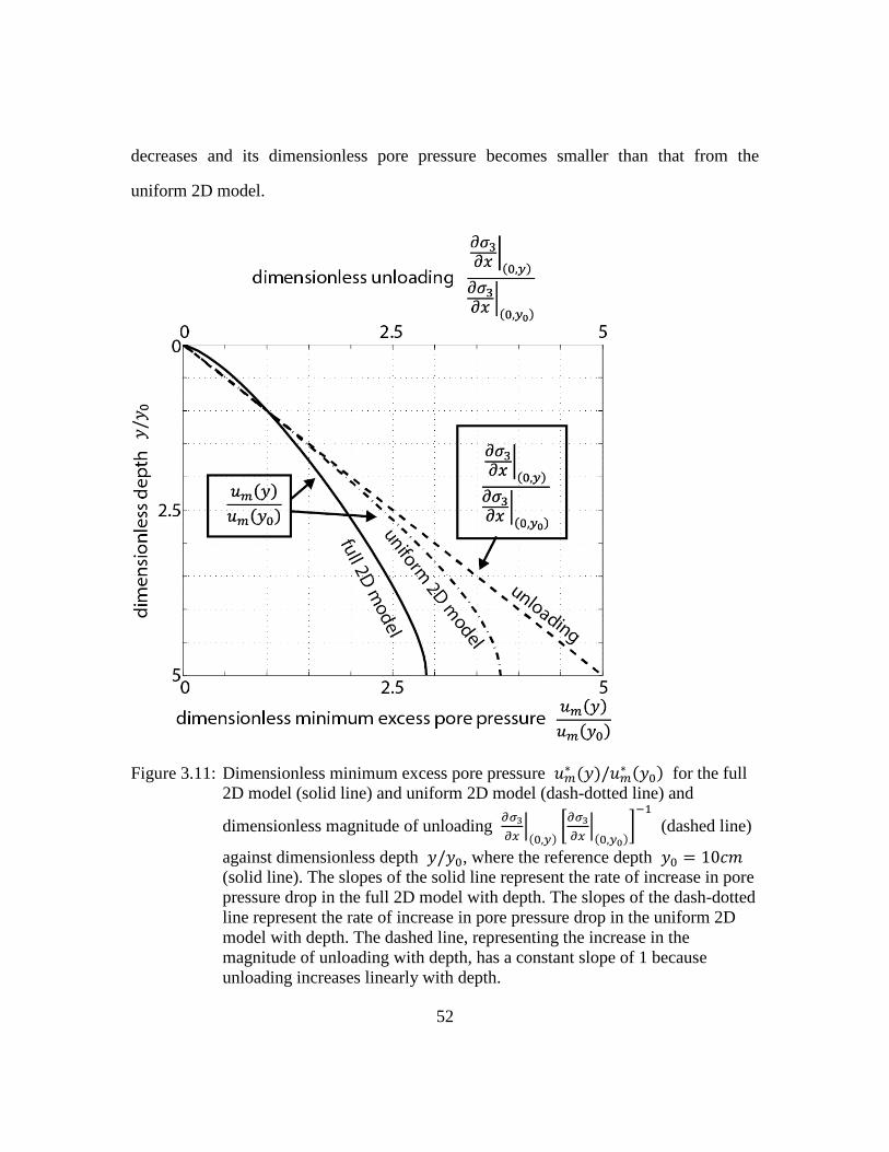
52

decreases and its dimensionless pore pressure becomes smaller than that from the

uniform 2D model.

Figure 3.11: Dimensionless minimum excess pore pressure 𝑢𝑚∗ (𝑦)/𝑢𝑚∗ (𝑦0) for the full 2D model (solid line) and uniform 2D model (dash-dotted line) and

dimensionless magnitude of unloading 𝜕𝜎3𝜕𝑥�

(0,𝑦)�𝜕𝜎3𝜕𝑥�

(0,𝑦0)�−1

(dashed line)

against dimensionless depth 𝑦/𝑦0, where the reference depth 𝑦0 = 10𝑐𝑚 (solid line). The slopes of the solid line represent the rate of increase in pore pressure drop in the full 2D model with depth. The slopes of the dash-dotted line represent the rate of increase in pore pressure drop in the uniform 2D model with depth. The dashed line, representing the increase in the magnitude of unloading with depth, has a constant slope of 1 because unloading increases linearly with depth.

53

Because the pore pressure drop increases at a similar rate as the increase in

unloading (hence the changes in stresses) in the uniform 2D model, the normalized

effective stress ratio 𝑅′/𝑅𝑚′ of the deposit does not change significantly with the depth

(Figure 3.12). In other words, the stability of the deposit does not depend on its thickness

if the dilation potential 𝛽 were a constant. However, traxial tests show that 𝛽 decreases

with increasing mean effective stress (Equation 3.15), hence increasing depth of the

deposit. As a result, the full 2D model shows that the stability of the deposit deceases

with increasing depth of the deposit (Figure 3.7D and Figure 3.9). This result highlights

the importance of including spatial variations of material properties in the study of

breaching slope failure.

Figure 3.12: Contour of normalized effective stress ratio 𝑅′/𝑅𝑚′ for the uniform 2D model: a 2D model with uniform dilation potential 𝛽.

54

Last, I compare the excess pore pressure solution between the uniform 2D model

(dash-dotted line, Figure 3.10) and the 1D steady state model (dashed line, Figure 3.10)

to show how the vertical drainage affects the excess pore pressure solution. I find the

location of the maximum pore pressure drop (𝑥𝑚) from the uniform 2D model is 1cm, or

10%, less than the value predicted by the 1D model while the normalized excess pore

pressure at 𝑥 > 𝑥𝑚 from the uniform 2D model is closer to hydrostatic than that from

the 1D model (Figure 3.10). In the 1D model, excess pore pressure can only drain from

the breaching front while in the uniform 2D model the excess pore pressure can also

drain from the top surface. As a result, the excess pore pressure drains faster and is closer

to the hydrostatic pressure with the addition of the vertical pore water flow component. I

will show in the next section that this change accelerates erosion near the top of the

breaching front.

3.7 VARIATION OF EROSION RATE IN THE VERTICAL DIRECTION

Here I study variation in the velocity of the breaching front at different depths

with a 2D model. Previous studies and the analysis from Chapter 2 propose that the front

velocity is simply controlled by the dissipation of pore pressure through the front itself

(Van Rhee, 2007). The reason for this is that in order for the breaching front to retreat,

sediments must be released, requiring dissipation of the negative excess pore pressure

that otherwise stabilize the deposit.

I start by adopting the erosion rate model from Chapter 2, where the water flux

from the failure surface into the deposit is required to compensate the pore volume

increase from dilation. However, the water flux into the deposit comes from both the

55

breaching front and the top surface of the deposit. Following Chapter 2 and consider

both water flow from the vertical and horizontal directions, we have

𝑣(𝑦) = − 𝑘𝐸0𝑢𝑚∗ (𝑦)�

𝜕𝑢∗

𝜕𝑥�

(0,𝑦)+ 𝜕𝑢∗

𝜕𝑦�

(𝑥𝑚,0)� (3.18)

where E0 is an empirical parameter that quantifies the amount of dilation that needs to

be compensated by the water flux and um∗ is the minimum excess pore pressure at a

given depth y. The parameter E0 is a function of the friction angle of the deposit. I

choose a value for 𝐸0 so that the average erosion rate over depth matches the observed

erosion rate of 4mm/s. Because the maximum pore pressure drop is very close to the

breaching front, the horizontal flux dominates the dissipation of pore pressure near the

breaching front (Figure 3.7A, 3.8A). The excess pore pressure gradient in the vertical direction at the top surface 𝜕𝑢

∗

𝜕𝑦�

(𝑥𝑚,0) is at least one order of magnitude smaller than the

excess pore pressure gradient in the horizontal direction at the breaching front 𝜕𝑢∗

𝜕𝑥�

(0,𝑦).

Therefore, the water flux in the vertical direction can be ignored. However, this does not

mean the vertical pore pressure dissipation does not affect the erosion rate. Previous

sections show that vertical dissipation of pore pressure affects the pore pressure

distribution in the horizontal direction as well as the pore pressure values. In other words, vertical flow affects 𝜕𝑢

∗

𝜕𝑥�𝑥=0

and 𝑢𝑚∗ (𝑦). Hence the vertical flow affects the erosion

rate even though the term 𝜕𝑢∗

𝜕𝑦�𝑦=0

can be ignored in Equation 3.18.

I couple the Equation 3.18 to the 2D pore pressure model (Equation 3.16) and

solve for the erosion rate 𝑣. I model dilation potential as a function of the effective

stresses (Equation 3.15). Solutions show that 𝑣 is near uniform for depths greater than

15cm (changes less than 25%) (Figure 3.13). 𝑣 increases near the top of breaching front.

At the top of the deposit the erosion rate is 10.5mm/s, 2.5 times faster than the average

erosion rate of 4mm/s. The erosion rate is close to uniform for 70% of the deposit

56

because the coefficient of consolidation is uniform in the deposit. Chapter 2 shows that

erosion is in equilibrium with the dissipation of pore pressure at steady state and erosion

rate is proportional to the coefficient of consolidation. The erosion rate near the top

boundary is faster because the boundary condition affects pore pressure dissipation

greatly. Near the top, the pore pressure drains faster due to the closer distance to the top

boundary. The faster erosion rate near the top could explain the decrease in local slope of

the breaching front within the top 5cm of the deposit (Figure 3.1). I argue that the faster

erosion near the top does not reduce the average slope of the breaching front due to the

turbidity current that sediment released during breaching generates. Erosion near the base

of the deposit is strongly influenced by this plunging current (Figure 3.1). Previous

studies observe active recirculation of water and sediment at the base of the deposit,

potentially creating a zone of enhanced erosion (Van Rhee and Bezuijen, 1998; Eke,

2008). The erosion from the plunging current could compensate for any difference in

velocity calculated from pore pressure, and in some cases erosion from the current can

overcompensate and allow the base to erode faster. In conclusion, I find the erosion rate

is uniform for most of the deposit and changes in slope angle of the breaching front is

unlikely to occur for a deposit with a uniform coefficient of consolidation.

57

Figure 3.13: Modeled erosion rate, or velocity of the breaching front, 𝑣 against depth. Dilation potential is a function of stresses in this model (Equation 14).

3.8 CONCLUSIONS AND DISCUSSION

Breaching is a type of retrogressive submarine slope failure with a near-vertical

failure surface that retreats at a slow and constant rate. During breaching the deposit

dilates and generates negative excess pore pressure. In this Chapter I investigate the

mechanics of breaching with 2D pore pressure and erosion rate models. I model dilation

using lab experiment results. For a given depth, dilation is largest at the breaching front

and decays with distance from the breaching front. As a result, the maximum pore

pressure drop is close to the breaching front. Dilation decreases with increasing depth,

therefore the increase of the pore pressure drop is less rapid than the increase of the

magnitude of unloading with increasing depth. Consequently, the stability of the deposit

associated with dilation decreases with increasing thickness of the deposit and at some

depth breaching could no longer occur.

58

Addition of the vertical dissipation of pore pressure results in much better fit

between the model results and the observations. First, the vertical dissipation reduces the

magnitude of excess pore pressure compared to 1D model, especially for the part of the

deposit that is away from the breaching front. Second, the vertical dissipation moves the

maximum pore pressure drop closer to the breaching front. Both changes affect the

stability of the deposit because the stability of the deposit is a function of the excess pore

pressure. They also affect the erosion rate because the erosion rate is a function of both

the magnitude and horizontal distribution of the excess pore pressure.

I model the erosion rate of breaching in 2D for the first time. I couple the

retreating of the breaching front to the dissipation of the negative excess pore pressure

generated by breaching. Because the pore pressure drop is close to the breaching front,

the sediment release is mainly controlled by dissipation of excess pore pressure in the

horizontal direction. As a result, the erosion rate can be treated as a constant in the

vertical direction except for the top of the deposit, suggesting the slope of the breaching

front is stable during breaching. The top draining boundary accelerates the erosion near

the top of the deposit, relaxing the slope of the breaching front near the top.

I only considered variation of material properties due to differences in stress in

this study. Another common cause for variation of material properties in a deposit is

stratification. Consider a deposit consists of interbedded sand and silty sand deposits, the

coefficient of consolation and the dilation potential could be different between those two

types of sediment. Future studies can use the 2D analysis presented in this chapter to find

out how this type of heterogeneity affects breaching.

This and previous studies on breaching form a foundation for us to study slope

failure in dilative deposits in general. Slope failures in dilative deposits should be

common in the field. To assess this hypothesis I use the in situ relative density (𝐼𝐷) and

59

the mean effective stress of a deposit to estimate whether natural clean sand deposits are

susceptible to dilation upon their failure (Been and Jefferies, 1985; Bolton, 1986).

Relative density is calculated with in situ void ratio (𝑒), maximum void ratio (𝑒𝑚𝑎𝑥), and

minimum void ratio (𝑒𝑚𝑖𝑛), such that

𝐼𝐷 = (𝑒𝑚𝑎𝑥 − 𝑒)/(𝑒𝑚𝑎𝑥 − 𝑒𝑚𝑖𝑛) (3.19)

The maximum and minimum void ratio (𝑒𝑚𝑎𝑥, 𝑒𝑚𝑖𝑛) are often not measured in field

studies but they can be estimated from grain size measurements (Beard and Weyl, 1973).

I use this method to estimate the relative density of clean sands on the continental shelf

published in literature (Table 3.2). I assume these natural deposits are less than 10m

thick, which corresponds to a confining stress less than 100kPa in the deposit. Bolton’s

study suggests that deposits having a relative density larger than 20% can dilate when the

confining stress is less than 100kPa (Bolton, 1986). A majority of the published cases I

found have relative densities (𝐼𝐷) larger than 20%, suggesting that dilative sand is

common in such environments (Breslau, 1967; Pryor, 1972; Beard and Weyl, 1973;

Bennett and Stockstill, 1999; Richardson et al., 2001; Curry et al., 2004). Slope failures

in dilative deposits could play a more important role in changing the morphology on the

60

Location 𝑫𝟓𝟎

(mm) 𝑰𝒓: relative density

Reference

Fort Walton Beach, FL 0.42 1.2 Richardson et al., 2001

Fort Walton Beach, FL 0.45 0.5* Curry, et al., 2004

Galveston, TX/New Orland, LA 0.12 1 Beard and Weyl, 1973

Coast of Holland 0.25 0.94 Bennett and Stockstill, 1999

Western North Atlantic 0.2-0.14 0.33-1.2 Breslau, 1967

Irish Sea 0.14 0.97 Jackson, 1975 Galveston, TX/New Orland, LA 0.24 0.13 Beard and Weyl, 1973

East Texas Gulf Coast 0.9 -0.29 Pryor, 1972

* Curry et al. [2004] did measure maximum and minimum void ratio directly therefore the relative density is not estimation.

Table 3.2: Estimated relative density (ID) of clean sand deposits in published literature. Larger values of ID means the deposit has smaller porosity/void ratio. ID > 1 means the in situ porosity is smaller than the estimated minimum value and ID < 0 means the in situ porosity is larger than the estimated maximum value. Assuming the deposits are less than 10m thick, the condition for the deposit to dilate is 𝐼𝑑 > 0.2 according to Bolton [1986].

61

Chapter 4: Dual-mode slope failure

4.1 INTRODUCTION

Submarine slope failure is an important mechanism that redistributes sediments

on the seascape (Piper and Normark, 2009). To accurately interpret their sedimentary

records and surface morphological changes we need to know the full spectrum of

possible types of slope failures. The study of submarine slope failure has emphasized

liquefaction slope failure, typically in mud rich deposits. Those slope failures leave

scarps that are up to a few kilometers long and have runoff distances of hundreds of

kilometers (Hampton et al., 1996; McAdoo et al., 2000). As a result, they are well

documented in the sedimentary records and provide us with rich information to study.

Some types of slope failure, however, do not produce obvious sedimentary records and

were discovered through direct observation. For example, breaching slope failure that

occurs in cohesionless sand was discovered during sand mining (de Koning, 1970; Van

den Berg et al., 2002). Breaching is a retrogressive slope failure where sediments are

released at a slow (mm/s) and approximately constant rate from a near-vertical failure

surface. Breaching generates sustained turbidity currents and leaves no discernible scarp

(Van den Berg et al., 2002). Breaching could be responsible for releasing long shore drift

deposits at the head of submarine canyons into their canyon axis (Mastbergen and Van

den Berg, 2003; Eke et al., 2011). Because of the lack of obvious preserved geomorphic

or sedimentologic features, slope failures like breaching are better suited for experimental

studies, where we can understand their mechanics. In this chapter I identify a new type of

slope failure that occurs in sand-rich subaqueous deposits. This style of slope failure is a

62

variant of breaching that includes both the classic slow and steady release of sediment

and periodic sliding.

Past studies suggest that breaching and sliding can be regarded as two end-

member types of slope failure and the differences between them are due to different

modes of shear deformation and their associated pore pressure responses (Meijer and van

Os, 1976; Van den Berg et al., 2002). Liquefaction slope failure is characterized by

dramatic slumping/sliding events with fast release of sediments. The sliding is a result of

contraction of pores during shear and a rise in pore pressure. This rise in pore pressure

reduces the effective stress in the deposit, which greatly weakens the deposit and leads to

slope failure (Terzaghi, 1951; Hampton et al., 1996; Flemings et al., 2008). On the other

hand, breaching slope failure is associated with dilation of pores during shear and a

decrease in pore pressure (Meijer and van Os, 1976; Van den Berg et al., 2002). The drop

in pore pressure increases the effective stress and strength of the deposit. The increase in

strength keeps the deposit from sliding and only allows sediments on the failure surface

to be released at a controlled rate.

Pure breaching represents a steady state, dilative slope failure. Dilative slope

failure is defined by sediment that dilates under shear stress. Chapter 2 shows that during

breaching the excess pore pressure is negative and reaches a steady state due to the

equilibrium between slope failure and pore pressure dissipation. Chapter 2 also shows

that the steady negative excess pore pressure is able to maintain a stable deposit during

breaching when the dilation is more than a threshold value. However, the steady state

negative excess pore pressure can fail at maintaining a stable deposit when dilation is less

than the threshold value. To completely understand how sediments are released during

dilative slope failure we need to understand what happens when the steady state pore

pressure is not able to maintain a stable deposit. I use experiments to study this problem.

63

Experimental studies are important means for us to understand the mechanics of slope

failure because it is much easier to make direct measurements of parameters like pore

pressure in a controlled lab environment. The knowledge we gain from the experimental

study can guide us in making effective measurements in the field.

In this study I use flume experiments to identify a new type of slope failure and I

define its mechanics using both pore pressure measurements and numerical pore pressure

models. First, I use an ultrasonic imaging to capture the characteristic feature of this new

type of slope failure, periodic alternations between breaching and sliding. Second, I

combine pore pressure measurements with a numerical pore pressure model and

accompanying stability analysis to examine the conditions when pore pressure drop from

dilation is not enough to maintain a stable deposit during breaching, resulting in periodic

sliding. I also show that sliding induces large pore pressure drops within the remaining

deposit, stabilizing it and switching the mode of slope failure back to breaching. Last, I

use the numerical model to discuss the conditions that could lead to this new type of

slope failure instead of pure breaching in dilative deposits.

4.2 EXPERIMENT SETUP

I built a rectangular deposit inside a water tight flume (Figure 4.1) out of

siliciclastic, well-sorted fine sand (𝐷50 = 0.19𝑚𝑚). This deposit hosting flume, referred

as the inner flume, rests on the floor of a larger flume (referred as the outer flume). The

inner flume is 1.2 m tall (vertical dimension in Figure 4.1), 0.15 m wide, and 0.58 m long

(horizontal dimension in Figure 4.1) and it constrains the deposit on all sides until one

narrow wall is removed as a vertical sliding gate. The inner flume is positioned in the

center of the outer flume with its sliding gate more than 2m away from the end of the

64

outer flume. This 2m distance allows sufficient space for the failed sediments to flow

away from the deposit. I built each original deposit by raining sediment through the water

column at a controlled rate. Because the sedimentation rate in the lab is much higher than

that in the field, the deposit can have higher porosities than a deposit built with natural

sedimentation rate (Vaid and Negussey, 1988). To minimize this difference I used a

rubber mallet to condense the sediment by tapping on the surface of the deposit when it

was at ⅓, ⅔, and full height. I also placed 23 kg of deadweight on top of each fully built

deposit for 24 hours to facilitate further consolidation. Each constructed deposit had 6

thin (~ 0.01 m), roughly evenly spaced in the vertical direction and horizontal layers of

brown colored medium sand that served as marker beds so that internal deformations in

the deposit could be visualized. Deposit porosity was ~36 %, with a relative density of 85

%; a relative density that is commonly observed in the field (e.g., Curry et al., 2004).

Each final deposit was 0.58m long (horizontal dimension in Figure 4.1), 0.15m wide, and

depending on the experiment between 0.96m to 1.0m thick.

I collect three types of measurements in each experiment. First, I record the pore

pressure in the deposit with gauge pressure transducers at 7 locations along the length of

the deposit and at a constant depth (Figure 4.1). The transducers, whose outer diameters

are 2.4cm, are placed outside of the outer flume and they are plumbed to the deposit with

a series of thin tubes, whose outer diameters are 0.32cm. Using the thin tubes allows us to

make measurements at higher resolution and minimize the disturbance to the deposit. The

distance between the sensors and the surface of the deposit varies between 0.08m to

0.12cm in different experiments. I intentionally place the sensors close to the top of the

deposit because the pore pressure signal in the lower portion of the deposit is complicated

by the adjacent redeposition of failed sediments. The transducers records pore pressure at

each location at a frequency of 1Hz and an accuracy of 21Pa.

65

Figure 4.1: Side view of the setup of the experiment.

Second, I measure the location of the failure surface using an ultrasonic

transceiver. In this study, the interface between water and the deposit has a large contrast

in acoustic impedance so that the boundary is well imaged by the strong reflection of

ultrasonic waves, similar to the way that distinct lithological boundaries are recorded by

strong reflectors in seismic images. Because each deposit itself is relatively homogeneous

in composition, the interior of each deposit appear acoustically transparent, similar to the

way a homogeneous bed appears transparent in a seismic image. The transceiver collects

acoustic data at a frequency of 10MHz, and measures the distance between its head and

the deposit-water interface to a resolution of 0.14mm over a footprint of 1.8cm2.

66

Technical details of this measuring tool are presented in Perillo et al. (in prep.). I orient

the transceiver so that it is measuring the retreat of the failure surface at a position ~16cm

below the top of the deposit (Figure 4.1). Therefore the surface retreat measurements and

the pore pressure measurements are spatially close to each other; because the tubes I use

to measure pore pressure can interfere with the ultrasonic waves I am not able to measure

the surface retreat at the exact depth where the pore pressure are measured. Video

capturing the evolution of the entire failing deposit is also collected during each run.

4.3 DUAL-MODE FAILURE

I initiate slope failure by quickly pulling out the sliding gate from the inner flume.

Removal of this gate takes about 2s. The deposit does not collapse immediately after the

gate is removed. Instead it maintains a vertical surface referred to as the failure front

(Figure 4.2A). The failure front retreats at a relatively slow and steady rate, releasing

individual grains from the otherwise stable deposit. The falling grains generate a

sustained turbidity current (Figure 4.2A). All of these observations are consistent with

breaching slope failure presented in Chapter 2 and previous studies (Van Rhee and

Bezuijen, 1998; Van den Berg et al., 2002; Eke et al., 2011). The character of the slope

failure starts to diverge from the case of pure breaching after 10s when a sliding plane

oriented at 80∘ to the horizontal forms in the deposit (Figure 4.2B). The sediment wedge

positioned above this plane starts to slide downward as a relatively coherent block. As the

wedge slides down, sediment on its surface, as well as sediment constituting the exposed

sliding plane continues to be released at the slow and constant rate observed during the

breaching interval prior to the sliding event. With continued sliding the wedge deforms

and entrains water until it fully disintegrates, becoming part of the turbidity current

67

generated by the slope failure. Interestingly, the onset of wedge sliding acts to stabilize

the rest of the deposit. No new sliding plane forms and following collapse of the wedge a

new failure front is established. In short, the slope failure diverges from breaching

temporary when sliding occurs and then slope failure returns to breaching mode after the

sliding event. There are multiple sliding events during an experiment, each separated by

16s on average and having an average sliding duration of 4s. Each sliding event is

preceded and followed by breaching. During each breaching interval the slope of the

failure front usually steepens from ~80∘ immediately post sliding to 90∘, sometimes

even exceeding 90∘. To summarize, the observed slope failure temporarily switches

from breaching to sliding every 16s, then switches back to breaching after 4s of sliding. I

call this cyclic failure process the dual-mode slope failure: breaching and sliding modes

co-existing in the same slope failure event. The dual-mode also refers to the two different

styles of failure front retreat: slow and steady retreat from breaching coexists with

episodic fast retreat from sliding. Van Rhee and Bezuijen [1998] noted that slumping

events can occur during breaching experiments but did not explore the mechanics of the

slumping or study whether it represents a new type of slope failure.

68

Figure 4.2: Dual-mode slope failure captured by video and sonar. A: sketch of breaching mode slope failure. B: sketch of the sliding mode slope failure as the wedge starts to slide down slope. The sliding wedge is thicker near its top therefore as it slides down the location of the failure front could temporary prograde instead of retreat (e.g., circled area in subfigure C). C: ultrasound image showing the retreating of the failure front with time. The gray scale represents the amplitude of the reflected acoustic wave; the white color represents largest amplitudes, i.e., strongest reflectors. The coordinates of the brightest reflectors (e.g., point a) represent the distance the failure front has retreated (horizontal axis, 𝑑) at a given time 𝑡 (vertical axis).

69

I use ultrasound imaging to quantify the two styles of failure front retreat. In

Figure 4.2, the position of the failure front is defined by bright reflectors on the

ultrasound image. For example, point “a” in Figure 4.2C shows that the failure front has

retreated 8cm at 25s since removal of the sliding gate. The two styles of failure front

retreat are represented by two different slopes in Figure 4.2C. The steeper slopes

represent the slow retreat of the failure front with time, i.e., breaching. The near

horizontal slopes on the image represent fast retreat of the failure front with time, i.e.,

sliding. The ultrasound image shows that failure front moves forward (closer to the sonar)

for a few centimeters before it suddenly retreats from sliding (circle “b” in Figure 4.2C).

The forward movement of the failure front is due to the passage of the sliding wedge.

Because the sliding wedge is wider (size in the horizontal dimension) near its top, the

water-sediment boundary temporarily moves forward as the wider part of the wedge

passes through the measuring point for the sonar. I interpret that sliding starts at the time

the failure front starts to move forward and ends at the time when the next breaching

period (slow retreating) begins. The distance the fast retreating mode covers measures the

size of the wedge and I refer to it as the sliding size. The sliding event that occurs at 62s

has no forward moving component for the failure front because the sliding wedge is the

thickest where the sonar measurements are made.

I digitize the ultrasound image and use it to calculate the erosion rates and

durations of the two modes the failure front retreats. Breaching on average has an erosion

rate of 0.25 cm/s and erodes 44% of the deposit, while sliding events have an equivalent

erosion rate of 21mm/s and erodes 56% of the deposit. The image shows that for each

breaching period, the erosion rate is a constant. The erosion rate in different breaching

periods is similar, within a ±0.05 cm/s range. The sliding sizes are 6.1 ± 1.6 𝑐𝑚; there

is no systematic variation of sliding size with time. .

70

The dual-mode slope failure is similar to the process of episodic landslide

discovered by Iverson et al. (2000). Iverson et al (2000) found that slope failure in

partially saturated clay-rich soil can be episodic when the initial porosity of the soil is

small. The dense soil dilates and drops pore pressure when unloaded. No displacement is

observed when the pore pressure is low. Sudden displacement of the deposit along a basal

slope occurs when the pore pressure rises to a certain threshold. The episodic horizontal

displacement observed by Iverson et al (2000) is similar to the episodic vertical sliding I

observe in this study. I show in the next section that the pore pressure measurements from

this study are also similar to those from Iverson et al (2000). However, there are two

major differences between the two experiments. First, I observe active retreating of the

failure front between sliding events while in the experiments of Iverson et al (2000)

release of sediments only occurs when sliding occurs. In other words, the experiments

from Iverson et al (2000) show a pure episodic sliding behavior while this study shows

breaching with episodic sliding occurring on the same slope failure. Second, Iverson et al

(2000) address the stability of sediments along a pre-defined slide plane. In this study

there are no pre-defined slide planes; I capture and study how these planes emerge in the

deposit as it becomes unstable.

4.4 PORE PRESSURE MEASUREMENTS

The dual-mode retreat of the failure front produces two different signals in the

pore pressure recordings. I use pore pressure recorded at the 4 sensors that are closest to

the original free surface (u1, u2, u3, and u4 in Figure 4.1) to illustrate how sliding and

breaching affect the pore pressure respectively (Figure 4.3A). Before the initiation of

breaching the pore pressure is at hydrostatic level and the excess pore pressure 𝑢∗ = 0

71

(−10𝑠 < 𝑡 < −5𝑠). The pore pressure changes greatly when preparing the release of the

gate (−5𝑠 < 𝑡 < 0𝑠). These changes are due to external forces applied on the flume and

I do not consider them in this study. Immediately following the release of the sliding gate

(region with yellow shading in Figure 4.3A) the pore pressure drops in all four sensors.

This drop comes from both shear dilation and isotropic unloading, with majority of the

drop produced by shear dilation. After the initial drop, the negative excess pore pressure

starts to dissipate through pore water flow. These pore pressure changes are consistent

with those observed during pure breaching as presented in Chapter 2 and other studies

(Meijer and van Os, 1976). Between 18s and 20s, the pore pressure at sensors u1, u2, and

u3 drops; the magnitude of pore pressure drop ranges from 100Pa in u3 to 300Pa in u1.

This pore pressure drop is different from the pore pressure drop observed in pure

breaching experiments, like the one in Figure 2.2 from Chapter 2. In pure breaching, the

pore pressure drops in response to the slow release of sediments from the failure front.

Significant pore pressure drop is limited to the deposit within 2cm of the failure front. In

this experiment the drops in pore pressure occurs at all 4 sensors, affecting a larger

portion of the deposit than pure breaching does.

72

Figure 4.3: Measured excess pore pressure 𝑢∗ in the deposit. A: measured excess pore pressure at the 4 locations closest to the initial gate (labeled in different colors) against time 𝑡. The grey color shaded area contains measurements made before releasing the gate. The yellow color shaded area indicates the duration of initiation (pulling gate out). B: measured excess pore pressure from all the sensors (squares) against distance from failure front (𝑥) at 3 different time: 10s (dash dotted line), 18s (dashed line), and 20s (solid line). 𝑥 = 0 is the failure front.

73

Another way to look at the negative excess pore pressure is to plot it against

distance to the failure front, i.e., plotting negative excess pore pressure in the Lagrangian

reference frame whose origin retreats with the front. I study the excess pore pressure in

all the sensors at t=12s, 18s (pre first sliding), and 20s (post first sliding event) in Figure

4.3B. The pore pressure profiles at different times show that the spatial distribution of the

negative excess pore pressure is similar at all 4 sensors. The magnitude of negative

excess pore pressure increases from the failure front (𝑥 = 0) into the deposit (𝑥 > 0). The

magnitude of excess pore pressure reaches its maximum value between 8cm and 15cm

away from the failure front then it decreases with increasing distance. From 12s to 18s

the slope failure is in breaching mode (Figure 4.2C); the magnitude of the negative

excess pore pressure decreases as the excess pore pressure dissipates everywhere in the

deposit. At 𝑡 = 18𝑠, the first sliding event occurs (Figure 4.2C) and it finishes at

𝑡 = 20𝑠. The excess pore pressure drops significantly for 𝑥 < 10𝑐𝑚 between 18s and

20s. After the sliding 𝑡 > 20𝑠 the magnitude of the negative excess pore pressure

decreases as the excess pore pressure dissipates, until the next sliding occurs at 25s.

Each sliding event is associated with a sudden drop in excess pore pressure except

for the sliding at 62s (Figure 4.4). The top of the sliding wedge at 𝑡 = 62𝑠 is below

where the pressure sensors are located and this could be the reason why no pore pressure

drop is recorded at this time. On the other hand, pore pressure drop due to mechanisms

like breaching (e.g., point “a” in Figure 4.4) is not associated with any sliding events and

the magnitude of those drops is much smaller than the drops from sliding. The slope

failure switches back to breaching mode after the pore pressure drops from sliding,

suggesting that the deposit is stable after sliding. The excess pore pressure rises after each

sliding. The excess pore pressure at a fixed point can drop at a rate slower than that

during sliding before the next sliding happens, e.g., 𝑡 ∈ [30𝑠, 45𝑠] in Figure 4.4. This

74

type of small pore pressure drop could be due to spatial variation of the excess pore

pressure. The failure front moves closers to the sensors with time and the magnitude of

negative excess pore pressure is larger nearer to the failure front.

Figure 4.4: Excess pore pressure measurements for all the sensors against time (top figure) compared to the position of the slope failure surface against time (bottom figure, it is Figure 4.2C viewed in a different orientation). The two time series are aligned at the moment the gate starts to slide (𝑡 = 0). The red dashed lines mark the time when the excess pore pressure (𝑢∗) suddenly drops in the top figure.

75

The periodic fluctuation in the excess pore pressure means that it never reaches a

steady state in dual-mode slope failure. During pure breaching the excess pore pressure

rises after the initiation but ultimately reaches a steady state value. Chapter 2 shows that

during pure breaching the steady state pore pressure for the deposit is able to maintain the

stability of the deposit therefore no sliding occurs. I hypothesize that as the excess pore

pressure rises toward its steady state the stability of the deposit decreases; the deposit

becomes unstable before the pore pressure reaches its steady state in dual-mode slope

failure. I use a 2D model to test the hypotheses in the next section by studying how the

stability of the deposit changes as the pore pressure evolves during dual-mode slope

failure.

4.5 2D TRANSIENT PORE PRESSURE MODEL

In this section I build a 2D pore pressure model to simulate the transient pore

pressure during dual-mode slope failure. In the next section I use the pore pressure

solutions in stability analysis to test whether the stability of the deposit does indeed

decrease as the excess pore pressure rises. Because the changes in pore pressure are

cyclic I only need to simulate one cycle of pore pressure changes. Specifically I model

the rise of excess pore pressure from initiation until the beginning of the first sliding

event, i.e., when the deposit is first unstable. In this period of time the slope failure is in

breaching mode. Therefore the pore pressure changes in response to two factors (Meijer

and van Os, 1976). First, the slow release of sediments from breaching generates negative

excess pore pressure, or pore pressure drops. Second, pore water flow dissipates the

negative excess pore pressure, i.e., decreases the magnitude of the negative excess pore

pressure. Following Chapter 3, I model the changes in the excess pore pressure 𝑢∗ as a

76

combination of pore pressure dissipation due to pore water flow and pore pressure

generation due to changes in the horizontal stress 𝜎ℎ. In the Lagrangian reference frame

whose origin moves with the failure front, the changes in excess pore pressure with time 𝜕𝑢∗

𝜕𝑡 in a deposit with infinite length follows,

𝜕𝑢∗

𝜕𝑡= 𝐶𝑣𝑥

𝜕2𝑢∗

𝜕𝑥2+ 𝐶𝑣𝑦

𝜕2𝑢∗

𝜕𝑦2+ 𝑣 𝜕𝑢∗

𝜕𝑥− 𝑣𝛽 𝜕𝜎ℎ

𝜕𝑥, for 0 < x < ∞ and 0 < y < H.

(4.1)

where 𝑐𝑣𝑥 and 𝑐𝑣𝑦 are the coefficient of consolidation of the deposit in the horizontal

(x) and vertical (y) directions (unit is 𝑚2𝑠−1), 𝑣 is the erosion rate of breaching (unit

is 𝑚𝑠−1), 𝛽 is the dilation potential (dimensionless), and H is the total height (unit is

𝑚). Dilation potential 𝛽 quantifies how much more pore pressure drop comes from

dilation than from isotropic unloading; larger 𝛽 means there is more dilation and larger

pore pressure drops. The first two terms on the right hand side of Equation 4.1, 𝐶𝑣𝑥

𝜕2𝑢∗

𝜕𝑥2+ 𝐶𝑣𝑦

𝜕2𝑢∗

𝜕𝑦2, represent the pore pressure dissipation due to pore water flow. The

third term 𝑣 𝜕𝑢∗

𝜕𝑥 represents the pore pressure changes due to the retreating failure front.

The last term 𝑣𝛽 𝜕𝜎ℎ𝜕𝑥

is the source for pore pressure drop; it is can be viewed as the

changes in horizontal stress in the Lagrangian reference frame 𝑣𝜕𝜎ℎ/𝜕𝑥 amplified by

the dilation potential 𝛽.

I apply the boundary conditions

𝑢∗(0,𝑦) = 0, 𝑢∗(𝑥, 0) = 0, (4.2) 𝜕𝑢∗ 𝜕𝑥

|(∞,𝑦) = 0, 𝜕𝑢∗

𝜕𝑦|(𝑥,𝐻) = 0, (4.3)

and the initial condition 𝑢∗(𝑡 = 0) = 𝑦𝑢0

ℎ0 , (4.4)

where 𝑢0 is the measured excess pore pressure (unit is 𝑃𝑎) at 𝑡 = 2𝑠 and ℎ0 = 10𝑐𝑚,

the depth at which the measurements are made. Those conditions are the same as the ones

77

in Chapter 3. I model the horizontal stress 𝜎ℎ as an exponential function with distance

from the failure front, same as in Chapter 2 and Chapter 3. 𝜕𝜎ℎ𝜕𝑥

= 𝑘0𝜌𝑠𝑔𝑦𝑒−𝜂𝑥 (4.5)

where k0 is the ratio between the horizontal and vertical stress in the far field

(dimensionless), ρs is the density of the submerged sediment (unit is 𝑘𝑔𝑚−3), g is the

gravitational acceleration (unit is 𝑚𝑠−2), and η is a constant that describes the decay of

unloading with distance to the failure front (unit is 𝑚−1). The ultrasound image shows

that the erosion rate for breaching 𝑣 is steady with time and Chapter 3 shows that 𝑣 can

be considered uniform in the vertical direction, therefore I consider 𝑣 as a constant in

this model and 𝑣 = 2.5𝑚𝑚/𝑠 according to the ultrasound image.

I use the same modeling parameters from Chapter 3 since the composition and

relative density of the sediments are the same in both studies. I set the total thickness of

the deposit 𝐻 to be 100cm to match the average thickness in the experiment. It is

impractical to have a deposit with infinite length in a numerical model; I set the model

length 𝐿 = 100𝑐𝑚 . The solution shows the excess pore pressure does not change

significantly at 𝑥 = 100𝑐𝑚 therefore the solution can be used as an approximation to

the solution from a deposit with infinite length. I use the finite difference method with

fully implicit time stepping method in solving for the excess pore pressure. The spatial

grid size is 1cm (50 × 𝐷50 of the sediment) and the time step size is 0.1s. Because 𝛽 is

a function of the excess pore pressure the governing equation (Equation 4.1) is nonlinear.

I use single point iterative method to solve for 𝛽 and 𝑢∗ at the same time.

I compare the excess pore pressure measured from u1 (solid line in Figure 4.5),

the sensor that is closest to the initiation position of the sliding gate (Figure 4.1), with the

model solution at the same location (dash dotted line in Figure 4.5) to demonstrate the

changes of the pore pressure solution with time. The modeled pore pressure follows the

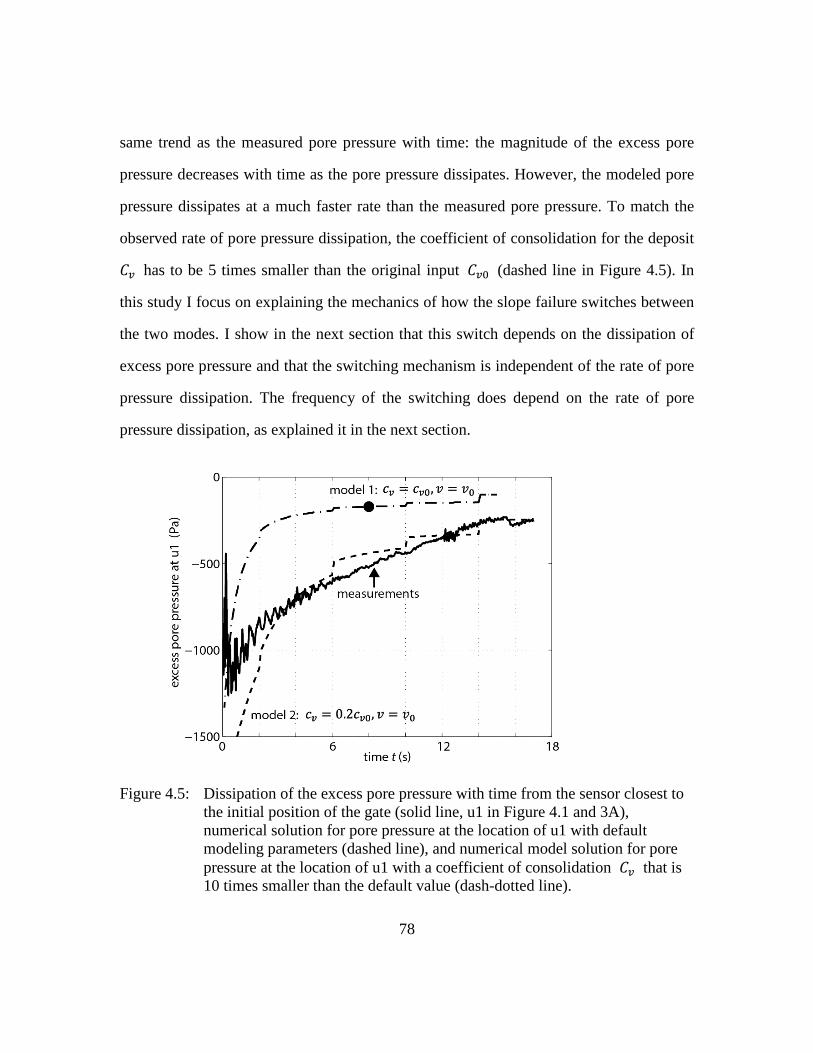
78

same trend as the measured pore pressure with time: the magnitude of the excess pore

pressure decreases with time as the pore pressure dissipates. However, the modeled pore

pressure dissipates at a much faster rate than the measured pore pressure. To match the

observed rate of pore pressure dissipation, the coefficient of consolidation for the deposit

𝐶𝑣 has to be 5 times smaller than the original input 𝐶𝑣0 (dashed line in Figure 4.5). In

this study I focus on explaining the mechanics of how the slope failure switches between

the two modes. I show in the next section that this switch depends on the dissipation of

excess pore pressure and that the switching mechanism is independent of the rate of pore

pressure dissipation. The frequency of the switching does depend on the rate of pore

pressure dissipation, as explained it in the next section.

Figure 4.5: Dissipation of the excess pore pressure with time from the sensor closest to the initial position of the gate (solid line, u1 in Figure 4.1 and 3A), numerical solution for pore pressure at the location of u1 with default modeling parameters (dashed line), and numerical model solution for pore pressure at the location of u1 with a coefficient of consolidation 𝐶𝑣 that is 10 times smaller than the default value (dash-dotted line).

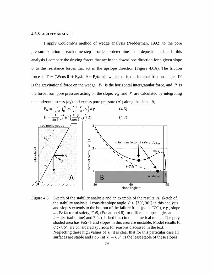
79

4.6 STABILITY ANALYSIS

I apply Coulomb’s method of wedge analysis (Nedderman, 1992) to the pore

pressure solution at each time step in order to determine if the deposit is stable. In this

analysis I compare the driving forces that act in the downslope direction for a given slope

θ to the resistance forces that act in the upslope direction (Figure 4.6A). The friction

force is T = (Wcos θ + Fhsin θ − P)tanϕ, where ϕ is the internal friction angle, 𝑊

is the gravitational force on the wedge, 𝐹ℎ is the horizontal intergranular force, and 𝑃 is

the force from pore pressure acting on the slope. 𝐹ℎ and 𝑃 are calculated by integrating

the horizontal stress (𝜎3) and excess pore pressure (𝑢∗) along the slope θ,

Fh = 1tanθ ∫ 𝜎ℎ �

ℎ−𝑦𝑡𝑎𝑛𝜃

, 𝑦�ℎ0 𝑑𝑦 (4.6)

P = 1sin θ ∫ 𝑢∗ � ℎ−𝑦

𝑡𝑎𝑛 𝜃 ,𝑦�ℎ

0 𝑑𝑦 (4.7)

Figure 4.6: Sketch of the stability analysis and an example of the results. A: sketch of the stability analysis. I consider slope angle 𝜃 ∈ [30∘, 90∘] in this analysis and slopes extends to the bottom of the failure front (point “O” ), e.g., slope 𝑠1. B: factor of safety, FoS, (Equation 4.8) for different slope angles at 𝑡 = 2𝑠 (solid line) and 7.4s (dashed line) in the numerical model. The grey shaded area has FoS<1 and slopes in this area are unstable. Model results for 𝜃 > 86∘ are considered spurious for reasons discussed in the text. Neglecting these high values of 𝜃 it is clear that for this particular case all surfaces are stable and FoSm at 𝜃 = 65∘ is the least stable of these slopes.

80

I use factor of safety, FoS, to evaluate the stability of the deposit, where

FoS = tan𝜙(Wcos θ +Fhsin θ −P)+Fhcos θWsinθ

(4.8)

When FoS<1 for a certain slope, the driven force 𝑊 sin𝜃 is larger than the resistance

force on the the slope and the deposit will start to slide along that surface. This stability

condition shows that when the pore pressure drops, i.e., the excess pore pressure 𝑢∗ is

more negative, the factor of safety FoS is larger and the deposit is more stable. As the

magnitude of the negative excess pore pressure dissipates, FoS becomes smaller and the

deposit could become less stable. I assume the peak friction angle 𝜙 = 42∘ is a constant

in the model; the value for 𝜙 is calculated using triaxial shear test results presented in

Chapter 3.

To demonstrate the stability analysis, I substitute the modeled pore pressure at

𝑡 = 2𝑠 into Equation 4.8 and calculate the FoS for slopes between 30∘ and 89∘; slopes

larger than 89∘ are indistinguishable from 90∘ because the grid size is coarse. I only

consider surfaces that extend all the way down to the bottom of the failure front (i.e.,

slopes like 𝑠1 but not slopes like 𝑠2 in Figure 4.6A). Model results beginning at

θ = 30∘ show FoS decreasing as slope angle increases until a local minimum value is

reached at θ = 65∘ (Figure 4.6B) and then FoS increases with increasing slope angle for

𝜃 ∈ [79∘, 86∘]. FoS is calculated to rapidly decrease for surfaces with 𝜃 > 86∘, to the

point where FoS<1 at θ = 88∘ (Figure 4.6B), suggesting that slopes steeper than 88∘

are unstable. However, such high sliding slope angles never appeared in the experiment.

There are two possible reasons for this discrepancy. First, due to limitations of the

computational grid size, FoS for slopes larger than 86∘ are underestimated by the model.

I find that by reducing the grid size the FoS for slopes steeper than 86∘ increases and

slopes higher than 88∘ become stable. Second, the steeper slopes could have larger

friction angles associated with them. The peak friction angle for sand increases with

81

decreasing mean effective stress (Been and Jefferies, 1985; Bolton, 1986). High angle

slopes are located nearer to the failure front, where the mean effective stresses is smaller.

Therefore the steeper slopes have higher friction angles and are more stable than

predicted by the stability analysis with constant friction angle. In the following analysis I

exclude the slopes larger than 86∘ because of these two reasons.

The modeled minimum values for factor of safety, FoSm, decrease with time.

Therefore, the deposit becomes less stable with time. The decrease of FoSm with time is

due to the decrease of the magnitude of the negative excess pore pressure with time

(Equation 4.8 and Figure 4.7). The model calculates a FoSm < 1 at 7.4s along the slope

𝜃 = 81∘ (Figure 4.6, dashed line). As a result, the wedge above the slope 𝜃 = 81∘ is

predicted to start sliding. This prediction matches the experimental observation

reasonably well. The model also predicts the slope becoming unstable 7.4s after

initiation, before the excess pore pressure reaches its steady state. However, this duration

is 2.6 times shorter than the observed duration between initiation and first sliding event in

the laboratory (18s, Figure 4.2C). The discrepancy is most likely due to the

overestimation of the pore pressure dissipation rate in the model as discussed in the last

section (Figure 4.5). The model also predicts a much smaller value for 𝑢10∗ when sliding

occurs (-220Pa, Figure 4.7) than what is measured in the lab (-780Pa). This discrepancy

could be due to the assumption that the deposit is a perfect rectangle. In the experiment

the failure front can take on a slope angle larger than 90∘, i.e., the slope is overhanging.

Overhanging of the deposit reduces its stability, causing slope failure to occur at more

negative excess pore pressures.

82

Figure 4.7: Modeled minimum factor of safety, FoSm (solid line), and minimum excess pore pressure at 𝑦 = 10𝑐𝑚, 𝑢10∗ (dashed line), against time, 𝑡. I choose 𝑢10∗ against time to represent the trends of excess pore pressure in the deposit. When FoSm<1 (at 𝑡 = 7.4𝑠), the deposit becomes unstable and sliding occurs.

4.7 MECHANICS OF DUAL-MODE SLOPE FAILURE

The stability analysis shows that dissipation of the excess pore pressure during

breaching weakens the deposit and leads to instability, i.e., sliding. Therefore the rate of

pore pressure dissipation determines the release interval for slides. The rate of pore

pressure dissipation is proportional to the coefficient of consolidation 𝐶𝑣 (Equation 4.1).

The pore pressure dissipates faster when 𝐶𝑣 is larger. As a result, the time it takes for the

83

pore pressure to reach the critical state where the deposit is no longer stable is shorter. In

other words, larger 𝐶𝑣 corresponds to shorter sliding period, 𝑡𝑠, or a higher sliding

frequency, 𝑓𝑠. I study the sensitivity in the time it takes for the deposit to become

unstable, the sliding period, 𝑡𝑠 , by changing the values of permeability 𝑘 in the

numerical model input. Numerical results show that 𝑡𝑠 ∝ 1/𝐶𝑣. To show the physical

meaning of the relationship between 𝐶𝑣 and 𝑡𝑠, I simplify the transient pore pressure

model so an analytical form of the transient pore pressure solution can be obtained. I

simplify the model by considering only the horizontal pore pressure dissipation. Hence, 𝜕𝑢∗

𝜕𝑡= 𝐶𝑣

𝜕2𝑢∗

𝜕𝑥2+ 𝑣 𝜕𝑢∗

𝜕𝑥− 𝑣𝜂𝛽𝑠0𝑒−𝜂𝑥 (4.9)

with the initial condition

𝑢∗(𝑡 = 0) = 𝑢0 (4.10)

Chapter 3 shows that horizontal pore pressure dissipation dominates the changes

in the pore pressure during breaching, therefore we can use the 1D model to study the mechanics of dual-mode slope failure. I define ⟨𝑢0⟩ = 𝑢0

𝛽𝑠0, ⟨𝑢𝑡⟩ = 𝑢∗

𝛽𝑠0, and ⟨𝑡⟩ = 𝑡𝑣2

𝐶𝑣.

Then the transient pore pressure equation can be transformed into the dimensionless form 𝜕⟨𝑢𝑡⟩𝜕⟨𝑡⟩

= 𝜕2⟨𝑢𝑡⟩𝜕⟨𝑥⟩2

+ 𝜕⟨𝑢𝑡⟩𝜕⟨𝑥⟩

− 𝜉𝑒−𝜉⟨𝑥⟩ (4.11)

where 𝜉 = 𝜂𝐶𝑣𝑣

is the controlling parameter for the steady state solution (Chapter 2). I

assume the solution to the excess pore pressure ⟨𝑢𝑡⟩ can be separated as the sum of a

transient component ⟨𝑢1⟩(⟨𝑥⟩, ⟨𝑡⟩) and a steady state component ⟨𝑢2⟩(⟨𝑥⟩) , i.e.,

⟨𝑢𝑡⟩ = ⟨𝑢1⟩ + ⟨𝑢2⟩. Observation shows that d𝑣d𝑡

= 0, therefore Equation 4.11 can be

decomposed into the following two equations 𝜕⟨𝑢1⟩𝜕⟨𝑡⟩

= 𝜕2⟨𝑢1⟩𝜕⟨𝑥⟩2

+ 𝜕⟨𝑢1⟩𝜕⟨𝑥⟩

(4.12)

0 = d2⟨𝑢2⟩d⟨𝑥⟩2

+ d⟨𝑢2⟩d⟨𝑥⟩

− 𝜉𝑒−𝜉⟨𝑥⟩ (4.13)

Equation 4.13 is the same as the 1D steady state pore pressure model (Equations 2.1-2.3), therefore ⟨𝑢2⟩ = exp(−𝜉⟨𝑥⟩)−exp(−⟨𝑥⟩)

𝜉−1 (Equation 2.6) and 𝑣 = 𝛿𝜂𝐶𝑣 (Equation 2.4). With

84

Equation 4.12, the initial condition Equation 4.10, and the fact that lim⟨𝑡⟩→∞⟨𝑢1⟩ = 0

(the transient pore pressure ultimately disappears), we have

⟨𝑢1⟩ = 𝑒−𝜆⟨𝑡⟩(⟨𝑢0⟩ − ⟨𝑢2⟩) (4.14)

where 𝜆 is a constant and does not depend on ⟨𝑥⟩ or ⟨𝑡⟩. Therefore

⟨𝑢𝑡⟩ = 𝑒−𝜆⟨𝑡⟩(⟨𝑢0⟩ − ⟨𝑢2⟩) + ⟨𝑢2⟩ (4.15)

The solution shows that the transient component of the pore pressure

𝑒−𝜆⟨𝑡⟩(⟨𝑢0⟩ − ⟨𝑢2⟩) is the dissipation of the difference between the initial excess pore

pressure and the steady state excess pore pressure. Rearranging the equation ⟨𝑢𝑡⟩−⟨𝑢2⟩⟨𝑢0⟩−⟨𝑢2⟩

= 𝑒−𝜆⟨𝑡⟩ (4.16)

Therefore, log �⟨𝑢𝑡⟩−⟨𝑢2⟩⟨𝑢0⟩−⟨𝑢2⟩

� = −𝜆⟨𝑡⟩ (4.17)

Transforming equation into the dimensional form log �𝑢

∗−𝑢𝑠∗

𝑢0∗−𝑢𝑠∗� = −𝜆𝑣2

𝐶𝑣𝑡 (4.18)

where 𝑢𝑠∗ = ⟨𝑢2⟩𝛽𝑠0. Substitute in the steady state solution that 𝑣 = 𝛿𝜂𝐶𝑣 (Equation

2.4). The solution is reduced to log �𝑢

∗−𝑢𝑠∗

𝑢0∗−𝑢𝑠∗� = −𝜆𝛿𝜂(𝑣𝑡) (4.18)

The dimensionless transient excess pore pressure solution shows that the time it

takes for the excess pore pressure to reach a given value 𝑢∗ from its initial value 𝑢0∗ is

proportional to 1/𝑣, hence 1/𝐶𝑣 . Sliding occurs when the pore pressure reaches a

critical value 𝑢𝑐∗ defined by the friction angle and stresses on the deposit, shown in the

stability analysis (Figure 4.7). Therefore, the time it takes for sliding to reoccur is the

same time it takes for the pore pressure to dissipate from its value post sliding, 𝑢0∗ , to the

critical value 𝑢𝑐∗. Hence the period between two sliding events (𝑡𝑠) is proportional to 1/𝐶𝑣, or the sliding frequency 𝑓𝑠 (defined as 1

𝑡𝑠) is proportional to 𝐶𝑣.

85

The dimensionless transient excess pore pressure solution (Equation 4.18) also

shows that the distance between two sliding events is a constant. The distance between

two sliding events 𝑥𝑠 is defined by the velocity of the failure front during this period

(i.e., breaching period) multiplied to the time, therefore 𝑥𝑠 = 𝑣𝑡𝑠 . Because 𝑣 ∝ 𝐶𝑣

(solution from Equations 4.13 and 2.3) and 𝑡𝑠 ∝ 1/𝐶𝑣, 𝑥𝑠 should be insensitive to 𝐶𝑣.

Equation 4.18 shows that 𝑥𝑠 equals − log�𝑢𝑐

∗−𝑢𝑠∗

𝑢0∗−𝑢𝑠

∗�

𝜆𝛿𝜂, and is indeed not dependent on 𝐶𝑣. The

sliding frequency and spatial separation are important parameters in studying how

sediments are released from dual-mode slope failure. Future experiments with different

coefficient of consolidation values are needed to test this result (more discussions are

presented in Chapter 6).

Pore pressure measurements show pore pressure drops after sliding (Figure 4.4). I

hypothesize that sliding drops the pore pressure by suddenly unloading the sediment.

Because a larger sliding wedge will generate a larger unloading, the magnitude of pore

pressure drop from sliding should depend on the size of the sliding wedge (Figure 4.2C).

I test this hypothesis by comparing the sliding wedge size against the magnitude of

associated pore pressure drop from measurements (Table 4.1). The number of sliding

events is small in any one experiment but the data support the hypothesis that larger

sliding size corresponds to larger pore pressure drops. The 4th sliding event in Table 4.1

is an exception: its sliding size is larger than that of the first event, but the corresponding

pore pressure drop is smaller. One possible reason is that the 4th sliding event lasts longer

than other events (Figure 4.2C). As a result, the pore pressure drop has more time to

dissipate and results in an apparent smaller pore pressure drop at the end of the sliding

event. I find the positive trend between sliding size and magnitude of pore pressure drop

86

exists for every individual experiment. I conclude that sliding causes the pore pressure to

drop.

Sliding event # 1 2 3 4

Size of sliding

wedge (cm)

4.3 7.2 7.4 4.5

Magnitude of

pore pressure

drop (Pa)

342 823 856 150

Table 4.1. Size of the 4 sliding wedges compared to the associated magnitude of pore pressure drop. The number of the sliding events is according to the order they occur in time (Figure 4.4).

According to Equation 4.9, the factor of safety FoS decreases when the magnitude

of the negative excess pore pressure diminishes. The stability analysis shows that when

sliding occurs only the minimum FoS is slightly less than 1 (Figure 4.7). As a result, FoS

is >1 for all slopes immediately after sliding produces additional negative excess pore

pressures. After the deposit becomes stable, the slope failure switches back to breaching

mode. To sum up, the cyclic switching between breaching and sliding in dual-mode slope

failure is due to the evolution of excess pore pressure. Dissipation of the excess pore

pressure during breaching leads to the emergence of a single unstable slope; sliding

occurs along this slope. Sliding drops the pore pressure and switches the slope failure

mode back to breaching. This switching mechanism is similar to the one that controls the

episodic landslide observed in Iverson et al (2000).

87

4.8 CONDITIONS FOR DUAL-MODE SLOPE FAILURE TO OCCUR

I propose that a necessary condition for dual-mode slope failure to occur is that

the deposit has to become unstable before the pore pressure field reaches its steady state

associated with pure breaching. The instability occurs due to dissipation of the negative

excess pore pressure generated by the initial failure. If the deposit is stable at the steady

state pore pressure, sliding would never occur and the slope failure will simply continue

as pure breaching (like the case in Chapter 2). I explore the conditions that could lead to

sliding by studying how the stability of the deposit changes with friction angle 𝜙 and

different dilation potentials 𝛽 (Equation 4.1).

Studies show that the peak friction angle of sand increases at smaller mean

effective stress. Therefore, deposit located near the top surface of the sediment

accumulation has a larger peak friction angle than the rest of the deposit; a thinner

deposit will also has a larger overall peak friction angle than a thicker deposit. Peak

friction angles at mean effective stresses less than 10kPa (which is common in a deposit

that is less than 1m thick) are difficult to measure. Sture et al. (1998) find the friction

angle of sand can be higher than 50∘ for a mean effective stress of 1.3kPa. I setup a

numerical model with 50cm total deposit thickness and 𝜙 = 50∘ to study the sensitivity

of the stability analysis results to changes in 𝜙. Model results show that the minimum

factor of safety FoSm from the thinner deposit-higher 𝜙 model is greater than that from

the model with 1m thickness, even when the pore pressure values are the same (Figure

4.8). The thinner deposit is always stable because FoSm>1 even after the pore pressure

reaches its steady state (marked by the star in Figure 4.8). This result explains why pure

breaching can occur in the same sand used in this study (Chapter 2).

88

Figure 4.8: Minimum factor of safety against the minimum excess pore pressure at 𝑦 = 10𝑐𝑚, which represents the pore pressure in the deposit. The solid line with circle at the right end marks the model for the deposit in the experiment, referred as the base model. The dashed dotted line with square in the right end (most of the line covered by the solid line) marks a model that is the same as the base model except the dilation potential is increased by 2 times. The dashed line with star in the right end marks a model with 0.5m thickness, same dilation potential as base model, and higher friction angle than the base model.

Sensitivity study shows that the stability of the deposit also depends on the

dilation potential 𝛽. I setup a new numerical model in which the value of 𝛽 is double

the original input (dash dotted line in Figure 4.8). With larger 𝛽 the pore pressure drop

increases and as a result, the minimum factor of safety FoSm increases in value compared

89

to the base case (𝐻 = 1𝑚,𝛽 = 𝛽0). This results in FoSm>1 after the pore pressure reaches

its steady state (filled square in Figure 4.8). Simply put, more dilation leads to a more

stable deposit and less dilation can lead to sliding. Previous studies show that a deposit

with larger porosity dilates less than the same sediment with smaller porosity (Been and

Jefferies, 1985; Bolton, 1986). Therefore dilative deposits with a larger porosity are more

likely to generate dual-mode slope failure than a deposit of the same sediment with a

smaller porosity.

I propose that dual-mode slope failure cannot occur in contractive deposits, i.e.,

the pore volume in the sediment deposit cannot decrease under shear. This would limit

dual-mode slope failure to deposits that experience no volumetric strain under shear and

the deposits that dilate under shear. This condition ensures that sliding drops the pore

pressure and the negative excess pore pressure act to maintain the stability of the deposit.

4.9 POTENTIAL FIELD SITES FOR DILATIVE SLOPE FAILURE

I argue that dual-mode slope failure and pure breaching slope failure captures the

full range of failure styles in dilative deposits (Figure 4.9). Any slope failure initiation

mechanism, like releasing the gate in this study, increases the shear in the deposit.

Dilative deposits generate pore pressure drops with increases in shear. The pore pressure

drop from dilation keeps the deposit stable temporary and the slope failure is in breaching

mode (step 2 in Figure 4.9). As the negative excess pore pressure dissipates the slope

failure can potentially evolve along two different paths. One type of slope failure has the

deposit becoming unstable before the excess pore pressure becomes steady (step 3b in

Figure 4.9). In this case the slope failure then switches to the sliding mode and dual-mode

90

slope failure follows. Pure breaching slope failure occurs if the deposit is stable even

after the excess pore pressure reaches its steady state (step 3a in Figure 4.9).

Dilative slope failure should be common in the field. Dilative slope failure

requires sandy deposits that can dilate. Sand-rich deposits are common at locations on the

continental shelf with strong long-shore currents. These long-shore currents tend to

entrain sediments finer than sand, removing them from long-shore drift deposits and

producing deposits with relatively narrow distributions of grain sizes (Dill, 1964; Visher

and Part, 1967; Limber et al., 2008). Sandy deposits in such regions are likely to be

dilative for two reasons. First, studies show that relatively well-sorted sand deposits tend

to have dense, i.e., dilative, packing. For example, numerous experiments show that

simply depositing uniform grains by pouring them into a container produces deposits

with relative densities (Equation 3.19) of above 40% (Smith et al., 1929; Onoda and

Liniger, 1990; Radin, 2008), well above the dilation limit of 20% for 1m thick deposits

(Bolton, 1986). Second, experiments show that external energy input like tapping

condenses sediment deposits (Rutgers, 1962; Scott et al., 1964); waves in the ocean can

provide such energy. In summary, long-shore drift and wave-reworked deposits favor the

production of dilative deposits. Measurements presented in Dill (1964) show that the long

shore drift deposits at the head of Scripps Submarine Canyon are indeed dilative. More

systematic studies are required to fully assess how common dilative deposits are in the

field and I discuss this in the Chapter 6: Future Research.

One process that can lead to the initiation of dilative slope failure is focused bed

erosion during storms on the continental shelf (Figure 4.10). Here I use Scripps

Submarine Canyon as an example of where storms cause for release of sediments

accumulated at the canyon head. Studies show that long shore drift deposits at this site

disappear during storms while turbidty currents are observed moving down the canyon

91

(Chamberlain, 1964; Dill, 1964; Shepard and Marshall, 1973). The disappearance of

these canyon-head deposits cannot be a product of liquefaction slope failure because

these deposits actually dilate instead of contract under shear (Dill, 1964). Dilative slope

failure is the more likely candidate responsible for delivering those sediments into the

deep ocean. The proposed focused erosion by currents need only create a surface slope

that is more than the angle of repose for those sediments to initiate slope failure (Figure

4.10). The initial unstable slope angle does not have to be 90∘, as is the case in these

experiments. I observe that during dual-mode slope failure (this chapter) and pure

breaching (Figure 2.3), the failure front steepens with time. As a result, any initially

unstable slope can evolve into a nearly vertical failure surface.

92

Figure 4.9: Summary sketch of the evolution and possible styles of dilative slope failure.

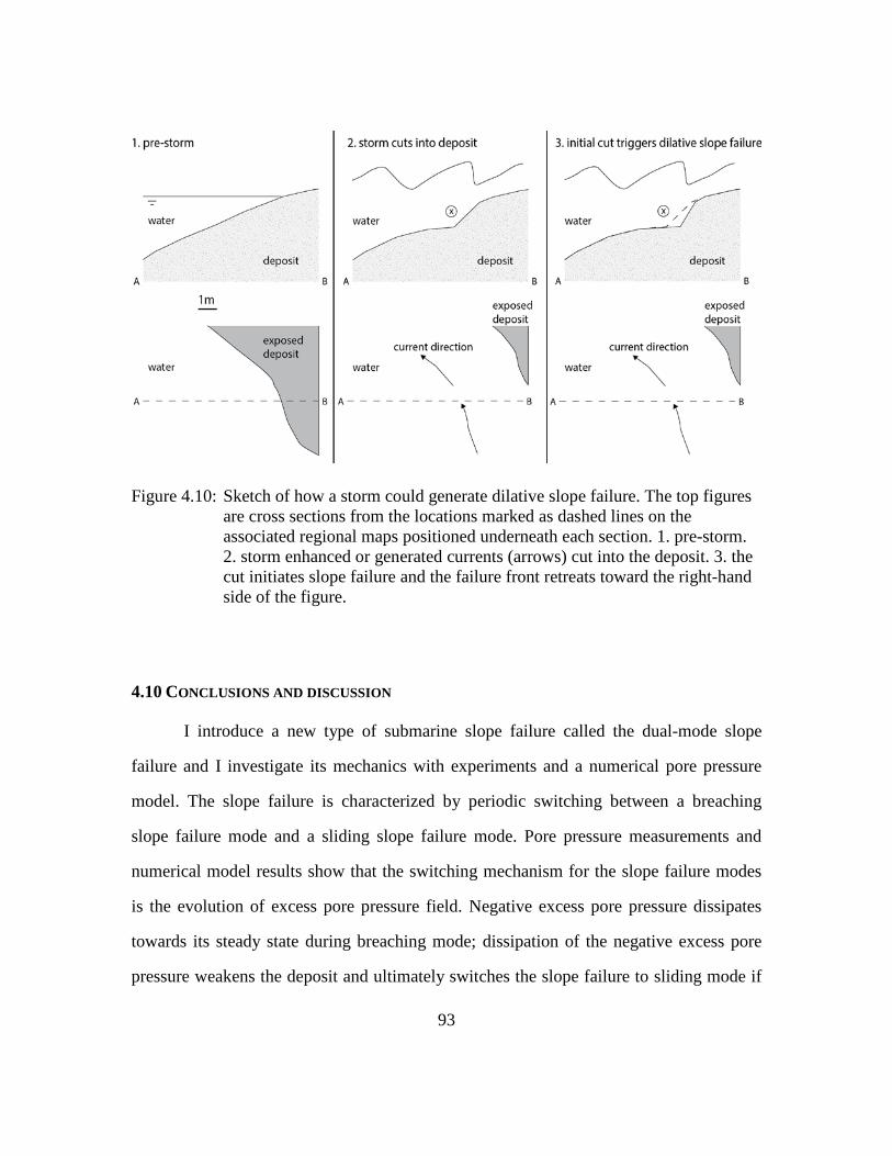
93

Figure 4.10: Sketch of how a storm could generate dilative slope failure. The top figures are cross sections from the locations marked as dashed lines on the associated regional maps positioned underneath each section. 1. pre-storm. 2. storm enhanced or generated currents (arrows) cut into the deposit. 3. the cut initiates slope failure and the failure front retreats toward the right-hand side of the figure.

4.10 CONCLUSIONS AND DISCUSSION

I introduce a new type of submarine slope failure called the dual-mode slope

failure and I investigate its mechanics with experiments and a numerical pore pressure

model. The slope failure is characterized by periodic switching between a breaching

slope failure mode and a sliding slope failure mode. Pore pressure measurements and

numerical model results show that the switching mechanism for the slope failure modes

is the evolution of excess pore pressure field. Negative excess pore pressure dissipates

towards its steady state during breaching mode; dissipation of the negative excess pore

pressure weakens the deposit and ultimately switches the slope failure to sliding mode if

94

the deposit becomes unstable. Sliding increases the magnitude of the negative excess

pore pressure; this strengthens the deposit and switches the slope failure back to the

breaching mode.

I further describe the sensitivity of the dual-mode slope failure using a theoretical

stability analysis. I find that sliding occurs in deposits with small dilation potentials or

small friction angles. However, the stability analysis only considers those slopes that

intersect the bottom of the failure front. Future studies are needed to consider all possible

sliding planes (e.g., surface 𝑠2 in Figure 4.6A). We also need a better understanding of

how the friction angle of sand varies in low stress conditions to properly assess the

stability of slopes in a sand deposit at Earth’s submarine and terrestrial surface.

Nonetheless, the conclusion that dissipation of the negative excess pore pressure leads to

sliding should still hold.

This study shows that sediments can be released at two drastically different rates

during a single slope failure event. The dual-mode of sediment release could affect the

characteristics of the turbidity current that the slope failure generates. For example, the

faster sediment release from sliding could generate a sudden increase in sediment

concentration and current velocity. The two modes of sediment release could also

generate different sedimentary records. Future study on these topics is needed for us to

accurately interpret sedimentary records and morphological changes on Earth.

95

Chapter 5: Conclusions

This study investigates the mechanics of dilative slope failure by combining lab

experiments with mathematical models. There are two types of dilative slope failure. One

type is pure breaching; it is characterized by a slow (mm/s) and steady retreat of a near-

vertical failure front that releases sediments only from its surface. Breaching is associated

with negative excess pore pressure and the pore pressure reaches a steady state during

breaching. The other type is dual-mode slope failure; it is a combination of breaching

style sediment release with episodic sliding events when a triangular wedge of sediment

falls all in once. Dual-mode slope failure is associated with periodic excess pore pressure

fluctuations: the excess pore pressure drops with sliding events and rises during

breaching periods.

All dilative slope failure requires the sediment to dilate under shear stress and

consequently release sediments down-slope. In chapter 1 and 3, I show that a dilative

deposit is common for clean sand and silty sand deposits in the field. Therefore, dilative

slope failure should be common in the field, and it is potentially an important mechanism

that delivers sand and silt into deep sea through the turbidity current it generates. The

analysis of the sediment release rate in this study provides process based boundary

conditions on sediment input for turbidity current models. These findings can improve

our interpretations on sedimentary records produced by dilative slope failure.

Dilation potential, a new material parameter, controls whether pure breaching

occurs or dual-mode slope failure occurs. Pure breaching requires large dilation potential

so that the pore pressure drop from breaching is large enough to keep the deposit stable;

the pore pressure reaches a steady state in this case. When the pore pressure drop from

breaching is not large enough to keep the deposit stable, periodic sliding occurs. Sliding

96

drops the pore pressure more than breaching and generates a transient negative excess

pore pressure. The transient pore pressure stabilizes the deposit temporarily so that the

slope failure returns to breaching mode again. The transient pore pressure dissipates

during breaching period and sliding occurs again when the transient pore pressure is not

able to keep the deposit stable.

This study finds that spatial variations of dilation potential and other mechanical

properties of the deposit affect the pore pressure distribution in the deposit and the

mechanics of slope failure. The stability analysis in Chapter 4 shows that because the

dilation potential and friction angle decreases with thickness of a deposit pure breaching

on the sand used in this study is limited to short deposits less than 1m. This study only

considers the variation of dilation potential as a function of stresses. However, the

dilation potential and other material properties can also change due to stratification of the

sediments. For example, an inter-bedded sand and silty deposit has different material

properties in each of the two types of beds. Additional study is required to determine how

variation of material properties due to stratification affects the mechanics of dilative slope

failure. The analytical methods established in Chapter 3 and Chapter 4 can be used as a

foundation for this type of future study.

The two types of dilative slope failure release sediments in two different ways.

Breaching releases sediments at a constant rate; the rate is proportional to the coefficient

of consolidation of the deposit because the rate of pore pressure generated is in

equilibrium with the pore pressure dissipation during breaching. Sliding releases

sediments in two ways. During breaching the sediments are released at a constant and

slow rate and during sliding a wedge of sediment is released all at once. In other words,

dual-mode slope failure releases sediments with a constant rate with periodic surges; the

frequency of the surge is proportional to the coefficient of consolidation, i.e., the rate of

97

pore pressure dissipation, of the deposit. Future study is needed to assess how the

different ways of sediment release affects the turbidity current the two types of slope

failure generates.

98

Chapter 6: Future Research

This dissertation describes the framework for studying dilative subaqueous slope

failure and slope failures in general. The observations and model results opens up new

questions. Models in this study show that two material properties, the dilation potential 𝛽

and the coefficient of consolidation 𝐶𝑣, control the type of slope failure to be expected

and the rate of sediment release from the slope failure. These results open doors to two

areas for future research. First, future studies on systems with a wide range of 𝛽 and 𝐶𝑣

are needed to test these results. Second, field studies are needed to map the values for

these two material properties in the field so we can properly assess the potential of

dilative slope failure in the field. Below I recommend 5 research projects in these two

areas. These projects will enhance our understanding of the mechanics of dilative slope

failure and will help us to better understand how slope failures and ensuing turbidity

currents are initiated in the field.

6.1 STUDY DILATIVE SLOPE FAILURE WITH CENTRIFUGE MODELS

The flume experiment presented in this study is a 1:1 scale of prototypes in the

nature, i.e., a 1-m thick deposit in the flume represents a 1m thick deposit in the nature.

As a result, the size of the facility limits the size of prototypes I can study in the lab.

Centrifuge models can greatly reduce the sizes of the deposit required in lab experiments

and enable us to explore prototype deposits that are tens of meters thick with model

deposits that are only tens of centimeters tall (Pahwa et al., 1987). In a centrifuge model,

the radial direction models the vertical direction in its prototype, i.e., the force in the

radial direction in a centrifuge models the gravity in an actual deposit and the length of

99

deposit in the radial direction of the centrifuge characterizes the height of the prototype

deposit. A centrifuge applies a centrifugal acceleration to the model that is much greater

than 1g. As a result, the centrifuge deposit can model a prototype deposit with a thickness

that is much larger (e.g., 150 times larger, Pahwa et al., 1987) than that of the centrifuge

deposit. For example, Pahwa et al. (1987) studies slope stability with a centrifuge deposit

that is 10cm long, and it models a prototype deposit that is 15m thick.

Reducing the model size has a few other benefits besides allowing us to study

thicker prototype deposits. First, because a centrifuge model needs much less sediments it

is easier to use rigorous vacuum saturation procedures to ensure a fully de-aired deposit

(Pahwa et al., 1987). The vacuum saturation methods are impractical for a flume

experiment. Second, because the deposit can be prepared dry before saturation it is easier

to build a homogeneous deposit, especially when using sediments with a wide range of

grain sizes. For sediments with a wide distribution of grain sizes the sedimentation

method used in this study (raining dry sediments through water column) would cause

sorting in the deposit due to different settling velocities of the grains. Third, because a

centrifuge model is much smaller than a 1:1 flume model, it greatly reduces the time

required to prepare a deposit. This is very important for studying sediments that have

small coefficients of consolidation, 𝐶𝑣, like deposits with significant amounts of silt or

clay. Abnormal pressure can build up when preparing a deposit with those sediments.

The abnormal pressure can come from the pressure gradient applied to saturate the

deposit if the deposit is settled dry or from sedimentation if the deposit is settled wet. The

characteristic time scale for pore pressure dissipation is 𝐿2/𝐶𝑣, where 𝐿 is the size of

100

the deposit. Therefore, reducing the size of the deposit greatly reduces the time needed

for the abnormal pore pressure generated from preparation to dissipate.

There are well established methods to map experimental results from centrifuge

models to prototypes (Pahwa et al., 1987). But there are two possible roadblocks that may

require careful investigation. First, the time it takes for pore pressure dissipation in a

centrifuge model scales differently from time related to other quantities, like the velocity

of the breaching front (Pahwa et al., 1987). This is because the characteristic time for

pore pressure dissipation is 𝐿2/𝐶𝑣, which scales to the square of the length. However, the

characteristic time for the breaching front to travel a given distance 𝐿 scales linearly

with the distance itself. This difference in effect reduces the viscosity of the pore fluid

(Pahwa et al., 1987). Second, the centrifuge model in effect magnifies the length scale of

the model to represent a much larger prototype; therefore grain size is increased when

using centrifuge models. With a model like the one used by Pahwa et al. (1987), one

grain in the centrifuge model can represent a centimeter of deposit in the prototype The

change in grain size could affect the distribution of stresses in a granular deposit and the

erosion process. It is important to find out how this issue and the different scaling for

pore pressure dissipation time affect the dynamics of the dilative slope failure and the

interpretation of centrifuge model results.

6.2 VARYING 𝑪𝒗 This study shows that the coefficient of consolidation 𝐶𝑣 controls the release of

sediments during slope failure. But there is a lack of experimental results to support this

result. Testing whether 𝐶𝑣 controls the rate of sediment release as shown in this study

101

requires experiments with different 𝐶𝑣. 𝐶𝑣 is a function of the mechanical properties of

the deposit (permeability 𝑘 and compressibility 𝑚𝑢) and the viscosity of the liquid 𝜇.

To change 𝐶𝑣 one can either use different types of sediments that have different

mechanical properties and/or different types of fluid that have different 𝜇.

Both the compressibility and the permeability are difficult to quantify and to

accurately adjust to desired values. Therefore it is not easy to control 𝐶𝑣 accurately by

using different types of sediments. The viscosity 𝜇 is easier to control. This is usually

done by mixing water with a water soluble fluid that has a much higher viscosity, like

glycol or glycerol (𝜇 at least 2 orders of magnitude larger than 𝜇 of water). The

viscosity of the mixtures can be accurately determined from the proportions of each fluid

and the ambient temperature (Bohne et al., 1984). I propose a series of experimental

studies using different mixtures of water and glycol or glycerol to test the relationship

between 𝐶𝑣 and erosion rate for breaching as well as the relationship between 𝐶𝑣 and

the sliding frequency. This study is best carried out in a centrifuge or with a small flume,

where only a small quantity of the fluid is required and the temperature of the fluid can

be easily controlled. In this proposed study, both the erosion rate for breaching and the

sliding frequency can be measured using an ultrasonic transceiver, as developed in

Chapter 4.

6.3 DEVELOP BETTER MODELS FOR MATERIAL PROPERTIES There are a few discrepancies between the model and the observations, for

example the model overestimates the erosion rate. I showed that some of the

102

discrepancies can be explained by an underestimation of the compressibility for the fine

sand and/or an overestimation of the compressibility for the silty sand. One possible

source for the mismatch of compressibility is that the stress path in the isotropic

unloading test (where 𝑚𝑢 is measured) is different from the stress path in the flume

experiments. In the isotropic test, there is no differential stress acting on the sediment

while the mean stress decreases. However, in the flume experiment the differential stress

increases as the sediment is close to the failure front (Figure 3.9). This difference in the

differential stress could result in different values for the compressibility.

Future studies are needed to understand how differential stress affects the

compressibility of granular materials like sand. One possible approach is to run isotropic

unloading tests with different differential stresses. In each of these tests the differential

stress would be kept constant while the mean stress decreases gradually. The isotropic

unloading test presented in Chapter 3 represents the case where the differential stress is 0.

Future tests can utilize the vertical load cell in a triaxial shearing device (Figure 3.2) to

provide a nonzero differential stress.

6.4 EXPERIMENT WITH DIFFERENT INITIAL SLOPE ANGLES All the experiments in this study have a 90∘ slope as the initial failure front

(Figure 2.3 and Figure 4.1). While this slope angle does not necessarily represent the

conditions in the field, it simplifies the problem so I was able to find the material

parameters that control dilative slope failure. I argue that the initial failure front slope

angle does not change the mechanics of dilative slope failure. In the dual-mode

experiment the slope angle for the failure front is reduced to 80∘ after sliding, and this

103

slope angle increases during the subsequent breaching period. In some cases, the slope

angle of the failure front can increase beyond 90∘. This observation suggests that the

slope angle for the failure front self-adjusts to around 90∘. We need to know whether this

self-adjustment can happen for any unstable initial slope angle, e.g., can the slope steepen

from 60∘ to around 90∘ , to better understand how initial conditions controls the

mechanics of dilative slope failure. Future studies with initial slope angles of the failure

front less than 90∘ are needed for this analysis. The results are important not only in

understanding how the initial condition affects the mechanics of slope failure, but also in

assessing the potential of dilative slope failure in the field.

6.5 STUDY HOW COMMON DILATION IS IN THE FIELD This study argues that dilative slope failure should be common on the continental

shelf, especially in long shore drift deposits (Conclusions and Discussion section in

Chapter 4). Unfortunately there are no systematic studies on the packing of natural

deposits to directly test this argument. Studies on the packing of natural deposits are

needed for us to predict where dilative slope failure occurs; they can also help engineer

and geophysics communities in understanding the mechanical properties of deposits in

different depositional environments.

I propose a series of field campaigns and accompanying experimental studies to

understand the packing of natural deposits. The field component needs to focus on a

small number of representative depositional environments on the continental shelf. A key

environment to include is the head of submarine canyons where long shore drift deposits

are accumulated, like the head of Scripps Submarine Canyon. A number of previous

104

studies noticed “grain flow” in those regions (Dill, 1964); some studies speculated those

regions are potential sites for breaching slope failure to occur (Van den Berg et al., 2002;

Mastbergen and Van den Berg, 2003; Eke et al., 2011). The field part of the study should

collect at least three types of data: the in situ porosity, grain size distribution, and the

thickness of the deposits. The study should also collect sediment samples for lab analysis

and experiments. In situ porosity can be measured using a resistivity tool, following the

well-established methods (Curry et al., 2004). Grain size distribution can be measured

from sediment samples taken from the field.

The experimental studies should include at least two components. First, we need

to measure the maximum and minimum void ratios for the sediment samples collected

from the field. Those two lab measurements and the in situ porosity measurements can

tell us the relative density of the sediments in the field and determine whether the

deposits are dilative (Bolton, 1986). Second, we should study how depositional

procedures affect the porosity of deposits. For example, how is the porosity related to the

sedimentation rate? Or how can waves consolidate a deposit. This type of study can help

us better predict the porosity and mechanical properties of deposits in the field.

105

Appendix A: Supplementary material for Chapter 2

A.1 PORE PRESSURE MEASUREMENTS FROM ALL 9 LOCATIONS

The pore pressure is monitored at 9 locations (Figure A.1). The first 5 (counting

from left) of the 9 pore pressure profiles are similar to each other, including the two

(colored blue and red) described in detail in Chapter 2. The other 4 sensors recorded the

pore pressure drop in response to the initiation, but did not record the pore pressure

response to slope failure. This is due to the shortening of the breaching front through

time; the locations of the other 4 sensors were below the bottom of the breaching front

when the front is close by. As a consequence, the horizontal unloading from slope failure

did not affect those locations and the sensors do not record any significant pore pressure

drop.

At around 100s and 160s, when the blue and red sensor recorded the second pore

pressure drop (in response to retrogressive slope failure), the next sensor (red sensor at

100s and green sensor at 160s) seem to have recorded some changes in pore pressure.

This may have been caused by the presence of the tubes in the deposit. When the erosion

occurs around the tube small slumps are generated sometimes and can cause observable

pore pressure change at the next sensor location.

A.2 ESTIMATE THE MODELING PARAMETER 𝛈 AND 𝐬𝟎

I use the initial pore pressure response (pore pressure immediately after initiation)

to fit the two parameters. Because the largest pore pressure drop occurs very close to the

normal pore pressure boundary (the breaching front) and the permeability of the silty

106

sand is large we can not consider the initial response as undrained. Instead I use a

numerical model to simulate the pore pressure response to the initiation.

In this model I use the following equation, ∂u�𝜕𝑡

= 𝐶𝑣𝜕2𝑢∗�

𝜕𝑥�2+ 𝛽𝑎0 (A.1)

where 𝑎0 is the rate of stress change at the breaching front. This stress distribution

model is consistent with what I use for the breaching model (Equation 2.2 in Chapter 2). I

assume that the stress change at the breaching front is at a constant rate during the lifting

of the restraining plate. The time for removal of plate is 0.5s based on observation, then

𝑎0 = 2𝑠0. The total simulation time is 0.5s. The spatial distribution of the initial pore

pressure response is only sensitive to 𝜂 and the magnitude of the initial pore pressure

response depends on s0 . Therefore I can use the recorded initial pore pressure

distribution and magnitude to constrain those two parameters.

A.3 ESTIMATE THE DILATION POTENTIAL OF SAND AT SCRIPPS CANYON FROM PUBLISHED SIMPLE SHEAR TEST RESULTS

I estimate the dilation potential β for sand at Scripps Canyon head from

published simple shear tests results on the sediment specimen collected from the region

(Dill, 1964). First, I estimate the mean effective stress 𝑝′ and differential stress 𝑞 of the

specimen during the test. I assume the measured stresses are at critical state where the

stress Mohr circle of the specimen is tangential to the failure envelope (Figure A.2).

The geometric relationships suggests that (Figure A.2) 𝑞 = τ

cos𝜙 (A.2)

𝑝 = σn + 𝜏 tan𝜙 (A.3)

107

where ϕ is the internal friction angle of the deposit and I assume it to be 30∘ for the

analysis in Chapter 2.

Since the test is done in a drained condition, i.e., no excess pore pressure, the

mean effective stress 𝑝′ is the same as the mean stress 𝑝. I assume the measured

volumetric strain 𝜀𝑣 is a combination of the volumetric strain due to 𝑝′ and 𝑞,

𝜀𝑣 = −𝑚𝑢𝑝′ + 𝑚𝑞𝑞 (A.4)

Both 𝑚𝑢 and 𝑚𝑞 for the specimen are unknown. Due to lack of additional test

data, I assume a typical compressiblity value of 10−8 𝑃𝑎−1 for the specimen. Then I

calculate the value for 𝑚𝑞 from Equation A.4 and the dilation potential with

𝛽 = 12

+ 𝑚𝑞

2𝑚𝑢. (A.5)

108

Figure A.1: Excess pore pressure measured at 9 locations during one breaching experiment. The two lines colored blue and red are the two sensors presented in Chapter 2.

109

Figure A.2: Stress Mohr circle for the testing specimen at critical state. Measured normal stress 𝜎𝑁 is OB, measured shear stress 𝜏 is BC. The mean stress 𝑝 is OA, and the differential stress 𝑞 is AC. Line OC is the failure envelope and the angle AOC is the internal friction angle 𝜙

110

Appendix B: Additional steps in processing triaxial test data

Because sediment failure occurs when the differential stress reaches its maximum

value I only consider the part of the data before the differential stress 𝑞 reaches its

maximum value (from point A to point B in Figure B.1). By definition, 𝑚𝑡 is the local

slope between the volumetric strain 𝜀𝑣 and the differential stress. Due to noise in the

stress measurements the local slope between 𝜀𝑣 and 𝑞 has large uncertainties (e.g.,

point C in Figure B.1). To avoid the uncertainties I first calculate the average slope

between 𝜀𝑣 and 𝑞, denoted as 𝑚𝑡���� (e.g., slope AC in Figure B.1), where 𝑚𝑡���� = 𝜀𝑣

𝑞 (B.1)

𝑚𝑡���� is converted into 𝑚𝑡 with the following, 𝑚𝑡 = ∂(𝑞𝑚𝑡����)

∂𝑞= 𝑚𝑡���� + 𝑞 ∂𝑚𝑡����

∂𝑞 (B.2)

𝑚𝑡���� and the differential stress 𝑞 satisfies the power law relationship (Figure B.2), 𝑚𝑡����𝑀𝑡����

= � 𝑞𝑞𝑚𝑎𝑥

�4.8

(B.3)

where 𝑞𝑚𝑎𝑥 is the maximum differential stress and 𝑀𝑡���� is the 𝑚𝑡���� at maximum

differential stress; it is also the maximum 𝑚𝑡����. From Equations B.2 and B.3,

𝑚𝑡 = 5.8𝑚𝑡���� (B.4)

111

Figure B.1: Total volumetric strain 𝜀𝑣 against differential stress 𝑞 from a triaxial shear test with an initial mean effective stress of 14kPa. Point A marks the start of the shear. Point B marks the maximum differential stress; it also represents the point of shear failure of the specimen.

112

Figure B.2: Normalized 𝑚𝑡���� (definition in Equation B.1) against normalized differential stress. Each solid line represents results from one test. The dashed line is the best fit power-law relationship for all the test results (Equation B.3).

113

Appendix C: Procedure for measuring pore pressure in the flume

I measure pore pressure with Measurement Specialties LM series gauge pressure

transducer. The transducer measures pore pressure over a circular 0.5 inch diameter

diaphragm. There are two drawbacks in installing the transducers in the deposit and

measuring pore pressure directly over the diaphragm. First, data resolution would equal

the diaphragm size. Previous studies show that the pore pressure can change dramatically

over a few centimeters (Meijer and van Os, 1976; Van Rhee and Bezuijen, 1998).

Therefore pore pressure needs to be measured at sub-centimeter resolution, which is less

than the diameter of the diaphragm. Second, the transducer can disturb surrounding

sediment, which could lead to misleading measurements that does not represent

undisturbed deposits. For example, because the transducer is rigid sediments around it

could have less volumetric strain and pore pressure changes with changes in stress. To

avoid those two issues I connect the transducer to the interior of the deposit using a series

of thin tubes (1/8 inch outer diameter and 1/16 inch inner diameter) and tube fittings

(Figure C.1). This system allows pore pressure to be measured with a much higher

resolution at 1/16 inch. This setup also reduces the amount of deposit that is disturbed.

The tubing system is composed of two parts, one part attached to the inner flume

and the other part attached to pressure transducers. Those two parts are hydraulically

connected by a piece of nylon tube. The part attached to the inner flume consists of a tube

connector that connects the nylon tube on the outside of the inner flume and a piece of

stainless steel tube on the inside of the inner flume (Figure C.1A). The steel tube is used

to control the position of the measuring point. The part attached to the transducer consists

of a plastic cap that encapsulates the diaphragm of the transducer in a water tight

chamber; this chamber is connected to the nylon tube through a piece of tube fitting on

114

the cap (Figure C.1B). Once the tubes and the cap are filled with water the pressure at the

end of the steel tube equals the pressure in the cap, which is monitored by the transducer.

I record the voltage output from the transducers with a 1 kHz data logger (records

data once every 0.001 second for each transducer). With the high recording frequency

sharp drops of pore pressure are easily captured and the values of the minimum pore

pressure can be accurately recovered. The transducer records pore pressure with an

accuracy of 21Pa and can record a maximum pore pressure of 7000Pa.

In the following sections I describe the procedure to setup a pressure transducer

with its accompanying tubing system. To setup multiple transducers simply repeat the

procedure. The setup involves 4 stages. First, I install the tube fittings around the

transducer and on the inner flume. Second, I connect the transducer and the measuring

point. Third, I flush the tubing system with water. Last, I calibrate the transducers in situ.

C.1 INSTALL TUBE FITTINGS

C.1.1 Tube fitting attached to the transducer

Components needed

1. One measurement Specialties LM31-00000F-001PG gauge pressure

transducer.

2. One threaded plastic cap with straight edges, thread size NPD 1/2

3. One stainless steel screw for plastic, buttoned cap, length less than 1/2 of the

outer diameter (OD for short) of the plastic cap.

4. One rubber O-ring, with inner diameter (ID for short) the same or slightly

smaller than the screw diameter.

115

5. One brass or stainless steel Yor-Lok tube fitting for tube OD ⅛ in, male pipe

end.

6. One roll of Teflon tape.

Tools needed

1. Two adjustable wrenches.

2. One screw driver.

3. One handheld electric drill with drill bits.

4. Thread formers whose sizes match the end size of the tube fitting and the

screw.

Procedure

1. Drill a hole that is slightly smaller than the end size of the tube fitting at the

end of the plastic cap using the handheld drill; make sure to drill through the

wall of the cap.

2. Use the thread former to create thread along the newly drilled hole that

matches the tube fitting.

3. Wrap the male end of the tube fitting with Teflon tape and drive it through the

end hole and tighten with the wrenches from either side.

4. Drill a hole that is slightly smaller than the size of the screw through the side

of the plastic cap at a location close to the end of the cap.

5. Use the thread former that matches the screw to create thread along the newly

drilled hole.

6. Place the rubber O-ring underneath the cap of the screw, then drive the screw

into the side hole with the screw driver. Tighten the screw to the point where

the rubber O-ring is slighted compressed between the screw cap and the

plastic cap. It is important to not drive the screw in too much because the

116

screw cap can push the rubber O-ring out and the plastic cap would not be

able to seal water.

7. Wrap the thread on the pressure transducer with Teflon tape and drive it into

the end cap, tighten with the wrenches.

C.1.2 Tubing system attached to the inner flume

Components needed

1. One brass Yor-Lok through the wall tube connector.

2. One tube of silicon sealant.

Tools needed

1. Two wrenches.

2. One handheld electric drill with drill bits.

Procedure

1. Drill straight holes at desired locations through sidewall of the inner flume.

2. Remove the detachable nut from the connector and push the connector

through the hole.

3. To hydraulically seal, apply silicon sealant into the gap between the connector

and inner wall of the hole it went through.

4. Put the removable nut back on and wrench tighten so that the connector is

stable.

5. Set the inner flume aside to let the sealant to cure for 24 hours.

C.2 INSTALLING TUBES

Components needed

1. One piece of stainless steel tube, OD ⅛ in, ID 1/16 in, length 3 in.

117

2. One piece of clear/semi-clear flexible nylon tube, OD ⅛ in, ID 1/16 in, length

10 ft.

Tools needed

1. Two wrenches.

Procedure

1. Install the stainless steel tube into the tube fitting that is inside the inner flume

and tighten the screw onto the stainless steel tube to create a seal.

2. Install one end of the nylon tubing into the tube fitting that is outside of the

inner flume, tighten the screw.

3. Install the other side of the nylon tubing in step 2 to the tube fitting on the

plastic cap, tighten screw.

C.3 FLUSH THE TUBING SYSTEM

To ensure accurate measurement of pore pressure the tubes and the cap over the

transducer need to be filled with water and air free.

Tools needed

1. One handheld vacuum cleaner (because water can get into the device a cheap

handheld vacuum cleaner is better suited than a vacuum pump).

2. One screw driver.

Procedure

1. Place the inner flume inside the outer flume and set the sliding gate aside.

2. Fill the outer flume with water.

3. Remove the screw on the side of the plastic cap over the pressure transducer

and set it aside.

118

4. Rotate the plastic cap so that the side with the opening (where the screw was)

is facing up and fix the cap onto a stable surface.

5. Point the inlet of the vacuum cleaner at the opening on the cap.

6. Turn on the vacuum cleaner to drain air from the tube system. At the same

time monitor the water flowing in the nylon tube.

7. Turn off the vacuum cleaner when the water in the tube is close to the plastic

cap and let the pressure difference between the end of the stainless steel tube

and the chamber over the pressure transducer drive water into the cap and

flow out of the opening.

8. When there is no more air bubble coming out of the opening, drive the

threaded screw with an O-ring underneath its cap back into the opening.

Tighten the screw until the O-ring is slightly compressed between the cap of

the screw and the cap.

9. Check for water leaks from the tube fitting and the plastic cap over the

transducer.

C.4 CALIBRATION OF THE TRANSDUCERS

I calibrate the transducers in situ, i.e., when they are connected to the tubing

systems, after they have been filled with water. The calibration factor is calculated as the

changes in pressure per unit change in voltage output. I change the pressure by changing

the water level in the flumes; the change in pressure is simply the change in water level

multiplied by the unit weight of water.

Procedures

1. Setup the transducers according to previous sections.

119

2. Connect the transducers to the data logging system.

3. Control the pump and the drain of the outer flume to adjust the water level in

the flumes to desired initial height.

4. Close off pumps and drains, record the water level. Take care to not disturb

the water surface.

5. Turn on the data logging system and record for 30 seconds. Stop logging data

and save the file. Record the file name with the water level measurements.

6. Turn on the water pump to slowly increase the water level by a few

centimeters (it is impractical to accurately control the change in water level in

a flume).

7. Turn off water pump and allow the water surface to settle. Record the water

level when the water surface is stable.

8. Turn on the data logging system and record for 30 seconds. Stop logging data

and save the file. Record the file name with the water level measurements.

9. Repeat steps 6-9 a few times until the final water level is at least 10cm above

original water level at step 3.

10. Open the drain of the outer flume to slowly drop the water level by a few

centimeters.

11. Shut off drain and allow the water table to settle. Record the water level when

the water surface is stable.

12. Turn on the data logging system and record for 30 seconds. Stop logging data

and save the file. Record the file name with the water level measurements.

13. Repeat 10-12 a few times until the final water level is close to the original

water level at step 3.

120

14. Repeat steps 6-13 as many times as needed to get a consistent calibration

factor.

Process data

1. Calculate the difference between each recorded water level and the first

recorded water level to get the changes in water level, Δ𝑙.

2. Calculate the changes in pressure with Δ𝑢 = Δ𝑙𝜌𝑤𝑔, where 𝜌𝑤 is the density

of water and 𝑔 is gravitational acceleration.

3. Calculate the average voltage reading for each of the 30 second recordings.

4. Calculate the difference between each averaged voltage reading and the first

voltage reading to get the change in voltage, Δ𝑉.

5. Use linear regression to find the best fit between Δ𝑢 and Δ𝑉; the slope of

this fit is the calibration factor for the transducer.

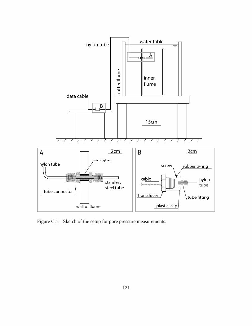
121

Figure C.1: Sketch of the setup for pore pressure measurements.

122

Appendix D: Procedure for setting up flume

Here I describe the procedure to setup and run slope failure experiments in the

flume (Figure D.1).

D.1 SETUP OF THE EXPERIMENT

1. Clean outer flume and affix mesh screen at water outlet to catch sediment.

2. Line the sliding door slot on the inner flume with silica grease to ease

movement of the door.

3. Load inner flume into outer flume.

4. Align so that inner flume is parallel to the outer flume and the inner flume is

in the center of the outer flume (Figure D.1). Inner flume sits ~2m upstream

from outlet of the outer flume.

5. Fill flume with water up to near top of outer flume.

6. Flush the tubing system according to procedures in Appendix C.

7. Insert the sliding gate for the inner flume in place.

8. Load sand into buckets, measure and record the weight of each bucket.

9. Deposit sand into the inner flume with scoops. Control the deposition rate of

sand so that sediment falls as individual grains and no air is trapped in the

inner flume.

10. Vigorously tap on the deposit with the rubber mallet when flume is 1/3, ½,

2/3, and 3/3 full of sand.

11. For every 1/6 of the deposit built, deposit a small amount of sand with a

different color than the rest of the deposit. Spread the sand so that it forms a

thin bed.

123

12. Measure and record the weight of each bucket after filling.

13. If preparing for a dense deposit: once flume is full, place two 25lb deadweight

blocks on top of sand and let sit for at least 16 hrs.

D.2 RUNNING THE EXPERIMENT

1. Remove weights placed on top of the deposit.

2. Attach sonar probes to their respective instrument arms. The horizontal sonar

should be perpendicular to the sliding gate with its head located between 5cm

to 10cm from the sliding gate.

3. Attach camera to a tripod and set it up at desired location, with the camera

frame level (some cameras have internal inclinometer to assist the

adjustment).

4. Attach black masking in locations needed to minimize reflection and shadow

cast in the view of the camera.

5. Turn on and check sonar probes and pressure transducers. Verify the setup for

the probes are all correct, setup their respective recording file names and write

them down with the time of experiment and sediment used.

6. Measure and record the depth of the deposit in the inner flume.

7. Measure and record the sonar head’s position with respect to the floor of the

inner flume and the sliding gate.

8. Start camera recording video and stop watch concurrently.

9. Begin recording data and end stop watch concurrently, record the time interval

as the time offset between video and data recordings.

124

10. Slide out front door of inner flume from standing position atop outer flume, as

quickly as possible.

125

Figure D.1: Setup of the flume and measuring instruments for slope failure experiments.

126

References

ASTM, 1970, Standard Method of Test for Permeability of Garnular Soils (Constant Head): West Conshohocken, PA, ASTM International.

-, 2006, Standard test method for one-dimensional consolidation properties of saturated cohesive soils using controlled-strain loading (Standard D 4186-06): West Conshohocken, PA.

Balmforth, N. J., and Kerswell, R. R., 2005, Granular collapse in two dimensions: Journal of Fluid Mechanics, v. 538, p. 399-428.

Beard, D. C., and Weyl, P. K., 1973, Influence of texture on porosity and permeability of unconsolidated sand: American Association of Petroleum Geologists Bulletin, v. 57, no. 2, p. 349-369.

Been, K., and Jefferies, M., State parameter for sands, in Proceedings International Journal of Rock Mechanics and Mining Sciences and Geomechanics Abstracts1985, Volume 22, Elsevier Science, p. 198-198.

Bennett, R. H., and Stockstill, J., 1999, Sediment analyses and dive team reports, final report part II. NATO phase II field exercise in the C-1 area off the coast of Holland.: SEAPROBE, Inc.

Bohne, D., Fischer, S., and Obermeier, E., 1984, Thermal, Conductivity, Density, Viscosity, and Prandtl‐Numbers of Ethylene Glycol‐Water Mixtures: Berichte der Bunsengesellschaft für physikalische Chemie, v. 88, no. 8, p. 739-742.

Bolton, M., 1986, The strength and dilatancy of sands: Geotechnique, v. 36, no. 1, p. 65-78.

Breslau, L. R., 1967, The normally-incident reflectivity of the sea floor at 12 kc and its correlation with physical and geological properties of naturally-occurring sediments: DTIC Document.

Casagrande, A., 1936, Characteristics of cohesionless soils affecting the stability of slopes and earth fills: Contributions to Soil Mechanics 1925-1940, p. 257-276.

Chamberlain, T. K., 1964, Mass transport of sediment in the heads of Scripps Submarine Canyon, California, [Chapter] 4, in Miller, R. L., ed., Papers in Marine Geology, Shepard Commemorative Volume: New York, Macmillan, p. 42-64.

Curry, C. W., Bennett, R. H., Hulbert, M. H., Curry, K. J., and Faas, R. W., 2004, Comparative study of sand porosity and a technique for determining porosity of undisturbed marine sediment: Marine Georesources and Geotechnology, v. 22, no. 4, p. 231-252.

de Koning, I. J., 1970, Neue Erkenntnisse beim Gewinnen und Transport von Sand im Spiilprojekt Venserpolder: VDI Tagung" Bauen im Ausland", Hamburg. New knowledge about the mining and transport of sand, from the reclamation project Venserpolder (The Netherlands), p. 1-9.

Demmel, J. W., Eisenstat, S. C., Gilbert, J. R., Li, X. S., and Liu, J. W., 1999, A supernodal approach to sparse partial pivoting: SIAM Journal on Matrix Analysis and Applications, v. 20, no. 3, p. 720-755.

127

Dill, R. F., 1964, Contemporary submarine erosion in Scripps Submarine Canyon [Ph.D. Dissertation]: University of California, San Diego, 269 p.

Dill, R. F., 1969, Earthquake effects on fill of Scripps submarine canyon: Geological Society of America Bulletin, v. 80, no. 2, p. 321-328.

Dromart, G., Quantin, C., and Broucke, O., 2007, Stratigraphic architectures spotted in southern Melas Chasma, Valles Marineris, Mars: Geology, v. 35, no. 4, p. 363-366.

Eke, E., 2008, Breaching as a mechanism for generating sustained turbidity currents [M.S. Thesis]: University of Illinois at Urbana-Champaign, 88 p.

Eke, E., Viparelli, E., and Parker, G., 2011, Field-scale numerical modeling of breaching as a mechanism for generating continuous turbidity currents: Geosphere, v. 7, no. 5, p. 1063-1076.

Flemings, P., Long, H., Dugan, B., Germaine, J., John, C., Behrmann, J., Sawyer, D., and IODP, E., 2008, Pore pressure penetrometers document high overpressure near the seafloor where multiple submarine landslides have occurred on the continental slope, offshore Louisiana, Gulf of Mexico: Earth and Planetary Science Letters, v. 269, no. 3-4, p. 309-325.

Freeze, R. A., and Cherry, J. A., 1977, Groundwater, Prentice-Hall. Gibson, R., 1958, The progress of consolidation in a clay layer increasing in thickness

with time: Geotechnique, v. 8, no. 4, p. 171-182. Hampton, M. A., Lee, H. J., and Locat, J., 1996, Submarine landslides: Reviews of

Geophysics, v. 34, no. 1, p. 33-59. Hostler, S. R., 2004, Wave propagation in granular materials [Ph.D. Dissertation]:

California Institute of Technology, 111 p. Houthuys, R., 2011, A sedimentary model of the Brussels Sands, Eocene, Belgium:

Geologica Belgica, v. 14, no. 1-2, p. 55-74. Iverson, R., 2005, Regulation of landslide motion by dilatancy and pore pressure

feedback: Journal of Geophysical Research-Earth Surface, v. 110, no. F2. Iverson, R., Reid, M., Iverson, N., LaHusen, R., Logan, M., Mann, J., and Brien, D.,

2000, Acute sensitivity of landslide rates to initial soil porosity: Science, v. 290, no. 5491, p. 513-516.

Jaky, J., 1944, The coefficient of earth pressure at rest: Journal of the Society of Hungarian Architects and Engineers, v. 78, no. 22, p. 355-358.

Kneller, B. C., and Branney, M. J., 1995, Sustained high-density turbidity currents and the deposition of thick massive sands: Sedimentology, v. 42, no. 4, p. 607-616.

Lamb, M. P., and Mohrig, D., 2009, Do hyperpycnal-flow deposits record river-flood dynamics?: Geology, v. 37, no. 12, p. 1067-1070.

Li, X. S., Demmel, J. W., Gilbert, J. R., Grigori, L., Shao, M., and Yamazaki, I., 1999, SuperLU Users’ Guide.

Limber, P. W., Patsch, K. B., and Griggs, G. B., 2008, Coastal sediment budgets and the littoral cutoff diameter: A grain size threshold for quantifying active sediment inputs: Journal of Coastal Research, v. 24, no. 2B, p. 122-133.

128

Lowe, D. R., 1976, Subaqueous liquefied and fluidized sediment flows and their deposits: Sedimentology, v. 23, no. 3, p. 285-308.

Lube, G., Huppert, H. E., Sparks, R. S. J., and Freundt, A., 2005, Collapses of two-dimensional granular columns: Physical Review E, v. 72, no. 4.

Mastbergen, D., and Van den Berg, J., 2003, Breaching in fine sands and the generation of sustained turbidity currents in submarine canyons: Sedimentology, v. 50, no. 4, p. 625-637.

McAdoo, B. G., Pratson, L. F., and Orange, D. L., 2000, Submarine landslide geomorphology, US continental slope: Marine Geology, v. 169, no. 1-2, p. 103-136.

Meijer, K. L., and van Os, A. G., 1976, Pore pressures near moving underwater slope: Journal of the Geotechnical Engineering Division, v. 102, no. 4, p. 361-372.

Metz, J. M., Grotzinger, J. P., Mohrig, D., Milliken, R., Prather, B., Pirmez, C., McEwen, A. S., and Weitz, C. M., 2009, Sublacustrine depositional fans in southwest Melas Chasma: Journal of Geophysical Research-Planets, v. 114, p. E1002.

Morgenstern, N., 1967, Submarine slumping and the initiation of turbidity currents: Marine geotechnique, p. 189-220.

Mulder, T., Syvitski, J. P., Migeon, S., Faugeres, J.-C., and Savoye, B., 2003, Marine hyperpycnal flows: initiation, behavior and related deposits. A review: Marine and Petroleum Geology, v. 20, no. 6, p. 861-882.

Nedderman, R., 1992, Statics and kinematics of granular materials, Cambridge University Press.

Oda, M., 1972, The mechanism of fabric changes during compressional deformation of sand: Soils and foundations, v. 12, no. 2, p. 1-18.

Oda, M., Konishi, J., and Nemat-Nasser, S., 1980, Some experimentally based fundamental results on the mechanical behaviour of granular materials: Geotechnique, v. 30, no. 4, p. 479-495.

Onoda, G. Y., and Liniger, E. G., 1990, Random loose packings of uniform spheres and the dilatancy onset: Physical Review Letters, v. 64, no. 22, p. 2727.

Pahwa, A., Whitman, R. V., and Germaine, J. T., 1987, Quick release tests on centrifuge of wall retraining saturated sand backfill: Department of Civil Engineering, Massachusetts Institute of Technology.

Perillo, M. M., Buttles, J., Mohrig, D., Kane, I., and Pontén, A., in prep., New acoustic reflection technique for direct and noninvasive visualization of subaqueous, high-concentration sediment-laden flows.

Piper, D. J. W., and Normark, W. R., 2009, Processes that initiate turbidity currents and their influence on turbidites: a marine geology perspective: Journal of Sedimentary Research, v. 79, no. 5-6, p. 347-362.

Polya, G., and Szegö, G., 1970, Aufgaben und Lehrsätze aus der Analysis: 1. Band: Reihen, Integralrechnung, Funktionentheorie, Springer.

Pryor, W., 1972, Reservoir inhomogeneities of some recent sand bodies: Old SPE Journal, v. 12, no. 3, p. 229-245.

129

Radin, C., 2008, Random close packing of granular matter: Journal of Statistical Physics, v. 131, no. 4, p. 567-573.

Richardson, M. D., Briggs, K. B., Bibee, L. D., Jumars, P. A., Sawyer, W. B., Albert, D. B., Bennett, R. H., Berger, T. K., Buckingham, M. J., and Chotiros, N. P., 2001, Overview of SAX99: Environmental considerations: Oceanic Engineering, IEEE Journal of, v. 26, no. 1, p. 26-53.

Rutgers, R., 1962, Packing of Spheres: Nature, v. 193, no. 4814, p. 465-466. Scott, G. D., Charlesworth, A. M., and Mark, M. K., 1964, On the Random Packing of

Spheres: Journal of Chemical Physics, v. 40, p. 611-612. Shepard, F. P., and Marshall, N. F., 1973, Storm-generated current in La Jolla Submarine

Canyon, California: Marine Geology, v. 15, no. 1, p. M19-M24. Siavoshi, S., and Kudrolli, A., 2005, Failure of a granular step: Physical Review E, v. 71,

no. 5, p. 051302. Skempton, S. A., 1954, The pore pressure coefficients A and B: Géotechnique, v. 4, p.

143-147. Smith, W., Foote, P. D., and Busang, P., 1929, Packing of homogeneous spheres:

Physical Review, v. 34, no. 9, p. 1271. Sture, S., Costes, N. C., Batiste, S. N., Lankton, M. R., AlShibli, K. A., Jeremic, B.,

Swanson, R. A., and Frank, M., 1998, Mechanics of granular materials at low effective stresses: Journal of Aerospace Engineering, v. 11, no. 3, p. 67-72.

Terzaghi, K., 1951, Mechanism of landslides, Harvard University, Dept. of Engineering. Terzaghi, K., 1956, Varieties of submarine slope failures, in Proceedings 8th Texas

Conference on Soil Mechanics and Foundation Engineering, Austin, TX, 1956, p. 1-41.

Vaid, Y., and Negussey, D., 1988, Preparation of reconstituted sand specimens: Advanced triaxial testing of soil and rock, ASTM STP, v. 977, p. 405-417.

Van den Berg, J., Van Gelder, A., and Mastbergen, D., 2002, The importance of breaching as a mechanism of subaqueous slope failure in fine sand: Sedimentology, v. 49, no. 1, p. 81-95.

Van Rhee, C., Erosion of granular at high flow velocity, in Proceedings The 17th International Conference on the Hydraulic Transport of Solids, Cape Town, 7-11 May, 2007 2007, BHR group, p. 551-560.

Van Rhee, C., and Bezuijen, A., The breaching of sand investigated in large-scale model tests, in Proceedings Costal Engineering, Copenhagen, Denmark, 1998, Volume 3, American Society of Civil Engineers, p. 2509-2519.

Visher, G. S., and Part, 1967, Relation of grain size to sedimentary processes, American Association of Petroleum Geologists Bulletin, Volume 51: United States, American Association of Petroleum Geologists : Tulsa, OK, United States, p. 484-484.

Visscher, W. M., and Bolsterl.M, 1972, Random packing of equal and unequal spheres in 2 and 3 dimensions: Nature, v. 239, no. 5374, p. 504-507.

Wood, D., 1990, Soil Behaviour and Critical State Soil Mechanics, Cambridge University Press, Cambridge.