Dynamics of Bidding in a P2P Lending Service:Effects of Herding and Predicting Loan Success

Simla Ceyhan∗

Stanford Universitysimlac@stanford.edu

Xiaolin Shi∗Stanford University

shixl@stanford.edu

Jure LeskovecStanford University

jure@cs.stanford.edu

ABSTRACTOnline peer-to-peer (P2P) lending services are a new type of socialplatform that enables individuals borrow and lend money directlyfrom one to another. In this paper, we study the dynamics of bid-ding behavior in a P2P loan auction website, Prosper.com. We in-vestigate the change of various attributes of loan requesting listingsover time, such as the interest rate and the number of bids. We ob-serve that there is herding behavior during bidding, and for most ofthe listings, the numbers of bids they receive reach spikes at verysimilar time points. We explain these phenomena by showing thatthere are economic and social factors that lenders take into accountwhen deciding to bid on a listing.We also observe that the profitsthe lenders make are tied with their bidding preferences. Finally,we build a model based on the temporal progression of the bidding,that reliably predicts the success of a loan request listing, as well aswhether a loan will be paid back or not.

Categories and Subject Descriptors: H.4 [Information SystemsApplications]: Miscellaneous General Terms: Economics, Exper-imentation Keywords: Peer-to-peer lending service, user behavior,auction, dynamics

1. INTRODUCTIONOnline peer to peer lending platforms such as Prosper [19], Kiva

[14] and Lending Club [16] directly connect individuals who wantto borrow money to those who want to lend it. These platformseliminate the need for a financial institution as an intermediary be-tween lenders and borrowers, with the consequence that the lossresulting from defaulting on a loan is directly borne by the lendersthemselves. The risk is distributed among the lenders proportionalto the amount of money they lend to a given borrower. The lend-ing process typically involves an auction on the loan’s interest rate:lenders who provide the lowest interest rates win the bids, i.e. theyget to lend the money to the borrower. In this sense, the interestrate is an analogy to the price a bidder offers in the auction, and theamount of money a lender offers is an analogy to the risk a bidderis willing to take.

Communities such as Prosper create a social structure and in-teractions that are interesting from many perspectives. On the onehand, lenders have at their disposal a very rich set of data that couldpotentially affect their decision making. They have access to finan-cial information concerning borrowers, such as credit scores, past

∗Authors contributed equally to this work.

Copyright is held by the International World Wide Web Conference Com-mittee (IW3C2). Distribution of these papers is limited to classroom use,and personal use by others.WWW, ’11 IndiaACM 978-1-4503-0632-4/11/03.

borrowing histories, and demographic indicators (race, gender, andlocation). On the other hand there is a non-trivial risk of loan de-fault, and as such the lenders face a clear trade-off between interestrates and the amounts they bid. Finally, P2P lending platforms fill aniche for borrowers who cannot get a loan from traditional financialinstitutions or who need small personal loans, and are expected tobecome increasingly popular given the current economic climate.A recent study [10] predicts that within the next three years, peer-to-peer lending will increase by 66% to a total volume of 5 billionUSD in outstanding loans in 2013.

The loan auction mechanism for such a community works as fol-lows: a borrower posts a loan with the amount of money she wantsto borrow and the maximum interest rate she is willing to accept.Lenders submit their minimum interest rate as well as the amountof money that they wish to lend to the borrower. The listing lastsfor a pre-determined duration of time. At the end of this time, theauction is either successful, if enough money has been bid on thelisting, or is void if there is not enough money received by it. Forthe successful listings, the P2P lending platform then combines thebids with the lowest interest rates into a loan to the borrower andtakes care of the collection of money and repayments.

In this paper, we study the dynamics of such bidding mechanismin the case of P2P lending provider Prosper Loans Marketplace. Weinvestigate the factors that affect the bidding process throughouta listing’s lifetime. We observe that bids for a single listing donot occur uniformly over the listing’s lifetime. There is a clearconcentration of bids at the beginning and at the end of a listing’slife, as well as at the point where the total requested amount ofmoney is about to be satisfied. We explain this phenomenon byshowing that there are three main economic factors that lenderstake into account when deciding to bid on a listing: lenders’ beliefabout the probability of a listing being fully funded, the probabilityof winning the bid, as well as the interest rate. In addition, a socialfactor that makes lenders prefer for new listings also takes effect.These factors change over the lifetime of a listing, and result in thenon-uniform distribution of bids over time.

We also examine the performance of individual lenders and ob-serve that it is related to their bidding preferences. Lenders who bidat the end of the listings are more likely to win the bids. Lenderswho bid around the time when the requested amount by the bor-rower is satisfied are least likely to win the bid and less likely tomake profits. Moreover, the strategy of lenders minimizing theirrisks by decentralizing does only help mildly.

Finally, we build logistic regression models to predict the list-ing success. Given our previous observations regarding the non-uniform temporal bidding behavior, it is not surprising that the list-ing bid trajectory plays an important role on these models. Onlybased on the temporal progression of the bidding behavior, we

can well estimate if a listing gets funded or not as well as predictwhether its borrower will pay it back or not. We show that thereis information to be gained from “how the market feels" that is notpresent in the set of features constructed from standard factors suchas credit grade or debt-to-income ratio. To the best of our knowl-edge, this is the first study that also focuses on the prediction of theperformance of loans in addition to fundability success.

The rest of the paper is organized as follows: Section 2 sum-marizes the related research in peer-to-peer lending marketplaces.Section 3 briefly describes the dataset and basic statistics aboutProsper. Section 4 explores the dynamics of bidding on a listingand looks at the performance of individual lenders while Section 5describes a model that predicts a listing’s success and being paid-back or not. Conclusions are discussed in Section 6.

2. RELATED WORKHaving emerged recently, dynamics of peer-to-peer lending has

been relatively unexplored. So far, one line of research has focusedon understanding the general dynamics of the online peer-to-peerlending marketplace. Hulme and Wright [12] provide a study ofpeer-to-peer lending focusing on “Zopa.com". Berger and Gliesner[3], with a more general approach, analyze the role of intermedi-aries on electronic marketplaces. Freedman and Jin [7], examinethe functioning of online lending based on Prosper’s transactiondata. They study the effect of social network in identifying risksand find evidence both for and against it.

Prosper market data has been freely available via an API. Thisallowed researchers study the Prosper market and consumer creditmarkets in general. Using Prosper data, Freedman and Jin [8] lookat the change of borrower and lender behavior over time as newpolicies were introduced. Iyer et al. [13] examine how well lenderson Prosper use information, both traditional and non-traditional,to infer a borrower’s actual credit scores. They show that whilelenders mostly rely on standard banking variables to draw infer-ences on creditworthiness, they also use non-standard, subjectivesources of information in their screening process, especially in thelower credit categories. Similarly, Klafft [15] focuses on lenderbehavior and demonstrates that careful lenders who choose theirborrowers in accordance with a number of easy-to-observe selec-tion criteria can still expect their investments to be profitable. Ourwork also analyzes Prosper data in order to understand online peer-to-peer lending throughly. However, we focus on the dynamics ofbidding behavior and investigate the change of several attributes ofthe loan request listing during the auction duration.

Another line of research looks at the determinants of success inonline peer-to-peer communities. Analyzing Prosper data, Herzen-stein et al. [11], found that borrowers’ financial strength and effortswhen they post a listing are major factors in determining whether itwill be funded or not. Similarly, Ryan et al. [20], analyze fundabil-ity determinants in Prosper. The purpose of this study is to weightthe relative relevance of each of the financial and social featuresindependently, and determine their influence in the success on theconversion of a listing to a loan. Their study shows that financialfeatures are determinant. In this paper, we also build a regressionmodel to predict fundability success. However, rather than usingborrower related features in our model, we also explore temporaldynamics of a listing and show that they reliably predict the suc-cess of a listing.

On the other hand, Chen et al. [4] analyze the mechanisms ofsocial lending from a theoretical standpoint. Again focusing onProsper, they show that its mechanism is exactly the same as theVCG mechanism applied to a modified instance of the problem.They provide a complete analysis and characterization of the Nash

equilibria of the Prosper mechanism and show that while the Pros-per mechanism is a simple uniform price mechanism, it can lead tomuch larger payments for the borrower than the VCG mechanism.

Our work is also related to empirical studies on Ebay, where re-searchers try to understand the bidding characteristics. For exam-ple, Shah et al. [21] focus on individual users and monitor all ofa bidder’s engagements in the dataset. They identify the main bid-ding strategies such as “late bidding" (bidding during the last hour),“evaluator" (bidding the true valuation early) and “sceptic" (bid-ding only the minimum required amount) using rule-based meth-ods. Lucking-Reiley, et al. [18] analyze the effect of various eBayfeatures on the final price of auctions. They find that seller’s feed-back rating have a measurable effect on his auction prices, withnegative comments having a much greater effect than positive com-ments. In another study, Dietrich et al. [5] empirically show thatthe segmentation of the eBay marketplace affects bidding behav-ior. They state that successful strategies for a certain product cate-gory or seller type can be useless in different market segments. Inour work, with a similar approach to Prosper data, we also wantto understand the bidding dynamics and Prosper features that af-fect bidding behavior. However, Prosper mechanism, with multiplewinners, is different from eBay auctions in which a single bid at orabove the seller’s reservation price results in a successful auction.

Finally, our work is similar in spirit to the empirical studies onbidding dynamics in sponsored search. Most of the academic lit-erature on sponsored search is theoretical in nature, characterizingbehavior or payoffs of bidders. However, there are some studies,similar to our work, that examine actual bidding data on a largescale to determine how real-world auctions can best be analyzedand understood. One example is the study of Asdemir [1], wherehe analyzes how advertisers bid for search phrases in pay-per-clicksearch engine auctions. Similarly, by examining sponsored searchauctions run by Overture (now part of Yahoo!) and Google, Edel-man and Ostrovsky present evidence of strategic bidder behaviorin these auctions in [6]. In [2] Auerbach et al. empirically investi-gate whether advertisers are maximizing their return on investmentacross multiple keywords in sponsored search auctions and in [9],they utilize sponsored search data drawn from a wide array of Over-ture/Yahoo! auctions and examine how bids are distributed and theevidence for strategic behavior.

3. PROSPER MARKETPLACEAfter creating a personal profile, borrowers and lenders become

members of the Prosper community. When a borrower wants torequest a loan through the marketplace, she creates a listing for aspecific amount and sets a maximum interest rate that she is willingto pay. She also chooses the duration for which the request willremain active. Each loan request, from now on we will refer toas ‘listing’, includes information about the borrower such as hercurrent credit rate and debt-to-income ratio. This information isverified by Prosper and made public to potential lenders. Lendersbid for the privilege of supplying all or part of the requested loansspecifying the amount and interest rate at which they are willing tolend. When the specified time has elapsed, if the aggregate amountoffered by lenders exceeds the amount requested by the borrower,the listing becomes successful. For the successful listings, the bidswith the lowest rates “win” and are combined into a single loan tothe borrower, with Prosper acting as the broker between the lendersand the borrower.

Bidding on Prosper is done in a Dutch auction format, whichmeans that multiple lenders can get a piece of the same loan invarying amounts. In a Dutch auction, the borrower starts the auc-tion with a maximum interest rate and multiple lenders bid that rate

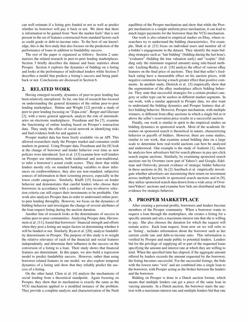
Funded Non-fundedFrac. of Amount Collected 1 0.054 (0.15)

Bid Count 135.1 (142.6) 6.4 (34.6)Duration(days) 7.61 (2.0) 7.45 (2.0)Borrower Rate 0.213 (0.07) 0.195 (0.08)

Lender Rate 0.183 (0.07) 0.192 (0.08)Amount Requested $6,126 (5587) $7,541 (6383)

Debt to Income Ratio 0.16 (0.15) 0.23 (0.45)

Table 1: Data statistics of funded and unfunded listings: mean,and in parentheses, standard deviation.

Paid Not-paidBid Count 124.7 (137.8) 121.5 (144.0)

Duration(days) 7.5 (2.0) 7.67 (2.0)Borrower Rate 0.178 (0.07) 0.242(0.06)

Lender Rate 0.154 (0.06) 0.216 (0.06)Amount Requested $ 5,670 (5350) $6,573 (6171)

Debt to Income Ratio 0.28 (0.92) 0.38 (1.12)

Table 2: Data statistics of paid and not-paid listings: mean, andin parentheses, standard deviation.

down until the auction times out. Prosper provided us with datathat contains all the bidding and membership data from November2005 to August 2009. The data encloses approximately 5 millionbids, 900,000 members and 350,000 listings. At the end of sum-mer 2009, Prosper introduced automated plan system, which bidson behalf of the lenders once a listing that matches their plan isposted. However, note that our data is from the period before thisfeature was introduced and thus it only consists of bids by individ-ual lenders.

On average, every borrower posts 1.7 listings and every lenderbids on 2.6 unique listings. There are 24,295 successful (funded)listings that have ended up in loans, which is about 8% of all list-ings. Out of those listings, 70% of them had competition, by whichwe mean that they continued receiving bids even after the amountrequested was satisfied. While 7668 (32%) of the loans were paidback, 7595 (31%) of them defaulted. For the rest, payoff is inprogress. Table 1 shows the mean and, in parentheses, the standarddeviation of a number of statistics related to both funded and non-funded listings. Funded listings have much higher number of bids,as a result, the average percentage of the amount collected by thenon-funded listings is quite low, only 5%. Not surprisingly, on av-erage funded listings have higher starting interest rates (21.3% vs.19.5%), lower final interest rates (18.3% vs. 19.2%) and lower re-quested amounts when compared to the unfunded listings. Durationis slightly higher for the funded listings than unfunded ones. Fi-nally, borrowers with funded listings have a lower debt-to-incomeratio. Similarly, we also looked at the summary statistics of theloans that were paid back and not paid back (i.e., defaulted), seeTable 2. Note that interest rate and debt-to-income ratio for loansthat are not paid back is significantly higher than the ones that gotpaid. Also, while on average, the amount requested is higher forthe defaulted listings, the number of bids is slightly lower.

Figure 1 shows that the probability of a listing being funded in-creases with the number of bids it receives. Notice that this proba-bility increases sharply early on, but it flattens down as the numberof bids increases.

Every listing on Prosper is assigned a Prosper Rating to analyzeits level of risk. This rating represents an estimated average an-nualized loss rate range. The loss rate is based on the historicalperformance of borrowers on Prosper loans with similar character-istics and is determined by two scores: the first is the credit score,obtained from a credit reporting agency; the second is an in-housecustom score, the Prosper Score, built on the Prosper population.The use of these two scores determines an estimated loss rate for

Figure 1: The probability of a listing being funded vs numberof bids.

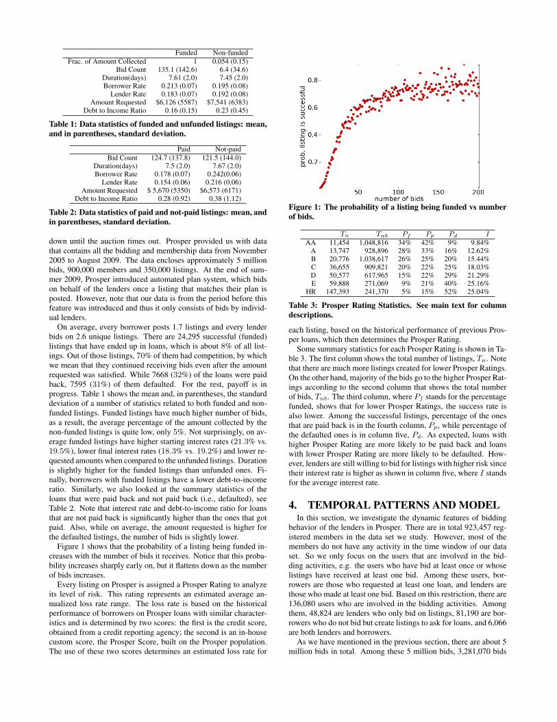
Tn Tnb Pf Pp Pd IAA 11,454 1,048,816 34% 42% 9% 9.84%

A 13,747 928,896 28% 33% 16% 12.62%B 20,776 1,038,617 26% 25% 20% 15.44%C 36,655 909,821 20% 22% 25% 18.03%D 50,577 617,965 15% 22% 29% 21.29%E 59,888 271,069 9% 21% 40% 25.16%

HR 147,393 241,370 5% 15% 52% 25.04%

Table 3: Prosper Rating Statistics. See main text for columndescriptions.

each listing, based on the historical performance of previous Pros-per loans, which then determines the Prosper Rating.

Some summary statistics for each Prosper Rating is shown in Ta-ble 3. The first column shows the total number of listings, Tn. Notethat there are much more listings created for lower Prosper Ratings.On the other hand, majority of the bids go to the higher Prosper Rat-ings according to the second column that shows the total numberof bids, Tnb. The third column, where Pf stands for the percentagefunded, shows that for lower Prosper Ratings, the success rate isalso lower. Among the successful listings, percentage of the onesthat are paid back is in the fourth column, Pp, while percentage ofthe defaulted ones is in column five, Pd. As expected, loans withhigher Prosper Rating are more likely to be paid back and loanswith lower Prosper Rating are more likely to be defaulted. How-ever, lenders are still willing to bid for listings with higher risk sincetheir interest rate is higher as shown in column five, where I standsfor the average interest rate.

4. TEMPORAL PATTERNS AND MODELIn this section, we investigate the dynamic features of bidding

behavior of the lenders in Prosper. There are in total 923,457 reg-istered members in the data set we study. However, most of themembers do not have any activity in the time window of our dataset. So we only focus on the users that are involved in the bid-ding activities, e.g. the users who have bid at least once or whoselistings have received at least one bid. Among these users, bor-rowers are those who requested at least one loan, and lenders arethose who made at least one bid. Based on this restriction, there are136,080 users who are involved in the bidding activities. Amongthem, 48,824 are lenders who only bid on listings, 81,190 are bor-rowers who do not bid but create listings to ask for loans, and 6,066are both lenders and borrowers.

As we have mentioned in the previous section, there are about 5million bids in total. Among these 5 million bids, 3,281,070 bids

Histogram

Time getting full amount / Entire bidding time

Frequency

0.0 0.2 0.4 0.6 0.8 1.0

01000

2000

3000

4000

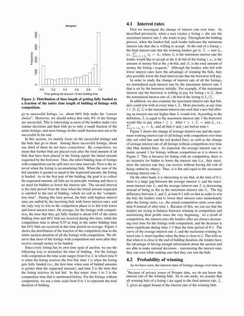
Figure 2: Distribution of time length of getting fully funded asa fraction of the entire time length of bidding of listings withcompetition.

go to successful listings, i.e. about 66% bids make the “correctchoice”. Moreover, we should notice that only 8% of the listingsare successful. This is interesting as most of the lenders make verysimilar decisions and their bids go to only a small fraction of theentire listings, and most listings in this small fraction turn out to besuccessful in the end.

In this section, we mainly focus on the successful listings andthe bids that go to them. Among these successful listings, aboutone third of them do not have competition. By competition, wemean that further bids are placed even after the total amount of allbids that have been placed in the listing equals the initial amountrequested by the borrower. Thus, the entire bidding time of listingswith competition can be split into two time intervals. First is the in-terval when the listing is accumulating bids. When the sum of thebid amounts is greater or equal to the requested amount, the listingis funded. As in the first part of the bidding, the goal is to collectthe requested amount, all bids are in principle winning and there isno need for bidders to lower the interest rate. The second intervalis the time period from the time when the initial amount requestedis satisfied to the end of bidding, which we call as the “competi-tion time”. During this time period, the bids with highest interestrates are outbid by the incoming bids with lower interest rates, andthe only way to win in the competition phase is to bid with lowerand lower interest rates. On average, for the listings with competi-tion, the time that they get fully funded is about 0.65 of the entirebidding time and 46% bids are received during this time, while thecompetition time is about 0.35 as long as the entire bidding timebut 54% bids are received in this time period on average. Figure 2shows the distribution of the fraction of the competition time to theentire auction duration of all the listings with competition. We ob-serve that most of the listings with competition end soon after theyreceive enough money to be funded.

Since every listing has its own time span of auction, we use thefollowing way to normalize the time of bidding. For the listingswith competition the time scale ranges from 0 to 2, in which time 0is when the listing receives the first bid, time 1 is when the listinggets fully funded (i.e., the first time when sum of bidded amountsis greater than the requested amount), and time 2 is the time thatthe listing receives its last bid. In this sense, time 1 to 2 is thecompetition time that is mentioned before. For the listings withoutcompetition, we use a time scale from 0 to 1 to represent the totalduration of bidding.

4.1 Interest ratesFirst we investigate the change of interest rate over time. As

described previously, when a user creates a listing i, she sets themaximum interest rate Ii she wants to pay. Throughout the biddingprocess, when the lenders bid, each lender indicates the minimuminterest rate that she is willing to accept. At the end of a listing i,the final interest rate that the winning lenders get is: Ii = min Ik,s.t.,

∑j,Ij<Ik

aj = Ai, where Ik is the minimum interest rate thelender would like to accept at the k-th bid of the listing i, aj is theamount of money bid at the j-th bid, and Ai is the total amount ofmoney the listing i requests.1 Although the lenders who bid withlower interest rates have the advantage of winning the bids, theyalso possibly lower the final interest rate that the borrower will pay.

In order to study the change of interest rate of all the listings,we normalized each interest rate by the maximum interest rate Ithat is set by the borrower initially. For example, if the maximuminterest rate the borrower is willing to pay for listing i is Ii, thenthe normalized interest rate of j-th bid of the listing is Ij/Ii.

In addition, we also examine the maximum interest rate that bid-ders could win with at every time t, It. More precisely, at any timet ∈ [0, 2], It is the maximum interest rate such that a new bid offer-ing an interest rate not higher than It would win. According to thedefinition, It is equal to the maximum interest rate I the borrowerwould like to pay when t ≤ 1. After t > 1, It = min Ik, s.t.,∑j,Ij<Ik

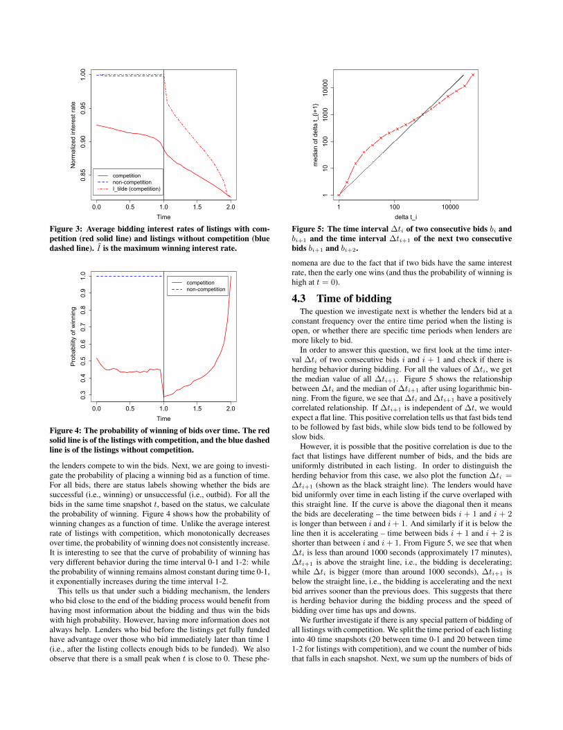
aj = Ai, and all bids k and j are before time t.Figure 3 shows the change of average interest rate and the maxi-

mum winning interest rate of all listings with competition over time(the red solid line and the red dashed line), as well as the changeof average interest rate of all listings without competition over time(the blue dashed line). As expected, the average interest rate re-mains around 1 for listings without competition as it is shown inFigure 3. This is because for listing with no competition, there isno incentive for bidder to lower the interest rate (i.e., they maxi-mize the interest rate they can receive without having the risk ofbeing outbid by others). Thus, it is flat and equal to the maximumwinning interest rate It.

On the other hand, it is interesting to see that, at the time of 0-1,there is a large gap between the average interest It and the maxi-mum interest rate It, and the average interest rate It is decreasinginstead of being as flat as the maximum interest rate It. The bigdifference between It and It at time 0-1 tells us that in order to winthe bid, the lenders tend to lower their interest rates immediatelyafter the listing starts, i.e., the actual competition starts soon aftertime 0 instead of after time 1. Because of this, we can see that thelenders are trying to balance between winning in competition andmaximizing their profits since the very beginning. As a result ofcompetition, the interest rates the lenders offer are always decreas-ing over time for the listings with competition, and the decrease ismore significant during time 1-2 than the time period of 0-1. Thecurve of the average interest rate It and the maximum winning in-terest rate It meet together when the time is close to 2. This tells usthat when it is close to the end of bidding duration, the lenders havethe advantage of having enough information about the auction andare able to make rational decisions – maximizing the interest ratesthey can earn while making sure that they can win the bids.

4.2 Probability of winningAs we have seen, the interest rates of listings change over time as

1Because of privacy issues of Prosper data, we do not know theinterest rate of the winning bids. So in our study, we assume thatall winning bids of a listing i are equal to the final interest rate, Ii.Ii gives an upper bound of the interest rate of the winning bids.

0.0 0.5 1.0 1.5 2.0

0.85

0.90

0.95

1.00

Time

Nor

mal

ized

inte

rest

rate

competitionnon-competitionI_tilde (competition)

Figure 3: Average bidding interest rates of listings with com-petition (red solid line) and listings without competition (bluedashed line). I is the maximum winning interest rate.

0.0 0.5 1.0 1.5 2.0

0.3

0.4

0.5

0.6

0.7

0.8

0.9

1.0

Time

Pro

babi

lity

of w

inni

ng

competitionnon-competition

Figure 4: The probability of winning of bids over time. The redsolid line is of the listings with competition, and the blue dashedline is of the listings without competition.

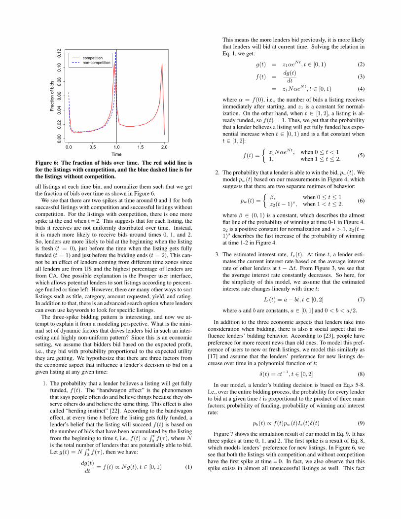
the lenders compete to win the bids. Next, we are going to investi-gate the probability of placing a winning bid as a function of time.For all bids, there are status labels showing whether the bids aresuccessful (i.e., winning) or unsuccessful (i.e., outbid). For all thebids in the same time snapshot t, based on the status, we calculatethe probability of winning. Figure 4 shows how the probability ofwinning changes as a function of time. Unlike the average interestrate of listings with competition, which monotonically decreasesover time, the probability of winning does not consistently increase.It is interesting to see that the curve of probability of winning hasvery different behavior during the time interval 0-1 and 1-2: whilethe probability of winning remains almost constant during time 0-1,it exponentially increases during the time interval 1-2.

This tells us that under such a bidding mechanism, the lenderswho bid close to the end of the bidding process would benefit fromhaving most information about the bidding and thus win the bidswith high probability. However, having more information does notalways help. Lenders who bid before the listings get fully fundedhave advantage over those who bid immediately later than time 1(i.e., after the listing collects enough bids to be funded). We alsoobserve that there is a small peak when t is close to 0. These phe-

1 100 10000

110

100

1000

10000

delta t_i

med

ian

of d

elta

t_{i+

1}

Figure 5: The time interval ∆ti of two consecutive bids bi andbi+1 and the time interval ∆ti+1 of the next two consecutivebids bi+1 and bi+2.

nomena are due to the fact that if two bids have the same interestrate, then the early one wins (and thus the probability of winning ishigh at t = 0).

4.3 Time of biddingThe question we investigate next is whether the lenders bid at a

constant frequency over the entire time period when the listing isopen, or whether there are specific time periods when lenders aremore likely to bid.

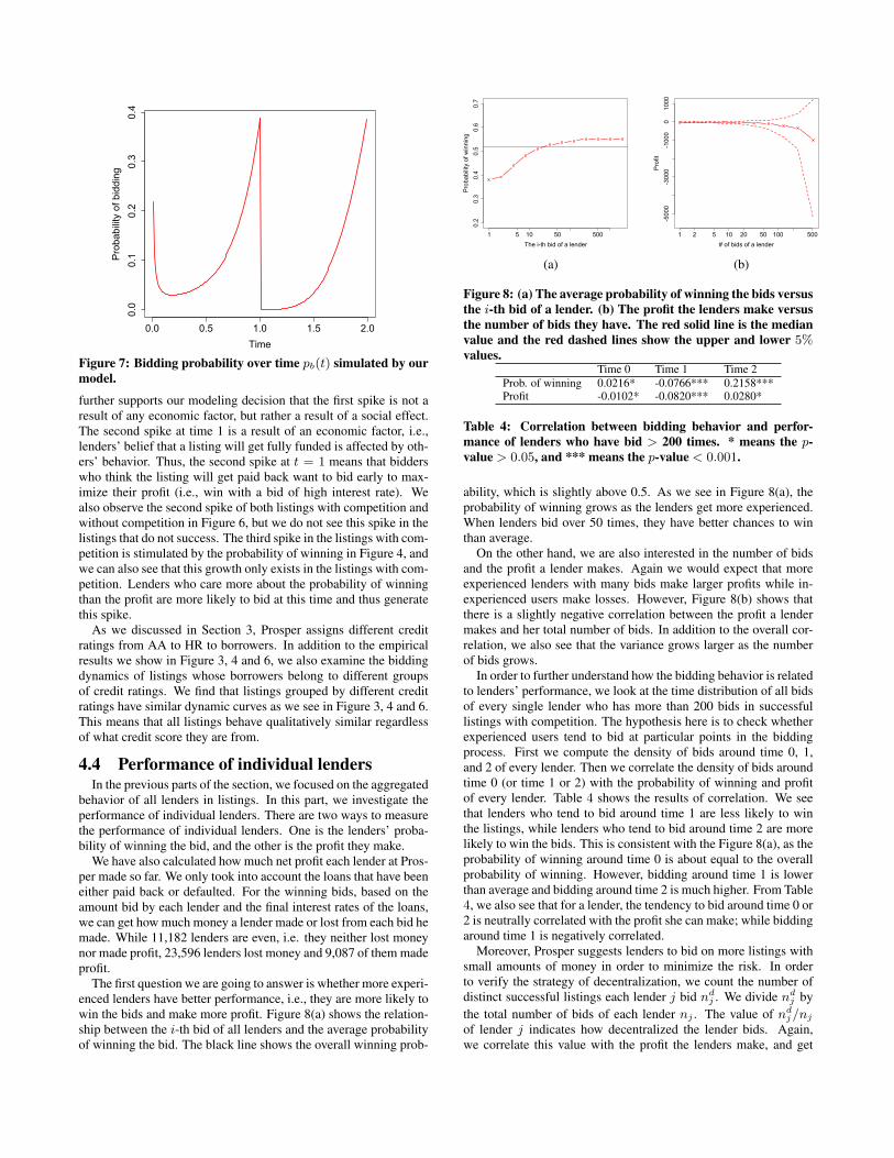
In order to answer this question, we first look at the time inter-val ∆ti of two consecutive bids i and i + 1 and check if there isherding behavior during bidding. For all the values of ∆ti, we getthe median value of all ∆ti+1. Figure 5 shows the relationshipbetween ∆ti and the median of ∆ti+1 after using logarithmic bin-ning. From the figure, we see that ∆ti and ∆ti+1 have a positivelycorrelated relationship. If ∆ti+1 is independent of ∆t, we wouldexpect a flat line. This positive correlation tells us that fast bids tendto be followed by fast bids, while slow bids tend to be followed byslow bids.

However, it is possible that the positive correlation is due to thefact that listings have different number of bids, and the bids areuniformly distributed in each listing. In order to distinguish theherding behavior from this case, we also plot the function ∆ti =∆ti+1 (shown as the black straight line). The lenders would havebid uniformly over time in each listing if the curve overlaped withthis straight line. If the curve is above the diagonal then it meansthe bids are decelerating – the time between bids i + 1 and i + 2is longer than between i and i+ 1. And similarly if it is below theline then it is accelerating – time between bids i + 1 and i + 2 isshorter than between i and i+ 1. From Figure 5, we see that when∆ti is less than around 1000 seconds (approximately 17 minutes),∆ti+1 is above the straight line, i.e., the bidding is decelerating;while ∆ti is bigger (more than around 1000 seconds), ∆ti+1 isbelow the straight line, i.e., the bidding is accelerating and the nextbid arrives sooner than the previous does. This suggests that thereis herding behavior during the bidding process and the speed ofbidding over time has ups and downs.

We further investigate if there is any special pattern of bidding ofall listings with competition. We split the time period of each listinginto 40 time snapshots (20 between time 0-1 and 20 between time1-2 for listings with competition), and we count the number of bidsthat falls in each snapshot. Next, we sum up the numbers of bids of

0.0 0.5 1.0 1.5 2.0

0.00

0.02

0.04

0.06

0.08

0.10

0.12

Time

Frac

tion

of b

ids

competitionnon-competition

Figure 6: The fraction of bids over time. The red solid line isfor the listings with competition, and the blue dashed line is forthe listings without competition.

all listings at each time bin, and normalize them such that we getthe fraction of bids over time as shown in Figure 6.

We see that there are two spikes at time around 0 and 1 for bothsuccessful listings with competition and successful listings withoutcompetition. For the listings with competition, there is one morespike at the end when t = 2. This suggests that for each listing, thebids it receives are not uniformly distributed over time. Instead,it is much more likely to receive bids around times 0, 1, and 2.So, lenders are more likely to bid at the beginning when the listingis fresh (t = 0), just before the time when the listing gets fullyfunded (t = 1) and just before the bidding ends (t = 2). This can-not be an effect of lenders coming from different time zones sinceall lenders are from US and the highest percentage of lenders arefrom CA. One possible explanation is the Prosper user interface,which allows potential lenders to sort listings according to percent-age funded or time left. However, there are many other ways to sortlistings such as title, category, amount requested, yield, and rating.In addition to that, there is an advanced search option where lenderscan even use keywords to look for specific listings.

The three-spike bidding pattern is interesting, and now we at-tempt to explain it from a modeling perspective. What is the mini-mal set of dynamic factors that drives lenders bid in such an inter-esting and highly non-uniform pattern? Since this is an economicsetting, we assume that bidders bid based on the expected profit,i.e., they bid with probability proportional to the expected utilitythey are getting. We hypothesize that there are three factors fromthe economic aspect that influence a lender’s decision to bid on agiven listing at any given time:

1. The probability that a lender believes a listing will get fullyfunded, f(t). The “bandwagon effect” is the phenomenonthat says people often do and believe things because they ob-serve others do and believe the same thing. This effect is alsocalled “herding instinct” [22]. According to the bandwagoneffect, at every time t before the listing gets fully funded, alender’s belief that the listing will succeed f(t) is based onthe number of bids that have been accumulated by the listingfrom the beginning to time t, i.e., f(t) ∝

∫ t0f(τ), where N

is the total number of lenders that are potentially able to bid.Let g(t) = N

∫ t0f(τ), then we have:

dg(t)

dt= f(t) ∝ Ng(t), t ∈ [0, 1) (1)

This means the more lenders bid previously, it is more likelythat lenders will bid at current time. Solving the relation inEq. 1, we get:

g(t) = z1αeNt, t ∈ [0, 1) (2)

f(t) =dg(t)

dt(3)

= z1NαeNt, t ∈ [0, 1) (4)

where α = f(0), i.e., the number of bids a listing receivesimmediately after starting, and z1 is a constant for normal-ization. On the other hand, when t ∈ [1, 2], a listing is al-ready funded, so f(t) = 1. Thus, we get that the probabilitythat a lender believes a listing will get fully funded has expo-nential increase when t ∈ [0, 1) and is a flat constant whent ∈ [1, 2]:

f(t) =

{z1Nαe

Nt, when 0 ≤ t < 11, when 1 ≤ t ≤ 2. (5)

2. The probability that a lender is able to win the bid, pw(t). Wemodel pw(t) based on our measurements in Figure 4, whichsuggests that there are two separate regimes of behavior:

pw(t) =

{β, when 0 ≤ t ≤ 1z2(t− 1)s, when 1 < t ≤ 2. (6)

where β ∈ (0, 1) is a constant, which describes the almostflat line of the probability of winning at time 0-1 in Figure 4.z2 is a positive constant for normalization and s > 1. z2(t−1)s describes the fast increase of the probability of winningat time 1-2 in Figure 4.

3. The estimated interest rate, Ie(t). At time t, a lender esti-mates the current interest rate based on the average interestrate of other lenders at t − ∆t. From Figure 3, we see thatthe average interest rate constantly decreases. So here, forthe simplicity of this model, we assume that the estimatedinterest rate changes linearly with time t:

Ie(t) = a− bt, t ∈ [0, 2] (7)

where a and b are constants, a ∈ [0, 1] and 0 < b < a/2.

In addition to the three economic aspects that lenders take intoconsideration when bidding, there is also a social aspect that in-fluence lenders’ bidding behavior. According to [23], people havepreference for more recent news than old ones. To model this pref-erence of users to new or fresh listings, we model this similarly as[17] and assume that the lenders’ preference for new listings de-crease over time in a polynomial function of t:

δ(t) = ct−1, t ∈ [0, 2] (8)

In our model, a lender’s bidding decision is based on Eq.s 5-8.I.e., over the entire bidding process, the probability for every lenderto bid at a given time t is proportional to the product of three mainfactors; probability of funding, probability of winning and interestrate:

pb(t) ∝ f(t)pw(t)Ie(t)δ(t) (9)

Figure 7 shows the simulation result of our model in Eq. 9. It hasthree spikes at time 0, 1, and 2. The first spike is a result of Eq. 8,which models lenders’ preference for new listings. In Figure 6, wesee that both the listings with competition and without competitionhave the first spike at time = 0. In fact, we also observe that thisspike exists in almost all unsuccessful listings as well. This fact

0.0 0.5 1.0 1.5 2.0

0.0

0.1

0.2

0.3

0.4

Time

Pro

babi

lity

of b

iddi

ng

Figure 7: Bidding probability over time pb(t) simulated by ourmodel.

further supports our modeling decision that the first spike is not aresult of any economic factor, but rather a result of a social effect.The second spike at time 1 is a result of an economic factor, i.e.,lenders’ belief that a listing will get fully funded is affected by oth-ers’ behavior. Thus, the second spike at t = 1 means that bidderswho think the listing will get paid back want to bid early to max-imize their profit (i.e., win with a bid of high interest rate). Wealso observe the second spike of both listings with competition andwithout competition in Figure 6, but we do not see this spike in thelistings that do not success. The third spike in the listings with com-petition is stimulated by the probability of winning in Figure 4, andwe can also see that this growth only exists in the listings with com-petition. Lenders who care more about the probability of winningthan the profit are more likely to bid at this time and thus generatethis spike.

As we discussed in Section 3, Prosper assigns different creditratings from AA to HR to borrowers. In addition to the empiricalresults we show in Figure 3, 4 and 6, we also examine the biddingdynamics of listings whose borrowers belong to different groupsof credit ratings. We find that listings grouped by different creditratings have similar dynamic curves as we see in Figure 3, 4 and 6.This means that all listings behave qualitatively similar regardlessof what credit score they are from.

4.4 Performance of individual lendersIn the previous parts of the section, we focused on the aggregated

behavior of all lenders in listings. In this part, we investigate theperformance of individual lenders. There are two ways to measurethe performance of individual lenders. One is the lenders’ proba-bility of winning the bid, and the other is the profit they make.

We have also calculated how much net profit each lender at Pros-per made so far. We only took into account the loans that have beeneither paid back or defaulted. For the winning bids, based on theamount bid by each lender and the final interest rates of the loans,we can get how much money a lender made or lost from each bid hemade. While 11,182 lenders are even, i.e. they neither lost moneynor made profit, 23,596 lenders lost money and 9,087 of them madeprofit.

The first question we are going to answer is whether more experi-enced lenders have better performance, i.e., they are more likely towin the bids and make more profit. Figure 8(a) shows the relation-ship between the i-th bid of all lenders and the average probabilityof winning the bid. The black line shows the overall winning prob-

1 5 10 50 500

0.2

0.3

0.4

0.5

0.6

0.7

The i-th bid of a lender

Pro

babi

lity

of w

inni

ng

1 2 5 10 20 50 100 500

-5000

-3000

-1000

01000

# of bids of a lender

Profit

(a) (b)

Figure 8: (a) The average probability of winning the bids versusthe i-th bid of a lender. (b) The profit the lenders make versusthe number of bids they have. The red solid line is the medianvalue and the red dashed lines show the upper and lower 5%values.

Time 0 Time 1 Time 2Prob. of winning 0.0216* -0.0766*** 0.2158***Profit -0.0102* -0.0820*** 0.0280*

Table 4: Correlation between bidding behavior and perfor-mance of lenders who have bid > 200 times. * means the p-value > 0.05, and *** means the p-value < 0.001.

ability, which is slightly above 0.5. As we see in Figure 8(a), theprobability of winning grows as the lenders get more experienced.When lenders bid over 50 times, they have better chances to winthan average.

On the other hand, we are also interested in the number of bidsand the profit a lender makes. Again we would expect that moreexperienced lenders with many bids make larger profits while in-experienced users make losses. However, Figure 8(b) shows thatthere is a slightly negative correlation between the profit a lendermakes and her total number of bids. In addition to the overall cor-relation, we also see that the variance grows larger as the numberof bids grows.

In order to further understand how the bidding behavior is relatedto lenders’ performance, we look at the time distribution of all bidsof every single lender who has more than 200 bids in successfullistings with competition. The hypothesis here is to check whetherexperienced users tend to bid at particular points in the biddingprocess. First we compute the density of bids around time 0, 1,and 2 of every lender. Then we correlate the density of bids aroundtime 0 (or time 1 or 2) with the probability of winning and profitof every lender. Table 4 shows the results of correlation. We seethat lenders who tend to bid around time 1 are less likely to winthe listings, while lenders who tend to bid around time 2 are morelikely to win the bids. This is consistent with the Figure 8(a), as theprobability of winning around time 0 is about equal to the overallprobability of winning. However, bidding around time 1 is lowerthan average and bidding around time 2 is much higher. From Table4, we also see that for a lender, the tendency to bid around time 0 or2 is neutrally correlated with the profit she can make; while biddingaround time 1 is negatively correlated.

Moreover, Prosper suggests lenders to bid on more listings withsmall amounts of money in order to minimize the risk. In orderto verify the strategy of decentralization, we count the number ofdistinct successful listings each lender j bid ndj . We divide ndj bythe total number of bids of each lender nj . The value of ndj/njof lender j indicates how decentralized the lender bids. Again,we correlate this value with the profit the lenders make, and get

a weak positive correlation 0.02 (with p-value < 0.001). Thismeans lenders slightly benefit from the strategy of decentralizingtheir bids.

5. PREDICTING THE LOAN SUCCESSIn Prosper, listings for which at least 100% of the requested

amount is collected, are considered “fundable” (successful) andthey translate into an active loan. However, listings which do notreach full funding are considered unsuccessful (“not fundable") andno loan is created. Out of the loans that are funded, some are repaidon time and others are cancelled or their borrowers default on them.

In this section, we examine a simple model that predicts whethera listing is going to be funded or not, and whether it will be paidback or not. A similar study is conducted at [11] and [20], wherethe authors focus on borrower and listing attributes. Their goal is toprovide a ranking of the relative importance of various fundabilitydeterminants, rather than providing a predictive model. However,our goal here is different as we do not just want to make our pre-dictions based on some large number of features but are insteadinterested in modeling how the temporal dynamics of bidding be-havior predicts the loan outcome (funded vs. not funded and paidvs. not paid). Thus we are interested in how much signal is in "howthe market feels" as opposed to traditional features such as creditgrade or debt-to-income ratio.

We started our analysis by looking at the time series history ofloan listings. In other words, we examine the progression of thetotal amount bid on a given loan as a function of time. We used atime scale from 0 to 1, in which time 0 is when the listing receivesthe first bid and time 1 is when it gets the last bid. Let Ai be thetotal amount bid for listing i and

∑j≤k aj = Ak, where aj is the

amount of money bid at the j-th bid, so Ak is the total amount ofmoney bid till the k-th bid. For each listing, we looked at YR = Ak

Aias a function of time. Figure 9 shows the four main types of curveswe observed. This observation led us to the hypothesis that the totalamount bid on a given listing follows a sigmoid curve as a functionof time. As a result, we fit a sigmoid (logistic) curve to each listingtime series, defined by

y(t) =1

1− e−q(t−φ),

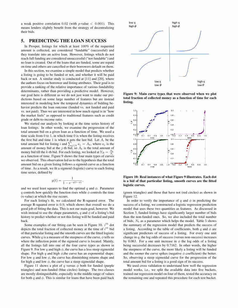
and we used least squares to find the optimal q and φ. Parameterq controls how quickly the function rises while φ controls the time(x-value) at which the rise occurs.

For each listing’s fit, we calculated the R-squared error. Theaverage R-squared error is 0.9, which shows that overall we do agood job of fitting the data. This is not our main goal, however. Wewish instead to use the shape parameters, q and φ of a listing’s bidhistory to predict whether or not this listing will be funded and paidback.

Some examples of our fitting can be seen in Figure 10. ith dotdepicts the total fraction of collected money at the time of ith bidof that particular listing and the smooth curves are the fitted logisticcurves. While q is a measure of the steepness of the curve, φ tells uswhere the inflection point of the sigmoid curve is located. Mainly,all the listings fall into one of the four curve types as shown inFigure 9. For low q and high φ, the curve has a less steep sigmoidalshape. For high q and high φ,the curve has an exponential shape.For low q and low φ, the curve has diminishing returns shape andfor high q and low φ, the curve has a steep sigmoidal shape.

Figure 11 shows a plot of q versus φ both for funded (purpletriangles) and non-funded (blue circles) listings. The two classesare mostly distinguishable, especially in the middle range of valuesfor both q and φ. This is similar for loans that have been paid back

Figure 9: Main curve types that were observed when we plottotal fraction of collected money as a function of time for eachlisting.

Figure 10: Real instances of what Figure 9 illustrates. Each dotis a bid of that particular listing, smooth curves are the fittedlogistic curves.

(green triangles) and those that have not (red circles) as shown inFigure 12.

In order to verify the importance of q and φ in predicting thesuccess of a listing, we constructed a logistic regression predictionmodel that uses these two quantities as features. As discussed inSection 3, funded listings have significantly larger number of bidsthan the non-funded ones. So, we also included the total numberof bids, Nb as a parameter which helps the model. Table 5 showsthe summary of the regression model that predicts the success ofa listing. According to the table of coefficients, both q and φ aresignificant predictors of success of a listing. For every one unitchange in q, the log odds of success (versus non-success) increasesby 0.063. For a one unit increase in φ the log odds of a listingbeing successful decreases by 0.7162. In other words, the higherthe steepness of the curve, the more likely a listing will be fundedand the sooner the curve spikes (negative φ coefficient) the better.So, observing a steep sigmoidal curve for the progression of thetotal amount bid for a listing is a good sign of its success.

We used cross validation to understand how well the regressionmodel works, i.e., we split the available data into five buckets,trained our regression model on four of them, tested the accuracy onthe remaining one and repeated this procedure for each test bucket.

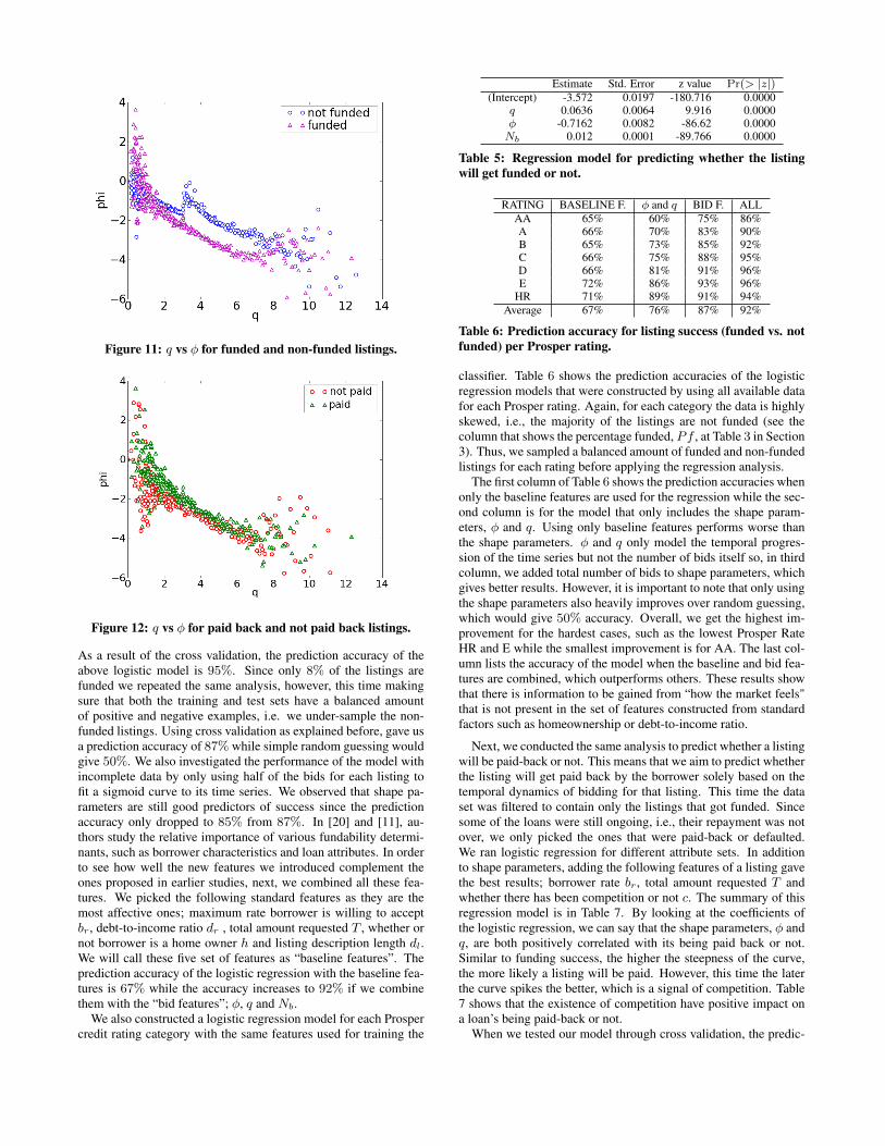
Figure 11: q vs φ for funded and non-funded listings.

Figure 12: q vs φ for paid back and not paid back listings.

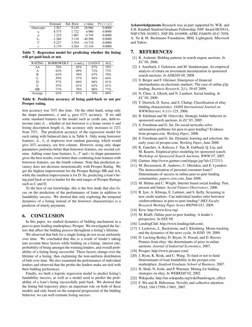
As a result of the cross validation, the prediction accuracy of theabove logistic model is 95%. Since only 8% of the listings arefunded we repeated the same analysis, however, this time makingsure that both the training and test sets have a balanced amountof positive and negative examples, i.e. we under-sample the non-funded listings. Using cross validation as explained before, gave usa prediction accuracy of 87% while simple random guessing wouldgive 50%. We also investigated the performance of the model withincomplete data by only using half of the bids for each listing tofit a sigmoid curve to its time series. We observed that shape pa-rameters are still good predictors of success since the predictionaccuracy only dropped to 85% from 87%. In [20] and [11], au-thors study the relative importance of various fundability determi-nants, such as borrower characteristics and loan attributes. In orderto see how well the new features we introduced complement theones proposed in earlier studies, next, we combined all these fea-tures. We picked the following standard features as they are themost affective ones; maximum rate borrower is willing to acceptbr , debt-to-income ratio dr , total amount requested T , whether ornot borrower is a home owner h and listing description length dl.We will call these five set of features as “baseline features”. Theprediction accuracy of the logistic regression with the baseline fea-tures is 67% while the accuracy increases to 92% if we combinethem with the “bid features”; φ, q and Nb.

We also constructed a logistic regression model for each Prospercredit rating category with the same features used for training the

Estimate Std. Error z value Pr(> |z|)(Intercept) -3.572 0.0197 -180.716 0.0000

q 0.0636 0.0064 9.916 0.0000φ -0.7162 0.0082 -86.62 0.0000Nb 0.012 0.0001 -89.766 0.0000

Table 5: Regression model for predicting whether the listingwill get funded or not.

RATING BASELINE F. φ and q BID F. ALLAA 65% 60% 75% 86%A 66% 70% 83% 90%B 65% 73% 85% 92%C 66% 75% 88% 95%D 66% 81% 91% 96%E 72% 86% 93% 96%

HR 71% 89% 91% 94%Average 67% 76% 87% 92%

Table 6: Prediction accuracy for listing success (funded vs. notfunded) per Prosper rating.

classifier. Table 6 shows the prediction accuracies of the logisticregression models that were constructed by using all available datafor each Prosper rating. Again, for each category the data is highlyskewed, i.e., the majority of the listings are not funded (see thecolumn that shows the percentage funded, Pf , at Table 3 in Section3). Thus, we sampled a balanced amount of funded and non-fundedlistings for each rating before applying the regression analysis.

The first column of Table 6 shows the prediction accuracies whenonly the baseline features are used for the regression while the sec-ond column is for the model that only includes the shape param-eters, φ and q. Using only baseline features performs worse thanthe shape parameters. φ and q only model the temporal progres-sion of the time series but not the number of bids itself so, in thirdcolumn, we added total number of bids to shape parameters, whichgives better results. However, it is important to note that only usingthe shape parameters also heavily improves over random guessing,which would give 50% accuracy. Overall, we get the highest im-provement for the hardest cases, such as the lowest Prosper RateHR and E while the smallest improvement is for AA. The last col-umn lists the accuracy of the model when the baseline and bid fea-tures are combined, which outperforms others. These results showthat there is information to be gained from “how the market feels"that is not present in the set of features constructed from standardfactors such as homeownership or debt-to-income ratio.

Next, we conducted the same analysis to predict whether a listingwill be paid-back or not. This means that we aim to predict whetherthe listing will get paid back by the borrower solely based on thetemporal dynamics of bidding for that listing. This time the dataset was filtered to contain only the listings that got funded. Sincesome of the loans were still ongoing, i.e., their repayment was notover, we only picked the ones that were paid-back or defaulted.We ran logistic regression for different attribute sets. In additionto shape parameters, adding the following features of a listing gavethe best results; borrower rate br , total amount requested T andwhether there has been competition or not c. The summary of thisregression model is in Table 7. By looking at the coefficients ofthe logistic regression, we can say that the shape parameters, φ andq, are both positively correlated with its being paid back or not.Similar to funding success, the higher the steepness of the curve,the more likely a listing will be paid. However, this time the laterthe curve spikes the better, which is a signal of competition. Table7 shows that the existence of competition have positive impact ona loan’s being paid-back or not.

When we tested our model through cross validation, the predic-

Estimate Std. Error z value Pr(> |z|)(Intercept) 2.567 9.145 28.066 0.0000

q 8.575 1.722 4.980 0.0000φ 1.219 1.807 6.749 0.0000br -1.260 3.110 -40.506 0.0000T -5.227 3.554 -14.710 0.0000c 5.179 4.264 12.144 0.0000

Table 7: Regression model for predicting whether the listingwill get paid-back or not.

RATING BORROWER F. φ and q LOAN F. ALLAA 70% 85% 87% 78%A 62% 69% 72% 73%B 63% 58% 67% 70%C 59% 57% 64% 64%D 57% 60% 60% 61%E 55% 61% 62% 61%

HR 77% 78% 80% 77%Average 63% 67% 70% 69%

Table 8: Prediction accuracy of being paid-back or not perProsper rating.

tion accuracy was 70% this time. On the other hand, using onlythe shape parameters, φ and q, gave 67% accuracy. If we addsome standard features to the model such as credit rate, debt-to-income ratio dr , whether or not borrower is a home owner h andlisting description length dl, the accuracy only increases to 72%from 70%. The prediction accuracy of the regression model foreach rating with balanced data is in Table 8. Only using borrowerfeatures; dr , h, dl improves over random guessing, which wouldgive 50% accuracy, see first column. However, using only shapeparameters performs better than borrower features, see second col-umn. Adding some loan features, br , T and c to shape parametersgives the best results, even better than combining loan features withborrower features, see the fourth column. Note that prediction ac-curacy does not decrease monotonically with Prosper Rating. Weget the highest improvement for the Prosper Ratings HR and AA,while the smallest improvement is for D. So, predicting a loan’s be-ing paid back or not is harder for the mid ranges of Prosper Ratingssuch as C and D.

To the best of our knowledge, this is the first study that also fo-cus on the prediction of the performance of loans in addition tofundability success. We showed that only exploring the temporaldynamics of a listing instead of the borrower characteristics is apredictor of timely payments.

6. CONCLUSIONIn this paper, we studied dynamics of bidding mechanism in a

peer-to-peer lending marketplace, Prosper. We investigated the fac-tors that affect the bidding process throughout a listing’s lifetime.

We observed that bids for a single listing do not occur uniformlyover time. We concluded that this is a result of lender’s takinginto account three factors while bidding on a listing: interest rate,probability of being amongst the winning lenders, and overall prob-ability of a listing being successful. These factors change over thelifetime of a listing, thus explaining the non-uniform distributionof bids over time. We also examined the performance of individuallenders and observed that the profits the lenders make are tied withtheir bidding preferences.

Finally, we built a logistic regression model to predict listing’sfundability success, as well as a model used to predict the prob-ability of a loan’s being successfully paid back. We showed thatthe listing bid trajectory plays an important role on both of thesemodels and only based on the temporal progression of the biddingbehavior, we can well estimate listing success.

Acknowledgements Research was in-part supported by W.R. andS.H. Kimball Stanford Graduate Fellowship, NSF Award 0835614,NSF CNS-1010921, NSF IIS-1016909, AFRL FA8650-10-C-7058,A. Yu & M. Bechmann Foundation, IBM, Lightspeed, Microsoftand Yahoo.

7. REFERENCES[1] K. Asdemir. Bidding patterns in search engine auctions. In

EC’06, 2006.[2] J. Auerbach, J. Galenson, and M. Sundararajan. An empirical

analysis of return on investment maximization in sponsoredsearch auctions. In ADKDD’08, 2008.

[3] S. Berger and F. Gleisner. Emergence of financialintermediaries on electronic markets: The case of online p2plending. Business Research, 2(1), 39-65 2009.

[4] N. Chen, A. Ghosh, and N. Lambert. Social lending. InEC’09, 2009.

[5] T. Dietrich, D. Seese, and S. Chalup. Classification of ebaybidding characteristics. IADIS International Journal onWWW/Internet, 4:111–125, 2006.

[6] B. Edelman and M. Ostrovsky. Strategic bidder behavior insponsored search auctions. In EC’05, 2005.

[7] S. Freedman and G. Jin. Do social networks solveinformation problems for peer-to-peer lending? Evidencefrom prosper.com. Working Paper, 2008.

[8] S. Freedman and G. Jin. Dynamic learning and selection: theearly years of prosper.com. Working Paper, June 2008.

[9] K. Ganchev, A. Kulesza, J. Tan, R. Gabbard, Q. Liu, andM. Kearns. Empirical price modeling for sponsored search.Workshop on Sponsored Search Auctions, WWW’07, 2007.

[10] Gartner. http://www.gartner.com/it/page.jsp?id=1272313.[11] M. Herzenstein, R. Andrews, U. Dholakia, and E. Lyanders.

The democratization of personal consumer loans?Determinants of success in online peer-to-peer lendingcommunities. papers.ssrn.com, June 2008.

[12] M. Hulme and C. Wright. Internet based social lending: Past,present and future. Social Futures Observatory, 2006.

[13] R. Iyer, A. Khwaja, E. Luttmer, and S. Kelly. Screening innew credit markets: Can individual lenders infer borrowercreditworthiness in peer-to-peer lending? HKS FacultyResearch Working Paper Series RWP09-031, 2009.

[14] Kiva. http://www.kiva.org/.[15] M. Klafft. Online peer-to-peer lending: A lender’s

perspective. In EEE’08.[16] LendingClub. http://www.lendingclub.com/.[17] J. Leskovec, L. Backstrom, and J. Kleinberg. Meme-tracking

and the dynamics of the news cycle. In KDD ’09, 2009.[18] D. Lucking-Reiley, D. Bryan, N. Prasad, and D. Reeves.

Pennies from ebay: the determinants of price in onlineauctions. Journal of Industrial Economics, 2007.

[19] Prosper. http://www.prosper.com/.[20] J. Ryan, K. Reuk, and C. Wang. To fund or not to fund:

Determinants of loan fundability in the prosper.commarketplace. Stanford Graduate School of Business, 2007.

[21] H. Shah, N. Joshi, and P. Wurman. Mining for biddingstrategies on ebay. In WEBKDD’02, 2002.

[22] Wikipedia. http://en.wikipedia.org/wiki/bandwagon_effect.[23] F. Wu and B. Huberman. Novelty and collective attention.

PNAS, 104:17599–17601, 2007.