Dynamics Lab Manual

Dynamics Laboratory

Observation Note Book

By

Mr.B.Ramesh, M.E.,(Ph.D), Associate professor,

Department of Mechanical Engineering, St. Joseph’s College of Engineering,

Jeppiaar Trust, Chennai-119 Ph.D. Research Scholar, College of Engineering Guindy Campus, Anna

University, Chennai.

St. Joseph’s College of Engineering

Jeppiaar Educational Trust (Christian Minority Institution)

Jeppiaar Nagar, Rajiv Gandhi Road, Chennai – 600 119

ME 2307 Dynamics Laboratory


V Semester Mechanical Engineering 2010 – 2011

Name :

Roll No. :

Reg. No. :

Year :

Branch :

Section :

iii

Syllabus

ME2307 DYNAMICS LAB 0 0 3 2

Aim: OBJECTIVES: i) To supplement the principles learnt in kinematics and Dynamics of Machinery. ii) To understand how certain measuring devices are used for dynamic testing. LIST OF EXPERIMENTS 1. a) Study of gear parameters. b) Experimental study of velocity ratios of simple, compound, Epicyclic and differential gear trains. 2. a) Kinematics of Four Bar, Slider Crank, Crank Rocker, Double crank, Double rocker, Oscillating cylinder Mechanisms. b) Kinematics of single and double universal joints. 3. a) Determination of Mass moment of inertia of Fly wheel and Axle system. b) Determination of Mass Moment of Inertia of axisymmetric bodies using Turn Table apparatus. c) Determination of Mass Moment of Inertia using bifilar suspension and compound pendulum. 4. Motorized gyroscope – Study of gyroscopic effect and couple. 5. Governor - Determination of range sensitivity, effort etc., for Watts, Porter, Proell, and Hartnell Governors. 6. Cams – Cam profile drawing, Motion curves and study of jump phenomenon 7. a) Single degree of freedom Spring Mass System – Determination of natural frequency and verification of Laws of springs – Damping coefficient determination. b) Multi degree freedom suspension system – Determination of influence coefficient. 8. a) Determination of torsional natural frequency of single and Double Rotor systems.- Undamped and Damped Natural frequencies. b) Vibration Absorber – Tuned vibration absorber. 9. Vibration of Equivalent Spring mass system – undamped and damped vibration. 10. Whirling of shafts – Determination of critical speeds of shafts with concentrated loads. 11. a). Balancing of rotating masses. (b) Balancing of reciprocating masses. 12. a) Transverse vibration of Free-Free beam – with and without concentrated masses.

b) Forced Vibration of Cantilever beam – Mode shapes and natural frequencies. c) Determination of transmissibility ratio using vibrating table.

Students should be familiar with the use of the following device/equipments depending upon availability. Tachometers – Contact and non contact Dial gauge Stroboscope Accelerometers – Vibration pickups Displacement meters. Oscilloscope Vibration Shaker F.F.T. Analyzer, and (9) Dynamic Balancing Machine.

LIST OF EQUIPMENT

(for a batch of 30 students) 1. Cam analyzer. 2. Motorised gyroscope. 3. Governor apparatus - Watt, Porter, Proell and Hartnell governors. 4. Whirling of shaft apparatus. 5. Dynamic balancing machine. 6. Static and dynamic balancing machine. 7. Vibrating table 8. Vibration test facilities apparatus 9. Gear Model 10. Kinematic Models to study various mechanisms

5

Contents

01. Porter Governor

02. Proell Governor

03. Torsional vibration of single rotor system

04. Torsional vibration of two rotor system

05. Undamped free vibration of spring mass system

06. Determination of whirling speed of shafts

07. Compound Pendulum

08. Hartnell Governor

09. Bifilar suspension

10. Cam analysis

11. Balancing of rotating masses

12. Determination of Gyroscopic couple

13. Determination of influence coefficient (Multi degree freedom suspension method)

14. Determination of transmissibility ratio by using Vibration Lab

15. Determination of frequency of transverse of given square sectioned shaft with

concentric fly wheel load.

16. Undamped free vibration of equivalent spring mass system.

17. Forced vibration phenomenon of equivalent spring mass system with different

damping condition.

6

ME 2307 Dynamics Laboratory


Prepared by: Mr. B. Ramesh, M.E.(Ph.D.) Associate Professor, Department of Mechanical Engineering.

INDEX Name of the staff : Sl.

No.

Date

of

Expt

Name of the Experiment Page

No.

Date

of

Sub.

Re-

marks

Staff

sign

Date

01

02

03

04

05

06

07

08

09

10

11

12

13

14

15

16

17

7

9

Exp. No. : Porter Governor Date : Aim : To determine the characteristic curves of the porter governor. Apparatus Required: 1. Digital rpm indicator with sensor 3. Sleeve weights 2. Porter arm setup 4. Measuring tape. Description of the setup: The drive unit consists of a DC electric motor connected through belt and pulley arrangement. Motor and test setup are mounted on a M.S. fabricated frame. The governor spindle is driven by motor through V belt and is supported in a ball bearing. The optional governor mechanisms can be mounted on spindle. Digital speed is controlled by the electronic control unit. A rpm indicator with sensor to determine the speed. A graduated scale is fixed to the sleeve and guided in vertical direction. Sleeve displacement is to be noted on the scale provided. The centre sleeve of the Porter and Proell governors incorporates a weight sleeve to which weights may be added. The Hartnell governor provides means of varying spring rate and initial compression level and mass of rotating weight. This enables the Hartnell governor to be operated as a stable or unstable governor. DC motor with drive: ½ HP motor and DC drive control for speed variation. Separate linkages for governor arrangements ( Porter, Proell and Hartnell ) are provided using same motor and base. Procedure: The governor mechanism under test is fitted with the chosen rotating weights and spring, where applicable, and inserted into the drive unit. The following simple procedure may then be followed. The control unit is switched on and the speed control knob is slowly turned to increase the governor speed until the centre sleeve rises off the lower stop and aligns with some divisions on the graduated scale. The sleeve position and speed are then recorded. The governor speed is then increased in steps to give suitable sleeve movements and readings are recorded at each stage throughout the range of sleeve movement possible. The radius of rotation for corresponding sleeve displacement is measured directly by switching off the electronic control unit. Precautions: 1) Take the sleeve displacement reading when the pointer remains steady. 2) See that at higher speed the load on the sleeve does not hit the upper sleeve of the governor. 3) While closing the test bring the pointer to zero position and then switch off the motor.

Tabulation:

Sl. No.

Speed , N ( rpm )

Sleeve displacement , X ( mm )

Diameter of rotation , mm

Radius of rotation , r

( mm )

Controlling force , F ( N )

1

2

3

4

5

6

Observation: Mass of each ball, m = , kgf Mass added = , g Formulae: Controlling Force, F = mω2 r , N Where, m = mass of each ball , kgf ω = angular velocity = ( 2πN ) / 60 , rps where, N = speed , rpm r = radius of rotation , m Graphs: (i) Displacement vs Speed (ii) Radius of rotation vs Controlling force

Model calculation:

Reading No. : ---------

12

Result: Thus the characteristic curves of the porter governor are determined.

13

Exp. No. : Proell Governor Date : Aim : To determine the characteristic curves of the proell governor. Apparatus Required: 1. Digital rpm indicator with sensor 3. Sleeve weights 2. Proell arm setup 4. Measuring tape. Description of the setup: The drive unit consists of a DC electric motor connected through belt and pulley arrangement. Motor and test setup are mounted on a M.S. fabricated frame. The governor spindle is driven by motor through V belt and is supported in a ball bearing. The optional governor mechanisms can be mounted on spindle. Digital speed is controlled by the electronic control unit. A rpm indicator with sensor to determine the speed. A graduated scale is fixed to the sleeve and guided in vertical direction. Sleeve displacement is to be noted on the scale provided. The centre sleeve of the Porter and Proell governors incorporates a weight sleeve to which weights may be added. The Hartnell governor provides means of varying spring rate and initial compression level and mass of rotating weight. This enables the Hartnell governor to be operated as a stable or unstable governor. DC motor with drive: ½ HP motor and DC drive control for speed variation. Separate linkages for governor arrangements ( Porter, Proell and Hartnell ) are provided using same motor and base. Procedure: The governor mechanism under test is fitted with the chosen rotating weights and spring, where applicable, and inserted into the drive unit. The following simple procedure may then be followed. The control unit is switched on and the speed control knob is slowly turned to increase the governor speed until the centre sleeve rises off the lower stop and aligns with some divisions on the graduated scale. The sleeve position and speed are then recorded. The governor speed is then increased in steps to give suitable sleeve movements and readings are recorded at each stage throughout the range of sleeve movement possible. The radius of rotation for corresponding sleeve displacement is measured directly by switching off the electronic control unit. Precautions: 1) Take the sleeve displacement reading when the pointer remains steady. 2) See that at higher speed the load on the sleeve does not hit the upper sleeve of the governor. 3) While closing the test bring the pointer to zero position and then switch off the motor.

15

Tabulation:

Sl. No.

Speed , N ( rpm )


Diameter of rotation, mm

Radius of rotation , r

( mm )


1

2

3

4

5

6

16

Observation: Mass of each ball, m = , kgf Mass added = , g Formulae: Controlling Force, F = mω2 r , N Where, m = mass of each ball , kgf ω = angular velocity = ( 2πN ) / 60 , rps where, N = speed , rpm r = radius of rotation , m Graphs: (i) Displacement vs Speed (ii) Radius of rotation vs Controlling force

17

Model calculation:

Reading No. : ---------

18

Result: Thus the characteristic curves of the proell governor are determined.

19

Exp. No. : Torsional vibration of single rotor system Date : Aim : To determine the period and frequency of torsional vibration of the single rotor system experimentally and compare it with the theoretical values. Apparatus Required : 1) Shaft 4) Measuring tape 2) Spanner 5) Stop watch and 3) Chuck key 6) Weights Description of the setup: One end of the shaft is gripped in the chuck and heavy disc free to rotate in ball bearing is fixed at the other end of the shaft. The bracket with fixed end of shaft can be clamped at any convenient position along the beam. Thus length of the shaft can be varied during the experiment. Specially designed chuck is used for clamping the end of the shaft. The ball bearing support to the flywheel provides negligible damping during experiment. The bearing housing is fixed to side member of the main frame. Procedure: 1) Fix the bracket at any convenient position along the beam. 2) Grip the shaft at the bracket by means of chuck. 3) Fix the rotor on the other end of the shaft. 4) Note down the length of the shaft. 5) Twist the rotor through some angle and release. 6) Note down the time required for n = 5 oscillations. 7) Repeat the procedure for different lengths of shaft. Observation: Modulus of rigidity, G = 0.35 x 1011 , N/m2 Shaft diameter , d = 0.55 , cm Diameter of disc A , DA = 23 , cm Mass of disc A, mA = 3.3 + 1.5 = 4.8 , kgf

Tabulation :

Sl. No.

Length of the shaft,

L ( m)

Time taken for n = 5 oscillations , t ( sec )

Period of vibration ( sec )

Frequency of vibration ( Hz )

t1 t t t t t2 3 4 5 m T exp T theo F exp F theo

1

2

3

4

5

Formulae: Experimental period of vibration , T exp = tm / n , sec Where, tm = mean time taken for n oscillations n = number of oscillations = 5 Theoretical period of vibration , T theo = 2π { sqrt (I / Kt ) } , sec Where, Moment of inertia, I = mA ( DA

2 / 8 ) , Nms2 Where, mA = mass of the disc A , kgf DA = diameter of the disc A , m Torsional stiffness, Kt = ( G Ip ) / L , Nm Where, G = modulus of rigidity , N/m2 L = length of the shaft , m Polar moment of inertia , Ip = ( π / 32 ) d4 , m4 Experimental frequency of vibration , F exp = 1 / T exp , Hz Theoretical frequency of vibration , F theo = 1 / T theo , Hz

Model calculation:

Reading No. : ---------

24

Result: The period and frequency of torsional vibration of the single rotor system are determined experimentally and verified with the theoretical values.

25

27

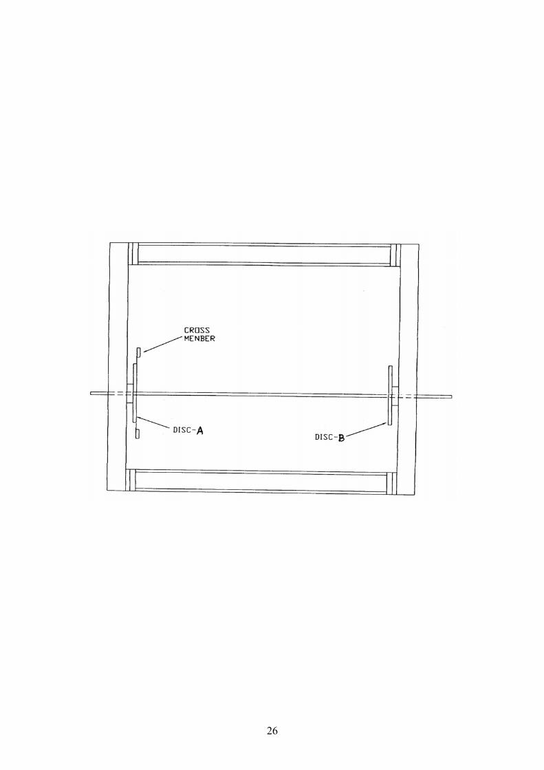
Exp. No. : Torsional vibration of two rotor system Date : Aim : To determine the period and frequency of torsional vibration of the two rotor system experimentally and compare it with the theoretical values. Apparatus Required : 1) Shaft 4) Measuring tape 7) Cross arms 2) Spanner 5) Stop watch 3) Chuck key 6) Weights and Description of the setup: Two discs having different mass moment of inertia are clamped one at each end of shaft by means of collet. Mass moment of inertia of any disc can be changed by attaching the cross lever with weights. Both discs are free to oscillate in the ball bearings. This provides negligible damping during experiment. Procedure: 1) Fix the discs A and B to the shaft and fit the shaft in bearing. 2) Deflect the discs A and B in opposite directions by hand and release. 3) Note down the time required for n = 5 oscillations. 4) Fit the cross arm to the disc A and attach equal masses to the ends of cross arm and again note down time. 5) Repeat the above procedure with different equal masses attached to the ends of cross arm. Observation: Diameter of the disc A , DA = 230 , mm Diameter of the disc B , DB = 200 , mm Mass of the disc A, mA = 3.3 , kgf Mass of the disc B, mB = 1.74 , kgf Modulus of rigidity of the shaft, G = 0.35 x 1011 , N/m2 Shaft diameter , d = 5.5 , mm Length of the shaft between discs, L = , m Mass of the cross arms with bolts and nuts = 0.725 , kgf

Tabulation:

Sl.No.

Mass added to the disc

A, ( kgf )

Moment of inertia of disc A ,

IA ( Nms2 )

Moment of inertia of disc B ,

IB ( Nms2 )

Time taken for n = 5 oscillations ( sec )

Period of vibration ( sec )

Frequency of vibration ( Hz )

t1 t2 t3 t4 t5 tm T exp T theo F exp F theo

1

2

3

Formulae: Experimental period of vibration , T exp = tm / n , sec Where, tm = mean time taken for n oscillations n = number of oscillations = 5 Theoretical period of vibration , T theo = 2π { sqrt [(IA IB) / Kt(IA + IB)] }, sec Where, Moment of inertia of disc A, IA = mA ( DA

2 / 8 ) , Nms2 Moment of inertia of disc B, IB = mB ( DB

2 / 8 ) , Nms2 Torsional stiffness, Kt = ( G Ip ) / L , Nm Where, G = modulus of rigidity of the shaft , N/m2 L = length of the shaft between discs , m Polar moment of inertia , Ip = ( π / 32 ) d4 , m4 Where, d = shaft diameter , m Experimental frequency of vibration , F exp = 1 / T exp , Hz Theoretical frequency of vibration , F theo = 1 / T theo , Hz

Model calculation:

Reading No. : ---------

30

Result: The period and frequency of torsional vibration of the two rotor system are determined experimentally and verified with the theoretical values.

31

33

Exp. No. : Undamped free vibration of

spring mass system Date : Aim : To determine stiffness of the given helical spring, period and frequency of undamped free vibration (longitudinal vibration) of spring mass system experimentally and compare it with the theoretical values. Apparatus Required : 1) Helical spring 4) Measuring tape and 2) Platform 5) Stop watch 3) Weights Description of the setup: It consists of an open coil helical spring of which one end is fixed to the screw rod and a platform to the other end. This platform is used to add weights and a lock nut is also provided to clamp the weights added. Procedure: 1) Fix one end of the helical spring to the upper screw rod. 2) Measure the free length of the spring. 3) Attach the other end to the platform and add some weight. 4) Note down the deflection. 5) Stretch the spring through some distance and release. 6) Observe the time taken for n = 20 oscillations. 7) Repeat the steps from 3 to 6 for other known weights. Observation: Length of the spring before loading = , m Formulae: Stiffness of the spring, K exp = Load / deflection = W / X , N/m Deflection, X = ( Length of the spring after loading – length of the spring before loading ) ,m Experimental period of vibration , T exp = tm / n , sec Where, tm = mean time taken for n oscillations n = number of oscillations = 20 Theoretical period of vibration , T theo = 2π { sqrt [ W / ( g Kexpm) ] }, sec

Tabulation:

Sl.No.

Load added, W Length of the spring after

loading ( m )

Deflection, X

( m )

Stiffness, K exp = W / X

( N / m )

Time taken for n = 20 oscillations

( sec )

Period of vibration

( sec )

Frequency of vibration

( Hz )

( kg ) ( N ) t1 t2 t3 t4 t5 tm T exp T theo F exp F theo

1

2

3

4

K expm =

Where, W = Load added , N Kexpm = Experimental mean stiffness , N/m Experimental frequency of vibration , F exp = 1 / T exp , Hz Theoretical frequency of vibration , F theo = 1 / T theo , Hz Graph : Deflection vs Load added

Model calculation:

Reading No. : ---------

36

Result: Stiffness of the spring, i) Experimentally, K expm = , N/m ii) Graphically = , N/m The period and frequency of undamped free vibration (longitudinal vibration) of spring mass system are determined experimentally and verified with the theoretical values.

37

39

Exp. No. : Determination of whirling speed of shafts Date : Aim: To determine the whirling speed for various diameter shafts experimentally and compare it with the theoretical values. Apparatus Required: 1) Shaft – 3 nos. 4) AC voltage regulator 2) Digital tachometer 3) Chuck key and Description of the setup: The apparatus is used to study the whirling phenomenon of shafts. This consists of a frame in which the driving motor and fixing blocks are fixed. A special design is provided to clear out the effects of bearings of motor spindle from those of testing shafts. Procedure: 1) The shaft is to be mounted with the end condition as simply supported. 2) The speed of rotation of the shaft is gradually increased. 3) When the shaft vibrates violent in fundamental mode ( I mode ), the speed is noted down. 4) The above procedure is repeated for the remaining shafts. Observation: Young’s modulus, E (for steel) = 2.06 x 1011 , N / m2 Young’s modulus, E (for copper) = 1.23 x 1011 , N / m2 Length of the shaft, L = , m Shaft 1 (steel) Shaft 2 (copper) Shaft 3(steel) m1 = 0.0584 kg m2 = 0.16496 kg m3 = 0.16051 kg d1 = 0.0031 m d2 = 0.00484 m d3 = 0.00511 m l1 = m l2 = m l3 = m Formulae: Theoretical whirling speed, Nctheo = {0.4985 / [sqrt (δs / 1.27 )] } x 60 , rpm Static deflection due to mass of the shaft (UDL), δs = (5wL4) / (384 EI) Where, w = weight of the shaft per metre , N/m L = Length of the shaft, m E = Young’s modulus for the shaft material, N/m2 I = Mass moment of inertia of the shaft = ( π / 64 ) d4 , m4

Tabulation:

Sl.No. Diameter of shaft ( m )

Mass moment of inertia of the shaft ,

I ( m4) x 10-12

Weight of the shaft per m, w ( N/m )

Whirling speed ( rpm )

Ncexp Nctheo

1

2

3

Model calculation:

Reading No. : ---------

Result : The whirling speed for various diameter shafts are determined experimentally and verified with the theoretical values.

43

45

Exp. No. : Compound Pendulum Date : Aim: To determine moment of inertia by using compound pendulum and period and radius of gyration of the given steel bar experimentally and compare it with the theoretical values. Apparatus Required: 1) Steel bar 3) Stop watch and 2) Knife edge support 4) Measuring tape Description of the setup: The compound pendulum consists of 100 cm length and 5 mm thick steel bar. The bar is supported by the knife edge. It is possible to change the length of suspended pendulum by supporting the bar in different holes. Procedure: 1) Support the steel bar in any one of the holes. 2) Note the length of suspended pendulum to measure OG. 3) Allow the bar to oscillate and determine Texp by knowing the time taken for n = 10 oscillations. 4) Repeat the experiment with different length of suspension. Observation: Length of the steel bar, L = , cm Number of holes = Distance between two holes = , cm Mass of the steel bar = 1.575 , kgf Formulae: Experimental periodic time, T exp = t / n , sec Where, t = time taken for n oscillations n = number of oscillations = 10 Theoretical periodic time, T theo = 2π { sqrt [ ( Ktheo

2 + ( OG )2 ) / ( g (OG)) ] }, sec Where, Ktheo = Theoretical radius of gyration , cm = ( L ) / 2√3

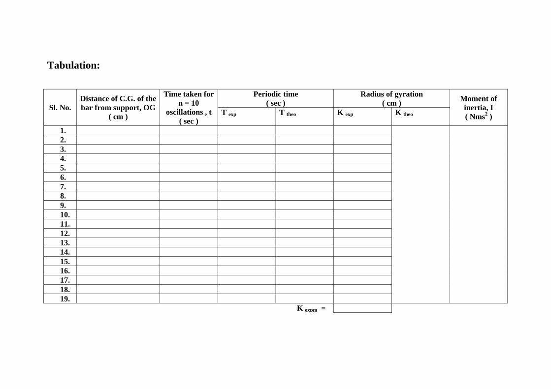
Tabulation:

Sl. No. Distance of C.G. of the bar from support, OG

( cm )

Time taken for n = 10

oscillations , t ( sec )

Periodic time ( sec )

Radius of gyration ( cm ) Moment of

inertia, I ( Nms2 ) T exp T theo K exp K theo

1. 2. 3. 4. 5. 6. 7. 8. 9. 10. 11. 12. 13. 14. 15. 16. 17. 18. 19. K expm =

OG = distance of the C.G. of bar from support , cm Experimental periodic time, T exp = 2π { sqrt [ ( Kexp

2 + ( OG )2 ) / ( g (OG)) ] }, sec Moment of inertia , I = m Kexpm

2 , Nms2 Where, Kexpm = mean experimental radius of gyration , m m = mass of the steel bar , kgf

Model calculation:

Reading No. : ---------

48

Result: i) Moment of inertia of the given steel bar = , Nms2 ii) Mean experimental radius of gyration, Kexpm = , cm iii) Theoretical radius of gyration , Ktheo = , cm

49

51

Exp. No. : Hartnell Governor Date : Aim : To determine the characteristic curves of the Hartnell governor. Apparatus Required: 1. Digital rpm indicator with sensor 3. Sleeve weights 2. Hartnell arm setup 4. Measuring tape. Description of the setup: The drive unit consists of a DC electric motor connected through belt and pulley arrangement. Motor and test setup are mounted on a M.S. fabricated frame. The governor spindle is driven by motor through V belt and is supported in a ball bearing. The optional governor mechanisms can be mounted on spindle. Digital speed is controlled by the electronic control unit. A rpm indicator with sensor to determine the speed. A graduated scale is fixed to the sleeve and guided in vertical direction. Sleeve displacement is to be noted on the scale provided. The centre sleeve of the Porter and Proell governors incorporates a weight sleeve to which weights may be added. The Hartnell governor provides means of varying spring rate and initial compression level and mass of rotating weight. This enables the Hartnell governor to be operated as a stable or unstable governor. DC motor with drive: ½ HP motor and DC drive control for speed variation. Separate linkages for governor arrangements ( Porter, Proell and Hartnell ) are provided using same motor and base. Procedure: The governor mechanism under test is fitted with the chosen rotating weights and spring, where applicable, and inserted into the drive unit. The following simple procedure may then be followed. The control unit is switched on and the speed control knob is slowly turned to increase the governor speed until the centre sleeve rises off the lower stop and aligns with some divisions on the graduated scale. The sleeve position and speed are then recorded. The governor speed is then increased in steps to give suitable sleeve movements and readings are recorded at each stage throughout the range of sleeve movement possible. The radius of rotation for corresponding sleeve displacement is measured using the formula. Precautions: 1) Take the sleeve displacement reading when the pointer remains steady. 2) See that at higher speed the load on the sleeve does not hit the upper sleeve of the governor. 3) While closing the test bring the pointer to zero position and then switch off the motor.

Tabulation:

Sl. No.

Speed , N ( rpm )


Radius of rotation , r ( mm )


1

2

3

Observation: Mass of each ball, m = , kgf Initial radius of rotation, ro = , m Formulae: Controlling Force, F = mω2 r , N Where, m = mass of each ball , kgf ω = angular velocity = ( 2πN ) / 60 , rps where, N = speed , rpm r = radius of rotation , m = ro + X ( a / b ) , m where, ro = initial radius of rotation , m X = sleeve displacement , m a = , m b = , m Graphs: (i) Displacement vs Speed (ii) Radius of rotation vs Controlling force

53

Model calculation:

Reading No. : ---------

54

Result: Thus the characteristic curves of the Hartnell governor are determined.

55

Exp. No. : Bifilar Suspension Date : Aim: To determine the radius of gyration of given bar by using bifilar suspension and periodic time experimentally and compare it with the theoretical values. Apparatus Required: 1) Vibration lab machine 4) Stop watch and 2) Measuring tape 5) Bar 3) Weights Description of the setup: A uniform rectangular section bar is suspended from the pendulum support frame by two parallel cords. Top ends of the cords pass through the two small chucks fitted at the top. Other ends are secured in the bifilar bar. It is possible to adjust the length of the cord by loosing the chucks. The suspension may also be used to determine the radius of gyration of any body. In this case the body under investigation is bolted to the centre. Radius of gyration of the combined bar and body is then determined. Procedure: 1) Suspend the bar from chuck and adjust the length of the cord ‘L’ conveniently. Note the suspension length of each cord must be the same. 2) Allow the bar to oscillate about the vertical axis passing through the centre and measure the periodic time T by knowing the time for say n = 10 oscillations. 3) Repeat the experiment by mounting the weights at equal distance from the centre ( D / 2 as shown ). Observation: Distance between two cords, 2a = , cm Distance from centre to cord, a = , cm Length of the bar,l = , cm Mass added = , g Formulae: Experimental periodic time, T exp = tm / n , sec Where, tm = mean time taken for n oscillations n = number of oscillations = 10

Tabulation:

Sl. No.

Suspension length, L

( cm )

Time taken for n = 10 oscillations ( sec )

Periodic time ( sec )

Radius of gyration ( cm )

t1 t t t2 t3 4 5 tm T exp T theo K exp K theo

1

2

Kexpm =

Experimental periodic time, T exp = [ (2π K exp ) / a ] [ sqrt ( L / g ) ] , sec Where, Kexp = experimental radius of gyration , cm a = distance from centre to cord , cm L = suspension length , cm Theoretical periodic time, Ttheo = [ (2π K theo ) / a ] [ sqrt ( L / g ) ] , sec Theoretical radius of gyration, K theo = l / ( 2 √3 ) , cm Where, l = length of the bar , cm

Model calculation:

Reading No. : ---------

60

Result: Radius of gyration of given bar: i) Experimentally, Kexpm = , cm ii) Theoretically, Ktheo = , cm The periodic time of the given bar is determined experimentally and verified with the theoretical values.

61

Exp. No. : Cam Analysis Date : Aim : To draw the profile of the circular arc cam with flat face follower using the given apparatus. Description : The machine is a motorized unit consisting of a cam shaft driven by a AC/DC motor. The shaft runs in a ball bearing. At the free end of the cam shaft a cam can be easily mounted. The follower is properly guided in gun metal bushes. A graduated circular protractor is fitted co-axial with the shaft and a dial gauge can be fitted to note the follower displacement for the angle of cam rotation. A spring is used to provide controlling force to the follower system. Weights on the follower rod can be adjusted as per the requirements. The arrangement of speed regulation is provided. The machine is particularly very useful for testing the cam performance for jump phenomenon during operation. This machine clearly shows the effect of change of forces on jump action of cam follower during operation. It is used for testing various cam follower pairs, i.e., (a) Circular arc cam with flat follower, (b) An eccentric cam with flat follower, (c) Sharp edged cam with flat follower. The unit is provided with the push rod in the two bush bearings. Should the unit be disassembled, for any, reason while assembling following precautions should be taken: (a) The horizontality of the upper and lower glands should be checked by a spirit level. (b) The supporting pillars should be properly tightened with the lock nuts provided. Jump phenomenon: The jump phenomenon occurs in case of cam operating under the action of compression spring load. This is a transient coefficient that occurs only with high speed, highly flexible cam follower systems. With jump, cam and the follower separate owing to excessively unbalanced forces exceeding the spring force during the period of negative acceleration. This is undesirable since the fundamental function of the cam follower system, the constraint and control of follower motion are not maintained. Also related are the short life of the cam flank surface, high noise, vibrations and poor action. Jump and crossover shock: A cam follower retained against the cam with a compression retaining spring will under certain conditions, jump or bounce out of contact with the cam. This condition is most likely to occur with low values of damping and with high speed cams of quite flexible follower trains. Crossover shock occurs in a positive drive cam mechanism when contact moves from one side of the cam to the other. Clearance and backlash are taken up

Tabulation: Forward

stroke Dwell Return stroke Dwell

Angle in degree

Follower lift in mm

Follower lift = ,mm Circular arc cam with flat face follower – Diagram :

64

during the crossover and impact occurs. Crossover takes place on the rise or return motion when the acceleration changes sign and when the velocity is at its peak. The effects can be reduced by preloading the system to remove backlash, by designing for low peak velocity and by using rigid follower train. Roth Bart states that jump will not occur in high speed systems if at least two full cycles of vibration occur during the positive acceleration time-interval of the motion. If a smaller number of cycles exist during this period, then, he states, the system should be investigated mathematically to determine if jump exists. This condition can be expressed by the equation : [Bl K] / 360 ≥ 2 where Bl is the angle through which the cam rotates during positive acceleration period. This figure can probably be reduced slightly for appreciable amounts of damping. Spring ko loses compression when jump begins and is carried motion with the mass. The resulting motion now gets rather complicated because the mass, too, must be redistributed. Probably a good first approximation could be obtained by concentrating a portion of the mass at the bottom of spring and treating the motion as a system of two degrees of freedom. It must be noted, through that the system will vibrate at a new frequency after jump begins and then analysis of the motion using the old frequency is not a true description of the motion. Spring Ko loses its compression whenever X exceeds by the amount of Ko was initially compressed during assembly. Thus to set up a criteria for jump, it is necessary to calculate the pre-compression of K. To observe the phenomenon of jump(use of a stroboscope is necessary). The speed of cam rotation and stroboscope frequency of neon lamp are gradually and simultaneously increased and at the time of jump to occur the follower is seen to loose contact with cam. The jump speed thus can be obtained from the stroboscope. When jump occurs the follower pounds on the cam surface giving a good thumping sound. Upward inertia force = Downward retaining force [W/g] ω2r = W + S This is the equilibrium of force equation when jump will just start. W = weight of follower assembly ω = angular velocity = [2πN] / 60 rad/sec S = spring force (kg) = stiffness of spring x compression length r = distance according to the geometry of cam = l / (2π) where l is lift of the follower. To study the effect of follower assembly weight on the jump speed when the spring force is kept constant, keep the initial spring compression at a certain level and observe jump speed for different follower weights by adding them successively and plot the graph of follower weights vs jump speed. ω2 = [(W + S) / (Wr) ]g Therefore , ω = sqrt[ (g/r)(1 + (s/W) )] This relation shows that as the follower weight increases the jump speed goes on decreasing. Procedure : Rotate the cam shaft with the help of the hand through some angle and note down the angle of cam rotation indicated on the protractor and the corresponding follower displacement indicated in the dial gauge. Continue the experiment for

65

Displacement, velocity and acceleration diagrams of the flat face follower : Calculation:

66

Profile of the circular arc cam :

68

69

different angles of cam rotation and draw the graph X vs θ. The X vs θ plot can be used to find out velocity and acceleration of the follower system. The exact profile of the cam can be obtained by taking observations X vs θ, where X = displacement of the follower from reference initial position and θ = angle of cam rotation with reference from axis of symmetry chosen. Observation : Base circle radius or minimum radius of the cam, r1 = mm Nose radius , r2 = mm Result: Thus the profile of the circular arc cam with flat face follower has been drawn.

Dynamics Lab Manual

Documents

Transcript of Dynamics Lab Manual