Dynamics and responses to mortality rates ofcompeting ... · Dynamics and responses to mortality...

http://www.elsevier.com/locate/ytpbi

Theoretical Population Biology 64 (2003) 163–176

Dynamics and responses to mortality rates of competing predatorsundergoing predator–prey cycles

Peter A. Abrams,a,� Chad E. Brassil,a and Robert D. Holtb

aDepartment of Zoology, The University of Toronto, 25 Harbord Street, Toronto, Ont., Canada M5S 3G5b Department of Zoology, University of Florida, P.O. Box 118525, Gainesville, FL 32611-8525, USA

Received 30 April 2002

Abstract

Two or more competing predators can coexist using a single homogeneous prey species if the system containing all three

undergoes internally generated fluctuations in density. However, the dynamics of species that coexist via this mechanism have not

been extensively explored. Here, we examine both the nature of the dynamics and the responses of the mean densities of each

predator to mortality imposed upon it or its competitor. The analysis of dynamics uncovers several previously undescribed

behaviors for this model, including chaotic fluctuations, and long-term transients that differ significantly from the ultimate patterns

of fluctuations. The limiting dynamics of the system can be loosely classified as synchronous cycles, asynchronous cycles, and

chaotic dynamics. Synchronous cycles are simple limit cycles with highly positively correlated densities of the two predator species.

Asynchronous cycles are limit cycles, frequently of complex form, including a significant period during which prey density is nearly

constant while one predator gradually, monotonically replaces the other. Chaotic dynamics are aperiodic and generally have

intermediate correlations between predator densities. Continuous changes in density-independent mortality rates often lead to

abrupt transitions in mean population sizes, and increases in the mortality rate of one predator may decrease the population size of

the competing predator. Similarly, increases in the immigration rate of one predator may decrease its own density and increase the

density of the other predator. Proportional changes in one predator’s birth and death rate functions can have significant effects on

the dynamics and mean densities of both predator species. All of these responses to environmental change differ from those observed

when competitors coexist stably as the result of resource (prey) partitioning. The patterns described here occur in many other

competition models in which there are cycles and differences in the linearity of the responses of consumers to their resources.

r 2003 Elsevier Science (USA) All rights reserved.

0. Introduction

Much current thought on competition is based uponthe Lotka–Volterra model of two competing species.Because this model always has a stable equilibrium whentwo species coexist, the role of population cycles isseldom considered in empirical studies when trying tounderstand the interactions between coexisting compe-titors. The Lotka–Volterra model also leads to expecta-tions about the responses of the densities of eachcompetitor to parameters affecting the fitness of theother species, such as its mortality rate. For instance,continuous increase in the per capita mortality rate of

one species decreases its equilibrium density andincreases the equilibrium density of its competitor.Similar qualitative behaviors characterize many modelsof direct competition in which there is stable coex-istence. Similarly, increasing the immigration rate ofthat species will increase its density and decrease that ofits competitor. Because empirical studies of competitorand community structure are guided by theoreticalexpectations, it is important to identify situations inwhich these expectations are unlikely to be realized. Inthis paper, we show that models with explicit resourcedynamics, differences in the linearity of the predators’responses, and the potential for sustained oscillations,can exhibit sharply different effects. Because it has longbeen known that consumer–resource interactions caneasily produce cycles (Rosenzweig and MacArthur,1963), and that cycles can alter conditions for coex-istence (Armstrong and McGehee, 1980), it is surprising

ARTICLE IN PRESS

�Corresponding author. Fax: +416-978-8532.

E-mail addresses: [email protected] (P.A. Abrams), bras-

[email protected] (C.E. Brassil), [email protected] (R.D.

Holt).

0040-5809/03/$ - see front matter r 2003 Elsevier Science (USA) All rights reserved.

doi:10.1016/S0040-5809(03)00067-4

that the implications of cycling for interactions betweencompetitors have not received more attention.

In a previous article (Abrams and Holt, 2002), weargued that a mechanism of coexistence proposed byKoch (1974) and by Armstrong and McGehee (1976a, b,1980), McGehee and Armstrong (1977) may play animportant role in species coexistence in natural commu-nities. This mechanism is based on differences in thenonlinearity of two competitors’ responses to a singleresource combined with consumer–resource cycles gen-erated by the interaction of one of those consumers withthe resource. The more linear species has a relativelyhigh resource requirement, and therefore cannot excludethe species with the more nonlinear response. The lattergenerates cycles when alone with the resource; thesecycles increase the mean resource density so that linearspecies can invade. If the ‘robustness’ of coexistence ismeasured by the range of prey (resource) requirementsfor zero population growth (i.e., efficiencies) that allowcoexistence, then Armstrong and McGehee’s model canproduce very robust coexistence. The range of efficien-cies allowing coexistence via Armstrong and McGehee’smechanism is often as wide as the range of efficienciesallowing coexistence of competing predators which donot cycle, but which have a high degree of partitioningof prey species (Abrams and Holt, 2002). This observa-tion, together with the fact that a significant number ofspecies cycle (Ellner and Turchin, 1995; Kendall et al.,1998), suggests that cases of coexistence via theArmstrong–McGehee mechanism may be reasonablycommon. However, well-supported empirical examplesof coexistence due to competitor–resource cyclesare absent from the published literature. By describingthe dynamics of such competitive systems, and howthey respond to changes in mortality rates, we hopeto find dynamical signals that may help identifyexamples in natural systems. Moreover, Armstrongand McGehee’s (1980) model exhibits a wider rangeof dynamics than has been described previously,including chaos, alternative limit cycles, and long-lastingtransients.

1. The model

We begin by analyzing the model that Armstrong andMcGehee (1980) used to illustrate nonequilibrial coex-istence of two species on a single biotic resource. Thissystem is characterized by logistic prey growth, a linearfunctional response for one predator, and a type-2functional response for the other predator. We arguebelow that this model displays many dynamics that arecommon to a much broader set of models characterizedby differences in the linearity consumer species andendogenously generated cycles. The dynamics of the twopredators (consumers), P1 and P2; and the prey

(resource), N; are given by

dP1

dt¼ P1

B1C1N

1 þ hC1N� D1

� �;

dP2

dt¼ P2ðB2C2N � D2Þ;

dN

dt¼ rN 1 � N

K

� �� C1NP1

1 þ hC1N� C2NP2: ð1a; b; cÞ

The parameter Bi is the conversion efficiency of foodinto offspring for predator i; h is the handling time perprey item for predator 1, Di is a density independentdeath rate, Ci is a searching predator’s attack rate, and r

and K are logistic growth parameters. The variables inthis equation can be scaled to reduce the number ofparameters, as follows: t0 ¼ rt; N 0 ¼ N=K ; and P1

0 ¼P1=ðKB1Þ; and P2

0 ¼ P2=ðKB2Þ: After making substitu-tions and dropping the primes on the new variables, themodel becomes

dP1

dt¼ P1

a1N

1 þ bN� d1

� �;

dP2

dt¼ P2ða2N � d2Þ;

dN

dt¼ Nð1 � NÞ � a1NP1

1 þ bN� a2NP2; ð2a; b; cÞ

where the new parameters are a1 ¼ KB1C1=r; a2 ¼KB2C2=r; b ¼ KC1h; d1 ¼ D1=r; d2 ¼ D2=r: Below werefer to predator 1 as the nonlinear predator, andpredator 2 as the linear predator.

There is no equilibrium point with positive densitiesof all three species. However, the species can coexist forsome range of the parameters a2 and d2 if P1 and N

undergo limit cycles in the absence of the secondpredator (McGehee and Armstrong, 1977; Armstrongand McGehee, 1980). Limit cycles occur in thesubsystem lacking predator 2 if

d1oa1ðb � 1Þbðb þ 1Þ : ð3Þ

The right-hand side of this inequality will be referred toas the stability threshold value of d1: Here we onlyconsider cases where d1; a1 and b satisfy (3). We considercoexistence to occur if each predator species can increasewhen it is rare and the other predator and prey areundergoing their limiting dynamics (stable point or limitcycle). This differs from Armstrong and McGehee’s(1980) definition of coexistence, and there are circum-stances when such ‘mutual invasion’ definitions ofcoexistence may be misleading (Armstrong and McGehee,1980). The most serious problem is the possibility thatinitial invasion is eventually followed by exclusion of theinvading species. This outcome was never observed in anynumerical solution of Eq. (2), or in any other modelthat we consider here. Previous examples of thisphenomenon (the reversal of initially successful inva-sion) have had alternative attractors for the subsystem

ARTICLE IN PRESSP.A. Abrams et al. / Theoretical Population Biology 64 (2003) 163–176164

being invaded (Abrams and Shen, 1989; Case, 1995),unlike the models considered here. A second potentialproblem with the mutual invasion definition of coex-istence is that invasion from very low densities may beimpossible, yet an attractor with bounded positivedensities of all species may be attainable, given asufficiently high initial density. This was also notobserved in our simulations. Were such outcomes tooccur, maintenance of all three species in a stochasticenvironment would be unlikely, as each predator wouldprobably experience low enough densities to lead toeventual extinction.

1.1. Numerical methods

Given our mutual invasion definition, two conditionsmust be met for coexistence. First, predator species 1must be able to invade the system with predator 2 andthe prey at equilibrium. This subsystem has a globallystable equilibrium; the invasion condition isd2=a24d1=ða1Fbd1Þ: Secondly, predator species 2 mustbe able to invade the system in which predator 1 and theprey are undergoing limit cycle dynamics. Invasion ofpredator 2 is possible if d2=a2o/NS1; where /NS1

denotes the average prey density over a limit cycle. Thiscondition follows from the requirement that the timeaverage of the per capita growth rate of predator 2 mustbe positive when it is too rare to influence resourcelevels.

In the numerical results below, we include a smallimmigration rate of prey. This prevents unrealisticallylow prey densities, and is biologically plausible becauseprey are usually more widely distributed than are theirspecialist predators. Prey immigration leads to a term, I ;being added to the right-hand side of Eq. (1c), and ascaled term, i (=I=ðKrÞ) being added to Eq. (2c). If i isseveral orders of magnitude less than one, there are onlysmall effects on equilibrium predator densities and onthe stability condition given by Eq. (3), but the prey isbuffered from excursions to very low densities. In thesimulations of Eq. (2) reported below, we generallyassumed i ¼ 0:0001; minimum prey densities are typi-cally no less than 10�4 times the carrying capacity.

Previous work (Abrams and Holt, 2002) shows thatcoexistence is only possible over a wide range of deathrates (or resource requirements) for each competingpredator if the parameter b in Eq. (2) is much greaterthan unity. Here we generally assume that b ¼ 10; whichis on the order of that observed in several experimentalstudies (Abrams et al., 1990; Gross et al., 1993; Messier,1994; Eby et al., 1995; Ruesink, 1997). A more limitedset of simulations was carried out for smaller b (=1.25,3, or 5). Given that b ¼ 10; the nature of the populationcycles produced by species 1 in the absence of species 2 isdetermined by the parameters a1 and d1: In our mostextensive simulations, we examined system dynamics for

a range of a1 values spanning the prey’s intrinsic growthrate {a1 ¼ 0:2; a1 ¼ 1; a1 ¼ 5}. For each a1; weexamined death rates, d1; approximately 20% or 60%below the stability threshold set by inequality (3); i.e.d1 ¼ 0:06545a1; and 0:03273a1: For each of these 6parameter combinations, we numerically determined thedynamics produced over a wide grid of a2 and d2 valuesthat allow both predator species to coexist. The resultsfrom this initial set of simulations were used then toexplore in more detail areas of parameter space in whicha variety of different dynamic behaviors were observed.This included much larger and much smaller values ofthe parameters, ai; and values of d1 both closer to andfurther below the stability threshold value.

Numerical integrations were carried out using afourth order Runge–Kutta procedure with adaptivestep size (Press et al., 1992) coded in C. All numericalintegrations were run for at least 20,000 time units toattain the limiting dynamics. Many results were checkedusing the function NDSolve in Mathematica 4.0(Wolfram Research, 1999) with a setting of infinity forthe AccuracyGoal. Lyapunov exponents were calculatedusing a routine based on Wolf et al. (1985) and coded inC; these results were checked using the programDynamics II (Nusse and Yorke, 1998). Lyapunovexponents were estimated over an additional 20,000time units.

1.2. Dynamical patterns

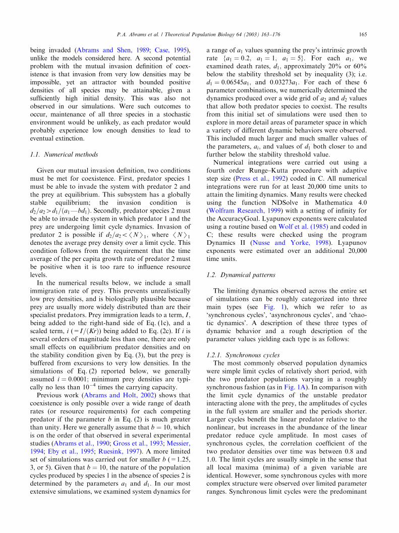
The limiting dynamics observed across the entire setof simulations can be roughly categorized into threemain types (see Fig. 1), which we refer to as‘synchronous cycles’, ‘asynchronous cycles’, and ‘chao-tic dynamics’. A description of these three types ofdynamic behavior and a rough description of theparameter values yielding each type is as follows:

1.2.1. Synchronous cycles

The most commonly observed population dynamicswere simple limit cycles of relatively short period, withthe two predator populations varying in a roughlysynchronous fashion (as in Fig. 1A). In comparison withthe limit cycle dynamics of the unstable predatorinteracting alone with the prey, the amplitudes of cyclesin the full system are smaller and the periods shorter.Larger cycles benefit the linear predator relative to thenonlinear, but increases in the abundance of the linearpredator reduce cycle amplitude. In most cases ofsynchronous cycles, the correlation coefficient of thetwo predator densities over time was between 0.8 and1.0. The limit cycles are usually simple in the sense thatall local maxima (minima) of a given variable areidentical. However, some synchronous cycles with morecomplex structure were observed over limited parameterranges. Synchronous limit cycles were the predominant

ARTICLE IN PRESSP.A. Abrams et al. / Theoretical Population Biology 64 (2003) 163–176 165

type of dynamics observed over the vast majority of{d2; a2} parameter space permitting coexistence whenthe value of d1=a1 was significantly (i.e., on the order of50% or more) below the stability threshold set bycondition (3). For example, when a1 ¼ a2 ¼ 5; synchro-

nous cycles occurred over the entire range of d2

permitting coexistence when d1 was less than 1/2 of itsstability threshold value (d1o0:2045). Synchronouscycles also represent the only type of dynamics observedwhen b is close to 1 or when both d2 and a2 aresufficiently small relative to 1, even if d1=a1 is near thestability threshold. One interpretation of the Arm-strong–McGehee model is that it involves ‘temporalniche partitioning’, in which each species enjoys acompetitive advantage during some time period. Thisis true, but our results show that such niche partitioningdoes not imply temporal displacement in peaks andtroughs in abundance.

1.2.2. Asynchronous cycles

In these relatively long-period cycles, there are phasesof nearly constant prey densities and opposite, nearlymonotonic, changes in the densities of the two predatorspecies (decline in the linear, and increase in thenonlinear predator) during a significant fraction of thecycle period. These periods of gradual replacement ofthe linear predator are characterized by prey densitiesslightly below the replacement level required by thelinear predator, and are followed by brief periods ofcycling accompanied by rapid shifts in the relativeabundances of the two predators. These reversals occurwhen the linear species becomes so rare it can no longerprevent cycles driven by the nonlinear predator. Fig. 1Bis an example of this type of cycle. Asynchronous cyclesare often complex in structure, having several differentlocal maxima in density of each variable over the time-course of a single cycle. The correlation coefficientbetween the densities of the two predators undergoingasynchronous cycles is usually negative; if positive, it isgenerally less than 0.3. However, the dividing linebetween this type of cycle and the synchronous ones isto some extent arbitrary, because the fraction of thecycle during which prey density was relatively constantvaried considerably, as did the constancy of the prey.For later figures, we adopt a somewhat arbitrarycriterion of a negative correlation coefficient of predatordensities for distinguishing asynchronous from synchro-nous cycles. Asynchronous cycles were not observedwhen the value of the parameter b was close to 1, theminimum b for which cycles are possible. The range ofother parameters producing asynchronous cycles in-creases as b increases. Given that b is large, asynchro-nous cycles having very long periods are often observedfor a narrow range of death rates, d2; near the lowerboundary of the range of d2 allowing coexistence. In thiscase, the two predators are very nearly equal in theirprey requirements. Asynchronous cycles with shorterperiods are observed for other, broader ranges ofparameters. Asynchronous cycles appeared to occurover the broadest ranges of parameters when the attackrate of the nonlinear predator, a1; was on the order of 1

ARTICLE IN PRESS

Densities (N1 thick, N2 thin, R dashed)

(A) Synchronous

4960 4970 4980 4990 5000

0.1

0.2

0.3

0.4

0.5

(B) Asynchronous

14200 14400 14600 14800 15000

0.5

1

1.5

2

2.5

(C) Chaotic

4750 4800 4850 4900 4950 5000

0.2

0.4

0.6

0.8

Time

Fig. 1. Examples of the three basic categories of dynamics in the

Armstrong–McGehee model (Eq. (2) with an added resource immigra-

tion rate of i ¼ 0:0001). In all panels, the nonlinear predator (species 1)

is given by the thick solid line, the linear predator (species 2) is given by

the thin solid line, and the resource is the dashed line. Panel 1A is an

example of a synchronous cycle (parameter values are: a1 ¼ a2 ¼ 5;

d1 ¼ 0:327273; d2 ¼ 1:2; b ¼ 10). Panel 1B is an example of an

asynchronous cycle (parameter values are: a1 ¼ a2 ¼ 1; d1 ¼ 0:076;d2 ¼ 0:4; b ¼ 10). Panel 1C is an example of chaotic dynamics

(parameter values are: a1 ¼ a2 ¼ 5; d1 ¼ 0:327273; d2 ¼ 1:7; b ¼ 10).

Note the different scaling of the x- and y-axis in the different panels.

P.A. Abrams et al. / Theoretical Population Biology 64 (2003) 163–176166

or less, given that b was large relative to 1. When theseconditions on a1 and b were satisfied, asynchronouscycles were most common when d1 was relatively closeto its stability threshold value. These conditionsallow the linear predator to maintain stability of theresource population for significant periods of time as itsown population gradually declines, and the populationof the nonlinear predator increases; eventually, theinherent instability of the latter predominates and so ineffect, the system shifts between alternative dynamicaldomains.

1.2.3. Chaotic dynamics

Chaotic dynamics (identified by a positive value of thelargest of the three Lyapunov exponents) producedmore ambiguous correlations between the densities ofthe two species. Chaotic dynamics occurred over asubstantial fraction of parameter space when: (i) thevalue of b in Eq. (2) was relatively large; (ii) the value ofd1 in Eq. (2) was moderately close to the stabilitythreshold given by Eq. (3); (iii) the scaled attack rate (a1)of the nonlinear predator was significantly greater thanunity; and (iv) the prey requirement for zero growth ofspecies 2, d2=a2 (=N2�), was intermediate in the rangeof values allowing coexistence. Chaos was rare or absentif the demographic rates of the linear predator weresufficiently slow relative to the prey (d2; a251). Whena1 ¼ a2 ¼ 5; chaotic dynamics were only observed whend1 was greater than approximately 1/2 of its stabilitythreshold value (d1 ¼ 0:40909). For these values of ai

with b ¼ 10; chaos was absent for d1p0:21; and thebroadest range of d2 values produced chaos when d1 wasbetween approximately 0.28 and 0.38. Fig. 1C is anexample of chaotic dynamics in this system when d1 ¼0:3273 and d2 ¼ 1:7:

Most of the above results can be understood byconsidering the ability of the linear competitor tocontrol the dynamics of the resource while the nonlinearspecies increases to a density where it is able to drivecycles of the prey. Such phases are a key characteristic ofasynchronous cycles. Small demographic rates of thenonlinear species and a value of d1 near the stabilitythreshold both reduce the strength of the destabilizingeffect of the nonlinear species, while large demographicrates of the linear species increase its ability totemporarily stabilize resource densities. These condi-tions lead to asynchronous cycles or chaos. The oppositeconditions increase the relative impact of the nonlinearspecies on resource dynamics, and tend to lead tosynchronized cycles. Nonsynchronous dynamics requirea large half saturation constant (large b); this largelydecouples the demographic rates of the nonlinear speciesfrom resource density over a wide range of resourcedensities. In this case, damped cycles driven by the linearpredator and the prey do not entrain cycles in thenonlinear predator, because the latter experiences little

variation in its per capita growth rate when the resourcefluctuations are modest.

The above classification of dynamics is neithercomplete nor unambiguous. There are a variety ofintermediate cases; for example, chaotic dynamics with avery small positive maximum Lyapunov exponent arisethat appear superficially similar to the asynchronouscycles in Fig. 1B. Another example is roughly asyn-chronous cycles in which the phase of nearly constantprey density is replaced by one in which prey densityfluctuates above and below the prey requirements of thelinear predator. Fig. 2 (see next paragraph) illustratesanother type of dynamics observed for a narrow rangeof parameter values. Nevertheless, most of the observeddynamics could be clearly assigned to one of the abovethree categories.

Alternative attractors were found for small regions ofparameter space. In all cases observed, the twoalternatives were a synchronous limit cycle of smallamplitude and an asynchronous cycle with much largeramplitude fluctuations in densities and a much longerperiod. For some parameter sets, asynchronous cycleswere also observed as long-lasting transients for a rangeof parameters in which the ultimate attractor was asimple synchronous cycle. Such cases were characterizedby having all Lyapunov exponents very close to zero.This occurred for parameters where the linear specieshad a death rate close to the minimum value that wouldallow it to coexist with the nonlinear species. In thesecases, dynamics similar to those shown in Fig. 1B couldpersist for thousands of time units, but would eventuallyresolve into the pattern shown in Fig. 1A. An exampleof an intermediate stage in such a transition is given inFig 2. In this transition period between the two types ofdynamics, there is a slow long-period cycle withnegatively correlated densities of the two predators that

ARTICLE IN PRESS

3400 3600 3800 4000

0.05

0.1

0.15

0.2

Predator densities

Time

Fig. 2. An intermediate stage in the transition between a long-lasting

but transient asynchronous cycle to a synchronous cycle. Parameter

values are: a1 ¼ a2 ¼ 5; d1 ¼ 0:327273; d2 ¼ 0:97; i ¼ 0:0001; b ¼ 10:

The density of predator 1 is given by the upper (dashed) line, and

predator 2 by the lower (solid) line.

P.A. Abrams et al. / Theoretical Population Biology 64 (2003) 163–176 167

is overlain upon a rapid, smaller-amplitude cycle withpositively correlated densities. There are some narrowparameter ranges where the attractor of the system haddynamics similar to those shown in Fig. 2.

Fig. 3 illustrates typical patterns of occurrence ofdifferent dynamics over continuous ranges of theparameters a2 and d2: Given that we restricted theparameter b to large values (b ¼ 10 in most simulations),the type of dynamics depended on the four remainingparameters, a1; a2; d1; and d2: Figs. 3A and B show the

range of dynamics that occur over a grid of potential a2

and d2 values for cases in which a1 is significantly greaterthan 1 (a1 ¼ 5). This grid is shown for two values of d1

that are approximately 0.93 and 0.80 times the stabilitythreshold. Dynamics are classified into the categoriesidentified above. We have used a conservative method ofclassifying cycles as asynchronous cycles based on aperiodic attractor with a negative correlation coefficientbetween the densities of the two predators. In bothFigs. 3A and B, a broad intermediate range of d2

ARTICLE IN PRESS

(A) a1 = 5, d1 = 0.38 (B) a1 = 5, d1 = 0.327273

1.5 2 2.5 3 3.5d2

4

4.5

5

5.5

6

a 2

0.5 1 1.5 2 2.5 3d2

4

4.5

5

5.5

6

a 2

(C) a1 = 1, d1 = 0.076 (D) a1 = 1, d1 = 0.0654545

0.2 0.3 0.4 0.5 0.6 0.7 0.8d2

0.7

0.8

0.9

1

1.1

1.2

1.3

a 2

0.1 0.2 0.3 0.4 0.5 0.6 0.7d2

0.7

0.8

0.9

1

1.1

1.2

1.3

a 2

(E) a1 = 5, d1 = 0.327273

0 0.2 0.4 0.6 0.8 1d2

0

0.2

0.4

0.6

0.8

1

a 2

Fig. 3. Dynamics across a grid of {a2; d2} values for different combinations of a1 and d1: The values of a1 and d1 are given on top of each panel. The

value of b is 10 in all cases. The color-coding of dynamical behaviors is: red-exclusion; blue-chaotic; green-indeterminate (absolute value of all

Lyapunov exponents less than 0.001); white-synchronous cycles; gray-asynchronous cycles. Cycles were classified as synchronous if the correlation

coefficient of predator densities was greater than zero, and asynchronous if the correlation coefficient was less than zero. All simulations used a

common set of initial densities.


produces either asynchronous cycles or chaotic dy-namics. However, the relative sizes and locations ofparameter values producing asynchronous cycles arequite different in the two figures, with asynchronouscycles being more common when d1 is larger. In bothfigures, there is a narrow range of d2 close to theminimum that will allow coexistence, where very long-period asynchronous cycles occur; these generally haveall Lyapunov exponents very close to zero. The effect oflower values of the predator attack rates is illustrated byFigs. 3C and D, in which a1 ¼ a2 ¼ 1: In Figs. 3C andD, d1 is respectively approximately 0.93 and 0.8 timesthe stability threshold (as in Figs. 3A and B). Most ofthe differences between Fig. 3C and D and thecorresponding Figs. 3A and B are the result of thedecrease in a1 rather than a2; comparable figures fora1 ¼ 1 and a2 ¼ 5 are very similar to Figs. 3C and D.The lower value of a1 eliminates most of the chaoticdynamics. When d1 is 93% of its threshold (Fig. 3C),there is a very narrow band of chaos, similar in form toasynchronous cycles, at the boundary between exclusionof the nonlinear predator and coexistence. When d1 is80% of its threshold and the ai are relatively small (Fig.3D), there is a narrow band of chaotic dynamics atintermediate values of d2: In 3C, the majority of thepossible {a2; d2} parameter combinations produce asyn-chronous cycles. This would also be true of Fig. 3D if weused a correlation coefficient of 0.3 as the dividing linebetween synchronous and asynchronous. Some of thepanels in Fig. 3 appear to be characterized byqualitatively different types of dynamics occurring asroughly parallel bands in (a2; d2) space. However, theranges of qualitatively different types of dynamics doeschange with a sufficiently large proportional change inboth a2 and d2; as is shown in Fig. 3E, where both a2

and d2 have been reduced from their values in Fig. 3B sothat d2o0:5: At very low demographic rates of the linearpredator (a2 and d2), synchronous cycles are thepredominant dynamics when coexistence occurs. Valuesof a2 and d2 much larger than 5 (results not shown) tendto make some of the chaotic dynamics more nearlyperiodic; here there are many cases where dynamics aredifficult to classify as chaotic or as asynchronous cyclesbecause of the small magnitude of the maximumLyapunov exponent.

We have not illustrated cases where d1 is considerablybelow the value at which the system becomes stable.Three of our initial sets of parameters assumed that d1 is0.4 times the stability threshold value. For all of these,simple synchronous cycles occur across all of theparameter space where coexistence occurs. This pre-dominance of synchronous cycles characterized allparameter combinations of a1 and d1 where d1 wassubstantially below the stability threshold. We also donot illustrate cases with very large values of both ai anddi: These parameter ranges generally produce more

periodic and fewer chaotic dynamics than do thoseillustrated here, but they also frequently produceextremely low minimum predator densities.

Fig. 4 presents a different cross-section of parameterspace, where a2 and d2 are fixed, and dynamic behaviorsacross a range of a1 and d1 values are illustrated. Theregion of asynchronous or chaotic dynamics is aminority of the range of parameters where the twopredators can coexist in this figure; nevertheless, thisregion constitutes a significant fraction of parameterspace. That fraction decreases when a1 is decreased. Ingeneral, the results from Figs. 3 and 4 support thequalitative comments made above regarding the occur-rence of the three classes of dynamical behaviors acrossthe range of parameter values that permit coexistence.

2. Responses of mean predator densities to altered

demographic parameters

In this section we examine how the mean densities ofthe two competitors are affected by changes in demo-graphic rates. One goal of this exercise is to clarify howcompetition in this model differs from competition inmodels with stable, equilibrial coexistence arising fromclassical niche partitioning. There are a number ofproperties common to models of the latter type, asdescribed in the Introduction. As shown below, theresponses of predator densities to changes in demo-graphic rates are very different in the Armstrong–McGehee model. We again largely confine our numer-ical results to cases in which b ¼ 10; and assume a small

ARTICLE IN PRESS

a2 = 5.0, d2 = 1.5

0.15 0.2 0.25 0.3 0.35 0.4 0.45d1

4

4.5

5

5.5

6

a 1Fig. 4. Dynamics across a grid of {a1; d1} values for a representative

value of a2 and d2 (a2 ¼ 5; d2 ¼ 1:5 with b ¼ 10). Methods and color-

coding are identical to those for Fig. 3.


amount of prey immigration. We measure interspecificeffects by calculating changes in mean densities, becausethis is the best single measure of the impact of theaffected species on other species in the community(Abrams and Roth, 1994a, b; Abrams et al., 1998), andis the measure used in virtually all field studies that havequantified interspecific interactions. Clearly changes inthe pattern of variation can also be important for bothecological and evolutionary questions, but these will notbe pursued here. Mean densities in chaotic systems areinfluenced by the length of the time over which the meanis calculated, but the 104 time unit interval used hereproduced a very close (51% difference) approximationof the mean for much longer periods for most chaoticparameter sets (longer time intervals were used when theperiod of the fluctuation was very long, as in Fig. 1B).

We begin by considering equal proportional changesin both demographic rate parameters, Bi and Di for oneof the two competitors in Eq. (1). This is equivalent toproportional changes in ai and di in Eq. (2), but the

change in Bi also changes the scaling of the density ofpredator i: Thus we will use the unscaled equations toexamine the effects of changes in demographic rates onpopulation densities. Such changes are analogous tochanges in intrinsic growth rates, r; in the two-speciesLotka–Volterra model, in that model they have noimpact on the ultimate densities of either species, andonly determine the speed of approach to equilibrium.An example of the mean densities of both competitors inthe Armstrong–McGehee model is shown as a functionof the demographic rates of the linear predator speciesin Fig. 5. In general, slower dynamics for this speciesimply simpler dynamics of the entire system. At thelowest demographic rates shown, the dynamics aresimple synchronized cycles, and the mean density ofspecies 2 decreases rapidly (and that of species 1increases rapidly) as the demographic rates of species 2are increased. Cycles become more complicated andasynchronous as the demographic scaling factor in-creases above unity. The complicated multimodal

ARTICLE IN PRESS

(A) Mean P 1

1 2 3 4 5 6 7

1.2

1.3

1.4

1.5

1.6

Demographic speed, P2

(B) Mean P2

1 2 3 4 5 6 7

0.08

0.12

0.14

0.16

0.18

Demographic speed, P2

Fig. 5. Population densities of the two predators as a function of the demographic rates of species 2, the linear predator. The baseline parameters

from Eqs. (1) are C1 ¼ C2 ¼ 1; h1 ¼ 10; B1 ¼ B2 ¼ 1; D1 ¼ 0:06; D2 ¼ 0:4; r ¼ 1; K ¼ 1: ‘Demographic speed’ means the scaling factor multiplying

both B2 and D2: Values smaller than 1 result in synchronized limit cycle dynamics, while values equal to or larger than 1 all produce chaotic

dynamics.


pattern of mean densities shown in the figure is theconsequence of changes in the complexity of theasynchronous cycles with increasing demographic speed.In general, qualitative changes in the nature of thepopulation fluctuations as demographic rates shift willcause significant changes in the mean densities of thetwo predators for most parameter values. Fig. 3 showsthat such qualitative shifts are likely to occur frequentlywith proportional changes in the two demographic rateparameters of one or both species. Proportional changesin both a1 and d1 are the only difference between Figs.3B and D, and between Figs. 3A and C; in these cases,slower dynamics of the nonlinear species greatlydecrease on the range of parameters that produce chaos,and increase the range of parameters leading toasynchronous cycles. Faster dynamics of predator 1have the opposite effects. Large proportional decreasesin a2 and d2 cause asynchronous or chaotic dynamics toshift to synchronous limit cycles (Fig. 3E), accompaniedby significant changes in mean predator densities.

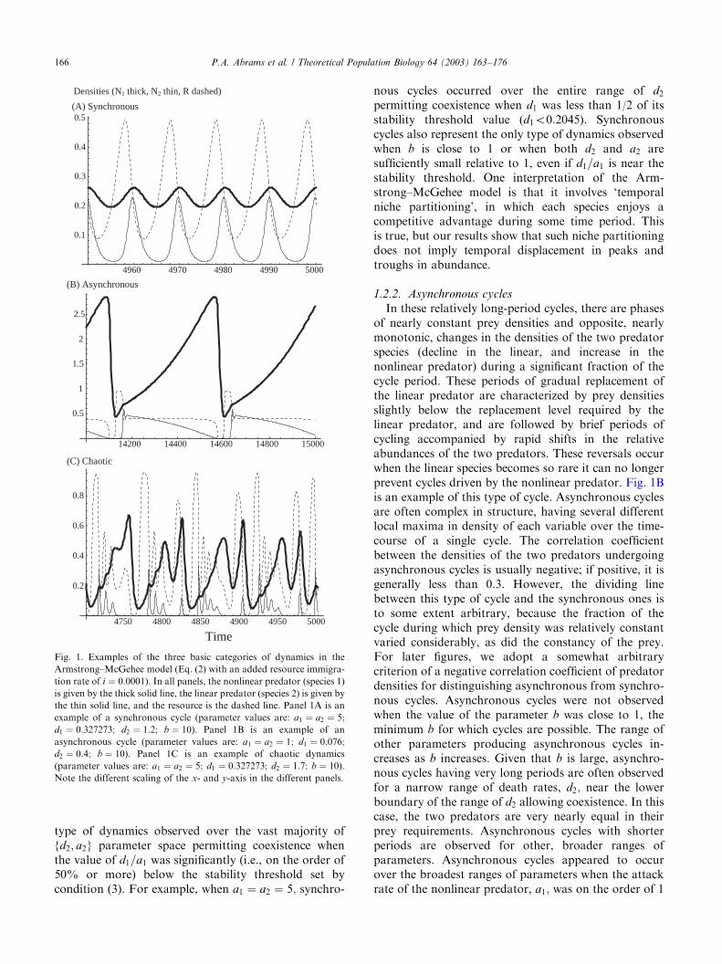
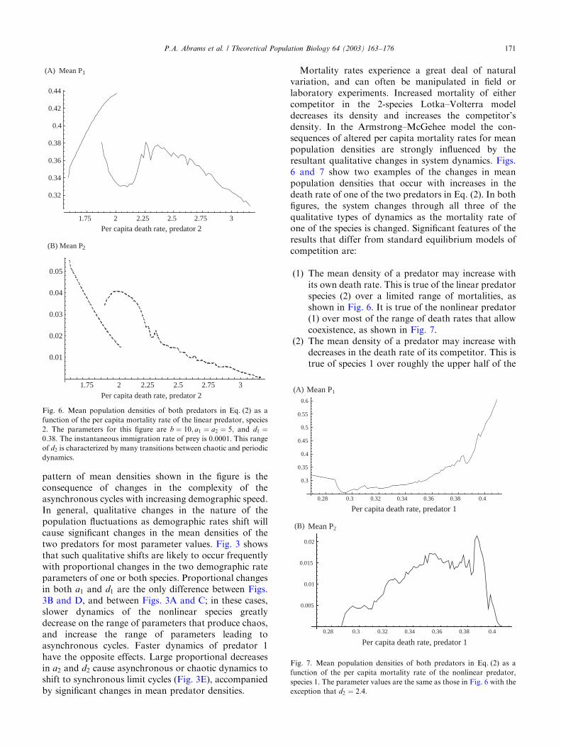
Mortality rates experience a great deal of naturalvariation, and can often be manipulated in field orlaboratory experiments. Increased mortality of eithercompetitor in the 2-species Lotka–Volterra modeldecreases its density and increases the competitor’sdensity. In the Armstrong–McGehee model the con-sequences of altered per capita mortality rates for meanpopulation densities are strongly influenced by theresultant qualitative changes in system dynamics. Figs.6 and 7 show two examples of the changes in meanpopulation densities that occur with increases in thedeath rate of one of the two predators in Eq. (2). In bothfigures, the system changes through all three of thequalitative types of dynamics as the mortality rate ofone of the species is changed. Significant features of theresults that differ from standard equilibrium models ofcompetition are:

(1) The mean density of a predator may increase withits own death rate. This is true of the linear predatorspecies (2) over a limited range of mortalities, asshown in Fig. 6. It is true of the nonlinear predator(1) over most of the range of death rates that allowcoexistence, as shown in Fig. 7.

(2) The mean density of a predator may increase withdecreases in the death rate of its competitor. This istrue of species 1 over roughly the upper half of the

ARTICLE IN PRESS

(A) Mean P1

1.75 2 2.25 2.5 2.75 3

0.32

0.34

0.36

0.38

0.4

0.42

0.44

(B) Mean P2

1.75 2 2.25 2.5 2.75 3

0.01

0.02

0.03

0.04

0.05

Per capita death rate, predator 2


Fig. 6. Mean population densities of both predators in Eq. (2) as a

function of the per capita mortality rate of the linear predator, species

2. The parameters for this figure are b ¼ 10; a1 ¼ a2 ¼ 5; and d1 ¼0:38: The instantaneous immigration rate of prey is 0.0001. This range

of d2 is characterized by many transitions between chaotic and periodic

dynamics.

Mean P1

0.28 0.3 0.32 0.34 0.36 0.38 0.4

0.3

0.35

0.4

0.45

0.5

0.55

0.6

Mean P2

0.28 0.3 0.32 0.34 0.36 0.38 0.4

0.005

0.01

0.015

0.02



(A)

(B)

Fig. 7. Mean population densities of both predators in Eq. (2) as a

function of the per capita mortality rate of the nonlinear predator,

species 1. The parameter values are the same as those in Fig. 6 with the

exception that d2 ¼ 2:4:


range of death rates of its competitor that permitcoexistence (Fig. 6). It should also be noted that themean density of species 1 when alone is approxi-mately given by its density at the right-hand side ofFig. 6 (d2 ¼ 3:2); the graph shows that the presenceof species 2 increases the mean density of species 1for all of the possible range of mortality rates ofspecies 2 that allow coexistence. In Fig. 7, anincrease in species 1 mortality decreases the densityof species 2 over the upper part of the range of percapita mortality rates of species 1 that allowcoexistence. In fact, raising the death rate of species1 actually results in exclusion of species 2 in thisexample, because the system becomes stable at d1 ¼0:409: However, a small additional increase in d1 to0.42 in Fig. 7 would reverse the outcome, andspecies 2 would then exclude 1. This example is alsointeresting because both species increase in responseto increased mortality of species 1 over most of therange of potential death rates.

(3) When there are alternative attractors, the meanpopulation densities of a given predator oftenrespond in opposite directions to changes in oneof the two per capita death rates in the twoattractors (as is true in Fig. 6 over most of therange of mortality rates of predator 2 wherealternative attractors occur).

(4) A change in the mortality rate of one predator thatalters the number of predator species present oftenresults in a discontinuous change in the meandensities of both predators. Although not shown inFig. 6, there are large and abrupt changes in thedensities of both predators when the death rate ofthe linear predator drops to a level where thenonlinear predator is excluded. When d2 decreasesfrom 1.59 to 1.58 in that example, the density ofpredator 2 increases from 0.053 to 0.1364, while thedensity of predator 1 drops from 0.348 to zero.These discontinuous changes in mean densities atthe lower end of the range of d2 that allowscoexistence appear to occur for all of parameterspace yielding coexistence for Eq. (2). In all cases,the linear predator attains a much higher abun-dance when the nonlinear predator is excluded.

Many of these features of the responses of densities tomortality rates can be understood heuristically byconsidering the consequences of altered mortality forthe amplitude of predator–prey cycles. Higher predatormortality decreases the amplitude of limit cycles in thenonlinear subsystem composed of the predator andprey. Higher mortality also results in a relatively slowincrease in the predator’s mean density in this subsystem(Abrams and Roth, 1994a; Abrams et al., 1997). Thelatter effect arises from the fact that mortality actuallyincreases the predator’s density at the equilibrium point,

but the large amplitude cycles reduce the mean growthrate, and therefore density, of the predator. Thepresence of the linear predator dampens these oscilla-tions, and this effect alone would increase the meandensity of the nonlinear predator above its mean densityin isolation. This is why all of the cases where predator 2is present in Fig. 6 have a higher mean density ofpredator 1 than when predator 2 is absent (i.e. atd2 ¼ 3:2). The increase in the mean densities of bothpredators with increased mortality of predator 1 (true ofmost of the range of d1 shown in Fig. 7) is a consequenceof smaller amplitude cycles. Similarly, the decrease inthe density of the nonlinear predator (species 1) withincreasing d2 in Fig. 6 is a consequence of the weakeningeffect of the linear species in damping the preyoscillations driven by the nonlinear predator.

The discontinuities in mean predator density thatoccur (e.g., just beyond the left-hand side of Fig. 6, andat the right-hand side of Fig. 7) result from majorchanges in the amplitude of cycles at those points, withconcomitant change in mean resource density. In Fig. 7,species 2 is excluded when d1 reaches its stabilitythreshold. Which species is excluded when d1 isincreased above the stability threshold given by Eq. (3)depends on the prey requirement for zero growth in thelinear species. Exclusion of the linear species 2 is morelikely if its own prey requirement is relatively high. Theexact requirement for exclusion of species 2 at high d1 asthe result of stabilization of the system from inequality(3) is d2=a24ðb � 1Þ=ð2bÞ:

If the per capita mortality rate of species 1 issufficiently low relative to the stability threshold,complicated and/or chaotic dynamics are typicallyreplaced by simple synchronous cycles; changes in meandensities with altered death rates are in the directionexpected based on the intuitive notion that negativeeffects (i.e., higher mortality) inflicted on one competitorincrease the mean density of its competitors.

Other parameters that could change in this systeminclude immigration rates and prey carrying capacity.Prey immigration tends to be stabilizing, and sogenerally increases dominance of the nonlinear preda-tor. Increasing K is equivalent to proportional increasesin both ai and in b; this environmental change increasesthe amplitude of cycles, and generally increases theabundance of the species with the linear functionalresponse, which benefits more from periods of high preydensity.

3. Dynamics and responses to mortality rates in related

models

The specific system illustrated in Armstrong andMcGehee (1980) (Eq. (1) above) is only one exemplar ofa mechanism that arises in a broad range of models. It is


important to gain insight into how the above resultschange when model components are changed, particu-larly with respect to changes that increase the prob-ability of coexistence of predator species. There are toomany different conceivable modifications of Eq. (1) topermit as thorough an exploration as has been carriedout above. In this section we present preliminary resultsregarding the following modifications: (1) different preygrowth functions; (2) an accelerating rather than a linearfunctional response for the stable predator; (3) immi-gration of one or both predators; (4) a type-2 functionalresponse for both predators; (5) more than one resource.Many other mechanisms producing temporal variationin densities may also alter the responses of competingspecies to environmental change (e.g., Chesson, 1986,1994, 2000), but these will not be discussed here.

A flexible description of prey density-dependence isprovided by the ‘theta-logistic’ (Gilpin and Ayala, 1973)model, where dN=dt ¼ rN½1 � ðN=KÞy: We have car-ried out a number of simulations where y is eithersignificantly larger or smaller than 1. Moderate changesin y do not change the general conclusions reachedabove. Larger values of y increase the range of relativemortalities that allow coexistence (Abrams and Holt,2002). The dynamics observed across a range of deathrates resemble the case of y ¼ 1; with the same threegeneral classes of dynamics identified above. Synchro-nous cycles were observed in all systems when d1 issufficiently lower than its threshold value for stability,regardless of d2: The responses of mean densities toaltered per capita mortality rates were, however,affected by the form of density dependence. Fig. 8shows the responses of the mean predator densities toaltered per capita mortality rates of the linear predatorfor two systems that differ only in their densitydependent exponent, y: The major difference betweenthese and comparable models with y ¼ 1 (logisticgrowth), is that the abrupt jump in mean density whend2 is just large enough to allow the nonlinear predator toexist does not occur at large values of y: This jump ismore pronounced for small values of y than for thelogistic model.

Abrams and Holt (2002) showed that, if the specieswith a linear functional response was replaced by onewith an accelerating functional response, the range ofmortality rates or other parameters allowing coexistence(the ‘coexistence bandwidth’; Armstrong, 1976) wasexpanded. We carried out some numerical analyses ofsuch a model to determine the range of dynamics andresponses to mortality rates. The accelerating functionalresponse strengthens the stabilizing impact of the stablepredator species on the 3-species system. As a result,there was an increase in the range of parameter spacewithin which the stable predator could control the preyfluctuations and produce asynchronous cycles, particu-larly when the death rate of the unstable predator was

relatively close to its stability threshold value. Chaoticdynamics, when they occurred, were generally shifted torelatively low values of the death rate of the stablepredator, within the range allowing coexistence.

Predator immigration may permit the local coex-istence of two or more predator species at significantdensities over a broader range of parameters than forthe models described above, with their closed predatorpopulations. We have explored the dynamics of a modelconsisting of Eq. (1) with constant immigration of allspecies. Low levels of predator immigration do not alterthe general features reported above: the same threecategories of dynamics were observed for approximatelythe same ranges of parameter values. Immigration ofpredator 2 does eliminate some cases of extremely lowdensities of that predator. High immigration of thenonlinear predator reduces the amplitude of its cycles

ARTICLE IN PRESS

(A) θ = 0.5

Mean P1 (solid), P2 (dashed)

0.15 0.2 0.25 0.3 0.35

0.2

0.4

0.6

0.8

1

1.2

(B) θ = 4 Mean P1 (solid), P2 (dashed)

0.15 0.2 0.25 0.3 0.35 0.4 0.45

0.5

1

1.5

2

2.5



Fig. 8. The mean densities of the two predators as functions of the per

capita mortality rate of the linear predator species for two models in

which the prey has y-logistic growth, with y ¼ 0:5 in the top panel and

y ¼ 4 in the bottom panel. Otherwise the model is identical to Eq. (2)

with the following common parameters for both panels: b ¼ 10; a1 ¼a2 ¼ 1; d1 ¼ 0:05: There is no prey immigration.


with the prey, and therefore reduces the range ofparameters over which there can be persistence of alinear predator that does not also have immigration.The responses of mean population densities of bothpredators to an altered immigration rate of one of thepredators is typically very nonlinear. For example,increased immigration of predator 1 in a system whoseother parameters are those given in Fig. 7, often causes adecrease in the mean density of predator 1, untilimmigration is nearly sufficient to cause extinction ofpredator 2. The mean density of predator 2 changes in ahighly nonlinear manner with increasing immigration ofpredator 1 as a consequence of the nonlinear effect ofimmigration on cycle amplitude. Moreover, relativelysmall immigration rates can allow coexistence of three ofmore predator species at significant densities, somethingwhich requires very delicate balancing of parameterswhen there is no immigration (Chesson, 1994; Abramsand Holt, 2002). Thus, in a metapopulation context,there may be local diversities much greater than twopredator species, given predator–prey cycles and differ-ences in the linearity of predator responses to preydensity.

We have also examined models in which each of thetwo predators has a saturating functional response, butdiffer in the half-saturation constant (b in Eq. (2)). Thissystem has previously been studied numerically by Hsuand Hubbell (1978) and Abrams and Holt (2002). Aspointed out in Abrams and Holt (2002), coexistencerequires very precise balancing of parameters when bothspecies have substantial half-saturation constants. Thus,coexistence in this more general model is likely toinvolve significant differences in handling time, suchthat the functional response of one predator is close tolinearity, while the other has a half-saturation constant(b) much greater than unity. These conditions lead todynamics very similar to those that characterize Eq. (1).

There are many other possible models of competingpredators that differ in the linearity of their responses,and undergo predator–prey cycles. For example,Abrams and Holt (2002) consider a case with two preyspecies, and two predators that differ in their relativeconsumption rates of the different prey. Such modelscan exhibit an even wider range of dynamics than do thesystems considered here, but our simulations of cases inwhich there is high similarity between the two predatorsin their relative prey capture rates displayed a range ofdynamics similar to those described for the comparablesingle-resource Armstrong–McGehee system. Their re-sponses to changes in predator parameter values are alsosimilar to the figures presented here.

Models that add random or seasonal variation in oneor more parameters to the basic structure of Eq. (2) havealso been studied. These results will be reported in moredetail elsewhere (Abrams, under review). In most cases,small levels of variation have relatively small effects on

the qualitative form of the dynamics or the responses toparameter values. However, larger amounts of variationcan cause major changes in the parameter rangesallowing coexistence as well as in the dynamics ofspecies when they do coexist (Abrams, unpublishedmanuscript). This is not surprising, given that seasonalvariation in prey growth is capable of producing a widerange of complicated dynamics even in predator–preymodels otherwise characterized by a stable equilibriumpoint (Rinaldi and Muratori, 1993; Abrams, 1997b).

4. Discussion

The models explored here show that competitionbetween cycling species that differ in the linearity oftheir responses differs in many ways from the expecta-tion of stable, Lotka–Volterra systems. Smooth changesin parameter values can cause abrupt transitions in thestability of particular attractors of this dynamicalsystem. One can thus see discontinuous changes inmean population densities with continuous changes inmortality. The phenomenon of abrupt changes indynamical systems with continuous parameter changeis common, and has been reviewed for other ecologicalsystems elsewhere (e.g. May, 1977; Scheffer et al., 2001).However, these sorts of abrupt jumps are not a propertyof familiar two-species models of competition withoutcycles. Changes in the quantitative or qualitative aspectsof population cycling explain the counter-intuitiveresponses of mean densities to changes in mortality.These include the fact that mortality applied to onepredator species can decrease the mean density of itscompetitor, or even lead to its extinction. Other counter-intuitive responses of mean densities to parameter shiftshave been noted in other models of interacting popula-tions (Armstrong and McGehee, 1980; Holt, 1983;Abrams and Roth, 1994a, b; Abrams, 1997a, b; Abramset al., 1997, 1998; Rinaldi and DeFeo, 1999) when thereare sustained fluctuations and when per capita growthrates are nonlinear functions of densities. The currentmodel actually presents a methodological problem forsome population definitions of competition, becauseaddition of the linear predator often increases the meandensity of the nonlinear predator.

Several of the dynamical transitions we have heredocumented should be useful in identifying cases wherethe coexistence-promoting mechanism described heremay be operating. Bifurcations in dynamics have beenuseful in identifying the mechanism of populationregulation in flour beetles (Dennis et al., 2001) and themechanism driving predator–prey cycles in a rotifer-algasystem (Fussmann et al., 2000). Altering the per capitamortality of a species is often possible in both field andlab settings. If the Armstrong–McGehee mechanismpromotes coexistence in a system, our analysis has


identified some characteristic transitions in the dynamicsthat occur, particularly when the mortality rate of thestable species is increased. It may also be possible toslow the population dynamics or reduce the prey-capture rates of one or both predators in someexperimental setting (e.g. Luckinbill, 1973); thesemanipulations are also expected to lead to characteristictransitions between different types of dynamics.

The three broad classes of dynamics observed for thesimple Armstrong–McGehee (1980) model also arise ina variety of related models that share the same basicmechanism of coexistence. The asynchronous type ofcycles are particularly significant, because they suggestthat short-term observations may often give a highlymisleading picture of the long-term behavior of systemsof cycling competitors. The period of gradual replace-ment of the stable predator by the unstable one may lastmany generations, and give an impression of ultimatecompetitive exclusion. However, the relative abundancesof the two species can eventually be reversed in a veryshort time span. Although simple limit cycles withpositively correlated predator populations occur overthe largest area of parameter space, this does not meanthat such cycles in fact represent the most commondynamic pattern in natural systems exhibiting thismechanism of coexistence. Systems in which theunstable predator has a death rate close to the stabilitythreshold are more likely to avoid stochastic extinctionsthan are systems with lower predator mortality rates.Mortality rates near the threshold are in turn associatedwith a high probability of chaotic dynamics, complexlimit cycles, or alternative attractors. Although complexdynamics have been described for nonlinear consumer–resource models of competition (Vandermeer, 1993),very little modeling of competition considers thepossibility of cycling, let alone the consequences of thechanges in cycling that are caused by changes in aparameter of the competing species.

Finally, it should be noted that many naturalpopulations that are harvested are themselves predatorsin food webs, which are likely to display unstabledynamics. The changes in death rates explored abovecan be broadly interpreted as changes in harvestingrates. Our results suggest that one could be lulled into afalse sense of security because a focal species maintainshigh average abundance (or even increases) as its harvestincreases (see also Abrams, 2002).

Acknowledgments

An operating grant from the Natural Sciences andEngineering Research Council of Canada and a fellow-ship from the J.S. Guggenheim Foundation providedfinancial support to PAA. RDH acknowledges supportfrom the National Science Foundation (USA) and the

University of Florida Foundation. CEB was supportedby an Ontario Graduate Scholarship. We are greatlyindebted to the National Center for Ecological Analysisand Synthesis for sponsoring the working group oncompetition theory, which provided the intellectualimpetus for this work. NCEAS is supported by NSF(Grant #DEB-0072909), the University of California,and UC Santa Barbara.

References

Abrams, P.A., 1997a. Evolutionary responses of foraging-related

traits in unstable predator–prey systems. Evol. Ecol. 11,

673–686.

Abrams, P.A., 1997b. Variability and adaptive behavior; implications

for interactions between stream organisms. J. N. Am. Benth. Soc.

16, 358–374.

Abrams, P.A., 2002. Will small population sizes warn us of impending

extinctions? Am. Nat. 160, 293–305.

Abrams, P.A., Hill, C., Elmgren, R., 1990. The functional response of

the predatory polychaete, Harmothoe sarsi to the amphipod,

Pontoporeia affinis. Oikos 59, 261–269.

Abrams, P.A., Holt, R.D., 2002. The impact of consumer–resource

cycles on the coexistence of competing consumers. Theor. Popul.

Biol. 62, 281–296.

Abrams, P.A., Holt, R.D., Roth, J.D., 1998. Shared predation when

populations cycle. Ecology 79, 201–212.

Abrams, P.A., Namba, T., Mimura, M., Roth, J.D., 1997. Comment

on Abrams and Roth: the relationship between productivity and

population densities in cycling predator–prey systems. Evol. Ecol.

11, 371–373.

Abrams, P.A., Roth, J.D., 1994a. The responses of unstable food

chains to enrichment. Evol. Ecol. 8, 150–171.

Abrams, P.A., Roth, J.D., 1994b. The effects of enrichment on three-

species food chains with nonlinear functional responses. Ecology

75, 1118–1130.

Abrams, P.A., Shen, L., 1989. Population dynamics of systems with

consumers that maintain a constant ratio of intake rates of two

resources. Theor. Popul. Biol. 35, 51–89.

Armstrong, R.A., 1976. Fugitive species: experiments with fungi and

some theoretical considerations. Ecology 57, 953–963.

Armstrong, R.A., McGehee, R., 1976a. Coexistence of two competi-

tors on one resource. J. Theor. Biol. 56, 499–502.

Armstrong, R.A., McGehee, R., 1976b. Coexistence of species

competing for shared resources. Theor. Popul. Biol. 9, 317–328.

Armstrong, R.A., McGehee, R., 1980. Competitive exclusion. Am.

Nat. 115, 151–170.

Case, T.J., 1995. Surprising behavior from a familiar model and

implications for competition theory. Am. Nat. 146, 961–966.

Chesson, P., 1986. Environmental variation and the coexistence of

species. In: Diamond, J.M., Case, T.J. (Eds.), Community Ecology.

Harper and Row, New York, pp. 240–256.

Chesson, P., 1994. Multispecies competition in variable environments.

Theor. Popul. Biol. 45, 227–276.

Chesson, P., 2000. Mechanisms of maintenance of species diversity.

Ann. Rev. Ecol. Systems 31, 343–366.

Dennis, B., Desharnais, R.A., Cushing, J.M., et al., 2001. Estimating

chaos and complex dynamics in an insect population. Ecol.

Monogr. 71, 277–303.

Eby, L.A., Rudstam, L.G., Kitchell, J.F., 1995. Predator responses

to prey population dynamics-an empirical analysis based on

lake trout growth rates. Can. J. Fish. Aquat. Sci. 52,

1564–1571.

ARTICLE IN PRESSP.A. Abrams et al. / Theoretical Population Biology 64 (2003) 163–176 175

Ellner, S.P., Turchin, P., 1995. Chaos in a noisy world; new

methods and evidence from time-series analysis. Am. Nat. 145,

343–375.

Fussmann, G.F., Ellner, S.P., Shertzer, K.W., 2000. Crossing

the hopf bifurcation in a live predator–prey system. Science 290,

1358–1360.

Gilpin, M.E., Ayala, F.J., 1973. Global models of growth and

competition. Proc. Natl. Acad. Sci. (USA) 70, 3590–3593.

Gross, J.E., Shipley, L.A., Hobbs, N.T., Spalinger, D.E., Wunder,

B.A., 1993. Functional response of herbivores in food-concentrated

patches: tests of a mechanistic model. Ecology 74, 778–791.

Holt, R.D., 1983. Immigration and the dynamics of peripheral

populations. In: Miyata, K., Rhodin, A. (Eds.), Advances in

Herpetology and Evolutionary Biology. Harvard University Press,

Cambridge, pp. 680–694.

Hsu, S.B, Hubbell, S.P., Waltman, P., 1978. A contribution to the

theory of competing predators. Ecol. Monog. 48, 337–349.

Kendall, B.E., Predergast, J., Bj^rnstad, O., 1998. The macroecology

of population dynamics: taxonomic and biogeographic patterns of

population cycles. Ecol. Lett. 1, 160–164.

Koch, A.L., 1974. Competitive coexistence of two predators utilizing

the same prey under constant environmental conditions. J. Theor.

Biol. 44, 387–395.

Luckinbill, L.S., 1973. Coexistence in laboratory populations of

Paramecium aurelia and its predator Didinium nasutum. Ecology

54, 1320–1327.

May, R.M., 1977. Thresholds and breakpoints in ecosystems with a

multiplicity of stable states. Nature 269, 471–477.

McGehee, R., Armstrong, R.A., 1977. Some mathematical problems

concerning the ecological principle of competitive exclusion. J.

Differential Equations 29, 214–234.

Messier, F., 1994. Ungulate population models with predation: a case

study with the North American Moose. Ecology 75, 478–488.

Nusse, H.E., Yorke, J.A., 1998. Dynamics: Numerical Explorations,

2nd Edition. Springer, New York.

Press, W.H., Teukolsky, S.A., Vetterling, W.T., Flannery, B.P., 1992.

Numerical Recipes in C. Cambridge University Press, Cambridge.

Rinaldi, S., DeFeo, O., 1999. Top-predator abundance and chaos in

tritrophic food chains. Ecol. Lett. 2, 6–10.

Rinaldi, S., Muratori, S., 1993. Conditioned chaos in seasonally

perburbed predator–prey models. Ecol. Model 69, 79–97.

Rosenzweig, M.L., MacArthur, R.H., 1963. Graphical representation

and stability conditions of predator–prey interactions. Am. Nat.

97, 209–223.

Ruesink, J.L., 1997. Variation in per capita interaction strength:

thresholds due to nonlinear dynamics and nonequilibrium condi-

tions. Proc. Natl. Acad. Sci. (USA) 95, 6843–6847.

Scheffer, M., Carpenter, S., Foley, J.A., Folke, C., Walker, B., 2001.

Catastrophic shifts in ecosystems. Nature 413, 591–596.

Vandermeer, J.H., 1993. Loose coupling of predator–prey cycles:

entrainment, chaos, and intermittency in the classic MacArthur

consumer–resource equations. Am. Nat. 141, 687–716.

Wolf, A., Swift, J.B., Swinney, H.L., Vastano, J.A., 1985. Determining

Lyapunov exponents from a time series. Physica D 16, 285–317.

Wolfram Research, 1999. Mathematica 4.0. Wolfram Research,

Champaign, IL.


Dynamics and responses to mortality rates ofcompeting ... · Dynamics and responses to mortality...

Documents

Transcript of Dynamics and responses to mortality rates ofcompeting ... · Dynamics and responses to mortality...