Dynamics and Control of Multibody Systems

1

Dynamics and Control of Multibody Systems

Marek Vondrak1, Leonid Sigal2 and Odest Chadwicke Jenkins1

1Brown University, 2Univesity of Toronto

1U.S.A., 2Canada

1. Introduction

Over the past decade, physics-based simulation has become a key enabling technology for

variety of applications. It has taken a front seat role in computer games, animation of virtual

worlds and robotic simulation. New applications are still emerging and physics is becoming

an integral part of many new technologies that might have been thought of not being

directly related to physics. For example, physics has been recently used to explain and

recover the motion of the subject from video (Vondrak et al., 2008). Unfortunately, despite

the availability of various simulation packages, the level of expertise required to use

physical simulation correctly is quite high. The goal of this chapter is thus to establish

sufficiently strong grounds that would allow the reader to not only understand and use

existing simulation packages properly but also to implement their own solutions if

necessary. We choose to model world as a set of constrained rigid bodies as this is the most

commonly used approximation to real world physics and such a model is able to deliver

predictable high quality results in real time. To make sure bodies, affected by various forces,

move as desired, a mechanism for controlling motion through the use of constraints is

introduced. We then apply the approach to the problem of physics-based animation

(control) of humanoid characters.

We start with a review of unconstrained rigid body dynamics and introduce the basic

concepts like body mass properties, state parameterization and equations of motion. The

derivations will follow (Baraff et al., 1997) and (Erleben, 2002), using notation from (Baraff,

1996). For background information, we recommend reading (Eberly, 2003; Thornton et al.,

2003; Bourg, 2002). We then move to Lagrangian constrained rigid body dynamics and show

how constraints on body accelerations, velocities or positions can be modeled and

incorporated into simpler unconstrained rigid body dynamics. Various kinds of constraints

are discussed, including equality constraints (required for the implementation of “joint

motors”), inequality constraints (used for the implementation of “joint angle limits”) and

bounded equality constraints (used for implementation of motors capable of generating

limited motor forces). We then reduce the problem of solving for constraint forces to the

problem of solving linear complementarity problems. Finally, we show how this method

can be used to enforce body non-penetration and implement a contact model, (Trinkle et al.,

1997; Kawachi et al., 1997). Source: Motion Control, Book edited by: Federico Casolo,

ISBN 978-953-7619-55-8, pp. 580, January 2010, INTECH, Croatia, downloaded from SCIYO.COM

www.intechopen.com

Motion Control 2

Lastly, we illustrate how before mentioned constraints can be used to implement composite articulated bodies and how these bodies can be actuated by generating appropriate motor torques at joints, following (Kokkevis, 2004). Various kinds of convenient joint parameterizations with different degrees of freedom, together with options for their actuation, are discussed.

Fig. 1. Examples of constrained rigid body systems. Constraints glue bodies together at designated points, actuate the structures or enforce non-penetration.

1.1 Related work

While physical simulation is conceptually well understood, control of articulated high

degree of freedom bodies (or characters) remains a challenging problem. On the simulation

side there currently exist a number of commercial and open source engines that deliver

robust and computationaly efficient performance (e.g., Crisis, Havoc, Newton, Open

Dynamics Engine (ODE), PhysX). Quantitative analysis of performance among some of

these and other popular choices are discussed in (Boeing et al., 2007). However, control over

the motion of characters within these simulators is still very limited. Those packages that do

provide means for building user defined dynamic controllers (e.g., Euphoria by

NaturalMotion and Dynamic Controller Toolbox (Shapiro et al., 2007)) still lack fidelity and

ability to model stylistic variations that are important for producing realistic motions.

In this chapter, we describe trajectory-based control (either in terms of joint angles or rigidly

attached points) implemented in the form of constraints. This type of the control is simple,

general, stable, and is available (or easy to implement) within any simulator environment

that supports constraints (e.g., Crisis, ODE, Newton). That said, other control strategies have

also been proposed and are applicable for appropriate domains and tasks. For example,

where modeling of high fidelity trajectories is hard, one can resort to sparse set of key-poses

with proportional derivative (PD) control (Hodgins et al., 1995); such controllers can

produce very stable motions (e.g., human gait (Yin et al., 2007)) but often look artificial or

robotic. Locomotion controllers with stable limit cycle behavior are popular and appealing

www.intechopen.com

Dynamics and Control of Multibody Systems 3

choices for various forms of cyclic gates (Laszlo et al, 1996); particularly in the robotics and

biomechanics communities (Goswami et al., 1996).

At least in part the challenges in control stem from the high dimensionality of the control

space. To that end few approaches have attempted to learn low-dimensional controllers

through optimization (Safonova et al., 2004). Other optimization-based techniques are also

popular, but often require initial motion (Liu et al., 2005) or existing controller (Yin et al.,

2008) for adaptation to new environmental conditions or execution speed (McCann et al.,

2006). Furthermore, because it is unlikely that a single controller can produce complex

motions of interest, approaches that focus on building composable controllers (Faloutsos et

al., 2001) have also been explored. Alternatively, controllers that attempt to control high

degree-of-freedom motions using task-based formulations, that allow decoupling and

composing of controls required to complete a particular task (e.g., maintain balance) from

controls required to actuate redundant degrees of freedom with respect to the task, are also

appealing (Abe et al., 2006). In robotics such strategies are known as operational space

control (Khatib, 1987; Nakamura et al., 1987).

Here we discuss and describe trajectory-based control that we believe to strike a balance between the complexity and effectiveness in instances where desired motion trajectories are available or easy to obtain. Such control has been illustrated to be effective in the emerging applications, such as tracking of human motion from video (Vondrak et al., 2008).

2. Rigid body dynamics

Rigid bodies are solid structures that move in response to external forces exerted on them. They are characterized by mass density functions describing their volumes (“mass properties”), positions and orientations (“position information”) in the world space and their time derivatives (“velocity information”).

2.1 Body space, mass properties, position, orientation

Properties of rigid bodies are derived from an assumption that rigid bodies can be modeled as particle systems consisting of a large (infinite) number of particles constrained to remain at the same relative positions in the body spaces. Internal spatial interaction forces prevent bodies from changing their shapes and so as a result, any rigid body can only translate or rotate with respect to a fixed world frame of reference. This allows one to associate local coordinate frames with the bodies and define their shapes/volumes in terms of local body spaces that map to the world reference frame using rigid transformations. We describe a volume of a rigid body by a mass density function 貢: 三戴介三袋 that determines

the body’s mass distribution over points 堅王長 in the body space. The density function is non-zero for points forming the body’s shape and zero elsewhere and its moments characterize the body’s response to the exerted forces. We are namely interested in total mass 兼噺完貢岫堅王長岻 d堅王長, center of mass 堅王頂陳長噺完追王弐諦岫追王弐岻暢 d堅王長, principal moments of inertia 荊掴掴噺完岾盤堅王槻長匪態髪岫堅王佃長岻態匪貢岫堅王長岻 d堅王長, 荊槻槻噺完岫岫堅王掴長岻態髪岫堅王佃長岻態岻貢岫堅王長岻 d堅王長, 荊佃佃噺完岾岫堅王掴長岻態髪盤堅王槻長匪態峇貢岫堅王長岻 d堅王長 and

products of inertia 荊掴槻噺完盤堅王掴長堅王槻長匪貢岫堅王長岻 d堅王長, 荊掴佃噺完岫堅王掴長堅王佃長岻貢岫堅王長岻 d堅王長, 荊槻佃噺完盤堅王槻長堅王佃長匪貢岫堅王長岻 d堅王長

that we record into inertia matrix

www.intechopen.com

Motion Control 4

荊長墜鳥槻噺嵜荊掴掴伐荊掴槻伐荊掴佃伐荊掴槻荊槻槻伐荊槻佃伐荊掴佃伐荊槻佃荊佃佃崟. To place a rigid body’s volume in the world, we need to know the mapping from the body

space to the world space. For that, we assume that the body’s center of mass lies at the origin of

the body space, 堅王頂陳長噺ど屎王, and construct a mapping 岷迎, 捲王峅 so that a point 喧王長 in the body space

will get mapped to the world space point 喧王 by applying a rotation 迎, represented by a ぬ抜ぬ

rotation matrix mapping body space axes to the world space axes (orientation of the body in

the world space), followed by applying a translation 捲王 that corresponds to the world space

position of the body’s center of mass (position of the body in the world space), 喧王噺迎糾喧王長髪捲王.

2.2 Velocity

Having placed the body in the world coordinate frame, we would like to characterize the motion of this body over time. To do so we need to compute time derivatives of the position

and orientation of the body, i.e. 擢擢痛岷迎, 捲王峅. We decompose instantaneous motion over

infinitesimally short time periods to the translational (linear) motion of the body’s center of mass and a rotational (angular) motion of the body’s volume. We first define linear velocity 懸王噺捲王岌 as the time derivative of the rigid body’s position 捲王, characterizing the instantaneous linear motion and describing the direction and speed of the body translation. Next, we describe the rotational motion as a rotation about a time varying axis that passes through the center of mass. We define angular velocity 降屎屎王 as a world-space vector whose direction describes the instantaneous rotation axis and whose magnitude [堅欠穴糾嫌貸怠] defines the instantaneous rotation speed. Linear and angular velocities are related such that they can describe velocities of arbitrary points or vectors attached to the body. For example, if 堅王噺喧王伐捲王 is a vector between the point on the body, 喧王, the center of mass of the body, 捲王,

then 堅王岌噺降屎屎王抜堅王 and 喧王岌噺懸王髪降屎屎王抜堅王. This can be used to derive a formula for 迎岌 that says 迎岌噺降屎屎王茅糾迎, where 降屎屎王茅 is a “cross-product matrix” such that 降屎屎王茅糾堅王噺降屎屎王抜堅王. It is worth noting that because 喧王 is fixed in the body centric coordinate frame, so is the vector 堅王.

Fig. 2. Illustration of the two constrained bodies in motion.

繋王岫喧王岻

酵王岾喧王, 繋王岫喧王岻峇

Body B

喧王喋

喧王X

Z

Y 岷迎凋, 捲王凋峅

Body A

系王椎岫圏王凋, 圏王喋岻柑噺喧王喋伐喧王凋噺ど屎王樺三戴

喧王凋

Ball-and-Socket Joint:

捲王凋

www.intechopen.com


2.3 Force

From previous section we have 擢擢痛岷迎, 捲王峅噺岷降屎屎王茅糾迎, 懸王峅 relating changes of the position and

orientation to the values of the body’s linear and angular velocities. Now, we would like to characterize how the linear and angular velocities of a rigid body change in response to forces exerted on the body. Intuitively, these changes should depend on the location where the force is applied as well as mass distribution over the body volume. So we need to know not only the directions and magnitudes of the exerted forces, but also the points at which these forces are applied.

To capture the effects for a single force 繋王岫喧王岻 acting at a world space point 喧王, we define a

force-torque pair 峙繋王岫喧王岻, 酵王岾喧王, 繋王岫喧王岻峇峩, where 酵王岾喧王, 繋王岫喧王岻峇噺岫喧王伐捲王岻抜繋王岫喧王岻 is the torque due to

the force 繋王岫喧王岻. The torque can be imagined as a scale of the angular velocity 降屎屎王 that the rigid

body would gain if 繋王岫喧王岻 was the only force acting on the body and the force was exerted at 喧王. To capture the overall effects of all force-torque pairs 範繋王沈 , 酵王沈飯 due to all forces acting on the body, it is sufficient to maintain only the corresponding aggregate statistics: total force 繋王担誰担叩狸噺 ∑ F屎王辿辿 and total torque 酵王痛墜痛銚鎮噺 ∑ 酵王沈沈 about the center of mass of the body, 捲王 . Now, we express the body’s linear and angular velocities in the form of linear and angular momentums whose instantaneous changes can be directly related to the values of the total forces and torques acting on the body. The reason for doing so is that it is actually the momentums that remain unchanged when no forces act on the body, not the velocities. We

define linear momentum 鶏屎王噺兼糾懸王 and angular momentum 詣屎王噺荊糾降屎屎王 where 荊噺迎糾荊長墜鳥槻糾迎脹.

The relation between the velocity and force information is then given by derivatives of

linear and angular momentum with respect to time, 鶏屎王岌噺繋王痛墜痛銚鎮 and 詣屎王岌噺酵王痛墜痛銚鎮. 2.4 Equations of motion

We are now ready to present complete equations describing motion of a set of rigid bodies in Newtonian dynamics under the effect of forces. The equations are first order ordinary differential equations (ODEs). To simulate the system, one has to numerically integrate the equations of motion, which can be done by using standard numerical ODE solvers. We explore several formulations of the equations of motion below.

2.4.1 Momentum form

We start with the momentum form that makes the linear and angular momentum a part of a rigid body’s state and builds directly upon the concepts presented in earlier sections. To make the body’s state complete, only the position and orientation information has to be

added to the state. Therefore, the state is described by a vector 検王, 検王噺盤捲王, 迎, 鶏屎王, 詣屎王匪, where 捲王 is

the position of the body’s center of mass, 迎 is the orientation of the body and 鶏屎王 and 詣屎王 are the body’s linear and angular momentums. The equation of motion for the rigid body in the

momentum form is then given by 擢槻屎王擢痛噺岫懸王, 降屎屎王茅糾迎, 繋王痛墜痛銚鎮 , 酵王痛墜痛銚鎮岻, where 繋王痛墜痛銚鎮 and 酵王痛墜痛銚鎮 are the

total external force and torque exerted on the body and 懸王 and 降屎屎王 are auxiliary quantities

derived from the state vector 検王, 懸王噺兼貸怠糾鶏屎王, 荊噺迎糾荊長墜鳥槻糾迎脹 , 荊貸怠噺迎糾荊長墜鳥槻貸怠糾迎脹 , 降屎屎王噺荊貸怠糾詣屎王.

If there are 券 rigid bodies in the system, the individual ODE equations are combined into a single ODE by concatenating the body states 検王怠, 橋 , 検王津 into a single state vector 検王噺岫検王怠, 橋 , 検王津岻 and letting

擢槻屎王擢痛噺岾擢槻屎王迭擢痛 , 橋 , 擢槻屎王韮擢痛峇.

www.intechopen.com

Motion Control 6

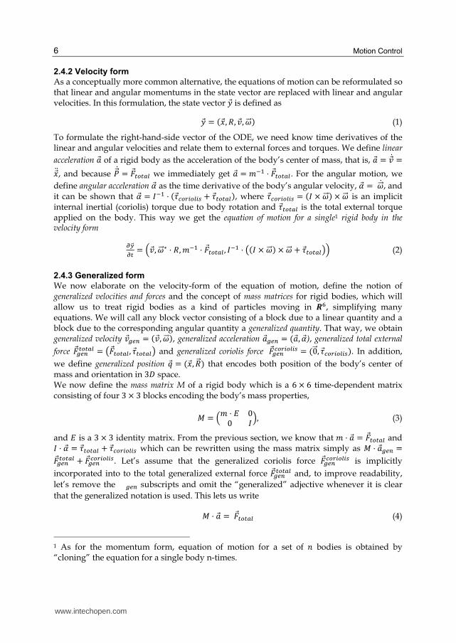
2.4.2 Velocity form

As a conceptually more common alternative, the equations of motion can be reformulated so that linear and angular momentums in the state vector are replaced with linear and angular velocities. In this formulation, the state vector 検王 is defined as

検王噺岫捲王, 迎, 懸王, 降屎屎王岻 (1)

To formulate the right-hand-side vector of the ODE, we need know time derivatives of the linear and angular velocities and relate them to external forces and torques. We define linear

acceleration 欠王 of a rigid body as the acceleration of the body’s center of mass, that is, 欠王噺懸王岌噺捲王岑 , and because 鶏屎王岌噺繋王痛墜痛銚鎮 we immediately get 欠王噺兼貸怠糾繋王痛墜痛銚鎮. For the angular motion, we

define angular acceleration 糠王 as the time derivative of the body’s angular velocity, 糠王噺降屎屎王岌 , and it can be shown that 糠王噺荊貸怠糾岫酵王頂墜追沈墜鎮沈鎚髪酵王痛墜痛銚鎮岻, where 酵王頂墜追沈墜鎮沈鎚噺岫荊抜降屎屎王岻抜降屎屎王 is an implicit internal inertial (coriolis) torque due to body rotation and 酵王痛墜痛銚鎮 is the total external torque applied on the body. This way we get the equation of motion for a single1 rigid body in the velocity form

擢槻屎王擢痛噺岾懸王, 降屎屎王茅糾迎, 兼貸怠糾繋王痛墜痛銚鎮 , 荊貸怠糾盤岫荊抜降屎屎王岻抜降屎屎王髪酵王痛墜痛銚鎮匪峇 (2)

2.4.3 Generalized form

We now elaborate on the velocity-form of the equation of motion, define the notion of generalized velocities and forces and the concept of mass matrices for rigid bodies, which will allow us to treat rigid bodies as a kind of particles moving in 三滞, simplifying many equations. We will call any block vector consisting of a block due to a linear quantity and a block due to the corresponding angular quantity a generalized quantity. That way, we obtain generalized velocity 懸王直勅津噺岫懸王, 降屎屎王岻, generalized acceleration 欠王直勅津噺岫欠王, 糠王), generalized total external

force 繋王直勅津痛墜痛銚鎮噺盤繋王痛墜痛銚鎮 , 酵王痛墜痛銚鎮匪 and generalized coriolis force 繋王直勅津頂墜追沈墜鎮沈鎚噺岫ど屎王, 酵王頂墜追沈墜鎮沈鎚岻. In addition,

we define generalized position 圏王噺岫捲王, 迎屎王岻 that encodes both position of the body’s center of mass and orientation in ぬ経 space. We now define the mass matrix M of a rigid body which is a は抜は time-dependent matrix consisting of four ぬ抜ぬ blocks encoding the body’s mass properties,

警噺岾兼糾継どど荊峇, (3)

and 継 is a ぬ抜ぬ identity matrix. From the previous section, we know that 兼糾欠王噺繋王痛墜痛銚鎮 and 荊糾糠王噺酵王痛墜痛銚鎮髪酵王頂墜追沈墜鎮沈鎚 which can be rewritten using the mass matrix simply as 警糾欠王直勅津噺繋王直勅津痛墜痛銚鎮髪繋王直勅津頂墜追沈墜鎮沈鎚. Let’s assume that the generalized coriolis force 繋王直勅津頂墜追沈墜鎮沈鎚 is implicitly

incorporated into to the total generalized external force 繋王直勅津痛墜痛銚鎮 and, to improve readability,

let’s remove the 直勅津 subscripts and omit the “generalized” adjective whenever it is clear

that the generalized notation is used. This lets us write

警糾欠王噺繋王痛墜痛銚鎮 (4)

1 As for the momentum form, equation of motion for a set of 券 bodies is obtained by “cloning” the equation for a single body n-times.

www.intechopen.com


which yields a relation between the total force 繋王痛墜痛銚鎮 and the total acceleration 欠王. Because the

relation is linear, this equation also holds for any force 繋王 acting on the body and the

corresponding acceleration 欠王噺警貸怠糾繋王 the body would gain in response to the application of 繋王2. The relation resembles Newton’s Second Law for particles and rigid bodies can thus be imagined as special particles with time-varying masses 警 that move in 三滞. 3. Constraints

One of the challenges one has to face in physical simulation is how to generate appropriate forces so that rigid bodies would move as desired. Instead of trying to generate these forces directly, we describe desired motion in terms of motion constraints on accelerations, velocities or positions of rigid bodies and then use constraint solver to solve for the forces. We still use the same equations of motion (and numerical solvers) to drive our bodies like before, but this time, we introduce constraint forces that implicitly act on constrained bodies so that given motion constraints are enforced. We study the approach of Lagrange multiplier method that handles each constraint in the same uniform way and allows to combine constraints automatically. Examples of constrained rigid bodies are given in Fig. 1. In general, the motion constraint on the position or orientation of a body will subsequently result in the constraints on its velocity and acceleration (to ensure that there is no velocity or acceleration in the constrained direction, leading to violation of constraint after integration of the equations of motion); similarly a constraint on velocity will impose a constraint on the acceletation. We will discuss these implications in the following section. A first-order rigid body dynamics with impulsive formulation of forces (discussed in Section 3.3.1) allows one to ignore the acceleration constraints in favor of simplicity, but at expense of inability to support higher-order integration schemes.

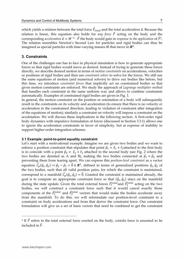
3.1 Example: point-to-point equality constraint

Let’s start with a motivational example. Imagine we are given two bodies and we want to enforce a position constraint that stipulates that point 喧王怠噺捲王怠髪堅王怠attached to the first body is to coincide with a point 喧王態噺捲王態髪堅王態 attached to the second body (see Fig. 2 where the two bodies are denoted as A and B), making the two bodies connected at 喧王怠噺喧王態 and preventing them from tearing apart. We can express this position-level constraint as a vector

equation 系王椎岫圏王怠, 圏王態岻柑噺喧王態伐喧王怠噺ど屎王樺三戴, defined in terms of generalized positions 圏王怠, 圏王態 of

the two bodies, such that all valid position pairs, for which the constraint is maintained,

correspond to a manifold 系王椎岫圏王怠, 圏王態岻噺ど屎王. Granted the constraint is maintained already, the

goal is to compute an appropriate constraint force so that 岫圏王怠, 圏王態岻 stays on the manifold

during the state update. Given the total external forces 繋王怠痛墜痛銚鎮and 繋王態痛墜痛銚鎮 acting on the two bodies, we will construct a constraint force such that it would cancel exactly those

components of the 繋王怠痛墜痛銚鎮 and 繋王態痛墜痛銚鎮 vectors that would make the bodies accelerate away from the manifold. To do this, we will reformulate our position-level constraint to a constraint on body accelerations and from that derive the constraint force. Our constraint formulation will give us a set of basis vectors that need be combined to get the constraint

2 If 繋王 refers to the total external force exerted on the body, coriolis force is assumed to be

included in 繋王.

www.intechopen.com

Motion Control 8

force. Appropriate coefficients of this combination are computed by solving a system of linear equations. Let’s assume that at the current time instant the bodies are positioned so that the constraint

is maintained, that is, 系王椎噺ど屎王. To make sure the constraint will also be maintained in the

future, we have to enforce 系王岌椎噺ど屎王. Let’s have a look at what 系王岌椎 looks like, 系王椎岌噺擢擢痛岫喧王態伐喧王怠岻噺擢擢痛岫捲王態髪堅王態伐捲王怠伐堅王怠岻噺捲王岌態髪降屎屎王態抜堅王態伐捲王岌怠伐降屎屎王怠抜堅王怠噺捲王岌態伐堅王態抜降屎屎王態伐捲王岌怠髪堅王怠抜降屎屎王怠噺捲王岌態伐堅王態茅糾降屎屎王態伐捲王岌怠髪堅王怠茅糾降屎屎王怠噺岫伐継堅王怠茅岻糾懸王怠髪岫継伐堅王態茅岻糾懸王態噺岫伐継堅王怠茅継伐堅王態茅岻糾磐懸王怠懸王態卑噺岫蛍怠蛍態岻糾磐懸王怠懸王態卑, where 蛍怠 and 蛍態 are ぬ抜は matrices called the Jacobian matrices due to the

position constraint 系王椎 and the first and the second body. So we need to enforce another

constraint 系王塚岫懸王怠, 懸王態岻柑噺蛍怠糾懸王怠髪蛍態糾懸王態噺ど屎王, this time formulated in terms of generalized velocities 懸王怠, 懸王態. This is good because we were able to reformulate the original constraint specified in terms of generalized positions to a constraint specified in terms of generalized velocities.

Let’s assume that the velocity constraint also holds, that is, 系王塚噺ど屎王, and let’s guarantee the

velocity constraint will be maintained in the future by requesting 系王塚岌噺ど屎王 (this will also

guarantee that the original position-level constraint will be maintained, because 系王椎噺ど屎王 at

the current time instant). We have 系王塚岌噺擢擢痛岫蛍怠糾懸王怠髪蛍態糾懸王態岻噺蛍怠糾欠王怠髪蛍態糾欠王態髪蛍岌怠糾懸王怠髪蛍岌態糾懸王態

and so we obtain a constraint 系王銚岫欠王怠, 欠王態岻柑噺蛍怠糾欠王怠髪蛍態糾欠王態伐潔王噺ど屎王, where 蛍怠 and 蛍態 are the

Jacobian matrices defined above, 蛍岌怠and 蛍岌態 are their time derivatives and 潔王噺伐蛍岌怠糾懸王怠伐蛍岌態糾懸王態. This constraint is formulated directly in terms of generalized accelerations 欠王怠, 欠王態 and because

we already know the relation between accelerations and forces, this constrains the forces

that can act on the two bodies. To complete the formulation of 系王銚, we need to get the value

of 潔王. It is usually easier to compute 潔王 directly from 系王塚岌 rather than by computing the time

derivatives of the Jacobian matrices. We can for example do, 系王椎岑噺系王塚岌噺擢擢痛盤伐捲王岌怠伐降屎屎王怠抜堅王怠匪髪擢擢痛盤捲王岌態伐降屎屎王態抜堅王態匪噺岾伐捲王岑怠伐降屎屎王岌怠抜堅王怠伐降屎屎王怠抜岫降屎屎王怠抜堅王怠岻峇髪岾捲王岑態髪降屎屎王岌態抜堅王態髪降屎屎王態抜岫降屎屎王態抜堅王態岻峇噺岾伐捲王岑怠髪堅王怠茅糾降屎屎王岌怠伐降屎屎王怠抜岫降屎屎王怠抜堅王怠岻峇髪岾捲王岑態伐堅王態茅糾降屎屎王岌態髪降屎屎王態抜岫降屎屎王態抜堅王態岻峇噺岫伐継堅王怠茅継伐堅王態茅岻糾磐欠王怠欠王態卑伐降屎屎王怠抜岫降屎屎王怠抜堅王怠岻髪降屎屎王態抜岫降屎屎王態抜堅王態岻 and obtain 潔王噺降屎屎王怠抜岫降屎屎王怠抜堅王怠岻伐降屎屎王態抜岫降屎屎王態抜堅王態岻. So given our original constraint 系王椎岫圏王怠, 圏王態岻柑噺喧王態伐喧王怠噺ど屎王 and assuming 系王椎噺ど屎王 and 系王椎岌噺ど屎王 we were able to reduce the problem of maintaining 系王椎噺ど屎王 to the problem of enforcing 系王岑椎噺ど屎王 which is an acceleration-level constraint with 蛍怠噺岫伐継堅王怠茅岻, 蛍態噺岫継伐堅王態茅岻 and 潔王噺降屎屎王怠抜岫降屎屎王怠抜堅王怠岻伐降屎屎王態抜岫降屎屎王態抜堅王態岻. We now need to compute the generalized constraint

forces 繋王怠頂 and 繋王態頂 to be applied to the first and second body, respectively. Lagrange multiplier method computes these forces as a linear combination of the rows of the Jacobian matrices

(that are known apriori), 繋王怠頂噺蛍怠脹糾膏王, 繋王態頂噺蛍態脹糾膏王, and solves for the unknown coefficients

(multipliers) 膏王 in the combination so that 蛍怠糾欠王怠髪蛍態糾欠王態噺潔王 after the external forces 繋王怠痛墜痛銚鎮 and 繋王態痛墜痛銚鎮 and constraint forces 繋王怠頂 and 繋王態頂 were applied to the bodies. This can be imagined as follows. Each row of the three rows in 蛍怠糾欠王怠髪蛍態糾欠王態噺潔王樺三戴 defines a hypersurface in

www.intechopen.com


the space of points 岫欠王怠, 欠王態岻 and the 岫欠王怠, 欠王態岻 acceleration is valid if 岫欠王怠, 欠王態岻 lies on each of these hypersurfaces. Now, the normal of the 倹-th hypersurface equals the 倹-th row of 岫蛍怠蛍態岻 and so in order to project 岫欠王怠, 欠王態岻 onto the 倹-th hypersurface, the force 膏珍糾岫蛍怠岻珍 has to be

applied to the first body and 膏珍糾岫蛍態岻珍 has to be applied to the second body.

Let’s solve for the multipliers 膏王. For that, let’s concatenate individual vectors and matrices into global vectors and matrices characterizing the whole rigid body system, we get 欠王噺岫欠王怠, 欠王態岻, 蛍噺岫蛍怠蛍態岻, 繋王痛墜痛銚鎮噺盤繋王怠痛墜痛銚鎮 , 繋王態痛墜痛銚鎮匪, 繋王頂噺蛍脹糾膏王噺盤繋王怠頂 , 繋王態頂匪, 警噺磐警怠どど警態卑 and 蛍糾欠王噺潔王. From the section on equations of motion, we get that the acceleration 欠王 of the rigid

body system after the total external force 繋王痛墜痛銚鎮 and constraint force 繋王頂 are added to the

system equals 欠王噺警貸怠糾盤繋王痛墜痛銚鎮髪繋王頂匪噺警貸怠糾盤繋王痛墜痛銚鎮髪蛍脹糾膏王匪噺警貸怠糾繋王痛墜痛銚鎮髪警貸怠糾蛍脹糾膏王.

This acceleration has to satisfy the constraint 蛍糾欠王噺潔王 and so 蛍糾警貸怠糾繋王痛墜痛銚鎮髪蛍糾警貸怠糾蛍脹糾膏王噺潔王, 岫蛍糾警貸怠糾蛍脹岻糾膏王髪盤蛍糾警貸怠糾繋王痛墜痛銚鎮伐潔王匪噺ど屎王, finally producing a system of linear

equations 畦糾膏王髪決屎王噺ど屎王, where 畦噺蛍糾警貸怠糾蛍脹 is a ぬ抜ぬ matrix, 決屎王噺蛍糾警貸怠糾繋王痛墜痛銚鎮伐潔王 is a ぬ抜な vector and 膏王樺三戴 are the multipliers to be solved for. Once 膏王 are known, constraint

force 繋王頂噺蛍脹糾膏王噺盤繋王怠頂 , 繋王態頂匪 is applied to the bodies.

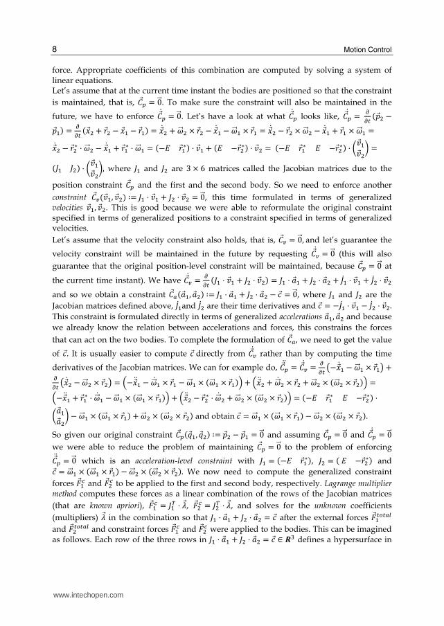
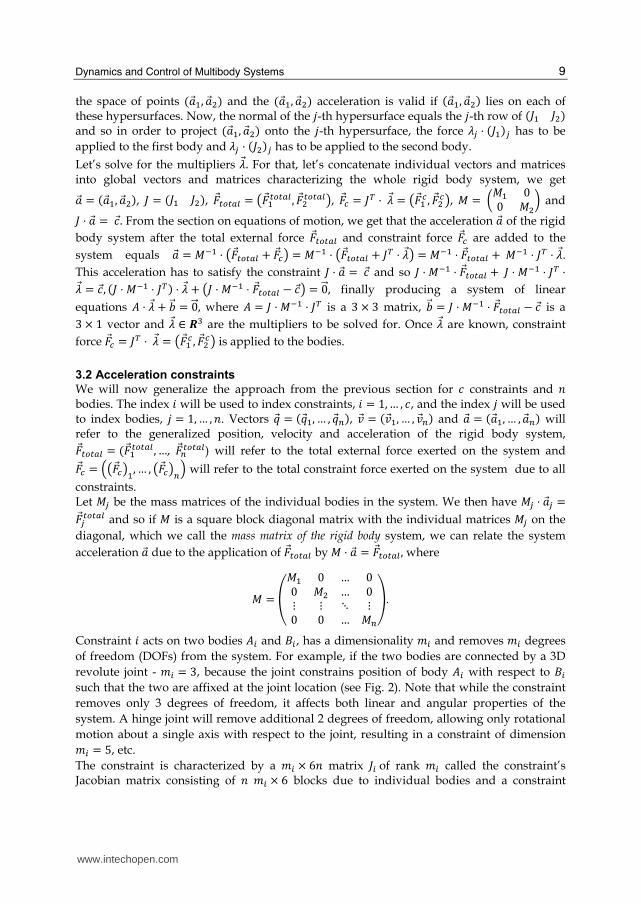
3.2 Acceleration constraints

We will now generalize the approach from the previous section for 潔 constraints and 券 bodies. The index 件 will be used to index constraints, 件噺な, … , 潔, and the index 倹 will be used to index bodies, 倹噺な, … , 券. Vectors 圏王噺岫圏王怠, … , 圏王津岻, 懸王噺岫懸王怠, … , 懸王津岻 and 欠王噺岫欠王怠, … , 欠王津岻 will refer to the generalized position, velocity and acceleration of the rigid body system, 繋王痛墜痛銚鎮噺岫繋王怠痛墜痛銚鎮 , …, 繋王津痛墜痛銚鎮) will refer to the total external force exerted on the system and 繋王頂噺岾盤繋王頂匪怠, … , 盤繋王頂匪津峇 will refer to the total constraint force exerted on the system due to all

constraints. Let 警珍 be the mass matrices of the individual bodies in the system. We then have 警珍糾欠王珍噺繋王珍痛墜痛銚鎮 and so if 警 is a square block diagonal matrix with the individual matrices 警珍 on the

diagonal, which we call the mass matrix of the rigid body system, we can relate the system

acceleration 欠王 due to the application of 繋王痛墜痛銚鎮 by 警糾欠王噺繋王痛墜痛銚鎮 , where

警噺蛮警怠ど … どど警態 … ど教教狂教どど … 警津妃.

Constraint 件 acts on two bodies 畦沈 and 稽沈, has a dimensionality 兼沈 and removes 兼沈 degrees

of freedom (DOFs) from the system. For example, if the two bodies are connected by a 3D

revolute joint - 兼沈噺ぬ, because the joint constrains position of body 畦沈 with respect to 稽沈 such that the two are affixed at the joint location (see Fig. 2). Note that while the constraint

removes only 3 degrees of freedom, it affects both linear and angular properties of the

system. A hinge joint will remove additional 2 degrees of freedom, allowing only rotational

motion about a single axis with respect to the joint, resulting in a constraint of dimension 兼沈噺の, etc.

The constraint is characterized by a 兼沈抜は券 matrix 蛍沈 of rank 兼沈 called the constraint’s Jacobian matrix consisting of 券兼沈抜は blocks due to individual bodies and a constraint

www.intechopen.com

Motion Control 10

equation right-hand-side vector 潔王沈 of length 兼沈. 蛍沈 has only two non-zero blocks, one due to the first constrained body 畦沈 and one due to the second constrained body 稽沈, referred to by 蛍沈,凋日 and 蛍沈,喋日 . According to the Lagrange multiplier approach, the constraint is enforced by

applying a constraint force 繋王頂沈噺蛍沈脹糾膏王沈噺岾盤繋王頂沈匪怠, … , 盤繋王頂沈匪津峇 to the rigid body system,

determined by the values of 兼沈 multipliers 膏王沈. Each row 倦噺な, … , 兼沈 of 蛍沈 removes one DOF

from the system and contributes to the constraint force 繋王頂沈 by exerting a force 盤膏王沈匪賃糾岫蛍沈岻賃 on

the system. Due to the way 蛍沈 is defined, 盤繋王頂沈匪凋日噺蛍沈,凋日脹糾膏王沈 and 盤繋王頂沈匪喋日噺蛍沈,喋日脹糾膏王沈 are the only

non-zero blocks of 繋王頂沈 and 盤繋王頂沈匪凋日 is the constraint force applied to the first body and 盤繋王頂沈匪喋日 is

the constraint force applied to the second body. Let’s stack the individual 兼沈抜は券 Jacobian matrices 蛍沈 by rows to a single 兼抜は券 Jacobian

matrix 蛍, where 兼噺 ∑ 兼沈沈 is the total number of DOFs removed from the system. 蛍 is then a

block matrix with 潔抜券 blocks whose non-zero blocks are given by 蛍沈,凋日 and 蛍沈,喋日 . Then the

total constraint force 繋王頂 exerted on the system equals 繋王頂噺 ∑ 繋王頂沈沈噺蛍脹糾膏王, where 膏王噺岫膏王怠, … , 膏王頂岻

is a 兼抜な vector of Lagrange multipliers due to all constraints. Because constraints should

not be conflicting, 蛍 is assumed to have full rank.

Let 畦噺蛍糾警貸怠糾蛍脹 , 潔王噺岫潔王怠, … , 潔王頂岻 and 決屎王噺蛍糾警貸怠糾繋王痛墜痛銚鎮伐潔王. Matrix 畦 is a 兼抜兼 matrix and

can be treated as if it consisted of 潔抜潔 blocks due to individual constraint pairs such that

the value of the 岫件怠, 件態岻-th block of size 兼沈迭抜兼沈鉄 due to the 件怠-th constraint and the 件態-th

constraint is given by 畦沈迭,沈鉄噺 ∑ 蛍沈迭,珍糾警珍貸怠珍糾盤蛍沈鉄,珍匪脹. Because the individual matrices 警珍 and 警珍貸怠 are positive definite, 警 and 警貸怠 are positive definite and so because 蛍 is assumed to

have full rank, 畦 is also positive definite. We will use 畦沈 (with slight abuse of notation) to

denote the 件-th block row of 畦 due to constraint 件. Vector 決屎王 is a vector of length 兼 consisting

of 潔 blocks due to the individual constraints. We use 決屎王沈 to refer to the 件-th block of 決屎王 of

length 兼沈 due to constraint 件. We will now discuss specific types of constraints. Each constraint 件 will generate a constraint

force of the same form 繋王頂沈噺蛍沈脹糾膏王沈 but different constraint types will lead to different

conditions on the legal values of the multipliers 膏王, essentially constraining the directions the

constraint force can act along (can it push, can it pull or can it do both?).

3.2.1 Equality constraints

We define acceleration level equality constraint 件 as follows. The constraint acts on two bodies 畦沈 and 稽沈, has a dimensionality 兼沈 and is specified by two 兼沈抜は matrices 蛍沈,凋日 and 蛍沈,喋日 and a

right-hand-side vector 潔王沈 of length 兼沈. The constraint requests that 蛍沈,凋日糾欠王凋日髪蛍沈,喋日糾欠王喋日噺潔王沈 for accelerations 欠王凋日 and 欠王喋日 . The 蛍沈,凋日 and 蛍沈,喋日 matrices are called the Jacobian blocks due to the first and the second body

and are supposed to have full rank. This terminology stems from the fact that if the

acceleration-level constraint implements a position-level constraint 系王椎盤圏王凋日 , 圏王喋日匪噺ど屎王 or a

velocity-level constraint 系王塚盤懸王凋日 , 懸王喋日匪噺ど屎王 then 蛍沈,凋日噺擢寵王妊擢槌屎王豚日 and 蛍沈,喋日噺擢寵王妊擢槌屎王遁日 or 蛍沈,凋日噺擢寵王寧擢塚屎王豚日 and 蛍沈,喋日噺擢寵王寧擢塚屎王遁日. The constraint is an equality constraint because it is described by a linear

equality.

www.intechopen.com


Let’s derive conditions on 膏王 due to the acceleration level equality constraint 件. Using our rigid body system dynamics equation, we get that the system acceleration 欠王 after the total

external force 繋王痛墜痛銚鎮 and total constraint force 繋王頂噺蛍脹糾膏王 are applied to the system equals 欠王噺警貸怠糾岫繋王痛墜痛銚鎮髪蛍脹糾膏王岻. The constraint equation requests that 蛍沈糾欠王伐潔王沈噺ど屎王 which means

that 蛍沈糾欠王伐潔王沈噺岫蛍糾欠王伐潔王岻沈噺盤蛍糾警貸怠糾繋王痛墜痛銚鎮髪蛍糾警貸怠糾蛍脹糾膏王伐潔王匪沈噺岾岫蛍糾警貸怠糾蛍脹岻糾膏王髪盤蛍糾警貸怠糾繋王痛墜痛銚鎮伐潔王匪峇沈噺盤畦糾膏王髪決屎王匪沈噺畦沈糾膏王髪決屎王沈噺ど屎王. Hence we get that equality constraint 件 requires that

畦沈糾膏王髪決屎王沈噺ど屎王 (5)

which is an equality constraint on the values of 膏王. 3.2.2 Inequality constraints

Let’s think of enforcing a different kind of constraint such that the equality sign 噺 in the

constraint’s formulation is replaced with either a greater-than-or-equal sign 半 or a less-than-

or-equal sign 判. For example, if 系椎岫圏王怠, 圏王態岻 measures a distance of a ball from the ground

plane, we might want to enforce a one-dimensional position constraint 系椎岫圏王怠, 圏王態岻半ど

requesting that the ball lies above the ground. Assuming that both 系椎岫圏王怠, 圏王態岻噺ど and 系椎岌岫圏王怠, 圏王態岻噺ど (the ball rests on the ground), the constraint can be implemented by

maintaining 系岑椎岫圏王怠, 圏王態岻半ど, which is an acceleration-level greater-or-equal constraint.

3.2.2.1 Greater-or-equal constraints

We define acceleration level greater-or-equal constraint 件 as follows. The constraint acts on two

bodies 畦沈 and 稽沈, has a dimensionality 兼沈 and is specified by two 兼沈抜は matrices 蛍沈,凋日 and 蛍沈,喋日 and a right-hand-side vector 潔王沈 of length 兼沈. The constraint requests that 蛍沈,凋日糾欠王凋日髪蛍沈,喋日糾欠王喋日半潔王沈 for accelerations 欠王凋日 and 欠王喋日 . Let’s present conditions on 膏王 due to the acceleration level greater-or-equal constraint 件. Similarly to the equality case, 蛍沈,凋日糾欠王凋日髪蛍沈,喋日糾欠王喋日半潔王沈 can be rewritten as (1) 蛍沈,凋日糾欠王凋日髪蛍沈,喋日糾欠王喋日伐潔王沈噺蛍沈糾欠王伐潔王沈噺畦沈糾膏王髪決屎王沈半ど屎王, which is an inequality greater-or-equal constraint on

the values of 膏王. Now, let’s recall that in Lagrange multiplier approach, the goal of 繋王頂沈 is to cancel

those components of 繋王痛墜痛銚鎮 that would make the bodies accelerate towards invalid states. In the case of an equality constraint, the bodies were restricted to remain on the intersections of

the hypersurfaces due to the constraint’s DOFs and 繋王頂沈 cancelled accelerations along the directions of the hypersurface normals. In the case of a greater-or-equal constraint, however, the bodies can move away from a hypersurface along the direction of the hypersurface’s normal, but not in the opposite direction. In other words, positive accelerations along the

positive directions of the normals are unconstrained and therefore (2) 膏王沈半ど屎王 (the constraint force can not pull the bodies back to the hypersurface). In addition, (3) if the bodies are

already accelerating to the front of the hypersurface 倦, 盤蛍沈,凋日糾欠王凋日髪蛍沈,喋日糾欠王喋日伐潔王沈匪賃伴ど, then

the constraint force due to that hypersurface must vanish, that is 盤膏王沈匪賃噺ど, so that no energy

would be added to the system (constraint force is as “lazy” as possible). These conditions

can be restated in terms of the 件-th block row of matrix 畦 and the 件-th block of vector 決屎王 as follows,

www.intechopen.com

Motion Control 12 畦沈糾膏王髪決屎王沈半ど屎王膏王沈半ど屎王盤畦沈糾膏王髪決屎王沈匪糾膏王沈噺ど, (6)

where 盤畦沈糾膏王髪決屎王沈匪糾膏王沈噺 ∑ 盤畦沈糾膏王髪決屎王沈匪陳日賃退怠賃糾盤膏王沈匪賃噺ど in fact means that 盤畦沈糾膏王髪決屎王沈匪賃糾盤膏王沈匪賃

for な判倦判兼沈 because both the products have to be positive. It is said that the components

of 畦沈糾膏王髪決屎王沈 are complementary to the corresponding components of 膏王沈. 3.2.2.2 Less-or-equal constraints

We define acceleration level less-or-equal constraint 件 as follows. The constraint acts on two bodies 畦沈 and 稽沈, has a dimensionality 兼沈 and is specified by two 兼沈抜は matrices 蛍沈,凋日 and 蛍沈,喋日 and a right-hand-side vector 潔王沈 of length 兼沈. The constraint requests that 蛍沈,凋日糾欠王凋日髪蛍沈,喋日糾欠王喋日判潔王沈 for accelerations 欠王凋日 and 欠王喋日 . Analogously to the previous case, we obtain the following set of conditions on multipliers 膏王 due to the acceleration level less-or-equal constraint 件. In addition to the condition 蛍沈糾欠王伐潔王沈噺畦沈糾膏王髪決屎王沈判ど屎王, multipliers due to constraint 件 have to be negative and complementary

to 膏王沈, 畦沈糾膏王髪決屎王沈判ど屎王膏王沈判ど屎王盤畦沈糾膏王髪決屎王沈匪糾膏王沈噺ど. (7)

Less-or-equal constraints 件 can trivially be converted to greater-or-equal constraints by

negating the Jacobian blocks and the right-hand-side vector 潔王沈 and so they do not have to be

handled as a special case.

3.2.3 Bounded equality constraints

Let’s suppose we want to implement a one-dimensional constraint that would behave like

an equality constraint 蛍沈糾欠王噺潔王沈 such that the constraint would break if the magnitude 舗蛍沈脹舗糾嵳盤膏王沈匪怠嵳 of the constraint force 繋王頂沈噺蛍沈脹糾膏王沈 required to maintain the constraint exceeds a

certain limit. Such a capability could, for example, be used for the implementation of various

kinds of motors with limited power. Now, because 舗蛍沈脹舗 is known, limiting the force

magnitude (in this case) is equivalent to specifying the lower and upper bound on the value

of the multiplier 盤膏王沈匪怠 . Hence, without loss of generality we can assume the bounds on 膏王沈 are given instead. In the general case of a multi-dimensional constraint, we assume that each

multiplier has its own bounds, independent of the values of other multipliers, so that the

problem of solving for 膏王 remains tractable.

We define acceleration level bounded equality constraint 件 as follows. The constraint acts on two

bodies 畦沈 and 稽沈, has a dimensionality 兼沈 and is specified by two 兼沈抜は matrices 蛍沈,凋日 and 蛍沈,喋日 , a right-hand-side vector 潔王沈 of length 兼沈 and 膏王沈 bounds 膏王沈鎮墜判ど屎王 and 膏王沈朕沈半ど屎王. The

constraint requests that 盤膏王沈鎮墜匪賃判盤膏王沈匪賃判盤膏王沈朕沈匪賃 and implements the equality constraint 蛍沈,凋日糾欠王凋日髪蛍沈,喋日糾欠王喋日噺潔王沈 for accelerations 欠王凋日 and 欠王喋日 subject to constraint force limits given

by 膏王沈鎮墜 and 膏王沈朕沈 . www.intechopen.com


We will now elaborate on what constraint force limits due to the acceleration level bounded

equality constraint 件 really mean and what the corresponding conditions on 膏王 look like.

Following up on the hypersurface interpretation of the equality constraint 蛍沈糾欠王伐潔王沈噺ど屎王, if the bodies are to move off the hypersurface 倦 due to the 倦-th constraint DOF in the direction

of the surface normal, a negative 盤膏王沈匪賃 is required to cancel the acceleration. Now, if the

value of 盤膏王沈匪賃 required to fully cancel the acceleration is less than the allowed lower limit 盤膏王沈鎮墜匪賃, clamped 盤膏王沈匪賃半盤膏王沈鎮墜匪賃 would not yield a constraint force strong enough to cancel

the prohibited acceleration and in the end 蛍沈糾欠王伐潔王沈伴ど屎王. Similarly, if the bodies are to move

off the hypersurface in the opposite direction, a positive 盤膏王沈匪賃 is required to cancel the

acceleration. If 盤膏王沈匪賃 is clamped such that 盤膏王沈匪賃判盤膏王沈朕沈匪賃 and the acceleration is not cancelled

fully then 蛍沈糾欠王伐潔王沈隼ど屎王. Putting this discussion into equations and assuming 盤膏王沈鎮墜匪賃判ど

and 盤膏王沈朕沈匪賃半ど, we get 盤膏王沈鎮墜匪賃判盤膏王沈匪賃判盤膏王沈朕沈匪賃盤膏王沈匪賃噺盤膏王沈鎮墜匪賃馨盤畦沈糾膏王髪決屎王沈匪賃半ど盤膏王沈匪賃噺盤膏王沈朕沈匪賃馨盤畦沈糾膏王髪決屎王沈匪賃判ど盤膏王沈鎮墜匪賃隼盤膏王沈匪賃隼盤膏王沈鎮墜匪賃馨盤畦沈糾膏王髪決屎王沈匪賃噺ど. (8)

Fig. 3. Visualization of complementarity conditions on the pairs 盤膏沈 , 拳沈岫膏王岻匪 due to different

kinds of one dimensional constraints 件, where 拳沈盤膏王匪柑噺畦沈糾膏王髪決沈噺蛍沈糾欠王伐潔沈. Thick lines

indicate permissible values for the 盤膏沈 , 拳沈岫膏王岻匪 pairs. As can be seen, equality constraint

requests 拳沈岫膏王岻 to be zero and lets 膏沈 take an arbitrary value. Greater-or-equal constraint

requests both 拳沈岫膏王岻 and 膏沈 to be non-negative and complementary to each other. Bounded

equality constraint generalizes the two previous cases by introducing explicit limits 膏沈鎮墜判ど

and 膏沈朕沈半ど on the values of 膏沈 . For improved readability, 屎屎屎王 accents have been removed from one-dimensional vectors related to the constraint 件.

ど

ど

拳沈岫膏王岻

膏沈

ど

拳沈岫膏王岻

ど膏沈

蛍沈糾欠王噺潔沈 Equality constraint Greater-or-equal constraint

蛍沈糾欠王半潔沈

ど

ど膏沈

拳沈岫膏王岻

膏沈鎮墜膏沈朕沈

蛍沈糾欠王噺潔沈 Bounded equality constraint

www.intechopen.com

Motion Control 14

Bounded equality constraints are generalization of both inequality and equality constraints.

For example, if we set 膏王沈鎮墜噺ど屎王 and 膏王沈朕沈噺 ∞屎屎屎王 then the bounded equality constraint 件 turns to a greater-or-equal constraint 件 with the same Jacobian blocks and right-hand-side vector 潔王沈. Similarly, by setting 膏王沈鎮墜噺伐∞屎屎屎王 and 膏王沈朕沈噺ど屎王, the constraint turns to a less-or-equal constraint.

Finally, by setting 膏王沈鎮墜噺伐∞屎屎屎王 and 膏王沈朕沈噺 ∞屎屎屎王, the constraint turns to an unbounded equality constraint.

3.2.4 Reduction to LCP

In the previous section we have discussed several constraint types and showed what

conditions on the multipliers 膏王 they impose. Our goal is now to solve for 膏王 obeying the

presented conditions so that the constraint force 繋王頂噺蛍脹糾膏王 could be exerted on the system.

As it turns out, the problem of solving for 膏王 is equivalent to solving of specific kinds of linear

complementarity problems (LCPs) for which efficient algorithms exist and so we can compute 膏王 by using a LCP solver, (Smith, 2004; Vondrak, 2006; Cline, 2002). To simplify the discussion, we assume that every inequality and bounded equality constraint 件 is one-dimensional, 兼沈噺な. As a result, we can simply write 膏沈 instead of 盤膏王沈匪怠, etc.

If all the constraints are unbounded equalities, the corresponding conditions on 膏王 are given

by 畦糾膏王髪決屎王噺ど屎王 which is a linear system that can be solved efficiently by standard

factorization techniques. If all constraints are greater-or-equal constraints, we get a pure

linear complementarity problem of the form 畦糾膏王髪決屎王半ど屎王, 膏王半ど屎王, 膏王糾盤畦糾膏王髪決屎王匪噺ど屎王, which can

be solved by a standard LCP solver. If there are 倦 unbounded equality constraints and 潔伐倦

greater-or-equal constraints, we get a mixed linear complementarity problem 畦勅槌糾膏王髪決屎王勅槌噺ど屎王, 畦沈津勅槌糾膏王髪決屎王沈津勅槌半ど屎王, 膏王沈津勅槌半ど屎王, 膏王沈津勅槌糾盤畦沈津勅槌糾膏王髪決屎王沈津勅槌匪噺ど, where 畦勅槌 , 決屎王勅槌 denotes the

rows of 畦, 決屎王 due to equality constraints and 畦沈津勅槌, 決屎王沈津勅槌 denotes the rows of 畦, 決屎王 due to

inequality constraints. Mixed LCPs can be solved by mixed LCP solvers. Finally, if there are 倦 unbounded equality constraints and 潔伐倦 bounded equality-constraints (including

inequality constraints 件 with appropriately set 膏王沈 limits), we get a lo-hi linear complementarity

problem 畦勅槌糾膏王髪決屎王勅槌噺ど屎王, 膏沈鎮墜判膏沈判膏沈朕沈 , 膏沈噺膏沈鎮墜馨畦沈糾膏王髪決沈半ど, 膏沈噺膏沈朕沈馨畦沈糾膏王髪決沈判ど, 膏沈鎮墜隼膏沈隼膏沈朕沈馨畦沈糾膏王髪決沈噺ど, where 件 indexes unbounded equality and inequality

constraints. This is the most general form that can handle all constraint forms we have

discussed and can also be solved efficiently.

3.3 Velocity constraints

So far we have discussed how constraints can be implemented on the accelerations. It is

useful, however, to specify constraints on the velocities as well. Let’s recall the example with

the ball and the ground plane where the goal is to enforce a one-dimensional position-level

constraint 系椎岫圏王怠, 圏王態岻半ど stipulating that the ball has to stay above the ground. Now, if 系椎岫圏王怠岫建岻, 圏王態岫建岻岻噺ど and 系椎岌岫圏王怠岫建岻, 圏王態岫建岻岻隼ど at the current time 建 (the ball strikes the ground

plane) then 系椎岫圏王怠岫建髪鉛岻, 圏王態岫建髪鉛岻岻隼ど at the time instant 建髪香 regardless of accelerations at

time 建 for a sufficiently small 香. In order to ensure that the constraint is maintained at 建髪香,

velocities at time 建 have to change so that 系椎岌岫圏王怠岫建岻, 圏王態岫建岻岻半ど. This, however, is a constraint

on the velocity.

www.intechopen.com


3.3.1 Impulsive dynamics

We will now outline the concept of impulsive forces and first-order rigid body dynamics.

With regular forces, the effects of forces on positions and orientations of rigid bodies are

determined by second-order (Newtonian) dynamics in which velocities change through the

integration of forces while positions change through the integration of velocities. With

impulsive forces, the effects of forces on positions and orientations are determined by first-

order (impulsive) dynamics in which velocities change directly through the application of

impulsive forces and positions change through the integration of velocities.

We postulate impulsive force 蛍王庁 as a force with “units of momentum”. If 鶏屎王 and 詣屎王 are the linear

and angular momentums of a rigid body and 蛍王庁 is applied to the body at the world space

position 堅王, then the linear momentum 鶏屎王 changes by the value Δ鶏屎王噺蛍王庁 and the angular

momentum 詣屎王 changes by the value Δ詣屎王噺蛍王邸, where 蛍王邸噺岫堅王伐捲王岻抜蛍王庁 is impulsive torque due to

the impulsive force 蛍王庁. Impulsive forces and torques can be seen as “ordinary” forces and torques that directly change the body’s linear and angular momentums, instead of affecting their time derivatives. Similarly to the second-order dynamics, we couple linear and corresponding angular

quantities to generalized quantities. That way, we obtain generalized momentum 繋王沈陳椎痛墜痛銚鎮噺岫鶏屎王, 詣屎王岻 and generalized impulsive force (impulse) 繋王沈陳椎噺岫蛍王庁 , 蛍王邸岻. Then if 警 is the mass matrix of

the rigid body and 懸王 is the body’s generalized velocity, we immediately get 警糾懸王噺繋王沈陳椎痛墜痛銚鎮 from the definition of the linear and angular momentum. Moreover, our momentum update rules state that the change Δ懸王 of generalized velocity 懸王 due to the application of the

generalized impulse 繋王沈陳椎 equals Δ懸王噺警貸怠糾繋王沈陳椎. Therefore the first-order dynamics relating

velocities 懸王 to impulses 繋王沈陳椎 is given by

警糾懸王噺繋王沈陳椎 (9)

and 繋王沈陳椎痛墜痛銚鎮 can be seen as a generalized total external impulse acting on the body that consists

of the only term – the inertial term 岫鶏屎王, 詣屎王岻. This directly compares to the case of second-order

dynamics that relates accelerations 欠王 to forces 繋王 by 警糾欠王噺繋王. If we have a set of 券 rigid bodies with mass matrices 警怠, … , 警津, generalized velocities 懸王怠, … , 懸王津 and total external impulses 盤繋王沈陳椎痛墜痛銚鎮匪怠, … , 盤繋王沈陳椎痛墜痛銚鎮匪津 then the first-order dynamics of

the system is given by 警糾懸王噺繋王沈陳椎痛墜痛銚鎮, where 警 is a mass matrix of the system made of 警怠, … , 警津, 懸王噺岫懸王怠, … , 懸王津岻 and 繋王沈陳椎痛墜痛銚鎮噺岾盤繋王沈陳椎痛墜痛銚鎮匪怠, … , 盤繋王沈陳椎痛墜痛銚鎮匪津峇. Analogously to the

acceleration case, we call 懸王 the velocity of the system and 繋王沈陳椎痛墜痛銚鎮 the total external impulse

exerted on the system (system momentum).

3.3.2 Constraints

We can now transfer everything we know about acceleration-level constraints, defined with

respect to accelerations and forces, to the realm of velocity-level constraints, defined with

respect to velocities and impulsive forces. There is no need to do any derivations because

acceleration-level formulation of rigid body dynamics exactly corresponds to the velocity-

level formulation of the impulsive dynamics. The only differences are due to the fact that

we will now work with system velocities 懸王, impulsive constraint forces 繋王沈陳椎頂 and

www.intechopen.com

Motion Control 16

momentums 繋王沈陳椎痛墜痛銚鎮 instead of accelerations 欠王, constraint forces 繋王頂 and total external forces 繋王痛墜痛銚鎮. In consequence, the same algorithms can be used to implement velocity constraints.

We define velocity level constraint 件 as follows. The constraint acts on two bodies 畦沈 and 稽沈, has a dimensionality 兼沈 and is specified by two 兼沈抜は matrices 蛍沈,凋日 and 蛍沈,喋日and a right-

hand-side vector 倦屎王沈 of length 兼沈. The constraint requests either 蛍沈,凋日糾懸王凋日髪蛍沈,喋日糾懸王喋日噺倦屎王沈, 蛍沈,凋日糾懸王凋日髪蛍沈,喋日糾懸王喋日判倦屎王沈 or 蛍沈,凋日糾懸王凋日髪蛍沈,喋日糾懸王喋日半倦屎王沈 and is implemented by exerting a constraint

impulse 盤繋王頂沈匪沈陳椎噺蛍沈脹糾膏王沈 determined by the values of multipliers 膏王沈. In addition, if bounds

on the valid multiplier values 膏王沈鎮墜判ど屎王 and 膏王沈朕沈半ど屎王 are provided, then the constraint describes

a bounded equality constraint 件 that requests 盤膏王沈鎮墜匪賃判盤膏王沈匪賃判盤膏王沈朕沈匪賃 and implements the

equality constraint 蛍沈,凋日糾懸王凋日髪蛍沈,喋日糾懸王喋日噺倦屎王沈 for velocities 懸王凋日 and 懸王喋日 subject to constraint

impulse limits given by 膏王沈鎮墜 and 膏王沈朕沈 . Multipliers 膏王 can be computed by solving the same LCP

problems like before. If there are 潔 constraints, we will get 畦噺蛍糾警貸怠糾蛍脹 and 決屎王噺蛍糾警貸怠糾繋王沈陳椎痛墜痛銚鎮伐倦屎王, where 倦屎王噺盤倦屎王怠, … , 倦屎王頂匪.

3.4 Position constraints

Motion control constraints are most often specified on the position level because it is the natural way of expressing desired motion. In the earlier section, we have already discussed how position level constraints can be implemented either on the acceleration or velocity level, but this time, we will do it more thoroughly and will also show how prior constraint errors due to numerical inaccuracies could be reduced during simulation. We never enforce constraints directly on the position level. Position level enforcement would require use of custom equations of motion specific to the set of constraints. As a result equations would have to change each time the constraint set is updated. For the rest of the section, we will assume we have 券 rigid bodies and 潔 position-level constraints. We define position level constraint 件 as follows. The constraint acts on two bodies 畦沈 and 稽沈, has a dimensionality 兼沈 and is specified by a function 系王椎沈盤圏王凋日 , 圏王喋日匪樺三陳日 that is differentiable with respect to time so that its velocity level and acceleration level formulations (consistent with our prior definitions) can be obtained by differentiation. Position level equality constraint 件 requests that 系王椎沈盤圏王凋日 , 圏王喋日匪噺ど屎王 for generalized positions 圏王凋日 and 圏王喋日 and the value of 系王椎沈盤圏王凋日 , 圏王喋日匪 can intuitively be thought of as a measurement of the position error for bodies at the position configuration 岫圏王凋日 , 圏王喋日岻. Position level greater-or-equal constraint 件 requests that 系王椎沈盤圏王凋日 , 圏王喋日匪半ど屎王 and position level less-or-equal constraint 件 requests that 系王椎沈盤圏王凋日 , 圏王喋日匪判ど屎王. 3.4.1 Acceleration or velocity level

We use constraint forces to implement position level constraints in an incremental way. We start from an initial state that is consistent with the constraint formulation (such that positions and velocities are valid with respect to the position level and velocity level formulations of the constraints) and then apply constraint forces to ensure that the velocity level and position level constraints remain maintained. Alternatively, we start from a state that is consistent with the position level formulations and then apply constraint impulses to ensure that the position level constraints remain maintained. Please note that whenever an impulse is applied to a body, its velocity changes. In consequence, conditions that have to be met so that a particular constraint could be

www.intechopen.com


implemented on the acceleration level need no longer be valid after the impulse is applied and so it cannot be reliably determined in advance which constraints can be implemented on the acceleration level. To address this issue, we implement all constraints on the velocity level whenever there is at least one position constraint that has to be implemented on the velocity level.

3.4.2 Equality constraints with stabilization

Consider the position level equality constraint 系王椎沈盤圏王凋日 , 圏王喋日匪噺ど屎王. By differentiating 系王椎沈盤圏王凋日 , 圏王喋日匪噺ど屎王 with respect to time, we get a corresponding velocity level formulation of

the position constraint in the form of 系王塚沈盤懸王凋日 , 懸王喋日匪噺ど屎王, where 系王塚沈盤懸王凋日 , 懸王喋日匪噺擢擢痛系王椎沈盤圏王凋日 , 圏王喋日匪噺蛍沈,凋日糾懸王凋日髪蛍沈,喋日糾懸王喋日 . By differentiating this velocity constraint, we get a corresponding

acceleration level formulation 系王銚沈盤欠王凋日 , 欠王喋日匪噺ど屎王, where 系王銚沈盤欠王凋日 , 欠王喋日匪噺擢擢痛系王塚沈盤懸王凋日 , 懸王喋日匪噺蛍沈,凋日糾欠王凋日髪蛍沈,喋日糾欠王喋日伐潔王沈 and 潔王沈噺伐蛍岌沈,凋日糾懸王凋日伐蛍岌沈,喋日糾懸王喋日 . The position level constraint 件系王椎沈噺ど屎王 can

thus be implemented incrementally either (1) on the acceleration level, by starting from a

state where 系王椎沈噺系王岌椎沈噺ど屎王 and applying constraint forces so that 系王岑椎沈噺ど屎王 or (2) on the velocity

level, by starting from a state where 系王椎沈噺ど屎王 and applying constraint impulses so that 系王岌椎沈噺ど屎王. In the first case, constraint forces are applied under the assumption that 系王椎沈噺系王岌椎沈噺ど屎王, while

in the second case, constraint impulses are applied under the assumption that 系王椎沈噺ど屎王. In

practice, however, these assumptions often do not hold for various pragmatic reasons. For example, the numerical solver that integrates the equations of motion incurs an integration error or constraint forces are computed with an insufficient precision. Let’s assume we implement the position level constraint 件 on the velocity level. If the

constraint is currently broken, that is 系王椎沈塙ど屎王, we want to generate a constraint impulse so

that the constraint error 系王椎沈 will be driven towards a zero vector. This is called constraint

stabilization. Fortunately, simple stabilization can be implemented by following a procedure

suggested in (Cline, 2002). Instead of requiring that 系王岌椎沈噺ど, we can require that

系王岌椎沈噺伐系王椎沈糾糠 , (10)

where 糠 is a small positive value (dependent on the integration step size) that determines the speed with which the constraint is stabilized. Then, if 建 is the current time, we have 系王椎沈岫建髪 Δ建岻蛤系王椎沈岫建岻髪 Δ建糾系王岌椎沈岫建岻噺系王椎沈岫建岻糾岫な伐 Δ建糾糠岻 and so we can reduce the position error

by simply biasing the request on the desired velocity. Analogously to the previous case, if we implement the position level constraint 件 on the

acceleration level, we need to reduce both the position error 系王椎沈 as well as velocity error 系王岌椎沈 .

That could be done by biasing the request on the desired acceleration 系王岑椎沈 . Instead of

requiring that 系王岑椎沈噺ど屎王 we can require

系王岑椎沈噺伐系王椎沈糾糠伐系王岌椎沈糾紅, (11)

where 糠 and 紅 are positive constants. Because 系王岌椎沈噺蛍沈糾懸王 we get 系王岑椎沈噺伐系王椎沈糾糠伐蛍沈糾懸王糾紅.

Plugging these equations into our constraint definitions, we can therefore implement the position level equality constraint 件 with stabilization by submitting either the velocity level

www.intechopen.com

Motion Control 18

equality constraint 蛍沈,凋日糾懸王凋日髪蛍沈,喋日糾懸王喋日噺伐系王椎沈糾糠 or the acceleration level equality constraint 蛍沈,凋日糾欠王凋日髪蛍沈,喋日糾欠王喋日噺伐系王椎沈糾糠伐蛍沈糾懸王糾紅伐蛍岌沈糾懸王. Moreover, if we want to implement

powering limits, these constraints can be submitted as bounded equality constraints with appropriate force limits.

3.4.3 Inequality constraints with stabilization

Let’s assume for simplicity that we work with a one-dimensional position level greater-or-

equal constraint 系椎沈半ど, like the one that would stipulate that the ball lies above the ground.

This constraint is fundamentally different from a equality constraint because no velocity or acceleration constraints are actually imposed until the constrained bodies reach the

boundary 岶岫圏王凋日,圏王喋日岻 | 系椎沈岫圏王凋日,圏王喋日岻噺ど岼 of the set of valid positions 岶岫圏王凋日,圏王喋日岻 | 系椎沈盤圏王凋日,圏王喋日匪半ど岼

in the position space. We will now discuss three cases, depending on whether 系椎沈伴ど, 系椎沈噺ど

or 系椎沈隼ど at the current state.

If 系椎沈伴ど then the bodies did not reach the boundary of the set of valid positions and so no

constraints will be imposed. This corresponds to the case when the ball is in the air and does not touch the ground.

If 系椎沈噺ど then the bodies lie at the boundary of the set of valid positions (the ball touches the

ground) and 系岌椎沈半ど has to be enforced in order to maintain 系椎沈半ど. This 系岌椎沈半ど constraint

can be implemented (1) on the acceleration level by submitting 系岑椎沈半ど if 系岌椎沈噺ど, (2) on the

acceleration level by ignoring the constraint if 系岌椎沈伴ど (the velocity-level constraint will hold

regardless of the value of 系岑椎沈 if a sufficiently small integration step is taken) or (3) on the

velocity level by directly requesting 系岌椎沈半ど. The constraint must be implemented on the

velocity level if 系岌椎沈隼ど. In practice, we make use of comparisons with tolerances when

discriminating between the cases (1) – (3) and add extra terms to the velocity level and acceleration level formulations so that the original position level constraint would be

stabilized, i.e. we use 蛍沈,凋日糾欠王凋日髪蛍沈,喋日糾欠王喋日半伐系王椎沈糾糠伐蛍沈糾懸王糾紅伐蛍岌沈糾懸王 and 蛍沈,凋日糾懸王凋日髪蛍沈,喋日糾懸王喋日半伐系王椎沈糾糠. If 系椎沈隼ど then the system state is invalid (ball penetrates the ground) and should be rejected.

To handle this case, we would like to locate the state when 系椎沈噺ど so that we could fall-back

onto the previous case 系椎沈噺ど. For that, we can either (1) roll the simulation state back to the

previous state and then use a bisection-like algorithm to locate the latest valid state 系椎沈噺ど

or (2) we can ignore the position error and act as if 系椎沈噺ど (this way, we would only rely on

the constraint stabilization mechanism to recover 系椎沈半ど).

3.5 Contact

In this section we briefly discuss the problem of enforcing body non-penetration and

modeling friction. We will account for these phenomena through constraints that will be

associated with contacts reported by a collision detection library. Given the system state at

time 建, we will use the library to find which shapes are in contact and then formulate non-

penetration and friction constraints specific to time 建 to constrain relative body motion at the

contacting points. We informally define contacts as relevant coinciding points of contacting

pairs of body shapes where contact forces or impulses should act in order to prevent

penetration. We assume collision detection library describes contacts by vectors

www.intechopen.com

Dynamics and Control of Multibody Systems 19 盤畦沈 , 稽沈 , 喧王沈 , 券屎王沈 , 券屎王岌沈匪 such that contact 件 involves bodies 畦沈 and 稽沈 contacting at the world space

point 喧王沈噺喧王凋日噺喧王喋日 (喧王凋日 and 喧王喋日 are the corresponding points attached to 畦沈 and 稽沈), the

contact surface normal at 喧王沈 is given by a unit vector 券屎王沈 pointing towards 稽沈 and 券屎王岌沈 is the

time derivative of 券屎王沈. Let us denote 堅王凋日噺喧王凋日伐捲王凋日 and 堅王喋日噺喧王喋日伐捲王喋日 . We can then request non-penetration at contact 件 by stipulating that 系沈津柑噺券屎王沈糾盤喧王喋日伐喧王凋日匪半ど,

which is a one-dimensional position level greater-or-equal constraint. Let’s have a look at its time derivatives to retrieve the constraint’s Jacobian blocks and the right-hand-side vector.

We have 系岌沈津噺券屎王岌沈糾盤喧王喋日伐喧王凋日匪髪券屎王沈糾盤喧王岌喋日伐喧王岌凋日匪, 系岑沈津噺券屎王岑沈糾盤喧王喋日伐喧王凋日匪髪券屎王岌沈糾盤喧王岌喋日伐喧王岌凋日匪髪券屎王岌沈糾盤喧王岌喋日伐喧王岌凋日匪髪券屎王沈糾盤喧王岑喋日伐喧王岑凋日匪噺券屎王岑沈糾盤喧王喋日伐喧王凋日匪髪に糾券屎王岌沈糾盤喧王岌喋日伐喧王岌凋日匪髪券屎王沈糾盤喧王岑喋日伐喧王岑凋日匪. Because 喧王凋日噺捲王凋日髪堅王凋日 and 喧王喋日噺捲王喋日髪堅王喋日 we get 喧王岌凋日噺懸王凋日髪降屎屎王凋日抜堅王凋日, 喧王岌喋日噺懸王喋日髪降屎屎王喋日抜堅王喋日 , 喧王岑凋沈噺欠王凋日髪糠王凋日抜堅王凋日髪降屎屎王凋日抜盤降屎屎王凋日抜堅王凋日匪, 喧王岑喋沈噺欠王喋日髪糠王喋日抜堅王喋日髪降屎屎王喋日抜岫降屎屎王喋日抜堅王喋日岻. Considering that 喧王凋日噺喧王喋日 at the contact, we then have 系岌沈津噺券屎王沈糾盤喧王岌喋日伐喧王岌凋日匪噺券屎王沈糾懸王喋日髪券屎王沈糾盤降屎屎王喋日抜堅王喋日匪伐券屎王沈糾懸王凋日伐券屎王沈糾盤降屎屎王凋日抜堅王凋日匪噺券屎王沈糾懸王喋日髪盤堅王喋日抜券屎王沈匪糾降屎屎王喋日伐券屎王沈糾懸王凋日伐盤堅王凋沈抜券屎王沈匪糾降屎屎王凋日 and 系岑沈津噺に糾券屎王岌沈糾盤喧王岌喋日伐喧王岌凋日匪髪磐券屎王沈糾欠王喋日髪盤堅王喋日抜券屎王沈匪糾糠王喋日伐券屎王沈糾欠王凋日伐盤堅王凋日抜券屎王沈匪糾糠王凋沈髪券屎王沈糾岾降屎屎王喋日抜盤降屎屎王喋沈抜堅王喋沈匪峇伐券屎王沈糾岾降屎屎王凋日抜盤降屎屎王凋沈抜堅王凋沈匪峇卑. By comparing these equations against our constraint definitions,

we obtain 蛍沈,凋日噺岾伐券屎王沈脹伐盤堅王凋日抜券屎王沈匪脹峇, 蛍沈,喋日噺岾券屎王沈脹盤堅王喋日抜券屎王沈匪脹峇 and 蛍岌沈糾懸王直勅津噺に糾券屎王岌沈糾盤懸王喋日髪降屎屎王喋日抜堅王喋日伐懸王凋日伐降屎屎王凋沈抜堅王凋沈匪髪券屎王沈糾岾降屎屎王喋日抜盤降屎屎王喋沈抜堅王喋沈匪伐降屎屎王凋日抜盤降屎屎王凋沈抜堅王凋沈匪峇.

The non-penetration constraint has the following direct interpretation. The value of 系沈津

measures relative body separation at contact 件, 系岌沈津 measures normal velocity at the contact and 系岑沈津 measures normal acceleration. If 膏沈津 is the Lagrange multiplier due to the acceleration level

formulation of the constraint 系岑沈津柑噺蛍沈糾欠王直勅津伐潔沈半ど then 膏沈津 equals the normal force magnitude

and 伐券屎王沈糾膏沈津 force is exerted on 畦沈 at 喧王凋沈 and 券屎王沈糾膏沈津 is exerted on 稽沈 at 喧王喋沈. Our conditions

from equation (6) due to non-penetration constraints thus say that both the normal acceleration and the normal force magnitude have to be non-negative and complementary to each other. If 膏沈津 is the Lagrange multiplier due to the velocity level formulation of the constraint 系岌沈津柑噺蛍沈糾懸王直勅津半ど then 伐系岌沈津 measures the relative approaching body velocity and 膏沈津 equals

the normal impulse magnitude required to stop the bodies at 喧王沈 so that 系岌沈津半ど. This fact can be utilized to model impacts. Instead of stopping the bodies, we would like to take the velocity 伐系岌沈津 and have it opposed so that the bodies would bounce. This effect can be achieved by a minor modification of the original velocity level non-penetration constraint, (Baraff, 1997). Given a coefficient of restitution 香沈樺岷ど,な峅 at the contact 件 determining how bouncy the contacting surface is, we replace the non-penetration velocity level constraint 蛍沈糾懸王直勅津半ど with a constraint 蛍沈糾懸王直勅津半伐香沈糾系岌沈津.

Friction is usually modeled according to Coulomb friction law, (Trinkle et al., 1997). Coulomb law introduces friction forces acting along the contact’s tangential plane. It extends the complementarity conditions on the normal acceleration and normal force magnitude by adding conditions on the direction and magnitude of the friction force, by relating the direction and magnitude to the relative tangential velocity at the contact and the corresponding normal force magnitude. The relation is quadratic and is most often linearized by considering two separate friction directions that the friction force can act along, (Trinkle et al., 1997).

www.intechopen.com

Motion Control 20

In this linearization, friction at contact 件 is approximated by two additional friction bounded equality constraints that constrain relative body motion in two tangential directions perpendicular to each other and the contact normal. That is, if 券屎王沈 is the contact normal at

contact 件 and 建王沈掴 and 建王沈槻 are two unit vectors such that 建王沈掴糾建王沈槻噺ど and 建王沈掴抜建王沈槻噺券屎王沈 then it is

requested that 系沈掴柑噺建王沈掴糾盤喧王喋日伐喧王凋日匪噺ど and 系沈槻柑噺建王沈槻糾盤喧王喋日伐喧王凋日匪噺ど subject to force limits.

Friction constraints are special because their force limits are functions of the normal forces. If the corresponding non-penetration constraint 系沈津半ど is implemented on the acceleration level then the friction constraints are implemented on the acceleration level as well by

bounded equality constraints 系岑沈掴噺ど and 系岑沈槻噺ど with force limits 岫膏沈掴岻鎮墜噺盤膏沈槻匪鎮墜噺伐航沈糾膏沈津

and 岫膏沈掴岻朕沈噺盤膏沈槻匪朕沈噺航沈糾膏沈津, where 航沈半ど is a static friction coefficient and 膏沈津 is the normal

force magnitude at contact 件. Otherwise, the constraints are implemented on the velocity

level by 系岌沈掴噺ど and 系岌沈槻噺ど with force limits 岫膏沈掴岻鎮墜噺盤膏沈槻匪鎮墜噺伐航沈糾膏沈津 and 岫膏沈掴岻朕沈噺盤膏沈槻匪朕沈噺航沈糾膏沈津, where 航沈半ど is an impulsive friction coefficient and 膏沈津 is the normal impulse magnitude at contact 件, (Kawachi et al., 1997). Note that for the friction constraints, force limits are not constant and depend on the values

of 膏沈津. This implies we have to use a specialized solver to solve for 膏王 or estimate 膏沈津 first (e.g.,

we might ignore friction constraints and solve for an estimate of 膏王, then fix the friction force limits using the estimated values of 膏沈津), (Smith, 2004). Friction constraints have analogous Jacobians and equation right-hand-side vectors as non-penetration constraints. It is just that 券屎王沈 vectors in the corresponding formulations are replaced with 建王沈掴 and 建王沈槻 vectors.

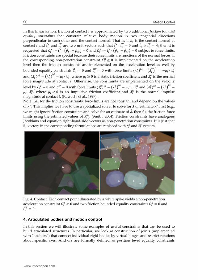
Fig. 4. Contact. Each contact point illustrated by a white spike yields a non-penetration

acceleration constraint 系岑沈津半ど and two friction bounded equality constraints 系岑沈掴噺ど and 系岑沈槻噺ど.

4. Articulated bodies and motion control

In this section we will illustrate some examples of useful constraints that can be used to build articulated structures. In particular, we look at construction of joints (implemented with “anchors”) that connect individual rigid bodies by virtual hinges and restrict rotations about specific axes. Anchors are formally defined as position level equality constraints

www.intechopen.com


(implemented either on the velocity or acceleration level) that restrict relative body positions and/or orientations. They implement various virtual joints (e.g., ball-and-socket or hinges) that connect bodies. This way, complex articulated jointed structures could be implemented.

4.1 Ball-and-socket joint

We start with a ball-and-socket joint that was discussed earlier (in the form of “point-to-point” constraints) in Section 3. The joint is defined in terms of two anchor points fixed in the coordinate frames of the first and the second constrained body. Ball-and-socket joint requires the anchors to occupy the same position in the world coordinate frame. As such, it removes 3 degrees of freedom from the system.

If 件 is the constraint index, 畦沈 and 稽沈 are the indices of the constrained bodies and 堅王凋日長 and 堅王喋日長

are the positions of the two anchors on the first and second body, expressed in the

corresponding body-centric coordinate frames, then 喧王凋日噺捲王凋日髪迎凋日糾堅王凋日長 and 喧王喋日噺捲王喋日髪迎喋日糾堅王喋日長 are the world space positions of the anchors and the goal is to ensure that 喧王凋日噺喧王喋日 . Let

us denote 堅王凋日噺喧王凋日伐捲王凋日 and 堅王喋日噺喧王喋日伐捲王喋日 . These vectors are fixed in the coordinate frame

of the first and the second body respectively, resulting in 堅王岌凋日噺降屎屎王凋日抜堅王凋日 and 堅王岌喋日噺降屎屎王喋日抜堅王喋日 . Following the derivation from the previous section, our constraint can then be formulated in

the form of equations 系王椎沈柑噺喧王喋日伐喧王凋日噺捲王喋日髪堅王喋日伐捲王凋日伐堅王凋日噺ど屎王, 系王岌椎沈柑噺懸王喋日髪降屎屎王喋日抜堅王喋日伐懸王凋日伐降屎屎王凋日抜堅王凋日噺ど屎王 and 系王岑椎沈柑噺欠王喋日伐堅王喋日茅糾糠王喋日髪降屎屎王喋日抜盤降屎屎王喋日抜堅王喋日匪伐欠王凋日髪堅王凋日茅糾糠王凋日伐降屎屎王凋日抜盤降屎屎王凋日抜堅王凋日匪噺ど屎王 and so we obtain 蛍沈,凋日噺盤伐継堅王凋日茅匪, 蛍沈,喋日噺盤継伐堅王喋日茅匪, 蛍岌沈糾懸王直勅津噺降屎屎王喋日抜盤降屎屎王喋日抜堅王喋日匪伐降屎屎王凋日抜岫降屎屎王凋日抜堅王凋日岻, 系王椎沈噺喧王喋日伐喧王凋日, 兼沈噺ぬ. These terms can be directly substituted into the

acceleration level or velocity level formulations of the position level equality constraint.

4.2 Universal joint

Universal joint 件 attaches two bodies 畦沈 and 稽沈 like a point-to-point joint that additionally removes one rotational degree of freedom so that the constrained bodies can only rotate about two remaining axes. The two axes are defined explicitly and are perpendicular to one another. The first axis is attached to the first body 畦沈 and the second axis is attached to the second body 稽沈. The joint is defined by the positions of the two anchors 堅王凋日長 and 堅王喋日長 attached to the first and

the second body and the directions of the two joint axes 憲屎王凋日長 and 憲屎王喋日長 attached to the first and

the second body. Given the world space positions 喧王凋日噺捲王凋日髪迎凋日糾堅王凋日長 and 喧王喋日噺捲王喋日髪迎喋日糾堅王喋日長

of the anchors and the world space directions 憲屎王凋日噺迎凋日糾憲屎王凋日長 and 憲屎王喋日噺迎喋日糾憲屎王喋日長 of the axes,

the constraint requires the anchors to occupy the same world space position 喧王凋日噺喧王喋日 and

requests the axes to be perpendicular in world space such that 憲屎王凋日糾憲屎王喋日噺ど. The constraint removes four degrees of freedom, 兼沈噺ね, and is defined by four constraint

rows 盤系王椎沈匪賃噺ど, 倦噺な, … , ね of which the first three rows are due to the ball-and-socket joint

discussed earlier and the fourth row is given by 盤系王椎沈匪替柑噺伐憲屎王凋日糾憲屎王喋日噺ど. The unstabilized

velocity level formulation of the constraint is obtained by differentiating 系王椎沈 with respect to

time. We have already seen this formulation for the first three rows and so only need to

consider 岾系王岌椎沈峇替. We have 岾系王岌椎沈峇替柑噺擢擢痛盤伐憲屎王凋日糾憲屎王喋日匪噺伐盤降屎屎王凋日抜憲屎王凋日匪糾憲屎王喋日伐憲屎王凋日糾盤降屎屎王喋日抜憲屎王喋日匪噺降屎屎王喋日糾盤憲屎王凋日抜憲屎王喋日匪伐降屎屎王凋日糾盤憲屎王凋日抜憲屎王喋日匪噺ど and thus 盤蛍沈,凋日匪替噺岾ど伐盤憲屎王凋日抜憲屎王喋日匪脹峇 and 盤蛍沈,喋日匪替噺www.intechopen.com

Motion Control 22

岾ど盤憲屎王凋日抜憲屎王喋日匪脹峇. Note that 降屎屎王喋日糾盤憲屎王凋日抜憲屎王喋日匪伐降屎屎王凋日糾盤憲屎王凋日抜憲屎王喋日匪噺盤憲屎王凋日抜憲屎王喋日匪糾盤降屎屎王喋日伐降屎屎王凋日匪

equals the relative angular velocity (rotation speed) about the axis 憲屎王凋日抜憲屎王喋日 and so the

velocity-level constraint 岾系王岌椎沈峇替噺ど explicitly prohibits relative body rotation about 憲屎王凋日抜憲屎王喋日 . In turn, the two constrained bodies can only rotate about 憲屎王凋日 and 憲屎王喋日 . The unstabilized acceleration level formulation of the constraint is obtained by differentiating the velocity level formulation with respect to time. The first three rows of the unstabilized acceleration constraint are again the same as in the ball-and-socket joint case

and the fourth row is given by 岾系王岑椎沈峇替柑噺擢擢痛岾盤憲屎王凋日抜憲屎王喋日匪糾盤降屎屎王喋日伐降屎屎王凋日匪峇噺磐擢通屎屎王豚日擢痛抜憲屎王喋日髪憲屎王凋日抜擢通屎屎王遁日擢痛峇糾盤降屎屎王喋日伐降屎屎王凋日匪髪盤憲屎王凋日抜憲屎王喋日匪糾盤糠王喋日伐糠王凋日匪噺岾盤降屎屎王凋沈抜憲屎王凋日匪抜憲屎王喋日髪憲屎王凋日抜盤降屎屎王喋沈抜憲屎王喋日匪峇糾盤降屎屎王喋日伐降屎屎王凋日匪髪盤憲屎王凋日抜憲屎王喋日匪糾盤糠王喋日伐糠王凋日匪噺ど because 憲屎王凋日 is attached to the first body 畦沈 and 憲屎王喋日 is attached to the second body 稽沈. We thus obtain 盤蛍岌沈糾懸王直勅津匪替噺岾盤降屎屎王凋沈抜憲屎王凋日匪抜憲屎王喋日髪憲屎王凋日抜盤降屎屎王喋沈抜憲屎王喋日匪峇糾盤降屎屎王喋日伐降屎屎王凋日匪.

4.3 Hinge joint

Hinge joint 件 attaches two bodies like a ball-and-socket joint but additionally removes two more rotational degrees of freedom so that the constrained bodies 畦沈 and 稽沈 can only rotate about a single common axis (hinge axis). The joint is defined by the positions of the two

anchors 堅王凋日長 and 堅王喋日長 attached to the first and the second body and the directions of the axes 憲屎王凋日長 and 憲屎王喋日長 attached to the first and the second body. Given the world space positions 喧王凋日噺捲王凋日髪迎凋日糾堅王凋日長 and 喧王喋日噺捲王喋日髪迎喋日糾堅王喋日長 of the anchors and the world space directions 憲屎王凋日噺迎凋日糾憲屎王凋日長 and 憲屎王喋日噺迎喋日糾憲屎王喋日長 of the axes, the constraint requires the anchors to occupy

the same position in the world coordinate frame 喧王凋日噺喧王喋日 and requests the hinge axes to

align in world space such that 憲屎王凋日噺憲屎王喋日 . This time, we will show the velocity level formulation of the constraint directly because such a formulation allows to naturally express conditions on what rotation axes the constrained bodies cannot rotate about. The constraint removes 5 degrees of freedom, 兼沈噺の, and is

defined by five velocity constraint rows 岾系王岌椎沈峇賃噺ど, 倦噺な, … , の of which the first three rows

are due to the point-to-point joint discussed earlier. We will now define the remaining two

constraint rows 岾系王岌椎沈峇替噺ど and 岾系王岌椎沈峇泰噺ど.

Let 訣王 and 月屎王 be two world space vectors perpendicular to 憲屎王凋沈 and assume that 憲屎王凋日噺憲屎王喋日. To

make sure that the two bodies can rotate only about 憲屎王凋沈, the relative angular velocity 盤降屎屎王喋日伐降屎屎王凋日匪糾拳屎屎王 about any axis 拳屎屎王 perpendicular to 憲屎王凋沈 (relative rotation speed about 拳屎屎王岻 must

be zero. This can be enforced by simply requiring that the relative angular velocity about 訣王

and 月屎王 is zero. We thus get 岾系王岌椎沈峇替柑噺訣王糾降屎屎王喋日伐訣王糾降屎屎王凋日噺ど and 岾系王岌椎沈峇泰柑噺月屎王糾降屎屎王喋日伐月屎王糾降屎屎王凋日噺ど

and so can write 盤蛍沈,凋日匪替噺盤ど屎王脹伐訣王脹匪, 盤蛍沈,喋日匪替噺盤ど屎王脹訣王脹匪 and 盤蛍沈,凋日匪泰噺岫ど屎王脹伐月屎王脹岻, 盤蛍沈,喋日匪泰噺岫ど屎王脹月屎王脹岻. Now, if the constraint is broken and the hinge axes are not aligned, we can express the orientation error by a vector 憲屎王喋日抜憲屎王凋日. To stabilize the constraint and eventually bring the

axes back into alignment, we want to rotate the bodies about 権王噺通屎屎王遁日抜通屎屎王豚日嵶通屎屎王遁日抜通屎屎王豚日嵶 with a speed

www.intechopen.com


proportional to 舗憲屎王喋日抜憲屎王凋日舗. Because 権王 lies in the plane perpendicular to 憲屎王凋日, the stabilization

can be decomposed to requests on rotation speeds about 訣王 and 月屎王 and thus directly

incorporated into the constraint equations as 岾系王岌椎沈峇替柑噺訣王糾降屎屎王喋日伐訣王糾降屎屎王凋日伐訣王糾岫憲屎王喋日抜憲屎王凋日岻糾糠噺ど and 岾系王岌椎沈峇泰柑噺月屎王糾降屎屎王喋日伐月屎王糾降屎屎王凋日伐月屎王糾岫憲屎王喋日抜憲屎王凋日岻糾糠噺ど, where 糠 is the stabilization constant.

We can thus write 盤系王椎沈匪替蛤訣王糾盤憲屎王凋日抜憲屎王喋日匪 and 盤系王椎沈匪泰蛤月屎王糾盤憲屎王凋日抜憲屎王喋日匪. The unstabilized acceleration level formulation of the constraint is obtained by differentiating the velocity level formulation with respect to time. The first three rows of the unstabilized acceleration constraint are the same like in the point-to-point case and the

remaining two rows are given by 岾系王岑椎沈峇替柑噺盤降屎屎王凋日抜訣王匪糾盤降屎屎王喋日伐降屎屎王凋日匪髪訣王糾盤糠王喋日伐糠王凋日匪噺ど and 岾系王岑椎沈峇泰柑噺盤降屎屎王凋日抜月屎王匪糾盤降屎屎王喋日伐降屎屎王凋日匪髪月屎王糾盤糠王喋日伐糠王凋日匪噺ど because 訣王 and 月屎王 can be assumed to be

attached to the first body 畦沈. We thus obtain 盤蛍岌沈糾懸王直勅津匪替噺盤降屎屎王凋日抜訣王匪糾盤降屎屎王喋日伐降屎屎王凋日匪 and 盤蛍岌沈糾懸王直勅津匪泰噺盤降屎屎王凋日抜月屎王匪糾盤降屎屎王喋日伐降屎屎王凋日匪. By now we have defined all the terms 蛍沈,凋日, 蛍沈,喋日 , 蛍岌沈糾懸王直勅津, 系王椎沈 and 兼沈 required to implement hinge joint either on the velocity or acceleration level with

stabilization.

5. Motion control and motors

In this section we show how to actuate the articulated body defined in the previous section. In particular, we show how constraints can be used to define motors that can be applied at the joints of articulated body, similarly to (Kokkevis, 2004). Motors control angles or displacements along certain axes; they also control rotational or translational speed. Motors provide mechanisms to actuate body pairs by controlling their relative linear and angular properties. Given desired relative positions, orientations or velocities that need be followed by a motor, the motor formulates appropriate position level or velocity level constraints. These constraints are then implemented on the velocity or acceleration level by submitting corresponding (bounded) equality or inequality constraints with stabilization. Most often, motors are combined with anchors so that bodies can be actuated about the valid (originally unconstrained) degrees of freedom at joints, like a hinge axis or universal joint’s axes. Anchors discussed earlier were implemented by equality constraints that were always “active”. Once constrained bodies are connected by a joint, the corresponding anchor constraint becomes effective and is incrementally maintained. With motors, the corresponding constraint changes in accordance with desired motion. The motor constraint is not permanent and the system state is often inconsistent with the constraint formulation when the constraint is requested to be followed. As a result, the constraint has to be stabilized and it is the constraint stabilization mechanism and/or impulses due to first-order dynamics that generate the energy needed to actuate the bodies. For example, when a position motor, following a desired position of the second body relative to the position of the first body, is implemented on the acceleration level by submitting an acceleration constraint, both constraint position and velocity errors have to be stabilized and the necessary actuation energy is generated by the constraint’s stabilization mechanism. Stabilization parameters determine how long it takes the motor to approach the desired position.

www.intechopen.com

Motion Control 24

We will now discuss various types of motors. Each particular type will define a motor-specific measure of relative body state relating the state of one actuated body to the state of the other actuated body. Then, given the desired (intended) value and the current value of this measure (e.g., relative angle, relative orientation, relative position in space, relative rotation speed, relative angular velocity, relative linear velocity), the motor formulates motion control constraints that would drive the measure towards its desired value. We distinguish between linear and angular motors. Pure linear motors affect only linear properties of the bodies while pure angular motors affect only angular properties. As a convention, we assume that the measure used by motor 件 actuating bodies 畦沈 and 稽沈 always relates the state of the second body 稽沈 to the state of the first body 畦沈. In addition, for the sake of convenience, we assume that the position level measure is defined with respect to the initial state at time 建待 (in other words the position measure is always equal to a zero vector at 建待).

5.1 3-DOF linear motor We start with a simple 3-DOF velocity level linear motor 件 that controls relative linear velocity

of 畦沈 and 稽沈 along world space axes. The motor velocity measure 憲屎王岌岫建岻柑噺懸王喋日岫建岻伐懸王凋日岫建岻 is equivalent to relative body velocity in the world coordinate frame and is independent of

relative angular properties. Then, given a desired value 憲屎王岌鳥岫建岻 of this measure, we impose a

three dimensional velocity level constraint, 兼沈噺ぬ, 系王塚沈柑噺憲屎王岌岫建岻伐憲屎王岌鳥岫建岻噺ど屎王. This constraint affects only linear properties of the two bodies and can be implemented either directly on

the velocity level or the acceleration level by requesting 系王岌塚沈柑噺欠王喋日岫建岻伐欠王凋日岫建岻噺伐系王塚沈糾紅, where 紅 is a velocity stabilization parameter. The formulations produce 蛍沈,凋日噺岫伐継ど岻, 蛍沈,喋日噺岫継ど岻 and 蛍岌沈糾懸王直勅津噺ど.

Now, if we are to implement a 3-DOF position level linear motor 件 that controls relative position of two bodies 畦沈 and 稽沈 in the world coordinate frame, we can define the motor position measure 憲屎王岫建岻 as a vector of current relative body displacements along the world

space axes, that is, 憲屎王岫建岻柑噺岾捲王喋日岫建岻伐捲王凋日岫建岻峇伐岾捲王喋日岫建待岻伐捲王凋日岫建待岻峇 and then, given a desired

value 憲屎王鳥岫建岻 of the measure, we can impose a three dimensional position level constraint, 兼沈噺ぬ, 系王椎沈岫建岻柑噺憲屎王岫建岻伐憲屎王鳥岫建岻噺ど屎王. We get 系王岌椎沈噺憲屎王岌岫建岻伐憲屎王岌鳥岫建岻蛤憲屎王岌岫建岻噺懸王喋日岫建岻伐懸王凋日岫建岻 and can

once again implement the position level constraint on the velocity level by requesting 系王塚沈柑噺懸王喋日岫建岻伐懸王凋日岫建岻噺伐系王椎沈糾糠, where 糠 is a position stabilization constant. This lets us

implement the position level linear motor by using the corresponding velocity level linear motor.

5.2 3-DOF angular motor Let’s first present a 3-DOF velocity level angular motor 件 that directly controls relative angular velocity of 畦沈 and 稽沈 in the world coordinate frame, both in terms of the rotation direction and speed. This motor is an angular analog to the 3-DOF linear velocity motor presented

earlier and hence we can simply define the three dimensional motor velocity measure 憲屎王岌 (t) as 憲屎王岌岫建岻柑噺降屎屎王喋日岫建岻伐降屎屎王凋日岫建岻. Then, given a desired value 憲屎王岌鳥岫建岻 of the velocity, we impose a three

dimensional velocity level constraint, 兼沈噺ぬ, 系王塚沈柑噺憲屎王岌岫建岻伐憲屎王岌鳥岫建岻噺ど屎王 that can be implemented either directly on the velocity level or the acceleration level by requesting

www.intechopen.com


系王岌塚沈噺伐系王塚沈糾紅, where 紅 is a velocity stabilization parameter. We then get 蛍沈,凋日噺岫ど伐継岻, 蛍沈,喋日噺岫ど継岻 and 蛍岌沈糾懸王直勅津噺ど.

We now present a 3-DOF position level angular motor 件, implemented according to (Vondrak, 2006), that controls relative orientation of the two bodies. The motor constraint will be formulated directly on the velocity level. This simplifies the formulation but still allows us to directly specify the world space axis that the actuated bodies have to rotate about and how fast in order to reach the desired relative orientation. We define orientation of 稽沈 relative

to the orientation of 畦沈 at time 建 as 迎凋日貸怠岫建岻糾迎喋日岫建岻.

To formulate the constraint, we first need to define the motor measure, relative orientation, 戟岫建岻. Following our convention, 戟岫建岻 measures orientation of 稽沈 relative to 畦沈 relative to the initial relative orientation 迎凋日貸怠岫建待岻糾迎喋日岫建待岻 and hence 戟岫建岻 is defined as 戟岫建岻柑噺迎凋日貸怠岫建岻糾迎喋日岫建岻糾迎喋日貸怠岫建待岻糾迎凋日岫建待岻. When we are given a desired value 戟鳥岫建岻 for the relative

orientation, we need to find the world space rotation axis 拳屎屎王 and an angle 権 that the two bodies have to rotate about so that 戟噺戟鳥 after the rotation is applied. For that, we define

relative 稽沈 to 畦沈 rotational error 戟勅岫建岻柑噺迎凋日貸怠岫建岻糾迎喋日岫建岻糾迎喋日貸怠岫建待岻糾迎凋日岫建待岻糾戟鳥貸怠岫建岻 which we

then decompose to a rotation axis 拳屎屎王凋日長 (attached to 畦沈) and an angle 権樺岷ど, 講岻. We then

transform 拳屎屎王凋日長 to world coordinate frame obtaining the axis 拳屎屎王噺迎凋日岫建岻糾拳屎屎王凋日長 . Because the

relative rotation about 拳屎屎王 by 権 is the only valid relative rotation consistent with our orientation request, we can finally constrain relative body angular velocity by stipulating

that 系王塚沈柑噺降屎屎王喋沈伐降屎屎王凋日噺伐拳屎屎王糾権糾糠, where 糠 is a position stabilization constant. This lets us

implement the position level angular motor by using the corresponding velocity level

angular motor that follows 憲屎王岌鳥岫建岻噺伐拳屎屎王糾権糾糠. 5.3 1-DOF motors

We will now present a template for 1-DOF linear and/or angular position and velocity motors that control relative displacement or angle (generally called the offset) and their time derivatives along or about given fixed axes attached to the first body in the actuated body pair. Unlike the previous cases, our 1-DOF motor will not define its position-level motor measure 憲岫建岻, the offset of 稽沈 from 畦沈 relative to the initial offset at time 建待, explicitly. In contrast, it will be assumed that at any time 建 the value of 憲岫建岻 specific to the motor could be determined. That is because 1-DOF motors will be most often combined with anchors and the value of 憲岫建岻 will be specific to the anchor type. For example, the hinge joint’s hinge axis could be controlled by a 1-DOF motor and the value of 憲岫建岻 in that case would equal the rotation angle of 稽沈 about the hinge axis relative to the initial relative orientation of 稽沈 and 畦沈. The motors will additionally provide support for enforcing one-dimensional joint displacement and angle limits because the enforcement in the 1-DOF case can be implemented by using simple one-dimensional constraints, given the value of 憲岫建岻.

5.3.1 1-DOF angular motor

Let’s consider the 1-DOF angular position and velocity motor 件 that actuates bodies 畦沈 and 稽沈 and is specified by a rotation axis 拳屎屎王凋日長 attached to the first body 畦沈, motor angle measure 憲岫建岻

and motor angle limits 権沈鎮墜 and 権沈朕沈. Given the world space rotation axis 拳屎屎王沈噺迎凋日糾拳屎屎王凋日長 , the

value of the angle measure 憲岫建岻 is supposed to equal the angle the second body 稽沈 is rotated about 拳屎屎王沈 with respect to the first body 畦沈, relative to the initial relative body orientation. We

www.intechopen.com

Motion Control 26

then define velocity measure 憲岌岫建岻 as the time derivative of the angle measure 憲岫建岻. The velocity measure equals the relative rotation speed about 拳屎屎王沈 and so is given by 憲岌岫建岻噺拳屎屎王沈糾盤降屎屎王喋日伐降屎屎王凋日匪. We will say the motor’s axis is limited, if the angle limits are in effect and we

will say the axis is powered if the motor is to follow either a desired angle 憲鳥岫建岻 or a desired rotation speed 憲岌鳥岫建岻. We now show velocity level constraints with stabilization implementing the motor. The constraints ensure that angle limits are obeyed and a desired angle or angular velocity is

followed. If the axis is limited and 憲岫建岻判権沈鎮墜 then it is requested that 系塚沈柑噺拳屎屎王沈糾盤降屎屎王喋日伐降屎屎王凋日匪伐岾権沈鎮墜伐憲岫建岻峇糾糠半ど, where 糠 is a position level stabilization constant. If the axis is limited

and 憲岫建岻半権沈朕沈 then 系塚沈柑噺拳屎屎王沈糾盤降屎屎王喋日伐降屎屎王凋日匪伐岾権沈朕沈伐憲岫建岻峇糾糠判ど is requested. If the motor is

to follow a desired angle 憲鳥岫建岻 then it is requested that 系塚沈柑噺拳屎屎王沈糾盤降屎屎王喋日伐降屎屎王凋日匪伐盤憲鳥岫建岻伐憲岫建岻匪糾糠噺ど. If the motor is to follow a desired angular velocity 憲岌鳥岫建岻 then we request 系塚沈柑噺拳屎屎王沈糾盤降屎屎王喋日伐降屎屎王凋日匪伐憲岌鳥岫建岻噺ど. Each constraint produces the same Jacobian blocks 蛍沈,凋日噺盤ど屎王脹伐拳屎屎王沈脹匪 and 蛍沈,喋日噺盤ど屎王脹拳屎屎王沈脹匪. By differentiation, we obtain 蛍岌沈糾懸王直勅津噺盤降屎屎王凋日抜拳屎屎王沈匪糾盤降屎屎王喋日伐降屎屎王凋日匪. 5.3.2 1-DOF linear motor

To formulate a 1-DOF linear position and velocity motor 件 we proceed similarly to the 1-DOF

angular motor case. The motor is specified by a translation axis 拳屎屎王凋日長 attached to the center of

mass of 畦沈, motor displacement measure 憲岫建岻 of the second body’s center of mass from the first body’s center of mass along 拳屎屎王沈 (relative to the initial displacement) and motor

displacement limits 権沈鎮墜 and 権沈朕沈. Because 拳屎屎王凋日 is attached to 畦沈, the relative displacement 憲岫建岻

is a function of 迎凋日岫建岻 and so both linear and angular properties have to be constrained.

Here, we constrain the linear properties only and assume the associated anchor will impose additional constraints to maintain proper body orientation, if necessary. This lets us formulate the same set of constraints as in the previous section, but this time, linear

velocities are constrained instead of angular velocities. We get 蛍沈,凋日噺盤伐拳屎屎王沈脹ど屎王脹匪, 蛍沈,喋日噺盤拳屎屎王沈脹ど屎王脹匪 and 蛍岌沈糾懸王直勅津噺盤降屎屎王凋日抜拳屎屎王沈匪糾盤懸王喋日伐懸王凋日匪. 5.4 Trajectory motor

When controlling motion of loop-free articulated structure it is sometimes convenient to specify desired position of selected points (markers), rigidly attached to the segments, instead of specifying desired angles at joints. Given the desired positions of markers, one could use inverse kinematics to solve for desired angles. These desired angles can then be submitted as constraints for motors, resulting in the motion of the body that would implicitly satisfy desired positions of the markers. We propose to use a different approach, previously used in (Vondrak et al., 2008), based on first-order inverse dynamics – given the desired positions of markers, we solve for desired angular velocities that should be followed by the structure’s angular motors so that markers would reach their desired positions. Using inverse dynamics is simpler in our case, because we already formulated how to solve for velocities that satisfy a given set of constraints (by solving for the impulses). Let’s assume our articulated structure is made up of 券 rigid body segments connected by 券伐な actuated joints of various kinds. We assume the root segment 堅 has index な and that

www.intechopen.com


the segment 件噺に, … , 券 is connected to its parent segment by joint 件. In addition, let’s connect the root segment 堅噺な to an external fixed body (i.e., the world, implemented as a rigid body with infinite mass) by an additional 6-DOF motor 堅 that is a combination of the 3-DOF linear and the 3-DOF angular motors presented earlier. The external fixed body establishes a coordinate frame in world space and so the position measure 圏王追樺三滞 of the combined 6-DOF motor defines the global position and orientation of the structure’s root segment in world space. The other motor measures 圏王沈, 件噺に, … , 券, recursively parameterize the positions and orientations of the remaining segments in world space and so we can define the kinematic state 圏王 of the structure as a vector 圏王噺岫圏王怠, 圏王態, … , 圏王津岻. We also define the

structure’s velocity 圏王岌噺盤圏王岌怠, 圏王岌態, … , 圏王岌津匪 which is a concatenation of the structure’s motor

velocity measures. Now, if there are 兼 markers 倹噺な, … , 兼 attached to the kinematic structure such that the

world space position of marker 倹 at state 圏王 is given by 権王珍岫圏王岻 and its corresponding desired

world space position is given by 権王鳥珍 , the inverse kinematics approach would solve for

desired position measures 圏王鳥 so that (1) 権王珍岫圏王鳥岻噺権王鳥珍 for all 倹噺な, … , 兼 and (2) 岫圏王鳥岻怠噺圏王怠.

The first constraint requests the markers to reach their desired positions at state at 圏王鳥 while the second constraint fixes the position and orientation of the root segment to ensure that requests (1) cannot be satisfied by simple translation or rotation of the root segment. Once 圏王鳥 values are known, structure’s motors would be programmed to follow 圏王鳥.

With the inverse dynamics approach, we want to solve for desired velocity measures 圏王岌鳥 so

that (1) 権王岌珍噺伐盤権王珍岫圏王岻伐権王鳥珍匪糾糠, for all 倹噺な, … , 兼, where 糠 is a position stabilization constant

and (2) 盤圏王岌鳥匪怠噺圏王岌怠. The first constraint requests the markers to be moved towards their

desired positions while the second constraint ensures that constraints (1) cannot be solved by forced translation or rotation of the root segment. Because each equation (1) is actually a

constraint on relative velocities of two points (anchors), in practice, the value of 圏王岌鳥 can be

computed by (1) attaching 兼 ball-and-socket joints between anchors 権王珍岫圏王岻 on the structure

parts and anchors 権王鳥珍 on the world body, (2) programming the root segment’s 6-DOF motor

to follow the current values of the velocity measures 圏王岌怠 and taking an auxiliary simulation

step from the current time 建 to a time 建髪 Δ建 to retrieve the figure velocities 圏王岌岫建髪 Δ建岻 (if we need to enforce additional constraints, e.g. due to joint angle limits or angle-based actuation of other joints, we can just let those constraints be active at this time). These velocities can

then be used as the desired velocities 圏王岌鳥. We can thus let 圏王岌鳥柑噺圏王岌岫建髪 Δ建岻. Once the 圏王岌鳥 values are known, we roll the simulation state back to 建 and reprogram the structure’s motors to

follow 圏王岌鳥.

5.5 Control example

In this section, we illustrate the use of joint and motor constraints to build a simple humanoid character that will be animated using a physical simulation. Motion control constraints will be set up such that desired motion specified by given motion capture data will be followed. We assume that the desired motion is physically valid. We compose the character out of rigid bodies corresponding to the character’s body parts (in lieu of Section 4) and then connect these parts by actuated ball-and-socket joints that have 3-DOF angular motors associated with them so that the character’s motion could be controlled. We use 3-DOF linear and 3-DOF angular motors to directly control the position

www.intechopen.com

Motion Control 28

and orientation of the character’s root segment in world space. The direct control of the root segment (while not entirely physically plausible) makes control simple, such that we don’t have to worry about character’s balance and/or unanticipated collisions with the environment. In addition, to allow the motion of the character to adjust to external disturbances, such as dragging of body parts by a mouse, in a plausible way, we set the angular motors actuating the character’s upper body, head and arms to generate bounded constraint forces3. To produce the final animation, we program the character’s motors to follow desired positions and joint orientations given by motion capture and simulate the rigid body system forward in time. Figure 5 shows animation results generated by (Vondrak, 2006) using the described character model. The top row shows the animation when no external disturbances are present. The middle row illustrates effects of attaching a basket to the character’s right hand by a hinge joint. The axis motor is programmed to maintain zero rotation speed subject to force limits so that friction between the hand and the basket handle could be modeled. The bottom row extends the previous case by replacing the basket with an umbrella. The umbrella is pulled to the front of the character’s head by a ball-and-socket joint attached to the right wrist and an anchor in front of the head. In addition, two 1-DOF angular motors are attached to the umbrella and the external world body to keep the umbrella’s “pitch” and “bank” angles close to zero so that the umbrella will be held upright regardless of the character’s pose.

Fig. 5. Physics-based animation of an articulated character under the effects of different external disturbances. Top row shows the original motion of a subject preparing to make a jump when no external disturbances are present, the other rows show adjusted motion when objects are attached to the character’s right hand. 3 Motors actuating lower body and legs are programmed to generate almost unbounded forces so that the direct control of the character’s (root) position and orientation is consistent with the actual motion of the lower body.

www.intechopen.com


6. Discussion and conclusions

Physics-based simulation has emerged as a popular approach for realistic animation and analysis of rigid and articulated bodies in motion. This chapter briefly reviewed basic principles of unconstrained rigid body mechanics and then focused on the more challenging constrained rigid body mechanics principles. We have outlined basic concepts of rigid and articulated body modeling and simulation and advocated a constraint-based motion control that is based on motors implemented by constraints imposed on the position, velocity and/or acceleration of joint angles or points rigidly attached to the bodies. The formulated approach to control is simple and accurate within the context of readily available physics-based engines. That said, general control of complex articulated models, such as humanoids, is very challenging, especially in absence of trajectories that constrain all or most parts of the body over time. In particular, design of controllers that reproduce dynamics and energetics of human motion as well as can model dynamic variations due to the physical morphology or style of the individual remains an open issue. A variety of other approaches to motion control exist (see Section 1.1). For instance, task-based control (where the user specifies the task instead of joint angles or trajectories, e.g., pick up a mug from the table) has been emerging as the new alternative direction in the control and has a number of appealing properties from the point of view of animators and game designers. Discussing these alternative approaches falls outside the scope of this chapter. Lastly, we also do not consider numerical and performance aspects of the constraint-based motion control method and do not discuss various integration methods that clearly affect the quality (and the speed) of resulting simulations (see (Boeing et al., 2007) for discussion). That said, constraint-based motion control has become the standard approach for animating virtual worlds with stunning realism. This approach is versatile enough to model distinct phenomena like body articulation, joint actuation and contact in a uniform way; it is also capable of producing stable high quality simulations with predictable results in real time. Consequently, constraint-based control has become the default motion control strategy employed by all major commercial and open-source simulation packages.

7. References

Abe, Y.; Popovic, J. (2006). Interactive animation of dynamic manipulation. In: Eurographics/ACM SIGGRAPH Symposium on Computer Animation

Baraff, D. (1996). Linear-Time Dynamics using Lagrange Multipliers, In: SIGGRAPH’96, pages 137 – 146, New Orleans

Baraff, D.; Witkin, A. & Kass M. (1997). An Introduction to Physically-Based Modeling, In: SIGGRAPH’97. Course Notes

Bourg, D. (2002). Physics for Game Developers, O’Reilly & Associates, Inc. Boeing, A. &Braunl, T (2007). Evaluation of real-time physics simulation systems. In:

International Conference on Computer Graphics and Interactive Techniques (Graphite), pages 281 – 288

Cline, M. (2002). Rigid Body Simulation with Contact and Constraints, In: Master’s Thesis, The University of British Columbia Eberly, D. (2003). Game Physics (Interactive 3d technology series), MorganKaufman Erleben, K. (2002). Rigid Body Simulation, In: Lecture Notes http://www.diku.dk/forskning/image/teaching/Courses/e02/RigidBodySimulation/

www.intechopen.com

Motion Control 30

Faloutsos, P.; van de Panne, M. & Terzopoulos, D. (2001). Composable controllers for physics-based character animation. In: ACM Transactions on Computer Graphics (SIGGRAPH)

Goswami, A.; Espiau, B. & Keramane, A (1996). Limi cycles and their stability in a passive bipedal gait, In: IEEE Robotics and Automation

Havok Inc. (2007). Havok behavior. http://www.havok.com/ Hodgins, J.; Wooten, W.; Brogan, D. & O'Brien, J. (1995). Animating human athletics. In:

ACM Transactions on Computer Graphics (SIGGRAPH) Kawachi, K.; Suzuki, H. & Kimura, F. (1997). Simulation of Rigid Body Motion with

Impulsive Friction Force, In: Proceedings of IEEE International Symposium on Assembly and Task Planning, pages 182 – 187

Khatib, O. (1987). A unified approach to motion and force control of robot manipulators: The operational space formulation, In: IEEE Journal on Robotics and Automation 3, 1 (February), pages 43–55

Kokkevis, E. (2004). Practical Physics for Articulated Characters Laszlo, J. F.; van de Panne, M. & Fiume, E. (1996). Limit Cycle Control and its Application to

the Animation of Balancing and Walking, In: ACM Transactions on Computer Graphics (SIGGRAPH)

Liu, C. K.; Hertzmann, A. & Popovic, Z. (2005). Learning physics-based motion style with nonlinear inverse optimization, In: ACM Transactions on Graphics, 24(3):1071.1081

McCann, J.; Pollard, N. S. & Srinivasa, S. (2006). Physics-Based Motion Retiming, In: ACM Transactions on Computer Graphics (SIGGRAPH)/Eurographics Symposium on Computer Animation

Nakamura, Y.; Hhanafusa, H. & Yoshikawa, T. (1987). Task-priority based redundancy control of robot manipulators, In: International Journal of Robotics Research, 6(2), pages 3–15

PhysX. NVIDIA. http://www.nvidia.com/object/physx_new.html Safonova A.; Hodgins J. K. & Pollard N. S. (2004). Synthesizing Physically Realistic Human

Motion in Low-Dimensional, Behavior-Specific Spaces, In: ACM Transactions on Graphics 23(3), SIGGRAPH

Shapiro, A.; Chu, D.; Allen, B. & Faloutsos, P. (2007). A Dynamic Controller Toolkit, In: ACM Transactions on Graphics Video Game Symposium (Sandbox)

Smith, R. (2004). Open Dynamics Engine, In: http://www.ode.org/ Thornton, S. & Marion, J. (2003). Classical Dynamics of Particles and Systems,

Books Cole, 5th Edition Trinkle, J.; Pang, J.; Sudarsky, S. & Lo, G. (1997). On Dynamic Multi-Rigid-Body Contact

Problems with Coulomb Friction, In: Zeitschrift für Angewandte Mathematik, pages 267 – 279

Vondrak, M. (2006). Crisis Physics Engine, In: http://crisis.sourceforge.net/ Vondrak, M.; Sigal, L. & Jenkins, C. (2008). Physical Simulation for Probabilistic Motion

Tracking, In: Computer Vision and Pattern Recognition (CVPR 2008), pages 1 - 8 Yin, K.; Coros, S.; Beaudoin, P. & van de Panne, M. (2008). Continuation Methods for

Adapting Simulated Skills, In: ACM Transactions on Graphics (SIGGRAPH) Yin, K.; Loken, K. & van de Panne, M. (2007). SIMBICON: Simple Biped Locomotion

Control, In: ACM Transactions on Graphics (SIGGRAPH)

www.intechopen.com

Motion ControlEdited by Federico Casolo

ISBN 978-953-7619-55-8Hard cover, 590 pagesPublisher InTechPublished online 01, January, 2010Published in print edition January, 2010

InTech EuropeUniversity Campus STeP Ri Slavka Krautzeka 83/A 51000 Rijeka, Croatia Phone: +385 (51) 770 447 Fax: +385 (51) 686 166www.intechopen.com

InTech ChinaUnit 405, Office Block, Hotel Equatorial Shanghai No.65, Yan An Road (West), Shanghai, 200040, China

Phone: +86-21-62489820 Fax: +86-21-62489821

The book reveals many different aspects of motion control and a wide multiplicity of approaches to theproblem as well. Despite the number of examples, however, this volume is not meant to be exhaustive: itintends to offer some original insights for all researchers who will hopefully make their experience available fora forthcoming publication on the subject.

How to referenceIn order to correctly reference this scholarly work, feel free to copy and paste the following:

Marek Vondrak, Leonid Sigal and Odest Chadwicke Jenkins (2010). Dynamics and Control of MultibodySystems, Motion Control, Federico Casolo (Ed.), ISBN: 978-953-7619-55-8, InTech, Available from:http://www.intechopen.com/books/motion-control/dynamics-and-control-of-multibody-systems

© 2010 The Author(s). Licensee IntechOpen. This chapter is distributedunder the terms of the Creative Commons Attribution-NonCommercial-ShareAlike-3.0 License, which permits use, distribution and reproduction fornon-commercial purposes, provided the original is properly cited andderivative works building on this content are distributed under the samelicense.

https://creativecommons.org/licenses/by-nc-sa/3.0/

Dynamics and Control of Multibody Systems

Documents

Transcript of Dynamics and Control of Multibody Systems