Dynamics and Control for E cient...

Prof. Dr. Fumiya Iida

Master-Thesis

Supervised by: Author:Fabian Gunther Steve W. Heim

Dynamics and Control forEfificient Hopping

An analysis of cross-domain dynamics ofsimple natural dynamic hoppers, and theimplications for energy-optimal control.

Autumn Term 2013

Acknowledgements

I would like to thank my supervisor Fabian Gunther, whose never-ending questions,prodding and advice kept this thesis -and my motivation- on track. His approachhas always been systematic, clear and seasoned with a touch of humor, somethingthat is not so easy to find and much to be appreciated.I would also like to thank professor Fumiya Iida for the opportunity and trust inletting me define the goal of the project.I would also like to thank Fabio Giardina, whose second-generation segmented-beamhopper provided the ideal platform to easily test out the hypothesis’ worked outin this thesis. Fabio also shared an office with me, and the frequent discussionprovided great insight as well as the occassionally needed respite from the endlessdifferential equations.Many more people contributed to making this thesis both valuable and enjoyable,and I wish to thank them all.

i

Abstract

This thesis deals with the dynamics and control of energy-optimal gaits for simplenatural-frequency hoppers. The conclusions extend our understanding of how to de-sign efficient systems.We show an equivalent formulation of the energy-optimizationproblem which leads to a bang-bang control input. Further, we show that for lo-comoting at natural-frequency, finding the optimal-control can be done via param-eter search. A parameter search with reduced parameter-space was done for thesegmented-beam hopper CHIARO, yielding a Cost of Transport of 0.49 at forwardvelocity of 0.25m

s .We also propose an extended model for curved-beam hopperswhich includes the electro-mechanical dynamics of the motor-pendulum system.The resulting equations of motion shed light on how to design the hoppers. Fur-ther, they show that for curved-beam hoppers, designing the physical morphologyis of greater importance than control.

Contents

Abstract i

1 Introduction 11.1 Why Study Legged Robots? . . . . . . . . . . . . . . . . . . . . . . . 11.2 On Comparing Gaits and Efficiency of Legged Systems . . . . . . . . 11.3 Natural Dynamics and Morphological Computation . . . . . . . . . . 31.4 Motivation at BIRL . . . . . . . . . . . . . . . . . . . . . . . . . . . 41.5 Goal of this Thesis . . . . . . . . . . . . . . . . . . . . . . . . . . . . 6

2 Mathematical Principles 72.1 Optimal Control in a nutshell . . . . . . . . . . . . . . . . . . . . . . 7

2.1.1 Pontryagin’s Minimum Principle . . . . . . . . . . . . . . . . 72.1.2 Bang-Bang as an optimal controller . . . . . . . . . . . . . . 82.1.3 Formulating equivalent cost functions . . . . . . . . . . . . . 8

2.2 Efforts, Flows and Cross-Domain Power Analysis . . . . . . . . . . . 92.2.1 The Fundamental System Variables . . . . . . . . . . . . . . 102.2.2 Unified System Components . . . . . . . . . . . . . . . . . . . 112.2.3 The DC-Motor as an Electro-Mechanical Example . . . . . . 12

2.3 Positive Work, Negative Work and the Hopping at Natural Frequency 13

3 Efficient Control of Segmented Beam Hoppers 153.1 The hopping robot CHIARO . . . . . . . . . . . . . . . . . . . . . . 153.2 Separating the stability problem from the energy-optimality problem 173.3 Bang-Bang for CHIARO . . . . . . . . . . . . . . . . . . . . . . . . . 183.4 Picking a Equivalent Cost Function . . . . . . . . . . . . . . . . . . . 18

3.4.1 Minimizing Damping Losses for a 1-D Hopper . . . . . . . . . 193.4.2 Extending the Cost Function . . . . . . . . . . . . . . . . . . 23

3.5 Heuristic Parameter Search in the Real World . . . . . . . . . . . . . 243.5.1 How to Find the Switching Function via Parameter Search . 243.5.2 Reducing the Parameter Space . . . . . . . . . . . . . . . . . 253.5.3 Real-World Results with CHIARO . . . . . . . . . . . . . . . 27

4 C-shaped Curved Beam Hoppers: electro-mechanical dynamics 294.1 Modeling the Electro-Mechanical Dynamics . . . . . . . . . . . . . . 29

4.1.1 Previous Models of the C-Shaped Hopper . . . . . . . . . . . 304.1.2 An Extended Model Including the Motor-Pendulum Dynamics 304.1.3 Deriving the Equations of Motion . . . . . . . . . . . . . . . 31

4.2 Analysis of Scaling Effects . . . . . . . . . . . . . . . . . . . . . . . . 334.2.1 Source Voltage as an Indirect Control Input . . . . . . . . . . 334.2.2 Scaling to Emphasize Centripetal Force . . . . . . . . . . . . 344.2.3 Some Remarks on Energy-Optimal Control for the Curved-

Beam Hopper . . . . . . . . . . . . . . . . . . . . . . . . . . . 35

iii

5 Conclusions 37

Bibliography 39

A Why energy-optimal control inputs must be stable 41

B Equations of Motion for the 1-D Hopper with Motor-Pendulum 43

C Matlab Code: Simulations of curved beam hopper 45

iv

Chapter 1

Introduction

1.1 Why Study Legged Robots?

Humans have always been fascinated with motion and dynamics, whether for prac-tical purposes such as transport, the amusement of watching complex artistic move-ments, or the pure exhilaration of high speeds. While this is often achieved withmachines, the most immediate source of motion has of course always been our ownbodies, or that of animals. While we easily master the control of our bodies intu-itively, we’re still far from understanding the underlying mathematical principlesthat actually govern them. This makes studying motion, of any sort, rewarding initself. Apart from this, for the specific field robotics and legged locomotion, thereare three primary motivations.

1. As an alternative to wheels, legs can be much more versatile: they providegreater ground clearance, can navigate spaces and very rough terrain, anddon’t need to trace a continuous path, but can choose as a foothold any pointwithin the leg’s reach. Therefore understanding how to design and controllegged robots promises a generation of very versatile and mobile platforms.

2. Legged robots allow an engineering approach to understanding how naturesolves this problem. Biologists typically deal with inverse problems: the sys-tem is already designed and built, and their task is to understand how it worksand why. Building bio-mimetic robots allows the testing of specific theoriesin a controlled manner.

3. Finally, from a bio-medical point of view, understanding more on how leggedsystems work would allow engineers to design better prosthetics, in particularactive prosthetics. Also important today is the application of robotic rehabil-itation, where mechatronic devices assist humans in learning tasks after, forexample, suffering a stroke.

1.2 On Comparing Gaits and Efficiency of LeggedSystems

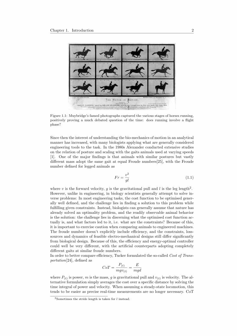
Modern understanding of the difference between running and walking dates to thephotographic studies of Muybridge in the 1870s, when he demonstrated throughchronophotography the presence of a flight phase1 during running for horses as seenin figure 1.1 and, subsequently, various other animals.

1Flight phase: a phase during a single cycle in which no body-parts touch the ground.

1

Chapter 1. Introduction 2

Figure 1.1: Muybridge’s famed photographs captured the various stages of horses running,positively proving a much debated question of the time: does running involve a flightphase?

Since then the interest of understanding the bio-mechanics of motion in an analyticalmanner has increased, with many biologists applying what are generally consideredengineering tools to the task. In the 1980s Alexander conducted extensive studieson the relation of posture and scaling with the gaits animals used at varying speeds[1]. One of the major findings is that animals with similar postures but vastlydifferent mass adopt the same gait at equal Froude numbers[25], with the Froudenumber defined for legged animals as

Fr =v2

gl(1.1)

where v is the forward velocity, g is the gravitational pull and l is the leg length2.However, unlike in engineering, in biology scientists generally attempt to solve in-verse problems: In most engineering tasks, the cost function to be optimised gener-ally well defined, and the challenge lies in finding a solution to this problem whilefulfilling given constraints. Instead, biologists can generally assume that nature hasalready solved an optimality problem, and the readily observable animal behavioris the solution: the challenge lies in discerning what the optimised cost function ac-tually is, and what factors led to it, i.e. what are the constraints? Because of this,it is important to exercise caution when comparing animals to engineered machines.The froude number doesn’t explicitly include efficiency, and the constraints, loss-sources and dynamics of feasible electro-mechanical designs still differ significantlyfrom biological design. Because of this, the efficiency and energy-optimal controllercould well be very different, with the artificial counterparts adopting completelydifferent gaits at similar froude numbers.In order to better compare efficiency, Tucker formulated the so-called Cost of Trans-portation[24], defined as

CoT =P(t)

mgv(t)=

E

mgd

where P(t) is power, m is the mass, g is gravitational pull and v(t) is velocity. The al-ternative formulation simply averages the cost over a specific distance by solving thetime integral of power and velocity. When assuming a steady-state locomotion, thistends to be easier as precise real-time measurements are no longer necessary. CoT

2Sometimes the stride length is taken for l instead.

3 1.3. Natural Dynamics and Morphological Computation

has since become a commonly used benchmark for comparing efficiency in leggedrobots, with the ideal reference benchmark usually being the biological counterpartfor a specific gait. This dimensionless number also has it’s drawbacks, namely itdoesn’t reward speed, as the alternate formulation shows. Power usually doesn’tscale well with speed, so we see that the alternate formulation is less misleading. Ifwe reconsider that animals adopt specific gaits based on the froude number, eachgait is an energy-optimal solution for that specific speed and morphology, and notthe specific distance covered. So it is not surprising that a slower walking gait willhave lower CoT compared to a faster running gait, but are energy-optimal solutionsat their respective speeds.

1.3 Natural Dynamics and Morphological Compu-tation

Contemporaneously to Alexander, Tad McGeer also broke ground in the area ofefficient legged locomotion, developing the principles of passive dynamics with hisPassive Dynamic Walker (PDW)[15]. This mechanical contraption was built sim-ilarly to a pair of human legs, including a unilaterally knee-constraint, and couldstably walk down gentle slopes. What was so impressive is that it did so with nosensing and no actuation and ergo no control. If the legs were held upright, theywould topple as soon as let go, but if started on a gentle slope they would settle intoa dynamically stable limit-cycle! The gentle slope causes a continuous conversion ofpotential to kinetic energy, necessary to make up for minor losses from joint-frictionand impact. Nonetheless it proves the possibility of solving extremely efficient, dy-namically stable locomotion through morphological design instead of control. Later,Ruina’s lab at Cornell designed the Cornell Ranger[3], a powered ’passive’ dynamicwalker3 which currently holds the world record for distance travelled on a singlebattery charge (currently at 65.2 km) and the lowest CoT, at 0.28, very close to thefabled 0.2 of human walking.All these designs showed the advantage of locomoting at the natural frequency of thesystems. Indeed, it has been shown that human walking can be modeled with thisprinciple as an inverted pendulum during the stance phase, and a regular double-pendulum during swing phase in order to analyze stability and velocities[8].Further studies, including this time ground reaction forces measured through force-plates, showed the importance of the spring-like nature of muscles and tendonsin legs and led to the so-called spring-loaded inverted pendulum (SLIP) model[4].From an energetic point of view, the springs seem an obvious choice to recycle theimpact energy of each step, since legged-locomotion involves a lot of up and downs.Indeed, early models assumed that during walking control minimized vertical dis-placement of the body mass, under the assumption that this would minimize thenecessary work to be done each step. The SLIP model side-stepped this by lettingthe springs do the work on the body-mass instead of the actuators.Springs were found to be important not only for energetics, but also for stability.At the AI Lab of the University of Zurich, it was found that often in nature thephysical morphology of certain animals is such that they simplify specific tasksthat engineers would usually solve through computation. The term morphologi-cal compuation was coined to describe this phenomenon. Fast and stable runningfor quadruped and bipeds is generally been considered a difficult control problem4,

3Generally ’passive’ means in complete absence of actuation, and the term ’natural dynamics’are used to indicate that actuation is done in harmony with the un-actuated dynamics o thesystem.

4During most running gaits quadrupeds have less than three contact points on the ground at atime, meaning there is no static support polygon: they must rely on dynamic stability solutions.


Figure 1.2: Passive Dynamic Walkers, mechanical systems that require no control or ac-tuation to locomote stably, all have a powerful commonality: by exploiting the naturaldynamics of the system, energy loss is kept very low. The first PDW systems were prob-ably wooden tinker toys which would shuffle down an incline, such as the the penguinin A. In B to D are represented purpose-built PDW-systems to study the phenomenon,including a replica of Tad McGeer’s famous first walker (C).

but the Puppy robot[19] [10] demonstrated very robust locomotion with only feed-forward actuation by greatly enlarging the stable basin of attraction through cleveruse of springs in the legs.

1.4 Motivation at BIRL

At the Bio-Inspired Robotics Lab of ETH Zurich, under professor Fumiya Iida,we are currently tackling how to exploit natural dynamics for efficient locomotion,starting with very simple systems in order to isolate and identify design principles.As the simplest form of a hopping system, it is useful to reduce the system to a singlemass, upon which we can freely apply forces such that ballistic flight is achieved, asseen in figure 1.3. In this case, the path of the mass resembles that of a bouncingball. In this case, the force applied to the mass must do two things. First, it mustaccelerate the mass from stand-still until it achieves ballistic flight. Second, it must’catch’ the mass again and decelerate it, in other words, it must do negative workon the system: the force applied removes energy from the system.If this force is applied by an actuator without energy-storage, the actuator expendsenergy once to transfer it to the system, and then once again to remove it form thesystem. This leads us to the first design principle: Minimize Unsprung Mass.By placing springs under the mass, the kinetic energy of the system at landing canbe stored in the potential energy of the spring and released again to achieve thenext step. Any kinetic energy carried by unsprung mass is instead lost on impact,and needs to be replaced again by the actuator.While an ideal system with no unsprung mass would hop perpetually, this is ofcourse not so for real systems: every joint, actuator and even spring has someinherent friction or damping through which energy is also dissipated. The secondprinciple is to Minimize Friction . This can be done in many ways. Simplifyingthe system to have as few joints as possible elegantly avoids the problem. A properchoice of motors and gearing is also very important: most conventional gears displaylarge amounts of friction and/or are display poor backdriveability: they may efficientwhen driven from the motor-side, but display extremely high friction when driven

5 1.4. Motivation at BIRL

y

g

u(t) = F

x

Figure 1.3: If hopping is treated as a mass moving along ballistic trajectories, the forceapplied must do all the work on the system: both to accelerate it until lift-off as well asslow it down at landing.

Unsprung Mass

Sprung Massg

u(t) = F

Figure 1.4: The kinetic energy carried by the sprung mass will be absorbed into the springthen released again for the next step. Instead, the kinetic energy of the unsprung mass islost at impact, and the input force must do an equal amount of positive work to replaceit. Therefore, minimizing unsprung mass is important for achieving efficient locomotion.


from the shaft. Using gearless or low-geared motors is one way of reducing this,however it should be noted that motor-torque output is proportional to current. Inorder to achieve the same torque without gears, motors must run with much highercurrent, leading to greater heat-losses in the motors. Therefore it is important tofind a good balance in the design.Treating the system now as a mass-spring system, it displays certain resonant fre-quencies at which power losses are minimal. This brings us to the final principle,already explored with the passive dynamic walkers: Minimize negative work.Negative work is defined as when an effort, i.e. force, is applied in opposite direc-tion to it’s corresponding flow, i.e. velocity5, in other words it removes energy froma system and represents negative power. Exciting a system away from it’s eigen-frequency implies doing negative work, in other words, the actuator is acting bothas an actuator as well as a brake in order to force the system to follow a motionthat is not natural. This should be avoided either by adjusting the control input oradjusting the system dynamics, e.g. by tuning the spring stiffness.

1.5 Goal of this Thesis

So far, efficient locomotion through natural dynamics has been usually approachedas a mechanical design challenge. We state the following hypothesis. Applyingoptimal control theory to the systems locomoting at natural dynamics, such as theC-shaped curved beam hopper and the segmented-beam hoppers, leads to lower Costof Transport.

5For more on efforts and flows, see section 2.2.

Chapter 2

Mathematical Principles

In this thesis, we deal deal with the energy-optimal control of simple hopping robots,the dynamics of which span both the mechanical and the electrical domain. Beforeproceeding, we will introduce the mathematical concepts and notation that will befrequently used throughout the rest of this thesis. In particular we will quicklyexpose the reader to optimal control theory, also a unified approach to modelingcross-domain systems and finally we will touch on stable-limit cycles and what thismeans for efficient hopping.

2.1 Optimal Control in a nutshell

Optimal control is an extension of the calculus of variations used to find controlpolicies. It is a very powerful tool, as it can prove a certain control trajectory tobe optimal, i.e. there exists no other trajectory that yields a better solution. It isimportant to keep in mind that claiming a control policy is ’optimal’ has no mean-ing by itself: it must always be the optimal policy for a specific cost function. Ofthe many principles belonging to optimal control theory, we will make use of Pon-tryagin’s Minimum Principle (PMP) which is applied to continuous time systems.Without going into the proofs, the main points of the PMP are presented here. Formore details, see [2].

2.1.1 Pontryagin’s Minimum Principle

Consider the standard continuous-time optimality problem, formulated as follows:

min~u(t)

∫ T

0

g(~x(t),~u(t)) dt

subject to ~x(t) = ~f(~x(t),~u(t))

(2.1)

where ~x(t) is the vector of state variables, g(~x(t),~u(t)) is the cost function and ~f(~x(t),~u(t))

are the system dynamics. The objective of the optimization problem is to find atrajectory of control inputs u(t) which minimizes the integral of the cost functiong(~x(t),~u(t)) over a certain time, usually while fulfilling certain specific boundary con-ditions. In the 1950s, the Russian mathematician Pontryagin first derived the min-imum principle to solve this optimization problem analytically. The optimisationproblem is equivalent to solving the following problem:

7

Chapter 2. Mathematical Principles 8

~u∗(t) = argminu

[H(~x(t),~u(t),~p(t))] (2.2)

H(~x(t),~u(t),~p(t)) = g(~x(t), ~u(t)) + ~p ᵀ(t)~f(~x(t),~u(t)) (2.3)

~p(t) = −∇xH(~x∗(t),~u∗

(t),~p(t)) (2.4)

where H(~x(t),~u(t),~p(t)) is the so-called Hamiltonian function, a superscripted star suchas in ~u∗(t) indicates an optimal trajectory and ~p(t) is a vector of adjoint variables,

with size equal to ~x(t). The adjoint variables indicate the sensitivity of the finalcost to perturbations to the dynamics, in other words the cost of deviating fromthe optimal trajectory. In order to solve the equivalent problem, several boundaryconditions for the differential equations ~p(t) = −∇xH(~x∗(t), ~u

∗(t), ~p(t)) can be used,

depending on the exact formulation: whether initial or ending values of ~x(t) areknown or free, if there is a terminal cost, etc. For more details on the types ofboundary conditions and a complete derivation, see [2]. Equation (2.2) shows thatthe nature of the differential equations to be solved depends on the dynamics of thesystem. In our case, the dynamics are non-linear and thus so are the differentialequations, making them very difficult to solve analytically or in most cases havingno analytical solution.

2.1.2 Bang-Bang as an optimal controller

There is a special case for the solution to PMP. That is, if the Hamiltonian islinear in ~u(t), the optimal controller must be a bang-bang controller. Abang-bang controller is a controller that always takes the extreme values allowed,i.e. either it’s maximum or it’s minimum value. Recall that for a function F(x) tobe linear, it should fulfill the following condition:

F(x1+x2) = F(x1) + F(x2)

Let’s clarify this statement: when the Hamiltonian function is linear in ~u(t) it canbe rewritten as:

H(~x(t),~u(t),~p(t)) = σ1(~x(t),~p(t)) + ~σ ᵀswitch(~x(t),~p(t))

~u(t) (2.5)

where σ1(~x(t),~p(t)) gathers all terms that do not multiply ~u(t) and ~σswitch(~x(t),~p(t))

gathers all those that do. In order to minimise the Hamiltonian, we must make~σ ᵀswitch(~x(t),~p(t))

~u(t) as negative as possible. Thus, for each element of ~σswitch(~x(t),~p(t))

that is positive, the corresponding element of ~u(t) should be as negative as possible,while for negative element of ~σswitch(~x(t),~p(t)), the corresponding elements of ~u(t)should be as positive as possible. The function ~σswitch(~x(t),~p(t)) is called in thesecases the switching function, as it’s sign determines whether the maximal or theminimal bang is input. This is an important result from control theory of which wewill make use in the next chapters.

2.1.3 Formulating equivalent cost functions

Very often the most intuitive cost function to formulate turns out to be extremelydifficult to solve. To side-step this, alternative equivalent cost functions are usedinstead. For example, take the system represented in figure 2.1:with system dynamics:

x(t) = u(t)

9 2.2. Efforts, Flows and Cross-Domain Power Analysis

u(t) = F

x(t)

x0 xfinal

Figure 2.1: In our example problem we want to apply a force to a block to move it fromit’s starting position to a specified final position xfinal. Maximizing the velocity overthe distance or minimizing the time to reach the distance can be shown to be physicallyequivalent.

Imagine that we want to move the block from point x0 to xfinal as quickly aspossible. Intuitively, we want to maximize the velocity of the block. Mathematically,maximizing the velocity is equivalent to minimizing the negative of the velocity1

minu(t)

∫ T

0

−x(t) dt

In this case the cost function is g(x,u) = −x(t). Alternatively, we could formulatethe cost function as g(x,u) = 1, and so minimize

minu(t)

∫ T

0

1 dt

This means minimize the time it takes to move the block between x0 and xfinal.These two cost function, while mathematically different, are physically equivalentas minimizing the time to move a certain distance is paramount to maximizingthe velocity over this distance. Caution should be used when setting up equivalentcost functions, as the conditions that guarantee equivalency can be tricky and evenmisleading.

2.2 Efforts, Flows and Cross-Domain Power Anal-ysis

Engineers tend to specialize in specific domains: electrical, mechanical, thermal orfluid just to name a few. In this section we will present a unified set of systemvariables, with which dynamics systems in different domains can be described. Inparticular, it will be shown how power flows in and out of the system dependingon the relationships between these variables, and the equivalents between differentdomains. Because in this thesis we focus on electro-mechanical systems, we will

1By convention, we always talk about ’minimizing’ in optimal control. Everything can beequally formulated as a maximization problem as well.


only present equivalencies for these two physical domains. For a more completetreatment of the subject, see [6].

2.2.1 The Fundamental System Variables

When considering the dynamics of any system, the energy-content and thereforethe state of the system can always be described by a pair of kinetic and a pairof kinematic variables, regardless of the domain. The kinetic variables are themomentum p(t) and effort e(t), while the kinematic variables are the displacementd(t) and flow f(t). These are called the fundamental system variables.A displacement d(t) is what is conventionally identified as a coordinate of the system.In the mechanical domain, it can be a linear or a rotational position. In the electricaldomain, it is a charge. The corresponding flow f(t) is the time derivative of thedisplacement:

f(t) =dq(t)

dt(2.6)

q(t) =

∫f(t)dt (2.7)

In the mechanical domain, the flow f(t) is a linear or rotational velocity, while inthe eletrical domain it is a displacement of charge over time, i.e. a current. Thekinetic variables, momentum and effort, share a similar relationship: the effort e(t)relating to a specific coordinate is the time derivative of the momentum p(t) of thatsame coordinate:

e(t) =dp(t)

dt(2.8)

p(t) =

∫e(t)dt (2.9)

In the mechanical domain, as the name itself suggests, the momentum refers to thelinear or angular momentum, while the corresponding effort is a force or a torque.In the electrical domain, the momentum corresponds to the flux linkage, while theeffort is a voltage. Each coordinate of a system can be fully described by these fourvariables. The relationship between the kinetic and kinematic pair is representedin figure 2.2.A big advantage of these variables is that it makes it clearer that work, power andenergy can be defined in the same way regardless of the domain. For example, inthe mechanical domain work we say that a force does work on a body when thebody is displaced, whether the displacement is caused by the force or not. Then aninfinitesimal increment in work is defined as

dW(t) = F(t)dx(t)

= e(t)dq(t)

where W(t) is work, F(t) is force and x(t) is position. The corresponding power issimply the rate of work over time, or effort times flow:

P(t) =dW(t)

dt

= F(t)

dx(t)

dt= F(t)x(t)

= e(t)dq

dt= e(t)f(t)

11 2.2. Efforts, Flows and Cross-Domain Power Analysis

Domain Electrical Linear Me-chanical

Rotational Mechan-ical

Displacementq(t)

Charge Q(t) Position x(t) Angular Position φ(t)

Flow f(t) Current I(t) Velocity x(t) Angular Velocity φ(t)Momentump(t)

Flux Linkageλ(t)

Mechanical Mo-mentum p(t)

2Angular MomentumL(t)

Effort e(t) Voltage V(t) Force F(t) Torque τ(t)Ideal Inductor Inductor Point Mass Moment of InertiaIdeal Resistor Resistor Damper Rotational DamperIdeal Capaci-tor

Capacitor Spring Rotation Spring

Table 2.1: Equivalents of electrical and mechanical domains.

where P(t) is the power. Plugging in the corresponding efforts and flows of rotationalor electrical coordinates, we see that we get exactly what would be expected:

General Power: P(t) = e(t)f(t)

Linear Mechanical: Plin(t) = F(t)x(t)

Rotational Mechanical: Prot(t) = τ(t)φ(t)

Electrical: Pelec(t) = V(t)I(t)

where τ(t) is a torque, φ(t) is the corresponding flow, an angular velocity; V(t) is avoltage and I(t) is the corresponding current. Note that while the usual notationfor current I(t) doesn’t explicitly show it as a time-derivative, it is: current is the

flow of charge, i.e. I(t) = ˙Q(t). This is equivalent to the usual notation of angular

velocity as ω(t) = φ(t).Also in all cases, energy is defined as the time integral of power, and therefore ofthe effort times the flow:

E(t) =

∫e(t)f(t)dt

2.2.2 Unified System Components

So far we’ve seen how kinetic and kinematic variables are related through power,however they also relate through specific system component. The most importantthree are the ideal inductors, resistors and capacitors.. The naming of these compo-nents makes it clear what they represent in the electrical domain; their counterpartsin the mechanical domain are presented in table

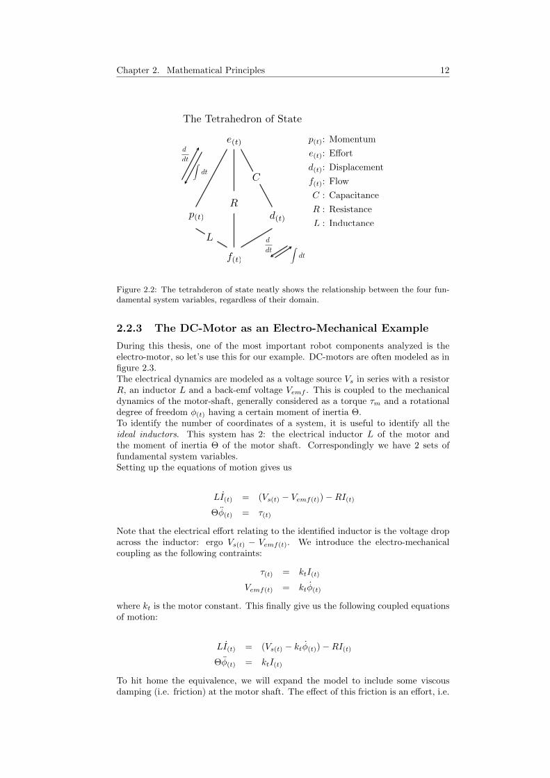
The way these components relates the universal variables of state is best shownwith the so-called tetrahedron of state, seen in figure 2.2.

In short, both springs and capacitors store a displacement and release a proportionalforce. Inductors, mass and moments of inertia store momentum and release a pro-portional flow. Both electrical resistors and mechanical dampers dissipate energyby creating an opposing effort (whether a voltage, force or torque) proportional tothe corresponding flow (current, linear or angular velocity).


e(t)

f(t)

d(t)p(t)

C

R

L

d

dt Zdt

d

dtZ

dt

p(t): Momentum

e(t): E↵ort

d(t): Displacement

f(t): Flow

C : Capacitance

R : Resistance

L : Inductance

The Tetrahedron of State

Figure 2.2: The tetrahderon of state neatly shows the relationship between the four fun-damental system variables, regardless of their domain.

2.2.3 The DC-Motor as an Electro-Mechanical Example

During this thesis, one of the most important robot components analyzed is theelectro-motor, so let’s use this for our example. DC-motors are often modeled as infigure 2.3.The electrical dynamics are modeled as a voltage source Vs in series with a resistorR, an inductor L and a back-emf voltage Vemf . This is coupled to the mechanicaldynamics of the motor-shaft, generally considered as a torque τm and a rotationaldegree of freedom φ(t) having a certain moment of inertia Θ.To identify the number of coordinates of a system, it is useful to identify all theideal inductors. This system has 2: the electrical inductor L of the motor andthe moment of inertia Θ of the motor shaft. Correspondingly we have 2 sets offundamental system variables.Setting up the equations of motion gives us

LI(t) = (Vs(t) − Vemf(t))−RI(t)Θφ(t) = τ(t)

Note that the electrical effort relating to the identified inductor is the voltage dropacross the inductor: ergo Vs(t) − Vemf(t). We introduce the electro-mechanicalcoupling as the following contraints:

τ(t) = ktI(t)

Vemf(t) = ktφ(t)

where kt is the motor constant. This finally give us the following coupled equationsof motion:

LI(t) = (Vs(t) − ktφ(t))−RI(t)Θφ(t) = ktI(t)

To hit home the equivalence, we will expand the model to include some viscousdamping (i.e. friction) at the motor shaft. The effect of this friction is an effort, i.e.

13 2.3. Positive Work, Negative Work and the Hopping at Natural Frequency

+ _ + _

R L

Vemf

DC-motor model

⌧(t)I(t)

⇥Vs(t)

�(t)

Figure 2.3: The standard DC-motor model composed of a voltage source in series withan inductor, resistor and the back-emf voltage, which couples the electrical dynamics withthe mechanical dynamics of the shaft.

torque, that is proportional and of opposite sign to the flow, i.e. angular velocity.The equations of motion become

LI(t) =(Vs(t) − ktφ(t))−RI(t)Θφ(t) = ktI(t)−dφ(t)

Seem familiar? As we saw earlier, a mechanical damping element affects the me-chanical dynamics in exactly the same way an electrical resistor affects the electricaldynamics. Keeping all this in mind, the stepping across domains seems much lessarduous: we are merely increasing the degrees of freedom of the system.

2.3 Positive Work, Negative Work and the Hop-ping at Natural Frequency

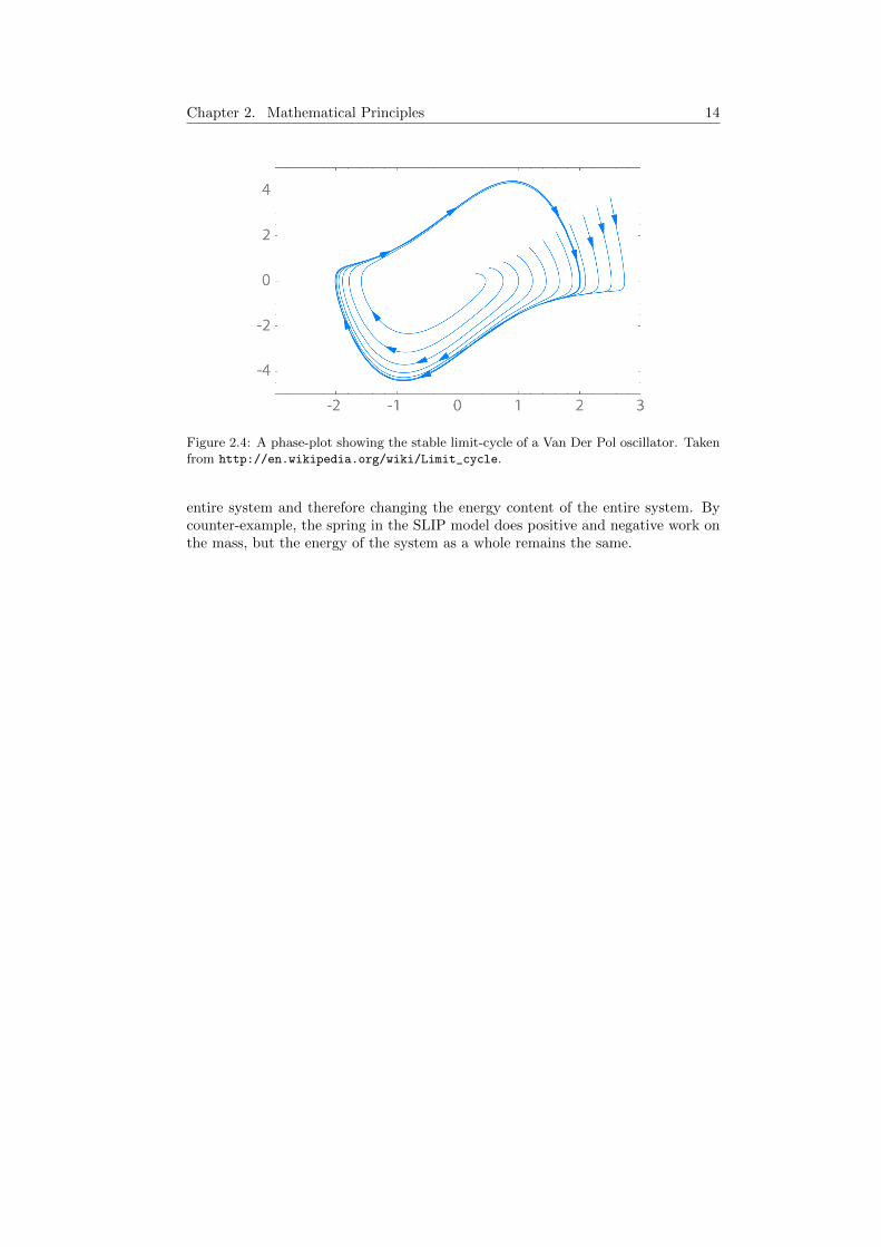
The key concept being exploited at the Bio-Inspired Robotics Lab is natural fre-quency. All of our hoppers are driven at their natural frequency and settle intostable limit-cycle gaits. A stable limit-cycle defines a behaviour where the phase-plot of a system describes a closed loop, and nearby trajectories spiral into thelimit-cycle, as seen in figure 2.4.The advantage of these gaits is that at their resonant frequency, very little energyis lost from external work. To clarify, we define work as either positive or negative:considering an arbitrary effort, we say that an effort e(t) does positive work ona system when it has the same direction i.e. sign as it’s correspondingflow f(t). It does negative work if the signs are opposite. Positive workincreases the total energy of the system. Negative work removes energyfrom the system.NOTE: we will consider work done by an actuator, i.e. a control input, as un-recoverable. This is purely a system convention: there are of course systems, e.g.hybrid cars, where the negative work done by the actuator is stored, e.g. examplein a battery. In this thesis, any time this is possible we will consider the storagecomponent (which must be either an ideal capacitor or an ideal inductance, see 2.2)as part of the system model. When we talk about work, we mean work done on the


Figure 2.4: A phase-plot showing the stable limit-cycle of a Van Der Pol oscillator. Takenfrom http://en.wikipedia.org/wiki/Limit_cycle.

entire system and therefore changing the energy content of the entire system. Bycounter-example, the spring in the SLIP model does positive and negative work onthe mass, but the energy of the system as a whole remains the same.

http://en.wikipedia.org/wiki/Limit_cycle

Chapter 3

Efficient Control ofSegmented Beam Hoppers

Next to the curved-beam hoppers presented in the next chapter, recently somesegmented-beam hoppers have been developed in the BIRL lab. Segmented-beamhoppers feature standard rigid bodies, with standard pull-springs providing elas-tic energy storage. The first generation segmented beam hopper, developed byBenedikt Mathis [14], proved the viability of this concept as an alternative designto curved-beam hoppers capable of efficient hopping gaits. The advantages of seg-mented beam hoppers with respect to the curved-beam hoppers are two-fold: First,they are much more straight-forward to model.Second, having a simple design anddirect actuation of the joint, control can be applied much more effectively. Thischapter focuses on the second part, in particular, how do we approach design-ing an energy-optimal controller for such a robot?

3.1 The hopping robot CHIARO

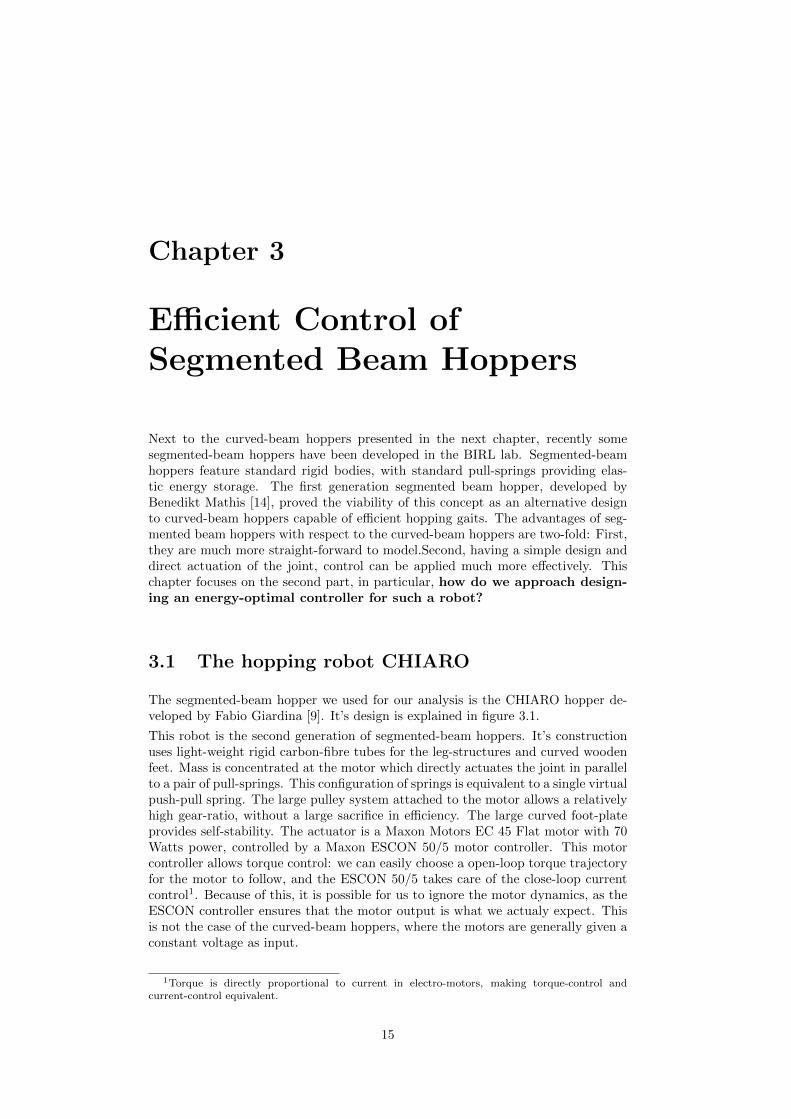
The segmented-beam hopper we used for our analysis is the CHIARO hopper de-veloped by Fabio Giardina [9]. It’s design is explained in figure 3.1.

This robot is the second generation of segmented-beam hoppers. It’s constructionuses light-weight rigid carbon-fibre tubes for the leg-structures and curved woodenfeet. Mass is concentrated at the motor which directly actuates the joint in parallelto a pair of pull-springs. This configuration of springs is equivalent to a single virtualpush-pull spring. The large pulley system attached to the motor allows a relativelyhigh gear-ratio, without a large sacrifice in efficiency. The large curved foot-plateprovides self-stability. The actuator is a Maxon Motors EC 45 Flat motor with 70Watts power, controlled by a Maxon ESCON 50/5 motor controller. This motorcontroller allows torque control: we can easily choose a open-loop torque trajectoryfor the motor to follow, and the ESCON 50/5 takes care of the close-loop currentcontrol1. Because of this, it is possible for us to ignore the motor dynamics, as theESCON controller ensures that the motor output is what we actualy expect. Thisis not the case of the curved-beam hoppers, where the motors are generally given aconstant voltage as input.

1Torque is directly proportional to current in electro-motors, making torque-control andcurrent-control equivalent.

15

Chapter 3. Efficient Control of Segmented Beam Hoppers 16

Figure 3.1: The CHIARO hopper used for the analysis. The design was kept as light aspossible, with most of the 0.7 Kg mass concentrated at the motor. The motor actuatesthe single joint through a drive belt over a large pulley. The springs act in parallel toteh actuator. A large, curved foot-plate provides both lateral and sagittal stability. Thisfoot-plate is designed so that it can be easily replaced or adjusted. A key result fromGiardina’s work is that the stable limit-cycle behaviour of the robot is strongly influencedby the curvature of the foot-plate and the angle of attack with which it is fixed to the leg.

17 3.2. Separating the stability problem from the energy-optimality problem

2 3 4 5 6 70.4

0.5

0.6

0.7

0.8

0.9

1

1.1

fT

[Hz]

β[r

ad

]

R=0.2 m

0 < σ(α) < 5

5 < σ(α) < 10

10 < σ(α) < 15

15 < σ(α)

2 3 4 5 6 70.4

0.5

0.6

0.7

0.8

0.9

1

1.1

fT

[Hz]

β[r

ad

]

R=0.3 m

2 3 4 5 6 70.4

0.5

0.6

0.7

0.8

0.9

1

1.1

fT

[Hz]

β[r

ad

]

R=0.4 m

2 3 4 5 6 70.4

0.5

0.6

0.7

0.8

0.9

1

1.1

fT

[Hz]

β[r

ad

]

R=0.6 m

Figure 3.2: These graphs from [9] show the regions of self-stability to for various configu-rations of the robot CHIARO, obtained in simulation. Each graph represents a differenta specific foot curvature R. The y-axis represents different angles of attack at which thefoot-plate is attached to the robot leg. Each dot along the x-axis represents a frequencyat which the robot was driven with an open-loop sinusoidal input. Darker dots representfaster convergence to a stable limit-cycle.

3.2 Separating the stability problem from the energy-optimality problem

For most systems, robotic or not, control traditionally has the role of maintainingstability. We use a novel approach based on the following hypothesis: we can disre-gard stability in the design of an energy-optimal controller. This claim is based onthe principle of morphological computation. Morphological computation is when acomputational task no longer needs to be computed because the problem has beenoffloaded to the physical morphology of the system. During the design of CHIARO,Giardina showed the robot was self-stable2 through a series of experiments. Specificdesign parameters, namely the foot curvature and foot angle-of-attack were modi-fied. For each combination of these two parameters, the robot was driven severaltimes with an open-loop sinusoidal torque at different frequencies. If the robot fellover, that frequency was considered an unstable input, if it didn’t fall over, it wasmarked as a stable input. For many combinations of foot curvature and foot angle-of-attack were modified, the robot would settle into a stable limit-cycle for a widerange of frequencies. This indicates a large region of self-stability of the robot forsinusoidal control inputs, as represented in figure 3.2.This is a key feature of the CHIARO robot. In appendix A we show that this conceptof self-stability can be extended to a wide range of periodic control inputs and moreimportantly, that energy-optimal control inputs must be stable. This allows twothings: first, the design of an energy-optimal controller can be done unrestricted bystability issues. Second, this assumption allows for the design of a periodicopen-loop controller input , since for any periodic control input we assume that

2Self-stable it is meant that the robot settles into a stable limit-cycle for a wide range of open-loop control inputs. In other words, feed-back control is unnecessary to achieve stable limit-cyclegaits.


the system will settle into a stable limit-cycle. It is important to note that thisgait optimization is done over two stages: indeed, for each specific combination ofdesign parameters, a specific control input frequency was found to yield the lowestCost Of Transport. Only by iterating over both the design parameters as well asthe control parameter is it possible to identify the overall most efficient gait. Thisis due to the fact that, by delegating stability to the morphology, important factorssuch as the lift-off and landing angle of the robot are determined by the physicalmorphology and no longer by the controller input. Thus, whenever we speak of anenergy-optimal control input, it is optimal for a specific morhpology.

3.3 Bang-Bang for CHIARO

Bang-bang controllers (see subsection 2.1.2) are attractive and often used in prac-tice due to their simplicity. In our case, if the energy-optimal controller can beassumed to be a bang-bang controller it is actually not strictly necessary to solvethe switching function; finding the energy-optimal controller can be can be reducedto a parameter search, as will be explained in section 3.5. However, equation (2.5)shows that the optimal controller is only proven to be a bang-bang controller if theHamiltonian function is linear in u(t). In our case, the system dynamics ~f(~x(t),u(t)),while being complicated and non-linear in the state variables, are indeed linear inthe motor torque, our only control input3. Recalling that the Hamiltonian functionhas the following form

H(~x(t),u(t),~p(t)) = g(~x(t), u(t)) + ~p ᵀ(t)~f(~x(t),u(t))

the only remaining condition for the Hamiltonian function to be linear is that thecost function g(~x(t),u(t)) also be linear in u(t). Note that the vector notation on u(t)has been dropped because we only have a single control input for our robots.Thus, for us to be able to claim that the energy-optimal control input is bang-bang,we must find a cost function g(~x(t),u(t)) that fulfills two conditions:

1. The cost function g(~x(t),u(t)) must be linear in u(t).

2. Minimising∫g(~x(t),u(t))dt must be equivalent to minimising energy-input.

3.4 Picking a Equivalent Cost Function

A common cost function used for energy optimization problems is the quadraticcost on the control input: u2(t). The objective of this cost function is to minimisethe torque to zero and not to negative, since the sign only indicates direction. Thesquare elegantly removes the sign problem, while making it nicely convex and penal-ising larger errors exponentially more. Most importantly, quadratic problems havebeen extensively studied and easy to set up and dispose of powerful algorithms tosolve, meaning numerical solutions can be found for readily, including for leggedgaits [22]. Unfortunately in our case this is unsatisfactory as it would violate thelinearity requirement. Further, minimising torque is only equivalent to optimisingfor energy under certain conditions, since energy depends on both effort and flowi.e. both torque and angular velocity and at the same time voltage and current.So how do we formulate a cost function that is equivalent to minimising negativework and is linear in u(t)?

The cost function we will choose is the following:

3See [9] for the dynamics of a model of the CHIARO robot validated with real-world results.

19 3.4. Picking a Equivalent Cost Function

g

u(t) = F

a) b)

y(t)

Figure 3.3: Two simple 1-D spring-mass model allows us to easily analyse the dynamics.a) without damping and b) with. Since the dynamics of the segmented-leg hopper are alsolinear in u(t), the two systems are equivalent for our purpose.

g(~x(t),~u(t)) =n∑i=1

Rifi(t) (3.1)

subject to (3.2)

uj(t) = [0, ujMax]fj(t) ≥ 0 (3.3)

u(j(t) = [ujMin, 0]fj(t) < 0 (3.4)

where fi(t) are the flow variables of the system and Ri are the ideal resistors (e.g.damping or resistance) related to those flows, as described in 2.2. In other words,our cost function is to minimise the damping losses of the system. To the costfunction, we’ve added the following contraint: the control inputs (which we assumeto be effort variables) are not allowed to do negative work, they must exert effortin the same direction as their corresponding flow. In the subsection we will explainthis concept more clearly through an example and show under what conditions itis equivalent to minimising energy input.

3.4.1 Minimizing Damping Losses for a 1-D Hopper

To clearly explain our solution we will introduce very simple hoppers, representedin figure 3.3. The dynamics of these hoppers are much simpler, but the linearityof their dynamics in terms of u(t) is the same as in the segmented-beam hoppers,making them equivalent for our purpose.

This system has only a single coordinate making it easier to analyse, and it’s equa-tions of motion are as follow:

~x(t) =

(y(t)y(t)

)

x1(t) = y(t) = x2(t)

x2(t) = y(t) =ks(y0 − x1(t))− dx2(t) − g + u(t)

m


where ~x(t) is the state vector, formed by the displacement variable y(t) and the flowvariable y(t): the vertical position and velocity, respectively. ks and d are the springand damper constants respectively, g is the gravitational pull, u(t) is the the controlinput, i.e. the force acting on the mass, and finally m is the mass. For clarity, fromnow on we will use y(t) and y(t) directly instead of the state vector ~x(t), and we willassume m to have unitary value.For this system, the solution proposed ((3.11)) takes the following form:

g(y(t),u(t)) = dy(t) (3.5)

u(t) = [0, umin] if y(t) < 0 (3.6)

u(t) = [0, umax] if y(t) >= 0. (3.7)

In the following it will be shown why this is equivalent to minimising energy input.It is assumed that we are at steady-state hopping with a peak hopping height ofh0 and no energy losses during flight-phase. We will further limit ourselves to thestance-phase: this is done on the assumption that the force of the control inputu(t) is achieved by the leg pushing against the ground. During flight the robothas nothing to push against and therefore cannot achieve any force4. Switchingbetween flight and stance phase is determined by the crossing of y(t) = y0, where y0is the unsprung leg length. Velocity at touch-down can be calculated by the changein potential energy from maximum hopping height h0 to touch-down height y0, asy(TD) = −v0 = −

√(2mg(h0 − y0)), where TD indicated time at touch-down. To

fulfill the assumption of steady-state hopping, kinetic energy at lift-off must be thesame as at touch-down, ergo y(TO) = v0. So the boundary conditions of the stancephase are:

y(TD) = y0

y(TD) = −v0y(TO) = y0

y(TO) = v0

Every state pair{y(T ), y(T )

}(with T an arbitrary point in time) represents a specific

energy content, as together they represent the total potential energy (both fromgravitational pull and energy stored in the spring) as well as kinetic energy. Theinitial and terminal state-pairs are completely equivalent, not only in total energybut also in division between potential and kinetic energy. The sole difference is thevelocity having opposite direction. In the case of an ideal spring-mass system withno losses (figure 3.3 a)), the system’s state trajectory will automatically move frominitial to terminal condition, as seen in figure 3.4.For easier comparison, the position y(t) during stance is mapped to a continuousphase between −π representing touch-down and π representing take-off, with thezero-point representing maximum compression, at which point y(phase=0) = 0, asrepresented in figure 3.5. This is a piece-wise linear mapping, splitting the stance-phase into two equivalent phases: spring-compression, spanning from −π to 0, andspring-expansion, spanning from 0 to π.Actuator input is required once damping is considered, as in model 3.3 b), as theenergy lost from damping will result in a lower velocity, and therefore lower totalenergy, at take-off, as seen in figure 3.6.

4For the CHIARO robot similar arguments can be made indicating energy-input during flightshould be negligible. In either way though it does not affect the resulting cost-function: dealingwith only stance-phase merely simplifies the explanation.


0.22 0.24 0.26 0.28 0.3 0.32−1

−0.8

−0.6

−0.4

−0.2

0

0.2

0.4

0.6

0.8

1

Posit ion y( t)

Velocityy(t)

Stance with no damping

Initial stateTerminal state

Figure 3.4: A phase plot of the state variables for an undamped hopper at stance: velocityover position. In the undamped hopper control input is unnecessary, as the state-trajectorymoves naturally from the initial condition (red circle) to the terminal condition (greentriangle).

−pi −pi/2 0 pi/2 pi

−1

−0.8

−0.6

−0.4

−0.2

0

0.2

0.4

0.6

0.8

1

Phase

Velocityy(t)[m

s]

Phase plot of stance with no damping

Initial state

Terminal state

Figure 3.5: For the purpose of comparison, the stance phase is mapped to a phase spanningfrom −π, representing touch-down, to π, representing take-off, with zero representingmaximum compression where velocity is also zero.


−pi −pi/2 0 pi/2 pi

−1

−0.8

−0.6

−0.4

−0.2

0

0.2

0.4

0.6

0.8

1

Phase

Velocityy(t)m s

Phase plot of stance with damping

Undamped

Damped

Initial state

Terminal state

Figure 3.6: Damping losses in the system are directly proportional to the velocity of thesystem, in other words to the are under the curve. To ensure steady-state hopping, energymust be added again to the system to push the velocity to the terminal condition (greentriangle); doing this however also increases the damping losses, making the problem non-trivial.

The task of control is to then add energy to the system to push the trajectory backup to terminate at the proper terminal condition, while minimising energy-input.The path of the trajectory is important as the damping factor penalises higherspeeds5, making the control input non-conservative.The most intuitive cost-function would be to simply minimise work of the actuator:

g(y(t), u(t)) = |u(t) · y(t)|

but the absolute value, which is necessary since both negative and positive workshould to be minimised, makes the cost function non-linear. Considering that theboundary conditions fix the energy at take-off, and the fact that during stancestability considerations are unnecessary, the input force must do a total amountof positive work equal the total amount of negative work done on the system.This leads us to two conclusions: first, the control input should never do negativework. All the negative work done by the actuator must also be replaced by theactuator. This leads to the conditions on u(t) in (3.5). The second conclusionis that minimising the negative work performed by the damper is equivalent tominimising the energy input of the actuator. Taking a closer look at the energylosses, we see that

Fd = −dy(t)

Wd =

∫Pd(t)dt =

∫Fdy(t)dt

=

∫−dy2(t)dt = −d

∫dy2

dt2dt =

∫−dy(t)dy.

Since the mapping of the position to phase is a linear mapping6 this is equivalent

5We assume a standard linear damper, proportional to velocity.6It involves a mere scaling and mirroring about the maximum-compression point.


Figure 3.7: The blue line represents an energy-optimal trajectory with limits placed onthe control input u(t). The shaded green area is the bounded area between the passivedamped and undamped system trajectories, in which the optimal control input trajectoryshould move, depending on it’s limits.

to minimising the the absolute of the velocity over the stance phase. If we combinethese two conclusions, we get the following cost:

g(y(t),u(t)) = |y(t)| (3.8)

u(t) = [0, umin] if y(t) < 0 (3.9)

u(t) = [0, umax] if y(t) >= 0. (3.10)

The constraints on the control input in (3.5) is to ensure that the control input onlycontributes positive work to the system. Doing positive work with the control inputu(t) means increasing the velocity y(t), thus pushing the trajectory away from the0-axis and increasing damping force. While it may seem tempting to do negativework with u(t) to minimise damping forces, the actuator would simply be replacingthe physical damping and acting as a virtual damper with even higher dampingcoefficient. The constraint on u(t) sidesteps this problem.Since these constraints do not allow the control input to push the velocity trajectorycloser to 0, the passive, damped trajectory (solid blue line) represents the inner limit.And since the cost function minimises the curve under the trajectory, the passiveundamped trajectory (dashed black line) represents the outer limit. From this,the minimizing control input would be to allow the hopper to passively follow thedamped trajectory until the very last instant, then apply an infinite force to bringthe trajectory to the terminal condition. Since real-world actuators are limited inthe amount of force or torque they can apply, it becomes necessary to input themaximum force over as short a period of time as possible, as late as possible, asshown in figure 3.7.

3.4.2 Extending the Cost Function

Thus we have proved that minimizing energy input is equivalent to minimizing thedamping losses when hopping at natural frequency. In the most general formulation


3.11 (see below) this has simply been extended to include an arbitrary number ofcoordinates:

g(~x(t),~u(t)) =n∑i=1

Rifi(t) (3.11)

subject to (3.12)

uj(t) = [0, ujMax]fj(t) ≥ 0 (3.13)

u(j(t) = [ujMin, 0]fj(t) < 0 (3.14)

where fi(t) are the flow variables of the system, and Ri are is the dissipation (e.g.damping or resistance) related to those flows, as described in 2.2. This generalizedformulation also allows the consideration of damping losses in other domains, suchas the internal resistance of the motor. In electric motors, power loss stems fromthe internal resistance of the motor and is proportional to current. This fits per-fectly with our original statement (3.11): as we saw in section 2.2, current is theflow variable in the electrical domain, and electrical resistors are equivalent to me-chanical dampers. Taking further into consideration that motor torque is directlyproportional to the motor current via the motor constant, the cost function of oursimple 1-D hopper example can be extended as so:

g(~x(t),u(t)) = by(t) +RmotI(t) = by(t) +Rmotu(t)

kt

where kt is the motor constant. While it is easy for us to write it this way, suchthat we can still consider the system as the familiar 1-D hopper, we’ve actuallyalready extended it to 2-D: one dimension being the vertical displacement y(t) inthe mechanical domain, the other being the displacement of charge Q(t) in theelectrical domain. Recall that the current I(t) is a flow variable and merely the time

derivative it’s corresponding displacement: i.e. I(t) =dQ(t)

dt . In a similar fashion,the system can be extended to arbitrary degrees of freedom.Impact losses can also be accounted for as an instantaneous loss of kinetic energyat impact. This would merely change the initial boundary condition of the stance-phase

{y(TD), y(TD)

}to contain less energy than the terminal condition of lift-off.

The control input would then have to not only replace energy lost through dampingbut also that lost through impact.

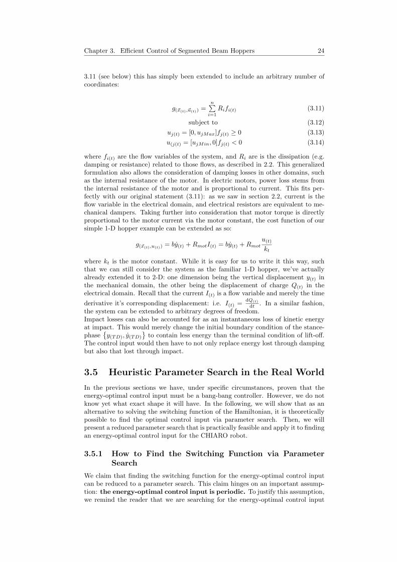
3.5 Heuristic Parameter Search in the Real World

In the previous sections we have, under specific circumstances, proven that theenergy-optimal control input must be a bang-bang controller. However, we do notknow yet what exact shape it will have. In the following, we will show that as analternative to solving the switching function of the Hamiltonian, it is theoreticallypossible to find the optimal control input via parameter search. Then, we willpresent a reduced parameter search that is practically feasible and apply it to findingan energy-optimal control input for the CHIARO robot.

3.5.1 How to Find the Switching Function via ParameterSearch

We claim that finding the switching function for the energy-optimal control inputcan be reduced to a parameter search. This claim hinges on an important assump-tion: the energy-optimal control input is periodic. To justify this assumption,we remind the reader that we are searching for the energy-optimal control input

25 3.5. Heuristic Parameter Search in the Real World

Figure 3.8: Some arbitrary, possible bang-bang trajectories are shown in the figures above.In the previous section it was proven that the energy-optimal control input must have abang-bang shape, with the bangs being of value [umin, 0, umax] depending on the sign ofthe flow variable; because of this, none of the above control trajectories can be excludedoutright.

for stable gaits, i.e. gaits that settle into stable limit-cycles. Stable limit cycles areper definition periodic. We can then solve the optimization problem over a singlecycle, which, repeating itself, ensures that the total infinite-horizon solution is alsoperiodic. Therefore, not only must the energy-optimal control input be pe-riodic, it’s period is the same as the stable-limit cycle.Now that we havedetermined that the control input is periodic, we can tackle the question: how dowe determine its shape? In the previous section we proved only that the controllermust be a bang-bang controller. The number and timing of the switches can bearbitrary, e.g. any of the trajectories of u(t) shown in figure 3.8 is theoreticallypossible.Since the control input is periodic, it is possible to represent by decomposing it intoa series of adequately chosen periodic functions, such as a Fourier series

u(t) =a02

+

N∑

n=1

[an cos(2πnt

P) + bn sin(

2πnt

P)]

where P is the period and an and bn are the coefficients. Since it is known thatu(t) is bang-bang, the decomposition can be further simplified. For example, itwould make sense more sense to use a square wave instead of sin and cos waves.We’ve chose n an even simpler approach. Instead of directly representing u(t), wesearch for a direct equivalent to the switching function: since the control inputu(t) is periodic, the zero-crossings of the switching function must also be periodic.Hence, finding a fourier series with the same zero-crossings is equivalent to findingthe switching function itself.

3.5.2 Reducing the Parameter Space

The final test of a theory is its capacity to solve the problems whichoriginated it.-George Dantzig


0 0.5 1 1.5 2 2.5

−0.6

−0.4

−0.2

0

0.2

0.4

0.6

0.8

1

1.2

1.4

Time [s ]

Switching Function and Control Input

Switching Function fswitch ( t)

Control Input u ( t) [A]

Figure 3.9: The switching function has a mere 3 parameters which can be easily sweepedthrough: Frequency f , offset and umax. The sign of the switching function determineswhether the control input is the high ban umax or 0. The offset determines the durationof the the bang by shifting the sinusoid up or down: a positive offset will result in a longerumax, a negative offset in a shorter umax.

Previously we’ve shown that finding the proper switching function can be reducedto a parameter search of a fourier series. In other words, it is equivalent to a systemidentification problem. Instead of searching the infinitely large parameter space,the space is can be greatly reduced through the use of heuristics, e.g. by cuttingthe high-frequency content. In defining a set of parameters, we’ve closely followedthe design principle of ecological balance: i.e. there should be a balance in thecomplexity of the physical morphology and the control of the system. To this end,we have defined the simplest switching function possible likely to produce goodresults:

fswitch(t) = sin(2πft) + offset (3.15)

u(t) = umax iffswitch(t) ≥ 0 (3.16)

= 0 iffswitch(t) < 0 (3.17)

where fswitch(t) is the switching function. The search-space contains a single fre-quency, f , an offset offset and the maximum value umax. The resulting trajectoryof the switching function and control input can be seen in figures 3.9. The frequencyis used to match the natural frequency of the hopping gait. The offset is used todetermine the duration of the bang. Finally, the torque applied during the bangis limited to umax in order to limit the total energy input to the system. This isdependent on both the duration (and therefore the offset) and umax; we have foundhowever through testing that with extremely high torques the hops become moreaggressive, less stable and less efficient. The decrease in efficiency is presumably dueto increased impact losses. Since kinetic energy scales quadratically with velocity, sodo the impact losses of unsprung mass: while they might be negligible for mediumvelocities, they become exponentially more costly at higher vertical velocities.

It may be surprising that the control input is limited to [0, umax]. This is equivalentto limiting the motor to do work in a single direction. There are two reasons for this.First, since the CHIARO robot has only a single actuator and a single spring, it isreasonable to approximate the energy-optimal control input with a single direction,that of spring expansion. Second, extending the search space to include umin isnot trivial as it brings the complication of coordinating two separate signals. Wetherefore argue that this is a first complexity wall, and to surmount goes against

27 3.5. Heuristic Parameter Search in the Real World

the principle of ecological balance. Our experimental results lend weight that thissimplification does not sacrifice much in efficiency.

3.5.3 Real-World Results with CHIARO

Having reduced the parameter space to a mere 3 parameters, sweeping through itbecomes very easy to do. Our best result was found after roughly an hour of testingon the best model of all: the actual robot. The parameters and the resultingperformance are shown in table 3.5.3, next to the best results using a sinusoidalinput. For comparison, the sinusoid control input has the shape

usin(t) = C sin(2πft)

where C is the maximum current and f is the frequency. The physical configurationused for CHIARO is the same in both cases. We remind the reader that the stablelimit-cycle, and therefore the optimal gait, depends on both the control input aswell as the physical design parameters. While the results presented here are specificto these design paramters, it also keeps the comparison with the sinusoidal inputunbiased.

Control Input Bang-Bang SinusoidFrequency f [Hz] 4 3.7

Maximum Current [A] umax = 0.57 C = 0.33Offset -0.7 -

Cost of Transport 0.49 1Forward Velocity [ms ] 0.25 0.2

Interestingly the bang-bang controller achieved a better result at a slightly higherfrequency and higher forward velocity. The result is most impressive however whenput into context. The CHIARO hopper uses hopping gaits, so an appropriate bio-logical system to use as a benchmark should also use a hopping gait. The closestanimal to which we have data at this time is the tammar wallaby, the smallest ofthe wallaby family with an average weight of about 5 Kgs and 7 Kgs for femalesand males respectively, and an average height of 45 cm. The cost of transport forTammar wallabies has been recorded at 0.4373 [23]. From this, we see that thebang-bang input is not simply twice as efficient as the previous sinusoidal input: itis over ten times closer to it’s biological counterpart!

Chapter 4

C-shaped Curved BeamHoppers: electro-mechanicaldynamics

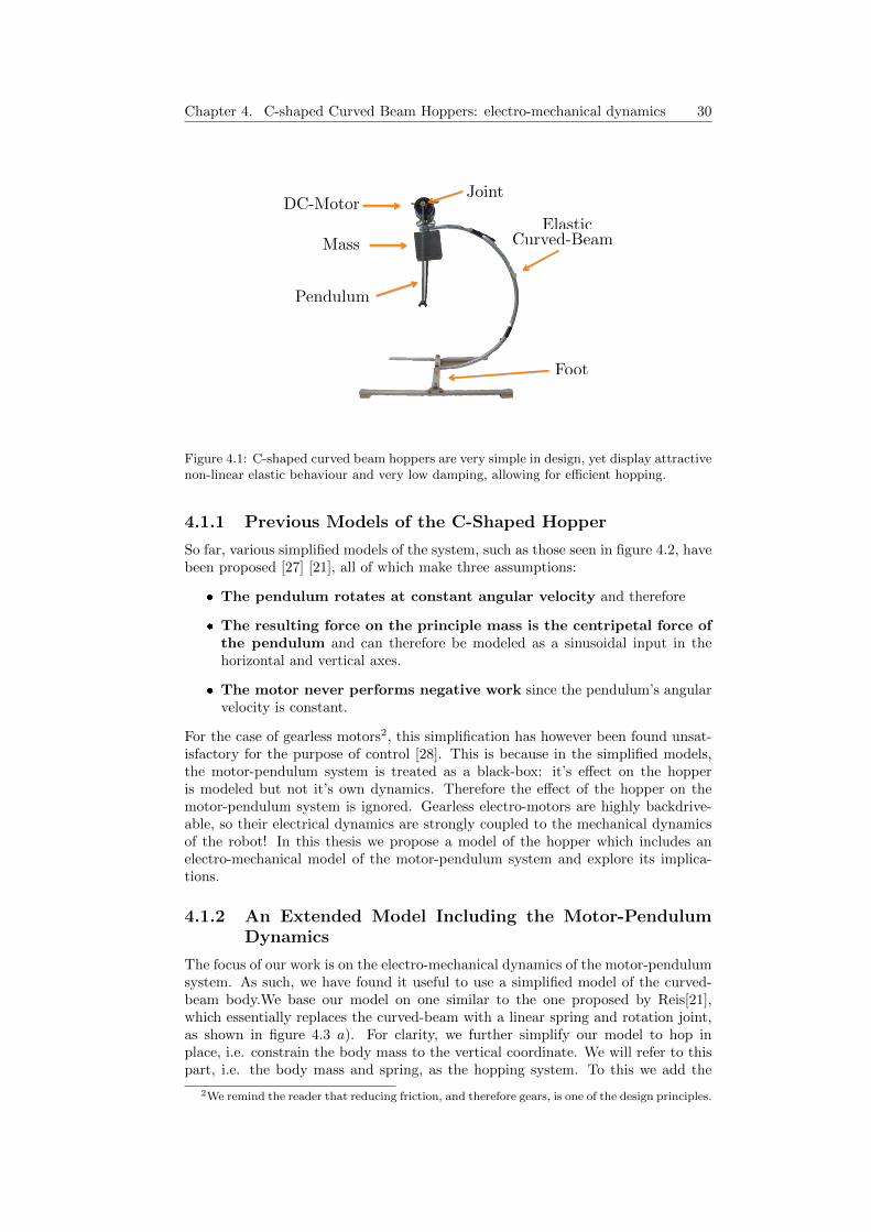
C-shaped hoppers, such as the one in figure 4.1, are designed around an elasticcurved beam: like a hunting bow, these curved beams have a stiff elastic propertywith very little damping. By using the curved beam as both the main body-structureand the spring, it is possible have both very low damping in the spring as well asminimize unsprung mass. A large foot is used at the bottom of the spring toguarantee stability, and a simple DC-motor and a payload are fixed to the top ofthe elastic curved-beam. The only joint connects the motor to a pendulum. Themotor inputs energy to the system by spinning the pendulum: with the properchoice of rotational speed, the system is excited at it’s natural resonant frequencyand begins to hop.

One of the benefits of this actuation is that the actuator never has to support theentire payload, so a very low-power motor is adequate. In various trials, power inputhas even been selected so low that the motor cannot start swinging the pendulumfrom it’s resting position by itself, but requires an initial push1: once the swingingwas started, the power input was able to make up for the damping losses and tolocomote properly. On the other hand, the indirect actuation makes it difficultto properly understand the system dynamics. It becomes even more daunting toconsider the dynamics both in the mechanical as well as the electrical domain. Inthis chapter we will explain however that this is both very important as well as veryuseful.

4.1 Modeling the Electro-Mechanical Dynamics

In this thesis, we propose a new model of the hopper which include the electro-mechanical dynamics of the motor-pendulum system. This is done to better under-stand how to control the system efficiently, however it also sheds light on the effectsof scaling on the dynamics.

1Much in the same way old prop-airplanes required someone to give the propeller an initialswing.

29

Chapter 4. C-shaped Curved Beam Hoppers: electro-mechanical dynamics 30

Mass

Pendulum

Foot

DC-MotorJoint

ElasticCurved-Beam

Figure 4.1: C-shaped curved beam hoppers are very simple in design, yet display attractivenon-linear elastic behaviour and very low damping, allowing for efficient hopping.

4.1.1 Previous Models of the C-Shaped Hopper

So far, various simplified models of the system, such as those seen in figure 4.2, havebeen proposed [27] [21], all of which make three assumptions:

� The pendulum rotates at constant angular velocity and therefore

� The resulting force on the principle mass is the centripetal force ofthe pendulum and can therefore be modeled as a sinusoidal input in thehorizontal and vertical axes.

� The motor never performs negative work since the pendulum’s angularvelocity is constant.

For the case of gearless motors2, this simplification has however been found unsat-isfactory for the purpose of control [28]. This is because in the simplified models,the motor-pendulum system is treated as a black-box: it’s effect on the hopperis modeled but not it’s own dynamics. Therefore the effect of the hopper on themotor-pendulum system is ignored. Gearless electro-motors are highly backdrive-able, so their electrical dynamics are strongly coupled to the mechanical dynamicsof the robot! In this thesis we propose a model of the hopper which includes anelectro-mechanical model of the motor-pendulum system and explore its implica-tions.

4.1.2 An Extended Model Including the Motor-PendulumDynamics

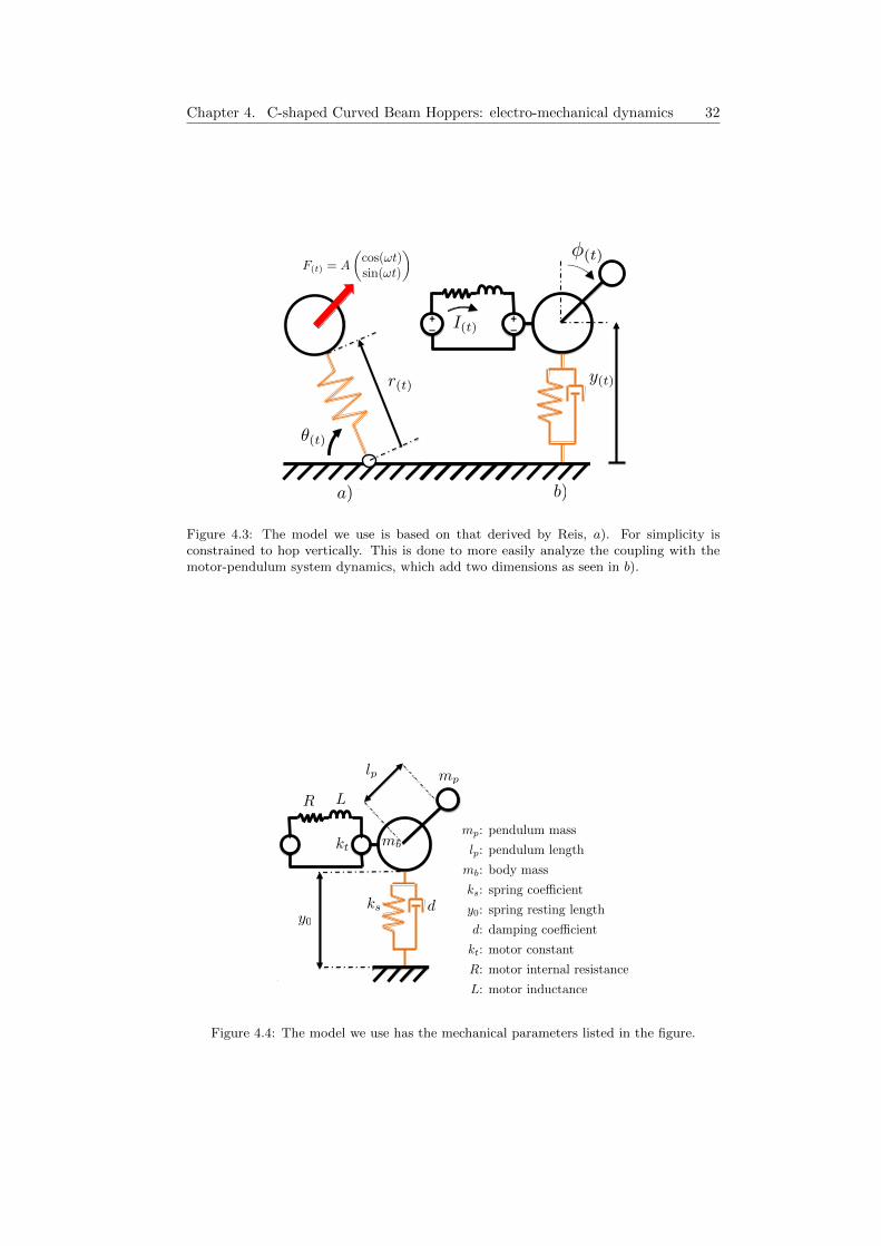
The focus of our work is on the electro-mechanical dynamics of the motor-pendulumsystem. As such, we have found it useful to use a simplified model of the curved-beam body.We base our model on one similar to the one proposed by Reis[21],which essentially replaces the curved-beam with a linear spring and rotation joint,as shown in figure 4.3 a). For clarity, we further simplify our model to hop inplace, i.e. constrain the body mass to the vertical coordinate. We will refer to thispart, i.e. the body mass and spring, as the hopping system. To this we add the

2We remind the reader that reducing friction, and therefore gears, is one of the design principles.

31 4.1. Modeling the Electro-Mechanical Dynamics

g F(t) = Fc cos(!t + �)

y1(t)

y2(t)

y3(t)

Figure 4.2: These simplistic models effectively capture the dynamic behavior of the curved-beam hoppers without needing to fully describe the system.

pendulum’s rotational coordinate and the charge coordinate of the electro-motor3

to describe the motor-pendulum system. The full model can be seen in figure 4.3b). The physical parameters of the model are shown in figure 4.4.Just as was shown in 2.2.3, we proceed to derive the equations of motion of thissystem by first identifying the ideal inductors, of which there are three: the bodymass mb, the pendulum mas moment of inertia Θp = mpl

2p and electrical inductor

of the motor L. The state vector of the system is therefore identified as

~q(t) =

q1(t)q2(t)q3(t)

=

y(t)φ(t)Q(t)

where y(t) is the vertical position of the body mass, φ(t) is the angular position ofthe pendulum and Q(t) is the electrical charge in the motor. Note that in the motor

we’re only interested in the corresponding flow: the current I(t) = Q(t). Howeverwe will leave the notation Q(t) for consistency.In the robot setup, we can only perform open-loop voltage control at the moment,meaning our control input vector is

~u(t) =

00

Vs(t)

4.1.3 Deriving the Equations of Motion

The equations of motion for this model are derived with the Euler-Lagrange methodand can be perused in appendix B. They have the form of

M(~q(t))~q(t) = F(~q(t),~q(t),~u(t))

whereM(~q(t)) is the mass-matrix multiplying the state accelerations, and F(~q(t),~q(t),~u(t))

contains all other terms. The matrix M(~q(t)) is

3For more details on the electro-motor model, see subsection 2.2.3.


✓(t)

�(t)

y(t)

a)

r(t)

F(t) = A

✓cos(!t)sin(!t)

◆

+ _ + _ I(t)

b)

Figure 4.3: The model we use is based on that derived by Reis, a). For simplicity isconstrained to hop vertically. This is done to more easily analyze the coupling with themotor-pendulum system dynamics, which add two dimensions as seen in b).

+ _+ _

LR

lp mp

mb

y0

ks d

kt

mp: pendulum mass

lp: pendulum length

mb: body mass

ks: spring coe�cient

y0: spring resting length

d: damping coe�cient

kt: motor constant

R: motor internal resistance

L: motor inductance

Figure 4.4: The model we use has the mechanical parameters listed in the figure.

33 4.2. Analysis of Scaling Effects

M(~q(t)) =

(mb +mp) −mplp sin(φ(t)) 0−mplp sin(φ(t)) mpl

2p 0

0 0 L

which is non-diagonal and clearly shows the implicit, non-linear coupling betweenthe pendulum dynamics and the body mass dynamics. The electrical dynamicsof the motor are linearly coupled with the dynamics of the pendulum. However,because our only control input is the open-loop source voltage Vs(t), it is importantto include the electrical dynamics of the motor.These non-linear differential-algebraic equations can be solved as are by using theimplicit-Euler method4. Alternatively, we can solve them to yield explicit first-orderdifferential equations of the form

~q(t) = M−1(~q(t)F(~q(t),~q(t),~u(t))

which results in very long equations. However they can be directly integratedwith the simpler explicit-Euler method. Also, it allows us to directly analyze theeffects of scaling on each individual coordinate, which we will do in the followingtwo subsections.

4.2 Analysis of Scaling Effects

The resulting equations of motions describing the system dynamics are as one mightexpect, highly non-linear and very complicated. To be able to make sense out ofthem, it is useful to make certain assumptions on the parameters in order to simplifythe equations of motion by excluding negligible terms. In the following subsectionswe will do exactly this understand specific aspects of the curved-beam hopper behav-ior, shedding light on principles for designing hoppers with a predictable behavior.

4.2.1 Source Voltage as an Indirect Control Input

The goal of our controller is to input energy to the hopping system, in other wordswe want to do positive work on the body mass mb. For this purpose it is helpfulto explicitly describe the corresponding effort of the body mass coordinate: thevertical force exerted on the body mass by the motor-pendulum system. Throughfree-body diagram analysis this force can be calculated as

Fy(t) = −mp(y(t) − lp cos(φ(t))φ2(t) − lp sin(φ(t)φ(t) + g)−

sin(φ(t))τm

lp

τm = ktQ(t) =Vs(t) − ktφ(t)

R

This shows the effect of our control input Vs(t) on the body mass is very indirect.The instantaneous-force exerted is much more dependent on the state of the systemrather than on the control input, meaning it is more important to design thesystem to have an efficient limit-cycle than to control it.This can be further exasperated by design: from equation (4.2.1) we see that thedependence of Fy(t) on the system state is directly proportional to the pendulummass mp and length lp, while it’s dependence on Vs(t) is inversely proportional to lpand independent on mp

4Also known as backwards Euler method


With a proper selection of design parameters, the term Vs(t) can therefore be madenegligible, and the vertical force can be approximated as:

Fy(t) = −mp(y(t) − lp cos(φ(t))φ2(t) − lp sin(φ(t)φ(t) + g)

4.2.2 Scaling to Emphasize Centripetal Force

In the previous subsection we analyzed the the vertical force exerted by the motor-pendulum on the hopper body to see the effect of the control input Vs(t) on the hop-ping system. From equation (4.2.1) we can also understand under what parameter-set the effect of the motor-pendulum on the hopper can be approximated as a si-nusoidal force source. This lends mathematical weight to the assumptions in madeprevious models (see subsection 4.1.1) and shows us how to design new hopperswith predictable behaviors.From equation (4.2.1) we can directly see that picking a large pendulum length lpincreases the importance of the centripetal force of the pendulum and minimizesthat of the motor torque. Further, choosing small values for the pendulum weightmp minimizes the importance of the hopper’s acceleration as well as the weight ofthe pendulum, mpg. Thus for long, light pendulums, the resulting force can beapproximated as

Fy(t) = mplp(cos(φ(t))φ2(t) − sin(φ(t))φ(t))

The second term cannot be simply neglected as it factors both mp as well as lp.Instead, we will check the conditions under which the angular acceleration becomesminimal. Intuitively, this is the case when the impacts of the hopper landing at theend of a flight-phase do not influence the the dynamics of the pendulum.To observe this, we make use of the previously derived explicit equations of motion4.1.3. Having already made the assumption of a long and light pendulum, theseequations of motion can be simplified to:

y(t) =ks(y0 − y(t))−

kt sin(φ(t))

lpQ(t) +mplp cos(φ(t))φ

2(t) −mbg

mb

φ(t) =ktQ(t)

mpl2p+ sin(φ(t))[

2g

lp+dy(t) − ks(y0 − y(t)

mblp

Q(t) = −RLQ(t) +

Vs(t) − ktφ(t)L

These equations show that the effect of impacts on the pendulum dynamics is min-imized by selecting large values for pendulum length lp and body-mass mb, as wellas selecting low values for the spring’s inherent damping d and the spring stiffnessks. While the first three parameter conditions are generally respected in the hop-pers built at BIRL, high spring stiffness is usually desired as it also important indetermining the gait frequency[7][11].

Thus we see that the centripetal force of the pendulum is the dominant force actingon our hoppers, but not the only one!

35 4.2. Analysis of Scaling Effects

4.2.3 Some Remarks on Energy-Optimal Control for the Curved-Beam Hopper

Like the segmented-beam hopper presented in chapter 3, the curved-beam hoppersalso locomote by hopping at natural frequency. Therefore we can make the sameclaim: to minimize damping losses of the system is equivalent to minimizing en-ergy input to the system. The energy-optimal control problem can therefore be setup with exactly the same approach as for the segmented-beam hopper. We haveseen that the coupling of the efforts of each coordinate system to the control inputu(t) = Vs(t) is very complicated but always linear! It should be of little surprisethen that the energy-optimal control input should have a bang-bang shape.Because the couplings are so complicated however, it becomes much more diffi-cult to reduce the parameter space sufficiently to find the switching function via aparameter search, as we did for the segmented-beam hopper CHIARO. However,previous discussion on how scaling affects the system dynamics show that throughproper selection of parameters the coupling of the various degrees of freedom canbe greatly simplified. It is surmised that under the circumstances described, theenergy-optimal control input could very well be that used in the real-world ex-periments: drive the motor at constant voltage. In other words, the switchingfunction maintains the same sign all the time, so the optimal control input neverchanges. This would explain the spectacularly low Cost of Transport achieved insome hoppers[11], and only mediocre ones for other hoppers with only slight differ-ences in design. So the true question we should asking ourselves is not ’what is theproper voltage to drive the hopper?’ but rather ’what is the proper morphologyso that a constant voltage is the energy-optimal controller?’ This new wayof looking at things does not, however, detract the importance of control: rather,it emphasizes the importance of considering the relationship between the controllerdesign and the morphological design, and indirectly, that they should be designedsimultaneously instead of as two separate steps.

Chapter 5

Conclusions

In this thesis we have treated energy-optimal control for simple natural-frequencyhoppers built at the Bio-Inspired Robotics Lab. The groundwork has been laid forcross-domain dynamics analysis of the hoppers as well as for applying optimal con-trol theory, in particular for energy-efficient locomotion. Also, we’ve shown that forhopping at natural frequency, minimizing damping and impact losses is equivalentto minimizing energy-input for a system under the constraint of doing only positivework. With this equivalence, it was shown that the Hamiltonian function result-ing from Pontryagin’s Minimum Principle is linear in the control input ~u(t): theenergy-optimal control input must therefore have a bang-bang shape.It has also been demonstrated that the control input for stable-limit cycle hoppingmust also be periodic: from this result, the switching function of the bang-bang con-trol input can be represented as a Fourier sum and solved as a parameter search. Incases where the parameter space can be sufficiently reduced, this makes the searcheasy to find in the real-world. We have proposed a highly reduced parameter spacefor the segmented-beam hopper CHIARO, and achieved excellent real-world re-sults: CoT = 0.49 at a forward velocity of 0.25m

s . As reference, the previousresults with the CHIARO hopper using a sinusoid input yielded CoT = 1 at a veloc-ity of 0.2m

s . The closest biological counterpart we could find data for is the TammarWallaby, with CoT = 0.437. Our results are therefore not only a big improvementon previous results, but also extremely close to the biological counterpart. The ex-cellent results also emphasizes the principle of ecological balance: for systems withsimple physical morphology, the neural control should be equally simple.The model of the curved-beam hopper has also been extended to include the electro-mechanical dynamics of the motor-pendulum system. From the resulting equationsof motion the following statements can be made:

� First, they show that the control input, the motor source voltage Vs(t), has lit-tle direct effect on the body mass dynamics of the hopper. This suggests thatfeed-back control is of little importance. Designing the system’s morphologyto enter efficient stable limit-cycles is much more important.

� Second, they show under what conditions the the effect of the motor-pendulumsystem can be approximated as a sinusoidal force-source. The benefits of thisare twofold. It gives us an important design principle to build hoppers withpredictable behavior: the pendulum should be long and light comparedto the body mass. Also it gives mathematical weight to the assumptionsmade in (to the best of my knowledge) all previous models of the curved-beamhopper.

37

Chapter 5. Conclusions 38

� Finally, they show that the energy-optimal control problem for the curved-beam hopper can be set up in the same way as discussed earlier, with thesame conclusion: the optimal control-input must be bang-bang in shape. Areduction of the parameter space for this system was not explored. However itseems likely that with the same design-parameters discussed above this wouldlead to control-input that is currently being used: a constant voltage input orin terms of bang-bang control, a single constant bang. This is supported bythe fact that, using this control input some curved-beam hopper demonstrateextremely high efficiency while other don’t. It also suggests an alternativequestion to finding the optimal control input: instead, we should ask ’Howdo we design the morphology so that a given, simple control-inputis optimal?’. This puts emphasis on the importance of morphological com-putation when designing efficient systems.

Recommended Further Work For the segmented-beam hoppers, for which wehave accurate models that can be simulated, we recommend developing a numericalframework for solving the optimization problem proposed here. Numerically solv-ing the differential equations obtained from PMP would further justify the currentresults. More importantly, it allow solving the optimization problem for more com-plicated system, where the parameter space cannot be reduced as easily or whenthe system in question renders the Hamiltonian function non-linear in ~u(t).In the case of the curved-beam hoppers, we have here shed light on the dynamicsof one of the most important components: the motor-pendulum system. However,there is still another critical component for which an accurate model remains elusive:the curved-beam spring. More specifically, the non-linear elasticity is the featurethat is difficult to model but also what makes it so attractive as a spring. A system-atic method for building curved-beam springs with predictable elasticity properties,and the identification of these properties would be very beneficial. After all, withthe focus placed now more heavily on designing the morphology, it is fundamentalto have the tools to do so!

Bibliography

[1] R McN Alexander. The gaits of bipedal and quadrupedal animals. The Inter-national Journal of Robotics Research, 3(2):49–59, 1984.

[2] Dimitri P Bertsekas, Dimitri P Bertsekas, Dimitri P Bertsekas, and Dimitri PBertsekas. Dynamic programming and optimal control, volume 1. Athena Sci-entific Belmont, 1995.

[3] Pranav A Bhounsule, Jason Cortell, and Andy Ruina. Design and control ofranger: an energy-efficient, dynamic walking robot. In Proc. CLAWAR, pages441–448, 2012.

[4] Reinhard Blickhan. The spring-mass model for running and hopping. Journalof biomechanics, 22(11):1217–1227, 1989.

[5] Giovanni A Cavagna, Norman C Heglund, and C Richard Taylor. Mechanicalwork in terrestrial locomotion: two basic mechanisms for minimizing energyexpenditure. American Journal of Physiology-Regulatory, Integrative and Com-parative Physiology, 233(5):R243–R261, 1977.

[6] Brian C. Fabien. Analytical System Dynamics: Modelling and Simulation.Springer, 2009.

[7] Claire T Farley and Octavio Gonzalez. Leg stiffness and stride frequency inhuman running. Journal of biomechanics, 29(2):181–186, 1996.

[8] Hartmut Geyer, Andre Seyfarth, and Reinhard Blickhan. Compliant leg be-haviour explains basic dynamics of walking and running. Proceedings of theRoyal Society B: Biological Sciences, 273(1603):2861–2867, 2006.

[9] Fabio Giardina and Fabian Guenther. Development and analysis of a self-stable,one-legged hopping robot, 2013.

[10] Fumiya Iida and Rolf Pfeifer. Self-stabilization and behavioral diversity ofembodied adaptive locomotion. In Embodied artificial intelligence, pages 119–129. Springer, 2004.

[11] Fumiya Iida, Murat Reis, Nandan Maheshwari, Keith Gunura, and SimonHauser. Legged robot locomotion based on free vibration. In Advanced MotionControl (AMC), 2012 12th IEEE International Workshop on, pages 1–6. IEEE,2012.

[12] Cornelius Lanczos. The variational principles of mechanics, volume 4. CourierDover Publications, 1970.

[13] Thijs Mandersloot, Martijn Wisse, and Christopher G Atkeson. Control-ling velocity in bipedal walking: A dynamic programming approach. In Hu-manoid Robots, 2006 6th IEEE-RAS International Conference on, pages 124–130. IEEE, 2006.

39

Bibliography 40

[14] Benedikt Mathis, XiaoXiang Yu, and Fabian Guenther. Efficient locomotionof a segmented beam hopper based on free vibration, 2013.

[15] Tad McGeer. Passive dynamic walking. the international journal of roboticsresearch, 9(2):62–82, 1990.

[16] Dominik Naef, Nandan Maheshwari, Xiaoxiang Yu, and Murat Reis. Shapeoptimization of a curved beam hopping robot, 2012.

[17] Rolf Pfeifer. Building fungus eaters: Design principles of autonomous agents.From animals to animats, 4:3–12, 1996.

[18] Rolf Pfeifer and Josh Bongard. How the body shapes the way we think: a newview of intelligence. MIT press, 2007.

[19] Rolf Pfeifer and Fumiya Iida. Morphological computation: Connecting body,brain and environment. Japanese Scientific Monthly, 58(2):48–54, 2005.

[20] Marc H Raibert et al. Legged robots that balance, volume 3. MIT press Cam-bridge, MA, 1986.

[21] Murat Reis and Fumiya Iida. Hopping robot based on free vibration of an elasticcurved beam. In Advanced Intelligent Mechatronics (AIM), 2011 IEEE/ASMEInternational Conference on, pages 892–897. IEEE, 2011.

[22] L Roussel, C Canudas-de Wit, and A Goswami. Comparative study of methodsfor energy-optimal gait generation for biped robots. PUBLISHED BY ST. PE-TERSBURG INSTITUTE FOR INFORMATICS AND AUTOMATION OFTHE RUSSIAN ACADEMY OF SCIENCES (SPIIRAS), page 1213, 1997.

[23] Jonas Rubenson, Denham B Heliams, Shane K Maloney, Philip C Withers,David G Lloyd, and Paul A Fournier. Reappraisal of the comparative costof human locomotion using gait-specific allometric analyses. The Journal ofexperimental biology, 210(20):3513–3524, 2007.

[24] Vance A Tucker. Energetic cost of locomotion in animals. Comparative Bio-chemistry and Physiology, 34(4):841–846, 1970.

[25] Christopher L Vaughan and Mark J O’Malley. Froude and the contribution ofnaval architecture to our understanding of bipedal locomotion. Gait & posture,21(3):350–362, 2005.

[26] DA Wells. Application of the lagrangian equations to electrical circuits. Journalof Applied Physics, 9(5):312–320, 1938.

[27] Xiaoxiang Yu and Fumiya Iida. Minimalistic models of an energy-efficientvertical-hopping robot. Industrial Electronics, IEEE Transactions on,61(2):1053–1062, 2014.

[28] Xiaoxiang Yu and Christos Lataniotis. Cpg-inspired control of curved beamhoppers, 2012.

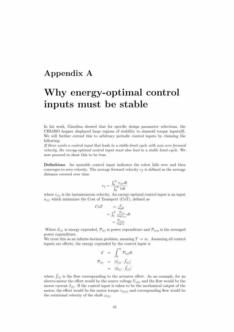
Appendix A

Why energy-optimal controlinputs must be stable

In his work, Giardina showed that for specific design parameter selections, theCHIARO hopper displayed large regions of stability to sinusoid torque inputs[9].We will further extend this to arbitrary periodic control inputs by claiming thefollowing:If there exists a control input that leads to a stable-limit cycle with non-zero forwardvelocity, the energy-optimal control input must also lead to a stable limit-cycle. Wenow proceed to show this to be true.

Definitions An unstable control input indicates the robot falls over and thenconverges to zero velocity. The average forward velocity vf is defined as the averagedistance covered over time

vf =

∫∞0v(t)dt∫∞

01dt

where v(t) is the instantaneous velocity. An energy-optimal control input is an inputu(t) which minimizes the Cost of Transport (CoT), defined as

CoT = Emgd

=∫ T0

P(t)

mgv(t)dt

=Pavg

mgvf

Where E(t) is energy expended, P(t) is power expenditure and Pavg is the averagedpower expenditure.We treat this as an infinite-horizon problem, meaning T →∞. Assuming all controlinputs are efforts, the energy expended by the control input is

E =

∫ ∞

0

P(t)dt

P(t) = |~e(t) · ~f(t)|

= |~u(t) · ~f(t)|

where ~f(t) is the flow corresponding to the actuator effort. As an example, for anelectro-motor the effort would be the source voltage Vs(t) and the flow would be themotor current I(t). If the control input is taken to be the mechanical output of themotor, the effort would be the motor torque τm(t) and corresponding flow would bethe rotational velocity of the shaft ω(t).

41

Appendix A. Why energy-optimal control inputs must be stable 42

Proof by contradiction Let us assume that the energy-optimal control inputis not stable, i.e. it causes the robot to fall over eventually and converge to zerovelocity. The average forward velocity then tends towards zero, vf → 0. Fromequation (A.1) we see that power is greater equal to zero, and since the control in-put is a non-zero periodic input, the averaged power expenditure is strictly greaterthan zero, Pavg. Equation (A) shows that the Cost of Transport then tends towardsinfinity, CoT →∞.From our statement, we have made the assumption that there exists a (possiblynon-optimal) periodic control input that leads to a stable gait with vf > 0. In or-der to not be the energy-optimal control input, this input must have a higher CoTthan the energy-optimal input, ergo it must have a CoT that tends towards infinitymore quickly. We will now show that the averaged power expenditure of any stablelimit-cycle gait is bounded, meaning the CoT is also bounded and therefore lowerthan that of any unstable gait.We have previously defined a stable gait as one that converges towards a stable limit-cycle. In a limit cycle the phase portrait of the kinematic variables

{d(t), f(t)

}1 of

the system describe a closed loop. The kinematic variables together describe thetotal energy content of the system: the displacement determines the potential en-ergy and the flow determines the kinetic energy. Since in a limit cycle the kinematicvariables are bounded, then so is the energy content of the system. This in turnmeans the power applied to the system, i.e. the rate at which the system energycontent can be changed, is also bounded, and the averaged power expenditure ofthe control input cannot tend to infinity.

1Displacement d(t) and flow f(t). For more, see chapter 2.2

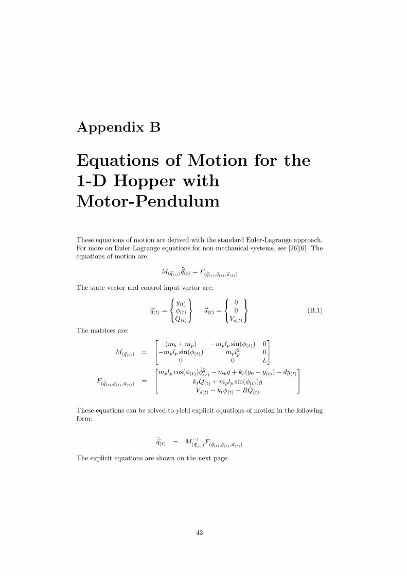
Appendix B

Equations of Motion for the1-D Hopper withMotor-Pendulum

These equations of motion are derived with the standard Euler-Lagrange approach.For more on Euler-Lagrange equations for non-mechanical systems, see [26][6]. Theequations of motion are:

M(~q(t))~q(t) = F(~q(t),~q(t),~u(t))

The state vector and control input vector are:

~q(t) =

y(t)φ(t)Q(t)

~u(t) =

00

Vs(t)

(B.1)

The matrices are:

M(~q(t)) =

(mb +mp) −mplp sin(φ(t)) 0−mplp sin(φ(t)) mpl

2p 0

0 0 L

F(~q(t),~q(t),~u(t))=

mplp cos(φ(t))φ

2(t) −mbg + ks(y0 − y(t))− dy(t)

ktQ(t) +mplp sin(φ(t))g

Vs(t) − ktφ(t) −RQ(t)

These equations can be solved to yield explicit equations of motion in the followingform:

~q(t) = M−1(~q(t))F(~q(t),~q(t),~u(t))

The explicit equations are shown on the next page.

43

Appendix B. Equations of Motion for the 1-D Hopper with Motor-Pendulum 44

y (t)

=(m

b+mp)(ktQ

(t)

+mpl p

sin

(φ(t))g

)−mpl p

sin

(φ(t))(mpl p

cos(φ(t)φ2 (t)

+ks(y

0−y (t)

)−dy (t)−

(mb

+mp)g

)

mpl2 p

(mb

+mp(1−

sin2(φ

(t))

φ(t)

=−mpl p

sin

(φ(t))(ktQ

(t)

+mpl p

sin

(φ(t))g

)+mpl2 p

(mpl p

cos(φ(t))φ

2 (t)

+ks(y

0−y (t)

)−dy (t)−

(mb

+mp)g

mpl2 p

(mb

+mp(1−

sin2(φ

(t))

Q(t)

=−R LQ

(t)

Vs(t)−ktφ(t)

L

Appendix C

Matlab Code: Simulations ofcurved beam hopper

function [trajT,traj] = motorPendulumHopper% 1D spring hopper with moto−pendulum electro−mechanical dynamics included% v.2 corrects state (r0−r), previously (r−r0).% This version uses matlab's provided ode45 solver.% For more control (and faster runtime), use the regular implicit−euler% solver, or the explicit−euler (along with explicit EoM)

%% Tabula Rasaclear all % clear all variables from workspaceclose all % close all open figuresformat long

%%% Parameters from paper "Minimalistic Models of an Energy Efficient% Vertical Hopping Robot

g = 9.81; % acceleration due to gravity [m/sˆ2]%%%%%% Motor Parameterskb = 0.0199; % Torque Constant: 19.9 [mNm/A] (datasheet)kt = 0.0199; % kb = kt. Speed Constant: 479 rpm/V, converted to back−emf

% constant, gives 0.0199.R = 0.358; % [ohm] (datasheet)L = 0.000070; % 0.07 [mH] (datasheet)Im = 3.59e−4; % 35.9 [gcmˆ2] (datasheet)

%%%%%% Robot parametersmp = 0.3; % pendulum ˜ 15 [g]lp = 0.145; % estimated CoGmb = 5.76; %[Kg]ks = 1200; %[N/m]Spring Constant measurement from Fabienr0 = 0.5;b = 0.2;%1.2; %[N s/m] estimated damping from Xiao Xiang's paper ICRA 2013

Ip = mp*lpˆ2 + Im;

vsAmp = 3;%parameters vector:% p = [g kb kt R L Im mp lp mb ks r0 Ip];

%% Initial Conditions

vs0 = vsAmp;

45

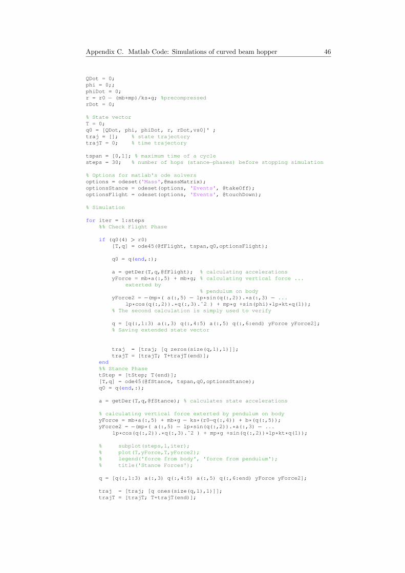
Appendix C. Matlab Code: Simulations of curved beam hopper 46

QDot = 0;phi = 0;;phiDot = 0;r = r0 − (mb+mp)/ks*g; %precompressedrDot = 0;

% State vectorT = 0;q0 = [QDot, phi, phiDot, r, rDot,vs0]' ;traj = []; % state trajectorytrajT = 0; % time trajectory

tspan = [0,1]; % maximum time of a cyclesteps = 30; % number of hops (stance−phases) before stopping simulation

% Options for matlab's ode solversoptions = odeset('Mass',@massMatrix);optionsStance = odeset(options, 'Events', @takeOff);optionsFlight = odeset(options, 'Events', @touchDown);

% Simulation

for iter = 1:steps%% Check Flight Phase

if (q0(4) > r0)[T,q] = ode45(@fFlight, tspan,q0,optionsFlight);

q0 = q(end,:);

a = getDer(T,q,@fFlight); % calculating accelerationsyForce = mb*a(:,5) + mb*g; % calculating vertical force ...

exterted by% pendulum on body

yForce2 = −(mp*( a(:,5) − lp*sin(q(:,2)).*a(:,3) − ...lp*cos(q(:,2)).*q(:,3).ˆ2 ) + mp*g +sin(phi)*lp*kt*q(1));

% The second calculation is simply used to verify

q = [q(:,1:3) a(:,3) q(:,4:5) a(:,5) q(:,6:end) yForce yForce2];% Saving extended state vector

traj = [traj; [q zeros(size(q,1),1)]];trajT = [trajT; T+trajT(end)];

end%% Stance PhasetStep = [tStep; T(end)];[T,q] = ode45(@fStance, tspan,q0,optionsStance);q0 = q(end,:);

a = getDer(T,q,@fStance); % calculates state accelerations

% calculating vertical force exterted by pendulum on bodyyForce = mb*a(:,5) + mb*g − ks*(r0−q(:,4)) + b*(q(:,5));yForce2 = −(mp*( a(:,5) − lp*sin(q(:,2)).*a(:,3) − ...

lp*cos(q(:,2)).*q(:,3).ˆ2 ) + mp*g +sin(q(:,2))*lp*kt*q(1));

% subplot(steps,1,iter);% plot(T,yForce,T,yForce2);% legend('force from body', 'force from pendulum');% title('Stance Forces');

q = [q(:,1:3) a(:,3) q(:,4:5) a(:,5) q(:,6:end) yForce yForce2];

traj = [traj; [q ones(size(q,1),1)]];trajT = [trajT; T+trajT(end)];

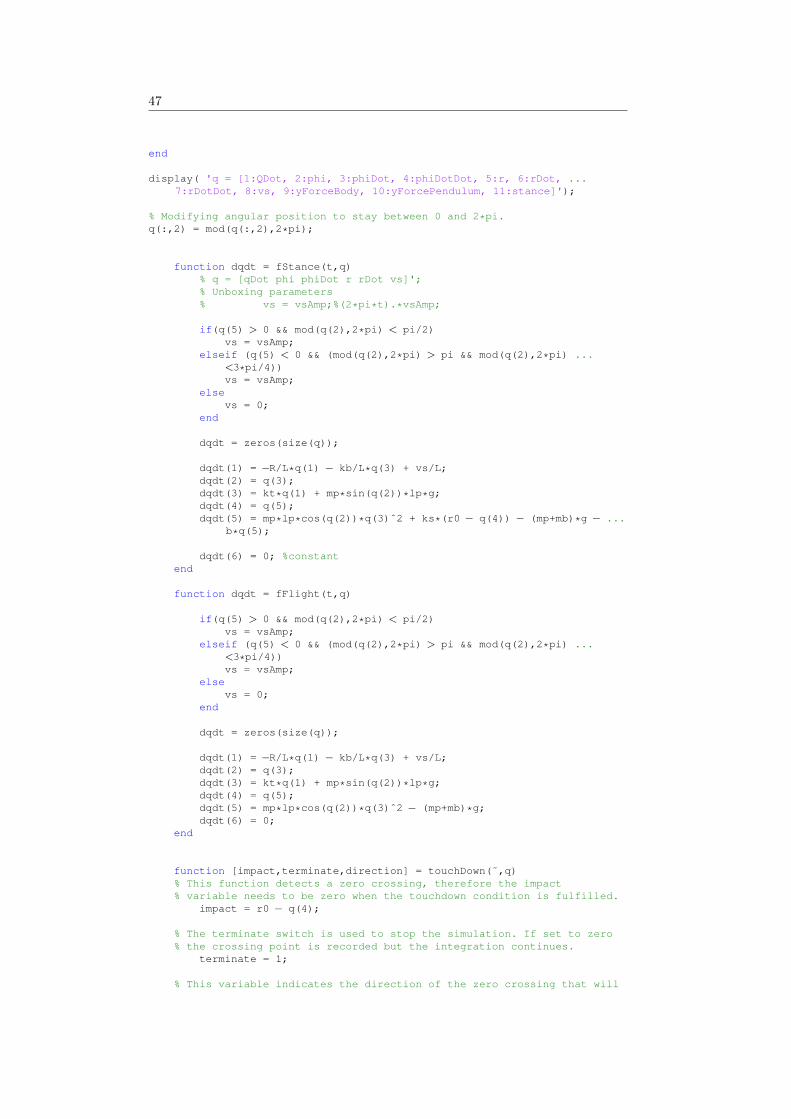
47

end

display( 'q = [1:QDot, 2:phi, 3:phiDot, 4:phiDotDot, 5:r, 6:rDot, ...7:rDotDot, 8:vs, 9:yForceBody, 10:yForcePendulum, 11:stance]');

% Modifying angular position to stay between 0 and 2*pi.q(:,2) = mod(q(:,2),2*pi);

function dqdt = fStance(t,q)% q = [qDot phi phiDot r rDot vs]';% Unboxing parameters% vs = vsAmp;%(2*pi*t).*vsAmp;

if(q(5) > 0 && mod(q(2),2*pi) < pi/2)vs = vsAmp;

elseif (q(5) < 0 && (mod(q(2),2*pi) > pi && mod(q(2),2*pi) ...<3*pi/4))vs = vsAmp;

elsevs = 0;

end

dqdt = zeros(size(q));

dqdt(1) = −R/L*q(1) − kb/L*q(3) + vs/L;dqdt(2) = q(3);dqdt(3) = kt*q(1) + mp*sin(q(2))*lp*g;dqdt(4) = q(5);dqdt(5) = mp*lp*cos(q(2))*q(3)ˆ2 + ks*(r0 − q(4)) − (mp+mb)*g − ...

b*q(5);

dqdt(6) = 0; %constantend

function dqdt = fFlight(t,q)

if(q(5) > 0 && mod(q(2),2*pi) < pi/2)vs = vsAmp;

elseif (q(5) < 0 && (mod(q(2),2*pi) > pi && mod(q(2),2*pi) ...<3*pi/4))vs = vsAmp;

elsevs = 0;

end

dqdt = zeros(size(q));

dqdt(1) = −R/L*q(1) − kb/L*q(3) + vs/L;dqdt(2) = q(3);dqdt(3) = kt*q(1) + mp*sin(q(2))*lp*g;dqdt(4) = q(5);dqdt(5) = mp*lp*cos(q(2))*q(3)ˆ2 − (mp+mb)*g;dqdt(6) = 0;

end

function [impact,terminate,direction] = touchDown(˜,q)% This function detects a zero crossing, therefore the impact% variable needs to be zero when the touchdown condition is fulfilled.

impact = r0 − q(4);

% The terminate switch is used to stop the simulation. If set to zero% the crossing point is recorded but the integration continues.

terminate = 1;

% This variable indicates the direction of the zero crossing that will


% be detected:% 1 => negative −> positive% −1 => positive −> negative% 0 => both

direction = 1;end

function [impact,terminate,direction] = takeOff(˜,q)impact = r0 − q(4);terminate = 1;direction = −1;

end

function M = massMatrix(˜,q)M = [

1 0 0 0 0 0;0 1 0 0 0 0;0 0 mp*lpˆ2 0 −mp*lp*sin(q(2)) 0;0 0 0 1 0 0;0 0 −mp*lp*sin(q(2)) 0 (mb+mp) 0;0 0 0 0 0 1;];

end

function acc = getDer(T,q,fHandle)acc = [];for iter2 = 1:numel(T)

mass = massMatrix(T(iter2),q(iter2,:));f = fHandle(T(iter2),q(iter2,:));acc = [acc; (mass\f')'];

endend

end

function [xNew] = forwardEuler(x0, fHandle, h)% forward euler solution for autonomous function

xNew = x0 + h*fHandle(0,x0);end

function [xNew,iter] = implicitEuler(x0,fHandle,DfHandle,h,tol,maxIt)% fHandle are the system dynamics% DfHandle is the jacobian, d fHandle / d x%

% bogus value for time (to be compatible with Matlab odes, all functions% accept t, but don't use it)t = 1;

xk1=x0; % first estimate for x(k+1)% deltaX = 1;for iter=1:maxIt

deltaX = −DfHandle(t,xk1) \ fHandle(t,xk1);if(deltaX < tol)

breakend

xk1 = xk1 + deltaX;if(iter == maxIt)

display('max iteration reached');end

end

xNew = x0 + h*fHandle(t,x0);

49

end

% Write and Read to a NI USB−6008 DAQ deviceclear allclose allclc

%% Digital input enables ESCONdio = digitalio('nidaq', 'Dev1');hline = addline(dio, 0:11, 'out');putvalue(dio, [8 8 8 8 8 8 8 8 8 8 8 8])

%% Initialization

ai = analoginput('nidaq', 'Dev1'); % Analog Inputao = analogoutput('nidaq', 'Dev1'); % Analog Outputao0 = addchannel(ao, 0); % Add desired channel for outputai0 = addchannel(ai, [0,1]); % Add desired channel for input

% (See also NI SCB 68 PIN positions)

timelength = 5; % total motor control time (s)freq = 3.5 % Signal frequency (Hz)A = 3.5; % Current amplituder c = 0.95/10; % Current to voltage ratio. e.g. 0.95/10

% −> 0.95 Ampere if the analog output is 10Vai value = [0,0]; % Initialize Input valueao array = 1; % Initialize Output valuetime array = 0; % Initialize timeoffset = 0; % offset to shift sinusoid zero crossing

tic % Start time

%% Start Control loopdisp('Start of loop')while time array(end)<timelength

%%%%% Define trajectory of control input (current) here:ao value = A*sign(sin(2*pi*freq*time array(end)) + offset );ao value = max(−0.1,ao value);ao array=[ao array;ao value*r c]; % Write current in vectorputsample(ao, ao value) % Set current at analog outputtime array=[time array;toc]; % Write time in vectortmp=getsample(ai); % Get motor winding 1 Voltageai value = [ai value;tmp]; % Write motor winding 1 Voltage in vector

endao value = 0;putsample(ao, ao value)disp('End of loop')

%% Disable ESCONdio = digitalio('nidaq', 'Dev1');hline = addline(dio, 0:11, 'out');putvalue(dio, [0 0 0 0 0 0 0 0 0 0 0 0])delete(ai)delete(ao)

%% Transform VoltageR2 = 22.2; % Voltage divider resistance 2 (kOhm)R1 = 98; % Voltage divider resistance 1 (kOhm)K = R2/(R1+R2); % Voltage reduction constantVoltIn= −ai value(:,1)/K;

%% Filter Results


n p = 5.8; % Filter band (percent)av = mean(VoltIn); % Average voltageav ub = av*(1 + n p); % Voltage upper boundav lb = av*(1 − n p); % Voltage lower boundV Filt = VoltIn;

for i = 2:length(VoltIn)if VoltIn(i) >= av ub | | VoltIn(i) <= av lb

V Filt(i) = V Filt(i−1);end

end

%Add additional Gauss−filterva = 15; %VarianceV Filt G = V Filt;V sum = 0;G sum = 0;for i = 1:length(VoltIn)

for j = 1:length(VoltIn)G x = 1/(sqrt(2*pi)*va)*exp(−(j−i)ˆ2/(2*vaˆ2));G sum = G x + G sum;V sum = G x*V Filt(j) + V sum;

endV Filt G(i) = V sum/G sum;

V sum = 0;G sum = 0;

end

%% Plot results% plot(time array,VoltIn)hold onplot(time array,ao array,'r')plot(time array,V Filt,'k')plot(time array,V Filt G,'b')legend('Current [A]','Voltage [V]');xlabel('Time [s]')ylabel('V/A')

%% Calculate expended energyE o = 0;for i = 1:length(V Filt G)−1

%if time array(i)>=1 %No transitiondt = time array(i+1)−time array(i);E n = E o + 2*abs(V Filt G(i))*abs(ao array(i))*dt;E o = E n;

%endend

E exp = E nV = V Filt G(end)*2

%% Calculate PowerP = [];for i = 1:length(V Filt G)

P(i) = 2*abs(V Filt G(i))*abs(ao array(i));endP = P';

Dynamics and Control for E cient...

Documents

Transcript of Dynamics and Control for E cient...