DYNAMICS AND ASYMPTOTIC BEHAVIORS OF

BIOCHEMICAL NETWORKS

BY LIMING WANG

A dissertation submitted to the

Graduate School—New Brunswick

Rutgers, The State University of New Jersey

in partial fulfillment of the requirements

for the degree of

Doctor of Philosophy

Graduate Program in Mathematics

Written under the direction of

Eduardo D. Sontag

and approved by

New Brunswick, New Jersey

October, 2008

ABSTRACT OF THE DISSERTATION

Dynamics and Asymptotic Behaviors of Biochemical

Networks

by Liming Wang

Dissertation Director: Eduardo D. Sontag

The purpose of this dissertation is to study the dynamics and asymptotic behaviors of

biochemical networks using a “modular” approach. New mathematics is motivated and

developed to analyze modules in terms of the number of steady states and the stability

of the steady states.

One of the main contributions of the thesis is to extend Hirsch’s generic conver-

gence result from monotone systems to systems “close” to monotone using geometric

singular perturbation theory. A monotone system is a dynamical system for which

the comparison principle holds, that is, “bigger” initial states lead to “bigger” future

states. In monotone systems, every net feedback loop is positive. On the other hand,

negative feedback loops are important features of many systems, since they are re-

quired for adaptation and precision. We show that, provided that these negative loops

act at a comparatively fast time scale, the generic convergence property still holds.

This is an appealing result, which suggests that monotonicity has broader implications

than previously thought. One particular application of great interest is that of dou-

ble phosphorylation dephosphorylation cycles. Other recurring modules in biochemical

networks are also analyzed in detail.

For systems without time scale separation, we study the global stability of one

ii

special class of systems, called monotone tridiagonal systems with negative feedback.

The key technique is to rule out periodic orbits using the theory of second compound

matrices.

We also investigate the effect of diffusion on the stability of a constant steady state

for systems with more general structures represented by graphs. This work extends the

passivity-based stability criterion developed by Arcak and Sontag to reaction diffusion

equations.

Upon assembling different modules, the dynamics of individual modules might be

affected. One particular effect is called “retroactivity” in the systems biology literature.

We propose designs and conditions under which the retroactivity can be attenuated.

iii

Acknowledgements

First of all, I would like to thank Professor Eduardo Sontag, who shows me what an

outstanding mathematician and great adviser should be. It is difficult to overstate my

gratitude to him. He always makes himself available and gives priority to his students.

It often happens that he meets me in his office on the same day after a long ride on the

plane or a surgery from the dentist’s office. He is the fastest person I know in replying

emails, usually within minutes even at late night or during weekends. His enthusiasm,

wisdom, and energy to work are contagious and set a role model in my future career.

During my writing of the thesis, he guides me through difficulties using his knowledge

and expertise, makes great efforts to state and explain things clearly and simply, and

reads my work with unbelievable amount of diligence. I am fortunate to have him as

my thesis adviser.

Besides academic, I learned a great deal from him in other areas especially in using

computers. He taught me tricks in google search and shared with me his code for

reminding incoming emails (which reveals the mystery why he answers email so fast). He

influences me in many different ways, from small things like writing styles to attitudes

about life and society.

I want to thank my committee members: Professor Konstantin Mischaikow for his

advice and patience, Professor Yanyan Li for his discussion and vision, Professor Zoran

Gajic for his discussion and reading of my thesis.

I thank all professors and secretaries in the math department who have helped me in

various ways. I am particularly grateful to Professor Eugene Speer for his help arrang-

ing my teaching while I had family difficulties, to Professor Joel Lebowitz, Professor

Sussmann Hector, and Professor Roger Nussbaum, for their invaluable discussions. Dur-

ing my time at Rutgers, Professors Zhengchao Han, Michael Saks, Feng Luo, Stephen

iv

Greenfield, Charles Weibel, Xiaojun Huang, Xiaochun Rong, and Jian Song have been

very kind to me answering my questions on academic and various other issues. Special

thanks to our secretaries Pat Barr, Lynn Braun, Maureen Clausen, Donna Smith, and

Jacqueline Drayton. You made my life of working and studying here more smooth.

Outside the math department, I want to thank the Center for Discrete Mathematics

and Theoretical Computer Science (DIMACS) for the wonderful conferences and sum-

mer and winter research support, to thank BioMaPS Institute for Quantitative Biology

for the excellent lunch seminars and summer schools. I would also like to thank the

faculty members at DIMACS and BioMaPS especially Professor Fred Roberts for his

support and Professor Anirvan Sengupta for the inspiring discussions.

I am grateful to Professor Natalia Komarova now in the University of California,

Irvine for initiating my research career and collaborating on my first real paper. I

am also indebted to Professor Isaac Edery and his postdoc Eun Young Kim for their

guidance, patience, and trust while I was in the lab doing biochemistry experiments

about circadian clocks.

I would like to thank all professors not in Rutgers who answered my various ques-

tions and gave suggestions to make my thesis possible. I am particularly grateful to

Professor Frank Hoppensteadt for his discussions and reprints, to Professor Hal Smith

for his comments and encouragement, to Professor Kaspar Nipp and Professor Christo-

pher Jones for their explanation of geometric singular perturbation theory, to Professor

Jeremy Gunawardena for his inspiring ideas, and to Professor Michael Li for useful

discussions.

I want to thank colleagues in our group and colleagues with whom I have collabo-

rated: German Enciso at Harvard, Yuan Wang and Yuandan Lin at Florida Atlantic

University, Patrick de Leenheer at University of Florida, Murat Arcak at Rensselaer

Polytechnic Institute, David Angeli at Imperial College London, Madalena Chaves at

INRIA Sophia Antipolisin, Domitilla Del Vecchio at University of Michigan, Verica

Gajic and Paola Vera-Licona at Rutgers for sharing ideas and working together.

I am indebted to my many student colleagues for providing a stimulating and fun

environment in which to learn and grow. An illustrious list includes: Aobing Li,

v

Yongzhong Xu, Xiaoqing Li, Ren Guo, Ellen Bao, Ming Shi, Yuan Zhang, Biao Yin,

Yu Wang, Corina Calinescu, Brian Lins, Brian Manning, Benjamin Kennedy and Thuy

Pham in the math department, Eliane Traldi and Mauro Lapelosa in Biomaps. Special

thanks to my officemate Thomas Robinson for sharing the computer with me during

my writing of the thesis.

I am so lucky to have my friends: Xiaomin Chen, Jun Dai, Zhiyan Liu, Ruoming

Pang, Lei Wang, Ming Xu, Huijing Tao, Yilei Shao, Zuofu Zhu, Yang Huang, Yuan Sun,

Jing Zhou, and Alex Lv with whom I spent most of my weekends. You made my life

more colorful in this rural countryside. Thank you all for the help through my difficult

times, for the emotional support, entertainment, and caring you provided. I also want

to thank my old roommates in Peking University: Xiaodan Wei and Li Ye, who are now

in New Jersey. You bring back my beautiful memories and keep our friendship fresh.

Enormously thanks to my husband Bin Tian. His constant corrections and support,

his wisdom and caring make the past few years a wonderful period in my life. I would

also like to thank my precious little ones Sunny Xin Tian and Nichole Yi Tian for the

smiles they bring to me everyday.

Finally and most importantly, I wish to thank my parents, Xianying Ma and Wansen

Wang. They make me who I am, support me unconditionally, teach me diligently, and

love me more than anything in the universe.

vi

Dedication

To my parents Xianying Ma and Wansen Wang.

vii

Table of Contents

Abstract . . . . . . . . . . . . . . . . . . . . . . . . . . . . . . . . . . . . . . . . ii

Acknowledgements . . . . . . . . . . . . . . . . . . . . . . . . . . . . . . . . . iv

Dedication . . . . . . . . . . . . . . . . . . . . . . . . . . . . . . . . . . . . . . . vii

1. Introduction . . . . . . . . . . . . . . . . . . . . . . . . . . . . . . . . . . . 1

2. Multistationarity in Biochemical Networks . . . . . . . . . . . . . . . . 5

2.1. Introduction . . . . . . . . . . . . . . . . . . . . . . . . . . . . . . . . . . 5

2.2. “Futile Cycle” Motifs . . . . . . . . . . . . . . . . . . . . . . . . . . . . . 6

2.2.1. Introduction . . . . . . . . . . . . . . . . . . . . . . . . . . . . . 6

2.2.2. Model assumptions . . . . . . . . . . . . . . . . . . . . . . . . . . 8

2.2.3. Mathematical formalism . . . . . . . . . . . . . . . . . . . . . . . 10

2.2.4. Number of positive steady states . . . . . . . . . . . . . . . . . . 15

Lower bound on the number of positive steady states . . . . . . . 15

Upper bound on the number of positive steady states . . . . . . 22

Fine-tuned upper bounds . . . . . . . . . . . . . . . . . . . . . . 25

2.2.5. Conclusions . . . . . . . . . . . . . . . . . . . . . . . . . . . . . . 30

2.3. Another Motif in Biological Networks . . . . . . . . . . . . . . . . . . . 30

2.3.1. Introduction . . . . . . . . . . . . . . . . . . . . . . . . . . . . . 30

2.3.2. Mathematical formalism . . . . . . . . . . . . . . . . . . . . . . . 31

2.3.3. Positive steady states . . . . . . . . . . . . . . . . . . . . . . . . 33

2.4. Arkin’s Example . . . . . . . . . . . . . . . . . . . . . . . . . . . . . . . 35

3. Singularly Perturbed Monotone Systems . . . . . . . . . . . . . . . . . 38

3.1. Introduction . . . . . . . . . . . . . . . . . . . . . . . . . . . . . . . . . . 38

viii

3.2. Monotone Systems for Ordinary Differential Equations . . . . . . . . . . 41

3.3. Geometric Singular Perturbation Theory . . . . . . . . . . . . . . . . . . 47

3.4. Main Results on Singularly Perturbed Monotone Systems . . . . . . . . 52

3.4.1. Statement of the main theorem . . . . . . . . . . . . . . . . . . . 52

3.4.2. Extensions of the vector fields . . . . . . . . . . . . . . . . . . . . 54

3.4.3. Further analysis of the dynamics and the proof of Theorem 3.22 57

3.5. Applications . . . . . . . . . . . . . . . . . . . . . . . . . . . . . . . . . . 63

3.5.1. Enzyme competitive inhibition . . . . . . . . . . . . . . . . . . . 63

3.5.2. Double phosphorylation dephosphorylation futile cycle . . . . . . 69

3.5.3. A genetic circuit example . . . . . . . . . . . . . . . . . . . . . . 76

3.5.4. A network example . . . . . . . . . . . . . . . . . . . . . . . . . . 83

3.6. Conclusions . . . . . . . . . . . . . . . . . . . . . . . . . . . . . . . . . . 87

4. Monotone Tridiagonal Systems with Negative Feedback . . . . . . . 89

4.1. Introduction . . . . . . . . . . . . . . . . . . . . . . . . . . . . . . . . . . 89

4.2. Preliminaries . . . . . . . . . . . . . . . . . . . . . . . . . . . . . . . . . 90

4.3. Ruling out periodic orbits . . . . . . . . . . . . . . . . . . . . . . . . . . 92

4.4. Applications . . . . . . . . . . . . . . . . . . . . . . . . . . . . . . . . . . 96

4.4.1. Linear Monotone Tridiagonal Systems with Nonlinear Negative

Feedback . . . . . . . . . . . . . . . . . . . . . . . . . . . . . . . 96

4.4.2. Goldbeter Model . . . . . . . . . . . . . . . . . . . . . . . . . . . 100

5. A Class of Reaction Diffusion Systems with Interconnected Structure104

5.1. Introduction . . . . . . . . . . . . . . . . . . . . . . . . . . . . . . . . . . 104

5.2. Review of the Ordinary Differential Equation Case . . . . . . . . . . . . 107

5.3. Extension to Partial Differential Equation Systems . . . . . . . . . . . . 110

5.3.1. Notations and assumptions . . . . . . . . . . . . . . . . . . . . . 110

5.3.2. Existence and uniqueness . . . . . . . . . . . . . . . . . . . . . . 112

5.3.3. Stability of the homogeneous equilibrium . . . . . . . . . . . . . 113

ix

6. Retroactivity in Biological Networks . . . . . . . . . . . . . . . . . . . . 125

6.1. Introduction . . . . . . . . . . . . . . . . . . . . . . . . . . . . . . . . . . 125

6.2. Retroactivity from the output to the state variables . . . . . . . . . . . 128

6.3. Retroactivity from the state to the input variables . . . . . . . . . . . . 133

6.4. Applications . . . . . . . . . . . . . . . . . . . . . . . . . . . . . . . . . . 136

7. Future Work . . . . . . . . . . . . . . . . . . . . . . . . . . . . . . . . . . . 145

References . . . . . . . . . . . . . . . . . . . . . . . . . . . . . . . . . . . . . . . 147

Vita . . . . . . . . . . . . . . . . . . . . . . . . . . . . . . . . . . . . . . . . . . . 154

x

1

Chapter 1

Introduction

A promising approach to handling the complexity of biochemical networks is to decom-

pose networks into small modules. In the influential papers [34] by Hartwell et al and

[50] by Lauffenburger, the authors point out the critical role of modules in biological

organization. Subsequently, a wave of interesting work emerged regarding modularity

in biochemical networks, see for instance, [2, 5, 69, 72, 77].

In a “bottom-up modularity” approach, one first identifies basic modules (motifs)

in the network, then uses mathematical modeling to analyze these relatively simple

motifs. Finally, the whole network can be set up by integrating these basic building

blocks and studying their interconnections.

Following this approach, the present work relies upon a “graphical” way of analyzing

individual modules as well as the interconnections among them.

In Chapter 2, we introduced such a module, which in biochemistry is sometimes

called a “futile cycle”. It involves two or more inter-convertible forms of one protein.

The protein, denoted here by S0, is ultimately converted into a product, denoted here

by Sn, through a cascade of “activation” reactions triggered or facilitated by an enzyme

E; conversely, Sn is transformed back (or “deactivated”) into the original S0, helped

on by the action of a second enzyme F , see Figure 1.1.

F

E

F

E

S S0 2S1

F

E

F

E

SSS nn−1n−2

Figure 1.1: A futile cycle of size n.

Futile cycles constitute a ubiquitous motif in cellular signaling pathways. Typically,

2

the enzymatic activation and de-activation are given by phosphorylation dephospho-

rylation reactions. One very important instance is that of Mitogen-Activated Protein

Kinase (MAPK) cascades, which regulate primary cellular activities such as prolifera-

tion, differentiation, and apoptosis ([9, 14, 42, 100]) in eukaryotes from yeast to humans.

We set up a mathematical model based on mass action kinetics, and study the

number of positive steady states of this system. We show analytically that

1. for some parameter ranges, there are at least n+1 (if n is even) or n (if n is odd)

steady states;

2. there never are more than 2n−1 steady states (in particular, this implies that for

n = 2, including single levels of MAPK cascades, there are at most three steady

states);

3. for parameters near the standard Michaelis-Menten quasi-steady state conditions,

there are at most n+ 1 steady states; and

4. for parameters far from the standard Michaelis-Menten quasi-steady state condi-

tions, there is at most one steady state.

Chapter 3 is motivated by studying the dynamics and stability of a double phos-

phorylation dephosphorylation futile cycle. When the amount of enzymes E and F

is negligible compared to the amount of the total substrate S, the system is strongly

monotone. In a strongly monotone system, every net feedback loop is positive. The

resulting dynamics is relatively simple. Hirsch’s Generic Convergence Theorem for

monotone system ([36, 37, 38, 39, 82]) says that almost every bounded solution of a

strongly monotone system converges to a set of equilibria.

The futile cycle example as well as many systems in biology are not monotone, at

least with respect to any standard orthant order. Negative feedback is required for

adaptation and precision. However, we show in Chapter 3 that if the negative feedback

acts on a sufficiently fast time scale, the most important dynamical property of strongly

monotone systems – convergence to steady states – is preserved. Geometric singular

3

perturbation is the major tool used in the proofs. Several applications are worked out

at the end of this chapter.

Chapter 4 deals with negative feedback without the assumption of time scale sepa-

ration. We focus on global asymptotic stability of monotone tridiagonal systems with

negative feedback. Monotone tridiagonal systems possess the Poincare-Bendixson prop-

erty, which implies that, if orbits are bounded, if there is a unique steady state and this

unique steady state is asymptotically stable, and if one can rule out periodic orbits,

then the steady state is globally asymptotically stable.

To rule out periodic orbits, we use the theory of second additive compound ma-

trices. Sanchez in [75] studied the special case of cyclic systems. Our results treat

a more general class of systems which includes cyclic systems. A specific and classi-

cal instance of tridiagonal systems with negative feedback is the Goldbeter model for

circadian oscillations in the Drosophila PER (“period”) protein ([30]). We apply our

main theoretical results to this model and provide conditions under which the unique

equilibrium is globally asymptotically stable.

Chapter 5 studies global asymptotic stability for more general interconnected sys-

tems with positive and negative feedback. The connections in such systems are repre-

sented by graphs, which are not restricted to the tridiagonal case. We present a stability

test for a class of such systems inspired by the work of Arcak and Sontag in [8] and

Jovanovic, Arcak, and Sontag in [46].

In their novel work [8], Arcak and Sontag developed a passivity-based stability cri-

terion for general interconnected systems in a “well-mixed” environment (no diffusion),

under the assumption that a unique equilibrium exists. Jovanovic, Arcak, and Sontag

studied the effect of diffusion in [46] but only for the special case of cyclic graphs. Chap-

ter 5 extends the result in [46] so as to encompass the broader class of interconnected

systems. By constructing a composite convex Lyapunov function, we prove that the

unique equilibrium of the ordinary differential equations is globally asymptotically sta-

ble when diffusion is added to the system. The interconnection structure of the network

and the signs of the interconnection terms are incorporated into a dissipativity matrix,

which is crucial in constructing the Lyapunov function.

4

Chapter 6 focuses on the interconnections among different modules. In general,

when two modules are connected, the dynamics of the individual module might be

affected. If we define the upstream system and downstream system in the direction

of which the signal is traveling, the effect from downstream to upstream will be called

“retroactivity”. We discuss in Chapter 6 conditions under which the retroactivity can

be attenuated. The results here extend those by Del Vecchio, Ninfa, and Sontag in [94]

to a more general class of interconnected systems and fill in mathematical details using

singular perturbation arguments.

The present thesis is based on the author’s papers listed below:

• The material in Section 2.2 was published in the Journal of Mathematical Biol-

ogy [98] in joint with Eduardo Sontag.

• A preliminary version of Chapter 3 is published in Proceedings of the second

Multidisciplinary International Symposium on Positive Systems: Theory and Ap-

plications [97]. More general results are published in the Journal of Nonlinear

Science [99]. Both of them are collaborated with Eduardo Sontag.

• The material in Chapter 4 is part of a joint paper [96] coauthored with Patrick de

Leenheer and Eduardo Sontag accepted to the 2008 IEEE conference on Decision

and Control.

• Chapter 5 is a paper in preparation for submission joint with Eduardo Sontag

and Murat Arcak.

• Chapter 6 is also a paper that is being prepared for submission coauthored with

Domitilla Del Vecchio and Eduardo Sontag.

5

Chapter 2

Multistationarity in Biochemical Networks

2.1 Introduction

One of the ideas to understand the complexity in biochemical networks is to decompose

them into subunits that describe processes arising frequently in the networks. The

smaller subunits are often simpler to analyze, and provide insights to properties of the

whole network.

One aspect of studying the asymptotic behavior of subunits is to examine their

numbers of steady states. A system with more than one steady state is said to be

multistationary, and different levels of multistationarity can be regarded as the system’s

capacity for information storage.

Multistationarity and multistability have attracted much attention in recent years,

see, for instance, [4, 5, 28, 67, 78, 79, 97, 99]. In this chapter, we use different approaches

to study several ubiquitous motifs in biochemical networks. The first motif is called

“futile cycle”. We not only show the existence of multistationarity in this motif, but also

provide lower and upper bounds for the number of positive steady states. The second

motif is also a “futile cycle” but with different mechanism. We show that instead of

multistationarity this motif can only support a unique positive steady state regardless

of the values of the kinetic parameters involved. The last example is a system which

admits a unique steady state in the deterministic model, while exhibits bistability in

the stochastic model.

6

2.2 “Futile Cycle” Motifs

2.2.1 Introduction

One particular motif that has attracted much attention in recent years is the cycle

formed by two or more inter-convertible forms of one protein. The protein, denoted

here by S0, is ultimately converted into a product, denoted here by Sn, through a

cascade of “activation” reactions triggered or facilitated by an enzyme E; conversely,

Sn is transformed back (or “deactivated”) into the original S0, helped on by the action

of a second enzyme F . See Figure 1.1.

Such structures, often called “futile cycles” (also called substrate cycles, enzymatic

cycles, or enzymatic inter-conversions, see [74]), serve as basic blocks in cellular signaling

pathways and have pivotal impact on the signaling dynamics. Futile cycles underlie

signaling processes such as guanosine triphosphate cycles [20], bacterial two-component

systems and phosphorelays [11, 32], actin treadmilling [15], and glucose mobilization

[47], as well as metabolic control [86] and cell division and apoptosis [87] and cell-cycle

checkpoint control [52]. One very important instance is that of Mitogen-Activated

Protein Kinase (MAPK) cascades, which regulate primary cellular activities such as

proliferation, differentiation, and apoptosis [9, 14, 42, 100] in eukaryotes from yeast to

humans.

MAPK cascades usually consist of three tiers of similar structures with multiple

feedbacks [13, 25, 102], see Figure 2.1. Each individual level of the MAPK cascades is

a futile cycle as depicted in Figure 1.1 with n = 2, see also Figure 2.2.

The paper [58] by Markevich, Hoek, and Kholodenko is the first to demonstrate

the possibility of multistationarity at a single cascade level, and motivated the need for

analytical studies of the number of steady states. Conradi et al. studied the existence of

multistationarity in their paper [18], employing algorithms based on Feinberg’s chemical

reaction network theory (CRNT). (For details on CRNT, see [22, 23].) The CRNT

algorithm confirms multistationarity in a single level of MAPK cascades, and provides

a set of kinetic constants which can give rise to multistationarity. However, the CRNT

algorithm does not provide information regarding the precise number of steady states

7

Figure 2.1: This is a schematic view of the MAPK cascades from the paper [5] byAngeli, Ferrell, and Sontag. In this picture, z1, z2, and z3 (y1, y2, and y3) stand for theunphosphorylated, monophosphorylated, and double phosphorylated forms of MAPK(MAPKK), respectively; x represents the protein MAPKKK.

F

E

F

E

S S0 2S1

Figure 2.2: A futile cycle of size two.

and how the number varies with the change of parameters.

In [33], Gunawardena proposed a novel approach to the study of steady states

of futile cycles. His approach, which was focused in the question of determining the

proportion of maximally phosphorylated substrate, was developed under the simplifying

quasi-steady state assumption that substrate is in excess. Nonetheless, our study of

multistationarity uses in a key manner the basic formalism in [33], even for the case

when substrate is not in excess.

In Section 2.2.2, we state our basic assumptions regarding the model. The basic

formalism and background for the approach are given in Section 2.2.3. The main focus

is on Section 2.2.4, where we derive various bounds on the number of steady states of a

futile cycle of size n. The first result is a lower bound for the number of steady states.

Currently available results on lower bounds, as in [90], can only handle the case when

quasi-steady state assumptions are valid; we substantially extend these results to the

8

fully general case by means of a perturbation argument which allows one to get around

these restricted assumptions. Another novel feature of our results is the derivation of

an upper bound of 2n − 1, valid for all kinetic constants. Models in molecular cell

biology are characterized by a high degree of uncertainly in parameters, hence such

results valid over the entire parameter space are of special significance. However, when

more information on the parameters is available, we have sharper upper bounds, see

Theorems 2.7 and 2.8. A summary of our results can be found in Section 2.2.5.

We remark that the results here do not address the stability of the steady states.

However, we see from simulations that the stable and unstable steady states tend to

alternate if ranked by the ratio of their steady state concentrations of the kinase and

the phosphatase. Complementary work dealing with the dynamical behavior of futile

cycles of size two is studied in [4] and Section 3.5.2. In Section 3.5.2, we will show

that the system exhibits generic convergence to steady states but no more complicated

behavior, at least within restricted parameter ranges, while [4] showed a persistence

property (no species tends to be eliminated) for any possible parameter values. See [7]

for a global convergence result in the single-phosphorylation case.

2.2.2 Model assumptions

Before presenting mathematical details, let us first discuss the basic biochemical as-

sumptions that go into the model. In general, phosphorylation and dephosphorylation

can follow either a distributive or a processive mechanism. In the processive mecha-

nism, the kinase (phosphatase) facilitates two or more phosphorylations (dephosphory-

lations) before the final product is released, whereas in the distributive mechanism, the

kinase (phosphatase) facilitates at most one phosphorylation (dephosphorylation) in

each molecular encounter. In the case of n = 2, a futile cycle that follows the processive

mechanism can be represented by reactions as follows:

S0 + E ←→ ES0 ←→ ES1 −→ S2 +E

S2 + F ←→ FS2 ←→ FS1 −→ S0 + F ;

9

and the distributive mechanism can be represented by reactions:

S0 + E ←→ ES0 −→ S1 + E ←→ ES1 −→ S2 + E

S2 + F ←→ FS2 −→ S1 + F ←→ FS1 −→ S0 + F.

Biological experiments have demonstrated that both dual phosphorylation and dephos-

phorylation in MAPK are distributive, see [13, 25, 102]. In their paper [18], Conradi et

al. showed mathematically that if either phosphorylation or dephosphorylation follows

a processive mechanism, then the steady state will be unique, which, it is argued in

[18], contradicts experimental observations. We therefore assume that both phosphory-

lations and dephosphorylations in the futile cycles follow the distributive mechanism.

Our structure of futile cycles in Figure 1.1 also implicitly assumes a sequential

instead of a random mechanism. By a sequential mechanism, we mean that the kinase

phosphorylates the substrates in a specific order, and the phosphatase works in the

reversed order.

A few kinases are known to be sequential, for example, the auto-phosphorylation

of FGF-receptor-1 kinase [27]. This assumption dramatically reduces the number of

different phospho-forms and simplifies our analysis. In a special case when the kinetic

constants of each phosphorylation are the same and the kinetic constants of each de-

phosphorylation are the same, the random mechanism can be easily included in the

sequential case.

To model the reactions, we assume mass action kinetics, which is standard in math-

ematical modeling of molecular events in biology.

10

2.2.3 Mathematical formalism

Let us set up a mathematical framework for studying the steady states of a futile cycle

of size n. We first write down all the elementary chemical reactions in Figure 1.1:

S0 + Ekon0−→←−koff0

ES0

kcat0→ S1 + E

...

Sn−1 + E

konn−1−→←−

koffn−1

ESn−1

kcatn−1→ Sn + E

S1 + Flon0−→←−loff0

FS1

lcat0→ S0 + F

...

Sn + F

lonn−1−→←−

loffn−1

FSnlcatn−1→ Sn−1 + F

where kon0, etc., are kinetic parameters for binding and unbinding, ES0 denotes the

complex consisting of the enzyme E and the substrate S0, and so forth. These reactions

can be modeled by 3n + 3 differential-algebraic equations according to mass action

kinetics:

ds0dt

= −kon0s0e+ koff0c0 + lcat0

d1,

dsidt

= −konisie+ koffi

ci + kcati−1ci−1 − loni−1sif + loffi−1

di + lcatidi+1, (2.1)

i = 1, . . . , n − 1,

dcjdt

= konjsje− (koffj+ kcatj

)cj , j = 0, . . . , n− 1,

ddkdt

= lonk−1skf − (loffk−1

+ lcatk−1)dk, k = 1, . . . , n,

11

together with the algebraic “conservation equations”:

Etot = e+n−1∑

0

ci,

Ftot = f +

n∑

1

di, (2.2)

Stot =

n∑

0

si +

n−1∑

0

ci +

n∑

1

di.

The variables s0, . . . , sn, c0, . . . , cn−1, d1, . . . , dn, e, f stand for the concentrations of

S0, . . . , Sn, ES0, . . . , ESn−1, FS1, . . . , FSn, E, F

respectively. For each positive vector

κ =(kon0 , . . . , konn−1 , koff0, . . . , koffn−1

, kcat0, . . . , kcatn−1

,

lon0, . . . , lonn−1 , loff0, . . . , loffn−1

, lcat0, . . . , lcatn−1

) ∈ R6n+

(of “kinetic constants”) and each positive triple C = (Etot, Ftot, Stot), we have a

different system Σ(κ, C).

Let us write the coordinates of a vector x ∈ R3n+3+ as:

x = (s0, . . . , sn, c0, . . . , cn−1, d1, . . . , dn, e, f),

and define a mapping

Φ : R3n+3+ × R

6n+ × R

3+ −→ R

3n+3

with components Φ1, . . . ,Φ3n+3 where the first 3n components are

Φ1(x, κ, C) = −kon0s0e+ koff0c0 + lcat0

d1,

and so forth, listing the right hand sides of the equations (2.1), Φ3n+1 is

e+

n−1∑

0

ci −Etot,

and similarly for Φ3n+2 and Φ3n+3, we use the remaining equations in (2.2).

For each κ, C, let us define a set

Z(κ, C) = x |Φ(x, κ, C) = 0.

12

Observe that, by definition, given x ∈ R3n+3+ , x is a positive steady state of Σ(κ, C) if

and only if x ∈ Z(κ, C). So, the mathematical statement of the central problem is to

count the number of elements in Z(κ, C). Our analysis will be greatly simplified by the

following preprocessing. Let us introduce a function

Ψ : R3n+3+ × R

6n+ × R

3+ −→ R

3n+3

with components Ψ1, . . . ,Ψ3n+3 defined as

Ψ1 = Φ1 + Φn+1,

Ψi = Φi + Φn+i + Φ2n+i−1 + Ψi−1, i = 2, . . . , n,

Ψj = Φj, j = n+ 1, . . . , 3n + 3.

It is easy to see that

Z(κ, C) = x |Ψ(x, κ, C) = 0,

but now the first 3n equations are

Ψi = lcati−1di − kcati−1

ci−1 = 0, i = 1, . . . , n,

Ψn+1+j = konjsje− (koffj

+ kcatj)cj = 0, j = 0, . . . , n − 1,

Ψ2n+k = lonk−1skf − (loffk−1

+ lcatk−1)dk = 0, k = 1, . . . , n,

and can be easily solved as

si+1 = λi(e/f)si, (2.3)

ci =esiKMi

, (2.4)

di+1 =fsi+1

LMi

, (2.5)

where

λi =kcati

LMi

KMilcati

, KMi=kcati

+ koffi

koni

, LMi=lcati

+ loffi

loni

, i = 0, . . . , n− 1. (2.6)

For each κ, we introduce three functions ϕκ0 , ϕκ1 , ϕ

κ2 : R+ −→ R+ as follows,

ϕκ0 (u) = 1 + λ0u+ λ0λ1u2 + · · · + λ0 · · ·λn−1u

n,

ϕκ1 (u) =1

KM0

+λ0

KM1

u+ · · · + λ0 · · ·λn−2

KMn−1

un−1,

ϕκ2 (u) =λ0

LM0

u+λ0λ1

LM1

u2 + · · ·+ λ0 · · · λn−1

LMn−1

un.

13

We may now write

n∑

0

si = s0

(

1 + λ0

(

e

f

)

+ λ0λ1

(

e

f

)2

+ · · ·+ λ0 · · ·λn−1

(

e

f

)n)

= s0ϕκ0

(

e

f

)

,

n−1∑

0

ci = es0

(

1

KM0

+λ0

KM1

(

e

f

)

+ · · ·+ λ0 · · ·λn−2

KMn−1

(

e

f

)n−1)

= es0ϕκ1

(

e

f

)

, (2.7)

n∑

1

di = fs0

(

λ0

LM0

(

e

f

)

+λ0λ1

LM1

(

e

f

)2

+ · · · + λ0 · · ·λn−1

LMn−1

(

e

f

)n)

= fs0ϕκ2

(

e

f

)

.

Although the equation Ψ = 0 represents 3n + 3 equations with 3n + 3 unknowns,

next we will show that it can be reduced to two equations with two unknowns, which

have the same number of positive solutions as Ψ = 0. Let us first define a set

S(κ, C) = (u, v) ∈ R+ × R+ |Gκ,C1 (u, v) = 0, Gκ,C2 (u, v) = 0,

where Gκ,C1 , Gκ,C2 : R2+ −→ R are given by

Gκ,C1 (u, v) = v (uϕκ1 (u)− ϕκ2(u)Etot/Ftot)− Etot/Ftot + u,

Gκ,C2 (u, v) = ϕκ0(u)ϕκ2 (u)v2 + (ϕκ0(u)− Stotϕκ2(u) + Ftotuϕ

κ1(u) + Ftotϕ

κ2(u)) v − Stot.

The precise statement is as follows.

Lemma 2.1 There exists a mapping δ : R3n+3 −→ R

2 such that, for each κ, C, the

map δ restricted to Z(κ, C) is a bijection between the sets Z(κ, C) and S(κ, C).

Proof. Let us define the mapping δ : R3n+3 −→ R

2 as δ(x) = (e/f, s0), where

x = (s0, . . . , sn, c0, . . . , cn−1, d1, . . . , dn, e, f).

If we can show that δ induces a bijection between Z(κ, C) and S(κ, C), we are done.

First, we claim that δ(Z(κ, C)) ⊆ S(κ, C). Pick any x ∈ Z(κ, C), we have that x

satisfies (2.3)-(2.5). Moreover, Φ3n+2(x, κ, C) = 0 yields

Etot = e+ es0ϕκ1(e

f),

and thus

e =Etot

1 + s0ϕκ1(e/f). (2.8)

14

Using Φ3n+1(x, κ, C) = 0 and Φ3n+2(x, κ, C) = 0, we get

EtotFtot

=e(1 + s0ϕ

κ1 (e/f))

f(1 + s0ϕκ2 (e/f))

, (2.9)

which is Gκ,C1 (e/f, s0) = 0 after multiplying by 1 + s0ϕκ2(e/f) and rearranging terms.

To check that Gκ,C2 (e/f, s0) = 0, we start with Φ3n+3(x, κ, C) = 0, i.e.

Stot =n∑

0

si +n−1∑

0

ci +n∑

1

di.

Using (2.7) and (2.8), this expression becomes

Stot = s0ϕκ0(e

f) +

Etots0ϕκ1(e/f)

1 + s0ϕκ1(e/f)

+Ftots0ϕ

κ2 (e/f)

1 + s0ϕκ2 (e/f)

= s0ϕκ0(e

f) +

eFtots0ϕκ1 (e/f)

f(1 + s0ϕκ2 (e/f))+Ftots0ϕ

κ2(e/f)

1 + s0ϕκ2 (e/f),

where the last equality comes from (2.9).

After multiplying by 1 + s0ϕκ2 (e/f), and simplifying, we get

ϕκ0(e

f)ϕκ2(

e

f)s20 +

(

ϕκ0 (e

f)− Stotϕ

κ2(e

f) +

e

fFtotϕ

κ1(e

f) + Ftotϕ

κ2(u)

)

s0 − Stot = 0,

that is, Gκ,C2 (e/f, s0) = 0. since both Gκ,C1 (e/f, s0) and Gκ,C2 (e/f, s0) are zero, δ(x) ∈

S(κ, C).

Next, we will show that S(κ, C) ⊆ δ(Z(κ, C)). For any y = (u, v) ∈ S(κ, C), let the

coordinates of x be defined as:

s0 = v, si+1 = λiusi, e =Etot

1 + s0ϕκ1(u), f =

e

u, ci =

esiKMi

, di+1 =fsi+1

LMi

,

for i = 0, . . . , n− 1. It is easy to see that the vector

x = (s0, . . . , sn, c0, . . . , cn−1, d1, . . . , dn, e, f)

satisfies Φ1(x, κ, C) = 0, . . . ,Φ3n+1(x, κ, C) = 0. If Φ3n+2(x, κ, C) and Φ3n+3(x, κ, C) are

also zero, then x is an element of Z(κ, C) with δ(x) = y. Given the condition that

Gκ,Ci (u, v) = 0 (i = 1, 2) and u = e/f, v = s0, we have Gκ,C1 (e/f, s0) = 0, and therefore

(2.9) holds. Since

e =Etot

1 + s0ϕκ1(e/f)

15

in our construction, we have

Ftot = f(1 + s0ϕκ2(e/f)) = f +

n∑

1

di.

To check Φ3n+3(x, κ, C) = 0, we use

Gκ,C2 (e/f, s0)

1 + s0ϕκ2 (e/f)= 0,

as Gκ,C2 (e/f, s0) = 0 and 1 + s0ϕκ2(e/f) > 0. Applying (2.7)-(2.9), we have

n∑

0

si +

n−1∑

0

ci +

n∑

1

di = s0ϕκ0(e/f) +

eFtots0ϕκ1 (e/f)

f(1 + s0ϕκ2(e/f))+Ftots0ϕ

κ2 (e/f)

1 + s0ϕκ2 (e/f)= Stot.

It remains for us to show that the map δ is one to one on Z(κ, C). Suppose that

δ(x1) = δ(x2) = (u, v), where

xi = (si0, . . . , sin, c

i0, . . . , c

in−1, d

i1, . . . , d

in, e

i, f i), i = 1, 2.

By the definition of δ, we know that s10 = s20 and e1/f1 = e2/f2. Therefore, s1i = s2i for

i = 0, . . . , n. Equation (2.8) gives

e1 =Etot

1 + vϕκ1 (u)= e2.

Thus, f1 = f2, and c1i = c2i , d1i+1 = d2

i+1 for i = 0, . . . , n − 1 because of (2.3)-(2.5).

Therefore, x1 = x2, and δ is one to one.

The above lemma ensures that the two sets Z(κ, C) and S(κ, C) have the same

number of elements. From now on, we will focus on S(κ, C), the set of positive solutions

of equations Gκ,C1 (u, v) = 0, Gκ,C2 (u, v) = 0, i.e.

Gκ,C1 (u, v) = v (uϕκ1(u)− ϕκ2(u)Etot/Ftot)− Etot/Ftot + u = 0, (2.10)

Gκ,C2 (u, v) = (ϕκ0(u)− Stotϕκ2 (u) + Ftotuϕ

κ1 (u) + Ftotϕ

κ2 (u)) v (2.11)

+ ϕκ0(u)ϕκ2 (u)v2 − Stot = 0.

2.2.4 Number of positive steady states

Lower bound on the number of positive steady states

One approach to solving (2.10)-(2.11) is to view Gκ,C2 (u, v) as a quadratic polynomial

in v. Since Gκ,C2 (u, 0) < 0, equation (2.11) has a unique positive root, namely

v =−Hκ,C(u) +

√

Hκ,C(u)2 + 4Stotϕκ0(u)ϕκ2 (u)

2ϕκ0(u)ϕκ2 (u), (2.12)

16

where

Hκ,C(u) = ϕκ0(u)− Stotϕκ2(u) + Ftotuϕ

κ1(u) + Ftotϕ

κ2(u). (2.13)

Substituting this expression for v into (2.10), and multiplying by ϕκ0(u), we get

F κ,C(u) :=−Hκ,C(u) +

√

Hκ,C(u)2 + 4Stotϕκ0(u)ϕκ2 (u)

2ϕκ2 (u)

(

uϕκ1 (u)− EtotFtot

ϕκ2(u)

)

− EtotFtot

ϕκ0 (u) + uϕκ0 (u) = 0. (2.14)

So, any (u, v) ∈ S(κ, C) should satisfy (2.12) and (2.14). On the other hand, any

positive solution u of (2.14) (notice that ϕκ0(u) > 0) and v given by (2.12) (always

positive) provide a positive solution of (2.10)-(2.11), that is, (u, v) is an element in

S(κ, C). Therefore, the number of positive solutions of (2.10)-(2.11) is the same as the

number of positive solutions of (2.12) and (2.14). But v is uniquely determined by u in

(2.12), which further simplifies the problem to one equation (2.14) with one unknown

u. Based on this observation, we have the following theorem.

Theorem 2.2 For each positive numbers Stot, γ, there exist ε0 > 0 and κ ∈ R6n+ such

that the following property holds. Pick any Etot, Ftot such that

Ftot = Etot/γ < ε0Stot/γ, (2.15)

then the system Σ(κ, C) with C = (Etot, Ftot, Stot) has at least n+1 (n) positive steady

states when n is even (odd).

Proof. For each κ, γ, Stot, let us define two functions R+ × R+ −→ R as follows:

Hκ,γ,Stot(ε, u) = Hκ,(εStot,εStot/γ,Stot)(u) (2.16)

= ϕκ0 (u)− Stotϕκ2(u) + ε

Stotγ

uϕκ1 (u) + εStotγ

ϕκ2(u),

and

F κ,γ,Stot(ε, u) = F κ,(εStot,εStot/γ,Stot)(u) (2.17)

=−Hκ,γ,Stot(ε, u) +

√

Hκ,γ,Stot(ε, u)2 + 4Stotϕκ0(u)ϕκ2 (u)

2ϕκ2 (u)

× (uϕκ1 (u)− γϕκ2 (u))− γϕκ0(u) + uϕκ0 (u).

17

By Lemma 2.1 and the argument before this theorem, it is enough to show that there

exist ε0 > 0 and κ ∈ R6n+ such that for all ε ∈ (0, ε0), the equation F κ,γ,Stot(ε, u) = 0

has at least n + 1 (n) positive solutions when n is even (odd). (Then, given Stot, γ,

Etot, and Ftot satisfying (2.15), we let ε = Etot/Stot < ε0, and apply the result.)

A straightforward computation shows that when ε = 0,

F κ,γ,Stot(0, u) = Stot (uϕκ1 (u)− γϕκ2 (u))− γϕκ0(u) + uϕκ0 (u)

= λ0 · · ·λn−1un+1 + λ0 · · ·λn−2

(

1 +StotKMn−1

(1− γβn−1)− γλn−1

)

un

+ · · ·+ λ0 · · · λi−2

(

1 +StotKMi−1

(1− γβi−1)− γλi−1

)

ui + · · · (2.18)

+

(

1 +StotKM0

(1− γβ0)− γλ0

)

u− γ,

where the λi’s and KMi’s are defined as in (2.6), and βi = kcati

/lcati. The polynomial

F κ,γ,Stot(0, u) is of degree n+ 1, so there are at most n+ 1 positive roots. Notice that

u = 0 is not a root because F κ,γ,Stot(0, u) = −γ < 0, which also implies that when n is

odd, there can not be n+ 1 positive roots. Now fix any Stot and γ. We will construct

a vector κ such that F κ,γ,Stot(0, u) has n+ 1 distinct positive roots when n is even.

Let us pick any n+1 positive real numbers u1 < · · · < un+1, such that their product

is γ, and assume that

(u− u1) · · · (u− un+1) = un+1 + anun + · · ·+ a1u+ a0, (2.19)

where a0 = −γ < 0 keeping in mind that ai’s are given. Our goal is to find a vector

κ ∈ R6n+ such that (2.18) and (2.19) are the same. For each i = 0, . . . , n − 1, we pick

λi = 1. Comparing the coefficients of ui+1 in (2.18) and (2.19), we have

StotKMi

(1 + a0βi) = ai+1 − a0 − 1. (2.20)

Let us pick KMi> 0 such that

KMi

Stot(ai+1 − a0 − 1)− 1 < 0, then take

βi =

KMi

Stot(ai+1 − a0 − 1)− 1

a0> 0

in order to satisfy (2.20). From the given

λ0, . . . , λn−1,KM0 , . . . ,KMn−1 , β0, . . . , βn−1,

18

we will find a vector

κ =(kon0 , . . . , konn−1 , koff0, . . . , koffn−1

, kcat0, . . . , kcatn−1

,

lon0, . . . , lonn−1 , loff0, . . . , loffn−1

, lcat0, . . . , lcatn−1

) ∈ R6n+

such that βi = kcati/lcati

, i = 0, . . . , n − 1, and (2.6) holds. This vector κ will guar-

antee that F κ,γ,Stot(0, u) has n + 1 positive distinct roots. When n is odd, a similar

construction will give a vector κ such that F κ,γ,Stot(0, u) has n positive roots and one

negative root.

One construction of κ (given λi,KMi, βi, i = 0, . . . , n − 1) is as follows. For each

i = 0, . . . , n− 1, we start by defining

LMi=λiKMi

βi,

consistently with the definitions in (2.6). Then, we take

koni= 1, loni

= 1,

and

koffi= αiKMi

, kcati= (1− αi)KMi

, lcati=

1− αiβi

KMi, loffi

= LMi− lcati

,

where αi ∈ (0, 1) is chosen such that

loffi= LMi

− 1− αiβi

KMi> 0.

This κ satisfies βi = kcati/lcati

, i = 0, . . . , n− 1, and (2.6).

In order to apply the Implicit Function Theorem, we now view the functions defined

by formulas in (2.16) and (2.17) as defined also for ε ≤ 0, i.e. as functions R×R+ −→ R.

It is easy to see that F κ,γ,Stot(ε, u) is C1 on R×R+ because the polynomial under the

square root sign in F κ,γ,Stot(ε, u) is never zero. On the other hand, since F κ,γ,Stot(0, u)

is a polynomial in u with distinct roots, ∂Fκ,γ,Stot∂u (0, ui) 6= 0. By the Implicit Function

Theorem, for each i = 1, . . . , n + 1, there exist open intervals Ei containing 0, open

intervals Ui containing ui, and a differentiable function

αi : Ei → Ui

19

such that αi(0) = ui, Fκ,γ,Stot(ε, αi(ε)) = 0 for all ε ∈ Ei, and the images αi(Ei)’s are

non-overlapping. If we take

(0, ε0) :=n+1⋂

1

Ei⋂

(0,+∞),

then for any ε ∈ (0, ε0), we have αi(ε) as n+1 distinct positive roots of F κ,γ,Stot(ε, u).

The case when n is odd can be proved similarly.

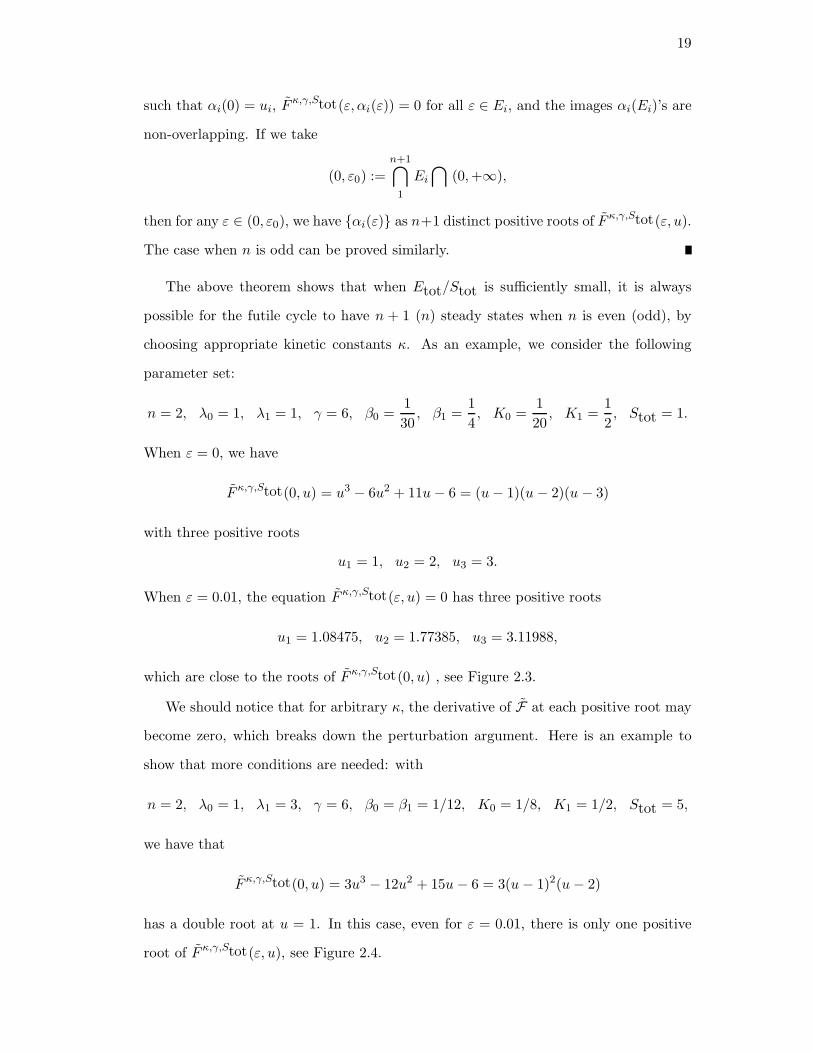
The above theorem shows that when Etot/Stot is sufficiently small, it is always

possible for the futile cycle to have n + 1 (n) steady states when n is even (odd), by

choosing appropriate kinetic constants κ. As an example, we consider the following

parameter set:

n = 2, λ0 = 1, λ1 = 1, γ = 6, β0 =1

30, β1 =

1

4, K0 =

1

20, K1 =

1

2, Stot = 1.

When ε = 0, we have

F κ,γ,Stot(0, u) = u3 − 6u2 + 11u− 6 = (u− 1)(u− 2)(u − 3)

with three positive roots

u1 = 1, u2 = 2, u3 = 3.

When ε = 0.01, the equation F κ,γ,Stot(ε, u) = 0 has three positive roots

u1 = 1.08475, u2 = 1.77385, u3 = 3.11988,

which are close to the roots of F κ,γ,Stot(0, u) , see Figure 2.3.

We should notice that for arbitrary κ, the derivative of F at each positive root may

become zero, which breaks down the perturbation argument. Here is an example to

show that more conditions are needed: with

n = 2, λ0 = 1, λ1 = 3, γ = 6, β0 = β1 = 1/12, K0 = 1/8, K1 = 1/2, Stot = 5,

we have that

F κ,γ,Stot(0, u) = 3u3 − 12u2 + 15u− 6 = 3(u− 1)2(u− 2)

has a double root at u = 1. In this case, even for ε = 0.01, there is only one positive

root of F κ,γ,Stot(ε, u), see Figure 2.4.

20

1 2 3 4

-2.0

-1.5

-1.0

-0.5

0.5

1.0

1.5

Figure 2.3: The plot of the functions F κ,γ,Stot(0, u) and F κ,γ,Stot(0.01, u) on [0, 4].The dashed line represents the function F when ε = 0. The polynomial F κ,γ,Stot(0, u)has three positive roots u = 1, 2, and 3. The solid line represents the function F whenε = 0.01. The three positive roots of F κ,γ,Stot(0.01, u) are close to the three roots ofF κ,γ,Stot(0, u) respectively.

However, the following lemma provides a sufficient condition for ∂Fκ,γ,Stot∂u (0, u) 6= 0,

for any positive u such that F κ,γ,Stot(0, u) = 0.

Lemma 2.3 For each positive numbers Stot, γ, and vector κ ∈ R6n+ , if

Stot

∣

∣

∣

∣

1− γβjKMj

∣

∣

∣

∣

≤ 1

n(2.21)

holds for all j = 1, · · · , n− 1, then ∂Fκ,γ,Stot∂u (0, u) 6= 0.

Proof. Recall that (dropping the u’s in ϕκi , i = 0, 1, 2)

F κ,γ,Stot(0, u) = uϕκ0 + Stot(uϕκ1 − γϕκ2)− γϕκ0 .

So

∂F κ,γ,Stot

∂u(0, u) = ϕκ0 + Stot(uϕ

κ1 − γϕκ2)′ − (γ − u)(ϕκ0 )′.

Since F κ,γ,Stot(0, u) = 0,

Stot(uϕκ1 − γϕκ2) = (γ − u)ϕκ0 ,

that is,

γ − u =Stot(uϕ

κ1 − γϕκ2)

ϕκ0.

21

u1 2 3

K5

0

5

10

Figure 2.4: The plot of the function F κ,γ,Stot(0.01, u) on [0, 3]. There is a uniquepositive real solution around u = 2.14, the double root u = 1 of F κ,γ,Stot(0, u) bifurcatesto two complex roots with non-zero imaginary parts.

Therefore, ∂Fκ,γ,Stot∂u (0, u) equals

ϕκ0 + Stot(uϕκ1 − γϕκ2)′ − Stot(uϕ

κ1 − γϕκ2)

ϕκ0(ϕκ0 )′

= ϕκ0 +Stotϕκ0

(

ϕκ0(uϕκ1 − γϕκ2)′ − (uϕκ1 − γϕκ2)(ϕκ0 )′)

= ϕκ0 +Stotϕκ0

((1 + λ0u+ λ0λ1u2 + · · ·+ λ0 · · · λn−1u

n)×(

1

KM0

(1− γβ0) + 2λ0

KM1

(1− γβ1)u+ · · ·+ nλ0 · · · λn−2

KMn−1

(1− γβn−1)un−1

)

−(

λ0 + 2λ0λ1u+ · · · + nλ0 · · ·λn−1un−1)

×(

1

KM0

(1− γβ0)u+λ0

KM1

(1− γβ1)u2 + · · ·+ λ0 · · ·λn−2

KMn−1

(1− γβn−1)un

)

= ϕκ0 +Stotϕκ0

n∑

i=0

λ0 · · · λi−1ui

n−1∑

j=0

(j + 1− i)λ0 · · ·λj−1

KMj

(1− γβj)uj

=1

ϕκ0

n∑

i=0

λ0 · · ·λi−1uin∑

j=0

λ0 · · ·λj−1uj

+ Stot

n∑

i=0

λ0 · · ·λi−1ui

n−1∑

j=0

(j + 1− i)λ0 · · · λj−1

KMj

(1− γβj)uj)

=1

ϕκ0

n∑

i=0

λ0 · · ·λi−1ui

×

λ0 · · ·λn−1un +

n−1∑

j=0

λ0 · · ·λj−1uj

(

1 + Stot(j + 1− i)1− γβjKMj

)

,

22

where the product λ0 · · ·λ−1 is defined to be 1 for the convenience of notation.

Because of (2.21),

Stot

∣

∣

∣

∣

(j + 1− i)1− γβjKMj

∣

∣

∣

∣

≤ 1,

we have ∂Fκ,γ,Stot∂u (0, u) > 0.

Theorem 2.4 For each positive numbers Stot, γ, and vector κ ∈ R6n+ satisfying condi-

tion (2.21), there exists ε1 > 0 such that for any Ftot, Etot satisfying Ftot = Etot/γ <

ε1Stot/γ, the number of positive steady states of system Σ(κ, C) is greater or equal to

the number of (positive) roots of F κ,γ,Stot(0, u).

Proof. Suppose that F κ,γ,Stot(0, u) has m roots: u1, . . . , um. Applying Lemma 2.3, we

have

∂F κ,γ,Stot

∂u(0, uk) 6= 0, k = 1, . . . ,m.

By the perturbation arguments as in Theorem 2.2, we have that there exists ε1 > 0

such that F κ,γ,Stot(ε, u) has at least m roots for all 0 < ε < ε1.

The above result depends heavily on a perturbation argument, which only works

when Etot/Stot is sufficiently small. In the next section, we will give an upper bound

of the number of steady states with no restrictions on Etot/Stot, and independent of

κ and C.

Upper bound on the number of positive steady states

Theorem 2.5 For each κ, C, the system Σ(κ, C) has at most 2n − 1 positive steady

states.

Proof. An alternative approach to solving (2.10)-(2.11) is to first eliminate v from

(2.10) instead of from (2.11), i.e.

v =Etot/Ftot − u

uϕκ1 (u)− (Etot/Ftot)ϕκ2 (u)

:=A(u)

B(u), (2.22)

23

when uϕκ1(u) − (Etot/Ftot)ϕκ2 (u) 6= 0. Then, we substitute (2.22) into (2.11), and

multiply by (uϕκ1 (u)− (Etot/Ftot)ϕκ2 (u))2 to get

P κ,C(u) := ϕκ0ϕκ2

(

EtotFtot

− u)2

+ (ϕκ0 − Stotϕκ2 + Ftotuϕ

κ1 + Ftotϕ

κ2 ) (2.23)

×(

EtotFtot

− u)(

uϕκ1 −EtotFtot

ϕκ2

)

− Stot

(

uϕκ1 −EtotFtot

ϕκ2

)2

= 0.

Therefore, if uϕκ1(u)−(Etot/Ftot)ϕκ2(u) 6= 0, the number of positive solutions of (2.10)-

(2.11) is no greater than the number of positive roots of P κ,C(u).

In the special case when uϕκ1(u) − (Etot/Ftot)ϕκ2 (u) = 0, by (2.10), we must have

u = Etot/Ftot, and thus ϕκ1 (Etot/Ftot) = ϕκ2(Etot/Ftot). Substituting into (2.11),

we get a unique v defined as in (2.12) with u = Etot/Ftot. Since u = Etot/Ftot is a

root of P κ,C(u), also in this case the number of positive solutions to (2.10)-(2.11) is no

greater than the number of positive roots of P κ,C(u).

It is easy to see that P κ,C(u) is divisible by u. Consider the polynomial Qκ,C(u) :=

P κ,C(u)/u of degree 2n+1. We will first show that Qκ,C(u) has no more than 2n positive

roots, then we will prove by contradiction that 2n distinct positive roots can not be

achieved.

It is easy to see that in the polynomial Qκ,C(u) the coefficient of u2n+1 is

(λ0 · · ·λn−1)2

LMn−1

> 0,

and the constant term is

EtotFtotKM0

> 0.

So the polynomial Qκ,C(u) has at least one negative root, and thus has no more than

2n positive roots.

Suppose that S(κ, C) has cardinality 2n, then Qκ,C(u) must have 2n distinct positive

roots, and each of them has multiplicity one. Let us denote the roots of Qκ,C(u) as

u1, . . . , u2n in ascending order, and the corresponding v’s given by (2.22) as v1, . . . , v2n.

We claim that none of them equals Etot/Ftot. If so, we would have ϕκ1(Etot/Ftot) =

ϕκ2(Etot/Ftot), and Etot/Ftot would be a double root of Qκ,C(u), contradiction.

Since Qκ,C(0) > 0, Qκ,C(u) is positive on intervals

I0 = (0, u1), I1 = (u2, u3), . . . , In−1 = (u2n−2, u2n−1), In = (u2n,∞),

24

and negative on intervals

J1 = (u1, u2), . . . , Jn = (u2n−1, u2n).

As remarked earlier, ϕκ1(Etot/Ftot) 6= ϕκ2 (Etot/Ftot), the polynomial Qκ,C(u) evalu-

ated at Etot/Ftot is negative, and therefore, Etot/Ftot belongs to one of the J intervals,

say Js = (u2s−1, u2s), for some s ∈ 1, . . . , n.

On the other hand, the denominator of v in (2.22), denoted as B(u), is a polynomial

of degree n and divisible by u. If B(u) has no positive root, then it does not change

sign on the positive axis of u. But v changes sign when u passes Etot/Ftot, thus v2s−1

and v2s have opposite signs, and one of (u2s−1, v2s−1) and (u2s, v2s) is not a solution to

(2.10)-(2.11), which contradicts the fact that both are in S(κ, C).

Otherwise, there exists a positive root u of B(u) such that there is no other positive

root of B(u) between u and Etot/Ftot. Plugging u into Qκ,C(u), we see that Qκ,C(u) is

always positive, therefore, u belongs to one of the I intervals, say It = (u2t, u2t+1) for

some t ∈ 0, . . . , n. There are two cases.

1. Etot/Ftot < u. We have

u2s−1 < Etot/Ftot < u2t < u.

Notice that v changes sign when u passes Etot/Ftot, so the corresponding v2s−1

and v2t have different signs, and either (u2s−1, v2s−1) /∈ S(κ, C) or (u2t, v2t) /∈

S(κ, C), contradiction.

2. Etot/Ftot > u. We have

u < u2t+1 < Etot/Ftot < u2s.

Since v changes sign when u passes Etot/Ftot, so the corresponding v2t+1 and

v2s have different signs, and either (u2t+1, v2t+1) /∈ S(κ, C) or (u2s, v2s) /∈ S(κ, C),

contradiction.

Therefore, Σ(κ, C) has at most 2n− 1 steady states.

25

Fine-tuned upper bounds

In the previous section, we have seen that any (u, v) ∈ S(κ, C), u 6= Etot/Ftot must

satisfy (2.22)-(2.23), but not all solutions of (2.22)-(2.23) are elements in S(κ, C). Sup-

pose that (u, v) is a solution of (2.22)-(2.23), it is in S(κ, C) if and only if u, v > 0. In

some special cases, for example, when the enzyme is in excess, or the substrate is in

excess, we could count the number of solutions of (2.22)-(2.23) which are not in S(κ, C)

to get a better upper bound.

The following is a standard result on continuity of roots; see for instance Lemma

A.4.1 in [83].

Lemma 2.6 Let g(z) = zn+a1zn−1 + · · ·+an be a polynomial of degree n and complex

coefficients having distinct roots

λ1, . . . , λq,

with multiplicities

n1 + · · ·+ nq = n,

respectively. Given any small enough δ > 0 there exists a ε > 0 so that, if

h(z) = zn + b1zn−1 + · · ·+ bn, |ai − bi| < ε for i = 1, . . . , n,

then h has precisely ni roots in Bδ(λi) for each i = 1, . . . , q, where Bδ(λi) is the open

ball in C centered at λi with radius δ.

Theorem 2.7 For each γ > 0 and κ ∈ R6n+ such that ϕκ1(γ) 6= ϕκ2 (γ), and each Stot >

0, there exists ε2 > 0 such that for all positive numbers Etot, Ftot satisfying Ftot =

Etot/γ < ε2Stot/γ, the system Σ(κ, C) has at most n+ 1 positive steady states.

Proof. Let us define a function R+ × C −→ C as follows,

Qκ,γ,Stot(ε, u) = Qκ,(εStot,εStot/γ,Stot)(u),

and a set Bκ,γ,Stot(ε) consisting of the roots of Qκ,γ,Stot(ε, u) which are not posi-

tive or the corresponding v’s determined by u’s as in (2.22) are not positive. Since

Qκ,γ,Stot(ε, u) is a polynomial of degree 2n+ 1, if we can show that there exists ε2 > 0

26

such that for any ε ∈ (0, ε2), Qκ,γ,Stot(ε, u) has at least n roots counting multiplicities

that are in Bκ,γ,Stot(ε), then we are done.

In order to apply Lemma 2.6, we regard the function Qκ,γ,Stot as defined on R×C.

At ε = 0:

Qκ,γ,Stot(0, u) = (ϕκ0ϕκ2 (γ − u)2 + (ϕκ0 − Stotϕ

κ2)(uϕκ1 − γϕκ2 )(γ − u)

− Stot(uϕκ1 − γϕκ2 )2)/u

= (ϕκ0(γ − u)u(ϕκ1 − ϕκ2) + Stotu(uϕκ1 − γϕκ2)(ϕκ2 − ϕκ1 ))/u

= (ϕκ2 − ϕκ1 )(uϕκ0 + Stot(uϕκ1 − γϕκ2)− γϕκ0)

= (ϕκ2 − ϕκ1 )F κ,γ,Stot(0, u)

Let us denote the distinct roots of Qκ,γ,Stot(0, u) as

u1, . . . , uq,

with multiplicities

n1 + · · ·+ nq = 2n+ 1,

and the roots of ϕκ1 − ϕκ2 as

u1, . . . , up, p ≤ q,

with multiplicities

m1 + · · ·+mp = n, ni ≥ mi, for i = 1, . . . , p.

For each i = 1, . . . , p, if ui is real and positive, then there are two cases (ui 6= γ as

ϕκ1(γ) 6= ϕκ2 (γ)).

1. ui > γ. We have

uiϕκ1(ui)− γϕκ2 (ui) > γ(ϕκ1(ui)− ϕκ2 (ui)) = 0.

2. ui < γ. We have

uiϕκ1(ui)− γϕκ2 (ui) < γ(ϕκ1(ui)− ϕκ2 (ui)) = 0.

27

In both cases, uiϕκ1(ui)− γϕκ2 (ui) and γ − ui have opposite signs, i.e.

(uiϕκ1(ui)− γϕκ2 (ui))(γ − ui) < 0.

Let us pick δ > 0 small enough such that the following conditions hold.

1. For all i = 1, . . . , p, if ui is not real, then Bδ(ui) has no intersection with the real

axis.

2. For all i = 1, . . . , p, if ui is real and positive, the following inequality holds for

any real u ∈ Bδ(ui),

(uϕκ1 (u)− γϕκ2(u))(γ − u) < 0. (2.24)

3. For all i = 1, . . . , p, if ui is real and negative, then Bδ(ui) has no intersection with

the imaginary axis.

4. Bδ(uj)⋂

Bδ(uk) = ∅ for all j 6= k = 1, . . . , q.

By Lemma 2.6, there exists ε2 > 0 such that for all ε ∈ (0, ε2), polynomial Qκ,γ,Stot(ε, u)

has exactly nj roots in each Bδ(uj), j = 1, . . . , q, denoted by ukj (ε), k = 1, . . . , nj .

We pick one such ε, and we claim that none of the roots in Bδ(ui), i = 1, . . . , p with

the v defined as in (2.22) will be an element in S. If so, we are done, since there are∑p

1 ni ≥∑p

1mi = n such roots of Qκ,γ,Stot(ε, u) which are in Bκ,γ,Stot(ε).

For each i = 1, . . . , p, there are two cases.

1. ui is not real. Then condition 1 guarantees that uki (ε) is not real for each k =

1, . . . , ni, and thus is in Bκ,γ,Stot(ε).

2. ui is real and positive. Pick any root uki (ε) ∈ Bδ(ui), k = 1, . . . , ni, the corre-

sponding vki (ε) equals

γ − uki (ε)uki (ε)ϕ

κ1 (uki (ε))− γϕκ2 (uki (ε))

< 0

followed from (2.24). So (uki (ε), vki (ε)) /∈ S(κ, C), and uki (ε) ∈ Bκ,γ,Stot(ε).

3. ui is real and negative. By condition 3, uki (ε) is not positive for all k = 1, . . . , ni.

28

The next theorem considers the case when enzyme is in excess.

Theorem 2.8 For each γ > 0, κ ∈ R6n+ such that ϕκ1 (γ) 6= ϕκ2(γ), and each Etot >

0, there exists ε3 > 0 such that for all positive numbers Ftot, Stot satisfying Ftot =

Etot/γ > Stot/(ε3γ), the system Σ(κ, C) has at most one positive steady state.

Proof. For each γ > 0, κ ∈ R6n+ such that ϕκ1(γ) 6= ϕκ2 (γ), and each Etot > 0, we define

a function R+ × C −→ C as follows:

Qκ,γ,Etot(ε, u) = Qκ,(Etot,Etot/γ,εEtot)(u).

Let us define the set Cκ,γ,Etot(ε) as the set of roots of Qκ,γ,Etot(ε, u) which are not

positive or the corresponding v’s determined by u’s as in (2.22) are not positive. If we

can show that there exists ε3 > 0 such that for any ε ∈ (0, ε3) there is at most one

positive root of Qκ,γ,Etot(ε, u) that is not in Cκ,γ,Etot(ε), we are done.

In order to apply Lemma 2.6, we now view the function Qκ,γ,Etot as defined on

R× C. At ε = 0, Qκ,γ,Etot(0, u) equals

(γ − u)(

(γ − u)ϕκ0ϕκ2 +

(

ϕκ0 +Etotγ

uϕκ1 +Etotγ

ϕκ2

)

(uϕκ1 − γϕκ2)

)

/u

:= (γ − u)Rκ,γ,Etot(u).

Let us denote the distinct roots of Qκ,γ,Etot(0, u) as

u1(= γ), u2, . . . , uq,

with multiplicities

n1 + · · ·+ nq = 2n+ 1,

and u2, . . . , uq are the roots of Rκ,γ,Etot(u) other than γ.

Since ϕκ1 (γ) 6= ϕκ2(γ), Rκ,γ,Etot(u) is not divisible by u− γ, and thus n1 = 1.

For each i = 2, . . . , q, we have (γ − ui)ϕκ0(ui)ϕκ2(ui) equals

−(

ϕκ0(ui) +Etotγ

uiϕκ1(ui) +

Etotγ

ϕκ2(ui)

)

(uiϕκ1(ui)− γϕκ2(ui)) .

29

If ui > 0, then ϕκ0(ui)ϕκ2(ui) and ϕκ0 (ui)+

Etotγ uiϕ

κ1 (ui)+

Etotγ ϕκ2 (ui) are both positive.

Since uiϕκ1(ui)− γϕκ2 (ui) and γ − ui are non zero, uiϕ

κ1(ui)− γϕκ2 (ui) and γ − ui must

have opposite signs, that is

(uiϕκ1(ui)− γϕκ2 (ui))(γ − ui) < 0.

Let us pick δ > 0 small enough such that the following conditions hold for all i =

2, . . . , q,

1. If ui is not real, then Bδ(ui) has no intersection with the real axis.

2. If ui is real and positive, then for any real u ∈ Bδ(ui), the following inequality

holds,

(uϕκ1 (u)− γϕκ2(u))(γ − u) < 0. (2.25)

3. If ui is real and negative, then Bδ(ui) has no intersection with the imaginary axis.

4. Bδ(uj)⋂

Bδ(uk) = ∅ for all i 6= k = 2, . . . , q.

By Lemma 2.6, there exists ε3 > 0 such that for all ε ∈ (0, ε3), the polynomial

Qκ,γ,Etot(ε, u)

has exactly nj roots in each Bδ(uj), j = 1, . . . , q, denoted by ukj (ε), k = 1, . . . , nj .

We pick one such ε, and if we can show that all of the roots in Bδ(ui), i = 2, . . . , q are

in Cκ,γ,Etot(ε), then we are done, since the only roots that may not be in Cκ,γ,Etot(ε)

are the roots in Bδ(u1), and there is one root in Bδ(u1).

For each i = 2, . . . , p, there are three cases.

1. ui is not real. Then condition 1 guarantees that uki (ε) is not real for all k =

1, . . . , ni.

2. ui is real and positive. Pick any root uki (ε), k = 1, . . . , ni, the corresponding vki (ε)

equals

γ − uki (ε)uki (ε)ϕ

κ1 (uki (ε)) − γϕκ2(uki (ε))

< 0.

So, uki (ε) is in Cκ,γ,Etot(ε).

30

3. ui is real and negative. By conditions 3, uki (ε) is not positive for all k = 1, . . . , ni.

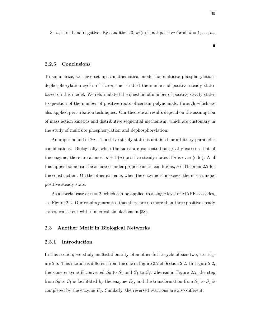
2.2.5 Conclusions

To summarize, we have set up a mathematical model for multisite phosphorylation-

dephosphorylation cycles of size n, and studied the number of positive steady states

based on this model. We reformulated the question of number of positive steady states

to question of the number of positive roots of certain polynomials, through which we

also applied perturbation techniques. Our theoretical results depend on the assumption

of mass action kinetics and distributive sequential mechanism, which are customary in

the study of multisite phosphorylation and dephosphorylation.

An upper bound of 2n−1 positive steady states is obtained for arbitrary parameter

combinations. Biologically, when the substrate concentration greatly exceeds that of

the enzyme, there are at most n + 1 (n) positive steady states if n is even (odd). And

this upper bound can be achieved under proper kinetic conditions, see Theorem 2.2 for

the construction. On the other extreme, when the enzyme is in excess, there is a unique

positive steady state.

As a special case of n = 2, which can be applied to a single level of MAPK cascades,

see Figure 2.2. Our results guarantee that there are no more than three positive steady

states, consistent with numerical simulations in [58].

2.3 Another Motif in Biological Networks

2.3.1 Introduction

In this section, we study multistationarity of another futile cycle of size two, see Fig-

ure 2.5. This module is different from the one in Figure 2.2 of Section 2.2. In Figure 2.2,

the same enzyme E converted S0 to S1 and S1 to S2, whereas in Figure 2.5, the step

from S0 to S1 is facilitated by the enzyme E1, and the transformation from S1 to S2 is

completed by the enzyme E2. Similarly, the reversed reactions are also different.

31

S S S0 1 2

E E1 2

F F1 2

Figure 2.5: Another “futile cycle” motif. The protein S0 is transformed by the enzymeE1 to S1, which is in turn brought to S2 by another enzyme E2. Conversely, the proteinS2 is changed to S1 with the help of the enzyme F2, and S1 is converted back to S0

through a different enzyme F1.

The difference between these two modules affects their asymptotic behaviors. We

will show in this section that the module, with different enzymes in the S0 to S2

direction and different enzymes in the transformation from S2 back to S0, admits a

unique positive steady state for any values of kinetic parameters involved in the system.

This suggests that the competition between S0 and S1 for the enzyme E is crucial for

multistationarity in the module shown in Figure 2.2. Regarding the dynamical behavior

of the motif in Figure 2.5, we show in Section 3.2 that the unique positive steady state

is globally asymptotically stable in R7≥0.

2.3.2 Mathematical formalism

Let us first write down all of the chemical reactions involved in Figure 2.5:

S0 + E1

k1−→←−k−1

C1k2→ S1 + E1

S1 + E2

k3−→←−k−3

C2k4→ S2 + E2

S2 + F2

k5−→←−k−5

C3k6→ S1 + F2

S1 + F1

k7−→←−k−7

C4k8→ S0 + F1.

Here, k1, etc., are kinetic parameters for binding and unbinding; C1 denotes the complex

consisting of the enzyme E1 and substrate S0; C2 denotes the complex formed by the

enzyme E2 and substrate S1; the complex consisting of the enzyme F2 and substrate

32

S2 is denoted by C3, and the complex formed by the enzyme F1 and substrate S1 is

denoted by C4.

These reactions can be modeled by differential equations according to mass action

kinetics:

ds0dt

= −k1s0e1 + k−1c1 + k8c4

ds1dt

= −k3s1e2 + k−3c2 − k7s1f1 + k−7c4 + k6c3 + k2c1

ds2dt

= −k5s2f2 + k−5c3 + k4c2

dc1dt

= k1s0e1 − (k−1 + k2)c1 (2.26)

dc2dt

= k3s1e2 − (k−3 + k4)c2

dc3dt

= k5s2f2 − (k−5 + k6)c3

dc4dt

= k7s1f1 − (k−7 + k8)c4,

together with the algebraic “conservation equations”:

E1,tot = e1 + c1

E2,tot = e2 + c2

F1,tot = f1 + c4 (2.27)

F2,tot = f2 + c3

Stot =2∑

i=0

si +4∑

i=1

ci.

The variables s0, s1, s2, c1, . . . , c4, e1, e2, f1, f2 stand for the concentrations of

S0, S1, Sn, C1, . . . , C4, E1, E2, F1, F2,

respectively. The total amount of the chemicals are denoted by

E1,tot, E2,tot, F1,tot, F2,tot, and Stot,

which are positive constants.

33

2.3.3 Positive steady states

At the steady state of system (2.26), we have the right hand side of (2.26) equal zero:

0 = −k1s0e1 + k−1c1 + k8c4 (2.28)

0 = −k3s1e2 + k−3c2 − k7s1f1 + k−7c4 + k6c3 + k2c1 (2.29)

0 = −k5s2f2 + k−5c3 + k4c2 (2.30)

0 = k1s0e1 − (k−1 + k2)c1 (2.31)

0 = k3s1e2 − (k−3 + k4)c2 (2.32)

0 = k5s2f2 − (k−5 + k6)c3 (2.33)

0 = k7s1f1 − (k−7 + k8)c4. (2.34)

In this section, the analysis is restricted to the steady states, that is solutions

of (2.28)-(2.34) together with (2.27). We will prove that the positive solutions of (2.28)-

(2.34) and (2.27) are unique. The strategy is to first express variables

s0, s2, c1, . . . , c4, e1, e2, f1, f2

in terms of s1, then to show that there is a unique positive s1 satisfying (2.28)-(2.34)

and (2.27). It thus follows that the steady state value of other variables are also unique.

We start by solving equations (2.31) to (2.34), from which we obtain c1, . . . , c4 as

functions of s0, s1, and s2:

c1 =s0E1,totKm1 + s0

c2 =s1E2,totKm2 + s1

(2.35)

c3 =s2F2,totKm3 + s2

c4 =s1F1,totKm4 + s1

.

Here, Km1,Km2,Km3,Km4 are the Michaelis-Menten constants defined as

Km1 =k−1 + k2

k1, Km2 =

k−3 + k4

k3,

Km3 =k−5 + k6

k5, Km4 =

k−7 + k7

k8.

34

If we could find relations to link s0 to s1 and to link s2 to s1, then c1, . . . , c4 can be

written as functions of s1 solely. We achieve this by first adding up equation (2.28) and

equation (2.31), which gives

k2c1 = k8c4. (2.36)

Invoking (2.35), we have

k2

s0E1,totKm1 + s0

= k8

s1F1,totKm4 + s1

, (2.37)

from where we can solve s0 as a function of s1. Let us denote by s0 = γ1(s1) the

solution of equation (2.37). Notice that γ1 is an strictly increasing function of s1 with

γ1(0) = 0.

Similarly, by adding up equation (2.30) and equation (2.33), we have

k4c2 = k6c3,

which leads to s2 = γ2(s1), where γ2 is an strictly increasing function of s1 with γ2(0) =

0.

Now, we can rewrite c1, . . . , c4 as functions of s1:

c1 =γ1(s1)E1,totKm1 + γ1(s1)

:= ϕ1(s1)

c2 =s1E2,totKm2 + s1

:= ϕ2(s1) (2.38)

c3 =γ2(s1)F2,totKm3 + γ2(s1)

:= ϕ3(s1)

c4 =s1F1,totKm4 + s1

:= ϕ4(s1).

It is easy to see that ϕ1, . . . , ϕ4 are all strictly increasing functions of s1 with ϕi(0) =

0, i = 1, . . . , 4.

On the hand, by the conservation relations in (2.27), we have

Stot = γ1(s1) + s1 + γ2(s1) +

4∑

i=1

ϕi(s1) := α(s1). (2.39)

The function α(s1) is thus strictly increasing in s1 and satisfies α(0) = 0. As a result,

for any given Stot > 0, equation (2.39) has a unique positive solution of s1.

Once we have the steady state value of s1, by (2.38), the steady state values of

c1, . . . , c4 are uniquely determined. The steady state value of s0 and s2 are given by

35

γ1(s1) and γ2(s1) respectively. Moreover, the conservation relations in (2.27) yield the

steady state values of e1, e2, f1, and f2.

To summarize, for any given positive numbers Stot, E1,tot, E2,tot, F1,tot, and F2,tot,

system (2.26)-(2.27) admits a unique positive steady state.

2.4 Arkin’s Example

In [74], Samoilov, Plyasunov, and Arkin provided an example of a set of chemical

reactions whose full stochastic (Master Equation) model exhibits bistable behavior,

but the deterministic (mean field) version yields a unique positive steady state.

The reactions that they introduced consist of a futile cycle of size one driven by a

second reaction which induces “deterministic noise” on the concentration of the forward

enzyme. The model is as follows:

N +Nk1−→←−k−1

N +E

Nk2−→←−k−2

E

S + Ek3−→←−k−3

C1k4−→P + E

P + Fk5−→←−k−5

C2k6−→S + F .

In fact [74] does not prove mathematically that this reaction’s deterministic model

has a single-steady state property, but shows numerically that, for a particular value of

the kinetic constants ki, a unique steady state (subject to stoichiometric constraints)

exists. In this section, we provide a proof of uniqueness valid for all possible parameter

values.

We use lower case letters n, e, s, c1, p, c2, f to denote the concentrations of the cor-

responding chemicals, as functions of t. The reactions can be modeled by the following

36

differential equations:

dn

dt= −k1n

2 + k−1ne− k2n+ k−2e

de

dt= −k3se+ k−3c1 + k4c1 + k1n

2 − k−1ne+ k2n− k−2e

ds

dt= −k3se+ k−3c1 + k6c2

dc1dt

= k3se− k−3c1 − k4c1 (2.40)

dp

dt= k4c1 − k5pf + k−5c2

dc2dt

= k5pf − k−5c2 − k6c2

df

dt= −k5pf + k−5c2 + k6c2.

Observe the following conservation relations hold:

Etot = e+ n+ c1

Ftot = f + c2

Stot = s+ c1 + c2 + p.

Theorem 2.9 For any given positive numbers Etot, Ftot, Stot, k1 and so on, sys-

tem (2.40) has a unique positive steady state.

Proof. Existence follows from the Brower fixed point theorem, since the reduced

system evolves on a compact convex set (intersection of the positive orthant and the

affine subspace given by the stoichiometry class).

We now fix one stoichiometry class and a set of kinetic parameters to prove unique-

ness. At the steady states, we have the right hand side of (2.40) equal zero. The idea is

to express the steady state values of variables e, s, c1, c2, and p in terms of n, and then

show that there is a unique steady state value of n.

From dn/dt = 0, we obtain that:

e =k1n

2 + k2n

k−1n+ k−2:= α(n).

From dc1/dt = 0, we have:

s =(k−3 + k4)c1

k3e=

(k−3 + k4)c1k3α(n)

. (2.41)

37

Solving dc2/dt = 0 for p and then substituting f = Ftot − c2 gives:

p =(k−5 + k6)c2k5(Ftot − c2)

. (2.42)

Finally, from d(p − f)/dt = 0, we obtain:

c2 =k4

k6c1 . (2.43)

The derivative of α(n) is

α′(n) =k1k−1n

2 + 2k1k−2n+ k2k−2

(k−2 + k−1n)2> 0 for all n ≥ 0,

and thus α(n) is a strictly increasing function on [0,+∞).

Notice that

c1 = Etot − (e+ n) = Etot − (α(n) + n).

As a result the steady state value of c1 as a function of n is strictly decreasing on

[0,+∞). Following from (2.41)-(2.43), the steady state values of c2, s, and p are also

strictly decreasing in n for n ≥ 0.

Recall that

Stot = s+ c1 + c2 + p.

The right hand side of the above equation is strictly decreasing in n. Therefore, for

any given Stot > 0, there is a unique positive steady state value of n. The steady state

values of other variables are now functions of n, and it follows that the steady state is

unique and positive.

38

Chapter 3

Singularly Perturbed Monotone Systems

3.1 Introduction

Monotone dynamical systems constitute a rich class of models, for which global and

almost-global convergence properties can be established. They are particularly useful

in biochemical applications and also appear in areas like coordination ([60]) and other

problems in control ([16]). One of the fundamental results in monotone systems theory

is Hirsch’s Generic Convergence Theorem ([36, 37, 38, 39, 82]). Informally stated,

Hirsch’s result says that almost every bounded solution of a strongly monotone system

converges to the set of equilibria. There is a rich literature regarding the application of

this powerful theorem, as well as of other results dealing with everywhere convergence

when equilibria are unique ([19, 44, 82]), to models of biochemical systems.

Unfortunately, many models in biology are not monotone, at least with respect to

any standard orthant order. This is because in monotone systems (with respect to

orthant orders) every net feedback loop should be positive, but, on the other hand,

in many systems negative feedback loops often appear as well, as they are required

for adaptation and precision. In order to address this drawback, as well as to study

properties of large systems which are monotone but which are hard to analyze in their

entirety, a recent line of work introduced an input/output approach that is based on the

analysis of interconnections of monotone systems. For example, the approach allows

one to view a non-monotone system as a negative feedback loop around a monotone

open-loop system, thus leading to results on global stability provided that the loop gain

is small enough (small-gain theorem for monotone systems) and to the emergence of

oscillations under transmission delays, and to the construction of relaxation oscillators

by slow adaptation rules on feedback gains. See [84, 85] for expositions and many

39

references.

The method presented here is in the same character. Intuitively, negative loops

that act at a comparatively fast time scale should not affect the main characteristics of

monotone behavior. The main purpose of this chapter is to show that this is indeed the

case, in the sense that singularly perturbed strongly monotone systems inherit generic

convergence properties. A system that is not monotone may become monotone once

that fast variables are replaced by their steady-state values.

A trivial linear example that illustrates this point is

x = −x− y,

εy = −y + x,

with ε > 0. This system is not monotone with respect to any orthant cone. On the other

hand, for ε≪ 1, the fast variable y tracks x, so the slow dynamics is well-approximated

by x = −2x, which is strongly monotone, because every scalar system is; hence, for

ε ≪ 1 one may expect that convergence still holds. (In this example, there is global

convergence to zero for all ε.) In order to prove a precise time-separation result, we

employ tools from geometric singular perturbation theory.

This point of view is of special interest in the context of biochemical systems; for

example, Michaelis Menten kinetics are mathematically justified as singularly perturbed

versions of mass action kinetics ([21, 65]). One particular example of great interest

in view of current systems biology research is that of dual “futile cycle” motifs, as

illustrated in Figure 2.2. This is a special case of Figure 1.1 when n = 2, see Section

2.2.1 for discussions of its biological applications.

Numerical simulations suggested that the above system could be either monostable

or bistable, see [58]. The latter will give rise to switch-like behavior, which is ubiquitous

in cellular pathways ([28, 70, 78, 79]). In either case, the system under meaningful bio-

logical parameters shows convergence, not other dynamical properties such as periodic

behavior or even chaotic behavior. Analytical studies done for the quasi-steady-state

version of the model (slow dynamics), which is a monotone system, indicate that the

reduced system is indeed monostable or bistable, see [67]. Thus, it is of great interest

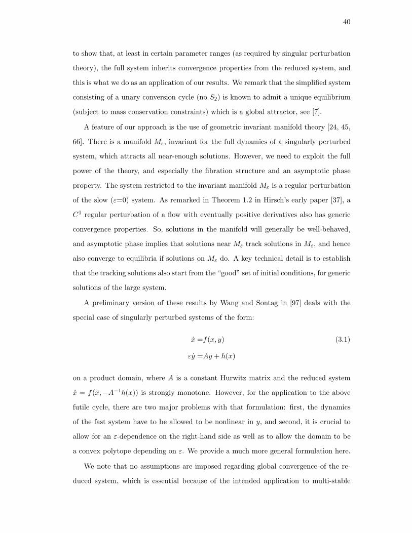
40

to show that, at least in certain parameter ranges (as required by singular perturbation

theory), the full system inherits convergence properties from the reduced system, and

this is what we do as an application of our results. We remark that the simplified system

consisting of a unary conversion cycle (no S2) is known to admit a unique equilibrium

(subject to mass conservation constraints) which is a global attractor, see [7].

A feature of our approach is the use of geometric invariant manifold theory [24, 45,

66]. There is a manifold Mε, invariant for the full dynamics of a singularly perturbed

system, which attracts all near-enough solutions. However, we need to exploit the full

power of the theory, and especially the fibration structure and an asymptotic phase

property. The system restricted to the invariant manifold Mε is a regular perturbation

of the slow (ε=0) system. As remarked in Theorem 1.2 in Hirsch’s early paper [37], a

C1 regular perturbation of a flow with eventually positive derivatives also has generic

convergence properties. So, solutions in the manifold will generally be well-behaved,

and asymptotic phase implies that solutions near Mε track solutions in Mε, and hence

also converge to equilibria if solutions on Mε do. A key technical detail is to establish

that the tracking solutions also start from the “good” set of initial conditions, for generic

solutions of the large system.

A preliminary version of these results by Wang and Sontag in [97] deals with the

special case of singularly perturbed systems of the form:

x =f(x, y) (3.1)

εy =Ay + h(x)

on a product domain, where A is a constant Hurwitz matrix and the reduced system

x = f(x,−A−1h(x)) is strongly monotone. However, for the application to the above

futile cycle, there are two major problems with that formulation: first, the dynamics

of the fast system have to be allowed to be nonlinear in y, and second, it is crucial to

allow for an ε-dependence on the right-hand side as well as to allow the domain to be

a convex polytope depending on ε. We provide a much more general formulation here.

We note that no assumptions are imposed regarding global convergence of the re-

duced system, which is essential because of the intended application to multi-stable

41

systems. This seems to rule out the applicability of Lyapunov-theoretic and input-to-

state stability tools ([17, 89]).

3.2 Monotone Systems for Ordinary Differential Equations

In this section, we review several useful definitions and theorems regarding monotone

systems. As we wish to provide results valid for arbitrary orders, not merely orthants,

and some of these results, though well-known, are not readily available in a form needed

for reference, we provide some technical proofs.

Definition 3.1 A nonempty, closed set C ⊂ RN is a cone if

1. C + C ⊂ C,

2. R+C ⊂ C,

3. C⋂

(−C) = 0.

We always assume C 6= 0. Associated to a cone C is a partial order on RN . For any

x, y ∈ RN , we define

x ≥ y ⇔ x− y ∈ C

x > y ⇔ x− y ∈ C, x 6= y.

When IntC is not empty, we can define

x≫ y ⇔ x− y ∈ IntC.

The most typical example would be C = RN≥0, in which case x ≥ y means that each

coordinate of x is bigger or equal than the corresponding coordinate of y. This order

gives rise to the class of “cooperative systems” (to be defined later) which is a special

class of the systems discussed below. Other orthant orders in RN also arise naturally

in biological systems, as we will see in our applications.

Definition 3.2 The dual cone of C is defined as

C∗ = λ ∈ (RN )∗ |λ(C) ≥ 0.

42

An immediate consequence is

x ∈ C ⇔ λ(x) ≥ 0,∀λ ∈ C∗

x ∈ IntC ⇔ λ(x) > 0,∀λ ∈ C∗ \ 0.

With this partial order on RN , we analyze certain features of the dynamics of an

ordinary differential equation

dz

dt= F (z), (3.2)

where F : RN → R

N is a C1 vector field. For any z ∈ RN , we denote the maximally

defined solution of (3.2) with initial condition z by t→ φt(z), t ∈ I(z), where I(z) is an

open interval in R that contains zero. For each t ∈ R, the set of z ∈ RN for which φt(z)

is defined is an open set W (t) ⊆ RN , and φt : W (t)→ W (−t) is a C1 diffeomorphism.

The collection of maps φt, t ∈ R is called the flow of (3.2). We also write just z(t) for

the solution of (3.2), if the initial condition z(0) is clear from the context. The forward

trajectory of z ∈ RN is a parametrized curve t → φt(z) (t ≥ 0, t ∈ I(x)). Its image is

the forward orbit of z, denoted as O+(z). The backward trajectory and the backward

orbit O−(z) are defined analogously.

Definition 3.3 A set U ⊆ RN is called positively (respectively, negatively) invariant if

O+(U) ⊆ U (respectively, O−(U) ⊆ U). It is called invariant if it is both positively and

negatively invariant.

We are interested in a special class of ordinary differential equations that preserve

the order along the trajectories. For simplicity, the solutions of (3.2) are assumed to

exist for all t ≥ 0 in the sets considered in the following.

Definition 3.4 The flow φt of (3.2) is said to have (eventually) positive derivatives on

a set V ⊆ RN with respect to a cone C, if [Dzφt(z)]x ∈ IntC for all x ∈ C \0, z ∈ V ,

and t ≥ 0 (t ≥ t0 for some t0 > 0 independent of z).

Next, we give a special class of systems with the property of positive derivatives.

43

Definition 3.5 A square N ×N matrix A = (aij) is said to be reducible if the indices

1, 2, . . . , N can be divided into two disjoint nonempty sets i1, i2, . . . , iu and j1, j2, . . . , jv

(with u + v = N) such that aiαjβ = 0 for all α = 1, 2, . . . , u and β = 1, 2, . . . , v. A

square matrix that is not reducible is said to be irreducible.

Proposition 3.6 A matrix is reducible if and only if it can be placed into block upper-

triangular form by simultaneous row and column permutations. In addition, a matrix

is reducible if and only if its associated digraph is not strongly connected.

Definition 3.7 System (3.2) is called irreducible on a set V ⊆ RN if the Jacobian

matrix DF (z) is irreducible for all z ∈ V .

Definition 3.8 System (3.2) is cooperative (respectively, competitive) with respect to

the nonnegative orthant RN≥0 on a set V ⊆ R

N if

∂Fi∂zj

(z) ≥ 0 (respectively,≤ 0)

for all i 6= j and z ∈ V . Moreover, system (3.2) is called a strictly cooperative (resp.

competitive) system with respect to the nonnegative orthant on V , if (3.2) is cooperative

and the partial derivatives are never zero.

Hereafter in this thesis, without special mentioning of the cone, “cooperative” means

cooperative with respect to the nonnegative orthant.

Systems that are irreducible and cooperative have nice properties. For example:

Lemma 3.9 (Theorem 1.1 in [36]). If (3.2) is irreducible and cooperative on a convex

open set W ⊆ RN , then the flow of (3.2) has positive derivatives.

A careful reading of the proof in [36] of the above result leads to the following

lemma:

Lemma 3.10 If (3.2) is strictly cooperative on a convex open set W ⊆ RN , then the

flow of (3.2) has positive derivatives.

It is worth noticing that [Dzφt(z)]x ∈ IntC is equivalent to λ([Dzφt(z)]x) > 0 for

all λ ∈ C∗ with |λ| = 1, where | · | denotes the Euclidean norm. We will use this fact in

44

the proofs of the following lemmas. Lemma 3.11 deals with “regular” perturbations in

the dynamics. It generalizes Theorem 1.2 of [36] from the nonnegative orthant RN≥ to

an arbitrary cone C.

Lemma 3.11 Assume V ⊂ RN is a compact set in which the flow φt of (3.2) has

eventually positive derivatives. Then there exists δ > 0 with the following property. Let

ψt denote the flow of a C1 vector field G such that the C1 norm of F (z)−G(z) is less

than δ for all z in V . Then there exists t∗ > 0 such that if ψs(z) ∈ V for all s ∈ [0, t]

where t ≥ t∗, then [Dzψt(z)]x ∈ IntC for all z ∈ V and x ∈ C \ 0. If, in addition, V

is positively invariant under the flow ψt, then ψt has eventually positive derivatives in

V .

Proof. Pick t∗ = t0 > 0, so that λ([Dzφt(z)]x) > 0 for all t ≥ t0, z ∈ V, λ ∈ C∗, x ∈ C

with |λ| = 1, |x| = 1. Then there exists δ > 0 with the property that when the C1 norm

of F (z)−G(z) is less than δ, we have λ([Dzψt(z)]x) > 0 for t0 ≤ t ≤ 2t0.

For t > 2t0, we write t = r + kt0, where t0 ≤ r < 2t0 and k ∈ N. If ψs(z) ∈ V for

all s ∈ [0, t], we can define zj := ψjt0(z) for j = 0, . . . , k. For any x ∈ C \ 0, using the

chain rule, we have

[Dzψt(z)]x = [Dzψr(zk)][Dzψt0(zk−1)] · · · [Dzψt0(z0)]x,

and thus [Dzψt(z)]x ∈ IntC.

Furthermore, if V is positively invariant under the flow ψt, then for any z ∈ V the

condition ψs(z) ∈ V for s ∈ [0, t] is satisfied for all t ≥ 0. As a result, the flow ψt has

eventually positive derivatives in V .

Definition 3.12 The system (3.2) or the flow φt of (3.2) is called monotone (resp.

strongly monotone) in a set W ⊆ RN , if for all t > 0 and z1, z2 ∈W ,

z1 ≥ z2 ⇒φt(z1) ≥ φt(z2)

(resp. φt(z1)≫ φt(z2) when z1 6= z2).

It is eventually (strongly) monotone if there exists t0 > 0 such that φt is (strongly)

monotone for all t ≥ t0.

45

If the partial derivatives ∂Fi/∂zj have constant sign for all i 6= j, system (3.2) is

said to have “definite feedback relations”. For such systems, we can define their “signed

influence digraphs” as follows. Vertexes of the signed influence digraph associated with

system (3.2) consist of the dependent variables zi, i = 1, . . . , N . There is no directed

edge from zj to zi if ∂Fi/∂zj ≡ 0. The edge from zj to zi is positive if ∂Fi/∂zj ≥ 0,

and the edge from zj to zi is negative if ∂Fi/∂zj ≤ 0.

System (3.2) is monotone with respect to some orthant order if there is no negative

(non-oriented) loops in the signed influence digraph, see [49, 82, 92]. If further the

graph is strongly connected, meaning that there is a path from zi to zj for each i 6= j,

then system (3.2) is strongly monotone with respect to some orthant order.

As an example, let us recall the motif introduced in Section 2.3. The signed influence

digraph of its ordinary differential equation model (2.26) is depicted in Figure 3.1. It

is clear from Figure 3.1 that the signed influence digraph contains no negative edges,

as a result system (2.26) is monotone. Moreover, the digraph is strongly connected, so

system (2.26) is strongly monotone with respect to the nonnegative orthant R7≥0. On

the other hand, system (2.26) has a unique positive equilibrium, see Section 2.3. By a

result in [19], we know that every bounded solution in R7≥0 of system (2.26) converges

to that unique equilibrium.

c1 cc2

0s s1

c

s2

3 4

Figure 3.1: The signed influence digraph of system (2.26). In a signed influence digraph,we use solid lines to represent edges with positive signs, and dashed lines to denote edgeswith negative signs. In this digraph, there are no edges with negative signs.

In Section 3.5.2, we show that the double phosphorylation dephosphorylation motif

admits a signed influence digraph that contains negative loops, and therefore is not

monotone.

Definition 3.13 An set W ⊆ RN is called p-convex, if W contains the entire line

46

segment joining x and y whenever x ≤ y, x, y ∈W .

Proposition 3.14 Let W ⊆ RN be p-convex. If the flow φt has (eventually) positive

derivatives in W , then it is (eventually) strongly monotone in W .

Proof. For any z1 > z2 ∈W,λ ∈ C∗ \ 0 and t > 0 (t ≥ t0 for some t0 > 0), we have

λ(φt(z1)− φt(z2)) =

∫ 1

0λ(

[Dzφt(sz1 + (1− s)z2)](z1 − z2))

ds > 0.

Therefore, φt is (eventually) strongly monotone in W .

The following two lemmas are variations of Hirsch’s Generic Convergence Theorem.

Lemma 3.15 Suppose that the flow φt of (3.2) has eventually positive derivatives in a

p-convex open set W ⊆ RN . Let W c ⊆ W be the set of points whose forward orbit has

compact closure in W . If the set of equilibria is totally disconnected (e.g., countable),

then the forward trajectory starting from almost every point in W c converges to an

equilibrium.

Lemma 3.15 is a generalization of Theorem 4.1 in [37] to arbitrary cones, done in the

same manner as in Lemma 3.11, so we omit the proof here. In our futile cycle example,

as well as in most biochemical systems after reduction by elimination of stoichiometric

constraints, the set of equilibria is discrete, and thus Lemma 3.15 will apply. However,

the more general result in Lemma 3.17 is also true, and applies even when the set of

equilibria is not discrete. It follows as a direct application of Theorem 2.26 in [39].

Definition 3.16 A point x in a set W ⊆ RN is called strongly accessible from below

(respectively, above) if there exists a sequence yn in W converging to x such that

yn < yn+1 < x (respectively, yn > yn+1 > x).

Lemma 3.17 Suppose that the flow φt of (3.2) has compact closure and eventually

positive derivatives in a p-convex open set W ⊆ RN . If any point in W can be strongly

accessible either from above or from below in W , then the forward trajectory from every

point, except for initial conditions in a nowhere dense set, converges to an equilibrium.

47

3.3 Geometric Singular Perturbation Theory

The theory of geometric singular perturbation can be traced back to the works of

Fenichel [24] , Mitropolsky and Lykova [59] in 1970’s. Later on, the works by Henry [35],

Knobloch and Aulbach [48], Nipp [66], and Sakamoto [73] also presented results similar

to [24]. By now, the theory is fairly standard, and there have been enormous appli-

cations to traveling waves of partial differential equations, see [45] and the references

there. For control theoretical applications, see [1, 43].

In this section, we revisit Fenichel’s theorems on geometric singular perturbation,

in the form stated in [73] by Sakamoto.

Consider a general singular perturbation system,

dx

dt= f(x, y, ε) (3.3)

εdy

dt= g(x, y, ε),

where x ∈ Rn, y ∈ R

m, and ε ∈ [0, ε0] for some ε0 > 0. We shall denote various

hypotheses about system (3.3) with the letter S.

S1 The functions f and g, defined on (x, y, ε) ∈ Rn×R

m × I, are of class Crb for some

positive integer r. (A function h is of class Crb if it is in Cr, and its derivatives

up to order r as well as f itself are bounded.)

S2 There is a function m0 whose derivatives up through order r are bounded (except

for the function itself), such that g(x,m0(x), 0) = 0.

The manifold, defined as

M0 := (x, y) | y = m0(x), x ∈ Rn

is often called the limiting slow manifold.

When ε = 0, system (3.3) degenerates to

dx

dt= f(x,m0(x), 0) (3.4)

y = m0(x),

48

where trajectories are restricted to the limiting slow manifold M0.

When ε 6= 0, we may change the time scale to τ = t/ε, and study the following

equivalent system of (3.3):

dx

dτ= εf(x, y, ε) (3.5)

dy

dτ= g(x, y, ε).

System (3.5) is often referred to as the fast time scale representation in contrast to the

slow time scale representation (3.3).

In the limit of ε = 0, system (3.5) becomes:

dx

dτ= 0 (3.6)

dy

dτ= g(x, y, 0).

We remark that system (3.6) focuses on the beginning part of a trajectory, while

system (3.4) gives the asymptotic behavior of a trajectory. One of the main goals

of Geometric Singular Perturbation theory is to connect these two limiting systems

using ideas from invariant manifold to gain deeper insights of the full system (3.3), see

Figure 3.2.

Definition 3.18 We say that M0 is normally hyperbolic relative to (3.5) if all eigen-

values of the matrix Dyg(x,m0(x), 0) have nonzero real part for every x ∈ Rn.

The notation Dyg(x,m0(x), 0) means the partial derivatives of g(x, y, ε) with respect

to the y coordinate evaluated at the point (x,m0(x), 0). Fenichel studied manifolds

that are normally hyperbolic. For our purpose of application, we are solely interested

in manifolds with the following property.

S3 All eigenvalues of the matrix Dyg(x,m0(x), 0), x ∈ Rn have negative real parts

smaller than −µ, where µ is a positive constant.

Theorem 3.19 Under assumptions S1 to S3, there exists a positive number ε1 < ε0

such that for every ε ∈ (0, ε1] the following properties hold.

49

M0

y=m (x)0

y

x1

x2

Figure 3.2: An illustration of the two limiting systems (3.6) and (3.4). The surfacebounded by dashed curves is the limiting slow manifold M0. The dashed trajectorieson M0 are solutions to system (3.4). The dashed straight lines perpendicular to M0

are the solutions to system (3.6). The solid curve is the true trajectory of system (3.3)when ε 6= 0 .

1. There is a Cr−1b function

m : Rn × [0, ε1]→ R

m

such that the set Mε defined by

Mε := (

x,m(x, ε))

|x ∈ Rn

is invariant under the flow generated by (3.17). Moreover,

supx∈Rn

|m(x, ε) −m0(x)| = O(ε), as ε→ 0.

In particular, we have m(x, 0) = m0(x) for all x ∈ Rn.

2. The stable manifold of Mε, consisting of all points (x0, y0) such that

supτ≥0|y(τ ;x0, y0)−m

(

x(τ ;x0, y0), ε)

|eµτ4 <∞,

where(

x(τ ;x0, y0), y(τ ;x0, y0))

is the solution of (3.3) passing through (x0, y0) at

τ = 0, is a Cr−1-immersed submanifold in Rn×Rm of dimension n+m, denoted

by W s(Mε).

50

3. There is a positive constant δ0 such that if

supτ≥0|y(τ ;x0, y0)−m

(

x(τ ;x0, y0), ε)

| < δ0,

then (x0, y0) ∈W s(Mε).

4. The manifold W s(Mε) is a disjoint union of Cr−1-immersed manifolds W sε (ξ) of

dimension m:

W s(Mε) =⋃

ξ∈Rn

W sε (ξ).

For each ξ ∈ Rn, let Hε(ξ)(τ) be the solution for τ ≥ 0 of

dx

dτ= εf(x,m(x, ε), ε), x(0) = ξ ∈ R

n.

Then, the manifold W sε (ξ) is the set

(x0, y0) | supτ≥0|x(τ)|eµτ

4 <∞, supτ≥0|y(τ)|eµτ

4 <∞,

where

x(τ) = x(τ ;x0, y0)−Hε(ξ)(τ),

y(τ) = y(τ ;x0, y0)−m(

Hε(ξ)(τ), ε)

.

5. The fibers are “positively invariant” in the sense that W sε (Hε(ξ)(τ)) is the set

(

x(τ ;x0, y0), y(τ ;x0, y0))

| (x0, y0) ∈W sε (ξ)

for each τ ≥ 0, see Figure 3.3.

6. The fibers restricted to the δ0 neighborhood of Mε, denoted by W sε,δ0

, can be

parametrized as follows. Let [−δ0, δ0] denote the cube (η1, . . . , ηn) | |ηi| ≤ δ0.

There are two Cr−1b functions

Pε,δ0 : Rn × [−δ0, δ0]→ R

n

Qε,δ0 : Rm × [−δ0, δ0]→ R

m,

and a map

Tε,δ0 : Rn × [−δ0, δ0]→ R

n × Rm

51

mapping (ξ, η) to (x, y), where

x = ξ + Pε,δ0(ξ, η), y = m(x, ε) +Qε,δ0(ξ, η)

such that

W sε,δ0(ξ) = Tε,δ0(ξ, [−δ0, δ0]).

Remark 3.20 The δ0 in property 3 can be chosen uniformly for ε ∈ (0, ε0].

Notice that property 4 ensures that for each (x0, y0) ∈W s(Mε), there exists a ξ such

that

|x(τ ;x0, y0)−Hε(ξ)(τ)| → 0,

|y(τ ;x0, y0)−m(

Hε(ξ)(τ), ε)

| → 0.

as τ →∞. This is often referred to as the “asymptotic phase” property, see Figure 3.3.

Mε

qqq

pp

01

1

22

0p

Figure 3.3: An illustration of the “positive invariant” and “asymptotic phase” prop-erties. Let p0 be a point on the fiber W s

ε (q0) (vertical curve). Suppose the solutionof (3.17) starting from q0 ∈ Mε evolves to q1 ∈ Mε after time τ1, then the solution of(3.17) starting from p0 will evolve to p1 ∈ W s

ε (q1) after time τ1. At time τ2, q1 andp1 evolve to q2, p2 respectively. These two solutions at any given time are always onthe same fiber. If the solution starting from q0 converges to an equilibrium, then thesolution starting from p0 also converges to an equilibrium.

52

3.4 Main Results on Singularly Perturbed Monotone Systems

3.4.1 Statement of the main theorem

Consider the following system:

dx

dt= f0(x, y, ε) (3.7)

εdy

dt= g0(x, y, ε),

where x ∈ Rn, y ∈ R

m, and ε ∈ [0, ε0] for some ε0 > 0. We will be interested in the

dynamics of this system on an ε-dependent domain Dε. The corresponding fast system

is:

dx

dτ= εf0(x, y, ε) (3.8)

dy

dτ= g0(x, y, ε).

We make the following assumptions, where the integer r > 1 is fixed from now on:

A1 Let U ⊂ Rn and V ⊂ R

m be open and bounded. The functions

f0 : U × V × [0, ε0]→ Rn

g0 : U × V × [0, ε0]→ Rm

are both of class Cr.

A2 There is a function

m0 : U → V

of class Cr, such that g0(x,m0(x), 0) = 0 for all x in U .

It is often helpful to consider z = y −m0(x), and the fast system (3.8) in the new

coordinates becomes:

dx

dτ= εf1(x, z, ε) (3.9)

dz

dτ= g1(x, z, ε),

53

where

f1(x, z, ε) = f0(x, z +m0(x), ε),

g1(x, z, ε) = g0(x, z +m0(x), ε) − ε[Dxm0(x)]f1(x, z, ε).

When ε = 0, the system (3.9) degenerates to

dz

dτ= g1(x, z, 0), x(τ) ≡ x0 ∈ U, (3.10)

seen as equations on z | z +m0(x0) ∈ V .

A3 The steady state z = 0 of (3.10) is globally asymptotically stable on z | z +

m0(x0) ∈ V for all x0 ∈ U .

A4 All eigenvalues of the matrix Dyg0(x,m0(x), 0) have negative real parts for every

x ∈ U , i.e. the matrix Dyg0(x,m0(x), 0) is Hurwitz on U .

A5 There exists a family of convex compact sets Dε ⊂ U × V , which depend continu-

ously on ε ∈ [0, ε0], such that (3.7) is positively invariant on Dε for ε ∈ (0, ε0].

A6 The flow ψ0t of the limiting system (set ε = 0 in (3.7)):

dx

dt= f0(x,m0(x), 0) (3.11)

has eventually positive derivatives on K0 with respect to some cone C. Here K0

is the projection of

D0

⋂

(x, y) | y = m0(x), x ∈ U

onto the x-axis.

A7 The set of equilibria of (3.7) on Dε is totally disconnected.

Remark 3.21 In mass-action chemical kinetics, the vector fields are polynomials, so

A1 follows naturally. Assumption A3 implies that y = m0(x) is a unique solution of

g0(x, y, 0) = 0 on U . Continuity in A5 is understood with respect to the Hausdorff

metric.

Our main theorem is:

54

Theorem 3.22 Under assumptions A1 to A7, there exists a positive constant ε∗ < ε0

such that for each ε ∈ (0, ε∗), the forward trajectory of (3.7) starting from almost every

point in Dε converges to some equilibrium.

Remark 3.23 A variant of this result is to assume that the reduced system (3.11) has

a unique equilibrium. In this case, one may improve the conclusions of the theorem to

global (not just generic) convergence, by appealing to results of Hirsch and others that

apply when equilibria are unique. The proof is simpler in that case, since the foliation

structure given by Fenichel’s theory is not required.

3.4.2 Extensions of the vector fields

Our approach to solve the varying domain problem is motivated by Nipp [66]. The

idea is to extend the vector fields from U × V × [0, ε] to Rn × R

m × [0, ε0], then apply

Theorem 3.19 on Rn × R

m × [0, ε0], and finally restrict the flows to Dε for the generic

convergence result.

Under assumption A5 (continuity of Dε in ε), we can pick a compact set K ⊂ U

such that Kε ⊆ K for ε sufficiently small. Without loss of generality, we assumeKε ⊆ K

for all ε ∈ [0, ε0]. The following is a routine “smooth patching” result.

Lemma 3.24 For any q ∈ Cr(U), there exists a compact-supported function q(x) ∈

Cr(Rn) such that q(x) ≡ q(x) on K. In particular, this implies that q(x) ∈ Crb (Rn).

Proof. It is a standard procedure to use convolution of the characteristic function and

mollifiers to obtain a C∞ cutoff function ϕ such that ϕ = 1 on K and ϕ(k) = 0 outside

of U for all k = 0, 1, . . . .

We define

q(x) =

q(x)ϕ(x) x ∈ U ;

0 x /∈ U.By the definition above, q(x) ≡ q(x) on K. Moreover, it is easy to see that q(x) has

compact support and q(x) ∈ Cr(Rn).

We will be focusing on extending the vector field of system (3.9) in the (x, z) co-

ordinates, then transform it back to the (x, y) coordinates. First, we look at the x

55

direction, and restrict z in the following set

Ld0 := z ∈ Rm | |z| ≤ d0 ⊂

⋂

x∈K

z | z +m0(x) ∈ V .

for some fixed d0.

Lemma 3.25 Under assumptions A1 and A4, there exist functions f1, g1, and m0

with the following properties:

f1 ∈ Crb (Rn × Ld0 × [0, ε0]), f1 ≡ f1 on K × Ld0 × [0, ε0], (3.12)

g1 ∈ Cr−1b (Rn × Ld0 × [0, ε0]), g1 ≡ g1 on K × Ld0 × [0, ε0], (3.13)

m0 ∈ Crb (Rn), m0 ≡ m0 on K. (3.14)

Moreover, all eigenvalues of the matrix Dz g1(x, 0, 0) have negative real parts less than

−µ for every x ∈ Rn.

Proof. Applying Lemma 3.24, we obtain functions f1 and m0 satisfying properties in

(3.12) and (3.14), respectively. The extension of g1 requires more work since we need

to make sure that the Jacobian of the extended function is Hurwitz on all of Rn. Let

us rewrite the differential equation for z in system (3.9) as:

dz

dτ=(

B(x) + C(x, z))

z + εH(x, z, ε) − ε[Dxm0(x)]f1(x, z, ε),

where

B(x) = Dyg0(x,m0(x), 0) and C(x, 0) = 0.

Applying Lemma 3.24, we can extend the functions C and H to C and H, respectively.

Let µ be a positive constant such that the real parts of all eigenvalues of B(x) is less

than −µ for every x ∈ K. The extension of B is defined as:

B(x) =

B(x)ϕ(x)− µ(1− ϕ(x))In x ∈ U ;

−µ(1− ϕ(x))In x /∈ U,

where the function ϕ is defined as in the proof of Lemma 3.24. It is easy to see that

B(x) ∈ Crb (Rn), and that all eigenvalues of B(x) will have negative real parts less than

−µ for every x ∈ Rn.

56

Finally, the extension g1 is defined as:

g1(x, z, ε) =(

B(x) + C(x, z))

z + εH(x, z, ε) − ε[Dxm0(x)]f1(x, z, ε).

The function g1 satisfies property (3.13) and all eigenvalues of the matrixDz g1(x, 0, 0) =

B(x) have negative real parts less than −µ for every x ∈ Rn.

Lemma 3.26 For any 0 < d1 < d0, under assumptions A1 and A4, there exist func-

tions f1 and g1, with the following properties:

f1 ∈ Crb (Rn × Rm × [0, ε0]), f1 ≡ f1 on R

n × Ld1 × [0, ε0], (3.15)

g1 ∈ Cr−1b (Rn ×R

m × [0, ε0]), g1 ≡ g1 on Rn × Ld1 × [0, ε0]. (3.16)

Proof. To extend functions f1 and g1 in the z direction from Ld0 to Rm, we consider

the restriction of those functions to the interior of Ld0 , then follow the same procedure

as in Lemma 3.24 to extend them in the z direction and to keep the extended functions

in agreement with the original ones on Ld1 . Let us denote the extensions of f1, C, and

H in the z direction by f1, C, and H, respectively. Then property (3.15) is satisfied

trivially. In the product(

B(x)+ C(x, z))

z, we view the factor z as an identity function

of z, and denote by z the extension of this identity function to Rm done in the same

manner as in Lemma 3.24. The function g1 defined as

g1 =(

B(x) + C(x, z))

z(z) + εH(x, z, ε) − ε[Dxm0(x)]f1(x, z, ε)

satisfies property (3.16).

Now we transform back to the (x, y) coordinate, and define

f(x, y, ǫ) = f1(x, y − m0(x), ε),

g(x, y, ǫ) = g1(x, y − m0(x), ε).

Property (3.16) implies g1(x, 0, 0) = 0, and thus g(x, m0(x), 0) = 0. To summarize, the

system

dx

dτ= εf(x, y, ε) (3.17)

dy

dτ= g(x, y, ε),

satisfies the following properties:

57

E1 The functions

f ∈ Crb (Rn × Rm × [0, ε0]),

g ∈ Cr−1b (Rn ×R

m × [0, ε0]).

E2 The function m0 ∈ Crb (Rn) satisfies

g(x, m0(x), 0) = 0, ∀x ∈ Rn.

E3 All eigenvalues of the matrix Dyg(x, m0(x), 0) have negative real parts less than

−µ for every x ∈ Rn.

E4 The function m0 coincides with m0 on K, and the functions f and g coincide with

f0 and g0 respectively on

Ωd1 := (x, y) |x ∈ K, |y −m0(x)| ≤ d1.

Properties E1 to E3 are the assumptions for geometric singular perturbation theorems,

and property E4 ensures that on Ωd1 the flow of (3.8) coincides with the flow of (3.17).

If we apply geometric singular perturbation theorems to (3.17) on Rn × R

m × [0, ε0],

the exact same results are true for (3.8) on Ωd1 . For the rest of the paper, we identify

the flow of (3.17) and the flow of (3.8) on Ωd1 without further mentioning this fact.

3.4.3 Further analysis of the dynamics and the proof of Theorem 3.22

Properties E1 to E3 correspond to assumptions S1 to S3 in Lemma 3.19. As a result,

there exists a positive number ε1 < ε0 such that conclusions in Lemma 3.19 hold.

The first property of Lemma 3.19 concludes the existence of an invariant manifold

Mε. There are two reasons to introduce Mε. First, on Mε the x-equation is decoupled

from the y-equation:

dx

dt= f(x,m(x, ε), ε) (3.18)

y(t) = m(x(t), ε).

This reduction allows us to analyze a lower dimensional system, whose dynamics may

have been well studied. Second, when ε approaches zero, the limit of (3.18) is (3.11). If

58

(3.11) has some desirable property, it is natural to expect that this property is inherited

by (3.18). An example of this principle is provided by the following Lemma:

Lemma 3.27 There exists a positive constant ε2 < ε1, such that for each ε ∈ (0, ε2),

the flow ψεt of (3.18) has eventually positive derivatives on Kε, which is the projection

of Mε⋂

Dε to the x-axis.

Proof. Assumption A6 states that the flow ψ0t of the limiting system (3.11) has

eventually positive derivatives on K0. By the continuity of m(x, ε) and Dε at ε=0, we

can pick ε2 small enough such that the flow ψ0t has eventually positive derivatives on

Kε for all ε ∈ (0, ε2). Applying Lemma 3.11, we conclude that the flow ψεt of (3.18) has

eventually positive derivatives on Kε provided Kε is positively invariant under (3.18),

which follows easily from the fact that (3.17) is positively invariant on Dε and Mε is

an invariant manifold.

The next lemma asserts that the generic convergence property is preserved for (3.18).

Lemma 3.28 For each ε ∈ (0, ε2), there exists a set Cε ⊆ Kε such that the forward

trajectory of (3.18) starting from any point of Cε converges to some equilibrium, and

the Lebesgue measure of Kε \ Cε is zero.

Proof. There exists a convex open set Wε containing Kε such that flow ψεt of (3.18)

has eventually positive derivatives on Wε. Assumption A5 assures that Kε ⊆W cε . The

proof is completed by applying Lemma 3.15 under the assumption A7.

By now, we have discussed flows restricted to the invariant manifold Mε, see Fig-

ure 3.4. Next, we will explore conditions for a point to be on W s(Mε), the stable

manifold of Mε. Property 3 of Lemma 3.19 provides a sufficient condition, namely, any

point (x0, y0) such that

supτ≥0|y(τ ;x0, y0)−m

(

x(τ ;x0, y0), ε)

| < δ0 (3.19)

is on W s(Mε). In fact, if we know that the difference between y0 and m(x0, ε) is

sufficiently small, then the above condition is always satisfied. This follows from the

proof of Claim 1 in [66].

59

M

Mε

0

Dε

Figure 3.4: This is a sketch of the manifolds M0 (surface bounded by dashed curves),Mε (surface bounded by solid curves), and Dε (the cube). It highlights two majorcharacters of Mε. First, Mε is close to M0. Second, the trajectories on Mε converge toequilibria if those on M0 do.

Lemma 3.29 There exists ε3 > 0, δ0 > d > 0, such that for each ε ∈ (0, ε3), if the

initial condition satisfies |y0−m(x0, ε)| < d, then (3.19) holds, i.e. (x0, y0) ∈W s(Mε).

See Figure 3.5 for a graphical interpretation of Lemma 3.29.

Before we get further into the technical details, let us give an outline of the proof of

the main theorem. The proof can be decomposed into three steps. First, we show that

almost every trajectory on Dε⋂

Mε converges to some equilibrium. This is precisely

Lemma 3.28. Second, we show that almost every trajectory starting from W s(Mε)

converges to some equilibrium. This follows from Lemma 3.28 and the “asymptotic

phase” property in Lemma 3.19, but we still need to show that the set of non-convergent

initial conditions is of measure zero. The last step is to show that all trajectories in Dε

will eventually stay in W s(Mε), which is our next lemma:

Lemma 3.30 There exist two positive numbers τ0 and ε4 < ε3, such that

(x(τ0), y(τ0)) ∈W s(Mε)

for all ε ∈ (0, ε4), where (x(τ), y(τ)) is the solution to (3.8) with the initial condition

(x0, y0) ∈ Dε.

60

M

Mε

0

d

W (M )s

ε

Figure 3.5: In this picture, the box bounded by the dashed-dot curves consists of allpoints (x0, y0) with the property |y0 −m(x0, ε)| < d. The surface bounded by dashedcurves is the limiting slow manifold M0. The surface bounded by the solid curve is theinvariant manifold Mε. Trajectories in the stable manifold W s(Mε) are attracted toMε. Lemma 3.29 states that all the points inside the dashed-dot box belong to in thestable manifold W s(Mε).

Proof. It is convenient to consider the problem in the (x, z) coordinates. Let (x(τ), z(τ))

be the solution to (3.9) with initial condition (x0, z0), where z0 = y0 −m(x0, 0). We

first show that there exists a τ0 such that |z(τ0)| ≤ d/2.

Expanding g1(x, z, ε) at the point (x0, z, 0), the equation of z becomes

dz

dτ= g1(x0, z, 0) +

∂g1∂x

(ξ, z, 0)(x − x0) + εR(x, z, ε)

for some ξ(τ) between x0 and x(τ) (where ξ(τ) can be picked continuously in τ). Let

us write

z(τ) = z0(τ) + w(τ),

where z0(τ) is the solution to (3.10) with the initial condition z0(0) = z0, and w(τ)

satisfies

dw

dτ= g1(x0, z, 0) − g1(x0, z

0, 0) +∂g1∂x

(ξ, z, 0)(x − x0) + εR(x, z, ε) (3.20)

=∂g1∂z

(x0, ζ, 0)w + ε∂g1∂x

(ξ, z, 0)

∫ τ

0f1(x(s), z(s), ε) ds + εR(x, z, ε),

with the initial condition w(0) = 0 and some ζ(τ) between z0(τ) and z(τ) (where ζ(τ)

can be picked continuously in τ).

61

By assumption A3, there exists a positive τ0 such that |z0(τ)| ≤ d/4 for all τ ≥ τ0.

Notice that we are working on the compact set Dε, so τ0 can be chosen uniformly for

all initial conditions in Dε.

We write the solution of (3.20) as:

w(τ) =

∫ τ

0

∂g1∂z

(x0, ζ, 0)w ds + ε

∫ τ

0

(∂g1∂x

(ξ, z, 0)

∫ s′

0f1(x, z, ε) ds

′ +R(x, z, ε))

ds.

Since the functions f1, R and the derivatives of g1 are bounded on Dε, we have:

|w(τ)| ≤∫ τ

0L|w| ds + ε

∫ τ

0

(

M1

∫ s′

0M2 ds

′ +M3

)

ds,

for some positive constants L,Mi, i = 1, 2, 3. The notation |w| means the Euclidean

norm of w ∈ Rm. Moreover, if we define

α(τ) =

∫ τ

0

(

M1

∫ s′

0M2 ds

′ +M3

)

ds,

then

|w(τ)| ≤∫ τ

0L|w| ds + εα(τ0),

for all τ ∈ [0, τ0] as α is increasing in τ . Applying Gronwall’s inequality ([83]), we have:

|w(τ)| ≤ εα(τ0)eLτ ,

which holds in particular at τ = τ0. Finally, we choose ε4 small enough such that

εα(τ0)eLτ0 < d/4 and |m(x, ε)−m(x, 0)| < d/2 for all ε ∈ (0, ε4). Then we have:

|y(τ0)−m(x(τ0), ε)| ≤ |y(τ0)−m(x(τ0), 0)| + |m(x(τ0), ε) −m(x(τ0), 0)|

< |z(τ0)|+ d/2

≤ |z0(τ0)|+ |w(τ0)|+ d/2

< d/4 + d/4 + d/2 = d.

That is, (x(τ0), y(τ0)) ∈W s(Mε) by Lemma 3.29.

By now, we have completed all three steps, and are ready to prove Theorem 3.22,

see Figure 3.6 for a graphical illustration of the proof.

Proof. (Theorem 3.22). Let ε∗ = minε2, ε4. For ε ∈ (0, ε∗), it is equivalent to prove

the result for the fast system (3.8). Pick an arbitrary point (x0, y0) in Dε, and there

are three cases:

62

M

Mε

0

o

p

qd

Dε

e

W (M )s

ε

Figure 3.6: This picture illustrates the key points in the proof of Theorem 3.22. Nota-tions follow from Figure 3.4 and Figure 3.5. The point q is on the invariant manifoldMε, and it converges to the equilibrium e. The point p belongs to the stable manifoldW s(Mε), and p is on the same fiber (vertical curve) with q. As a result, p also convergesto the equilibrium e. The point o in this picture represents an arbitrary point in Dε.After time τ0, the trajectory starting from o evolves to the point q, and eventuallyconverges to the equilibrium e.

1. y0 = m(x0, ε), that is, (x0, y0) ∈Mε⋂

Dε. By Lemma 3.28, the forward trajectory

converges to an equilibrium except for a set of measure zero.

2. 0 < |y0 −m(x0, ε)| < d. By Lemma 3.29, we know that (x0, y0) is in W s(Mε).

Then, property 4) of Lemma 3.19 guarantees that the point (x0, y0) is on some

fiber W sε,d(ξ), where ξ ∈ Kε. If ξ ∈ Cε, that is, the forward trajectory of ξ con-

verges to some equilibrium, then by the “asymptotic phase” property of Lemma

3.19, the forward trajectory of (x0, y0) also converges to an equilibrium. To deal

with the case when ξ is not in Cε, it is enough to show that the set

Bε,d =⋃

ξ∈Kε\Cε

W sε,d(ξ)

has measure zero in Rm+n. Define

Sε,d = (Kε \ Cε)× Ld.

By Lemma 3.28, Kε \ Cε has measure zero in Rn, thus Sε,d has measure zero in

Rn×R

m. On the other hand, Property 6) in Lemma 3.19 implies Bε,d = Tε,d(Sε,d).

63

Since Lipschitz maps send measure zero sets to measure zero sets, Bε,d is of

measure zero.

3. |y0 −m(x0, ε)| ≥ d. By Lemma 3.30, the point(

x(τ0), y(τ0))

is in W s(Mε) and

we are back to case 2. The proof is completed if the set φε−τ0(Bε,d) has measure

zero, where φετ is the flow of (3.8). This is true because φετ is a diffeomorphism

for any finite τ .

3.5 Applications

Several applications using Theorem 3.22 are worked out in detail. These applications

cover common biological examples ranging from molecular level enzymatic reactions to

macro level networks.

3.5.1 Enzyme competitive inhibition

Enzymes are proteins that act as catalysts. They help convert other molecules called

substrates into products, but they themselves are not changed by the reaction. The

size of an enzyme is usually large compared to the substrate molecules whose reaction

it catalyzes. Embedded on an enzyme are active sites, where the substrate can bind to

form a complex. Active sites are usually highly specific, and they bind only substrates

with similar structures.

Enzyme inhibitors are those molecules that can bind to the active sites of an enzyme

and decrease the enzyme’s activity. Here we focus on one class of enzyme inhibitors

called competitive inhibitors. Competitive inhibitors closely resemble the chemical

structure and molecular geometry of the substrate. The inhibitors compete for the

same active site with the substrate molecules. When a inhibitor occupies the active

site of the enzyme, it prevents any substrate molecules from reacting with the enzyme,

see Figure 3.7. Many drugs are designed using competitive inhibitors, for example,

Allegra R©.

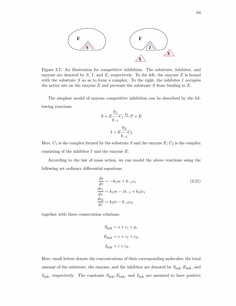
64

I

E E

S

SS

Figure 3.7: An illustration for competitive inhibition. The substrate, inhibitor, andenzyme are denoted by S, I, and E, respectively. To the left, the enzyme E is boundwith the substrate S so as to form a complex. To the right, the inhibitor I occupiesthe active site on the enzyme E and prevents the substrate S from binding to E.

The simplest model of enzyme competitive inhibition can be described by the fol-

lowing reactions:

S + Ek1−→←−k−1

C1k2→ P + E

I + Ek3−→←−k−3

C2

Here, C1 is the complex formed by the substrate S and the enzyme E; C2 is the complex

consisting of the inhibitor I and the enzyme E.

According to the law of mass action, we can model the above reactions using the

following set ordinary differential equations:

ds

dτ= −k1se+ k−1c1 (3.21)

dc1dτ

= k1se− (k−1 + k2)c1

dc2dτ

= k3ie− k−3c2,

together with three conservation relations:

Stot = s+ c1 + p,

Etot = e+ c1 + c2,

Itot = i+ c2.

Here, small letters denote the concentrations of their corresponding molecules; the total

amount of the substrate, the enzyme, and the inhibitor are denoted by Stot, Etot, and

Itot, respectively. The constants Stot, Etot, and Itot are assumed to have positive

65

values. System (3.21) consists of differential equations of three variables s, c1, and c2.

The rest of the variables e, p, and i can be solved from the conservation relations once

s, c1, and c2 are determined through system (3.21).

Let us first solve for the steady states of (3.21). At the steady states, we have the

right hand side of system (3.21) equal zero, that is,

0 = −k1se+ k−1c1 (3.22)

0 = k1se− (k−1 + k2)c1 (3.23)

0 = k3ie− k−3c2. (3.24)

Adding up equation (3.22) and equation (3.23), we have c1 = 0. Plugging c1 = 0 back

into equation (3.22), we have either s = 0 or e = 0. If e = 0, then by equation (3.24),

c2 = 0 too. As a result, Etot = e + c1 + c2 = 0 also, which contradicts Etot > 0. So

s = 0.

On the other hand, because c1 = 0, we have

e = Etot − c1 − c2 = Etot − c2. (3.25)

Plugging i = Itot − c2 and (3.25) into equation (3.24), we obtain a quadratic equation

for c2:

c22 − (Itot +Etot +Keq)c2 + ItotEtot = 0. (3.26)

Here,

Keq =k−3

k3

is called the equilibrium constant, which relates to the relative preference for the chem-

icals to be in the combined state C2 compared to the dissociated state I and E.

Let us rewrite equation (3.26) as

c22 −Ac2 +B = 0 (3.27)

where

A = Itot + Etot +Keq > 0, B = ItotEtot > 0.

66

It is easy to see that both roots of equation (3.26) are positive. However, the larger

root is greater than Itot because the right hand side of equation (3.26) evaluated at

c2 = Itot is

−EtotKeq < 0.

If c2 takes a value greater than Itot, then i = Itot − c2 is negative, which has no

biological meaning. Therefore, system (3.21) has a unique nonnegative steady state

(s∗, c∗1, c∗2) = (0, 0,

A−√A2 − 4B

2).

The signed influence digraph of system (3.21) is shown in Figure 3.8.

c1 c2

s

Figure 3.8: The signed influence digraph of system (3.21). We use solid lines to representedges with positive signs, and dashed line to denote edges with negative signs. The loopsformed by s, c1, and c2 are negative.

It is clear from Figure 3.8 that system (3.21) is not monotone with respect to any

orthant order, and thus the flows of (3.21) do not have positive derivatives by Lemma

3.14. However, in enzymatic reactions, it is often true that the amount of enzymes is

much less than the amount of substrates. Thus, it is reasonable to rescale the system

by defining

x =s

Stot, y1 =

c1Etot

, y2 =c2Etot

,

ε =EtotStot

, c =ItotStot

, t = τε,

and to assume that ε≪ 1 and c is a positive constant of order one.

System (3.21) in the new coordinates becomes

dx

dt= −k1xStot(1− y1 − y2) + k−1y1

εdy1

dt= k1xStot(1− y1 − y2)− (k−1 + k2)y1 (3.28)

εdy2

dt= k3Stot(c− εy2)(1− y1 − y2)− k−3y2.

67

These equations are in the form of (3.7). The conservation relations suggest taking

ε0 = c and

D = Dε := (x, y1, y2) | 0 ≤ x ≤ 1, 0 ≤ y1 + y2 ≤ 1, y1, y2 ≥ 0.

The set D is positively invariant for all ε ∈ (0, ε0] with respect to the flow of (3.28).

This is because the inner product of the outward-pointing normal vector at every point

of the boundary ∂D and the vector fields of (3.7) at that point is always nonnegative.

Corresponding to the steady state (s∗, c∗1, c∗2) of system (3.21), we have the steady

state

(x∗, y∗1 , y∗2) = (0, 0,

2cStot

α+√

α2 − 4β)

of system (3.28), where

α = cStot + εStot +Keq, β = εcS2tot.

Assumption A7 thus holds.

The projection of D to the x coordinate is defined as the set

K = Kε := x | 0 ≤ x ≤ 1,

for all ε ∈ [0, ε0].

Setting ε = 0 in (3.28), the y equations degenerate to algebraic equations:

0 = k1xStot(1− y1 − y2)− (k−1 + k2)y1

0 = k3Stotc(1− y1 − y2)− k−3y2.

Solving for y1 and y2, we obtain

y1 =

KeqKm

xKeqStot

+ c+KeqKm

x:= m1

0(x)

y2 =c

KeqStot

+ c+KeqKm

x:= m2

0(x).

Here,

Km =k−1 + k2

k1

68

is the Michaelis-Menten constant, which relates to the relative preference for the chem-

icals to be in the combined state C1 compared to the two dissociated states.

The reduced system (ε = 0 in (3.28))

dx

dt= −k1xStot(1−m1

0(x)−m20(x)) + k−1m

10(x)

is of dimension one, and thus flows of the reduced system have positive derivatives on

K0 automatically. Therefore, assumption A6 also holds.

Consider the matrix

B(x) := Dyg0(x,m0(x), 0) =

−k1 (xStot +Km) −k1xStot

−k3Stotc −k3

(

Stotc+Keq)

and a set U in the following form:

U = x | − σ < x < 1 + σ.

The determinant of B(x) is

det(B(x)) = k1k3(KmStotc+KeqxStot +KmKeq),

and the trace of B(x) is

−k1 (xStot +Km)− k3

(

Stotc+Keq)

.

As a result, for

σ < min

KmStotc+KmKeq

KeqStot,k1Km + k3

(

Stotc+Keq)

k1Stot

,

the determinant of B(x) is positive, and trace of B(x) is negative for any x ∈ (−σ, 1 +

σ). Therefore, the matrix B(x) is Hurwitz on U , which guarantees assumption A4.

Assumptions A1 and A2 follows naturally for sufficiently small σ.

It remains to check assumption A3. Notice that the fast limiting system corre-

sponding to (3.9) is:

dz

dτ= B(x0)z, x0 ∈ U.

This system is linear in z with a Hurwitz matrix B(x0) for every x0 ∈ U . Therefore,

assumption A3 also holds.

Now we have checked assumptions A1 to A7, applying Theorem 3.22, we have:

69

Theorem 3.31 There exists a positive ε∗ < ε0 such that for each ε ∈ (0, ε∗), the

forward trajectory of (3.28) starting from almost every point in D converges to some

equilibrium.

In fact, for this example every trajectory not merely almost every trajectory converges

to a equilibrium, see Remark 3.23.

3.5.2 Double phosphorylation dephosphorylation futile cycle

In section 2.2, we introduced an important motif called the futile cycle. Typically, the

enzymatic activation and de-activation in a futile cycle are given by phosphorylation and

dephosphorylation, and the cycle is thus called phosphorylation and dephosphorylation

futile cycle. In this section, we study the dynamical property of a phosphorylation

dephosphorylation futile cycle of size two, see Figure 2.2.

Let us first write down the chemical reactions involved:

S0 + Ek1−→←−k−1

C1k2→ S1 + E

k3−→←−k−3

C2k4→ S2 + E

S2 + Fh1−→←−h−1

C3h2→ S1 + F

h3−→←−h−3

C4h4→ S0 + F.

Based on mass action kinetics, we have the following set of ordinary differential equa-

tions:

ds0dτ

= h4c4 − k1s0e+ k−1c1

ds2dτ

= k4c2 − h1s2f + h−1c3

dc1dτ

= k1s0e− (k−1 + k2)c1 (3.29)

dc2dτ

= k3s1e− (k−3 + k4)c2

dc4dτ

= h3s1f − (h−3 + h4)c4

dc3dτ

= h1s2f − (h−1 + h2)c3,

70

together with three conservation relations:

Stot = s0 + s1 + s2 + c1 + c2 + c4 + c3,

Etot = e+ c1 + c2,

Ftot = f + c4 + c3,

where small letters denote the concentrations of their corresponding molecules. We can

draw the signed influence digraph of system (3.29), see Figure 3.9.

c2

c1 c

c

s s0 2

3

4

Figure 3.9: The signed influence digraph of the full system (3.29). We use solid linesto represent edges with positive signs, and dashed line to denote edges with negativesigns. The subgraph inside the dotted circle is not sign consistent.

Inside the dotted circle of Figure 3.9, the loops formed by nodes c1, c2, and s0 are

sign inconsistent. This is because on one hand, we have c2 directly inhibits c1; on

the other hand, c2 activates c1 through s0. As a result, the full system (3.29) is not

monotone.

However, as in Section 3.5.1, we can assume that the amount of enzyme is much

less than the amount of substrate, which in our case corresponds to Etot ≪ Stot and

Ftot ≪ Stot. Time scale separation arises under this assumption. We introduce new

variables:

x1 =s0Stot

, x2 =s2Stot

, y1 =c1Etot

, y2 =c2Etot

,

y3 =c4Ftot

, y4 =c3Ftot

, ε =EtotStot

, c =FtotEtot

, t = τε.

In terms of the new variables (rescaling the concentrations and time), system (3.29)

71

becomes:

dx1

dt=− k1Stotx1(1− y1 − y2) + k−1y1 + h4cy3

dx2

dt=− h1Stotcx2(1− y3 − y4) + h−1cy4 + k4y2

εdy1

dt=k1Stotx1(1− y1 − y2)− (k−1 + k2)y1 (3.30)

εdy2

dt=k3Stot(1− x1 − x2 − εy1 − εy2 − εcy3 − εcy4)(1− y1 − y2)− (k−3 + k4)y2

εdy3

dt=h3Stot(1− x1 − x2 − εy1 − εy2 − εcy3 − εcy4)(1− y3 − y4)− (h−3 + h4)y3

εdy4

dt=h1Stotx2(1− y3 − y4)− (h−1 + h2)y4.

These equations are in the form of (3.7). The conservation laws suggest taking

ε0 = 1/(1 + c) and

Dε =(x1, x2, y1, y2, y3, y4) | 0 ≤ y1 + y2 ≤ 1,

0 ≤ y3 + y4 ≤ 1, x1, x2, y1, y2, y3, y4 ≥ 0,

0 ≤ x1 + x2 + ε(y1 + y2 + cy3 + cy4) ≤ 1.

For ε ∈ (0, ε0], taking the inner product of the normal of ∂Dε and the vector fields,

it is easy to check that (3.30) is positively invariant on Dε, so A5 holds. We want to

emphasize that in this example the domain Dε is a convex polytope varying with ε.

In Section 2.2, we study the number of positive steady states of a general phospho-

rylation dephosphorylation futile cycle of size n, and provide explicit lower and upper

bounds of the number of positive steady states. In any case, system (3.30) has at most

a finite number of positive steady states, and thus A7 holds.

The projection of Dε to the x coordinate is defined as

K = Kε = (x1, x2) | 0 ≤ x1 + x2 ≤ 1

for all ε ∈ [0, ε0].

72

At ε = 0, solving g0(x, y, 0) = 0, we get

y1 =x1

Km1Stot

+ Km1(1−x1−x2)Km2

+ x1

,

y2 =

Km1(1−x1−x2)Km2

Km1Stot

+ Km1(1−x1−x2)Km2

+ x1

,

y3 =

Km3(1−x1−x2)Km4

Km3Stot

+ Km3(1−x1−x2)Km4

+ x2

,

y4 =x2

Km3Stot

+ Km3(1−x1−x2)Km4

+ x2

,

where Km1,Km2,Km3 and Km4 are the Michaelis-Menten constants defined as

Km1 =k−1 + k2

k1, Km2 =

k−3 + k4

k3, Km3 =

h−1 + h2

h1, Km4 =

h−3 + h4

h3.

Now, we need to find a proper set U ⊂ R2 satisfying assumptions A1-A4. Suppose

that U has the form

U = (x1, x2) |x1 > −σ, x2 > −σ, x1 + x2 < 1 + σ,

for some positive σ, and V is any bounded open set such that Dε is contained in U ×V ,

then A1 follows naturally. Moreover, if

σ ≤ σ0 := min

Km1Km2

Stot(Km1 +Km2),

Km3Km4

Stot(Km3 +Km4)

,

A2 also holds. To check A4, let us look at the matrix:

B(x) := Dyg0(x,m0(x), 0) =

B1(x) 0

0 B2(x)

,

where the column vectors of B1(x) are

B11(x) =

−k1Stotx1 − (k−1 + k2)

−k3Stot(1− x1 − x2)

,

B21(x) =

−k1Stotx1

−k3Stot(1− x1 − x2)− (k−3 + k4)

,

73

and the column vectors of B2(x) are

B12(x) =

−h3Stot(1− x1 − x2)− (h−3 + h4)

−h1Stotx2

,

B22(x) =

−h3Stot(1− x1 − x2)

−h1Stotx2 − (h−1 + h2)

.

If both matrices B1 and B2 have negative traces and positive determinants, then A4

holds. The trace of B1 is

−k1Stotx1 − (k−1 + k2)− k3Stot(1− x1 − x2)− (k−3 + k4).

It is negative provided that

σ ≤ k−1 + k2 + k−3 + k4

Stot(k1 + k3).

The determinant of B1 is

k1(k−3 + k4)Stotx1 + k3(k−1 + k2)Stot(1− x1 − x2) + (k−1 + k2)(k−3 + k4).

It is positive if

σ ≤ (k−1 + k2)(k−3 + k4)

Stot(

k1(k−3 + k4) + k3(k−1 + k2)) .

The condition for B2 can be derived similarly. To summarize, if we take

σ = min

σ0,k−1 + k2 + k−3 + k4

Stot(k1 + k3),

(k−1 + k2)(k−3 + k4)

Stot(

k1(k−3 + k4) + k3(k−1 + k2)) ,

h−1 + h2 + h−3 + h4

Stot(h1 + h3),

(h−1 + h2)(h−3 + h4)

Stot(

h1(h−3 + h4) + h3(h−1 + h2))

,

then the assumptions A1, A2 and A4 will hold.

Notice that dy/dt in (3.30) is linear in y when ε = 0, so g1 (defined as in (3.9)) is

linear in z, and hence the equation for z can be written as:

dz

dτ= B(x0)z, x0 ∈ U,

where the matrix B(x0) is Hurwitz for every x0 ∈ U . Therefore, A3 also holds.

74

It remains to show that assumption A6 is satisfied. Let us look at the reduced

system (ε = 0 in (3.30)):

dx1

dt=− k2x1

Km1Stot

+ Km1(1−x1−x2)Km2

+ x1

+h4c

Km3(1−x1−x2)Km4

Km3Stot

+ Km3(1−x1−x2)Km4

+ x2

:= F1(x1, x2) (3.31)

dx2

dt=− h2cx2

Km3Stot

+ Km3(1−x1−x2)Km4

+ x2

+k4

Km1(1−x1−x2)Km2

Km1Stot

+ Km1(1−x1−x2)Km2

+ x1

:= F2(x1, x2).

It is easy to see that F1 is strictly decreasing in x2, and F2 is strictly decreasing in

x1 on

K0 = (x1, x2) |x1 ≥ 0, x2 ≥ 0, x1 + x2 ≤ 1.

The reduced system (3.31) is a strictly competitive system, see Figure 3.10.

2x x1

Figure 3.10: The “signed influence digraph” of the reduced system (3.31). The nodesx1 and x2 inhibit each other, and the overall effect is positive.

Under the change of variable x∗1 = x1, x∗2 = −x2, system (3.31) becomes irreducible

and cooperative on the set K0. Moreover, because the partial derivatives are strictly

decreasing for (3.31), system (3.31) in the new coordinates (x∗1, x∗2) is irreducible and

cooperative on the set U (defined before) for sufficiently small σ. It then follows from

Lemma 3.9 that flow of (3.31) in the new coordinates has positive derivatives with

respect to the nonnegative orthant, and flow in the original coordinates has positive

derivatives with respect to the orthant

(x1, x2) |x1 ≤ 0, x2 ≥ 0.

As a result assumption A6 is satisfied for U with sufficiently small σ > 0 independent

of ε. Applying Theorem 3.22, we have:

Theorem 3.32 There exists a positive ε∗ < ε0 such that for each ε ∈ (0, ε∗), the

forward trajectory of (3.30) starting from almost every point in Dε converges to some

equilibrium.

75

Parameter Value

k1 0.02

k−1 1

k2 0.01

k3 0.032

k−3 1

k4 15

h1 0.045

h−1 1

h2 0.092

h3 0.01

h−3 1

h4 0.5

Stot 500

Etot 50

Ftot 100

Table 3.1: Parameters used in the simulation of system (3.29).

We simulate system (3.29) with parameters given in Table 3.1. The simulation

result confirms our conclusion in Theorem 3.32 and shows the key feature of singular

perturbation systems, that is, trajectories quickly converge to the invariant manifold,

then track trajectories on the invariant manifold, see Figure 3.11.

It is worth pointing out that the conclusion we obtained from the above theorem is

only valid for small enough ε; that is, the concentration of the enzyme should be much

smaller than the concentration of the substrate. Unfortunately, this is not always true

in biological systems, especially when feedbacks are present. However, if the sum of

the Michaelis-Menten constants and the total concentration of the substrate are much

larger than the concentration of enzyme, a different scaling:

x1 =s0A, x2 =

s2A, ε′ =

EtotA

, t = τε′,

where A = Stot+Km1+Km2+Km3+Km4 will allow us to obtain the same convergence

result.

76

Figure 3.11: This picture shows the projection of trajectories to the s0s2c1-plane. Thevertical axis is the concentration of the complex (“M-MAPKK” in the picture) formedby the protein MAPK and the enzyme MAPKK, denoted by c1 in the equations. Thehorizontal axises consist of concentrations of the protein MAPK (“M” in the picture)and the doubly phosphorylated form MAPK (“Mpp” in the picture), which correspondto s0 and s2 respectively in system (3.29). The vertical curves are solutions to system(3.29) with different initial conditions. The central horizontal curve is the projectionof the invariant manifold Mε to the s0s2c1-plane. We can see from this picture thatsolutions converge quickly to the invariant manifold, then follow trajectories on theinvariant manifold.

3.5.3 A genetic circuit example

Separation of time scales also arises in gene regulatory networks. Processes like binding

and unbinding of transcription factors often occur at a much faster time scale (usually

seconds) than other processes such as transcription and translation (usually several

minutes), see also Alon’s book [3] and references there. Protein-protein interaction

often depends on the size of the proteins and number of intimidate steps, and it could

be slow in some cases.

Consider a genetic circuit consisting of one gene a, which transcribes protein A. The

protein A can then form dimers, called B, and bind to the upstream regulatory sites

controlling the transcription of gene a, see Figure 3.12.

77

B

Aa

Figure 3.12: A genetic circuit. The transcription of gene a is regulated by two promoterbinding sites. The product of gene a, protein A, can form dimer B, which in turn bindsto the promoter site to activate the transcription of gene a.

We make the following assumptions about the system.

1. Binding and unbinding of the transcription factors occur at a much faster time

scale than other processes such as transcription, translation, degradation, and

protein-protein interaction.

2. The transcription rate of gene a is dramatically increased when the dimer B binds

to one of the regulatory sites.

3. The two regulatory sites are symmetric in terms of binding and unbinding of B

as well as the transcription rate.

4. The transcription rate is greater when both sites are bound with B than only one

site is occupied.

Reactions in the system are listed as follows:

Mσ→M +A, A+A

k+−→←−k−B,

B +D0

β1+−→←−

β1−

DBα1→ DB +M,

B +DB

β2+−→←−

β2−

DBBα2→ DBB +M,

D0α0→M, A

γa→ ∅, Mγm→ ∅,

78

Symbol Biological Meaning

D0 DNA without binding of B

DB DNA bound with one B

D′BB DNA bound with two Bs

A Protein A

B Dimmer formed by two As

M mRNA of gene a

σ Translation rate for protein A

k+ Dimerization rate of two As

k− Disassociation rate of B

β1+ Binding rate of B to D0

β1− Unbinding rate of B from DB

β2+ Binding rate of B to DB

β2− Unbinding rate of B from DBB

α0 Basal transcription rate of gene a

α1 Transcription rate of gene a when DNA is bound with one B

α2 Transcription rate of gene a when DNA is bound with two Bs

Table 3.2: Explanation of notations used in the genetic circuit.

The notations are given in Table 3.2.

According to our assumptions 2 to 4, we have

α0 ≪ α1 < α2. (3.32)

Based on mass action kinetics, the dynamics of this system can be modeled by the

following ordinary differential equations:

a′ = 2k−b− 2k+a2 + σm− γaa,

b′ = k+a2 − k−b− β1

+d0b+ β1−db − β2

+dbb+ β2−dbb,

m′ = α0d0 + α1db + α2dbb − γmm, (3.33)

d′b = β1+d0b− β1

−db,

d′bb = β2+dbb− β2

−dbb,

with the conservation relation

Dtot = d0 + db + dbb.

Here prime stands for d/dt, and the small letter represents the concentration of the

chemical in the corresponding capital letter.

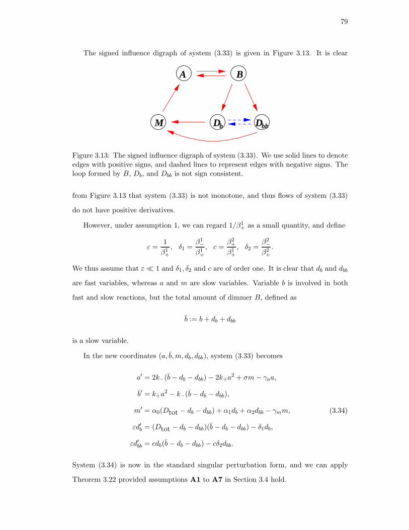
79

The signed influence digraph of system (3.33) is given in Figure 3.13. It is clear

M

B

Db bbD

A

Figure 3.13: The signed influence digraph of system (3.33). We use solid lines to denoteedges with positive signs, and dashed lines to represent edges with negative signs. Theloop formed by B, Db, and Dbb is not sign consistent.

from Figure 3.13 that system (3.33) is not monotone, and thus flows of system (3.33)

do not have positive derivatives.

However, under assumption 1, we can regard 1/β1+ as a small quantity, and define

ε =1

β1+

, δ1 =β1−

β1+

, c =β2

+

β1+

, δ2 =β2−

β2+

.

We thus assume that ε≪ 1 and δ1, δ2 and c are of order one. It is clear that db and dbb

are fast variables, whereas a and m are slow variables. Variable b is involved in both

fast and slow reactions, but the total amount of dimmer B, defined as

b := b+ db + dbb

is a slow variable.

In the new coordinates (a, b,m, db, dbb), system (3.33) becomes

a′ = 2k−(b− db − dbb)− 2k+a2 + σm− γaa,

b′ = k+a2 − k−(b− db − dbb),

m′ = α0(Dtot − db − dbb) + α1db + α2dbb − γmm, (3.34)

εd′b = (Dtot − db − dbb)(b− db − dbb)− δ1db,

εd′bb = cdb(b− db − dbb)− cδ2dbb.

System (3.34) is now in the standard singular perturbation form, and we can apply

Theorem 3.22 provided assumptions A1 to A7 in Section 3.4 hold.

80

It is straightforward to check that the set D, defined as

D = Dε := (a, b,m, db, dbb) | 0 ≤ a+ b ≤ σM0

γa, 0 ≤ m ≤M0,

a, b, db, dbb ≥ 0, 0 ≤ db + dbb ≤ minb, Dtot,

is positive invariant, and thus A5 holds. Here M0 is any number greater than

α2Dtotγm

.

The projection of D to the (a, b,m)-plane is

K = Kε = (a, b,m) | 0 ≤ a+ b ≤ σM0

γa, 0 ≤ m ≤M0, a, b ≥ 0.

Setting ε = 0 in (3.34), the equations for db and dbb degenerate to:

0 = (Dtot − db − dbb)(b− db − dbb)− δ1db, (3.35)

0 = db(b− db − dbb)− δ2dbb.

It is not straightforward to solve for db, dbb as functions of b from equations in (3.35).

We use the following approach to achieve this. Recall that

b = b− db − dbb. (3.36)

Substituting (3.36) into (3.35), we have

0 = (Dtot − db − dbb)b− δ1db, (3.37)

0 = dbb− δ2dbb.

Solving equations in (3.37), we get

db =Dtotb

δ1 + b+ b2/δ2:= ϕ1(b),

dbb =Dtotb

2/δ2δ1 + b+ b2/δ2

:= ϕ2(b).

For each i = 1, 2, ϕi is a strictly increasing and C∞ function of b on [0,+∞). As a

result,

b = b+ ϕ1(b) + ϕ2(b) (3.38)

81

is also a strictly increasing and C∞ function of b on [0,+∞). By the Implicit Function

Theorem, there exists a function b = f(b) such that (3.38) holds and f ′ > 0 on [0,+∞).

Now, we can write the solution of (3.35) as

db = ϕ1(f(b)) := h1(b)

dbb = ϕ2(f(b)) := h2(b).

The reduced system (ε = 0 in (3.34)) is

a′ = 2k−f(b)− 2k+a2 + σm− γpa := F1(a, b,m),

b′ = k+a2 − k−f(b) := F2(a, b,m), (3.39)

m′ =Dtot(α0δ1 + α1f(b) + α2f(b)2/δ2)

δ1 + f(b) + f(b)2/δ2− γmm := F3(a, b,m).

The partial derivatives are

∂F1

∂b> 0,

∂F1

∂m> 0,

∂F2

∂a≥ 0,

on K with ∂F2/∂a = 0 only when a = 0;

∂F3

∂b= Dtotδ2

(α2 − α1)f(b)2 + 2(α2 − α0)δ1f(b) + (α1 − α0)δ1δ2(δ1δ2 + δ2f(b) + f(b)2)2

> 0

under the condition (3.32). As a result, we can find an open set U of the following form

U := (a, b,m) | − σ < a+ b <σM0

γa+ σ,−σ < m < M0 + σ

and all of the partial derivatives, except ∂F2/∂a, are positive on U for small enough

σ. We next extend the function F2(a, b) to zero on the set U \ K. It is easy to see

that F2 is C1 with nonnegative partial derivatives. The signed influence digraph of

system (3.39) clearly shows that (3.39) is irreducible and cooperative, see Figure 3.14.

By Lemma 3.9, flow of (3.39) has positive derivatives with respect to the nonnegative

orthant on U for sufficiently small σ > 0.

To check A3, we fix the slow variables a, b,m, and show that the equilibrium db =

h1(b), dbb = h2(b) of fast limiting system

dbdτ

= (Dtot − db − dbb)(b− db − dbb)− δ1db, (3.40)

dbbdτ

= cdb(b− db − dbb)− cδ2dbb

82

A

M

B

Figure 3.14: The signed influence digraph of system (3.33). We use solid lines to denoteedges with positive signs, and dashed lines to represent edges with negative signs. Thereare no edges with negative signs. The digraph is strongly connected.

is globally asymptotically stable. Notice that the set

O := (db, dbb) | db ≥ 0, dbb ≥ 0, 0 ≤ db + dbb ≤ minDtot, b

is positively invariant, and the Jacobian matrix J of the system (3.40) is

−(b− db − dbb)− (Dtot − db − dbb)− δ1 −(b− db − dbb)− (Dtot − db − dbb)

c(b− db − dbb)− cdb −cdb − cδ2

.

It is clear that the divergence of does not change sign on the the simply connected

domain O. By the Bendixson’s criterion, there are no periodic orbits inside O.

The determinant of J ,

det(J) = c((A+B + δ1)δ2 + δ1db + (A+B)A),

is positive, where

A := b− db − dbb, B := Dtot − db − dbb.

The trace of J ,

trace(J) = −(A+B + δ1 + cdb + cδ2)

is negative. Therefore, the matrix J is Hurwitz, and the unique steady state (db, dbb) =

(h1(b), h2(b)) is asymptotically stable. Since we have ruled out the existence of periodic

orbits, by the Poincare-Bendixson Theorem, this unique steady state is also globally

asymptotically stable.

On the other hand, because the matrix J is Hurwitz, assumption A4 is also satisfied.

It remains to check A7. As in the futile cycle example in Section 2.2, the number of

83

positive steady states is bounded by the number of roots of certain polynomials. So

assumption A7 holds.

Applying Theorem 3.22, we have:

Theorem 3.33 There exists a positive ε∗ < ε0 such that for each ε ∈ (0, ε∗), the

forward trajectory of (3.34) starting from almost every point in D converges to some

equilibrium.

3.5.4 A network example

Consider the following system:

dxidt

= γi(y1, . . . , ym)− βi(x1, . . . , xn), i = 1, . . . , n, (3.41)

εdyjdt

= −djyj − αj(x1, . . . , xn), dj > 0, j = 1, . . . ,m,

where αj , βi and γi are smooth functions. We assume that

1. The reduced system

dxidt

= γi(−α1

d1, . . . ,−αm

dm)− βi(x1, . . . , xn) := Fi(x1, . . . , xn), i = 1, . . . , n

has partial derivatives that satisfy:

∂Fi∂xk

=

m∑

l=1

− 1

di

∂γi∂yl

∂αl∂xk− ∂βi∂xk

> 0 for i 6= k. (3.42)

2. For each i,

limu→+∞

minx∈Si(u)

βi(x) = +∞ (3.43)

and

limu→−∞

maxx∈Si(u)

βi(x) = −∞ (3.44)

where Si(u) is the set of vectors in Rn whose ith coordinate is u. (For n = 1, this

means simply that limx→±∞ βi(x) = ±∞.)

3. There exists a positive constant Mj such that |αj(x)| ≤Mj for all x ∈ Rn.

84

4. The number of roots of the system of equations

γi(α1(x), . . . , αm(x)) = βi(x), i = 1, . . . ,m

is countable.

We are going to show that on any large enough region, and provided that ε is

sufficiently small, almost every trajectory converges to some equilibrium. To emphasize

the need for small ε, we also show that when ε > 1, a limit cycle could appear.

Assumption 4 implies A7, and because of the form of (3.41), A3 and A4 follow

naturally. Under condition 1, A6 holds by applying Lemma 3.10.

We define

V = y ∈ Rm | |yj| < bj , j = 1, . . . ,m ,

where bj is an arbitrary positive number greater than Mj/dj . Picking such bj assures

yjdyj/dt < 0 for all x ∈ R and |yj| = bj , i.e. the vector field points transversely inside

on the boundary of V . Let

U = x ∈ Rn | − ai,2 < xi < ai,1, i = 1, . . . , n

where ai,1 can be any positive number such that

βi(x) > Ni := max|yj |≤bj

|γi(y1, . . . , ym)|

for all x ∈ Rn whose ith coordinate satisfies xi ≥ ai,1; the number ai,2 can be chosen

as any positive number such that

βi(x) < −Ni

for all x ∈ Rn whose ith coordinate satisfies xi ≤ −ai,2. All large enough ai,j ’s satisfy

this condition, because of the unboundedness assumption on β.

By the definition of U , it is easy to see that xidxi/dt < 0 on the boundary of U for all

y ∈ V , and thus the vector field will point to the interior of U ×V . Let D = Dε be any

convex compact set in U × V . It follows that D satisfies assumption A5. Assumptions

A1 and A2 follow naturally by the definition of U and V . Since all assumptions A1-A7

85

are satisfied, by By our main theorem, for sufficiently small ε, the forward trajectory

of (3.41) starting from almost every point in D converges to some equilibrium.

On the other hand, convergence does not hold for large ε. Let

n = 1, β(x) =x3

3− x, α1(x) = 2 tanh x,

m = 1, γ(y) = y, d = 1.

System (3.41) becomes

dx

dt= y − x3

3+ x (3.45)

εdy

dt= −y − 2 tanh x.

It is easy to verify that (0, 0) is the only equilibrium, and the Jacobian matrix at

(0, 0) is

1 1

−2/ε −1/ε

.

When ε > 1, the trace of the above matrix is 1 − 1/ε > 0, its determinant is 1/ε > 0,

so the (only) equilibrium in D is repelling.

On the other hand, the set D is chosen such that the vector fields point transversely

inside on the boundary of D. By the Poincare-Bendixson Theorem, there exists a limit

cycle in D, see Figure 3.15.

For the same system (3.45), when ε > 0 is small, forward trajectory starting from

almost every point in D converges to the origin, see Figure 3.16.

Remark 3.34 The conditions (3.42), (3.43), and (3.44) are satisfied, in particular, if

one assumes the following easier to check conditions on the functions βi’s, αj ’s, and

γi’s. The functions βi are required to satisfy:

∂βi∂xk

(x) < 0

for all i 6= k = 1, . . . , n (strict cooperativity condition among xi variables), and also so

that:

limx1→+∞,...,xn→+∞

βi(x1, . . . , xn) = +∞ (3.46)

limx1→−∞,...,xn→−∞

βi(x1, . . . , xn) = −∞. (3.47)

86

Figure 3.15: A simulation of system (3.45) with ε = 5. The horizontal axis is x, andthe vertical axis is y. Limit cycle appears.

These last conditions are very natural. They are satisfied, for example, if there is a

linear decay term −λixi in the differential equation for each xi, and all other variables

appear saturated in this rate. Since ∂βi

∂xk(x) < 0 for all i 6= k, (3.46)-(3.47) imply that

conditions (3.43) and (3.44) both hold.

Regarding the remaining functions, we ask:

m∑

l=1

∂γi∂yl

∂αl∂xk

≤ 0 (3.48)

for all i 6= k = 1, . . . , n. This condition can be guaranteed to hold based only upon

the signs of the partial derivatives: it holds true if there is no indirect negative effect

(through the variables yl) of any variable xk on any other variable xi. The diagram

shown in Figure 3.17 illustrates one such influence graph (signs indicate signs of partial

derivatives), for n = m = 2. Observe that this example cannot describe a monotone

system (with respect to any orthant cone, i.e., it is not cooperative under any possible

change of coordinates of the type xi → −xi or yl → −yl). An entirely analogous example

87

Figure 3.16: A simulation of system (3.45) with ε = 0.5. The horizontal axis is x, andthe vertical axis is y. Solutions converge to the equilibrium at the origin.

can be done for any n = m, the key property being that each variable xi “represses” its

associated variables yi and the yl’s “enhance” some or all other variables.

3.6 Conclusions

Singular perturbation techniques are routinely used in the analysis of biological systems.

The geometric approach is a powerful tool for global analysis, since it permits one to

study the behavior for finite ε on a manifold in which the dynamics is “close” to the

slow dynamics. Moreover, and most relevant to us, a suitable fibration structure allows

the “tracking” of trajectories and hence the lifting to the full system of the exceptional

set of non-convergent trajectories, if the slow system satisfies the conditions of Hirsch’s

Theorem. Using the geometric approach, we were able to provide a global convergence

theorem for singularly perturbed strongly monotone systems, in a form that makes it

applicable to the study of double futile cycles and other biochemical processes.

88

+

++

+

− −

x2

1x

1y

2y

Figure 3.17: The sign diagram of an example satisfying condition (3.48). The negativesign means one inhibits the other, and the positive sign means one enhances the other.

89

Chapter 4

Monotone Tridiagonal Systems with Negative Feedback

4.1 Introduction

Tridiagonal systems are those in which each of the state variables x1, . . . , xn is only

allowed to interact with its “neighbors”, see Figure 4.1. The dynamical behaviors of

. . . x n2x1x xn−1

Figure 4.1: An example of tridiagonal system of size n.

tridiagonal systems have been well studied; see, for instance, Smillie [80] and Smith [81].

Such systems arise in many models in biology. In biochemical networks, examples

include those in which a set of genes gi control the production of proteins Pi, each

of which acts as a transcription factor for the next gene gi+1 (binding and unbinding

to the promoter region of gi+1 affects the concentration of free protein Pi as well as

the transcription rate of gi+1). Somewhat different, though mathematically similar,

biological examples arise from sequences of protein post-translational modifications such

as phosphorylations and (providing the backward interaction) dephosphorylations.

Especially in biology, it is usual to find situations involving feedback from the last to

the first component. A very common situation involves negative (repressive) feedback,

which allows set-point regulation of protein levels, or which enables the generation of

oscillations. A specific and classical instance of this is the Goldbeter model for circadian

clocks in the Drosophila PER (“period”) protein ([30]). In all such examples, it is of

interest to find conditions that characterize oscillatory versus non-oscillatory regimes.

In this chapter, we provide sufficient conditions for global asymptotic stability of

monotone tridiagonal systems with negative feedback. Of course, when negated, we also

90

have then necessary conditions on parameters that must hold in order for oscillations

to exist.

4.2 Preliminaries

In this section, we introduce some definitions and notions that are used throughout

this chapter. A key result about systems with Poincare-Bendixson property is also

presented.

By default, all matrices and vectors considered in this chapter have real values.

Definition 4.1 A square matrix A is called quasi-monotone if it has nonnegative off-

diagonal entries.

Definition 4.2 A real vector is called nonnegative (positive) if all its components are

nonnegative (positive).

Definition 4.3 A square matrix A is called Hurwitz if all eigenvalues of the matrix A

have negative real parts.

If A and B are two n × n matrices such that Aij ≤ Bij for all i, j = 1, . . . , n, then we

denote this by A ≤ B.

For an arbitrary n× n matrix A, we let |A| be the n× n matrix defined as

|Aij | =

Aij, if i = j

|Aij |, if i 6= j.

Consider a general ordinary differential equation

y = G(y), y ∈ U, (4.1)

where U is an open set in Rn, and the vector field G is of class C1. Suppose that

system (4.1) has a periodic solution p(t).

Definition 4.4 The periodic solution p(t) is said to be orbitally (Lyapunov) stable if

for an arbitrarily small neighborhood W of p(t), all forward trajectories which start in

a sufficiently small neighborhood of p(t) do not emerge from W .

91

Definition 4.5 The periodic solution p(t) is said to be orbitally asymptotically sta-

ble if it is orbitally Lyapunov stable and if all the phase curves with initial condition

sufficiently close to p(t) approach p(t) asymptotically as t→ +∞.

We remark that a non-constant periodic solution can not be asymptotically stable

because solutions with initial conditions at different points of the cycle do not approach

one another as t→ +∞.

Definition 4.6 A set K is called absorbing in U for (4.1) if the solution y(t) with

initial condition in K1 stays in K for each compact set K1 ⊂ U and t sufficiently large.

A tridiagonal system with feedback has the form:

xi = fi(xi−1, xi, xi+1), i = 1, . . . , n− 1 (4.2)

xn = fn(xn−1, xn),

where x0 is identified with xn, and the vector field F = (f1, . . . , fn) is defined on an

open set U .

In typical applications, the variables xi represent nonnegative physical quantities,

such as concentrations of chemical species. In such cases, the equations describing the

system are initially only specified for vectors x belonging to the nonnegative orthant

Rn≥0. However, in most cases, one may restrict the system to the interior of R

n≥0, or

one may also view any such system as a system defined on a slightly larger open set

U . This is done by appropriately extending the functions fi to a neighborhood of the

orthant.

Definition 4.7 System (4.2) is called a monotone tridiagonal feedback system if there

exist scalars δi ∈ +1,−1, i = 1, . . . , n, such that for all 1 ≤ i ≤ n− 1,

δi∂fi(xi−1, xi, xi+1)

∂xi−1> 0, and

∂fi(xi−1, xi, xi+1)

∂xi+1≥ 0, (4.3)

for all x ∈ U , and

δn∂fn(xn−1, xn)

∂xn−1> 0 (4.4)

for all x ∈ U .

92

Monotone tridiagonal feedback systems are known to have the Poincare-Bendixson

property ([56]), that is, any nonempty compact omega limit set that contains no equi-

libria is a closed orbit. There are two types of monotone tridiagonal feedback systems

depending on the sign of the product δ1 · · · δn. If the sign is positive (negative), then

system (4.2) is called a monotone tridiagonal system with positive (negative) feedback.

In this paper, we focus on the negative feedback case, and from now on we assume

without loss of generality (after suitable rescaling of the state components with scaling

factor +1 or −1) that system (4.2) satisfies conditions (4.3) and (4.4) with

δ1 = −1 and δi = +1, for i = 2, . . . , n. (4.5)

For a system with the Poincare-Bendixson property, if it has an absorbing set K and

a unique equilibrium x∗, we can obtain global stability of x∗ by ruling out the existence

of periodic orbits. To achieve this, the following argument is used, see also [55].

We assume that every periodic orbit is orbitally asymptotically stable. Then the

boundary of the region of attraction of x∗ must contain a periodic orbit since it is

invariant. As a result, there exist points in the region of attraction of x∗ whose orbit

converges to the periodic orbit, which is impossible. More precisely,

Theorem 4.8 (Theorem 2.2 in [55]) For a general ordinary differential equation sys-

tem (4.1) with Poincare-Bendixson property, if the following assumptions hold:

1. There exists a compact absorbing set K ⊂ U .

2. There is a unique equilibrium point x∗, and it is locally asymptotically stable.

3. Each periodic orbit is orbitally asymptotically stable.

Then x∗ is globally asymptotically stable in U .

4.3 Ruling out periodic orbits

In this section, we use the theory of second compound matrices to show that all periodic

orbits are orbitally asymptotically stable. This is inspired by the work of Sanchez in [75],

93

which studied the globally asymptotic stability of cyclic systems with negative feedback.

Cyclic systems are those for which

∂fi(xi−1, xi, xi+1)

∂xi+1≡ 0 for all x ∈ U, i = 1, . . . , n

in (4.2). Cyclic systems are known to have Poincare-Bendixson property ([57]) and

other nice properties ([29]).

Recall the definition of the second additive compound matrix:

Definition 4.9 Let A be a matrix of order n. The second compound matrix A[2] is a

matrix of order(

n2

)

which is defined as follows:

A[2]ij =

Ai1i1 +Ai2i2 , if (i) = (j),

(−1)r+sAirjs if exactly one entry ir of (i) does

not occur in (j) and js does not

occur in (i), for some r, s ∈ 1, 2,

0 if (i) differs from (j) in both entries.

Here, (i) = (i1, i2) is the ith member of the lexicographic order of integer pairs for which

1 ≤ i1 < i2 ≤ n.

For future reference we state the following well-known facts from the theory of second

compound matrices, see [12, 54].

Lemma 4.10 Let the eigenvalues of a real n×n matrix A be denoted by λi, i = 1, . . . , n.

Then the eigenvalues of A[2] are given by λi + λj for i < j with i = 1, . . . , n and

j = 2, . . . , n.

Lemma 4.11 A matrix A of order n is Hurwitz if and only if A[2] is Hurwitz and the

sign of det(A) is (−1)n.

Let us denote by DF (x) the Jacobian of system (4.2). The following observation is

crucial to our proof.

Lemma 4.12 The second additive compound matrix DF [2](x) is quasi-monotone for

any x ∈ U .

94

Proof. Recall that the only non-zero off-diagonal entries of DF (x) are

DF (x)ii−1 > 0, DF (x)ii+1 ≥ 0

for i = 2, . . . , n− 1,

DF (x)12 ≥ 0, DF (x)nn−1 > 0, DF (x)1n < 0.

Thus the off-diagonal entries of DF [2](x) are non-zero only when one of the following

five cases happens:

1. The pairs i = (i1, i2), j = (i1, i2 − 1) for some i2 > i1 + 1. In this case

DF[2]ij (x) = (−1)2+2DF (x)i2i2−1 > 0.

2. The pairs i = (i1, i2), j = (i1, i2 + 1) for some i2 > i1. In this case

DF[2]ij (x) = (−1)2+2DF (x)i2i2+1 ≥ 0.

3. The pairs i = (i1, i2), j = (i1 − 1, i2) for some i2 > i1. In this case

DF[2]ij (x) = (−1)1+1DF (x)i1i1−1 > 0.

4. The pairs i = (i1, i2), j = (i1 + 1, i2) for some i2 > i1 + 1. In this case

DF[2]ij (x) = (−1)1+1DF (x)i1i1+1 ≥ 0.

5. The pairs i = (1, i2), j = (i2, n) for some 1 < i2 < n. In this case

DF[2]ij (x) = (−1)1+2DF (x)1n > 0.

Therefore, the second additive compound matrix DF [2](x) has only nonnegative off-

diagonal entries.

Second additive compound matrices can be used to study the stability of periodic

orbits. The following lemma states a result by Muldowney ([53, 63]), also used in [55,

75, 76].

95

Lemma 4.13 A given periodic solution p(t) of (4.1) is orbitally asymptotically stable

provided the linear system

z = DG[2](p(t))z

is asymptotically stable.

By Lemma 4.12 we know that for system the matrix ofDF [2](p(t)) is quasi-monotone

for all times. In this case, it turns out that to establish asymptotic stability for

z = DF [2](p(t))z, (4.6)

it is enough to check that for all t, the matrix DF [2](p(t)) is bounded above (compo-

nentwise) by a quasi-monotone and Hurwitz matrix B. This follows for instance from

Proposition 3 in [76]. Here we use a lemma by De Leenheer in [96].

Lemma 4.14 (De Leenheer). Let x = A(t)x be a linear time-varying system where

A(t) is a continuous function. If there are positive vectors c, d such that |A(t)|d ≤ −c

(componentwise) for all t, then x = 0 is asymptotically stable.

Now, we are ready to state and proof our main theorem.

Theorem 4.15 Assume that the first two conditions in Theorem 4.8 hold, and that

there exists a quasi-monotone Hurwitz matrix B such that B ≥ DF [2](x) for all x ∈ K.

Then x∗ is globally asymptotically stable for system (4.2).

Proof. Let us assume that p(t) is a nontrivial periodic solution and show that it

must be orbitally asymptotically stable. Since B is quasi-monotone and Hurwitz, it

follows that there exist positive vectors c and d such that Bd ≤ −c (componentwise)

by Theorem 15.1.1 in [40]. On the other hand, we have B −DF [2](p(t)) ≥ 0, and thus(

B −DF [2](p(t)))

d ≥ 0.

Notice that |DF [2](p(t))| = DF [2](p(t)) for all t > 0 since DF [2](p(t)) is quasi-

monotone. We thus have

|DF [2](p(t))|d ≤ Bd ≤ −c,

which by Lemma 4.14 yields that (4.6) is asymptotically stable. Applying Lemma 4.13,

we know that p(t) is orbitally asymptotically stable for system (4.2). The conclusion

now follows from an application of Theorem 4.8.

96

4.4 Applications

4.4.1 Linear Monotone Tridiagonal Systems with Nonlinear Negative

Feedback

We restrict our attention to systems of the form:

x1 = −d1x1 + β1x2 + g(xn)

xi = αixi−1 − dixi + βixi+1, i = 2, . . . , n − 1 (4.7)

xn = αnxn−1 − dnxn.

We denote by F = (f1, . . . , fn) the vector field of system (4.7). The following assump-

tions are made about system (4.7).

A1 For each i = 1, . . . , n, j = 2, . . . , n, and k = 1, . . . , n− 1, di, αj , and βk are positive

numbers.

A2 The function g : R≥0 → R≥0 is smooth and strictly decreasing with g(0) > 0.

A3 The matrix T , defined as

T =

−d1 β1 0 · · · 0

α2 −d2 β2 · · · 0

· · · · · · · · · · · · · · ·

0 · · · 0 αn −dn

,

is Hurwitz.

It is clear from assumptions A1 and A2 that system (4.7) is a monotone tridiago-

nal system with negative feedback on the interior of Rn≥0. Moreover, the nonnegative

orthant is forward invariant for system (4.7).

Lemma 4.16 Under assumptions A1 to A3, system (4.7) has a unique steady state

x∗ ∈ Rn>0.

Proof. The steady state x∗ satisfies

Tx∗ +G(x∗n) = 0.

97

Let us start from solving the nth equation of T x∗ +G(x∗n) = 0, which gives

αnx∗n−1 = dnx

∗n, that is, x∗n−1 =

dnαnx∗n.

Substituting x∗n−1 = dnx∗n/αn in the (n− 1)th equation

αn−1x∗n−2 + βn−1x

∗n = dn−1x

∗n−1,

we obtain

x∗n−2 =1

αn−1αndet(Tn−1n,n−1n)x

∗n.

Here Ti1,...,ik,i1,...,ik denote the k×k submatrix of T consisting of rows and columns from

i1 to ik. Repeating this procedure for other equations of T x∗+G(x∗n) = 0 in backward

order, we have

x∗j =1

∏ni=j+1 αi

(−1)n−jdet(Tj+1,...,n,j+1,...,n)x∗n, j = 1, . . . , n− 1. (4.8)

The coefficient in front of x∗n in equation (4.8) is positive for each j since the matrix T

is Hurwitz (assumption A3). By substituting (4.8) to the equation

d1x∗1 − β1x

∗2 = g(x∗n),

we obtain

1∏ni=2 αi

(−1)n det(T )x∗n = g(x∗n).

Under assumption A3, the left-hand side is a linear increasing function in x∗n. The

right hand side is a decreasing function with g(0) > 0. So there is a unique root x∗n in

(0,∞). The other components are also positive and unique because of (4.8).

Define a vector function

G(xn) = (g(xn) 0 . . . 0)T .

System (4.7) can be rewritten as

x = Tx+G(xn).

98

Lemma 4.17 Under assumptions A1 to A3, system (4.7) has a compact absorbing set

K ⊂ Rn>0, defined as

K = x |x− δ ≤ x ≤ x+ δ,

where x = (x1, . . . , xn) = −T−1G(0), x = (x1, . . . , xn) = −T−1G(xn), and δ is a

positive vector such that x− δ > 0.

Proof. By a similar argument as in the proof of Lemma 4.16, it is easy to see that x

and x are both in the interior of Rn≥0. As a result, there exists a positive vector δ such

that x− δ > 0. We pick such a δ from now on.

Let K1 be any compact subset of Rn>0 and x(t) be the solution to system (4.7) with

an arbitrary initial condition x0 ∈ K1. We first show that x(t) is bounded from above

by the constant x for large enough t.

Consider the following system:

u = Tu+G(0). (4.9)

Let u(t) be the solution of (4.9) with the initial condition u(0) = x0. The point x is

the steady state of the linear system (4.9), and it is globally asymptotically stable.

On the other hand, since g(xn) is strictly decreasing in xn on [0,+∞), we have

x ≤ Tx + G(0). By the comparison principle for monotone systems ([82]), it follows

that the solution x(t) of (4.7) is bounded from above by u(t) for all t ≥ 0, that is,

x(t) ≤ u(t) for all t ≥ 0. As a result,

lim supt≥0

x(t) ≤ limt→0

u(t) = x,

which implies that there exists a positive constant t0 such that x(t) ≤ x + δ for all

t > t0. This t0 can be chosen uniformly for all x0 ∈ K1.

Similarly, we can consider the system

v = Tv +G(xn), (4.10)

and let v(t) be the solution of (4.10) with an arbitrary initial condition x0 ∈ K1. Since

g(xn) is strictly decreasing in xn, and xn(t) is bounded from above by xn for all t > t0,

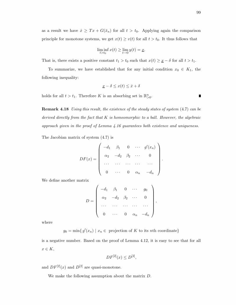
99

as a result we have x ≥ Tx + G(xn) for all t > t0. Applying again the comparison

principle for monotone systems, we get x(t) ≥ v(t) for all t > t0. It thus follows that

lim inft>t0

x(t) ≥ limt→0

y(t) = x.

That is, there exists a positive constant t1 > t0 such that x(t) ≥ x− δ for all t > t1.

To summarize, we have established that for any initial condition x0 ∈ K1, the

following inequality:

x− δ ≤ x(t) ≤ x+ δ

holds for all t > t1. Therefore K is an absorbing set in Rn>0.

Remark 4.18 Using this result, the existence of the steady states of system (4.7) can be

derived directly from the fact that K is homeomorphic to a ball. However, the algebraic

approach given in the proof of Lemma 4.16 guarantees both existence and uniqueness.

The Jacobian matrix of system (4.7) is

DF (x) =

−d1 β1 0 · · · g′(xn)

α2 −d2 β2 · · · 0

· · · · · · · · · · · · · · ·

0 · · · 0 αn −dn

.

We define another matrix

D =

−d1 β1 0 · · · g0

α2 −d2 β2 · · · 0

· · · · · · · · · · · · · · ·

0 · · · 0 αn −dn

,

where

g0 = min g′(xn) | xn ∈ projection of K to its nth coordinate

is a negative number. Based on the proof of Lemma 4.12, it is easy to see that for all

x ∈ K,

DF [2](x) ≤ D[2],

and DF [2](x) and D[2] are quasi-monotone.

We make the following assumption about the matrix D.

100

A4 The matrix D is Hurwitz.

Lemma 4.19 Under assumptions A1 to A4, the steady state x∗ obtained in Lemma

4.16 is asymptotically stable.

Proof. By Lemma 4.10, if D is Hurwitz, then so is D[2]. Moreover, DF [2](x∗) is also

Hurwitz because λPF (DF [2](x∗)) ≤ λPF (D[2]) ([10]).

The steady state x∗ is asymptotically stable if DF (x∗) is Hurwitz. It follows from

Lemma 4.11 that this will be the case if DF [2](x∗) is Hurwitz and the determinant of

DF (x∗) has the sign of (−1)n. Indeed, this is true under the condition that the matrix

T is Hurwitz. To see this, we compute det(DF (x∗)), and it equals

(−1)n(−g′(x∗n))α2α3 · · ·αn + det(T ).

It is clear that det(DF (x∗)) has the sign of (−1)n, which completes the proof.

Now we have checked all conditions in Theorem 4.15. Applying Theorem 4.15 to

system (4.7), we have the following result.

Theorem 4.20 Under assumptions A1 to A4, the steady state x∗ is globally asymp-

totically stable for system (4.7) on Rn>0.

4.4.2 Goldbeter Model

Circadian rhythms are pervasive features found in diverse organisms ranging from bac-

teria to humans. The rhythm is robust over a range of temperatures, and persists in

constant conditions (for example constant darkness) with a period of about 24 hours.

Disturbance in the human circadian rhythm could lead to many health problems such

as delayed sleep phase syndrome and various sleep disorders.

In this section, we consider one of the simplest and classical models of circadian

rhythms by Goldbeter ([30, 31]), and present conditions under which the rhythm is

disrupted, more precisely, there is a globally asymptotically stable steady state. The

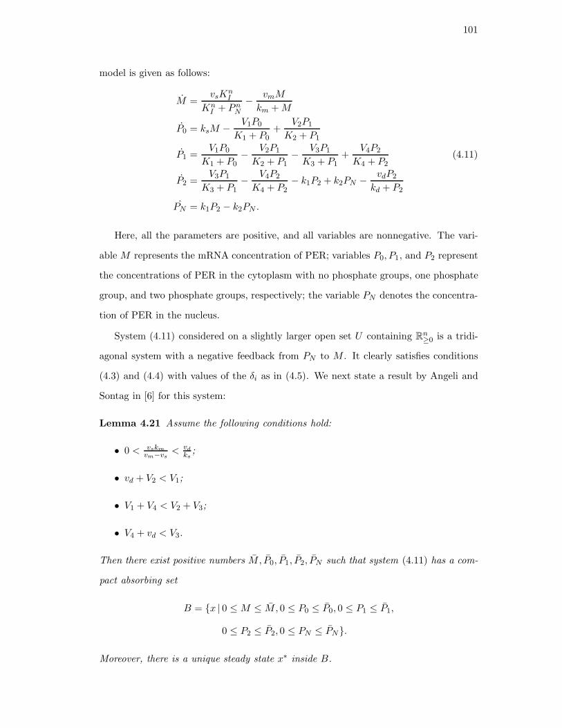
101

model is given as follows:

M =vsK

nI

KnI + PnN

− vmM

km +M

P0 = ksM −V1P0

K1 + P0+

V2P1

K2 + P1

P1 =V1P0

K1 + P0− V2P1

K2 + P1− V3P1

K3 + P1+

V4P2

K4 + P2(4.11)

P2 =V3P1

K3 + P1− V4P2

K4 + P2− k1P2 + k2PN −

vdP2

kd + P2

˙PN = k1P2 − k2PN .

Here, all the parameters are positive, and all variables are nonnegative. The vari-

able M represents the mRNA concentration of PER; variables P0, P1, and P2 represent

the concentrations of PER in the cytoplasm with no phosphate groups, one phosphate

group, and two phosphate groups, respectively; the variable PN denotes the concentra-

tion of PER in the nucleus.

System (4.11) considered on a slightly larger open set U containing Rn≥0 is a tridi-

agonal system with a negative feedback from PN to M . It clearly satisfies conditions

(4.3) and (4.4) with values of the δi as in (4.5). We next state a result by Angeli and

Sontag in [6] for this system:

Lemma 4.21 Assume the following conditions hold:

• 0 < vskm

vm−vs< vd

ks;

• vd + V2 < V1;

• V1 + V4 < V2 + V3;

• V4 + vd < V3.

Then there exist positive numbers M, P0, P1, P2, PN such that system (4.11) has a com-

pact absorbing set

B = x | 0 ≤M ≤ M, 0 ≤ P0 ≤ P0, 0 ≤ P1 ≤ P1,

0 ≤ P2 ≤ P2, 0 ≤ PN ≤ PN.

Moreover, there is a unique steady state x∗ inside B.

102

Observe that the vector field of (4.11) contains functions of Michaelis-Menten form,

that is,

h(y) =vy

K + y, y ∈ [0, y].

Taking the derivative of h, we have

h′(y) =vK

(K + y)2> 0.

As a result, the maximum and minimum of h′(x) on [0, y] are h′(0) and h′(y), respec-

tively. Based on this observation, it is easy to see that the second additive compound

matrix DF [2](x) is bounded by the matrix D[2], where the matrix D is defined as the

sum of the diagonal matrix

diag− vmkm(km + M)2

,− V1K1

(K1 + P0)2,− V2K2

(K2 + P1)2− V3K3

(K3 + P1)2,

− V4K4

(K4 + P2)2− vdkd

(kd + P2)2− k1,−k2

and the matrix

0 0 0 0 g0

ks 0 V2K2

0 0

0 V1K1

0 V4K4

0

0 0 V3K3

0 k2

0 0 0 k1 0

.

Here

g0 = −vs(n − 1)n−1

n (n+ 1)n+1

n

4nKI

is the minimum of vsKnI /(K

nI + PnN ) on [0,∞). Following a similar argument as in the

proof of Lemma 4.19, we have:

Lemma 4.22 Suppose that the assumptions in Lemma 4.21 hold and that the matrix

D is Hurwitz. If the sign of det(DF (x∗)) is −1, then x∗ is asymptotically stable.

Applying Theorem 4.15, we obtain the following result for system (4.11).

Theorem 4.23 Suppose that the assumptions in Lemma 4.21 hold and that the matrix

D is Hurwitz. If the sign of det(DF (x∗)) is −1, then x∗ is globally asymptotically stable.

103

This result provides conditions under which oscillations will be blocked. On the other

hand, when there is a oscillation, conditions in Theorem 4.23 fail to hold for that set

of kinetic parameters.

104

Chapter 5

A Class of Reaction Diffusion Systems with

Interconnected Structure

5.1 Introduction

Spatial information is crucial in many physiological processes such as cell division,

motility, and migration. During evolution, cells developed mechanism to detect spatial

localization of signaling proteins. A classical example is the process of morphogenesis.

In a human embryo, the change from a cluster of nearly identical cells to different

tissues and organs is controlled by chemicals that can be modified by environmental

factors. In MAPK cascades introduced in Chapter 2 and Chapter 3, the spatial gradient

of phosphorylated mitogen-actived protein kinase kinase (MEK) also plays important

roles.

Chemicals in an organism usually move around in a random way. This random

motion can be regarded as a diffusion process. On the other hand, chemicals may react

with each other, and thus form a reaction diffusion system. We shall point out that

the addition of diffusion could destabilize constant steady states. The phenomenon

of Turing’s pattern formation is a well known example of diffusion driven instability,

see [21, 64, 68, 93] for more on this subject. In this Chapter, in contrast to the loss of

stability, we show that if a passivity-based stability condition (will be defined precisely

later) holds for the ordinary differential equation system, then the global stability of

the same constant steady state is preserved when diffusion is added.

In their novel work [8] , Arcak and Sontag developed a passivity-based stabil-

ity condition for general interconnected systems without incorporating spatial fac-

tors (diffusion). The structure of a general interconnected system can be described

by a directed graph without self-loops. We use node i ∈ 1, . . . , N to represent

105

the ith subsystem. If there is a directed link l from node i to node j, we write

i = s(l), j = t(l), l ∈ L−i ⊆ 1, . . . ,M, and l ∈ L+j . See Figure 5.1 for an example

of such graphs. Let xi represent the state of the ith subsystem. Different subsystems

x1 x2

x3

x x

x4

4

5 6

3

7

1

2

5

6

Figure 5.1: An example of branched network in [8]. The dashed lines 4 and 7 indicatenegative feedback signals, and the solid lines indicate the positive influence.

are connected according to the structure of the graph. The set of ordinary differential

equations describing the dynamics is given by:

xi = −fi(xi) + gi(xi)∑

l∈L+i

hl(xs(l)), i = 1, . . . , N. (5.1)

A key notion used in [8] is passivity, which evolved from the idea of energy con-

servation and dissipation in electrical and mechanical systems ([101]). To determine

the stability of the whole system, Arcak and Sontag constructed a dissipativity ma-

trix (denoted by E below). The matrix E carries information about the structure of

the network, the signs of the interconnected terms, and the passivity properties of the

subsystems.

Under the assumption that system (5.1) has a unique steady state and that the

matrix E is diagonally stable, that is, there exists a diagonal matrix

Q = diagq1, . . . , qM > 0

such that

ETQ+QE < 0,

106

Arcak and Sontag proved globally stability of the steady state by constructing a Lya-

punov function V . Similar stability tests based on dissipativity were developed in

the earlier work of Vidyasagar [95], Moylan and Hill et al [62], and Sundareshan and

Vidyasagar [88].

The work by Jovanovic, Arcak, and Sontag in [46] studied the effect of diffusion to

a special class of systems whose interconnected graphs are cyclic, see Figure 5.2. The

21 ... nx x x

Figure 5.2: A cyclic system of size n. The dashed line represents the inhibition fromxn to x1.

present work extends the results in [46] to encompass the broader class of interconnected

systems represented by graphs, see Figure 5.1.

The effect of diffusion to the persistence of stability is one of the important ques-

tions to the theory of reaction diffusion equations. Let us consider a general ordinary

differential equation system:

dzidt

= Fi(z) (5.2)

zi(0) = z0i , (5.3)

and its corresponding partial differential equation system:

∂ui∂t

= Aiui + Fi(u) on Ω× (0,+∞), (5.4)

∂ui∂ν

= 0 on ∂Ω × (0,+∞), (5.5)

ui(ξ, 0) = u0i (ξ) on Ω, (5.6)

for each i = 1, . . . N . Here Ai is a second order differential operator defined as

Ai =

N∑

j,k=1

aijk(ξ)∂

∂ξj

∂

∂ξk+

N∑

k=1

aik(ξ)∂

∂ξk.

In the work [71] by Redheffer, Redlinger, and Walter, the authors used the convexity

of a Lyapunov function associated with (5.2) to prove the global existence of classical

solutions to (5.4)-(5.5) under the assumption that the elliptic operator Ai’s are the same

107

for all i = 1, . . . , N . Moreover, they obtained La Salle type of result for systems with

strictly convex Lyapunov functions. Morgan in [61] studied the case when the elliptic

operator

Ai ≡ ai∂

∂ξi

∂

∂ξi,

where ai is a positive constant. He made the assumption that there exists a Lyapunov

structure function H ∈ C2(M,R≥0), where M is a unbounded region of RN for which

(5.4) is invariant. Under various assumptions on the function H, Morgan in [61] ob-

tained boundedness and stability results for (5.4). Along these lines is the paper [26]

by Fitzgibbon, Hollis, and Morgan with an emphasis on stability in L∞.

In the present work, instead of assuming conditions on the Lyapunov function, we

provide a specific form of the Lyapunov function, and present a self-contained proof

for the global stability of the constant equilibrium without the restriction of constant

diffusion coefficients.

5.2 Review of the Ordinary Differential Equation Case

In [8], the authors made the following assumptions about system (5.1).

A1 For each i = 1, . . . , N and l = 1, . . . ,M , the functions fi, gi, and hl are locally

Lipschitz with fi(0) = 0, and gi(θ) > 0, hl(θ) ≥ 0 for all θ ≥ 0.

A2 System (5.1) admits an equilibrium x∗ ∈ RN≥0.

A3 For each node i, the function fi/gi satisfies the sector property

(θ − x∗i )(

fi(θ)

gi(θ)− fi(x

∗i )

gi(x∗i )

)

> 0, ∀θ ∈ R≥0 \ x∗i . (5.7)

A4 For each node i, and for each link l ∈ L−i , the function hl satisfies one of the

following sector properties for all θ ∈ R≥0 \ x∗i

(θ − x∗i )(hl(θ)− hl(x∗i )) > 0, (5.8)

(θ − x∗i )(hl(θ)− hl(x∗i )) < 0. (5.9)

108

We define κl to be +1 when (5.8) holds, and −1 when (5.9) holds. The above

conditions (5.8) and (5.9) can be unified as

κl(θ − x∗i )(hl(θ)− hl(x∗i )) > 0. (5.10)

A5 For each node i, and for each link l ∈ L−i , there exists a constant γl > 0 such that

κlhl(θ)− hl(x∗i )fi(θ)gi(θ)− fi(x∗i )

gi(x∗i )

≤ γl, ∀θ ∈ R≥0 \ x∗i . (5.11)

The following is a restatement of the main result in [8].

Theorem 5.1 Suppose that the system (5.1) satisfies assumptions A1 to A5, and the

M ×M dissipativity matrix

Elk =

−1/γl if k = l

κk if s(l) = t(k)

0 otherwise.

is diagonally stable with the diagonal matrix Q = diagq1, . . . , qM > 0 such that

ETQ+QE < 0.

Then the equilibrium x∗ is asymptotically stable. If further, for each node i, one of the

following two conditions holds, then x∗ is globally asymptotically stable in RN≥0:

1. L−i is nonempty and there exists at least one link l ∈ L−i such that

limθ→+∞

∫ θ

x∗i

hl(σ)− hl(x∗i )gi(σ)

dσ =∞. (5.12)

2. L−i is empty and

limθ→+∞

∫ θ

x∗i

σ − x∗igi(σ)

dσ =∞, (5.13)

and there exists a class-K∞ function ω(·) such that

(θi − x∗i )(

fi(θ)

gi(θ)− fi(x

∗i )

gi(x∗i )

)

≥ |θ − x∗i |ω(|θ − x∗i |), ∀θ ∈ R≥0. (5.14)

109

Recall that ω : R≥0 → R≥0 is a class-K∞ function if ω is continuous, strictly

increasing, unbounded, and satisfies ω(0) = 0.

The above theorem is proved by constructing a composite Lyapunov function V :

RN≥0 − x∗ → [0,∞) defined as:

V (x− x∗) =

M∑

l=1

qlVl(xs(l) − x∗s(l)), (5.15)

where

Vl(xs(l) − x∗s(l)) = κl

∫ xs(l)

x∗s(l)

hl(σ)− hl(x∗s(l))gi(σ)

dσ. (5.16)

Here, the set RN≥0 − x∗ consists of all vectors of the form c − x∗, c ∈ R

N≥0. Under

assumptions A1 to A5, the following properties of V are shown in [8]:

1. V is continuously differentiable.

2. V is positive definite, meaning that V (x−x∗) ≥ 0 for all x ∈ RN≥0, and V (x−x∗) =

0 if and only if x = x∗.

3. Let x(t) = (x1(t), . . . , xN (t)) be a solution to system (5.1). For each l = 1, . . . ,M ,

the derivative of Vl along xs(l)(t)− x∗s(l) with respect to t is

dVl(xs(l)(t)− x∗s(l))dt

≤ yl(t)M∑

k=1

Elkyk(t),

where

yl(t) := κl(

hl(x(t)) − hl(x∗s(l)))

.

Stability of x∗ can be derived from the above properties plus other conditions, see [8]

as well as below (for the more general PDE case) for details. The work here concerns

the persistence of the stability of x∗ when diffusion is added to the system. To simplify

our discussion, we hereafter assume that the graph, describing interconnections among

different subsystems, has no leaves, that is, the set L−i is nonempty for all i = 1, . . . , N .

110

5.3 Extension to Partial Differential Equation Systems

5.3.1 Notations and assumptions

Throughout this paper, we shall denote by Ω a bounded, open, and connected set in

Rr with smooth boundary, ∂Ω. By smooth, we mean that the boundary ∂Ω can be

locally described as the level set of a function of class C4 with nonvanishing gradient.

We denote by Ω the union of Ω and ∂Ω. Let t ∈ [0,+∞) represent time and ξ =

(ξ1, . . . , ξr) ∈ Rr represent the spatial coordinate. For each i = 1, . . . , N , the function

ψi : Ω× [0, Tmax)→ R≥0 describes the state of the ith subsystem at spatial coordinate

ξ and time t. Here, [0, Tmax) is the maximal interval of existence of the solution to the

following initial boundary value problem:

∂ψi∂t

= ∇ · (di(ξ)∇ψi)− fi(ψi) + gi(∂ψi)∑

l∈L+i

hl(ψsource(l)) on Ω× (0,+∞),

(5.17)

∂ψi∂ν

= 0 on ∂Ω× (0,+∞),

(5.18)

ψi(ξ, 0) = ψ0i (ξ) on Ω,

(5.19)

for each i = 1, . . . , N . (More details on existence and uniqueness are given below.) The

notation ∂∂ν above represents the derivative with respect to the outward normal on ∂Ω.

Let ∇ be the gradient operator, and by convention,

∇ · u =∂u

∂ξ1+ · · · + ∂u

∂ξr,

∇ · ∇u = ∆u =∂2u

∂ξ21+ · · ·+ ∂2u

∂ξ2r.

In what follows, the range of the function ψ(ξ, t) is in RN≥0. We denote by L1,N (Ω) the

set

(φ1, . . . , φN ) | φi ∈ L1(Ω), i = 1, . . . , N,

and denote by L1,N≥0 (Ω) the set

φ ∈ L1,N (Ω) | φi(ξ) ≥ 0 for all ξ ∈ Ω, i = 1, . . . , N.

111

The norm ‖φ‖1,Ω for any φ ∈ L1,N (Ω) is defined as

‖φ‖1,Ω =

N∑

i=1

∫

Ω|φi(ξ)| dξ.

By abuse of notation, we use ‖φi‖1,Ω for∫

Ω |φi(ξ)| dξ.

For the PDE system (5.17)-(5.19), we make the following assumptions.

A6 For each i = 1, . . . N , the function di is of class C3(Ω), and there exists a positive

constant d0 such that di(ξ) ≥ d0 for all ξ ∈ Ω.

I1 For each i = 1, . . . N , the function ψ0i is of class C(Ω), and ψ0

i (ξ) ≥ 0 for all ξ ∈ Ω.

We also assume stronger regularities of the reaction part, and hereafter assumption A1

will be replaced by

A1′ For each i = 1, . . . , N and l = 1, . . . ,M , the functions fi, gi, and hl are of class C2

with fi(0) = 0 and gi(θ) > 0, hl(θ) ≥ 0 for all θ ≥ 0. The functions fi, gi, and hl

can be extended as C2 functions to an open subset of R which contains R≥0.

Remark 5.2 If we know that the functions fi, gi, and hl can be extended as C2 func-

tions to an open set containing R≥0, then the functions fi, gi, and hl can be extended as

C2 functions on all of R. Let p : U → R be a C2 function, where U is an open interval

containing R≥0. Let ϕ be a C∞ function such that ϕ = 1 on R≥0, and ϕ = 0 outside

of U . The function P , defined as

P (θ) =

ϕ(θ)p(θ) θ ∈ U

0 θ /∈ U,

is a C2 function on all of R, and it satisfies P = p on R≥0.

This extension from R≥0 to R is used when we apply Lemma 5.3, see assumption

R3 introduced later.

In order to lift the Lyapunov function from the ODE system to the PDE system,

we need an additional assumption which insures convexity of the Lyapunov function V

for the ODE system (5.1).

112

A7 For each note i, and for each link l ∈ L−i ,

κl

(

hl(θ)− hl(x∗i )gi(θ)

)′

≥ 0, ∀θ ∈ R≥0 \ x∗i . (5.20)

Convex Lyapunov functions have been used in studies of boundedness, global existence,

and stability of reaction diffusion systems, see, for instance, [61] and [71].

5.3.2 Existence and uniqueness

Next, we use results from Chapter 7 of [82] to derive the existence and uniqueness of

classical solutions of system (5.17)-(5.19), as well as the positive invariance property of

RN≥0 in the state space.

Consider the general reaction diffusion system (5.4)-(5.6) with the following assump-

tions.

R1 For each i, j, k = 1, . . . , N , aijk = aikj; aijk and aik is of class C2(Ω).

R2 The differential operator Ai is uniformly elliptic in Ω in the sense that there exists

a constant α > 0 such that for all v ∈ RN ,

N∑

j,k=1

aijk(ξ)vjvk ≥ α‖v‖2, ξ ∈ Ω.

R3 For each i = 1, . . . , N , the function Fi : R→ R is of class C2, and satisfies

Fi(u) ≥ 0 whenever u ∈ RN≥0 and ui = 0.

R4 For each i = 1, . . . N , the function u0i is of class C(Ω), and u0

i (ξ) ≥ 0 for all ξ ∈ Ω.

Theorem 3.1 and Corollary 3.2 in Chapter 7 of [82] are developed by expressing

system (5.4)-(5.5) as an abstract ordinary differential equation in an appropriate Banach

space. We next quote the existence and uniqueness results.

Recall that a solution u(x, t), where (x, t) ∈ Ω × [0, Tmax), is a called a classical

solution of (5.4)-(5.5), if u(x, t) satisfies (5.4)-(5.5), and

u(x, t) ∈ C2(Ω× [0, Tmax))⋂

C1(Ω× [0, Tmax)).

113

Lemma 5.3 (Theorem 3.1 and Corollary 3.2 in Chapter 7 of [82]). Let the assump-

tions R1 to R3 hold for the system (5.4)-(5.5). Then, for each initial condition u0

satisfying R4, the system (5.4)-(5.6) has a unique noncontinuable classical solution

u(ξ, t) ∈ RN≥0, defined on [0, Tmax) where Tmax = Tmax(u

0) ≤ +∞. If Tmax < +∞,

then u(ξ, t) is unbounded as t→ Tmax.

We emphasize that Lemma 5.3 implies that RN≥0 is positively invariant for system (5.4)-

(5.5). Hence after, we will focus on solutions in RN≥0.

For our system (5.17)-(5.18), it is easy to see that assumption A6 implies R1 and

R2; assumptions A1′ and I1 imply R3 and R4, respectively. Applying Lemma 5.3,

we have the following theorem.

Theorem 5.4 Under assumptions A1′ to A7, for every initial condition ψ0 satisfying

assumption I1, system (5.17)-(5.19) has a unique noncontinuable classical solution ψ ∈

RN≥0, defined on [0, Tmax). If Tmax < +∞, then ψ is unbounded as t→ Tmax.

To simplify our discussion, we hereafter assume that solutions obtained in Theo-

rem 5.4 are all bounded, and thus exist for all t ∈ [0,+∞). Separate analysis is usually

required to prove the boundedness of solutions using properties of the Lyapunov func-

tion and a priori estimates. In the special case when all the elliptic operators are the

same, one may invoke the result in [71] to conclude boundedness. In this Chapter, we

assume boundedness of solutions and focus on stability analysis.

5.3.3 Stability of the homogeneous equilibrium

The equilibrium x∗ of the ODE system (5.1) corresponds to the homogeneous equilib-

rium

ψ∗(ξ) ≡ x∗,∀ξ ∈ Ω

of the PDE system (5.17)-(5.18). Before we state our main result, we shall clarify some

terms that will be used later.

Definition 5.5 The equilibrium ψ∗ of system (5.17)-(5.18) is said to be

114

• stable in the L1 sense if for any ε > 0, there exists δ(ε) > 0, such that for any

initial condition ψ0 satisfying I1 and ‖ψ0 − ψ∗‖1,Ω < δ(ε), the solution ψ(x, t) of

(5.17)-(5.18) stays within ε distance from ψ∗, that is, ‖ψ(·, t)−ψ∗‖1,Ω < ε for all

t ≥ 0;

• asymptotically stable in the L1 sense if it is stable and there exists some δ0 > 0

such that for any initial condition ψ0 satisfying I1 and ‖ψ0 − ψ∗‖1,Ω < δ0, we

have limt→+∞ ‖ψ(·, t) − ψ∗‖1,Ω = 0;

• globally asymptotically stable in the L1 sense if it is stable and for any initial

condition ψ0 satisfying I1, we have

limt→+∞

‖ψ(·, t) − ψ∗‖1,Ω = 0.

Here, we choose to work in L1 because it is convenient to apply Jensen’s inequality,

see the proof in Lemma 5.10. Notice that once we have stability in L1, we can obtain

stability in Lp for all p ∈ (1,+∞) using Holder’s inequality and the assumption that

all solutions are bounded.

Theorem 5.6 Suppose that system (5.17)-(5.19) satisfies assumptions A1′ through

A7, and the dissipativity matrix E is diagonally stable with the diagonal matrix Q =

diagq1, . . . , qM > 0 such that

ETQ+QE < 0.

Then ψ∗ is globally asymptotically stable in the L1(Ω) sense.

We denoted by L1,N≥0 (Ω) − ψ∗ the set of all functions of the form φ − ψ∗, φ ∈ L1,N

≥0 .

Define a Lyapunov function candidate W : L1,N≥0 (Ω)− ψ∗ → R≥0:

W (φ− ψ∗) =

M∑

l=1

qlWl(φs(l) − ψ∗s(l)), (5.21)

where Wl : L1≥0(Ω)− ψ∗s(l) → R≥0 is given by:

Wl(φs(l) − ψ∗s(l)) = κl

∫

Ω

∫ φs(l)(ξ)

ψ∗

s(l)(ξ)

hl(σ)− hl(x∗s(l))gs(l)(σ)

dσdξ =

∫

ΩV(

φs(l)(ξ)− ψ∗s(l)(ξ))

dξ.

(5.22)

We next explore some properties of W in the following lemmas.

115

Lemma 5.7 Under assumption A4, the function W is positive definite, that is, for

any φ ∈ L1,N≥0 ,

W (φ− ψ∗) ≥ 0,

and

W (φ− ψ∗) = 0 if and only if ‖φ− ψ∗‖1,Ω = 0.

Proof. Pick any φ ∈ L1,N≥0 (Ω). The inequality (5.10) in assumption A4 implies that

Wl(φs(l) −ψ∗s(l)) ≥ 0 for all l = 1, . . . ,M . As a result W (φ− ψ∗) ≥ 0. Furthermore, for

each l, Wl(φs(l) − ψ∗s(l)) = 0 only when φs(l) differs from ψ∗s(l) on a measure zero subset

of Ω, that is, ‖φs(l) − ψ∗s(l)‖1,Ω = 0. Since L−i is not empty for each node i, it follows

that W (φ− ψ∗) = 0 if and only if ‖φ− ψ∗‖1,Ω = 0.

Lemma 5.8 Under the assumptions in Theorem 5.6, W is continuous at ψ∗ in the

following sense. Let φn, n = 1, 2, . . . , be a sequence of L1,N≥0 (Ω) functions. If

limn→+∞

‖φn − ψ∗‖1,Ω = 0,

then

limn→+∞

W (φn − ψ∗) = 0.

In order to prove Lemma 5.8, we use the following result.

Lemma 5.9 Let qn(·), n = 1, 2, . . . , be a family of L1≥0(Ω) functions. Let G(·) be a

continuous function from R≥0 to R≥0 with G(s) = 0 if and only if s = s0. Moreover,

we assume that G(s)→ +∞ as s→ +∞. Then

limn→+∞

∫

Ω|qn(ξ)− s0| dξ = 0

implies

limn→+∞

∫

ΩG(qn(ξ)) dξ = 0.

Proof. Let µ(·) denote the Lebesgue measure. Since µ(Ω) is finite, Lebesgue’s domi-

nated convergence theorem also holds if almost everywhere convergence is replaced by

convergence in measure. As a result, it is enough to show that for any c > 0,

limn→∞

µ(

ξ ∈ Ω | G(qn(ξ)) > c)

= 0.

116

Define

αc := inf|s− s0| | G(s) ≥ c.

Since G(s) → +∞ as s → +∞, we know that αc is well-defined for each c > 0.

Moreover, because G is continuous and G(s) = 0 only when s = s0, we have αc > 0.

The set

ξ ∈ Ω | G(qn(ξ)) > c ⊂

ξ ∈ Ω | |qn(ξ)− s0| ≥αc2

,

and thus,

µ(

ξ ∈ Ω | G(qn(ξ)) > c)

≤ µ(

ξ ∈ Ω | |qn(ξ)− s0| ≥αc2

)

. (5.23)

On the other hand,

∫

Ω|qn(ξ)− s0| dξ ≥ µ

(

ξ ∈ Ω | |qn(ξ)− s0| ≥αc2

) αc2.

If limn→+∞

∫

Ω |qn(ξ)− s0| dξ = 0, then limn→+∞ µ(

ξ ∈ Ω | |qn(ξ)− s0| ≥ αc/2)

= 0.

Combining with (5.23), we have

limn→+∞

µ(

ξ ∈ Ω | G(qn(ξ)) > c)

= 0,

which completes the proof.

Proof. (Lemma 5.8). It is enough to show that for each l,

limn→+∞

‖φns(l) − ψ∗s(l))‖1,Ω = 0 (5.24)

implies

limn→+∞

Wl(φns(l) − ψ∗s(l)) = 0.

For each l = 1, . . . ,M , let

qn = φns(l), s0 = x∗s(l), G(s) = κl

∫ s

s0

hl(σ)− hl(x∗s(l))gs(l)(σ)

dσ.

By the definition of G, we have G(s) = 0 only when s = s0. Using the inequality (5.10)

in assumption A4, we know that G(s) ≥ 0 on R≥0 and G(s) is a strictly increasing

function for s ≥ s0. Moreover, G is a convex function for s ≥ s0 because of assumption

A7. Therefore G(s)→ +∞ as s→ +∞. Equation (5.24) says that

limn→+∞

∫

Ω|qn(ξ)− s0| dξ = 0.

117

Applying Lemma 5.9, we have

limn→+∞

Wl(φns(l) − ψ∗s(l)) = lim

n→+∞

∫

ΩG(qn(ξ)) dξ = 0.

The next lemma is a generalization of Appendix A in [46] to the general graph case.

Lemma 5.10 Under the assumptions in Theorem 5.6, there exists a class K∞ function

α(·) such that

W (φ− ψ∗) ≥ α(‖φ − ψ∗‖1,Ω) for any φ ∈ L1,N≥0 (Ω). (5.25)

Proof. For each l = 1, . . . , N , we define two functions p+s(l) : R≥0 → R≥0 and p−s(l) :

[0, x∗s(l)]→ R≥0:

p+s(l)(s) = κl

∫ s

0

hl(σ′ + x∗s(l))− hl(x∗s(l))gs(l)(σ′ + x∗s(l))

dσ′,

p−s(l)(s) = κl

∫ −s

0

hl(σ′ + x∗s(l))− hl(x∗s(l))gs(l)(σ′ + x∗s(l))

dσ′.

Because of inequality (5.10) in assumption A4, the first derivatives of p±s(l) are positive,

(p+s(l))

′(s) = κlhl(s + x∗s(l))− hl(x∗s(l))

gs(l)(s+ x∗s(l))> 0,

(p−s(l))′(s) = −κl

hl(−s+ x∗s(l))− hl(x∗s(l))gs(l)(−s+ x∗s(l))

> 0.

The second derivatives are nonnegative under assumption A7,

(p+s(l))

′′(s) = κl

(

hl(s + x∗s(l))− hl(x∗s(l))gs(l)(s + x∗s(l))

)′

≥ 0,

(p−s(l))′′(s) = κl

(

hl(−s+ x∗s(l))− hl(x∗s(l))gs(l)(−s+ x∗s(l))

)′

≥ 0.

Therefore, the function p+s(l) is of class K∞ and convex; the function p−s(l) is convex,

continuous, strictly increasing, and p−s(l)(0) = 0 . For any φ ∈ L1,N≥0 (Ω), using Jensen’s

118

inequality, we have

Wl(φs(l) − ψ∗s(l)) =

∫

Ω+s(l)

p+s(l)(|φs(l)(ξ)− ψ∗s(l)(ξ)|) dξ (5.26)

+

∫

Ω−

s(l)

p−s(l)(|φs(l)(ξ)− ψ∗s(l)(ξ)|) dξ,

≥ µ(Ω+s(l)) p

+s(l)

(‖φs(l) − ψ∗s(l)‖1,Ω+s(l)

µ(Ω+s(l))

)

(5.27)

+ µ(Ω−s(l)) p−s(l)

(‖φs(l) − ψ∗s(l)‖1,Ω−

s(l)

µ(Ω−s(l))

)

, (5.28)

and

Ω+s(l) := ξ ∈ Ω | φs(l)(ξ)− ψ∗s(l)(ξ) ≥ 0

Ω−s(l) := ξ ∈ Ω | φs(l)(ξ)− ψ∗s(l)(ξ) < 0.

We claim that, for each i, there exists a convex K∞ function ps(l) : R≥0 → R≥0 satisfying

ps(l)(s) ≤

minp+s(l)(s), p

−s(l)(s) if 0 ≤ s ≤ x∗s(l);

p+s(l)(s) if s > x∗s(l).

(5.29)

The existence of the function ps(l) will be deferred to the end of the proof. Applying

Jensen’s inequality to (5.26) again, we have

Wl(φs(l) − ψ∗s(l)) ≥ µ(Ω+s(l)) ps(l)

(‖φs(l) − ψ∗s(l)‖1,Ω+s(l)

µ(Ω+s(l))

)

+ µ(Ω−s(l)) ps(l)

(‖φs(l) − ψ∗s(l)‖1,Ω−

s(l)

µ(Ω−s(l))

)

≥ µ(Ω) ps(l)

(‖φs(l) − ψ∗s(l)‖1,Ω+s(l)

+ ‖φs(l) − ψ∗s(l)‖1,Ω−

s(l)

µ(Ω)

)

= µ(Ω) ps(l)

(

‖φs(l) − ψ∗s(l)‖1,Ωµ(Ω)

)

.

We define two functions β0 : RN≥0 → R≥0 and α0 : R≥0 → R≥0:

β0(v) = µ(Ω)

M∑

l=1

ql ps(l)

(

vs(l)

µ(Ω)

)

,

α0(r) = minPN

1 vi=rβ0(v).

119

The function α0 is well-defined because the set v ∈ RN≥0 |

∑N1 vi = r is compact for

each r ≥ 0. For any φ ∈ L1,N≥0 (Ω), let vi = ‖φi − ψ∗i ‖1,Ω, i = 1, . . . , N , then

W (φ− ψ∗) ≥ β0(v) ≥ α0(

N∑

1

vi) = α0(‖φ − ψ∗‖1,Ω). (5.30)

Next, we will show the existence of a K∞ function α(·) such that (5.25) holds. First,

it is easy to see that α0(0) = 0 since pi(0) = 0 for each i = 1, . . . , N . Moreover, the

function α0 is radially unbounded because the functions pi’s are. Now we have a radially

unbounded function α0 with α0(0) = 0. It is a standard exercise to show that there

exists a K∞ function α such that α0(r) ≥ α(r) for all r ≥ 0. Combining with (5.30),

our conclusion follows.

Next, we show the existence of the function pi for each i = 1, . . . , N . First, we

denote by P−i the convex and K∞ function satisfying p−i = P−i on [0, x∗i ]. Then, we

define

pi(s) :=

∫ s

0

∫ r1

0min(p+

i (s))′′, (P−i (s))′′ dr2 dr1.

It is straightforward to check that pi is a convex and K∞ function. Finally, pi satisfies

(5.29) because

p+i (s) = (p+

i )′(0) +

∫ s

0

∫ r1

0(p+i (s))′′ dr2 dr1 ≥ pi(s),

P−i (s) = (P−i )′(0) +

∫ s

0

∫ r1

0(P−i (s))′′ dr2 dr1 ≥ pi(s).

Lemma 5.11 Under the assumptions in Theorem 5.6, for any solution ψ(ξ, t) of sys-

tem (5.17)-(5.18), the derivative of W along ψ(·, t)−ψ∗ with respect to t is nonnegative,

and the derivative equals zero only for those t’s such that ‖ψ(·, t) − ψ∗‖1,Ω = 0.

Proof. In this proof, for the convenience of notations, we may drop the dependence on

ξ and t when there is no confusion. For each l = 1, . . . ,M , by the definition of Wl, we

havedWl

(

ψs(l)(·, t)− ψ∗s(l))

dt=

d

dt

∫

ΩV(

ψs(l)(ξ, t)− ψ∗s(l)(ξ))

dξ.

120

Since ψ is a classical solution, V is C2, and Ω is compact, using a similar argument as

in Leibniz Integral Rule, we can exchange the order differentiation and integration to

get

dWl

(

ψs(l)(·, t) − ψ∗s(l))

dt=

∫

Ω

dVl(xs(l) − x∗s(l))dxs(l)

∣

∣

∣

∣

∣

xs(l)=ψs(l)(ξ,t)

∂ψs(l)(ξ, t)

∂tdξ (5.31)

= κl

∫

Ω

(

hl(ψs(l)(ξ, t))− hl(ψ∗s(l)(ξ))gs(l)(ψs(l)(ξ, t))

)

∂ψs(l)

∂t(ξ, t) dξ

= κl

∫

Ω

(

hl(ψs(l))− hl(ψ∗s(l))gs(l)(ψs(l))

)

∇ · (ds(l)∇ψs(l)) dξ

+ κl

∫

Ω

(

hl(ψs(l))− hl(ψ∗s(l)))

(

−fs(l)(ψs(l))

gs(l)(ψs(l))+ us(l)

)

dξ,

where

us(l)(ξ, t) :=∑

k∈L+s(l)

hk(ψs(k)(ξ, t)). (5.32)

Using integration by parts and the Neumann boundary condition on ψs(l), we have

dWl(ψs(l)(·, t) − ψ∗s(l))dt

= −κl∫

Ω

(

hl(ψs(l))− hl(ψ∗s(l))gs(l)(ψs(l))

)′

∇ψTs(l) ds(l)∇ψs(l) dξ

+ κl

∫

Ω

(

hl(ψs(l))− hl(ψ∗s(l)))

(

−fs(l)(ψs(l))

gs(l)(ψs(l))+ us(l)

)

dξ

≤ κl∫

Ω

(

hl(ψs(l))− hl(ψ∗s(l)))

(

−fs(l)(ψs(l))

gs(l)(ψs(l))+ us(l)

)

dξ.

The last inequality is obtained using (5.20). By (5.32),

u∗s(l) =∑

k∈L+s(l)

hk(ψ∗s(k)) =

fs(l)(ψ∗s(l))

gs(l)(ψ∗s(l))

,

and thus,

dWl(ψs(l)(·, t) − ψ∗s(l))dt

≤κl∫

Ω

(

hl(ψs(l))− hl(ψ∗s(l)))

×(

−fs(l)(ψs(l))

gs(l)(ψs(l))+fs(l)(ψ

∗s(l))

gs(l)(ψ∗s(l))

+ us(l) − u∗s(l)

)

dξ.

Next, using (5.11) and the fact that κl(hl(ψs(l))− hl(ψ∗s(l))) and − fs(l)(ψs(l))

gs(l)(ψs(l))+

fs(l)(ψ∗

s(l))

gs(l)(ψ∗

s(l))

have opposite signs due to (5.7) and (5.10), we obtain

κl

(

hl(ψs(l))− hl(ψ∗s(l)))

(

−fs(l)(ψs(l))

gs(l)(ψs(l))+fs(l)(ψ

∗s(l))

gs(l)(ψ∗s(l))

)

≤ − 1

γl

(

hl(ψs(l))− hl(ψ∗s(l)))2.

121

Defining

yl(ξ, t) := κl(

hl(ψs(l)(ξ, t))− hl(ψ∗s(l)(ξ, t)))

, (5.33)

we have

us(l) − u∗s(l) =∑

k∈L+s(l)

(

hk(ψs(k))− hk(ψ∗s(k)))

=∑

k∈L+s(l)

κkyk.

It follows that,

dWl(ψs(l)(·, t)− ψ∗s(l))dt

≤ − 1

γl

∫

Ωy2l (ξ, t) dξ +

∫

Ωyl(ξ, t)

(

us(l)(ξ, t)− u∗s(l))

dξ

= − 1

γl

∫

Ωy2l (ξ, t) dξ +

∫

Ωyl(ξ, t)

∑

k∈L+s(l)

κkyk(ξ, t) dξ

=

∫

Ωyl(ξ, t)

M∑

k=1

Elkyk(ξ, t) dξ.

The last equality holds because of the definition of the dissipativity matrix E.

For the derivative of the composite Lyapunov function, we have

dW (ψ(·, t) − ψ∗)dt

≤M∑

l=1

ql

∫

Ωyl(ξ, t)

M∑

k=1

Elkyk(ξ, t) (5.34)

=1

2

∫

ΩyT (ξ, t)(ETQ+QE)y(ξ, t) dξ

≤ −λ2

∫

ΩyT (ξ, t)y(ξ, t) dξ ≤ 0,

where −λ < 0 is the largest eigenvalue of the matrix ETQ+QE. The equality in (5.34)

holds for those t’s such that∫

Ω y2l (ξ, t) dξ = 0 for all l = 1, . . . ,M . By the definition

of yl (equation (5.33)) and the inequality (5.10) in assumption A4,∫

Ω y2l (ξ, t) dξ = 0 if

and only if ‖ψs(l)(·, t)−ψ∗s(l)‖1,Ω = 0. As a result, the equality holds in (5.34) for those

t’s such that ‖ψ(·, t) − ψ∗‖1,Ω = 0.

Lemma 5.12 Let pn(·), n = 1, 2, . . . , be a family of L1 functions from Ω to R≥0.

Assume that for every n = 1, 2, . . . , the function pn(·) satisfies pn(ξ) ≤ K for all ξ ∈ Ω,

where K is a positive constant. Let H(·) be a continuous function from R≥0 to R≥0

with H(r) = 0 if and only if r = r0. Then

limn→+∞

∫

ΩH(pn(ξ)) dξ = 0

122

implies

limn→+∞

∫

Ω|pn(ξ)− r0| dξ = 0.

Proof. Since µ(Ω) is finite, Lebesgue’s dominated convergence theorem also holds if

almost everywhere convergence is replaced by convergence in measure. As a result, it is

enough to show that pn converges to r0 in measure, that is, for any c > 0, limn→∞ µ(

ξ ∈

Ω | |pn(ξ) − r0| > c)

= 0. We assume without loss of generality that K > 2r0. Pick

any c > 0. If c > K − r0, then µ(

ξ ∈ Ω | |pn(ξ)− r0| > c)

= 0, and we are done. For

c ≤ K − r0, we define

γc := minH(r) | |r − r0| ∈ [c,K − r0].

Since H(r) = 0 only when r = r0, γc has to be positive. Moreover,

ξ ∈ Ω | |pn(ξ)− r0| > c ⊂

ξ ∈ Ω | H(pn(ξ)) ≥γc2

,

and thus,

µ(

ξ ∈ Ω | |pn(ξ)− r0| > c)

≤ µ(

ξ ∈ Ω | H(pn(ξ)) ≥γc2

)

. (5.35)

On the other hand,

∫

ΩH(pn(ξ)) dξ ≥ µ

(

ξ ∈ Ω | H(pn(ξ)) ≥γc2

) γc2.

If limn→+∞

∫

ΩH(pn(ξ)) dξ = 0, then limn→+∞ µ(

ξ ∈ Ω | H(pn(ξ)) ≥ γc/2)

= 0.

Combining with (5.35), we have

limn→+∞

µ(

ξ ∈ Ω | |pn(ξ)− r0| > c)

= 0.

Now we are ready to prove our main result, Theorem 5.6.

Proof. [Theorem 5.6] We first show that ψ∗ is stable. By Lemma 5.8, for any given

ε > 0, there exists δ > 0 such that for any ψ0 satisfying I1, ‖ψ0 − ψ∗‖1,Ω < δ implies

W (ψ0 − ψ∗) < ε. Let ψ(ξ, t) be the solution of (5.17)-(5.19) with initial condition ψ0.

By Lemma 5.11, we have

W (ψ(·, t) − ψ∗) ≤W (ψ(·, 0) − ψ∗) ≤W (ψ0 − ψ∗) < ε for all t ∈ (0,∞).

123

On the other hand, Lemma 5.10 says

W (ψ(·, t) − ψ∗) ≥ α(‖ψ(·, t) − ψ∗‖1,Ω).

As a result, ‖ψ(·, t)−ψ∗‖1,Ω < α−1(ε) for all t ∈ (0,∞), which gives the stability of ψ∗.

Next, we show that for any ψ0 satisfying I1, the solution ψ(ξ, t) of (5.17)-(5.19)

satisfies limt→+∞ ‖ψ(·, t)−ψ∗‖1,Ω = 0. By Lemma 5.11, W (ψ(·, t)−ψ∗) is nonincreasing

in time, and it is bounded from below by zero, thus it has a limit c ≥ 0 as t → +∞.

If c = 0, using Lemma 5.10 we obtain the asymptotic stability of ψ∗. If c > 0, that

is, limt→+∞W (ψ(·, t) − ψ∗) = c > 0, then by the continuity and positive definiteness

property of W , there exists a d > 0 such that ‖ψ(·, t) − ψ∗)‖1,Ω > d for all large t.

Next, we claim that this implies that there exists a constant m > 0 such that

supt>0

∫

ΩyT (ξ, t)y(ξ, t) dξ > m.

We will prove this claim by contradiction. Suppose that there is a sequence tn, n =

1, 2, . . . , such that

limn→+∞

∫

Ωy2l (ξ, tn) dξ = 0

for all l = 1, . . . ,M . By the definition of yl in (5.33),

limn→+∞

∫

Ω

(

hl(ψs(l)(ξ, tn))− hl(ψ∗s(l)(ξ)))2dξ = 0. (5.36)

Letting pn(ξ) = ψs(l)(ξ, tn),H(r) =(

hl(r)− hl(x∗s(l)))2

, and r0 = x∗s(l), equation (5.36)

says that

limn→+∞

∫

ΩH(

pn(ξ))

dξ = 0.

Therefore, applying Lemma 5.12, we have that

limn→+∞

∫

Ω|ψs(l)(ξ, tn)− ψ∗s(l)(ξ)| dξ = 0 for all l = 1, . . . ,M.

Notice that in the above argument we used the assumption that ψ(ξ, t) is bounded.

Since L−i is not empty for each node i, we thus have limn→+∞ ‖ψ(·, tn) − ψ∗‖1,Ω = 0,

which contradicts ‖ψ(·, t) − ψ∗)‖1,Ω > d > 0 for all large t. This proves the claim.

Pick an m > 0 so that supt>0

∫

Ω yT (ξ, t)y(ξ, t) dξ > m > 0. Inequality (5.34) implies

dW (ψ(ξ, t)− ψ∗)dt

≤ −λm2.

124

It then follows from

W (ψ(·, t)− ψ∗) ≤W (ψ(·, 0) − ψ∗)− λm

2t

thatW (ψ(·, t)−ψ∗) will eventually become negative. This contradicts the nonnegativity

of W .

125

Chapter 6

Retroactivity in Biological Networks

6.1 Introduction

The concept of retroactivity comes from engineering studies of electrical systems. In

electrical engineering, complex electronic devices are built by assembling independent

functional units called modules. Fundamental challenges include to understand how a

signal affects the dynamics of the module from which the signal is sent and to find ways

to reduce this effect. Engineers solve this problem usually by changing the input and

output strengths. For example, in electronic amplifiers, retroactivity is reduced by a

large amplification gain of the operational amplifier and a large negative feedback that

regulates the output voltage.

In their novel work [94], Del Vecchio, Ninfa, and Sontag developed a theoretical

framework to formulate the notion of retroactivity and to quantify the effect of retroac-

tivity in biological settings. The effect of retroactivity arises widely in biological net-

works. Consider a cell containing a network that can produce certain protein Z. This

protein Z in turn activates another downstream system. The terms “upstream” and

“downstream” refer to the direction in which we think the signal is traveling. Let us

consider one possible way that Z could activate its downstream system. The protein Z

can bind to some promoter site in the downstream system to produce a new protein and

thus start a chain of reactions, see Figure 6.1. However, upon binding to the promoter

region, the amount of the “free” protein Z is changed, and the dynamic of the upstream

system might be affected. We call this phenomena of a upstream system affected by

the connection to a downstream system as retroactivity. In general, when two modules

are connected, such a phenomena is expected.

126

Z Zk(t)

Figure 6.1: The box to the left is the upstream system. We assume that it is drivenby some external signal k(t). The product Z goes to the down stream system (rightbox), and binds to the promoter region of some promoter to produce new proteins.The retroactivity from the downstream system to upstream system is represented bythe dashed line.

In this chapter, a more complicated case of three connected components are consid-

ered. We study the retroactivity effect on the overall dynamics, and propose designs

and conditions under which the overall retroactivity can be attenuated. Let us denote

by U the upper system and by u its internal state. The function k(t) represents the

outside signal driving the system U . The downstream system of U is denoted by X

with internal state x. Let i be the input from U to X and r be the retroactivity from X

to U . The downstream system of X is denoted by Y with internal state y. The symbol

o stands for the output from X to Y , and the symbol s stands for the retroactivity

from Y to X. See Figure 6.2 for a schematic diagram of such systems. Throughout this

chapter, we shall refer to u as the input variable, x as the state variable, and y as the

output variable.

U X Yxu y

i o

sr

k(t)

Figure 6.2: A diagram of three interconnected systems with input k(t). The signaltravels from U to X and then to Y .

To analyze the retroactivity from Y to X, we disconnect Y from the system, see

Figure 6.3. We focus on the change of the dynamics in module X when module Y is

removed.

Finally, we remove both module X and module Y (Figure 6.4), and study the

dynamics of module U in isolation. We compare the dynamics of U in Figure 6.4 with

the dynamics of U in Figure 6.2, and provide conditions under which the dynamics in

U is not affected when modules X and Y are connected to the system.

127

U Xxu

i

r

k(t)

Figure 6.3: A diagram of the remaining system when we disconnect module Y from thesystem shown in Figure 6.2.

Uu

k(t)

Figure 6.4: A diagram of the remaining system when we disconnect module X fromthe system shown in Figure 6.3.

The dynamics of the whole system in Figure 6.2 can be modeled by a set of ordinary

differential equations:

du

dt= f(t, u, x) (6.1)

dx

dt= g(u, x, y)

dy

dt= h(x, y).

We remark that the stability analysis for monotone tridiagonal systems with negative

feedback, as done in Chapter 4, does not apply here since the right hand side of (6.1)

depends on t.

In [94], Vecchio, Ninfa, and Sontag proposed two designs to attenuate retroactivity.

One is transcriptional activation, and the other is phosphorylation. The phosphoryla-

tion design uses the assumption that reactions in Y are on the same time scale as those

in X, and are much faster than reactions in U . In this chapter, we show that even

when the reactions in Y are on a slower time scale, we would still be able to design a

mechanism to attenuate the retroactivity.

For this reason, a key to our design is to have reactions in X act on a much faster

time scale than the reactions in U and Y . We emphasize that under this assumption it

is still possible that u and y are fast variables, since they may be affected by reactions

in the X component through retroactivity r and input o, respectively. Following this

128

design, system (6.1) takes a special form:

du

dt= F (t, u, x) +

1

εKα(u, x, y, ε), u(0) = u0

εdx

dt= Gα(u, x) + εL(x, y), x(0) = x0 (6.2)

dy

dt= H(x, y), y(0) = y0,

where 0 ≤ ε ≤ ε0, 0 < α < α0 for some positive numbers ε0 and α0. The point (u, x, y)

belongs to a compact set U×X×Y ⊂ Rl×R

n×Rm, and Kα(u, x, y, 0) is not identically

zero on U ×X × Y .

The functions

F : (0,∞)× U ×X → Rl

Kα : U ×X × Y × [0, ε0]→ Rl for each α

Gα : U ×X → Rn for each α

L : X × Y → Rn

H : X × Y → Rm.

Retroactivity effects r and s are encoded in functions Kα/ε and εL, respectively. Our

goal is to provide conditions under which retroactivity r and s can be neglected. This

chapter is organized as follows. In Section 6.2, we study the retroactivity s to the state

variable x. Section 6.3 focuses on retroactivity r to the input variable u. In Section

6.4, we workout a common biological example in detail to illustrate how retroactivity

can be attenuated using our theoretical results.

6.2 Retroactivity from the output to the state variables

Let us fix α from now on, and vary it in the next section when we consider the retroac-

tivity from the state variable x to the input variable u.

Notice that the equation of u in (6.2) contains a fast-varying term Kα(u, x, y, ε)/ε.

In order to eliminate it, we perform a change of variables. Consider a diffeomorphism

V : U ×X × Y → O × Y,

129

where O is a compact subset of Rl × R

n. The map V has a special form

V (u, x, y) = (V1(u, x), x, y)

keeping the x and y coordinates unchanged, and

V1 : U ×X → PuO,

where PuO is the projection of O to its u-coordinate. We denote by W the inverse of

V and write u = V1(u, x), so that u = W1(u, x) (the first coordinate of W ). Suppose

that:

∂V1

∂(u, x)(u, x)

Kα(u, x, y, ε)

Gα(u, x) + εL(x, y)

= 0l,1, (6.3)

where 0l,1 is a zero matrix of size l times 1. Then, in the coordinates (u, x, y) = V (u, x, y)

obtained under the change of variables V , the equations for system (6.2) become:

du

dt=∂V1

∂u(W1(u, x), x)F (t,W1(u, x), x) := f(t, u, x), u(0) = u0

εdx

dt= Gα(W1(u, x), x) + εL(x, y), x(0) = x0 (6.4)

dy

dt= H(x, y), y(0) = y0,

where u0 = V1(u0, x0). From now on, we assume that Gα(W1(u, x), x) = 0 has a unique

solution x = γα(u) in the set O.

Next, we consider the system when module Y is removed, see Figure 6.3.

The set of ordinary differential equations describes the dynamics of the remaining

system is

du∗

dt= f(t, u∗, x∗), u∗(0) = u0 (6.5)

εdx∗

dt= Gα(W1(u

∗, x∗), x∗), x∗(0) = x0.

Our purpose in this section is to compare the x-coordinate of the solutions of (6.4)

and (6.5). We will achieve this in two steps, by first comparing (6.4) to its reduced

system when ε = 0 and then comparing (6.5) with its reduced system.

We remark that the result in this section can be obtained by applying a regular

perturbation argument to system (6.4) directly. We take a detour here since we need the

130

results, for example Theorem 6.1, in the next section when considering the retroactivity

from the state variable x to the input variable u.

The reduced algebraic-differential system of (6.4) (ε = 0 in (6.4) with the initial

condition of x ignored) is:

d¯u

dt= f(t, ¯u, γα(¯u)), ¯u(0) = u0

x = γα(¯u), (6.6)

dy

dt= H(γα(¯u), y), y(0) = y0.

We assume that

I The reduced system (6.6) has a unique continuous solution (¯u(t), x(t), y(t)) on some

interval 0 ≤ t ≤ Tα.

II The function f has continuous derivatives up to order two with respect to its ar-

guments (t, u, x) in some neighborhood of the points (t, ¯u(t), x(t)), 0 ≤ t ≤ Tα.

Similar conditions hold for functions Gα, L and H.

III The eigenvalues of the matrix ∂Gα

∂x (W1(¯u(t), x(t)), x(t)) have real parts smaller than

a fixed negative number −η on the interval [0, Tα].

The standard result in singular perturbation theory on finite intervals ([41, 51, 91])

for systems of the form

dx

dt= f(t, x, y, ε)

εdy

dt= g(t, x, y, ε)

leads to the following theorem.

Theorem 6.1 Given functions f,Gα, L,H as in (6.4) and initial conditions u0, y0 as

in (6.6), let the assumptions I through III hold. For any t1 ∈ (0, Tα), there exist three

positive numbers rα, εα, and Kα with the following property. If |x0 − γα(u0)| < rα and

0 < ε < εα, then the initial value problem (6.4) has a unique solution (u(t), x(t), y(t))

such that

|u(t)− ¯u(t)| ≤ Kαε, |x(t)− γα(¯u(t))| ≤ Kαε, |y(t)− y(t))| ≤ Kαε (6.7)

131

for any t ∈ [t1, Tα], where | · | denotes the Euclidean norm.

For the isolated U,X-system (6.5), notice that it is already in the standard singular

perturbation form. The corresponding reduced algebraic-differential system is:

d¯u∗

dt= f(t, ¯u∗, γα(¯u∗)), ¯u∗(0) = u0 (6.8)

x∗ = γα(¯u∗).

We assume that

I∗ The reduced system (6.8) has a unique continuous solution (¯u∗(t), x∗(t)) on some

interval 0 ≤ t ≤ T ∗α.

II∗ The function f has continuous derivatives up to order two with respect to its

arguments (t, u∗, x∗) in some neighborhood of the points (t, ¯u∗(t), x∗(t)), 0 ≤ t ≤

T ∗α. Similar conditions hold for the function Gα.

III∗ The eigenvalues of the matrix ∂Gα

∂x (W1(¯u∗(t), x∗(t)), x∗(t)) have real parts smaller

than a fixed negative number −η∗ on the interval [0, T ∗α ].

Again, applying singular perturbation theorems on finite time interval, we have the

following theorem.

Theorem 6.2 Given functions f and Gα as in (6.5) and initial conditions u0 as in

(6.8), let the assumptions I∗ through III∗ hold. For any t∗1 ∈ (0, T ∗α), there exist three

positive numbers r∗α, ε∗α, and K∗α with the following property. If |x0 − γα(u0)| < r∗α and

0 < ε < ε∗α, then the initial value problem (6.5) has a unique solution (u∗(t), x∗(t)) such

that

|u∗(t)− ¯u∗(t))| ≤ K∗αε, |x∗(t)− γα(¯u∗(t))| ≤ K∗αε (6.9)

for any t ∈ [t∗1, T∗α].

Remark 6.3 Notice that system (6.8) is a subsystem of (6.6), ¯u∗ and ¯u share the

same initial condition, and the output y of the ¯u, x-system in (6.6) does not affect the

dynamics of ¯u and x. If assumption I holds for system (6.6), then (¯u∗(t), x∗(t)) =

(¯u(t), x(t)) on [0, Tα] is the unique solution to (6.8). For the same reason, assumptions

II and III imply assumptions II∗ and III∗ with T ∗α = Tα.

132

Based on the above observation, we can combine Theorem 6.1 and Theorem 6.2 to

compare the x-coordinate of the solutions of (6.4) and (6.5).

Theorem 6.4 Given functions f,Gα, L,H as in (6.4), u0 as in (6.6). Let the as-

sumptions I through III hold. For any t1 ∈ (0, Tα), there exist three positive numbers

r′α, ε′α, and K ′α with the following property. If |x0 − γα(u0)| < r′α and 0 < ε < ε′α, then

the initial value problems (6.4) and (6.5) have unique solutions (u(t), x(t), y(t)) and

(u∗(t), x∗(t)), respectively, such that

|x(t)− x∗(t)| ≤ K ′αε

for any t ∈ [t1, Tα].

Proof. Let rα, εα and Kα be as in Theorem 6.1 and r∗α, ε∗α and K∗α be as in Theorem 6.2.

Define

r′α = minrα, r∗α, ε′α = minεα, ε∗α, K ′α = Kα +K∗α.

By Theorem 6.1 and Theorem 6.2, if |x0−γα(u0)| < r′α and 0 < ε < ε′α, then the initial

value problems (6.4) and (6.5) have unique solutions (u(t), x(t), y(t)) and (u∗(t), x∗(t)),

respectively. Moreover, they satisfy

|x(t)− x∗(t)| ≤ |x(t)− γα(¯u(t))| + |γα(¯u∗(t))− x∗(t)|

≤ Kαε+K∗αε = K ′αε

for any t ∈ [t1, Tα].

The above theorem shows that when ε is sufficiently small, the retroactivity from y

to x can be ignored.

133

6.3 Retroactivity from the state to the input variables

In this section, we assume for simplicity that the function F in (6.2) does not depend

on x, that is,

du

dt= F (t, u) +

1

εKα(u, x, y, ε), u(0) = u0

εdx

dt= Gα(u, x) + εL(x, y), x(0) = x0 (6.10)

dy

dt= H(x, y), y(0) = y0.

In order to study the retroactivity from x to u,we disconnect the system X from U , see

Figure 6.4.

The corresponding ordinary differential equation describing the dynamics in Fig-

ure 6.4 is

du

dt= F (t, u), u(0) = u0. (6.11)

The goal in this section is to find conditions under which the u-coordinate of the

solution (u(t), x(t), y(t)) of (6.10) can be approximated on some time interval [0, T ) (to

be defined later) by the solution u(t) of (6.11).

Let (¯u(t), x(t), y(t)) be the solution of (6.6) on [0, Tα] (as in assumption I). We

introduce a new function u(t), defined as W1(¯u(t), x(t)). We next compare u(t) to u(t).

Differentiating u(t) with respect to t, we have (to simplify notations, we drop the t in

functions such as ¯u(t)):

du

dt=∂W1

∂u(¯u, x)

d¯u

dt+∂W1

∂x(¯u, x)

dx

dt

=∂W1

∂u(¯u, x)

∂V1

∂u(u, x)F (t, u) +

∂W1

∂x(¯u, x)

∂γα∂u

(¯u)∂V1

∂u(u, x)F (t, u)

= F (t, u) +∂W1

∂x(¯u, x)

∂γα∂u

(¯u)∂V1

∂u(u, x)F (t, u)

=

(

I +∂W1

∂x(¯u, x)

∂γα∂u

(¯u)∂V1

∂u(u, x)

)

F (t, u),

which we rewrite as

du

dt= βα(t)F (t, u), (6.12)

where

βα(t) = I +∂W1

∂x(¯u, x)

∂γα∂u

(¯u)∂V1

du(u, x). (6.13)

134

The function u(t) can be viewed as the solution of (6.12) with the initial condition

W1(u0, γα(u0)). We shall keep in mind that u(t) and equation (6.12) do not involve ε,

since u(t) is defined through ¯u(t) and x(t), which are solutions of (6.6).

We make the following assumption.

IV There exists a positive constant K0 such that for all α ∈ [0, α0],

supt∈[0,Tα]

||βα(t)− I|| ≤ K0ρ(α),

where || · || is the induced L2 matrix norm and ρ is an increasing function in α

with ρ(0) = 0.

By continuity of solutions as a function of initial conditions and inputs (see for

instance, Theorem 6.1 in [83]), for any δ > 0, there exist two positive numbers αδ and

r0 such that for that fixed αδ, if the initial conditions satisfy

|u0 −W1(u0, γαδ(u0))| < r0,

then

|u(t)− u(t)| ≤ δ/2 on [0, T0],

where T0 = minTαδ, T. Let us fix this αδ from now on, and let (u(t), x(t), y(t)) be

the solution of (6.10) on [0, T0]. We next study the difference between u(t) and u(t).

When considering u(t), ε is not zero, and we expect to specify a range of ε such that

u(t) is close to u(t) on some time interval.

Pick any t1 ∈ (0, T0], and fix it. Let us denote

u(t) = ¯u(t) + g1αδ

(t), x(t) = x(t) + g2αδ

(t),

where x(t) = γ(¯u(t)). By Theorem 6.1, the function giαδ(t), i = 1, 2 satisfies

|giαδ(t)| ≤ Kαδ

ε on [t1, T0].

135

Therefore, using the Mean Value Theorem, we have

u(t) = W1(u(t), x(t))

= W1(¯u(t) + g1αδ

(t), x(t) + g2αδ

(t))

= W1(¯u, x(t)) +∂W1

∂u(ξu(t), ξx(t))g1

αδ(t) +

∂W1

∂x(ξu(t), ξx(t))g2

αδ(t)

= u(t) +∂W1

∂u(ξu(t), ξx(t))g1

αδ(t) +

∂W1

∂x(ξu(t), ξx(t))g2

αδ(t)

for some ξu(t) ∈ U and ξx(t) ∈ X. Thus,

|u(t)− u(t)| ≤ 2MKαδε,

where M is the upper bound of the partial derivatives of W1 on U ×X. If we choose

0 < ε <δ

4MKαδ

,

then

|u(t)− u(t)| < δ/2 on [t1, T0].

To summarize, we have established the following result.

Theorem 6.5 Let assumption IV hold for all α ∈ [0, α0]. For any δ > 0, there exist

two positive numbers αδ and r0 with the following property. Let assumptions I to III

hold for α = αδ. For any t1 ∈ (0, T0] where T0 = minTαδ, T, there exists ε1 > 0 such

that for any 0 < ε < ε1 and initial conditions with |u0 −W1(u0, γαδ(u0))| < r0, the

u-coordinate of the solution (u(t), x(t), y(t)) of (6.10) and the solution u(t) of (6.11)

satisfy

|u(t)− u(t)| ≤ δ on [t1, T0].

Theorem 6.5 says that we could make the solution of (6.11) as close as we want to

the u solution of (6.10) by choosing small enough ε. In another word, when subsequent

modules X and Y are connected to the system, the retroactivity r can be controlled at

a low level by speeding up the dynamics in X. In the next section, we illustrate this

idea using a common biological example.

136

6.4 Applications

Consider the “futile cycle” motif introduced in Chapter 2. Here for simplicity, we use

the “futile cycle” of size one and connect to it with input and output systems. More

precisely, we have a kinase Z, which can phosphorylate the substrate X to Xp. The

phosphatase Y then dephosphorylates Xp and brings it back to X. We assume that the

total amount of the phosphatase Y is conserved. The protein Xp can bind to a promoter

denoted by P in the downstream system. Upon binding, transcription initiates. This

is a typical signaling mechanism proposed in [94].

X Xp

Y

Zk(t)

Xp

Z

P

Figure 6.5: We use circles to represent proteins and promoters to distinguish fromsystems and state variables in other figures. To the left is the module used to producethe protein Z. In the center, we have the “futile cycle” of size one. The substrate X isphosphorylated by the kinase Z. Their product Xp goes into the downstream systemand binds to the promoter region of promoter P . Retroactivity is represented by dashedlines.

The corresponding reactions are given as follows.

k(t)−→ Zκ−→∅

X + Zβ1−→←−β2

C1k1−→ Xp + Z

Xp + Yα1−→←−α2

C2k2−→ X + Y

Xp + Pkon−→←−koff

C,

where k(t) is a smooth function from [0,∞) to [0,M ] for some positive constant M .

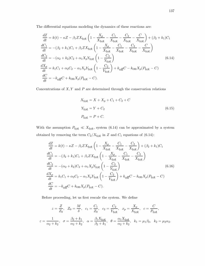
137

The differential equations modeling the dynamics of these reactions are:

dZ

dt= k(t)− κZ − β1ZXtot

(

1− Xp

Xtot− C1

Xtot− C2

Xtot− C

Xtot

)

+ (β2 + k1)C1

dC1

dt= −(β2 + k1)C1 + β1ZXtot

(

1− Xp

Xtot− C1

Xtot− C2

Xtot− C

Xtot

)

dC2

dt= −(α2 + k2)C2 + α1XpYtot

(

1− C2

Ytot

)

(6.14)

dXp

dt= k1C1 + α2C2 − α1XpYtot

(

1− C2

Ytot

)

+ koffC − konXp(Ptot − C)

dC

dt= −koffC + konXp(Ptot − C).

Concentrations of X,Y and P are determined through the conservation relations

Xtot = X +Xp + C1 + C2 + C

Ytot = Y + C2 (6.15)

Ptot = P + C.

With the assumption Ptot ≪ Xtot, system (6.14) can be approximated by a system

obtained by removing the term C2/Xtot in Z and C1 equations of (6.14):

dZ

dt= k(t)− κZ − β1ZXtot

(

1− Xp

Xtot− C1

Xtot− C2

Xtot

)

+ (β2 + k1)C1

dC1

dt= −(β2 + k1)C1 + β1ZXtot

(

1− Xp

Xtot− C1

Xtot− C2

Xtot

)

dC2

dt= −(α2 + k2)C2 + α1XpYtot

(

1− C2

Ytot

)

(6.16)

dXp

dt= k1C1 + α2C2 − α1XpYtot

(

1− C2

Ytot

)

+ koffC − konXp(Ptot − C)

dC

dt= −koffC + konXp(Ptot − C).

Before proceeding, let us first rescale the system. We define

z =Z

Z0, Z0 =

M

δ, c1 =

C1

Z0, c2 =

C2

Ytot, xp =

Xp

Xtot, c =

C

Ptot,

ε =1

α2 + k2, σ =

β2 + k1

α2 + k2, α =

β1Xtotβ2 + k1

, θ =α1Xtotα2 + k2

, k1 = µ1β2, k2 = µ2α2.

138

System (6.16) in terms of the new variables and parameters becomes

dz

dt=k(t)

Z0− κz +

1

ε

[

−σαz(

1− xp −Z0

Xtotc1 −

YtotXtot

c2

)

+ σc1

]

εdc1dt

= −σc1 + σαz

(

1− xp −Z0

Xtotc1 −

YtotXtot

c2

)

εdc2dt

= −c2 + θxp(1− c2) (6.17)

εdxpdt

=σµ1Z0

(1 + µ1)Xtotc1 +

Ytot(1 + µ2)Xtot

c2 −Ytotθ

Xtotxp(1− c2)

+ ε

(

koffPtotXtot

c− konxpPtot(1− c))

dc

dt= −koffc+ konxpXtot(1− c).

System (6.17) is defined on U×X×Y , where U = [0, 1],X = [0, 1]×[0, 1]×[0, 1], Y =

[0, 1]. We consider the solution to (6.17) with the initial condition

(u(0), c1(0), c2(0), xp(0), c(0)) = (u0, c01, c02, x

0p, c

0) ∈ U ×X × Y. (6.18)

System (6.17) with initial condition (6.18) is now in the form of (6.2). Here, z is the

input, c1, c2, and xp are the state variables, and c is the output. We define V as

V (z, c1, c2, xp, c) = (z + c1, c1, c2, xp, c),

and thus,

z = V1(z, c1, c2, xp) = z + c1, z = W1(z, c1, c2, xp) = z − c1.

The transformation V satisfies condition (6.3), and the new system under the change

of variables is

dz

dt=k(t)

Z0− κz, z(0) = z0 := z0 + c01,

εdc1dt

= −σc1 + σα(z − c1)(

1− xp −Z0

Xtotc1 −

YtotXtot

c2

)

, c1(0) = c01,

εdc2dt

= −c2 + θxp(1− c2), c2(0) = c02, (6.19)

εdxpdt

=σµ1Z0

(1 + µ1)Xtotc1 +

Ytot(1 + µ2)Xtot

c2 −Ytotθ

Xtotxp(1− c2)

+ ε

(

koffPtotXtot

c− konxpPtot(1− c))

, xp(0) = x0p,

dc

dt= −koffc+ konxpXtot(1− c), c(0) = c0.

139

It is defined on O × Y , where

O = (z, c1, c2, xp) | 0 ≤ z, c2, xp ≤ 1, 0 ≤ c1 ≤ z.

From the conservation relations in (6.15), it is easy to see that system (6.19) is forward

invariant in O×Y , that is, solutions starting inside O×Y never leave O×Y in forward

times. An immediate consequence is that the solution (z(t), c1(t), c2(t), xp(t), c(t)) to

the initial value problem (6.19) exists for all t ∈ [0,∞).

Setting ε = 0, the differential equations of c1, c2, and xp degenerate to algebraic

equations:

0 = −σc1 + σα(z − c1)(

1− xp −Z0

Xtotc1 −

YtotXtot

c2

)

0 = −c2 + θxp(1− c2) (6.20)

0 =σµ1Z0

(1 + µ1)Xtotc1 +

Ytot(1 + µ2)Xtot

c2 −Ytotθ

Xtotxp(1− c2).

Lemma 6.6 For any θ ∈ (0, 1], α ∈ (0,∞), the algebraic equations (6.20) on the set

O × Y admit a unique solution (c1, c2, xp) = (γ1(z), γ2(z), γ3(z)) := γ(z), where the

vector function γ depends on θ, α, and other parameters in system (6.19). (We do not

write these parameters explicitly in γ to simplify the notations.)

Proof. From the last two equations of (6.20), we can solve c1 and c2 in terms of xp,

and get

c1 = χθxp

1 + θxp, c2 =

θxp1 + θxp

, (6.21)

where the constant

χ =(1 + µ1)µ2Xtotµ1(1 + µ2)σZ0

.

Plugging (6.21) into the first equation of (6.20) with z = z − c1, we obtain a quadratic

equation in xp (viewing z as a constant):

αθzx2p +B(z)xp − αz = 0, (6.22)

where

B(z) = χθ + αz − αθz +YtotXtot

αθz +Z0

Xtotχαθz.

140

When z = 0, equation (6.22) becomes a linear equation, and the solution is xp = 0,

which in turn gives c1 = c2 = z = 0. In the case of z 6= 0, notice that when θ ∈ (0, 1],

B(z) is an increasing function in z, and thus B(z) > 0 for z > 0. Moreover, the y-

intercept of the quadratic (left hand side of (6.22)) is −αz < 0. Therefore, (6.22) has

a unique positive root

xp(z) =−B(z) + ∆1/2(z)

2αθz:= ζ3(z), (6.23)

where

∆(z) = B2(z) + 4α2θz2.

By L’Hospital’s Rule,

limz→0

xp(z) =−B′(0) + ∆−1/2(0)B(0)B′(0)

2αθ= 0,

so the function ζ3(z) defined in (6.23) is continuous at z = 0. Plugging (6.23) into

(6.21), we obtain c1 and c2 as functions of z, denoted as c1 = ζ1(z), c2 = ζ2(z). Next,

we show that the function ζ3(z) has continuous derivative with ζ ′3(z) > 0 for all z on

[0,∞). To see this, we differentiate ζ3(z) with respect to z and obtain

ζ ′3(z) =−zB′(z) + z∆−1/2(z)(B(z)B′(z) + 4α2θz) +B(z)−∆1/2(z)

2αθz2. (6.24)

Using the equality

B(z) = B′(z)z + χθ,

the numerator of (6.24) becomes

∆−1/2(z)(χθ∆1/2(z) + z(B(z)B′(z) + 4α2θz)−∆(z))

= ∆−1/2(z)(χθ∆1/2(z) +B(z)(zB′(z) −B(z)))

= ∆−1/2(z)(χθ∆1/2(z) + χθB(z))

= χθ(1 +B(z)∆−1/2(z)).

So,

ζ ′3(z) =χ(1−B(z)∆−1/2(z))

2αz2> 0 for all z > 0. (6.25)

Using the Binomial Formula, we have

limz→0+

ζ ′3(z) =χ(

1−(

1− 2α2θz2

B2(0)

))

2αz2=

α

χθ,

141

and

limz→0+

ζ3(z)

z=B(0)

(

−1 + 1 + 2α2θz2

B(0)2

)

2αθz2=

α

χθ.

Therefore, ζ ′3(z) is continuous at z = 0. To summarize, we have proved that the function

ζ3(z) has continuous derivative with ζ ′3(z) > 0 for all z on [0,∞).

Because of (6.21), the function ζ1(z) also has continuous derivative with ζ ′1(z) > 0

for all z on [0,∞). Recall that z = z+c1 = z+ζ1(z). By the Inverse Function Theorem,

we can solve z as a function of z, denoted as z = ω(z). Therefore,

γ(z) = (ζ1 ω(z), ζ2 ω(z), ζ3 ω(z))

is a solution of (6.20) on O×Y , and the uniqueness of ω and ζ’s implies the uniqueness

of γ.

Now the reduced algebraic-differential equations of (6.19) can be written as

d¯z

dt=k(t)

Z0− κ¯z, ¯z(0) = z0,

c1 = γ1(¯z),

c2 = γ2(¯z), (6.26)

xp = γ3(¯z),

dc

dt= −koffc+ konγ3(¯z)Xtot(1− c), c(0) = c0.

Since (6.26) is forward invariant on [0, 1] × Y , the solution (¯z(t), c1, c2, xp, c) to (6.26)

is defined for all t > 0. As a result, assumption I holds for any positive real number T

independent of α. It is easy to see that assumption II holds trivially.

Lemma 6.7 Assumption III holds for all α ∈ (0,∞).

Proof. Let us write the Jacobian matrix ∂Gα

∂x evaluated along

(¯z(t), c1(t), c2(t), xp(t), c(t))

as

J(t) =

−A(t) − YtotXtot

σα(z(t)− c1(t)) −σα(z(t)− c1(t))

0 −1− θxp(t) θ(1− c2(t))σµ1Z0

(1+µ1)Xtot

Ytot(1+µ2)Xtot

+YtotXtot

θxp(t) −YtotXtot

θ(1− c2(t))

,

142

where

A(t) = σ +Z0

Xtotσα(z(t)− c1(t)) + σα(1 − xp(t)−

Z0

Xtotc1(t)−

YtotXtot

c2(t)) > 0.

We first show that all the eigenvalues of J(t) have negative real parts. It is enough to

show that all the eigenvalues of J∗(t) have negative real parts, where J∗(t) is defined

as

J∗(t) =

1 0 0

0 1 0

0 0XtotYtot

J(t)

1 0 0

0 1 0

0 0YtotXtot

=

−A(t) − YtotXtot

σα(z(t)− c1(t)) −YtotXtot

σα(z(t)− c1(t))

0 −1− θxp(t)YtotXtot

θ(1− c2(t))σµ1Z0

(1+µ1)Ytot1

1+µ2+ θxp(t) − Ytot

Xtotθ(1− c2(t))

.

Let us rewrite the matrix J∗(t) as

J∗(t) =

−A(t) −I(t) −I(t)

0 −R(t) D(t)

E F (t) −D(t)

,

where E is a positive constant; A,R,D,F are positive functions of t; I,D are nonneg-

ative functions of t defined in the obvious way. Hereafter, we drop the t to simplify

the notations. By Routh-Hurwitz criterion. All the eigenvalues of J∗(t) have negative

real part if the first column of the Routh-Hurwitz table does not change signs. The

elements in the first column of the Routh-Hurwitz table are

a1 = 1,

a2 = D +R+A,

b1 =1

a2

(

µ2

1 + µ2(D2 +RD) +D2A+ 2DRA+R2A+AEI +DA2 +RA2

)

,

c1 = EID + EIR+ADµ2

1 + µ2.

It is straightforward to see that a1, a2, b1 are positive, and c1 ≥ 0. The last element

c1 is zero only when both I and D are zero, that is, c2 = 1, z = c1. However, this

143

would not happen, since z = c1 gives z = 0, and thus, xp = 0. By (6.21), both c1 and

c2 are zero, which contradicts c2 = 1. So, the last element is always positive too. By

Routh-Hurwitz criterion, all the eigenvalues of J∗(t) have negative real part, and so

does J(t). It follows that for any T > 0, we can find a positive number η such that all

the eigenvalues of J(t) have negative real part smaller than −η on [0, T ].

Lemma 6.8 Assumption IV holds for all α ∈ (0,∞) and θ ∈ (0, 1].

Proof. The function βα(t) defined as in (6.13) equals 1− γ′1(z(t)). Thus, |βα(t)− 1| =

|γ′1(z(t))| ≤ |ζ ′1(z)ω′(z)|. Notice that,

0 < ω′(z) =1

1 + ζ ′1(z)< 1 and ζ ′1(z) > 0,

so,

|βα(t)− 1| < ζ ′1(z) =χθζ ′3(z)

(1 + θζ3)2≤ χθζ ′3(z).

Applying the Binomial Formula to (6.25), we have

ζ ′3(z) ≤χ(

1−(

1− 2α2θz2

B2(z)

))

2αz2=

χαθ

B2(z)≤ α

χθ.

Therefore,

|βα(t)− 1| ≤ α,

which satisfies assumption IV.

Now we have checked assumptions I to IV on system (6.17). Applying Theorem 6.5,

we have

Theorem 6.9 Let θ ∈ (0, 1]. For any δ > 0, there exists two positive numbers αδ and

r0 with the following property. For any T ∈ (0,∞), and any t1 ∈ [0, T ], there exists

ε1 > 0 such that for any 0 < ε < ε1 and initial conditions with |z0− (z0−γ1(z0))| < r0,

that is, |γ1(z0) − c01| < r0, the z-coordinate of the solution (z(t), c1(t), c2(t), xp(t), c(t))

of (6.17) and the solution z(t) of

dz

dt=k(t)

Z0− κz, z(0) = z0

144

satisfy

|z(t) − z(t)| ≤ δ, on [t1, T ].

145

Chapter 7

Future Work

In Section 2.2, we have provided upper and lower bounds on the number of positive

steady states of a “futile cycle” of size n. However, there are still many questions re-

mained to answer. For instance, is the upper bound 2n − 1 always achievable? How

many positive steady states are there if the activation and deactivation follow mecha-

nisms other than distributive and sequential?

Notice also that there is an apparent gap between the upper bound 2n − 1 for any

parameters and the upper bound of n+1 (n) if n is even (odd) when the substrate is in

excess. If we think the ratio Etot/Ftot as a parameter ε, then when ε ≪ 1, there are

at most n+ 1 (n) steady states when n is even (odd), which coincides with the largest

possible lower bound. When ε ≫ 1, there is a unique steady state. If the number

of steady states changes “continuously” with respect to ε, then we do not expect the

number of steady states to exceed n + 1 (n) if n is even (odd). A natural conjecture

would be that the number of steady states never exceeds n+ 1 under any condition.

We also plan to develop an abstract approach generalizing the results for “futile

cycles”, so that we may also handle multistationarity of other ubiquitous motifs arising

in biochemistry networks.

In Chapter 3, we showed that multi-timescale non-monotone systems can become

monotone once the fast variables are replaced by their steady state values. There are

many directions to explore.

The first is to fill in the details when the reduced system has a unique steady

state. As mentioned in Remark 3.23, one may obtain convergence, not merely generic

convergence to the steady state. The proof is simpler in that case since the foliation

structure is not needed.

146

In the other direction, we could drop the assumption of countability and instead

provide theorems on generic convergence to the set of equilibria, or even to equilibria

if hyperbolicity conditions are satisfied, in the spirit of what is done in the theory of

strongly monotone systems.

It will be also interesting to incorporate spatial factors in singularly perturbed mono-

tone systems and to study the associated reaction diffusion systems. On the other hand,

numerical approximation would also be useful in applications.

Another exciting direction is to study the system where the fast dynamics is mono-

tone, but not the slow system. In that case, one has almost every or even every tra-

jectory converges to the limiting slow manifold. This is a very appealing property

compared to the usual local stability property, since the latter only yields perturbation

result for initial conditions close to the limiting slow manifold.

It is also important to see how the results in Chapter 3 can be extended to systems

with oscillations.

In Chapter 5, for simplicity we assume boundedness of solutions. However, by

the virtue of Lyapunov function, a bootstrap argument could be applied to obtain

boundedness of the solutions.

The other direction is to extend the global stability of the constant equilibrium to

C2 norm. In Chapter 5, the stability is in terms of L1, using a priori estimates for

parabolic equations, it is possible to obtain global stability in C2.

147

References

[1] E.H. Abed. Singularly perturbed Hopf bifurcation. IEEE Trans. Circuits &Systems, 32:1270–1280, 1985.

[2] U. Alon. Biological networks: the tinkerer as an engineer. Science, 301:1866–1867, 2003.

[3] U. Alon. An Introduction to Systems Biology: Design Principles of BiologicalCircuits. Chapman-Hall/CRC Taylor & Francis, Boca Raton, FL, 2007.

[4] D. Angeli, P. de Leenheer, and E.D. Sontag. A Petri net approach to the studyof persistence in chemical reaction networks. Mathematical Biosciences, 210:598–618, 2007. Preprint: arXiv q-bio.MN/068019v2, 10 Aug 2006.

[5] D. Angeli, J. E. Ferrell, and E.D. Sontag. Detection of multistability, bifurcations,and hysteresis in a large class of biological positive-feedback systems. Proc. Natl.Acad. Sci. USA, 101(7):1822–1827, 2004.

[6] D. Angeli and E.D. Sontag. Oscillations in I/O monotone systems. IEEE Trans-actions on Circuits and Systems, Special Issue on Systems Biology, 55:166–176,2008. Preprint version in arXiv q-bio.QM/0701018, 14 Jan 2007.

[7] D. Angeli and E.D. Sontag. Translation-invariant monotone systems, and a globalconvergence result for enzymatic futile cycles. Nonlinear Analysis Series B: RealWorld Applications, 9:128–140, 2008.

[8] M. Arcak and E.D. Sontag. A passivity-based stability criterion for a class ofinterconnected systems and applications to biochemical reaction networks. Math-ematical Biosciences and Engineering, 5:1–19, 2008. Preprint: arxiv0705.3188v1[q-bio], May 2007.

[9] A.R. Asthagiri and D.A. Lauffenburger. A computational study of feedback ef-fects on signal dynamics in a Mitogen-Activated Protein Kinase (MAPK) pathwaymodel. Biotechnol. Prog., 17:227–239, 2001.

[10] A. Berman and R. Plemmons. Nonnegative Matrices in the Mathematical Sci-ences. Classics in Applied Mathematics. Society for Industrial Mathematics, 1994.Subsequent edition (January 1, 1987).

[11] J.J. Bijlsma and E.A. Groisman. Making informed decisions: regulatory interac-tions between two-component systems. Trends Microbiol., 11:359–366, 2003.

[12] V.A. Boichenko, G.A. Leonov, and V. Reitmann. Dimension Theory for OrdinaryDifferential Equations. Teubner, Teubner, Germany, 2005.

148

[13] W.R. Burack and T.W. Sturgill. The activating dual phosphorylation of MAPKby MEK is nonprocessive. Biochemistry, 36:5929–5933, 1997.

[14] L. Chang and M. Karin. Mammalian MAP kinase signaling cascades. Nature,410:37–40, 2001.

[15] H. Chen, B.W. Bernstein, and J.R. Bamburg. Regulating actin filament dynamicsin vivo. Trends Biochem. Sci., 25:19–23, 2000.

[16] L. Chisci and P. Falugi. Asymptotic tracking for state-constrained monotonesystems. In Proc. 44th IEEE Conf. Decision and Control, 2005. Seville, paperThC17.5.

[17] P.D. Christofides and A.R. Teel. Singular perturbations and input-to-state sta-bility. IEEE Trans. Automat. Contr, 41:1645–1650, 1996.

[18] C. Conradi, J. Saez-Rodriguez, E.-D. Gilles, and J. Raisch. Using chemical re-action network theory to discard a kinetic mechanism hypothesis. Proc. FOSBE2005 (Foundations of Systems Biology in Engineering), Santa Barbara, Aug. 2005,pages 325–328, 2005.

[19] E.N. Dancer. Some remarks on a boundedness assumption for monotone dynam-ical systems. Proc. of the AMS, 126:801–807, 1998.

[20] S. Donovan, K.M. Shannon, and G. Bollag. GTPase activating proteins: criticalregulators of intracellular signaling. Biochim. Biophys Acta, 1602, 2002.

[21] L. Edelstein-Keshet. Mathematical Models in Biology. SIAM, Philadelphia, PA,2005.

[22] P. Ellison and M. Feinberg. How catalytic mechanisms reveal themselves in mul-tiple steady-state data: I. Basic principles. Journal of Molecular Catalysis. A,Chemical, 154:155–167, 2000.

[23] M. Feinberg. Chemical reaction network structure and the stability of complexisothermal reactors: II. Multiple steady states for networks of deficiency one.Chem. Eng. Sci., 43:1–25, 1988.

[24] N. Fenichel. Geometric singular perturbation theory for ordinary differentialequations. J. of Differential Equations, 31:53–98, 1979.

[25] J.E. Ferrell and R.R. Bhatt. Mechanistic studies of the dual phosphorylation ofmitogen-activated protein kinase. J. Biol. Chem., 272:19008–19016, 1997.

[26] W.B. Fitzgibbon, S.L. Hollis, and J.J. J.J. Morgan. Stability and Lyapunovfunctions for reaction-diffusion systems. SIAM J. Math. Anal., 28(3):595–610,1997.

[27] C.M. Furdui, E.D. Lew, J. Schlessinger, and K.S. Anderson. Autophosphoryla-tion of fgfr1 kinase is mediated by a sequential and precisely ordered reaction.Molecular Cell, 21:711–717, 2006.

[28] T.S. Gardner, C.R. Cantor, and J.J. Collins. Construction of a genetic toggleswitch in Escherichia coli. Nature, 403:339–342, 2000.

149

[29] T. Gedeon and K. Mischaikow. Structure of the global attractor of cyclic feedbacksystems. Journal of Dynamics and Differential Equations, 7(1):141–190, 1995.

[30] A. Goldbeter. A model for circadian oscillations in the Drosophila period protein(PER). Prof. Royal Soc. London B., 261:319–324, 1995.

[31] A. Goldbeter. Biochemical Oscillations and Cellular Rhythms. Cambridge Univ.,1996.

[32] A.D. Grossman. Genetic networks controlling the initiation of sporulation andthe development of genetic competence in bacillus subtilis. Annu Rev Genet.,29:477–508, 1995.

[33] J. Gunawardena. Multisite protein phosphorylation makes a good threshold butcan be a poor switch. Proc. Natl. Acad. Sci., 102:14617–14622, 2005.

[34] L.H. Hartwell, J.J. Hopfield, S. Leibler, and A.W. Murray. From molecular tomodular cell biology. Nature, 402:C47–52, 1999.

[35] H. Henry. Geometric Theory of Semilinear Parabolic Equations. Springer Verlag,Berlin-New York, 1981.

[36] M. Hirsch. Differential equations and convergence almost everywhere in stronglymonotone flows. Contemporary Mathematics, 17:267–285, 1983.

[37] M. Hirsch. Systems of differential equations that are competitive or cooperativeII: Convergence almost everywhere. SIAM J. Mathematical Analysis, 16:423–439,1985.

[38] M. Hirsch. Stability and convergence in strongly monotone dynamical systems.J. Reine Angew. Math., 383:1–53, 1988.

[39] M. Hirsch and H.L. Smith. Monotone dynamical systems. Elsevier, Amsterdam,2005. Handbook of Differential Equations, Ordinary Differential Equations: Vol-ume 2.

[40] J. Hofbauer and K. Sigmund. Evolutionary Games and Replicator Dynamics.Cambridge Univ., Cambridge, U.K., 1998.

[41] F.C. Hoppensteadt. Properties of solutions of ordinary differential equations withsmall parameters. Comm. Pure Appl. Math., 24, 1971.

[42] C-Y.F. Huang and J.E. Ferrell Jr. Ultrasensitivity in the mitogen-activated pro-tein kinase cascade. Proc. Natl. Acad. Sci. USA, 93:10078–10083, 1996.

[43] A. Isidori. Nonlinear Control Systems: An Introduction. Springer-Verlag, Lon-don, third edition edition, 1995.

[44] J.F. Jiang. On the global stability of cooperative systems. Bulletin of the LondonMath. Soc., 6:455–458, 1994.

[45] C.K.R.T. Jones. Geometric singular perturbation theory. In Dynamical Systems(Montecatini. Terme), Lect. Notes in Math. 1609. Springer-Verlag, Berlin, 1994.

150

[46] M.R. Jovanovic, M. Arcak, and E.D. Sontag. A passivity-based approach tostability of spatially distributed systems with a cyclic interconnection structure.IEEE Transactions on Circuits and Systems, Special Issue on Systems Biology,55:75–86, 2008. Preprint: arXiv math.OC/0701622, 22 January 2007.

[47] G. Karp. Cell and Molecular Biology. Wiley, 2002.

[48] K.W. Knobloch and B. Aulbach. Singular perturbations and integral manifolds.J. Math. Phys. Sci., 13:415–424, 1984.

[49] H. Kunze and D. Siegel. A graph theoretical approach to monotonicity withrespect to initial conditions. In X. Liu and D. Siegel, editors, Comparison Methodsand Stability Theory. Marcel Dekker, New York, 1994.

[50] D.A. Lauffenburger. Cell signaling pathways as control modules: complexity forsimplicity? Proc Natl Acad Sci USA, 97:5031–5033, 2000.

[51] J. Levin and N. Levinson. Singular perturbations of nonlinear systems of differ-ential equations and an associated boundary layer equation. J. Rat. Mech., 3,1954.

[52] D.J. Lew and D.J. Burke. The spindle assembly and spindle position checkpoints.Annu. Rev. Genet., 37:251–282, 2003.

[53] M. Li and J. Muldowney. Dynamics of differential equations on invariant mani-folds. Journal of Differential Equations, 168:295–320, 2000.

[54] M.Y. Li and L. Wang. A criterion for stability of matrices. Journal of Mathe-matical Analysis and Applications, 225:249–264, 1998.

[55] M.Y. Li and L. Wang. Global stability in some SEIR models. IMA Math. Appl.,126:295–311, 2000.

[56] J. Mallet-Paret and G. Sell. The Poincare-Bendixson theorem for monotone cyclicfeedback systems with delay. Journal of Differential Equations, 125:441–489,1996.

[57] J. Mallet-Paret and H.L. Smith. The Poincare-Bendixson theorem for mono-tone cyclic feedback systems. Journal of Dynamics and Differential Equations,2(4):367–421, 1990.

[58] N.I. Markevich, J.B. Hoek, and B.N. Kholodenko. Signaling switches and bista-bility arising from multisite phosphorylation in protein kinase cascades. J. CellBiol., 164:353–359, 2004.

[59] J. Mitropolsky and O. Lykova. Integral manifolds in nonlinear mechanics. Nauka,Moscow, 1973.

[60] L. Moreau. Stability of continuous-time distributed consensus algorithms. InProc. 43rd IEEE Conf. Decision and Control, Paradise Island, Bahamas, 2004.paper ThC10.4.

[61] J. Morgan. Boundedness and decay results for reaction-diffusion systems. SIAMJ. Math. Anal., 22(5):1172–1189, 1990.

151

[62] P.J. Moylan and D.J. Hill. Stability criteria for large-scale systems. IEEE Trans.Autom. Control, 23(2):143–149, 1978.

[63] J. Muldowney. Compound matrices and ordinary differential equations. RockyMountain Journal of Mathematics, 20:857–872, 1990.

[64] J. Murray. Mathematical Biology. Springer-Verlag, Berlin, Germany, 1989.

[65] J.D. Murray. Mathematical Biology, 3rd Edition. Springer, New York, 2002.

[66] K. Nipp. Smooth attractive invariant manifolds of singularly perturbed ode’s.Technical report, ETH-Zrich, 1992. Research Report No.92-13, Seminar fr Ange-wandte Mathematik.

[67] F. Ortega, J. Garces, F. Mas, B.N. Kholodenko, and M. Cascante. Bistabil-ity from double phosphorylation in signal transduction: Kinetic and structuralrequirements. FEBS J, 273:3915–3926, 2006.

[68] H. Othmer and E. Pate. Scale-invariance in reaction-diffusion models of spatialpattern formation. Proc. Natl. Acad. Sci., 77:4180–4184, 1980.

[69] J.A. Papin, J.L. Reed, and B.O. Palsson. Hierarchical thinking in network biol-ogy: the unbiased modularization of biochemical networks. Trends Biochem Sci.,29:641647, 2004.

[70] J.R. Pomerening, E.D. Sontag, and J.E. Ferrell Jr. Building a cell cycle oscillator:hysteresis and bistability in the activation of Cdc2. Nature Cell Biology, 5:346–351, 2003.

[71] R. Redheffer, R. Redlinger, and W. Walter. A theorem of Lasalle-Lyapunov typefor parabolic systems. SIAM J. Math. Anal., 19(1):121–132, 1988.

[72] J. Saez-Rodriguez, A. Kremling, and E.D. Gilles. Dissecting the puzzle of life:Modularization of signal transduction networks. Comput Chem Eng., 29:619629,2005.

[73] K. Sakamoto. Invariant manifolds in singular perturbation problems for ordinarydifferential equations. Proceedings of the Royal Society of Edinburgh, 116A:45–78,1990.

[74] M. Samoilov, S. Plyasunov, and A.P. Arkin. Stochastic amplification and signal-ing in enzymatic futile cycles through noise-induced bistability with oscillations.Proc. Natl. Acad. Sci. USA, 102, 2005.

[75] L. Sanchez. Global asymptotic stability of the goodwin system with re-pression. Preprint, Universidad Politecnica de Cartagena, 2006. (Online atwww.ugr.es/ecuadif/files/cyclicneg.pdf).

[76] L. Sanchez. Dynamics of the modified Michaelis-Menten system. Journal ofMathematical Analysis and Applications, 317:71–79, 2006.

[77] H.M. Sauro and B.N. Kholodenko. Quantitative analysis of signaling networks.Prog. Biophys. Mol. Biol., 86:543, 2004.

152

[78] E.E. Sel’kov. Stabilization of energy charge, generation of oscillation and multiplesteady states in energy metabolism as a result of purely stoichiometric regulation.Eur. J. Biochem, 59(1):151–157, 1975.

[79] W. Sha, J. Moore, K. Chen, A.D. Lassaletta, C.S. Yi, J.J. Tyson, and J.C. Sible.Hysteresis drives cell-cycle transitions in Xenopus laevis egg extracts. Proc. Natl.Acad. Sci., 100:975–980, 2003.

[80] J. Smillie. Competitive and cooperative tridiagonal systems of differential equa-tions. SIAM J. Math. Anal., 15, 1984.

[81] H.L. Smith. Periodic tridiagonal competitive or cooperative systems of differentialequations. SIAM J. Appl. Anal., 22:1102–1109, 1991.

[82] H.L. Smith. Monotone dynamical systems: An introduction to the theory of com-petitive and cooperative systems. AMS, Providence, RI, 1995. MathematicalSurveys and Monographs, vol. 41.

[83] E.D. Sontag. Mathematical Control Theory. Deterministic Finite-DimensionalSystems, volume 6 of Texts in Applied Mathematics. Springer-Verlag, New York,second edition, 1998.

[84] E.D. Sontag. Some new directions in control theory inspired by systems biology.IET Systems Biology, 1:9–18, 2004.

[85] E.D. Sontag. Molecular systems biology and control. Eur. J. Control, 11(4-5):396–435, 2005.

[86] L. Stryer. Biochemistry. Freeman, New York, 1995.

[87] M.L. Sulis and R. Parsons. PTEN: from pathology to biology. Trends Cell Biol.,13:478–483, 2003.

[88] M.K. Sundareshan and M. Vidyasagar. L2-stability of large-scale dynamical sys-tems: Criteria via positive operator theory. IEEE Transactions on AutomaticControl, AC-22:396–400, 1977.

[89] A.R. Teel, L. Moreau, and D. Nesic. A unification of time-scale methods forsystems with disturbances. IEEE Trans. Automat. Contr, 48:1526–1544, 2003.

[90] M Thompson and J. Gunawardena. Multi-bit information storage by multisitephosphorylation, 26 Jun 2007. Submitted, preprint version in arXiv:0706.3735v1.

[91] A.N. Tikhonov. Systems of differential equations containing a small parametermultiplying the highest derivatives. Mat. Sb., 31:575–586, 1952.

[92] C.C. Travis and W.M. Post. Dynamics and comparative statistics of mutualisticcommunities. J. Theor. Biol., 78:553–571, 1979.

[93] A. Turing. The chemical basis of morphogenesis. Philos. Trans. Roy. Soc.,B273:37–72, 1952.

[94] D. Del Vecchio, A.J. Ninfa, and E.D. Sontag. Modular cell biology: retroactivityand insulation. Nature/EMBO Molecular Systems Biology, 4(161), 2008.

153

[95] M. Vidyasagar. Input-Output Analysis of Large Scale Interconnected Systems.Springer-Verlag, Berlin, 1981.

[96] L. Wang, P. De Leenheer, and E.D. Sontag. Global stability for tridiagonal sys-tems with negative feedback. Accepted to the 2008 IEEE conference on Decisionand Control.

[97] L. Wang and E.D. Sontag. Almost global convergence in singular perturbationsof strongly monotone systems. In C. Commault and N. Marchand, editors, Posi-tive Systems, pages 415–422. Springer-Verlag, Berlin/Heidelberg, 2006. (LectureNotes in Control and Information Sciences Volume 341, Proceedings of the sec-ond Multidisciplinary International Symposium on Positive Systems: Theory andApplications (POSTA 06) Grenoble, France).

[98] L. Wang and E.D. Sontag. On the number of steady states in a multiple futilecycle. Journal of Mathematical Biology, 57:29–52, 2008.

[99] L. Wang and E.D. Sontag. Singularly perturbed monotone systems and an ap-plication to double phosphorylation cycles. J. Nonlinear Sciences, 2008. DOI10.1007/s00332-008-9021-2.

[100] C. Widmann, G. Spencer, M.B. Jarpe, and G.L. Johnson. Mitogen-activatedprotein kinase: Conservation of a three-kinase module from yeast to human.Physiol. Rev., 79:143–180, 1999.

[101] J.C. Willems. Dissipative dynamical systems Part I: General theory; Part II:Linear systems with quadratic supply rates. Archive for Rational Mechanics andAnalysis, 45:321–393, 1972.

[102] Y. Zhao and Z.Y. Zhang. The mechanism of dephosphorylation of extracellularsignal-regulated kinase 2 by mitogen-activated protein kinase phosphatase 3. J.Biol. Chem., 276:32382–32391, 2001.

154

Vita

Liming Wang

2008 Ph. D. in Mathematics, Rutgers University

2001 B. Sc. in Mathematics, Peking University, Beijing, China.

Publications

1. Liming Wang and Eduardo D. Sontag. On the number of steady states in amultiple futile cycle, J. Math. Bio., doi:10.1007/s00285-007-0145-z, 2008.

2. Liming Wang and Eduardo D. Sontag. Singularly perturbed monotone systemsand an application to double phosphorylation cycles, J. Nonlinear Sci., Journal ofNonlinear Science, doi:10.1007/s00332-008-9021-2, 2008.

3. Liming Wang and Eduardo D. Sontag. A remark on singular perturbations ofstrongly monotone systems, Proc. IEEE Conf. Decision and Control, 2006.

4. Liming Wang and Eduardo D. Sontag, Almost global convergence in singular per-turbations of strongly monotone systems, Second Multidisciplinary InternationalSymposium on Positive Systems: Theory and Applications, 2006.

5. Natalia L. Komarova and Liming Wang, Initiation of colorectal cancer: where dothe two hits hit?, Cell Cycle 3(13), 2004.