DynamicOptimizationofHigh-AltitudeSolarAircraft ... · battmax 59.5kWh Maximumdischargerate P...
34
Dynamic Optimization of High-Altitude Solar Aircraft Trajectories Under Station-Keeping Constraints R. Abraham Martin * , Nathaniel S. Gates † , Andrew Ning ‡ , and John D. Hedengren § Brigham Young University, Provo, UT, 84602 This paper demonstrates the use of nonlinear dynamic optimization to calculate energy- optimal trajectories for a high-altitude, solar-powered Unmanned Aerial Vehicle (UAV). The objective is to maximize the total energy in the system while staying within a 3 km mission radius and meeting other system constraints. Solar energy capture is modeled using the vehicle orientation and solar position, and energy is stored both in batteries and in potential energy through elevation gain. Energy capture is maximized by optimally adjusting the angle of the aircraft surface relative to the sun. The UAV flight and energy system dynamics are optimized over a 24-hour period at an eight-second time resolution using Nonlinear Model Predictive Control (NMPC). Results of the simulated flights are presented for all four seasons, showing 8.2% increase in end-of-day battery energy for the most limiting flight condition of the winter solstice. I. Introduction The economic motivations of satellite-like abilities without satellite cost have long inspired the development of High- Altitude Long Endurance Unmanned Aerial Vehicles (HALE UAVs). The possibilities for long-term communications and surveillance have attracted specific interest in the area. Beginning with a series of preliminary studies by NASA in the 1980s and continuing to the present time, this research has continually pushed the boundaries of modern technology [1–3]. Notable projects include the NASA Helios platform, the AC propulsion SoLong, and the Qinetiq/Airbus Zephyr, which holds the current world records for both high-altitude and long endurance UAV flight [4–6]. Other current projects are working to extend the range and endurance of HALE UAVs to facilitate long-term internet broadcasting to areas without coverage [7]. Since many HALE UAVs are powered by solar panels and usebatteries for energy storage, advancing these technologies is a crucial part of increasing endurance [8]. However, other factors also play an important role, including the design of the aircraft [9], and the way in which it is operated [10]. Trajectory optimization is one way in which HALE UAV endurance can be extended while using existing technologies, materials and designs. This project examines the use of advanced optimization methods to calculate energy-optimal trajectories for solar-powered * Graduate Student, Department of Chemical Engineering, 350 CB, Provo, UT 84602 † Graduate Student, Department of Chemical Engineering, 350 CB, Provo, UT 84602 ‡ Assistant Professor, Department of Mechanical Engineering, Crabtree Building, Provo, UT 84602 § Associate Professor, Department of Chemical Engineering, 350 CB, Provo, UT 84602
Transcript of DynamicOptimizationofHigh-AltitudeSolarAircraft ... · battmax 59.5kWh Maximumdischargerate P...
Dynamic Optimization of High-Altitude Solar AircraftTrajectories Under Station-Keeping Constraints
R. Abraham Martin∗, Nathaniel S. Gates†, Andrew Ning‡, and John D. Hedengren§Brigham Young University, Provo, UT, 84602
This paper demonstrates the use of nonlinear dynamic optimization to calculate energy-
optimal trajectories for a high-altitude, solar-powered Unmanned Aerial Vehicle (UAV). The
objective is to maximize the total energy in the system while staying within a 3 km mission
radius andmeeting other system constraints. Solar energy capture is modeled using the vehicle
orientation and solar position, and energy is stored both in batteries and in potential energy
through elevation gain. Energy capture is maximized by optimally adjusting the angle of the
aircraft surface relative to the sun. The UAV flight and energy system dynamics are optimized
over a 24-hour period at an eight-second time resolution using Nonlinear Model Predictive
Control (NMPC). Results of the simulated flights are presented for all four seasons, showing
8.2% increase in end-of-day battery energy for the most limiting flight condition of the winter
solstice.
I. IntroductionThe economic motivations of satellite-like abilities without satellite cost have long inspired the development of High-
Altitude Long Endurance Unmanned Aerial Vehicles (HALE UAVs). The possibilities for long-term communications
and surveillance have attracted specific interest in the area. Beginning with a series of preliminary studies by NASA in
the 1980s and continuing to the present time, this research has continually pushed the boundaries of modern technology
[1–3]. Notable projects include the NASA Helios platform, the AC propulsion SoLong, and the Qinetiq/Airbus Zephyr,
which holds the current world records for both high-altitude and long endurance UAV flight [4–6]. Other current
projects are working to extend the range and endurance of HALE UAVs to facilitate long-term internet broadcasting to
areas without coverage [7]. Since many HALE UAVs are powered by solar panels and use batteries for energy storage,
advancing these technologies is a crucial part of increasing endurance [8]. However, other factors also play an important
role, including the design of the aircraft [9], and the way in which it is operated [10]. Trajectory optimization is one
way in which HALE UAV endurance can be extended while using existing technologies, materials and designs. This
project examines the use of advanced optimization methods to calculate energy-optimal trajectories for solar-powered∗Graduate Student, Department of Chemical Engineering, 350 CB, Provo, UT 84602†Graduate Student, Department of Chemical Engineering, 350 CB, Provo, UT 84602‡Assistant Professor, Department of Mechanical Engineering, Crabtree Building, Provo, UT 84602§Associate Professor, Department of Chemical Engineering, 350 CB, Provo, UT 84602

UAVs under tight station-keeping constraints, such as those imposed by positioning the UAV as a node in a network
constellation.
A. Elevation Optimization
Energy conservation is a key to long endurance solar flight, and a common method for saving energy in HALE UAV
flights is to climb during the day. This stores excess solar energy as potential energy, which can then be extracted during
the night by gliding [6]. This in turn reduces the mass of batteries required for continuous flight, and allows for a lighter
vehicle overall [11].
A sizeable body of work exists on the topic of potential energy storage, and several of the most relevant papers are
described here. Gao et al. explore the equivalence of battery storage and potential energy storage, finding that energy
storage in elevation is most efficient when the initial altitude is low, and the duration of solar radiation is short [6].
The same authors also propose an energy management strategy to control when energy is stored and released from
batteries and elevation [12]. Sachs et al. show that with an optimized elevation profile, it is theoretically possible to
completely eliminate the need for a battery on a solar-powered aircraft [11]. However, their approach makes several key
assumptions. First, the authors assume that the vehicle is traveling in a straight line path from west to east, meaning that
the day-night cycle is shortened significantly with increasing vehicle speed. Second, the authors assume that the aircraft
is able to fly at a range of altitudes spanning nearly 65,000 feet to achieve the zero battery result. In the current project,
the vehicle is restricted both in distance from the starting point and in altitude range. However, the work of Sachs et
al. may still be treated as a theoretical upper bound on the achieved results.
Spangelo et al. study a number of scenarios in which the aircraft is restricted to the surface of a vertical cylinder
[13, 14]. Periodic motion constraints are implemented using periodic splines, and the average net battery power is
maximized. The authors show that their optimized path increases the average power by 30% when compared to a
constant altitude, constant speed path. The current work expands upon this study by allowing the vehicle to travel
anywhere within the volume of the vertical cylinder, rather than only on the surface. This increased flight region allows
for more complex flight maneuvers, and the possibility of more optimal solutions than achieved by previous authors.
B. Incidence Optimization
Another approach to energy conservation is to fly in such a way that the angle between the sun and the solar panels
on the vehicle wings is optimized. This technique maximizes the amount of solar energy that can be obtained throughout
the day. Whitfield has shown in simulations that this type of optimization can increase the possible flight time over
an area of interest by up to two months during a year-long flight. He uses a dual-optimal path planning technique to
plan flight maneuvers a short time window into the future, allowing the vehicle to adapt to changing conditions over
the course of a long flight [15]. Dai et al. describe a similar system in which point-to-point path optimization is done
2

using a quaternion representation for aircraft kinematics and solar collection [16]. The resulting optimization problem
is solved using a linear relaxation followed by branch and bound. Klesh and Kabamba also investigate this type of
optimization, deriving a dimensionless power ratio that can be used to decide between loitering and direct flights and
predict the qualitative features of a flight [17, 18]. Through a semi-exhaustive search, Ozoroski et al. show that when
the station-keeping radius is large, the optimal flight pattern is to fly perpendicular to the sun azimuth with vertically
mounted solar panels [19]. Alternatively, Edwards et al. demonstrate that for a constant orbit with low sun elevation
angles, high bank angles provide up to a 15% net power gain over a wings-level orbit [20]. The current work differs from
these studies by relaxing the constant altitude and or bank angle constraints, and by imposing a tighter station-keeping
constraint. As will be shown, this leads to a unique family of solutions due to the necessity of frequent turns to stay
within the mission radius.
C. Combined Elevation and Incidence Optimization
The current work combines and improves upon the previous two approaches by including both elevation and
incidence angle optimization. The most similar completed research on this topic was performed by Hosseini et al. in
2016. The authors describe a system for long endurance surveillance that uses elevation change to store energy. In
addition, the system also accounts for the additional energy available by changing the vehicle orientation. The objective
is to maximize the final state of charge of the aircraft battery by optimizing the vehicle position throughout the day at a
resolution of one hour. The problem is posed as a nonlinear optimization problem, and is reformulated through direct
collocation before solution using a sequential quadratic programming algorithm [21, 22].
The current project improves upon previous work in this area by utilizing a more detailed system model that
includes kinematics, aerodynamics, solar power, atmospheric effects, and battery power. Further mission constraints are
introduced, such as a limited distance from a central point. Additionally, the solution is performed at a higher time
resolution, with system dynamics and aircraft trajectories repeatedly optimized over the duration of the flight using a
nonlinear model predictive control (NMPC) approach. This approach has proven effective in complex UAV control and
estimation problems such as aerial recovery [23], but has not previously been applied to HALE energy optimization.
D. Paper Contributions
This paper contributes to the field by advancing the state of the art in the following areas.
1) The optimization is solved at a finer time resolution over the twenty-four hour period than comparable solutions
in the literature (8 seconds vs 1 hour), exposing system dynamics masked by the larger time step.
2) A unique family of solutions is discovered by imposing a station-keeping constraint within an order of magnitude
of the minimum turning radius of the aircraft. The solutions found are shown to increase the final battery energy
of the HALE UAV system studied by 8–9% over the course of a twenty-four hour flight, with an addition of 8.2%
3

final battery energy for the winter solstice (most limiting energy case).
3) The solar-powered HALE trajectory optimization is posed using a nonlinear model predictive control formulation,
reducing the computational complexity of the problem and making a solution computationally feasible at a fine
time resolution.
The paper presents an off-line study that uses environmental modeling, mission and dynamic constraints, and a
dynamic simulation model to optimize HALE missions based on initial flight conditions. A receding horizon strategy
is used in which the simulation time window advances after each solution, and the new forward simulation period is
re-optimized.
II. System Model and Optimization Approach
A. System Modeling
The model for the HALE system is divided into several interconnected sections, including the aircraft dynamics,
solar and atmospheric modeling, power and propulsion, and the system energy balance. This section describes the
individual submodules and their interconnecting links.
1. Aircraft Definition and Mission Conditions
For the purposes of this study, the HALE UAV aircraft is modeled as a large flying wing similar to Facebook’s Aquila.
Using publicly available information on wingspan [24] as a reference, the remaining aircraft dimensions and geometry
are estimated from published photographs of Aquila [25]. The batteries used are assumed to have the same specific
energy as those used by the Zephyr [26]. The payload is assumed to be 25 kg, which would consist of communications
equipment for the mission[27]. Conservative input constraints on lift coefficient, bank angle, thrust, and flight path
angle are added to ensure that the resulting paths are relatively smooth and physically achievable. Detailed parameters
for the UAV system are listed in Table 1, with spanwise parameters in Table 2. The positions of the spanwise parameters
are shown in Figure 1.
Mission conditions for the flight are chosen to represent a HALEUAV acting as a stationary node in a communications
network. To this end, the maximum operational radius is set to 3 km from a center point, which is in the typical range for
such applications [28, 29]. It is typical for HALE UAVs to operate above regulated airspace, which in the United States
ends at 18288 m (60,000 ft) [30]. This altitude is used as a lower limit for the mission. A large portion of the world’s
population lives below 35°latitude, and this is chosen as an upper limit for the mission latitude [26]. Albuquerque New
Mexico is conveniently located at 35 °N, and is chosen as the location for the simulated tests. Four optimization cases
are considered for this study, corresponding to 2017 solar data from the winter solstice, spring equinox, summer solstice,
and fall equinox. Conditions for the four test cases are summarized in Table 3.
4
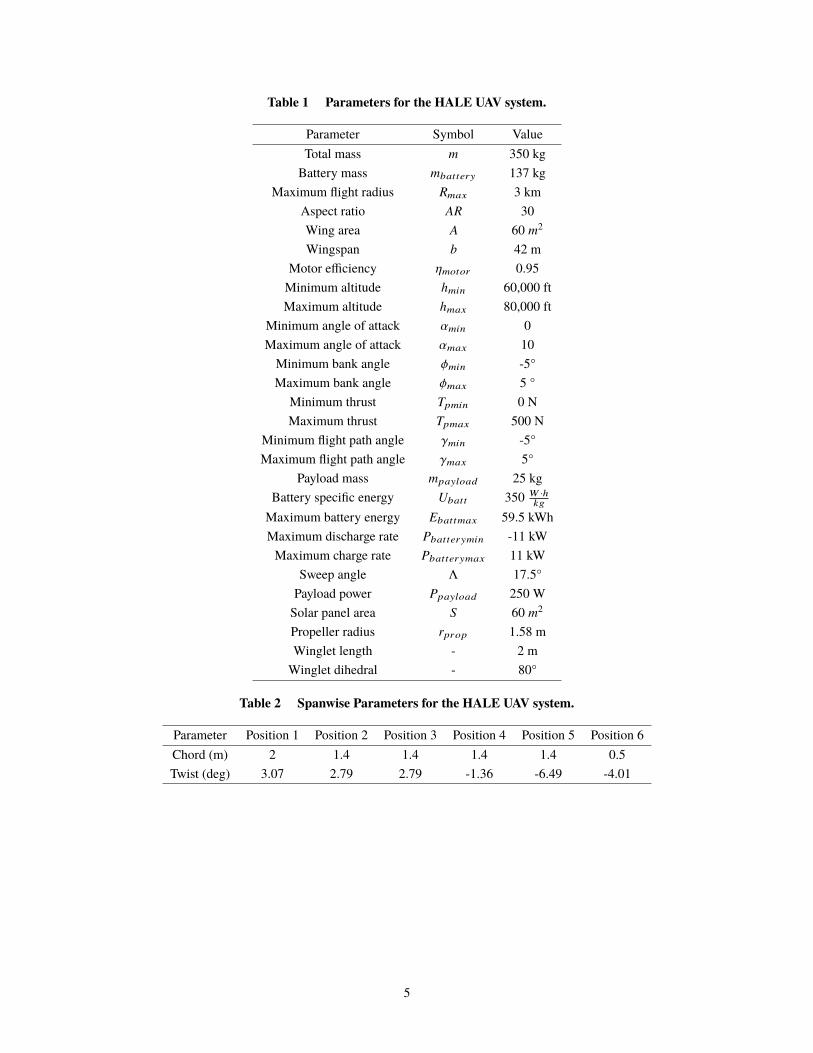
Table 1 Parameters for the HALE UAV system.
Parameter Symbol ValueTotal mass m 350 kgBattery mass mbattery 137 kg
Maximum flight radius Rmax 3 kmAspect ratio AR 30Wing area A 60 m2
Wingspan b 42 mMotor efficiency ηmotor 0.95Minimum altitude hmin 60,000 ftMaximum altitude hmax 80,000 ft
Minimum angle of attack αmin 0Maximum angle of attack αmax 10Minimum bank angle φmin -5°Maximum bank angle φmax 5 °
Minimum thrust Tpmin 0 NMaximum thrust Tpmax 500 N
Minimum flight path angle γmin -5°Maximum flight path angle γmax 5°
Payload mass mpayload 25 kgBattery specific energy Ubatt 350 W ·h
kg
Maximum battery energy Ebattmax 59.5 kWhMaximum discharge rate Pbatterymin -11 kWMaximum charge rate Pbatterymax 11 kW
Sweep angle Λ 17.5°Payload power Ppayload 250 WSolar panel area S 60 m2
Propeller radius rprop 1.58 mWinglet length - 2 mWinglet dihedral - 80°
Table 2 Spanwise Parameters for the HALE UAV system.
Parameter Position 1 Position 2 Position 3 Position 4 Position 5 Position 6Chord (m) 2 1.4 1.4 1.4 1.4 0.5Twist (deg) 3.07 2.79 2.79 -1.36 -6.49 -4.01
5

Fig. 1 Graphical view of aircraft configuration showing position of spanwise parameters [26].
Table 3 Conditions for the selected optimization cases.
Case Parameter ValueAll Location Albuquerque, New MexicoAll Latitude 35°NAll Longitude 106.6°WAll Elevation 18.28 km (60,000 ft)
Winter Solstice Date December 21, 2017Spring Equinox Date March 20, 2017Summer Solstice Date June 20, 2017Fall Equinox Date September 22, 2017
2. Aircraft Dynamics
The basic kinematic model for the HALE system is adapted from the six degree of freedom model presented by
Beard and McLain [31]. Aerodynamic forces and load factors are computed using the equations:
q =12ρV2 (1)
L = qCLS (2)
D = qCDS (3)
where q is the dynamic pressure, ρ is the air density, and V is the aircraft velocity. The variables L and D represent the
6

lift and drag forces, whereas CL and CD are the wing lift and drag coefficients, respectively. The surface area of the
wing is represented by S.
The aircraft dynamics are modeled using a point-mass model, which describes the aircraft behavior in response to
thrust, angle of attack, and bank angle inputs. This model is chosen because it captures the major aspects of the aircraft
movement while remaining simple enough to optimize at a fine time resolution. The equations of motion for zero wind
flight are
ÛV =Tp − D
m− g sin(γ) (4)
Ûγ = LmV
cos(φ) − g
Vcos(γ) (5)
Ûψ = LmV
sin(φ)cos(γ) (6)
Ûh = V sin(γ) (7)
Ûx = V cos(ψ) cos(γ) (8)
Ûy = V sin(ψ) cos(γ) (9)
where the states x, y, and h are the aircraft north, east, and altitude positions in the inertial reference frame. The aircraft
mass is represented by m, g is gravity, and φ is the aircraft bank angle. The variable Tp represents thrust, γ is the flight
path angle, and ψ is the heading angle.
Aircraft polars are determined using the aircraft analysis tool ASWING [32]. An aircraft is constructed using the
E216 low Reynolds number airfoil as a basis, and the wing lift and drag coefficients are computed using a general
extended lifting-line 3D aerodynamic representation. The aircraft is trimmed at each flight condition when performing
the aerodynamic calculations, and data is collected for a range of angles of attack and Reynolds numbers. The angle of
attack range is chosen in order to avoid stall, and the optimization is constrained to stay within this bound.
To facilitate optimization, the full wing lift curve from ASWING is approximated by a nonlinear surface fit of the
form:
CL(α, Re) = a1 + a2α + a3Re + a4α2 + a5Re2 + a6αRe (10)
which returns CL given α in degrees, the Reynolds number Re, and the coefficients in Table 4.
The full wing drag coefficient CD from ASWING is also approximated by a nonlinear surface fit of the form shown in
Equation (11), which returns CD given α in degrees, the Reynolds number, and the coefficients listed in Table 5.
CD(α, Re) = b1 + b2Re + b3Re2 + b4α + b5αRe + b6αRe2 + b7α2 + b8α
2Re + b9α2Re2 (11)
7

Table 4 Coefficient values for aircraft lift surface fit.
Coefficient Valuea1 3.77421E-01a2 1.24316E-01a3 7.64615E-07a4 -5.68228E-03a5 -6.44553E-13a6 -2.65058E-08
Table 5 Coefficient values for aircraft drag surface fit.
Coefficient Valueb1 6.44815E-02b2 -1.87841E-07b3 1.79326E-13b4 -1.11385E-02b5 3.75046E-08b6 -3.10591E-14b7 1.09753E-03b8 -2.36796E-09b9 1.58461E-15
To improve the approximation, both equations are fit using only the section of data that is actually used in the flights,
Re from 150,000 to 450,000, and α from 0°to 10°. A sample of the data collected from ASWING at several Reynolds
numbers and the corresponding surface fits are shown in Figure 2.
3. Solar Flux Model
Base solar flux values are calculated using the Simple Model of the Atmospheric Radiative Transfer of Sunshine
(SMARTS) [33], which is a widely used model for predicting clear sky solar irradiance. For a given day, time, and
location, the SMARTS model accounts for solar position and a variety of atmospheric effects to calculate the amount of
energy available from the sun. Table 6 lists the settings used to configure the SMARTS model in this project.
The SMARTS model is time consuming to run, making it unsuitable for a large-scale optimization problem with
millions of potential function calls. To circumvent this problem, the SMARTS model is run prior to the optimization to
generate sun elevation and azimuth information at one-minute intervals for a given day, as well as solar flux data for a
flat plate directly tracking the sun. This data generation takes approximately fifteen minutes on a 2.4 GHz quad-core
Intel i7 processor with 16 GB of RAM. Any required values for time points between the one minute resolution data are
obtained by linear interpolation.
Because it is impossible for the surface of the aircraft to perfectly track the sun, it is necessary to adjust the direct
8

Fig. 2 The aircraft lift coefficient vs. drag coefficient at various Reynolds numbers. The solid lines representthe aerodynamic data gathered from ASWING, while the dashed lines show the surface fit in the range used inthe flights.
Table 6 SMARTS parameter settings used to generate solar flux values.
Parameter ValueSite Latitude 40.2338
Ground Elevation 1.387 kmAircraft Altitude 20 kmAtmosphere US Standard Atmosphere 1976Water Vapor From reference atmosphere and altitude
Ozone DefaultGaseous Absorption DefaultCO2 Concentration 370 ppmv
Extraterrestrial Spectrum Gueymard 2004Aerosol Model Shettle and Fenn Tropospheric
Atmospheric Turbidity 0.001503Regional Albedo Dry Long Grass
Tilt Sun Tracking SurfaceSpectral Range 280-4000 nmSolar Constant 1366.1 W/m2
Solar Constant Correction Factor 1.0Output Global Tracking Irradiance
Circumsolar Calculations BypassSmoothing Filter Bypass
Illuminance BypassUV Bypass
9

tracking flux from SMARTS to account for the actual orientation of the aircraft. This is done through the obliquity
factor, µsolar , as detailed below. First, the sun direction vector ¯SN is calculated from the solar azimuth (φs) and zenith
(θs) as shown in Equation (12).
¯SN =
cos(φs) sin(θs)
sin(φs) sin(θs)
cos(θs)
(12)
Next the surface normal of the wing N is calculated using the aircraft pose:
N =
cos(−φ) sin(−θ) sin(ψ) − cos(ψ) sin(−φ)
cos(−φ) cos(ψ) sin(−θ) + sin(−φ) sin(ψ)
cos(−φ) cos(−θ)
(13)
where θ represents the aircraft pitch angle, defined here as θ = α + γ. In these calculations, the wing is assumed to be a
flat surface. Finally, the obliquity factor µsolar is calculated as the dot product of the normalized sun vector and the
normalized surface normal (Eq. (14)).
µsolar =¯SN| | ¯SN | |
· N| |N | |
(14)
To model the effect of solar radiation on the solar panel efficiency, the solar panel system is first modeled using
the methods described by Villalva et al. [34]. This framework relates the output solar panel voltage and current to
the input solar flux and panel temperature. The model is then tuned, using the approach described by Vika [35], to
data from Alta Devices 2017 specifications for single-junction GaAs cells, which represent a light, flexible, efficient
solar array appropriate for high-altitude aircraft applications. Finally, these results are then fit with a reduced order
model to produce Equation (15), with the coefficients detailed in Table 7. The behavior of the efficiency correction is
demonstrated in Figure 3a at -56.5°C, the 1976 Standard Atmosphere temperature at 18 km.
Table 7 Coefficient values for solar panel efficiency fit.
Coefficient Valuec1 0.0496c2 0.01c3 1.5692E-5c4 0.1414
10

ηpanel(Gsol) = c1 log10(Gsol + c2) − c3Gsol + c4 (15)
Using this equation for solar panel efficiency simplifies the dynamic optimization problem compared with solving
the full system of implicit equations proposed by Villalva [34]. Here, the variable ηpanel represents the efficiency of the
solar panel, and Gsol is the orientation corrected solar irradiance in W/m2.
The primary quantity of interest of course is the energy available to the UAV from the sun. The total solar power
received by the wing, Psolar , is calculated as
Psolar = µsolarηpanelSFs (16)
where Fs is the direct tracking flux calculated by the SMARTS model for the given location and time.
As modeled, the solar energy received by the UAV depends upon the position of the sun and time of day, the pose of
the aircraft, and the efficiency of the solar panel. These considerations combine to create a highly nonlinear response, as
demonstrated in Figure 3b, which shows the effect of a circular orbit path on the solar energy received.
0 200 400 600 800 1000 1200 1400Flux (W/m^2)
0.05
0.10
0.15
0.20
0.25
Effic
ienc
y
Solar Panel Efficiency
(a) Solar panel efficiency.
10 15 20 25 30
Time (Hr)
0
2000
4000
6000
8000
10000
12000
Sola
r Po
wer
Rec
ieve
d (W
)
(b) Solar power (W) received in circular orbit.
Fig. 3 The efficiency of the solar panels at -56.5°C (3a), and the total solar power received during a steady-statecircular orbit on the winter solstice (3b).
4. Standard Atmosphere Model
The dependence of air density on elevation is modeled using the relevant section of the 1976 Standard Atmosphere,
as described by
11

ρair = ρ11 exp[−
(g
RairT11
)(h − 11000)
](17)
where ρ11 and T11 are respectively the air density and temperature at 11 km, and Rair is the gas constant for air. Values
for these parameters are given in Table 8.
Table 8 Standard Atmosphere reference parameters.
Parameter ValueRair 287.041 m2
s2K
ρ11 0.364 kg
m3
T11 216.66 K
5. Propulsion Model
To complete the energy balance calculations for the system, the amount of energy used by the aircraft in flight must
be calculated. The maximum theoretical efficiency of the propeller is calculated as
Adisk = π R2prop (18)
ηprop =2
1 +(
Tp
Adisk v2 rho2+ 1
)1/2 (19)
where the variable Adisk is the area of the disk swept out by the propeller. Rprop is the radius of the propeller, and
ηprop is the propeller efficiency. The propeller efficiency is then multiplied by the motor efficiency ηmotor to obtain
the total efficiency of the propulsion system ηpropulsion, which in turn is used to calculated the power required by the
propulsion system Ppropulsion
ηpropulsion = ηpropηmotor (20)
Ppropulsion =vTp
ηpropulsion(21)
Finally, the total power required for flight PN is calculated as
PN = Ppayload + Ppropulsion (22)
where Ppayload represents the power required by the payload of the aircraft, which for the case of this study would be
12

communication equipment.
6. Energy Balance
The energy balance for the system is defined as
Ptotal = Psolar − Pbattery − Ppropulsion − Ppayload ≥ 0 (23)
That is to say, the power supplied by the solar panels (Psolar ) and the battery (Pbattery) must balance the power required
by the propulsion system (Ppropulsion) and the aircraft payload (Ppayload). For feasible flight, Ptotal must be greater
than or equal to 0. For energy leaving the battery, Pbattery is defined as negative; for energy entering the battery,
Pbattery is defined as positive. Energy stored in the battery is represented as
ÛEbattery = Pbattery (24)
In addition, potential energy stored as elevation is considered by comparing the current height with the initial height
h0, as in
Epotential = mg(h − h0) (25)
Combined with the energy stored in the battery, this leads to the following definition of the total energy (Etotal) stored
in the system
Etotal = Ebattery + Epotential (26)
The significance of this quantity is described in the next section.
B. Trajectory Optimization
The goal of the trajectory optimization for HALE aircraft is generally to extend the flight for as long as possible
while meeting mission constraints and satisfying system dynamics. While factors such as mechanical wear and material
fatigue play a role in flight time, the main factor in potential flight length for a solar-powered HALE vehicle is the total
energy available to the system. The objective function for the optimization is therefore posed as
13

maximize∫ t f
t0
Etotal(Tp, α, φ, Pbattery)
with respect to Tp, α, φ, Pbattery
subject to√
x2 + y2 ≤ Rmax
hmin ≤ h ≤ hmax
Tpmin ≤ Tp ≤ Tpmax
CLmin ≤ CL(α) ≤ CLmax
φmin ≤ φ ≤ φmax
Pbatterymin ≤ Pbattery ≤ Pbatterymax
γmin ≤ γ ≤ γmax
Ebatt ≤ Ebattmax
Ptotal ≥ 0
(27)
where t0 represents the initial time, t f is the final time, and Rmax is the mission flight radius.
As outlined in Equation (27), the system is constrained by a mixture of physical constraints and the mission
constraints defined previously. The mission constraints imposed are derived from a mission in which the UAV functions
as a stationary node in a communications network. Physical constraints on the system include limitations on the thrust,
angle of attack, bank angle, and battery charge and discharge rates. For the purposes of this study, the minimum battery
charge is left unconstrained. This permits the examination of cases that do not close the 24-hour energy loop, and are
thus technically infeasible.
The trajectory optimization is performed using the Python package GEKKO, which is a wrapper around APMonitor,
a freely available software suite for large-scale dynamic optimization [36, 37]. As formulated, the UAVmodel is a system
of differential and algebraic equations, or DAE system. The DAE system is converted to a system of algebraic equations
through orthogonal collocation on finite elements, also known as direct transcription. In this process, the differential
equations are approximated by Lagrange interpolating polynomials, with internal nodes selected by Lobatto quadrature.
The conversion to an algebraic system allows the application of large-scale nonlinear solvers to the optimization
problem. In this case the open-source IPOPT solver is used to solve the resulting system of equations [38]. Sparse
first- and second-derivatives of the objective function and equations are supplied through automatic differentiation.
The optimization problem is solved using a simultaneous approach, which involves solving the model equations and
optimizing the objective function in parallel.
Because of the small mission radius, the energy-optimal trajectory problem must be solved at a finer time resolution
than has been treated in the majority of the current literature. The effect of the time step on the shape of the trajectory is
14

demonstrated in Figure 4. The choice of time resolution is especially critical because the mission radius constraint
requires that multiple turns be made within a short time window, which is impossible with a time step that is too
large. In addition, a larger time step allows the vehicle to turn nearly instantaneously, which skews the solar collection
calculations. However, although the increased granularity associated with a shorter time step is important for a good
solution, when a small time step is used for the entire 24-hour period, the optimization problem becomes large and
much more difficult to solve.
3 0 33
0
360 sec
3 0 33
0
330 sec
3 0 33
0
315 sec
3 0 33
0
3
N (k
m)
12 sec
3 0 33
0
310 sec
3 0 33
0
38 sec
3 0 33
0
36 sec
3 0 3E (km)
3
0
35 sec
3 0 33
0
34 sec
Fig. 4 Effect of time step on trajectory solution. Each orbit comprises approximately 8 minutes of flight time4 hours after dawn.
To resolve this issue, the trajectory optimization is posed as a nonlinear model predictive control or receding horizon
problem. The trajectory is optimized for a fifteen minute horizon at an eight second time step. The first 10 time steps of
the solution are saved, and the optimization moves forward 10 time steps, or 80 seconds. Solar position data is updated,
and the process is repeated until the full 24-hour solution is completed.
The eight-second time step is chosen as a balance between computational complexity and fully capturing the desired
system dynamics. Timing results for optimization solutions at a variety of time steps are shown in Table 9. These timing
15

results were obtained on a Dell R815 Server, with a 2.3 GHz AMD Opteron Processor 6276, and 64 GB RAM. Each
used a horizon length of 15 minutes, and a time-shift of 80 seconds. .
Table 9 Timing results for time step study. These 24-hour trajectory optimizations were performed with ahorizon length of 15 minutes, and a time-shift of 80 seconds.
Time Step Solve Time(sec) (hr)60 2.0045 1.2530 2.3520 4.1315 6.0512 7.2410 9.628 13.516 21.465 27.264 37.30
The fifteen minute horizon is chosen to allow the UAV to complete approximately two complete orbits within the
time span of each optimal solution. A key observation is that the horizon needs to be long enough to allow at least one
complete orbit along the edge of the circular constrained path, with two orbits adding an extra safety margin. If not, the
optimizer will recommend a series of smaller circles that precess around the orbit, caused because it cannot see far
enough into the future to recognize that it will bank around and obtain solar energy again if it keeps to a wider orbit.
C. Steady-State Initialization and Benchmark Case
For comparison with the optimized case, a steady-state circular orbit trajectory is computed. This orbit path is
also used as an initial guess for the optimized trajectory. Before integrating the steady-state trajectory, trim conditions
for a constant radius orbit must be found. Additionally, for fair comparison with the optimized trajectory, these trim
conditions must correspond to a minimum power turn. Minimum power trim conditions for the circular orbit are found
by solving the following optimization problem.
16
minimize PN (Tp, α, φ,V, h)
with respect to Tp, α, φ,V
subject to Ûv = 0
Ûγ = 0
ÛR = 0
R = Rmax
where R =√
x2 + y2
(28)
This optimization problem is solved in a multi-layered approach, using the solvers available in the Python Scipy
optimization package. A root finder is used to find equilibrium conditions for the three differential terms by manipulating
Tp , φ, and α. The root finder is then wrapped into a larger constrained minimization problem using SLSQP to find the
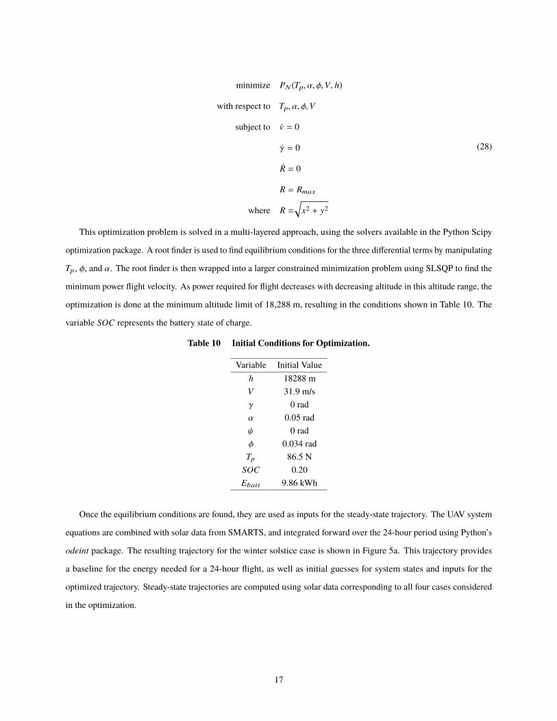
minimum power flight velocity. As power required for flight decreases with decreasing altitude in this altitude range, the
optimization is done at the minimum altitude limit of 18,288 m, resulting in the conditions shown in Table 10. The
variable SOC represents the battery state of charge.
Table 10 Initial Conditions for Optimization.
Variable Initial Valueh 18288 mV 31.9 m/sγ 0 radα 0.05 radψ 0 radφ 0.034 rad
Tp 86.5 NSOC 0.20Ebatt 9.86 kWh
Once the equilibrium conditions are found, they are used as inputs for the steady-state trajectory. The UAV system
equations are combined with solar data from SMARTS, and integrated forward over the 24-hour period using Python’s
odeint package. The resulting trajectory for the winter solstice case is shown in Figure 5a. This trajectory provides
a baseline for the energy needed for a 24-hour flight, as well as initial guesses for system states and inputs for the
optimized trajectory. Steady-state trajectories are computed using solar data corresponding to all four cases considered
in the optimization.
17

D. State Machine Benchmark Case
In addition to the steady-state trajectory, the optimized trajectory is also compared against a state-machine-driven
trajectory. This state-machine-driven trajectory is another commonly studied path in which the aircraft flies in a circular
path, but ascends and descends throughout the day according to a set of rules. Essentially, the aircraft ascends on the
outer surface of a cylinder, levels out at the maximum height, and then descends along the same cylinder to the minimum
height. The state machine case presents an alternative study of the effects of potential energy storage on the total system
energy. In general, the following sequence occurs:
• Level flight until battery is filled
• Ascend until maximum height is reached or battery begins to drain
• Level flight until battery begins to drain
• Descend to minimum height
• Resume level flight
Throughout the flight, the state machine flies at the minimum power velocity for its current altitude, which is
computed using the same approach used in Section C. The climb angle is chosen as the average climb angle from the
optimized flight. The descent angle is adjusted throughout the descent as follows. First the thrust needed to maintain
minimum power level flight is computed. Then the flight path angle is decreased until the component of gravity in the
aircraft direction of motion is equal to the necessary thrust. This approach yields the shallowest possible zero power
dive. The thrust and flight path angle are recalculated repeatedly throughout the descent as the air density changes. A
sample of the trajectory generated by the state machine for the summer solstice is shown in Figure 5b.
E (km)
3 2 1 0 1 2 3 N (km)3 2 10 1 2 3
Alt (
km)
1416182022
StartFinish
(a) Steady-state circular orbit trajectory.
E (km)
3 2 1 0 1 2 3 N (km)3 2 10 1 2 3
Alt (
km)
192021222324
StartFinish
(b) State machine trajectory.
Fig. 5 The steady-state circular orbit path used both as a benchmark case and an initial guess for the opti-mization (5a), and a sample of a trajectory generated by the state machine planner for the summer solstice(5b).
18

III. Results and DiscussionThis section presents the results of the optimizations performed using the methods described in the previous two
sections.
A. Solar Data
Figure 6 shows the solar flux calculated using the SMARTS package for the winter solstice, using the settings
described in Table 6. This solar flux is the total solar energy passing through the atmosphere to the location of the
aircraft, prior to adjustments for orientation and panel efficiency. This raw solar flux data is used as an input to the
trajectory optimization.
6 8 10 12 14 16 18 20Time (Hr)
0
200
400
600
800
1000
1200
1400
Avai
labl
e Fl
ux (W
/m2 )
Total Solar Flux Available
SpringFallSummerWinter
Fig. 6 Available solar flux calculated by SMARTS for the four test cases.
The second piece of solar information needed is the sun position, which is also obtained from SMARTS in the
form of azimuth and elevation angles throughout the day. The solar angles for the winter solstice at 35° N are shown in
Figure 7a. Note that in the winter at this latitude, the sun zenith angle reaches its minimum value at slightly over 60°,
which implies a maximum elevation angle of approximately 30°. As will be shown in the next section, this relatively
low elevation angle has a large impact on the optimal trajectory for the winter season.
B. Trajectory Results
This section examines the trajectories generated by the optimization process described above. The optimizer finds
unique orbit shapes for each season that evolve throughout the course of the day. Samples of shapes for the four seasons
are shown, as well as full trajectories for each of the test cases. The characteristic shape of the winter solstice orbit
is investigated in depth, as well as the effect of potential energy storage on the optimal solutions. The effect of the
station-keeping radius and the sensitivity of the solution to this mission constraint are also explored.
19

0 2 4 6 8 10 12 14
Time (Hr)
0
50
100
150
200
250
300An
gle
(Deg
rees
)Solar Azimuth and Zenith (Winter)
Sun AzimuthSun Zenith
(a) Solar Angles Winter Solstice
0 2 4 6 8 10 12 14
Time (Hr)
0
50
100
150
200
250
300
Angl
e (D
egre
es)
Solar Azimuth and Zenith (Summer)
Sun AzimuthSun Zenith
(b) Solar Angles Summer Solstice
Fig. 7 Solar azimuth and zenith calculated by SMARTS for the winter and summer solstices (daylight hours).
0 2 4 6 8 10 12 14
Time (Hr)
0
50
100
150
200
250
300
Angl
e (D
egre
es)
Solar Azimuth and Zenith (Spring)
Sun AzimuthSun Zenith
(a) Solar Angles Spring Equinox
0 2 4 6 8 10 12 14
Time (Hr)
0
50
100
150
200
250
300
Angl
e (D
egre
es)
Solar Azimuth and Zenith (Fall)
Sun AzimuthSun Zenith
(b) Solar Angles Fall Equinox
Fig. 8 Solar azimuth and zenith calculated by SMARTS for the spring and fall equinoxes (daylight hours).
1. Full Trajectory Results and Characteristic Shape
To begin, Figure 9 shows the full trajectory results for the four optimization cases. It can easily be seen that in all
cases, the optimized solution differs significantly from the steady-state orbit. These changes and their significance are
examined in more detail in the following sections.
The optimal trajectory assumes a characteristic shape for each season. This shape optimizes the amount of solar
energy collected, while minimizing the power required for flight. The resulting orbits are shown in Figure 10. The
characteristic shape of the winter solstice trajectory is analyzed further in Section 2.
2. Single Orbit Analysis
As it can be somewhat difficult to understand the behavior of the optimized solution from the full trajectory, a single
orbit from the winter solstice trajectory will now be examined. The trajectory and accompanying information are shown
in Figure 11 with the aircraft traveling clockwise around the path. This orbit occurs two hours after dawn, and lasts
20

E (km)
3 2 1 0 1 2 3 N (km)3 2 10 1 2 3
Alt (
km)
192021222324
StartFinish
(a) Winter Solstice
E (km)
3 2 1 0 1 2 3 N (km)3 2 10 1 2 3
Alt (
km)
192021222324
StartFinish
(b) Summer Solstice
E (km)
3 2 1 0 1 2 3 N (km)3 2 10 1 2 3
Alt (
km)
192021222324
StartFinish
(c) Spring Equinox
E (km)
3 2 1 0 1 2 3 N (km)3 2 10 1 2 3
Alt (
km)
192021222324
StartFinish
(d) Fall Equinox
Fig. 9 Full optimized trajectories for the four optimized cases at 35°N. These trajectories maximize the energygained from solar and potential energy storage while minimizing the power required for flight.
approximately eight minutes.
As seen in Figure 11, the optimized winter trajectory forms a roughly fabiform shape. The UAV begins at the
north-west corner of the orbit, then turns and flies towards the sun for approximately the first 3.5 minutes. During this
leg of the flight the UAV reduces the angle of attack, reducing drag and decreasing the angle of incidence between the
sun and the solar panels. The velocity increases as the UAV descends by 500 feet to the minimum altitude, and thrust is
simultaneously decreased, allowing the battery to charge during the short glide.
The UAV turns back towards the north-west at approximately four minutes into the trajectory. Notice that the major
axis aligns exactly with the orientation of the sun vector at this point in time. This alignment enables the optimized
solution to maximize the energy received by exhibiting the following behavior. First, the aircraft pitches upwards and
slows down while increasing thrust. The aircraft climbs by 500 feet during this leg of the path, and the bank angle is
also decreased to nearly zero. These maneuvers reduce the angle of incidence between the sun vector and the surface
normal of the wing, increasing the total solar flux received and the energy available for charging the battery. Although
21

3 2 1 0 1 2 3E (km)
3
2
1
0
1
2
3
N (k
m)
(a) Winter Solstice
3 2 1 0 1 2 3E (km)
3
2
1
0
1
2
3
N (k
m)
(b) Summer Solstice
3 2 1 0 1 2 3E (km)
3
2
1
0
1
2
3
N (k
m)
(c) Spring Equinox
3 2 1 0 1 2 3E (km)
3
2
1
0
1
2
3
N (k
m)
(d) Fall Equinox
Fig. 10 The characteristic shape of the optimized trajectory in each of the four seasons two hours after dawn.The pointer indicates the direction towards the sun.
the aircraft is traveling more slowly, it eventually reaches the boundary of the mission radius constraint, forcing it to
reverse its course and begin the cycle again.
The fabiform trajectory progresses throughout the day, with the major axis continually reorienting towards the sun.
When the sun goes down, the motivation for the shape disappears, and the aircraft begins to slowly circle the outer
edge of the mission radius in a configuration similar to the steady-state trajectory. This behavior results in the most
aerodynamically efficient path for the night-time hours.
Although each season induces the trajectory to assume a unique shape, the behaviors described in this section are
common to all the optimized solutions. In each case, the aircraft velocity and orientation is controlled to maximize the
time spent with the aircraft surface angled towards the sun, and to minimize the time spent facing away from the sun.
22

3 2 1 0 1 2 3E (km)
3
2
1
0
1
2
3
N (k
m)
2
4
6
1
5
3
7
00
60.0
60.5
kft
Height
0
5
Deg
Angle of Attack
0 1 2 3 4 5 6 7Time (min)
0
5
Deg
Bank Angle
5000
7500
10000
W
Solar Power Received
0
5000
W
Power Needed
0 1 2 3 4 5 6 7Time (min)
2500
5000
7500
W
Power to Battery
30
35m
/s
Velocity
0
100
200
N
Thrust
0 1 2 3 4 5 6 7Time (min)
70
80
90
N
Drag
Fig. 11 Optimized trajectory information for the winter solstice two hours after dawn. The golden markerpoints towards the sun.
It is instructive to consider the variant on the described solution that is obtained by a different choice of objective
function. Figure 12 shows the orbit found by using an objective function that attempts only to maximize battery energy
without any consideration for potential energy. While the shape of the trajectory is nearly identical, several important
differences can be seen. The aircraft climbs only 150 ft, as opposed to over 500 ft. Battery charging is relegated almost
exclusively to the time when the aircraft is flying slowly away from the sun with a high angle of attack. As shown in
Table 11, the total energy objective gathers more solar power, but also uses more propulsion energy. Unexpectedly, the
total energy objective also charges the battery slightly more than the battery energy objective. It is hypothesized that
this outcome is related to the non-convex nature of the problem, combined with the gradient based solvers used, and that
the change in the objective function helps the optimizer escape a local minimum.
23

3 2 1 0 1 2 3E (km)
3
2
1
0
1
2
3
N (k
m)
2
4
6
1
53
7
00
60.0
60.1
kft
Height
0
5
Deg
Angle of Attack
0 1 2 3 4 5 6 7Time (min)
0
5
Deg
Bank Angle
5000
7500
10000
W
Solar Power Received
2000
4000
6000
W
Power Needed
0 1 2 3 4 5 6 7Time (min)
2000
4000
6000
W
Power to Battery
30
35m
/s
Velocity
50
100
150
N
Thrust
0 1 2 3 4 5 6 7Time (min)
70
80
90
100
N
Drag
Fig. 12 Optimized trajectory information for the winter solstice two hours after dawn using only a batteryenergy objective without a potential energy term. The golden marker points towards the sun.
Table 11 Comparison of objective functions for a single orbit.
Total Energy Objective Battery Energy Objective
Solar Energy In (MJ) 3.689 3.379Propulsion Energy Out (MJ) 1.482 1.371
Net Energy (MJ) 2.207 2.008
3. Trajectory Stages
An examination of the optimized trajectory for a 24-hour period reveals that the trajectory may be broken into
several intuitive stages: charge, climb, descend and power conservation.
Stage 1: Charge
24

E (km)
3 2 1 0 1 2 3 N (km)3 2 10 1 2 3
Alt (
km)
1416182022
StartFinish
(a) Charge
E (km)
3 2 1 0 1 2 3 N (km)3 2 10 1 2 3
Alt (
km)
1416182022242628
StartFinish
(b) Climb
E (km)
3 2 1 0 1 2 3 N (km)3 2 10 1 2 3
Alt (
km)
1416182022242628
StartFinish
(c) Descent
E (km)
3 2 1 0 1 2 3 N (km)3 2 10 1 2 3
Alt (
km)
1416182022
StartFinish
(d) Power Conservation
Fig. 13 Stages of the 24-hour optimized trajectory for the winter solstice.
The first stage begins at dawn, with the aircraft battery mostly discharged (Fig. 13a). A similar effect to that observed
by Edwards et al. is also found here, in that the aircraft maintains a tight circle at a steep bank angle near sunrise [20].
The radius of the circle gradually relaxes as the sun rises. The aircraft remains near the minimum height and uses the
fabiform shape described above to maximize the amount of solar energy captured. The fabiform trajectory progresses
throughout the morning, with the major axis continually reorienting towards the sun.
Stage 2: Climb
As the battery reaches full charge, the aircraft begins to store additional energy by climbing (Fig. 13b). The aircraft
climbs as quickly as possible given constraints on energy, thrust, and flight path angle. The climb is performed using a
modified version of the energy-optimal orbit. As the air density decreases with altitude, the fabiform shape gradually
morphs into a circular path. The climb continues until no excess energy is available for climbing, or until the maximum
height constraint is reached. Note that the charging stage precedes climbing because more power is required to fly at
higher altitudes, and the sooner the aircraft climbs the sooner the power requirement increases.
Stage 3: Descent
As the amount of sunlight begins to diminish in the evening, a point is eventually reached at which a full battery
charge can no longer be maintained. This point occurs up to an hour before sunset, and at this point the aircraft begins
25

to descend. Again, as the sun nears the horizon the radius of the orbit begins to contract, and the bank angle increases.
When the sun goes down, the motivation for the tighter shape disappears, and the aircraft begins to slowly descend
along the outer edge of the mission radius in a low power glide (Fig. 13c). At this point, the only power drain on the
battery is that required by the payload.
Stage 4: Power Conservation
When the aircraft reaches the minimum elevation constraint, it continues to circle the outer edge of the mission
radius, maintaining altitude while maximizing aerodynamic efficiency and minimizing power usage (Fig. 13d). This
behavior is identical to the steady-state trajectory, and continues throughout the night.
4. Potential Energy Storage and Power Usage
Using the set of parameters outlined in Table 1, the aircraft battery is sized so that it reaches maximum capacity
during a steady-state orbit on the winter solstice, and no energy is stored in elevation during the steady-state cases. In
the optimized cases the battery is charged to maximum capacity during the day, and the aircraft begins to ascend, storing
potential energy in elevation. This stored energy is released by gliding during the evening and night-time hours. The
degree to which the aircraft ascends depends on the amount of excess energy available, and varies throughout the year.
The UAV is able to significantly reduce power requirements by gliding. Figure 14 shows the power input, power
output, and altitude throughout the flight for the winter solstice optimized trajectory. When the battery fills (1) the
aircraft begins to climb, and power requirements increase sharply. After sunset (2), the power required is temporarily
reduced from 2870 W at level flight to just 250 W for payload requirements in a low power glide. When the aircraft
reaches the minimum altitude, the power needed returns to the steady-state value. Gliding extends the amount of time
that the battery is at full charge, and increases the charge left at the end of the day. Energy results are further described
in Section C.
5. Station-Keeping Radius Effect
Another important factor is the station-keeping radius constraint. This constraint more than any other differentiates
these results from similar work in the literature, and gives rise to the unique trajectory solutions presented here. The
effect of this constraint is explored by varying the radius of the winter solstice solution from 1.5 km to 6 km. As seen in
Figure 15, the characteristic shape of the solution obtained changes with increasing or decreasing radius size. Note
however, that while the specific shape of the trajectory changes with changing radius constraints, the general behavior is
quite similar to that already presented. That is, the aircraft pitches upwards as it flies away from the sun, maximizing
solar energy capture. As the mission radius size increases, the path becomes more and more linear, similar to the
situations encountered by Ozoroski et al. [19]. Another effect of increased radius size is that each orbit takes longer,
leading to the angle of the path progressing farther with each orbit to track the sun. This progression can be seen in the
26

0 6 12 18 24
0
5
10
15
Sola
r Po
wer
(kW
) 1 23
0 6 12 18 24
0
5
10
15
Pow
er N
eede
d (k
W) 1 23
0 6 12 18 24Time (hr)
0
5
10
15
Pow
er to
Bat
tery
(kW
)
1 23
0 6 12 18 24Time (hr)
18
20
22
24
Hei
ght (
km)
1 23
Fig. 14 Power input and output for the optimized winter trajectory. The three vertical lines correspond to (1)when the battery reaches full capacity, (2) sunset, and (3) reaching minimum height.
discontinuity in Fig. 15b, where the next orbit would be at a slightly different angle than the one shown.
1.5 1.0 0.5 0.0 0.5 1.0 1.5E (km)
1.5
1.0
0.5
0.0
0.5
1.0
1.5
N (k
m)
0.0
2.0
4.0
6.0
8.0
Angl
e of
Atta
ck (d
eg)
(a) Maximum radius 1.5 km.
6 4 2 0 2 4 6E (km)
6
4
2
0
2
4
6
N (k
m)
-2.0
0.0
2.0
4.0
6.0
8.0
Angl
e of
Atta
ck (d
eg)
(b) Maximum radius 6 km.
Fig. 15 Changing the mission maximum flight radius leads to different characteristic orbit shapes.
C. Total Energy Results
Perhaps the most important result from this study is the increase in total energy available to the system under the
optimized trajectory conditions. Maximizing total energy is the objective function of the optimization, and total energy
is an important factor in determining the endurance of the HALE system. Figures 16 and 17 show the total energy stored
27

by the system for both the steady-state and optimized trajectories for all four seasons. As an additional comparison, the
steady-state and optimized trajectories are compared against the trajectory generated by a state machine.
0 6 12 18 24Time (Hr)
0
10
20
30
40
50
60
70
Ene
rgy
Stor
ed (k
Wh)
Energy Storage (Winter)
Optimized Total EnergyOptimized Battery EnergySM Total EnergySS Battery Energy
(a) Winter Solstice Total Energy
0 6 12 18 24Time (Hr)
0
10
20
30
40
50
60
70
Ene
rgy
Stor
ed (k
Wh)
Energy Storage (Summer)
Optimized Total EnergyOptimized Battery EnergySM Total EnergySS Battery Energy
(b) Summer Solstice Total Energy
Fig. 16 Battery energy and total (battery + potential) energy stored in the system by the optimized andsteady-state trajectories for the winter and summer solstices.
0 6 12 18 24Time (Hr)
0
10
20
30
40
50
60
70
Ene
rgy
Stor
ed (k
Wh)
Energy Storage (Spring)
Optimized Total EnergyOptimized Battery EnergySM Total EnergySS Battery Energy
(a) Spring Equinox Total Energy
0 6 12 18 24Time (Hr)
0
10
20
30
40
50
60
70
Ene
rgy
Stor
ed (k
Wh)
Energy Storage (Fall)
Optimized Total EnergyOptimized Battery EnergySM Total EnergySS Battery Energy
(b) Fall Equinox Total Energy
Fig. 17 Battery energy and total (battery + potential) energy stored in the system by the optimized andsteady-state trajectories for the spring and fall solstices.
As shown in these figures, the optimized solution provides a clear benefit in terms of total energy. In all cases, the
battery is charged more rapidly, and reaches full capacity sooner than in the steady-state orbit case. The battery remains
at full charge for some time in the middle of the day, opening an opportunity for the aircraft to store potential energy
by climbing as discussed above. The optimized trajectory also climbs and descends more efficiently than the state
machine trajectory, leading to an increased final energy. This behavior is especially important near sunset, when the
optimizer is able to match its descent to the optimal descent rate based on altitude and available solar power, whereas
the state-machine descends at a minimum-power rate. This result is discussed further in Section D.
The total energy available to the system at the end of the 24-hour flight period for each of the four optimized cases is
presented in Table 12 and Figure 18. For comparison, the table also lists the total energy information for the steady-state
28

and state machine trajectories. As shown, the optimized trajectory outperforms the steady-state trajectory in terms of
energy for all the studied cases.
Table 12 Total Energy Results for Optimized Trajectories.
Season Trajectory Max Total Energy (kWh) Final Total Energy (kWh) Improvement (kWh)
Winter Steady State 47.83 5.51 -Winter State Machine 47.84 5.53 0.02Winter Optimized 53.29 9.44 3.93Spring Steady State 48.05 12.55 -Spring State Machine 53.56 15.71 3.16Spring Optimized 53.56 16.48 3.92Summer Steady State 48.07 19.18 -Summer State Machine 53.56 22.05 2.87Summer Optimized 53.56 23.04 3.87Fall Steady State 48.05 12.55 -Fall State Machine 53.56 15.61 3.06Fall Optimized 53.56 16.46 3.91
Fall Winter Summer SpringSeason
0
5
10
15
20
Tota
l Ene
rgy
(kW
h)
SS Final Total EnergySM Final Total EnergyOpt Final Total Energy
Fig. 18 Total energy results for optimized trajectories.
D. Discussion
The results presented have a number of implications. First, an aircraft design that is infeasible due to an inability to
close the energy gap may be brought to feasibility simply by changing the way that it flies. Alternatively, a feasible
aircraft design may be given an additional energy safety margin, as shown in the cases presented here. From a different
perspective, an aircraft that is unable to close the energy gap due to payload demands may not be able to function near
the winter solstice, but can increase the number of available days of service by using an optimized trajectory.
Another application of these results is the potential to adapt the design of the aircraft energy systems to take
advantage of the additional energy available. For example, due to the increased efficiency of solar capture in the
29

optimized trajectory, the number or area of solar panels could be reduced, reducing the cost of the aircraft. Battery
sizing is also a potential area of benefit. Because the optimized solution moves the beginning of battery discharge
farther towards sunset, it may be possible to reduce the battery size and still fly through the night. This modification
would reduce both the cost and the weight of the aircraft, potentially enabling additional improvements. A major area of
future work is integrating the trajectory optimization with a full energy system design optimization.
An interesting takeaway from the total energy results is that for the majority of the year, both the optimized trajectory
and the state machine reach maximum total energy. The major difference between the two solutions thereafter appears
to be the descent rate. This observation means that in cases where the state machine is able to reach maximum energy,
it may be possible to match the performance of the optimizer simply by introducing a descent rate that more closely
matches that of the optimized trajectory . Such a solution would reduce the complexity required in the trajectory for
much of the year, leaving the optimizer to deal with the more difficult flights near the winter solstice when a simple orbit
does not produce excess energy for climbing.
There are several other important aspects of this problem that remain to be addressed in future work. High-altitude
winds are a major factor in HALE UAV flights, and further studies will adapt the kinematic and aerodynamic models
used in this paper to include wind, as well as creating models to predict wind speeds and directions at different
altitudes. The authors expect that including wind in the optimization will increase the difficulty of the optimization, and
significantly modify the results presented above.
Another area of work is to investigate the prospect of parameterizing the optimized trajectories. The results of the
optimization are relatively periodic, and it may be possible to predict them directly based on the input conditions. This
would greatly improve the practical usability of the solutions, as the current optimization methods used are relatively
slow, and require larger computational resources than may be onboard a UAV.
The battery model used in the current work is very simple, and does not include charge and discharge round trip
efficiencies. Including a higher fidelity battery model would improve the accuracy of the results, and may influence the
timing of the trajectory stages.
Another important effect is that of temperature. At the altitudes in question, average temperatures of approximately
-55°C are expected. Initial work by the authors indicates that there is a strong temperature effect on the battery and
solar panel subsystems, with lower temperatures improving solar panel performance but reducing battery performance.
Future work will include modeling these effects in greater detail, and incorporating them into the optimization so that
the optimizer will take these effects into account when planning the trajectory and speed of flight.
IV. ConclusionTo conclude, this paper has presented a solution to the trajectory planning and energy management problem for
solar-powered high-altitude long-endurance unmanned aerial vehicles. A mission is defined in which a solar aircraft
30

must stay within a 3 km flight radius and an altitude range between 60,000 and 80,000 ft. System models are developed
for the aircraft and energy system, and experimental conditions described. A nonlinear model predictive control
formulation is proposed to make the problem computationally feasible, and used to solve the trajectory optimization at
an 8 second time step with a receding horizon approach. The optimization is tested at four different points during the
year, and total energy results are compared against a steady-state orbit trajectory. The optimized trajectory is shown to
outperform the steady-state orbit in all cases, with a maximum improvement in final battery energy of 8.2% over a
24-hour period.
Funding SourcesThe authors gratefully acknowledge funding from the Facebook Connectivity Lab. Any opinions, findings, or
conclusions expressed herein are those of the authors and do not necessarily reflect the views of Facebook.
AcknowledgmentsWe express gratitude to Tim McLain and Randy Beard for their insightful assistance with the aircraft dynamics
model. We thank Kevin Moore and Judd Mehr for their time and advice in many discussions regarding the aircraft
model used in the paper and the interpretation of the optimization results. We also gratefully acknowledge the time
and expertise of Taylor McDonnell, and his invaluable assistance in generating the ASWING data used to create the
aerodynamic models for the paper.
References[1] Hall, D. W., Watson, D. A., Tuttle, R. P., and Hall, S. A., “Mission Analysis of Solar Powered Aircraft,” NASA CR-172583, 1985.
[2] Phillips, W. H., “Some Design Considerations for Solar-Powered Aircraft,” NASA Tech. Rep. 1675, 1980.
[3] Hall, D. W., Fortenbach, C. D., Dimiceli, E. V., and Parks, R. W., “A Preliminary Study of Solar Powered Aircraft and
Associated Power Trains,” NASA CR-3699, 1983.
[4] Noll, T. E., Brown, J. M., Perez-Davis, M. E., Ishmael, S. D., Tiffany, G. C., and Gaier, M., “Volume I: Mishap Report,”
Investigation of the Helios Prototype Aircraft Mishap, NASA, 2004, pp. 1–100. URL https://www.nasa.gov/pdf/
64317main_helios.pdf, [online paper; accessed 8-March-2018].
[5] Zhu, X., Guo, Z., and Hou, Z., “Solar-powered airplanes: A historical perspective and future challenges,” Progress in Aerospace
Sciences, Vol. 71, 2014, pp. 36–53. doi:10.1016/j.paerosci.2014.06.003, URL http://dx.doi.org/10.1016/j.paerosci.
2014.06.003.
[6] Gao, X. Z., Hou, Z. X., Guo, Z., Fan, R. F., and Chen, X. Q., “The Equivalence of Gravitational Potential and Rechargeable
Battery for High-Altitude Long-Endurance Solar-Powered Aircraft on Energy Storage,” Energy Conversion and Management,
31

Vol. 76, 2013, pp. 986–995. doi:10.1016/j.enconman.2013.08.023, URL http://dx.doi.org/10.1016/j.enconman.2013.
08.023.
[7] Graham, W., “Facebook’s UAV Flies, Builds on Developments in Solar Power,” Aviation Week, 30 Mar. 2015. URL
http://aviationweek.com/technology/facebook-s-uav-flies-builds-developments-solar-power.
[8] Nickol, C. L., Guynn, M. D., Kohout, L. L., and Ozoroski, T. A., “High Altitude Long Endurance UAV Analysis of Alternatives
and Technology Requirements Development,” 45th AIAA Aerospace Sciences Meeting and Exhibit, Vol. 45, 8-11 Jan. 2007, p.
1050. doi:10.2514/6.2007-1050, URL http://dx/doi.org/10.2514/6.2007-1050.
[9] Burton, M., and Hoburg, W., “Solar-Electric and Gas Powered, Long-Endurance UAV Sizing via Geometric Programming,”
18th AIAA/ISSMO Multidisciplinary Analysis and Optimization Conference, 2017, p. 4147. URL https://doi.org/10.
2514/6.2017-4147.
[10] Balakrishna, A., “Optimal Control Strategies for Trajectory Optimization with Applications to Continuous Solar Flight,” Intel
Science Talent Search Competition, 2014 (submitted for publication).
[11] Sachs, G., Lenz, J., and Holzapfel, F., “Unlimited Endurance Performance of solar UAVs with Minimal or Zero Electric Energy
Storage,” AIAA Guidance, Navigation, and Control Conference, Aug. 2009, pp. 1–13. URL https://doi.org/10.2514/6.
2009-6013.
[12] Gao, X. Z., Hou, Z. X., Guo, Z., Liu, J. X., andChen, X. Q., “EnergyManagement Strategy for Solar-PoweredHigh-Altitude Long-
Endurance Aircraft,” Energy Conversion and Management, Vol. 70, 2013, pp. 20–30. doi:10.1016/j.enconman.2013.01.007,
URL http://dx.doi.org/10.1016/j.enconman.2013.01.007.
[13] Spangelo, S. C., and Gilbert, E. G., “Power Optimization of Solar-Powered Aircraft with Specified Closed Ground Tracks,”
Journal of Aircraft, Vol. 50, No. 1, 2013, pp. 232–238. doi:10.2514/1.C031757, URL http://arc.aiaa.org/doi/abs/10.
2514/1.C031757.
[14] Spangelo, S., Gilbert, E., Klesh, A., Kabamba, P., and Girard, A., “Periodic Energy-Optimal Path Planning for Solar-Powered
Aircraft,” AIAA Guidance, Navigation, and Control Conference, 2009, p. 6016.
[15] Whitfield, C. A., “An Adaptive Dual-Optimal Path-Planning Technique for Unmanned Air Vehicles with Application to Solar-
Regenerative High Altitude Long Endurance Flight,” ProQuest Dissertations and Theses, Vol. 3368434, 2009, p. 108. URL
http://ezproxy.net.ucf.edu/login?url=http://search.proquest.com/docview/304988183?accountid=
10003%5Cnhttp://sfx.fcla.edu/ucf?url_ver=Z39.88-2004&rft_val_fmt=info:ofi/fmt:kev:
mtx:dissertation&genre=dissertations+&+theses&sid=ProQ:ProQuest+Dissertations+&+The.
[16] Dai, R., Lee, U., Hosseini, S., and Mesbahi, M., “Optimal Path Planning for Solar-Powered UAVs Based on Unit Quaternions,”
2012 IEEE 51st Annual Conference on Decision and Control (CDC), IEEE, 2012, pp. 3104–3109.
32

[17] Klesh, A. T., and Kabamba, P. T., “Energy-Optimal Path Planning for Solar-Powered Aircraft in Level Flight,” AIAA
Guidance, Navigation, and Control Conference, Vol. 3, 20–23 Aug. 2007, pp. 2966–2982. doi:10.2514.40139, URL
https://doi.org/10.2514/6.2007-6655.
[18] Klesh, A. T., and Kabamba, P. T., “Solar-Powered Aircraft: Energy-Optimal Path Planning and Perpetual Endurance,”
Journal of Guidance, Control, and Dynamics, Vol. 32, No. 4, 2009, pp. 1320–1329. doi:10.2514/1.40139, URL https:
//doi.org/10.2514/1.C031757.
[19] Ozoroski, T. A., Nickol, C. L., and Guynn, M. D., “High Altitude Long Endurance UAV Analysis Model Development and
Application Study Comparing Solar Powered Airplane and Airship Station-Keeping Capabilities,” NASA TM-2015-218677, Jan.
2015.
[20] Edwards, D. J., Kahn, A. D., Kelly, M., Heinzen, S., Scheiman, D. A., Jenkins, P. P., Walters, R., and Hoheisel, R., “Maximizing
Net Power in Circular Turns for Solar and Autonomous Soaring Aircraft,” Journal of Aircraft, Vol. 53, No. 5, 2016, pp.
1237–1247. doi:10.2514/1.C033634, URL http://dx.doi.org/10.2514/1.C033634.
[21] Hosseini, S., and Mesbahi, M., “Energy-Aware Aerial Surveillance for a Long-Endurance Solar-Powered Unmanned Aerial
Vehicles,” Journal of Guidance, Control, and Dynamics, Vol. 39, No. 9, 2016, pp. 1980–1993. doi:10.2514/1.G001737, URL
https://doi.org/10.2514/1.G001737.
[22] Hosseini, S., and Mesbahi, M., “Optimal Path Planning and Power Allocation for a Long Endurance Solar-Powered UAV,” 2013
American Control Conference, 2013, pp. 2588–2593. doi:10.1109/ACC.2013.6580224, URL https://doi.org/10.1109/
ACC.2013.6580224.
[23] Sun, L., Castagno, J. D., Hedengren, J. D., and Beard, R. W., “Parameter Estimation for Towed Cable Systems Using Moving
Horizon Estimation,” IEEE Transactions on Aerospace and Electronic Systems, Vol. 51, No. 2, 2015, pp. 1432–1446. URL
https://doi.org/10.1109/TAES.2014.130642.
[24] Newton, C., “Inside the Test Flight of Facebook’s First Internet Drone,” TheVerge.com, Jul. 2016. URL https://www.
theverge.com/a/mark-zuckerberg-future-of-facebook/aquila-drone-internet.
[25] Gomez, M. L., “Flying Aquila: Early Lessons from the First Full-Scale Test Flight and the Path Ahead,” Facebook Code, Jul.
2016. URL https://code.facebook.com/posts/268598690180189/flying-aquila-early-lessons-from-the-
first-full-scale-test-flight-and-the-path-ahead/.
[26] McDonnell, T. G., Mehr, J. A., and Ning, A., “Multidisciplinary Design Optimization Analysis of Flexible Solar-Regenerative
High-Altitude Long-Endurance Aircraft,” 2018 AIAA/ASCE/AHS/ASC Structures, Structural Dynamics, and Materials
Conference, 2018, p. 0107. URL https://doi.org/10.2514/6.2018-0107.
[27] Lombardo, T., “Solar Powered Airborne Internet Provider,” Engineering.com, Aug 2015. URL https://www.engineering.
com/AdvancedManufacturing/ArticleID/10498/Solar-Powered-Airborne-Internet-Provider.aspx.
33

[28] Alsamhi, S. H., and Rajput, N., “An Intelligent HAP for Broadband Wireless Communications: Developments, QoS and
Applications,” International Journal of Electronics and Electrical Engineering, Vol. 3, No. 2, 2015, pp. 134–143. URL
http://dx.doi.org/10.12720/ijeee.3.2.134-143.
[29] Gavan, J., Tapuchi, S., and Grace, D., “Concepts and Main Applications of High-Altitude-Platform Radio Relays,” URSI Radio
Science Bulletin, Vol. 82, No. 3, 2009, pp. 20–31. URL https://doi.org/10.23919/URSIRSB.2009.7909716.
[30] Liang, D., Marnane, W., and Bradford, S., “Comparison of US and European Airports and Airspace to Support Concept
Validation,” Progress in Astronautics and Aeronautics, Vol. 193, 2001, pp. 27–48.
[31] Beard, R. W., and McLain, T. W., Small Unmanned Aircraft: Theory and Practice, Princeton University Press, 2012, pp. 1,
36–37, 60, 164, 172.
[32] Drela, M., “Integrated simulation model for preliminary aerodynamic, structural, and control-law design of aircraft,” 40th
Structures, Structural Dynamics, and Materials Conference and Exhibit, 1999, p. 1394.
[33] Gueymard, C. A., “Prediction and Validation of Cloudless Shortwave Solar Spectra Incident on Horizontal, Tilted, or Tracking
Surfaces,” Solar Energy, Vol. 82, No. 3, 2008, pp. 260 – 271. doi:https://doi.org/10.1016/j.solener.2007.04.007, URL
http://www.sciencedirect.com/science/article/pii/S0038092X07001004.
[34] Villalva, M. G., Gazoli, J. R., and Ruppert Filho, E., “Comprehensive Approach to Modeling and Simulation of Photovoltaic
Arrays,” IEEE Transactions on Power Electronics, Vol. 24, No. 5, 2009, pp. 1198–1208. URL https://doi.org/10.1109/
TPEL.2009.2013862.
[35] Vika, H. B., “Modelling of Photovoltaic Modules with Battery Energy Storage in Simulink/Matlab,” Trondheim Norwegian
University of Science and Technology, 2014. URL http://hdl.handle.net/11250/257839.
[36] Hedengren, J. D., Shishavan, R. A., Powell, K. M., and Edgar, T. F., “Nonlinear modeling, estimation and predictive control
in APMonitor,” Computers & Chemical Engineering, Vol. 70, 2014, pp. 133–148. URL https://doi.org/10.1016/j.
compchemeng.2014.04.013.
[37] Beal, L. D. R., Hill, D. C., Martin, R. A., and Hedengren, J. D., “GEKKO Optimization Suite,” Processes, Vol. 6, No. 8, 2018,
p. 106. URL http://dx.doi.org/10.3390/pr6080106.
[38] Wächter, A., and Biegler, L. T., “On the Implementation of an Interior-Point Filter Line-Search Algorithm for Large-Scale
Nonlinear Programming,” Mathematical Programming, Vol. 106, No. 1, 2006, pp. 25–57. URL http://dx.doi.org/10.
1007/s10107-004-0559-y.
34