DYNAMICO-1.0, an icosahedral hydrostatic dynamical core ...

Geosci. Model Dev., 8, 3131–3150, 2015

www.geosci-model-dev.net/8/3131/2015/

doi:10.5194/gmd-8-3131-2015

© Author(s) 2015. CC Attribution 3.0 License.

DYNAMICO-1.0, an icosahedral hydrostatic dynamical core

designed for consistency and versatility

T. Dubos1, S. Dubey2, M. Tort1, R. Mittal3, Y. Meurdesoif4, and F. Hourdin5

1IPSL/Lab. de Météorologie Dynamique, École Polytechnique, Palaiseau, France2Dept. of Mathematics, Indian Institute of Technology Delhi, Hauz Khas, New Delhi, India3IBM India Research Laboratory, New Delhi, India4IPSL/Lab. de Sciences du Climat et de l’Environnement, CEA-CNRS, Gif-sur-Yvette, France5IPSL/Lab. de Météorologie Dynamique, CNRS – UPMC, Paris, France

Correspondence to: T. Dubos ([email protected])

Received: 13 October 2014 – Published in Geosci. Model Dev. Discuss.: 19 February 2015

Revised: 16 July 2015 – Accepted: 3 September 2015 – Published: 7 October 2015

Abstract. The design of the icosahedral dynamical core DY-

NAMICO is presented. DYNAMICO solves the multi-layer

rotating shallow-water equations, a compressible variant of

the same equivalent to a discretization of the hydrostatic

primitive equations in a Lagrangian vertical coordinate, and

the primitive equations in a hybrid mass-based vertical co-

ordinate. The common Hamiltonian structure of these sets of

equations is exploited to formulate energy-conserving spatial

discretizations in a unified way.

The horizontal mesh is a quasi-uniform icosahedral C-grid

obtained by subdivision of a regular icosahedron. Control

volumes for mass, tracers and entropy/potential temperature

are the hexagonal cells of the Voronoi mesh to avoid the

fast numerical modes of the triangular C-grid. The horizon-

tal discretization is that of Ringler et al. (2010), whose dis-

crete quasi-Hamiltonian structure is identified. The prognos-

tic variables are arranged vertically on a Lorenz grid with all

thermodynamical variables collocated with mass. The ver-

tical discretization is obtained from the three-dimensional

Hamiltonian formulation. Tracers are transported using a

second-order finite-volume scheme with slope limiting for

positivity. Explicit Runge–Kutta time integration is used

for dynamics, and forward-in-time integration with horizon-

tal/vertical splitting is used for tracers. Most of the model

code is common to the three sets of equations solved, mak-

ing it easier to develop and validate each piece of the model

separately.

Representative three-dimensional test cases are run and

analyzed, showing correctness of the model. The design per-

mits to consider several extensions in the near future, from

higher-order transport to more general dynamics, especially

deep-atmosphere and non-hydrostatic equations.

1 Introduction

In the last 2 decades, a number of groups have explored

the potential of quasi-uniform grids for overcoming well-

known deficiencies of the latitude–longitude mesh applied

to atmospheric general circulation modelling (Williamson,

2007). Particularly compelling has been the computational

bottleneck created by the convergence of the meridians at

the pole, which prevents efficient distribution of the compu-

tational load among many computers. Quasi-uniform grids

have no such singular points and are free of this bottleneck.

The first attempts at using quasi-uniform grids (Sadourny

et al., 1968; Sadourny, 1972) failed at delivering important

numerical properties that could be achieved on Cartesian

longitude–latitude grids (Arakawa, 1966; Sadourny, 1975a,

b; Arakawa and Lamb, 1981). For this reason the balance has

been in favour of longitude–latitude grids until the recent ad-

vent of massively parallel computing that provided a strong

incentive to revisit these grids.

Since one reason for using quasi-uniform grids is the ca-

pability of benefiting from the computing power of mas-

sively parallel supercomputers, many groups have set high-

resolution modelling as a primary target. For the dynamical

core, which solves the fluid dynamical equations of motion,

Published by Copernicus Publications on behalf of the European Geosciences Union.

3132 T. Dubos et al.: DYNAMICO-1.0, an icosahedral hydrostatic dynamical core

this generally implies solving a non-hydrostatic set of equa-

tions. Indeed, the hydrostatic primitive equations commonly

used in climate-oriented global circulation models (GCMs)

assume that the modelled motions have horizontal scales

much larger than the scale height, typically about 10 km on

Earth. Some hydrostatic models on quasi-uniform grids have

been developed but essentially as a milestone towards a non-

hydrostatic model (Wan et al., 2013).

In fact in many areas of climate research high-resolution

modelling can still be hydrostatic. For instance palaeo-

climate modelling must sacrifice atmospheric resolution for

simulation length, so that horizontal resolutions typical of the

Coupled Model Intercomparison Project (CMIP)-style cli-

mate modelling are so far beyond reach, and would definitely

qualify as high-resolution for multi-millenial-scale simula-

tions. Similarly, three-dimensional modelling of giant plan-

ets is so far unexplored since resolving their small Rossby

radius requires resolutions of a fraction of a degree. Mod-

elling at Institut Pierre Simon Laplace (IPSL) focusses to a

large extent on climate timescales and has diverse interests

ranging from palaeo-climate to modern climate and plane-

tology. When IPSL embarked in 2009 in an effort to develop

a new dynamical core alongside Laboratoire de Météorolo-

gie Dynamique – Zoom (LMD-Z) (Hourdin et al., 2013), a

medium-term goal was therefore set to focus on hydrostatic

dynamics in order to best serve the IPSL community with

increased efficiency and versatility.

By versatility we mean the ability to relax in the dynam-

ical core certain classical assumptions that are accurate for

the Earth atmosphere but not necessarily for planetary atmo-

spheres, or may have small but interesting effects on Earth.

For instance in LMD-Z it is possible to assume for dry air

a non-ideal perfect gas with temperature-dependent thermal

capacities and this feature is used to model Venus (Lebon-

nois et al., 2010). In a similar vein a parallel effort has

been undertaken to relax the shallow-atmosphere approx-

imation in LMD-Z and solve the deep-atmosphere quasi-

hydrostatic equations (White and Bromley, 1995; Tort and

Dubos, 2014a). Although this feature is not yet implemented

in DYNAMICO, the same prognostic variables have been

adopted in DYNAMICO as in the deep-atmosphere LMD-Z

(Tort et al., 2014b), in order to facilitate upcoming general-

izations of DYNAMICO, including generalizations to non-

hydrostatic dynamics.

LMD-Z is a finite-difference dynamical core but the kine-

matic equations (transport of mass, entropy/potential temper-

ature, chemical species) are discretized in flux form, lead-

ing to the exact discrete conservation of total mass, total

entropy/potential temperature and species content. Upwind-

biased reconstructions and slope limiters are used for the

transport of species, which is consistent with mass transport

and monotonic (Hourdin and Armengaud, 1999). Horizon-

tal dynamics is discretized in vector-invariant form follow-

ing the enstrophy-conserving scheme of Sadourny (1975b).

Unlike the vast majority of hydrostatic dynamical cores, Sim-

mons and Burridge (1981) is not used for vertical momentum

transport and hydrostatic balance. Another discretization is

used, which also exactly preserves energy (Hourdin, 1994).

Due to this emphasis on exact discrete conservation proper-

ties in LMD-Z, a critical design goal of DYNAMICO was to

have at least equivalent properties of conservation and con-

sistency.

Pursuing both objectives of consistency and versatility

(as defined above) implies that generic approaches must be

found, rather than solutions tailored to a specific equation

set. For instance the equivalence of mass and pressure, the

proportionality of potential and internal energies are valid

only for the hydrostatic primitive equations and cease to be

valid in a deep-atmosphere geometry, or even in a shallow-

atmosphere geometry with a complete Coriolis force (Tort

and Dubos, 2014a). The Bernoulli function appearing in the

vector-invariant form of the equations of motion is the sum

of kinetic energy and geopotential only if an ideal perfect

gas (with temperature-independent thermal capacities) is as-

sumed (Tort and Dubos, 2014b). The same assumption is re-

quired to have internal energy and enthalpy proportional to

temperature, as in Simmons and Burridge (1981). For ver-

satility the dynamical core should not critically rely on such

accidental relationships. This raises the question of what as-

sumptions can be made that are both common to all po-

tential target equation sets and sufficient to obtain the de-

sired consistency properties. The answer to this question

that has emerged during the DYNAMICO project is that

the Hamiltonian formulation of the equations of motion is

a sufficient common structure from which discrete consis-

tency can be obtained for all well-formed equation sets.

This idea is not really new. In fact it has been advocated

for some time now by Salmon (1983, 2004) who applied

it to the Saint-Venant equations. However, the Hamiltonian

approach has been applied only once to date to derive a

full-fledged three-dimensional dynamical core, by Gassmann

(2013). Gassmann (2013) uses the Hamiltonian formulation

of the fully compressible equations in Eulerian coordinates.

This Hamiltonian theory has been recently extended for com-

pressible hydrostatic flows and for non-Eulerian vertical co-

ordinates (Tort and Dubos, 2014b; Dubos and Tort, 2014) and

serves as the basis to formulate the discretization of dynam-

ics in DYNAMICO.

In addition to the above approach, building blocks for DY-

NAMICO include a positive-definite finite-volume transport

scheme (Lauritzen et al., 2014b) and finite-difference opera-

tors generalizing Sadourny’s scheme to general unstructured

spherical meshes. A partial generalization has been achieved

by Bonaventura and Ringler (2005) but still lacked a dis-

crete conservation of potential vorticity/potential enstrophy

and exact discrete geostrophic equilibria, two properties tied

together as discussed by Thuburn (2008). A full generaliza-

tion was obtained later by Thuburn et al. (2009) and Ringler

et al. (2010) assuming a Delaunay–Voronoi pair of primal

and dual meshes, or more generally orthogonal primal and

Geosci. Model Dev., 8, 3131–3150, 2015 www.geosci-model-dev.net/8/3131/2015/

T. Dubos et al.: DYNAMICO-1.0, an icosahedral hydrostatic dynamical core 3133

dual meshes (see Sect. 2). Thuburn et al. (2014) further gen-

eralize to a wide class of non-orthogonal dual meshes, tar-

geting the cubed sphere which has a better balance between

the degrees of freedom for mass and velocity, thus avoiding

numerical modes present in triangular meshes and their dual

(Gassmann, 2011; Weller et al., 2012). However the accu-

racy of finite differences on the cubed sphere is poor and a

triangular–hexagonal grid yields much more accurate results

for a number of degrees of freedom similar to that of the

cubed sphere (Thuburn et al., 2014). On Delaunay–Voronoi

meshes placing mass inside triangles leads to a branch of

non-stationary numerical modes that must be controlled by a

non-trivial amount of dissipation (Rípodas et al., 2009; Wan

et al., 2013), while placing mass inside Voronoi domains

leads to stationary numerical modes, which requires no or

very little dissipation for stable integrations (Ringler et al.,

2010; Skamarock et al., 2012; Gassmann, 2013). DYNAM-

ICO follows the second option.

The present paper is organized as follows. Section 2 de-

scribes how the transport of mass, potential temperature and

other tracers is handled by DYNAMICO. For this the grid

and the discrete representation of scalar and vector fields are

introduced. Mass fluxes through control volumes boundaries

are provided by the dynamics, as described in Sect. 3. Fol-

lowing the Hamiltonian approach, the primary quantity is the

total energy, which is discretized first vertically then horizon-

tally then yields the discrete expressions for the Bernoulli

function and other quantities appearing in the curl-form

equation of motion. Section 4 is devoted to energetic con-

sistency. The discrete energy budget of DYNAMICO is de-

rived, and the underlying Hamiltonian structure of the TRiSK

scheme (Thuburn et al., 2009; Ringler et al., 2010) is identi-

fied. In Sect. 5 sample numerical results are presented, veri-

fying the correctness of DYNAMICO and its ability to per-

form climate-style integrations. Our main contributions are

summarized and discussed in Sect. 6, and future work is out-

lined.

2 Kinematics

In this section we describe how the transport of mass, po-

tential temperature and other tracers is handled by DYNAM-

ICO, using mass fluxes computed by the dynamics as de-

scribed in Sect. 3. We use bold face letters for vectors in

three-dimensional physical space and for points on the unit

sphere. Space-dependent fields are functions of a vector n on

the unit sphere and a generalized vertical coordinate η. Espe-

cially the geopotential8(n,η, t) is a dependent quantity. Us-

ing the dot notation for the Lagrangian (material) derivative,

u= n is an angular velocity tangent to the unit sphere 6, i.e.

n ·u= 0. The Eulerian position r of a fluid parcel in physi-

cal space is determined by the geopotential 8 considered as

a vertical Eulerian coordinate and n, i.e. r = r(8,n). An ex-

pression for r(8,n) is not needed to solve the transport equa-

tions and needs to be specified only when dealing with the

dynamics (see Sect. 3). Denoting ∂α = ∂/∂α for α = n, η, t ,

the continuous flux-form budget for mass, potential temper-

ature θ and tracer q are

∂tµ+ ∂n ·U + ∂ηW = 0, (1)

∂t2+ ∂n · (θU)+ ∂η (θW)= 0, (2)

∂tQ+ ∂n · (qU)+ ∂η (qW)= 0, (3)

where µ is the pseudo-density such that total mass is∫µd2ndη,2= µθ,Q= µq, U = µu is the horizontal mass

flux vector,W = µη is the mass flux per unit surface through

model layers η = cst.

The following subsections describe the grid, indexing con-

ventions, the discrete mass and potential temperature bud-

gets, and finally the positive-definite finite-volume scheme

used for additional tracers.

2.1 Icosahedral–hexagonal grid, staggering and

discrete objects

The mesh is based on a tessellation of the unit sphere

(Sadourny et al., 1968). Each triangle has a global index v

and each vertex has a global index i. Several points are asso-

ciated with each index i or v. Mesh generation and smooth-

ing is described in Appendix A and numerical stability issues

arising in the calculation of spherical-geometric entities are

raised and solved in Appendix B. By joining v points one ob-

tains the hexagonal–pentagonal mesh, with control volumes

indexed by i and vertices indexed by v. Mass will be asso-

ciated with hexagonal control volumes and i points, so we

will refer to this mesh as the primal mesh, while the trian-

gular mesh will be referred to as dual. Additional quantities

are associated with primal edges joining v points, and dual

edges joining i points. Both types of edges are indexed by e.

These notations follow Thuburn et al. (2009). Lorenz stag-

gering is used in the vertical. Full vertical levels are indexed

by k = 1. . .K . Interfaces between full levels are indexed by

l = 1/2. . .L=K + 1/2.

Following the spirit of discrete exterior calculus (DEC;

see, e.g. Thuburn and Cotter, 2012), we associate to each

scalar or vector field a discrete description reflecting the

underlying differential-geometric object, i.e. 0-forms (scalar

functions), 1-forms (vector fields with a curl), 2-forms (vec-

tor fields with a divergence) and 3-forms (scalar densities).

Scalar densities include µ and 2. We describe them by dis-

crete values µik,2ik defined as their integral over the three-

dimensional control volumes (µik is in units of kg). Scalar

functions include θik =2ik/µik and specific volume αik; 2-

forms include the fluxes of mass and potential temperature.

The horizontal mass flux vector U = µu is described by its

integrals Uek over a vertical boundary between two hexago-

nal control volumes and the vertical mass flux per unit sur-

face W = µη by its integral Wil over the pseudo-horizontal

boundary between two adjacent control volumes located one

above another (unit: kg s−1).

www.geosci-model-dev.net/8/3131/2015/ Geosci. Model Dev., 8, 3131–3150, 2015


p⇤l , �l

pk = p⇤k, �k, uk, vk, µk, ⇥k

k

l

1

p⇤l , �l

pk = p⇤k, �k, uk, vk, µk, ⇥k

k

l

1

p⇤l , �l

pk = p⇤k, �k, µk

Uk, vk, ⇥k

k + 1

l = k + 1/2

k

ve

⇥i

qv

Ue

1

p⇤l , �l


Uk, vk, ⇥k

k + 1

l = k + 1/2

k

ve

⇥i

qv

Ue

1

p⇤l , �l


Uk, vk, ⇥k

k

l = k + 1/2

l � 1

ve

⇥i

qv

Ue

1

p⇤l , �l


Uk, vk, ⇥k

k

l = k + 1/2

l � 1

ve

⇥i

qv

Ue

1

p⇤l , �l


Uk, vk, ⇥k

k + 1

l = k + 1/2

k

ve

⇥i

qv

Ue

1

p⇤l , �l


Uk, vk, ⇥k

k + 1

l = k + 1/2

k

ve

⇥i

qv

Ue

1

p⇤l , �l


Uk, vk, ⇥k

k + 1

l = k + 1/2

k

ve

⇥i

qv

Ue

1

p⇤l , �l


Uk, vk, ⇥k

k + 1

l = k + 1/2

k

ve

⇥i

qv

Ue

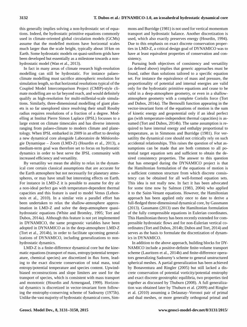
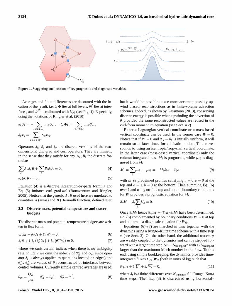
1Figure 1. Staggering and location of key prognostic and diagnostic variables.

Averages and finite differences are decorated with the lo-

cation of the result, i.e. δk8 lies at full levels,ml lies at inter-

faces, and8ek

is collocated with Uek (see Fig. 1). Especially,

using the notations of Ringler et al. (2010)

δiUk =−∑

e∈EC(i)

neiUek, δe8k =∑

i∈CE(e)

nei8ik,

δvvk =∑

e∈EV (v)

tevvek.

Operators δi , δe and δv are discrete versions of the two-

dimensional div, grad and curl operators. They are mimetic

in the sense that they satisfy for any Ae,Bi the discrete for-

mulae∑e

AeδeB +∑i

BiδiA= 0, (4)

δv(δeB)= 0. (5)

Equation (4) is a discrete integration-by-parts formula and

Eq. (5) imitates curl grad= 0 (Bonaventura and Ringler,

2005). Notice that the genericA,B used here are unrelated to

quantities A (areas) and B (Bernoulli function) defined later.

2.2 Discrete mass, potential temperature and tracer

budgets

The discrete mass and potential temperature budgets are writ-

ten in flux form:

∂tµik + δiUk + δkWi = 0, (6)

∂t2ik + δi(θ∗kUk

)+ δk

(θ∗i Wi

)= 0, (7)

where we omit certain indices when there is no ambiguity

(e.g. in Eq. 7 we omit the index e of θ∗ek and Uek since oper-

ator δi is always applied to quantities located on edges) and

θ∗ek , θ∗

il are values of θ reconstructed at interfaces between

control volumes. Currently simple centred averages are used:

θik =2ik

µik, θ∗ek = θk

e, θ∗il = θi

l, (8)

but it would be possible to use more accurate, possibly up-

wind biased, reconstructions as in finite-volume advection

schemes. Indeed, as shown by Gassmann (2013), conserving

discrete energy is possible when upwinding the advection of

θ provided the same reconstructed values are reused in the

curl-form momentum equation (see Sect. 4.2).

Either a Lagrangian vertical coordinate or a mass-based

vertical coordinate can be used. In the former case W = 0.

Notice that if W = 0 and θik = θk is initially uniform, it will

remain so at later times for adiabatic motion. This corre-

sponds to using an isentropic/isopycnal vertical coordinate.

In the latter case (mass-based vertical coordinate) only the

column-integrated mass Mi is prognostic, while µik is diag-

nosed from Mi :

Mi =

∑k

µik, µik =−Miδka− δkb (9)

with al,bl predefined profiles satisfying a = 0,b = 0 at the

top and a = 1,b = 0 at the bottom. Then summing Eq. (6)

over k and using no-flux top and bottom boundary conditions

for W provides a prognostic equation for Mi :

∂tMi + δi∑k

Uk = 0. (10)

Once ∂tMi hence ∂tµik = (δka)∂tMi have been determined,

Eq. (6) complemented by boundary conditions W = 0 at top

and bottom is a diagnostic equation for Wil .

Equations (6)–(7) are marched in time together with the

dynamics using a Runge–Kutta time scheme with a time step

τ (see Sect. 3). On the other hand, the additional tracers q

are weakly coupled to the dynamics and can be stepped for-

ward with a larger time step1t =Ntransportτ with 1/Ntransport

larger than the maximum Mach number in the flow. To this

end, using simple bookkeeping, the dynamics provides time-

integrated fluxes Uek ,Wil (both in units of kg) such that

δtµik + δiUk + δkWi = 0, (11)

where δt is a finite difference overNtransport full Runge–Kutta

time steps. Then Eq. (3) is discretized using horizontal–



vertical splitting (Easter, 1993; Hourdin and Armengaud,

1999):

Q(1)ik =Q

(0)ik −

1

2δk

(q(0)i Wi

)µ(1)ik = µ

(0)ik −

1

2δkWi

Q(2)ik =Q

(1)ik − δi

(q(1)e Ue

)µ(2)ik = µ

(1)ik − δiUe

Q(3)ik =Q

(2)ik −

1

2δk

(q(2)i Wi

),

where Qik is the cell-integrated value of qµ (in kg), Q(0)ik

(Q(3)) is the value ofQik at old time t (new time t+Ntranspτ ),

Q(m)ik , µ

(m)ik form= 1,2 are intermediate values, and q(m) are

pointwise values of the tracer reconstructed from Q(m) and

µ(m) (see below). The reconstruction operators satisfy the

consistency principle that q(m) = 1 whenever Q(m)= µ(m).

As a result Q(3)= µ(3) whenever Q(0)

= µ(0); i.e. the tracer

budget is consistent with the mass budget.

The vertical reconstruction is one-dimensional, piecewise

linear, slope limited, and identical to Van Leer’s scheme I

(Van Leer, 1977; Hourdin and Armengaud, 1999). The hor-

izontal advection scheme is identical to SLFV-SL of Lau-

ritzen et al. (2012) and is detailed in Dubey et al. (2015).

It relies on cellwise-linear reconstructions of q. For this a

gradient is estimated in each cell using nearby values (Satoh

et al., 2008) and limited to maintain positivity (Dukowicz

and Kodis, 1987). The position at which the reconstructed

value is evaluated is determined in a semi-Lagrangian fash-

ion (Miura, 2007).

3 Dynamics

We now turn to the discretization of the momentum budget.

A Hamiltonian formulation of the hydrostatic primitive equa-

tions in a generalized vertical coordinate is used (Dubos and

Tort, 2014). From this formulation the energy budget is ob-

tained invoking only integration by parts, a structure easy to

reproduce at the discrete level in order to conserve energy.

Before arriving, at the end of this section, at the fully discrete

three-dimensional equations, we start from the Hamiltonian

of the hydrostatic primitive equations. Introducing a vertical

discretization (of the Hamiltonian) produces (the Hamilto-

nian of) a compressible multi-layer Saint-Venant model. The

Boussinesq approximation, enforced by a Lagrange multi-

plier, yields a standard multi-layer Saint-Venant model. Fi-

nally, the horizontal discretization is described.

3.1 Continuous Hamiltonian

An ideal perfect gas with pα = RT and constant Cp = R/κ

is assumed where p is pressure, α specific volume and T

temperature. Then

π = Cp(p/pr)κ

θ = T (p/pr)−κ

α =RT

p=κθπ

p,

where π is the Exner function and θ potential tempera-

ture. Note that, letting U(α,θ) be specific internal energy,

∂U/∂α =−p, ∂U/∂θ = π , U +αp− θπ = 0.

We work within the shallow-atmosphere and spherical

geopotential approximation, so that gravity g is a constant,

the elementary volume is a2g−1d8d2n and r · r = g−282+

a2u ·u. The primitive equations are generated by the Hamil-

tonian:

H [µ,v,2,8] = (12)

1∫0

dη

⟨µ

(a2 u(v,n) ·u(v,n)

2+U

(1

gµ

∂8

∂η,2

µ

)+8

)⟩+p∞a

2g−1〈8(η = 1)〉 ,

where 〈f (n,η)〉 =∫6f d2n with 6 the unit sphere and v =

a2 (u+n×�) is prognostic (Dubos and Tort, 2014). In

Eq. (12) H is a functional of the three-dimensional fields

µ,v,2,8 and u(v,n)= a−2v−n×�. The terms in the in-

tegral are kinetic, internal and potential energy. The last term

in Eq. (12) represents the work of pressure p∞ exerted at the

top η = 1 of the computational domain and sets the upper

boundary condition p = p∞.

Discretizing Hamiltonian Eq. (12) in the vertical direction

yields a multi-layer Hamiltonian (Bokhove, 2002):

H =∑k

Hk[µk,vk,2k,8k+1/2,8k−1/2

](13)

+p∞a2g−1

∫6

8Nd2n

Hk =

⟨µk

(a2 u(vk,n) ·u(vk,n)

2+U

(δk8

gµk,2k

µk

)+8

k)⟩,

where µk =∫ ηk+1/2

ηk−1/2µdη,2k =

∫ ηk+1/2

ηk−1/22dη. Notice that

µk,vk are at full model levels while geopotential 8l is

placed at interfaces.

In order to reduce Eq. (13) to a multi-layer shallow-water

system, the Boussinesq approximation is made by introduc-

ing into Eq. (13) Lagrange multipliers λk enforcing µk =

a2ρrδk8g

:

Hk =

⟨µk

(a2 u(vk) ·u(vk)

2+ (1− θk)8

k)

(14)

+λk

(µk

ρr− a2 δk8

g

)⟩+p∞a

2g−1〈8(η = 1)〉 ,

where θk is now the non-dimensional buoyancy of each layer.

Notice that the last term can be omitted (p∞ = 0). Indeed,



changing p∞ only adds a constant to λik and does not change

the motion (see Sect. 3.3).

3.2 Fully discrete Hamiltonian

We now discretize horizontally the Hamiltonians (Eqs. 14,

13, 12). In addition to the kinematic degrees of freedom

µik, 2ik we need to discretize the velocity degrees of free-

dom. Since we shall need the curl of v, it is a 1-form in

the nomenclature of discrete differention geometry. Hence

we describe v by the discrete integrals vek =∫0e

v(n,ηk) · dl

(unit: m2 s−1), where 0e is a triangular edge. An approxima-

tion of H is then given by

H [µik, 2ik, 8il, vek]=K +P (15)

K = a2∑ike

µikAie

Aiu2ek where uek =

vek −Re

a2de,

P =∑ik

µik

(8i

k+U

(a2Aiδk8i

gµik,2ik

µik

))+p∞a

2g−1∑i

Ai8iL,

where Re = a2∫0e(�×n) · dl is the planetary contribution

to ve, de is the (angular) length of triangular edge 0e and Aieis an (angular) area associated with edge 0e and to a cell i

to which its belongs, with Aie = 0 if 0e is not part of the

boundary of cell i. uek is a first-order estimate of the com-

ponent of u along 0e. In planar geometry, Aie =14lede is a

consistent formula for Aie because it satisfies Ai =∑eAie

(Ringler et al., 2010). It is therefore also consistent in spheri-

cal geometry, with Ai '∑eAie. Letting Aie =

14lede simpli-

fies somewhat the kinetic energy term:

K =a2

2

∑ek

(µkA

)eledeu

2ek =

a2

2

∑ik

µik

Ailedeu2

e

i.

Comparing Eqs. (15) and (13) it is clear that Eq. (15) is

also a valid horizontal discretization of Eq. (13). Regarding

Eq. (14), a discretization of the kinetic energy part is simply

K as above. The other terms are discretized in a straightfor-

ward way:

H =K +∑ik

[µik

(1−

2ik

µik

)8i

k(16)

+λik

(µik

ρr− a2Ai

δk8i

g

)]+p∞a

2g−1∑i

Ai8iL

with λik the pointwise value of λ (0-form).

3.3 Discrete equations of motion

We now write the equations of motion corresponding to the

discrete Hamiltonians. First, mass fluxes must be computed

for use by kinematics. They are computed as

Uek =∂H

∂vek=

(µkA

)eleuek. (17)

Uek is therefore a centred estimate of the mass flux across the

face orthogonal to edge 0e.

Next hydrostatic balance is expressed as ∂H/∂8il = 0 or

equivalently H ′ = 0, where H ′ is induced by arbitrary, inde-

pendent variations of 8 only. For the compressible Hamilto-

nian Eq. (15) this yields

H ′ =∑ik

(µik8

′

i

k−a2Aiδk8

′

i

gpik

)+p∞a

2g−1∑i

Ai8′

iL

=

∑il

(µil+a2Ai

gδlpi

)8′il

+

∑i

(µiK

2+a2Ai

g(p∞−piK)

)8′iL.

Therefore, a2Aiδlpi + gµil= 0 with the upper boundary

condition piK = p∞+gµiL/(2a2Ai). These are discrete ver-

sions for ∂ηp+µg = 0 and p(η = 1)= p∞. pik can be de-

termined starting from the top level. Alternatively one can

define a pressure p∗il at layer interfaces by p∗iL = p∞ and

δkp∗

i +gµik = 0, then let pik = p∗

i

k. Especially surface pres-

sure is psi = p∞+ g∑kµik . When η is mass-based, one

finds from Eq. (9) that p∗il = alpsi +Cl with surface pressure

psi = p∞+gMi andCl = gbl+(1−al)p∞; i.e. the usual way

to diagnose the vertical pressure profile from surface pressure

is recovered. Once pik has been determined, the specific vol-

ume αik = α(pik,θik) follows. The geopotential is obtained

by integrating:

δk8i =gµikαik

a2Ai, 8i 1/2 =8

si , (18)

starting from the ground, where 8si is the time-independent

surface geopotential.

On the other hand, for the incompressible Hamiltonian

Eq. (16), geopotential 8il is obtained by enforcing the con-

straint ∂H/∂λik = 0, i.e. Eq. (18) but with specific volume

αik = 1/ρr independent from pressure. Furthermore,

H ′ =∑ik

[(1− θik)µik8

′

i

k− λika

2Aiδk8′

i

g

]+p∞a

2g−1∑i

Ai8′

iL

=

∑il

((1− θi)µi

l+a2Ai

gδlλi

)8′il

+

∑i

((1− θiK)

µiK

2− (p∞− λik)a

2g−1Ai

)8′iL.

Therefore, λik satisfies the same equations as pik but with

(1− θik)µik instead of µik , which shows that θik acts indeed

as a buoyancy θ = (ρr − ρ)/ρr . The Lagrange multipliers



λik enforcing the incompressibility constraint are to be inter-

preted as the pressure at full model levels, a typical outcome

within the Boussinesq approximation (Holm et al., 2002).

Finally, the horizontal momentum balance is written in

vector-invariant form. When W = 0,

∂tvek + δeBk + θ∗

ekδeπk + (qkUk)⊥e = 0, (19)

where

πik =∂H

∂2ik, Bik =

∂H

∂µik,

and the⊥ operator is defined in Ringler et al. (2010) through

antisymmetric weights wee′ =−we′e :

(qkUk)⊥e =

∑e′

wee′qee′Ue′ where qee′ =q∗e′k+ q∗ek

2(20)

with q∗ek a value of potential vorticity reconstructed at

e points from values at v points qvk = δvvk/µv , where µvkis µ integrated over triangular control volumes defined as

an area-weighted sum of neighbouring µik (Ringler et al.,

2010). Currently, a centred average q∗ek = qke is used but

other reconstructions, including upwind-biased reconstruc-

tions, could be used as well (Ringler et al., 2010). The

weights wee′ are obtained by Thuburn et al. (2009), Eq. (33)

as a function of the ratios Riv = Aiv/Ai satisfying∑vRiv =

1, i.e.∑vAiv = Ai . Using the compressible Hamiltonian

Eq. (15) one finds

πik = π(αik, θik), (21)

Bik =Kik +8ik, (22)

where Kik = a2 ledeu

2e

i

Ai(23)

is an approximation of kinetic energy 12a2u ·u. Therefore

geopotential at full levels is defined as a centred average

of 8il and Exner pressure is diagnosed in each control vol-

ume using the equation of state. Because pik = p(αik,θik),

Eq. (21) simplifies to πik = cp(pik/pr)κ . In practice πik and

αik are both diagnosed from pik,θik when solving the hydro-

static balance.

On the other hand, using the incompressible Hamiltonian

Eq. (16) yields

Bik =Kik +8ik+λik

ρr, πik =−8ik. (24)

As already mentioned, changing p∞ only modifies the upper

boundary condition and only adds a constant to λik . Since

only δeBk is important for dynamics, the value of p∞ is ar-

bitrary and can be set to 0. Now if θik = θk is horizontally

uniform, θ∗ek = θk and

δeBk + θ∗

ekδeπk = δe

(Kk +

λk

ρr+ (1− θk)8

k),

and Eq. (19) takes the expected form for a multi-layer

shallow-water model. In the more general case where θikis not uniform, Eq. (19) is a discretization of the vector-

invariant form of Ripa equations (Ripa, 1993).

WhenW 6= 0 an additional term takes into account vertical

momentum transport:

∂tvek+ δeBk+ θ∗

ekδeπk+ (qkUk)⊥e +

(Wk

µk

)eδlv∗e = 0, (25)

where v∗el is a value of ve reconstructed at interfaces. Here

a centred average v∗el = vel is used. The above discretization

does not possess particular conservation properties and other

equally accurate formulae could be explored.

3.4 Time marching

After spatial discretization one obtains a large set of ordinary

algebraic equations

∂y

∂t= f (y), (26)

where y = (Mi,2ik,vik) with a mass-based coordinate and

y = (µik,2ik,vik) with a Lagrangian coordinate. Geopoten-

tial8ik is diagnosed from y when computing the trends f (y)

(details below). Equation (26) is advanced in time using a

scheme of Runge–Kutta type. Temporal stability is limited by

the external mode, which propagates at the speed of sound c.

For a p stage scheme, about (p/Cmax)× cT /δx evaluations

of f are necessary to simulate a time T with resolution δx

where Cmax is the maximum time step allowed to integrate

the differential equation dx/dt = ix. It is therefore desirable

to maximize the effective Courant number Ceff = Cmax/p.

The design goals of the time scheme are to be fully explicit

for simplicity, second-order accurate and with a favourable

effective Courant number for efficiency.

Two-stage Runge–Kutta schemes of the order of 2 are un-

conditionally unstable for imaginary eigenvalues and ruled

out. All explicit p step RK schemes of order p are equivalent

for linear equations; p = 3 and p = 4 yield C(3)max =

√3 and

C(4)max = 2

√2, respectively; hence, CRK3

eff = 1/√

3< CRK4eff =

1/√

2. Kinnmark and Gray (1984b) provided p stage Runge–

Kutta schemes with optimal Cmax = p− 1 and an order of 2

for odd p (referred to as RK2.p below). Third- and fourth-

order accuracy are achievable at a small price in terms of

stability, i.e. Cmax =

√(p− 1)2− 1 (Kinnmark and Gray,

1984a). Hence, for p = 4 and p = 5 optimal schemes are

RK4 and RK2.5, the latter having Ceff = 0.8, about 13 %

larger than CRK4eff . Currently, the following scheme yn 7−→



yn+1 is implemented for RK4:

y1= yn+

τ

4f (yn)

y2= yn+

τ

3f (y1)

y3= yn+

τ

2f (y2)

yn+1 = yn+ τf (y3),

where τ ≤ 2√

2δx/c is the time step and yn ' y(nτ). This is

a low-storage scheme since the same memory space can be

used for y1,y2,y3 and yn+1. It is also very easy to imple-

ment. It is fourth-order accurate for linear equations but only

second-order accurate for non-linear equations. A similar se-

quence is used for RK2.5.

Furthermore, the last step is similar to an Euler step; hence,

δtµik + δi

(τU3

k

)+ δk

(τW 3

i

)= 0,

so that the time-integrated mass fluxes expected by the trans-

port scheme are simply U ek = τU3ek,W il = τW

3il or their

sum over Ntransport successive time steps (see Sect. 3).

Recap: computation of trends in a mass coordinate

At the beginning of this computation vek,Mi,2ik are known.

Cell-integrated mass µik and potential temperature θik are

diagnosed using Eqs. (9) and (8). Pressure pik follows from

hydrostatic balance (see Sect. 3.3), then Exner pressure and

specific volume πik, αik . Geopotential is obtained bottom–

up using Eq. (18), then the Bernoulli function (Eqs. 22 and

23).

From µik,vek horizontal mass fluxes Uek are obtained

then, by vertical integration, ∂Mi/∂t . Then ∂µi/∂t is ob-

tained and injected into the mass budget (Eq. 1) to compute

the vertical mass flux Wil by a top–down integration. The

potential temperature fluxes and trend are then computed us-

ing Eqs. (7) and (8). Finally, the velocity trend is computed

following Eq. (25).

Recap: computation of trends in a Lagrangian

coordinate

At the beginning of this computation vek, µik, 2ik are

known. Potential temperature θik is diagnosed using Eqs. (9)

and (8). Pressure pik (compressible equations) or λik (incom-

pressible equations) follows from hydrostatic balance (see

Sect. 3.3). Geopotential is obtained bottom–up using Eq. (18)

and either αik = α(θik,pik) or αik = 1/ρr , then the Bernoulli

function and Exner pressure using either Eqs. (22) or (24).

Fromµik,vek horizontal mass fluxesUek are obtained then

∂µi/∂t . The trends of potential temperature and velocity are

finally computed using Eq. (7) with Wil = 0 and Eq. (19).

3.5 Filters

Centred schemes need stabilization to counteract the genera-

tion of grid-scale features in the flow. Linear sources of grid-

scale noise, e.g. dispersive numerical errors, may be handled

by filters, e.g. upwinding or hyperviscosity. Other sources are

genuinely non-linear, e.g. the downward cascade of energy

or enstrophy. Here we handle these sources through hyper-

viscosity as well, rather than with a proper turbulence model,

e.g. Smagorinsky (1963), following a widespread although

disputable practice (see Gassmann, 2013).

For this purpose hyper-diffusion is applied everyNdiff time

step in a forward-Euler manner:

2ik :=2ik −NdiffτL

2pθ

τθDpθ 2ik (27)

vek := (28)

vek −Ndiffτ

[L

2pω

τωDpω (vek −Re)+

L2pδ

τδDpδ (vek −Re)

],

where the exponent p is 1 or 2, the dissipation timescales

τθ ,τω,τδ serve to adjust the strength of filtering, the length

scales Lθ ,Lω,Lδ are such that L−2θ ,L−2

ω ,L−2δ are the

largest eigenvalue of the horizontal dissipation operators

Dθ ,Dω,Dδ defined as

Dθ2i =−δi

[le

deδe

(2i

Ai

)]Dωve =−δe

(1

Avδvve

)Dδve =−δe

(1

Aiδi

(le

deve

)).

These positive-definite operators correspond to diffusing a

scalar, vorticity and divergence. Notice, however, that fil-

tering with p > 1, although it damps grid-scale noise, typ-

ically neither removes oscillations entirely nor guarantees

positivity of the filtered field (see e.g. Jiménez, 2006).

L−2θ ,L−2

ω ,L−2δ are precomputed by applying Dθ ,Dω,Dδ

many times in sequence on random data, so that their largest

eigenvalue is given by ratio of the norm of two successive

iterates. This process converges very quickly and in practice

20 iterations are sufficient. The dissipation timescales and the

exponents can be set to different values for θ,ω,δ.Ndiff is de-

termined as the largest integer that ensures stability, i.e. such

that Ndiffτ be smaller than all three dissipation timescales.

4 Energetics

4.1 Conservation and stability

In addition to its aesthetic appeal, discrete conservation of

energy has practical consequences in terms of numerical sta-

bility, which we discuss here using arguments similar to



energy-Casimir stability theory (Arnold, 1965). Indeed, if a

dynamical system conserves a convex integral quantity, then

any state of the system which is a minimum of that quantity

is necessarily a stable steady state. For instance the states of

rest of the shallow-water equations minimize a linear combi-

nation of total energy and mass. Each additional conserved

integral quantity widens the family of steady states that can

be proven to be stable. In the discussion below we assume

that the discrete equations of motion conserve total energy.

The additional conserved quantities then depend on the ver-

tical coordinate used.

Assuming a Lagrangian vertical coordinate, the additional

integral quantities conserved by the discrete equations of mo-

tion are, for each layer, the horizontally integrated mass and

potential temperature∑iµik ,

∑i2ik , which form a subset

of the Casimir invariants of the continuous equations (Dubos

and Tort, 2014). Stationary points of the pseudo-energyH ′ =

H−∑k8k

∑iµik−

∑kπk

∑i2ik are such that ∂H/∂vek = 0

(state of rest), ∂H/∂2ik = πik = πk and ∂H/∂µik =8ik=

8k . In the absence of topography, uniform 8ik

and πik in

each layer are achieved if θik, µik, 8il do not depend on the

horizontal position i. Such states of rest are stable provided

H ′ is convex.

The above reasoning shows that linearization of the dis-

crete equations of motion around a steady state making H ′

convex yields linear evolution equations with purely imagi-

nary eigenvalues. Forward integration in time is then linearly

stable provided the relevant Courant–Friedrichs–Lewy con-

dition is satisfied. In particular, it is not necessary for linear

stability that the time-marching scheme conserves energy.

With a mass-based vertical coordinate, the exchange

of mass between layers reduces the set of discrete

Casimir invariants to total mass and potential temperature∑iMi,

∑ik2ik . Considering the linear combination H ′ =

H−8∑iMi−π

∑ik2ik one finds the condition ∂H/∂2ik =

π . It is impossible to satisfy both hydrostatic balance and a

uniform Exner pressure; hence, no feasible state minimizes

H ′. On the other hand, if cell-integrated entropy Sik is prog-

nosed instead of potential temperature, one finds that isother-

mal states of rest minimize H ′ =H −8∑iMi − T

∑ikSik

(not shown).

We now proceed to derive the discrete energy budgets cor-

responding to a Lagrangian and a mass-based vertical coor-

dinate. In these calculations only the adiabatic terms are con-

sidered, and the effect of the hyperviscous filters is omitted.

4.2 Lagrangian vertical coordinate

When W = 0, the continuous-time energy budget reads:

dH

dt=

∑ik

∂H

∂λik∂tλik +

∑il

∂H

∂8il∂t8il +

∑ik

∂H

∂µik∂tµik

+

∑ik

∂H

∂2ik∂t2ik +

∑ik

∂H

∂vek∂tvek

=−

∑ik

∂H

∂µikδi∂H

∂vek−

∑ik

∂H

∂2ikδi

(θ∗ek

∂H

∂vek

)−

∑ek

∂H

∂vek

(δe∂H

∂µik+ θ∗ekδe

∂H

∂2ik

)−

∑ee′k

wee′q∗

ee′∂H

∂vek

∂H

∂ve′k.

Using the discrete integration-by-parts formula (4) and the

antisymmetry propertywee′+we′e = 0, one finds dH/dt = 0.

More generally, similar calculations yield the temporal

evolution of an arbitrary quantity F(µik,2ik,vek,8il,λik):

dF

dt=

∑ik

∂F

∂λik∂tλik +

∑il

∂F

∂8il∂t8il +{F,H }µ (29)

+{F,H }2+{F,H }v,

{F,H }µ =∑ek

(∂H

∂vekδe∂F

∂µik−∂F

∂vekδe∂H

∂µik

), (30)

{F,H }2 =∑ek

θ∗ek

(∂H

∂vekδe∂F

∂2ik−∂F

∂vekδe∂H

∂2ik

), (31)

{F,H }v =−∑ee′k

wee′q∗

ee′∂F

∂vek

∂H

∂ve′k. (32)

Equations (29)–(32) imitate at the discrete level the Hamil-

tonian formulations obtained in Dubos and Tort (2014).

Discrete conservation of energy then appears as a con-

sequence of the antisymmetry of the brackets {F,H }µ,

{F,H }2, {F,H }v , the formulation of hydrostatic bal-

ance as ∂H/∂8il = 0, and, in the incompressible case,

of the constraint ∂H/∂λik = 0. The antisymmetry of

{F,H }µ, {F,H }2 is equivalent to the discrete integration-

by-parts formula (4), itself equivalent to the discretization

of the horizontal div and grad operators being compatible

(see e.g. Taylor and Fournier, 2010). The antisymmetry of

{F,H }v results from wee′ =−wee′ and qee′ = qe′e (Ringler

et al., 2010).

4.3 One-layer shallow-water equations

In the simplest case of a single layer without topography

(8s = 0), the incompressible Hamiltonian Eq. (14) with2=



0, ρr = 1, a = 1, p∞ = 0 reduces to

H =1

2

∑e

(µA

)eledeu

2ek +

∑i

[µi8i

2

]=

1

2

∑e

heledeu

2ek +

1

2

∑i

gAih2i ,

where 8i = ghi is the geopotential at the “top” of the model

and we have taken into account the constraint µi = Aihi ,

where hi is interpreted as the thickness of the fluid layer.

Hamiltonian H is precisely the one considered in Ringler

et al. (2010). The discrete equations of motion also reduce to

their energy-conserving scheme (not shown). Equation (29)

reduces to

dF

dt= {F,H }µ+{F,H }v. (33)

This is a discrete imitation of the shallow-water Poisson

bracket. Had we used the enstrophy-conserving scheme

of Ringler et al. (2010) instead of the energy-conserving

scheme, {F,H }v would have been:

{F,H }Zv =−∑ee′k

wee′q∗

e′k

∂F

∂vek

∂H

∂ve′k. (34)

This discrete bracket is not antisymmetric. Comparing

Eqs. (32) and (34), one sees that the energy-conserving

bracket (32) is the antisymmetrization of Eq. (34); i.e.

{F,H }v =1

2

({F,H }Zv −{H,F }

Zv

).

In the limit of the linearized shallow-water equations on the

f sphere (Thuburn et al., 2009), both brackets (32)–(34) re-

duce to

{F,H }linv =−f

h

∑ee′k

wee′∂F

∂vek

∂H

∂ve′k, (35)

where f is the constant value of the Coriolis parameter and

h is the background fluid layer thickness; i.e. he = h+h′e,

h′e� h.

In Ringler et al. (2010), the energy-conserving discretiza-

tions of the mass flux, kinetic energy and Coriolis term were

devised by choosing a certain form and stencil for each of

them with undetermined coefficients, deriving the energy

budget, and choosing the undetermined coefficients in such

a way that all contributions cancel out. In hindsight this deli-

cate task could have been avoided by following the approach

used here, inspired by Gassmann (2013) and advocated since

some time already by Salmon (1983, 2004): discretizing the

energy and the brackets, instead of the equations of mo-

tion themselves. The critical part is to discretize the brack-

ets. Starting from the linearized bracket (35) implicitly de-

rived in Thuburn et al. (2009), a straightforward non-linear

generalization is Eq. (34), which can be antisymmetrized to

yield Eq. (32). From this point of view all the critical build-

ing blocks of Ringler et al. (2010) were already obtained in

Thuburn et al. (2009). The present approach generalizes this

scheme to three-dimensional equations in a generalized ver-

tical coordinate, exploiting recent advances in the relevant

Hamiltonian formulation (Dubos and Tort, 2014).

4.4 Mass-based vertical coordinate

When a mass-based coordinate is used instead of a La-

grangian vertical coordinate, additional terms proportional

to the vertical mass flux Wil appear in the equations of mo-

tion and in the energy budget. These terms cancel each other

for the continuous equations but not necessarily for the dis-

crete equations. It is possible to obtain a cancellation by im-

itating at the discrete level a relationship between the func-

tional derivatives of H due to invariance under a vertical re-

labelling (remapping) (Dubos and Tort, 2014). This strategy

has been recently implemented in a longitude–latitude deep-

atmosphere quasi-hydrostatic dynamical core (Tort et al.,

2014b). Tort et al. (2014b) estimate the numerical heat source

due to the vertical transport terms as less than 10−3 W m−2

in idealized climate experiments (Held and Suarez, 1994).

Hence, cancelling this very small numerical heat source is

not yet implemented in DYNAMICO and energy is not ex-

actly conserved when a mass-based vertical coordinate is

used.

So far we see no indication that this would damage long-

duration simulations (see numerical results in Sect. 5) but in

the future strict energy conservation may be offered as an

option, together with the choice to prognose entropy instead

of potential temperature.

4.5 Relation with Gassmann (2013)

At this point some important differences with respect to the

approach of Gassmann (2013) can be highlighted. Firstly,

since the vertical coordinate is non-Eulerian, geopotential 8

depends on time and appears as an argument of the Hamil-

tonian. It therefore produces additional terms in the energy

budget that vanish as shown in Sect. 4.2. On the other hand

vertical momentum is not prognostic, since the equations are

hydrostatic.

Second, Gassmann (2013) prognoses contravariant mo-

mentum components while we prognose vek , which are

equivalent to covariant velocity components. Indeed, the lat-

ter appear as the preferred prognostic variables in the Euler–

Lagrange equations of motion (Tort and Dubos, 2014b) and

their Hamiltonian formulation in a general vertical coordi-

nate (Dubos and Tort, 2014). An immediate advantage of

prognosing vek is that vorticity is trivially and naturally ob-

tained along the lines of DEC. Furthermore, the horizontal

mass flux appears in the mass and tracer budgets through

its contravariant components, and the functional derivatives

of the Hamiltonian with respect to covariant momentum



latitude

Heig

ht (k

m)

−60 −30 0 30 60

2

4

6

8

10

0

0.1

0.2

0.3

0.4

0.5

0.6

0.7

0.8

0.9

latitude

Heig

ht (k

m)

−60 −30 0 30 60

2

4

6

8

10

0

0.1

0.2

0.3

0.4

0.5

0.6

0.7

0.8

0.9

1

(a) Horizontal resolution 110km(M = 80), 60 vertical levels.

latitude

Heig

ht (k

m)

−60 −30 0 30 60

2

4

6

8

10

0

0.1

0.2

0.3

0.4

0.5

0.6

0.7

0.8

0.9

latitude

Heig

ht (k

m)

−60 −30 0 30 60

2

4

6

8

10

0

0.1

0.2

0.3

0.4

0.5

0.6

0.7

0.8

0.9

1

(b) Horizontal resolution 55km(M = 160), 120 vertical levels.

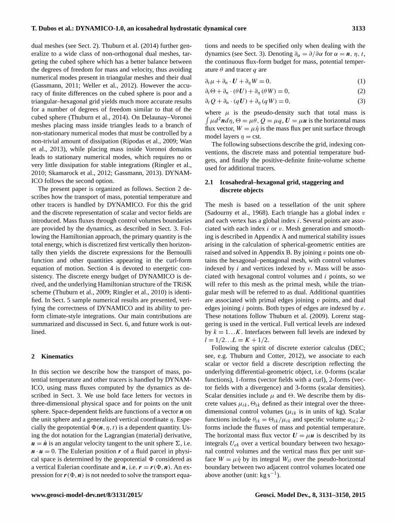
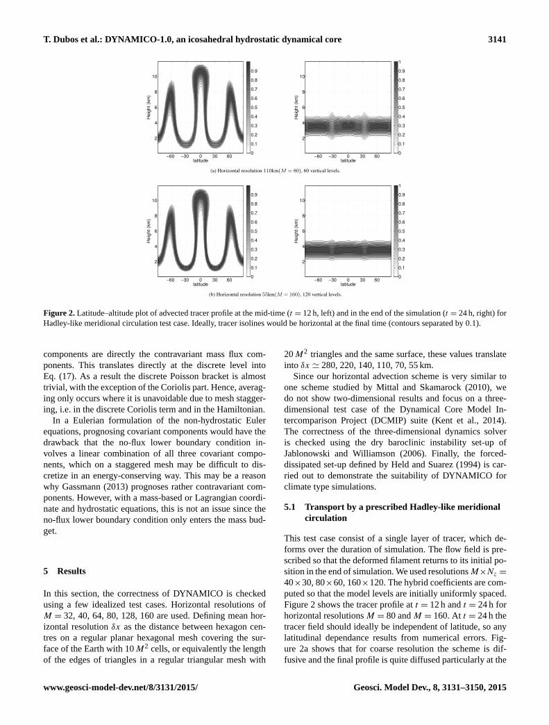
Figure 2. Latitude–altitude plot of advected tracer profile at the mid-time (t = 12 h, left) and in the end of the simulation (t = 24 h, right) for

Hadley-like meridional circulation test case. Ideally, tracer isolines would be horizontal at the final time (contours separated by 0.1).

components are directly the contravariant mass flux com-

ponents. This translates directly at the discrete level into

Eq. (17). As a result the discrete Poisson bracket is almost

trivial, with the exception of the Coriolis part. Hence, averag-

ing only occurs where it is unavoidable due to mesh stagger-

ing, i.e. in the discrete Coriolis term and in the Hamiltonian.

In a Eulerian formulation of the non-hydrostatic Euler

equations, prognosing covariant components would have the

drawback that the no-flux lower boundary condition in-

volves a linear combination of all three covariant compo-

nents, which on a staggered mesh may be difficult to dis-

cretize in an energy-conserving way. This may be a reason

why Gassmann (2013) prognoses rather contravariant com-

ponents. However, with a mass-based or Lagrangian coordi-

nate and hydrostatic equations, this is not an issue since the

no-flux lower boundary condition only enters the mass bud-

get.

5 Results

In this section, the correctness of DYNAMICO is checked

using a few idealized test cases. Horizontal resolutions of

M = 32, 40, 64, 80, 128, 160 are used. Defining mean hor-

izontal resolution δx as the distance between hexagon cen-

tres on a regular planar hexagonal mesh covering the sur-

face of the Earth with 10M2 cells, or equivalently the length

of the edges of triangles in a regular triangular mesh with

20M2 triangles and the same surface, these values translate

into δx ' 280, 220, 140, 110, 70, 55 km.

Since our horizontal advection scheme is very similar to

one scheme studied by Mittal and Skamarock (2010), we

do not show two-dimensional results and focus on a three-

dimensional test case of the Dynamical Core Model In-

tercomparison Project (DCMIP) suite (Kent et al., 2014).

The correctness of the three-dimensional dynamics solver

is checked using the dry baroclinic instability set-up of

Jablonowski and Williamson (2006). Finally, the forced-

dissipated set-up defined by Held and Suarez (1994) is car-

ried out to demonstrate the suitability of DYNAMICO for

climate type simulations.

5.1 Transport by a prescribed Hadley-like meridional

circulation

This test case consist of a single layer of tracer, which de-

forms over the duration of simulation. The flow field is pre-

scribed so that the deformed filament returns to its initial po-

sition in the end of simulation. We used resolutionsM×Nz =

40×30, 80×60, 160×120. The hybrid coefficients are com-

puted so that the model levels are initially uniformly spaced.

Figure 2 shows the tracer profile at t = 12 h and t = 24 h for

horizontal resolutionsM = 80 andM = 160. At t = 24 h the

tracer field should ideally be independent of latitude, so any

latitudinal dependance results from numerical errors. Fig-

ure 2a shows that for coarse resolution the scheme is dif-

fusive and the final profile is quite diffused particularly at the



Table 1. Global error norms for Hadley-like meridional circu-

lation test case. Horizontal resolution is defined as 2R where

3√

3/2 10M2R2= 4πa2 is the radius of the 10M2 perfect and

identical hexagons that would be needed to cover the surface 4πa2.

M Resolution Nz l1 l2 l∞

40 220 km 30 0.7085 0.529 0.600

80 110 km 60 0.3136 0.285 0.4035

160 55 km 120 5.39× 10−2 7.01× 10−2 0.1705

downward bending points. Figure 2b show that the increas-

ing resolution decreases the diffusive nature of the advection

scheme. Moreover, the slope limiter successfully avoids the

generation of spurious oscillations in the numerical solution.

Table 1 shows the global error norms for different horizontal

and vertical resolutions.

As expected from two-dimensional test cases (Lauritzen

et al., 2014b), our transport scheme is more diffusive than

finite-volume schemes on essentially Cartesian meshes such

as those presented in Kent et al. (2014). Sample solutions

(their Fig. 6) and error norms (their Table 6) they present in-

dicate that our scheme achieves, at resolution δx, an accuracy

similar to these schemes at resolution 2δx.

5.2 Baroclinic instability

The baroclinic instability benchmark of Jablonowski and

Williamson (2006) is extensively used to test the response of

three-dimensional atmospheric models to a controlled, evolv-

ing instability. The initial state for this test case is the sum of

a steady-state, baroclinically unstable, zonally symmetric so-

lution of the hydrostatic primitive equation and of a localized

zonal wind perturbation triggering the instability in a deter-

ministic and reproducible manner.

Even without the overlaid zonal wind perturbation, the ini-

tial state would not be perfectly zonally symmetric because

the icosahedral grid, as other quasi-uniform grids, is not zon-

ally symmetric. Therefore, the initial state possesses, in ad-

dition to the explicit perturbation, numerical deviations from

zonal symmetry. This initial error, as well as truncation er-

rors made at each time step by the numerical scheme, is not

homogeneous but reflects the non-homogeneity of the grid.

It nevertheless has the same symmetry as the grid, here wave

number 5 symmetry. Due to the dynamical instability of the

initial flow, the initial error is expected to trigger a wave num-

ber 5 mode of instability (provided such an unstable mode

with that zonal wave number exists). Depending on the am-

plitude of the initial truncation error, this mode can become

visible, a case of grid imprinting (Lauritzen et al., 2010).

Figure 3 presents results obtained at resolutions M = 32,

64, 128 (mean resolution 280, 140, 70 km) using 30 hybrid

vertical levels and fourth-order filters (p = 2 in Eqs. 27, 28).

Dissipation time and time step are set to τ = 6, 3, 1.5 h and

δt = 600, 300, 150 s, respectively. The right column shows

120 180 240 300 360−90

−60

−30

0

30

60

90

920

940

960

980

1000

120 180 240 300 360−90

−60

−30

0

30

60

90

920

940

960

980

1000

120 180 240 300 360−90

−60

−30

0

30

60

90

920

940

960

980

1000

60 120 180 240 300−90

−60

−30

0

30

60

90

240

260

280

300

60 120 180 240 300−90

−60

−30

0

30

60

90

240

260

280

300

60 120 180 240 300−90

−60

−30

0

30

60

90

240

260

280

300

Figure 3. Dry baroclinic instability test case (Jablonowski and

Williamson, 2006). (Left) surface pressure in hPa at day 12 (con-

tours separated by 10 hPa). (Right) temperature in K at day 9 (con-

tours separated by 10 K) and 850 hPa. Resolution increases from top

to bottom rows: 280 km, M = 32 (top), 140 km, M = 64 (middle),

70 km, M = 128 (bottom).

the temperature field at pressure level 850 hPa at day 9. At

this day the baroclinic wave is well developed. The wave

crest is reasonably sharp at M = 32, and becomes sharper at

a higher resolution. The simulated temperature field is quali-

tatively similar to those obtained at comparable resolutions

by other models (e.g. Jablonowski and Williamson, 2006,

Figs. 6, 7).

The left column shows surface pressure at day 12, after

the baroclinic wave has broken, letting time for grid im-

printing to develop. Grid imprinting in the Southern Hemi-

sphere, measured quantitatively as in Lauritzen et al. (2010)

as the root mean square departure of surface pressure from

its unperturbed value of 1000 hPa, exceeds 0.5 hPa at day 9

at M = 32, at day 11 at M = 64 and at day 13 at M = 128.

Comparing with Fig. 12 of Lauritzen et al. (2010), these val-

ues are in the low end of icosahedral models.

5.3 Thermally forced idealized general circulation

Held and Suarez (1994) propose a benchmark to evalu-

ate the statistically steady states produced by the dynam-

ical cores used in climate models. Detailed radiative, tur-

bulence and moist convective parametrization are replaced

with very simple forcing and dissipation. The simple forc-

ing and dissipation are designed in terms of a simple relax-

ation of the temperature field to a zonally symmetric state

and Rayleigh damping of low-level winds to represent the



Figure 4. Time-zonal statistics of Held and Suarez (1994) exper-

iment at resolution 280 km (M = 32) with dissipation time τ =

6 h. Contour intervals are 5 m s−1 (zonal wind), 10 K (tempera-

ture), 20 m2 s−2 (eddy momentum flux), 5 K m s−1 (eddy heat flux),

40 m2 s−2 (eddy kinetic energy) and 5 K2 (temperature variance).

boundary-layer friction. We use 19 hybrid vertical levels and

fourth-order filters (p = 2 in Eqs. 27, 28) at resolutions 280

and 140 km (M = 32, 64). Statistics are computed over the

last 1000 days excluding the initial 200 days, left for spin-

up time of the model. Temporal statistics are computed from

daily samples on the native grid at constant model level, then

interpolated to a lat–long mesh and zonally averaged.

Figure 4 presents statistics obtained when using horizontal

resolution of 280 km (M = 32) and dissipation time τ = 6 h.

The model is stable for longer dissipation times (τ = 24 h)

but smaller values produce smoother fields. Statistics ob-

tained at resolution 140 km (M = 64) with τ = 3 h are pre-

sented in Fig. 5. First-order statistics (panels ab) are close

to those presented in Held and Suarez (1994) and present

very little sensitivity to resolution. Second-order statistics

are slightly more sensitive to resolution and increase slightly

fromM = 32 toM = 64. Temperature variance atM = 64 is

close to that presented in Held and Suarez (1994) and slightly

smaller than that obtained by Wan et al. (2013) on a triangu-

lar icosahedral grid at comparable resolution R2B5.

Figure 5. Time-zonal statistics of Held and Suarez (1994) experi-

ment at resolution 140 km (M = 64) with dissipation time τ = 3 h.

Contour intervals as in Fig. 4.

6 Conclusions

6.1 Contributions

A number of building blocks of DYNAMICO are either di-

rectly found in the literature or are adaptations of standard

methods: explicit Runge–Kutta time stepping, mimetic hori-

zontal finite-difference operators (Bonaventura and Ringler,

2005; Thuburn et al., 2009; Ringler et al., 2010), piecewise-

linear slope-limited finite-volume reconstruction (Dukowicz

and Kodis, 1987; Tomita et al., 2001), swept-area calculation

of scalar fluxes (Miura, 2007), and directionally split time

integration of three-dimensional transport (e.g. Hourdin and

Armengaud, 1999). It is therefore useful to highlight the two

specific contributions brought forward, in our opinion, in the

design of DYNAMICO, and that can be of broader applica-

bility for model design.

The first contribution is to separate kinematics from dy-

namics as strictly as possible. This separation means that

the transport equations for mass, scalars and entropy use no

information regarding the specific momentum equation be-

ing solved. This includes the equation of state as well as

any metric information, which is factored into the prognosed



degrees of freedom and into the quantities derived from

them (especially the mass flux). Metric information is not

used to prognose tracer, mass and potential temperature. It

is confined in a few operations computing the mass flux,

Bernoulli function and Exner function from the prognostic

variables. This formulation is in line with more general lines

of thought known as physics-preserving discretizations (Ko-

ren et al., 2014) and discrete differential geometry (Thuburn

and Cotter, 2012). Similarly, while we use the exact same hy-

brid vertical coordinate as most hydrostatic primitive equa-

tion models, we insist that it should be considered as mass

based rather than pressure based. Indeed, the coincidence (up

to time-independent multiplicative and additive factors) of

mass and pressure is a peculiarity of the traditional shallow-

atmosphere hydrostatic equations with a pressure top bound-

ary condition. Recognizing the fundamentally kinematic def-

inition of the hybrid coordinate in terms of mass rather than

pressure emphasizes its relevance for solving other equation

sets, especially non-hydrostatic (Laprise, 1992).

The second contribution is to combine this kinematics–

dynamics separation with a Hamiltonian formulation of the

equations of motion to achieve energetic consistency. This

approach extends the work of Gassmann (2013) to hydro-

static equations of motion and non-Eulerian vertical coor-

dinates. This extension relies itself on a recent correspond-

ing extension of the Hamiltonian theory of atmospheric fluid

motion (Tort and Dubos, 2014b; Dubos and Tort, 2014).

The Hamiltonian approach further confines the equation-

dependent parts of the numerical scheme to a single quan-

tity, the total energy of the system expressed in terms of the

prognostic variables and, in the case of hydrostatic equations,

geopotential. The latter is a pseudo-prognostic variable that

is an argument of the Hamiltonian but is diagnosed at each

time step by enforcing the hydrostatic constraint, found to be

simply the condition that the derivatives of the Hamiltonian

with respect to geopotential degrees of freedom vanish. This

variational formulation of hydrostatic balance was first iden-

tified in the context of the deep-atmosphere quasi-hydrostatic

equations (Tort et al., 2014b) then generalized (Dubos and

Tort, 2014) and applied to DYNAMICO within the shallow-

atmosphere approximation. Ultimately, the choice of a spe-

cific equation set boils down to choosing and discretizing the

Hamiltonian, without changing the general structure of the

algorithm computing the tendencies.

These two advances yield our design goals: consistency

and versatility. The desired ability to solve different equation

sets is currently limited to the hydrostatic primitive equations

and the multi-layer Saint-Venant or Ripa equations, but little

work is required to solve other similar equations like the re-

cently derived non-traditional spherical shallow-water equa-

tions (Tort et al., 2014a). Whichever set of equations needs

to be solved in the future, including the fully compressible

Euler equations, energetic consistency is guaranteed if the

general approach followed here and in Tort et al. (2014b) is

applied. Furthermore, this approach is not limited to finite-

difference schemes but can be extended to finite element

schemes.

We would also like to emphasize what the Hamiltonian

approach does not achieve. Good numerical dispersion cru-

cially depends on grid staggering (for finite differences) or on

the finite element spaces used to represent the various quan-

tities. It is entirely possible to design an energy-conserving

schemes with disastrous numerical dispersion properties.

Other properties, such as exact geostrophic equilibria or a

discrete potential vorticity budget, come in addition to the

antisymmetry of the discrete Poisson bracket, as discussed

in Sect. 4 (see also Cotter and Thuburn, 2014). However,

the Hamiltonian formulation provides a divide-and-conquer

strategy by allowing for the easy transfer of these additional

properties to new sets of equations once they have been ob-

tained for a specific one.

6.2 Outlook for DYNAMICO

A Lagrangian vertical coordinate is currently available as an

option. In the absence of the vertical remapping that must

necessarily take place occasionally in order to prevent La-

grangian surfaces to fold or cross each other, this option can

not be used over meaningful time intervals. However, it is

convenient for development purposes since it allows one to

investigate separately issues related to the vertical and hori-

zontal discretizations. Nevertheless, a future implementation

of vertical remapping would be a useful addition. There is

room for improvement on other points. In particular, it may

be worth improving the accuracy of the transport scheme, es-

pecially for water vapour and other chemically or radiatively

active species. Regarding potential temperature, Skamarock

and Gassmann (2011) have found that a third-order trans-

port scheme for the potential temperature could significantly

reduce phase errors in the propagation of baroclinic waves.

Whether more accurate transport of potential temperature is

beneficial for climate modelling remains to be determined.

The Hamiltonian framework leaves a complete freedom

with respect to the choice of a discrete Hamiltonian. Here

the simplest possible second-order accurate approximation

is used, but other forms may yield additional properties, such

as a more accurate computation of the geopotential. Ongo-

ing work suggests that it is possible to design a Hamiltonian

such that certain hydrostatic equilibria are exactly preserved

in the presence of arbitrary topography. Such a property is

sometimes achieved by finite-volume schemes (Botta et al.,

2004; Audusse et al., 2004), and its absence is one manifes-

tation of the so-called pressure-gradient force error (Gary,

1973).

DYNAMICO is stabilized by (bi)harmonic operators of

which we refer as filters rather than dissipation. Indeed, they

are numerical devices aimed at stabilizing the model rather

than physically based turbulence models such as nonlinear

viscosity (Smagorinsky, 1963). Turbulence models induce a

well-defined dissipation rate of resolved kinetic energy that



should enter as a positive source term in the entropy budget

in order to close the energy budget. Emulating this process

in a discrete model can however prove difficult (Gassmann,

2013). Indeed, in order to convert into heat the kinetic energy

destroyed by filters, one needs to recast their contribution to

the energy budget as a positive-definite sum. Whether this

can be done in DYNAMICO is left for future investigation.

Coupling DYNAMICO to the LMD-Z terrestrial physics

package suite is ongoing. For planetary applications, it will

be important to also check the discrete angular momentum

budget (Lebonnois et al., 2012; Lauritzen et al., 2014a).

In the near future DYNAMICO should become able to

solve richer, quasi-hydrostatic equations (White and Brom-

ley, 1995; Tort and Dubos, 2014a) and to take into account

deviations of the geopotential from spherical geometry (Tort

and Dubos, 2014b). Extension to fully compressible Euler

equations is the next step and should leave its general struc-

ture unchanged (Dubos and Tort, 2014).



Appendix A: Mesh generation and smoothing

Among various possible ways of generating the triangular

mesh, we follow the method of Sadourny et al. (1968). Start-

ing from a spherical icosahedron made of 20 equal spheri-

cal triangles, edges are divided into equal M geodesic arcs,

then the arcs joining the newly generated vertices are divided

equally. The number of total grid points for resolution M is

N = 10M2+ 2.

The hexagonal mesh is constructed as the Voronoi diagram

of the triangular mesh (Augenbaum and Peskin, 1985). This

ensures that primal and dual edges are orthogonal, a require-

ment of the numerical scheme. The edge between control

volumes Vi and Vj is a geodesic arc equidistant from Gi and

Gj . A corner P of a Voronoi cell is shared by three Voronoi

cells and is hence equidistant from all three associated gen-

erators Gi , Gj and Gk .

Numerical errors can be reduced by various optimization

methods (e.g. Miura and Kimoto, 2005). We use Lloyd’s iter-

ative algorithm (Du et al., 1999), a fixed-point iteration aimed

at letting generators and centroids Ci of control volumes co-

incide:

Ci =

∫Vi

x dA∥∥∥∫Vix dA

∥∥∥ . (A1)

The optimization process is efficient for coarse grids but

tends to stagnate at high grid resolution (Du et al., 2006).

Therefore, we simply stop the optimization process after a

fixed user-defined number iterations. Optimization is per-

formed only once during the grid generation and even a few

thousand iterations are computationally not very costly.

Appendix B: Accurate and stable spherical primitives

Although round-off errors may not be an urgent concern with

double-precision computations at presently common resolu-

tions, it may become if formulae with high round-off error

are used in sequence, if single precision is used for speed, or

at high resolutions. In this Appendix we describe geometric

primitives that are not sensitive to round-off error, or more

precisely that are not more sensitive to round-off errors than

equivalent planar primitives. These primitives are required

in the grid generation and optimization process and compute

centroids, circumcenters and spherical areas.

Let Gi , Gj and Gk be generators in anti-clockwise or-

der. The sides of spherical triangle GiGjGj are O(h) with

h∼ 1/M small and the vectors Gi , Gj and Gk are known

up to a round-off error ε. The circumcenter p is a unit

vector equidistant from each generator. Using the fact that

Gi,GjGk,p have unit norm and some algebra yields the

system:

10−7

10−6

10−5

10−4

10−3

10−2

10−1

100

10−16

10−14

10−12

10−10

10−8

10−6

grid size

Err

Direct Formula

Stable Formula

Figure B1. Error in circumcenter calculation using direct for-

mula (B2) and stable formula (B3). For a given value of the grid

size h, the triangle is defined by three points on the unit sphere

a,b/‖b‖ ,c/‖c‖ where b = a+ hb,c = a+ hc and b, c are random

vectors whose Cartesian components are statistically independent,

centred, Gaussian random variables with unit variance. For each h,

100 b, c are generated and the largest error is reported.

p ·p = 1, (Gj −Gi) ·p = (Gk −Gi) ·p (B1)

= (Gj −Gk) ·p = 0.

A solution of Eq. (B1) is given by

p =p1∥∥p1

∥∥ where p1 = (Gi −Gj )× (Gi −Gk), (B2)

used for instance by Miura and Kimoto (2005). Due to finite

precision the computation of (Gi −Gj )× (Gi −Gk) has an

error O(εh). Furthermore, p1 is O(h2). Therefore, Eq. (B2)

yields p with an error that isO(ε/h). In order to avoid divid-

ing by the small factor∥∥p1

∥∥, we take advantage of the fact p

is close to Gi . Hence, it is better to solve for p−Gi , which

yields

p =p2∥∥p2

∥∥ where p2−Gi =p1

2p1 ·p1

(B3)

×

(‖Gj −Gi‖

2(Gi −Gk)+‖Gk −Gi‖2(Gj −Gi)

).

Each input to p2−Gi has a relative errorO(ε/h) and p2−Gi

itself is O(h), yielding an overall absolute error O(ε). Now

p2 is O(1) and known within O(ε), hence p as well. In or-

der to check the accuracy of formulae (B2), (B3) we present

in Fig. B1 Err=maxl,m=i,j,k∥∥(p−Gl)

2− (p−Gm)

2∥∥ for

a random set of spherical triangular cells of decreasing size.

With the direct formula (B2) Err increases as the trian-

gle size decreases (as predicted by the scaling Err∼ ε/h),



demonstrating the sensitivity of Eq. (B2) to round-off error.

Equation (B2) becomes useless when h∼ ε/h, which would

happen with single-precision calculations at resolutions of

about 1/1000 the planetary radius, i.e. 6 km on Earth. Con-

versely, Eq. (B3) is stable and determines the position of p

within round-off error.

Regarding the spherical centre of mass (Eq. A1), an ex-

act Gauss formula exists for polygonal control volumes (not

shown). Again this formula has large cancellation errors and

yields Ci with a round-off error O(ε/h). For a spherical

triangle, the planar centre of mass (equal-weight barycen-

tre) projected onto the unit sphere yields a third-order ac-

curate estimate of the true centre of mass. Therefore, sub-

dividing a polygon into spherical triangles and forming an

area-weighted sum of their barycentres yields a second-order

accurate estimate of Ci . This accuracy is sufficient for our

purposes. An accurate and stable alternative is to decom-

pose polygons into triangles and quadrangles, map the unit

square to a spherical quadrangle or triangle and use high-

order Gauss–Legendre quadrature to evaluate Eq. (A1).

Finally, computing the area A of a spherical polygon

should not be done using the simple but again unstable de-

fect formula. Instead we decompose polygons into triangles

and use l’Huillier formula:

tanA

4=

√tan

s

2tan

s− a

2tan

s− b

2tan

s− c

2, (B4)

where A is the desired triangular area, 2s = a+ b+ c and

a,b,c are the geodesic lengths of the sides of the triangle,

computed as dist(p,q)= sin−1‖p× q‖. Formula (B4) re-

duces for small triangles to the planar Henon formula, which

demonstrates its stability.



Code availability

Results presented in this article are based on release r339

of DYNAMICO. Instructions to download, compile, and run

the code are provided at http://forge.ipsl.jussieu.fr/dynamico/

wiki. DYNAMICO is licensed under the terms of the Ce-

CILL open-source license.

Acknowledgements. The authors would like to thank two anony-

mous referees for their detailed and constructive criticism. S. Dubey

has benefitted from the support of the Indo-French Centre for

the Promotion of Advanced Research (IFCPRA/CEFIPRA) under

the sponsored project number 4107-1. T. Dubos, Y. Meurdesoif

and F. Hourdin acknowledge the support of the French Agence

Nationale de la Recherche (ANR) under reference ANR-14-CE23-

0010-01.

Edited by: A. Sandu

References

Arakawa, A.: Computational design for long-term numerical inte-

gration of the equations of fluid motion: Two-dimensional in-

compressible flow. Part I, J. Comput. Phys, 1, 119–143, 1966.

Arakawa, A. and Lamb, V. R.: A Potential Enstrophy and En-

ergy Conserving Scheme for the Shallow Water Equations, Mon.

Weather Rev., 109, 18–36, 1981.

Arnold, V. I.: Conditions for non-linear stability of plane steady

curvilinear flows of an ideal fluid, Dokl. Akad. Nauk Sssr, 162,

773–777, 1965.

Audusse, E., Bouchut, F., Bristeau, M.-O., Klein, R., and Perthame,

B.: A Fast and Stable Well-Balanced Scheme with Hydrostatic

Reconstruction for Shallow Water Flows, SIAM J. Sci. Comput.,

25, 2050–2065, 2004.

Augenbaum, J. M. and Peskin, C. S.: On the construction of the

Voronoi mesh on a sphere, J. Comput. Phys, 59, 177–192, 1985.

Bokhove, O.: Eulerian Variational Principles for Stratified Hydro-

static Equations, J. Atmos. Sci, 59, 1619–1628, 2002.

Bonaventura, L. and Ringler, T.: Analysis of Discrete Shallow-

Water Models on Geodesic Delaunay Grids with C-Type Stag-

gering, Mon. Weather Rev., 133, 2351–2373, 2005.

Botta, N., Klein, R., Langenberg, S., and Lützenkirchen, S.: Well

balanced finite volume methods for nearly hydrostatic flows, J.

Comput. Phys, 196, 539–565, 2004.

Cotter, C. J. and Thuburn, J.: A finite element exterior calculus

framework for the rotating shallow-water equations, J. Comput.

Phys, 257, 1506–1526, 2014.

Du, Q., Faber, V., and Gunzburger, M.: Centroidal Voronoi Tessel-

lations: Applications and Algorithms, SIAM Rev., 41, 637–676,

1999.

Du, Q., Emelianenko, M., and Ju, L.: Convergence of the Lloyd Al-

gorithm for Computing Centroidal Voronoi Tessellations, SIAM

J. Numer. Anal., 44, 102–119, 2006.

Dubey, S., Dubos, T., Hourdin, F., and Upadhyaya, H. C.:

On the inter-comparison of two tracer transport schemes

on icosahedal grids, Appl. Math. Model., 39, 4828–4847,

doi:10.1016/j.apm.2015.04.015, 2015.

Dubos, T. and Tort, M.: Equations of Atmospheric Motion in Non-

Eulerian Vertical Coordinates: Vector-Invariant Form and Quasi-

Hamiltonian Formulation, Mon. Weather Rev., 142, 3860–3880,

2014.

Dukowicz, J. K. and Kodis, J. W.: Accurate Conservative Remap-

ping (Rezoning) for Arbitrary Lagrangian-Eulerian Computa-

tions, SIAM J. Sci. Stat. Comp., 8, 305–321, 1987.

Easter, R. C.: Two Modified Versions of Bott’s Positive-Definite

Numerical Advection Scheme, Mon. Weather Rev., 121, 297–

304, 1993.

Gary, J. M.: Estimate of Truncation Error in Transformed Coordi-

nate, Primitive Equation Atmospheric Models, J. Atmos. Sci., 30,

223–233, 1973.

Gassmann, A.: Inspection of hexagonal and triangular C-grid dis-

cretizations of the shallow water equations, J. Comput. Phys,

230, 2706–2721, 2011.

Gassmann, A.: A global hexagonal C-grid non-hydrostatic dynam-

ical core (ICON-IAP) designed for energetic consistency, Q. J.

Roy. Meteor. Soc., 139, 152–175, 2013.

Held, I. M. and Suarez, M. J.: A Proposal for the Intercomparison of

the Dynamical Cores of Atmospheric General Circulation Mod-

els, B. Am. Meteorol. Soc., 75, 1825–1830, 1994.

Holm, D. D., Marsden, J. E., and Ratiu, T. S.: The Euler-Poincaré

Equations in Geophysical Fluid Dynamics, 251–299, Cambridge

University Press, Cambridge, 2002.

Hourdin, F.: Transport de l’énergie dans le modèle du LMD,

internal report, IPSL, available at: http://lmdz.lmd.jussieu.

fr/developpeurs/notes-techniques/ressources/energy.pdf (last ac-

cess: 5 October 2015) 1994.

Hourdin, F. and Armengaud, A.: The Use of Finite-Volume Meth-

ods for Atmospheric Advection of Trace Species. Part I: Test

of Various Formulations in a General Circulation Model, Mon.

Weather Rev., 127, 822–837, 1999.

Hourdin, F., Grandpeix, J.-Y., Rio, C., Bony, S., Jam, A., Cheruy, F.,

Rochetin, N., Fairhead, L., Idelkadi, A., Musat, I., Dufresne, J.-

L., Lahellec, A., Lefebvre, M.-P., and Roehrig, R.: LMDZ5B: the

atmospheric component of the IPSL climate model with revisited

parameterizations for clouds and convection, Clim. Dynam., 40,

2193–2222, 2013.

Jablonowski, C. and Williamson, D. L.: A baroclinic instability test

case for atmospheric model dynamical cores, Q. J. Roy. Meteor.

Soc., 132, 2943–2975, 2006.

Jiménez, J.: Hyperviscous vortices, J. Fluid Mech., 279, 169–176,

2006.

Kent, J., Ullrich, P. A., and Jablonowski, C.: Dynamical core model

intercomparison project: Tracer transport test cases, Q. J. Roy.

Meteor. Soc., 140, 1279–1293, 2014.

Kinnmark, I. P. E. and Gray, W. G.: One step integration methods of

third-fourth order accuracy with large hyperbolic stability limits,

Math. Comput. Simulat., 26, 181–188, 1984a.

Kinnmark, I. P. E. and Gray, W. G.: One step integration methods

with maximum stability regions, Math. Comput. Simulat., 26,

87–92, 1984b.

Koren, B., Abgrall, R., Bochev, P., Frank, J., and Perot, B.: Physics-

compatible numerical methods, J. Comput. Phys., 257, 1039,

doi:10.1016/j.jcp.2013.10.015, 2014.

Laprise, R.: The Euler Equations of Motion with Hydrostatic Pres-

sure as an Independent Variable, Mon. Weather Rev., 120, 197–

207, 1992.


http://forge.ipsl.jussieu.fr/dynamico/wiki

http://forge.ipsl.jussieu.fr/dynamico/wiki

http://dx.doi.org/10.1016/j.apm.2015.04.015

http://lmdz.lmd.jussieu.fr/developpeurs/notes-techniques/ressources/energy.pdf

http://lmdz.lmd.jussieu.fr/developpeurs/notes-techniques/ressources/energy.pdf

http://dx.doi.org/10.1016/j.jcp.2013.10.015


Lauritzen, P. H., Jablonowski, C., Taylor, M. A., and Nair, R. D.:

Rotated Versions of the Jablonowski Steady-State and Baroclinic

Wave Test Cases: A Dynamical Core Intercomparison, J. Adv.

Model. Earth Syst., 2, 15, doi:10.3894/james.2010.2.15, 2010.

Lauritzen, P. H., Skamarock, W. C., Prather, M. J., and Tay-

lor, M. A.: A standard test case suite for two-dimensional lin-

ear transport on the sphere, Geosci. Model Dev., 5, 887–901,

doi:10.5194/gmd-5-887-2012, 2012.

Lauritzen, P. H., Bacmeister, J. T., Dubos, T., Lebonnois, S., and

Taylor, M. A.: Held-Suarez simulations with the Community At-

mosphere Model Spectral Element (CAM-SE) dynamical core:

A global axial angular momentum analysis using Eulerian and

floating Lagrangian vertical coordinates, J. Adv. Model. Earth

Syst., 6, 129–140, 2014a.

Lauritzen, P. H., Ullrich, P. A., Jablonowski, C., Bosler, P. A., Cal-

houn, D., Conley, A. J., Enomoto, T., Dong, L., Dubey, S., Guba,

O., Hansen, A. B., Kaas, E., Kent, J., Lamarque, J.-F., Prather,

M. J., Reinert, D., Shashkin, V. V., Skamarock, W. C., Sørensen,

B., Taylor, M. A., and Tolstykh, M. A.: A standard test case suite

for two-dimensional linear transport on the sphere: results from

a collection of state-of-the-art schemes, Geosci. Model Dev., 7,

105–145, doi:10.5194/gmd-7-105-2014, 2014b.

Lebonnois, S., Hourdin, F., Eymet, V., Crespin, A., Fournier, R., and

Forget, F.: Superrotation of Venus’ atmosphere analyzed with a

full general circulation model, J. Geophys. Res., 115, E06006,

doi:10.1029/2009je003458, 2010.

Lebonnois, S., Covey, C., Grossman, A., Parish, H., Schubert, G.,

Walterscheid, R., Lauritzen, P., and Jablonowski, C.: Angular

momentum budget in General Circulation Models of superrotat-

ing atmospheres: A critical diagnostic, J. Geophys. Res., 117,

doi:10.1029/2012je004223, 2012.

Mittal, R. and Skamarock, W. C.: Monotonic Limiters for a Second-

Order Finite-Volume Advection Scheme Using Icosahedral-

Hexagonal Meshes, Mon. Weather Rev., 138, 4523–4527, 2010.

Miura, H.: An Upwind-Biased Conservative Advection Scheme for

Spherical Hexagonal-Pentagonal Grids, Mon. Weather Rev., 135,

4038–4044, 2007.

Miura, H. and Kimoto, M.: A Comparison of Grid Quality of Op-

timized Spherical Hexagonal-Pentagonal Geodesic Grids, Mon.

Weather Rev., 133, 2817–2833, 2005.

Ringler, T. D., Thuburn, J., Klemp, J. B., and Skamarock, W. C.:

A unified approach to energy conservation and potential vortic-

ity dynamics for arbitrarily-structured C-grids, J. Comput. Phys,

229, 3065–3090, 2010.

Ripa, P.: Conservation laws for primitive equations models with

inhomogeneous layers, Geophys. Astrophys. Fluid, 70, 85–111,

1993.

Rípodas, P., Gassmann, A., Förstner, J., Majewski, D., Giorgetta,

M., Korn, P., Kornblueh, L., Wan, H., Zängl, G., Bonaventura, L.,

and Heinze, T.: Icosahedral Shallow Water Model (ICOSWM):

results of shallow water test cases and sensitivity to model pa-

rameters, Geosci. Model Dev., 2, 231–251, doi:10.5194/gmd-2-

231-2009, 2009.

Sadourny, R.: Conservative Finite-Difference Approximations of

the Primitive Equations on Quasi-Uniform Spherical Grids, Mon.

Weather Rev., 100, 136–144, 1972.

Sadourny, R.: The Dynamics of Finite-Difference Models of the

Shallow-Water Equations, J. Atmos. Sci, 32, 680–689, 1975a.

Sadourny, R.: Compressible Model Flows on the Sphere, J. Atmos.

Sci, 32, 2103–2110, 1975b.

Sadourny, R., Arakawa, A. K. I. O., and Mintz, Y. A. L. E.: Inte-

gration of the nondivergent barotropic vorticity equation with an

icosahedral-hexagonal grid for the Sphere1, Mon. Weather Rev.,

96, 351–356, 1968.

Salmon, R.: Practical use of Hamilton’s principle, J. Fluid Mech.,

132, 431–444, 1983.

Salmon, R.: Poisson-Bracket Approach to the Construction of

Energy- and Potential-Enstrophy-Conserving Algorithms for the

Shallow-Water Equations, J. Atmos. Sci, 61, 2016–2036, 2004.

Satoh, M., Matsuno, T., Tomita, H., Miura, H., Nasuno, T., and Iga,

S.: Nonhydrostatic icosahedral atmospheric model (NICAM) for

global cloud resolving simulations, J. Comput. Phys., 227, 3486–

3514, 2008.

Simmons, A. J. and Burridge, D. M.: An Energy and Angular-

Momentum Conserving Vertical Finite-Difference Scheme and

Hybrid Vertical Coordinates, Mon. Weather Rev., 109, 758–766,

1981.

Skamarock, W. C. and Gassmann, A.: Conservative Transport

Schemes for Spherical Geodesic Grids: High-Order Flux Opera-

tors for ODE-Based Time Integration, Mon. Weather Rev., 139,

2962–2975, 2011.

Skamarock, W. C., Klemp, J. B., Duda, M. G., Fowler, L. D., Park,

S.-H., and Ringler, T. D.: A Multiscale Nonhydrostatic Atmo-

spheric Model Using Centroidal Voronoi Tesselations and C-

Grid Staggering, Mon. Weather Rev., 140, 120402131411002–

3105, doi:10.1175/mwr-d-11-00215.1, 2012.

Smagorinsky, J.: General circulation experiments with the primitive

equations: I. The basic experiment∗, Mon. Weather Rev., 91, 99–

164, 1963.

Taylor, M. A. and Fournier, A.: A compatible and conservative spec-

tral element method on unstructured grids, J. Comput. Phys, 229,

5879–5895, 2010.

Thuburn, J.: Numerical wave propagation on the hexagonal C-grid,

J. Comput. Phys., 227, 5836–5858, 2008.

Thuburn, J. and Cotter, C. J.: A Framework for Mimetic Dis-

cretization of the Rotating Shallow-Water Equations on Arbitrary

Polygonal Grids, SIAM J. Sci. Comput., 34, B203–B225, 2012.

Thuburn, J., Ringler, T. D., Skamarock, W. C., and Klemp, J. B.:

Numerical representation of geostrophic modes on arbitrarily

structured C-grids, J. Comput. Phys, 228, 8321–8335, 2009.

Thuburn, J., Cotter, C. J., and Dubos, T.: A mimetic, semi-implicit,

forward-in-time, finite volume shallow water model: compari-

son of hexagonal–icosahedral and cubed-sphere grids, Geosci.

Model Dev., 7, 909–929, doi:10.5194/gmd-7-909-2014, 2014.

Tomita, H., Tsugawa, M., Satoh, M., and Goto, K.: Shallow Water

Model on a Modified Icosahedral Geodesic Grid by Using Spring

Dynamics, J. Comput. Phys., 174, 579–613, 2001.

Tort, M. and Dubos, T.: Dynamically consistent shallow-

atmosphere equations with a complete Coriolis force, Q. J. Roy.

Meteor. Soc., 140, 2388–2392, 2014a.

Tort, M. and Dubos, T.: Usual Approximations to the Equations of

Atmospheric Motion: A Variational Perspective, J. Atmos. Sci,

71, 2452–2466, 2014b.

Tort, M., Dubos, T., Bouchut, F., and Zeitlin, V.: Consistent shallow-

water equations on the rotating sphere with complete Coriolis

force and topography, J. Fluid Mech., 748, 789–821, 2014a.


http://dx.doi.org/10.3894/james.2010.2.15

http://dx.doi.org/10.5194/gmd-5-887-2012


http://dx.doi.org/10.1029/2009je003458

http://dx.doi.org/10.1029/2012je004223



http://dx.doi.org/10.1175/mwr-d-11-00215.1



Tort, M., Dubos, T., and Melvin, T.: An Energy-conserving Quasi-

hydrostatic Deep-atmosphere Dynamical Core, Q. J. Roy. Me-

teor. Soc., accepted, 2014b.

Van Leer, B.: Towards the ultimate conservative difference scheme.

IV. A new approach to numerical convection, J. Comput. Phys,

23, 276–299, 1977.

Wan, H., Giorgetta, M. A., Zängl, G., Restelli, M., Majewski, D.,

Bonaventura, L., Fröhlich, K., Reinert, D., Rípodas, P., Korn-

blueh, L., and Förstner, J.: The ICON-1.2 hydrostatic atmo-

spheric dynamical core on triangular grids – Part 1: Formulation

and performance of the baseline version, Geosci. Model Dev., 6,

735–763, doi:10.5194/gmd-6-735-2013, 2013.

Weller, H., Thuburn, J., and Cotter, C. J.: Computational Modes and

Grid Imprinting on Five Quasi-Uniform Spherical C Grids, Mon.

Weather. Rev., 140, 2734–2755, 2012.

White, A. A. and Bromley, R. A.: Dynamically consistent, quasi-

hydrostatic equations for global models with a complete repre-

sentation of the Coriolis force, Q. J. Roy. Meteor. Soc., 121, 399–

418, 1995.

Williamson, D. L.: The Evolution of Dynamical Cores for Global

Atmospheric Models, J. Meteor. Soc. Jpn., 85B, 241–269, 2007.



DYNAMICO-1.0, an icosahedral hydrostatic dynamical core ...

Documents

Transcript of DYNAMICO-1.0, an icosahedral hydrostatic dynamical core ...