Dynamic Behaviour of Railway Bridges. Vehicles Lateral DynamicBehaviour

Rui F. Silva Dias a,b

aInstituto Superior Tecnico - UTL LisbonbComputational Mechanical Group of the Civil Engineering School of Madrid

Abstract

This paper describes the study of the influence of bridge lateral dynamic displacements in the lateral behaviour ofrailway vehicles when crossing the Arroyo las Piedras viaduct, located in the new high speed line between Cordobaand Malaga, in Spain. Several problems associated to this phenomenon are outlined: bridge lateral displacements,track irregularities and effects due to wheel-rail contact problems. Different vehicle models were developed and thedynamic analysis performed, considering the actions of those effects, in order to evaluate the safety and comfort limitsof the passengers.

Key words: Arroyo las Piedras viaduct, Lateral dynamic behaviour, Virtual path, Track irregularities, Klingel motioneffects, Fictitious vehicles

1. Introduction

Due to railway traffic, high-speed bridges areaffected by vertical loads and by longitudinal andtransversal horizontal forces. These transversal ho-rizontal forces are generated by lateral motions ofthe vehicles from two sources in a straight track:horizontal track irregularities and sinusoidal motionof conical wheels along cylindrical rail heads.

Measures and parametric studies performed bythe subcommittee ERRI D181, discussed in the re-port RP6 [4], and by subcommittee ERRI D214,discussed in the report RP5 [5], have shown thatthese effects play an important role in the phe-nomenon of bridge-train interaction, in which wereestablished some design recommendations in orderto cover these lateral effects. Subsequently, thoserequirements were adopted by the new engineeringcodes EN1991-2 [9], EN1990-A2 [8] and IAPF [6].

Email address: rui@mecanica.upm.es (Rui F. Silva Dias).

Usually, lateral vibrations in railway bridges doesnot affect the safety of the structure but can putin risk the comfort or the security of the passen-gers, due to train derailment. On the other hand,can contribute to an accelerated degradation of therailway, like ballast migration and instability, ortrack structural damage, which affects the stabilityof vehicles motion.

Additionally, lateral displacements in railwaybridges are caused by vertical loads due to railwaytraffic in bridges with double track, when theseloads act eccentrically. This phenomenon is relatedwith the torsional behaviour of the deck, causingthe piers to bend over laterally, displacing the deckin the lateral direction too. The local torsional ef-fects within spans, induced by the same verticalloads, also have a lateral component that increasethese displacements.

In this paper the study developed in order to eva-luate the level of vehicles lateral vibrations on theArroyo las Piedras viaduct [21], is described. Along

Preprint submitted to Instituto Superior Tecnico 26 November 2007

θ

δ1

Support Midspan

δ1 δ2

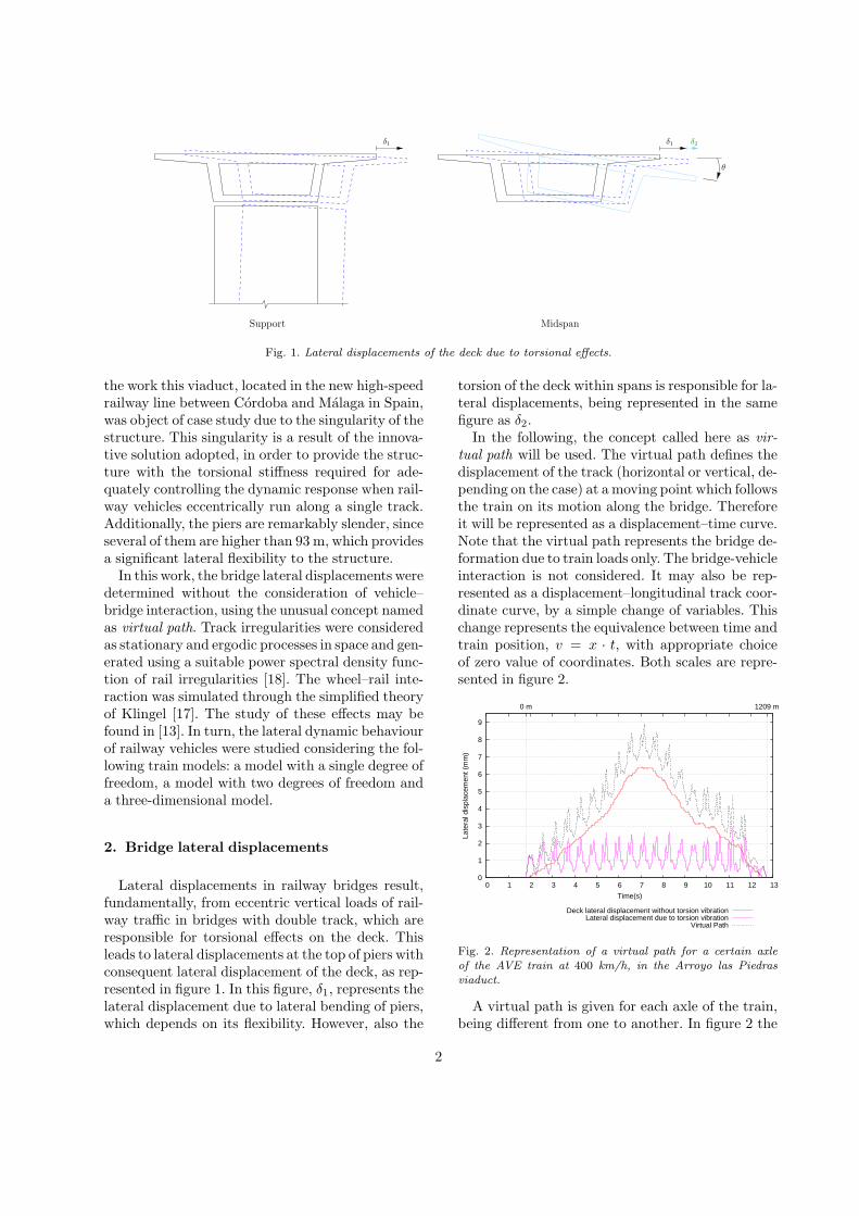
Fig. 1. Lateral displacements of the deck due to torsional effects.

the work this viaduct, located in the new high-speedrailway line between Cordoba and Malaga in Spain,was object of case study due to the singularity of thestructure. This singularity is a result of the innova-tive solution adopted, in order to provide the struc-ture with the torsional stiffness required for ade-quately controlling the dynamic response when rail-way vehicles eccentrically run along a single track.Additionally, the piers are remarkably slender, sinceseveral of them are higher than 93 m, which providesa significant lateral flexibility to the structure.

In this work, the bridge lateral displacements weredetermined without the consideration of vehicle–bridge interaction, using the unusual concept namedas virtual path. Track irregularities were consideredas stationary and ergodic processes in space and gen-erated using a suitable power spectral density func-tion of rail irregularities [18]. The wheel–rail inte-raction was simulated through the simplified theoryof Klingel [17]. The study of these effects may befound in [13]. In turn, the lateral dynamic behaviourof railway vehicles were studied considering the fol-lowing train models: a model with a single degree offreedom, a model with two degrees of freedom anda three-dimensional model.

2. Bridge lateral displacements

Lateral displacements in railway bridges result,fundamentally, from eccentric vertical loads of rail-way traffic in bridges with double track, which areresponsible for torsional effects on the deck. Thisleads to lateral displacements at the top of piers withconsequent lateral displacement of the deck, as rep-resented in figure 1. In this figure, δ1, represents thelateral displacement due to lateral bending of piers,which depends on its flexibility. However, also the

torsion of the deck within spans is responsible for la-teral displacements, being represented in the samefigure as δ2.

In the following, the concept called here as vir-tual path will be used. The virtual path defines thedisplacement of the track (horizontal or vertical, de-pending on the case) at a moving point which followsthe train on its motion along the bridge. Thereforeit will be represented as a displacement–time curve.Note that the virtual path represents the bridge de-formation due to train loads only. The bridge-vehicleinteraction is not considered. It may also be rep-resented as a displacement–longitudinal track coor-dinate curve, by a simple change of variables. Thischange represents the equivalence between time andtrain position, v = x · t, with appropriate choiceof zero value of coordinates. Both scales are repre-sented in figure 2.

0

1

2

3

4

5

6

7

8

9

0 1 2 3 4 5 6 7 8 9 10 11 12 13

1209 m0 m

Late

ral d

ispl

acem

ent (

mm

)

Time(s)

Deck lateral displacement without torsion vibrationLateral displacement due to torsion vibration

Virtual Path

Fig. 2. Representation of a virtual path for a certain axleof the AVE train at 400 km/h, in the Arroyo las Piedrasviaduct.

A virtual path is given for each axle of the train,being different from one to another. In figure 2 the

2

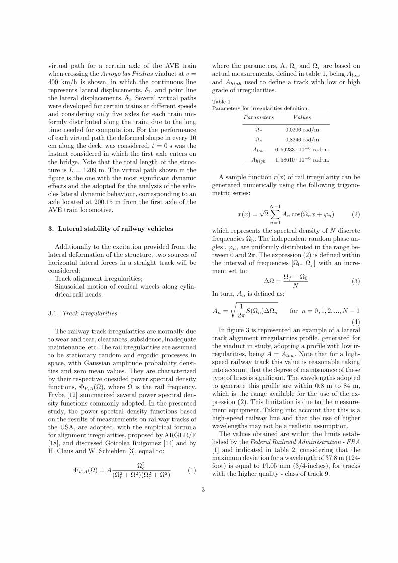
virtual path for a certain axle of the AVE trainwhen crossing the Arroyo las Piedras viaduct at v =400 km/h is shown, in which the continuous linerepresents lateral displacements, δ1, and point linethe lateral displacements, δ2. Several virtual pathswere developed for certain trains at different speedsand considering only five axles for each train uni-formly distributed along the train, due to the longtime needed for computation. For the performanceof each virtual path the deformed shape in every 10cm along the deck, was considered. t = 0 s was theinstant considered in which the first axle enters onthe bridge. Note that the total length of the struc-ture is L = 1209 m. The virtual path shown in thefigure is the one with the most significant dynamiceffects and the adopted for the analysis of the vehi-cles lateral dynamic behaviour, corresponding to anaxle located at 200.15 m from the first axle of theAVE train locomotive.

3. Lateral stability of railway vehicles

Additionally to the excitation provided from thelateral deformation of the structure, two sources ofhorizontal lateral forces in a straight track will beconsidered:– Track alignment irregularities;– Sinusoidal motion of conical wheels along cylin-

drical rail heads.

3.1. Track irregularities

The railway track irregularities are normally dueto wear and tear, clearances, subsidence, inadequatemaintenance, etc. The rail irregularities are assumedto be stationary random and ergodic processes inspace, with Gaussian amplitude probability densi-ties and zero mean values. They are characterizedby their respective onesided power spectral densityfunctions, ΦV,A(Ω), where Ω is the rail frequency.Fryba [12] summarized several power spectral den-sity functions commonly adopted. In the presentedstudy, the power spectral density functions basedon the results of measurements on railway tracks ofthe USA, are adopted, with the empirical formulafor alignment irregularities, proposed by ARGER/F[18], and discussed Goicolea Ruigomez [14] and byH. Claus and W. Schiehlen [3], equal to:

ΦV,A(Ω) = AΩ2

c

(Ω2r + Ω2)(Ω2

c + Ω2)(1)

where the parameters, A, Ωc and Ωr are based onactual measurements, defined in table 1, being Alow

and Ahigh used to define a track with low or highgrade of irregularities.

Table 1Parameters for irregularities definition.

Parameters V alues

Ωr 0,0206 rad/m

Ωc 0,8246 rad/m

Alow 0, 59233 · 10−6 rad·m,

Ahigh 1, 58610 · 10−6 rad·m.

A sample function r(x) of rail irregularity can begenerated numerically using the following trigono-metric series:

r(x) =√

2N−1∑n=0

An cos(Ωnx + ϕn) (2)

which represents the spectral density of N discretefrequencies Ωn. The independent random phase an-gles , ϕn, are uniformly distributed in the range be-tween 0 and 2π. The expression (2) is defined withinthe interval of frequencies [Ω0, Ωf ] with an incre-ment set to:

∆Ω =Ωf − Ω0

N(3)

In turn, An is defined as:

An =

√12π

S(Ωn)∆Ωn for n = 0, 1, 2, ..., N − 1

(4)In figure 3 is represented an example of a lateral

track alignment irregularities profile, generated forthe viaduct in study, adopting a profile with low ir-regularities, being A = Alow. Note that for a high-speed railway track this value is reasonable takinginto account that the degree of maintenance of thesetype of lines is significant. The wavelengths adoptedto generate this profile are within 0.8 m to 84 m,which is the range available for the use of the ex-pression (2). This limitation is due to the measure-ment equipment. Taking into account that this is ahigh-speed railway line and that the use of higherwavelengths may not be a realistic assumption.

The values obtained are within the limits estab-lished by the Federal Railroad Administration - FRA[1] and indicated in table 2, considering that themaximum deviation for a wavelength of 37.8 m (124-foot) is equal to 19.05 mm (3/4-inches), for trackswith the higher quality - class of track 9.

3

-10

-8

-6

-4

-2

0

2

4

6

8

10

0 200 400 600 800 1000 1200

Tra

ck a

lignm

ent i

rreg

ular

ities

(m

m)

Distance (m)

Track Irregularities example

-8

-6

-4

-2

0

2

4

6

8

0 20 40 60 80 100

Tra

ck a

lignm

ent i

rreg

ular

ities

(m

m)

Distance (m)

Track IrregularitiesPerfect track

Fig. 3. Example of a track lateral alignment irregularities profile for a track with low irregularities in a total length of 1209 m.Representation of the same profile for a length of 100 m.

Table 2FRA Track Safety Limits for track alignment irregularities[1].

Class of track A (inches) B (inches) C (inches)

9................ 1/2 1/2 3/4

The parameters defined in this table A, B and Care defined as follows:– A - The deviation from uniformity of the mid-

chord offset for a 31-foot chord may not be morethan the limits indicated;

– B - The deviation from uniformity of the mid-chord offset for a 62-foot chord may not be morethan the limits indicated;

– C - The deviation from uniformity of the mid-chord offset for a 124-foot chord may not be morethan the limits indicated.

3.2. Physical Behaviour of the Wheelset on aStraight Track

When a wheelset is disturbed from the central po-sition on tangent track (e.g., due to track irregula-rities and bridge lateral displacements) or when thecurve is too tight, large horizontal forces, called creepforces, are generated at the wheel-rail interface.

These horizontal forces are responsible not onlyfor the steering and centring capability but also, un-fortunately, these restoring forces due to coned orprofiled wheels can result in the vehicle following asinusoidal path on tangent track. In 1883, Klingel[17] described theoretically this phenomenon as a pe-riodical movement of the wheelset, which is definedby the following expression, as reviewed in [10]:

Fig. 4. Representation of Klingel motion on a tangent track.

y = y0 sin(2πx

LK) (5)

in which y0 and LK are, respectively, the amplitudeand the wavelength of the sinusoidal lateral displace-ment. In turn, the wavelength is defined as follows:

LK = 2π

√rs

2γ(6)

where r is the wheel radius in central position ofthe wheelset, s the track width and γ the conicity ofthe wheel tread (inclination). For the present studythe Klingel movement was defined considering theparameters indicated in table 3.

Table 3Klingel movement parameters definition.

Parameters V alues

r 0,455 m

s 1,435 m

γ 1:20

Lk 16,055 m

f 6,21

These values were defined according to [10].

4

The amplitude of the sinusoidal movement is de-fined as y0 = 0.007 m, according to a case studyreported in [15].

Hence, the expression (5) results in:

y = 0.007 sin(2πx

16.055) (7)

or as a function of time:

y = 0.007 sin(2πv · t

16.055) (8)

as represented in figure 5. According to the expres-sion (9), this movement has a frequency of excita-tion f = 6.21 Hz at v = 400 km/h.

f =v

LK[Hz] (9)

-0.008

-0.006

-0.004

-0.002

0

0.002

0.004

0.006

0.008

0 0.5 1 1.5 2

Late

ral D

ispl

acem

ent [

m]

Time [s]

Fig. 5. Lateral displacements of the wheelset given by the the-ory of Klingel. Example of the movement for a time intervalof 2 seconds at 400 km/h.

However the reality is more complex, speciallyconcerning the contact physics and taking into ac-count the inertia of the wheelset, the lateral motionrequires tangential forces in the contact area. As isremarked in [10] the Klingel theory is simple andinstructive but does not include the effect of cou-ple axles, mass forces, and adhesion forces. Wheel-rail forces are functions of at least four independentvariables (multi-dimensional problem), particularlycreep forces:

Flateral = f(sx, sy, ω, a/b) (10)

where sx, sy and ω represent the creepages and a/bthe shape of the contact area. In a computer simu-lation, the computation of these forces is repeatedmany times for each wheel in each integration step.Therefore a short calculation time is very impor-tant. Among many theories developed around thisproblem, the simplified theory used in Kalker’s pro-gramme FASTSIM [16] appears to be one of the most

efficient. As a first approach of the problem this willbe not considered in the present work.

4. Lateral vehicle car characteristics

The weight of a vehicle car body is transmitted tothe rails by elements that are called trucks (USA) orbogies (Europe). Generally, two bogies are used foreach vehicle or, like the AVE train, there is a bogiein each joint of two vehicle. In passenger and freightvehicles, each bogie usually consists of two wheel-axle sets that are connected through some type ofprimary suspension to the bogie frame. This framesupports the weight of the car body through a sec-ondary suspension system located between the carbody and the bogie frame. There are two differentkind of bogies: passenger bogies and freight bogies.Between them there are several differences that arestudied in [13]. In figure 6, a vehicle model extractedfrom [22], is represented. In order to study the lateraldynamic behaviour of vehicles, only certain degreesof freedom, presented in the figure, will be conside-red. The locomotive car body is assumed to be rigidand is assigned degrees of freedom with respect tolateral displacement We and roll θe. For each bogiethe lateral displacement wt and roll θer motions, areallowed. The yaw motion is not considered in thestudy. For the wheelsets only the lateral displace-ments, ww, are permitted. In the same figure, lc andls represents, respectively, the longitudinal and thelateral distances between the suspensions and thecentre mass point of the vehicle car body, being de-fined as lc = 6.12 m and ls = 1.23 m. These valueswere adopted from the geometry of the front car ofthe AVE train.

In railway vehicles, both vertical and lateral stiff-ness of the primary suspension are always high,which is necessary for a stable running of thewheelsets. In comparison, the secondary suspen-sion is much soft. Additionally the mass of the carbody is always high (about 32 ton). The result is adistinct dynamic behaviour between car body andbogies, decoupled by a frequency ratio of about1:10. It is known that the frequency of lateral vi-bration of the trains is low, between 0.2 Hz to 1 Hz,being the excitations with frequencies multiple ofthese values responsible for resonance effects in thedynamic lateral response of vehicles. The frequencyof vibration of the vehicles, presented in table 4,results from the expression:

5

Fig. 6. Three-dimensional vehicle model. Extracted from Yean-Seng Wu [22].

6

f0[Hz] =12π

·√

K

M(11)

where M is the suspended mass and K the total la-teral stiffness of the train. In the same table, late-ral and vertical mechanical characteristics are indi-cated for the ETR 500 car, taking into account thatthis was the vehicle car with the maximum lateralaccelerations obtained through this study, conside-ring the effects previously described.

Table 4Suspension and mass characteristics of the ETR-500 car.

Car ETR-500

Lateral Stiffness (kN/m)

Primary 8700

Secondary 256

Total 259

Lateral Damping (kN/m((m/s))

Primary -

Secondary 40

Total 40

Vertical Stiffness (kN/m)

Primary 3220

Secondary 722

Total 590

Vertical Damping (kN/m((m/s))

Primary 15

Secondary 65

Total 12

Suspended Mass (ton) 34.23

Frequency of lateral vibration (Hz) 0.43

The inertia mechanical properties adopted for thedifferent components of the train models, car bodyand bogies, are defined in table 5. This informationwas adopted from the characteristic values of thehead car of the Bilbao metro unit. These values wereused in [11] in order to develop a vehicle model ofthis unit and study the rail corrugation evolution.These are not the characteristics of a high-speed rail-way vehicle but, taking into account that no moreinformation was provided due to confidentiality is-sues, they were adopted. However, it is consideredthat these characteristics are reasonable and the useof more accurate values would not bring importantdifferences.

The properties of the wheelsets are not defined inthis table, taking account of the fact that for thepresent study the wheels are considered as fixed tothe rails and massless. If the interaction forces be-tween wheel-rail interface were taken into account,

Table 5Inertia properties.

V ehicle Components Inertia( kg.m2)

Carbody (x) 80346

Carbody (y) 1050380

Carbody (z) 1043910

Bogie (x) 983

Bogie (y) 1799

Bogie (z) 2909

the mechanical properties of wheelset should havebeen considered.

Fig. 7. Vertical dimensions of the train model adopted. Ex-tracted and modified from [22]

In figure 7, the vertical distances between the cen-tre of mass of the different components of these ve-hicles are presented. hcs represents the vertical dis-tance between the car body centre of gravity and la-teral secondary suspension system, hts the verticaldistance between lateral secondary suspension sys-tem and the bogie centre of gravity, htp the verticaldistance between centre of gravity of bogie and la-teral primary suspension system and r0 the nomi-nal radius of wheel. These values were adopted fromYean-Seng Wu [22] and are defined in table 6.

Table 6Geometric vertical properties of vehicle model. See figure 7.

Item V alue (m)

hcs 0.75

hts 0.42

htp 0.20

r0 0.455

7

5. Vehicle models dynamic analysis

For the analysis of the different vehicle modelsdeveloped for this study, the following combinationof effects were considered:

(i) Displacements due to virtual path;(ii) Displacements due to virtual + track irregu-

larities;(iii) Displacements due to virtual + track irregu-

larities + klingel movement.

5.1. Vehicle model with one degree of freedom

This model was developed in order to analyse, inthe most simplified way, the dynamic behaviour ofthe car body when submitted to a lateral motion onthe wheels. The reduction of the lateral vibrationof the car body into a system with a single degreeof freedom is represented in figure 8. This model isformed by a spring with stiffness k, a dashpot ofdamping, c, and a point mass M .

v

x(t)

y(t)

ck

M

x(t)

M

F(t) = ky(t) + cy(t)

M

Fig. 8. Reduction of the lateral vibration of railway vehiclescar bodies into a system with a single degree of freedom.

The motion of this system is described, accordingto Newton’s second law and D’Alembert’s principle,by the differential equation (12), as follows:

Mx(t) + cx(t) + kx(t) = F (t) (12)

where x(t) is the displacement of the mass M attime t and F (t), equal to:

F (t) = ky(t) + cy(t) (13)being y(t) the base motion imposed on the systemat time t.

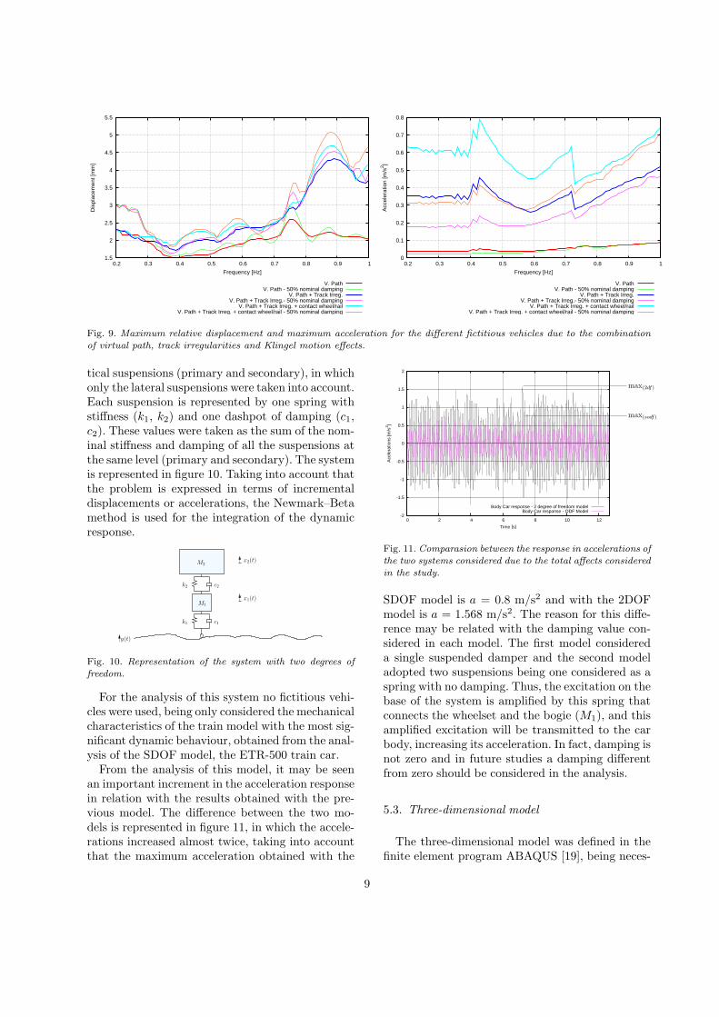
In order to understand how the frequencies of vi-bration of vehicles influence its dynamic behaviourdue to these effects, the study of several fictitiousvehicles was performed. These vehicles have as ref-erence some of the characteristic values of the realvehicles provided for this study. Taking these valuesinto account the characteristics of the fictitious ve-hicles resulted from a decrement of the mass, stiff-ness and damping values of these ones in order toobtain the frequency of vibration needed, between0.2 Hz and 1.0 Hz. In order to perform the dynamicanalysis of this model, a programme in Matlab code(OCTAVE)[7] was developed, using the Newmark–Beta method or the so called trapezoidal method, tointegrate the dynamic response in time of the differ-ent vehicles. The maximum relative lateral displace-ments and the maximum lateral accelerations ob-tained for the different fictitious vehicles due to thecombination of the three effects considered in thisstudy, are presented in figure 9. Note that there arepresented the results for the same fictitious vehiclesbut considering a reduction of 50% of the nominaldamping, in order to evaluate the influence of thisreduction.

Is possible to see that the consideration of Klingelmovement effects is so important as the considera-tion of track irregularities, being the effect of bridgelateral displacements not so relevant. The incrementof the dynamic response is more significant for thecase of lateral accelerations than for lateral displace-ments. As may be seen, the maximum accelerationcorresponds to the vehicle model with a frequency ofvibration equal to f0 = 0.43 Hz, which correspondsto ETR-500 vehicle car. The reason for this effectis related with the fact that the combination of allthe effects considered for this study has a predom-inant frequency of excitation multiple of f0 = 0.43Hz. Finally, was concluded that the reduction of thenominal damping in 50% does not have a significantimportance in the vehicles dynamic response.

5.2. Model with two degrees of freedom

The model presented in the last section consideredjust one suspended mass, which represented the carbody mass. With a model with two degrees of free-dom, the influence of bogies mass in the lateral dy-namic response of the car body, was considered. Thismodel was developed in the finite element programFEAP [20] and contains two rigid bodies with mass(M1, M2) connected by two type of lateral and ver-

8

1.5

2

2.5

3

3.5

4

4.5

5

5.5

0.2 0.3 0.4 0.5 0.6 0.7 0.8 0.9 1

Dis

plac

emen

t [m

m]

Frequency [Hz]

V. PathV. Path - 50% nominal damping

V. Path + Track Irreg.V. Path + Track Irreg.- 50% nominal damping

V. Path + Track Irreg. + contact wheel/railV. Path + Track Irreg. + contact wheel/rail - 50% nominal damping

0

0.1

0.2

0.3

0.4

0.5

0.6

0.7

0.8

0.2 0.3 0.4 0.5 0.6 0.7 0.8 0.9 1

Acc

eler

atio

n [m

/s2 ]

Frequency [Hz]

V. PathV. Path - 50% nominal damping

V. Path + Track Irreg.V. Path + Track Irreg.- 50% nominal damping

V. Path + Track Irreg. + contact wheel/railV. Path + Track Irreg. + contact wheel/rail - 50% nominal damping

Fig. 9. Maximum relative displacement and maximum acceleration for the different fictitious vehicles due to the combinationof virtual path, track irregularities and Klingel motion effects.

tical suspensions (primary and secondary), in whichonly the lateral suspensions were taken into account.Each suspension is represented by one spring withstiffness (k1, k2) and one dashpot of damping (c1,c2). These values were taken as the sum of the nom-inal stiffness and damping of all the suspensions atthe same level (primary and secondary). The systemis represented in figure 10. Taking into account thatthe problem is expressed in terms of incrementaldisplacements or accelerations, the Newmark–Betamethod is used for the integration of the dynamicresponse.

y(t)

c2

c1

x2(t)

x1(t)M1

M2

k2

k1

Fig. 10. Representation of the system with two degrees offreedom.

For the analysis of this system no fictitious vehi-cles were used, being only considered the mechanicalcharacteristics of the train model with the most sig-nificant dynamic behaviour, obtained from the anal-ysis of the SDOF model, the ETR-500 train car.

From the analysis of this model, it may be seenan important increment in the acceleration responsein relation with the results obtained with the pre-vious model. The difference between the two mo-dels is represented in figure 11, in which the accele-rations increased almost twice, taking into accountthat the maximum acceleration obtained with the

-2

-1.5

-1

-0.5

0

0.5

1

1.5

2

0 2 4 6 8 10 12

Ace

lera

tions

[m/s

2 ]

Time [s]

Body Car response - 2 degree of freedom modelBody Car response - ODF Model

max(sodf)

max(2df)

Fig. 11. Comparasion between the response in accelerations ofthe two systems considered due to the total affects consideredin the study.

SDOF model is a = 0.8 m/s2 and with the 2DOFmodel is a = 1.568 m/s2. The reason for this diffe-rence may be related with the damping value con-sidered in each model. The first model considereda single suspended damper and the second modeladopted two suspensions being one considered as aspring with no damping. Thus, the excitation on thebase of the system is amplified by this spring thatconnects the wheelset and the bogie (M1), and thisamplified excitation will be transmitted to the carbody, increasing its acceleration. In fact, damping isnot zero and in future studies a damping differentfrom zero should be considered in the analysis.

5.3. Three-dimensional model

The three-dimensional model was defined in thefinite element program ABAQUS [19], being neces-

9

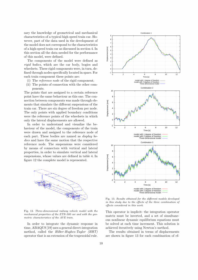
sary the knowledge of geometrical and mechanicalcharacteristics of a typical high speed train car. Ho-wever, part of the data used in the development ofthe model does not correspond to the characteristicsof a high-speed train car as discussed in section 4. Inthis section all the data needed for the performanceof this model, were defined.

The components of the model were defined asrigid bodies, which are the car body, bogies andwheelsets. These rigid components were, in turn, de-fined through nodes specifically located in space. Foreach train component these points are:

(i) The reference node of the rigid component;(ii) The points of connection with the other com-

ponents.The points that are assigned to a certain referencepoint have the same behaviour as this one. The con-nection between components was made through ele-ments that simulate the different suspensions of thetrain car. There are six degree of freedom per node.The only points with applied boundary conditionswere the reference points of the wheelsets in whichonly the lateral displacements are allowed.

In order to understand and visualize the be-haviour of the model, the components of the trainwere drawn and assigned to the reference node ofeach part. These bodies are named as display bo-dies and have the same motion that the respectivereference node. The suspensions were consideredby means of connectors with vertical and lateralproperties, in order to simulate vertical and lateralsuspensions, whose values are defined in table 4. Infigure 12 the complete model is represented.

Fig. 12. Three-dimensional railway vehicle model with themechanical properties of the ETR-500 car and with the geo-metric characteristics of the AVE train.

In order to integrate the dynamic response intime, ABAQUS [19] uses a general direct-integrationmethod, called the Hilber-Hughes-Taylor (HHT)operator that is an extension of the trapezoidal rule.

-1

0

1

2

3

4

5

6

7

8

9

0 2 4 6 8 10 12

Dis

plac

emen

t [m

m]

Time [s]

Combination 1

model with 1 degree of freedommodel with 2 degrees of freedom

Three-dimensional model

-2

0

2

4

6

8

10

0 2 4 6 8 10 12

Dis

plac

emen

t [m

m]

Time [s]

Combination 2

model with 1 degree of freedommodel with 2 degree of freedom

Three-dimensional model

-2

0

2

4

6

8

10

0 2 4 6 8 10 12

Dis

plac

emen

t [m

m]

Time [s]

Combination 3

model with 1 degree of freedommodel with 2 degree of freedom

Three-dimensional model

Fig. 13. Results obtained for the different models developedin this study due to the effects of the three combination ofeffects considered in this work.

This operator is implicit: the integration operatormatrix must be inverted, and a set of simultane-ous nonlinear dynamic equilibrium equations mustbe solved at each time increment. This solution isachieved iteratively using Newton’s method.

The results obtained in terms of displacementsare shown in figure 13 for each combination of ef-

10

1.5

1.6

1.7

1.8

1.9

2

2.1

2.2

2.3

2.4

2.5

2.6

0.5 1 1.5 2 2.5 3 3.5

Rel

ativ

e di

spla

cem

ents

(m

m)

Combination of effects

Model with 1 degree of freedomModel with 2 degree of freedom

Three-dimensional model

0

0.2

0.4

0.6

0.8

1

1.2

1.4

1.6

0.5 1 1.5 2 2.5 3 3.5

Acc

eler

atio

ns (

m/s

2 )

Combination of effects

Model with 1 degree of freedomModel with 2 degree of freedom

Three-dimensional model

11%

42%

100%

Comfort limit

Fig. 14. Representation of the maximum relative displacements to the track (virtual path) and the maximum accelerations,for the three models developed and for the three effects considered in this study: 1–Virtual path; 2–virtual path + trackirregularities;3–virtual path + track irregularities + Klingel movement effects.

fects defined in the beginning of this section. Addi-tionally, the results obtained with the other vehiclemodels due to the same combination of effects, arepresented in the same figures, in which it may beseen that the results are in good agreement. The dy-namic responses do not have significant differences,being these increased with the increment of the ex-citation.

Figure 14 presents the results in terms of maxi-mum relative displacements and accelerations of thethree models, considering each combination of ef-fects. It may be seen that for each combination,the differences between responses are insignificant,with a maximum variation of 0.35 mm. In terms ofaccelerations these differences are higher, as it wasexpected, taking into account that the accelerationvalues result from a second time derivative of dis-placements.

In the same figure the percentage of influence ofeach combination of effects in the total lateral dy-namic response of the vehicles that crosses the Ar-royo las Piedras viaduct, is defined. These valueswere obtained taking into account the response ofthe three-dimensional model. In this analysis it wasconcluded that the influence of the lateral displace-ments of the viaduct represents 11% of the totalresponse of railway vehicles. In turn, the combina-tion of bridge lateral displacements with track irre-gularities contributed 42% for the total dynamic re-sponse, being approximately 31% the contributionof track irregularities. Finally, the consideration ofKlingel motion effects contributed 58% for the to-tal dynamic response of the vehicle model, being themore significant effect.

6. Conclusions and suggestions forsubsequent studies

From the analysis it was concluded that there isno risk of excessive vibration at the railway vehicleswhen crossing the Arroyo las Piedras viaduct. Theaccelerations values obtained are within the limitsestablished by the FRA [1] and by SNFC (FrenchNational Railway Company), for the criterion of pas-senger comfort, which defines that the lateral acce-lerations in car bodies should not exceed the limit,a = 1.5 m/s2.

Although the simplifying assumptions consideredin this study, the results obtained are reasonable andsignificant as a first approach to the problem. Howe-ver, further studies should be performed, in whichmore realistic parameters should be considered. Aspecial attention to the parameters used to generatetrack irregularities profiles and to the effects pro-duced by the forces generated in the wheel-rail in-terface, should be given.

7. Acknowledgements

The author gratefully acknowledge the supportedprovided by J. M. Goicolea, Felipe Galbaldon (Es-cuela de Caminos de Madrid) and Jorge Proenca(Instituto Superior Tecnico), the information sup-plied by Jorge Nasarre y Goicochea from Caminosde Hierro de Espana, to Manuel Cuadrado andCIDI-Calculo, Investigacion y Desarollo para la In-genıeria, S.L. [2], who performed the virtual paths,and finally to J.Vinolas and A.Alonso from CEIT-

11

Centro de estudios e Investigaciones Tecnicas deGuipuzcoa [11].

References

[1] FRA Federal Railroad Administration. Tracksafety standards; final rule. 49 CFR Part 213,Part II, June 22, 1998.

[2] S.L. CIDI-Calculo, Investigacion y Desarollopara la Ingenıeria. Analısis de las deforma-ciones laterales del viaducto del arroyo de laspiedras - primer informe. Documento n1 - In-dice A, Noviembre 2006.

[3] H. Claus and W. Schiehlen. Modeling and sim-ulation of railway bogie structural vibrations.Dynamic of Vehicles on roads and tracks, Au-gust 22, 1997.

[4] ERRI D181. Forces laterales sur les ponts fer-roviaires. ERRI D181/RP6, 1996.

[5] ERRI D214. Etude numerique de l’influence desirregularites de voie dans les cas de resonancedes ponts. ERRI D214/RP5, 1999.

[6] Ministerio de Fomento. Instruccion de accionesa considerar en el proyecto de puentes de fer-rocarril. Borrador, pendiente de publicacion,2002.

[7] John W. Eaton. Octave v.2.0.16. OCTAVE,A high-level interactive language for numericalcomputations., 2000.

[8] EN1990-A2. Basis of structural design - annexa2: Application for bridges (normative). Eu-ropean Committee for Standardization (Cen),Brussels, 2005.

[9] EN1991-2. Actions on structures - part2: Gen-eral actions - traffic loads on bridges. EuropeanCommittee for Standardization (Cen), Brus-sels, 2003.

[10] Coenraad Esveld. Modern railway track. Sec-ond Edition, 2001.

[11] J.Vinolas A.Alonso F.Gonzalez, J.Perez. Useof active steering in railway bogies to reducerail corrugation on curves. CEIT- Centro de es-tudios e Investigaciones Tecnicas de Gipuzkoa,2007.

[12] L. Fryba. Dynamic of railway bridges. ThomasTelford, Prague, 1996.

[13] Vijay K. Garg and Rao V. Dukkipati. Dynam-ics of Railway Vehicle Systems. academic Press,1984.

[14] Felipe Gabaldon Castillo J.M. Goicolea andJuan Jose Montejo. Estudio dinamico del sis-

tema de vıa en placa - calculo de las accionesdinamicas producidas el trafico ferroviario.Grupo de Mecanica computacional - Escuela deCaminos de Madrid, mayo 2007.

[15] Jorge Ambrosio Joao Pombo and Miguel Silva.A new wheel-rail contact model for railway dy-namics. IDMEC - Instituto Superior Tecnico.

[16] J.J. Kalker. Fast algorithm for the simplifiedtheory of rolling contact. Vehicle System Dy-namics, pages 1–13, 1982.

[17] Klingel. Uber den lauf der eisenbahnwagen aufgerader bahn. Organ Fortschr. des Eisenbahn-wesens, 20:113–123, 1883.

[18] Arbeitsgemeinschaft Rheine-Freren.Rad/schiene-versuchs- und demonstrations-fahrzeug, definitionsphase r/s-vd. Ergebnis-bericht der Arbeitsgruppe Lauftechnik, MAN,Munchen, 1980.

[19] SIMULIA. Abaqus version 6.5. ABAQUS, fi-nite element analysis, 2004.

[20] R.L. Taylor and J.c. Simo. Feap v.7.1f. FEAP,Finite Element Analysis Program, 1999.

[21] Ache-Asociacion Cientıfico tecnica delHormigon Estructrural. Viaduct de ”arroyo laspiedras” primer viaducto mixto de las lıneas dealta velocidade espanolas. Hormigon y acero,243, Primer Trimestre de 2007.

[22] Yeong-Bin Yang Yean-Seng Wu and Jong-DarYau. Three-dimensional analysis of train-rail-bridge interaction problems. 2001.

12