Dynamic vehicle routing: solution methods and ... vehicle routing: solution methods and...
199
HAL Id: tel-00742706 https://tel.archives-ouvertes.fr/tel-00742706 Submitted on 17 Oct 2012 HAL is a multi-disciplinary open access archive for the deposit and dissemination of sci- entific research documents, whether they are pub- lished or not. The documents may come from teaching and research institutions in France or abroad, or from public or private research centers. L’archive ouverte pluridisciplinaire HAL, est destinée au dépôt et à la diffusion de documents scientifiques de niveau recherche, publiés ou non, émanant des établissements d’enseignement et de recherche français ou étrangers, des laboratoires publics ou privés. Dynamic vehicle routing : solution methods and computational tools Victor Pillac To cite this version: Victor Pillac. Dynamic vehicle routing : solution methods and computational tools. Automatic Con- trol Engineering. Ecole des Mines de Nantes, 2012. English. <NNT : 2012EMNA0049>. <tel- 00742706>
-
Upload
truongdang -
Category
Documents
-
view
226 -
download
0
Transcript of Dynamic vehicle routing: solution methods and ... vehicle routing: solution methods and...

HAL Id: tel-00742706https://tel.archives-ouvertes.fr/tel-00742706
Submitted on 17 Oct 2012
HAL is a multi-disciplinary open accessarchive for the deposit and dissemination of sci-entific research documents, whether they are pub-lished or not. The documents may come fromteaching and research institutions in France orabroad, or from public or private research centers.
L’archive ouverte pluridisciplinaire HAL, estdestinée au dépôt et à la diffusion de documentsscientifiques de niveau recherche, publiés ou non,émanant des établissements d’enseignement et derecherche français ou étrangers, des laboratoirespublics ou privés.
Dynamic vehicle routing : solution methods andcomputational tools
Victor Pillac
To cite this version:Victor Pillac. Dynamic vehicle routing : solution methods and computational tools. Automatic Con-trol Engineering. Ecole des Mines de Nantes, 2012. English. <NNT : 2012EMNA0049>. <tel-00742706>


Preface
This Ph.D. thesis has been prepared at the Department of Industrial Engineering at Universidad de
Los Andes (Colombia) and the Department of Automation and Production at École des Mines de Nantes
(France), between October 2009 and September 2012. It has been supervised by Professor Andrés L.
Medaglia at Universidad de Los Andes and Christelle Guéret at École des Mines de Nantes.
Financial support for this work was provided by the CPER (Contrat de Projet Etat Region) Vallée
du Libre; and the Centro de Estudios Interdisciplinarios Básicos y Aplicados en Complejidad (CEIBA,
Colombia). Vallée du Libre is an open platform aiming to connect research laboratories with the needs
of industry via the development of open source software. CEIBA is an excellence research center
funded by the Colombian Administrative Department of Science, Technology and Innovation (COL-
CIENCIAS) and participating universities and institutions, Universidad de Los Andes being among
them.
The present dissertation is composed by an introductory chapter, Vve research papers, written in
collaboration with the coauthors mentioned at the beginning of each paper, and a conclusion. Each
research paper is self-contained, meaning that it comprises a description of the underlying problem,
its contributions, computational experiments, conclusions, and its own bibliography. In addition to
the research papers, the thesis includes six appendices: Appendices A, B, and C describe the software
libraries and framework developed to support the research presented in the Vve papers. Appendix D
and E present an instance generator and the best known solutions for the instances introduced in this
thesis. Finally, Appendix F summarizes the record of publications of the work developed during this
thesis.
Nantes, October 10, 2012, Victor Pillac
III


Acknowledgments
This research project would not have been possible without the help and support of many people, in
particular my two very complimentary advisors. I would like to express my gratitude to Dr. Christelle
Guéret for her valuable advice before taking the decision to start this dissertation, for believing in me
from the Vrst months, and for her support during the moments of doubts. With her I learned that
research was not exclusively about brilliant ideas, but also about methodology, attention to detail, and
perseverance. I would also like to thank Dr. Andrés Medaglia for giving me the taste of operations
research in his excellent master degree course on linear programming. I am also thankful to him for
opening the doors of the University of Los Andes, and giving me the opportunity to join the Copa
team. He taught me to deVne clear research objectives, mark the boundaries of what can be achieved
in limited time, and to keep trying until things are perfect.
I want to thank Dr. Pascal Van Hentenryck for accepting the invitation to be part of my committee
and reviewing the present dissertation, and also for oUering me the opportunity to pursue my investi-
gation with his team. I also want to thank Dr. Christian Prins for being part of my committee and our
always interesting discussions in congresses and conferences. In addition, I would like to thank Dr.
Dominique Feillet for his participation in the jury and his advice along the way. I also thank Dr. Pierre
Dejax for being part of the jury and for sharing his experience in both academia and industry, which
gave me a broader vision for my career choices. Finally, I would like to thank Dr. Raha Akhavan not
only for being part of my jury but also for her unconditional support, valuable advice, and inspiring
determination.
A special thank goes to Dr. Jorge Mendoza for his mentoring, both academically and personally,
for the productive discussions, for introducing me to the world of academics and showing me that
fun and science can go well together, but most importantly for the simple fact of being a friend and
believing in me. I would also like to thank Dr. Juan Guillermo for sharing his expertise on routing
and metaheuristics, and for always being here to discuss ideas even when he was busy Vnishing his
dissertation. A special mention goes to Dr. Verena Schmid for the fruitful (and fun) discussions. Finally,
I want to particularly thank Dr. Michel Gendreau for our productive collaboration and for his valuable
advice on research and life.
Going through this three years journey would not have been possible without the help and support
of friends and colleagues on both sides of the Atlantic. On the French side, a special thank goes
for Mariem and Lama who kindly accepted me in their oXce and shared an occasional tea, Carlos
(a.k.a. the Colombian connexion) and the Colombian crew in Nantes Adriana, Carolina, Diana, Lili,
V

Michael 1, Paula, Saia, who made me feel at home when missing Colombia. On the Colombian side,
many thanks also go to the Copa team and in particular to current and former members Agar, Agon,
Jaime, Jorge, José Luis, Juan David, Leonardo, and Maria Isabel. Outside the University, life would
not have been possible without the support of Catalina, the hospitality of Guillermo and Martha, and
the good friendship of David (a.k.a the French ambassador) and the franco-colombian alliance who
were always ready to go for a hike, share a good meal and a good laugh, and made me feel home
when missing France. Finally, all my gratitude goes to my all time friends Alex, Anneso, Christophe,
Gwendal, Julie, Kevin, Perrine, Romain, and Yann for all the good moments shared together, for always
being here, and for quietly listening to my complaints during these three years.
I gratefully acknowledge the Vnancial support provided by the EMN, the CPER Vallée du Libre, the
Excellence Center for the Modeling and Simulation of Complex Phenomena and Processes (CEIBA),
and the Department of Industrial Engineering at Uniandes.
Finally, I would like to dedicate this thesis to my parents Jacky and Dominique and my sister Julie
for their love and support throughout my studies and life, and to Paul, Louis, and Ana Paula, to which
I wish to grow in happiness and to live a life full of opportunities.
1. Almost Colombian
VI

Contents
Preface III
Acknowledgments V
Contents VII
Introduction 1
1 Literature review 15
2 Dynamic and deterministic routing 43
3 Dynamic and stochastic routing 67
4 Case study: the Technician Routing and Scheduling Problem 89
Conclusions & perspectives 123
Appendices 127
A EXcient implementation 129
B A library for the modeling of vehicle routing problems 139
C A library of heuristics for vehicle routing problems 143
D An instance generator for the TRSP 157
E Best known solutions for the TRSP 161
F List of contributions 165
G Résumé 169
VII


Introduction
Within the wide scope of logistics management, transportation plays a central role and is a crucial
activity in the delivery of goods and services. Among others, it allows for the timely distribution
between suppliers, production units, warehouses, retailers, and Vnal customers. Transportation also
has an important footprint in the trade economy and on the environment. According to Hesse and
Rodrigue (2004), the total logistic costs in the year 2000 in the United States (US) represented 10% of
the GDP (Gross Domestic Product), while transportation on its own accounted for 5.9% of the GDP.
In addition, a recent report from the Energy Information Administration (EIA, 2011) indicates that
transportation was responsible for 27% of the greenhouse gas emissions in the US in 2009, while the
European Environment Agency estimates this share to be 24% in the European Union (EEA, 2011).
Therefore, improving the eXciency of transportation activities is a critical step to increase com-
petitiveness and reduce the environmental impact of organizations. In this sense, operating a Weet
of vehicles is a cornerstone problem that arises both in the service industry, with, among others, the
transportation of less-able people, the scheduling of school buses, or the on-site maintenance activi-
ties; and in the goods industry, with, for instance, the transport of raw materials between suppliers
and factories, the relocation of trucks in carrier companies, or the pickup and delivery of goods in the
retail industry.
More speciVcally, Vehicle Routing Problems (VRPs) deal with the design of a set of minimal-cost
routes that serve the demand for goods or services of a set of geographically spread customers, satis-
fying a group of operational constraints. Since its Vrst deVnition by Dantzig and Ramser (1959), the
amount of published material on VRP has exponentially increased. As an evidence of this trend, the
recent study by Eksioglu et al. (2009) reports approximately 1,500 indexed publications on vehicle rout-
ing (as of 2006). The volume of publications is closely related to the variety of routing problems, and
the diversity of approaches proposed to tackle them.
The original Capacitated Vehicle Routing Problem (CVRP or simply VRP) formulation is a gener-
alization of the Traveling Salesman Problem (TSP) presented by Flood (1956). The VRP is deVned on a
graph G = (V, E ,C,q), with V = v0, ..., vn being the set of vertices, E the arc set, C = (ce)e∈E a
cost matrix deVned on E , and q = (qi)i∈V a vector of demands for a certain commodity. Traditionally,
vertex v0 is called the depot, while the remaining vertices represent customers that require a commodity
to be delivered. The VRP consists in Vnding a set of routes of minimal cost for an unlimited Weet of
vehicles of identical capacity Q, starting and ending at the depot, such that each of the customers is
visited exactly once, while not exceeding the capacity of the vehicles.
The above deVnition has been extended in a variety of forms to model a wide range of practical
LUNAM - EMN - Uniandes 1/192 Pillac V. - Ph D. Dissertation

INTRODUCTIONapplications. Among the most common extensions are those that include time-window constraints
that enforce the visit of each vertex within a given time interval; the pickup and delivery constraints
that require the commodity to be picked-up at certain vertices before being delivered to others; the
distance constraints that limit the total distance traveled by a vehicle; and accessibility constraints that
limit the set of vehicles allowed to visit a given vertex. On the other hand, common variants of the
original problem statement include multiple depots, from which vehicles can start and end their routes;
the possibility to split customer deliveries; and heterogeneous and/or limited Weets. Finally, related
problems consider multi-period horizons; the combination of routing with inventory management;
multiple levels of routing with trucks feeding hubs from which smaller vehicles start delivery routes
(Nguyen et al., 2012a,b); vehicles with trailers that can be detached to visit customers with accessibility
constraints; and arc-routing problems in which the demand is located on the arcs (Belenguer et al.,
2010; Corberán and Prins, 2010).
Parallel to the myriad of variants, a number of optimization approaches have been proposed to
tackle routing problems. We refer the interested reader to the surveys by Baldacci et al. (2007); Cordeau
et al. (2007); Laporte (2009), and Toth and Vigo (2002) for a complete review of both exact and approx-
imate approaches.
Recent exact approaches for the VRP are based on three base formulations: vehicle Wow, commod-
ity Wow, and set partitioning. Vehicle Wow formulations (Lysgaard et al., 2004; Naddef and Rinaldi,
2002) deVne an integer variable for each arc that counts the number of times a vehicle travels through
it. Commodity Wow formulations (Baldacci et al., 2004) are based on a continuous variable for each arc
that models the Wow of commodities between vertices. Finally, set partitioning formulations (Baldacci
et al., 2010, 2007; Feillet, 2010; Feillet et al., 2005, 2004; Fukasawa et al., 2006; Rousseau et al., 2007)
consider the set of all feasible routes and select a subset of routes of minimal cost such that all the con-
straints are satisVed. As it is often impossible to enumerate the whole set of feasible solutions, such
approaches generally rely on a column generation scheme that iteratively generates feasible routes for
the set covering model.
Despite the advances in algorithms and the constant growth of computational power, state-of-the-
art exact approaches are only able to solve problems with approximately one hundred vertices, which
is well below the typical size of problems faced in industry. In addition, exact approaches are closely
tied to a speciVc VRP variant, and may take several hours to produce a solution. As a consequence,
a number of (faster) approximate approaches have been developed to tackle the VRP and its variants.
Approximate approaches can be divided in three categories: classical heuristics, metaheuristics, and
matheuristics.
Classical heuristics are further divided in three categories: constructive, two-phase, and improve-
ment heuristics. A well-known constructive heuristic is the Clarke and Wright (1964) savings algo-
rithm that starts by creating one route per customer and then iteratively merges routes until the total
distance can no longer be reduced. Petal heuristics (Gillett and Miller, 1974; Renaud et al., 1996; Ryan
et al., 1993) are another class of constructive heuristics that start by generating a set of feasible routes,
and then solve a set partitioning model to build a feasible solution. The two-phase approaches include
the cluster-Vrst, route-second (CR) and route-Vrst, cluster-second (RC) heuristics. The CR heuristics
were introduced by Fisher and Jaikumar (1981) and consists in grouping customers into clusters with-
LUNAM - EMN - Uniandes 2/192 Pillac V. - Ph D. Dissertation
INTRODUCTIONout violating the vehicle capacity, and then solving a TSP for each cluster. The RC heuristics start by
designing a giant tour visiting all customers that is then split into feasible routes. Prins (2004) demon-
strated that properly-designed RC heuristics can bring signiVcant improvements when embedded in
more complex methods (Mendoza et al., 2010, 2011; Prins, 2009b; Prins et al., 2009; Villegas et al., 2010,
2011a). Finally, improvement heuristics attempt to improve a solution by considering moves that alter
the sequence of customers within a route and/or exchange customers between diUerent routes. Each
type of move deVnes a neighborhood of the considered solution. Among the most widely used neigh-
borhoods are swap, 2-opt, 3-opt (Lin, 1965), Or-opt (Or, 1976), and string exchange. The eXciency of
improvement heuristics depends to a great extent on the implementation of the neighborhood explo-
ration. For instance, Irnich et al. (2006) propose a decomposition scheme, namely sequential search,
and report speedup factors of up to 104 for the exploration of the 3-opt neighborhood against a naive
implementation.
Metaheuristics are optimization paradigms which main objective is to overcome limitations of the
classical heuristics, in particular, their tendency to get trapped in local optima and their lack of robust-
ness. Among the most popular single-solution metaheuristics are Tabu Search (TS) (Gendreau et al.,
1994; Glover, 1986; Taillard, 1993; Toth and Vigo, 2003), Simulated Annealing (SA) (Kirkpatrick et al.,
1983; Osman, 1993), Greedy Randomized Adaptive Search Procedure (GRASP) (Feo and Resende, 1989;
Hashimoto et al., 2011; Prins, 2009a; Villegas et al., 2010), and Large Neighborhood Search (LNS) (Bent
and Van Hentenryck, 2004; Pisinger and Ropke, 2007, 2010; Shaw, 1998). Population-based metaheuris-
tics include Genetic Algorithms (GA) (Holland, 1975), Memetic Algorithms (MA) (Bontoux et al., 2010;
El-Fallahi et al., 2008; Labadi et al., 2008a,b; Mendoza et al., 2010; Prins, 2009b; Vidal et al., 2011), and
Ant Colony Optimization (ACO) (Bontoux and Feillet, 2008; Reimann et al., 2004). We refer the inter-
ested reader to the work by Bräysy and Gendreau (2005); Cordeau et al. (2005, 2002); Prins et al. (2010),
and Gendreau et al. (2002) for an in-depth analysis of the latest advances in metaheuristics in the Veld
of vehicle routing.
Finally, a recent trend combines heuristics with exact approaches, in what is commonly referred to
as matheuristics (Maniezzo et al., 2009). In their review, Puchinger and Raidl (2005) make a distinction
between collaborative and integrative matheuristics. In collaborative approaches, heuristics and exact
algorithms exchange information to build a solution. This is for instance the case of the Lagrangean re-
laxation granular TS introduced by Prins et al. (2007), or the approach proposed by Archetti et al. (2008)
for the VRP with split deliveries. More recently, researchers have used mixed integer programming as
a post-optimization procedure to aggregate partial solutions explored in a metaheuristic. For instance,
Villegas et al. (2011b) tackled the Truck and Trailer Routing Problem by Vrst generating solutions us-
ing a GRASP based approach, and then solving a set-covering problem (SC) using the routes generated
during the search. Pillac et al. (2012f) applied a similar approach using the solutions generated by an
Adaptive Large Neighborhood Search. Finally, Mendoza and Villegas (2011, 2012) propose a simple yet
eUective matheuristic for the VRP with Stochastic Demands (VRPSD) that generates a large number
of routes using randomized constructive heuristics and then solves a SC to build a solution, reporting
state-of-the-art results. On the other hand, integrative matheuristics embed one technique into an-
other. A sample of integrative heuristics include the Large Neighborhood Search algorithms in which
an exact approach (either Integer Programming or Constraint Programming) is used to optimally ex-
LUNAM - EMN - Uniandes 3/192 Pillac V. - Ph D. Dissertation

INTRODUCTIONplore the neighborhood of a solution (De Franceschi et al., 2006; Mouthuy et al., 2012; Prescott-Gagnon
et al., 2009; Rousseau et al., 2002); the hybrid TS proposed by Ngueveu et al. (2010), which solves a
b-matching problem to guide a TS procedure; or the heuristic column generation proposed by Massen
et al. (2012).
Despite the development of eXcient optimization algorithms that produce high quality solutions,
Sörensen et al. (2008) point out that commercial routing software does not take full advantage from
state-of-the-art algorithms but instead embed a large toolbox of simpler heuristics. The gap between
academic research and industrial practice can be explained by the fact that the two communities face
diverging incentives. Academia is driven by the publication of ground-breaking results on well-known
sets of instances, or alternatively by the deVnition of novel optimization problems. Therefore, research
is biased toward highly specialized methods able to solve a particular problem with optimal or nearly-
optimal results. In contrast, industry requires that the resources invested on the development of a
new decision support system (DSS) translate in signiVcant gains once the system is operational. In this
perspective, it is more eXcient to develop and maintain a set of simple optimization components that Vt
a variety of problems and produce relatively good results, than to invest resources in the development
of complex approaches tailored for a speciVc problem that will only bring marginal improvements.
Nonetheless, a thriving trend in the routing community attempts to develop methods able to tackle
a variety of practical problems. This trend follows two main streams: rich vehicle routing (Doerner and
Schmid, 2010; Schmid et al., 2012), which focuses on routing problems that simultaneously consider
features from several VRP variants; and uniVed optimization approaches, which are designed to account
for a variety of business constraints, like the Adaptive Large Neighborhood Search introduced by
Pisinger and Ropke (2007) or the UniVed Hybrid Genetic Search proposed by Vidal et al. (2012).
An alternative approach to foster technology transfer from academia to industry is the release
of state-of-the-art algorithms as open source projects. Successful stories at the intersection of the
operations research and computer science communities include the COIN-OR project 2, which puts
together a variety of frameworks from metaheuristics to linear and non-linear solvers; GLPK 3, a solver
for linear and mixed integer programming; Paradiseo 4, a framework for the design of metaheuristics;
and Choco 5, a Constraint Programming solver implemented in Java. There exists a limited number of
open-source projects that provide optimization frameworks for vehicle routing. As surveyed by Lodi
and Punnen (2004), most of these initiatives are devoted to the resolution of the TSP, and to the best
of our knowledge, the remaining focus on the CVRP. For instance, SYMPHONY (Ralphs et al., 2012;
Ralphs, 2003; Ralphs et al., 2003) and CVRPSD (Lysgaard et al., 2004) tackle the optimal resolution of
the CVRP using mathematical programming. Other projects include VRPH (Groër et al., 2010), a C/C++
framework based on local search; jCW (Mendoza et al., 2008), an object oriented implementation in
Java of generalized saving heuristics; and jSplit (Villegas et al., 2008), a Java framework for the rapid
development of cluster-Vrst, route-second heuristics.
Most routing algorithms and software often rely on the assumption that all the information is
known with certainty. However, in many applications, part or all the information is uncertain. An
2. http://coin-or.org3. http://www.gnu.org/s/glpk4. http://paradiseo.gforge.inria.fr5. http://www.emn.fr/z-info/choco-solver
LUNAM - EMN - Uniandes 4/192 Pillac V. - Ph D. Dissertation

INTRODUCTIONobvious example are travel times that Wuctuate greatly depending on traXc or weather conditions, es-
pecially in urban areas. These problems are referred to as static and stochastic, and common examples
include: stochastic customers, where a customer needs to be serviced with a given probability (Bert-
simas, 1988; Waters, 1989); stochastic times, in which either service or travel times are modeled by
random variables (Kenyon and Morton, 2003; Laporte et al., 1992; Verweij et al., 2003); and lastly,
stochastic demands (Christiansen and Lysgaard, 2007; Dror et al., 1989; Laporte et al., 2002; Mendoza
et al., 2011, 2009; Secomandi, 2000; Secomandi and Margot, 2009) where customer demands are known
as probability distributions. Further details on the static stochastic vehicle routing can be found in the
reviews by Bertsimas and Simchi-Levi (1996); Cordeau et al. (2007), and Gendreau et al. (1996).
In addition, recent advances in communication and geolocation technologies now allow compa-
nies to economically track their Weet in real time. These new technologies lead to the development of
Intelligent Transport Systems (ITS), and more precisely Advanced Fleet Management Systems (AFMS),
that combine hardware and software solutions to provide real time information on the Weet, customers,
and road networks. The development of ITS and AFMS creates new challenges and opportunities for
operations research. Vehicle routing is no longer limited to the design of a-priori routes that cannot be
altered once the vehicles have departed the depot. Instead, it can now consider real-time reoptimiza-
tion of routes, leading to what is referred to as dynamic vehicle routing problems. Nonetheless, Crainic
et al. (2009) point out that while the hardware part of ITS has considerably evolved, the correspond-
ing Decision Support Systems (DSS) and optimization models have not yet reached their maturity.
Therefore, the advent of such systems require the development of a new class of eXcient optimization
algorithms able to manage Weets in real time.
The purpose of this dissertation is to review the state-of-the-art in the area of dynamic routing, de-
sign new algorithms for this class of problems; implement general-purpose software components that
are both reusable and adaptable to a wide range of variants; apply the proposed algorithms to a real-
world routing application; and Vnally, to release the proposed components as open-source packages to
accelerate technology transfer from academia to industry.
Chapter 1 presents a comprehensive review of the literature on dynamic vehicle routing. We clas-
sify problems from the perspective of quality and evolution of information, identifying four categories
depending on whether they are static or dynamic, and deterministic or stochastic. In the remaining
discussion, we focuse on dynamic vehicle routing problems, for which we give a general deVnition
and present metrics to measure their degree of dynamism. In addition, we illustrate the relevance of
dynamic routing by listing applications in the service industry, transport of goods, and transport of
persons. We provide an extensive review of solution methods for both dynamic and deterministic and
dynamic and stochastic problems, present performance evaluation metrics, and list available bench-
marks. We conclude by drawing directions for future research in this emerging Veld. This paper was
submitted to the European Journal of Operational Research (Pillac et al., 2011a) and two earlier versions
were published as technical reports (Pillac et al., 2011b, 2010a).
Chapter 2 focuses on dynamic and deterministic routing problems in which part or all of the input
is unknown and revealed dynamically during the design or execution of routes. An important feature
is that no information is available on the dynamically revealed data, therefore solution methods cannot
anticipate changes in input, but may only react to them. In this chapter, we consider routing problems
LUNAM - EMN - Uniandes 5/192 Pillac V. - Ph D. Dissertation
INTRODUCTIONin which new customers appear during the execution of routes, requiring updates in the routing plan.
We propose a fast re-optimization approach, namely parallel Adaptive Large Neighborhood Search
(pALNS), which produces high quality routing in limited computational time. We then illustrate its
performance on a set of Dynamic Vehicle Routing Problem with Time Windows (D-VRPTW) instances
derived from the Solomon (1987) benchmark. Noting that the common assumption that vehicle drivers
do not know their next destination until they Vnish serving their current customer may not be de-
sirable from a practical perspective, we introduce the notion of driver inconvenience and deVne a
bi-objective optimization problem that minimizes the routing cost while maintaining its consistency
throughout the day. We consider a context in which vehicles have an initial routing plan at the be-
ginning of the day, that is then periodically updated by a decision maker. We introduce a measure
of the driver inconvenience resulting from each update, and propose a bi-objective approach based
on pALNS, namely pBiALNS, that is able to produce a set of non-dominated solutions in reasonable
computational time. These solutions oUer diUerent tradeoUs between cost eXciency and consistency,
and can be used by the decision maker to update the vehicle routing introducing a controlled num-
ber of changes. Our computational experiments study the tradeoU between cost eXciency and route
consistency, and show that pBiALNS is able to produce a variety of alternative solutions in a few sec-
onds. This chapter was published as a technical report (Pillac et al., 2012b), and an earlier version was
presented at the ROADEF 2012 conference (Pillac et al., 2012g). Details on the implementation of the
pALNS and pBiALNS algorithms are presented in Appendix C.
In dynamic and stochastic problems part or all the input is unknown and revealed dynamically dur-
ing the execution of the routes, yet exploitable stochastic knowledge is available on the dynamically
revealed information. Chapter 3 presents an event-driven framework based on a multiple scenario
approach called jMSA. This framework is Wexible, parallelized, and easily embeddable in a decision
support system. It can cope with a wide variety of dynamic vehicle routing problems and may be ex-
tensible to other dynamic combinatorial optimization problems. jMSA generates and maintains a pool
of scenarios, each containing a realization of the random variables modeling the dynamically revealed
data. This pool is then used to take the routing decisions whenever required. We illustrate the Wexi-
bility of the framework by solving the VRP with Stochastic Demands and show that our approach is
competitive against the state-of-the-art algorithms. This chapter was accepted for publication in Deci-
sion Support Systems (Pillac et al., 2012a), an earlier version of this work was published as a technical
report (Pillac et al., 2011d), while preliminary results were presented at the ALIO-INFORMS 2010 and
the ROADEF 2011 conferences (Pillac et al., 2010b, 2011c). Appendix C presents the implementation of
the algorithm used to optimize scenarios, namely Adaptive Variable Neighborhood Search (AVNS).
In Chapter 4, we formally introduce the Technician Routing and Scheduling Problem (TRSP), which
is motivated by the optimization problem faced by an industrial partner. The TRSP consists in routing
a crew of technicians to serve a set of requests. Distinctive features of this problem are: the fact that
technicians start and end their tour at their home; the consideration of skills, tools, and spare parts
that restricts the set of technicians that can serve a speciVc request; the possibility for technicians
to pick up additional tools and spare parts at a central depot; and Vnally, the objective function that
considers the minimization of the total working time and the balancing of tours. The Vrst paper
in this chapter proposes a parallel adaptive large neighborhood search coupled with a set-covering
LUNAM - EMN - Uniandes 6/192 Pillac V. - Ph D. Dissertation

INTRODUCTION BIBLIOGRAPHYpost-optimization, namely pALNS+SC, used to tackle the static TRSP. We illustrate the performance
of pALNS+SC on the Solomon (1987) VRPTW instances, then we introduce a new set of instances
for the TRSP, generated from the Solomon (1987) instances as described in Appendix D, and solve
them using pALNS+SC. This paper was submitted to Optimization Letters (Pillac et al., 2012f) and
preliminary results were presented at the MIC 2011 conference (Pillac et al., 2011e). The second paper
tackles the dynamic TRSP and proposes two solution methods. The Vrst is an adaptation of the fast-
reoptimization approach presented in Chapter 2. The second is a multiple plan approach, which is a
variant of the multiple scenario approach presented in Chapter 3. This work is available as a technical
report (Pillac et al., 2012d) and preliminary results were presented at the ODYSSEUS 2012 and EURO
2012 conferences (Pillac et al., 2012c,e).
Finally, Appendices A, B, and C describe software libraries and frameworks developed to support
the research presented in the Vve papers, Appendix D presents an instance generator for the TRSP,
Appendix E details the best known solutions for the new instances, and Appendix F summarizes the
record of publications developed during this thesis.
Bibliography
Archetti, C., Speranza, M., and Savelsbergh, M. (2008). An optimization-based heuristic for the split deliveryvehicle routing problem. Transportation Science, 42(1):22–31.
Baldacci, R., Bartolini, E., Mingozzi, A., and Roberti, R. (2010). An exact solution framework for a broad class ofvehicle routing problems. Computational Management Science, 7:229–268, doi:10.1007/s10287-009-0118-3.
Baldacci, R., Hadjiconstantinou, E., and Mingozzi, A. (2004). An exact algorithm for the capacitated vehiclerouting problem based on a two-commodity network Wow formulation. Operations Research, 52(5):723–738,doi:10.1287/opre.1040.0111.
Baldacci, R., Toth, P., and Vigo, D. (2007). Recent advances in vehicle routing exact algorithms. 4OR: A QuarterlyJournal of Operations Research, 5(4):269–298, doi:10.1007/s10288-007-0063-3.
Belenguer, J.-M., Benavent, E., Labadi, N., Prins, C., and Reghioui, M. (2010). Split-delivery capac-itated arc-routing problem: Lower bound and metaheuristic. Transportation Science, 44(2):206–220,doi:10.1287/trsc.1090.0305.
Bent, R. and Van Hentenryck, P. (2004). A two-stage hybrid local search for the vehicle routing problem withtime windows. Transportation Science, 38(4):515–530, doi:10.1287/trsc.1030.0049.
Bertsimas, D. (1988). Probabilistic combinatorial optimization problems. PhD thesis, Massachusetts Institute ofTechnology, Dept. of Mathematics.
Bertsimas, D. and Simchi-Levi, D. (1996). A new generation of vehicle routing research: robust algorithms,addressing uncertainty. Operations Research, 44(2):286–304.
Bontoux, B., Artigues, C., and Feillet, D. (2010). A memetic algorithm with a large neighborhoodcrossover operator for the generalized traveling salesman problem. Computers & OR, 37(11):1844–1852,doi:10.1016/j.cor.2009.05.004.
Bontoux, B. and Feillet, D. (2008). Ant colony optimization for the traveling purchaser problem. Computers &OR, 35(2):628–637, doi:10.1016/j.cor.2006.03.023.
Bräysy, O. and Gendreau, M. (2005). Vehicle routing problem with time windows, Part II: Metaheuristics. Trans-portation Science, 39(1):119–139.
LUNAM - EMN - Uniandes 7/192 Pillac V. - Ph D. Dissertation
INTRODUCTION BIBLIOGRAPHYChristiansen, C. and Lysgaard, J. (2007). A branch-and-price algorithm for the capacitated vehicle routing prob-
lem with stochastic demands. Operations Research Letters, 35(6):773–781.
Clarke, G. and Wright, J. W. (1964). Scheduling of vehicles from a central depot to a number of delivery points.Operations Research, 12(4):568–581, doi:10.1287/opre.12.4.568.
Corberán, A. and Prins, C. (2010). Recent results on arc routing problems: An annotated bibliography. Networks,56(1):50–69, doi:10.1002/net.20347.
Cordeau, J.-F., Gendreau, M., Hertz, A., Laporte, G., and Sormany, J.-S. (2005). New heuristics for the vehiclerouting problem. In Langevin, A. and Riopel, D., editors, Logistics Systems: Design and Optimization, pages279–297. Springer US.
Cordeau, J.-F., Gendreau, M., Potvin, J. Y., and Semet, F. (2002). A guide to vehicle routing heuristics. The Journalof the Operational Research Society, 53(5):512–522.
Cordeau, J.-F., Laporte, G., Savelsbergh, M. W., and Vigo, D. (2007). Vehicle routing. In Barnhart, C. and Laporte,G., editors, Transportation, volume 14 of Handbooks in Operations Research and Management Science, chapter 6,pages 367–428. Elsevier.
Crainic, T. G., Gendreau, M., and Potvin, J.-Y. (2009). Intelligent freight-transportation systems: Assessment andthe contribution of operations research. Transportation Research Part C: Emerging Technologies, 17(6):541–557,doi:10.1016/j.trc.2008.07.002.
Dantzig, G. and Ramser, J. (1959). The truck dispatching problem. Management Science, 6(1):80–91.
De Franceschi, R., Fischetti, M., and Toth, P. (2006). A new ILP-based reVnement heuristic for vehicle routingproblems. Mathematical Programming, 105(2):471–499.
Doerner, K. and Schmid, V. (2010). Survey: Matheuristics for rich vehicle routing problems. In Blesa, M., Blum, C.,Raidl, G., Roli, A., and Sampels, M., editors, Hybrid Metaheuristics, volume 6373 of Lecture Notes in ComputerScience, pages 206–221. Springer Berlin / Heidelberg.
Dror, M., Laporte, G., and Trudeau, P. (1989). Vehicle routing with stochastic demands: Properties and solutionframeworks. Transportation Science, 23(3):166–176, doi:10.1287/trsc.23.3.166.
EEA (2011). Laying the foundations for greener transport – term 2011: transport indicators tracking progresstowards environmental targets in Europe. Technical Report EEA Report No 7/2011, European EnvironmentAgency.
EIA (2011). Emission of greenhouse gases in the United States 2009. Technical Report DOE/EIA-0573(2009), U.S.Energy Information Administration.
Eksioglu, B., Vural, A. V., and Reisman, A. (2009). The vehicle routing problem: A taxonomic review. Computers& Industrial Engineering, 57(4):1472 – 1483, doi:10.1016/j.cie.2009.05.009.
El-Fallahi, A., Prins, C., and Calvo, R. W. (2008). A memetic algorithm and a tabu search for the multi-compartment vehicle routing problem. Computers & OR, 35(5):1725–1741, doi:10.1016/j.cor.2006.10.006.
Feillet, D. (2010). A tutorial on column generation and branch-and-price for vehicle routing problems. 4OR,8(4):407–424, doi:10.1007/s10288-010-0130-z.
Feillet, D., Dejax, P., and Gendreau, M. (2005). The proVtable arc tour problem: Solution with a branch-and-pricealgorithm. Transportation Science, 39(4):539–552, doi:10.1287/trsc.1040.0106.
Feillet, D., Dejax, P., Gendreau, M., and Gueguen, C. (2004). An exact algorithm for the elementary shortest pathproblem with resource constraints: Application to some vehicle routing problems. Networks, 44(3):216–229,doi:10.1002/net.20033.
Feo, T. and Resende, M. (1989). A probabilistic heuristic for a computationally diXcult set covering problem.Operations Research Letters, 8(2):67–71.
LUNAM - EMN - Uniandes 8/192 Pillac V. - Ph D. Dissertation

INTRODUCTION BIBLIOGRAPHYFisher, M. L. and Jaikumar, R. (1981). A generalized assignment heuristic for vehicle routing. Networks, 11(2):109–
124, doi:10.1002/net.3230110205.
Flood, M. (1956). The traveling-salesman problem. Operations Research, 4(1):61–75.
Fukasawa, R., Longo, H., Lysgaard, J., Aragão, M. P. d., Reis, M., Uchoa, E., and Werneck, R. F. (2006). Robustbranch-and-cut-and-price for the capacitated vehicle routing problem. Mathematical Programming, 106:491–511, doi:10.1007/s10107-005-0644-x.
Gendreau, M., Hertz, A., and Laporte, G. (1994). A tabu search heuristic for the vehicle routing problem. Man-agement Science, pages 1276–1290.
Gendreau, M., Laporte, G., and Potvin, J. (2002). Metaheuristics for the capacitated VRP. In Toth, P. and Vigo, D.,editors, The Vehicle Routing Problem, volume 9 ofMonographs on Discrete Mathematics and Applications, pages129–154. SIAM Philadelphia.
Gendreau, M., Laporte, G., and Séguin, R. (1996). Stochastic vehicle routing. European Journal of OperationalResearch, 88(1):3 – 12, doi:10.1016/0377-2217(95)00050-X.
Gillett, B. E. and Miller, L. R. (1974). A heuristic algorithm for the vehicle-dispatch problem. Operations Research,22(2):340–349, doi:10.1287/opre.22.2.340.
Glover, F. (1986). Future paths for integer programming and links to artiVcial intelligence. Computers & Opera-tions Research, 13(5):533 – 549, doi:10.1016/0305-0548(86)90048-1.
Groër, C., Golden, B., and Wasil, E. (2010). A library of local search heuristics for the vehicle routing problem.Mathematical Programming Computation, 2:79–101, doi:10.1007/s12532-010-0013-5.
Hashimoto, H., Boussier, S., Vasquez, M., and Wilbaut, C. (2011). A GRASP-based approach for techni-cians and interventions scheduling for telecommunications. Annals of Operations Research, 183:143–161,doi:10.1007/s10479-009-0545-0.
Hesse, M. and Rodrigue, J.-P. (2004). The transport geography of logistics and freight distribution. Journal ofTransport Geography, 12(3):171 – 184, doi:10.1016/j.jtrangeo.2003.12.004.
Holland, J. (1975). Adaptation in natural and artiVcial systems. Number 53. University of Michigan Press, AnnArbor, MI.
Irnich, S., Funke, B., and Grünert, T. (2006). Sequential search and its application to vehicle-routing problems.Computers & Operations Research, 33(8):2405 – 2429, doi:10.1016/j.cor.2005.02.020.
Kenyon, A. S. and Morton, D. (2003). Stochastic vehicle routing with random travel times. Transportation Science,37(1):69.
Kirkpatrick, S., Gelatt, C. D., and Vecchi, M. P. (1983). Optimization by simulated annealing. Science,220(4598):671–680, doi:10.1126/science.220.4598.671.
Labadi, N., Prins, C., and Reghioui, M. (2008a). An evolutionary algorithm with distance measure for the splitdelivery capacitated arc routing problem. In Recent Advances in Evolutionary Computation for CombinatorialOptimization, pages 275–294.
Labadi, N., Prins, C., and Reghioui, M. (2008b). A memetic algorithm for the vehicle routing problem with timewindows. RAIRO - Operations Research, 42(3):415–431, doi:10.1051/ro:2008021.
Laporte, G. (2009). Fifty years of vehicle routing. Transportation Science, 43(4):408–416,doi:10.1287/trsc.1090.0301.
Laporte, G., Louveaux, F., and Mercure, H. (1992). The vehicle routing problem with stochastic travel times.Transportation Science, 26(3):161–170.
Laporte, G., Louveaux, F., and Van Hamme, L. (2002). An integer L-shaped algorithm for the capacitated vehiclerouting problem with stochastic demands. Operations Research, 50(3):415–423.
LUNAM - EMN - Uniandes 9/192 Pillac V. - Ph D. Dissertation

INTRODUCTION BIBLIOGRAPHYLin, S. (1965). Computer solutions of the traveling salesman problem. Bell System Technical Journal, 44:2245–
2269.
Lodi, A. and Punnen, A. (2004). TSP software. In Du, D.-Z., Pardalos, P. M., Gutin, G., and Punnen, A., editors,The Traveling Salesman Problem and Its Variations, volume 12 of Combinatorial Optimization, pages 737–749.Springer US.
Lysgaard, J., Letchford, A. N., and Eglese, R. W. (2004). A new branch-and-cut algorithm for the capacitatedvehicle routing problem. Mathematical Programming, 100:423–445.
Maniezzo, V., Sttzle, T., and Voß, S., editors (2009). Matheuristics: Hybridizing Metaheuristics and MathematicalProgramming. Springer Publishing Company, Incorporated.
Massen, F., Deville, Y., and Van Hentenryck, P. (2012). Pheromone-based heuristic column generation for vehiclerouting problems with black box feasibility. Integration of AI and OR Techniques in Contraint Programming forCombinatorial Optimzation Problems, pages 260–274.
Mendoza, J. E., Castanier, B., Guéret, C., Medaglia, A. L., and Velasco, N. (2010). A memetic algorithm forthe multi-compartment vehicle routing problem with stochastic demands. Computers & Operations Research,37(11):1886–1898, doi:10.1016/j.cor.2009.06.015.
Mendoza, J. E., Castanier, B., Guéret, C., Medaglia, A. L., and Velasco, N. (2011). Constructive heuristics for themulticompartment vehicle routing problem with stochastic demands. Transportation Science, 45(3):346–363,doi:10.1287/trsc.1100.0353.
Mendoza, J. E., Guéret, C., Medaglia, A. L., Velasco, N., Villegas, J. G., et al. (2008). JCW: an object-orientedframework for the rapid development of vehicle routing heuristics based on savings. In Proceedings of theXIV Lati Ibero-American Congress on Operations Research (CLAIO’08), Cartagena, Colombia. ISBN: 978 958825283-4.
Mendoza, J. E., Medaglia, A. L., and Velasco, N. (2009). An evolutionary-based decision support system for vehiclerouting: The case of a public utility. Decision Support Systems, 46(3):730 – 742, doi:10.1016/j.dss.2008.11.019.
Mendoza, J. E. and Villegas, J. G. (2011). A space biased-sampling approach for the vehicle routing problem withstochastic demands. In Di Gaspero, L., Schaerf, A., and Stützle, T., editors, Proceedings of the 9th MetaheuristicsConference (MIC 2011), pages 643–645. Università degli Studi di Udine.
Mendoza, J. E. and Villegas, J. G. (2012). A multi-space sampling heuristic for the vehicle routing problem withstochastic demands. Optimization Letters, Accepted manuscript, doi:10.1007/s11590-012-0555-8.
Mouthuy, S., Hentenryck, P. V., and Deville, Y. (2012). Constraint-based very large-scale neighborhood search.Constraints, 17(2):87–122, doi:10.1007/s10601-011-9114-7.
Naddef, D. and Rinaldi, G. (2002). Branch-and-cut algorithms for the capacitated VRP. In Toth, P. and Vigo, D.,editors, The vehicle routing problem, volume 9 of Monographs on Discrete Mathematics and Applications, pages53–81. SIAM Philadelphia.
Ngueveu, S. U., Prins, C., and Calvo, R. W. (2010). A hybrid tabu search for the m-peripatetic vehicle routingproblem. In Sharda, R. and Voß, S., editors, Matheuristics, volume 10 of Annals of Information Systems, pages253–266. Springer US.
Nguyen, V.-P., Prins, C., and Prodhon, C. (2012a). A multi-start iterated local search with tabu listand path relinking for the two-echelon location-routing problem. Eng. Appl. of AI, 25(1):56–71,doi:10.1016/j.engappai.2011.09.012.
Nguyen, V.-P., Prins, C., and Prodhon, C. (2012b). Solving the two-echelon location routing problem by a graspreinforced by a learning process and path relinking. European Journal of Operational Research, 216(1):113–126,doi:10.1016/j.ejor.2011.07.030.
LUNAM - EMN - Uniandes 10/192 Pillac V. - Ph D. Dissertation

INTRODUCTION BIBLIOGRAPHYOr, I. (1976). Traveling salesman-type combinatorial optimization problems and their relation to the logistics of
regional blood banking. PhD thesis, Department of Industrial Engineering and Management Science, North-western University.
Osman, I. H. (1993). Metastrategy simulated annealing and tabu search algorithms for the vehicle routing prob-lem. Annals of Operations Research, 41:421–451, doi:10.1007/BF02023004.
Pillac, V., Gendreau, M., Guéret, C., and Medaglia, A. L. (2011a). A review of dynamic vehicle routing problems.European Journal of Operational Research, Accepted manuscript:34, doi:10.1016/j.ejor.2012.08.015.
Pillac, V., Gendreau, M., Guéret, C., and Medaglia, A. L. (2011b). A review of dynamic vehicle routing problems.Technical Report CIRRELT-2011-62, CIRRELT.
Pillac, V., Guéret, C., and Medaglia, A. L. (2010a). Dynamic vehicle routing: State of the art and prospects.Technical Report 10/4/AUTO, École des Mines de Nantes, France.
Pillac, V., Guéret, C., and Medaglia, A. L. (2010b). Solving the vehicle routing problem with stochastic demandswith a multiple scenario approach. In ALIO-INFORMS 2010, Buenos Aires (Argentina).
Pillac, V., Guéret, C., and Medaglia, A. L. (2011c). A dynamic approach for the vehicle routing problem withstochastic demands. In ROADEF 2011, St Étienne, France.
Pillac, V., Guéret, C., and Medaglia, A. L. (2011d). An event-driven optimization framework for dynamic vehiclerouting. Technical Report 11/2/AUTO, École des Mines de Nantes, France.
Pillac, V., Guéret, C., and Medaglia, A. L. (2011e). On the technician routing and scheduling problem. InDi Gaspero, L., Schaerf, A., and Stützle, T., editors, Proceedings of the 9th Metaheuristics Conference (MIC2011), pages 675–678. Università degli Studi di Udine.
Pillac, V., Guéret, C., and Medaglia, A. L. (2012a). An event-driven optimization framework for dynamic vehiclerouting. Decision Support Systems, Accepted manuscript, doi:10.1016/j.dss.2012.06.007.
Pillac, V., Guéret, C., and Medaglia, A. L. (2012b). A fast re-optimization approach for dynamic vehicle routing.Technical Report 12/X/AUTO, École des Mines de Nantes, France.
Pillac, V., Guéret, C., and Medaglia, A. L. (2012c). A multiple plan approach for the dynamic technician routingand scheduling problem. In 25th European Conference on Operational Research (EURO 2012), Vilnius, Lithuania.
Pillac, V., Guéret, C., and Medaglia, A. L. (2012d). On the dynamic technician routing and scheduling problem.Technical Report 12/Y/AUTO, École des Mines de Nantes, France.
Pillac, V., Guéret, C., and Medaglia, A. L. (2012e). On the dynamic technician routing and scheduling problem. InProceedings of the 5th International Workshop on Freight Transportation and Logistics (ODYSSEUS 2012), pages509–512, Mykonos, Greece.
Pillac, V., Guéret, C., and Medaglia, A. L. (2012f). A parallel matheuristic for the technician routing and schedul-ing problem. Optimization Letters, Accepted manuscript.
Pillac, V., Guéret, C., and Medaglia, A. L. (2012g). Route stability in dynamic vehicle routing: a bi-objectiveapproach. In ROADEF 2012, Angers, France.
Pisinger, D. and Ropke, S. (2007). A general heuristic for vehicle routing problems. Computers & OperationsResearch, 34(8):2403–2435, doi:10.1016/j.cor.2005.09.012.
Pisinger, D. and Ropke, S. (2010). Large neighborhood search. In Gendreau, M. and Potvin, J.-Y., editors, Handbookof Metaheuristics, volume 146 of International Series in Operations Research & Management Science, pages 399–419. Springer US.
Prescott-Gagnon, E., Desaulniers, G., and Rousseau, L. (2009). A branch-and-price-based large neighborhoodsearch algorithm for the vehicle routing problem with time windows. Networks, 54(4):190–204.
LUNAM - EMN - Uniandes 11/192 Pillac V. - Ph D. Dissertation

INTRODUCTION BIBLIOGRAPHYPrins, C. (2004). A simple and eUective evolutionary algorithm for the vehicle routing problem. Computers &
Operations Research, 31(12):1985–2002, doi:10.1016/S0305-0548(03)00158-8.
Prins, C. (2009a). A GRASP × evolutionary local search hybrid for the vehicle routing problem. In Bio-inspiredAlgorithms for the Vehicle Routing Problem, volume 161 of Studies in Computational Intelligence, pages 35–53.Springer Berlin / Heidelberg.
Prins, C. (2009b). Two memetic algorithms for heterogeneous Weet vehicle routing problems. Engineering Appli-cations of ArtiVcial Intelligence, 22(6):916–928, doi:10.1016/j.engappai.2008.10.006.
Prins, C., Labadi, N., Prodhon, C., and Calvo, R. W. (2010). Metaheuristics for logistics and vehicle routing.Computers & OR, 37(11):1833–1834, doi:10.1016/j.cor.2010.04.004.
Prins, C., Labadi, N., and Reghioui, M. (2009). Tour splitting algorithms for vehicle routing problems. Interna-tional Journal of Production Research, 47(2):507–535, doi:10.1080/00207540802426599.
Prins, C., Prodhon, C., Ruiz, A., Soriano, P., and WolWer Calvo, R. (2007). Solving the capacitated location-routing problem by a cooperative lagrangean relaxation-granular tabu search heuristic. Transportation Science,41(4):470–483, doi:10.1287/trsc.1060.0187.
Puchinger, J. and Raidl, G. (2005). Combining metaheuristics and exact algorithms in combinatorial optimization:A survey and classiVcation. In ArtiVcial Intelligence and Knowledge Engineering Applications: A BioinspiredApproach, volume 3562 of Lecture Notes in Computer Science, pages 113–124. Springer Berlin / Heidelberg.
Ralphs, T., Kopman, L., Pulleyblank, W., and Trotter, L. (2012). The SYMPHONY sourcecode. Available athttps://projects.coin-or.org/SYMPHONY.
Ralphs, T. K. (2003). Parallel branch and cut for capacitated vehicle routing. Parallel Computing, 29(5):607–629.
Ralphs, T. K., Kopman, L., Pulleyblank, W., and Trotter, L. (2003). On the capacitated vehicle routing problem.Mathematical Programming, 94(2):343–359.
Reimann, M., Doerner, K., and Hartl, R. F. (2004). D-Ants: Savings based ants divide and conquer the vehiclerouting problem. Computers & Operations Research, 31(4):563 – 591, doi:10.1016/S0305-0548(03)00014-5.
Renaud, J., Boctor, F. F., and Laporte, G. (1996). An improved petal heuristic for the vehicle routing problem. TheJournal of the Operational Research Society, 47(2):329–336.
Rousseau, L.-M., Gendreau, M., and Feillet, D. (2007). Interior point stabilization for column generation. Oper.Res. Lett., 35(5):660–668, doi:10.1016/j.orl.2006.11.004.
Rousseau, L.-M., Gendreau, M., and Pesant, G. (2002). Using constraint-based operators to solve the vehiclerouting problem with time windows. Journal of Heuristics, 8(1):43–58, doi:10.1023/A:1013661617536.
Ryan, D. M., Hjorring, C., and Glover, F. (1993). Extensions of the petal method for vehicle routing. The Journalof the Operational Research Society, 44(3):289–296.
Schmid, V., Doerner, K., and Laporte, G. (2012). Rich routing problems arising in supply chain management.European Journal of Operational Research, Accepted manuscript.
Secomandi, N. (2000). Comparing neuro-dynamic programming algorithms for the vehicle routing problem withstochastic demands. Computers & Operations Research, 27(11-12):1201–1225, doi:10.1016/S0305-0548(99)00146-X.
Secomandi, N. and Margot, F. (2009). Reoptimization approaches for the vehicle-routing problem with stochasticdemands. Operations Research, 57(1):214–230, doi:10.1287/opre.1080.0520.
Shaw, P. (1998). Using constraint programming and local search methods to solve vehicle routing problems. InPrinciples and Practice of Constraint Programming – CP98, volume 1520 of Lecture Notes in Computer Science,pages 417–431. Springer Berlin / Heidelberg.
LUNAM - EMN - Uniandes 12/192 Pillac V. - Ph D. Dissertation

INTRODUCTION BIBLIOGRAPHYSolomon, M. M. (1987). Algorithms for the vehicle-routing and scheduling problems with time window con-
straints. Operations Research, 35(2):254–265.
Sörensen, K., Sevaux, M., and Schittekat, P. (2008). Multiple neighbourhood search in commercial VRP packages:Evolving towards self-adaptive methods. In Cotta, C., Sevaux, M., and Sörensen, K., editors, Adaptive andMultilevel Metaheuristics, volume 136 of Studies in Computational Intelligence, pages 239–253. Springer Berlin/ Heidelberg.
Taillard, A. (1993). Parallel iterative search methods for vehicle routing problems. Networks, 23(8):661–673,doi:10.1002/net.3230230804.
Toth, P. and Vigo, D., editors (2002). The vehicle routing problem, volume 9 ofMonographs on Discrete Mathematicsand Applications. SIAM Philadelphia.
Toth, P. and Vigo, D. (2003). The granular tabu search and its application to the vehicle-routing problem. IN-FORMS Journal on Computing, 15(4):333–346.
Verweij, B., Ahmed, S., Kleywegt, A., Nemhauser, G., and Shapiro, A. (2003). The sample average approximationmethod applied to stochastic routing problems: a computational study. Computational Optimization andApplications, 24(2):289–333.
Vidal, T., Crainic, T., Gendreau, M., and Prins, C. (2011). A hybrid genetic algorithm with adaptive diversitymanagement for a large class of vehicle routing problems with time windows. Technical Report CIRRELT-2011-61, CIRRELT.
Vidal, T., Crainic, T., Gendreau, M., and Prins, C. (2012). A uniVed solution framework for multi-attribute vehiclerouting problems. Technical Report CIRRELT-2012-23, CIRRELT.
Villegas, J. G., Medaglia, A. L., Mendoza, J. E., C., P., Prodhon, C., and Velasco, N. (2008). Split-based frameworkfor the vehicle routing problem. In Proceedings of the XIV Lati Ibero-American Congress on Operations Research(CLAIO’08), Cartagena, Colombia. ISBN: 978 958 825283-4.
Villegas, J. G., Prins, C., Prodhon, C., Medaglia, A. L., and Velasco, N. (2010). GRASP/VND and multi-startevolutionary local search for the single truck and trailer routing problem with satellite depots. EngineeringApplications of ArtiVcial Intelligence, 23(5):780–794, doi:10.1016/j.engappai.2010.01.013.
Villegas, J. G., Prins, C., Prodhon, C., Medaglia, A. L., and Velasco, N. (2011a). A GRASP with evolutionarypath relinking for the truck and trailer routing problem. Computers & Operations Research, 38(9):1319 – 1334,doi:10.1016/j.cor.2010.11.011.
Villegas, J. G., Prins, C., Prodhon, C., Medaglia, A. L., and Velasco, N. (2011b). A matheuristic for the truck andtrailer routing problem. Working paper.
Waters, C. (1989). Vehicle-scheduling problems with uncertainty and omitted customer. The Journal of theOperational Research Society, 40(12):1099–1108.
LUNAM - EMN - Uniandes 13/192 Pillac V. - Ph D. Dissertation

1Literature review
In this chapter we present a thorough review of the current state of the art in dynamic vehicle
routing applications and approaches.
The full reference of the paper presented in this chapter is:
– Pillac, V., Gendreau, M., Guéret, C., and Medaglia, A. L. (2011)
A review of dynamic vehicle routing problems
European Journal of Operational Research, Accepted manuscript,
doi:10.1016/j.ejor.2012.08.015.
Two previous versions of this work were published as technical reports:
– Pillac, V., Gendreau, M., Guéret, C., and Medaglia, A. L. (2011)
A review of dynamic vehicle routing problems
Technical report, CIRRELT. CIRRELT-2011-62.
– Pillac, V., Guéret, C., and Medaglia, A. L. (2010)
Dynamic Vehicle Routing: State of the Art and Prospects
Technical report, École des Mines de Nantes, France. Report 10/4/AUTO.
LUNAM - EMN - Uniandes 15/192 Pillac V. - Ph D. Dissertation

A Review of Dynamic Vehicle Routing Problems
V. Pillac1,2, M. Gendreau3,4, C. Guéret1, A. L. Medaglia2
1 LUNAM, Ecole des Mines de Nantes, IRCCyN UMR 6597, Nantes, France
2 Universidad de los Andes, Industrial Engineering Department, Bogotá, Colombia
3 Département de Mathématiques et de Génie Industriel, École Polytechnique de Montréal, Montréal, Canada
4 Centre Interuniversitaire de Recherche sur les Reseaux d’Entreprise, la Logistique et le Transport (CIRRELT), Montréal, Canada
Journal : European Journal of Operational Research
State : Accepted manuscript - doi:10.1016/j.ejor.2012.08.015
Abstract : A number of technological advances have led to a renewed interest on dy-
namic vehicle routing problems. This survey classiVes routing problems from
the perspective of information quality and evolution. After presenting a gen-
eral description of dynamic routing, we introduce the notion of degree of
dynamism, and present a comprehensive review of applications and solution
methods for dynamic vehicle routing problems.
Keywords : Transportation ; Combinatorial optimization ; Vehicle routing ; Dynamic ve-
hicle routing ; Stochastic and dynamic vehicle routing
1.1 Introduction
The Vehicle Routing Problem (VRP) formulation was Vrst introduced by Dantzig and Ramser
(1959), as a generalization of the Traveling Salesman Problem (TSP) presented by Flood (1956). The
VRP is generally deVned on a graph G = (V, E , C), where V = v0, ..., vn is the set of vertices;
E = (vi, vj)|(vi, vj) ∈ V2, i 6= j the arc set; and C = (cij)(vi,vj)∈E a cost matrix deVned over E ,representing distances, travel times, or travel costs. Traditionally, vertex v0 is called the depot, while
the remaining vertices in V represent customers (or requests) that need to be serviced. The VRP consists
in Vnding a set of routes for K identical vehicles based at the depot, such that each of the vertices is
visited exactly once, while minimizing the overall routing cost.
Beyond this classical formulation, a number of variants have been studied. Among the most com-
mon are the Capacitated VRP (CVRP), where each customer has a demand for a good and vehicles have
Vnite capacity; the VRP with Time Windows (VRPTW), where each customer must be visited during
a speciVc time frame; the VRP with Pick-up and Delivery (PDP), where goods have to be picked-up
and delivered in speciVc amounts at the vertices; and the Heterogeneous Weet VRP (HVRP), where
vehicles have diUerent capacities. Routing problems that involve moving people between locations are
referred to as Dial-A-Ride-Problem (DARP) for land transport; or Dial-A-Flight-Problem (DAFP), for
air transport.
In contrast to the classical deVnition of the vehicle routing problem, real-world applications often
include two important dimensions: evolution and quality of information (Psaraftis, 1980). Evolution
of information relates to the fact that in some problems the information available to the planner may
LUNAM - EMN - Uniandes 17/192 Pillac V. - Ph D. Dissertation

CHAPTER 1. LITERATURE REVIEW 1.1. INTRODUCTIONchange during the execution of the routes, for example, with the arrival of new customer requests.
Quality of information reWects possible uncertainty on the available data, for instance, when the de-
mand of a customer is only known as a range estimate of its real demand. In addition, depending on
the problem and the available technology, vehicle routes can either be designed statically (a-priori)
or dynamically. For instance, the VRP with Stochastic Demands (VRPSD), can be seen from both
perspectives. From a static perspective, the problem is to design a set of robust routes a-priori, that
will undergo minor changes during their execution (Bertsimas and Simchi-Levi, 1996; Gendreau et al.,
1996). From a dynamic perspective, the problem consists in designing the vehicle routes in an online
fashion, communicating to the vehicle which customer to serve next as soon as it becomes idle (Novoa
and Storer, 2009; Secomandi, 2001; Secomandi and Margot, 2009). Based on these dimensions, Table 1.1
identiVes four categories of routing problems.
Information quality
Deterministic input Stochastic input
Informationevolution
Input knownbeforehand
Static and deterministic Static and stochastic
Input changesover time
Dynamic and deterministic Dynamic and stochastic
Table 1.1: Taxonomy of vehicle routing problems by information evolution and quality.
In static and deterministic problems, all input is known beforehand and vehicle routes do not change
once they are in execution. This classical problem has been extensively studied in the literature, and
we refer the interested reader to the recent reviews of exact and approximate methods by Baldacci
et al. (2007); Cordeau et al. (2007b); Laporte (2007, 2009), and Toth and Vigo (2002).
Static and stochastic problems are characterized by input partially known as random variables,
which realizations are only revealed during the execution of the routes. Additionally, it is assumed that
routes are designed a-priori and only minor changes are allowed afterwards. For instance, allowable
changes include planning a trip back to the depot or skipping a customer. Applications in this category
do not require any technological support. Uncertainty may aUect any of the input data, yet the three
most studied cases are (Cordeau et al., 2007b): stochastic customers, where a customer needs to be
serviced with a given probability (Bertsimas, 1988; Waters, 1989); stochastic times, in which either
service or travel times are modeled by random variables (Kenyon and Morton, 2003; Laporte et al.,
1992; Verweij et al., 2003); and lastly, stochastic demands (Christiansen and Lysgaard, 2007; Dror et al.,
1989; Laporte et al., 2002; Mendoza et al., 2011, 2009; Secomandi, 2000; Secomandi and Margot, 2009).
Further details on the static stochastic vehicle routing can be found in the reviews by Bertsimas and
Simchi-Levi (1996); Cordeau et al. (2007b), and Gendreau et al. (1996).
In dynamic and deterministic problems, part or all of the input is unknown and revealed dynami-
cally during the design or execution of the routes. For these problems, vehicle routes are redeVned in
an ongoing fashion, requiring technological support for real-time communication between the vehicles
and the decision maker (e.g., mobile phones and global positioning systems). This class of problems
are also referred to as online or real time by some authors (Jaillet and Wagner, 2008a).
LUNAM - EMN - Uniandes 18/192 Pillac V. - Ph D. Dissertation
CHAPTER 1. LITERATURE REVIEW 1.2. DYNAMIC VEHICLE ROUTING PROBLEMSSimilarly, dynamic and stochastic problems have part or all of their input unknown and revealed
dynamically during the execution of the routes, but in contrast with the latter category, exploitable
stochastic knowledge is available on the dynamically revealed information. As before, the vehicle
routes can be redeVned in an ongoing fashion with the help of technological support.
Besides dynamic routing problems, where customer visits must be explicitly sequenced along the
routes, there are other related vehicle dispatching problems, such as managing a Weet of emergency
vehicles(Brotcorne et al., 2003; Gendreau et al., 2001; Haghani and Yang, 2007), or the so-called dynamic
allocation problems in the area of long haul truckload trucking (Godfrey and Powell, 2002; Powell et al.,
2002; Spivey and Powell, 2004). In this paper, we focus solely on dynamic problems with an explicit
routing dimension.
The remainder of this document is organized as follows. Section 1.2 presents a general description
of dynamic routing problems and introduce the notion of degree of dynamism. Section 1.3 reviews
diUerent applications in which dynamic routing problems arise, while Section 1.4 provides a compre-
hensive survey of solution approaches. Finally, Section 1.5 concludes this paper and gives directions
for further research.
1.2 Dynamic vehicle routing problems
1.2.1 A general deVnition
The Vrst reference to a dynamic vehicle routing problem is due to Wilson and Colvin (1977). They
studied a single vehicle DARP, in which customer requests are trips from an origin to a destination that
appear dynamically. Their approach uses insertion heuristics able to perform well with low computa-
tional eUort. Later, Psaraftis (1980) introduced the concept of immediate request: a customer requesting
service always wants to be serviced as early as possible, requiring immediate replanning of the current
vehicle route.
A number of technological advances have led to the multiplication of real-time routing applica-
tions. With the introduction of the Global Positioning System (GPS) in 1996, the development and
widespread use of mobile and smart phones, combined with accurate Geographic Information Systems
(GIS), companies are now able to track and manage their Weet in real time and cost eUectively. While
traditionally a two-step process (i.e., plan-execute), vehicle routing can now be done dynamically, in-
troducing greater opportunities to reduce operational costs, improve customer service, and reduce
environmental impact.
The most common source of dynamism in vehicle routing is the online arrival of customer requests
during the operation. More speciVcally, requests can be a demand for goods (Attanasio et al., 2004; Goel
and Gruhn, 2008; Hvattum et al., 2006, 2007; Ichoua et al., 2006; Mes et al., 2007; Mitrović-Minić and La-
porte, 2004; Van Hemert and Poutré, 2004) or services (Beaudry et al., 2010; Bent and Van Hentenryck,
2005; Bertsimas and Van Ryzin, 1991; Gendreau et al., 1999; Larsen et al., 2004; Thomas, 2007). Travel
time, a dynamic component of most real-world applications, has been recently taken into account (At-
tanasio et al., 2007; Barcelo et al., 2007; Chen et al., 2006; Fleischmann et al., 2004; Güner et al., 2012;
Haghani and Jung, 2005; Lorini et al., 2011; Potvin et al., 2006; Tagmouti et al., 2011; Taniguchi and
LUNAM - EMN - Uniandes 19/192 Pillac V. - Ph D. Dissertation
CHAPTER 1. LITERATURE REVIEW 1.2. DYNAMIC VEHICLE ROUTING PROBLEMSShimamoto, 2004; Zeimpekis et al., 2007a); while service time has not been explicitly studied (but can
be added to travel time). Finally, some recent work considers dynamically revealed demands for a set
of known customers (Novoa and Storer, 2009; Novoa, 2005; Secomandi, 2000; Secomandi and Margot,
2009) and vehicle availability (Li et al., 2009a,b; Mu et al., 2011), in which case the source of dynamism
is the possible breakdown of vehicles. In the following we use the preVx “D-” to label problems in
which new requests appear dynamically.
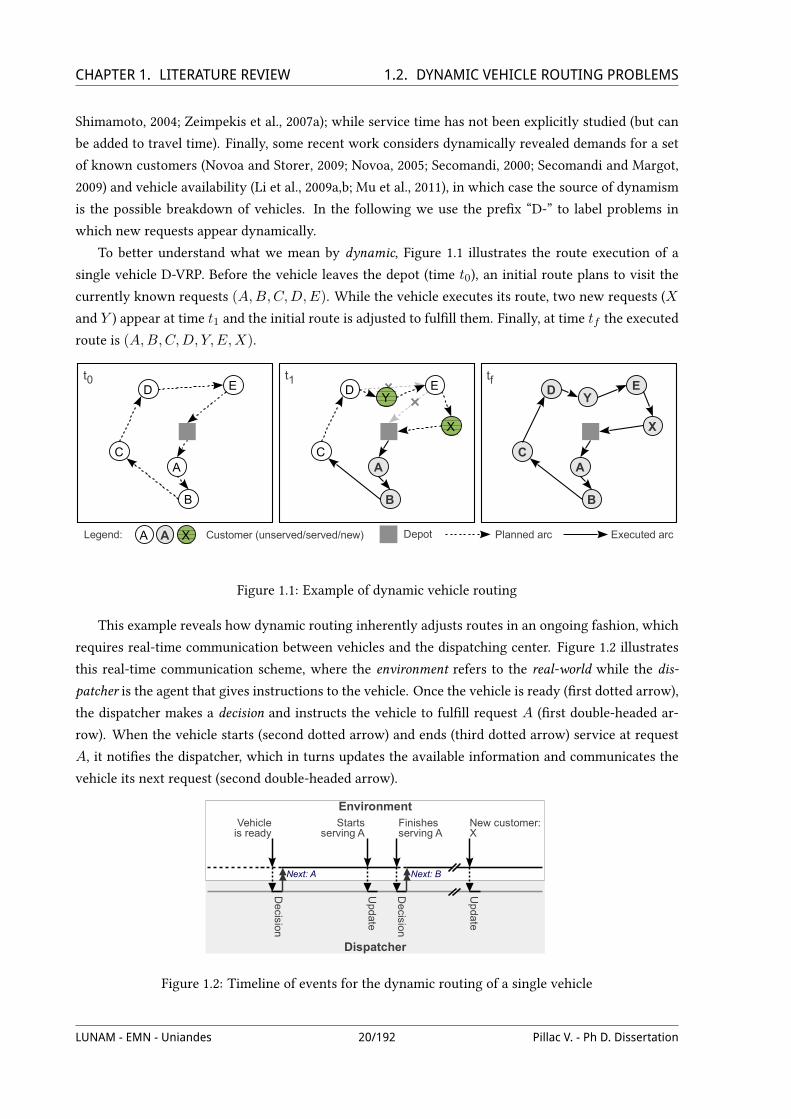
To better understand what we mean by dynamic, Figure 1.1 illustrates the route execution of a
single vehicle D-VRP. Before the vehicle leaves the depot (time t0), an initial route plans to visit the
currently known requests (A,B,C,D,E). While the vehicle executes its route, two new requests (X
and Y ) appear at time t1 and the initial route is adjusted to fulVll them. Finally, at time tf the executed
route is (A,B,C,D, Y,E,X).
! "
Figure 1.1: Example of dynamic vehicle routing
This example reveals how dynamic routing inherently adjusts routes in an ongoing fashion, which
requires real-time communication between vehicles and the dispatching center. Figure 1.2 illustrates
this real-time communication scheme, where the environment refers to the real-world while the dis-
patcher is the agent that gives instructions to the vehicle. Once the vehicle is ready (Vrst dotted arrow),
the dispatcher makes a decision and instructs the vehicle to fulVll request A (Vrst double-headed ar-
row). When the vehicle starts (second dotted arrow) and ends (third dotted arrow) service at request
A, it notiVes the dispatcher, which in turns updates the available information and communicates the
vehicle its next request (second double-headed arrow).
Dispatcher
EnvironmentVehicle
is readyStarts
serving AFinishesserving A
Decision
Upd
ate
Decision
New customer: X
Up
date
Next: A Next: B
Figure 1.2: Timeline of events for the dynamic routing of a single vehicle
LUNAM - EMN - Uniandes 20/192 Pillac V. - Ph D. Dissertation

CHAPTER 1. LITERATURE REVIEW 1.2. DYNAMIC VEHICLE ROUTING PROBLEMS1.2.2 DiUerences with static routing
In contrast to their static counterparts, dynamic routing problems involve new elements that in-
crease the complexity of their decisions (more degrees of freedom) and introduce new challenges while
judging the merit of a given route plan.
In some contexts, such as the pick-up of express courier (Gendreau et al., 1999), the transport
company may deny a customer request. As a consequence, it can reject a request either because
it is simply impossible to service it, or because the cost of serving it is too high. This process of
acceptance/denial has been used in many approaches (Attanasio et al., 2004; Fagerholt et al., 2009;
Gendreau et al., 1999; Ichoua et al., 2000, 2003, 2006; Li et al., 2009a) and is referred to as service
guarantee (Van Hentenryck and Bent, 2006).
In dynamic routing, the ability to redirect a moving vehicle to a new request nearby allows for
additional savings. Nevertheless, it requires real-time knowledge of the vehicle position and being able
to communicate quickly with drivers to assign them new destinations. Thus, this strategy has received
limited interest, with the main contributions being the early work by Regan et al. (1995, 1998, 1996),
the study of diversion issues by Ichoua et al. (2000), and the work by Branchini et al. (2009).
Dynamic routing also frequently diUers in the objective function (Psaraftis, 1995). In particular,
while a common objective in the static context is the minimization of the routing cost, dynamic rout-
ing may introduce other notions such as service level, throughput (number of serviced requests), or
revenue maximization. Having to answer to dynamic customer requests also introduces the notion of
response time: a customer might request to be serviced as soon as possible, in which case the main
objective may become to minimize the delay between the arrival of a request and its service.
Dynamic routing problems require making decisions in an online manner, which often compro-
mises reactiveness with decision quality. In other words, the time invested searching for better de-
cisions, comes at the price of a lower reactiveness to input changes. This aspect is of particular im-
portance in contexts where customers call for a service and a good decision must be made as fast as
possible.
1.2.3 Measuring dynamism
DiUerent problems (or instances of a same problem) can have diUerent levels of dynamism, which
can be characterized according to two dimensions (Ichoua et al., 2007): the frequency of changes and
the urgency of requests. The former is the rate at which new information becomes available, while the
latter is the time gap between the disclosure of a new request and its expected service time. From this
observation three metrics have been proposed to measure the dynamism of a problem (or instance).
Lund et al. (1996) deVned the degree of dynamism δ as the ratio between the number of dynamic
requests nd and the total number of requests ntot as follows:
δ =ndntot
(1.1)
Based on the fact that the disclosure time of requests is also important (Psaraftis, 1988, 1995), Larsen
(2001) proposed the eUective degree of dynamism δe. This metric can be interpreted as the normalized
LUNAM - EMN - Uniandes 21/192 Pillac V. - Ph D. Dissertation

CHAPTER 1. LITERATURE REVIEW 1.3. A REVIEW OF APPLICATIONSaverage of the disclosure times. Let T be the length of the planning horizon,R the set of requests, and
ti the disclosure time of request i ∈ R. Assuming that requests known beforehand have a disclosure
time equal to 0, δe can be expressed as:
δe =1
ntot
∑i∈R
tiT
(1.2)
Larsen (2001) also extended the eUective degree of dynamism to problems with time windows to
reWect the level of urgency of requests. He deVnes the reaction time as the diUerence between the
disclosure time ti and the end of the corresponding time window li, highlighting that longer reaction
times mean more Wexibility to insert the request into the current routes. Thus, the eUective degree of
dynamism measure is extended as follows:
δeTW =1
ntot
∑i∈R
(1− li − ti
T
)(1.3)
It is worth noting that these three metrics only take values in the interval [0, 1] and all increase
with the level of dynamism of a problem. Larsen et al. (2002, 2007) use the eUective degree of dynamism
to deVne a framework classifying D-VRPs among weakly, moderately, and strongly dynamic problems,
with values of δe being respectively lower than 0.3, comprised between 0.3 and 0.8, and higher than
0.8.
Although the eUective degree of dynamism and its variations have proven to capture well the
time-related aspects of dynamism, it could be argued that they do not take into account other possible
sources of dynamism. In particular, the geographical distribution of requests, or the traveling times
between requests, are also of great importance in applications aiming at the minimization of response
time. Although not considered, the frequency of updates in problem information has a dramatical
impact on the time available for optimization.
1.3 A review of applications
Recent advances in technology have allowed the emergence of a wide new range of applications
for vehicle routing. In particular, the last decade has seen the development of Intelligent Transport
Systems (ITS), which are based on a combination of geolocation technologies, with precise geographic
information systems, and increasingly eXcient hardware and software for data processing and opera-
tions planning. We refer the interested reader to the study by Crainic et al. (2009) for more details on
ITS and the contributions of operations research to this relatively new domain.
Among the ITS, the Advanced Fleet Management Systems (AFMS) are speciVcally designed for
managing a corporate vehicle Weet. The core problem is generally to deliver (pick-up) goods or persons
to (from) locations distributed in a given area. While customer requests can either be known in advance
or appear dynamically during the day, vehicles are dispatched and routed in real time, potentially, by
taking into account changing traXc conditions, uncertain demands, or varying service times. A key
technological feature of AFMS is the optimization component. Traditionally, vehicle routing relies on
LUNAM - EMN - Uniandes 22/192 Pillac V. - Ph D. Dissertation

CHAPTER 1. LITERATURE REVIEW 1.3. A REVIEW OF APPLICATIONSteams of human dispatchers, meaning a critical operational process is bound to the competence and
experience of dispatchers, as well as the management costs that are directly linked to the size of the
Weet (Attanasio et al., 2007). Advances in computer science have allowed a technological transfer from
operational research to AFMS, as presented in the studies by Attanasio et al. (2007); Du et al. (2007);
Godfrey and Powell (2002); Powell and Topaloglu (2005); Roy (2001); Simao et al. (2009), and Slater
(2002).
The remainder of this section presents applications where dynamic routing has been or can be
implemented. The interested reader is also referred to the work by Gendreau and Potvin (1998) and
Ichoua et al. (2007) for complementary reviews.
1.3.1 Services
In this category of applications, a service request is deVned by a customer location and a possible
time window; while vehicle routes just fulVll service requests without considering side constraints such
as capacity. Perhaps the simplest, yet most illustrative case in this category is the dynamic traveling
salesman problem (Larsen et al., 2004).
A common application of dynamic routing can be found in the area of maintenance operations.
Maintenance companies are often committed by contract to their customers, which specify periodical
or planned visits to perform preventive maintenance, and may also request corrective maintenance on
short notice. Therefore, each technician is Vrst given a route with known requests at the beginning
of the day, while new urgent requests are inserted dynamically throughout the day. An interesting
feature of this problem is the possible mix of skills, tools, and spare part requirements, which have to
be matched in order to service the request. This problem has been studied by Borenstein et al. (2010)
with an application to British Telecom.
Another application of dynamic routing arises in the context of the French non-proVt organization
SOS Médecins. This organization operates with a crew of physicians, who are called on duty via a call
center coordinated with other emergency services. When a patient calls, the severity of the case is
evaluated, and a visit by a practitioner is planned accordingly. As in other emergency services, having
an eXcient dispatching system reduces the response time, thus improving service level for the society.
On the other hand, it is important to decide in real-time whether or not to send a physician, so that it
is possible to ensure a proper service level in areas where emergencies are likely to appear.
Dynamic aspects can also appear on arc routing problems. This is for instance the case in the
study by Tagmouti et al. (2011) on the operation of a Weet of vehicles for winter gritting applications.
Their work consider a network of streets or road segments that need to be gritted when aUected by a
moving storm. Depending on the movements of the storm, new segments may have to be gritted, and
the routing of vehicles has to be updated accordingly.
1.3.2 Transport of goods
Due to the fact that urban areas are often characterized by highly variable traveling times, trans-
port of goods in such areas have led to the deVnition of a speciVc category of applications known
as city logistics. City logistics can be deVned as an integrated vision of transport activities in urban
LUNAM - EMN - Uniandes 23/192 Pillac V. - Ph D. Dissertation

CHAPTER 1. LITERATURE REVIEW 1.3. A REVIEW OF APPLICATIONSareas, taking into account factors such as traXc and competition or cooperation between transport
companies (Taniguchi and Thompson, 2002). Barcelo et al. (2007) developed a general framework for
city logistics applications. They describe the diUerent modules ranging from modeling the city road
network and acquiring real-time traXc data to the dynamic routing of a Weet of vehicles. Zeimpekis
et al. (2007a) proposed a Decision Support System (DSS) for city logistics which takes into account
dynamic travel and service times.
A typical application in city logistics is the courier service present in most urban areas. Couriers
are dispatched to customer locations to collect packages, and either deliver them to their destination
(short haul) or to a unique depot (long haul). Depending on the level of service paid by the customer,
couriers may consolidate pick-ups from various customers, or provide an expedited service. Companies
oUering courier services often have an heterogeneous Weet composed of bicycles, motorbikes, cars,
and small vans. The problem is then to dynamically route couriers, taking into account not only the
known requests, their type, pick-up and delivery locations, and time windows, but also considering
traXc conditions and varying travel times. A case study by Attanasio et al. (2007) outlines the beneVts
of using an optimization-enabled AFMS at eCourier Ltd, a London based company oUering courier
services. The authors illustrate that aside from the improvements in service quality, response time,
and courier eXciency, the use of an automated system allows decoupling the Weet size from the need
for more dispatchers. Further results motivated by a similar application can be found in Gendreau et al.
(2006) and Ghiani et al. (2009).
The delivery of newspapers and magazines is a domain in which customer satisfaction is of Vrst
importance. When a magazine or newspaper is not delivered, a subscriber contacts a call center and
is oUered to choose between a voucher or a future delivery. In the latter case, the request is then
forwarded to the delivery company, which assigns it to a driver that will do a priority delivery. Tradi-
tionally, this process relies on an exchange of phone calls, faxes, and printed documents, that ultimately
communicate the driver about the pending delivery, once he/she comes back to the depot. As an al-
ternative, Bieding et al. (2009) propose a centralized application that makes use of mobile phones to
communicate with drivers and intelligently perform the routing in real time, reducing costs and im-
proving customer satisfaction. More recently, Ferrucci et al. (2011) developed an approach that makes
use historical data to anticipate future requests.
Another application in which customer requests need to be answered with short delays can be
found in companies with a direct service model, such as grocery delivery services. In general, the
customer selects products on a website, and then chooses a time frame for the delivery at his home.
Traditionally, the vendor deVnes an arbitrary number of customers that can be serviced within a time
window, and the time window is made unavailable to customers as soon as the capacity is reached.
Campbell and Savelsbergh (2005) deVned the Home Delivery Problem, in which the goal is to maximize
the total expected revenue by dynamically deciding whether or not to accept a customer request within
a speciVc time window. In comparison with the traditional approach, this means that the time windows
available for a customer are dynamically deVned taking into consideration the possible future requests.
The authors propose a Greedy Randomized Adaptive Search Procedure (GRASP) and compare diUerent
cost functions to capture the problem uncertainty. Later, Azi et al. (2011) proposed an Adaptive Large
Neighborhood Search (ALNS) that take into account uncertainty by generating scenarios containing
LUNAM - EMN - Uniandes 24/192 Pillac V. - Ph D. Dissertation

CHAPTER 1. LITERATURE REVIEW 1.3. A REVIEW OF APPLICATIONSpossible demand realizations.
Apart from classical routing problems, related operational problems also arise in many organi-
zations. The review by Stahlbock and Voss (2008) on operations research applications in container
terminals describes the dynamic stacker crane problem (Balev et al., 2009; Berbeglia et al., 2010), which
considers the routing of container carriers loading and unloading ships in a terminal. Other applica-
tions include transport of goods inside warehouses (Smolic-Rocak et al., 2010), factories, and hospitals,
where documents or expensive medical instruments must be transferred eXciently between services
(Fiegl and Pontow, 2009).
1.3.3 Transport of persons
The transport of persons is in general–and by many aspects–similar to the transport of goods, yet
it is characterized by additional constraints such as regulation on waiting, travel, and service times.
Taxis are arguably the most common on-demand individual transport systems. Requests are com-
posed of a pick-up location and time, possibly coupled with a destination. They can be either known in
advance, for instance when a customer books a cab for the next day, or they can arrive dynamically, in
which case a taxi must be dispatched in the shortest time. When customers cannot share a vehicle, the
closest free taxi is generally the one which takes the ride, leaving limited space for optimization. The
study by Caramia et al. (2002), generalized by Fabri and Recht (2006), focuses on a multi-cab metropoli-
tan transportation system, where a taxi can transport more than one passenger at the same time. In
this case the online algorithms minimize the total traveled distance, while assigning requests to ve-
hicles and computing the taxi routes. This multi-cab transportation system can be generalized as an
on-demand or door-to-door transport service.
Many applications involve the transport of children, the elderly, disabled people, or patients, from
their home to schools, place of work, or medical centers. Xiang et al. (2008) studied a DARP with
changing travel speeds, vehicle breakdowns, and traXc congestion; while Dial (1995), followed by
Horn (2002a,b, 2004), studied demand-responsive transport systems. An extensive review of this class
of problems can be found in the studies by Cordeau et al. (2007a) and Berbeglia et al. (2010).
A singular application of on-demand transportation systems can be found in major hospitals, with
services possibly spread across various buildings on several branches. Depending on the medical
procedure or facility capacity, a patient may need to be transferred on short notice from one service
to another, possibly requiring trained staU or speciVc equipment for his/her care. This application has
been studied by Beaudry et al. (2010); Kergosien et al. (2011), and Melachrinoudis et al. (2007).
Air taxis developed as a Wexible response to the limitations of traditional airlines. Air taxis oUer
passengers the opportunity to travel through smaller airports, avoiding waiting lines at check-in and
security checks. Air taxi companies oUer an on-demand service: customers book a Wight a few days in
advance, specifying whether they are willing to share the aircraft, stop at an intermediate airport, or
have Wexible traveling hours. Then, the company accommodates these requests, trying to consolidate
Wights whenever possible. The underlying optimization problems have not been subject to much at-
tention, except in the studies by Cordeau et al. (2007a); Espinoza et al. (2008a,b); Fagerholt et al. (2009),
and Yao et al. (2007). Similar problems arises in helicopter transportation systems, typically used by oil
LUNAM - EMN - Uniandes 25/192 Pillac V. - Ph D. Dissertation

CHAPTER 1. LITERATURE REVIEW 1.4. SOLUTION METHODSand gas companies to transport personnel between oUshore petroleum platforms (Gribkovskaia et al.,
2008; Romero et al., 2007).
1.4 Solution Methods
Few research was conducted on dynamic routing between the work of Psaraftis (1980) in 1980
and the late 1990s. However, the last decade has seen a renewed interest for this class of problems
(Eksioglu et al., 2009), with solution techniques ranging from linear programming to metaheuristics.
This section presents the major contributions in this Veld, and the reader is referred to the reviews,
books, and special issues by Gendreau and Potvin (1998, 2004); Ghiani et al. (2003); Goel (2008); Ichoua
(2001); Ichoua et al. (2006, 2007); Jaillet and Wagner (2008b); Larsen et al. (2008), and Zeimpekis et al.
(2007b), to complement our review.
1.4.1 Dynamic and deterministic routing problems
This section presents approaches that have been successfully applied to dynamic routing, in the
absence of stochastic information. In this context, critical information is revealed over time, meaning
that the complete instance is only known at the end of the planning horizon. As a consequence, exact
methods only provide an optimal solution for the current state, but do not guarantee that the solution
will remain optimal once new data becomes available. Therefore, most dynamic approaches rely on
heuristics that quickly compute a solution to the current state of the problem. Approaches for dynamic
and deterministic vehicle routing problems can be divided into two categories: those based on periodic
reoptimization, and those based on continuous reoptimization.
1.4.1.1 Periodic reoptimization
To the best of our knowledge, the Vrst periodic reoptimization approach is due to Psaraftis (1980),
with the development of a dynamic programming approach. His research focuses on the DARP and
consists in Vnding the optimal route each time a new request is known. The main drawback of dynamic
programming is the well-known curse of dimensionality (Powell, 2007, Chap. 1), which prevents its
application to large instances.
More generally, periodic reoptimization approaches start at the beginning of the day with a Vrst
optimization that produces an initial set of routes. Then, an optimization procedure periodically solves
a static problem corresponding to the current state, either whenever the available data changes, or at
Vxed intervals of time –referred to as decision epochs (Chen and Xu, 2006) or time slices (Kilby et al.,
1998). The advantage of periodic reoptimization is that it can be based on algorithms developed for
static routing, for which extensive research has been carried out. The main drawback is that all the
optimization needs to be performed before updating the routing plan, thus increasing delays for the
dispatcher.
Yang et al. (2004) addressed the real-time truckload PDP, in which a Weet of trucks has to service
point-to-point transport requests arriving dynamically. Important assumptions are that all trucks can
only handle one request at a time, with no possible preemption, and they travel at the same constant
LUNAM - EMN - Uniandes 26/192 Pillac V. - Ph D. Dissertation

CHAPTER 1. LITERATURE REVIEW 1.4. SOLUTION METHODSspeed. The authors propose MYOPT, a rolling horizon approach based on a linear program (LP) that
is solved whenever a new request arrives. Along the same line of linear programming, Chen and
Xu (2006) designed a dynamic column generation algorithm (DYCOL) for the D-VRPTW. The authors
propose the concept of decision epochs over the planning horizon, which are the dates when the op-
timization process runs. The novelty of their approach relies on dynamically generating columns for
a set-partitioning model, using columns from the previous decision epoch. The authors compared
DYCOL to a traditional column generation with no time limit (COL). Computational results based on
the Solomon benchmark (Solomon, 1987) demonstrate that DYCOL yields comparable results in terms
of objective function, but with running times limited to 10 seconds, opposed to the various hours
consumed by COL.
Montemanni et al. (2005) developed an Ant Colony System (ACS) to solve the D-VRP. Similar to
Kilby et al. (1998), their approach uses time slices, that is, they divide the day in periods of equal
duration. A request arriving during a time slice is not handled until the end of the time bucket, thus
the problem solved during a time slice only considers the requests known at its beginning. Hence, the
optimization is run statically and independently during each time slice. The main advantage of this
time partition is that similar computational eUort is allowed for each time slice. This discretization
is also possible by the nature of the requests, which are never urgent, and can be postponed. An
interesting feature of their approach is the use of the pheromone trace to transfer characteristics of a
good solution to the next time slice. A similar approach was also used by Gambardella et al. (2003) and
Rizzoli et al. (2007).
1.4.1.2 Continuous reoptimization
Continuous reoptimization approaches perform the optimization throughout the day and maintain
information on good solutions in an adaptive memory (Taillard et al., 2001). Whenever the available
data changes, a decision procedure aggregates the information from the memory to update the current
routing. The advantage is that the computational capacity is maximized, possibly at the expense of a
more complex implementation. It is worth noting that because the current routing is subject to change
at any time, vehicles do not know their next destination until they Vnish the service of a request.
To the best of our knowledge, the Vrst continuous reoptimization approach is due Gendreau et al.
(1999) with the adaptation of the parallel Tabu Search (TS) framework introduced by Taillard et al.
(1997) to a D-VRPTW problem arising in the local operation of long distance express courier services.
Their approach maintains a pool of good routes–the adaptive memory–which is used to generate initial
solutions for a parallel TS. The parallelized search is done by partitioning the routes of the current
solution, and optimizing them in independent threads. Whenever a new customer request arrives, it is
checked against all the solutions from the adaptive memory to decide whether it should be accepted or
rejected. This framework was also implemented for the D-VRP (Ichoua et al., 2000, 2003), while other
variations of TS have been applied to the D-PDP (Barcelo et al., 2007; Chang et al., 2003) and the DARP
(Attanasio et al., 2004; Beaudry et al., 2010).
Bent and Van Hentenryck (2004b) introduced theMultiple Plan Approach (MPA) as a generalization
of the TS with adaptive memory (Gendreau et al., 1999). The general idea is to populate and maintain
LUNAM - EMN - Uniandes 27/192 Pillac V. - Ph D. Dissertation
CHAPTER 1. LITERATURE REVIEW 1.4. SOLUTION METHODSa solution pool (the routing plans) that are used to generate a distinguished solution. Whenever a new
request arrives, a procedure is called to check whether it can be serviced or not; if it can be serviced,
then the request is inserted in the solution pool and incompatible solutions are discarded. Pool updates
are performed periodically or whenever a vehicle Vnishes servicing a customer. This pool-update phase
is crucial and ensures that all solutions are coherent with the current state of vehicles and customers.
The pool can be seen as an adaptive memory that maintains a set of alternative solutions.
In an early work, Benyahia and Potvin (1998) studied the D-PDP and proposed a Genetic Algorithm
(GA) that models the decision process of a human dispatcher. More recently, GAs were also used for
the same problem (Cheung et al., 2008; Haghani and Jung, 2005) and for the D-VRP (Van Hemert and
Poutré, 2004). Genetic algorithms in dynamic contexts are very similar to those designed for static
problems, although they generally run throughout the planning horizon and solutions are constantly
adapting to the changes made to the input.
1.4.2 Dynamic and stochastic routing problems
Dynamic and stochastic routing problems can be seen as an extension of their deterministic coun-
terparts, where additional (stochastic) knowledge is available in the dynamically revealed input. Ap-
proaches for this class of problems can be divided in two categories: those based on sampling and
those based on stochastic modeling. As their name suggests, sampling strategies incorporate stochastic
knowledge by generating scenarios based on realizations drawn from random variable distributions.
Each scenario is then optimized by solving the static and deterministic problem they deVne. On the
other hand, approaches based on stochastic modeling integrate stochastic knowledge analytically. The
advantage of sampling is its relative simplicity and Wexibility on distributional assumptions, while its
drawback is the massive generation of scenarios to accurately reWect reality. Alternatively, stochastic
modeling strategies formally capture the stochastic nature of the problem, but they are highly technical
in their formulation and require to eXciently compute possibly complex expected values. Examples of
these two strategies follow.
1.4.2.1 Stochastic modeling
Powell et al. (1988) formulated a truckload PDP as a Markov Decision Process (MDP). Later, MDPs
were used by Thomas and White (2004) and Thomas (2007) to solve a VRP in which known customers
may ask for service with a known probability. Kim et al. (2005) also used MDPs to tackle the VRP with
dynamic travel times. Unfortunately, the curse of dimensionality and the simplifying assumptions
make this approach unsuitable in most real-world applications. Nonetheless, it allowed new insights
in the Veld of dynamic programming.
To cope with the scalability problems of traditional dynamic programming, Approximate Dynamic
Programming (ADP) steps forward in time, approximates the value function, and ultimately avoids
the evaluation of all possible states. We refer the interested reader to Powell (2007, 2009) for a more
detailed description of the ADP framework. ADP has been successfully applied to freight transport
(Powell et al., 2007; Powell and Topaloglu, 2003) and Weet management problems (Godfrey and Powell,
2002; Powell and Topaloglu, 2005; Simao et al., 2009). In particular, Novoa and Storer (2009) propose
LUNAM - EMN - Uniandes 28/192 Pillac V. - Ph D. Dissertation

CHAPTER 1. LITERATURE REVIEW 1.4. SOLUTION METHODSan ADP algorithm to dynamically solve the VRPSD.
Linear programming has also been adapted to the dynamic and stochastic context. The OPTUN ap-
proach, proposed by Yang et al. (2004) as an extension of MYOPT (see § 1.4.1.1), considers opportunity
costs on each arc to reWect the expected cost of traveling to isolated areas. Consequently, the opti-
mization tends to reject isolated requests, and avoids traversing arcs that are far away from potential
requests. Later, Yang et al. (2005) studied the emergency vehicle dispatching and routing and proposed
a mathematical formulation that was later used by Haghani and Yang (2007) on a similar problem.
1.4.2.2 Sampling
Sampling approaches rely on the generation of scenarios containing possible realizations of the
random variables. Figure 1.3 illustrates how scenarios are generated for the D-VRP. Solely based on the
current customers, the optimal tour would be (A,B,E,D,C) (1.3a.), which ignores two zones (gray
areas) where customers are likely to appear. By sampling the customer spatial distributions, customers
X , Y , and Z are generated, and the new optimal tour is (C,X, Y,B,A,Z,E,D) (1.3b.). Removing the
sampled (potential) customers leads to the tour (C,B,A,E,D) (1.3c.) which is suboptimal regarding
a myopic cost evaluation, but leaves room to accommodate new customers at a lower cost.
E
D C
A
B
a. A-priori optimal tour
E
D C
A
B
X
YZ
b. Optimal tour with sampled cus-tomers
E
D C
A
B
X
YZ
c. Optimized scenario without sampledcustomers
Legend: TourA Customer (actual/sampled)A Depot Customer distribution density
Figure 1.3: Scenario generation in sampling approaches.
The Multiple Scenario Approach (MSA) is a predictive adaptation of the MPA framework discussed
in § 1.4.1.2. The idea behind MSA is to take advantage of the time between decisions to continuously
improve the current scenario pool. During the initialization, the algorithm, generates a Vrst set of sce-
narios based on the requests known beforehand. Throughout the day, scenarios are then reoptimized
and new ones are generated and added to the pool. When a decision is required, the scenario optimiza-
tion procedure is suspended, and MSA uses the scenario pool to select the request to service next. MSA
then discards the scenarios that are incompatible with the current routing, and resumes the optimiza-
tion. Computational experiments on instances adapted from the Solomon benchmark (Solomon, 1987)
showed that MSA outperforms MPA both in terms of serviced customers and traveled distances, espe-
cially for instances with high degrees of dynamism (Bent and Van Hentenryck, 2004b). Flatberg et al.
(2007) adapted the SPIDER commercial solver to use multiple scenarios and a consensus algorithm to
LUNAM - EMN - Uniandes 29/192 Pillac V. - Ph D. Dissertation

CHAPTER 1. LITERATURE REVIEW 1.4. SOLUTION METHODStackle the D-VRP, while Pillac et al. (2012) implemented an event-driven optimization framework based
on MSA and showed signiVcant improvements over state-of-the-art algorithms for the D-VRPSD.
An important component of scenario based-approaches such as MSA is the decision process, which
deVnes how the information from the scenario pool is used to reach upon a decision regarding the next
customer to visit. The most common algorithms used to reach a decision in MSA are: consensus, expec-
tation, and regret. The consensus algorithm (Bent and Van Hentenryck, 2004b,c) selects the customer
appearing Vrst with the highest frequency among scenarios. Expectation (Bent and Van Hentenryck,
2004a,c; Chang et al., 2000) consists in evaluating the cost of visiting each customer Vrst by forcing
its visit in all scenarios and performing a complete optimization. Finally, regret (Bent and Van Hen-
tenryck, 2004a) approximates the expectation algorithm and avoids the reoptimization of all scenarios.
Even though these algorithms were initially designed for the routing of a single vehicle, they can be
extended to the multi-vehicle case (Van Hentenryck and Bent, 2006).
Hvattum et al. (2006) developed the Dynamic Sample Scenario Hedge Heuristic (DSHH), an ap-
proach similar to the consensus algorithm for D-VRP. This method divides the planning horizon into
time intervals. At the beginning of each interval, DSHH revises the routing by assigning a subset of
promising requests to the vehicles, depending on the frequency of their assignment over all scenarios.
DSHH later led to the development of the Branch and Regret Heuristic (BRH), where scenarios are
merged to build a unique solution.
Various local search approaches have been developed for the stochastic and dynamic problems.
Ghiani et al. (2009) developed an algorithm for the D-PDP that only samples the near future to reduce
the computational eUort. The main diUerence with MSA is that no scenario pool is used and the selec-
tion of the distinguished solution is based on the expected penalty of accommodating requests in the
near future. Azi et al. (2011) developed an Adaptive Large Neighborhood Search (ALNS) for a dynamic
routing problem with multiple delivery routes, in which the dynamic decision is the acceptance of a
new request. The approach maintains a pool of scenarios, optimized by an ALNS, that are used to
evaluate the opportunity value of an incoming request.
Tabu search has also been adapted to dynamic and stochastic problems. Ichoua et al. (2006) and
Attanasio et al. (2007) tackled with tabu search the D-VRPTW and the D-PDP, respectively.
1.4.2.3 Other strategies
In addition to the general frameworks described previously, the use of stochastic knowledge allows
for the design and implementation of other strategies that try to adequately respond to upcoming
events.
The waiting strategy consists in deciding whether a vehicle should wait after servicing a request,
before heading toward the next customer; or planning a waiting period on a strategic location. This
strategy is particularly important in problems with time windows, where time lags appear between
requests. Mitrović-Minić et al. (2004) proved that in all cases it is better to wait after servicing a
customer, but a more reVned strategy can lead to further improvements. The problem is in general
to evaluate the likelihood of a new request in the neighborhood of a serviced request and to plan a
waiting period accordingly. The waiting strategy has been implemented in various frameworks for
LUNAM - EMN - Uniandes 30/192 Pillac V. - Ph D. Dissertation
CHAPTER 1. LITERATURE REVIEW 1.4. SOLUTION METHODSthe D-VRP (Branke et al., 2005; Thomas, 2007), D-VRPTW (Bent and Van Hentenryck, 2007; Branchini
et al., 2009; Ichoua et al., 2006; Van Hentenryck and Bent, 2006), D-PDP (Ghiani et al., 2009; Mitrović-
Minić et al., 2004), and Dynamic and Stochastic TSP (Ghiani et al., 2008). The strategy has shown good
results, especially in the case of a limited Weet facing a high request rate (Van Hentenryck and Bent,
2006).
Aside from the waiting after or before servicing a customer, a vehicle can be relocated to a strategic
position, where new requests are likely to arrive. This strategy is the keystone of emergency Weet de-
ployment, also known as Emergency Vehicle Dispatching–or Redeployment–Problem (Gendreau et al.,
2001; Haghani and Yang, 2007). The relocation strategy has also been applied to other vehicle routing
problems, such as the D-VRP (Larsen, 2001),D-VRPTW (Bent and Van Hentenryck, 2007; Branchini
et al., 2009; Ichoua et al., 2006; Van Hentenryck and Bent, 2006), D-TSPTW (Larsen et al., 2004), D-PDP
(Ghiani et al., 2009; Pureza and Laporte, 2008), and the Resource Allocation Problem (RAP) (Godfrey
and Powell, 2002).
Request buUering, introduced by Pureza and Laporte (2008), consists in delaying the assignment of
some requests to vehicles in a priority buUer, so that more urgent requests can be handled Vrst.
1.4.3 Performance evaluation
In contrast to static problems, where measuring the performance of an algorithm is straightforward
(i.e., running time and solution quality), dynamic problems require the introduction of new metrics to
assess the performance of a particular method.
Sleator and Tarjan (1985) introduced the competitive analysis (Jaillet and Wagner, 2008a; Larsen
et al., 2007). Let P be a minimization problem and I the set of all instances of P . Let z∗(Ioff) be the
optimal cost for the oYine instance Ioff corresponding to I ∈ I . For oYine instance Ioff , all input
data from instance I , either static or dynamic, is available when building the solution. In contrast, the
data of the online version I is revealed in real time, thus an algorithm A has to take into account new
information as it is revealed and produce a solution relevant to the current state of knowledge. Let
zA(I) = z(xA(I)) be the cost of the Vnal solution xA(I) found by the online algorithmA on instance
I . AlgorithmA is said to be c-competitive, or equivalently to have a competitive ratio of c, if there exists
a constant α such that
zA(I) ≤ c · z∗ (Ioff) + α , ∀ I ∈ I (1.4)
In the case where α = 0, the algorithm is said to be strictly c-competitive, meaning that in all cases
the objective value of the solution found by A will be at most of c times the optimal value. The
competitive ratio metric allows a worst-case absolute measure of an algorithm performance in terms
of the objective value. We refer the reader to Borodin and El-Yaniv (2005) for an in-depth analysis of
this measure, and to Jaillet and Wagner (2008a) and Fink et al. (2009) for results on various routing
problems.
The main drawback of the competitive analysis is that it requires to prove the previously stated
inequality analytically, which may be complex for real-world applications. The value of information
proposed by Mitrović-Minić et al. (2004) constitutes a more Wexible and practical metric. We denote by
LUNAM - EMN - Uniandes 31/192 Pillac V. - Ph D. Dissertation
CHAPTER 1. LITERATURE REVIEW 1.5. CONCLUSIONSzA(Ioff) the value of the objective function returned by algorithm A for the oYine instance Ioff . The
value of information VA(I) for algorithm A on instance I is then deVned as
VA(I) =zA(I)− zA(Ioff)
zA(Ioff)(1.5)
The value of information can be interpreted as the gap between the solution returned by an algorithm
A on a instance I and the solution returned by the same algorithm when all information from I is
known beforehand. In contrast with the competitive ratio, the value of information gives information
on the performance of an algorithm based on empirical results, without requiring optimal solutions
for the oYine instances. It captures the impact of the dynamism on the solution yield by the algorithm
under analysis. For instance, Gendreau et al. (1999) report a value of information between 2.5% and
4.1% for their tabu search algorithm for the D-VRPTW, while Tagmouti et al. (2011) reports values
between 10% and 26.7% for a variable neighborhood search descent applied to a dynamic arc routing
problem.
1.4.4 Benchmarks
To date, there is no reference benchmark for dynamic routing problems. Although, it is worth
noting that various authors based their computational experiments on adaptations of the Solomon
(1987) instances for static routing (Bent and Van Hentenryck, 2004a,b; Chen et al., 2006; Chen and Xu,
2006; Gendreau et al., 1999). Van Hentenryck and Bent (2006, Chap. 10) describe how the original
benchmark by Solomon (1987) can be adapted to dynamic problems.
The interested reader is referred to the website of Pankratz and Krypczyk (2009) for an updated list
of publicly available instances sets for dynamic vehicle routing problems.
1.5 Conclusions
Recent technological advances provide companies with the right tools to manage their Weet in
real time. Nonetheless, these new technologies also introduce more complexity in Weet management
tasks, unveiling the need for decision support systems adapted to dynamic contexts. Consequently,
during the last decade, the research community have shown a growing interest for the underlying op-
timization problems, leading to a new family of approaches speciVcally designed to eXciently address
dynamism and uncertainty. By analyzing the current state of the art, some directions can be drawn for
future research in this relatively new Veld.
First, further work should aim at creating a taxonomy of dynamic vehicle routing problem, possibly
by extending existing research on static routing (Eksioglu et al., 2009). This would allow a more precise
classiVcation of approaches, evaluate similarities between problems, and foster the development of
generic frameworks.
Second, there is currently no reference benchmark for dynamic vehicle routing problems. There-
fore, there is a strong need for the development of publicly available benchmarks for the most common
dynamic vehicle routing problems.
LUNAM - EMN - Uniandes 32/192 Pillac V. - Ph D. Dissertation
CHAPTER 1. LITERATURE REVIEW BIBLIOGRAPHYThird, with the advent of multi-core processors on desktop computers, and low-cost graphical pro-
cessing units (GPU), parallel computing is now readily available for time-consuming methods such as
those based on sampling. Although early studies considered distributed optimization (Gendreau et al.,
1999), most approaches reviewed in this document do not take advantage of parallel architectures. The
development of parallel algorithms is a challenge that could reduce the time needed for optimization
and provide decision makers with highly reactive tools.
Fourth, our review of the existing literature revealed that a large fraction of work done in the area
of dynamic routing does not consider stochastic aspects. We are convinced that developing algorithms
that make use of stochastic information will improve the Weet performance and reduce operating costs.
Thus this line of research should become a priority in the near future.
Finally, researchers have mainly focused on the routing aspect of the dynamic Weet management.
However, in some applications there is more that can be done to improve performance and service
level. For instance, in equipment maintenance services, the call center has a certain degree of freedom
in Vxing service appointments. In other words, it means that the customer time windows can be
deVned, or inWuenced, by the call center operator. As a consequence, a system in which aside from
giving a yes/no answer to a customer request, suggests convenient times for the company would be
highly desirable in such contexts.
Acknowledgements Financial support for this work was provided by the CPER (Contrat de Projet
Etat Region) Vallée du Libre; and the Centro de Estudios Interdisciplinarios Básicos y Aplicados en
Complejidad (CEIBA, Colombia). This support is gratefully acknowledged.
Bibliography
Attanasio, A., Bregman, J., Ghiani, G., and Manni, E. (2007). Real-time Weet management at Ecourier Ltd. InZeimpekis, V., Tarantilis, C. D., Giaglis, G. M., and Minis, I., editors, Dynamic Fleet Management, volume 38 ofOperations Research/Computer Science Interfaces, chapter 10, pages 219–238. Springer US.
Attanasio, A., Cordeau, J. F., Ghiani, G., and Laporte, G. (2004). Parallel tabu search heuristics for the dynamicmulti-vehicle dial-a-ride problem. Parallel Computing, 30(3):377–387, doi:10.1016/j.parco.2003.12.001.
Azi, N., Gendreau, M., and Potvin, J. Y. (2011). A dynamic vehicle routing problem with multiple delivery routes.Annals of Operations Research, In-press:13.
Baldacci, R., Toth, P., and Vigo, D. (2007). Recent advances in vehicle routing exact algorithms. 4OR: A QuarterlyJournal of Operations Research, 5(4):269–298, doi:10.1007/s10288-007-0063-3.
Balev, S., Guinand, F., Lesauvage, G., and Olivier, D. (2009). Dynamical handling of straddle carriers activities ona container terminal in uncertain environment - a swarm intelligence approach -. In Proceedings of the 2009International Conference on Complex Systems and Applications (ICCSA 2009), Le Havre, France. University ofLe Havre.
Barcelo, J., Grzybowska, H., and Pardo, S. (2007). Vehicle routing and scheduling models, simulation and citylogistics. In Zeimpekis, V., Tarantilis, C. D., Giaglis, G. M., and Minis, I., editors, Dynamic Fleet Management,volume 38 of Operations Research/Computer Science Interfaces, pages 163–195. Springer US.
Beaudry, A., Laporte, G., Melo, T., and Nickel, S. (2010). Dynamic transportation of patients in hospitals. ORSpectrum, 32:77–107, doi:10.1007/s00291-008-0135-6.
LUNAM - EMN - Uniandes 33/192 Pillac V. - Ph D. Dissertation
CHAPTER 1. LITERATURE REVIEW BIBLIOGRAPHYBent, R. and Van Hentenryck, P. (2004a). Regrets only! online stochastic optimization under time constraints. In
Proceedings of the 19th National Conference on ArtiVcial Intelligence (AAAI-04), pages 501–506. AAAI Press.
Bent, R. and Van Hentenryck, P. (2004b). Scenario-based planning for partially dynamic vehicle routing withstochastic customers. Operations Research, 52(6):977–987.
Bent, R. and Van Hentenryck, P. (2004c). The value of consensus in online stochastic scheduling. In Proceedingsof the 14th International Conference on Automated Planning and Scheduling (ICAPS-04). AAAI Press.
Bent, R. and Van Hentenryck, P. (2005). Online stochastic and robust optimization. In Maher, M., editor, Advancesin Computer Science – ASIAN 2009, volume 3321 of Lecture Notes in Computer Science, pages 286–300. SpringerBerlin / Heidelberg.
Bent, R. and Van Hentenryck, P. (2007). Waiting and relocation strategies in online stochastic vehicle routing.In Veloso, M., editor, Proceedings of ohe 20th International Joint Conference on ArtiVcal Intelligence (IJCAI-07),pages 1816–1821.
Benyahia, I. and Potvin, J. Y. (1998). Decision support for vehicle dispatching using genetic programming. IEEETransactions on Systems Man and Cybernetics Part A - Systems and Humans, 28(3):306–314.
Berbeglia, G., Cordeau, J.-F., and Laporte, G. (2010). Dynamic pickup and delivery problems. European Journalof Operational Research, 202(1):8 – 15, doi:10.1016/j.ejor.2009.04.024.
Bertsimas, D. (1988). Probabilistic combinatorial optimization problems. PhD thesis, Massachusetts Institute ofTechnology, Dept. of Mathematics.
Bertsimas, D. and Simchi-Levi, D. (1996). A new generation of vehicle routing research: robust algorithms,addressing uncertainty. Operations Research, 44(2):286–304.
Bertsimas, D. and Van Ryzin, G. (1991). A stochastic and dynamic vehicle-routing problem in the Euclideanplane. Operations Research, 39(4):601–615.
Bieding, T., Görtz, S., and Klose, A. (2009). On line routing per mobile phone a case on subsequent deliveries ofnewspapers. In Nunen, J. A., Speranza, M. G., and Bertazzi, L., editors, Innovations in Distribution Logistics,volume 619 of Lecture Notes in Economics and Mathematical Systems, pages 29–51. Springer Berlin Heidelberg.
Borenstein, Y., Shah, N., Tsang, E., Dorne, R., Alsheddy, A., and Voudouris, C. (2010). On the partitioning ofdynamic workforce scheduling problems. Journal of Scheduling, 13(4):411–425, doi:10.1007/s10951-009-0152-6.
Borodin, A. and El-Yaniv, R. (2005). Online Computation and Competitive Analysis. Cambridge University Press,Cambridge.
Branchini, R. M., Armentano, V. A., and Lokketangen, A. (2009). Adaptive granular local searchheuristic for a dynamic vehicle routing problem. Computers & Operations Research, 36(11):2955–2968,doi:10.1016/j.cor.2009.01.014.
Branke, J., Middendorf, M., Noeth, G., and Dessouky, M. (2005). Waiting strategies for dynamic vehicle routing.Transportation Science, 39(3):298–312, doi:10.1287/trsc.1040.0095.
Brotcorne, L., Laporte, G., and Semet, F. (2003). Ambulance location and relocation models. European Journal ofOperational Research, 147(3):451–463, doi:10.1016/S0377-2217(02)00364-8.
Campbell, A. and Savelsbergh, M. (2005). Decision support for consumer direct grocery initiatives. TransportationScience, 39(3):313–327.
Caramia, M., Italiano, G., Oriolo, G., PaciVci, A., and Perugia, A. (2002). Routing a Weet of vehicles for dynamiccombined pick-up and deliveries services. In Proceedings of the Symposium on Operation Research 2001, pages3–5, Duisburg, Germany.
LUNAM - EMN - Uniandes 34/192 Pillac V. - Ph D. Dissertation

CHAPTER 1. LITERATURE REVIEW BIBLIOGRAPHYChang, H., Givan, R., and Chong, E. (2000). On-line scheduling via sampling. In Proceedings of the ArtiVcial
Intelligence Planning and Scheduling (AIPS 2000), pages 62–71.
Chang, M. S., Chen, S., and Hsueh, C. (2003). Real-time vehicle routing problem with time windows and simul-taneous delivery/pickup demands. Journal of the Eastern Asia Society for Transportation Studies, 5:2273–2286.
Chen, H.-K., Hsueh, C.-F., and Chang, M.-S. (2006). The real-time time-dependent vehicle routing problem.Transportation Research Part E: Logistics and Transportation Review, 42(5):383–408, doi:10.1016/j.tre.2005.01.003.
Chen, Z. and Xu, H. (2006). Dynamic column generation for dynamic vehicle routing with time windows.Transportation Science, 40(1):74–88.
Cheung, B. K. S., Choy, K. L., Li, C.-L., Shi, W., and Tang, J. (2008). Dynamic routing model and solution methodsfor Weet management with mobile technologies. International Journal of Production Economics, 113(2):694–705,doi:10.1016/j.ijpe.2007.10.018.
Christiansen, C. and Lysgaard, J. (2007). A branch-and-price algorithm for the capacitated vehicle routing prob-lem with stochastic demands. Operations Research Letters, 35(6):773–781.
Cordeau, J.-F., Laporte, G., Potvin, J.-Y., and Savelsbergh, M. W. (2007a). Transportation on demand. In Barnhart,C. and Laporte, G., editors, Transportation, volume 14 of Handbooks in Operations Research and ManagementScience, chapter 7, pages 429–466. Elsevier.
Cordeau, J.-F., Laporte, G., Savelsbergh, M. W., and Vigo, D. (2007b). Vehicle routing. In Barnhart, C. and Laporte,G., editors, Transportation, volume 14 of Handbooks in Operations Research and Management Science, chapter 6,pages 367–428. Elsevier.
Crainic, T. G., Gendreau, M., and Potvin, J.-Y. (2009). Intelligent freight-transportation systems: Assessment andthe contribution of operations research. Transportation Research Part C: Emerging Technologies, 17(6):541–557,doi:10.1016/j.trc.2008.07.002.
Dantzig, G. and Ramser, J. (1959). The truck dispatching problem. Management Science, 6(1):80–91.
Dial, R. B. (1995). Autonomous dial-a-ride transit introductory overview. Transportation Research Part C: Emerg-ing Technologies, 3(5):261–275.
Dror, M., Laporte, G., and Trudeau, P. (1989). Vehicle routing with stochastic demands: Properties and solutionframeworks. Transportation Science, 23(3):166–176, doi:10.1287/trsc.23.3.166.
Du, T., Wang, F. K., and Lu, P.-Y. (2007). A real-time vehicle-dispatching system for consolidating milk runs.Transportation Research Part E: Logistics and Transportation Review, 43(5):565–577, doi:10.1016/j.tre.2006.03.001.
Eksioglu, B., Vural, A. V., and Reisman, A. (2009). The vehicle routing problem: A taxonomic review. Computers& Industrial Engineering, 57(4):1472 – 1483, doi:10.1016/j.cie.2009.05.009.
Espinoza, D., Garcia, R., Goycoolea, M., Nemhauser, G. L., and Savelsbergh, M.W. P. (2008a). Per-seat, on-demandair transportation part I: Problem description and an integer multicommodity Wow model. TransportationScience, 42(3):263–278, doi:10.1287/trsc.1070.0227.
Espinoza, D., Garcia, R., Goycoolea, M., Nemhauser, G. L., and Savelsbergh, M. W. P. (2008b). Per-seat, on-demand air transportation part II: Parallel local search. Transportation Science, 42(3):279–291,doi:10.1287/trsc.1070.0228.
Fabri, A. and Recht, P. (2006). On dynamic pickup and delivery vehicle routing with several time windows andwaiting times. Transportation Research Part B: Methodological, 40(4):335 – 350, doi:10.1016/j.trb.2005.04.002.
Fagerholt, K., Foss, B. A., and Horgen, O. J. (2009). A decision support model for establishing an air taxi service:a case study. Journal of The Operational Research Society, 60(9):1173–1182, doi:10.1057/palgrave.jors.2602635.
Ferrucci, F., Bock, S., and Gendreau, M. (2011). Real-time distribution of perishable goods using past requestinformation to anticipate future requests. Operations Research, Accepted manuscript:34.
LUNAM - EMN - Uniandes 35/192 Pillac V. - Ph D. Dissertation
CHAPTER 1. LITERATURE REVIEW BIBLIOGRAPHYFiegl, C. and Pontow, C. (2009). Online scheduling of pick-up and delivery tasks in hospitals. Journal of Biomed-
ical Informatics, 42(4):624 – 632, doi:10.1016/j.jbi.2009.02.003.
Fink, I., Krumke, S. O., and Westphal, S. (2009). New lower bounds for online k-server routing problems. Infor-mation Processing Letters, 109(11):563 – 567, doi:10.1016/j.ipl.2009.01.024.
Flatberg, T., Hasle, G., Kloster, O., Nilssen, E. J., and Riise, A. (2007). Dynamic and stochastic vehicle routing inpractice. In Zeimpekis, V., Tarantilis, C. D., Giaglis, G. M., and Minis, I., editors, Dynamic Fleet Management,volume 38 of Operations Research/Computer Science Interfaces, pages 41–63. Springer US.
Fleischmann, B., Gnutzmann, S., and Sandvoss, E. (2004). Dynamic vehicle routing based on online traXc infor-mation. Transportation Science, 38(4):420–433, doi:10.1287/trsc.1030.0074.
Flood, M. (1956). The traveling-salesman problem. Operations Research, 4(1):61–75.
Gambardella, L., Rizzoli, A., Oliverio, F., Casagrande, N., Donati, A., Montemanni, R., and Lucibello, E. (2003).Ant colony optimization for vehicle routing in advanced logistics systems. In Proceedings of the InternationalWorkshop on Modelling and Applied Simulation (MAS 2003), pages 3–9.
Gendreau, M., Guertin, F., Potvin, J.-Y., and Séguin, R. (2006). Neighborhood search heuristics for a dynamic ve-hicle dispatching problem with pick-ups and deliveries. Transportation Research Part C: Emerging Technologies,14(3):157–174, doi:10.1016/j.trc.2006.03.002.
Gendreau, M., Guertin, F., Potvin, J.-Y., and Taillard, E. (1999). Parallel tabu search for real-time vehicle routingand dispatching. Transportation Science, 33(4):381–390, doi:10.1287/trsc.33.4.381.
Gendreau, M., Laporte, G., and Séguin, R. (1996). Stochastic vehicle routing. European Journal of OperationalResearch, 88(1):3 – 12, doi:10.1016/0377-2217(95)00050-X.
Gendreau, M., Laporte, G., and Semet, F. (2001). A dynamic model and parallel tabu search heuristic for real-timeambulance relocation. Parallel Computing, 27(12):1641 – 1653, doi:10.1016/S0167-8191(01)00103-X.
Gendreau, M. and Potvin, J.-Y. (1998). Dynamic vehicle routing and dispatching. In Crainic, Teodor G. andLaporte, Gilbert, editors, Fleet management and logistics, chapter 5, pages 115–126. Kluwer, Boston.
Gendreau, M. and Potvin, J.-Y., editors (2004). Transportation Science, volume 4. INFORMS. Special issue onreal-time Weet management.
Ghiani, G., Guerriero, F., Laporte, G., and Musmanno, R. (2003). Real-time vehicle routing: Solution con-cepts, algorithms and parallel computing strategies. European Journal of Operational Research, 151(1):1 –11, doi:10.1016/S0377-2217(02)00915-3.
Ghiani, G., Laporte, G., Manni, E., and Musmanno, R. (2008). Waiting strategies for the dynamic and stochastictraveling salesman problem. International Journal of Operations Research, 5(4):233–241.
Ghiani, G., Manni, E., Quaranta, A., and Triki, C. (2009). Anticipatory algorithms for same-daycourier dispatching. Transportation Research Part E: Logistics and Transportation Review, 45(1):96 – 106,doi:10.1016/j.tre.2008.08.003.
Godfrey, G. and Powell, W. B. (2002). An adaptive dynamic programming algorithm for dynamic Weet manage-ment, I: Single period travel times. Transportation Science, 36(1):21–39.
Goel, A. (2008). Fleet Telematics: Real-time management and planning of commercial vehicle operations, volume 40of Operations Research Computer Science Interfaces Series. Springer Verlag.
Goel, A. and Gruhn, V. (2008). A general vehicle routing problem. European Journal of Operational Research,191(3):650–660, doi:10.1016/j.ejor.2006.12.065.
Gribkovskaia, I., Laporte, G., and Shlopak, A. (2008). A tabu search heuristic for a routing problem arising inservicing of oUshore oil and gas platforms. Journal of the Operational Research Society, 59(11):1449–1459.
LUNAM - EMN - Uniandes 36/192 Pillac V. - Ph D. Dissertation

CHAPTER 1. LITERATURE REVIEW BIBLIOGRAPHYGüner, A. R., Murat, A., and Chinnam, R. B. (2012). Dynamic routing under recurrent and non-
recurrent congestion using real-time its information. Computers & Operations Research, 39(2):358 – 373,doi:10.1016/j.cor.2011.04.012.
Haghani, A. and Jung, S. (2005). A dynamic vehicle routing problemwith time-dependent travel times. Computers& Operations Research, 32(11):2959 – 2986, doi:10.1016/j.cor.2004.04.013.
Haghani, A. and Yang, S. (2007). Real-time emergency response Weet deployment: Concepts, systems, simula-tion & case studies. In Zeimpekis, V., Tarantilis, C. D., Giaglis, G. M., and Minis, I., editors, Dynamic FleetManagement, volume 38 of Operations Research/Computer Science Interfaces, pages 133–162. Springer US.
Horn, M. E. T. (2002a). Fleet scheduling and dispatching for demand-responsive passenger services. Transporta-tion Research Part C: Emerging Technologies, 10(1):35 – 63, doi:10.1016/S0968-090X(01)00003-1.
Horn, M. E. T. (2002b). Multi-modal and demand-responsive passenger transport systems: a modelling frame-work with embedded control systems. Transportation Research Part A: Policy and Practice, 36(2):167 – 188,doi:10.1016/S0965-8564(00)00043-4.
Horn, M. E. T. (2004). Procedures for planning multi-leg journeys with Vxed-route and demand-responsive passenger transport services. Transportation Research Part C: Emerging Technologies, 12(1):33–55,doi:10.1016/j.trc.2002.08.001.
Hvattum, L. M., Lokketangen, A., and Laporte, G. (2006). Solving a dynamic and stochastic vehi-cle routing problem with a sample scenario hedging heuristic. Transportation Science, 40(4):421–438,doi:10.1287/trsc.1060.0166.
Hvattum, L. M., Lokketangen, A., and Laporte, G. (2007). A branch-and-regret heuristic for stochastic anddynamic vehicle routing problems. Networks, 49(4):330–340, doi:10.1002/net.20182.
Ichoua, S. (2001). Problèmes de gestion de Wottes de véhicules en temps réel. PhD thesis, Universite de Montreal,Montreal, Canada.
Ichoua, S., Gendreau, M., and Potvin, J.-Y. (2000). Diversion issues in real-time vehicle dispatching. TransportationScience, 34(4):426–438, doi:10.1287/trsc.34.4.426.12325.
Ichoua, S., Gendreau, M., and Potvin, J.-Y. (2003). Vehicle dispatching with time-dependent travel times. EuropeanJournal of Operational Research, 144(2):379 – 396, doi:10.1016/S0377-2217(02)00147-9.
Ichoua, S., Gendreau, M., and Potvin, J.-Y. (2006). Exploiting knowledge about future demands for real-timevehicle dispatching. Transportation Science, 40(2):211–225, doi:10.1287/trsc.1050.0114.
Ichoua, S., Gendreau, M., and Potvin, J.-Y. (2007). Planned route optimization for real-time vehicle routing. InZeimpekis, V., Tarantilis, C. D., Giaglis, G. M., and Minis, I., editors, Dynamic Fleet Management, volume 38 ofOperations Research/Computer Science Interfaces, pages 1–18. Springer US.
Jaillet, P. andWagner, M. R. (2008a). Generalized online routing: New competitive ratios, resource augmentation,and asymptotic analyses. Operations Research, 56(3):745–757, doi:10.1287/opre.1070.0450.
Jaillet, P. and Wagner, M. R. (2008b). Online vehicle routing problems: A survey. In The Vehicle Routing Problem:Latest Advances and New Challenges, volume 43 of Operations Research/Computer Science Interfaces Series,pages 221–237. Springer US.
Kenyon, A. S. and Morton, D. (2003). Stochastic vehicle routing with random travel times. Transportation Science,37(1):69.
Kergosien, Y., Lenté, C., Piton, D., and Billaut, J.-C. (2011). A tabu search heuristic for the dynamictransportation of patients between care units. European Journal of Operational Research, In Press,doi:10.1016/j.ejor.2011.04.033:–, doi:10.1016/j.ejor.2011.04.033.
Kilby, P., Prosser, P., and Shaw, P. (1998). Dynamic VRPs: a study of scenarios. Technical Report APES-06-1998,University of Strathclyde, Glasgow, Scotland.
LUNAM - EMN - Uniandes 37/192 Pillac V. - Ph D. Dissertation

CHAPTER 1. LITERATURE REVIEW BIBLIOGRAPHYKim, S., Lewis, M., and C., W. C. (2005). Optimal vehicle routing with real-time traXc information. IEEE
Transactions on Intelligent Transportation Systems, 6(2):178–188.
Laporte, G. (2007). What you should know about the vehicle routing problem. Naval Research Logistics, 54(8):811–819, doi:10.1002/nav.20261.
Laporte, G. (2009). Fifty years of vehicle routing. Transportation Science, 43(4):408–416,doi:10.1287/trsc.1090.0301.
Laporte, G., Louveaux, F., and Mercure, H. (1992). The vehicle routing problem with stochastic travel times.Transportation Science, 26(3):161–170.
Laporte, G., Louveaux, F., and Van Hamme, L. (2002). An integer L-shaped algorithm for the capacitated vehiclerouting problem with stochastic demands. Operations Research, 50(3):415–423.
Larsen, A. (2001). The Dynamic Vehicle Routing Problem. PhD thesis, Technical University of Denmark (DTU).
Larsen, A., Madsen, O. B. G., and Solomon, M. M. (2002). Partially dynamic vehicle routing - models and algo-rithms. The Journal of the Operational Research Society, 53(6):637–646, doi:10.1057/palgrave.jors.2601352.
Larsen, A., Madsen, O. B. G., and Solomon, M. M. (2004). The a priori dynamic traveling salesman problem withtime windows. Transportation Science, 38(4):459–472, doi:10.1287/trsc.1030.0070.
Larsen, A., Madsen, O. B. G., and Solomon, M. M. (2007). ClassiVcation of dynamic vehicle routing systems. InZeimpekis, V., Tarantilis, C. D., Giaglis, G. M., and Minis, I., editors, Dynamic Fleet Management, volume 38 ofOperations Research/Computer Science Interfaces Series, chapter 2, pages 19–40. Springer US.
Larsen, A., Madsen, O. B. G., and Solomon, M. M. (2008). Recent developments in dynamic vehicle routingsystems. In The Vehicle Routing Problem: Latest Advances and New Challenges, volume 43 of Operations Re-search/Computer Science Interfaces Series, pages 199–218. Springer US.
Li, J.-Q., Mirchandani, P. B., and Borenstein, D. (2009a). A lagrangian heuristic for the real-time vehiclerescheduling problem. Transportation Research Part E: Logistics and Transportation Review, 45(3):419–433,doi:10.1016/j.tre.2008.09.002.
Li, J.-Q., Mirchandani, P. B., and Borenstein, D. (2009b). Real-time vehicle rerouting problems with time windows.European Journal of Operational Research, 194(3):711 – 727, doi:10.1016/j.ejor.2007.12.037.
Lorini, S., Potvin, J.-Y., and ZuUerey, N. (2011). Online vehicle routing and scheduling with dynamic travel times.Computers & Operations Research, 38(7):1086 – 1090, doi:10.1016/j.cor.2010.10.019.
Lund, K., Madsen, O. B. G., and Rygaard, J. M. (1996). Vehicle routing problems with varying degrees of dy-namism. Technical report, IMM Institute of Mathematical Modelling.
Melachrinoudis, E., Ilhan, A. B., and Min, H. (2007). A dial-a-ride problem for client transportation in a health-care organization. Computers & Operations Research, 34(3):742–759, doi:10.1016/j.cor.2005.03.024.
Mendoza, J. E., Castanier, B., Guéret, C., Medaglia, A. L., and Velasco, N. (2011). Constructive heuristics for themulticompartment vehicle routing problem with stochastic demands. Transportation Science, 45(3):346–363,doi:10.1287/trsc.1100.0353.
Mendoza, J. E., Medaglia, A. L., and Velasco, N. (2009). An evolutionary-based decision support system for vehiclerouting: The case of a public utility. Decision Support Systems, 46(3):730 – 742, doi:10.1016/j.dss.2008.11.019.
Mes, M., Van der Heijden, M., and Van Harten, A. (2007). Comparison of agent-based scheduling to look-ahead heuristics for real-time transportation problems. European Journal of Operational Research, 181(1):59–75, doi:10.1016/j.ejor.2006.02.051.
Mitrović-Minić, S., Krishnamurti, R., and Laporte, G. (2004). Double-horizon based heuristics for the dynamicpickup and delivery problem with time windows. Transportation Research Part B: Methodological, 38(8):669 –685, doi:10.1016/j.trb.2003.09.001.
LUNAM - EMN - Uniandes 38/192 Pillac V. - Ph D. Dissertation

CHAPTER 1. LITERATURE REVIEW BIBLIOGRAPHYMitrović-Minić, S. and Laporte, G. (2004). Waiting strategies for the dynamic pickup and delivery problem with
time windows. Transportation Research Part B: Methodological, 38(7):635–655, doi:10.1016/j.trb.2003.09.002.
Montemanni, R., Gambardella, L. M., Rizzoli, A. E., and Donati, A. V. (2005). Ant colony system for a dynamicvehicle routing problem. Journal of Combinatorial Optimization, 10(4):327–343, doi:10.1007/s10878-005-4922-6.
Mu, Q., Fu, Z., Lysgaard, J., and Eglese, R. (2011). Disruption management of the vehicle routing problem withvehicle breakdown. Journal of the Operational Research Society, 62(4):742–749.
Novoa, C. and Storer, R. (2009). An approximate dynamic programming approach for the vehiclerouting problem with stochastic demands. European Journal of Operational Research, 196(2):509–515,doi:10.1016/j.ejor.2008.03.023.
Novoa, C. M. (2005). Static and dynamic approaches for solving the vehicle routing problem with stochastic demands.PhD thesis, Lehigh University, Pennsylvania, United States. AAT 3188502.
Pankratz, G. and Krypczyk, V. (2009). Benchmark data sets for dynamic vehicle routing problems. http:
//www.fernuni-hagen.de/WINF/inhalte/benchmark_data.htm.
Pillac, V., Guéret, C., and Medaglia, A. L. (2012). An event-driven optimization framework for dynamic vehiclerouting. Decision Support Systems, Accepted manuscript, doi:10.1016/j.dss.2012.06.007.
Potvin, J. Y., Xu, Y., and Benyahia, I. (2006). Vehicle routing and scheduling with dynamic travel times. Computers& Operations Research, 33(4):1129–1137.
Powell, W., Shapiro, J., and Simao, H. (2002). An adaptive dynamic programming algorithm for the heterogeneousresource allocation problem. Transportation Science, 36(2):231–249, doi:10.1287/trsc.36.2.231.561.
Powell, W. B. (2007). Approximate dynamic programming: solving the curses of dimensionality, volume 703 ofWiley Series in Probability and Statistics. Wiley-Interscience, Hoboken, New Jersey.
Powell, W. B. (2009). What you should know about approximate dynamic programming. Naval Research Logistics,56(3):239–249.
Powell, W. B., Bouzaiene-Ayari, B., and Simao, H. (2007). Dynamic models for freight transportation. In Barnhart,C. and Laporte, G., editors, Transportation, volume 14 of Handbooks in Operations Research and ManagementScience, chapter 5, pages 285–365. North-Holland.
Powell, W. B., SheX, Y., Nickerson, K. S., Butterbaugh, K., and Atherton, S. (1988). Maximizing proVts forNorth American Van Lines’ truckload division: A new framework for pricing and operation. INTERFACES,18(1):21–41.
Powell, W. B. and Topaloglu, H. (2003). Stochastic programming in transportation and logistics. Handbooks inOperations Research and Management Science, 10:555–636.
Powell, W. B. and Topaloglu, H. (2005). Fleet management. In Wallace, S. and Ziemba, W., editors, Applicationsof Stochastic Programming, volume 5 of MPS-SIAM series on Optimization, chapter 12, pages 185–215. SIAM.
Psaraftis, H. (1980). A dynamic-programming solution to the single vehicle many-to-many immediate requestdial-a-ride problem. Transportation Science, 14(2):130–154.
Psaraftis, H. (1988). Dynamic vehicle routing problems. In Golden, B. and Assas, A., editors, Vehicle Routing:Methods and Studies, pages 223–248. Elsevier Science Publishers B.V.
Psaraftis, H. N. (1995). Dynamic vehicle routing: Status and prospects. Annals of Operations Research, 61(1):143–164, doi:10.1007/BF02098286.
Pureza, V. and Laporte, G. (2008). Waiting and buUering strategies for the dynamic pickup and delivery problemwith time windows. INFOR, 46(3):165–175, doi:10.3138/infor.46.3.165.
Regan, A., Mahmassani, H., and Jaillet, P. (1995). Improving eXciency of commercial vehicle operations usingreal-time information: potential uses and assignment strategies. Transportation Research Record, 1493:188–198.
LUNAM - EMN - Uniandes 39/192 Pillac V. - Ph D. Dissertation

CHAPTER 1. LITERATURE REVIEW BIBLIOGRAPHYRegan, A., Mahmassani, H., and Jaillet, P. (1998). Evaluation of dynamic Weet management systems - simulation
framework. In Forecasting, Travel Behavior, And Network Modeling, number 1645 in Transportation ResearchRecord, pages 176–184.
Regan, A. C., Mahmassani, H. S., and Jaillet, P. (1996). Dynamic decision making for commercial Weet operationsusing real-time information. Transportation Research Record: Journal of the Transportation Research Board,1537:91–97.
Rizzoli, A., Montemanni, R., Lucibello, E., and Gambardella, L. (2007). Ant colony optimization for real-worldvehicle routing problems. Swarm Intelligence, 1(sa):135–151.
Romero, M., Sheremetov, L., and Soriano, A. (2007). A genetic algorithm for the pickup and delivery problem: Anapplication to the helicopter oUshore transportation. In Theoretical Advances and Applications of Fuzzy Logicand Soft Computing, volume 42 of Advances in Soft Computing, pages 435–444. Springer Berlin / Heidelberg.
Roy, J. (2001). Recent trends in logistics and the need for real-time decision tools in the trucking industry. InSystem Sciences, 2001. Proceedings of the 34th Annual Hawaii International Conference on.
Secomandi, N. (2000). Comparing neuro-dynamic programming algorithms for the vehicle routing problem withstochastic demands. Computers & Operations Research, 27(11-12):1201–1225, doi:10.1016/S0305-0548(99)00146-X.
Secomandi, N. (2001). A rollout policy for the vehicle routing problem with stochastic demands. OperationsResearch, 49(5):796–802, doi:10.1287/opre.49.5.796.10608.
Secomandi, N. and Margot, F. (2009). Reoptimization approaches for the vehicle-routing problem with stochasticdemands. Operations Research, 57(1):214–230, doi:10.1287/opre.1080.0520.
Simao, H., Day, J., George, A., GiUord, T., Nienow, J., and Powell, W. B. (2009). An approximate dynamic program-ming algorithm for large-scale Weet management: A case application. Transportation Science, 43(2):178–197.
Slater, A. (2002). SpeciVcation for a dynamic vehicle routing and scheduling system. International Journal ofTransport Management, 1(1):29 – 40, doi:10.1016/S1471-4051(01)00004-0.
Sleator, D. and Tarjan, R. (1985). Amortized eXciency of list update and paging rules. Communications of theACM, 28(2):202–208.
Smolic-Rocak, N., Bogdan, S., Kovacic, Z., and Petrovic, T. (2010). Time windows based dynamic rout-ing in multi-agv systems. IEEE Transactions on Automation Science and Engineering, 7(1):151–155,doi:10.1109/TASE.2009.2016350.
Solomon, M. M. (1987). Algorithms for the vehicle-routing and scheduling problems with time window con-straints. Operations Research, 35(2):254–265.
Spivey, M. and Powell, W. B. (2004). The dynamic assignment problem. Transportation Science, 38(4):399–419.
Stahlbock, R. and Voss, S. (2008). Operations research at container terminals: a literature update. OR Spectrum,30(1):1–52, doi:10.1007/s00291-007-0100-9.
Tagmouti, M., Gendreau, M., and Potvin, J.-Y. (2011). A dynamic capacitated arc routing problem withtime-dependent service costs. Transportation Research Part C: Emerging Technologies, 19(1):20 – 28,doi:10.1016/j.trc.2010.02.003.
Taillard, E., Badeau, P., Gendreau, M., Guertin, F., and Potvin, J. (1997). A tabu search heuristic for the vehiclerouting problem with soft time windows. Transportation Science, 31(2):170–186.
Taillard, E. D., Gambardella, L. M., Gendreau, M., and Potvin, J.-Y. (2001). Adaptive memory programming: AuniVed view of metaheuristics. European Journal of Operational Research, 135(1):1 – 16, doi:10.1016/S0377-2217(00)00268-X.
LUNAM - EMN - Uniandes 40/192 Pillac V. - Ph D. Dissertation
CHAPTER 1. LITERATURE REVIEW BIBLIOGRAPHYTaniguchi, E. and Shimamoto, H. (2004). Intelligent transportation system based dynamic vehicle routing and
scheduling with variable travel times. Transportation Research Part C: Emerging Technologies, 12(3-4):235–250,doi:10.1016/j.trc.2004.07.007.
Taniguchi, E. and Thompson, R. (2002). Modeling city logistics. Transportation Research Record: Journal of theTransportation Research Board, 1790(1):45–51.
Thomas, B. W. (2007). Waiting strategies for anticipating service requests from known customer locations.Transportation Science, 41(3):319–331, doi:10.1287/trsc.1060.0183.
Thomas, B. W. and White, Chelsea C., I. (2004). Anticipatory route selection. Transportation Science, 38(4):473–487, doi:10.1287/trsc.1030.0071.
Toth, P. and Vigo, D., editors (2002). The vehicle routing problem, volume 9 ofMonographs on Discrete Mathematicsand Applications. SIAM Philadelphia.
Van Hemert, J. I. and Poutré, J. L. (2004). Dynamic routing problems with fruitful regions: Models and evolution-ary computation. In Yao, X., Burke, E., Lozano, J. A., Smith, J., Merelo-Guervós, J. J., Bullinaria, J. A., Rowe, J.,Tino, P., Kabán, A., and Schwefel, H.-P., editors, Parallel Problem Solving from Nature, volume 3242 of LectureNotes in Computer Science, pages 692–701. Springer Berlin / Heidelberg.
Van Hentenryck, P. and Bent, R. (2006). Online stochastic combinatorial optimization. MIT Press.
Verweij, B., Ahmed, S., Kleywegt, A., Nemhauser, G., and Shapiro, A. (2003). The sample average approximationmethod applied to stochastic routing problems: a computational study. Computational Optimization andApplications, 24(2):289–333.
Waters, C. (1989). Vehicle-scheduling problems with uncertainty and omitted customer. The Journal of theOperational Research Society, 40(12):1099–1108.
Wilson, N. and Colvin, N. (1977). Computer control of the Rochester dial-a-ride system. Technical Report ReportR77-31, Dept. of Civil Engineering, Massachusetts Institute of Technology, Cambridge, Massachusetts.
Xiang, Z., Chu, C., and Chen, H. (2008). The study of a dynamic dial-a-ride problem under time-dependent and stochastic environments. European Journal of Operational Research, 185(2):534–551,doi:10.1016/j.ejor.2007.01.007.
Yang, J., Jaillet, P., and Mahmassani, H. (2004). Real-time multivehicle truckload pickup and delivery problems.Transportation Science, 38(2):135–148, doi:10.1287/trsc.1030.0068.
Yang, S., Hamedi, M., and Haghani, A. (2005). Online dispatching and routing model for emergency vehicleswith area coverage constraints. In Network Modeling 2005, number 1923 in Transportation Research Record,pages 1–8.
Yao, Y., Ergun, O., and Johnson, E. (2007). Integrated model for the dynamic on-demand air transportationoperations. In Zeimpekis, V., Tarantilis, C. D., Giaglis, G. M., and Minis, I., editors, Dynamic Fleet Management,volume 38 of Operations Research/Computer Science Interfaces Series, pages 95–111. Springer US.
Zeimpekis, V., Minis, I., Mamassis, K., and Giaglis, G. M. (2007a). Dynamic management of a delayed deliveryvehicle in a city logistics environment. In Zeimpekis, V., Tarantilis, C. D., Giaglis, G. M., and Minis, I., editors,Dynamic Fleet Management, volume 38 of Operations Research/Computer Science Interfaces Series, chapter 9,pages 197–217. Springer US.
Zeimpekis, V., Tarantilis, C. D., Giaglis, G. M., and Minis, I., editors (2007b). Dynamic Fleet Management, vol-ume 38 of Operations Research Computer Science Interfaces Series. Springer US.
LUNAM - EMN - Uniandes 41/192 Pillac V. - Ph D. Dissertation


2Dynamic and deterministic routing
In dynamic and deterministic problems, part or all of the input is unknown and revealed dynami-
cally during the design or execution of the routes. This class of problems are also referred to as online
or real time by some authors (Jaillet and Wagner, 2008).
In this chapter we present a fast re-optimization approach able to produce high quality routing in
limited computational time, then we introduce a bi-objective dynamic routing problem and study the
trade-oU between route consistency and cost eXciency in dynamic routing.
The full reference of the paper presented in this chapter is:
– Pillac, V., Guéret, C., and Medaglia, A. L. (2012)
A fast re-optimization approach for dynamic vehicle routing
Technical report, École des Mines de Nantes, France. Report 12/6/AUTO.
Previous versions of this work were presented in the ROADEF 2012 conference:
– Pillac, V., Guéret, C., and Medaglia, A. L. (2012)
Route stability in dynamic vehicle routing: a bi-objective approach
In ROADEF 2012, Angers, France.
LUNAM - EMN - Uniandes 43/192 Pillac V. - Ph D. Dissertation

Fast re-optimization approaches for dynamic vehicle routing
V. Pillac1,2, C. Guéret1, A. L. Medaglia2
1 LUNAM, Ecole des Mines de Nantes, IRCCyN UMR 6597, Nantes, France
2 Universidad de los Andes, Industrial Engineering Department, Bogotá, Colombia
Journal : Technical Report 12/6/AUTO
State : Working paper
Abstract : The present work deals with dynamic vehicle routing problems in which new
customers appear during the design or execution of the routing. We propose
a parallel Adaptive Large Neighborhood Search (pALNS) that produces high
quality routes in a limited computational time. Then, we introduce the no-
tion of driver inconvenience and deVne a bi-objective optimization problem
that minimizes the cost of routing while maintaining its consistency through-
out the day. We consider a problem setting in which vehicles have an initial
routing plan at the beginning of the day, that is periodically updated by a de-
cision maker. We introduce a measure of the driver inconvenience resulting
from each update and propose a bi-objective approach based on pALNS that
is able to produce a set of non-dominated solutions in reasonable computa-
tional time. These solutions oUer diUerent tradeoUs between cost eXciency
and consistency, and can be used by the decision maker to update the routing
of the vehicles introducing a controlled number of changes.
Keywords : Dynamic vehicle routing ; route consistency ; bi-objective optimization
2.1 Introduction
The problem of operating a Weet of vehicles arises in many contexts, from pickup and delivery
of goods to the transportation of patients in hospitals. More speciVcally, Vehicle Routing Problems
(VRP) deal with the design of a set of minimal-cost vehicle routes that serve the demand for goods
or services of a group of geographically spread customers, satisfying operational constraints. From
an information perspective, such problems generally include two dimensions: evolution and quality of
information (Psaraftis, 1980). Information evolution relates to the fact that the data available to the
planner may change during the execution of the routes, for example with the arrival of new customer
requests. Information quality reWects possible uncertainty on the available data, for instance, when the
demand of a customer is only known as a range estimate of its real demand, or when the geographical
distribution of customers can be forecasted. Based on these dimensions, Pillac et al. (2011) classify
vehicle routing problems in four categories depending on whether the problem is static/dynamic and
deterministic/stochastic. Dynamism in routing can emerge from diUerent aspects of the problem. The
most common source of dynamism is the arrival of new customers with a demand for goods or ser-
vices. Other sources of dynamic include dynamically revealed demands for a set of known customers,
LUNAM - EMN - Uniandes 45/192 Pillac V. - Ph D. Dissertation

CHAPTER 2. DYN. & DETERMINISTIC ROUTING 2.1. INTRODUCTIONdynamic travel times, and vehicle availability.
The present work focuses on dynamic and deterministic routing, also referred to as online routing,
in which part or all of the input is unknown and revealed dynamically and unpredictably during the
execution of the routes. Vehicle routes are redeVned in an ongoing fashion, requiring technological
support for real time communication between the vehicles and the decision maker (e.g., mobile phones
and global positioning systems). More speciVcally, we study the Dynamic Vehicle Routing Problem
with TimeWindows (D-VRPTW), in which a limited Weet of identical capacitated vehicles must deliver
a product to a set of customers over a single day horizon. Each customer has a geographic position,
requires a known quantity of product, and must be served within a given time frame. While a set of
(static) customers is known beforehand, new (dynamic) customers may appear during the day.
t0
CA
B
DE
a. Initial routing
t1
CA
B
DE
X
Y
b. New customers
CA
B
DE
X
Y
tf
c. Final routing
Figure 2.1: Illustration of a typical dynamic vehicle routing problem.
Figure 2.1 illustrates the routing of two vehicles in a dynamic context. Before the vehicles leave the
depot (2.1a.), two routes are designed to visit the currently known customers: (A,B,C) and (D,E).
While the vehicles execute their route, two new customers (X and Y ) appear at time t1 (2.1b.). At this
stage, the dispatcher must decide whether or not it should accept or reject the new requests. In this case,
Y is far from the current routes and vehicles, therefore its service may not be feasible or may be too
costly. Customer Y is thus rejected and a penalty is paid. On the other hand,X is accepted and inserted
in the second route. Finally, at time tf the executed route are (A,B,C) and (D,X,E) (2.1c.). This
example reveals how dynamic routing inherently adjusts routes in an ongoing fashion, which requires
real-time communication between vehicles and the dispatching center. In this context, the problem is
Vrst to design an initial set of routes, visiting all the static customers. Then, each time a new customer
appears, the problem is to decide whether it can be served or not, and eventually, to reoptimize the
vehicle routes. We assume that by rejecting customers we incur a penalty that can be interpreted as
an outsourcing cost. Dynamic routing problems introduce new challenges as they require to react
quickly to changes in the available data. According to Ichoua et al. (2007), the level of dynamism of a
problem can be characterized according to two dimensions: the frequency of changes and the urgency
of customer requests. The former is the rate at which new information becomes available, while the
latter is the period of time between the disclosure of a new customer and its expected service time.
From this observation diUerent metrics have been proposed to measure the dynamism of a problem
(or instance). Lund et al. (1996) deVned the degree of dynamism δ as the ratio between the number of
LUNAM - EMN - Uniandes 46/192 Pillac V. - Ph D. Dissertation

CHAPTER 2. DYN. & DETERMINISTIC ROUTING 2.1. INTRODUCTIONdynamic customers nd and the total number of customers ntot: δ = nd
ntot. Larsen (2001) extended the
degree of dynamism to take into account the disclosure date and the time windows of the dynamic
customers.
To the best of our knowledge, the Vrst application of an optimization technique to dynamic routing
is due to Psaraftis (1980) with the development of a dynamic programming approach. His research
focuses on the Dial A Ride Problem (DARP) and consists in Vnding the optimal route each time a
new customer is known. The main drawback of dynamic programming is the well-known curse of
dimensionality (Powell, 2007, Chap. 1), which often prevents its application to large instances. Few
research was conducted on dynamic routing between Psaraftis (1980) and the late 1990s. However,
the last decade has seen a renewed interest in dynamic routing, with numerous approaches tackling a
variety of problems. This section classiVes the major contributions in this Veld in two categories: 1)
periodic reoptimization and 2) continuous reoptimization. The reader is referred to the reviews, books,
and special issues by Gendreau and Potvin (2004); Ghiani et al. (2003); Ichoua et al. (2007); Larsen et al.
(2008); Pillac et al. (2011), and Zeimpekis et al. (2007), to complement our review.
Figure 2.1 presents an overview of periodic reoptimization approaches: the algorithm starts at the
beginning of the day and a Vrst optimization produces an initial solution S0. Then, the procedure waits
for an update in the available data, or for a Vxed period of time, followed by a new optimization trigger
that leads to an updated solution St+1. The advantage of periodic reoptimization approaches is that
they can be based on algorithms developed for static routing, for which extensive research has been
conducted. Their main drawback is that all the optimization has to be performed before updating the
solution, which can increase the delays for the dispatcher, while the computational power is unused
during waiting times.
Start
Optimize
End of day?
NO
YES
Optimize Updated solution St+1
End
Wait for update
Initial solution S0
Figure 2.2: Overview of periodic reoptimization approaches
Periodic reoptimization approaches were used in diUerent contexts to tackle dynamic routing
problems. Chen and Xu (2006) designed a dynamic column generation algorithm (DYCOL) for the
D-VRPTW. The authors use the concept of decision epochs over the planning horizon, which are the
dates when the optimization process runs. It is worth noting that a new customer is not handled
until the next decision epoch, hence, the optimization is run statically and independently at each de-
LUNAM - EMN - Uniandes 47/192 Pillac V. - Ph D. Dissertation

CHAPTER 2. DYN. & DETERMINISTIC ROUTING 2.1. INTRODUCTIONcision epoch. The main advantage of this time partition is that similar computational eUort is allowed
for each time slice. The novelty of their approach relies on dynamically generating columns for a
set-partitioning model, using columns from the previous decision epoch. The authors compared DY-
COL to a traditional column generation with no time limit (COL). Computational results based on the
Solomon benchmark (Solomon, 1987) demonstrate that DYCOL yields comparable results in terms of
objective function, but with running times limited to 10 seconds, opposed to the various hours con-
sumed by COL. Using a notion similar to decision epochs, Montemanni et al. (2005) developed an Ant
Colony System (ACS) to solve the D-VRP. An interesting feature of their approach is the use of the
pheromone trace to transfer characteristics of a good solution to the next time slice. ACS was also
used by Gambardella et al. (2003) and Rizzoli et al. (2007). Other heuristic approaches, such as Tabu
Search (TS), were also used to tackle the Dynamic Pickup and Delivery Problem (D-PDP) (Barcelo
et al., 2007; Chang et al., 2003) and the Dynamic Dial-a-Ride Problem (D-DARP) (Attanasio et al., 2004;
Beaudry et al., 2010).
In contrast, continuous reoptimization approaches perform the optimization throughout the day in
an optimization loop and store information on good solutions in an adaptive memory (see Figure 2.1). In
parallel, a decision loop aggregates the information from the memory whenever needed. The advantage
of such approaches is that the computational power utilization is maximized, at the price of possibly
cumbersome implementation.
Decision loopOptimization loop
Start
Update
End of day?
NO
YES
Optimize
End
Wait for update
Adaptivememory
End of day?
NO
YES
Make decision
End
Updated solution St+1
Optimize Initial solution S0
Figure 2.3: Overview of continuous reoptimization approaches
To the best of our knowledge, the Vrst application of continuous reoptimization is due to Gendreau
et al. (1999). Their approach consists in the adaptation of the Tabu Search (TS) framework introduced
by Taillard et al. (1997) to a dynamic context motivated by the local operation of long distance ex-
press courier services, which can be seen as a D-VRPTW. The general idea is to maintain a pool of
good routes–the adaptive memory (Taillard et al., 2001)–which is used to generate initial solutions for
a parallel tabu search. The parallelized search is done by partitioning the routes of the current so-
lution and optimizing them in independent threads. Whenever a new customer request arrives, it is
LUNAM - EMN - Uniandes 48/192 Pillac V. - Ph D. Dissertation

CHAPTER 2. DYN. & DETERMINISTIC ROUTING 2.1. FAST REOPTIMIZATIONchecked against all the solutions from the adaptive memory to decide whether it should be accepted or
rejected. This framework was also implemented for the D-VRP (Ichoua et al., 2000, 2003). Bent and Van
Hentenryck (2004) generalized this framework and introduced the Multiple Plan Approach (MPA) to
tackle the D-VRPTW. The general idea is to populate and maintain a solution pool (the routing plans)
that are used to generate a distinguished solution. Whenever a new customer arrives, a procedure is
called to check whether it can be served or not; if it can be served, then the customer is inserted in
the solution pool and incompatible solutions are discarded. Pool updates are performed periodically
or whenever a vehicle Vnishes servicing a customer. This pool-update phase is crucial and ensures
that all solutions are coherent with the current state of vehicles and customers. The pool can be seen
as an adaptive memory that maintains a set of alternative solutions. Following a diUerent approach,
Benyahia and Potvin (1998) studied the D-PDP and proposed a Genetic Algorithm (GA) that models
the decision process of a human dispatcher. More recently, other GAs were also used for the same
problem (Cheung et al., 2008; Haghani and Jung, 2005) and for the D-VRP (Van Hemert and Poutré,
2004). Genetic algorithms in dynamic contexts are very similar to those designed for static problems,
except that they run throughout the planning horizon and solutions are constantly adapting to the
changes made to the input.
In this work we propose two parallelized periodic reoptimization approaches. Section 2.2 presents
a parallel adaptive large neighborhood search to tackle the D-VRPTW; Section 2.3 introduces a bi-
objective extension of the D-VRPTW and proposes a reoptimization approach; Vnally, Section 2.4 con-
cludes this work and gives directions for further research.
2.2 Fast reoptimization for dynamic routing
The proposed approach is based on a parallel Adaptive Large Neighborhood Search (pALNS) al-
gorithm which is used to compute an initial solution, and then, to reoptimize the solution whenever
a new customer request arrives. In the remainder of this section we present the original Adaptive
Large Neighborhood Search (ALNS) algorithm, discuss the proposed parallelization scheme and the
reoptimization approach, and present computational results on the D-VRPTW.
2.2.1 The Adaptive Large Neighborhood Search
The ALNS algorithm, originally proposed by Pisinger and Ropke (2007), is an extension of the
Large Neighborhood Search (LNS) algorithm (Shaw, 1998). LNS works by successively destroying
(removing customers) and repairing (inserting customers back) a current solution, using destroy and
repair operators. ALNS adds an adaptive layer that randomly selects operators depending on their past
performance, automatically Vtting the algorithm to the instance at hand. We refer the interested reader
to Pisinger and Ropke (2010) for a detailed description of LNS, ALNS, and related methods.
Algorithm 2.1 presents the outline of the ALNS approach. ALNS starts with an initial solution Π0.
Then for I iterations, the algorithm selects destroy and repair operators (line 4) with a roulette wheel
that reWects their past performance. Destroy operators remove a subset of customers from the current
solution, while repair operators reinsert them using heuristics that are known to perform well on the
LUNAM - EMN - Uniandes 49/192 Pillac V. - Ph D. Dissertation
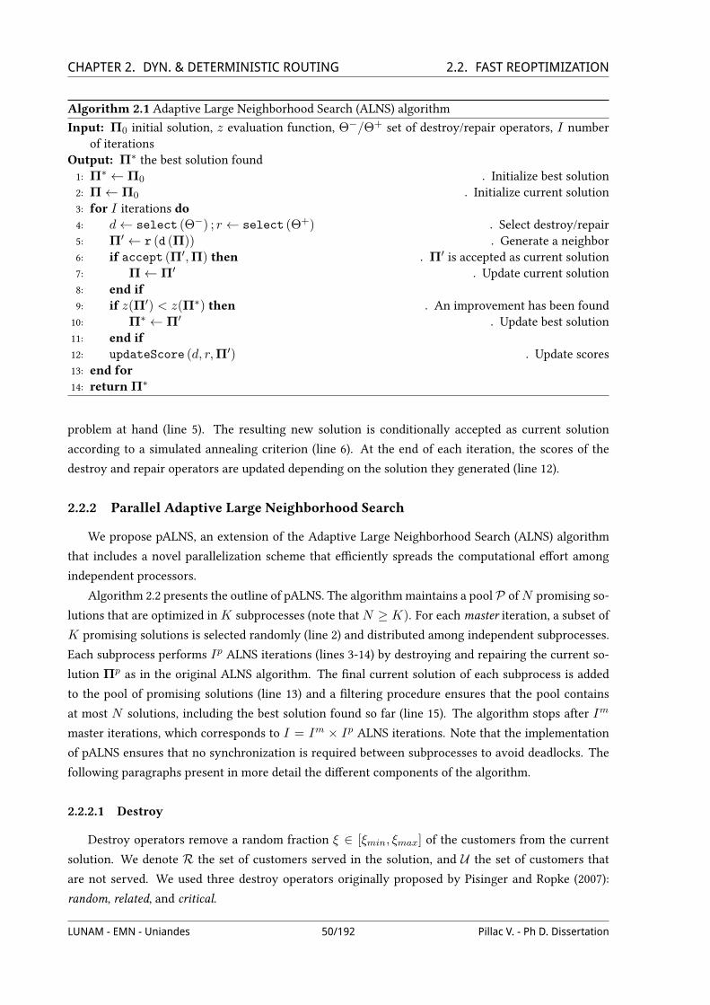
CHAPTER 2. DYN. & DETERMINISTIC ROUTING 2.2. FAST REOPTIMIZATIONAlgorithm 2.1 Adaptive Large Neighborhood Search (ALNS) algorithm
Input: Π0 initial solution, z evaluation function, Θ−/Θ+ set of destroy/repair operators, I numberof iterations
Output: Π∗ the best solution found1: Π∗ ← Π0 . Initialize best solution2: Π← Π0 . Initialize current solution3: for I iterations do4: d← select (Θ−) ; r ← select (Θ+) . Select destroy/repair5: Π′ ← r (d (Π)) . Generate a neighbor6: if accept (Π′,Π) then . Π′ is accepted as current solution7: Π← Π′ . Update current solution8: end if9: if z(Π′) < z(Π∗) then . An improvement has been found10: Π∗ ← Π′ . Update best solution11: end if12: updateScore (d, r,Π′) . Update scores13: end for14: return Π∗
problem at hand (line 5). The resulting new solution is conditionally accepted as current solution
according to a simulated annealing criterion (line 6). At the end of each iteration, the scores of the
destroy and repair operators are updated depending on the solution they generated (line 12).
2.2.2 Parallel Adaptive Large Neighborhood Search
We propose pALNS, an extension of the Adaptive Large Neighborhood Search (ALNS) algorithm
that includes a novel parallelization scheme that eXciently spreads the computational eUort among
independent processors.
Algorithm 2.2 presents the outline of pALNS. The algorithmmaintains a pool P ofN promising so-
lutions that are optimized inK subprocesses (note thatN ≥ K). For eachmaster iteration, a subset of
K promising solutions is selected randomly (line 2) and distributed among independent subprocesses.
Each subprocess performs Ip ALNS iterations (lines 3-14) by destroying and repairing the current so-
lution Πp as in the original ALNS algorithm. The Vnal current solution of each subprocess is added
to the pool of promising solutions (line 13) and a Vltering procedure ensures that the pool contains
at most N solutions, including the best solution found so far (line 15). The algorithm stops after Im
master iterations, which corresponds to I = Im × Ip ALNS iterations. Note that the implementation
of pALNS ensures that no synchronization is required between subprocesses to avoid deadlocks. The
following paragraphs present in more detail the diUerent components of the algorithm.
2.2.2.1 Destroy
Destroy operators remove a random fraction ξ ∈ [ξmin, ξmax] of the customers from the current
solution. We denote R the set of customers served in the solution, and U the set of customers that
are not served. We used three destroy operators originally proposed by Pisinger and Ropke (2007):
random, related, and critical.
LUNAM - EMN - Uniandes 50/192 Pillac V. - Ph D. Dissertation

CHAPTER 2. DYN. & DETERMINISTIC ROUTING 2.2. FAST REOPTIMIZATIONAlgorithm 2.2 Parallel Adaptive Large Neighborhood Search (pALNS) algorithm
Input: P initial solutions, z evaluation function, Θ−/Θ+ set of destroy/repair operators,N maximumsize of the solution pool, K number of subprocesses, Im number of master iterations, Ip numberof iterations performed in parallel.
Output: Π∗, the best solution found1: for Im iterations do2: P ′ ← selectSubset (P,K) . Select a subset ofK solutions3: parallel forall Π in P ′ do4: Πp ← Π . Current solution for this subprocess5: for Ip iterations do6: d← select (Θ−) ; r ← select (Θ+) . Select destroy/repair7: Π′ ← r (d (Πp)) . Destroy and repair current solution8: if accept (Π′,Πp) then9: Πp ← Π′ . Π′ is accepted as current solution10: end if11: updateScore (d, r,Π′) . Update d and r scores12: end for13: P ← P ∪ Πp . Add Πp to the pool P14: end forall15: P ← retain (P, N) . Retain at most N solutions in the pool P16: end for17: return Π∗ = arg minΠ∈P z(Π)
The random destroy operator selects customers randomly and removes them from their actual
tours.
The related destroy attempts to remove customers that share some characteristics. Let the relat-
edness rij of customers i and j be a measure of how related two customers are (the lower the rij , the
more related i and j). The procedure starts by randomly removing a seed customer i (U = i), then it
iteratively selects a customer i ∈ U , and removes the most related customer j∗:
j∗ = arg minj∈Rrij (2.1)
There are diUerent ways to measure the relatedness. We propose a new metric that can be precalcu-
lated, namely a-priori relatedness, that does not depend on the actual position of customers in tours:
rsij =
(1 +
cijMc
)θc (1 +|bi − bj |Mt
)θt(2.2)
Where cij is the distance between i and j, bi and bj are the end of the time windows of customers i
and j,Mc andMt are scaling constants, θc and θt deVne the weight given to the geographic distance
between the two customers, and the diUerence between due dates respectively.
On the other hand, time-oriented relatedness (Pisinger and Ropke, 2007) measures the diUerence be-
LUNAM - EMN - Uniandes 51/192 Pillac V. - Ph D. Dissertation

CHAPTER 2. DYN. & DETERMINISTIC ROUTING 2.2. FAST REOPTIMIZATIONtween the current times of service Ai and Aj of customers i and j:
rtij = |Ai −Aj | (2.3)
Finally, critical destroy consists in removing the customer i∗ such that the cost of the resulting
solution is minimal:
i∗ = arg maxi∈Rci−1,i+1 − ci−1,i − ci,i+1 (2.4)
Where i− 1 and i+ 1 are the predecessor and successor of i.
In practice related and critical operators are randomized and the byp|R|c-th best customer is se-
lected, where y is a random number in [0, 1) and p ≥ 1 is a parameter that controls the level of
randomness (the lower the p, the more randomness is introduced).
2.2.2.2 Repair
Repair operators attempt to insert customers that are currently unserved. Our implementation is
based on regret-q heuristics (Potvin and Rousseau, 1993): at each iteration the algorithm inserts (at
the best position) the customer with the lowest regret value. The regret-q value rqi of customer i is a
measure of how desirable it is to insert i in the current iteration assuming that the best insertion will
no longer be feasible in the next iteration. It is deVned as:
rqi =
q∑h=2
(∆zhi −∆z1
i
)(2.5)
Where ∆zqi is the cost of the q-th best insertion of customer i ∈ U . Note that ties are resolved by
selecting the customer with the lowest ∆z1i value, and therefore regret-1 corresponds to the classical
best insertion heuristic. We used three regret levels: regret-1, regret-2, and regret-3.
2.2.2.3 Adaptive layer
At each iteration, the pALNS algorithm selects a destroy and a repair operator using a selection
roulette, such that operator θ ∈ Θ is selected with probability wθ , where Θ is either the set of destroy
(Θ−) or repair (Θ+) operators. Probabilities are initialized with value 1|Θ.| , and then updated every l
iterations (a segment) as follows:
wθ ← (1− ρ)wθ + ρsθ∑θ∈Θ. sθ
(2.6)
Where ρ ∈ [0, 1] is the reaction factor which deVnes how quickly probabilities are adjusted, and sθis the score of operator θ in the last l iterations. The scores sθ are reset to 0 every l iterations and
updated at the end of each iteration depending on the new solution: a score of σ1 is granted for a new
best solution, σ2 for an improving solution, σ3 for a non-improving but accepted solution, and σ4 for a
rejected solution. It is worth noting that in contrast with the adaptive scheme originally proposed by
LUNAM - EMN - Uniandes 52/192 Pillac V. - Ph D. Dissertation

CHAPTER 2. DYN. & DETERMINISTIC ROUTING 2.2. FAST REOPTIMIZATIONPisinger and Ropke (2007), this formula ensures that
∑θ∈Θ wθ = 1 at all time, which makes it easier
to interpret the relative weight of each component.
2.2.2.4 Objective function
The initial solution or the solution resulting from the destroy operator can leave some customers
unserved (U 6= ∅). Therefore we need to be able to evaluate a partial solution Π′ to account for the
unserved customers. Given an evaluation function z and an initial solution Π0, Pisinger and Ropke
(2007) deVne the cost of partial solution Π′ as follows:
zφ(Π′) = z(Π′) + φ|U|z(Π0) (2.7)
Where φ is a parameter that controls the unserved customer penalty.
2.2.2.5 Acceptance criterion
As in the original ALNS, the pALNS algorithm relies on a simulated annealing acceptance criterion
which accepts a new solution Π′ with probability ez(Π)−z(Π′)
T , where T is the temperature parameter.
The temperature is initialized with the value T0 and it is reduced at each iteration by a cooling fac-
tor c. The two parameters T0 and c are set depending on the initial solution and the target number of
iterations (Ropke and Pisinger, 2006). Given an initial solution Π0, T0 is deVned such that a solution
with value (1 + w)z(Π0) is accepted with probability p, and c is set such that the temperature after n
iterations is equal to αT0.
2.2.2.6 Computation of an initial solution
The pALNS algorithm requires an initial solution which is computed with a regret-3 constructive
heuristic: starting with empty routes for each vehicle, the algorithm iteratively inserts the customer
with the lowest regret value as described in §2.2.2.2.
2.2.2.7 Solution pool
The solution pool acts as a shared memory and allows subprocesses to collaborate eXciently. In
the original algorithm, the simulated annealing acceptance criterion results in a search scheme that
starts from a diversiVcation phase, in which poor solutions may be accepted as current solutions,
and progressively switch to an intensiVcation phase, in which only improving solutions are accepted.
The use of a solution pool that would contains the N best solutions found so far tend to break this
scheme, as poor solutions may never be kept in the pool and will therefore not be exploited properly.
To overcome this limitation we propose to maintain a pool of diverse solutions that are promising in
terms of cost.
This is achieved by the retainmethod (line 15) which ensures thatP contains at mostN solutions:
if |P| > N then the method retains the N best solutions according to the Vtness function f :
f(Π) = (1− λ)rankz(Π) + λrankd(Π) (2.8)
LUNAM - EMN - Uniandes 53/192 Pillac V. - Ph D. Dissertation

CHAPTER 2. DYN. & DETERMINISTIC ROUTING 2.2. FAST REOPTIMIZATIONWhere λ is a weight between 0 and 1, rankz(Π) is the rank of solution Π according to its objec-
tive value, and rankd(Π) is the rank of Π according to its average broken-pairs distance (Prins, 2009)
relative to the other solutions from P . The broken pairs distance counts the number of arcs that dif-
fer between two solutions. This Vtness function is inspired by the biased Vtness introduced by Vidal
et al. (Vidal et al., 2011) in a genetic algorithm with diversity management. The weight λ can either be
Vxed a-priori, or adjusted throughout the search to switch from diversiVcation (λ = 1) to intensiVca-
tion (λ = 0). Note that we ensure that P always contains the best solution found so far.
2.2.3 Parallel reoptimization approach for the D-VRPTW
Figure 2.4 illustrates the proposed reoptimization approach: the algorithm starts by producing an
initial solution S0 by using a constructive heuristic coupled with the pALNS described in the previous
section. Then each time a new customer appears, it Vxes the currently executed portion of the routes,
and re-runs the pALNS for a limited number of iterations to produce an updated solution S′t. If pALNS
is able to insert the new customer request, then the customer is accepted and S′t becomes the new
current solution, otherwise the customer is rejected and St remains as the current solution.
Start
pALNS
End of day?
NO
YES
pALNS
Updated solution St+1
End
NO
Wait until a new customer appears
Initial solution S0
Accept? Select new currentsolution
YES
Candidate solutionSt'
Figure 2.4: Overview of the proposed approach
It is important to note that the immediate commitment of idle vehicles to customers may lead to
diXculties when new customers appear. Figure 2.5 illustrates this with a single vehicle. Suppose that
at time t a vehicle is assigned to a customer i, if the vehicle is dispatched immediately to i (upper
left time line), it will travel to i then wait at its destination until the start of the time window (black
brackets). On the other hand, if a waiting strategy is used (lower left time line), the vehicle will remain
idle until the latest moment such that it will not wait at i. If at time t+ 1 a new customer j appears, in
the Vrst case j cannot be served as the vehicle is already waiting at i, while in the second case a visit
to j can be inserted right before i. As a consequence, vehicles are considered to remain idle at their
current location until the latest departure time such that it will not wait at the next customer, leaving
LUNAM - EMN - Uniandes 54/192 Pillac V. - Ph D. Dissertation
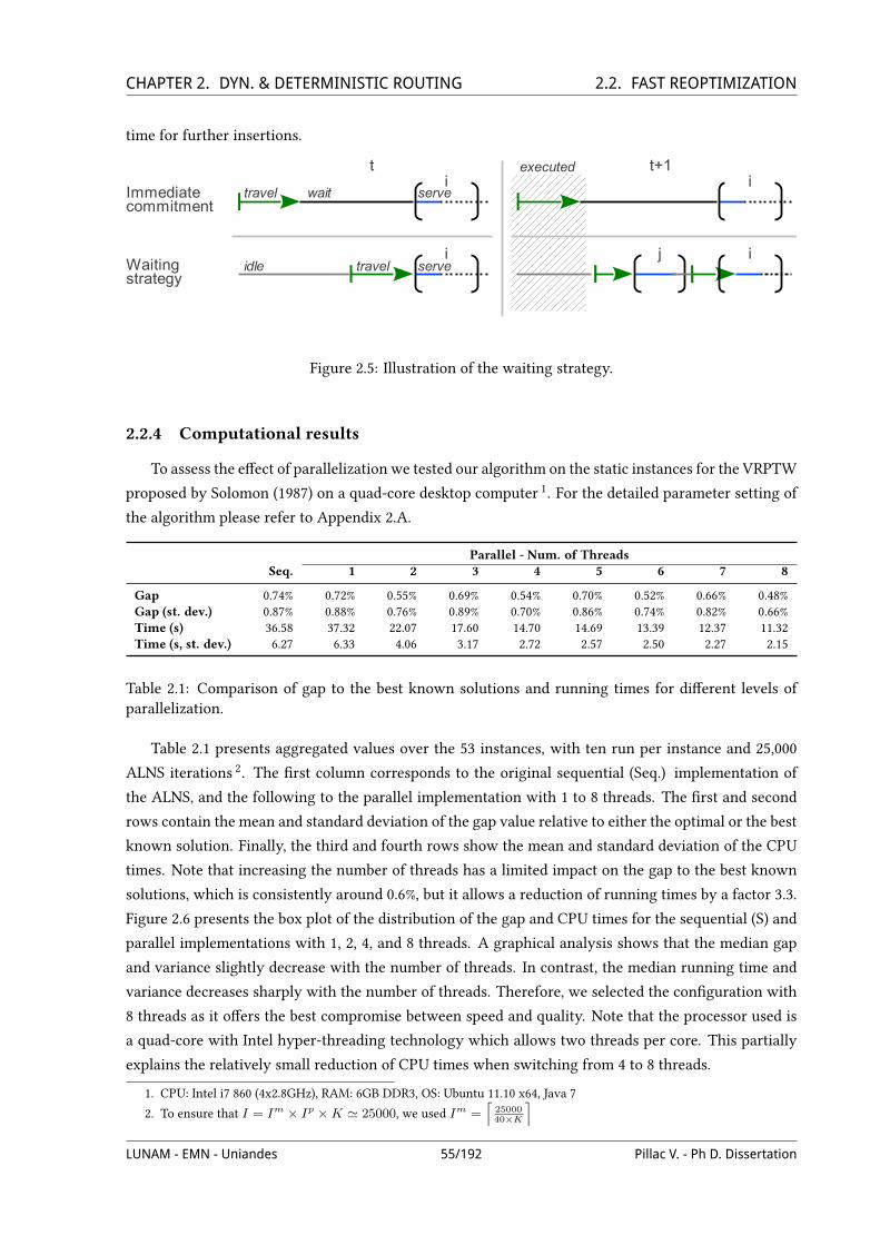
CHAPTER 2. DYN. & DETERMINISTIC ROUTING 2.2. FAST REOPTIMIZATIONtime for further insertions.
i
i
i
ij
Immediatecommitment
Waitingstrategy
t t+1
travel wait serve
idle travel serve
executed
Figure 2.5: Illustration of the waiting strategy.
2.2.4 Computational results
To assess the eUect of parallelization we tested our algorithm on the static instances for the VRPTW
proposed by Solomon (1987) on a quad-core desktop computer 1. For the detailed parameter setting of
the algorithm please refer to Appendix 2.A.
Parallel - Num. of ThreadsSeq. 1 2 3 4 5 6 7 8
Gap 0.74% 0.72% 0.55% 0.69% 0.54% 0.70% 0.52% 0.66% 0.48%Gap (st. dev.) 0.87% 0.88% 0.76% 0.89% 0.70% 0.86% 0.74% 0.82% 0.66%Time (s) 36.58 37.32 22.07 17.60 14.70 14.69 13.39 12.37 11.32Time (s, st. dev.) 6.27 6.33 4.06 3.17 2.72 2.57 2.50 2.27 2.15
Table 2.1: Comparison of gap to the best known solutions and running times for diUerent levels ofparallelization.
Table 2.1 presents aggregated values over the 53 instances, with ten run per instance and 25,000
ALNS iterations 2. The Vrst column corresponds to the original sequential (Seq.) implementation of
the ALNS, and the following to the parallel implementation with 1 to 8 threads. The Vrst and second
rows contain the mean and standard deviation of the gap value relative to either the optimal or the best
known solution. Finally, the third and fourth rows show the mean and standard deviation of the CPU
times. Note that increasing the number of threads has a limited impact on the gap to the best known
solutions, which is consistently around 0.6%, but it allows a reduction of running times by a factor 3.3.
Figure 2.6 presents the box plot of the distribution of the gap and CPU times for the sequential (S) and
parallel implementations with 1, 2, 4, and 8 threads. A graphical analysis shows that the median gap
and variance slightly decrease with the number of threads. In contrast, the median running time and
variance decreases sharply with the number of threads. Therefore, we selected the conVguration with
8 threads as it oUers the best compromise between speed and quality. Note that the processor used is
a quad-core with Intel hyper-threading technology which allows two threads per core. This partially
explains the relatively small reduction of CPU times when switching from 4 to 8 threads.
1. CPU: Intel i7 860 (4x2.8GHz), RAM: 6GB DDR3, OS: Ubuntu 11.10 x64, Java 7
2. To ensure that I = Im × Ip ×K ' 25000, we used Im =⌈
2500040×K
⌉LUNAM - EMN - Uniandes 55/192 Pillac V. - Ph D. Dissertation
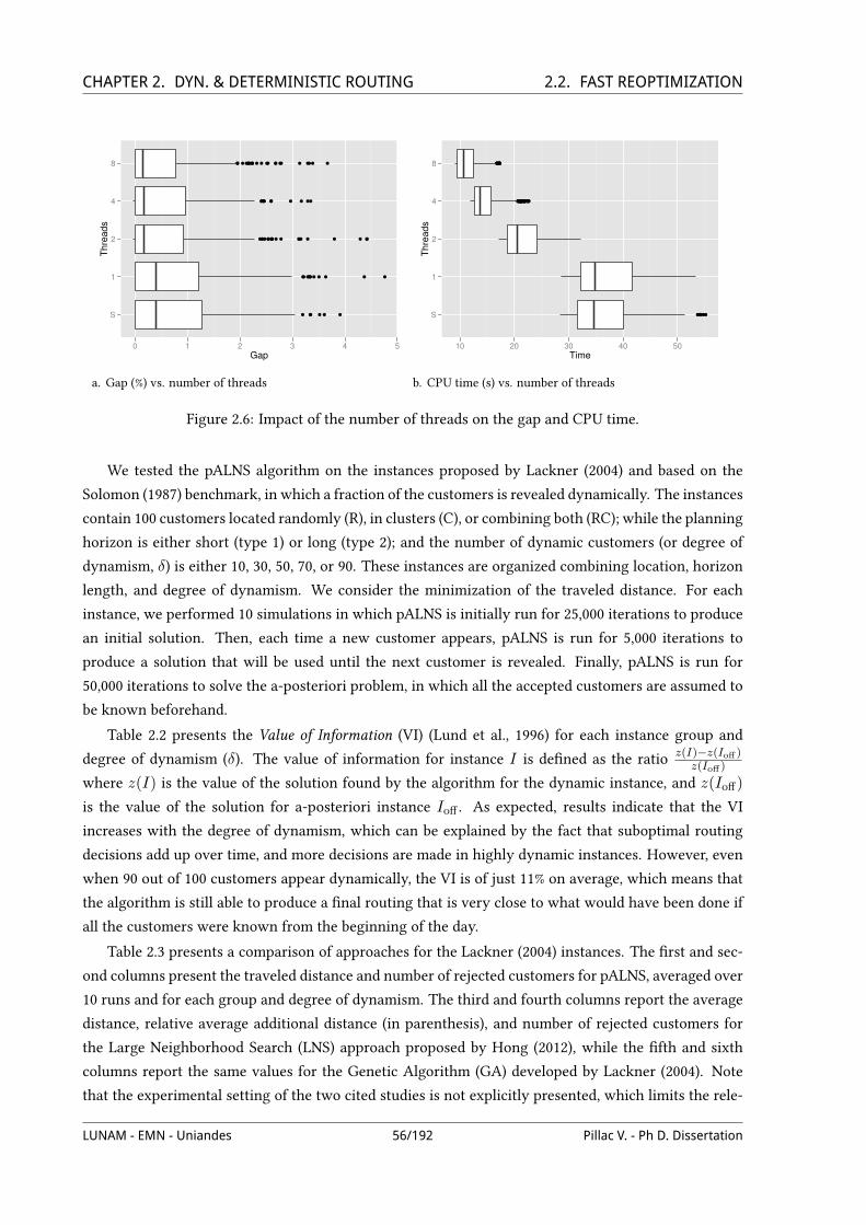
CHAPTER 2. DYN. & DETERMINISTIC ROUTING 2.2. FAST REOPTIMIZATION
S
1
2
4
8
0 1 2 3 4 5
Gap
Th
rea
ds
a. Gap (%) vs. number of threads
S
1
2
4
8
10 20 30 40 50
Time
Th
rea
ds
b. CPU time (s) vs. number of threads
Figure 2.6: Impact of the number of threads on the gap and CPU time.
We tested the pALNS algorithm on the instances proposed by Lackner (2004) and based on the
Solomon (1987) benchmark, in which a fraction of the customers is revealed dynamically. The instances
contain 100 customers located randomly (R), in clusters (C), or combining both (RC); while the planning
horizon is either short (type 1) or long (type 2); and the number of dynamic customers (or degree of
dynamism, δ) is either 10, 30, 50, 70, or 90. These instances are organized combining location, horizon
length, and degree of dynamism. We consider the minimization of the traveled distance. For each
instance, we performed 10 simulations in which pALNS is initially run for 25,000 iterations to produce
an initial solution. Then, each time a new customer appears, pALNS is run for 5,000 iterations to
produce a solution that will be used until the next customer is revealed. Finally, pALNS is run for
50,000 iterations to solve the a-posteriori problem, in which all the accepted customers are assumed to
be known beforehand.
Table 2.2 presents the Value of Information (VI) (Lund et al., 1996) for each instance group and
degree of dynamism (δ). The value of information for instance I is deVned as the ratio z(I)−z(Ioff)z(Ioff)
where z(I) is the value of the solution found by the algorithm for the dynamic instance, and z(Ioff)
is the value of the solution for a-posteriori instance Ioff . As expected, results indicate that the VI
increases with the degree of dynamism, which can be explained by the fact that suboptimal routing
decisions add up over time, and more decisions are made in highly dynamic instances. However, even
when 90 out of 100 customers appear dynamically, the VI is of just 11% on average, which means that
the algorithm is still able to produce a Vnal routing that is very close to what would have been done if
all the customers were known from the beginning of the day.
Table 2.3 presents a comparison of approaches for the Lackner (2004) instances. The Vrst and sec-
ond columns present the traveled distance and number of rejected customers for pALNS, averaged over
10 runs and for each group and degree of dynamism. The third and fourth columns report the average
distance, relative average additional distance (in parenthesis), and number of rejected customers for
the Large Neighborhood Search (LNS) approach proposed by Hong (2012), while the Vfth and sixth
columns report the same values for the Genetic Algorithm (GA) developed by Lackner (2004). Note
that the experimental setting of the two cited studies is not explicitly presented, which limits the rele-
LUNAM - EMN - Uniandes 56/192 Pillac V. - Ph D. Dissertation

CHAPTER 2. DYN. & DETERMINISTIC ROUTING 2.3. BI-OBJECTIVE D-VRP
δ R1 C1 RC1 R2 C2 RC2 Avg.
10 2.05% 2.89% 3.06% 1.70% 1.66% 1.61% 2.14%30 4.67% 5.83% 5.83% 4.34% 1.74% 4.70% 4.54%50 6.41% 9.28% 9.03% 8.15% 2.82% 5.38% 6.93%70 8.29% 11.18% 10.24% 10.17% 5.41% 8.60% 9.03%90 9.33% 12.49% 11.84% 11.83% 6.51% 12.33% 10.71%
Table 2.2: Average value of information for the Lackner (2004) instances
vance of direct comparisons. Nonetheless, Vgures show that our approach is competitive both in terms
of traveled distance and number of rejected customers. In addition, average running times are of just
5.3s for the initial optimization, and 2.0s for subsequent reoptimizations, which is signiVcantly less
than the 33s and 47s reported by Hong (2012) and Lackner (2004) respectively.
2.3 Route consistency in dynamic routing:a bi-objective approach
Most studies on dynamic routing consider that routes are designed online, which means that ve-
hicle drivers do not know their next destination until they Vnish serving their current customer. Al-
though this assumption is theoretically appealing and allows a better optimization of the cost func-
tion, it may not be desirable if drivers are used to know their routes from the beginning of the day.
In practice, having a set of routes known a-priori that are then changed may be desirable over purely
dynamic routing. Hence there is a need for approaches able to maintain consistency in the vehicles
routes throughout the day while ensuring cost eXciency.
To the best of our knowledge, all studies on dynamic routing focus on the optimization of a single
criterion, such as the minimization of the total traveled distance or the maximization of the number of
served customers. On the other hand, and as surveyed by Jozefowiez et al. (2008), a growing number of
studies on static routing consider multiple objectives in an attempt to better Vt operational contexts. In
this section we present a preliminary study that takes into account driver inconvenience. The proposed
approach is an adaptation of the pALNS algorithm that simultaneously minimizes a cost function and
maximizes the route consistency throughout the day.
2.3.1 Measuring consistency
Assuming that an initial set of routes are handed to the drivers at the beginning of the day, it seems
natural to consider them as the reference routes for each driver. To prevent multiple and unnecessary
changes in routes, we assume that drivers will only be informed of changes in their routes at the
last possible moment. As a consequence, a change will take eUect only when necessary. From the
driver’s perspective, four types of changes can be made to the route: one or more customers may be a)
inserted between existing customers; b) removed; c) swapped within the same route; d) substituted by
a customer previously unvisited. In this context, minimizing inconvenience is therefore equivalent to
minimizing the number of changes communicated to the driver.
LUNAM - EMN - Uniandes 57/192 Pillac V. - Ph D. Dissertation

CHAPTER 2. DYN. & DETERMINISTIC ROUTING 2.3. BI-OBJECTIVE D-VRP
pALNS Hong (2012) Lackner (2004)
Group δ Dist. Rej. Dist. Rej. Dist. Rej.
R1 10 1197.4 0.25 1257.1 ( 4.99%) 0.17 1278.1 ( 6.74%) 0.4730 1212.9 0.80 1286.6 ( 6.08%) 0.58 1337.9 ( 10.30%) 0.7250 1225.0 1.25 1295.8 ( 5.78%) 0.67 1330.0 ( 8.57%) 0.7870 1237.3 1.71 1331.3 ( 7.60%) 1.75 1336.1 ( 7.98%) 0.9490 1230.1 2.55 1335.9 ( 8.60%) 2.33 1278.3 ( 3.92%) 0.75
C1 10 850.6 0.11 895.8 ( 5.31%) 0.22 996.4 ( 17.14%) 0.0030 874.9 0.11 962.1 ( 9.97%) 0.33 1066.9 ( 21.95%) 0.0050 903.4 0.11 1001.2 ( 10.82%) 0.22 1236.1 ( 36.82%) 0.0070 919.1 0.11 1031.7 ( 12.25%) 0.22 1261.3 ( 37.24%) 0.0090 929.9 0.11 1039.8 ( 11.81%) 0.22 1479.6 ( 59.11%) 0.00
RC1 10 1389.4 0.04 1436.2 ( 3.37%) 1.13 1426.9 ( 2.70%) 0.4630 1421.5 0.28 1492.2 ( 4.98%) 1.13 1439.7 ( 1.28%) 0.4250 1463.4 0.23 1514.7 ( 3.50%) 1.38 1448.1 ( -1.05%) 0.4670 1470.1 0.58 1511.3 ( 2.80%) 1.88 1488.4 ( 1.25%) 0.5890 1495.5 0.51 1513.9 ( 1.23%) 2.00 1475.2 ( -1.36%) 0.42
R2 10 893.0 0.00 950.0 ( 6.39%) 0.09 1052.9 ( 17.90%) 0.0330 915.6 0.00 985.5 ( 7.63%) 0.00 1085.4 ( 18.54%) 0.1550 948.6 0.00 1016.5 ( 7.17%) 0.00 1138.8 ( 20.05%) 0.2170 967.7 0.00 1032.0 ( 6.65%) 0.09 1116.9 ( 15.42%) 0.3090 981.7 0.00 1047.8 ( 6.73%) 0.09 1193.3 ( 21.55%) 0.52
C2 10 597.2 0.00 594.7 ( -0.42%) 0.00 629.1 ( 5.35%) 0.0030 597.6 0.00 651.4 ( 9.01%) 0.00 632.3 ( 5.81%) 0.0450 604.0 0.00 605.0 ( 0.17%) 0.00 689.3 ( 14.12%) 0.1370 619.2 0.00 636.5 ( 2.79%) 0.00 743.8 ( 20.12%) 0.2190 625.7 0.00 636.8 ( 1.78%) 0.00 792.5 ( 26.66%) 0.29
RC2 10 1024.4 0.00 1103.3 ( 7.70%) 0.00 1220.9 ( 19.18%) 0.0030 1053.1 0.00 1166.0 ( 10.73%) 0.25 1244.9 ( 18.21%) 0.0450 1060.5 0.00 1190.5 ( 12.26%) 0.13 1244.9 ( 17.38%) 0.0070 1091.4 0.00 1239.5 ( 13.57%) 0.00 1269.3 ( 16.30%) 0.0090 1130.3 0.00 1257.2 ( 11.23%) 0.13 1346.8 ( 19.16%) 0.13
Average 0.29 (+6.75%) 0.50 (+15.61%) 0.27
Table 2.3: Comparison of approaches for the Lackner (2004) instances.
LUNAM - EMN - Uniandes 58/192 Pillac V. - Ph D. Dissertation
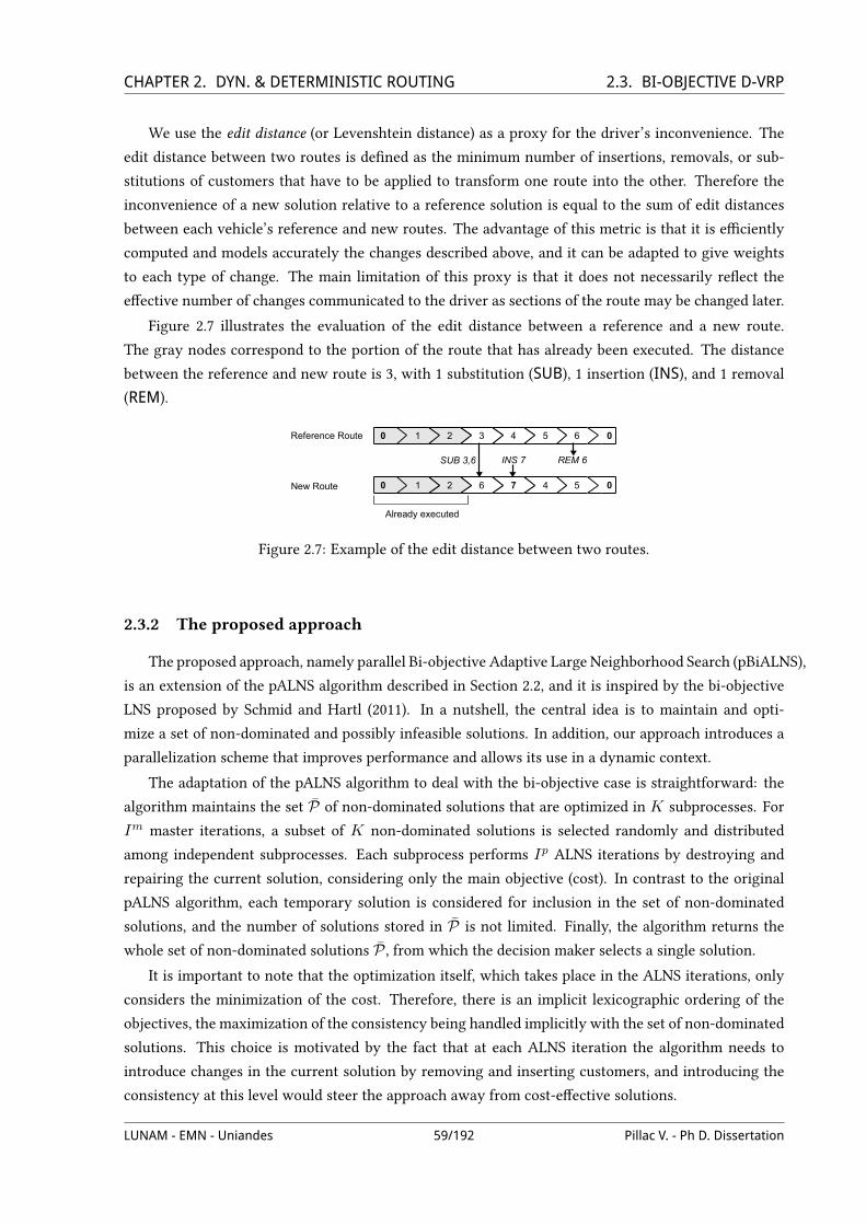
CHAPTER 2. DYN. & DETERMINISTIC ROUTING 2.3. BI-OBJECTIVE D-VRPWe use the edit distance (or Levenshtein distance) as a proxy for the driver’s inconvenience. The
edit distance between two routes is deVned as the minimum number of insertions, removals, or sub-
stitutions of customers that have to be applied to transform one route into the other. Therefore the
inconvenience of a new solution relative to a reference solution is equal to the sum of edit distances
between each vehicle’s reference and new routes. The advantage of this metric is that it is eXciently
computed and models accurately the changes described above, and it can be adapted to give weights
to each type of change. The main limitation of this proxy is that it does not necessarily reWect the
eUective number of changes communicated to the driver as sections of the route may be changed later.
Figure 2.7 illustrates the evaluation of the edit distance between a reference and a new route.
The gray nodes correspond to the portion of the route that has already been executed. The distance
between the reference and new route is 3, with 1 substitution (SUB), 1 insertion (INS), and 1 removal
(REM).
0
06
5
5
4
4
7
3
6
2
2
0
0
Reference Route 1
1New Route
Already executed
SUB 3,6 INS 7 REM 6
Figure 2.7: Example of the edit distance between two routes.
2.3.2 The proposed approach
The proposed approach, namely parallel Bi-objective Adaptive Large Neighborhood Search (pBiALNS),
is an extension of the pALNS algorithm described in Section 2.2, and it is inspired by the bi-objective
LNS proposed by Schmid and Hartl (2011). In a nutshell, the central idea is to maintain and opti-
mize a set of non-dominated and possibly infeasible solutions. In addition, our approach introduces a
parallelization scheme that improves performance and allows its use in a dynamic context.
The adaptation of the pALNS algorithm to deal with the bi-objective case is straightforward: the
algorithm maintains the set P of non-dominated solutions that are optimized in K subprocesses. For
Im master iterations, a subset of K non-dominated solutions is selected randomly and distributed
among independent subprocesses. Each subprocess performs Ip ALNS iterations by destroying and
repairing the current solution, considering only the main objective (cost). In contrast to the original
pALNS algorithm, each temporary solution is considered for inclusion in the set of non-dominated
solutions, and the number of solutions stored in P is not limited. Finally, the algorithm returns the
whole set of non-dominated solutions P , from which the decision maker selects a single solution.
It is important to note that the optimization itself, which takes place in the ALNS iterations, only
considers the minimization of the cost. Therefore, there is an implicit lexicographic ordering of the
objectives, the maximization of the consistency being handled implicitly with the set of non-dominated
solutions. This choice is motivated by the fact that at each ALNS iteration the algorithm needs to
introduce changes in the current solution by removing and inserting customers, and introducing the
consistency at this level would steer the approach away from cost-eUective solutions.
LUNAM - EMN - Uniandes 59/192 Pillac V. - Ph D. Dissertation
CHAPTER 2. DYN. & DETERMINISTIC ROUTING 2.3. BI-OBJECTIVE D-VRPNote that pBiALNS may visit infeasible solutions that do not visit all customers. Therefore, we
deVne a dominance relation that ensures that no feasible solution will be dominated by an infeasible
solution:
DeVnition 1 (Dominance). A solution Π dominates (denoted ≺) a solution Π′ if and only if Π is as good
as Π′ in both objectives, and strictly better in one objective, and either Π is feasible or both Π and Π′ are
infeasible.
2.3.3 Computational results
We tested the pBiALNS approach on the Lackner (2004) instances described in §2.2.4 with a similar
experimental setting. pALNS is Vrst run for 25,000 iterations to produce the reference (initial) solu-
tion; then, each time a new customer appears pBiALNS is run for 5,000 iterations to produce a set
of candidate new solutions to choose from; Vnally, pALNS is run for 50,000 iterations to produce the
a-posteriori solution to the problem.
Figure 2.8 represents the objective space explored by pBiALNS after 5,0000 iterations for one in-
stance, at a given step of the simulation (ie., after a new customer appeared). The graph illustrates the
diversity of solutions oUered to the decision maker, ranging from the least-cost solution (upper left)
to the most similar to the reference solution (lower right). For the purpose of benchmarking and to
assess the tradeoU between the two objectives, we deVne a threshold selection policy and select the non-
dominated solution that is closest to the reference, allowing a deviation in cost of at most γ percent
from the least-cost solution (green diamond). This policy models the behavior of an expert dispatcher
who would select one solution among the non-dominated set.
! "
#$%
Figure 2.8: Objective space for instance R101 and illustration of the threshold policy.
Table 2.4 presents (a) the average edit distance between the Vnal solution and the reference solu-
tion, and (b) the average gap between the cost of the Vnal solution and the cost of a solution evaluated
a-posteriori and the average number of rejected requests, for diUerent values of γ and degree of dy-
namism (δ). Running times are of 2.5 seconds on average at each decision. As expected, the edit
distance relative to the reference solution is negatively correlated to γ, and is minimal for γ = ∞. In
this case we always choose the solution which is the closest to the reference solution, in other words
LUNAM - EMN - Uniandes 60/192 Pillac V. - Ph D. Dissertation
CHAPTER 2. DYN. & DETERMINISTIC ROUTING 2.4. CONCLUSIONSwe simply insert new customers in the current solution, which leads to a distance equal to the number
of accepted dynamic customers. It is important to note that the quality of the routing, measured by the
gap to the static solution, is positively correlated to γ. This conVrms the intuition that poor routing
decisions tend to add up over time and can lead to larger deviations at the end of the day. Our results
also indicate that, for problems with low degree of dynamism, it can be worth sacriVcing quality of
solution to gain route stability. For instance, with δ = 10, the value γ = 5% leads to a gap of 6%
versus 2% with γ = 0%, but it reduces the number of required changes by a factor 3. However, this
statement no longer holds for instances with higher degrees of dynamism where numerous changes
are necessary to insert all customers. In this case it is better to focus on optimizing the routing, as it
does not lead to excessive instability in routes.
(a) Average edit distance to reference solution
γδ 0% 1% 2% 5% 10% ∞
10 32.8 19.3 17.0 12.9 12.6 9.830 59.4 48.1 44.2 39.2 36.4 29.650 78.2 70.3 65.9 61.4 58.2 49.470 87.6 84.0 81.7 78.5 75.7 69.290 95.7 94.5 93.9 92.7 91.3 88.9
(b) Average gap to a-posteriori solution (%) and number of rejected requests (in parenthesis)
γδ 0% 1% 2% 5% 10% ∞
10 2.0 (0.1) 2.8 (0.1) 4.2 (0.1) 6.1 (0.1) 8.1 (0.1) 11.2 (0.2)30 4.3 (0.3) 5.6 (0.3) 6.5 (0.3) 10.9 (0.2) 16.3 (0.2) 29.3 (0.4)50 6.4 (0.3) 7.6 (0.3) 9.1 (0.4) 13.1 (0.3) 18.7 (0.3) 50.1 (0.6)70 9.0 (0.4) 10.3 (0.4) 11.8 (0.5) 15.3 (0.5) 20.5 (0.4) 71.0 (0.8)90 9.8 (0.7) 10.8 (0.7) 11.6 (0.6) 14.4 (0.6) 19.4 (0.7) 95.5 (1.1)
Table 2.4: Evolution of the distance to reference solution and gap to a-posteriori solution for diUerentdegrees of dynamism and values of γ
2.4 Conclusions
In this work we proposed an eXcient parallelization scheme for an Adaptive Large Neighborhood
Search, namely pALNS. This algorithm distributes the optimization of promising solutions across mul-
tiple processors, resulting in factor 3.3 speedups on a quad-core desktop machine. The eXciency of
pALNS relies on the presence of a promising solution pool with diversity management, which pre-
vents deadlocks between optimization threads, and improves the exploration of the search space. We
illustrated the eXciency of pALNS on the Solomon (1987) CVRPTW instances, for which it produces
solutions in average 0.7% away from the optimal/best known solution in just 12s.
We also introduced a fast-reoptimization approach based on pALNS to tackle the dynamic VRPTW.
This approach consists in running pALNS to produce an initial solution at the beginning of the day,
LUNAM - EMN - Uniandes 61/192 Pillac V. - Ph D. Dissertation

CHAPTER 2. DYN. & DETERMINISTIC ROUTING BIBLIOGRAPHYand then running it for a limited number of iterations whenever a new customer appears. We tested
our approach on the instance set proposed by Lackner (2004). Computational results show that pALNS
is capable of achieving state of the art results in competitive time, bringing improvements of up to 12%
over previous approaches.
Finally, we presented a preliminary bi-objective extension of the classical D-VRPTW that attempts
to captures the drivers inconvenience resulting from dynamic routing. It is based on the notion of
having a reference routing plan handled to the drivers at the beginning of the period, that will then
undergo changes as new customers arrive. We introduced an inconvenience metric that measures the
consistency between an updated routing plan and the reference plan. We proposed a fast bi-objective
optimization approach based on pALNS, namely pBiALNS, which maintains and optimizes in parallel
the set of non-dominated solutions.
This optimization algorithm was used coupled with a threshold policy modeling an expert dis-
patcher to tackle the D-VRPTW instances proposed by Lackner (2004). Our results indicate that there
is a clear tradeoU between minimizing the traveled distance and maintaining consistency in routes.
Furthermore, it appears that for problems with a low degree of dynamism it can be worth sacriVcing
cost eXciency to maintain consistency. In contrast, in highly dynamic problems the priority should be
given to the minimization of the cost, as it does not lead to excessive inconsistency in routing.
Future research should focus on the development of a continuous reoptimization approach based
on pALNS that runs throughout the day and maintains a pool of alternative promising solutions as
adaptive memory. In addition, pALNS could be improved by having completely independent subpro-
cesses that pull their starting solution from the pool, and push their Vnal solution, without waiting for
other subprocesses to Vnish. pBiALNS could be reVned to better approximate the Pareto front, Vrst
in the selection of the non-dominated solutions to optimize, then by applying a local search or a path
relinking between non-dominated solutions.
Acknowledgements Financial support for this work was provided by the CPER Vallée du Libre
(Contrat de Projet Etat Region, France); and the CEIBA (Centro de Estudios Interdisciplinarios Básicos
y Aplicados en Complejidad, Colombia). This support is gratefully acknowledged.
Bibliography
Attanasio, A., Cordeau, J. F., Ghiani, G., and Laporte, G. (2004). Parallel tabu search heuristics for the dynamicmulti-vehicle dial-a-ride problem. Parallel Computing, 30(3):377–387, doi:10.1016/j.parco.2003.12.001.
Barcelo, J., Grzybowska, H., and Pardo, S. (2007). Vehicle routing and scheduling models, simulation and citylogistics. In Zeimpekis, V., Tarantilis, C. D., Giaglis, G. M., and Minis, I., editors, Dynamic Fleet Management,volume 38 of Operations Research/Computer Science Interfaces, pages 163–195. Springer US.
Beaudry, A., Laporte, G., Melo, T., and Nickel, S. (2010). Dynamic transportation of patients in hospitals. ORSpectrum, 32:77–107, doi:10.1007/s00291-008-0135-6.
Bent, R. and Van Hentenryck, P. (2004). Scenario-based planning for partially dynamic vehicle routing withstochastic customers. Operations Research, 52(6):977–987.
Benyahia, I. and Potvin, J. Y. (1998). Decision support for vehicle dispatching using genetic programming. IEEETransactions on Systems Man and Cybernetics Part A - Systems and Humans, 28(3):306–314.
LUNAM - EMN - Uniandes 62/192 Pillac V. - Ph D. Dissertation
CHAPTER 2. DYN. & DETERMINISTIC ROUTING BIBLIOGRAPHYChang, M. S., Chen, S., and Hsueh, C. (2003). Real-time vehicle routing problem with time windows and simul-
taneous delivery/pickup demands. Journal of the Eastern Asia Society for Transportation Studies, 5:2273–2286.
Chen, Z. and Xu, H. (2006). Dynamic column generation for dynamic vehicle routing with time windows.Transportation Science, 40(1):74–88.
Cheung, B. K. S., Choy, K. L., Li, C.-L., Shi, W., and Tang, J. (2008). Dynamic routing model and solution methodsfor Weet management with mobile technologies. International Journal of Production Economics, 113(2):694–705,doi:10.1016/j.ijpe.2007.10.018.
Gambardella, L., Rizzoli, A., Oliverio, F., Casagrande, N., Donati, A., Montemanni, R., and Lucibello, E. (2003).Ant colony optimization for vehicle routing in advanced logistics systems. In Proceedings of the InternationalWorkshop on Modelling and Applied Simulation (MAS 2003), pages 3–9.
Gendreau, M., Guertin, F., Potvin, J.-Y., and Taillard, E. (1999). Parallel tabu search for real-time vehicle routingand dispatching. Transportation Science, 33(4):381–390, doi:10.1287/trsc.33.4.381.
Gendreau, M. and Potvin, J.-Y., editors (2004). Transportation Science, volume 4. INFORMS. Special issue onreal-time Weet management.
Ghiani, G., Guerriero, F., Laporte, G., and Musmanno, R. (2003). Real-time vehicle routing: Solution con-cepts, algorithms and parallel computing strategies. European Journal of Operational Research, 151(1):1 –11, doi:10.1016/S0377-2217(02)00915-3.
Haghani, A. and Jung, S. (2005). A dynamic vehicle routing problemwith time-dependent travel times. Computers& Operations Research, 32(11):2959 – 2986, doi:10.1016/j.cor.2004.04.013.
Hong, L. (2012). An improved lns algorithm for real-time vehicle routing problem with time windows. Computers& Operations Research, 39(2):151 – 163, doi:10.1016/j.cor.2011.03.006.
Ichoua, S., Gendreau, M., and Potvin, J.-Y. (2000). Diversion issues in real-time vehicle dispatching. TransportationScience, 34(4):426–438, doi:10.1287/trsc.34.4.426.12325.
Ichoua, S., Gendreau, M., and Potvin, J.-Y. (2003). Vehicle dispatching with time-dependent travel times. EuropeanJournal of Operational Research, 144(2):379 – 396, doi:10.1016/S0377-2217(02)00147-9.
Ichoua, S., Gendreau, M., and Potvin, J.-Y. (2007). Planned route optimization for real-time vehicle routing. InZeimpekis, V., Tarantilis, C. D., Giaglis, G. M., and Minis, I., editors, Dynamic Fleet Management, volume 38 ofOperations Research/Computer Science Interfaces, pages 1–18. Springer US.
Jaillet, P. and Wagner, M. R. (2008). Generalized online routing: New competitive ratios, resource augmentation,and asymptotic analyses. Operations Research, 56(3):745–757, doi:10.1287/opre.1070.0450.
Jozefowiez, N., Semet, F., and Talbi, E.-G. (2008). Multi-objective vehicle routing problems. European Journal ofOperational Research, 189(2):293 – 309, doi:10.1016/j.ejor.2007.05.055.
Lackner, A. (2004). Dynamische Tourenplanung mit ausgewählten Metaheuristiken. PhD thesis, Georg-August-Universität Göttingen.
Larsen, A. (2001). The Dynamic Vehicle Routing Problem. PhD thesis, Technical University of Denmark (DTU).
Larsen, A., Madsen, O. B. G., and Solomon, M. M. (2008). Recent developments in dynamic vehicle routingsystems. In The Vehicle Routing Problem: Latest Advances and New Challenges, volume 43 of Operations Re-search/Computer Science Interfaces Series, pages 199–218. Springer US.
Lund, K., Madsen, O. B. G., and Rygaard, J. M. (1996). Vehicle routing problems with varying degrees of dy-namism. Technical report, IMM Institute of Mathematical Modelling.
Montemanni, R., Gambardella, L. M., Rizzoli, A. E., and Donati, A. V. (2005). Ant colony system for a dynamicvehicle routing problem. Journal of Combinatorial Optimization, 10(4):327–343, doi:10.1007/s10878-005-4922-6.
LUNAM - EMN - Uniandes 63/192 Pillac V. - Ph D. Dissertation

CHAPTER 2. DYN. & DETERMINISTIC ROUTING BIBLIOGRAPHYPillac, V., Gendreau, M., Guéret, C., and Medaglia, A. L. (2011). A review of dynamic vehicle routing problems.
Technical Report CIRRELT-2011-62, CIRRELT.
Pisinger, D. and Ropke, S. (2007). A general heuristic for vehicle routing problems. Computers & OperationsResearch, 34(8):2403–2435, doi:10.1016/j.cor.2005.09.012.
Pisinger, D. and Ropke, S. (2010). Large neighborhood search. In Gendreau, M. and Potvin, J.-Y., editors, Handbookof Metaheuristics, volume 146 of International Series in Operations Research & Management Science, pages 399–419. Springer US.
Potvin, J.-Y. and Rousseau, J.-M. (1993). A parallel route building algorithm for the vehicle routing and schedulingproblem with time windows. European Journal of Operational Research, 66(3):331 – 340, doi:10.1016/0377-2217(93)90221-8.
Powell, W. B. (2007). Approximate dynamic programming: solving the curses of dimensionality, volume 703 ofWiley Series in Probability and Statistics. Wiley-Interscience, Hoboken, New Jersey.
Prins, C. (2009). Two memetic algorithms for heterogeneous Weet vehicle routing problems. Engineering Appli-cations of ArtiVcial Intelligence, 22(6):916–928, doi:10.1016/j.engappai.2008.10.006.
Psaraftis, H. (1980). A dynamic-programming solution to the single vehicle many-to-many immediate requestdial-a-ride problem. Transportation Science, 14(2):130–154.
Rizzoli, A., Montemanni, R., Lucibello, E., and Gambardella, L. (2007). Ant colony optimization for real-worldvehicle routing problems. Swarm Intelligence, 1(sa):135–151.
Ropke, S. and Pisinger, D. (2006). An adaptive large neighborhood search heuristic for the pickup and deliveryproblem with time windows. Transportation Science, 40(4):455–472.
Schmid, V. and Hartl, R. F. (2011). Large neighborhood search for solving the Bi-Objective Capacitated m-Ring-Star Problem. In Di Gaspero, L., Schaerf, A., and Stützle, T., editors, Proceedings of the 9th MetaheuristicsConference (MIC 2011), pages 700–703. Università degli Studi di Udine.
Shaw, P. (1998). Using constraint programming and local search methods to solve vehicle routing problems. InPrinciples and Practice of Constraint Programming – CP98, volume 1520 of Lecture Notes in Computer Science,pages 417–431. Springer Berlin / Heidelberg.
Solomon, M. M. (1987). Algorithms for the vehicle-routing and scheduling problems with time window con-straints. Operations Research, 35(2):254–265.
Taillard, E., Badeau, P., Gendreau, M., Guertin, F., and Potvin, J. (1997). A tabu search heuristic for the vehiclerouting problem with soft time windows. Transportation Science, 31(2):170–186.
Taillard, E. D., Gambardella, L. M., Gendreau, M., and Potvin, J.-Y. (2001). Adaptive memory programming: AuniVed view of metaheuristics. European Journal of Operational Research, 135(1):1 – 16, doi:10.1016/S0377-2217(00)00268-X.
Van Hemert, J. I. and Poutré, J. L. (2004). Dynamic routing problems with fruitful regions: Models and evolution-ary computation. In Yao, X., Burke, E., Lozano, J. A., Smith, J., Merelo-Guervós, J. J., Bullinaria, J. A., Rowe, J.,Tino, P., Kabán, A., and Schwefel, H.-P., editors, Parallel Problem Solving from Nature, volume 3242 of LectureNotes in Computer Science, pages 692–701. Springer Berlin / Heidelberg.
Vidal, T., Crainic, T., Gendreau, M., and Prins, C. (2011). A hybrid genetic algorithm with adaptive diversitymanagement for a large class of vehicle routing problems with time windows. Technical Report CIRRELT-2011-61, CIRRELT.
Zeimpekis, V., Tarantilis, C. D., Giaglis, G. M., and Minis, I., editors (2007). Dynamic Fleet Management, volume 38of Operations Research Computer Science Interfaces Series. Springer US.
LUNAM - EMN - Uniandes 64/192 Pillac V. - Ph D. Dissertation
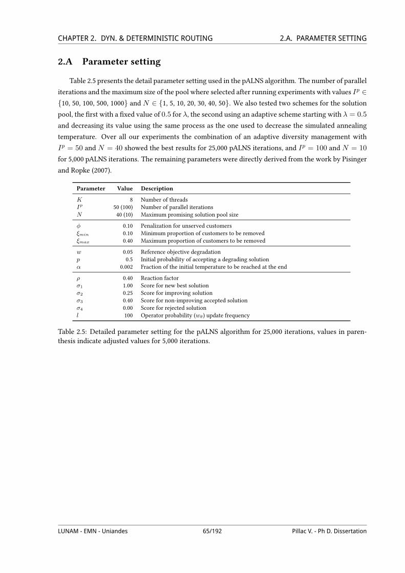
CHAPTER 2. DYN. & DETERMINISTIC ROUTING 2.A. PARAMETER SETTING2.A Parameter setting
Table 2.5 presents the detail parameter setting used in the pALNS algorithm. The number of parallel
iterations and the maximum size of the pool where selected after running experiments with values Ip ∈10, 50, 100, 500, 1000 and N ∈ 1, 5, 10, 20, 30, 40, 50. We also tested two schemes for the solution
pool, the Vrst with a Vxed value of 0.5 for λ, the second using an adaptive scheme starting with λ = 0.5
and decreasing its value using the same process as the one used to decrease the simulated annealing
temperature. Over all our experiments the combination of an adaptive diversity management with
Ip = 50 and N = 40 showed the best results for 25,000 pALNS iterations, and Ip = 100 and N = 10
for 5,000 pALNS iterations. The remaining parameters were directly derived from the work by Pisinger
and Ropke (2007).
Parameter Value Description
K 8 Number of threadsIp 50 (100) Number of parallel iterationsN 40 (10) Maximum promising solution pool size
φ 0.10 Penalization for unserved customersξmin 0.10 Minimum proportion of customers to be removedξmax 0.40 Maximum proportion of customers to be removed
w 0.05 Reference objective degradationp 0.5 Initial probability of accepting a degrading solutionα 0.002 Fraction of the initial temperature to be reached at the end
ρ 0.40 Reaction factorσ1 1.00 Score for new best solutionσ2 0.25 Score for improving solutionσ3 0.40 Score for non-improving accepted solutionσ4 0.00 Score for rejected solutionl 100 Operator probability (wθ) update frequency
Table 2.5: Detailed parameter setting for the pALNS algorithm for 25,000 iterations, values in paren-thesis indicate adjusted values for 5,000 iterations.
LUNAM - EMN - Uniandes 65/192 Pillac V. - Ph D. Dissertation


3Dynamic and stochastic routing
In dynamic and stochastic problems, part or all the input is unknown and revealed dynamically
during the execution of the routes, and exploitable stochastic knowledge is available on the dynam-
ically revealed information. Vehicle routes can be redeVned in an ongoing fashion with the help of
technological support.
Our focus being on developing software components that can be used for a wide range of appli-
cations, we chose to develop an event-driven framework based on the Multiple Scenario Approach
proposed by Van Hentenryck and Bent (2006). In this chapter we present the general framework and
its implementation, and then illustrate the validity of this approach by tackling the Dynamic Vehicle
Routing Problem with Stochastic Demands (D-VRPSD).
LUNAM - EMN - Uniandes 67/192 Pillac V. - Ph D. Dissertation

CHAPTER 3. DYN. & STOCHASTIC ROUTING
The full reference of the paper presented in this chapter is:
– Pillac, V., Guéret, C., and Medaglia, A. L. (2012)
An event-driven optimization framework for dynamic vehicle routing
Decision Support Systems, Accepted manuscript
doi:10.1016/j.dss.2012.06.007.
A previous version of the paper was published as a technical report:
– Pillac, V., Guéret, C., and Medaglia, A. L. (2011)
An event-driven optimization framework for dynamic vehicle routing
Technical report, École des Mines de Nantes, France. Report 11/2/AUTO.
Preliminary results of this work were presented two conferences:
– Pillac, V., Guéret, C., and Medaglia, A. L. (2011)
A dynamic approach for the vehicle routing problem with stochastic demands
In ROADEF 2011, St Etienne, France.
– Pillac, V., Guéret, C., and Medaglia, A. L. (2010)
Solving the vehicle routing problemwith stochastic demands with a multiple scenario approach
In ALIO-INFORMS 2010, Buenos Aires (Argentina).
LUNAM - EMN - Uniandes 68/192 Pillac V. - Ph D. Dissertation
An event-driven optimization framework fordynamic vehicle routing
V. Pillac1,2, C. Guéret1, A. L. Medaglia2
1 LUNAM, Ecole des Mines de Nantes, IRCCyN UMR 6597, Nantes, France
2 Universidad de los Andes, Industrial Engineering Department, Bogotá, Colombia
Journal : Decision Support Systems
State : Accepted manuscript - doi:10.1016/j.dss.2012.06.007
Abstract : The real-time operation of a Weet of vehicles introduces challenging opti-
mization problems. In this work, we propose an event-driven framework
which anticipates unknown changes arising in the context of dynamic ve-
hicle routing. The framework is intrinsically parallelized to take advantage
of modern multi-core and multi-threaded computing architectures. It is also
designed to be easily embeddable in decision support systems that cope with
a wide range of contexts and side constraints. We illustrate the Wexibility
of the framework by showing how it can be adapted to tackle the dynamic
vehicle routing problem with stochastic demands.
Keywords : Dynamic vehicle routing ; event-driven framework ; multiple scenario ap-
proach ; online stochastic optimization ; D-VRPSD ; D-VRP
3.1 Introduction
The problem of operating a Weet of vehicles arises in many contexts, from pickup and delivery
of goods to relocation of trucks in carrier companies. More speciVcally, Vehicle Routing Problems
(VRP) deal with the design of a set of minimal-cost vehicle routes that serve the demand for goods
or services of a group of geographically spread customers, satisfying operational constraints. From
an information perspective, such problems generally include two dimensions: evolution and quality
of information (Psaraftis, 1980). Information evolution relates to the fact that in some problems the
information available to the planner may change during the execution of the routes, for example with
the arrival of new customer requests. Information quality reWects possible uncertainty on the available
data, for instance, when the demand of a customer is only known as a range estimate of its real
demand. In addition, depending on the problem and the available technology, vehicle routes can either
be designed a-priori or online. Based on these dimensions, Table 3.1 identiVes four categories of routing
problems.
The static and deterministic category includes the classical Vehicle Routing Problem (VRP) as de-
Vned by Dantzig and Ramser (1959) in which all information is known beforehand and with certainty.
In contrast, problems from the static and stochastic class are characterized by input partially known
as random variables, which realizations are only revealed during the execution of the routes. Addi-
tionally, it is assumed that routes are designed a-priori and only minor changes are allowed afterward.
LUNAM - EMN - Uniandes 69/192 Pillac V. - Ph D. Dissertation

CHAPTER 3. DYN. & STOCHASTIC ROUTING 3.1. INTRODUCTION
Information qualityDeterministic input Stochastic input
Informationevolution
Input knownbeforehand
Static and deterministic Static and stochastic
Input changes overtime
Dynamic and deterministic Dynamic and stochastic
Table 3.1: Taxonomy of vehicle routing problems by information evolution and quality.
A common example is the VRP with Stochastic Demands (VRPSD), in which customer demands are
uncertain. We refer the interested reader to the surveys by Cordeau et al. (2007), Baldacci et al. (2007),
and Laporte (2009) for a recent review of these two classes of problems.
In dynamic and deterministic problems, also referred to as online problems, part or all of the in-
put is unknown and revealed dynamically and unpredictably during the design or execution of the
routes. On the other hand, dynamic and stochastic problems include partial stochastic knowledge on
the dynamically revealed information. For these problems, vehicle routes are redeVned in an ongoing
fashion, requiring technological support for real time communication between the vehicles and the
decision maker (e.g., mobile phones and global positioning systems). Techniques for both classes are
reviewed in the studies by Ichoua et al. (2007) and Pillac et al. (2011).
Dynamism in routing can emerge from diUerent aspects of the problem. The most common source
of dynamism is the arrival of new customers with a demand for goods or services. Other researchers
consider dynamically revealed demands for a set of known customers, dynamic travel times, and vehi-
cle availability.
Fig. 3.1 illustrates the Dynamic Vehicle Routing Problem (D-VRP), in which new customers appear
while the vehicle is executing its route. Before the vehicle leaves the depot (at time t0), an initial route
plans to visit the currently known customers (A,B,C,D,E). While the vehicle executes its route, two
new customers (X and Y ) appear (at time t1) and the initial route is adjusted to accommodate them.
Finally (at time tf ), the executed route is (A,B,C,D, Y,E,X). This example reveals that dynamic
routing requires to adjust the routes in an ongoing fashion, which implies real-time communication
between vehicles and the dispatching center.
! "
Figure 3.1: Example of dynamic vehicle routing
LUNAM - EMN - Uniandes 70/192 Pillac V. - Ph D. Dissertation

CHAPTER 3. DYN. & STOCHASTIC ROUTING 3.2. LITERATURE REVIEWUntil recently, the lack or high cost of real-time communication technologies steered vehicle rout-
ing research away from dynamic problems (Eksioglu et al., 2009). Nevertheless, recent advances in
communication and geolocation technologies now allow companies to economically track their Weet
in real time. These new technologies lead to the development of Intelligent Transport Systems (ITS),
and more precisely Advanced Fleet Management Systems (AFMS), that combine hardware and soft-
ware solutions to provide real time information on the Weet, customers, and road networks.
The development of ITS and AFMS creates new challenges and opportunities for operations re-
search. The advent of these systems demands a new class of eXcient optimization algorithms to
handle various diXcult aspects of Weet management. Nevertheless, Crainic et al. (2009) suggest that
while the hardware part of ITS has considerably evolved, the corresponding Decision Support Systems
(DSS) and optimization models have not yet reached their maturity.
From a practical perspective, we can identify the following desirable characteristics of a dynamic
routing DSS:
– Event-driven. Organizations are expected to react quickly to changes in their environment. Hav-
ing a DSS which is periodically updated implies longer reaction delays. Thus, a DSS should
be driven by the same transactional events that keep the business operating (e.g., customer re-
quests).
– Parallelized. As dynamic routing requires fast decisions, the underlying optimization algorithms
should be parallelized, taking advantage of the now ubiquitous parallel (and distributed) com-
puting architectures able to perform several tasks concurrently.
– Flexible. The landscape of vehicle routing problem variants is vast. Thus, a DSS should be easily
extensible to account for operational constraints in a continuously evolving environment.
In this paper, we propose an application-oriented optimization framework for dynamic and stochas-
tic vehicle routing that is event-driven, parallelized and Wexible. The rest of this document is organized
as follows. Section 3.2 reviews the literature on dynamic routing optimization techniques and related
decision support systems. Section 3.3 describes the proposed framework, Section 3.4 illustrates its
application to the dynamic VRPSD, and Section 3.5 presents experimental results. Finally, Section 3.6
concludes this paper and discusses how the framework can be generalized and extended to other dy-
namic optimization settings.
3.2 Literature review
A growing body of research has been carried out on dynamic routing, leading to new optimization
techniques and innovative DSS. In this section we will review some of the most signiVcant contribu-
tions in the dynamic routing Veld.
3.2.1 Dynamic routing
A wide range of techniques have been developed to address the dynamic nature of routing prob-
lems. Dynamic methods can be divided in two categories: non-anticipative, which only react to up-
dates in the problem data; and anticipative, which take into account knowledge on the dynamically
LUNAM - EMN - Uniandes 71/192 Pillac V. - Ph D. Dissertation

CHAPTER 3. DYN. & STOCHASTIC ROUTING 3.2. LITERATURE REVIEWrevealed information to anticipate the future. Non-anticipative methods are designed for dynamic and
deterministic problems. They generally are a direct adaptation of static methods such as integer pro-
gramming (Yang et al., 2004), large neighborhood search (Goel and Gruhn, 2008), tabu search (Beaudry
et al., 2010; Gendreau et al., 1999; Ichoua et al., 2003), genetic algorithms (Benyahia and Potvin, 1998;
Haghani and Jung, 2005), or ant colony optimization (Montemanni et al., 2005). Conversely, antici-
pative methods often make better decisions by using stochastic information available in the form of
probability distributions. Anticipative methods are further classiVed into one of two families: stochastic
modeling or sampling.
Anticipative methods based on stochastic modeling accurately describe the problem’s stochasticity.
In an early work, Powell (1988) formulated the D-VRP as a Markov Decision Process (MDP). Never-
theless, the exponential growth of the state and action spaces causes traditional MDP to stall. This
problem has led to the development of Approximate Dynamic Programming (ADP). The main idea be-
hind ADP is to decompose the time in decision epochs. At each decision epoch the goal is to minimize
the current deterministic cost plus an approximation of the expected future cost. This technique has
been successfully applied to diUerent dynamic Weet management problems (Godfrey and Powell, 2002;
Powell and Topaloglu, 2005; Simao et al., 2009) and vehicle routing with stochastic demands (Novoa
and Storer, 2009). The strength of ADP is that it accurately encapsulates stochastic information in
the model, but at the expense of a higher complexity and stronger assumptions on the probability
distributions.
On the other hand, anticipative methods based on sampling are to some extent simpler, but require
more eUort to capture the problem’s stochasticity. These methods sample the probability distributions
to generate scenarios that are used to make decisions. Such approaches include the dynamic sample
scenario hedge heuristic proposed by Hvattum et al. (2006), the tabu search heuristics proposed by
Ichoua et al. (2006) and Attanasio et al. (2007), and the Multiple Scenario Approach (MSA) proposed by
Van Hentenryck and Bent (2006).
Among the anticipative methods based on sampling, MSA is unique in the sense that it provides a
more general framework for dynamic problems. More speciVcally, MSA maintains a pool of scenarios
with realizations of the problem random variables and a solution to the corresponding deterministic
problem. A distinctive feature of MSA is that the next customer to visit is selected based on the whole
scenario pool by means of a decision process. The algorithm starts by initializing the scenario pool
based on the currently known information. Periodically, MSA updates the scenario pool to reWect the
current environment state, selects the next customer, and optimizes the scenarios. As new information
is disclosed, some scenarios might become obsolete and are removed from the pool, leaving space for
new ones.
The strength of MSA is that optimization is performed on scenarios and only requires to solve a
static and deterministic problem. Therefore this approach is very Wexible as it can virtually be adapted
to any problem, provided an optimization algorithm for its static and deterministic version. Nonethe-
less, its integration in a real-world context is far from trivial, especially considering communication
between the method and its environment. Additionally, the fact that it relies on time steps induces
delays between the arrival of new information and its processing.
LUNAM - EMN - Uniandes 72/192 Pillac V. - Ph D. Dissertation

CHAPTER 3. DYN. & STOCHASTIC ROUTING 3.3. PROPOSED FRAMEWORK3.2.2 Decision support systems for dynamic routing
There exists a wide range of DSS for the operation of a Weet of vehicles, as surveyed by Zak (2010).
In the following paragraphs we will focus on dynamic routing DSS and review the body of research in
this area.
The operation of a Weet of vehicles in an urban area is a key component of city logistics (Taniguchi
et al., 2001), and the core subject of various DSS developments. For instance, Fleischmann et al. (2004)
presented an event-based DSS that takes into account changing travel times and the arrival of new
customers in the context of a local area courier service. The framework continuously optimizes a sin-
gle routing plan in which new customers are inserted either with an assignment model or insertion
algorithms. A similar problem was addressed by Attanasio et al. (2007) who showed that the proposed
DSS allows for an eXcient operation (low administrative cost) as the Weet size (number of couriers)
increases, a key competitive advantage in this sector. Comparable conclusions were drawn by Petrakis
et al. (2012) for the dynamic routing and scheduling of Veld technicians. Likewise, Barcelo et al. (2007)
presented a Wexible DSS for vehicle routing and scheduling in city logistics and its application to the
delivery of goods in two Italian cities. Their DSS includes a real time traXc simulator, connection to
common GIS systems, and various routing models and optimization modules. Dahl and Derigs (2011)
studied the eUectiveness of a DSS that allows for cooperation between carriers, increasing the utiliza-
tion of vehicles. In a diUerent context, Zeimpekis et al. (2007) developed a DSS that takes into account
unexpected events such as traXc conditions or vehicle breakdowns to re-optimize an existing distri-
bution schedule. Li et al. (2007) also studied vehicle breakdowns in an application to waste collection
in Brazil.
Dynamic DSS generally rely on speciVc technology to ensure the communication between vehicles
and the dispatching center (Zeimpekis et al., 2007). In contrast Bieding et al. (2009) propose a DSS
based on a WAP (Wireless Application Protocol) server and mobile phones to manage the delivery
of newspapers. The use of web technologies for DSS is promising, as highlighted by the study by
Bhargava et al. (2007), especially for dynamic routing, as it allows users to access the DSS with mobile
devices such as cell phones or tablet computers.
As pointed out by Crainic et al. (2009), there is a gap between state-of-the-art optimization tech-
niques and the optimizers embedded in real-life DSS. This may be explained by the complexity and
level of specialization of certain approaches, that render diXcult their extension and integration in
an application-oriented context. To address this issue, we propose a Wexible optimization framework,
based on MSA, easily embeddable in any DSS for dynamic routing.
3.3 Proposed framework
The framework, called jMSA, is a Wexible, parallel, and event-driven Java implementation of the
multiple scenario approach. The proposed framework has been designed to facilitate and accelerate
the development and deployment of MSA-based algorithms embeddable in DSS. This section presents
the proposed framework in detail.
LUNAM - EMN - Uniandes 73/192 Pillac V. - Ph D. Dissertation

CHAPTER 3. DYN. & STOCHASTIC ROUTING 3.3. PROPOSED FRAMEWORK3.3.1 Scenarios and decisions
Scenarios capture uncertainty in MSA. Each scenario contains a realization of the random variables,
and a solution to the static and deterministic problem deVned by this realization. For instance, in the
Dynamic VRPSD (D-VRPSD), in which vehicles can be dynamically rerouted, each scenario contains
a realization of the customer demands; while in the D-VRP, it contains a set of sampled (potential)
customers, aside from the known customers. An optimization algorithm is used to solve the static and
deterministic routing problem deVned by both actual and sampled data. Virtually, any optimization
algorithm can be used to optimize scenarios. Nonetheless, it should be fast enough to be able to
optimize the whole scenario pool between two events. Additionally, as the same scenario may be
optimized more than once, it should be capable of escaping from local optima to further improve the
solution.
Fig. 3.2 illustrates how scenarios are generated for the D-VRP. Solely based on the actual customers,
the optimal tour would be (A,B,E,D,C), which ignores two zones (gray areas) where customers are
likely to appear. By sampling the customer spatial distributions, customersX , Y and Z are generated,
and the new optimal tour is (C,X, Y,B,A,Z,E,D). Removing the sampled customers leads to the
tour (C,B,A,E,D) which is sub-optimal based on a myopic cost evaluation, but leaves room to
accommodate new customers at a lower cost.
A-priori optimal tour Optimal tour with sampledcustomers
Resulting scenario
E
D C
A
B
E
D C
A
B
X
YZ
E
D C
A
B
X
YZ
Legend: TourA Customer (actual/sampled)A Depot Customer distribution density
Figure 3.2: Scenario generation in MSA
Another key element in MSA is the decision process, which deVnes how to select the next customer
to serve based on the information of the scenario pool. MSA’s accuracy relies to a great extent on the
decision process, being the most common algorithms expectation, consensus, and regret. The expectation
algorithm (Chang et al., 2000) evaluates the cost of visiting each customer Vrst, by forcing its visit
and reoptimizing each scenario. The consensus algorithm (Bent and Van Hentenryck, 2004b) selects
the customer appearing Vrst with the highest frequency. Finally, the regret algorithm (Bent and Van
Hentenryck, 2004a) approximates the cost of visiting each customer Vrst.
The jMSA framework uniVes these decision processes in the generic Algorithm 3.1, in which a
subset of candidate customers (line. 1) is evaluated against the scenario pool (line. 6) to select the best
one (line. 9). The evaluation of each customer reWects how desirable it is to serve it Vrst depending on
the objective. In most routing problems, the customer with the highest evaluation should be the one
LUNAM - EMN - Uniandes 74/192 Pillac V. - Ph D. Dissertation

CHAPTER 3. DYN. & STOCHASTIC ROUTING 3.3. PROPOSED FRAMEWORKthat ensures the lowest expected routing distance when visited Vrst.
Algorithm 3.1 A general algorithm for the decision process in jMSA
Input: scenario pool P , set of pending customersROutput: r∗ the next customer to serve1: C ← selectCandidates (R,P) . Select a subset of candidate customers2: f∗ ← −∞, r∗ ← ∅3: for all r ∈ C do4: f ← 05: for all s ∈ P do6: f ← f + evaluateRequestProfit (r, s)7: end for8: if f > f∗ then9: f∗ ← f, r∗ ← r10: end if11: end for12: return r∗
3.3.2 Event-driven interaction
The original description of MSA is implicitly based on the discretization of time in intervals. This
implies a time lag between an update in the problem data, such as the arrival of a new customer, and
the response of the system, corresponding to the time before the next time interval. Consequently, in
jMSA we propose a description of MSA from an event-driven perspective, suitable for its integration
as a component of a real-world decision support system.
Figure 3.3: Time line of events for the dynamic routing of a single vehicle
Fig. 3.3 illustrates a typical sequence of events while routing a single vehicle in a dynamic context.
The environment refers to the real-world, the DSS is assumed to be based on the MSA algorithm, and
active (idle) times are represented with a continuous (dotted) segment. While the vehicle is parked
at the depot, the MSA procedure initializes a scenario pool based on the currently known customers.
Once the vehicle is ready (Vrst dotted arrow), MSA analyzes the scenario pool and instructs the vehicle
to service customer A (Vrst double-headed arrow). While the vehicle is traveling towards customer A,
MSA generates and reoptimizes the scenario pool. When the vehicle reaches its destination, an event
is sent to the system (second dotted arrow) and triggers an update of the scenario pool. The remaining
LUNAM - EMN - Uniandes 75/192 Pillac V. - Ph D. Dissertation
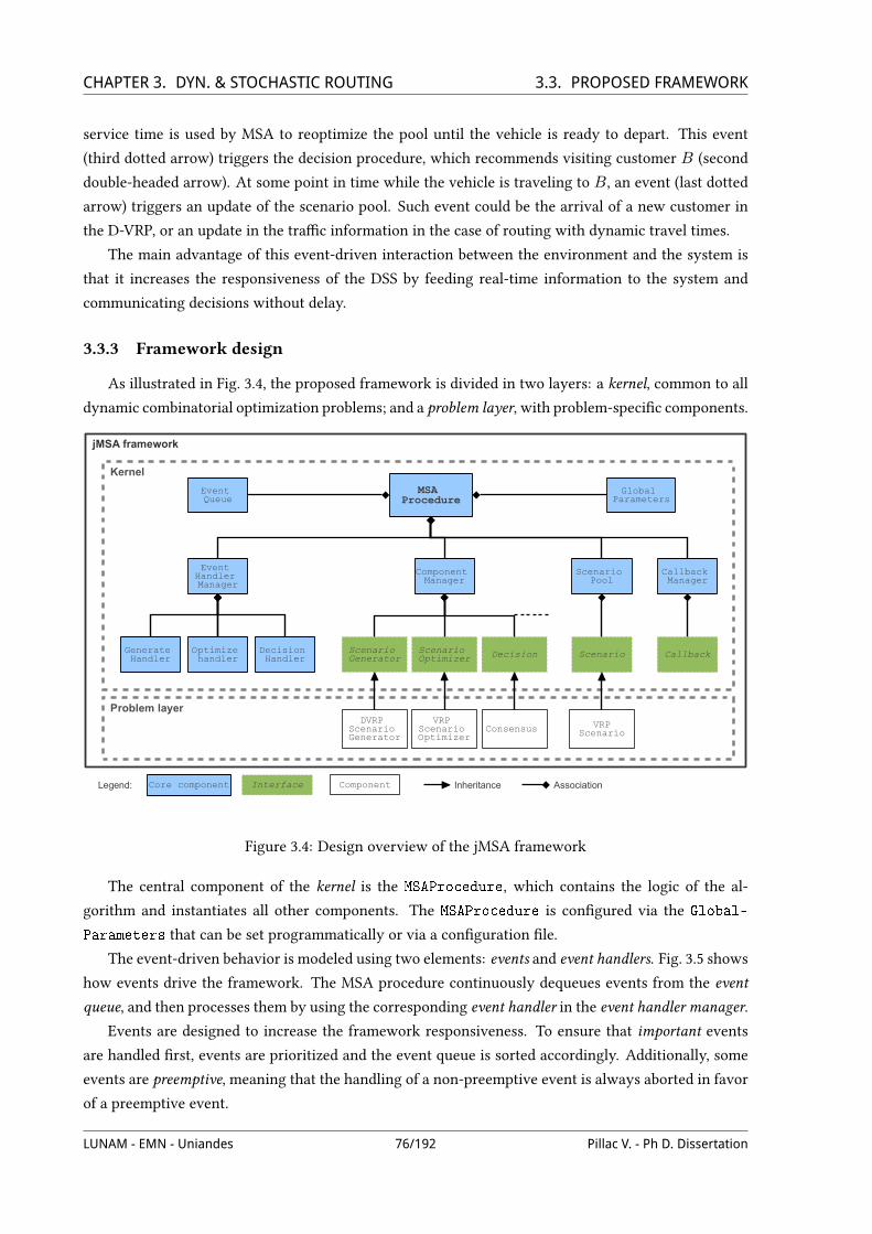
CHAPTER 3. DYN. & STOCHASTIC ROUTING 3.3. PROPOSED FRAMEWORKservice time is used by MSA to reoptimize the pool until the vehicle is ready to depart. This event
(third dotted arrow) triggers the decision procedure, which recommends visiting customer B (second
double-headed arrow). At some point in time while the vehicle is traveling to B, an event (last dotted
arrow) triggers an update of the scenario pool. Such event could be the arrival of a new customer in
the D-VRP, or an update in the traXc information in the case of routing with dynamic travel times.
The main advantage of this event-driven interaction between the environment and the system is
that it increases the responsiveness of the DSS by feeding real-time information to the system and
communicating decisions without delay.
3.3.3 Framework design
As illustrated in Fig. 3.4, the proposed framework is divided in two layers: a kernel, common to all
dynamic combinatorial optimization problems; and a problem layer, with problem-speciVc components.
Problem layer
Kernel
MSA Procedure
Event Handler Manager
Callback Manager
Component Manager
Scenario Pool
Global Parameters
Generate Handler
Optimize handler
Decision Handler
Scenario Generator
Scenario Optimizer Decision Scenario
DVRP Scenario Generator
VRP Scenario Optimizer
Consensus VRPScenario
jMSA framework
Callback
ComponentInterface Inheritance AssociationCore componentLegend:
Event Queue
Figure 3.4: Design overview of the jMSA framework
The central component of the kernel is the MSAProcedure, which contains the logic of the al-
gorithm and instantiates all other components. The MSAProcedure is conVgured via the Global-
Parameters that can be set programmatically or via a conVguration Vle.
The event-driven behavior is modeled using two elements: events and event handlers. Fig. 3.5 shows
how events drive the framework. The MSA procedure continuously dequeues events from the event
queue, and then processes them by using the corresponding event handler in the event handler manager.
Events are designed to increase the framework responsiveness. To ensure that important events
are handled Vrst, events are prioritized and the event queue is sorted accordingly. Additionally, some
events are preemptive, meaning that the handling of a non-preemptive event is always aborted in favor
of a preemptive event.
LUNAM - EMN - Uniandes 76/192 Pillac V. - Ph D. Dissertation

CHAPTER 3. DYN. & STOCHASTIC ROUTING 3.3. PROPOSED FRAMEWORK
MSA procedure
Initialize scenario pool
Handle event
End
Start
YES
NOEnd of the day?
Dequeue next event
Event handler manager
Generate handler
NO
Optimize scenario
Add scenario to pool
Generate scenario
YES
Poolfull?
Scenario Optimization
Decision handler
Evaluatescenarios
Next customer to be served
Optimize handler
Optimize scenarios
Scenario Generation
… (other handlers)
Event queue
New Customer
Resource
Pool Update
Decision
Scenario Generation
Scenario Optimization
Legend: Process Event (non-preemptive)
Event(preemptive)
Figure 3.5: Event-driven MSA framework
Event handlers deVne at a very high level what actions are triggered by a given event. By design,
these handlers do not contain any problem-speciVc logic which is instead delegated to components.
The component manager contains references to all components and acts as an interface between event
handlers and problem-speciVc implementations.
Fig. 3.6 illustrates how event handlers and components interact for the ScenarioGeneration
event. First, GenerateHandler calls the generateScenario method of the ComponentManager that
internally uses the registered ScenarioGenerator. Then it calls the optimizeScenariomethod, del-
egated to the instance of ScenarioOptimizer in use, and adds the scenario to the pool. The process
repeats until the pool is full, moment when the event handling terminates by raising a Scenario-
Optimization event that is further pushed to the event queue.
The framework includes a callback system that provides users with further control over the MSA
procedure. Users may implement a callback simply by extending the Callback interface provided
in the framework, and registering it in the MSA procedure. User-deVned callbacks are automatically
invoked at speciVc points of the procedure and allow customized uses such as logging to a Vle or
dynamic parameter tunning.
Tied, yet decoupled to the kernel, the jMSA framework oUers a problem-speciVc layer containing
components that provide ready-to-use functionalities for common dynamic combinatorial optimization
problems. Fig. 3.4 illustrates some components that could be combined for the D-VRP. Consensus is an
implementation of the consensus algorithm that is common to many dynamic problems solved under
MSA; VRPScenario is an implementation of Scenario for routing problems containing a set of routes;
LUNAM - EMN - Uniandes 77/192 Pillac V. - Ph D. Dissertation

CHAPTER 3. DYN. & STOCHASTIC ROUTING 3.3. PROPOSED FRAMEWORKComponentManager ScenarioGeneratorGenerateHandler ScenarioOptimizer
generateScenario
optimizeScenario
addToPool
scenario
scenario
While pool not full
generateScenario
handleEvent
raise(ScenarioOptimization)
MSAProcedure
Figure 3.6: Interaction between the GenerateHandler and the diUerent components.
VRPScenarioOptimizer is a generic solver for the VRP; and Vnally DVRPScenarioGenerator is the
only component speciVc to the D-VRP that is responsible for the generation of new scenarios.
This two-layer architecture ensures Wexibility and extensibility. While kernel elements are deVned
at a high level and are designed to be problem independent, the problem layer provides implemen-
tations for speciVc problems. Thus, users only have to deVne or extend components, in particular
for scenario generation and optimization, without worrying how they will be integrated in the MSA
procedure.
3.3.4 Parallelization via multi-threading
The ubiquitous presence of multi-core processors can be exploited in parallelizable algorithms such
as MSA. Nevertheless, parallelization often comes at the price of a higher implementation complexity.
The jMSA framework oUers multi-threaded parallelization of the most time-consuming tasks, hiding
it from the user. That is, under jMSA, users do not have to explicitly write a parallel algorithm, but
simply rely on the ComponentManager which internally distributes tasks among diUerent threads.
Fig. 3.7 illustrates how threads interact within the jMSA framework. At time t0 the MSA thread
dequeues an OptimizePool event, and processes it with the corresponding OptimizeHandler. In
parallel to the MSA thread, two other threads are started by the ComponentManager to optimize the
scenarios of the pool. At t1, a preemptive NewCustomer and a Decision event are pushed by the
environment, causing the MSA thread to prematurely abort the optimization. To avoid inconsistencies,
the main thread waits for the pool executor to terminate, sends a signal to the callback thread to
notify that the OptimizePool event was handled, and raises a GenerateScenarios event. Finally,
the procedure dequeues the NewCustomer event, which has a higher priority than the Decision event,
and processes it.
It is worth noting that aside from time-consuming tasks such as scenario generation and opti-
mization, parallelization is also used to execute callbacks. Callbacks can be particularly useful when
LUNAM - EMN - Uniandes 78/192 Pillac V. - Ph D. Dissertation
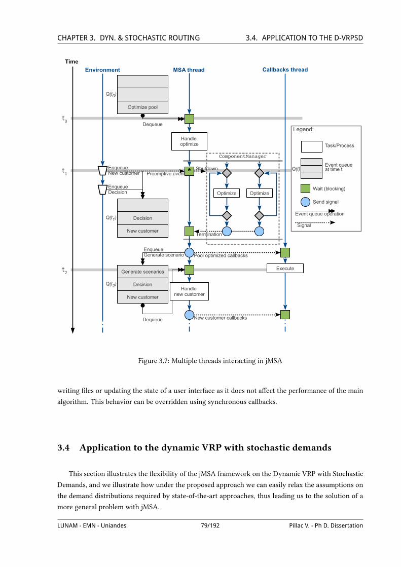
CHAPTER 3. DYN. & STOCHASTIC ROUTING 3.4. APPLICATION TO THE D-VRPSD
t1
t2
t0
Optimize
Termination
ComponentManager
Execute
Optimize
Dequeue
Handle new customer
Pool optimized callbacks
New customer callbacks
Handle optimize
Enqueue Generate scenario
MSA thread Callbacks threadEnvironment
Enqueue Decision
Dequeue
Enqueue New customer Preemptive event * Shutdown
Time
Legend:
Wait (blocking)
Send signal
Signal
Event queue operation
Event queueat time t
Task/Process
Optimize pool
Q(t0)
New customer
DecisionQ(t1)
New customer
Decision
Generate scenarios
Q(t2)
Q(t)
Figure 3.7: Multiple threads interacting in jMSA
writing Vles or updating the state of a user interface as it does not aUect the performance of the main
algorithm. This behavior can be overridden using synchronous callbacks.
3.4 Application to the dynamic VRP with stochastic demands
This section illustrates the Wexibility of the jMSA framework on the Dynamic VRP with Stochastic
Demands, and we illustrate how under the proposed approach we can easily relax the assumptions on
the demand distributions required by state-of-the-art approaches, thus leading us to the solution of a
more general problem with jMSA.
LUNAM - EMN - Uniandes 79/192 Pillac V. - Ph D. Dissertation

CHAPTER 3. DYN. & STOCHASTIC ROUTING 3.4. APPLICATION TO THE D-VRPSD3.4.1 Problem description
The fundamental diUerence between the classic VRP and the VRPwith Stochastic Demands (VRPSD)
is that in the latter customer demands are known as random variables. The randomness in the VRPSD
implies that a customer demand realization might exceed the vehicle remaining capacity, leading to a
route failure that requires a recourse action. An intuitive recourse action is for the vehicle to go back
to the depot to restore its initial capacity and then resume its route (Mendoza et al., 2009), or to al-
low the service of additional customers before returning to the depot (Novoa, 2005). It is important
to stress that in this context all customers are known beforehand and the only dynamically revealed
information is the realization of the customer demands.
Uncertainty in the VRPSD has been addressed by various solution approaches, of which the two
most studied are the Chance Constrained Programming (CCP) and the Stochastic Programming with
Recourse (SPR). Both methods are based on a two-stage approach: the Vrst phase builds a robust routing
plan; while the second phase takes recourse (corrective) actions as the realizations of the customer
demands are unveiled. The conceptual diUerence between the two approaches lies in the objective
of the Vrst-stage optimization: in CCP, the goal is to ensure an upper bound on the probability of a
failure, regardless of the expected cost of the second phase; while SPR seeks the minimization of the
total expected cost, including recourse actions.
The Dynamic VRPSD (D-VRPSD) is an extension of the VRPSD in which it is possible to freely
reroute vehicles upon new demand realizations, allowing more complex recourse actions. Literature on
the D-VRPSD is scarce, with the main contributions being the work by Novoa (2005), Novoa and Storer
(2009), Secomandi (2001), and Secomandi and Margot (2009). The only publicly available instances for
the D-VRPSD are those from Novoa (2005), therefore we will use the same problem deVnition deVned
therein to allow a fair comparison between algorithms. In our work, as in all studies on the D-VRPSD,
we consider the single-vehicle case with discrete and uniformly distributed demand distributions. If
at some point the realization ξ of the demand of a customer exceeds the vehicle remaining capacity
Q, the vehicle serves the quantity Q, and returns to the depot to restore its capacity. Afterwards, a
subsequent visit to the customer is planned to serve the remaining demand ξ − Q.
3.4.2 Scenarios and decisions
In the context of the D-VRPSD, scenarios contain diUerent realizations of the customer demands,
along with a feasible routing for these values. Given that the vehicle can go back to the depot during
its service, a scenario can contain diUerent routes that will be executed in a sequential order by the
same vehicle.
The fact that customer locations are identical across scenarios suggests that diUerent scenarios
might have similar routes. Therefore, we use the consensus algorithm to select the next customer to
visit. Let us consider the scenario pool of Fig. 3.8. The customers who have already been served (4
and 1) appear Vrst in all scenarios, while customers 2, 3, 5, and 6, appear in varying order depending
on the scenario sampled demands. Considering that customer 2 appears Vrst in 2 out of 4 scenarios,
by consensus it is selected as the next customer to visit. With the notations from Algorithm 3.1, the
function selectCandidates (line 1) returns the set of unserved customers while evaluateRequest-
LUNAM - EMN - Uniandes 80/192 Pillac V. - Ph D. Dissertation

CHAPTER 3. DYN. & STOCHASTIC ROUTING 3.4. APPLICATION TO THE D-VRPSDProfit (line. 6) returns 1 if customer r appears Vrst in the scenario; 0, otherwise. It is worth noting
that the consensus decision might recommend the vehicle to return to the depot for a preventive
replenishment, that is, before the vehicle runs out of capacity.
0
0
0
05
5
6
63
6
3
2
3
2
1
1
1
1
0
0
0
0
Scenario 1
Scenario 2
Scenario 3
Scenario 4
4
4
4
4
...
...
...
Already executed
Next client
Figure 3.8: Example of the decision process by consensus in a 4-scenario pool. Each scenario containscustomers who have been visited (in white) and customers yet to be visited (in gray).
3.4.3 Optimization
To optimize scenarios we use an Adaptive Variable Neighborhood Search (AVNS), which is an
extension of the Variable Neighborhood Search (VNS) (Mladenovic and Hansen, 1997). The main dif-
ference between AVNS and VNS is that neighborhoods are not explored sequentially, but randomly
selected with a bias depending on their previous performance. Our implementation uses an average
ratio of the improvement to time as a metric of neighborhood performance, and maintains this infor-
mation between calls to the optimization procedure. Neighborhoods with a better performance are
more likely to be explored Vrst, leading to a self-tuning algorithm. Our MSA scheme beneVts from
this automatic self-tuning behavior as the optimization procedure is called numerous times on similar
instances (i.e., scenarios).
Algorithm 3.2 presents an outline of the AVNS algorithm. The algorithm initializes with the whole
set of neighborhood structures (line. 2), then it selects a neighborhood (line. 4) to randomly perturb
the current solution (line. 5), and improves it by applying a local search procedure (line. 6). If the new
solution is improving (line. 8) then it becomes the current solution (line. 9), and the set of active neigh-
borhood structures is reset (line. 10). Otherwise, the current neighborhood is removed from the set of
active neighborhoods (line. 12). At each iteration, the performance of the current neighborhood is up-
dated (line. 7). This process iterates until all neighborhoods have been explored with no improvement.
In our experiments we used the two neighborhoods structures Or-opt and string-exchange for the
perturbation, and a Variable Neighborhood Descent (VND) based on swap and 2-opt as local search
(line. 6). A more detailed description of these neighborhoods can be found in the paper by Irnich et al.
(2006). The initial solution is obtained by a Clarke andWright (CW) heuristic (Clarke andWright, 1964)
in which the saving list is randomized, as presented in Mendoza et al. (2010), leading to the CW+AVNS
algorithm.
LUNAM - EMN - Uniandes 81/192 Pillac V. - Ph D. Dissertation
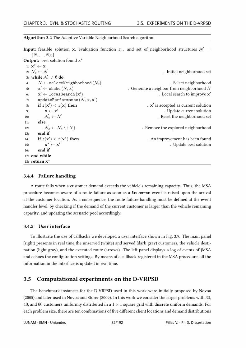
CHAPTER 3. DYN. & STOCHASTIC ROUTING 3.5. EXPERIMENTS ON THE D-VRPSDAlgorithm 3.2 The Adaptive Variable Neighborhood Search algorithm
Input: feasible solution x, evaluation function z , and set of neighborhood structures N =N1, .., NK
Output: best solution found x∗
1: x∗ ← x2: Nc ← N . Initial neighborhood set3: while Nc 6= ∅ do4: N ← selectNeighborhood (Nc) . Select neighborhood5: x′ ← shake (N,x) . Generate a neighbor from neighborhood N6: x′ ← localSearch (x′) . Local search to improve x′
7: updatePerformance (N ,x,x′)8: if z(x′) < z(x) then . x′ is accepted as current solution9: x← x′ . Update current solution10: Nc ← N . Reset the neighborhood set11: else12: Nc ← Nc \ N . Remove the explored neighborhood13: end if14: if z(x′) < z(x∗) then . An improvement has been found15: x∗ ← x′ . Update best solution16: end if17: end while18: return x∗
3.4.4 Failure handling
A route fails when a customer demand exceeds the vehicle’s remaining capacity. Thus, the MSA
procedure becomes aware of a route failure as soon as a Resource event is raised upon the arrival
at the customer location. As a consequence, the route failure handling must be deVned at the event
handler level, by checking if the demand of the current customer is larger than the vehicle remaining
capacity, and updating the scenario pool accordingly.
3.4.5 User interface
To illustrate the use of callbacks we developed a user interface shown in Fig. 3.9. The main panel
(right) presents in real time the unserved (white) and served (dark gray) customers, the vehicle desti-
nation (light gray), and the executed route (arrows). The left panel displays a log of events of jMSA
and echoes the conVguration settings. By means of a callback registered in the MSA procedure, all the
information in the interface is updated in real time.
3.5 Computational experiments on the D-VRPSD
The benchmark instances for the D-VRPSD used in this work were initially proposed by Novoa
(2005) and later used in Novoa and Storer (2009). In this work we consider the larger problems with 30,
40, and 60 customers uniformly distributed in a 1× 1 square grid with discrete uniform demands. For
each problem size, there are ten combinations of Vve diUerent client locations and demand distributions
LUNAM - EMN - Uniandes 82/192 Pillac V. - Ph D. Dissertation

CHAPTER 3. DYN. & STOCHASTIC ROUTING 3.5. EXPERIMENTS ON THE D-VRPSD
Figure 3.9: A graphical user interface for jMSA
by two vehicle capacities, leading to a complete testbed of 30 instances. Optimal values where obtained
using the COIN-OR Symphony VRP solver (Ralphs, 2006; Ralphs et al., 2003).
To assess the optimization component in isolation, we conducted an experiment on 100 diUerent
demand realizations for all 30 instances. Fig. 3.10 presents the distribution of gaps to optimal values
for CW+AVNS and a CW+2-opt heuristic used for comparison. Note that CW+AVNS clearly dominates
CW+2-opt, with 90% of all instances solved with a gap of less than 4%. Additionally, CW+AVNS runs
relatively fast, with average CPU times between 50 ms and 650 ms for the larger instances.
!
Figure 3.10: Optimal gap distribution of the CW+AVNS algorithm vs. CW+2-opt for all Novoa (2005)instances
To facilitate the comparison between approaches for the D-VRPSD, we report the results in terms
LUNAM - EMN - Uniandes 83/192 Pillac V. - Ph D. Dissertation
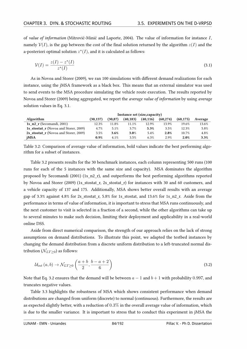
CHAPTER 3. DYN. & STOCHASTIC ROUTING 3.5. EXPERIMENTS ON THE D-VRPSDof value of information (Mitrović-Minić and Laporte, 2004). The value of information for instance I ,
namely V(I), is the gap between the cost of the Vnal solution returned by the algorithm z(I) and the
a-posteriori optimal solution z∗(I), and it is calculated as follows:
V(I) =z(I)− z∗(I)
z∗(I)(3.1)
As in Novoa and Storer (2009), we ran 100 simulations with diUerent demand realizations for each
instance, using the jMSA framework as a black box. This means that an external simulator was used
to send events to the MSA procedure simulating the vehicle route execution. The results reported by
Novoa and Storer (2009) being aggregated, we report the average value of information by using average
solution values in Eq. 3.1.
Instance set (size,capacity)Algorithm (30,137) (30,87) (40,183) (40,116) (60,274) (60,175) Average1s_n2_r (Secomandi, 2001) 12.3% 11.8% 11.1% 12.9% 13.9% 19.6% 13.6%1s_stostat_r (Novoa and Storer, 2009) 4.7% 5.1% 3.7% 5.3% 3.5% 12.3% 5.8%2s_stostat_r (Novoa and Storer, 2009) 3.5% 3.6% 3.0% 5.4% 2.8% 10.7% 4.8%jMSA 0.9% 4.1% 3.5% 6.3% 2.9% 2.0% 3.3%
Table 3.2: Comparison of average value of information, bold values indicate the best performing algo-rithm for a subset of instances.
Table 3.2 presents results for the 30 benchmark instances, each column representing 500 runs (100
runs for each of the 5 instances with the same size and capacity). MSA dominates the algorithm
proposed by Secomandi (2001) (1s_n2_r), and outperforms the best performing algorithms reported
by Novoa and Storer (2009) (1s_stostat_r, 2s_stostat_r) for instances with 30 and 60 customers, and
a vehicle capacity of 137 and 175. Additionally, MSA shows better overall results with an average
gap of 3.3% against 4.8% for 2s_stostat_r, 5.8% for 1s_stostat, and 13.6% for 1s_n2_r. Aside from the
performance in terms of value of information, it is important to stress that MSA runs continuously, and
the next customer to visit is selected in a fraction of a second, while the other algorithms can take up
to several minutes to make such decision, limiting their deployment and applicability in a real-world
online DSS.
Aside from direct numerical comparison, the strength of our approach relies on the lack of strong
assumptions on demand distributions. To illustrate this point, we adapted the testbed instances by
changing the demand distribution from a discrete uniform distribution to a left-truncated normal dis-
tribution (NLT≥0) as follows:
Uint (a, b)→ NLT≥0
(a+ b
2,b− a+ 2
6
)(3.2)
Note that Eq. 3.2 ensures that the demand will be between a− 1 and b+ 1 with probability 0.997, and
truncates negative values.
Table 3.3 highlights the robustness of MSA which shows consistent performance when demand
distributions are changed from uniform (discrete) to normal (continuous). Furthermore, the results are
as expected slightly better, with a reduction of 0.3% in the overall average value of information, which
is due to the smaller variance. It is important to stress that to conduct this experiment in jMSA the
LUNAM - EMN - Uniandes 84/192 Pillac V. - Ph D. Dissertation

CHAPTER 3. DYN. & STOCHASTIC ROUTING 3.6. CONCLUSIONSInstance set (size,capacity)
Algorithm (30,137) (30,87) (40,183) (40,116) (60,274) (60,175) AverageUniform 0.9% 3.9% 3.5% 6.3% 2.9% 2.0% 3.3%Normal 0.7% 3.6% 3.4% 6.2% 2.2% 1.9% 3.0%
Table 3.3: Comparison of average VI for discrete uniform and normal distributions.
only change required was to use a diUerent random number generator, which illustrates the Wexibility
of our approach. Other approaches based on stochastic modeling (Novoa and Storer, 2009; Novoa,
2005; Secomandi, 2001) are not as Wexible and depend on distributional assumptions, thus limiting
their application scope.
3.6 Conclusions
In this paper we presented the design and implementation of jMSA, an object-oriented event-driven
framework for the Multiple Scenario Approach (MSA). By doing a high-level abstraction of MSA to a
problem independent level, we modeled it as an event-driven process that allows high reactivity to
changes occurring in online and highly dynamic operational environments. We implemented jMSA as
a Wexible framework that is easily embeddable in decision support systems. By design, jMSA includes
a callback system that gives the user further control over MSA and allow complex interactions with
third party components. Additionally, we integrated into the framework the parallelization of time
consuming tasks with no compromise for the framework user, which is a key aspect considering the
wide availability of multi-core personal computers.
We illustrated the use of jMSA on the Dynamic Vehicle Routing Problem with Stochastic Demands
(D-VRPSD). The optimization of scenarios is performed by an Adaptive Variable Neighborhood Search
(AVNS) which improves an initial solution generated with a randomized Clarke and Wright heuristic.
The strength of AVNS is that it automatically adjusts its search scheme depending on the problem’s
structure by keeping track of the neighborhood performance throughout the execution of the MSA
procedure. Computational experiments show that our approach is competitive with state-of-the-art
algorithms that take full advantage of the stochastic aspects, while it provides a more Wexible scheme
that can be used to tackle problems with diUerent demand distributions.
Acknowledgements Financial support for this work was provided by the CPER (Contrat de ProjetÉtat Region) Vallée du Libre; and the Centro de Estudios Interdisciplinarios Básicos y Aplicados enComplejidad (CeiBA, Colombia). This support is gratefully acknowledged. The authors would alsolike to thank Olivier Péton from the École des Mines de Nantes for his insightful comments. Finally,the constructive comments of the Editor-in-Chief, Dr. Andrew B. Whinston, and the review process ofDSS led us to an improved paper.
Bibliography
Attanasio, A., Bregman, J., Ghiani, G., and Manni, E. (2007). Real-time Weet management at Ecourier Ltd. InZeimpekis, V., Tarantilis, C. D., Giaglis, G. M., and Minis, I., editors, Dynamic Fleet Management, volume 38 ofOperations Research/Computer Science Interfaces, chapter 10, pages 219–238. Springer US.
LUNAM - EMN - Uniandes 85/192 Pillac V. - Ph D. Dissertation

CHAPTER 3. DYN. & STOCHASTIC ROUTING BIBLIOGRAPHYBaldacci, R., Toth, P., and Vigo, D. (2007). Recent advances in vehicle routing exact algorithms. 4OR: A Quarterly
Journal of Operations Research, 5(4):269–298, doi:10.1007/s10288-007-0063-3.
Barcelo, J., Grzybowska, H., and Pardo, S. (2007). Vehicle routing and scheduling models, simulation and citylogistics. In Zeimpekis, V., Tarantilis, C. D., Giaglis, G. M., and Minis, I., editors, Dynamic Fleet Management,volume 38 of Operations Research/Computer Science Interfaces, pages 163–195. Springer US.
Beaudry, A., Laporte, G., Melo, T., and Nickel, S. (2010). Dynamic transportation of patients in hospitals. ORSpectrum, 32:77–107, doi:10.1007/s00291-008-0135-6.
Bent, R. and Van Hentenryck, P. (2004a). Regrets only! online stochastic optimization under time constraints. InProceedings of the 19th National Conference on ArtiVcial Intelligence (AAAI-04), pages 501–506. AAAI Press.
Bent, R. and Van Hentenryck, P. (2004b). Scenario-based planning for partially dynamic vehicle routing withstochastic customers. Operations Research, 52(6):977–987.
Benyahia, I. and Potvin, J. Y. (1998). Decision support for vehicle dispatching using genetic programming. IEEETransactions on Systems Man and Cybernetics Part A - Systems and Humans, 28(3):306–314.
Bhargava, H. K., Power, D. J., and Sun, D. (2007). Progress in web-based decision support technologies. DecisionSupport Systems, 43(4):1083 – 1095, doi:10.1016/j.dss.2005.07.002.
Bieding, T., Görtz, S., and Klose, A. (2009). On line routing per mobile phone a case on subsequent deliveries ofnewspapers. In Nunen, J. A., Speranza, M. G., and Bertazzi, L., editors, Innovations in Distribution Logistics,volume 619 of Lecture Notes in Economics and Mathematical Systems, pages 29–51. Springer Berlin Heidelberg.
Chang, H., Givan, R., and Chong, E. (2000). On-line scheduling via sampling. In Proceedings of the ArtiVcialIntelligence Planning and Scheduling (AIPS 2000), pages 62–71.
Clarke, G. and Wright, J. W. (1964). Scheduling of vehicles from a central depot to a number of delivery points.Operations Research, 12(4):568–581, doi:10.1287/opre.12.4.568.
Cordeau, J.-F., Laporte, G., Savelsbergh, M. W., and Vigo, D. (2007). Vehicle routing. In Barnhart, C. and Laporte,G., editors, Transportation, volume 14 of Handbooks in Operations Research and Management Science, chapter 6,pages 367–428. Elsevier.
Crainic, T. G., Gendreau, M., and Potvin, J.-Y. (2009). Intelligent freight-transportation systems: Assessment andthe contribution of operations research. Transportation Research Part C: Emerging Technologies, 17(6):541–557,doi:10.1016/j.trc.2008.07.002.
Dahl, S. and Derigs, U. (2011). Cooperative planning in express carrier networks – an empirical studyon the eUectiveness of a real-time decision support system. Decision Support Systems, 51(3):620–626,doi:10.1016/j.dss.2011.02.018.
Dantzig, G. and Ramser, J. (1959). The truck dispatching problem. Management Science, 6(1):80–91.
Eksioglu, B., Vural, A. V., and Reisman, A. (2009). The vehicle routing problem: A taxonomic review. Computers& Industrial Engineering, 57(4):1472 – 1483, doi:10.1016/j.cie.2009.05.009.
Fleischmann, B., Gnutzmann, S., and Sandvoss, E. (2004). Dynamic vehicle routing based on online traXc infor-mation. Transportation Science, 38(4):420–433, doi:10.1287/trsc.1030.0074.
Gendreau, M., Guertin, F., Potvin, J.-Y., and Taillard, E. (1999). Parallel tabu search for real-time vehicle routingand dispatching. Transportation Science, 33(4):381–390, doi:10.1287/trsc.33.4.381.
Godfrey, G. and Powell, W. B. (2002). An adaptive dynamic programming algorithm for dynamic Weet manage-ment, I: Single period travel times. Transportation Science, 36(1):21–39.
Goel, A. and Gruhn, V. (2008). A general vehicle routing problem. European Journal of Operational Research,191(3):650–660, doi:10.1016/j.ejor.2006.12.065.
LUNAM - EMN - Uniandes 86/192 Pillac V. - Ph D. Dissertation
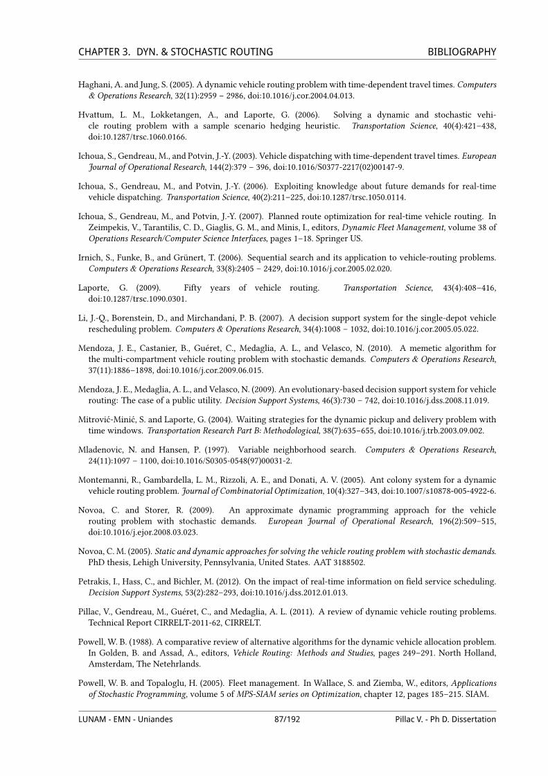
CHAPTER 3. DYN. & STOCHASTIC ROUTING BIBLIOGRAPHYHaghani, A. and Jung, S. (2005). A dynamic vehicle routing problemwith time-dependent travel times. Computers
& Operations Research, 32(11):2959 – 2986, doi:10.1016/j.cor.2004.04.013.
Hvattum, L. M., Lokketangen, A., and Laporte, G. (2006). Solving a dynamic and stochastic vehi-cle routing problem with a sample scenario hedging heuristic. Transportation Science, 40(4):421–438,doi:10.1287/trsc.1060.0166.
Ichoua, S., Gendreau, M., and Potvin, J.-Y. (2003). Vehicle dispatching with time-dependent travel times. EuropeanJournal of Operational Research, 144(2):379 – 396, doi:10.1016/S0377-2217(02)00147-9.
Ichoua, S., Gendreau, M., and Potvin, J.-Y. (2006). Exploiting knowledge about future demands for real-timevehicle dispatching. Transportation Science, 40(2):211–225, doi:10.1287/trsc.1050.0114.
Ichoua, S., Gendreau, M., and Potvin, J.-Y. (2007). Planned route optimization for real-time vehicle routing. InZeimpekis, V., Tarantilis, C. D., Giaglis, G. M., and Minis, I., editors, Dynamic Fleet Management, volume 38 ofOperations Research/Computer Science Interfaces, pages 1–18. Springer US.
Irnich, S., Funke, B., and Grünert, T. (2006). Sequential search and its application to vehicle-routing problems.Computers & Operations Research, 33(8):2405 – 2429, doi:10.1016/j.cor.2005.02.020.
Laporte, G. (2009). Fifty years of vehicle routing. Transportation Science, 43(4):408–416,doi:10.1287/trsc.1090.0301.
Li, J.-Q., Borenstein, D., and Mirchandani, P. B. (2007). A decision support system for the single-depot vehiclerescheduling problem. Computers & Operations Research, 34(4):1008 – 1032, doi:10.1016/j.cor.2005.05.022.
Mendoza, J. E., Castanier, B., Guéret, C., Medaglia, A. L., and Velasco, N. (2010). A memetic algorithm forthe multi-compartment vehicle routing problem with stochastic demands. Computers & Operations Research,37(11):1886–1898, doi:10.1016/j.cor.2009.06.015.
Mendoza, J. E., Medaglia, A. L., and Velasco, N. (2009). An evolutionary-based decision support system for vehiclerouting: The case of a public utility. Decision Support Systems, 46(3):730 – 742, doi:10.1016/j.dss.2008.11.019.
Mitrović-Minić, S. and Laporte, G. (2004). Waiting strategies for the dynamic pickup and delivery problem withtime windows. Transportation Research Part B: Methodological, 38(7):635–655, doi:10.1016/j.trb.2003.09.002.
Mladenovic, N. and Hansen, P. (1997). Variable neighborhood search. Computers & Operations Research,24(11):1097 – 1100, doi:10.1016/S0305-0548(97)00031-2.
Montemanni, R., Gambardella, L. M., Rizzoli, A. E., and Donati, A. V. (2005). Ant colony system for a dynamicvehicle routing problem. Journal of Combinatorial Optimization, 10(4):327–343, doi:10.1007/s10878-005-4922-6.
Novoa, C. and Storer, R. (2009). An approximate dynamic programming approach for the vehiclerouting problem with stochastic demands. European Journal of Operational Research, 196(2):509–515,doi:10.1016/j.ejor.2008.03.023.
Novoa, C. M. (2005). Static and dynamic approaches for solving the vehicle routing problem with stochastic demands.PhD thesis, Lehigh University, Pennsylvania, United States. AAT 3188502.
Petrakis, I., Hass, C., and Bichler, M. (2012). On the impact of real-time information on Veld service scheduling.Decision Support Systems, 53(2):282–293, doi:10.1016/j.dss.2012.01.013.
Pillac, V., Gendreau, M., Guéret, C., and Medaglia, A. L. (2011). A review of dynamic vehicle routing problems.Technical Report CIRRELT-2011-62, CIRRELT.
Powell, W. B. (1988). A comparative review of alternative algorithms for the dynamic vehicle allocation problem.In Golden, B. and Assad, A., editors, Vehicle Routing: Methods and Studies, pages 249–291. North Holland,Amsterdam, The Netehrlands.
Powell, W. B. and Topaloglu, H. (2005). Fleet management. In Wallace, S. and Ziemba, W., editors, Applicationsof Stochastic Programming, volume 5 of MPS-SIAM series on Optimization, chapter 12, pages 185–215. SIAM.
LUNAM - EMN - Uniandes 87/192 Pillac V. - Ph D. Dissertation
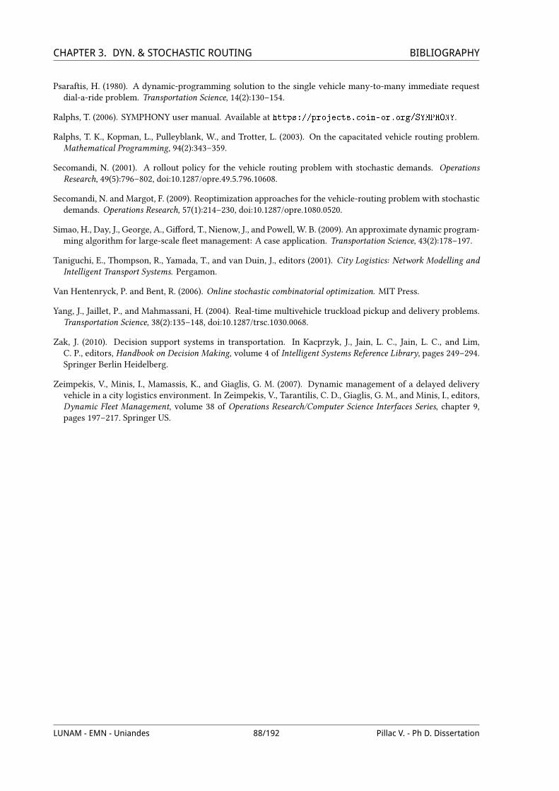
CHAPTER 3. DYN. & STOCHASTIC ROUTING BIBLIOGRAPHYPsaraftis, H. (1980). A dynamic-programming solution to the single vehicle many-to-many immediate request
dial-a-ride problem. Transportation Science, 14(2):130–154.
Ralphs, T. (2006). SYMPHONY user manual. Available at https://projects.coin-or.org/SYMPHONY.
Ralphs, T. K., Kopman, L., Pulleyblank, W., and Trotter, L. (2003). On the capacitated vehicle routing problem.Mathematical Programming, 94(2):343–359.
Secomandi, N. (2001). A rollout policy for the vehicle routing problem with stochastic demands. OperationsResearch, 49(5):796–802, doi:10.1287/opre.49.5.796.10608.
Secomandi, N. and Margot, F. (2009). Reoptimization approaches for the vehicle-routing problem with stochasticdemands. Operations Research, 57(1):214–230, doi:10.1287/opre.1080.0520.
Simao, H., Day, J., George, A., GiUord, T., Nienow, J., and Powell, W. B. (2009). An approximate dynamic program-ming algorithm for large-scale Weet management: A case application. Transportation Science, 43(2):178–197.
Taniguchi, E., Thompson, R., Yamada, T., and van Duin, J., editors (2001). City Logistics: Network Modelling andIntelligent Transport Systems. Pergamon.
Van Hentenryck, P. and Bent, R. (2006). Online stochastic combinatorial optimization. MIT Press.
Yang, J., Jaillet, P., and Mahmassani, H. (2004). Real-time multivehicle truckload pickup and delivery problems.Transportation Science, 38(2):135–148, doi:10.1287/trsc.1030.0068.
Zak, J. (2010). Decision support systems in transportation. In Kacprzyk, J., Jain, L. C., Jain, L. C., and Lim,C. P., editors, Handbook on Decision Making, volume 4 of Intelligent Systems Reference Library, pages 249–294.Springer Berlin Heidelberg.
Zeimpekis, V., Minis, I., Mamassis, K., and Giaglis, G. M. (2007). Dynamic management of a delayed deliveryvehicle in a city logistics environment. In Zeimpekis, V., Tarantilis, C. D., Giaglis, G. M., and Minis, I., editors,Dynamic Fleet Management, volume 38 of Operations Research/Computer Science Interfaces Series, chapter 9,pages 197–217. Springer US.
LUNAM - EMN - Uniandes 88/192 Pillac V. - Ph D. Dissertation
4Case study: the Technician Routing and Scheduling
Problem
The two papers presented in this chapter are motivated by a real-world optimization problem
submitted by an industrial partner. This company provides software solutions for organizations that
have to route a crew of technicians to service geographically distributed customer requests that can
be either static or dynamic. Static requests are known in advance and correspond to appointments
with customers or preventive maintenance operations. On the other hand, dynamic requests appear
dynamically throughout the day and are, for instance, emergencies or corrective maintenance opera-
tions. Requests may require a technician with diUerent skills, a certain set of tools, and a number of
spare parts to be serviced. In addition, technicians generally start and end their day at their home,
and may visit a central depot to pickup tools and spare parts. Finally, the objectives include the mini-
mization of the traveled distance, the minimization of the working time, the balancing of the workload
between technicians, and the minimization of the constraints violations.
From this practical application, we introduced a new optimization problem, namely, the Technician
Routing and Scheduling Problem (TRSP), which deals with a limited crew of technicians that serves a
set of requests. In the TRSP, each technician has a set of skills, tools, and spare parts, while requests
require a subset of each. The problem is then to design a set of tours of minimal total duration such
that each request is visited exactly once, within its time window, by a technician with the required
skills, tools, and spare parts.
A distinctive feature of this problem is that it introduces several compatibility constraints between
technicians and requests. While skills are intrinsic attributes, technicians may carry diUerent tools
and spare parts over the planning horizon. Technicians start their tour from home, with a set of tools
(renewable resources) and spare parts (consumed once the technician serves a request) that allow them
LUNAM - EMN - Uniandes 89/192 Pillac V. - Ph D. Dissertation
CHAPTER 4. CASE STUDY: THE TRSPto serve an initial set of requests. Technicians may have the opportunity to replenish their tools and
spare parts at a central depot at any time to service more requests.
The TRSP naturally arises in a wide range of applications, including telecoms, public utilities,
and maintenance operations. However technician routing and scheduling problems have received
limited attention until recently, and to the best of our knowledge there is no work that considers
simultaneously skills, tools, spare parts, and the arrival of new requests, three important components
of real-world applications. The paper in Section 4.1 introduces a parallel matheuristic able to solve the
static TRSP, while the paper in Section 4.2 presents two approaches to tackle the dynamic TRSP.
LUNAM - EMN - Uniandes 90/192 Pillac V. - Ph D. Dissertation

CHAPTER 4. CASE STUDY: THE TRSP 4.1. THE STATIC TRSP4.1 The static TRSP
The paper presented in this section proposes a parallel matheuristic to solve the static TRSP. From
a practical perspective, this algorithm can be used either to design an initial solution to the problem
considering only static requests, or to compute an a-posteriori solution to a dynamic problem that can
be used to assess the performance of a dynamic approach.
The full reference of the paper presented in this section is:
– Pillac, V., Guéret, C., and Medaglia, A. L. (2011)
A parallel matheuristic for the technician routing and scheduling problem
Optimization Letters, Accepted manuscript, doi:10.1007/s11590-012-0567-4.
Preliminary results were presented in MIC 2011 international conference:
– Pillac, V., Guéret, C., and Medaglia, A. L. (2011)
On the technician routing and scheduling problem
In Di Gaspero, L., Schaerf, A., and Stützle, T., editors, Proceedings of the 9th Metaheuristics
Conference (MIC 2011), pages 675–678. Università degli Studi di Udine.
LUNAM - EMN - Uniandes 91/192 Pillac V. - Ph D. Dissertation


A Parallel Matheuristic for the Technician Routing and Scheduling Problem
V. Pillac1,2, C. Guéret1, A. L. Medaglia2
1 LUNAM, Ecole des Mines de Nantes, IRCCyN UMR 6597, Nantes, France
2 Universidad de los Andes, Industrial Engineering Department, Bogotá, Colombia
Journal : Optimization Letters
State : Accepted manuscript - doi:10.1007/s11590-012-0567-4
Abstract : The Technician Routing and Scheduling Problem (TRSP) consists in rout-
ing staU to serve requests for service, taking into account time windows,
skills, tools, and spare parts. Typical applications include maintenance op-
erations and staU routing in telecoms, public utilities, and in the health
care industry. In this paper, we present a formal deVnition of the TRSP,
discuss its relation with the Vehicle Routing Problem with Time Windows
(VRPTW), and review related research. From a methodological perspective,
we describe a matheuristic composed of a constructive heuristic, a parallel
Adaptive Large Neighborhood Search (pALNS), and a mathematical program-
ming based post-optimization procedure that successfully tackles the TRSP.
We validate the matheuristic on the Solomon VRPTW instances, where we
achieve an average gap of 0.23%, and matched 44 out of 55 optimal solutions.
Finally, we illustrate how the matheuristic successfully solves a set of TRSP
instances extended from the Solomon benchmark.
Keywords : Vehicle routing ; Technician routing and scheduling ; Matheuristic ; ALNS ;
pALNS ; VRPTW
4.1.1 Introduction
The Technician Routing and Scheduling Problem (TRSP) deals with a limited crew of technicians
K that serves a set of requestsR. In the TRSP, each technician has a set of skills, tools, and spare parts,
while requests require a subset of each. The problem is then to design a set of tours of minimal total
duration such that each request is fulVlled exactly once, within its time window, by a technician with
the required skills, tools, and spare parts. It is important to note that the departure of technicians may
be delayed to minimize the waiting time at each visited request, thus reducing the duration of tours.
The TRSP naturally arises in a wide range of settings, including telecoms, public utilities, and compa-
nies planning maintenance operations. The TRSP can be seen as an extension of the Vehicle Routing
Problem with Time Windows (VRPTW), where technicians play the role of vehicles and requests are
made by clients. Thus, it belongs to the class of NP-Hard problems.
A distinctive feature of this problem is the presence of compatibility constraints between techni-
cians and requests. While skills are intrinsic attributes, technicians may carry diUerent tools and spare
parts over the planning horizon. Technicians start their tour from their home, with a set of tools and
spare parts that allows them to serve an initial set of requests. They also have the opportunity to
LUNAM - EMN - Uniandes 93/192 Pillac V. - Ph D. Dissertation

CHAPTER 4. CASE STUDY: THE TRSP 4.1. THE STATIC TRSPreplenish their tools and spare parts at a central depot at any time to serve more requests. Tools can be
seen as renewable resources, while spare parts are non-renewable and consumed once the technician
serves a request.
The remainder of this paper is organized as follows: Section 4.1.2 reviews the literature on prob-
lems related to the TRSP; Section 4.1.3 introduces the proposed matheuristic; Section 4.1.4 presents
experimental results; and Vnally, Section 4.1.5 concludes this work and outlines directions for future
research.
4.1.2 Literature review
The technician scheduling problem is closely related to the TRSP, but does not consider the rout-
ing aspects, nor the tool and spare part constraints. It was featured in the 2007 French Operational
Research Society (ROADEF) challenge. We refer the reader to the work by Cordeau et al. (2010) and
Hashimoto et al. (2011) for two solution approaches to a multi-day variant in which teams are assem-
bled to serve requests. Kovacs et al. (2011) studied an extension of this problem, namely, the Service
Technician Routing and Scheduling Problem (STRSP), which considers routing costs, skills, and team
building.
Bredström and Rönnqvist (2008) present a generic mixed integer programming formulation for a
Vehicle Routing and Scheduling Problem with Time Windows (VRSPTW) in which some clients must
be visited simultaneously by two or more vehicles. The authors do not explicitly consider skills, but the
proposed model accounts for compatibility constraints between vehicles and requests. Parragh (2010)
also tackled a variant with synchronization between technician visits.
A practical consideration in technician routing is that it may not be possible or desirable to serve
all requests. Xu and Chiu (2001) studied a variant of the TRSP in which the objective is to maximize
the number of requests served while accounting for skill constraints and request urgency. Tang et al.
(2007) also considered requests with diUerent urgency levels. The authors use a multi-period maximum
collection problem formulation with time-dependent rewards modeling customer preferences. Tsang
and Voudouris (1997) solved a problem faced by British Telecom where technician skills aUect the time
required to serve a request.
Finally, home care routing and scheduling problems are related to the TRSP in the sense that they
consider patients that need to be visited by staU with speciVc skills and within a given time frame. We
refer the interested reader to the case studies by Bertels and Fahle (2006), Eveborn et al. (2006), and
Akjiratikarl et al. (2007).
In summary, technician routing problems have received limited attention and to the best of our
knowledge, no work considers tools or spare parts, two important components of real-world appli-
cations. The present work, based on a real problem, addresses this aspect and proposes a parallel
matheuristic approach for the TRSP.
4.1.3 The proposed matheuristic
This section outlines the proposed matheuristic that comprises a fast constructive heuristic, a par-
allel adaptive large neighborhood search, and a mathematical programming based post-optimization.
LUNAM - EMN - Uniandes 94/192 Pillac V. - Ph D. Dissertation

CHAPTER 4. CASE STUDY: THE TRSP 4.1. THE STATIC TRSP4.1.3.1 Regret constructive heuristic
Regret heuristics (Potvin and Rousseau, 1993) are constructive heuristics that incorporate a look
ahead component. At each iteration the algorithm inserts the request with the greatest regret value at
the best position, where the regret value is an estimation of the additional cost incurred if a request is
not inserted at its best position.
More formally, let U be the set of requests to be inserted and δki be the cost of inserting request
i at its best position in its k-th best route. The regret-q heuristic inserts at its best position request
i∗ = arg maxi∈U∑q
k=2
(δki − δ1
i
)(ties are broken by choosing the request with the lowest δ1
i value).
It is worth noting that regret-1 corresponds to the well-known best insertion heuristic.
When evaluating the insertion of a request in a tour we need to consider the possibility to plan a
trip to the main depot to pick up additional tools and spare parts. The procedure Vrst checks for the
best feasible insertion without considering trips to the depot. If no feasible insertion is found, it then
considers each possible combination of request and main depot insertions. Insertion feasibility and cost
are evaluated in constant time using the concepts of waiting time and forward time slack introduced by
Savelsbergh (1992).
We use a regret-3 heuristic to design an initial set ofK solutions that will then be improved by the
parallel adaptive large neighborhood search.
4.1.3.2 Parallel Adaptive Large Neighborhood Search
Shaw (1998) introduced the Large Neighborhood Search algorithm (LNS), which works by succes-
sively destroying and repairing a current solution. Pisinger and Ropke (2007) extended LNS by using
several destroy and repair operators and adding an adaptive layer to select them, leading to the Adap-
tive LNS algorithm (ALNS). In this work, we propose a parallel version of ALNS, namely pALNS, that
takes advantage of parallel architectures to achieve signiVcant speedups.
Algorithm 4.1 presents the outline of pALNS. The algorithm maintains a pool P of N promising
solutions that are optimized in K subprocesses (note that N ≥ K). For each master iteration, a
subset of K promising solutions is selected randomly (line 4) and distributed among independent
subprocesses. Then for Ip iterations, each subprocess selects destroy and repair operators with a
roulette wheel mechanism that adaptively reWects their past performance (line 8). The current solution
is then successively destroyed and repaired, producing a temporary solution (line 9). The temporary
solution is either accepted as the subprocess current solution or rejected according to a simulated
annealing criterion (line 10) The weights of the destroy and repair operators are updated depending
on their performance (line 16) and the tours from the solution are stored for the post-optimization
(line 17). The Vnal current solution of each subprocess is added to the pool of promising solutions
(line 19). When all subprocesses have terminated, a Vltering procedure ensures that the pool contains
at most N solutions, including the best solution found so far (line 21). The algorithm stops after Im
master iterations, which corresponds to I = Im × Ip ×K ALNS iterations. What follows is a detailed
description of the main components of pALNS.
LUNAM - EMN - Uniandes 95/192 Pillac V. - Ph D. Dissertation
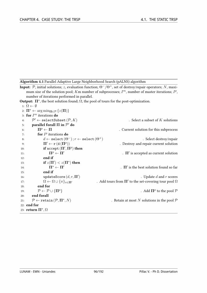
CHAPTER 4. CASE STUDY: THE TRSP 4.1. THE STATIC TRSP
Algorithm 4.1 Parallel Adaptive Large Neighborhood Search (pALNS) algorithm
Input: P , initial solutions; z, evaluation function; Θ−/Θ+, set of destroy/repair operators; N , maxi-mum size of the solution pool; Km number of subprocesses; Im, number of master iterations; Ip,number of iterations performed in parallel.
Output: Π∗, the best solution found; Ω, the pool of tours for the post-optimization.1: Ω← ∅2: Π∗ ← arg minΠ∈P z(Π)3: for Im iterations do4: P ′ ← selectSubset (P,K) . Select a subset ofK solutions5: parallel forall Π in P ′ do6: Πp ← Π . Current solution for this subprocess7: for Ip iterations do8: d← select (Θ−) ; r ← select (Θ+) . Select destroy/repair9: Π′ ← r (d (Πp)) . Destroy and repair current solution10: if accept (Π′,Πp) then11: Πp ← Π′ . Π′ is accepted as current solution12: end if13: if z(Π′) < z(Π∗) then14: Π∗ ← Π′ . Π′ is the best solution found so far15: end if16: updateScore (d, r,Π′) . Update d and r scores17: Ω← Ω ∪ ππ∈Π′ . Add tours from Π′ to the set-covering tour pool Ω18: end for19: P ← P ∪ Πp . Add Πp to the pool P20: end forall21: P ← retain (P,Π∗, N) . Retain at most N solutions in the pool P22: end for23: return Π∗,Ω
LUNAM - EMN - Uniandes 96/192 Pillac V. - Ph D. Dissertation
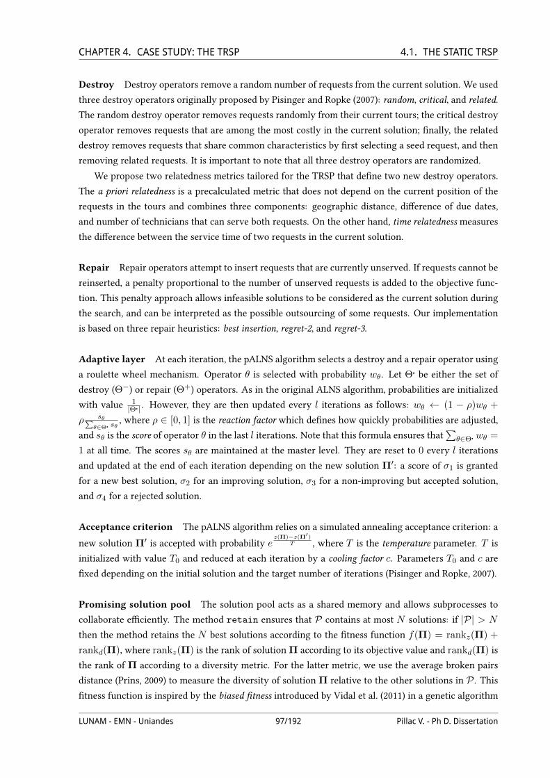
CHAPTER 4. CASE STUDY: THE TRSP 4.1. THE STATIC TRSPDestroy Destroy operators remove a random number of requests from the current solution. We used
three destroy operators originally proposed by Pisinger and Ropke (2007): random, critical, and related.
The random destroy operator removes requests randomly from their current tours; the critical destroy
operator removes requests that are among the most costly in the current solution; Vnally, the related
destroy removes requests that share common characteristics by Vrst selecting a seed request, and then
removing related requests. It is important to note that all three destroy operators are randomized.
We propose two relatedness metrics tailored for the TRSP that deVne two new destroy operators.
The a priori relatedness is a precalculated metric that does not depend on the current position of the
requests in the tours and combines three components: geographic distance, diUerence of due dates,
and number of technicians that can serve both requests. On the other hand, time relatedness measures
the diUerence between the service time of two requests in the current solution.
Repair Repair operators attempt to insert requests that are currently unserved. If requests cannot be
reinserted, a penalty proportional to the number of unserved requests is added to the objective func-
tion. This penalty approach allows infeasible solutions to be considered as the current solution during
the search, and can be interpreted as the possible outsourcing of some requests. Our implementation
is based on three repair heuristics: best insertion, regret-2, and regret-3.
Adaptive layer At each iteration, the pALNS algorithm selects a destroy and a repair operator using
a roulette wheel mechanism. Operator θ is selected with probability wθ . Let Θ be either the set of
destroy (Θ−) or repair (Θ+) operators. As in the original ALNS algorithm, probabilities are initialized
with value 1|Θ| . However, they are then updated every l iterations as follows: wθ ← (1 − ρ)wθ +
ρ sθ∑θ∈Θ sθ
, where ρ ∈ [0, 1] is the reaction factor which deVnes how quickly probabilities are adjusted,
and sθ is the score of operator θ in the last l iterations. Note that this formula ensures that∑
θ∈Θ wθ =
1 at all time. The scores sθ are maintained at the master level. They are reset to 0 every l iterations
and updated at the end of each iteration depending on the new solution Π′: a score of σ1 is granted
for a new best solution, σ2 for an improving solution, σ3 for a non-improving but accepted solution,
and σ4 for a rejected solution.
Acceptance criterion The pALNS algorithm relies on a simulated annealing acceptance criterion: a
new solution Π′ is accepted with probability ez(Π)−z(Π′)
T , where T is the temperature parameter. T is
initialized with value T0 and reduced at each iteration by a cooling factor c. Parameters T0 and c are
Vxed depending on the initial solution and the target number of iterations (Pisinger and Ropke, 2007).
Promising solution pool The solution pool acts as a shared memory and allows subprocesses to
collaborate eXciently. The method retain ensures that P contains at most N solutions: if |P| > N
then the method retains the N best solutions according to the Vtness function f(Π) = rankz(Π) +
rankd(Π), where rankz(Π) is the rank of solution Π according to its objective value and rankd(Π) is
the rank of Π according to a diversity metric. For the latter metric, we use the average broken pairs
distance (Prins, 2009) to measure the diversity of solution Π relative to the other solutions in P . ThisVtness function is inspired by the biased Vtness introduced by Vidal et al. (2011) in a genetic algorithm
LUNAM - EMN - Uniandes 97/192 Pillac V. - Ph D. Dissertation
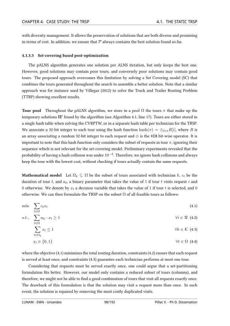
CHAPTER 4. CASE STUDY: THE TRSP 4.1. THE STATIC TRSPwith diversity management. It allows the preservation of solutions that are both diverse and promising
in terms of cost. In addition, we ensure that P always contains the best solution found so far.
4.1.3.3 Set-covering based post-optimization
The pALNS algorithm generates one solution per ALNS iteration, but only keeps the best one.
However, good solutions may contain poor tours, and conversely poor solutions may contain good
tours. The proposed approach overcomes this limitation by solving a Set Covering model (SC) that
combines the tours generated throughout the search to assemble a better solution. Note that a similar
approach was for instance used by Villegas (2012) to solve the Truck and Trailer Routing Problem
(TTRP) showing excellent results.
Tour pool Throughout the pALNS algorithm, we store in a pool Ω the tours π that make up the
temporary solutions Π′ found by the algorithm (see Algorithm 4.1, line 17). Tours are either stored in
a single hash table when solving the CVRPTW, or in a separate hash table per technician for the TRSP.
We associate a 32-bit integer to each tour using the hash function hash(π) = ⊕i∈πR[i], where R is
an array associating a random 32-bit integer to each request and ⊕ is the XOR bit-wise operator. It is
important to note that this hash function only considers the subset of requests in tour π, ignoring their
sequence which is not relevant for the set-covering model. Preliminary experiments revealed that the
probability of having a hash collision was under 10−3. Therefore, we ignore hash collisions and always
keep the tour with the lowest cost, without checking if tours actually contain the same requests.
Mathematical model Let Ωk ⊆ Ω be the subset of tours associated with technician k, ct be the
duration of tour t, and ati a binary parameter that takes the value of 1 if tour t visits request i and
0 otherwise. We denote by xt a decision variable that takes the value of 1 if tour t is selected, and 0
otherwise. We can then formulate the TRSP on the subset Ω of all feasible tours as follows:
min∑t∈Ω
ctxt (4.1)
s.t.,∑t∈Ω
ati · xt ≥ 1 ∀i ∈ R (4.2)∑t∈Ωk
xt ≤ 1 ∀k ∈ K (4.3)
xt ∈ 0, 1 ∀t ∈ Ω (4.4)
where the objective (4.1) minimizes the total routing duration, constraints (4.2) ensure that each request
is served at least once, and constraints (4.3) guarantee each technician performs at most one tour.
Considering that requests must be served exactly once, one could argue that a set-partitioning
formulation Vts better. However, our model only contains a reduced subset of tours (columns), and
therefore, we might not be able to Vnd a good combination of tours that visit all requests exactly once.
The drawback of this formulation is that the solution may visit a request more than once. In such
event, the solution is repaired by removing the most costly duplicated visits.
LUNAM - EMN - Uniandes 98/192 Pillac V. - Ph D. Dissertation

CHAPTER 4. CASE STUDY: THE TRSP 4.1. THE STATIC TRSP4.1.4 Computational results
In this section we report computational results for the proposed matheuristic. All experiments were
run using Java 7 and Gurobi 4.60 on an Ubuntu 11.10 64-bit machine, with an Intel i7 860 processor
(4 × 2.8GHz) and 6GB of RAM, using K = 8 subprocesses. The pALNS algorithm was run for 25600
iterations (Ip = 100, Im = 32) and a time limit of 30 minutes was enforced for the set-covering model.
Because the destroy operators are randomized, pALNS is a non-deterministic algorithm, therefore we
run it 10 times for each instance. The detailed parameter settings are shown in Pillac et al. (2011).
4.1.4.1 Validation on the VRPTW
The TRSP being a natural extension of the VRPTW, we validate our matheuristic on the 56 VRPTW
instances from the Solomon benchmark (Solomon, 1987). The instances contain 100 requests located
randomly (R), in clusters (C), or combining both (RC); with either a short (type 1) or long (type 2)
planning horizon. These instances are organized combining location and horizon (i.e., C1, C2, R1, R2,
RC1, and RC2), each group containing between 8 and 12 instances. For the VRPTW, we consider the
minimization of the traveled distance 1 and replace constraints (4.3) from the set covering model by∑t∈Ω xt ≤ 25 to model the 25-vehicle homogeneous Weet deVned in the Solomon (1987) instances.
Improvement Gap to BKS/Opt Best known solutions Time (s)
Group ∆pALNS ∆SC pALNS pALNS+SC #Opt. #BKS pALNS SC |Ω|
C1 37.89% 0.00% 0.00% 0.00% 9/9 - 14.6 0.4 11550C2 26.41% 0.02% 0.02% 0.00% 8/8 - 26.5 0.2 3479R1 24.28% 0.44% 0.59% 0.14% 10/12 - 13.1 27.2 27303R2 32.21% 0.25% 0.76% 0.51% 5/10 1/1 24.5 2.1 14161RC1 25.06% 1.21% 1.38% 0.15% 6/8 - 12.6 25.1 25327RC2 36.56% 0.43% 0.99% 0.55% 6/8 - 21.3 1.3 11822
All 30.20% 0.38% 0.62% 0.23% 44/55 1/1 18.6 10.1 16293
Table 4.1: Computational results for the Solomon (1987) instances (average over 10 runs).
Table 4.1 summarizes the average results for each instance group. The Vrst column deVnes the
instance group, the second column contains the relative improvement between the initial solution
and the solution returned by pALNS (∆pALNS), the third column reports the relative improvement
between the pALNS solution and the pALNS+SC solution (∆SC ). The fourth and Vfth columns contain
the average gap to the optimal or best known solution for pALNS and pALNS+SC. The sixth column
reports the number of optimal solutions found (Opt.) over the number of known optimal solutions,
while the seventh column reports the number of best known solutions (BKS) found over the number
of heuristic BKS. Columns eight and nine show the average computational times for the pALNS and
SC, and the last column reports the average size of the tour pool.
The overall average gap for pALNS+SC is just 0.23%, while Pisinger and Ropke (2007) report a
value of 0.36% using an ALNS with a larger number of destroy and repair operators 2. This illustrates
1. Note that we truncate the distances to one decimal, as it is common practice when solving the Solomon (1987) instanceswith the distance minimization as solely objective.
2. In addition, it is important to note that 7 optimal solutions were not known at the time of their study, using the samevalues the average gap for our approach is of 0.16%.
LUNAM - EMN - Uniandes 99/192 Pillac V. - Ph D. Dissertation
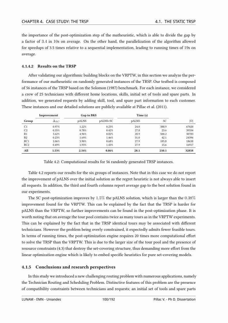
CHAPTER 4. CASE STUDY: THE TRSP 4.1. THE STATIC TRSPthe importance of the post-optimization step of the matheuristic, which is able to divide the gap by
a factor of 3.4 in 10s on average. On the other hand, the parallelization of the algorithm allowed
for speedups of 3.5 times relative to a sequential implementation, leading to running times of 19s on
average.
4.1.4.2 Results on the TRSP
After validating our algorithmic building blocks on the VRPTW, in this section we analyze the per-
formance of our matheuristic on randomly generated instances of the TRSP. Our testbed is composed
of 56 instances of the TRSP based on the Solomon (1987) benchmark. For each instance, we considered
a crew of 25 technicians with diUerent home locations, skills, initial set of tools and spare parts. In
addition, we generated requests by adding skill, tool, and spare part information to each customer.
These instances and our detailed solutions are publicly available at Pillac et al. (2011).
Improvement Gap to BKS Time (s)
Group ∆SC pALNS pALNS+SC pALNS SC |Ω|
C1 0.97% 1.22% 0.23% 24.0 388.9 67020C2 0.35% 0.78% 0.42% 27.8 23.6 39334R1 3.62% 4.96% 0.82% 28.9 500.2 30783R2 0.23% 1.69% 1.46% 31.0 42.1 24396RC1 3.06% 3.90% 0.68% 27.9 185.8 18638RC2 0.49% 1.93% 1.43% 27.9 15.6 16917
All 1.53% 2.54% 0.86% 28.1 210.1 32858
Table 4.2: Computational results for 56 randomly generated TRSP instances.
Table 4.2 reports our results for the six groups of instances. Note that in this case we do not report
the improvement of pALNS over the initial solution as the regret heuristic is not always able to insert
all requests. In addition, the third and fourth columns report average gap to the best solution found in
our experiments.
The SC post-optimization improves by 1.5% the pALNS solution, which is larger than the 0.38%
improvement found for the VRPTW. This can be explained by the fact that the TRSP is harder for
pALNS than the VRPTW, so further improvements can be found in the post-optimization phase. It is
worth noting that on average the tour pool contains twice as many tours as in the VRPTW experiments.
This can be explained by the fact that in the TRSP identical tours may be associated with diUerent
technicians. However the problem being overly constrained, it expectedly admits fewer feasible tours.
In terms of running times, the post-optimization engine requires 20 times more computational eUort
to solve the TRSP than the VRPTW. This is due to the larger size of the tour pool and the presence of
resource constraints (4.3) that destroy the set-covering structure, thus demanding more eUort from the
linear optimization engine which is likely to embed speciVc heuristics for pure set-covering models.
4.1.5 Conclusions and research perspectives
In this study we introduced a new challenging routing problemwith numerous applications, namely
the Technician Routing and Scheduling Problem. Distinctive features of this problem are the presence
of compatibility constraints between technicians and requests; an initial set of tools and spare parts
LUNAM - EMN - Uniandes 100/192 Pillac V. - Ph D. Dissertation

CHAPTER 4. CASE STUDY: THE TRSP BIBLIOGRAPHYavailable to the technicians; the possibility for technicians to visit a main depot to pick up additional
tools and spare parts; and the scheduling aspects introduced by the objective of minimizing the total
tour duration.
We proposed a parallel matheuristic, which comprises three components: a regret constructive
heuristic, a parallel adaptive large neighborhood search (pALNS), and a set-covering post-optimizer
(SC). The parallelization of the ALNS allows a speed increase by a factor of 3.4 on a quad-core com-
puter, while the post-optimization phase assembles a better solution by using tours gathered during
the search. The resulting matheuristic maintains the Wexibility of the ALNS, while improving its per-
formance and reducing the need for complex operators.
We validated and measured the performance of the proposed matheuristic on the Solomon VRPTW
benchmark, showing a negligible gap of 0.23% to the optimal and best known solutions (BKS), and
Vnding 44 of the 55 optimal solutions in under 30s. Results on randomly generated instances of the
TRSP illustrate the improvement that pALNS and SC bring over a constructive heuristic solution.
Future work will focus on the extension of the problem to a dynamic setting, in which unexpected
delays and new requests may occur. To this end, we are focusing our research eUorts on developing
fast optimization procedures able to react in real time to changes in the problem information.
Acknowledgements Financial support for this work was provided by the CPER (Contrat de Projet
Etat Region) Vallée du Libre (France); and the Centro de Estudios Interdisciplinarios Básicos y Aplica-
dos en Complejidad (CEIBA, Colombia). This support is gratefully acknowledged. The authors would
also like to thank Olivier Péton from the Ecole des Mines de Nantes and the anonymous reviewers for
their insightful comments and suggestions.
BibliographyAkjiratikarl, C., Yenradee, P., and Drake, P. R. (2007). Pso-based algorithm for home care worker scheduling in
the uk. Computers & Industrial Engineering, 53(4):559 – 583, doi:10.1016/j.cie.2007.06.002.
Bertels, S. and Fahle, T. (2006). A hybrid setup for a hybrid scenario: combining heuristics for the home healthcare problem. Computers & Operations Research, 33(10):2866 – 2890, doi:10.1016/j.cor.2005.01.015.
Bredström, D. and Rönnqvist, M. (2008). Combined vehicle routing and scheduling with temporalprecedence and synchronization constraints. European Journal of Operational Research, 191(1):19–31,doi:10.1016/j.ejor.2007.07.033.
Cordeau, J.-F., Laporte, G., Pasin, F., and Ropke, S. (2010). Scheduling technicians and tasks in a telecommunica-tions company. Journal of Scheduling, 13(4):393–409, doi:10.1007/s10951-010-0188-7.
Eveborn, P., Flisberg, P., and Ronnqvist, M. (2006). LAPS CARE - an operational system for staU planning ofhome care. European Journal of Operational Research, 171(3):962–976, doi:10.1016/j.ejor.2005.01.011.
Hashimoto, H., Boussier, S., Vasquez, M., and Wilbaut, C. (2011). A GRASP-based approach for techni-cians and interventions scheduling for telecommunications. Annals of Operations Research, 183:143–161,doi:10.1007/s10479-009-0545-0.
Kovacs, A., Parragh, S., Doerner, K., and Hartl, R. (2011). Adaptive large neighborhood search for service techni-cian routing and scheduling problems. Journal of Scheduling, In press:1–22, doi:10.1007/s10951-011-0246-9.
Parragh, S. N. (2010). Solving a real-world service technician routing and scheduling problem. In Proceedings ofthe Seventh Triennial Symposium on Transportation Analysis (TRISTAN VII).
LUNAM - EMN - Uniandes 101/192 Pillac V. - Ph D. Dissertation
CHAPTER 4. CASE STUDY: THE TRSP BIBLIOGRAPHYPillac, V., Guéret, C., and Medglia, A. L. (2011). A parallel matheuristic for the technician routing and scheduling
problem: supplementary material (online).
Pisinger, D. and Ropke, S. (2007). A general heuristic for vehicle routing problems. Computers & OperationsResearch, 34(8):2403–2435, doi:10.1016/j.cor.2005.09.012.
Potvin, J.-Y. and Rousseau, J.-M. (1993). A parallel route building algorithm for the vehicle routing and schedulingproblem with time windows. European Journal of Operational Research, 66(3):331 – 340, doi:10.1016/0377-2217(93)90221-8.
Prins, C. (2009). Two memetic algorithms for heterogeneous Weet vehicle routing problems. Engineering Appli-cations of ArtiVcial Intelligence, 22(6):916–928, doi:10.1016/j.engappai.2008.10.006.
Savelsbergh, M. (1992). The vehicle routing problem with time windows: minimizing route duration. INFORMS,4(2):146–154, doi:10.1287/ijoc.4.2.146.
Shaw, P. (1998). Using constraint programming and local search methods to solve vehicle routing problems. InPrinciples and Practice of Constraint Programming – CP98, volume 1520 of Lecture Notes in Computer Science,pages 417–431. Springer Berlin / Heidelberg.
Solomon, M. M. (1987). Algorithms for the vehicle-routing and scheduling problems with time window con-straints. Operations Research, 35(2):254–265.
Tang, H., Miller-Hooks, E., and Tomastik, R. (2007). Scheduling technicians for planned maintenance of ge-ographically distributed equipment. Transportation Research Part E: Logistics and Transportation Review,43(5):591–609, doi:10.1016/j.tre.2006.03.004.
Tsang, E. and Voudouris, C. (1997). Fast local search and guided local search and their application to britishtelecom’s workforce scheduling problem. Operations Research Letters, 20(3):119 – 127, doi:10.1016/S0167-6377(96)00042-9.
Vidal, T., Crainic, T., Gendreau, M., and Prins, C. (2011). A hybrid genetic algorithm with adaptive diversitymanagement for a large class of vehicle routing problems with time windows. Technical Report CIRRELT-2011-61, CIRRELT.
Villegas, J. G. (2012). Vehicle routing problems with trailers. 4OR: A Quarterly Journal of Operations Research,doi:10.1007/s10288-011-0186-4.
Xu, J. and Chiu, S. (2001). EUective heuristic procedures for a Veld technician scheduling problem. Journal ofHeuristics, 7(5):495–509.
LUNAM - EMN - Uniandes 102/192 Pillac V. - Ph D. Dissertation

CHAPTER 4. CASE STUDY: THE TRSP 4.2. THE DYNAMIC TRSP4.2 The dynamic TRSP
The technical report presented in this section introduces the dynamic TRSP and proposes two
optimization approaches to tackle it. The Vrst is based on the fast reoptimization framework presented
in Chapter 2, and the second is an adaptation of the jMSA framework described in Chapter 3.
The full reference of the paper presented in this section is:
– Pillac, V., Guéret, C., and Medaglia, A. L. (2011)
On the dynamic technician routing and scheduling problem
Technical report 12/5/AUTO.
Preliminary results were presented in two international conferences:
– Pillac, V., Guéret, C., and Medaglia, A. L. (2012)
A Multiple Plan Approach for the Dynamic Technician Routing and Scheduling Problem
In 25th European Conference on Operational Research (EURO 2012), Vilnius, Lithuania.
– Pillac, V., Guéret, C., and Medaglia, A. L. (2012)
On the dynamic technician routing and scheduling problem
In Proceedings of the 5th International Workshop on Freight Transportation and Logistics
(ODYSSEUS 2012), Mykonos, Greece.
LUNAM - EMN - Uniandes 103/192 Pillac V. - Ph D. Dissertation

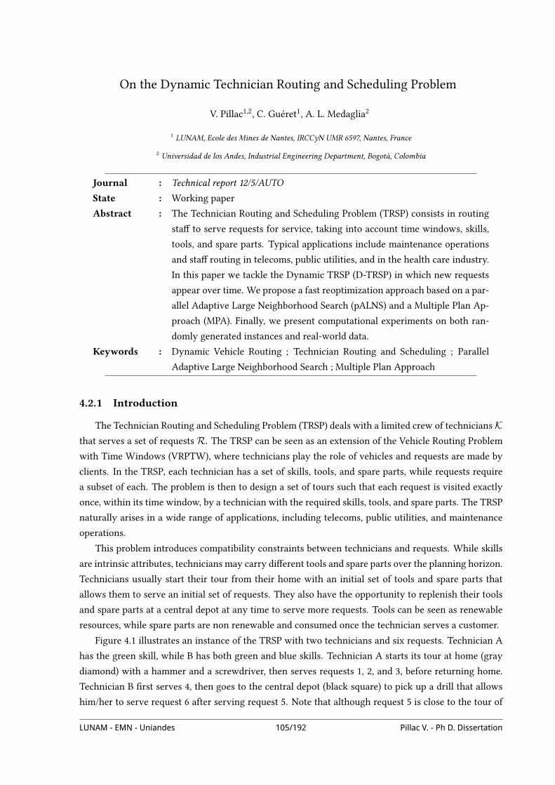
On the Dynamic Technician Routing and Scheduling Problem
V. Pillac1,2, C. Guéret1, A. L. Medaglia2
1 LUNAM, Ecole des Mines de Nantes, IRCCyN UMR 6597, Nantes, France
2 Universidad de los Andes, Industrial Engineering Department, Bogotá, Colombia
Journal : Technical report 12/5/AUTO
State : Working paper
Abstract : The Technician Routing and Scheduling Problem (TRSP) consists in routing
staU to serve requests for service, taking into account time windows, skills,
tools, and spare parts. Typical applications include maintenance operations
and staU routing in telecoms, public utilities, and in the health care industry.
In this paper we tackle the Dynamic TRSP (D-TRSP) in which new requests
appear over time. We propose a fast reoptimization approach based on a par-
allel Adaptive Large Neighborhood Search (pALNS) and a Multiple Plan Ap-
proach (MPA). Finally, we present computational experiments on both ran-
domly generated instances and real-world data.
Keywords : Dynamic Vehicle Routing ; Technician Routing and Scheduling ; Parallel
Adaptive Large Neighborhood Search ; Multiple Plan Approach
4.2.1 Introduction
The Technician Routing and Scheduling Problem (TRSP) deals with a limited crew of techniciansKthat serves a set of requests R. The TRSP can be seen as an extension of the Vehicle Routing Problem
with Time Windows (VRPTW), where technicians play the role of vehicles and requests are made by
clients. In the TRSP, each technician has a set of skills, tools, and spare parts, while requests require
a subset of each. The problem is then to design a set of tours such that each request is visited exactly
once, within its time window, by a technician with the required skills, tools, and spare parts. The TRSP
naturally arises in a wide range of applications, including telecoms, public utilities, and maintenance
operations.
This problem introduces compatibility constraints between technicians and requests. While skills
are intrinsic attributes, technicians may carry diUerent tools and spare parts over the planning horizon.
Technicians usually start their tour from their home with an initial set of tools and spare parts that
allows them to serve an initial set of requests. They also have the opportunity to replenish their tools
and spare parts at a central depot at any time to serve more requests. Tools can be seen as renewable
resources, while spare parts are non renewable and consumed once the technician serves a customer.
Figure 4.1 illustrates an instance of the TRSP with two technicians and six requests. Technician A
has the green skill, while B has both green and blue skills. Technician A starts its tour at home (gray
diamond) with a hammer and a screwdriver, then serves requests 1, 2, and 3, before returning home.
Technician B Vrst serves 4, then goes to the central depot (black square) to pick up a drill that allows
him/her to serve request 6 after serving request 5. Note that although request 5 is close to the tour of
LUNAM - EMN - Uniandes 105/192 Pillac V. - Ph D. Dissertation

CHAPTER 4. CASE STUDY: THE TRSP 4.2. THE DYNAMIC TRSPtechnician A, only technician B can serve it due to skill constraints.
Skills
Tools
A
B
1
6
3
5
2Pickup
4
Main depot
Home
Home
Skills
Tools
Figure 4.1: Example of a technician routing and scheduling problem with two technicians, three tools,and two skills
The static deVnition of the TRSP was introduced by the authors in Pillac et al. (2012b). In this work,
we tackle a dynamic variant of the problem, namely the D-TRSP, in which new requests appear while
the technicians are executing their routes. In this context, two types of decisions have to be taken in
real time. First, whenever a technician Vnishes serving a request, it must be decided what will be the
next request to visit. Second, whenever a request appears, the algorithm must decide whether it is
possible or desirable to accept it or not. If not the request is said to be rejected, it leads to a cost penalty
corresponding to the outsourcing/postponing of the request.
Despite its numerous practical applications and its challenging features, static technician routing
and scheduling problems have received limited attention until recently, and to the best of our knowl-
edge, no study simultaneously considers skills, tools, and spare parts. For instance, Xu and Chiu (2001)
studied the Field Technician Scheduling Problem (FTSP) seen as a variant of the VRPTW, in which
the objective is to maximize the number of requests served while accounting for skill constraints,
request priorities, multiple depots, and overtime. The authors describe a mixed integer formulation
and develop three heuristics including a GRASP algorithm. Similarly, Weigel and Cao (1999) present
a software solution developed for Sears, a US retailer that serves its customers with home delivery
and on-site technical assistance. The proposed solution works by Vrst assigning technicians to re-
quests, and then optimizing technician routes individually. Tsang and Voudouris (1997) studied the
technician workforce scheduling problem faced by British Telecom. Their study does not consider
skill constraints, but uses a proVciency factor that reduces the service time depending on the techni-
cian experience. They propose a Fast Local Search and a Guided Local Search to solve this problem.
Borenstein et al. (2010) extended this problem accounting for dynamic requests and skill compatibility
constraints. They cluster the requests using a k-mean algorithm followed by a heuristic that assigns
technicians to areas. Finally, they propose a rule-based system that assigns and sequences the requests.
They conclude their study by assessing the impact of soft clustering and show that it can increase sys-
LUNAM - EMN - Uniandes 106/192 Pillac V. - Ph D. Dissertation

CHAPTER 4. CASE STUDY: THE TRSP 4.2. THE DYNAMIC TRSPtem performance under certain assumptions.
Maintenance operations planning is a problem closely related to the TRSP. Blakeley et al. (2003)
present the optimization of periodic maintenance operations for Schindler Elevator Corporation in
North America, a company that manufactures, installs, and maintains elevators and escalators. The
problem faced by this company consists in designing a set of routes for technicians to perform periodic
maintenance and repairs taking into account travel times, working regulations, and skill constraints.
A similar application was studied by Tang et al. (2007) who formulate the problem as a multi-period
maximum collection problem in which time-dependent rewards are granted for the completion of a
request. This approach allows the modeling of soft constraints such as the desirability of performing
a task in a given day (job-to-time penalties). The authors propose a Tabu Search (TS) algorithm that
yields near-optimal solutions on real instances in reasonable time.
In 2007 the French Operations Research Society (ROADEF) organized a challenge based on a prob-
lem submitted by France Telecom. The problem consists in Vnding a schedule for technicians to ex-
ecute a set of tasks on a multiple-day horizon. Each task requires one or more skills with diUerent
minimum proVciency levels, while technicians can have multiple skills with a given proVciency. An
important aspect is the creation of teams that work together during one day, combining the skills of
their members, and the possibility to outsource the execution of a task. However, this problem ig-
nores the routing aspects. Cordeau et al. (2010) proposed a mathematical model and an Adaptive Large
Neighborhood Search (ALNS), while Hashimoto et al. (2011) proposed a Greedy Randomized Adaptive
Search procedure (GRASP) approach to tackle this problem.
Work regulation is an important aspect of technician routing and scheduling. Tricoire (2006)
presents a technician routing problem faced by Veolia, a water distribution and treatment company. In
this application, technicians have the skills to perform all requests that are divided in two categories:
user requested interventions and company scheduled visits. As new requests appear on a daily basis,
the routing of technicians is performed on a rolling horizon, taking into account work regulations and
customer service standards. The main contributions are a column generation approach and a memetic
algorithm (Bostel et al., 2008). Their approaches take advantage of partial solutions from previous
plans in the rolling horizon framework to reduce computational times.
A number of technological advances have led to a renewed interest in dynamic vehicle routing
problems, leading to the development of new optimization approaches. Pillac et al. (2011a) classify
dynamic routing problems in two categories: deterministic and stochastic. In both cases the informa-
tion available to the stackholder changes over time. In stochastic setting, data is available on the dy-
namically revealed information in the form of known probability distributions, while in deterministic
problems, changes are simply unpredictable. The present work falls in the dynamic and deterministic
category, for which approaches are based either on periodic reoptimization or continuous reoptimization.
Periodic reoptimization approaches start at the beginning of the day by producing an initial set of
routes that are communicated to the vehicles. As the available information is updated along the day,
or at given intervals of time, an optimization is performed using the currently available information to
update the routing. Such approaches can be based on algorithms developed for static problems and are
therefore relatively easy to implement, however, they may introduce delays between the update of the
information and the routing plan. Such approaches include the Ant Colony Systems (ACS) proposed by
LUNAM - EMN - Uniandes 107/192 Pillac V. - Ph D. Dissertation
CHAPTER 4. CASE STUDY: THE TRSP 4.2. THE DYNAMIC TRSPMontemanni et al. (2005) to solve the Dynamic VRP (D-VRP). A novel feature of their approach is the
use of the pheromone trace to transfer characteristics of a good solution between reoptimizations. ACS
was also used by Gambardella et al. (2003) and Rizzoli et al. (2007). Other heuristic approaches, such as
Tabu Search (TS), were also used to tackle the Dynamic Pickup and Delivery Problem (D-PDP) (Barcelo
et al., 2007; Chang et al., 2003) and the Dynamic Dial-a-Ride Problem (D-DARP) (Attanasio et al., 2004;
Beaudry et al., 2010).
Continuous reoptimization approaches run throughout the day and are generally based on an adap-
tive memory (Taillard et al., 2001) that stores alternative solutions. The adaptive memory is then used
to react to changes in the available information, thus avoiding a complete reoptimization of the prob-
lem. Gendreau et al. (1999) developed a parallel TS with adaptive memory to tackle a Dynamic VRPTW
(D-VRPTW), that was later applied to the D-VRP (Ichoua et al., 2000, 2003). Bent and Van Hentenryck
(2004) generalized this framework and introduced the Multiple Plan Approach (MPA) to tackle the D-
VRPTW. Following a diUerent approach, Benyahia and Potvin (1998) studied the Dynamic Pickup and
Delivery Problem (D-PDP) and proposed a Genetic Algorithm (GA) that models the decision process
of a human dispatcher. More recently, GAs were also used for the same problem (Cheung et al., 2008;
Haghani and Jung, 2005) and for the D-VRP (Van Hemert and Poutré, 2004).
To the best of our knowledge, no work considers simultaneously skills, tools, spare parts, and dy-
namically arriving requests, four important components of technician routing and scheduling. The
present work addresses this aspect and proposes two optimization approaches for the dynamic ver-
sion of the problem, noted D-TRSP, where new requests arrive during the execution of the routes.
Section 4.2.2 introduces a fast reoptimization approach based on a parallel adaptive large neighbor-
hood search; then Section 4.2.3 introduces a continuous reoptimization algorithm based on a multiple
plan approach; Vnally, Section 4.2.4 presents the computational results and Section 4.2.5 concludes this
paper and draws directions for future research.
4.2.2 A fast reoptimization approach
The proposed approach is based on the parallel Adaptive Large Neighborhood Search (pALNS)
reoptimization algorithm introduced by Pillac et al. (2012a), which is used to Vrst compute an initial
solution, and then to reoptimize the solution whenever a new customer request arrives. The pALNS
extends the Adaptive Large Neighborhood Search (ALNS) algorithm (Pisinger and Ropke, 2007), which
in turn is an extension of the Large Neighborhood Search (LNS) algorithm (Pisinger and Ropke, 2010;
Shaw, 1998). LNS works by successively destroying (removing customers) and repairing (inserting
customers back) a current solution, using destroy and repair operators. ALNS adds a layer that ran-
domly selects operators depending on their past performance, allowing a self-adaptive version of the
algorithm to the instance at hand.
Algorithm 4.2 presents the outline of pALNS as introduced in Pillac et al. (2012a). The algorithm
maintains a pool P ofN promising solutions that are optimized inK subprocesses (note thatN ≥ K).
For each master iteration, a subset of K promising solutions is selected randomly (line 3) and dis-
tributed among independent subprocesses. Then for Ip iterations, each subprocess selects destroy and
repair operators with a roulette wheel that adaptively reWects their past performance (line 7). The
LUNAM - EMN - Uniandes 108/192 Pillac V. - Ph D. Dissertation

CHAPTER 4. CASE STUDY: THE TRSP 4.2. THE DYNAMIC TRSPresulting new solution is either accepted as the subprocess current solution or rejected according to
a simulated annealing criterion (line 9), the weights of the destroy and repair operators are updated
depending on their performance (line 15). The Vnal current solution is added to the pool of promising
solutions (line 17) and a Vltering procedure ensures that the pool contains at most N solutions, in-
cluding the best solution found so far (line 19). The algorithm stops after Im master iterations, which
corresponds to I = Im × Ip ALNS iterations.
Algorithm 4.2 Parallel Adaptive Large Neighborhood Search (pALNS) algorithm
Input: P , initial solutions; z, evaluation function; Θ−/Θ+, set of destroy/repair operators; N , maxi-mum size of the solution pool; Km number of subprocesses; Im, number of master iterations; Ip,number of iterations performed in parallel.
Output: Π∗, the best solution found1: Π∗ ← arg minΠ∈P z(Π)2: for Im iterations do3: P ′ ← selectSubset (P,K) . Select a subset ofK solutions4: parallel forall Π in P ′ do5: Πp ← Π . Current solution for this subprocess6: for Ip iterations do7: d← select (Θ−) ; r ← select (Θ+) . Select destroy/repair8: Π′ ← r (d (Πp)) . Destroy and repair current solution9: if accept (Π′,Πp) then10: Πp ← Π′ . Π′ is accepted as current solution11: end if12: if z(Π′) < z(Π∗) then13: Π∗ ← Π′ . Π′ is the best solution found so far14: end if15: updateScore (d, r,Π′) . Update d and r scores16: end for17: P ← P ∪ Πp . Add Πp to the pool P18: end forall19: P ← retain (P,Π∗, N) . Retain at most N solutions in the pool P20: end for21: return Π∗
the pALNS algorithm uses three destroy operators (random, related, and critical), and three repair
operators (regret-1, regret-2, regret-3). The promising solution pool P maintains the N best solutions
according to a Vtness function that considers both the cost of the solution and its diversity relative to
the other solutions in the pool. The interested reader is referred to the work by Pillac et al. (2012a) and
Pillac et al. (2012b) for more details on the approach.
To tackle the D-TRSP, we modiVed the related destroy operator, which attempts to remove a subset
of requests that share some characteristics. We deVne the relatedness rij of requests i and j as a
measure of how related two requests are (the lower the rij , the more related i and j). The procedure
starts by randomly removing a seed request i (U = i), then it iteratively selects a request i ∈ U ,and removes the most related request j∗ = arg minj∈R′ rij from the set of unserved requests R′.In practice the selection process is randomized and the byp|R′|c-th most related request is selected,
where y is a random number in [0, 1) and p ≥ 1 is a parameter that controls the level of randomness
LUNAM - EMN - Uniandes 109/192 Pillac V. - Ph D. Dissertation
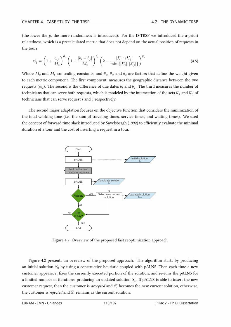
CHAPTER 4. CASE STUDY: THE TRSP 4.2. THE DYNAMIC TRSP(the lower the p, the more randomness is introduced). For the D-TRSP we introduced the a-priori
relatedness, which is a precalculated metric that does not depend on the actual position of requests in
the tours:
rsij =
(1 +
cijMc
)θc (1 +|bi − bj |Mt
)θt (2− |Ki ∩ Kj |
min |Ki|, |Kj |
)θs(4.5)
Where Mc and Mt are scaling constants, and θc, θt, and θs are factors that deVne the weight given
to each metric component. The Vrst component, measures the geographic distance between the two
requests (cij). The second is the diUerence of due dates bi and bj . The third measures the number of
technicians that can serve both requests, which is modeled by the intersection of the sets Ki and Kj oftechnicians that can serve request i and j respectively.
The second major adaptation focuses on the objective function that considers the minimization of
the total working time (i.e., the sum of traveling times, service times, and waiting times). We used
the concept of forward time slack introduced by Savelsbergh (1992) to eXciently evaluate the minimal
duration of a tour and the cost of inserting a request in a tour.
Start
pALNS
End of day?
NO
YES
pALNS
Updated solution St+1
End
NO
Wait until a new customer appears
Initial solution S0
Accept? Select new currentsolution
YES
Candidate solutionSt'
Figure 4.2: Overview of the proposed fast reoptimization approach
Figure 4.2 presents an overview of the proposed approach. The algorithm starts by producing
an initial solution S0 by using a constructive heuristic coupled with pALNS. Then each time a new
customer appears, it Vxes the currently executed portion of the solution, and re-runs the pALNS for
a limited number of iterations, producing an updated solution S′t. If pALNS is able to insert the new
customer request, then the customer is accepted and S′t becomes the new current solution, otherwise,
the customer is rejected and St remains as the current solution.
LUNAM - EMN - Uniandes 110/192 Pillac V. - Ph D. Dissertation

CHAPTER 4. CASE STUDY: THE TRSP 4.2. THE DYNAMIC TRSP4.2.3 A Multiple Plan Approach
The second proposed approach for the D-TRSP is based on the Multiple Plan Approach (MPA)
introduced by Bent and Van Hentenryck (2004) to tackle the D-VRPTW. MPA is a generalization of the
tabu search with adaptive memory proposed by Gendreau et al. (1999). The general idea is to populate
and maintain a solution pool (the routing plans) that are used to generate a distinguished solution.
Whenever a new request arrives, a procedure is called to check whether it can be served or not; if it can
be served, then the request is inserted in each plan of the solution pool and incompatible solutions are
discarded. Pool updates are performed periodically or whenever a vehicle Vnishes serving a customer.
This pool-update phase is crucial and ensures that all solutions are coherent with the current state of
vehicles and customers. The pool can be seen as an adaptive memory that maintains a set of alternative
solutions.
The present work is based on the event-driven optimization framework for dynamic vehicle routing
proposed by the authors, namely jMSA (Pillac et al., 2011b). By design, jMSA is a Wexible, parallel, and
event-driven Java implementation of the Multiple Scenario Approach (MSA) (Van Hentenryck and
Bent, 2006), which is an extension of MPA for dynamic and stochastic routing problems. The proposed
framework is designed to facilitate and accelerate the development and deployment of MSA-based
algorithms embeddable in decision support systems.
Kernel
Problem layer
Events Handlers
MPAprocedure Event
queueHandlermanager
Callback
Components Plan
Planpool
Plan generator
Plan optimizer
Plan updater
…
Figure 4.3: Design overview of the jMSA framework
Figure 4.3 outlines the main aspects of the jMSA framework: the kernel contains the components
that deVne the event-driven behavior, and a generic deVnition of the problem layer components. To
adapt the framework for a speciVc problem, the user needs only to implement a subset of components,
mainly to generate, optimize, and update plans. The following paragraphs give more details on how
jMSA was adapted to tackle the D-TRSP.
Figure 4.4 presents a conceptual overview of the MPA procedure as implemented in the jMSA
framework. jMSA starts two subprocesses: a main loop and an event loop. The main loop is responsible
for continuously generating and optimizing a set of alternative solutions (the routing plans) stored
in the plan pool. This main loop maximizes the utilization of the computational resources when the
LUNAM - EMN - Uniandes 111/192 Pillac V. - Ph D. Dissertation

CHAPTER 4. CASE STUDY: THE TRSP 4.2. THE DYNAMIC TRSP
Event loopMain loop
Start
Generateplans
End of day?
NO
YES
Optimizeplans
End
Wait until next event
Planpool
End of day?
YES
Make decision
End
Update pool
NO
Routing decision
Figure 4.4: Overview of the multiple plan approach implemented with jMSA
system is idle, i.e., when no decision is required. On the other hand, the event loop reacts to events
from the environment, which can be of two types: a) a customer calls in and requests a service; b)
a technician Vnishes serving a request and becomes idle. In the Vrst case, the algorithm looks for a
feasible insertion of the new request in all the solutions in the pool. If at least a given fraction of the
solutions can accommodate the request, then it is accepted, otherwise it is rejected. In the second case,
the algorithm selects a solution from the pool and assigns a request to all idle technicians. The event
loop is also responsible for updating the pool and ensuring that all plans are coherent with the current
state of the environment.
4.2.3.1 Plan generation
The goal of the plan pool is to maintain a set of diverse solutions for the current routing problem
that could be used later to cope with the arrival of new requests. It is therefore necessary to have a
randomized constructive heuristic that will produce a set of solutions that are both diverse and of good
quality.
Our implementation is based on a randomized regret-3 heuristic (Potvin and Rousseau, 1993) which
iteratively inserts requests at their best position. More formally let U be the set of requests that are
currently not visited in the solution and let ∆zki be the cost of insertion of request i ∈ U in its k-th
best route. The regret-q value rqi associated with request i is a measure of how desirable it is to insert i
in the current iteration assuming that the best insertion will no longer be feasible in the next iteration.
It is deVned as:
rqi =
q∑k=2
(∆zki −∆z1
i
)(4.6)
The randomized regret-3 algorithm iteratively selects the next request to insert using a roulette wheel
LUNAM - EMN - Uniandes 112/192 Pillac V. - Ph D. Dissertation

CHAPTER 4. CASE STUDY: THE TRSP 4.2. THE DYNAMIC TRSPin which each request is given a probability pi:
pi =r3i∑
j∈U r3j
(4.7)
4.2.3.2 Optimization procedure
The optimization procedure continuously optimizes the pool of solutions. The fact that a solution
might go through the optimization process more than once requires an algorithm able to escape from
local optima to further improve a solution. Therefore, we implemente an Adaptive Large Neighborhood
Search (ALNS) similar to the pALNS presented in Section 4.2.2. Note that the choice of having a
sequential optimization algorithm is motivated by the fact that jMSA will optimize various plans in
parallel.
Algorithm 4.3 outlines the ALNS algorithm. ALNS starts with an initial solution Π. Then for I
iterations, the algorithm selects destroy and repair operators (line 4) with a roulette wheel that reWects
their past performance. The destroy operator removes a subset of requests from the current solution
that are then reinserted by the repair operator (line 5). The resulting new solution is accepted as
current solution according to a simulated annealing criterion (line 6). At the end of each iteration,
the scores of the destroy and repair operators are updated depending on the solution they generated
(line 12).
Algorithm 4.3 Adaptive Large Neighborhood Search (ALNS) algorithm
Input: Π0 initial solution, z evaluation function, Θ−/Θ+ set of destroy/repair operators, I numberof iterations
Output: Π∗ the best solution found1: Π∗ ← Π0 . Initialize best solution2: Π← Π0 . Initialize current solution3: for I iterations do4: d← select (Θ−) ; r ← select (Θ+) . Select destroy/repair5: Π′ ← r (d (Π)) . Generate a neighbor6: if accept (Π′,Π) then . Π′ is accepted as current solution7: Π← Π′ . Update current solution8: end if9: if z(Π′) < z(Π∗) then . An improvement has been found10: Π∗ ← Π′ . Update best solution11: end if12: updateScore (d, r,Π′) . Update scores13: end for14: return Π∗
4.2.3.3 Interactions with the decision maker
The decision maker interacts with MPA by raising events. In the context of the D-TRSP, there are
two major events: the arrival of a new request and the end-of-service of a request.
LUNAM - EMN - Uniandes 113/192 Pillac V. - Ph D. Dissertation

CHAPTER 4. CASE STUDY: THE TRSP 4.2. THE DYNAMIC TRSPArrival of new requests Whenever a new request appears, a procedure attempts to insert it in
all the plans in the pool. The procedure starts by trying to insert the request directly, if it fails, it
removes a fraction of the requests and uses regret-3 to attempt to reinsert all requests. If at least a
given fraction of the plans can accommodate the new request then it is accepted and the plans are
updated accordingly, otherwise the request is marked as rejected.
Real-time routing decisions When a technician Vnishes serving a request and becomes idle, a de-
cision needs to be taken on what will be his/her next assignment. To this end we use the consensus
algorithm (Van Hentenryck and Bent, 2006) which aggregates the information contained in the plans
from the pool to select a distinguished solution and assign requests to idle technicians. The intuition
behind consensus is to assign to each technician the requests that appear Vrst with the highest fre-
quency across plans. As multiple technicians are involved, the consensus algorithm selects a solution
from the pool that maximizes the consensus across all technicians. Algorithm 4.4 presents the details
of the algorithm. Consensus starts by counting the number of times each request appears Vrst in a
tour across all solutions from the pool (lines 1 to 6). Then the algorithm evaluates each solution by
summing the evaluations of the Vrst request of each of its tours (line 11). Finally, the solution Π∗
with the highest evaluation is returned, and the Vrst unserved request of each tour in Π∗ is the next
assignment of the corresponding technician.
Algorithm 4.4 The consensus algorithmInput: P a pool of alternative solutionsOutput: Π∗ a distinguished solution1: e← [0]i∈R . Initialize the evaluation of all requests2: for all Π ∈ P do . For each solution in the pool3: for all π ∈ Π do . For each tour in the solution4: e[π0]← e[π0] + 1 . Increment the evaluation of the Vrst unserved request π0
5: end for6: end for7: s∗ ← 08: for all Π ∈ P do9: s← 0 . Initialize the evaluation of this scenario10: for all π ∈ Π do11: s← s+ e[π0] . Update the evaluation of this scenario12: end for13: if s > s∗ then14: Π∗ ← Π15: end if16: end for17: return Π∗
Waiting strategy It is important to note that the immediate commitment of idle technicians to
requests may lead to diXculties when new requests appear. Figure 4.5 illustrates this with a single
technician. Suppose that at time t a technician is assigned to a request i, if the technician is committed
immediately to i, it will travel to i then wait at its destination until the start of the time window (black
LUNAM - EMN - Uniandes 114/192 Pillac V. - Ph D. Dissertation

CHAPTER 4. CASE STUDY: THE TRSP 4.2. THE DYNAMIC TRSPbrackets). On the other hand, if a waiting strategy is used, the technician will remain idle until the
latest moment such that it will not wait at i. Assume now that at time t+1 a new request j appears, in
the Vrst case j cannot be served as the technician is already waiting at i (the hashed section is already
executed), while in the second case it can be inserted right before i.
i
i
i
ij
Immediatecommitment
Waitingstrategy
t t+1
travel wait serve
idle travel serve
executed
Figure 4.5: Advantage of a waiting strategy.
The proposed waiting strategy is implemented as follows: Vrst, the procedure evaluates the latest
departure time so that the technician will not have to wait at its next request. If this departure time is
within a given range, then it is assumed there is not enough time to change the technician’s route and
the technician is committed to the next request. Otherwise, the technician remains in an idle state for
a given time, after what a new decision is taken, leaving time for further changes in assignments.
4.2.4 Preliminary results
We tested the pALNS and MPA approaches on a set of 56 randomly generated instances based on
the Solomon (1987) testbed. The instances contain 100 requests located randomly (R), in clusters (C),
or combining both (RC); while the planning horizon is either short (type 1) or long (type 2). These
instances are organized combining location and horizon (i.e., C1, C2, R1, R2, RC1, and RC2). We
considered 5 skills, 5 tools, and 5 types of spare parts. For each request, we selected 1 skill, and
between 0 and 2 tools and spare part types. Each of the 25 technicians has between 2 and 4 skills, and
an initial set of 0 to 5 tools, and 2 to 5 spare parts. In addition, we generated release dates for either 10,
30, 50, 70, or 90 requests, leading to a complete testbed of 280 dynamic instances.
We compare the two proposed approaches with a regret-3 heuristic. This simple approach starts
with the same initial solution as pALNS. Each time a new request appears, it attempts to insert it
in the current solution using a regret heuristic, rejecting it if it cannot be inserted. The parameter
setting for the pALNS reoptimization approach is identical to the one presented in Pillac et al. (2012a),
we allowed for 25,000 iterations for the calculation of the initial solution, and 5,000 for subsequent
reoptimizations. The maximum pool size for MPA was set to 50 plans, while the ALNS algorithms used
the same parameters as in Pillac et al. (2012a), with a maximum of 5,000 iterations per optimization.
The same simulation procedure was used to test the three approaches. First, the simulator allows
them time to either design an initial solution (pALNS and regret-3) or initialize the pool of plans
(MPA). Then the procedure simulates the routing of the technicians using an average traveling speed
and taking into account waiting times. Whenever a technician becomes idle, the simulator uses the
LUNAM - EMN - Uniandes 115/192 Pillac V. - Ph D. Dissertation

CHAPTER 4. CASE STUDY: THE TRSP 4.2. THE DYNAMIC TRSPcurrent solution (pALNS and regret-3) or distinguished plan (MPA) to select the next assignment for
this technician. The simulator handles the new requests and depending on the approach response it
marks them as accepted or rejected. Finally, it Vnds an a-posteriori solution to the problem deVned by
all the accepted requests using pALNS with 50,000 iterations.
4.2.4.1 Minimizing the total working time
The static TRSP problem (Pillac et al., 2012b) considers the minimization of the total working time.
In a dynamic setting, this objective leads to the premature ending of tours: technicians are sent home
as soon as possible to reduce the duration of their tour, ignoring the fact that additional requests may
appear in the future. To prevent this behavior we deVne a cutoU policy that ensures for an instance I
that technicians will no be sent back to their home until time tc(I). Considering that each instance
have a diUerent horizon [0, T (I)], we deVne the relative cutoU α(G) for instance group G. The value
of α(G) is deVned such that all requests of instance I ∈ G will be known before α(G)T (I) with a
certain probability. In our experiments, α(G) corresponds to the 90-percentile of the distribution ofrdImaxT (I)
I∈G
where rdImax is the last release date for instance I3.
A direct consequence of this policy is that the minimal tour duration for instance I is either 0 (if the
technician is not used), or α(G)T (I). Therefore the total duration at the end of the day is signiVcantly
longer than the one found when solving the static problem.
pALNS MPA regret-3
δ Gap (%) R Gap (%) R Gap (%) R
10 65.7 0.0 152.8 1.5 59.9 0.430 79.5 0.1 160.1 3.2 84.6 0.650 93.0 0.1 150.6 4.6 100.4 1.070 100.3 0.2 153.9 6.3 113.8 1.490 102.8 0.4 154.0 6.0 122.3 1.8
Avg. 88.3 0.2 154.3 4.4 96.2 1.0
Table 4.3: Average gap to a-posteriori solution and number of rejected requests for the D-TRSP in-stances minimizing the total duration.
Table 4.3 reports the results for the 56 instances and 5 degrees of dynamism when minimizing
the total duration. The Vrst column contains the degree of dynamism (δ) deVned as the number of
dynamic requests. The second and third columns report the average gap to an a-posteriori solution 4
and the average number of rejected requests (R) for the pALNS. The fourth and Vfth columns contain
these statistics for the MPA, and the seventh and eighth columns for the regret-3 heuristic. Note that
running times for pALNS are of 12s on average for the calculation of the initial solution and 2.8s for
subsequent reoptimizations, while decision times are negligible for both MPA and regret-3.
3. With this deVnition: αC1 = 0.380, αC2 = 0.509, αR1 = 0.357, αR2 = 0.419, αRC1 = 0.321, αRC2 = 0.400
4. The gap for instance I is deVned as the ratio z(I)−z(I)z(I)
where z(I) is the value of the solution found by the algorithmfor the dynamic instance, and z(I) is a lower bound obtained by solving the static a-posteriori instance with 50,000 iterationsof the pALNS algorithm.
LUNAM - EMN - Uniandes 116/192 Pillac V. - Ph D. Dissertation

CHAPTER 4. CASE STUDY: THE TRSP 4.2. THE DYNAMIC TRSPFirstly, it can be observed that gaps are large regardless of the approach. This is due to the fact
that the a-posteriori solution does not consider the cutoU strategy enforced in the dynamic context.
Therefore the gap should not be interpreted as an absolute performance metric, but instead as a metric
that allows comparisons between approaches. Secondly, the results show that, as expected, both the
gap and number of rejected requests increase with the degree of dynamism. Finally, they indicate that
the pALNS approach leads to better solutions both in terms of quality of the routing (measured by
the gap) and ability to cope with new requests (measured by R). In contrast, MPA performs poorly
and is dominated by the simpler regret-3 reoptimization approach. This can be explained by the fact
that the decision process in MPA does not take into account the cost (total duration) of plans to select
the distinguished plan, while the other two approaches explicitly focus on the cost. In addition, our
experiments show that MPA tends to use more technicians, starting more tours than pALNS and regret-
3. Considering that technicians then have to wait until the cutoU time, this leads to a greater total
duration. On the other hand, the higher number of rejected requests can be explained by the fact that
MPA is more conservative than the other approaches, as it requires that a fraction of the plans can
accommodate the new requests, while the other approaches only require a feasible insertion in the
current solution.
4.2.4.2 Minimizing the total distance
The cutoU policy forces technicians to wait at their current location before returning home. Thus,
the minimization of the working time may not be as relevant in a dynamic context as it is for the static
case. To assess the validity of this objective, we performed the same experiments with the minimization
of the traveled distance.
pALNS MPA regret-3
δ Gap (%) R Gap (%) R Gap (%) R
10 2.4 0.1 9.1 1.9 10.5 0.330 5.4 0.1 11.0 4.6 30.5 0.450 10.8 0.3 14.4 5.6 44.1 1.070 11.8 0.2 21.3 8.7 57.5 1.290 17.9 0.4 23.9 8.1 64.1 1.4
Avg. 9.7 0.2 16.1 5.9 41.3 0.8
Table 4.4: Average gap to a-posteriori solution and number of rejected requests for the D-TRSP in-stances minimizing the total distance.
Table 4.4 compares the diUerent approaches when the objective only considers the minimization
of the traveled distance. As before, the gap and number of rejected requests generally increases with
the degree of dynamism. These results show that pALNS consistently outperforms the two other
approaches, both in terms of gap and number of rejected requests. However, in this case MPA is the
second best-performing approach in terms of gap, but it remains third with respect to the number
of rejected requests. As before, our experiments show that MPA uses more technicians on average.
However, what was a disadvantage when minimizing the total duration helps MPA in reducing the
LUNAM - EMN - Uniandes 117/192 Pillac V. - Ph D. Dissertation

CHAPTER 4. CASE STUDY: THE TRSP 4.2. THE DYNAMIC TRSPtotal distance. Nonetheless, the remark regarding the number of rejected requests remains valid: the
approach seems to be overly conservative.
pALNS MPA regret-3
δ ∆WT∆WT∆WT ∆Dist∆Dist∆Dist ∆WT∆WT∆WT ∆Dist∆Dist∆Dist ∆WT∆WT∆WT ∆Dist∆Dist∆Dist
10 -8.0 -40.9 -13.3 -58.1 -1.4 -33.630 -9.8 -45.5 -15.8 -57.2 -7.7 -31.750 -16.4 -46.5 -11.4 -55.1 -11.0 -31.470 -18.5 -47.6 -12.8 -54.1 -10.8 -30.290 -20.2 -45.4 -10.1 -52.9 -11.9 -32.0
Avg. -14.6 -45.2 -12.6 -55.4 -8.5 -31.8
Table 4.5: DiUerence in total working time and distance when minimizing the total distance instead ofthe total working time (in %).
Finally, Table 4.5 presents the eUect of the change in the objective function in both total working
time (∆WT ) and traveled distance (∆Dist) for the three approaches. As expected, minimizing the
distance instead of the working time leads to a reduction of the total traveled distance by 45%, 55%,
and 32% for pALNS, MPA, and regret-3, respectively. More surprisingly, it also leads to a reduction
of the total working time by 15%, 13%, and 8%. This can be explained by the cutoU policy that is
contradictory with the minimization of the working, which mainly focuses on minimizing waiting
times. In contrast, focusing on the minimization of the traveled distance always leads to a reduction of
the travel time, which in turn reduces the duration of tours.
4.2.5 Conclusions
In this paper we introduced a new dynamic optimization problem, namely the Dynamic Technician
Routing and Scheduling Problem (D-TRSP). This problem arises in numerous practical contexts such
as public utilities, telecoms, and maintenance operations.
We propose two solution methods to tackle the D-TRSP. The Vrst is a periodic reoptimization ap-
proach based on a parallel Adaptive Large Neighborhood Search (pALNS) that produces a new routing
plan each time a new request appears. The second is a continuous reoptimization approach based on
the Multiple Plan Approach (MPA) that continuously optimizes a pool of routing plans that are then
use to take routing decisions.
Our preliminary computational results indicate that the pALNS based reoptimization approach
dominates MPA and a simpler regret-3 heuristic, by yielding high quality results in limited time. In
addition, its relative simplicity makes it a good candidate for practical applications. MPA results were
disappointing, but this can be attributed to the decision process which does not takes into account the
plan costs, and an overly conservative request acceptance criterion.
In addition, we have demonstrated that the minimization of the total working time, although per-
fectly sound in a static context, does not Vt well in a dynamic environment. In particular, we have
shown that minimizing the total distance ultimately leads to solutions that are better both in terms of
total distance and duration.
LUNAM - EMN - Uniandes 118/192 Pillac V. - Ph D. Dissertation

CHAPTER 4. CASE STUDY: THE TRSP BIBLIOGRAPHYFurther work will focus on improving MPA to take better decisions and reject less requests. In
addition, we are testing the proposed approach on real world data from an industrial partner. Finally,
the uncertainty should be modeled to better anticipate the arrival of new requests and improve the
quality of the decisions.
Acknowledgements Financial support for this work was provided by the CPER Vallée du Libre
(Contrat de Projet Etat Region, France); and the CEIBA (Centro de Estudios Interdisciplinarios Básicos
y Aplicados en Complejidad, Colombia). This support is gratefully acknowledged.
Bibliography
Attanasio, A., Cordeau, J. F., Ghiani, G., and Laporte, G. (2004). Parallel tabu search heuristics for the dynamicmulti-vehicle dial-a-ride problem. Parallel Computing, 30(3):377–387, doi:10.1016/j.parco.2003.12.001.
Barcelo, J., Grzybowska, H., and Pardo, S. (2007). Vehicle routing and scheduling models, simulation and citylogistics. In Zeimpekis, V., Tarantilis, C. D., Giaglis, G. M., and Minis, I., editors, Dynamic Fleet Management,volume 38 of Operations Research/Computer Science Interfaces, pages 163–195. Springer US.
Beaudry, A., Laporte, G., Melo, T., and Nickel, S. (2010). Dynamic transportation of patients in hospitals. ORSpectrum, 32:77–107, doi:10.1007/s00291-008-0135-6.
Bent, R. and Van Hentenryck, P. (2004). Scenario-based planning for partially dynamic vehicle routing withstochastic customers. Operations Research, 52(6):977–987.
Benyahia, I. and Potvin, J. Y. (1998). Decision support for vehicle dispatching using genetic programming. IEEETransactions on Systems Man and Cybernetics Part A - Systems and Humans, 28(3):306–314.
Blakeley, F., Arguello, B., Cao, B., Hall, W., and Knolmajer, J. (2003). Optimizing periodic maintenance operationsfor schindler elevator corporation. INTERFACES, 33(1):67–79, doi:10.1287/inte.33.1.67.12722.
Borenstein, Y., Shah, N., Tsang, E., Dorne, R., Alsheddy, A., and Voudouris, C. (2010). On the partitioning ofdynamic workforce scheduling problems. Journal of Scheduling, 13(4):411–425, doi:10.1007/s10951-009-0152-6.
Bostel, N., Dejax, P., Guez, P., and Tricoire, F. (2008). Multiperiod planning and routing on a rolling horizon forVeld force optimization logistics. In Sharda, R., Golden, B., Raghavan, S., and Wasil, E., editors, The VehicleRouting Problem: Latest Advances and New Challenges, volume 43 of Operations Research/Computer ScienceInterfaces, pages 503–525. Springer US.
Chang, M. S., Chen, S., and Hsueh, C. (2003). Real-time vehicle routing problem with time windows and simul-taneous delivery/pickup demands. Journal of the Eastern Asia Society for Transportation Studies, 5:2273–2286.
Cheung, B. K. S., Choy, K. L., Li, C.-L., Shi, W., and Tang, J. (2008). Dynamic routing model and solution methodsfor Weet management with mobile technologies. International Journal of Production Economics, 113(2):694–705,doi:10.1016/j.ijpe.2007.10.018.
Cordeau, J.-F., Laporte, G., Pasin, F., and Ropke, S. (2010). Scheduling technicians and tasks in a telecommunica-tions company. Journal of Scheduling, 13(4):393–409, doi:10.1007/s10951-010-0188-7.
Gambardella, L., Rizzoli, A., Oliverio, F., Casagrande, N., Donati, A., Montemanni, R., and Lucibello, E. (2003).Ant colony optimization for vehicle routing in advanced logistics systems. In Proceedings of the InternationalWorkshop on Modelling and Applied Simulation (MAS 2003), pages 3–9.
Gendreau, M., Guertin, F., Potvin, J.-Y., and Taillard, E. (1999). Parallel tabu search for real-time vehicle routingand dispatching. Transportation Science, 33(4):381–390, doi:10.1287/trsc.33.4.381.
LUNAM - EMN - Uniandes 119/192 Pillac V. - Ph D. Dissertation
CHAPTER 4. CASE STUDY: THE TRSP BIBLIOGRAPHYHaghani, A. and Jung, S. (2005). A dynamic vehicle routing problemwith time-dependent travel times. Computers
& Operations Research, 32(11):2959 – 2986, doi:10.1016/j.cor.2004.04.013.
Hashimoto, H., Boussier, S., Vasquez, M., and Wilbaut, C. (2011). A GRASP-based approach for techni-cians and interventions scheduling for telecommunications. Annals of Operations Research, 183:143–161,doi:10.1007/s10479-009-0545-0.
Ichoua, S., Gendreau, M., and Potvin, J.-Y. (2000). Diversion issues in real-time vehicle dispatching. TransportationScience, 34(4):426–438, doi:10.1287/trsc.34.4.426.12325.
Ichoua, S., Gendreau, M., and Potvin, J.-Y. (2003). Vehicle dispatching with time-dependent travel times. EuropeanJournal of Operational Research, 144(2):379 – 396, doi:10.1016/S0377-2217(02)00147-9.
Montemanni, R., Gambardella, L. M., Rizzoli, A. E., and Donati, A. V. (2005). Ant colony system for a dynamicvehicle routing problem. Journal of Combinatorial Optimization, 10(4):327–343, doi:10.1007/s10878-005-4922-6.
Pillac, V., Gendreau, M., Guéret, C., and Medaglia, A. L. (2011a). A review of dynamic vehicle routing problems.Technical Report CIRRELT-2011-62, CIRRELT.
Pillac, V., Guéret, C., and Medaglia, A. L. (2011b). An event-driven optimization framework for dynamic vehiclerouting. Technical Report 11/2/AUTO, École des Mines de Nantes, France.
Pillac, V., Guéret, C., and Medaglia, A. L. (2012a). A fast re-optimization approach for dynamic vehicle routing.Technical Report 12/X/AUTO, École des Mines de Nantes, France.
Pillac, V., Guéret, C., and Medaglia, A. L. (2012b). A parallel matheuristic for the technician routing and schedul-ing problem. Optimization Letters, Accepted manuscript.
Pisinger, D. and Ropke, S. (2007). A general heuristic for vehicle routing problems. Computers & OperationsResearch, 34(8):2403–2435, doi:10.1016/j.cor.2005.09.012.
Pisinger, D. and Ropke, S. (2010). Large neighborhood search. In Gendreau, M. and Potvin, J.-Y., editors, Handbookof Metaheuristics, volume 146 of International Series in Operations Research & Management Science, pages 399–419. Springer US.
Potvin, J.-Y. and Rousseau, J.-M. (1993). A parallel route building algorithm for the vehicle routing and schedulingproblem with time windows. European Journal of Operational Research, 66(3):331 – 340, doi:10.1016/0377-2217(93)90221-8.
Rizzoli, A., Montemanni, R., Lucibello, E., and Gambardella, L. (2007). Ant colony optimization for real-worldvehicle routing problems. Swarm Intelligence, 1(sa):135–151.
Savelsbergh, M. (1992). The vehicle routing problem with time windows: minimizing route duration. INFORMS,4(2):146–154, doi:10.1287/ijoc.4.2.146.
Shaw, P. (1998). Using constraint programming and local search methods to solve vehicle routing problems. InPrinciples and Practice of Constraint Programming – CP98, volume 1520 of Lecture Notes in Computer Science,pages 417–431. Springer Berlin / Heidelberg.
Solomon, M. M. (1987). Algorithms for the vehicle-routing and scheduling problems with time window con-straints. Operations Research, 35(2):254–265.
Taillard, E. D., Gambardella, L. M., Gendreau, M., and Potvin, J.-Y. (2001). Adaptive memory programming: AuniVed view of metaheuristics. European Journal of Operational Research, 135(1):1 – 16, doi:10.1016/S0377-2217(00)00268-X.
Tang, H., Miller-Hooks, E., and Tomastik, R. (2007). Scheduling technicians for planned maintenance of ge-ographically distributed equipment. Transportation Research Part E: Logistics and Transportation Review,43(5):591–609, doi:10.1016/j.tre.2006.03.004.
LUNAM - EMN - Uniandes 120/192 Pillac V. - Ph D. Dissertation
CHAPTER 4. CASE STUDY: THE TRSP BIBLIOGRAPHYTricoire, F. (2006). Optimisation des Tournées de Véhicules et de Personnels de Maintenance : Application à la
Distribution et au Traitement des Eaux. PhD thesis, École Nationale Supérieure des Techniques Industrielles etdes Mines de Nantes. EDSTIM 366-250.
Tsang, E. and Voudouris, C. (1997). Fast local search and guided local search and their application to britishtelecom’s workforce scheduling problem. Operations Research Letters, 20(3):119 – 127, doi:10.1016/S0167-6377(96)00042-9.
Van Hemert, J. I. and Poutré, J. L. (2004). Dynamic routing problems with fruitful regions: Models and evolution-ary computation. In Yao, X., Burke, E., Lozano, J. A., Smith, J., Merelo-Guervós, J. J., Bullinaria, J. A., Rowe, J.,Tino, P., Kabán, A., and Schwefel, H.-P., editors, Parallel Problem Solving from Nature, volume 3242 of LectureNotes in Computer Science, pages 692–701. Springer Berlin / Heidelberg.
Van Hentenryck, P. and Bent, R. (2006). Online stochastic combinatorial optimization. MIT Press.
Weigel, D. and Cao, B. (1999). Applying gis and or techniques to solve sears technician-dispatching and homedelivery problems. INTERFACES, 29(1):112–130, doi:10.1287/inte.29.1.112.
Xu, J. and Chiu, S. (2001). EUective heuristic procedures for a Veld technician scheduling problem. Journal ofHeuristics, 7(5):495–509.
LUNAM - EMN - Uniandes 121/192 Pillac V. - Ph D. Dissertation

Conclusions
Recent technological advances provide companies with the right tools to manage their Weet in real
time. Nonetheless, these new technologies also introduce more complexity in Weet management tasks,
unveiling the need for decision support systems dedicated to dynamic vehicle routing. In this con-
text, the contributions of this Ph.D. thesis are threefold: Vrst, we presented a comprehensive review
of the literature on dynamic vehicle routing; second, we designed, implemented, and made publicly
available Wexible optimization frameworks that can cope with a wide variety of dynamic vehicle rout-
ing problems; and third, we deVned a new vehicle routing problem faced by an industrial partner and
introduced new sets of instances.
In the literature review, we introduced a new taxonomy dividing vehicle routing problems in four
categories, depending on whether they are static or dynamic, and deterministic or dynamic. Further,
we presented several real-world applications and surveyed the current state-of-the-art solution tech-
niques for dynamic routing. We classify approaches for dynamic and deterministic routing problems
into periodic and continuous reoptimization, depending on whether the optimization algorithm is run
periodically or throughout the planning horizon. Similarly, we identiVed two categories of approaches
for dynamic and stochastic problems: stochastic modeling approaches which model accurately the
stochasticity of the problem, and sampling based approaches, that rely on the generation of scenarios
to capture the uncertainty of the problem at hand. Finally, we outline promising research directions
for dynamic routing. In particular, we stressed the need for both parallel algorithms that make use of
modern computer architectures to reduce running times, and Wexible approaches able to capture the
uncertainty of dynamic routing problems. In this thesis, we developed parallel and Wexible approaches
for both dynamic and deterministic and dynamic and stochastic vehicle routing problems.
We tackled dynamic and deterministic routing problems with a parallel Adaptive Large Neighbor-
hood Search (pALNS). The proposed pALNS inherits the Wexibility of ALNS and is therefore able to
cope with a wide variety of side constraints, while its parallel architecture improves running times by
a factor of 3.5 on a regular desktop machine. The proposed algorithm relies on a promising solution
pool for which we designed a diversity management scheme that allows the eXcient exploration of the
solution space. We demonstrated the eXciency of pALNS on the reference benchmark introduced by
Solomon (1987) for the Vehicle Routing Problem with TimeWindows (VRPTW), achieving gaps to best
known and optimal solutions of 0.5% under 12s. Then, we proposed a simple yet eUective reoptimiza-
tion approach for the Dynamic-VRPTW that makes use of pALNS to reoptimize the routing whenever
a new customer appears, and illustrated its performance on the Lackner (2004) benchmark instances,
leading to improvements of up to 12% relative to state-of-the-art approaches.
LUNAM - EMN - Uniandes 123/192 Pillac V. - Ph D. Dissertation

CONCLUSIONSWe presented a bi-objective optimization problem that arises in the context of dynamic vehicle
routing. It is generally assumed that routes can be designed in an online fashion, implying that drivers
do not know their next destination until the very last moment. We proposed to consider the driver
inconvenience resulting from the online routing of vehicles by accounting for the route consistency
throughout the planning horizon. The approach we proposed, namely pBiALNS, is an extension of the
pALNS framework that maintains the set of non-dominated solutions according to the minimization
of the cost function, and the minimization of the edit distance relative to a reference solution which
reWects the number of changes made to the routes. Our computational results indicate that pBiALNS
is able to quickly produce a set of alternative solutions for the decision maker to choose from, and
illustrate the tradeoU between the two objectives, revealing that under certain conditions it may be
worth sacriVcing quality of routing to gain route consistency.
We addressed dynamic and stochastic routing problems with a Wexible event-driven optimization
framework, namely jMSA, that eXciently captures uncertainty. It is based on a multiple scenario ap-
proach and it is easily embeddable in decision support systems. One of its key features is that it
intrinsically handles the parallelization of time consuming tasks without any intervention from the
user. Besides, the fact that it is event-driven makes it reactive and application-oriented. We illustrated
the Wexibility and accuracy of our approach by tackling the Dynamic Vehicle Routing Problem with
Stochastic Demands (D-VRPSD), producing state-of-the-art results on the Novoa (2005) benchmark in-
stances with average gaps of 3.3%, compared to the 4.8% reported in Novoa and Storer (2009) with a
speciVcally tailored algorithm.
Finally, we deVned a novel optimization problem inspired from a real-world application, namely
the Technician Routing and Scheduling Problem (TRSP). The TRSP considers the routing of a Weet of
technicians that serve a set of requests, considering skills, tools, spare parts, and time windows. The
TRSP objectives include the minimization of the total working time and tour balancing. We introduced
two sets of instances for the TRSP, one based on the Solomon (1987) benchmark, and the other derived
from real-world data 5. To tackle the static version of the problem, we designed a parallel matheuristic
(pALNS+SC) that combines the pALNS algorithm with a set-covering post-optimization. Our compu-
tational experiments indicate that pALNS+SC is competitive with state-of-the-art approaches for the
VRPTW: it solves instances from the Solomon (1987) benchmark at 0.23% of the optimal or best known
solution in under 30s, and is able to Vnd 44 out of 55 optimal solutions. In addition, it solves the TRSP
instances with 100 customers in under 240s. We proposed two approaches for the dynamic TRSP, the
Vrst based on the pALNS algorithm, and the second on a Multiple Plan Approach (MPA) implemented
within the jMSA framework.
An important contribution of this work is the release as open-source software of the components
and algorithms developed to support the presented results 6. It represents 55000 lines of codes and in-
cludes a generic library for the modeling of vehicle routing problems; an implementation of commonly
used heuristics such as ALNS, VNS, GRASP, and the algorithms proposed in this thesis; and the jMSA
framework. We hope that this initiative will foster the development of other open-source projects
dedicated to vehicle routing, and that it will facilitate technology transfer to industry.
5. Benchmark instances available at http://hdl.handle.net/1992/11456. Source code available at http://victorpillac.wordpress.com/libraries-for-the-vrp
LUNAM - EMN - Uniandes 124/192 Pillac V. - Ph D. Dissertation

CONCLUSIONS BIBLIOGRAPHYTo summarize, the present thesis brings the following contributions with respect to the current
state of the art: Vrst, pALNS is the Vrst parallel periodic-optimization algorithm able to cope with
a wide variety of D-VRP variants; second, jMSA is the Vrst event-oriented description of the Multiple
Scenario Approach, and we hope it will constitute a reference point for application-driven optimization
frameworks for dynamic routing; third, we introduced a dynamic bi-objective routing problem that
takes into account driver inconvenience and attempt to maintain route consistency throughout the
day; fourth, we deVned the TRSP, a new optimization problem with numerous applications; and Vfth,
we published a new open-source library for static and dynamic vehicle routing.
From our experience, periodic reoptimization approaches such as pALNS represent a good alter-
native for practical applications as they are relatively simple to implement and provide satisfactory
results. In that sense, it is worth noting that pALNS is currently used by the industrial partner that
motivated the deVnition of the TRSP. However, they suUer from two limitations: Vrst, they transfer the
computational eUort at decision time, which induces potentially long response times when the size of
the problem grows; second, they do not keep information on good solutions from one run to the other.
Consequently, we consider that optimization algorithms for dynamic vehicle routing problems
should focus on event-driven continuous-reoptimization approaches. Although their implementation
may be more complex, they are the best Vt to take full advantage of modern multi-core architecture as
the optimization can be spread over multiple threads. Moreover, they allow for faster interactions with
the decision maker when a decision is required. Whenever possible, stochastic information should
be used to better anticipate the future. In our opinion, the generation of scenarios by sampling is
a promising and practical direction. In contrast to stochastic modeling approaches, sampling-based
optimization handles stochasticity decoupled from the optimization algorithms, thus they are able to
cope with a wider scope of business constraints.
Future work should focus on the development of simple and Wexible continuous reoptimization
frameworks for dynamic and deterministic routing. Such framework could be based on pALNS and
optimize a set of promising and diverse solutions throughout the planning horizon. It could then be
extended to include stochastic knowledge by generating scenarios. An interesting direction of research
would be to Vnd smart ways to limit the computational complexity of the resulting optimization prob-
lem, which could be achieved by putting emphasis on capturing the uncertainty on the near future,
or by avoiding very unlikely scenarios. In addition, new eXcient ways to aggregate information from
scenarios should be developed as this appear to be a key component in such approaches.
The dynamic management of a Weet of vehicles raises numerous theoretical and practical problems
that require the development of eXcient and accurate algorithms. Although it has received an increas-
ing interest in the last decades, there is still room for innovation and we hope that the present thesis
will bring signiVcant insights for further research.
Bibliography
Lackner, A. (2004). Dynamische Tourenplanung mit ausgewählten Metaheuristiken. PhD thesis, Georg-August-Universität Göttingen.
Novoa, C. and Storer, R. (2009). An approximate dynamic programming approach for the vehicle
LUNAM - EMN - Uniandes 125/192 Pillac V. - Ph D. Dissertation

CONCLUSIONS BIBLIOGRAPHYrouting problem with stochastic demands. European Journal of Operational Research, 196(2):509–515,doi:10.1016/j.ejor.2008.03.023.
Novoa, C. M. (2005). Static and dynamic approaches for solving the vehicle routing problem with stochastic demands.PhD thesis, Lehigh University, Pennsylvania, United States. AAT 3188502.
Solomon, M. M. (1987). Algorithms for the vehicle-routing and scheduling problems with time window con-straints. Operations Research, 35(2):254–265.
LUNAM - EMN - Uniandes 126/192 Pillac V. - Ph D. Dissertation

Appendices


AEXcient implementation
This appendix provides details on the implementation of the data structures used for the VRPTW
and TRSP experimentations.
A.1 Tour representation
A tour π is represented by a doubly linked list. This choice is motivated by the fact that it is
generally not required to have constant time access to a node at a given index, while the majority of
operations on tours consist in removing and inserting nodes, or truncating and concatenating subtours.
More speciVcally:
π = [k, π0, πl,πππ−,πππ+]
With:
k the technician id
π0(πl) the Vrst (last) node visited by the tour
πππ−(πππ+) the predecessor (successor) array
For convenience, we will use the notations i− 1 = πππ−i (i− 1 is the predecessor of i) and i+ 1 = πππ+i
(i+ 1 is the successor of i). πππ−(πππ+) are implemented with two integer arrays of dimension |R|+ 2|K|,initialized with an arbitrary value (noted , for instance −1), and are then updated to represent the
LUNAM - EMN - Uniandes 129/192 Pillac V. - Ph D. Dissertation

APPENDIX A. EFFICIENT IMPLEMENTATION A.1. TOUR REPRESENTATIONtour. For instance, tour π = (0, 3, 4, 2, 5) associated with technicien 3 will be represented as follows:
π =
k = 3
π0 = 0
πl = 5
πππ− = [,, 4, 0, 3, 2]
πππ+ = [3,, 5, 4, 2,]
(A.1)
In addition, a tour contains the following information:
Main depot visited For each node in the tour we store a boolean Wag that states whether the main
depot was visited before or not.
Remaining number of spare parts For each node in the tour we store the number of spare parts
for each type that are still available after its service. If the main depot is visited before then this value
is considered as inVnite.
Earliest arrival date The earliest time at which the technician can arrive to the node.
Aπ0 = aπ0 (A.2)
Ai+1 = max Ai, ai+ si + ci,i+1 ∀i ∈ π, i 6= π0 (A.3)
Earliest departure time Using the earliest arrival date, we can evaluate the earliest departure time
Di at node i:
Dπ0 = aπ0 + sπ0 (A.4)
Di = maxAi, ai+ si ∀i ∈ π, i 6= π0 (A.5)
Latest feasible arrival time The latest feasible arrival time deVnes the latest arrival time that en-
sures that the rest of the tour will remain feasible:
lπl = bπl (A.6)
li = min bi, li+1 − si − ci,i+1 ∀i ∈ π, i 6= πl (A.7)
Waiting time The time the technician has to wait between the earliest arrival date and the start of
the time window.
Wi = max 0, ai −Ai ∀i ∈ π (A.8)
LUNAM - EMN - Uniandes 130/192 Pillac V. - Ph D. Dissertation

APPENDIX A. EFFICIENT IMPLEMENTATION A.1. TOUR REPRESENTATIONCumulated waiting time The cumulated waiting time between a node and the end of the tour.
W πli =
πl∑j=i
Wj ∀i ∈ π (A.9)
Forward time slack The forward time slack Fi, introduced by Savelsbergh (1992), measures how
much the departure from node i can be delayed without causing the route to become infeasible. By
extension, F ji (also noted F i,...,ji ) is the forward time slack at node i relative to the path (or subtour)
(i, . . . , j) (Note that Fi = F πli and F ii = +∞):
F ji = mini<q≤j
bq −Di +
∑i≤p<q
cp,p+1 +∑i<p<q
sp
(A.10)
Note that bq is the latest feasible arrival at node q, whileDi+∑
i≤p<q cp,p+1+∑
i<p<q sp is the earliest
arrival time at q when departing at timeDi from i. Using the theorem presented by Savelsbergh (1992),
we can derive the following recursive deVnition for F ji :
F ii = +∞ (A.11)
F j+1i = min
F ji , bj+1 −Aj+1 +W j
i+1
∀i, j ∈ π, i < j (A.12)
Proof. Theorem 1 (Savelsbergh, 1992) states that
F(i1,...,j1,i2,...,j2)i1
= min
F j1i1 , F j2i2 +∑
i1<q≤j1
Wq +Di2 − (Dj1 + cj1i2)
(A.13)
With respect to the original deVnition and notations, we replace the time windows end li by bi+si and
the travel times cij with the sum of travel time and service time cij + sj . This leads to the following:
F(i1,...,j1,i2,...,j2)i1
= min
F j1i1 , F j2i2 +∑
i1<q≤j1
Wq +Di2 − (Dj1 + cj1i2 + si2)
(A.14)
Therefore:
F j+1i = F
(i,...,j,j+1...,j+1)i1
= min
F ji , F j+1j+1 +
∑i<q≤j
Wq +Dj+1 − (Dj + cjj+1 + sj+1)
= min
F ji , bj+1 + sj+1 −Dj+1 +W j
i+1 +Dj+1 −Dj − cjj+1 − sj+1
= min
F ji , bj+1 −Aj+1 +W j
i+1
LUNAM - EMN - Uniandes 131/192 Pillac V. - Ph D. Dissertation
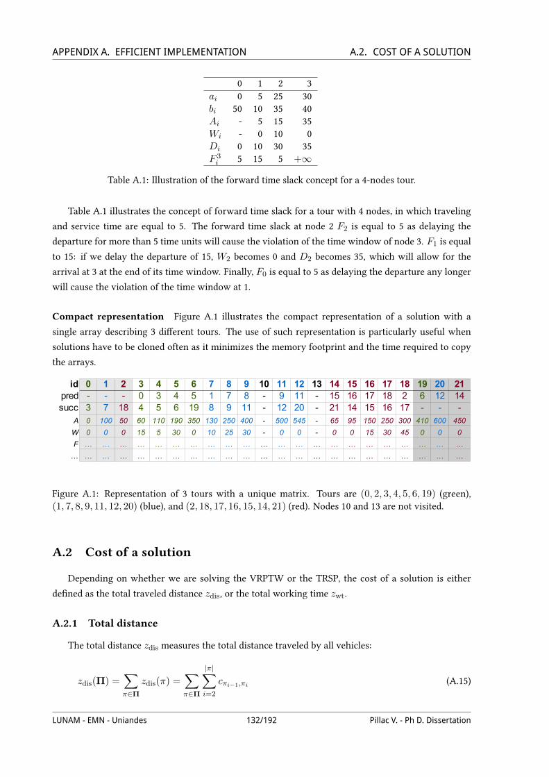
APPENDIX A. EFFICIENT IMPLEMENTATION A.2. COST OF A SOLUTION0 1 2 3
ai 0 5 25 30bi 50 10 35 40Ai - 5 15 35Wi - 0 10 0Di 0 10 30 35F 3i 5 15 5 +∞
Table A.1: Illustration of the forward time slack concept for a 4-nodes tour.
Table A.1 illustrates the concept of forward time slack for a tour with 4 nodes, in which traveling
and service time are equal to 5. The forward time slack at node 2 F2 is equal to 5 as delaying the
departure for more than 5 time units will cause the violation of the time window of node 3. F1 is equal
to 15: if we delay the departure of 15, W2 becomes 0 and D2 becomes 35, which will allow for the
arrival at 3 at the end of its time window. Finally, F0 is equal to 5 as delaying the departure any longer
will cause the violation of the time window at 1.
Compact representation Figure A.1 illustrates the compact representation of a solution with a
single array describing 3 diUerent tours. The use of such representation is particularly useful when
solutions have to be cloned often as it minimizes the memory footprint and the time required to copy
the arrays.
Figure A.1: Representation of 3 tours with a unique matrix. Tours are (0, 2, 3, 4, 5, 6, 19) (green),(1, 7, 8, 9, 11, 12, 20) (blue), and (2, 18, 17, 16, 15, 14, 21) (red). Nodes 10 and 13 are not visited.
A.2 Cost of a solution
Depending on whether we are solving the VRPTW or the TRSP, the cost of a solution is either
deVned as the total traveled distance zdis, or the total working time zwt.
A.2.1 Total distance
The total distance zdis measures the total distance traveled by all vehicles:
zdis(Π) =∑π∈Π
zdis(π) =∑π∈Π
|π|∑i=2
cπi−1,πi (A.15)
LUNAM - EMN - Uniandes 132/192 Pillac V. - Ph D. Dissertation
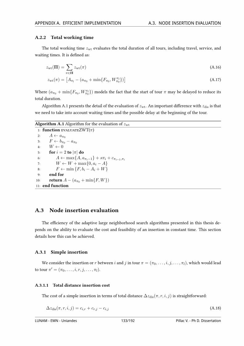
APPENDIX A. EFFICIENT IMPLEMENTATION A.3. NODE INSERTION EVALUATIONA.2.2 Total working time
The total working time zwt evaluates the total duration of all tours, including travel, service, and
waiting times. It is deVned as:
zwt(Π) =∑π∈Π
zwt(π) (A.16)
zwt(π) =[Aπl − (aπ0 + minFπ0 ,W
πlπ0)]
(A.17)
Where (aπ0 + minFπ0 ,Wπlπ0) models the fact that the start of tour π may be delayed to reduce its
total duration.
Algorithm A.1 presents the detail of the evaluation of zwt. An important diUerence with zdis is that
we need to take into account waiting times and the possible delay at the beginning of the tour.
Algorithm A.1 Algorithm for the evaluation of zwt
1: function evaluateZWT(π)2: A← aπ0
3: F ← bπ0 − aπ0
4: W ← 05: for i = 2 to |π| do6: A← maxA, aπi−1+ sπi + cπi−1,πi
7: W ←W + max0, ai −A8: F ← min F, bi −Ai +W9: end for10: return A− (aπ0 + minF,W)11: end function
A.3 Node insertion evaluation
The eXciency of the adaptive large neighborhood search algorithms presented in this thesis de-
pends on the ability to evaluate the cost and feasibility of an insertion in constant time. This section
details how this can be achieved.
A.3.1 Simple insertion
We consider the insertion or r between i and j in tour π = (π0, . . . , i, j, . . . , πl), which would lead
to tour π′ = (π0, . . . , i, r, j, . . . , πl).
A.3.1.1 Total distance insertion cost
The cost of a simple insertion in terms of total distance ∆zdis(π, r, i, j) is straightforward:
∆zdis(π, r, i, j) = ci,r + cr,j − ci,j (A.18)
LUNAM - EMN - Uniandes 133/192 Pillac V. - Ph D. Dissertation

APPENDIX A. EFFICIENT IMPLEMENTATION A.3. NODE INSERTION EVALUATIONA.3.1.2 Working time insertion cost
The evaluation of the cost of an insertion in terms of working time is more complicated as it
will impact the arrival time at the successors and may require an earlier departure from the depot.
Nonetheless, Savelsbergh (1992) points out that it can be achieved in constant time using precalculated
data as the waiting and forward time slack.
Arrival time at the last node We start by evaluating the arrival time and the waiting time at the
inserted request r:
Ar = Di + cir Wr = max0, ar −Ar (A.19)
Then, we evaluate the arrival time at the successor j:
A′j = maxAr, ar+ sr + crn (A.20)
Finally, we calculate the resulting arrival time at the last node:
A′πl = Aπl + max
0,∆−W πlj
(A.21)
where ∆ = A′j−Aj is the change in arrival time at j, andW πlj is the cumulated waiting time between
j and πl that will possibly absorb the delay.
Cumulated waiting time The new cumulated waiting time is:
W ′πlπ0
= W iπ0
+Wr + max0,W πlj −∆ (A.22)
Forward time slack The new forward time slack F ′π0is:
F ′π0= min
F iπ0
, br −Ar +W iπ0, F
(j,...,πl)j +W i
π0+Wr + maxAj , aj −A′j
(A.23)
Cost of the insertion Finally, the cost of the insertion is:
∆zwt(π, r, i, j) = zwt(π′)− zwt(π)
= (A′πl − (ak + minF ′π0,W ′
πlπ0))− (Aπl − (ak + minFπ0 ,W
πlπ0))
= max
0,∆−W πlj
−minF ′π0
,W ′πlπ0+ minFπ0 ,W
πlπ0 (A.24)
A.3.1.3 Feasibility
If the inserted node is a request, the technician must have the required skills, tools, and spare parts
to service it. In addition, the insertion must not violate time window constraints. This can be checked
LUNAM - EMN - Uniandes 134/192 Pillac V. - Ph D. Dissertation

APPENDIX A. EFFICIENT IMPLEMENTATION A.3. NODE INSERTION EVALUATIONin constant time using the values calculated in §A.3.1.2 by verifying that:
Ar ≤ brA′j ≤ lj
(A.25)
A.3.2 Simultaneous insertion
We consider the insertion of r betweenm and n and q between i and j in tour π = (π0, . . . ,m, n,-
. . . , i, j, . . . , πl), which would lead to tour π′ = (π0, . . . ,m, r, n, . . . , i, q, j, . . . , πl). This case is useful
when considering the simultaneous insertion of a request and a visit to the main depot.
A.3.2.1 Total distance insertion cost
Similarly to the simple insertion case, the cost of the insertion is:
∆zwt(π, r,m, n, q, i, j) = cm,r + cr,n − cm,n + ci,q + cq,j − ci,j (A.26)
In the case in which q is inserted immediately after r (n = q and i = r), the cost of the insertion
is:
∆zwt(π, r,m, n, q, i, j) = cm,r + cr,q + cq,j − cm,j (A.27)
A.3.2.2 Working time insertion cost
Arrival time at the last node We Vrst evaluate the arrival and waiting time at the inserted node r:
Ar = Dm + cmr Wr = max0, ar −Ar (A.28)
Then we evaluate the new arrival time at n:
A′n = maxAr, ar+ sr + crn (A.29)
Next we evaluate the new earliest departure time at i:
D′i = Di + max0,∆n −W in (A.30)
Where ∆n = A′n − An is the change in the arrival time at n. We can then evaluate the arrival time at
q:
Aq = D′i + ciq Wq = max0, aq −Aq (A.31)
And the new arrival time at j
A′j = maxAq, aq+ sq + cqj (A.32)
LUNAM - EMN - Uniandes 135/192 Pillac V. - Ph D. Dissertation

APPENDIX A. EFFICIENT IMPLEMENTATION A.3. NODE INSERTION EVALUATIONAnd the new arrival time at the last node:
A′πl = Aπl + max0,∆j −W πlj (A.33)
Where ∆j = A′j −Aj .
Total waiting time Similarly to the analysis made for the single insertion case, the new total waiting
time can be computed as follows:
W ′πlπ0
= Wmπ0
+Wr + max0,W in −∆n+Wq + max0,W πl
j −∆j (A.34)
Note that max0,W in −∆n is the waiting time on the path (n, . . . , i), which absorbs the change in
arrival time at n, and max0,W πlj −∆j is the waiting time on the path (j, . . . , πl) which will absorb
the change in arrival time at j.
Forward time slack We consider Vve paths: (π0, . . . ,m), (r), (n, . . . , i), (q), and (j, . . . , πl).
From Equation (A.23):
F (π0,...,m,r,n,...,i)π0
= minFmπ0
, br −Ar +Wmπ0, F (n,...,i)
n +Wmπ0
+Wr + maxAn, an −A′n
(A.35)
And for the whole new path:
F ′π0= min
F iπ0,
br −Ar +Wmπ0,
F(n,...,i)n +Wm
π0+Wr + maxAn, an −A′n,
bq −Aq +W ′iπ0,
F(j,...,πl)j +W ′iπ0
+Wq + maxAj , aj −A′j
(A.36)
WhereW ′iπ0is the new waiting time between π0 and i:
W ′iπ0
= Wmπ0
+Wr + max0,W in −∆n (A.37)
Cost of the insertion The cost of the insertion is equal to
∆zwt(π, r,m, n, q, i, j) = zwt(π′)− zwt(π)
= (A′πl − (ak + minF ′π0,W ′
πlπ0))− (Aπl − (ak + minFπ0 ,W
πlπ0))
= max
0,∆j −W πlj
−minF ′π0
,W ′πlπ0+ minFπ0 ,W
πlπ0 (A.38)
Special case A special case of the simultaneous insertion is when the second node is the successor of
the Vrst (i = r and n = q)). The resulting tour would then be (π0, . . . ,m, r, q, j, . . . , πl), and this case
must be treated separately. We chose to merge r and q into a single node R and to adapt the formulas
from the single insertion case. In particular the waiting time at R isWR = Wr +Wq , and the second
term of Equation (A.23) becomes minbr −Ar +Wnπ0, bq −Aq +Wn
π0+Wr.
LUNAM - EMN - Uniandes 136/192 Pillac V. - Ph D. Dissertation

APPENDIX A. EFFICIENT IMPLEMENTATION A.4. PREPROCESSINGA.3.2.3 Feasibility
The feasibility of a simultaneous insertion is similar to the single insertion case, in particular, we
ensure that time windows are not violated by making sure that the solution veriVes:
Ar ≤ brA′n ≤ lnAq ≤ bqA′j ≤ lj
(A.39)
A.4 Preprocessing
The algorithms can be speed up by performing some preprocessing on the data. This section details
the main procedures used.
A.4.1 Infeasible arcs
During the preprocessing we remove from the graphA the edges (i, j) such that j cannot be visited
after i without violating time window constraints. This is achieved by ensuring that:
ai + si + cij ≤ bj ∀(i, j) ∈ A (A.40)
A.4.2 Technician-request compatibility
This procedure checks for each technician k and request r if the technician has the required skills to
serve the request. In addition, it also checks if it can serve the request without violating time windows,
in other words if ak + ckr ≤ ar and ar + crk ≤ bk.
BibliographySavelsbergh, M. (1992). The vehicle routing problem with time windows: minimizing route duration. INFORMS,
4(2):146–154, doi:10.1287/ijoc.4.2.146.
LUNAM - EMN - Uniandes 137/192 Pillac V. - Ph D. Dissertation

BA library for the modeling of vehicle routing
problems
VroomModeling is a Wexible library that has been developed to model a wide range of instances
of vehicle routing problems. The general idea is to clearly separate the problem information (nodes,
locations, Weet, requests) from the routing logic (cost calculation, route optimization); but also to ensure
a high Wexibility in the model. This is achieved with the deVnition of node, request and vehicle objects
as a combination of base properties (e.g. a node necessarily has a geographic location) and attributes
that are mapped to attribute keys. For instance in this representation a node can also have a time
window or a compatibility constraint with vehicles (some vehicles may not be able to access the node).
An important design characteristic is the separation between the node, which represents a physical
location, for instance a client, and a request which is associated with one (pickup/delivery) or two
nodes (pickup and delivery), and represent a request for service.
LUNAM - EMN - Uniandes 139/192 Pillac V. - Ph D. Dissertation

APPENDIX B. VROOM MODELING
Figure B.1: Overview of the VroomModeling library.
Figure B.1 presents an overview of the VroomModeling library. The root object is the instance
(Instance), it contains a reference to a problem deVnition (VehicleRoutingProblemDefinition),
a planning period (PlanningPeriod), a Weet (Fleet) composed by one or more vehicles (Vehicle),
and a list of requests (Request). It is important to note that the calculation of distances and costs is
delegated to an instance of CostCalculatorDelegate, separating this logic from the representation
of routes. On the other hand, a solution (Solution) contains a reference to an instance, and a set of
routes (Route). A route is associated with a vehicle, and contains a sequence of node visits (Node-
Visit) that model the visit of a node associated with a given request. It is worth noting that the three
classes Vehicle, Node, and Request, inherits from ObjectWithAttributes which allows for the
deVnition of any number of additional attributes such as time windows or compatibility constraints.
LUNAM - EMN - Uniandes 140/192 Pillac V. - Ph D. Dissertation

APPENDIX B. VROOM MODELING
Figure B.2: Illustration of a possible use of the VroomModeling library.
Figure B.2 illustrates how a complex VRP problem could be modeled using the VroomModeling
library. In this example, vehicles have trailers, nodes have a time window and compatibility constraints
with vehicles, and requests have a time window and a stochastic demand.
LUNAM - EMN - Uniandes 141/192 Pillac V. - Ph D. Dissertation


CA library of heuristics for vehicle routing problems
VroomHeuristics is a library of common heuristics and metaheuristics. Although they were
implemented to tackle vehicle routing problems, the design of the algorithms in this library is Wexible
enough to solve other optimization problems.
Figure C.1 presents an overview of the library. There are two top-level interfaces that deVne
two types of heuristics: IInitialization and ILocalSearch. The Vrst deVnes algorithms that
will design a solution (ISolution) from scratch, while the second take an initial solution as in-
put and attempt to improve it. We implemented two initialization procedure: a Clarke and Wright
(CW) savings algorithm (ClarkeAndWrightHeuristic), and a Versatile Local Search (VLS) algorithm
that combines GRASP, ELS, and ILS (VersatileLocalSearch). The main local search component is
the LocalSearchBase class, which contains a reference to both a stopping and acceptance criterion
(IStoppingCriterion and IAcceptanceCriterion). The library contains two local search algo-
rithms: Variable Neighborhood Search (VNS - VariableNeighborhoodSearch), and Adaptive Large
Neighborhood Search (ALNS - AdaptiveLargeNeighborhoodSearch). The library also provide a
generic deVnition of a neighborhood (INeighborhood) that can either be used to Vnd a move (IMove)
that will lead to a neighbor of a solution, or as a local search procedure to Vnd the local optima starting
with a given solution. In addition, VroomHeuristics contains a generic deVnition of a component
handler (IComponentHandler) that can be used to handle components such as neighborhoods in VNS
or destroy/repair operators in ALNS. Finally, constraints are deVned and handled separately with the
interface IConstraint and the class ConstraintHandler. All constraint implementations should be
able to check the feasibility of both a solution and a move relative to a solution.
LUNAM - EMN - Uniandes 143/192 Pillac V. - Ph D. Dissertation

APPENDIX C. VROOM HEURISTICS C.1. CLARKE AND WRIGHT
Figure C.1: Design overview of the VroomHeuristics framework.
C.1 Clarke and Wright
The savings algorithm, or Clarke and Wright heuristic (CW) (Clarke and Wright, 1964), is a con-
structive heuristic for vehicle routing problems. It starts by creating one route for each customer, and
then iteratively merges routes using the notion of savings.
Algorithm C.1 presents an outline of the CW heuristic. The algorithm starts by initializing a list
of candidate mergings, which savings are calculated line 6 and correspond to the decrease in cost
resulting from the removal of arcs (0, i) and (0, j) while adding arc (i, j). Then the algorithm considers
all possible mergings between routes in order of decreasing savings. For each candidate merging (i, j),
the mergingFeasible function (line 11) checks if i) both nodes i and j are either Vrst or last in their
routes πi and πj ; ii) the route that would result from the merging satisfy all constraints. The latter
is achieved within the VroomHeuristics framework using a ConstraintHandler and modeling the
merging as a move (IMove). If the merging is feasible, then it is executed and route πj is appended to
πi (line 12). The algorithm terminates when there is no additional feasible merging.
Figure C.2 presents an overview of the proposed implementation of the CW algorithm, namely
jCW. The main component is the ClarkeAndWrightHeuristic that uses a generic deVnition of a sav-
ing algorithm (ISavingAlgorithm) and relies on global parameters for its setup (CWParameters). The
LUNAM - EMN - Uniandes 144/192 Pillac V. - Ph D. Dissertation
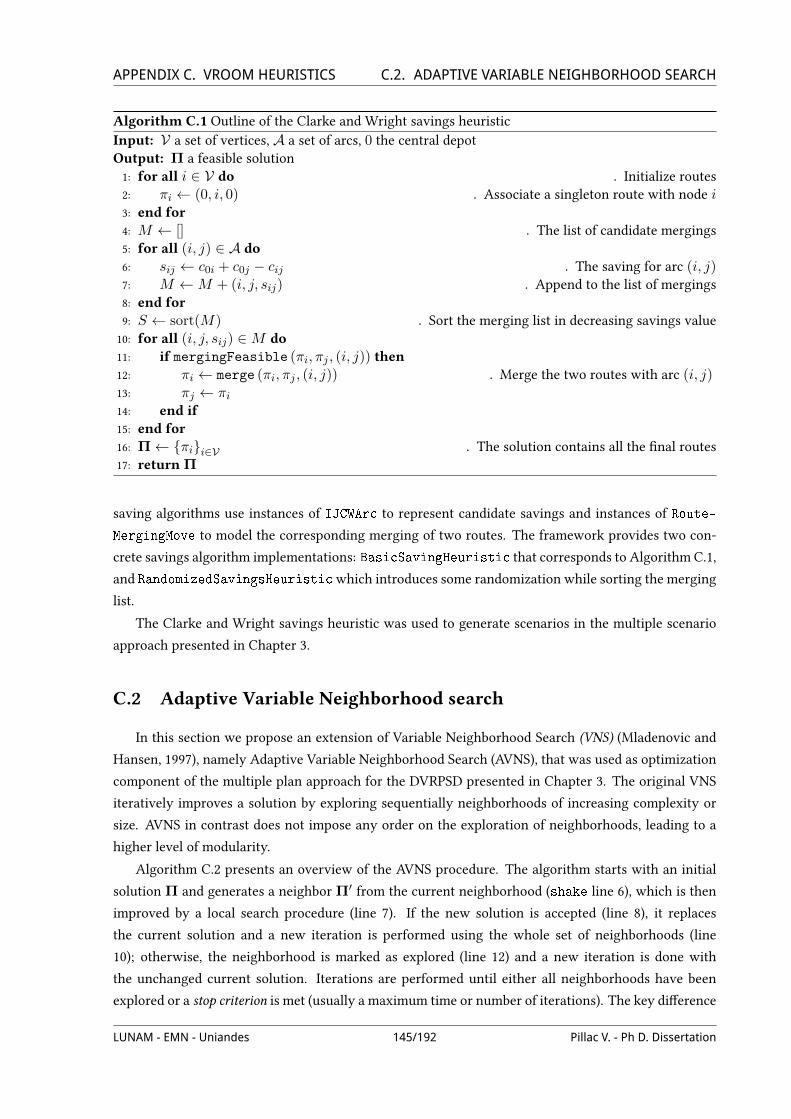
APPENDIX C. VROOM HEURISTICS C.2. ADAPTIVE VARIABLE NEIGHBORHOOD SEARCHAlgorithm C.1 Outline of the Clarke and Wright savings heuristicInput: V a set of vertices, A a set of arcs, 0 the central depotOutput: Π a feasible solution1: for all i ∈ V do . Initialize routes2: πi ← (0, i, 0) . Associate a singleton route with node i3: end for4: M ← [] . The list of candidate mergings5: for all (i, j) ∈ A do6: sij ← c0i + c0j − cij . The saving for arc (i, j)7: M ←M + (i, j, sij) . Append to the list of mergings8: end for9: S ← sort(M) . Sort the merging list in decreasing savings value10: for all (i, j, sij) ∈M do11: if mergingFeasible (πi, πj , (i, j)) then12: πi ← merge (πi, πj , (i, j)) .Merge the two routes with arc (i, j)13: πj ← πi14: end if15: end for16: Π← πii∈V . The solution contains all the Vnal routes17: return Π
saving algorithms use instances of IJCWArc to represent candidate savings and instances of Route-
MergingMove to model the corresponding merging of two routes. The framework provides two con-
crete savings algorithm implementations: BasicSavingHeuristic that corresponds to Algorithm C.1,
and RandomizedSavingsHeuristicwhich introduces some randomization while sorting the merging
list.
The Clarke and Wright savings heuristic was used to generate scenarios in the multiple scenario
approach presented in Chapter 3.
C.2 Adaptive Variable Neighborhood search
In this section we propose an extension of Variable Neighborhood Search (VNS) (Mladenovic and
Hansen, 1997), namely Adaptive Variable Neighborhood Search (AVNS), that was used as optimization
component of the multiple plan approach for the DVRPSD presented in Chapter 3. The original VNS
iteratively improves a solution by exploring sequentially neighborhoods of increasing complexity or
size. AVNS in contrast does not impose any order on the exploration of neighborhoods, leading to a
higher level of modularity.
Algorithm C.2 presents an overview of the AVNS procedure. The algorithm starts with an initial
solution Π and generates a neighbor Π′ from the current neighborhood (shake line 6), which is then
improved by a local search procedure (line 7). If the new solution is accepted (line 8), it replaces
the current solution and a new iteration is performed using the whole set of neighborhoods (line
10); otherwise, the neighborhood is marked as explored (line 12) and a new iteration is done with
the unchanged current solution. Iterations are performed until either all neighborhoods have been
explored or a stop criterion is met (usually a maximum time or number of iterations). The key diUerence
LUNAM - EMN - Uniandes 145/192 Pillac V. - Ph D. Dissertation

APPENDIX C. VROOM HEURISTICS C.2. ADAPTIVE VARIABLE NEIGHBORHOOD SEARCH
Figure C.2: Design overview of the Clarke and Wright heuristic framework.
LUNAM - EMN - Uniandes 146/192 Pillac V. - Ph D. Dissertation

APPENDIX C. VROOM HEURISTICS C.2. ADAPTIVE VARIABLE NEIGHBORHOOD SEARCHwith respect to the original VNS algorithm is the call to the selectNeighborhood function at line
5. It allows for non-sequential exploration of neighborhoods, with the goal of exploring the best
neighborhoods Vrst.
Algorithm C.2 The Adaptive Variable Neighborhood Search algorithm.Input: Π a feasible solution, z an evaluation function and N = N1, .., NK a set of neighborhood
structuresOutput: Π∗ the best solution found1: function VNS(Π)2: Π∗ ← Π3: Nc ← N . Initial neighborhood set4: while Nc 6= ∅ and stop condition not met do5: N ← selectNeighborhood(Nc) . Select neighborhood6: Π′ ← shake(N,Π) . Generate a neighbor from neighborhood N7: Π′ ← ls(Π′) . Local search to improve Π′
8: if accept(Π′,Π) then . Π′ is accepted as current solution9: Π← Π′ . Update current solution10: Nc ← N . Reset the neighborhood set11: else12: Nc ← Nc \ N . Remove the explored neighborhood13: end if14: if z(Π′) < z(Π∗) then . An improvement has been found15: Π∗ ← Π′ . Update best solution16: end if17: end while18: return Π∗
19: end function
C.2.1 Implementation
Figure C.3 presents a UML diagram of the VNS implementation. The key classes are the following:
VariableNeighborhoodSearch is the class containing the implementation of Algorithm C.2, where
the shake, local search and neighborhood selection are delegated to instances of other classes (template
method pattern); ILocalSearch is the generic deVnition of local search, an instance of this class is
responsible for the local search in the VNS algorithm (ls line 7); INeighborhood is a generic deVni-
tion of a neighborhood structure. IComponentHandler is an interface for classes responsible of the
neighborhood selection strategy.
It is worth noting that the following variants (Hansen et al., 2003) can be easily implemented in
this framework:
Shake Local search
VND Best neighbor None
RVNS Random neighbor None
BVNS Random neighbor Any
GVNS Random neighbor VND
LUNAM - EMN - Uniandes 147/192 Pillac V. - Ph D. Dissertation

APPENDIX C. VROOM HEURISTICS C.2. ADAPTIVE VARIABLE NEIGHBORHOOD SEARCH
Figure C.3: Design overview of the VNS implementation.
LUNAM - EMN - Uniandes 148/192 Pillac V. - Ph D. Dissertation
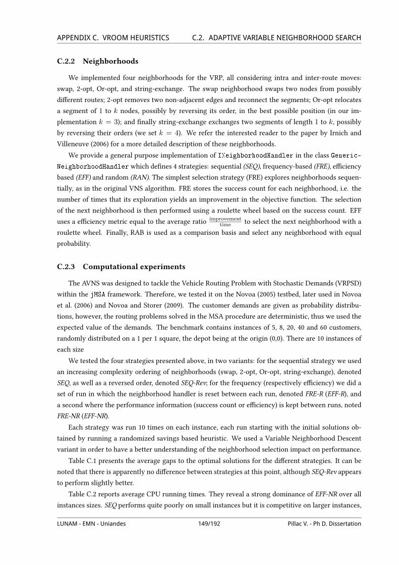
APPENDIX C. VROOM HEURISTICS C.2. ADAPTIVE VARIABLE NEIGHBORHOOD SEARCHC.2.2 Neighborhoods
We implemented four neighborhoods for the VRP, all considering intra and inter-route moves:
swap, 2-opt, Or-opt, and string-exchange. The swap neighborhood swaps two nodes from possibly
diUerent routes; 2-opt removes two non-adjacent edges and reconnect the segments; Or-opt relocates
a segment of 1 to k nodes, possibly by reversing its order, in the best possible position (in our im-
plementation k = 3); and Vnally string-exchange exchanges two segments of length 1 to k, possibly
by reversing their orders (we set k = 4). We refer the interested reader to the paper by Irnich and
Villeneuve (2006) for a more detailed description of these neighborhoods.
We provide a general purpose implementation of INeighborhoodHandler in the class Generic-
NeighborhoodHandlerwhich deVnes 4 strategies: sequential (SEQ), frequency-based (FRE), eXciency
based (EFF) and random (RAN). The simplest selection strategy (FRE) explores neighborhoods sequen-
tially, as in the original VNS algorithm. FRE stores the success count for each neighborhood, i.e. the
number of times that its exploration yields an improvement in the objective function. The selection
of the next neighborhood is then performed using a roulette wheel based on the success count. EFF
uses a eXciency metric equal to the average ratio improvementtime to select the next neighborhood with a
roulette wheel. Finally, RAB is used as a comparison basis and select any neighborhood with equal
probability.
C.2.3 Computational experiments
The AVNS was designed to tackle the Vehicle Routing Problem with Stochastic Demands (VRPSD)
within the jMSA framework. Therefore, we tested it on the Novoa (2005) testbed, later used in Novoa
et al. (2006) and Novoa and Storer (2009). The customer demands are given as probability distribu-
tions, however, the routing problems solved in the MSA procedure are deterministic, thus we used the
expected value of the demands. The benchmark contains instances of 5, 8, 20, 40 and 60 customers,
randomly distributed on a 1 per 1 square, the depot being at the origin (0,0). There are 10 instances of
each size
We tested the four strategies presented above, in two variants: for the sequential strategy we used
an increasing complexity ordering of neighborhoods (swap, 2-opt, Or-opt, string-exchange), denoted
SEQ, as well as a reversed order, denoted SEQ-Rev; for the frequency (respectively eXciency) we did a
set of run in which the neighborhood handler is reset between each run, denoted FRE-R (EFF-R), and
a second where the performance information (success count or eXciency) is kept between runs, noted
FRE-NR (EFF-NR).
Each strategy was run 10 times on each instance, each run starting with the initial solutions ob-
tained by running a randomized savings based heuristic. We used a Variable Neighborhood Descent
variant in order to have a better understanding of the neighborhood selection impact on performance.
Table C.1 presents the average gaps to the optimal solutions for the diUerent strategies. It can be
noted that there is apparently no diUerence between strategies at this point, although SEQ-Rev appears
to perform slightly better.
Table C.2 reports average CPU running times. They reveal a strong dominance of EFF-NR over all
instances sizes. SEQ performs quite poorly on small instances but it is competitive on larger instances,
LUNAM - EMN - Uniandes 149/192 Pillac V. - Ph D. Dissertation

APPENDIX C. VROOM HEURISTICS C.3. VERSATILE LOCAL SEARCHwhile the tendency reverses for SEQ-Rev. This last observation can be explained by the fact that this
last strategy will explore Vrst the more complex neighborhoods (string-exchange and Or-opt), which
are of complexity O(k2n2) and O(kn2), thus requiring a quadratically increasing time to explore. As
expected, we can note that preserving the performance information from one run to another (R vs.
NR) slightly improves the performance.
Finally, Table C.3 shows that the EFF-NR strategy also have a lower CPU time standard deviation,
meaning that it is the most stable in terms of running times. A similar analysis has been done for the
gap standard deviation but no tendency can be drawn.
C.3 Versatile Local Search
The Versatile Local Search package (VLS) contains an implementation of the Greedy Random-
ized Adaptive Search Procedure (GRASP) with multi-start evolutionary local search proposed by Prins
(2009) and Villegas et al. (2010). This approach is an hybrid between GRASP, Iterated Local Search
(ILS), and Evolutionary Local Search (ELS), and was initially designed as optimization component for
the jMSA framework.
Algorithm C.3 presents the outline of the approach which comprises three nested loops. The
GRASP loop (lines 1–20) builds a solution with a randomized constructive heuristic (line 2) and then
improves the solution with a local search (line 3). The resulting solution is passed to the ILS loop (lines
4–16), and the ELS loop (lines 6–12). The ELS randomly modiVes the current solution (line 5) and then
apply a local search to it (line 6). The best solution from the ELS iteration is then taken as current
solution for the next ILS iteration.
Figure C.4 illustrates the implementation of the VLS algorithm withing the VroomHeuristics
framework. The central component is the VersatileLocalSearch class which is conVgured via VLS-
GlobalParameters and contains a reference to an initialization (IInitialization), local search
(ILocalSearch), and perturbation (IVLSPerturbation).
C.4 Adaptive Large Neighborhood Search
Figure C.5 presents an overview of the implementation of the Adaptive Large Neighborhood Search
(ALNS) and parallel ALNS (pALNS) algorithms described in Chapter 2. The main component is the
AdaptiveLargeNeighborhoodSearch class, which is conVgured via (ALNSGlobalParameters). It
relies on two component handlers (ALNSComponentHandler) that are responsible for the evaluation
and selection of the destroy and repair operators (IDestroy and IRepair). ParallelALNS provides
the parallel implementation and uses an abstract deVnition of a solution pool (IPALNSSolutionPool)
to manage the pool of solutions.
The pALNS and ALNS algorithms were used in Chapter 2 and 4 to tackle both static and dynamic
routing problems.
LUNAM - EMN - Uniandes 150/192 Pillac V. - Ph D. Dissertation

APPENDIX C. VROOM HEURISTICS C.4. MSSHC
Size SEQ SEQ-Rev FRE-R FRE-NR EFF-R EFF-NR RAN-R5 4.60 4.60 4.60 4.60 4.60 4.60 4.608 4.76 4.75 4.75 4.75 4.76 4.76 4.75
20 6.48 6.45 6.45 6.48 6.45 6.46 6.4640 7.33 7.28 7.31 7.28 7.28 7.33 7.3060 8.15 8.12 8.15 8.14 8.14 8.13 8.14
Table C.1: Average gap to the optimal solution (in %).
Algorithm C.3 The Versatile Local Search algorithm.Input: I an instance, initialization a randomized constructive heuristics, localSearch a local
search procedure, perturbation a randomized perturbation procedure., z an evaluation function.Output: Π∗ the best solution found1: for i = 1 to ns do . GRASP loop2: Π← initialization(I) . Build a new solution3: Π← localSearch(S) . Apply a local search4: for j = 1 to ni do . ILS loop5: Π′ ← Π . Starting solution for the ELS6: for k = 1 to nc do . ELS loop7: Π′′ ← perturbation(Π′) . Randomly perturb the solution8: Π′′ ← localSearch(Π′′) . Apply a local search9: if z(Π′′) < z(Π′) then10: Π← Π′′ . Store the best solution produced by ELS11: end if12: end for13: if z(Π′) < z(Π) then14: Π← Π′ . Update the current solution with the best ELS solution15: end if16: end for17: if z(Π) < z(Π∗) then18: Π∗ ← Π . Update the overall best solution19: end if20: end for21: return Π∗
LUNAM - EMN - Uniandes 151/192 Pillac V. - Ph D. Dissertation

APPENDIX C. VROOM HEURISTICS C.4. MSSHC
Figure C.4: Design overview of the Versatile Locale Search framework.
Figure C.5: Design overview of the Adaptive Large Neighborhood Search framework.
LUNAM - EMN - Uniandes 152/192 Pillac V. - Ph D. Dissertation

APPENDIX C. VROOM HEURISTICS C.5. MSSHCSize SEQ SEQ-Rev FRE-R FRE-NR EFF-R EFF-NR RAN-R
5 2 0 1 0 0 0 08 4 1 1 1 1 1 1
20 18 58 22 14 20 15 1940 142 575 232 273 190 120 21260 485 2385 861 603 656 430 812
Table C.2: Average CPU running times (ms).
Size SEQ-R SEQ-Rev FRE-R FRE-NR EFF-R EFF-NR RAN-R5 64.6 140.7 92.2 67.8 61.7 37.9 56.38 4.5 0.7 0.9 0.7 0.6 0.5 1.3
20 0.8 0.8 0.8 0.8 0.8 0.8 0.840 64.6 140.7 92.2 67.8 61.7 37.9 56.360 135.8 674.5 362.8 157.6 187.5 158.3 193.6
Table C.3: Standard deviation of CPU running times (ms).
C.5 Multi-space sampling with heuristic concentration
This section describes an approach based on the work of Mendoza and Villegas (2011), namely
Multiple Space Sampling with Heuristic Concentration (MSSHC), which generates feasible routes using
randomized constructive heuristics, and then builds a solution by solving a set-covering problem.
Algorithm C.4 presents an overview of the method. For each constructive heuristic, the algorithm
generates a number of giant TSP-like tours (line 5), that are then split into a set of feasible routes (line
6). Finally, a set-covering model is solved to select a subset of routes conforming a solution of minimal
cost (line 10).
Algorithm C.4 The MSSHC algorithmInput: H a set of constructive heuristics, I number of iterationsOutput: Π∗ the best solution that can be built from the generated routes1: P ← ∅ . Initialize route pool
2: IH ←⌈I|H|
⌉. Number of samples per heuristic
3: for all H ∈ H do4: for i = 1 to IH do5: π ← generateGiantTour (H) . Generate a giant tour6: P ′ ← split (π) . Split the giant tour into multiple feasible routes7: P ← P ∪ P ′ . Add the routes to the pool8: end for9: end for10: Π∗ ← solveSC (P) . Solve the set covering problem11: return Π∗
We tested this approach on the TRSP but it appeared that pALNS+SC was clearly dominating both
in terms of objective function and computational time. Our intuition is that the presence of time
windows makes it more diXcult to generate good routes during the split procedure. However this
method has shown very good results on the VRPSD and its simplicity makes it a good candidate for
problems without time windows.
LUNAM - EMN - Uniandes 153/192 Pillac V. - Ph D. Dissertation

APPENDIX C. VROOM HEURISTICS C.5. MSSHCC.5.1 Implementation
Figure C.6 presents an overview of the MSSHC framework. The main class is RCHSCSolver which
uses a collection of randomized constructive heuristics (TRSPRndConstructiveHeuristic) and a set
covering solver (SCGurobiSolver). Note that at present time this implementation is tied with the data
model used for the experiments on the TRSP.
Figure C.6: Design overview of the MSSHC framework.
C.5.2 Constructive heuristics
Giant tours are generated using a randomized variant of four well known heuristics for the TSP,
that draw a random number χ between 0 and the number of unvisited customers. Random Nearest
Neighbor (RNN) selects the χ-th closest customer to the last customer of the tour and appends it to the
tour. Random Nearest (Furthest) Insertion (RNI/RFI) selects the χ-th closest (furthest) customer to any
of the customers currently in the tour and inserts it in the best position. Random Best Insertion (RBI)
selects and inserts the χ-th best insertion for all unserved customers.
C.5.3 Split procedure
Algorithm C.5 presents the split procedure as introduced by Prins (2004), which is basically a label-
ing algorithm that Vnds the shortest path on an auxiliary graph representing all the feasible partitions
of the giant tour into routes.
LUNAM - EMN - Uniandes 154/192 Pillac V. - Ph D. Dissertation

APPENDIX C. VROOM HEURISTICS C.5. MSSHCAlgorithm C.5 The split procedureInput: π a giant tour of length n, z an evaluation functionOutput: P ′ the optimal splitting of π into a set of routes1: P ′ ← ∅2: L← [+∞]i=1..n . Initialize labels to +∞3: L1 ← 0 . Initialize labels of the Vrst node to 04: P ← [∅]i=1..n . Initialize the predecessor array5: for i = 1 to n do6: j ← i7: f ← true
8: while f and j ≤ n do9: f ← isFeasible
(π[i,j]
). Check route feasibility
10: if f and Li + z(π[i,j]) < Lj then .We found an improving feasible arc11: Lj ← Li + z(π[i,j]) . Update j’s label12: Pj ← π[i,j] . Update j’s predecessor13: end if14: j ← j + 115: end while16: end for17: i← n18: while i 6= 1 do19: P ′ ← P ′ ∪ Pi . Add the route to the set of optimal routes20: i← P 0
i .Move to the Vrst node of the route21: end while22: return P ′
C.5.4 Heuristic concentration
The heuristic concentration consists in selecting a subset of routes that constitutes a minimal cost
feasible solution of the problem at hand. This can be modeled as the following set-covering problem:
Min∑t∈P
ctxt (C.1)
s.t. ∑t∈P
xtati ≥ 1 ∀i ∈ R (C.2)
xt ∈ 0, 1 ∀t ∈ P (C.3)
Where P is the set of generated routes and ati a parameter taking the value of 1 if route t visits node i.
Constraint C.2 ensures that each customer is visited at least once. Considering that customers
must be visited exactly once, one could argue that a set-partitioning formulation would Vt better our
purpose. Nonetheless, our model only contains a limited subset of columns, and therefore we may not
be able to Vnd a good combination of columns that ensures the unique covering of all customers. As
a result, the Vnal solution may visit a customer more than once. This is easily dealt with by removing
the most costly visits. In all cases we are ensured that the repaired solution x∗SC+rep, is at least as
good as the optimal solution x∗SC of the set-covering, and by transitivity of the set-partitioning x∗SP ,
LUNAM - EMN - Uniandes 155/192 Pillac V. - Ph D. Dissertation

APPENDIX C. VROOM HEURISTICS BIBLIOGRAPHYas illustrated in Equation C.4
z(x∗SC) ≤ z(x∗SP ) ∧ z(x∗SC+rep) ≤ z(x∗SC)⇒ z(x∗SC+rep) ≤ z(x∗SP ) (C.4)
BibliographyClarke, G. and Wright, J. W. (1964). Scheduling of vehicles from a central depot to a number of delivery points.
Operations Research, 12(4):568–581, doi:10.1287/opre.12.4.568.
Hansen, P., Mladenovic, N., and Moreno Pérez, J. A. (2003). Busqueda de entorno variable. Inteligencia ArtiVcial,Revista Iberoamericana de Inteligencia ArtiVcial, 19(19):77–92.
Irnich, S. and Villeneuve, D. (2006). The shortest-path problem with resource constraints and k-cycle eliminationfor k ≥ 3. INFORMS Journal on Computing, 18(3):391–406, doi:10.1287/ijoc.1040.0117.
Mendoza, J. E. and Villegas, J. G. (2011). A space biased-sampling approach for the vehicle routing problem withstochastic demands. In Di Gaspero, L., Schaerf, A., and Stützle, T., editors, Proceedings of the 9th MetaheuristicsConference (MIC 2011), pages 643–645. Università degli Studi di Udine.
Mladenovic, N. and Hansen, P. (1997). Variable neighborhood search. Computers & Operations Research,24(11):1097 – 1100, doi:10.1016/S0305-0548(97)00031-2.
Novoa, C., Berger, R., Linderoth, J., and Storer, R. (2006). A set-partitioning-based model for the stochasticvehicle routing problem. Technical Report 06T-008, Texas State University, 601 University Drive San Marcos,TX 78666.
Novoa, C. and Storer, R. (2009). An approximate dynamic programming approach for the vehiclerouting problem with stochastic demands. European Journal of Operational Research, 196(2):509–515,doi:10.1016/j.ejor.2008.03.023.
Novoa, C. M. (2005). Static and dynamic approaches for solving the vehicle routing problem with stochastic demands.PhD thesis, Lehigh University, Pennsylvania, United States. AAT 3188502.
Prins, C. (2004). A simple and eUective evolutionary algorithm for the vehicle routing problem. Computers &Operations Research, 31(12):1985–2002, doi:10.1016/S0305-0548(03)00158-8.
Prins, C. (2009). A GRASP × evolutionary local search hybrid for the vehicle routing problem. In Bio-inspiredAlgorithms for the Vehicle Routing Problem, volume 161 of Studies in Computational Intelligence, pages 35–53.Springer Berlin / Heidelberg.
Villegas, J. G., Prins, C., Prodhon, C., Medaglia, A. L., and Velasco, N. (2010). GRASP/VND and multi-startevolutionary local search for the single truck and trailer routing problem with satellite depots. EngineeringApplications of ArtiVcial Intelligence, 23(5):780–794, doi:10.1016/j.engappai.2010.01.013.
LUNAM - EMN - Uniandes 156/192 Pillac V. - Ph D. Dissertation
DAn instance generator for the TRSP
We adapted the VRPTW instances proposed by Solomon (1987) by adding skills, tools, and spare
parts information. The instances contain 100 requests located randomly (R), in clusters (C), or com-
bining both (RC); while the planning horizon is either short (type 1) or long (type 2). These instances
are organized combining location and horizon (i.e., C1, C2, R1, R2, RC1, and RC2). For all instances the
crew size is Vxed, and the traveling speed of technicians is assumed to be unitary.
D.1 Parameters
The parameters of the generator are the following:
|S|, |T |, |P| number of skills, tools, and spare parts types;
DtS distribution of the number of skills per technician;
DtT distribution of the number of tools available to each technician;
DtP distribution of the number of diUerent spare part types available to each technician;
DtPC distribution of the number of spare parts of any available type available to each technician;
DrS distribution of the number of skills required by each request;
DrT distribution of the number of tools required by each request;
DrP distribution of the number of diUerent spare part types required by each request;
DrPC distribution of the number of spare parts of any required type required by each request.
We then numerate skills, tools and spare parts in a natural order (e.g., S = 0, 1, ..., |S| − 1).
LUNAM - EMN - Uniandes 157/192 Pillac V. - Ph D. Dissertation

APPENDIX D. AN INSTANCE GENERATOR FOR THE TRSP D.2. TOOLS AND SPARE PARTSD.2 Tools and spare parts
To ensure a certain coherence between skills and spare parts, we deVne for each skill a subset of
associated tools/spare parts. For instance the skill screw will be associated with the tools (drill, screw
driver) and spare parts (screw, rawplug). We therefore have:
Ts the set of tools associated with skill s,
Ts =t| : s ∗ d |T ||S| e ≤ t < (s+ 1) ∗ d |T ||S| e
Ps the set of spare parts associated with skill s,
Ps =p| : s ∗ d |P||S| e ≤ p < (s+ 1) ∗ d |P||S| e
D.3 Technicians
We associate to each vehicle of the original instance a technician k, and generate additional infor-
mation to match the TRSP deVnition.
Home depot We randomly generate a home depot hk for each technician k in a 100× 100 square.
Skills We sample the DtS distribution to generate a random number ηs, and then pick ηs skills from
the skill set S to form Sk, the skill set of technician k.
Tools We sample the DtT distribution to generate a random number ηt, and then pick ηt tools from
the union of the tool subsets⋃s∈Sk Ts.
Spare parts We sample the DtP distribution to generate a random number ηp, and then pick ηpspare part types from the union of the spare part types subsets
⋃s∈Sk Ps; then for each selected spare
part type pwe generate the number of parts of type p available to the technician by sampling theDtPCdistribution.
D.4 Requests
We associate to each customer of the original instance a request i, and generate additional infor-
mation to match the TRSP deVnition.
Skills We sample theDrS distribution to generate a random number ηs, and then pick ηs skills from
the skill set S to form Si, the skill set of request i.
Tools We sample the DrT distribution to generate a random number ηt, and then pick ηt tools from
the union of the tool subsets⋃s∈Si Ts.
Spare parts We sample the DrP distribution to generate a random number ηp, and then pick ηpspare part types from the union of the spare part types subsets
⋃s∈Si Ps; then for each p we generate
the number of parts of type p required by the request by sampling the DrPC distribution.
LUNAM - EMN - Uniandes 158/192 Pillac V. - Ph D. Dissertation
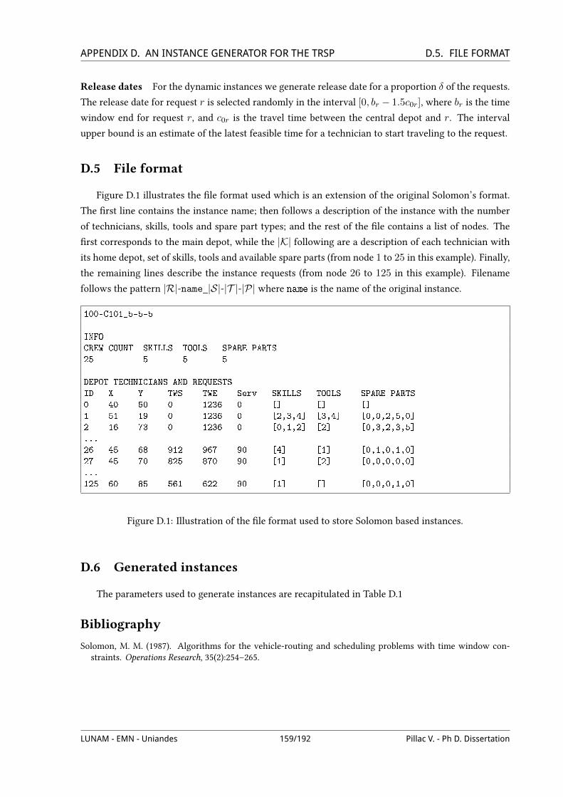
APPENDIX D. AN INSTANCE GENERATOR FOR THE TRSP D.5. FILE FORMATRelease dates For the dynamic instances we generate release date for a proportion δ of the requests.
The release date for request r is selected randomly in the interval [0, br − 1.5c0r], where br is the time
window end for request r, and c0r is the travel time between the central depot and r. The interval
upper bound is an estimate of the latest feasible time for a technician to start traveling to the request.
D.5 File format
Figure D.1 illustrates the Vle format used which is an extension of the original Solomon’s format.
The Vrst line contains the instance name; then follows a description of the instance with the number
of technicians, skills, tools and spare part types; and the rest of the Vle contains a list of nodes. The
Vrst corresponds to the main depot, while the |K| following are a description of each technician with
its home depot, set of skills, tools and available spare parts (from node 1 to 25 in this example). Finally,
the remaining lines describe the instance requests (from node 26 to 125 in this example). Filename
follows the pattern |R|-name_|S|-|T |-|P| where name is the name of the original instance.
100-C101_5-5-5
INFO
CREW COUNT SKILLS TOOLS SPARE PARTS
25 5 5 5
DEPOT TECHNICIANS AND REQUESTS
ID X Y TWS TWE Serv SKILLS TOOLS SPARE PARTS
0 40 50 0 1236 0 [] [] []
1 51 19 0 1236 0 [2,3,4] [3,4] [0,0,2,5,0]
2 16 73 0 1236 0 [0,1,2] [2] [0,3,2,3,5]
...
26 45 68 912 967 90 [4] [1] [0,1,0,1,0]
27 45 70 825 870 90 [1] [2] [0,0,0,0,0]
...
125 60 85 561 622 90 [1] [] [0,0,0,1,0]
Figure D.1: Illustration of the Vle format used to store Solomon based instances.
D.6 Generated instances
The parameters used to generate instances are recapitulated in Table D.1
BibliographySolomon, M. M. (1987). Algorithms for the vehicle-routing and scheduling problems with time window con-
straints. Operations Research, 35(2):254–265.
LUNAM - EMN - Uniandes 159/192 Pillac V. - Ph D. Dissertation

APPENDIX D. AN INSTANCE GENERATOR FOR THE TRSP BIBLIOGRAPHY
Parameter Value|S| 5|T | 5|P| 5
DtS Uint(2, 4)DtT Uint(0, 5)DtP Uint(2, 5)DtPC Uint(2, 5)
DrS 1DrT Uint(0, 2)DrP Uint(0, 2)DrPC 1
Table D.1: Parameter setting for the instance generation
LUNAM - EMN - Uniandes 160/192 Pillac V. - Ph D. Dissertation
EBest known solutions for the TRSP
This appendix presents the value of the best known solutions for the TRSP instances introduced in
this thesis.
E.1 Summary of best known solutions
Tables E.1, E.2, and E.3 present a summary of the best known solutions for instances from group
C, R, and RC respectively. Note that the objective function only considers the minimization of the
duration, the distance is reported for reference only.
The interested reader is referred to the webpage http://hdl.handle.net/1992/1152 for the
detailed solutions.
LUNAM - EMN - Uniandes 161/192 Pillac V. - Ph D. Dissertation
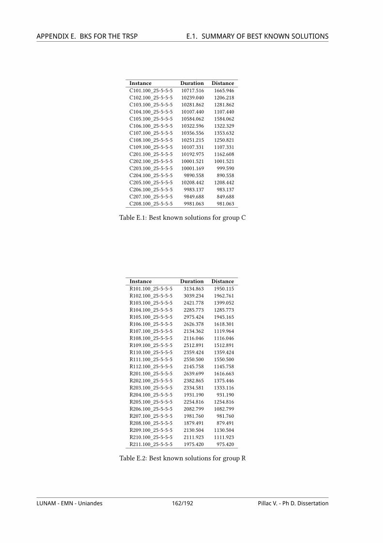
APPENDIX E. BKS FOR THE TRSP E.1. SUMMARY OF BEST KNOWN SOLUTIONS
Instance Duration DistanceC101.100_25-5-5-5 10717.516 1665.946C102.100_25-5-5-5 10239.040 1206.218C103.100_25-5-5-5 10281.862 1281.862C104.100_25-5-5-5 10107.440 1107.440C105.100_25-5-5-5 10584.062 1584.062C106.100_25-5-5-5 10322.596 1322.329C107.100_25-5-5-5 10356.556 1353.632C108.100_25-5-5-5 10251.215 1250.821C109.100_25-5-5-5 10107.331 1107.331C201.100_25-5-5-5 10192.975 1162.608C202.100_25-5-5-5 10001.521 1001.521C203.100_25-5-5-5 10001.169 999.590C204.100_25-5-5-5 9890.558 890.558C205.100_25-5-5-5 10208.442 1208.442C206.100_25-5-5-5 9983.137 983.137C207.100_25-5-5-5 9849.688 849.688C208.100_25-5-5-5 9981.063 981.063
Table E.1: Best known solutions for group C
Instance Duration DistanceR101.100_25-5-5-5 3134.863 1950.115R102.100_25-5-5-5 3039.234 1962.761R103.100_25-5-5-5 2421.778 1399.052R104.100_25-5-5-5 2285.773 1285.773R105.100_25-5-5-5 2975.424 1945.165R106.100_25-5-5-5 2626.378 1618.301R107.100_25-5-5-5 2134.362 1119.964R108.100_25-5-5-5 2116.046 1116.046R109.100_25-5-5-5 2512.891 1512.891R110.100_25-5-5-5 2359.424 1359.424R111.100_25-5-5-5 2550.500 1550.500R112.100_25-5-5-5 2145.758 1145.758R201.100_25-5-5-5 2639.699 1616.663R202.100_25-5-5-5 2382.865 1375.446R203.100_25-5-5-5 2334.581 1333.116R204.100_25-5-5-5 1931.190 931.190R205.100_25-5-5-5 2254.816 1254.816R206.100_25-5-5-5 2082.799 1082.799R207.100_25-5-5-5 1981.760 981.760R208.100_25-5-5-5 1879.491 879.491R209.100_25-5-5-5 2130.504 1130.504R210.100_25-5-5-5 2111.923 1111.923R211.100_25-5-5-5 1975.420 975.420
Table E.2: Best known solutions for group R
LUNAM - EMN - Uniandes 162/192 Pillac V. - Ph D. Dissertation

APPENDIX E. BKS FOR THE TRSP E.1. SUMMARY OF BEST KNOWN SOLUTIONS
Instance Duration DistanceRC101.100_25-5-5-5 2856.488 1804.244RC102.100_25-5-5-5 2843.178 1825.804RC103.100_25-5-5-5 2495.567 1494.851RC104.100_25-5-5-5 2162.514 1162.514RC105.100_25-5-5-5 2711.491 1684.443RC106.100_25-5-5-5 2761.863 1761.863RC107.100_25-5-5-5 2570.403 1570.403RC108.100_25-5-5-5 2354.422 1354.422RC201.100_25-5-5-5 2686.012 1685.053RC202.100_25-5-5-5 2487.727 1486.713RC203.100_25-5-5-5 2310.010 1303.007RC204.100_25-5-5-5 2064.163 1064.163RC205.100_25-5-5-5 2588.166 1560.131RC206.100_25-5-5-5 2359.699 1350.841RC207.100_25-5-5-5 2233.678 1233.678RC208.100_25-5-5-5 1914.536 914.536
Table E.3: Best known solutions for group RC
LUNAM - EMN - Uniandes 163/192 Pillac V. - Ph D. Dissertation


FList of contributions
F.1 International peer-reviewed journal papers
Pillac, V., Guéret, C., Medaglia, A. L. (2012), An event-driven optimization framework for dynamic
vehicle routing, Decision Support Systems, Accepted manuscript, doi:10.1016/j.dss.2012.06.007
Pillac, V., Gendreau, M., Guéret, C., Medaglia, A. L. (2012), A review of dynamic vehicle routing prob-
lems, European Journal of Operational Research, Accepted manuscript, doi:10.1016/j.ejor.2012.08.015.
Pillac, V., Guéret, C., Medaglia, A. L. (2012), A parallel matheuristic for the Technician Routing and
Scheduling Problem, Optimization Letters, Accepted manuscript, doi:10.1007/s11590-012-0567-4.
F.2 Technical reports
Pillac, V., Guéret, C., Medaglia, A. L. (2012), A fast re-optimization approach for dynamic vehicle rout-
ing, Technical Report 12/6/AUTO, Ecole des Mines de Nantes, France
http://hal.archives-ouvertes.fr/hal-00739782/en
Pillac, V., Guéret, C., Medaglia, A. L. (2012), On the Dynamic Technician Routing and Scheduling
Problem, Technical Report 12/5/AUTO, Ecole des Mines de Nantes, France
http://hal.archives-ouvertes.fr/hal-00739781/en
Pillac, V., Gendreau, M., Guéret, C., Medaglia, A. L. (2011), A review of dynamic vehicle routing prob-
LUNAM - EMN - Uniandes 165/192 Pillac V. - Ph D. Dissertation
APPENDIX F. CONTRIBUTIONS F.3. PEER-REVIEWED CONFERENCE PROCEEDINGSlems, CIRRELT Research Paper, CIRRELT-2011-62,
https://www.cirrelt.ca/DocumentsTravail/CIRRELT-2011-62.pdf
Pillac, V., Guéret, C., Medaglia, A. L. (2011), An event-driven optimization framework for dynamic
vehicle routing, Technical Report 11/2/AUTO, Ecole des Mines de Nantes, France,
http://hal.archives-ouvertes.fr/hal-00623479/en
Pillac, V., Guéret, C., Medaglia, A. L. (2010), Dynamic Vehicle Routing Problems: State of the art and
Prospects, Technical Report 10/4/AUTO, Ecole des Mines de Nantes, France,
http://hal.archives-ouvertes.fr/hal-00623474/en
F.3 Peer-reviewed conference proceedings
Pillac, V., Guéret, C., Medaglia, A. L. (2012),On the Dynamic Technician Routing and Scheduling
Problem, Proceedings of the 5th International Workshop on Freight Transportation and Logistics
(ODYSSEUS 2012), 509–512, Mikonos (Greece).
http://hal.archives-ouvertes.fr/hal-00674408/en
Pillac, V., Guéret, C., Medaglia, A. L. (2011), On the Technician Routing and Scheduling Problem,
Proceedings of the 9th Metaheuristics International Conference (MIC 2011), 675-678, Udine (Italy),
http://hal.archives-ouvertes.fr/hal-00623486/en
F.4 Conference presentations
Pillac, V., Guéret, C., Medaglia, A. L. (2012), A Multiple Plan Approach for the Dynamic Technician
Routing and Scheduling Problem, 25th European Conference on Operational Research (EURO 2012),
Vilnius (Lithuania),
http://hal.archives-ouvertes.fr/hal-00674444/en
Pillac, V., Guéret, C., Medaglia, A. L. (2012), Route stability in dynamic vehicle routing: a bi-objective
approach, ROADEF 2012, Angers (France),
http://hal.archives-ouvertes.fr/hal-00674440/en
Pillac, V., Guéret, C., Medaglia, A. L. (2011), A dynamic approach for the vehicle routing problem with
stochastic demands, ROADEF 2011, St Etienne (France),
http://hal.archives-ouvertes.fr/hal-00623481/en
Pillac, V., Guéret, C., Medaglia, A. L. (2010), Solving the Vehicle Routing Problem with Stochastic
Demands with a Multiple Scenario Approach, ALIO-INFORMS 2010, Buenos Aires (Argentina),
http://hal.archives-ouvertes.fr/hal-00623472/en
LUNAM - EMN - Uniandes 166/192 Pillac V. - Ph D. Dissertation
APPENDIX F. CONTRIBUTIONS F.5. SOFTWARE LIBRARIESF.5 Software libraries
We released the libraries under the GNU General Public License version 3 (GPL3) 1 to allow their
use in non-commercial applications only. This choice is motivated by two aspects: Vrst, the libraries
depend to a certain extent on the Stochastic Simulation in Java (SSJ) 2 which is itself released under
GPL 3; second the libraries may be included in the near future in an open-source project with a broader
scope and a more permissive license, therefore we wanted to restrict the use of the present libraries in
favor of the broader project. All the cited libraries are publicly available at:
http://victorpillac.wordpress.com/libraries-for-the-vrp
Pillac, V., Guéret, C., Medaglia, A. L., VroomModeling: A general purpose modeling library for vehicle
routing problems.
Pillac, V., Guéret, C., Medaglia, A. L., VroomHeuristics: A set of general heuristics for vehicle routing
problems.
Pillac, V., Guéret, C., Medaglia, A. L., jMSA: An event-driven optimization framework for dynamic
vehicle routing.
1. GNU General Public License v.3 - http://www.gnu.org/licenses/gpl.html2. SSJ library - http://www.iro.umontreal.ca/~simardr/ssj/
LUNAM - EMN - Uniandes 167/192 Pillac V. - Ph D. Dissertation


GRésumé en français
Les activités de transport jouent un rôle crucial tant dans le domaine de la production que dans
celui des services. En particulier, elles permettent d’assurer la distribution de biens et de services entre
fournisseurs, unités de production, entrepôts, distributeurs, et clients Vnaux. Le transport a également
un fort impact sur l’économie et sur l’environnement. Selon Hesse and Rodrigue (2004), le coût total
des activités logistiques était de 10% du Produit Intérieur Brut (PIB) aux États Unis en 2010, et le
transport à lui seul représentait 5.9% du PIB. Par ailleurs, un rapport récent de la la Energy Information
Administration (EIA, 2011) indique que le transport était responsable de 27% des émissions de gaz à
eUet de serre en 2009 (toujours aux États Unis), alors que la European Environment Agency estime
cette part à 24% pour l’Union Européenne (EEA, 2011).
En conséquence, améliorer l’eXcacité des activités de transport est une étape critique pour aug-
menter la compétitivité et réduire l’impact environnemental des organisations. Dans ce sens, l’opéra-
tion d’une Wotte de véhicules constitue un problème clef qui apparaît autant dans les entreprises de
services, avec entre autres le transport de personnes handicapées, la planiVcation des tournées de bus
scolaires, ou les activités de maintenance sur site, que dans l’industrie avec, par exemple, le transport
de matières premières entre fournisseurs et usines, le repositionnement de camions dans les sociétés
de transport longue distance, ou la collecte et la livraison de produits dans les societés de vente par
correspondance.
Plus particulièrement, les problèmes de tournées de véhicules (Vehicle Routing Problems - VRPs)
considèrent la conception d’un ensemble de tournées de coût minimal servant les demandes en produits
ou services d’un ensemble de clients distribués géographiquement, tout en respectant un ensemble de
contraintes opérationnelles. Depuis sa déVnition par Dantzig and Ramser (1959), le nombre de publica-
tions sur le VRP a augmenté exponentiellement. L’étude récente de Eksioglu et al. (2009) est une preuve
de cette évolution : elle reporte environ 1500 publications indexées traitant des tournées de véhicules
LUNAM - EMN - Uniandes 169/192 Pillac V. - Ph D. Dissertation
ANNEXE G. RÉSUMÉ(à la date de la rédaction de l’article). Le volume de publications est intimement lié à la grande diversité
de problèmes de tournées, et la variété des approches proposées pour les traiter.
La formulation originale du problème de tournées de véhicules avec capacité (CVRP ou simplement
VRP) est une généralisation du problème du voyageur de commerce (Travelling Salesman Problem -
TSP) proposé par Flood (1956). Le VRP est déVni sur un graphe G = (V, ε,C,q), où V = v0, . . . , vnest l’ensemble des nœuds, ε est l’ensemble des arcs, C = (ce)e∈ε est une matrice de coûts déVnie sur les
arcs, et q = (qi)i∈V est un vecteur de demandes pour un certain produit. Traditionnellement, le nœud
v0 est appelé dépôt, alors que les nœuds restants représentent des clients qui requièrent une certaine
quantité du produit considéré. Le VRP consiste à concevoir un ensemble de tournées de coût minimal
pour une Wotte illimitée de véhicules de capacité Q, commençant et Vnissant au dépôt, de telle sorte
que chaque client soit visité exactement une fois, tout en respectant la capacité des véhicules.
Cette déVnition a été étendue sous diverses formes pour modéliser une variété d’applications pra-
tiques. Parmi les contraintes additionnelles les plus étudiées se trouvent la prise en compte de fenêtres
de temps qui imposent de visiter un client durant une certaine période ; la prise en compte simultanée
des opérations de collecte et de livraison qui impose qu’un produit soit d’abord collecté à une certaine
position pour être ensuite livré à une autre, les contraintes de distances ou durées maximales qui li-
mitent le nombre de clients visités dans une tournée ; ou les contraintes d’accessibilité qui réduisent
l’ensemble des véhicules pouvant desservir un client. Par ailleurs, les variantes communes de la déVni-
tion originale du problème incluent la prise en compte de multiples dépôts, avec des véhicules pouvant
commencer et terminer leur tournées à des dépôts distincts ; des Wottes de véhicules hétérogènes et/ou
limitées. Finalement, d’autres problèmes proches considèrent des horizons multi-périodes ; la prise en
compte simultanée de la gestion de stocks ; les tournées à niveaux multiples dans lesquelles certains
véhicules alimentent des hubs desquels partent d’autres tournées de livraison ; des véhicules avec une
remorque pouvant être détachée pour servir des clients avec des contraintes d’accessibilité ; et des
problèmes de tournées sur les arcs dans lesquels la demande est localisée sur les arcs.
En parallèle de cette multitude de variantes, de nombreuses méthodes d’optimisation ont été propo-
sées pour résoudre les problèmes de tournées de véhicules. Nous renvoyons le lecteur vers les études de
la littérature de Baldacci et al. (2007), Cordeau et al. (2007), Laporte (2009), et Toth and Vigo (2002) pour
un panorama complet des méthodes exactes et approchées. La majorité des algorithmes et logiciels de
tournées de véhicules reposent sur l’hypothèse que toute l’information est connue avec certitude. Ce-
pendant, dans certaines applications, une partie ou l’ensemble des informations sont incertaines. Un
exemple fréquent est l’incertitude sur les temps de transport qui varient grandement, en fonction des
conditions météorologiques et de traVc, en particulier dans les zones urbaines. Ces problèmes sont
qualiVés de statiques et stochastiques et des exemples communs incluent des clients présents avec une
certaine probabilité, des temps de trajet et de service stochastiques, et enVn des demandes stochas-
tiques lorsque la demande des clients n’est connue que sous forme de probabilité.
Par ailleurs, les avancés récentes des moyens de communication et de géolocalisation permettent
aux entreprises de suivre et d’interagir avec leur Wotte en temps réel. Ces nouvelles technologies ont
amené à la création des systèmes de transport intelligents (Intelligent Transport Systems - ITS), et plus
précisément des système de gestion avancée de Wotte (Advanced Fleet Management Systems - AFMS),
qui combinent des solutions matérielles et logicielles pour présenter en temps réel l’information dis-
LUNAM - EMN - Uniandes 170/192 Pillac V. - Ph D. Dissertation

ANNEXE G. RÉSUMÉ G.1. ÉTAT DE L’ART SUR LES TOURNÉES DYNAMIQUESponible sur la Wotte, les clients, et les réseaux routiers. Le développement des ITS et AFMS crée de
nouveaux déVs et opportunités pour la recherche opérationnelle. Les tournées de véhicules ne sont
plus limitées à une conception a-priori de tournées ne pouvant être modiVées par la suite. À l’inverse,
les véhicules peuvent désormais être orientés en temps réel, déVnissant une nouvelle catégorie de pro-
blème de tournées dynamiques.
t0
CA
B
DE
a. Tournées initiales
t1
CA
B
DE
X
Y
b. Nouveaux clients
CA
B
DE
X
Y
tf
c. Tournées Vnales
Figure G.1 – Illustration d’un problème de tournées de véhicules dynamique.
La Vgure G.1 illustre le routage dynamique de deux véhicules. Initialement (G.1a.), deux tournées
sont déVnies pour servir l’ensemble des clients actuellement connus : (A,B,C) et (D,E). À l’instant
t1 et alors que les véhicules ont commencé leurs tournées (G.1b.), deux nouveaux client X et Y appa-
raissent. A ce stade, deux décisions doivent être prises : la première consiste a décider si les nouveaux
clients doivent être acceptés ou rejetés, la seconde a pour but d’insérer les clients acceptés dans les
tournées. Par exemple, le client X est proche de la seconde tournée et peut donc être accepté et inséré
entreD et E. En revanche, le client Y est éloigné des tournées et de la position actuelle des véhicules,
il est donc potentiellement impossible de le servir, ou son service impliquerait un coût trop important
(détour). En conséquence, la décision est prise de le rejeter. EnVn, les tournées Vnales sont (A,B,C)
et (D,X,E) (G.1c.). La qualité du routage dynamique des véhicules peut se mesurer en comparant les
tournées Vnales avec les tournées qui auraient pu être conçues en supposant connu l’ensemble des
clients acceptés. Cette solution, dite statique, est obtenue en résolvant le problème de tournées déVni
par les clients A, B, C , D, E, et X .
Le but de cette thèse est d’étudier l’état de l’art des approches dédiées aux tournées dynamiques ;
de concevoir des algorithmes innovants pour cette catégorie de problèmes ; d’implémenter des com-
posant logiciels génériques à la fois réutilisables, extensibles, et applicables à un grand nombre de
variantes ; d’appliquer les algorithmes proposés à un cas d’étude réel ; et, Vnalement, de rendre pu-
blique l’ensemble des contributions sous forme de librairies open-source pour accélérer les transferts
de technologies entre l’académie et l’industrie.
G.1 État de l’art sur les tournées dynamiques
Dans ce premier chapitre nous présentons une étude détaillée de la littérature traitant des pro-
blèmes de tournées de véhicules dynamiques. Dans un premier temps nous déVnissons une classiV-
cation des problèmes de tournées suivant deux axes : l’évolution et la qualité de l’information, ce qui
LUNAM - EMN - Uniandes 171/192 Pillac V. - Ph D. Dissertation
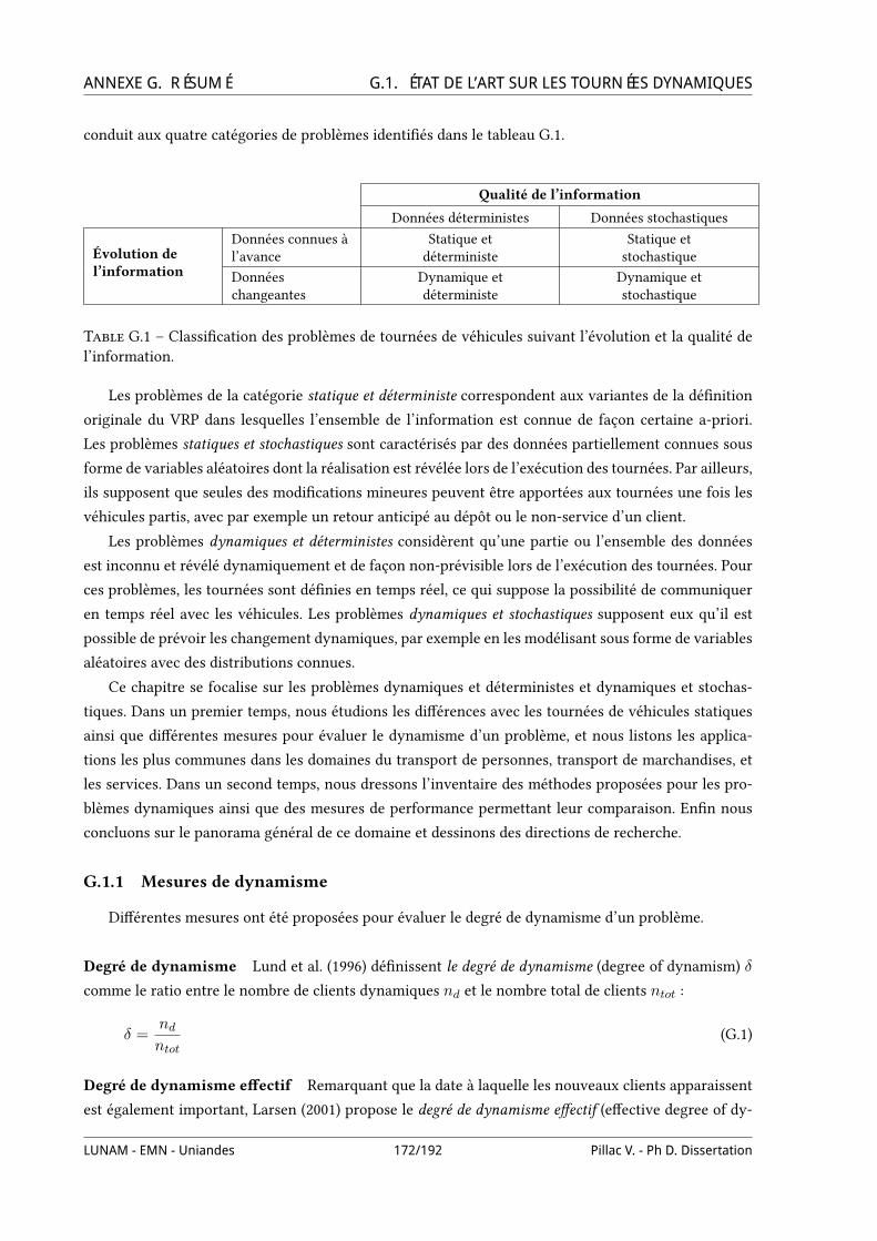
ANNEXE G. RÉSUMÉ G.1. ÉTAT DE L’ART SUR LES TOURNÉES DYNAMIQUESconduit aux quatre catégories de problèmes identiVés dans le tableau G.1.
Qualité de l’information
Données déterministes Données stochastiques
Évolution del’information
Données connues àl’avance
Statique etdéterministe
Statique etstochastique
Donnéeschangeantes
Dynamique etdéterministe
Dynamique etstochastique
Table G.1 – ClassiVcation des problèmes de tournées de véhicules suivant l’évolution et la qualité del’information.
Les problèmes de la catégorie statique et déterministe correspondent aux variantes de la déVnition
originale du VRP dans lesquelles l’ensemble de l’information est connue de façon certaine a-priori.
Les problèmes statiques et stochastiques sont caractérisés par des données partiellement connues sous
forme de variables aléatoires dont la réalisation est révélée lors de l’exécution des tournées. Par ailleurs,
ils supposent que seules des modiVcations mineures peuvent être apportées aux tournées une fois les
véhicules partis, avec par exemple un retour anticipé au dépôt ou le non-service d’un client.
Les problèmes dynamiques et déterministes considèrent qu’une partie ou l’ensemble des données
est inconnu et révélé dynamiquement et de façon non-prévisible lors de l’exécution des tournées. Pour
ces problèmes, les tournées sont déVnies en temps réel, ce qui suppose la possibilité de communiquer
en temps réel avec les véhicules. Les problèmes dynamiques et stochastiques supposent eux qu’il est
possible de prévoir les changement dynamiques, par exemple en les modélisant sous forme de variables
aléatoires avec des distributions connues.
Ce chapitre se focalise sur les problèmes dynamiques et déterministes et dynamiques et stochas-
tiques. Dans un premier temps, nous étudions les diUérences avec les tournées de véhicules statiques
ainsi que diUérentes mesures pour évaluer le dynamisme d’un problème, et nous listons les applica-
tions les plus communes dans les domaines du transport de personnes, transport de marchandises, et
les services. Dans un second temps, nous dressons l’inventaire des méthodes proposées pour les pro-
blèmes dynamiques ainsi que des mesures de performance permettant leur comparaison. EnVn nous
concluons sur le panorama général de ce domaine et dessinons des directions de recherche.
G.1.1 Mesures de dynamisme
DiUérentes mesures ont été proposées pour évaluer le degré de dynamisme d’un problème.
Degré de dynamisme Lund et al. (1996) déVnissent le degré de dynamisme (degree of dynamism) δ
comme le ratio entre le nombre de clients dynamiques nd et le nombre total de clients ntot :
δ =ndntot
(G.1)
Degré de dynamisme eUectif Remarquant que la date à laquelle les nouveaux clients apparaissent
est également important, Larsen (2001) propose le degré de dynamisme eUectif (eUective degree of dy-
LUNAM - EMN - Uniandes 172/192 Pillac V. - Ph D. Dissertation
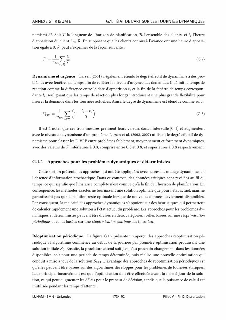
ANNEXE G. RÉSUMÉ G.1. ÉTAT DE L’ART SUR LES TOURNÉES DYNAMIQUESnamism) δe. Soit T la longueur de l’horizon de planiVcation, R l’ensemble des clients, et ti l’heure
d’apparition du client i ∈ R. En supposant que les clients connus à l’avance ont une heure d’appari-
tion égale à 0, δe peut s’exprimer de la façon suivante :
δe =1
ntot
∑i∈R
tiT
(G.2)
Dynamisme et urgence Larsen (2001) a également étendu le degré eUectif de dynamisme à des pro-
blèmes avec fenêtres de temps aVn de reWéter le niveau d’urgence des demandes. Il déVnit le temps de
réaction comme la diUérence entre la date d’apparition ti et la Vn de la fenêtre de temps correspon-
dante li, soulignant que les temps de réaction plus longs introduisent une plus grande Wexibilité pour
insérer la demande dans les tournées actuelles. Ainsi, le degré de dynamisme est étendue comme suit :
δeTW =1
ntot
∑i∈R
(1− li − ti
T
)(G.3)
Il est à noter que ces trois mesures prennent leurs valeurs dans l’intervalle [0, 1] et augmentent
avec le niveau de dynamisme d’un problème. Larsen et al. (2002, 2007) utilisent le degré eUectif de dy-
namisme pour classer les D-VRP entre problèmes faiblement, moyennement et fortement dynamiques,
avec des valeurs de δe inférieures à 0.3, comprise entre 0.3 et 0.8, et supérieures à 0.8 respectivement.
G.1.2 Approches pour les problèmes dynamiques et déterministes
Cette section présente les approches qui ont été appliquées avec succès au routage dynamique, en
l’absence d’information stochastique. Dans ce contexte, des données critiques sont révélées au Vl du
temps, ce qui signiVe que l’instance complète n’est connue qu’à la Vn de l’horizon de planiVcation. En
conséquence, les méthodes exactes ne fournissent une solution optimale que pour l’état actuel, mais ne
garantissent pas que la solution reste optimale lorsque de nouvelles données deviennent disponibles.
Par conséquent, la majorité des approches dynamiques s’appuient sur des heuristiques qui permettent
de calculer rapidement une solution à l’état actuel du problème. Les approches pour les problèmes dy-
namiques et déterministes peuvent être divisés en deux catégories : celles basées sur une réoptimisation
périodique, et celles basées sur une réoptimisation continue des tournées.
Réoptimisation périodique La Vgure G.1.2 présente un aperçu des approches réoptimisation pé-
riodique : l’algorithme commence au début de la journée par première optimisation produisant une
solution initiale S0. Ensuite, la procédure attend soit jusqu’au prochain changement dans les données
disponibles, soit pour une période de temps déterminée, puis réalise une nouvelle optimisation qui
conduit à mise à jour de la solution St+1. L’avantage des approches de réoptimisation périodiques est
qu’elles peuvent être basées sur des algorithmes développés pour les problèmes de tournées statiques.
Leur principal inconvénient est que l’optimisation doit être eUectuée avant la mise à jour de la solu-
tion, ce qui peut augmenter les délais pour le preneur de décision, tandis que la puissance de calcul est
inutilisée pendant les temps d’attente.
LUNAM - EMN - Uniandes 173/192 Pillac V. - Ph D. Dissertation

ANNEXE G. RÉSUMÉ G.1. ÉTAT DE L’ART SUR LES TOURNÉES DYNAMIQUESStart
Optimize
End of day?
NO
YES
Optimize Updated solution St+1
End
Wait for update
Initial solution S0
Figure G.2 – Approches de réoptimisation périodique
Decision loopOptimization loop
Start
Update
End of day?
NO
YES
Optimize
End
Wait for update
Adaptivememory
End of day?
NO
YES
Make decision
End
Updated solution St+1
Optimize Initial solution S0
Figure G.3 – Approches de réoptimisation continue
Réoptimisation continue Les approches dites de réoptimisation continue sont basées sur un al-
gorithme d’optimisation qui s’execute tout au long de la journée. Comme l’illustre la Figure G.1.2,
la boucle d’optimisation stocke ses résultats dans une mémoire adaptative. En parallèle, une seconde
boucle utilise les données de la mémoire adaptative pour prendre des décisions, par exemple pour dé-
cider si un nouveau client peut être servi ou non, ou pour sélectionner le prochain client à aUecter à
un véhicule. L’avantage de ces approches est que l’utilisation de la puissance de calcul est maximisée,
au prix d’une implémentation plus complexe.
G.1.3 Approches pour les problèmes dynamiques et stochastiques
Les problèmes de tournées dynamiques et stochastiques peuvent être vus comme une extension de
leurs homologues déterministes, dans lesquels les données dynamiquement révélées peuvent être mo-
delées comme un processus stochastique. Les approches pour cette classe de problèmes peuvent être
LUNAM - EMN - Uniandes 174/192 Pillac V. - Ph D. Dissertation

ANNEXE G. RÉSUMÉ G.2. TOURNÉES DYNAMIQUES ET DÉTERMINISTESdivisées en deux catégories : celles basées sur l’échantillonnage et celles basées sur la modélisation sto-
chastique. Comme leur nom l’indique, les stratégies d’échantillonage incorporent les informations sto-
chastiques en générant des scénarios basés sur une réalisation possible des variables aléatoires. Chaque
scénario est ensuite optimisé par la résolution du problème statique et déterministe qu’il déVnit. Les ap-
proches basées sur la modélisation stochastique intègrent quant à elles les informations stochastiques
analytiquement. L’avantage de l’échantillonnage est sa relative simplicité et sa Wexibilité, tandis que
son inconvénient est qu’il peut requérir de générer un grand nombre de scénarios pour reWéter Vdèle-
ment la réalité. Alternativement, les stratégies de modélisation stochastique saisissent formellement la
nature stochastique du problème, mais leur formulation et les algorithmes d’optimisation sous-jacents
sont plus complexes.
Référence de l’article présenté dans ce chapitre :
– Pillac, V., Gendreau, M., Guéret, C., and Medaglia, A. L. (2011) A review of dynamic vehicle
routing problems European Journal of Operational Research, Accepted manuscript,
doi :10.1016/j.ejor.2012.08.015.
Des versions précédentes de cet article ont été publiées comme rapports techniques avec réfé-
rences :
– Pillac, V., Gendreau, M., Guéret, C., and Medaglia, A. L. (2011) A review of dynamic vehicle
routing problems Technical report, CIRRELT. CIRRELT-2011-62.
– Pillac, V., Guéret, C., and Medaglia, A. L. (2010) Dynamic Vehicle Routing : State of the Art and
Prospects Technical report, École des Mines de Nantes, France. Report 10/4/AUTO.
G.2 Tournées dynamiques et déterministes
Dans ce chapitre nous proposons une méthode de réoptimisation rapide pour les tournées de vé-
hicules dynamiques et nous étudions des aspects bi-objectifs liés à la prise en compte de la constance
des tournées au cours de la journée.
G.2.1 Méthode de réoptimisation rapide
La méthode de réoptimisation proposée est basée sur l’algorithme de recherche adaptative à voisi-
nage large ALNS (Adaptive Large Neighborhood Search) proposée par Pisinger and Ropke (2007), lui
même une extension de la recherche à voisinages larges LNS (Large Neighborhood Search) introduite
par Shaw (1998). LNS consiste a successivement détruire puis réparer une solution courante. ALNS ra-
joute une couche adaptive qui sélectionne aléatoirement les opérateurs de destruction et de réparation
en fonction de leur performance antérieure.
L’algorithme G.1 présente l’approche ALNS. ALNS part d’une solution initiale Π0, puis, pour I ité-
rations l’algorithme choisit un opérateur de destruction et un opérateur de réparation (ligne 4) avec une
roulette qui reWète leur performance passée. Les opérateurs de destruction enlèvent un sous-ensemble
de clients de la solution courante, alors que les opérateurs de réparation les réinsèrent en utilisant
LUNAM - EMN - Uniandes 175/192 Pillac V. - Ph D. Dissertation
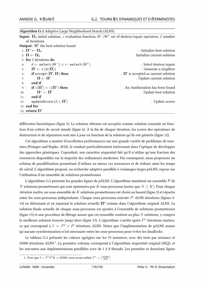
ANNEXE G. RÉSUMÉ G.2. TOURNÉES DYNAMIQUES ET DÉTERMINISTESAlgorithm G.1 Adaptive Large Neighborhood Search (ALNS)
Input: Π0 initial solution, z evaluation function, Θ−/Θ+ set of destroy/repair operators, I numberof iterations
Output: Π∗ the best solution found1: Π∗ ← Π0 . Initialize best solution2: Π← Π0 . Initialize current solution3: for I iterations do4: d← select (Θ−) ; r ← select (Θ+) . Select destroy/repair5: Π′ ← r (d (Π)) . Generate a neighbor6: if accept (Π′,Π) then . Π′ is accepted as current solution7: Π← Π′ . Update current solution8: end if9: if z(Π′) < z(Π∗) then . An Amélioration has been found10: Π∗ ← Π′ . Update best solution11: end if12: updateScore (d, r,Π′) . Update scores13: end for14: return Π∗
diUérentes heuristiques (ligne 5). La solution obtenue est acceptée comme solution courante en fonc-
tion d’un critère de recuit simulé (ligne 6). À la Vn de chaque itération, les scores des opérateurs de
destruction et de réparation sont mis à jour en fonction de la solution qu’ils ont générée (ligne 12).
Cet algorithme a montré d’excellentes performances sur une grande variété de problèmes de tour-
nées (Pisinger and Ropke, 2010), le rendant particulièrement intéressant dans l’optique de développer
des approches génériques. Cependant, son caractère séquentiel fait qu’il n’utilise qu’une fraction des
ressources disponibles sur la majorité des ordinateurs modernes. Par conséquent, nous proposons un
schéma de parallélisation permettant d’utiliser au mieux ces ressources et de réduire ainsi les temps
de calcul. L’algorithme proposé, ou recherche adaptive parallèle à voisinages larges pALNS, repose sur
l’utilisation d’un ensemble de solutions prometteuses.
L’algorithme G.2 présente les grandes lignes de pALNS. L’algorithme maintient un ensemble P de
N solutions prometteuses qui sont optimisées parK sous-processus (notez queN ≥ K). Pour chaque
itération maître, un sous-ensemble deK solutions prometteuses est choisi au hasard (ligne 2) et répartis
entre les sous-processus indépendants. Chaque sous-processus exécute Ip ALNS itérations (lignes 3-
14) en détruisant et en réparant la solution actuelle Πp comme dans l’algorithme original ALNS. La
solution Vnale actuelle de chaque sous-processus est ajoutée à l’ensemble de solutions prometteuses
(ligne 13) et une procédure de Vltrage assure que cet ensemble contient au plusN solutions, y compris
la meilleure solution trouvée jusqu’alors (ligne 15). L’algorithme s’arrête après Im itérations maitres,
ce qui correspond à I = Im × Ip itérations ALNS. Notez que l’implémentation de pALNS assure
qu’aucune synchronisation n’est nécessaire entre les sous-processus pour éviter les deadlocks.
Le tableau G.2 présente les valeurs agrégées sur les 53 instances, avec dix tests par instance et
25000 itérations ALNS 1. La première colonne correspond à l’algorithme séquentiel original (SEQ), et
les suivantes aux implémentations parallèles avec de 1 à 8 threads. Les première et deuxième lignes
1. Pour que I = ImIpK ' 25000, nous avons utilisé Im =⌈
2500040K
⌉LUNAM - EMN - Uniandes 176/192 Pillac V. - Ph D. Dissertation

ANNEXE G. RÉSUMÉ G.2. TOURNÉES DYNAMIQUES ET DÉTERMINISTESAlgorithm G.2 Parallel Adaptive Large Neighborhood Search (pALNS)
Input: P initial solutions, z evaluation function, Θ−/Θ+ set of destroy/repair operators,N maximumsize of the solution pool, K number of subprocesses, Im number of master iterations, Ip numberof iterations performed in parallel.
Output: Π∗, the best solution found1: for Im iterations do2: P ′ ← selectSubset (P,K) . Select a subset ofK solutions3: parallel forall Π in P ′ do4: Πp ← Π . Current solution for this subprocess5: for Ip iterations do6: d← select (Θ−) ; r ← select (Θ+) . Select destroy/repair7: Π′ ← r (d (Πp)) . Destroy and repair current solution8: if accept (Π′,Πp) then9: Πp ← Π′ . Π′ is accepted as current solution10: end if11: updateScore (d, r,Π′) . Update d and r scores12: end for13: P ← P ∪ Πp . Add Πp to the pool P14: end forall15: P ← retain (P, N) . Retain at most N solutions in the pool P16: end for17: return Π∗ = arg minΠ∈P z(Π)
contiennent la moyenne et l’écart-type des écarts aux meilleures solutions connues ou solutions opti-
males. EnVn, les troisième et quatrième lignes indiquent la moyenne et l’écart type des temps de calcul.
Notez que l’augmentation du nombre de threads a un impact limité sur l’écart avec les meilleures solu-
tions connues, lequel est toujours autour de 0,6%, mais elle permet une réduction des temps d’exécution
par un facteur 3,3.
Parallèle - Nombre de ThreadsSeq. 1 2 3 4 5 6 7 8
Ecart 0.74% 0.72% 0.55% 0.69% 0.54% 0.70% 0.52% 0.66% 0.48%Ecart (dev. st.) 0.87% 0.88% 0.76% 0.89% 0.70% 0.86% 0.74% 0.82% 0.66%Temps (s) 36.58 37.32 22.07 17.60 14.70 14.69 13.39 12.37 11.32Temps (s, dev. st.) 6.27 6.33 4.06 3.17 2.72 2.57 2.50 2.27 2.15
Table G.2 – Comparaison de l’écart avec les meilleurs et temps de calcul pour diUérents niveaux deparallélisation.
La Vgure G.4 illustre l’approche de réoptimisation proposée : l’algorithme commence par produire
une solution initiale S0 en utilisant une heuristique constructive couplé avec l’algorithme pALNS décrit
dans la section précédente. Ensuite, chaque fois qu’un nouveau client apparaît, il Vxe la partie en cours
d’exécution des tournées, et réexécute pALNS pour un nombre limité d’itérations pour produire une
solution mise à jour S′t. Si pALNS est capable d’insérer la demande de nouveaux clients, le client est
accepté et S′t devient la nouvelle solution courante, sinon le client est rejeté et St est maintenue comme
solution actuelle.
Le tableau G.3 présente l’écart moyen entre la solution produite par la méthode de réoptimisation
LUNAM - EMN - Uniandes 177/192 Pillac V. - Ph D. Dissertation
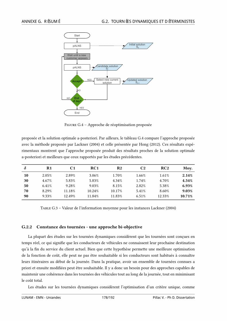
ANNEXE G. RÉSUMÉ G.2. TOURNÉES DYNAMIQUES ET DÉTERMINISTESStart
pALNS
End of day?
NO
YES
pALNS
Updated solution St+1
End
NO
Wait until a new customer appears
Initial solution S0
Accept? Select new currentsolution
YES
Candidate solutionSt'
Figure G.4 – Approche de réoptimisation proposée
proposée et la solution optimale a-posteriori. Par ailleurs, le tableau G.4 compare l’approche proposée
avec la méthode proposée par Lackner (2004) et celle présentée par Hong (2012). Ces résultats expé-
rimentaux montrent que l’approche proposée produit des résultats proches de la solution optimale
a-posteriori et meilleurs que ceux rapportés par les études précédentes.
δ R1 C1 RC1 R2 C2 RC2 Moy.
10 2.05% 2.89% 3.06% 1.70% 1.66% 1.61% 2.14%30 4.67% 5.83% 5.83% 4.34% 1.74% 4.70% 4.54%50 6.41% 9.28% 9.03% 8.15% 2.82% 5.38% 6.93%70 8.29% 11.18% 10.24% 10.17% 5.41% 8.60% 9.03%90 9.33% 12.49% 11.84% 11.83% 6.51% 12.33% 10.71%
Table G.3 – Valeur de l’information moyenne pour les instances Lackner (2004)
G.2.2 Constance des tournées - une approche bi-objective
La plupart des études sur les tournées dynamiques considèrent que les tournées sont conçues en
temps réel, ce qui signiVe que les conducteurs de véhicules ne connaissent leur prochaine destination
qu’à la Vn du service du client actuel. Bien que cette hypothèse permette une meilleure optimisation
de la fonction de coût, elle peut ne pas être souhaitable si les conducteurs sont habitués à connaître
leurs itinéraires au début de la journée. Dans la pratique, avoir un ensemble de tournées connues a
priori et ensuite modiVées peut être souhaitable. Il y a donc un besoin pour des approches capables de
maintenir une cohérence dans les tournées des véhicules tout au long de la journée, tout en minimisant
le coût total.
Les études sur les tournées dynamiques considèrent l’optimisation d’un critère unique, comme
LUNAM - EMN - Uniandes 178/192 Pillac V. - Ph D. Dissertation

ANNEXE G. RÉSUMÉ G.2. TOURNÉES DYNAMIQUES ET DÉTERMINISTES
pALNS Hong (2012) Lackner (2004)
Groupe δ Dist. Rej. Dist. Rej. Dist. Rej.
R1 10 1197.4 0.25 1257.1 ( 4.99%) 0.17 1278.1 ( 6.74%) 0.4730 1212.9 0.80 1286.6 ( 6.08%) 0.58 1337.9 ( 10.30%) 0.7250 1225.0 1.25 1295.8 ( 5.78%) 0.67 1330.0 ( 8.57%) 0.7870 1237.3 1.71 1331.3 ( 7.60%) 1.75 1336.1 ( 7.98%) 0.9490 1230.1 2.55 1335.9 ( 8.60%) 2.33 1278.3 ( 3.92%) 0.75
C1 10 850.6 0.11 895.8 ( 5.31%) 0.22 996.4 ( 17.14%) 0.0030 874.9 0.11 962.1 ( 9.97%) 0.33 1066.9 ( 21.95%) 0.0050 903.4 0.11 1001.2 ( 10.82%) 0.22 1236.1 ( 36.82%) 0.0070 919.1 0.11 1031.7 ( 12.25%) 0.22 1261.3 ( 37.24%) 0.0090 929.9 0.11 1039.8 ( 11.81%) 0.22 1479.6 ( 59.11%) 0.00
RC1 10 1389.4 0.04 1436.2 ( 3.37%) 1.13 1426.9 ( 2.70%) 0.4630 1421.5 0.28 1492.2 ( 4.98%) 1.13 1439.7 ( 1.28%) 0.4250 1463.4 0.23 1514.7 ( 3.50%) 1.38 1448.1 ( -1.05%) 0.4670 1470.1 0.58 1511.3 ( 2.80%) 1.88 1488.4 ( 1.25%) 0.5890 1495.5 0.51 1513.9 ( 1.23%) 2.00 1475.2 ( -1.36%) 0.42
R2 10 893.0 0.00 950.0 ( 6.39%) 0.09 1052.9 ( 17.90%) 0.0330 915.6 0.00 985.5 ( 7.63%) 0.00 1085.4 ( 18.54%) 0.1550 948.6 0.00 1016.5 ( 7.17%) 0.00 1138.8 ( 20.05%) 0.2170 967.7 0.00 1032.0 ( 6.65%) 0.09 1116.9 ( 15.42%) 0.3090 981.7 0.00 1047.8 ( 6.73%) 0.09 1193.3 ( 21.55%) 0.52
C2 10 597.2 0.00 594.7 ( -0.42%) 0.00 629.1 ( 5.35%) 0.0030 597.6 0.00 651.4 ( 9.01%) 0.00 632.3 ( 5.81%) 0.0450 604.0 0.00 605.0 ( 0.17%) 0.00 689.3 ( 14.12%) 0.1370 619.2 0.00 636.5 ( 2.79%) 0.00 743.8 ( 20.12%) 0.2190 625.7 0.00 636.8 ( 1.78%) 0.00 792.5 ( 26.66%) 0.29
RC2 10 1024.4 0.00 1103.3 ( 7.70%) 0.00 1220.9 ( 19.18%) 0.0030 1053.1 0.00 1166.0 ( 10.73%) 0.25 1244.9 ( 18.21%) 0.0450 1060.5 0.00 1190.5 ( 12.26%) 0.13 1244.9 ( 17.38%) 0.0070 1091.4 0.00 1239.5 ( 13.57%) 0.00 1269.3 ( 16.30%) 0.0090 1130.3 0.00 1257.2 ( 11.23%) 0.13 1346.8 ( 19.16%) 0.13
Moyenne 0.29 (+6.75%) 0.50 (+15.61%) 0.27
Table G.4 – Comparaison des approches pour les instances Lackner (2004).
LUNAM - EMN - Uniandes 179/192 Pillac V. - Ph D. Dissertation

ANNEXE G. RÉSUMÉ G.3. TOURNÉES DYNAMIQUES ET STOCHASTIQUESla minimisation de la distance totale parcourue ou la maximisation du nombre de clients desservis.
D’autre part, un nombre croissant d’études sur les tournées statiques prend en compte des objectifs
multiples dans le but de mieux répondre aux diUérents contextes opérationnels (Jozefowiez et al., 2008).
Dans cette section, nous présentons une étude préliminaire qui prend en compte la gêne des
conducteurs. L’approche proposée est une adaptation de l’algorithme pALNS qui minimise simulta-
nément une fonction de coût et maximise la constance des tournées tout au long de la journée. Les ré-
sultats expérimentaux préliminaires montrent que pour les instances faiblement dynamiques il semble
intéressant de favoriser la constance des tournées, alors que pour les instances fortement dynamiques
il est plus proVtable de ne considerer que la minimisation de la fonction de coût.
Référence de l’article présenté dans ce chapitre :
– Pillac, V., Guéret, C., and Medaglia, A. L. (2012) A fast re-optimization approach for dynamic
vehicle routing Technical report, École des Mines de Nantes, France. Report 12/6/AUTO.
Des résultats préliminaires sur le cas bi-objectifs ont été présentés à la conférence ROADEF 2012 :
– Pillac, V., Guéret, C., and Medaglia, A. L. (2012) Route stability in dynamic vehicle routing : a
bi-objective approach In ROADEF 2012, Angers, France.
G.3 Tournées dynamiques et stochastiques
Dans les problèmes de tournées dynamiques et stochastiques, tout ou partie des données n’est pas
connue initialement et est révélée dynamiquement au cours de l’exécution des tournées. Cependant, à
la diUérence des problèmes dynamiques et déterministes, des informations stochastiques exploitables
sont disponibles et permettent de prévoir les changements. Notre accent étant mis sur le développe-
ment de composants logiciels qui peuvent être utilisés pour une large gamme d’applications, nous
avons choisi de développer un framework (jMSA) orienté évènements basé sur l’approche multiples
scénarios MSA (Multiple Scenario Approach) proposé par Van Hentenryck and Bent (2006). Dans ce
chapitre, nous présentons le framework jMSA, son implémentation, puis nous illustrons la validité de
cette approche en abordant le problème de tournées dynamiques avec demandes stochastiques (D-
VRPSD).
G.3.1 Multiple Scenario Approach
MSA est une méthode de réoptimisation continue qui capture l’incertain en générant des scénarios
ensuite utilisés pour prendre les décisions.
La Vgure G.5 illustre la génération d’un scénario. En ne considérant que les clients connus actuel-
lement (G.5a.) la tournée optimale a-priori s’éloigne d’une région où des clients sont susceptibles d’ap-
paraître en début de matinée (zone verte). L’échantillonnage (G.5b.) génère des clients Vctifs dans cette
zone et permet d’orienter l’optimisation vers une tournée qui visite en premier cette région (G.5c.).
Une fois un nombre suXsant de scénarios généré, une procédure de décision est utilisée pour agréger
l’information contenue dans chacun des scénario aVn de prendre des décisions qui tiennent compte de
la stochasticité du problème.
LUNAM - EMN - Uniandes 180/192 Pillac V. - Ph D. Dissertation

ANNEXE G. RÉSUMÉ G.3. TOURNÉES DYNAMIQUES ET STOCHASTIQUES
A-priori optimal route
AM
B
C D
A
a. Tournées a-priori
Sampled customers
AM
B
C D
A X
YZ
b. Echantillonage
Route with sampled customers
AM
B
C D
A X
YZ
c. Tournées résultantes
Figure G.5 – Génération de scenarios dans MSA
G.3.2 Framework proposé
La Vgure G.6 présente une vue d’ensemble du framework proposé. Le composant central est MSA-
Procedure qui contient la logique générale de la méthode, et dont les paramètres sont déVnis dans
GlobalParameters. Notre implémentation repose sur une Vle d’évènements EventQueue. La procé-
dure principale extrait le premier évènement de la Vle et sélectionne le handler correspondant dans
le EventHandlerManager. Le handler contient la logique nécessaire au traitement de l’évènement à
un niveau indépendant du problème considéré. AVn d’assurer la généricité du framework, la logique
spéciVque à un problème est déléguée aux implémentations des diUérents composants, lesquels sont
gérés par le ComponentManager. Dans cet exemple, la logique relative à la génération d’un scena-
rio est déVnie par la classe concrète DVRPScenarioGenerator, qui implémente l’interface Scenario
Generator. EnVn, un système de callbacks permet à l’utilisateur d’interagir avec la méthode sans de-
voir modiVer le code du framework, via le CallbackManager et des implémentations de l’interface
Callback.
Un aspect important du framework est la parallélisation transparente des opérations les plus exi-
geantes en temps de calcul. La Vgure G.7 illustre les interactions entre threads (Vls d’exécution) dans le
framework jMSA. À l’instant t0, le thread MSA déVle un évènement OptimizePool, et le traite avec le
handler OptimizeHandler correspondant. En parallèle du thread MSA, deux nouveaux threads sont
créés par le ComponentManager pour optimiser les scénarios. À l’instant t1, un évènement préemptif
NewCustomer et un évènement Decision sont enVlés par l’environnement, causant l’arrêt prématuré
de l’optimisation. EnVn, la procédure déVle et traite l’évènement NewCustomer, lequel a une priorité
plus élevée que l’évènement Decision.
G.3.3 Résultats expérimentaux
La diUérence fondamentale entre le VRP classique et le VRP avec demandes stochastiques (VRPSD)
est que dans ce dernier les demandes des clients sont modélisées par des variables aléatoires. Le ca-
ractère aléatoire du VRPSD implique que la réalisation de la demande des clients peut dépasser la
capacité restante du véhicule, conduisant à l’échec de la tournée. Il est important de souligner que,
dans ce contexte, tous les clients sont connus à l’avance et la seule information révélée dynamique est
la réalisation de la demande des clients. Le VRPSD dynamique (D-VRPSD) est une extension du VRPSD
dans laquelle il est possible de rediriger les véhicules librement suivant la réalisation des demandes.
LUNAM - EMN - Uniandes 181/192 Pillac V. - Ph D. Dissertation
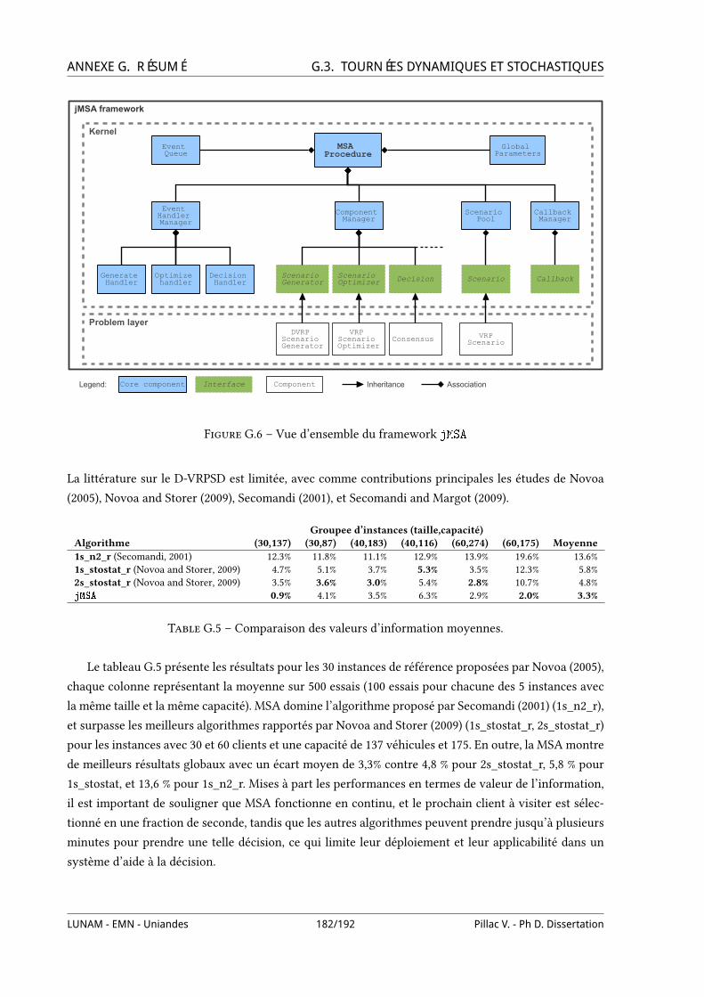
ANNEXE G. RÉSUMÉ G.3. TOURNÉES DYNAMIQUES ET STOCHASTIQUES
Problem layer
Kernel
MSA Procedure
Event Handler Manager
Callback Manager
Component Manager
Scenario Pool
Global Parameters
Generate Handler
Optimize handler
Decision Handler
Scenario Generator
Scenario Optimizer Decision Scenario
DVRP Scenario Generator
VRP Scenario Optimizer
Consensus VRPScenario
jMSA framework
Callback
ComponentInterface Inheritance AssociationCore componentLegend:
Event Queue
Figure G.6 – Vue d’ensemble du framework jMSA
La littérature sur le D-VRPSD est limitée, avec comme contributions principales les études de Novoa
(2005), Novoa and Storer (2009), Secomandi (2001), et Secomandi and Margot (2009).
Groupee d’instances (taille,capacité)Algorithme (30,137) (30,87) (40,183) (40,116) (60,274) (60,175) Moyenne1s_n2_r (Secomandi, 2001) 12.3% 11.8% 11.1% 12.9% 13.9% 19.6% 13.6%1s_stostat_r (Novoa and Storer, 2009) 4.7% 5.1% 3.7% 5.3% 3.5% 12.3% 5.8%2s_stostat_r (Novoa and Storer, 2009) 3.5% 3.6% 3.0% 5.4% 2.8% 10.7% 4.8%jMSA 0.9% 4.1% 3.5% 6.3% 2.9% 2.0% 3.3%
Table G.5 – Comparaison des valeurs d’information moyennes.
Le tableau G.5 présente les résultats pour les 30 instances de référence proposées par Novoa (2005),
chaque colonne représentant la moyenne sur 500 essais (100 essais pour chacune des 5 instances avec
la même taille et la même capacité). MSA domine l’algorithme proposé par Secomandi (2001) (1s_n2_r),
et surpasse les meilleurs algorithmes rapportés par Novoa and Storer (2009) (1s_stostat_r, 2s_stostat_r)
pour les instances avec 30 et 60 clients et une capacité de 137 véhicules et 175. En outre, la MSA montre
de meilleurs résultats globaux avec un écart moyen de 3,3% contre 4,8 % pour 2s_stostat_r, 5,8 % pour
1s_stostat, et 13,6 % pour 1s_n2_r. Mises à part les performances en termes de valeur de l’information,
il est important de souligner que MSA fonctionne en continu, et le prochain client à visiter est sélec-
tionné en une fraction de seconde, tandis que les autres algorithmes peuvent prendre jusqu’à plusieurs
minutes pour prendre une telle décision, ce qui limite leur déploiement et leur applicabilité dans un
système d’aide à la décision.
LUNAM - EMN - Uniandes 182/192 Pillac V. - Ph D. Dissertation

ANNEXE G. RÉSUMÉ G.3. TOURNÉES DYNAMIQUES ET STOCHASTIQUES
t1
t2
t0
Optimize
Termination
ComponentManager
Execute
Optimize
Dequeue
Handle new customer
Pool optimized callbacks
New customer callbacks
Handle optimize
Enqueue Generate scenario
MSA thread Callbacks threadEnvironment
Enqueue Decision
Dequeue
Enqueue New customer Preemptive event * Shutdown
Time
Legend:
Wait (blocking)
Send signal
Signal
Event queue operation
Event queueat time t
Task/Process
Optimize pool
Q(t0)
New customer
DecisionQ(t1)
New customer
Decision
Generate scenarios
Q(t2)
Q(t)
Figure G.7 – Parallelisation dans jMSA
Référence de l’article présenté dans ce chapitre :
– Pillac, V., Guéret, C., and Medaglia, A. L. (2012) An event-driven optimization fra-
mework for dynamic vehicle routing Decision Support Systems, Accepted manuscript
doi :10.1016/j.dss.2012.06.007.
Une version précédente de cet article a été publiée comme rapport technique :
– Pillac, V., Guéret, C., and Medaglia, A. L. (2011) An event-driven optimization framework
for dynamic vehicle routing Technical report, École des Mines de Nantes, France. Report
11/2/AUTO.
LUNAM - EMN - Uniandes 183/192 Pillac V. - Ph D. Dissertation

ANNEXE G. RÉSUMÉ G.4. TOURNÉES DE TECHNICIENS
Des résultats préliminaires ont été présentées dans deux conférences :
– Pillac, V., Guéret, C., and Medaglia, A. L. (2011) A dynamic approach for the vehicle routing
problem with stochastic demands In ROADEF 2011, St Etienne, France.
– Pillac, V., Guéret, C., and Medaglia, A. L. (2010) Solving the vehicle routing problem with sto-
chastic demands with a multiple scenario approach
In ALIO-INFORMS 2010, Buenos Aires (Argentina).
G.4 Application au problème de tournées de techniciens
Les deux articles présentées dans ce chapitre sont motivés par un problème d’optimisation réel pré-
senté par un partenaire industriel. Cette société fournit des solutions logicielles à destination d’organi-
sations gèrant une équipe de techniciens pour servir un ensemble de requêtes distribuées géographi-
quement. Ces requêtes peuvent être soit statiques soit dynamiques. Les requêtes statiques sont connues
à l’avance et correspondent aux rendez-vous avec des clients ou des opérations de maintenance pré-
ventive. Les demandes dynamiques apparaissent dynamiquement tout au long de la journée et sont, par
exemple, les situations d’urgence ou des opérations de maintenance corrective. Les requêtes peuvent
nécessiter un technicien avec des compétences diUérentes, un certain ensemble d’outils, et un certain
nombre de pièces de rechange. En outre, les techniciens commencent et terminent généralement leur
journée à leur domicile, et peuvent visiter un dépôt central pour récupérer des outils et des pièces de
rechange. EnVn, les objectifs comprennent la minimisation de la distance parcourue, la minimisation
du temps de travail, l’équilibrage de la charge de travail entre les techniciens, et la minimisation des
violations de contraintes.
A partir de cette application pratique, nous avons introduit un nouveau problème d’optimisation,
à savoir, le problème de planiVcation de tournées de technicien (TRSP - Technician Routing and Sche-
duling Problem) qui considère une équipe de techniciens K qui sert un ensemble de requêtes R. LeTRSP peut être vu comme une extension du problème de tournées de véhicules avec fenêtres de temps
(VRPTW), où les techniciens jouent le rôle de véhicules et les requêtes sont faites par les clients.
Comme illustré par la Vgure G.8, dans le TRSP, chaque technicien dispose d’un ensemble de com-
pétences, d’outils et de pièces de rechange, tandis que les requêtes nécessitent un sous-ensemble de
chaque. Le problème est alors de concevoir un ensemble de tournées tels que chaque requête soit vi-
sitée dans sa fenêtre de temps, par un technicien ayant les compétences, outils, et pièces de rechange
requises.
Un trait distinctif de ce problème est qu’il introduit plusieurs contraintes de compatibilité entre les
techniciens et les demandes. Si les compétences sont des attributs intrinsèques, les techniciens peuvent
disposer de diUérents outils et pièces de rechange sur l’horizon de planiVcation. Les techniciens com-
mencent leur tournée à leur domicile, avec un ensemble d’outils (ressources renouvelables) et de pièces
de rechange (consommées une fois que le technicien sert une requête) qui leur permettent de servir
une première série de requêtes. Les techniciens ont alors l’opportunité de renouveler leurs outils et
pièces de rechange dans un dépôt central à tout moment pour servir plus de requêtes.
Le TRSP se pose naturellement dans une large gamme d’applications, avec entre autres les télé-
communications, les services publics, et les opérations de maintenance. Cependant ce problème n’a
LUNAM - EMN - Uniandes 184/192 Pillac V. - Ph D. Dissertation
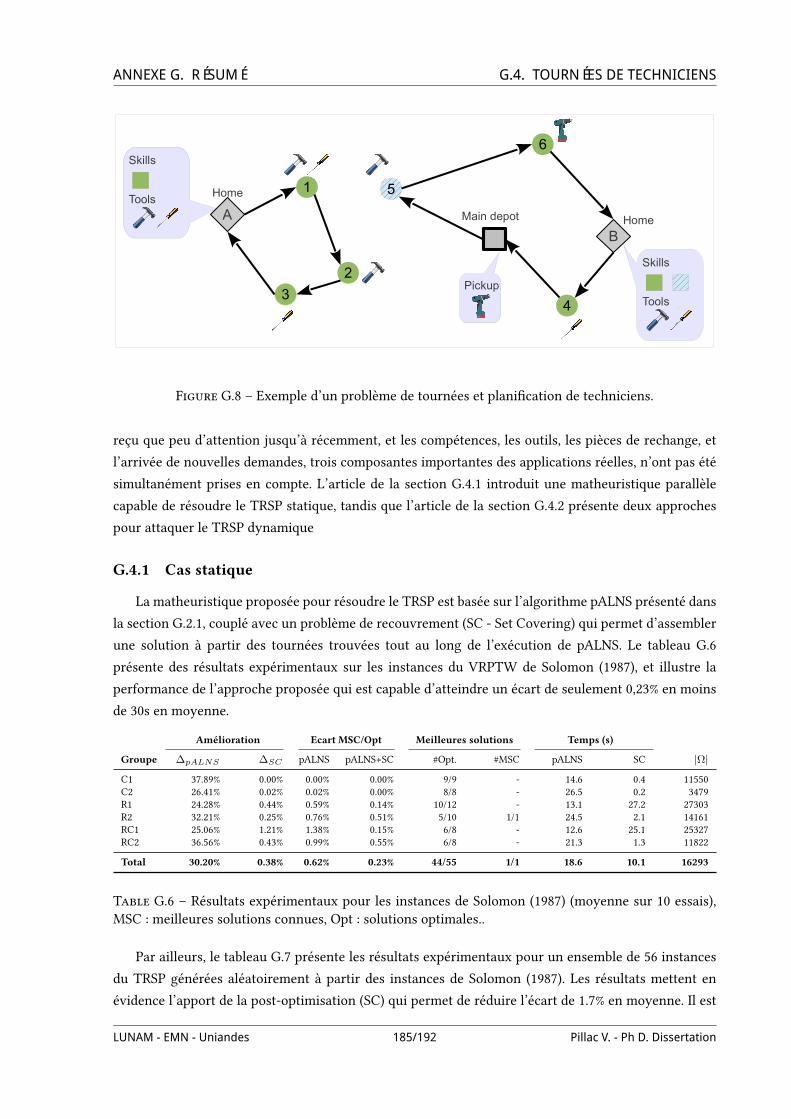
ANNEXE G. RÉSUMÉ G.4. TOURNÉES DE TECHNICIENS
Skills
Tools
A
B
1
6
3
5
2Pickup
4
Main depot
Home
Home
Skills
Tools
Figure G.8 – Exemple d’un problème de tournées et planiVcation de techniciens.
reçu que peu d’attention jusqu’à récemment, et les compétences, les outils, les pièces de rechange, et
l’arrivée de nouvelles demandes, trois composantes importantes des applications réelles, n’ont pas été
simultanément prises en compte. L’article de la section G.4.1 introduit une matheuristique parallèle
capable de résoudre le TRSP statique, tandis que l’article de la section G.4.2 présente deux approches
pour attaquer le TRSP dynamique
G.4.1 Cas statique
La matheuristique proposée pour résoudre le TRSP est basée sur l’algorithme pALNS présenté dans
la section G.2.1, couplé avec un problème de recouvrement (SC - Set Covering) qui permet d’assembler
une solution à partir des tournées trouvées tout au long de l’exécution de pALNS. Le tableau G.6
présente des résultats expérimentaux sur les instances du VRPTW de Solomon (1987), et illustre la
performance de l’approche proposée qui est capable d’atteindre un écart de seulement 0,23% en moins
de 30s en moyenne.
Amélioration Ecart MSC/Opt Meilleures solutions Temps (s)
Groupe ∆pALNS ∆SC pALNS pALNS+SC #Opt. #MSC pALNS SC |Ω|
C1 37.89% 0.00% 0.00% 0.00% 9/9 - 14.6 0.4 11550C2 26.41% 0.02% 0.02% 0.00% 8/8 - 26.5 0.2 3479R1 24.28% 0.44% 0.59% 0.14% 10/12 - 13.1 27.2 27303R2 32.21% 0.25% 0.76% 0.51% 5/10 1/1 24.5 2.1 14161RC1 25.06% 1.21% 1.38% 0.15% 6/8 - 12.6 25.1 25327RC2 36.56% 0.43% 0.99% 0.55% 6/8 - 21.3 1.3 11822
Total 30.20% 0.38% 0.62% 0.23% 44/55 1/1 18.6 10.1 16293
Table G.6 – Résultats expérimentaux pour les instances de Solomon (1987) (moyenne sur 10 essais),MSC : meilleures solutions connues, Opt : solutions optimales..
Par ailleurs, le tableau G.7 présente les résultats expérimentaux pour un ensemble de 56 instances
du TRSP générées aléatoirement à partir des instances de Solomon (1987). Les résultats mettent en
évidence l’apport de la post-optimisation (SC) qui permet de réduire l’écart de 1.7% en moyenne. Il est
LUNAM - EMN - Uniandes 185/192 Pillac V. - Ph D. Dissertation
ANNEXE G. RÉSUMÉ G.4. TOURNÉES DE TECHNICIENSégalement à noter que les temps de calcul pour la post-optimisation (SC) sont nettement supérieurs
à ceux observés pour le VRPTW, ce qui peut être attribué à des contraintes additionnelles dans le
problème de recouvrement.
Amélioration Ecart MSC Temps (s)
Groupe ∆SC pALNS pALNS+SC pALNS SC |Ω|
C1 0.97% 1.22% 0.23% 24.0 388.9 67020C2 0.35% 0.78% 0.42% 27.8 23.6 39334R1 3.62% 4.96% 0.82% 28.9 500.2 30783R2 0.23% 1.69% 1.46% 31.0 42.1 24396RC1 3.06% 3.90% 0.68% 27.9 185.8 18638RC2 0.49% 1.93% 1.43% 27.9 15.6 16917
Total 1.53% 2.54% 0.86% 28.1 210.1 32858
Table G.7 – Résultats expérimentaux pour 56 instances générées aléatoirement.
Référence de l’article présenté dans ce chapitre :
– Pillac, V., Guéret, C., and Medaglia, A. L. (2011) A parallel matheuristic for the technician rou-
ting and scheduling problem Optimization Letters, Accepted manuscript, doi :10.1007/s11590-
012-0567-4.
Des résultats préliminaires de ce travail ont été présentés à la conférence MIC 2011 :
– Pillac, V., Guéret, C., and Medaglia, A. L. (2011) On the technician routing and scheduling pro-
blem In Di Gaspero, L., Schaerf, A., and Stützle, T., editors, Proceedings of the 9th Metaheuristics
Conference (MIC 2011), pages 675–678. Università degli Studi di Udine.
G.4.2 Cas dynamique
Nous avons traité le cas dynamique du TRSP avec trois approches : la réoptimisation rapide basée
sur pALNS proposée dans la section G.2.1 ; une approche par plans multiples MPA (Multiple Plan
Approach), qui est une réduction au cas déterministe de MSA, implémentée dans le framework jMSA ;
et une heuristique simple (regret-3) permettant de modéliser le comportement d’un preneur de décision
humain.
pALNS MPA regret-3
δ Ecart (%) Rej. Ecart (%) Rej. Ecart (%) Rej.
10 2.4 0.1 9.1 1.9 10.5 0.330 5.4 0.1 11.0 4.6 30.5 0.450 10.8 0.3 14.4 5.6 44.1 1.070 11.8 0.2 21.3 8.7 57.5 1.290 17.9 0.4 23.9 8.1 64.1 1.4
Moy. 9.7 0.2 16.1 5.9 41.3 0.8
Table G.8 – Ecart moyen avec la solution a-posteriori et nombre de requêtes rejetées (Rej.) pour lesinstances du D-TRSP en minimisant la distance totale.
LUNAM - EMN - Uniandes 186/192 Pillac V. - Ph D. Dissertation
ANNEXE G. RÉSUMÉ G.5. CONCLUSIONSLe tableau G.8 présente une comparaison de ces trois méthodes. Il apparaît que pALNS domine
clairement les deux autres approches tant en termes d’écart avec la solution a-posteriori, qu’en termes
de nombre de requêtes rejetées. Il est à noter cependant que les résultats de MPA sont à un stade
préliminaire, et donc perfectibles.
Référence de l’article présenté dans ce chapitre :
– Pillac, V., Guéret, C., and Medaglia, A. L. (2011) On the dynamic technician routing and sche-
duling problem Technical report 12/5/AUTO.
Des travaux préliminaires ont été présentés aux conférences suivantes :
– Pillac, V., Guéret, C., and Medaglia, A. L. (2012) A Multiple Plan Approach for the Dynamic
Technician Routing and Scheduling Problem In 25th European Conference on Operational Re-
search (EURO 2012), Vilnius, Lithuania.
– Pillac, V., Guéret, C., and Medaglia, A. L. (2012) On the dynamic technician routing and sche-
duling problem In Proceedings of the 5th International Workshop on Freight Transportation and
Logistics (ODYSSEUS 2012), Mykonos, Greece.
G.5 Conclusions
Les progrés technologiques récents fournissent aux organisations les outils adaptés pour gérer leur
Wotte en temps réel. Cependant, ces nouvelles technologies introduisent également plus de complexité
dans la gestion des Wottes de véhicules, révélant un besoin pour des systèmes d’aide à la décision dédiés
aux problèmes de tournées de véhicules dynamiques. Dans ce contexte, les contributions de la présente
thèse sont les suivantes : premièrement, nous avons présenté une étude exhaustive de la littérature ;
deuxièmement, nous avons conçu, implémenté, et rendu publiques des frameworks d’optimisation à
la fois Wexibles et extensibles capables de traiter une grande variété de problèmes de tournées dyna-
miques ; et troisièmement, nous avons déVni et attaqué un problème de tournées rencontré par un
partenaire industriel.
Nous estimons que les travaux futurs devraient se centrer autour du développement d’approches
de réoptimisation continue simples et Wexibles, par exemple en étendant l’algorithme pALNS présenté
dans cette thèse. Il serait également intéressant de trouver des stratégies pour limiter la complexité des
problèmes d’optimisation sous-jacents, par exemple en mettant plus d’eUort sur l’optimisation du futur
proche, ou en éliminant des scénarios trop pessimistes. EnVn, une attention particulière devrait être
mise sur la conception de nouvelles procédures permettant de consolider l’information contenue dans
un ensemble de scénarios pour prendre de meilleurs décisions en un temps plus court.
La gestion en temps réel d’une Wotte de véhicules soulève de nombreux problèmes, tant théoriques
que pratiques, et nécessite le développement d’algorithmes rapides et eXcaces. Bien que ce domaine
ait reçu un intérêt croissant au cours des dernières décennies, il existe toujours de nombreuses op-
portunités de recherche et nous espérons que la présente thèse sera une source de réWexion pour des
travaux futurs.
LUNAM - EMN - Uniandes 187/192 Pillac V. - Ph D. Dissertation

ANNEXE G. RÉSUMÉ BIBLIOGRAPHIEBibliographie
Baldacci, R., Toth, P., and Vigo, D. (2007). Recent advances in vehicle routing exact algorithms. 4OR : A QuarterlyJournal of Operations Research, 5(4) :269–298, doi :10.1007/s10288-007-0063-3.
Cordeau, J.-F., Laporte, G., Savelsbergh, M. W., and Vigo, D. (2007). Vehicle routing. In Barnhart, C. and Laporte,G., editors, Transportation, volume 14 of Handbooks in Operations Research and Management Science, chapter 6,pages 367–428. Elsevier.
Dantzig, G. and Ramser, J. (1959). The truck dispatching problem. Management Science, 6(1) :80–91.
EEA (2011). Laying the foundations for greener transport – term 2011 : transport indicators tracking progresstowards environmental targets in Europe. Technical Report EEA Report No 7/2011, European EnvironmentAgency.
EIA (2011). Emission of greenhouse gases in the United States 2009. Technical Report DOE/EIA-0573(2009), U.S.Energy Information Administration.
Eksioglu, B., Vural, A. V., and Reisman, A. (2009). The vehicle routing problem : A taxonomic review. Computers& Industrial Engineering, 57(4) :1472 – 1483, doi :10.1016/j.cie.2009.05.009.
Flood, M. (1956). The traveling-salesman problem. Operations Research, 4(1) :61–75.
Hesse, M. and Rodrigue, J.-P. (2004). The transport geography of logistics and freight distribution. Journal ofTransport Geography, 12(3) :171 – 184, doi :10.1016/j.jtrangeo.2003.12.004.
Hong, L. (2012). An improved lns algorithm for real-time vehicle routing problem with time windows. Computers& Operations Research, 39(2) :151 – 163, doi :10.1016/j.cor.2011.03.006.
Jozefowiez, N., Semet, F., and Talbi, E.-G. (2008). Multi-objective vehicle routing problems. European Journal ofOperational Research, 189(2) :293 – 309, doi :10.1016/j.ejor.2007.05.055.
Lackner, A. (2004). Dynamische Tourenplanung mit ausgewählten Metaheuristiken. PhD thesis, Georg-August-Universität Göttingen.
Laporte, G. (2009). Fifty years of vehicle routing. Transportation Science, 43(4) :408–416,doi :10.1287/trsc.1090.0301.
Larsen, A. (2001). The Dynamic Vehicle Routing Problem. PhD thesis, Technical University of Denmark (DTU).
Larsen, A., Madsen, O. B. G., and Solomon, M. M. (2002). Partially dynamic vehicle routing - models and algo-rithms. The Journal of the Operational Research Society, 53(6) :637–646, doi :10.1057/palgrave.jors.2601352.
Larsen, A., Madsen, O. B. G., and Solomon, M. M. (2007). ClassiVcation of dynamic vehicle routing systems. InZeimpekis, V., Tarantilis, C. D., Giaglis, G. M., and Minis, I., editors, Dynamic Fleet Management, volume 38 ofOperations Research/Computer Science Interfaces Series, chapter 2, pages 19–40. Springer US.
Lund, K., Madsen, O. B. G., and Rygaard, J. M. (1996). Vehicle routing problems with varying degrees of dyna-mism. Technical report, IMM Institute of Mathematical Modelling.
Novoa, C. and Storer, R. (2009). An approximate dynamic programming approach for the vehicle rou-ting problem with stochastic demands. European Journal of Operational Research, 196(2) :509–515,doi :10.1016/j.ejor.2008.03.023.
Novoa, C. M. (2005). Static and dynamic approaches for solving the vehicle routing problem with stochastic demands.PhD thesis, Lehigh University, Pennsylvania, United States. AAT 3188502.
Pisinger, D. and Ropke, S. (2007). A general heuristic for vehicle routing problems. Computers & OperationsResearch, 34(8) :2403–2435, doi :10.1016/j.cor.2005.09.012.
LUNAM - EMN - Uniandes 188/192 Pillac V. - Ph D. Dissertation

ANNEXE G. RÉSUMÉ BIBLIOGRAPHIEPisinger, D. and Ropke, S. (2010). Large neighborhood search. In Gendreau, M. and Potvin, J.-Y., editors,Handbook
of Metaheuristics, volume 146 of International Series in Operations Research & Management Science, pages 399–419. Springer US.
Secomandi, N. (2001). A rollout policy for the vehicle routing problem with stochastic demands. OperationsResearch, 49(5) :796–802, doi :10.1287/opre.49.5.796.10608.
Secomandi, N. and Margot, F. (2009). Reoptimization approaches for the vehicle-routing problem with stochasticdemands. Operations Research, 57(1) :214–230, doi :10.1287/opre.1080.0520.
Shaw, P. (1998). Using constraint programming and local search methods to solve vehicle routing problems. InPrinciples and Practice of Constraint Programming – CP98, volume 1520 of Lecture Notes in Computer Science,pages 417–431. Springer Berlin / Heidelberg.
Solomon, M. M. (1987). Algorithms for the vehicle-routing and scheduling problems with time windowconstraints. Operations Research, 35(2) :254–265.
Toth, P. and Vigo, D., editors (2002). The vehicle routing problem, volume 9 ofMonographs on Discrete Mathematicsand Applications. SIAM Philadelphia.
Van Hentenryck, P. and Bent, R. (2006). Online stochastic combinatorial optimization. MIT Press.
LUNAM - EMN - Uniandes 189/192 Pillac V. - Ph D. Dissertation
Thèse de Doctorat
Victor PillacDynamic vehicle routing:solution methods and computational toolsMéthodes de résolution et outils informatiquespour les tournées de véhicules dynamiques
RésuméLes activités de transport jouent un rôle crucial au-tant dans le domaine de la production que danscelui des services. En particulier, elles permettentd’assurer la distribution de biens et de servicesentre fournisseurs, unités de production, entre-pôts, distributeurs, et clients finaux. Plus spécifi-quement, les problèmes de tournées de véhicules(VRP) considèrent la mise au point d’un ensemblede tournées de coût minimal servant la demandeen biens ou en services d’un ensemble de clientsdistribués géographiquement, tout en vérifiant unensemble de contraintes opérationnelles. Alorsqu’il s’agissait d’un problème statique, des avan-cées technologiques récentes permettent aux or-ganisations de gérer leur flotte de véhicules entemps réel. Cependant, ces nouvelles technolo-gies introduisent également une plus grande com-plexité dans les tâches de gestion de flotte, révé-lant une demande pour des outils d’aide à la dé-cision dédiés aux problèmes de tournées de vé-hicules dynamiques. Dans ce contexte, les contri-butions de la présente thèse de doctorat s’orga-nisent autour de trois axes : (i) elle présente unétat de l’art détaillé des problèmes de tournées dy-namiques ; (ii) elle introduit des frameworks d’opti-misation génériques adaptés à une grande variétéde problèmes ; (iii) elle définit un problème de tour-nées novateur et aux nombreuses applications.
AbstractWithin the wide scope of logistics management,transportation plays a central role and is a crucialactivity in both production and service industry.Among others, it allows for the timely distributionof goods and services between suppliers, produc-tion units, warehouses, retailers, and final custo-mers. More specifically, Vehicle Routing Problems(VRPs) deal with the design of a set of minimal-cost routes that serve the demand for goods orservices of a set of geographically spread custo-mers, satisfying a group of operational constraints.While it was traditionally a static problem, recenttechnological advances provide organizations withthe right tools to manage their vehicle fleet in realtime. Nonetheless, these new technologies alsointroduce more complexity in fleet managementtasks, unveiling the need for decision support sys-tems dedicated to dynamic vehicle routing. In thiscontext, the contributions of this Ph.D. thesis arethreefold : (i) it presents a comprehensive reviewof the literature on dynamic vehicle routing ; (ii)it introduces flexible optimization frameworks thatcan cope with a wide variety of dynamic vehiclerouting problems ; (iii) it defines a new vehicle rou-ting problem with numerous applications.
Mots clésTournées de véhicules dynamiques ; optimisationbi-objectif ; optimisation combinatoire en tempsréel ; tournées de techniciens
Key WordsDynamic vehicle routing ; bi-objectiveoptimization ; online combinatorial optimization ;optimization framework ; technician routing andscheduling ; open source
L’UNIVERSITÉ NANTES ANGERS LE MANS


![[Vehicle Routing and Transportation 3] - Universiteit Hasselt · [Vehicle Routing and Transportation 3] D16 ... Algorithm for the Multi-Objective Vehicle Routing Problem with Time](https://static.fdocuments.in/doc/165x107/5acb82947f8b9aa3298e93a2/vehicle-routing-and-transportation-3-universiteit-hasselt-vehicle-routing-and.jpg)