Dynamic Valuation Decomposition

within Stochastic Economies 1

by

Lars Peter HansenUniversity of Chicago and NBER

lhansen@uchicago.edu

September 5, 2011

1Originally prepared for the Fisher-Schultz Lecture at the 2006 European Meetings of the EconometricSociety and revised for one of the 2008 Koopman’s Lectures in 2008 at Yale University. I appreciatehelpful comments by Emilio Barucci, Jaroslav Borovicka, Buz Brock, Valentin Haddad, Peter Hansen,Mark Hendricks, Eric Janofsky, Jim Marrone, Nour Meddahi, Monika Piazzesi, Phil Reny, Chris Rogers,Jose Scheinkman, Grace Tsiang, Harald Uhlig, Jessica Wachter and Neng Wang, Amir Yaron. This paperis very much influenced by my joint work with John Heaton, Nan Li and Jose Scheinkman on this topic.This material is based in part upon work supported by the National Science Foundation under AwardNumber SES0519372.

The manner in which risk operates upon time preference will differ, among

other things, according to the particular periods in the future to which the risk

applies. Irving Fisher (Theory of Interest, 1930)

Abstract

I explore the equilibrium value implications of economic models that incorporate

responses to a stochastic environment with growth. I propose dynamic valuation de-

compositions (DVD’s) designed to distinguish components of an underlying economic

model that influence values over long investment horizons from components that im-

pact only the short run. A DVD uses an explicit economic model to represent the

values of stochastically growing cash flows or claims to consumption using a stochas-

tic discount process that both discounts the future and adjust for risk. A stochasti-

cally growing cash flow identifies state dependent exposures to future shocks and the

stochastically declining discount factor process encodes the prices of those exposures

over alternative investment horizons. A DVD extracts these exposure and price com-

ponents. A DVD is enabled by constructing operators indexed by the elapsed time

between the date of pricing and the date of the future payoff (i.e. the future realiza-

tion of a consumption or dividend claim). Thus formulated, methods from applied

mathematics permit me to characterize valuation behavior as the time between price

determination and payoff realization becomes large. An outcome of this analysis is

the construction of a deterministic growth or decay rate and a multiplicative mar-

tingale component of processes used to represent stochastic growth and discounting

within a dynamic economic model.

1 Introduction

In this paper I propose to augment the toolkit for modeling economic dynamics with meth-

ods that reveal important economic components of valuation in economies with stochastic

growth. These tools enable informative decompositions of a model’s dynamic implications

for valuation. They are the outgrowth of my observation of and participation in an empir-

ical literature that aims to understand the links between financial market indicators and

macroeconomic aggregates at alternative time horizons.

A more direct source of motivation is the burgeoning quantitative literature in macroeo-

nomics and finance that features contributions of risk and uncertainty to valuation over

alternative investment horizons, including for instance the work by Parker and Julliard

(2003), Campbell and Vuolteenaho (2004), Hansen et al. (2008), Lettau and Wachter

(2007), and van Binsbergen et al. (2011). This literature is a direct outgrowth of Rubin-

stein (1976)’s fundamental paper on valuing stochastically flows that grow stochastically

over time. I will not attempt to survey this literature, but instead I will suggest new ways

for understanding the valuation implications over alter native investment horizons.

Current dynamic models that relate macroeconomics and asset pricing are constructed

from an amalgam of assumptions about preferences (such as risk aversion or habit persis-

tence, etc), technology (productivity of capital or adjustment costs to investment), markets,

and exposure to unforeseen shocks. Some of these components have more transitory effects

while others have a lasting impact. In part my aim is to illuminate the roles of these model

ingredients by presenting a structure that uses features long-term implications for value as

a benchmark. By value I mean either market or shadow prices of physical, financial or even

hypothetical assets. These methods provide a sharp contrast to more typically short-term

characterizations of risk-return tradeoffs.

These methods are designed to address three questions:

• What are the value implications of nonlinear economic models with stochastic growth

and volatility?

• How do risk exposures and prices change as we alter the investment horizon?

• To which components of the uncertainty are long-term valuations most sensitive?

Recent models in the asset pricing literature feature state dependence in risk pricing, and

recent models in both the asset pricing and macroeconomic literatures incorporate volatility

1

specifications that evolve stochastically over time. These literatures motive my interest

in the first question. Although insightful characterizations of intertemporal asset pricing

have been obtained using log-linear models and log-linear approximations around a growth

trajectory, the methods I describe offer a different vantage point. These methods are

designed for the study of valuation in the presence of stochastic inputs that have long-run

consequences, including stochastic volatility. In this paper I will develop these methods

and so doing, I will draw upon some diverse results from stochastic process theory and time

series analysis applied in novel ways.

This leads me to the second question. Many researchers study valuation under uncer-

tainty by risk prices and exposures, and through them, the equilibrium risk-return tradeoff.

In equilibrium, expected returns change in response to shifts in the exposure to various com-

ponents of macroeconomic risk. The tradeoff is typically depicted over a single period in a

discrete-time model or over an instant of time in a continuous time model. I will extend the

log-linear analysis in Hansen et al. (2008) and Bansal et al. (2008) by deriving counterparts

to this familiar exercise for alternative investment horizons. Specifically, I will perform a

sensitivity analysis that recovers price elasticities for exposure to the durable components

of risk for alternative investment horizons.

I consider the third question because when we, as researchers, build dynamic economic

models, we typically specify transitional dynamics over a unit of time for discrete-time

models or an instant of time for continuous time models. Long-term implications are en-

coded in such specifications; but they can be hard to decipher, particularly in nonlinear

stochastic models in which stochastic growth or stochastic discounting are compounded

over time. For convenience I explore methods that use a characterization of long-term lim-

iting behavior as a frame of reference. I see three reasons why this is important. First some

economic inputs are more credible when they target low frequency behavior. Second these

inputs may be essential for meaningful long-run extrapolation of value. Nonparametric sta-

tistical alternatives suffer because of limited empirical evidence on the long-term behavior

of macroeconomic aggregates and financial cash flows. More meaningful extrapolation of

value implications may be obtained within a framework that limits what happens over long

investment horizons in ways that are interpretable. Finally, such an approach allows me to

investigate how investor beliefs about the distant future and uncertainty about those be-

lieves influence current-period values and risk prices. While it is hard to project accurately

the future, the approach I describe shows formally under what circumstances investors’

concern about the future can have important consequences for current-period behavior and

2

valuation.

My analysis is supported by two mathematical representations: an additive decompo-

sition of what is called an additive functional, and a multiplicative factorization of what

is called a multiplicative functional. An additive functional has increments represented as

time invariant functions of underlying Markov process. A multiplicative functional is the

exponential of an additive functional. The additive decomposition that I use is familiar

from time series analysis (see section 3). The multiplicative factorization is novel relative

to the time series literature, but it is germane for the study of valuation (see sections 4,

5 and 6), and it has close ties to an applied mathematics literature that give probabilistic

characterizations of the behavior of large deviations. The idea that the decomposition and

factorization are related can be anticipated from the work of Alvarez and Jermann (2005)

and Hansen et al. (2008). As I will argue, the decomposition and factorization are distinct

in important ways but they are also related and can be used as complementary tools in the

study of growth and valuation (see section 7). I illustrate the usefulness of these tools in

section 8 in studying a model with recursive utility investors. In the next section I describe

the underlying mathematical framework.

2 Probabilistic specification

While there are variety of ways to introduce nonlinearity into time series models, for

tractability I concentrate on introducing this nonlinearity within a Markov specification. I

use a Markov process summarizing the state of the economy as a building block in models of

economic variables that can grow stochastically over time. I feature continuous-time mod-

els with sharp distinctions between two kinds of shocks: small shocks modeled as Brownian

increments and large shocks modeled as Poisson jumps.2

2.1 Underlying Markov process

Let X be a Markov process defined on a state space E . Throughout my discussion I will

use the notation x to be a hypothetical realized value of the Xt for any calendar date t.

Suppose that the process X can be decomposed into two components: Xc +Xd where Xc

has a continuous sample path and Xd records the jumps. The process X is right continuous

2Some of what follows can be extended to a more general class of Levy processes.

3

with left limits. With this in mind I define:

Xt− = limu↓0

Xt−u.

I depict local evolution of Xc as:

dXct = µ(Xt−)dt+ σ(Xt−)dWt

where W is a possibly multivariate standard Brownian motion. The process Xd is a

jump process. This process is modeled using a finite conditional measure η(dx∗|x) where∫η(dx∗|Xt−) is the jump intensity. That is, ε

∫η(dx∗|Xt−) is the approximate probability

that there will be a jump for small time interval ε. The conditional measure η(dx∗|x) scaled

by the jump intensity is the probability distribution for the jump conditioned on a jump

occurring. Thus the entire Markov process is parameterized by (µ, σ, η).

I will often think of the process X as stationary, but strictly speaking this is not neces-

sary for some of my results. As I next show, nonstationary processes may be constructed

from X.

2.2 Convenient functions of the Markov process

To obtain flexible characterizations, I model processes in a flexible and tractable way that

are typically derived from a more complete specification of an economic model. Motivated

in part by work like that of Rubinstein (1976)’s study of equilibrium valuation of stochas-

tically growing cash flows, I consider two processes and how they interact: one process

captures stochastic discounting and the other stochastic growth. Both processes are mod-

eled as functionals built from an underlying Markov process. Specifically, the stochastic

discount functional captures the compounding of discount rates and adjustments for risk

for these alternative investment horizons. The representation of asset prices in this manner

is well known from the theory of frictionless markets. The stochastic growth functional

captures the compounding of growth rates over alternative time horizons. The growth

functional could be aggregate consumption a technology shock process or some other eco-

nomic aggregate that is used as a reference point for macroeconomic growth. Alternatively,

it could be a cash flow whose value is to be ascertained. While stochastic discount factor

functionals decay over the investment horizon, stochastic growth functionals increase. I

model both conveniently as multiplicative functionals of the underlying Markov process or

4

their additive counterparts formed by taking logarithms. Time series econometric models

typically apply to logarithms, and thus I describe additive functionals of a Markov process.

Formally, an additive functional Y is constructed from the underlying Markov process

such that that Yt+τ − Yt = φτ (Xu for t < u ≤ t + τ) for any t ≥ 0 and any τ ≥ 0.

For convenience, it is initialized at Y0 = 0. Notice that what I call an additive functional

is actually a stochastic process defined for all t ≥ 0. Even when the underlying Markov

process X is stationary, an additive functional will typically not be. Instead it will have

increments that are stationary and hence the Y process can display arithmetic growth

(or decay) even when the underlying process X does not. An additive functional can be

normally distributed, but I will also be interested in other specifications. For instance, I

will feature some specifications with stochastic volatility. The implied state dependence in

the volatility specification mixes the normal distributions as the process evolves over time.

Conveniently, the linear combination of two additive functionals is additive.

I consider a family of such functionals parameterized by (β, ξ, χ) where:

i) β : E → R and∫ t0|β(Xu)|du <∞ for every positive t;

ii) ξ : E → Rm and∫ t0|ξ(Xu)|2du <∞ for every positive t;

iii) χ : E × E → R, χ(x, x) = 0.

Yt =

∫ t

0

β(Xu)du+

∫ t

0

ξ(Xu−) · dWu +∑

0<u≤t

χ(Xu, Xu−) (1)

The additive functional Y in (1) has three components, each of which accumulates linearly

over time. The first component is a simple integral,∫ t0β(Xu)du, and as a consequence

it is locally predictable. The second component is a stochastic integral,∫ t0ξ(Xu) · dWu,

and it reflects how “small shocks” alter the functional Y . These small shocks are modeled

as Brownian increments. This component is a so-called local martingale (defined using

stopping times), but I will feature cases in which it is a (global) martingale. Recall that

the best forecast of the future value of a martingale is the current value of the martingale.

The third component shows how jumps in the underlying process X induce jumps in the

additive functional. If X jumps at date t, Y also jumps at date t by the amount χ(Xt, Xt−).

The term∑

0≤u≤t χ(Xu, Xu−) thus reflect the impact of “large shocks”. This component is

not necessarily a martingale because the jumps may have a predictable component. The

5

integral

β(x) =

∫Eχ(x∗, x)η(dx∗|x). (2)

captures this predictability locally. Integrating β over time and subtracting it from the

jump component of Y gives an additive local martingale:

∑0<u≤t

χ(Xu, Xu−)−∫ t

0

β(Xu)du.

I will be primarily interested in specifications of χ for which this constructed process is a

martingale.

In summary, an additive functional grows or decays stochastically in a linear way. Its

dynamic evolution can reflect the impact of small shocks represented as a state-dependent

weighting of a Brownian increment and the impact of large shocks represented by a possibly

nonlinear response to jumps in the underlying process X. As I mentioned previously, the

logarithms of economic aggregates can be conveniently represented as additive functionals

as can the logarithms of stochastic discount factors used to represent economic values.3 I

next consider the level counterparts to such functionals.

While a multiplicative functional can be defined more generally, I will consider ones

that are constructed as exponentials of additive functionals: M = exp(Y ). Thus the ratio

Mt+τ/Mt is constructed as a function of Xu for t < u ≤ t + τ .4 Multiplicative functionals

are necessarily initialized at one.

Even when X is stationary, a multiplicative process can grow (or decay) stochastically

in an exponential fashion. Although its logarithm will have stationary increments, these

increments are not restricted to have a zero mean.

3 Additive decomposition

In this section I review and extend existing methods to identify permanent shocks. I develop

these methods to allow me to investigate how such permanent shocks affect valuation over

different investment horizons.

3For economic aggregates, it is necessary to subtract of the date zero logarithms in order that Y0 = 0.The restriction that Y0 = 0 is essentially a convenient normalization.

4This latter implication gives the key ingredient of a more general definition of a multiplicative func-tional.

6

Applied macroeconomic researchers often characterize steady-state relations by inferring

a scaling process or processes that capture growth components common to several time

series. The steady-state implications apply after appropriately scaling the economic time

series. Similarly, econometricians feature the cointegration of multiple times series that

grow together because because their logarithms depend linearly on a small number of

permanent shocks. See Engle and Granger (1987).5 Thus by applying economic reasoning

we expect certain time series move together. In a related literature, Beveridge and Nelson

(1981), Blanchard and Quah (1989) and many others use long-run implications to identify

shocks; they assert that supply or technology shocks broadly conceived are the only ones

that influence output in the long run. These methods aim to measure the potency of

shocks in the long run while permitting short-run dynamics. I explore these methods for

identifying permanent shocks in the setting of additive functionals by extracting additive

martingale components. The increments to these additive martingale components are the

permanent shocks.6

My initial investigation of additive functionals is consistent with the common practice of

building models that apply to logarithms of macroeconomic or financial times series. While

there are alternative ways to decompose time series, what follows is the one that is most

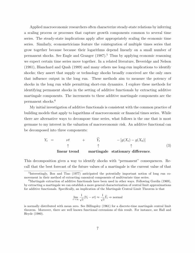
germane to my interest in the valuation of macroeconomic risk. An additive functional can

be decomposed into three components:

Yt = νt + Yt − [g(Xt)− g(X0)]

↑ ↑ ↑linear trend martingale stationary difference.

(3)

This decomposition gives a way to identify shocks with “permanent” consequences. Re-

call that the best forecast of the future values of a martingale is the current value of that

5Interestingly, Box and Tiao (1977) anticipated the potentially important notion of long run co-movement in their method of extracting canonical components of multivariate time series.

6Martingale extraction of additive functionals have been used in other ways. Following Gordin (1969),by extracting a martingale we can establish a more general characterization of central limit approximationsfor additive functionals. Specifically, an implication of the Martingale Central Limit Theorem is that

limt→∞

1√t(Yt − νt) ≈

1√tYt ⇒ normal

is normally distributed with mean zero. See Billingsley (1961) for a discrete-time martingale central limittheorem. Moreover, there are well known functional extensions of this result. For instance, see Hall andHeyde (1980).

7

martingale. Thus permanent shocks are reflected in the increment to the martingale com-

ponent of (3). Isolating such shocks allow me to identify the exposure of economic time

series to macroeconomic risk that dominate the fluctuation of Y over long time horizons.

By contrast, g(Xt)− g(X0) evolves as a stationary process translated by the term −g(X0),

which is time invariant. Thus this term contributes only transitory variation to the process

Y .

The remainder of this section is organized as follows. First I verify formally the mar-

tingale property for Y , and then I show how to construct this decomposition. I finish the

section with two illustrative examples that are designed to pedagogically revealing with

sufficient richness to capture the dynamic structure of many existing models. One example

considers a model in which stochastic volatility is introduced into a continuous-time coun-

terpart of a vector autoregression. This example allows for volatility to fluctuate over time

in a manner that can be highly persistent. The second example considers a mixture-of-

normals model, in which the increments of Y are conditional normal, but the mean and the

exposure to a vector of Brownian increments changes over time in accordance to a finite

state Markov process. Both examples include particular forms of nonlinearity that have

received considerable attention in both the macroeconomics and asset-pricing literatures.

A reader may be concerned that these chosen examples rely too heavily on normal

distributions. While the instantaneous increments are conditional normal over finite time

intervals, these normal distributions get “mixed” over time. This mixing is a common

device for modeling distributions with fat tails.7

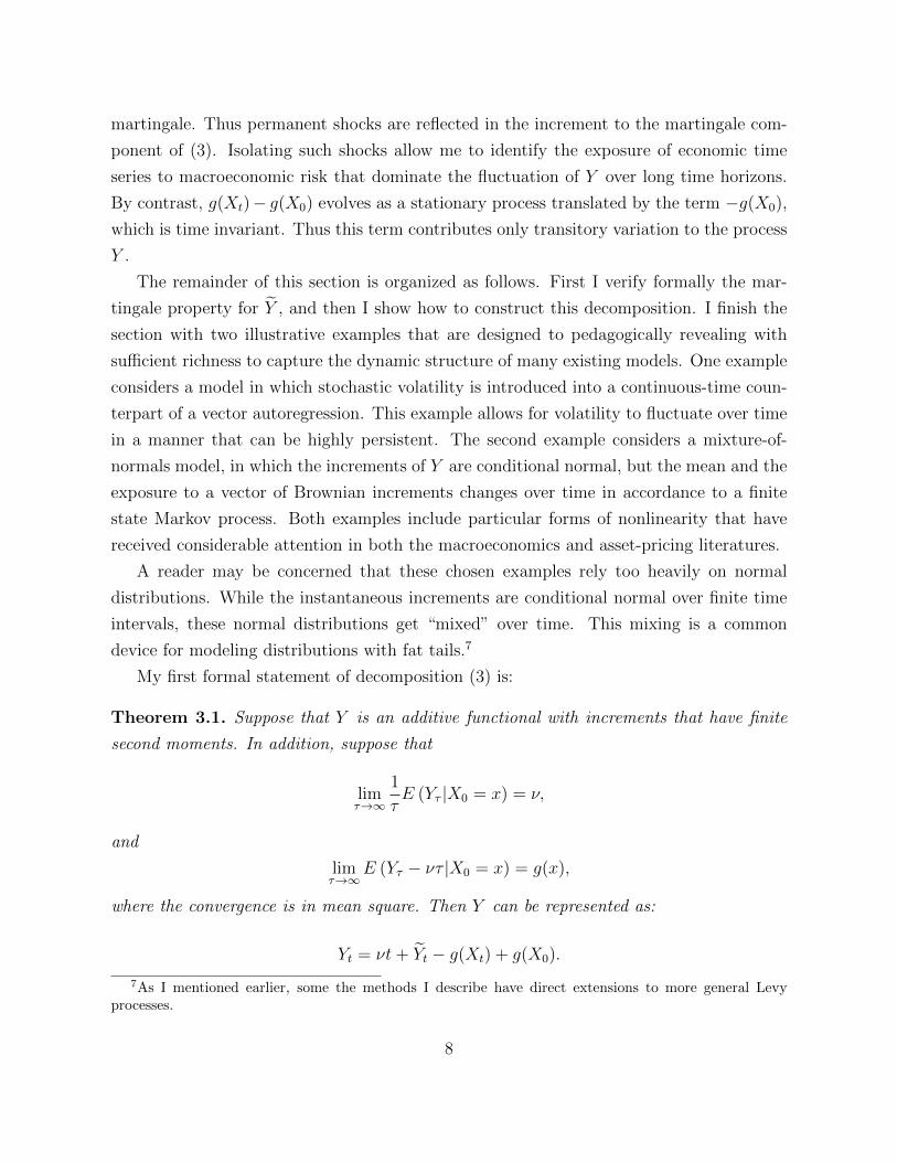
My first formal statement of decomposition (3) is:

Theorem 3.1. Suppose that Y is an additive functional with increments that have finite

second moments. In addition, suppose that

limτ→∞

1

τE (Yτ |X0 = x) = ν,

and

limτ→∞

E (Yτ − ντ |X0 = x) = g(x),

where the convergence is in mean square. Then Y can be represented as:

Yt = νt+ Yt − g(Xt) + g(X0).

7As I mentioned earlier, some the methods I describe have direct extensions to more general Levyprocesses.

8

where {Yt} is an additive martingale.

Proof. See Appendix A

I next show how to use the local evolution of the additive functional to construct the

components of this decomposition. Recall the representation given in (1):

Yt =

∫ t

0

β(Xu)du+

∫ t

0

ξ(Xu−) · dWu +∑

0≤u≤t

χ(Xu, Xu−),

and the construction of β in formula (2). Then

Yt =

∫ t

0

ξ(Xu) · dWu +∑

0≤u≤t

χ(Xu, Xu−)−∫ t

0

β(Xu)du (4)

is a local martingale. In what follows let

κ(x) = β(x) + β(x) = β(x) +

∫Eχ(x∗, x)η(dx∗|x)

where κ(x) is the drift or local mean of Y when the Markov state is x. Thus

Yt = Yt +

∫ t

0

κ(Xu)du.

I now have one of the ingredients for the decomposition: η = E [κ(Xt)].

To obtain a solution g to a long-run forecasting problem, I construct an equation from

the local evolution of the Markov process X. I presume that Yt is itself a martingale. Thus

from Theorem 3.1,

g(x) = limτ→∞

E

[∫ τ

0

κ(Xu)du− τη|X0 = x

]. (5)

To derive an alternative operational formula for g, I equate two alternative expressions for

the local mean of Y :

κ(x) = η − limt↓0

1

tE [g(Xt)− g(x)|X0 = x] = 0, (6)

where the second one use the additive decomposition. Combining this formula with the

local evolution for the Markov state X gives an equation that can be solved for g.8 In

8See, for instance, Hansen and Scheinkman (1995) for a discussion showing when this local condition

9

the case of a multivariate diffusion, this equation is a second-order differential equation as

an implication of Ito’s formula. There are well known extensions to accommodate jumps.

Given a function g that solves equation (6), this same function translated by a constant

also satisfies the equation. I resolve this multiplicity conveniently by choosing g so that g

has mean zero when integrated with respect to a stationary distribution.

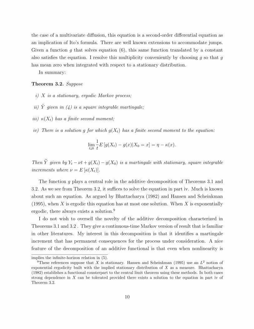
In summary:

Theorem 3.2. Suppose

i) X is a stationary, ergodic Markov process;

ii) Y given in (4) is a square integrable martingale;

iii) κ(Xt) has a finite second moment;

iv) There is a solution g for which g(Xt) has a finite second moment to the equation:

limt↓0

1

tE [g(Xt)− g(x)|X0 = x] = η − κ(x).

Then Y given by Yt− νt+ g(Xt)− g(X0) is a martingale with stationary, square integrable

increments where ν = E [κ(Xt)].

The function g plays a central role in the additive decomposition of Theorems 3.1 and

3.2. As we see from Theorem 3.2, it suffices to solve the equation in part iv. Much is known

about such an equation. As argued by Bhattacharya (1982) and Hansen and Scheinkman

(1995), when X is ergodic this equation has at most one solution. When X is exponentially

ergodic, there always exists a solution.9

I do not wish to oversell the novelty of the additive decomposition characterized in

Theorems 3.1 and 3.2 . They give a continuous-time Markov version of result that is familiar

in other literatures. My interest in this decomposition is that it identifies a martingale

increment that has permanent consequences for the process under consideration. A nice

feature of the decomposition of an additive functional is that even when nonlinearity is

implies the infinite-horizon relation in (5).9These references suppose that X is stationary. Hansen and Scheinkman (1995) use an L2 notion of

exponential ergodicity built with the implied stationary distribution of X as a measure. Bhattacharya(1982) establishes a functional counterpart to the central limit theorem using these methods. In both casesstrong dependence in X can be tolerated provided there exists a solution to the equation in part iv ofTheorem 3.2.

10

introduced, the sum of two additive functionals is an additive functional. Moreover, the

sum of the martingale components is the martingale component for the sum of the additive

functionals provided that the constructions use a common information structure. When

there are multiple additive functionals under consideration and they have a common growth

term and a common martingale component, then one obtains a special case of the the

cointegration model of Engle and Granger (1987) and others.

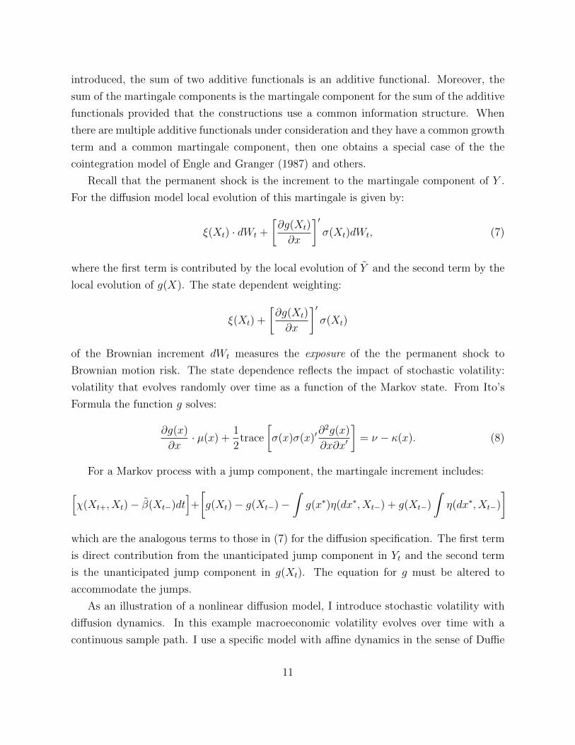
Recall that the permanent shock is the increment to the martingale component of Y .

For the diffusion model local evolution of this martingale is given by:

ξ(Xt) · dWt +

[∂g(Xt)

∂x

]′σ(Xt)dWt, (7)

where the first term is contributed by the local evolution of Y and the second term by the

local evolution of g(X). The state dependent weighting:

ξ(Xt) +

[∂g(Xt)

∂x

]′σ(Xt)

of the Brownian increment dWt measures the exposure of the the permanent shock to

Brownian motion risk. The state dependence reflects the impact of stochastic volatility:

volatility that evolves randomly over time as a function of the Markov state. From Ito’s

Formula the function g solves:

∂g(x)

∂x· µ(x) +

1

2trace

[σ(x)σ(x)′

∂2g(x)

∂x∂x′

]= ν − κ(x). (8)

For a Markov process with a jump component, the martingale increment includes:[χ(Xt+, Xt)− β(Xt−)dt

]+

[g(Xt)− g(Xt−)−

∫g(x∗)η(dx∗, Xt−) + g(Xt−)

∫η(dx∗, Xt−)

]which are the analogous terms to those in (7) for the diffusion specification. The first term

is direct contribution from the unanticipated jump component in Yt and the second term

is the unanticipated jump component in g(Xt). The equation for g must be altered to

accommodate the jumps.

As an illustration of a nonlinear diffusion model, I introduce stochastic volatility with

diffusion dynamics. In this example macroeconomic volatility evolves over time with a

continuous sample path. I use a specific model with affine dynamics in the sense of Duffie

11

and Kan (1994) in order that I that can illustrate conveniently constructions that interest

me.

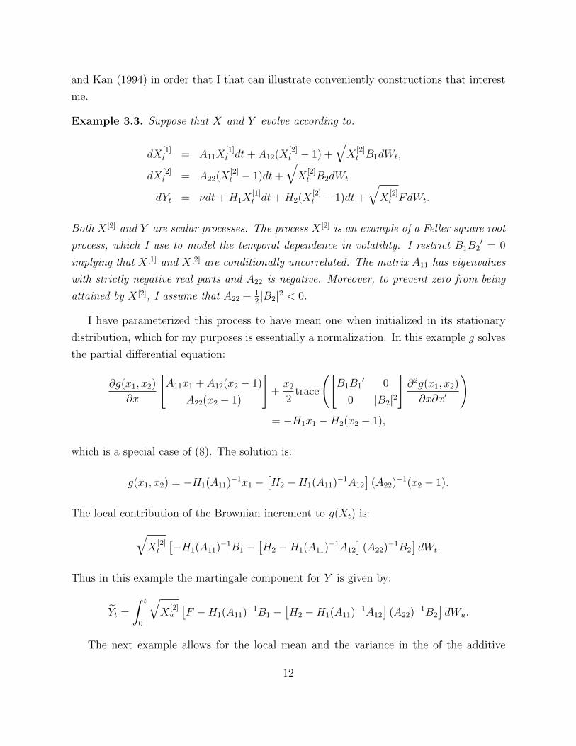
Example 3.3. Suppose that X and Y evolve according to:

dX[1]t = A11X

[1]t dt+ A12(X

[2]t − 1) +

√X

[2]t B1dWt,

dX[2]t = A22(X

[2]t − 1)dt+

√X

[2]t B2dWt

dYt = νdt+H1X[1]t dt+H2(X

[2]t − 1)dt+

√X

[2]t FdWt.

Both X [2] and Y are scalar processes. The process X [2] is an example of a Feller square root

process, which I use to model the temporal dependence in volatility. I restrict B1B2′ = 0

implying that X [1] and X [2] are conditionally uncorrelated. The matrix A11 has eigenvalues

with strictly negative real parts and A22 is negative. Moreover, to prevent zero from being

attained by X [2], I assume that A22 + 12|B2|2 < 0.

I have parameterized this process to have mean one when initialized in its stationary

distribution, which for my purposes is essentially a normalization. In this example g solves

the partial differential equation:

∂g(x1, x2)

∂x

[A11x1 + A12(x2 − 1)

A22(x2 − 1)

]+x22

trace

([B1B1

′ 0

0 |B2|2

]∂2g(x1, x2)

∂x∂x′

)= −H1x1 −H2(x2 − 1),

which is a special case of (8). The solution is:

g(x1, x2) = −H1(A11)−1x1 −

[H2 −H1(A11)

−1A12

](A22)

−1(x2 − 1).

The local contribution of the Brownian increment to g(Xt) is:√X

[2]t

[−H1(A11)

−1B1 −[H2 −H1(A11)

−1A12

](A22)

−1B2

]dWt.

Thus in this example the martingale component for Y is given by:

Yt =

∫ t

0

√X

[2]u

[F −H1(A11)

−1B1 −[H2 −H1(A11)

−1A12

](A22)

−1B2

]dWu.

The next example allows for the local mean and the variance in the of the additive

12

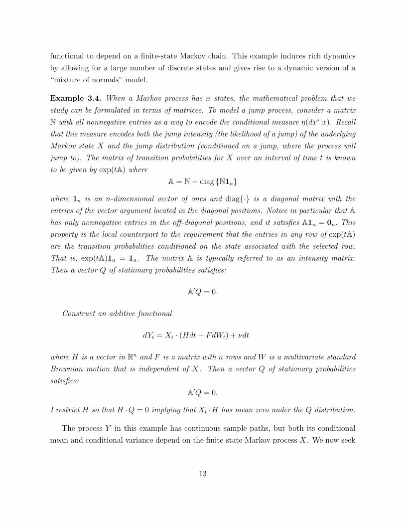
functional to depend on a finite-state Markov chain. This example induces rich dynamics

by allowing for a large number of discrete states and gives rise to a dynamic version of a

“mixture of normals” model.

Example 3.4. When a Markov process has n states, the mathematical problem that we

study can be formulated in terms of matrices. To model a jump process, consider a matrix

N with all nonnegative entries as a way to encode the conditional measure η(dx∗|x). Recall

that this measure encodes both the jump intensity (the likelihood of a jump) of the underlying

Markov state X and the jump distribution (conditioned on a jump, where the process will

jump to). The matrix of transition probabilities for X over an interval of time t is known

to be given by exp(tA) where

A = N− diag {N1n}

where 1n is an n-dimensional vector of ones and diag{·} is a diagonal matrix with the

entries of the vector argument located in the diagonal positions. Notice in particular that Ahas only nonnegative entries in the off-diagonal positions, and it satisfies A1n = 0n. This

property is the local counterpart to the requirement that the entries in any row of exp(tA)

are the transition probabilities conditioned on the state associated with the selected row.

That is, exp(tA)1n = 1n. The matrix A is typically referred to as an intensity matrix.

Then a vector Q of stationary probabilities satisfies:

A′Q = 0.

Construct an additive functional

dYt = Xt · (Hdt+ FdWt) + νdt

where H is a vector in Rn and F is a matrix with n rows and W is a multivariate standard

Brownian motion that is independent of X. Then a vector Q of stationary probabilities

satisfies:

A′Q = 0.

I restrict H so that H ·Q = 0 implying that Xt ·H has mean zero under the Q distribution.

The process Y in this example has continuous sample paths, but both its conditional

mean and conditional variance depend on the finite-state Markov process X. We now seek

13

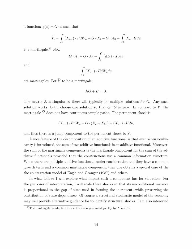
a function: g(x) = G · x such that

Yt =

∫ t

0

(Xu−) · FdWu +G ·Xt −G ·X0 +

∫ t

0

Xu ·Hdu

is a martingale.10 Now

G ·Xt −G ·X0 −∫ t

0

(AG) ·Xudu

and ∫ t

0

(Xu−) · FdWudu

are martingales. For Y to be a martingale,

AG+H = 0.

The matrix A is singular so there will typically be multiple solutions for G. Any such

solution works, but I choose one solution so that Q · G is zero. In contrast to Y , the

martingale Y does not have continuous sample paths. The permanent shock is:

(Xu−) · FdWu +G · (Xt −Xt−) + (Xu−) ·Hdu,

and thus there is a jump component to the permanent shock to Y .

A nice feature of the decomposition of an additive functional is that even when nonlin-

earity is introduced, the sum of two additive functionals is an additive functional. Moreover,

the sum of the martingale components is the martingale component for the sum of the ad-

ditive functionals provided that the constructions use a common information structure.

When there are multiple additive functionals under consideration and they have a common

growth term and a common martingale component, then one obtains a special case of the

the cointegration model of Engle and Granger (1987) and others.

In what follows I will explore what impact such a component has for valuation. For

the purposes of interpretation, I will scale these shocks so that its unconditional variance

is proportional to the gap of time used in forming the increment, while preserving the

contribution of state dependence. Of course a structural stochastic model of the economy

may well provide alternative guidance for to identify structural shocks. I am also interested

10The martingale is adapted to the filtration generated jointly by X and W ,

14

in the decomposition because it provides a comparison for a related result that follows.11

Prior to our development of an alternative decomposition, I discuss some limiting char-

acterizations that will interest us.

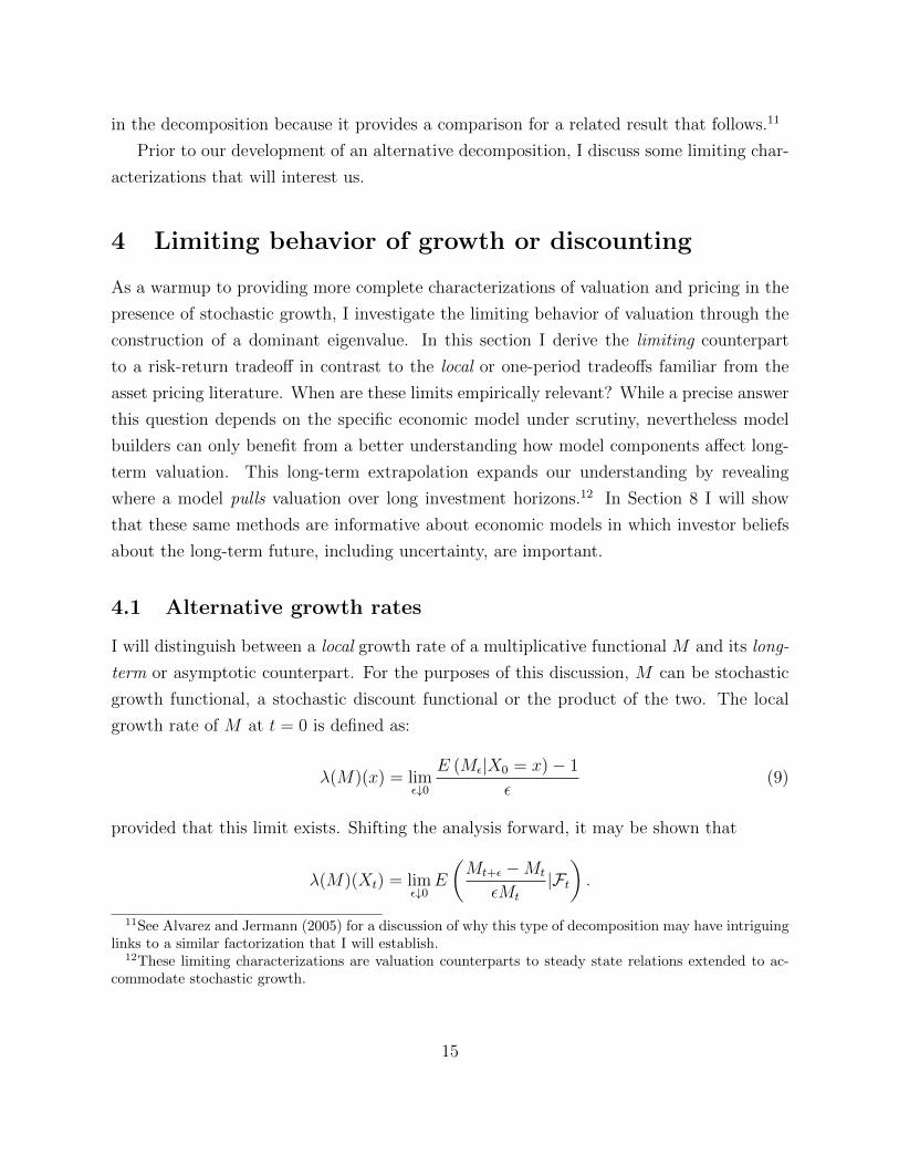
4 Limiting behavior of growth or discounting

As a warmup to providing more complete characterizations of valuation and pricing in the

presence of stochastic growth, I investigate the limiting behavior of valuation through the

construction of a dominant eigenvalue. In this section I derive the limiting counterpart

to a risk-return tradeoff in contrast to the local or one-period tradeoffs familiar from the

asset pricing literature. When are these limits empirically relevant? While a precise answer

this question depends on the specific economic model under scrutiny, nevertheless model

builders can only benefit from a better understanding how model components affect long-

term valuation. This long-term extrapolation expands our understanding by revealing

where a model pulls valuation over long investment horizons.12 In Section 8 I will show

that these same methods are informative about economic models in which investor beliefs

about the long-term future, including uncertainty, are important.

4.1 Alternative growth rates

I will distinguish between a local growth rate of a multiplicative functional M and its long-

term or asymptotic counterpart. For the purposes of this discussion, M can be stochastic

growth functional, a stochastic discount functional or the product of the two. The local

growth rate of M at t = 0 is defined as:

λ(M)(x) = limε↓0

E (Mε|X0 = x)− 1

ε(9)

provided that this limit exists. Shifting the analysis forward, it may be shown that

λ(M)(Xt) = limε↓0

E

(Mt+ε −Mt

εMt

|Ft).

11See Alvarez and Jermann (2005) for a discussion of why this type of decomposition may have intriguinglinks to a similar factorization that I will establish.

12These limiting characterizations are valuation counterparts to steady state relations extended to ac-commodate stochastic growth.

15

Since Mt = exp(Yt) and

Yt =

∫ t

0

β(Xu)du+

∫ t

0

ξ(Xu−) · dWu +∑

0≤u≤t

χ(Xu, Xu−)

as in (1), the local growth rate is computed to be

λ(M)(x) = β(x) +1

2|ξ(x)|2 +

∫(exp[χ(y, ·)]− 1) η(dy|x) (10)

using, when necessary, continuous-time stochastic calculus. Notice that direct exposure to

Brownian motion risk, reflected in ξ, and jump risk, reflected in χ, contributes to this local

growth rate. This growth rate is state dependent.

By contrast, define the long-term growth (or decay) rate as:

limt→∞

1

tlogE [Mt|X0 = x] = ρ(M)

provided that this limit is well defined. Compounding has nontrivial consequences for the

long-term growth rate when the local growth rate is state-dependent. I will characterize

this asymptotic limit and explore the relation between the local growth rate and the asymp-

totic growth rate. Here I am interpreting growth liberally so as to include discounting as

well. What I develop in this section is also germane to the study of long-term implications

of compounding of short-term discount rates that are state dependent. While characteriza-

tions of this compounding are straightforward for log-normal models and more generally for

term-structure models, in the study of valuation it is in fact the co-dependence of macroe-

conomic growth and stochastic discounting that becomes of central interest even more so

than when the two components are studied separately.13

4.2 Risk-return tradeoffs

Prior to developing further some mathematical tools, let me represent continuous-time

risk-return relations using the notation that I just developed. To accomplish this, I use

alternative constructions of M including ones with multiple components. The stochastic

process components have explicit economic interpretations including stochastic discount

factor processes or growth processes used to represent hypothetical financial claims to be

13See for instance Alvarez and Jermann (2005) for a study of the impact of compounding stochasticdiscount factors over multiple investment horizons.

16

priced. My use of stochastic discount factor processes to reflect valuation is familiar from

empirical asset pricing. For instance, see Hansen and Richard (1987), Cochrane (2001), and

Singleton (2006). A stochastic discount factor for a given payoff horizon discounts the future

and it adjusts for risk when used to assign values to a future payoff. A stochastic discount

factor process assigns values to a cash flow process. Cash flows may be a consumption pro-

cess that will be realized in future dates or a dividend process on an infinitely-lived security.

This process typically decays asymptotically. Such decay is needed for an infinitely-lived

security with a growing cash flow to have a finite value as in the case of equity.

For an investment horizon t, a cash flow or payoff Gt and a stochastic discount factor

St, the logarithm of the expected return relative to a riskless benchmark is:

1t

logE [Gt|X0 = x] − 1t

logE [StGt|X0 = x] + 1t

logE [St|X0 = x]

log log log

expected payoff − price − riskfree return.

(11)

The term:E [Gt|X0 = x]

E [StGt|X0 = x]

is the expected return on the investment over the horizon t, and the term

1

E [St|X0 = x]

is the expected return on a riskless investment. Thus formula (11) measures the risk

premium on the investment. I divide by t to facilitate comparisons across investment

horizons.

I now consider two limiting cases. The first calculation essentially reproduces the

continuous-time risk-return tradeoff familiar from the asset pricing literature, but uses

the mathematical formulation that I have laid out. The instantaneous expected excess

return takes limits of (11) as t declines to zero:

instantaneous excess return = λ(G)(x)− λ(GS)(x) + λ(S)(x). (12)

The first two terms together give the continuous-time limiting formula for the instantaneous

expected rate of return. The instantaneous riskless rate is given by −λ(S)(x). Thus the

three terms on the right-hand side of (12) give the excess expected return. By altering the

17

exposures to risk capture by ξ and χ, we trace out a set of feasible excess returns implied

by the an economic model of the stochastic discount factor S. This local relation is best

conceived of as an approximation because asset trading at sufficiently high frequencies is

typically altered by trading details associated with the market micro-structure.

Consider now the long-term limiting counterpart. We have counterparts to all three

terms:

long-term excess return = ρ(G)− ρ(GS) + ρ(S) (13)

This formula takes limits of (11) as the investment horizon made arbitrarily long and as

a consequence state dependence is absent. By changing the risk exposures, Hansen and

Scheinkman (2009a) suggest this as a way to build a long-term counterpart to a risk-return

tradeoff.

Asset pricing models also have implications for the intermediate investment horizons,

but the two calculations given in (12) and (13) provide an interesting starting point for the

study of the term structure of risk-premia for growth-rate risk.

Covariances play a prominent role in representing risk premia in asset valuation. This

is reflected most directly in the instantaneous risk-return relation (12) when I abstract

from the jump component. Let ξg be loading of G on the Brownian increment, and let

ξs be the loading of S on the Brownian increment. Then a simple calculation shows that

instantaneous expected excess return is: −ξg · ξs, which can be verified by using formulas

(10) and (12). This dot product is the instantaneous covariance between logG and − logS.

Since ξg is the local exposure to risk, −ξs can be interpreted as the vector of prices to

exposure to alternative components to the multivariate Brownian increment.

Consider next a long-run counterpart reflected in (13). While the product of two mul-

tiplicative functionals is multiplicative, by multiplying this functions we do not simply add

the growth rates;

ρ (SG) 6= ρ (S) + ρ (G) .

Co-dependence is important when characterizing even the limiting behavior of the product

SG or any other multiplicative functionals. As we have seen from (13), the discrepancy

gives a long-term notion of risk premium. If S and G happen to be jointly log normal for

each t, then the long-term excess return is

ρ(G)− ρ(GS) + ρ(S) = limt→∞

1

tCov (− logSt, logGt)

18

While this illustrates that co-dependence plays a central role in characterizing risk premia,

we will not require log-normality in what follows. Compounding even locally normal mod-

els with state dependence can lead to important departures from analogous calculations

premised on log-normality.

Prior to proceeding, I comment a bit on the previous literature. The study of the

dynamics of risk premia is familiar from the work of Wachter (2005), Lettau and Wachter

(2007), Hansen et al. (2008) and Bansal et al. (2008). Hansen et al. (2008) characterize the

resulting limiting risk premia and the associated risk prices in a log-linear environment.14

Hansen and Scheinkman (2009a) extend this approach to fundamentally nonlinear models

with a Markov structure.

4.3 Long-term entropy of stochastic discount factors

In their study of the behavior of stochastic discount factors, Alvarez and Jermann (2005),

Backus et al. (2011b) and Backus et al. (2011a) construct a one-period measure of “entropy”

of the stochastic discount factor. Alvarez and Jermann (2005) motivate this measure as

a generalized notion of discount factor volatility and Backus et al. (2011b) connect the

one-period version of this measure to a measure of entropy in applied mathematics as a

discrepancy measure between the so-called risk neutral density from mathematical finance

and a unitary density.15 A conditional version of their measure for investment horizon t is:

entropy = logE (St|X0 = x)− E (logSt|X0 = x) .

The nonnegativity of this measure is a direct consequence of Jensens Inequality. The local

counterpart to their entropy measure is given by

instantaneous entropy = limε↓0

logE (Sε|X0 = x)

ε− lim

ε↓0

E (logSε|X0 = x)

ε

= λ(S)(x)− κ(logS)(x)

≥ 0

14Hansen et al. (2008) also consider the limiting behavior of holding period returns. This limit includescontributions from the principle eigenfunction and the principal eigenvalue of the associated valuationoperator for pricing cash flows with stochastic growth components.

15This link to a risk neutral distribution does not carry over to longer investment horizons, and for goodreason as I will discuss later.

19

where κ(logS) is the local mean of logS computed in section 3.16 I include the local growth

rate λ on right-hand side because:

limε↓0

logE (Sε|X0 = x)

ε= lim

ε↓0

E (Sε|X0 = x)− 1

ε= λ(x).

In the calculation of instantaneous entropy, −λ(S) is the instantaneous short-term interest

rate. For the diffusion specification:

instantaneous entropy =1

2|ξs(x)|2,

which is one half times the local variance of logS in Markov state x. Introducing jumps

leads to an adjustment that includes higher moments as is emphasized by Backus et al.

(2011b) and Backus et al. (2011a):

instantaneous entropy =1

2|ξs(Xt)|2 +

∫(exp[χ(x∗, x)]− 1− χ(x∗, x)) η(dx∗|x).

The contribution of higher moments is evident in the power series expansion of the expo-

nential.

Bansal and Lehmann (1997) provide an upper bound for the discrete-time counterpart

to the term κ(logS) using the negative of the maximal growth-rate on a return portfolio.

Empirical researches often find it convenient to average out the state dependence. Notice

in particular that E [κ(logS)] = ν(logS) which is the coefficient on the time trend in

the decomposition of Y . These calculations are meant to extend the volatility bounds on

stochastic discount factors deduced by Shiller (1982) and Hansen and Jagannathan (1991)

using asset market data. By including data on risk-free rates and using the bound deduced

by Bansal and Lehmann (1997), entropy bounds can be constructed as a diagnostic for

asset pricing models.

The long-term counterpart to this notion of entropy is given by:

long-term entropy = ρ(S)− ν(logS) ≥ 0

where ν(logS) the coefficient on the time trend in the additive decomposition of logS.

While ν(logS) is the unconditional mean of κ(S)(Xt), as we have already argued ρ(S) is

16The analysis in section 3 applies to a general additive functional. I now modify the notation to makeit clear which additive functional is being used in the computation.

20

not the mean of λ(S)(Xt). Comparing the instantaneous and long-term measures, informs

us about the impact of compounding stochastic discount factors over multiple investment

horizons. Arguably, if the long-term measure exceeds that of the instantaneous measure,

then there is a potential for risk adjustments to be more pronounced over longer investment

horizons.

Why are these various limits interesting? Say that the approximations require com-

pounding growth or discounting over an extremely long time span. Then one might worry

that resulting impacts are little consequence in applications. Even in this case, however,

comparing the short-term risk-return tradeoff to the long-term counterpart helps us to un-

derstand when this tradeoff has an important horizon component to it. Thus I use these

long-run variation measures to amplify on Fisher (1930)’s conjecture about the importance

of the dynamic valuation of risk over the whole prospective investment horizon. My com-

parisons of long-term valuation measures to short-term counterparts gives me a starting

point for understanding the full dynamics.

In the next two sections I lay out a mathematical structure that will provide support

for a more refined analysis.

5 A revealing example with discrete states

Prior to a more general development, I illustrate calculations by reconsidering the specifica-

tion in Example 3.4 in which the dynamics are governed by a Markov chain that visits only

a finite number of states. In this example our mathematical problem can be formulated in

terms of transition matrices for valuation applicable to a discrete state space.

I characterize long-run stochastic growth (or decay) by posing and solving an approxi-

mation problem using what is called a principal eigenvector and eigenvalue. The principal

eigenvector has only positive entries. As I will illustrate, there is a well-defined sense in

which this eigenvector dominates over long valuation horizons. The approximation problem

that I will study more generally has its origins from what is known as Perron-Frobenius

theory of matrices.

For a multiplicative functional associated with an n-state jump process, state dependent

growth or decay rates are modeled using β and χ where

β(x) = H · x+ ν1n

21

Recall that β dictates the growth or decay absent any jump and χ dictates how the mul-

tiplicative function jumps as a function of the jumps in the underlying Markov process. I

represent function exp[χ(x∗, x)] as an n by n matrix K with positive entries and unit entries

in the diagonal positions. Also, I construct a diagonal matrix D where the jth diagonal

entry is given by the jth entry of H plus the jth diagonal entry of 12FF ′ plus ν. Form an n

by n matrix BB = K ◦ A + D

where ◦ used in the matrix multiplications denotes element-by-element (Hadamard) multi-

plication. This construction of B modifies A to include state dependent growth (or decay)

associated with the corresponding multiplicative functional. In particular, I exploit local

normality which allows me to compute the expectation of the exponential of normally dis-

tributed random variable by making a variance adjustment. The off-diagonal entries of Bare all positive, but typically B1n is not equal to 0n.

I form an indexed family of operators, in this case matrices, indexed by the time horizon

by exponentiating the matrix Mt = exp (tB):

Mtf(x) = E [exp(Yt)f(Xt)|X0 = x] .

One possible choice of f = 1n, which is of interest because

1

tlogMt1n(x)

is the expected growth rate in exp(Y ) over a time horizon t. Then conveniently

Mt = exp(tB).

The date t matrix Mt reflects the expected growth, discounting or the composite of both

over an interval of time t. The entries of Mt are all nonnegative, and I presume that for

some time horizon t, the entries are strictly positive. The matrix Mt is typically not a

probability matrix in our applications, however. (Column sums are not unity.) Instead

Mt reflects continuous compounding of stochastic growth or discounting over a horizon t.

The matrix B encodes the instantaneous contributions to growth or discounting, and it

generates the family of matrices {Mt : t ≥ 0}. Specifically, the vector

λ = B1n

22

contains the state dependent growth rates.

Given an n × 1 vector f , Perron-Frobenius theory characterizes limiting behavior of1t

logMtf by first solving:

Be = ρe.

where e is a column eigenvector restricted to have strictly positive entries and the corre-

sponding ρ is a real eigenvalue. Consider also the transpose problem

B′e∗ = ρe∗ (14)

where e∗ also has positive entries. Depending on the application, ρ can be positive or

negative. Importantly, ρ is larger than the real part of any other eigenvalue of the matrix

B.

Exponentiating a matrix preserves the eigenvectors. The new eigenvalues are the expo-

nential of those of the initial matrix. As a consequence, Mt has an eigenvector given by e

and with an associated eigenvalue equal to exp(ρt). The multiplication by t implies that

the magnitude of exp(ρt) relative to the other eigenvalues of Mt becomes arbitrarily large

as t gets large. As a consequence,

limt→∞

1

tlogMtf = ρ1n (15)

limt→∞

(logMtf − tρ1n) = log(f · e∗)1n + log e (16)

for any vector f for which f ·e∗ > 0, where I have normalized e∗ so that e∗ ·e = 1. Formally,

(15) defines ρ as the long-run growth rate of the family of matrices {Mt : t ≥ 0}. The

vector log e gives the dominant state dependence over long horizons. The logarithm of the

eigenvector e exposes the impact of state-dependent compounding of growth or discounting

over long horizons.

In the next section I will give a more general statement of this approximation that

allows for Markov states to be continuous.

6 A Multiplicative Factorization

So far, I have focused on the behavior of long-term growth or decay rates related to valua-

tion. I turn now to extracting more information by refining the analysis. I do so in three

ways. First, to accommodate continuous Markov states, I use operators in place of the ma-

23

trices (Subsection 6.1). Following Hansen and Scheinkman (2009a), I represent a family of

valuation operators (indexed by the investment horizon) using a multiplicative functional.

The multiplicative functional is the product of a stochastic discount factor functional and

a stochastic growth functional. Second, I factor the multiplicative functional to extract the

long-term growth or decay component as an exponential function of the investment horizon

and to extract the long-horizon risk component as a positive martingale (Subsection 6.2).

Roughly speaking, this factorization is the multiplicative counterpart to Section 3’s addi-

tive decomposition, but there are important differences. These differences require that I

adopt a Perron-Frobenious approach that generalizes the discussion of Section 5 . I use the

martingale component to provide an alternative representation of the valuation operators,

convenient for long-term approximation (Subsections 6.3 - 6.5). Third, I characterize “risk-

price” elasticities for varying investment horizons which show how valuation changes when

I change the risk exposure of stochastically growing cash flows (Subsection 6.6). These

methods give the core ingredients for what I call dynamic value decompositions or DVD’s.

6.1 Operator families

Asset values are fruitfully depicted using valuation operators that assign (state dependent)

prices to future payoffs or consumption at alternative investment horizons. These operators

must be linked when there is trading at intermediate dates, and are necessarily recursive.

My interest is in economies with Markov characterizations.

Following Hansen and Scheinkman (2009a), a central ingredient in my analysis is the

construction of a family of operators from a multiplicative functional M . Formally, with

any multiplicative functional M we associate a family of operators:

Mtf(x) = E [Mtf(Xt)|X0 = x] (17)

indexed by t. When M has finite first moments, this family of operators is at least well

defined on the space of bounded functions.17

Notice that I have used a multiplicative functional M to represent the operators for

alternative investment horizons t. Why feature multiplicative functionals? The operator

families that interest must satisfy the Law of Iterated Values, which imposes a recursive

structure on valuation. In the case of models with frictionless trade at all dates, this struc-

17See Hansen and Scheinkman (2009a) for a a more general and explicit formulation of the domain ofsuch operators.

24

ture is enforced by the absence of arbitrage opportunities. Since I wish to accommodate

macroeconomic growth in the payoff, I construct M = SG where Gtf(Xt) is the priced

payoff.

Formula (17) depicts values at date zero. The corresponding formula for trading at date

τ < t for investment horizon t− τ is:

Mt−τf(x) = E

[Mt

Mτ

f(Xt)|Xτ = x

].

At date zero we could purchase the payoff GτMt−τf (Xτ ) at date τ and then use this payoff

at date τ to purchase a claim to Gtf(Xt). The date zero price of this transaction is:

MτMt−τf(x) = E

(SτGτE

[Mt

Mτ

f(Xt)|Xτ

]|X0 = x

)= E

(MτE

[Mt

Mτ

f(Xt)|Fτ]|X0 = x

)= E [Mtf(Xt)|X0 = x]

= Mtf(x).

Notice that Mtf(x) is the date zero purchase price of the payoff Gtf(Xt) without resorting

to an intermediate trade. On the right-hand side of the first equation Sτ is used to represent

the date zero prices of payoffs at date τ where the payoff is GτMt−τf(Xτ ). An outcome

of these relations is the recursive structure to valuation that links Mt to the sequential

application of Mt−τ and Mτ . Important to my analysis is that this recursive valuation

embeds macroeconomic growth in the consumption payoffs.

The Law of Iterated Values in a Markov setting is captured formally as a statement

that the family of operators should be a semigroup.

Definition 6.1. A family of operators {Mt} is a (one-parameter) semigroup if a) M0 = Iand b) MtMτ = Mt+τ for t ≥ 0 and τ ≥ 0.

I now explain why I use multiplicative functionals to represent operator families. I do

so because a multiplicative functional M guarantees that the resulting operator family

{Mt : t ≥ 0} constructed using (17) is a one-parameter semigroup.18

18Lewis (1998), Linetsky (2004) and Boyarchenko and Levendorskii (2007) use operator methods of thistype to study of the term structure of interest rates and option pricing while abstracting from stochasticgrowth.

25

6.2 Martingale extraction

I now propose a multiplicative factorization of stochastic growth or discount functionals

with three components: a) an exponential function of time, b) a positive martingale, c) a

ratio of functions of the Markov process at zero and t:

Mt = exp (ρt) Mt

[e(X0)e(Xt)

]↑ ↑ ↑

growth or martingale ratio

decay change in probability state dependence

(18)

Component a) governs the long-term growth or decay. It is constructed from a principal

eigenvalue. I will use component b), the positive martingale, to build an alternative proba-

bility measure.19 Component c) is the function of the Markov state that is most important

over long valuation horizons.

I build the factorization as follows. First I solve:

Mtf(x) = E [Mte(Xt)|X0 = x] = exp(ρt)e(x) (19)

for any t where e is strictly positive as in (14). The function e can be viewed as a principal

eigenfunction of the semigroup with ρ being the corresponding eigenvalue.20 Notice that

for alternative values of t, I have used the same positive eigenfunction e. The associated

eigenvalues are related via an exponential formula. Since equation (19) holds for any t, it

can be localized by computing:

limt↓0

Mte(x)− exp(−ρt)e(x)

t= 0, (20)

which gives an equation in e and ρ to be solved. The local counterpart to this equation is

Be = ρe, (21)

19As an alternative approach, Rogers (1997) proposes a convenient parameterization of a martingalefrom which one can construct examples of multiplicative functionals of the form (18). Given my interestin structural economic models of asset pricing and in products of stochastic discount factor and growthfunctionals, I will instead explore factorizations of pre-specified multiplicative functionals.

20My reference to e as an eigenfunction is a bit loose because I have not prespecified a space of functionsthat it resides in. Instead I use the formalization of Hansen and Scheinkman (2009a) that defines aneigenfunction using a martingale approach.

26

where

limt↓0

Mte(x)− e(x)

t= Be(x)

The operator B is the so-called generator of the semigroup constructed with the multi-

plicative functional M . It is an operator on a space of appropriately defined functions.

Heuristically, it captures the local evolution of the semigroup. In the case of a diffusion

model, this generator is known to be a second-order differential operator:

Bf =

(β +

1

2|ξ|2)f + (σξ′ + µ) · ∂f

∂x+

1

2trace

(σσ′

∂2f

∂x∂x′

).

It is convenient to express the corresponding eigenvalue equation in terms of log e after

dividing the equation by e:

ρ =

(β +

1

2|ξ|2)

+ (σξ′ + µ) · ∂ log e

∂x+

1

2trace

(σσ′

∂2 log e

∂x∂x′

)+

1

2

(∂ log e

∂x

)′σσ′

(∂ log e

∂x

)We have seen the finite-state counterpart to this equation in section 5.

Typically it suffices to solve the local equation (21) to obtain a solution to (19). See

Hansen and Scheinkman (2009a) for a more detailed discussion of this issue. In the finite-

state Markov model of section 5, convenient and well known sufficient conditions exist for

there to be a unique (up to scale) positive eigenfunction satisfying (19). More generally,

however, this uniqueness will not hold. Instead I will obtain uniqueness from additional

considerations.

Given a solution to (19), I construct a martingale via:

Mt = exp(−ρt)Mt

[e(Xt)

e(X0)

],

which is itself a multiplicative functional. The multiplicative decomposition (18) follows

immediately by letting e = 1e

and solving for M in terms of M , ρ and e.

6.3 Martingale and a change in probability

Why might a multiplicative martingales be of interest? A positive martingale scaled to

have unit expectation is known to induce an alternative probability measure. This trick is

a familiar one from asset pricing, but it is valuable in many other contexts. Since M is a

27

martingale, I form the distorted or twisted expectation:

E [f(Xt)|X0] = E[Mtf(Xt)|X0

]. (22)

For each time horizon t, I define an alternative conditional expectation operator. The

martingale property is needed so that the resulting family of conditional expectation oper-

ators obeys the Law of Iterated Expectations. It insures consistency between the operators

defined using Mt+τ and Mt for expectations of random variables that are in the date t

conditioning information sets. Moreover, with this (multiplicative) construction of a mar-

tingale, the process remains Markov under the change in probability measure. While (22)

defines conditional expectations, I also use the notation E to define the the corresponding

unconditional expectations when a stationary distribution exists and the process is ergodic

under the change of measure.

I present a method for long-term approximation where a martingale component of M

is used to change the probability measure. This alternative probability measure gives me a

framework for a formal study of long-term approximation on which I can use the existing

toolkit for the study of Markov processes that are “stochastically stable.”

Definition 6.2. The process X is stochastically stable under the measure · if

limt→∞

E [f(Xt)|X0 = x] = E [f(Xt)]

for any f for which E(f) is well defined and finite and computed using a stationary distri-

bution associated with the · Markov transition.21

Theorem 6.3. Given a multiplicative functional M , suppose that e and ρ satisfy equation

(20) and that X is stochastically stable under the · probability measure. Then

E [Mtf(Xt)|X0 = x] = exp(ρt)E

[f(Xt)

e(Xt)|X0 = x

]e(x).

Moreover,

limt→∞

exp(−ρt)E [Mtf(Xt)|X0 = x] = E [f(Xt)e(Xt)] e(x)

provided that E [f(Xt)e(Xt)] is finite where e = 1/e.

21This is stronger than ergodicity because it rules out periodic components. Ergodicity requires thattime series averages converge but not necessarily that conditional expectation operators converge. Thelimit used in this definition could be state by state or it could in mean-square under the change of measure.

28

It follows from Theorem 6.3 that once we scale by the growth rate ρ, we obtain a one-

factor representation of long-term behavior. Changing the function f simply changes the

coefficient on the function e. Thus the state dependence is approximately proportional to

e as the horizon becomes large. For this method to justify our previous limits, we require

that f e have a finite expectation under the · probability measure. The class of functions f

for which this approximation works depends on the stationary distribution for the Markov

state of the · probability measure and the function e.

As I noted previously, there is an extensive set of tools for studying the stability of

Markov processes that can be brought to bear on this problem. For instance, see Meyn

and Tweedie (1993) for a survey of such methods based on the use of Foster-Lyapunov

criteria. See Rosenblatt (1971), Bhattacharya (1982) and Hansen and Scheinkman (1995)

for alternative approaches based on mean-square approximation. While there may be

multiple representations of the form (18), Hansen and Scheinkman (2009a) show that there

is at most one such representation for which the process X is stochastically stable.

The valuation dynamics are best understood in terms of this alternative probability

measure as reflected in the formula:

logMtf(x)− ρt = log e(x) + log E [f(Xt)e(Xt)|X0 = x] (23)

where E is used to denote the expectation operator under the twisted measure, e = 1e

and f is a positive function of the Markov state. Thus after adjusting for the growth (or

decay) rate ρ, the implied values of a cash flow (as a function of the investment horizon) are

represented conveniently in terms of the dynamics under the twisted probability measure.

This alternative probability measure gives me a framework for a formal study of long-term

approximation on which I can use the existing toolkit for the study of Markov processes

that are stochastically stable.

In light of the stochastic stability, the limit as the investment horizon t becomes large

of (23) is

limt→∞

[logMtf(x)− tρ] = log e(x) + log E [f(Xt)e(Xt)] .

The second term on the right-hand side computes the unconditional expectation of f e

under the twisted probability measure, provided of course that this expectation is finite

and positive. This generalizes result (16) for the finite-state Markov chain example given in

section (5). By applying this approximation to M = SG, I have an operational method for

creating a more refined characterization of the behavior of long-term values. As is evident in

29

this approximation, component c) of (18) is built directly from the principle eigenfunction

e. It captures state dependence, and it provides a way to characterize the convergence

to the limiting growth (or decay) rate ρ. The choice of f contributes a constant term

log E [f(Xt)e(Xt)], while the principle eigenfunction e determines the state dependence

independent of f .

6.4 Change of measure revisited

Mathematical finance uses a different change of measure based on a different factorization.

Let M be a multiplicative functional. Following Ito and Watanabe (1965), a multiplicative

supermartingale can be factored as:

Mt = exp

[∫ t

0

λ(M)(Xu)du

]Mt

where λ(M)(x) is given by (9) in Section 4 and is the local growth rate for M and M is a

local martingale. When the local martingale M is a martingale, then this martingale gives

an alternative change in measure. If the local growth (or decay) rate λ(M) does not depend

on the the Markov state, this factorization coincides with the one that we have been using.

On the other hand, if this rate is state dependent, the two decompositions differ.

Mathematical finance uses the Ito and Watanabe (1965)-style factorization applied to

a stochastic discount factor process S. Then λ(S)(Xt) is the negative of the instantaneous

interest rate and the change of measure is the so-called “risk neutral measure”. When

interest rates vary over time, in effect they adjust for risk for finite investment horizons. This

risk-neutral adjustment only eliminates the need for local risk adjustments complicating its

interpretation for characterizing asset pricing dynamics.

6.5 Holding-period returns on cash flows

A return to equity with cash flows or dividend that have stochastic growth components can

be viewed as a bundle or portfolios of holding period returns on cash flows with alternative

payout dates. (See Lettau and Wachter (2007) and Hansen et al. (2008).) As an application

of the multiplicative factorization, I now extend a result obtained by Hansen et al. (2008)

for log-normal models applied to holding-period returns on cash flows. Let M = SG, and

30

form the gross return over horizon t:

GtMτ [f(Xt)]

Mt+τ [f(X0)]

Apply the change in measure and represent this as:

exp(−ρt)Gt

[e(Xt)

e(X0)

](E[f(Xt+τ )e(Xt+τ )|Xt]

E[f(Xt+τ )e(Xt+τ )|X0]

)

The last term converges to unity as the payoff horizon τ increases, and the first two terms

do not depend on τ . Thus the limiting return is:

exp(−ρt)Gt

[e(Xt)

e(X0)

]. (24)

This limit has a cash flow component Gt and a state-dependent valuation component:e(Xt)e(X0)

. Both of these terms contribute to the return exposure to risk. Finally there is an

exponential adjustment ρ, which is in effect a value-based measure of duration of the cash

flow G and is independent of the Markov state. When ρ is near zero, the cash flow values

deteriorate very slowly as the investment horizon is increased.

The holding-period return process, (24), is itself a multiplicative functional with the

same martingale component as G. Since

−ρ(SG) = −ρ(G) + [ρ(G)− ρ(SG)]

and −ρ(G) offsets the growth in G, the growth rate of the limiting holding-period return

process is ρ(G)− ρ(SG), which is minus the logarithm of the expected long-term return.

6.6 Perturbations and elasticities

Derivatives computed at a baseline configuration of parameters reveal sensitivity of a val-

uation model to small changes in a parameters. For instance, in Hansen et al. (2008) the

pricing implications of a parameterized family of valuation models depend on the intertem-

poral elasticity of the investors. They compute derivatives as an alternative to solving the

model for the alternative parameter configurations. A risk price is also a derivative. It is a

marginal change in a risk premium induced by a marginal change in risk exposure. Thus a

key to constructing a risk price is to parameterize the risk exposure of a hypothetical cash

31

flow as in Hansen and Scheinkman (2009b) and Borovicka et al. (2011). These elasticities

are the ingredients for dynamic value decompositions. Other perturbations would also be

of interest.

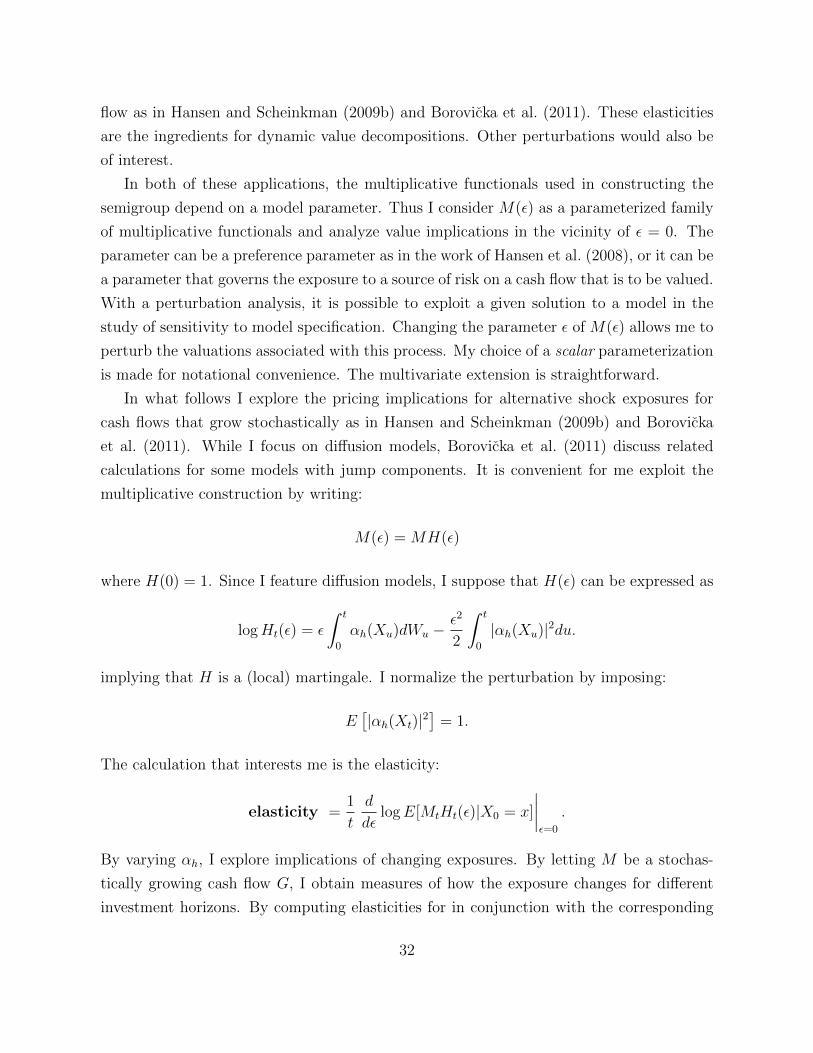
In both of these applications, the multiplicative functionals used in constructing the

semigroup depend on a model parameter. Thus I consider M(ε) as a parameterized family

of multiplicative functionals and analyze value implications in the vicinity of ε = 0. The

parameter can be a preference parameter as in the work of Hansen et al. (2008), or it can be

a parameter that governs the exposure to a source of risk on a cash flow that is to be valued.

With a perturbation analysis, it is possible to exploit a given solution to a model in the

study of sensitivity to model specification. Changing the parameter ε of M(ε) allows me to

perturb the valuations associated with this process. My choice of a scalar parameterization

is made for notational convenience. The multivariate extension is straightforward.

In what follows I explore the pricing implications for alternative shock exposures for

cash flows that grow stochastically as in Hansen and Scheinkman (2009b) and Borovicka

et al. (2011). While I focus on diffusion models, Borovicka et al. (2011) discuss related

calculations for some models with jump components. It is convenient for me exploit the

multiplicative construction by writing:

M(ε) = MH(ε)

where H(0) = 1. Since I feature diffusion models, I suppose that H(ε) can be expressed as

logHt(ε) = ε

∫ t

0

αh(Xu)dWu −ε2

2

∫ t

0

|αh(Xu)|2du.

implying that H is a (local) martingale. I normalize the perturbation by imposing:

E[|αh(Xt)|2

]= 1.

The calculation that interests me is the elasticity:

elasticity =1

t

d

dεlogE[MtHt(ε)|X0 = x]

∣∣∣∣ε=0

.

By varying αh, I explore implications of changing exposures. By letting M be a stochas-

tically growing cash flow G, I obtain measures of how the exposure changes for different

investment horizons. By computing elasticities for in conjunction with the corresponding

32

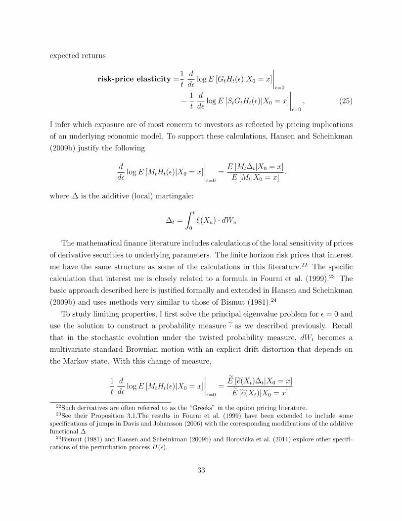
expected returns

risk-price elasticity =1

t

d

dεlogE [GtHt(ε)|X0 = x]

∣∣∣∣ε=0

− 1

t

d

dεlogE [StGtHt(ε)|X0 = x]

∣∣∣∣ε=0

, (25)

I infer which exposure are of most concern to investors as reflected by pricing implications

of an underlying economic model. To support these calculations, Hansen and Scheinkman

(2009b) justify the following

d

dεlogE [MtHt(ε)|X0 = x]

∣∣∣∣ε=0

=E [Mt∆t|X0 = x]

E [Mt|X0 = x].

where ∆ is the additive (local) martingale:

∆t =

∫ t

0

ξ(Xu) · dWu

The mathematical finance literature includes calculations of the local sensitivity of prices

of derivative securities to underlying parameters. The finite horizon risk prices that interest

me have the same structure as some of the calculations in this literature.22 The specific

calculation that interest me is closely related to a formula in Fourni et al. (1999).23 The

basic approach described here is justified formally and extended in Hansen and Scheinkman

(2009b) and uses methods very similar to those of Bismut (1981).24

To study limiting properties, I first solve the principal eigenvalue problem for ε = 0 and

use the solution to construct a probability measure · as we described previously. Recall

that in the stochastic evolution under the twisted probability measure, dWt becomes a

multivariate standard Brownian motion with an explicit drift distortion that depends on

the Markov state. With this change of measure,

1

t

d

dεlogE [MtHt(ε)|X0 = x]

∣∣∣∣ε=0

=E [e(Xt)∆t|X0 = x]

E [e(Xt)|X0 = x]

22Such derivatives are often referred to as the “Greeks” in the option pricing literature.23See their Proposition 3.1.The results in Fourni et al. (1999) have been extended to include some

specifications of jumps in Davis and Johansson (2006) with the corresponding modifications of the additivefunctional ∆.

24Bismut (1981) and Hansen and Scheinkman (2009b) and Borovicka et al. (2011) explore other specifi-cations of the perturbation process H(ε).

33

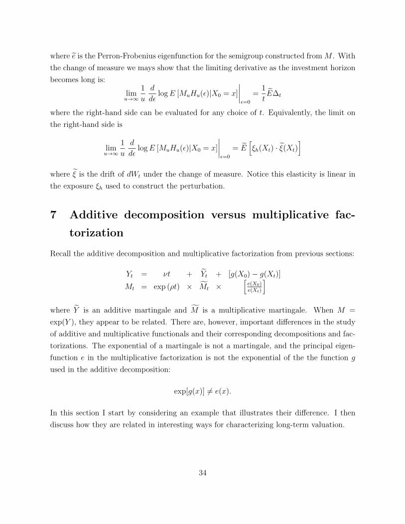
where e is the Perron-Frobenius eigenfunction for the semigroup constructed from M . With

the change of measure we mays show that the limiting derivative as the investment horizon

becomes long is:

limu→∞

1

u

d

dεlogE [MuHu(ε)|X0 = x]

∣∣∣∣ε=0

=1

tE∆t

where the right-hand side can be evaluated for any choice of t. Equivalently, the limit on

the right-hand side is

limu→∞

1

u

d

dεlogE [MuHu(ε)|X0 = x]

∣∣∣∣ε=0

= E[ξh(Xt) · ξ(Xt)

]where ξ is the drift of dWt under the change of measure. Notice this elasticity is linear in

the exposure ξh used to construct the perturbation.

7 Additive decomposition versus multiplicative fac-

torization

Recall the additive decomposition and multiplicative factorization from previous sections:

Yt = νt + Yt + [g(X0)− g(Xt)]

Mt = exp (ρt) × Mt ×[e(X0)e(Xt)

]where Y is an additive martingale and M is a multiplicative martingale. When M =

exp(Y ), they appear to be related. There are, however, important differences in the study

of additive and multiplicative functionals and their corresponding decompositions and fac-

torizations. The exponential of a martingale is not a martingale, and the principal eigen-

function e in the multiplicative factorization is not the exponential of the the function g

used in the additive decomposition:

exp[g(x)] 6= e(x).

In this section I start by considering an example that illustrates their difference. I then

discuss how they are related in interesting ways for characterizing long-term valuation.

34

7.1 They are different

Consider again Example 3.3, and recall the dynamic evolution for the stochastic volatility

model:

dX[1]t = A11X

[1]t dt+ A12(X

[2]t − 1) +

√X

[2]t B1dWt,

dX[2]t = A22(X

[2]t − 1)dt+

√X

[2]t B2dWt

dYt = νdt+H1X[1]t dt+H2(X

[2]t − 1)dt+

√X

[2]t FdWt.

Form

Mt = exp(Yt).

Guess a solution e(x) = exp (α · x) where x =

[x1

x2

]and α =

[α1

α2

]. To compute ρ(M), I

solve a special case of (21):

ν + x1′ (A11

′α1 +H1′) + (x2 − 1) (A12

′α1 + A22α2 +H2) +1

2x2|α′B + F |2 = ρ.

which I derive as a special case of (21). Thus the coefficients on x1 and x2 are zero when:

A11′α1 +H1

′ = 0

A12′α1 + A22α2 +H2 +

1

2|α1′B1 + α2B2 + F |2 = 0. (26)

I solve the first equation for α1 and the second one for α2 given α1. The solution to the

first equation is:

α1 = −(A11′)−1H1

′

The second equation is quadratic in α2, so there may be two solutions. Specifically,

α2 =−(B2 · F + A22

|B2|2

)±√|B2 · F + A22|2 − |B2|2 (|F −H1(A11)−1B1|2 + 2H2 − 2H1(A11)−1A12)

|B2|2, (27)

provided that the term under the square root sign is positive. Notice in particular that this

term will be positive for sufficiently small |B2|.As an implication of the Girsanov Theorem, associated with each solution is an alter-

35

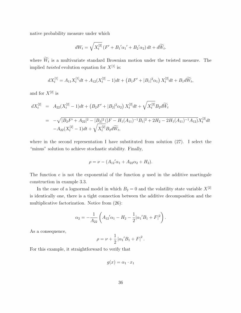
native probability measure under which

dWt =

√X

[2]t (F ′ +B1

′α1′ +B2

′α2) dt+ dWt.

where Wt is a multivariate standard Brownian motion under the twisted measure. The

implied twisted evolution equation for X [1] is:

dX[1]t = A11X

[1]t dt+ A12(X

[2]t − 1)dt+

(B1F

′ + |B1|2α1

)X

[2]t dt+B1dWt,

and for X [2] is

dX[2]t = A22(X

[2]t − 1)dt+

(B2F

′ + |B2|2α2

)X

[2]t dt+

√X

[2]t B2dWt

= −√|B2F ′ + A22|2 − |B2|2 (|F −H1(A11)−1B1|2 + 2H2 − 2H1(A11)−1A12)X

[2]t dt

−A22(X[2]t − 1)dt+

√X

[2]t B2dWt,

where in the second representation I have substituted from solution (27). I select the

“minus” solution to achieve stochastic stability. Finally,

ρ = ν − (A12′α1 + A22α2 +H2).

The function e is not the exponential of the function g used in the additive martingale

construction in example 3.3.

In the case of a lognormal model in which B2 = 0 and the volatility state variable X [2]

is identically one, there is a tight connection between the additive decomposition and the

multiplicative factorization. Notice from (26):

α2 = − 1

A22

(A12

′α1 −H2 −1

2|α1′B1 + F |2

).

As a consequence,

ρ = ν +1

2|α1′B1 + F |2 .

For this example, it straightforward to verify that

g(x) = α1 · x1

36

and hence e(x) ∝ exp[g(x)]. While the exponential of a martingale is not a martingale,

in this case the exponential of the additive martingale will become a martingale provided

that we multiply the additive martingale by an exponential function of time. This simple

adjustment exploits the lognormal specification as follows:

Mt = exp

(Yt −

t

2|F −HA−1B|2

).

is a martingale. See Hansen et al. (2008) for a more complete discussion of such results for

log normal models and applications to asset pricing.

7.2 But related

While an additive decomposition is fundamentally different from a multiplicative factoriza-

tion, there is an interesting connection. Consider two additive functionals that the same

linear growth and additive martingale components. Thus we may write

exp(Y

[1]t

)= exp(νt) exp

(Yt

)(exp[g[1](X0)

]exp [g[1](Xt)]

),

exp(Y

[2]t

)= exp(νt) exp

(Yt

)(exp[g[2](X0)

]exp [g[2](Xt)]

).

While we know that exp(Y ) is not a martingale, the existence of this common component

remains informative:

Theorem 7.1. Consider two additive functionals Y [1] and Y [2] that the same linear growth

component and additive martingale component Y . Then M [1] = exp(Y [1])

and M [2] =

exp(Y [2])

share the same exponential growth rate and multiplicative martingale component

and this martingale component is given by the martingale component of Y . Conversely sup-

pose that M [1] and M [2] share the same exponential growth rate and the same multiplicative

component M . Provided that log M has a well defined additive decomposition and log e[1]

and log e[2] have finite second moments, logM [1] and logM [2] have a common linear growth

component and a common additive martingale component.

Thus the additive martingale decomposition used to identify the permanent shock to

logM identifies multiplicative functionals with common multiplicative components growth

37

components. For instance the valuation of two cash flows with the same permanent compo-

nents identified via an additive decomposition have long-term values that are approximately

the same. Analogously, two stochastic discount factor processes whose logarithms share the

martingale component have the same limiting valuation implications. We elaborate on this

in what follows.

7.3 Temporary model components

I now suggest what it means for there to be temporary components to stochastic discount

factors and hence the their assignment of values. Consider a benchmark valuation model

represented by a stochastic discount factor, M = S, or the product of a stochastic discount

functional and a reference growth functional M = SG. I ask: what modifications have

transient implications for valuation? Given an M implied by a benchmark valuation model,

recall our additive decomposition:

logMt = ηt+ Yt − g(Xt) + g(X0)

where Y is an additive martingale and and our multiplicative factorization (18):

Mt = exp(ρt)Mte(X0)

e(Xt)

where M is a multiplicative martingale. Moreover, suppose that under the associated ·probability measure X satisfies a stochastic stability condition 6.2.

Consider an alternative model of the form:

M∗t = Mt

f ∗(Xt)

f ∗(X0)(28)

for some f ∗ where M is used to represent a benchmark model and M∗ an alternative model.

As argued by Bansal and Lehmann (1997) and others, a variety of asset pricing models can

be represented like this with the time-separable power utility model used to construct M

for a given process in aggregate consumption. Function f may be induced by changes in

the preferences of investors such as habit persistence or social externalities. I will illustrate

38

such representations in section 8. In light of (28), a candidate factorization for M∗ is:

M∗t = exp(ρt)Mt

e(X0)f(Xt)

e(Xt)f(X0).

The exponential and martingale components remain the same as for the factorization of

M . This gives me an operational notion of a transient change in valuation.

Definition 7.2. The difference in the semigroups associated with M∗ and M is transient if

their multiplicative factorizations share the same exponential growth (or decay) component:

exp(ρt) and the same martingale component: M for which the process X is stochastically

stable under the implied change in probability measure.

When the difference between the semigroups associated with M and M∗ is transient,

long-term components to the additive decomposition and multiplicative factorization re-

main the same. The first conclusion requires that

E

([log f(Xt)

]2]<∞

Under this restriction, we may form the additive decomposition for M by first constructing

the additive decomposition for M and then replacing g with

g∗(x) = g(x)− log f ∗(x).

Consider next the multiplicative factorization. I will illustrate such representations in

section 8. In light of (28), a candidate factorization for M∗ is:

M∗t = exp(ρt)Mt

e(X0)f(Xt)

e(Xt)f(X0).

The exponential and martingale components remain the same as for the factorization of

M . The principal eigenfunctions, however, can be different. For instance, the principal

eigenfunction for M∗ given by (28) is:

e∗ =e

f ∗.

The difference between e and e∗ alters the family of transient functions because for f to be

39

transient for M∗:

E [f(Xt)e(Xt)f∗(Xt)] <∞.

In particular, this restriction depends on f ∗. Thus the collection of functions for which

the long-term approximation methods are applicable is altered although the change of

probability measure remains the same.

With these qualifications, consider two models with stochastic discount factors S and

S∗. Provided that the semigroups associated with these are transient, then the semigroups

associated with SG and S∗G are transient and the difference in the long-term risk premium

vanishes as the investment horizon becomes large for the stochastically growing cash flow

G.

long-term excess return = ρ(G)− ρ(SG) + ρ(S) = ρ(G)− ρ(S∗G) + ρ(S∗)

Moreover,

long-term entropy = ρ(S)− η(logS) = ρ(S∗)− η(logS∗)

Alternatively, consider two stochastically growing cash flows, G and G∗, where logG

and logG∗ have a common time trend and martingale component. Then the semigroups

associated with SG and SG∗ have transient differences. Since their long-term risk exposure

is approximately the same, they have the same long-term risk prices. Again the long-term

excess returns will be the same for the two cash flows.

8 Recursive utility and sentiments

In this section I do two things. First I use a multiplicative factorization to provide a

novel characterization of the impact of recursive utility on asset valuation I obtain this

characterization by exploring parameter configurations that magnify the impact of senti-

ments about the future of the macroeconomy in the valuation of macroeconomic growth

and its volatility. After obtaining this characterization I show how to use the apparatus

of dynamic value decompositions to compare two models: a model in which investors have

power utility preferences for which the forward-looking channel is absent and a model with

recursive utility as featured in Kreps and Porteus (1978), Epstein and Zin (1989) in which

the forward-looking channel is present.25

25The origins of the recursive utility model are in Koopmans (1960).

40

8.1 Continuation values in discrete time

By examining continuation values, I explore the impact on stochastic discount factors

computed as shadow prices of an underlying consumption process fit to time series data.

This recursive utility specification gives a potential role for forward-looking sentiments to

be present in even short-term risk return tradeoffs, a point featured by Bansal and Yaron

(2004). While there are well-known formulations of recursive utility in continuous time,

for pedagogical reasons I initiate my discussion in discrete time. Consider a discrete-time

specification with grid points spaced distance ε apart from one another. For instance when

ε = 2−j, I envision a sequence of time intervals that are continually sliced in half as j

increases. I use the homogeneous-of-degree-one aggregator specified in terms of current

period consumption Ct and the continuation value Vt:

Vt =[ε(rCt)

1−θ + exp(−δε) [Rt(Vt+ε)]1−θ] 1

1−θ.

where

Rt (Vt+ε) =(E[(Vt+ε)

1−γ|Ft]) 1

1−γ

adjusts the continuation value Vt+ε for risk. The parameter r does not alter preferences but

simply scales the continuation values. I include it to allow me to choose r in a judicious

manner when I take limits. Next I divide by Ct to obtain:

VtCt

=

[εr1−θ + exp(−δ)

[Rt

(Vt+εCt+ε

Ct+εCt

)]1−θ] 11−θ

, (29)

which exploits the aggregator function’s homogeneous of degree one . In what follows I will

consider infinite-horizon specifications, which leads me to solve a fixed-point problem. Thus

I will explore the construction of the continuation value Vt as a function of Ct, Ct+ε, Ct+2ε, ....

The corresponding intertemporal marginal rate of substitution over an interval ε is:

St+εSt

= exp(−εδ)(Ct+εCt

)−θ [Vt+εRt(Vt+ε)

]θ−γ

= exp(−εδ)(Ct+εCt

)−γ Vt+εCt+ε

Rt

(Vt+εCt+ε

Ct+εCt

)θ−γ (30)

Absent market frictions, when I evaluate this intertemporal marginal rate of substitution at

41

the equilibrium consumption, I have a discrete-time specification of the stochastic discount

factor between date t and t + ε. This formula reproduces the representation of valuation

used by Rubinstein (1976) and Lucas (1978) when γ = θ, but it contains a forward-looking

adjustment reflected in the ratio of the continuation value to its risk-adjusted counterpart

as in the first line of (30)

In what follows I will take a “Lucas (1978)-type approach” by positing a process for

aggregate consumption, without modeling formally production via the accumulation of

capital. This will allow me to feature the impact of changing investor preferences on prices,

although in general we expect these changes to have impact on consumption outcomes.

More generally, we may envision the consumption process that I prescribe below as the

equilibrium outcome of an economy in which consumption is endogenously determined.

Let consumption C be a multiplicative functional. Such functionals are initialized at

one. For notational convenience, I will maintain this specification, but it is straightfor-

ward to change the initialization. Given the Markov specification for consumption and the

homogeneity of the utility recursion, I consider continuation values that can be depicted

as:VtCt

= h(Xt).

Then from (29), the fixed-point equation for infinite-horizon valuation is:

h(x) =

r1−θ + exp(−δε)

[E

([h(Xt+ε)]

1−γ(Ct+εCt

)1−γ

|Xt = x

)] 1−θ1−γ

11−θ

. (31)

The next subsection shows a close relation between this fixed-point problem and a principal

eigenvalue problem.

8.2 An interesting limit

In this subsection I explore the range of allowable discounting, through the parameter δ, in

an infinite horizon. To allow δ to attain its limit value I have to adjust the scale r appropri-

ately so that the limiting continuation value is positive yet finite.26 This exercise has a clear

interpretation: I vary δ and thereby alter the forward-looking channel on continuation val-

26The mathematical characterization that follows is very similar to that of Runolfsson (1994) who studiesergodic risk-sensitive control problems using eigenfunction methods. Our analysis differs from that ofRunolfsson because we include stochastic growth in our specification.

42

ues in the recursive utility specification. As I have already emphasized, these continuation

values can be important contributors to the stochastic discount factors used to represent

asset values. As a consequence, even short-term risk pricing will be maximally affected by

beliefs about future growth rates in the macroeconomy and the accompanying uncertainty.

More generally, the continuation values are a mechanism through which sentiments about

the future matter in asset valuation. The limit I characterize is more than an idle curiosity:

empirical investigations often target the forward-looking preference component as a way to

enhance risk prices as a way to magnify risk premia.

In what follows I assume that γ > 1 and consider the limit as (r)1−θ decreases to zero

and δ tends to a conveniently chosen limit. Later I will be more precise about this limit.

To explore this limit, I am led to I use the multiplicative functional C1−γ to construct:

Vtf(x) = E (exp[(1− γ) logC(Xt)]f(Xt)|X0 = x) .

Suppose that

Vte(x) = exp(ρt)e(x). (32)

for some positive function e and some scalar ρ. Choose e so that the associated martingale

Mt =e(Xt)

e(X0)exp(−tρ)

induces a change of probability measure with stochastically stable dynamics. By solving

equation (32), I also solve a limiting version of equation (31) provided that I also set

δ = ρθ − 1

γ − 1.

Theorem 8.1. Suppose that C is a multiplicative functional and that there is as stochas-

tically stable multiplicative martingale representation for S1−γ constructed using an eigen-

function e and eigenvalue ρ. Then

VtCt

= h(Xt) = e(Xt)1

1−γ

The corresponding stochastic discount factor is:

St = exp(−tρ)

(CtC0

)−γ [e(Xt)

e(X0)

] γ−θγ−1

.

43

Moreover, SC is a multiplicative martingale when θ = 1.

Notice that with the theorem, I have illustrated or perhaps more accurately asserted

a link between the construction of a value function for the recursive utility model and a

Perron-Frobenius eigenfunction. This eigenfunction contributes what I called in Section 7 a

transient model component relative to a power utility specification of a Rubinstein (1976),

Lucas (1978) or Breeden (1979) model with power 1 − γ (or equivalently to a preference

specification in which θ = γ). The parameter θ, the inverse of the intertemporal elasticity

of substitution, contributes to the transient term:

[e(Xt)

e(X0)

] γ−θγ−1

and can have important consequences for short-term risk pricing. It is well known that

recursive utility models with large values of γ can have substantially different implications

for short-term risk pricing and interest rates when γ = θ versus when θ = 1 because the

impact of the intertemporal elasticity of substitution.

I add some formality to this discussion by first defining

ζ =γ − 1

θ − 1.

I presume that θ 6= 1 in what follows because the θ = 1 case requires a separate argument.

Rewrite (31) as:

h(x)1−γ =

εr1−θ + exp(−δε)

[E

([h(Xt+ε)]

1−γ(Ct+εCt

)1−γ

|Xt = x

)] 1ζ

ζ

While the function h depends on the parameter r, this parameter does not alter the un-

derlying preferences of the investor. Consider the limiting equation as (r)1−θ declines to

zero:

h(x)1−γ = exp(−δζε)

[E

([h(Xt+ε)]

1−γ(Ct+εCt

)1−γ

|Xt = x

)]. (33)

Notice that (33) is a special case of the Perron-Frobenius eigenvalue problem considered in

(32) provided that

δ =ρ

ζ.

44

The rate ρ will often be negative as it is the growth rate of C1−γ and γ > 1. In this case

the restriction on δ is positive when θ < 1 and negative when θ > 1. However, there are

examples in which ρ becomes positive for large γ because of the role of cumulative impact

of stochastic volatility over the long run. For this limit equation, h and the stochastic

discount factor functional are those given by Theorem 8.1.

Both of these formulas have direct extensions to continuous time. Duffie and Epstein

(1992) provide a general treatment of representing recursive preferences in continuous time.

For our focal parameterization, the continuous-time counterpart to fixed point equation (31)

is

−ζr1−θh(x)θ−γ + δζh(x)1−γ = limε↓0

Vε (h1−γ) (x)− h(x)1−γ

ε

(see Appendix B).

To understand better why the conclusion of Theorem 8.1 is a limiting case, use the

change-of-probability measure associated with Perron-Frobenius eigenfunction to write:

exp(−δε)[Rt

(Vt+εCt+ε

Ct+εCt

)]1−θ= exp(−δε) exp[(1− ς)ρε]e(x)ζ

[E([h (Xt+ε)]

1−γ e(Xt+ε)−1|Xt = x

)] 1ζ

Let

g(x) = h(x)1−θe(x)−ζ ,

and

ξ = δ − ζρ

Then the recursion used to construct continuation values as a function of the Markov state

by solving:

g(x) = εr1−θe(x)−ζ + exp(−ξε)[E(

[g (Xt+ε)]ζ |Xt = x

)] 1ζ

(34)

This transformed recursion has absorbed growth into a conveniently chosen change of mea-

sure.

More can be done with the equation. Hansen and Scheinkman (2011) use moment

restrictions on e under the change of probability measure in conjunction with Jensen’s

Inequality to establish the existence of an “interesting” fixed point to equation (34) for g,

that is to:

g(x) = r1−θe(x)−ζ + exp(−ξε)[E(

[g (Xt+ε)]ζ |Xt = x

)] 1ζ. (35)

45

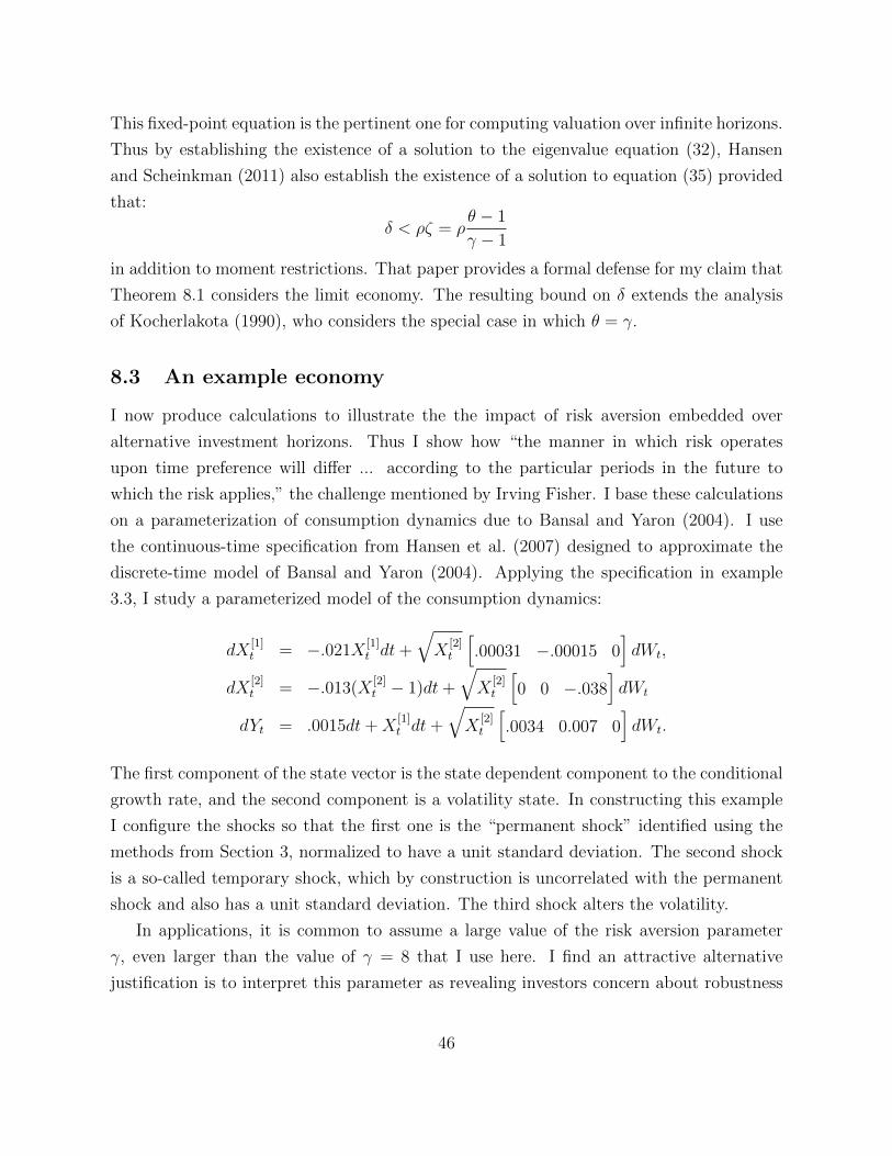
This fixed-point equation is the pertinent one for computing valuation over infinite horizons.

Thus by establishing the existence of a solution to the eigenvalue equation (32), Hansen

and Scheinkman (2011) also establish the existence of a solution to equation (35) provided

that:

δ < ρζ = ρθ − 1

γ − 1

in addition to moment restrictions. That paper provides a formal defense for my claim that

Theorem 8.1 considers the limit economy. The resulting bound on δ extends the analysis

of Kocherlakota (1990), who considers the special case in which θ = γ.

8.3 An example economy

I now produce calculations to illustrate the the impact of risk aversion embedded over

alternative investment horizons. Thus I show how “the manner in which risk operates

upon time preference will differ ... according to the particular periods in the future to

which the risk applies,” the challenge mentioned by Irving Fisher. I base these calculations

on a parameterization of consumption dynamics due to Bansal and Yaron (2004). I use

the continuous-time specification from Hansen et al. (2007) designed to approximate the

discrete-time model of Bansal and Yaron (2004). Applying the specification in example

3.3, I study a parameterized model of the consumption dynamics:

dX[1]t = −.021X

[1]t dt+

√X

[2]t

[.00031 −.00015 0

]dWt,

dX[2]t = −.013(X

[2]t − 1)dt+

√X

[2]t

[0 0 −.038

]dWt

dYt = .0015dt+X[1]t dt+

√X

[2]t

[.0034 0.007 0

]dWt.

The first component of the state vector is the state dependent component to the conditional

growth rate, and the second component is a volatility state. In constructing this example

I configure the shocks so that the first one is the “permanent shock” identified using the

methods from Section 3, normalized to have a unit standard deviation. The second shock

is a so-called temporary shock, which by construction is uncorrelated with the permanent

shock and also has a unit standard deviation. The third shock alters the volatility.

In applications, it is common to assume a large value of the risk aversion parameter

γ, even larger than the value of γ = 8 that I use here. I find an attractive alternative

justification is to interpret this parameter as revealing investors concern about robustness

46

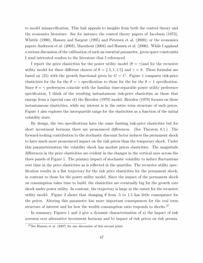
to model misspecification. This link appeals to insights from both the control theory and

the economics literature. See for instance the control theory papers of Jacobson (1973),

Whittle (1990), Hansen and Sargent (1995) and Petersen et al. (2000); or the economics

papers Anderson et al. (2003), Maenhout (2004) and Hansen et al. (2006). While I applaud

a serious discussion of the calibration of such an essential parameter, given space constraints

I send interested readers to the literature that I referenced.

I report the price elasticities for the power utility model (θ = γ)and for the recursive

utility model for three different choices of θ = {.5, 1, 1.5} and γ = 8. These formulas are

based on (25) with the growth functional given by G = C. Figure 1 compares risk-price

elasticities for the for the θ = γ specification to those for the for the θ = 1 specification.

Since θ = γ preferences coincide with the familiar time-separable power utility preference

specification, I think of the resulting instantaneous risk-price elasticities as those that

emerge from a (special case of) the Breeden (1979) model. Breeden (1979) focuses on these

instantaneous elasticities, while my interest is in the entire term structure of such prices.

Figure 1 also explores the interquartile range for the elasticities as a function of the initial

volatility state.

By design, the two specifications have the same limiting risk-price elasticities but for

short investment horizons there are pronounced differences. (See Theorem 8.1.) The

forward-looking contribution to the stochastic discount factor induces the permanent shock

to have much more pronounced impact on the risk prices than the temporary shock. Under

this parameterization the volatility shock has modest prices elasticities. The magnitude

differences in the price elasticities are evident in the changes in the vertical axes across the

three panels of Figure 1. The primary impact of stochastic volatility to induce fluctuations

over time in the price elasticities as is reflected in the quartiles. The recursive utility spec-

ification results in a flat trajectory for the risk price elasticities for the permanent shock,

in contrast to those for the power utility model. Since the impact of the permanent shock

on consumption takes time to build, the elasticities are eventually big for the growth rate

shock under power utility. In contrast, the trajectory is large at the outset for the recursive

utility model. Figure 2 shows that changing θ from .5 to 1.5 has little consequence for

the prices. Altering this parameter has more important consequences for the real term

structure of interest and for how the wealth consumption ratio responds to shocks.27

In summary, Figures 1 and 2 give a dynamic characterization of a) the impact of risk

aversion over alternative investment horizons and b) impact of risk prices on risk premia.

27See Hansen et al. (2007) for one discussion of this second point.

47

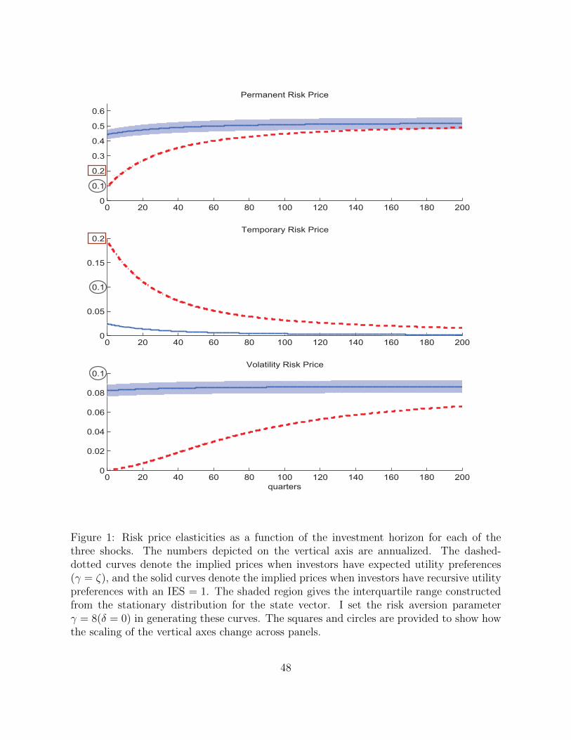
0 20 40 60 80 100 120 140 160 180 2000

0.1

0.2

0.3

0.4

0.5

0.6

Permanent Risk Price

0 20 40 60 80 100 120 140 160 180 2000

0.05

0.1

0.15

0.2Temporary Risk Price

0 20 40 60 80 100 120 140 160 180 2000

0.02

0.04

0.06

0.08

0.1Volatility Risk Price

quarters

Student Version of MATLAB

Figure 1: Risk price elasticities as a function of the investment horizon for each of thethree shocks. The numbers depicted on the vertical axis are annualized. The dashed-dotted curves denote the implied prices when investors have expected utility preferences(γ = ζ), and the solid curves denote the implied prices when investors have recursive utilitypreferences with an IES = 1. The shaded region gives the interquartile range constructedfrom the stationary distribution for the state vector. I set the risk aversion parameterγ = 8(δ = 0) in generating these curves. The squares and circles are provided to show howthe scaling of the vertical axes change across panels.

48

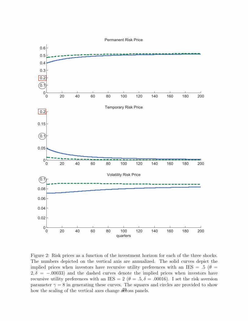
0 20 40 60 80 100 120 140 160 180 2000

0.1

0.2

0.3

0.4

0.5

0.6

Permanent Risk Price

0 20 40 60 80 100 120 140 160 180 2000

0.05

0.1

0.15

0.2Temporary Risk Price

0 20 40 60 80 100 120 140 160 180 2000

0.02

0.04

0.06

0.08

0.1Volatility Risk Price

quarters

Student Version of MATLAB

Figure 2: Risk prices as a function of the investment horizon for each of the three shocks.The numbers depicted on the vertical axis are annualized. The solid curves depict theimplied prices when investors have recursive utility preferences with an IES = .5 (θ =2, δ = −.00033) and the dashed curves denote the implied prices when investors haverecursive utility preferences with an IES = 2 (θ = .5, δ = .00016). I set the risk aversionparameter γ = 8 in generating these curves. The squares and circles are provided to showhow the scaling of the vertical axes change across panels.49

They display the impact of the forward-looking channel embedded in recursive utility,

which is especially prominent for “permanent shocks” to aggregate consumption. This

same prominence shows up when γ = ζ only for long-investment horizons.

These calculations deliberately extrapolate value implications beyond the support of the

data by looking at pricing implications for hypothetical cash flows at different horizons. In

this sense, I am using the models as “structural”. These pricing calculations are of direct

interest and they are informative for welfare cost calculations using the methods in Hansen

et al. (1999) and Alvarez and Jermann (2004). In order to feature the role of preferences,

I hold fixed the consumption dynamics when I make comparisons across specifications. I

do not mean to preclude interest in other approaches such as in Hansen et al. (1999) and

Tallarini (2000) that introduce explicitly capital accumulation into the analysis. In these

examples the more primitive starting point has only minor implications for risk pricing.

Motivated by the work of Alvarez and Jermann (2005), Backus et al. (2011a) and Backus

et al. (2011b), I also report the entropy measures for the stochastic discount factors for

alternative investment horizons. In contrast to the localization method I used to construct

elasticities, these measures are global. They depend on all of the shocks and they abstract

from the interaction between growth and discounting. The top panel of Figure 3 compares

power utility and recursive utility. Like the risk-price elasticities, the entropy measures are

much less sensitive to the investment horizon than for the recursive utility specification of

preferences than for power utility one. The bottom panel of Figure 3 shows that the impact

of changing the intertemporal elasticity parameter θ between .5 and 1.5 is small.

50

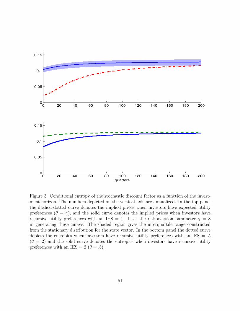
0 20 40 60 80 100 120 140 160 180 2000

0.05

0.1

0.15

quarters

0 20 40 60 80 100 120 140 160 180 2000

0.05

0.1

0.15

Figure 3: Conditional entropy of the stochastic discount factor as a function of the invest-ment horizon. The numbers depicted on the vertical axis are annualized. In the top panelthe dashed-dotted curve denotes the implied prices when investors have expected utilitypreferences (θ = γ), and the solid curve denotes the implied prices when investors haverecursive utility preferences with an IES = 1. I set the risk aversion parameter γ = 8in generating these curves. The shaded region gives the interquartile range constructedfrom the stationary distribution for the state vector. In the bottom panel the dotted curvedepicts the entropies when investors have recursive utility preferences with an IES = .5(θ = 2) and the solid curve denotes the entropies when investors have recursive utilitypreferences with an IES = 2 (θ = .5).

51

9 Conclusion

Decompositions of additive functionals have proved valuable in macroeconomic time se-

ries as an aid in identifying shocks and quantifying their impact. The increments to the

martingale components of these decompositions are the permanent shocks. In this paper

I have considered an alternative decomposition. To support a dynamic value decompo-

sition (DVD), I featured multiplicative factorizations of stochastic discount and growth

functionals. This factorizations allowed me to

a) characterize a long-term risk-return relation;

b) construct risk prices for alternative investment horizons and characterize their long-term

behavior;

c) compare implications for valuation of alternative structural economic models.

The methods I described require a “structural” model because they extrapolate value

implications by featuring the pricing of synthetically constructed martingale cash flows.

Valuation of such cash flows reveals the dynamics of risk prices. While local risk prices

are familiar to the literature on asset pricing, my aim was to explore the entire term

structure of such prices. To support a DVD, I produced dynamic risk-price elasticities that

measure the impact of pricing over alternative investment horizons. These methods have

been extended by Borovicka et al. (2011) to produce “shock price” elasticities that are the

valuation counterparts to impulse response functions used in economic dynamics. While

I have featured on risk-price dynamics, these methods I described can also be applied to

study the dynamics of risk exposure in the presence of stochastic growth. Consumption or

cash flows will typically have different risk exposures at alternative investment horizons.

The methods suggested here suggest a way to measure such exposure elasticities.

The examples that I have studied feature the role of investor preferences. While I fea-

tured the role of forward-looking channel in recursive utility preferences, Borovicka et al.

(2011) have used DVD methods to study asset pricing models with other specifications of

investor preferences. They include an analysis of a model with long-lasting consumption

externalities in preferences of the type featured by Campbell and Cochrane (1999) and

others. A similar analysis could be applied to some equilibrium models with market fric-

tions. The solvency constraint models of Luttmer (1992), Alvarez and Jermann (2000) and

Lustig (2007) have the same multiplicative martingale components as the corresponding

52

representative consumer models without market frictions. While suggestive, a formal study

of the type I have just presented for other models would reveal the precise nature of the

transient modification to stochastic discount factors induced by solvency constraints and

other forms of market imperfections.28 Applying these methods to the disaster-recovery

models of Rietz (1988), Barro (2006) and Gourio (2008) could expand on the compar-

isons made across specifications of the consumption dynamics. Gourio (2008) shows that

adding recoveries following disasters has an important impact on local (one-period) risk

premia. Recoveries make the consequences of disasters “transient”: specification changes

such as those reported in Gourio (2008) could have important consequences for the entire

term-structure of risk prices.

To conclude I want to be clear on two matters. First, while a concern about the role of

economics in model specification is a prime motivator for this analysis, I do not mean to

shift focus exclusively on the limiting characterizations. Specifically, my analysis of long-

term approximation in this paper is not meant to pull discussions of transient implications

off the table. Instead I mean to add some clarity into our understanding of how valuation

models work by understanding better which model levers move which parts of the complex

machinery. As I showed in two examples from the asset pricing literature, the initial points

in the risk price elasticity trajectories, the local risk prices, can be far from their limits.

Moreover, the outcome of the analysis is informative even if it reveals that in some models

blur the distinction between permanent and transitory model components.

Second, while my discussion of statistical approximation has been notably absent, I do

not have to remind time series econometricians of the particular measurement challenges

associated with the long run. Indeed there is a substantial literature on such issues. My

aim is to suggest a framework for the use of such measurements; but I understand that

some of the measurement challenges remain, and I suspect that prior information about the

underlying economic model will be required for sensible applications. I believe some of the

same statistical challenges with which we econometricians struggle should be passed along

to the hypothetical investors that populate our economic models. When decision-making

agents within an economic model face difficulties in making probabilistic extrapolations

of the future, the associated ambiguities in statistical inferences or concerns about model

misspecification may well be an important component to the behavior of asset prices.

28See Hansen and Renault (2010) for a discussion of alternative specifications of stochastic discountfactors.

53

A Proof of Theorem 3.1

Proof. Let Y ∗t = Yt− νt. Let Ft be the sigma algebra generated by the X process between

time 0 and time t. As a consequence of the Law of Iterated Expectations and the mean-

square convergence,

g(Xt) + Y ∗t = limτ→∞

E(Y ∗t+τ − Y ∗t |Xt

)+ Y ∗t

= limτ→∞

E(Y ∗t+τ − Y ∗t |Ft

)+ Y ∗t

= limτ→∞

E(Y ∗t+τ |Ft

)= lim

τ→∞E[E(Y ∗t+τ − Y ∗t+ε|Ft+ε

)+ Y ∗t+ε|Ft

]= E

[g(Xt+ε) + Y ∗t+ε|Ft

]Thus {Y ∗t + g(Xt)} is a martingale with initial value g(X0). After subtracting g(X0),

Yt = Y ∗t + g(Xt)− g(X0)

remains a martingale, but it has initial value zero as required for an additive functional.

B Continuous-time value function recursion

Recall the forward expectational difference equation for recursive utility:

h(x)1−γ =

εr1−θ + exp(−δε)

[E

([h(Xt+ε)]

1−γ(Ct+εCt

)1−γ

|Xt = x

)] 1ζ

ζ

Raise both sides to the power 1ζ

and rearrange terms:

h(x)1−θ − εr1−θ = exp(−δε)

[E

([h(Xt+ε)]

1−γ(Ct+εCt

)1−γ

|Xt = x

)] 1ζ

.

Next raise both sides to the power ζ:

[h(x)1−θ − εr1−θ

]ζ= exp(−δζε)Vε

(h1−γ

)(x)

54

Finally, subtract [h(x)]1−γ from both sides, divide by ε and take limits:

−ζ(r)1−θ [h(x)]θ−γ = −ζδ [h(x)]1−γ + limε↓0

Vε (h1−γ) (x)− [h(x))]1−γ

ε.

C Risk premia for finite payoff horizons

In this appendix I give differential equations I solve to compute the risk-price trajectories

for the model with consumption predictability. The analytical tractability is familiar from

the literature on affine models (e.g. see Duffie and Kan (1994)).

Consider Example 3.3. The additive functional is:

dYt = νdt+H1X[1]t dt+H2(X

[2]t − 1)dt+

√X

[2]t FdWt.

Form

Mt = exp(Yt).

My aim is to compute

Mt1(x) = E [Mt|X0 = x]

where the left-hand side notation reflects the fact that operator is evaluated at the unit

function and this evaluation depends on the state x. I use the following formula for this

computation.

BMtf =d

dt[Mtf(x)] (36)

Guess a solution

Mt1(x) = E [Mt|X0 = x] = exp [α(t) · x+ %(t)]

where x =

[x1

x2

]and α(t) =

[α1(t)

α2(t)

]. Notice that

d

dtexp [α(t) · x+ %(t)] = exp [α(t) · x+ %(t)]

([d

dtα(t)

]· x+

d

dt%(t)

).

Moreover,

B exp [α(t) · x+ %(t)]

exp [α(t) · x+ %(t)]= ν +H1x1 +H2(x2 − 1)

+x1′A11

′α1(t) + (x2 − 1)[A12′α1(t) + A22α2(t)]

55

+x22|F + α1(t)

′B1 + α2(t)B2|2.

First use (36) to produce a differential equation for α1(t):

d

dtα1(t) = H1

′ + A11′α1(t).

by equating coefficients on x1. This differential equation has as its initial condition α1(0) =

0. Similarly, by equation coefficient on x2,

d

dtα2(t) = H2 + A12

′α1(t) + A22α2(t) +1

2|F + α1(t)

′B1 + α2(t)B2|2

This uses the solution for α1(t) as an input. The initial condition is α2(0) = 0. Finally,

d

dt%(t) = ν −H2 − A12

′α1(t)− A22α2(t).

The initial condition is %(0) = 0.

56

References

Alvarez, Fernando and Urban Jermann. 2000. Efficiency, Equilibrium, and Asset Pricing

with Risk of Default. Econometrica 775–798.

Alvarez, Fernando and Urban J. Jermann. 2004. Using Asset Prices to Measure the Welfare

Cost of Business Cycles. Journal of Political Economy 112 (6):1223–1256.

———. 2005. Using Asset Prices to Measure the Persistence of the Marginal Utility of

Wealth. Econometrica 73 (6):pp. 1977–2016.

Anderson, Evan W., Lars Peter Hansen, and Thomas J. Sargent. 2003. A Quartet of

Semigroups for Model Specification, Robustness, Prices of Risk, and Model Detection.

Journal of the European Economic Association 1 (1):68–123.

Backus, David, Mikhail Chernov, and Ian Martin. 2011a. Disasters Implied by Equity

Index Options. forthcoming, Journal of Finance .

Backus, David, Mikhail Chernov, and Stanley Zin. 2011b. Sources of Entropy in Represen-

tative Agent Models. Unpublished working paper.

Bansal, Ravi and Bruce N. Lehmann. 1997. Growth-optimal Portfolio Restrictions on Asset

Pricing Models. Macroeconomic Dynamics 1 (2):333–354.

Bansal, Ravi and Amir Yaron. 2004. Risks for the Long Run: A Potential Resolution of

Asset Pricing Puzzles. Journal of Finance 59 (4):1481–1509.

Bansal, Ravi, Robert Dittmar, and Dana Kiku. 2008. Cointegration and Consumption

Risks in Asset Returns. Review of Financial Studies forthcoming.

Barro, Robert J. 2006. Rare Disasters and Asset Markets in the Twentieth Century. Quar-

terly Journal of Economics 59 (4):823–866.

Beveridge, Stephen and Charles R. Nelson. 1981. A New Approach to the Decomposition

of Economic Time Series into Permanent and Transitory Components with Particular

Attention to the Measurement of the ‘Business Cycle’. Journal of Monetary Economics

7 (2):151–174.

Bhattacharya, Rakhi N. 1982. On the Functional Central Limit Theorem and the Law of

the Iterated Logarithm. Zeitschrift fur Wahrscheinlichkeitstheorie und verwandte Gebiete

60:185–201.

Billingsley, Patrick. 1961. The Lindeberg-Levy Theorem for Martingales. American Math-

ematical Monthly 12.

van Binsbergen, Jules, Michael Brandt, and Ralph Koijen. 2011. On the Timing and Pricing

of Dividends. American Economic Review forthcoming.

Bismut, Jean-Michel. 1981. Martingales, the Malliavin Calculus and Hypoellipticity under

General Hormander’s Conditions. Zeitschrift fur Wahrscheinlichkeitstheorie und ver-

wandte Gebiete 56:469–505.

Blanchard, Oliver J. and Daniel Quah. 1989. The Dynamic Effects of Aggregate Demand

and Supply Disturbances. American Economic Review 79 (4):655–673.

Borovicka, Jaroslav, Lars Peter Hansen, Mark Hendricks, and Joe A. Scheinkman. 2011.

Risk Price Dynamics. Journal of Financial Econometrics 9:3–65.

Box, George E. and George C. Tiao. 1977. Canonical Analysis of Multiple Time Series.

Biometrika 64:355–366.

Boyarchenko, Nina and Sergei Levendorskii. 2007. The Eigenfunction Expansion Method

in Multi-Factor Quadratic Term Structure Models. Mathematical Finance 17:503–540.

Breeden, Douglas T. 1979. An Intertemporal Asset Pricing Model with Stochastic Con-

sumption and Investment Opportunities. Journal of Financial Economics 7 (3):265–296.

Campbell, John Y. and John H. Cochrane. 1999. By Force of Habit. Journal of Political

Economy 107 (2):205–251.

Campbell, John Y. and Tuomo Vuolteenaho. 2004. Bad Beta, Good Beta. American

Economic Review 94 (5):1249–1275.

Cochrane, John H. 2001. Asset Pricing. Princeton, N.J.: Princeton University Press.

Davis, Mark H. A. and Martin P. Johansson. 2006. Malliavin Monte Carlo Greeks for Jump

Diffusions. Stochastic Processes and their Applications 116 (1):101–129.

Duffie, Darrell and Larry G. Epstein. 1992. Stochastic Differential Utility. Econometrica

60 (2):353–394.

Duffie, Darrell and Rui Kan. 1994. Multi-Factor Term Structure Models. Philosophical

Transactions: Physical Sciences and Engineering 347 (1684):577–586.

Engle, Robert and Clive W. J. Granger. 1987. Co-integration and Error Correction: Rep-

resentation, Estimation and Testing. Econometrica 55:251–276.

Epstein, L. and S. Zin. 1989. Substitution, Risk Aversion and the Temporal Behavior of

Consumption and Asset Returns: A Theoretical Framework. Econometrica 57 (4):937–

969.

Fisher, Irving. 1930. Theory of Interest. New York: The Macmillan Company.

Fourni, Eric, Jean-Michel Lasry, Jrme Lebuchoux, Pierre-Louis Lions, and Nizar Touzi.

1999. Applications of Malliavin Calculus to Monte Carlo Methods in Finance. Finance

and Stochastics 3 (4):391–413.

Gordin, Mikhail I. 1969. The Central Limit Theorem for Stationary Processes. Soviet

Mathematics Doklady 10:1174–1176.

Gourio, Francios. 2008. Disasters and Recoveries. American Economic Review 98 (2):68–73.

Hall, Peter and C. C. Heyde. 1980. Martingale Limit Theory and its Application. Proba-

bility and Mathematical Statistics. Boston: Academic Press.

Hansen, Lars Peter and Ravi Jagannathan. 1991. Implications of Security Market Data for

Models of Dynamic Economies. Journal of Political Economy 99:225–262.

Hansen, Lars Peter and Eric Renault. 2010. Pricing Kernels, vol. 3, 1418–1428. John Wiley

and Sons, Ltd.

Hansen, Lars Peter and Scott F. Richard. 1987. The Role of Conditioning Information in

Deducing Testable Restrictions Implied by Dynamic Asset Pricing Models. Econometrica

50:587–614.

Hansen, Lars Peter and Thomas J. Sargent. 1995. Discounted Linear Exponential Quadratic

Gaussian Control. IEEE Transactions on Automatic Control 40.

Hansen, Lars Peter and Jose Scheinkman. 1995. Back to the Future: Generating Moment

Implications for Continuous Time Markov Processes. Econometrica 63:767–804.

———. 2009a. Long-Term Risk: An Operator Approach. Econometrica 77:117–234.

———. 2011. Recursive utility and stochastic growth. Unpublished manuscript.

Hansen, Lars Peter and Jose A. Scheinkman. 2009b. Pricing Growth-Rate Risk. Finance

and Stochastics forthcoming.

Hansen, Lars Peter, Thomas J. Sargent, and Jr. Tallarini, Thomas D. 1999. Robust Per-

manent Income and Pricing. The Review of Economic Studies 66 (4):873–907.

Hansen, Lars Peter, Thomas J. Sargent, Guahar A. Turmuhambetova, and Noah Williams.

2006. Robust Control and Model Misspecification. Journal of Economic Theory 128:45–

90.

Hansen, Lars Peter, John C. Heaton, Junghoon Lee, and Nikolai Roussanov. 2007. In-

tertemporal Substitution and Risk Aversion. In Handbook of Econometrics, vol 6A,

edited by James J. Heckman and Edward E. Leamer. Amsterdam: North-Holland.

Hansen, Lars Peter, John C. Heaton, and Nan Li. 2008. Consumption Strikes Back?:

Measuring Long-Run Risk. Journal of Political Economy 116:260–302.

Ito, Kiyosi and Shin Chi Watanabe. 1965. Transformation of Markov Processes by Multi-

plicative Functionals. Annals of Institute Fourier 15:13–30.

Jacobson, David H. 1973. Optimal Stochastic Linear Systems with Exponential Perfor-

mance Criteria and Their Relation to Deterministic Differential Games. IEEE Transac-

tions for Automatic Control AC-18:1124–131.

Kocherlakota, Narayana. 1990. On the discount factor in growth economies. Journal of

Monetary Economics 25:43–47.

Koopmans, Tjalling C. 1960. Stationary Ordinal Utility and Impatience. Econometrica

28:287–309.

Kreps, David M. and Evan L. Porteus. 1978. Temporal Resolution of Uncertainty and

Dynamic Choice. Econometrica 46 (1):185–200.

Lettau, Martin and Jessica Wachter. 2007. Why is Long-Horizon Equity Less Risky? A

Duration-Based Explanation of the Value Premium. Journal of Finance 62:55–92.

Lewis, Alan L. 1998. Applications of Eigenfunction Expansions in Continuous-Time Fi-

nance. Mathematical Finance 8 (4):349–383.

Linetsky, Vadim. 2004. Lookback Options and Diffusion Hitting Times: A Spectral Ap-

proach. Finance and Stochastics 8:373–398.

Lucas, Robert E. 1978. Asset Prices in an Exchange Economy. Econometrica 46 (6):1429–

1445.

Lustig, Hanno. 2007. The Market Price of Aggregate Risk and the Wealth Distribution.

Working paper, UCLA.

Luttmer, Ezro. 1992. Asset Pricing in Economies with Frictions. Ph.D. thesis, University

of Chicago.

Maenhout, Pascal J. 2004. Robust Portfolio Rules and Asset Pricing. Review of Financial

Studies 17 (4):951–983.

Meyn, Sean P. and Richard L. Tweedie. 1993. Stability of Markovian Processes III: Foster-

Lyapunov Criteria for Continuous Time Processes. Advances in Applied Probability

25:518–548.

Parker, Johnathan A. and Christian Julliard. 2003. Consumption Risk and Expected Stock

Returns. American Economic Review Papers and Proceedings 93:376–382.

Petersen, Ian R., Matthew R. James, and Paul Dupuis. 2000. Minimax Optimal Control

of Stochastic Uncertain Systems with Relative Entropy Constraints. IEEE Transactions

on Automatic Control 45:398–412.

Rietz, Thomas A. 1988. The Equity Risk Premium: A Solution. Journal of Monetary

Economics 22 (1):117–131.

Rogers, L. C. G. 1997. The Potential Approach to the Term Structure of Interest Rates

and Foreign Exchange Rates. Mathematical Finance 7 (2):157–164.

Rosenblatt, Murray. 1971. Markov Processes: Structure and Asymptotic Behavior. Berlin:

Springer-Verlag.

Rubinstein, Mark. 1976. The Valuation of Uncertain Income Streams and the Pricing of

Options. The Bell Journal of Economics 7:407–425.

Runolfsson, Thordur. 1994. Optimal Control of Stochastic System with an Exponential-of-

integral Performance Criterion. Systems and Control Letters 22:451 – 456.

Shiller, Robert J. 1982. Consumption, Asset Markets and Macroeconomic Fluctuations.

Carnegie-Rochester Conference Series on Public Policy 17:203238.

Singleton, Kenneth J. 2006. Empirical Dynamic Asset Pricing: Model Specification and

Econometric Assessment. Priceton, N.J.: Princeton University Press.

Tallarini, Thomas D. 2000. Risk-sensitive real business cycles. Journal of Monetary Eco-

nomics 45 (3):507–532.

Wachter, Jessica. 2005. Solving Models with External Habit. Finance Research Letters

2:210–226.

Whittle, Peter. 1990. Risk Sensitive and Optimal Control. West Suffix, England: John

Wiley and Sons.