Dynamic treatment with Leksell Gamma Knife® Perfexion™

DEGREE PROJECT, IN , SECONDOPTIMIZATION AND SYSTEMS THEORY LEVEL

STOCKHOLM, SWEDEN 2015

Dynamic treatment with LeksellGamma Knife® Perfexion™

A RELAXED PATH SECTOR DURATIONOPTIMIZATION

RIKARD KARLANDER

KTH ROYAL INSTITUTE OF TECHNOLOGY

SCI SCHOOL OF ENGINEERING SCIENCES

Dynamic treatment with Leksell Gamma Knife® Perfexion™ - A relaxed path sector duration optimization

R I K A R D K A R L A N D E R

Master’s Thesis in Optimization and Systems Theory (30 ECTS credits) Master Programme in Industrial Engineering and Management

Royal Institute of Technology year 2015 Supervisor at Elekta, Stockholm, was Håkan Nordström

Supervisor at KTH was Krister Svanberg Examiner was Krister Svanberg

TRITA-MAT-E 2015:45 ISRN-KTH/MAT/E--15/45--SE Royal Institute of Technology School of Engineering Sciences KTH SCI SE-100 44 Stockholm, Sweden URL: www.kth.se/sci

Abstract

Stereotactic radiosurgery is an increasingly popular method for treating brain tumoursand lesions. The Leksell Gamma Knife® Perfexion�by Elekta is one of the leadinginstruments for stereotactic radiosurgery. Today the treatment with the Gamma Knifeis performed in a static step-and-shoot manner, where several ”shots” of gamma raysare delivered to specific regions within the tumour in order to cover it. The treatmentgenerally requires many such shots and thus, in combination with the positioning betweenshots, the treatment becomes time consuming. There is an interest in a continuousdose delivery where the dose would be delivered through a continuous path through thetumour, i.e. a dynamic treatment. The notion is that this would shorten treatmenttimes as well as increase plan quality and dose homogeneity within the tumour. Aprevious model for continuous dose delivery from 2014 poses the problem as path findingcombined with an optimization of the speed along the path [1]. This thesis aims toimprove that model by providing a new, smoothed path as well as allowing the pathto be relaxed during the optimization. The findings show that treatment times canbe significantly reduced and dose homogeneity as well as plan quality increased throughdynamic treatment. The relaxation of the path during the optimization further improvedall dynamic models. Furthermore, several interesting properties of dynamic treatmentplans have been studied and presented including dose volume histograms, isodose curvesand collimator settings.

Sammanfattning

Stereotaktisk radiokirurgi ar en allt vanligare behandling av hjarntumorer och andrahjarnskador. Leksell Gamma Knife® Perfexion�ar ett av de ledande instrumenten inomstereotaktisk radiokirurgi. Idag utfors behandlingar med gammakniven enligt en statisk,stegvis modell dar en mangd sa kallade skott av gammastralar bestralar olika omradeni tumoren for att tacka hela volymen. Generellt sett kraver behandlingar manga skott,vilket, i kombination med den tid det tar att ompositionera patienten infor varje skott,gor behandlingen tidskravande. Det finns darfor ett intresse for kontinuerlig dosleveransover en bana genom tumoren, en sa kallad dynamisk plan. Detta skulle kunna forkor-ta behandlingstiden markant samt aven forbattra plankvaliten och doshomogeniteten itumoren. En studie fran 2014 foreslar att en dynamisk planering kan formuleras somen optimering av banan foljt av en optimering av hastigheten langs banan [1]. Syftetmed den har uppsatsen ar att forbattra den modellen genom en forbattrad bana, vilketinvolverar att relaxera banans placering genom att inkludera den i hastighetsoptime-ringen. Resultaten fran studien visar att behandlingstiden for en tumor kan bli drastisktminskad med dynamisk behandling samtidigt som plankvaliten och doshomogenitetenokar. Den nya funktionen som tillater att banan forandras under hastighetsoptimeringenger ytterligare forbattringar till de dynamiska planerna. Slutligen sa presenteras fleraintressanta aspekter och egenskaper hos dynamiska planer sa som dos/volym-histogram,isodoskurvor och kollimatorinstallningar.

Acknowledgements

I would like to direct a special thanks to Dr. Hakan Nordstrom for always being availableto listen and advice on any issues at hand as well as for all the great discussions overthe course of the project. I would like to thank Elekta and my colleagues here for givingme the opportunity to explore such an interesting topic and providing feedback and agreat working environment. My anonymous proof readers deserve credit for pointing outall the overseen details. Finally I would like to thank my supervisor at KTH, ProfessorKrister Svanberg, for the advice and discussions.

Rikard Karlander, Stockholm, 2015-06-04

Contents

1 Introduction 1

2 Background 32.1 Leksell Gamma Knife® . . . . . . . . . . . . . . . . . . . . . . . . . . . . 32.2 Treatment planning . . . . . . . . . . . . . . . . . . . . . . . . . . . . . . 42.3 Dynamic treatment . . . . . . . . . . . . . . . . . . . . . . . . . . . . . . . 72.4 Path planning . . . . . . . . . . . . . . . . . . . . . . . . . . . . . . . . . . 9

2.4.1 Path finding . . . . . . . . . . . . . . . . . . . . . . . . . . . . . . . 92.4.2 Smoothing . . . . . . . . . . . . . . . . . . . . . . . . . . . . . . . 9

3 Method 123.1 Problem set up . . . . . . . . . . . . . . . . . . . . . . . . . . . . . . . . . 123.2 Path planning . . . . . . . . . . . . . . . . . . . . . . . . . . . . . . . . . . 12

3.2.1 Path finding . . . . . . . . . . . . . . . . . . . . . . . . . . . . . . . 133.2.2 Path smoothing . . . . . . . . . . . . . . . . . . . . . . . . . . . . . 143.2.3 Discretization . . . . . . . . . . . . . . . . . . . . . . . . . . . . . . 14

3.3 Sector duration optimization . . . . . . . . . . . . . . . . . . . . . . . . . 163.3.1 Dose constraints . . . . . . . . . . . . . . . . . . . . . . . . . . . . 163.3.2 Objective function . . . . . . . . . . . . . . . . . . . . . . . . . . . 163.3.3 Single collimator delivery . . . . . . . . . . . . . . . . . . . . . . . 173.3.4 Same duration . . . . . . . . . . . . . . . . . . . . . . . . . . . . . 183.3.5 Movement limitations . . . . . . . . . . . . . . . . . . . . . . . . . 183.3.6 Full linearized model . . . . . . . . . . . . . . . . . . . . . . . . . . 20

3.4 Relaxation of the original path . . . . . . . . . . . . . . . . . . . . . . . . 213.5 Redundant isocentres . . . . . . . . . . . . . . . . . . . . . . . . . . . . . . 243.6 Solvers . . . . . . . . . . . . . . . . . . . . . . . . . . . . . . . . . . . . . . 24

4 Results 254.1 Discretization interval . . . . . . . . . . . . . . . . . . . . . . . . . . . . . 254.2 Relaxed Path . . . . . . . . . . . . . . . . . . . . . . . . . . . . . . . . . . 28

i

CONTENTS

4.3 Dose distribution and homogeneity . . . . . . . . . . . . . . . . . . . . . . 344.4 Example plan . . . . . . . . . . . . . . . . . . . . . . . . . . . . . . . . . . 364.5 Redundant Isocentres . . . . . . . . . . . . . . . . . . . . . . . . . . . . . 40

5 Discussion 42

6 Conclusions 46

Bibliography 48

ii

1Introduction

Cancer is one of the most feared diseases in the world. In 2012 a total of 14.1 millionadults worldwide got diagnosed with cancer and this number is expected to rise to 24million in 2035. 256 000 cases or around 2 % of the total diagnoses in 2012 were foundto be brain related cancers with a high mortality rate; around 189 000 people died frombrain cancer the same year.[2, 3]

An increasingly popular treatment method for such brain-related issues is stereotac-tic radiosurgery (SRS) using Elekta’s Leksell Gamma Knife® Perfexion�; more than 70000 patients are treated each year. Tumour control, i.e. when the tumour is completelykilled or fully controlled, is typically achieved in more than 85 % of the patients [4]. AnSRS treatment is non-invasive and the Gamma Knife uses a large set of radiation beamsto focus the radiation to a very precise isocentre in the brain. This allows for both anefficient and fast treatment that usually only requires one session. Today SRS with theGamma Knife is performed in a step-and-shoot manner i.e. radiation is “turned on” anda shot is delivered followed by the radiation being “turned off” while the patient is movedto a new location. There a new shot will be delivered and the process will repeat. Theshort breaks occurring when the patient moves and the machine settings are changedare today an undesirable time cost. It has therefore been proposed by Elekta that acontinuously moving and shooting Gamma Knife would be a natural step in its develop-ment. This could not only shorten the treatment time but also potentially increase thequality of the treatment due to the fact that a continuous delivery can apply a differentradiation pattern to the tumour than a step-and-shoot device could do in a reasonableamount of shots.

There has been two previous studies of continuous path treatment but the field is yetin many ways unexplored territory. The most comprehensive study is made by Ghobadi(2014) and she divides the problem into two sections after finding an initial set of strate-

1

CHAPTER 1. INTRODUCTION

gically placed isocentres [1]. It is suggested that firstly a Hamiltonian path be foundbetween the isocentres and secondly an optimization is performed in order to determinethe optimal velocity by finding the duration times in each isocentre. However, this modelconsiders basic path finding techniques and keeps a fixed path through the optimization.At the same time the dose calculations used in the optimization are not the actual onesused by Elekta and are not adapted to a moving target and so it could be of interest toapply the real dose calculations in order to verify the model.

The purpose of this thesis is to provide an improved model of dynamic treatmentplanning of the Gamma Knife by improving the path. This will be done through the in-vestigation of path finding and smoothing techniques, allowing the path to be iterativelyrelaxed from its original position and by improving the duration optimization by involv-ing the authentic dose calculations. In addition the results of this thesis should give afurther understanding of the properties of dynamic treatment. This will be achieved byapplying the proposed methods on a set of case tumours.

2

2Background

2.1 Leksell Gamma Knife®

Radiotherapy is a way of treating cancer through several radiation sessions, exposingthe patient to continuous radiation. Radiosurgery also uses radiation to kill tumoursbut is distinctive from radiotherapy in that it generally only requires one very high andprecise dose in order kill the tumour, hence resembling traditional surgery. The LeksellGamma Knife® is a tool for performing stereotactic radiosurgery (SRS). The field ofstereotactic brain surgery refers to non-invasive surgery utilizing a coordinate systemto determine the target of surgery. It was first practiced by Lars Leksell in the early1950s and has since become increasingly popular due to its effectiveness and limitedcomplications compared to ordinary skull surgery. Leksell together with Borje Larssonand Ladislav Steiner developed the first Gamma Knife in 1967 and it has since beenupgraded and released in different versions. The latest on the market, released in 2006,is called Perfexion�. Today some 250 operating units are found across the globe and anincreasing number of patients, currently more than 70 000, are treated each year. Al-though cancerous tumours are the main targets of the treatment, lesions like abnormalblood vessels and functional disorders can also be treated.

The Gamma Knife consists of a major body of iron, lead and tungsten to protectfrom the radiation. The 192 radioactive Cobalt-60 sources are placed around a colli-mator body (Figure 2.1), resembling a cone with the top cut off. The patient’s head isplaced inside the collimator body during the treatment. Each source radiates a beamand all beams share a common focal point referred to as the isocentre. This clever de-sign allows each of the individually weak radioactive beams to pass through the patient’sbrain without damaging any tissue but at the isocentre their accumulated radiation willbe very high, killing the lesion. Because of the high dose, high precision is required.The positional precision is better than 0.5 mm and shots have very steep dose gradients,

3

2.2. TREATMENT PLANNING CHAPTER 2. BACKGROUND

which spares surrounding healthy tissue. The collimator body is divided into eight indi-vidually controlled sectors each comprising 24 radioactive sources. Each sector has fourdifferent choices of collimator states. Either it is closed or it can have collimator sizes of4, 8 or 16 mm. This gives the Gamma Knife more than 65 000 possible shots.

Figure 2.1: The collimator body. Co60 sources are placed in the holes of a sector locatedon the outside of the body. Each sector can move back and forth thus moving the sourcesto different collimator openings. The beams (white) converge to the shared isocentre.

Apart from containing the collimator body, the stationary part of the Gamma Knifealso has the patient position system (PPS) attached to it. The PPS consists of a movingcouch where the patient lies during treatment. It is attached to the Gamma Knife be-cause it makes the precision independent of any irregularities in the floor. The couch canbe moved in three dimensions and is used to position the patient such that the isocentreis placed in the target of the treatment. To further enhance precision of each shot, ametal frame is attached to the patient’s skull and the PPS, ensuring maximum precisionduring treatment.

2.2 Treatment planning

Planning a treatment is a complex task since it requires placing several shots inside thetarget, making sure the whole target is covered while sparing surrounding healthy tissue.Organs at risk (OAR), e.g. the brainstem, that are extra sensitive to radiation, must begiven special attention. The target of a treatment is generally a tumour but could also beother kinds of lesions in the brain such as blood vessels. Presently the planning is madein the Elekta software Leksell GammaPlan, which uses CT or MRI images as inputs to

4


Figure 2.2: Leksell Gamma Knife Perfexion. The patient’s head is located within thecollimator body. The beams can be seen to meet in the isocentre within the tumour wherethey deliver a high dose of radiation. The bed on which the patient is lying is part of thePatient Positioning System (PPS) that can move in three dimensions.

identify and outline the tumour and relevant OARs. GammaPlan allows for both man-ual, so called forward planning and automatic, inverse planning. In forward planningshots are placed manually while in inverse planning a desired treatment dose is set asinput. The inverse planning consists of two steps. A pre-optimization fills the targetwith shots based on geometrical criteria. The shots are modelled from a set of templateshots, based on different sector setups in the collimator body. The algorithm works itsway from the surface and in, filling each level completely and favoring large shots as canbe seen in the example in Figure 2.4. The second step after the shots have been placedis the optimization of position, relative weight and collimator setting of each shot. Theoptimization is always used in the inverse planning and can be used for forward planningas well, using a treatment plan as input. The objective function consists of functions forcoverage, selectivity, gradient index and beam-on time. The prioritization between theseare governed by three weights: α controls coverage and selectivity, β gradient index andγ the beam-on time. The default setting in GammaPlan is α = 0.5, β = 0 and γ = 0.In each iteration a simplified dose calculation is performed.

Below can be found the definitions of coverage, selectivity and gradient index. PIVstands for the Prescribed Isodose Volume, which means the volume covered by the pre-scribed isodose. The prescribed isodose is the minimum dose that is prescribed to bedelivered to the target. TV stands for Target Volume. TVPI stands for the target vol-ume covered by the prescribed isodose. The gradient index measures the dose decay. It

5


consists of the volume covered by half the prescribed isodose, PIV50%, divided by thePIV . [5]

Figure 2.3: A screenshot from Leksell GammaPlan showing the tumour through variousz-planes.

Figure 2.4: An example of a two step pre-optimization, placing shots in the target.

6

2.3. DYNAMIC TREATMENT CHAPTER 2. BACKGROUND

CoverageTVPITV

(2.1)

SelectivityTVPIPIV

(2.2)

Gradient IndexPIV50%

PIV(2.3)

A study by Ian Paddick [6] has set the standards for how to measure the quality ofradiosurgical plans. The proposed measure is called the Paddick Conformity Index andit is the product of coverage and selectivity. In other words it is the fraction betweenthe square of TVPI and the product of the PIV and TV. This index is typically below 1with 1 being the ideal value. The Paddick CI tells if the treatment plan is good both inthe sense of coverage and selectivity in a percentage referred to as the plans conformity,e.g. the plan has 90 % conformity, i.e. a Paddick CI of 0.9 [6]. However the Paddick CIdoes not reveal if a plan gives over-or undertreatment. For this reason it is of interestto study the coverage and selectivity separately as well. A coverage below 1 indicatesundertreatment of the tumour. A selectivity below 1 indicates overtreatment of tissueoutside the tumour.

Paddick Conformity IndexTV 2

PI

PIV ∗ TV(2.4)

A metric of increasing popularity is the volume that gets exposed to at least 12 Gy,called V12. This radiation level has been found to be related to the occurrence of ra-dionecrosis, i.e. death of tissue due to radiation exposure. A lesion with V 12 > 8.5 cm3

has > 10% risk of radionecrosis and should be considered for multi fraction treatmentaccording to [7]. The tumour is also included in this volume since radionecrosis in thetumour could cause negative side effects for the surrounding tissue.

The final measure of interest is the time taken up by the treatment. In a traditionalstep-and-shoot plan this time consists of the computation time of the planning, the timethe radiation is activated, called the Beam-on-Time (BOT), and the time it takes toswitch positions and settings when the radiation is off between shots. The switchingtime is 6 seconds per shot. In a dynamic treatment the radiation is always on so theonly times are computation time and BOT. This is one of the reasons why dynamictreatment is expected to be faster than step-and-shoot treatments.

2.3 Dynamic treatment

Luan et. al. (2009) made the first study on dynamic or continuous path SRS forthe Gamma Knife. Their approach was to paint the tumour with a 3D-paint brush.

7

2.3. DYNAMIC TREATMENT CHAPTER 2. BACKGROUND

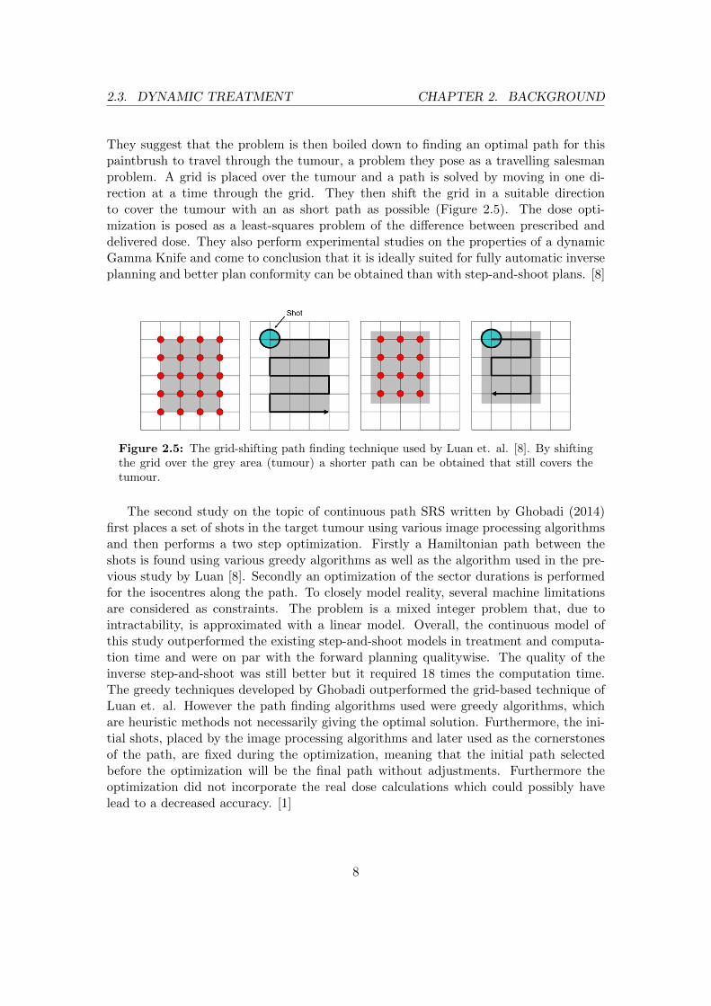
They suggest that the problem is then boiled down to finding an optimal path for thispaintbrush to travel through the tumour, a problem they pose as a travelling salesmanproblem. A grid is placed over the tumour and a path is solved by moving in one di-rection at a time through the grid. They then shift the grid in a suitable directionto cover the tumour with an as short path as possible (Figure 2.5). The dose opti-mization is posed as a least-squares problem of the difference between prescribed anddelivered dose. They also perform experimental studies on the properties of a dynamicGamma Knife and come to conclusion that it is ideally suited for fully automatic inverseplanning and better plan conformity can be obtained than with step-and-shoot plans. [8]

Figure 2.5: The grid-shifting path finding technique used by Luan et. al. [8]. By shiftingthe grid over the grey area (tumour) a shorter path can be obtained that still covers thetumour.

The second study on the topic of continuous path SRS written by Ghobadi (2014)first places a set of shots in the target tumour using various image processing algorithmsand then performs a two step optimization. Firstly a Hamiltonian path between theshots is found using various greedy algorithms as well as the algorithm used in the pre-vious study by Luan [8]. Secondly an optimization of the sector durations is performedfor the isocentres along the path. To closely model reality, several machine limitationsare considered as constraints. The problem is a mixed integer problem that, due tointractability, is approximated with a linear model. Overall, the continuous model ofthis study outperformed the existing step-and-shoot models in treatment and computa-tion time and were on par with the forward planning qualitywise. The quality of theinverse step-and-shoot was still better but it required 18 times the computation time.The greedy techniques developed by Ghobadi outperformed the grid-based technique ofLuan et. al. However the path finding algorithms used were greedy algorithms, whichare heuristic methods not necessarily giving the optimal solution. Furthermore, the ini-tial shots, placed by the image processing algorithms and later used as the cornerstonesof the path, are fixed during the optimization, meaning that the initial path selectedbefore the optimization will be the final path without adjustments. Furthermore theoptimization did not incorporate the real dose calculations which could possibly havelead to a decreased accuracy. [1]

8

2.4. PATH PLANNING CHAPTER 2. BACKGROUND

2.4 Path planning

2.4.1 Path finding

In order to perform continuous path treatment a continuous path must be found. Thepath finding problem can be described as follows: for a given set of points a path issought that optimizes plan quality and treatment time. It can be argued that the pathshould only be allowed to pass each spot just once and it should if possible avoid cross-ing itself. Apart from the criteria of no crossings, the problem can be illustrated by theTravelling Salesman problem (TSP)[1, 8]. In the TSP, a salesman must visit a set ofcities exactly once and then return home in the shortest distance or time. The TSP isone of the most famous problems in the theory of computational algorithms as it is oldand intractable for large numbers of cities: it is known to be NP-hard [9]. The findingof a path for the continuous dose delivery of the Gamma Knife can be seen as a TSPwhere the salesman must visit a certain set of isocentres in the most efficient way butnot necessarily return home. Both Luan et. al. and Ghobadi use the TSP for finding anefficient path through the tumour [1, 8]. Hence, the TSP will be given special attention.

The NP-hard nature of the TSP suggests that approximative methods must be usedto find a solution as optimal as possible. Such heuristic methods have been given im-mense amount of research over the past half century resulting in a variety of good andbetter solvers. However, for problems of limited size, e.g. a TSP with a few hundrednodes, the problem could be solved exactly using common integer programming algo-rithms such as the branch-and-cut approach [10]. Based on previous research by Ghobadiand information from Elekta, there is usually less than 100 initial isocentres being placed[1], indicating that the TSP at hand is likely to be small and thus allowing for an exactsolution.

2.4.2 Smoothing

When performing radiosurgery with the Gamma Knife the patient is usually awake andit is of interest to make the treatment as comfortable as possible for the patient. It istherefore reasonable to limit the acceleration of the PPS in order to avoid rough move-ment. This adds a complication to the path given by the solution of the TSP since thatpath is made up of linear segments which means that at every isocentre, the PPS mustdecelerate and then accelerate in the new direction. With a limit on acceleration thiscould be time inefficient. A vehicle with limitations on velocity and acceleration is in theliterature referred to as a Dubins vehicle and several studies point out the inefficiencyof paths for these vehicles that incorporate sharp turns that require a complete stop[9, 12]. An important field of study on this topic is the motion planning of robots withsuch machine constraints. Studies suggest using curve creation or interpolation to createa smooth path based on the robots starting and stopping directions.

9


The most common approach is to first solve a TSP with line segments and then createcurves along that path, using the nodes of the TSP as control points in some fashion.Castanon et.al. test several methods for generating curve segments using Dubins curvegeneration and come to the conclusion that a three point, receding horizon algorithmgenerates the most efficient path. They solve a general TSP to get the order of pointsand then use the first three points and the direction at the first point to calculate acurve through the three points in order to generate the direction of the second point.The algorithm is then iterated for point 2, 3 and 4 with the direction of 2 to get thedirection at point 3 and so on. This is superior to the ordinary, two-point algorithmbecause it provides a look-ahead property. They also discuss an algorithm called Ran-dom Asymetric Algorithm (RAA), which couples the TSP solver and the smoothing.For this algorithm, directions are randomly assigned to all points, whereby two-pointcurve segments are calculated between all points, thus creating an assymetric TSP. Thisalgorithm is best suited when the number of points per area is high. Out of the testedalgorithms of the study, the receding horizon performed best.[12]

A different algorithm that still uses the same thinking of looking ahead as in [12]is the alternative version of Cardinal splines, Catmull-Rom splines as presented in [13].The Catmull-Rom method is based on piecewise cubic interpolation with four consecu-tive control points. The curve will pass through the two middle points while the outerpoints are used for calculating the tangents in the middle points. The tangent in point

Pj is given as P ′j =1− T

2(Pj+1 − Pj−1), where T is the tension of the curve[13]. If this

is performed with the four points, all which must be passed, it closely resembles thereceding horizon algorithm but with four points in each iteration instead of three.

Figure 2.6: A Catmull-Rom spline with five control points. The tangents to each point,given as arrows, can be seen to have the same direction as the distance between the twoneighbouring points, e.g. the tangent at point p2 has the same direction as the line connectingpoints p1 and p3.

Jolly et. al. use Bezier curves to plan obstacle avoidance paths for football playingrobots with acceleration constraints. According to the authors, the Bezier curve issuperior to splines for this purpose since it requires few assumptions and approximations

10


and only passes through the first and last control point. They pose an efficient way ofcalculating Bezier curves between two points.[14] Lepetic et. al. suggest that four controlpoints is optimal with respect to travel time efficiency.[15]

11

3Method

3.1 Problem set up

Planning a continuous radiosurgical treatment with the Gamma Knife consists of severalsteps. First a path through the target must be drawn, requiring a number of procedures.Secondly the path must be discretized and dose rates must be calculated for each point.The dose rates are dose per time unit and will later be multiplied with the durationsto obtain the total dose of the treatment. Finally an optimization of the durations andcollimator settings in each discretized isocenter is done. The primary focus of this thesisis to improve the path planning and optimization and so the dose calculations used arethe ones provided by Elekta.

Figure 3.1: The progress of dynamic treatment planning

3.2 Path planning

The path planning technique used here is based on finding the shortest way throughseveral isocentres. These isocentres must be provided in advance and are given usinga grassfire algorithm that effectively packs a tumour with shots of different sizes. This

12

3.2. PATH PLANNING CHAPTER 3. METHOD

algorithm is provided by Elekta and as it is not built for the purpose of path planningit tends to produce either too many or too few isocentres. This is solved by choosing toproduce too many isocentres and removing isocentres that are too close to each other.

3.2.1 Path finding

The first step in the path planning is finding a draft of the path including obtainingthe visiting order for the initial isocentres. Finding a path through the isocentres, vis-iting each isocentre exactly once means the problem can be modelled by the previouslydescribed Travelling Salesman Problem (TSP). Even though the TSP is known to beNP-hard an optimal solution can be obtained in a short time for problems of only a fewhundred nodes, which is the case for us. The TSP is posed as a binary integer program,

minimizex

n∑i=0

n∑j=0,j 6=i

cijxij

subject to∑

i=0,i 6=jxi,j = 1 j = 0,...,n

∑j=0,j 6=i

xi,j = 1 i = 0,...,n

ns∑k=1

xk ≤ ns − 1 x ∈ s, s ∈ S

xij ∈ {0,1} i,j = 0,...,n

where xij = 1 if the edge between isocentres i and j is used and 0 otherwise and cij isthe cost of travelling from isocentre i to j. In this case the cost is the distance. The firsttwo constraints ensure that each isocentre has exactly two edges connected to it. Thethird constraint prevents any subtours. The set S = {s1, s2, ...} contains all subtours sthat have occurred, e.g. s1 = {x1,2, x2,5, x5,1}. The sum of the edges xk ∈ s must be atmost one less than the number of elements, ns, in the subtour. Thus, that particularsubtour can never occur again. The set S is filled with subtours through iterating theoptimization and adding the occurring subtours. This is performed until no subtoursoccur [16]. The method used to solve the binary integer program is the branch-and-cutapproach.

The general TSP assumes that travel distance is proportional to travel time, whichis what essentially is to be minimized. However in continuous radiosurgery treatmentthe distances are not necessarily proportional to the time as the speed is variable alongthe path. A solution to the TSP may therefore be suboptimal timewise even if it isthe shortest path. The shortest path however puts a limit on the maximum time of thetreatment since the PPS has a minimum speed. Therefore, there is value in choosing

13


the exact solution to the TSP. In order to compare this path finding technique, the mostsuccessful path finding technique of [1], i.e. the spiral greedy path, is tested as well. Thistechnique works its way through layers along the z-axis, using greedy path finding oneach level and then interlinking the levels. This creates a spiral-like path.

3.2.2 Path smoothing

The solution of the TSP is a path of line segments with sharp corners. This means thatthe PPS must decelerate into and then accelerate out of every isocentre, creating threeproblems. Firstly, rapid or rough movements are undesirable for patients, thus changesin the velocity should be minimized. Secondly the stopping means that there might bean unwanted increase in radiation in the isocentre compared to the path up to it. Thiswould decrease the homogeneity of the plan. Finally, studies have shown that for ma-chines with constraints on acceleration and speed, sharp turns could mean a slower routeeven if it is shorter than a smooth turn.[12] Therefore the TSP solution is smoothed. Thereceding horizon algorithm [12] has proved efficient as has the similar method of Catmull-Rom splines [13]. Out of computational ease, the Catmull-Rom splines are chosen asthe smoothing method. It could well be that the smallest differences between smoothedpaths will not matter, since such changes could be compensated for by speed changes.Therefore basic Bezier curves [17] without any look ahead property are compared to theCatmull-Rom splines. The code that has been used in this study for the Catmull-Romsplines is written by Dr. Murtaza Ali Khan of the Royal University for Women, Bahrainand for the Bezier curves written by Will Robertson of the University of Adelaide [18, 19].

3.2.3 Discretization

The current dose engine calculates the dose rates (dose per time unit) from isocentrepoints. During a continuous treatment the patient will be constantly moving so thereare no fixed isocentres. There is no possibility to update the current dose engine withinthe scope of this thesis and it is not computationally tractable to calculate dose frompoints along the path with an infinitesimal gap. Therefore a discretization of the path isneeded. The old, initial isocentres will be removed since they are unevenly distributedalong the path with an often too long distance between them. Instead new, discretizedisocentres will be placed along the smoothed path with a fixed interval. From now onthe discretized isocentres are referred to as isocentres while the initial isocentres usedfor the pathfinding are referred to as initial isocentres.

Evenly distributed isocentres would give a better approximation of a continuous paththan randomly distributed ones. It is important to note that the path between two ofthese isocentres will always be understood as a line by the computer and a curve betweentwo isocentres will not be compensated for by the dose calculations. Therefore, despitethe first smoothing, the final path will be understood as line segments connecting the

14


isocentres. The distances between isocentres are used in the optimization and must nec-essarily be accurate. Since the final path is that of line segments, the distances shouldbe based on the actual distance between two isocentres and not the distance betweenthem along the smoothed path. Still, the isocentres will be placed along the smoothedpath. The discretization would therefore work as a stepping process from point to pointalong the path starting in an isocentre and not stopping until a point is found that hasa euclidean distance equal to the discretization interval between it and the isocentre. Inthis point a new isocentre is placed and the process is reiterated from there. Since thisis done along the smoothed path the smoothing will still be of importance. With a shortenough interval the final path will closely resemble the smoothed path.

An appropriate discretization interval has to be computationally tractable but stillclosely approximate the behaviour of the continuous movement. To find such an intervalwe set up a basic comparison of the volume covered with dose from shots placed along aline with a small enough gap (0,01 mm) to approximate the continuous movement andshots placed with an increasing gap. A single classical shot, i.e. with all sectors using thesame collimator, resembles an ellipsoid. The smallest possible shot without any closedsectors is a classical 4 mm shot. This would require the shortest interval of all shots inorder to still approximate a beam so it was therefore selected. The difference betweenthe two covered volumes was allowed to be 5 % and it is illustrated in Figure 3.2. Theinterval was increased until the limit of 5 % was hit. The maximum interval of the 4mm collimator was 0.6 mm. This is therefore an ideal discretization interval.

Figure 3.2: Three 4 mm-shots placed consecutively to approximate a continuously movingbeam. The black lines would represent the edges of the beam. The difference in volumebetween beam and shots can be seen as small bumps between each shot. The difference involume was set to be at most 5 %.

15

3.3. SECTOR DURATION OPTIMIZATION CHAPTER 3. METHOD

3.3 Sector duration optimization

At this point we have a smooth path with evenly distributed, discretized isocentres. Foreach of these isocentres the dose rates have been calculated and collected in the doserate matrix D. What remains is to decide the speed and collimator settings. To getthe optimal collimator settings and speed along the path, a sector duration optimizationis performed. In short, the optimization minimizes the spill of dose outside the targetwhile maintaining the dose in the target within a given span by optimizing the collimatorsettings and beam on times in the discretized isocentres along the path. The optimizationis based on the linearly approximated model presented in [1] and the parts added in thispaper will be explicitly stated. The original model is a mixed integer program but itbecomes intractable as the problem quickly grows large with thousands of variables.Thus, a linear approximation was used, relaxing the integer constraints. The selectedmodel was the one with the best overall performance, i.e. using all options except limitedcollimator movement[1].

3.3.1 Dose constraints

In order to better understand the objective function, the dose constraints are presentedfirst. A plan must make sure to cover the tumour with at least a certain dose, T s. Ahomogeneous dose distribution within the tumour is also desirable and thus an upperlimit of target dose is set, T s. The target volume is referred to as TV. The set R, consti-tuting rings or layers of voxels around the target, is used when minimizing the dose spilland is further described in the next section. In the presence of sensitive organs at risk(OAR) they will be given a maximum allowed dose if they are close enough to the TV.Any overlap between the rings in R and the OAR, Ringϑτ , is given a maximum alloweddose. At times we added additional rings in the brainstem in order to force an evenlower dose. The dose in voxel j, zjs, is given by multiplying the dose rates in the doserate matrix D with the beam on times for each collimator setting, sector and isocentre.The set Θ contains all isocentres, the set B contains the eight sectors of an isocentre andthe set C consists of the three collimator settings.

T s ≤ zjs ≤ T s s ∈ {TV,Ringϑτ} (3.1)

zjs =∑θ∈Θ

∑b∈B

∑c∈C

Dθbcjstθbc j = 1,...,vs, s ∈ {TV,Ringϑτ , R} (3.2)

3.3.2 Objective function

The goal of the objective function is to minimize the dose outside of the target. How-ever, it is inconvenient and unnecessary to consider all voxels outside. If the dose canbe minimized in the voxels closest to the target it should also be low enough in voxelsfurther away from the target, which are less exposed. Thus we form rings/layers, r ∈ R,

16


around the target in which we minimize the dose. To optimize selectivity, i.e. minimizedose spillage, the positive difference between the actual dose in a voxel of the ring, zjrand the upper limit of that ring, T r is penalized with weight, wr. vr is the number ofvoxels in ring r.

∑r∈R

vr∑j=1

1

vr[wr(zjr − T r)+]

We use a different formulation when applying this in Matlab, since the solver linprogrequires an objective function on the form cTx. Thus we reformulated the objectivefunction by replacing the positive difference term with the variable zjr.

∑r∈R

vr∑j=1

1

vr[wrzjr] (3.3)

To this is added the following constraints, which guarantee that the zjr always takeon the positive difference or else is 0.

zjr ≥ zjr − T r j = 1,...,vr, r ∈ R (3.4)

zjr ≥ 0 j = 1,...,vr, r ∈ R (3.5)

3.3.3 Single collimator delivery

Only one collimator size per sector can be used at a time. However, since each collimatorsize per sector has its own time variable it is possible that several collimators per sectorare on at the same time. In order to avoid this the following constraint is formulated:

∑c∈C

tθbc ≤ maxc∈C{tθbc} b ∈ B, θ ∈ Θ (3.6)

This constraint is not linear and must be approximated. A maximum constraint forany two variables a,b ≥ 0 can be written using absolute value terms:

a+ b ≤ max{a,b} =a+ b+ |a− b|

2(3.7)

a+ b ≤ |a− b| (3.8)

A common way of approximating an absolute value is by introducing non-negativedummy variables for positive and negative values, p and n. The absolute value is then

17


approximated using the following two equations:

|a− b| = p+ n (3.9)

a− b = p− n (3.10)

Thus Ghobadi rewrites (3.6) into the following two constraints with the third equationbeing added to the objective function in order to ensure that at least one of p and n is0 in each pair [1]. In this study wcol = 1 is used.

tθbci + tθbcj ≤ pθb(ci,cj) + nθb(ci,cj) θ ∈ Θ, b ∈ B, ci, cj ∈ C(i 6= j) (3.11)

tθbci − tθbcj = pθb(ci,cj) − nθb(ci,cj) θ ∈ Θ, b ∈ B, ci, cj ∈ C(i 6= j) (3.12)

wcol∑θ∈Θ

∑b∈B

∑ci,cj∈C(i 6=j)

(pθb(ci,cj) + nθb(ci,cj)) (3.13)

3.3.4 Same duration

Because of both clinical reasons and machine limitations the sectors at each isocentreshould have the same duration. It could increase dose homogeneity and reduce beamon time at the same time as the opening and closing of sectors takes some time andthus produces a dose that is currently not accounted for in GammaPlan. The allowedduration difference between two neighbouring sectors, εduration, is a non-negative userdefined parameter. In this study, in order to eliminate duration differences, εduration = 0.

∑c∈C

tθbic −∑c∈C

tθbi+1c ≤ εduration θ ∈ Θ, bi ∈ B (3.14)∑c∈C

tθbi+1c −∑c∈C

tθbic ≤ εduration θ ∈ Θ, bi ∈ B (3.15)

3.3.5 Movement limitations

The limited movement of the PPS poses several constraints that needs to be addressedin the optimization. The first is concerning the upper and lower bounds on the speedof the PPS. A similar constraint in the model in [1] is replaced in this study with twonew constraints. Since the optimization returns the duration in discretized isocentresrather than speed we put limits on the duration in each isocentre. These limits are basedon the speed limits and the distance between the current isocentre and its succeedingneighbour. Since we require the same duration from all sectors the constraint can be

18


based on that the total duration in each isocentre should be within eight times the limit.

∑b∈B

∑c∈C

tθbc ≤ 8tθmax θ ∈ Θ (3.16)∑b∈B

∑c∈C

tθbc ≥ 8tθmin θ ∈ Θ (3.17)

The speed limits are 0.1−6 mm/s for the x- and y-axis and 0.1−50 mm/s for the z-axis.Out of convenience, in order not to have to supply the direction at each point, this issimplified so that the upper limit is 6 mm/s in all directions. For the same reason wewant to set a single minimum speed that is allowable in all directions. The largest min-imum speed will be

√3 times the minimum axis-speed (x, y and z-diagonal direction).

This converts to a minimum speed of vmin = 10.4 mm/min. The smallest maximumspeed is the axis-speed which converts to vmax = 360 mm/min.

tθmin =dθvmin

(3.18)

tθmax =dθvmax

(3.19)

It is also of interest to limit the acceleration in the treatment. Intuitively, smoothmovement would benefit dose homogeneity as well as patient comfort while staying withinthe capabilities of the PPS. Constraints on acceleration can be posed as limiting thedifference in the speed between two consecutive isocentres. The set Pn−2 consists of then-2 first isocentres in the path.

|vθi − vθi+1| ≤ εspeed θi ∈ Pn−2 (3.20)

The speed at isocentre i is defined as the distance between θi and θi+1, dθi , dividedby the beam-on-time in θi, tθi . The speed constraint can therefore be rewritten in thefollowing way, including the definition of the total beam-on-time in each isocentre: [1]

dθi + dθi+1

εspeed≤ |tθi − tθi+1

| θi ∈ Pn−2 (3.21)

tθi = maxb∈B{∑c∈C

tθibc} θi ∈ Θ (3.22)

In a similar way like the one used previously these constraints can be linearly ap-proximated using dummy variables pθi and nθi .

dθi + dθi+1

εspeed≤ pθi + nθi θi ∈ Pn−2 (3.23)

19


tθi − tθi+1= pθi − nθi θi ∈ Pn−2 (3.24)

tθi ≥∑c∈C

tθibc θi ∈ Θ, b ∈ B (3.25)

εspeed = 1mm/s was used in this study. In addition the following penalty term withweights wmax and wspeed needs to be added to the objective function to complete theapproximation. The wmax part must be added in order to enforce the equality of con-straint (3.22), it will be minimized and thus force equality on the inequality constraint.The wspeed part is added in order to force one of the two dummy variables in each pairto be close to zero. wmax = 10 and wspeed = 1 was used in this study.

wmax∑θ∈Θ

tθ + wspeed∑θ∈Θ

(pθ + nθ) (3.26)

3.3.6 Full linearized model

The full linearized sector duration optimization model used in the final part of the plan-ning is presented below.

minimize∑r∈R

vr∑j=1

1

vr[wrzjr] + wcol

∑θ∈Θ

∑b∈B

∑ci,cj∈C(i 6=j)

(pθb(ci,cj) + nθb(ci,cj))

+ wmax∑θ∈Θ


(pθ + nθ) (SDO)

subject to T s ≤ zjs ≤ T s s ∈ {TV,Ringϑτ} (3.1)

zjs =∑θ∈Θ

∑b∈B

∑c∈C

Dθbcjstθbc j = 1,...,vs, s ∈ {TV,Ringϑτ , R} (3.2)

zjr ≥ zjr − T r j = 1,...,vr, r ∈ R (3.4)

zjr ≥ 0 j = 1,...,vr, r ∈ R (3.5)

tθbci + tθbcj ≤ pθb(ci,cj) + nθb(ci,cj) θ ∈ Θ, b ∈ B, ci, cj ∈ C(i 6= j) (3.11)

tθbci − tθbcj = pθb(ci,cj) − nθb(ci,cj) θ ∈ Θ, b ∈ B, ci, cj ∈ C(i 6= j) (3.12)∑c∈C

tθbic −∑c∈C



tθbic ≤ εduration θ ∈ Θ, bi ∈ B (3.15)∑b∈B

∑c∈C

tθbc ≤ 8tθmax θ ∈ Θ (3.16)

20

3.4. RELAXATION OF THE ORIGINAL PATH CHAPTER 3. METHOD

∑b∈B

∑c∈C


dθi + dθi+1


tθi − tθi+1= pθi − nθi θi ∈ Pn−2 (3.24)∑

c∈Ctθbc ≤ tθ θ ∈ Θ, b ∈ B (3.25)

pθb(ci,cj), nθb(ci,cj) ≥ 0 θ ∈ Θ, b ∈ B, ci, cj ∈ C(i 6= j)

pθ, nθ ≥ 0 θ ∈ Θ

tθbc ≥ 0 θ ∈ Θ, b ∈ B, c ∈ C

The differences between this model of the SDO and the one presented in [1] areconstraints (3.4), (3.5), (3.16), (3.17) and the reformulation of the objective function(3.3). The constraints (3.11), (3.12), (3.23), (3.24) and (3.25) are what makes thisproblem a linear approximation due to the introduction of dummy variables. Situationswhere the originals of these constraints are not met are discussed in sections 4.4, 4.5 and5.

3.4 Relaxation of the original path

The path planning is based on isocentres placed for a step-and-shoot treatment and so itdoes not fully take the continuous movement into account. In the model proposed in [1],the path is then fixed during the sector duration optimization. This imposes a restrictionon the quality of the plan as only the speed and collimator settings are allowed to varybut not the actual path. In the best of scenarios, the optimization itself would find theperfect path without any prior checkpoints, though this would be highly intractable dueto the propelling number of degrees of freedom.

It would, however, be possible to allow a certain flexibility by relaxing the positionof each discretized isocentre along the path during the optimization, a so called relaxedpath sector duration optimization (RP-SDO). By introducing variables ∆x,∆y,∆z forthe offsets of the isocentres from their discretized positions, the path is allowed to shifta limited number of steps in each direction. This adds 3 ∗ nθ new variables, which inthe context of the optimization is fairly few, so the number of variables does not go outof control. When isocentres are moved, new dose rates must be calculated. Since itwould be very time consuming to do this in every iteration we instead look to use fixeddose rate gradients that can be multiplied with the step length. The dose rate kernelsare approximately translation invariant so from the original dose calculations, dose rategradients can be calculated in each direction; ∇drx,∇dry,∇drz. The change in doserates is close to linear and thus the dose rate gradients are calculated as the difference

21


between two dose rate matrices, shifted one step in each direction along the respectiveaxis, divided by two. The dose in a single voxel is now calculated as follows:

zjs =∑θ∈Θ

∑b∈B

∑c∈C

tθbc(Dθbcjs + ∆xθ∇drxθbcjs + ∆yθ∇dryθbcjs + ∆zθ∇drzθbcjs) (3.27)

Figure 3.3: Using the relaxed path extension to the original sector duration optimizationeach discretized isocentre would be allowed to move freely in a cube with 2 mm sides centredaround the isocentres original position.

The products between the t and ∆ variables turn the dose constraint into a non-linear,non-convex constraint. However, it could still be used in the planning. If the initial guessfor the new optimization is the optimal solution of the linear SDO model with all ∆ = 0,the new plan will be at least as good as the plan received from the linear SDO model.Thus the non-convexity is handled by providing a high quality initial point. It would beproblematic to allow too big steps as that would reduce the precision of the distancesdθi used in the same speed constraints as well as increasing the complexity by increasingthe feasible region. Finally, since the dose rate gradients are only approximated, largesteps could see precision drop drastically. Thus the length of the allowed steps is limitedto 1 mm in each direction, resulting in the following constraints:

−1 ≤ ∆xθ ≤ 1 (3.28)

−1 ≤ ∆yθ ≤ 1 (3.29)

−1 ≤ ∆zθ ≤ 1 (3.30)

The progress flow for the RP-SDO function is shown in Figure 3.4.

Figure 3.4: The progress of dynamic treatment planning with RP-SDO

22


The complete mathematical model including the relaxation of the path looks likethis:

minimize∑r∈R

vr∑j=1

1

vr[wrzjr] + wcol

∑θ∈Θ

∑b∈B

∑ci,cj∈C(i 6=j)

(pθb(ci,cj) + nθb(ci,cj))

+ wmax∑θ∈Θ


(pθ + nθ) (RP-SDO)

subject to T s ≤ zjs ≤ T s s ∈ {TV,Ringϑτ} (3.1)

zjs =∑θ∈Θ

∑b∈B

∑c∈C

tθbc(Dθbcjs + ∆xθ∇drxθbcjs (3.27)

+ ∆yθ∇dryθbcjs + ∆zθ∇drzθbcjs) j = 1,...,vs, s ∈ {TV,Ringϑτ , R}zjr ≥ zjr − T r j = 1,...,vr, r ∈ R (3.4)

zjr ≥ 0 j = 1,...,vr, r ∈ R (3.5)

tθbci + tθbcj ≤ pθb(ci,cj) + nθb(ci,cj) θ ∈ Θ, b ∈ B, ci, cj ∈ C(i 6= j)

(3.11)

tθbci − tθbcj = pθb(ci,cj) − nθb(ci,cj) θ ∈ Θ, b ∈ B, ci, cj ∈ C(i 6= j)

(3.12)∑c∈C

tθbic −∑c∈C



tθbic ≤ εduration θ ∈ Θ, bi ∈ B (3.15)∑b∈B

∑c∈C

tθbc ≤ 8tθmax θ ∈ Θ (3.16)∑b∈B

∑c∈C


dθi + dθi+1


tθi − tθi+1= pθi − nθi θi ∈ Pn−2 (3.24)∑

c∈Ctθbc ≤ tθ θ ∈ Θ, b ∈ B (3.25)

pθb(ci,cj), nθb(ci,cj) ≥ 0 θ ∈ Θ, b ∈ B, ci, cj ∈ C(i 6= j)

pθ, nθ ≥ 0 θ ∈ Θ

tθbc ≥ 0 θ ∈ Θ, b ∈ B, c ∈ C− 1 ≤ ∆xθ ≤ 1 θ ∈ Θ (3.28)

− 1 ≤ ∆yθ ≤ 1 θ ∈ Θ (3.29)

− 1 ≤ ∆zθ ≤ 1 θ ∈ Θ (3.30)

23

3.5. REDUNDANT ISOCENTRES CHAPTER 3. METHOD

Since the dose rate gradients are only approximations there will inevitably be a differ-ence between the recalculated final dose and the approximated final dose. The deviationscan cause dose constraints to break, a highly undesirable scenario. To address this, a fi-nal optimization using the linear SDO model is performed after the non-linear RP-SDO,using the new, shifted isocentres and corresponding, exact dose rates. This way we canmake sure that the constraints are satisfied not only for the approximated dose rates butfor the exact ones as well.

Due to the non-linearity of this problem the Matlab solver fmincon was used, whichaccepts non-linear constraints. The Hessian and gradient of the objective function aswell as the non-linear constraints and their gradients were supplied as functions.

3.5 Redundant isocentres

A plan sometimes has several isocentres that are assigned the minimal time, i.e. thePPS moves with maximum speed through those parts of the path. These isocentresare referred to as redundant isocentres. Moving through these isocentres generally alsocauses rapid acceleration and deceleration. Intuitively, this signals that those segmentswould be left out of the path if possible, but all isocentres are forced to be on through theconstraints. The constraint forcing all isocentres to be used should necessarily be activein order to avoid the path being split up into several segments as well as maintainingthe accuracy in the use of the distances between isocentres. It is still appealing to tryand remove the redundant segments from the path.

The first step is to identify the discretized isocentres that are redundant and groupthem into segments of consecutive isocentres. It would seem that a long segment ofredundant isocentres is more interesting to remove. A limit is put on the length of asegment, i.e. the number of isocentres in it, for it to be removed. The limit in thisstudy is set to 1 isocentre to try to remove all redundant isocentres. Secondly thesesegments are removed from the path and replaced with a curve segment between the twoend points using the old slopes of these points. The new path is remade with a tightertension if it falls outside the tumour. Following this, new isocentres are placed along thenew segment. This is finally followed by new dose rate calculations and a sector durationoptimization.

3.6 Solvers

Several solvers were examined and evaluated in order to optimize plan quality and com-putation time. For the initial, linear sector duration optimization, using the Matlabfunction linprog, the interior point and dual-simplex solvers were compared. The non-linear relaxed path sector duration optimization is solved using Matlab’s fmincon, whichonly provides one solver for large-scale problems and that is the interior-point method.

24

4Results

4.1 Discretization interval

The methods were performed on four case tumours provided by Elekta. The targetshave volumes of 2.1, 4.1, 4.4 and 5.3 cm3, are tumours of the type acoustic schwan-noma and can be seen in Figure 4.1. The treatment isodose was 13 Gy for all tumours.The original, clinical forward step-and-shoot plans that were actually used to treat thetumours were available for comparison with the dynamic plans. In addition, inverseplans from an experimental version of GammaPlan were provided for tumours 1, 2 and3. The aim of these plans was to match the results of the dynamic plans, specificallygradient index, while having as short treatment times as possible. The path findingtechnique presented in this study, i.e. the optimal TSP solution, is compared to thepath finding technique called spiral greedy, by Ghobadi (2014)[1]. The same smoothingand discretization was applied to both paths. For the basic linear sector duration opti-mization (SDO), two solvers were tested and compared; the interior point-method andthe dual-simplex-method. Both returned similar plan quality but the dual-simplex wasdistinctively faster so it was selected for use. For smoothing, the Catmull-Rom splinesproved slightly more efficient than the Bezier curves and were thus used.

In order to increase tractability and computation speed, a certain sampling was per-formed on the voxels of each tumour. Each tumour was placed in a grid with 1 mmintervals in x, y and z-direction and extending far outside the tumour. The voxelswithin each tumour were then sampled as far as each second voxel in each direction tobe used in the dose constraints of the optimization. The ideal discretization interval of0.6 mm results in a high number of isocentres, leading to intractable problems. Differentdiscretization intervals are therefore used and compared.

Table 4.1 shows a comparison between different intervals for isocentre discretization

25

4.1. DISCRETIZATION INTERVAL CHAPTER 4. RESULTS

along the path using different path finding techniques. The discretization interval in mmis presented as well as the number of isocentres along the path with this discretization.The Paddick Conformity Index (Equation (2.4)) and its two constitutents coverage (Eq.(2.1)) and selectivity (Eq. (2.2)) are used as measures of plan quality and should all beas close to 1 as possible. V12 is the volume in cm3 of tissue, including the tumour, that isexposed to 12 Gy or more. PI stands for Prescribed Isodose and is the planned minimumdose to the tumour divided by the maximum dose given and gives an understanding ofthe homogeneity of the plan. The number of collimator changes is the number of timesa collimator setting is changed in a sector during the treatment. Multi sectors refer towhen there are multiple collimator settings active in a single sector in a single isocentre,i.e. when constraint (3.6) is not fulfilled. The Beam-on-time (BOT) is the time of thetreatment in minutes. It should be noted that a finer interval is a more accurate approx-imation of an actual dynamic treatment.

Figure 4.1: The case tumours (acoustic schwannomas) used in this study

(a) Case tumour 1

(b) Case tumour 2

(c) Case tumour 3

(d) Case tumour 4

26

4.1. DISCRETIZATION INTERVAL CHAPTER 4. RESULTS

Table

4.1:

Com

pari

son

of

dis

cret

izati

on

inte

rvals

Description

Disc.

Inte

r-

val

#disc.

iso.

Paddick

CI

Cov.

Sel.

V12

PI

#coll.

changes

#

multi

secto

rs

BOT

Comp.

Tim

e

Clin

ical

pla

n21

shot

s0.

751

0.75

-50

%-

-38

.5-

Inve

rse

pla

n12

shot

s0.

820.

980.

84-

50%

--

12.6

Sp

iral

gree

dy

830

0.90

0.98

0.92

6.4

68%

105

1711

.21.

1

Sp

iral

gree

dy

646

0.90

0.98

0.92

6.4

68%

143

2411

.01.

8

Sp

iral

gree

dy

479

0.92

0.97

0.95

6.2

68%

152

511

.13.

9

Sp

iral

gree

dy

3111

0.93

0.97

0.95

6.2

67%

164

311

.06.

8

Op

tim

alT

SP

819

0.89

0.98

0.91

6.4

68%

7726

12.2

0.9

Op

tim

alT

SP

629

0.90

0.98

0.93

6.3

68%

9636

11.0

1.2

Op

tim

alT

SP

456

0.92

0.97

0.94

6.3

69%

108

1611

.02.

4

Op

tim

alT

SP

2122

0.92

0.97

0.95

6.2

68%

166

1511

.18.

0

The

case

tum

our

isca

se2.

The

Clinic

alP

lan

isth

efo

rwar

dp

lan

use

din

the

actu

altr

eatm

ent

ofth

etu

mou

r.T

he

inve

rse

pla

nis

the

exp

erim

enta

lp

lan

from

Gam

maP

lan.

The

two

pat

hfi

ndin

gte

chn

iques

use

dar

esp

iral

gree

dy

and

opti

mal

TSP

.T

he

dis

cret

izati

on

inte

rval

isgiv

enin

mm

.P

add

ick

Con

form

ity

Index

(2.4

),co

ver

age

(2.1

)an

dse

lect

ivit

y(2

.2)

mea

sure

spla

nquality

.V

12

isth

evo

lum

eco

vere

dby

12

Gy

orm

ore,

incl

udin

gth

etu

mou

r.C

ollim

ator

chan

ges

refe

rto

the

chan

ging

of

asi

ngle

collim

ator

sett

ing

ina

sect

or

bet

wee

ntw

ois

oce

ntr

es.

Mu

lti

sect

ors

refe

rto

sect

ors

wit

htw

oor

mor

eac

tive

collim

ator

sett

ings

ina

single

isoce

ntr

e.B

eam

-on

-tim

e(B

OT

)is

the

trea

tmen

tti

me

inm

inute

san

dth

eco

mp

uta

tion

tim

eis

also

mea

sure

din

min

ute

s.

27

4.2. RELAXED PATH CHAPTER 4. RESULTS

It is evident that the quality of the treatment plan increases when using a finer dis-cretization while the computation time goes up as a result of the increased number ofvariables due to the higher numbers of isocentres. The BOT remains independent of dis-cretization interval. The number of collimator changes goes up as a result of the increasednumber of potential changes but if one compares the relative increase in isocentres withthe relative increase in the number of collimator changes it can be seen that the numberof collimator changes per isocentre actually decreases with a finer discretization inter-val. The number of multi sectors decreases as well, possibly because some of the multisectors get split up among new isocentres when the interval is decreased. With a shorterdistance between isocentres the need for multi sectors decreases. V12 slightly decreaseswith the discretization interval. Notably, coverage decreases in favor of selectivity. Thisis explained by the sampling of the voxels. Had no sampling occurred all voxels in thetumour would have had a hard constraint on the lower dose and so coverage would havebeen 1. Selectivity gets favoured because the objective function aims at optimizing it.

There seems to be no evident difference between the two path finding techniquesexcept that he number of multi shots per isocentre is slightly lower for the spiral greedypath but the number of collimator changes per isocentre is lower for the optimal TSPpath, lending no advantage to any path finding. It rather seems that a higher numberof isocentres allows for better precision and thus better plan quality and thus that it isthe discretization interval rather than the path finding that is the determining factor ofthe outcome of the plan. All dynamic plans outperformed the clinical forward plan bothquality- and timewise. The situation is the same compared to the inverse plan,but thedifferences are much smaller.

Figure 4.2 compares optimal TSP paths with 8 mm and 2 mm discretization intervalfor case tumour 2. In Figures 4.2a and 4.2b can be seen the original path (red), whichthe isocentres are discretized along. Isocentres are marked as blue dots. It is a notabledifference as there are only 19 isocentres on the 8 mm path but 122 on the 2 mm path.The final path is interpreted as the lines between consecutive isocentres so the finalpath can look considerably different from the original path. Figures 4.2c and 4.2d showthe final paths. The 8 mm path is seemingly coarse and does not clearly resemble theoriginal path. The 2 mm path, however, closely resembles the original path due to theshort distances between each isocentre. Naturally, the shorter the interval, the closerthe final path becomes to the original, smooth path.

4.2 Relaxed Path

Table 4.2 shows the progression of the treatment plan for case tumour 2 when the methodof relaxing the isocentre locations during the optimization is applied. SDO stands forSector Duration Optimization and is a basic dynamic treatment using this optimization.Relaxed path sector duration optimization (RP-SDO) has two entries. the difference isonly that ”RP-SDO approx” has its final dose calculated using an approximate dose rate

28


Figure 4.2: Paths and discretization

(a) 8 mm discretization interval onoriginal path

(b) 2 mm discretization interval onoriginal path

(c) 8 mm discretization interval, ac-tual path

(d) 2 mm discretization interval, ac-tual path

matrix while ”RP-SDO exact” uses an exact dose rate matrix. ”Reoptimized (SDO)”means that the results from the RP-SDO have been optimized again with the SDO.

The two RP-SDO entries stem from the same optimization. The final dose and re-sults for the approximated relaxed path are calculated using the same approximated dosematrices used in the optimization itself, i.e. it is the de facto result from the RP-SDO.However, since a plan should be modelled as exact as possible the dose rate matrix isrecalculated when the positional shift of the isocentres is known. The new dose rates arethe correct ones and are used to calculate the exact relaxed path results.

There is a drop in coverage for the exact relaxed path, due to the approximated doserates being overestimated. Not all the sampled voxels within the tumour reaches thetreatment dose of 13 Gy when the approximated dose rates are replaced by the exact

29


ones. In order to restore coverage the plan is reoptimized with the basic SDO. This tendsto increase coverage on the cost of selectivity, since coverage tends to be below the limit.For the final results, all constraints are fulfilled and the plan has a distinctly higher planquality than the dynamic basic. Table 4.2 shows the results for tumour 2 but they aresimilar for the other cases. It should be noted that the best plan is either of the basicSDO, exact relaxed path or the reoptimized as these all use exact dose matrices. In thisparticular case the exact relaxed path is the best choice as it has the highest PaddickConformity Index and lowest V12 while still having a relatively high coverage.

Table 4.2: The effect of relaxing the path

DescriptionPaddick

CICov. Sel. V12 PI BOT

Comp.

Time

SDO 0.88 0.99 0.88 7.4 61% 12.1 0.6

RP-SDOapprox.

0.91 0.98 0.93 6.9 58% 10.7 11.4

RP-SDO exact 0.91 0.97 0.94 6.7 59% 10.7 11.4

Reoptimized(SDO)

0.90 0.99 0.91 7.1 58% 10.8 0.2

The tumour is case 2 and the discretization interval is 8 mm. The methods are performed inthe order listed and the results from one step is used as input in the consecutive step. Theapproximate and exact relaxed path are calculated based on the same results from a singleRP-SDO, and the computation time is for both combined. The approximate relaxed pathrepresents the output from the RP-SDO while the exact relaxed path uses that output butwith a recalculated, exact dose rate matrix. Both BOT and computation time are measured inminutes and V12 in cm3.

Table 4.4 provides an overall comparison between all case tumours and their clini-cal, experimental inverse, dynamic basic and relaxed path plans respectively. The pathplanning technique used is the exact TSP-solution. The relaxed path (RP) results arechosen either from the exact relaxed path or the reoptimized plans, with the plan withbetter quality being selected. Both of these are valid plans as they are based on thereal dose rate matrix while the approximated relaxed path should not be used since itis based on approximate dose rates. In all cases the dynamic plans show a significantlybetter selectivity than the clinical forward plans and the inverse plans. The RP planstend to perform better than the basic SDO plans. Coverage of the dynamic plans wouldbe on par with the clinical plans if no sampling took place. Treatment times are roughlythe same between RP and SDO plans but they are 3 to 4 times shorter than the clinicalplans. The dynamic plans are also shorter than the inverse plans but with no clearpattern. Computation times of the RP plans vary with no clear pattern. The gradientindex, defined in Eq. (2.3), is the only measure that is better for the clinical and inverse

30


plans than for the dynamic plans.

For a visual understanding of these effects one can view the isodose curves in threeslices of the treatment area before and after the RP-SDO in Figure 4.3. The case tu-mour is tumour 3 and the thick, blue line represents the tumour and the thick red linerepresents the brainstem. The thinner curves are isodose lines, from the center and outrepresenting doses of 16, 13, 12, 8 and 5 Gy. Although the 13 Gy curves are alreadyclose to the tumour for the SDO-plans the RP-SDO pulls the isodose curves even closerto the tumour surface, thus increasing selectivity and most importantly, decreasing thedose in the brainstem.

It should be noted that in all cases most isocentres moved maximum distances in atleast two directions, often all three. This implies that further movement likely would bebeneficial. Since the model is currently limited to a short step the RP-SDO was rerunusing the already moved isocentres as the new starting guess. Thus the isocentres wereallowed to move one more time. The results are presented in Table 4.3. This proved toincrease plan quality even further and at the same time slightly decrease the treatmenttime. Computation times were slightly higher for the second RP-SDO.

Table 4.3: Rerunning the RP-SDO

Case DescriptionDisc.

Int.

Paddick

CICov. Sel. V12 BOT

Comp.

Time

1 SDO 5 0.86 0.99 0.87 3.5 7.3 1

1 RP first run 5 0.87 0.98 0.89 3.4 6.9 19

1 RP second run 5 0.90 0.98 0.92 3.3 6.9 23

4 SDO 8 0.81 0.99 0.82 9.7 13.6 1

4 RP first run 8 0.87 0.98 0.89 8.9 12.9 8

4 RP second run 8 0.89 0.96 0.92 8.6 12.3 9

The table displays the effect of rerunning the RP-SDO on an already relaxed set of isocentres usingthe optimal x-vector for the first RP-SDO as x0 in the second RP-SDO. BOT and computation time

are measured in minutes and V12 in cm3.

31


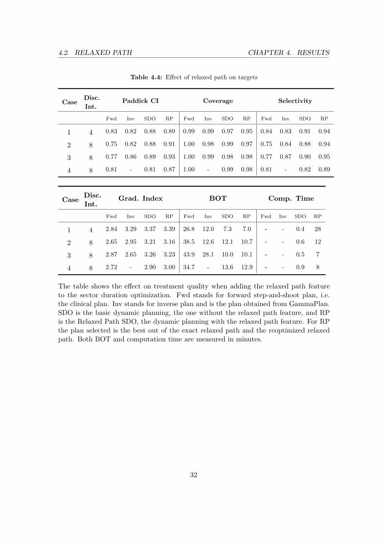
Table 4.4: Effect of relaxed path on targets

CaseDisc.

Int.Paddick CI Coverage Selectivity

Fwd Inv SDO RP Fwd Inv SDO RP Fwd Inv SDO RP

1 4 0.83 0.82 0.88 0.89 0.99 0.99 0.97 0.95 0.84 0.83 0.91 0.94

2 8 0.75 0.82 0.88 0.91 1.00 0.98 0.99 0.97 0.75 0.84 0.88 0.94

3 8 0.77 0.86 0.89 0.93 1.00 0.99 0.98 0.98 0.77 0.87 0.90 0.95

4 8 0.81 - 0.81 0.87 1.00 - 0.99 0.98 0.81 - 0.82 0.89

CaseDisc.Int.

Grad. Index BOT Comp. Time

Fwd Inv SDO RP Fwd Inv SDO RP Fwd Inv SDO RP

1 4 2.84 3.29 3.37 3.39 26.8 12.0 7.3 7.0 - - 0.4 28

2 8 2.65 2.95 3.21 3.16 38.5 12.6 12.1 10.7 - - 0.6 12

3 8 2.87 2.65 3.26 3.23 43.9 28.1 10.0 10.1 - - 0.5 7

4 8 2.72 - 2.90 3.00 34.7 - 13.6 12.9 - - 0.9 8

The table shows the effect on treatment quality when adding the relaxed path featureto the sector duration optimization. Fwd stands for forward step-and-shoot plan, i.e.the clinical plan. Inv stands for inverse plan and is the plan obtained from GammaPlan.SDO is the basic dynamic planning, the one without the relaxed path feature, and RPis the Relaxed Path SDO, the dynamic planning with the relaxed path feature. For RPthe plan selected is the best out of the exact relaxed path and the reoptimized relaxedpath. Both BOT and computation time are measured in minutes.

32


Figure 4.3: Isodose lines and effect of relaxing the path. Isodose lines from center and outare at 16, 13, 12, 8 and 5 Gy.

(a) Dynamic basic plan

(b) Dynamic basic plan

(c) Dynamic basic plan

(d) Relaxed path plan

(e) Relaxed path plan

(f) Relaxed path plan

33

4.3. DOSE DISTRIBUTION AND HOMOGENEITY CHAPTER 4. RESULTS

4.3 Dose distribution and homogeneity

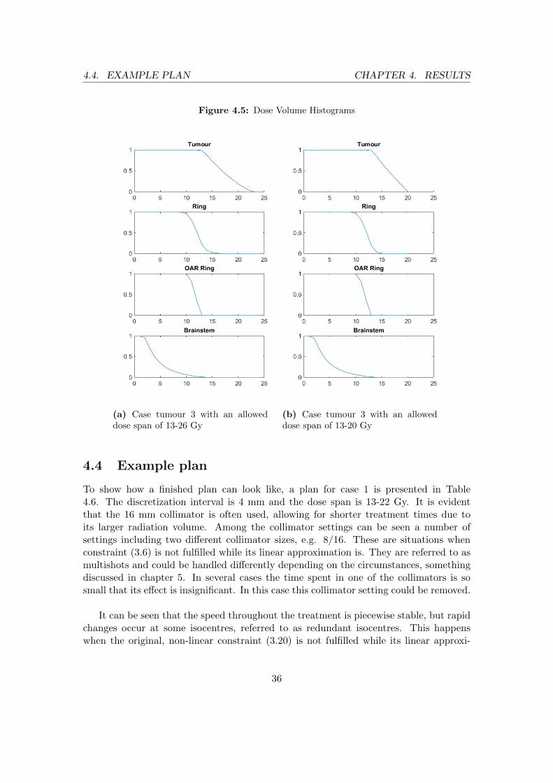
As a complement to the quality metrics it is of interest to study the dose distributionin different volumes. Figure 4.4 shows two dose volume histograms (DVH) showing thepercentage of the specified volume that gets over a certain dose from the plan. The casetumour is case 1. Figure 4.5 shows two DVHs for case tumour 3. Firstly the tumourvolume can be seen to have close to a linear decline, starting at the lower limit of 13 Gy.In Figure 4.4a the upper limit of 26 Gy has no volume, but instead the maximum dose inany voxel for that tumour is around 22 Gy. In Figure 4.4b the upper limit of 19 is reachedby a few voxels. The next DVH is for the rings/layers, R. The drop is much sharpercompared to the tumour. The closest ring is penalized on values above 8.7 Gy and theouter ring on 7.8 Gy. In the third DVH can be seen the voxels overlapping between ringand OAR. The hard upper limit is 13 and the decline is steep. The last DVH shows thepart of the brainstem close to the tumour. The decline is slow compared to the othersbut the dose is also considerably lower with little volume above 10 Gy. Overall the onlymajor difference in the DVHs is the dose homogeneity of the tumour, with the tighterdose span giving a more homogeneous dose distribution. The same applies to the DVHsin Figure 4.5.

Traditionally a homogeneous dose distribution has belonged to radiotherapy whileradiosurgery has allowed for a broader dose span in the target. Recall that one of theproposed advantages of a continuous dose delivery was that a more homogeneous dosedistribution could be achieved. Table 4.5 shows the effects on case tumour 1 when forc-ing different levels of homogeneity by varying the upper dose limit in the tumour. Thelower limit is fixed at 13 Gy as it is the treatment dose. The prescribed isodose, i.e. thetreatment dose of 13 Gy divided by the maximum dose given, is virtually unchangedbetween the first two entries. This can be understood by looking at Figure 4.4 wherewe see that the maximum dose of the 13-26 Gy-span is close to 22 Gy. Thus these twospans produce more or less the same results. When we tighten the dose span further,to 13-19 Gy, the prescribed isodose reaches 79 % and the quality increases as well, atthe cost of a minute extra BOT. The dose span could not be tightened further due toinfeasibility of the optimization. This worked similarly for the other tumours, reachingtreatment isodoses of around 75 %. This should be compared to the clinically prescribedisodoses which are all around 50 %.

Figure 4.3 presents a visual example of a dose distribution. The target is case tumour3 and the prescribed isodose interval is 13-26 Gy. The isodose lines from center and outare 16, 13, 12, 8 and 5 Gy respectively. It can be seen that the entire tumour is coveredby 13 Gy and most of it by 16 Gy. The dose can also be seen to decrease slightly fasterin the direction of the brainstem.

34

4.3. DOSE DISTRIBUTION AND HOMOGENEITY CHAPTER 4. RESULTS

Figure 4.4: Dose Volume Histograms

(a) Case tumour 1 with an alloweddose span of 13-26 Gy

(b) Case tumour 1 with an alloweddose span of 13-19 Gy

Table 4.5: Varying dose homogeneity

Dose spanPaddick

CICov. Sel. V12 PI BOT

Comp.

Time

13-26 Gy 0.88 0.99 0.88 3.4 68 % 7.3 1

13-22 Gy 0.88 0.99 0.89 3.4 69 % 7.4 1

13-19 Gy 0.90 0.99 0.90 3.3 79 % 8.3 1

The case tumour is case 1. The table shows the effect of decreasing the alloweddose span in the tumour.

35

4.4. EXAMPLE PLAN CHAPTER 4. RESULTS

Figure 4.5: Dose Volume Histograms

(a) Case tumour 3 with an alloweddose span of 13-26 Gy

(b) Case tumour 3 with an alloweddose span of 13-20 Gy

4.4 Example plan

To show how a finished plan can look like, a plan for case 1 is presented in Table4.6. The discretization interval is 4 mm and the dose span is 13-22 Gy. It is evidentthat the 16 mm collimator is often used, allowing for shorter treatment times due toits larger radiation volume. Among the collimator settings can be seen a number ofsettings including two different collimator sizes, e.g. 8/16. These are situations whenconstraint (3.6) is not fulfilled while its linear approximation is. They are referred to asmultishots and could be handled differently depending on the circumstances, somethingdiscussed in chapter 5. In several cases the time spent in one of the collimators is sosmall that its effect is insignificant. In this case this collimator setting could be removed.

It can be seen that the speed throughout the treatment is piecewise stable, but rapidchanges occur at some isocentres, referred to as redundant isocentres. This happenswhen the original, non-linear constraint (3.20) is not fulfilled while its linear approxi-

36


mation is. The rapid acceleration at such an isocentre is undesirable in a final plan. Inan attempt to decrease the speed differences we forced a lower maximum speed than 6mm/s. The results show that the maximum speed could be drastically reduced to 0.5mm/s with only minor effects on plan quality.

Table 4.7 shows an excerpt of a plan for case tumour 3 with the normal maximumspeed of 6 mm/s. It can be seen that two isocentres get very close to the limit and causelarge speed changes. Table 4.8 shows the same plan excerpt but the maximum speed hashere been pushed down to 0.5 mm/s. As opposed to the original plan, the new plan hasa much more even speed distribution, with less acceleration required. Accordingly onecan notice that the presence of 4 mm collimators is higher in the second plan as opposedto the original plan. Since more time is spent in the isocentres a smaller collimator isselected so that the total dose does not increase. The Paddick CI is slightly lower forthe tighter speed plan compared to the original (0.88 to 0.89) and the treatment time isslightly higher (11.2 to 10.4 minutes) but overall the plans show similar properties. Theresults are analogous for the other tumours.

37


Table 4.6: Example plan

Sectors

Time Speed 1 2 3 4 5 6 7 8

10 0.38 16 16 16 16 16 16 16 16

1 6 8 16 16 16 16 16 16 16

1 6 16 8 16 16 16 16 16 16

23 0.17 16 16 16 16 16 16 16 16

1 6 8 8 8 8 8 8 16 16

11 0.36 16 4 4 16 16 8 16 16

17 0.23 16 8 8 8 8 8/16 8 16

23 0.17 16 16 16 16 16 4 8/16 16

23 0.17 16 8/16 16 16 16 8/16 16 16

23 0.17 8 16 4 16 16 8 16 8

1 6 16 16 16 16 8 8 16 8

23 0.17 16 16 16 16 8 8 4 16

23 0.17 16 16 16 16 16 8 4/8 8/16

23 0.17 16 16 16 16 16 16 16 16

9 0.43 16 16 16 16 4/16 16 16 16

1 6 16 8 16 16 16 4 16 16

5 0.83 16 8/16 16 16 16 16 16 16

23 0.17 16 8 8 16 8 8 16 8/16

13 0.31 16 16 8 16 8 4 16 16

15 0.27 8 16 16 8 8 8 16 8

1 6 4 4 16 16 16 4 16 16

23 0.17 16 16 16 16 16 16 16 16

19 0.21 16 8/16 16 16 16 16 16 16

23 0.17 8 16 8 16 16 16 8 16

24 0.17 8/16 8/16 8/16 4/16 8/16 8/16 8/16 8/16

Collimator settings, durations in each isocentre in seconds and speed in mm/s for a plan for case 1,limits 13-21.7 Gy, 4mm discretization. For space reasons the entire plan is not showed, only the 25first isocentres out of 31 but the last 6 isocentres show similar settings. Multishots are represented bya combination of the active collimators. 38


Table 4.7: Plan excerpt with standard speed limits

Sectors

Time Speed 1 2 3 4 5 6 7 8

1 5.55 8 4 4 16 16 16 16 16

16 0.37 16 8 8/16 16 16 16 16 16

35 0.17 16 8/16 16 16 16 16 16 16

10 0.59 16 16 16 16 16 16 16 16

8 0.72 16 16 16 16 16 16 16 8/16

35 0.17 8 8 8 8/16 16 16 16 8/16

16 0.38 16 16 16 16 16 16 16 16

1 6 16 8 16 4 16 4 16 16

Collimator settings and durations in each isocentre in seconds for a plan for case 3, 6 mm discretizationinterval. Maximum allowed speed was 6 mm/s.

Table 4.8: Plan excerpt with tight speed limits

Sectors

Time Speed 1 2 3 4 5 6 7 8

12 0.5 8 4 4 16 16 8/16 16 16

12 0.5 16 8 8 16 16 4 16 16

35 0.17 16 8 16 16 16 16 16 16

12 0.5 16 16 8 16 16 16 16 4/16

12 0.5 16 4 4 16 16 16 16 8/16

35 0.17 8/16 8 8 16 4/8 16 16 8/16

12 0.5 16 16 4/16 4 16 16 16 16

12 0.5 16 4 16 4 16 4 16 16

Collimator settings and durations in each isocentre in seconds for a plan for case 3, 6 mm discretizationinterval. Maximum allowed speed was 0.5 mm/s.

39

4.5. REDUNDANT ISOCENTRES CHAPTER 4. RESULTS

4.5 Redundant Isocentres

Final plans of all tumours have been studied in order to detect redundant isocentres. Ithas become evident that it is at short discretization intervals that the number of redun-dant isocentres becomes significant. At higher intervals all isocentres are needed in theplan but the more isocentres there are the clearer it becomes which parts of the pathcould be skipped. Table 4.9 shows the effects of removing isocentres from the originalpath for each case tumour with a relatively short discretization interval. Unfortunatelythe function could not be combined with the relaxed path function as that cannot handlethe sizes of the problems that come with the short intervals.

It can be seen that the quality of the plan remains similar after removal of redundantisocentres. The number of redundant segments decreases slightly. That the change is notbigger could in most cases be explained by that the path between the two end points ofa segment is redundant regardless of the way travelled between the two. It is clear thatthe number of isocentres is reduced by the function. Figure 4.6 shows the paths for casetumour 3. It can be seen that long black segments have been replaced by shorter redsegments. But there are also places where original, black segments have been replacedby near similar red segments.

Table 4.9: Removal of redundant isocenters

Case Description#

isocentres

#

red.

segs.

Paddick

CICov. Sel. BOT

Comp.

Time

1 SDO 31 6 0.88 0.99 0.89 7.6 1.0

1 Remove iso 30 4 0.88 0.99 0.89 7.6 1.0

2 SDO 56 13 0.94 0.99 0.94 11.8 5.0

2 Remove iso 49 11 0.94 0.99 0.94 11.7 3.5

3 SDO 56 11 0.94 0.99 0.95 10.5 5.6

3 Remove iso 47 6 0.94 0.99 0.95 10.4 3.5

4 SDO 70 9 0.87 0.98 0.88 13.3 3.9

4 Remove iso 60 9 0.88 0.98 0.89 13.2 2.5

The table shows the effect of removing redundant isocentres, isocentres that are passed at maximumspeed. SDO refers to the basic sector duration optimization. Remove iso means that the precedingdynamic plan has had its redundant isocentres removed and replaced by new segments and then re-optimized using the basic SDO. # of isocentres indicate the number of discretized isocentres used inthe optimization, # redundant segments means the number of segments (connected isocentres) that areredundant. BOT and computation time are measured in minutes. The discretization interval is 4 mmfor all tumours.

40

4.5. REDUNDANT ISOCENTRES CHAPTER 4. RESULTS

Figure 4.6: A treatment plan for case 3 where the redundant isocentre method has beenapplied. The red path is the path after removal of redundant isocentres and the red dotsare corresponding discretized isocentres. The black path is the part of the original pathremoved of the redundant isocentre function and the black dots are the removed isocentres.

41

5Discussion

It is evident that the expectation of shorter beam-on time (BOT) with dynamic plansis correct. All dynamic plans are vastly faster than the forward plans and clearly fasterthan the inverse plans. By studying the collimator settings it becomes clear that themajor reason for the cut in BOT is the heavy reliance on 16 mm collimators in thedynamic plans. This is not found in the forward plans, where collimators 4 and 8 areused more frequently instead. It is reasonable that this causes the BOT to decrease sincethe 16 mm collimator has a significantly larger volume of radiation and thus can covervolumes in a shorter time span than the 8 and 4 mm collimators. When using step-and-shoot, smaller shots will be needed to achieve proper precision along the edges but dueto the movement and therefore possibly very short durations in each isocentre duringthe dynamic plan, a larger shot size can achieve better precision than it could duringstep-and-shoot. The one negative consequence the use of 16 mm collimators has for thedynamic plans is the increased gradient index, which indicates a slower dose decreaseoutside the tumour. It could be argued that this is no problem as long as the volume of10 or 12 Gy does not reach a critical limit where the risk of e.g. radionecrosis becomestoo high. In our case tumours the approximate limit of 8.5 cm3 is passed only briefly forthe largest tumour, with 8.6 cm3 for the second run RP-SDO. In this particular case aharder penalization, alternatively a fractionated treatment, could be considered. If onewould prefer a lesser dose outside of the tumour an idea would be to encourage smallercollimator sizes but at the cost of treatment time. It is also technically possible to closeone or several sectors for different kinds of shots. In the current SDO and RP-SDOthis is forbidden due to the same-duration and all-isocentres-on constraints. It would beinteresting to allow sectors to be closed during the treatment as long as it works wellwith the other constraints. This would provide a range of new possible shots.

There is no clear difference in the two path finding techniques used (optimal TSPand spiral greedy) when they are based on the same original isocentre distribution. It

42

CHAPTER 5. DISCUSSION

seems to be the number of discretized isocentres that goes into the optimization thatdetermines the plan quality since the number of isocentres correlates quite well with theother metrics. The path is now strongly controlled by the pre-optimization isocentreplacement algorithm that places initial isocentres that the path finding algorithms thenfind a path through. The placement algorithms have not been the focus of this studybut it would definitely be of interest to further extend them and tailor algorithms specif-ically for continuous treatments. Perhaps they could be combined with path finding.Alternatively the popular SLAM technique could be used for finding the most effectivepath [20]. It can also be noted that the longer and tighter the path is, and thus the morevolume covered by the path, the tighter the dose span can be set. This is because eachisocentre can focus more on local dose delivery and thus radiate on a smaller volume.With an extended sampling of the Ringϑτ the V12 of the brainstem can be furthereddecreased, something we noted when we added more ring segments inside the brainstem.

A possible reason for the major differences in plan quality between the dynamic andthe clinical plans is that we do not know the reasoning behind the clinical plans andwhat goals they tried to achieve. They could have, for example favoured as little dose aspossible in the brainstem and used that as the main driver for the planning. Not know-ing the reasoning makes it a bit harder to draw a quick comparison, yet the comparisonmade here still gives a hint of the relationship between forward and dynamic plans. Thedynamic plans also perform better than the experimental inverse plans when these try tomatch the metrics of the dynamic plans. This indicates a great outlook for the dynamicplans.

The relaxed path function improves the results from the dynamic basic plan. Thehigh plan qualities were obtained on fairly large discretization intervals and as we haveseen the quality tends to be even higher as one decreases the interval and approachesthe actual continuous movement. The RP-function provides the biggest improvement todynamic planning in this thesis. Intuitively it makes sense to include the path findingin the SDO where all aspects of the treatment are concerned and not just the distancesas in the basic path finding. This also proves to be the case and this function should befurther extended in future studies. At the moment it is limited to a step length of only 1mm in each direction. This is because the solver slows down significantly with a furtherincreased freedom. We tackled this issue by rerunning the optimization with significantimprovements of the plan quality as a result. This could be a potential alternative toallowing a bigger step. A higher computational power combined with a more efficientcode would be required to allow a greater step length. Computational efficiency alsolimits the discretization interval that can be used. To properly model a real continuousmovement the discretization interval should be 0.6 mm, but this becomes intractable atthe moment. An alternative to using discretized isocentres to calculate the dose alongthe path could be to use Monte Carlo simulations.

We see a dip in coverage when calculating the exact relaxed path because the dose

43


rate gradients used in the algorithm are overestimating the dose. Better approximationsof the gradient of the dose rates could increase the performance of the relaxation of thepath during the RP-SDO as the isocentres could be more optimally placed. Rerunningthe RP-SDO several times would be an alternative to this as well. This would implic-itly allow steps greater than 1 mm but would not require any coarser dose rate gradients.

In all plans, so called multishots were present. These shots have two active collimatorsin a single sector in a single isocentre and are a consequence of the linear approximationof constraint (3.6). This is a limitation of the algorithm as it treats them as if theyradiate at the same point when they actually would have to be active along differentsegments of the path due to the machine limitation of only one active sector at a time.As long as a linear approximation is necessary for tractability the planner must figure outways to handle the multishots. In some cases the BOT of one collimator is remarkablyshort with the other one having well over 95 % of the BOT. In these cases it could beargued that the entire time be spent in the latter isocentre thus removing the multishotattribute. Sometimes the multishots serve as transitions between two collimator sizes ofthe surrounding isocentres. In these cases one could simply let the multishot act as thetransition. Then there are those multishots that fit into neither of these categories. Forthese, as well as for sections of the path where many collimator changes occur, it must beconsidered what is actually possible to do and how to best convert the theoretical plansthis study provides and turn them into practical plans. A change of collimator settingstakes a few seconds and could cause deviations in the dose calculations. A dose ratecalculation that specifically handled the collimator switching would solve this problemand further improve the model.

The final plans using a lower discretization interval all had redundant isocentresalong the way. They were considered distinctively redundant because the surroundingisocentres typically had speeds below 1 mm/s while these had 6 mm/s. Less than 1second was spent in each of them. That the constraints regarding same speed doesnot take care of this is explained by the fact that the constraints are only linear ap-proximations of constraint (3.20). The redundant isocentre algorithm was successful inremoving some of these, especially the larger segments. However it was not capable ofcompletely removing them, understandable since removing one or two isocentres andthen replacing them with a new segment often generates a fairly similar path. It shouldstill, though, be a good idea to run the redundant isocentre function before the RP-SDO,thus decreasing the number of input isocentres. Unfortunately it was not possible heredue to computational issues. The redundant isocentre function worked best on shortdiscretization intervals while the RP-SDO generally only worked for long intervals. Inany case the idea and function of removing redundant isocentres could be improved. Itis without doubt desirable to remove such outlying isocentres when it comes to speedas the redundant isocentres cause rapid accelerations and decelerations. Judging fromthe results, any isocentre that was actually used during treatment seldom had speedsabove 2 mm/s. A potential way of eliminating the rapid speed changes would be to

44


force a lower top speed, which proved quite successful in our trials. This could come atthe cost of a lower plan quality but is an option as long as plan quality stays good enough.

The plans of this study are theoretical in the sense that they are not perfectly adjustedto the machine. However, the theoretical plans are a starting point for practical plans.Future studies should look at how to take a theoretical plan and actually convert it intosomething that can be run on a real Gamma Knife. An example is how to handle theacceleration e.g. when and how should the PPS accelerate and decelerate? Now we onlyprovide speeds in points along the path. Such a future study should also investigatethe best way to handle multishots. Finally this thesis has applied its methods to fourtumours of the type acoustic schwannomas with fairly convex volumes. It would beof interest to apply the techniques to different potential targets, especially with highlynon-convex shapes such as a C-shaped tumour.

45

6Conclusions

The purpose of this thesis has been to provide an improved model for dynamic treatmentplanning with the Leksell Gamma Knife® Perfexion�. The model chosen as the basis isthe continuous treatment model presented in [1]. The improvements that this thesis hasprovided are a new function allowing the relaxation of the path during the sector dura-tion optimization (RP-SDO) as well as a group of new constraints used to better alignthe model with the actual machine and its constraints. Incentives as well as a modelfor removing so called redundant isocentres and thus improve the path has also beenpresented. Furthermore this study contributes with further understanding of dynamictreatments, how it affects the dose distribution and how a plan can look like. Onceagain it has been shown that dynamic treatment plans show great promise compared tostep-and-shoot plans, both in terms of plan quality and treatment time. We have alsoshown that a very high dose homogeneity can be reached with dynamic treatments, withprescribed isodoses of up to 80 %.

The results show a positive impact when the path is relaxed during the optimization.This functionality is a promising direction in search of the optimal dynamic treatmentplan. Further studies should look at how to improve the computational tractability ofthe function so as to allow further degrees of freedom. If possible future studies couldalso apply methods of global optimization to improve the quality of the solution of theRP-SDO. In many ways this study provides theoretical plans with several properties,which must be figured out how to handle in a practical implementation of the plan.These properties include how to change collimators and how to handle multishots. Afuture study could take on where this study ends and connect the theoretical dynamicalplans with the actual machine and go from theoretical to practical plans. Finally, futurework should also include improved pre-path planning placement of isocentres, tailoredfor dynamic plans, to improve the initial paths.

46

Bibliography

[1] K. Ghobadi, Optimization methods for patient positioning in leksell gamma knifeperfexion, Ph.D. thesis, Graduate Department of Mechanical and Industrial Engi-neering, University of Toronto (2014).

[2] World Cancer Research Fund International, Worldwide data,http://www.wcrf.org/int/cancer-facts-figures/worldwide-data, online; accessed2015-03-10.

[3] Cancer Research UK, Brain, other cns and intracranial tumours statistics,http://www.cancerresearchuk.org/cancer-info/cancerstats/keyfacts/brain-cancer/,online; accessed 2015-03-10.

[4] Elekta, Why Gamma Knife® surgery?, http://www.elekta.com/healthcare-professionals/products/elekta-neuroscience/gamma-knife-surgery/why-gamma-knife-surgery.html, online; accessed 2015-03-10.

[5] Elekta, Inverse Planning in Leksell GammaPlan 10 (2014).

[6] I. Paddick, A simple scoring ratio to index the conformity of radiosurgical treatmentplans, Journal of Neurosurgery 93(3) (2000) 219–222.

[7] G. Minniti, E. Clarke, G. Lanzetta, M. F. Osti, G. Trasimeni, A. Bozzao, A. Ro-mano, R. M. Enrici, Stereotactic radiosurgery for brain metastases: analysis ofoutcome and risk of brain radionecrosis, Radiat Oncol 6 (48) (2011) 1–9.

[8] S. Luan, N. Swanson, Z. Chen, L. Ma, Dynamic gamma knife radiosurgery, Physicsin Medicine and Biology 54 (2009) 1579–1591.

[9] A. Yazici, A smooth tour construction approach for a mobile robot with kinematicconstraints, International Journal of Advanced Robotic Systems 10.

[10] F. S. Hillier, G. J. Liebermann, Introduction to Operations Research, 10th Edition,McGraw-Hill Education, 2014.

47

BIBLIOGRAPHY

[11] M. Grotschel, The travelling salesman problem and its applications, Presentationnotes, combinatorial Optimization at Work Berlin (2009).

[12] D. A. Castanon, X. Ma, Receding horizon planning for dubins traveling salesmanproblems, IEEE conference on Decision and Control 45.

[13] M. A. Khan, M. Sarfraz, Motion tweening for skeletal animation by cardinal spline,Communications in Computer and Information Science 254 (2011) 179–188.

[14] K. Jolly, R. Sreerama Kumar, R. Vijayakumar, A bezier curve based path plan-ning in a multi-agent robot soccer system without violating the acceleration limits,Robotics and Autonomous Systems 57 (2006) 23–33.

[15] M. Lepetic, G. Klancar, I. Skrjanc, D. Matko, B. Potocnik, Time optimal path plan-ning considering acceleration limits, Robotics and Autonomous Systems 45 (2003)199–210.

[16] MathWorks, Travelling salesman problem, http://se.mathworks.com/help/

optim/ug/travelling-salesman-problem.html (May 2015).

[17] J. D. Hobby, Smooth, easy to compute interpolating splines, Discrete and Compu-tational Geometry 1 (1986) 123–140.

[18] M. Khan, N Dimensional Cardinal Spline (Catmull-Rom) Spline Interpola-tion, http://www.mathworks.com/matlabcentral/fileexchange/7326-n-dimensional-cardinal-spline–catmull-rom–spline-interpolation, accessed: 2015-05-02 (2012).

[19] W. Robertson, Smooth 3d bezier curves with implicit control points,http://www.mathworks.com/matlabcentral/fileexchange/42302-smooth-3d-bezier-curves-with-implicit-control-points/content/hobbysplines.m, accessed: 2015-02-25(2013).

[20] E. Lopez, C. De Bernardis, T. Martinez-Marin, An Active SLAM Approach forAutonomous Navigation of Nonholonomic Vehicles., in: ECMR, 2011, pp. 291–296.

48

http://se.mathworks.com/help/optim/ug/travelling-salesman-problem.html

http://se.mathworks.com/help/optim/ug/travelling-salesman-problem.html

TRITA -MAT-E 2015:45

ISRN -KTH/MAT/E--15/45--SE

www.kth.se

Dynamic treatment with Leksell Gamma Knife® Perfexion™

Documents

Transcript of Dynamic treatment with Leksell Gamma Knife® Perfexion™