Dynamic term structure models: The best way to enforce … · Dynamic term structure models: The...
45
Dynamic term structure models: The best way to enforce the zero lower bound Martin M. Andreasen y Aarhus University and CREATES Andrew Meldrum z Bank of England August 30, 2013 Preliminary version Abstract This paper studies whether term structure models for US nominal bond yields should enforce the zero lower bound through a quadratic policy rate or a shadow rate. We address the question by estimating quadratic term structure models (QTSMs) and shadow rate models using the sequential regression (SR) approach. Our ndings suggest that QTSMs outperform shadow rate models in terms of in-sample t with two and three latent factors, but not when a fourth factor is included to properly t short-term yields. A fourth factor is also required in both models to match the slope coe¢ cient in the Campbell-Shiller regressions for excess returns. Importantly, only shadow rate models reproduce the expectation hypothesis in these regressions when excess returns are risk-adjusted, suggesting that the Q dynamics are best captured by shadow rate models. Keywords: Bias correction, Perturbation approximation, Quadratic term structure models, Shadow rate models, SR estimation approach. JEL: C10, C50, G12. M. Andreasen greatly acknowledge nancial support from the Danish Center for Scientic Computing (DCSC). He also appreciates nancial support to CREATES - Center for Research in Econometric Analysis of Time Series (DNRF78), funded by the Danish National Research Foundation. We also note that the views expressed in the present paper are those of the authors and do not necessarily reect those of the Bank of England or members of the Monetary Policy Committee or Financial Policy Committee. y Department of Economics and Business, Aarhus university, Fuglesangs AllØ 4, 8210 Aarhus V, Denmark. Email: [email protected]. Telephone number: +45 8716 5982. z Bank of England, Threadneedle Steet, London, EC2R 8AH, UK. Email: [email protected]. Telephone number: +44 (0)20 7601 5607. 1
Transcript of Dynamic term structure models: The best way to enforce … · Dynamic term structure models: The...

Dynamic term structure models:
The best way to enforce the zero lower bound�
Martin M. Andreaseny
Aarhus University and CREATES
Andrew Meldrumz
Bank of England
August 30, 2013
Preliminary version
Abstract
This paper studies whether term structure models for US nominal bond yields should enforce
the zero lower bound through a quadratic policy rate or a shadow rate. We address the question by
estimating quadratic term structure models (QTSMs) and shadow rate models using the sequential
regression (SR) approach. Our �ndings suggest that QTSMs outperform shadow rate models in
terms of in-sample �t with two and three latent factors, but not when a fourth factor is included
to properly �t short-term yields. A fourth factor is also required in both models to match the
slope coe¢ cient in the Campbell-Shiller regressions for excess returns. Importantly, only shadow
rate models reproduce the expectation hypothesis in these regressions when excess returns are
risk-adjusted, suggesting that the Q dynamics are best captured by shadow rate models.
Keywords: Bias correction, Perturbation approximation, Quadratic term structure models,
Shadow rate models, SR estimation approach.
JEL: C10, C50, G12.
�M. Andreasen greatly acknowledge �nancial support from the Danish Center for Scienti�c Computing (DCSC). Healso appreciates �nancial support to CREATES - Center for Research in Econometric Analysis of Time Series (DNRF78),funded by the Danish National Research Foundation. We also note that the views expressed in the present paper arethose of the authors and do not necessarily re�ect those of the Bank of England or members of the Monetary PolicyCommittee or Financial Policy Committee.
yDepartment of Economics and Business, Aarhus university, Fuglesangs Allé 4, 8210 Aarhus V, Denmark. Email:[email protected]. Telephone number: +45 8716 5982.
zBank of England, Threadneedle Steet, London, EC2R 8AH, UK. Email: [email protected] number: +44 (0)20 7601 5607.
1

1 Introduction
Nominal bond yields have reached historically low levels during the recent �nancial crisis, with short
rates at or close to the zero lower bound (ZLB) in several countries. This development has highlighted
a well-known shortcoming of a¢ ne term structure models (ATSMs) as they generally are unable to
ensure positive bond yields. One way to account for the ZLB is to abandon the a¢ ne speci�cation
of the policy rate and let this rate be quadratic in the pricing factors with appropriate restrictions.
Adopting this extension leads to the well-known class of quadratic term structure models (QTSMs)
studied in Ahn, Dittmar & Gallant (2002), Leippold & Wu (2002), Realdon (2006) among others.
Another way to enforce the ZLB is to restrict policy rates to be non-negative by the max-function as
in the class of shadow rate models suggested by Black (1995). The two ways to account for the ZLB
imply di¤erent dynamics for bond yields but little is currently known about their relative performance
on US bond yields.1 That is, should dynamic term structure models (DTSMs) for US bond yields
enforce the ZLB by an appropriately speci�ed quadratic policy rate or by relying on a shadow rate?
The aim of this paper is to address this question by comparing the in- and out-of-sample perfor-
mance of QTSMs and shadow rate models with two, three, and four pricing factors on postwar US
data. In doing so we face two well-known challenges in the term structure literature. The �rst relates
to multi-factor shadow rate models where no closed-form solution is available for bond yields, and
we therefore suggest a fourth-order perturbation approximation where the max-function is replaced
by a polynomial approximation. To correct for potential pricing errors induced by the approximated
max-function, a novel bias-correction to the perturbation solution is derived from bond yields under
perfect foresight. We provide a simple recursive implementation of our perturbation approximation,
allowing us to obtain solutions to monthly three- and four-factor models with a 10-year interest rate in
about 1.7 and 3.7 seconds, respectively. These approximations are shown to be highly accurate with
the root mean squared pricing errors around 5 annualized basis points across all maturities.
The second challenge relates to estimation of non-linear DTSMs with latent pricing factors as
implied by QTSMs and shadow rate models. One possibility is to approximate the unknown likelihood
function for these models by sequential Monte Carlo methods as in Doucet, de Freitas & Gordon (2001),
but this procedure is very time consuming for multi-factor DTSMs and therefore rarely attempted.
1Kim & Singleton (2012) explore a similar question on Japanese bond yields in models with two latent pricing factors.
2

A computational more feasible alternative is to use a non-linear extension of the Kalman �lter and
a quasi-maximum likelihood (QML) approach, but its asymptotic properties are generally unknown.2
We overcome these di¢ culties by using the sequential regression (SR) approach by Andreasen &
Christensen (2013), where latent pricing factors are obtained by cross-section regressions and model
parameters are found by a three-step moment-based estimation procedure. The SR approach gives
consistent and asymptotically normal estimates and these properties hold under weaker restrictions
than typically imposed in likelihood-based inference for DTSMs. For instance, the SR approach allows
measurement errors in bond yields to display heteroskedasticity and correlation in both the cross-
section and time series dimension. This estimation procedure is particularly well-suited in our context
because the considered QTSMs and shadow rate models only di¤er in their risk-neutral distributions,
which may be estimated independently of their physical distributions in the SR approach. Hence,
the ability of these models to match in-sample bond yields reported below hold for any considered
functional form of the market price of risk. We �nally highlight the computational e¢ ciency of the SR
approach which allow us to estimate three- and four-factor QTSMs in about 10 to 20 minutes. The
estimation time for the shadow rate models based on our perturbation approximation is slightly longer
but still feasible. Hence, the framework we suggest for solving and estimating DTSMs enforcing the
ZLB remains conveniently tractable.
We highlight the following results from our work using monthly US data from July 1961 to May
2013. First, a quadratic policy rate is the best way to enforce the ZLB in two- and three-factor models
when measured by the in-sample �t. On the other hand, in four-factor models, a quadratic policy
rate and a shadow rate speci�cation deliver broadly the same �t of bond yields, and we are therefore
unable to rank the two mechanisms for enforcing the ZLB in this case. Second, the QTSM requires
four pricing factors to match the unconditional �rst and second moments of bond yields, whereas
only three factors are required in the shadow rate model. We also �nd that both models rely on
four pricing factors to match the dynamics of bond yields under the P measure and hence pass the
LPY(i) test of Dai & Singleton (2002). Importantly, only shadow rate models pass the closely related
2Recent applications of the procedure in DTSMs enforcing the ZLB may be found in Ichiue & Ueno (2007), Kim &Singleton (2012), Bauer & Rudebusch (2013), Christensen & Rudebusch (2013), and Ichiue & Ueno (2013). For someATSMs without the ZLB restriction, the �ndings by Duan & Simonato (1999) and de Jong (2000) suggest that the biasin a QML approach based on the extended Kalman �lter may be small. We refer to Andreasen (Forthcoming) for adiscussion of the asymptotic properties related to a QML approach when estimating non-linear state space models.
3

LPY(ii) test, suggesting that the Q dynamics is best captured by a shadow rate speci�cation. Thrid,
the shadow rate model appears to o¤er the best forecasting performance, where it out-performs a
benchmark Gaussian ATSM at short maturity and the QTSM at longer maturities. In conclusion, our
work therefore suggests that DTSMs for US bond yields should enforce the ZLB by adopting a shadow
rate speci�cation instead of a quadratic policy rate, possibly using four pricing factors.
The rest of the paper is organized as follows. Section 2 presents the considered DTSMs, and
Section 3 introduces the perturbation method for computing bond yiels in a general class of DTSMs,
including shadow rate models. We describe how the considered DTSMs may be estimated by the SR
approach in Section 4. In-sample results are reported in Section 5 and the out-of-sample results are
presented in Section 6. Concluding comments are provided in Section 7.
2 Dynamic term structure models
We start by describing the Gaussian ATSM in Section 2.1 which serves as our benchmark. The next
two subsections present a QTSM and a shadow rate model, respectively, where we restrict focus to
pricing factors with Gaussian distributions under both the risk-neutral and physical measure as in the
Gaussian ATSM. That is, we consider an a¢ ne speci�cation for the market price of risk. We do not
study the multivariate version of the model by Cox, Ingersoll & Ross (1985) with independent pricing
factors or its extension with correlated factors as in the Am (m) model by Dai & Singleton (2000),
although such models also account the ZLB. The main reason being that the Am (m) model is unable
to reproduce key properties of term premia in the US, whereas these properties are nicely matched by
the Gaussian ATSM as shown by Dai & Singleton (2002). In addition, Kim & Singleton (2012) �nd
that the in-sample �t of the QTSM and the shadow rate model clearly outperforms the Am (m) model
on Japanese bond yields.
2.1 The benchmark ATSM
The discrete-time Gaussian ATSM is characterized by three equations. The �rst speci�es the one-
period risk-free interest rate rt to be a¢ ne in nx pricing factors xt, i.e.
rt = �+ �0xt; (1)
4

where � is a scalar and � is an nx � 1 vector. This speci�cation is typically motivated by referring
to some type of Taylor rule as in Clarida, Gali & Gertler (2000). The second equation describes the
dynamics of the pricing factors under the risk-neutral measure Q as a vector autoregressive (VAR)
process
xt+1 = ��+ (I��)xt +�"Qt+1; (2)
where "Qt+1 � NID (0; I). The mean level of the pricing factor is controlled by � of dimension nx� 1,
while the persistence and conditional volatility of the factors are determined by the nx � nx matrices
� and �, respectively. In the absence of arbitrage, the price at time t of an k-period zero-coupon
bond is given by Pt;k = EQt [exp f�rtgPt+1;k�1]. Given the assumptions in (1) and (2), bond prices
are exponentially a¢ ne in the factors, i.e.
Pt;k = exp�Ak +B
0kxt
(3)
for k = 1; 2; :::;K, where the recursive formulae for Ak and Bk are easily derived.
The �nal equation speci�es the functional form for the market price of risk f (xt) with dimension
nx � 1. The relationship between the physical measure P and the Q measure is given by "Qt+1 =
"Pt+1 + f (xt), and the factor dynamics under P are therefore given by
xt+1 = ��+(I��)xt +�f (xt) +�"Pt+1; (4)
where "Pt+1 � NID (0; I). To obtain an a¢ ne process for the pricing factors under P, we let f (xt) =
��1 (f0 + f1xt), where f0 has dimension nx� 1 and f1 is an nx� nx matrix. The P dynamics are then
given by
xt+1 = ��+ f0+(I��+ f1)xt +�"Pt+1: (5)
The pricing factors are considered to be latent (i.e. unobserved) and a set of normalization re-
strictions are needed to identify the model. We therefore require i) � = 1, ii) � = 0, iii) � to be
diagonal, and iv) � to be triangular.3 This identi�cation scheme constrains the Q dynamics for the
pricing factors whereas the P dynamics are unrestricted. The latter is convenient when the model is3There exist other normalization schemes, for instance the one recently suggested by Joslin, Singleton & Zhu (2011).
We prefer the considered normalization scheme because it is closely related to the one adopted for QTSMs.
5

estimated by the SR approach, as we explain in Section 4.
2.2 The QTSM
The discrete-time QTSM di¤ers from the Gaussian ATSM by letting the policy rate be quadratic in
the pricing factors, i.e.
rt = �+ �0xt + x
0txt; (6)
where is a symmetric nx � nx matrix. This speci�cation may also be motivated from a Taylor
rule if it displays time-varying parameters as considered in Ang, Boivin, Dong & Loo-Kung (2011).
Introducing quadratic terms in the policy rate is useful because they allow the model to enforce the
ZLB. The non-negativity conditions for bond yields are i) � � 14�
0�1� and ii) to be positive
semi-de�nite (Realdon (2006)). It is worth noting that this way of imposing the ZLB may be applied
independently of the chosen dynamics for the pricing factors, and a quadratic policy rule therefore
serves as a mechanism to enforce the ZLB.
Given the policy rate in (6), it is convenient to adopt the same speci�cation for the pricing factors
as in (2), because it gives the closed-form solution for zero-coupon bonds
Pt;k = expn~Ak + ~B
0kxt + x
0t~Ckxt
o(7)
for k = 1; 2; :::;K, with the recursive formulae for ~Ak, ~Bk, and ~Ck derived in Realdon (2006). Hence,
the quadratic terms in (6) imply that all bond yields yt;k � � 1k logPt;k are quadratic in the pricing
factors and bond yields therefore display heteroskedasticity.
For comparability with the benchmark ATSM, we maintain the a¢ ne speci�cation for the market
price of risk, meaning that the P dynamics for the pricing factors in the QTSM are given by (5). As in
the benchmark ATSM, not all parameters are identi�ed in the QTSM with latent factors. We therefore
follow Ahn et al. (2002) and impose the restrictions: i) is symmetric with diagonal elements equal
to one, ii) � � 0, iii) � = 0, iv) � is diagonal, and v) � is triangular. This normalization scheme
implies an unrestricted P dynamics for the pricing factors and that the ZLB may be enforced by letting
� = 0.
6

2.3 The shadow rate model
The ZLB may also be enforced in DTSMs by introducing a shadow interest rate s (xt) as suggested
by Black (1995).4 This shadow rate is unconstrained by the ZLB and may therefore attain negative
values. Absent any transaction and storing costs for money, Black (1995) observes that the nominal
interest rate cannot be negative because investors may always decide to hold cash. In other words,
the nominal interest rate has an option element. This argument leads to the following speci�cation
rt = max (0; s (xt)) ; (8)
where the actual policy rate rt is the non-negative part of the shadow rate. As with the quadratic
policy rule, the concept of a shadow rate serves as a mechanism to enforce the ZLB and may be applied
independently of the functional form for s (xt) and the considered factor dynamics.
For comparability with the benchmark ATSM, we let the shadow rate be a¢ ne in the pricing
factors, i.e.
s (xt) = �+ �0xt; (9)
but other speci�cations may also be considered (see for instance Kim & Singleton (2012)). For the
same reason, we also restrict focus to an a¢ ne process for the pricing factors under the risk-neutral
and physical measure as in the benchmark ATSM, but other speci�cations could be considered. That
is, we impose (4) and (5) in our shadow rate model. Finally, the identi�cation conditions for the
shadow rate model are identical to those for the benchmark ATSM in Section 2.1.
3 A perturbation approximation to shadow rate models
Shadow rate models do not attain closed-form expressions for bond prices, except for one-factor models
with a Gaussian or square-root process driving the shadow rate (Gorovoi & Linetsky (2004)). Given
that one-factor models typically are considered too stylized, numerical approximations are therefore
needed when studying multi-factor shadow rate models. The methods used in the literature include
i) lattices (Ichiue & Ueno (2007)), ii) �nite-di¤erence methods (Kim & Singleton (2012)), iii) Monte
Carlo integration (Bauer & Rudebusch (2013)), iv) an option pricing approximation (Krippner (2012),
4The idea of considering a shadow rate is also brie�y mentioned in Rogers (1995).
7

Christensen & Rudebusch (2013)), and v) ignoring Jensen�s inequality term to solve a Gaussian model
by a truncated normal distribution (Ichiue & Ueno (2013)). Each approximation method has its pros
and cons and no consensus has so far emerged on the preferred method.
The present paper introduces an entirely di¤erent approximation procedure as we suggest a per-
turbation method to compute bond prices by Taylor series expansions around the deterministic steady
state - often equivalent to the unconditional mean.5 The perturbation method is attractive because it
delivers high accuracy and remains computationally tractable even with three and four pricing factors.
We proceed as follows. Section 3.1 introduces the considered class of DTSMs, and Section 3.2
derives the fourth-order Taylor series approximation to bond prices. Shadow rate models are not
di¤erentiable everywhere as required to apply the perturbation method, and we therefore suggest
replacing the max-function by a fully di¤erentiable function in Section 3.3. To correct for potential
pricing errors induced by the approximated max-function, Section 3.3 also derives a bias correction
to the perturbation solution by considering bond yields under perfect foresight. Section 3.4 �nally
describes how to compute conditional expectations of bond yields and hence term premia by the
perturbation method.
3.1 A class of DTSMs
The evolution of the pricing factors in the considered class of DTSMs is given by
xt+1 = h (xt) + ���t+1; (10)
where �t+1 has dimension n� � 1. These innovations are assumed to be independent and identically
distributed with mean zero and covariance matrix I, �t+1 s IID (0; I). It is also assumed that each
element of �t+1 has a symmetric probability distribution with �nite fourth moment.6 We impose
no further restrictions on the innovations, meaning that �t+1 may be non-Gaussian. The statistical
properties of �t+1 may be speci�ed under any probability measure. In most cases, however, the
Q measure is preferred to the P measure as it implies higher accuracy because the perturbation5This approximation method is widely used in stochastic consumption-based equilibrium models (see Judd & Guu
(1997), Schmitt-Grohé & Uribe (2004), Aruoba, Fernandez-Villaverde & Rubio-Ramirez (2006), among others).6Symmetric probability distributions imply that derivatives of bond prices taken k times with respect to x and n times
with respect to the perturbation parameter � are zero when n is an uneven integer. It is, however, straightforward toallow for non-symmetric probability distributions in the perturbation method and account for skewness or rare disasters(see for instance Andreasen (2012)).
8

approximation is computed at the deterministic steady state. For instance, simple algebra shows that
a second-order approximation under the Q measure reproduces the exact solution for bond prices in
the benchmark ATSM, whereas a fourth-order expansion is needed under the P measure.
The matrix � has dimension nx � n� and denotes the square root of the covariance matrix for the
innovations. An auxiliary parameter � � 0 scales this matrix and allow us to switch between the
stochastic model (� = 1) and the deterministic model (� = 0). A de�ning feature of the perturbation
method is to compute the Taylor series expansions in xt and �. Although the approximation is
carried out at the deterministic steady state where � = 0 and xt+1 = xt = xss, the derived Taylor
series expansions are still able to capture e¤ects of uncertainty by letting � = 1.7
The function h (xt) in (10) may be non-linear and is required to be four times di¤erentiable for
all xt 2 Rnx in order to derive the fourth-order Taylor series expansion for bond prices. No further
restrictions are imposed on the h-function, meaning that xt may be non-stationary. Additional lags of
the pricing factors may be included in (10) by an appropriate extension of xt. Similarly, the assumption
that innovations only enter linearly in (10) is also without loss of generality, because a system with
non-linearities between pricing factors and innovations may be rewritten into an extended system with
only linear innovations.8 Hence, (10) also accommodates factor dynamics with time-varying volatility,
for instance when speci�ed by stochastic volatility or GARCH.
The fundamental asset pricing equation gives the well-known recursive expression for zero-coupon
bond prices at time t with k periods to maturity
Pt;k = Et [M (xt;xt+1)Pt+1;k�1] : (11)
Here, Et is the conditional expectation given information available at time t and under the same prob-
ability measure as the innovations in (10). The stochastic discount factor is denoted by M (xt;xt+1)
and required to be four times di¤erentiable for all (xt;xt+1) 2 Rnx � Rnx to derive the fourth-order
Taylor series expansion. As an illustration, consider the stochastic discount factor for the benchmark
7Note that the steady state is a �xed-point in (10) and that this point corresponds to the unconditional mean inlinear systems.
8Two examples are provided in Andreasen, Fernandez-Villaverde & Rubio-Ramirez (2013)
9

ATSM, which is exp f�rtg under the Q measure and
M (xt;xt+1) = exp
��rt �
1
2(f0 + f1xt)
0 (f0 + f1xt)� (f0 + f1xt)0 ��t+1�
(12)
when the pricing is done under the P measure.
The true solution for bond prices in the class of DTSMs considered is Pt;k = Pk (xt; �). The
perturbation method approximates these unknown functions by Taylor series expansions around the
deterministic steady state. When applying these approximations, it is often useful to adopt a log-
transformation of bond prices as continuously compounded interest rates are linear functions of logPt;k.
We therefore re-write (11) as
exp�pt;k�= Et
hM (xt;xt+1) exp
�pt+1;k�1
�i(13)
with pt;k � logPt;k and apply (13) for the approximation. A fourth-order Taylor series expansion of
pt;k in xt and � is given by
pk (xt; �) t pk (xss; 0) +Pnx�1=1
�pkx (�1) +
3
6pk��x (�1)�
2
��xt (�1) (14)
+1
2
Pnx�1=1
Pnx�2=1
�pkxx (�1; �2) +
6
24pk��xx (�1; �2)�
2
��xt (�1) �xt (�2)
+1
6
Pnx�1=1
Pnx�2=1
Pnx�3=1
pkxxx (�1; �2; �3) �xt (�1) �xt (�2) �xt (�3)
+1
6
Pnx�1=1
Pnx�2=1
Pnx�3=1
Pnx�4=1
pkxxxx (�1; �2; �3; �4) �xt (�1) �xt (�2) �xt (�3) �xt (�4)
+1
2pk���
2 +1
24pk�����
4
where �xt� xt � xss for k = 1; 2; :::;K.9 Here, pk�jxn refers to the derivative of pt;k with respect to �
taken j times and with respect to xt taken n times. These derivatives are evaluated at the deterministic
steady state. Due to the log-transformation of bond prices, the perturbation approximation to bond
yields is simply given by
yappk (xt) = �1
kpk (xt; �) : (15)
9Only non-zero terms are included in (14). See Schmitt-Grohé & Uribe (2004) and Andreasen (2012) for furtherdetails.
10

3.2 Computing the perturbation approximation to DTSMs
One possibility for computing the unknown terms in (14) uses (10) and (13) for k = 1; 2; :::;K to
jointly �nd all bond price derivatives by standard solution algorithms for the perturbation method.10
In the context of DTSMs, this procedure is not numerically e¢ cient because the h-function is taken
to be unknown and the recursive relationship between bond prices is ignored. We therefore present a
fully e¢ cient two-step solution algorithm tailored to the considered class of DTSMs.
Step 1: The �rst step computes all derivatives for bond prices with one period to maturity. Letting
k = 1 in (13), we get
pt;1 = log (Et [M (xt;xt+1)� 1]) ; (16)
as zero-coupon bonds pay one unit of currency at maturity. When the pricing is done under Q, the
stochastic discount factor does not depend on xt+1 and (16) simpli�es to pt;1 = log (M (xt)). The
terms p1x, p1xx, p
1xxx, and p
1xxxx therefore follow by simple di¤erentiation, and all derivatives with
respect to the perturbation parameter � are zero, i.e. p1�� = 0, p1���� = 0, p
1��x = 0, and p
1��xx = 0.
11
If the pricing is done under under P, we suggest to specify the probability distribution of �t+1 and
manually compute Et [M (xt;xt+1)]. Based on this expression, all required bond price derivatives for
p1 then follow by simple di¤erentiation.
Step 2: The second step uses the perturbation method to recursively compute the remaining bond
price derivatives. Based on (10) and (13) for a given k, we de�ne the function
F k (xt; �) � Et[exp�pt;k (xt; �)
��M
�h (xt; �) + ���t+1;xt
�(17)
� exp�pt+1;k�1
�h (xt; �) + ���t+1; �
��]:
The relationship for bond prices in (13) always holds, meaning that F k (xt; �) = 0 and F kxi�j (x; �) = 0
for all values of x and �. For consumption-based equilibrium models, Andreasen & Zabczyk (2010)
show that these conditions determine the remaining bond price derivatives up to third order. The
same property clearly holds for DTSMs, and we provide the expressions for bond price derivatives up
10They include Dynare and Dynare++ by Kamenik (2005), Perturbation AIM by Swanson, Anderson & Levin (2005),and codes accompanying Schmitt-Grohé & Uribe (2004).11When computing p1x, p
1xx, p
1xxx, and p
1xxxx from pt;1 = log (M (xt)) we recommend using software for symbolic
di¤erentiation. In MATLAB, this is carried out by using the "di¤" or "jacobian" function.
11

to fourth order in Appendix A. These Ricatti equations have a simple recursive structure and the
remaining bond price derivatives are therefore easily obtained by simple summations.12
3.3 The perturbation approximation and shadow rate models
Additional considerations are needed when applying the perturbation method to shadow rate models
because the max-function in the policy rate and hence M (xt;xt+1) are not di¤erentiable everywhere.
We address this problem by replacing the max-function in (8) by a fully di¤erentiable approximation
to this function. The considered approximation is obtained from a fourth-order polynomial where
parameters are calibrated to match the max-function in a relevant interval for the policy rate. We let
dmax frt; 0g denote the approximated max-function which is displayed in Figure 1.13To correct for potential pricing errors induced by the approximated max-function, we derive a novel
bias correction to the perturbation solution from bond yields under perfect foresight.14 To present our
bias correction, let eyk (xt) denote bond yields under perfect foresight. For the shadow rate model, wehave
eyk (xt) = 1
k
�kPi=1max
��+ �0xt+i; 0
�(18)
for k = 1; 2; :::;K, where
xt+i =���1
�I� (I��)i
����+ (I��)i xt: (19)
Let eyappk (xt) denote bond yields under perfect foresight when using the approximated max-functiondmax frt; 0g. Its value in the the shadow rate model is given byeyappk (xt) =
1
k
�kPi=1
dmax��+ �0xt+i; 0� (20)
12The generality of the considered class of DTSMs imply somewhat involved expressions for several third- and fourth-order derivatives in Appendix A. These terms greatly simplify when i) the pricing under Q as all derivatives ofM (xt;xt+1)with respect to xt+1 are zero and/or ii) h (xt) is linear with hxx = 0, hxxx = 0, and hxxxx = 0.13Other functions may be applied to approximate the max-function, for instance f (r) = r exp(nr)=(exp(nr) + 1)
which is fully di¤erentiable and converges to max fr; 0g for n �! 1. However, the perturbation approximation in (14)only uses a fourth-order Taylor-series expansion of f (r). Although this particular fourth order polynomial may displayhigh accuracy close to the deterministic steady state, its accuracy may easily deteriorate far from this point when n islarge. It is for this reason that we prefer to specify a fourth-order polynomial and calibrate its parameters such that theapproximated max-function displays satisfying behaviour in a relevant interval for the policy rate.14A bias correction is sometimes also referred to as a control variate technique and widely used in �nance to improve
the accuracy of numerical approximations (see for instance Hull (2012)).
12

for k = 1; 2; :::;K with xt+i determined from (19). Hence, the bias induced by the approximated
max-function under perfect foresight is given by
ebk (xt) = eyk (xt)� eyappk (xt) (21)
for k = 1; 2; :::;K. For the perturbation solution in (14), we assume the bias bk (xt) due to the
approximated max-function is a¢ ne in the bias under perfect foresight, i.e. bk (xt) = 0;k+ 1;kebk (xt)where 0;k and 1;k are free parameters. The intercept 0;k is included to correct potential biases in
pk�� and pk����, whereas 1;kebk (xt) captures biases depending on the level of the pricing factors xt.
Hence, the considered bias-adjusted perturbation approximation to bond yields is
yBiasAdjk (xt) = yappk (xt) + bk (xt) (22)
= 0;k + yappk (xt) + 1;k
ebk (xt) ;where yappt;k is given by (15). To calibrate 0;k and 1;k we rely on the Monte Carlo method to obtain the
exact solution for bond yields yk (xt). The pricing errors zt;k implied by the bias-adjusted perturbation
approximation are then given by
yk (xt) = 0;k + yappk (xt) + 1;k
ebk (xt) + zt;k (23)
for k = 1; 2; :::;K and t = 1; 2; :::; T , or
yk � yappk = 1 0;k +ebk 1;k + zk, (24)
where yk, yappk , 1, ebk, and zk have dimension T � 1 for k = 1; 2; :::;K. We then suggest calibrating
0;k and 1;k by minimizing the squared pricing errors, which is equivalent to regressing yk � yappk on
Xk ��1 ebk �, i.e. 264 �0;k
�1;k
375 = �X0kXk��1X0k �yk � yappk �(25)
for k = 1; 2; :::;K. This calibration of the bias correction is clearly model-dependent because the
13

considered shadow rate model and its parameters a¤ect yappt;k and ebt;k. To account for this dependencewe therefore suggest the following joint estimation and calibration procedure, where steps 2 to 5 may
be iterated if desired:
Step 1: Let 0;k = 0 and 1;k = 1 for k = 1; 2; :::;K and estimate the model.
Step 2: Simulate fxsgTs=1 from the estimated model.
Step 3: For fxsgTs=1, compute yk, yappk and ebk for k = 1; 2; :::;K.
Step 4: Use (25) to computen �0;k;
�1;k
oKk=1.
Step 5: Re-estimate the model givenn �0;k;
�1;k
oKk=1
from step 4.
3.4 Expected future short rates and term premia
We de�ne term premia as the di¤erence between bond yields and average expected future short rates,
i.e.
TPk (xt) = yk (xt)�1
k
Pk�1i=0 E
Pt [y1 (xt+i)] (26)
for k = 1; 2; :::;K as in Dai & Singleton (2002). Bond yields yk (xt) are approximated by (15) and we
therefore only need to compute EPt [y1 (xt+i)]. These conditional expectations are also straightforward
to approximate by the perturbation method as shown in Appendix B. The formulas in Appendix B
may be used to obtain conditional expectations of bond yields for any maturity, implying that our
results are also useful when including survey data on future bond yields in DTSMs as suggested by
Kim & Orphanides (2012). It is �nally worth noticing that we do not need to bias correct bond yields
or expected future short rates when computing term premia in shadow rate models, because these bias
corrections are identical and therefore cancel out in (26).
4 The estimation procedure
All considered DTSMs are estimated using the sequential regression (SR) approach by Andreasen
& Christensen (2013). Several reasons motivate our choice. First, QTSMs and shadow rate models
introduce a non-linear �ltering problem which is easily addressed by the SR approach as latent pricing
14

factors are estimated by a sequence of non-linear cross-section regressions. Second, the SR approach
gives consistent and asymptotically normal estimates under weaker restrictions than typically con-
sidered for likelihood-based inference. The robust nature of the estimation approach is particularly
attractive in our context because all the considered DTSMs di¤er only in their Q dynamics which may
be estimated independently of the P dynamics in the SR approach. Hence, the models�abilities to
match in-sample bond yields in the SR approach apply for any functional form of the market price of
risk f (xt). Finally, the computational e¢ ciency of the SR approach is very appealing, as it allows us
to estimate three- and four-factor models without any di¢ culty.
We next present the SR approach and describe how the latent factors and model parameters are
estimated in the models considered.
4.1 The SR approach
The SR approach may be applied to DTSMs where bond yields are potentially non-linear functions of
latent pricing factors and measured with errors vt;k, i.e.
yt;k = gk (xt;�1) + vt;k: (27)
The functional relationship between the pricing factors and bond yields is parameterized by �1, which
corresponds to the risk-neutral parameters in no-arbitrage DTSMs. For the benchmark ATSM, the
g-function is linear in the pricing factors, i.e. gATSMk
�xt;�
ATSM1
�� � 1
k (Ak +B0kxt) and �
ATSM1 ��
� vec (diag(�))0 vech (�)0�0. The QTSM induces a slightly more complicated expression for
bond yields because gQTSMk
�xt;�
QTSM1
�� � 1
k
�~Ak + ~B
0kxt + x
0t~Ckxt
�and �QTSM1 �
� ��ATSM1
�0�0 vec ()0
�0.
In the shadow rate model, gSHk�xt;�
SH1
�� 0;k+eyappk (xt)+ 1;k
ebk (xt) and therefore also non-linear inthe pricing factors with �SH1 = �ATSM1 . It is important to stress that the SR approach does not impose
any distributional assumptions on the measurement errors vt;k, which may display heteroskedasticity
and correlation in both the cross-section and the time series dimension.
The SR approach allows the pricing factors under the P measure to evolve according to a general
Markov process of the form
xt+1 = h�xt; �
Pt+1;�1;�2
�: (28)
15

The h-function may depend on �1 containing the risk-neutral parameters and �2, which in our case are
f0 and f1 specifying the market price of risk. All the DTSMs considered have a linear and unrestricted
transition function which we represent by
xt+1 = h0 + hxxt + "Pt+1; (29)
with h0 � ��+ f0, hx � I��+ f1, and "Pt+1 � NID (0;��0). Adopting this parametrization of
the h-function, we have �2 ��h00 vec (hx)
0 vech (�)0�0.
The subsequent sections describe how the latent pricing factors fxtgTt=1 and the model parameters
(�1;�2) are estimated in the SR approach using a three-step procedure.
4.1.1 The SR approach: Step 1
The latent pricing factors are estimated by running the cross-section regressions
xt (�1) = arg minxt2Xt
Qt =1
2ny;t
ny;tXk=1
(yt;k � gk (xt;�1))2 (30)
for t = 1; 2; :::; T , where ny;t refers to the number of bond yields in time period t. The estimated
factors are denoted fx2;t (�1)gTt=1 because they are computed for a given �1. These regressions have a
closed-form solution for the benchmark ATSM as gATSMk is linear in the pricing factors. For the QTSM
and the shadow rate model, the regressions in (30) are non-linear and solved using the Levenberg-
Marquardt method with the pricing factors from the period time period x2;t�1 (�1) serving as ideal
starting values for t = 2; 3; :::; T .
The model parameters �1 are obtained by pooling all squared residuals from (30) and minimizing
their sum with respect to �1, i.e.
�step11 = arg min
�12�1Qstep11:T =
1
2N
TXt=1
ny;tXk=1
(yt;k � gk (xt (�1) ;�1))2 ; (31)
where N �PTt=1 ny;t. Given standard regularity conditions, Andreasen & Christensen (2013) show
16

consistency and asymptotic normality of �step11 , i.e.
pN��step11 � �o1
�d�! N
�0;�A�1o
��1B�1o
�A�1o
��1�; (32)
where the superscript "o" denotes the true value. These asymptotic properties are derived by letting
the number of bond yields in each time period ny tend to in�nity, implying N ! 1. The expected
value of the average Hessian matrix A�1o may be estimated consistently by
A�1 =1
N
TPt=1
ny;tPk=1
��1t;k
���1t;k
�0; (33)
where
�1t;k (�1) �
@x02;t (�1)
@�1
@gk (x2;t (�1) ;�1)
@x2;t (�1)+@gk (x2;t (�1) ;�1)
@�1(34)
and �1t;k � �1
t;k
��step11
�. The average of the score function B�1o is estimated using an extension of
the Newey-West estimator that is robust to heteroskedasticity, cross-section correlation, and autocor-
relation in vt;k. The most general speci�cation considered in Andreasen & Christensen (2013) is given
by
B�1 =1
N
TPt=1
ny;tPk=1
wTPkT=�wT
wDPkD=�wD
�1� jkT j
1 + wT
��1� jkDj
1 + wD
�(35)
���1t;k
���1t+kT ;j+kD
�0 b~vt;kb~vt+kT ;k+kDwhere wD is the bandwidth for bond yields in the cross-section dimension when ordered by duration
(i.e. maturity) and wT is the corresponding bandwidth for the time series dimension.
4.1.2 The SR approach: Step 2
The parameters �2 in (29) are estimated using fxtgTt=1 and moment conditions accounting for the
uncertainty futgTt=1 in the estimated pricing factors, i.e. xt = xot +ut where xot denotes the true factor
value. We follow Andreasen & Christensen (2013) and consider the moments
qT (�2) �1
T
TPt=1qt (�2) = 0; (36)
17

where
qt (�2) �
266666664
"Pt+1
vec�"Pt+1x
0t � Cov (ut+1;ut) + hxV ar (ut)
�vech
0B@ "Pt+1�"Pt+1
�0 � V ar �"Pt+1�� V ar (ut)� hxV ar (ut)h0x+Cov (ut+1;ut)h
0x + hxCov (ut;ut+1)
1CA
377777775(37)
and "Pt+1 � xt+1 � h0 � hxxt. Consistent estimators of V ar (ut), Cov (ut+1;ut), and Cov (ut;ut+1)
are provided in Andreasen & Christensen (2013) using output from the �rst estimation step, and �2
can therefore be estimated consistently by generalized methods of moments when the number of time
periods T tends to in�nity. All considered models in the present paper have unrestricted P dynamics,
and the moment conditions in (36) may then be solved in closed form. This solution is obtained by
correcting all second moments for estimation uncertainty in fxtgTt=1 and running the regression
�hstep2x hstep20
�=
�T�1Pt=1
�xt+1x
0t � dCov (ut+1;ut) xt+1
��(38)
�
0B@T�1Pt=1
264 xtx0t � dV ar (ut) xt
x0t 1
3751CA�1
dV ar �"Pt+1�step2 =1
T � 1T�1Pt=1(b�t+1b�0t+1 � dV ar (ut)� hxdV ar (ut) h0x (39)
+ dCov (ut+1;ut) h0x + hxdCov (ut;ut+1));with �step2 obtained from a Cholesky decomposition of dV ar �"Pt+1�step2. When T tends to in�nity,
Andreasen & Christensen (2013) show that the asymptotic distribution of �2 is
pT��step22 � �o2
�d�! N
�0;�RS�1R0
��1�; (40)
where R �@qT (�o2)0
@�2and S �
1P�=�1
E�qt (�2)qt�� (�2)
0�. We estimate R using numerical di¤erentiation
and S by the Newey-West estimator.
18
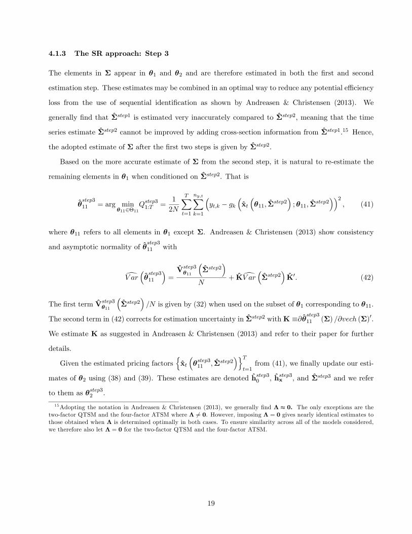
4.1.3 The SR approach: Step 3
The elements in � appear in �1 and �2 and are therefore estimated in both the �rst and second
estimation step. These estimates may be combined in an optimal way to reduce any potential e¢ ciency
loss from the use of sequential identi�cation as shown by Andreasen & Christensen (2013). We
generally �nd that �step1 is estimated very inaccurately compared to �step2, meaning that the time
series estimate �step2 cannot be improved by adding cross-section information from �step1.15 Hence,
the adopted estimate of � after the �rst two steps is given by �step2.
Based on the more accurate estimate of � from the second step, it is natural to re-estimate the
remaining elements in �1 when conditioned on �step2. That is
�step311 = arg min
�112�11Qstep31:T =
1
2N
TXt=1
ny;tXk=1
�yt;k � gk
�xt
��11; �
step2�;�11; �
step2��2
; (41)
where �11 refers to all elements in �1 except �. Andreasen & Christensen (2013) show consistency
and asymptotic normality of �step311 with
dV ar ��step311
�=Vstep3�11
��step2
�N
+ KdV ar ��step2� K0: (42)
The �rst term Vstep3�11
��step2
�=N is given by (32) when used on the subset of �1 corresponding to �11.
The second term in (42) corrects for estimation uncertainty in �step2 withK �@�step311 (�) =@vech (�)0.
We estimate K as suggested in Andreasen & Christensen (2013) and refer to their paper for further
details.
Given the estimated pricing factorsnxt
��step311 ; �step2
�oTt=1
from (41), we �nally update our esti-
mates of �2 using (38) and (39). These estimates are denoted hstep30 , hstep3x , and �step3 and we refer
to them as �step32 .
15Adopting the notation in Andreasen & Christensen (2013), we generally �nd � t 0. The only exceptions are thetwo-factor QTSM and the four-factor ATSM where � 6= 0. However, imposing � = 0 gives nearly identical estimates tothose obtained when � is determined optimally in both cases. To ensure similarity across all of the models considered,we therefore also let � = 0 for the two-factor QTSM and the four-factor ATSM.
19

5 Empirical results: In-sample performance
This section estimates the benchmark ATSM, the QTSM, and the shadow rate model on post-war
US data. For comparability with much of the existing literature on the ZLB, we �rst study models
with two pricing factors before exploring the performance of three-factor models. We �nd several
short-comings of these two- and three-factor models and we therefore also estimate models with four
pricing factors. Our analysis is structured as follows. Section 5.1 presents the data, and our model
estimates are discussed in Section 5.2. We examine the accuracy of the bias-adjusted perturbation
approximation for the shadow rate model in Section 5.3. The two subsequent sections explore how
well the models match various aspects of bond yields.
5.1 Data
We use start-of-month nominal bond yields in the US from July 1961 to May 2013 as provided by
Gürkaynak, Sack & Wright (2007). The SR approach is constructed for a setting where many observ-
ables are available each time period, and we therefore include more bond yields for the estimation than
typically used in the literature. Simulation results by Andreasen & Christensen (2013) suggest that
about 15 bond yields are su¢ cient and that any e¢ ciency loss of the SR approach compared to Max-
imum Likelihood may be small with 25 bond yields. Given our interest in the 10-year term structure,
we include all bond yields in the 0.25-10 year maturity range when sampled at a quarterly frequency.
That is, whenever possible, we include 40 bond yields having the maturities f0:25; 0:50; :::; 9:75; 10g.16
Due to a lack of long-term Treasury notes before September 1971, bonds yields in the 7-10 year ma-
turity range are not available before this date. We address this problem by explicitly accounting for
missing values in the SR approach.
5.2 Model estimates
The estimation results for the two-factor models are reported in Table 1. The benchmark ATSM
displays the usual properties with stationary and highly persistent factors under both the Q and P
measure as diag(�) > 0 and hx has eigenvalues 0:9913 and 0:9646. The same properties hold for the
16These bond yields are computed using the estimated parametric form for the yield curve in Gürkaynak et al. (2007).Ongoing work explores the robustness of our results when using non-parametric estimation methods to extract the yieldcurves from coupon bonds.
20

pricing factors in the QTSM, where enforces the ZLB by having strictly positive eigenvalues (0:0359
and 1:9641). We also �nd that the two pricing factors in the QTSM are positively correlated (0.44)
whereas they display negative correlation in the ATSM (-0.65). The estimates for the shadow rate with
two pricing factors are generally very similar to those for the two-factor benchmark ATSM, but we also
�nd some di¤erences. For instance, the pricing factors in the shadow rate model are weakly positively
correlated (0.15) and the conditional volatility of the second pricing factor is �22 = 6:45 � 10�4 and
hence larger than the corresponding estimate in the ATSM of �22 = 3:97� 10�4.17
< Table 1 about here >
Turning to three- and four-factor models in Tables 2 and 3, respectively, all models imply stationary
and highly persistent pricing factors under both the Q and P measure. Our estimates imply that the
ZLB in the three-factor QTSM is enforced by letting be positive de�nite, whereas is found to
be positive semi-de�nite in the four-factor QTSM as has one eigenvalue equal to zero.18 We also
note that several estimates for the three- and four-factor benchmark ATSM di¤er substantially from
the corresponding estimates in the shadow rate models. This �nding indicates that one should be
cautious of directly using parameters from the benchmark ATSM in the shadow rate model to explore
the implications of the ZLB.
< Table 2 and 3 about here >
5.3 Calibration and accuracy of the perturbation approximation
For each of the considered shadow rate models, we calibrate the scaling of the bias correction from
simulated time series of 2; 000 observations using preliminary estimates with 0;k = 0 and 1;k = 1
for k = 1; 2; :::;K. The �true�solution to bond yields is here obtained by the Monte Carlo integration
with 10; 000 draws. The calibrated values ofn �0;k;
�1;k
oKk=1
for the shadow rate model with two,
three, and four pricing factors are displayed in the left column of Figure 2. We generally �nd that
the �1;k parameters start at one and then decrease with maturity. Most calibrated intercepts �0;k are
17For the robust standard errors in Table 1 we use a bandwidth of 5 in the Newey-West estimate of S in (40) andwD = wT = 10 in (35). These standard errors are broadly similar when using slightly smaller or larger bandwidths.18This implies that the estimates are on the boundary of the domain for the parameters and that the standard errors in
Table 3 only serve as an approximation. Ongoing work aims to compute more accurate standard errors using a bootstrapprocedure.
21

very close to zero, except for bond yields with long maturities in the four-factor model. Given these
calibrated values ofn �0;k;
�1;k
oKk=1, the three shadow rate models are then re-estimated to obtain the
results reported in Tables 1-3.
We next explore the accuracy of the fourth-order perturbation approximation when using the
estimated pricing factors and model parameters. The charts in the right column of Figure 2 show
the root mean squared pricing errors (RMSEs) for bond yields by maturity, where the �true�solution
to bond yields is computed using Monte Carlo integration with 10; 000 draws. The RMSEs without
the bias correction are marked with black lines and found to be between 15 and 30 annualized basis
points for all the shadow rate models considered. Adding the unscaled bias correction ( 0;k = 0 and
1;k = 1) to the fourth-order perturbation approximation substantially reduces the RMSEs as they
fall to between 5 and 15 annualized basis points. Using the optimal scaling of the bias correctionn �0;k;
�1;k
oKk=1
further reduces the RMSEs to about 5 annualized basis points, except for bond yields
with short maturities in the two-factor models where the RMSEs are around 10 annualized basis
points.
< Figure 2 about here >
Further evidence on the satisfying performance of the bias-adjusted fourth-order perturbation
approximation usingn �0;k;
�1;k
oKk=1
is provided in Figure 3, showing bond yields and pricing errors
for a selected number of maturities in the estimated three-factor model.19 This �gure shows that the
RMSEs are low when interest rates are far from zero but also when they approach the ZLB during
2002-2004 and after 2008. As a result, the maximal pricing errors rarely exceed �10 annualized basis
points and this shows that our approximation achieves high accuracy for bond yields throughout the
sample.
< Figure 3 about here >
Another notable advantage of the suggested perturbation approximation is its computational speed.
It only takes 0.6 seconds to obtain all bond yields in the two-factor model. The computational
requirement only increase gradually with the number of pricing factors, as we are able to solve the
three- and four-factor shadow rate models in just 1.7 and 3.7 seconds, respectively.20
19Similar plots for the two- and four-factor shadow rate models are available on request.20The computations are done in MATLAB 2012a using an Intel(R) Core(TM) i5-320M CPU 2 2.50Ghz.
22

These �ndings lead us to the conclusion that the bias-adjusted perturbation approximation is
highly accurate when applied to bond yields in shadow rate models. We also �nd that this method is
computationally very appealling because its execution time remains highly tractable even in models
with four pricing factors.
5.4 Goodness of �t for bond yields
We next study the in-sample �t by looking at the objective functions for the models considered. The
�rst part of Table 4 reports ~Qstep11:T � 100qQstep11:T =2 which measures the standard deviation of all
residuals in annualized basis points for the �rst step in the SR approach. With two pricing factors,
the QTSM clearly provides the best �t with ~Qstep11:T = 10:15, whereas the shadow rate model and the
benchmark ATSM have ~Qstep11:T = 11:37 and ~Qstep11:T = 11:50, respectively. The QTSM also delivers the
best �t with three pricing factors where ~Qstep11:T = 4:81, whereas the worst �t is seen in the shadow
rate model�~Qstep11:T = 5:34
�. Turning to four-factor models, we �nd that the QTSM and the shadow
rate model obtain the same �t of bond yields with ~Qstep11:T = 2:03, whereas the benchmark ATSM has
~Qstep11:T = 2:40. It is important to note that these results are obtained without using the law of motion
for the pricing factors under P, and our results therefore hold for any functional form of the market
price of risk f (xt).
The second part of Table 4 shows the scaled objective functions from the third step in the SR
approach, i.e. ~Qstep31:T � 100qQstep31:T =2, where � is estimated from the time-series dimension instead
of the cross-section dimension as in the �rst step. Here, ~Qstep31:T is only marginally larger than ~Qstep11:T
for all models, meaning that the in-sample �t of bond yields is almost una¤ected by the alternative
estimate of �. It is therefore reasonable to believe that the dependence on the P dynamics through
� is minimal in our case and that results in the third step of the SR approach largely remain robust
to the chosen functional form of f (xt).
< Table 4 about here >
A more careful examination of the in-sample �t is provided in Figure 4, where charts in the
�rst column show recursively computed objective functions using the estimates in Tables 1 to 3, i.e.n~Qstep31:t
oTt=1. These charts suggest that the in-sample �t generally deteriorates during the 1970�s and
improve afterwards, and that the relative performance of the three models is fairly stable throughout
23

the sample. The same type of plots are provided in the second column in Figure 4 but only when the
objective functions are computed from January 1998 to May 2013 to explore the �t when bond yields
are close to the ZLB. We emphasize that these plots are computed using the estimates from the full
sample, i.e. those in Tables 1 to 3. In this time period, the QTSM clearly delivers the best in-sample
�t regardless of the number of pricing factors, whereas the shadow rate model only outperforms the
benchmark ATSM with four pricing factors.
Another way to explore the in-sample �t of bond yields is provided in the �nal column in Figure
4, showing the standard deviation of the residuals by maturity, i.e. �k = 100q
1T
PTt=1 v
2t;k for k =
1; 2; :::;K with expressed �k in annualized basis points. All two-factor models clearly struggle to match
bond yields at the short and long end of the term structure as �0:25y = 40 and �10y = 15. Including a
third pricing factor substantially reduces the residuals at the long end of the term structure (�10y = 6),
but the residuals remain high at the short end with �0:25y > 15 in all models. One way to address
this shortcoming of three-factor models is to include a fourth pricing factor as the standard deviation
of the residuals at the short end then fall below 7 annualized basis points. In other words, a fourth
pricing factors is required to properly match short-term bond yields.
< Figure 4 about here >
Based on these �ndings we conclude that a quadratic policy rate is the best way to enforce the
ZLB in two- and three-factor models when measured by the in-sample �t. In four-factor models, a
quadratic policy rate and a shadow rate speci�cation deliver broadly the same �t of bond yields, and
we are therefore unable to rank the two mechanisms for enforcing the ZLB in this case.
5.5 Matching key moments for bond yields
The QTSM with nx pricing factors has nx (nx + 1) =2� 1 additional parameters compared to the two
other models, and the quadratic model is therefore likely to do well when measured by the in-sample
�t. Issues related to over�tting may be partially addressed by also evaluating the considered models
by their ability to match moments not directly included in the estimation. The �rst set of moments
we explore are the unconditional �rst and second moments of bond yields in Figure 5. All models
match the upward sloping unconditional yield curve fairly well, except for the three-factor QTSM. We
also note that most models provide relatively low estimates of the unconditional mean in bond yields.
24

The decreasing pattern in the unconditional volatility of bond yields is broadly matched by nearly all
models, except for the three-factor QTSM.
< Figure 5 about here >
Another set of moments typically considered to assess the performance of DTSMs are derived in
Dai & Singleton (2002). They start by considering the regressions for excess returns
yt+1;k�1 � yt;k = �k + �kyt;k � rtk � 1 + ut;k (43)
where ut;k denotes the residual. The expectation hypothesis implies �k = 0 and �k = 1 for k =
1; 2; :::;K, but this prediction is clearly rejected for US data, as �k is negative and decreases with
maturity. The ability of DTSMs to reproduce the observed pattern in f�kgKk=1 is referred to as LPY(i)
by Dai & Singleton (2002) and tests whether the models are able to capture the P dynamics of bond
yields. The charts in the �rst column of Figure 6 examine the performance of the considered DTSMs
along this dimension, where the corresponding model-moments of �k are computed from simulated
time series of 500,000 observations. We �rst note that the benchmark ATSM does extremely well
along this dimension, even with just two pricing factors. The QTSMs and the shadow rate models
struggle to match the downward sloping pattern in �k with two and three pricing factors. Much better
performance is obtained in the four-factor models, as they match the negative and decreasing pattern
in �k.
The second set of moment conditions studied in Dai & Singleton (2002) are derived by modifying
the regressions in (43) as follows
yt+1;k�1 � yt;k �et;kk � 1 = �
Qk + �
Qk
yt;k � rtk � 1 + uQt;k (44)
where et;k � EPt [log (Pt+1;k�1) = log (Pt;k)� rt] denotes the excess holding period return and uQt;k is the
residual. If the risk premia adjustment in et;k is correctly speci�ed, then we recover the expectation
hypothesis with �Qk = 1 for all k as shown by Dai & Singleton (2002). The ability of DTSMs to
generate this implication is referred to as LPY(ii) by Dai & Singleton (2002) and tests if the models
are correctly speci�ed under the Q measure. Given that all of the models considered in the present
paper only di¤er in their Q distribution, we view LPY(ii) as a very informative test to discriminate
25

between the models. Charts in the second column of Figure 6 study the ability of the models to
reproduce �Qk = 1 for all k. We interestingly �nd that both the benchmark ATSM and the QTSM
struggle with two and three pricing factors as the regression loadings di¤er substantially from one.
Slightly better performance is observed for these models with four pricing factors, but substantial
deviations remain. In sharp contrast to the performance of these models, all the shadow rate models
do extremely well along this dimension as they nearly reproduce a regression coe¢ cient of one. This
suggests that the shadow rate model is much better at matching the Q dynamics than the benchmark
ATSM and the QTSM.21
< Figure 6 about here >
We �nally plot the 10-year term premium in Figure 7 for all estimated models. For the two-factor
models, we observe some di¤erences in reported term premia which is expected given the relative
large residuals in these models. For three- and four-factor models, we observe that the benchmark
ATSM and the shadow rate model provide broadly similar estimates of term premia, except after 2008
where bond yields approach the ZLB. We also note that the estimated term premia in the three- and
four-factor QTSMs are somewhat higher than those obtained from the three- and four-factor shadow
rate models.
< Figure 7 about here >
These �ndings lead us to the following conclusions. In the QTSM, four pricing factors are needed
to match the unconditional �rst and second moments whereas only three factors are required in the
shadow rate model. We also �nd that both models rely on four pricing factors to match the dynamics
of bond yields under the P measure and hence pass the LPY(i) test. Importantly, only shadow rate
models pass the LPY(ii) test, suggesting that the Q dynamics are best captured by a shadow rate
speci�cation.
21Ongoing work explores if the inability of the benchmark ATSM and the QTSM to pass the LPY(ii) test is caused bythe low interest rates after 2000.
26

6 Empirical results: performance out-of-sample
Another commonly used method to correct for potential over�tting is to conduct a forecasting exercise
out-of-sample. This is the topic of the current section where we evaluate the forecasting performance of
the benchmark ATSM, the QTSM, and the shadow rate model with three pricing factors from January
2009 to May 2013.22 We focus on this period because the Federal Open Market Committee has set a
target range of 0-0.25% for the e¤ective Federal Funds Rate, meaning that policy rate has been at its
e¤ective ZLB. The forecasting study is carried out by estimating all three-factor models recursively
every month to forecasts bond yields up to 12 months ahead. Given that the last 12 months of data is
reserved for evaluating the �nal forecasts, each model is estimated a total of 41 times which is easily
done due to the computational e¢ ciency of the SR approach relative to commonly used estimation
alternatives.
Figure 8 shows root mean squared prediction error (RMSPE) statistics from the three models at
forecast horizons of 1, 3, 6, and 12 months, alongside RMSPE statistics under the assumption that
bond yields of all maturities follow random walks. Three main results emerge. First, the one-month
ahead forecasting performance of all models is similar, with none of the models outperforming a random
walk for any maturity. Second, the forecasting performance of the benchmark ATSM for short-term
bond yields becomes substantially worse at the 12-month horizon, which is qualitatively in line with
the �ndings by Pooter, Ravazzolo & van Dijk (2010). In contrast, the forecasting performance of the
QTSM and, in particular, the shadow rate model does not deteriorate with the forecast horizon for
short-term bond yields. At a 12-month horizon the shadow rate model even performs signi�cantly
better than a random walk at forecasting bond yields with 3-month and 1-year maturities.23 The
reason why the QTSM and shadow rate model perform better in this respect is likely to be because
they can generate a lower degree of mean reversion in bond yields than the benchmark ATSM when
yields are close to the ZLB. For example, in May 2012 the 12-month ahead forecasts of the 3-month
rate are 0.60% in the ATSM, 0.10% in the QTSM, and 0.16% in the shadow rate model.
Third, the relative performance of the QTSM is worse for long-term bond yields, particularly at
longer forecasting horizons. It seems plausible that for bond yields not currently close to the lower
22Ongoing work explores the forecasting performance of the considered two- and four-factor models and on longer timeperiods.23Outperformance at the 5% signi�cance level is based on the Harvey, Leybourne & Newbold (1997) small sample
modi�cation of the Diebold & Mariano (1995) test.
27

bound, the need to estimate more parameters in the QTSM outweighs any bene�ts from including
quadratic terms in the policy rate. Even the shadow rate model does not come close to beating a
random walk for long-term bond yields, which seems broadly consistent with the �ndings in Pooter
et al. (2010).
< Figure 8 about here >
In conclusion, the shadow rate model appears to o¤er the best forecasting performance in terms
of RMSPE, where it out-performs the benchmark ATSM at short maturity and the QTSM at longer
maturities.
7 Conclusion
This paper studies whether DTSMs for US nominal bond yields should enforce the ZLB through a
quadratic policy rate or a shadow rate. The question is addressed by estimating QTSMs and shadow
rate models with two, three, and four latent pricing factors using the SR approach. Bond yields
in the shadow rate models are e¢ ciently computed by a fourth-order perturbation approximation,
extended with a novel bias correction for interest rates under perfect foresight. When measured in
terms of in-sample �t, we generally �nd that QTSMs outperform shadow rate models, except with
four pricing factors where both models deliver the same �t of bond yields. However, some of the
good performance for the QTSMs are likely related to some degree of over�tting, as these models
perform worse than shadow rate models on moments not directly incorporated in the estimation. This
includes the ability of the models to match unconditional �rst and second moments for bond yields,
and importantly pass the LPY(i) and LPY(ii) tests of Dai & Singleton (2002). Furthermore, the
shadow rate models also seem to outperform QTSMs in a proper out-of-sample forecasting exercise.
Our work therefore suggests that DTSMs for US bond yields should enforce the ZLB by adopting a
shadow rate speci�cation instead of a quadratic policy rate, possibly using four pricing factors.
28

A Computing bond prices by the perturbation method
A.1 Notation
We let the indices � and relate to elements of xt, while � corresponds to elements of �t. Subscriptson these indices capture the sequence in which derivatives are taken. For example, �1 correspondsto the �rst time a function is di¤erentiated with respect to xt, while �2 is used when di¤erentiatingwith respect to xt the second time, and so on. As typically done in the literature, we adopt the tensornotation. Hence, [pkx] 1 denotes the 1-th element of the 1�nx vector of derivatives of pk with respectto x. Similarly, the derivative of h with respect to x is an nx�nx matrix and [hx] 1�1 is the element ofthis matrix located at the intersection of the 1-th row and the �1-th column. This notation facilitateswriting summation as h
pk�1x
i 1[hx]
1�1=Pnx 1=1
@ pk�1
@ x 1
@ h 1
@x�1;
and hpk�1xx
i 1 2
[hx] 2�2[hx]
1�1=Pnx 1=1
Pnx 2=1
@2 pk�1
@ x 1@ x 2
@ h 2
@x�2
@ h 1
@x�1;
where, for instance, h 1 denotes the 1-th function of mapping h and x�1 is the �1-th element ofvector x. Here, and throughout, we omit the function arguments as all functions are evaluated at thedeterministic steady state.
The recursions for bond price derivatives that di¤er from zero are stated below. Here, we relyon derivatives of the h-function and the M-function. We adopt the notation that hxn refers toderivatives of the h-function with respect to xt taken n times. Similarly,Mzjyn refers to the derivativeof M with respect to z taken j times and with respect to y taken n times, for z;y 2fxt;xt+1g.All these derivatives are evaluated at the deterministic steady state. Given that the h-function andthe M-function are known, all required derivatives with respect to these functions follow by simpledi¤erentiation. In evaluating the expressions below, it is useful to recall the limits for the adoptedindices
�1; �2; �3; �4 = 1; 2; :::nx
1; 2; 3; 4 = 1; 2; :::nx
�1; �2; �3; �4 = 1; 2; :::; n�
where nx denotes the number of pricing factors in xt and n� refers to the number of innovations.Finally, the validity of the stated bond price derivatives have been veri�ed in relation to Dynare++on a number of test examples.
A.2 Bond price derivatives: �rst-order termshpkx
i�1=�p1x��1+hpk�1x
i 1[hx]
1�1
A.3 Bond price derivatives: second-order termshpkxx
i�1�2
=�p1xx��1�2
+hpk�1xx
i 1 2
[hx] 2�2[hx]
1�1+hpk�1x
i 1[hxx]
1�1�2
29

hpk��
i=
�p1���+hpk�1��
i+hpk�1xx
i 1 2
[�] 2�2[�]
1�1[I]�1�2
+hpk�1x
i 2[�]
2�2
hpk�1x
i 1[�]
1�1[I]�1�2+ 2M�1 �Mxt+1
� 1[�]
1�1
hpk�1x
i 2[�]
2�2[I]�2�1
A.4 Bond price derivatives: third-order terms
hpkxxx
i�1�2�3
=�p1xxx
��1�2�3
+hpk�1xxx
i 1 2 3
[hx] 3�3[hx]
2�2[hx]
1�1
+hpk�1xx
i 1 2
[hxx] 2�2�3
[hx] 1�1+hpk�1xx
i 1 2
[hx] 2�2[hxx]
1�1�3
+hpk�1xx
i 1 3
[hx] 3�3[hxx]
1�1�2
+hpk�1x
i 1[hxxx]
1�1�2�3
hpk��x
i�3
=�p1��x
��3� 2
�p1x��3
�Mxt+1
� 1[�]
1�1M�1
hpk�1x
i 2[�]
2�2[I]�2�1
+2��Mxt+1xt+1
� 1 3
[hx] 3�3+�Mxt+1xt
� 1�3
�[�]
1�1M�1
hpk�1x
i 2[�]
2�2[I]�2�1
+2�Mxt+1
� 1[�]
1�1M�1
hpk�1xx
i 2 3
[hx] 3�3[�]
2�2[I]�2�1
+hpk�1xx
i 2 3
[hx] 3�3[�]
2�2
hpk�1x
i 1[�]
1�1[I]�1�2
+hpk�1x
i 2[�]
2�2
hpk�1xx
i 1 3
[hx] 3�3[�]
1�1[I]�1�2
+hpk�1xxx
i 1 2 3
[hx] 3�3[�]
2�2[�]
1�1[I]�1�2+hpk�1��x
i 3[hx]
3�3
A.5 Bond price derivatives: fourth-order terms�pkxxxx
��1�2�3�4
=�p1xxxx
��1�2�3�4
+�pk�1xxxx
� 1 2 3 4
[hx] 4�4[hx]
3�3[hx]
2�2[hx]
1�1
+�pk�1xxx
� 1 2 3
�[hxx]
3�3�4
[hx] 2�2[hx]
1�1+ [hx]
3�3[hxx]
2�2�4
[hx] 1�1
�+�pk�1xxx
� 1 2 3
[hx] 3�3[hx]
2�2[hxx]
1�1�4
+�pk�1xxx
� 1 2 4
[hx] 4�4[hxx]
2�2�3
[hx] 1�1
+�pk�1xx
� 1 2
�[hxxx]
2�2�3�4
[hx] 1�1+ [hxx]
2�2�3
[hxx] 1�1�4
�+�pk�1xxx
� 1 2 4
[hx] 4�4[hx]
2�2[hxx]
1�1�3
+�pk�1xx
� 1 2
�[hxx]
2�2�4
[hxx] 1�1�3
+ [hx] 2�2[hxxx]
1�1�3�4
�+�pk�1xxx
� 1 3 4
[hx] 4�4[hx]
3�3[hxx]
1�1�2
+�pk�1xx
� 1 3
�[hxx]
3�3�4
[hxx] 1�1�2
+ [hx] 3�3[hxxx]
1�1�2�4
�+�pk�1xx
� 1 4
[hx] 4�4[hxxx]
1�1�2�3
+�pk�1x
� 1[hxxxx]
1�1�2�3�4
�pk��xx
��3�4
= ��pkx��4
�pkx��3
�pk�����pkxx��3�4
�pk�����pkx��3
�pk��x
��4��pkx��4
�pk��x
��3
+�p1��xx
��3�4
+�p1��x
��3
�p1x��4+�p1��x
��4
�p1x��3+�p1��� �p1x��4
�p1x��3+�p1��� �p1xx��3�4
+��p1��x
��3+�p1��� �p1x��3
� �pk�1x
� 4[hx]
4�4
30

+��p1��x
��4+�p1��� �p1x��4
� �pk�1x
� 3[hx]
3�3
+�p1��� ��
pk�1x
� 4[hx]
4�4
�pk�1x
� 3[hx]
3�3+�pk�1xx
� 3 4
[hx] 4�4[hx]
3�3+�pk�1x
� 3[hxx]
3�3�4
�+2M�1
��Mxt+1xt+1xt+1
� 1 3 4
[hx] 4�4+�Mxt+1xt+1xt
� 1 3�4
�[hx]
3�3[�]
1�1
�pk�1x
� 2[�]
2�2[I]�2�1
+2M�1 �Mxt+1xt+1
� 1 3
[hxx] 3�3�4
[�] 1�1
�pk�1x
� 2[�]
2�2[I]�2�1
+2M�1��Mxt+1xtxt+1
� 1a3 4
[hx] 4�4+�Mxt+1xtxt
� 1a3�4
�[�]
1�1
�pk�1x
� 2[�]
2�2[I]�2�1
+2M�1��Mxt+1xt+1
� 1 3
[hx] 3�3+�Mxt+1xt
� 1a3
[�] 1�1
� �pk�1x
� 4[hx]
4�4
�pk�1x
� 2[�]
2�2[I]�2�1
+2M�1��Mxt+1xt+1
� 1 3
[hx] 3�3+�Mxt+1xt
� 1a3
�[�]
1�1
�pk�1xx
� 2 4
[hx] 4�4[�]
2�2[I]�2�1
+2M�1��Mxt+1xt+1
� 1 4
[hx] 4�4+�Mxt+1xt
� 1a4
�[�]
1�1
�pk�1x
� 3[hx]
3�3
�pk�1x
� 2[�]
2�2[I]�2�1
+2M�1 �Mxt+1
� 1[�]
1�1
�pk�1x
� 4[hx]
4�4
�pk�1x
� 3[hx]
3�3
�pk�1x
� 2[�]
2�2[I]�2�1
+2M�1 �Mxt+1
� 1[�]
1�1
�pk�1xx
� 3 4
[hx] 4�4[hx]
3�3
�pk�1x
� 2[�]
2�2[I]�2�1
+2M�1 �Mxt+1
� 1[�]
1�1
�pk�1x
� 3[hxx]
3�3�4
�pk�1x
� 2[�]
2�2[I]�2�1
+2M�1 �Mxt+1
� 1[�]
1�1
�pk�1x
� 3[hx]
3�3
�pk�1xx
� 2 4
[hx] 4�4[�]
2�2[I]�2�1
+2M�1��Mxt+1xt+1
� 1 4
[hx] 4�4+�Mxt+1xt
� 1a4
�[�]
1�1
�pk�1xx
� 2 3
[hx] 3�3[�]
2�2[I]�2�1
+2M�1 �Mxt+1
� 1[�]
1�1
�pk�1x
� 4[hx]
4�4
�pk�1xx
� 2 3
[hx] 3�3[�]
2�2[I]�2�1
+2M�1 �Mxt+1
� 1[�]
1�1
�pk�1xxx
� 2 3 4
[hx] 4�4[hx]
3�3[�]
2�2[I]�2�1
+2M�1 �Mxt+1
� 1[�]
1�1
�pk�1xx
� 2 3
[hxx] 3�3�4
[�] 2�2[I]�2�1
+��p1x��3
�p1x��4+�p1xx��3�4
� �pk�1x
� 2[�]
2�2
�pk�1x
� 1[�]
1�1[I]�1�2
+�p1x��3
�pk�1x
� 4[hx]
4�4
�pk�1x
� 2[�]
2�2
�pk�1x
� 1[�]
1�1[I]�1�2
+2�p1x��3
�pk�1xx
� 2 4
[hx] 4�4[�]
2�2
�pk�1x
� 1[�]
1�1[I]�1�2
+�p1x��4
�pk�1x
� 3[hx]
3�3
�pk�1x
� 2[�]
2�2
�pk�1x
� 1[�]
1�1[I]�1�2
+�pk�1x
� 4[hx]
4�4
�pk�1x
� 3[hx]
3�3
�pk�1x
� 2[�]
2�2
�pk�1x
� 1[�]
1�1[I]�1�2
+�pk�1xx
� 3 4
[hx] 4�4[hx]
3�3
�pk�1x
� 2[�]
2�2
�pk�1x
� 1[�]
1�1[I]�1�2
+�pk�1x
� 3[hxx]
3�3�4
�pk�1x
� 2[�]
2�2
�pk�1x
� 1[�]
1�1[I]�1�2
+2�pk�1x
� 3[hx]
3�3
�pk�1xx
� 2 4
[hx] 4�4[�]
2�2
�pk�1x
� 1[�]
1�1[I]�1�2
+2�p1x��4
�pk�1xx
� 2 3
[hx] 3�3[�]
2�2
�pk�1x
� 1[�]
1�1[I]�1�2
+2�pk�1x
� 4[hx]
4�4
�pk�1xx
� 2 3
[hx] 3�3[�]
2�2
�pk�1x
� 1[�]
1�1[I]�1�2
+2�pk�1xxx
� 2 3 4
[hx] 4�4[hx]
3�3[�]
2�2
�pk�1x
� 1[�]
1�1[I]�1�2
+2�pk�1xx
� 2 3
[hxx] 3�3�4
[�] 2�2
�pk�1x
� 1[�]
1�1[I]�1�2+2�pk�1xx
� 2 3
[hx] 3�3[�]
2�2
�pk�1xx
� 1 4
[hx] 4�4[�]
1�1[I]�1�2
+��p1x��3
�p1x��4+�p1xx��3�4
� �pk�1xx
� 1 2
[�] 2�2[�]
1�1[I]�1�2
+�p1x��3
�pk�1x
� 4[hx]
4�4
�pk�1xx
� 1 2
[�] 2�2[�]
1�1[I]�1�2
+�p1x��3
�pk�1xxx
� 1 2 4
[hx] 4�4[�]
2�2[�]
1�1[I]�1�2+�p1x��4
�pk�1x
� 3[hx]
3�3
�pk�1xx
� 1 2
[�] 2�2[�]
1�1[I]�1�2
+�pk�1x
� 4[hx]
4�4
�pk�1x
� 3[hx]
3�3
�pk�1xx
� 1 2
[�] 2�2[�]
1�1[I]�1�2
+�pk�1xx
� 3 4
[hx] 4�4[hx]
3�3
�pk�1xx
� 1 2
[�] 2�2[�]
1�1[I]�1�2
31

+�pk�1x
� 3[hxx]
3�3�4
�pk�1xx
� 1 2
[�] 2�2[�]
1�1[I]�1�2+�pk�1x
� 3[hx]
3�3
�pk�1xxx
� 1 2 4
[hx] 4�4[�]
2�2[�]
1�1[I]�1�2
+�p1x��4
�pk�1xxx
� 1 2 3
[hx] 3�3[�]
2�2[�]
1�1[I]�1�2+�pk�1x
� 4[hx]
4�4
�pk�1xxx
� 1 2 3
[hx] 3�3[�]
2�2[�]
1�1[I]�1�2
+�pk�1xxxx
� 1 2 3 4
[hx] 4�4[hx]
3�3[�]
2�2[�]
1�1[I]�1�2+�pk�1xxx
� 1 2 3
[hxx] 3�3�4
[�] 2�2[�]
1�1[I]�1�2
+��p1x��3
�p1x��4+�p1xx��3�4
� �pk�1��
�+�p1x��3
�pk�1x
� 4[hx]
4�4
�pk�1��
�+�p1x��3
�pk�1��x
� 4[hx]
4�4
+�p1x��4
�pk�1x
� 3[hx]
3�3
�pk�1��
�+�pk�1x
� 4[hx]
4�4
�pk�1x
� 3[hx]
3�3
�pk�1��
�+�pk�1xx
� 3 4
[hx] 4�4[hx]
3�3
�pk�1��
�+�pk�1x
� 3[hxx]
3�3�4
�pk�1��
�+�pk�1x
� 3[hx]
3�3
�pk�1��x
� 4[hx]
4�4+�p1x��4
�pk�1��x
� 3[hx]
3�3
+�pk�1x
� 4[hx]
4�4
�pk�1��x
� 3[hx]
3�3+�pk�1��xx
� 3 4
[hx] 4�4[hx]
3�3+�pk�1��x
� 3[hxx]
3�3�4
Finally, let m4 (�t+1) denotes the fourth moment of �t+1 (�1; 1) for �1 = 1; 2; :::; ne. Hence,m4 (�t+1) is an ne � ne � ne � ne matrix.
�pk����
�= �3
�pk��� �pk���+�p1����
�+ 3
�p1��� �p1���
+6M�1 �Mxt+1xt+1
� 1 4
[�] 4�4[�]
1�1
�pk�1x
� 3[�]
3�3
�pk�1x
� 2[�]
2�2
�m4��2�1�3�4
+4M�1 �Mxt+1xt+1xt+1
� 1 2 4
[�] 4�4[�]
2�2[�]
1�1
�pk�1x
� 3[�]
3�3
�m4��3�1�2�4
+6M�1 �Mxt+1xt+1
� 1 2
[�] 2�2[�]
1�1
�pk�1xx
� 3 4
[�] 4�4[�]
3�3
�m4��3�1�2�4
+ 6�p1��� �pk�1��
�+4M�1 �Mxt+1
� 1[�]
1�1
�pk�1x
� 4[�]
4�4
�pk�1x
� 3[�]
3�3
�pk�1x
� 2[�]
2�2
�m4��1�2�3�4
+12M�1 �Mxt+1
� 1[�]
1�1
�pk�1xx
� 3 4
[�] 4�4[�]
3�3
�pk�1x
� 2[�]
2�2
�m4��1�2�3�4
+12M�1 �Mxt+1
� 1[�]
1�1
�pk�1��
� �pk�1x
� 2[�]
2�2[I]�2�1
+4M�1t
�Mxt+1
� 1[�]
1�1
�pk�1xxx
� 2 3 4
[�] 4�4[�]
3�3[�]
2�2
�m4��1�2�3�4
+12M�1 �Mxt+1
� 1[�]
1�1
�pk�1x��
� 2[�]
2�2[I]�2�1
+�pk�1x
� 4[�]
4�4
�pk�1x
� 3[�]
3�3
�pk�1x
� 2[�]
2�2
�pk�1x
� 1[�]
1�1
�m4��1�2�3�4
+6�pk�1xx
� 3 4
[�] 4�4[�]
3�3
�pk�1x
� 2[�]
2�2
�pk�1x
� 1[�]
1�1
�m4��1�2�3�4
+4�pk�1xxx
� 2 3 4
[�] 4�4[�]
3�3[�]
2�2
�pk�1x
� 1[�]
1�1
�m4��1�2�3�4
+3�pk�1xx
� 2 3
[�] 3�3[�]
2�2
�pk�1xx
� 1 4
[�] 4�4[�]
1�1
�m4��1�2�3�4
+12�pk�1x��
� 2[�]
2�2
�pk�1x
� 1[�]
1�1[I]�1�2+ 6
�pk�1x
� 3[�]
3�3
�pk�1��
� �pk�1x
� 1[�]
1�1[I]�1�3
+6�pk�1��
� �pk�1xx
� 1 4
[�] 4�4[�]
1�1[I]�1�4+�pk�1xxxx
� 1 2 3 4
[�] 4�4[�]
3�3[�]
2�2[�]
1�1
�m4��1�2�3�4
+6�pk�1xx��
� 1 2
[�] 2�2[�]
1�1[I]�1�2+ 3
�pk�1��
� �pk�1��
�+�pk�1����
�
B Computing conditional expectations by the perturbation method
Suppose we have a perturbation approximation to the variable rt and want to compute its conditionalexpectations, i.e. r1;t � Et [rt+1], r2;t � Et [rt+2], r3;t � Et [rt+3], etc. The law of iterated expectationsimplies r2;t � Et [rt+2] = Et [Et+1 [rt+2]] = Et [r1;t+1] and so on. We therefore only need a formula tocompute r1;t � Et [rt+1] as all remaining expectations follow by iterating this formula. Hence, considerthe problem
b (xt; �) = Et [r (xt+1; �)] ; (45)
and observe thatF (xt; �) � Et
��b (xt; �) + r
�h (xt) + ���t+1; �
��= 0; (46)
32

given (10). The conditional expectation Et is evaluated under the same measure as the innovations�t+1. The expression in (46) must hold for all values of (xt; �) and for all possible derivatives ofF (xt; �). Using these conditions, it is possible to compute all derivatives of b with respect to (xt; �)around the deterministic steady state, given derivatives of h (xt) and r (xt+1; �) around the samepoint. In presenting the formulas below, we adopt the same notation as in Appendix A.
B.1 Conditional expectations: �rst-order terms
[bx]�1 = [rx] 1 [hx] 1�1
B.2 Conditional expectations: second-order terms
[bxx]�1�2 = [rxx] 1 2 [hx] 2�2[hx]
1�1+ [rx] 1 [hxx]
1�1�2
[b��] = [rxx] 1 2 [�] 1�1[�]
2�2[I]�2�1+ [r��]
B.3 Conditional expectations: third-order terms
[bxxx]�1�2�3 = [rxxx] 1 2 3 [hx] 3�3[hx]
2�2[hx]
1�1
+ [rxx] 1 2 [hxx] 2�2�3
[hx] 1�1+ [rxx] 1 2 [hx]
2�2[hxx]
1�1�3
+ [rxx] 1 3 [hx] 3�3[hxx]
1�1�2
+ [rx] 1 [hxxx] 1�1�2�3
[b��x]�3 = [rxxx] 1 2 3 [hx] 3�3[�]
1�1[�]
2�2[I]�2�1+ [r��x] 3 [hx]
3�3
B.4 Conditional expectations: fourth-order terms
[bxxxx]�1�2�3�4 = [rxxxx] 1 2 3 4 [hx] 4�4[hx]
3�3[hx]
2�2[hx]
1�1
+ [rxxx] 1 2 3 [hxx] 3�3�4
[hx] 2�2[hx]
1�1+ [rxxx] 1 2 3 [hx]
3�3[hxx]
2�2�4
[hx] 1�1
+ [rxxx] 1 2 3 [hx] 3�3[hx]
2�2[hxx]
1�1�4
+ [rxxx] 1 2 4 [hx] 4�4[hxx]
2�2�3
[hx] 1�1
+ [rxx] 1 2 [hxxx] 2�2�3�4
[hx] 1�1+ [rxx] 1 2 [hxx]
2�2�3
[hxx] 1�1�4
+ [rxxx] 1 2 4 [hx] 4�4[hx]
2�2[hxx]
1�1�3
+ [rxx] 1 2 [hxx] 2�2�4
[hxx] 1�1�3
+ [rxx] 1 2 [hx] 2�2[hxxx]
1�1�3�4
+ [rxxx] 1 3 4 [hx] 4�4[hx]
3�3[hxx]
1�1�2
+ [rxx] 1 3 [hxx] 3�3�4
[hxx] 1�1�2
+ [rxx] 1 3 [hx] 3�3[hxxx]
1�1�2�4
+ [rxx] 1 4 [hx] 4�4[hxxx]
1�1�2�3
+ [rx] 1 [hxxxx] 1�1�2�3�4
[b��xx]�3�4 = [rxxxx] 1 2 3 4 [hx] 4�4[hx]
3�3[�]
1�1[�]
2�2[I]�2�1
+ [rxxx] 1 2 3 [hxx] 3�3�4
[�] 1�1[�]
2�2[I]�2�1
+ [r��xx] 3 4 [hx] 4�4[hx]
3�3+ [r��x] 3 [hxx]
3�3�4
[b����] = [rxxxx] 1 2 3 4 [�] 4�4[�]
3�3[�]
1�1[�]
2�2
�m4 (�t+1)
��1�2�3�4
+6 [rxx��] 1 2 [�] 1�1[�]
2�2[I]�2�1+ [r����]
33

References
Ahn, D.-H., Dittmar, R. F. & Gallant, A. R. (2002), �Quadratic term structure models: Theory andevidence�, The Review of Financial Studies 15(1), 243�288.
Andreasen, M. M. (2012), �On the e¤ects of rare disasters and uncertainty shocks for risk premia innon-linear DSGE models�, Review of Economic Dynamics 15, 295�316.
Andreasen, M. M. (Forthcoming), �Non-linear DSGE models and the central di¤erence kalman �lter�,Journal of Applied Econometrics .
Andreasen, M. M. & Christensen, B. J. (2013), �The SR approach: A new estimation procedure fornon-linear and non-gaussian dynamic term structure models�, Working Paper .
Andreasen, M. M., Fernandez-Villaverde, J. & Rubio-Ramirez, J. F. (2013), �The Pruned State SpaceSystem for Non-Linear DSGE Models: Theory and Empirical Applications to Estimation�, NBERWorking Paper .
Andreasen, M. M. & Zabczyk, P. (2010), �An e¢ cient method of computing higher order bond priceperturbation approximations�, Working Paper .
Ang, A., Boivin, J., Dong, S. & Loo-Kung, R. (2011), �Monetary policy shifts and the term structure�,Review of Economic Studies .
Aruoba, S. B., Fernandez-Villaverde, J. & Rubio-Ramirez, J. F. (2006), �Comparing solution methodsfor dynamic equilibrium economies�, Journal of Economic Dynamics and Control 30, 2477�2508.
Bauer, M. D. & Rudebusch, G. D. (2013), �Monetary policy expectations at the zero lower bound�,Working Paper .
Black, F. (1995), �Interest rates as options�, The Journal of Finance 50(5), 1371�1376.
Christensen, J. H. E. & Rudebusch, G. D. (2013), �Estimating shadow-rate term structure modelswith near-zero yields�, Federal Reserve Bank of San Francisco: Working Paper 2013-07 .
Clarida, R., Gali, J. & Gertler, M. (2000), �Monetary policy rules and macroeconomic stability: Evi-dence and some theory�, The Quarterly Journal of Economics 115, 147�180.
Cox, J. C., Ingersoll, J. E. & Ross, S. A. (1985), �A theory of the term structure of interest rates�,Econometrica 53(2), 385�407.
Dai, Q. & Singleton, K. J. (2000), �Speci�cation analysis of a¢ ne term structure models�, Journal ofFinance 55, 1946�1978.
Dai, Q. & Singleton, K. J. (2002), �Expectation puzzles, time-varying risk premia and a¢ ne modelsof the term structure�, Journal of Financial Economics 63, 415�441.
de Jong, F. (2000), �Time series and cross-section information in a¢ ne term-structure models�, Journalof Business and Economic Statistics 18, 300�314.
Diebold, F. X. & Mariano, R. S. (1995), �Comparing predictive accuracy�, Journal of Business andEconomic Statistics 13, 253�263.
34

Doucet, A., de Freitas, N. & Gordon, N. (2001), �Sequential monte carlo methods in practice�, Springer.
Duan, J.-C. & Simonato, J.-G. (1999), �Estimating and testing exponential-a¢ ne term structure mod-els by Kalman �lter�, Review of Quantitative Finance and Accounting 13, 111�135.
Gorovoi, V. & Linetsky, V. (2004), �Black�s model of interest rates as options, eigenfunction expansionsand japanese interest rates�, Mathematical Finance 14(1), 49�78.
Gürkaynak, R., Sack, B. & Wright, J. (2007), �The U.S. treasury yield curve: 1961 to the present�,Journal of Monetary Economics 54, 2291�2304.
Harvey, D. I., Leybourne, S. J. & Newbold, P. (1997), �Testing the equality of prediction mean squarederrors�, International Journal of Forecasting 13, 281�291.
Hull, J. C. (2012), Options, Futures, and Other Derivatives, eighth edn, Pearson.
Ichiue, H. & Ueno, Y. (2007), �Equilibrium interest rate and the yield curve in a low interest rateenviroment�, bank of Japan Working Paper 07-E-18.
Ichiue, H. & Ueno, Y. (2013), �Estimating term premia at the zero bound: An analysis of japanese,us, and uk yields�, Bank of Japan Working Paper Series 13-E-8.
Joslin, S., Singleton, K. J. & Zhu, H. (2011), �A new perspective on gaussian dynamic term structuremodels�, The Review of Financial Studies 24, 926�970.
Judd, K. L. & Guu, S.-M. (1997), �Asymptotic methods for aggregate growth models�, Journal ofEconomic Dynamics and Control 21, 1025�1042.
Kamenik, O. (2005), �Solving SDGE models: A new algorithm for the sylvester equation�, Computa-tional Economics 25, 167�187.
Kim, D. H. & Orphanides, A. (2012), �Term structure estimation with survey data on interest rateforecasts�, Journal of Financial and Quantitative Analysis 47, 241�272.
Kim, D. H. & Singleton, K. J. (2012), �Term structure models and the zero bound: An empiricalinvestigation of japanese yields�, Journal of Econometrics 170, 32�49.
Krippner, L. (2012), �Modifying Gaussian term structure models when interest rates are near the zerolower bound�, Reserve Bank of New Zealand, Discussion Paper Series .
Leippold, M. & Wu, L. (2002), �Asset pricing under the quadratic class�, The Journal of Financialand Quantitative Analysis 37(2), 271�295.
Pooter, M. D., Ravazzolo, F. & van Dijk, D. (2010), �Term stucture forecasting using macro factors andforecast combination�, Board of Governors of the Federal Reserve System, Internationl FinanceDiscusion Paper 993.
Realdon, M. (2006), �Quadratic term structure models in discrete time�, Finance Research Letters3, 277�289.
Rogers, L. C. G. (1995), �Which model for term-structure of interest rates should one use?�, Mathe-matical Finance, IMA 65, 93�116.
35

Schmitt-Grohé, S. & Uribe, M. (2004), �Solving dynamic general equilibrium models using a second-order approximation to the policy function�, Journal of Economic Dynamics and Control 28, 755�775.
Swanson, E., Anderson, G. & Levin, A. (2005), �Higher-order perturbation solutions to dynamic,discrete-time rational expectations models�, Working Paper .
36

Table 1: Estimation results: Two-factor modelsRobust standard errors for elements in �
step3
11 are computed using (42) and (35) with wD = 10 and wT = 10.
For elements in �step3
2 , robust standard errors are computed using (40) with S obtained by the Newey-Westestimator with a bandwidth of 5. The estimates for the shadow rate model are obtained using a fourth-orderperturbation approximation where the scaling of the bias correction is calibrated as described in Section 3.3using a simulated time series of 2,000 observations. Estimates with one or two stars denote signi�cance at the5 percent and 1 percent level, respectively.
ATSM QTSM Shadow rateEstimate SE Estimate SE Estimate SE
� 0:0082�� 0:0012 - - 0:0093 0:020221 - - 0:9641�� 0:1775 - -�11 0:0064�� 0:0011 0:0037 0:0056 0:0034 0:0163�22 0:0348�� 0:0010 0:0420� 0:0203 0:0420 0:0626�1 - - 0:0686 0:0652 - -�2 - - 0:0227� 0:0112 - -h0 (1; 1) 2:75� 10�5 3:57� 10�5 4:65� 10�5 3:98� 10�4 �1:24� 10�5 3:42� 10�5h0 (2; 1) �7:07� 10�5 5:47� 10�5 2:53� 10�5 6:99� 10�4 �3:46� 10�5 5:41� 10�5hx (1; 1) 1:0056�� 0:0080 0:9866�� 0:0066 0:9918�� 0:0064hx (1; 2) 0:0370�� 0:0121 0:0330�� 0:0105 0:0226�� 0:0086hx (2; 1) �0:0159 0:0116 0:0242 0:0141 0:0062 0:0107hx (2; 2) 0:9503�� 0:0173 0:9241�� 0:0228 0:9544�� 0:0194�11 4:80�� � 10�4 2:34� 10�5 0:0032�� 2:04� 10�4 4:23�� � 10�4 2:01� 10�5�21 �3:67�� � 10�4 2:88� 10�5 �0:0045�� 8:77� 10�4 �3:56�� � 10�4 5:11� 10�5�22 3:97�� � 10�4 5:64� 10�5 0:0058�� 6:70� 10�4 6:45�� � 10�4 8:69� 10�5
37

Table 2: Estimation results: Three-factor modelsRobust standard errors for elements in �
step3
11 are computed using (42) and (35) with wD = 10 and wT = 10.
For elements in �step3
2 , robust standard errors are computed using (40) with S obtained by the Newey-Westestimator with a bandwidth of 5. The estimates for the shadow rate model are obtained using a fourth-orderperturbation approximation where the scaling of the bias correction is calibrated as described in Section 3.3using a simulated time series of 2,000 observations. Estimates with one or two stars denote signi�cance at the5 percent and 1 percent level, respectively.
ATSM QTSM Shadow rateEstimate SE Estimate SE Estimate SE
� 0:0113�� 0:0016 - - 0:0078�� 0:000712 - - 0:8513�� 0:0846 - -13 - - 0:8768 0:4848 - -23 - - 0:9858�� 0:1486 - -�11 0:0026 0:0018 0:0010 0:0022 0:0098�� 0:0013�22 0:0318�� 0:0025 0:0372�� 0:0064 0:1280�� 0:0006�33 0:0996�� 0:0020 0:1349 0:1173 0:0092�� 0:0006�1 - - 0:0935 0:1738 - -�2 - - 0:0422�� 0:0150 - -�3 - - 0:0012 0:0082 - -h0 (1; 1) �3:45� 10�5 5:48� 10�5 �1:53� 10�4 3:54� 10�4 �0:0017 0:0010h0 (2; 1) 1:10� 10�4 1:12� 10�4 �0:0018 0:0011 �2:67� 10�5 5:63� 10�5h0 (3; 1) �2:54� 10�4 1:33� 10�4 0:0044�� 0:0014 0:0017 0:0010hx (1; 1) 0:9927�� 0:0075 0:9821�� 0:0081 0:3427 0:2587hx (1; 2) 0:0313�� 0:0082 0:0184�� 0:0058 0:3914 0:6854hx (1; 3) 0:0166 0:0148 0:0072 0:0135 �0:6019� 0:2547hx (2; 1) 0:0189 0:0152 0:0461�� 0:0170 �0:0026 0:0133hx (2; 2) 0:9520�� 0:0247 1:0053�� 0:0193 0:8745�� 0:0294hx (2; 3) 0:0535 0:0408 0:0774 0:0403 �0:0039 0:0132hx (3; 1) �0:0361� 0:0173 �0:0695�� 0:0201 0:6497� 0:2529hx (3; 2) 0:0016 0:0235 �0:0531�� 0:0259 �0:3483 0:6690hx (3; 3) 0:8581�� 0:0374 0:8111�� 0:0454 1:5949�� 0:2490�11 3:72�� � 10�4 2:33� 10�5 0:0025�� 1:77� 10�4 0:0160�� 0:0011�21 �4:30�� � 10�4 7:09� 10�5 �0:0025�� 6:18� 10�4 �3:19�� � 10�4 4:11� 10�5�22 7:26�� � 10�4 5:13� 10�5 0:0061�� 5:22� 10�4 5:23�� � 10�4 3:36� 10�5�31 1:99�� � 10�4 5:91� 10�5 6:36� 10�4 5:40� 10�4 �0:0158�� 0:0011�32 �6:12�� � 10�4 3:67� 10�5 �0:0061�� 6:47� 10�4 �2:28�� � 10�4 3:37� 10�5�33 4:38�� � 10�4 4:78� 10�5 0:0036�� 3:15� 10�4 3:90�� � 10�4 3:75� 10�5
38

Table 3: Estimation results: Four-factor modelsRobust standard errors for elements in �
step3
11 are computed using (42) and (35) with wD = 10 and wT = 10.
For elements in �step3
2 , robust standard errors are computed using (40) with S obtained by the Newey-Westestimator with a bandwidth of 5. The estimates for the shadow rate model are obtained using a fourth-orderperturbation approximation where the scaling of the bias correction is calibrated as described in Section 3.3using a simulated time series of 2,000 observations. Estimates with one or two stars denote signi�cance at the5 percent and 1 percent level, respectively.
ATSM QTSM Shadow rateEstimate SE Estimate SE Estimate SE
� 0:0088 0:0105 - - 0:0134 0:021412 - - 0:8744�� 0:0335 - -13 - - 0:7860�� 0:0550 - -14 - - 0:8890�� 0:0227 - -23 - - 0:9800�� 0:0643 - -24 - - 0:9993�� 0:0127 - -34 - - 0:9735�� 0:0817 - -�11 0:0087�� 0:0028 0:0007 0:0011 0:0360 0:0529�22 0:0757�� 0:0030 0:0380�� 0:0040 0:6022 0:9565�33 0:4415�� 0:0027 0:5665�� 0:0606 0:0619 0:1029�44 0:0086� 0:0037 0:0644�� 0:0122 0:0015 0:0021�1 - - 0:1204 0:0897 - -�2 - - 0:0191 0:0221 - -�3 - - 0:0218�� 0:0032 - -�4 - - 0:0063 0:0186 - -h0 (1; 1) �0:0122 0:0063 �0:0005 0:0006 1:60� 10�4 2:53� 10�4h0 (2; 1) 5:13� 10�4 7:49� 10�5 0:0027 0:0025 �4:32� 10�4 2:30� 10�4h0 (3; 1) �1:81� 10�4 9:72� 10�5 0:0101�� 0:0021 �1:88� 10�4 2:76� 10�4h0 (4; 1) 0:0121 0:0062 �0:0041 0:0026 �3:55� 10�5 6:44� 10�5hx (1; 1) �5:0208�� 1:3957 0:9844�� 0:0080 0:9942�� 0:0449hx (1; 2) 1:1644 2:8339 0:0162�� 0:00567 �0:2261�� 0:0667hx (1; 3) �15:06�� 3:3068 0:0292 0:0154 0:0952 0:0566hx (1; 4) �5:9616�� 1:3913 0:0085 0:0088 0:0162 0:0291hx (2; 1) 0:0384�� 0:0149 0:0490 0:0331 �0:0024 0:0257hx (2; 2) 0:9100�� 0:0327 1:0165�� 0:0363 0:5857�� 0:0565hx (2; 3) 0:1664�� 0:0431 �0:2174�� 0:0720 0:0111 0:0347hx (2; 4) 0:0382�� 0:0148 0:0973� 0:0493 �0:0586� 0:0258hx (3; 1) �0:0494�� 0:0165 �0:0412 0:0226 �0:0442 0:0469hx (3; 2) �0:0188 0:0348 �0:0174 0:0224 0:2780�� 0:0732hx (3; 3) 0:6017�� 0:0566 0:61733�� 0:0627 0:8344�� 0:0587hx (3; 4) �0:0495�� 0:0166 �0:0138 0:0281 �0:0125 0:0314hx (4; 1) 5:9955�� 1:3876 �0:0438 0:0359 0:0249�� 0:0076hx (4; 2) �1:1177 2:8174 �0:0405 0:0386 0:0513�� 0:0139hx (4; 3) 15:02�� 3:2861 0:2902�� 0:0795 0:0160 0:0101hx (4; 4) 6:9364�� 1:3831 0:8654�� 0:0491 0:9946�� 0:0072�11 0:0884�� 0:0061 0:0025�� 1:77� 10�4 0:0018�� 1:12� 10�4�21 �5:97�� � 10�4 6:16� 10�5 �0:0056�� 0:0011 4:33�� � 10�4 1:14� 10�4�22 6:47�� � 10�4 4:45� 10�5 0:0125�� 7:05� 10�4 9:14�� � 10�4 8:41� 10�5�31 3:43�� � 10�4 9:63� 10�5 �0:0016�� 5:68� 10�4 �0:0018�� 1:10� 10�4�32 �5:15�� � 10�4 7:47� 10�5 0:0020�� 7:31� 10�4 �3:12�� � 10�4 3:75� 10�5�33 6:31�� � 10�4 4:81� 10�5 0:0065�� 7:46� 10�4 4:80�� � 10�4 4:16� 10�5�41 �0:0880�� 0:0060 0:0045�� 0:0010 �1:89�� � 10�4 2:84� 10�5�42 �1:89�� � 10�4 3:85� 10�5 �0:0130�� 7:83� 10�4 �2:07� 10�5 1:66� 10�5�43 �1:14�� � 10�4 2:37� 10�5 �0:0026�� 2:42� 10�4 �1:02�� � 10�4 2:93� 10�5�44 3:71�� � 10�4 4:64� 10�5 0:0027�� 2:50� 10�4 2:99�� � 10�4 1:73� 10�5
39

Table 4: In-sample �t: The objective functionsThis table reports 100
qQstep11:T =2 and 100
qQstep31:T =2 for the �rst and third step in the SR approach. Figures in
bold highlight the best in-sample �t for a given estimation step.
Step 1 Step 3ATSM QTSM Shadow rate ATSM QTSM Shadow rate
Two factors 11.50 10.15 11.37 11.59 10.40 11.42Three factors 5.14 4.81 5.34 5.15 4.83 5.53Four factors 2.40 2.03 2.03 2.40 2.03 2.04
40

Figure 1: The approximated max-functionThe approximated max-function is given by dmax fr; 0g = a0 + a1r + a2r2 + a3r3 + a4r4, where a0 = 0:00072 ,a1 = 0:53, a2 = 65:80, a3 = �2661:14, and a4 = 10000. This speci�cation is obtained by calibrating theapproximated max-function to the true max-function on the displayed interval for annualized interest rates,i.e. 0.10 corresponds to an annual rate of 10 percent.
0.05 0 0.05 0.1 0.15 0.20.05
0
0.05
0.1
0.15
0.2
True max func tion Approx . max func tion
41

Figure 2: Accuracy of the perturbation approximationThe calibrated values of �0 and
�1 are computed from simulated time series for the pricing factors of 2,000
observations using preliminary model estimates obtained with 0 = 0 and 1 = 1. The RMSEs by maturityare computed using the estimated pricing factors on US data. In both cases, the true solution for bond yieldsare obtained by Monte Carlo integration using 10,000 draws.
0 1 2 3 4 5 6 7 8 9 100.2
0
0.2
0.4
0.6
0.8
1
1.2
Maturity in years
2fac tor model
γ0,k* γ1,k
*
0 1 2 3 4 5 6 7 8 9 100
5
10
15
20
25
30
35
Ba
sis
po
ints
Maturity in years
2fac tor model
BiasAdj(γ0*,γ1*) BiasAdj(0,1) No BiasAdj
0 1 2 3 4 5 6 7 8 9 100.2
0
0.2
0.4
0.6
0.8
1
Maturity in years
3fac tor model
0 1 2 3 4 5 6 7 8 9 100
5
10
15
20
25
30
35
Ba
sis
po
ints
Maturity in years
3fac tor model
0 1 2 3 4 5 6 7 8 9 100.2
0
0.2
0.4
0.6
0.8
1
Maturity in years
4fac tor model
0 1 2 3 4 5 6 7 8 9 100
5
10
15
20
25
30
35
Ba
sis
po
ints
Maturity in years
4fac tor model
Figure 3: The three-factor shadow rate model: Bond yields and pricing errorsBond yields and the pricing errors are computed using the pricing factors estimated from US data for thethree-factor shadow rate model. In both cases, the true solution for bond yields are approximated by MonteCarlo integration using 10,000 draws.
1965 1970 1975 1980 1985 1990 1995 2000 2005 2010
5
10
15
Pe
rce
nt
Bond yield: 3month
1965 1970 1975 1980 1985 1990 1995 2000 2005 2010
10
0
10
Ba
sis
po
ints
Approximation error : 3month
1965 1970 1975 1980 1985 1990 1995 2000 2005 2010
5
10
15
Pe
rce
nt
Bond yield: 1year
1965 1970 1975 1980 1985 1990 1995 2000 2005 2010
10
0
10
Ba
sis
po
ints
Approximation error : 1year
1965 1970 1975 1980 1985 1990 1995 2000 2005 2010
5
10
15
Pe
rce
nt
Bond yield: 3year
1965 1970 1975 1980 1985 1990 1995 2000 2005 201010
0
10
Ba
sis
po
ints
Approximation error : 3year
1965 1970 1975 1980 1985 1990 1995 2000 2005 2010
5
10
15
Pe
rce
nt
Bond yield: 5year
1965 1970 1975 1980 1985 1990 1995 2000 2005 201010
5
0
5
Ba
sis
po
ints
Approximation error : 5year
1965 1970 1975 1980 1985 1990 1995 2000 2005 20102468
101214
Pe
rce
nt
Bond yield: 10year
1965 1970 1975 1980 1985 1990 1995 2000 2005 201010
5
0
5
Ba
sis
po
ints
Approximation error : 10year
42

Figure 4: The in-sample �tCharts in the �rst column report 100
qQstep31:T =2. Charts in the second column report 100
qQstep31998:T =2 and the
�nal column reports �k. All charts are computed using the estimates obtained from the full sample.
1970 1980 1990 2000 2010
8
9
10
11
12
13
14
15
Basi
s po
ints
2fac tor models : Rec urs ive fi t
1998 2000 2002 2004 2006 2008 2010 2012
6
8
10
12
Basi
s po
ints
2fac tor models : Rec urs ive fi t after 1998
ATSM QTSM Shadow rate
0 2 4 6 8 100
10
20
30
40
Basi
s po
ints
Maturi ty in years
2fac tor models : Std of res iduals per maturi ty
1970 1980 1990 2000 20103
4
5
6
7
8
9
Basi
s po
ints
3fac tor models : Rec urs ive fi t
1998 2000 2002 2004 2006 2008 2010 2012
1
2
3
4
Basi
s po
ints
3fac tor models : Rec urs ive fi t after 1998
0 2 4 6 8 100
5
10
15
20
Basi
s po
ints
Maturi ty in years
3fac tor models : Std of res iduals per maturi ty
1970 1980 1990 2000 20100.5
1
1.5
2
2.5
3
3.5
Basi
s po
ints
4fac tor models : Rec urs ive fi t
1998 2000 2002 2004 2006 2008 2010 2012
0.5
1
1.5
2
Basi
s po
ints
4fac tor models : Rec urs ive fi t after 1998
0 2 4 6 8 100
2
4
6
8
Basi
s po
ints
Maturi ty in years
4fac tor models : Std of res iduals per maturi ty
Figure 5: Unconditional means and standard deviationsAll model-based moments are obtained from simulated time series of 500,000 observations using the estimatesfrom Tables 1 to 3.
0 1 2 3 4 5 6 7 8 9 102
3
4
5
6
7
8
Maturi ty in years
2fac tor models : Mean values
Data ATSM QTSM BLACK
0 1 2 3 4 5 6 7 8 9 102.5
3
3.5
4
4.5
5
5.5
6
Maturi ty in years
2fac tor models : Standard dev iations
0 1 2 3 4 5 6 7 8 9 102
3
4
5
6
7
8
Maturi ty in years
3fac tor models : Mean values
0 1 2 3 4 5 6 7 8 9 102.5
3
3.5
4
4.5
5
5.5
6
Maturi ty in years
3fac tor models : Standard dev iations
0 1 2 3 4 5 6 7 8 9 102
3
4
5
6
7
8
Maturi ty in years
4fac tor models : Mean values
0 1 2 3 4 5 6 7 8 9 102.5
3
3.5
4
4.5
5
5.5
6
Maturi ty in years
4fac tor models : Standard dev iations
43

Figure 6: LPY tests for the P and Q dynamicsCharts in the �rst column show b�k and charts in the second column report b�Qk . All model-based moments areobtained from simulated time series of 500,000 observations using the estimates from Tables 1 to 3.
1 2 3 4 5 6 7 8 9
2.5
2
1.5
1
0.5
0
Maturi ty in years
2fac tor models : LPY(i)
Data ATSM QTSM BLACK
0 1 2 3 4 5 6 7 8 9 1025
20
15
10
5
0
5
Maturi ty in years
2fac tor models : LPY(i i)
1 2 3 4 5 6 7 8 9
2.5
2
1.5
1
0.5
0
Maturi ty in years
3fac tor models : LPY(i)
0 1 2 3 4 5 6 7 8 9 105
0
5
10
15
20
Maturi ty in years
3fac tor models : LPY(i i)
1 2 3 4 5 6 7 8 93
2.5
2
1.5
1
0.5
Maturi ty in years
4fac tor models : LPY(i)
0 1 2 3 4 5 6 7 8 9 102
0
2
4
6
Maturi ty in years
4fac tor models : LPY(i i)
Figure 7: The 10-year term premia and the shadow rate
1970 1980 1990 2000 2010
0
100
200
300
400
Ba
sis
po
ints
2 fac tor models
ATSM QTSM Shadow rate
1998 2000 2002 2004 2006 2008 2010 2012
0
50
100
150
200
250
300
Ba
sis
po
ints
2 fac tor models : After 1998
1998 2000 2002 2004 2006 2008 2010 201210
5
0
5
2fac tor models : The s hadow rate after 1998
1970 1980 1990 2000 2010
0
100
200
300
400
Ba
sis
po
ints
3 fac tor models
1998 2000 2002 2004 2006 2008 2010 2012
0
100
200
300
Ba
sis
po
ints
3 fac tor models : After 1998
1998 2000 2002 2004 2006 2008 2010 20121
0
1
2
3
4
5
6
3fac tor models : The s hadow rate after 1998
1970 1980 1990 2000 2010
0
100
200
300
400
Ba
sis
po
ints
4 fac tor models
1998 2000 2002 2004 2006 2008 2010 2012
0
100
200
300
Ba
sis
po
ints
4 fac tor models : After 1998
1998 2000 2002 2004 2006 2008 2010 20121
0
1
2
3
4
5
6
4fac tor models : The s hadow rate after 1998
44

Figure 8: Out-of-sample forecasting: Three-factor modelsThis �gure reports the root mean squared prediction errors (RMSPEs) for out-of-sample forecasts inthree-factor models from January 2009 to May 2013. The RMSPEs are computed by estimating thethree-factor models recursively and constructing 12-month ahead forecasts.
0 2 4 6 8 100
0.2
0.4
0.6
0.8
1
1.2
1.4
1.6
1.8
2
Perc
enta
ge p
oint
s
Maturity (years)
1 month ahead
ATSM QTSM Shadow rate Random walk
0 2 4 6 8 100
0.2
0.4
0.6
0.8
1
1.2
1.4
1.6
1.8
2
Perc
enta
ge p
oint
s
Maturity (years)
3 months ahead
0 2 4 6 8 100
0.2
0.4
0.6
0.8
1
1.2
1.4
1.6
1.8
2
Perc
enta
ge p
oint
s
Maturity (years)
6 months ahead
0 2 4 6 8 100
0.2
0.4
0.6
0.8
1
1.2
1.4
1.6
1.8
2
Perc
enta
ge p
oint
s
Maturity (years)
12 months ahead
45