Dynamic Structural Equation Modeling of Intensive ......Dynamic Structural Equation Modeling of...
99
Dynamic Structural Equation Modeling of Intensive Longitudinal Data Oisín Ryan Utrecht University [email protected] July, 2017 Slides from Ellen L. Hamaker 1 / 55
Transcript of Dynamic Structural Equation Modeling of Intensive ......Dynamic Structural Equation Modeling of...
Dynamic Structural Equation Modelingof Intensive Longitudinal Data
Oisín RyanUtrecht University
July, 2017
Slides from Ellen L. Hamaker
1 / 55

Cattell’s data box
vari
able
s
2 / 55
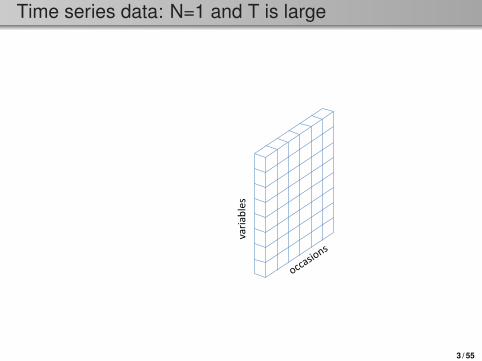
Time series data: N=1 and T is large
vari
able
s
3 / 55

Idiographic (N=1) research in psychology
N=1 research has included:• Cattell’s P-technique: factor analysis of N=1 data• Dynamic factor analysis: considering lagged relationships• Measurement burst design: multiple waves of intensive
measurements• Intervention research: ABAB design etc.
Critique of this kind of research:• within-person fluctuations are just noise• results are not generalizable• no one has these data
4 / 55

New technology
Secure continuous remote alcohol monitor (SCRAM)
Smart glasses
Smart phones
Smart watches
Smart tattoo
Activity trackers
Implants
5 / 55

Intensive longitudinal data
Different forms of intensive longitudinal data:• daily diary (DD); self-report end-of-day• experience sampling method (ESM); self-report of subjective
experience• ecological momentary assessment (EMA); healthcare related
self-report• ambulatory assessment (AA); physiological measurements• event-based measurements; self-report after a particular event• observational measurements; expert rater
For more info on methodology, check out:• Seminar of Tamlin Conner and Joshua Smyth on YouTube
(https://www.youtube.com/watch?v=nQBBVp9vBIQ)• Society for Ambulatory Assessment (http://www.saa2009.org/)• Life Data (https://www.lifedatacorp.com/)• Quantified Self (http://quantifiedself.com/)
6 / 55
Characteristics of these kind of data
Data structure:• one or more measurements per day• typically for multiple days• sometimes multiple waves (i.e., Nesselroade’s measurement-burst
design)
Advantages of ESM, EMA and AA• no recall bias• high ecological validity• physiological measures over a large time span• monitoring of symptoms and behavior, with new possibilities for
feedback and intervention (e-Health and m-Health)• window into the dynamics of processes
7 / 55
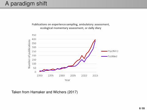
A paradigm shift
Taken from Hamaker and Wichers (2017)
8 / 55
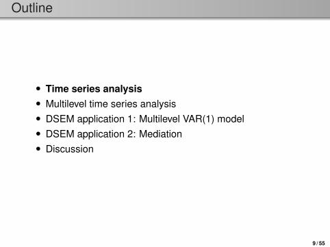
Outline
• Time series analysis• Multilevel time series analysis• DSEM application 1: Multilevel VAR(1) model• DSEM application 2: Mediation• Discussion
9 / 55

What is time series analysis?
Time series analysis is a class of techniques that is used ineconometrics, seismology, meteorology, control engineering,and signal processing.
Main characteristics:• N=1 technique• T is large (say >50)• concerned with trends, cycles and autocorrelation structure (i.e., serial
dependency)• goal: forecasting (6= prediction)
10 / 55

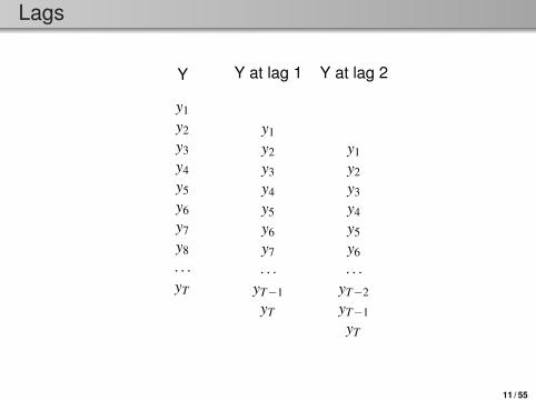
Lags
Y
y1y2y3y4y5y6y7y8. . .yT
Y at lag 1
y1y2y3y4y5y6y7. . .
yT−1yT
Y at lag 2
y1y2y3y4y5y6. . .
yT−2yT−1yT
11 / 55

Lags
Y
y1y2y3y4y5y6y7y8. . .yT
Y at lag 1
y1y2y3y4y5y6y7. . .
yT−1yT
Y at lag 2
y1y2y3y4y5y6. . .
yT−2yT−1yT
11 / 55
Lags
Y
y1y2y3y4y5y6y7y8. . .yT
Y at lag 1
y1y2y3y4y5y6y7. . .
yT−1yT
Y at lag 2
y1y2y3y4y5y6. . .
yT−2yT−1yT
11 / 55
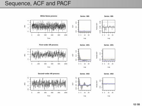
Sequence, ACF and PACF
White Noise process
Time
WN
0 200 400 600 800 1000
−3
−1
13
0 5 15 25
0.0
0.4
0.8
Lag
AC
F
Series WN
0 5 15 25
−0.
060.
000.
06
Lag
Par
tial A
CF
Series WN
First−order AR process
Time
AR
1
0 200 400 600 800 1000
−4
02
4
0 5 15 25
0.0
0.4
0.8
Lag
AC
F
Series AR1
0 5 15 25
0.0
0.4
Lag
Par
tial A
CF
Series AR1
Second−order AR process
Time
AR
2
0 200 400 600 800 1000
−15
−5
515
0 5 15 25
−0.
50.
00.
51.
0
Lag
AC
FSeries AR2
0 5 15 25
−0.
50.
5
LagP
artia
l AC
F
Series AR2
12 / 55

Outline
• Time series analysis• Multilevel time series analysis• DSEM application 1: Multilevel VAR(1) model• DSEM application 2: Mediation• Discussion
13 / 55
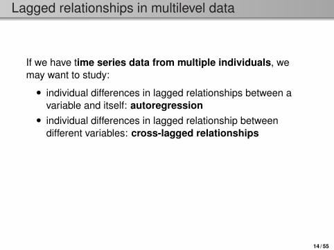
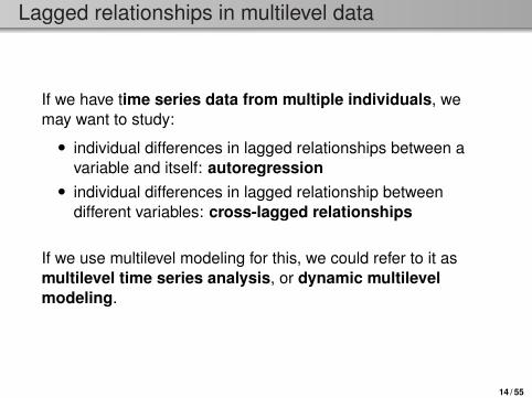
Lagged relationships in multilevel data
If we have time series data from multiple individuals, wemay want to study:
• individual differences in lagged relationships between avariable and itself: autoregression• individual differences in lagged relationship between
different variables: cross-lagged relationships
If we use multilevel modeling for this, we could refer to it asmultilevel time series analysis, or dynamic multilevelmodeling.
14 / 55
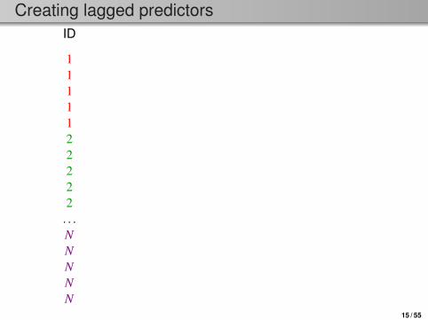
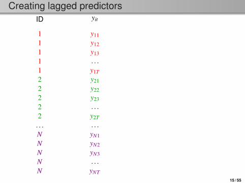
Creating lagged predictorsID
1111122222. . .NNNNN
yit
y11y12y13. . .y1T
y21y22y23. . .y2T
. . .yN1yN2yN3. . .yNT
yit−1
y11y12. . .
y1T−1
y21y22. . .
y2T−1. . .
yN1yN2. . .
yNT−1
xit−1
x11x12. . .
x1T−1
x21x22. . .
x2T−1. . .
xN1xN2. . .
xNT−1
15 / 55
Creating lagged predictorsID
1111122222. . .NNNNN
yit
y11y12y13. . .y1T
y21y22y23. . .y2T
. . .yN1yN2yN3. . .yNT
yit−1
y11y12. . .
y1T−1
y21y22. . .
y2T−1. . .
yN1yN2. . .
yNT−1
xit−1
x11x12. . .
x1T−1
x21x22. . .
x2T−1. . .
xN1xN2. . .
xNT−1
15 / 55

Creating lagged predictorsID
1111122222. . .NNNNN
yit
y11y12y13. . .y1T
y21y22y23. . .y2T
. . .yN1yN2yN3. . .yNT
yit−1
y11y12. . .
y1T−1
y21y22. . .
y2T−1. . .
yN1yN2. . .
yNT−1
xit−1
x11x12. . .
x1T−1
x21x22. . .
x2T−1. . .
xN1xN2. . .
xNT−1
15 / 55

Creating lagged predictorsID
1111122222. . .NNNNN
yit
y11y12y13. . .y1T
y21y22y23. . .y2T
. . .yN1yN2yN3. . .yNT
yit−1
y11y12. . .
y1T−1
y21y22. . .
y2T−1. . .
yN1yN2. . .
yNT−1
xit−1
x11x12. . .
x1T−1
x21x22. . .
x2T−1. . .
xN1xN2. . .
xNT−115 / 55
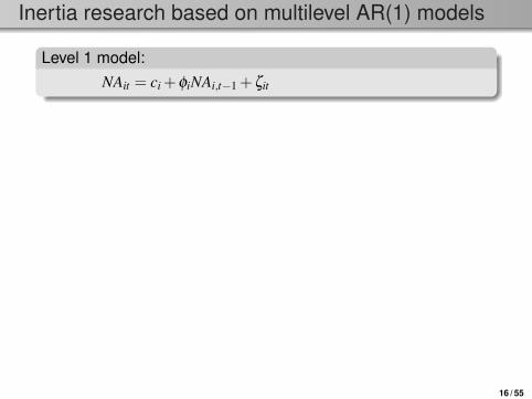
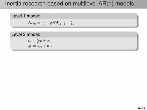
Inertia research based on multilevel AR(1) models
Level 1 model:NAit = ci +φiNAi,t−1 +ζit
Level 2 model:ci = γ00 +u0i
φi = γ01 +u1i
This research line was initiated by Suls, Green and Hillis(1998), and continued by the group of Kuppens.
The focus is on individual differences in the autoregressiveparameter φi (=inertia, carry-over, regulatory weakness), whichis shown to be:• positively related to current depression, neuroticism, and being female• predictive of later depression (Kuppens and Koval)
16 / 55

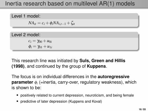
Dynamic networks based on multilevel VAR(1) models
Level 1 model:y1it = c1i +φ11iy1it−1 + · · ·+φ1kiykit−1 +ζ1it
y2it = c2i +φ21iy1it−1 + · · ·+φ2kiykit−1 +ζ2it
. . .ykit = cki +φk1iy1it−1 + · · ·+φkkiykit−1 +ζkit
Initiated by Bringmann et al. (2013), and further popularizedby the software from Sacha Epskamp.
The focus is on cross-lagged parameters between variables(=nodes; typically symptoms), and on measures based onthese (e.g., centrality).
Main idea is that stronger connections lead to an increasedrisk of developing and maintaining psychopathology.
17 / 55

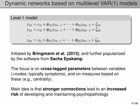
A fundamental problem in a nutshell
Number of words per minute
P e r
c e n t a
g e o
f t y
p o s
Cross-sectional relationship
Number of words per minute
P e r c
e n t a
g e o
f t y p
o s
Within-person relationship
Number of words per minute
P e r
c e n t a
g e o
f t y
p o s
Between-person relationship
Taken from Hamaker (2012).
18 / 55

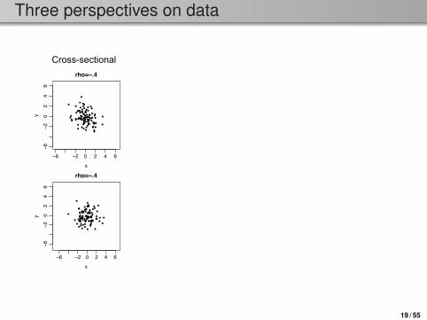
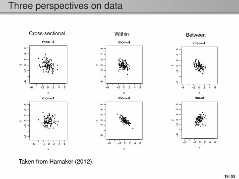
Three perspectives on data
−6 −2 0 2 4 6
−6−2
02
46
rho=−.4
x
y
−6 −2 0 2 4 6
−6−2
02
46
rho=−.4
x
y
−6 −2 0 2 4 6
−6−2
02
46
rho=−.4
x
y
−6 −2 0 2 4 6
−6−2
02
46
rho=−.4
x
y
−6 −2 0 2 4 6
−6−2
02
46
rho=−.8
x
y
−6 −2 0 2 4 6
−6−2
02
46
rho=0
x
y
Cross-sectional
−6 −2 0 2 4 6
−6−2
02
46
rho=−.4
x
y
−6 −2 0 2 4 6
−6−2
02
46
rho=−.4
x
y
−6 −2 0 2 4 6
−6−2
02
46
rho=−.4
x
y
−6 −2 0 2 4 6
−6−2
02
46
rho=−.4
x
y
−6 −2 0 2 4 6
−6−2
02
46
rho=−.8
x
y
−6 −2 0 2 4 6
−6−2
02
46
rho=0
x
y
Within Between
−6 −2 0 2 4 6
−6−2
02
46
rho=−.4
x
y
−6 −2 0 2 4 6
−6−2
02
46
rho=−.4
x
y
−6 −2 0 2 4 6
−6−2
02
46
rho=−.4
x
y
−6 −2 0 2 4 6
−6−2
02
46
rho=−.4
x
y
−6 −2 0 2 4 6
−6−2
02
46
rho=−.8
x
y
−6 −2 0 2 4 6
−6−2
02
46
rho=0
x
y
Taken from Hamaker (2012).
19 / 55

Three perspectives on data
−6 −2 0 2 4 6
−6−2
02
46
rho=−.4
x
y
−6 −2 0 2 4 6
−6−2
02
46
rho=−.4
x
y
−6 −2 0 2 4 6
−6−2
02
46
rho=−.4
x
y
−6 −2 0 2 4 6
−6−2
02
46
rho=−.4
x
y
−6 −2 0 2 4 6
−6−2
02
46
rho=−.8
x
y
−6 −2 0 2 4 6
−6−2
02
46
rho=0
x
y
Cross-sectional
−6 −2 0 2 4 6
−6−2
02
46
rho=−.4
x
y
−6 −2 0 2 4 6
−6−2
02
46
rho=−.4
xy
−6 −2 0 2 4 6
−6−2
02
46
rho=−.4
x
y
−6 −2 0 2 4 6
−6−2
02
46
rho=−.4
x
y
−6 −2 0 2 4 6
−6−2
02
46
rho=−.8
x
y
−6 −2 0 2 4 6
−6−2
02
46
rho=0
xy
Within
Between
−6 −2 0 2 4 6
−6−2
02
46
rho=−.4
x
y
−6 −2 0 2 4 6
−6−2
02
46
rho=−.4
x
y
−6 −2 0 2 4 6
−6−2
02
46
rho=−.4
x
y
−6 −2 0 2 4 6
−6−2
02
46
rho=−.4
x
y
−6 −2 0 2 4 6
−6−2
02
46
rho=−.8
x
y
−6 −2 0 2 4 6
−6−2
02
46
rho=0
x
y
Taken from Hamaker (2012).
19 / 55
Three perspectives on data
−6 −2 0 2 4 6
−6−2
02
46
rho=−.4
x
y
−6 −2 0 2 4 6
−6−2
02
46
rho=−.4
x
y
−6 −2 0 2 4 6
−6−2
02
46
rho=−.4
x
y
−6 −2 0 2 4 6
−6−2
02
46
rho=−.4
x
y
−6 −2 0 2 4 6
−6−2
02
46
rho=−.8
x
y
−6 −2 0 2 4 6
−6−2
02
46
rho=0
x
y
Cross-sectional
−6 −2 0 2 4 6
−6−2
02
46
rho=−.4
x
y
−6 −2 0 2 4 6
−6−2
02
46
rho=−.4
xy
−6 −2 0 2 4 6
−6−2
02
46
rho=−.4
x
y
−6 −2 0 2 4 6
−6−2
02
46
rho=−.4
x
y
−6 −2 0 2 4 6
−6−2
02
46
rho=−.8
x
y
−6 −2 0 2 4 6
−6−2
02
46
rho=0
xy
Within Between
−6 −2 0 2 4 6
−6−2
02
46
rho=−.4
x
y
−6 −2 0 2 4 6
−6−2
02
46
rho=−.4
x
y
−6 −2 0 2 4 6
−6−2
02
46
rho=−.4
x
y
−6 −2 0 2 4 6
−6−2
02
46
rho=−.4
x
y
−6 −2 0 2 4 6
−6−2
02
46
rho=−.8
x
y
−6 −2 0 2 4 6
−6−2
02
46
rho=0
x
y
Taken from Hamaker (2012).
19 / 55

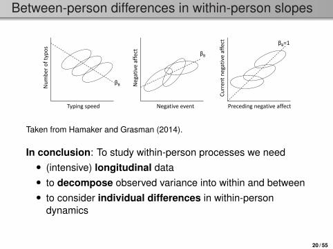
Between-person differences in within-person slopes
βB
Typing speed
Nu
mb
er o
f ty
po
s
Negative event
Neg
ativ
e af
fect
Cu
rren
t n
egat
ive
affe
ct
Preceding negative affect
βB
βB=1
Taken from Hamaker and Grasman (2014).
In conclusion: To study within-person processes we need• (intensive) longitudinal data• to decompose observed variance into within and between• to consider individual differences in within-person
dynamics
20 / 55
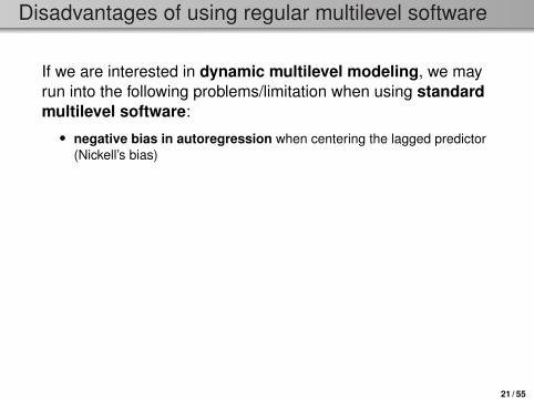
Disadvantages of using regular multilevel software
If we are interested in dynamic multilevel modeling, we mayrun into the following problems/limitation when using standardmultilevel software:
• negative bias in autoregression when centering the lagged predictor(Nickell’s bias)
• only one outcome variable (thus, separate models for multivariateoutcomes)
• only observed variables (no measurement error, moving averageterms, factor models)
• missing data result in many missing cases• unequally spaced observations
Dynamic structural equation modeling (DSEM) in Mplustackles all these problems.
21 / 55
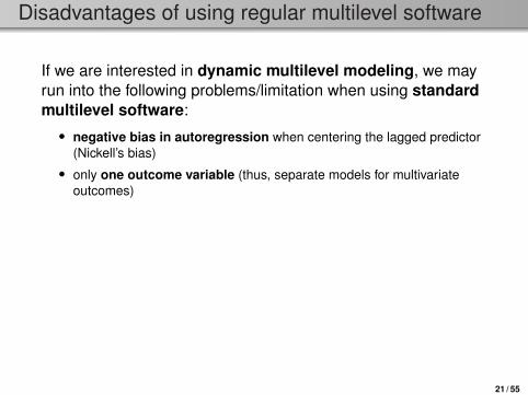
Disadvantages of using regular multilevel software
If we are interested in dynamic multilevel modeling, we mayrun into the following problems/limitation when using standardmultilevel software:• negative bias in autoregression when centering the lagged predictor
(Nickell’s bias)
• only one outcome variable (thus, separate models for multivariateoutcomes)
• only observed variables (no measurement error, moving averageterms, factor models)
• missing data result in many missing cases• unequally spaced observations
Dynamic structural equation modeling (DSEM) in Mplustackles all these problems.
21 / 55
Disadvantages of using regular multilevel software
If we are interested in dynamic multilevel modeling, we mayrun into the following problems/limitation when using standardmultilevel software:• negative bias in autoregression when centering the lagged predictor
(Nickell’s bias)• only one outcome variable (thus, separate models for multivariate
outcomes)
• only observed variables (no measurement error, moving averageterms, factor models)
• missing data result in many missing cases• unequally spaced observations
Dynamic structural equation modeling (DSEM) in Mplustackles all these problems.
21 / 55

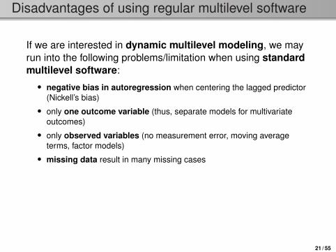
Disadvantages of using regular multilevel software
If we are interested in dynamic multilevel modeling, we mayrun into the following problems/limitation when using standardmultilevel software:• negative bias in autoregression when centering the lagged predictor
(Nickell’s bias)• only one outcome variable (thus, separate models for multivariate
outcomes)• only observed variables (no measurement error, moving average
terms, factor models)
• missing data result in many missing cases• unequally spaced observations
Dynamic structural equation modeling (DSEM) in Mplustackles all these problems.
21 / 55
Disadvantages of using regular multilevel software
If we are interested in dynamic multilevel modeling, we mayrun into the following problems/limitation when using standardmultilevel software:• negative bias in autoregression when centering the lagged predictor
(Nickell’s bias)• only one outcome variable (thus, separate models for multivariate
outcomes)• only observed variables (no measurement error, moving average
terms, factor models)• missing data result in many missing cases
• unequally spaced observations
Dynamic structural equation modeling (DSEM) in Mplustackles all these problems.
21 / 55

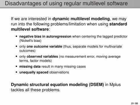
Disadvantages of using regular multilevel software
If we are interested in dynamic multilevel modeling, we mayrun into the following problems/limitation when using standardmultilevel software:• negative bias in autoregression when centering the lagged predictor
(Nickell’s bias)• only one outcome variable (thus, separate models for multivariate
outcomes)• only observed variables (no measurement error, moving average
terms, factor models)• missing data result in many missing cases• unequally spaced observations
Dynamic structural equation modeling (DSEM) in Mplustackles all these problems.
21 / 55
Outline
• Time series analysis• Multilevel time series analysis• DSEM application 1: Multilevel VAR(1) model• DSEM application 2: Mediation• Discussion
22 / 55
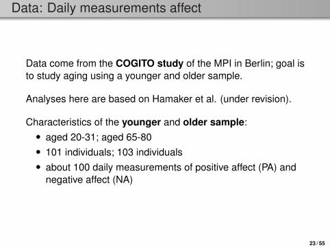
Data: Daily measurements affect
Data come from the COGITO study of the MPI in Berlin; goal isto study aging using a younger and older sample.
Analyses here are based on Hamaker et al. (under revision).
Characteristics of the younger and older sample:• aged 20-31; aged 65-80• 101 individuals; 103 individuals• about 100 daily measurements of positive affect (PA) and
negative affect (NA)
23 / 55
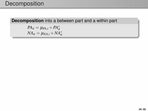
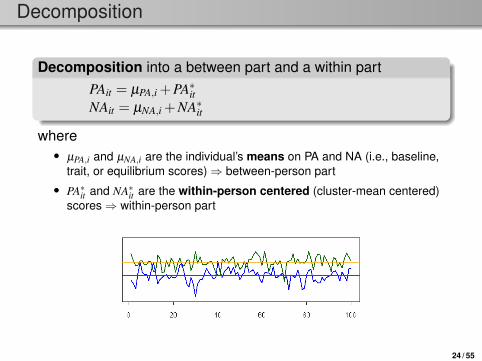
Decomposition
Decomposition into a between part and a within partPAit = µPA,i +PA∗itNAit = µNA,i +NA∗it
where• µPA,i and µNA,i are the individual’s means on PA and NA (i.e., baseline,
trait, or equilibrium scores)⇒ between-person part• PA∗it and NA∗it are the within-person centered (cluster-mean centered)
scores⇒ within-person part
24 / 55
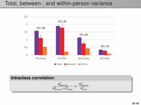
Total, between-, and within-person variance
0
0.5
1
1.5
2
2.5
PA young PA older NA young NA older
Total Between Within
ICC=.89
ICC=.76
ICC=.68
ICC=.64
Intraclass correlation:σ2
betweenσ2
between+σ2within
=σ2
betweenσ2
total
25 / 55
Bivariate model: Multilevel vector AR(1) model
ζ𝑃𝑃𝑃𝑃,𝑡𝑡
ζ𝑁𝑁𝑃𝑃,𝑡𝑡
𝜙𝜙𝑃𝑃𝑃𝑃
𝜙𝜙𝑁𝑁𝑃𝑃
𝜙𝜙𝑃𝑃𝑁𝑁
𝜙𝜙𝑁𝑁𝑁𝑁
𝜙𝜙𝑁𝑁𝑁𝑁 𝜙𝜙𝑃𝑃𝑁𝑁 𝜙𝜙𝑁𝑁𝑃𝑃 𝜙𝜙𝑃𝑃𝑃𝑃 𝜇𝜇𝑁𝑁𝑃𝑃 𝜇𝜇𝑃𝑃𝑃𝑃
Within
Between 𝑃𝑃𝑃𝑃𝑡𝑡 𝑁𝑁𝑃𝑃𝑡𝑡
𝑃𝑃𝑃𝑃𝑡𝑡(𝑤𝑤)
𝑁𝑁𝑃𝑃𝑡𝑡(𝑤𝑤)
𝑃𝑃𝑃𝑃𝑡𝑡(𝑤𝑤) 𝑁𝑁𝑃𝑃𝑡𝑡
(𝑤𝑤)
𝜇𝜇𝑁𝑁𝑃𝑃 𝜇𝜇𝑃𝑃𝑃𝑃
Decomposition 𝑃𝑃𝑃𝑃𝑡𝑡−1
(𝑤𝑤)
𝑁𝑁𝑃𝑃𝑡𝑡−1(𝑤𝑤)
26 / 55
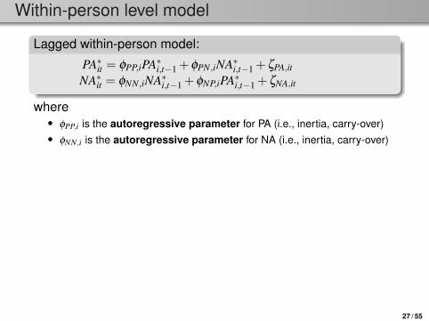
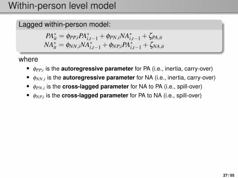
Within-person level model
Lagged within-person model:
PA∗it = φPP,iPA∗i,t−1 +φPN,iNA∗i,t−1 +ζPA,it
NA∗it = φNN,iNA∗i,t−1 +φNP,iPA∗i,t−1 +ζNA,it
where• φPP,i is the autoregressive parameter for PA (i.e., inertia, carry-over)• φNN,i is the autoregressive parameter for NA (i.e., inertia, carry-over)
• φPN,i is the cross-lagged parameter for NA to PA (i.e., spill-over)• φNP,i is the cross-lagged parameter for PA to NA (i.e., spill-over)• ζPA,it is the innovation for PA (residual, disturbance, dynamic error)• ζNA,it is the innovation for NA (residual, disturbance, dynamic error)
Parameters estimated at this level are the residual variancesand covariance:[
ζPA,it
ζNA,it
]∼MN
[[00
],
[θ11θ21 θ22
]]
27 / 55
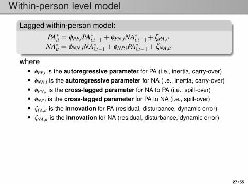
Within-person level model
Lagged within-person model:
PA∗it = φPP,iPA∗i,t−1 +φPN,iNA∗i,t−1 +ζPA,it
NA∗it = φNN,iNA∗i,t−1 +φNP,iPA∗i,t−1 +ζNA,it
where• φPP,i is the autoregressive parameter for PA (i.e., inertia, carry-over)• φNN,i is the autoregressive parameter for NA (i.e., inertia, carry-over)• φPN,i is the cross-lagged parameter for NA to PA (i.e., spill-over)• φNP,i is the cross-lagged parameter for PA to NA (i.e., spill-over)
• ζPA,it is the innovation for PA (residual, disturbance, dynamic error)• ζNA,it is the innovation for NA (residual, disturbance, dynamic error)
Parameters estimated at this level are the residual variancesand covariance:[
ζPA,it
ζNA,it
]∼MN
[[00
],
[θ11θ21 θ22
]]
27 / 55
Within-person level model
Lagged within-person model:
PA∗it = φPP,iPA∗i,t−1 +φPN,iNA∗i,t−1 +ζPA,it
NA∗it = φNN,iNA∗i,t−1 +φNP,iPA∗i,t−1 +ζNA,it
where• φPP,i is the autoregressive parameter for PA (i.e., inertia, carry-over)• φNN,i is the autoregressive parameter for NA (i.e., inertia, carry-over)• φPN,i is the cross-lagged parameter for NA to PA (i.e., spill-over)• φNP,i is the cross-lagged parameter for PA to NA (i.e., spill-over)• ζPA,it is the innovation for PA (residual, disturbance, dynamic error)• ζNA,it is the innovation for NA (residual, disturbance, dynamic error)
Parameters estimated at this level are the residual variancesand covariance:[
ζPA,it
ζNA,it
]∼MN
[[00
],
[θ11θ21 θ22
]]
27 / 55
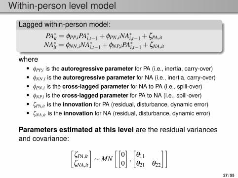
Within-person level model
Lagged within-person model:
PA∗it = φPP,iPA∗i,t−1 +φPN,iNA∗i,t−1 +ζPA,it
NA∗it = φNN,iNA∗i,t−1 +φNP,iPA∗i,t−1 +ζNA,it
where• φPP,i is the autoregressive parameter for PA (i.e., inertia, carry-over)• φNN,i is the autoregressive parameter for NA (i.e., inertia, carry-over)• φPN,i is the cross-lagged parameter for NA to PA (i.e., spill-over)• φNP,i is the cross-lagged parameter for PA to NA (i.e., spill-over)• ζPA,it is the innovation for PA (residual, disturbance, dynamic error)• ζNA,it is the innovation for NA (residual, disturbance, dynamic error)
Parameters estimated at this level are the residual variancesand covariance:[
ζPA,it
ζNA,it
]∼MN
[[00
],
[θ11θ21 θ22
]]27 / 55
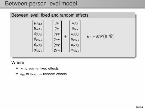
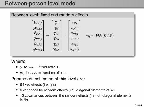
Between-person level model
Between level: fixed and random effects
µPA,i
µNA,i
φPP,i
φPN,i
φNP,i
φNN,i
=
γP
γN
γPP
γPN
γNP
γNN
+
uP,i
uN,i
uPP,i
uPN,i
uNP,i
uNN,i
ui ∼MN(0,Ψ)
Where:• γP to γNN ⇒ fixed effects• uP,i to uNN,i ⇒ random effects
Parameters estimated at this level are:• 6 fixed effects (i.e., γ ’s)• 6 variances for random effects (i.e., diagonal elements of Ψ)• 15 covariances between the random effects (i.e., off-diagonal elements
in Ψ)
28 / 55
Between-person level model
Between level: fixed and random effects
µPA,i
µNA,i
φPP,i
φPN,i
φNP,i
φNN,i
=
γP
γN
γPP
γPN
γNP
γNN
+
uP,i
uN,i
uPP,i
uPN,i
uNP,i
uNN,i
ui ∼MN(0,Ψ)
Where:• γP to γNN ⇒ fixed effects• uP,i to uNN,i ⇒ random effects
Parameters estimated at this level are:• 6 fixed effects (i.e., γ ’s)• 6 variances for random effects (i.e., diagonal elements of Ψ)• 15 covariances between the random effects (i.e., off-diagonal elements
in Ψ)28 / 55

Bivariate model: Mplus code
VARIABLE: NAMES ARE id sessdatena1 na2 na3 na4 na5 na6 na7 na8 na9 na10pa1 pa2 pa3 pa4 pa5 pa6 pa7 pa8 pa9 pa10sessionNr age_pre sex CESDpre CESDpost dayNA dayPA older;
CLUSTER = id; ! Specify the person id variableUSEVAR = dayPA dayNA; ! Specify which variables are used in the modelMISSING = ALL(-999);
LAGGED = dayPA(1) dayNA(1); ! This creates lagged variablesTINTERVAL = sessdate(1); ! This is to account for unequal intervals
ANALYSIS: TYPE IS TWOLEVEL RANDOM; ! This allows for random slopesESTIMATOR = BAYES; ! DSEM requires Bayesian estimationPROC = 2; ! Using 2 processors makes it fasterBITER = (5000); ! This implies at least 5000 iterations are usedTHIN = 10; ! Thinning helps with getting more stable results
29 / 55
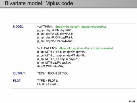
Bivariate model: Mplus code
MODEL: %WITHIN% ! Specify the random lagged relationshipsp_pp | dayPA ON dayPA&1;p_pn | dayPA ON dayNA&1;p_np | dayNA ON dayPA&1;p_nn | dayNA ON dayNA&1;
%BETWEEN% ! Allow all 6 random effects to be correlatedp_pp WITH p_pn-p_nn dayPA dayNA;p_pn WITH p_np-p_nn dayPA dayNA;p_np WITH p_nn dayPA dayNA;p_nn WITH dayPA dayNA;dayPA WITH dayNA;
OUTPUT: TECH1 TECH8 STDYX;
PLOT: TYPE = PLOT3;FACTORS =ALL;
30 / 55
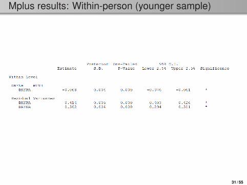
Mplus results: Within-person (younger sample)
31 / 55
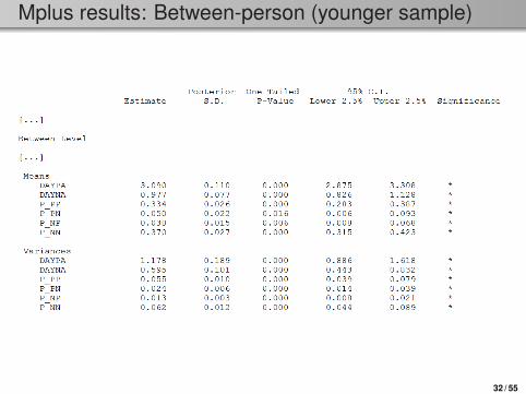
Mplus results: Between-person (younger sample)
32 / 55
Comparing cross-lagged parameters
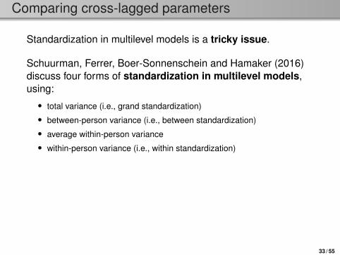
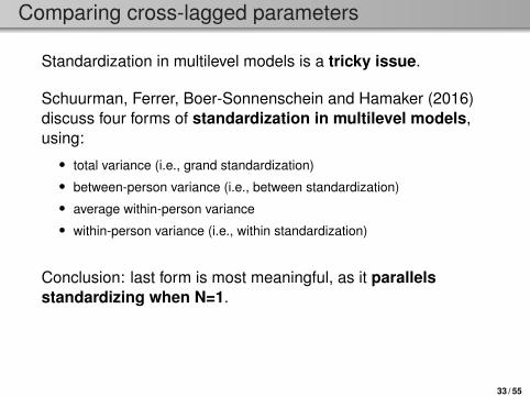
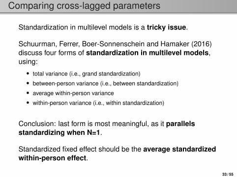
Standardization in multilevel models is a tricky issue.
Schuurman, Ferrer, Boer-Sonnenschein and Hamaker (2016)discuss four forms of standardization in multilevel models,using:• total variance (i.e., grand standardization)• between-person variance (i.e., between standardization)• average within-person variance• within-person variance (i.e., within standardization)
Conclusion: last form is most meaningful, as it parallelsstandardizing when N=1.
Standardized fixed effect should be the average standardizedwithin-person effect.
33 / 55
Comparing cross-lagged parameters
Standardization in multilevel models is a tricky issue.
Schuurman, Ferrer, Boer-Sonnenschein and Hamaker (2016)discuss four forms of standardization in multilevel models,using:• total variance (i.e., grand standardization)• between-person variance (i.e., between standardization)• average within-person variance• within-person variance (i.e., within standardization)
Conclusion: last form is most meaningful, as it parallelsstandardizing when N=1.
Standardized fixed effect should be the average standardizedwithin-person effect.
33 / 55

Mplus standardized results (younger sample)
34 / 55
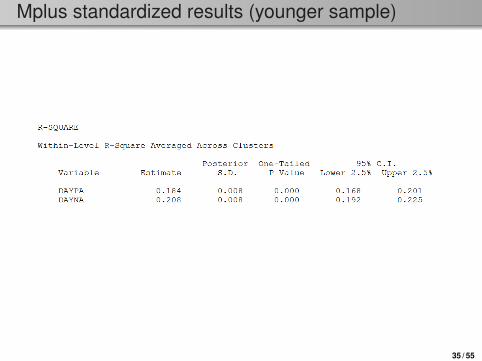
Mplus standardized results (younger sample)
35 / 55
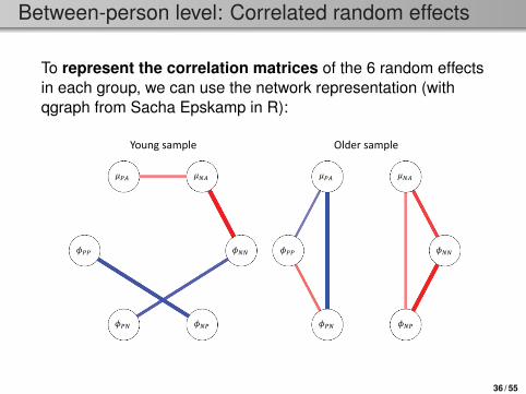
Between-person level: Correlated random effects
To represent the correlation matrices of the 6 random effectsin each group, we can use the network representation (withqgraph from Sacha Epskamp in R):
log( ) log( )
log (- )
log( ) log( )
log (- )
Young sample Older sample
Mod
el 1
M
odel
2
36 / 55

Outline
• Time series analysis• Multilevel time series analysis• DSEM application 1: Multilevel VAR(1) model• DSEM application 2: Mediation• Discussion
37 / 55
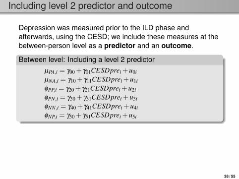
Including level 2 predictor and outcome
Depression was measured prior to the ILD phase andafterwards, using the CESD; we include these measures at thebetween-person level as a predictor and an outcome.
Between level: Including a level 2 predictorµPA,i = γ00 + γ01CESDprei +u0i
µNA,i = γ10 + γ11CESDprei +u1i
φPP,i = γ20 + γ21CESDprei +u2i
φPN,i = γ30 + γ31CESDprei +u3i
φNN,i = γ40 + γ41CESDprei +u4i
φNP,i = γ50 + γ51CESDprei +u5i
Between level: Including a level 2 outcomeCESDposti = γ60 + γ61CESDprei + γ62µPA,i + γ63µNA,i
+γ64φPP,i + γ65φPN,i + γ66φNN,i + γ67φNP,i +u6i
38 / 55
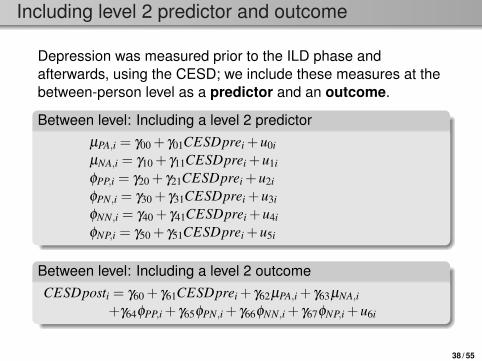
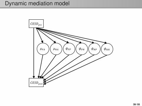
Dynamic mediation model
𝐶𝐶𝐸𝐸𝐸𝐸𝐸𝐸𝑝𝑝𝑝𝑝𝑝𝑝
𝜙𝜙𝑃𝑃𝑃𝑃 𝜙𝜙𝑃𝑃𝑃𝑃 𝜙𝜙𝑃𝑃𝑃𝑃 𝜙𝜙𝑃𝑃𝑃𝑃 𝜇𝜇𝑃𝑃𝑃𝑃 𝜇𝜇𝑃𝑃𝑃𝑃
𝐶𝐶𝐸𝐸𝐸𝐸𝐸𝐸𝑝𝑝𝑜𝑜𝑜𝑜𝑜𝑜
39 / 55
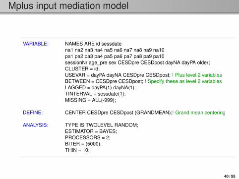
Mplus input mediation model
VARIABLE: NAMES ARE id sessdatena1 na2 na3 na4 na5 na6 na7 na8 na9 na10pa1 pa2 pa3 pa4 pa5 pa6 pa7 pa8 pa9 pa10sessionNr age_pre sex CESDpre CESDpost dayNA dayPA older;CLUSTER = id;USEVAR = dayPA dayNA CESDpre CESDpost; ! Plus level 2 variablesBETWEEN = CESDpre CESDpost; ! Specify these as level 2 variablesLAGGED = dayPA(1) dayNA(1);TINTERVAL = sessdate(1);MISSING = ALL(-999);
DEFINE: CENTER CESDpre CESDpost (GRANDMEAN);! Grand mean centering
ANALYSIS: TYPE IS TWOLEVEL RANDOM;ESTIMATOR = BAYES;PROCESSORS = 2;BITER = (5000);THIN = 10;
40 / 55

Bivariate model: Mplus code
MODEL: %WITHIN% ! Same as beforep_pp | dayPA ON dayPA&1;p_pn | dayPA ON dayNA&1;p_np | dayNA ON dayPA&1;p_nn | dayNA ON dayNA&1;
%BETWEEN% ! Mediation model with parameter namesp_pp-p_nn dayPA dayNA ON CESDpre (a1-a6);CESDpost ON p_pp-p_nn dayPA dayNA CESDpre (b1-b7);
MODEL CONSTRAINT: ! Compute the indirect effectsnew (ab_p_pp); ab_p_pp=a1*b1;new (ab_p_pn); ab_p_pn=a2*b2;new (ab_p_np); ab_p_np=a3*b3;new (ab_p_nn); ab_p_nn=a4*b4;new (ab_dayPA); ab_dayPA=a5*b5;new (ab_dayNA); ab_dayNA=a6*b6;
OUTPUT: TECH1 TECH8 STDYX;
PLOT: TYPE = PLOT3;FACTOR =ALL;
41 / 55
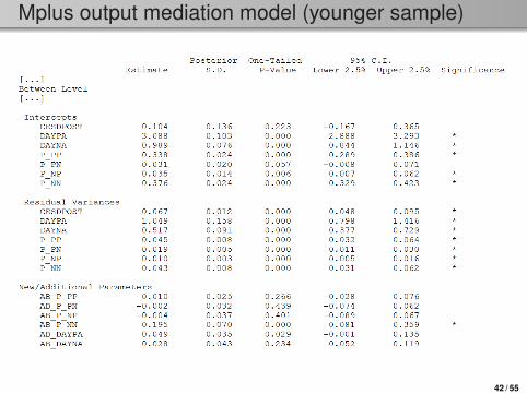
Mplus output mediation model (younger sample)
42 / 55
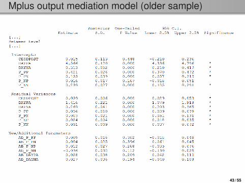
Mplus output mediation model (older sample)
43 / 55
Outline
• Time series analysis• Multilevel time series analysis• DSEM application 1: Multilevel VAR(1) model• DSEM application 2: Mediation• Discussion
44 / 55
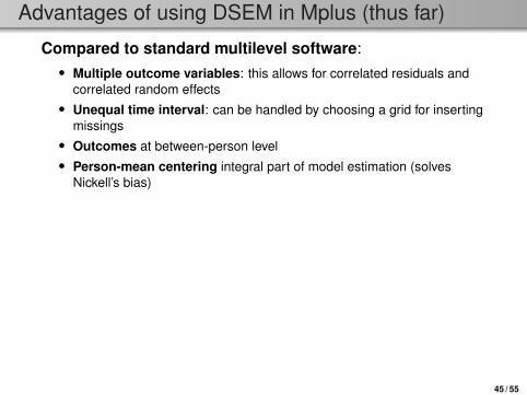
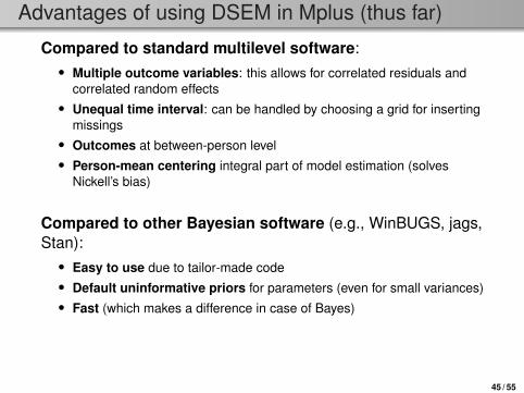
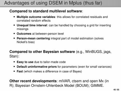
Advantages of using DSEM in Mplus (thus far)
Compared to standard multilevel software:• Multiple outcome variables: this allows for correlated residuals and
correlated random effects• Unequal time interval: can be handled by choosing a grid for inserting
missings• Outcomes at between-person level• Person-mean centering integral part of model estimation (solves
Nickell’s bias)
Compared to other Bayesian software (e.g., WinBUGS, jags,Stan):• Easy to use due to tailor-made code• Default uninformative priors for parameters (even for small variances)• Fast (which makes a difference in case of Bayes)
Other recent developments: mlVAR, ctsem and open Mx (inR); Bayesian Ornstein-Uhlenbeck Model (BOUM); GIMME.
45 / 55
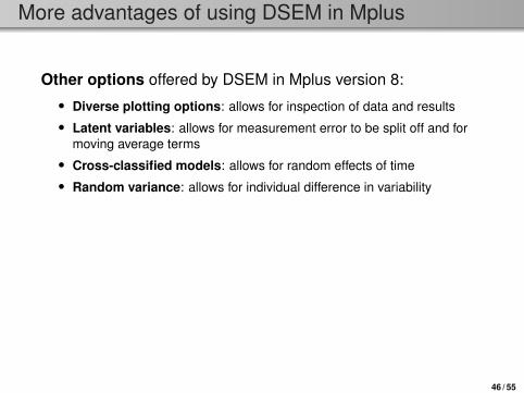
More advantages of using DSEM in Mplus
Other options offered by DSEM in Mplus version 8:• Diverse plotting options: allows for inspection of data and results• Latent variables: allows for measurement error to be split off and for
moving average terms• Cross-classified models: allows for random effects of time• Random variance: allows for individual difference in variability
Future options Mplus will offer:• Regime-switching models: allows for a process to switch between
distinct states• Residual dynamic modeling: allows for easy combination of time
trends and residual lagged relationships
46 / 55
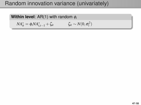
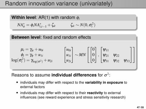
Random innovation variance (univariately)
Within level: AR(1) with random φi
NA∗it = φiNA∗i,t−1 +ζit ζit ∼ N(0,σ2i )
Between level: fixed and random effects
µi = γµ +u0i
φi = γφ +u1i
log(σ2i ) = γlog(σ2)+u2i
u0i
u1i
u2i
∼MN
000
,ψ11
ψ21 ψ22ψ31 ψ32 ψ33
Reasons to assume individual differences for σ2:• individuals may differ with respect to the variability in exposure to
external factors• individuals may differ with respect to their reactivity to external
influences (see reward experience and stress sensitivity research)
47 / 55
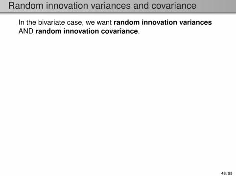
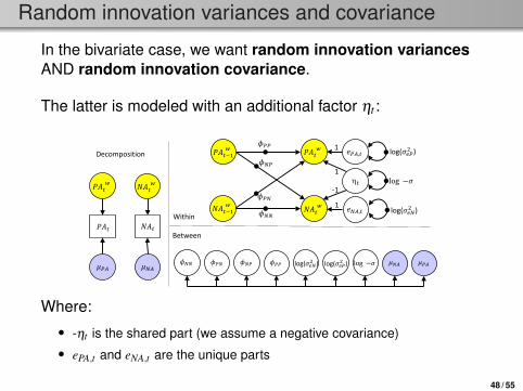
Random innovation variances and covariance
In the bivariate case, we want random innovation variancesAND random innovation covariance.
The latter is modeled with an additional factor ηt :
𝑒𝑒𝑃𝑃𝑃𝑃,𝑡𝑡
𝑒𝑒𝑁𝑁𝑃𝑃,𝑡𝑡
η𝑡𝑡
1
1
1
-1
𝜙𝜙𝑃𝑃𝑃𝑃
𝜙𝜙𝑁𝑁𝑃𝑃
𝜙𝜙𝑃𝑃𝑁𝑁
𝜙𝜙𝑁𝑁𝑁𝑁
𝜙𝜙𝑁𝑁𝑁𝑁 𝜙𝜙𝑃𝑃𝑁𝑁 𝜙𝜙𝑁𝑁𝑃𝑃 𝜙𝜙𝑃𝑃𝑃𝑃 𝜇𝜇𝑁𝑁𝑃𝑃 𝜇𝜇𝑃𝑃𝑃𝑃 log(𝜎𝜎𝑒𝑒𝑁𝑁2 ) log(𝜎𝜎𝑒𝑒𝑃𝑃2 ) log (−𝜎𝜎)
Within
Between
log(𝜎𝜎𝑒𝑒𝑁𝑁2 )
log(𝜎𝜎𝑒𝑒𝑃𝑃2 )
log (−𝜎𝜎)
𝑃𝑃𝑃𝑃𝑡𝑡 𝑁𝑁𝑃𝑃𝑡𝑡
𝑃𝑃𝑃𝑃𝑡𝑡(𝑤𝑤)
𝑁𝑁𝑃𝑃𝑡𝑡(𝑤𝑤)
𝑃𝑃𝑃𝑃𝑡𝑡(𝑤𝑤) 𝑁𝑁𝑃𝑃𝑡𝑡
(𝑤𝑤)
𝜇𝜇𝑁𝑁𝑃𝑃 𝜇𝜇𝑃𝑃𝑃𝑃
Decomposition 𝑃𝑃𝑃𝑃𝑡𝑡−1(𝑤𝑤)
𝑁𝑁𝑃𝑃𝑡𝑡−1(𝑤𝑤)
Where:• -ηt is the shared part (we assume a negative covariance)• ePA,t and eNA,t are the unique parts
48 / 55
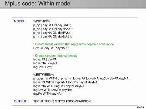
Mplus code: Within model
MODEL: %WITHIN%p_pp | dayPA ON dayPA&1;p_pn | dayPA ON dayNA&1;p_np | dayNA ON dayPA&1;p_nn | dayNA ON dayNA&1;
! Create latent variable that represents negative covarianceCov BY dayPA1 dayNA-1;
! Create random (log) varianceslogvarPA | dayPA;logvarNA | dayNA;logCov | Cov;
%BETWEEN%p_pp-p_nn WITH p_pn-p_nn logvarPA logvarNA logCov dayPA dayNA;logvarPA WITH logvarNA logCov dayPA dayNA;logvarNA WITH logCov dayPA dayNA;logCov WITH dayPA dayNA;dayPA WITH dayNA;
OUTPUT: TECH1 TECH8 STDYX FSCOMPARISON;
49 / 55

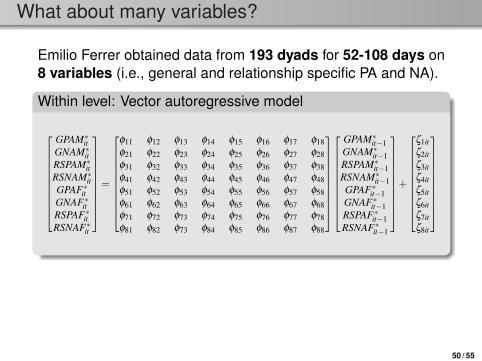
What about many variables?
Emilio Ferrer obtained data from 193 dyads for 52-108 days on8 variables (i.e., general and relationship specific PA and NA).
Within level: Vector autoregressive model
GPAM∗itGNAM∗itRSPAM∗itRSNAM∗itGPAF∗itGNAF∗itRSPAF∗itRSNAF∗it
=
φ11 φ12 φ13 φ14 φ15 φ16 φ17 φ18φ21 φ22 φ23 φ24 φ25 φ26 φ27 φ28φ31 φ32 φ33 φ34 φ35 φ36 φ37 φ38φ41 φ42 φ43 φ44 φ45 φ46 φ47 φ48φ51 φ52 φ53 φ54 φ55 φ56 φ57 φ58φ61 φ62 φ63 φ64 φ65 φ66 φ67 φ68φ71 φ72 φ73 φ74 φ75 φ76 φ77 φ78φ81 φ82 φ73 φ84 φ85 φ86 φ87 φ88
GPAM∗it−1GNAM∗it−1RSPAM∗it−1RSNAM∗it−1GPAF∗it−1GNAF∗it−1RSPAF∗it−1RSNAF∗it−1
+
ζ1itζ2itζ3itζ4itζ5itζ6itζ7itζ8it
which gives:GPAM∗it = φ11GPAM∗it−1 +φ12GNAM∗it−1 + · · ·+φ18RSNAF∗it−1 +ζ1it. . .RSNAF∗it = φ81GPAM∗it−1 +φ82GNAM∗it−1 + · · ·+φ88RSNAF∗it−1 +ζ8it
50 / 55
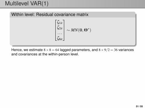
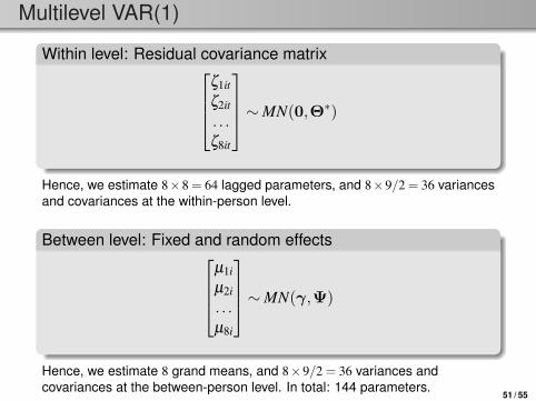
Multilevel VAR(1)
Within level: Residual covariance matrixζ1it
ζ2it
. . .ζ8it
∼MN(0,Θ∗)
Hence, we estimate 8×8 = 64 lagged parameters, and 8×9/2 = 36 variancesand covariances at the within-person level.
Between level: Fixed and random effectsµ1i
µ2i
. . .µ8i
∼MN(γ,Ψ)
Hence, we estimate 8 grand means, and 8×9/2 = 36 variances andcovariances at the between-person level. In total: 144 parameters.
51 / 55
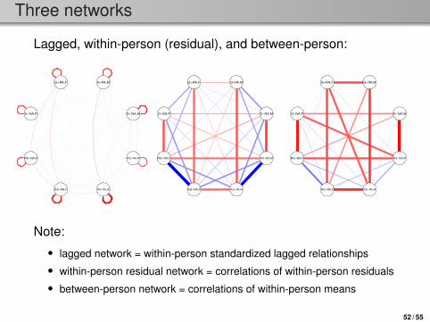
Three networks
Lagged, within-person (residual), and between-person:
G−PA.M
G−NA.M
RS−NA.M
RS−PA.MRS−PA.F
RS−NA.F
G−NA.F
G−PA.F G−PA.M
G−NA.M
RS−NA.M
RS−PA.MRS−PA.F
RS−NA.F
G−NA.F
G−PA.F G−PA.M
G−NA.M
RS−NA.M
RS−PA.MRS−PA.F
RS−NA.F
G−NA.F
G−PA.F
Note:• lagged network = within-person standardized lagged relationships• within-person residual network = correlations of within-person residuals• between-person network = correlations of within-person means
52 / 55

References
• Bringmann, Vissers, Wichers, Geschwind, Kuppens, Peeters, Borsboom &Tuerlinckx (2013). A network approach to psychopathology: New insights intoclinical longitudinal data. PLoS ONE, 8, e60188, 1-13.
• Hamaker (2012). Why researchers should think “within-person”: A paradigmaticrationale. In M. R. Mehl & T. S. Conner (Eds.). Handbook of Research Methodsfor Studying Daily Life, 43-61. New York, NY: Guilford Publications.
• Hamaker, Asparouhov, Brose, Schmiedek & Muthén (submitted). At the frontiersof modeling intensive longitudinal data: Dynamic structural equation models forthe affective measurements from the COGITO study. Multivariate BehavioralResearch.
• Hamaker & Grasman (2015). To center or not to center? Investigating inertiawith a multilevel autoregressive model. Frontiers in Psychology, 5, 1492.
• Hamaker & Wichers (2017). No time like the present: Discovering the hiddendynamics in intensive longitudinal data. Current Directions in PsychologicalScience, 26, 10-15.
• Jongerling, Laurenceau & Hamaker (2015). A multilevel AR(1) model: Allowingfor inter-individual differences in trait-scores, inertia, and innovation variance.Multivariate Behavioral Research, 50, 334-349.
53 / 55
References
• Koval, Kuppens, Allen & Sheeber (2012). Getting stuck in depression: The rolesof rumination and emotional inertia. Cognition & Emotion, 26, 1412-1427.
• Kuppens, Allen & Sheeber (2010). Emotional inertia and psychologicalmaladjustment. Psychological Science, 21, 984-991.
• Kuppens, Sheeber, Yap, Whittle, Simmons & Allen (2012). Emotional inertiaprospectively predicts the onset of depressive Multilevel AR(1) model 33 disorderin adolescence. Emotion, 12, 283-289.
• Schuurman, Ferrer, de Boer-Sonnenschein & Hamaker (2016). How to comparecross-lagged associations in a multilevel autoregressive model. PsychologicalMethods, 21, 206-221.
• Suls, Green & Hillis (1998). Emotional reactivity to everyday problems, affectiveinertia, and neuroticism. Personality and Social Psychology Bulletin, 24,127-136.
54 / 55