Dynamic Skyline Queries in Large Graphs - …tozsu/publications/other/zlDASFAA10.pdf · Dynamic...

Dynamic Skyline Queries in Large Graphs

Lei Zou1, Lei Chen2, M. Tamer Ozsu3, and Dongyan Zhao1,4 ?

1 Institute of Computer Science and Technology, Peking University, Beijing, China,{zoulei,zdy}@icst.pku.edu.cn

2 Hong Kong of Science and Technology, Hong Kong, China,[email protected]

3 University of Waterloo, Waterloo, Canada,[email protected]

4 Key Laboratory of Computational Linguistics (PKU), Ministry of Education, China

Abstract. Given a set of query points, a dynamic skyline query reports all datapoints that are not dominated by other data points according to the distancesbetween data points and query points. In this paper, we study dynamic skylinequeries in a large graph (DSG-query for short). Although dynamic skylines havebeen studied in Euclidean space [16], road network [6], and metric space [4, 7],there is no previous work on dynamic skylines over large graphs. We employa filter-and-refine framework to speed up the query processing that can answerDSG-query efficiently. We propose a novel pruning rule based on graph propertiesto derive the candidates for DSG-query, that are guaranteed not to introduce falsenegatives. In the refinement step, with a carefully-designed index structure, wecompute short path distances between vertices in O(H), where H is the numberof maximal hops between any two vertices. Extensive experiments demonstratethat our methods outperform existing algorithms by orders of magnitude.

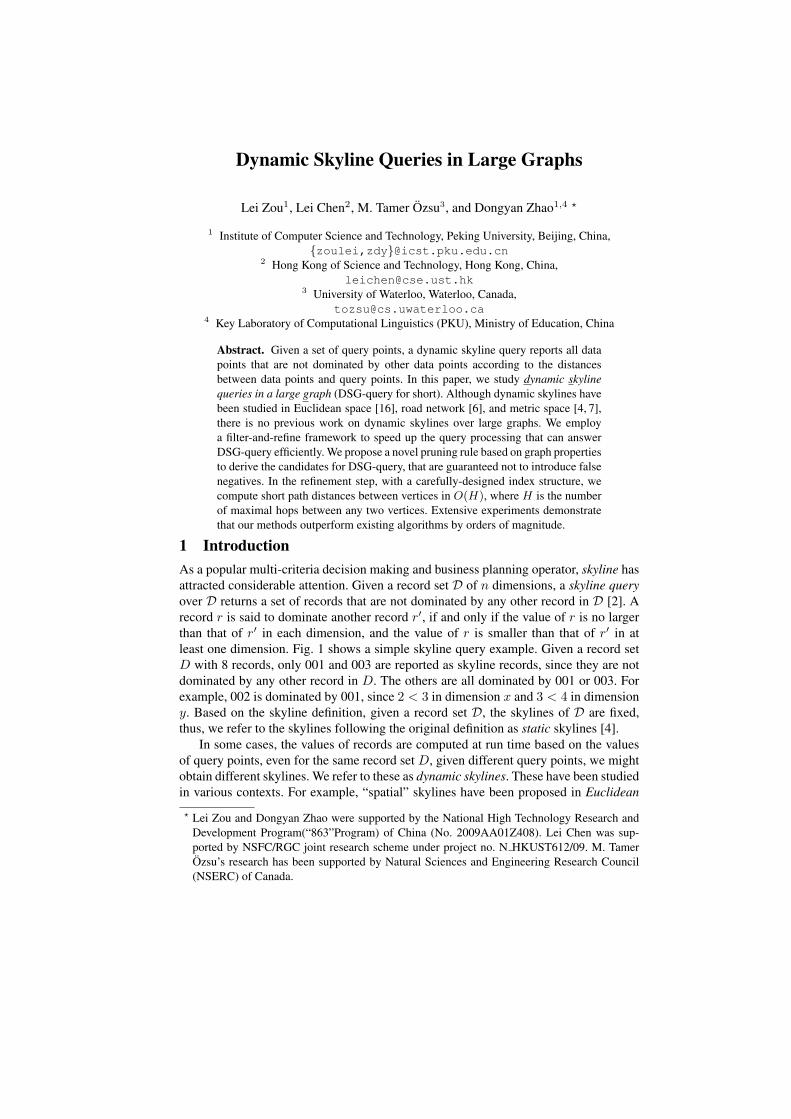
1 IntroductionAs a popular multi-criteria decision making and business planning operator, skyline hasattracted considerable attention. Given a record set D of n dimensions, a skyline queryover D returns a set of records that are not dominated by any other record in D [2]. Arecord r is said to dominate another record r′, if and only if the value of r is no largerthan that of r′ in each dimension, and the value of r is smaller than that of r′ in atleast one dimension. Fig. 1 shows a simple skyline query example. Given a record setD with 8 records, only 001 and 003 are reported as skyline records, since they are notdominated by any other record in D. The others are all dominated by 001 or 003. Forexample, 002 is dominated by 001, since 2 < 3 in dimension x and 3 < 4 in dimensiony. Based on the skyline definition, given a record set D, the skylines of D are fixed,thus, we refer to the skylines following the original definition as static skylines [4].

In some cases, the values of records are computed at run time based on the valuesof query points, even for the same record set D, given different query points, we mightobtain different skylines. We refer to these as dynamic skylines. These have been studiedin various contexts. For example, “spatial” skylines have been proposed in Euclidean

? Lei Zou and Dongyan Zhao were supported by the National High Technology Research andDevelopment Program(“863”Program) of China (No. 2009AA01Z408). Lei Chen was sup-ported by NSFC/RGC joint research scheme under project no. N HKUST612/09. M. TamerOzsu’s research has been supported by Natural Sciences and Engineering Research Council(NSERC) of Canada.

2 Lei Zou et al.

space [16]. Specifically, given a set of query points Q = {qi} (i = 1...n), for eachrecord r ∈ D, we compute a new vector rd of dimension n, where rd’s i-th dimensionis computed as Euclidean Distance between r and qi. The spatial skylines refer to allvectors rd whose values are not dominated by other r′d in the record set D. A similarquery, called multi-source skyline query in road networks, is studied by Deng et al. [6],where the values of records are defined as the shortest path lengths on road networksfrom data points to query points.

ID X Y

001 2 3

002 3 4

003 4 2

004 4 5

005 6 7

006 6 3

1 2 3 4 5 6 7 8

1

2

3

4

5

6

7

8

Skyline

Records

001

003

00

2

004

005

006

Record Set D

X

Y

007 7 6

008 5 4

008

006

007

v0 v1

v2v3v4

1( , )iDist v q 2( , )i

Dist v q

1 1

ID

v0

q1

q2

2 1v3

3 2v4

(b) Running Example (a) Static Skylines

Fig. 1. (a)Static Skyline Query and (b) Running Example

Compared to static skylines, dynamic skylines offer users more flexibility in spec-ifying their search criteria. In other words, different users can specify different sets ofquery points. Meanwhile, the flexibility of dynamic skyline queries brings new chal-lenges for efficient query processing. A naive solution computes all the new vectorsaccording to the query points, and then searches the skylines over the generated vec-tors. This approach is clearly inefficient, since it requires scanning the whole record setD to compute the new vectors.

In this paper, we study the problem of dynamic skyline queries over graph data,which is formally defined as follows:Definition 1. Dominate. Given a large undirected and edge-weighted graph G and aset of query vertices Q = {qi}, i = 1...n, in graph G, for two data vertices v′ and vin G (v and v′ are not query vertices), we say that v′ dominates v, if and only if thefollowing holds: (∀i, Dist(v′, qi) ≤ Dist(v, qi)) ∧ (∃j, Dist(v′, qj) < Dist(v, qj) , whereDist(v, qi) is the shortest path distance between v and qi in graph G.Definition 2. Problem Definition. Given a large undirected and edge-weighted graphG and a set Q of query vertices Q = {qi}, i = 1...n, in graph G, a dynamic skylinequery in graph (DSG-query) reports all data vertices v in graph G (v 6= qi) where eachv is not dominated by any other vertex v′ in G. All skyline vertices of query Q in graphG are denoted as Skyline(G,Q).Example 1 (Running Example). Consider a graph G and two query vertices q1 and q2

(denoted as shaded vertices) in Fig. 1b. The number in the vertex is the vertex ID. Forsimplicity, we assume that all edges have the same weight 1. Obviously, in this example,there is only one skyline vertex, that is v0.

Similar to the cases in the Euclidean space, dynamic skylines over graph data arequite useful. For example, given a social network modeled as a large graph, where eachvertex corresponds to an individual, and each edge denotes the friendship between twocorresponding individuals, we can use shortest path distance to define the relationship

Dynamic Skyline Queries in Large Graphs 3

score between two individuals in a social network [18]. Assuming that there are twoimportant latent customers (two query vertices), a company may look for a salesmanwho has “closer” relationship to these customers than any other salesmen. In fact, thecompany is looking for the skyline salesmen with respect to the two given potentialcustomers c1 and c2. A salesman r is a skyline if and only if there exists no othersalesman r′, such that Dist(r′, c1) < Dist(r, c1) and Dist(r′, c2) < Dist(r, c2),where Dist(r, ci) denotes the shortest path distance between r and ci. Finally, considera Peer-to-Peer (P2P) network with a number of peers that are interested in some movies.In order to reduce the communication cost, we can put replicas of the movies on a nodethat is near these peers. Obviously, dynamic skylines with respect to these peers in thetopology map (a graph) of this P2P network can provide some candidate nodes forstoring the replicas.

Although efficient solutions have been proposed for dynamic skylines over Eu-clidean space [16], these cannot be applied to graphs. In a graph, the shortest pathdistance is often used as a measure between two vertices, rather than Euclidean dis-tance. Thus, it is impossible to utilize existing pruning rules, such as MBR and VoronoiDiagrams that have been used in Euclidean space [16].

The most related work is multi-source skyline query processing in road networks[6], which also uses shortest path distance as the measure. Three different algorithmshave been proposed to find dynamic skylines in road networks. Two of the algorithms(EDC and LBC) [6] utilize Euclidean distance as the lower bound of shortest path dis-tance in a road network to perform pruning. However, for a general graph G, we cannotdefine Euclidean distances to bound the shortest path distances between any two ver-tices in G, since there is no coordinate associated with each vertex. Therefore, EDCand LBC algorithms cannot be applied to DSG-Query. The third algorithm (CE) is notefficient. It expands each query point towards all directions, which may generate toomany candidate objects and cause unnecessary shortest path distance computation, asconfirmed by our experiments (Section 4).

Dist(v, qi) in DSG-query is a metric distance. Thus, the approaches that addressskyline queries in metric space (e.g. [4]) are of interest. However, these solutions areonly designed for the general metric space, and the methods are not optimized for largegraphs. Experiments in Section 4 show that our methods outperform these general ap-proaches by orders of magnitude. For a DSG-query, there exist two challenges: 1) HugeSearch Space: each vertex in graph G (except for query vertices) is a candidate forDSG-query; and 2) Expensive Shortest Path Computation: In order to find final sky-line vertices, we need to compute Dist(v, qi) (see Definitions 1 and 2). However, theexpansion process in shortest path algorithms (e.g. Dijkstra’s Algorithm [5]) is verytime-consuming, especially in very large graphs.

In order to address the above challenges, we adopt the “filter-and-refine” frame-work. During the filtering process, we prune most false positives (the vertices that can-not be skyline vertices) to generate a set of candidate vertices. We compute Dist(v, qi)for each candidate vertex during refinement using an index structure. Furthermore, wecan compute Dist(v, qi) in O(H)where His the number of maximal hops between any twovertices in the graph, without expensive expansions that are employed in previous solutions. Insummary, we make the following contributions:

4 Lei Zou et al.

1. We propose shared-shortest-paths (SSP) pruning for DSG-query, that considers graph prop-erties, and that filters out most false positive vertices. We also give a theoretical analysis ofthe pruning power of SSP-pruning.

2. During offline processing of DSG-query, we build carefully-designed index structures thatsupport both filtering and verification processes in online DSG-query.

3. Based on novel pruning rules and index structures, we propose the SSP query algorithm (seeAlgorithm 3) for DSG-query.

4. We show by extensive experiments that our methods have good pruning power and fast queryresponse time.

The remainder of this paper is organized as follows. Some background knowledge is discussed inSection 2. A novel pruning rule is proposed in Section 3. The index structures and SSP-query al-gorithm are also presented in Section 3. We evaluate the efficiency of our methods with extensiveexperiments in Section 4. We discuss related work in Section 5 in detail. Finally, we conclude thepaper in Section 6.

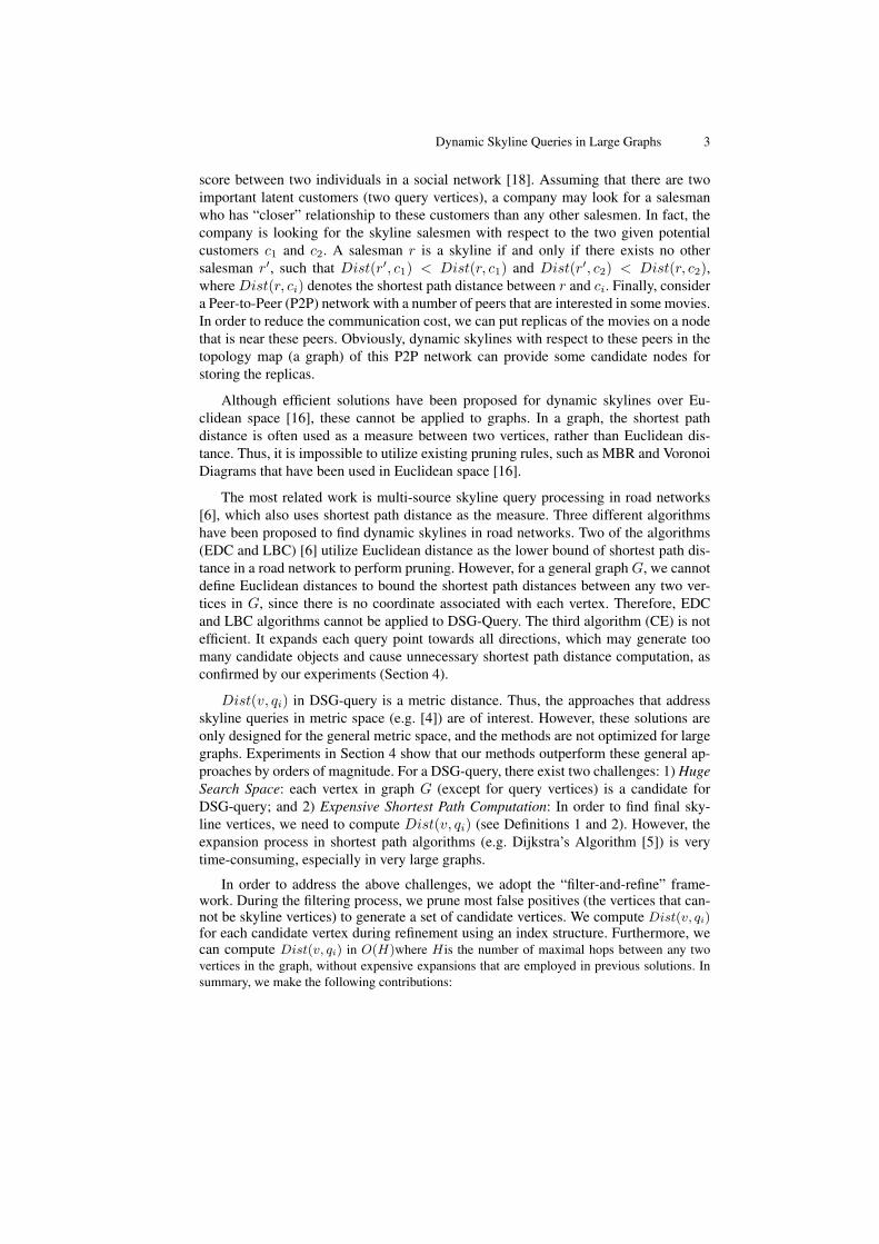
2 PreliminariesDefinition 3. Shortest Path Tree. (SP -Tree for short) Given a large graph G and a vertex v, weperform a single-source shortest path algorithm (such as Dijkstra algorithm [5]) from vertex vto get a tree SP (v). The root of SP (v) is v, and all paths from v to another node v′ in SP (v) isthe shortest path from v to v′ in graph G.

v0

v1 v2

v3

v4

v1

v0 v2

v3

v4

v2

v0 v1 v3

v4

v3

v4 v2

v0 v1

v2

v0 v1

v3

v4

SP(v0) SP(v1) SP(v2) SP(v3) SP(v4)

Fig. 2. Shortest Path Trees

Fig. 2 shows all SP -Trees for graph G of Example 1. We can perform Dijkstra’s algorithm[5] offline to obtain the SP -Tree. Note that, for a vertex v in a large graph G, there may existmore than one SP -Tree rooted at v. Actually, for a vertex v in G, we can select any SP -Treerooted at v without affecting the correctness of our methods. We will prove this claim in Section3 (see Lemma 4). We utilize SP-Tree in our SSP query algorithm (see Section 3).Definition 4. Minimum Common Ancestor. Given a SP -Tree SP (v) in a large graph G and aset of nodes {v1, ..., vn} in SP (v), a node v′ is the minimum common ancestor of {v1, ..., vn}(denoted as MCA(v1...vn, SP (v))) if and only if1) v′ is the ancestor of all nodes v1, ..., vn; and2) there exists no other node v′′, where v′′ is the ancestor of all nodes v1, ..., vn, and v′ is theancestor of v′′.

Take SP (v3) in Fig. 2, for example, MCA(v0, v1, SP (v3)) = v2.

3 Shared Shortest Path Algorithm3.1 SSP Pruning AlgorithmWe first note an interesting property of graphs: many pairwise shortest paths in a graphhave shared parts. We propose a pruning strategy (SSP Pruning) that exploits these


q1

qn

'v v

to be pruned V0

V1 V2

V3

V4

V2

V0 V1

V3

V4

SP(V0)

q1 q2

SP(V4)

q1

q2

(a) (b)

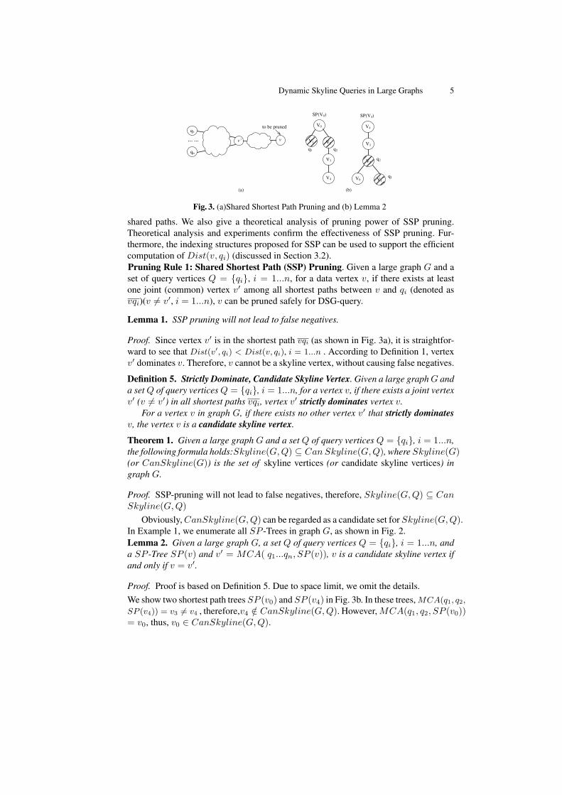
Fig. 3. (a)Shared Shortest Path Pruning and (b) Lemma 2

shared paths. We also give a theoretical analysis of pruning power of SSP pruning.Theoretical analysis and experiments confirm the effectiveness of SSP pruning. Fur-thermore, the indexing structures proposed for SSP can be used to support the efficientcomputation of Dist(v, qi) (discussed in Section 3.2).Pruning Rule 1: Shared Shortest Path (SSP) Pruning. Given a large graph G and aset of query vertices Q = {qi}, i = 1...n, for a data vertex v, if there exists at leastone joint (common) vertex v′ among all shortest paths between v and qi (denoted asvqi)(v 6= v′, i = 1...n), v can be pruned safely for DSG-query.

Lemma 1. SSP pruning will not lead to false negatives.

Proof. Since vertex v′ is in the shortest path vqi (as shown in Fig. 3a), it is straightfor-ward to see that Dist(v′, qi) < Dist(v, qi), i = 1...n . According to Definition 1, vertexv′ dominates v. Therefore, v cannot be a skyline vertex, without causing false negatives.

Definition 5. Strictly Dominate, Candidate Skyline Vertex. Given a large graph G anda set Q of query vertices Q = {qi}, i = 1...n, for a vertex v, if there exists a joint vertexv′ (v 6= v′) in all shortest paths vqi, vertex v′ strictly dominates vertex v.

For a vertex v in graph G, if there exists no other vertex v′ that strictly dominatesv, the vertex v is a candidate skyline vertex.

Theorem 1. Given a large graph G and a set Q of query vertices Q = {qi}, i = 1...n,the following formula holds:Skyline(G,Q) ⊆ Can Skyline(G,Q), where Skyline(G)(or CanSkyline(G)) is the set of skyline vertices (or candidate skyline vertices) ingraph G.

Proof. SSP-pruning will not lead to false negatives, therefore, Skyline(G,Q) ⊆ CanSkyline(G,Q)

Obviously, CanSkyline(G,Q) can be regarded as a candidate set for Skyline(G,Q).In Example 1, we enumerate all SP -Trees in graph G, as shown in Fig. 2.Lemma 2. Given a large graph G, a set Q of query vertices Q = {qi}, i = 1...n, anda SP -Tree SP (v) and v′ = MCA( q1...qn, SP (v)), v is a candidate skyline vertex ifand only if v = v′.

Proof. Proof is based on Definition 5. Due to space limit, we omit the details.We show two shortest path trees SP (v0) and SP (v4) in Fig. 3b. In these trees, MCA(q1, q2,

SP (v4)) = v3 6= v4 , therefore,v4 /∈ CanSkyline(G,Q). However, MCA(q1, q2, SP (v0))= v0, thus, v0 ∈ CanSkyline(G,Q).

6 Lei Zou et al.

Using Lemma 2, we propose a conceptually simple framework for SSP-pruning.During offline processing, we enumerate all SP -Trees in graph G. Given a set Q ofquery vertices Q = {qi}, i = 1...n, in each SP (v), if v′ = MCA(q1... qn, SP (v)) andv′ = v, v will be inserted into candidate set CL. Otherwise, v can be pruned safely. Wecan find CanSkyline(G,Q) by sequentially scanning all SP -Trees.

However, due to large space cost, it is impractical to store all SP -Trees of a largegraph G. The space cost of each SP -Tree is O(|V (G)|), where |V (G)| is the numberof vertices in G. Therefore, we would need O(|V (G)|2) space to store all SP -Trees ingraph G. For example, if G has 10K vertices, the total space cost is O(108). To alleviatethis space cost, in this work, we only store 1-hop SP -Trees.

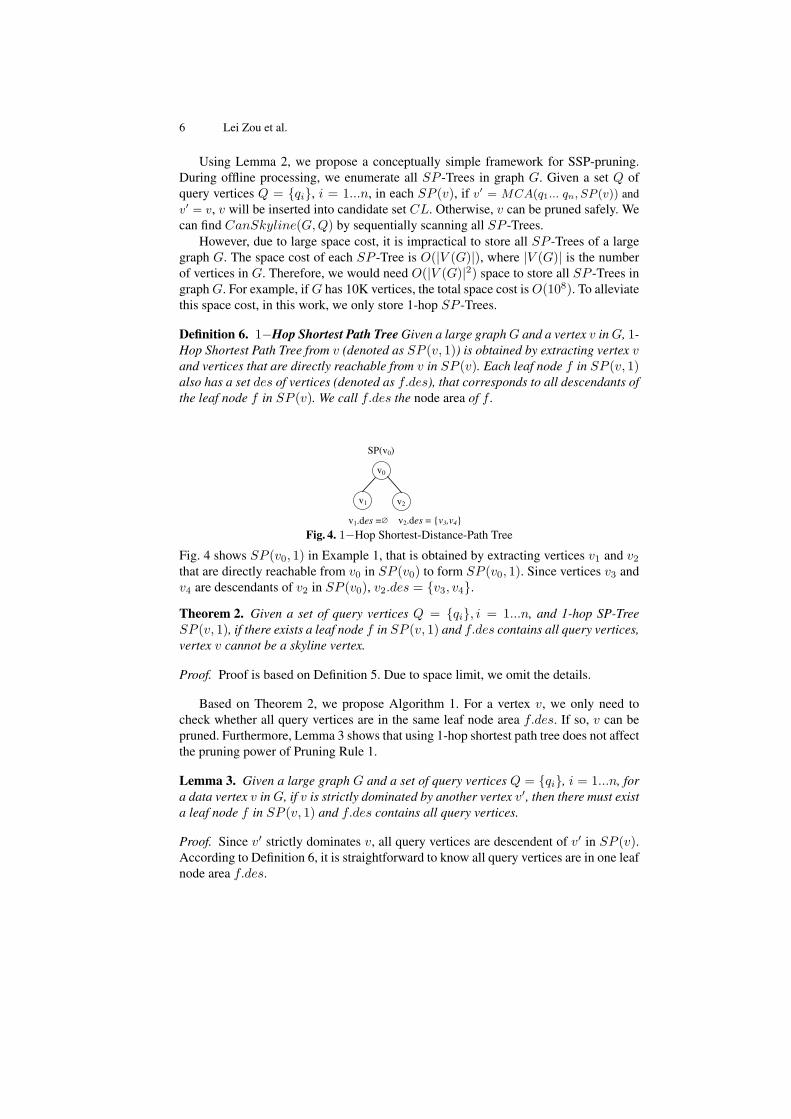
Definition 6. 1−Hop Shortest Path Tree Given a large graph G and a vertex v in G, 1-Hop Shortest Path Tree from v (denoted as SP (v, 1)) is obtained by extracting vertex vand vertices that are directly reachable from v in SP (v). Each leaf node f in SP (v, 1)also has a set des of vertices (denoted as f.des), that corresponds to all descendants ofthe leaf node f in SP (v). We call f.des the node area of f .

v0

v1 v2

SP(v0)

v2.des = {v3,v4}v1.des =

Fig. 4. 1−Hop Shortest-Distance-Path Tree

Fig. 4 shows SP (v0, 1) in Example 1, that is obtained by extracting vertices v1 and v2

that are directly reachable from v0 in SP (v0) to form SP (v0, 1). Since vertices v3 andv4 are descendants of v2 in SP (v0), v2.des = {v3, v4}.

Theorem 2. Given a set of query vertices Q = {qi}, i = 1...n, and 1-hop SP-TreeSP (v, 1), if there exists a leaf node f in SP (v, 1) and f.des contains all query vertices,vertex v cannot be a skyline vertex.

Proof. Proof is based on Definition 5. Due to space limit, we omit the details.

Based on Theorem 2, we propose Algorithm 1. For a vertex v, we only need tocheck whether all query vertices are in the same leaf node area f.des. If so, v can bepruned. Furthermore, Lemma 3 shows that using 1-hop shortest path tree does not affectthe pruning power of Pruning Rule 1.

Lemma 3. Given a large graph G and a set of query vertices Q = {qi}, i = 1...n, fora data vertex v in G, if v is strictly dominated by another vertex v′, then there must exista leaf node f in SP (v, 1) and f.des contains all query vertices.

Proof. Since v′ strictly dominates v, all query vertices are descendent of v′ in SP (v).According to Definition 6, it is straightforward to know all query vertices are in one leafnode area f.des.


Algorithm 1 Prune False Positives by SSP pruningSSP-pruning(G,Q,S)Require: Input: A large graph G and a set Q of query vertices Q = {qi}, all 1-hop SP Trees,

and a set S of verticesOutput: Candidate Set CL

1: for each vertex v in S do2: if all query vertices qi are in only one leaf node n.des of SP (v, 1) then3: continue (Pruned by Theorem 2 )4: else5: insert v into candidate set CL.6: report CL

Lemma 4. Given a vertex v that has more than one SP -Tree rooted at v (SP1(v), ..., SPb(v)),choosing any SP-Tree rooted at v for SSP pruning does not lead to false negatives.

Proof. No matter which SPj(v) is selected, if all query vertices are contained in f.desof SPj(v), f strictly dominates v. Therefore, Lemma 4 holds.

However, the space cost of the set f.des in each leaf node f is still a problem. Thenumber of vertices in f.des is always large. In order to reduce the space cost, we buildhierarchical clusters on vertices in G. If f.des contains all vertices in a cluster P , wecan use P ′s ID instead of the vertices in P in f.des. For example, Fig. 5a shows ahierarchical cluster of Example 1. Cluster P2 has two vertices: v3 and v4. Fig. 5b showsthat v3 and v4 are both in v2.des of SP (v0, 1). Therefore, we only need to insert P2

instead of v3 and v4 in v2.des of SP (v0, 1), as shown in Fig. 5c. Intuitively, if somevertices often occur together in f.des, they should be grouped together. Based on thisintuition, we propose distance definitions (Definitions 7 and 8) that account for clusteredvertices. In Example 1, vertices v3 and v4 should be grouped into one cluster, since theyoccur together in three 1-hop SP -Trees (i.e. SP (v0, 1), SP (v1, 1) and SP (v2, 1)).Similarly, v1 and v2 should be clustered together. Essentially, the coherence of verticesin 1-hop SP-Tree is derived from their shared shortest paths of SP -Trees.

P

P0 P2

v1 v2 v3 v4v0

Hierachical Cluster Tree

P1

SP(v0,1)

v0

v1 v2

v2.Des={P2}

dst src lef

P2 v0 v2

... ... ...

TAB_1SPT

v0

v1 v2

SP(v0,1)

v2.Des={v3,v4}

(a) (b) (c) (d)

Fig. 5. Hierarchical Cluster Tree and 1-Hop SP -Tree

In order to build a hierarchical cluster on vertices, we propose the following distancefunctions, which are used to measure the probability that two vertices appear together.

Definition 7. Vertex Distance. Given three vertices v, v1 and v2, if there exists a leafnode f in SP (v, 1) and f.des contains both v1 and v2, we say that v1 and v2 occurtogether in SP (v, 1). Let the number of vertices v in which v1 and v2 occur together in

8 Lei Zou et al.

SP (v, 1) be T . Then, vertex distance between v1 and v2 (denoted as V exDis(v1, v2))is defined as:

V exDis(v1, v2) =T

|V (G)|Definition 8. Cluster Distance. Given two clusters P1 and P2 and a vertex v, if thereexists a leaf node f in SP (v, 1) and f.des contains all vertices in P1 and P2, we saythat P1 and P2 occur together in SP (v, 1). Let the number of vertices v in which P1

and P2 occur together in SP (v, 1) be D. Then, cluster distance between P1 and P2

(denoted as CluDis(P1, P2)) is defined as:

CluDis(P1, P2) =D

|V (G)|We employ bottom-up clustering to build the hierarchical clusters. First, based on

vertex distances (Definition 7), we utilize clustering algorithms to find clusters on ver-tices. Then, based on cluster distance (Definition 8), small clusters are grouped intolarger ones. We can recursively build a hierarchical cluster tree HT on vertices in graphG, as shown in Fig. 5a.

In practice, we store 1-hop SP-Tree in tables using a commercial RDBMS. The tableformat is shown in Fig. 5d, where ‘dst’ denotes a destination vertex (or a destinationcluster),‘src’ denotes a source vertex, and ‘lef ’ denotes that the leaf node f whosenode area f.des contains the destination dst in SP (src, 1). We illustrate the methodsusing Fig. 5. Since the cluster P2 is in v2.des of SP (v0, 1), there is a row ‘P2, v0, v2’in table TAB 1SPT , which means that v2.dst contains P2 in SP (v0, 1).

Pruning Power of SSP Pruning We discuss the pruning power of SSP pruning. Tofacilitate analysis, we assume that all query vertices are selected independently. First,in Lemma 5, we discuss the probability that one vertex v can be pruned in DSG-querywith n query vertices.

Lemma 5. Given a vertex v in graph G, there are C leaf nodes in SP (v, 1). The num-ber of vertices in each leaf node area fc.des is denoted as |fc.des|, c = 1...C. Givena query set of Q = {qi}, i = 1...n, the probability Pr(v) that v is pruned can beevaluated by the following formula.

Pr(v) =1

|V (G)|nC∑

i=1

|fi.des|n (1)

Proof. If all query vertices are in one leaf node area fc.des of SP (v, 1), fc strictlydominates v ( Definition 5). Therefore, according to Algorithm 1 and SSP pruning, vcan be filtered out safely. The probability that one query vertex qi is in node area fc.des

is |fc.des||V (G)| . Since all query vertices are selected independently, the probability that all

query vertices are in the same node area fc.des is ( |fc.des||V (G)| )

n. Since there are C leafnodes in SP (v, 1), we obtain:

Pr(v) =1

|V (G)|nC∑

i=1

|fi.des|n


Theorem 3. Given a large graph G with |V (G)| vertices, and a query set of Q = {qi},i = 1...n, the expected number of pruned vertices can be evaluated by the followingformula.

|V (G)|∑i=1

Pr(vi) (2)

where Pr(vi) is evaluated by Equation 1.

In the above analysis, we assume that all query vertices are selected independently.We evaluate Equation 2 in experiments (see Section 4) and show that the simple modelcan provide a good approximation of SSP’s pruning power.3.2 Computing Shortest Path DistanceAs stated in Section 1, given a DSG query, we adopt filter-and-refine framework tofind the answers. In the refinement phase, in order to avoid the expensive expansionin shortest-path algorithms, we can compute Dist(vj , qi) directly based on 1-hop SP -Trees. The recursive algorithm (DisQ algorithm) shows the computation of Dist(v, q).DisQ is a recursive function. If the destination vertex q is in SP (v, 1), we can reportDist(v, q) directly (Lines 2-3). Otherwise, if the leaf node area f.des in SP (v, 1) con-tains q, we recursively call DisQ(f, q) to compute Dist(f, q) (Line 5). Finally, wereport Dist(v, q) = Dist(v, f) + Dist(f, q) (Line 6).

Algorithm 2 Shortest-Distance QueryDisQ(v, q)

Require: Input: v and q: two vertices in graph G; SP (v): all 1-Hop SP-TreesOutput: Dist(v, q): the shortest distance between the two vertices v and q.

1: if vertex q is a leaf node in SP (v, 1) then2: Return Dist(v, q)3: else4: There is leaf node f in SP (v, 1), and f.des contains q.5: Call DisQ(f, q) to compute Dist(f, q)6: Return Dist(v, f)+Dist(f, q).

Theorem 4. The time complexity of DisQ(v, q) Algorithm (see Algorithm 2) in theworst case is O(H), where H is the number of maximal hops between any two verticesin graph G.

Proof. Algorithm 2 is a recursive algorithm. Since the number of maximal hops be-tween any two vertices is H , we recursively call DisQ(v, q) at most H times. In eachiteration, the time complexity is O(1). Therefore, the time complexity of Algorithm 2is O(H).

3.3 Putting It All Together: SSP Query Algorithm

We propose SSP-query algorithm in Algorithm 3, which calls SSP pruning algorithm(Algorithm 1) to obtain candidates in CL (Line 1). After that, Algorithm 2 is executedto compute Dist(v, q) (Line 4). Skyline vertices are obtained by BNL algorithm [2](Line 5). Finally, we report the final results RS (Line 6).

10 Lei Zou et al.

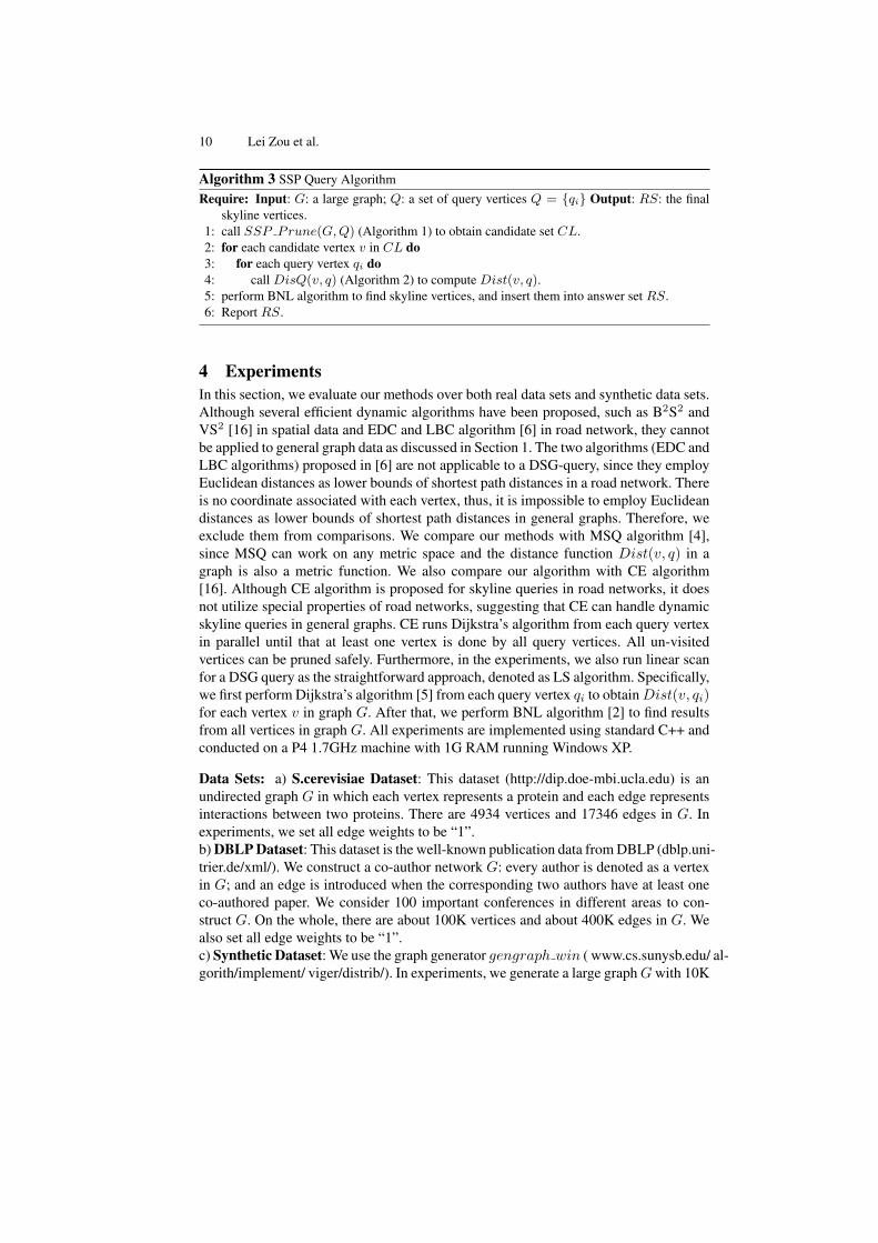
Algorithm 3 SSP Query AlgorithmRequire: Input: G: a large graph; Q: a set of query vertices Q = {qi} Output: RS: the final

skyline vertices.1: call SSP Prune(G, Q) (Algorithm 1) to obtain candidate set CL.2: for each candidate vertex v in CL do3: for each query vertex qi do4: call DisQ(v, q) (Algorithm 2) to compute Dist(v, q).5: perform BNL algorithm to find skyline vertices, and insert them into answer set RS.6: Report RS.

4 ExperimentsIn this section, we evaluate our methods over both real data sets and synthetic data sets.Although several efficient dynamic algorithms have been proposed, such as B2S2 andVS2 [16] in spatial data and EDC and LBC algorithm [6] in road network, they cannotbe applied to general graph data as discussed in Section 1. The two algorithms (EDC andLBC algorithms) proposed in [6] are not applicable to a DSG-query, since they employEuclidean distances as lower bounds of shortest path distances in a road network. Thereis no coordinate associated with each vertex, thus, it is impossible to employ Euclideandistances as lower bounds of shortest path distances in general graphs. Therefore, weexclude them from comparisons. We compare our methods with MSQ algorithm [4],since MSQ can work on any metric space and the distance function Dist(v, q) in agraph is also a metric function. We also compare our algorithm with CE algorithm[16]. Although CE algorithm is proposed for skyline queries in road networks, it doesnot utilize special properties of road networks, suggesting that CE can handle dynamicskyline queries in general graphs. CE runs Dijkstra’s algorithm from each query vertexin parallel until that at least one vertex is done by all query vertices. All un-visitedvertices can be pruned safely. Furthermore, in the experiments, we also run linear scanfor a DSG query as the straightforward approach, denoted as LS algorithm. Specifically,we first perform Dijkstra’s algorithm [5] from each query vertex qi to obtain Dist(v, qi)for each vertex v in graph G. After that, we perform BNL algorithm [2] to find resultsfrom all vertices in graph G. All experiments are implemented using standard C++ andconducted on a P4 1.7GHz machine with 1G RAM running Windows XP.

Data Sets: a) S.cerevisiae Dataset: This dataset (http://dip.doe-mbi.ucla.edu) is anundirected graph G in which each vertex represents a protein and each edge representsinteractions between two proteins. There are 4934 vertices and 17346 edges in G. Inexperiments, we set all edge weights to be “1”.b) DBLP Dataset: This dataset is the well-known publication data from DBLP (dblp.uni-trier.de/xml/). We construct a co-author network G: every author is denoted as a vertexin G; and an edge is introduced when the corresponding two authors have at least oneco-authored paper. We consider 100 important conferences in different areas to con-struct G. On the whole, there are about 100K vertices and about 400K edges in G. Wealso set all edge weights to be “1”.c) Synthetic Dataset: We use the graph generator gengraph win ( www.cs.sunysb.edu/ al-gorith/implement/ viger/distrib/). In experiments, we generate a large graph G with 10K


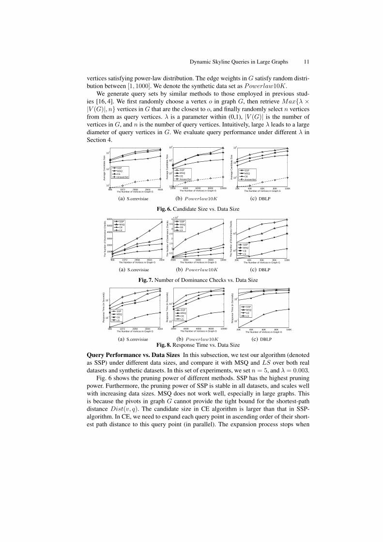
vertices satisfying power-law distribution. The edge weights in G satisfy random distri-bution between [1, 1000]. We denote the synthetic data set as Powerlaw10K.

We generate query sets by similar methods to those employed in previous stud-ies [16, 4]. We first randomly choose a vertex o in graph G, then retrieve Max{λ ×|V (G)|, n} vertices in G that are the closest to o, and finally randomly select n verticesfrom them as query vertices. λ is a parameter within (0,1), |V (G)| is the number ofvertices in G, and n is the number of query vertices. Intuitively, large λ leads to a largediameter of query vertices in G. We evaluate query performance under different λ inSection 4.

986 1972 2958 3944 4934

101

102

103

Ave

rage

Can

dida

te S

ize

The Number of Vertices in Graph G

SSPMSQCEAnswerSet

(a) S.cerevisiae

2000 4000 6000 8000 1000010

1

102

103

104

Ave

rage

Can

dida

te S

ize


SSPMSQCEAnswerSet

(b) Powerlaw10K

20K 40K 60K 80K 100K

102

103

104

Ave

rage

Can

dida

te S

ize


SSPMSQCEAnswerSet

(c) DBLP

Fig. 6. Candidate Size vs. Data Size

986 1972 2958 3944 49340

1000

2000

3000

4000

5000

6000

The

Num

ber

of D

omin

ance

Che

cks


SSPMSQCELS

(a) S.cerevisiae

2000 4000 6000 8000 100000

0.5

1

1.5

2

2.5

3

3.5

4x 10

4

The

Num

ber

of D

omin

ance

Che

cks


SSPMSQCELS

(b) Powerlaw10K

20K 40K 60K 80K 100K

104

105

The

Num

ber

of D

omin

ance

Che

cks


SSPMSQCELS

(c) DBLP

Fig. 7. Number of Dominance Checks vs. Data Size

986 1972 2958 3944 4934

10−2

10−1

Res

pons

e T

ime

(in S

econ

ds)


SSPMSQCELS

(a) S.cerevisiae

2000 4000 6000 8000 10000

10−2

10−1

Res

pons

e T

ime

(in S

econ

ds)


SSPMSQCELS

(b) Powerlaw10K

20K 40K 60K 80K 100K

10−1

100

Res

pons

e T

ime

(in S

econ

ds)


SSPMSQCELS

(c) DBLPFig. 8. Response Time vs. Data Size

Query Performance vs. Data Sizes In this subsection, we test our algorithm (denotedas SSP) under different data sizes, and compare it with MSQ and LS over both realdatasets and synthetic datasets. In this set of experiments, we set n = 5, and λ = 0.003.

Fig. 6 shows the pruning power of different methods. SSP has the highest pruningpower. Furthermore, the pruning power of SSP is stable in all datasets, and scales wellwith increasing data sizes. MSQ does not work well, especially in large graphs. Thisis because the pivots in graph G cannot provide the tight bound for the shortest-pathdistance Dist(v, q). The candidate size in CE algorithm is larger than that in SSP-algorithm. In CE, we need to expand each query point in ascending order of their short-est path distance to this query point (in parallel). The expansion process stops when

12 Lei Zou et al.

there exists at least one vertex that is visited by all query points. Therefore, as men-tioned in [6], CE may result in many candidates and cause unnecessary shortest-pathdistance computation.

Fig. 7 illustrates the number of dominance checks in different methods during DSG-query. With increasing data size, the number of dominance checks also increases in allalgorithms. SSP requires fewer dominance checks than other algorithms by orders ofmagnitude, which again confirms the superior efficiency of SSP.

Fig. 8 shows the total response time in different methods. MSQ, CE and LS all needto perform Dijkstra’s algorithm [5] from each query vertex qi. The time complexityof Dijkstra’s algorithm is O(|V (G)|2). In CE algorithm, we also need to expand eachquery vertex by Dijkstra’s algorithm. The cost of running Dijkstra’s algorithm consti-tutes the major portion of the response time. Figure 6 shows that |CL| is about 1

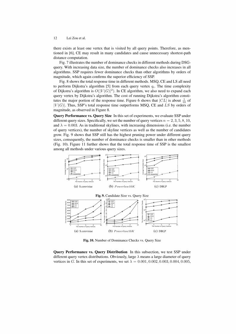
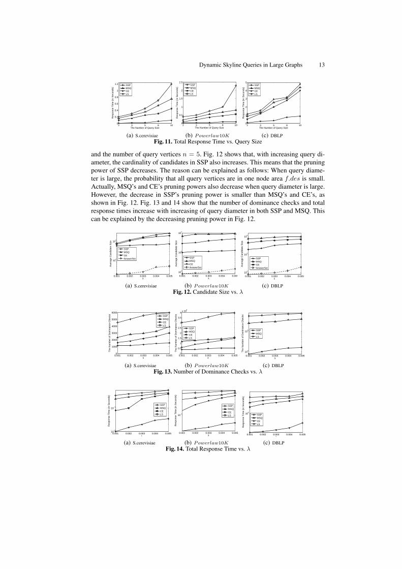
10 of|V (G)|. Thus, SSP’s total response time outperforms MSQ, CE and LS by orders ofmagnitude, as observed in Figure 8.Query Performance vs. Query Size In this set of experiments, we evaluate SSP underdifferent query sizes. Specifically, we set the number of query vertices n = 2, 3, 5, 8, 10,and λ = 0.003. As in traditional skylines, with increasing dimensions (i.e. the numberof query vertices), the number of skyline vertices as well as the number of candidatesgrow. Fig. 9 shows that SSP still has the highest pruning power under different querysizes, consequently, the number of dominance checks is smaller than in other methods(Fig. 10). Figure 11 further shows that the total response time of SSP is the smallestamong all methods under various query sizes.

2 3 5 8 1010

1

102

103

Ave

rage

Can

dida

te S

ize

The Numer of Query Vertices

SSPMSQCEAnswerSet

(a) S.cerevisiae

2 3 5 8 10

102

103

104

Ave

rage

Can

dida

te S

ize

The Number of Query Vertices

SSPMSQCEAnswerSet

(b) Powerlaw10K

2 3 5 8 10

102

103

104

Ave

rage

Can

dida

te S

ize


SSPMSQCEAnswerSet

(c) DBLP

Fig. 9. Candidate Size vs. Query Size

2 3 5 8 100

1000

2000

3000

4000

5000

6000

7000

8000

9000

The

Num

ber

of D

omin

ance

Che

cks


SSPMSQCELS

(a) S.cerevisiae

2 3 5 8 100

1

2

3

4

5

6

7x 10

4

The

Num

ber

of D

omin

ance

Che

cks


SSPMSQCELS

(b) Powerlaw10K

2 3 5 8 10

104

105

106

The

Num

ber

of D

omin

ance

Che

cks


SSPMSQCELS

(c) DBLP

Fig. 10. Number of Dominance Checks vs. Query Size

Query Performance vs. Query Distribution In this subsection, we test SSP underdifferent query vertex distributions. Obviously, large λ means a large diameter of queryvertices in G. In this set of experiments, we set λ = 0.001, 0.002, 0.003, 0.004, 0.005,


2 3 5 8 100

0.2

0.4

0.6

0.8

1

1.2

Res

pons

e T

ime

(in S

econ

ds)

The Number of Query Size

SSPMSQCELS

(a) S.cerevisiae

2 3 5 8 100

0.5

1

1.5

2

2.5

Res

pons

e T

ime

(in S

econ

ds)


SSPMSQCELS

(b) Powerlaw10K

2 3 5 8 100

1

2

3

4

5

Res

pons

e T

ime

(in S

econ

ds)


SSPMSQCELS

(c) DBLPFig. 11. Total Response Time vs. Query Size

and the number of query vertices n = 5. Fig. 12 shows that, with increasing query di-ameter, the cardinality of candidates in SSP also increases. This means that the pruningpower of SSP decreases. The reason can be explained as follows: When query diame-ter is large, the probability that all query vertices are in one node area f.des is small.Actually, MSQ’s and CE’s pruning powers also decrease when query diameter is large.However, the decrease in SSP’s pruning power is smaller than MSQ’s and CE’s, asshown in Fig. 12. Fig. 13 and 14 show that the number of dominance checks and totalresponse times increase with increasing of query diameter in both SSP and MSQ. Thiscan be explained by the decreasing pruning power in Fig. 12.

0.001 0.002 0.003 0.004 0.005

102

103

Ave

rage

Can

dida

te S

ize

λ

SSPMSQCEAnswerSet

(a) S.cerevisiae

0.001 0.002 0.003 0.004 0.005

102

103

104

Ave

rage

Can

dida

te S

ize

λ

SSPMSQCEAnswerSet

(b) Powerlaw10K

0.001 0.002 0.003 0.004 0.005

102

103

104

Ave

rage

Can

dida

te S

ize

λ

SSPMSQCEAnswerSet

(c) DBLPFig. 12. Candidate Size vs. λ

0.001 0.002 0.003 0.004 0.0050

1000

2000

3000

4000

5000

6000

The

Num

ber

of D

omin

ance

Che

cks

λ

SSPMSQCELS

(a) S.cerevisiae

0.001 0.002 0.003 0.004 0.0050

0.5

1

1.5

2

2.5

3

3.5

4x 10

4

The

Num

ber

of D

omin

ance

Che

cks

λ

SSPMSQCELS

(b) Powerlaw10K

0.001 0.002 0.003 0.004 0.005

104

105

The

Num

ber

of D

omin

ance

Che

cks

λ

SSPMSQLS

(c) DBLPFig. 13. Number of Dominance Checks vs. λ

0.001 0.002 0.003 0.004 0.00510

−2

10−1

Res

pons

e T

ime

(in S

econ

ds)

λ

SSPMSQCELS

(a) S.cerevisiae

0.001 0.002 0.003 0.004 0.005

10−1

Res

pons

e T

ime

(in S

econ

ds)

λ

SSPMSQCELS

(b) Powerlaw10K

0.001 0.002 0.003 0.004 0.005

100

Res

pons

e T

ime

(in S

econ

ds)

λ

SSPMSQCELS

(c) DBLPFig. 14. Total Response Time vs. λ

14 Lei Zou et al.

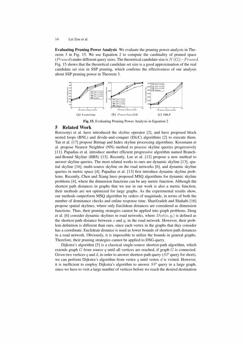
Evaluating Pruning Power Analysis We evaluate the pruning power analysis in The-orem 3 in Fig. 15. We use Equation 2 to compute the cardinality of pruned space(Pruned) under different query sizes. The theoretical candidate size is |V (G)|−Pruned.Fig. 15 shows that the theoretical candidate set size is a good approximation of the realcandidate set size in SSP pruning, which confirms the effectiveness of our analysisabout SSP pruning power in Theorem 3.

2 3 5 8 100

100

200

300

400

500

600

700

800

900

Ave

rage

Can

dida

te S

ize


SSP−λ=0.003SSP−λ=0.001SSP−λ=0.005Analysis

(a) S.cerevisiae

2 3 5 8 100

500

1000

1500

Ave

rage

Can

dida

te S

ize



(b) Powerlaw10K

2 3 5 8 100

1000

2000

3000

4000

5000

6000

7000

Ave

rage

Can

dida

te S

ize



(c) DBLP

Fig. 15. Evaluating Pruning Power Analysis in Equation 2

5 Related WorkBorzsonyi et al. have introduced the skyline operator [2], and have proposed blocknested loops (BNL) and divide-and-conquer (D&C) algorithms [2] to execute them.Tan et al. [17] propose Bitmap and Index skyline processing algorithms. Kossmann etal. propose Nearest Neighbor (NN) method to process skyline queries progressively[11]. Papadias et al. introduce another efficient progressive algorithm named Branch-and-Bound Skyline (BBS) [13]. Recently, Lee et al. [12] propose a new method toanswer skyline queries. The most related works to ours are dynamic skyline [13], spa-tial skyline [16], multi-source skyline on the road networks [6], and dynamic skylinequeries in metric space [4]. Papadias et al. [13] first introduce dynamic skyline prob-lems. Recently, Chen and Xiang have proposed MSQ algorithms for dynamic skylineproblems [4], where the dimension functions can be any metric function. Although theshortest path distances in graphs that we use in our work is also a metric function,their methods are not optimized for large graphs. As the experimental results show,our methods outperform MSQ algorithm by orders of magnitude, in terms of both thenumber of dominance checks and online response time. Sharifzadeh and Shahabi [16]propose spatial skylines, where only Euclidean distances are considered as dimensionfunctions. Thus, their pruning strategies cannot be applied into graph problems. Denget al. [6] consider dynamic skylines in road networks, where Dist(o, qi) is defined asthe shortest-path distance between o and qi in the road network. However, their prob-lem definition is different than ours, since each vertex in the graphs that they considerhas a coordinate. Euclidean distance is used as lower bounds of shortest-path distancesin a road network. Obviously, it is impossible to utilize the bounds in general graphs.Therefore, their pruning strategies cannot be applied to DSG-query.

Dijkstra’s algorithm [5] is a classical single-source shortest-path algorithm, whichextends graph G from source q until all vertices are reached, if graph G is connected.Given two vertices q and d, in order to answer shortest-path query (SP query for short),we can perform Dijkstra’s algorithm from vertex q until vertex d is visited. However,it is inefficient to employ Dijkstra’s algorithm to answer SP query in a large graph,since we have to visit a large number of vertices before we reach the desired destination


vertex d. Therefore, materialization techniques should be applied to speed up onlinequery. Lim and Chan [3] propose DiskSP algorithm to answer SP queries. Based ongraph partitions, they propose super-graph. Jing et al in [9] propose Hierarchical En-coding Path View (HEPV) for SP query. Another hierarchical graph model called HiTiis proposed by Jung and Pramanik [10]. Actually, any efficient SP -query algorithm canbe utilized in the refinement process of DSG-query, which is orthogonal to our prun-ing strategies. There are a lot of work on spatial networks [15, 14]. Generally speak-ing, these methods always utilize some spatial properties for processing. For example,Samet et al. [15] propose a best-first algorithm to find the k nearest neighbors in a spatialnetwork. Data objects are indexed by quadtrees, which is a spatial indexing structure.For general graph problems, it is impossible to employ these spatial properties, such asspatial indexing, spatial coherence, Voronoi Diagrams and Euclidean distances, sincevertices in general graphs have no coordinate. The main contributions of our work arethat we only employ graph properties to develop pruning rules and process DSG-query.

Ranked keyword search queries on a graph (such as BLINKS and BANKS algo-rithm [8, 1]) need to retrieve the top-k answers according to some ranking criteria, whereeach answer is a substructure of the graph containing all query keywords. However,these algorithms adopt “expanding” strategy. As shown in experiments, the “expand-ing” strategy is quite expensive in our problem.

6 ConclusionsIn this paper, we propose dynamic skyline queries in graphs (DSG-query for short).For DSG-query, we propose a novel pruning strategy, that is shared shortest path (SSP)pruning. Based on SSP Pruning, we build careful-designed indexing structures. Exten-sive experiments confirm the effectiveness of our methods.References

1. G. Bhalotia, et al. Keyword searching and browsing in databases using banks. In ICDE,2002.

2. S. Borzsonyi, et al. The skyline operator. In ICDE, 2001.3. E. P. F. Chan and H. Lim. Optimization and evaluation of shortest path queries. VLDB J.,

16(3), 2007.4. L. Chen and X. Lian. Dynamic skyline queries in metric spaces. In EDBT, 2008.5. T. H. Cormen, et al. Introduction to algorithms. The MIT Press, 2001.6. K. Deng, et al. Multi-source skyline query processing in road networks. In ICDE, 2007.7. D. Fuhry, et al. Efficient skyline computation in metric space. In TR-KSU-CS-2008-02,

Department of Computer Science Kent State University, 2008.8. H. He, et al. Blinks: ranked keyword searches on graphs. In SIGMOD, 2007.9. N. Jing, et al. Hierarchical encoded path views for path query processing: An optimal model

and its performance evaluation. IEEE Trans. Knowl. Data Eng., 10(3), 1998.10. S. Jung and S. Pramanik. An efficient path computation model for hierarchically structured

topographical road maps. IEEE Trans. Knowl. Data Eng., 14(5), 2002.11. D. Kossmann, et al. Shooting stars in the sky: An online algorithm for skyline queries. In

VLDB, 2002.12. K. C. K. Lee, et al. Approaching the skyline in z order. In VLDB, 2007.13. D. Papadias, et al. An optimal and progressive algorithm for skyline queries. In SIGMOD,

2003.14. D. Papadias, et al. Query processing in spatial network databases. In VLDB, 2003.15. H. Samet and J. S. H. Alborzi. Scalable network distance browsing in spatial databases. In

SIGMOD, 2008.16. M. Sharifzadeh and C. Shahabi. The spatial skyline queries. In VLDB, 2006.17. K.-L. Tan, et al. Efficient progressive skyline computation. In VLDB, 2001.18. H. Tong and C. Faloutsos. Center-piece subgraphs: Problem definition and fast solutions. In

SIGKDD, 2006.

Dynamic Skyline Queries in Large Graphs - …tozsu/publications/other/zlDASFAA10.pdf · Dynamic...

Documents

Transcript of Dynamic Skyline Queries in Large Graphs - …tozsu/publications/other/zlDASFAA10.pdf · Dynamic...