Dynamic simulation of ac/dc systems with reference to ...
131
DYNAMIC SIMULATION OF AC/DC SYSTEMS WITH REFERENCE TO CONVERTOR CONTROL AND UNIT CONNECTION A thesis presented for the degree of Doctor of Philosophy in Electrical Engineering in the University of Canterbury, New Zealand by S. Sankar, B.E., M.Tech ::;-" 1991
Transcript of Dynamic simulation of ac/dc systems with reference to ...

DYNAMIC SIMULATION OF AC/DC SYSTEMS
WITH REFERENCE TO
CONVERTOR CONTROL AND UNIT CONNECTION
A thesis
presented for the degree of
Doctor of Philosophy in Electrical Engineering
in the
University of Canterbury,
New Zealand
by
S. Sankar, B.E., M.Tech ::;-"
1991

il:NGINEERING LI[~flARY
11
Abstract
This thesis investigates the limitations of conventional steady state formu
lation when applied to the unit connected generator-HV dc convertor systems and
justifies the need for dynamic simulation.
The merits of available dynamic simulation algorithms, namely the state
variable and EMTP techniques are discussed with reference to generator-convertor
modelling. The state variable is selected and an existing algorithm (TCS) is improved
to permit flexible controller modelling. The TCS algorithm is verified by comparison
with another dynamic simulation program, EMTDC, which is based on EMTP algo
rithm. Both TCS and EMTDC are shown capable of predicting the same dynamic
performance following disturbances.
The limitations of steady state formulation for unit connected HV dc systems
are demonstrated with the help of TCS and it is shown that the characteristics must
be derived using a dynamic simulation program.
Comparative operational capability charts are developed using TCS for con
ventional and unit connected HV dc schemes, showing the limitations of the latter to
provide temporary overloads. Harmonic current and voltage ratings spectra for the
region of operational capability of the unit connection are also derived.
The operating characteristics and harmonic problems of variable speed unit
connected generator-HV dc convertor systems are later analysed. With reference to a
typical hydro electric test system, it is shown that it is possible to operate the turbine
generator units within a wide range of frequencies at high efficiencies and with good
voltage controllability.

111
Contents
List of Figures .
VI
List of Tables VIU
List of Principal Symbols
Acknowledgements
Publications Associated With This Thesis
1 INTRODUCTION 1.1 Background ............ . 1.2 The Unit Connected HV dc System 1.3 Modelling . . . . . . . . . .
1.3.1 Dynamic Simulation 1.4 Thesis Outline ....... .
2 INCORPORATION OF HVDC CONTROLLER DYNAMICS IN TCS 2.1 Introduction ........ . 2.2 HV dc Controllers Hierarchy 2.3 Convertor Control ..... . 2.4 Modular Approach to HV dc Controls 2.5 Combined Power and Control TCS Solution 2.6 Illustrative Test Cases
2.6.1 Test Case - 1 '" 2.6.2 Test Case - 2 ... 2.6.3 General Discussion
2.7 Conclusion ........ .
3 A COMPARISON OF SIMULATION ALGORITHMS 3.1 Introduction .................. . 3.2 Criterion for Comparison ........... . 3.3 Algorithmic Differences of TCS and EMTDC . 3.4 Test System .................. .
IX
Xl
XU
1 1 2 5 6 8
9 9
10 11 13 16 18 18 23 27 28
29 29 29 31 32

3.5 Steady State Initialisation 3.6 Disturbance Simulation ..
3.6.1 Symmetrical Fault 3.6.2 Asymmetrical Faults
3.7 Algorithmic Efficiencies. 3.8 Conclusion ......... .
4 DYNAMIC SIMULATION OF GENERATOR-HVDC TOR UNITS 4.1 Introduction .......... . 4.2 Per-Unit System ....... . 4.3 Validation of Generator Model. 4.4 Initialisation of Unit Connection Simulation 4.5 Notch Removal for Firing Angle Measurement 4.6 Calculation of Steady State Quantities 4.7 Conclusion ................... .
CONVER-
IV
33 34 34 36 39 41
42 42 43 44 45 50 50 52
5 ANALYSIS OF THE COMMUTATION PROCESS IN A GENERATOR-HVDC CONVERTOR UNIT 53 5.1 Introduction.................. 53 5.2 Factors Affecting the Commutation Process 55 5.3 Modelling of the Commutation Process . . . 56 5.4 Limitation of Commutation Reactance . . . 58 5.5 Inapplicability of Conventional Formulation 59
5.5.1 Unit Connection with Rotor Symmetry 60 5.5.2 Unit Connection with Rotor Saliency. 62
5.6 Simplified Machine - HVdc Convertor Simulation 63 5.7 Comparison of Results 66 5.8 Conclusion...................... 67
6 OPERATIONAL CAPABILITY OF UNIT CONNECTIONS 69 6.1 Introduction.............. 69 6.2 Control Philosophy and Test System . . . . . 70 6.3 Capability Charts. . . . . . . . . . . . . . . . 72 6.4 Designing with Higher Nominal Firing Angle. 74 6.5 Effect of Field Forcing 76 6.6 Current Harmonics . . 77 6.7 Generator Rating . . . 78 6.8 AC Voltage Harmonics 80 6.9 DC Harmonics .' . 81 6.10 Conclusion. . . . . . . . 82
7 CHARACTERISTICS OF VARIABLE SPEED OPERATION OF UNIT CONNECTIONS 84 7.1 Introduction.................... 84 7.2 Variable Speed Operation of Hydraulic Turbines 85

7.3 7.4 7.S 7.6
7.7
Test System . . . . . . . . . . . . . . Operating Characteristics ..... . Evaluation of the Need for an OLTC Harmonic Effects . . . . . . . . . . . 7.6.1 Reduction of the Effective Pulse Number 7.6.2 Interaction Between Terminals. Conclusion . .
8 CONCLUSIONS
References
A TCS Controller Modules
B Test System Data for TCS and EMTDC Comparison B.1 AC System B.2 AC Filters B.3 DC Filters . B.4 DC Line .. B.S bC Convertor
B.S.1 Rectifier B.S.2 Invertor
B.6 Controllers. . . B.6.1 Current Control. B.6.2 Extinction Angle Control. B.6.3 Transducer Delays
C TCS Controller Data File
D Transformations: d,q,O to a,b,c
E Unit Connected Test System Data E.1 Non-Salient Machine E.2 Salient Machine . E.3 DC System .....
E.3.1 Convertor .. E.3.2 Convertor Transformer
v
86 87 91 91 92 92 93
94
98
105
108 108 109 110 110 110 110 111 111 111 111 112
113
116
118 118 119 119 119 119

VI
List of Figures
1.1 HV dc rectifier station- conventional arrangement. . . 2 1.2 HV dc rectifier station- unit connected arrangement . 2 1.3 HV dc rectifier station- group connected arrangement 5
2.1 Phase locked oscillator reference. . . . . . . . . . . 12 2.2 Example of controller corresponding with Table 2.2 15 2.3 TCS flowchart. . . . . . . . . . . . . . . . . . . . . 17 2.4 HVdc test system .. . . . . . . . . . . . . . . . . . 18 2.5 Controller dynamics-I: (a)Rectifier current controller (b)Invertor ex-
tinction angle controller ............ . . . . . . . . . . . .. 19 2.6 Controller dynamics-2: (a)Rectifier current controller (b)Invertor ex-
tinction angle controller ............... . . . . .. . . .. 19 2.7 Invertor ac voltages and dc current waveforms for a single-phase to
ground fault . . . . . . . . . . . . . . . . . . . . . . . . . . . . . . .. 21 2.8 Invertor valve conduction patterns for a single-phase to ground fault.
(a) Control dynamics-l (b) Control dynamics-2 ............ 22 2.9 Controller blocks of Test case - 2 .................... 23 2.10 Rectifier dc current obtained from integrated TCS and stability program 24 2.11 Rectifier and invertor powers from (a) stability program (b) integrated
TCS and stability program. . . . . . . . . . . . . . . . . . . . . . .. 25 2.12 Rectifier and invertor terminal ac voltages from (a) stability program
(b) integrated TCS and stability program. 26
3.1 Test system for the comparison .. . . . . 32 3.2 Test system controllers . . . . . . . . . . . 33 3.3 Three phase fault at the invertor end (a)(b) dc current, (c)(d) ac volt-
ages, (e )(f) valves conduction . . . . . . . . . . . . . . . . .. 35 3.4 Line-to-Ground fault at the invertor end (a)(b) valves conduction,
(c)(d) dc current, (e) (f) ac voltages. . . . . . . . . . . . . . . . . .. 37 3.5 Line-Line fault at the invertor end (a)(b) dc current, (c)(d) ac voltages,
(e)(f) valves conduction ......................... 38 3.6 Comparison of valve conduction pattern (L-L fault) ( a) EMTDC with-
out system subdivision, (b) TCS, (c) EMTDC with system subdivision 40

Vll
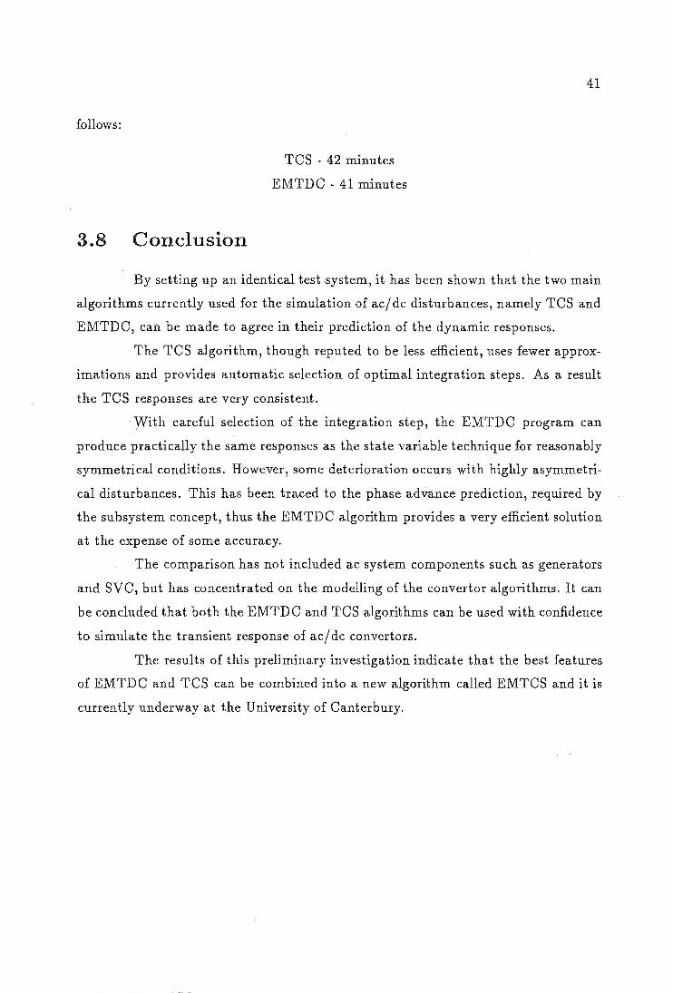
4.1 Short circuit test waveforms of the salient machine (a) terminal volt-ages (b) stator currents. . . . . . . . . . . . . . . . . . . . . . . . .. 46
4.2 Short circuit test waveforms of the non-salient machine (a) terminal voltages (b) stator currents. . . . . . . . . . . . . . . . . . . . . . .. 47
4.3 Generator rotor currents and dc current derived from dynamic simulation 48 4.4 Generator terminal voltages (two phases) derived from dynamic simu-
lation. . . . . . . . . . . . . . . . . . . . . . . . . . . . . . 49 4.5 Generator phase currents derived from dynamic simulation 49
5.1 Twelve pulse unit connected generator-HV dc convertor . . 59 5.2 Generator currents derived from TCS for a=O and Ide = 1. 0 pu 61 5.3 Generator terminal voltages derived from TCS for a=O and Ide = 1. 0 pu 62 5.4 Phasor diagram of a salient pole machine. . . . . 64 5.5 A typical dc current waveform derived from TCS 68
6.1 Twelve pulse unit connected generator-HV dc convertor 71 6.2 Operational capability charts with amin (i) Conventional (ii) Unit con-
nection . . . . . . . . . . . . . . . . . . . . . . . . . . . . . . . . . .. 72 6.3 Variation of commutation angle obtained from TCS . . . . . . . . .. 74 6.4 Operational capability charts with a,,01ll=20 deg. (i) Conventional (ii)
Unit connection. . . . . . . . . . . . . . . . . . . . . . . . . . . 75 6.5 Operational capability charts with control margin (i) a nom =20 deg.
(ii) amin ~5 deg. . . . . . . . . . . . . . . . . . . . . . . . 76 6.6 Current harmonic content of the 12-pulse convertor . . . 78 6.7 Equivalent Negative Sequence current derived from TCS 79 6.8 Effect of rotor saliency on voltage harmonic distortion. 80 6.9 DC voltage harmonics derived from TCS . . . 82
7.1 Power-frequency characteristics of the turbine 86 7.2 DC side waveforms derived from TCS (a) voltage (b) current 88 7.3 Variable frequency operating characteristic at 100% turbine efficiency 89 7.4 Variable frequency operating characteristic at 96% turbine efficiency. 90

VIll
List of Tables
2.1 Control system - TCS interface variables 14 2.2 Sample control data file ......... 15
4.1 Variation of dc component in the stator current 51
5.1 Variation of commutation parameters ofthe non-salient rotor generator with dc current (a=O) ................ . . . . . . . . .. 61
5.2 Variation of commu.tation parameters for the non-salient rotor gener-ator with firing angle (Idc=l.O pu) . . . . . . . . . . . . . . . . . . .. 61
5.3 Variation of commutation parameters for the salient-rotor generator with firing angle (Idc=l.O pu) .. . . . . . . . . . . . . . . . . . . .. 63
5.4 Commutation angle in degrees from TCS and simplified models for non-salient machine. . . . . . . . . . . . . . . . . . . . . . . . . . .. 66
5.5 Commutation angle in degrees from TCS and simplified models for non-salient machine. . . . . . . . . . . . . . . . . . . . . . . . . . .. 67
5.6 Commutation angle in degrees from TCS and simplified models for salient machine . . . . . . . . . . . . . . . . . . . . . . . 67
6.1 Relationship between dc current setting and power levels 73 6.2 Extra Excitation requirement to increase the capability 77
7.1 Turbine Power/Speed Characteristics . . . 87 7.2 Effect of firing angle control on generator . 90
B.1 AC System data. . . . . . 108 B.2 Sending end tuned filters . 109 B.3 Receiving end tuned filters 109 B.4 High-pass filters 109 B.5 DC filters . . . . . . . . . 110

lX
List of Principal Symbols
e machine open circuit voltage (instantaneous)
E - machine open circuit voltage (rms)
Ee - commutating voltage
f - frequency
in - nominal frequency
G conductance matrix
h - harmonic order
1 instantaneous current
I - current vector
Id - direct axis current
Ide - dc current
- negative sequenc~ equivalent current
Ig machine stator current
1h - hth harmonic current
1q - quadrature axis current
Lg generator inductance matrix
Lrr - rotor-rotor sub-matrix of Lg
Lrs - rotor-stator sub-matrix of Lg
LST - stator-rotor sub-matrix of Lg
Lss - stator-stator sub-matrix of Lg
N - machine speed
Pdc - dc power
Rg - machine resistance vector
t - time
u - commutation angle
U - control variable vector
V - voltage vector
lIdc - dc voltage
1II. - hth harmonic voltage
lit - terminal voltage
X - state variable vector
Xc - commutation reactance
x
Xd - direct axis reactance
Xi - quadrature component of commutation reactance
Xq - quadrature axis reactance
X t - transformer reactance
Xr - real component of commutation reactance
X" - machine sub-transient reactance
X~ - direct axis sub-transient reactance
X~ - quadrature axis sub-transient reactance
Y - output variable vector
Z - dependent variable vector
o - convertor firing angle
Omin - minimum firing angle
Omax - maximum firing angle
Oord firing angle order
Ore! firing angle reference
I - invertor extinction angle
Ilow lowest extinction angle
Ire! - extinction angle reference
8; - angle between generator stator current and internal emf
t::. t time step
()o - switching instant
€ synchronising error
¢ - power factor angle

Xl
Acknowledgements
I would like to thank my supervisor Prof. Jos Arrillaga., for his advice,
assistance, friendship and patience during the course of this work. Also, my sincere
thanks are due to Dr. Chris Arnold and Dr. Neville Watson for their valuable
suggestions and help.
The financial support of Transpower New Zealand Ltd. IS gratefully ac
knowledged.
I would also like to thank Dr.C.Callaghan, Dr.N.Pahlawaththa and my other
postgraduate colleagues G.Anderson, J .R.Camacho, J .de Souza, A.Medina, A.Miller,
M.Villablanca, A.Wood and M.Zavahir for their helpful suggestions and friendship.
Also) the encouragement and help given by my friend Dr .K.S. Chandrasekhar is greatly
acknowledged.
Finally thanks are due to my family and friends for their support and un
derstanding.

Xll
Publications Associated With This Thesis
The following publications are associated with research presented in this thesis.
Sankar,S., Arrillaga,J., Arnold,C.P and Watson,N.R.,"Inclusion of HVDC controller
dynamics in transient convertor simulation", Transactions of IPENZ, Vol 16,
2/EMCh, Nov. 1989, pp 25-30.
Arrillaga,J., Sankar,S., Watson,N.R., and Arnold,C.P.,"Operational capability of
generator-HVDC convertor units", presented at the 1991 IEEE PES Winter
Meeting, New York.
Arrillaga,J., Sankar,S., Watson,N.R., and Arnold,C.P.,"A comparison of transient
simulation algorithms", accepted for the 5th lEE International conf. on ac/ dc
systems, London, to be held in Sept. 1991.
The following paper has also been submitted for publication, but has yet to
be officially accepted (as of 28 February, 1991).
Arrillaga,J., Sankar,S., Arnold,C.P. and Watson,N.R.,"Characteristics of unit con
nected generator-HVDC convertors operating at variable speeds", submitted for
1991 IEEE PES Summer Meeting.

1
Chapter 1
INTRODUCTION
1.1 Background
.The modern HVdc technology which started with a simple 2-terminal dc link
between Gotland and Mainland Sweden in 1954, has developed to a stage now where
a 5-terminal dc system is a commercially viable possibility [IEEE 1990]. During this
period, the dc power transfer capacity has increased from a mere 20 MW to 6000
MW. The reason for this rapid growth can be mainly attributed to the availability
of cheaper high voltage, high power semi-conductor thyristors and the increasing
confidence on the reliability of dc systems. In some of the projects, HV dc was the
only option available to the system planners (e.g., Sakuma frequency convertor and
New Zealand scheme). The present need of energy requires increase exploitation
of renewable energy resources such as hydro-energy source located far away from
load centres. At present, HVdc transmission is a recognised methodology for such
applications.
In conventional HV dc design, the generators from isolated power plant are
allocated to a common ac bus which feed all the convertors. Also the filters are con
nected at the convertor terminal. When the generated power is supplied exclusively to
the HV dc transmission link, such as in an isolated power station, the unit connection
of individual generators to HV dc convertors proposed as early as 1973 [Calverley] is
an attractive alternative. The importance of HV dc system unit connection is realised
to the extent that CIGRE has formed a separate working group to study various
aspects of such systems [CIGRE 1988].

2
AUX.
Figure 1.1: HV dc rectifier station- conventional arrangement
AUK.
Figure 1.2: HV dc rectifier station- unit connected arrangement
1.2 The Unit Connected HVdc System
Figures 1.1 and 1.2 show the essential elements of a conventional scheme and
unit connected scheme respectively. In the unit connected scheme, the generators are
connected directly to the convertor transformers and the paralleling (or the series
parallel combination) of units is done at the dc side.

3
Advantages
The unit connected HVdc scheme has several advantages over the conven
tional scheme and they are summarized as follows:
• Each generator operates individually and so there is no synchronisation or sta
bility problem among them.
• Elimination of ac harmonic filters result in the reduction of station cost and
space and also eliminates the potential resonance and self-excitation problems.
• Only a single unit transformer is needed in place of generator and convertor
transformers.
• Possible elimination of On-Load Tap-Changers on transformers.
• There is no need of an ac busbar system and also the layout eliminates one level
of breakers.
• The unit connected HV dc station would possibly result in a compact and light
design due to the absence of high-voltage ac switchyard and filters, separate
convertor buildings and associated services and several ac collector lines between
the power house and the switchyard.
The Manitoba HVdc Research Centre, Canada undertook a study [Ingram
1988] of the economic benefits of the unit connected concept, taking advantage of
known costs from the Limestone generating station on the Nelson River. The conclu
sion of this study are that for a 1250 MW hydro plant with dimensions and ratings
similar to Manitoba Hydro's Limestone station, a directly connected HV dc thyristor
convertor would realise savings in the order of $M75 Cdn (in 1987 dollars) compared
to a conventional design with separate convertor station.
Disadvantages
The unit connected schemes would have the following limitations:
• The generator must absorb the entire harmonics produced by the individual
convertor units. Their major effect upon the generator is extra heating of the
4
rotor surface and the damper winding due to the induced harmonic currents in
the rotor circuit.
• In the event that generators are operated at frequencies other than power fre
quency, a separate source of power for station auxiliaries must be arranged.
• A convertor unit outage would prevent the delivery of power from that unit
generator and also would decrease the transmission voltage.
Applications
The potential application of unit-connected HV dc schemes are those cases
where the whole output of the generating station can be transmitted via HVdc. Ap
plications where this is possible could be:
• transfer of large power from very remote hydro generating stations to the load
centres
• connection of large power stations into existing complex ac systems (such as
Mine-Mouth application)
• interconnection of off-shore power station into existing ac networks
• variable frequency operation such as pump-storage schemes
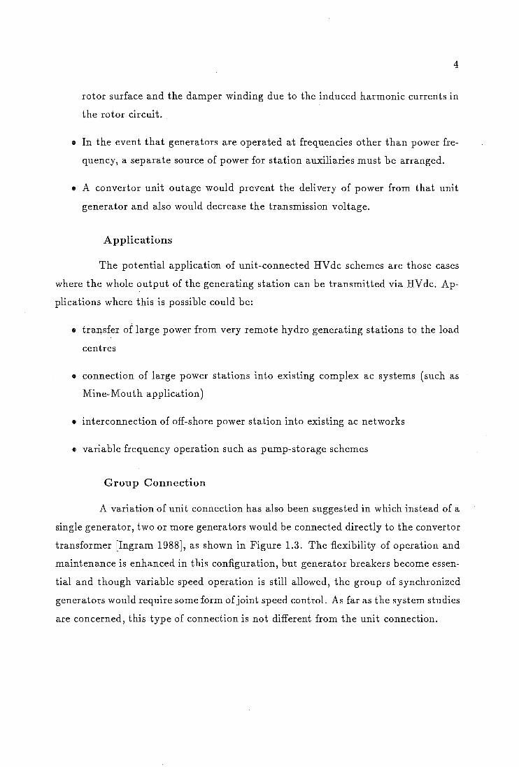
Group Connection
A variation of unit connection has also been suggested in which instead of a
single generator, two or more generators would be connected directly to the convertor
transformer [Ingram 1988], as shown in Figure 1.3. The flexibility of operation and
maintenance is enhanced in this configuration, but generator breakers become essen
tial and though variable speed operation is still allowed, the group of synchronized
generators would require some form of joint speed control. As far as the system studies
are concerned, this type of connection is not different from the unit connection.
5
AUII.
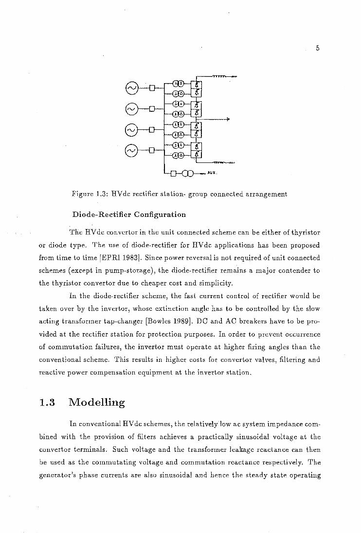
Figure 1.3: HV dc rectifier station- group connected arrangement
Diode-Rectifier Configuration
The HV dc convertor in the unit connected scheme can be either of thyristor
or diode type. The use of diode-rectifier for HV dc applications has been proposed
from time to time [EPRI 1983]. Since power reversal is not required of unit connected
schemes (except in pump-storage), the diode-rectifier remains a major contender to
the thyristor convertor due to cheaper cost and simplicity.
In the diode-rectifier scheme, the fast current control of rectifier would be
taken over by the invertor, whose extinction angle has to be controlled by the slow
acting transformer tap-changer [Bowles 1989]. DC and AC breakers have to be pro
vided at the rectifier station for protection purposes. In order to prevent occurrence
of commutation failures, the invertor must operate at higher firing angles than the
conventional scheme. This results in higher costs for convertor valves, filtering and
reactive power compensation equipment at the invertor station.
1.3 Modelling
In conventional HV dc schemes, the relativelylow ac system impedance com
bined with the provision of filters achieves a practically sinusoidal voltage at the
convertor terminals. Such voltage and the transformer leakage reactance can then
be used as the commutating voltage and commutation reactance respectively. The
generator's phase currents are also sinusoidal and hence the steady state operating

6
conditions can be derived using conventional single-frequency phasor theory.
A t present, the operating characteristics of unit connection are also discussed
with reference to the conventional steady state formulation [Krishnayya 1973, Hausler
1980, Campos Barros 1989].
However, in the absence of harmonic filters, the use of such formulation must
be reconsidered. Each and every convertor commutation process represents a line-to
line short circuit across the generator terminal and hence the commutation reactance
must include the generator sub-transient reactance as well as transformer leakage.
The convertor terminal voltage is not sinusoidal and so the generator internal emf
must be used as the commutating voltage.
Moreover, rotor saliency causes non-linear harmonic interaction between the
generator and the convertor which affects the output voltage of the unit connection
and this effect can not be analysed using single frequency steady state formulation.
Therefore the main objective of this work is to show the need for dynamic
simulation in unit connection studies.
1.3.1 Dynamic Simulation
Dynamic simulation programs have already been used to establish the con
trollability of the unit connection during disturbances [Campos Barros 1977, Hun
gasutra 1989, Rangel 1989]. In this work, dynamic simulation is used to assess the
applicability of the steady state formulation and derive the operating characteristics
of the unit connected HVdc convertor.
Two basically different approaches are currently used in HV dc dynamic sim
ulation, i.e the Electromagnetic Transient Program (EMTP) and the state variable
technique. The EMTP type programs use constant step length, whereas the step
length can be altered in state variable algorithms.
The equivalent circuit of a generator-HV dc convertor system contain time
varying parameters which require modification of the system impedance matrix from
step to step in the dynamic simulation. Also the voltage crossings, firing instants
and commutation intervals can not be predicted and hence the integration steps need
to be adjusted accordingly. Such requirements and the relatively small number of
components involved make the state variable algorithm ideally suited to the dynamic
simulation of unit connected schemes.

7
A dynamic simulation program, TCS, developed at the University of Can
terbury, NZ is used for this work. Transient Convertor Simulation (TCS) is a program
specifically developed to analyse the dynamic behaviour HV dc systems and is formu
lated in terms of state space theory [Arrillaga 1983b].
The basic algorithm of TCS was established at the University of Manchester
Institute of Science and Technology [AI-Khashali 1976, Campos Barros 1976]. Further
work on TCS continued at the University of Canterbury by progressively improving
the accuracy of the results by developing better models for the various power system
components.
In ac/ dc dynamic simulation programs, normally ac systems are represented
as equivalents. The means of representing ac system as time varying equivalents was
developed by Heffernan[1981] and Turner[198l]. Based on the recent advancements
[Reeve 1988] on these models, further work on this topic is currently underway at the
University of Canterbury; NZ.
Following HVdc disturbances, the convertor transformers may be subjected
to overexcitation, dc magnetisation and in-rush effects, all of which must be accurately
represented in dynamic simulation studies. Practical ways of modelling the magnetic
history of the convertor transformer in TCS were developed by Joosten [1989].
The frequency response of power system components affects the transient
response due to the multitude of frequencies present in transient waveforms. Given
the size and complexity of a power system, it is not practical to model each of its
components individually. Watson [1987] developed methods of obtaining a practical
and computationally efficient equivalent circuit for TCS that accurately represents
the frequency dependence of the actual system being represented.
During all these developments, TCS contained in-built basic controllers i.e.,
current and extinction angle controllers based on the direct digital control technique
[Arrillaga 1970]. The representation of any other controllers other than basic con
trollers required expert understanding of the program in order to introduce appro
priate modifications. Hence the starting point of this investigation was to implement
a more realistic and flexible controller models in TCS which would make TCS more
powerful in analysing ac/ dc systems.

8
1.4 Thesis Outline
Chapter 2 describes the modelling of realistic and flexible HV dc controller
models in TCS and also the importance of such models.
As in any other model simulations, in order to establish the confidence,
the analytical tools must be validated. Chapter 3 discusses the process involved in
comparing various simulation tools and the comparison between TCS and EMTDC
for a sample dc system.
The TCS program is then used for unit connected HV dc system studies.
Chapter 4 discusses the initialisation process and the derivation of steady state values
involved with the dynamic simulation of generator-HV dc convertor units using TCS.
In chapter 5, the commutation process in unit connected HVdc systems is
analysed and the inapplicability of conventional dc system equations for unit connec
tions is demonstrated using TCS.
In order to evaluate the performance of a unit connected system compared to
a conventional scheme, comparative operational capability charts must be developed.
Chapter 6 analyses the operational capability of unit connected HV dc systems using
TCS.
In the absence of local load, the unit connection concept could be extended
to generate power at varying frequencies to suit the optimal operation of the turbines.
Chapter 7 analyses the operating characteristics and harmonic problems of variable
speed unit connected HV dc systems.
Finally, chapter 8 draws conclusions and offers suggestions for further re
search directions.
9
Chapter 2
INCORPORATION OF HVDe
CONTROLLER DYNAMICS IN
TCS
2.1 Introduction
The dynamic behaviour of ac/ dc power systems is presently assessed in two
separate ways.
The transient recovery of the convertors following ac or dc disturbances is
normally tested in physical simulators. This is due to the ability of the simulators to
represent the control systems realistically.
On the other hand, the assessment of voltage and power stability is carried
out with the help of digital computer models using idealised controls and specified
convertor recoveries.
However the accurate quantitative prediction of convertor and ac/ dc system
stability, requires a time domain simulation of the complete system with detailed
representation of the power and control system components.
Such assessment cannot be realistically made by physical simulators due
to their practical limitations [Mattensson 1986] in representing actual generators,
transformers, frequency- dependent lines etc. The only feasible alternative is the
digital solution.
It has already been shown that the Transient Convertor Simulation (TCS)

10
algorithm can include very accurate frequency-dependent ac system equivalents [Wat
son 1988] and time-varying machine dynamics [Heffernan 1981].
This chapter describes the incorporation of realistic and flexible HVDC con
troller models in TCS algorithm.
2.2 HVde Controllers Hierarchy
HV dc controllers follow a strict hierarchical organisation and they are gen
'erally classified as follows:
- Thyristor and valve control
It is the lowest hierarchical level represented by thyristor and valve control
units. The objective of a thyristor control unit is to convert a thyristor triggering
signal from ground potential to a gate current pulse. In modern HV dc plants, the
communication from ground to the thyristor level is realised using light and glass fibre
light guides and the energy needed for firing the thyristor is normally obtained from
the voltage across the thyristor. The valve control unit converts the control pulse for
the valve from the convertor firing control system into light pulses for each individual
thyristor.
- Convertor control
The next level in the hierarchy is the convertor control. When the conver
tors are connected in series, a separate convertor firing control system is needed for
each convertor. Some protective actions are also implemented at the convertor level.
Examples are the valve short-circuit protection, the commutation failure protection
and convertor differential protection. Further, sequence control functions like block
ing and deblocking of the convertor and equipment for measuring phase current and
ac voltage are also found here.
- Pole control
The current control amplifier and the current order limiter with the voltage
dependent current order limiter (VDCOL) are found in this level. A pole master
control which makes use of the inter-station telecommunication system is also defined
at this level. Many of the power modulation tasks like stabilization of connected ac
networks by modulating the transmitted power from measured frequency deviation,
are performed at the pole level.
11
- Bipole and station control
The complexity of the control equipment at the highest level is kept at a
minimum whether this is the bipolar level or there is still a higher hierarchical level
as for a transmission system, which includes two bipoles. A control desk with setting
devices and reactive power control systems are normally found on the highest level.
The two lower levels of controls, valve and convertor controls and also the
current controllers differ little from scheme to scheme and thus in earlier TOS studies,
the logic of such modes was incorporated into the algorithm. Moreover, the repre
sentation of any other control modes required expert understanding of the program
in order to introduce appropriate modifications.
A more flexible and realistic way of representing BV dc controllers including
pole and station controls, has now been implemented whereby the control system is
built-up in a modular form using a defined set of functions and inputs. However, the
basic convertor control is built within the program.
2.3 Convertor Control
In the early dc schemes, convertor controllers used the individual phase
control technique. With the experience gained from them, it was learnt that they are
prone to harmonic instability due to non-characteristic harmonics generated by the
convertor, especially when the ac system impedance is high [Ainsworth 1967]. Since
then the equi-distant pulse control has been the norm for HV dc convertor control.
Unlike the individual phase control, the equi-distant pulse control does not depend
on the ac voltage waveform for firing angle calculation. The distance between the
firings are equal under steady state and hence the non-characteristic harmonics are
minimised.
The basic form of equi-distant pulse controller is based on the phase-locked
oscillator principle proposed by Ainsworth [1968]. Since then various versions of the
original phase-locked oscillator control system have subsequently appeared and they
have been well documented in the literature also [Arrillaga 1983a]. The convertor
controller model implemented in TOS is based on the phase locked oscillator principle.
It is explained here with respect to a 6-pulse bridge convertor.
There are two possible ways in which the convertor controller can be specified

a ordcl'
a actual - - Synclll'onlzlng Enol' E <
C(4)
Vulve 4 fil'es
Figure 2.1: Phase locked oscillator reference
12
in the program; the input to the convertor controller can be either the firing angle
order (aord) or the control voltage to the oscillator, in which case the firing angle is
automatically adjusted.
The controller basically consists of a 6-pulse saw tooth oscillator, whose
frequency is controllable. Under normal steady state operation, each pulse is displaced
by 60 degrees in time. The output of the oscillator is compared with the firing angle
order issued from the pole control and whenever an oscillator pulse exceeds aord, a
firing pulse is issued. As an example, Figure 2.1 shows one phase of the commutating
voltage at the convertor terminal (assuming a perfect filter) and also the first (0(1))
and fourth pulse (0(4)) from the oscillator. Whenever a firing pulse exceeds the
level indicated by aord, whose value is converted to seconds (To) from degrees, that
particular valve 'ON' pulse is applied.
If for some reason (which could occur during initialisation and disturbance),
the oscillator frequency is out of phase with the power frequency, then the actual firing
angle will be different from the firing angle order, as shown in Figure 2.1. Under such
circumstances, the oscillator frequency needs to be varied so that it gets phase-locked
with power frequency. This is accomplished through a negative feedback loop. If the
duration between the zero crossing of the commutating voltage and the beginning of
a corresponding oscillator pulse is E (which could be called the synchronising error),

then the oscillator frequency is changed according to the following equation:
where,
T60(osc)
T60(ac)
Tn
T60(osc) T60(ac)
- 1/6 period of oscillator
- 1/6 period of ac system
- Nominal period of oscillator
60 degrees for 6-pulse convertor
30 degrees for 12-pulse convertor
synchronising error
- synchronising time constant
13
(2.1 )
The ac system period is updated at every 60 degrees and so the synchronising error €
is redefined at every 60 degrees. The synchronising time constant allows the user to
select the response of the phase-locked oscillator, i.e the speed of synchronisation. If
the individual phase control is to be simulated, then Ts is selected to be a very small
value.
The measured ac system periods are generally subject to jitter and some
times even to multiple cross-over points. Hence if it is necessary in the program, it
is possible to pass the ac system periods through a low-pass filter to calculate the
correct values.
When a 12-pulse convertor configuration is modelled, a common firing con
troller is used for the two bridges, rather than two individual controllers. This is done
automatically in the program by disabling the second firing controller. Instead of a
six-pulse oscillator, a 12-pulse oscillator is used and correspondingly the oscillator
frequency is updated at every 30 degrees.
2.4 Modular Approach to
HVdc Controls
The controllers at higher levels vary from one application to another. Fur
thermore, during the planning phase it could be necessary to test a number of different
control alternatives to solve a specific problem.
14
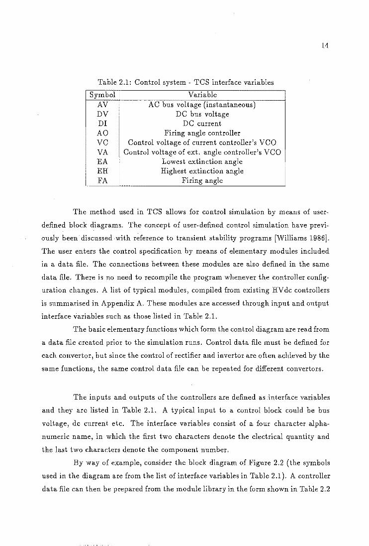
Table 2.1: Control system - TCS interface variables
Symbol Variable AV AC bus voltage (instantaneous) DV DC bus voltage Dr DC current AO Firing angle controller VC Control voltage of cu:r:rent controller's VCO VA Control voltage of ext. angle controller's VCO EA Lowest extinction angle EH Highest extinction angle FA Firing angle
The method used in TCS allows for control simulation by means of user
defined block diagrams. The concept of user-defined control simulation have previ
ously been discussed with reference to transient stability programs [Williams 1986].
The user enters the control specification by means of elementary modules included
in a data file. The connections between these modules are also defined in the same
data file. There is no need to recompile the program whenever the controller config
uration changes. A list of typical modules) compiled from existing HV dc controllers
is summarised in Appendix A. These modules are accessed through input and output
interface variables such as those listed in Table 2.1.
The basic elementary functions which form the control diagram are read from
a data file created prior to the simulation runs. Control data file must be defined for
each convertor, but since the control of rectifier and invertor are often achieved by the
same functions, the same control data file can be repeated for different convertors.
The inputs and outputs of the controllers are defined as interface variables
and they are listed in Table 2.1. A typical input to a control block could be bus
voltage, dc current etc. The interface variables consist of a four character alpha
numeric name, in which the first two characters denote the electrical quantity and
the last two characters denote the component number.
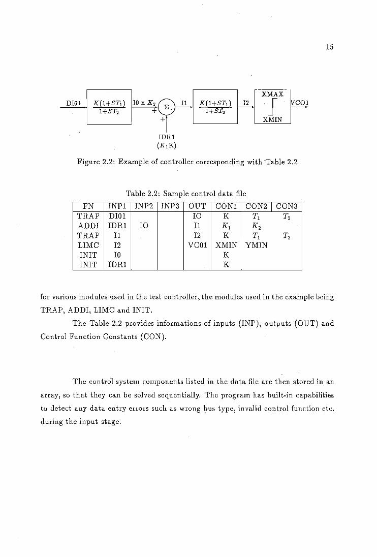
By way of example, consider the block diagram of Figure 2.2 (the symbols
used in the diagram are from the list of interface variables in Table 2.1). A controller
data file can then be prepared from the module library in the form shown in Table 2.2
15
XMAX
J DIOl K(l+STt} 10 x K2 1+ST2 +
K(l+STt} 12 1+ST2
XMIN
Figure 2.2: Example of controller corresponding with Table 2.2
Table 2.2: Sample control data file
FN INP1 INP2 INP3 OUT CON1 CON2 CON3 TRAP DID1 10 K Tl T2 ADDI IDR1 10 11 Kl K2 TRAP 11 12 K Tl T2 LIMC 12 VC01 XMIN YMIN IN IT 10 K INIT IDR1 K
for various modules used in the test controller, the modules used in the example being
TRAP, ADDI, LIMC and INIT.
The Table 2.2 provides informations of inputs (INP), outputs (OUT) and
Control Function Constants (CON).
The control system components listed in the data file are then stored in an
array, so that they can be solved sequentially. The program has built-in capabilities
to detect any data entry errors such as wrong bus type, invalid control function etc.
during the input stage.
16
2.5 Combined Power and Control
TCS Solution
The formulation of Transient Convertor Simulation (TCS) state-space equa
tions is well documented [Arrillaga 1983b]. The skeleton of the state variable method
is the simu1taneou~ solution of a system of differential equations, which is achieved
by means of an implicit integration routine.
State equations have the form:
X AX BU EZ (2.2)
Y = CX+DU (2.3)
where,
U input voltages and currents
X state variables
Y output voltages and currents
Z dependent variables
The details of controller function type, inputs, outputs are stored in arrays.
For the transfer functions, state-space equations (i.e differential equations) are written
as in the basic TCS formulation and are solved one at a time in order down the arrays.
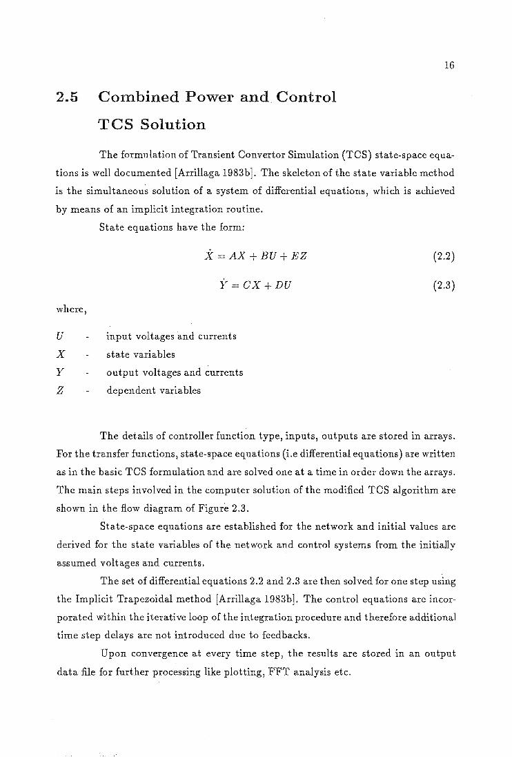
The main steps involved in the computer solution of the modified TCS algorithm are
shown the flow diagram of Figure 2.3.
State-space equations are established for the network and initial values are
derived for the state variables of the network and control systems from the initially
assumed voltages and currents.
The set of differential equations 2.2 and 2.3 are then solved for one step using
the Implicit Trapezoidal method [Arrillaga 1983b]. The control equations are incor
porated within the iterative loop of the integration procedure and therefore additional
time step delays are not introduced due to feedbacks.
Upon convergence at every time step, the results are stored in an output
data file for further processing like plotting, FFT analysis etc.

Read component and control system data
Establish state equations for the network
Initialisation at Time = a
Estimate new values for the network state variables
Solve control blocks sequentially
Convergence ?
y Yes
Time"" Time + (';t
No
Storage of results for further processing
End of
No
Network modifications
Yes
Figure 2.3: TOS flowchart
17
18
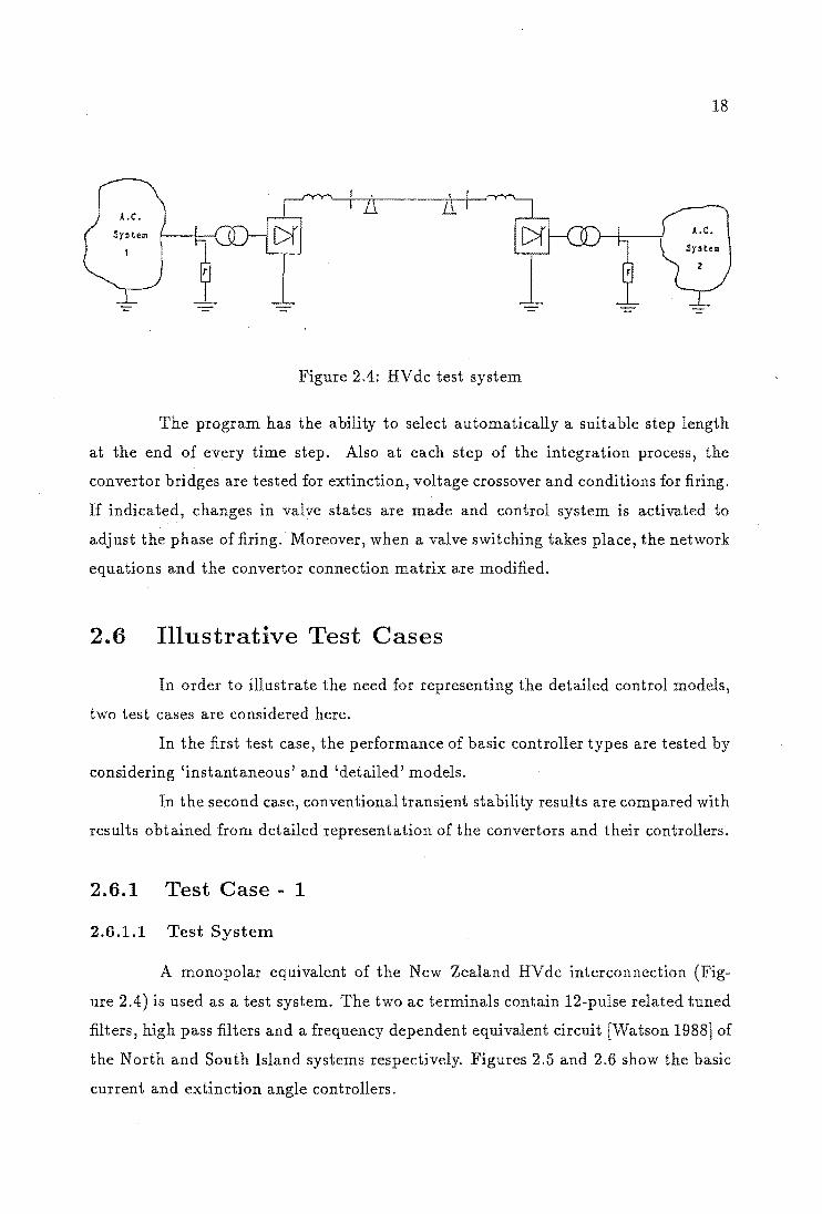
Figure 2.4: HV dc test system
The program has the ability to select automatically a suitable step length
at the end of every time step. Also at each step of the integration process, the
convertor bridges are tested for extinction, voltage crossover and conditions for firing.
1£ indicated, changes in valve states are made and control system is activated to
adjust the phase of firing. Moreover, when a valve switching takes place, the network
equations and the convertor connection matrix are modified.
2.6 Illustrative Test Cases
In order to illustrate the need for representing the detailed control models,
two test cases are considered here.
In the first test case, the performance of basic controller types are tested by
considering 'instantaneous' and 'detailed' models.
In the second case, conventional transient stability results are compared with
results obtained from detailed representation of the convertors and their controllers.
2.6.1 Test Case - 1
2.6.1.1 Test System
A monopolar equivalent of the New Zealand HVdc interconnection (Fig
ure 2.4) is used as a test system. The two ac terminals contain 12-pulse related tuned
filters, high pass filters and a frequency dependent equivalent circuit [Watson 1988] of
the North and South Island systems respectively. Figures 2.5 and 2.6 show the basic
current and extinction angle controllers.

DI01
TRANSDUCER
1 1+0.0018
EA"t~ A2
AREF (0.266 tad.)
10 +
0.0999(1+0.0018) 1+0.0038
IDR1 (4.0 p.u)
0.0234(1+0.0148) 1+0.0038
A3 0.1
J -0.1
19
-0.25
COlr V" + -
+ (a)
V"o
(b)
Figure 2.5: Controller dynamics-I: (a)Rectifier current controller (b)Invertor extinc
tion angle controller
DI01~ 11
IDRI
EA02~ A2 ---=t
AREF
0.0999 12
0.0234 A3
'--___ --J
0.25 J VCO~(?)~ -0.25 ¥
(a)
Vco
0.1
J (b)
-0.1
Figure 2.6: Controller dynamics-2: (a)Rectifier current controller (b)Invertor extinc
tion angle controller

20
Referring to Figure 2.5(a), the dc current from convertor 1 (DIOl) is the
input to the current transducer, which is represented as a single-pole transfer function
on the assumption that the DO-OT response is reasonably linear over the current
range expected during disturbances. The transducer output 10 is compared with a
current reference (IDRl), which is set using the function INIT. Their difference (11)
is the input to the controller dynamics function which, through a limiter, produces
the control voltage (VOOl) signal fed to the oscillator. A similar description applies
to the extinction angle controller of Figure 2.6.
The HV dc system recovery from major disturbances is an essential criterion
used in the selection of controller dynamics. Thus in order to test the performance
of the basic controller types of Figures 2.5 and 2.6, a single phase to ground fault is
applied at the invertor end of the test system.
2.6.1.2 Line to Ground Fault Recovery
The results of a solid line-to-line fault of two-cycles duration at the invertor
end terminals are shown in Figure 2.7.
Figure 2.7 (a) displays the dc current during disturbance and after fault
clearance by the circuit breaker; the continuous line indicates the modified TOS
solution responses with detailed representation of the controller dynamics (controller-
1) and the dotted line, the TOS solution with instantaneous controller (controller - 2).
The voltage waveforms at the invertor end are shown in Figure 2.7 (b) for the case
including the controller dynamics.
While in both 'ideal' (i.e. instantaneous) and 'real' (i.e. detailed) cases the
link is seen to recover from the disturbance, the variation of dc current from fault
occurrence to final recovery is very different in the two cases.
The dynamic behaviour of the convertor itself is better explained with ref
erence to the valve conduction patterns, displayed for the 'ideal' and 'real' controllers
in the bar-graph diagrams of Figures 2.8( a) and (b) respectively. These graphs show
a number of consequential commutation failures following the application of the fault
and a marginally faster recovery for the case with controller dynamics.

21
(a)
1.00~------'--------r.~----~--------r-------'--------r-------'--------r-------'--------1
-c. 21<11
-;3 .. 4" ~
l : ~ --,1;3.50: .
.!J- : . : r-12I .. e~ ~ ~ : a : 0-1.~~~:~ ____ ~ ________ ~ __ ~ __ ~ _______ J > 21110.0 22111.111 24111.111 261<1.0 290.111
... t ,
B. 111
7.111
S.I1I
a. I1l
1. 111
::: t·.!: U ::\t:'} ::
J
aD", " TIME (MILLISECS)
(b)
L t )
U
111, n~ ______ J-______ J~ ______ .. J. _______ J ____ ~~=::-=---~=J-------·JL-----=~=~~~:=;~:---~4~O;~0. 0 2111111,111 220.111 240.0 250.0
TIME (MILLISECS) (!,;OLIO) OYMoOI'T'tO'" - 1
Oyrtcll""j 0_ - 2. (DOTTED)
Figure 2.7: Invertor ac voltages and dc current waveforms for a single-phase to ground
fault

L • JI f
~
L • .II E
~
12 ~ 11~!~ ____________ ~
-1
2211l.0 2190."
12 i -1 11H:~------------~--------
-1
22
(a)
28111. III a211l. III aSIIl.1Il a911l." 411l11l.1Il
TIME (Mll.l.1SEC:S)
(b)
2911l.0
Figure 2.8: Invertor valve conduction patterns for a single-phase to ground fault. (a)
Control dynamics-l (b) Control dynamics-2

2.6.2
transducer
fl~~
frefl
ama" ®am~ I
+ ' -! Qmin
Figure 2.9: Controller blocks of Test case - 2
Test Case - 2
23
In present transient stability programs the HV dc convertors are modelled us
ing Quasi-Steady-State (QSS) equations [Williams 1986] and the controller dynamics
are represented with suitable transfer functions. In these programs, the implementa
tion of firing angle control is instantaneous, whereas in practice firing signals occur
at discrete intervals of about 1.5 or 3 mS depending on the pulse number. Moreover,
transient stability programs can not realistically model the control system response
following commutation failures.
An integrated approach was proposed [Heffernan 1980, Turner 1980] wherein
the conventional single phase multi machine stability analysis is combined with a
detailed 3-phase transient convertor simulation and detailed convertor controls.
In this example, with the help of TCS and the stability program, the effect
of representing detailed control systems is illustrated.

--~ "'--'
~ ~ ~
S 0
2.0
1.5
1.0
0.5
0.0 0.5 0.6
24
TCS + TS
0.7 0.8 0.9 1.0
TIME (s)
Figure 2.10: Rectifier dc current obtained from integrated TCS and stability program
2.6.2.1 Test System
The New Zealand ac/ dc system is used as the test system. The ac system,
represented in the transient stability program consists of 39 and 24 buses on the
sending end and receiving end of the dc link respectively. Thevenin equivalents were
derived using a Short Circuit program to represent the ac systems in TCS. Detailed
current and extinction angle controllers, shown in Figure 2.9 are also modelled in
TCS.
2.6.2.2 Fault Study
The results of a 3-phase fault of 2-cycles duration at the invertor end ac
terminal are shown in Figures 2.10 to 2.12.
Figure 2.10 displays the dc current during the disturbance and fault recovery.
The dc power transfer through the dc link is shown in Figure 2.11.

25
600
- -400 - .-,.-
/'
200 -
~ ':::::----'---' (a)
~ o -~ 0 P-i -200 -
- Rectifier -400 -
--- - Invertor
-600 i I I I
0.5 0.6 0.7 0.8 0.9 1.0
TIME(s)
600
- -- ,...,.,.,.---.-----400
~ 200
'---'
~ 0 (b)
~ 0 P-i -200
Rect i fi er -400
Invertor
-600 0.5 0.6 0.7 0.8 0.9 1.0
TIME(s) Figure 2.11: Rectifier and invertor powers from (a) stability program (b) integrated
TOS and stability program

1.25 ,...------------------------,
1.00 =--- --...:..--/'
./ ....--.. /
~ 0.75 - /
t3 I
...::c:: ~ 0.50 f-a ::>-
0.25 '- I Rect ifi er - ......
-- --- Invertor
0.00 I I 1 I
0.5 0.6 0.7 0.8 0.9 1.0
TIME(s)
1.25 ,-----------------------,
1.00
....--..
~ 0.75
t5 ~ H 0.50 §2
0.25
./
\ / 1/ I , I
I I
, , I' ,/
-----------
Rec t ifi er
----- Invertor
0.00 L..--___ -L-___ -.L ____ ..l...-___ --L.-___ ----l
0.5 0.6 0.7 0.8 0.9 1.0
TIME(s)
26
(a)
(b)
Figure 2.12: Rectifier and invertor terminal ac voltages from (a) stability program
(b) integrated TCS and stability program

27
The response of the link obtained from the conventional transient stability
program is shown in Figure 2.11(a) and the corresponding response obtained from
the integrated TOS and stability program is displayed in Figure 2.11(b). The effect of
detailed controller model during the disturbance and recovery period is clearly seen
in Figures 2.11( a) and (b).
Figures 2.12( a) and (b) show the invertor terminal ac voltage obtained from
the conventional and the integrated TOS-stability programs respectively.
2.6.3 General Discussion
The above test cases serve to illustrate the ability of the digital solution
to model the effect of controller dynamics, which is shown to be of fundamental
importance the assessment of convertor recovery from disturbances.
The physical simulator is reputed to be an ideal tool for the setting of con
troller dynamics constants due to its ability to quickly perform repetitive studies.
The digital model, while slower in performing studies with different con
troller constants, is more flexible in altering the controller functions and can set
up very accurately any specified point on wave of fault application, any level of
transformer residual magnetisation, any pattern and duration of fault clearance etc.
Moreover the digital solution can represent the ac system components as accurately
as required (only limited by the availability of information). In particular, the ability
to represent the convertor transformer magnetising history during the disturbance
and the frequency-dependence of the ac system (even with detailed mutual effects)
to any required degree of accuracy make the digital solution a viable alternative to
the physical simulator.
The above remarks clearly show the difficulty involved in attempting 'quan
titative' verifications of the computer results with reference to simulator studies. All
that can be done is to check the 'qualitative' nature of the results with reference to
typical patterns of fault recoveries expected; the results displayed in the last section
are in line with such expected behaviour.
28
2.7 Conclusion
A detailed control system simulation has been added to the Transient Con
vertor Simulation (TCS) program currently used to predict the convertor recovery
from disturbances. Apart from the extra modelling flexibility provided, representa
tion of the control dynamics has been shown to influence dramatically the convertor
performance following fault clearances.
The enhanced TCS program provides an important tool for the computer
simulation of the operation of HV dc interconnections, particularly during ac and
dc system disturbances. This program can be used to further develop control and
protection schemes that will lead to improved overall system performance.

29
Chapter 3
A COMPARISON OF
SIMULATION ALGORITHMS
3.1 Introduction
The incorporation of HV dc controller dynamics into TCS program was dis
cussed in the previous chapter along with the need for such models. However, the
simulation technique must be compared with another simulation tool for a wider
acceptance.
Attempts to validate dynamic simulation algorithms for use in HV dc trans
mission are normally carried out by comparison to disturbances recorded from actual
systems or physical simulators. This type of verification is by necessity of a qualitative
nature.
A quantitative comparison is made in this chapter between the results pre
dicted by two fundamentally different computer models, i.e. between algorithms
derived from EMTP and state variable techniques (TCS program).
3.2 Criterion for COITlparison
Three conditions must be met for a rigorous approach to the problem of
verification of a computer algorithm, i.e.
1. Comparing the proposed algorithm with one or more fundamentally different
models.

30
2. Setting up identical test system conditions in each model.
3. Presenting all the relevant information needed to detect any deviations and the
instances of their occurrence.
With reference to HV dc transmission, the possibility of using real system in
formation to assess the predictive ability of a computer simulation program, although
often expected, is unrealistic owing to practical difficulties in meeting condition 2.
Among the problems involved are the random 'points on wave' in which disturbances
appear and disappear, the random states of magnetisation of convertor transformers
upon fault clearances, the unavailability of realistic information of the actual system
parameters prior to and throughout the disturbance etc. The use of a scaled-down
physical simulator, still considered an acceptable alternative, is not entirely free from
the problems listed above and its comparisons with computer models tend to empha
size the qualitative rather than quantitative behaviour [Cazzani 1988].
More often than not, 'good matches' are derived using the experimental
information and adjusting by trial and error the computer model parameters [Mat
tensson 1986]. However such heuristic approaches give little confidence on the general
applicability of the algorithm in question.
A more realistic comparison in terms of conditions 1 to 3 above is the use
of two or more alternative and fundamentally different computer solutions. Two
basically different approaches are currently used in HV dc transient simulation i.e
the Electromagnetic Transient Program (EMTP) and the state variable technique.
The EMTP method and a diakoptical solution have been combined into an efficient
algorithm, the EMTDC, for the analysis of ac/dc power systems [Woodford 1983].
State variable solutions often reputed less efficient, are formulated in a more
'physical' form and use less approximations. They therefore provide suitable tools for
a rigorous comparison. 1£ the response of the two methods, i.e. EMTDC and TCS to
various disturbances can be made to agree, it will be reasonable to accept the validity
of both. 1£ they do not agree, at least one of them will not meet the criterion and
without additional information, it will be difficult to reach a positive conclusion as to
the value of either.

3.3 Algorithmic Differences of TCS
and EMTDC
31
TOS is a program specifically developed to analyse the dynamic behaviour
of HVdc systems and is formulated in terms of state space theory [Arrillaga 1983b].
The EMTDO algorithm [Woodford 1983] is based on the Electromagnetic
Transients Program, EMTP [Dommel 1969]. The trapezoidal rule is used for inte
grating the ordinary differential equations of lumped inductors and capacitors and
converting them into a resistor in parallel with a current source, while lumped re
sistors are modelled simply as resistive branches. Hence a network of lumped R,L,O
components is transformed into an equivalent circuit of resistive branches and current
sources.
Using nodal analysis, a conductance matrix [G] is formed from the inverse
resistance value of each branch in the circuit. A column matrix [I] is also formed,
its elements consisting of the sum of the current sources at each node. The nodal
voltages [V] are therefore,
(3.1 )
Valve or ac system components switchings are implemented by changing the
value of the appropriate resistors.
For greater efficiency, EMTDO uses the subsystem concept which groups the
system into appropriate identifiable components such as generators, ac networks, con
vertors and dc lines, each of which is solved independently of the others at each time
step. The subsystem solution requires the prediction ofthe incremental voltage wave
form for the next step of the solution at the points of interface between subsystems.
Thus to reduce error and avoid numerical instability, the use of subsystems requires
the presence of sufficient capacitance and inductance to prevent large deviations of
the voltages and currents from one step to the next.
The usage of subsystems result in greater reduction in computation time.
Further efficiency is obtained by using a constant integration step throughout the
solution.
The dc convertor along with a three phase transformer is modelled as a
separate network, by taking advantage of the subsystem concept. It is also possible
to model a convertor explicitly as a set of resistive branches (which represent valves),

3 ph ac
system
Rectifier T-line
-1-[)f rfc filter
, Invertor
AC filter
Figure 3.1: Test system for the comparison
in which case the dc system is solved as a unified solution.
3.4 Test System
3 ph
ac system
32
The dynamic comparison will concentrate on the HV dc convertor, which
constitutes the specific reason for the existence of the EMTDC and TCS programs.
A realistic comparison of the HV dc convertor behaviour provided by the
two alternative algorithms can be achieved with reference to the simple test system
illustrated in Figure 3.1. It consists of a monopolar dc link with a single bridge at
each end provided with the basic control functions as illustrated in Figure 3.2.
The ac systems are modelled as modified Thevenin equivalents in parallel
with the filters [Bowles 1970j. The dc line is represented by means of several pi
sections, dc filters and smoothing reactors. Details of the test system parameters are
given in Appendix B.
In the TCS algorithm, the power system is built-up by appropriate connec
tion of the network components and the control system is formed by cascading the
individual controller functions available in the data file. Appendix C gives the TCS
controller data file.

33
transducer
M· aord In. a
Figure 3.2: Test system controllers
In the EMTDC program, the power and control systems are formed using
the data file and user defined subroutines. In the present test system, the electric
network is conveniently divided into three subsystems comprising the sending and
receiving end ac systems and the dc system [Manitoba 1988}. Also the convertors are
modelled as separate subsystems.
3.5 Steady State Initialisation
Prior to the dynamic comparison, it is necessary to start up the system
from a de-energised state and observe the operating conditions under steady state.
For this purpose, both TCS and EMTDC were run for 0.5 seconds of simulation time
to let the system settle down to the steady state. Both TCS and EMTDC have the
facility to store the steady state results in a separate file for further studies and so
a snapshot was taken at 0.5 seconds in both programs. The steady state run was
first used to identify and correct various anomalies in data preparation (such as the
per-unit systems) and information retrieval (such as the elimination of zero sequence
34
at the convertor voltages in the case of EMTDC).
It was observed then that the two programs settled down to the same oper
ating point with the rectifier firing angle at 15 degrees and the extinction angle at 18
degrees. The reference dc current was 1.45 kA, with 0.1 pu current margin. The filter
reactive powers were observed to be of the same magnitude in both programs and all
the valve conducting states changes took place with less than one degree differences
in the two programs.
3.6 Disturbance Simulation
Major disturbances in ac/ dc power systems lead to multiple commutation
failures at the invertors. Hence for a credible validation, the two transient algorithms
should produce the same pattern of commutation failures. Such patterns together
with full convertor recoveries are displayed in this section for typical severe ac system
disturbances.
3.6.1 Symmetrical Fault
A three phase short-circuit of 2 cycles duration and causing a 40% voltage
reduction in the three phases of receiving end system was used to determine the
highest EMTDC integration step needed to reproduce the performance of the TCS
algorithm. These were found to be 20 and 10JLs for ac system and convertor models
respecti vely.
Figures 3.3(a) and (c) show the dc current and three phase ac voltage wave
forms derived with the TCS algorithm. Corresponding results simulated with the
EMTDC program are illustrated in Figures 3.3(b) and (d).
For a rigorous approach to the question of algorithmic verification, it is
important to present all the relevant information needed to detect any deviations be
tween the results and the instances of their occurrence. This can be achieved without
the need for large amounts of numerical information by comparing the valve conduc
tion times. The bar diagrams of Figures 3.3( e) and (f) provide detailed information of
the valve conduction times and with them a clear indication of commutation failure
events.

::-c tI !lD r;j ., '0 >
tcs (a)
o.~
O'8.5!:-O:----=-O.-!;~":"S---7o-';:.a;-;:o----::O:-C.6::c5;------,O;;-.-!::7::;'0---~O.75 . TIME (s)
(c) 150r---------------------------~
,00
""
" -50
(e)
s
l-II) S
.0
E .. :l C V 3
> ~ > "
0 0.50 O.!U
TIME (s)
35
emtdc (b) •. 5r------------------------------------
O.~
O·g.I5:-:0:::----0::-.-!;5-;;-5----=O~.6:::",-----:Oc:-.':-6":------:cO~. 7"''',-----:0:-1.75 TIME (s)
(d) 150r------------------------------~
G
~ 5 !------------.0
E ., :l ;:
<I >
OJ > "
TIME (s)
(f)
TIME (s)
Figure 3.3: Three phase fault at the invertor end (a )(b) dc current, (c)( d) ac voltages,
(e )(f) valves conduction

36
All the corresponding switching instants are within 0.5 degrees and the num
ber of commutation failures predicted by both programs is eight. As a result, the
convertor recovery following fault clearance is exactly the same in both cases. The
severity of the disturbance simulated in this test case provides sufficient evidence of
the validity of the two algorithms.
3.6.2 Asymmetrical Faults
Previous attempts to validate computer simulation versus field tests [Wood
ford 1985], while providing reasonable qualitative matches for balanced fault condi
tions, have shown unrealistic differences in cases of unbalanced disturbances.
The same integration step that achieved perfect matching for the symmet
rical fault were used to assess the convertor response to a line-to-ground (L-G) fault,
causing a complete loss of voltage in one phase of the receiving end ac system voltage.
While the overall recovery time and the number of commutation failures are
the same for the specified disturbance, small differences are now observed in the valve
conducting patterns. For instance, with reference to Figures 3.4 ( a) and (b), valve
5 attempts to conduct at about 0.515 seconds in the EMTDC simulation, whereas
it does not conduct at all in the TCS simulation. Thus some small deviations are
observed in the dc current and ac voltage waveforms illustrated in Figures 3.4( c),( d)
and 3.4(e),(f) respectively.
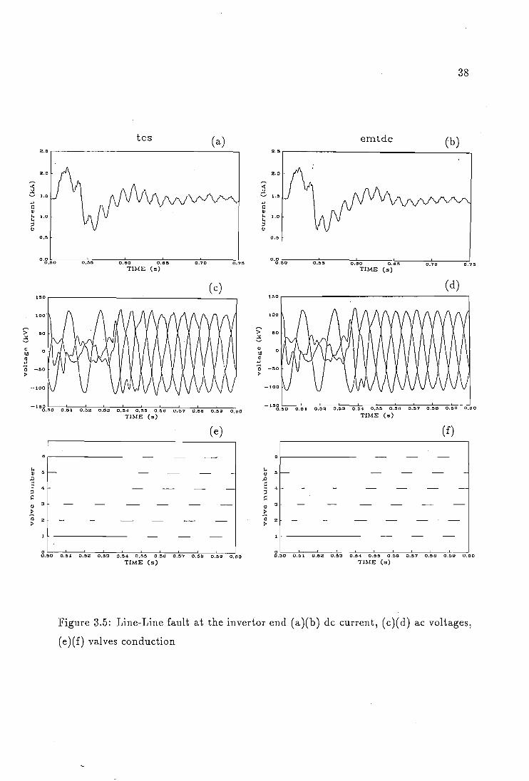
A further test case was carried out consisting of a 2 cycle line-to-line (L-L)
fault causing a 70% voltage reduction in two phases of the receiving end system.
The results, shown in Figure 3.5, again indicate similar fault recoveries for the two
algorithms. However, the valve conducting patterns of Figure 3.5(e), (f), although
showing the same number of commutation failures, illustrate some differences between
TCS and EMTDC; for instance, valve 4 has two brief conduction periods in EMTDC
which are totally absent in the TCS simulation.
The above differences in valves conducting patterns III the asymmetrical
cases are not due to the differences in the controller outputs, which have been checked
to be the same at those particular instants and therefore, they must be due to differ
ences in the software implementation.
An important algorithmic difference between TCS and EMTDC is the use
of the subsystem concept by the latter. In EMTDC, the commutating voltages at

0
I. II ~
.0 E • ;l r: II
3
> <l " >
0 Q,SO
2.~
2.0
~ l.~ .., r: II J.. J..
1.0
;l u
o.~
0.0 0.:;'0
,50
,00
S; 50
C II til
0
Q ... a -50 >
-100
-150 o.~o
37
tcs (a) emtdc (b)
0
J.. ~ I)
.0 E ;l
., I': U
3
> Q 2· >
0 0.01 o,oa 0,63 0,04 O.5!) 0.66 0.iS7 o.~a O.OQ' o.so o,~o O.:U 0.::'2 O.~3 0.::'''' 0.05 0,60 0.07 0,:)(' O.Og 0,60
TI:I>!E (s) Tn-!E (s)
(c) (d) 2.~
..; .:.: ~
... I': IJ J.. 1.0 J.. ::l u
o.~
0.0 o,~o 0.60 0,6::5 0.70 0,70-
0.50 Q,O!) 0,00 0,00 0.70 0.70
TIME (s) TIME (s)
(e) (f) 150
~
::-.:.: ~
U to Q ... Q -50
>
-100
-lao , , . I , , , , !-.l
0.:5:1 O.~2 0.:':.1 O.!t4 0.55 0,56 0,5.0 0.51 O.~2 O.~3 0.54 O,5~ O.::H) O.~7 0.59 o.~o 0.(10
TIME (s) TIME (s)
Figure 3.4: Line-to-Ground fault at the invertor end (a)(b) valves conduction, (c) (d)
dc current, (e)( f) ac voltages
2.'
~ 1.0
.... ~ v h h
1.0
;J u
0.'
0.0 0,60
100
s:- ao ::. V 0 bD ~ .... '0 -ao >
-100
-150 0.50
38
tcs (a) emtdc (b) 2.'
~ C. .... t:
" h h
1.0
;J u
0.'
0.0 0.06 0.80 0.65 0.70 C.7!! 0.50 o.~~ 0.00 a.e:!! 0.70 0.75
TIME (s) TIME (s)
(c) (d) 100
100
s:- ao ::. " 0 bD ~ .... 0 -'0
>
-100
-150 O.:H 0,52 0.1)::1 0.5'" O.!l5 0.50 0.57 O.5U 0,50 0,00 O.fH 0.52 O.:!I:J 0.54 O.!l5 0.06 O.~7 0.58 0.59 0.60
0.50
TIME (9) TIME (9)
(e) (f)
'" ~ .0
E ;j
.\ -
i:1 tJ 3
> Ii 2 >
I·
o .L 0.50 0.51 0.52 0,53 0.51 0.55 0.:)0 0.57 0.50 o.~g 0.130
TIME (9)
Figure 3.5: Line-Line fault at the invertor end (a) (b) dc current, (c)(d) ac voltages,
(e) (f) valves conduction

39
the tth interval are derived from those calculated in the previous interval (t - b..t) by
an approximate phase advance prediction [Manitoba 1988]. This is achieved by the
following equa Hon (for phase- A voltage) :
(3.2)
However, this equation is based on the assumption that the voltages are
perfectly balanced and therefore their use is only accurate under balanced steady-state
or symmetrical faults conditions. Thus neglecting the considerable negative sequence
voltage content during 1-G and 1-1 fault simulations can cause some error in the
derivation of the commutating voltages (which alters the valve commutation intervals)
and voltage crossings (which alters the valve extinction angles). This may account
for the small differences in the valve conduction patterns between the EMTDC and
TCS results observed during the asymmetric disturbances.
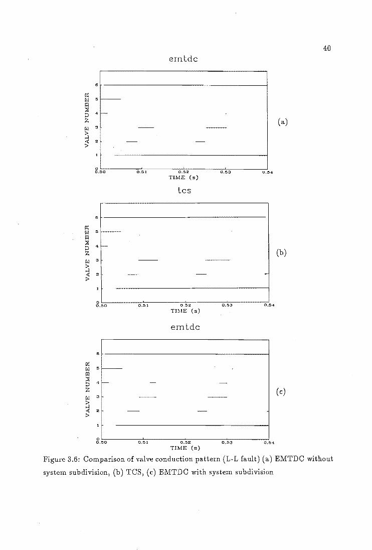
In order to test the effect of the phase advance prediction, the 1-1 fault was
repeated without using the subsystem concept, that is with the whole system analysed
simultaneously. . A comparison of bar diagrams while the fault (and therefore the
asymmetry) is ON is illustrated in Figure 3.6. Clearly the EMTDC response without
system subdivision (Figure 3.6(a)) is much closer to that of TCS (Figure 3.6(b)) than
the standard EMTDC using the subsystem concept (Figure 3.6( c)).
3.7 Algorithmic Efficiencies
The comparison of algorithmic efficiency is not straightforward, as it de
pends on subjective judgements regarding what constitutes an equivalent dynamic
performance.
As expected, the use of the standard EMTDC algorithm, with the recom
mended integration steps, provides a very efficient solution. If the results plotted in
Figure 3.5 are considered sufficiently close, the EMTDC program is about four times
faster than TCS.
However if a closer agreement is required, such as that provided by the
unified solution (displayed in Figure 3.6(a) and (b)) with a step length of 10,uS, the
situation changes quite dramatically. For the test system with a 1-1 fault and a
250 mS simulation run, the total computing times on a VAX-3500 computer were as
40
emtdc
6
(a)
o~--------~~------~~--------~--______ ~ 0.50 0.51 0.52 0.53 0.54
TIME (5)
tcs
6
(b)
-
OL---------~~------~~------~~--------~. 0.50 0.51 0.52 0.53 0.54
TI11E (5)
ernLdc
6
(c)
.50 0.51 0.52 0.5:3 0.54
TIME (5)
Figure 3.6: Comparison of valve conduction pattern (L-L fault) (a) EMTDC without
system subdivision, (b) TCS, (c) EMTDC with system subdivision
follows:
3.8 Conclusion
TCS - 42 minutes
EMTDC - 41 minutes
41
By setting up an identical test system, it has been shown that the two main
algorithms currently used for the simulation of ac/ dc disturbances, namely TCS and
EMTDC, can be made to agree in their prediction of the dynamic responses.
The TCS algorithm, though reputed to be less efficient, uses fewer approx
imations and provides automatic selection of optimal integration steps. As a result
the TCS responses are very consistent .
. With careful selection of the integration step, the EMTDC program can
produce practically the same responses as the state variable technique for reasonably
symmetrical conditions. However, some deterioration occurs with highly asymmetri
cal disturbances. This has been traced to the phase advance prediction, required by
the subsystem concept, thus the EMTDC algorithm provides a very efficient solution
at the expense of some accuracy.
The comparison has not included ac system components such as generators
and SVC, but has concentrated on the modelling of the convertor algorithms. It can
be concluded that both the EMTDC and TCS algorithms can be used with confidence
to simulate the transient response of ac/ dc convertors.
The results of this preliminary investigation indicate that the best features
of EMTDC and TCS can be combined into a new algorithm called EMTCS and it is
currently underway at the University of Canterbury,

42
Chapter 4
DYN MIC SIMULATION OF
GENERATOR-HVDC
CONVERTOR UNITS
4.1 Introduction
Dynamic simulation of generator and HV dc convertors using TCS algorithms
have previously been used to establish the controllability of generator-HV dc convertor
units during disturbances [Campos Barros 1976] and in thyristor bridge excitation
system studies [Heffernan 1980]. In this work, TCS is used to assess the applicability
of conventional steady state formulation and derive the operating characteristics of
unit connections.
Iterative analysis in harmonic space [Eggleston 1985] and EMTDC program
[Naidu 1989] have also been used to study the generator-convertor units. These
studies were restricted to harmonic analysis.
The synchronous machine model in TCS is represented in phase quantities,
in order to handle assymetries, non-linearities and distortion effects by direct param
eter modification or indirectly. A d-q axis representation is used for the rotor circuit,
which uses the main field winding in the d-axis with two damper windings. The
machine is treated as a motor when writing down its electrical axes equations; the
terminal voltage can be expressed in matrix form as [Campos Barros 1976],

43
( 4.1)
where,
w = ~~ is the angular velocity.
Lg [Lss Lsr 1 Lrs Lrr
the subscripts sand r are stator and rotor respectively. Since most man
ufacturer data is in the two axes d-q-O form, this must be transformed to yield the
direct phase quantities (a,b,c).
Appendix D gives the transformation of manufacturer's data into the phase
quantities.
In this chapter, the per-unit system used to simulate the unit connections
and the validation of the generator model are given. Also the initialisation process
involved in TCS to study the unit connections and the calculation of steady state
quantities from the waveforms are explained.
4.2 Per-Unit System
In steady state analysis such as load flow, the convention is to choose rated
current and voltage (fundamental frequency rms values) as base values. Acj dc con
vertors are treated as voltage and frequency transformers and the base values of the
dc side variables are defined according to their relation with the ac side variables
[Arrillaga 1983b].
In a transient program like TCS, the valves are treated as switches and
hence the instantaneous ac line voltage and current will be the same on both sides
of the switch, i.e. on the ac and dc sides. For this reason, the base values of the dc
side must be chosen as the base values of the ac side and so it is preferable to take
instantaneous rather than rms base values.
In order to keep the figures for the per unit values of transformers and
generators within the usual bounds, the base values are chosen such that the base

44
impedance is kept equal to the three-phase value. A system that would satisfy this
requirement is as follows:
Base current
Base current
Base power
peak phase current of the star equivalent
peak phase voltage of the star equivalent
peak phase power of the star equivalent
In terms of usual three phase values it gives:
T.r rn2V, .J2Viine,rms vbase = V.{, phase,rms = V3
Basepower 2 3" (Three phase base power)
4.3 Validation of Generator Model
( 4.2)
( 4.3)
( 4.4)
Even though the generator model in TCS is an established one and has been
used for other studies [Campos Barros 1976 and Heffernan 1980], validation tests are
still required to make sure that the program represents the required synchronous
machine parameters. Computer simulated open-circuit and short-circuit tests are
used for this purpose.
Simultaneously short-circuiting the three phases of a synchronous machine
when running unloaded is an accepted method of determining the principal transient
reactances.
For an unloaded machine, neglecting resistance, the short circuit stator cur
rent of any phase is given by [Concordia 1951],
~ ( 4.5)
where aD is the switching angle. The above equation shows that the initial current
is composed of a fundamental component depending only on X:;) a dc component
depending on X; and X:; and a small double frequency component depending on the
difference between X:; and X;, i.e. the sub-transient saliency.

45
Figure 4.1 shows oscillogram of the open-circuit voltage and short-circuit
stator currents of the salient machine given in Appendix E. The peak-to-peakopen
circuit voltage is, e= 1.5472 pu and the initial short circuit stator current is, i= 7.677
pu. So)
XII _ e d-·
'/, 0.2015 (4.6)
The direct axis sub-transient reactance for the machine as given in Appendix E is 0.2
pu.
Figure 4.2 shows oscillogram of the open circuit and short circuit stator
currents of the non-salient machine given in Appendix E. From the initial short circuit
current and open circuit voltage ) X~ is calculated to be 0.149 pu and the value given
in Appendix E is 0.145 pu. It can be seen from the oscillogram shown in Figure 4.2
that the short circuit current does not have any double frequency component.
The close agreement of the calculated subtransient reactances together with
the general pattern of the sub transient and transient periods indicate the correctness
of the programmed data.
4.4 Initialisation of Unit
Connection Simulation
The susceptibility of simulations involving detailed synchronous machine
models to inaccurate initial conditions was shown by Campos Barros [1976] and Hef
fernan [1980] to be a major problem in their work, which involved generator-rectifier
systems. When the dynamic simulation is started with idealised steady state con
ditions derived from fundamental frequency power flow, the initial estimate of state
variables introduce transients in machine currents. These transients decay very slowly
with the machine time constants. This difficulty is solved without extra-long adjust
ment runs by increasing the resistances of the rotor circuits and thereby artificially
reducing the machine time constants. The inflated resistances are reduced to the
original value after a few cycles and the desired operating point is reached. Figure
4.3 shows the dc current and machine rotor currents during the initialisation period.
During the initialisation, it is very important to specify accurate values
for convertor transformer magnetisation currents. If inaccurate initial magnetisation
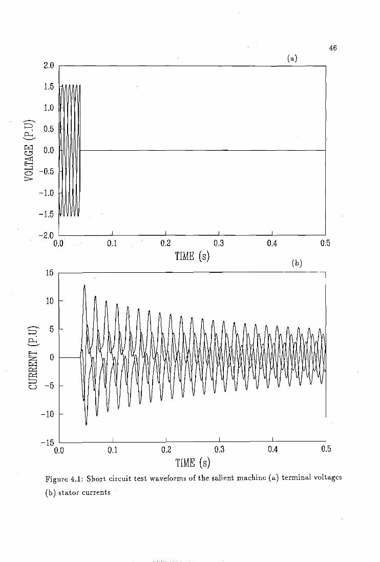
46
2.0 (a)
1.5
1.0 .,.--...., p 0.....
0.5 ~
~ 0.0 0 E=S .......:I -0.5 0 >-
-1.0
-1.5
-2.0 r I r I
0.0 0.1 0.2 0.3 0.4 0.5
TIME (s) (b)
15
10 f--
~ r ,.-.. 5 '- r ( ( ~ f f f P P--l '--"
E--< Z ~ ~ ~ P u
II \) ~ J 0
{ I I I
-5 I-v V v v v V
-10 f--
-15 L-________ L-� ______ ~I ________ ~I ________ ~I ________ ~
0.5 0.0 0.1 0.2 0.3 0.4 TIME (s)
Figure 4.1: Short circuit test waveforms of the salient machine (a) terminal voltages
(b) stator currents

pc::J o ~
(a) 2.0 r------------------~----.
47
1.5
1.0
0.5
0.0
c3 -0.5 :::>
-1.0
-1.5
-2.0 L-____ ~1 ____ 1L_ ___ ____.J1L_ ___ ____.J1L_ ___ __.J
0.0 0.1 0.2 0.3 0.4 0.5
TIME (8) (b)
20 .---------------------------------------~
15
10
-10
-15 -20 L-______ ~ ________ ~ ________ L_ ______ ~ ________ _
0.2 0.3 0.4 0.5 0.0 0.1
TIME (8) Figure 4.2: Short circuit test waveforms of the non-salient machine (a) terminal
voltages (b) stator currents

48
3
field current
2
dc current 1
o d-a.xis da.mper current
-1
-2
-3 o 2 4 6 8 10
TIME (CYCLES) Figure 4.3: Generator rotor currents and dc current derived from dynamic simulation
currents are specified, then a dc offset is introduced in the magnetising current whose
value depends on the error. The rate of decay of this magnetising current offset is
dependent on the transformer resistance involved. Since this is usually low for power
transformers, the time taken for the offset to disappear is considerably high and this
problem has been reported by Heffernan also. The effect of this magnetisation offset
is to create a dc component in the stator currents. In this work, the correct values
of magnetisation current for a particular loading condition are obtained by doing a
preliminary run (e.g. for 0.5 degrees).
Figures 4.4 and 4.5 show the generator terminal voltage (only two phases of
the voltage waveform are shown for clarity) and stator currents derived from TCS.
Since there are no harmonic filters at the generator terminal, it would be
difficult to know the excitation required for a particular dc voltage and dc current.
One way to get around this problem is to model the excitation control with dc voltage
as the controlled quantity instead of machine terminal voltage.
Dynamic simulation is extremely demanding computationally, as the pro
gram must run for many cycles to remove the transient components from the wave-

1.25
1.00
0.75
0.50 --~ 0.25 CL. ---Pr=1 0.00 0 ~ -0.25 ......:l 0 ::::.-
-0.50
-0.75
-1.00
-1.25 0.0
II' ~ I
1
I-I
~ I )
'I , \ j
0.5 1.0
TIME (CYCLES) 1.5
1
't I 1....,1 I
2.0
49
Figure 4.4: Generator terminal voltages (two phases) derived from dynamic simula
tion
1.0 r-------------------------,
0.5
----0 P-. '--'
E--< 0.0 Z ):::t:::1 0=: 0=: 0 u
-0.5
-1.0 L-------L. ____ ----1 _____ .l....-____ --.J
0.0 0.5 1.0 1.5 2.0 TIME (CYCLES)
Figure 4.5: Generator phase currents derived from dynamic simulation

50
forms. The initialisation process can be speeded up by a preliminary study using the
simplified steady state formulation described in section 5.6.
An approximate value of field current can be calculated using the steady
state simulation. The field current gets adjusted to the exact value by the excitation
control modelled in TCS, to obtain the specified operating point.
4.5 Notch Removal for Firing Angle
Measurement
In the absence of harmonic filters, the terminal voltage waveform would
be severely distorted and such a waveform is shown in Figure 4.4. A look at the
waveform clearly shows that the use of generator terminal voltage as the -rATA-r".n
waveform for the firing controller will introduce considerable discontinuities in the
voltage crossings caused by the commutation notches. On the other hand, the internal
emf is inaccessible for monitoring purposes. One possible solution is the provision of
control filters to obtain the fundamental voltages; however the phase of such a filtered
signal will alter with the firing angle and the loading conditions.
A better alternative is to 'ignore' the commutation notches, that is to use
a sine wave derived 'on-line' from the actual waveform by filling-in the gaps during
the commutation regions. This is not equivalent to 'filtering' and the fundamental
frequency wave will therefore not be phase-shifted.
4.6 Calculation of Steady State
Quantities
In this work, the dynamic simulation program is used to derive the steady
state characteristics of unit connections. The steady state quantities like dc voltage,
dc current, terminal voltage and machine currents are calculated from the TCS wave
forms using the FFT. To reduce sampling errors at points of discontinuity, a high
number of samples (1024 samples per cycle) is used.
In order to determine whether a particular run has reached steady state or
not, FFT analysis is carried out at intervals of 5 cycles. The absence of any significant

51
Table 4.1: Variation of dc component in the stator current
Time R - phase Y - phase B - phase (cycle number) (%) (%) (%)
40 -1.597 1.558 0.038 41 -2.616 2.070 0.553 44 -2.227 2.083 0.190 45 -2.291 2.056 0.236
difference in the fundamental quantities between two consecutive FFT sets of results
indicates steady state. In this work, 0.005 pu has been used as the steady state
criterion.
The computation time for a back-to-back system comprising generator, 12-
pulse rectifier & invertor and primary controls is about 7 minutes per cycle on a VAX
3500, with a time step of 1 degree. Normally, 20 to 25 cycles would be required to
reach a steady state with reasonable initial values.
In spite of adopting the techniques described in section 4.4 for initialis
ing generator-HV dc convertor units, the FFT analysis detects the presence of small
amounts of dc components in the stator currents. The magnitude of this dc compo
nent from a sample run is indicated in Table 4.1.
It can be seen from the Table 4.1 that the dc component magnitude does not
follow any defined pattern and varies from one phase to another. From the numerous
runs carried out during this work, the maximum value of the dc component was found
to be less than 3%.
When the convergence tolerance for the state variables is changed from 10-5
to 10-10 and the step length reduced from 1 degree to 0.2 degree, the dc off-set levels
decrease by almost 50%. But still they were in the order of 1.5 to 1.8%. With this
reduced step length and improved convergence tolerance for the state variables, the
computational time was extremely high ( 30 minutes of cpu time per cycle).
The effect of this dc component is to create a small component of power
frequency rotor current and a power frequency component on dc current.

52
4.7 Conclusion
Various runs using generator-convertor units have showed the validity of gen
erator model and per-unit systems adopted in TCS. Proper initialisation techniques
and identification of steady state for unit connected systems have been established
for further studies. An alternative to the control system filter has been proposed for
firing angle reference. Further work is still required to eliminate the dc component
completely from the machine stator currents.

53
Chapter 5
ANALYS S OF THE
COMMUTATION PROCESS IN
A GENERATOR-HVDC
CONVERTOR UNIT
5.1 Introduction
The mechanism of commutation in a static convertor connected to an ac
system is a well-known process, in which the commutation is considered as a short
circuting process between the phases connected to incoming and outgoing valves.
The difference in the open-circuit voltages of the two phases is treated as the effective
voltage for commutation and during commutation, this effective voltage produces a
circulating current flowing through the valves from the incoming valve to outgoing
valve. Under normal condition, the commutation process is completed when the
magnitude of the circulating current reaches the total current value, i.e. when the
current in the outgoing valve reaches zero.
During commutation, circulating currents are reflected in the convertor
transformer primary circuit and in the ac system. Thus any impedances associ
ated with the paths of the circulating currents affect the build-up of circulating cur
rents and hence influence the commutation process. The combined effect of such
impedances causes an equivalent commutation impedance which includes one com-

54
ponent due to the convertor transformer and another due to the ac system.
The influence of convertor transformer impedance on the commutation pro
cess was thoroughly investigated by Chen [1962]. He showed that the winding re
sistances, stray and distributed capacitances and the mutual inductance effects have
little effect on the commutation process. The reactance that influences the commu
tation process is independent of dc current and the dc ripple level and this reactance
is equal to the transformer leakage reactance.
With perfect filtering or with a combination of filters and transformer phase
shift, the voltage on the ac side of the convertor transformers may be assumed to
be sinusoidal and hence the system reactance has no influence on the commutation
process. In the absence of filters, pure sinusoidal voltages only exist behind the
system source reactance and in such case, the commutation reactance is the sum of
transformer reactance and the system reactance .
. In the ca'se of a unit connected HVdc system, the generator, unit transform
ers and HV dc convertors are connected as a unit isolated from the rest of the system.
This arrangement is different from the conventional arrangement due to the absence of
harmonic filters and its isolation from the rest of the system. Hence the commutation
process would be influenced not just by the convertor transformers alone.
The farthest component from the convertor is the turbine, which is a me
chanical element. The typical response of a turbine governor is of the order of a
second and compared to the convertor commutation period, the turbine governor will
have no effect on the commutation process.
The other components in the system are the two electromagnetic elements:
generator and transformer. The influence of transformer on the commutation pro
cess is same as in the conventional arrangement. The effect of the generator on the
commutation process is analysed in this chapter. Earlier studies on Generator-HV dc
convertors have been restricted to the harmonic analysis [EI-Serafi 1980, Eggleston
1988].

5.2 Factors Affecting the
Commutation Process
55
In a generator-HV dc convertor unit, in the absence of ac harmonic filters,
each and every commutation represents a line-to-line short circuit across the generator
terminal. As a result, the machine is driven into sub-transient state every 60 degrees
in a 6-pulse convertor system and every 30 degrees in a 12-pulse convertor system.
So, the reactance that effects the commutation process is the sub-transient reactance
and the commutating voltage seen by the convertor would be the machine internal
emf behind the sub-transient reactance.
There are two different effects on these parameters. Firstly, during the
commutation period, which would be close to 30 degrees in a 12-pulse convertor
system, the machine reactance would vary towards the direction of transient value.
For a typical machine (given in Appendix E ), the variation in the reactance value
for a commutation period of 30 degrees is calculated to be only 3.8%.
Secondly, due to the unsymmetrical nature of the rotor, the machine reac
tance varies around the rotor surface. This reactance value depends on the rotor
position and has minimum and maximum values of direct and quadrature axis sub
transient reactances respectively.
Apart from the above two effects, the frequency conversion nature of the
synchronous machine introduces another dimension of complexity to the commutation
process. In a perfectly non-salient machine, when a harmonic current of order h enters
the stator, a flux of harmonic order (h-1) is set up in the rotor, which in turn induces
a stator voltage of the original harmonic order h of the same sequence. On the other
hand, in the case of a salient machine, when a positive sequence current of harmonic
order h enters the stator, it sets up two counter rotating fields of (h-1), inducing
a positive sequence component of order h and a negative sequence voltage of order
(h-2). Similarly, a negative sequence current of order h produces a negative sequence
voltage component of order h and a positive sequence voltage component of order
(h+2). Thus in the presence of stator harmonic currents and also rotor saliency, the
internal generator emf will contain frequencies other than the fundamental and thus
the commutating voltage will not be sinusoidal.

56
5.3 Modelling of the Commutation
Process
In conventional schemes involving power generating plants and HV dc con
version, the relatively low ac system impedance combined with the provision of filters
achieves a practically sinusoidal voltage at the convertor terminals. Such voltage and
the transformer leakage can then be used as the commutating voltage and commuta
tion reactance respectively.
The generator's phase currents are also sinusoidal and therefore the steady
state operating conditions can be derived using conventional single-frequency pha
sor theory. Under these conditions, the excitation field of the generators produces
an internal emf behind synchronous reactance. The equations which describe the
commutation are [Arrillaga 1983a]:
u = cos-1 (cosa (5.1 )
(5.2)
cos¢ 1 2(cosa + cos(a + u)) (5.3)
At present, similar equations are used to represent the commutation process
for unit connections also [Hausler 1980, Campos Barros 1989]. The commutation
reactance is taken as a linear combination of generator sub-transient reactance X"
and transformer reactance X! that depend on the chosen pulse number.
For a six-pulse configuration, the commutation reactance Xc of a unit con
nected bridge convertor is taken as,
(5.4)
For a 12-pulse configuration and using as the power base the nominal rating of one
convertor transformer, the commutation reactance in per-unit is:
(5.5)
If the generator rotor is non-salient, the machine sub-transient reactance is:
X" X~

57
where XJ is direct-axis sub-transient reactance.
For a salient machine, the value of X" is normally taken as the average of
X:'; and X~ [Eggleston 1985], i.e.,
X" ~(X" + X") 2 d q
When the dc power and dc voltage are specified, the nominal valve side com
mutating voltage (Ec) is calculated from equation 5.2. Once the commutating voltage
is calculated for the nominal case, the dc voltage for other operating points (e.g. for
different dc currents and firing angles) is found by keeping the same commutating
voltage. This voltage is adjusted only when the generator is operated at a frequency
other than the nominal frequency and for a different transformer ratio.
The problem with the above formulation is the variant nature of generator
emf behind the sub-transie,:tt reactance and the effect of saliency as explained in
section 5.2.
Alternatively, unit connected system studies can be studied using the fol
lowing models:
1. Simplified model using voltage behind reactance
2. Detailed dynamic simulation of generator-HV dc convertor units
3. Finite Element technique
A simplified single phase model which takes into account the variation of
commutation voltage and reactance has been developed to study unit connected sys
tems and this is explained in section 5.6.
A more realistic tool for the unit connection is dynamic simulation and will
be used here to show the inapplicability of conventional quasi-steady state equations
and the limitations of the simplified model.
Finally, Finite Element techniques have been successfully applied in the
field of electromagnetics and are at present used to design electrical machines. It is
understood that GEe, United Kingdom has developed a program to study generator
HV dc convertor units using Finite Element technique which involves the detailed
simulation of dc convertors also [Preston 1990].

58
5.4 Limitation of Commutation
Reactance
As seen from equation 5.1, the commutation period is a function of commu
tation reactance and firing angle, for the same commutating voltage and dc current.
If the reactances are too high, the commutation lasts longer than the interval between
firings. Hence a new commutation is started in the valve firing sequence before the
previous one has been completed. In the case of a six-pulse convertor, if the com
mutation angle is greater than 60 degrees, it causes a pole-to-pole dc short circuit.
For a 12-pulse convertor, a commutation angle larger than 30 degrees causes the two
bridges to have regions of simultaneous commutation on the same phases and this
will increase the commutation reactance in proportion to the duration of the simul
taneous overlapping region., The resulting commutation reactance for commutation
angles greater than 30 degrees becomes [Hausler 1980]'
Xc {(u 30)Xcl + (60 - u)Xc2 }/30 (5.6)
where, X"
XcI = 2 + X t
./Yc2 = X" + X t
In the conventional scheme, the effective commutating reactance is the con
vertor transformer leakage reactance and so the commutation angle is always well
below these limits during normal operation. As explained in section 5.3, the commu
tation reactance of the unit connected systems includes the generator sub-transient
reactance also and so it will be much higher than the conventional scheme. One way
of reducing the commutation reactance is to keep the transformer leakage reactance
comparatively low. The commutation angle can also be reduced by operating the
convertor at a slightly higher firing angle, but this increases the harmonic levels.
Another way of reducing commutation reactance is to design generators with
low X~. Reduction in X~ would tend to lead to designs with a reduced stator electric
loading and a slightly oversized machine to get sub-transient reactances down to 0.1
to 0.15 p.u leveL The lower reactances will lead to higher fault currents and torques
but these conditions will only occur for faults on the ac system between the machine
and the convertor.

TO INVERTOR
Figure 5.1: Twelve pulse unit connected generator-HV dc convertor
5.5 Inapplicability of Conventional
Formulation
59
In order to show the inapplicability of using conventional quasi-steady state
equations for unit connected dc systems and in particular the use of specified com
mutating voltage, a test system consisting of typical components has been considered
for the dynamic simulations. The standard HV dc convertor consists of 12-pulse units
and the corresponding unit connected configuration shown in Figure 5.1 is used as
the test system. The dc side of the convertor is connected to an invertor through a
smoothing reactor and line impedance.
The potential applications of unit connection include both salient pole gener
ators and as well as turbo-generators, and hence both type of machines are considered
here to illustrate the inapplicability of conventional approach. The dc system data
and machine parameters are given in Appendix E.
The objective of this study is to calculate the dc voltage and commutation
angle of the unit connected system under steady state for various dc currents and
firing angles by keeping the same generator field excitation. In order to achieve this,
the rectifier was modelled with constant firing angle control and the invertor with
constant current control. Various operating points were obtained by changing firing
angle and current settings.
The dynamic simulation program TOS was run for a particular operating
condition, i.e., for a specified dc current and firing angle. Once the simulation reached

60
the steady state, the dc voltage was calculated by averaging the dc voltage waveform
over one cycle. The commutation angle is readily available from the valve switching
times. From the values of VdCl I dc , 0 and u and using the equations 5.1 and 5.2, the
. commutating voltage and reactance are given by,
E _ Vdc 1 c- 2 3f(coso t(coso-cos(o+u)))
(5.7)
X _ (coso - cos(o + u))Ec
c - V2I dc (5.8)
The commutation reactance Xc includes both machine and transformer reactances.
5.5.1 Unit Connection with Rotor
Symmetry
To illustrate the limitations of the steady state formulation and in particular
the use of a specified commutating voltage, a range of operating points were analysed
using TCS, for constant excitation. From the results, the commutating voltage Ec
and the reactance Xc were calculated using equations 5.7 and 5.8. The results listed
in Tables 5.1 and 5.2 for varying dc current and firing angle respectively show consid
erable variation in the commutation parameters. The commutation reactances shown
in the tables are the machine contribution to the total commutation reactance.
For operating conditions close to the nominal, the values of Ec and Xc are
accurate. This can be explained with reference to the current waveform shown in
Figure 5.2, which consists mainly of commutation (or short circuit) regions and are
thus accurately represented by conventional sub-transient theory. However, as the dc
current reduces, the commutation intervals also diminish while the dc regions increase.
Moreover, the error introduced by neglecting the dc current ripple increases at lower
current levels because the ripple is mainly voltage dependant.
In a HV dc convertor system, during the non-commutation period, the ter
minal voltage would follow the commutating voltage and if the commutation voltage
is Ec (ph-ph rms), then the peak value of convertor terminal voltage is E:/!. From
Table 5.1, the commutating voltage is 1.325 pu and so the peak voltage should be
1.082 pu, which can be seen in Figure 5.3.

61
Table 5.1: Variation of commutation parameters of the non-salient rotor generator
with dc current (a:=:O)
Ide (p.u) u (deg) Ec (p.u) Xc(P·u) 1.0 25.52 1.325 0.146 0.8 21.98 1.414 0.144 0.7 19.53 1.502 0.135 0.6 16.99 1.532 0.112 0.5 15.14 1.596 0.114 0.2 9.4 1.683 0.115
Table 5.2: Variation of commutation parameters for the non-salient rotor generator
with firing angle (Idc=1.0 pu)
a(deg) u (deg) Ec (p.u) Xc (p.u) 0 25.52 1.325 0.146 5 21.56 1.283 0.148 10 17.91 1.277 0.145 45 9.39 1.042 0.147
6 .---------------------------------------------~
4
-4
-6 ~----------~----------~----------~--------~ 0,70 0.71 0.72
TIME (8) 0.73
Figure 5.2: Generator currents derived from TCS for a=O and
0.74
1.0 pu

1.2
1.0
0.8
0.6
.-- 0.4 ~ P-. 0.2 ---R 0.0 cD E:l -0.2 .......:::I 0
-0.4 ::::>
-0.6
-0.8
-1.0
-1.2 0.70 0.71 0.72
TIME (8) 0.73
62
0.74
Figure 5.3: Generator terminal voltages derived from TCS for a=O and Idc=1.0 pu
5.5.2 Unit Connection with Rotor
Saliency
In this type of machine, the rotor saliency causes the subtransient reactances
to vary depending on the rotor position. For a unit connected salient generator-HV dc
convertor, the rotor position and therefore the commutation reactance varies with the
convertor firing angle. In order to demonstrate the rotor saliency effect and also the in
applicability of conventional steady state formulation, a range of dynamic simulation
cases were run for varying levels of Ide and a. The overlap angle (u) and the averaged
dc voltage (Vdc) derived from the dynamic simulation were used in equations 5.7 and
5.8 to calculate the commutation voltage and reactance.
As in the case of a non-salient rotor, the steady state results are subject
to increasing error as the dc current reduces. The saliency effect is clearly demon
strated in Table 5.3 for a constant (nominal) current and variable a. Table 5.3 shows
the commutating voltage and the machine sub-transient reactance derived from the
calculated commutation reactance. The machine contribution to the commutation
reactance starts at 0.204 p.u for a=O, increases to a peak of 0.32 at a=65 degrees
and then decreases to 0.25 when a=80 degrees. All these values are between the

63
Table 5.3: Variation of commutation parameters for the salient-rotor generator with
firing angle (Idc=l.O pu)
a(deg) Ec (p.u) Xc (p.u) 0 1.277 0.204 5 1.266 0.237 10 1.238 0.235 20 1.250 0.253 30 1.212 0.270 45 1.195 0.293 50 1.201 0.307 65 1.180 0.321 80 0.885 0.253
XJ(0.2) and X:(0.367) machine sub-transient reactances. As the correspondence be
tween convertor firing and machine rotor angle can not be pre-determined, the steady
state formulation is impractical.
Moreover the commutating voltage of the unit connection (i.e. the machine
internal emf) will contain unspecifiable levels of harmonic distortion, due to the fre
quency conversion process as explained in section 5.2. Consequently the conventional
formulation of the commutation process and its incorporation with steady state equa
tions is inapplicable to the unit connection.
5.6 Simplified Machine - HV dc
Convertor Simulation
The generator-HV dc convertor units can be simulated in a simplified man
ner using approximate single phase, single frequency equations. In this method, the
conventional dc system equations are combined with the well-known synchronous ma
chine equations to form a set of non-linear equations. This set of non-linear equations
is solved iteratively to get the operating point. With reference to the unit connection
scheme depicted in Figure 5.1 and assuming a smooth dc current, the phasor diagram

64
I
Figure 5.4: Phasor diagram of a salient pole machine
of Figure 5.4 interrelates the machine fundamental quantities.
It has been explained in the last section that a major difficulty in using the
conventional dc system equations for unit connection is the varying nature of the
machine contribution to the commutation reactance and whose value depends on the
rotor position. In this model, the machine contribution of the commutation reactance
is considered to be of two equivalent components Xi and Xr that produce voltages
which are in-phase and quadrature to the ac current respectively. With respect to
the phasor diagram shown in Figure 5.4, the following equations can be written:
Let,
-1 IqX~' -1 tan I X" - tan I
d.L d d
X. _ ~ V cos7f; I - III
In the case of a perfectly non-salient machine,
(5.9)
(5.10)
(5.11)
(5.12)

65
For a given unit connected system, if the nominal dc power, dc current and
firing angle are specified, the following steps can be carried out until convergence to
calculate the other quantities like commutation overlap angle, power factor, terminal
voltage and field excitation requirement:
step-l : Assume Oi
step-2 iIi = y!-Ide
Id = iIi sinOi
Iq = iIi COSOi
step-3 . ~ V = (J2 X,,2 + J2 X"2)~ • d d q q
x. - b..Veosl/l • - III
X - b..Vsinl/l r - III
step-4 : E - Vdo+(;:Ido(Xi+Xt)) e - 3'12eoso:
11'
U = cos- 1 (cosa - V2(.~:xt}Ide) - a
cos¢ = Hcosa + cos(a + u))
step-5 update 0; using
E = Be + jid(Xd - X:n + jiq(Xq - X~/)
step-6 : Proceed to step-2 until convergence
If another operating point is to be determined for the same excitation, a
similar procedure can be adopted by specifying any two of the following quantities:
dc power, dc voltage, dc current and firing angle. The dc equations used in the above
analysis are valid only when the commutation angle is less than 30 degrees.
When variable speed operation is considered, the internal emf has to be
adjusted according to the following:
(5.13)
where En is the emf corresponds to the nominal frequency, in is the nominal frequency

Table 5.4: Commutation angle in degrees from TCS and simplified models for
non-salient machine
Ide (p.u) TCS simplified model 1.0 25.52 25.35 0.8 21.98 21.20 0.7 19.53 19.33 0.6 16.99 I 17.51 0.5 15.14 • 15.70
i 0.2 9.40 l 9.57
66
and K j is the factor due to induction. Typical values of K j are 1.0 at 50.0 Hz and
1.1 at 34.0 Hz.
5.7 Comparison of Results
The simplified Generator-HV dc convertor simulation described in the pre
vious section is based on the single-phase, single-frequency formulation. Also it does
not represent the saliency adequately. In order to assess the validity of the simplified
analysis, a comparison has been made with TCS results. For the same test system
described in section 5.5, the commutation angle was calculated for various operating
points using both TCS and the simplified simulation.
Table 5.4 shows the commutation angle calculated using both methods for
the non-salient machine by keeping the same field excitation and firing angle. Ta
ble 5.5 shows the commutation angle for the same system at different firing angles.
These tables show a difference of 3.5% for the commutation angles obtained from the
simplified simulation as compared with the TCS results.
Table 5.6 shows the commutation angle calculated for the system usmg
salient machine from TCS and the simplified simulation. It is seen that the com
mutation angles calculated from the simplified simulation for the salient case have a

Table 5.5: Commutation angle in degrees from TCS and simplified models for
non-salient machine
a(deg) simplified model 0 25.52 25.35 5 21.56 20.96 10 17.91 17.66 45 9.39 9,43
67
Table 5.6: Commutation angle in degrees from TCS and simplified models for salient
machine a(deg) TCS i simplified model
5 26.10 28.34 10 22.60 24.60 20 17.70 19.20 30 15.15 15.73 45 12.70 12.66 50 12.33 11.99
maximum difference of 8.8% as compared with TCS. This is due to the fact that the
simplified model does not represent the frequency conversion.
Moreover, the simplified analysis is based on the assumption that the dc
current is perfectly smooth. Figure 5.5 shows the dc current obtained from TCS with
the smoothing reactances of 0 H each at rectifier and invertor ends. Neglecting the
dc ripple in the dc system formulation introduces additional error in the simplified
analysis.
5.8 Conclusion
The limitations of the formulation based on the concepts of commutating
voltage and commutating reactance when applied to unit connected generators-HV dc
convertors have been demonstrated.

1.1
1.0
~ 0.9
-----~ 0.8
~ :::::> u 0.7
0.6
0.5 0.70 0.71 0.72
TIME (8) 0.73
Figure 5.5: A typical dc current waveform derived from TOS
68
0.74
A simplified machine-HV dc convertor simulation is presented. Although this
analysis is useful to initialise the time domain simulation, they have been shown to
be inadequate by themselves in providing accurate information, particularly in the
presence of generator rotor saliency.
Only dynamic simulation can provide the dc volt age/ current regulation char
acteristic of the unit connection.

69
Chapter 6
o ERATIONAL CAPABILITY
OF UNIT CONNECTIONS
6.1 Introduction
Existing information on the subject of unit connected generator-HV dc con
vertors emphasizes the reduced number and cost of components involved as com
pared with conventional configurations [Calverley 1973, Krishnayya 1987, Kanngiesser
1983]. Thus the main arguments currently used in favour of the unit connection are
the absence of harmonic filters, generator transformer and convertor transformer tap
changers. Other important properties making the unit connection a cost effective
solution are its flexibility in the selection of generator frequency [Naidu 1989], the
simplicity of generator controls and even the possibility of using diode instead of
thyristor controlled rectification [Bowles 1989].
A critical factor so far ignored in the comparison between conventional and
unit connected schemes is the maximum operational capability of the system rather
than the rating capability of the individual plant components. Normally, dc systems
are designed to permit certain continuous and temporary overloads. As an example,
the New Zealand hybrid dc link is designed to operate with 25% continuous overload
[Gleadow 1989J. The temporary over loading capability is necessary for transient sta
bility purposes. When comparing the unit connection with the conventional scheme,
this additional capability must be taken into consideration, or in other words the
maximum capability of unit connection must be known.

70
Capability charts represent a method of graphically displaying power system
performance. Normally, the capability charts are drawn on the complex power plane
and define the real and reactive power that may be supplied from a busbar during
steady state operation [Walker 1953]. The power available is depicted by a region on
the plane, the boundaries of the region represent the critical operating limits of the
system. In recent times, algorithms have been developed to draw capability charts to
include HVdc convertors and dc links also [de Silva 1987].
For operational purposes the unit connected group can be considered as an
HV dc generator that provides P dc and Vdc at the convertor output. Hence, in this
work the operational capability of unit connections are demonstrated with the help
of Vdc-1dc-Pdc characteristics rather than the conventional P-Q charts.
As demonstrated in the previous chapter, the unit connected HV dc schemes
can not .be analysed using single frequency steady state formulation. The dynamic
simulation algorithms have already been used to establish the controllability of the
unit connection during disturbances [Campos Barros 1977]. The same algorithms are
used here to develop realistic capability charts.
Harmonic current and voltage ratings spectra for the region of operational
capability of the unit connection are also derived in this chapter.
6.2 Control Philosophy and Test
System
One of the major advantages of dc transmission is its controllability. In
the conventional schemes, the active power (or current) is controlled by the rectifier
and the ac terminal voltage at the sending end is kept to the nominal value by the
generator excitation control. The invertor usually determines the direct voltage in
such a way that the maximum permissible value is kept constant at the rectifier dc
terminals independent of the load. The tap changers on the convertor transformers
are adjusted to keep the firing angle, a , within a band in order to provide a sufficient
control margin. Under such circumstances, the dc system capability is matched with
ac system requirements during the steady state.
In the case of unit connection, the terminal ac voltage magnitude becomes

71
TO INVERTOR
Figure 6.1: Twelve pulse unit connected generator-HVdc convertor
irrelevant due to the absence of local loads and also the fact that the de voltage is
influenced by the voltage behind the sub-transient reactance rather than the terminal
voltage. S6 the conventional AVR action that maintains the terminal voltage constant
becomes irrelevant. Instead, the generator excitation control could be used to take
over the function of on-load tap changers to keep the firing angle, a , within the pre
determined range [Kanngiesser 1989]. This control philosophy has been taken into
consideration in deriving the operational capability of the unit connection.
The circuit of Figure 6.1 is used as a basis for the development of capability
charts. That is a 12-pulse standard HV dc convertor group connected directly to the
terminals of a single generator. The parameters used for the simulation can be found
in Appendix E.
The critical operating factor of a unit connected generator-HV dc convertor
unit will be to maintain the specified dc power (or current) under control at minimum
delay angle to try and reduce generator losses in the rotor (by using minimum exci
tation) and the stator (by reducing the harmonic current). Hence the model assumes
that the immediate control action following small changes or large disturbances will
be taken care of by the convertor controller, whereas in the steady state the AVR
will attempt to reduce the control angle to the minimum setting. The overall control
of a unit connected scheme will thus be faster and continuous as compared with tap
changer control action and consequently the overall energy loss should reduce. The
reduction of generator losses is more critical in the case of the unit connection as the
generator rating must take into account the convertor harmonics.

120
100
A'
40
20
o 0.0
\ \ \
\ \
\ (i) \
\ \.
\
0.3
-- lOMW
- --0.6 0.9
CURRENT (leA)
72
-- --- --
- - - --1.2 1.5
Figure 6.2: Operational ~apability charts with Umin (i) Conventional (ii) Unit con-
nection
6.3 Capability Charts
In many cases the unit connection application will relate to hydroelectric
schemes and hence a salient pole generator is considered here to derive the capability
charts. Also to try and keep the commutation reactance within reasonable limits, the
transformer leakage reactance has been reduced to a low but realizable 5% level.
The absence of simple equations capable of establishing general relationships
in terms of commutating voltage and commutation reactance makes it impossible to
provide charts of general applicability. Each individual scheme needs to be modelled
to derive operating capability charts.
The average dc voltages for each value of U and Ide are derived from the
TOS results as described in Chapter 4. Figure 6.2 displays the voltage regulation
characteristic for the unit connected test system. The convertor open circuit voltage
is fixed by the maximum level of excitation (point A).
In order to compare the operating capability of the unit connection with
that of a conventional scheme, it is necessary to start by assuming that both have
been designed to provide a nominal operating point (say point B in Figure 6.2) that
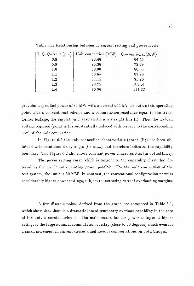
73
Table 6.1: Relationship between dc current setting and power levels
D.C. Current (p.u) Unit connection (MW) Conventional (MW) 0.8 70.46 64.45 0.9 75.36 72.29 1.0 80.00 80.00 1.1 80.65 87.96 1.2 81.15 95.76 1.3
I
70.25 103.51 1.4 18.96 111.22
provides a specified power of 80 MW with a current of 1 kA. To obtain this operating
point with a conventional scheme and a commutation reactance equal to the trans
former leakage, the regulation characteristic is a straight line (i). Thus the no-load
voltage required (point A') is substantially reduced with respect to the corresponding
level of the unit connection.
In Figure 6.2 the unit connection characteristic (graph (ii)) has been ob
tained with minimum delay angle (i.e Qmin) and therefore indicates the capability
boundary. The Figure 6.2 also shows constant power characteristics (in dotted lines).
The power setting curve which is tangent to the capability chart that de
termines the maximum operating power possible. For the unit connection of the
test system, the limit is 80 MW. In contrast, the conventional configuration permits
considerably higher power settings, subject to increasing current overloading margins.
A few discrete points derived from the graph are compared in Table 6.1,
which show that there is a dramatic loss of temporary overload capability in the case
of the unit connected scheme. The main reason for the power collapse at higher
ratings is the large nominal commutation overlap (close to 30 degrees) which even for
a small increment in current causes simultaneous commutations on both bridges.

30
25
---c.S Ji:1 20 ~ ---~
15 0 z <G
~ 10 ~ 0 u
5
0 0 10 20 30 40 50
FIRING ANGLE (DEG.)
Figure 6.3: Variation of commutation angle obtained from TCS
6.4 Designing with Higher Nominal
Firing Angle
74
60
In the previous section, the maximum operating capability of unit connected
scheme was discussed with reference to the minimum firing angle and the maximum
excitation. While the unit connection can be designed to provide a specified nominal
power, the absence of filters limits the operational capability at larger current levels
and thus reduces the ability of HV dc link to provide temporary power increases. This
reduction in operational capability imposes transient stability restrictions. One way
of increasing the transient stability margin is to design the unit connected system
with a slightly higher nominal firing angle.
Figure 6.3 shows the variation of commutation angle for various firing angles
with the constant field excitation, obtained from TCS. It can be seen from the figure
that the commutation angle reduces from 28.9 degrees at O:=O:min (zero degrees for
the test system) to 17.7 degrees at 0:=20 degrees. Hence if the nominal firing angle
is chosen as 20 degrees, that would permit relatively higher current levels before the
commutation angle reaches 30 degrees.
Choosing a higher firing angle reduces the dc voltage and hence the trans-

75
140 ... .?
\ \ \ d; \..!b "\'1,; '/o~
120 \ \1> \' ~ ~~ -:!rlt. ".It-
\ ~~ ~ " " " I " " " " I \ "" " 100 " """ \ \ \ " '-..--...
" '-
~ (i) \ \ '-I \ " '- ...... '"--'" 80 \ "-
f.":>::l \ \ " " "- --\ " '- "-0 \ " '- --" '- "- ......
~ \ " " '-'- 6'o,\f~ ......
...... eo \ " " '- --H " " '- "- -- -- ...... §2 \ ...... '- .s0,\f -- ...... ""'"
" " -- H, --'- '-'- --\ " 40 '- __ 4~ AI!!:: -- __
" '- "-
"- -- -- -.J°"yw -- -- --" "- --"- -- -- -- _ 20A-nv- - - -...... - -20 "- - - - --- -__ 1~MW
0 0.0 0.3 0.6 0.9 1.2 1.5
CURRENT (kA) Figure 6.4: Operational capability charts with a nom=20 deg. (i) Conventional (ii)
Unit connection
mission efficiency. For the unit connected test system, it was found that in order to
have the same dc voltage and dc current as in the previous case (i.e point B of Figure
6.2) for a firing angle of 20 degrees, the increase in required field excitation is 8.7%.
Figure 6.4 shows the voltage regulation characteristic for the unit connected
test system with a nominal firing angle of 20 degrees. Unlike in the amin-case, the
commutation angle is less than 30 degrees for a current level upto 1.5 p.u. But the
amount of extra power that can be obtained is increased by only 6.25%.
Operating the unit connected system at a higher firing angle results in more
control margin for the rectifier control from the minimum firing angle. Normally the
minimum firing angle for rectifier is about 5 degrees. Figure 6.5 shows the voltage
regulation characteristics for a=20 degrees and a=5 degrees. It is seen from the fig
ure that by having a firing angle margin of 15 degrees, the power transfer capability
has increased by 26.0%. But the higher firing angle would also produce higher cur
rent harmonics and hence more rotor losses. For the test system, the total current
harmonics increased ftom 3.55% for anom=O degree to 6.93% for a nom =20 degrees.

120
100
80
60
40
20
, I
\ \
\
\ \
\
\
"-
\ \
" " "-
"-........
" "-
" " "-
"-
....... - --- ~ _ 2.:!..M~ - -- -___ ~M~ __ _ - - - -o L-________ L-________ L-______ ~~~----~--------~
0.0 0.3 0.6 0.9
CURRENT (kA) 1.2 1.5
76
Figure 6.5: Operational capability charts with control margin (i) a nom=20 deg. (ii)
deg.
6.5 Effect of Field Forcing
In the previous section it was seen that the operating capability could be
increased by having some firing angle margin. Referring to the Figure 6.5, the ca
pability of unit connected test system is increased by 26% (point A) when rectifier
firing angle is decreased to 5 degrees from the nominal value of 20 degrees, which can
be utilised to supply extra power. But, when the system is operated with a low firing
angle, the rectifier loses its control margin. Also, at the maximum power (point A in
Figure 6.5), the dc voltage is reduced by 4%, which would reduce the transmission
efficiency also.
As discussed in section 6.2, the generator excitation control for unit connec
tions could be used to take over the function of On Load Tap Changers to keep the
firing angle within the pre-determined range. This excitation control was modelled in
TCS to calculate the additional amount of excitation required to keep the dc voltage
at 1.0 p.u. Table 6.2 shows the extra excitation requirement to maintain a nominal

Table 6.2: Extra Excitation requirement to increase the capability
D.C. Power (p.u)
firing angle of 20 degrees.
1.1 1.2 1.3 1.4
.
Extra Excitation (%) 3.051 • 7.759
11.511 19.415
•
77
When the excitation requirement becomes high, extra materials are required
to keep temperatures down. Also, when the excitation levels increase, the air-gap flux
density tends to increase, resulting in air-gap instability.
6.6 Current Harmonics
In the. conventional scheme, the current rating ofthe generator is practically
determined by the fundamental frequency component, as the filters will absorb the
steady state harmonic current components. On the other hand, since filter circuits are
omitted in the unit connections, the current harmonics generated by the rectifier have
to be absorbed by the generator. Their major effect upon the generator is an extra
heating of the rotor surface and the damper winding due to the induced harmonic
currents in the rotor circuit.
In order to compute the amount of harmonic currents generated by the
convertors, a time domain simulation was carried out, from which under steady state
condition the current waveform entering the generator was analyzed into fundamental
and harmonic currents. This harmonic analysis was performed by varying the firing
angle and keeping the same generator excitation.
Figure 6.6 shows the levels of 11th and 13th harmonic currents. For compar
ison with the conventional scheme, the harmonics were also calculated using the clas
sical analysis with the transformer reactance as the commutation reactance and the
convertor terminal ac voltage as the commutating voltage [Kimbark 1971]. The dotted
lines in Figure 6.6 show the harmonic current levels for the conventional scheme.
Two different effects are observed. First a considerable reduction in the

10
8
2
o
/ /
o
,/
/
15
- -- -------
- --
unit-connection
- - - - conventional
30 45 60 75 FIR. ANGLE (DEG.)
Figure 6.6: Current harmonic content of the 12-pulse convertor
78
gO
current harmonic levels of the unit connection, which is due to the better shape
caused by the increased commutation overlap. The second effect is the oscillatory
nature of the harmonic currents with a, in the case of unit connection. This effect is
caused by the variation of commutation parameters as explained in chapter 5.
6.7 Generator Rating
The calculation of generator rating for the unit connection should include
the total rms current rather than the fundamental frequency component alone. This
is to ensure that the extra harmonic loading of the machine does not result in extra
temperature rise for the machine as a whole and specifically in the hot spots of the
machine. The equivalent continuous negative sequence current is often used as the
indicator to find out whether the generator can withstand the extra heating, without
any derating.
Normally the generators are provided with a thermal cushion to sustain
an equivalent of 10% negative sequence current loading [IEEE 1973]. The negative
sequence current loading is a rough indicator of the permissible extra losses due to
unbalanced operation. The diode-rectifier as well as the controlled rectifier with

79
20 .-------------------------------------------~
5
o o 15 30 45 60 75 90
FIRING ANGLE (DEG.)
Figure 6.7: Equivalent Negative Sequence current derived from TCS
equidistant pulse firing devices represent an almost ideal symmetrical load. The
remaining unsymmetries are due to differences in transformer or generator phase
reactances as well as in differences in the firing angles. It has been shown [Reeve
1969] that these effects are negligible in terms of negative sequence load. Hence it is
possible to utilise the generator's extra margin for the additional harmonic losses.
To facilitate comparison of the rotor heating effect of the convertor loads
with standard specification ratings of generators, an equivalent continuous negative
sequence current len is defined as that which causes equal rotor heating as the con
vertor load it specifies. The equivalent negative sequence current of the generator due
to harmonic currents is given by [Krishnayya 1973]:
(6.1)
The variation of equivalent negative sequence current with varying delay
angle for the unit connected test system is shown in Figure 6.7. The results show
that for a 12-pulse convertor, the total harmonic losses represent less than 16% ofthe
losses caused by the permissible continuous negative sequence load. At the normal
firing angle range (in the vicinity of 15 degrees), the harmonic losses represent less
than 10% for the unit connected test system.

c.!J
~ g2 .........
S r:x:1 ~
60
50
40
30
20
10
0 0 15 30 45 60
FIR. ANGLE (DEG.)
salient rn/ c
- - non-salient m! c
75
Figure 6.8: Effect of rotor saliency on voltage harmonic distortion
80
90
6.8 AC Voltage Harmonics
In the absence of filters, ac voltage waveform would be considerably dis
torted. Moreover, the synchronous machine acts like a frequency convertor in the
presence of harmonic currents and creates additional voltage harmonics.
In unit connected HV de systems, ac voltage harmonics are important In
assessing the quality of ac voltage waveforms and the insulation strength of stator
windings. The operation of convertor firing controllers are dependent on the quality
of ac voltage waveform. The voltage distortion at the generator terminal of an unit
connection can be assessed by using either a time domain simulation program like
TCS or the iterative analysis in harmonic domain [Eggleston 1985].
In order to assess the amount of voltage distortion at the generator terminal
of the unit connected test system (including a salient machine), the dynamic simula
tion program TCS was carried out for various firing angles with constant generator
excitation. Under steady state conditions, the terminal ac voltage at the generator
was analysed into fundamental and harmonic components. The continuous lines in
Figure 6.8 show the voltage harmonic levels with respect to firing angles.
In order to show the effect of rotor saliency on voltage harmonic distor-
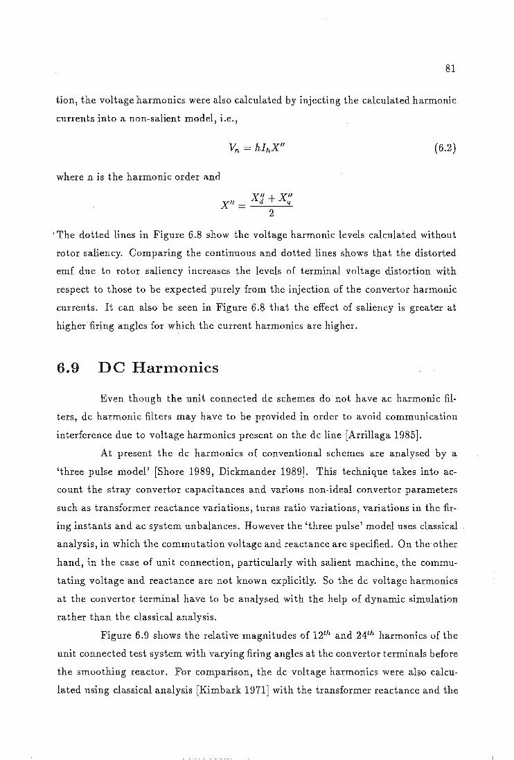
81
tion, the voltage harmonics were also calculated by injecting the calculated harmonic
currents into a non-salient model, i.e.,
(6.2)
where n is the harmonic order and
)("
I The dotted lines in Figure 6.8 show the voltage harmonic levels calculated without
rotor saliency. Comparing the continuous and dotted lines shows that the distorted
emf due to rotor saliency increases the levels of terminal voltage distortion with
respect to those to be expected purely from the injection of the convertor harmonic
currents. It can also be seen in Figure 6.8 that the effect of saliency is greater at
higher firing angles for which the current harmonics are higher.
6.9 DC Harmonics
Even though the unit connected dc schemes do not have ac harmonic fil
ters, dc harmonic filters may have to be provided in order to avoid communication
interference due to voltage harmonics present on the dc line [Arrillaga 1985].
At present the dc harmonics of conventional schemes are analysed by a
'three pulse model' [Shore 1989, Dickmander 1989J. This technique takes into ac
count the stray convertor capacitances and various non-ideal convertor parameters
such as transformer reactance variations, turns ratio variations, variations in the fir
ing instants and ac system unbalances. However the 'three pulse' model uses classical
analysis, in which the commutation voltage and reactance are specified. On the other
hand, in the case of unit connection, particularly with salient machine, the commu
tating voltage and reactance are not known explicitly. So the dc voltage harmonics
at the convertor terminal have to be analysed with the help of dynamic simulation
rather than the classical analysis.
Figure 6.9 shows the relative magnitudes of 12th and 24th harmonics of the
unit connected test system with varying firing angles at the convertor terminals before
the smoothing reactor. For comparison, the dc voltage harmonics were also calcu
lated using classical analysis [Kimbark 1971] with the transformer reactance and the

82
20
uni t connection
conventional
~lh \ --,.-..... .....
..... ,/
./ ./
-- .J~ -" ----...... ./
o ......
o 10 20 30 40 50 60
FIRING ANGLE (DEG.) Figure 6.9: DC voltage harmonics derived from TCS
terminal voltage as the commutation reactance and voltage respectively. These are
shown in dotted line. Figure 6.9 shows that the relative magnitudes of dc voltage
harmonics are higher than those of the conventional scheme.
6.10 Conclusion
The absence of simple equations capable of establishing general relationships
in terms of commutating voltage and commutating reactance makes it impossible to
provide charts of general applicability. Each individual scheme needs to be modelled
to derive operating capability charts and also to determine the harmonic ratings.
While the unit connection can be designed to provide any specified nominal
power, the absence of filters limits the operational capability at larger current levels
and thus reduces the ability of the HV de link to provide temporary power increases.
This reduction in operational capability imposes transient stability restrictions that
must be taken into account in economic comparisons and its conventional alternative.
It is possible to increase the operational capability of unit connections by
providing control margin and also by field forcing during the overload condition. But
this alternatives would result in extra cost.

83
Harmonic spectra has been derived for a typical test case with the aid of
dynamic simulation. The results show as expected, a reduction in harmonic current
levels caused by the increased commutation overlaps. However the generator harmonic
voltages in the presence of rotor saliency are considerably higher. The dc voltage
harmonics show higher values than in the conventional scheme.

84
Chapter 7
C ARACTERISTICS OF
VARIABLE SP ED
OPE ATION OF UNIT
CONNECTIONS
7 .1 Introduction
The synchronous nature of a conventional power system requires the gener
ation of a common frequency at all the interconnecting power stations. Apart from
the need for a complex frequency control, the common frequency restriction prevents
the individual generating units from operating at their optimal efficiencies.
In the absence of local load, the unit connection concept can be extended to
generate power at varying frequencies to suit the optimal operation of the turbines.
Examples of possible application for such schemes are remote hydro stations, wind
farms and tidal power stations.
The existing information available on the variable speed operation of unit
connections have only highlighted the economic advantages [Ingram 1988, Naidu
1989]. Very little is known about their operating characteristics.
The main characteristics of constant frequency unit connected schemes were
discussed in the previous chapter. In this chapter, the main factors affecting the
operating characteristics of a 12-pulse unit connected generator-convertor system to
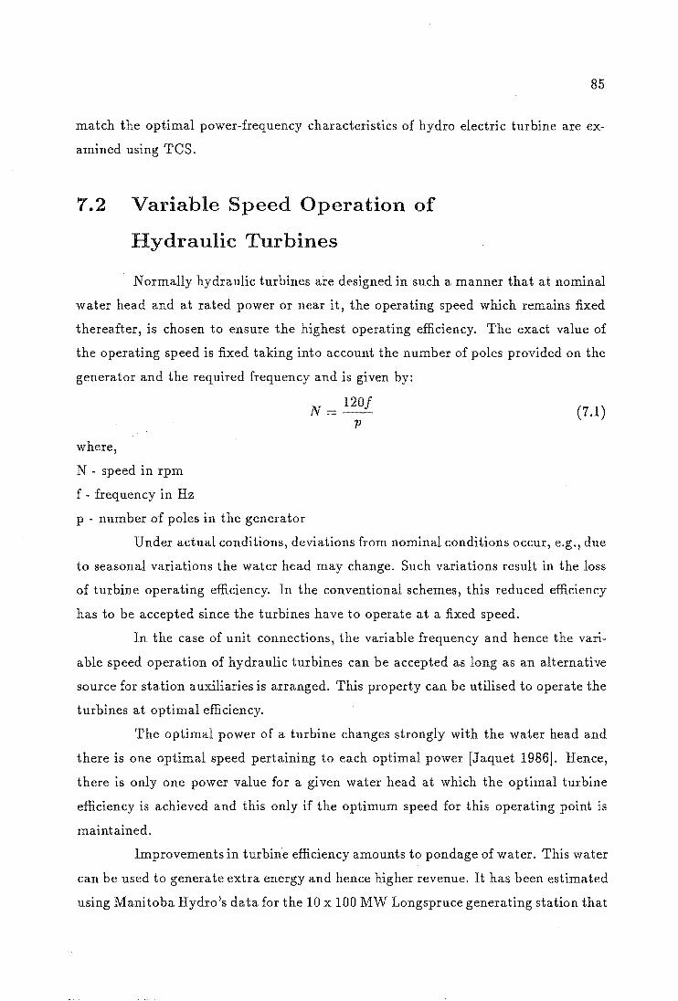
85
match the optimal power-frequency characteristics of hydro electric turbine are ex
amined using TCS.
7.2 Variable Speed Operation of
Hydraulic Turbines
Normally hydraulic turbines are designed in such a manner that at nominal
water head and at rated power or near it, the operating speed which remains fixed
thereafter, is chosen to ensure the highest operating efficiency. The exact value of
the operating speed is fixed taking into account the number of poles provided on the
generator and the required frequency and is given by:
where,
N - speed in rpm
f - frequency in Hz
p - number of poles in the generator
N = 1201 p
(7.1)
Under actual conditions, deviations from nominal conditions occur, e.g., due
to seasonal variations the water head may change. Such variations result in the loss
of turbine operating efficiency. In the conventional schemes, this reduced efficiency
has to be accepted since the turbines have to operate at a fixed speed.
In the case of unit connections, the variable frequency and hence the vari
able speed operation of hydraulic turbines can be accepted as long as an alternative
source for station auxiliaries is arranged. This property can be utilised to operate the
turbines at optimal efficiency.
The optimal power of a turbine changes strongly with the water head and
there is one optimal speed pertaining to each optimal power [Jaquet 1986]. Hence,
there is only one power value for a given water head at which the optimal turbine
efficiency is achieved and this only if the optimum speed for this operating point is
maintained.
Improvements in turbine efficiency amounts to pondage of water. This water
can be used to generate extra energy and hence higher revenue. It has been estimated
using Manitoba Hydro's data for the 10 x 100 MW Longspruce generating station that

86
60
50
..-N 40 ::r:: "--'
>--u 30 z
J:::l P 01' J:::l
20 ~ Pz;...
10
0 0 20 40 60 60 100
POWER (MW)
Figure 7.1: Power-frequency characteristics of the turbine
the annual savings due to variable speed operation would be of the order of US$L24M
[Naidu 1989].
7.3 Test System
Some information has recently become available on the efficiency of hydro
turbines operating at varying speeds [Jaquet 1986, Vogele 1986J. In the Pan Jia Kou
scheme, China, consideration has been given to variable speed operation because of
the large differences in water head expected (between 36 and 86 metres). Figure
7.1 shows a range of power-frequency characteristics relating to this scheme for an
acceptable range of turbine efficiencies. Table 7.1 shows the discrete values of power
and frequency values for 100% and 96% efficiencies.
The generator, transformer and convertor plant will have to be rated for the
power generated at the maximum frequency.
In the absence of detailed information of the Pan Jia Kou generator char
acteristics, the data selected has been taken from a typical hydro machine of similar

87
Table 7.1: Turbine Power/Speed Characteristics
100% turbine efficiency 96% turbine efficiency Power Frequency Power Frequency (MW) (Hz) (MW) (Hz)
82 49.6 85 54.0 60 46.0 51 46.0 36 40.0 30 39.2 22 34.4
power rating and is given in Appendix E. Also to try and keep the commutation re
actance within re.asonable limits, the transformer leakage reactance has been reduced
to a low but realizable 5% value.
The dc system cOI).sidered is a back-to-back system in which the rectifier
is at constant firing angle and the invertor controls the power. The rectifier firing
angle is chosen as zero degrees. The controllers were modelled in TCS using modular
controller models described in chapter 2 and typical d.c voltage and current waveforms
derived with the TCS algorithm are shown in Figure 7.2.
All the waveforms are processed by the Fast Fourier Transform to obtain
information of Vde and Ide (averaged), as well as the harmonic content of the voltage
and currents on both sides of the convertor. To reduce sampling errors at points
of discontinuity, a high number of samples is recommended for the FFT processing
(1024 samples per cycle are used in the present work). But, the variable frequency
introduces small errors in the FFT processing due to spectral leakage [Arrillaga 1985]
caused by the presence of non-harmonic frequency modulation between the two ter
minals.
7.4 Operating Characteristics
It is a general requirement in ac systems as well as in dc systems that a
generator maintains an almost constant voltage over the full power range. However
the generator no-load voltage should vary when operated over a wide range of speed

88
(a)
BO~----------~----------------~
60
II 1\ \ \ 1\ .1 . \ II II \ 1\ 1\ 1\ 1\ 1\ 1\ 1\ 1\ 1\ \ 1\ 1\ \
t ~ ~ ¥ ~ ~ ~ t l ~ ~ ~ ~ ~ l l l v y v v ~
20 -
O~----_·------~I----~I----~I----~
0.05 0.06 0.07 0.08 0.09 0.10
TIME (s)
(b)
O.B
0.7
0.6 --. ~ 0.5 '--"
E-J ~ 0.4 p:; p:; ;::J 0.3 u
0.2
0.1
0.0 0.05 0.06 0.07 0.08 0.09 0.10
TIME (s)
Figure 7.2: DC side waveforms derived from TCS (a) voltage (b) current

89
1.2 60 vol tage
1.0 50
---. --- 0.8 40 N P ::r:: P--. ---"'----" ::-r£l 0.6 30
u CJ Z ~ r:LI E-t :=> --:l 0' <:)
0.4 20 r:LI
:> p:: J::z:..
0.2 10
0.0 0 0 20 40 60 80 100
POWER (MW)
Figure 7.3: Variable frequency operating characteristic at 100% turbine efficiency
according to:
(7.2)
where E is the generator no-load voltage, f is the frequency and the subscript n
represents the nominal value. The factor Kj due to induction is frequency dependent
and increases from 1 to 1.1 p.u when the frequency drops from 50 to 34 Hz.
In order to assess the voltage regulation during the variable speed operation
of unit connections, the dynamic simulations were carried out for 100% and 96%
efficiency cases shown in Figure 7.1. The results of the simulation are illustrated in
Figures 7.3 and 7.4.
Figure 7.3 shows some important results for the case of 100% efficiency.
As the frequency is reduced from 50 Hz, the d.c voltage increases from 1 p.u to a
maximum of 1.085 p.u (corresponding to a frequency of 46 Hz). However the voltage
increase (8.5%) can be compensated by firing angle or excitation control. Further
reductions in frequency appear to have very little effect on the d.c voltage down to
the minimum 34.4 Hz specified for maximum efficiencies.
For the reduced efficiency case (96%), Figure 7.4 shows a larger d.c voltage
regulation (from 0.99 to 1.09 p.u), that is a 9% overvoltage, which again can be
maintained constant by firing angle or excitation control. The larger firing angle will

1.2 r-------------------------.
1.0
S 0.8 P-. -----t3 0.6
~ o :> 0.4
0.2
0.0 '------L------L--_--1 ____ --L-___ --.J
60
50
40
30
20
10
0 o 20 40 60 80 100 POWER (MW)
90
-N ::::c: "'--"
:::-u z ~ :::::> 0-~ ~ r:=..
Figure 7.4: Variable frequency operating characteristic at 96% turbine efficiency
Table 7.2: Effect of firing angle control on generator
! f (Hz) Pdc (MW) a (deg.) Vd/Vdn Vg/"Vgn · 19 (kA) 54 85 0 1.086 1.066 3.409 54 85 11 1.0 1.005 3.616 50 80 0 1.0 1.0 3.434
39.2 30 0 0.997 0.9738 1.325
increase the reactive power absorbed by the convertor, which will in turn reduce the
generator terminal voltage to the required level.
For the test system under consideration, the maximum firing angle variation
required to keep the d.c voltage constant (between 39.2 and 54 Hz) is 11 degrees and
the maximum generator terminal voltage in that region is L005 p.u. The effect of
increased firing angle control on the generator voltage (fundamental rms) and current
(total rms) rating is illustrated in Table 7.2. The generator current has increased by
6% but the generator terminal voltage remains almost constant.

91
7.5 Evaluation of the Need for an
OLTC
For a unit connection operating under constant speed, On Load Tap Chang
ers (OLTC) are not required at the rectifier transformer. Generator excitation control
can take over the task of OLTC, as illustrated in the previous chapter. This further
reduces the capital cost and improves the reliability. However, since the generator
emf varies due to a wide variation of turbine speed, the need for OLTC have to be
evaluated for unit connections during the variable speed operation.
Figures 7.3 and 7.4 show different dc voltage responses to the variable fre
quency unit connection systems at 100% and 96% efficiencies.
With reference to Figure 7.3 (100% turbine efficiency operation), an increase
of frequency from 49.6 to 51 Hz would extend the operating region from 80 to 85 MW.
However the machine internal emf only increases by about 2% and the extra power
demands a substantial increase in dc current. As a result, the dc voltage is depressed
to 0.9 p.u. The use of a 10% range of OLTC makes it possible to provide the extra
power with nominal dc voltage. However further increases of frequency and power
would require unrealistically high tap change control.
In contrast, Figure 7.4 (96 % turbine efficiency) shows good controllability at
the upper end of the frequency range, but some dc voltage reductions for frequencies
below 34 Hz. However the voltage reduction at low frequency (0.03 p.u at 33.3 Hz)
is of little significance.
Considering the limited effectiveness of the OLTC, it would be difficult to
justify the extra cost. Instead, a slightly reduced turbine efficiency (96% in the test
case) is an acceptable alternative for power generation beyond the nominal frequency.
7.6 Harmonic Effects
The total generator harmonic distortion in the variable frequency application
is determined, as in the constant frequency case, by maximum power rating. Although
there will be a reduction in the generator cooling capability at the lower speeds, the
power and current levels will also be reduced.
There are two problems specific to variable frequency operation in need of

92
examination, i.e. reductions in harmonic frequencies at low speeds and frequency
interactions between the two ends of the HV dc link.
7.6.1 Reduction of the Effective Pulse
Number
The frequencies of the harmonic components on the dc side of the convertor
will reduce in proportion to the generated frequency. For the test case under consid
eration, the lowest frequency of the dominant harmonic will be 400 Hz (i.e. 33.33 x
12). This is an effective reduction in the pulse number from 12 to 8, with reference to
50 Hz. Moreover the dc current harmonic levels do not decrease with power because
these are caused by the dc voltage ripple, which is kept practically constant.
Harmonic elimination by filters is impractical with variable frequency and
the only way to meet the Equivalent Disturbing Current levels (NZED 1983], if re
quired by legislation, will be to reduce the dc voltage at lower frequencies. However
this solution would destroy the benefit of variable frequency.
Dynamic simulation studies for varying firing angles indicate that the 400
Hz content is in the order of 1 % of the dc operating current, which may be sufficient
to cause electromagnetic interference [Arrillaga 1985].
7.6.2 Interaction Between Terminals
The lowest dominant frequency of the rectifier (i.e 400 Hz for the test case)
corresponds to the 8th harmonic of 50 Hz and will cause some 7th and 9th harmonic
currents at the invertor end.
Similarly the dominant frequency of the invertor end (i.e 600 Hz) corresponds
to the 18th harmoni c of the lowest genera ted frequency of the test system (33 .33Hz ).
Simulation results for optimum efficiency power generation at that frequency with a
20 degrees firing angle show the appearance of up to 1 and 0.5% content of 17th and
19th harmonics respectively in the generator currents.
As the generated frequency increases above 33.33 Hz, both the rectifier and
invertor ac current waveforms will contain small amounts of variable frequency com
ponents (not necessarily harmonic related).
There are also small amounts of intermodulated frequencies (the sum and

93
difference of the characteristic frequencies produced by the two convertors). As the
generated frequency goes through the full range, the differences between dc ripple
harmonics will produce all frequencies, including the natural frequency of the dc
transmission system.
For the unit connected test system, the intermodulated frequencies which
are small amounts of non-characteristic harmonics could not be quantified, due to the
presence of dc component in the machine stator currents explained in chapter 4.
The harmonic distortion of the generator currents increases as the frequency
reduces. Comparative values of Total Harmonic Distortion Factor (( j'L-Il)/ II) cor
responding to 33.33 and 50 Hz are 0.155 and 0.035 respectively.
However the generator currents at low frequencies are only a fraction of the
nominal levels and the increased waveform distortion is not a problem.
7 .. 7 Conclusion
The characteristics of variable speed unit connected generator-convertor
plant have been derived using dynamic simulation algorithm.
Dynamic simulation results have shown the capability of a unit connected
hydro system to provide controllable dc voltage for frequencies in the range of 33.33
to 50 Hz. At the upper end of the frequency, power increases beyond the nominal
level cannot be achieved at the full efficiency without extra excitation or On Load Tap
Changers. However considering the limited effectiveness of the On Load Tap Changer,
it is unlikely that their presence will be justified; instead, excursions offrequency (and
power) beyond the nominal levels can still be achieved at full dc voltage, if a small
(about 4%) reduction in turbine efficiency can be accepted.
The use of lower frequencies has been shown to cause two special problems.
One is a reduction in the dominant harmonic frequency of the dc line which may cause
electromagnetic interference. The second problem is the appearance of relatively
small values of many non-characteristic frequency components in the dc line and ac
phase currents, which must be taken into consideration when designing unit connected
schemes.

94
Chapter 8
CONCLUSIONS
A critical factor so far ignored in the comparison between conventional and
unit connected schemes is the maximum operational capability of the system rather
than the rating capability of the individual plant components. The operating charac
teristics of the unit connection are normally discussed with reference to the conven
tional steady state formulation. However, in the absence of harmonic filters, the use
of such formulation must be reconsidered. The main objective of this thesis has been
to assess the validity of conventional steady state formulation and show the need for
dynamic simulation to derive the steady state characteristics of unit connected HV dc
systems.
Dynamic simulation programs are being used as an alternative to physical
simulators in assessing the performance of ac/ dc systems. Two basically different
approaches are currently used in HV dc dynamic simulation, i.e., the Electromagnetic
Transient Program (EMTP) and state variable technique. Transient Convertor Simu
lation (TCS) program based on the state variable algorithm, which has the ability to
predict exact voltage crossings, firing instants and commutation intervals, has been
used in this thesis to derive unit connection characteristics.
The TCS program, developed at the University of Canterbury, contains
models such as time varying ac system equivalents, frequency dependent equivalents
and convertor transformer magnetic history to represent an ac/ dc system. The main
criticism made against this program has been the lack of realistic controller models.
Work has been carried out to provide more realistic and flexible controller models,
which have been incorporated in TCS program.

95
Ideally, the digital programs should be validated by comparison with sys
tem recordings. However, such comparisons are unrealistic because of the difficulties
involved in setting up identical test system conditions in each model. Thus the only
other realistic comparison is between two digital programs, based on fundamentally
different algorithms. In this thesis, TCS has been compared with another dynamic
simulation program, EMTDC which is based on EMTP algorithm. The compari
son has concentrated on the convertor algorithms and has shown that the two algo
rithms predict the same convertor responses following large disturbances. Hence, both
EMTDC and TCS algorithms can be used with confidence to simulate the transient
response of ac/ dc convertors.
The comparison of TCS and EMTDC has not included ac system compo
nents such as generators. Since both TCS and EMTDC contain similar machine
models, the dynamic simulation of generator-HVdc convertor units needs to be com
pared with a different model simulation. This comparison is necessary to validate the
dynamic simulation of unit connected systems. As the continuation of this work, TCS
must be compared with Finite Element program used by GEC, UK which contains a
comprehensive machine model.
The commutation process in unit connected HV dc systems has been analysed
using TCS. It has been shown that the conventional steady state formulation based
on the use of specified commutating voltage and reactance is not applicable to the
unit connection. A modified steady state formulation, which does not require the
specification of commutating voltage and reactance, has been proposed. However,
in the presence of machine rotor saliency, even this formulation is not applicable for
unit connection and so dynamic simulation must be used to derive the unit connected
HV dc system steady state characteristics.
Each individual unit connected HVdc scheme requires extensive dynamic
analysis to determine its characteristics. With reference to a typical unit connected
system, the operating capability charts have been derived using TCS and compared
with a corresponding conventional scheme. The results have shown that the unit
co:n.nections have limitations in their operational capability and additional costs are
involved to increase their capability to that of conventional schemes. This factor,
which has so far been neglected, must be taken into consideration while comparing
unit connections with conventional schemes.

96
The steady state analyses of unit connections have further been extended
to include variable frequency operation so as to match the optimal turbine efficiency.
In constant frequency operation, the On Load Tap Changers (OLTC) would not be
needed, whereas their need must be evaluated during variable speed operation, due
to a wide variation of generator internal emf. Again, dynamic simulation is necessary
for such an evaluation. It has been shown, with reference to the test system, that
it is possible to operate the turbine-generator units without an OLTC within a wide
range of frequencies, at high efficiencies and with good voltage controllability.
In the conventional scheme, the current rating of the generator is determined
by the fundamental frequency component, as the filters absorb the steady state har
monic current components. On the other hand, the unit connected generator must be
rated for total rms current. Derivation of harmonic spectra using conventional formu
lation cannot be used for unit connected systems and must be derived from dynamic
simulation. Moreover, under variable speed operation, the interactions between the
terminals produce non-characteristic harmonic and non-harmonic frequencies which
cannot be analysed using conventional formulation. Dynamic simulation and FFT
have been combined to derive the harmonic spectra for the unit connected test system
under constant and variable speed operation. However, the use of variable frequency
introduces small errors in the FFT processing due to spectral leakage caused by the
presence of non-harmonic frequency modulation between the two terminals.
The FFT analyses of machine stator currents derived from TCS have shown
the presence of small amounts of dc component, which otherwise should not be
present. By adopting various numerical techniques, the magnitude of this dc com
ponent has been reduced considerably. However, it has been difficult to quantify the
expected uncharacteristic harmonics during variable speed operation due to the pres
ence of this dc component in the stator currents. Hence, further work is still required
to eliminate this dc component.
Dynamic simulation of generator-HVdc convertor units is extremely de
manding computationally and the initial values for the simulation are estimated from
the single-phase simplified analysis. It should be possible to reduce the computation
time by starting the dynamic simulation from better initial values. Work is currently
underway at the University of Canterbury to model the generator, convertor and
transformer in harmonic domain, which would be computationally more efficient for

97
steady state analysis of unit connections. Better initial values for dynamic analysis
can also be obtained from such programs.
The conventional ac/ dc load flow and transient stability programs cannot
be used for systems involving unit connections, since they are based on the steady
state formulation. Instead, the characteristics derived from dynamic simulation can
be used in such programs to represent unit connected systems and this work is also
currently underway at the University of Canterbury.
98
References
[Ainsworth 1967] Ainsworth, J.D. "Harmonic instability between controlled static
convertors and a.c networks", Proc. lEE, Vol. 114, No.7, pp 949-
957.
[Ainsworth 1968] Ainsworth, J.D. "The phase-locked oscillator-a new control system
for controlled static convertors", IEEE Trans., PAS-87, pp 859-864.
[Al-Khasali 1976J AI-Khasali, H.J. "Generalised dynamic modelling of high voltage
dc-ac transmission systems", Ph.D Thesis, University of Manchester
Institute of Science and Technology, UK, 1976.
[Arrillaga 1970] Arrillaga, J., Galanos, G., and Powner. E.T. "Direct digital control
of h.v.d.c convertors", IEEE Trans., PAS-89, No.8, pp 2056-2065.
[Arrillaga 1983a] Arrillaga, J. "High voltage direct current transmission", Peter Pere
grinus Ltd., London, 1983.
[Arrillaga 1983b] Arrillaga, J., Arnold, C.P. and Harker, B.J "Computer modelling
of electrical power systems", John Wiley & Sons Ltd., 1983.
[Arrillaga 1985J Arrillaga, J., Bradley, D.A. and Bodger, P.S."Power system har
monics", John Wiley & Sons, 1985.
[Bowles 1970]
[Bowles 1989]
Bowles, J., "A.C system and transformer representation for HV de
transmission studies", IEEE Trans., PAS-88, No.7, pp 1603-1609.
Bowles, J., "HV dc unit connected generators- receiving end con
trol", paper no. IV-07, International colloquium on HV dc power
transmission, 13-15 August 1989, Recife, Brazil.

99
[Calverley 1973] Calverley, T.E., Ottaway, C.H. and Tufnell, D.H.A., "Concepts of a
unit generator convertor transmission system", lEE Conference on
High Voltage DC and AC Transmission, London, 1973.
[Campos Barros 1976] Campos Barros, J.G., "Dynamic modelling of synchronous
machines connected to HV de transmission systems", Ph.d Thesis,
University of Manchester Institute of Science and Technology, UK,
1976.
[Campos Barros 1977] Campos Barros, J.G., "Stability of isolated generator-HVdc
convertor units", IEEE Summer Power Meeting, 1977, paper no.
A-77508-5.
[Campos Barros 1989] Campos Barros, J.G., "Direct connection of generators to
HV de convertors: main characteristics, comparative advantages and
prospectives in Brazil", paper no. IP-17, presented at II Symposium
of specialists in 'electric operation and expansion planning', 21-25
August 1989, Sao Paulo, Brazil.
[Cazzani 1988] Cazzani, M., Schiappacasse, A., Testi, G., Pincella, C., and Valfre,
L., "HV de simulator versus computer modelling for SACOI 2 HV de
link insulation co-ordination studies", paper no. 14-11, International
conference on Large High Voltage Electric Systems (CIGRE), 28
Aug. - 3 Sep., 1988, Paris.
[Chen 1962] Chen, W.Y., "An investigation of commutation problems in a static
power convertor", Ph.d Thesis, University of Manchester Institute
of Science and Technology, UK, 1962.
[CIGRE 1988] "Records of meetings of SC-11 and SC-14, CIGRE, Paris, France,
1988.
[Concordia 1951] Concordia, C., "Synchronous Machines Theory and Performance",
John Wiley & Sons, 1951.
[de Silva 1987] de Silva, J.R., "Capability charts for power systems)), Ph.D Thesis,
University of Canterbury, New Zealand, 1987.

100
[Dickmander 1989] Dickmander, D.L. and Peterson, K.J., "Analysis of de harmonics
using the three-pulse model for the Intermountain power project
HV dc transmission", IEEE Trans., Power Delivery, Vol. 4, No.2, pp
1195-1204.
[Dommel1969] Dommel, H.W., "Digital computer solution of electromagnetic tran
sients in single and multiple networks", IEEE Trans., PAS-88, No.
4, pp 388-99.
[Dunfield 1967] Dunfield, J.C. and Barton, T.H., "Effect of m.m.f permeance har
monics in electrical machines (with special reference to a syn
chronous machine)", Proc. lEE, Vol. 14, No. 10, 1967.
[Eggleston 1985] Eggleston, J.F., "Harmonic modelling of transmission systems con
taining synchronous machines and static convertors", Ph.D Thesis,
UniversIty of Canterbury, New Zealand, 1985.
[EI-Serafi 1980] EI-Serafi, A.M. and Shehata, S.A., "Effect of synchronous machine
parameters on its harmonic analysis under thyristor bridge opera
tion", IEEE Trans., PAS-99, No.1, pp 59-67.
[EPRI1983] "Methodology for integration of HV dc links in large ac systems -
Phase 1: Reference manual", EPRI project report, no. EL-3004,
1983.
[Giesner 1971] Giesner, D.B., "The dynamic behaviour of acJdc power systems un
der ac fault conditions", Ph.D Thesis, University of Manchester In
stitute of Science and Technology, UK, 1971.
[Gleadow 1989] Gleadow, J.C., O'Brien, M.T., Fletcher, D.E. and Bisewski, B.J.,
"Uprating the HVdc system in New Zealand" paper no. VIII-01,
International colloquium on HV dc power transmission, 13-15 August
1989, Recife, Brazil.
[Hausler 1980] Hausler, M. and Kanngiesser, K.W., "Generator- convertor unit con
nection with thyristor and diode rectifiers", Proc. of Symposium on
'Incorporating power transmission into system planning', sponsored
by US DOE, Phoenix, Arizona, USA, March 24-27,1980, pp 255-271.

101
[Heffernan 1980] Heffernan, M.D., "Analysis of ac/ dc system disturbances", Ph.D
Thesis, University of Canterbury, New Zealand, 1980.
[Heffernan 1981] Heffernan, M.D., Arrillaga, J., Turner, K.S. and Arnold, C.P.,
"Computation of ac/dc system disturbances. Part-1: Interactive
co-ordination of generator and convertor transient models", IEEE
Trans. PAS-100, No. 11, pp 4341-4348.
[Hungasutra 1989] Hungasutra, S. and Mathur, R.M.," Unit connected generation
with diode valve rectifier scheme", IEEE Trans., Power Systems,
Vol. 4, No.2, pp 538-543.
[IEEE 1973]
[IEEE 1990]
IEEE Working Group report, "A standard for generator continuous
unbalanced current capability", IEEE Trans., PAS-73, pp 320-329.
IEEE committee report on "Application aspects of multi terminal
dc power transmission", IEEE Trans., Power Delivery, VoL 5, No.
4, Nov. 1990, pp 2084-2098.
[Ingram 1988] Ingram, L., "A practical design for an integrated HV dc unit con
nected hydro-electric generating station", IEEE Trans., Power De
livery, VoL 3, No.4, pp 1615-1620.
[Jaquet 1986] Jaquet, M., "The Pan Jia Kou pumped storage station, part I: Hy
draulic equipment", Fourth ASME International Hydro power Fluid
Machinery Symposium, Anaheim, Decmeber 1986.
[Jones 1967] Jones, C.V., "The unified theory of electrical machines", Butter
worths, 1967.
[Joosten 1989] Joosten, A.P.B., Arrillaga, J., Arnold, C.P. and Watson, N.R., "Sim
ulation of HV dc system disturbances with reference to the mag
netising history of the convertor transformers", IEEE PES summer
meeting, Long Beach, California, July 9-14, 1989.
[Kanngiesser 1983] Kanngiesser, K.W., "Unit connection of generator and convertor
to be integrated in HV dc or HVac energy transmission", Interna
tional symposium on HVdc technology, Rio de Janeiro, Brazil, 1983.

102
[Kanngiesser 1989] Kanngiesser, K.W., "Controlfunctions and their allocation within
an unit connection", paper no. IV-01, International colloquium on
HV dc power transmission, 13-15 August 1989, Recife, Brazil.
[Kimbark 1968] Kimbark, E.W., "Power system stability: Synchronous machines",
Dover publications, New York, 1968.
[Kimbark 1971] Kimbark, E.W., "Direct current transmission, voL 1", Wiley Inter
science, 1971.
[Krishnayya 1973] Krishnayya, P.C.S., "Stresses on generators and transformers of
block and double-block connections proposed for HV dc power sta
tion infeed" , lEE conf. on 'High voltage dc and/or ac power trans
mission', Publication No. 107, pp 279-286.
[Krishnayya 1987] Krishnayya, P.C.S., "A review of unit connected generator
convertor connections for HV dc transmission", IEEE/ CSEE Joint
conference on 'High voltage transmission systems", Beijing, China,
1987.
[Manitoba 1988] EMTDC users manual prepared by Manitoba HV dc centre, Canada.
[Mattensson 1986] Mattensson, H., Bahrman, M., Eitzmann, M., Osborn, D. and
Wong, W. "Digital programs and simulators as tools for studying
HV dc systems validation considerations", IEEE Montech'86 con
ference on 'HVdc power transmission', 29 Sept.-1 Oct. 1986.
[Naidu 1989] Naidu, M. and Mathur, R.M.," Evaluation of unit connected vari
able speed hydro-power station for HV dc power transmission", IEEE
Trans., Power Systems, Vol. 4, No.2, pp 668-676.
[NZED 1983] "Limitations of harmonic levels", notice issued by Electricity Divi
sion, Ministry of Energy, NZ.
[Preston 1990] Private communication with Dr.T.E.Preston of Large Machines De
partment, GEC, UK.

[Rangel 1989]
[Reeve 1969]
[Reeve 1988]
[Shore 1989]
[Turner 1980]
[Turner 1981]
[Vogele 1986]
103
Rangel, R.D., Pedroso, A.S. and Campos Barros, J.G.," Dynamic
performance of salient-pole unit connected generators", paper no.
IV-03, International colloquium on HVdc power transmission, 13-15
August 1989, Recife, Brazil.
Reeve, J., Baron, J.A and Krishnayya, P.C.S., " A general approach
to harmonic current generation by HVDC convertors", IEEE Trans.,
PAS-88, No.7, pp 989-995.
Reeve, J. and Adapa, R., "A new approach to dynamic analysis of
ac networks incorporating detailed modelling of dc systems. Part 1:
Principles and Implementation & Part 2: Application to interaction
of dc and weak ac systems", IEEE Trans., Power Delivery, Vol. 3,
No.4, pp 2005-2019.
Shore, N.L., Anderson, G., Canelhas, A.P. and Asplund, G., "A
three-pulse model of dc side harmonic flow in HV dc systems" , IEEE
Trans., Power Delivery, Vol. 4, No.3, pp 1945-1953.
Turner, K.S.,"Transient stability analysis of integrated ac and
dc power systems", Ph.D Thesis, University of Canterbury, New
Zealand, 1980.
Turner, K.S., Heffernan, M.D., Arnold, C.P. and Arrillaga, J.,
"Computation of ac/ dc system disturbances. Part-2: Derivation of
power frequency variables from convertor transient response" , IEEE
Trans. PAS-I00, No. 11, pp 4349-4355.
Vogele, J. and Weber, K., "The Pan Jia Kou pumped storage sta
tion, part II: Electrical equipment", Fourth ASME International Hy
dro power Fluid Machinery Symposium, Anaheim, Decmeber 1986.
[Walker 1953] Walker, J.H., "Operating characteristics of salient-pole machines",
Proc. lEE, Vol. 100, Pt. 2, pp 13-24.
[Watson 1987] Watson, N.R., "Frequency-dependent ac system equivalents for har
monic studies & transient convertor simulation" , Ph.D Thesis, Uni
versity of Canterbury, New Zealand, 1987.

104
[Watson 1988] Watson, N.R. and Arrillaga, J., "Frequency dependent ac system
equivalents for harmonic studies and transient convertor simula
tion", IEEE Trans., Power Delivery, Vol. 3, No.3, pp 1196-2003.
[Williams 1986] Williams, B., "Transient stability studies of large power systems
with multiterminal HVde links", M.E Thesis, University of Canter
bury, New Zealand, 1986.
[Woodford 1983] Woodford, D.A., Gole. A. and Menzies, R.W., "Digital simulation
of dc links and ac machines", IEEE Trans., PAS-102, No.6, pp
1616-1623.
[Woodford 1985] Woodford, D.A., "Validation of digital simulation of dc links" 1 IEEE
Trans., No.9, pp 2588-2595.

105
Appendix A
TCS Controller Modules
This appendix contains the basic controller modules available in TCS to
build any user defined controller. Apart from these modules, any other required
module can be easily incorporated into the program without knowing the structure
of TCS, by adding the required function sub-program.
Function Control block Description
lK Input: X
COSI . X Y . Output: Y -=-. COS(X+K) r-=-
Constants : K .
lK Input: X
TANI -!..... ,:L.
Output: Y TAN(X+K)
Constants: K:

106
Function Control block De3cription
Input: X
ABCD ,.L _A+E. ~, Output: Y C±D.
Constants: A,B,C,D
- Input: X
TRAP -L K(l±.T,l ~ Output: Y l±.T,
Con,stants : K,T!, Tz
,YMAX Input: X
INTG X 1. ~ Output: Y - s
YMIN~ Constants: YMIN,YMAX
Input: X
LIMS -L ymax
y~ax rL Output: Y xmin
Constants: XMIN,XMAX,YMIN,YMAX
1 K 2 X 2 Input :XI ,X2 ,X3
ADD I KIXI E
Y Output: Y
KaXa Constants: 1<11 1(')., 1<3
!K Input: X1,XZ
MULT T Output: Y =KX1XZ
Constants: K
, Input: Xl, X').
DIVD -=.=.....,. -=--... Output: Y

107
Function Control block De3cription
Input: X
-L ymax
r--L LIMC ymi~mnx Output: Y xmin
Constants: XMIN,XMAX,YMIN,YMAX
}Xl Input: X,X1,X2
LlMV -L jX2 ~ Output: Y Xl
lx2 - .
Input: X
EQUA 4 y=x f' Output: Y
Input: X 1,X2
-& -L MAXI Y=max(Xt, X 2 ) Output: Y
~
Xl ~
Input: X 1,X2
~ MINI Y=min(Xl ,X2) Output: Y X 2 ~
Kl Input: X
IN IT -L Initialisation X=K
Constants: K
lK Input: X
SINI -L Y
Output: Y SIN(X+K) t---'-
Constants: K
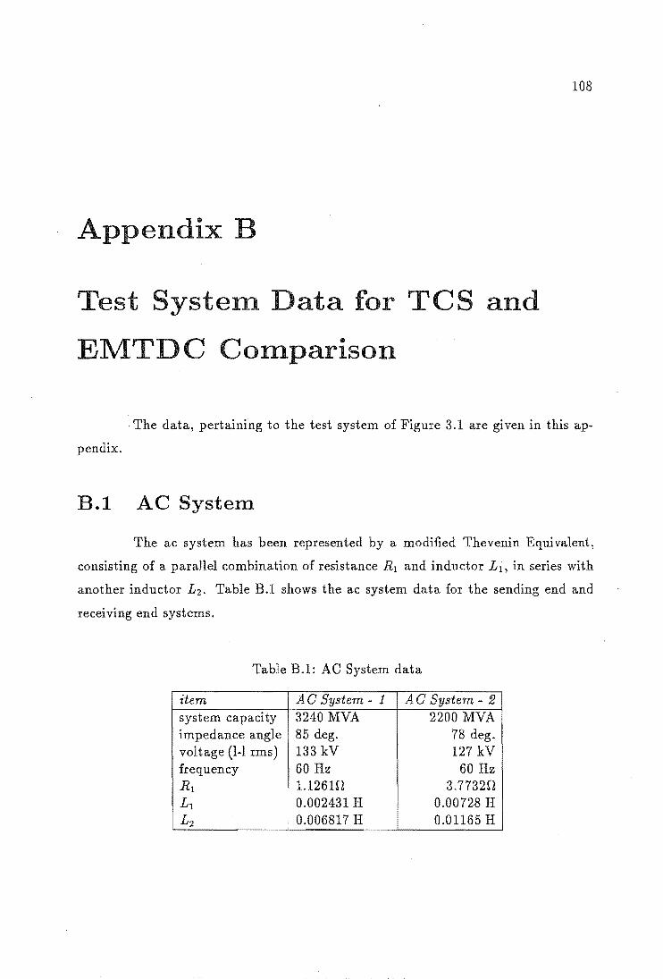
108
Appendix B
Test System Data for TCS and
EMTDC Comparison
. The data, pertaining to the test system of Figure 3.1 are given in this ap-
pendix.
B.l AC System
The ac system has been represented by a modified Thevenin Equivalent,
consisting of a parallel combination of resistance Rl and inductor L 1 , in series with
another inductor L 2 • Table B.1 shows the ac system data for the sending end and
receiving end systems.
Table B.1: AC System data
item AO System - 1 AO System - 12 system capacity 3240 MVA 2200 MVA impedance angle 85 deg. 78 deg. voltage (1-1 rms) 133 kV 127 kV frequency 60 Hz 60 Hz Rl 1.12610 3.7732fl Ll 0.002431 H 0.00728 H L2 • 0.006817 H 0.01165 H

109
B.2 AC Filters
Tuned filters of 5th , 7th , 11th and 13th harmonic are used along with a high
pass filter, on both rectifier and invertor ac buses. The total filter capacity is of 178
MVA each. Tables B.2 and B.3 show the filter data for sending end and receiving
end systems respectively. Table BA shows high-pass filter data, in which the parallel
combination of Rand L is in series with C.
Table B.2: Sending end tuned filters
· Element Unit Filter order I ·5 7 11 13 .
C p,F 5.153 2.6294 4.3204 3.0929 1 L H 0.05457 0.05457 0.01351 0.01351 !
R n 1.7776 2.6664 1.776 • 1. 776
Table B.3: Receiving end tuned filters
Element Unit Filter order 5 17 11 1 13
C p,F 6.3522 3.2408 4.9828 3.5678 L H 0.0442 0.0442 0.01167 0.01167 R n • 2.1032 2.1032 0.7887 0.7887
Table BA: High-pass filters
Element Unit Sending end Receiving end C p,F 12.373 15.367 L
! ~ 0.0012887 0.00107 R 18.6648 11.0418

110
B.3 DC Filters
6th harmonic tuned filters are used on both Rectifier and Invertor dc buses.
Table B.5 shows the dc filter data.
Table B.5: DC filters
! Element Unit Rectifier Invertor ! C p,F 0.8 0.8
I~ H I 0.2444 0.2444 it 12 12
B.4 DC Line
The dc transmission line has been represented as the cascade of 12-pi sec-
tions.
Length
Resistance
Inductance
Capacitance
: 556 km
0.0250hms/km
1.63866 mH/km
: 0.0182073 f.LF
B.5 DC Convertor
B.5.1 Rectifier
Type : 6-pulse
Minimum firing angle 5 deg.
Maximum firing angle 155 deg.
Transformer impedance 0.2 p.u
Transformer rating 341 MV A
Transformer voltage 134/134 kV
Smoothing inductor : 0.75 H

Current reference
B.5.2 Invertor
Type
Minimum firing angle
Maximum firing angle
1.45kA
6-pulse
108 deg.
180 deg.
Transformer impedance : 0.2 p.u
Transformer rating
Transformer voltage
Smoothing inductor
323 MVA
127/127 kV
0.75 H
Extinction angle reference 18 deg.
Current margin . : 180 A
B.6 Controllers
111
The following constants are used by the current and extinction angle con
trollers of Figure 3.2.
B.6.1 Current Control
Proportional gain, Kp : 0.07997 deg/amp
Integral gain, Ki : 5.88 deg/ amp - sec
B.6.2 Extinction Angle Control
Proportional gain, Kp
Integral gain , Ki
: 0.27 rad/rad
: 14.754/sec

112
B.6.3 Transducer Delays
Rectifier : 5 IDS
Invertor : 18 IDS

113
Appendix C
TCS Controller Data File
This appendix gives the TCS controller data file of the test system, used for
the comparison with EMTDC. Since TCS works on per-unit quantities, the controller
constants given in Appendix B have to be converted accordingly.
If 10 and f are the base current and frequency respectively, then the propor
tional and integral constants for the current controllers must be converted according
to the following:
Kp(tcs) = 17.453IoK p rad/pu
K. - 2.77iQ Kj rad/rad .(tcs) - f
Similarly, the extinction angle controllers are converted according to the
following:
Kp(tcs) Kp rad/rad
K. ) - 0,1591(, /rad .(tC3 - f

\
\
CONTROLLER DATA FOR COMPARISON WITH EMTDC
\FN INP1 INP2 INP3 OUT CONi
\--
\
CON2
\ ***** RECTIFIER CURRENT CONTROLLER ******
\
TRAP DI04 10 1.0 0.0
ADDI IDR1 10 Ii -1.0 1.0
MULT Ii PONE 111 0.8821
MULT Ii PONE 122 0.1720
INTG 122 123 0.0873 2.7
ADDI Iii 123 12 1.0 1.0
LIMC 12 A004 0.0873 2.7
INIT 10 1.0
INIT IDR1 2.27
INIT PONE 1.0
\
\ ***** INVERTOR CURRENT CONTROLLER ******
\
TRAP DI05 100 1.0 0.0
ADDI IDR2 100 13 -1.0 1.0
MULT 13 PONE 131 0.8821
MULT 13 PONE 132 0.1720
INTG 132 133 1.9 3.14
ADDI 131 133 14 1.0 1.0
LIMC 14 ALCC 1.9 3.14
IN IT IDR2 2.00
INIT 100 1.0
\
CON3 CON4
1.885
6.885
\ ***** INVERTOR EXTINCTION ANG. CONTROLLER ******
\
ADDI AREF EA05 A2 -1.0 1.0
114

115
MULT A2 PONE A31 0.27
MULT A2 PONE A32 0.0391
INTG A32 A33 1.9 3.14
ADDI A31 A33 A3 1.0 1.0
LIMe A3 ALEX 1.9 3.14
MINI ALee ALEX ADOS
INIT AREF 0.314
END

116
Appendix D
Transformations: d,q,O to a,b,c
Under ideal conditions of sinusoidally distributed stator windings and in
ternal symmetry, there is a mathematical equivalence between the a,b,c and d,q,O
frame of references for stator circuits. The transformation is non-singular and may
be defined as [Concordia 1951, Kimbark 1968J :
Ld 1 1 3/2] Lo
• ] Lq - 1 1 3/2 Lab (D.l)
La 1 -2 0 La2
Under idealised conditions, La2 Lab2' i.e the second harmonic variation
of the stator interphase mutual inductance is equal in magnitude to the variation
of the phase self inductance. This formulation, together with the absence of fourth
harmonic terms is considered to be approximate [Dunfield 1967, Jones 1967J.
and also,
The a,b,c quantities are derived from the inverse transform of equation as :
La2 = Lab2
La4 Lab". 0
1/3
1/6
1/3
1/3
1/6
1/3
1/3] -2/~ (D.2)
The rotor quantities are kept as direct and quadrature axis parameters,
when transforming to the a,b,c frame of reference. This is convenient because of the

117
actual winding arrangement. However, the rotor resistances and inductances must be
scaled down by 2/3, in order to compensate for the rationalisation done to the d,q,O
equations.
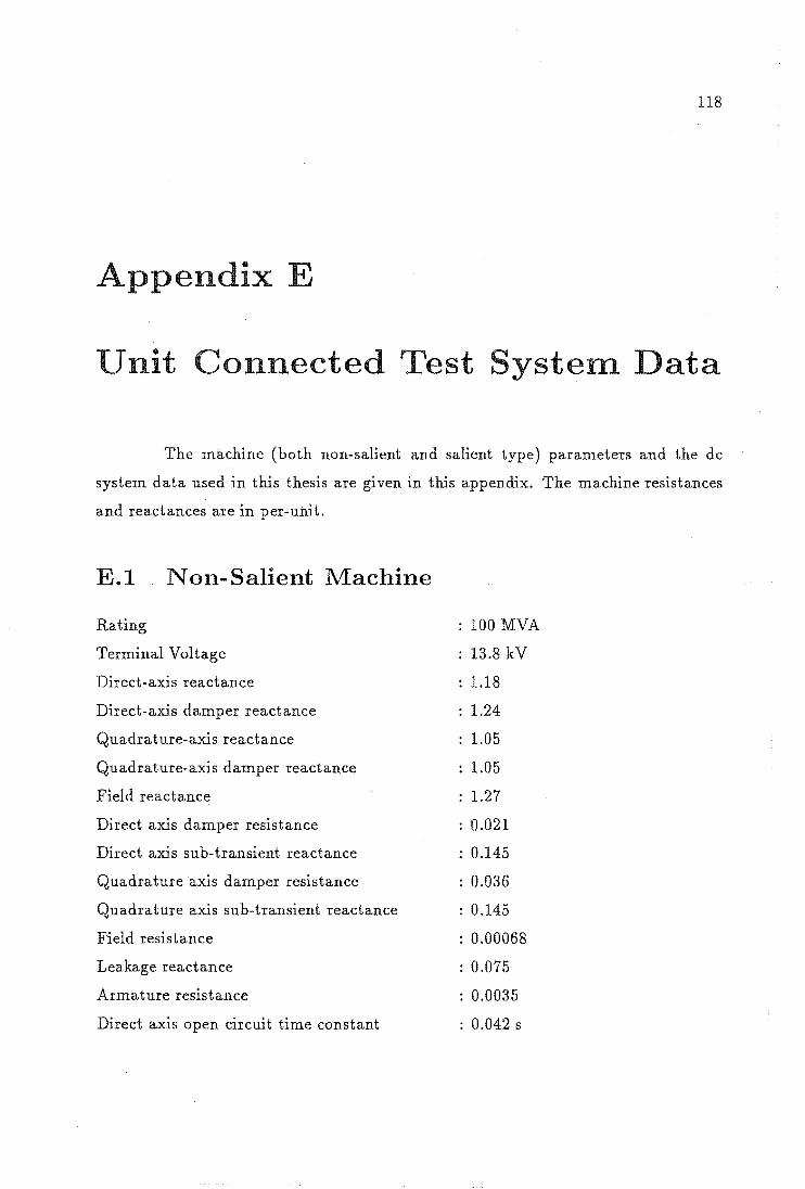
118
Appendix E
Unit Connected Test System Data
The machine (both non-salient and salient type) parameters and the dc
system data used in this thesis are given in this appendix. The machine resistances
and reactances are in per-uhit.
E.l Non-Salient Machine
Rating 100 MVA
Terminal Voltage
Direct-axis reactance
Direct-axis damper reactance
Quadrature-axis reactance
Quadrature-axis damper reactance
Field reactance
Direct axis damper resistance
Direct axis sub-transient reactance
Quadrature axis damper resistance
Quadrature axis sub-transient reactance
Field resistance
Leakage reactance
Armature resistance
Direct axis open circuit time constant
13.8 kV
1.18
1.24
1.05
1.05
1.27
: 0.021
: 0.145
: 0.036
: 0.145
: 0.00068
: 0.075
0.0035
0.042 s
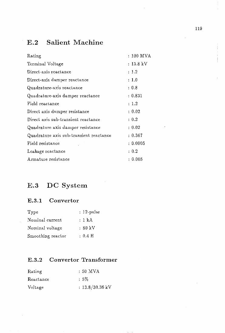
E.2 Salient Machine
Rating 100 MVA
Terminal Voltage
Direct-axis reactance
Direct-axis damper reactance
Quadrature-axis reactance
Quadrature-axis damper reactance
Field reactance
Direct axis damper resistance
Direct axis sub-transient reactance
Quadrature axis damper resistance
Quadrature axis su b- transient reactance
Field resistance
Leakage reactance
Armature resistance
E.3 DC SysteITl
E.3.1 Convertor
Type
Nominal current
Nominal voltage
Smoothing reactor
12-pulse
1 kA
80 kV
0.4 H
E.3.2 Convertor Transformer
Rating
Reactance
Voltage
: 50 MVA
5%
13.8/30.36 kV
13.8 kV
1.2
1.0
0.8
0.831
1.2
0.02
0.2
0.02
0.367
0.0005
: 0.2
: 0.005
119


![[MEAN WELL] 1982 (Charger) DC/AC (Inverter) 8000 (DoE ... · PDF fileAC/DC DC/DC (Converter) (Adaptor) (Charger) DC/AC (Inverter) 8000 LED ... AC AC AC GE12/18/24/30 I AC AC Plug-AU](https://static.fdocuments.in/doc/165x107/5a73363b7f8b9abb538e72a6/mean-well-1982-charger-dcac-inverter-8000-doe-a-acdc-dcdc-converter.jpg)