Dynamic Set: Amortized Analysis
22
Tutorial 4 Dynamic Set: Amortized Analysis
Transcript of Dynamic Set: Amortized Analysis

Tutorial 4
Dynamic Set Amortized Analysis
Computer Algorithms Design and Analysis
ReviewBinary tree
Complete binary treeFull binary tree
2-tree P115 Unlike common binary tree the base case is not an empty tree but a external node
Heap Binary search tree (BST)Balanced BST
Red-Black treehellip
Computer Algorithms Design and Analysis
In the classes we learned the following data structures
BSTHash Table
Closed address Linked listOpen address Rehashing
Dynamic SetUnion-FindwUnion-cFind
Computer Algorithms Design and Analysis
Amortized Analysis
Analyze the cost of a sequence of operationsThe total cost is averaged over all operations performedSome of the operations might be expensiveThe average cost is small
Average performance in the worst caseGives an upper bound
Computer Algorithms Design and Analysis
Amortized Analysis vs Average-case analysis
No probability is involvedGuarantee the average performance of each operation in the worst case
Amortized Analysis vs Adversary AnalysisAdversary gives worst case lower bound Amortized gives average case upper boundAdversary applies for all algorithms theoretically Amortized only applies in some special algorithms
Computer Algorithms Design and Analysis
Example Stack Operations
Consider the following two stack operationsPush push an object onto the stackPopAll pop all object from the stack
There are n operations what is the upper bound of total cost
Computer Algorithms Design and Analysis
Solution 1 Aggregate methodWe can prove the total cost of n operations in the worst cast is O(n)
The total cost of PopAll operations lt= the total cost of Push operationsThe total cost of Push lt=nThus the total cost of n operations lt=2n
So the average cost is O(n)n=O(1) in the worst case
Computer Algorithms Design and Analysis
Solution 2 Accounting methodActual cost
Push1 PopAll k where k is the number of objects in the stack
Accounting costPush 1PopAll -k
Amortized costPush 2PopAll 0
We can prove the total accounting cost is nonnegativeThus for any sequence of n operations the total amortized cost is an upper bound which is 2n
Computer Algorithms Design and Analysis
Solution 3 Potential methodDefine the potential function Φ on a stack to be the number of objects in the stackObviously it satisfies
Φ(D0)=0 Φ(Di)gt=0Amortized cost
If a Push operationPotential difference is Φ(Di)-Φ(Di-1)=(k+1)-k=1So the amortized cost of Push operation is
crsquoi=ci+Φ(Di)-Φ(Di-1)=1+1=2If a PopAll operation
Potential difference is Φ(Di)-Φ(Di-1)=0-k=-kSo the amortized cost of PopAll operation is
crsquoi=ci+Φ(Di)-Φ(Di-1)=k+(-k)=0So the total amortized cost is an upper bound which is 2n
Computer Algorithms Design and Analysis
Types of Amortized Analysis
Aggregate methodAccounting methodPotential method
Computer Algorithms Design and Analysis
(1) Aggregate Method
Consider a sequence of n operationsShow that for all n the n operations takes worse-case time T(n) in totalTherefore each operation is T(n)n (amortized cost) in the worst caseNote that this amortized cost applies to each operation even there are several types of operationsAggregate Method vs Accounting method and Potential method
The accounting method and potential method may assign different amortized cost to different type of operations
Computer Algorithms Design and Analysis
(2) Accounting MethodAssign different charges to different operationsSome operations are charged more or less than their actually costAmortized equation
amortized cost = actual cost + accounting costThe total accounting cost is the difference between the total amortized cost and the total actual costThe total accounting cost must be nonnegative at all times
AssumeEach operation i has an actual cost CiWe charge operation i a fictitious amortized cost CrsquoiWe must ensure that
Thus the total amortized costs provide an upper bound on the total actual costs
Computer Algorithms Design and Analysis
(3) Potential MethodIdea view the bank account as the potential energy of the data structureFramework
Start with an initial data structure D0 (n operations are going to perform on D0)Each operation i has an actual cost Ci Di is the data structure that results after applying the ith operation on data structure Di-1Operation i transforms Di-1 to DiDefine a potential function Φ DirarrR such that Φ(D0)=0 and Φ(Di) ge0 for all iThe amortized cost Crsquoi is defined as
Crsquoi= Ci+ Φ(Di)- Φ(Di-1)
Computer Algorithms Design and Analysis
The amortized cost bounded the actual cost
Choose an appropriate potential function is important
Computer Algorithms Design and Analysis
Example Dynamic TableGoal Make a table as small as possibleProblem What if we donrsquot know the proper size in advanceSolution Dynamic tables
Each time we insert a new element into the table we check whether there is an empty unit If so the insertion needs only 1 operateIf the table overflows we ldquogrowrdquo it by allocating a new larger table (double size of the original one) Move all items from the old table into the new one insert the new element and then free the storage for the old table The total number of operations is 1+(the size of the old table)
Computer Algorithms Design and Analysis
Insert 1Insert 2Insert 3 Insert 4Insert 5Insert 6Insert 7
1 1
2
1
2
3
4
1
2
3
4
5
6
7
Overflow
Overflow
Overflow
Computer Algorithms Design and Analysis
Worst-case analysis
Consider a sequence of n insertions The worst-case time to execute one insertion is Θ(n) Therefore the worst-case time for n insertions is n Θ(n)= Θ(n2)
WRONG
Computer Algorithms Design and Analysis
Solution 1 aggregate methodLet Ci= the cost of the ith insertion
if i-1 is an exact power of 21 otherwisei
iC ⎧
= ⎨⎩
i 1 2 3 4 5 6 7 8 9 10table size 1 2 4 4 8 8 8 8 16 16
Ci 1 2 3 1 5 1 1 1 9 1Overhead 0 1 2 0 4 0 0 0 8 0
=1+2lg(i-1)
Computer Algorithms Design and Analysis
The cost of n insertion is
lg( 1)
1 0
2 2 3 ( )nn
ji
i j
C n n n n nminus⎢ ⎥⎣ ⎦
= =
= + le + = = Θsum sum
Computer Algorithms Design and Analysis
Solution 2 accounting methodActual costAccounting costAmortized cost Cirsquo=3we can prove Thus a upper bound of n insertion is
1
3 ( )n
ii
C n n=
= = Θsum
i 1 2 3 4 5 6 7 8 9 10table size 1 2 4 4 8 8 8 8 16 16
Ci 1 2 3 1 5 1 1 1 9 1Overhead 0 1 2 0 4 0 0 0 8 0
Store 1 2 2 2 2 2 2 2 2 2Crsquoi 2 3 3 3 3 3 3 3 3 3
Consume 0 -1 -2 0 -4 0 0 0 -8 0
lg( 1)1 2 if i-1 is an exact power of 21 otherwise
i
iCminus⎧ +
= ⎨⎩
lg( 1)2 2 if i-1 is an exact power of 22 otherwise
i
iaminus⎧ minus
= ⎨⎩
Computer Algorithms Design and Analysis
Solution 3 Potential methodDefine a potential function We have
If i-1 is an exact power of 2
If i-1 is not an exact power of 2
So we have an upper bound
lg lg0( ) 2 2 (assume 2 =0)iiD i ⎡ ⎤ ⎡ ⎤⎢ ⎥ ⎢ ⎥Φ = minus
lg lg( 1)
lg lg( 1)
(2 2 ) (2( 1) 2 )
2 (2 2 ) 2 (2( 1) ( 1)) 3
i ii
i i
C i i i
i i i i
minus⎡ ⎤ ⎡ ⎤⎢ ⎥ ⎢ ⎥
minus⎡ ⎤ ⎡ ⎤⎢ ⎥ ⎢ ⎥
= + minus minus minus minus
= + minus minus = + minus minus minus minus =
lg lg( 1)
lg lg( 1)
1 (2 2 ) (2( 1) 2 )
1 2 (2 2 ) 3
i ii
i i
C i i minus⎡ ⎤ ⎡ ⎤⎢ ⎥ ⎢ ⎥
minus⎡ ⎤ ⎡ ⎤⎢ ⎥ ⎢ ⎥
= + minus minus minus minus
= + minus minus =
1
3 ( )n
ii
C n n=
= = Θsum
Computer Algorithms Design and Analysis
i 1 2 3 4 5 6 7 8 9 10
table size 1 2 4 4 8 8 8 8 16 16
Ci 1 2 3 1 5 1 1 1 9 1
Overhead 0 1 2 0 4 0 0 0 8 0
Φ(Di) 1 2 2 4 2 4 6 8 2 4
Crsquoi 2 3 3 3 3 3 3 3 3 3
ΔΦ 1 1 0 2 -2 2 2 2 -6 2
- Tutorial 4 Dynamic Set Amortized Analysis
- Amortized Analysis
- Example Stack Operations
- Types of Amortized Analysis
- (1) Aggregate Method
- (2) Accounting Method
- (3) Potential Method
- The amortized cost bounded the actual cost
- Example Dynamic Table
- Worst-case analysis
-

Computer Algorithms Design and Analysis
(3) Potential MethodIdea view the bank account as the potential energy of the data structureFramework
Start with an initial data structure D0 (n operations are going to perform on D0)Each operation i has an actual cost Ci Di is the data structure that results after applying the ith operation on data structure Di-1Operation i transforms Di-1 to DiDefine a potential function Φ DirarrR such that Φ(D0)=0 and Φ(Di) ge0 for all iThe amortized cost Crsquoi is defined as
Crsquoi= Ci+ Φ(Di)- Φ(Di-1)
Computer Algorithms Design and Analysis
The amortized cost bounded the actual cost
Choose an appropriate potential function is important
Computer Algorithms Design and Analysis
Example Dynamic TableGoal Make a table as small as possibleProblem What if we donrsquot know the proper size in advanceSolution Dynamic tables
Each time we insert a new element into the table we check whether there is an empty unit If so the insertion needs only 1 operateIf the table overflows we ldquogrowrdquo it by allocating a new larger table (double size of the original one) Move all items from the old table into the new one insert the new element and then free the storage for the old table The total number of operations is 1+(the size of the old table)
Computer Algorithms Design and Analysis
Insert 1Insert 2Insert 3 Insert 4Insert 5Insert 6Insert 7
1 1
2
1
2
3
4
1
2
3
4
5
6
7
Overflow
Overflow
Overflow
Computer Algorithms Design and Analysis
Worst-case analysis
Consider a sequence of n insertions The worst-case time to execute one insertion is Θ(n) Therefore the worst-case time for n insertions is n Θ(n)= Θ(n2)
WRONG
Computer Algorithms Design and Analysis
Solution 1 aggregate methodLet Ci= the cost of the ith insertion
if i-1 is an exact power of 21 otherwisei
iC ⎧
= ⎨⎩
i 1 2 3 4 5 6 7 8 9 10table size 1 2 4 4 8 8 8 8 16 16
Ci 1 2 3 1 5 1 1 1 9 1Overhead 0 1 2 0 4 0 0 0 8 0
=1+2lg(i-1)
Computer Algorithms Design and Analysis
The cost of n insertion is
lg( 1)
1 0
2 2 3 ( )nn
ji
i j
C n n n n nminus⎢ ⎥⎣ ⎦
= =
= + le + = = Θsum sum
Computer Algorithms Design and Analysis
Solution 2 accounting methodActual costAccounting costAmortized cost Cirsquo=3we can prove Thus a upper bound of n insertion is
1
3 ( )n
ii
C n n=
= = Θsum
i 1 2 3 4 5 6 7 8 9 10table size 1 2 4 4 8 8 8 8 16 16
Ci 1 2 3 1 5 1 1 1 9 1Overhead 0 1 2 0 4 0 0 0 8 0
Store 1 2 2 2 2 2 2 2 2 2Crsquoi 2 3 3 3 3 3 3 3 3 3
Consume 0 -1 -2 0 -4 0 0 0 -8 0
lg( 1)1 2 if i-1 is an exact power of 21 otherwise
i
iCminus⎧ +
= ⎨⎩
lg( 1)2 2 if i-1 is an exact power of 22 otherwise
i
iaminus⎧ minus
= ⎨⎩
Computer Algorithms Design and Analysis
Solution 3 Potential methodDefine a potential function We have
If i-1 is an exact power of 2
If i-1 is not an exact power of 2
So we have an upper bound
lg lg0( ) 2 2 (assume 2 =0)iiD i ⎡ ⎤ ⎡ ⎤⎢ ⎥ ⎢ ⎥Φ = minus
lg lg( 1)
lg lg( 1)
(2 2 ) (2( 1) 2 )
2 (2 2 ) 2 (2( 1) ( 1)) 3
i ii
i i
C i i i
i i i i
minus⎡ ⎤ ⎡ ⎤⎢ ⎥ ⎢ ⎥
minus⎡ ⎤ ⎡ ⎤⎢ ⎥ ⎢ ⎥
= + minus minus minus minus
= + minus minus = + minus minus minus minus =
lg lg( 1)
lg lg( 1)
1 (2 2 ) (2( 1) 2 )
1 2 (2 2 ) 3
i ii
i i
C i i minus⎡ ⎤ ⎡ ⎤⎢ ⎥ ⎢ ⎥
minus⎡ ⎤ ⎡ ⎤⎢ ⎥ ⎢ ⎥
= + minus minus minus minus
= + minus minus =
1
3 ( )n
ii
C n n=
= = Θsum
Computer Algorithms Design and Analysis
i 1 2 3 4 5 6 7 8 9 10
table size 1 2 4 4 8 8 8 8 16 16
Ci 1 2 3 1 5 1 1 1 9 1
Overhead 0 1 2 0 4 0 0 0 8 0
Φ(Di) 1 2 2 4 2 4 6 8 2 4
Crsquoi 2 3 3 3 3 3 3 3 3 3
ΔΦ 1 1 0 2 -2 2 2 2 -6 2
- Tutorial 4 Dynamic Set Amortized Analysis
- Amortized Analysis
- Example Stack Operations
- Types of Amortized Analysis
- (1) Aggregate Method
- (2) Accounting Method
- (3) Potential Method
- The amortized cost bounded the actual cost
- Example Dynamic Table
- Worst-case analysis
-
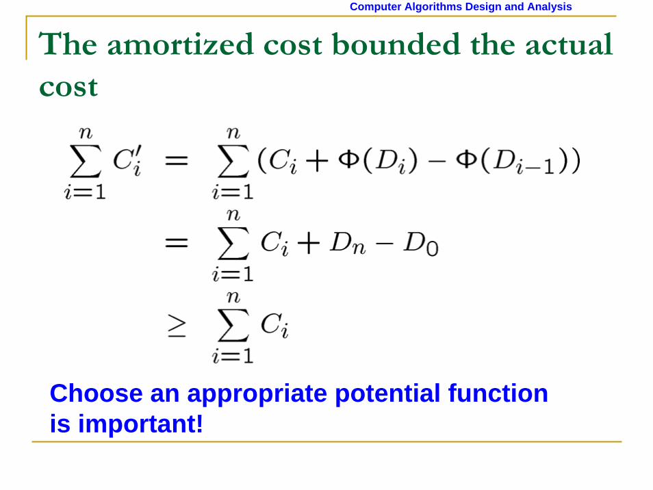
Computer Algorithms Design and Analysis
The amortized cost bounded the actual cost
Choose an appropriate potential function is important
Computer Algorithms Design and Analysis
Example Dynamic TableGoal Make a table as small as possibleProblem What if we donrsquot know the proper size in advanceSolution Dynamic tables
Each time we insert a new element into the table we check whether there is an empty unit If so the insertion needs only 1 operateIf the table overflows we ldquogrowrdquo it by allocating a new larger table (double size of the original one) Move all items from the old table into the new one insert the new element and then free the storage for the old table The total number of operations is 1+(the size of the old table)
Computer Algorithms Design and Analysis
Insert 1Insert 2Insert 3 Insert 4Insert 5Insert 6Insert 7
1 1
2
1
2
3
4
1
2
3
4
5
6
7
Overflow
Overflow
Overflow
Computer Algorithms Design and Analysis
Worst-case analysis
Consider a sequence of n insertions The worst-case time to execute one insertion is Θ(n) Therefore the worst-case time for n insertions is n Θ(n)= Θ(n2)
WRONG
Computer Algorithms Design and Analysis
Solution 1 aggregate methodLet Ci= the cost of the ith insertion
if i-1 is an exact power of 21 otherwisei
iC ⎧
= ⎨⎩
i 1 2 3 4 5 6 7 8 9 10table size 1 2 4 4 8 8 8 8 16 16
Ci 1 2 3 1 5 1 1 1 9 1Overhead 0 1 2 0 4 0 0 0 8 0
=1+2lg(i-1)
Computer Algorithms Design and Analysis
The cost of n insertion is
lg( 1)
1 0
2 2 3 ( )nn
ji
i j
C n n n n nminus⎢ ⎥⎣ ⎦
= =
= + le + = = Θsum sum
Computer Algorithms Design and Analysis
Solution 2 accounting methodActual costAccounting costAmortized cost Cirsquo=3we can prove Thus a upper bound of n insertion is
1
3 ( )n
ii
C n n=
= = Θsum
i 1 2 3 4 5 6 7 8 9 10table size 1 2 4 4 8 8 8 8 16 16
Ci 1 2 3 1 5 1 1 1 9 1Overhead 0 1 2 0 4 0 0 0 8 0
Store 1 2 2 2 2 2 2 2 2 2Crsquoi 2 3 3 3 3 3 3 3 3 3
Consume 0 -1 -2 0 -4 0 0 0 -8 0
lg( 1)1 2 if i-1 is an exact power of 21 otherwise
i
iCminus⎧ +
= ⎨⎩
lg( 1)2 2 if i-1 is an exact power of 22 otherwise
i
iaminus⎧ minus
= ⎨⎩
Computer Algorithms Design and Analysis
Solution 3 Potential methodDefine a potential function We have
If i-1 is an exact power of 2
If i-1 is not an exact power of 2
So we have an upper bound
lg lg0( ) 2 2 (assume 2 =0)iiD i ⎡ ⎤ ⎡ ⎤⎢ ⎥ ⎢ ⎥Φ = minus
lg lg( 1)
lg lg( 1)
(2 2 ) (2( 1) 2 )
2 (2 2 ) 2 (2( 1) ( 1)) 3
i ii
i i
C i i i
i i i i
minus⎡ ⎤ ⎡ ⎤⎢ ⎥ ⎢ ⎥
minus⎡ ⎤ ⎡ ⎤⎢ ⎥ ⎢ ⎥
= + minus minus minus minus
= + minus minus = + minus minus minus minus =
lg lg( 1)
lg lg( 1)
1 (2 2 ) (2( 1) 2 )
1 2 (2 2 ) 3
i ii
i i
C i i minus⎡ ⎤ ⎡ ⎤⎢ ⎥ ⎢ ⎥
minus⎡ ⎤ ⎡ ⎤⎢ ⎥ ⎢ ⎥
= + minus minus minus minus
= + minus minus =
1
3 ( )n
ii
C n n=
= = Θsum
Computer Algorithms Design and Analysis
i 1 2 3 4 5 6 7 8 9 10
table size 1 2 4 4 8 8 8 8 16 16
Ci 1 2 3 1 5 1 1 1 9 1
Overhead 0 1 2 0 4 0 0 0 8 0
Φ(Di) 1 2 2 4 2 4 6 8 2 4
Crsquoi 2 3 3 3 3 3 3 3 3 3
ΔΦ 1 1 0 2 -2 2 2 2 -6 2
- Tutorial 4 Dynamic Set Amortized Analysis
- Amortized Analysis
- Example Stack Operations
- Types of Amortized Analysis
- (1) Aggregate Method
- (2) Accounting Method
- (3) Potential Method
- The amortized cost bounded the actual cost
- Example Dynamic Table
- Worst-case analysis
-
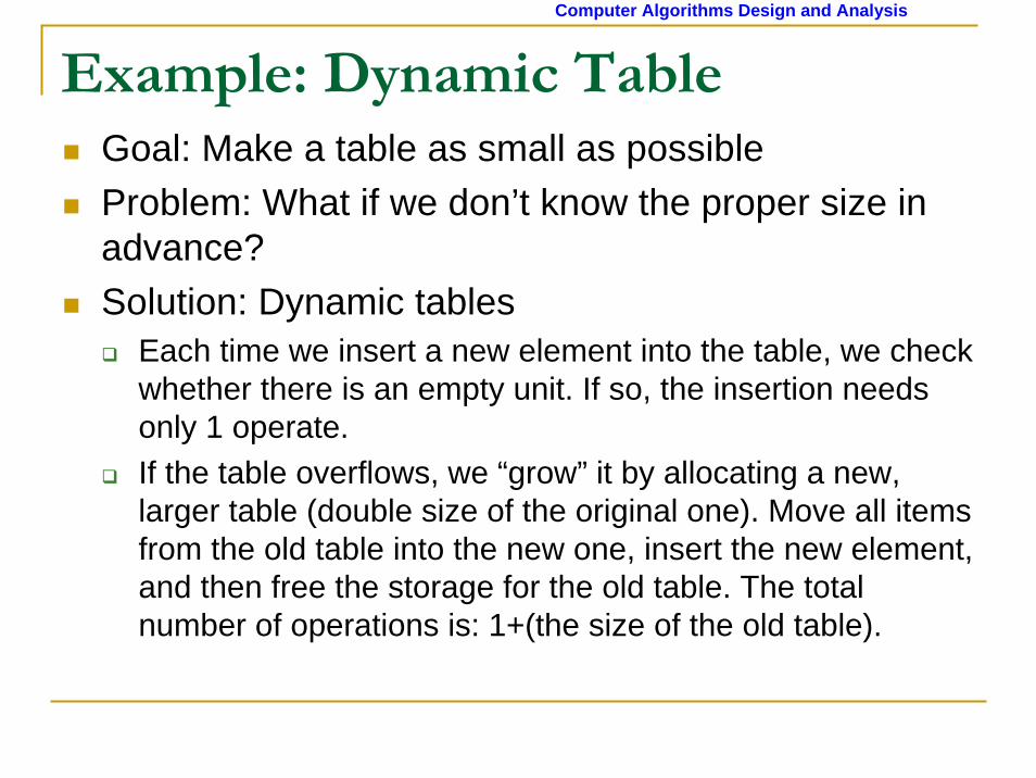
Computer Algorithms Design and Analysis
i 1 2 3 4 5 6 7 8 9 10
table size 1 2 4 4 8 8 8 8 16 16
Ci 1 2 3 1 5 1 1 1 9 1
Overhead 0 1 2 0 4 0 0 0 8 0
Φ(Di) 1 2 2 4 2 4 6 8 2 4
Crsquoi 2 3 3 3 3 3 3 3 3 3
ΔΦ 1 1 0 2 -2 2 2 2 -6 2
- Tutorial 4 Dynamic Set Amortized Analysis
- Amortized Analysis
- Example Stack Operations
- Types of Amortized Analysis
- (1) Aggregate Method
- (2) Accounting Method
- (3) Potential Method
- The amortized cost bounded the actual cost
- Example Dynamic Table
- Worst-case analysis
-


![binary heap, d-ary heap, binomial heap, amortized analysis ... · Amortized Complexity [amortizovaná složitost] In an amortized analysis , the time required to perform a sequence](https://static.fdocuments.in/doc/165x107/5ed29bc1016d386359233e54/binary-heap-d-ary-heap-binomial-heap-amortized-analysis-amortized-complexity.jpg)