Dynamic Revenue Analysis: Experience of the...

Dynamic Revenue Analysis: Experience of the States cslf.gsu.edu

Dynamic Revenue Analysis: Experience

of the States Peter Bluestone and Carolyn Bourdeaux

APRIL 21, 2015

A joint report with the Fiscal Research Center


ACKNOWLEDGMENTS

Special thanks to David Sjoquist, Sally Wallace, Maggie Reeves, Andrew Feltenstein, and Mark

Rider for their careful edits and comments on this report. Their efforts are much appreciated; any

errors are our own.

http://cslf.gsu.edu/


Table of Contents

Introduction 1

Literature Review: The Effects of State-Level Tax Changes on the Economy 2

Dynamic Revenue Analysis 6

Economic Theory 6

Types of Dynamic Models 10

Input-Output Models 10

Computable General Equilibrium Models 11

The REMI Model 12

Experience from the States 14

Overview 14

State Case Studies 15

California: Dynamic Revenue Analysis Model 15

Oregon: Oregon Tax Incidence Model 19

Nebraska: Tax Revenue Analysis in Nebraska 20

Massachusetts: REMI 21

Ohio: REMI 22

New Mexico: REMI 23

Kansas: STAMP 24

Conclusion: Pros and Cons of Dynamic Revenue Models 26

References 28

About the Authors 33

About the Center for State and Local Finance 33

1


Introduction

Revenue analysis, as traditionally employed by most states, estimates the direct or “static” effect

of a tax policy change and may also include an estimate of behavioral responses to a tax change.

Behavioral effects are most often calculated for tax changes where elasticities (or the

responsiveness to a tax change in the market directly affected) are well known or easy to

estimate. For example, an analysis of an increase in the tobacco tax will typically estimate 1) the

increased revenue based on current tobacco sales, which is the static effect, and 2) the offsetting

revenue decrease from lower tobacco product sales as people respond to the increase in price,

which is the behavioral effect. For simplicity, when the term “static revenue estimate” is used in

this report it refers to either a pure static effect or a static and direct behavioral effect.

Dynamic revenue analysis considers the behavioral implications in the market directly affected by

the tax change but goes further, taking into account the subtle interactions and feedback effects

on behavior within the entire economy. The dynamic analysis typically used at the state level

considers how a tax change will affect the economic behavior of individuals and firms throughout

the economy and then attempts to predict the effect of the change on economic variables and

subsequently on governmental tax revenues. For example, a dynamic model considers that an

increase in tobacco taxes affects a smoker’s choice of whether to buy a pack of cigarettes, but

also how it affects the income that smokers have available to purchase other products, the

revenues of the tobacco industry, the jobs provided through the industry, the purchase of

products to support cigarette production, etc. These economy-wide changes associated with one

policy change may affect state tax revenues.1

This report examines the empirical evidence on the relationship between state level tax changes

and the economy, the theoretical economic interactions behind dynamic revenue analysis, the

different types of dynamic models that have been developed, and then states’ experiences with

these models.

Overall, we find that the empirical literature shows a negative effect of state-level tax increases

on economic variables and a positive effect from tax cuts, but the effect size may be small or

indeterminate. An important consideration is that state tax revenues are typically used to pay for

government spending on public services, and these expenditures also have dynamic effects which

may mute or cancel the effects of a tax change.

In terms of state experiences with dynamic revenue estimation, states have found that dynamic

analysis is considerably more costly and complex than traditional static revenue analysis and

1 In several places this report refers to a hypothetical increase in the tax on cigarettes in an effort to illustrate the

subtle differences between static and dynamic modeling. We use the tax on cigarettes because it is easy conceptually to understand. However, please note that traditional excise taxes on specific products, such as cigarettes, are not readily analyzed using current dynamic modeling techniques because the dynamic effects are just too small.


2


depends on the accuracy of thousands of parameters needed to estimate the interaction effects

across various economic actors within and external to a state. The dynamic revenue models

reviewed in this report show widely varying dynamic effects from tax changes, ranging from 1

percent to as much as 30 percent. (By dynamic effect, we mean the difference between the static

estimate and a revenue estimate using a dynamic model.)

States appear to go into dynamic revenue estimation with the expectation that they can use the

estimates for budgeting or forecasting, but not only are dynamic estimates highly sensitive to

different specifications, but even with a sizable tax change and a large projected dynamic effect,

the dynamic revenues generated (or lost) will still usually be within the average error rate for a

state’s overall revenue estimate. Many models also assume that the dynamic revenue

adjustments take five to six year to fully materialize. The implications are that at least for

budgetary purposes the difference between the dynamic and static effects of tax changes are too

small, too imprecise, and too temporally distant to build into a state’s revenue estimate and thus

capture as a fiscal savings or loss. That being said, dynamic analysis can provide useful

information for comparing alternative policy choices and for examining the economic implications

of different policies.

Literature Review: The Effects of State-Level Tax Changes on the Economy

Dynamic models are grounded in economic theory and are abstractions of the economy, but

research-based evidence from the actual performance of the economy provides an important

guide in the development of dynamic models. This section briefly discusses the research-based

findings on the impact of state tax policy on the economy, as well as the estimated magnitude of

such effects.2 The research, for the most part, concludes that while there is a negative effect of

taxes on the economy, the magnitude of the effect may be small or indeterminate and may be

washed out in whole or in part depending on which expenditures categories are changed in order

to maintain a balanced budget.

In conducting an analysis of the effect of state taxes on state economic activity there are some

key considerations:

● Balanced Budget Requirements and Service Mix: Most states face some form of annual

balanced budget requirement. While states may have some wiggle room (such as running

deficits in their pensions or moving payments from year to year), states generally cannot run

large multi-year deficits, and even if they could, they face the discipline of the credit markets.

2 Because state and local revenue and expenditure portfolios are heavily intertwined, most state level research

focuses on state and local revenues and expenditures. As a result, we will often refer to state and local taxes and expenditures but are largely focused on policy changes and their implications at the state level.


3


Because of the balanced budget constraints, a cut in taxes must be paired with an increase in

other taxes or a cut in expenditures, which in turn has dynamic effects on economic

indicators. Thus, any empirical analysis must consider both taxes and expenditures.

Further, state and local governments are heavily involved in funding services that are often

found to have dynamic effects of their own. Such economically “productive” services are

often identified as education, transportation, and other investments in human and physical

capital. This implies that the composition of changes in expenditures needs to be considered

in any empirical analysis.

● Federalism: There are several factors to consider in correctly measuring the economic impact

of tax changes. Firms and households within a state not only face state tax rates but local tax

rates as well. Thus, any analysis needs to consider both. Additionally, some state taxes are

deductible from federal taxes and some states allow a deduction for federal taxes paid. The

net effect of these deductions needs to be considered in an analysis of the economic impact

of tax changes.

Last, states compete with one another. What often matters to firms in making location

decisions are a state’s taxes relative to those in other states. So, any empirical analysis needs

to consider taxes in competing states.

EFFECT OF STATE TAXES ON THE ECONOMY

In the 1990s, there were arguably two key reviews of the literature on the effect of taxes on the

state economy: Bartik (1991) and Wasylenko (1997). The authors concluded that taxes had a

statistically significant negative impact on state economic output—though the size of the effect

was potentially subject to measurement error and most likely small. Bartik (1991) found across a

set of 48 studies that a 10 percent decline in state and local taxes (holding constant

governmental spending) induced between 1 and 6 percent growth (around 3 percent on average)

in long-run economic activity indicators such as personal income, employment or investment.3 He

noted that non-revenue neutral tax changes typically must be accompanied by an expenditure

increase or decrease—which in turn would have an offsetting economic effect. Studies that failed

to control for offsetting expenditure effects often found a much smaller tax effect since the

expenditure effects were muting the tax effects.4

In updating and expanding Bartik’s literature review, Wasylenko (1997) found that the

responsiveness of economic factors to tax changes ranged from an implausible 157 percent to

3 In this section we are referring to the elasticities described in the papers. To make the numbers roughly comparable

we typically use a 10 percent tax change as the benchmark, although the elasticities in academic papers will typically reference a 1 percent change. So most of the actual reported elasticities have been adjusted (made larger by a decimal point) to reference a 10 percent change.

4 Empirical analysis attempts to isolate an effect, but in the real world, expenditure effects cannot be held constant or isolated. A problem in dynamic models is that they sometimes do not include expenditure effects which is to say, they simply model what would happen if “magic money” were given to a government to provide tax relief.


4


negative 5 percent (in this case tax increases promoted economic growth). However, Wasylenko

reported that overall, results measuring the impact of state and local taxes tended to cluster

around 1 percent (growth/decline) for a 10 percent (decline/growth) in taxes, and business tax

responsiveness ranged between 0 and 2.6 percent. In sum, the two studies suggest that a 10

percent tax change would stimulate between a 1 and 3 percent change in a long-term economic

growth measure.

By and large, more recent studies continue to find an inverse or negative effect of tax changes on

economic variables, but typically the effect is small and in some cases statistically insignificant.5

Holcombe and Lacombe used a cross-border county matching technique to tease out the effect

of different marginal income tax rates on state level personal income from 1960-1990. They

found that for the average pair of states, the state with the higher marginal income tax rate

would experience a per 3.4 percent decline in personal income per capita by the end of the 30-

year period (Holcombe and Lacombe 2004). Other findings of a negative effect of aggregate state

and local taxes revenues include Mullen and Williams (1994), Deskins and Hill (2008), and Goff,

Lebedinsky and Lile (2011), though Deskins and Hill find no effect after 2003.

Examining specific taxes, Bruce, Deskins and Fox (2007) find that personal income and sales taxes

have a negative effect on the corporate income tax base, but that corporate income tax changes

have no effect on economic activity. Interestingly, they show that this effect is largely driven by

corporate tax sheltering—so while economic activity may stay the same, state tax revenues may

decline. Gius and Frese (2002) find a negative economic effect from the personal income tax but

no effect from the corporate income tax (perhaps for the reasons described in Bruce, Deskins and

Fox 2007). Harden and Hoyt (2003) find the effect of the corporate income tax is negative, but

personal income and sales taxes have no effect. Agostini (2007) finds a negative effect from

corporate taxes on foreign direct investment.

Coomes and Hoyt (2008) find the personal income tax has a small but statistically significant

negative effect on migration out of a state. Chernick (1997) also finds that higher taxes on high-

income individuals (tax progressivity) had a negative effect on long-run growth, but that this

effect was largely driven by tax sheltering in a few northeastern states. Revisiting the topic in

2010, he found no effect (Chernick 2010), a finding supported by Leigh (2008) and Young and

Varner (2011). Ojede and Yamarik (2012) found property and sales taxes have a negative effect

on economic growth, but the income tax has no effect. Reed and Rogers (2004) find no effect

from a New Jersey income tax cut on economic activity. Bruce and Deskins (2012) show mixed

(but small) effects of taxes on entrepreneurial activities, with sales tax being positive, corporate

income tax negative, and progressivity in the income tax actually positive (but controlling for the

top income tax rate in the state).

5 In a few cases it is even positive, but based on our review to date, this effect is often explained by failing to control

for the expenditure side effects.


5


One important outlier is a study by Reed (2008), which finds that the negative impact of taxes on

the economy is robust to a number of specifications, and the effect is economically significant. In

one model, he finds that a 10 percent increase in aggregate state and local taxes at the state level

would cause a relatively large 13.7 percent decline in the growth rate of personal income per

capita after five years. The size of this effect is also notable given that he does not control for

balanced budget requirements and so is essentially finding that this growth number includes the

potential offsetting effects of changes in government spending.6

STATE TAXES VERSUS STATE GOVERNMENT EXPENDITURES

There are a number of studies that show government spending on productive services will offset,

or even overpower the negative effects of taxes. Articles supporting the significant positive

effects of these governmental expenditures include Helms (1985), Mofidi and Stone (1990),

Tomljanovich (2004), Bania, Gray and Stone (2007), and Gabe and Bell (2004). In perhaps the

most detailed examination of these effects, Gabe and Bell (2004) look at the impact of increasing

taxes to fund selected educational expenditures among Maine counties and find a relatively large

effect: a 10 percent tax-financed increase in spending on educational instruction and operations

leads to a 6 to 7 percent increase in business openings in a jurisdiction and a 7 percent increase in

additional investments per municipality.

Surveys of business location decisions often mirror these findings and show that while taxes are

important, state taxes are only one of many characteristics firms and individuals consider when

choosing a state. In the case of firm location, public safety, labor cost, quality of the workforce,

and transportation may play a much more significant role than taxes (Fisher 1997, Karakaya and

Canel 1998).

CONCLUSION

The general take away from the literature is that, yes, taxes create a drag on the economy, but

taxes cannot be considered in isolation. Taxes pay for something, and many of the services state

governments provide can have just as much impact on the economy as taxes. Rather than

considering taxes in isolation, policymakers should think of government as holding a portfolio of

expenditures that are financed by a particular portfolio of revenues. The trick is to maintain a

balanced portfolio. Importantly, the research presented here only considers the economic effects

of taxes, not the ease of administration, fairness, or stability of a state’s tax portfolio. These other

criteria should also be considered when evaluating tax changes.

6 Another segment of the tax literature where there are large and significant tax effects occur in “intra-regional”

studies—or studies of the impact of tax rates on metropolitan areas or localities in close geographic proximity that essentially share the same labor pool (for more discussion see Mark, McGuire and Papke 2000). These studies suggest that localities in hot competition for business and investment would be well advised to keep an eye on their neighbors’ tax rates.


6


Dynamic Revenue Analysis

This section briefly discusses the theoretical ideas that underpin dynamic models and then

describes the models most commonly used by states.

ECONOMIC THEORY

Perhaps no economist is as associated with the “dynamic effects” of tax changes in the popular

imagination as Arthur Laffer and his famous Laffer curve (Canto, Joines, and Laffer 1978). The

Laffer curve shows that it is possible for a government to lower its tax rate yet increase its tax

revenue. The intuition is that there are two points for which the tax revenue on income or profit

is certain. At a 0 percent tax rate, the tax revenue is zero. At the 100 percent tax rate, tax revenue

is also zero because no work or production will occur if all revenue is taxed away. Given these two

rates of taxation for which tax revenue raised is zero, there must be a third rate between 0

percent and 100 percent at which the maximum revenue would be generated. The Laffer curve

suggests that when tax rates are too high, a government could actually increase tax revenue by

lowering its taxes (the tax rate falls in the shaded region labeled “prohibitive range” of the

diagram in Figure 1). In theory, the Laffer model is correct, though there is much debate over the

“prohibitive range”; however, the relationships described by Laffer are but one small piece of the

dynamic effects occurring in an economy.

Figure 1. The Laffer Curve

Source: Mirowski (1982)

The economic model from which the Laffer curve is derived is a simple, one-good model with two

factors of production, labor and capital. Because of its simplicity, the Laffer model offers limited

guidance in real world applications. As noted in the research section, taxes are (typically) used to

pay for something, such as wages for teachers or contracts with construction workers to build or


7


repair roads, and this in turn has an effect on employment (labor) as well as the relative

productivity of labor and capital. Similarly, companies can substitute toward capital and away

from labor if labor becomes more expensive; people can move into and out of a state; businesses

can invest in a state or invest elsewhere. People might choose to actually work less rather than

work more in response to a tax cut (further reducing revenues) because they would experience

an increase in after-tax wages and could work less while making the same amount of money. The

effects of tax changes create complex ripple effects across an economy that are not easily

described by the simple relationship illustrated by the Laffer curve.

Dynamic revenue analysis, while informed by some of the basic economic tenets of Laffer’s work,

is a much richer analysis, involving a more complex set of economic relationships among

households, firms, capital and government. In describing the Dynamic Revenue Analysis Model

(DRAM) for California, the economists who developed the model used the diagram shown in

Figure 2.

Figure 2. The Complete Circular Flow Diagram for DRAM

Source: Berck, Golan, and Smith (1996)

Dynamic models are generally comprised of a set of mathematical equations that represent the

economic behaviors of firms and households, government, and the rest of the world (that is, the

foreign firms and households described in Figure 2). In particular, the equations describe how

firms and households respond to changes in prices. Firms and households are the central actors

in the economy. Firms are assumed to want to maximize profits; households want to maximize

utility, or the satisfaction received from consuming a bundle of goods and services. Firms

purchase the services of factors of production, i.e., capital and labor, and purchase inputs from

House-holds Firms

Goods &Services

Factors

Inter-mediates

Foreign

Households

ForeignFirms

IncomeTaxes

SocialInsurance

SalesTaxes

ImportDuties

Non-ResidentIncome Tax

DemandSupplyFeesLicenses

Rents

Rents

CorporateIncomeTaxes

RevenueSupplyDemandExpenditure

PropertyTaxes


8


other firms in order to produce goods and services they believe households demand. Households

supply labor and capital and demand various goods and services that they consume. The

decisions of firms and households are assumed to depend on prices, including the price of goods

and services, the price of labor (wages) and the price of capital. An equilibrium in the model exists

when prices are such that the quantity supplied of any good or service or any factor of production

equals the quantity demanded.

When there is a “shock” to the system such as a tax change, the model will no longer be in

equilibrium because prices, including the tax, will have changed. Firms and households will adjust

their behavior based on the new economic signals, and as a result prices will adjust. Eventually,

the model will reach a new equilibrium. For example, for firms, if the price of an input has

increased (perhaps because it is taxed), the firm may substitute a cheaper input or adjust the

price of its product. Consumers react to price changes by consuming more of a good if the price

goes down and less if the price goes up. In addition, consumers may find a substitute for a good

or service whose price has increased. These consumer decisions, in turn, influence the supply and

demand for factors of production, such as the amount of labor and capital that firms employ.

These dynamic relationships between consumers and firms are captured in a static fashion in the

famous crossing supply and demand lines from “Economics 101”; however, in dynamic models

supply and demand depend, in differing levels of importance, on all prices across the economy,

not just the price of one particular good or service.

State level dynamic models are largely “supply side” models and are based on economic theories

that are heavily concerned with the supply of labor and capital and their subsequent influence on

the level of production or income in an economy. One of the key assumptions of these models is

that the economy is in equilibrium before any policy shock, and that over the long term the

economy will adjust to accommodate various shocks and reach a new equilibrium. Of importance

is that in equilibrium there is no involuntary unemployment. This assumption does not mean that

labor supply will not change—households can change the hours they work, and people can

migrate into and out of an economy—but this change will occur only after an external shock, such

as a tax change or productivity innovation. The shock will break the existing equilibrium and

cause households to change the amount of labor and capital they provide and cause labor and

capital to flow in and out of different sectors. These adjustments will continue until a new

equilibrium is established.

In contrast, “demand side” models, often associated with Keynesian macroeconomic theories,

assume that there can be a disequilibrium where there may not be full employment, such as in a

recession. Demand side models are concerned with policies that change demand in an economy

for near-term effects (see box on the following page for a more detailed description), while

supply side models are concerned with policies that change the long-term productivity of the

economy.


9


Typically dynamic models measure and will report employment, industry output (e.g., gross state

product), personal income, consumption, and the amount of labor and capital, both before and

after a hypothetical external shock such as a tax change. These economy-wide shifts can then be

translated into estimates of the impact on state (and local) governmental revenues.

The model described by Figure 2 shows the effect of taxes on different parts of the economy,7

but as noted in the empirical literature, the economy is also influenced by changes in variables

such as government expenditures and related benefits such as the supply of qualified workers

and low commute times. In fact, state-level dynamic models are actually more frequently used to

project the economic impact of governmental investments such as building a new road or

attracting a new business to a jurisdiction rather than projecting the impact of a tax change. For

instance, many states regularly use dynamic modeling to project the economic impact of

transportation projects. Forces entirely unrelated to state government taxing or spending may

also affect these models—including weather, natural disasters, or global economic forces such as

the price of gasoline. Understanding that there is more than one lever is important in dynamic

models assessing state level taxation. Just as empirical models can be biased by not including

7 For detailed descriptions of the interacting effects that ripple through the economy see Berck, Golan and Smith

(1996) or Charney and Vest (2003).

“Demand Side” Dynamic Effects

When the country faces a recession, typically macroeconomic discussion turns to a Keynesian form of dynamic modeling. John Maynard Keynes, a 19th-century British economist, theorized that in certain situations, the economy would be in disequilibrium: Of primary importance, there might be an excess supply of willing labor (unemployment) and insufficient demand given the current wages. People who wanted to work would not be employed and capital might be sitting on the sidelines. He hypothesized that this was a problem of inadequate demand. For example, if the economy was stalled and unemployment was high, consumers might be anxious and would reduce demand for goods, which would mean that producers would cut production, which would cause wages to fall or unemployment to increase, further reducing demand for goods, and so on. To change this downward spiral and restore confidence, he argued that national governments should run deficits temporarily by either cutting taxes or increasing expenditures. A tax cut (or governmental expenditure) would give households more money to spend, which would then cause demand for goods to increase. As a result, companies would start to hire to meet demand, and unemployment would fall.

The effects of demand side stimulus are generally considered to be short-run effects—putting the economy back on the path to equilibrium. So, the demand side dynamic effects of a tax cut focus on the effect of a tax cut on aggregate demand and the resulting change in tax revenue.


10


expenditures, dynamic models also need to accommodate the expenditure side effects of an

increase or decrease in taxes.8

TYPES OF DYNAMIC MODELS

A common set of models used to assess dynamic effects are input-output (IO) models,

Computable General Equilibrium (CGE) models, and blended models such as the proprietary

Regional Economic Models, Inc. (REMI).9 All of these are models that policymakers can use to try

to predict how various policy or economic changes might affect the regional or national

economy.

Input-Output Models

An input-output model is built around matrices that mathematically describe the relationships

between different industries and the associated factors of production in the economy. Key

elements include sales by all industries to all other industries within a region (for example, a

state), imports from outside the region by industry category, exports from the region by industry

category, and household and government consumption patterns. These models were originally

developed, and most of the data is collected, at the national level. However, a frequently used

type of IO model, IMPLAN (IMpact analysis for PLANning), has scaled the national variables for

regional (state level) use.

An IO model can show how a change in the demand for the output of one industry, known as the

direct effect, changes the output of industries that sell to that firm, known as the indirect effect.

The income of workers in both the direct industry and the industries indirectly affected, are spent

locally, creating additional jobs and regional income, called the induced effect.

An IO model assumes the technology for making one unit of output requires fixed combinations

of inputs, much like a recipe. For instance, to make output C, one unit of input A is combined with

two units of input B. There are no inherent limits on the supply of inputs, A and B or the amount

of C the can be produced. So for instance, if a new company comes to town, implicit in the model

is that there are people available to hire at the current wage rate and therefore, wages do not

rise as more labor is employed. IO models also assume that prices stay constant. Thus, to

estimate the impact of a tax that affects prices, an analyst must first manually convert the price

change into a change in demand and then feed the results back into the IO model. One of the

great strengths of IO models is the high level of detail with respect to industry inter-relationships.

Some contain 500 or more sectors of the economy and thousands of metrics that describe inter-

linkages between industries and their use of factors of production. IO models are generally used

8 Models of expenditure-side effects, such as the effect of a transportation project on the economy, have been rightly

criticized for assuming these projects are paid for with “magic money” as well. In a balanced budget environment, non-revenue neutral tax changes have expenditure effects and non-revenue neutral expenditure changes require revenue changes.

9 For an excellent in depth technical discussion of these models, see Charney and Vest (2003).


11


for impact analysis or to quantify the multiplier effects of exogenous changes to the economy,

such as a new firm location in a region.10

However, IO models do not incorporate long-term or endogenous economic effects, such as price

adjustments from economic shocks. Because of the rich interconnections described in IO models,

they are often embedded in more complex CGE models or econometric simulation models, but

they are generally not recommended for estimating the effects of economy-wide long-term

effects such as a tax reform or tax change (Charney and Vest 2003).

Computable General Equilibrium Models

A Computable General Equilibrium (CGE) model is grounded in a series of equations intended to

simulate the behavior of firms, households, government and the rest of the world both in terms

of their supply of goods and services and factors of production (labor and capital) and their

consumption of goods and services and use of factors of production. These relationships are

mediated by each actor’s response to changes in prices, wages and return on capital. Figure 2

shows the basic inter-relationships that are mathematically described by a CGE model, but the

model itself is actually even more complex. Each sector of the economy that is modeled has to

have its own production function that will depend upon the prices for all other produced goods

and factor inputs. At the same time, each consumer category has its own utility function and

endowment of assets. Because each sector has to be modeled in such detail, typically CGE

models will draw on IO models but may significantly simplify or aggregate the number of sectors

described, and as such are less useful in modeling the multiplier effects of a discrete industry or

small economic change. For instance, the California DRAM model, which had only 28 industry

sectors, still required a set of around 1,100 equations that had to be solved to reach the new

equilibrium (Berck, Golan and Smith, 1996, 10).11

CGE models start with the premise that the economy is in equilibrium per the previous supply

side discussion. In other words, the demand for labor equals the supply of labor, the demand for

capital equals the supply of capital, and so forth across the economy, with households maximizing

their utility given budget and price constraints and firms maximizing their profits given production

functions and prices. The model simultaneously assesses the impact of a particular external

shock, such as a tax change, on prices, as well as on household and firm behavior, changes as a

result of the new prices. A new equilibrium is then determined. At this new equilibrium, supply

and demand will once again be equal across the different sectors of the economy, but all goods

and factor prices will have changed and production and demand will also have changed.

Some other important considerations related to CGE models include the following:

10 Exogenous changes are those that come from outside of the economic system or model. This type of change is

usually contrasted with endogenous, which is used in economics to describe evolving properties of the economic model that come from within the model itself.

11 Note that DRAM also included other sectors such as governmental sectors, households, etc.


12


CGE models may differ from one another in their assumptions and behaviors modeled. Thus, for

example, some CGE models might assume that the goods in one state are perfectly substitutable

for the same good in another state. Some models may assume labor is perfectly mobile while

others assume complete immobility of labor.12

The results from dynamic models are sensitive to the various elasticities that explain the

interaction and responsiveness of one variable to another. Both California and Oregon CGE

models found the elasticities describing population migration and trade flows to be particularly

problematic (Berck, Golan and Smith 1996, Oregon Legislative Revenue Office and Oregon State

University 2001). Population migration for instance is likely to be dependent on differentials in

housing costs across states (Tannenwald, Sure, and Johnson 2011), but these differentials were

not included in either the Oregon or the California model specifications, both only included after

tax income and employment opportunities in their migration equations.13

CGE models also are affected by the calibration of the model to a base year or in more modern

CGE models, a set of base years. The base-year calibration entails adjusting the parameters of the

model’s equations using base year economic conditions in order to produce an initial equilibrium

that matches the actual, observed equilibrium. Notably, different parameters can produce the

same equilibrium but may produce very different long-run effects in response to a policy shock.

More modern calibration approaches will attempt to generate an in-sample dynamic simulation

that approximates observed dynamic paths of macro endogenous variables over time. Thus, for

example, the model will be calibrated so that the paths of Gross Domestic Product (GDP),

investment, consumption and so forth follow their historic paths.

Many of the CGE models historically used by states (such as California’s DRAM) do not give any

timeframe when equilibrium will be reached. Typically, the assumption is that it would take five

or six years to reach a new equilibrium (Charney and Vest 2003). Some newer CGE models allow

an adjustment process so that the new equilibrium is reached through a series of steps, with each

step representing changes after an additional year.

In sum, while these models might be helpful in generally understanding how a policy change will

affect different sectors of the economy, because of their complexity, they are very sensitive to

specification of equations and parameter values.

The REMI Model

The REMI model uses IO matrices, CGE techniques and econometric models to attempt to ensure

that dynamic effects more closely resemble historic patterns. REMI is particularly notable for

12 The assumptions around the mobility of labor and capital are often referred to as closure rules in U.S. regional

models (Charney and Vest 2003). 13 REMI has updated its migration equations to reflect new real estate pricing and homeowner lock-in due to declining

home values.


13


econometrically estimating labor flow and industry location (Charney and Vest 2003). Like

standard IO models, REMI has inter-industry linkages and can determine direct, indirect, and

induced effects of tax changes. The REMI model determines these new wages and prices

endogenously, unlike the standard IO model, which takes the supply of labor and materials and

capital as infinite at current wages and prices.

The REMI model looks somewhat like a CGE model in modeling behavioral responses to economic

changes. For instance, when a new firm locates in a region, the demand for labor increases,

bidding up wages. But, higher wages cause workers to migrate into the region, increasing the

supply of labor, which tends to reduce wages, although not to their initial equilibrium value. The

net effect on wages depends on industry-specific factors, such as the industry wage rate, worker

productivity, rate of in- or out-migration of labor and time. REMI, like CGE models, goes through a

similar process in determining adjustments for the other factors of production (Charney and Vest

2003).

However, REMI and most CGE models differ in how these effects are calculated over time. In

particular, rather than using short-term or long-term closure rules, REMI uses historic experience

(panel data econometric models) to estimate labor response and production costs over time for

each region. This econometric model allows REMI to capture “amenities,” such as a good

transportation network, and further allows the adjustment path in response to an external shock

to be plotted over time rather than occurring at some indeterminate time in the future where

equilibrium has been reached (Charney and Vest 2003). Because REMI uses some

econometrically derived equations for key parts of their model, REMI also does not assume that

all input and output markets necessarily clear at the end of the time period analyzed.

REMI versus CGE

REMI blends econometric and CGE models and also includes some macroeconomic modeling

associated with demand side dynamic estimation. REMI includes an estimated “time path” for

economic effects to occur and incorporates more sectors of the economy than most CGE models.

For instance, in 1996, REMI was modeling 53 industries where sophisticated CGE models, such as

DRAM in California, only included 28 (Berck, Golan, Smith 1996). REMI’s econometric grounding

does mean that the model assumes past behavior predicts future behavior.

On the other hand, REMI is proprietary and expensive to use and maintain and may be less

customizable than a CGE model. While REMI has extensive documentation, the model is

enormously complex and for proprietary reasons, it remains something of a black box. A CGE

model will be more transparent, at least to those who use and design it. In the case of California’s

CGE model, for instance, the assumptions and equations have been published in extensive detail

and are therefore subject to public scrutiny. Some of the critiques of REMI, such as difficulties

modeling tax changes that affect the price of goods (see Charney and Vest 2003, 38), have been


14


addressed with recent add-ons to the REMI model such as TAX PI, though this service comes at a

price.

Both REMI and CGE models require some significant technical skill and understanding to operate

and maintain. Obviously, building a CGE model requires even more extensive knowledge and skill.

Importantly, even though REMI is an “off the shelf” solution, in some cases, parameters must be

calculated manually before being entered into REMI, and the operator often has to understand

the economic theories behind these parameters and the basic intuitions behind REMI in order to

enter the parameters correctly and then appropriately interpret the results.

Experience from the States OVERVIEW

A review of the literature, other state surveys, as well as the responses

to a Federation of Tax Administrators (FTA) listserv request suggests

that at least 21 states have experimented with dynamic scoring of tax

proposals (Hepner and Reed 2003, Charney and Vest 2010b, Colorado

Legislative Council Staff 2004, Bean, Wortley, and Haas 1997, Arizona

Joint Legislative Budget Committee Staff 2006, Institute on Taxation and

Economic Policy 2014). The majority used or are using REMI for their

analyses.14 Three states are notable for developing complete CGE

models for tax analysis: California, Oregon and Nebraska. All of these

models are largely grounded in the California Dynamic Revenue Analysis

Model (DRAM). Additionally, the Beacon Hill Institute at Suffolk

University has developed the State Tax Analysis Modeling Program

(STAMP). According to the Institute, STAMP has been used since 1994

and has been applied to tax policy in at least 24 states (Beacon Hill

Institute at Suffolk University).15

Several states’ legislative staff have published memos reviewing other

state experiences with dynamic scoring of tax policy,16 and the

conclusions from these memos are as follows:

14 This list is not necessarily comprehensive. In some of the states listed, the FTA listserv responses suggest that all

institutional memory of the use of dynamic scoring has been lost. Additionally, in some of these states the results from dynamic models are not made public but are just presented to officials who request the analysis. For another different count of states using dynamic modeling see Mikesell (2012).

15 For an interesting exchange about the validity of the STAMP model and by extension CGE models more generally, see the Beacon Hill Institute at Suffolk University (2010, 2014), Charney (2010a, b), and Institute on Taxation and Economic Policy (2014). The STAMP model as well as other CGE models are widely associated with advocacy for pro-growth/limited government policies and are often developed at the behest of policymakers who want to see pro-growth results from tax reductions or tax reform.

16 Scoring is a term that refers to estimating the revenue effect of some tax policy.

States Experimenting with Dynamic Scoring

(Model Used) Arkansas (REMI) Arizona (REMI) California (CGE: DRAM) Connecticut (REMI) Kansas (REMI) Kentucky (REMI) Iowa (REMI) Illinois (REMI) Louisiana (REMI) Massachusetts (REMI) Michigan (REMI) Minnesota (REMI) New Mexico (REMI) Nebraska (CGE: TRAIN) New York (REMI) Ohio (REMI) Oregon (CGE: OTIM) Rhode Island (REMI) Texas (REMI) West Virginia (IO)

Wyoming (REMI)


15


● The models are expensive to purchase (REMI) or to develop (CGE) and require significant

technical expertise to use in both cases. In 2004, Colorado legislative staff surveyed seven

states and found REMI cost $46,000 to purchase and then $10,000 to $15,000 in annual fees.

They also estimated that a customized CGE model costs approximately $300,000 to develop

for a state (Colorado Legislative Council Staff 2004). Mikesell (2012) estimates that these

models cost at least around $200,000 to develop.

● Policymakers are often disappointed in the results, particularly as it relates to the economic effects of

tax reductions. The dynamic effects produced by these models are either not as large as expected or

may even be negative once the expenditure side effects have been taken into account. In New

Mexico and California, policymakers ultimately found that the effects were not significantly different

from static estimates (Arizona Joint Legislative Budget Committee Staff 2006, Francis 2007);

Arkansas, Louisiana and Texas staff also noted policymaker disappointment in the size of the effects

(Colorado Legislative Council Staff 2004, Hamilton 2015).17

● Although states often attempt to model small tax changes, most economists recommend that

dynamic modeling only be used for large changes that cut across many sectors of the economy. For

instance, Texas required the policies to have $75 million or larger static effect (Mikesell 2012), and in

California, economists recommended a similar threshold before applying dynamic scoring (Berck,

Golan, and Smith 1996, Colorado Legislative Council Staff 2004).

The following section reviews seven states’ experiences with dynamic scoring, including the

results from each of the CGE models, results from REMI in Massachusetts in the early 1990s, and

then more recently in New Mexico and Ohio, as well as results from the STAMP analysis of

Kansas’s recent tax reform. To the extent the data is available, we attempt to present comparable

numbers such as the dynamic effects on state revenues and changes in employment, personal

income, and investment; however, in a number of cases, these numbers are not reported or the

analyses do not provide the baseline over which raw numbers are calculated, which limits

comparability. In all cases, the dynamic revenue effects are available relative to the static

estimated revenue change, and in general, the metrics should give the reader some sense of the

range of effects that might be expected from dynamic scoring of tax changes.

STATE CASE STUDIES

California: Dynamic Revenue Analysis Model (DRAM)

In 1994, California adopted legislation that required dynamic scoring for all tax proposals whose

static revenue impact was greater than $10 million annually. California chose to build its own CGE

model, referred to as the Dynamic Revenue Analysis Model (DRAM). However, the law sunset

after five years, and the model was largely phased out for tax purposes though policymakers

17 Comments on the FTA listserv suggest that other state staff have found a similar response after presenting the

results of dynamic models; others noted that disappointment was largely a function of whether someone supported a tax proposal or not.


16


might still use it for some environmental analysis (Vasche 2006). One of the problems faced with

continuing the model for tax purposes was that “key personnel left the agency and were not

replaced, and the results were not sufficiently different from static analysis to influence policy

decisions” (Arizona Joint Legislative Budget Committee Staff 2006). Because the design of DRAM

is particularly well documented and formed the foundation for most of the other CGE models

currently in use, we explore the basic mechanics of dynamic revenue effects at the state level

using the California example.

DRAM modeled both the impact of tax changes on the economy and the economic effects of any

offsetting expenditure changes. DRAM was developed with 75 distinct sectors: 28 industrial, two

factors of production (labor and capital), seven household sectors divided by income levels, one

investment sector, 36 government sectors and one sector representing the rest of the world,

both the United States and foreign countries (Berck, Golan, and Smith 1996). On the

governmental side, DRAM included federal, state and local governments. The state sector was

most intensively modeled. Of the 36 governmental sectors, DRAM included 21 state government

sectors, 15 accounted for revenue flows and six for expenditure flows. The flows were in turn

segmented by fund type (general fund, special revenue fund, etc.). The revenue flows were

generated by specific taxes or fees, such as the personal income tax, sales tax and corporate

income tax. The state expenditure flows were further divided into key state government

functions, such as K-12 education, higher education and transportation. A revenue change could

be associated directly with a related expenditure change. So, if the state raised income tax rates,

the personal income tax funds generated were fed into the DRAM and allocated to the relevant

expenditure flow categories. Personal income tax goes to the general fund in California, while

transportation has its own dedicated revenues sources and does not receive general fund

revenue. Thus, an increase in personal income taxes collected was not distributed to the

transportation sector of the state budget, but it flowed into other parts of the state budget,

increasing jobs in those sectors. The related ripple effects from these new jobs spread through

the California economy. Importantly, the model largely focused on the jobs associated with

governmental spending rather than the productivity gains that might be associated with certain

expenditure flows, such as gains associated with a more educated population or better

transportation infrastructure (Berck, et al. 1996).

On the private sector side, the model then worked much as described in Section 3, with the

model estimating the price for labor, the price for capital and the price for goods across each of

the 28 industry sectors. A change in personal income tax would mean consumers in California

would have less money to spend or invest in the private sector, but also that they might

substitute leisure for work because the purchasing power of an additional hour of labor had

declined. Some labor might migrate out of the state to another state where the after-tax wages

were relatively more lucrative. Each of these actions had a ripple effect. As labor supply declined

due to out-migration and a preference for leisure, pre-tax cost of labor rose; faced with higher

labor costs, producers would increase wages but might also substitute capital for labor


17


demanding less labor… and so forth through a series of reactions until quantity of labor supplied

was equal to quantity demanded. Despite some of the countervailing forces, in all scenarios, the

costs of doing business would have risen in response to a tax increase when the market reached

equilibrium (Berck, Golan, and Smith 1996). As noted in the general discussion of CGE models,

DRAM solved for this equilibrium point without estimating effects at any time intervals along the

way. The model simply calculated the prices, labor supply, investment inflows and other

economic variables at the new equilibrium, which was assumed to take five to six years to reach

(Vasche 2006, Charney and Vest 2003).

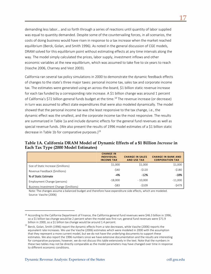
California ran several tax policy simulations in 2000 to demonstrate the dynamic feedback effects

of changes to the state’s three major taxes: personal income tax, sales tax and corporate income

tax. The estimates were generated using an across-the-board, $1 billion static revenue increase

for each tax funded by a corresponding rate increase. A $1 billion change was around 1 percent

of California’s $72 billion general funds budget at the time.18 The revenue increase (or decrease)

in turn was assumed to affect state expenditures that were also modeled dynamically. The model

showed that the personal income tax was the least responsive to the tax change, i.e., the

dynamic effect was the smallest, and the corporate income tax the most responsive. The results

are summarized in Table 1a and include dynamic effects for the general fund revenues as well as

special revenue funds. (We also present the results of 1996 model estimates of a $1 billion static

decrease in Table 1b for comparative purposes.)19

Table 1A. California DRAM Model of Dynamic Effects of a $1 Billion Increase in Each Tax Type (2000 Model Estimates)

CHANGE IN INDIVIDUAL INCOME TAX

CHANGE IN SALES

AND USE TAX

CHANGE IN BANK AND

CORPORATION TAX

Size of Static Increase ($millions) $1,000 $1,000 $1,000

Revenue Feedback ($millions) -$40 -$120 -$180

% of Static Estimate -4% -12% -18%

Employment Change (persons) -18,000 - 10,000 -11,000

Business Investment Change ($millions) -$83 -$109 -$479

Note: The changes assume a balanced budget and therefore have expenditure side effects, which are modeled. Source: Vasche (2006)

18 According to the California Department of Finance, the California general fund revenues were $46.3 billion in 1996,

so a $1 billion tax change would be 2 percent when the model was first run; general fund revenues were $71.9 billion in 2000, so a $1 billion tax change would be around 1.4 percent.

19 Berck, Golan, Smith (1996) report the dynamic effects from a rate decreases, while Vasche (2006) reports the equivalent rate increases. We use the Vasche (2006) estimates which were modeled in 2000 with the assumption that they represent a more current model, but we do not have the underlying documents to support these estimates. We also report the 1996 numbers since we have extensive documentation and the results are interesting for comparative purposes; however, we do not discuss this table extensively in the text. Note that the numbers in these two tables may not be directly comparable as the model parameters may have changed over time in response to different economic conditions.


18


Table 1B. California DRAM Model of Dynamic Effects of a $1 Billion Decrease in Each Tax Type (1996 Model Estimates)


CHANGE IN SALES

AND USE TAX

CHANGE IN BANK AND

CORPORATION TAX

Size of Static Increase ($million) $1,000 $1,000 $1,000

Revenue Feedback ($millions) $10 $77 $184

% of Static Estimate 1% 7.7% 18%

Employment Change (persons) 18,000 10,000 12,000

Employment Growth (% change) 0.14% 0.08% 0.10%

Personal Income ($millions) -$738 $107 $1,600

Personal Income (% change) -0.10% 0.01% 0.21%

Wages (% change) -0.21% -0.038% 0.028%

Return on Capital (% change) 0.01% 0.02% -0.40%

Gross Investment Change ($millions) $6 $16 $147

Gross Investment (% change) 0.009% 0.023% 0.217%

Note: The changes assume a balanced budget and therefore have expenditure side effects, which are modeled. Source: Berck, Golan and Smith (1996)

To raise $1 billion (static revenue estimate) through the personal income tax required an increase

of 4 percent across all brackets. For instance, the brackets at the highest income level would rise

from 9.3 percent to 9.7 percent. The resulting dynamic effect was around 4 percent from

reduced economic activity due to the tax increase. (The dynamic feedback effect is usually

expressed as a percentage of the initial static revenue estimate.) So after five or six years, the

increase in personal income tax rates would only raise $960 million due to the dynamic

adjustments ($40 million would be “lost”) (Vasche 2006). Importantly, because income taxes are

deductible from federal taxes, this mutes some of the effect of a state-level tax change.

Additionally, higher income groups hold a portion of their earnings outside the state, which can

reduce the dynamic effects (Berck, Golan, and Smith 1996).

To generate a $1 billion (static revenue estimate) increase in sales tax would require raising the

sales tax rate by about 5 percent. The DRAM showed that such an increase in sales and use tax

had a partially offsetting dynamic revenue reduction of about 12 percent (Vasche 2006). As the

sales tax rose, consumers might forego purchases of some discretionary goods or substitute away

from goods that were taxed, which now cost more due to the higher sales tax. Reduction in

demand led to less production, and less demand for labor and capital, which in turn would cause

wages to decline and the demand for capital to decline. The retail sales tax also affected

intermediate goods by increasing the production costs of goods. The sales tax increase caused

exports to decline because the state’s goods were more expensive and therefore less

competitive. The overall net effect would be to depress economic activity (Berck, Golan, and

Smith 1996).


19


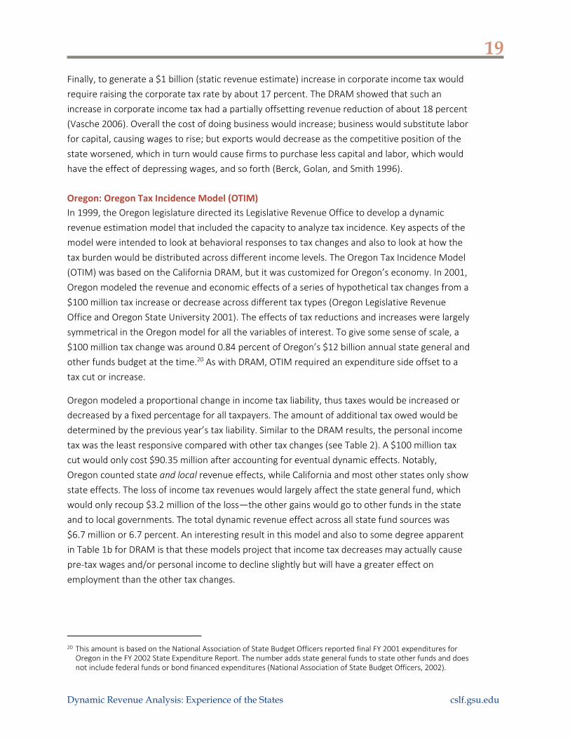
Finally, to generate a $1 billion (static revenue estimate) increase in corporate income tax would

require raising the corporate tax rate by about 17 percent. The DRAM showed that such an

increase in corporate income tax had a partially offsetting revenue reduction of about 18 percent

(Vasche 2006). Overall the cost of doing business would increase; business would substitute labor

for capital, causing wages to rise; but exports would decrease as the competitive position of the

state worsened, which in turn would cause firms to purchase less capital and labor, which would

have the effect of depressing wages, and so forth (Berck, Golan, and Smith 1996).

Oregon: Oregon Tax Incidence Model (OTIM)

In 1999, the Oregon legislature directed its Legislative Revenue Office to develop a dynamic

revenue estimation model that included the capacity to analyze tax incidence. Key aspects of the

model were intended to look at behavioral responses to tax changes and also to look at how the

tax burden would be distributed across different income levels. The Oregon Tax Incidence Model

(OTIM) was based on the California DRAM, but it was customized for Oregon’s economy. In 2001,

Oregon modeled the revenue and economic effects of a series of hypothetical tax changes from a

$100 million tax increase or decrease across different tax types (Oregon Legislative Revenue

Office and Oregon State University 2001). The effects of tax reductions and increases were largely

symmetrical in the Oregon model for all the variables of interest. To give some sense of scale, a

$100 million tax change was around 0.84 percent of Oregon’s $12 billion annual state general and

other funds budget at the time.20 As with DRAM, OTIM required an expenditure side offset to a

tax cut or increase.

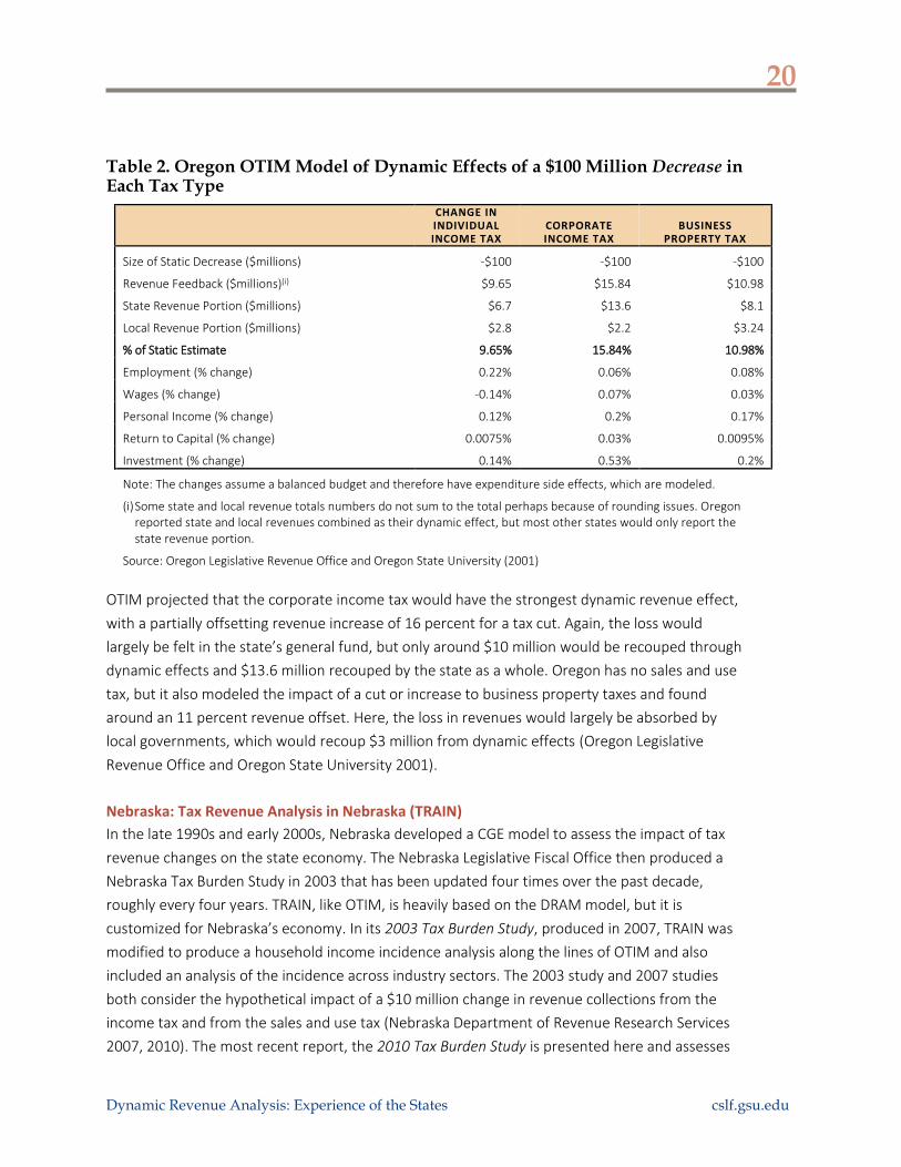
Oregon modeled a proportional change in income tax liability, thus taxes would be increased or

decreased by a fixed percentage for all taxpayers. The amount of additional tax owed would be

determined by the previous year’s tax liability. Similar to the DRAM results, the personal income

tax was the least responsive compared with other tax changes (see Table 2). A $100 million tax

cut would only cost $90.35 million after accounting for eventual dynamic effects. Notably,

Oregon counted state and local revenue effects, while California and most other states only show

state effects. The loss of income tax revenues would largely affect the state general fund, which

would only recoup $3.2 million of the loss—the other gains would go to other funds in the state

and to local governments. The total dynamic revenue effect across all state fund sources was

$6.7 million or 6.7 percent. An interesting result in this model and also to some degree apparent

in Table 1b for DRAM is that these models project that income tax decreases may actually cause

pre-tax wages and/or personal income to decline slightly but will have a greater effect on

employment than the other tax changes.

20 This amount is based on the National Association of State Budget Officers reported final FY 2001 expenditures for

Oregon in the FY 2002 State Expenditure Report. The number adds state general funds to state other funds and does not include federal funds or bond financed expenditures (National Association of State Budget Officers, 2002).


20


Table 2. Oregon OTIM Model of Dynamic Effects of a $100 Million Decrease in Each Tax Type


CORPORATE INCOME TAX

BUSINESS

PROPERTY TAX

Size of Static Decrease ($millions) -$100 -$100 -$100

Revenue Feedback ($millions)(i) $9.65 $15.84 $10.98

State Revenue Portion ($millions) $6.7 $13.6 $8.1

Local Revenue Portion ($millions) $2.8 $2.2 $3.24

% of Static Estimate 9.65% 15.84% 10.98%

Employment (% change) 0.22% 0.06% 0.08%

Wages (% change) -0.14% 0.07% 0.03%

Personal Income (% change) 0.12% 0.2% 0.17%

Return to Capital (% change) 0.0075% 0.03% 0.0095%

Investment (% change) 0.14% 0.53% 0.2%

Note: The changes assume a balanced budget and therefore have expenditure side effects, which are modeled.

(i) Some state and local revenue totals numbers do not sum to the total perhaps because of rounding issues. Oregon reported state and local revenues combined as their dynamic effect, but most other states would only report the state revenue portion.

Source: Oregon Legislative Revenue Office and Oregon State University (2001)

OTIM projected that the corporate income tax would have the strongest dynamic revenue effect,

with a partially offsetting revenue increase of 16 percent for a tax cut. Again, the loss would

largely be felt in the state’s general fund, but only around $10 million would be recouped through

dynamic effects and $13.6 million recouped by the state as a whole. Oregon has no sales and use

tax, but it also modeled the impact of a cut or increase to business property taxes and found

around an 11 percent revenue offset. Here, the loss in revenues would largely be absorbed by

local governments, which would recoup $3 million from dynamic effects (Oregon Legislative

Revenue Office and Oregon State University 2001).

Nebraska: Tax Revenue Analysis in Nebraska (TRAIN)

In the late 1990s and early 2000s, Nebraska developed a CGE model to assess the impact of tax

revenue changes on the state economy. The Nebraska Legislative Fiscal Office then produced a

Nebraska Tax Burden Study in 2003 that has been updated four times over the past decade,

roughly every four years. TRAIN, like OTIM, is heavily based on the DRAM model, but it is

customized for Nebraska’s economy. In its 2003 Tax Burden Study, produced in 2007, TRAIN was

modified to produce a household income incidence analysis along the lines of OTIM and also

included an analysis of the incidence across industry sectors. The 2003 study and 2007 studies

both consider the hypothetical impact of a $10 million change in revenue collections from the

income tax and from the sales and use tax (Nebraska Department of Revenue Research Services

2007, 2010). The most recent report, the 2010 Tax Burden Study is presented here and assesses


21


the impact of a $100 million tax change. To give a sense of scale, Nebraska’s state general fund

and other state fund expenditures in FY 2010 were $6.9 billion,21 so a $100 million tax change is

around 1.4 percent of annual expenditures. As shown in Table 3, a $100 million hypothetical

change in individual income tax from an across-the-board reduction in tax rates would produce a

6.4 percent feedback effect, while a change in the sales tax from an across-the-board reduction

would produce a 21 percent feedback effect (Nebraska Department of Revenue Research

Services 2013). These are effects on state revenues only. The incidence analysis suggests that a

cut in sales tax has progressive effects and income tax is somewhat regressive. The impact of the

income tax changes are also more evenly distributed across industry sectors while the sales tax

change heavily affects the retail business sector (Nebraska Department of Revenue Research

Services 2013).

Table 3. Nebraska Train Model of Dynamic Effects of a $100 Million Decrease in Each Tax Type


SALES AND USE TAX

Size of Static Decrease ($millions) -$100 -$100

Revenue Feedback ($millions) $6.4 $20.6

% of Static Estimate 6.4% 20.6%

Employment Change Total (persons) 1,788 2,615

Employment Change Private Sector (persons) 1,594 2,538

Personal Disposable Income ($millions) $121.6 $181.2

Investment ($millions) $64.8 $123.34

Note: The changes assume a balanced budget and therefore have expenditure side effects, which are modeled.

Source: Nebraska Department of Revenue Research Services (2013)

Massachusetts: REMI

Massachusetts was one of the first states to use dynamic analysis to assess tax changes at the

state level in 1993. The model used a combination of internally developed microsimulation,

which calculated the direct impact of tax policy changes and then fed the result to the REMI

model to assess larger dynamic effects. The model was used to assess a variety of tax reform

proposals between 1993 and 1995, including raising the state’s investment tax credit (Clayton-

Matthews 1993). The state, under then-Gov. William Weld, passed a series of aggressive business

tax policy changes including phasing out state capital gains taxes, in part using the argument that

the fiscal impact would not be as large as the static forecast because of projected dynamic

effects. Ultimately, overall revenues came in below the static revenue forecast in fiscal year 1995.

Democrats accused the Republican governor of failing to appropriately account for the effects of

21 Expenditures based on the National Association of State Budget Officers’ FY 2011 State Expenditure Report final

expenditure amounts reported for FY 2010 (National Association of State Budget Officers 2010).


22


the tax changes, and not long after, the dynamic model was abandoned (Sullivan 2004, Moccia

1995).

Initial runs of the REMI model did produce a series of dynamic effect tables that were reported in

State Tax Notes and are shown below in Table 4 (Clayton-Matthews 1993). These are

hypothetical cuts of $100 million by tax types. Importantly, they are not balanced estimates, i.e.,

they are not revenue neutral since the model did not account for any expenditure side effects

from revenue losses. The impact of the income tax is largely in alignment with the other state

income tax estimates even though there is no balanced budget requirement in this model; the

sales tax estimate meanwhile is small compared to the other states (12 percent in California and

21 percent in Nebraska), while the most significant dynamic effect are the changes in the

corporate income tax at 30.4 percent, significantly higher than the California impact at 18 percent

or Oregon at 15 percent.

Table 4. Massachusetts REMI Model Dynamic Effects of a $100 Million Decrease in Each Tax Type


CHANGE IN SALES

AND USE TAX

CHANGE IN CORPORATE INCOME TAX

Size of Static Increase ($millions) -$100 -$100 -$100

Revenue Feedback ($millions) +$6.4 +$4.9 +$30.4

% of Static Estimate 6.4% 4.9% 30.4%

Employment Change (persons) 1,600 1,500 10,500

Personal Income ($millions) $66.2 $57.9 $409.4

Investment ($millions) $21.7 $31 $302.4

Note: The changes do NOT assume a balanced budget, and therefore the expenditure side effects are not modeled. This suggests that the revenue side effects are overstated.

Source: Clayton-Matthews (1993)

Ohio: REMI

In 2005, the Ohio Department of Development contracted with REMI to perform a

comprehensive analysis of a broad tax reform package. REMI modeled six elements of the

comprehensive tax package passed by the Ohio legislature: a 21 percent reduction in the state

personal income tax; a 0.5 percentage point reduction in the state sales tax; the elimination of

the tangible personal property tax on machinery and equipment, inventory, and furniture and

fixtures; the elimination of the corporate franchise tax; increases in the excise tax on tobacco and

alcohol; and the creation of a broad-base, low-rate commercial activities tax. The REMI report

concluded that the combined package of tax changes would generate a reduction in tax revenue

of $3.06 billion in FY 2010, when the plan would be fully implemented. Dynamic positive effects

of the tax changes were $216 million that year, approximately a 1 percent dynamic effect,

offsetting some of the revenue losses. While the REMI report was favorably received by the Ohio


23


governor and legislature, the model did not include expenditure implications that might have

offset in whole or in part the dynamic effect from the tax cut (Honeck and Schiller 2005).22

New Mexico: REMI

New Mexico used a dynamic model to estimate the effects of an actual tax change. In 2003, New

Mexico enacted a tax reform plan that reduced its top personal income tax rate from 8.2 percent

to 4.9 percent over five years. The state also phased in a 50 percent cut in state capital-gains tax

over the same time period. The New Mexico Legislative Finance Committee modeled these tax

cuts in 2004 using a statewide REMI model that was developed as a pilot project.

While staff found the economic variables such as employment, personal income and output

interesting, ultimately with respect to state revenues, the dynamic effects were not that much

greater than the static estimates and well within the margin of error. For instance, as shown in

Table 5, in FY 2004, the first year the cuts were to be implemented, the estimate from the static

model showed the state losing $21.8 million in revenue, while the estimate from the REMI model,

capturing the dynamic economic effects, showed a loss of $21 million. (To put in context, New

Mexico’s FY 2004 general fund revenues were $4.6 billion.) The static revenue estimate was just

3.7 percent less than the dynamic estimate. Over time the percentage difference between the

estimates from the static model and the estimates from the dynamic REMI model declined. By

the end of the forecasting period, FY 2008, the estimate from the static model was 2.3 percent

more than the estimate from the dynamic REMI model. The staff speculated that the dynamic

effects were so small because the model required some form of expenditure cuts to offset the

revenue loss. Because the REMI model was costly to operate as a dynamic revenue estimation

tool and seemed to provide little additional value over traditional static analysis, the pilot project

was not renewed (Francis 2007, New Mexico Legislative Finance Committee Staff 2004).

Notably, the tax changes were projected to prompt investment in the state but were not

projected to improve employment or personal income. This effect is similar to the results found

in 1996 runs of DRAM as well as in the OTIM results. The DRAM modelers noted that while the

model showed wages declining, in actuality, wages rarely do decline in nominal terms—instead

this should be interpreted as a drag on growth in wages and personal income (Berck, Golan, and

Smith 1996). While it is not clear what exactly is driving the effect in New Mexico, the tax cuts

caused a reduction in expenditures (or expenditure growth), which affected wages—notably the

model predicted that the loss of government jobs would not be offset by the gain in private

sector jobs. Also, the gains from a reduction in income tax may be shared by employees and

employers would have the effect of reducing or slowing the growth of pre-tax wages, even as

employees have more after-tax wage income (as shown in Table 5, personal income declines but

22

Throughout the report REMI stated that the necessary offsetting spending cuts were not modeled in the analysis. But without the full analysis, including the offsetting spending cuts, Policy Matters Ohio argued the report had very little value to policymakers and citizens (Honeck and Schiller 2005).


24


total disposable personal income increases). While not shown here, the New Mexico dynamic

estimates projected a dynamic decline in income tax revenues relative to the static estimate, but

also projected that this would be made up through increased economic activity and associated

enhanced collections in the gross receipts tax and corporate income tax (New Mexico Legislative

Finance Committee Staff 2004).

Table 5. New Mexico REMI Model of Tax Reform

FY 2004 FY 2005 FY 2006 FY 2007 FY 2008

Static Analysis ($millions) -$21.8 -$83 -$167.2 -$275.2 -$360.3

Dynamic Analysis ($millions) -$21 -$80.8 -$163 -$268.7 -$352.2

Difference $0.8 $2.2 $4.2 $6.5 $8.1

% Dynamic Effect 3.7% 2.7% 2.5% 2.4% 2.2%

Employment (thousands) -0.031 -0.086 -0.156 -0.225 -0.242

Employment: Private Nonfarm 0.311 0.846 1.601 2.417 2.950

Employment: Government -0.342 -0.932 -1.759 -2.641 -3.191

Personal Income ($millions) -$1.5 -$5.0 -$9.0 -$11.5 -$9.5

Disposable Personal Income ($millions) $30.0 $84.0 $165.5 $260.0 $332.0

Output ($millions) $0.597 $1.824 $4.326 $10.064 $16.627

Source: New Mexico Legislative Finance Committee Staff (2004)

Kansas: STAMP

In 2012 and 2013, Kansas made a series of significant tax changes. Because the dynamic analysis

pertains only to the 2012 changes (HB2117), these are the ones discussed here. In 2012, the state

reduced its income tax brackets from three to two and then reduced the rates, increased the

standard deduction, cleared out a number of income tax credits and most significantly exempted

all non-wage income from a pass-through entity from the income tax (for instance, all limited

liability corporations would now pay no tax on profits). This tax cut represented an estimated 13

percent static revenue loss to the state general fund revenues (see Table 6). Although the state

staff did not present a dynamic revenue analysis, the Kansas Policy Institute produced a report

that used the Beacon Hill at Suffolk Institute’s STAMP model to examine the dynamic effects of

HB2117 and the 2012 tax changes (Davidson, et al. 2012).

As shown in Table 6, STAMP estimated the dynamic effect from these tax changes modeling the

tax cut on pass through income in two different ways. In their pass-through model, the tax cut is

treated as a cut in corporate income tax because this tax change was anticipated largely to affect

small businesses. Then they modeled this cut using the standard model, which treated the

reduction as an income tax cut applied to individuals. The pass-through model, where the tax cuts

are largely a benefit to businesses, predicted less of an employment gain (33,430 over six years)

than the standard model that assumed the benefits were largely influencing household choices

via the income tax (41,690 over six years), but gross investment in the economy would be higher


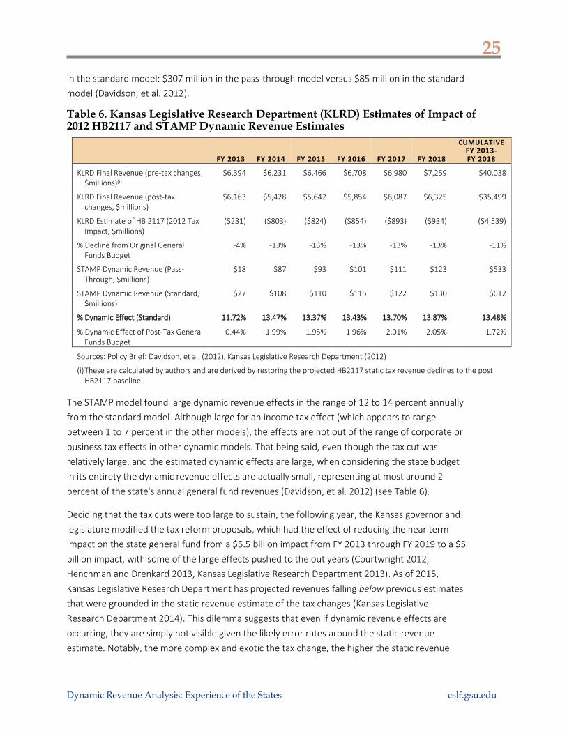
25


in the standard model: $307 million in the pass-through model versus $85 million in the standard

model (Davidson, et al. 2012).

Table 6. Kansas Legislative Research Department (KLRD) Estimates of Impact of 2012 HB2117 and STAMP Dynamic Revenue Estimates

FY 2013

FY 2014

FY 2015

FY 2016

FY 2017

FY 2018

CUMULATIVE FY 2013- FY 2018

KLRD Final Revenue (pre-tax changes, $millions)(i)

$6,394 $6,231 $6,466 $6,708 $6,980 $7,259 $40,038

KLRD Final Revenue (post-tax changes, $millions)

$6,163 $5,428 $5,642 $5,854 $6,087 $6,325 $35,499

KLRD Estimate of HB 2117 (2012 Tax Impact, $millions)

($231) ($803) ($824) ($854) ($893) ($934) ($4,539)

% Decline from Original General Funds Budget

-4% -13% -13% -13% -13% -13% -11%

STAMP Dynamic Revenue (Pass-Through, $millions)

$18 $87 $93 $101 $111 $123 $533

STAMP Dynamic Revenue (Standard, $millions)

$27 $108 $110 $115 $122 $130 $612

% Dynamic Effect (Standard) 11.72% 13.47% 13.37% 13.43% 13.70% 13.87% 13.48%

% Dynamic Effect of Post-Tax General Funds Budget

0.44% 1.99% 1.95% 1.96% 2.01% 2.05% 1.72%

Sources: Policy Brief: Davidson, et al. (2012), Kansas Legislative Research Department (2012)

(i) These are calculated by authors and are derived by restoring the projected HB2117 static tax revenue declines to the post HB2117 baseline.

The STAMP model found large dynamic revenue effects in the range of 12 to 14 percent annually

from the standard model. Although large for an income tax effect (which appears to range

between 1 to 7 percent in the other models), the effects are not out of the range of corporate or

business tax effects in other dynamic models. That being said, even though the tax cut was

relatively large, and the estimated dynamic effects are large, when considering the state budget

in its entirety the dynamic revenue effects are actually small, representing at most around 2

percent of the state's annual general fund revenues (Davidson, et al. 2012) (see Table 6).

Deciding that the tax cuts were too large to sustain, the following year, the Kansas governor and

legislature modified the tax reform proposals, which had the effect of reducing the near term

impact on the state general fund from a $5.5 billion impact from FY 2013 through FY 2019 to a $5

billion impact, with some of the large effects pushed to the out years (Courtwright 2012,

Henchman and Drenkard 2013, Kansas Legislative Research Department 2013). As of 2015,

Kansas Legislative Research Department has projected revenues falling below previous estimates

that were grounded in the static revenue estimate of the tax changes (Kansas Legislative

Research Department 2014). This dilemma suggests that even if dynamic revenue effects are

occurring, they are simply not visible given the likely error rates around the static revenue

estimate. Notably, the more complex and exotic the tax change, the higher the static revenue


26


estimate error rates are likely to be, and even if the static estimate was quite accurate, the

average error rate nationally around static estimates is around 3.5 percent (Pew Center on the

States and The Nelson A. Rockefeller Institute of Government 2011), which is to say that even

very large dynamic effects fall within this range.

Other Considerations

Several studies have attempted to model much more explicitly the choice between a tax increase

and an expenditure cut, particularly in response to fiscal stress. Two studies, one in Michigan and

one in Arizona, have used dynamic modeling to assess the tradeoffs and found that although tax

increases and expenditure cuts both cause job losses—the job losses are substantially higher

when cutting government expenditures. The key argument behind this analysis is that the impact

of tax increases is exported to other states and internationally, while expenditure cuts (laying off

teachers, police, state workers, etc.) are much more likely to be entirely absorbed within a state’s

economy (Bartik and Erickcek 2004, Charney 2010a).

A critique of all dynamic models is that the models do not account for any economic productivity

gains from governmental investment in areas such as education and transportation. Instead

governmental spending is largely modeled as just a “jobs” program (Institute on Taxation and

Economic Policy 2014, Berck, Golan, and Smith 1996).

A final point is that state and local governments are institutionally divided, and a change in state

tax policy can produce a countervailing change in local tax policy. Additionally, a tax change in

one state can produce a reaction by another state. No current dynamic models account for such

reaction effects, but such reactions to state policies are not uncommon and may have a

significant impact on a state’s economy.

Conclusion: Pros and Cons of Dynamic Revenue Models

Dynamic modeling has some interesting applications to policy analysis and provides potentially

useful information on the different ways that policies ripple through the economy. For instance,

noting that some tax changes may cause job losses or declines in wages even while growing the

productivity of the economy is helpful information if a policymaker is largely concerned about job

growth. Also, the general trend that corporate tax changes have larger dynamic effects than

income or sales tax changes may also be of interest to policymakers. Another key benefit is a

much more refined look at the incidence of tax policy changes. Both Oregon and Nebraska used

their models to look at the impact across the state’s income distribution, but Nebraska extended

the incidence analysis further to look at the effects on industries across different sectors of the

economy. The effects may vary depending on the ratio of labor to capital that is used in that

industry. Dynamic models may be also quite useful in comparing tax and expenditure tradeoffs.


27


Where dynamic modeling falls short, and what is apparently often disappointing to policymakers,

is that dynamic revenue analysis has not proved to be a particularly appropriate tool for

budgetary decision-making or forecasting. The assumption that the models themselves precisely

capture the working of a state’s economy may be problematic. A state’s economy is a vastly

complex system. The results obtained from dynamic models rely heavily on assumptions made by

the model builders and on the availability of data. Even with the advances in computing power

and increased data availability, simplifying assumptions are needed. Further the results from

dynamic models are sensitive to the values used to explain the interaction and responsiveness of

one variable to another, and at the sub-national level in particular, actual data for a number of

variables (for instance, trade flows) may themselves have to be estimated. Because of the high

level of uncertainty in these and other parameters, modelers have to rely on educated guesses.

This lack of precision can significantly reduce the model’s reliability and limit predictive power.

Perhaps not surprisingly, the models above show a significant range of dynamic revenue effects

from 1 percent to an upper bound in the 20 to 30 percent range (the 30 percent number is likely

overstated because the model did not include expenditure offsets). Notably, large economic

effects predicted by some of these models are out of alignment with empirical research that

generally finds the effect of tax changes may be small.

Even assuming that the dynamic models are highly accurate, relatively large dynamic effects, such

as those estimated in Kansas, take time to materialize and are ultimately small when compared to

a state’s general fund revenues (and even more minuscule when compared to the overall size of

the economy). The practical effect is that dynamic effects are likely to be invisible to the average

citizen, state policymakers or state budget staff.

In light of these concerns, states contemplating the use of dynamic models should consider

several issues. First, what do policymakers want to learn from dynamic revenue estimation?

Based on this review of state experiences, policymakers and analysts need to recognize that

dynamic revenue modeling can be useful for informing a policy debate, but policymakers should

generally not expect large effects and should not budget to these effects. Policymakers in states

such as Massachusetts in the 1990s and more recently, Kansas found that waiting for dynamic

effects to actually materialize in state revenue streams was problematic. Second, states need to

consider the resources required to develop, customize and then interpret the results from a

dynamic model. These models are expensive and complicated, and more than a few states have

simply decided that added value of the information is simply not worth the money, time and

effort required to purchase, develop and then maintain the models.


28


References

Agostini, Claudio A. (2007). “The Impact of State Corporate Taxes on FDI Location.” Public Finance

Review 35 (3): 335-60.

Arizona Joint Legislative Budget Committee Staff (2006). “Overview of Dynamic Revenue

Forecasting.” Edited by Arizona Joint Legislative Budget Committee.

Bania, Neil, Jo Anna Gray, and Joe A Stone (2007). “Growth, Taxes, and Government

Expenditures: Growth Hills for U.S. States.” National Tax Journal 60 (2): 193-204.

Bartik, Timothy J. (1991). “Who Benefits from State and Local Economic Development Policies?”

Kalamazoo, MI: W.E. Upjohn Institute for Employment Research.

Bartik, Timothy J, and George A Erickcek (2004). “Economic Impact of Various Budgetary Policy

Options for the State of Michigan to Resolve Its Budget Deficit for FY 2004.” Kalamazoo, MI:

W.E. Upjohn Institute for Employment Research.

Beacon Hill Institute at Suffolk University (2014). “Response to the ITEP Critique of the BHI STAMP

Model [webpage].” Accessed March 30, 2015. Retrieved from www.beaconhill.org/STAMP-

Method/ResponsetoITEPbybullet2014-0531.pdf.

Beacon Hill Institute at Suffolk University (2010). “The Beacon Hill Institute's Tax Analysis

Modeling Program: A Response to Charney.” Boston, MA.

Beacon Hill Institute at Suffolk University (webpage). Accessed January 28, 2015. Retrieved from

http://www.beaconhill.org/STAMP_Web_Brochure/STAMP_States Applied.html.

Bean, Mitchell E., Jay Wortley, and Mark P. Haas (1997). “Dynamic Revenue Estimating: Will it

Work for Michigan.” A joint report of the House Fiscal Agency, Senate Fiscal Agency, and the

Department of the Treasury, Lansing, MI.

Berck, Peter, Elise Golan, and Bruce Smith (1996). “Dynamic Revenue Analysis in California: An

Overview.” State Tax Notes 11: 1227-37.

Berck, Peter, Elise Golan, Bruce Smith, John Barnhart, and Andrew Dabalen (1996). “Dynamic

Revenue Analysis for California.” Sacramento, CA: California Department of Finance.

Bruce, Donald, and John Deskins (2012). “Can State Tax Policies Be Used to Promote

Entrepreneurial Activity?” Small Business Economics 38 (4): 375-97.

Bruce, Donald, John Deskins, and William F. Fox (2007). “On the Extent, Growth, and Efficiency

Consequences of State Business Tax Planning.” In Taxing Corporate Income in the 21st

Century, edited by Alan J. Auerbach Jr., James R. Hines, and Joel Slemrod. Cambridge

University Press.


http://www.beaconhill.org/STAMP-Method/ResponsetoITEPbybullet2014-0531.pdf

http://www.beaconhill.org/STAMP-Method/ResponsetoITEPbybullet2014-0531.pdf

http://www.beaconhill.org/STAMP_Web_Brochure/STAMP_States%20Applied.html

29


Canto, Victor A, Douglas H Joines, and Arthur B Laffer (1978). “Taxation, GNP and Potential GNP.”

Proceedings of the Business and Economic Statistics Section in San Diego, American Statistical

Association.

Charney, Alberta (2010a). “Sales Tax Increase vs. Expenditure Cuts: An Economic Impact Study.”

Tuscon, AZ: The University of Arizona, Eller College of Management.

Charney, Alberta (2010b). “UA Estimates of Tax/Expenditure Impacts Compared to those of the

Goldwater Institute (prepared by Beacon Hill) and REMI.” Tuscon, AZ: The University of

Arizona, Eller College of Management.

Charney, Alberta, and Marshall Vest (2003). “Modeling Practices and Their Ability to Assess

Tax/Expenditure Economic Impacts.” AUBER Conference, New Orleans. October.

Chernick, Howard (2010). “Redistribution at the State and Local Level: Consequences for

Economic Growth.” Public Finance Review 38 (4): 409-49.

Chernick, Howard (1997). “Tax Progressivity and State Economic Performance.” Economic

Development Quarterly 11 (3): 249-67.

Clayton-Matthews, Alan (1993). “The Massachusetts Dynamic Analysis Model.” State Tax Notes 5:

639.

Colorado Legislative Council Staff (2004). “Dynamic Modeling in Other States.” Denver, CO.

Condon, Jeffrey, Andrew Feltenstein, Florenz Plassman, Mark Rider, and David Sjoquist (2015). “A

Multiregional Model of Growth-Oriented State Tax Reforms: An Application to Georgia and

Five Comparison States.” FRC Report 269. Fiscal Research Center, Georgia State University.

Coomes, Paul A, and William H Hoyt (2008). “Income Taxes and the Destination of Movers to

Multistate MSAs.” Journal of Urban Economics 63 (3): 920-37.

Courtwright, Chris (2012). “Kansas State and Local Tax Structure Post-2012: Selected

Observations and Implications of New Law.” In Principal Economist, edited by theKansas

Legislative Research Department. Retrieved from http://www.slideshare.net/

cyoho/stateandlocalstructurejune2012-2 (accessed January 26, 2015).

Davidson, Todd, David Tuerck, Paul Bachman, and Michael Head (2012). “Tax Reform Gears

Kansas for Growth: A Dynamic Analysis of Additional Revenue and Jobs Generated by Tax

Reform.” Wichita, KS: Kansas Policy Institute.

Deskins, John, and Brian Hill (2008). “State Taxes and Economic Growth Revisited: Have

Distortions Changed?” The Annals of Regional Science 44 (2): 331-48.


http://www.slideshare.net/%20cyoho/stateandlocalstructurejune2012-2

http://www.slideshare.net/%20cyoho/stateandlocalstructurejune2012-2

30


Fisher, Ronald C. (1997). “The Effects of State and Local Public Services on Economic

Development.” New England Economic Review March/April: 53-66.

Francis, Norton (2007). “Dynamic Scoring.” Memorandum. Santa Fe, NM: New Mexico Legislative

Finance Committee.

Gabe, Todd M., and Kathleen P. Bell (2004). “Tradeoffs between Local Taxes and Government

Spending as Determinants of Business Location.” Journal of Regional Science 44 (1): 21-41.

Gius, Mark P., and Phillip Frese (2002). “The Impact of State Personal and Corporate Tax Rates on

Firm Location.” Applied Economics Letters 9 (1): 47-9.

Goff, Brian, Alex Lebedinsky, and Stephen Lile (2011). “A Matched Pairs Analysis of State Growth

Differences.” Contemporary Economic Policy 30 (2): 293-305.

Hamilton, Billy (2015). “Big Black Box: Dynamic Scoring and its Discontents.” State Tax Notes 75:

221-5

Helms, Jay (1985). “The Effect of State and Local Taxes on Economic Growth: A Time Series-Cross

Section Approach.” The Review of Economics and Statistics 67 (4): 574-82.

Henchman, Joseph, and Scott Drenkard (2013). “Kansas Tax Reform Improves on Last Year's

Efforts.” Fiscal Fact 374. Washington, DC: Tax Foundation.

Hepner, Mickey, and W. Robert Reed (2003). “Dynamic Scoring in The Public and Private Sectors.”

Washington, DC: World Council on Economic Policy for The Heritage Foundation.

Holcombe, Randall G., and Donald J. Lacombe (2004). “The Effect of State Income Taxation on Per

Capita Income Growth.” Public Finance Review 32 (3): 292-312.

Honeck, Jon, and Zack Schiller (2005). “REMI Report Presents Just Half the Equation.” Cleveland,

OH and Columbus, OH: Policy Matters Ohio.

Institute on Taxation and Economic Policy (2014). “STAMP is an Unsound Tool for Gauging the

Economic Impact of Taxes.” Washington, DC.

Kansas Legislative Research Department (2014). “Memo on SGF Receipts Estimates for FY 2015,

FY 2016 and FY 2017.” Edited by Kansas Legislature. Topeka, KS.

Kansas Legislative Research Department (2013). “Second Conference Committee Report Brief

House Bill 2059.” Edited by Kansas Legislature. Retrieved from www.kslegislature.org.

Kansas Legislative Research Department (2012). “Supplemental Note on Senate Substitute for

House Bill 2117.” Edited by Kansas Legislature. Retrieved from www.kslegislature.org.


http://www.kslegislature.org/

http://www.kslegislature.org/

31


Karakaya, Fahri, and Cem Canel (1998). “Underlying Dimensions of Business Location Decisions.”

Industrial Management & Data Systems 98 (7): 321-29.

Leigh, Andrew (2008). “Do Redistributive State Taxes Reduce Inequality?” National Tax Journal 61

(1): 81-104.

Mark, Stephen T., Therese J. McGuire, and Leslie E. Papke (2000). “The Influence of Taxes on

Employment and Population Growth: Evidence from the Washington DC Metropolitan Area.”

National Tax Journal 53 (1): 105-23.

Mikesell, John (2012). “Revenue Estimation/Scoring by States: An Overview of Experience and

Current Practices with Particular Attention to the Role of Dynamic Models.” Public Budgeting

and Finance 32: 1-24

Mirowski, Philip (1982). “What's Wrong with the Laffer Curve?” Journal of Economic Issues 16 (3):

815-28.

Moccia, Tom (1995). “Debate Erupts Over Revenue Estimating in Massachusetts.” State Tax Notes

8: 1256.

Mofidi, Alaeddin, and Joe Stone (1990). “Do State and Local Taxes Affect Economic Growth?” The

Review of Economics and Statistics 72 (4): 986-91.

Mullen, John, and Martin Williams (1994). “Marginal Tax Rates and State Economic Growth.”

Regional Science and Urban Economics 24: 687-705.

National Association of State Budget Officers (2010). “State Expenditure Report 2010.” Available

at: www.nasbo.org/publications-data/state-expenditure-report/state-expenditure-report-

2010-fiscal-2009-2011-data.

National Association of State Budget Officers (2002). “State Expenditure Report 2002.” Available

at: www.nasbo.org/publications-data/state-expenditure-report/state-expenditure-report-

2002-fiscal-2001-2003-data.

Nebraska Department of Revenue Research Services (2013). “2010 Nebraska Tax Burden Study.”

Lincoln, NE.

Nebraska Department of Revenue Research Services (2007). “2003 Nebraska Tax Burden Study.”

Lincoln, NE.

New Mexico Legislative Finance Committee Staff (2004). “2004 Post-Session Fiscal Review.” Santa

Fe, NM: New Mexico Legislative Finance Committee.

Ojede, Andrew, and Steven Yamarik (2012). “Tax Policy and State Economic Growth: The Long-

Run and Short-Run of It.” Economics Letters 116 (2):161-65.


http://www.nasbo.org/publications-data/state-expenditure-report/state-expenditure-report-2010-fiscal-2009-2011-data




32


Oregon Legislative Revenue Office, and Oregon State University (2001). “The Oregon Tax

Incidence Model.” Report 1-01 (March). Salem, OR: Legislative Revenue Office.

Pew Center on the States, and The Nelson A. Rockefeller Institute of Government (2011). “States'

Revenue Estimating: Cracks in the Crystal Ball.” Albany, NY: The Nelson A. Rockefeller

Institute and Washington, D.C.: Pew Charitable Trusts.

Plassmann, Florenz (2005). “The Advantage of Avoiding the Armington Assumption in Multi-

Region Models.” Regional Science and Urban Economics 35 (6): 777-94.

Reed, W. Robert (2008). “The Robust Relationship between Taxes and U.S. State Income

Growth.” National Tax Journal 61 (1): 57-80.

Reed, W. Robert, and Cynthia Rogers (2004). “Tax Cuts and Employment Growth in New Jersey:

Lessons from a Regional Analysis.” Public Finance Review 32 (3): 269-91.

Sullivan, Martin (2004). “Practical Aspects of Dynamic Revenue Estimation.” A Report of the

Heritage Center for Data Analysis. June 14. Washington, DC: The Heritage Foundation.

Tannenwald, Robert, Jon Sure, and Nicholas Johnson (2011). "Higher State Taxes Bring More

Revenue, Not More Migration." State Tax Notes Special Report September 12: 705-18.

Tomljanovich, Marc (2004). “The Role of State Fiscal Policy in State Economic Growth.”

Contemporary Economic Policy 22 (3): 318-30.

Vasche, Jon (2006). “Whatever Happened to Dynamic Revenue Analysis in California?”

Proceedings at the Annual Revenue Estimation & Tax Research Conference, Federation of Tax

Administrators, Portland, OR., September 17-20.

Wasylenko, Michael (1997). “Taxation and Economic Development: the State of the Economic

Literature.” New England Economic Review March/April: 37-52.

Young, Cristobal, and Charles Varner (2011). “Millionaire Migration and State Taxation of Top

Incomes: Evidence from a Natural Experiment.” National Tax Journal 64 (2): 255-84.


33


About the Authors

Peter Bluestone is a Senior Research Associate with the Fiscal Research Center

and the Center for State and Local Finance. He is a Georgia State University

Urban Fellows Recipient. His research interests include urban economics,

environmental economics and state and local fiscal policy. He received his

Ph.D. in Economics from Georgia State University.

Carolyn Bourdeaux is the Director of the Center for State and Local Finance and

an Associate Professor of Public Management and Policy at Georgia State

University. From 2007-2010, she took a leave of absence from the Andrew

Young School to work as Director of the Georgia Senate Budget and Evaluation

Office. Her research interests include education finance, tax policy, state

budget decision-making and program and performance-based budgeting.

About the Center for State and Local Finance

The Center for State and Local Finance (CSLF) mission is to develop the people and ideas for next

generation public finance. Key initiatives include: 1) Developing executive education programs in

public finance to provide professional development for the next generation of practitioners in

state and local finance; 2) Building technical assistance capacity in next generation technologies

for the public sector that include the use of “big data” and improved analytics to better inform

policymakers and to better target solutions to public sector problems; 3) Supporting scholarship

on critical challenges in state and local fiscal and economic policy; and 4) Building a strong

capacity to translate and communicate academic research for the practitioner audience.

CSLF Reports, Policy Briefs, and other publications maintain a position of neutrality on public policy

issues in order to safeguard the academic freedom of the authors. Thus, interpretations or

conclusion in CSLF publications should be understood to be solely those of the author(s).

For more information on the Center for State and Local Finance, visit our website at: cslf.gsu.edu.



Dynamic Revenue Analysis: Experience of the...

Documents

Transcript of Dynamic Revenue Analysis: Experience of the...