DYNAMIC RESPONSE OF BRIDGES TO NEAR-FAULT, FORWARD ...
285
DYNAMIC RESPONSE OF BRIDGES TO NEAR-FAULT, FORWARD DIRECTIVITY GROUND MOTIONS By ELIOT BONVALOT A thesis submitted in partial fulfillment of the requirements of the degree of MASTER OF SCIENCE IN CIVIL ENGINEERING WASHINGTON STATE UNIVERSITY Department of Civil and Environmental Engineering AUGUST 2006
Transcript of DYNAMIC RESPONSE OF BRIDGES TO NEAR-FAULT, FORWARD ...

DYNAMIC RESPONSE OF BRIDGES TO NEAR-FAULT,
FORWARD DIRECTIVITY GROUND MOTIONS
By
ELIOT BONVALOT
A thesis submitted in partial fulfillment of the requirements of the degree of
MASTER OF SCIENCE IN CIVIL ENGINEERING
WASHINGTON STATE UNIVERSITY Department of Civil and Environmental Engineering
AUGUST 2006

To the faculty of Washington State University:
The members of the Committee appointed to examine the thesis of ELIOT BONVALOT
find it satisfactory and recommend that it be accepted.
Chair
ii ii

ACKNOWLEDGEMENTS
This research was performed in the Department of Civil and Environmental
Engineering at Washington State University, Pullman, Washington. Funding was
provided by the Federal Highway Administration. The Washington State Department of
Transportation provided technical support throughout the project. Their support is greatly
appreciated.
I am grateful to Dr. William Cofer, the chairman of my committee, for his
patience and guidance through this project. I would also like to thank Dr. Adrian
Rodriguez-Marek and Dr. Cole C. McDaniel for their participation and assistance on my
committee. A special thanks for Mr. Adel Al-Assaf and Mr. Reza Sehhati. You have not
only been a help with research, but sincere friends to me. I would also like to thank my
family for the encouragement they have been.
iii iii

DYNAMIC RESPONSE OF BRIDGES TO NEAR-FAULT,
FORWARD DIRECTIVITY GROUND MOTIONS
Abstract
By Eliot Bonvalot, M.S. Washington State University
August 2006
Chair: William F. Cofer
Research over the last decade has shown that pulse-type earthquake ground
motions that result from forward-directivity effects can result in significant damage to
structures. The objective of this research is to use recent ground motion data to improve
the understanding of the response of typical reinforced concrete and precast concrete
bridges to pulse-type ground motions that result from forward directivity effects.
Nonlinear, dynamic finite element analysis was applied to three bridges, and they
generally survived forward directivity ground motions without significant damage to the
columns. However, column flexural failure was predicted for one of them when subjected
to two of the forward directivity ground motions. The bridge models often indicated
distress at the abutments, including pounding, and exceedance of abutment strength
limits.
The response of bridges to forward directivity ground motions was found to be
highly dependent upon the coincidence of the bridge fundamental period and the ground
motion velocity pulse period. The severity of the demand is controlled by the ratio of the
pulse period to bridge fundamental period.
iv iv

Analysis results showed that most of the damage in the bridge columns during
forward directivity ground motions occurred at the beginning of the record in response to
the velocity pulse. Therefore, a ground motion consisting of a sinusoidal single pulse may
be sufficient to evaluate bridge performance for forward directivity ground motions.
A study of the effect of foundation flexibility showed that not including Soil-
Structure-Interaction might lead to over-conservatism, especially for the FDGMs.
Nonlinear SDOF analyses were performed, but they are not recommended in the
case of forward directivity ground motions since the results were not consistent.
However, the use of the acceleration response spectra to compute the expected response
of the bridges was found to be quite successful for both non-forward directivity and
forward directivity ground motions. A response modification factor must be used to
include the inelasticity effect on the maximum base shear in the columns.
Due to the variation in the acceleration response spectra with period caused by
forward directivity ground motions, to amplify the spectra for design does not provide a
reliable basis for representing near-fault, forward directivity ground motions. Depending
on the importance of the bridge being designed or assessed, the appropriate approach
taken with forward directivity ground motions should be carefully considered by the
designer.
v v
TABLE OF CONTENTS
Page ACKNOWLEDGEMENTS……………………….………………………….….………iii ABSTRACT………………………………………………………………….….………iv TABLE OF FIGURES……………………………………………………….….….........xi TABLE OF TABLES…………………………………………………………..……...xxiii CHAPTER 1: Introduction.............................................................................1
1.1) Introduction and Background ............................................................................. 1
1.2) Research objectives............................................................................................. 2
1.3) Seismic Activity in Western Washington State .................................................. 3
1.4) Bridge Modeling ................................................................................................. 4
CHAPTER 2: Literature Review ...................................................................5
2.1) Near-Fault (NF), Forward Directivity Ground Motions (FDGMs) .................... 5
2.1.1) Strike-slip and dip-slip fault........................................................................ 5
2.1.2) Fault Normal/Fault Parallel......................................................................... 6
2.1.3) Near-Fault, Forward Directivity effects...................................................... 8
2.2) The Seattle fault ................................................................................................ 13
2.3) Structural response to FDGM ........................................................................... 17
2.3.1) Effects on Buildings.................................................................................. 17
2.3.2) Effects on Bridges..................................................................................... 20
2.4) Current near-fault seismic design provisions for bridges ................................. 22
2.5) Soil-Structure Interaction.................................................................................. 24
vi vi

2.5.1) Foundation models.................................................................................... 24
2.5.1.1) Spread footings ................................................................................. 25
2.5.1.2) Pile foundations ................................................................................ 26
2.5.2) Damping.................................................................................................... 28
2.5.3) Previous Research Papers ......................................................................... 29
CHAPTER 3: Column Modeling and ABAQUS ........................................32
3.1) The Orozco columns ......................................................................................... 32
3.1.1) Geometry and reinforcement .................................................................... 32
3.1.2) Loading and test setup .............................................................................. 33
3.1.3) Recorded responses from testing .............................................................. 35
3.1.4) Finite Element Modeling of the Columns................................................. 36
3.1.4.1) Global geometric modeling............................................................... 36
3.1.4.2) Material models ................................................................................ 40
3.1.4.2.1) Concrete......................................................................................... 40
3.1.4.2.2) Longitudinal Steel.......................................................................... 47
3.1.5) ABAQUS Results ..................................................................................... 48
3.2) Lehman column ................................................................................................ 49
3.2.1) Geometry and reinforcement .................................................................... 49
3.2.2) Loading and test setup .............................................................................. 51
3.2.3) Recorded responses from testing .............................................................. 52
3.2.4) Finite Element modeling of the column.................................................... 54
3.2.5) ABAQUS Results ..................................................................................... 55
3.3) Conclusion ........................................................................................................ 56
vii vii

CHAPTER 4: Seismic Analysis of Bridges..................................................58
4.1) Seismic Excitations........................................................................................... 58
4.1.1) Ground Motion Selection.......................................................................... 58
4.1.2) Ground Motion Characteristics................................................................. 59
4.2) Coordinate Axes................................................................................................ 61
4.3) WSDOT Bridge Selection................................................................................. 62
4.4) WSDOT Bridge 405/46N-E.............................................................................. 63
4.4.1) Geometry and reinforcement .................................................................... 63
4.4.2) Structural Model ....................................................................................... 70
4.4.2.1) Boundary and Connectivity Conditions............................................ 75
4.4.2.2) Damping............................................................................................ 79
4.4.2.3) Loading and Ground Motions........................................................... 79
4.4.2.4) Bridge Frequency Content ................................................................ 80
4.5) WSDOT Bridge 520/19E-N.............................................................................. 82
4.5.1) Geometry and reinforcement .................................................................... 82
4.5.2) Structural Model ....................................................................................... 89
4.5.2.1) Bridge Frequency Content ................................................................ 90
4.6) WSDOT Bridge 90/26A ................................................................................... 91
4.6.1) Geometry and reinforcement .................................................................... 91
4.6.2) Structural Model ....................................................................................... 97
4.6.2.1) Boundary and Connectivity Conditions............................................ 99
4.6.2.2) Loading and Ground Motions......................................................... 103
4.6.2.3) Bridge Frequency Content .............................................................. 103
viii viii

CHAPTER 5: WSDOT Bridge Results .....................................................106
5.1) General Bridge Behavior ................................................................................ 106
5.1.1) Bridge 405 and Bridge 520 ..................................................................... 106
5.1.2) Bridge 90................................................................................................. 111
5.2) Forward Directivity Effect – Frequency Content ........................................... 116
5.1.2.1) Longitudinal Response.................................................................... 124
5.1.2.2) Transverse Response....................................................................... 133
5.3) Velocity Pulse Period Effect........................................................................... 135
5.4) Soil-Structure Interaction Effect ..................................................................... 139
5.5) Comparison with a SDOF system................................................................... 140
5.6) AASHTO prediction comparison ................................................................... 143
5.7) Acceleration Spectra prediction comparison .................................................. 150
CHAPTER 6: Conclusion ...........................................................................152
REFERENCE...............................................................................................157
APPENDIX A...............................................................................................169
A.1 Shear Capacity Degradation Model ..................................................................... 169
A.2 Foundation Stiffnesses – FEMA 356 (2000) ....................................................... 170
A.3 Longitudinal Abutment Response – Caltrans (2004)........................................... 172
A.4 AASHTO (2004) procedure................................................................................. 175
APPENDIX B ...............................................................................................177
B.1 Ground Motions Characteristics .......................................................................... 177
B.2 Bridge 405 Input Data.......................................................................................... 190
B.2.1 Material Properties ........................................................................................ 190
ix ix

B.3 Bridge Output Data .............................................................................................. 191
B.4 Bridges Finite Element Input Files ...................................................................... 195
x x

TABLE OF FIGURES
Figure 1.1.1: Typical cross-section of northwestern Washington State showing
hypocenters of earthquakes since 1970. After Ludwin et al. (1991). .................................... 4
Figure 2.1.1: Schematic Diagrams of surface fault displacement (Slemmons, 1977)........... 6
Figure 2.1.2: The large velocity pulse occurs in the fault-normal direction (Somerville,
1993) ...................................................................................................................................... 7
Figure 2.1.3: Rupture-directivity effects in the recorded displacement time histories of the
1989 Loma Prieta earthquake, for the fault-normal (top) and fault-parallel (bottom)
components. (EERI, 1995)..................................................................................................... 8
Figure 2.1.4: Zones of directivity .......................................................................................... 9
Figure 2.1.5: Map of the Landers region showing the location of the rupture of the 1992
Landers earthquake (which occurred on three segments), the epicenter, and the recording
stations at Lucerne and Joshua Tree. The strike normal velocity time histories at Lucerne
and Joshua Tree exhibit forward and backward directivity effects, respectively. (From
Somerville, 1997)................................................................................................................. 10
Figure 2.1.6: An example of forward directivity effect on Site A (Abrahamson, 1998)..... 11
Figure 2.1.7: Schematic diagrams showing the orientations of fling step and directivity
pulse for strike-slip and dip-slip faulting. (Somerville et al., 1997) .................................... 12
Figure 2.2.1: Map showing tracklines of USGS high-resolution, multichannel, seismic-
reflection profiles near the Seattle fault zone. (USGS; http://earthquake.usgs.gov/) .......... 14
Figure 2.2.2: The Seattle Area Map showing the Seattle fault zone (Brocher et al. 2004) . 16
Figure 2.5.1: Schematic of discrete foundation models for the spread footing foundation:
(a) bent structure; (b) foundation models. (McGuire et al., 1994)....................................... 26
xi xi

Figure 2.5.2: Schematic of models for the pile foundation: (a) bent structure; (b)
foundation models. (Cofer, 1994)........................................................................................ 28
Figure 2.5.3: Collapsed of an 18-span viaduct section of Hanshin Expressway (from
Ghasemi, 1996) .................................................................................................................... 30
Figure 3.1.1: Column elevation (Orozco, 2002) .................................................................. 33
Figure 3.1.2: Input time history (Orozco, 2002).................................................................. 34
Figure 3.1.3: test setup (Orozco, 2002)................................................................................ 35
Figure 3.1.4: Overall view after pulse loading (Orozco, 2002) ........................................... 35
Figure 3.1.5: Recorded response: hysteretic force-displacement curve and dashed
Ruaumoko (Carr, 1996) prediction (Orozco, 2002)............................................................. 36
Figure 3.1.6: Response of columns with different sized elements (Légeron, 2005) ........... 37
Figure 3.1.7: Column with 6 elements (13 points) .............................................................. 38
Figure 3.1.8: Default 3 radially, 8 circumferentially integration points, through the beam
cross section and two integration point locations (in red) along the length of the 3-node
element................................................................................................................................. 38
Figure 3.1.9: Column model in ABAQUS........................................................................... 39
Figure 3.1.10: Input time history during the ABAQUS analysis......................................... 39
Figure 3.1.11: Stress-Strain Model Proposed for Monotonic Loading of Confined and
Unconfined Concrete (Mander & Priestley, 1988) .............................................................. 43
Figure 3.1.12: Stress–Strain Relationship for the Concrete in Compression ...................... 44
Figure 3.1.13: Experimental Behavior of Concrete under Tension (Mazars, 1989)............ 44
Figure 3.1.14: Tensile Stress-Strain Curve of the Concrete ................................................ 45
Figure 3.1.15: Behavior of concrete (Légeron, 2005) ......................................................... 46
xii xii

Figure 3.1.16: Steel Stress-Strain Curve.............................................................................. 48
Figure 3.1.17: Comparison of Orozco (light gray) and ABAQUS results (solid red) ......... 49
Figure 3.2.1: Specimen Geometry and Reinforcement of the Lehman column. (Lehman,
2000) .................................................................................................................................... 50
Figure 3.2.2: Experimental configuration (Lehman, 2000) ................................................. 51
Figure 3.2.3: Imposed displacement during the test (Lehman, 2000) ................................. 52
Figure 3.2.4: Final damage state (Lehman, 2000) ............................................................... 53
Figure 3.2.5: Force – Displacement Response (Lehman, 2000).......................................... 54
Figure 3.2.6: Imposed displacement during the ABAQUS analysis ................................... 55
Figure 3.2.7: Comparison of Lehman and ABAQUS results .............................................. 56
Figure 4.1.1: Non FDGMs Acceleration Spectra (Log. scale) ............................................ 59
Figure 4.1.2: Non FDGMs Acceleration Spectra................................................................. 60
Figure 4.2.1: Bridge Coordinate Axes ................................................................................. 61
Figure 4.3.1: Bridge location ............................................................................................... 62
Figure 4.3.2: The Seattle Area Map showing the Seattle fault zone and bridge location
(Brocher et al. 2004) ............................................................................................................ 63
Figure 4.4.1: Bridge 405 Aerial View ................................................................................. 64
Figure 4.4.2: Bridge 405 Elevation...................................................................................... 65
Figure 4.4.3: Bridge 405 Plan .............................................................................................. 65
Figure 4.4.4 Bridge 405 Deck cross-section........................................................................ 65
Figure 4.4.5: Bridge 405 Column Sections (Crossbeam & Circular column) ..................... 66
Figure 4.4.6: Crossbeam plan view...................................................................................... 66
Figure 4.4.7: Bridge 405 Hinge Elevation (between crossbeam and deck)......................... 67
xiii xiii

Figure 4.4.8: Bearing Pad .................................................................................................... 67
Figure 4.4.9: Bridge 405 Girder Stop .................................................................................. 67
Figure 4.4.10: Bridge 405 Bent Elevation ........................................................................... 68
Figure 4.4.11: Bridge Foundation Spread Footing for Bents............................................... 69
Figure 4.4.12: Bridge 405 Abutment and Deck Elevation View......................................... 69
Figure 4.4.13: Bridge 405 East and West Abutments.......................................................... 70
Figure 4.4.14: Bridge 405 Spine Model............................................................................... 71
Figure 4.4.15: Bridge 405 deck cross-section...................................................................... 71
Figure 4.4.16: Bridge 405 deck solid and spine models ...................................................... 72
Figure 4.4.17: Bridge 405 deck in torsion ........................................................................... 72
Figure 4.4.18: Bridge 405 cross-sections............................................................................. 74
Figure 4.4.19: FE model of the soil, abutment and deck interaction in the transverse
direction ............................................................................................................................... 75
Figure 4.4.20: FE model of the soil, abutment and deck interaction, in the longitudinal
direction ............................................................................................................................... 76
Figure 4.4.21: Force-Displacement Curve of the abutment gap spring and connector in
series .................................................................................................................................... 76
Figure 4.4.22: Bridge Model Boundary Conditions ............................................................ 78
Figure 4.4.23: Applied earthquake at the foundation nodes ................................................ 80
Figure 4.4.24: Longitudinal mode of vibration.................................................................... 81
Figure 4.4.25: Transverse mode of vibration....................................................................... 82
Figure 4.5.1: Bridge 520 Aerial View ................................................................................. 83
Figure 4.5.2: Bridge 520 Elevation...................................................................................... 83
xiv xiv

Figure 4.5.3: Bridge 520 Plan .............................................................................................. 84
Figure 4.5.4: Bridge 520 Deck cross-section....................................................................... 84
Figure 4.5.6: Bridge 520 Column Sections (Crossbeam & Circular column) ..................... 85
Figure 4.5.7: Crossbeam plan view...................................................................................... 85
Figure 4.5.8: Bridge 520 Hinge Elevation (between crossbeam and deck)......................... 86
Figure 4.5.9: Bearing Pad .................................................................................................... 86
Figure 4.5.10: Bridge 520 Girder Stop ................................................................................ 86
Figure 4.5.11: Bridge 520 Bent Elevation ........................................................................... 87
Figure 4.5.12: Bridge Foundation Spread Footing for Bents............................................... 88
Figure 4.5.13: Bridge 520 West Abutment and Deck Elevation View................................ 88
Figure 4.5.14: Bridge 520 East and West Abutments.......................................................... 89
Figure 4.5.15: Bridge 520 East and West Abutments.......................................................... 89
Figure 4.6.1: Bridge 90 Aerial View ................................................................................... 91
Figure 4.6.2: Bridge 90 Aerial Views.................................................................................. 92
Figure 4.6.3: Bridge 90 Elevation........................................................................................ 92
Figure 4.6.4: Bridge 90 Plan ................................................................................................ 93
Figure 4.6.5: Bridge 90 Concrete box girder cross-section ................................................. 93
Figure 4.6.6: Guided Bearing Pad........................................................................................ 94
Figure 4.6.7: Fixed Bearing Pad .......................................................................................... 94
Figure 4.6.8: Bridge 90 columns.......................................................................................... 95
Figure 4.6.9: Wing Wall ...................................................................................................... 96
Figure 4.6.10: Bridge 90 Abutment and Deck Elevation View........................................... 96
Figure 4.6.11: Bridge 90 East and West Abutments............................................................ 96
xv xv
Figure 4.6.12: Bridge 90 Spine Model................................................................................. 97
Figure 4.6.13: Bridge 405 deck meshed cross-section ........................................................ 98
Figure 4.6.14: Bridge 90 Deck FEMs.................................................................................. 98
Figure 4.6.15: Output Results of Bridge 90 Deck FEM – Torsion Model .......................... 98
Figure 4.6.16: Rebar locations in the column cross-section ................................................ 99
Figure 4.6.17: FE model of the soil, abutments, and deck interaction in the longitudinal
direction ............................................................................................................................. 100
Figure 4.6.18: Abutment Force-Displacement Curves ...................................................... 100
Figure 4.6.19: P-Y curve comparison example ................................................................. 101
Figure 4.6.20: Bridge 90 Model Boundary Conditions ..................................................... 102
Figure 4.6.21: Applied earthquake at the foundation nodes. ............................................. 103
Figure 4.6.22: Bridge 90 Longitudinal mode of vibration................................................. 104
Figure 4.6.23: Bridge 90 Transverse mode of vibration.................................................... 105
Figure 5.1.1: Moquegua GM Time History ....................................................................... 107
Figure 5.1.2: Cathedral in Moquegua, a stone structure with stone walls and stone vaults,
sustained damage and lost one of its vaults (Photo by E. Fierro) ...................................... 107
Figure 5.1.3: Moment-Curvature hysteresis curves in the transverse (red) and longitudinal
(black) column direction .................................................................................................... 108
Figure 5.1.4: Force-Displacement hysteresis curves in the transverse (left) and
longitudinal (right) direction.............................................................................................. 108
Figure 5.1.5: Transverse (red) and longitudinal (black) column displacement time history109
Figure 5.1.6: Transverse (red) and longitudinal (black) column base shear time history . 109
xvi xvi

Figure 5.1.7: Bridge 405 Force – Displacement hysteresis curve, in the longitudinal
direction, including the column shear capacity in dashed green ....................................... 110
Figure 5.1.8: Total Strain Energy in the system ................................................................ 110
Figure 5.1.9: Abutment Hysteresis Force-Displacement (left) and Force Time History
curve (right) ....................................................................................................................... 111
Figure 5.1.10: Izmit GM Time History.............................................................................. 112
Figure 5.1.11: A mosque stood with a few other structures amid the rubble of collapsed
buildings in the town of Golcuk, 60 miles east of Istanbul (Associated Press Photo, Enric
Marti, 1999). ...................................................................................................................... 112
Figure 5.1.12: Moment-Curvature hysteresis curves at the column top (blue) and at the
pile (red) in the longitudinal direction ............................................................................... 113
Figure 5.1.13: Column Force-Displacement hysteresis curves in the longitudinal (left)
and transverse (right) direction .......................................................................................... 114
Figure 5.1.14: Force-Displacement hysteresis curves in the longitudinal (left) and
transverse (right) direction................................................................................................. 114
Figure 5.1.15: Total Strain Energy in the system .............................................................. 115
Figure 5.1.16: Abutment Hysteresis Force-Displacement (left) and Force Time History
curve (right) ....................................................................................................................... 115
Figure 5.2.1: Bridge 405 ARS of the FN components of the Ground Motions................. 117
Figure 5.2.2: Bridge 405 ARS of the FP components of the Ground Motions.................. 117
Figure 5.2.3: Bridge 520 ARS of the FN components of the Ground Motions................. 118
Figure 5.2.4: Bridge 520 ARS of the FP components of the Ground Motions.................. 118
Figure 5.2.5: Bridge 90 ARS of the FN components of the Ground Motions................... 119
xvii xvii

Figure 5.2.6: Bridge 90 ARS of the FP components of the Ground Motions.................... 119
Figure 5.2.7: Bridge 405 Max Longitudinal Base Shear, Sa’s at Tl = 0.65s ...................... 125
Figure 5.2.8: Bridge 520 Max Longitudinal Base Shear, Sa’s at Tl = 0.80s ...................... 125
Figure 5.2.9: Bridge 90 Max Longitudinal Column Shear, Sa’s at Tl = 0.82s ................... 125
Figure 5.2.10: Bridge 405 Max Longitudinal relative Displacement, Sa’s at Tl = 0.65s ... 125
Figure 5.2.11: Bridge 520 Max Longitudinal relative Displacement, Sa’s at Tl = 0.80s ... 126
Figure 5.2.12: Bridge 90 Max Longitudinal relative Displacement, Sa’s at Tl = 0.82s ..... 126
Figure 5.2.13: Bridge 405 Energy dissipated by plastic deformation in the system through
time for the non-FD (dashed) and FDGMs (solid) ............................................................ 127
Figure 5.2.14: Bridge 520 Energy dissipated by plastic deformation in the system through
time for the non-FD (dashed) and FDGMs (solid) ............................................................ 128
Figure 5.2.15: Bridge 90 Energy dissipated by plastic deformation in the system through
time for the non-FD (dashed) and FDGMs (solid). Column failure noted for KJM Inv and
RRS Inv records................................................................................................................. 128
Figure 5.2.16: Bridge 405 Force-Displacement and Moment-Curvature hysteresis curve
from the FD KJM GM, in the longitudinal direction......................................................... 129
Figure 5.2.17: Bridge 90 Moment-Curvature hysteresis curve of column C4 from the FD
KJM ground motion, in the longitudinal direction, including the USC prediction curve in
dashed red .......................................................................................................................... 130
Figure 5.2.18: Bridge 90 Force – Displacement hysteresis curve of column C4 from the
FD KJM GM, in the longitudinal direction, including the column shear capacity in
dashed green....................................................................................................................... 130
Figure 5.2.19: Bridge 405 Max Transverse Base Shear, Sa’s at Tt = 0.18 s ...................... 133
xviii xviii

Figure 5.2.20: Bridge 520 Max Transverse Base Shear, Sa’s at Tt = 0.17 s ...................... 134
Figure 5.2.21: Bridge 90 Max Transverse Column (C4) Shear, Sa’s at Tt = 0.47 s............ 134
Figure 5.2.22: Bridge 405 Max Transverse relative Displacement, Sa’s at Tt = 0.18 s ..... 134
Figure 5.2.23: Bridge 520 Max Transverse relative Displacement, Sa’s at Tt = 0.17 s ..... 134
Figure 5.2.24: Bridge 90 Max Transverse Column (C4) relative Displacement, Sa’s at Tt =
0.47 s .................................................................................................................................. 135
Figure 5.3.1: Bridge 405 (left), Bridge 520 (right), and Bridge 90 (down) Max
Displacement Vs. Velocity Pulse Period ........................................................................... 136
Figure 5.3.2: Bridge 405 (left), Bridge 520 (right), and Bridge 90 (down) Max
Displacement Vs. Peak Ground Acceleration (PGA) ........................................................ 137
Figure 5.3.3: Bridge 405 (left), Bridge 520 (right), and Bridge 90 (down) Max
Displacement Vs. Peak Ground Velocity (PGV) of the FDGMs ...................................... 137
Figure 5.3.4: Velocity Pulse Period Models Vs. Moment Magnitude (from Rodriguez-
Marek, 2000)...................................................................................................................... 139
Figure 5.4.1: Bridge 520 longitudinal (left) and transverse (right) Max Base Shear, with
or without SSI .................................................................................................................... 140
Figure 5.4.2: Bridge 520 longitudinal (left) and transverse (right) Max Column
Displacement, with or without SSI .................................................................................... 140
Figure 5.5.1: (Bridge 405) Maximum SDOF displacement compared to the longitudinal
ABAQUS model response ................................................................................................. 142
Figure 5.5.2: (Bridge 520) Maximum SDOF displacement compared to the longitudinal
ABAQUS model response ................................................................................................. 143
xix xix

Figure 5.6.1: Uniform hazard response spectra for 2% and 10% probability of exceedance
in 50 years for San Francisco, California........................................................................... 144
Figure 5.6.2: Bridge 405 ARS of the FN components of the ground motions, and the one
used for the AASHTO design procedure ........................................................................... 145
Figure 5.6.3: Bridge 405 ARS of the FP components of the GMs, and the one used for the
AASHTO design procedure............................................................................................... 145
Figure 5.6.4: Bridge 520 ARS of the FN component of the GMs, and the one used for the
AASHTO design procedure............................................................................................... 146
Figure 5.6.5: Bridge 520 ARS of the FP component of the GMs, and the one used for the
AASHTO design procedure............................................................................................... 146
Figure 5.6.6: Bridge 90 ARS of the FN component of the GMs, and the one used for the
AASHTO design procedure............................................................................................... 147
Figure 5.6.7: Bridge 90 ARS of the FP component of the GMs, and the one used for the
AASHTO design procedure............................................................................................... 147
Figure 5.6.8: Bridge 405 Maximum longitudinal (left) and transverse (right) governing
column base shears compared to the AASHTO (2004) design prediction ........................ 148
Figure 5.6.9: Bridge 520 Maximum longitudinal (left) and transverse (right) governing
column base shears compared to the AASHTO (2004) design prediction ........................ 148
Figure 5.6.10: Bridge 90 Maximum longitudinal (left) and transverse (right) column
shears (column C4) compared to the AASHTO (2004) design prediction......................... 149
Figure 5.6.11: Bridge 405 (left), Bridge 520 (right) and Bridge 90 (down) maximum
governing column displacements compared to the AASHTO (2004) design prediction .. 149
xx xx

Figure 5.7.1: Bridge 405 (left), Bridge 520 (right) and Bridge 90 (down) maximum
governing column shears compared to the ARS................................................................ 151
Figure 5.7.2: Bridge 405 (left) and Bridge 520 (right) maximum governing column
displacement compared to the ARS................................................................................... 151
Figure A.1-1: k curve......................................................................................................... 170
Figure A.2-1: Elastic Solutions for Rigid Footing Spring Constraints (FEMA 356, 2000)171
Figure A.3-1: Effective Abutment Stiffness ...................................................................... 173
Figure A.3-2: Effective Abutment Area ............................................................................ 174
Figure A.3-3 Bridge 405 Abutments force-displacement curve........................................ 174
Figure A.3-4 Bridge 90 Abutments force-displacement curve.......................................... 175
Figure A.3-1: AASHTO bridge seismic design procedure chart....................................... 175
Figure B.1-1: Characteristics of SYL - Sylmar - Olive View Med FF.............................. 178
Figure B.1-2: Characteristics of BAM - Bam Station........................................................ 179
Figure B.1-3: Characteristics of RRS - 5968 (77) Rinaldi Receiving Sta ......................... 180
Figure B.1-4: Characteristics of F14 - Fault Zone14......................................................... 181
Figure B.1-5: Characteristics of T75 - TCU075-W (g) ..................................................... 182
Figure B.1-6: Characteristics of KJM - Kobe.................................................................... 183
Figure B.1-7: Characteristics of LCN – 24 Lucerne.......................................................... 184
Figure B.1-8: Characteristics of IZT - Izmit, Kocaeli 1999 .............................................. 185
Figure B.1-9: Characteristics of 702 - Fire Station #28, Nisqually 2001 .......................... 186
Figure B.1-10: Characteristics of MOQ – Moquegua, Peru 2001 ..................................... 187
Figure B.1-11: Characteristics of SSU - Santa Susana, Northridge 1994 ......................... 188
Figure B.1-12: Characteristics of T71 - TCU-071, Chi Chi 1999 ..................................... 189
xxi xxi

Figure B.2-1: Compressive stress-strain concrete curve.................................................... 190
Figure B.2-2: Tensile stress-strain concrete curve............................................................. 190
Figure B.2-3: Compressive stress-strain steel 60 curve..................................................... 191
xxii xxii

TABLE OF TABLES
Table 2.2.1: Seattle fault dip ................................................................................................ 15
Table 3.2.1: Steel properties ................................................................................................ 51
Table 4.1.1: FDGM characteristics...................................................................................... 60
Table 4.2.1: Local and Global Coordinate Systems ............................................................ 61
Table 4.4.1: Torsional results and comparison .................................................................... 73
Table 4.4.2 Frequency content of Bridge 405...................................................................... 81
Table 4.5.1: Frequency content of Bridge 520 .................................................................... 90
Table 4.6.1: Frequency content of Bridge 90 .................................................................... 104
Table 5.2.1: Summary of the GM characteristics and the Bridge 405 column response
parameters .......................................................................................................................... 121
Table 5.2.2: Summary of the GM characteristics and the Bridge 520 column response
parameters .......................................................................................................................... 122
Table 5.2.3: Summary of the GM characteristics and the Bridge 90 column response
parameters .......................................................................................................................... 123
Table 5.2.4: fundamental bridge periods and FDGM’s velocity pulse periods (Tv) .......... 127
Table 5.2.5: Bridge 405 Abutment pounding .................................................................... 131
Table 5.2.6: Bridge 520 Abutment pounding .................................................................... 132
Table 5.2.7: Bridge 90 Abutment pounding ...................................................................... 132
Table A.2 -1 Bridge 405 Footing Spring stiffnesses.......................................................... 171
Table A.2 -2 Bridge 520 Footing Spring stiffnesses.......................................................... 171
Table A.2 -3 Bridge 90 Footing Spring stiffnesses............................................................ 172
Table B.2-1: Material densities.......................................................................................... 191
xxiii xxiii

Table B.3-1: Bridge 405 results for the northwest column................................................ 192
Table B.3-2: Bridge 520 results for the northwest column................................................ 193
Table B.3-3: Bridge 90 results for the northern column (C4)............................................ 194
xxiv xxiv

CHAPTER 1: Introduction
1.1) Introduction and Background
Ground motion recordings have provided increasing proof that ground shaking
near a fault rupture may be characterized by a large, long-period pulse, capable of
causing severe structural damage. This occurs for sites located in the direction of rupture
propagation, where the fault rupture propagates towards the site at a speed close to the
shear wave velocity. This phenomenon is known as Forward Directivity (FD). As a
result, most of the seismic energy from the rupture arrives within a short time window at
the beginning of the record. The radiation pattern of shear dislocation around the fault
causes the fault-normal component to be typically more severe than the fault-parallel
component. This phenomenon affects the response of structures located in the near-fault
region, which is assumed to extend approximately 20 to 30 km (13 to 19 miles) from the
seismic source, and therefore requires consideration in the design process.
Recent structural design codes, e.g. the 1997 Uniform Building Code, partially
account for near-fault effects by introducing source type and distance dependent near-
fault factors to the traditional design spectrum. However, these factors are inadequate to
provide consistent protection because they pay little attention to the physical structure
response characteristics to near-fault ground motions. Moreover, emerging concepts of
performance-based seismic design require a quantitative understanding of response
covering the range from nearly elastic behavior to highly inelastic behavior. Much work
is needed to identify and quantify the site dependent characteristics of near-fault ground
1 1

motions and to address issues concerning the response of different types of structures to
these ground motions.
The objective of this research is to use the wealth of recent ground motion data to
improve the understanding of the response of typical reinforced concrete and precast
concrete bridges to pulse-type ground motions that result from forward-directivity
effects.
1.2) Research objectives
The specific objectives of this research include:
• Determine the influence of Forward Directivity Ground Motions (FDGMs) on
structural response.
• Determine the influence of Soil-Structure-Interaction (SSI) on the seismic
demand to structures subject to FDGMs.
• Provide design and assessment recommendations for bridges likely to be affected
by near-fault FDGMs.
This research will benefit the profession by reducing the uncertainty associated
with near-fault ground motions and the resulting structural response. Many structures are
founded in close proximity to faults and must account for this hazard. However, current
methods do not properly consider FDGMs. This is partly due to the lack of recorded
near-fault ground motions and the difficulty in characterizing the near-fault ground
motions for sites without recorded time histories.
2 2

The tasks that were performed include:
- Bridges were selected for analysis and development of bridge models
- Three-dimensional nonlinear finite element models of the bridges were developed
to study the response of the structures to FDGMs. In addition, the influence of
soil-structure interaction on the response of bridges subject to FDGMs was
investigated.
- The bridge models were analyzed for a suite of both Forward Directivity and non-
Forward Directivity earthquake records created by Gillie (2005) specifically for
this research. Key performance parameters included member flexural and shear
force demands, member inelastic rotation demands, bridge deck connection
demands, bridge abutment demands, and overall system drift demands (Priestley,
2003). Since site response can play an important role in both the FDGM pulse
period and the pulse amplitude, the influence of site response was incorporated
into the ground motions and modeled with springs simulating the soil conditions
expected at the bridge sites.
1.3) Seismic Activity in Western Washington State
The Seattle area is located near the Cascadia Subduction Zone (CSZ) where the
Juan de Fuca plate is being subducted beneath the North American plate. Subduction
zones typically exhibit two types of earthquakes: interplate, and intraplate. These events
typically occur at depths of 30-70 km. In addition, a subduction zone will also show
shallow crustal events at depths 0-30 km as shown in Figure 1.3.1.
3 3

Intraplate
Shallow Crustal
Events
Events
Figure 1.1.1: Typical cross-section of northwestern Washington State showing
hypocenters of earthquakes since 1970. After Ludwin et al. (1991).
1.4) Bridge Modeling
Three WSDOT bridges, designated as 405/46N-E, 520/19E-N, and 90/26A were
selected for study in this research. The bridges were selected by the WSDOT based on
their proximity to a fault. Being constructed during the 1990’s, they are characteristic of
the actual design practice.
Each bridge was modeled with a 3D nonlinear dynamic implicit Finite Element
Model (FEM). Soil-structure-interaction was included in the models as well. ABAQUS
V6.5 was used to model each bridge. ABAQUS is a robust finite element software with
the capability for modeling the nonlinear response of structures when subjected to
earthquakes. The modeling of the bridges is described in more detail in Chapter 4. The
results are shown in Chapter 5, with conclusions and recommendations in Chapter 6.
4 4

CHAPTER 2: Literature Review
In this chapter, a review of the near-fault, forward directivity origins and effects is
presented. After a brief description of the Seattle fault, the structural response to FDGM,
the current near-fault design code provisions for bridges, and the effects of soil-structure
interaction are also discussed.
2.1) Near-Fault (NF), Forward Directivity Ground Motions
(FDGMs)
These paragraphs attempt to clarify the basic geotechnical and seismological
notions involved in this research. Depending on the site location and the fault rupture
type, ground motions can develop Forward Directivity (FD) or non-forward directivity
behavior.
2.1.1) Strike-slip and dip-slip fault
There are three different kinds of faults (Figure 2.1.1):
- Normal, dip-slip fault. The fault plane of a normal fault dips away from the
uplifted crustal block. Faulting occurs in response to extension.
- Reverse, dip-slip fault. The fault plane of a reverse fault dips beneath the
uplifted crustal block. Faulting occurs in response to compression.
- Strike-slip fault. Crustal blocks slide past each other. The slip may be left lateral
or right lateral.
5 5

Figure 2.1.1: Schematic Diagrams of surface fault displacement (Slemmons, 1977)
2.1.2) Fault Normal/Fault Parallel
Somerville pointed out two types of radiation patterns. The SH (tangential
motion) radiation pattern contains a maximum coincident with the direction of rupture
propagation (see Figure 2.1.2). On the contrary, the SV (radial motion) radiation pattern
demonstrates a minimum in the rupture direction. This results, counter-intuitively, in the
large velocity pulse being visible only in the fault-normal direction, with no noticeable
pulse in the fault-parallel direction (Abrahamson, 1998; and Somerville and Graves,
1993). In fact, the peak velocity in the fault-normal direction under these conditions is
often twice the value of that in the fault parallel direction (Mayes and Shaw, 1997). For
sites within 10 km of the rupture surface, one would expect to see a pulse in the same
direction as the ground slippage, that is, in the fault-parallel direction in the case of a
6 6

Strike-slip event. Indeed, a static residual displacement is visible; however, this static
displacement does not correspond to a significant pulse in the velocity time history. There
is a pulse due to static displacement, but it is a long period pulse and typically is not
damaging to structures. One can appreciate the difference between fault-normal and fault-
parallel in Figure 2.1.3.
Figure 2.1.2: The large velocity pulse occurs in the fault-normal direction
(Somerville, 1993)
7 7

Figure 2.1.3: Rupture-directivity effects in the recorded displacement time histories of the 1989 Loma Prieta earthquake, for the fault-normal (top) and fault-parallel
(bottom) components. (EERI, 1995)
2.1.3) Near-Fault, Forward Directivity effects
Directivity effects can be classified as forward, reverse (or backward), and
neutral. Forward directivity occurs when the rupture propagates toward a site and the
direction of slip on the fault is also toward the site, while reverse directivity is when the
rupture progresses away from the site. Within the research community, the term
“directivity effects” has come to mean “forward directivity effects” because forward
directivity is more likely to be responsible for the ground motions that cause damage.
8 8

Figure 2.1.4 portrays the three zones of directivity, with the star representing the
epicenter and the black line indicating the fault.
Epicenter
Site A
Reverse Neutral
Forward
Neutral Fault
Figure 2.1.4: Zones of directivity
Somerville et al. (1997), illustrate the directivity effect in strike-slip faulting using
the strike-normal components of ground velocity from two near-fault recordings of the
magnitude 7.3 Landers earthquake (Figure 2.1.5).
9 9

Figure 2.1.5: Map of the Landers region showing the location of the rupture of the 1992 Landers earthquake (which occurred on three segments), the epicenter, and
ing stations at Lucerne and Joshua Tree. The strike normal velocity time histories at Lucerne and Joshua Tree exhibit forward and backward directivity
effects, respectively. (From Somerville, 1997)
the record
10 10

The rupture often propagates at a velocity close to the velocity of shear wave
radiation (Abrahamson 1998; Somerville et al. 1997). The energy is accumulated in front
of the propagating rupture and is express d as a large velocity pulse. This energy
propagation is similar to a sonic boom because the energy is concentrated immediately
ahead at the rupture front as is shown for Site A in Figure 2.1.6.
e
Figure 2.1.6: An example of forward directivity effect on Site A (Abrahamson, 1998)
In strike-slip faulting, the directivity pulse occurs on the strike-normal component
w
rientations of fling ip-slip faulting are
hile the fling step occurs on the strike parallel component. In dip-slip faulting, both the
fling step and the directivity pulse occur on the strike-normal component. The
step and directivity pulse for strike-slip and do
shown schematically in Figure 2.1.7.
11 11

Figure 2.1.7: Schematic diagrams showing the orientations of fling step and nd dip-slip faulting. (Somerville et al., 1997)
Although Forward Directivity Ground Motions (FDGMs) pose a significant threat
to structures, this threat is not equal for all structures. For example, coincidence of the
structure and pulse period intuitively leads to a large structural response for a given
earthquake. The FDGM pulse period is proportional to the earthquake magnitude,
lengthening as the earthquake magnitude increases. As a result, damage due to smaller
magnitude earthquakes can be more significant for short period structures than damage
due to larger magnitude earthquakes, since the near-fault pulse period is closer to th
fund icts
conv ith
arthqu
directivity pulse for strike-slip a
e
amental period of the structure in the smaller magnitude earthquake. This contrad
entional engineering intuition that directly correlates damage potential w
e ake magnitude, thus highlighting the need for a unique way to accurately assess
the potential for structural damage due to FDGMs. Although consisting only of a few
cycles, the pulses can impose large inelastic drift on structures, resulting in significant
permanent deformations.
Stewart et al. (2001) stated that ground motions close to a ruptured fault can be
significantly different than those further away from the seismic source. The near-fault
12 12

zone is typically assumed to be within a distance of about 20-30 km (12-19 miles) from a
ruptured fault. Within this near-fault zone, ground motions are significantly influenced by
the rupture mechanism, the direction of rupture propagation relative to the site, and
possible permanent ground displacements resulting from the fault slip.
The study of the near-source large velocity pulse is a fairly new topic in
earthquake engineering. It has been studied by Attalla et al. (1998), Hall and Aagaard
(1998), Hall et al. (1995), and Somerville and Graves (1993). Somerville and al. (1997)
describ
s. In contrast, the
two com
2.2) The Seattle fault
ntists found
evidence of other surface faults. Field evidence shows that large earthquakes with
ed the effects of rupture directivity with an empirical model and provided
guidelines for the specification of response spectra and time histories. Chopra and
Chintanapakdee (2001) compared the response of SDOF systems to fault-normal and
fault-parallel ground motions. The fault-normal component of many, but not all, near-
fault ground motions imposes much larger deformation and strength demands compared
to the fault-parallel component over a wide range of vibration period
ponents of most far-fault records are quite similar in their demands.
Scientists discovered the Seattle Fault in 1965 when studying gravity data for the
Puget Sound region (USGS). In 1987, scientists began finding evidence of great
earthquakes of magnitude 8 to magnitude 9 in the Cascadia Subduction Zone off the
Washington Coast; these earthquakes occur about every 500 to 600 years. Five years
later, a team of scientists discovered the first evidence that the Seattle Fault was active
with a magnitude 7.3 earthquake that also generated a tsunami in Puget Sound about
1,100 years ago. In the mid to late 1990s, using high-resolution imaging, scie
13 13

magnitude 6.5 or greater have occurred on six major fault systems in the Puget Sound
region. Scientists estimate that these earthquakes have a recurrence interval of 333 years.
The Seattle Fault is a geologic fault in the North American Plate that runs from the
Issaquah Alps to Hood Canal in Washington state. It passes through Seattle, Washington
just south of Downtown and is believed to be capable of generating an earthquake of at
least Mw = 7.0. The Seattle Fault therefore has the potential to cause extensive damage to
the city.
The Seattle Fault has not been responsible for an earthquake since the city's
settlement in the 1850’s. The Seattle fault is the best-studied fault within the tectonically
active Puget Lowland in western Washington.
Figure 2.2.1: Map showing tracklines of USGS high-resolution, multichannel,
seismic-reflection profiles near the Seattle fault zone. (USGS; http://earthquak
e.usgs.gov/)
Opinions diverge regarding the Seattle fault geometry, the style of upper crustal
deformation, and the driving force for motion on the fault. These impact the ability to
assess the se hly defined
slip, 4-7 km wide and 60-65 km long. The dip direction is south. Various
ismic hazard of the fault. The Seattle fault geometry can be roug
as reverse, dip-
14 14

dips ha
ve been proposed for the Seattle fault zone as shown in Table 2.2.1. Both Johnson
et al. (1994, 1999) and Calvert and Fisher (2001) identified four sub-parallel, south-
dipping fault strands in the Seattle fault zone. Figure 2.2.2 shows the estimated location
of the fault trace and, consequently, the Seattle fault zone.
Table 2.2.1: Seattle fault dip
Author Dip evaluation Based on Johnson et al. (1994, 1999) 45°–60° for the top 6 km of the
p 1 km high-resolution seismic reflection fault and 45°–65° for the to
Calvert and Fisher (2001) 60° for the top 1 km of the fault P-wave velocities from seismic-reflection data
Pratt et al. (1997) 45° for the top 6 km, shallowing to 20°–25° at depths of 6–16 km
Industry data
Brocher et al. (2001) Unspecified steep dip (>65° in their Figures) extending to a depth of 28 km.
Van Wagoner et al. (2002) a
diffuse zone of seismicity with an
e
Projected epicenters from the earthquake catalog delineate
even higher dip, 70°–80°, extending from the surfaclocation of the Seattle fault zone to a depth of 25 km
U. S. ten Brink, P. C. Molzer of 35°–45° down to a The seismic reflection and fraction data
Dip range depth of 7 km re
15 15
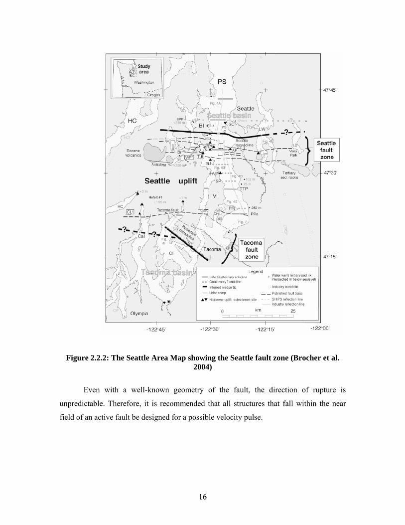
Figure 2.2.2: The Seattle Area Map showing the Seattle fault zone (Brocher et al. 2004)
Even with a well-known geometry of the fault, the direction of rupture is
unpredictable. Therefore, it is recommended that all structures that fall within the near
field of an active fault be designed for a possible velocity pulse.
16 16

2.3) Structural response to FDGM
This section features reviews of articles involving descriptions of near-fault
ground motions, and the effects of near-source large velocity pulses on structures.
The effects of FDGMs on structures were first recognized in the 1970’s (Bertero,
1976). However, engineers largely ignored FDGMs in structural design until after the
1994 Northridge earthquake. Since then, a number of studies have been directed at the
effect of near-fault ground motions on structural response, prompting revision of design
codes. In current practice, rupture directivity effects are generally taken into account by
modifications to the elastic acceleration response spectrum at 5% damping (Somerville et
al. 1997, Somerville 2003).
2.3.1) Effects on Buildings
The study of the effects of near-source ground motions on structures has generally
been limited to the effects on buildings. Bertero et al. (1978) studied buildings that were
severely damaged during the 1971 San Fernando earthquake and the implications of
pulses on pre-1971 aseismic design methods. Their result showed that the near-fault
ground motions with pulses can induce strong structural responses. In the same way,
Anderson and Naeim (1984) showed that near-field ground motions with pulses could
induce dramatically high response in fixed-base buildings. Hall et al. (1995) performed
an analytical study on a 20-story steel moment frame structure and a three-story base-
isolated building in the Greater Los Angeles area. They simulated a magnitude 7.25
earthquake on a blind-thrust fault. They indicated that the demands made by the near-
fault ground motions could far exceed the capacity of flexible high-rise and base-isolated
buildings. Iwan (1996), Attalla et al. (1998), and Hall and Aagaard (1998) completed
17 17

further analytical studies on near-source effects on buildings. Iwan (1997) stated that the
pulses in the near-field ground motions travel through the height of the buildings as
waves, and that the conventional techniques using the modal superposition method and
the response spectrum analysis may not capture the effect of these pulses. Iwan also
proposed the use of a drift spectrum for near-field ground motions. But Chopra and
Chintanapakdee (1998), in their preliminary investigation, concluded that the response
spectrum analysis is accurate for engineering applications and should be preferred over
the drift spectrum. Malhotra (1999) studied the response characteristics of near-fault
pulse-like ground motions and showed that ground motions with high peak ground
velocity (PGV) to peak ground acceleration (PGA) ratios have wide acceleration-
sensitive regions in their response spectra. This phenomenon will increase the base shear,
inter-story drift, and ductility demand of high-rise buildings. Chai and Loh (1999) used
three types of velocity pulse to determine the strength reduction factor of structures. They
found that the strength demand depends on the pulse duration and the ratio of pulse
duration to the natural period of the structure.
Nakashima et al. (2000) examined the response behavior of steel moment frames
subjected to near-fault ground motions recorded in recent earthquakes in Japan, Taiwan
and the US, and found that the largest story drifts are all similar among Japanese,
Taiwanese and the American near-fault records.
By investigating the response of single degree of freedom (SDOF) systems under
near-fault and far-field earthquake motions in the context of spectral regions, Chopra and
Chintanapakdee (2001) found that for the same ductility factor, the near-fault ground
motions impose a larger strength demand than the far-field motions do. Loh et al. (2002)
18 18

carried out a series of experimental studies to develop a regression-based hysteretic
model. They used this hysteretic model to study the basin effect and the near-fault effect
of ground motion subjected to Chi-Chi earthquakes. Alavi and Krawinkler (2004) studied
the behavior of moment-resisting frame structures subjected to near-fault ground
motions. The results demonstrate that structures with a period longer than the pulse
period respond very differently from structures with a shorter period. For the former,
early yielding occurs in higher stories but the high ductility demands migrate to the
bottom stories as the ground motion becomes more severe. For the latter, the maximum
demand always occurs in the bottom stories.
Recent near-fault ground motion research with respect to structures includes work
by Makris and Black (2004) on dimensional analysis of structures subjected to near-fault
ground motions, Iwan (1995) on specification of near-fault ground motions, Yang and
Agrawal (2002) on the use of passive and semi-active control systems for near fault
applications, Filiatrault and Trembley (1998) on the use of passive dampers in near field
applications, Symans et al. (2003) on the use of passive dampers in wood structures
subject to near-fault ground motions, and Krawinkler and Alavi (1998) on improving
design procedures for near-fault ground motions.
The papers of Sucuogly et al. (1999) and Makris and Black (2004) examined the
influence of peak ground velocity on the failure probability of structures. Sucuogly et al.
(1999) make a clear distinction between acceleration pulses and velocity pulses and
indicate correctly that “structural damage caused by ground excitation is closely related
with the dominant acceleration pulse. If the peak ground velocity is reached immediately
following the dominant acceleration pulse, then the peak velocity reflects the impulsive
19 19

character or strength in the acceleration records.” Makris and Black (2004) investigated
the “goodness” of peak ground velocity as a dependable intensity measure for the
earthquake shaking of civil structures. The paper identifies two classes of near-fault
ground motions: those where the peak ground velocity is the integral of a distinguishable
acceleration pulse and those where the peak ground velocity is the result of a succession
of high-frequency acceleration spikes. It is shown that the shaking induced by the former
class is in general much more violent than the shaking induced by the latter class.
2.3.2) Effects on Bridges
Bridges less than about 10 km from a fault rupture may be subjected to very large
accelerations, velocities, and displacements that challenge traditional methods of seismic
design. Not only is it difficult to design bridges that will be built at these locations, but
also many of the assumptions used in determining the demands on these bridges may no
longer hold true. For instance, engineers perform an elastic analysis to derive the
demands on a bridge, under the assumption that the maximum linear and nonlinear
displacements are about equal (Newmark 1971). This assumption may not be valid close
to the fault rupture.
Recently, many simulations and analyses have been performed for specific
bridges. Mayes and Shaw (1997) evaluated the response of 16 columns designed using
the Caltrans Bridge Design Specifications to several seismic events involving near-fault
ground motions. Liao et al. (2000) studied the dynamic behavior of a five-span concrete
pier bridge subjected to both near-fault and far-field ground motions. Their results also
support the conclusion that higher ductility demands and base shear are caused by near-
fault earthquake ground motions than by far-field earthquake ground motions.
20 20

Orozco and Ashford (2002) investigated three flexural columns subjected to a
large pulse and subsequent cyclic loading at increasing multiples of yield ductility. These
columns were compared to columns tested at UC Irvine (Hamilton 2000) under a non-
pulse cyclic loading. It was found that the flexural columns performed well. During the
pulse they exhibited increased strength and smaller plastic hinge lengths when compared
to the non-pulse loading, but the ultimate strengths and ductilities were similar.
Ghasemi and Park (2004) subjected the Bolu Viaduct, struck by the 1999 Duzce
earthquake in Turkey, to near-fault ground motions. They took into account a static
ground dislocation in the fault-parallel direction. This analysis showed that the
displacement of the superstructure relative to the piers exceeded the capacity of the
bearings at an early stage of the earthquake, causing damage to the bearings as well as to
the energy dissipation units. The analysis also indicated that shear keys, both longitudinal
and transverse, played a critical role in preventing collapse of the deck spans.
Shen and Tsai (2004) evaluated the performance of a seismically isolated bridge
under a Near-Fault Earthquake. The near-fault effect amplifies the seismic response of
the isolated bridge when the pulse period is close to the effective period of the isolation
system. In the same way, Wen-I Liao et al. (2004) performed a comparison of the
dynamic response of isolated and non-isolated continuous girder bridges subjected to
near-fault ground motions. Only the longitudinal response was considered. The effects on
base shear reduction of a seismically isolated bridge with the far-field ground motion
input is more significant than those with the near-fault ground motion input. The
PGV/PGA value is identified as the key parameter that controls the response
21 21

characteristics of bridges under near-fault ground motion. The base shear and
displacement demand of isolated bridges are significantly influenced by this parameter.
Despite the number of recent research projects on near-fault ground motions,
significant work is still needed to provide an improved understanding of the response of
structures to FDGMs and to develop appropriate design provisions (Alavi and Krawinkler
2000; Milonakis and Reinhorn 2001; Zhang and Iwan 2002). There is still significant
uncertainty in how to properly account for FDGMs, as illustrated by the latest changes to
the design for FDGMs in building codes (e.g. AASHTO) and the current lack of
recognition of the effect of the near-fault pulse period on the response of structures.
Research is needed in the area of soil-structure interaction in near-fault ground motions
as well to determine the influence of soil type on the FDGMs and the corresponding
structural response.
2.4) Current near-fault seismic design provisions for bridges
This paragraph should give a better understanding of the basis in the current
provisions for both the ground motion demand and the bridge capacity under FDGM’s.
As a consequence of recent earthquakes, including the 1989 Loma Prieta, 1994
Northridge and 1995 Hyogo-ken Nanbu earthquakes, seismic design codes for highway
bridges have been revised. Design Specifications of Highway Bridges were fully revised
in 1996 in Japan. In 1994, Part 2 Bridges in Eurocode 8 Design Provisions for
Earthquake Resistance of Structures was proposed as the European Pre-standard (Pinto
1995). In New Zealand, the Transit New Zealand Bridge Manual was revised in 1995
(TNZ 1995, Chapman 1995). In the United States, the American Association of Highway
and Transportation Officials (AASHTO) published two codes for the design of highway
22 22

bridges: Standard Specifications for Highway Bridges and LRFD Bridge Design
Specifications. The Department of Transportation of the State of California (Caltrans) has
developed independent seismic design specifications, which are similar to, but not the
same as, the AASHTO provisions. The ATC-32 recommendation was published to
improve Caltrans seismic design practice (ATC 1996). Caltrans recently developed the
Seismic Design Methodology (Caltrans 1999a) and the Seismic Design Criteria (Caltrans
1999b).
Concerning bridges, AASHTO LRFD Bridge Design Specification (Section
3.10.2) states that “special studies to determine site- and structure-specific acceleration
coefficients shall be performed by a qualified professional if the site is located close to an
active fault.” Caltrans (Feb. 2004) states that a “site-specific response spectrum is
required when a bridge is located in the vicinity of a major fault.” (Section 6.1.2.2 and 2.1
Caltrans Seismic Design Criteria, February 2004 Version 1.3)
The 1997 edition of the UBC for the first time introduced two near-source factors:
acceleration-related Na and velocity-related Nv, the purpose of which is to increase the
soil-modified ground motion parameters Ca and Cv when there are active faults capable of
generating large-magnitude earthquakes within 15 km or 9 miles of a Seismic Zone 4
site. These factors became necessary in view of the artificial truncation of Z-values to 0.4
in UBC Seismic Zone 4. These near-source factors are not found in the 2000 IBC because
the artificial truncation of ground motion is not a feature of that code.
23 23

2.5) Soil-Structure Interaction
Soil-structure interaction refers to the effect that the foundation soil has on the
dynamic response of a structure and, conversely, the effect of the structure on the soil
motion.
Modak (1995) stated that ground conditions at the site affect the earthquake
response of structures. Two aspects of this influence are important:(1) site effect – the
amplifying (or attenuating) effect of local geology on the intensity as well as its filtering
effect on the frequency characteristics of the transmitted seismic waves, and (2) soil-
structure-interaction – the effect of the surrounding soil properties of a structure on the
structural response.
From the analytical standpoint, one may view soil-structure-interaction as
consisting of two distinct effects: (a) inertial interaction, which arises from the motion of
the foundation relative to the surrounding soil associated with the transmission of inertial
forces from the structure to the adjoining soil; and (b) kinematic interaction, which can
occur in the absence of inertial forces, that arise when a relatively stiff structural
foundation can not conform to the distortion of the soil generated by the passage of
seismic waves. (Derecho and Huckelbridge 1991)
2.5.1) Foundation models
Many researchers have developed foundation models. The following paragraphs
describe those models.
24 24

2.5.1.1) Spread footings
Spread footings are typically built in competent material. In such cases, the
foundation is so stiff that a fixed connection is adequate for describing its behavior.
When the soil is marginal, the foundations should be modeled by spring elements or other
methods. A simple method is to represent the foundation by a 6x6 stiffness matrix that
can be determined from the foundation dimensions and the average elastic properties of
the supporting soil. A general formulation of the elastic stiffness terms in the matrix has
been developed for a rigid footing on a semi-infinite elastic half-space by closed-form
solutions. The stiffness in the three translational and three rotational directions is
provided, along with four off-diagonal terms. The embedment effects of the foundation
may be included to modify the stiffness coefficient (Lam and Martin, 1986).
McGuire et al. (1994) tested many discrete foundation elements to model the
behavior of the spread footing foundation. Five foundation models were considered, as
shown in Figure 2.5.1. One model consisted of fixed supports, one consisted of elastic
supports, and three had damped elastic supports that required three, five, and eleven
parameters per degree-of-freedom, respectively. Results showed that it is not necessary to
use a complex damped model. Employing simple spring-only foundation models (at least
to account for soil far-field effects) is enough to represent the bridge foundation. The
spring stiffness values are based on the static stiffness of an elastic half-space. Damped
models can be used for soft soil (Veletsos and Verbic 1973, and Wolf 1988).
25 25

Figure 2.5.1: Schematic of discrete foundation models for the spread footing foundation: (a) bent structure; (b) foundation models. (McGuire et al., 1994)
2.5.1.2) Pile foundations
Bridge foundations are supported on piles because of weak soil, potential scour,
or other factors. The pile foundations may include a single shaft or a group of piles
integrated by a pile cap that supports a bent or abutment. There are various methods for
modeling piles and pile foundations. A common nonlinear procedure is the p-y method
that produces a family of nonlinear lateral force-displacement relations at various depths
26 26

along an individual pile (Reese 1977, Matlock et al. 1981). These relationships can be
used to develop a 6x6 stiffness matrix at the top of each pile. The pile stiffnesses are
combined to develop a 6x6 stiffness matrix for the foundation. Computer software, such
as L-Pile and Group (Reese 2000), has been developed for applying this procedure to
model piles and pile foundations.
Dameron and Sobash (1997) used a spring/damper to model the interactions
between structure and foundation, and foundation and soil (or water). Comparison
between linear and nonlinear foundation models shows that a linear foundation model
does a poor job of predicting the response after the initial ground motion pulse.
McGuire et al. (1994, and Cofer et al., 1994) also studied pile foundations. Four
foundation models were compared, as well as fixed-base supports. Three of the four
foundation models were discrete springs or spring/damper systems, which modeled the
pile cap behavior “seen” by the column bases. The fourth foundation model was a
Winkler-type pile foundation. These five support conditions are shown in Figure 2.5.2.
The Winkler-pile was modeled with standard linear elastic beam elements and the
soil was represented as a distributed elastic stiffness, which depended upon soil
properties and the radius of the pile. For pile foundations, either the Winkler pile or pile
head models may be used, but the pile head models are recommended because far fewer
elements are required for the analysis.
27 27

rences
between the piles (including pile cap) and the surrounding soil, it manifests primarily at
higher frequencies and low soil damping. If gaps open between the foundation and soil,
particularly if the top soil layers are cohesive, can be complex. A simple approach that
Figure 2.5.2: Schematic of models for the pile foundation: (a) bent structure; (b) foundation models. (Cofer, 1994)
2.5.2) Damping
Radiation damping is an important factor that can influence foundation–soil–
structure interaction. Since radiation damping is a result of the stiffness diffe
there can be no radiation damping. Hence, the accurate modeling of radiation damping,
28 28

has been adopted by many researchers (e.g. Maragakis and Jennings 1987, Spyrakos
1992, Zhang and Makris 2002) is to use frequency independent springs and dashpots to
represent the soil–foundation system. Such models, however, do not consider possible
gaps during seismic excitation. Given the uncertainties in modeling the overall soil–
foundation behavior and the fact that frequency independent dashpots generally
deamplify the structural system response, it is not uncommon to neglect radiation
damping altogether. In their investigation of the observed behavior of a two span
overcrossing, Makris et al. (1995) were able to simulate the response of the bridge
without the need for radiation damping. The simulations by Ciampoli and Pinto (1995) of
2.5.3) Previous Research Papers
A number of papers in recent years have described investigations on the
subjected to earthquake loads. However, Sweet did not approximate the geometry of pile
groups, as he was unable to analyze a full m
the other hand, McCallen and Romstadt (1994) performed a remarkable full-scale
model through standard modulus reduction and damping curves developed by Seed et al.,
1984). In studies by Chen and Penzien (1977) and Dendrou et al. (1985), the bridge
a bridge also did not incorporate radiation damping. Additionally, recent investigations
by Bielak and al. (2003) and Tongaonkar and Jangid (2003) indicate that in some cases
radiation damping can be ignored with only minor effects on the system behavior.
influence of the SSI on the behavior of bridges. In particular, Sweet (1993), and
McCallen and Romstadt (1994) performed finite element analyses of bridge structures
odel with available computer hardware. On
analysis of the soil–foundation–bridge system. The soil material (cohesionless soil) was
modeled using an equivalent elastic approach (using the Ramberg–Osgood material
29 29

system was analyzed including the soil, but the models used very coarse finite element
meshes.
Tongaonkar and Jangid (2002) showed that SSI affects the bearing displacements
at the abutment and that ignoring these effects will cause the analysis to underestimate
the design displacement at abutments, which may be crucial from the design point of
view.
anshin Expressway (see Figure 2.5.3). Gazetas
and My
The effects of Soil-Structure-Interaction (SSI) are considered to be beneficial to
the structure under the following conditions: (1) There are no significant permanent
deformations in the structure resulting from yielding of the pier, or (2) the energy
dissipation (hysteretic loops) of the system with SSI is smaller than that with a fixed
foundation, leading to the conclusion that there is less damage to the structure.
The most dramatic failure during the Kobe earthquake was the collapse of an
elevated section of the pile-supported H
lonakis (1998) presented an analysis suggesting that period lengthening due to
foundation flexibility may have resulted in increased structural forces during the
earthquake due to forward directivity effects.
F 2.5.3: Collapsed of an 18-span viaduct section of Hanshin Expressway (from igureGhasemi, 1996)
30 30

Jeremic and Kunnath (2004) studied the SSI of the I-880 viaduct. Foundation
springs were obtained from a detailed 3D finite element model of the pile group
founda
) directions.
The SSI can either be beneficial or detrimental to the structure depending on the
ground motion. Their analysis demonstrated the difficulty associated with developing
guidelines for design since SSI effects are not only a function of the structural system and
the soil–foundation behavior but also dependent on the ground motion. In general, this
suggests that SSI effects should be evaluated on a case-by-case basis without generalizing
the findings of a particular study.
McGuire’s results (1994) indicate that the effect of incorporating foundation
models on the predicted response is very dependent on the natural frequencies of the
structure and the frequency content of the earthquake.
Mylonakis and Papastamatiou (2001), who studied bridge response on soft soil to
nonuniform seismic excitation, observed that foundation rotations due to kinematic and
inertial soil structure interaction tend to increase the response of the piers at low
frequencies, but reduce response at high frequencies.
Dicleli (2006) concluded that, in the near-fault zones, linear elastic analysis may
generally be used for the preliminary design of bridges. However, for the final design of
bridges located in the near-fault zones, three dimensional nonlinear time history analysis
seems more appropriate.
tion system using elastic soil properties. The site is located within 10 km of the
Hayward Fault and is also in the immediate vicinity of the San Andreas Fault. The
spectra contain rupture directivity effects. They were generated for both fault-parallel
(FP) and fault-normal (FN
31 31

CHAPTER 3: Column Modeling and ABAQUS
Determining the appropriate force-displacement characterization for the columns
in the modeled bridges is a key aspect in obtaining accurate results since the bridge
stiffness is primarily influenced by the column elastic and inelastic response. Using
ABAQUS, columns that had been tested previously were modeled.
The bridge columns that were considered were well-confined since they were
chosen to represent bridges that were recently designed (1989-1993). Under design
guidelines that specify appropriate column confinement, two tests were chosen to be
modeled. Orozco (2002) tested well-confined columns under a large velocity pulse.
Lehman (2000) studied well-confined columns (in accordance to the Applied Technology
Council, ATC 32) with different longitudinal reinforcement ratios and aspect ratios to
characterize the response of modern bridge columns to lateral loads.
3.1) The Orozco columns
3.1.1) Geometry and reinforcement
The test specimen had a diameter of 410 mm (16 in) that corresponds to a 1.83 m
(72 in) prototype bridge column diameter. In addition, the test specimen had a height of
1.83 m (72 in) that corresponds to the prototype bridge column height of 8.23 m (324 in).
The height of the bridge column was measured from the top of the footing to the center of
the load stub. An elevation view of the column is seen in Figure 3.1.1.
The longitudinal reinforcing steel consisted of twelve 13 mm (0.5 in) diameter
(#4) bars that were spaced equally, which produced a steel/concrete ratio of 1.2%. The
32 32

longitudinal steel had a yield strength of 416 MPa (Grade 60), conforming to ASTM 706
or equivalent, with a yield stress that should not exceed 520 MPa (75 ksi). The transverse
reinforcement was 16 mm² (W2.5) ASTM with a yield strength of 555 MPa (Grade 80).
The spiral was spaced at 32 mm (1.25 in) on center continuous from the base of the
footing to the top of the load stub.
The concrete cover from the face of the bridge column to the face of the spiral
was 13 mm (0.5 in). The concrete compressive strength of the column measured on the
day of the test was 32.1 MPa (see section 3.2.2 for a description of the tests).
Figure 3.1.1: Column elevation (Orozco, 2002)
3.1.2) Loading and test setup
To study the effects of the large velocity pulse, two 22% scale bridge columns
were tested. The bridge columns were subjected to a velocity pulse followed by a cyclic
loading history. The specimen was loaded dynamically.
33 33

The test was completed with an actuator at a rate of 1 m/s (39 in/s). The input
displacement time history was designed to model a near-fault displacement history. The
loading history was composed of a cyclic loading history based on drift ratios of 0.5%,
1.0%, 1.5%, 2.0%, 3.0%, 4.0%, 5.0%, and 6.0%. Each drift ratio had three peaks in both
the positive and negative directions. The input time histories were a combination of the
pulse and the cyclic loading history. The saw-toothed displacement time history of the
test is plotted in Figure 3.1.2.
Figu 02)
The tes en was secured to the
ring the test.
re 3.1.2: Input time history (Orozco, 20
t setup is shown in Figure 3.1.3. The test specim
strong floor by eight 35 mm (1-3/8 in), yield strength 1040 MPa (Grade 150) high
strength bars stressed to 667 KN (150 kips). A 979 KN (220 kip) capacity actuator, with a
+/- 610 mm (24 in) stroke, was attached in between the strong wall and load stub. No
axial force was imposed to the column du
34 34

Figure 3.1.3: test setup (Orozco, 2002)
3.1.3)
Test re elevant to this
research is the force-displacement hysteretic curve which characterizes the column
behavior. One can see the Force-Displacement prediction given by the software
um
Recorded responses from testing
sults are shown in Figures 3.1.4 and 3.1.5. What is most r
Rua oko (Carr, 1996) in Figure 3.1.5.
Figure 3.1.4: Overall view after pulse loading (Orozco, 2002)
35 35

F
ic
nts. The length of the elements was made equal
to (or a bit higher t p 996), as follows:
igure 3.1.5: Recorded response: hysteretic force-displacement curve and dashed Ruaumoko (Carr, 1996) prediction (Orozco, 2002)
3.1.4) Finite Element Modeling of the Columns
3.1.4.1) Global geometric modeling
The Finite Element nonlinear static analysis was performed on
ABAQUS/Standard with a 3D model. The columns were discretized by 3-node quadrat
Timoshenko (shear flexible) beam eleme
han) the plastic hinge length, L , given by Priestley (1
36 36

The plastic hinge length is approximated as
blyeblyep dfdfLL 044.0022.008.0 ≥+= (fye in MPa) (3.1)
blyeblyep dfdfLL 3.015.008.0 ≥+= (fye in ksi) (3.2)
Where L is the length from the plastic hinge to the point of contraflexure. For a column
in double bending, L is at the column ye
s
the equation accounts for the stra longitudinal steel in the footing.
The p
ent is important since behavior results
or a column are functions of the element length (Figure 3.1.6).
mid-height. f is the effective yield strength of the
teel and dbl is the diameter of the longitudinal reinforcing steel. The second portion in
in penetration of the
lastic hinge length is important because it directly affects the post-yield
displacements. The choice in the size of the elem
f
Figure 3.1.6: Response of column rent sizes with diffe d elements (Légeron, 2005)
The columns were all made of 6 elements (Figure 3.1.7), each integrated at the
top and bottom. For the four top elements, the default integration points were used
through the thickness for economy, as shown in Figure 3.1.8. More integration points (5
radially, 12 circumferentially) were imposed to the two bottom elements of the column
because more accuracy in the results is required there due to the occurrence of damage.
37 37

38 38
Figure 3.1.7: Column with 6 e
Figure 3.1.8: Default 3 radially, 8 circumferenbeam
the 3-node elem
the top
t
cross section and two integration point
The column was fixed at the bottom. An i
of the column as shown in Figure 3.1.9.
Elemen
lements (13 points)
tially integration points, through the ocations (in red) along the length of ent
l
mposed displacement ∆u was applied at

During the finite element analysis, there was no need to include three cycles at
each displacement level as was done in the tests, since ABAQUS will give the exact same
results for each cycle. The damage occurring in the column can be modeled only when
the demand (loading) increases. Figure 3.1.10 shows the imposed displacement history
used during the finite element analysis.
Figure 3.1.9: Column model in ABAQUS
-150
-100
-50
00 2 4 6 8 10 12 14
steps
disp
em
Figure 3.1.10: Input time history during the ABAQUS analysis
50
)
100
150
lac
ent (
mm
∆u
39 39

3.1.4.2) Material models
The material models used in ABAQUS are well established in practice. The
aterial models used in this study were the smeared crack concrete m
lasticity model that includes both kinematic and isotropic hardening. This section
s them and gives the final input material properties.
.1.4.2.1
The ABAQUS User Manual (2004) gives a description of the smeared crack concrete
s a general capability for modeling concrete in all types of structures,
nalysis of reinforced concrete structures;
•
rs for the smeared crack concrete model are the modulus of
elasticity, and the com
described below.
m odel, and the metal
p
describe
3 ) Concrete
model which:
• “provide
including beams, trusses, shells, and solids;
• can be used for plain concrete, even though it is intended primarily for the
a
can be used with rebar to model concrete reinforcement;
• consists of an isotropically hardening yield surface that is active when the stress is
dominantly compressive and an independent ‘crack detection surface’ that
determines if a point fails by cracking;
• uses oriented damaged elasticity concepts (smeared cracking) to describe the
reversible part of the material's response after cracking failure;
• requires that the linear elastic material model be used to define elastic properties.”
The input paramete
pressive and tensile stress-strain curves. These parameters are
40 40

Modulus of elasticity:
It has been determ oment of inertia of ined by Priestley (2003) that the m
reinforced concrete columns should be reduced to account for initial cracking. In
ABAQ
c
c c
ding stiffness of the element is properly modified.
Compressive stress – strain relationship:
US, because beam properties result from integration over the cross section, the
modulus of elasticity E had to be changed to take into account the effect of the moment
of inertia reduction. A new value of Ecc = Ec/2 was tested. The initial slope of the force-
displacement curve was found to be approximately equal to that of the experimental one.
Note that the actual predicted value of the concrete modulus of elasticity is given by
Priestley (1996):
E = 4780 √f’ (MPa) (3.3)
In this way, the effective ben
The properties for confined concrete differ from those for unconfined concrete.
Mander and Pri te subjected to
ssive loading and confined by transverse reinforcement. Since ABAQUS
cannot model the transverse reinforcement for the 3D beam element, the confined
concrete properties have to be computed from empirical data. The peak compressive
stress (f’cc) that can be developed in the confined concrete is (Mander and Priestley,
1988):
estley (1988) developed a stress-strain model for concre
uniaxial compre
⎟⎟⎠
⎞⎜⎜⎝
⎛−−+= 254.1
''2
''94.7
1254.2''c
l
c
lccc f
ff
fff (3.4)
41 41

Where:
(3.5)
lel fKf ='
sDAf
f spyhl '
2= (3.6)
'0.002 1 5 1'cc
ccc
ff
ε⎡ ⎤⎛ ⎞
= + −⎢ ⎥⎜ ⎟⎝ ⎠⎣ ⎦
(3.7)
Ke = Ae/Acc (3.8)
Acc = Ac (1-ρcc) (3.9)
In the above equations, fl is the maximum lateral confining stress at yield in the
fective confining stress, and Ke is the confinement
is the diameter of the confined column core; s is the vertical spacing of transverse
reinforcement; ρcc is the ratio of the area of longitudinal reinforcement to the area of core
o
perime e cc
cc
ip
transverse reinforcing steel. f’l is the ef
effectiveness coefficient. f’c is the compressive strength of unconfined concrete; fyh is the
yield strength in the transverse reinforcement; Asp is the area of the transverse reinforcing
bar; D’
f the section; Ac is the area of the core of the section enclosed by the center lines of the
ter spiral; A is the area of the effectively confined concrete core; and ε is the
strain when f’ is reached.
The ultimate strain reached in the confined concrete is based upon a relationsh
proposed by Priestley et al. (1996).
cc
suyhs f4.1004.0cu f '
ερε += (3.10)
42 42

According to Priestley et al., Equation 3.10 is intended to be used for design,
typically being conservative by 50%. However, this equation was used unchanged. Figure
to the
diamete sive stress-strain
3.1.11 summarizes the difference in behavior between unconfined and confined concrete.
The entire concrete section was assigned these confined concrete properties, including the
concrete cover. The behavior of the column is assumed to be governed by the confined
concrete section, because the concrete cover thickness is relatively small compared
r of the entire section. Figure 3.1.12 shows the typical compres
curve input into ABAQUS.
Figure 3.1.11: Stress-Strain Model Proposed for Monotonic Loading of Confined
and Unconfined Concrete (Mander & Priestley, 1988)
43 43

0.00E+00
5.0
44 44
0E+06
0 0.002 0.004 0.006 0.008 0.01 0.012 0.014 0.016 0.018 0.02
strain Figure 3.1.12: Stress–Strain Relationship for the Concrete in Compression
1.00E+07
1.50E+07
2.50E+07
3.00E+07
0E+07
ress
a)
2.00E+07
3.5
4.00E+07
4.50E+07
5.00E+07
st (P
Tension stress – strain relationship:
Very little research has been performed to specify the full stress-strain behavior
for tension in concrete. However, Mazars (1989) reports the relationship, shown in Figure
3.1.13.
Figure 3.1.13: Experimental Behavior of Concrete under Tension (Mazars, 1989)
(f`c, εc)
(f`cc, εcc)
(085.f` , ε ) c cu

Effects associated with the rebar and the concrete interface, such as bond slip and
e
relative size of the concrete aggregate compared to the rebar diameter, and the mesh.”
“The choice of tension stiffening parameters is important since, generally, more
tension stiffening makes it easier to obtain numerical solutions. Too little tension
stiffening will cause the local cracking failure in the concrete to introduce temporarily
unstable behavior in the overall response of the model.” (ABAQUS manual 2004)
The tensile concrete cracking stress is given by Priestley (1996):
f’t = 0.75 √f’c (MPa, concrete in flexural tension) (3.10)
The typical tensile stress – strain curve used during ABAQUS analysis is shown
in Figure 3.1.14.
dowel action, are modeled approximately by introducing some “tension stiffening” into
the concrete modeling to simulate load transfer across cracks through the rebar.
The ABAQUS Manual states that “the interaction between the rebars and the
concrete tends to reduce the mesh sensitivity, provided that a reasonable amount of
tension stiffening is introduced in the concrete model to simulate this interaction. This
requires an estimate of the tension stiffening effect, which depends on such factors as the
density of reinforcement, the quality of the bond between the rebar and the concrete, th
0.00E+00
strain
5.00E+05
1.50E+06
4.50E+06
0 0.0005 0.001 0.0015 0.002 0.0025 0.003 0.0035
ess
(
Figure 3.1.14: Tensile Stress-Strain Curve of the Concrete
3.50E+06
4.00E+06
1.00E+06
2.00E+06
2.50E+06
3.00E+06
str
Pa)
45 45

46 46
Damage in the concrete:
BAQUS gives many possible ways to model the damage occurring in the
concrete. Reinforced concrete columns exhibit many damage mechanisms including
pinching, spalling, bond failure, rebar buckling, and cracking. Figure 3.1.15 describes the
ain behavior of the concrete du
n.
A
m ring the damaging process. Because of the many
interacting effects, it is difficult to specify a structural model. The concrete smeared
cracking model was used to capture the overall damage behavior of the colum
Figure 3.1.15: Behavior of concrete (Légeron, 2005)
The model is a smeared crack model, in the sense that it does not track individual
“macro” cracks. Rather, constitutive calculations are performed independently at each
integration point of the finite element model, and the presence of cracks enters into these
calculations through the effect of the cracks on the stress and material stiffness associated
with the integration point.
When concrete is loaded in compression, it initially exhibits elastic response. As
the stress is increased, some nonrecoverable (inelastic) straining occurs, and the response
of the material softens. An ultimate stress is reached, after which the material loses
46 46

strength until it can no longer carry any stress. If the load is removed at some point after
inelastic straining has occurred, the unloading response is softer than the initial elastic
response. However, this effect is ignored in the model. When a uniaxial specimen is
loaded into tension, it responds elastically until, at a stress that is typically 7-10% of the
ultimate compressive stress, cracks form so quickly that - even on the stiffest testing
machines available - it is very difficult to observe the actual behavior. For the purpose of
developing the model, the material is assumed to lose strength through a softening
mechanism that is dominantly a damage effect, in the sense that open cracks can be
represented by a loss of elastic stiffness (as distinct from the nonrecoverable straining
that is associated with classical plasticity effects, such as that used for the compressive
behavior model). The model neglects any permanent strain associated with cracking; that
is, crack es
pressive
3.1.4.2.2) Longitudinal Steel
In ABAQUS, reinforcement in concrete structures is typically provided by means
of rebars, which are one-dimensional rods. Rebars are typically used with metal plasticity
models to describe the behavior of the rebar material and are superposed on a mesh of
standard element types used to model the concrete. Figure 3.1.16 shows the steel stress-
strain relation of the longitudinal rebars. This is based on the Caltrans 1999 grade 60 steel
values. Special models have been developed in ABAQUS for metals subject to cyclic
loading. The model chosen is one that includes both kinematic and isotropic hardening.
s are assumed to close completely when the stress across them becom
com
47 47

0.00E+00
1.00E+08
2.00E+08
3.00E+08
strain
ress
Once the finite element computations were
4.00E+08
5.00E+08
6.00E+0
7.00E+
0 0.025 0.05 0.075 0.1 0.125 0.15
st (P
a)
Figure 3.1.16: Steel Stress-Strain Curve
3.1.5) ABAQUS Results
done, the shear force at the bottom of
the column was plotted as a function of the i posed displacement to give the hysteretic
curves shown
8
08
m
in the following figures.
Figure 3.1.17 shows the force-displacement curves, compared with experimental
results. The solid red lines are from the finite element analyses.
48 48

Figure 3.1.17: Comparison of Orozco (light gray) and ABAQUS results (solid red)
3.2) Lehman column
The ABAQUS results were quite accurate when compared to those of Orozco’s
tests. To provide further validation of the modeling technique, a different set of test
results were obtained and analyzed (Lehman, 2000).
3.2.1) Geometry and reinforcement
The column diameter was selected to be 61 cm (2 feet) to model a 1.83 m (6 feet)
diameter prototype (8 feet) tall. The
(Ruaumoko, 1996)
column (one-third full scale). The column was 2.44m
49 49

concrete cov t specimen
are shown in Figure 3.2.1.
er was 1.9 cm (¾ inch) thick. Column and joint details of the tes
Figure 3.2.1: Specimen Geometry and Reinforcement of the Lehman column.
(Lehman, 2000)
The column was reinforced with 1.5% longitudinal steel (22 No.5 bars) and had
an aspect ratio of 4. The longitudinal reinforcement was spaced evenly around the
column circumference. The longitudinal reinforcement was embedded into the joint to a
depth of 54.61 cm (21.5 inches), approximately equivalent to 34 bar diameters. The
column s ches) in
iameter smooth wire spaced at 3.17 cm (1¼ inches). The spiral reinforcement was
continuous throughout the column height and joint depth. Table 3.2.1 gives the steel
piral reinforcement ratio was 0.7%. The spiral was 0.64 cm (¼ in
d
50 50

properties. The oncrete used on the day of the test was 30 compressive strength of the c
MPa (4.4 ksi).
Table 3.2.1: Steel properties
Bar Yield (ksi) Ultimate (ksi)
Longitudinal rebars 68.4 93.3
Spiral 96.9 98.9
3.2.2) Loading and test setup
the experimental configuration. The applied axial load of 667 KN (150 kips) was
A
average axial load ratios found in single-column
Axial and lateral loads were applied to the top of the column. Figure 3.2.2 depicts
approximately equivalent to 0.07f`cAg, where f`c = actual concrete compressive strength
and g is the column gross section area. The axial load ratio chosen corresponded to
bent bridge construction. The axial load
was applied through a spreader beam
the column. The lateral load was applied using a servo-controlled hydraulic actuator that
was atta
using post-tensioned rods placed on either side of
ched to the top of the column.
Figure 3.2.2: Experimental configuration (Lehman, 2000)
51 51

The imposed displacement history included three cycles at each displacement
level (Figure 3.2.3). Note that no initial pulse was applied and that the rate of loading was
very slow. The imposed displacement history depends upon the effective yield
displacement given by the following equation:
(3.11)
The computed effective yield displacement was 2.34 cm (0.92 inches).
Figure 3.2.3: Imposed displacement during the test (Lehman, 2000)
3.2.3) Recorded responses from testing
Bending and slip were observed to dominate the column response.
A brief chronological description of the visual indications was provided:
1. Cracking of the concrete
2. First yield of longitudinal steel
3. Spalling above the column-footing interface
4. Spirals and longitudinal steel exposed; complete loss of the concrete cover
52 52

5. Extension of spiral and longitudinal bar buckling
6. Spiral fracture
the bottom of the column, where all
visible bars on both faces buckled. Figure 3.2.5 shows the force-displacement hysteretic
curve recorded
7. Longitudinal bar fracture
8. Failure of the column
Figure 3.2.4 shows the final damage state at
during the test.
Figure 3.2.4: Final damage state (Lehman, 2000)
53 53

Figure 3.2.5: Force – Displacement Response (Lehman, 2000)
One observes pinching behavior due to the cracks starting from an imposed
displacement of 7.6 cm (3 in). Compared to the specimens from Orozco’s tests, this
column deve
3.2. te E
loped a lot more pinching.
4) Fini lement modeling of the column
The methods used to compute the geometry and the material parameters were the
same as described earlier (section 3.1.4). Figure 3.2.6 shows the imposed displacement
used during the finite element analysis.
54 54

displacement ti istory
-5
0
5
10
15
0 2 4 6 8 10 12
disp
lace
men
t (cm
)
3.2.5) ABAQUS Results
complete, the shear force at the
bottom of the colum
hysteretic curves shown in Figure 3.2.7. Figure 3.2.7 also shows the force-displacement
ental result he ABAQU odel was sh n to generate
an accurate backbone curve. The values of peak force and both initial and subsequent
stiffness were predicted quite accurately. The increased pinching observed with
Lehman’s tests was underestimated. Pinching likely results from damage between the
concrete and the rebars and it may be affected by the rate of loading. As a consequence,
the ABAQUS finite element model will have a tendency to overestimate the energy
dissipated from the column hysteretic behavior.
me h
-10
-15
steps Figure 3.2.6: Imposed displacement during the ABAQUS analysis
Once the finite element computations were
n was plotted as a function of the imposed displacement to give the
curves, compared with experim s. T S m ow
55 55

Force - Displacement Curve
-350
-250
-150
-50
50
150
250
350
-150 -100 -50 0 50 100 150
Displacement (mm)
Forc
e (K
N)
Lab Test Abaqus 3D
Figure 3.2.7: Comparison of Lehman and ABAQUS results
In order to verify that a model using ent software can
accurately simulate the cycl einforced concrete columns
when subjected to FDGM’s, two test specimens were modeled. While many material
properties for the concrete and steel reinforcing were defined using accepted practice, a
number of parameters are numerical in nature, rather than being based on known physical
properties. The latter were defined by matching the overall test results of Orozco, for
which pulse-type loading was used to simulate FDGM ground motion. Then, with
essentially the same values, the tests of Lehman were modeled. The following
conclusions may be drawn.
Both finite element models were shown to generate accurate backbone curves.
The values of peak force and both initial and subsequent stiffness were predicted quite
3.3) Conclusion
the ABAQUS finite elem
ic behavior of well-confined r
56 56

accurately. While the cyclic behavior was simulated relatively well for the dynamic test
of Orozco, the increased pinching observed with Lehman’s tests was underestimated.
Pinching likely results from damage between the concrete and the rebars and it may be
affected by the rate of loading. The loading rate during an earthquake more nearly
matches that of Orozco’s dynamic test than those of the others.
By modifying the geometry and the physical material properties of Orozco’s test
specimen to match those of Lehman’s test specimen, a reasonably accurate model was
conveniently obtained. All numerical material parameters were unchanged except for the
tensile damage variable, which was decreased to better match the strength behavior when
the loading did not include an initial pulse.
The ABAQUS model that was developed was shown to provide accurate
simulations for a test specimen that was designed and loaded specifically for FDGM. For
a similar specimen with a more traditional test sequence, the same model gave reasonably
accurate results, the only significant difference being that the hysteresis curve did not
fully represent the level of pinching. With the favorable results, the ABAQUS model can
be used with confidence to evaluate the seismic performance of bridges subjected to
rward directivity ground motions. fo
57 57

CHAPTER 4: Seismic Analysis of Bridges
4.1) Seismic Excitations
This section describes the ground motion selection process, in addition to the
main characteristics of the selected ground motions.
4.1.1) Ground Motion Selection
To obtain a set of non-Forward Directivity (FD) Ground Motions (GMs), a
probabilistic seismic hazard analysis (PSHA) for each bridge site, including
deaggregation, was performed by Gillie (2005), leading to a target design spectrum for
each bridge. Deaggregation helps determine which pairs of Mw and R to use when
choosing ground motions for site specific evaluations. Once the ranges of magnitude and
distance were determined, all ground motions that satisfied these requirements were
elected for further analysis from the PEER database (PEER 2000). In some cases the
distanc
one dimensional site response analysis
was performed on the ground motions to take into account the nature of the surrounding
soil at the foundation of each bridge. The non-FDGMs were composed of 3 sets, one for
each bridge, of 5 ground motions with both the fault normal and fault parallel
components. The FDGMs were selected based on the expected ground motions from the
Seattle Fault Zone. They did not have spectral matching and site response either to
preserve their period content integrity. For more details, see the thesis of Gillie (2005).
s
e and magnitudes were expanded to obtain motions that best satisfied the
following criteria: similar faulting type, recorded on rock, response spectra matching the
shape of the target spectra, and no FD characteristics. Spectral matching was applied to
the non-FDGMs to fit the target spectra. Finally, a
58 58

4.1.2) Ground Motion Characteristics
The non-FDGM spectral accelerations are showed in Figures 4.1.1 and 4.1.2. The
bridge acceleration spectra, in colors, were derived from the target spectrum (the Equal
Hazard Spectrum from the PSHA), to include site response. The spectral accelerations for
Bridge 405 and Bridge 520 were very similar because their soil properties were similar.
B520
B405
B90Target
Figure 4.1.1: Non FDGMs Acceleration Spectra (Log. scale)
59 59

60 60
Figure 4.1.2: Non FDGMs Acceleration Spectra
The selected
ground motion component, the record length and the Peak Ground Acceleration (PGA)
are indicated. The ground motion acceleration, velocity and displacement time histories,
spectral acceleration, and velocity are in Appendix B.1.
Table 4.1.1: FDGM characteristics
GM Magnitude Time (s) GM Component PGA (g)
FDGMs and their characteristics are listed in Table 4.1.1. For each
FN 0.733 Sylmar 6.7 20 FP 0.595 FN 0.314 T75 7.6 50
0.278 FP FN 0.854 KJM 6.9 FP 0.548
26
FN 0.880 BAM 6.5 15 FP 0.647 FN 1.015 F14 6.0 21 FP 0.857 FN 0.887
RRS 6.7 15 FP 0.390
B520
B405
B90
Target

4.2) Coordinate Axes
The longitu is of each bridge was oriented along the global X axis
following the positive right hand rule sign convention for the global Y and Z axes. Local
and global coordinate systems are defined in Table 4.2.1 below. Figure 4.2.1 shows the
different coordinate axes.
Table 4.2.1: Local and Global Coordinate Systems
Global Coordinate Axes Local Coordinate Axes
dinal ax
Bridge Direction Global Axes Trans. Elements Long. Elements Vert. Elements Transverse Y X Y Y
Longitudinal X Y X Z Vertical Z Z Z X
Figure 4.2.1: Bridge Coordinate Axes
Local Axes (Vertical Element)
Global Axes
61 61

4.3) WSDOT Bridge Selection
The bridges were selected based on their geographical location, close to the
Seattle fault region. Figures 4.3.1 and 4.3.2 show the locations of the bridges and the fault
region, respectively.
Figure 4.3.1: Bridge location
62 62

Figure 4.3.2: The Seattle Area Map showing the Seattle fault zone and bridge location (Brocher et al. 2004)
4.4) WSDOT Bridge 405/46N-E
4.4.1) Geometry and reinforcement
Bridge 405/46N-E is an overpass located at 116th Avenue N. E. in Bellevue,
Washington e junction
Bridge 90
Bridges 405 and 520
. In 1993, the bridge was built to service traffic on SR 405 at th
63 63

with SR 520. By today’s standards, the columns are considered well-reinforced, well-
tely lap-spliced. confined and adequa
Figure 4.4.1: Bridge 405 Aerial View
The bridge length is 50.3 m (165 ft) back to back of pavement seats and consists
of three spans ps are 15.85 m (52 ft) long with the center
ramp m
. The western and eastern ram
easuring 18.6 m (61 ft) in length. The bridge has no skew to it. Plan and elevation
views are shown below in Figures 4.4.2 and 4.4.3.
64 64

Figure 4.4.2: Bridge 405 Elevation
Figure 4.4.3: Bridge 405 Plan
The deck, shown in Figure 4.4.4, is composed of pre-tensioned concrete beams.
Each span includes three girders spaced 2.90 m (114.4 in) on center. Overlaid on top of
the girders is a 17.8 cm (7 in) thick, 8.46 m (27.75 ft) wide reinforced concrete deck slab.
Figure 4.4.4 Bridge 405 Deck cross-section
65 65

66 66
at the bottom of each
. Four No. 6 bars are located at the side edges and run longitudinally along the
. For shear reinforcement, No. 5 stirrups are spaced evenly along each member.
ns and crossbeam were cast monolithically adding considerable rigidity to
Figure 4.4.5: Bridge 405 Column Sections (Crossbeam & Circular column)
At each of the two bents, a 1.22x1.22 m (4x4 ft) crossbeam transversely connects
the two columns. Figure 4.4.5 below shows the geometry and steel reinforcement. Each
crossbeam extends 7 m (23 ft) in length (Figures 4.4.6 and 4.4.7). The steel reinforcement
consists of five No. 9 bars located at the top and five No. 8 bars
crossbeam
crossbeam
The colum
each bent.
Figure 4.4.6: Crossbeam plan view

Figure 4.4.7: Bridge 405 Hinge Elevation (between crossbeam and deck)
The I-girders rest upon laminated elastomeric bearing pads located on top of the
abutment seats. They are restrained in the transverse direction by girder stops. Figures
4.4.8 and 4.4.9 show the elastomeric bearing pad and the girder stops.
Figure 4.4.8: Bearing Pad Figure 4.4.9: Bridge 405 Girder Stop
At each bent, the bridge deck is monolithically constructed. The height of the
columns at both bents is approximately 8.53 m (28 ft). The clear column height is about
6.7 m m (13 ft) centerline to centerline. Each
colum s a cross-sectional diameter of 0.91 m (3 ft). Twelve evenly spaced No. 9 bars
provide the longitudinal reinforcement within each column. This provides a longitudinal
(22 ft). The columns are spaced at 3.96
n ha
67 67

reinforcing ratio of 1.18%. The clear cover measures 3.8 cm (1.5 in.). Transverse
reinforcement is provided by No. 5 bars spaced at 6.35 cm (2.5 in.) on center resulting in
a transverse reinforcem
Figure 4.4.10: Bridge 405 Bent Elevation
The footings are reinforced at the bottom with fourteen No. 7 bars and at the top
with eighteen No. 6 bars in
reinforced with twenty five No. 6 bars at the top and thirty eight No. 6 bars at the bottom.
A plan view of a spread footing is shown in Figure 4.4.11.
ent ratio of 1.50%. Figure 4.4.10 shows the elevation view of the
columns. Supporting each column is a spread footing.
The length, width and depth of the spread footings are 7.92 m (26 ft), 4.27 m (14
ft), and 0.91 m (3 ft), respectively.
the direction of the width. In the length direction, it is
68 68

69 69
Figure 4.4.11: Bridge Foundation Spread Footing for Bents
Both abutments are about 3 m (10 ft)
abutments, there is no transverse resistance in the t ake. A footing
measu epth
is located directly underneath the abutm
west and east abutments is shown in Figure 4.4.13.
undation Spread Footing for Bents
Both abutments are about 3 m (10 ft) deep. Due to no endwall being on the
abutments, there is no transverse resistance in the t ake. A footing
measu epth
is located directly underneath the abutm
west and east abutments is shown in Figure 4.4.13.
ring 8.6 m (28.1 ft) in length, 1.92 m (6.3 ft) in width, and 0.46 m (1.5 ft) in d
ent-deck seating block. The elevation view of the
ring 8.6 m (28.1 ft) in length, 1.92 m (6.3 ft) in width, and 0.46 m (1.5 ft) in d
ent-deck seating block. The elevation view of the
deep. Due to no endwall being on the
even of an earthqu even of an earthqu
Figure 4.4.12: Bridge 405 Abutment and Deck Elevation View

Figure 4.4.13: Bridge 405 East and West Abutments
The footings and abutment walls were constructed with WSDOT Class 4000
concrete providing a compressive strength of f’c = 27.6 MPa (4 ksi). The concrete in the
prestressed girders was specified to be class 6000. The concrete in the columns,
crossbeam, diaphragms, and slabs was specified to be class 5000. The reinforcing steel
conforms to AASHTO M31 Grade 60 with a yield strength of fy = 413.6 MPa (60 ksi)
4.4.2) Structural Model
The Finite Element nonlinear dynamic implicit analysis was performed on
AQUS/Sta rd with a 3D model. The bridge was discretized by 3-node quadratic
Timoshenko (shear flexible) beam elements, resulting in a so-called spine model, as
shown in Figure 4.4.14.
AB nda
mix
.
70 70

Figure 4.4.14 Brid e 405 Spine M: g odel
For the deck, ABAQUS can generate from a meshed region with 2D warping
elements beam cross-section properties that can be used in a subsequent beam element
analysis. Figure 4.4.15 shows the assigned deck cross-section.
Figure 4.4.15: Bridge 405 deck cross-section
The torsional rigidity is calculated over the two-dimensional region meshed with
warping elements. In the elastic range, warping is small and ABAQUS assumes that
warping prevention at the ends can be neglected. The axial warping stresses are therefore
assumed to be negligible, but the torsional shear stresses are assumed to be of the same
order of magnitude as the stresses due to axial forces and bending moments.
A solid Finite Element Model (FEM) of the Bridge 405 deck was created to
investigate the effect of these assumptions. A simple model, based on a cantilever beam
under flexure or torsion, was also modeled with a single beam element.
71 71

Figure 4.4.16: Bridge 405 deck solid and spine models
Figure 4.4.17: Bridge 405 deck in torsion
An axial torque of 360 kN
.m was applied at the end of both cantilever beam
models and the end rotation values were compared. The rotation of the spine cantilever
model with the original torsional stiffness was over three times that of the detailed finite
element model (Table 4.4.1). This result indicates that the restriction of warping has a
significant effect on torsional stiffness. Because of the rigid connection of the deck to the
cap beams, the restriction of warping is justified for the deck, and the torsional stiffness,
GJ, was increased accordingly for the bridge model.
72 72

Table 4.4.1: Torsional results and comparison
Solid FEM Spine model
GJ (T 6.31E+08 1.58E+0 9 2.52E+09orsional Stiffness) 9 1.89E+0 2.21E+09 Multiplication factor x 3 x 4 x 1 x 2.5 x 3.5 End Rotation d) 0.00336 0.01134 0.00454 0.00378 0.00324 0.00284 (ra
Th bendin acteris n both tions w The results
(horizonta and ve displa nts) fo odels were in close agreement,
matching within 6% error.
In conclus tor fness that was use e M dge
405 was the origin l stiffness valu by ABAQUS multiplied b
Figure 4.4 8 sh appli s-se ofiles to the different bridge elements.
The n ri n
column specimens, described in Chapter 3.
e g char tics i direc ere also compared.
l rtical ceme r both m
ion, the sional stif d for th spine FE of Bri
al torsiona e computed y 3.5.
.1 ows the ed cros ction pr
modeli g of the b dge colum s was based on that of Orozco’s and Lehman’s
73 73

74 7474 74
Figure 4.4.18: Bridge 405 cross-sections
0.(3
91 x 4.26 m x 14 ft)
1.22 x 1.22 m (4 x 4 ft)
0D
.91 t) iam
m (3 feter
74

4.4.2.1) Boundary and Connectivity Conditions
Where the deck meets each bent, there is no fixity between the girders and the cap
beam. Therefore, the internal transverse moment was released at the crossbeam
a hinge boundary condition.
Linear springs were used to connect th
nt. The
abutments were mod ar springs connected
the soi
.19: FE model of the soil, abutment and deck interaction in the transverse direction
The longitudinal stiffness of the bearing pads was based on equation 4.1. The
other stiffnesses of the bearing pads were set relatively high to model the resistance of the
girder stops in the transverse and rotati
to model
e deck to the abutments. These springs
represent the bearing pads. There was one bearing pad spring at each abutme
eled as a single node with a lumped mass. Line
l to the abutments to represent the Soil-Structure Interaction (SSI). The SSI was
determined following the FEMA 356 (2000) procedure (See Appendix A.2), based on the
geometric characteristics of the abutment footing.
Figure 4.4
onal degrees of freedom of the bridge.
hGAk = (4.1)
Where G is the shear modulus, A is the cross-sectional area, and h is the height. In
the l d in
parallel to the bearing pad spring to model the 5 cm (2 in) gap between the abutment and
ongitudinal direction, a nonlinear gap spring and a connector element were adde
Soil Abutment
Deck
SSI Bearing Pad
75 75

the deck (see Figure 4.4.20). The connector was defined as a nonlinear spring including
the plasticity effect to mo ting from pounding. The
connector force-displacement curve was determined following the Caltrans – Seismic
Design Criteria – procedure (see Appendix A.3).
Figure 4.4.20: FE model of the soil, abutment and deck interaction, in the
del the damage of the abutment resul
longitudinal direction
Gap Spring Element
3.00E+06
0.
5.
06
1.50E+06
2.00E+06
2.50E+06
Forc
e (N
)
00E+000 0.02 0.04 0.06 0.08 0.1 0.12 0.14
Deflection (m)
00E+05
1.00E+
Gap
Deck Soil Abutment
Bearing Pad
SSI
Connector
Figure 4.4.21: Force-Displacement Curve of the abutment gap spring and connector in series
76 76

At the bottom and top of the columns, rigid connections were used to replicate the
stiff foundation footing and crossbeam, respectively. The abutment and column footing
soil springs were applied at the abutment and column footing nodes. Figure 4.4.22 shows
a summary of the different applied boundary and connection conditions.
77 77

78 78
Fixed
Figure 4.4.22: Bridge Model Boundary Conditions
Gap
Deck Soil Abutment
Bearing Pad
SSI
Connector
Hinge
In the longitudinal direction For the 5 other DOF
and
For the 6 DOF
For the 6 DOF
SoilAbutment
SSI Bearing Pad
Deck
78

4.4.2.2) Damping
Rayleigh damping was specified for all bridge models. Equation 4.2 defines the
damping relationship in the equation of motion:
[ ] [ ] [ ]kMC βα += (4.2)
α and βwhere are damping factors. Generally, detailed damping ratio information is not
known about a structure, which results in the control frequencies having the sam
dampin
e
g ratio. Under this condition, α and β are found by:
⎭⎬⎫
⎩⎨⎧
+=
⎭⎬⎫
⎩⎨⎧
12 ij
ji
ωωωωξ
βα
(4.3)
Where and are two control natural frequencies and iω jω ξ is the damping ratio. For all
analyses, the damping ratio was specified as 5%.
gitudinal dir al components of the ground
ault normal components. Figure 4.4.23
shows the nodes at which the earthq ied. Gra as applied to the
whole model.
4.4.2.3) Loading and Ground Motions
The ground motions were applied at the foundation nodes in the transverse,
vertical and lon ections. If not known, the vertic
motions were taken as 66% of the respective f
uake was appl vity load w
79 79

Figure 4.4.23: Applied earthquake at the foun
4.4.2.4) Bridge Frequency Content
ABAQUS, through a frequency extraction procedure, performs eigenvalue
extraction to c ode shapes of the
bridge
(-ω2 MMN + KMN)ФN = 0 (4.4)
Where MMN is the mass matrix which is symmetric and positive definite, KMN is the
stiffness matrix, ФN is the eigenvector, and M and N are degrees of freedom. Table 4.4.2
summarizes the frequency content of Bridge 405. The first mode of vibration of Bridge
405 is in its longitudinal direction with a frequency of 1.5 Hz (period, T = 0.65 sec). The
bridge transverse direction is excited by its third mode of vibration with a frequency of
5.5 Hz (T = 0.18 sec). Figures 4.4.24 and 4.4.25 show the two modes of deformation.
dation nodes
alculate the natural frequencies and the corresponding m
model. It includes initial stress and load stiffness effects due to preloads and initial
conditions. The eigenvalue Equation 4.4 to solve for the natural frequencies of an
undamped finite element model is
80 80

Table 4.4.2 Frequency content of Bridge 405
Eigenvalue Output
Mode No Eigenvalue Frequency Generalized Mass Governing DOF
(Rad/Time) (Cycles/Time)
1 91.619 9.5718 1.5234 4.40E+05 X-Component
2 869.5 29.487 4.6931 1.10E+07 X-Rotation
3 1224.3 34.989 5.5687 2.65E+05 Y-Component
4 1236.7 35.166 5.5969 1.68E+07
5 1278.8 35.76 5.6913 2.91E+06
Participation Factors
Mode No X-Component Y-Component Z-Component X-Rotation Y-Rotation Z-Rotation
1 1.0133 -1.62E-16 -3.71E-15 4.93E-16 -5.77E-02 4.43E-15
2 2.19E-16 -1.51E-04 3.62E-06 -0.41261 -9.11E-05 -3.79E-03
3 8.01E-14 1.1277 -1.08E-07 -0.66719 2.71E-06 28.357
4 3.69E-15 6.46E-07 -7.84E-12 4.48E-07 6.04E-05 0.129
5 -7.33E-15 0.13137 -5.98E-06 0.57259 1.50E-04 3.3032
Effectiv ass e M
Mode No X-Component Y-Rotation Z-Rotation Y-Component Z-Component X-Rotation
1 4.52E+05 1.15E-26 6.05E-24 1.07E-25 1467.3 8.63E-24
2 5.23E-25 0.24894 1.44E-04 1.86E+06 9.10E-02 157.4
3 1.70E-21 1.94E-06 2.13E+08 3.37E+05 3.08E-09 1.18E+05
4 2.29E-22 7.00E-06 1.03E-15 3.37E-06 6.12E-02 2.79E+05
5 1.56E-22 50217 1.04E-04 9.54E+05 6.58E-02 3.18E+07
Figure 4.4.24: Longitudinal mode of vibration
81 81

Figure 4.4.25: Transverse mode of vibration
4.5) WSDOT Bridge 520/19E-N
ed at Northup way in Bellevue,
Washington. In 1993, the bridge was built to service traffic on SR 405 at the junction
ith SR 520. forced, well-
confine
4.5.1) Geometry and reinforcement
Bridge 520/19E-N is an overpass locat
w By today’s standards, the columns are considered well-rein
d and adequately lap-spliced.
82 82

Figure 4.5.1: Bridge 520 Aerial View
The bridge length is 50 m (162 ft) back to back of pavement seats and consists of
three spans. The southern and northern ramps are 13.4 m and 16.5 m (44 ft and 54 ft)
long with the center ramp measuring 19.5 m (64 ft) in length. The bridge has no skew to
it. Plan and elevation views are shown below in Figures 4.5.2 and 4.5.3.
Figure 4.5.2: Bridge 520 Elevation
83 83

Figure 4.5.3: Bridge 520 Plan
The deck is composed of pre-tensione as showed on Figure
.5.4. Each span includes three girders spaced 2.90 m (114.4 in) on center. Overlaid on
top of the girders is a 17.8 cm
deck slab.
ft) in length (Figures 4.5.7 and 4.5.8). The steel reinforcement
d concrete beams
4
(7 in) thick, 8.46 m (27.75 ft) wide reinforced concrete
Figure 4.5.4: Bridge 520 Deck cross-section
At each of the two bents, a 1.22x1.22 m (4x4 ft) crossbeam transversely connects
the two columns. Figure 4.5.6 below shows the geometry and steel reinforcement. Each
crossbeam extends 7 m (23
84 84

consists of six No. 9 bars located at the top and four No. 9 bars at the bottom of each
crossbeam. For shear reinforcement, No. 5 stirrups are spaced evenly along each member.
The columns and crossbeam were cast monolithically, adding considerable rigidity to
each bent.
Figure 4.5.6: Bridge 520 Column Sections (Crossbeam & Circular column)
Figure 4.5.7: Crossbeam plan view
85 85

Figure 4.5.8: Bridge 520 Hinge Elevation (between crossbeam and deck)
The I-girders rest upon laminated elastomeric bearing pads located on top of the
abutment seats. They ar y girder stops. Figures
4.5.9 and 4.5.10 show the elastomeric bearing pad and the girder stops.
e restrained in the transverse direction b
Figure 4.5.9: Bearing Pad Figure 4.5.10: Bridge 520 Girder Stop
At each bent, the bridge deck is monolithically constructed. The height of the
columns at both bents is approximately 10.6 m (34.7 ft). The clear column height is about
8.58 m (28.14 ft). The columns are spaced at 3.96 m (13 ft) centerline to centerline.
Each column has a cross-sectional diameter of 0.91 m (3 ft). Fourteen
evenly spaced No.
9 bars provide the longitudinal reinforcement within each column. This provides a
longitudinal reinforcing ratio of 1.37%. The clear cover measures 3.8 cm (1.5 in.).
86 86

Transverse reinforcement is provided by No. 5 bars spaced at 6.35 cm (2.5 in.) on center
resulting in a transverse reinforcement ratio of 1.50%. Figure 4.5.11 shows the elevation
view of the columns. Supporting each column is a spread footing.
Figure 4.5.11: Bridge 520 Bent Elevation
The length, width and depth of the spread footings are 7.92 m (26 ft), 4.57 m (15
ft), and 0.91 m (3 ft), respectively.
The footings are reinforced at the bottom with twenty one No. 7 bars and at the
top with fifteen N
o. 6 bars in the direction of the width. In the length direction, they are
reinforced with twenty five No. 6 bars at the top and thirty four No. 7 bars at the bottom.
A plan view of a spread footing is shown in Figure 4.5.12.
87 87

Figure 4.5.12: Bridge Foundation Spread Footing for Bents
Both abutments are about 6 m (20 ft) deep. Due to no endwall being on the
abutme
nts, there is no transverse resistance in the event of an earthquake. A footing
measuring 8.84 m (29 ft) in length, 5.48 m (18 ft) in width, and 0.76 m (2.5 ft) in depth is
located directly underneath the abutment-deck seating block. The elevation view of the
west and east abutments is shown in Figures 4.5.13, 4.5.14 and 4.5.15.
Figure 4.5.13: Bridge 520 West Abutment and Deck Elevation View
88 88

Figure 4.5.14: Bridge 520 East and West Abutments
Figure 4.5.15: Bridge 520 East and West Abutments
The footings and abutment walls were constructed with WSDOT Class 4000 mix
concrete providing a compressive strength of f’
ksi). The concrete in the
prestressed girders, columns, crossbeam, diaphragms, and slabs was specified to be class
5000. The reinforcing steel conforms to ASSHTO M31 Grade 60 with a yield strength of
fy = 413.6 MPa (60 ksi).
4.5.2) Structural Model
The Finite Element Model was built similarly to that of Bridge 405. See section
4.4.2.
c = 27.6 MPa (4
89 89

90 90
4.5.2.1) Bridge Frequency Content
Table 4.5.1 summarizes the frequency content of Bridge 520. The first mode of
vibration of Bridge 520 is in its longitudinal direction with a frequency of 1.25 Hz
(period, T = 0.8 sec). The bridge transverse direction is excited by its fourth mode of
vibration with a frequency of 6 Hz (T = 0.165 sec). The mode shapes are similar to those
of Bridge 405.
Table 4.5.1: Frequency content of Bridge 520
Eigenvalue Output
Mode No Eigenvalue Frequency Generalized Mass Governing DOF
(Rad/Time) (Cycles/Time)
1 61.88 7.8664 1.252 4.36E+05 X-Component
2 869.69 29.491 4.6936 1.01E+07 X,Z-Rotation
3 1237.8 35.182 5.5994 9.92E+06 X,Z-Rotation
4 1434.8 37.879 6.0287 2.46E+05 Y-Component
5 1844.5 42.948 6.8354 1.28E+07
6 3163.8 56.248 8.9522 97266
Participation Factors
Mode No X-Component Y-Component Z-Component X-Rotation Y-Rotation Z-Rotation
1 1.018 1.68E-15 9.82E-15 2.94E-14 -0.1071 8.52E-14
2 1.67E-14 1.56E-02 -3.87E-06 0.35949 8.96E-05 0.37407
3 -1.20E-14 1.55E-02 -2.95E-06 0.27272 1.36E-04 0.50582
4 4.84E-14 1.2805 -5.93E-07 -6.86E-02 -2.69E-05 31.189
5 -2.45E-14 1.41E-03 -2.15E-06 0.23298 6.73E-06 -7.83E-02
6 1.96E-13 2.07E-05 0.51242 2.18E-05 -5.184 5.83E-04
Effective Mass
Mode No X-Component Y-Component Z-Component X-Rotation Y-Rotation Z-Rotation
1 4.52E+05 1.23E-24 4.20E-23 3.77E-22 5002.9 3.17E-21
2 2.80E-21 2452.6 1.51E-04 1.31E+06 8.12E-02 1.41E+06
3 1.43E-21 2377.3 8.61E-05 7.38E+05 0.18399 2.54E+06
4 5.76E-22 4.03E+05 8.65E-08 1156.4 1.77E-04 2.39E+08
5 7.70E-21 25.45 5.93E-05 6.95E+05 5.79E-04 78459
6 3.74E-21 4.18E-05 25540 4.63E-05 2.61E+06 3.31E-02

4.6) WSDOT Bridge 90/26A
4.6.1) Geometry and reinforcement
Bridge 90/26A is an overpass located on Mercer Island near Seattle, Washington.
In 1992, the bridge was built to service traffic on 72nd avenue SE. The I-90 underground
Express Lane passes under the bridge (Figure 4.6.1). By today’s standards, the columns
are considered well-reinforced, well-confined and adequately lap-spliced.
Figure 4.6.1: Bridge 90 Aerial View
91 91

Figure 4.6.2: Bridge 90 Aerial Views
The bridge length is 91 m (298.5 ft) back to ent seats and consists
of five spans. The ramps are 16.3 m (53.5 16 m (52.5 ft), 24 m
(78.7 ft), and dge has no
kew to it. Plan and elevation views are shown below in Figures 4.6.3 and 4.6.4.
back of pavem
ft), 19.35 m (63.5 ft),
15 m (49.2 ft) long from South to North, respectively. The bri
s
Figure 4.6.3: Bridge 90 Elevation
92 92

93
The deck is composed of a reinforced concrete box girder. Th of th
is 10.2 m 33.5 the d .37 m ( The co nd e box
were cas ono y, as n Figur
Figure 4.6.4: Bridge 90 Plan
e width e deck
( ft) and epth is 1 4.5 ft). lumns a concret girder
t m lithicall shown i e 4.6.5.
Figure 4.6.5: Bridge 90 Concrete box girder cross-section
The concrete box rests upon laminated elastomeric fixed and guided bearing pads
located on top of the North and South abutment seats, respectively. They are restrained in
93

the transverse direction by wing and retaining walls, respectively, that can be seen in
solid red on Figure 4.6.4 (plan). Figures 4.6.6 and 4.6.7 show the elastomeric bearing
pads.
94 94
the transverse direction by wing and retaining walls, respectively, that can be seen in
solid red on Figure 4.6.4 (plan). Figures 4.6.6 and 4.6.7 show the elastomeric bearing
pads.
Figure 4.6.6: Guided Bearing Pad Figure 4.6.7: Fixed Bearing Pad
At each bent, the bridge deck is monolithically constructed. The clear height of
the columns is 6.10 m (20 ft), 7.21 m (23.6 ft), 5.97 m (19.7 ft), and 4.33 m (14.2 ft),
from south to no on, 0.61x1.22
m (2x4 ft). Twenty two No. 11 bars provide the longitudinal reinforcement within each
column. This provides a longitudinal reinforcing ratio of 3%. The clear cover measures
3.8 cm (1.5 in.). Transverse reinforcement is provided by No. 4 bars spaced at 30.5 cm
(12 in.) on center. Figure 4.6.8 shows a view of the columns. Supporting each column is
a pile shaft. The pile shaft lengths are respectively 16.15 m (53 ft), 15.5 m (50.8 ft), 16 m
(52.5 ft), and 14.4 m (47.25 ft) from south to north. At the bottom of each pile shaft is a
spread footing.
rth, respectively. Each column has a rectangular cross-secti
94 94

95
Figure 4.6.8: Bridge 90 columns
ame longitudinal reinforcement and the same cross-
section as that of its column, although the transverse reinforcement is made up of No. 5
and 6 r ft) deep. It is restrained transversely by
retaining walls ng measuring 9.7 m (32 ft) in
length, 3.8 m (12 ft) in width, and 0.91 m (3 ft) in depth is located directly underneath the
abutment-deck seating block.
s of the south and north abutments are shown in
Figure 4.6.10 and 4.6.11.
Each pile shaft has the s
ebars. The south abutment is about 6 m (20
(see Figure 4.6.3 plan in red). A footi
The north abutment is about 2.4 m (8 ft) deep. It is restrained transversely by
wing walls as shown in Figure 4.6.9. A footing measuring 9.7 m (32 ft) in length, 4.8 m
(16 ft) in width, and 0.91 m (3 ft) in depth is located directly underneath the abutment-
deck seating block. The elevation view
95

Figure 4.6.9: Wing Wall
Figure 4.6.10: Bridge 90 Abutment and Deck Elevation View
Figure 4.6.11: Bridge 90 East and West Abutments
96 96

The footings, wing walls, and abutment walls were constructed with WSDOT
Class “B” mix concrete providing a compressive strength of f’ = 20.7 MPa (3 ksi). The
concrete for the superstructure (slabs, girders, diaphragms, and barriers) was class AX,
providing a comp
c
ressive strength of f’c = 27.6 MPa (4 ksi). The concrete in the columns
was specified to be class RC, providing a compressive strength of f’c = 34.47 MPa (5 ksi).
The reinforcing steel conforms to AASHTO M31 Grade 60 with a yield strength of fy =
413.6 MPa (60 ksi).
4.6.2) Structural Model
As with the previous models, thi b e was discretized by 3-node quadratic
Tim s
shown in Figure 4.6.12. The bridge has a 4º slope downward from south to north.
s ridg
oshenko (shear flexible) beam elements, resulting in a so-called spine model, a
Figure 4.6.13 shows the assigned deck cross-section, for the computation of cross
sectional properties.
Figure 4.6.12: Bridge 90 Spine Model
97 97

Figure 4.6.13: Bridge 405 deck meshed cross-section
A solid Finite Element Model (FEM) of the Bridge 90 deck, shown in Figure
4.6.14, was created to confirm the torsional properties. As expected for a closed cross
section, the warping effects were much less significant than for the previous two bridge
decks. Thus, the torsional stiffness that was used for the spine FEM of Bridge 90 was
taken as the original torsional stiffness value computed by ABAQUS.
Figure 4.6.14: Bridge 90 Deck FEMs
Figure 4.6.15: Output Results of Bridge 90 Deck FEM – Torsion Model
98 98

The bending characteristics in both directions were also compared. The results
(horizontal and vertical displacements) for both models were in close agreement,
matching within 5% error. The modeling of the bridge columns was similar to that of the
previous bridge models. The rebars were distributed through the cross-section as shown
on Figure 4.6.16.
-0.3
-0.8 -0.6 -0.4 -0.2 0 0.2 0.4 0.6 0.8
-0.2
-0.1
0
0.3
0.2
0.1
Figure 4.6.16: Rebar locations in the column cross-section
4.6.2.1
s. Linear springs connected the soil to the abutments to represent the Soil-
Structure Interaction (SSI). The SSI was determined following the FEMA 356 (2000)
procedure (See Appendix A.2), based on the geometric characteristics of the abutment
footing.
The longitudinal stiffness of the fixed bearing pads was based on equation 4.3. In
Concrete coverLongitudinal Rebar
) Boundary and Connectivity Conditions
The Bridge 90 north abutment is connected to the deck with a compression seal
and fixed bearings restraining the longitudinal deck movement. The south abutment is
connected to the deck with a strip seal (gap = 7 cm), and guided bearings allowing
longitudinal deck movement. The abutments were modeled as a single node with a
lumped mas
99 99

the longitudinal direction, a nonlinear gap spring and a connector element were added in
parallel to the bearing pad spring to model the 7.6 cm (3 in) gap between the south
abutment and the deck. The north abutment was modeled similarly but did not have a
bearing pad spring in parallel (see Figure 4.6.17). The connector was defined as a
nonlinear spring including the plasticity effect to model the damage of the abutment
resulting from ined
ollowing the Caltr
longitudinal direction
e-displacement curve was determ pounding. The connector forc
f ans – Seismic Design Criteria procedure (see Appendix A.3).
Figure 4.6.17: FE model of the soil, abutments, and deck interaction in the
0.00E+00
1.00E+06
2.00E+06
3.00E+06
4.00E+06
5.00E+06
6.00E+06
-0.2 -0.15 -0.1 -0.05 0 0.05 0.1 0.15 0.2Deflection (m)
Forc
e (N
)
Abut SouthAbut North
Figure 4.6.18: Abutment Force-Displacement Curves
The columns were considered fixed with the deck. The abutment and column
footing soil springs were applied at the abutment and column footing nodes. Nonlinear
springs along the pile shafts were used to model the resistance provided by the
Deck Soil North
Pad
SSI
Abutment
Bearing
Gap Deck Soil
South AbutmentSSI
Connector
Connector
100 100

su
odel without free water at 6 depths. The results were verified and
compared to the procedure of W
rrounding soil. The L-Pile software (2002) was used to compute the P-Y curves, based
on the stiff clay soil m
elch and Reese (1972) (Figure 4.6.19). Figure 4.6.20
shows a summary of the different applied boundary conditions.
-1.00E+07
-8.00E+06
-6.00E+06
-4.00E+06
0.00E+00
2.00E+06
4.00E+06
6.00E+06
1.00E+07
-0.3 -0.2 -0.1 0 0.1 0.2 0.3Forc
e (
-2.00E+06
8.00E+06
Deflection (m)
N)
Welch & Reese
LPile
Figure 4.6.19: P-Y curve comparison example
101 101

102 102
nditions Figure 4.6.20: Bridge 90 Model Boundary Co
102

4.6.2.2) Loading and Ground
The ground motions were applied at the foundation nodes in the transverse, vertical,
and lon d motions
were taken as 66% of the respective fault normal components. Figure 4.6.21 shows the
earthquake applied to the model including SSI.
Motions
gitudinal directions. If not known, the vertical components of the groun
Figure 4.6.21: Applied earthquake at the foundation nodes.
4.6.2.3) Bridge Frequency Content
Table 4.6.1 summarizes the frequency content of Bridge 90. The first mode of
vibration of Bridge 90 is in its longitudinal direction with a frequency of 1.22 Hz (period, T
= 0.82 sec). The bridge transverse direction is excited by its second mode of vibration with
a frequency of 2.11 Hz (T = 0.47 sec). Figures 4.6.22 and 4.6.23 show the two modes of
deformation.
103
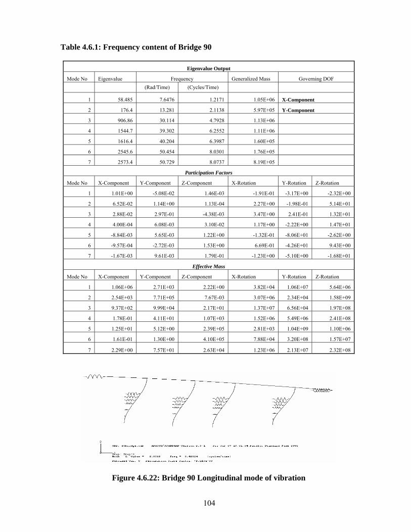
Table 4.6.1: Frequency content of Bridge 90
Eigenvalue Output
Mode No Eigenvalue Frequency Generalized Mass Governing DOF
(Rad/Time) (Cycles/Time)
1 58.485 7.6476 1.2171 1.05E+06 X-Component
2 176.4 13.281 2.1138 5.97E+05 Y-Component
3 906.86 30.114 4.7928 1.13E+06
4 1544.7 39.302 6.2552 1.11E+06
5 1616.4 40.204 6.3987 1.60E+05
6 2545.6 50.454 8.0301 1.76E+05
7 2573.4 50.729 8.0737 8.19E+05
Participation Factors
Mode No X-Component Y-Component Z-Component X-Rotation Y-Rotation Z-Rotation
1 1.01E+00 -5.08E-02 1.46E-03 -1.91E-01 -3.17E+00 -2.32E+00
2 6.52E-02 1.14E+00 1.13E-04 2.27E+00 -1.98E-01 5.14E+01
3 2.88E-02 2.97E-01 -4.38E-03 3.47E+00 2.41E-01 1.32E+01
4 4.00E-04 6.08E-03 3.10E-02 1.17E+00 -2.22E+00 1.47E+01
5 -8.84E-03 5.65E-03 1.22E+00 -1.32E-01 -8.06E+01 -2.62E+00
6 -9.57E-04 -2.72E-03 1.53E+00 6.69E-01 -4.26E+01 9.43E+00
7 -1.67E-03 9.61E-03 1. E-01 -1.23E+00 -5.10E+00 -1.68E79 +01
Effective Mass
Mode No X-Component Y-Component Z-Component X-Rotation Y-Rotation Z-Rotation
1 1.06E+06 2.71E+03 2.22E+00 3.82E+04 1.06E+07 5.64E+06
2 2.54E+03 7.71E+05 7.67E-03 3.07E+06 2.34E+04 1.58E+09
3 9.37E+02 9.99E+04 2.17E+01 1.37E+07 6.56E+04 1.97E+08
4 1.78E-01 4.11E+01 1.07E+03 1.52E+06 5.49E+06 2.41E+08
5 1.25E+01 5.12E+00 2.39E+05 2.81E+03 1.04E+09 1.10E+06
6 1.61E-01 1.30E+00 4.10E+05 7.88E+04 3.20E+08 1.57E+07
7 2.29E+00 7.57E+01 2.63E+04 1.23E+06 2.13E+07 2.32E+08
Figure 4.6.22: Bridge 90 Longitudinal mode of vibration
104

Figure 4.6.23: Bridge 90 Transverse mode of vibration
105

106
CHAPTER 5: WSDOT Bridge Results
Presented here are time-history analysis results from the nonlinear finite element
analyses of the three WSDOT bridges. The
response of columns, time-history responses, abutment behavior, and tables describing
maximum c rms
“Regular” and “Inverse” refer to how the
the bridge. “R dge
transverse and longitudinal directions, resp
The ground ach
bridge. In the following paragraphs, the resu
b ior of th iod.
Result comparisons with the provisions of
SDOF system are also p
5.1) G
5
B e 405 behavior will be described through its response to the non-FDGM
re ed que w =
8 The ea and
South American FP
acceleration tim stories are own in Figure 5 . r 1 ho th ar
e on the Cathedral in Moquegua.
results include figures showing the hysteretic
olumn relative displacements, shears, moments, and curvatures. The te
two ground m
an
otion com
on
ponents were applied to
eregular” means that the FN d FP comp ents w e applied to the bri
ectively, and vice versa for “Inverse”.
t motions were applied o the Finite Element Model (FEM) of e
lts are analyzed by describing the general
ehav
cord
.4).
ffect
e bridges and the effect of fo
AASHTO design m
rward directivity, a
e
nd
thods and with those of a
velocity pulse per
resented.
eneral Bridge Behavior
.1.1) Bridge 405 and Bridge 520
ridg
at Mo gua City during the southern Peru earthquake of June 23, 2001 (M
rthquake resulted from thrust faulting on the boundary between the Nazca
plates. The Moquegua ground motion latest about 2 min. The FN and
e hi sh .1.1 Figu e 5. .2 s ws e e thquake

107
-1.2
-1
-0.8
-0.6
-0.4
-0.2
0
0.2
0.4
0.6
0.8
1
1.2
0 140
Acceleration (
20 40 60 80 100 120
Time (sec)
g)
FN Component
FP Component
Fig
espo
ansv
urva
e p
a freeware program (USC_RC, Asadolla
Figure 5.1.1: Moquegua GM Time History
neure 5.1.2: Ca tone vaults, sus
The bridge, due to the etry, showed different
r nses i s tra f in its
tr erse oment-
c ture rela bserve
th inching behavior and the decreasing stiffness of the colu n the longitudinal
direction. For com mputed
from
cross-section fiber model. The computed curve closely matches the backbone curve from
the ABAQUS model.
n it
dire
nsverse and longitudinal directions. T
tionship for the southwest column is shown i
ction because of the high resistance provi
parison purposes, the backbone curve (
thedral in Moquegua, a stone structutained damage and lost one of its vau
boundary conditions and to its geom
h Esmaeily) which based the analysis on a
ded
re wilts
in
n F
he
da
(P
b
b
ig
th ho
rid
sto walls and sto by E. Fierro)
ge was very stif
y the bents. The m
ure
mn
d she
5.1.3
i
green
. O
) w
ne ca
as co
n o

1.50E+06
2.00E+06
5.00
1.00
E+05
E+06
Mom
ent (
N.m
)
-5.00E
0.00E
+05
+00-0.014 -0.009 -0.004 0.001 0.006 0.011
Long.
Trans
-1.50E
-1.00E
+06
+06
v.
USC
-2.00
CE+06
urvatu
d)
re (1/m)
F
ne a
igure 5.1.3:
The col o
columns per be ce
versus relative displacement n
longitudinal comp rse
o s shown in de
(Figure 5.1.6).
Moment-Curvature hysteresis curves in the transverse (re and longitudinal (black) column direction
umns
nt an
w
d s
ere
ing
in
le
do
cur
ub
va
le
tur
cu
e in
rva
th
tur
e l
e i
on
n t
gitudi
he tra
na
nsv
l di
er
rec
se
tio
dir
n.
ec
A
tio
plo
n d
t o
ue
f l
to
ate
th
ral
e tw
for
for the southwest colum
e c
is shown in Figure 5.1.4. The
ntonent of th olumn relative displaceme was higher than the transve
Figure 5.1.5. But, the column base shears were of the similar amplitu
4.00E+05
2.00E+
3.00E
05
+05
-4.00E+05
Disp (m)
-3.00E+
-1.00E+05
1.00E
-0.08 -0.06 -0.02
05
05-2.00E+
0.00E+-0.04
00
+05
0.00-0.10Forc
e (N
)
0.02 0.04 0.06 0.08 0.10
-4.00E+05
Disp (m)
-3.00E+
-2.00E+
05
05
-1.00E+05
4.00E+05
igure 5.1.4: Force-Displacement hysteresis curves in the transverse (left) and longitudinal (right) direction
2.00E+
3.00E+
05
05
0.00E+
1.00E+
200
05
0.00-0.1Forc
e (N
)
0 -0.08 -0.06 -0.04 -0.0 0.02 0.04 0.06 0.08 0.10
F
108

-8.00E-02
-6.00E-02
-2.00E-02
0E-02
0 20 40 60 80 100 120 140
Time (sec)
spl
-4.00E-02
0.00E+00
2.0
4.00E-02
8.00E-02
Di
acem
ent (
m)
6.00E-02
Figure 5.1.5: Transverse (red) and longitudinal (black) column displacement time
history
-4.00E+05
-3.00E+05
-2.00E+05
00E+000 20 40 60 80 100 120 140
Time (sec)
-1.00E+05
0.
Forc
e (N
1.00E+05
2.00E+05
3.00E+05
4.00E+05
)
history
re, very little risk of brittle shear failure in the columns.
Figure 5.1.6: Transverse (red) and longitudinal (black) column base shear time
A plot of force versus displacement is shown in Figure 5.1.7 for Bridge 405. In
dashed green, the shear capacity envelope proposed by Kowalsky and Priestley (2000) is
shown (see Appendix A.1). The column base shears never cross the shear capacity
envelope. There is, therefo
109

-4.00E+06
-3.00E+06
-2.00E+06
-1.00E+06
0.00E+00
1.00E+06
2.00E+06
3.00E+06
4.00E+06
-0.30 -0.20 -0.10 0.00 0.10 0.20 0.30
Displacement (m)
Forc
e (N
)
Figure 5.1.7: Bridge 405 Force – Displacement hysteresis curve, in the longitudinal
direction, including the column shear capacity in dashed green
The ABAQUS output variable defined as the internal energy (or total strain energy)
sums nternal
energy in the system increases gradually during the earthquake (see Figure 5.1.8).
the energy dissipated by plastic deformation and the kinetic energy. The i
0.00E+00
1.00E+05
2.00E+05
3.00E+05
4.00E+05
5.00E+05
6.00E+05
7.00E+05
8.00E+05
0 20 40 6 80 100 120 140Time (sec)
Inte
rnal
Ene
rgy
0
Figure 5.1.8: Total Strain Energy in the system
Figure 5.1.9 shows the longitudinal force response of the abutments from the
Moquegua ground motion. At abutments, the deck was restrained only by the bearing pad’s
shear resistance when pushed toward the soil (negative displacem orce-
Displacement curve). See Figure 4.4.13. But, when pushed in the opposite direction, one
can see the high stiffness provided by the abutment when the 5 cm (2 in) gap closes
(N.m
)
ent value on the F
110

111
(positive displacement value on the Force-Displacement curve). The north and south
abutments experience pounding several times (Figure on the right), but do not reach their
maximum allowable compressive force.
0.00E+00
2.00E+05
4.00E+05
6.00E+05
8.
-1.00E+06
-5.00E+05
0.00E+00
5.00E+05
1.00E+06
N)
1.50E+06
2.00E+06
2.50E+06
-0.08 -0.06 -0.04 -0.02 0 0.02 0.04 0.06 0.08
Displacement (m)
Forc
e (
00E
1.00E
+05
+06
1.40E+06
1.60E+06
1.80E+06
2.00E+06
0 20 40 60 80 100 120
Time (sec)Fo
rc
1.20E+06
e (N
)
North Abut
South Abut
Figure 5.1.9: Abutment Hysteresis Force-Displacement (left) and Force Time History curve (right)
e
geomet
,
The general behavior of Bridge 520 was similar to that of Bridge 405 since th
ry and the boundary conditions were similar. Further details on the analysis of
Bridge 520 will be presented in future sections in Chapter 5.
5.1.2) Bridge 90
The behavior of Bridge 90 is described through its response to the non FDGM
recorded in the Izmit Gulf during the Mw = 7.4 Kocaeli, Turkey, earthquake of August 17
1999. The earthquake resulted from strike-slip faulting on the east-west North Anatolian
fault. The FN and FP acceleration time histories are shown in Figure 5.1.10. Figure 5.1.11
shows the effect of the earthquake on the surrounding buildings of the mosque in the town
of Golcuk.
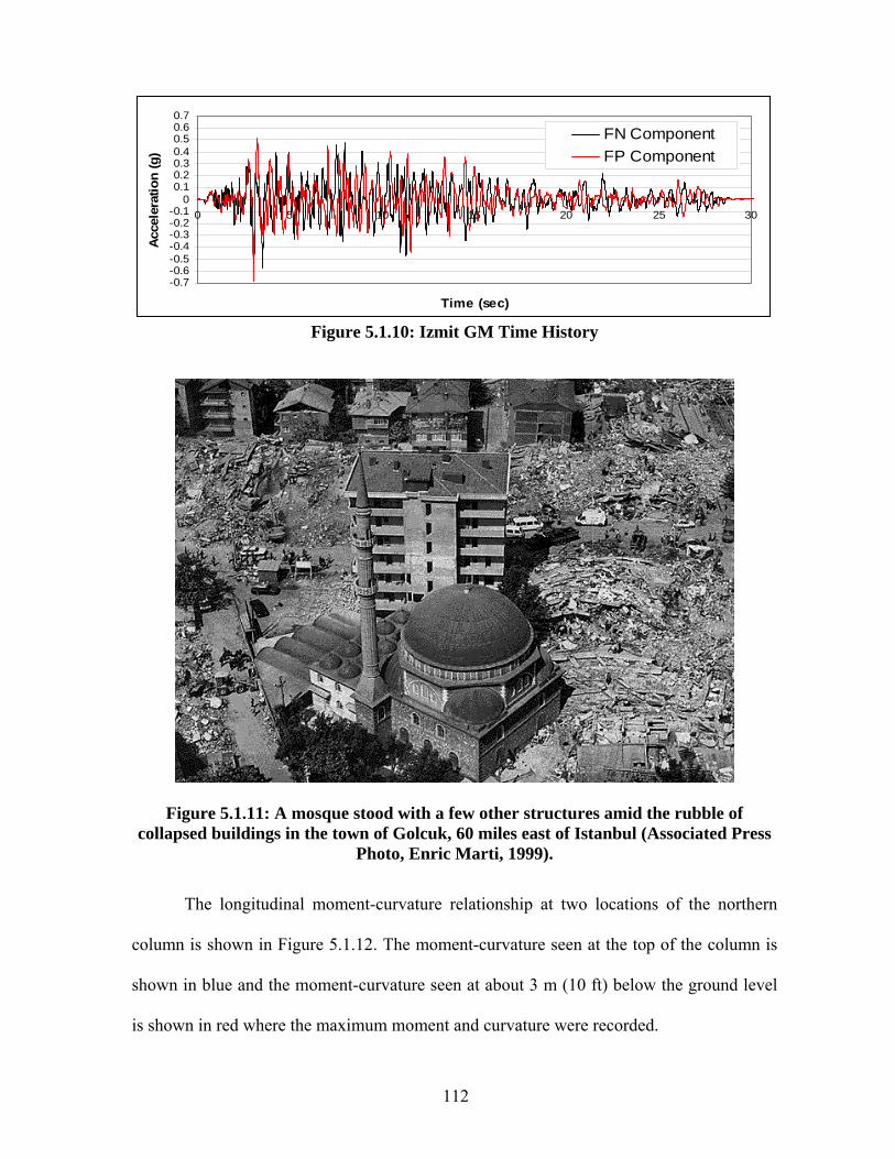
-0.7-0.6-0.5-0.4-0.3-0.2-0.1
00.10.20.30.40.50.60.7
0 5 10 15 20 25 30
Time (sec)
Acce
lera
tion
(g)
FN ComponentFP Component
Figure 5.1.10: Izmit GM Time History
Figure 5.1.11: A mosque stood with a few other structures amid the rubble of collapsed buildings in the town of Golcuk, 0 miles east of Istanbul (Associated Press
The longitudinal moment-curvature relationship at two locations of the northern
column is shown in Figure 5.1.12. The moment-curvature seen at the top of the column is
shown in blue and the moment-curvature seen at about 3 m (10 ft) below the ground level
is shown in red where the maximum moment and curvature were recorded.
6Photo, Enric Marti, 1999).
112

-3.00E+06
-2.00E+06
-1.00E+06
0.00E+00
1.00E+06
2.00E+06
3.00E+06
-0.025 -0.02 -0.015 -0.01 -0.005 0 0.005 0.01 0.015 0.02 0.025
Curvature (1/m)
Mom
ent (
N.m
)
Column TOP
Pile
Figure 5.1.12: Moment-Curvature hysteresis curves at the column top (blue) and at the pile (red) in the longitudinal direction
n
Figure
relative
displacement and the lowest resisting force. Conversely, the smallest column (C4, in red)
experienced the lowest relative displacement and the highest resisting force.
A plot of lateral force versus relative displacement for the four columns is shown o
5.1.13. The maximum forces were experienced at the column tops. The relative
displacements were computed between the column top and the ground level. The four
columns did not have the same response to the ground motions since they have different
heights and Bridge 90 is not symmetric. The column C1 is the southern column, C4 is the
northern one. The tallest column (C2, in green) experienced the highest
113

-1.00E+06
-6.00E+05
-4.00E+05
-2.00E+05
0.00E+00
2.00E+05
4.00E+05
8.00E+05
-0.10 -0.08 -0.06 -0.04 -0.02 0.00 0.02 0.04 0.06 0.08 0.10
Displacement (m)
Forc
e (
-8.00E+05
6.00E+05
1.00E+06
N)
C1
-1.00E+06
-8.00E+05
-6.00E+05
-4.00E+05
-2.00E+05
0.00E+00
4.00E+05
8.00E+05
1.00E+06
-0.08 -0.06 -0.04 -0.02 0 0.02 0.04 0.06 0.08
Dis
2.00E+05
6.00E+05
placement (m)
Forc
e (N
)
C1
C2 C2
C3
C4
C3
C4
Figure 5.1.13: Column Force-Displacement hysteresis curves in the longitudinal (left)and transverse (right) direction
A plot of force versus displacement is shown in Figure 5.1.14 for Bridge 90. In
purple, the shear capacity envelope proposed by Kowalsky and Priestley (2000) is shown
(see Appendix A.1). The column base shears never cross their shear capacity envelope.
There is very little risk of brittle shear failure in the columns.
-3.00E+06
-2.00E+06
-1.00E+06
0.00E+00
1.00E+06
2.00E+06
3.00E+06
-0.10 -0.08 -0.06 -0.04 -0.02 0.00 0.02 0.04 0.06 0.08 0.10
Forc
e (N
)
Displacement (m)
C1
C2
C3
C4
Shear Envelope
-2.00E+06
2.00E+06
-1.00E+06
0.00E+00
1.00E+06
3.00E+06
-0.1 -0.08 -0.06 -0.04 -0.02 0 0.02 0.04 0.06 0.08 0.1
Forc
e (N
)
C1C2C3C4Shear Envelope
-3.00E+06
Displacement (m)
transverse (right) direction
The internal energy in the system increases gradually during the earthquake due to
the energy dissipated by the columns (see Figure 5.1.15).
Figure 5.1.14: Force-Displacement hysteresis curves in the longitudinal (left) and
114

0.00E+00
2.00E+05
4.00E+05
6.00E+05
8.00E+05
1.00E+06
1.20E+06
1.40E+06
1.60E+06
0 5 10 15 20 25Time (sec)
Inte
rnal
Ene
rgy
Figure 5.1.15: Total Strain Energy in the system
t
f
Figure 5.1.16 shows the longitudinal force response of the abutments from the Izmi
ground motion. The abutments experienced pounding several times. Note also that they
reached their maximum allowable compression force and experienced several cycles o
plastic behavior.
-1.00E+06
1.00E+06
2.00E+06
3.00E+06
4.00E+06
5.00E+06
6.00E+06
-0.15 -0.1 -0.05 0 0.05 0.1 0.15
Forc
e)
0.00E+00
Displacement (m)
(N
North Abut
South Abut
0.00E+00
5.00E+05
1.00E+06
1.50E+06
2.00E+06
2.50E+06
3.00E+06
3.50E+06
4.00E+06
4.50E+06
5.00E+06
Time (s)
Forc
e (
)
0 5 10 15 20 25
N
North Abut
South Abut
Figure 5.1.16: Abutment Hysteresis Force-Displacement (left) and Force Time History curve (right)
(N.m
)
115

5.2) Forward Directivity Effect – Frequency Content
if the structure response is 'in tune' with
components of the ground mo resonance), which may be identified from the response
spectrum. Figures 5.2.1 to 5.2.6 show the acceleration response spectra (ARS) of the FN
and FP ground motion’s component for each bridge. The blue and red vertical dashed lines
are, respectively, the transverse and longitudinal fundamental
forward directivity “bump” effect is visible on the acceleration response spectra (ARS) of
the FN ground motion components. It is created by the velocity pulse, typical of a forward
directivity ground mo (Som
bridge for the non-FD ground motions since they have approximately the same frequency
content (see Chapter 4 - section 4.1.2).
Significant seismic damage may occur
tion (
mode shape periods. The
tion erville et al., 1997). The ARS show only one curve for each
116

Sa for the GMs FN component
SYLM
T7
KJ
Longi.T2 v.
FDGM
F1
RR
0
0.5
1.5
2
2.5
3
3.5
0 0.5 1 1.5 2 2.5 3
Period (sec)
Spec
tral
Acc
eler
atio
n (g
)T1 Trans
BAM
4M
S
1
AR
5
NON
BAM
SYLMAR
T75
KJM
T1 Longi.
T2 Transv.
NON FDGM
F14
RRS
Figure 5.2.1: Bridge 405 ARS of the FN components of the Ground Motions
Sa for the GMs FP component
BAM
SYLMAR
T75
KJM
T1 Longi.T2 Transv.
NON FDGM
F14
RRS
0
0.5
1
1.5
2
2.5
3
0 0.5 1 1.5 2 2.5 3
Period (sec)
Spec
tral
Acc
eler
atio
n (g
)
BAM
SYLMAR
T75
KJM
T1 Longi.
T2 Transv.
NON FDGM
F14
RRS
Figure 5.2.2: Bridge 405 ARS of the FP components of the Ground Motions
117

Sa for the FN component
BAM
SYLMAR
T1 LongitudinalT2 Transverse3.5
BAM
T75
KJM
F14
RRS
0.5
1
1.5
2.5
Spec
tral
Acc
eler
tion
(g)
NON FDGM
0
2
3
0
a
SYLMAR
T75
KJM
T1 Longitudinal
T2 Transverse
NON FDGM
F14
RRS
0.5 1 1.5 2 2.5 3 3.5 4
Period (sec)
Figure 5.2.3: Bridge 520 ARS of the FN components of the Ground Motions
Sa for the FP component
BAM
SYLMAR
KJM
T1 LongitudinalT2 Transverse
NON FDGM
2.5
T75
F14
RRS
0
0.5
1
1.5
2
3
0 0.5 1 1.5 2 2.5 3 3.5 4
Period (sec)
Spec
tral
Acc
eler
atio
n (g
)
BAM
SYLMAR
T75
KJM
T1 Longitudinal
T2 Transverse
NON FDGM
F14
RRS
Figure 5.2.4: Bridge 520 ARS of the FP components of the Ground Motions
118

Sa for the GMs FN component
BAM
SYLMAR
T75
KJM
T1 Longi.T2 Transv.
NON FDGM
F14
RRS
0
0.5
1
1.5
2
2.5
3
3.5
0 0.5 1 1.5 2 2.5 3
BAM
SYLMAR
T75
KJM
T1 Longi.
T2 Transv.
Period (sec)
Spec
tral
Ac
on (g
)ce
lera
ti
NON FDGM
F14
RRS
Figure 5.2.5: Bridge 90 ARS of the FN components of the Ground Motions
Sa for the GMs FP component
BAM
SYLMAR
T75
KJM
T1 Longi.T2 Transv.
NON FDGM
ratio
n
F14
RRS
0
0.5
1
1.5
2
2.5
3
Spec
tral
Acc
ele
BAM
SYLMAR
T75
KJM
T1 Longi.
0 0.5 1 1.5 2 2.5 3
Period (sec)
(g)
T2 Transv.
NON FDGM
F14
RRS
Figure 5.2.6: Bridge 90 ARS of the FP components of the Ground Motions
119

The ABAQUS output results (max displacement, max base shear, energy
dissipated) as a function of the spectral acceleration value (Sa) were compared. Tables
5.2.1, 5.2.2, and 5.2.3 show the ground motion characteristics, including the Peak Ground
Acceleration (PGA), and the spectral acceleration (Sa) value at the corresponding modes of
deformation for each bridge.
120

121
Table 5.2.1: Summary of the GM ch
Inverse
aracteristics and the Bridge 405 column response parameters
Earthquake Regular
Type GM
PGA (g) FP
PGA (g) FN F Direction
Br (
lastic
nergyMax. Base Shear (N)
Max. Disp. (m)
Plastic Energy Sa N Sa FP
Max. ase Shea N)
Max.Disp.(m)
PE
IZT 0.764 0.773 0. gi E 702 3E+0 .618E+05 0.0657 5.48E+04 80 0.80 Lon . 2.452 +05 0.0 5.1 4 2IZT 0.764 0.773 2. E 184 3E+0 .634E+05 0.0175 5.48E+04 50 2.50 Transv. 4.104 +05 0.0 5.1 4 3702 0.846 0.942 0. gi E 615 2 .621E+05 0.0664 5.36E+04 80 0.80 Lon . 2.708 +05 0.0 5.4 E+04 2702 0.846 0.942 2. E 183 2 .645E+05 0.0181 5.36E+04 50 2.50 Transv. 3.965 +05 0.0 5.4 E+04 3MOQ 0.668 1.042 0. gi E 173 0 .727E+05 0.0714 1.55E+05 80 0.80 Lon . 3.126 +05 0.0 1.7 E+05 2MOQ 0.668 1.042 2. E 684 0 .624E+05 0.0192 1.55E+05 50 2.50 Transv. 2.688 +05 0.0 1.7 E+05 3SSU 0.725 0.828 0. gi E 717 85 .522E+05 0.0791 5.52E+04 80 0.80 Lon . 2.523 +05 0.0 4. E+04 2SSU 0.725 0.828 2. E 188 5 4 3.659E+05 0.0188 5.52E+04 50 2.50 Transv. 3.537 +05 0.0 4.8 E+0T71 0.730 0.840 0. gi E 701 1 2.685E+05 0.0667 1.21E+05 80 0.80 Lon . 2.737 +05 0.0 6.9 E+04
Non FD
T71 0.730 0.840 2. E 199 1 3. +05 0.0194 1.21E+05 50 2.50 Transv. 3.798 +05 0.0 6.9 E+04 643EBAM 0.647 0.880 0. gi E 689 2 3.353E+05 0.0903 3.90E+04 95 0.69 Lon . 2.748 +05 0.0 1.9 E+04FD
(6.5) BAM 0.647 0.880 3. E 224 2 2.993E+05 0.0142 3.90E+04 12 1.72 Transv. 4.444 +05 0.0 1.9 E+04F14 0.857 1.015 2. gi E 605 1 3.237E+05 0.1625 7.76E+04 34 0.62 Lon . 2.497 +05 0.0 1.7 E+04FD
(6.0) F14 0.857 1.015 1. E 136 1 .061E+05 0.0177 7.76E+04 69 2.28 Transv. 3.518 +05 0.0 1.7 E+04 3KJM 0.548 0.854 2. gi E 087 0 .613E+05 0.2254 1.26E+05 00 1.31 Lon . 3.126 +05 0.1 6.1 E+04 3FD
(6.9) KJM 0.548 0.854 1. E 083 0 .210E+05 0.0078 1.26E+05 03 1.00 Transv. 2.234 +05 0.0 6.1 E+04 1RRS 0.390 0.887 2. gi E 495 8 .305E+05 0.1976 7.86E+04 12 0.47 Lon . 2.591 +05 0.0 9.7 E+03 3FD
(6.7) RRS 0.390 0.887 1. E 101 8E+0 .764 0.0108 7.86E+04 28 1.24 Transv. 2.643 +05 0.0 9.7 3 1 E+05Sylmar 0.595 0.733 0. gi E 151 3E+0 .609E+05 0.0645 1.83E+04 79 1.22 Lon . 3.120 +05 0.1 6.4 4 2FD
(6.7) Sylmar 0.595 0.733 1. E 102 3E+0 .915E+05 0.0105 1.83E+0430 1.20 Transv. 1.733 +05 0.0 6.4 4 1T75 0.278 0.314 0. gi E 477 4E+0 .663E+05 0.0574 7.91E+0350 0.41 Lon . 2.481 +05 0.0 2.3 3 2FD
(7.6) T75 0.278 0.314 0. E 054 4E+0 .702E+04 0.0032 7.91E+0370 0.42 Transv. 1.393 +05 0.0 2.3 3 8LCN 0.783 0.728 0. gi E 374 9E+0 .763E+05 0.0659 8.49E+0371 0.35 Lon . 2.312 +05 0.0 4.1 0 2FD
(7.3) LCN 0.783 0.728 0. E 076 9E+0 .184E+05 0.0099 8.49E+0388 1.26 Transv. 2.293 +05 0.0 4.1 0 2
121

e 2: m y h M r ri and the Bridge 520 column response parameters
Earthquake Regular Inverse
122
Tabl 5.2. Su mar of t e G cha acte stics
Type GM )
P
GA g) N S
PGA (gF
P(F N a D
Max Base Shear (N)
Max Disp (m)
Plastic Energy
Max e )
Max Disp (m)
Plastic Energy a F S FP irection
BasShear (N
IZT 0. 64 0 773 0.7 .70 7 . 0 0 L 2.140E+05 0.0970 2.77E+04 2 5 0.0971 2.92E+04ongi. .212E+0IZT 0. 64 0 773 2.0 .00 7 . 0 2 T 7E+05 0.0151 2.77E+04 1 5 0.0123 2.92E+04ransv. 2.09 .969E+0702 0. 46 0 942 0.7 .70 8 . 0 0 L 2.238E+05 0.0892 2.94E+04 2 5 0.0926 2.72E+04ongi. .161E+0702 0. 46 0 942 2.0 .00 8 . 0 2 T 2.040E+05 0.0142 2.94E+04 1 5 0.0123 2.72E+04ransv. .770E+0SSU 0. 25 0 828 0.7 .70 7 . 0 0 L 2.211E+05 0.0957 2.16E+04 2 5 0.0933 1.23E+04ongi. .211E+0SSU 0. 25 0 828 2.0 .00 7 . 0 2 T 2.237E+05 0.0136 2.16E+04 1 5 0.0119 1.23E+04ransv. .962E+0T71 0. 30 0 840 0.7 .70 7 . 0 0 L 2.266E+05 0.0934 4.35E+04 2 5 0.0953 6.59E+04ongi. .271E+0
Non FD
T71 0. 30 0 840 2.0 .00 7 . 0 2 T 2.046E+05 0.0137 4.35E+04 1 5 0.0141 6.59E+04ransv. .895E+0BAM 0. 47 0 880 1.1 .43 6 . 6 0 L 2.200E+05 0.0656 4.26E+02 5 0.1027 1.88E+04ongi. 2.707E+0FD
6.5) BAM 0. 47 0 880 2.3 .78 ( 6 . 9 1 T 3.065E+05 0.0205 4.26E+02 1 5 0.0118 1.88E+04ransv. .764E+0F14 0. 57 1 015 1.6 .57 8 . 9 0 L 2.013E+05 0.0625 2.79E+02 2 5 0.1922 5.21E+04ongi. .787E+0FD
6.0) F14 0. 57 1 015 1.9 .71 ( 8 . 4 1 T 2.282E+05 0.0118 2.79E+02 1 5 0.0152 5.21E+04ransv. .746E+0KJM 0. 48 0 854 2.5 .89 5 . 4 0 L 2.449E+05 0.1155 3.47E+04 3 5 0.3140 1.64E+05ongi. .018E+0FD
6.9) KJM 0. 48 0 854 0.9 .02 ( 5 . 8 1 T 1.261E+05 0.0070 3.47E+04 8 4 0.0070 1.64E+05ransv. .270E+0RRS 0. 90 0 887 2.1 .38 3 . 5 0 L 1.935E+05 0.0589 1.52E+01 2 5 0.2206 7.92E+04ongi. .786E+0FD
6.7) RRS 0. 90 0 887 1.2 .03 ( 3 . 0 1 T 1.573E+05 0.0083 1.52E+01 9 4 0.0086 7.92E+04ransv. .117E+0Sylm r 0. 95 0 733 0.7 .15 a 5 . 6 1 L 6E+05 0.0921 1.99E+04 2 5 0.0717 1.53E+03ongi. 2.22 .161E+0FD
6.7) Sylm r 0. 95 0 733 1.2 .07 ( a 5 . 5 1 T 1.539E+05 0.0088 1.99E+04 2 5 0.0169 1.53E+03ransv. .648E+0T75 0. 78 0 314 0.3 .20 2 . 4 0 L 1.336E+05 0.0346 0.00E+00 1 0.0533 0.00E+00ongi. .837E+05FD
7.6) T75 0. 78 0 314 0.6 .35 ( 2 . 7 0 T 7.139E+04 0.0042 0.00E+00 4.75 4 0.0026 0.00E+00ransv. 6E+0LCN 0. 83 0 728 0.6 .33 7 . 7 0 L 2.157E+05 0.0514 0.00E+00 2.39 5 0.0749 6.20E+02ongi. 9E+0FD
7.3) LCN 0. 83 0 728 1.2 .78 ( 7 . 1 1 Tr 1.314E+05 0.0065 0.00E+00 1.86 5 0.0111 6.20E+022E+0ansv.
122

Table 5.2.3: Summary of the GM characteristics and the Bridge 90 column respo
Earthquake Regular Inverse
123
nse parameters
Ty pe GM
PGA (g) FP
P
Sa FN Sa FP Direction Max Base Shear (N)
Max Disp (m)
PlaEne
ar
x p )
GA (g) FN
stic rgy
Max Base She (N)
MaDis(m
Plastic Energy
IZT .764 0 0.83 0.83 Longi. 7.638E+05 0.0753 1.96 5 0 54 50 .773 E+05 7.29 E+05 0.06 9 1. E+0IZT .764 0 1.68 1.68 Transv. 8.295E+05 0.0300 1.96 0 1 54 50 .773 E+05 8.51 E+05 0.03 8 1. E+0702 .846 0 0.83 0.83 Longi. 7.640E+05 0.0695 2.28 5 4 12 50 .942 E+05 7.45 E+05 0.06 1 1. E+0702 .846 0 1.68 1.68 Transv. 8.121E+05 0.0297 2.28 4 3 12 50 .942 E+05 9.08 E+05 0.03 6 1. E+0MOQ .668 0.83 0.83 Longi. 7.773E+05 0.0753 2.23 3 0.075 60 5 0 1.042 E+05 7.77 E+05 8 2. E+0MOQ .668 1.68 1.68 Transv. 8.166E+05 0.0258 2.23 8 0.029 60 5 0 1.042 E+05 8.81 E+05 8 2. E+0SSU .725 0.83 0.83 Longi. 7.791E+05 0.0702 1.24 9 0.078 83 50 0.828 E+05 8.04 E+05 8 1. E+0SSU .725 1.68 1.68 Transv. 7.060E+05 0.0329 1.24 8 0.035 83 50 0.828 E+05 8.78 E+05 9 1. E+0T71 .730 0.83 0.83 Longi. 7.647E+05 0.0704 1.89 7 0.076 25 50 0.840 E+05 7.53 E+05 4 3. E+0
NoFD
T7
n
1 .730 1.68 1.68 Transv. 7.081E+05 0.0296 1.89 5 0.031 25 50 0.840 E+05 8.60 E+05 1 3. E+0BAM .647 1.18 0.44 Longi. 7.398E+05 0.0466 1.28 9 0.092 61 5 0 0.880 E+04 7.94 E+05 1 1. E+0FD
(6. B
5) AM .647 0.95 0.81 Transv. 6.776E+05 0.0178 1.28 0 0.018 61 5 0 0.880 E+04 7.07 E+05 4 1. E+0F14 .857 1.54 0.58 Longi. 6.674E+05 0.0509 5.74E+04 9 0.127 40 50 1.015 9.23 E+05 4 1. E+0FD
(6. F1
0) 4 .857 2.63 1.69 Transv. 1.142E+06 0.0494 5.74E+04 4 0.031 40 50 1.015 6.57 E+05 4 1. E+0KJM .548 0 2.51 0.77 Longi. 7.049E+05 0.0677 1.19E+05 4 0.205 29 2 0 .854 9.45 E+05 3 5. E+0FD
(6. K
9) JM 0.548 0 2.04 1.51 Transv. 8.997E+05 0.0320 1.19E+05 1 0.036 29 2.854 6.06 E+05 6 5. E+0RRS 0.390 0 2.13 0.38 Longi. 6.455E+05 0.0515 2.61E+04 6 0.188 81 4.887 8.58 E+05 7 3. E+0FD
(6. R
7) RS 0.390 0 1.84 0.91 Transv. 9.938E+05 0.0333 2.61E+04 0 0.018 81 4.887 5.77 E+05 6 3. E+0Sylmar 0.595 0 0.74 1.13 Longi. 7.749E+05 0.0783 1.09E+05 6 0.062 12 4.733 7.01 E+05 3 7. E+0FD
(6. Sy
7) lmar 0.595 0 1.22 2.20 Transv. 7.307E+05 0.0241 1.09E+05 2 0.038 12 4.733 1.07 E+06 3 7. E+0T75 0.278 0 0.33 0.20 Longi. 6.680E+05 0.0402 4.18E+03 6 0.046 48 4.314 6.81 E+05 1 1. E+0FD
(7. T7
6) 5 0.278 0 0.67 0.68 Transv. 4.080E+05 0.0125 4.18E+03 9 0.013 48 4.314 4.72 E+05 2 1. E+0CN 0.783 0 0.59 0.30 Longi. 6.988E+05 0.0462 6.64E+03 3 0.043 95 3L .728 6.88 E+05 9 7. E+0FD
(7. L
3) CN 0.783 0.728 0.64 0.42 Transv. 4.829E+05 0.0102 6.64E+03 6 0.009 95 32 7. E+04.15 E+05
123

5.1.2.1) Longitudinal Response
be significantly higher than
those for the non-FDGMs due to their high relative value of spectral acceleration at this
period. The FD effect is seen ediate period range for the selected motions
(0.5s < T < 1s, see Figures 5.2.1 to 5.2.6) of the FN GM component (“Inverse” plots).
The range of spectral acceleration values is smaller for the FP component since the FD
effect is less pronounced.
The Figures 5.2.7 to 5.2.12 below show the effect of the spectral acceleration at
the bridge fundamental longitudinal frequency on the peak column response in the
longitudinal direction. The pink triangles represent the response from the FDGMs and the
blue diamonds represent the response from the Non-FDGMs. For the “Regular” plots (on
the figure’s left), the FP ground motion component was applied to the bridge longitudinal
direction, and for the “Inverse” plots (on the figure’s right), the FN ground motion
component was applied to the bridge longitudinal direction. Consequently, the range of
spectral acceleration values (X axes) was higher for “Inverse” than for “Regular” since
the FD effect is seen only in the FN ground motion component.
The column’s maximum base shear increases slightly with the spectral
acceleration due to the strain hardening effect after the column yielded. A similar trend is
seen for maximum column displacements, but its effect is more pronounced. Since the
column behaves plastically, the displacements increase rapidly in the plastic plateau
region. The maximum displacements for the FDGMs can
in the interm
124

Regular
0.00E+00
5.00E+04
1.00E+05
1.50E+05
2.00E+05
2.50E+05
3.00E+05
3.50E+05
4.00E+05
0.00 0.20 0.40 0.60 0.80 1.00 1.20 1.40Sa FP (g)
Max
Bas
e S
hear
(N)
Non FD
FD
Inverse
0.00E+005.00E+041.00E+051.50E+052.00E+052.50E+053.00E+053.50E+054.00E+05
0.00 0.50 1.00 1.50 2.00 2.50
Sa FN (g)
Max
. Bas
e Sh
ear (
N)
Non FD
FD
Figure 5.2.7: Bridge 405 Max Longitudinal Base Shear, Sa’s at Tl = 0.65s
Regular
0.00E+00
+05
05
0.00 0.20 0.40 0.60 0.80 1.00 1.20 1.40
5.00E+04
1.00E
1.50E+
2.00E+
2.50E
3.00E+05
3.50E+05
Sa FP (g)
Max
Bas
e S
hear
(N)
05
+05
Non FD
FD
Inverse
0.00E+00
5.00E+04
1.00E+05
0.00 0.50 1.00 1.50 2.00 2.50 3.00ax
. B
1.50E+05
3.50E+05
Sa FN (g)
Mas
e S 2.00E+05
2.50E+05
3.00E+05
hear
(N)
Non FD
FD
Figure 5.2.8: Bridge 520 Max Longitudinal Base Shear, Sa’s at Tl = 0.80s
Regular
1.00E+052.00E+05
4.00E+055.00E+05
7.00E+058.00E+059.00E+05
0.00 0.20 0.40 0.60 0.80 1.00 1.20Sa FP (g)
Ma
Bas
e Sh
(N)
0.00E+00
3.00E+05
6.00E+05
1.00E+06
x ea
r
Non FD
FD
Inverse
0.00E+001.00E+052.00E+05
4.00E+055.00E+05
7.00E+058.00E+059.00E+05
Sa FN (g)
Ma
Bas
e S
hr
(N)
3.00E+05
6.00E+05
1.00E+06
0.00 0.50 1.00 1.50 2.00 2.50 3.00
x.ea Non FD
FD
Figure 5.2.9: Bridge 90 Max Longitudinal Column Shear, Sa’s at Tl = 0.82s
Regular
0.000
0.050
0.100
0.150
0.200
0.250
0.00 0.20 0.40 0.60 0.80 1.00 1.20 1.40
Mx.
Dis
plm
ent (
Sa FP (g)
aac
em
) Non FD
FD
Inverse
0.000
0.050
0.100
0.150
0.250
0.00 0.50 1.00 1.50 2.00 2.50
ax. D
isp
acem
ent (
)
0.200
Sa FN (g)
Ml
m Non FD
FD
F14
RRS
KJM BAM
SYL
T75
RRS
BAM
F14
RRS KJM
BAM SYL
T75
KJM SYL
F14 RRS KJM BAM
L
T75
F14 KJM
T75 KJM
SYT75 F14 RRS
KJM BAM SYL
Figure 5.2.10: Bridge 405 Max Longitudinal relative Displacement, Sa’s at Tl = 0.65s
F14
KJM
SYL T75 F14 RRS
BAM T75
RRS BAM
SYL F14 RRS BAM SYL
T75
125

126
Regular
0.050
0.100
0.150
0.200
0.300
0.00 0.20 0.40 0.60 0.80 1.00 1.20 1.40Sa FP (g)
Max
. Dsp
lace
mt (
m)
0.000
0.250
0.350i
enNon FD
FD
Inverse
0.050
0.150
0.200
0.250
0.300
0.00 0.50 1.00 1.50 2.00 2.50 3.00Sa FN (g)
Max
. Dpl
acem
t (m
)
0.000
0.100
0.350
isen
Non FD
FD
Figure 5.2.11: Bridge 520 Max Longitudinal relative Displacement, S ’s at T = 0.80s a l
Regular
0.000
0.100
0.150
0.200
0.250
0.00 0.20 0.40 0.60 0.80 1.00 1.20Sa FP (g)
M D
ispl
ent (
m
0.050ax.
acem
)
Non FD
FD
Inverse
0.000
0.100
0.150
0.200
0.250
0.00 0.50 1.00 1.50 2.00 2.50 3.00Sa FN (g)
M D
ispl
ent (
m0.050ax
.ac
em)
Non FD
FD
Figure 5.2.12: Bridge 90 Max Longitudinal relative Displacement, Sa’s at Tl = 0.82s
The ene
F14
SYL T75 F14 RRS
KJM BAM
T75
F14
RRS
BAM SYL
T75 F14 RRS KJM
BAM SYL
T75
rgy dissipated by plastic deformation in the system often increases
abruptly during a FDGM, as show
to note that the level of is highly d upon th od of the bridge versus
that of the forward directivity pulse. Table 5.2.4 summarizes the different fundamental
bridge periods and velocity pulse periods of the FN ground motion component. When the
two periods are close, most of the damage occurs during the pulse, as in the KJM Inv,
RRS Inv, and F14 Inv earthquakes. For cases in which there is no pulse or the pulse
period does not match the fundamental period of the bridge, the damage is much lower
and it increases gradually. The damage curve for the KJM Inv and RRS Inv ground
motions for Bridge 90 did not reach a very high level since one of the columns failed
during the first seconds of the record, which made the finite element analysis terminate.
RRS
KJM
BAM SYL
KJM
n on Figures 5.2.13, 5.2.14, and 5.2.15. It is interesting
damage ependent e peri

127
Table 5.2.4: fundamental bridge periods and FDGM’s velocity pulse periods (Tv)
Period (sec) bridge 405 bridge 520 bridge 90 FDGM Tv (sec) Tlongitudinal 0.66 0.80 0.82 BAM 2.065 Ttransverse 0.18 0.17 0.47 F14 0.75 KJM 1 RRS 1.25 Sylmar 2.32 T75 2.5 LCN 5.5
F14 InvRRS Inv
1.00E+06
Sylmar InvT75 Inv
0 10 20 30 40 50 60 70 80 90 100Time
KJM Inv
MOQ Inv
0.00E+00
2.00E+05
4.00
6.00E+05
8.00E+05
1.20E+06
1.40E+06
1.60E+06
1.80E+06
2.00E+06
T71 InvE+05
(sec)
Ener
gy D
issi
pate
d
Sylmar Inv T75 Inv BAM Inv
F14 Inv KJM Inv 702 Inv
MOQ Inv IZT Inv SSU Inv
T71 Inv RRS Inv
through time for the non-FD (dashed) and FDGMs (solid)
(N.m
)
Figure 5.2.13: Bridge 405 Energy dissipated by plastic deformation in the system

Sylmar Inv
F14 Inv
KJM Inv
702 Inv
MOQ InvIZT InvR03 Inv
SSU Inv
T71 Inv
RRS Inv
2.00E+05
4.00E+05
6.00E+05
8.00E+05
1.00E+06
1.60E+06
1.80E+06
2.00E+06
0 10 20 30 40 50 60Time (sec)
Ener
gy D
issi
ped
0.00E+00
1.20E+06
1.40E+06
atSylmar Inv
T75 Inv
BAM Inv
128
F14 Inv
KJM Inv
702 Inv
MOQ Inv
IZT Inv
R03 Inv
SSU Inv
T71 Inv
RRS Inv
Figure 5.2.14: Bridge 520 Energy dissipated by plastic deformation in the system
through time for the non-FD (dashed) and FDGMs (solid)
Sylmar Inv
T75 Inv
BAM InvT71 Inv
F14 Inv
KJM Inv
702 Inv
MOQ Inv
IZT Inv
SSU Inv
RRS Inv
0.00E+00
2.00E+05
4.00E+05
6.00E+05
8.00E+05
1.00E+06
1.20E+06
0 10 20 30 40 50 60Time (sec)
Ener
gy D
issi
pate
d
1.40E+06
1.60E+06
Sylmar Inv T75 Inv
BAM Inv F14 Inv
KJM Inv 702 Inv
MOQ Inv IZT Inv
SSU Inv T71 Inv
RRS Inv
Figure 5.2.15: Bridge 90 Energy dissipated by plastic deformation in the system
through time for the non-FD (dashed) and FDGMs (solid). Column failure noted for KJM Inv and RRS Inv records.
(N.m
) (N
.m)

129
Plots of force versus displacement and moment versus curvature are shown in
Figure 5.2.16 for the most damaging ground motion considered on Bridge 405. The
hysteretic curves show the expected pinching behavior and decreased column stiffness
and strength due to the double-sided velocity pulse of the FDGM. From the plots, one can
see that the majority of plasticity and damage results from only a few large cycles.
-5.00E+05
-4.00E+05
-3.00E+05
-2.00E+05
-1.00E+05
0.00E+00
1.00E+05
2.00E+05
3.00E+05
4.00E+05
5.00E+05
-0.30 -0.20 -0.10 0.00 0.10 0.20 0.30
Disp (m)
Forc
e (N
)
-3.00E+06
-2.00E+06
-1.00E+06
0.00E+00
1.00E+06
2.00E+06
3.00E+06
-0.04 -0.03 -0.02 -0.01 0 0.01 0.02 0.03 0.04
Curvature (1/m)
Mom
ent (
N.m
)
Figure 5.2.16: Bridge 405 Force-Displacement and Moment-Curvature hysteresis
A plot of moment versus curvature is shown in Figure 5.2.17 for the most
d
was computed from the cross-section analys freeware (USC_RC, Asadollah Esmaeily).
The end of the curve indicates the failure of the column cross-section. The peak spectral
acceleration atched the longitudinal fundamental period of vibration of the
structure. This ground motion induced the bending failure of the shortest column (C4).
ABAQUS stopped the analysis when the maximum material capacity was reached at the
top of the column. It does not indicate the overall failure of the bridge but, rather, a local
lumn did not fail when it reached its first maximum
curvature at the end of the USC curve, but the second time. The maximum curvature
capacity from ABAQUS was slightly higher than the USC one. A plot of force versus
displacement is shown in Figure 5.2.18. The column reached its maximum displacement
curve from the FD KJM GM, in the longitudinal direction
amaging ground motion considered for Bridge 90. In dashed red, the backbone curve
is
closely m
failure. One can note that the co

capacity of approximately 20 cm (8 in). In dashed green, the shear capacity envelope
proposed by Kowalsky and Priestley (2000) is shown (see Appendix A.1). The column
shear capacity is shown to be higher than its bending capacity for any displacement level.
-4.00E+06
-3.00E+06
-2.00E+06
-1.00E+06
0.00E+00
1.00E+06
2.00E+06
3.00E+06
4.00E+06
-0.06 -0.04 -0.02 0 0.02 0.04 0.06
Curvature (1/m)
Mom
ent (
N.m
)
Top C4
USC
Figure 5.2.17: Bridge 90 Moment-Curvature hysteresis curve of column C4 from the FD KJM ground motion, in the longitudinal direction, including the USC prediction
curve in dashed red
-3.00E+06
-2.00E+06
-1.00E+06
0.00E+00
1.00E+06
2.00E+06
3.00E+06
-0.25 -0.20 -0.15 -0.10 -0.05 0.00 0.05 0.10 0.15 0.20 0.25
Displacement (m)
Forc
e (N
)
Figure 5.2.18: Bridge 90 Force – Displacement hysteresis curve of column C4 from
the FD KJM GM, in the longitudinal direction, including the column shear capacity in dashed green
Tables 5.2.5, 5.2.6 and, 5.2.7 summarize the response of the abutments during the
earthquakes. “Pounding” indicates that the gap closed, “# max pressure” is the number of
times the abutment reaches its maximum allowable pressure force, and “Deformation” is
130

the maximum plastic deformation in the springs. For Bridge 405, the non-FDGM’s did
not induce any damage in the abutments, but the FDGM BAM, Sylmar, F14, and KJM
did. Again, note that pounding only occurred once or twice, indicating that it results from
the forward directivity pulse. For Bridge 520, the non-FDGMs SSU and T71 induced
four to five repeated poundings of the abutments, but the level of damage is small. On the
other hand, the FDGMs KJM Inv and RRS Inv induced during only one pounding (even
though they touched twice) a much larger plastic deformation caused by the pulse. The
abutments of Bridge 405 and Bridge 520 behaved differently since their geometry and,
subsequently, their strength capacity were unique. The bearing pad displacement
capacity, never reached, of 50 cm (20 in) was the same, however. For Bridge 90, the non-
F
the other hand, the FDGMs KJM Inv and ing only one pounding a
m
Table 5.2.5: Bridge 405 Abutment pounding
DGMs induced repeated poundings of the abutments with varying levels of damage. On
RRS Inv induced dur
uch larger plastic deformation of 33 cm caused by the pulse.
Regular Inverse Type (Mw) GM Pounding
# max pressure Deformation (m) Pounding
# max pressure Deformation (m)
702 yes 0 0 yes 0 0
IZT yes 0 0 yes 0 0
MOQ yes 0 0 yes 0 0
SSU yes 0 0 yes 0 0
Non FD
T71 yes 0 0 yes 0 0
FD (6.9) KJM yes 1 0.014 yes 2 0.16
FD (6.5) BAM yes 0 0 yes 1 0.017
FD LCN yes 0 0 yes 0 0 (6.2) FD
(6.0) F14 yes 0 0 yes 2 0.09
FD (6.7) RRS yes 0 0 yes 1 0.13
Sylmar yes 2 0.04 yes 0 0 FD
(7.2) T75 yes 0 0 no 0 0
131

Table 5.2.6: Bridge 520 Abutment pounding
Regu
lar Inverse Type # max (Mw) GM Pounding pressure Deformation (m) Pounding
# max pressure Deformation (m)
702 yes 2 0.03 yes 1 0.014
IZT yes 2 0.03 yes 2 0.024
SSU yes 4 0.03 yes 2 0.012
Non FD
T71 yes 4 0.034 yes 5 0.036
FD (6.9) KJM yes 1 0.056 yes 2 0.18
FD (6.5) BAM yes 1 0.004 yes 2 0.043
FD (6.2) LCN yes 0 0 yes 1 0.015
FD (6.0) F14 yes 1 0.001 yes 2 0.014
FD RRS yes 0 0 yes 1 0.17 (6.7)
Sylmar yes 3 0.03 yes 2 0.011 FD
(7.2) T75 yes 0 0 yes 0 0
Table 5.2.7: Bridge 90 Abutment pounding
Regular Inverse Type (Mw) GM Pounding
# max pressure Deformation (m) Pounding
# max pressure Deformation (m)
702 yes 3 0.09 yes 2 0.08
IZT yes 5 0.1 yes 2 0.08
MOQ yes 8 0.08 yes 7 0.1
SSU yes 4 0.065 yes 4 0.1
Non FD
T71 yes 2 0.09 yes 3 0.1
FD (6.9) KJM yes 1 0.065 yes 1 0.33
FD (6.5) BAM yes 2 0.005 yes 1 0.11
FD (6.2) LCN yes 3 0.007 yes 1 0.07
FD (6.0) F14 yes 3 0.04 yes 1 0.19
FD (6.7) RRS yes 4 0.007 yes 1 0.33
Sylmar yes 4 0.06 yes 0.027 2 FD
(7.2) T75 yes 1 0.001 yes 4 0.02
132

5.1.2.2) Transverse Response
Figures 5.2.19 to 5.2.24 show the effect of the spectral acceleration on the column
response in the transverse direction. The column’s maximum base shears and
displacements increase nearly linearly with Sa. The bridge response is mainly governed
by the frequency content of the ground motion. The transverse fundamental periods of
Bridge 405 and 520 are around 0.2 sec. At this short period range (0 < T < 0.5s), the
Forward Directivity “bump” effect does not appear in the ARS and the non-FDGMs had
a greater spectral acceleration value. Consequently, the non-FDGMs often induced higher
maximum base shears and displacements.
As in the longitudinal direction, the maximum column responses were governed
b
the non-FDGMs than th
different. For the “Regular” plots (on the figures’ left), the FN ground motion component
was ap the figures’
right), t
y the ARS value but, in the transverse direction, those values were generally higher for
ose of the FDGMs because the fundamental bridge periods were
plied to the bridge transverse direction, and for the “Inverse” plots (on
he FP ground motion component was applied to the bridge transverse direction.
Regular
5.00E+041.00E+05
2.00E+052.50E+053.00E+05
4.00E+054.50E+05
0.00 0.
Mas
e Sh
eaN
)
0.00E+00
1.50E+05
3.50E+05
5.00E+05
50 1.00 1.50 2.00 2.50 3.00 3.50Sa FN (g)
ax B
r (
Non FD
FD
Inverse
5.00E+041.00E+05
2.00E+052.50E+053.00E+05
4.00E+054.50E+05
MSh
(N)
0.00E+00
1.50E+05
3.50E+05
5.00E+05
0.00 0.50 1.00 1.50 2.00 2.50 3.00
Sa FP (g)
ax B
ase
ear
Non FD
FD
Figure 5.2.19: Bridge 405 Max Transverse Base Shear, S ’s at T = 0.18 s
KJM
BAM F14
BAM
SYL
F14 RRS
SYL
T75
RRS KJM
T75
a t
133

Regular
0.00E+00
5.00E+04
1.50E+05
2.00E+05
2.50E+05
3.00E+05
Sa FN (g)
Ma
ase
Sh (N
)
1.00E+05
3.50E+05
0.00 0.50 1.00 1.50 2.00 2.50 3.00 3.50
x B
ear
Non FD
FD
Inverse
0.00E+00
5.00E+04
1.50E+05
2.00E+05
3.00E+05
3.50E+05
Sa FP (g)
Ma
ase
She
(N)
1.00E+05
2.50E+05
0.00 0.50 1.00 1.50 2.00 2.50
x B
ar
Non FD
FD
Figure 5.2.20: Bridge 520 Max Transverse Base Shear, Sa’s at Tt = 0.17 s
134
Regular
0.00E+00
5.00E+04
1.50E+05
2.00E+05
2.50E+05
3.00E+05
Sa FN (g)
Ma
ase
Sh (N
)
1.00E+05
3.50E+05
0.00 0.50 1.00 1.50 2.00 2.50 3.00 3.50
x B
ear
Non FD
FD
Inverse
0.00E+00
5.00E+04
1.50E+05
2.00E+05
3.00E+05
3.50E+05
Sa FP (g)
Ma
ase
She
(N)
1.00E+05
2.50E+05
0.00 0.50 1.00 1.50 2.00 2.50
x B
ar
Non FD
FD
Figure 5.2.20: Bridge 520 Max Transverse Base Shear, Sa’s at Tt = 0.17 s
Regular
0.00E+00
2.00E+05
4.00E+05
8.00E+05
1.20E+06
0.00 0.50 1.00 1.50 2.00 2.50 3.00
ax B
hear
(N
6.00E+05
1.00E+06
Sa FN (g)
Mas
e S
) Non FD
FD
Inverse
0.00E+00
2.00E+05
4.00E+05
8.00E+05
1.20E+06
0.00 0.50 1.00 1.50 2.00 2.50
Max
Ba
Shea
r (N
6.00E+05
1.00E+06
Sa FP (g)
se
) Non FD
FD
Figure 5.2.21: Bridge 90 Max Transverse Column (C4) Shear, Sa’s at Tt = 0.47 s
Regular
0.000
0.005
0.010
0.020
Sa FN (g)
Ma
ispl
ace
nt (m
)
0.015
0.025
0.00 0.50 1.00 1.50 2.00 2.50 3.00 3.50
x D
me
Non FD
FD
Inverse
0.005
0.010
0.020
0.025
0.00 0.50 1.00 1.50 2.00 2.50 3.00Sa FP (g)
Max
Dsp
lace
mnt
(m)
0.000
0.015
ie
Non FD
FD
Figure 5.2.22: Bridge 405 Max Transverse relative Displacement, Sa’s at Tt = 0.18 s
Regular
0.000
0.005
0.010
0.015
0.020
0.025
)
0.00 0.50 1.00 1.50 2.00 2.50 3.00 3.50
Sa FN (g)
Max
Dis
plac
emen
t (m Non FD
FD
Inverse
0.000
0.005
0.010
0.015
0.020
0.025
0.00 0.50 1.00 1.50 2.00 2.50Sa FP (g)
Max
Dis
plac
emen
t (m
)
Non FD
FD
Figure 5.2.23: Bridge 520 Max Transverse relative Displacement, Sa’s at Tt = 0.17 s
KJM
BAM F14
BAM
KJM
F14
RRS
KJM
BAM
SYL
T75
F14 RRS
KJM
BAM
SYL T75
F14 RRS KJM
BAM T75
KJM
F14
RRS SYL
T75
RRS KJM SYL
T75
F14
RRS
BAM
SYL T75
F14
RRS KJM
BAM
SYL T75
SYL F14 RRS
BAM SYL
T75
134

Inverse
0.000
0.010
0.020
0.030
Regular
0.060
)
0.000
0.010
0.020
0.030
0.040
0.050
0.00 0.50 1.00 1.50 2.00 2.50 3.00
Sa FN (g)
Max
Dis
plac
emen
t (m Non FD
FD 0.040
0.050
0.060
nt (m
)
0.00 0.50 1.00 1.50 2.00 2.50Sa FP (g)
Max
Dis
plac
eme
Non FD
FD
Figure 5.2.24: Bridge 90 Max Transverse Column (C4) relative Displacement, Sa’s at
Tt = 0.47 s
5.3) Velocity Pulse Period Effect
The effect of the d. A plot of maximum
longitudinal displacement from the FN component of the FDGMs versus velocity pulse
period is shown on Figure 5.3.1. Table 5.1.4 gives the different fundamental bridge
periods (Tlong and Ttrans) and the FDGM velocity pulse periods (Tv). One can see that the
maximum displacement in the governing columns is much higher when the velocity pulse
period is close to the fundamental longitudinal periods (in dashed red in the Figures) of
the bridges. These results were expected and agree with the results of section 5.2 since
the “bumps” seen in the FN FDGM response spectra (ARS) correspond to their pulse
period, or periods (Somerville et al., 1997). The pulse period range that is the most
influential on the bridge response does not exceed +/- 0.5 sec from the fundamental bridge
period. The severity of the demand was controlled by the ratio of the pulse period to
system period.
F14
RRS
KJM
BAM
SYL
T75
RRS KJM
BAM SYL
T75
F14
velocity pulse period was investigate
135

0.0000.000
0.050
0.100
0.00 1.00 2.00 3.00 4.00 5.00 6.00
Tv (sec)
Mx
Dis
pla
0.150
0.200a
cem
ent (
m)
0.250
0.050
0.150
0.200
0.250
0.00 1.00 2.00 3.00 4.00 5.00 6.00
Tv (sec)
Max
Dis
plm
ent (
0.100
0.300
0.350
ace
m)
0.000
0.050
0.00 1.00 2.00 3.00 4.00 5.00 6.00
Tv (sec)
Max
D
0.100isp
e
0.150
0.200
0.250
lace
mnt
(m)
Figure 5.3.1: Bridge 405 (left), Bridge 520 (right), and Bridge 90 (down) Max Displacement Vs. Velocity Pulse Period
A plot of maximum longitudinal displacement from the FN component of the
FDGMs versus peak ground acceleration (PGA) is shown on Figure 5.3.2. The maximum
displacements increase with the PGA but not uniformly. Figure 5.3.2 shows a general
trend but not a clear relationship. A ground motion with a high PGA value may induce
high d
y.
Tlong (Bridge 520) Tlong (Bridge 405)
amage in the columns, but not necessarily. A plot of maximum longitudinal
displacement from the FN component of the FDGMs versus peak ground velocity (PGV)
is shown on Figure 5.3.3. It shows scattered data points, leading to the conclusion that the
damage in the column is not a function of the PGV. Again, a ground motion with high
PGV value may induce high damage in the columns, but not necessaril
F14
BAM
T75
LCN
F14 RRS
BAM
T75
LCN
RRS
SYLM SYLM
KJM
Tlong (Bridge 90)
KJM
F14
RRS KJM
BAM
SYLM T75
LCN
136

137
0.000
0.050
0.150
0.200
0.250
0 0.2 0.4 0.6 0.8 1 1.2PGA (g)
Max
Dla
cem
(m)
0.100isp
ent
FDGM
non-FDGM
0.000
0.050
0.100
0.150
0.200
0.250
0.300
0.350
0 0.2 0.4 0.6 0.8 1 1.2
Max
Dsp
lace
m (m
)
FDGM
non-FDGM
PGA (g)
ien
t
0.000
0.050
0.150
0 0.2 0.4 0.6 0.8 1 1.2
PGA (g)
Max
Di
lace
m
0.100spen
t
0.200
0.250
(m)
FDGM
non-FDGM
Figure 5.3.2: Bridge 405 (left), Bridge 520 (right), and Bridge 90 (down) Max
Displacement Vs. Peak Ground Acceleration (PGA)
0.000
0.050
0.100
0.150
0.200
0.250
0.300
0.350
PGV (cm/s)
ax D
ispl
am
ent (
m)
0 50 100 150 200
Mce
0.000
0.050
0.100
0.200
0.250
0 50 100 150 200PGV (cm/s)
Mx
Dis
plac
emen
t (m
)
0.150
a
0.000
0.200
ace
m)
0.150
0.250
ent (
m
0.050
0.100
0 50 100 150 200
PGV (cm/s)
Mx
Dis
pla
Displacement Vs. Peak Ground Velocity (PGV) of the FDGMs Figure 5.3.3: Bridge 405 (left), Bridge 520 (right), and Bridge 90 (down) Max

The FDGM pulse period is proportional to the earthquake magnitude, lengthening
as the earthquake magnitude increases (Somerville 1998, Rodriguez-Marek 2000, and
Alavi and Krawinkler 2000) as shown in Figure 5.3.4. As a result, damage due to smaller
magnitude earthquakes can be more significant for short period structures than damage
due to larger magnitude earthquakes, since the near-fault pulse period is closer to the
fundam
urrent state of
knowle
ental period of the structure in the smaller magnitude earthquake. It was the case
in this research. The KJM ground motion recorded from the magnitude 6.9 Kobe
earthquake induced significantly higher damage to the columns than that from the LCN
ground motion recorded from a magnitude 7.3 earthquake. The uncertainty associated
with the pulse period determination is very high, however. At the c
dge on the FDGMs, it is hard to predict the velocity pulse period. The probability
of occurrence of a FDGM with a specific velocity pulse period is also difficult to predict.
To be conservative, a designer may choose to consider a FD ground motion with a
velocity pulse period matching the fundamental bridge period. However, such a choice
could be greatly conservative.
Since the bridge response is mainly governed by the first velocity pulse, a simple
ground motion consisting of a single pulse may be sufficient to evaluate bridge
performance for forward directivity ground motions.
138

Figure 5.3.4: Velocity Pulse Period Models Vs. Moment Magnitude (from Rodriguez-Marek, 2000)
5.4) Soil-Structure Interaction Effect
The Soil-Structure Interaction (SSI) effect was investigated through a comparison
of the response of Bridge 520 with and without foundation flexibility. The ef
(Rodriguez-Marek , 2000)
(Rodriguez-Marek , 2000)
fect of site
respons
the footings that connect to the soil. The deck in the model without SSI is free to move,
e on the ground motions was already taken into account (see section 4.1.1).
Without SSI effects, the ground motions were applied directly to the footing nodes, the
deck was unrestrained, and the abutments were not considered. Figures 5.4.1 and 5.4.2
show the maximum base shear and displacement, respectively, in the two bridge
directions for different ground motions when foundation flexibility was included (blue
diamonds) and when it was not (pink triangles). The results show that the bridge is much
more sensitive to the effects in the transverse direction than in the longitudinal direction.
The model with SSI has stiff springs in the transverse direction at both the abutments and
139

as opposed to the restraint provided with SSI included. This lack of restraint increases the
demand on the columns. In the longitudinal direction, the maximum base shears are
shown to be slightly decreased without SSI effects. There is no significant difference
because in both cases the column yield point was reached. The maximum relative
displacements generally increased when the SSI was not included, especially for the
FDGMs. Consequently, the damage on the columns also increased. The SSI should be
included by engineers in bridge design to avoid over-conservatism, especially when
forward directivity ground motions are taken into account.
IZT 702 SSU T71 BAMF14KJM
RRSSylmarLCNIZT
702SSU T71
BAMF14 KJM RRS
SylmarLCN
0.00E+00
1.00E+05
2.00E+05
3.00E+05
4.00E+05
5.00E+05
6.00E+05
7.00E+05
Max
. Bas
e Sh
ear (
N)
SSI NoSSI
IZT 702 SSU T71
BAM
F14
KJMRRS SylmarLCN
IZT 702SSU
T71
BAM
F14
KJMRRS
SylmarLCN
0.00E+00
1.00E+05
2.00E+05
3.00E+05
4.00E+05
5.00E+05
6.00E+05
7.00E+05
Max
Bas
e Sh
ear (
N)
SSI NoSSI
Figure 5.4.1: Bridge 520 longitudinal (left) and transverse (right) Max Base Shear,
with or without SSI
IZT 702 SSU T71 BAM
F14
KJM
RRS
SylmarLCN
IZT702
SSUT71
BAM
F14
KJM
RRS
SylmarLCN
0
0.05
0.1
0.15
0.2
0.25
0.3
0.35
0.4
0.45
Max
Dis
plac
emen
t (m
)
SSI NoSSI
IZT 702 SSU T71 BAM F14 KJM RRS SylmarLCN
IZT 702SSU
T71
BAMF14 KJM
RRS
SylmarLCN
0
0.1
0.2
0.3
0.4
0.5
0.6
0.7
Max
Dis
plac
emen
t (m
) SSI NoSSI
Figure 5.4.2: Bridge 520 longitudinal (left) and transverse (right) Max Column
Displacement, with or without SSI
5.5) Comparison with a SDOF system
In her research on FD ground motions, Gillie (2005) utilized the time-stepping
Newmark’s method to compute the nonlinear response of a SDOF system when subjected
140

to the fault normal ground motion component. All FD and non-FD motions were run
sing a Wen (1976) hysteretic relationship cal
odels of Bridge 520 and
inear SDOF analyses by Gillie (2005). A comparison to
OF models. The comparison was also not
possibl ot
ow re
S analyses
ere re e
were those computed
in the e mode of
ration of a structure is a key
aspect .5.1 and 5.5.2
ow t motion, of the maximum displacements found
onds, and nonlinear MDOF (ABAQUS) without
SSI in
regard Ms,
ere mixed. The use of a simple SDOF system to
otions is
t. The variation of the axial load on
the col not
u ibrated to a typical concrete hysteresis
loop. A comparison of the multi-degree-of-freedom (MDOF) m
Bridge 405 was made to the nonl
SDOF analyses was not possible for Bridge 90 because its column yielding force was
significantly different from those of the SD
e for the bridge transverse responses because the nonlinear SDOF system did n
sh alistic results at low period values. The non-FDGMs did not include spectral
matching or modification for site response, therefore, the non-FDGM ABAQU
w run without spectral matching or site response modification for comparison to th
non-FDGM SDOF analyses. The SDOF maximum displacements
case where the SDOF natural period matches the longitudinal bridg
vibration. Being able to accurately evaluate the modes of vib
to predicting its response using a nonlinear SDOF analysis. Figures 5
sh he comparison, for each ground
f he following models: nonlinear SDOF in pinrom t k circles, nonlinear MDOF
(ABAQUS) including SSI in red diam
blue squares. The SDOF maximum displacements are always unconservative with
to the ones computed with the ABAQUS bridge models for the non-FDG
while the results for the FDGMs w
predict the response of a complex structure under forward directivity ground m
not recommended since the results were not consisten
umns is not taken into account in the SDOF system and the P-Delta effect is
141

included. Moreover, the SDOF hysteretic model could not match the ABAQUS one.
DOF model There was also a slight uncertainty concerning the determination of the S
yielding force.
IZTSSU
SYL T75IZT SDOF
SDOF5
702702SDOFSDOF
SDOF
MOQT71
MOQSSU SDOF
F14F14SDOF
0.15ax D
i
KJMSYL
RRS
KJM
T75
DOF
SDOF
SDOF
0
0.0
0.1
0.
0.
0.
Msp
lace
men
T71
RRS
3
S0.35
2
0.25
t (m
)
4
ABAQUS
NoSSI
SDOF
t compared to the
onse
FDGMsNon-FDGMs
Figure 5.5.1: (Bridge 405) Maximum SDOF displacemenlongitudinal ABAQUS model resp
142

143
IZT
MOQSYL
IZTSSUSDOF
702SDOF0
SSUT75
702
RRS
SDOF SDOF
SDOF SDOF
0.05
0.1
0.15
0.2
0.3
0.35
0.45M
ax D
ien
t (m
)
T71MOQ SDOF
SDOF
F14F14
SDOF
KJMKJM
SYL
T75
RRS
T71
SDOF
0.25
spla
cem
0.4
0.5
ABAQUS
NoSSI
SDOF
F
using the Standard
SHTO). Following the AASHTO (LRFD
the maximum base shear was computed
and co e
near r oximate upper bound
tive
displac pectrum as a function of
eriod (given by the WSDOT). Figures 5.6.2 to 5.6.7 show the ARS of the FN and FP
FDGMNon-FDGMs s
igure 5.5.2: (Bridge 520) Maximum SDOF displacement compared to the longitudinal ABAQUS model response
5.6) AASHTO prediction comparison
Bridges in the United States are usually designed
Specifications for Highway Bridges, which was written by the American Association of
State Highway and Transportation Officials (AA
Bridge Design Specifications, 2004) procedure,
mpared to those of the finite element model. See Appendix A.4. A multimod
li esponse spectrum analysis was performed to obtain an appr
to the peak significant response (column maximum base shear, column max. rela
a user-supplied input sement) of the WSDOT bridges to
p

component of the non-FD and FD ground motions for each bridge. Moreover, the figures
ow the target ARS found from the PSHA llie, 2005) and the AASHTO ARS used
by the
The AA d in 1988
by the S PSHA (Gillie,
ability of exceedance in 50 years which corresponds to
a collap of
the acc were based on 10 percent probability of exceedance in 50
10%
probability of exceedance. One can see that the spectrum for 10% probability of
er spectrum. A factor of 1.5 that is used in the building codes
com
sh (Gi
WSDOT. One can see that the AASHTO curve was lower than the target ARS.
SHTO procedure uses an outdated acceleration coefficient map create
United States Geological Survey (USGS). Moreover, the USG
2005) was based on 2 percent prob
se protection, rare but possible. On the other hand, the AASHTO contour maps
eleration coefficient
years which corresponds to the design level. Figure 5.6.1 shows the ARS for 2 and
exceedance is below the oth
to pute the collapse level from the design spectrum was applied to the AASHTO
ARS.
Figure 5.6.1: Uniform hazard response spectra for 2% and 10% probability of
exceedance in 50 years for San Francisco, California
144

Sa for the GMs FN component
0.5
1.5
2.5
3
3.5
Spec
tral
Ac
g)BAM
T1 Longi.T2 Transv.
BAM
SYLMAR
T75F14KJM KJM
T1 Longi.
T2 Transv.
NON FDGM
F14
SYLMARNON FDGM AASHTO
T75
RRS
00
1
2
cele
ratio
n (
RRS
AASHTO
TargetTarget ARS
0.5 1 1.5 2 2.5 3
Period (sec) Figure 5.6.2: Bridge 405 ARS of the FN components of the ground motions, and the
design procedure
one used for the AASHTO
Sa for the GMs FP component
SYLMAR
0
0.5
3
0 3
ion
(g)
T1 Longi.T2 Transv.
NON FDGM
BAM KJM2.5
T75
F142
RRS1.5
ectr
al A
c
AASHTO
1
Sp
0.5 1 1.5 2 2.5
Period (sec)
cele
rat
BAM
SYLMAR
T75
KJM
T1 Longi.
T2 Transv.
NON FDGM
F14
RRS
AASHTO
Target
Figur
for the AASHTO design procedure
Target ARS
e 5.6.3: Bridge 405 ARS of the FP components of the GMs, and the one used
145

Sa for the FN component
AASHTO0.5
1.5
2.5
3
3.5
Spec
tral
Acc
eler
at (g
)BAM
T1 LongitudinalT2 Transverse
BAM
SYLMAR
T75F14
KJM KJM
T1 Longitudinal
T2 Transverse
NON FDGM
146
SYLMAR
T75NON FDGM
RRS
00
1
2ion
F14
RRS
AASHTO
TargetTarget ARS
0.5 1 1.5 2 2.5 3 3.5 4
Period (sec) 5.6.4: Bridge 520 ARS of the FN component of the GMs, and the one useFigure d for
the AASHTO design procedure
Sa for the FP component
T1 LongitudinalT2 Transverse
NON FDGM
BAMKJM
SYLMAR
T75
F14
AASHTO
0
0.5
1.5
2
2.5
3
0 3.5 4
od (sec)
Spec
tral
Acc
eler
ati
g)
BAMSYLMART75KJMT1 LongitudinalT2 TransverseNON FDGM
RRS
1
0.5 1 1.5 2 2.5 3
Peri
on (
F14RRSAASHTOTarget
et ARS Targ
Figure 5.6.5: Bridge 520 ARS of the FP component of the GMs, and the one used for rocedure the AASHTO design p

Sa for the GMs FN com3.5
ponent
SYLMAR
RRS
AASHTO
0.5
1
2
2.5
3
3
Spec
tral
Acc
eler
atio
n (g
)T1 Longi.T2 Transv.
BAM
SYLMABAM
R
T75
KJM
T1KJM
F14
Longi.
T2 Transv.
NO
NON FDGM1.5
147
T75
00 0.5 1 1.5 2 2.5
Period (s)
N FDGM
F14
RRS
AASHTO
Target Spectra
Figure 5.6.6: Bridge 90 ARS of the FN component of the GMs, and the one used for
Target ARS
the AASHTO design procedure
Sa for the GMs FP component
BAM
DGM
RRSAAHSTO
0
1
2
3
0 1 1.5 2 2.5 3
Period (s)
Spec
tral
Ac
on (g
)
T1 Longi.T2 Transv.BAM
SYLMAR
T75KJM
2.5
KJMSYLMAR
T1 Longi.
T2 Transv.
NON FDGM
F14NON F
1.5cele
rati
RRS
AAHSTO
T75
F14
0.5
0.5
Target
ent of the GMs, and the one used for
the AASHTO design procedure
Target ARS
Figure 5.6.7: Bridge 90 ARS of the FP compon

The maximum base shear comparisons are shown in Figures 5.6.8 to 5.6.10 for
each br onse Modification factor to take into account the inelastic effect of
.5 for multiple columns per bent and 2.0 for single column was subsequently applied to
the AA l”
importa ys
nconservative in comparison to the non-FDGMs and FDGMs for Bridge 405 and 520,
ison
M displacements and the design AASHTO displacements. AASHTO
(2004) the
use a site
idge. A Resp
3
SHTO maximum base shears assuming that the bridges were of the “essentia
nce category. The AASHTO predicted maximum base shears were alwa
u
and were always conservative for Bridge 90. Figure 5.6.11 shows the compar
between the FE
results are found to be unconservative in that respect, predominantly for
FDGMs. This is expected since AASHTO requires that bridges near faults
specific ground motion assessment.
IZT 702 MOQSSU
T71T75 LCNR03
BAM F14
KJMRRS
Sylmar
AASHTO 1.50E+05
Max
. B
0.00
5.00
1.00
2.00E+05
2.50
3.00
3.50
ase
Shea
r (N
)
E+00
E+04
E+05
E+05
E+05
E+05
E+054.00
non-FDGM AASHTO FDGM
IZT 702
R03BAM4.50E+05
5.00E+05
(N)
MOQ SSU T71F14
KJM
RRS
Sylmar
T75
LCN
AASHTO
0.00E+00
5.00E+04
00E+05
50E+05
2.00E+05
2.50E+05
3.00E+05
3.50E+05
4.00E+05
se S
hear
1.
1.
Max
. Ba
non-FDGM FDGM AASHTO
405 Maximum longitudinal (left) and transverse (right)
gover ion
Figure 5.6.8: Bridge ning column base shears compared to the AASHTO (2004) design predict
IZT 702 SSU T71SylmarLCN2.50E+05
BAM F13.00E+05
N) 4
KJMRRS
T75
0.00E+00
1.50E+05
2.
3.
ase
Shea
r (
AASHTO 1.00E+05
Max
. B
5.00E+04
00E+05
50E+05
non-FDGM AASHTO FDGM
IZT 702SSU
T71
BAM
F14
KJM
RRS
Sylmar
T75
LCN
3.50E+05
AASHTO
5.00E+04
M
0.00E+00
1.00E+05
1.50E+05
2.00E+05
3.00E+05
ax. B
ase
Sh
2.50E+05
ear (
N)
non-FDGM FDGM AASHTO
Figure 5.6.9: Bridge 520 Maximum longitudinal (left) and transverse (right)
governing column base shears compared to the AASHTO (2004) design prediction
148

IZT 702 MOQ SSU T71BAM SylmarT75 LCN
+05
F14 KJMRRS
8.00Ear (N
)AASHTOE+06
0.00
2.00E+05
E+00
4.00
6.00
1.00E+06
1.20M
ax S
he
E+05
E+05
1.40E+06
non-FDGM FDGM AASHTO
IZTN)
702 MOQ SSU T71KJM
RRSlmar
1.00E+06
1.40E+06
F14Sy
AASHTO1.20E+06
BAM
8.00E+05
hear
(
T75 LCN4.00E+05
6.00E+05
Max
S
2.00E+05
0.00E+00
non-FDGM FDGM AASHTO
t) column
Figure 5.6.10: Bridge 90 Maximum longitudinal (left) and transverse (righshears (column C4) compared to the AASHTO (2004) design prediction
IZT 702 IZT 702 SSU T71BAM
R03
MOQ SSUBAM
T71T75
LCN
F14
KJM
RRS
Sylmar
AASHTO
1.00E-01
0.00E+00
5.00E-02
1.50E-01
emen
t (
2.00E-01
2.50E-01
Max
. Dis
plac
m)
non-FDGM AASHTO FDGM
3.60E-01
F14
KJM
RRS
Sylmar
T75LCN
AASHTO
6.00E-02
1.10E-01
2.60E-01
3.10E-01
Max
. Di
ent (
m)
1.60E-01
2.10E-01
spla
cem
1.00E-02
non-FDGM
AASHTO
FDGM
0.25
IZT 702 MOQ SSU T7Sylmar
Max 1BAM
KJM
AASHTO
0.1
0.2
Dis
pla
non-FDGM
RRS
t (m
)
FDGM
F14
0.15
cem
en
AASHTO
T75 LCN0.05
0
t), Bridge 520 (right) and Bridge 90 (down) maximum
design Figure 5.6.11: Bridge 405 (lef
governing column displacements compared to the AASHTO (2004)prediction
149

5.7) Acceleration Spectra prediction comparison
ues of maximum base
mn of each bridge were
sponse of
linea . The maximum base shear and the
given by Equation 5.1 and 5.2,
spect
(5.1)
d a n
olumn (in
g), Sa (in g), ωn is the
maxim
etwee e prediction from the acceleration spectra for the
tively. One
an se for the maximum base
ound motions for all three bridges. The
vel o ears for
d not be
ately for Bridge 90 since its column heights varied significantly. For
Bridge ents in Figure 5.7.2 were
und rds, very close to the ABAQUS results. However, the
aximum predicted displacement of Bridge 520 was over-conservative for the Sylmar
Using the Acceleration Response Spectra (ARS), the val
shear and maximum relative displacement for the governing colu
c ed and compared to the ABAQUS results. The ARS are based on the reomput
a r SDOF to the different ground motions
m m relative displacement predicted by the ARS areaximu
re ively:
F = m x Sa
S = S / ω 2 (5.2)
Where F is the maximum base shear (in N), m the mass applied to the c
the ARS value at the fundamental longitudinal period of the bridgek
fundamental longitudinal angular frequency of the bridge (in rad/sec), and Sd the
um relative displacement (in m). Figures 5.7.1 and 5.7.2 show the comparison
n the ABAQUS model and thb
m m base shears and maximum governing column displacement, respecaximu
c e that the ARS prediction is shown to be conservative
shears, especially for non-forward directivity gr
le f conservatism varies greatly concerning the predicted maximum base sh
the forward directivity ground motions. The maximum displacements coul
compared accur
405 and 520, the predicted maximum relative displacem
fo to be, for most of the reco
m
150

ground motion. An R-factor to take into account the inelasticity effects is needed to better
he ARS to compute the expected approximate the maximum base shears. The use of t
maximum base shears and displacements is recommended for both non-forward
directivity and forward directivity ground motions.
IZT 702 MOQSSUT71 BAMF14KJM
RRSSylmar
T75 LCN
IZT 702 MOQSSUT71
E+05
E+05
BAMF14
RRS
r
T75LCN
0.00
6.00
8.00
1.40
Max
. Bas
e She
ar
KJMSylma
1.00
1.20E+06
E+00
2.00
4.00E+05
E+05
E+06
E+06
(
ABAQUS
ARS
IZT 702 SSUT71 BAMF14KJM
RRSSylmar
T75
LCN
IZT 702 SSUT716.00E+05as
e She
ar
BAM
F14
KJM
RRS
Sylmar
T75
LCN
2.00E+05
4.00E+05
1.00E+06
1.20E+06
Max
. B
ABAQUS
ARS
8.00E+05 (
0.00E+00
IZT 702 SSUT71 BAMF14KJMRRSSylmar
T75 LCN
IZT 702 SSUT71KJM2.00E+06
ar (
BAMRRS1.00E+06
F14
Sylmar
T75
LCN
5.00E+05
3.00E+06
he
2.50E+06
N
1.50E+06
Max
. S
0.00E+00
ABAQUS ARS
imum Figure 5.7.1: Bridge 405 (left), Bridge 520 (right) and Bridge 90 (down) max
governing column shears compared to the ARS
IZT702
MOQ SSU T71 BAMF14
KJM
RRS
Sylmar
T75LCN
IZT 702 MOQ SSU T71
BAMF14
KJM
T75
0.00
0.02
0.06
0.08
0.10
0.12
0.16
Dis
plac
emen
t (
RRS0.04
Max
.
Sylmar
LCN
0.14ABAQUS
ARS
IZT702
SSU T71
BAM F14
KJM
RRS
Sylmar
LCN
IZT 702 SSU T71
BAM
F14
RRS
Sylmar
LCN0.06
0.08
0.10
0.12
0.18
0.20
Max
. Dis
plac
emen
KJM0.14
0.16
t (
ABAQUS
ARS
T75T750.02
0.04
0.00
Figure 5.7.2: Bridge 405 (left) and Bridge 520 (right) maximum governing column
displacement compared to the ARS
151

CHAPTER 6: Conclusion
Three typical post-1990 Washington State Department of Transportation
(WSDOT) monolithic concrete bridges were chosen for nonlinear seismic evaluation
under both forward directivity and non-forward directivity ground motions. Additionally,
comparisons with results of a nonlinear a (SDOF)
analysis and those of the American Association of State Highway and Transportation
Officials (AASHTO) design provisions were made. The effects of soil-structure-
teraction (SSI) were investigated as well.
Significant seismic damage structure response is in tune with
components of the forward directivity ground motion. The forward directivity effects
may be identified from the response spectrum of the fault-normal component by the
“bump” that is created by the ground motion velocity pulse (Somerville et al., 1997). The
response of bridges to forward directivity ground motions is highly dependent upon the
period content of this velocity pulse. If the period of the pulse is close to the bridge
fundamental periods, significant damage can occur during a few cycles. The severity of
the demand is controlled by the ratio of the pulse period to bridge fundamental periods.
The nonlinear time history analysis results from ABAQUS showed that most of
the damage in the bridge columns during forward directivity ground motions occurred at
the beginning of the record in response to the double-sided velocity pulse. Therefore, a
simple ground motion consisting of a sinusoidal single pulse may be sufficient to
evaluate bridge performance for forward directivity ground motions.
The forward directivity velocity pulse period is proportional to the earthquake
magnitude, lengthening as the earthquake magnitude increases. As a result, damage due
nd linear single-degree-of-freedom
in
may occur if the
152

to smaller magnitude earthquakes can be more significant for shorter period structures
than damage resulting in larger ma
ground motions generated by the
smaller magnitude earthquake. This was the case for both the MDOF and SDOF analyses
all three bridges in this research. The results showed also that high peak ground
acceleration (PGA) and/or peak ground velocity (PGV) is only one of several conditions
that can cause high demand on the bridges.
The three bridge e
520/19
ctivity ground motions where the ground motion
velocity ntal period. In both cases, the
maximum curvature capacity of one of th he bridg models
often indicated distress at the abutments, including pounding, exceedance of abutment
strength limits, and s the bearing pads. The risk of the deck
exceeding the abutment bearin r
forward often reached,
corresponding to an exces
gnitude earthquakes, since the near-fault pulse period
is closer to the fundamental period of the structure in
s considered, Bridge 90/26A, Bridge 405/46N-E, and Bridg
E-N, all typical concrete overpasses ranging from 50 m (162 ft) to 91 m (298 ft) in
length, generally survived the earthquake motions without significant damage to the
columns. However, column flexural failure was predicted for the Bridge 90 model when
subjected to two of the forward dire
pulse period was similar to the bridge fundame
e columns was reached. T e
ignificant movement at
g pad displacement capacity was high for Bridge 90 unde
directivity ground motion. The abutment strength limit was
sive pressure from the abutment on its surrounding soil.
The effect of Soil-Structure-Interaction (SSI) was studied through the response of
the bridge models, with and without foundation flexibility. When the SSI was not
included in the bridge analysis, by replacing the abutment/soil springs with rollers and the
column footing springs with fixed bases, the bridge maximum base shears did not change
153

significantly in the longitudinal direction, while the base shears in the transverse direction
were affected greatly. When the SSI was not included in the bridge models, the bridge
maximum displacements in both directions in ignificantly as well. This increase
was particularly over-conservat ctivity ground motions which
The use of the acceleration response spectra to compute the expected response of
the bridges in terms of maximum base shears and relative displacements was found to be
quite successful for both non-forward directivity and forward directivity ground motions.
Care must be taken in the choice of the response modification factor (or R-factor) to
include the inelasticity effect on the maximum base shear in the columns.
The performance of the nonlinear SDOF bridge models were always slightly
unconservative compared to that of the full bridge models under non-forward directivity
ground motion. The results of a simple SDOF bridge model to predict the response of a
bridge under forward directivity ground motions ranged from very conservative for some
ground motions to slightly unconservative for other ground motions. Therefore, nonlinear
SDOF analyses are specifically not recommended in the case of forward directivity
ground motions since the results were not consistent. A more detailed multiple-degree-of-
freedom (MDOF) model should be used to assess bridge seismic performance so that SSI
and the interaction of the longitudinal and transverse responses of the bridges can be
included, particularly if a performance based design or assessment of the bridge is
required.
l
es were categorized as “essential”,
creased s
ive for the forward dire
already have a high displacement demand in many cases.
The AASHTO (2004) bridge design procedure using the ATC-6 collapse leve
acceleration response spectra, assuming that the bridg
154

was very unconservative for Bridge 405 and 520 cted maximum
base shears in arison to the nonlinear tim ry results for non-forward
directivity and forward dir r tio ed AASHTO maximum
base shears we nd to tl vati dge 90 for b h the forward
tions. The maximum AASHTO
displacements for the non-forward directivity gro to be close to
those from the near r lyses. However, the maximu ents
from the AASHTO procedure were found to be unconservative for all three bridges for
most of the fo dire o
requires that bridges near faults use a site specific ground motion assessment to assess the
un nty rw cti nd to th
ac tion s h t d ivity
am the c lic er ti ds e a
liable basis for representing near-fault, forward directivity ground motions.
ssessed, the
approp
with regard to the predi
comp e histo the
ectivity g ound mo ns. The predict
re fou be sligh y conser ve for Bri ot
directivity and non-forward directivity ground mo
und motions were found
nonli time histo y ana m displacem
rward ctivity gr und motions. This was expected since AASHTO
ce tair in the fo ard dire vity grou motions. Due e variation in the
celera response pectra wit period due o forward irect ground motions, to
plify design spe tra to imp itly consid the inelas c deman does not provid
re
Depending on the importance of the bridge being designed or a
riate approach taken with forward directivity ground motions should be carefully
considered by the designer. To follow the current AASHTO code provisions may lead to
unconservative displacement ductility demand unless the required site specific analysis,
for sites located close to an active fault, is performed. On the other hand, design for a
forward directivity ground motion with a velocity pulse period matching the fundamental
bridge period will require the bridge to resist very large demands. It must be kept in mind
that the predicted velocity pulse period is still subject to significant uncertainty, therefore
155

it is difficult from the current state of knowledge to include forward directivity ground
motion parameters within a probabilistic seismic hazard analysis.
156

REFERENCE
Abraha
. (2000) ear-fault ground motion effects in seismic design”,
Proceedings, 12th World Conference on Earthquake Engineering, New Zealand. Alavi B., Krawinkler H. (2001) “Effects of near-fault ground motions on frame structures”,
Earthquake Engineering Center Report No. 138., Department of Civil Engineering, Stanford University, February.
Alhamany A., J. Chicois, R. Fougères and A. Hamel (1992)
“Effet Bauschinger lors de la plasticité cyclique de l'aluminium pur monocristallin”,
J. Phys., III France 2,1491-1508 American Association of State Highway and Transportation Officials AASHTO LRFD Bridge Design Specifications (2004), Third Edition Anderson J. C. and F. N
“Design criteria sponse of multi-story
) g design earthquake”,
Journal of Structural Engineering, ASCE; 113(8):1709–24.
ttalla, M. “Near-Source Behavior of Buildings under Pulse-Type Earthquakes”, Proceedings of the sixth US National Conference on Earthquake Engineering, Seattle, Washington.
ABAQUS Software & Documentation, Version 6.5-1 (2004) ©ABAQUS, Inc.
mson Norman A. (1998) “Statistical properties of peak ground accelerations recorded by SMART 1 array”, Bull. Seismo. Soc. Am.., Volume 78, Issue 1, pp.26-41 Alavi Babak and Helmut Krawinkler (2004)
“Behavior of moment-resisting frame structures subjected to near-fault ground motions”,
Earthquake Engng Struct. Dyn. ; 33:687–706 (DOI: 10.1002/eqe.369) Alavi, B. and Krawinkler, H
“Consideration of n
aeim, (1984) and ground motion effects in the seismic re
buildings”, Proc. Applied technology Council, AC 10-1, Seminar on Earthquake Ground Motion and Building Damage Potential, San Francisco.
Anderson J. C., Bertero VV. (1987 “Uncertainties in establishin
A R., T.F. Paret, and S.A. Freeman, (1998)
157

Bertero, V. V., S.A. Mahin, and R.A. Herrera, (1978) “A Seismic Design Implication of Near-fault San Fernando Earthquake Records”, Earthquake Engineering and Structural Dynamics, Vol.6, pp. 31-34. Bertero , V. V. et al. (1976) “Establishment of design earthquakes: evaluation of present methods”,
Proceedings, Int. Symp. On Earthquake Structural Engineering, V. 1, St. Louis, pp. 551-580.
Bielak J., Loukakis K., Hisada Y., Yoshimura C. (2003)
“Domain reduction method for three-dimensional earthquake modeling in localized regions. Part I: Theory”,
Bulle Bray Jonathan D., Rodriguez-Marek Adrian (2004)
vity ground motions in the near-fault region”, 24, 815-828
Broche
Washington, as a Passive-Roof Duplex”, al Society of America, Vol. 94, No. 4, pp. 1379–1401
Brocher Thomas M., T. Parsons, R. J. Blakel ells (2001)
“Upper crustal structure in Puget LowlSeisJ. Geophys. Res. 106, 13,541–13,564.
“Imaging the Seattle Fault zone with high-resolution seismic tomography”,
96) “Ruaumoko – Program for Inelastic Dynamic Analysis”, Chai J. “Near-fault ground motion and its effect on civil structures”,
l Workshop on Mitigation of Seismic Effects on Transportation Structures, Taiwan. , p. 70–81
Chen M.A., Penzien, J. (1977) Report UCB/EERC-77/24, Earthquake Engineering Research Center.
tin of the Seismological Society of America;93(2):817–24.
“Characterization of forward-directi Soil Dyn. And Earthq. Engineering
r Thomas M., Richard J. Blakely, and Ray E. Wells (Aug. 2004) “Interpretation of the Seattle Uplift, Bulletin of the Seismologic
y, Christensen, M. A. Fisher, Wand, Washington: results from the 1998
mic Hazards Investigation in Puget Sound”,
Caltrans Seismic Design Criteria (2004) February 2004 Version 1.3, Section 6.1.2.2 and 2.1
Calvert, A. J., M. A. Fisher, and the SHIPS working group (2001)
Geophys. Res. Lett. 28, 2337–2340. Carr, A.J., (19
Department of Civil Engineering, University of Canterbury, New Zealand.
F., Loh CH. (1999)
Proceedings of the Internationa
“Nonlinear soil–structure interaction of skew highway bridge”,
158

Chopra A. K. and C. Chintanapakdee, (1998) “Accuracy of response spectrum estimates of structural response to near-field earthquake ground motions: preliminary results”,
ASCE Structures world Conf., San Francisco, Paper No. T136-1 Chopra Anil K., and Chatpan Chintanapakdee (2001) “Comparing response of SDOF systems to near-fault and far-fault earthquake
motions in the context of spectral regions”, Earthquake Engng Struct. Dyn.; 30:1769–1789 (DOI: 10.1002/eqe.92) Ciampoli M., Pinto PE. (1995)
“Effects of soil–structure interaction on inelastic seismic response of bridge piers”,
ASCE Journal of structural Engineering ;121(5):806–14. Cofer, W. F., McLean, D. I., and McGuire, J. W. (1994) “Analytical Modeling of Foundations for Seismic Analysis of Bridges”,
Final Technical Report No. WA-RD 328.1, Washington State Department of Transportation, February
Cofer, W. F., and Modak, S. (1997) “Modeling Pile Foundations for Seismic Analysis”,
Final Technical Report No. WA-RD 406.1 & 406.2, Washington State Transportation Center, June
Dameron R. A., V. P. Sobash and I. P. Lam (1997)
“Nonlinear Seismic Analysis of Bridge Structures. Foundation-Soil Representation and Ground Motion Input”,
Computers & Structures Vol. 64, No. 516, pp. 1251-1269 Dendrou B., Werner S.D., Toridis T. (1985)
”Three dimensional response of a concrete bridge system to traveling seismic waves”,
Computers and Structures ;20:593–603. Derecho, A. T. and Huckelbridge, A. A. (1991)
“Soil-structure interaction – a brief overview”, in S. K. Ghosh, ed., “Earthquake-Resistant Concrete Structures: Inelastic Response and Design”, SP 127, American Concrete Institute, Detroit, Michigan, pp239-259
Dicleli Murat, Buddaram Srikanth (2006)
“Equivalent linear analysis of seismic-isolated bridges subjected to near-fault ground motions with forward rupture directivity effect”, Engineering Structures, January
159

Federal Emergency Management Agency, FEMA 356 (2000) Prestandard and commenta bilitation of buildings Filiatrault, A., Trembley, R. (1998)
g Frames with Passive Friction Energy
Proceedings of NEHRP Conference and Workshop on Research on the
California Earthquake of January 17, 1994, Vol. 3. pp 554-561.
Gazetas G., Mylonakis G. (1998)
Proceedings of a Specialty Conference: Geotechnical Earthquake Engineering and Soil Dynamics III, August 1998. ASCE, p. 1119–74 Geotechnical Special Publication No. 75.
Ghasemi Hamid, Hisanori Otsuka, James D. Cooper, and Hiroyuki Nakajima (1996)
“Aftermath of the Kobe Earthquake”, FHWA, fall 1996, Vol. 60, No. 2
Gillie Joanna Lynn (2005) “Nonlinear Response Spectra of Forward-Directivity Ground Motions”, Masters of Science in Civil Engineering, Washington State University, Dec 2005 Hall, J. F., T.H. Heaton, M.W. Halling, and D.J. Wald, (1995) “Near-Source Ground Motion and its Effects on Flexible Buildings”, Earthquake Spectra, Vol. 11, pp. 569-605. Hall, J. F., and B.T. Aagaard, (1998) “Fundamentals of the Near-Source Problem”, 5th Caltrans Seismic Research Workshop, Sacramento, California, June. Ingham Tim J., Santiago Rodriguez, Roupen Donikian, John Chan (1999) “Seismic analysis of bridges with pile foundations”, Computers and Structures 72, 49±62 Iwan, W.D., (1996)
“Implications of Measured Near-Field Ground Motion on Structural Response”, Building an International Community of Structural Engineering Proceedings of Structures Congress XIV, Chicago, Illinois.
Jeremic Boris, Sashi Kunnath, Feng Xiong (2004) “Influence of soil–foundation–structure interaction on seismic response of the I-880 viaduct”,
Engineering Structures 26, 391–402
ry for the seismic reha
“Seismic Retrofit of Steel Moment ResistinDissipating Systems”,
Northridge,
“Seismic soil–structure interaction: new evidence and emerging issues”,
160

Johnson, S. Y., C. J. Potter, and J. M. Armentrout (1994) “Origin and evolution of the Seattle fault and Seattle Basin”, Washington, Geology 22,71–74. Johnson, S. Y., C. J. Potter, J. M. Armentrout, J. J. Miller, C. A. Finn, and Weaver (1996)
“The southern Whidbey Island fault: an active structure in the Puget Lowland”, Washington, Geol. Soc. Am. Bull. 108, 334–354.
Kalkan E., Kunnath S. (2006)
“Effects of Fling Step and Forward Directivity on Seismic Response of Buildings”, Earthquake Spectra, Vol. 22, No. 2, pages 367-390, May 2006
Kappos A.J., Manolis G.D., Moschonas I.F.
“Seismic assessment and design of R/C bridges with irregular configuration, including SSI effects”, International Journal of Engineering Structures; 24:1337–48.
Kowalsky, M.J., Priestley, M.J.N. (2000)
“Improved Analytical Model for Shear Strength of Circular Reinforced Concrete Columns in Seismic Regions”, ACI Structural Journal, 97(3), 388-397.
Krawink “Development of improved design procedures for near-fault ground motions”, SMIP 98, Seminar on Utilization of Strong Motion Data: Oakland, CA. Krawinkler, H. (2003) “Matching of Equivalent Pulses to Near-Fault Ground Motions”, Report to the Pacific Earthquake Engineering Research Center (PEER).
http://www.peertestbeds.net/Cct/Krawinkler_Pulse_Matching_Description.doc. L-Pile Plus 4, (2002) ENSOFT, INC.'s Lam, I., and G.R. Martin, (1986) “Seismic design of highway bridge foundations”,
FHWA-RD-86-103. U. S. Department of Transportation, FHA, R&D, McLean, VA
Légeron Frederic, Paultre P., Mazars J. (2005)
“Damage Mechanics Modeling of Nonlinear Seismic Behavior of Concrete Structures”
J. of Structural Engineering, ASCE, June
ler, H. and Alavi, B. (1998)
161

Lehman Dawn E., Moehle Jack P. (2000) “Seismic performance of well-confined concrete bridge columns”, PEER Re er Liao W.I., Loh CH., Wan S., Jean W.Y., Chai J.F. (2000) “Dynamic responses of bridges subjected to near-fault ground motions”, Journal of the Chinese Institute of Engineers; 23(4):455–64. Liao Wen-I, Chin-Hsiung Loh, Bor-Han Lee (2004)
“Comparison of dynamic response of isolated and non-isolated continuous girder bridges subjected to near-fault ground motions”,
Engineering Structures 26; 2173–2183, July Loh CH., Wan S., Liao WI. (2002)
“Effects of hysteretic model on seismic demands: consideration of near-fault ground motions”,
The Structural Design of Tall Buildings; 11:115–69. Makley, B. (2001)
“Seismic behavior of bridge shear columns subjected to near-field pulse loading”, Report presented to the University of California at San Diego, La Jolla, CA.
Makris N., Badoni D., Delis E., Gazetas G. (1995) « Prediction of observed bridge response with soil–pile–structure interaction”, ASCE Journal of Structural Engineering; 120(10):2992– 3011. Makris N., Black Cameron J. (2004)
“Evaluation of Peak Ground Velocity as a “Good” Intensity Measure for Near-
Malhotra Praveen K. (1999) “Response of Buildings to Near-Field Pulse-like Ground Motions”, Earthquake Engng. Struct. Dyn. 28, 1309, 1326 Mander, J.B., Priestley, M.J.N., Park, R. (1988) “Theoretical Stress-Strain Model for Confined Concrete”, Journal of Structural Engineering, 11(8), 1804-1826. Maragakis E.A., Jennings P.C. (1987) “Analytical models for the rigid body motions of skew bridges”, Earthquake Engineering and Structural Dynamics; 15(8):923–44. Matlock, H., SHC Foo, and Cheang, (1981) “Soil-pile interaction in liquefiable cohesionless soils during earthquake loading”, ICRAGEESD, Uni. Of Missouri, Rolla, MO
port 1998/01, University of California, Berkeley, Decemb
Source Ground Motions”, Journal of Engineering Mechanics, ASCE, September 2004
162

Mavroeidis, G. P., and Papageorgiou A. S. (2003) “A mathematical representation of near-fault ground motions”, Bulletin of the Seismological Society of America, 93(3), 1999-1131.
Mayes, R. L., and A. Shaw, (1997)
“The Effects of Near Fault Ground Motions on Bridge Columns”, Proceedings of the FHWA/NCEER Workshop on the National Representation of Seismic Ground Motion for New and Existing Highway Facilities. Burlingame, California, May
Mazars J., Pijaudier-Cabot G. (1989) “Continuum Damage Theory – Application to Concrete”, J. of Engng Mechanics, Vol. 115, No.2. February McCallen D.B., Romstadt K.M. (1994) “Analysis of a skewed short span, box girder overpass”, Earthquake Spectra; 10(4):729–55. McDaniel Cole, Rodriguez-Marek Adrian (2004)
“Dynamic Response of Bridges to Near-Fault, Forward Directivity Ground Motions”, Proposal for the project.
McGuire Jeffrey W., Cofer, W. F., McLean, D.I., and Marsh, M. L. (1994)
“Analytical Modeling of Spread Footing Foundations for Seismic Analysis of Bridges”, Transport
Modak Sukomal (1995) “Determination of Rheological parameters of pile foundations for bridges for earthquake analysis”,
Master of Science in Civil engineering, WSU Modak Sukomal (1997)
“Determination of Rheological parameters of pile foundations for bridges for earthquake analysis”,
WA-RD 406.2 WSDOT Technical Report Molzer P. C., M. A. Fisher, R. J. Blakely, R. C. Bucknam, T. Parsons, R. S. Crosson, and K. C. Creager
“Subsurface Geometry and Evolution of the Seattle Fault Zone and the Seattle Basin, Washington”,
by U. S. ten Brink
ation Research Record No. 1447, TRB, pp. 80-92
163

Mylonakis George, Dimitri Papastamatiou, John Psycharis, and Khaled Mahmoud (2001) “Simplified Modeling of Bridge Response on Soft Soil to nonuniform seismic excitation”,
Journal of Bridge Engineering Nakashima M., Matsumiya T., Asano K. (2000)
“Comparison in earthquake responses of steel moment frames subjected to near-fault strong motions recorded in Japan, Taiwan and the US”, Proceedings of the International Workshop on Annual Commemoration of Chi-Chi Earthquake, Technology Aspect, Taiwan, vol. II, p. 112–23.
Orozco Greg L. and Scott A. Ashford (2002) “Effects of Large Velocity Pulses on Reinforced Concrete Bridge Columns”, PEER Report 2002/23, University of California, Berkeley, April Park S. W., H. Ghasemi, J. Shen, P. G. Somerville, W. Yen and M. Yashinsky, (2004)
“Simulation of the seismic performance of the Bolu Viaduct subjected to near-fault ground motions”,
Earthquake Engng Struct. Dyn; 33:1249–1270 (DOI: 10.1002/eqe.395) Pacific Earthquake Engineering Research Center (PEER). (2000)
PEER Strong Motion Database [Online]. <http://peer.berkeley.edu/smcat/> Pratt, T. L., S. Y. Johnson, C. J. Potter, W. J. Stephenson, and C. A. Finn (1997)
“Seismic reflection images beneath Puget Sound, western Washington State: the Puget LoJ. Geophys. Res.
Priestley, M. J. N., Seible F., Calvi G. M. (1996) “Seismic Design and Retrofit of bridges”, John Wiley & sons, Inc., NYC Priestley, M. J. N. (2003)
“Myths and fallacies in earthquake engineering, revisited: The Malley-Milne lecture”,
Rose School, Collegio Allessandro Volta, Pavia, Italy. Reese, L. C. (1977) “Laterally loaded piles: program documentation”, ASCE 287-305 Reese L.C. (2000) LPILE plus 4.0 technical manual. Ensoft, Inc., Harpenden, U.K.
wland thrust sheet hypothesis”, , 102, 27,469–27,489.
164

Rodriguez-Marek, A. (2000) “Near-Fault Seismic Site Response”,
Ph. D. Dissertation, University of California at Berkeley, Fall 2000. Rodriguez-Marek, A., J.D. Bray and N.A. Abrahamson, (2001) “An Empirical Geotechnical Seismic Site Response Procedure”,
Earthquake Spectra, The Professional Journal of the Earthquake Engineering Research Institute, V. 17, No. 1, Feb., pp. 65-87.
Seed H.B., Wong R.T., Idriss I.M., Tokimatsu K. (1984) “Moduli and damping factors for dynamic analysis of cohesionless soils”, Earthquake Engineering Research Center Report UCB/EERC- 84/14, University of California at Berkeley Shen J.; Meng-Hao Tsai; Kuo-Chun Chang; and George C. Lee (2004)
“Performance of a Seismically Isolated Bridge under Near-Fault Earthquake Ground Motions”,
J. Structural Engng © ASCE, June Somerville, P. G. (1993) “Engineering applications of strong ground motion simulation”, Tectonophysics, 218 (1-3), 195-219. Somerville, P.G. (1998) “Development of an improved representation of near fault ground motions”, Proc. SMIP98 Seminar on Utilization of Strong Motion Data, California Strong Motion Instru Somerville, P.G. (2000) “Magnitude scaling of near fault ground motion”,
Proc. Int. Workshop on Annual Commemoration of Chi-Chi earthquake, Vol. 1, 59-70.
Somerville, P.G., Saikia, C., Wald, D., Graves, R. (1996)
“Implications of the Northridge earthquake for strong ground motions from thrust faults”, Bull. Seism. Soc. Am., 86, S115-S125.
Somerville, P.G., Smith, N.F., Graves, R.W. and Abrahamson, N.A. (1997)
“Modification of empirical strong ground motion attenuation relations to include the amplitude and duration effects of rupture directivity”,
Seismological Research Letters 68, 199-222.
mentation Program, Sacramento, CA, 1-20.
165

Somerville, P. G. (2003) “Characterizing Near-Fault ground motions for the design and evaluation of bridges”,
Pacific Earthquake Engineering Research Center (PEER) Available at http://www.peertestbeds.net/ucs.htm. Spyrakos C.C. (1992) “Seismic behavior of bridge piers including soil–structure interaction”, Computers and Structures; 43(2): 373–84. Stewart Jonathan P. (2001) “Characteristics of Near-Fault Ground Motions”, PEER report Sucuogly H., Erberik, and Yucemen (1999) “Influence of peak ground velocity on seismic failure probability” 4th Int. Conf. Of the European Association for Structural Dynamics, Prague Sweet J. (1993) “A technique for nonlinear soil–structure interaction”, Technical Report CAI-093-100, Caltrans, Sacramento, California. Symans, M., Cofer, W., Du, Y., Fridley, K. (2003)
“Evaluation of Fluid Dampers for Seis ic Energy Dissipation of Woodframe Structures”, CUREE R h in Earthquake Engineering, Richmond, CA.
Tongaonkar N.P., R.S. Jangid (2003) “Seismic response of isolated bridges with soil–structure interaction”, Soil Dynamics and Earthquake Engineering 23, 287–302 Tseng W-S, Penzien J. (2000) “Soil–foundation–structure interaction”, Bridge Engineering Handbook (Chapter 42), CRC Press: Boca Raton, FL. Uniform Building Code, UBC. Structural engineering design provisions (1997) International Conference of Building Officials, vol. 2. 1997. USGS Website
Partial Report for Seattle fault zone (Class A) No. 570 1.0: U.S. Geological Survey Open-File Report 03-417 http://qfaults.cr.usgs.gov.
m
eport No. W-20, Consortium of Universities for Researc
166

Veletsos A.S. and B. Verbic. (1973) “Vibration of viscoelastic foundations”, Earthq. Engin. Struct. Dyn., Vol. 2, pp 87-102 van Wagoner, T. M., R. S. Crosson, K. Creager, G. Medema, L. Preston, Symons, and T.
M. Brocher (2002) “Crustal structure and relocated earthquakes in the Puget Lowland, Washington from high-resolution seismic tomography”, J. Geophys. Res. (in press) Welch, R. C. and Reese, L. C. (1972)
“Laterally loaded behavior of drilled shafts”, Research Report 3-5-65-89, Center for Highway Research, University of Texas, Austin.
Wen, Y. (1976)
“Method for random vibration of hysteretic systems”, Journal of the Engineering Mechanics Division ASCE, 102(EM2): 249-263.
Wolf, J.P. (1988) “Dynamic soil-structure interaction”, Prentice-hall, inc, Englewood cliffs, new jersey Yashinsky M., M. J. Karshenas, (2003) “Fundamentals of seismic protection for bridges “, EERI Yoshimura C.
“Domain reduction method for three-dimensional earthquake modeling in localized regions. Part II: Verification and examples”,
Bulletin of the Seismological Society of America; 93(2):825–40. Zhang J., Makris N. (2001)
“Seismic response analysis of highway overcrossings including soil–structure interaction”,
PEER 2001/02, March 2001 Zhang, Y. and Iwan, W. D. (2002)
“Active interaction control of tall buildings subjected to near-field ground motions”, Journal of Structural Engineering, ASCE; 128, 69-79.
, Bielak J., Hisada Y. (2003)
167

APPENDIX
168

APPENDIX A
A.1 Shear Capacity Degradation Model
To capture strength degradation resulting from shear action, the method proposed
by Kowalsky and Priestley (2000) was used. According to the authors, the nominal shear
capacity of a reinforced concrete member is the summation of three components.
(A.1)
Where VS is the contributing shear capacity from the steel truss mechanism, VP is
the contribution from the compressively applied axial load, and VC is the contribution
from the concrete mechanism. Each shear component is represented below
mathematically for circular columns.
CPSA VVVV ++=
)cot(cov θ2π
sV yspS ) cDfA −−
= (A.2
LcDPPVP 2
tan −== α (Single Bending) (A.3)
LcDPPVP
−== αtan (Double Bending) (A.4)
)8.0(' gcC AfkV αβ= (A.5)
5.131 ≤−=≤VDMα (A.6)
1205.0 ≤+= lρβ (A.7)
In the above equations, D is the column diameter, c is the location of the neutral
axis, cov is the cover distance, P is the applied axial load, and ρl is the longitudinal
169

reinforcing steel ratio. The term k is determined from Figure A.1-1 below. There was
originally a uniaxial and a biaxial curve produced by Kowalsky and Priestley, but for this
research, to be conservative, the biaxial curve was used for the shear envelope, and it is
shown in Figure A.1-1.
Displacement Ductility
K (in
uni
ts o
f psi
)
0 2 4 6 8
01
23
4
Figure A.1-1: k curve
A.2 Foundation Stiffnesses – FEMA 356 (2000)
The footing spring stiffnesses were computed following FEMA 356
recommendations as described in Figure A.2-1. The computed spring stiffnesses are
shown on Table A.2-1.
170

Figure A.2-1: Elastic Solutions for Rigid Footing Spring Constraints (FEMA 356, 2000)
Table A.2 -1 Bridge 405 Footing Spring stiffnesses
G = 2.15E+08 Pa shear modulus of the soil
K11 = 6.06E+09 N/m X Axis K22 = 6.39E+09 N/m Y Axis K = 5.34E+09 N/m33 Vertical translation Z K44 = 3.5E+10 N-m/rad X Axis Rocking K55 = 7.86E+10 N-m/rad Y Axis Rocking K66 = 9.79E+10 N-m/rad Torsion Z
Table A.2 -2 Bridge 520 Footing Spring stiffnesses
G = 1.47E+08 Pa shear modulus of the soil K11 = 4.64E+09 N/m X Axis K22 = 4.87E+09 N/m Y Axis K33 = 3.87E+09 N/m Vertical translation Z K44 = 2.71E+10 N-m/rad X Axis Rocking K55 = 5.66E+10 N-m/rad Y Axis Rocking K66 = 7.07E+10 N-m/rad Torsion Z
171

Table A.2 -3 Bridge 90 Footing Spring stiffnesses
Foot 1 Foot 2 Foot 3 Foot 4 Unit G = 2.01E+08 2.01E+08 2.01E+08 2.01E+08 Pa shear modulus of the soil
K11 = 1.21E+10 1.07E+10 1.03E+10 1.17E+10 N/m X Axis K22 = 1.25E+10 1.13E+10 1.09E+10 1.21E+10 N/m Y Axis K33 = 8.88E+09 7.71E+09 7.27E+09 8.59E+09 N/m Vertical translation Z K44 = 8.74E+10 4.01E+10 2.93E+10 8.72E+10 N-m/rad X Axis Rocking K55 = 1.64E+11 9.94E+10 7.01E+10 1.64E+11 N-m/rad Y Axis Rocking K66 = 1.98E+11 1.16E+11 8.25E+10 1.98E+11 N-m/rad Torsion Z
A.3 Longitudinal Abutment Response – Caltrans (2004)
Caltrans (Seismic Design Criteria, Feb. 2004, Version 1.3) states that the linear
elastic demand model shall include an effective abutment stiffness, Keff, that accounts for
expansion gaps, an fill response. The
ss is nonlinear and is dependent upon on the material
properties of the abutment backfill. Bas sive earth pressure tests and the force
deflection results from large-scale abutment testing at UC Davis, the initial embankment
fill stiffness is Ki ≈ 20 kip.in/ft (11.5 kN.mm/m). The initial stiffness shall be adjusted
proportional to the backwall/diaphragm height, as documented in the following equation.
d incorporates a realistic value for the embankment
abutment embankment fill stiffne
ed on pas
(A.8)
Where, w is the width of the backwall or the diaphragm for seat and diaphragm
abutments, respectively.
The passive pressure resisting the movement at the abutment increases linearly
with the displacement, as shown in Figure A.3-1. The maximum passive pressure of 5.0
172

173
ollowing equations is based on the ultimate static force
ent testing conducted at UC Davis [Maroney, 1995].
ksf (239 kPa), presented in the f
developed in the full scale abutm
Figure A.3-1: Effective Abutment Stiffness
lating the ultimate longitudinal force
The effective abutment area for calcu
capacity of an abutment is presented in the following equation.
(A.10)
cally designed to break off in order to
e area considered effective for mobilizing
See Figure A.3-2.
m is typically designed to engage the
backfill imm laced longitudinally. Therefore, the effective
abutme . If the diaphragm has not been
re exerted by the abutment backfill, the
For seat abutments, the backwall is typi
protect the foundation from inelastic action. Th
the backfill longitudinally is equal to the area of the backwall.
For diaphragm abutments the entire diaphrag
ediately when the bridge is disp
nt area is equal to the entire area of the diaphragm
designed to resist the passive earth pressu
(A.9)

174
effective abutm ffit of the
girders. See Figure A.3-2.
effective abutm ffit of the
girders. See Figure A.3-2.
ent area is limited to the portion of the diaphragm above ve thethe so soent area is limited to the portion of the diaphragm abo
Finally, Bridge 405 abutm
displacement curve, including plasticity effect. See Figure A.3-3. B
similar force-displacem
Figure A.3-2: Effective Abutment Area
ent curve.
A
0.00E+00
5.00E+05
4.00E+06
r
1.
1.
2.
00E+
50E+
00E+
06
06
06
2.
3.
3.
50E+
00E+
50E+
06
06
06
4.50E+06
0 0.02
odeents were m
0.04
butment behavior
0.06
D
0.0
tio
8
n (m
0
)
.1 0.12 0.14
eflec
Foce
(N)
Figure A.3-3 e 405 Abu ts fo ispla nt cu Bridg tmen rce-d ceme rve
led with the following nonlinear force-
ridge 520 had a

175
-1.00
Di
E+0
spla
6
cem
0.00E+00
3.00E+06
4.00E+06
-0.15 -0.1 -0.05 0 0.05 0.1 0.15
N)1.00
2.00
E+06
E+06
5.00E+06
6.00E+06
ent (m)
Forc
e (
North Abut
South Abut
A.4 AAS
Figure A.3-1 shows the seismic design procedure followed to determine the forces
and displaceme
HTO (2004) proced
Figure A.3-1: AASHTO bridge seismic design procedure chart
Figure A.3-4 Bridge 90 Abutme
nts in the bridge.
ure
nts
force-displacement curve

The bridges were located in Seismic Zone 3. The Multimode Spectral Method
(Article 4.7.4.3.3) was used with ABAQUS to compute the seismic design forces and
displacements. The elastic seismic response spectra were given by the WSDOT. Two
load cases were computed from the previous analysis (Article 3.10.8). The maximum one
was selected:
- 100% of the absolute value of the force effects in one of the perpendicular
directions combined with 30% of the absolute value of the force effects in the
second perpendicular direction
- 100% of the absolute value of the force effects in the second perpendicular
direction combined with 30% of the absolute value of the force effects in the first
perpendicular direction.
176

APPENDIX B
B.1 Ground Motions Characteristics
The forward directivity ground motions (FDGM) and the non FDGMs of Bridge
405 are listed below. Presented are the acceleration, velocity, and displacement time
histories for both fault normal (FN) and fault parallel (FP) ground motion components.
177

Figure B.1-1: Characteristics of SYL - Sylmar - Olive View Med FF
178

Figure B.1-2: Characteristics of BAM - Bam Station
179

Figure B.1-3: Characteristics of RRS - 5968 (77) Rinaldi Receiving Sta
180

Figure B.1-4: Characteristics of F14 - Fault Zone14
181

Figure B.1-5: Characteristics of T75 - TCU075-W (g)
182

Figure B.1-6: Characteristics of KJM - Kobe
183

Figure B.1-7: Characteristics of LCN – 24 Lucerne
184

Figure B.1-8: Characteristics of IZT - Izmit, Kocaeli 1999
185

Figure B.1-9: Characteristics of 702 - Fire Station #28, Nisqually 2001
186

Figure B.1-10: Characteristics of MOQ – Moquegua, Peru 2001
187

Figure B.1-11: Characteristics of SSU - Santa Susana, Northridge 1994
188

Figure B.1-12: Characteristics of T71 - TCU-071, Chi Chi 1999
189

B.2 Bridge 405 Input Data
B.2.1 Material Properties
The above stress-strain curves were implemented in the ABAQUS Bridge 405
model. Figures B.2-1 to B.2-3 show the concrete compressive, tensile, and steel strain-
stress curves respectively. Table B.2-1 summarizes the material densities used in the
models.
Compressive concrete
0.00E+00
1.00E+07
2.00E+07
3.00E+07
4.00E+07
5.00E+07
6.00E+07
7.00E+07
8.00E+07
0 0.005 0.01 0.015 0.02Strain
Stre
ss (P
a)
Figure B.2-1: Compressive stress-strain concrete curve
tensile concrete
0.00E+00
1.00E+06
2.00E+06
3.00E+06
4.00E+06
5.00E+06
6.00E+06
0 0.0005 0.001 0.0015 0.002 0.0025 0.003 0.0035Strain
Stre
ss (P
a)
Figure B.2-2: Tensile stress-strain concrete curve
190

Table B.2-1: Material densities
Densities Concrete 2400 kg/m3
Steel 7500 kg/m3
stress-strain steel Grade 60
0.00E+00
1.00E+08
2.00E+08
3.00E+08
4.00E+08
5.00E+08
6.00E+08
7.00E+08
0 0.02 0.04 0.06 0.08 0.1 0.12 0.14 0.16
Strain
Stre
ss (P
a)
Figure B.2-3: Compressive stress-strain steel 60 curve
B.3 Bridge Output Data
Tables B.3-1, B.3-2, and B.3-3 show the bridge analysis results on the columns,
including the maximum curvature, moment, base shear, relative displacement and
damage when the GMs were applied in the “Regular” and “Inverse” fashion.
191

192
Table B.3-1: Bridge 405 results for the northwest column
Earthquake Regular Inverse
Ty
192
pe GM Direction
Max Curvature (1/m)
Max Moment (N.m)
Max Base Shear (N)
Max Disp (m) Damage
Max Curvature (1/m)
Max Moment (N.m)
Max Base Shear (N)
Max Disp (m) Damage
IZT Longi. 0.0125 1.502E+06 2.452E+05 0.0702 5.13E+04 0.0113 1.678E+06 2.618E+05 0.0657 5.48E+04IZT Transv. 0.0046 1.101E+06 4.104E+05 0.0184 5.13E+04 0.0035 9.085E+05 3.634E+05 0.0175 5.48E+04702 Longi. 0.0109 1.652E+06 2.708E+05 0.0615 5.42E+04 0.0119 1.589E+06 2.621E+05 0.0664 5.36E+04702 Transv. 0.0036 1.033E+06 3.965E+05 0.0183 5.42E+04 0.0048 8.906E+05 3.645E+05 0.0181 5.36E+04MOQ Longi. 0.0119 1.722E+06 2.688E+05 0.0684 1.70E+05 0.0119 1.680E+06 2.727E+05 0.0714 1.55E+05MOQ Transv. 0.0045 7.721E+05 3.126E+05 0.0173 1.70E+05 0.0054 8.668E+05 3.624E+05 0.0192 1.55E+05SSU Longi. 0.0130 1.579E+06 2.523E+05 0.0717 4.85E+04 0.0154 1.609E+06 2.522E+05 0.0791 5.52E+04SSU Transv. 0.0042 8.875E+05 3.537E+05 0.0188 4.85E+04 0.0043 8.986E+05 3.659E+05 0.0188 5.52E+04T71 Longi. 0.0122 1.601E+06 2.737E+05 0.0701 6.91E+04 0.0123 1.592E+06 2.685E+05 0.0667 1.21E+05
Non FD
T71 Transv. 0.0045 9.688E+05 3.798E+05 0.0199 6.91E+04 0.0044 9.102E+05 3.643E+05 0.0194 1.21E+05BAM Longi. 0.0115 1.607E+06 2.748E+05 0.0689 1.92E+04 0.0156 1.901E+06 3.353E+05 0.0903 3.90E+04FD
(6.5) BAM Transv. 0.0052 1.120E+06 4.444E+05 0.0224 1.92E+04 0.0031 7.411E+05 2.993E+05 0.0142 3.90E+04F14 Longi. 0.0089 1.565E+06 2.497E+05 0.0605 1.71E+04 0.0299 1.870E+06 3.237E+05 0.1625 7.76E+04FD
(6.0) F14 Transv. 0.0024 8.969E+05 3.518E+05 0.0136 1.71E+04 0.0041 6.093E+05 3.061E+05 0.0177 7.76E+04KJM Longi. 0.0202 1.903E+06 3.126E+05 0.1087 6.10E+04 0.0350 2.089E+06 3.613E+05 0.2254 1.26E+05FD
(6.9) KJM Transv. 0.0020 6.027E+05 2.234E+05 0.0083 6.10E+04 0.0020 2.370E+05 1.210E+05 0.0078 1.26E+05RRS Longi. 0.0073 1.623E+06 2.591E+05 0.0495 9.78E+03 0.0361 1.824E+06 3.305E+05 0.1976 7.86E+04FD
(6.7) RRS Transv. 0.0026 7.088E+05 2.643E+05 0.0101 9.78E+03 0.0037 4.579E+05 1.764E+05 0.0108 7.86E+04Sylmar Longi. 0.0199 1.752E+06 3.120E+05 0.1151 6.43E+04 0.0112 1.710E+06 2.609E+05 0.0645 1.83E+04FD
(6.7) Sylmar Transv. 0.0038 4.273E+05 1.733E+05 0.0102 6.43E+04 0.0027 4.057E+05 1.915E+05 0.0105 1.83E+04T75 Longi. 0.0052 1.552E+06 2.481E+05 0.0477 2.34E+03 0.0078 1.626E+06 2.663E+05 0.0574 7.91E+03FD
(7.6) T75 Transv. 0.0009 3.742E+05 1.393E+05 0.0054 2.34E+03 0.0005 2.386E+05 8.702E+04 0.0032 7.91E+03LCN Longi. 0.0032 1.415E+06 2.312E+05 0.0374 4.19E+00 0.0105 1.579E+06 2.763E+05 0.0659 8.49E+03FD
(7.3) LCN Transv. 0.0010 5.782E+05 2.293E+05 0.0076 4.19E+00 0.0020 5.855E+05 2.184E+05 0.0099 8.49E+03

Table B.3-2: Bridge 520 results for the northwest column
Earthquake Regular Inverse
Type GM Direction
Max Curvature (1/m)
Max Moment (N.m)
Max Base Shear (N)
Max Disp (m) Damage
Max Curvature (1/m)
Max Moment (N.m)
Max Base Shear (N)
Max Disp (m) Damage
IZT Longi. 0.0084 1.716E+06 2.140E+05 0.0970 2.77E+04 0.0086 1.721E+06 2.212E+05 0.0971 2.92E+04 IZT Transv. 0.0020 6.729E+05 2.097E+05 0.0151 2.77E+04 0.0016 5.998E+05 1.969E+05 0.0123 2.92E+04 702 Longi. 0.0072 1.716E+06 2.238E+05 0.0892 2.94E+04 0.0082 1.683E+06 2.161E+05 0.0926 2.72E+04 702 Transv. 0.0019 5.647E+05 2.040E+05 0.0142 2.94E+04 0.0017 5.219E+05 1.770E+05 0.0123 2.72E+04 SSU Longi. 0.0086 1.687E+06 2.211E+05 0.0957 2.16E+04 0.0071 1.738E+06 2.211E+05 0.0933 1.23E+04 SSU Transv. 0.0011 7.426E+05 2.237E+05 0.0136 2.16E+04 0.0014 6.420E+05 1.962E+05 0.0119 1.23E+04 T71 Longi. 0.0079 1.653E+06 2.266E+05 0.0934 4.35E+04 0.0089 1.707E+06 2.271E+05 0.0953 6.59E+04
Non FD
T71 Transv. 0.0019 5.564E+05 2.046E+05 0.0137 4.35E+04 0.0021 5.554E+05 1.895E+05 0.0141 6.59E+04 BAM Longi. 0.0037 1.573E+06 2.200E+05 0.0656 4.26E+02 0.0088 1.877E+06 2.707E+05 0.1027 1.88E+04 FD
(6.5) BAM Transv. 0.0022 9.855E+05 3.065E+05 0.0205 4.26E+02 0.0019 5.257E+05 1.764E+05 0.0118 1.88E+04 F14 Longi. 0.0035 1.518E+06 2.013E+05 0.0625 2.79E+02 0.0204 1.976E+06 2.787E+05 0.1922 5.21E+04 FD
(6.0) F14 Transv. 0.0011 6.737E+05 2.282E+05 0.0118 2.79E+02 0.0026 4.272E+05 1.746E+05 0.0152 5.21E+04 KJM Longi. 0.0115 1.870E+06 2.449E+05 0.1155 3.47E+04 0.0312 2.151E+06 3.018E+05 0.3140 1.64E+05 FD
(6.9) KJM Transv. 0.0011 3.711E+05 1.261E+05 0.0070 3.47E+04 0.0013 1.463E+05 8.270E+04 0.0070 1.64E+05 RRS Longi. 0.0030 1.472E+06 1.935E+05 0.0589 1.52E+01 0.0233 1.860E+06 2.786E+05 0.2206 7.92E+04 FD
(6.7) RRS Transv. 0.0007 4.769E+05 1.573E+05 0.0083 1.52E+01 0.0016 2.925E+05 9.117E+04 0.0086 7.92E+04 Sylmar Longi. 0.0081 1.683E+06 2.226E+05 0.0921 1.99E+04 0.0045 1.634E+06 2.161E+05 0.0717 1.53E+03 FD
(6.7) Sylmar Transv. 0.0007 5.076E+05 1.539E+05 0.0088 1.99E+04 0.0016 8.315E+05 2.648E+05 0.0169 1.53E+03 T75 Longi. 0.0015 1.046E+06 1.336E+05 0.0346 0.00E+00 0.0027 1.426E+06 1.837E+05 0.0533 0.00E+00 FD
(7.6) T75 Transv. 0.0003 2.401E+05 7.139E+04 0.0042 0.00E+00 0.0002 1.521E+05 4.756E+04 0.0026 0.00E+00 LCN Longi. 0.0026 1.439E+06 2.157E+05 0.0514 0.00E+00 0.0047 1.655E+06 2.399E+05 0.0749 6.20E+02 FD
(7.3) LCN Transv. 0.0005 3.684E+05 1.314E+05 0.0065 0.00E+00 0.0011 5.636E+05 1.862E+05 0.0111 6.20E+02
193
193

Table B.3-3: Bridge 90 results for the northern column (C4)
Earthquake Regular Inverse
Type GM Direction
Max Curvature (1/m)
Max Moment (N.m)
Max Base Shear (N)
Max Disp (m) Damage
Max Curvature (1/m)
Max Moment (N.m)
Max Base Shear (N)
Max Disp (m) Damage
IZT Longi. 0.0019 3.345E+06 7.638E+05 0.0753 1.96E+05 0.0150 2.653E+06 7.295E+05 0.0609 1.96E+05 IZT Transv. 0.1099 3.330E+06 8.295E+05 0.0300 1.96E+05 0.0030 2.393E+06 8.510E+05 0.0318 1.96E+05 702 Longi. 0.0181 2.578E+06 7.640E+05 0.0695 2.28E+05 0.0152 2.533E+06 7.455E+05 0.0641 2.28E+05 702 Transv. 0.0028 2.364E+06 8.121E+05 0.0297 2.28E+05 0.0025 2.635E+06 9.084E+05 0.0336 2.28E+05 MOQ Longi. 0.0204 2.759E+06 7.773E+05 0.0753 2.23E+05 0.0208 2.542E+06 7.773E+05 0.0758 2.60E+05 MOQ Transv. 0.0028 2.403E+06 8.166E+05 0.0258 2.23E+05 0.0026 2.616E+06 8.818E+05 0.0298 2.60E+05 SSU Longi. 0.0184 2.641E+06 7.791E+05 0.0702 1.24E+05 0.0206 2.754E+06 8.049E+05 0.0788 1.83E+05 SSU Transv. 0.0021 2.090E+06 7.060E+05 0.0329 1.24E+05 0.0035 2.479E+06 8.788E+05 0.0359 1.83E+05 T71 Longi. 0.0176 2.598E+06 7.647E+05 0.0704 1.89E+05 0.0204 2.561E+06 7.537E+05 0.0764 3.25E+05
Non FD
T71 Transv. 0.0024 2.114E+06 7.081E+05 0.0296 1.89E+05 0.0033 2.434E+06 8.605E+05 0.0311 3.25E+05 BAM Longi. 0.0103 2.622E+06 7.398E+05 0.0466 1.28E+04 0.0252 2.786E+06 7.949E+05 0.0921 1.61E+05 FD
(6.5) BAM Transv. 0.0020 2.626E+06 6.776E+05 0.0178 1.28E+04 0.0033 2.278E+06 7.070E+05 0.0184 1.61E+05 F14 Longi. 0.0117 2.376E+06 6.674E+05 0.0509 5.74E+04 0.0340 3.099E+06 9.239E+05 0.1274 1.40E+05 FD
(6.0) F14 Transv. 0.0037 3.544E+06 1.142E+06 0.0494 5.74E+04 0.0047 1.949E+06 6.574E+05 0.0314 1.40E+05 KJM Longi. 0.0160 2.609E+06 7.049E+05 0.0677 1.19E+05 0.0539 3.225E+06 9.454E+05 0.2053 1.19E+05 FD
(6.9) KJM Transv. 0.0041 2.856E+06 8.997E+05 0.0320 1.19E+05 0.0050 1.965E+06 6.061E+05 0.0366 1.19E+05 RRS Longi. 0.0121 2.200E+06 6.455E+05 0.0515 2.61E+04 0.0451 2.931E+06 8.586E+05 0.1887 3.81E+04 FD
(6.7) RRS Transv. 0.0036 3.301E+06 9.938E+05 0.0333 2.61E+04 0.0043 1.817E+06 5.770E+05 0.0186 3.81E+04 Sylmar Longi. 0.0199 2.910E+06 7.749E+05 0.0783 1.09E+05 0.0152 2.718E+06 7.016E+05 0.0623 1.09E+05 FD
(6.7) Sylmar Transv. 0.0025 2.036E+06 7.307E+05 0.0241 1.09E+05 0.0032 3.134E+06 1.072E+06 0.0383 1.09E+05 T75 Longi. 0.0080 2.356E+06 6.680E+05 0.0402 4.18E+03 0.0099 2.375E+06 6.816E+05 0.0461 1.48E+04 FD
(7.6) T75 Transv. 0.0010 1.242E+06 4.080E+05 0.0125 4.18E+03 0.0012 1.396E+06 4.729E+05 0.0132 1.48E+04 LCN Longi. 0.0097 2.552E+06 6.988E+05 0.0462 6.64E+03 0.0091 2.425E+06 6.883E+05 0.0439 7.95E+03 FD
(7.3) LCN Transv. 0.0011 1.674E+06 4.829E+05 0.0102 6.64E+03 0.0012 1.366E+06 4.156E+05 0.0092 7.95E+03
194
194

195
B.4 Bridges Finite Element Input Files
Bridge 405 *Heading ** Job name: 405bridge Model name: 405bridge *Preprint, echo=NO, model=YES, history=NO, contact=NO ** ** PARTS ** *Part, name=BRIDGE *Node 1, 0., 0., 0. 2, 1.98125005, 0., 0. 3, 3.9625001, 0., 0. 4, 5.9437499, 0., 0. 5, 7.92500019, 0., 0. 6, 9.90625, 0., 0. 7, 11.8874998, 0., 0. 8, 13.8687496, 0., 0. 9, 15.8500004, 0., 0. 10, 18.1737499, 0., 0. 11, 20.4974995, 0., 0. 12, 22.8212509, 0., 0. 13, 25.1450005, 0., 0. 14, 27.46875, 0., 0. 15, 29.7924995, 0., 0. 16, 32.1162491, 0., 0. 17, 34.4399986, 0., 0. 18, 36.4212494, 0., 0. 19, 38.4025002, 0., 0. 20, 40.3837509, 0., 0. 21, 42.3650017, 0., 0. 22, 44.3462486, 0., 0. 23, 46.3274994, 0., 0. 24, 48.3087502, 0., 0. 25, 50.2900009, 0., 0. 26, 15.8500004, -3.5, 0. 27, 15.8500004, -2.50939989, 0. 28, 15.8500004, -1.51880002, 0. 29, 15.8500004, -0.75940001, 0. 30, 15.8500004, 0., 0. 31, 15.8500004, 0.75940001, 0. 32, 15.8500004, 1.51880002, 0. 33, 15.8500004, 2.50939989, 0. 34, 15.8500004, 3.5, 0.

35, 34.4399986, -3.5, 0. 36, 34.4399986, -2.50939989, 0. 37, 34.4399986, -1.51880002, 0. 38, 34.4399986, -0.75940001, 0. 39, 34.4399986, 0., 0. 40, 34.4399986, 0.75940001, 0. 41, 34.4399986, 1.51880002, 0. 42, 34.4399986, 2.50939989, 0. 43, 34.4399986, 3.5, 0. 44, 15.8500004, -1.51880002, 0. 45, 15.8500004, -1.51880002, -0.26943332 46, 15.8500004, -1.51880002, -0.538866639 47, 15.8500004, -1.51880002, -0.808300018 48, 15.8500004, -1.51880002, -1.07773328 49, 15.8500004, -1.51880002, -1.34716666 50, 15.8500004, -1.51880002, -1.61660004 51, 15.8500004, -1.51880002, -1.8860333 52, 15.8500004, -1.51880002, -2.15546656 53, 15.8500004, -1.51880002, -2.42490005 54, 15.8500004, -1.51880002, -2.69433331 55, 15.8500004, -1.51880002, -2.96376657 56, 15.8500004, -1.51880002, -3.23320007 57, 15.8500004, -1.51880002, -3.50263333 58, 15.8500004, -1.51880002, -3.77206659 59, 15.8500004, -1.51880002, -4.04150009 60, 15.8500004, -1.51880002, -4.31093311 61, 15.8500004, -1.51880002, -4.58036661 62, 15.8500004, -1.51880002, -4.84980011 63, 15.8500004, -1.51880002, -5.11923313 64, 15.8500004, -1.51880002, -5.38866663 65, 15.8500004, -1.51880002, -5.65810013 66, 15.8500004, -1.51880002, -5.92753315 67, 15.8500004, -1.51880002, -6.19696665 68, 15.8500004, -1.51880002, -6.46640015 69, 15.8500004, 1.51880002, 0. 70, 15.8500004, 1.51880002, -0.26943332 71, 15.8500004, 1.51880002, -0.538866639 72, 15.8500004, 1.51880002, -0.808300018 73, 15.8500004, 1.51880002, -1.07773328 74, 15.8500004, 1.51880002, -1.34716666 75, 15.8500004, 1.51880002, -1.61660004 76, 15.8500004, 1.51880002, -1.8860333 77, 15.8500004, 1.51880002, -2.15546656 78, 15.8500004, 1.51880002, -2.42490005 79, 15.8500004, 1.51880002, -2.69433331 80, 15.8500004, 1.51880002, -2.96376657 81, 15.8500004, 1.51880002, -3.23320007
196

82, 15.8500004, 1.51880002, -3.50263333 83, 15.8500004, 1.51880002, -3.77206659 84, 15.8500004, 1.51880002, -4.04150009 85, 15.8500004, 1.51880002, -4.31093311 86, 15.8500004, 1.51880002, -4.58036661 87, 15.8500004, 1.51880002, -4.84980011 88, 15.8500004, 1.51880002, -5.11923313 89, 15.8500004, 1.51880002, -5.38866663 90, 15.8500004, 1.51880002, -5.65810013 91, 15.8500004, 1.51880002, -5.92753315 92, 15.8500004, 1.51880002, -6.19696665 93, 15.8500004, 1.51880002, -6.46640015 94, 34.4399986, -1.51880002, 0. 95, 34.4399986, -1.51880002, -0.26943332 96, 34.4399986, -1.51880002, -0.538866639 97, 34.4399986, -1.51880002, -0.808300018 98, 34.4399986, -1.51880002, -1.07773328 99, 34.4399986, -1.51880002, -1.34716666 100, 34.4399986, -1.51880002, -1.61660004 101, 34.4399986, -1.51880002, -1.8860333 102, 34.4399986, -1.51880002, -2.15546656 103, 34.4399986, -1.51880002, -2.42490005 104, 34.4399986, -1.51880002, -2.69433331 105, 34.4399986, -1.51880002, -2.96376657 106, 34.4399986, -1.51880002, -3.23320007 107, 34.4399986, -1.51880002, -3.50263333 108, 34.4399986, -1.51880002, -3.77206659 109, 34.4399986, -1.51880002, -4.04150009 110, 34.4399986, -1.51880002, -4.31093311 111, 34.4399986, -1.51880002, -4.58036661 112, 34.4399986, -1.51880002, -4.84980011 113, 34.4399986, -1.51880002, -5.11923313 114, 34.4399986, -1.51880002, -5.38866663 115, 34.4399986, -1.51880002, -5.65810013 116, 34.4399986, -1.51880002, -5.92753315 117, 34.4399986, -1.51880002, -6.19696665 118, 34.4399986, -1.51880002, -6.46640015 119, 34.4399986, 1.51880002, 0. 120, 34.4399986, 1.51880002, -0.26943332 121, 34.4399986, 1.51880002, -0.538866639 122, 34.4399986, 1.51880002, -0.808300018 123, 34.4399986, 1.51880002, -1.07773328 124, 34.4399986, 1.51880002, -1.34716666 125, 34.4399986, 1.51880002, -1.61660004 126, 34.4399986, 1.51880002, -1.8860333 127, 34.4399986, 1.51880002, -2.15546656 128, 34.4399986, 1.51880002, -2.42490005
197

129, 34.4399986, 1.51880002, -2.69433331 130, 34.4399986, 1.51880002, -2.96376657 131, 34.4399986, 1.51880002, -3.23320007 132, 34.4399986, 1.51880002, -3.50263333 133, 34.4399986, 1.51880002, -3.77206659 134, 34.4399986, 1.51880002, -4.04150009 135, 34.4399986, 1.51880002, -4.31093311 136, 34.4399986, 1.51880002, -4.58036661 137, 34.4399986, 1.51880002, -4.84980011 138, 34.4399986, 1.51880002, -5.11923313 139, 34.4399986, 1.51880002, -5.38866663 140, 34.4399986, 1.51880002, -5.65810013 141, 34.4399986, 1.51880002, -5.92753315 142, 34.4399986, 1.51880002, -6.19696665 143, 34.4399986, 1.51880002, -6.46640015 144, 15.8500004, -3.96239996, -6.46640015 145, 15.8500004, -2.74060011, -6.46640015 146, 15.8500004, -1.51880002, -6.46640015 147, 15.8500004, -0.75940001, -6.46640015 148, 15.8500004, 0., -6.46640015 149, 15.8500004, 0.75940001, -6.46640015 150, 15.8500004, 1.51880002, -6.46640015 151, 15.8500004, 2.74060011, -6.46640015 152, 15.8500004, 3.96239996, -6.46640015 153, 34.4399986, -3.96239996, -6.46640015 154, 34.4399986, -2.74060011, -6.46640015 155, 34.4399986, -1.51880002, -6.46640015 156, 34.4399986, -0.75940001, -6.46640015 157, 34.4399986, 0., -6.46640015 158, 34.4399986, 0.75940001, -6.46640015 159, 34.4399986, 1.51880002, -6.46640015 160, 34.4399986, 2.74060011, -6.46640015 161, 34.4399986, 3.96239996, -6.46640015 162, -0.0500000007, 0., 0. 163, 50.3400002, 0., 0. 164, 15.8500004, 0., -6.51640034 165, 34.4399986, 0., -6.51640034 166, -0.0500000007, 0., 0. 167, 50.3400002, 0., 0. 168, -0.0250000004, 0., 0. 169, 50.3149986, 0., 0. *Element, type=B32 1, 1, 2, 3 2, 3, 4, 5 3, 5, 6, 7 4, 7, 8, 9 5, 9, 10, 11
198

6, 11, 12, 13 7, 13, 14, 15 8, 15, 16, 17 9, 17, 18, 19 10, 19, 20, 21 11, 21, 22, 23 12, 23, 24, 25 13, 26, 27, 28 14, 28, 29, 30 15, 30, 31, 32 16, 32, 33, 34 17, 35, 36, 37 18, 37, 38, 39 19, 39, 40, 41 20, 41, 42, 43 21, 44, 45, 46 22, 46, 47, 48 23, 48, 49, 50 24, 50, 51, 52 25, 52, 53, 54 26, 54, 55, 56 27, 56, 57, 58 28, 58, 59, 60 29, 60, 61, 62 30, 62, 63, 64 31, 64, 65, 66 32, 66, 67, 68 33, 69, 70, 71 34, 71, 72, 73 35, 73, 74, 75 36, 75, 76, 77 37, 77, 78, 79 38, 79, 80, 81 39, 81, 82, 83 40, 83, 84, 85 41, 85, 86, 87 42, 87, 88, 89 43, 89, 90, 91 44, 91, 92, 93 45, 94, 95, 96 46, 96, 97, 98 47, 98, 99, 100 48, 100, 101, 102 49, 102, 103, 104 50, 104, 105, 106 51, 106, 107, 108 52, 108, 109, 110
199

53, 110, 111, 112 54, 112, 113, 114 55, 114, 115, 116 56, 116, 117, 118 57, 119, 120, 121 58, 121, 122, 123 59, 123, 124, 125 60, 125, 126, 127 61, 127, 128, 129 62, 129, 130, 131 63, 131, 132, 133 64, 133, 134, 135 65, 135, 136, 137 66, 137, 138, 139 67, 139, 140, 141 68, 141, 142, 143 69, 144, 145, 146 70, 146, 147, 148 71, 148, 149, 150 72, 150, 151, 152 73, 153, 154, 155 74, 155, 156, 157 75, 157, 158, 159 76, 159, 160, 161 *Elset, elset=DECK, generate 1, 12, 1 *BEAM GENERAL SECTION,elset=DECK, SECTION=MESHED 0.0,1.0,0.0 *INCLUDE, INPUT=Model405SectionGood.bsp *Elset, elset=XBEAM2, generate 13, 16, 1 *Elset, elset=XBEAM3, generate 17, 20, 1 *Elset, elset=COLUMNS, generate 21, 68, 1 *Elset, elset=FOOT2, generate 69, 72, 1 *Elset, elset=FOOT3, generate 73, 76, 1 *Nset, nset=NFOOT2 164, *Nset, nset=NFOOT3 165, *Nset, nset=NSABUTW 162, *Nset, nset=NSABUTE 163,
200

*Nset, nset=NABUTW 166, *Nset, nset=NABUTE 167, *Nset, nset=NGAPW 168, *Nset, nset=NGAPE 169, *Nset, nset=NSABUTSANDFOOT, generate 162, 165, 1 *Nset, nset=NBFOOT2 148, *Nset, nset=NBFOOT3 157, *Nset, nset=NBABUTW 1, *Nset, nset=NBABUTE 25, *Nset, nset=NBABUTSANDFOOT 1, 25, 148, 157 *Nset, nset=RPXB2 30, *Nset, nset=RPXB3 39, *Nset, nset=RPF2 148, *Nset, nset=RPF3 157, *Nset, nset=TIENODEF2 144, 145, 147, 149, 151, 152 *Nset, nset=TIENODEF3 153, 154, 156, 158, 160, 161 *Elset, elset="COLUMN SW", generate 21, 32, 1 *Nset, nset=BOTTOM 67, ** Region: (Section-1-XBEAM2:XBEAM2), (Beam Orientation:XBEAM2) ** Section: Section-1-XBEAM2 Profile: Profile-1 *Beam Section, elset=XBEAM2, material=CONCRETE, temperature=GRADIENTS, section=RECT 1.2192, 1.2192 0.,0.,-1. ** Region: (Section-2-XBEAM3:XBEAM3), (Beam Orientation:XBEAM3) ** Section: Section-2-XBEAM3 Profile: Profile-2 *Beam Section, elset=XBEAM3, material=CONCRETE, temperature=GRADIENTS, section=RECT 1.2192, 1.2192
201

0.,0.,-1. ** Region: (Section-3-COLUMNS:COLUMNS), (Beam Orientation:COLUMNS) ** Section: Section-3-COLUMNS Profile: Profile-3 *Beam Section, elset=COLUMNS, material="CONCRETE COLUMN", temperature=GRADIENTS, section=CIRC 0.4572 0.,1.,0. 5, 12 ** Region: (Section-4-FOOT2:FOOT2), (Beam Orientation:FOOT2) ** Section: Section-4-FOOT2 Profile: Profile-4 *Beam Section, elset=FOOT2, material=CONCRETE, temperature=GRADIENTS, section=RECT 0.9144, 4.2672 0.,0.,-1. ** Region: (Section-5-FOOT3:FOOT3), (Beam Orientation:FOOT3) ** Section: Section-5-FOOT3 Profile: Profile-5 *Beam Section, elset=FOOT3, material=CONCRETE, temperature=GRADIENTS, section=RECT 0.9144, 4.2672 0.,0.,-1. *Element, type=MASS, elset="_PickedSet38_ABUTE MASS_" 77, 167 *Mass, elset="_PickedSet38_ABUTE MASS_" 31715., *Element, type=MASS, elset="_PickedSet39_ABUTW MASS_" 78, 166 *Mass, elset="_PickedSet39_ABUTW MASS_" 31715., *Element, type=Spring2, elset="FOOTS DOF1-spring" 79, 164, 148 80, 165, 157 *Spring, elset="FOOTS DOF1-spring" 1, 1 6.06e+09 *Element, type=Spring2, elset="FOOTS DOF2-spring" 81, 164, 148 82, 165, 157 *Spring, elset="FOOTS DOF2-spring" 2, 2 6.39e+09 *Element, type=Spring2, elset="FOOTS DOF3-spring" 83, 164, 148 84, 165, 157 *Spring, elset="FOOTS DOF3-spring" 3, 3 5.34e+09 *Element, type=Spring2, elset="FOOTS DOF4-spring"
202

85, 164, 148 86, 165, 157 *Spring, elset="FOOTS DOF4-spring" 4, 4 3.5e+10 *Element, type=Spring2, elset="FOOTS DOF5-spring" 87, 164, 148 88, 165, 157 *Spring, elset="FOOTS DOF5-spring" 5, 5 7.86e+10 *Element, type=Spring2, elset="FOOTS DOF6-spring" 89, 164, 148 90, 165, 157 *Spring, elset="FOOTS DOF6-spring" 6, 6 9.79e+10 *End Part ** ** ** ASSEMBLY ** *Assembly, name=Assembly ** *Instance, name=BRIDGE-1, part=BRIDGE ** REBAR FOR WHOLE COLUMNS ** *REBAR,ELEMENT=BEAM,MATERIAL="Steel Rebar",NAME=RB1 COLUMNS, 0.00064473, 0.36295125, 0.20955 *REBAR,ELEMENT=BEAM,MATERIAL="Steel Rebar",NAME=RB2 COLUMNS,0.00064473, 0.20955, 0.36295125 *REBAR,ELEMENT=BEAM,MATERIAL="Steel Rebar",NAME=RB3 COLUMNS,0.00064473, 0, 0.4191 *REBAR,ELEMENT=BEAM,MATERIAL="Steel Rebar",NAME=RB4 COLUMNS,0.00064473, -0.20955, 0.36295125 *REBAR,ELEMENT=BEAM,MATERIAL="Steel Rebar",NAME=RB5 COLUMNS,0.00064473, -0.36295125, 0.20955 *REBAR,ELEMENT=BEAM,MATERIAL="Steel Rebar",NAME=RB6 COLUMNS,0.00064473, -0.4191, 0 *REBAR,ELEMENT=BEAM,MATERIAL="Steel Rebar",NAME=RB7 COLUMNS,0.00064473, -0.36295125, -0.20955 *REBAR,ELEMENT=BEAM,MATERIAL="Steel Rebar",NAME=RB8 COLUMNS,0.00064473, -0.20955, -0.36295125 *REBAR,ELEMENT=BEAM,MATERIAL="Steel Rebar",NAME=RB9 COLUMNS,0.00064473, 0, -0.4191 *REBAR,ELEMENT=BEAM,MATERIAL="Steel Rebar",NAME=RB10 COLUMNS,0.00064473, 0.20955, -0.36295125
203

*REBAR,ELEMENT=BEAM,MATERIAL="Steel Rebar",NAME=RB11 COLUMNS,0.00064473, 0.36295125, -0.20955 *REBAR,ELEMENT=BEAM,MATERIAL="Steel Rebar",NAME=RB12 COLUMNS,0.00064473, 0.4191, 0.0 *End Instance ** *Nset, nset=_PickedSet71, internal, instance=BRIDGE-1 13, *Orientation, name="DATUM CSYS-1" 1., 0., 0., 0., 1., 0. 1, 0. *Orientation, name="DATUM CSYS-XBEAM3" 0., 1., 0., -1., 0., 0. 1, 0. *Orientation, name="DATUM CSYS-XBEAM2" 0., 1., 0., 1., 0., 0. 1, 0. ** Constraint: Constraint-1 *Rigid Body, ref node=_PickedSet72, elset=BRIDGE-1.XBEAM2, position=CENTER OF MASS ** Constraint: Constraint-2 *Rigid Body, ref node=_PickedSet73, elset=BRIDGE-1.XBEAM3, position=CENTER OF MASS ** Constraint: Constraint-3 *Rigid Body, ref node=_PickedSet74, elset=BRIDGE-1.FOOT2, position=CENTER OF MASS ** Constraint: Constraint-4 *Rigid Body, ref node=_PickedSet75, elset=BRIDGE-1.FOOT3, position=CENTER OF MASS ** ** CONNECTORS ** *Element, type=CONN3D2, elset=_Conn-1_CnSet_ 1, BRIDGE-1.159, BRIDGE-1.143 *Connector Section, elset=_Conn-1_CnSet_ Beam, "DATUM CSYS-1", *Element, type=CONN3D2, elset=_Conn-10_CnSet_ 2, BRIDGE-1.39, BRIDGE-1.17 *Connector Section, elset=_Conn-10_CnSet_ Hinge, "DATUM CSYS-XBEAM3", *Element, type=CONN3D2, elset=_Conn-2_CnSet_ 3, BRIDGE-1.119, BRIDGE-1.41 *Connector Section, elset=_Conn-2_CnSet_ Beam, "DATUM CSYS-1",
204

*Element, type=CONN3D2, elset=_Conn-3_CnSet_ 4, BRIDGE-1.150, BRIDGE-1.93 *Connector Section, elset=_Conn-3_CnSet_ Beam, "DATUM CSYS-1", *Element, type=CONN3D2, elset=_Conn-4_CnSet_ 5, BRIDGE-1.69, BRIDGE-1.32 *Connector Section, elset=_Conn-4_CnSet_ Beam, "DATUM CSYS-1", *Element, type=CONN3D2, elset=_Conn-5_CnSet_ 6, BRIDGE-1.155, BRIDGE-1.118 *Connector Section, elset=_Conn-5_CnSet_ Beam, "DATUM CSYS-1", *Element, type=CONN3D2, elset=_Conn-6_CnSet_ 7, BRIDGE-1.94, BRIDGE-1.37 *Connector Section, elset=_Conn-6_CnSet_ Beam, "DATUM CSYS-1", *Element, type=CONN3D2, elset=_Conn-7_CnSet_ 8, BRIDGE-1.146, BRIDGE-1.68 *Connector Section, elset=_Conn-7_CnSet_ Beam, "DATUM CSYS-1", *Element, type=CONN3D2, elset=_Conn-8_CnSet_ 9, BRIDGE-1.44, BRIDGE-1.28 *Connector Section, elset=_Conn-8_CnSet_ Beam, "DATUM CSYS-1", *Element, type=CONN3D2, elset=_Conn-9_CnSet_ 10, BRIDGE-1.30, BRIDGE-1.9 *Connector Section, elset=_Conn-9_CnSet_ Hinge, "DATUM CSYS-XBEAM2", *Element, type=CONN3D2, elset="_Conn-Abut E_CnSet_" 11, BRIDGE-1.169, BRIDGE-1.167 *Connector Section, elset="_Conn-Abut E_CnSet_", behavior=ConnProp-AbutPlastic Axial, "DATUM CSYS-1", *Element, type=CONN3D2, elset="_Conn-Abut W_CnSet_" 12, BRIDGE-1.168, BRIDGE-1.166 *Connector Section, elset="_Conn-Abut W_CnSet_", behavior=ConnProp-AbutPlastic Axial, "DATUM CSYS-1", *Element, type=Spring2, elset="AD DOF1 BEARING-spring" 13, BRIDGE-1.167, BRIDGE-1.25
205

14, BRIDGE-1.166, BRIDGE-1.1 *Spring, elset="AD DOF1 BEARING-spring" 1, 1 7.53e+06 *Element, type=Spring2, elset="AD DOF1 GAP-spring" 15, BRIDGE-1.169, BRIDGE-1.25 16, BRIDGE-1.1, BRIDGE-1.168 *Spring, elset="AD DOF1 GAP-spring", nonlinear 1, 1 0,0 0,0.0508 5000000, 0.07867 *Element, type=Spring2, elset="AD DOF2-spring" 17, BRIDGE-1.167, BRIDGE-1.25 18, BRIDGE-1.166, BRIDGE-1.1 *Spring, elset="AD DOF2-spring" 2, 2 4.38e+10 *Element, type=Spring2, elset="AD DOF3-spring" 19, BRIDGE-1.167, BRIDGE-1.25 20, BRIDGE-1.166, BRIDGE-1.1 *Spring, elset="AD DOF3-spring" 3, 3 3e+11 *Element, type=Spring2, elset="AD DOF4-spring" 21, BRIDGE-1.167, BRIDGE-1.25 22, BRIDGE-1.166, BRIDGE-1.1 *Spring, elset="AD DOF4-spring" 4, 4 1e+11 *Element, type=Spring2, elset="AD DOF5-spring" 23, BRIDGE-1.167, BRIDGE-1.25 24, BRIDGE-1.166, BRIDGE-1.1 *Spring, elset="AD DOF5-spring" 5, 5 1e+08 *Element, type=Spring2, elset="AD DOF6-spring" 25, BRIDGE-1.167, BRIDGE-1.25 26, BRIDGE-1.166, BRIDGE-1.1 *Spring, elset="AD DOF6-spring" 6, 6 1e+08 *Element, type=Spring2, elset="SA DOF1-spring" 27, BRIDGE-1.162, BRIDGE-1.166 28, BRIDGE-1.163, BRIDGE-1.167 *Spring, elset="SA DOF1-spring" 1, 1
206

5.16e+09 *Element, type=Spring2, elset="SA DOF2-spring" 29, BRIDGE-1.162, BRIDGE-1.166 30, BRIDGE-1.163, BRIDGE-1.167 *Spring, elset="SA DOF2-spring" 2, 2 5.87e+09 *Element, type=Spring2, elset="SA DOF3-spring" 31, BRIDGE-1.162, BRIDGE-1.166 32, BRIDGE-1.163, BRIDGE-1.167 *Spring, elset="SA DOF3-spring" 3, 3 4.55e+09 *Element, type=Spring2, elset="SA DOF4-spring" 33, BRIDGE-1.162, BRIDGE-1.166 34, BRIDGE-1.163, BRIDGE-1.167 *Spring, elset="SA DOF4-spring" 4, 4 7.59e+09 *Element, type=Spring2, elset="SA DOF5-spring" 35, BRIDGE-1.162, BRIDGE-1.166 36, BRIDGE-1.163, BRIDGE-1.167 *Spring, elset="SA DOF5-spring" 5, 5 5.27e+10 *Element, type=Spring2, elset="SA DOF6-spring" 37, BRIDGE-1.162, BRIDGE-1.166 38, BRIDGE-1.163, BRIDGE-1.167 *Spring, elset="SA DOF6-spring" 6, 6 6.44e+10 *End Assembly ** ** MATERIALS ** *Material, name=CONCRETE *Damping, alpha=0.72, beta=0.003 *Density 2400., *Elastic 2e+10, 0.18 *Material, name="CONCRETE COLUMN" *Concrete 5.17e+07, 0. 7.07e+07, 0.0055 6.01e+07, 0.0135 0., 0.02
207

*Tension Stiffening 1., 0. 0.5, 0.00078 0.15, 0.00282 0., 0.004 *Damping, alpha=0.72, beta=0.003 *Density 2400., *Elastic 1.4e+10, 0.18 *Material, name="STEEL REBAR" *Damping, alpha=0.72, beta=0.003 *Elastic 2e+11, 0.3 *Plastic, hardening=COMBINED 2.76e+08, 0. 4.14e+08, 0.00862069 6.21e+08, 0.0586207 6.21e+08, 0.0886207 4.96e+08, 0.138621 0., 0.15 *Connector Behavior, name=ConnProp-AbutPlastic *Connector Elasticity, component=1 1.79e+08, *Connector Plasticity, component=1 *Connector Hardening, definition=Tabular 2.44e+06, 0., 0. 2.44e+06, 0.9, 0. ** ** BOUNDARY CONDITIONS ** ** Name: BC-FIXE Type: Displacement/Rotation *Boundary BRIDGE-1.NSABUTSANDFOOT, 1, 1 BRIDGE-1.NSABUTSANDFOOT, 2, 2 BRIDGE-1.NSABUTSANDFOOT, 3, 3 BRIDGE-1.NSABUTSANDFOOT, 4, 4 BRIDGE-1.NSABUTSANDFOOT, 5, 5 BRIDGE-1.NSABUTSANDFOOT, 6, 6 ** Name: BC-Fix GE Type: Displacement/Rotation *Boundary BRIDGE-1.NGAPE, 2, 2 BRIDGE-1.NGAPE, 3, 3 BRIDGE-1.NGAPE, 4, 4 BRIDGE-1.NGAPE, 5, 5 BRIDGE-1.NGAPE, 6, 6 ** Name: BC-Fix GW Type: Displacement/Rotation
208

*Boundary BRIDGE-1.NGAPW, 2, 2 BRIDGE-1.NGAPW, 3, 3 BRIDGE-1.NGAPW, 4, 4 BRIDGE-1.NGAPW, 5, 5 BRIDGE-1.NGAPW, 6, 6 ** ---------------------------------------------------------------- ** ** STEP: Step-1 - Gravity ** *Step, name="Step-1 - Gravity" *Static, stabilize=0.0002 1., 1., 1e-05, 1. ** ** LOADS ** ** Name: Load-1 Type: Gravity *Dload , GRAV, 9.81, 0., 0., -1. ** ** OUTPUT REQUESTS ** *Restart, write, frequency=0 *Monitor, dof=2, node=_PickedSet71, frequency=1 ** ** FIELD OUTPUT: F-Output-2 ** *Output, field *Element Output, directions=YES SF, ** ** FIELD OUTPUT: F-Output-1 ** *Node Output UT, ** ** FIELD OUTPUT: F-Output-3 ** *Element Output, elset=BRIDGE-1."COLUMN SW", directions=YES E, SE ** ** HISTORY OUTPUT: H-Output-1 ** *Output, history *Energy Output ALLIE, ALLKE, ALLPD **
209

** HISTORY OUTPUT: H-Output-5 ** *Element Output, elset="AD DOF1 GAP-spring" E11, S11 ** ** HISTORY OUTPUT: H-Output-2 ** *Element Output, elset="_Conn-Abut E_CnSet_" CTF1, CU1 ** ** HISTORY OUTPUT: H-Output-3 ** *Element Output, elset=BRIDGE-1."COLUMN SW" ELKE, ELPD, ELSE ** ** HISTORY OUTPUT: H-Output-4 ** *Output, history, frequency=10 *Element Output, elset="_Conn-Abut W_CnSet_" CTF1, CU1 *End Step ** ---------------------------------------------------------------- ** ** STEP: Step-2 - EQ ** *Step, name="Step-2 - EQ", amplitude=RAMP, inc=2000000 Submit the bridge to the earthquake *Dynamic,alpha=-0.05,haftol=1e+08 0.005,26.1,4.5e-10,0.02 *Solution technique, type=quasi-newton, reform kernel=15 ** ** BOUNDARY CONDITIONS ** ** Name: Acc DOF1 Type: Acceleration/Angular acceleration *Boundary, op=NEW, amplitude=KjmFN, type=ACCELERATION BRIDGE-1.NSABUTSANDFOOT, 1, 1, 9.81 ** Name: Acc DOF2 Type: Acceleration/Angular acceleration *Boundary, op=NEW, amplitude=KjmFP, type=ACCELERATION BRIDGE-1.NSABUTSANDFOOT, 2, 2, 9.81 ** Name: Acc DOF3 Type: Acceleration/Angular acceleration *Boundary, op=NEW, amplitude=KjmFN, type=ACCELERATION BRIDGE-1.NSABUTSANDFOOT, 3, 3, 6.54 ** Name: BC-FIXE Type: Displacement/Rotation *Boundary, op=NEW ** Name: BC-Fix GE Type: Displacement/Rotation *Boundary, op=NEW ** Name: BC-Fix GW Type: Displacement/Rotation
210

*Boundary, op=NEW ** Name: BC-FixRot Type: Displacement/Rotation *Boundary, op=NEW BRIDGE-1.NSABUTSANDFOOT, 4, 4 BRIDGE-1.NSABUTSANDFOOT, 5, 5 BRIDGE-1.NSABUTSANDFOOT, 6, 6 ** Name: BC-FixRot GE Type: Displacement/Rotation *Boundary, op=NEW BRIDGE-1.NGAPE, 4, 4 BRIDGE-1.NGAPE, 5, 5 BRIDGE-1.NGAPE, 6, 6 ** Name: BC-FixRot GW Type: Displacement/Rotation *Boundary, op=NEW BRIDGE-1.NGAPW, 4, 4 BRIDGE-1.NGAPW, 5, 5 BRIDGE-1.NGAPW, 6, 6 ** Name: BC-GE DOF2 Type: Acceleration/Angular acceleration *Boundary, op=NEW, amplitude=KjmFP, type=ACCELERATION BRIDGE-1.NGAPE, 2, 2, 9.81 ** Name: BC-GE DOF3 Type: Acceleration/Angular acceleration *Boundary, op=NEW, amplitude=KjmFN, type=ACCELERATION BRIDGE-1.NGAPE, 3, 3, 6.54 ** Name: BC-GW DOF2 Type: Acceleration/Angular acceleration *Boundary, op=NEW, amplitude=KjmFP, type=ACCELERATION BRIDGE-1.NGAPW, 2, 2, 9.81 ** Name: BC-GW DOF3 Type: Acceleration/Angular acceleration *Boundary, op=NEW, amplitude=KjmFN, type=ACCELERATION BRIDGE-1.NGAPW, 3, 3, 6.54 ** ** CONTROLS ** *Controls, reset *Controls, analysis=discontinuous *Controls, parameters=constraints 1e-05, 1e-05, 1e-05, 0.005, 0.1, 1e-05, 1e-05 ** ** OUTPUT REQUESTS ** *Restart, write, frequency=0 ** ** FIELD OUTPUT: F-Output-2 ** *Output, field, frequency=1 *Element Output, directions=YES SF, ** ** FIELD OUTPUT: F-Output-1
211

** *Node Output UT, ** ** FIELD OUTPUT: F-Output-3 ** *Element Output, elset=BRIDGE-1."COLUMN SW", directions=YES E, SE ** ** HISTORY OUTPUT: H-Output-1 ** *Output, history, frequency=1 *Energy Output ALLIE, ALLKE, ALLPD ** ** HISTORY OUTPUT: H-Output-5 ** *Element Output, elset="AD DOF1 GAP-spring" E11, S11 ** ** HISTORY OUTPUT: H-Output-2 ** *Element Output, elset="_Conn-Abut E_CnSet_" CTF1, CU1 ** ** HISTORY OUTPUT: H-Output-3 ** *Element Output, elset=BRIDGE-1."COLUMN SW" ELKE, ELPD, ELSE ** ** HISTORY OUTPUT: H-Output-4 ** *Output, history *Element Output, elset="_Conn-Abut W_CnSet_" CTF1, CU1 *End Step Bridge 520 *Heading ** Job name: 520bridgeGap2 Model name: 520bridgeGap2 *Preprint, echo=NO, model=YES, history=NO, contact=YES ** ** PARTS ** *Part, name=BRIDGE *Node
212

1, 0., 0., 0. 2, 1.67639995, 0., 0. 3, 3.35279989, 0., 0. 4, 5.02920008, 0., 0. 5, 6.70559978, 0., 0. 6, 8.38199997, 0., 0. 7, 10.0584002, 0., 0. 8, 11.7348003, 0., 0. 9, 13.4111996, 0., 0. 10, 15.8495998, 0., 0. 11, 18.2880001, 0., 0. 12, 20.7264004, 0., 0. 13, 23.1648006, 0., 0. 14, 25.6032009, 0., 0. 15, 28.0415993, 0., 0. 16, 30.4799995, 0., 0. 17, 32.9183998, 0., 0. 18, 34.9757996, 0., 0. 19, 37.0331993, 0., 0. 20, 39.0905991, 0., 0. 21, 41.1479988, 0., 0. 22, 43.2053986, 0., 0. 23, 45.2627983, 0., 0. 24, 47.3202019, 0., 0. 25, 49.3776016, 0., 0. 26, 13.4111996, -3.5, 0. 27, 13.4111996, -2.74060011, 0. 28, 13.4111996, -1.98119998, 0. 29, 13.4111996, -0.99059999, 0. 30, 13.4111996, 0., 0. 31, 13.4111996, 0.99059999, 0. 32, 13.4111996, 1.98119998, 0. 33, 13.4111996, 2.74060011, 0. 34, 13.4111996, 3.5, 0. 35, 32.9183998, -3.5, 0. 36, 32.9183998, -2.74060011, 0. 37, 32.9183998, -1.98119998, 0. 38, 32.9183998, -0.99059999, 0. 39, 32.9183998, 0., 0. 40, 32.9183998, 0.99059999, 0. 41, 32.9183998, 1.98119998, 0. 42, 32.9183998, 2.74060011, 0. 43, 32.9183998, 3.5, 0. 44, 13.4111996, -1.98119998, 0. 45, 13.4111996, -1.98119998, -0.357441515 46, 13.4111996, -1.98119998, -0.714883029 47, 13.4111996, -1.98119998, -1.07232451
213

48, 13.4111996, -1.98119998, -1.42976606 49, 13.4111996, -1.98119998, -1.78720748 50, 13.4111996, -1.98119998, -2.14464903 51, 13.4111996, -1.98119998, -2.50209045 52, 13.4111996, -1.98119998, -2.85953212 53, 13.4111996, -1.98119998, -3.21697354 54, 13.4111996, -1.98119998, -3.57441497 55, 13.4111996, -1.98119998, -3.93185639 56, 13.4111996, -1.98119998, -4.28929806 57, 13.4111996, -1.98119998, -4.64673948 58, 13.4111996, -1.98119998, -5.00418091 59, 13.4111996, -1.98119998, -5.36162233 60, 13.4111996, -1.98119998, -5.71906424 61, 13.4111996, -1.98119998, -6.07650566 62, 13.4111996, -1.98119998, -6.43394709 63, 13.4111996, -1.98119998, -6.79138851 64, 13.4111996, -1.98119998, -7.14882994 65, 13.4111996, -1.98119998, -7.50627136 66, 13.4111996, -1.98119998, -7.86371279 67, 13.4111996, -1.98119998, -8.22115421 68, 13.4111996, -1.98119998, -8.57859612 69, 13.4111996, 1.98119998, 0. 70, 13.4111996, 1.98119998, -0.357441515 71, 13.4111996, 1.98119998, -0.714883029 72, 13.4111996, 1.98119998, -1.07232451 73, 13.4111996, 1.98119998, -1.42976606 74, 13.4111996, 1.98119998, -1.78720748 75, 13.4111996, 1.98119998, -2.14464903 76, 13.4111996, 1.98119998, -2.50209045 77, 13.4111996, 1.98119998, -2.85953212 78, 13.4111996, 1.98119998, -3.21697354 79, 13.4111996, 1.98119998, -3.57441497 80, 13.4111996, 1.98119998, -3.93185639 81, 13.4111996, 1.98119998, -4.28929806 82, 13.4111996, 1.98119998, -4.64673948 83, 13.4111996, 1.98119998, -5.00418091 84, 13.4111996, 1.98119998, -5.36162233 85, 13.4111996, 1.98119998, -5.71906424 86, 13.4111996, 1.98119998, -6.07650566 87, 13.4111996, 1.98119998, -6.43394709 88, 13.4111996, 1.98119998, -6.79138851 89, 13.4111996, 1.98119998, -7.14882994 90, 13.4111996, 1.98119998, -7.50627136 91, 13.4111996, 1.98119998, -7.86371279 92, 13.4111996, 1.98119998, -8.22115421 93, 13.4111996, 1.98119998, -8.57859612 94, 32.9183998, 1.98119998, 0.
214

95, 32.9183998, 1.98119998, -0.357441515 96, 32.9183998, 1.98119998, -0.714883029 97, 32.9183998, 1.98119998, -1.07232451 98, 32.9183998, 1.98119998, -1.42976606 99, 32.9183998, 1.98119998, -1.78720748 100, 32.9183998, 1.98119998, -2.14464903 101, 32.9183998, 1.98119998, -2.50209045 102, 32.9183998, 1.98119998, -2.85953212 103, 32.9183998, 1.98119998, -3.21697354 104, 32.9183998, 1.98119998, -3.57441497 105, 32.9183998, 1.98119998, -3.93185639 106, 32.9183998, 1.98119998, -4.28929806 107, 32.9183998, 1.98119998, -4.64673948 108, 32.9183998, 1.98119998, -5.00418091 109, 32.9183998, 1.98119998, -5.36162233 110, 32.9183998, 1.98119998, -5.71906424 111, 32.9183998, 1.98119998, -6.07650566 112, 32.9183998, 1.98119998, -6.43394709 113, 32.9183998, 1.98119998, -6.79138851 114, 32.9183998, 1.98119998, -7.14882994 115, 32.9183998, 1.98119998, -7.50627136 116, 32.9183998, 1.98119998, -7.86371279 117, 32.9183998, 1.98119998, -8.22115421 118, 32.9183998, 1.98119998, -8.57859612 119, 32.9183998, -1.98119998, 0. 120, 32.9183998, -1.98119998, -0.357441515 121, 32.9183998, -1.98119998, -0.714883029 122, 32.9183998, -1.98119998, -1.07232451 123, 32.9183998, -1.98119998, -1.42976606 124, 32.9183998, -1.98119998, -1.78720748 125, 32.9183998, -1.98119998, -2.14464903 126, 32.9183998, -1.98119998, -2.50209045 127, 32.9183998, -1.98119998, -2.85953212 128, 32.9183998, -1.98119998, -3.21697354 129, 32.9183998, -1.98119998, -3.57441497 130, 32.9183998, -1.98119998, -3.93185639 131, 32.9183998, -1.98119998, -4.28929806 132, 32.9183998, -1.98119998, -4.64673948 133, 32.9183998, -1.98119998, -5.00418091 134, 32.9183998, -1.98119998, -5.36162233 135, 32.9183998, -1.98119998, -5.71906424 136, 32.9183998, -1.98119998, -6.07650566 137, 32.9183998, -1.98119998, -6.43394709 138, 32.9183998, -1.98119998, -6.79138851 139, 32.9183998, -1.98119998, -7.14882994 140, 32.9183998, -1.98119998, -7.50627136 141, 32.9183998, -1.98119998, -7.86371279
215

142, 32.9183998, -1.98119998, -8.22115421 143, 32.9183998, -1.98119998, -8.57859612 144, 13.4111996, -3.96239996, -8.57859612 145, 13.4111996, -2.74060011, -8.57859612 146, 13.4111996, -1.51880002, -8.57859612 147, 13.4111996, -0.75940001, -8.57859612 148, 13.4111996, 0., -8.57859612 149, 13.4111996, 0.75940001, -8.57859612 150, 13.4111996, 1.51880002, -8.57859612 151, 13.4111996, 2.74060011, -8.57859612 152, 13.4111996, 3.96239996, -8.57859612 153, 32.9183998, -3.96239996, -8.57859612 154, 32.9183998, -2.74060011, -8.57859612 155, 32.9183998, -1.51880002, -8.57859612 156, 32.9183998, -0.75940001, -8.57859612 157, 32.9183998, 0., -8.57859612 158, 32.9183998, 0.75940001, -8.57859612 159, 32.9183998, 1.51880002, -8.57859612 160, 32.9183998, 2.74060011, -8.57859612 161, 32.9183998, 3.96239996, -8.57859612 162, -0.0500000007, 0., 0. 163, 49.4276009, 0., 0. 164, 13.4111996, 0., -8.57859612 165, 32.9183998, 0., -8.57859612 166, -0.0500000007, 0., 0. 167, 49.4276009, 0., 0. 168, -0.0250000004, 0., 0. 169, 49.4025993, 0., 0. *Element, type=B32 1, 1, 2, 3 2, 3, 4, 5 3, 5, 6, 7 4, 7, 8, 9 5, 9, 10, 11 6, 11, 12, 13 7, 13, 14, 15 8, 15, 16, 17 9, 17, 18, 19 10, 19, 20, 21 11, 21, 22, 23 12, 23, 24, 25 13, 26, 27, 28 14, 28, 29, 30 15, 30, 31, 32 16, 32, 33, 34 17, 35, 36, 37 18, 37, 38, 39
216

19, 39, 40, 41 20, 41, 42, 43 21, 44, 45, 46 22, 46, 47, 48 23, 48, 49, 50 24, 50, 51, 52 25, 52, 53, 54 26, 54, 55, 56 27, 56, 57, 58 28, 58, 59, 60 29, 60, 61, 62 30, 62, 63, 64 31, 64, 65, 66 32, 66, 67, 68 33, 69, 70, 71 34, 71, 72, 73 35, 73, 74, 75 36, 75, 76, 77 37, 77, 78, 79 38, 79, 80, 81 39, 81, 82, 83 40, 83, 84, 85 41, 85, 86, 87 42, 87, 88, 89 43, 89, 90, 91 44, 91, 92, 93 45, 94, 95, 96 46, 96, 97, 98 47, 98, 99, 100 48, 100, 101, 102 49, 102, 103, 104 50, 104, 105, 106 51, 106, 107, 108 52, 108, 109, 110 53, 110, 111, 112 54, 112, 113, 114 55, 114, 115, 116 56, 116, 117, 118 57, 119, 120, 121 58, 121, 122, 123 59, 123, 124, 125 60, 125, 126, 127 61, 127, 128, 129 62, 129, 130, 131 63, 131, 132, 133 64, 133, 134, 135 65, 135, 136, 137
217

66, 137, 138, 139 67, 139, 140, 141 68, 141, 142, 143 69, 144, 145, 146 70, 146, 147, 148 71, 148, 149, 150 72, 150, 151, 152 73, 153, 154, 155 74, 155, 156, 157 75, 157, 158, 159 76, 159, 160, 161 *Elset, elset=DECK, generate 1, 12, 1 *BEAM GENERAL SECTION,elset=DECK, SECTION=MESHED 0.0,1.0,0.0 *INCLUDE, INPUT=Model520SectionGood.bsp *Elset, elset=XBEAM2, generate 13, 16, 1 *Elset, elset=XBEAM3, generate 17, 20, 1 *Elset, elset=COLUMNS, generate 21, 68, 1 *Elset, elset=FOOT2, generate 69, 72, 1 *Elset, elset=FOOT3, generate 73, 76, 1 *Nset, nset=NFOOT2 164, *Nset, nset=NFOOT3 165, *Nset, nset=NSABUTS 162, *Nset, nset=NSABUTN 163, *Nset, nset=NABUTS 166, *Nset, nset=NABUTN 167, *Nset, nset=NGAPS 168, *Nset, nset=NGAPN 169, *Nset, nset=NSABUTSANDFOOT, generate 162, 165, 1 *Nset, nset=NBFOOT2 148, *Nset, nset=NBFOOT3
218

157, *Nset, nset=NBABUTS 1, *Nset, nset=NBABUTN 25, *Nset, nset=NBABUTSANDFOOT 1, 25, 148, 157 *Nset, nset=RPXB2 30, *Nset, nset=RPXB3 39, *Nset, nset=RPF2 148, *Nset, nset=RPF3 157, *Nset, nset=TIENODEF2 144, 145, 147, 149, 151, 152 *Nset, nset=TIENODEF3 153, 154, 156, 158, 160, 161 *Elset, elset="COLUMN SW", generate 21, 32, 1 *Nset, nset=BOTTOM 67, ** Region: (Section-1-XBEAM2:XBEAM2), (Beam Orientation:XBEAM2) ** Section: Section-1-XBEAM2 Profile: Profile-1 *Beam Section, elset=XBEAM2, material=CONCRETE, temperature=GRADIENTS, section=RECT 1.2192, 1.2192 0.,0.,-1. ** Region: (Section-2-XBEAM3:XBEAM3), (Beam Orientation:XBEAM3) ** Section: Section-2-XBEAM3 Profile: Profile-2 *Beam Section, elset=XBEAM3, material=CONCRETE, temperature=GRADIENTS, section=RECT 1.2192, 1.2192 0.,0.,-1. ** Region: (Section-3-COLUMNS:COLUMNS), (Beam Orientation:COLUMNS) ** Section: Section-3-COLUMNS Profile: Profile-3 *Beam Section, elset=COLUMNS, material="CONCRETE COLUMN", temperature=GRADIENTS, section=CIRC 0.4572 0.,1.,0. 5,12 ** Region: (Section-4-FOOT2:FOOT2), (Beam Orientation:FOOT2) ** Section: Section-4-FOOT2 Profile: Profile-4 *Beam Section, elset=FOOT2, material=CONCRETE, temperature=GRADIENTS, section=RECT 0.9144, 4.572
219

0.,0.,-1. ** Region: (Section-5-FOOT3:FOOT3), (Beam Orientation:FOOT3) ** Section: Section-5-FOOT3 Profile: Profile-5 *Beam Section, elset=FOOT3, material=CONCRETE, temperature=GRADIENTS, section=RECT 0.9144, 4.572 0.,0.,-1. *Element, type=MASS, elset="_PickedSet38__PICKEDSET36_NABUTN_ABUTN MASS___" 77, 167 *Mass, elset="_PickedSet38__PICKEDSET36_NABUTN_ABUTN MASS___" 104000., *Element, type=MASS, elset="_PickedSet39__PICKEDSET37_NABUTS_ABUTS MASS___" 78, 166 *Mass, elset="_PickedSet39__PICKEDSET37_NABUTS_ABUTS MASS___" 145000., *Element, type=Spring2, elset="FOOTS DOF1-spring" 79, 164, 148 80, 165, 157 *Spring, elset="FOOTS DOF1-spring" 1, 1 4.64e+09 *Element, type=Spring2, elset="FOOTS DOF2-spring" 81, 164, 148 82, 165, 157 *Spring, elset="FOOTS DOF2-spring" 2, 2 4.87e+09 *Element, type=Spring2, elset="FOOTS DOF3-spring" 83, 164, 148 84, 165, 157 *Spring, elset="FOOTS DOF3-spring" 3, 3 3.87e+09 *Element, type=Spring2, elset="FOOTS DOF4-spring" 85, 164, 148 86, 165, 157 *Spring, elset="FOOTS DOF4-spring" 4, 4 2.71e+10 *Element, type=Spring2, elset="FOOTS DOF5-spring" 87, 164, 148 88, 165, 157 *Spring, elset="FOOTS DOF5-spring" 5, 5 5.66e+10
220

*Element, type=Spring2, elset="FOOTS DOF6-spring" 89, 164, 148 90, 165, 157 *Spring, elset="FOOTS DOF6-spring" 6, 6 7.07e+10 *End Part ** ** ** ASSEMBLY ** *Assembly, name=Assembly ** *Instance, name=BRIDGE-1, part=BRIDGE ** REBAR FOR WHOLE COLUMNS ** *REBAR,ELEMENT=BEAM,MATERIAL="Steel Rebar",NAME=RB1 COLUMNS, 0.00064473, 0.377596053, 0.181840675 *REBAR,ELEMENT=BEAM,MATERIAL="Steel Rebar",NAME=RB2 COLUMNS,0.00064473, 0.261304576 ,0.327665574 *REBAR,ELEMENT=BEAM,MATERIAL="Steel Rebar",NAME=RB3 COLUMNS,0.00064473,0.093258523 ,0.408592288 *REBAR,ELEMENT=BEAM,MATERIAL="Steel Rebar",NAME=RB4 COLUMNS,0.00064473,-0.093258523 ,0.408592288 *REBAR,ELEMENT=BEAM,MATERIAL="Steel Rebar",NAME=RB5 COLUMNS,0.00064473,-0.261304576 ,0.327665574 *REBAR,ELEMENT=BEAM,MATERIAL="Steel Rebar",NAME=RB6 COLUMNS,0.00064473,-0.377596053 ,0.181840675 *REBAR,ELEMENT=BEAM,MATERIAL="Steel Rebar",NAME=RB7 COLUMNS,0.00064473,-0.4191, 0 *REBAR,ELEMENT=BEAM,MATERIAL="Steel Rebar",NAME=RB8 COLUMNS,0.00064473,-0.377596053 ,-0.181840675 *REBAR,ELEMENT=BEAM,MATERIAL="Steel Rebar",NAME=RB9 COLUMNS,0.00064473,-0.261304576 ,-0.327665574 *REBAR,ELEMENT=BEAM,MATERIAL="Steel Rebar",NAME=RB10 COLUMNS,0.00064473,-0.093258523 ,-0.408592288 *REBAR,ELEMENT=BEAM,MATERIAL="Steel Rebar",NAME=RB11 COLUMNS,0.00064473,0.093258523 ,-0.408592288 *REBAR,ELEMENT=BEAM,MATERIAL="Steel Rebar",NAME=RB12 COLUMNS,0.00064473,0.261304576 ,-0.327665574 *REBAR,ELEMENT=BEAM,MATERIAL="Steel Rebar",NAME=RB13 COLUMNS,0.00064473,0.377596053 ,-0.181840675 *REBAR,ELEMENT=BEAM,MATERIAL="Steel Rebar",NAME=RB14 COLUMNS,0.00064473,0.4191, 0 *End Instance ** *Nset, nset=Monitor-1, instance=BRIDGE-1
221

30, *Orientation, name="DATUM CSYS-1" 1., 0., 0., 0., 1., 0. 1, 0. *Orientation, name="DATUM CSYS-XBEAM2" 0., 1., 0., 1., 0., 0. 1, 0. *Orientation, name="DATUM CSYS-XBEAM3" 0., 1., 0., -1., 0., 0. 1, 0. ** Constraint: RigidBody-1 *Rigid Body, ref node=_PickedSet28, elset=BRIDGE-1.FOOT2, position=CENTER OF MASS ** Constraint: RigidBody-2 *Rigid Body, ref node=_PickedSet29, elset=BRIDGE-1.FOOT3, position=CENTER OF MASS ** Constraint: RigidBody-3 *Rigid Body, ref node=_PickedSet30, elset=BRIDGE-1.XBEAM2, position=CENTER OF MASS ** Constraint: RigidBody-4 *Rigid Body, ref node=_PickedSet31, elset=BRIDGE-1.XBEAM3, position=CENTER OF MASS ** ** CONNECTORS ** *Element, type=CONN3D2, elset=_Conn-10_CnSet_ 1, BRIDGE-1.68, BRIDGE-1.146 *Connector Section, elset=_Conn-10_CnSet_ Beam, "DATUM CSYS-1", *Element, type=CONN3D2, elset=_Conn-11_CnSet_ 2, BRIDGE-1.44, BRIDGE-1.28 *Connector Section, elset=_Conn-11_CnSet_ Beam, "DATUM CSYS-1", *Element, type=CONN3D2, elset=_Conn-12_CnSet_ 3, BRIDGE-1.30, BRIDGE-1.9 *Connector Section, elset=_Conn-12_CnSet_ Hinge, "DATUM CSYS-XBEAM2", *Element, type=CONN3D2, elset=_Conn-3_CnSet_ 4, BRIDGE-1.143, BRIDGE-1.155 *Connector Section, elset=_Conn-3_CnSet_ Beam, "DATUM CSYS-1", *Element, type=CONN3D2, elset=_Conn-4_CnSet_ 5, BRIDGE-1.39, BRIDGE-1.17
222

*Connector Section, elset=_Conn-4_CnSet_ Hinge, "DATUM CSYS-XBEAM3", *Element, type=CONN3D2, elset=_Conn-5_CnSet_ 6, BRIDGE-1.119, BRIDGE-1.37 *Connector Section, elset=_Conn-5_CnSet_ Beam, "DATUM CSYS-1", *Element, type=CONN3D2, elset=_Conn-6_CnSet_ 7, BRIDGE-1.93, BRIDGE-1.150 *Connector Section, elset=_Conn-6_CnSet_ Beam, "DATUM CSYS-1", *Element, type=CONN3D2, elset=_Conn-7_CnSet_ 8, BRIDGE-1.69, BRIDGE-1.32 *Connector Section, elset=_Conn-7_CnSet_ Beam, "DATUM CSYS-1", *Element, type=CONN3D2, elset=_Conn-8_CnSet_ 9, BRIDGE-1.118, BRIDGE-1.159 *Connector Section, elset=_Conn-8_CnSet_ Beam, "DATUM CSYS-1", *Element, type=CONN3D2, elset=_Conn-9_CnSet_ 10, BRIDGE-1.94, BRIDGE-1.41 *Connector Section, elset=_Conn-9_CnSet_ Beam, "DATUM CSYS-1", *Element, type=CONN3D2, elset="_Conn-Abut N_CnSet_" 11, BRIDGE-1.169, BRIDGE-1.167 *Connector Section, elset="_Conn-Abut N_CnSet_", behavior=ConnProp-AbutPlastic Axial, "DATUM CSYS-1", *Element, type=CONN3D2, elset="_Conn-Abut S_CnSet_" 12, BRIDGE-1.168, BRIDGE-1.166 *Connector Section, elset="_Conn-Abut S_CnSet_", behavior=ConnProp-AbutPlastic Axial, "DATUM CSYS-1", *Element, type=Spring2, elset="AD DOF1-spring" 13, BRIDGE-1.167, BRIDGE-1.25 14, BRIDGE-1.166, BRIDGE-1.1 *Spring, elset="AD DOF1-spring" 1, 1 6.52e+06 *Element, type=Spring2, elset="AD DOF1 GAP N-spring" 15, BRIDGE-1.169, BRIDGE-1.25 *Spring, elset="AD DOF1 GAP N-spring", nonlinear
223

1, 1 0,0 0,0.0508 5000000,0.0663 *Element, type=Spring2, elset="AD DOF1 GAP S-spring" 16, BRIDGE-1.1, BRIDGE-1.168 *Spring, elset="AD DOF1 GAP S-spring",nonlinear 1, 1 0,0 0,0.0508 5000000,0.0663 *Element, type=Spring2, elset="AD DOF2-spring" 17, BRIDGE-1.167, BRIDGE-1.25 18, BRIDGE-1.166, BRIDGE-1.1 *Spring, elset="AD DOF2-spring" 2, 2 4.38e+10 *Element, type=Spring2, elset="AD DOF3-spring" 19, BRIDGE-1.167, BRIDGE-1.25 20, BRIDGE-1.166, BRIDGE-1.1 *Spring, elset="AD DOF3-spring" 3, 3 3e+11 *Element, type=Spring2, elset="AD DOF4-spring" 21, BRIDGE-1.167, BRIDGE-1.25 22, BRIDGE-1.166, BRIDGE-1.1 *Spring, elset="AD DOF4-spring" 4, 4 1e+11 *Element, type=Spring2, elset="AD DOF5-spring" 23, BRIDGE-1.167, BRIDGE-1.25 24, BRIDGE-1.166, BRIDGE-1.1 *Spring, elset="AD DOF5-spring" 5, 5 1e+08 *Element, type=Spring2, elset="AD DOF6-spring" 25, BRIDGE-1.167, BRIDGE-1.25 26, BRIDGE-1.166, BRIDGE-1.1 *Spring, elset="AD DOF6-spring" 6, 6 1e+10 *Element, type=Spring2, elset="SA DOF1-spring" 27, BRIDGE-1.162, BRIDGE-1.166 28, BRIDGE-1.163, BRIDGE-1.167
t="SA DOF1-spring" 1, 1 5.64e+09
*Spring, else
224

*Element, type=Spring2, elset="SA DOF2-spring" 29, BRIDGE-1.162, BRIDGE-1.166 30, BRIDGE-1.163, BRIDGE-1.167 *Spring, elset="SA DOF2-spring" 2, 2 5.94e+09 *Element, type=Spring2, elset="SA DOF3-spring" 31, BRIDGE-1.162, BRIDGE-1.166 32, BRIDGE-1.163, BRIDGE-1.167 *Spring, elset="SA DOF3-spring" 3, 3 4.5e+09 *Element, type=Spring2, elset="SA DOF4-spring" 33, BRIDGE-1.162, BRIDGE-1.166 34, BRIDGE-1.163, BRIDGE-1.167 *Spring, elset="SA DOF4-spring" 4, 4 3.13e+10 *Element, type=Spring2, elset="SA DOF5-spring" 35, BRIDGE-1.162, BRIDGE-1.166 36, BRIDGE-1.163, BRIDGE-1.167 *Spring, elset="SA DOF5-spring" 5, 5 7.35e+10 *Element, type=Spring2, elset="SA DOF6-spring" 37, BRIDGE-1.162, BRIDGE-1.166 38, BRIDGE-1.163, BRIDGE-1.167 *Spring, elset="SA DOF6-spring" 6, 6 8.48e+10 *End Assembly ** ** MATERIALS ** *Material, name=CONCRETE *Damping, alpha=0.6, beta=0.003 *Density 2400., *Elastic 2e+10, 0.18 *Material, name="CONCRETE COLUMN" *Concrete 5.17e+07, 0. 7.06e+07, 0.0055 6e+07, 0.0134 0., 0.02 *Tension Stiffening
225

1., 0. 0.5, 0.00078 0.15, 0.00282 0., 0.004 *Damping, alpha=0.6, beta=0.003 *Density 2400., *Elastic 1.72e+10, 0.18 *Material, name="STEEL REBAR" *Damping, alpha=0.6, beta=0.003 *Elastic 2e+11, 0.3 *Plastic, hardening=COMBINED 2.76e+08, 0. 4.14e+08, 0.00862069 6.21e+08, 0.0586207 6.21e+08, 0.0886207 4.96e+08, 0.138621 0., 0.15 *Connector Behavior, name=ConnProp-AbutPlastic *Connector Elasticity, component=1 3.22e+08, *Connector Plasticity, component=1 *Connector Hardening, definition=Tabular 2.3e+06, 0., 0. 2.3e+06, 0.85, 0. ** ** BOUNDARY CONDITIONS ** ** Name: BC-Fix GN Type: Displacement/Rotation *Boundary BRIDGE-1.NGAPN, 2, 2 BRIDGE-1.NGAPN, 3, 3 BRIDGE-1.NGAPN, 4, 4 BRIDGE-1.NGAPN, 5, 5 BRIDGE-1.NGAPN, 6, 6 ** Name: BC-Fix GS Type: Displacement/Rotation *Boundary BRIDGE-1.NGAPS, 2, 2 BRIDGE-1.NGAPS, 3, 3 BRIDGE-1.NGAPS, 4, 4 BRIDGE-1.NGAPS, 5, 5 BRIDGE-1.NGAPS, 6, 6 ** Name: Disp-BC-FIXE Type: Displacement/Rotation *Boundary BRIDGE-1.NSABUTSANDFOOT, 1, 1
226

BRIDGE-1.NSABUTSANDFOOT, 2, 2 BRIDGE-1.NSABUTSANDFOOT, 3, 3 BRIDGE-1.NSABUTSANDFOOT, 4, 4 BRIDGE-1.NSABUTSANDFOOT, 5, 5 BRIDGE-1.NSABUTSANDFOOT, 6, 6 ** ---------------------------------------------------------------- ** ** STEP: Step-1 - Gravity ** *Step, name="Step-1 - Gravity", nlgeom=YES *Static, stabilize=0.0002 1., 1., 1e-05, 1. ** ** LOADS ** ** Name: Load-1 Type: Gravity *Dload , GRAV, 9.81, 0., 0., -1. ** ** OUTPUT REQUESTS ** *Restart, write, frequency=0 *Monitor, dof=2, node=Monitor-1, frequency=1 ** ** FIELD OUTPUT: F-Output-2 ** *Output, field *Element Output, directions=YES SF, ** ** FIELD OUTPUT: F-Output-1 ** *Node Output UT, ** ** FIELD OUTPUT: F-Output-3 ** *Element Output, elset=BRIDGE-1."COLUMN SW", directions=YES E, SE ** ** HISTORY OUTPUT: H-Output-3 ** *Output, history *Energy Output ALLIE, ALLKE, ALLPD ** ** HISTORY OUTPUT: H-Output-5
227

** *Element Output, elset="AD DOF1 GAP N-spring" E11, S11 ** ** HISTORY OUTPUT: H-Output-6 ** *Element Output, elset="AD DOF1 GAP S-spring" E11, S11 ** ** HISTORY OUTPUT: H-Output-4 ** *Element Output, elset="_Conn-Abut N_CnSet_" CP1, CTF1, CU1 ** ** HISTORY OUTPUT: H-Output-1 ** *Element Output, elset="_Conn-Abut S_CnSet_" CP1, CTF1, CU1 ** ** HISTORY OUTPUT: H-Output-2 ** *Element Output, elset=BRIDGE-1."COLUMN SW" ELKE, ELPD, ELSE *End Step ** ---------------------------------------------------------------- ** ** STEP: Step-2 EQ ** *Step, name="Step-2 EQ", nlgeom=YES, amplitude=RAMP, inc=20000000 Submit EQ *Dynamic,alpha=-0.05,haftol=1e+08 0.005,30.,4e-10,0.005 ** ** BOUNDARY CONDITIONS ** ** Name: Acc-BC-1 Type: Acceleration/Angular acceleration *Boundary, op=NEW, amplitude=IztFN, type=ACCELERATION BRIDGE-1.NSABUTSANDFOOT, 1, 1, 9.81 ** Name: Acc-BC-2 Type: Acceleration/Angular acceleration *Boundary, op=NEW, amplitude=IztFP, type=ACCELERATION BRIDGE-1.NSABUTSANDFOOT, 2, 2, 9.81 ** Name: Acc-BC-3 Type: Acceleration/Angular acceleration *Boundary, op=NEW, amplitude=IztFN, type=ACCELERATION BRIDGE-1.NSABUTSANDFOOT, 3, 3, 6.54 ** Name: BC-Fix GN Type: Displacement/Rotation *Boundary, op=NEW ** Name: BC-Fix GS Type: Displacement/Rotation
228

*Boundary, op=NEW ** Name: BC-FixRot N Type: Displacement/Rotation *Boundary, op=NEW BRIDGE-1.NGAPN, 4, 4 BRIDGE-1.NGAPN, 5, 5 BRIDGE-1.NGAPN, 6, 6 ** Name: BC-FixRot S Type: Displacement/Rotation *Boundary, op=NEW BRIDGE-1.NGAPS, 4, 4 BRIDGE-1.NGAPS, 5, 5 BRIDGE-1.NGAPS, 6, 6 ** Name: BC-GN DOF2 Type: Acceleration/Angular acceleration *Boundary, op=NEW, amplitude=IztFP, type=ACCELERATION BRIDGE-1.NGAPN, 2, 2, 9.81 ** Name: BC-GN DOF3 Type: Acceleration/Angular acceleration *Boundary, op=NEW, amplitude=IztFN, type=ACCELERATION BRIDGE-1.NGAPN, 3, 3, 6.54 ** Name: BC-GS DOF2 Type: Acceleration/Angular acceleration *Boundary, op=NEW, amplitude=IztFP, type=ACCELERATION BRIDGE-1.NGAPS, 2, 2, 9.81 ** Name: BC-GS DOF3 Type: Acceleration/Angular acceleration *Boundary, op=NEW, amplitude=IztFN, type=ACCELERATION BRIDGE-1.NGAPS, 3, 3, 6.54 ** Name: Disp-BC-FIXE Type: Displacement/Rotation *Boundary, op=NEW ** Name: Disp-BC-Fix Rot Type: Displacement/Rotation *Boundary, op=NEW BRIDGE-1.NSABUTSANDFOOT, 4, 4 BRIDGE-1.NSABUTSANDFOOT, 5, 5 BRIDGE-1.NSABUTSANDFOOT, 6, 6 ** ** OUTPUT REQUESTS ** *Restart, write, frequency=0 *Monitor, dof=2, node=Monitor-1, frequency=1 ** ** FIELD OUTPUT: F-Output-2 ** *Output, field, frequency=1 *Element Output, directions=YES SF, ** ** FIELD OUTPUT: F-Output-1 ** *Node Output UT, **
229

** FIELD OUTPUT: F-Output-3 ** *Element Output, elset=BRIDGE-1."COLUMN SW", directions=YES E, SE ** ** HISTORY OUTPUT: H-Output-3 ** *Output, history, frequency=1 *Energy Output ALLIE, ALLKE, ALLPD ** ** HISTORY OUTPUT: H-Output-5 ** *Element Output, elset="AD DOF1 GAP N-spring" E11, S11 ** ** HISTORY OUTPUT: H-Output-6 ** *Element Output, elset="AD DOF1 GAP S-spring" E11, S11 ** ** HISTORY OUTPUT: H-Output-4 ** *Element Output, elset="_Conn-Abut N_CnSet_" CP1, CTF1, CU1 ** ** HISTORY OUTPUT: H-Output-1 ** *Element Output, elset="_Conn-Abut S_CnSet_" CP1, CTF1, CU1 ** ** HISTORY OUTPUT: H-Output-2 ** *Element Output, elset=BRIDGE-1."COLUMN SW" ELKE, ELPD, ELSE *End Step Bridge 90 *Heading ** Job name: 90bridge Model name: 90bridge *Preprint, echo=NO, model=NO, history=NO, contact=NO ** ** PARTS ** *Part, name=BRIDGE *Node
230

1, 0., 0., 0. 2, 2.03800011, 0., -0.108999997 3, 4.07499981, 0., -0.218999997 4, 6.11299992, 0., -0.328000009 5, 8.14999962, 0., -0.437000006 6, 10.1879997, 0., -0.546999991 7, 12.2259998, 0., -0.656000018 8, 14.2629995, 0., -0.764999986 9, 16.3010006, 0., -0.875 10, 18.7199993, 0., -1.03199995 11, 21.1389999, 0., -1.18900001 12, 23.559, 0., -1.347 13, 25.9780006, 0., -1.50399995 14, 28.3969994, 0., -1.66199994 15, 30.8169994, 0., -1.81900001 16, 33.2360001, 0., -1.97599995 17, 35.6559982, 0., -2.13400006 18, 37.6650009, 0., -2.28699994 19, 39.6749992, 0., -2.44099998 20, 41.6850014, 0., -2.5940001 21, 43.6949997, 0., -2.74799991 22, 45.7039986, 0., -2.90100002 23, 47.7140007, 0., -3.05500007 24, 49.723999, 0., -3.20799994 25, 51.7340012, 0., -3.36199999 26, 54.7369995, 0., -3.625 27, 57.7410011, 0., -3.88800001 28, 60.7439995, 0., -4.15199995 29, 63.7470016, 0., -4.41499996 30, 66.7509995, 0., -4.67799997 31, 69.7539978, 0., -4.94199991 32, 72.7580032, 0., -5.20499992 33, 75.7610016, 0., -5.46799994 34, 77.6660004, 0., -5.63999987 35, 79.5709991, 0., -5.81099987 36, 81.4759979, 0., -5.98199987 37, 83.3809967, 0., -6.15399981 38, 85.2860031, 0., -6.32499981 39, 87.1910019, 0., -6.49700022 40, 89.0960007, 0., -6.66800022 41, 91.0009995, 0., -6.84000015 42, 16.3010006, 0., -0.875 43, 16.3010006, 0., -1.17999995 44, 16.3010006, 0., -1.48399997 45, 16.3010006, 0., -1.78900003 46, 16.3010006, 0., -2.0940001 47, 16.3010006, 0., -2.39899993
231

48, 16.3010006, 0., -2.704 49, 16.3010006, 0., -3.0079999 50, 16.3010006, 0., -3.31299996 51, 16.3010006, 0., -3.61800003 52, 16.3010006, 0., -3.9230001 53, 16.3010006, 0., -4.22800016 54, 16.3010006, 0., -4.53200006 55, 16.3010006, 0., -4.83699989 56, 16.3010006, 0., -5.1420002 57, 16.3010006, 0., -5.44700003 58, 16.3010006, 0., -5.75199986 59, 16.3010006, 0., -6.05600023 60, 16.3010006, 0., -6.36100006 61, 16.3010006, 0., -6.66599989 62, 16.3010006, 0., -6.97100019 63, 16.3010006, 0., -8.58600044 64, 16.3010006, 0., -10.2010002 65, 16.3010006, 0., -11.816 66, 16.3010006, 0., -13.4309998 67, 16.3010006, 0., -15.0459995 68, 16.3010006, 0., -16.6609993 69, 16.3010006, 0., -18.2759991 70, 16.3010006, 0., -19.8910007 71, 16.3010006, 0., -21.5060005 72, 16.3010006, 0., -23.1210003 73, 35.6559982, 0., -2.13400006 74, 35.6559982, 0., -2.46099997 75, 35.6559982, 0., -2.78900003 76, 35.6559982, 0., -3.1170001 77, 35.6559982, 0., -3.44400001 78, 35.6559982, 0., -3.77200007 79, 35.6559982, 0., -4.0999999 80, 35.6559982, 0., -4.42700005 81, 35.6559982, 0., -4.75500011 82, 35.6559982, 0., -5.08300018 83, 35.6559982, 0., -5.40999985 84, 35.6559982, 0., -5.73799992 85, 35.6559982, 0., -6.06599998 86, 35.6559982, 0., -6.39300013 87, 35.6559982, 0., -6.72100019 88, 35.6559982, 0., -7.04899979 89, 35.6559982, 0., -7.37599993 90, 35.6559982, 0., -7.704 91, 35.6559982, 0., -8.03100014 92, 35.6559982, 0., -8.35900021 93, 35.6559982, 0., -8.68700027 94, 35.6559982, 0., -9.01399994
232

95, 35.6559982, 0., -9.34200001 96, 35.6559982, 0., -10.8940001 97, 35.6559982, 0., -12.4460001 98, 35.6559982, 0., -13.9969997 99, 35.6559982, 0., -15.5489998 100, 35.6559982, 0., -17.1009998 101, 35.6559982, 0., -18.6520004 102, 35.6559982, 0., -20.2040005 103, 35.6559982, 0., -21.7560005 104, 35.6559982, 0., -23.3080006 105, 35.6559982, 0., -24.8589993 106, 51.7340012, 0., -3.36199999 107, 51.7340012, 0., -3.69400001 108, 51.7340012, 0., -4.02600002 109, 51.7340012, 0., -4.3579998 110, 51.7340012, 0., -4.69000006 111, 51.7340012, 0., -5.02099991 112, 51.7340012, 0., -5.35300016 113, 51.7340012, 0., -5.68499994 114, 51.7340012, 0., -6.0170002 115, 51.7340012, 0., -6.34899998 116, 51.7340012, 0., -6.68100023 117, 51.7340012, 0., -7.01300001 118, 51.7340012, 0., -7.34499979 119, 51.7340012, 0., -7.67700005 120, 51.7340012, 0., -8.00800037 121, 51.7340012, 0., -8.34000015 122, 51.7340012, 0., -8.67199993 123, 51.7340012, 0., -9.00399971 124, 51.7340012, 0., -9.33600044 125, 51.7340012, 0., -10.9431515 126, 51.7340012, 0., -12.5502787 127, 51.7340012, 0., -14.1574059 128, 51.7340012, 0., -15.764533 129, 51.7340012, 0., -17.3719997 130, 51.7340012, 0., -18.9790001 131, 51.7340012, 0., -20.5860004 132, 51.7340012, 0., -22.1930008 133, 51.7340012, 0., -23.7999992 134, 51.7340012, 0., -25.4069996 135, 75.7610016, 0., -5.46799994 136, 75.7610016, 0., -5.77699995 137, 75.7610016, 0., -6.08599997 138, 75.7610016, 0., -6.39599991 139, 75.7610016, 0., -6.70499992 140, 75.7610016, 0., -7.01399994 141, 75.7610016, 0., -7.32299995
233

142, 75.7610016, 0., -7.63199997 143, 75.7610016, 0., -7.94099998 144, 75.7610016, 0., -8.2510004 145, 75.7610016, 0., -8.56000042 146, 75.7610016, 0., -8.86900043 147, 75.7610016, 0., -9.17800045 148, 75.7610016, 0., -9.48700047 149, 75.7610016, 0., -9.79599953 150, 75.7610016, 0., -11.2370005 151, 75.7610016, 0., -12.6780005 152, 75.7610016, 0., -14.1190004 153, 75.7610016, 0., -15.5600004 154, 75.7610016, 0., -17.0009995 155, 75.7610016, 0., -18.4419994 156, 75.7610016, 0., -19.882 157, 75.7610016, 0., -21.323 158, 75.7610016, 0., -22.7639999 159, 75.7610016, 0., -24.2049999 160, -0.0500000007, 0., 0. 161, 91.0500031, 0., -6.84000015 162, -0.0500000007, 0., 0. 163, 91.0500031, 0., -6.84000015 164, 16.3010006, 0., -8.58600044 165, 16.3010006, 0., -10.2010002 166, 16.3010006, 0., -11.816 167, 16.3010006, 0., -13.4309998 168, 16.3010006, 0., -15.0459995 169, 16.3010006, 0., -16.6609993 170, 16.3010006, 0., -18.2759991 171, 16.3010006, 0., -19.8910007 172, 16.3010006, 0., -21.5060005 173, 16.3010006, 0., -23.1210003 174, 35.6559982, 0., -10.8940001 175, 35.6559982, 0., -12.4460001 176, 35.6559982, 0., -13.9969997 177, 35.6559982, 0., -15.5489998 178, 35.6559982, 0., -17.1009998 179, 35.6559982, 0., -18.6520004 180, 35.6559982, 0., -20.2040005 181, 35.6559982, 0., -21.7560005 182, 35.6559982, 0., -23.3080006 183, 35.6559982, 0., -24.8589993 184, 51.7340012, 0., -10.9431515 185, 51.7340012, 0., -12.5502787 186, 51.7340012, 0., -14.1574059 187, 51.7340012, 0., -15.764533 188, 51.7340012, 0., -17.3719997
234

189, 51.7340012, 0., -18.9790001 190, 51.7340012, 0., -20.5860004 191, 51.7340012, 0., -22.1930008 192, 51.7340012, 0., -23.7999992 193, 51.7340012, 0., -25.4069996 194, 75.7610016, 0., -11.2370005 195, 75.7610016, 0., -12.6780005 196, 75.7610016, 0., -14.1190004 197, 75.7610016, 0., -15.5600004 198, 75.7610016, 0., -17.0009995 199, 75.7610016, 0., -18.4419994 200, 75.7610016, 0., -19.882 201, 75.7610016, 0., -21.323 202, 75.7610016, 0., -22.7639999 203, 75.7610016, 0., -24.2049999 *Element, type=B32 1, 1, 2, 3 2, 3, 4, 5 3, 5, 6, 7 4, 7, 8, 9 5, 9, 10, 11 6, 11, 12, 13 7, 13, 14, 15 8, 15, 16, 17 9, 17, 18, 19 10, 19, 20, 21 11, 21, 22, 23 12, 23, 24, 25 13, 25, 26, 27 14, 27, 28, 29 15, 29, 30, 31 16, 31, 32, 33 17, 33, 34, 35 18, 35, 36, 37 19, 37, 38, 39 20, 39, 40, 41 21, 42, 43, 44 22, 44, 45, 46 23, 46, 47, 48 24, 48, 49, 50 25, 50, 51, 52 26, 52, 53, 54 27, 54, 55, 56 28, 56, 57, 58 29, 58, 59, 60 30, 60, 61, 62 31, 62, 63, 64
235

32, 64, 65, 66 33, 66, 67, 68 34, 68, 69, 70 35, 70, 71, 72 36, 73, 74, 75 37, 75, 76, 77 38, 77, 78, 79 39, 79, 80, 81 40, 81, 82, 83 41, 83, 84, 85 42, 85, 86, 87 43, 87, 88, 89 44, 89, 90, 91 45, 91, 92, 93 46, 93, 94, 95 47, 95, 96, 97 48, 97, 98, 99 49, 99, 100, 101 50, 101, 102, 103 51, 103, 104, 105 52, 106, 107, 108 53, 108, 109, 110 54, 110, 111, 112 55, 112, 113, 114 56, 114, 115, 116 57, 116, 117, 118 58, 118, 119, 120 59, 120, 121, 122 60, 122, 123, 124 61, 124, 125, 126 62, 126, 127, 128 63, 128, 129, 130 64, 130, 131, 132 65, 132, 133, 134 66, 135, 136, 137 67, 137, 138, 139 68, 139, 140, 141 69, 141, 142, 143 70, 143, 144, 145 71, 145, 146, 147 72, 147, 148, 149 73, 149, 150, 151 74, 151, 152, 153 75, 153, 154, 155 76, 155, 156, 157 77, 157, 158, 159 *Nset, nset=NABUT_SOUTH
236

160, *Nset, nset=NABUT_NORTH 161, *Nset, nset=NSOIL_SOUTH 162, *Nset, nset=NSOIL_NORTH 163, *Nset, nset=NF11 164, *Nset, nset=NF12 165, *Nset, nset=NF13 166, *Nset, nset=NF14 167, *Nset, nset=NF15 168, *Nset, nset=NF16 169, *Nset, nset=NF17 170, *Nset, nset=NF18 171, *Nset, nset=NF19 172, *Nset, nset=NF110 173, *Nset, nset=NF21 174, *Nset, nset=NF22 175, *Nset, nset=NF23 176, *Nset, nset=NF24 177, *Nset, nset=NF25 178, *Nset, nset=NF26 179, *Nset, nset=NF27 180, *Nset, nset=NF28 181, *Nset, nset=NF29 182, *Nset, nset=NF210 183,
237

*Nset, nset=NF31 184, *Nset, nset=NF32 185, *Nset, nset=NF33 186, *Nset, nset=NF34 187, *Nset, nset=NF35 188, *Nset, nset=NF36 189, *Nset, nset=NF37 190, *Nset, nset=NF38 191, *Nset, nset=NF39 192, *Nset, nset=NF310 193, *Nset, nset=NF41 194, *Nset, nset=NF42 195, *Nset, nset=NF43 196, *Nset, nset=NF44 197, *Nset, nset=NF45 198, *Nset, nset=NF46 199, *Nset, nset=NF47 200, *Nset, nset=NF48 201, *Nset, nset=NF49 202, *Nset, nset=NF410 203, *Elset, elset=C1, generate 21, 30, 1 *Elset, elset=C2, generate 36, 46, 1 *Elset, elset=C3, generate 52, 60, 1 *Elset, elset=C4, generate
238

66, 72, 1 *Elset, elset=PILE1, generate 31, 35, 1 *Elset, elset=PILE2, generate 47, 51, 1 *Elset, elset=PILE3, generate 61, 65, 1 *Elset, elset=PILE4, generate 73, 77, 1 *Elset, elset=DECK, generate 1, 20, 1 *BEAM GENERAL SECTION,elset=DECK, SECTION=MESHED 0.0,1.0,0.0 *INCLUDE, INPUT=Model90Section.bsp *Elset, elset=COLUMNSANDPILES, generate 21, 77, 1 *Nset, nset=NDECKS 1, *Nset, nset=NDECKN 41, *Nset, nset=NF1MASS 72, *Nset, nset=NF2MASS 105, *Nset, nset=NF3MASS 134, *Nset, nset=NF4MASS 159, *Nset, nset=NSOILABUTANDFOOT 162, 163, 173, 183, 193, 203 *Nset, nset=NBASECOLUMNS 62, 95, 124, 149 *Nset, nset=NTOPCOLUMNS 43, 74, 107, 136 *Nset, nset=NSOILSPRINGS 162, 163, 164, 165, 166, 167, 169, 171, 173, 174, 175, 176, 177, 179, 181, 183 184, 185, 186, 187, 189, 191, 193, 194, 195, 196, 197, 199, 201, 203 *Nset, nset=NColumnsBottom 61, 94, 123, 148 ** Region: (Section-1-C1:Picked), (Beam Orientation:C1) *Elset, elset=_I2, internal 21, 22, 30 ** Section: Section-1-C1 Profile: Profile-1 *Beam Section, elset=_I2, material=CONCRETE_HINGE, temperature=GRADIENTS, section=RECT 1.2192, 0.6096 0.17365,0.984807,0.
239

** Region: (Section-C1 m:Picked), (Beam Orientation:C1) *Elset, elset=_PickedSet367, internal, generate 23, 29, 1 ** Section: Section-C1 m Profile: Profile-1 *Beam Section, elset=_PickedSet367, material=CONCRETE, temperature=GRADIENTS, section=RECT 1.2192, 0.6096 0.17365,0.984807,0. ** Region: (Section-2-PILE1:PILE1), (Beam Orientation:PILE1) ** Section: Section-2-PILE1 Profile: Profile-2 *Beam Section, elset=PILE1, material=CONCRETE, temperature=GRADIENTS, section=RECT 1.2192, 0.6096 0.17365,0.984807,0. ** Region: (Section-3-C2:Picked), (Beam Orientation:C2) *Elset, elset=_PickedSet368, internal 36, 37, 45, 46 ** Section: Section-3-C2 Profile: Profile-3 *Beam Section, elset=_PickedSet368, material=CONCRETE_HINGE, temperature=GRADIENTS, section=RECT 1.2192, 0.6096 0.17365,0.984807,0. ** Region: (Section-C2 m:Picked), (Beam Orientation:C2) *Elset, elset=_PickedSet371, internal, generate 38, 44, 1 ** Section: Section-C2 m Profile: Profile-1 *Beam Section, elset=_PickedSet371, material=CONCRETE, temperature=GRADIENTS, section=RECT 1.2192, 0.6096 0.17365,0.984807,0. ** Region: (Section-4-PILE2:PILE2), (Beam Orientation:PILE2) ** Section: Section-4-PILE2 Profile: Profile-4 *Beam Section, elset=PILE2, material=CONCRETE, temperature=GRADIENTS, section=RECT 1.2192, 0.6096 0.17365,0.984807,0. ** Region: (Section-5-C3:Picked), (Beam Orientation:C3) *Elset, elset=_PickedSet369, internal 52, 53, 59, 60 ** Section: Section-5-C3 Profile: Profile-5 *Beam Section, elset=_PickedSet369, material=CONCRETE_HINGE, temperature=GRADIENTS, section=RECT 1.2192, 0.6096 0.17365,0.984807,0. ** Region: (Section-C3 m:Picked), (Beam Orientation:C3) *Elset, elset=_PickedSet372, internal, generate 54, 58, 1
240

** Section: Section-C3 m Profile: Profile-1 *Beam Section, elset=_PickedSet372, material=CONCRETE, temperature=GRADIENTS, section=RECT 1.2192, 0.6096 0.17365,0.984807,0. ** Region: (Section-6-PILE3:PILE3), (Beam Orientation:PILE3) ** Section: Section-6-PILE3 Profile: Profile-6 *Beam Section, elset=PILE3, material=CONCRETE, temperature=GRADIENTS, section=RECT 1.2192, 0.6096 0.17365,0.984807,0. ** Region: (Section-7-C4:Picked), (Beam Orientation:C4) *Elset, elset=_PickedSet370, internal 66, 67, 71, 72 ** Section: Section-7-C4 Profile: Profile-7 *Beam Section, elset=_PickedSet370, material=CONCRETE_HINGE, temperature=GRADIENTS, section=RECT 1.2192, 0.6096 0.17365,0.984807,0. ** Region: (Section-C4 m:Picked), (Beam Orientation:C4) *Elset, elset=_PickedSet373, internal, generate 68, 70, 1 ** Section: Section-C4 m Profile: Profile-1 *Beam Section, elset=_PickedSet373, material=CONCRETE, temperature=GRADIENTS, section=RECT 1.2192, 0.6096 0.17365,0.984807,0. ** Region: (Section-8-PILE4:PILE4), (Beam Orientation:PILE4) ** Section: Section-8-PILE4 Profile: Profile-8 *Beam Section, elset=PILE4, material=CONCRETE, temperature=GRADIENTS, section=RECT 1.2192, 0.6096 0.17365,0.984807,0. *Element, type=MASS, elset=NABUT_NORTH_MASSABUTNORTH_ 78, 161 *Mass, elset=NABUT_NORTH_MASSABUTNORTH_ 158000., *Element, type=MASS, elset=NABUT_SOUTH_MASSABUTSOUTH_ 79, 160 *Mass, elset=NABUT_SOUTH_MASSABUTSOUTH_ 187000., *Element, type=MASS, elset=_PickedSet171_MASSFOOT1_ 80, 72 *Mass, elset=_PickedSet171_MASSFOOT1_ 140000., *Element, type=MASS, elset=_PickedSet172_MASSFOOT2_ 81, 105
241

*Mass, elset=_PickedSet172_MASSFOOT2_ 86000., *Element, type=MASS, elset=_PickedSet173_MASSFOOT3_ 82, 134 *Mass, elset=_PickedSet173_MASSFOOT3_ 66000., *Element, type=MASS, elset=_PickedSet174_MASSFOOT4_ 83, 159 *Mass, elset=_PickedSet174_MASSFOOT4_ 140000., *Element, type=Spring2, elset="AD N 1-spring" 84, 41, 161 *Spring, elset="AD N 1-spring", nonlinear 1, 1 0,-0.1 0,0 3325806.69182682,0.0131969565217391 3325806.69182682,0.15 *Element, type=Spring2, elset="AD N 1 BEARING-spring" 85, 161, 41 *Spring, elset="AD N 1 BEARING-spring" 1, 1 7.53e+06 *Element, type=Spring2, elset="AD N 2-spring" 86, 161, 41 *Spring, elset="AD N 2-spring" 2, 2 4.38e+10 *Element, type=Spring2, elset="AD N 3-spring" 87, 161, 41 *Spring, elset="AD N 3-spring" 3, 3 3e+11 *Element, type=Spring2, elset="AD N 4-spring" 88, 161, 41 *Spring, elset="AD N 4-spring" 4, 4 1e+11 *Element, type=Spring2, elset="AD N 5-spring" 89, 161, 41 *Spring, elset="AD N 5-spring" 5, 5 1e+08 *Element, type=Spring2, elset="AD N 6-spring" 90, 161, 41 *Spring, elset="AD N 6-spring" 6, 6
242

1e+08 *Element, type=Spring2, elset="AD S 1 GAP-spring" 91, 160, 1 *Spring, elset="AD S 1 GAP-spring", nonlinear 1, 1 0,-0.1 0,0 0,0.0762 4789161.63623063,0.0876021704347826 4789161.63623063,0.15 *Element, type=Spring2, elset="AD S 2-spring" 92, 160, 1 *Spring, elset="AD S 2-spring" 2, 2 4.38e+10 *Element, type=Spring2, elset="AD S 3-spring" 93, 160, 1 *Spring, elset="AD S 3-spring" 3, 3 3e+11 *Element, type=Spring2, elset="AD S 4-spring" 94, 160, 1 *Spring, elset="AD S 4-spring" 4, 4 1e+11 *Element, type=Spring2, elset="AD S 5-spring" 95, 160, 1 *Spring, elset="AD S 5-spring" 5, 5 1e+08 *Element, type=Spring2, elset="AD S 6-spring" 96, 160, 1 *Spring, elset="AD S 6-spring" 6, 6 1e+08 *Element, type=Spring2, elset="FOOT 11-spring" 97, 173, 72 *Spring, elset="FOOT 11-spring" 1, 1 1.3e+10 *Element, type=Spring2, elset="FOOT 12-spring" 98, 173, 72 *Spring, elset="FOOT 12-spring" 2, 2 1.38e+10 *Element, type=Spring2, elset="FOOT 13-spring" 99, 173, 72
243

244
*Spring, elset="FOOT 13-spring" 3, 3 9.99e+09 *Element, type=Spring2, elset="FOOT 14-spring" 100, 173, 72 *Spring, elset="FOOT 14-spring" 4, 4 1.11e+11 *Element, type=Spring2, elset="FOOT 15-spring" 101, 173, 72 *Spring, elset="FOOT 15-spring" 5, 5 3e+11 *Element, type=Spring2, elset="FOOT 16-spring" 102, 173, 72 *Spring, elset="FOOT 16-spring" 6, 6 3.32e+11 *Element, type=Spring2, elset="FOOT 21-spring" 103, 183, 105 *Spring, elset="FOOT 21-spring" 1, 1 1.07e+10 *Element, type=Spring2, elset="FOOT 22-spring" 104, 183, 105 *Spring, elset="FOOT 22-spring" 2, 2 1.13e+10 *Element, type=Spring2, elset="FOOT 23-spring" 105, 183, 105 *Spring, elset="FOOT 23-spring" 3, 3 7.71e+09 *Element, type=Spring2, elset="FOOT 24-spring" 106, 183, 105 *Spring, elset="FOOT 24-spring" 4, 4 4.01e+10 *Element, type=Spring2, elset="FOOT 25-spring" 107, 183, 105 *Spring, elset="FOOT 25-spring" 5, 5 9.94e+10 *Element, type=Spring2, elset="FOOT 26-spring" 108, 183, 105 *Spring, elset="FOOT 26-spring" 6, 6

245
1.16e+11 *Element, type=Spring2, elset="FOOT 31-spring" 109, 193, 134 *Spring, elset="FOOT 31-spring" 1, 1 1.03e+10 *Element, type=Spring2, elset="FOOT 32-spring" 110, 193, 134 *Spring, elset="FOOT 32-spring" 2, 2 1.09e+10 *Element, type=Spring2, elset="FOOT 33-spring" 111, 193, 134 *Spring, elset="FOOT 33-spring" 3, 3 7.27e+09 *Element, type=Spring2, elset="FOOT 34-spring" 112, 193, 134 *Spring, elset="FOOT 34-spring" 4, 4 2.93e+10 *Element, type=Spring2, elset="FOOT 35-spring" 113, 193, 134 *Spring, elset="FOOT 35-spring" 5, 5 7.01e+10 *Element, type=Spring2, elset="FOOT 36-spring" 114, 193, 134 *Spring, elset="FOOT 36-spring" 6, 6 8.25e+10 *Element, type=Spring2, elset="FOOT 41-spring" 115, 203, 159 *Spring, elset="FOOT 41-spring" 1, 1 1.26e+10 *Element, type=Spring2, elset="FOOT 42-spring" 116, 203, 159 *Spring, elset="FOOT 42-spring" 2, 2 1.33e+10 *Element, type=Spring2, elset="FOOT 43-spring" 117, 203, 159 *Spring, elset="FOOT 43-spring" 3, 3 9.69e+09 *Element, type=Spring2, elset="FOOT 44-spring"

246
118, 203, 159 *Spring, elset="FOOT 44-spring" 4, 4 1.11e+11 *Element, type=Spring2, elset="FOOT 45-spring" 119, 203, 159 *Spring, elset="FOOT 45-spring" 5, 5 2.99e+11 *Element, type=Spring2, elset="FOOT 46-spring" 120, 203, 159 *Spring, elset="FOOT 46-spring" 6, 6 3.32e+11 *Element, type=Spring2, elset="SA N 1-spring" 121, 163, 161 *Spring, elset="SA N 1-spring" 1, 1 6.56e+09 *Element, type=Spring2, elset="SA N 2-spring" 122, 163, 161 *Spring, elset="SA N 2-spring" 2, 2 1.02e+10 *Element, type=Spring2, elset="SA N 3-spring" 123, 163, 161 *Spring, elset="SA N 3-spring" 3, 3 5.89e+09 *Element, type=Spring2, elset="SA N 4-spring" 124, 163, 161 *Spring, elset="SA N 4-spring" 4, 4 4.9e+10 *Element, type=Spring2, elset="SA N 5-spring" 125, 163, 161 *Spring, elset="SA N 5-spring" 5, 5 1.27e+11 *Element, type=Spring2, elset="SA N 6-spring" 126, 163, 161 *Spring, elset="SA N 6-spring" 6, 6 1.51e+11 *Element, type=Spring2, elset="SA S 1-spring" 127, 162, 160 *Spring, elset="SA S 1-spring"

247
1, 1 6.45e+09 *Element, type=Spring2, elset="SA S 2-spring" 128, 162, 160 *Spring, elset="SA S 2-spring" 2, 2 6.98e+09 *Element, type=Spring2, elset="SA S 3-spring" 129, 162, 160 *Spring, elset="SA S 3-spring" 3, 3 5.57e+09 *Element, type=Spring2, elset="SA S 4-spring" 130, 162, 160 *Spring, elset="SA S 4-spring" 4, 4 3.35e+10 *Element, type=Spring2, elset="SA S 5-spring" 131, 162, 160 *Spring, elset="SA S 5-spring" 5, 5 1.08e+11 *Element, type=Spring2, elset="SA S 6-spring" 132, 162, 160 *Spring, elset="SA S 6-spring" 6, 6 1.3e+11 *Element, type=Spring2, elset="SF1 N11-spring" 133, 164, 63 *Spring, elset="SF1 N11-spring", nonlinear 1, 1 -0.192,-803663.651315909 -0.048,-568276.106627273 0,0 0.048,568276.106627273 0.192,803663.651315909 *Element, type=Spring2, elset="SF1 N12-spring" 134, 164, 63 *Spring, elset="SF1 N12-spring", nonlinear 2, 2 -0.096,-401943.302002273 -0.024,-284217.290854545 0,0 0.024,284217.290854545 0.096,401943.302002273 *Element, type=Spring2, elset="SF1 N21-spring" 135, 165, 64

248
*Spring, elset="SF1 N21-spring", nonlinear 1, 1 -0.192,-2012411.36324091 -0.048,-1422989.70893182 0,0 0.048,1422989.70893182 0.192,2012411.36324091 *Element, type=Spring2, elset="SF1 N22-spring" 136, 165, 64 *Spring, elset="SF1 N22-spring", nonlinear 2, 2 -0.096,-1186415.93164545 -0.024,-838922.026504545 0,0 0.024,838922.026504545 0.096,1186415.93164545 *Element, type=Spring2, elset="SF1 N31-spring" 137, 166, 65 *Spring, elset="SF1 N31-spring", nonlinear 1, 1 -0.192,-2417995.70793182 -0.048,-1709781.44302727 0,0 0.048,1709781.44302727 0.192,2417995.70793182 *Element, type=Spring2, elset="SF1 N32-spring" 138, 166, 65 *Spring, elset="SF1 N32-spring", nonlinear 2, 2 -0.096,-1569417.57717727 -0.024,-1109746.61926818 0,0 0.024,1109746.61926818 0.096,1569417.57717727 *Element, type=Spring2, elset="SF1 N41-spring" 139, 167, 66 *Spring, elset="SF1 N41-spring", nonlinear 1, 1 -0.192,-4235372.40945 -0.048,-2994859.76568409 0,0 0.048,2994859.76568409 0.192,4235372.40945 *Element, type=Spring2, elset="SF1 N42-spring" 140, 167, 66 *Spring, elset="SF1 N42-spring", nonlinear 2, 2

249
-0.096,-2928631.16457955 -0.024,-2070854.48753182 0,0 0.024,2070854.48753182 0.096,2928631.16457955 *Element, type=Spring2, elset="SF1 N51-spring" 141, 169, 68 *Spring, elset="SF1 N51-spring", nonlinear 1, 1 -0.192,-7269503.69871818 -0.048,-5140316.39798182 0,0 0.048,5140316.39798182 0.192,7269503.69871818 *Element, type=Spring2, elset="SF1 N52-spring" 142, 169, 68 *Spring, elset="SF1 N52-spring", nonlinear 2, 2 -0.096,-4820476.39461818 -0.024,-3408590.81715454 0,0 0.024,3408590.81715454 0.096,4820476.39461818 *Element, type=Spring2, elset="SF1 N61-spring" 143, 171, 70 *Spring, elset="SF1 N61-spring", nonlinear 1, 1 -0.192,-8891844.18483636 -0.048,-6287483.33436364 0,0 0.048,6287483.33436364 0.192,8891844.18483636 *Element, type=Spring2, elset="SF1 N62-spring" 144, 171, 70 *Spring, elset="SF1 N62-spring", nonlinear 2, 2 -0.096,-4820476.39461818 -0.024,-3408590.81715454 0,0 0.024,3408590.81715454 0.096,4820476.39461818 *Element, type=Spring2, elset="SF2 N11-spring" 145, 174, 96 *Spring, elset="SF2 N11-spring", nonlinear 1, 1 -0.192,-803663.651315909 -0.048,-568276.106627273

250
0,0 0.048,568276.106627273 0.192,803663.651315909 *Element, type=Spring2, elset="SF2 N12-spring" 146, 174, 96 *Spring, elset="SF2 N12-spring", nonlinear 2, 2 -0.096,-401943.302002273 -0.024,-284217.290854545 0,0 0.024,284217.290854545 0.096,401943.302002273 *Element, type=Spring2, elset="SF2 N21-spring" 147, 175, 97 *Spring, elset="SF2 N21-spring", nonlinear 1, 1 -0.192,-2012411.36324091 -0.048,-1422989.70893182 0,0 0.048,1422989.70893182 0.192,2012411.36324091 *Element, type=Spring2, elset="SF2 N22-spring" 148, 175, 97 *Spring, elset="SF2 N22-spring", nonlinear 2, 2 -0.096,-1186415.93164545 -0.024,-838922.026504545 0,0 0.024,838922.026504545 0.096,1186415.93164545 *Element, type=Spring2, elset="SF2 N31-spring" 149, 176, 98 *Spring, elset="SF2 N31-spring", nonlinear 1, 1 -0.192,-2417995.70793182 -0.048,-1709781.44302727 0,0 0.048,1709781.44302727 0.192,2417995.70793182 *Element, type=Spring2, elset="SF2 N32-spring" 150, 176, 98 *Spring, elset="SF2 N32-spring", nonlinear 2, 2 -0.096,-1569417.57717727 -0.024,-1109746.61926818 0,0 0.024,1109746.61926818

251
0.096,1569417.57717727 *Element, type=Spring2, elset="SF2 N41-spring" 151, 177, 99 *Spring, elset="SF2 N41-spring", nonlinear 1, 1 -0.192,-4235372.40945 -0.048,-2994859.76568409 0,0 0.048,2994859.76568409 0.192,4235372.40945 *Element, type=Spring2, elset="SF2 N42-spring" 152, 177, 99 *Spring, elset="SF2 N42-spring", nonlinear 2, 2 -0.096,-2928631.16457955 -0.024,-2070854.48753182 0,0 0.024,2070854.48753182 0.096,2928631.16457955 *Element, type=Spring2, elset="SF2 N51-spring" 153, 179, 101 *Spring, elset="SF2 N51-spring", nonlinear 1, 1 -0.192,-7269503.69871818 -0.048,-5140316.39798182 0,0 0.048,5140316.39798182 0.192,7269503.69871818 *Element, type=Spring2, elset="SF2 N52-spring" 154, 179, 101 *Spring, elset="SF2 N52-spring", nonlinear 2, 2 -0.096,-4820476.39461818 -0.024,-3408590.81715454 0,0 0.024,3408590.81715454 0.096,4820476.39461818 *Element, type=Spring2, elset="SF2 N61-spring" 155, 181, 103 *Spring, elset="SF2 N61-spring", nonlinear 1, 1 -0.192,-8891844.18483636 -0.048,-6287483.33436364 0,0 0.048,6287483.33436364 0.192,8891844.18483636 *Element, type=Spring2, elset="SF2 N62-spring"

252
156, 181, 103 *Spring, elset="SF2 N62-spring", nonlinear 2, 2 -0.096,-4820476.39461818 -0.024,-3408590.81715454 0,0 0.024,3408590.81715454 0.096,4820476.39461818 *Element, type=Spring2, elset="SF3 N11-spring" 157, 184, 125 *Spring, elset="SF3 N11-spring", nonlinear 1, 1 -0.192,-803663.651315909 -0.048,-568276.106627273 0,0 0.048,568276.106627273 0.192,803663.651315909 *Element, type=Spring2, elset="SF3 N12-spring" 158, 184, 125 *Spring, elset="SF3 N12-spring", nonlinear 2, 2 -0.096,-401943.302002273 -0.024,-284217.290854545 0,0 0.024,284217.290854545 0.096,401943.302002273 *Element, type=Spring2, elset="SF3 N21-spring" 159, 185, 126 *Spring, elset="SF3 N21-spring", nonlinear 1, 1 -0.192,-2012411.36324091 -0.048,-1422989.70893182 0,0 0.048,1422989.70893182 0.192,2012411.36324091 *Element, type=Spring2, elset="SF3 N22-spring" 160, 185, 126 *Spring, elset="SF3 N22-spring", nonlinear 2, 2 -0.096,-1186415.93164545 -0.024,-838922.026504545 0,0 0.024,838922.026504545 0.096,1186415.93164545 *Element, type=Spring2, elset="SF3 N31-spring" 161, 186, 127 *Spring, elset="SF3 N31-spring", nonlinear

253
1, 1 -0.192,-2417995.70793182 -0.048,-1709781.44302727 0,0 0.048,1709781.44302727 0.192,2417995.70793182 *Element, type=Spring2, elset="SF3 N32-spring" 162, 186, 127 *Spring, elset="SF3 N32-spring", nonlinear 2, 2 -0.096,-1569417.57717727 -0.024,-1109746.61926818 0,0 0.024,1109746.61926818 0.096,1569417.57717727 *Element, type=Spring2, elset="SF3 N41-spring" 163, 187, 128 *Spring, elset="SF3 N41-spring", nonlinear 1, 1 -0.192,-4235372.40945 -0.048,-2994859.76568409 0,0 0.048,2994859.76568409 0.192,4235372.40945 *Element, type=Spring2, elset="SF3 N42-spring" 164, 187, 128 *Spring, elset="SF3 N42-spring", nonlinear 2, 2 -0.096,-2928631.16457955 -0.024,-2070854.48753182 0,0 0.024,2070854.48753182 0.096,2928631.16457955 *Element, type=Spring2, elset="SF3 N51-spring" 165, 189, 130 *Spring, elset="SF3 N51-spring", nonlinear 1, 1 -0.192,-7269503.69871818 -0.048,-5140316.39798182 0,0 0.048,5140316.39798182 0.192,7269503.69871818 *Element, type=Spring2, elset="SF3 N52-spring" 166, 189, 130 *Spring, elset="SF3 N52-spring", nonlinear 2, 2 -0.096,-4820476.39461818

254
-0.024,-3408590.81715454 0,0 0.024,3408590.81715454 0.096,4820476.39461818 *Element, type=Spring2, elset="SF3 N61-spring" 167, 191, 132 *Spring, elset="SF3 N61-spring", nonlinear 1, 1 -0.192,-8891844.18483636 -0.048,-6287483.33436364 0,0 0.048,6287483.33436364 0.192,8891844.18483636 *Element, type=Spring2, elset="SF3 N62-spring" 168, 191, 132 *Spring, elset="SF3 N62-spring", nonlinear 2, 2 -0.096,-4820476.39461818 -0.024,-3408590.81715454 0,0 0.024,3408590.81715454 0.096,4820476.39461818 *Element, type=Spring2, elset="SF4 N11-spring" 169, 194, 150 *Spring, elset="SF4 N11-spring", nonlinear 1, 1 -0.192,-803663.651315909 -0.048,-568276.106627273 0,0 0.048,568276.106627273 0.192,803663.651315909 *Element, type=Spring2, elset="SF4 N12-spring" 170, 194, 150 *Spring, elset="SF4 N12-spring", nonlinear 2, 2 -0.096,-401943.302002273 -0.024,-284217.290854545 0,0 0.024,284217.290854545 0.096,401943.302002273 *Element, type=Spring2, elset="SF4 N21-spring" 171, 195, 151 *Spring, elset="SF4 N21-spring", nonlinear 1, 1 -0.192,-2012411.36324091 -0.048,-1422989.70893182 0,0

255
0.048,1422989.70893182 0.192,2012411.36324091 *Element, type=Spring2, elset="SF4 N22-spring" 172, 195, 151 *Spring, elset="SF4 N22-spring", nonlinear 2, 2 -0.096,-1186415.93164545 -0.024,-838922.026504545 0,0 0.024,838922.026504545 0.096,1186415.93164545 *Element, type=Spring2, elset="SF4 N31-spring" 173, 196, 152 *Spring, elset="SF4 N31-spring", nonlinear 1, 1 -0.192,-2417995.70793182 -0.048,-1709781.44302727 0,0 0.048,1709781.44302727 0.192,2417995.70793182 *Element, type=Spring2, elset="SF4 N32-spring" 174, 196, 152 *Spring, elset="SF4 N32-spring", nonlinear 2, 2 -0.096,-1569417.57717727 -0.024,-1109746.61926818 0,0 0.024,1109746.61926818 0.096,1569417.57717727 *Element, type=Spring2, elset="SF4 N41-spring" 175, 197, 153 *Spring, elset="SF4 N41-spring", nonlinear 1, 1 -0.192,-4235372.40945 -0.048,-2994859.76568409 0,0 0.048,2994859.76568409 0.192,4235372.40945 *Element, type=Spring2, elset="SF4 N42-spring" 176, 197, 153 *Spring, elset="SF4 N42-spring", nonlinear 2, 2 -0.096,-2928631.16457955 -0.024,-2070854.48753182 0,0 0.024,2070854.48753182 0.096,2928631.16457955

256
*Element, type=Spring2, elset="SF4 N51-spring" 177, 199, 155 *Spring, elset="SF4 N51-spring", nonlinear 1, 1 -0.192,-7269503.69871818 -0.048,-5140316.39798182 0,0 0.048,5140316.39798182 0.192,7269503.69871818 *Element, type=Spring2, elset="SF4 N52-spring" 178, 199, 155 *Spring, elset="SF4 N52-spring", nonlinear 2, 2 -0.096,-4820476.39461818 -0.024,-3408590.81715454 0,0 0.024,3408590.81715454 0.096,4820476.39461818 *Element, type=Spring2, elset="SF4 N61-spring" 179, 201, 157 *Spring, elset="SF4 N61-spring", nonlinear 1, 1 -0.192,-8891844.18483636 -0.048,-6287483.33436364 0,0 0.048,6287483.33436364 0.192,8891844.18483636 *Element, type=Spring2, elset="SF4 N62-spring" 180, 201, 157 *Spring, elset="SF4 N62-spring", nonlinear 2, 2 -0.096,-4820476.39461818 -0.024,-3408590.81715454 0,0 0.024,3408590.81715454 0.096,4820476.39461818 *End Part ** ** ** ASSEMBLY ** *Assembly, name=Assembly ** *Instance, name=BRIDGE-1, part=BRIDGE ** REBAR FOR WHOLE COLUMNS ** *REBAR,ELEMENT=BEAM,MATERIAL="Steel Rebar",NAME=RB1

257
COLUMNSANDPILES,0.001007385,-0.5588,-0.254 *REBAR,ELEMENT=BEAM,MATERIAL="Steel Rebar",NAME=RB2 COLUMNSANDPILES,0.001007385,-0.4064,-0.254 *REBAR,ELEMENT=BEAM,MATERIAL="Steel Rebar",NAME=RB3 COLUMNSANDPILES,0.001007385,-0.2032,-0.254 *REBAR,ELEMENT=BEAM,MATERIAL="Steel Rebar",NAME=RB4 COLUMNSANDPILES,0.001007385,0,-0.254 *REBAR,ELEMENT=BEAM,MATERIAL="Steel Rebar",NAME=RB5 COLUMNSANDPILES,0.001007385,0.2032,-0.254 *REBAR,ELEMENT=BEAM,MATERIAL="Steel Rebar",NAME=RB6 COLUMNSANDPILES,0.001007385,0.4064,-0.254 *REBAR,ELEMENT=BEAM,MATERIAL="Steel Rebar",NAME=RB7 COLUMNSANDPILES,0.001007385,0.5588,-0.254 *REBAR,ELEMENT=BEAM,MATERIAL="Steel Rebar",NAME=RB8 COLUMNSANDPILES,0.001007385,0.5588,-0.127 *REBAR,ELEMENT=BEAM,MATERIAL="Steel Rebar",NAME=RB9 COLUMNSANDPILES,0.001007385,0.5588,0 *REBAR,ELEMENT=BEAM,MATERIAL="Steel Rebar",NAME=RB10 COLUMNSANDPILES,0.001007385,0.5588,0.127 *REBAR,ELEMENT=BEAM,MATERIAL="Steel Rebar",NAME=RB11 COLUMNSANDPILES,0.001007385,0.5588,0.254 *REBAR,ELEMENT=BEAM,MATERIAL="Steel Rebar",NAME=RB12 COLUMNSANDPILES,0.001007385,0.4064,0.254 *REBAR,ELEMENT=BEAM,MATERIAL="Steel Rebar",NAME=RB13 COLUMNSANDPILES,0.001007385,0.2032,0.254 *REBAR,ELEMENT=BEAM,MATERIAL="Steel Rebar",NAME=RB14 COLUMNSANDPILES,0.001007385,0,0.254 *REBAR,ELEMENT=BEAM,MATERIAL="Steel Rebar",NAME=RB15 COLUMNSANDPILES,0.001007385,-0.2032,0.254 *REBAR,ELEMENT=BEAM,MATERIAL="Steel Rebar",NAME=RB16 COLUMNSANDPILES,0.001007385,-0.4064,0.254 *REBAR,ELEMENT=BEAM,MATERIAL="Steel Rebar",NAME=RB17 COLUMNSANDPILES,0.001007385,-0.5588,0.254 *REBAR,ELEMENT=BEAM,MATERIAL="Steel Rebar",NAME=RB18 COLUMNSANDPILES,0.001007385,-0.5588,0.127 *REBAR,ELEMENT=BEAM,MATERIAL="Steel Rebar",NAME=RB19 COLUMNSANDPILES,0.001007385,-0.5588,0 *REBAR,ELEMENT=BEAM,MATERIAL="Steel Rebar",NAME=RB20 COLUMNSANDPILES,0.001007385,-0.5588,-0.127 *REBAR,ELEMENT=BEAM,MATERIAL="Steel Rebar",NAME=RB21 COLUMNSANDPILES,0.001007385,-0.4064,0 *REBAR,ELEMENT=BEAM,MATERIAL="Steel Rebar",NAME=RB22 COLUMNSANDPILES,0.001007385,0.4064,0 *End Instance ** *Orientation, name="DATUM CSYS-1" 1., 0., 0., 0., 1., 0.

258
1, 0. ** ** CONNECTORS ** *Element, type=CONN3D2, elset=_Conn-1_CnSet_ 1, BRIDGE-1.42, BRIDGE-1.9 *Connector Section, elset=_Conn-1_CnSet_ Beam, "DATUM CSYS-1", *Element, type=CONN3D2, elset=_Conn-2_CnSet_ 2, BRIDGE-1.73, BRIDGE-1.17 *Connector Section, elset=_Conn-2_CnSet_ Beam, "DATUM CSYS-1", *Element, type=CONN3D2, elset=_Conn-3_CnSet_ 3, BRIDGE-1.106, BRIDGE-1.25 *Connector Section, elset=_Conn-3_CnSet_ Beam, "DATUM CSYS-1", *Element, type=CONN3D2, elset=_Conn-4_CnSet_ 4, BRIDGE-1.135, BRIDGE-1.33 *Connector Section, elset=_Conn-4_CnSet_ Beam, "DATUM CSYS-1", *End Assembly ** ** MATERIALS ** *Material, name=CONCRETE *Concrete 5.17e+07, 0. 4.4e+07, 0.0047 0., 0.007 *Tension Stiffening 1., 0. 0.5, 0.00078 0.15, 0.00282 0., 0.004 *Damping, alpha=0.2, beta=0.007 *Density 2400., *Elastic 1.72e+10, 0.18 *Material, name=CONCRETELIN *Damping, alpha=0.2, beta=0.007 *Density 2400.,

259
*Elastic 1.72e+10, 0.18 *Material, name=CONCRETE_HINGE *Concrete 5.17e+07, 0. 8.53e+07, 0.0098 7.25e+07, 0.0236 0., 0.04 *Tension Stiffening 1., 0. 0.5, 0.00101 0.15, 0.00363 0., 0.005 *Damping, alpha=0.2, beta=0.007 *Density 2400., *Elastic 1.72e+10, 0.18 *Material, name="STEEL REBAR" *Damping, alpha=0.2, beta=0.005 *Elastic 2e+11, 0.3 *Plastic, hardening=COMBINED 2.76e+08, 0. 4.14e+08, 0.00862069 6.21e+08, 0.0586207 6.21e+08, 0.0886207 4.96e+08, 0.138621 0., 0.15 ** ** BOUNDARY CONDITIONS ** ** Name: BC-FixBase Type: Displacement/Rotation *Boundary BRIDGE-1.NSOILSPRINGS, 1, 1 BRIDGE-1.NSOILSPRINGS, 2, 2 BRIDGE-1.NSOILSPRINGS, 3, 3 BRIDGE-1.NSOILSPRINGS, 4, 4 BRIDGE-1.NSOILSPRINGS, 5, 5 BRIDGE-1.NSOILSPRINGS, 6, 6 ** ---------------------------------------------------------------- ** ** STEP: Step-1 ** *Step, name=Step-1, nlgeom=YES *Static 1., 1., 1e-05, 1.

260
** ** LOADS ** ** Name: Load-1 Type: Gravity *Dload , GRAV, 9.81, 0., 0., -1. ** ** OUTPUT REQUESTS ** *Restart, write, frequency=0 ** ** FIELD OUTPUT: F-Output-1 ** *Output, field *Node Output RF, U *Element Output, directions=YES SE, SF ** ** HISTORY OUTPUT: H-Output-1 ** *Output, history *Element Output, elset=BRIDGE-1.COLUMNSANDPILES ELKE, ELPD, ELSE *End Step ** ---------------------------------------------------------------- ** ** STEP: Step-2 ** *Step, name=Step-2, nlgeom=YES, amplitude=RAMP, inc=200000 *Dynamic,alpha=-0.05,haftol=1e+08 0.01,22.,0.00022,0.02 ** ** BOUNDARY CONDITIONS ** ** Name: BC-FN Type: Acceleration/Angular acceleration *Boundary, op=NEW, amplitude=F14FN, type=ACCELERATION BRIDGE-1.NSOILSPRINGS, 2, 2, 9.81 ** Name: BC-FP Type: Acceleration/Angular acceleration *Boundary, op=NEW, amplitude=F14FP, type=ACCELERATION BRIDGE-1.NSOILSPRINGS, 1, 1, 9.81 ** Name: BC-Fix Type: Displacement/Rotation *Boundary, op=NEW BRIDGE-1.NSOILSPRINGS, 4, 4 BRIDGE-1.NSOILSPRINGS, 5, 5 BRIDGE-1.NSOILSPRINGS, 6, 6 ** Name: BC-FixBase Type: Displacement/Rotation

261
*Boundary, op=NEW ** Name: BC-Vert1 Type: Acceleration/Angular acceleration *Boundary, op=NEW, amplitude=F14FN, type=ACCELERATION BRIDGE-1.NSOILABUTANDFOOT, 3, 3, 6.54 ** ** CONTROLS ** *Controls, reset *Controls, analysis=discontinuous *Controls, parameters=line search 4, , , , 0.15 ** ** OUTPUT REQUESTS ** *Restart, write, frequency=0 ** ** FIELD OUTPUT: F-Output-1 ** *Output, field, frequency=1 *Node Output RF, U *Element Output, directions=YES SE, SF ** ** HISTORY OUTPUT: H-Output-1 ** *Output, history, frequency=1 *Element Output, elset=BRIDGE-1.COLUMNSANDPILES ELKE, ELPD, ELSE *End Step

![[Elearnica.ir]-CompaComparing_response_of_SDF_systems_to_near_fault_and_far_fault_earthquakering Response of SDF Systems to Near Fault and Far Fault Earthquake Mo](https://static.fdocuments.in/doc/165x107/577cc0681a28aba7118ffee3/elearnicair-compacomparingresponseofsdfsystemstonearfaultandfarfaultearthquakering.jpg)