Dynamic Principal Agent Models: A Continuous Time Approach Lecture I€¦ · Dynamic Principal...

Dynamic Principal Agent Models: A ContinuousTime Approach

Lecture IThe "Standard" Continuous Time Principal Agent Model

(Sannikov 2008)

Florian Ho¤mann Sebastian Pfeil

Stockholm April 2012- please do not cite or circulate -

1 / 71

Outline

I Part 1: A refresher of dynamic agency in discrete time.

I Introduce simple repeated moral hazard model,I Show core results from discrete time models.

I Part 2: The continuous time approach.

I Set-up of the basic principal agent model in continuous time.I Outline of core steps to derive the optimal contract in (class of)continuous time models.

I Discussion of techniques used to derive the optimal contract.I Discussion of properties of the optimal contract.

2 / 71

Part 1:A "Refresher" of Dynamic Agency in Discrete Time.

3 / 71

Basic Discrete Time Theory

I Model setup:

I Agent takes hidden action in time periods 1, 2, 3, ...I Output depends on agents hidden action.I Principal observes output and can commit to a long-term contractthat species payments to the agent as a function of output history.

I Main ndings:

I Optimal contract is history dependent (Rogerson 1985),I With innite horizon there exists a stationary representation withagents promised utility as state variable (Spear and Srivastava1987),

I E¢ ciency is attainable if agent becomes patient (Radner 1985).

4 / 71


Simple two period model t = 1, 2:

I Risk-neutral principal and risk-averse agent with common discount rate r .

I Agents period utility is given by

u(Ct ) h(At ),

where At denotes e¤ort and Ct denotes monetary compensation (assumethat the agent cannot save/borrow).

I For simplicity assume that At 2 f0, 1g and h(1) =: h, h(0) = 0.Normalize u(0) = 0.

I Output:

Yt =Y+

Ywith prob. π(At )

with prob. 1 π(At ),

where we denote π(1) =: π and π(0) =: π ∆π, ∆π > 0.

5 / 71


I Assume that the principal wants to implement high e¤ort in both periods.

I A contract C species 2+ 22 transfers contingent on output:

I period 1 compensation C i1 = C (Y1 = Yi ), i 2 f+,g,

I period 2 compensation C i ,j2 = C (Y1 = Y i ,Y2 = Y j ),i , j 2 f+,g.

I This can be rewritten in terms of contingent utilities:

ui1 = u(C i1), i 2 f+,g ,ui ,j2 = u(C i ,j2 ), i , j 2 f+,g .

6 / 71


I Incentive compatibility in t = 2 requires:

ui ,+2 ui ,2 h∆π

, i 2 f+,g .

I Denote the expected net utility from t = 2 conditional on Y1 by

W i2 = πui ,+2 + (1 π) ui ,2 h, i 2 f+,g ,

which is called the agents continuation value or promised wealth.

I Incentive compatibility in t = 1 then requires:

u+1 +1

1+ rW+2

u1 +

11+ r

W2

h

∆π,

! Continuation utilities a¤ect t = 1 incentives.

! Given W i2 , t = 1 incentives are una¤ected by u

i ,+2 and ui ,2 .

7 / 71


I Further, we have the t = 1 participation constraint:

W1 = π

u+1 +

11+ r

W+2

+ (1 π)

u1 +

11+ r

W2

h.

! Continuation utilities a¤ect t = 1 participation decision.

! Given W i2 , t = 1 participation is una¤ected by u

i ,+2 and ui ,2 .

I Solve the problem backwards:

1. For each W i2 solve the second period problem,

2. Given the optimal continuation contract, solve the rst periodproblem.

8 / 71

Basic Discrete Time TheoryI Proceeding in this manner one obtains:

1

u0(C i1)= π1

1

u0(C i ,+2 )+ (1 π1)

1

u0(C i ,2 )

= E

"1

u0(C i ,j2 )

Y1 = Y i#, i 2 f+,g ,

! "Inverse Euler Equation": Agents inverse marginal utility is amartingale.

! Providing incentives vs. smoothing consumption.

I Proof: Consider an optimal incentive compatible contract C .

I Construct a new contract eC that di¤ers from C only following rst periodrealization Y1 = Y+:

eu+1 = u+1 x ,eu+,j2 = u+,j2 + (1+ r) x , j 2 f+,g .

9 / 71


I Note that the new contract still induces high e¤ort:

I Trivial following Y1 = Y as eu,j2 = u,j2 , j 2 f+,g,I Following Y1 = Y+ high e¤ort still optimal as (1+ r) x is constantacross outcomes eu+,+2 eu+,2 = u+,+2 u+,2 ,

I E¤ort in t = 1 is still optimal, as for i 2 f+,g

eui1 + 11+ r

πeui ,+2 + (1 π) eui ,2

= ui1 +1

1+ r

πui ,+2 + (1 π) ui ,2

.

I Participation still optimal as fW1 = W1.

I So for x = 0 to be optimal, it must minimize expected payments to theagent

u1(u+1 x) +1

1+ r

πu1(u+,+2 + (1+ r) x)

+ (1 π) u1(u+,2 + (1+ r) x)

.

10 / 71


I The inverse Euler equation implies that the optimal contract with fullcommitment exhibits memory:

I I.e., t = 1 outcome a¤ects transfers both in t = 1 and in t = 2,I or: Transfers in both t = 1 and t = 2 are used to provide incentivesin t = 1,

I in particular: C+1 > C1 and W+

2 > W2 .

I Proof: Suppose by contradiction that C+,+2 = C,+2 and C+,2 = C,2 ,then

1u0(C+1 )

= π11

u0(C+,+2 )+ (1 π1)

1

u0(C+,2 )

= π11

u0(C,+2 )+ (1 π1)

1

u0(C,2 )=

1u0(C1 )

,

violating the incentive constraint in t = 1.

11 / 71


I The inverse Euler equation implies that the optimal contract tries to"front-load" the agents consumption:

I Intuitively: Keeping continuation utility low ensures a high marginalutility of consumption in t = 2 (incentives),

I If the agent had access to savings, he would save a strictly positiveamount.

I Proof:

u0(C i1) =1

E

1u 0(C i ,j2 )

Y1 = Y i < Ehu0(C i ,j2 )

Y1 = Y i i

by Jensens inequality, showing that u0(C ) is a submartingale.

12 / 71


I In the innitely repeated relationship the optimal contract exhibits aMarkov property:

I There exists a stationary representation with agents continuationutility as state variable:

Wt = Et

"∞

∑k=0

u(Ct+k ) h(1+ r)k

#.

I Intuition:

I Agents incentives are unchanged if we replace the continuationcontract that follows a given history with a di¤erent contract thathas the same continuation value.

I Thus, to maximize the principals prot after any history, thecontinuation contract must be optimal given W .

13 / 71


I Given W , the optimal contract is then computed recursively:

F (W ) = maxu+,u,W +,W

πY+ u1(u+)

+ (1 π)

Y u1(u)

+ 11+r [πF (W

+) + (1 π) F (W)]

,

subject to

π

u+ +

11+ r

W+

(1 π)

u +

11+ r

W

= W ,

u+ +1

1+ rW+

u +

11+ r

W

h∆π

.

14 / 71


I Much of the literature with innitely many periods has focussed onapproximation results of the rst-best with simple contracts under no oralmost no discounting:

I As r ! 0 the principals per period expected prot convergestowards its rst-best value.

I Intuition:

I Sample many observations, reward when "review" positive, punishelse:! Inference e¤ect.

I Risk averse agent subject to many i.i.d. risks over time:! By spreading rewards and punishments over time agent becomes"perfectly diversied".

15 / 71


Takeaway:

I In a dynamic model, incentives can be provided not only with current butalso with promise of future payments (deferred compensation):

I increase expected future payments after good results ("carrot"),I decrease expected future payments after bad results ("stick").

! The optimal contract is history dependent:! Better intertemporal risk sharing, statistical inference and punishmentoptions.

I With innite horizon there exists a stationary representation with agentscontinuation utility as state variable.

16 / 71

Part 2:The Continuous Time Approach.

17 / 71

The Setting

I Time is continuous with t 2 [0,∞).I Risk-neutral principal and risk-averse agent with common discount rate r .

I Agent puts e¤ort A =At 2

0,A

, 0 t < ∞

.

I Principal does not observe e¤ort but only output:

dYt = Atdt + σdZt ,

where Z = fZt ,Ft , 0 t < ∞g is a standard Brownian motion on(Ω,F ,Q).

I Agent receives consumption C = fCt 0, 0 t < ∞g, based onprincipals observation of output.

18 / 71

The Setting

I E¤ort costs h(a), continuous, increasing and convex, with h(0) = 0 andh0(0) > 0.

I Utility of consumption u(c), continuous, increasing and concave, withu(0) = 0 and lim

c!∞u0(c)! 0.

! Income e¤ect: As agents income increases, it becomes costlier tocompensate him for e¤ort.

! Agent can always guarantee himself a non-negative net utility byputting zero e¤ort.

19 / 71

The Setting

I Some crucial assumptions:

I Principal can commit to long-term contract,I Agent cannot (privately) save or borrow.

I Assumptions to be relaxed later:

I Principal and agent tied together forever:! Introduce valuable outside option for agent,! Allow principal to replace agent at some costs.

I Career path ! promotion.

20 / 71

The Principals Problem

I Focus on prot-maximizing full commitment contract at t = 0.

I An incentive compatible contract species consumption stream C and(recommended) e¤ort A to maximize principals (average) prot

EArZ ∞

0ert (At Ct ) dt

,

I subject to delivering the agent an initial (average) utility of W0

W0 = EArZ ∞

0ert (u(Ct ) h(At )) dt

, given e¤ort A,

I and incentive compatibility

W0 EeA r Z ∞

0ert

u(Ct ) h(At )

dt, given any e¤ort A.

21 / 71

The Principals Problem

I This is a di¢ cult problem:

I Large space of possible contracts (history dependence),I Complexity of incentive constraint:Agent also solves a dynamic optimization problem,! Two dynamic optimization problems embedded in one another.

I However, it is possible to reduce the problem to an optimal stochasticcontrol problem with agents continuation value as state variable andwith appropriate (local) incentive compatibility conditions.

22 / 71

5 Steps to Solve for the Optimal Contract

1. Dene agents continuation value fWt , 0 t < ∞g for any C and A.2. Using the Martingale Representation Theorem (MRT) derive thedynamics of Wt .

3. Necessary and su¢ cient conditions for the agents e¤ort level to beoptimal (local incentive compatibility).

4. Using a Hamilton Jacobi Bellman (HJB) equation, conjecture an optimalcontract.

5. Verify that the conjectured contract maximizes the principals prot.

23 / 71


Step 1:Dene agents continuation value fWt , 0 t < ∞g for any C and A.

24 / 71

The Agents Continuation Value - Denition

I In a dynamic model, incentives can be provided not only with current butalso with promise of future payments (deferred compensation):

I increase expected future payments after good results ("carrot"),I decrease expected future payments after bad results ("stick").

! The optimal contract is history dependent.

I The agents continuation value keeps track of accumulated promisesand is dened as the agents total future expected utility Wt :

Wt (C ,A) = EArZ ∞

ter (st) (u(Cs ) h(As )) ds

Ft .I Wt completely summarizes the past history and will serve as the uniquestate descriptor in the optimal contract (cf. Spear and Srivastava 1987).

I Intuitively: Agents incentives are unchanged if continuation contractafter a given history is replaced with a di¤erent contract that has thesame continuation value.

25 / 71

The Agents Continuation Value

I Optimal contract species as a function of W :

1. Agents consumption ! c(W ),2. Agents (recommended) e¤ort level ! a(W ),3. How W itself changes with the realization of output ! Law ofmotion of Wt driven by Yt ("pay for performance").

I Payments, recommended e¤ort and the law of motion must be consistent,in the sense that Wt is the agents true continuation value ("promisekeeping").

I It must be optimal for the agent to choose recommended e¤ort level("incentive compatibility").

26 / 71


Step 2:Using the Martingale Representation Theorem (MRT) derive the dynamicsof Wt .

27 / 71

The Agents Continuation Value - Dynamics

I Proposition 1: For any (C ,A), Wt is the agents continuation value ifand only if

dWt = r (Wt u(Ct ) + h(At )) dt + rΓt (dYt Atdt)| z =σdZ At

,

for some Ft -adapted process Γ and lims!∞ Et [ersWt+s ] = 0.

I Intuition: Continuation value Wt

I grows at discount rate and falls with ow of (net) utility ("promisekeeping", "consistency"),

I responds to output innovation according to sensitivity rΓt("incentives"),

I promises have to be paid eventually ! transversality condition.

28 / 71

Method: Martingale Representation Theorem

I Denition: M is a martingale if E [Mt+s j Ft ] = Mt .I Theorem: Let Zt be a Brownian motion on (Ω,F ,Q) and Ft theltration generated by this Brownian motion. If Mt is a martingale withrespect to this ltration, then there is an Ft -adapted process Γ such that

Mt = M0 +Z t0

ΓsdZs , 0 t T .

29 / 71

Proof of Proposition 1

I Dene the expected (average) lifetime utility evaluated conditional ontime t information:

Vt = EArZ ∞

0er (st) (u(Cs ) h(As )) ds

Ft= r

Z t0ers (u(Cs ) h(As )) ds + ertWt ,

which is a martingale under QA . ! Exercise!

I Applying MRT:

Vt = V0 + rZ t0ersΓsσdZAs ,

where ZAt =1σ

Yt

R t0 Asds

is a Brownian motion under QA .

30 / 71


I Recall

Vt = rZ t0ers (u(Cs ) h(As )) ds + ertWt

= V0 + rZ t0ersΓsσdZAs .

I Di¤erentiating the two expressions for Vt

dVt = rert (u(Ct ) h(At )) dt rertWtdt + ertdWt

= rertΓtσdZAt ,

gives the dynamics of Wt

, dWt = r (Wt u(Ct ) + h(At )) dt + rΓt (dYt Atdt)| z =σdZ At

.

31 / 71


I To prove the converse, note that Vt is a martingale when the agentfollows A. So:

W0 = V0 = E [Vt ]

= ErZ t0ers (u(Cs ) h(As )) ds

+ E

ertWt

.

I The result follows by taking the limit as t ! ∞

W0 = ErZ ∞

0ers (u(Cs ) h(As )) ds

.

I A similar argument holds for all Wt .

32 / 71


Step 3:Necessary and su¢ cient conditions for the agents e¤ort level to beoptimal (incentive compatibility).

33 / 71

IncentivesI Assume the principal wants to implement e¤ort At and recall

dWt = r (Wt u(Ct ) + h(At )) dt + rΓt (dYt Atdt) .

I The agent chooses his true e¤ort At to maximize

E [r (u(Ct ) h(At )) dt + dWt ] ,

withdWt = ("terms una¤ected by deviation") + rΓtdYt .

I Proposition 2: A contract is incentive compatible if and only if

At 2 argmaxa2[0,A]

(Γta h(a)) 8t 0.

! Assuming di¤erentiability Γt enforces At > 0 if

Γt = γ(At ) = h0(At ).

34 / 71


I Under contract (C ,A), consider an alternative strategy A and dene

Vt = rZ t0ers

u(Cs ) h(As )

ds + ertWt (C ,A),

the agents expected payo¤ from following A until time t and Athereafter.

I Di¤erentiating wrt t gives

dVt = rertu(Ct ) h(At )

dtrert (u(Ct ) h(At )) dt+rertΓt (dYt Atdt)| z

=d (ertWt (C ,A))

= rerth(At ) h(At )

dt + rertΓt (dYt Atdt) .

35 / 71


I If the agent is deviating to At for an additional moment, then

dYt = Atdt + σdZt ,

and

dVt = rerth(At ) h(At )

+ Γt

At At

dt + rertΓtσdZt .

I Let us now show that if any incremental deviation of this kind hurts theagent, then the whole deviation strategy A is worse than A ("one-shotdeviation principle").

36 / 71

Proof of Proposition 2I Claim: At is optimal for the agent if and only if:

At 2 argmaxa2[0,A]

(Γta h(a)) 8t 0. (1)

I Drift of Vt :

rert

Γt At h(At ) (ΓtAt h(At ))

.

I Necessity: If (1) does not hold on a set of positive measure, then chooseAt as maximizer in (1) ! positive drift ! 9t such that

E AVt> V0 = W0(C ,A).

I Su¢ ciency: If (1) does hold, then Vt is QA supermartingale for any A

W0(C ,A) = V0 E AV∞= W0(C , A).

37 / 71


Step 4:Using a Hamilton Jacobi Bellman (HJB) equation, conjecture an optimalcontract.

38 / 71

The Optimal Control Problem

I We now proceed to solve the principals problem using dynamicprogramming, with Wt as sole state variable. Intuition:

I Agents incentives are unchanged if we replace the continuationcontract that follows a given history with a di¤erent contract thathas the same continuation value.

I Thus, to maximize the principals prot after any history, thecontinuation contract must be optimal given Wt .

I Recall evolution of Wt :

dWt = r (Wt u(Ct ) + h(At )) dt + rΓt (dYt Atdt) .

I The principal

I controls Wt with Ct and Γt (which enforces At ),I must honor promises, i.e. E [ertWt ]! 0 as t ! ∞,I gets a ow of prots of r (At Ct ).

39 / 71

The Optimal Control Problem

I So, we need to solve the following control problem:

F (W0) = maxErZ ∞

0er (ut) (Au Cu) du

,

such that

dWt = r (Wt u(Ct ) + h(At )) dt + rΓt (dYt Atdt) ,W0 given,

with maximization over Ct 0, At 20,A

and Γt = γ(At ) determined

from incentive compatibility.

I For a recursive formulation denote by F (Wt ) the maximal total protthat the principal can attain from any incentive compatible contract attime t after Wt has been realized.

40 / 71

Deriving the HJB Equation

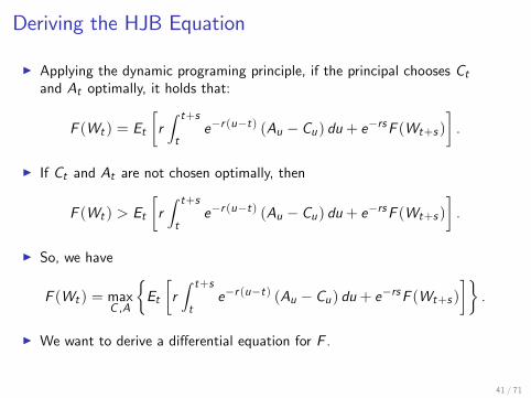
I Applying the dynamic programing principle, if the principal chooses Ctand At optimally, it holds that:

F (Wt ) = Et

rZ t+st

er (ut) (Au Cu) du + ersF (Wt+s )

.

I If Ct and At are not chosen optimally, then

F (Wt ) > Et

rZ t+st


.

I So, we have

F (Wt ) = maxC ,A

Et

rZ t+st


.

I We want to derive a di¤erential equation for F .

41 / 71

Method: Itôs Rule

I Theorem: Assume that the process X follows

dXt = µtdt + σtdZt ,

with µ and σ adapted processes and let f (Xt ) be a twice continuouslydi¤erentiable function. Then it holds that

df (t,Xt ) =

∂f∂t+ µt

∂f∂X

+12

σ2t∂2f∂X 2

dt + σt

∂f∂XdZt ,

or in integral form

f (Xt ) = f (X0) +Z t0

∂f∂t+ µs

∂f∂X

+12

σ2s∂2f∂X 2

ds +

Z t0

σs∂f∂XdZs .

42 / 71

Deriving the HJB EquationI Recall, given Wt = W it holds that

F (W ) EtrZ t+st


,

withdWs = r (Ws u(Cs ) + h(As )) ds + rΓsσdZs .

I Applying Itôs rule to ersF (Wt+s ) we get

ersF (Wt+s ) = F (W ) +Z t+st

er (ut)rΓuσF 0(Wu)dZu

+Z t+st

er (ut)rF (Wu) + r (Wu u(Cu) + h(Au)) F 0(Wu)

+ 12 r2Γ2uσ2F 00(Wu)

du.

I Substituting back in the inequality results in

0 EtrZ t+st

er (ut)Au Cu F (Wu) +

12 rΓ

2uσ2F 00(Wu)

+ (Wu u(Cu) + h(Au)) F 0(Wu)

du.

43 / 71

Deriving the HJB Equation

I Now divide by s and let s ! 0, to arrive at

F (Wt ) At Ct

+ (Wt u(Ct ) + h(At )) F 0(Wt ) +12 rΓ

2t σ2F 00(Wt )

.

I This has to hold for all possible (t,Wt = W ) and we get the HamiltonJacobi Bellman equation (HJB)

F (W ) = maxC ,A

A C

+ (W u(C ) + h(A)) F 0(W ) + 12 rΓ

2σ2F 00(W )

,

where the maximization is over (admissible) controls C 0 andA 2

0,A

subject to incentive compatibility Γ = γ(A).

44 / 71

The HJB - Intuition

I Assume Ct and At are chosen optimally and Wt = W is xed.

I Since the principal discounts at rate r , his expected ow of value at timet must be rF (Wt )dt.

I This has to be equal to

1. the expected instantaneous ow of output minus payments to theagent r (At Ct ) dt,

2. plus the expected change in the principals value functionE [dF (Wt )].

I Together we have

rF (W ) = maxC ,A

r (A C )

+r (W u(C ) + h(A)) F 0(W ) + 12 r2γ2(A)σ2F 00(W )

.

45 / 71

Retirement Value Function

I Always possible to retire theagent:

I the agent puts zeroe¤ort At = 0 8t,

I the rm does notproduce,

I the principal o¤ersconstant consumptionCt = C 8t.

I The principals retirementprot is

F0(u(C )) = C ,

which is decreasing, concaveand satises F0(u(0)) = 0.

46 / 71

Constructing an Improvement

I If W hits zero have to retire the agent, as C 0.I If W becomes large, then, due to income e¤ect, it becomes increasinglycostly to compensate for e¤ort, hence eventually retire the agentoptimally.

I Over the improvement interval A > 0, and the improvement curve is thesolution to the HJB

F 00(W ) = minC ,A>0

F (W ) A+ C (W u(C ) + h(A)) F 0(W )rγ2(A)σ2/2

,

subject to boundary conditions

F (0) = 0

F (Wgp) = F0(Wgp)

F 0(Wgp) = F 00(Wgp)

"value matching",

"value matching",

"smooth pasting".

47 / 71

Constructing an Improvement

I A concave solution F (W ) F0(W ) to this boundary value problemexists and is unique.

I The concavity of F (W ) is due to the fact that retirement is ine¢ cient.

48 / 71

The Optimal Contract - Summary

I F (W0) which solves the boundary value problem above is the principalsprot under the optimal contract for W0 2 [0,Wgp ].

I The agents promised wealth under the optimal contract follows

dWt = r (Wt u(c(Wt )) + h(a(Wt ))) dt

+rγ(Wt ) (dYt a(Wt )dt)

until retirement time τ where Wt hits either 0 or Wgp .

I For t < τ, Ct = c(Wt ) and At = a(Wt ) are the maximizers in the ODEfor F (W ).

I After time τ, the agent receives constant consumption Ct = F (Wτ)and puts zero e¤ort.

49 / 71


Step 5:Verify that the conjectured contract maximizes the principals prot.

50 / 71

Verication

I So far optimal contract has been conjectured based on a solution of theHJB.

I However, one should note that the HJB takes the form of a necessarycondition: "If F (W ) is the optimal value function and (C ,A) are chosenoptimally, then

I F (W ) satises the HJB, andI The optimal choices of (C ,A) realize the maximum in the HJB."

I Further, implicitly made a couple of technical assumptions, in particularon the di¤erentiability of F (W ) and the existence of optimal choices of(C ,A).

I The verication theorem below will show that the conjectured contractindeed maximizes the principals prot (su¢ ciency).

51 / 71

VericationI Consider the process

Gt = rZ t0ers (As Cs ) ds + ertF (Wt ).

I The drift of Gt is given by

rert

(At Ct ) F (Wt )+ (Wt u(Ct ) + h(At )) F 0(Ws ) +

12 r2Γ2t σ2F 00(Ws )

| z

0 from HJB

,

which is zero in the conjectured contract and 0 in any other incentivecompatible contract.

I Hence,

ErZ ∞

0ert (At Ct ) dt

= E [G∞] G0 = F (W0),

with equality under the optimal contract.

52 / 71

Discussion

Additional Properties of the Optimal Contract:Initialization, optimal consumption and optimal e¤ort prole.

53 / 71

Initialization

I Principal has all bargainingpower, W0 = W :

F 0(W ) = 0.

I Agent has all bargainingpower, W0 = Wc :

F (Wc ) = 0.

54 / 71

Discussion - Optimal E¤ort and Consumption

I From the HJB equation, e¤ort maximizes

a|zoutput

+ h(a)F 0(W )| z cost of compensating for e¤ort

+12rσ2γ(a)2F 00(W )| z

cost of providing incentives

.

! E¤ort typically is non-monotonic in W as

I F 0(W ) decreases in W (retirement is ine¢ cient),I while F 00(W ) increases at least for low values of W (exposing agentto risk is costly close to triggering retirement).

I The optimal consumption choice maximizes

c u(c)F 0(W ).

! When F 0(W ) 1/u0(0), consumption is zero ("probation"). Thisis the case for W 2 [0,W ] (increase drift of W to avoid retirement).

! For W > W consumption is increasing in W .

55 / 71

An Example

56 / 71

Discussion - Optimal E¤ort and Consumption

I Proposition 3: The drift of Wt points in the direction where F 00(W ) isincreasing, i.e., where it is cheaper to provide incentives.

I Proof: Di¤erentiating the HJB wrt W using the envelope theorem gives

(W u(C ) + h(A))| z drift of W

F 00(W ) +12rσ2γ2(A)F 000(W ) = 0. (2)

I Note next that (2) is, from Itôs Lemma, also equal to the drift of F 0(W ).! Together with the FOC for (interior consumption)

1u0(c(W ))

= F 0(W ),

this implies that 1/u0(C ) is a martingale ("Inverse Euler Equation").

I Reects the fact that agent cannot save: u0(C ) is a submartingale.! So if the agent could save he would want to do so as his marginalutility increases in expectation.

57 / 71

Contractual Environments

How do Contractual Environments A¤ect Agents Career?

58 / 71

Contractual Environments

I Di¤erent Contractual environments:

A.) The agent can quit and pursue an outside option,B.) the principal can replace the agent,C.) the principal can promote the agent.

I Properties of agents career:

1.) Wages (back-loaded vs. front-loaded),2.) short-term incentives (piece rates, bonuses) vs. long-term incentives

(permanent wage increases, terminations),3.) the agents e¤ort in equilibrium.

59 / 71

Solve the Model under Di¤erent Environments

I Principals generalized problem: Maximize prot until t = τ when theagent quits, retires, is replaced, or promoted

ErZ τ

0ert (At Ct ) dt + erτF0 (Wτ)

,

subject to incentive compatibility constraint and the agents participationconstraint for all t τ,

Wt W 0.

I The principals prot function F (W ) has to satisfy the same HJB asbefore, but the respective environment determines the boundaryconditions:

F (Wτ) = F0 (Wτ) .

60 / 71

A.) Prot Function with Outside Option

I Lower retirement point is higherthan w/o outside option:

W > 0.

I Principals prot is lower than w/ooutside option:

F (W ) < F (W ) .

61 / 71

B.) Prot Function with Replacement

I Retirement prot higher than w/oreplacement:

F0 (W ) = F0 (W ) +D.

I Principals prot is higher thanw/o replacement:

F (W ) > F (W ) .

I Less costly to retire the agent! upper retirement point lowerthan w/o replacement:

Wgp < Wgp .

62 / 71

C.) Promotion of the Agent

I Promoting the agent to a new position

I incurs the principal training cost K ,I increases the agents productivity by a factor of θ > 1,I Increases the agents outside option to Wp > 0.

I With a promoted agent, the principals prot function solves

F00p (W ) = min

C ,A>0

Fp(W ) θA+ C (W u(C ) + h(A)) F 0p(W )rγ2(A)σ2/

2θ2 ,

with boundary conditions

Fp(Wp) = 0,

Fp (Wgp) = F0 (Wgp) ,

F 0p (Wgp) = F 00 (Wgp) .

63 / 71

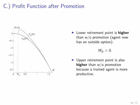
C.) Prot Function after Promotion

I Lower retirement point is higherthan w/o promotion (agent nowhas an outside option):

Wp > 0.

I Upper retirement point is alsohigher than w/o promotionbecause a trained agent is moreproductive.

64 / 71

C.) Prot Function before Promotion

I Principal must decide whether topromote or to retire the agent:

F0 (W ) = maxF0 (W ) ,Fp (W )K

.

I Here: Agent is promoted at Wgpwhere:

FWgp

= Fp

Wgp

K ,

F 0Wgp

= F 0p

Wgp

.

I Principals prot is higher thanw/o promotion:

F (W ) > F (W ) .

65 / 71

1.) Front-Loaded vs. Back-Loaded Compensation

I A fully dynamic setting allows us to study when wages should be morefront-loaded and when they should be more back-loaded.

I E.g. Lazear (1979) shows that:

I The employers can strengthen an employment relationship byo¤ering a rising wage pattern.

I By postponing pay to a later point in the agents career, he can beinduced to exert more e¤ort at the same costs for the principal.

I In the present setting:

I The Optimal contract trades o¤ this benet against costs from

I income e¤ect,I earlier retirement, andI distortion of agents consumption.

66 / 71

1.) Front-Loaded vs. Back-Loaded Compensation

I Measure for how back-loaded theagents compensation is:

I wage captures short-termcompensation.

I continuation value captureslong-term compensation.

! compare environments by lookingat continuation value for a givenwage.

67 / 71

2.) Short-Term Incentives vs. Long-Term Incentives

I Long-term and short-term incentives have been studied individually.

I Short-term incentives:

I Holmström and Milgrom (1987) "especially well suited forrepresenting compensation paid over short period" (from HM 1991).

I Lazear (2000): productivity in Safelite Glass Corporation increasedby 44 % when piece rates were introduced.

I Long-term incentives:

I Lazear and Rosen (1981): incentives can be created by promotions.

I Optimal mix of short-term and long-term incentives has not been studied.

68 / 71

2.) Short-Term Incentives vs. Long-Term Incentives

I Incentives are provided by tying the agents compensation to the projectsrisky outcome.

I Volatility of current consumption captures short-term incentives.I Volatility of continuation value captures long-term incentives.

! Use the relative volatility of the agents compensation as a measure forthe dynamics of incentive provision.

I Agent has outside option ) less long-term incentives.I Principal can replace the agent ) more long-term incentives.I Principal can promote the agent ) more long-term incentives.

69 / 71

3.) Equilibrium E¤ort Prole

I Higher e¤ort when the optimalcontract relies more on long-termincentives.

70 / 71

Sannikov (2008) Conclusions

I Clean and elegant method to study dynamic incentive problems.

I Linear over short periods as in Holmström and Milgrom (1987) butnonlinear in the long run.

I How does contractual environment a¤ect dynamics.

I Next: Look at a dynamic model of nancial contracting withrisk-neutrality (DeMarzo and Sannikov 2006).

71 / 71

Dynamic Principal Agent Models: A Continuous Time Approach Lecture I€¦ · Dynamic Principal...

Documents

Transcript of Dynamic Principal Agent Models: A Continuous Time Approach Lecture I€¦ · Dynamic Principal...