Dynamic pricing policies for an inventory model with...

Dynamic Pricing Policies for an Inventory Model with Random Windowsof Opportunities

Arnoud den Boer,1,2 Ohad Perry,3 Bert Zwart2

1Korteweg-de Vries Institute for Mathematics, University of Amsterdam

2Amsterdam Business School, University of Amsterdam

3Industrial Engineering and Management Sciences, Northwestern University, Evanston, Illinois 60208

Received 11 February 2016; revised 23 March 2017; accepted 24 March 2017DOI 10.1002/nav.21737

Published online 00 00 2017 in Wiley Online Library (wileyonlinelibrary.com).

Abstract: We study a single-product fluid-inventory model in which the procurement price of the product fluctuates according to acontinuous time Markov chain. We assume that a fixed order price, in addition to state-dependent holding costs are incurred, and thatthe depletion rate of inventory is determined by the sell price of the product. Hence, at any time the controller has to simultaneouslydecide on the selling price of the product and whether to order or not, taking into account the current procurement price and theinventory level. In particular, the controller is faced with the question of how to best exploit the random time windows in which theprocurement price is low. We consider two policies, derive the associated steady-state distributions and cost functionals, and applythose cost functionals to study the two policies. © 2017 Wiley Periodicals, Inc. Naval Research Logistics 00: 000–000, 2017

Keywords: single-product fluid-inventory model; optimal order policies; stochastic systems

1. INTRODUCTION

We consider a continuous review, single product, pricing-and-inventory problem in a random environment, where thepurpose of the seller is to maximize his expected profit bydetermining an order policy and sell prices. At the procure-ment side, the seller faces randomly fluctuating prices atwhich he can acquire new items, but also holding costs andfixed order costs. Based on these quantities, the seller needs todecide when to order new items, and how many. At the salesside, in accordance with current practice if dynamic pricing,the seller can change the sell price at any moment.

More specifically, the procurement price at which newitems can be acquired is modeled as a finite-state Markovchain, where each state represents a different procurementprice. Every time an order is placed, the seller pays somefixed order cost K, and any moment that the inventory-levelis x > 0, the seller faces holding costs at a rate h(x). We ini-tially assume that ordered items arrive instantaneously andlater generalize the model to include exponential lead times.The seller needs to determine an order policy (when to ordernew items, and how many), and a sell price policy (which sell

Correspondence to: Ohad Perry ([email protected])

price to charge at which moment), in order to optimize theexpected profit.

Determining optimal order policies and sell prices is typ-ically treated as separate problems, but it is intuitively clearthat it may be beneficial to consider these problems simulta-neously. For example, if the procurement price of new itemsis time-dependent and is currently high, it may be profitableto increase the sell price, so that the moment at which allinventory is sold-out is delayed. This increases the probabil-ity that, in the mean time, the procurement price of new itemsdecreases, so that new items can be ordered at considerablylower costs.

A Fluid Analysis

The complexity of the stochastic model we consider ren-ders exact analysis prohibitively hard, and we thereforeresort to fluid approximations. In our setting here, the fluidapproximation is a piecewise-continuous process having adeterministic evolution between jump epochs.

Fluid models are prevalent approximations for complexstochastic systems in general, and queueing and inventorysystems in particular. In a fluid inventory model, each itembecomes an “atom” in a continuous content process, and

© 2017 Wiley Periodicals, Inc.

2 Naval Research Logistics, Vol. 00 (2017)

the random depletion rate of inventory is replaced by themean demand rate, ignoring variability. Thus, fluid analysisis appropriate whenever the number of items sold betweendecision epochs, as well as the number of items ordered, islarge, such that each single item is relatively negligible.

By aggregating the effect of a large number of events, afluid inventory model provides the time-dependent averagebehavior of the system. Although this view can often be maderigorous (under appropriate regularity conditions) by provingthat the fluid model arises as a functional weak law of largenumbers for the stochastic inventory process under study (see,e.g., [10] and [21]), fluid dynamics are typically assumeddirectly in inventory systems, without any reference to anunderlying discrete system. For example, one of the mostfundamental inventory models - the (purely deterministic)economic order quantity (EOQ) model—can be thought ofas a fluid approximation for a stochastic inventory system.For a recent application, see [19] and references therein.

Other than their tractability and relative simplicity, fluidapproximations have the advantage of being less sensitive todistributional properties of the stochastic system they approx-imate, making fluid analysis robust to variations in the mod-eling assumptions. However, we emphasize at the outset thatour fluid model is itself a stochastic process, whose random-ness emanates from that of the environment. We elaboratebelow.

A Class of Stationary Markovian Policies

Our goal is to find an effective control for the inventoryprocess. Since the random environment must clearly be takeninto account when making ordering decisions, the fluid modelis a stochastic process. To facilitate long-run analysis, we limitattention to a class of stationary and Markovian policies,so that, in particular, the fluid model is a stationary Markovprocess under the control (namely, it achieves a unique steadystate). It is well known that, if a Markov process has a contin-uous segment, then it is either a transformation of a Brownianmotion or it is deterministic [13]. Since our model has non-increasing sample paths between jumps, it must exhibit adeterministic motion between jump epochs, so that it is apiecewise-deterministic Markov process, as in [15].

Now, in order for the controlled fluid process to be Markov,decisions must be made based on the current state of theprocess and the environment. Furthermore, for the process tobe ergodic (so that a unique stationary and limiting distrib-ution exists), the fluid process must be regenerative. There-fore, the class of controls we consider is continuous-reviewpolicies of (s, S) type. It is significant that, in addition tobeing mathematically attractive, these policies are also easyto employ and are prevalent in practice; see, for example,[25]. Note also that, with no lead times, (s, S) policies areequivalent to (r, Q) policies in which a fixed quantity Q > 0 is

ordered whenever the inventory level falls below some levelr ≥ 0.

In particular, for the order policy, we study two variantsof an (s, S)-policy. In the first order policy, which we denoteby OP1, S−s items are ordered if the inventory-level is at orbelow some s > 0 and at the same time the procurement priceis low. If the inventory hits zero and the procurement priceis high, Q items are ordered. Here s, S, Q are decision vari-ables, with 0 ≤ s < S, 0 < Q ≤ S. The second order policy,denote by OP2, orders are never placed when the procurementprice is high. If the inventory-level hits zero, the seller waitsuntil the procurement price becomes low, at which momenthe orders S items. We allow the sell price to change with theinventory level. Note that either policy takes advantage ofthe low procurement price, and we thus refer to the (random)time periods of low procurement price as random windowsof opportunity (for the seller).

We consider the pricing-and-inventory problem in station-arity. Under mild assumptions on the relation between thedemand rate and sell price, we show that the joint process ofinventory level and procurement price admits a unique sta-tionary distribution. For a fixed order policy OP1 or OP2, wederive balance equations for the stationary distribution of theinventory-level process, as in [5] and [14], from which thestationary distribution can be numerically computed. Thisenables us to express the long-run profit for both policies,as function of (s, S, Q, p(·)) in case of OP1, and (s, S, p(·))in case of OP2, where p(·) : [0, S] → R+ is the sell pricefunction.

For practical purposes, one uses a piecewise constant sell-price function p(·). For example, if p(·) has only two values,pl (for “low” price) and ph (for a “high” price), then when-ever the inventory level exceeds some (switching) thresh-old q, a sell price ph is charged, whereas a sell price pl ischarged whenever the inventory level is below q. In that case,(pl , ph, q) is a vector of finite decision variables which sat-isfy 0 < pl < ph and 0 ≤ q ≤ S; see Section 2 below for anelaboration.

To determine the optimal values of the decision variables,one needs to solve a (rather complicated) nonconvex nonlin-ear optimization problem. We conduct a numerical study tocompare the performance of OP1 and OP2. We also comparethem to a standard (s, S)-policy OP0, which does not takeinto account the random nature of the procurement priceprocess. By studying several instances, it turns out that OP1

in general performs better or equal than both OP2 and OP0.The difference in performance, especially between OP1 andOP0, can be quite large. This shows that it is beneficial totake into account random changes in the procurement prices.As should be expected, the policies OP0 and OP2 have noclear “best”: for some instances, the first is outperformedby the latter, while for other instances it is the other wayaround.

Naval Research Logistics DOI 10.1002/nav

Boer, Perry, and Zwart: Dynamic Pricing Policies for Inventory Model 3

1.1. Related Literature

Threshold policies have been shown to be optimal innumerous settings, including under Markovian-demand envi-ronments. A detailed development and literature review isfound in [4]. An early result by Iglehart and and Karlin [20]considers a discrete-time inventory model with demand thatis governed by a discrete-time Markov chain (DTMC). Inparticular, at each period the demand distribution is set bythe state of the DTMC. Song and Zipkin [30] analyze acontinuous-time inventory model having Markov-modulatedPoisson demand and backlogging, and prove that a state-dependent (s, S) policy is optimal under the assumption offixed ordering costs. See also [11], which considers a discrete-time version of the problem, and [12] which extends themodel to include lost sales. Related to [30] are the two papers[2] and [3], which consider EOQ-type models with Markov-modulated demand process. A multistage serial inventorymodel with Markov modulated demand in stage 1 is ana-lyzed in [9] and it is shown that, under linear holding andordering costs, an echelon base-stock with state-dependentorder-up-to levels policy is optimal.

The paper [6] considers a fluid-inventory model in whichthe demand rate changes according to a CTMC; wheneverthe inventory content hits 0 an order of size Qi is placedif the governing CTMC is at state i, i = 1, 2. See also [8]which considers a fluid inventory model in which the pro-curement prices change according to an exogenous CTMCand, unlike our model, this also affects the demand. (Weassume that demand is affected by the sell price, which is con-trolled by the decision maker.) In [28], the authors consideran inventory model which replenishes at a constant determin-istic rate, but decreases randomly (via jumps) when demandarrives (according to a compound renewal process); imply-ing that the demand at each arrival epoch is relatively verylarge. In contrast, in our model demand arrives continuouslyand is infinitesimal in the fluid model, and the orders arerelatively large, causing the jumps in the fluid model; seealso [29].

Threshold policies for EOQ-type fluid inventory modelsare considered in [18] and [24]. In both references it isassumed that discounts are offered by a supplier to a resellerrandomly in accordance with a Poisson process, but there areno “windows” openings. In these cases, the reseller has todecide at any discount epoch whether to replenish his inven-tory or not. In [27] a firm purchases a product in an auctionin order to satisfy its own demand in each period. In partic-ular, each period consists of two phases: in the first phase,the firm participates in N auctions, and in the second it sellsthe purchased products in its own market. The probability ofthe firm winning an auction is assumed to be a function ofits own bid as well as of the number of its opponents in theauction. In particular, there is no a-priori fixed procurement

price, although the firm does have some control over thatprice via its bidding strategy.

Price-Regulated Demand

Starting with the seminal work of Naor [26], a standardassumption in the economic analysis of queues is that cus-tomers’ arrival rate to a service system is completely deter-mined by the price and expected reward of joining the systemto get served. For example, one often assumes that the poten-tial arrival rate, known as the market size, is a constant �,and the arrival process to the system is a nonhomogeneousPoisson process having an instantaneous rate �f (p(t)) attime t when the price is p(t), where for 0 ≤ pm < pM ≤ ∞,f : [pm, pM) → [0, 1] is a known market response func-tion. In particular, f (p(t)) is the fraction of customers thatare expected to join the system when the price is p(t) ∈[pm, pM); see, for example, [1, 16, 22] and references therein.The market response function is determined by the proba-bility that a generic arrival will choose to buy a product atthe given sell price. In practice, that probability, and thusthe response function, are not known in complete certainty,although they can typically be evaluated via past demanddata; see [17] and the reference therein. In the aggregate time-dependent (functional) average approximation that the fluidmodel provides, the market size and response function com-pletely determine the depletion rate of the fluid content forany given sell price.

Organization

The remainder of this article is organized as follows: InSection 2, we describe the model and motivate the structureof the control policies. In Section 3, we develop the steady-state equations for the content level process. Those equationsare then applied in Section 4 in a numerical study, as describedabove. In Section 5, we extend the model and consider casesin which the procurement price of the item changes after non-exponential random time in states, and we also consider leadtimes.

2. THE MODEL

We consider a fluid inventory model of one product withzero lead time of the (s, S) type, operating in a stochasticallychanging cost environment. We use C := {C(t) : t ≥ 0} todenote the content-level process, assumed to be right con-tinuous with jumps at ordering epochs. As there are no leadtimes, the right continuity of C implies that, if t is a jumpepoch, then C(t−) < C(t), where C(t−) denotes the leftlimit at t.

Following the terminology in [7] and [30], we refer toprocurement price as the “state of the world.” In particular,



the procurement price of the product changes according toa two-state continuous-time Markov chain (CTMC) W :={W(t) : t ≥ 0}, with W attaining two values: wλ (high) andwμ (low). Naturally, wλ is strictly larger than wμ. (Other-wise, the state of the world is irrelevant.) More specifically,W moves between the two states wλ and wμ, and remainsat wλ for an exponential amount of time with rate λ, and inwμ for an exponential amount of time with rate μ. WhenW = wλ the controller faces a regular (expensive) price, andwhen W = wμ, the controller faces a discounted (cheap) pro-curement price. It is thus clear that the “state-of-the-world”process W may affect the decision of the controller whetheror not to buy at each decision epoch in order to replenish hisinventory.

We assume that a holding cost is incurred at rate h(x)dx

whenever C(t) = x, t ≥ 0, and that a fixed set-up cost Kis incurred when an order is placed, independent of theorder size. In addition, we assume that the demand rate is aknown one-to-one and onto function of the sell price. Underthis assumption, the controller can dynamically regulate therelease rate of inventory by changing the sell price. Therecan be several policies for determining the sell price. In thisstudy, we focus on the state of the content level C. Moreprecisely, since the more inventory present, the higher instan-taneous holding cost is paid, the controller has an incentiveto drain inventory at a higher rate when C is high, by low-ering the sell price. In the continuous settings, the optimalrelease rate may change continuously as a deterministic func-tion of C, so that infinitely many pricing policies can beapplied. For practical purposes, the optimal pricing policycan be approximated by searching for a finite set of sellprices p1 < p2 < · · · < pk (with k fixed) and thresholdsq1 > q2 > · · · > qk−1, such that the sell price is pi at time tif qi−1 < C(t) < qi , i = 1, 2 . . . , k −1. Clearly, as the num-ber of decision variables increases, the optimization problembecomes more complicated.

In the simple (s, S) model, the optimal control is com-prised of two factors: when to place an order (in the senseof fixing s) and how much to order (fixing level S). Thus, ifthe procurement price was always wμ we would have beenlooking for a level s such that, whenever the content-levelprocess C hits s, an order of size S–s is placed. In light ofthe randomness of the procurement price and zero lead-timeassumptions, it is desirable to place most of the orders, if notall of them, when the procurement price is wμ. In particular,the distinction between “most” and “all” depends on whetherit is optimal to place an order whenever both C(t) = 0 andW(t) = wλ, that is, whenever the content level drops to zeroat the time of an expensive cost-price period. In that case,one should consider two options: (i) order up to level Q ≤ S

or (ii) wait for the procurement price to change from wλ

to wμ.We thus consider two natural ordering policies:

Order Policy 1 (OP1)

Determine two levels s and S. If the content level C hitss and at the same time the procurement price is low, that is,C(t−) = s and W(t−) = wμ, then place an order of size S–s(so that C(t) = S. If, conversely, upon hitting level s the pro-curement price is high, that is, C(t−) = s and W(t−) = wλ,then wait until either (i) the procurement price changes towμ, at which point order up to S, or (ii) the content level hits0, at which point order up to level Q, where Q ≤ S

Order Policy 2 (OP2)

Similarly to OP1, except that never place an order while theprocurement price is high, that is, whenever W = wλ. Whenlevel 0 is hit (and it can only be reached during expensiveperiods) wait until the procurement price changes to cheap(wμ), at which point order up to level S. Note that, under OP2,there is no extra level Q (alternatively, Q ≡ S).

We further assume that there is a cost incurred for letting Cstay at state 0 for an interval. This cost can be due to unsatis-fied demand and loss of good will of customers and so forth.In particular, if C(t) = 0 on some interval [t1, t2], then a costa(t2 − t1) is incurred.

To fully describe the control, we need also to charac-terize the threshold q and the sell prices pl and ph. Thatis, under OP1 the control is determined by the decisionvariables (s, S, q, Q, pl , ph), while under OP2 the control isdetermined by the decision variables (s, S, q, pl , ph). Alter-natively, because of the equivalence between the sell pricesand the demand rate, we can replace pl and ph by dl and dh,respectively.

To distinguish between the two policies, we let C1 :={C1(t) : t ≥ 0} denote the content-level process under OP1,and C2 := {C2(t) : t ≥ 0}, denote the content-level processunder OP2. We still use the notation C in discussions in whichno specific process is considered (if the same is true for bothC1 and C2).

2.1. The Fluid Process Achieved via AsymptoticConsiderations

In our model, the content-level process C is assumedto decrease deterministically and continuously in betweenorders, with the instantaneous decrease rate determined bythe sell price. To see that this assumption follows from stan-dard assumptions in the literature (as was reviewed in Section1.1 above), recall that a fluid inventory model is achieved asa relaxation to a stochastic system, building on asymptoticconsiderations, as described in Section 1. In particular, ourmodel is appropriate as an approximation for a large inven-tory system in which large orders are placed rarely relative tothe interarrival times of customers that purchase those items.



For example, orders of several hundreds of items may bemade once every few weeks, and tens of items are sold daily.We now provide a quick overview of the arguments that canbe used to prove the limiting result.

Formally, the fluid model can be achieved as a stochastic-process limit of a sequence of stochastic inventory systemsindexed by n. With each n ≥ 1, there are associated parame-ters sn, Sn, qn, and Qn that increase linearly with n, so that, forexample, Sn/n → S > 0 as n → ∞, and an arrival processof customers purchasing the items with an arrival rate thatincreases proportionally to n as well.

Let Cn := {Cn : n ≥ 1} denote the content level processin system n, and let C̄n(t) := C(nt)/n, t ≥ 0. The fluidprocess C is an approximation for Cn in the sense thatC̄n(t) ≈ nC(t) for large-enough n. Observe that the fluidapproximates a large system Cn by accelerating time by afactor of n in C̄n. This implies that the state-of-the-worldprocess should be “slowed-down” (relative to the demandprocess) in order for it to have the same time scale as theinterorder times. Specifically, in system n, the procurementprice evolves according to a CTMC Wn := {Wn(t) : t ≥ 0},which spends an exponentially-distributed amount of time instate wλ and in wμ with mean nλ and nμ, respectively.

It remains to describe the demand process that leads tothe deterministic demand rate in the fluid model. To thisend, assume that the arrival process of customers consti-tutes a Poisson process with some rate � > 0. Assumefurther that each customer has a private valuation for the itemunder consideration, and that the valuations of customersare random variables that are independent across the cus-tomers and are identically distributed. Let V denote a genericrandom variable that has the customers’ valuation distribu-tion, and let FV denote its cumulative distribution function(cdf). Then an arrival will purchase an item with probabilityFc

V (p(x)) := P(V > p(x)) when the price is p(x), so thatFc

V (p(x)) is the proportion of all arrivals that purchase itemswhen the price is p(x). Given these assumptions, the instan-taneous demand rate when the content is x and the price isp(x), is

d(x) := �FcV (p(x)), (1)

so that the demand process is

N(∫ t

0�Fc

V (p(x))dx

), t ≥ 0,

where N is a unit-rate Poisson process. It follows from thefunctional strong-law of large number for the Poisson process(e.g., section 3.2 in [32]) and the continuity of the com-position mapping at continuous limits (e.g., [31], Theorem13.2.1]) that, uniformly over compact intervals,

N ◦ ∫ t

0 n�FcV (p(x))dx

n:=

N(∫ t

0 n�FcV (p(x))dx

)n

→∫ t

0�Fc

V (p(x))dx

as n → ∞ w.p.1.

In particular, we obtain that the fluid model C(t) is differ-entiable at all its continuity points, namely, at all points inwhich no orders arrive, and evolves according to the differ-ential equation C ′(x) = −d(x) between orders, for d(x) in(1). We thus see that the random demand process in the pre-limit is replaced with a deterministic demand process in thefluid limit.

3. STEADY-STATE ANALYSIS

We will analyze the inventory system in stationarity.Hence, we need to argue that a unique stationary distributionindeed exists for our system. We will analyze a system havinga general demand-rate function, which allows for a generalpricing policy analysis in our setting. Let p1 : [0, S] → R+and p2 : [0, S] → R+ be the pricing policies under OP1 andOP2, respectively. For x ∈ [0, S], let d1(x) := d(p1(x)) andd2(x) := d(p2(x)) denote the respective demand functions.

We make the following assumption, which will be shownto ensure that the system possesses a unique stationarydistribution. Let

Di(x) :=∫ x

0

1

di(y)dy, 0 ≤ x ≤ S. (2)

ASSUMPTION 1: The pricing policy employed is suchthat Di(S) < ∞ for i = 1, 2.

Note that Di(x) is the time to reach level 0 from level x,for all 0 < x ≤ S, if the input is shut off, that is, if thereare no new inventory orders during Di(x) time units. ThenAssumption 1 simply states that the content level can reachstate 0 in finite time, provided no new orders are placed duringthe time interval [0, Di(S)] and Ci(0) = S. This assumptionholds trivially whenever di is a simple function, i = 1, 2, whichis the case amenable to numerical studies and optimizations.

Note that, for i = 1, 2, the content level Ci is not Markov,but

Xi := {Xi(t) : t ≥ 0} := {(Ci(t), W(t)) : t ≥ 0}is a two-dimensional Markov process with state space S :=[0, S] × {

wλ, wμ

}. It is simple to show that X is regen-

erative and possesses a unique stationary distribution. LetW(∞) denote a random variable having the stationary dis-tribution of the process W, and let Ci(∞) be a random vari-able having the stationary distribution of Ci , i = 1, 2. Then



Xi(∞) := (Ci(∞), W(∞)) is a random variable with thestationary distribution of the process X i , i = 1, 2. All theserandom variables exist by the following theorem.

PROPOSITION 3.1: If Assumption 1 holds, then for i = 1,2, the joint process Xi = (Ci , W) is a (possibly delayed)regenerative process admitting a unique stationary distribu-tion.

PROOF: It is easy to see that X i , i = 1, 2, is nonlattice, andwill return to state x∗ := (S, wμ) in finite expected time,given our assumptions on the model. In particular, let Eμ andEλ denote two generic exponential random variables repre-senting the times that W spends in each of its states wμ andwλ, respectively, and let T denote the return time of C1 to S,and take X1(0) = (S, wμ). Then

E[T ] = E[T |W(D(S − s)) = wμ]P(W(D(S − s) = wμ)

+ E[T |W(D(S − s)) = wλ]P(W(D(S − s)) = wλ)

≤ D(S − s) + E[T |W(D(S − s)) = wλ].Now, if at time D(S − s) the state of the world is wλ, then thecontent process will either jump back to S if Eμ ≤ s, namely,with probability 1 − e−μD(s), or it will jump to Q if Eμ > s,that is, with probability e−μD(s). Therefore, letting TQ denotethe time to return to x∗ when starting in (Q, wλ), the secondterm in the right-hand side of the equality above satisfies

E[T |W(D(S − s)) = wλ] ≤ D(S)(1 − e−μD(s))

+ E[TQ]e−μD(s).

Observe that TQ is a geometric sum with success probabilityP(Eλ > D(Q)) = e−λD(Q) of random variables, where eachof the random variables in the sum is bounded from aboveby D(Q) w.p.1. The statement of the proposition follows forX1 from Assumption 1. Similar arguments can be employedto prove the result for X2. �

REMARK 3.1: It is clear from the arguments in the proofof Proposition 3.1 that it is sufficient to assume that D1(y) <

∞ for some y > S − s, that is, the content level can gobelow level s. However, OP2 requires that the content levelcan reach level zero in finite time.

3.1. Steady-State Equations

We now compute the unique stationary distribution of theprocesses C1 and C2. In some models, simplifications occurdue to a form of asymptotic independence between the con-tent level C and the “world” process W (using our notation),that is, C(∞) is independent of W(∞), so that the stationarydistribution of X is the product of the stationary distribu-tions of C and W. Such is the case, for example, when W

is a “well-behaved” Markov process which determines thedemand process; see, for example, [7] and references therein.However, such simplification cannot be expected to hold inour model, since the position of C(t) contains significantinformation on the value of W (t) at each t, even when thejoint process X is stationary (that is, if X(t) is distributed asX(∞) for all t ≥ 0). For example, if C(t) < s, then neces-sarily W(t) = wλ. However, there is still simplification inour case, which stems from the fact that the world process Wdoes not depend on the content level C, and can be analyzedseparately. We can thus find the stationary distribution of Cby computing relevant stationary quantities of W.

We next introduce integral representations for the steady-state density functions of the content level process. Letf1 : [0, S] → R+ and f2 : [0, S] → R+ denote the steady-state density functions of C1 and C2, respectively. The nexttheorem provides an integral representation for the steady-state densities f 1 and f 2. We present two equations for thedensity under OP1, for the two cases s < Q and s ≥ Q.

Consider the case s < Q, and take x > s. Let k1 denote thelong-run rate of upcrossings of level x, that is, the long-runaverage number of jumps from s to S. For the case s ≥ Q,let k̃1 denote the long-run rate of upcrossing of level x,s ≤ x ≤ S. We denote by k2 the long-run rate of upcrossingsof level x, x ≥ s, caused by jumps from level s under OP2.

The main difficulty in our model is in determining the long-run rate of jumps from level s, that is, the values of k1, k̃1,and k2. We first present the integral equations for the steady-state densities without specifying these constants: their valuesare computed in Lemma 3.4 below, after the solutions to thesteady-state densities, and their respective cdf’s are computedin terms of these constants.

Let π2 denote the atom at 0 of the stationary content levelC2, that is,

π2 := P(C2(∞) = 0) > 0. (3)

LEMMA 3.1 (integral equations for steady-state densities)The steady-state densities f1(x) of C1 and f2(x) of C2 exist.

Furthermore, f1(x) satisfies one of the following integralequations, depending on whether s ≤ Q or s > Q:

If s ≤ Q : d1(x)f1(x)

=

⎧⎪⎪⎪⎨⎪⎪⎪⎩

λ∫ x

0 f1(w) dw + d1(0)f1(0), 0 ≤ x < s,

λ∫ s

0 f1(w) dw + d1(0)f1(0) + k1, s ≤ x < Q,

λ∫ s

0 f1(w) dw + k1, Q ≤ x ≤ S.

If s > Q : d1(x)f1(x)

=

⎧⎪⎪⎪⎨⎪⎪⎪⎩

λ∫ x

0 f1(w) dw + d1(0)f1(0), 0 ≤ x < Q,

λ∫ s

0 f1(w) dw, Q ≤ x < s,

λ∫ s

0 f1(w) dw + k̃1, s ≤ x ≤ S.

(4)



The steady-state density f2(x) satisfies the integral equa-tion

d2(x)f2(x) ={

λ∫ x

0 f2(w) dw + λπ2, 0 ≤ x < s,

λ∫ s

0 f2(w) dw + λπ2 + k2, s ≤ x ≤ S.

(5)

PROOF: Existence of the stationary densities follows fromCorollary 4.1 in [23]. We explain the derivation of the inte-gral equation for f 1 for the case s ≤ Q. The other equationsare derived similarly.

First, d1(x)f1(x) in the left-hand side of (4) is the long-runrate of downcrossings level x, while the right-hand side rep-resents the long-run rate of upcrossings of level x, 0 ≤ x ≤ S.In steady state, the rate of downcrossing must equal to rate ofupcrossing that level, which is what (4) states. For a rigorousdefinition of “rate” we again refer to [23]. Here, the mean-ing will become clear from the proof. To see this, assume

that C1(0)d= C1(∞), namely, C1(0) has the steady-state dis-

tribution of the content level. That makes C1 a stationary

process, so that C1(t)d= C1(∞) for all t ≥ 0. Let τ be an

arbitrary point of a jump. Since jumps can only occur when0 ≤ C1 ≤ s, we separate the analysis into three cases asfollows:

1. 0 ≤ C1(τ−) < x < s. The last jump in the cyclebrings the content level up to level Q, and the otherjumps, if any, bring the content to level S (whereS ≥ Q). Thus, if C1(τ−) > 0, τ is a beginning of acheap period and C1(τ ) = S. If C1(τ−) = 0, thenτ is a time of depletion and C1(τ ) = Q. Both typesof jumps imply that the jump is an upcrossing oflevel x. Since the expensive period is exponentiallydistributed with rate λ, it follows by the well-knownPASTA (Poisson Arrivals See Time Average [33])property that if C1(τ−) > 0, then C1(τ−) and C1

are equal in distribution, and the rate at which levelx is upcrossed is λ. The rate at which C1(τ−) = 0 isd(0)f1(0). Thus, the rate at which level x is upcrossedis λ

∫ x

0 f1(w)dw + d(0)f1(0).2. 0 ≤ C1(τ−) ≤ s and s ≤ x < Q. Again, every

jump is an upcrossing of level x. However, in addi-tion to the previous case (i), there is also a possibilityto jump above level x from level s (when level s isreached during a cheap period). That long-run rate isdenoted by k1 (and will be computed in Lemma 3.4below).

3. 0 ≤ C1(τ−) ≤ s and Q ≤ x ≤ S. In this case, levelx cannot be upcrossed by a jump from level 0. Thus,the rate d1(0)f1(0) is removed. �

The arguments for f 1 in the case s > Q and for f 2 are similar.(Note however that f 2 has an atom π2 at level 0.)

3.2. Solutions to f 1 and f 2

We solve for f 1 and f 2 in (4) and (5) in terms of unknownsk1, k̃1 and k2 whose values are determined by the transientdistribution of the state of the world process W. We computethese unknowns explicitly in Lemma 3.4.

LEMMA 3.2 (Steady-state distribution). The steady-statedensity functions f 1 and f 2 satisfy

f1(x) =

⎧⎪⎨⎪⎩

c0d1(x)

eλD1(x), 0 < x < s,

(c0eλD1(s) + k1)D1(x), s ≤ x < Q,

(c0eλD1(s) + k1)D1(Q)/d1(x), Q ≤ x ≤ S,

and

f2(x) =⎧⎨⎩

λπ2d2(x)

eλD2(x), 0 < x < s,

(λF2(s) + λπ2 + k2)D2(x), s ≤ x < S,

where the constant k1, k̃1, and k2 are given in Lemma 3.4below, and c0 and π2 are the unique constants for which

∫ S

0f1(s)dx = 1 and π2 := 1 −

∫ S

0f2(x)dx.

PROOF: Let F1(x) := ∫ x

0 f1(s)ds denote the cdf, associ-ated with the density f 1. Let c0 := d1(0)f1(0). For 0 ≤ x < s,we write f1(x) − λ/d(x)F1(x) = c0/d1(x). Then, multiply-ing that equation by exp {−λD1(x)} and integrating (recallthat d

dxD1(x) = 1/d1(x)), we get

e−λD1(x)F1(x) =∫ x

0

c0

d1(s)e−λD1(s)ds = −c0

λe−λD1(x) + C1,

so that

F1(x) = −c0

λ+ C1e

λD1(x), x ∈ [0, s),

for some constant C1. Using the initial condition F1(0) = 0(and D1(0) = 0), we see that C1 = c0/λ. It follows that

F1(x) = c0

λ(eλD1(x) − 1), 0 ≤ x < s,

so that

f1(x) = c0

d1(x)eλD1(x), 0 ≤ x < s.

Hence,

f1(s−) = c0

d1(s)eλD1(s) and F1(s) = c0

λ[eλD1(s) − 1].



Next, consider x ∈ [s, Q). Then

d1(x)f1(x) = λF1(s) + c0 + k1

= c0eλD1(s) + k1.

Since the right-hand side of (4) over [Q, S] is a constant, theexpression for f 1 follows. Finally, the constant c0 is obtainedby applying the normalization condition

∫ S

0 f1(x) dx = 1,and is given in terms of k1.

The solution for f 2 is computed similarly. �

3.3. Jumps from Level s

It remains to find the constants k1, k̃1, and k2. To that end,we define the following conditional probabilities: Let θ1(s, S)

and θ2(s, S) denote the conditional probabilities that level sis downcrossed during a cheap period, under OP1 and OP2,respectively, given that the last jump prior to hitting s wasto level S. Let γ1(s, Q) denote the conditional probabilitythat level s is downcrossed during a cheap period under OP1,given that the last jump prior to hitting s was to level Q (whichunder OP1 corresponds to the beginning of a regenerativecycle). The closed-form expressions for θ1(s, S), θ2(s, S) andγ1(s, Q) are computed in Lemma 3.3 below. These expres-sions depend only on the (known) parameters of the costprocess C, and on the function D.

Observe that γ1(s, Q) = 0 if Q < s. Let 1 {s < Q} be theindicator function which equals 1 if s < Q and 0 otherwise.The proof of the following lemma is straightforward, and isthus omitted.

LEMMA 3.3:

θ1(s, S) = θ2(s, S) = λ

λ + μ+ μ

λ + μe−(λ+μ)[D1(S)−D1(s)],

γ1(s, Q) =(

λ

λ + μ− λ

λ + μe−(λ+μ)[D1(Q)−D1(s)]

)1{s < Q} .

In the next lemma, we express the constants k1, k̃1 and k2.

LEMMA 3.4: Consider x ∈ (s, S]. Then the long-run rateof upcrossings of level x under OP1 is given by k1 if s ≤ Q

and k̃1 if s ≥ Q. It is given by k2 under OP2, where

k1 := γ1(s, Q)d1(0)f1(0) + θ1(s, S)d1(S)f1(S),

k̃1 := θ1(s, S)d1(S)f1(S),

k2 := θ2(s, S)d2(s)f2(s), (6)

for γ1(s, Q), θ1(s, S) and θ2(s, S) in Lemma 3.3.

PROOF: We find k1. The computations of k̃1 and k2 aresimilar. (See also Remark 3.2 below.) Consider the state of the

content level immediately after a jump. Clearly, the processbetween jumps is a DTMC with two states – S and Q. Thetransition matrix of that DTMC at jump epochs is

P : =[PS,S PS,Q

PQ,S PQ,Q

]

=[θ1 + (1 − θ1)(1 − e−λD1(s)) (1 − θ1)e

−λD1(s)

1 − (1 − γ1)e−λD1(s) (1 − γ1)e

−λD1(s)

].

(7)

We now explain the entries of the transition matrix, startingwith the first row. The content level jumps to state S onlywhen the environment is cheap. There are two possibilitiesto make a transition from S to S: Either the content levelstarted at S and arrived at level s during a cheap period, inwhich case there is a jump immediately back to level S—this event occurs with probability θ1. Else, the content levelarrives at level s during an expensive period and there is nojump at s, but the expensive period is terminated before thecontent level reaches level 0. The probability of that latterevent is (1 − θ1)(1 − e−λD1(s)). This explains the first row ofthe transition matrix (7).

Turning to the second row, recall that the content levelreaches level 0 only when the environment is expensive, inwhich case the content level jumps to level Q. Thus, theDTMC at jumps epochs moves from Q to Q only if level swas reached during an expensive period, and the environmentremained expensive till the content level reached 0. The eventoccurs with probability PQ,Q = (1−γ1)e

−λD1(s). To see why,note that 1−γ1 is the probability of reaching s at “expensive”,given that the last jump was to Q, and e−λD1(s) is the prob-ability that the environment did not change to “cheap” afterlevel s was downcrossed, and before level 0 was reached.

We denote the stationary probabilities of the above Markovchain by νS and νQ, with ν := (νS , νQ). Calculating νP = ν

and νS + νQ = 1 gives

νS = 1 − (1 − γ1)e−λD1(s)

1 − (θ1 − γ1)e−λD1(s)and νQ = 1 − νS , (8)

where νS and νQ are interpreted as the limiting proportion ofjumps to levels S and Q, respectively. Hence,

k1 = (νSθ1 + νQγ1)d1(s)f1(s) (9)

is the long run rate of jumps from level s.We next show that the expression for k1 in (6) gives the

same expression as in (9): From (4) (the case s < Q) we seethat

d1(0)f1(0) = d1(S)f1(S) − d1(s)f1(s) =: c0,



and from the solution to f 1 we see that d1(s)f1(s) =c0e

λD(s) + k1. Substituting for d1(0)f1(0) and d1(S)f1(S)

in the expression for k1 in (6), we rewrite k1 to get

k1 = γ1c0 + θ1c0eλD1(s) − θ1c0

1 − θ1. (10)

It is then a matter of simple algebra to show that the expressionfor k1 in (10) is equal to

(1 − νSθ1 − νQγ1)−1(νSθ1 + νQγ1)c0e

λD1(s),

for νS and νQ in (8). We now use the solution for f 1 oncemore to replace c0e

λD1(s). In particular, from c0eλD1(s) =

d1(s)f1(s)− k1 we get the desired equality, that is, k1 in (10)is equal to the expression (9). This proves the claim. �

REMARK 3.2: The values of the terms in (6) have anintuitive interpretation. For example, the value of k1 canbe computed by conditioning on the last jump prior to hit-ting s, namely we condition on whether we started at levelQ or S, where these conditional probabilities are γ1(s, Q)

and θ1(s, S), respectively. Then the long-run rate of hitting s,when starting in Q, is also the long-run rate of hitting level 0from above, which is equal to d1(0)f1(0). The long-run rateof hitting s when starting in S, is the long-run rate of down-crossing S, which is equal to d(S)f1(S). This logic givesthe expression for k1 in (6). Similar reasonings give us theexpressions for k̃1 and k2.

3.4. Profit Functions Under OP1 and OP2

We can use the solutions for f 1 and f 2 and compute thelong-run profit functions for both policies. We denote byR1 := R1(s, S, Q, p(·)) the long-run average profit functiongenerated by OP1, and by R2 := R2(s, S, p(·)) the long-runprofit function generated by OP2.

PROPOSITION 3.2: We have

R1 =∫ S

0[p(w)d1(w) − h(w)]f1(w)dw

− [K + wμ(S − s)]k1 − λ

∫ s

0[K + wμ(S − w)]

× f1(w)dw − (K + wλQ)d1(0)f1(0) (11)

and

R2 =∫ S

0[p(w)d2(w) − h(w)]f2(w)dw

− [K + wμ(S − s)]k2 − λ

∫ s

0[K + wμ(S − w)]

× f2(w)dw − (K + wμS)λπ2 − ad(0)f2(0)

λ, (12)

for π2 = 1 − ∫ S

0 f2(x)dx in (3).

PROOF: The first terms on the right-hand sides of (11)and (12),

∫ S

0 [p(w)di(w) − h(w)]fi(w)dw, i = 1, 2, are theaverage income flowing into the system, since [p(w)di(w)−h(w)]dw is the infinitesimal flow into the system wheneverthe content level is w.

The cost [K + wμ(S − s)] is incurred every time level s isdowncrossed and W(t) = wμ, that is, the state of the worldis “cheap.” Conditioning on the state of the content level justafter the last jump, gives the long-run rate of downcrossinglevel s during a cheap period, as explained in the proof ofLemma 3.1.

The average ordering costs (Textranslationfailed), i = 1, 2,are paid after level s is downcrossed during an expensiveperiod and the next cheap period starts before the contentlevel drops to 0. The fact that the expensive period is exponen-tially distributed with rate λ implies that cheap periods arrivein accordance with a Poisson process with rate λ. Hence,the conditional ordering cost, given that the state is w, isK +wμ(S −w) and the deconditioning is taken with respectto the steady state density by PASTA.

The last term on the right-hand side of R1 is the orderingcost when the content level drops to 0 during an expensiveperiod and an immediate order of size Q is placed. Again,d(0)f1(0) is the long-run average number of hitting level 0from above.

The last two terms on the right-hand side of R2 are asso-ciated with the atom of C at state 0. First, under OP2 thecontroller will wait for the next cheap period to arrive, andthen will place an order of size S. The rate of those orderingcosts is λπ2 by PASTA. Second, there is a cost a(t2 − t1) forstaying at state 0 over the interval [t1, t2]. Since the long-runaverage time between two hits of level 0 is d(0)f2(0), wehave by renewal reward that

1/λ

1/(d(0)f2(0))= d(0)f2(0)

λ

is the long-run proportion of time spent in state 0. �

Under OP1, the average ordering cost is K +wμE(S−C1)

when W = wμ, but the last order of each cycle is placedin an expensive period with the ordering cost being K +wμE(S−C1). Under OP2, all orders are placed in cheap peri-ods with the expected ordering cost being K +wμE(S−C1).In particular, the set-up cost of the last order in the cycle isK + wμS.

4. NUMERICAL STUDY

We consider models with two sell prices, denoted by ph

and pl , so that only one threshold q for switching from thehigh price ph to the lower one pl should be determined. Notethat q = S or q = 0 is possible, in which case only one sell



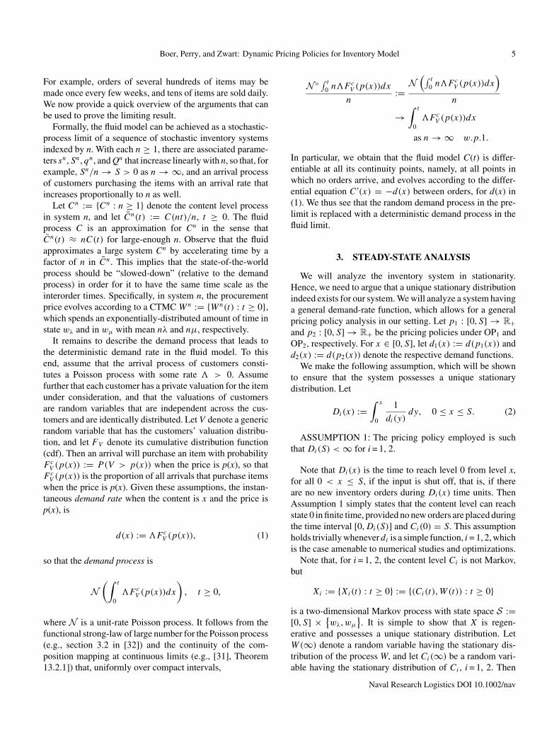
price is employed. Letting dl and dh denote the demand ratewhenever the sale price is pl and ph, respectively, we have thatC > q implies a demand rate dl , and C ≤ q implies a demandrate dh. We use a linear demand model d(p) = 50 − p, withdomain [0, 50 − 10−3], and linear holding costs h(x) = hx,for h > 0. In the plots in Fig. 1, we plot the sensitivity of theoptimal profit with respect to changes in one of the parame-ters (h, K , wμ, wλ, μ, λ, a). For different parameter values,we calculate the optimal (ph, pl , q, s, Q, S) under the poli-cies OP1 and OP2. We also compare their performance withan (s, S) policy, denoted by OP0, under which an order of sizeS−s is placed whenever the content process hits level s. In par-ticular, under OP0 the parameters (s, S, ph, pl) are optimizedwithout taking the stochastic fluctuations of the procurementprice into account. Instead, the procurement price under OP0is taken to be weighted average of wμ and wλ.

4.1. Scenario 1:(h, K , wμ, wλ, μ, λ, a) = (7, 233, 3.4, 43, 0.7, 0.05, 5)

In this scenario, the cheap periods are relatively rare, witha very cheap price. OP2 performs slightly better than OP1,and both outperform OP0. Table 1 lists the optimal profit anddecision variables for the order policies OP0, OP1, and OP2.Figure 1 shows sensitivity of the optimal profits w.r.t. changesin the parameters (h, K , wμ, wλ, μ, λ, a). For all policies, theprofit is decreasing in h, K, wμ, wλ, and μ, and increasingin λ. The profit of OP0 and OP1 does not depend on a; forOP2, the optimal profit is decreasing in a. Clearly, taking thefluctuating procurement prices into consideration make a bigdifference, as no profit can be make under OP0.

4.2. Scenario 2:(h, K , wμ, wλ, μ, λ, a) = (5, 100, 20, 25, 0.1, 0.05, 1)

Here the difference between cheap and expensive priceis less extreme, and cheap periods last longer. OP1 per-forms slightly better than OP0, and both outperform OP2.Table 2 lists the optimal profit and decision variables for theorder policies OP0, OP1, and OP2. Figure 2 shows sensi-tivity of the optimal profits w.r.t. changes in the parameters(h, K , wμ, wλ, μ, λ, a). For all policies, the profit is decreas-ing in h, K, wμ, wλ, and μ, and increasing in λ. The profitof OP0 and OP1 does not depend on a; for OP2, the optimalprofit is decreasing in a.

5. GENERALIZATIONS

In this section, we present two generalizations for the basicmodel analyzed above for the OP2 policy. We first consider amodel having the same structure as the basic model, but witha random environment process that is more general. We then

consider a model with exponential lead times, that is, whenthere is a positive random time from the moment an order ismade by the controller until the commodity arrives.

5.1. Phase-Type Expensive Periods

Our analysis can be extended to the case in which one ofthe periods, either the cheap or the expensive period, followsa phase-type distribution; in particular, the state-of-the-worldprocess W evolves as a CTMC with more than two states. Weemploy simple martingale arguments (the optional stoppingtheorem for an appropriate Wald’s martingale; see below)

For simplicity of exposition, we consider a model in whichthe expensive period is distributed as the sum of two indepen-dent exponential random variables. Specifically, assume thatthe cheap period is exponentially distributed with rate μ, andthat the expensive period is a sum of two independent expo-nential random variables X1 and X2, with X i having mean1/λi , i = 1, 2. We refer to X1 and X2 as the first and secondphase of the expensive period, respectively.

We designate the probabilities that level s is downcrossedat stationarity by the first phase and the second phase of theexpensive period, respectively, by ξ1 and ξ2. In the next theo-rem, we introduce the balance equation of the content level interms of f (S), ξ1, and ξ2. The computations of these quantitiesis carried out below.

LEMMA 5.1: For T := D(s) − D(x) it holds that

d(x)f (x) =

⎧⎪⎪⎪⎨⎪⎪⎪⎩

d(S)f (S)[ξ1

(λ1

λ1−λ2e−λ2T − λ2

λ2−λ1e−λ1T

)+ ξ2e

−λ2T]

0 < x < s,

d(S)f (S) s ≤ x ≤ S,

PROOF:

(i) s ≤ x ≤ S. In this region, every downcrossing oflevel x is followed by a downcrossing of level S withno jump in between. Thus, the long-run average num-ber of downcrossings of level x is equal to that of thelong run average number of downcrossings of levelS, so that d(x)f (x) = d(S)f (S).

(ii) 0 < x < s. For every x, we mark a downcrossingof level s as a downcrossing of type i if level s isdowncrossed during phase i of the expensive period,i = 1, 2. It follows from the definition that ξ1 is theprobability that the time until the next jump is a con-volution of two exponential random variables withrates λ1 and λ2. Similarly, ξ2 is the probability thatthe time to the next jump is exponential with rate λ2.

The probability of a type-1 downcrossing is therefore theprobability that the next jump will occur of two indepen-dent exponential random variables with rates λ1 and λ2, is



Figure 1. Sensitivity analysis for scenario 1. [Color figure can be viewed at wileyonlinelibrary.com]



Table 1. Profit and optimal solution under different order policiesfor scenario 1

Order policy Profit pl ph q s Q S

OP0 −1.76 46.79 50.00 0.25 0 3.20OP1 37.92 33.10 50.00 0.09 6.01 0.09 61.05OP2 38.45 33.10 50.00 0.01 5.94 60.97

Table 2. Profit and optimal solution under different order policiesfor scenario 2

Order policy Profit pl ph q s Q S

OP0 68.93 37.90 40.37 9.51 0 21.46OP1 69.12 37.78 40.37 9.99 0 20.5741 23.53OP2 38.85 37.32 50.00 0.01 0.01 25.06

larger than T := D(s) − D(x), conditional on level s beingdowncrossed during the first phase X1. This gives the firstexpression in the square brackets. Similarly, with probabil-ity ξ2 level s is downcrossed during the second phase of theexpensive period, and with probability e−λ2T no jump occursbetween the latter two downcrossings. �

Computing ξ1 and ξ2

To compute the probabilities ξ1 and ξ2, we construct anauxiliary proces

χ(t) := t + S1 + · · · + SN(t), t ≥ 0, with χ(0) = 0,

where Si , i ≥ 1, are independent and identically distributedrandom variables, each having the distribution of the expen-sive period, in particular, the Laplace transform of each Si

is

G̃(α) = λ1

λ1 + α· λ2

λ2 + α,

and {N(t) : t ≥ 0} is a Poisson process with rate μ. Then∑N(t)j=1 Sj is a compound Poisson process and χ is a non-

decreasing process that increases either linearly at rate 1between jumps, or by positive jumps of (random) size S,where S is a generic random variable with the distributionof S1.

We can think of each jump of χ as having two phases: Thefirst phase is distributed exponentially with rate λ1, and thesecond exponentially with rate λ2. The process χ can thusleave the interval [0, D(S) − D(s)) in three ways: (i) attain-ing the boundary point D(S) − D(s) on a linear segment ofthe path, (ii) upcrossing level D(S)−D(s) by the first phaseof the jump, and (iii) upcrossing level D(S) − D(s) by thesecond phase of the jump.

Define the stopping time

τ := inf {t > 0 : χ(t) ≥ D(S) − D(s)}

and consider Wald’s martingale associated with the process χ

Mα(t) := e−αχ(t)

E[e−αχ(t)] = e−αχ(t)−ϕ(α)t , α /∈ {−λ1, −λ2} ,

(13)

where

ϕ(α) := −[α + μ

(1 − λ1

λ1 + α· λ2

λ2 + α

)]. (14)

Clearly Mα(t) is bounded, so the optional stopping the-orem can be applied, yielding E[Mα(0)] = E[Mα(τ)], sothat

1 = E[e−αχ(τ)−ϕ(α)τ ]. (15)

Let B0, B1, and B2 be the events that χ reaches levelD(S) − D(s) by the drift, upcrossed by the first phase ofthe jump and upcrossed by the second phase of the jump,respectively. It follows from the memoryless property ofthe exponential random variable that if level D(S) − D(s)

is upcrossed by the first phase of the jump, then χ(τ)d=

D(S) − D(s) + X1 + X2, whered= denotes equality in dis-

tribution. If level D(S) − D(s) is upcrossed by the second

phase of the jump, then χ(τ)d= D(S) − D(s) + X2. Finally,

if level D(S) − D(s) is upcrossed by the continuous drift of

χ , then χ(τ)d= D(S) − D(s). Hence, by (15),

1 =2∑

i=0

E[e−αχ(τ)−ϕ(α)τ 1Bi]

= e−α(D(S)−D(s))E[e−ϕ(α)τ 1B0 ]+ λ1

λ1 + α

λ2

λ2 + αe−α(D(S)−D(s))E[e−ϕ(α)τ 1B1 ]

+ λ2

λ2 + αe−α(D(S)−D(s))E[e−ϕ(α)τ 1B2 ], (16)

for ϕ(α) in (14).To obtain the probabilities ξ0, ξ1, and ξ2 we substitute

ϕ(α) = 0 in (16). It is easy to see from (14) that ϕ(α) hasthree roots, with one of them, denoted by α0, being 0. Theother two roots, denoted by α1 and α2, are the solutions tothe quadratic equation

α2 + (λ1 + λ2 + μ)α + λ1μ + λ2μ + λ1λ2 = 0. (17)

Inserting the roots αi into (16) yields three equations with thethree unknowns ξi , i = 1, 2, 3. Formally,

1 = e−αi(D(S)−D(s))E[1B0 ]+ λ1

λ1 + αi

λ2

λ2 + αi

e−αi(D(S)−D(s))E[1B1 ]Naval Research Logistics DOI 10.1002/nav


Figure 2. Sensitivity analysis for scenario 2. [Color figure can be viewed at wileyonlinelibrary.com]



+ λ2

λ2 + αi

e−αi(D(S)−D(s))E[1B1 ]

= e−αi(D(S)−D(s))ξ0 + λ1

λ1 + αi

λ2

λ2 + αi

e−αi(D(S)−D(s))ξ1

+ λ2

λ2 + αi

e−αi(D(S)−D(s))ξ2, (18)

where the equation associated with α0 = 0 gives thenormalizing condition ξ0 + ξ1 + ξ2 = 1.

Computing f(S)

With ξ0, ξ1, and ξ2 in hand, we can express f (x) in termsof f (S) via the equations in Lemma 5.1. Finally, we use thenormalizing condition

∫ S

0f (x)dx = 1 − π ,

where π is the atom at 0. Specifically,

f (x) =⎧⎨⎩

k d(s)

d(x)f (S) 0 < x < s,

d(s)

d(x)f (S) s ≤ x ≤ S,

(19)

where

k = ξ1

(λ1e

−λ2(D(S)−D(s))

λ1 − λ2− λ2e

−λ2(D(S)−D(s))

λ1 − λ2

)− ξ2e

−λ2(D(S)−D(s)). (20)

To compute π , let I be the interval of time in which theinventory system is empty. Then

π = d(0)f (0)E[I ],

since 1/d(0)f (0) is the expected cycle length so that, byrenewal theory, E[I ]d(0)f (0) is the long run proportion oftime that the inventory system is empty.

To compute E[I ], we consider the possibilities of reachinglevel 0.

1. Level s is reached during the first phase of the expen-sive period and from here during the next D(s) timeunits the first phase is not changed. The probabil-ity of the latter event is ξ1e

−λ1D(s). Once level 0 isreached, the expected time until an order is placed is1/λ1 + 1/λ2.

2. Level s is reached during the first phase of the expen-sive period, but during the next D(s) time units thefirst phase end, so that level 0 is reached during thesecond phase. The probability of the latter event is

ξ1

∫ D(s)

0λ1e

−λ1ue−λ2(D(s)−u)du

= ξ1λ1

λ1 − λ2

(e−λ2D(s) − e−λ1D(s)

).

Once level 0 is reached, the expected time at level 0is 1/λ2.

3. Level s is reached during the second phase of theexpensive period and during the next D(s) time unitsthe second phase does not end. The probability ofthe latter event is ξ2e

−λ2D(s). Then level 0 is reachedduring the second phase, and the expected time at 0is 1/λ2.

Therefore,

E[I ] =(

1

λ1+ 1

λ2

)ξ1e

−λ1D(s)

+ 1

λ2

ξ1λ1

λ1 − λ2


)+ 1

λ2ξ2e

−λ2D(s),

so that

π = d(0)f (0)

[ (1

λ1+ 1

λ2

)ξ1e

−λ1D(s)

+ 1

λ2

ξ1λ1

λ1 − λ2


) + 1

λ2ξ2e

−λ2D(s)

],

where by (19),

f (0) = kd(s)

d(0)f (S),

for k in (20), and f (S) is obtained via

1 − π = kd(s)f (S)

∫ s

0

1

d(x)dx + d(s)f (S)

∫ S

s

1

d(x)dx.

In particular,

f (S) = 1 − π

kd(s)∫ s

01

d(x)dx + d(s)

∫ S

s1

d(x)dx

.

5.2. Exponential Lead Times

We assume exponential leadtime with parameter η. Whenthere are positive leadtimes, it makes sense to modify the con-trol by considering two levels in which, when downcrossed,the controller should place an order. We thus have three crit-ical levels 0 < s0 < s1 < S. The cycle starts with C(0) = S.Then the content level decreases at rate d(x) without anyjumps until it reaches level s1. If level s1 is reached during a



cheap period, an order is placed and it takes an exponentialamount of time with rate η until it arrives. Otherwise, if levels1 is reached during an expensive period, no order is placedand the content level decreases until the expensive period isterminated and replaced by a cheap period or until level s0 isreached. In any case, when level s0 is reached (either duringa cheap period or an expensive period) an order is placed andarrives after an exponential period of time with rate η.

THEOREM 5.1: Let f(x) denote the steady state densityof the content level C, and let F(x) denote the correspond-ing cumulative distribution function. Then f(x) satisfies theintegral equation

d(x)f (x)=

⎧⎪⎪⎪⎪⎪⎪⎨⎪⎪⎪⎪⎪⎪⎩

ηF(x), 0 ≤ x < s0,

ηF(s0) + η[γ + (1 − γ )(1 − e−λ[D(s1)−D(x)])][F(x) − F(s0)], s0 ≤ x < s1,

ηF(s0) + η[γ + (1 − γ )(1 − e−λ[D(s1)−D(s0)])][F(s1) − F(s0)], s1 ≤ x ≤ S,

where γ is the probability that level s1 is downcrossed duringthe cheap period.

PROOF:

(i) 0 ≤ x < s0. In this region, the order is on its way.Since the lead time is exponentially distributed thearrival process can be interpreted as a Poisson processwith rate η.

(ii) s0 ≤ x < s1. The jump may occur below s0 orabove s0. If the content level is below s0, jumps arrivewith rate ηF(s0). If the content level is above s0,then there are two possibilities: With probability γ

level s1 is downcrossed during a cheap period andan order is placed immediately; it will arrive after anexp(η) period of time. With probability 1 − γ levels1 is downcrossed during an expensive period and noorder is placed. However, if during the time periodfrom downcrossing of level s1 until level x is reachedthe procurement price is changed from expensive tocheap an order will be placed and it will take anexp(η) period until the order arrives (the probabilityof the latter event is 1 − e−λ[D(s1)−D(x)]). For eitherpossibility, the probability that the jump occurs atsome level between s0 and x is F(x) − F(s0).

(iii) s1 ≤ x < S. In this region, we note that no jumpsstarts when the content level is above level s1. Wethus have to distinguish between two possibilities.If the content level is below level s0 the rate of thejumps is ηF(s0). If the content level is above level s0

the rate of the jumps is

η[γ + (1 − γ )(1 − e−λ[D(s1)−D(s0)])][F(s1) − F(s0)].�

To compute γ , we extend the argument of the previoussection. Level S can be reached either during a cheap periodor an expensive period. Since after every jump the contentlevel is equal to S we define the embedded chain

P =(

pcc 1 − pcc

1 − pee pee

),

where pcc is the conditional probability that the next jumpoccurs during a cheap period given that the present procure-ment price is cheap and the state is S. Similarly, pee is theconditional probability that the next jump occurs during anexpensive period given that the present procurement price isexpensive and the state is S. Then the solution (ζ1, ζ2) to theequations

(ζ1, ζ2)

(pcc 1 − pcc

1 − pee pee

)= (ζ1, ζ2) and ζ1 + ζ2 = 1,

is the solution of the conditional steady state probability—ξ1 (ξ2) that level s1 is downcrossed during a cheap period(expensive period), given that at the starting point, that is, atlevel S, the procurement price is cheap (expensive). Finally

γ = ζ1pcc + ζ2(1 − pee).

Computing pcc and pee is similar to the computations inLemma 3.3.

6. SUMMARY

We considered Markovian fluid-inventory models operat-ing in a random environment, governed by the procurementprice. For the first model, in which the procurement pricechanges in accordance with a CTMC, two natural (s, S)-typepolicies were considered, and the respective stationary distri-butions for the random fluid content process were computed.In turn, those stationary distributions can be used to optimizethe control parameters for each policy. Two generalizations,the first involving a more complex random price environment,and the second incorporating lead times, were also analyzed.

There are two immediate related problems to address. First,the complexity of the optimization problem requires develop-ing an efficient algorithm to solve for the optimal solutions inmore complex settings than those considered in our numericalexamples here. Second, since it is unlikely that an overall opti-mal policy can be found, Brownian approximations for theunderlying regenerative process may be developed to obtainasymptotically-optimal control mechanisms. We leave thoseproblems for future research.



ACKNOWLEDGMENTS

This research is conducted while A.d.B. and O.P. wereaffiliated at CWI, and is made possible by an NWO VIDIgrant. O.P. was supported by NSF grant CMMI 1436518.

REFERENCES

[1] B. Ata and S. Shneorson, Dynamic control of an M/M/1 ser-vice system with adjustable arrival and service rates, ManageSci 52 (2006), 1778–1791.

[2] O. Berman, D. Perry, and W. Stadje, A fluid EOQ model with atwo-state random environment, Probab Eng Inf Sci 20 (2006),329–349.

[3] O. Boxma, D. Perry, and S. Zacks, A fluid EOQ model ofperishable items with intermittent high and low demand rates,Math Oper Res 40 (2014), 390–402.

[4] D. Beyer, C. Feng, S.P. Sethi, and M. Taksar, Markoviandemand inventory models, Springer, New York, 2010.

[5] P.H. Brill, Level crossing methods in stochastic models (2008),Springer Verlag, 2008.

[6] P.H. Brill and B.A. Chaouch, An EOQ model with randomvariations in demand, Manage Sci 41 (1995), 927–936.

[7] S. Browne and P. Zipkin, Inventory models with continuous,stochastic demands, Ann Appl Prob 1 (1991), 419–435.

[8] B. Chaouch, Inventory control and periodic price discountingcampaigns, Nav Res Logist 54 (2007), 94–108.

[9] F. Chen and J.S. Song, Optimal policies for multiecheloninventory problems with Markov-modulated demand, OperRes 49 (2001), 226–234.

[10] H. Chen and D.D. Yao, A fluid model for systems with randomdisruptions, Oper Res 40 (1992), 239–247.

[11] F. Cheng and S.P. Sethi, Optimality of (s, S) policies in inven-tory models with Markovian demand, Oper Res 45 (1997),931–939.

[12] F. Cheng and S.P. Sethi, Optimality of state-dependent (s, S)policies in inventory models with Markov-modulated demandand lost sales, Prod Oper Manage 8 (1999), 183–192.

[13] E. Cinlar and J. Jacod, Representation of semimartingaleMarkov processes in terms of Wiener processes and Poissonrandom measures, Semin Stochastic Process (1981), 159–242.Birkhäuser.

[14] J.W. Cohen, On up- and downcrossings, J Appl Prob 14 (1977),405–410.

[15] M.H.A. Davis, Piecewise-deterministic Markov processes: Ageneral class of non-diffusion stochastic models, J R Stat Soc46 (1984), 353–388.

[16] S. Dewan and H. Mendelson, User delay costs and inter-nal pricing for a service facility, Manage Sci 36 (1990),1502–1517.

[17] G. Gallego and G. Van Ryzin, Optimal dynamic pricingof inventories with stochastic demand over finite horizons,Manage Sci 40 (1994), 999–1020.

[18] M. Goh and M. Sharafali, Price-dependent inventory modelwith discount offers at random times, Prod Oper Manage 11(2002), 139–156.

[19] M. Hu and Y. Yang, Modified echelon (r, Q) policies withguaranteed performance bounds for stochastic serial inventorysystems, Oper Res 62 (2014), 812–828.

[20] D. Iglehart and S. Karlin, “Optimal policy for dynamic inven-tory process with nonstationary stochastic demands,” in: K.J.Arrow, S. Karlin, and H. Scarf (Editors), Studies in appliedprobability and management science, Stanford UniversityPress, Stanford, California, 1962, Chapter 8, pp. 127–148.

[21] O. Kella and W. Whitt, A storage model with a two-staterandom environment, Oper Res 40 (1992), S257–S262.

[22] H. Mendelson, Pricing computer services: Queueing effects,Commun ACM 28 (1985) 312–321.

[23] M. Miyazawa, Rate conservation laws: A survey, Queue Syst15 (1994), 1–58.

[24] K. Moinzadeh, Replenishment and stock policies for inventorysystems with random deal offerings, Manage Sci 43 (1997),334–342.

[25] S. Nahmias, Production and operations analysis, McGraw-Hill/Irwin, New York, 2005.

[26] P. Naor, The regulation of queue size by levying tolls,Econometrica 37 (1969), 15–24.

[27] K.S. Puranam and M.N Katehakis, On optimal bidding andinventory control in sequential procurement auctions: Themulti period case, Ann Oper Res 217 (2014), 447–462.

[28] J. Shi, M.N. Katehakis, and B. Melamed, Martingale methodsfor pricing inventory penalties under continuous replenish-ment and compound renewal demands, Ann Oper Res 208(2013), 593–612.

[29] J. Shi, M.N. Katehakis, B. Melamed, and Y. Xia, Optimalcontinuous replenishment for a production-inventory systemwith compound Poisson demands and lost sales, Oper Res 62(2014), 1048–1063.

[30] J.S. Song and P. Zipkin, Inventory control in a fluctuatingdemand environment, Oper Res 4 (1993), 351–370.

[31] W. Whitt, Stochastic process limits, Springer, New York, 2002.[32] W. Whitt, Internet supplement to stochastic-process lim-

its, 2002, Available at: http://www.columbia.edu/∼ww2040/supplement.html. Last accessed on February, 2017.

[33] R.W. Wolff, Stochastic modeling and the theory of queues,Prentice Hall, New Jersey, 1989.


Dynamic pricing policies for an inventory model with...

Documents

Transcript of Dynamic pricing policies for an inventory model with...