Dynamic Present Values and the Intertemporal CAPM

Bjørn Eraker

Wenyu Wang ∗

First version: April, 2011This version: September 8, 2012

Abstract

Merton’s (1973) intertemporal Capital Asset Pricing Model is difficult to reconcile with

present value computation when investment opportunities are random and time-varying.

Merton assumes a geometric price process, and his equilibrium is constructed by solving for

the instantaneous expected rate of return. We argue that this method is generally inconsis-

tent with present value computations. We derive an alternative version of the Intertemporal

CAPM based explicitly on present value computation with a strictly exogenous cash flow.

Our model is derived without restrictive assumptions about the structure of the equilib-

rium price process. An essential feature of our model is that prices respond endogenously to

shocks in expected return. In an example model, we show that shocks to stochastic volatil-

ity is negatively correlated with stock returns in equilibrium. The correlation increases in

absolute magnitude with risk aversion.

Keywords: ICAPM, Conditional CAPM, dynamic consistency, present value, dynamic

equilibrium, stochastic volatility

JEL codes: G1, G12.

∗Both authors are from the Wisconsin School of Business, Department of Finance. Corresponding author:Bjørn Eraker (beraker@bus.wisc.edu). We thank Ravi Bansal, John Campbell, John Cochrane, Darrell Duffie,Yu Guan, Holger Kraft, Yuliya Plyakha, Christian Schlag, Paul Schneider, Suresh Sundaresan, Mark Ready,Grigory Vilkov, Youchang Wu, and seminar participants at Goethe University, University of Warwick, Universityof Wisconsin, and Frontiers of Finance Conference, for helpful comments discussions. The usual disclaimers apply.

1

1 Introduction

One of the most fundamental concepts in finance is that the price of an asset equals the present

values of the assets’ future cash flows. If the price of an asset differs from its present value,

the price is generally inconsistent with equilibrium, and may create arbitrage opportunities.

For assets with well-defined future cash flows such as bonds, it is obvious how to construct asset

pricing models based on present values. However, for assets whose future payoffs are much harder

to model, as is the case with common stocks, the present value approach is less straightforward.

Indeed, in many asset pricing models, the financial market equilibria are often implemented by

assuming an exogenous price process and then solving for the expected rate of return period by

period. An example of this approach to constructing an equilibrium is found in Merton’s (1973)

seminal paper on the Intertemporal CAPM, which starts with the assumption that the price

process follows a Geometric Brownian Motion with time-varying expected rates of return and

volatility. The equilibrium is constructed by solving for the expected rate of return, or drift rate,

of the risky price process, which in equilibrium is a function of systematic risk.

We make two contributions in this paper. First, we critique the idea that dynamic equilibrium

models can be constructed simply by solving for the expected rate of return, period by period,

as in Merton (1973). Second, we derive a new CAPM model, which we call the “Present-Value

CAPM”. This model is based on the same general assumptions as the traditional one-period

CAPM except that it is derived through dynamic present value computations with time-varying

discount factors.

Our critique of Merton’s model is based on the fact that Merton derives his model under

the assumption of an exogenously specified price process. The problem with his analysis is that

the exogenous price process is not necessarily consistent with present value computation where

1) the supply of risky assets are exogenous to the model, and 2) the cash flows paid by the

risky asset are strictly exogenous. The first point was demonstrated in an unpublished paper

by Hellwig (1977).1 Hellwig’s analysis shows that the exogenous price assumption in Merton’s

model is problematic even when investors have a constant investment opportunity set. He shows

by example that if investors face a normally distributed dividend stream, and exhibit constant

absolute risk aversion, prices should also be normally distributed unless one is willing to impose

counter-intuitive supply behaviors of risky assets - specifically, the assets’ supply needs to be

inversely proportional to their prices. Conversely, Hellwig demonstrates that if supplies are

fixed, equilibrium prices are normally distributed, not log-normal as assumed by Merton.

1We are grateful to Suresh Sundaresan for pointing out to us the existence of Hellwig’s paper.

2

Our critique of Merton’s ICAPM is also that the price is assumed to be exogenously given.

Our argument, however, is linked to the dynamic structure of the model. The problem is that

expected rates of return play two different distinct roles. Since the assets’ price and future cash

flows are linked together by present value computation, either the current asset price or future

cash flow (or both) must adjust to reflect a change in the expected rate of return. However, the

ICAPM starts with an exogenous price process that a priori assumes that the asset price does not

depend on factors which impact time-varying discount rates, thus leaving no room for the current

asset price to adjust simultaneously to the change in discount rates. The direct consequence of

this restriction is that a corresponding change in future expected cash flow becomes the only way

to implement the change in expected return. This implied change in future expected cash flow

thus becomes an implicit assumption that is necessary for the price to be consistent with the

present value computations. Unfortunately, as we will argue, this implicit assumption is virtually

impossible to reconcile with reasonably constructed equilibria and is also at odds with casual

empirical observations of the relationship between financial prices, macro-economic growth, and

market volatility.

Our critique is relevant in the context of the large empirical literature on tests of the condi-

tional CAPM. The conditional CAPM is a dynamic implementation of the Sharpe-Lintner-Mossin

CAPM where their classic formula is assumed to hold period-by-period. The conditional CAPM

is often thought of as a discrete time version of Merton’s ICAPM, as in for example Merton

(1980)2 Thus, as we question the assumptions of Merton’s model, we also question the validity

of the conditional CAPM when the latter assumes, as in the ICAPM, that shocks to conditional

expected returns are independent from shocks to aggregate wealth. While we do not discuss the

consequences for empirical tests of the intertemporal or conditional, CAPM models in detail here,

it is clear that our critique has implications for tests of conditional asset pricing models. For

example, the misspecification of return distributions will lead to incorrectly specified likelihood

functions, which again, of course, will imply that empirical estimates of model parameters will

be biased.

So how do we construct asset pricing models that would not be subject to this critique?

The good news is that this is easy. In particular, pricing formulas that are derived explicitly

from dividend discounting as in Gordon (1959) obviously escape our critique. Early work on

dynamic present value models include Campbell and Shiller (1987), Campbell and Shiller (1988),

2It is possible to derive a conditional CAPM that is not subject to our critique using specialized assumptions.For example, ? derive the a single factor CAPM with time-varying betas and expected returns that is not subjectto our critique because their model has a single state-variable that drive changes in wealth as well as expectedreturn. Our critique does not apply to their model, or any other model which is derived explicitly through presentvalue computation.

3

and Campbell (1993). Recently, the long run risk (LRR) model of Bansal and Yaron (2004)

endogenizes asset prices as the dynamic present value of future consumption or dividends. Part

of the appeal of the LLR model is that risk premia are proportional to the inverse of the speed

of mean reversion of the long run risk factor. Similarly, in a model with stochastic volatility of

aggregate consumption, the volatility risk premium is proportional to the inverse of volatility

speed of mean reversion. This delivers potentially very large risk premia, which in turn generate

realistically large equity returns and volatilities as well as potentially explaining other asset

pricing puzzles. Cochrane (2011) discusses the dual interpretation of expected returns as a

growth rate and as a discount factor. The first implies trivially that returns can be forecasted by

expected returns. The latter implies a negative relationship between contemporaneous returns

and shocks to discount factors. Cochrane (2011) also postulates that much of the variation in

stock returns is due to changes in discount-rates themselves.

We propose a new capital asset pricing model based on the idea that we wish to derive an In-

tertemporal CAPM which maintains the property that prices obtain as present values. Investors

in our model have utility of terminal wealth, as in the classic one period CAPM. We devise a very

simple technique for constructing general, affine Present-Value based CAPM’s. Our technology

can be seen to generalize Merton (1973) to provide a more general price process. In particular,

we do not impose any prior assumptions about the process that governs the equilibrium price.

Our model is connected to the long run risk model in some important ways. First, our present

value framework yields risk premium specifications that bear close resemblance to the equivalent

expressions obtained in the LRR literature. Risk premia in our model are magnified by the

reciprocal of mean-reversion coefficients in a manner identical to the Intertemporal Elasticity

of Substitution (IES) → ∞ limit of the LRR model. In our experience, risk premia in LRR

models converge very quickly as the IES increases and imply that even values of IES in the 3-5

range will yield model solutions that are close to the IES →∞ limit. Our model shares similar

characteristics. Second, we do not model intermediate dividends or consumption but rather

terminal wealth, so our model resembles the traditional wealth-based CAPM. This is different

from LRR models at first glance. However, as we will show, when intermediate consumption is

small and negligible compared to the terminal wealth, the limiting case IES→∞ in LRR model

yields similar results to the wealth-based CAPM.3

While the model we develop in this paper has similarities with those in the extant literature,

it does differ in some important ways. Our model is not a dividend discounting model. Since

there are no intermediate dividends or consumption, we do not need to use the Campbell-Shiller

3The fact that Epstein-Zin preferences yield the wealth based CAPM as a special case when EIS → ∞ isshown in the original paper by Epstein and Zin (1989), p. 968.

4

linearization of the returns process to obtain closed-form expressions for stock prices. Our price

formulas are exact. This is a large advantage in structural estimation of models. 4

To see how our model shares similarities and differences with existing models, consider an

example. In a simple economy with a single asset where terminal payoff has stochastic volatility,

we derive the equilibrium return process as

lnRm,t+1 − rf = λ0 −γ

κ4σ2

t + σtεt. (1)

The process σt is stochastic, stationary, and is interpretable as the volatility of beliefs about

economic growth. εt is a random shock representing economic growth news. The volatility

process, σt, is Markov, and Et4σ2t ≈ κ(θ − σ2

t ) so that Et(lnRm,t+1) ≈ rf + γσ2t + constant

where the constant term reflects a risk compensation for variation in future expected cash flows

as well as volatility risk. The term −γ/κ4σ2t is an equilibrium volatility feedback term. This

volatility feedback term will lead to temporary price adjustments in order to reflect a higher or

lower risk premium depending on whether or not volatility is above or below its long run mean.

A positive shock to volatility leads to a simultaneous decrease in the price, allowing for higher

future expected returns. The model does not yield Merton’s ICAPM except in the special case

when the volatility process is constant. Generally, both volatility shocks and shocks to future

cash flows, εt, are priced risk factors.

Our Present-Value CAPM model is also important for several other reasons. One primary

advantage of our modeling approach is that we recover an equilibrium model in which risk

premia have long run risk interpretations, but without the explicit link to consumption dynamics

on which the Bansal and Yaron model and its descendants are based. This can be useful in

constructing realistic models of stock prices for the purpose of pricing derivatives. In our model

the volatility feedback effect is endogenous. If used to price equity options, our model can

produce a large volatility risk premium. The skewness in the return distribution under both

the objective and risk-neutral measures is a function of risk aversion. This allows, among other

things, the econometric identification of risk aversion from option prices as, among other things,

the steepness of the volatility smile can be explicitly linked to risk aversion in our example model

in equation 1.

Our model also has important implications for the empirical testing and evaluation of asset

pricing models. Our present value CAPM model implies that stochastic volatility will lead to a

4In long-run-risk models it is necessary to solve a set of non-linear equations for each new parameter updatein a numerical search (see Bansal, Kiku, and Yaron (2006)). Often these equations are difficult to solve for highfrequency data (see Eraker (2010)).

5

predictable component in returns. This is standard for the ICAPM, but in our model, shocks to

volatility generate temporary movements in stock prices that can be identified from the contem-

poraneous relation between the volatility shocks and returns. When the stock price goes down

in response to an increase in volatility, it will mean-revert. The speed in which this reversion

takes place is typically slow, which means that the correlation between volatility level and future

returns is low, whereas the contemporaneous correlation is strong. This has two econometric im-

plications. First, we can better identify the aggregate market risk-return relationship better from

the contemporaneous volatility feedback effect than we can from predictive regressions. Second,

econometric inference on the relationship between volatility and returns can be misleading if

inference is made from a model that ignores the contemporaneous relation. We investigate the

implication for inference on risk aversion in an intertemporal CAPM in a companion paper.

The rest of the paper is organized as follows: in the next section we outline the implicit rela-

tionship between future cash flows and risk in the ICAPM. Section three develops our new general

Present-Value CAPM for general valuation, and we discuss some specific examples. Section four

offers concluding remarks. Proofs and lengthy derivations are in the appendices.

2 A Critique of Merton’s ICAPM

In this section we outline our critique of Merton’s ICAPM model. The problem with Merton’s

model is that it starts by assuming an equilibrium price process. The assumed price process may

or may not be consistent with a reasonably defined dynamic equilibrium price. In particular, we

will show that there exists specifications of exogenously specified cash flows and utilities that are

impossible to reconcile with Merton’s model unless one is willing to make additional unwarranted

assumptions about the covariation between future cash flows and changes in expected returns.

We are not the first authors to criticize the exogenous price assumption in Merton’s model. In

an unpublished working paper, Hellwig (1977) questions the general validity of Merton’s model.

To proceed, we first briefly review Merton’s 1973 paper.

2.1 Merton’s ICAPM

Merton assumes that prices are driven by

dPi,tPi,t

= αi,tdt+ σi,tdzi,t (2)

6

where zi,t is a Brownian motion. The Brownian motions driving prices are correlated, ρi,j =

Corr(dzi,t, dzi,t). This notation follows that of Merton (1973), with the exception of the added t

subscripts for clarity. The processes governing the expected rates of return, αi and the conditional

stock market standard deviation, σi,t, are assumed to be stochastic processes,

dαi,t = aidt+ bidqi,t, (3)

dσi,t = fidt+ gidxi,t. (4)

Merton does not discuss whether the coefficients ai, bi, fi and gi are to be interpreted as constants,

Ito-processes, deterministic functions of time, or functions of the levels of αi and or σi.

Merton assumes that utility of agent i is given by

Et

[∫ Ti

t

U i(cs,i, s)ds+Bi(WTi,i)

], (5)

where U i is the agent i’s utility of his consumption stream cs,i and Bi is the Bequest utility.

Merton derives the following equilibrium expected rate of return of the ith asset,

αi,t − rt =σi,t(ρi,M − ρi,nρM,n)

σM,t(1− ρ2n,M)(αM,t − rt) +

σi,t(ρi,n − ρi,Mρm,n)

σn,t(1− ρ2n,M)(αn,t − rt). (6)

Here the subscript M refers to the market portfolio while n refers to an nth asset where returns

are assumed to be perfectly correlated with changes in the investment opportunity set (α, σ, r).

The coefficients ρi,j are correlations between assets i and j and are assumed to be constant.

2.2 Hellwig’s Critique

Hellwig (1977) criticizes Merton’s ICAPM. The premise is the same premise as ours - the price

process in Merton’s model is assumed rather than derived fully endogenously. While we discuss

the validity of Merton’s ICAPM in the context of a changing investment opportunity set, Hell-

wig’s analysis focuses specifically on the case where the investment opportunity set is constant.

In this case, equation (6) reduces to the standard Sharpe-Lintner-Mossing static CAPM formula

for logarithmic expected returns, α. Moreover, since by assumption α, σ, and r are constant,

equation (2) implies that prices are log-normal. Hellwig points out that log-normality is inconsis-

tent with dividend discounting if dividends follow an arithmetic process (i.e, if dDi,t = adt+bdBi,t

for constants a and b and a Brownian motion Bi) and investors have exponential utility, and if

assets are in fixed supply. Hellwig writes, p. 1

7

Merton’s analysis of capital market equilibrium is unsatisfactory: he determines

equilibrium prices by assumption rather than by demand and supply. First, he derives

the portfolio behavior under the assumption that asset prices follow a log-normal

process. Then he considers the implication of market clearing for average rates of

return under a log normal process. He fails to verify that the assumption of log-

normality itself is compatible with market clearing.

Hellwig further shows that by relaxing the log-normality assumption on asset prices, he can

recover the CAPM with normally distributed prices and fixed supply. This, he contends, is also

unsatisfactory as it conflicts with the idea of limited liability of equity.

Hellwig also considers the possibility of solving for assets’ supply in order to maintain the

log-normal price assumption under the same economic assumptions (i.e, constant investment

opportunities). He shows that the CAPM holds in this case, but only if prices follow an arithmetic

process (not geometric, log-normal). He concludes that

“... equilibrium risky assets can only be log-normally distributed, if all agents

have constant relative risk aversion, if the supply of each risky asset is inversely

proportional to its price.”

Hellwig’s analysis shows that the intertemporal CAPM of Merton is problematic even in the

case of constant investment opportunities. Again, the problem with Merton’s analysis is that

the price process is assumed rather than derived in equilibrium, and that equilibrium can be

established by just solving for the conditionally expected rate of return, αi,t.

The idea that any dynamic equilibrium model can be solved just by solving for the expected

rates of return under an assumed price dynamic is troublesome. The problem is that the expected

rate of return serves two purposes: it is both the average growth rate of investment as well as

the discount rate of future cash flows. It is not true in general that an assumed price process is

consistent with a reasonably defined equilibrium if only its expected return satisfies a first order

condition, as in Merton’s ICAPM.

2.3 Expected Returns in Dynamic Models

In this section we outline the basic critique of the idea of solving for expected rates of return

in dynamic models. We consider, without loss of generality, capital market equilibrium in the

8

context of a single asset market. Let us, as in Merton, assume that the price can be written as

a geometric process with time-varying drift and diffusion

dPtPt

= µtdt+ σtdBt (7)

orPt+1 − Pt

Pt= µt + σtεt+1, (8)

where dBt or εt+1 are exogenous shocks using the continuous or discrete time formulations,

respectively. Merton postulates that the equilibrium price process is found through solving for

the drift rate µt in (7) or (8). An equilibrium solution is taken to be a sequence of expected

returns, µt, that are measurable wrt. a time t information set (say Ft) available to the investor.

Merton (1980) gives the expected returns on the market portfolio as

µt = rf,t + γσ2t (9)

Empirical investigations of Merton’s ICAPM, including Merton (1980), typically implement this

exact specification for the conditional expected return for the market portfolio. This particular

model is a special case of Merton’s ICAPM when the relative risk aversion coefficient is constant

and equal to γ, and the model ignores the hedging demand terms that appear due to time-

variations in the investment opportunity set in Merton’s model. Merton (1980), p.329, footnote

12, argues that these hedging demands can be ignored whenever the (endogenous) consumption

stream is less sensitive to changes in state-variables (that affect the investment opportunity set)

than to changes in wealth, or alternatively that the variance of the change in wealth is much

larger than the variance of the change in the state-variables.

Our critique of Merton’s ICAPM is based upon the fact that it is not possible to write

down price processes as in (7) or (8) while maintaining time-varying expected returns without

simultaneously making implicit assumptions about how the future expected payoffs correlate

with changes in expected return. Suppose for the sake of argument that we consider the discrete

time model in (8) and that the market wide volatility σt is stochastic. For simplicity let us

assume a finite horizon, single asset, representative agent endowment economy. Assume that at

the terminal date T , the representative agent receives a payoff x̃ and before T , the representative

agent has no consumption. We ask the simple question: What is the value of a claim to this

payoff at dates t = 0, 1, .., T? We claim that it is impossible for the price process in (8) to

represent an equilibrium price process without making implicit assumptions about how shocks

to the expected terminal payoff x̃ correlate with shocks to risk, σt.

9

E 0( x̃ )<E 1( x̃)

A

B

0 1 T

E 0( x̃ )=E 1( x̃)

Figure 1: Possible price paths with and without volatility feedback.

The crucial point of our argument is that in an appropriately specified equilibrium price

process temporal variations in expected rates of return should be given by changes in the market

price of the risky asset. If there is a positive shock to expected returns, the price needs to adjust

negatively to this shock. We illustrate this in Figure 1. The solid line represents the expected

path at time 0. At time 1, there is a positive, unanticipated shock to volatility σ21 − σ2

0 > 0,

giving an increase in the required expected return going forward. There are two ways in which

the investor can receive a higher expected return. By keeping the expected terminal payoff

unchanged, E1(x̃) = E0(x̃), the price needs to adjust downward to point A in order to reflect

the higher expected returns going forward. This adjustment is possible if and only if the price

process incorporates an explicit equilibrium volatility feedback term in which the price moves by

exactly the right amount to generate the steeper expected price path going forward, as illustrated

with the dotted path.

The second possibility is that the expected terminal payoff increases. If there is no impact of

the increase in volatility on the price, it continues along the path anticipated at time zero (steady

state), and thus reaches point B in the figure. Since the expected rate of return between time

10

1 and T is now higher without the price being adjusted, it must be that the expected terminal

value increases, E1(x̃) > E0(x̃). In other words, a positive shock to expected return at time 1 is

only consistent with equilibrium if the future expected terminal payoff increases as well.

Our simple figure illustrates that without an explicit equilibrium volatility feedback in the

price process, the model will necessarily imply a positive correlation between the shocks to

expected returns and the shocks to expected future cash flows. Accordingly, any model that

does not explicitly incorporate dynamic volatility feedback effects in the specification of the

price process will at best be making implicit assumptions about a positive covariation between

shocks to expected returns and future cash flows, and in the worst case be inconsistent with

equilibrium in the sense that it breaks the present value computations.

We formalize this intuition in the following.

Consider a simple three-period economy. A single risky asset trades at dates 0 and 1. This

asset provides the representative investor with an aggregate terminal payoff, x̃, which she will

receive at date 2. Let P0 and P1 denote the price of this claim at times 0 and 1. Denote

by Rt = Pt+1/Pt the gross return. We assume the model to be consistent with present value

computation, giving the terminal condition P3 = x̃. We assume that the expected rates of return

are stochastic. At time 1, the investor receives news that may require her to demand a higher

or lower expected rate of return going forward. The expected return in the first period, µ1 is

known at time 0. We assume further that the expected return process is in “steady state,” by

which we mean that the investor does not anticipate a shock to expected returns at time 1, so

E0(µ2) = µ1.5

The investor receives news about the terminal payoff, x̃ and the next period’s expected return

µ2 at time 1. The relative change in the expected return, µ2/µ1 and the expected terminal payoff

E1(x̃)/E0(x̃) are random variables as of time 0. At time 1 both random variables are known.

We are interested in the covariation between these random variables and the following theorem

characterizes their relationship.

Theorem 1. Assume that the price process satisfies Corr(R1, µ2) = 0, its expected return process

µt is random, in steady state E0µ2 = µ1, and that the price process is consistent with present

value computations. Then

Corr

(E1(x̃)

E0(x̃),µ2

µ1

)> 0. (10)

5The term steady condition is similar to requiring that the expected return process’ initial condition is itsunconditional mean in a multi-period model.

11

The theorem verifies the simple intuition conveyed in Figure 1. If there is a shock to expected

returns at time 1, the future expected cash flow needs to increase to keep the price moving along

the steady state path. An immediate corollary follows

Corollary 1. Under the same assumptions as in Theorem 1, if

Corr

(E1(x̃)

E0(x̃),µ2

µ1

)= 0, (11)

the price process is inconsistent with present value computations.

Consider now how the endogenous price process we derive compares to the assumed price in

Merton. We get

dPtPt

= λ0dt+ λ′1dXt + σ(Xt)dBt (12)

= (λ∗0 + β′Xt) dt+ λ′1σx(t)dBxt + σ(Xt)dBt (13)

for state-variables Xt that follow a stationary, affine process6 where β has the usual interpretation

as the conditional expected returns’ sensitivity with respect to changes in the state-variables.

The innovation term dBxt captures the shocks to state-variables that may change the expected

rates of return, and the innovation term dBt represents the shocks to the terminal flow. The

equilibrium expected returns are thus given by (λ∗0 + β′Xt)dt.

In comparing this equilibrium price to Merton’s. He assumes

dPtPt

= µtdt+ σ(Xt)dBt. (14)

If the two methods yield the same equilibrium expected return, we have µt = λ∗0 + β′Xt, and

dPtPt

= (λ∗0 + β′Xt)dt+ σ(Xt)dBt. (15)

In comparing (13) to (15) we see that the latter is missing the term

λ′1σ(Xt)dBxt . (16)

This is precisely the term that allows prices to adjust to changes in discount rates/expected rates

of return. Without this term, prices are uncorrelated with shocks to expected returns, dBxt . In

6Specifically, if dXt = µ(Xt)dt + Σ(xt)dBxt where the drift and diffusion functions can be written µx(t) =

K0 +K1Xt and Σ(Xt) = H0 +∑N

i=1HiXt,i such that β = λ1K1.

12

this case, the price process either contains an implicit assumption that future cash flows will

increase to offset shocks to discount rates, or the resulting price process in (15) is not consistent

with an equilibrium based on present value computations. One may argue that the innovation

term dBt in equation (15) can be taken as a composite effect of dBxt and dBt terms in equation

(13). We can write (13) as a scalar Ito process, but the diffusion term of this scalar process

depends on the equilibrium parameter λ1.7 The difference between our model Merton’s in this

case is that we also solve for the endogenous diffusion function.

All stochastic present value models will have feedback terms similar to equation (16). For

example, in the Bansal-Yaron LRR models the capital gains are given by ∆ lnPt = ∆ lnDt +

B′∆Xt where Xt is a vector of state-variables (i.e., expected consumption growth and stochastic

volatility in their basic model). Thus, in their model the innovations to the priced risk factors

Xt will have immediate, contemporaneous impact on prices. Eraker and Shaliastovich (2008)

generalize the BY model to a continuous time-setting with general state-variables and recover

equilibrium stock price dynamics with the form of (12). These contemporaneous terms imply

that both cash flow news, dBt, and discount rate news, dBxt , impact prices. This gives a “bad-

beta/good-beta” interpretation as in Campbell and Vuolteenaho (2004). Our argument implies

that properly specified asset pricing models should have shocks that have a “bad-beta/good-

beta” interpretation. One implication of our argument is that at least two risk factors are priced

in a dynamic model. In the next section we give an example of such a model.

2.4 Conditional CAPM

A large body of empirical articles are concerned with empirical tests of CAPM models with time-

varying expected returns. In discrete time, the model is typically referred to as the conditional

CAPM. The literature seems to have originated from Merton (1980) who estimated γ based on

equation 9. French, Schwert, and Stambaugh (1987), Bollerslev, Engle, and Wooldridge (1988),

and Bali and Engle (2010a) also follow Merton (1980) and estimate γ based on equation 9.

Tests of the conditional CAPM using additional cross-sectional information include Gibbons

and Ferson (1985), Engle, Lilien, and Robins (1987), French, Schwert, and Stambaugh (1987),

Nelson (1988), Harvey (1989), Engle, Ng, and Rothschild (1990), Harvey (1991), Ng (1991),

Bodurtha and Nelson (1991), Ferson and Harvey (1993), Glosten, Jagannathan, and Runkle

(1993), Whitelaw (1994), Evans (1994), Moskowitz (2003), Guo and Whitelaw (2006), and Bali

and Engle (2010, 2010), among others.

7Specifically, λ′1σx(t)dBxt + σ(Xt)dBt = σ∗(t)dB∗t for σ∗(t) =

√Trσx(t)σx(t)′ + Trσ(Xt)σ(Xt)′) and B∗t =

(λ′1σx(t)dBxt + σ(Xt)dBt)./(

√Trσx(t)σx(t)′ + Trσ(Xt)σ(Xt)′)) (element by element).

13

The problem with the conditional CAPM literature is that the way the model is implemented,

with exogenous shocks to market volatility and betas, the model itself has no known theoretical

foundation other than Merton’s (1973) analysis8. We have argued, as did Hellwig (1977), that

Merton’s analysis is problematic because it does not verify that the assumed price dynamics are

consistent with equilibrium under reasonable assumption about how future cash flows covary

with expected returns and assumptions about the supply of risky assets. In the next section we

derive an equilibrium model which is based on a subset of the same assumptions as in Merton,

but where we relax Merton’s exogenous price assumption. As we shall see, this model does not

yield Merton’s ICAPM unless one considers the special case of constant investment opportunities.

3 The Present Value CAPM

In the following section we discuss our equilibrium dynamic asset pricing framework. We consider

first an economy with a single risky asset. This asset does not pay any intermediate dividends.

The asset has a terminal value at some fixed date T of x̃T . Absence of arbitrage implies PT = x̃T .

We take Pt to be the market value of x̃T at time t. x̃T is a random variable, and we will assume

that this variable follows some stochastic process. We assume that investors learn about x̃T over

time. One such example would be a random walk specification for x̃ would imply Etx̃T = x̃t such

that the current level of x̃t is interpretable as the expected future wealth.

We do not think of x̃t as a market value or wealth process. Rather, we take x̃t to be some

exogenous process that converges to terminal wealth. In a single firm or investment project,

it is natural to think of the terminal payoff as a cash distribution generated by an irreversible

investment. In the aggregate economy we think of x̃ as a portfolio of such irreversible investments

where intermediate cash flows are re-invested. The idea is that investors cannot disinvest physical

capital invested through corporations in response to increases in discount rates. This setup gives

an implicit sluggishness in physical capital, reflected in a completely exogenous terminal cash

flow, x̃T . It is understood that in general Pt 6= x̃t for all t 6= T . By not forcing the terminal wealth

process, x̃T , to equal its present value at all times t, we are avoiding any implicit assumptions

about the dynamics of its market price. This allows prices to be derived completely endogenously.

8While certain investment based models can generate time-varying expected returns with as single-state vari-able, as in for example ?, the empirical literature on conditional CAPM estimation typically specify an econometricmodels in which shocks to beta’s and market volatility are independent of shocks to wealth (or market return)itself.

14

The representative investor has utility of terminal wealth,

Etu(x̃T ). (17)

We assume that Etu′(x̃T ) > 0 and Etu

′′(x̃T ) < 0 for all t.

There are no intermediate dividends. The return from holding the market from time t to T

is therefore

Rt:T,m = x̃T/Pt

where Pt is the market value of the terminal payoff x̃T . We have PT = x̃T .

Let

Rt:T (α) = αRt:T,m + (1− α)Rt:T,f (18)

denote the gross return to a buy and hold portfolio initiated at time t. The term Rt:T,f is the

gross risk free rate of return from time t to T . We assume that the risk free return is independent

of x̃T . If we assume a short rate process, Rt,f , representing the risk free return over a unit of

time, we can write

Rt:T,f = Et

T∏s=t+1

Rs,f .

To facilitate direct comparison with the traditional one period CAPM, it can be useful to assume

that the path of interest rates is deterministic, or that the rates are constant. Note that Rt:T,f =

Et∏s

u=t+1Ru,fEs∏T

u=s+1Ru,f = Rt:s,fRs:T,f .

We define an equilibrium as a price process Pt that clears the market αt = 1 and maximizes

investors’ utility.

Proposition 2. The equilibrium market price Pt of the aggregate wealth claim x̃T is given by

Pt =Et {u′(x̃T )x̃T}

Et {u′(x̃T )}Rt:T,f

, ∀t ∈ [0, T ]. (19)

The price of an arbitrary asset, Pt,i, with terminal payoff x̃T,i in infinitesimal supply is

Pi,t =Et {u′(x̃T )x̃T,i}Et {u′(x̃T )}Rt:T,f

, ∀t ∈ [0, T ]. (20)

These prices obtain irrespectively of the frequency of trade and portfolio rebalancing. The pricing

kernel is

ξt =u′(x̃T )

Et {u′(x̃T )}Rt:T,f

. (21)

15

The Euler equation can also be written in multi-period return form as

Et {u′(x̃T )Rt:T,m} = Et {u′(x̃T )Rt:T,i} . (22)

This Euler equation appears in a slightly different form in Merton and Samuelson (1969) in the

context of pricing warrants. It follows directly from the first order conditions for optimal portfolio

allocation. It can also be derived by dynamic programming. The fact that this price process

obtains irrespectively of the frequency of portfolio rebalancing implies that the Euler equation

holds for both continuous and discrete time trading schemes.

A few notes on equations (19) and (20) are in order. These equations contain ratios of ex-

pectational expressions. The key to developing tractable pricing models is to be able to compute

these expectations. Below we will show that this is easy in the context of the usual workhorse

class of affine processes. It is important to see that our model differs from the usual case where

Pt equals x̃t for all t. We specifically do not impose this restriction. If we did, we would just

be reverting to Merton’s solution because our price dynamics would be entirely driven by the

assumed dynamics for x̃T .

3.1 Power Utility

Our theory will give closed form expressions for the evolution of stock prices in economies where

the representative agent has power utility of wealth,

u′(x̃T ) = x̃−γT

and the process that generates the final payoff, x̃T , is driven by exponential affine processes. This

means that we can write

Etu′(x̃T ) = Etx̃

−γT = exp(−γ ln x̃T ) = exp(α(γ, t, T ) + β(γ, t, T )′Xt) (23)

for some exogenously specified, stationary process Xt. where α and β solve Riccati ODE’s (see

appendix B).

16

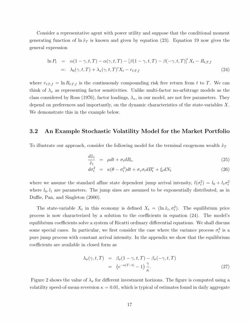
Consider a representative agent with power utility and suppose that the conditional moment

generating function of ln x̃T is known and given by equation (23). Equation 19 now gives the

general expression

lnPt = α(1− γ, t, T )− α(γ, t, T )− [β(1− γ, t, T )− β(−γ, t, T )]′Xt −Rt,T,f

=: λ0(γ, t, T ) + λx(γ, t, T )′Xt − rt:T,f (24)

where rt:T,f = lnRt:T,f is the continuously compounding risk free return from t to T . We can

think of λx as representing factor sensitivities. Unlike multi-factor no-arbitrage models as the

class considered by Ross (1976), factor loadings, λx, in our model, are not free parameters. They

depend on preferences and importantly, on the dynamic characteristics of the state-variables X.

We demonstrate this in the example below.

3.2 An Example Stochastic Volatility Model for the Market Portfolio

To illustrate our approach, consider the following model for the terminal exogenous wealth x̃T

dx̃tx̃t

= µdt+ σtdBt, (25)

dσ2t = κ(θ − σ2

t )dt+ σvσtdBvt + ξtdNt (26)

where we assume the standard affine state dependent jump arrival intensity, l(σ2t ) = l0 + l1σ

2t

where l0, l1 are parameters. The jump sizes are assumed to be exponentially distributed, as in

Duffie, Pan, and Singleton (2000).

The state-variable Xt in this economy is defined Xt = (ln x̃t, σ2t ). The equilibrium price

process is now characterized by a solution to the coefficients in equation (24). The model’s

equilibrium coefficients solve a system of Ricatti ordinary differential equations. We shall discuss

some special cases. In particular, we first consider the case where the variance process σ2t is a

pure jump process with constant arrival intensity. In the appendix we show that the equilibrium

coefficients are available in closed form as

λσ(γ, t, T ) = βσ(1− γ, t, T )− βσ(−γ, t, T )

=(e−κ(T−t) − 1

) γκ. (27)

Figure 2 shows the value of λσ for different investment horizons. The figure is computed using a

volatility speed-of-mean-reversion κ = 0.01, which is typical of estimates found in daily aggregate

17

0 5 10 15 20 25 30 35 40500

450

400

350

300

250

200

150

100

50

0

years

=2=3=4

Figure 2: The volatility sensitivity, λσ, for a T = 40 year investment horizon.

financial market time series. As can be seen from the figure, the volatility sensitivity is essentially

constant up to a few years prior to the terminal payoff. Thus, unless the investor is close to the

termination date, the volatility sensitivity is given by −γ/κ, which is the infinite horizon limit

of the model. We discuss the infinite horizon limit in more detail below.

3.3 Infinite Horizon Limit

It is useful to consider the infinite horizon limit of our model for two reasons. First, in the

infinite horizon limit return processes are stationary. Second, it is easy to find the equilibrium

coefficients, λx. To see the this, we note that any economy in which the fundamental ln x̃T

depends on a set of stationary state-variables we have

Proposition 3. If the infinite horizon limit exists, the value of the market portfolio is given by

(24) where the coefficients α and β solve the non-linear equation system

0 = K′β +1

2β′Hβ + l1

′(%(β̂)− 1

), (28)

α(s) =

(M′β +

1

2β′hβ + l0

′ (%(β)− 1)

)s (29)

18

where β = β(u,∞) is a constant vector.

Thus, in the infinite horizon limit the usual Riccati equations associated with affine asset

pricing models reduce to a quadratic, matrix-valued equation. It is straightforward to verify that

eqn. (28) reproduces the solution βσ(∞) = γ/κ. Using (29) we find that the example model in

(25) and (26) gives the constant term

λ0 =(θγ + l0

((1− µξβσ(1− γ))−1 − (1− µξβσ(−γ))−1

)). (30)

This term is interpretable as a steady-state, unconditional risk premium, E(d lnP )/dt− rf .

We can now apply Ito’s lemma to (24) to find

d lnP = λ0dt−γ

κdσ2

t + σtdBt (31)

Equation (31) is the continuous time analogue of equation (1) from the introductory section.

We now examine this equation in more detail.

Figure 3 plots a simulated sample path for the exogenous terminal payoff x̃t, its volatility σt,

and the endogenous returns and price relative to the fundamental, x̃t. We use a finite horizon

economy on purpose, illustrating that the price process converges to the fundamental x̃ at the

final date, T . Remember that Pt = x̃t if there is no risk premium. An increase in risk leads to

an increase in the risk premium, and hence lowers the P/x̃ ratio. The particular sample path

shown in the figure has a clustering of volatility jumps in the middle time period. These volatility

shocks are barely visible in the ”fundamental” x̃t shown on the bottom right, but very clearly

affect realized stock returns, shown on the bottom left. The volatility jumps are clearly visible

in the endogenous returns and lead to large negative returns (less than negative twenty percent),

mimicking crashes. The upper right plot shows the ratio of the price Pt to the fundamental x̃t.

This ratio is interpretable as a discount. The price P is below x̃ if and only if investors are

risk-averse. The P/x̃ ratio is plotted for different values of risk aversion γ, and shows clearly

how larger risk aversion leads to larger stock market crashes in response to volatility jumps.

Higher values of γ also give a higher unconditional return, as illustrated by the lower initial price

(relative to x̃0). The unconditional expected return is given by λ0 which is generally an increasing

function of γ as well as the parameters that govern the volatility dynamics. The expected rate

of return is higher than the unconditional average, λ0, whenever σ2t exceeds its long run mean

and vise versa.

19

0 200 400 600 800 10000

0.2

0.4

0.6

0.8

1x 10

−3 σt

time

Fun

dam

enta

l var

ianc

e, σ

t2

0 200 400 600 800 10000.55

0.6

0.65

0.7

0.75

0.8

0.85

0.9

0.95

1

time

P/x

γ=6

γ=4

γ=2

0 200 400 600 800 1000−0.3

−0.25

−0.2

−0.15

−0.1

−0.05

0

0.05

0.1Returns

time

exce

ss r

etur

n

0 200 400 600 800 10000.7

0.8

0.9

1

1.1

1.2

1.3

1.4

1.5

time

�

Figure 3: Asset pricing implications for the aggregate market model

It is also worthwhile to notice that in this simple model, σ2t is not the variance of the market

portfolio. Rather, taking the conditional variance of both sides of (31) we get Var(d lnP )/dt =

A+Bσ2t in general. This means that the expected rate of (logarithmic) return for the aggregate

stock market can be written as a linear function of the stock market variance, but does not obey

a direct proportionality relationship such as in (9). This has implications for empirical inference,

as the econometrician needs to obtain some estimate of σ2t rather than Vart(lnRt) in order to

estimate γ.

20

0 2 4 6 80

0.05

0.1

0.15

0.2

0.25

0.3Ex

cess

Ret

urn

0 2 4 6 80

0.05

0.1

0.15

0.2

0.25

0.3

Vola

tility

0 2 4 6 81

0.8

0.6

0.4

0.2

0

Cor

rela

tion

=0.01, v=0.008

=0.007, v=0.008

=0.01, v=0.01

=0.007, v=0.01

Figure 4: The figure shows annualized expected excess returns, volatility, and the correlationbetween changes in volatility and returns as a function of risk aversion, γ. The plots are basedon empirically reasonable values for the speed of mean reversion, κ, and volatility-of-volatility,σv.

Another special case of the stochastic volatility process (26) is obtained by setting the jump

term to zero. In this case the volatility process follows a square root process as in Heston (1993).

The equilibrium stock price process is given by

dPtPt

= (1

2λ2mσ

2v − λmκ)σ2

t dt+ λmσvσtdBσ + σtdB (32)

where

λm =√κ2 − σ2

v(γ2 + γ)−

√κ2 − σ2

v(γ2 − γ) (33)

is the volatility sensitivity of the stock price.

The strong negative relationship between market returns and changes in volatility suggests

that we can exploit this contemporaneous relationship to recover more accurate empirical es-

timates of γ than what is typically found by regressing future returns onto lagged conditional

market variance. Figure 4 shows how unconditional moments in our model depend on risk aver-

21

sion, γ, for different values of the model parameters θ, κ and σv. As can be seen from the bottom

plot, it is evident that the model is capable of producing a very large negative correlation be-

tween innovations in volatility and returns. As this correlation is typically estimated to be in

the range −0.5 to −0.9 range, we see that γ’s exceeding 4 are consistent with these estimates.

The figure also illustrates that the model can generate a very substantial equity premium, and

some even exceed the empirically plausible values. The model also produces empirically plausible

annualized volatility numbers that generally range from 10% to 20%. An example parameter

constellation that produces empirically plausible values are θ = 0.00752, κ = 0.007, σv = 0.0008

and γ = 5. These parameters imply an expected (log) excess rate of return of 9%, volatility

of 14.5% and a correlation of −0.57. A full empirical analysis of this model will be reported in

future work.

3.4 Comparison to Existing Models

3.4.1 Merton’s ICAPM

Our example model coincides with Merton’s ICAPM as a special case only when σt is constant.

When σt is random, our model is different in two important practical ways:

• There are at least two priced risk factors.

• The market portfolio is not a priced risk factor.

In our example model, shocks to expected future cash flows, dBt, are priced independently from

shocks to the stochastic volatility process. If we include additional random factors such stochastic

interest rates, shocks that drive these processes will also be priced giving at least two priced risk

factors.9 The return on the market portfolio is not a priced factor in our model because the

market return itself is driven by two priced risk factors. The standard market beta, conditionally

or unconditionally, is not a sufficient statistic in characterizing returns to risky assets.

It is important to emphasize that our modeling assumptions are special cases of Merton’s,

with the exception that we do not make any assumptions about the structure of the price process.

Yet our equilibrium price process is very different from those assumed in Merton. Moreover, if

the economy is driven by pure diffusion processes, our equilibrium price endogenizes both the

9Jagannathan and Wang (1996) point out that a single factor discrete time ICAPM can be interpreted ashaving two factor unconditional CAPM factor structure. By the same argument our model has at least twopriced risk factors conditionally and may generate as many or more factors unconditionally as conditionally.

22

expected instantaneous return as well as the diffusion process that governs the equilibrium price

process.

3.4.2 Consumption CAPM

To illustrate how our model compares to the consumption CAPM, consider again a representative

agent economy where the agent has CRRA utility over intermediate consumption. The agent

receives a per period aggregate dividend Dt which is consumed in equilibrium, Ct = Dt. Suppose

aggregate consumption follows

d lnCt = µdt+ σtdBct , (34)

where σ2t follows an affine jump-diffusion such as, for example, specified in (26).

Given these assumptions we can show that the market price of an asset that pays aggregate

future consumption is given by

Pt =1

C−γt e−ρt

[∫ ∞t

e−ρs+α(s,1−γ)+β(s,1−γ)σ2t+(1−γ) lnCtds

](35)

= Ct

∫ ∞0

e−ρs+α(s,1−γ)+β(s,1−γ)σ2t ds (36)

= CtF (σ2t ) (37)

where the aggregate price-dividend ratio F (σ2t ) is a function of spot volatility and as usual the

coefficients α and β are computed using standard affine jump-diffusion results as before. Note

that FV (Vt) 6= 0: the price-dividend ratio is not constant unless β(s, u) = 0 which is true only

when the volatility process degenerates to a constant.

3.4.3 Long Run Risk

Our model is connected to long run risk in important ways. In particular, our return process

in eqn. Equation (31) contains the volatility feedback term where −γ/κ is the volatility factor

loading. This volatility feedback term decreases in risk aversion and explodes as the speed of

mean-reversion κ becomes small. κ can be approximated as one minus the first order autocorrela-

tion of volatility so the volatility factor loading explodes as volatility autocorrelation approaches

unity.

23

The fact that the volatility factor loading increases with the reciprocal of κ is reminiscent

of the equilibrium factor loadings produced by LRR models. In fact, both models produce a

volatility feedback term which is proportional to −γ/κ. 10 Thus, our model reproduces the

key aspect of long-run-risk models - the longer the impact of a shock, the higher the associated

equilibrium risk premium. The long run risk effects will also show up if we modify our model to

have additional persistent state-variables. For example, including an AR(1)-like process (i.e. OU

process) for the conditional mean of x̃t will give a pricing effect similar to expected consumption

in Bansal & Yaron.

How is it that our model produces these long run risk effects? To answer this, it is important

to understand why those effects show up in the BY model in the first place. In LRR, the aggregate

wealth is defined as the present value of future aggregate consumption. The key is to see that

our utility-of-terminal wealth framework can be written as a special case of Esptein-Zin utility

when the agent is indifferent to the timing of his or her consumption flows. We now formalize

this insight.

As above, we assume that the economy is driven by a terminal payoff x̃T and state-variables

Xt. Epstein-Zin utility is defined through the recursion

U(x̃t, Xt) = {(1− β)u1− 1

ψ

t + β[Et(U(x̃t+1, Xt+1)1−γ)]

1− 1ψ

1−γ }1

1− 1ψ

where the per-period utility ut typically depends on intermediate consumption, say ct. The pa-

rameters β, γ and ψ represent the subjective discount factor, risk aversion, and IES, respectively.

Without intertemporal consumption, we have ut = 0 and the following result holds:

Proposition 4. Our terminal utility of wealth model

Vt = δT−tEt

{x̃1−γT

1− γ

}is a special case of EZ when limψ →∞ and ut = 0 (no utility from intermediate consumption).

Since the utility of terminal wealth specification is a special case of Epstein-Zin, we expect

that present value computations based on terminal utility of wealth look similar to present values

computed in an Epstein-Zin utility framework with large IES. This is of course precisely what

we observe in our model.

10In BY’s expression for A2 on p. 1487, remove the expected consumption growth, xt, by setting ρ = φe = 0,and take the limit ψ →∞ in their model. The approximate identity κ = 1− ν1 where ν1 is first order volatilityautocorrelation in the BY model gives A2 = 1

2 (1− γ)/κ.

24

Our model still has a large advantage over present value models based on discrete time

dividend discounting. It does not require linearization of the return process as in Campbell

and Shiller (1987). The Campbell-Shiller linearizations lead to approximation errors. The lin-

earization coefficients can also be hard to compute numerically which again leads to difficulties

in empirical estimation.11 Therefore our model is considerably easier to implement than LRR

models.

3.4.4 Reduced Form Models

Consider adding a quick fix to the problems described by allowing for a pre-specified correlation

term between the volatility shocks and the returns. For example, Heston (1993) proposes a

stochastic volatility model where the shocks to the volatility process are correlated with price

shocks. The correlation is assumed to be constant.

This solution is a reduced form approach which will yield a price process that is consistent

with equilibrium only in a few cases. Consider the case when our example volatility process

contains both jump and diffusive components, where the former has intensity that is a linear

function of the volatility level (i.e., arrival intensity parameters l0 and l1 and the volatility-of-

volatiliy parameter σv are assumed to be strictly positive.) In this case it is easy to show that

the equilibrium correlation between volatility and price shocks is a non-linear function of σt in

our model. This is inconsistent with the constant correlation in Heston’s (1993) model.

Even if we specify a reduced-form model that happens to be consistent with equilibrium, it is

not obvious what a particular numerical choice for ad hoc correlation terms should be. Thus, in

general, it is unlikely that a reduced form guess at a model structure will yield a model solution

or estimated model parameters that are consistent with equilibrium.

4 Conditional Beta

How does financial market volatility impact the real economy? It is quite reasonable to postulate

an equilibrium in which firms face higher financing costs when markets are volatile. Both equity

and debt financing become more costly when volatility is higher. This can have real effects on

firms’ cash flows. Also, economic uncertainty could curb spending, leading to a negative aggregate

11The linearization coefficients can be computed through a numerical solution to a fixed point problem. Thecomputation of the linearization coefficients should be done for each parameter update in a non-linear structuralestimation of LRR models, as in Bansal, Kiku, and Yaron (2006).

25

2 4 6 8 10 12 14 16 18 20

0.6

0.4

0.2

0

0.2

0.4

Forecast horizon (months)

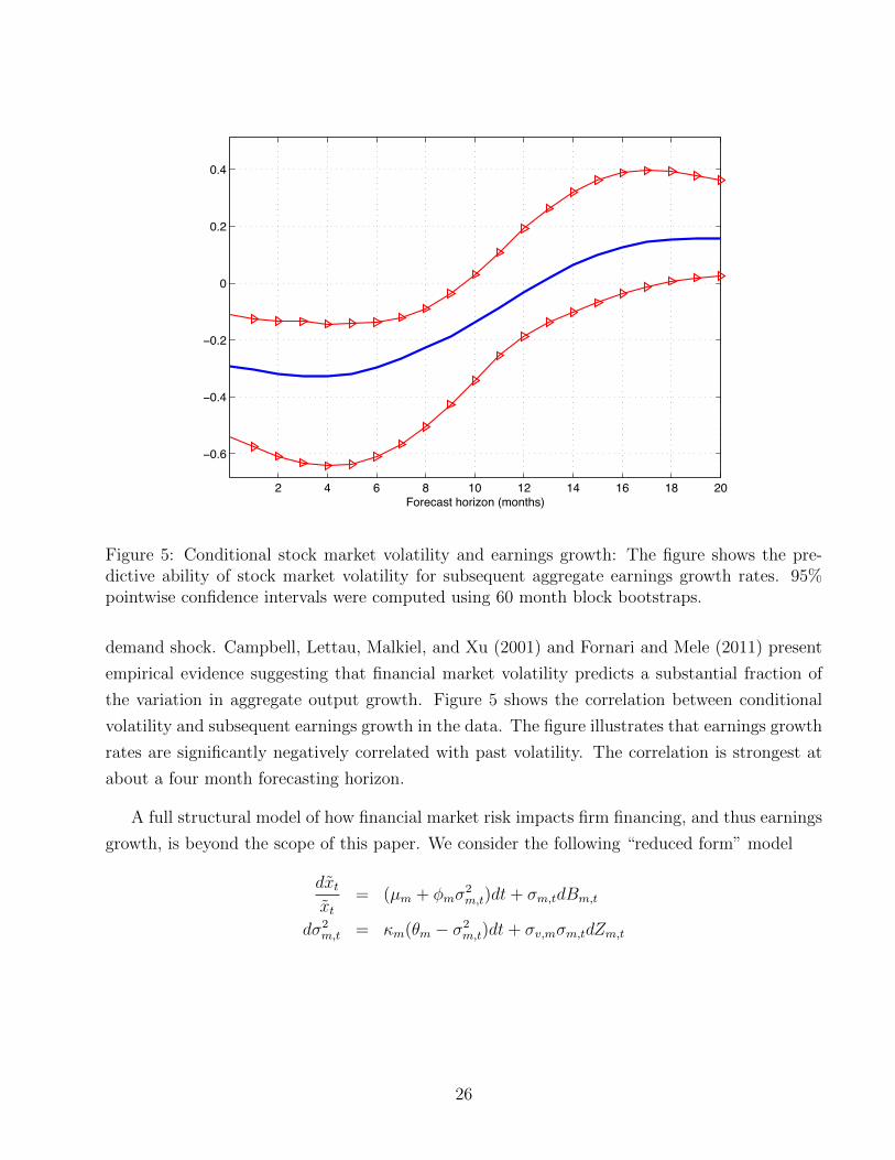
Figure 5: Conditional stock market volatility and earnings growth: The figure shows the pre-dictive ability of stock market volatility for subsequent aggregate earnings growth rates. 95%pointwise confidence intervals were computed using 60 month block bootstraps.

demand shock. Campbell, Lettau, Malkiel, and Xu (2001) and Fornari and Mele (2011) present

empirical evidence suggesting that financial market volatility predicts a substantial fraction of

the variation in aggregate output growth. Figure 5 shows the correlation between conditional

volatility and subsequent earnings growth in the data. The figure illustrates that earnings growth

rates are significantly negatively correlated with past volatility. The correlation is strongest at

about a four month forecasting horizon.

A full structural model of how financial market risk impacts firm financing, and thus earnings

growth, is beyond the scope of this paper. We consider the following “reduced form” model

dx̃tx̃t

= (µm + φmσ2m,t)dt+ σm,tdBm,t

dσ2m,t = κm(θm − σ2

m,t)dt+ σv,mσm,tdZm,t

26

The cash flow process and the idiosyncratic stochastic volatility process for asset i are specified

as

dx̃i,tx̃i,t

= (µi + φiσ2m,t)dt+ σi,tdBi,t + Ciσm,tdBm,t

dσ2i,t = κi(θi − σ2

i,t)dt+ σv,iσi,tdZi,t

The coefficients, φ and φi measure the sensitivity of fundamentals to the systematic volatility,

σm,t. If these coefficients are negative, shocks to volatility lead to subsequent lower growth rates.

If φi < φ, the cash flow sensitivity of stock i is greater than that of the average stock in the

economy. Individual assets also have asset-specific sensitivity to shocks in volatility as captured

by the term Ciσm,tdBm,t. Thus, we can think of the φi coefficients as capturing the sensitivity of

long run expected cash flows to systematic volatility, and Ci as capturing the sensitivity of firm

specific cash flows to aggregate cash flows, much like a beta in a standard CAPM model.

Under these assumptions about exogenous fundamentals, we show in Appendix A that the

equilibrium price processes given by

dPm,tPm,t

− rf,tdt = (1

2λ2mσ

2v,m − λmκm)σ2

m,tdt+ σm,tdBm,t + λmσv,mσm,tdZm,t (38)

and

dPi,tPi,t− rf,tdt = (

1

2λ2iσ

2v,m − λiκm)σ2

m,tdt+ σi,tdBi,t + Ciσm,tdBm,t + λiσv,mσm,tdZm,t (39)

where the coefficients, λm and λi are given by

λm =1

σ2v,m

[√κ2m − σ2

v,m(γ2 + (1− 2φm)γ)−√κ2m − σ2

v,m[γ2 − (1 + 2φm)γ + 2φm] (40)

and

λi =1

σ2v,m

[√κ2m − σ2

v,m(γ2 + (1− 2φm)γ)−√κ2m − σ2

v,m[γ2 + (1− 2Ci − 2φm)γ + 2φi](41)

The traditional conditional βt, defined as the ratio of the conditional covariance of individual

asset returns with the market divided by market variance, is equal to

βi =Ci + λiλmσ

2v,m

1 + λ2mσ2v,m

.

27

The conditional betas are constant with this particular model specification. More generally,

the betas will be ratios of linear functions of state-variables. It is generally not true that risk

premiums are linear functions of market beta in our model. Figure 6 illustrates this. This figure

plots expected returns as functions of the coefficients Ci and φi under two different assumptions

about the initial value of the market volatility σm,t. The figure shows that the expected rates

of return look as if they are almost linear functions of φ’s and C’s. Also, the expected returns

are differ greatly across the two different initial volatility regimes, suggesting that expected rates

of return can vary greatly over time in our model. In periods of low volatility, there may be a

discernible risk premium and therefore it may be difficult to detect a strong empirical relationship

between average returns and systematic risk during these periods. Conversely, in periods of high

volatility we should see a greater overall market risk premium, as well as a greater cross-sectional

dispersion in expected returns. When volatility moves up, high-risk stocks lose value relative to

their low risk counterparts, and vice versa. These implications are potentially important for

cross-sectional tests of asset pricing models. Ang, Hodrick, Xing, and Zhang (2006) find that

volatility predicts cross-sectional return premiums.

5 Concluding Remarks

Merton’s ICAPM is based on the idea that by postulating an exogenously given geometric process,

one can solve for the period-by-period expected rate of return in order to derive the equilibrium

price process. The problem with this approach is that the expected rate of return serves two

purposes. It is the average return per period but also the discount rate. The practice in academic

finance of simply solving for the expected rate of return ignores the issue of where expected returns

come from. As soon as one fixes the cash flow paid by an asset, whether it is a perpetual dividend

stream as with stocks, a state-contingent claim as with an option, or a fixed income stream as in

a bond, the present value should depend negatively on discount rates. This holds for all arbitrage

free bond pricing models and stock pricing models based explicitly on dividend discounting. Any

stock price process that claims to represent an equilibrium with time-varying expected returns

that does not incorporate contemporaneous discount rate shocks is either not an equilibrium or

is at best an equilibrium under the implicit assumption that future cash flows covary positively

with changes in discount factors, such that any change in the discount factor is exactly offset by

an increase in future expected payoffs.

We are not the first to criticize Merton’s model. In an unpublished paper Hellwig (1977),

shows that Merton’s exogenous price assumption is difficult to reconcile with particular choices

28

21

01

0.5

1

1.50

2

4

6

8

x 10 3

iCi

Con

ditio

nal e

xpec

ted

retu

rn

21

01

0.5

1

1.50.1

0.2

0.3

0.4

0.5

iCi

Con

ditio

nal e

xpec

ted

retu

rn

Figure 6: Expected annual rates of return as functions of the factor exposures, Ci and φi. Theupper (lower) graphs represent low (high) initial market volatility, σm,t respectively.

29

of dividend and utility specifications. Bick (1990) conducts a theoretical analysis searching for

particular utility functions consistent with an assumed equilibrium price process within Merton’s

ICAPM. The objective of this exercise seems by itself to contradict the assertion that “... the

assumptions of continuous trading and diffusion-type stochastic processes justify the use of vari-

ance as a sufficient statistic for risk without the objectionable assumptions of either quadratic

utility or normally-distributed stock returns” (Merton, 1980, p. 329).

Our critique of Merton’s analysis is relevant in the context of empirical implementations of

the intertemporal, or conditional CAPM. The direct consequence of our critique is that return

processes which have been assumed to be consistent with equilibrium are missing contempora-

neous feedback effects, and potentially also ignore priced risk factors associated with changing

discount rates. All in all, this could imply that empirical tests of conditional CAPM models are

potentially misleading. This is, in some sense, good news, since the empirical evidence on the

conditional CAPM is conflicting and not very supportive of the model.

We outline a general multi-period Euler equation that is aimed at developing a dynamic

CAPM consistent with present value computations. In doing so we start with a strictly exogenous

process that provides some terminal payoff at a terminal date T . By solving the agents’ portfolio

choice problem we obtain a simple Euler equation which can be used to find the equilibrium

price process. The usual combination of exponential affine processes, coupled with power utility

of wealth, accordingly produce closed-form equilibrium prices.

Our general idea can be expanded upon in numerous ways. In this paper we have been

wanting to keep the modeling as close to the traditional ICAPM as possible, and in doing so,

we have not considered the impact of stochastic interest rates. In examining equations (19)

and (20) it is clear that under the usual affine process - power utility combination, log returns

will have a term containing −d lnRt:T,f in continuous time. This term thus provides a feedback

term to stock prices suggesting that stocks should respond negatively to increases in interest

rates. It is possible to generalize this again, for example, by introducing stocks with differing

duration characteristics. It is easy to do this by allowing for the terminal payoff date to differ

across assets. This introduces different interest rate sensitivities across classes of stocks that

have different dividend durations.

It is possible to generalize our model in various other ways. In our basic setup we have assumed

that the terminal payoffs x̃T and x̃T,i are exogenous. In our model, these quantities are interpreted

as “fundamentals” to which the stock price will eventually converge. We have explicitly assumed

that the processes driving these fundamentals are strictly exogenous. In particular, we did not

assume that the mean expected growth rate of these processes were somehow determined in

30

equilibrium. This is what led us to gettin a different solution other than the standard ICAPM

style models without feedback terms.

It is perhaps difficult to interpret exactly how these terminal payoffs relate to tangible macro

economic quantities. As an investment project, x̃T,i should be interpreted as the date T value of

(reinvested) cash flows generated by the project up until that time. It is natural in this case to

interpret the investment project as irreversible. Our framework should in general be thought of

as one where there is some implicit friction on the conversion of physical capital into consumer

goods. If not, we could have interpreted x̃t,i as the value of a firm, in which case Pt,i 6= x̃t would

imply arbitrage. We believe our assumption is reasonable. Corporations do not sell off assets

instantaneously to compensate investors for shocks to uncertainty. They respond sluggishly, if

at all. Financial prices, on the other hand, respond immediately. The volatility feedback effect

implicitly evinces the existence of corporations’ sluggish responses to changes in financial market

volatility.

In future extensions of our model it is natural to consider macro-economic models in which

cash flows, x̃t,i are also endogenous. It is natural to think that the cash flows should depend on

financing costs, and as such, need to be solved in a bigger general equilibrium setup than we

consider here.

References

Ang, Andrew, Robert J. Hodrick, Yuhang Xing, and Xiaoyan Zhang, 2006, The Cross-Section of

Volatility and Expected Returns, Journal of Finance 61, 259299.

Bali, Turan, and Robert F. Engle, 2010a, Investigating ICAPM with Dynamic Conditional Cor-

relations, Journal of Monetary Economics 57(4), 377–390.

Bali, Turan, and Robert F. Engle, 2010b, Resurrecting the Conditional CAPM with Dynamic

Conditional Correlations, Working paper, Georgetown.

Bansal, Ravi, Dana Kiku, and Amir Yaron, 2006, Risks for the Long Run: Estimation and

Inference, working paper, Duke.

Bansal, Ravi, and Amir Yaron, 2004, Risks for the Long Run: A Potential Resolution of Asset

Pricing Puzzles, Journal of Finance 59, 1481–1509.

Bick, Avi, 1990, On Viable Diffusion Price Processes of the Market Portfolio, Journal of Finance

45, 673–689.

31

Bodurtha, James N., and Mark C. Nelson, 1991, Testing the CAPM with time-varying risks and

returns, Journal of Finance XLVL, 1485–1505.

Bollerslev, Tim, Robert F. Engle, and Jeffrey M. Wooldridge, 1988, A Capital Asset Pricing

Model with Time-Varying Covariances, Journal of Political Economy 96, 116–131.

Campbell, John, 1993, Intertemporal Asset Pricing without Consumption Data, American Eco-

nomic Review 83, 487–512.

Campbell, John, and Toumo Vuolteenaho, 2004, Bad Beta, Good Beta, American Economic

Review 94(5), 1249–1275.

Campbell, John Y., Martin Lettau, Burton G. Malkiel, and Yexiao Xu, 2001, Have Individual

Stocks Become More Volatile? An Empirical Exploration of Idiosyncratic Risk, Journal of

Finance 56, 1–43.

Campbell, John Y., and Robert J. Shiller, 1987, Cointegration and Tests of Present Value Models,

Journal of Political Economy 95, 1062–1088.

Campbell, John Y., and Robert J. Shiller, 1988, The Dividend-Price Ratio and Expectations of

Future Dividends and Discount Factors, Review of Financial Studies 1(3), 195–228.

Cochrane, John, 2011, Presidential Address: Discount Rates, Journal of Finance 66(4), 1047–

1108.

Duffie, D., and R. Kan, 1996, A yield-factor Model of Interest Rates, Mathematical Finance 6,

379–406.

Duffie, Darrell, Jun Pan, and Kenneth J. Singleton, 2000, Transform Analysis and Asset Pricing

for Affine Jump-Diffusions, Econometrica 68, 1343–1376.

Engle, R. F, David M. Lilien, and Russel P. Robins, 1987, Estimating the time varying risk

premia in the term structure: The ARCH-M model, Econometrica 55, 391–407.

Engle, Robert. F, Victor. K Ng, and Michael Rothschild, 1990, Asset pricing with a FACTOR

ARCH covariance structure: Empirical estimates for treasury bills, Journal of Econometrics

45, 213–237.

Eraker, Bjørn, 2010, The Volatility Premium, working paper.

Eraker, Bjørn, and Ivan Shaliastovich, 2008, An Equilibrium Guide to Designing Affine Pricing

Models, Mathematical Finance 18-4, 519–543.

32

Evans, Martin D., 1994, Expected returns, time-varying risk, and risk premia, Journal of Finance

XLIX, 655–679.

Ferson, Wayne E, and C. A. Harvey, 1993, The risk and predictability of international equity

returns, Review of Financial Studies 6, 527–566.

Fornari, Fabio, and Antonio Mele, 2011, Financial Volatility and Economic Activity, working

paper, LSE.

French, Kenneth R., William Schwert, and Robert F. Stambaugh, 1987, Expected stock returns

and volatility, Journal of Financial Economics 19(1), 3–29.

Gibbons, Michael, and Wayne Ferson, 1985, Testing asset pricing models with changing expec-

tations and an unobservable market portfolio, Journal of Financial Economics 14, 217–236.

Glosten, L. R, R Jagannathan, and D. E. Runkle, 1993, On the relation between the expected

value and the volatility of the nominal excess return on stocks, Journal of Finance 5, 1779–

1801.

Gordon, Myron J., 1959, Dividends, Earnings and Stock Prices, Review of Economics and Statis-

tics 41 (2), 99–105.

Guo, Hui, and Robert F. Whitelaw, 2006, Uncovering the Risk-Return Relation in the Stock

Market, Journal of Finance 61, 1433–1463.

Harvey, Campbell R., 1989, Time-varying conditional covariances in tests of asset pricing models,

Journal of Financial Economics 24, 289–317.

Harvey, Campbell R., 1991, The world price of covariance risk, Journal of Finance 46, 111–157.

Hellwig, Martin F., 1977, On the Validity of the Intertemporal Capital Asset Pricing Model,

Center for Operations Research and Econometrics (CORE) Discussion paper 7744.

Heston, Steve, 1993, Closed-Form Solution of Options with Stochastic Volatility with Application

to Bond and Currency Options, Review of Financial Studies 6, 327–343.

Jagannathan, Ravi, and Zhenyu Wang, 1996, The Conditional CAPM and the Cross-Section of

Expected Returns, Journal of Finance 51(1), 3–53.

Merton, Robert, 1973, An intertemporal capital asset pricing model, Econometrica 41, 867–887.

Merton, Robert C., 1980, On Estimating the Expected Return on the Market, Journal of Finan-

cial Economics 8, 323–361.

33

Merton, Robert C., and Paul Samuelson, 1969, A Complete Model of Warrant Pricing that

Maximizes Utility, Sloan Management Review Winter, 17–46. Reprinted in Merton, R. C.

“Continuous Time Finance,” Wiley–Blackwell, 1998.

Moskowitz, Tobias J., 2003, An Analysis of Covariance Risk and Pricing Anomalies, Review of

Financial Studies 16, 417–457.

Nelson, Mark, 1988, Time varying betas and risk premia in the pricing of foreward foreign

exchange contracts, Journal of Financial Economics 22, 335–354.

Ng, Lilian, 1991, Tests of the CAPM with time-varying covariances: A multivariate GARCH

approach, Journal of Finance XLVL, 1507–1521.

Ross, Stephen, 1976, The arbitrage pricing theory of capital market asset pricing, Journal of

Economic Theory 13, 341–360.

Whitelaw, Robert F., 1994, Time variations and covariations in the expectations and volatility

of stock market returns, Journal of Finance XLIX, 515–541.

34

Appendix A: Proofs

Proof of theorem 1. By definition, the expected rates of returns satisfy E0(R1) = E0(P1)/P0 =

1 + µ1 and E0(R0:2) = E0(R1R2) = E0(x̃)/P0 = E0(1 + µ2) = (1 + µ1) where the last equality

follows from the steady state assumption.

We need to prove that

Cov0(1

x, y) > 0

where

1

x=

1 + µ2

1 + µ1

y =E1(x̃)

E0(x̃).

Since we have

R1 =P1

P0

= xyE0[R1],

we can rewrite it as1

x

R1

E0[R1]= y.

Substitute y into Cov0(1x, y) to get:

Cov0

(1

x, y

)= Cov0

(1

x,

1

x

R1

E0[R1]

)= E0[

1

x(1

x

R1

E0[R1])]− E0(

1

x)E0(

1

x

R1

E0[R1])

= E0[(1 + µ2

1 + µ1

)2R1

E0[R1]]− E0(

1 + µ2

1 + γσ21

)E0(1 + µ2

1 + µ1

R1

E0[R1]).

No leverage, Cov0(µ22, R1) = 0, implies

E0

[(1 + µ2

1 + µ1

)2R1

E0[R1]

]= E0

[(1 + µ2)

2

(1 + µ1)2

]E0

[R1

E0[R1]

]=

E0[(1 + µ2)2]

(1 + µ1)2· 1

>(E0[1 + µ2])

2

(1 + µ1)2

= 1

35

Now, it is clear that

E0

(1 + µ2

1 + µ1

)E0

(1 + µ2

1 + µ1

R1

E0[R1]

)= E0

(1 + µ2

1 + µ1

)E0

(R1

E0[R1]

)= 1

Accordingly,

Cov0

(1

x, y

)= E0

[(1 + µ2

1 + µ1

)2R1

E0[R1]

]− E0

(1 + µ2

1 + µ1

)E0

(1 + µ2

1 + µ1

R1

E0[R1]

)> 1− 1

= 0

Proof of Proposition 2. The Euler equation follows directly from the first order conditions the

optimal portfolio problem, maxαEtu(x̃tRt:T (α)) and the market clearing condition α = 1. To

prove that the solution is independent of the frequency of trade, consider buying the market at

time t and hold it until time s. The value of this claim is

P ∗t =Et {u′(x̃T )Ps}Et {u′(x̃T )Rt:s,f}

= Et

{u′(x̃T )

Es {u′(x̃T )x̃T}Es {u′(x̃T )}Rs:T,f

}× 1

Et {u′(x̃T )}Rt:s,f

= EtEs

{u′(x̃T )

Et {u′(x̃T )}Es {u′(x̃T )x̃T}

Es {u′(x̃T )}Rt:T,f

}= Et

{Es {u′(x̃T )}Et {u′(x̃T )}

Es {u′(x̃T )x̃T}Es {u′(x̃T )}Rt:T,f

}= Et

{Es {u′(x̃T )x̃T}

Et {u′(x̃T )}Rt:T,f

}=

Et {u′(x̃T )x̃T}Et {u′(x̃T )}Rt:T,f

= Pt. (42)

Since P ∗t = Pt the market value is unchanged by portfolio re-balancing at date s.

Proof of Proposition 3. By assumption the infinite horizon limit exists, so β(T )→ β (constant).

Proof of Proposition 4. EZ utility is defined as

U(x̃t, Xt) = {(1− β)u1− 1

ψ

t + β[Et(U(x̃tt+1, Xt+1)1−γ)]

1− 1ψ

1−γ }1

1− 1ψ

36

In our economy, there is no intermediate consumption, so the period utility ut = 0.If at the

same time, we let ψ →∞, we can get:

U(x̃t, Xt) = β[Et(U(x̃tt+1, Xt+1)1−γ)]

11−γ

Let’s redefine Vt = U(x̃t,Xt)1−γ

1−γ and the subjective discount factor δ = β1−γ :

Vt = δEt[Vt+1]

= δEt[δEt+1[Vt+2]]

= δ2Et[Vt+2]

= ......

= δT−tEt[VT ]

= δT−tEt[U((x̃T , XT )1−γ

1− γ]

= δT−tEt[x̃1−γT

1− γ].

As a result, our terminal utility of wealth model is a special case of EZ when ψ → ∞ and

there is no intermediate consumption.

Deriving λσ in section 3.2. The coefficients characterizing the expectations in (24) gives the

ODEs

[∂β̂w∂s∂β̂σ∂s

]=

[0 0

−12−κ

][β̂w

β̂σ

]+

1

2

0[βw βσ

] [ 1 0

0 σ2v

][βw

βσ

] +

[0

l1(%(βσ)− 1)

]

We get βw = 1− γ and βw = −γ respectively. The ODE for βσ becomes

∂βσ∂s

= −1

2βw − κβσ +

1

2β2w + σ2

v β̂2σ + l1(%(βσ)− 1), βσ(0) = 0. (43)

In general, this equation does not admit an analytic solution. The parametric constraints σv =

l1 = 0 give the solution

βσ(u, s) =(e−κs − 1

) βw(u)(βw(u)− 1)

2κ. (44)

Equation 27 now follows.

37

Derivation of the beta model in section 4. The cash flow process and stochastic volatility process

of the market portfolio are specified as

dx̃tx̃t

= (µm + φmσ2m,t)dt+ σm,tdBm,t

dσ2m,t = κm(θm − σ2

m,t)dt+ σv,mσm,tdZm,t

The cash flow process and the idiosyncratic stochastic volatility process for asset i are specified

as

dx̃i,tx̃i,t

= (µi + φiσ2m,t)dt+ σi,tdBi,t + Ciσm,tdBm,t

dσ2i,t = κi(θi − σ2

i,t)dt+ σv,iσi,tdZi,t

As a result, the log cash flow processes are

d ln x̃t = (µm −1

2σ2m,t + φmσ

2m,t)dt+ σm,tdBm,t

d ln x̃i,t = (µi −1

2σ2i,t −

1

2C2i σ

2m,t + φiσ

2m,t)dt+ σi,tdBi,t + Ciσm,tdBm,t

We assume that covt(dBm,t, dBi,t) = 0; covt(dBm,t, dZm,t) = 0; covt(dBi,t, dZi,t) = 0; covt(dZm,t, dZi,t) =

0.

Let the state variable be Xt = (ln x̃t, ln x̃i,t, σ2m,t, σ

2i,t)

T . Assume that the representative agent

has power utility, u(x) = x1−γ

1−γ . By the F.O.C, the price of the asset i at time t, Pi,t is given as:

Pi,t =Et[x̃

−γT x̃i,T ]

Et[x̃−γm,T ]Rf,t:T

=Et[exp(u1XT )]

Et[exp(u0XT )]Rf,t:T

=exp{α(t, u1) + βT (t, u1)Xt}

exp{α(t, u0) + βT (t, u0)Xt}Rf,t:T

=1

Rf,t:T

e[α(t,u1)−α(t,u0)]+[βT (t,u1)−βT (t,u0)]Xt

=1

Rf,t:T

eλi,α(t)+λTi,β(t)Xt

where the vector u1 = (−γ, 1, 0, 0) and u0 = (−γ, 0, 0, 0). λi,β(t) = [λi,β1(t), λi,β2(t), λi,β3(t), λi,β4(t)]T

38

Similarly, the price of the market portfolio Pm,t is

Pm,t =Et[x̃

1−γT ]

Et[x̃−γT ]Rf,t:T

=1

Rf,t:T

e[α(t,um)−α(t,u0)]+[βT (t,um)−βT (t,u0)]Xt

=1

Rf,t:T

eλm,α(t)+λTm,β(t)Xt

where the vector um = (1− γ, 0, 0, 0).λm,β(t) = [λm,β1(t), λm,β2(t), λm,β3(t), λm,β4(t)]T

Using similar notation in Duffie et. al. (2000), we summarize the dynamics of state variable

Xt as:

dXt = µ(Xt)dt+ σ(Xt)dBXt

where µ(Xt) and σ(Xt) are affine functions of Xt :

µ(Xt) = K0 +K1Xt

(σ(Xt)σ(Xt)T )ij = (H0)ij + (H1)ij ·Xt

In our model, we can also write the variance-covariance matrix as

σ(Xt)σ(Xt)T = H0 +H1,wmwm,t +H1,wiwi,t +H1,σmσ

2m,t +H1,σiσ

2i,t

The matrices are defined as below:

K0 =

µm

µi

κmθm

κiθi

K1 =

0 0 φm − 1

20

0 0 φi − C2i

2−1

2

0 0 −κm 0

0 0 0 −κi

H0 = 04×4, H1,wm = 04×4, H1,wi = 04×4 and

H1,σm =

1 Ci 0 0

Ci C2i 0 0

0 0 σ2v,m 0

0 0 0 0

H1,σi =

0 0 0 0

0 1 0 0

0 0 0 0

0 0 0 σ2v,i

39

The coefficients α(t, u) and βT (t, u) in the formula of Pi,t are solved by the ODEs:

.

β = −KT1 β −

1

2βT ·H1 · β

=

0 0 0 0

0 0 0 012− φm C2

i

2− φi κm 0

0 12

0 κi

β − 1

2

0

0

βTH1,σmβ

βTH1,σiβ

.α = −KT

0 β

= −[ µm µi κmθm κiθi ]β

with boundary conditions:

β(T, u) = u

Stationarity of σt implies that.

β(t) = 0 when T − t→∞)

To solve the coefficients, let’s denote the vector β(t, u) = [βwm(t, u), βwi(t, u), βσm(t, u), βσi(t, u)]T .

It is clear that

.

βwm(t, u) = 0.

βwi(t, u) = 0

Let u = [u(1), u(2), u(3), u(4)], then we obtain

βwm(t, u) = u(1)

βwi(t, u) = u(2)

βσm(t, u) and βσi(t, u) are solved by two quadratic equations respectively:

σ2v,mβ

2σm − 2κmβσm + β2

wm + 2Ciβwmβwi − (1− 2φm)βwm − (C2i − 2φi)βwi + C2

i β2wi

= 0

σ2v,iβ

2σi− 2κiβσi + β2

wi− βwi = 0

40

The solutions of these two quadratic equations are given as:

βσm(t, u) =1

σ2v,m

(κm ±√

∆m(u))

∆m(u) = κ2m − σ2v,m[u2(1) + 2C1u(1)u(2)− (1− 2φm)u(1)− (C2

i − 2φi)u(2) + C2i u(2)2]

βσi(t, u) =1

σ2v,i

(κm ±√

∆i(u))

∆i(u) = κ2i − 2σ2v,i[

1

2u2(2)− 1

2u(2)]

The roots with ” + ” sign explode when σv,m and/or σv,i goes to zero. We drop these roots

because βσm(t, u) and βσi(t, u) are bounded.

Now let’s calculate the instantaneous excess return of asset i and market portfolio:

dPi,tPi,t− rf,tdt = [

.

λi,α(t) +.

λTi,β(t)Xt]dt+ λTi,β(t)dXt +1

2λTi,β(t)(dXtdX

Tt )λi,β(t)

= −KT0 λi,β(t)dt+ λTi,β(t)dXt +

1

2λTi,β(t)(dXtdX

Tt )λi,β(t)

dPm,tPm,t

− rf,tdt = [.

λm,α(t) +.

λTm,β(t)Xt]dt+ λTm,β(t)dXt +1

2λTm,β(t)(dXtdX

Tt )λm,β(t)

= −KT0 λm,β(t)dt+ λTm,β(t)dXt +

1

2λTm,β(t)(dXtdX

Tt )λm,β(t)

The second step follows because when T − t → ∞,.

λTi,β(t) =.

λTm,β = 0;.

λi,α(t) =.α(t, u1) −

.α(t, u0) = −KT

0 (β(t, u1)− β(t, u0)) = −KT0 λi,β(t). Similarly,

.

λm,α(t) = −KT0 λm,β(t).

Let’s use the formula of β(t, u) we obtained above and plug in u1 = (−γ, 1, 0, 0), u0 =

(−γ, 0, 0, 0) and um = (1− γ, 0, 0, 0) to calculate the expressions of λi,β(t) and λm,β(t) :

λi,β(t) = β(t, u1)− β(t, u0)

= [0, 1,1

σ2v,m

(√

∆m(u0)−√

∆m(u1)),1

σ2v,i

(√

∆i(u0)−√

∆i(u1))]T

= [0, 1,1

σ2v,m

(√

∆m(u0)−√

∆m(u1)), 0]T

= [0, 1, λi, 0]T

41

λm,β(t) = β(t, um)− β(t, u0)

= [1, 0,1

σ2v,m

(√

∆m(u0)−√

∆m(um)),1

σ2v,i

(√

∆i(u0)−√

∆i(um))]T

= [1, 0,1

σ2v,m

(√

∆m(u0)−√

∆m(um)), 0]T

= [1, 0, λm, 0]T

Now, let’s plug the solutions of λi,β(t) and λm,β(t) into the instantaneous excess return:

dPm,tPm,t

− rf,tdt = −KT0 λm,β(t)dt+ λTm,β(t)dXt +

1

2λTm,β(t)(dXtdX

Tt )λm,β(t)

= (1

2λ2mσ

2v,m − λmκm)σ2

m,tdt+ σm,tdBm,t + λmσv,mσm,tdZm,t

dPi,tPi,t− rf,tdt = −KT

0 λi,β(t)dt+ λTi,β(t)dXt +1

2λTi,β(t)(dXtdX

Tt )λi,β(t)

= (1

2λ2iσ

2v,m − λiκm)σ2

m,tdt+ σi,tdBi,t + Ciσm,tdBm,t + λiσv,mσm,tdZm,t

The expected instantaneous excess return of asset i and the market portfolio are:

Et[dPi,tPi,t− rf,tdt]/dt = (

1

2λ2iσ

2v,m − λiκm)σ2

m,t

Et[dPm,tPm,t

− rf,tdt]/dt = (1

2λ2mσ

2v,m − λmκm)σ2

m,t

The covariance between the instantaneous return of asset i and the instantaneous return of

market portfolio is:

Covt(dPi,tPi,t− rf,t,

dPm,tPm,t

− rf,tdt)/dt = (Ci + λiλmσ2v,m)σ2

m,t

The variance of instantaneous return of market portfolio is:

V art[dPm,tPm,t

− rf,t]/dt = (1 + λ2mσ2v,m)σ2

m,t

42

So the traditional betat is equal to:

betat =Ci + λiλmσ

2v,m

1 + λ2mσ2v,m

The formulas for λm and λi are:

λm =1

σ2v,m

(√

∆m(u0)−√

∆m(um))

=1

σ2v,m

[√κ2m − σ2

v,m(γ2 + (1− 2φm)γ)−√κ2m − σ2

v,m[γ2 − (1 + 2φm)γ + 2φm]

λi =1

σ2v,m

(√

∆m(u0)−√

∆m(u1))

=1

σ2v,m

[√κ2m − σ2

v,m(γ2 + (1− 2φm)γ)−√κ2m − σ2

v,m[γ2 + (1− 2Ci − 2φm)γ + 2φi]

Now, we can easily check that CAPM holds when σv,m → 0 and we set the parameter

φm = φi = 0 :

limσv,m→0

λm = − γ

κm

limσv,m→0

λi = −Ciγκm

limσv,m→0

betat = Ci

limσv,m→0

Et[dPi,tPi,t− rf,tdt]/dt = −λiκmσ2

m,t

= Ciγσ2m,t

limσv,m→0

Et[dPm,tPm,t

− rf,tdt]/dt = −λmκmσ2m,t

= γσ2m,t

43

As a result, CAPM holds in the sense that

limσv,m→0

Et[dPi,tPi,t− rf,tdt]/dt = lim

σv,m→0betat × Et[

dPm,tPm,t

− rf,tdt]/dt

Or equivalently,

limσv,m→0

Et[dPi,tPi,t− rf,tdt]/dt = γ lim

σv,m→0Covt(

dPi,tPi,t− rf,t,

dPm,tPm,t

− rf,tdt)/dt

Appendix B: Affine jump diffusions

An affine jump diffusion Xt is a Markov process in D ∈ Rn with a stochastic differential equation

representation

dXt = µ(Xt)dt+ Σ(Xt)dWt + ξt · dNt. (45)

Wt is a standard Brownian motion in Rn. The term ξt · dNt (element-by-element multiplica-

tion) captures independent Poisson jump arrivals of size ξt and with arrival intensity l(Xt) and

jump size distribution ξt on Rn. The distribution of jump sizes is specified through the Laplace

transform % : C→ C,

Eeuξ = %(u).

which is assumed to be well-defined. In our equilibrium theory, %(u) is assumed to exist for real

arguments u ∈ R and is interpretable as a moment generating function in that case.

The drift, diffusion and arrival intensities are assumed to be given by

µ(Xt) =M+KXt,

Σ(Xt)Σ(Xt)′ = h+

∑i

HiXt,i,

l(Xt) = l0 + l1Xt,

for (M,K) ∈ Rn×Rn×n, (h,H) ∈ Rn×n×Rn×n×n, (l0, l1) ∈ Rn×Rn×n. For X to be well defined,

there are additional joint restrictions on the parameters of the model, which are addressed in

Duffie and Kan (1996) and Duffie, Pan, and Singleton (2000). Our notation follows Eraker and

Shaliastovich (2008).

44

The affine jump diffusion framework allow us to compute conditional moment generating

function as

φ(u,Xt, s) = Et

(eu′Xt+s

). (46)

for u ∈ Rn.

Under appropriate technical regularity conditions ( see Duffie, Pan and Singleton (2000)), φ

is exponential affine in Xt,

φ(u,Xt, s) = eα(u,s)+β(u,s)′Xt ,

where α and β satisfy the ODE’s

∂β

∂s= K′β +

1

2β′Hβ + l1

′ (%(β)− 1) ,

∂α

∂s=M′β +

1

2β′hβ + l0

′ (%(β)− 1) ,

(47)

subject to boundary conditions β(u, 0) = u, α(u, 0) = 0. Note that the time argument s is

interpretable as a time to maturity, s = T − t. A change of variable from s to T − t leads to the

equivalent ODEs

∂β

∂t= −K′β − 1

2β′Hβ − l1′

(%(β̂)− 1

),

∂α

∂t= −M′β − 1

2β′hβ − l0′ (%(β)− 1) ,

(48)

with boundary conditions β(u, T, T ) = u, α(u, T, T ) = 0.

45