DYNAMIC NEIGBORHOODS: A CONCEPTUAL MODEL AND...

sid.inpe.br/mtc-m19/2012/02.13.16.37-TDI

DYNAMIC NEIGBORHOODS: A CONCEPTUAL

MODEL AND ITS IMPLEMENTATION FOR SPATIAL

DYNAMICS IN GEOGRAPHIC MODELING

Raian Vargas Maretto

Master Thesis at Post Graduation

Course applied in Remote Sensing,

advised by Drs. Antonio Miguel

Vieira Monteiro, and Tiago Garcia

de Senna Carneiro, approved in De-

cember 12, 2011.

URL of the original document:

<http://urlib.net/8JMKD3MGP7W/3BC43SH>

INPE

Sao Jose dos Campos

2011

http://urlib.net/8JMKD3MGP7W/3BC43SH

PUBLISHED BY:

Instituto Nacional de Pesquisas Espaciais - INPE

Gabinete do Diretor (GB)

Servico de Informacao e Documentacao (SID)

Caixa Postal 515 - CEP 12.245-970

Sao Jose dos Campos - SP - Brasil

Tel.:(012) 3208-6923/6921

Fax: (012) 3208-6919

E-mail: [email protected]

BOARD OF PUBLISHING AND PRESERVATION OF INPE INTEL-

LECTUAL PRODUCTION (RE/DIR-204):

Chairperson:

Dr. Gerald Jean Francis Banon - Coordenacao Observacao da Terra (OBT)

Members:

Dra Inez Staciarini Batista - Coordenacao Ciencias Espaciais e Atmosfericas (CEA)

Dra Maria do Carmo de Andrade Nono - Conselho de Pos-Graduacao

Dra Regina Celia dos Santos Alvala - Centro de Ciencia do Sistema Terrestre (CST)

Marciana Leite Ribeiro - Servico de Informacao e Documentacao (SID)

Dr. Ralf Gielow - Centro de Previsao de Tempo e Estudos Climaticos (CPT)

Dr. Wilson Yamaguti - Coordenacao Engenharia e Tecnologia Espacial (ETE)

Dr. Horacio Hideki Yanasse - Centro de Tecnologias Especiais (CTE)

DIGITAL LIBRARY:

Dr. Gerald Jean Francis Banon - Coordenacao de Observacao da Terra (OBT)


Deicy Farabello - Centro de Previsao de Tempo e Estudos Climaticos (CPT)

DOCUMENT REVIEW:


Yolanda Ribeiro da Silva Souza - Servico de Informacao e Documentacao (SID)

ELECTRONIC EDITING:

Viveca Sant´Ana Lemos - Servico de Informacao e Documentacao (SID)

sid.inpe.br/mtc-m19/2012/02.13.16.37-TDI

DYNAMIC NEIGBORHOODS: A CONCEPTUAL

MODEL AND ITS IMPLEMENTATION FOR SPATIAL

DYNAMICS IN GEOGRAPHIC MODELING

Raian Vargas Maretto

Master Thesis at Post Graduation

Course applied in Remote Sensing,

advised by Drs. Antonio Miguel

Vieira Monteiro, and Tiago Garcia

de Senna Carneiro, approved in De-

cember 12, 2011.

URL of the original document:

<http://urlib.net/8JMKD3MGP7W/3BC43SH>

INPE

Sao Jose dos Campos

2011

http://urlib.net/8JMKD3MGP7W/3BC43SH

Cataloging in Publication Data

Maretto, Raian Vargas.M335d Dynamic neigborhoods: a conceptual model and its implemen-

tation for spatial dynamics in geographic modeling / Raian VargasMaretto. – Sao Jose dos Campos : INPE, 2011.

xvi + 93 p. ; (sid.inpe.br/mtc-m19/2012/02.13.16.37-TDI)

Master Thesis (Remote Sensing) – Instituto Nacional dePesquisas Espaciais, Sao Jose dos Campos, 2011.

Advisers : Drs. Antonio Miguel Vieira Monteiro, and TiagoGarcia de Senna Carneiro.

1. neighborhoods. 2. dynamic neighborhoods. 3. cellular au-tomata. 4. generalized proximity matrices. 5. dynamic model-ing. I.Tıtulo.

CDU 681.306:502

Copyright c© 2011 do MCT/INPE. Nenhuma parte desta publicacao pode ser reproduzida, ar-mazenada em um sistema de recuperacao, ou transmitida sob qualquer forma ou por qualquermeio, eletronico, mecanico, fotografico, reprografico, de microfilmagem ou outros, sem a permissaoescrita do INPE, com excecao de qualquer material fornecido especificamente com o proposito deser entrado e executado num sistema computacional, para o uso exclusivo do leitor da obra.

Copyright c© 2011 by MCT/INPE. No part of this publication may be reproduced, stored in aretrieval system, or transmitted in any form or by any means, electronic, mechanical, photocopying,recording, microfilming, or otherwise, without written permission from INPE, with the exceptionof any material supplied specifically for the purpose of being entered and executed on a computersystem, for exclusive use of the reader of the work.

ii

v

“É melhor atirar-se à luta em busca de dias melhores, mesmo correndo o risco de perder tudo,

do que permanecer estático como os pobres de espírito, que não lutam, mas também não vencem,

que não conhecem a dor da derrota, mas não tem a glória de ressurgir dos escombros.

Esses pobres de espírito, ao final da jornada na Terra, não agradecem a Deus por terem vivido,

mas desculpam-se ante Ele por terem simplesmente passado pela vida”.

Bob Marley

vii

À minha família,

Eliomar Maretto, Marize Vargas Maretto e

Luan Vargas Maretto.

ix

AGRADECIMENTOS

Agradeço primeiramente a Deus, por ter me guiado e me dado forças para superar mais esta árdua etapa de minha vida.

A meus pais, Eliomar Maretto e Marize Vargas Maretto, e meu irmão, Luan Vargas Maretto, por serem um porto seguro, pelo ser humano que me tornei. Este trabalho concretiza um sonho não só meu, mas também deles. Sem vocês, eu nada seria.

A meus tios, primos, e minha avó, por todo o carinho e por, mesmo longe, sempre me apoiarem.

A minha namorada Ana Carolina Silva Gava, por ser minha grande companheira, estando sempre ao meu lado nesta difícil jornada longe de minha família, me dando todo o apoio e suporte emocional.

Ao Instituto Nacional de Pesquisas espaciais e seus professores, pela oportunidade, conhecimento passado, e pela utilização de infraestrutura.

À Coordenação de Aperfeiçoamento de Pessoal de Nível Superior (CAPES) pelo suporte financeiro.

A meus orientadores, Dr. Antônio Miguel Vieira Monteiro e Dr. Tiago Garcia de Senna Carneiro, pelo conhecimento passado, por terem me guiado durante todo este Mestrado, pela amizade, e pela confiança depositada em meu trabalho.

Aos irmãos diretores, André A. Gavlak, Giovanni Boggione, Hiran Zani, Kleber Trabaquini, Enrique M. Del Castillo, César E. Garcia, Thiago Bertani, Pedro Valle, Rogério Marinho e Carlos Stelle, por toda a amizade, e por terem sido uma segunda família para mim.

Aos irmãos Lino Augusto Carvalho, Galeno Oliveira, Talita Assis e Carolina Pinho, pela amizade e por terem sido uma parte de minha segunda família nestes anos.

Aos colegas da turma PG-SER/2009 e aos companheiros da saudosa Bat Caverna.

A meus companheiros de sala Pedro Andrade, Liliam Castro e Flávia Feitosa pela amizade, pelas discussões, sempre muito férteis, e por toda a ajuda neste trabalho.

À Drª Maria Isabel Sobral Escada e Drª Silvana Amaral Kampel por toda a ajuda no desenvolvimento do meu trabalho.

Aos companheiros do TENSO, pelas quase conquistas, por demonstrarem o real significado da “derrota com dignidade”, e por toda a diversão e esforço nos campeonatos disputados.

Aos amigos da tradicional “pelada de sexta”, por proporcionarem tantos momentos de diversão e tantas risadas.

De uma forma geral, a todos os que se fizeram presentes em minha vida nesta árdua jornada.

xi

ABSTRACT

Neighborhood configuration has a direct influence over the simulated output of Cellular Automata based models. In real world, spatial relations are not static, but changes over time. A dynamic model which aims to reproduce real world patterns needs to reflect these dynamics. This dissertation proposes a conceptual model, making use of an algebraic formalism that defines a set of operations for dealing with neighborhood structures that change over time, during simulation processes. It is an important feature for modeling experiments that aim to incorporate the natural complexity of many geographic phenomena. A computational implementation of the model has been provided. The Dynamic Neighborhood conceptualization was implemented as a new feature of TerraME (Terra Modeling Environment), an open platform for spatially explicit CA-based modeling and simulation. The implementation has extended the platform functionalities to cope with a new class of problems, where the dynamics involved implies on neighborhood structures that change over time, needing a runtime reconfiguration. A deforestation model has been developed using the Dynamic Neighborhood extension provided in TerraME to simulate the evolving deforestation patterns in the Xingú-Iriri frontier, at the south of Pará state, in the Brazilian Amazon. This model has been developed as a proof-of-concept to demonstrate the potential of the Dynamic Neighborhoods concept proposed, formalized and implemented in this dissertation for dealing with geographic modeling of spatial relations that change over time and, by doing so, they redraw its neighborhood definition along the simulation life cycle.

xii

VIZINHANÇAS DINÂMICAS: UM MODELO CONCEITUAL E SUA

IMPLEMENTAÇÃO PARA DINÂMICAS ESPACIAIS EM MODELAGEM

GEOGRÁFICA

RESUMO

A configuração de estruturas de vizinhança exerce uma influência direta nos resultados gerados por modelos baseados em Autômatos Celulares. No mundo real, relações espaciais entre objetos não são estáticas, elas mudam ao longo do tempo. Um modelo dinâmico que objetive reproduzir padrões do mundo real deve refletir estas dinâmicas. Este trabalho propõe uma definição conceitual, através de um formalismo algébrico, de um conjunto de operações que permitem que ambientes computacionais destinados a modelagem dinâmica espacialmente explícita possam incorporar mecanismos para tratar vizinhanças que se alteram ao longo do tempo, durante processos de simulação. Esta característica é muito importante para experimentos de modelagem que objetivem incorporar a complexidade natural de muitos fenômenos geográficos. O modelo conceitual de Vizinhanças Dinâmicas foi implementado e incorporado ao TerraME (Terra Modeling Environment), uma plataforma livre para desenvolvimento e simulação de modelos dinâmicos espacialmente explícitos baseados em Autômatos Celulares. Esta implementação ampliou as funcionalidades da plataforma, de forma a possibilitá-la lidar com uma nova classe de problemas, cujas dinâmicas envolvidas implicam em estruturas de vizinhança que se alterem ao longo do tempo, precisando assim, serem alteradas em tempo de execução durante as simulações. Um modelo de desmatamento foi desenvolvido utilizando-se a extensão para tratamento de Vizinhanças Dinâmicas, implementada em TerraME. Neste modelo, foi simulada a evolução dos padrões de desmatamento na frente de ocupação do Xingú-Iriri, no sul do estado do Pará. Este modelo foi desenvolvido como um experimento de prova de conceito, a fim de demonstrar o potencial dos conceitos de Vizinhanças Dinâmicas, propostos, formalizados e implementados neste trabalho, para lidar com a modelagem de relações espaciais que se alteram ao longo do tempo e com isto, re-configurar suas definições de vizinhanças durante o ciclo de vida do modelo.

xiii

LIST OF FIGURES

Figure 2.1 – Layered-CA structure, with vertical neighborhood relations. ................................... 7

Figure 2.2 – Selective refinement in Layered-CA, where each cell have different numbers of horizontal neighbors. Source: STRAATMAN et al. (2001) ........................................................ 8

Figure 2.3 – Flowchart of DINAMICA operation. Source: SOARES-FILHO et al. (2002) ........ 9

Figure 2.4 – Geo-referencing scheme in GAS (a) Direct – Buildings are represented by means of foundation contours, and roads by means of road boundaries; (b) Indirect – Locating a landowner by pointing to his/her properties. Source: Adapted from TORRENS and BENENSON (2005) .................................................................................................................... 11

Figure 2.5 – Neighborhood relationships for indirectly GA. Two households are neighbors if they are located in the same property or in neighboring properties. Source: TORRENS and BENENSON (2005) .................................................................................................................... 13

Figure 2.6 – Nested-CA structure. Source: CARNEIRO (2006). .............................................. 15

Figure 2.7 – Neighborhoods defined using the GPM concept. (a) Moore neighborhoods. (b) Two non-isotropic neighborhoods defined through a transportation network. Source: adapted from ANDRADE-NETO et al. (2008). ....................................................................................... 16

Figure 2.8 – Geometric transformation of an object in VecGCA. Source: MORENO et al. (2008). ......................................................................................................................................... 17

Figure 2.9 – (a) A VecGCA space and (b) the matrix that describes what states are favorable to the transition between what states. .............................................................................................. 18

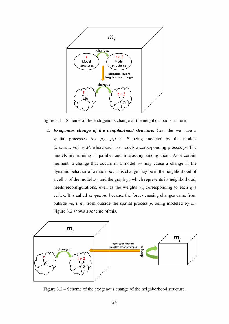
Figure 3.1 – Scheme of the endogenous change of the neighborhood structure. ........................ 24

Figure 3.2 – Scheme of the exogenous change of the neighborhood structure. .......................... 24

Figure 3.3 – Scheme of the hybrid change of the neighborhood structure. ................................. 25

Figure 3.4 – The TerraME Programming Environment. Source: CARNEIRO (2006). ............. 28

Figure 3.5 – TerraME Software Architecture. Source: CARNEIRO (2006). ............................ 29

Figure 3.6 – Class diagram: Spatial module of TerraME. ........................................................... 30

Figure 3.7 – Pseudocode of the reconfigure( ) function, where: cs is a Cellular Space and celli is the i-th cell during traversal of it. ................................................................................................ 33

Figure 3.8 – Entity-relationship model of the proposed structure to save neighborhoods in a TerraLib database. ....................................................................................................................... 34

Figure 3.9 – Screen display of the neighborhood’s observer. ..................................................... 35

Figure 3.10 – Operational scheme of the endogenous change of the neighborhood structures. . 36

Figure 3.11 – Operational scheme of the exogenous change of the neighborhood structures. ... 37

Figure 3.12 – Operational scheme of the hybrid change of the neighborhood structures. .......... 37

Figure 4.1 – (a) Legal Amazon, Terra do Meio and Xingu-Iriri Frontier (Rectangle area); (b) Circulation networks in the Xingu-Iriri frontier in 2006. Source: adapted from AMARAL et al. (2006). ......................................................................................................................................... 41

Figure 4.2 – Spatial distribution of the accumulated deforestation in 2000. Source: adapted from INPE (2011a). ............................................................................................................................. 42

Figure 4.3 – Spatial distribution of the attribute “percentage of deforestation” in the grid of 4km x 4km cells .................................................................................................................................. 43

Figure 4.4 – Roads Network. Source: Adapted from Amaral et al. (2006; 2007), Escada et al. (2005; 2007), Pinho et al. (2010), and Vieira et al. (2004). ........................................................ 44

Figure 4.5 – Rivers and Airstrips. Source: Adapted from Amaral et al (2006), ANA (2011) and INPE (2011). ............................................................................................................................... 45

xiv

Figure 4.6 – Hierarchy considered for the protected areas (Conservation Unities and Indigenous Lands). Source: Adapted from IBAMA (2011) and FUNAI (2011) .......................................... 47

Figure 4.7 – Human settlements and settlement projects. Source: Adapted from Amaral et al (2006) and INCRA (2011). ......................................................................................................... 48

Figure 4.8 – Neighborhoods generated to represent the influence of places and airstrips: (a) Intersection relationship; (b) Buffer neighborhood. .................................................................... 50

Figure 4.9 – Neighborhood relation between the polygons representing the cells and the polygons representing the UC, PA and TI. ................................................................................. 51

Figure 4.10 – Neighborhoods generated from roads and rivers: (a) Intersection-based relationship; (b) Buffer neighborhood. ........................................................................................ 53

Figure 4.11 – Flowchart showing the main steps of the deforestation model developed. The Reconfigure step brings in it the main contribution of this work. ............................................... 55

Figure 4.12 – Initial state of the system for the Experiments 1 and 2. Attributes: (a) Percentage of forest and (b) Percentage of deforestation. ............................................................................. 59

Figure 4.13 – Initial state of the system for the experiment 3 (a) and seasonality effects over roads (b). ..................................................................................................................................... 60

Figure 4.14 – Initial state of the system for the experiment 4. .................................................... 61

Figure 4.15 – Comparison between deforestation patterns generated in Experiments 1 and 2. .. 62



Figure 4.18 – Real Data and deforestation patterns generated in experiment 4. ......................... 65

xv

CONTENTS

1. INTRODUCTION ....................................................................................................... 1

1.1. Aims and Contributions of this work .................................................................................. 3

1.2. This work and INPE’s Research Agenda on Computational Platforms for Environmental Modeling and Simulation .............................................................................................................. 4

1.3. Outline of the work ............................................................................................................. 5

2. RELATED WORKS .................................................................................................... 7

2.1. Layered CA model .............................................................................................................. 7

2.1.1. Neighborhood definitions in Layered CA ........................................................................ 7

2.2. The DINAMICA model ...................................................................................................... 8

2.2.1. Neighborhoods definition in Dinamica EGO – A DINAMICA model implementation 10

2.3. Geographic Automata System (GAS) ............................................................................... 10

2.3.1. Neighborhoods Definition in OBEUS – A GAS model implementation ....................... 12

2.4. Nested-CA model .............................................................................................................. 13

2.4.1. Neighborhoods Structures in the Nested-CA model ...................................................... 15

2.5. VecGCA model ................................................................................................................. 16

2.5.1. Neighborhoods Definitions in VecGCA ........................................................................ 18

3. A DYNAMIC NEIGHBORHOOD MODEL PROPOSAL: CONCEPT,

FORMALIZATION AND IMPLEMENTATION ............................................................ 21

3.1. The Dynamic Neighborhoods (DN): A Conceptual Model .............................................. 21

3.1.1. Defining the GPM-Generalized Proximity Matrices ..................................................... 21

3.1.2. An Algebraic Definition for Dynamic Neighborhoods Structures ................................. 22

3.2. Dynamic Neighborhoods (DN): The Implementation Model ........................................... 27

3.2.1. The TerraME platform ................................................................................................... 28

3.2.2. The dynamic neighborhoods implementation ................................................................ 29

4. EXPLORING THE DYNAMIC NEIGHBORHOODS CONCEPTS IN A PROOF-OF-

CONCEPT EXPERIMENT: MODELLING DEFORESTATION PATTERNS THROUGH

CIRCULATION NETWORKS IN AN AMAZONIA FRONTIER SITE .......................... 39

4.1. Study area and its Circulation Network Dynamics ........................................................... 39

4.1.1. Model Racionality and Data Description ....................................................................... 41

4.2. The Deforestation Model .................................................................................................. 48

4.3. Simulation results .............................................................................................................. 57

5. CONCLUDING REMARKS ...................................................................................... 67

6. REFERENCES .......................................................................................................... 69

APPENDIX A: PARAMETERS OF THE PROOF-OF-CONCEPT MODEL – VALUES

AND REASONS ............................................................................................................... 77

xvi

APPENDIX B: THE USAGE OF DYNAMIC NEIGHBORHOOD CONCEPTS IN EACH

EXPERIMENT ................................................................................................................ 81

APPENDIX C: SOURCE CODE OF THE NEIGHBORHOODS RECONFIGURATION

IN THE PROOF-OF-CONCEPT MODEL ........................................................................ 83

1

1. INTRODUCTION

Over the 1970’s, a series of research projects on several Geography departments was

established based on a systemic view of the urban phenomena. A real city should be

properly characterized not only by its fixed infrastructure components. The spatial

distribution of different land uses competing, cooperating through interactions and

depending on a neighborhood definition, established by a spatial proximity criterion,

was a more realistic view. Spatial complex dynamics instead of static spatial relations

started to be the research focus. This research line has been since then, very influential

over the past years. The main instrument devised to investigate these complex spatial

dynamics was the use of computer modeling and simulation. It would provide an

empirical test bed for geographers, urban planners, architects, city engineers,

sociologists, and others the like to investigate their theoretical hypotheses and

conceptual models of the structure and functioning of urban systems and cities.

Almost at the same time, on the theoretical debate in the Geography field on

representational perspectives for the geographic spaces, the ideas of a cellular

geography (TOBLER, 1979) and cellular worlds (COUCLELIS, 1985, 1991, 1997) took

shape. On the other hand, the use of 2D (two-dimensional) Cellular Automata (CA)

computational structures in modeling and simulation of complex dynamics in physics

and chemistry had already a long tradition. After the widely adopted view for the

geographic space based on cells, computer CA-based models started to being used to

provide the mechanism for observing urban systems dynamics. Most of the works

presented on the related literature have followed this line from the 1990’s until

nowadays. It proved that the potential of Cellular Automata based models for urban

dynamics studies had become widely recognized (BATTY; XIE, 1994; BATTY, 2000;

BATTY, 2005; DEADMAN et al., 1993; PHIPPS; LANGLOIS 1997; WHITE;

ENGELEN, 1993, 1994, 1997; WHITE et al., 1998; WAGNER, 1997; ALMEIDA et

al., 2003a, 2003b, 2005, 2007; CLARKE et al., 1997; CLARKE; GAYDOS, 1998;

O’SULLIVAN; TORRENS, 2000; VANCHERI et al, 2008).

In CA-based models, the neighborhood definition is a recognized key modeling

component, because it determines how the geographic objects that build up the model

interact among them (HAGOORT et al., 2008). It determines how the cells, which

2

represent the geographic objects, are spatially related. If two cells are considered

neighbors of each other, it means that one is exerting some sort of influence over the

spatial, temporal and/or behavioral state of the other. Each neighborhood relation also

brings with it a way of value and differentiate that particular linkage. Usually, this is

translated into a weight mapping definition. Thus, the weight represents the strength of

the bounds that link those neighbors engaged during the model execution.

Dynamic models aim to represent complex dynamics of real world geographic

phenomena. In real world situations, neighborhoods relations rarely keep their structure

over time. Several studies have demonstrated that the CA-based dynamical models are

sensitive to the neighborhood configuration. Ménard and Marceau (2005) and Kocabas

and Dragicevic (2006) have demonstrated that their land use and urban growth model

are sensitive to different cell resolutions and neighborhood configurations. Hagoort et al

(2008) have investigated the impact of using neighborhood rules which are defined and

calibrated on an ad hoc basis by trial and error methods, and that do not evolve along

the model life cycle, on the simulated output of CA-based models.

In an attempt to avoid the problems raised by the use of fixed neighborhoods strategy, a

small number of works have been developed more recently. The most recent is the work

developed by Moreno et al. (2009), in which the authors present an implementation of a

dynamic neighborhoods scheme in a vector-based cellular automata model (VecGCA)

(MORENO et al., 2008). In their proposal, two objects are neighbors if they are

adjacent or separated by other objects in which their states are favorable to the transition

of states between them. In this approach, when the objects change their states, the

neighborhood structures are reconfigured. However, this approach is tightly connected

to the very specific CA extension they are proposing, the Vector Based Geographic

Cellular Automata (VecGCA) (MORENO et al., 2008). It either does not allow for

building neighborhoods structures based on the cells attributes or spatial relations than

adjacency.

To overcome the problems raised by the use of fixed neighborhoods structures, i. e.,

neighborhoods that cannot be reconfigured at runtime in Dynamic CA-based models,

this work proposes a formal model for providing runtime reconfiguration of

neighborhood structures in CA-based modeling frameworks. It allows modelers to

include neighborhood reconfiguration strategies in their modeling experiments. The

3

concepts developed, were implemented in TerraME (Terra Modeling Environment)

framework (www.terrame.org). TerraME is a computer platform that implements the

Nested Cellular Automata model (CARNEIRO, 2006), a CA extension proposed to

allow the representation of complex dynamic phenomena through multiple scales. In

order to demonstrate the concepts proposed and test its implementation, a deforestation

model that needs the Dynamic Neighborhoods concept was developed. Based on

Amaral et al. (2006), we simulate the evolving deforestation patterns in the Xingú-Iriri

frontier, south of Pará State, in the Brazilian Amazon. It is important to notice that the

main focus of this deforestation model in this work is not to reproduce exactly the real

deforestation patterns, but demonstrate the potential of the Dynamic Neighborhoods

concepts by verifying its impacts in a model developed based on empirical data over a

real world setting.

1.1. Aims and Contributions of this work

This work focus on creating the computational basis for providing runtime

reconfiguration of neighborhood structures in CA-based computational modeling

frameworks designed to cope with geographic phenomena. The conceptual model

developed allows modelers to deal with neighborhood reconfiguration strategies as part

of their model experiment. In order to do so we propose:

(1) A typology of modeling situations where a neighborhood structure

reconfiguration at runtime is a requirement from a modeler’s perspective. It

establishes three categories of changes for the neighborhood structure over

models life cycle: (a) Endogenous Change, (b) Exogenous Change, and (c)

Hybrid Changes.

(2) A conceptual model for defining neighborhood structures that change over time

based on an algebraic specification that makes use of graph-like structures. This

model provides the basis for defining a set of operators (functions) to deal with

the problem of allowing truly Dynamic Neighborhood structures to CA-based

computational environments.

(3) In order to evaluate the concepts proposed in (1) and (2), an implementation was

provided for the TerraME (Terra Modeling Environment) platform

http://www.terrame.org/

4

(CARNEIRO, 2006), an extended CA-based computational framework for

spatial dynamic modeling and simulation.

(4) A deforestation model that needs the Dynamic Neighborhoods concept was

developed as a proof-of-concept experiment. We simulate the evolving

deforestation patterns in the Xingú-Iriri frontier, south of Pará state, in the

Brazilian Amazon. This model was based on Amaral et al. (2006), that describes

the patterns of deforestation and the corresponding evolution of the

transportation networks in that region.

1.2. This work and INPE’s Research Agenda on Computational Platforms for Environmental Modeling and Simulation

INPE have been studying the Amazon rainforest, monitoring and measuring it

deforestation rates since the 1980’s. Recently, the interest for studying the human

actions in this region has increased considerably. At INPE, the GEOMA project

(http://www.geoma.lncc.br/) has set up engagements beyond the Measuring-and-

Monitoring scope and extended the internal research into the complete cycle of

Measuring-Monitoring-Modeling-and-Simulating. The main goal is to build integrated

computational models that can reproduce, at multiple scales, and based on empirical

data and hypotheses about the process, the dynamics of this region. These models

should be understood as a computational tool for testing and exploring hypotheses on

the dynamics of the social and natural systems of the region.

In a joint effort between INPE and UFOP1 (Federal University of Ouro Preto – MG),

the TerraME platform has been developed to model and simulate spatial dynamic

phenomena at multiple scales. This platform aims to provide the computational support

for institutional projects, and other studies which intend to use spatial dynamic

modeling as an empirical instrument for exploring complex dynamic systems. Through

the implementation of the dynamic neighborhoods capability in this platform, these

studies have a computer platform that can offer more flexibility for modelers. In this

way, this work expands the universe of problems which can be tackled with the

TerraME platform.

1 Universidade Federal de Ouro Preto (in portuguese).

http://www.geoma.lncc.br/

5

1.3. Outline of the work

This proposal is organized in five chapters. In Chapter 2, we present and analyze, from

the literature, the closest related works. In Chapter 3, we describe in detail our proposal.

In Chapter 4, we describe the deforestation model that is used here as a proof-of-concept

experiment. And in Chapter 5, some concluding remarks are presented.

7

2. RELATED WORKS

Over the recent years, a series of CA-based computational models for dealing with

complex spatial phenomena has been proposed in the literature. Some of them have

advanced and have also proposed computational frameworks for effectively

accomplishing modeling and simulation of these phenomena. All of them acknowledge

the importance of the problem of the neighborhood structures definition from a

modeler’s perspective. Five of these proposed models are presented and commented

here, with a particular emphasis on the specific ways they deal with the modeling of the

neighborhood structures.

2.1. Layered CA model

Straatman et al. (2001) have proposed the Layered-CA model, in an attempt to deal with

multi-scale dynamic models. It is composed by an iterative refinement of 2-dimensional

cellular automata, in a set of connected layers. Every cell in a certain layer can have one

parent in the higher layer and an arbitrary number of child cells in the lower layer, and it

composes a vertical neighborhood. It assumes that all layers cover the same area. Figure

2.1 shows this structure, which is similar to a quadtree (FINKEL; BENTLEY, 1974),

and allows embedding multiple models operating in different spatial resolutions.

Figure 2.1 – Layered-CA structure, with vertical neighborhood relations. Source: STRAATMAN et al. (2001)

2.1.1. Neighborhood definitions in Layered CA

There are two types of neighborhoods in the Layered-CA model, horizontal

neighborhoods and vertical ones. The vertical neighborhoods are composed by the

parents and children of the cells in a given layer. The horizontal neighborhoods can be

defined by simply boundary conditions, and the neighbors of a cell are the immediately

adjacent cells. If a selective refinement is made, as shown in Figure 2.2, all the refined

8

cells can have from 1 to 8 horizontal neighbors. The state of a given cell depends on

both, its vertical and horizontal neighbors.

Figure 2.2 – Selective refinement in Layered-CA, where each cell have different numbers of horizontal neighbors. Source: STRAATMAN et al. (2001)

2.2. The DINAMICA model

The DINAMICA model was initially presented for simulation of Amazonian landscape

dynamics (SOARES-FILHO et al., 2002; RODRIGUES et al., 2007). Basically, it is a

CA-based model that presents multi-scale vicinity-based transitional functions,

incorporating the spatial feedback approach to a stochastic multi-step simulation engine.

The calculation of the spatial dynamic transition probabilities can be done mainly by the

application of logistic regression. The main input for DINAMICA is a landscape map2,

as well as selected spatial variables structured in two cartographic subsets according to

their dynamic or static nature. The outputs are simulated landscape maps (one for each

time step), spatial transition probability maps, which depict the probability of a cell at a

position (x, y) to change from state i to state j (being i and j types of land-use and land-

cover class), and dynamic spatial variable maps. Figure 2.3 shows a flowchart of

DINAMICA operation.

DINAMICA works in various phases, and changes the transition rates according to a

parameter called Saturation Value. The transition rates are passed as a fixed parameter

within a given phase, and handled by the model when necessary during different

dynamic phases. The calculation of the amount of cells to be changed in a given

iteration is done by multiplying the number of cells of each land-use and land-cover

class, occurring in a time step, by the transition rate. The saturation value forces the

2 Land use and/or land cover map obtained from digital classification of orbital and/or airborne remote sensing images, or from GIS techniques.

9

stopping of the transition i – j when the number of cells in state j reaches a maximum

quantity.

The spatial transition probabilities are calculated for each cell and for each specified

transition through a polytomous logistic model. Logistic regression is used to depict the

probability of a cell to change to one of the states, chosen along the line of the transition

matrix. This procedure results in a set of maps depicting the probability of a cell to

change to another state.

Figure 2.3 – Flowchart of DINAMICA operation. Source: SOARES-FILHO et al. (2002)

10

2.2.1. Neighborhoods definition in Dinamica EGO – A DINAMICA model implementation

In DINAMICA, the neighborhood influence in the transition probabilities is modelled

by splitting the cell selection mechanism into two processes: (a) the expander function,

dedicated only to the expansion or contraction of previous patches of a certain land-use

and land-cover class; and (b) the patcher function, designed to generate or form new

patches through a seedling mechanism (SOARES-FILHO et al., 2002). The

combination of these two processes occurs through the equation below:

(1)

where Qij represents the total amount of transitions of type ij per simulation step; r and

s are, respectively, the percentage of transitions executed by each function, being

r + s = 1.

To compute the expander function the mechanisms provided by the framework

considers as cell candidates to be a neighbor only the adjacent cells in a [nxn] connected

window, where the modeler defines the n’s value.

2.3. Geographic Automata System (GAS)

The Geographic Automata System approach (BENENSON; TORRENS, 2004;

TORRENS; BENENSON, 2005) combines the concepts of CA based environments and

Multi-Agent Systems (MAS), extending it to enable the explicit consideration of space

and spatial behavior. It is an attempt in formalizing an object-based view of city

structure and functioning within a simulation perspective in urban planning. The GAS

concept treats urban infrastructure and social objects as spatially located automata

named Geographic Automata (GA) (BENENSON; TORRENS, 2004). The notions

incorporated into the GA are defined in Benenson and Kharbash (2005) as below:

1. An abstract automaton A is characterized by a (vector) state S, which

changes in time according to state transition rules T, depending on

current input I.

2. Cellular Automata theory considers A’s neighborhood N(A) and assumes

that input I is defined by an automata belonging to the N(A).

11

3. Agent A of a MAS can relocate in space, that is, its representation should

be capable of managing location and neighborhood change over time.

The minimal set of transition rules T for a Geographic Automaton G should thus

specify changes in:

1. Non-spatial attributes of G’s state;

2. Location of G;

3. Relationships among G and other Geographic Automata.

Geographic objects and their relationships are then specified as Geographic Automata.

In GAS, the space is represented as collections of Geographic Automata. It also defines

an independent set of geo-referencing rules for situating a GA in space. There are two

types of GA: Fixed Geographic Automata and Non-fixed Geographic Automata. Fixed

GA represents objects that not change their location over time. It may be subject to any

transition rules, except rules of motion. Non-fixed GA represent objects that change their

location over time, and the full range of transition rules can be applied over them. A GA

can be geo-referenced directly or indirectly. Fixed ones are geo-referenced by recording

their position coordinates, which does not change over time. Non-fixed GA are geo-

referenced indirectly by pointing to other Geographic Automata. Figure 2.4 illustrates

the two ways of geo-referencing GA in the GAS model. The structure of the urban

space is defined by spatial relationships between these sets of GA.

Figure 2.4 – Geo-referencing scheme in GAS (a) Direct – Buildings are represented by means of foundation contours, and roads by means of road boundaries; (b) Indirect – Locating a landowner by pointing to his/her properties. Source: Adapted from TORRENS and BENENSON (2005)

12

2.3.1. Neighborhoods Definition in OBEUS – A GAS model implementation

Object-Based Environment for Urban Simulation - OBEUS is a system that

operationalizes the GAS concept (BENENSON; KHARBASH, 2005). Conceptually,

the neighborhoods in a GAS modeling approach can be defined based on the types of

GA. For Fixed GA, the neighborhood can be defined by a set of possible spatial

relationships among Fixed Objects. For Non-fixed GA, the neighborhood relations are

dynamic in space and time. When the geo-referencing rules are based on indirect

location, two indirectly located objects can be considered neighbors when the object

they point to are neighbors, as shown in Figure 2.5. In this case, neighborhood cannot

be obtained directly, but making use of transitivity as a property of the relations.

OBEUS takes these GAS concepts and selects to follow the classical Entity-

Relationship Data Model (ERM) (HOWE, 1983) and the Object-Oriented (OO)

programming paradigm (BOOCH, 1994) as the main guidelines for its computational

implementation of a GAS-based Modeling platform. Therefore, it explicitly considers

relationships between entities. Such as in the Relational DBMS theory, relationship

objects and their properties are stored in tables just as the objects representing

geographic entities. The neighborhood structure, in this case, is represented as a set of

relationship objects linked to specific kinds of GA structures. The idea is to take

advantage of the relational-based computational engine by using a relationship class

and a table presentation. With that strategy, OBEUS claims it makes simpler to do on

the fly evaluations whether two GA´s are related, that is to say they are neighbors.

13

Figure 2.5 – Neighborhood relationships for indirectly GA. Two households are neighbors if they are located in the same property or in neighboring properties. Source: TORRENS and BENENSON (2005)

However, as the conceptual GAS model is a dynamic system, the properties of GA, as

well as their set of relationships, change over time. In OBEUS, the GAS computational

implementation, essential limitations are imposed to the semantics of the relationships,

in order to avoid inconsistencies:

1. First, it is assumed that relationships between fixed GA are also fixed, i. e.,

once established, they do not change;

2. Second, it is not permitted direct relationships between non-fixed GA. Thus,

non-fixed GA can only be related to fixed GA. Non-fixed GA maintain

relationships in a transitive way. A non-fixed GA is related to another non-

fixed GA only, and if only, they are both related to a specific fixed GA.

However, direct relationships between non-fixed objects are undoubtedly

important in the real world.

2.4. Nested-CA model

The Nested-CA model was introduced by Carneiro (2006). Essentially, it is a CA

extension oriented to the development of a computational approach for modeling and

14

simulation, where an ecological concept of scale plays a central role. It considers a scale

as a set of three fully integrated dimensions: a spatial, temporal, and behavioral one.

Handling each of them in isolation is not enough to produce the powerful computer

representation models one needs for dealing with complex geographical and ecological

phenomena. The Nested-CA approach (CARNEIRO, 2006) takes the ecological scale

concept as the central semantic unit for its computational model. The CA is extended

for fully integrated support of the Gibson’s scale concept (GIBSON et al., 2000). In the

Nested-CA, scales are taken as building-blocks, which can be hierarchically organized.

This strategy allows for the development of spatially-explicit models in which higher

hierarchical scales provide overall control to scales at the lower levels. Each scale has

its spatial dimension represented by one single CA. However, this CA has been

extended mainly in three ways: (1) first, it deals with less limited spatial representations,

allowing free geometry for the cell-shape definition. This feature makes it possible to

work with cellular worlds representations coupled with real-world geographical

databases that can take points, lines, grids, polygonal shapes and even voxels structures

into modeling (CARNEIRO et al., 2008); (2) second, it allows for a very flexible

definition of the cell’s neighborhood. Topological cells relationships are expressed in

terms of dynamic neighborhood graphs (AGUIAR et al., 2000); (3) and third, putting

the first two together, it can deal with N-dimensional spaces when and where this

feature is needed.

Last, but not least important, Event Schedulers for dealing with discrete events over a

continuous time basis are basic components for the time scale dimension, and Infinite-

State Machines (HENZINGER, 1996) are the building-blocks for the behavioral scale

dimension. Event Schedulers and State-Machines are embedded into the Nested-CA

macro structure, which represents the whole scale concept. That is actually what makes

the conceptual scale-based organization a Nested approach: it is nesting a set of

extended CA-structures and, it is computationally taking care of controlling this built

nest fully integrated and making it transparent to the model builder. Figure 2.6 shows

schematic representations of a Nested-CA model arrangement, based on its fundamental

scale units. A more detailed description can be found in (CARNEIRO, 2006).

15

Figure 2.6 – Nested-CA structure.

Source: CARNEIRO (2006). 2.4.1. Neighborhoods Structures in the Nested-CA model

The Nested-CA model defines neighborhood for cells that belong to its scales using the

Generalized Proximity Matrices (GPM) concept (AGUIAR et al., 2000). The GPM is

an extension of the of the spatial weights matrix originally proposed in the context of

statistical spatial data analysis (BAILEY; GATTREL, 1995) to be used in the context of

spatial dynamic modeling and simulation. The main idea is to accommodate the notion

of relative space when defining a neighborhood structure and extend that by using

graph-based structures (TAKEYAMA; COUCLELIS, 1997; O´SULLIVAN, 2001a,

2001b). In Nested-CA, the GPM is the basis for dealing with a neighborhood structures

definition. Isotropic and non-isotropic neighborhood structures (AGUIAR et al., 2000)

can be defined by using the GPM. Figure 2.7 illustrates the use of this concept to define

two neighborhoods considering a transportation network and two [3x3] traditional cell-

neighborhood structures.

16

Figure 2.7 – Neighborhoods defined using the GPM concept. (a) Moore neighborhoods.

(b) Two non-isotropic neighborhoods defined through a transportation network. Source: adapted from ANDRADE-NETO et al. (2008).

However, despite all the flexibility to define the neighborhood structures, once they are

defined, they cannot be reconfigured during the model life cycle, in particular they

cannot be changed automatically by situations that can pop up at running time, triggered

by the internal and/or external dynamics of the executing model. That is to say,

following the example of roads shown in Figure 2.7, if a new road is created by an event

during the model running time, this change will not be reflected in future decisions on

the next cycle of the model, because the cells neighborhood structure will not change

due to this new road included. It needs improvement.

2.5. VecGCA model

VecGCA model is a vector-based geographic CA model presented by Moreno et al.

(2008), where the space is represented as a collection of geo-referenced interconnected

irregular geographic objects. Each object is in a specific state and can have its proper

transition function, according to the area of the neighbor and the influence exerted by it.

During the execution of the model, these objects change its shape and size, when part of

its area changes its state.

The transition function is defined to quantify the area of each object that changes its

state and is evaluated for each neighbor of the object. Such area is related to the area of

the neighbor and its influence on the specific object, which is constant over the whole

17

surface of it. This function is equals to 0 when the influence of the neighbor is smaller

than a threshold value ( ), which represents the resistance of the object to change its

state to the state of the neighbor. The total area of the object is the upper limit, when the

whole object changes its state.

The geometric transformation reduces the area of the object by removing a quantity

from the region nearest to the corresponding neighbor. It is executed n times in each

time step, once for each neighbor, for which the transition function is greater than 0. It

is executed from the neighbor with the highest influence to that with the lowest

influence. To perform this transformation, the object is rasterized using a regular grid,

which the resolution is defined by the user. The necessary amount of cells changes their

state to satisfy the area calculated by the transition function.

Thus, the removed cells define a new object, which is then combined with the

corresponding neighbor. Figure 2.8 illustrates this process.

Figure 2.8 – Geometric transformation of an object in VecGCA. Source: MORENO et al. (2008).

In the original VecGCA, the neighborhood is defined as an external buffer d (region of

influence) around each geographic object, and the objects (adjacent or not) that are

18

partially or totally within the region of influence, defined by d, are the neighbors of the

central object.

2.5.1. Neighborhoods Definitions in VecGCA

In an attempt to reduce the sensitivity of the VecGCA model to the neighborhood

configuration, Moreno et al. (2009) implemented dynamic neighborhoods in the

VecGCA model. In this model, two objects are neighbors if they are adjacent, or

separated by other objects, which states are favorable to the transition of states between

them. There is no distance or fixed area that delineates it.

The neighborhood includes the whole space and is specific of each object. A binary

matrix like that shown in Figure 2.9 (b) describes if a state X is favorable to the

transition from the state Y to Z. The 1 value indicates that the state is favorable to the

transition, and 0 indicates the opposite. This matrix indicates, for example, that

commercial land is favorable to the transition from undeveloped to developed land,

from undeveloped to commercial land, and from park to developed land. Figure 2.9

illustrates this structure. Thus, we can say, for example, that the neighbors of the object

A are the objects B, C, D and E.

Figure 2.9 – (a) A VecGCA space and (b) the matrix that describes what states are favorable to the transition between what states.

Source: Adapted from MORENO et al. (2009). With this neighborhood definition, the influence value is variable on the surface of the

central object. Such value increases when the neighbor is closer to the central object,

with the maximum value (gmax) in the object’s border and decreasing inside the object.

19

If gmax is higher than the threshold value λ, then the geometric transformation is

performed. The transition function calculates a buffer size around the central object,

which is used in the geometric transformation procedure to take a portion of the central

object, adding it to the corresponding neighbor.

The neighborhood structures in VecGCA can be reconfigured at run time, but they are

entirely dependent on the previously transition table defined for the land-use and land-

change model as a whole. The mechanism for changing a specific neighborhood

structure is part of the running model as an adjustment of neighborhood relations, since

objects in the model have made their transition from one state of land use to another. It

does not produce a general mechanism for dealing with changes in neighborhood

structures over space and time, and has its use strict to models based on transition

tables.

21

3. A DYNAMIC NEIGHBORHOOD MODEL PROPOSAL: CONCEPT,

FORMALIZATION AND IMPLEMENTATION

This section presents a conceptual model for defining neighborhood structures that

change over time. This conceptual model is an algebraic specification based on a graph-

like structure, aimed to provide the basis for implementing a set of operators

(functions). These operators allow dealing with a truly dynamic neighborhood structures

definition for CA-based computational environments, designed for geographic modeling

and simulation.

As a proof-of-concept and for evaluation of the proposed conceptual model, it was

implemented in TerraME – Terra Modelling Environment (www.terrame.org), a

computer platform that implements the Nested-CA model (CARNEIRO, 2006),

presented in Section 2.4. This implementation was used to develop a deforestation

model that incorporates dynamic neighborhoods structures. This deforestation model,

described in Chapter 4, was based on the work of Amaral et al. (2006), which describe

the deforestation patterns and the corresponding evolution of the transportation network

in the Xingu-Iriri frontier, south of Pará State, in the Brazilian Amazon. It is important

to notice that, in this work, the main focus of the deforestation model developed is not

to reproduce exactly the real phenomenon, but present, in a real context, the possibilities

of using the Dynamic Neighborhoods concepts to modeling a complex phenomenon.

3.1. The Dynamic Neighborhoods (DN): A Conceptual Model

3.1.1. Defining the GPM-Generalized Proximity Matrices

Based on the idea that spatial relations in geographic space are more complex than

simply the Euclidean space metrics, currently most used and available in GIS systems,

Aguiar et al. (2003) proposed the concept of Generalized Proximity Matrices (GPM). It

is an extension of the of the spatial weights matrices, originally proposed in the

context of statistical spatial data analysis (BAILEY; GATTREL, 1995), to be used in

the context of spatial dynamic modeling and simulation. The main idea is to

accommodate the notion of a relative space when defining a neighborhood structure,

and extending that by using graph-based structures (TAKEYAMA; COUCLELIS,

1997; O´SULLIVAN, 2001a, 2001b). It combines the notion of space as a set of

absolute locations in a Cartesian coordinate system, named absolute space, with the

http://www.terrame.org/

22

notion of space as a set of spatial relations, which are dependent on topological

connections and fluxes along physical or virtual networks, named relative space.

The GPM allows the extension of spatial analysis formalisms and techniques to

incorporate relations on relative space, providing a new way for exploring complex

spatial patterns and non-local relationships in CA-based dynamic models. Recent

developments have extended the GPM approach, positioning it as a generic way for

expressing spatial relations between geographic objects such as cells and agents

(MOREIRA et al., 2008; 2009).

Formally, a GPM can be defined as follows:

Being a set O of spatial objects whose geometrical representations are defined over a

connected subset S 2. Given two objects oi and oj belonging to O, the proximity

relation between them is denoted wij. The GPM is defined as a set W of triplets (oi, oj,

wij), where each pair of elements (oi, oj) is associated to a combined proximity measure

wij. Additional information about the network relations between the objects in O are

given by a graph G over subset S.

The computation of each element wij of the GPM requires two proximity measures,

defined by the functions proxabs and proxrel, which are associated to absolute space

and relative space, respectively. Basically, each wij is calculated as following:

. (3.1)

3.1.2. An Algebraic Definition for Dynamic Neighborhoods Structures

Consider the following sets:

C: set of cell-objects, in which each cell ci C is a simplified representation of

an object oi O;

CSS: set of cellular spaces, where each cellular space CSi CSS is a subset of C

containing cells working in the same scale;

G: set of directed graph-like structures representing the relations among

elements from C. Each graph gi G, which represents the neighborhood of the

cell ci, is composed by a set Vi = {cj, ck,…, cm} of vertices and a set Ei = {(ci, cj),

(ci, ck),…, (ci, cm) } of edges.

23

W: GPM containing the weights of the relations among cells. Each element wij

W is the weight of the relation between the cells ci and cj;

M: set of dynamic models;

P: set of spatial processes, where each process pi P represents a geographic

phenomenon being modeled by a corresponding model mi M;

In order to define the following concepts, the function f from the equation 3.1 above

will be taken as the function fw FW, where FW is the family of functions for

computing wij. From the FW family, another family of functions F is defined, where a

specific function fNL F for each pair of cells (ci,cj) establishes a neighborhood law for

an entire CS set, or among two or more CS sets.

Having defined these sets and functions above, we will introduce a typology of

modeling situations in which a neighborhood structure runtime reconfiguration is a

requirement, from a modeler’s perspective, to produce more adherence between the

modeler’s knowledge of the phenomena dynamics and his/her possibilities of code that

into the executable model.

1. Endogenous change of the neighborhood structure: Consider we have a

spatial process pi P being modeled by a dynamic model mi M. During

the mi life, the modeling structures change, creating new objects or changing

existing ones. These changes are made by a modeling structure from mi.

Once it causes changes in the neighborhood of a cell ci, the graph gi needs

reconfigurations, and the weights wij corresponding to each gi vertex needs to

change, in order to ensure that the neighborhood follows the model

evolution. It is called endogenous because the forces causing changes came

from inside mi, i. e., from inside the spatial process pi being modeled. Figure

3.1 shows a scheme of this.

24

Figure 3.1 – Scheme of the endogenous change of the neighborhood structure. 2. Exogenous change of the neighborhood structure: Consider we have n

spatial processes {p1, p2,...,pn} P being modeled by the models

{m1,m2,…,mn} M, where each mi models a corresponding process pi. The

models are running in parallel and interacting among them. At a certain

moment, a change that occurs in a model mj may cause a change in the

dynamic behavior of a model mi. This change may be in the neighborhood of

a cell ci of the model mi, and the graph gi, which represents its neighborhood,

needs reconfigurations, even as the weights wij corresponding to each gi’s

vertex. It is called exogenous because the forces causing changes came from

outside mi, i. e., from outside the spatial process pi being modeled by mi.

Figure 3.2 shows a scheme of this.

Figure 3.2 – Scheme of the exogenous change of the neighborhood structure.

25

3. Hybrid change of the neighborhood structure: In this case, the two

previous ones occur in parallel. Considering n spatial processes {p1, p2, ...,

pn} P being modeled by the models {m1, m2, …, mn} M. At a certain

moment, changes occur in some modeling structures of a model mi and in

some structures of another model mj. The function fNL F used to define the

neighborhood of an object ci (represented by the graph gi G) of mi is

defined considering both, the modeling structures of mi and of mj. When

changes occur in the structures of any of both, it will reflect in the

neighborhood of ci, and gi needs to reflect these changes, even as the weights

wij corresponding to each gi’s vertex. It is called hybrid, because the forces

causing changes came from inside and from outside mi, i. e., from inside and

from outside the spatial process pi being modeled by mi. Figure 3.3 shows a

scheme of this.

Figure 3.3 – Scheme of the hybrid change of the neighborhood structure.

For providing truly dynamic neighborhood structures reconfiguration at model runtime,

first we need to define a set of basic functions and operators over those defined sets.

Thus, it is important to bear in mind that they shall provide the means for dealing with

the three (3) modeling situations described by the typology proposed here.

In order to do so, we need first to establish a set of atomic operators, which must

operate at the cell, ci C, level:

26

1. Add: (cj, fw(ci, cj), gi, W) (gi, W) denotes the operator that adds a cell cj in

the neighborhood of another cell ci. Basically, cj becomes a new node in the

graph gi = (Vi, Ei) G with a weight wij, calculated by the function fw, which

represents the strength of the relation. After adding cj in Vi and the edge (ci,

cj) in Ei, the weight wij is added in the GPM W. This operation is done as

follow:

(3.2)

2. Remove: (cj, gi, W) (gi, W) is an operator that removes the cell cj from the

neighborhood of another cell ci. Basically, the node corresponding to cj in

the graph gi G is removed, and the weight wij is removed from the GPM

W. This operation is done as follow:

(3.3)

3. SetWeight: (ci, fw(ci, cj), gi, W) (gi, W) is the operator that sets the weight

wij of the relation between the cells ci and cj. Basically, it changes the weight

of the node that represents the cell cj in the graph gi G by changing the

value of wij in the GPM W.

(3.4)

Besides the operators defined above, we need to establish some functions, which either

act in a lower level (the cell, ci C, level):

4. GetWeight: (cj, gi, W) wij is the function that given two cells ci (the

central cell in gi) and cj (neighbor), returns the weight wij of the relation

between them. Basically, it returns the element wij W.

5. NeighborhoodLaw: (ci, cj) Boolean is the function that defines the

condition for considering two cells neighbors. Usually, it is defined by the

modeler when the neighborhood is created, and does not change during the

model life cycle. It receives two cells ci and cj and returns “true” if they

27

satisfy the condition and “false” otherwise. This condition could be defined,

for example, in two ways:

a. over the set A = {(A1,≤), (A2,≤),…, (An,≤)} of partially ordered

domains of cells attributes, where ai is the value of attribute (Ai,≤), i.

e., ai (Ai,≤);

b. over spatial predicates. For example: given two cells ci and cj, they

are neighbors if ci “touch” cj.

6. Reconfigure: (ci, fNL(ci,cj), fW(ci,cj), CSS, gi, W) (gi, W) is the function

that reconfigures the whole neighborhood graph gi of cell ci, based on

instances of functions of the families F and FW, defined above. The traversal

of the Cellular Spaces {CS1,CS2,…,CSn} CSS is done by applying the

function fNL F to each pair of cells (ci,cj), where ci is the central cell of gi.

For each cj, it executes:

(3.5)

To apply the Remove function to the neighbors of all cells of a Cellular Space,

we need to traverse it by applying the function to each one of the cells.

Thus, the changes of the neighborhood structure can occur in two forms, which can

even occur simultaneously:

Changing the topology of gi, i. e., changing the number of arcs and nodes;

Keeping the topology of gi, i. e., changing only some values of wij.

3.2. Dynamic Neighborhoods (DN): The Implementation Model

To evaluate the proposed conceptual model, an implementation of it was made in

TerraME – Terra Modelling Environment, a computer platform that implements the

Nested-CA model (CARNEIRO, 2006). To describe the implementation model, first the

TerraME platform is described. After that, it is pointed the signatures for the functions

described before and an overview of how they were inserted in TerraME.

28

3.2.1. The TerraME platform

TerraME-Terra Modelling Environment- is an open source software platform which

implements the Nested-CA model and services for spatiotemporal data analysis and

management, for building spatially explicit dynamic models (CARNEIRO, 2006). The

TerraME Programming Language is an extension of the Lua programming language

(IERUSALIMSCHY et al., 1996), a powerful and expressive language specially

designed for extending applications. The source code of a model in TerraME can be

written in a text editor, and it is interpreted by the TerraME interpreter. Figure 3.4

shows a scheme of the TerraME Programming Environment.

Figure 3.4 – The TerraME Programming Environment.

Source: CARNEIRO (2006).

The inputs of the models are spatial data stored as GIS layers or in spatial data file

formats. The outputs are maps that describe the spatial distribution of the variables

involved with the phenomena being modeled. To support spatial data and spatial

operations, TerraME is coupled with the TerraLib GIS library (CÂMARA et al.,

2008), which provides services for model data input and output, data storage and spatial

data management and operations. The input data and the outputs of the model can be

visualized, manipulated, and analyzed in TerraView, a TerraLib-based GIS.

29

Like many other toolkits, TerraME was implemented in a layered architecture, shown

in Figure 3.5. In this structure, the components of each layer implement their services

calling the services of lower layers. It makes easier to reuse the layers and keeps the

dependences locally.

Figure 3.5 – TerraME Software Architecture.

Source: CARNEIRO (2006).

Conceptually, the TerraME modelling framework is divided into three modules: spatial,

temporal and behavioral. The temporal module implements the scheduler, i. e., all the

functions that control the time of the model. The behavioral one implements all the

functions that control the behavior of the components of the model, i. e. the state

machines that control the behavior of each cell (local) and of the whole (global). And

finally, the spatial module implements all the function that creates and manipulates the

geographic space in the model, i. e., the cellular spaces and its functionalities, the cells

and its functionalities, the trajectories and the neighborhoods. In this work, as we have

done improvements in the neighborhoods structures, the implementation of this work

was done in the spatial module.

3.2.2. The dynamic neighborhoods implementation

To incorporate the concept of dynamic neighborhoods in the TerraME modelling

framework, we implemented the functions and structures described in Section 3.1.2

using Lua and C++ languages. The functions signatures and their operating modes are

30

described in this section. Most of them were implemented firstly in the TerraME

kernel as functions written in C++, and afterwards, they were made available to the

modelers as Lua functions, inserted in the TerraME programming language. The spatial

module of TerraME is presented in the class diagram shown in Figure 3.6.

Figure 3.6 – Class diagram: Spatial module of TerraME. Source: CARNEIRO (2006).

Each neighborhood object is related to a cell object, and each cell object can have n

neighborhood objects related to it. The neighborhood object stores and controls who are

its neighbors, which are the weights for each relation, and what is the neighborhood law

used to create it. The atomic functions previously described: Add, Remove, SetWeight,

and GetWeight, which are used to manipulate the neighborhood objects, have the

following signatures, and operates as described below:

1. Neighborhood.addNeighbor( cell, weight ): this function receives a

reference to a cell object and a weight (a real number) as parameters. It

adds this cell with this weight to a neighborhood object, which is related

to another cell (the central cell in a graph gi G, described in Section

3.1).

2. Neighborhood.removeNeighbor( cell ): this function receives as

parameter a reference to a cell object, and removes it from a

neighborhood object.

3. Neighborhood.setWeight( cell, weight ): this function receives as

parameters a reference to a cell object and a weight, and replaces the

weight stored in the neighborhood object by this new one.

31

4. Neighborhood.getWeight( cell ): this function receives as parameter a

reference to a cell object and returns the weight stored in the

neighborhood object for it.

5. Neighborhood.isNeighbor( cell ): this function is an auxiliary function

that receive as parameter a reference to a cell object, and verifies if it is

in the current neighborhood, returning “true” if it is, and “false”

otherwise.

The neighborhood law and the fW (here called fWeight) functions, used in the

reconfigure function, were not implemented, because they are created by the modeler,

when constructing the model. But, these functions have a predefined signature, which

need to be defined as follows:

6. Boolean neighborhoodLaw( cell_1, cell_2 ): This function receives two

cells as parameters. It needs to define a condition, by which these two

cells will be considered neighbors or not. If these cells satisfy this

condition, the function returns “true”, otherwise it returns “false”.

7. Double fWeight( cell_1, cell_2 ): This function receives two cells as

parameters. It defines how the weight of the relation between them will

be computed. It returns a real number, the weight of the relation.

The reconfigure function has the following signature, and operates as described below:

8. Neighborhood.reconfigure( cs, neighborhoodLaw, fWeight ): This

function receives three parameters:

A cellular space (cs), where the cell, which the neighborhood is being

reconfigured, has neighbors;

The neighborhood law function that defines the condition to consider

two cells as neighbors;

The weighting function (fw) that calculates the weight of the relation

between two cells.

It transverses all Cellular Spaces related to the current neighborhood being

reconfigured, applying the neighborhoodLaw( ) function for each cell. In this

way, the reconfigure( ) function verifies what cells satisfy the condition

32

defined by the neighborhood law. If the current cell satisfies this condition, it

does:

a. First, applies the isNeighbor( ) function, to verify whether it is a

neighbor in the current neighborhood or not.

If the isNeighbor( ) function returns “false”, it just adds the

current cell in the structure with the weight computed by the

fWeight( ) function, using the add( ) function.

If it returns “true”, it just adjusts the weight of the relation,

changing the current weight by that calculated by fWeight( ),

using the setWeight( ) function.

If the current cell does not satisfy the condition defined by the

neighborhoodLaw( ) function, it does:

a. It also applies the isNeighbor( ) function;

And, if the isNeighbor( ) function returns “true”, it just

removes the current cell from the neighborhood, using the

function remove( ).

If it returns “false”, it does not do anything.

Figure 3.7 presents the pseudocode of the reconfigure( ) function, where cs

is a cellular space, cell is the “central” cell of the neighborhood, i. e., the

cell for which the neighborhood will be reconfigured, and celli is the i-th

cell during the traversal of the Cellular Spaces.

33

Figure 3.7 – Pseudocode of the reconfigure( ) function, where: cs is a Cellular Space and celli is the i-th cell during traversal of it.

In addition to these functions, other auxiliary functions are needed, which can be used

in the changes caused by the interaction among the models, in the exogenous and hybrid

modes of operation, and to enable future analyses of the neighborhood structures and

their evolution during the model execution. These functions aim to promote the

persistence of the neighborhoods, which can be done in two ways: in a file system, or in

a database scheme. One of these functions is:

1. CellularSpace.loadNeighborhoodFile(fileName, neighID): loads a full

neighborhood structure from a chosen file. It receives as parameters the

name of the file to be loaded and the unique identifier of the

neighborhood. This function supports three types of files: Binary

contiguity relationships file (*.gal), Generalized Weights Format

(ANSELIN, 2003) file (*.gwt) and the Generalized Proximity Matrices

file (*.gpm), which is an extension of the *.gal file for supporting the

GPM structure.

The functions described until here were already implemented. Beside it, other functions

are needed to make the neighborhoods’ persistence more consistent. The functions

described below were not implemented yet. These functions were designed and its

requirements and structures are described here:

2. CellularSpace.saveNeighborhoodFile(time, filename, neighID): This

function should saves the full neighborhood structures of an entire

34

cellular space in a chosen file during the simulation process. Its probable

parameters are: the current time of the model (time), the name of the file

to be created and the unique identifier of the neighborhood to be saved. It

should also supports the *gal, *.gwt and *.gpm files.

3. CellularSpace.saveNeighborhood(time, neighID): This function saves

the full neighborhood structures of an entire cellular space in a TerraLib

database during the simulation process. Its probable parameters are: the

current time of the model and the unique identifier of the neighborhood

to be saved. Figure 3.8 shows an entity-relationship model of the

proposed structure to save neighborhoods in a TerraLib database.

Figure 3.8 – Entity-relationship model of the proposed structure to save neighborhoods in a TerraLib database.

4. CellularSpace.loadNeighborhood(time, neighID): loads the full

neighborhood structures of an entire cellular space from a TerraLib

database, following the structure shown in Figure 3.8. Its probable

parameters are: the current time of the model and the unique identifier of

the neighborhood to be loaded.

35

5. Cell.saveNeighborhoodChanges(time, neighID): saves just part of the

neighborhood structures of an entire cellular space in a TerraLib

database. It is important because, in some cases, we have just a few

changes in the neighborhoods between two iterations, and it is better to

store just the parts that underwent changes than to store the full structure.

Saving the full structure in these cases, would lead to redundancy in the

stored data. Its probable parameters are: the current time of the model

and the unique identifier of the neighborhood to be saved.

6. CellularSpace.loadNeighborhoodChanges(time, neighID): loads just

part of the neighborhood structures of an entire cellular space from a

TerraLib database. Its probable parameters are: the current time of the

model and the unique identifier of the neighborhood to be loaded.

Rodrigues, (2008) has implemented in the TerraME framework, a tool for graphical

visualization of dynamic models, called TerraME Observer. This implementation was

made through the using of the Observer design pattern (GAMMA, 1995). Based on this

implementation, we have implemented an extension of it for graphical visualizing the

neighborhood graph of given cell objects. Figure 3.9 shows a screenshot of this

visualization. The vertices and edges of the graph are represented by lines, which start

in the central cell and ends in the neighbor one, and the weight of the relation is

represented by the color of this line.

Figure 3.9 – Screen display of the neighborhood’s observer.

36

After defining all these functions above, we can define how would be their use in terms

of implementing models that fit the typology previously proposed.

1. Implementation of the endogenous change of the neighborhood

structure: in this case, just the functions using internal rules to manage

the reconfiguration of the neighborhoods are used, i. e., the functions

addNeighbor( ), removeNeighbor( ), setWeight( ) and reconfigure( ).

Using these functions, the modeler can define rules, through which the

model will internally reconfigure the neighborhoods. Figure 3.10 shows a

scheme of how it will operate.

Figure 3.10 – Operational scheme of the endogenous change of the neighborhood structures.

2. Implementation of the exogenous change of the neighborhood

structure: in this case, not only the functions to manipulating internal

rules are used, but also the functions used to manage external data, i. e.,

data coming from another models or external sources. TerraME enables

the execution of several models in parallel and interacting between them,

through the Environment concept (CARNEIRO, 2006). Considering

there are two models executing in parallel and, at a certain moment,

changes occur inside Model 2, causing changes in the neighborhood

structure of certain objects of Model 1. When it happens, Model 2 saves

the neighborhood structure(s), or just the changes caused by it action, and

shoots a trigger warning Model 1, which loads the new structures.

Another case occurs when the models are not running in parallel, but the

37

operation is similar. When Model 2 is executed, it saves the structures for

each time, and Model 1, when being executed, loads these structures for

each time they are necessary. Figure 3.11 shows a scheme of how it

operates.

Figure 3.11 – Operational scheme of the exogenous change of the neighborhood structures.

3. Implementation of the hybrid change of the neighborhood structures:

In this case, we also use both, the functions for manipulating internal

rules and the functions used to manage external data. However, here the

two cases described above (endogenous and exogenous) will occur

simultaneously over the same structure. Figure 3.12 illustrates the

operational scheme of this case.

Figure 3.12 – Operational scheme of the hybrid change of the neighborhood structures.

39

4. EXPLORING THE DYNAMIC NEIGHBORHOODS CONCEPTS IN A PROOF-

OF-CONCEPT EXPERIMENT: MODELLING DEFORESTATION PATTERNS

THROUGH CIRCULATION NETWORKS IN AN AMAZONIA FRONTIER SITE

In order to prove the concepts proposed in this work and test its implementation, we

developed a deforestation model that needs the dynamic neighborhood concept. Based

on Amaral et al. (2006) we simulate the evolving deforestation patterns in the Xingu-

Iriri frontier, south of Pará State, in the Brazilian Amazon, over a period that goes from

2000 to 2009. There are two main reasons for choosing this case study to be our proof-

of-concept experiment: (1) the fact that there is previous studies at INPE that are still

going on (ALVES et al., 2010; AMARAL et al., 2009; ESCADA et al, 2005; AMARAL

et al, 2006) describing the process of land cover change and its relation to the evolution

of the transportation networks in that region; (2) the availability of an already built

geographical database.

Basically the deforestation model developed aims to analyze the evolution of the

deforestation patterns in the region, taking into account the circulation networks3 as a

major influence. These networks play a fundamental role in new frontiers, amplifying

existing tendencies and intensifying certain processes linked to observed deforestation

patterns (AMARAL et al., 2006). Circulation networks can accelerate the migratory

process, as well as the local economic activities. Thus, they play an important role on

local deforestation process.

Instead of concentrating the modeling process on the roads-only-induced-deforestation

approach, the dynamics of this region allows for looking at the coupled dynamics,

linking the observed deforestation patterns and the evolving circulation networks

(CÂMARA et al., 2005).

4.1. Study area and its Circulation Network Dynamics

The Xingu-Iriri frontier is a region between two important rivers, the Xingu River and

the Iriri River. It is a territory mostly located in São Félix do Xingu and Altamira

municipalities, also known as Terra do Meio (Figure 4.1 (a)). There are two main roads

crossing the region, the Canopus road and the Farmers’ road. Orthogonally to these

3 Circulation networks, for this study, are taken as informal multimodal transportation networks composed by roads, rivers and runways

40

main roads other secondary and auxiliary roads have been opened. In addition to that,

there are a set of airstrips providing access entry points to the territory through small

airplanes. All put together set up a multi-modal transportation network at a local scale

named here as circulation networks. A schematic representation of it is shown in Figure

4.1 (b). It is with São Félix do Xingu that this territory establishes its strongest

connectivity.

The Canopus road was built in the end of 80´s. The Farmers’ road was built in recent

years (2002-2003). After its construction a segment of the Canopus road, near the Xingu

River, was practically abandoned. Smallholders living nearby have undergone a

decrease in their mobility and their access capabilities to reach for essential services and

commerce.

Accordingly to Amaral et al (2006) the roads and rivers use patterns by the Terra do

Meio population is seasonal. During the flood season, the get around is done mainly by

the rivers. Some roads become blocked because of the large amount of holes, fall over

bridges and roads segments entirely flooded. During the dry season, some of those roads

start to be fixed and they come to be more used than the rivers.

Airstrips offer a peculiar access entry point to the region. Actually, they operate as

connection nodes in a multi-modal transportation network. Keeping in mind that in this

area, the circulation networks are based on precarious roads and rivers trails when

available.

41

Figure 4.1 – (a) Legal Amazon, Terra do Meio and Xingu-Iriri Frontier (Rectangle area); (b) Circulation networks in the Xingu-Iriri frontier in 2006. Source: adapted from AMARAL et al. (2006).

4.1.1. Model Racionality and Data Description

In order to monitor the annual deforestation produced by shallow cut in the Brazilian

Amazon, INPE (National Institute for Space Research – Brazil) has measuring, since

1988, the annual deforestation rates trough the PRODES project. In addition to these

rates, since 1997, INPE has been providing multi-temporal digital databases with the

spatial distribution of the deforestation (INPE, 2011a; CÂMARA et al., 2006). The

deforestation measured by PRODES consider only deforestation areas bigger than 6.25

42

hectares. Figure 4.2 presents a map showing the spatial distribution of the accumulated

deforestation in 2000, used as input for the deforestation model developed.

Figure 4.2 – Spatial distribution of the accumulated deforestation in 2000. Source: adapted from INPE (2011a).

Based on the deforestation map presented on Figure 4.2, a grid with squared cells of

4km x 4km (16 km2) was created and filled, generating two main attributes for each

cell, “percentage of forest” and “percentage of deforestation”, even as two others,

“percentage of non forest” and “percentage of river”. The filling of cells was made

through the Fill Cells plugin, a TerraView extension developed to calculate attribute

values of tables associated with cell type layers (AGUIAR et al., 2010). Figure 4.3

shows the spatial distribution of the attribute “percentage of forest” in the grid of cells,

which was used as input data for the deforestation model.

43

Figure 4.3 – Spatial distribution of the attribute “percentage of deforestation” in the grid of 4km x 4km cells

We consider that the roads network represents the main influence on the deforestation

process being modeled. Figure 4.4 illustrates the roads network used. These data were

collected in field works made by INPE researchers (AMARAL et al., 2006, 2007;

ESCADA et al., 2005, 2007; PINHO et al., 2010; VIEIRA et al., 2004). The influence

of the roads is not homogeneous in the whole network. For each road segment three

parameters, which defines how stronger is its influence, were defined:

Paving: it determines if the road segment is paved or not. Paved segments exert a

stronger influence then non-paved ones. Its values are: “Paved” and “Non-Paved”.

It is important to notice that the unique paved road in the region is the “PA-279”

(Figure 4.4), but once the main purpose of this deforestation model, in this work, is

to demonstrate the use of the DN concepts, we consider that during the model

execution some roads are paved, in order to increment the network dynamics. Thus,

at the beginning of the model, only the “PA-279” is paved, and then at each year

5% of the roads segments are paved.

Status: It determines if the road is active or not. This attribute is used to represent

the seasonality effects, deactivating the road segments located closest to rivers

during the flood season. Its values are: “Active” and “Inactive”. We consider that

when a road segment becomes inactive, it is impassable. Thus, inactive road

segments do not exert any influence over its surroundings.

44

Hierarchy: Based on the importance of each road to the region, a hierarchy was

defined. Its values are: “Primary” and “Secondary”. Thus, we consider that primary

roads exert a stronger influence than secondary ones. However, during the

simulation process, we increment the influence of some secondary roads, in order to

reproduce the big farmers’ behavior, which in general are located in remotest areas.

Year of creation: It determines when the roads appear in the deforestation model, i.

e., when they become to be considered by it.

Figure 4.4 – Roads Network. Source: Adapted from Amaral et al. (2006; 2007), Escada et al. (2005; 2007), Pinho et al. (2010), and Vieira et al. (2004).

The rivers form a network widely for transportation and flow of production in the

region. Thus, they also play an important role in deforestation process, mainly during

the flood season, when the condition of roads becomes precarious. Figure 4.5 illustrates

the rivers network used in the development of the deforestation model. The largest

rivers were extracted from PRODES data, and the smallest were selected, according to

their importance to the transportation in the region, from the digital data provided by the

National Water Agency (ANA4 – www.ana.gov.br).

4 Agência Nacional das Águas (in portuguese)

http://www.ana.gov.br/

45

The airstrips (Figure 4.5) are used to connect remotest areas, and they are mainly used

by big farmers. In the deforestation model developed, this network does not exert a

direct influence over the deforestation process, but represents a potentiality idea, where

each airstrip increases the influence of the others circulation networks surrounding it.

The airstrips data used (AMARAL et al., 2006) was collected in 2004, and we do not

have a multi-temporal data. Thus, in order to increase the dynamics of it, we consider

that 20% of the airstrips already exist in the beginning of the simulation, and at each

year, we enables more 20% until 2004, when all of them are enabled. However, some of

the airstrips are located inside the protected areas. Thus, we consider that after the

creation of these protected areas, they are disabled.

Figure 4.5 – Rivers and Airstrips. Source: Adapted from Amaral et al (2006), ANA (2011) and INPE (2011).

In an attempt to halt deforestation in the region, which has experienced highest

deforestation rates, in comparison to the rest of the Brazilian Amazon, in the last decade

(ESCADA et al., 2005), the Brazilian government, trough the Ministry of the

Environment (MMA5 – www.mma.gov.br), has developed a conservation policy

framework. The basis for this framework was a mosaic of conservation units (UC6),

5 Ministério do meio ambiente (in portuguese)

6 Unidades de conservação (in portuguese)

http://www.mma.gov.br/

46

presented in Figure 4.6, which was established as the National System of Conservation

Unities - SNUC7 (Federal Law number 9.985, July 18, 2000) – (IBAMA, 2000;

IBAMA, 2011). According to the SNUC, the conservation unities are divided in two

groups: “Integral Protection Conservation Units” and “Conservation Units for

Sustainable Use”. In the Integral Protection Conservation Units is not allowed any type

of land use. The Conservation Units for Sustainable Use is less restrictive, allowing

some types of land use, and thus exerts a weaker attenuation of the deforestation process

than the other group.

Another class of protected areas is the Indigenous Lands (TI8), under the Federal Government jurisdiction, through the National Indian Foundation (FUNAI9 - www.funai.gov.br). These protected areas exert attenuation similar to that exerted by the Conservation Units for Sustainable Use, because they also allow some types of land use. It is illustrated in Figure 4.6.

In the deforestation model developed, we consider both UC and TI as protected areas. Thus, based on their land use restrictions and history, we have established a hierarchy, in order reproduce the different restriction levels. It was defined as follow:

Level 1: Integral Protection Conservation Units. Level 2: Conservation Units for Sustainable Use, except the “APA Triunfo do

Xingu”, which presents less restrictions of land use; and the Indigenous Lands, except the “TI Apyterewa”, which is described above, in Level 3.

Level 3: TI Apyterewa. According to Amaral et al. (2006) and Vieira et al. (2004), this TI presents a longer occupation history. Thus, due to this history, we consider that it is less restrictive than the others.

Level 4: APA Triunfo do Xingú, which is less restrictive than the others Conservation Units for Sustainable Use.

7 Sistema National de Unidades de Conservação (in portuguese)

8 Terras Indígenas (in portuguese)

9 Fundação Nacional do Índio (in portuguese)

http://www.funai.gov.br/

47

Figure 4.6 – Hierarchy considered for the protected areas (Conservation Unities and Indigenous Lands). Source: Adapted from IBAMA (2011) and FUNAI (2011)

Spatial units of population (Urban seat, villages, districts and human settlements),

which we call places, are considered small “control centers” of the deforestation

process. They represent an idea of potentiality, amplifying the influence of the

circulation networks surrounding them. This influence is discussed in more details in

Section 4.2. Figure 4.7 illustrates the human settlements data used. These data were also

collected in some field works made by INPE researchers (AMARAL et al., 2006, 2007;

ESCADA et al., 2005, 2007; PINHO et al., 2010; VIEIRA et al., 2004). Each point

representing a place has only one parameter that represents its hierarchical level. Thus,

places at a higher hierarchical level exert a higher influence than that at a lower

hierarchical level. These levels are: Level 1 (Urban Seat), Level 2 (Districts), Level 3

(Villages), and Level 4 (Human settlements).

The National Institute for Colonization and Agrarian Reform (INCRA10) has created

some settlement projects (PA11) in the region, in order to promote an agrarian reform. In

the deforestation model developed, these PA represent an idea of potentiality,

10

Instituto Nacional de Colonização e Reforma Agrária (in portuguese) 11

Projetos de Assentamento (in portuguese)

48

amplifying the influence of the circulation networks located inside them, and thus,

intensifying the deforestation process in these areas. Figure 4.7 illustrates these areas.

Figure 4.7 – Human settlements and settlement projects. Source: Adapted from Amaral et al (2006) and INCRA (2011).

4.2. The Deforestation Model

A CA-based deforestation model was developed based on the processes described in

Amaral et al. (2006). Basically, it aims to simulate the evolving deforestation patterns,

between the years 2000 and 2009, in the described area, taking into account the

influence of circulation networks that have evolved over time. It is important to keep in

mind that the main purpose of this model is to demonstrate the potential of the Dynamic

Neighborhoods concepts and its algebraic formalism, by verifying its impacts in a

model developed based on empirical data over a real world setting. Thus, we must

emphasize that the deforestation model can be very much improved, in order to better

reproduce the reality, but this is not the focus of this work.

The basis for the modeling is building an estimate of the potential proportion of

deforested area in each cell. Basically, this estimate is made weighting each cell

considering:

49

1. Its relative position to an entry point (connection node) of a circulation network

or a place;

2. The presence of Conservation Unities (UC), Indigenous Lands (TI) or

Settlement Projects (PA).

In this model we contemplate the evolution of circulation networks by acknowledging

new roads that are built, road segments that can no longer or temporarily be used,

improvements on roads pavement and the opening and closing down of airstrips. In

addition, the seasonality was dealt within the model, by changing the mobility and the

connectivity patterns when the circulation networks are operating either in dry or flood

season. The dynamics associated with these evolving circulation networks produce,

from a modeler’s perspective, the need for changing the neighborhoods structures and

re-evaluating the relations weight.

As previously mentioned, the spatial units of population (places) are considered small

“control centers” of the deforestation process. In this sense, the connectivity amongst

them represents an idea of potentiality for a deforestation event to occur, amplifying the

circulation networks’ influence in the territory. This influence varies according to the

hierarchical level of each one of these places. Based on the places data presented in

Figure 4.7, two neighborhoods were created over the grid of cells, an intersection

neighborhood and a buffer neighborhood, both described below:

Intersection neighborhood: represents the relationship between the grid of cells

and the points representing the places, as shown in Figure 4.8 (a). Each cell has,

as its neighbor, the points located inside it. The relation is not weighted.

50

Figure 4.8 – Neighborhoods generated to represent the influence of places and airstrips: (a) Intersection relationship; (b) Buffer neighborhood.

Buffer Neighborhood: it was set up based on a distance of influence of each

place. For each place, a distance of influence is defined, based on its hierarchical

level. The weight wp of each relation is defined based the inverse of the squared

distance (dp) from the cell intersected by the place to the neighbor, as shown in

equation 4.1.

(4.1)

The conservation unities and the Indigenous Lands were considered protected areas,

once both have restrictions on land use. In the deforestation model developed, these

areas play an attenuation role for the deforestation. Inside them, the influence of the

circulation networks was decreased. In the “fully protected” conservation unities is not

allowed any land use activity, thus representing a larger attenuation than the

“sustainable use” ones and the Indigenous lands, which allow some types of land use

activities. The attenuation intensity varies according to the hierarchical level of each

protected area. In the neighborhood created between the protected areas and the cells,

51

each cell was connected to the conservation unit that has the largest intersection area, as

shown in Figure 4.9. This relation is not weighted. 12

Figure 4.9 – Neighborhood relation between the polygons representing the cells and the polygons representing the UC, PA and TI.

The settlement projects represent, even as the places, a potentiality idea, increasing the

influence of all the circulation networks located in its territory. The neighborhood

relationship defined between the PA and the cells follow the same idea of UC and TI,

connecting the cell to the polygon that has the largest intersection area, as shown in

Figure 4.9.

The airstrips are used to connect remotest areas. In the developed deforestation model,

this type of node does not have a direct influence over a deforestation event, but

represents, as well as the places and PA, a potentiality idea. Thus, the airstrips amplify

the influence of roads and rivers located close to them. The neighborhood defined to

represent the relation between the airstrips and cells are the same used in the case of

places, shown in Figure 4.8, but in this case, the weight of each cell is calculated

through the equation below:

, (4.2)

12 It is important to notice that we can see conflicting land uses in all types of conservation units. For this

experiment, in order to keep its complexity smaller, with focus on the changes derived from direct

influence of the circulation networks, we did not work on a fuzzy parameterization of the conservation

unities’ attenuation property, what can be done in future models.

52

where

iuc is the influence of conservation unities over the cell connected to the airstrip;

ip is the influence of places, that is multiplied by the weight wp of the

corresponding place, thus varying according to it;

iti is the influence of TIs;

ipa is the influence of PAs;

da is the distance from the cell intersected by the airstrip to the neighbor one.

The roads exert the largest influence on this experimental deforestation model, once it is

the most used transportation network. We consider that it is a direct influence,

allocating 85% of the total deforestation demand around them. Based on the roads

network presented in Figure 4.4, two neighborhoods were created over the grid of cells,

an intersection-based neighborhood and a buffer, both described below:

Intersection-based neighborhood: represents the relationship between the cells

and the lines representing the roads, as shown in Figure 4.10 (a). Each cell has,

as its neighbor, the lines intersecting it. In this case, the relations are not

weighted;

Buffer neighborhood: it was set up from an area of influence defined around

each cell intersected by a road segment. For each cell, a distance was defined

representing the distance of influence of the road that intersects it in the

surrounding area, based on the attributes of the considered road, even as the

influence of places, UC, PA, TI and airstrips. In addition, some secondary roads

randomly chosen had its influence increased, in order to reproduce the big

famers’ behavior, which in general are located in remotest areas. Thus, all the

cells located inside this area was considered neighbors from the one intersected

by the considered road segment, as shown in Figure 4.10 (b). The weight wr of

each neighbor is calculated through:

, (4.3)

where

o pf is the “Paving factor”, i. e., how much the paving of a road increases

its influence;

53

o sf is a value that we call “Secondary factor”, which represents much to

increase the influence of the randomly selected secondary roads;

o ia is the influence of airstrips;

o dr is the distance from the cell intersected by the road segment to the

neighbor one.

Figure 4.10 – Neighborhoods generated from roads and rivers: (a) Intersection-based relationship; (b) Buffer neighborhood.

For this study area over the established period, we took the rivers network as not

exerting as much influence as that of the roads network. In addition, its influence

depends on the presence of another modal node on the circulation network (an airstrip

or a road segment) or a place. Despite the rivers exert a lower influence, was considered

that it is also a direct influence, allocating 15% of the total deforestation demand around

them. Thus, based on the rivers network presented in Figure 4.5, we set up two

neighborhoods similar to that defined for the roads, show in Figure 4.10. Once the

influence exerted by rivers depends on the presence of another modal node on the

circulation network, or a place, the buffer around it was constructed only if the cell

intersected by the rivers (the central cell of the buffer) is in the buffer of a road, airstrip

or place. The weight (wri) of each neighbor cell in this buffer is defined through the

54

equation 4.4, where dri is the distance from the cell intersected by a river to the neighbor

cell.

(4.4)

Even though the temporal resolution of the PRODES deforestation data is annual, we

have considered a semiannual resolution to our deforestation model, in order to

reproduce the effects of the seasonal processes of the region. Basically, we have divided

the year in two periods: the dry season, comprehended between May and September;

and the flood season, comprehended between November and March, being April and

October transition months, according to CPTEC/INPE (FISCH et al, 2010). During the

dry season, all the circulation networks work as described above. But during the flood

season, due to the large volume of rain, the roads located closest to rivers become

unusable, being deactivated in the model by making use of the proposed operations

defined for dealing with dynamic neighborhood in this work.

Since May 2004, INPE has been providing monthly deforestation rates through the

DETER13 (Real Time Deforestation Detection System) project (INPE, 2011b; INPE,

2008). It is important to note that, as DETER uses optical remote sensing images to

monitor the deforestation, in a month with no deforestation detected, not necessarily no

deforestation happened. It happens because in some months, especially during the flood

season, it is impossible to acquire images without cloud cover. Thus, in order to

determine how much deforestation occurs in each season in the deforestation model

developed, we analyzed DETER data for three years: 2005, 2006 and 2008 (shown in

Appendix A). By taking an average of deforestation rates for each season in the three

years, was defined that 89% of the annual deforestation demand occurs during the dry

season, and 11% during the flood season.

Basically, the operation of the deforestation model developed can be summarized in the

following steps (Figure 4.11):

1 – Set up the initial state of the system;

2 – Starts the semiannual cycle;

13

Sistema de Detecção de Desmatamento em Tempo Real (in portuguese)

55

2.1 – Calculate the total area to deforest in the year (Annually executed);

2.2 – Calculate the area to deforest in the current season;

2.3 – Allocation process (Executed for each cell in the buffer of roads and

rivers);

a – Converts the “cell weight” in “quantity to change”;

b – Deforest cell;

2.4 – Report simulated outputs;

2.5 – Increment model time (semester = semester + 1);

2.6 – Reconfigure networks and its attributes.

Figure 4.11 – Flowchart showing the main steps of the deforestation model developed. The Reconfigure step brings in it the main contribution of this work.

Step 1 – Set up initial state of the system

Before start the simulation process, all the circulation networks’ attributes are

initialized. It also loads the intersection-based neighborhoods and set up the buffers.

Step 2 – Starts the semiannual cycle of the model

56

After all the initial state of the system was set up, the semiannual cycle was started.

Step 2.1 – Calculate total area to deforest in the year

This step is executed only if the current time is the beginning of the year. Basically, in

this step the total forest area is calculated, by summing the forest area of all the cells and

taking the percentage demanded to deforest. The annual deforest demand is a parameter

of the model, which values are shown in the Appendix B.

Step 2.2 – Calculate area to deforest in the current season

In this step, the seasonal area demanded to deforest is calculated, based on the

percentage demanded to the current season and the area calculated in the step 2.1.

Step 2.3 – Allocation process

This step constitutes a loop, which transverse the buffer neighborhood of the roads and

rivers allocating the deforest demand calculated for the current season. For each cell

visited, it executed the following steps:

Step 2.3(a) – Converts the “cell weight” in “quantity to change”

In order to allocate the deforestation proportionally to the influence applied by the

circulation networks over the cell being deforested, we consider the cell weight in the

buffer neighborhood of roads and rivers as its “potential for change”. If the cell forest

area represents less than 80% of its total area, we convert the cell weight to a scale

between 0.005 (0.5% of the cell forest area) and 0.2 (20% of the cell forest area),

otherwise it is converted to a scale between 0 (0% of the cell forest area) and 0.02 (2%

of the cell forest area). This scaling is done through:

, (4.5)

where

pchange is the percentage of the cell forest area which will be deforested;

maxDef is the maximum value which can be deforested (0.2 or 0.02, depending

on the cell forest area, as described above) in the current time step;

minDef is the minimum value which can be deforested (0.005 or 0, depending on

the cell forest area, as described above);

57

wmax is the maximum weight found in the buffer of the considered network (river

or road);

wmin is the minimum weight found in the buffer of the considered network;

w is the cell weight.

Step 2.3(b) – Deforest cell

In this step, the cell forest area is effectively decreased, according to the value

calculated in the previous step.

Step 2.4 – Report simulated outputs

After the allocation process is finished, the model save the simulated results in the

database, generating a map with the spatial distribution of the deforestation for the

current season.

Step 2.5 – Increment model time (semester = semester + 1)

In this step the model timer is increased.

Step 2.6 – Reconfigure networks and its attributes

In this step, all the neighborhoods are reconfigured through the use of the Dynamic

Neighborhoods concepts, proposed in this work.

4.3. Simulation results

The main goal of the deforestation model developed is to demonstrate the potential of

the Dynamic Neighborhoods concepts and tests its implementation. To accomplish this,

we made four modeling experiments, running the deforestation model simulation

considering different configurations and dynamics for the circulation networks. In the

first one, we do not use the Dynamic Neighborhoods concepts, in order to compare its

results with the others, which use the DN concepts. Through this comparison, we aim to

demonstrate the influence of the different neighborhoods configurations and its

dynamics in the simulated output. It is important to notice that all the experiments

consider the influences of the places (Urban seat, villages, districts and human

settlements), conservation unities, settlement projects, and indigenous lands, as

described in Sections 4.1.1 and 4.2. The analyses will be made through the attribute

“Percentage of Deforestation”. These experiments are described below:

58

Experiment 1: The model simulation was run considering only the roads

network, without the Dynamic Neighborhoods concept. We have created the

neighborhoods based on the existing roads network in 2000 (Initial State of the

system), and it does not change during the simulation. The influence of the

rivers and airstrips networks was not considered, even as the seasonality effects.

Thus, the step 2.6 of the model was not executed, and the whole deforestation

was allocated in the cells located in the buffer of roads. The temporal resolution

of the model was annual, instead of the semiannual resolution of the experiments

3 and 4, due to the absence of the seasonality effects. Figure 4.12 shows the

initial state of the system, even as the roads network considered in the model.

Experiment 2: The model was run considering only the roads network, but

using the Dynamic Neighborhoods concept, in order to reproduce the dynamics

of roads. It also does not consider the influence of the rivers and airstrips

networks, neither the seasonality effects. Thus, due to the absence of the

seasonality effects, in this experiment, the temporal resolution of the model was

also annual. The only difference between this experiment and the first one is the

changes occurring in the roads network through the time, i. e., in this

experiment, the step 2.6 of the model was executed. The initial state of the

system is shown in Figure 4.12.

59

Figure 4.12 – Initial state of the system for the Experiments 1 and 2. Attributes: (a) Percentage of forest and (b) Percentage of deforestation.

Experiment 3: In this experiment, the model was run considering the influence

of both, roads and rivers. As we come to consider the influence of the rivers

network, in this experiment, the seasonality effects was also considered,

deactivating roads’ segments located closest to rivers during the flood season,

and activating them during the dry season. Figure 4.13 shows the initial state of

the system (a), and the seasonality effects over the roads (b). It is important to

see that there are many segments deactivated. It happens because of its size. In

future works, it will be broken, in order to better reproduce the reality, but this is

not the focus now. In this work, just focus on the impact of this dynamics,

causing changes in the simulated deforestation patterns. The initial state of the

attribute “percentage of deforestation” is the same of the experiments 1 and 2,

shown in Figure 4.12.

60

Figure 4.13 – Initial state of the system for the experiment 3 (a) and seasonality effects over roads (b).

Experiment 4: In this experiment, the model was run considering the influence

of all the circulation networks (roads, rivers and airstrips), and its dynamics.

These dynamics are similar to the experiment 3, but adding the airstrips’

influence, as described in the Section 4.2. Figure 4.14 shows the initial state of

the system for this experiment.

61

Figure 4.14 – Initial state of the system for the experiment 4.

Figure 4.15 shows a comparison between the simulated results of the experiments 1 and

2. These experiments have presented simulation results furthest from the reality, but in

the comparison between them, it is important to notice some differences caused by the

addition of the DN concepts. In the experiment 2, this addition has led to the occurrence

of deforestation in some places where it does not occur in the experiment 1, even as to

most spread deforestation patterns in other regions. It happens due to the evolution of

the roads during the simulation process, with new segments being created, another

existing ones being paved and with the creation of new conservation unities and

settlement projects. In Figure 4.15, the main differences between these two experiments

are circled.

62

Figure 4.15 – Comparison between deforestation patterns generated in Experiments 1 and 2.


3. It is important to notice that, with the addition of the rivers network, new

deforestation foci appear along the rivers, even as along some roads. In addition, some

deforestation patterns become more spread, and others become narrower.

63



4. Since the influence exerted by the airstrips is not a direct one, the differences between

the deforestation patterns generated by these experiments are more subtle. In the

experiment 4, with the increase of the influence of some roads located closest to the

airstrips, the deforestation patterns around some of these roads become more condensed.

64


Through these experiments, we can see that different neighborhoods configurations and

dynamics can generate different simulated patterns in a CA-based model. It is possible

to notice that, the reconfiguration of the neighborhoods structures during the life cycle

of a model can introduce new possibilities for changing its simulated results. Thus, it is

possible to notice that the DN concepts have a large potential for provide new

perspectives to represent real world dynamics in CA-based models.

65

Figure 4.18 shows the real data and the deforestation patterns generated in the

experiment 4. As previously mentioned, in this work, the focus is not to reproduce

exactly the real deforestation patterns, and the model can be refined, in order to do this.

However, it is possible to notice that, despite the generated deforestation patterns are

not identical to the real data, in most areas the deforestation was correctly allocated. It

demonstrates the potential of this deforestation model to be refined in future works to be

able to better reproduce real deforestation patterns.

Figure 4.18 – Real Data and deforestation patterns generated in experiment 4.

67

5. CONCLUDING REMARKS

Several recent studies have demonstrated that the neighborhood configuration

influences directly the outcomes of CA-based models. Once neighborhoods change over

time, it becomes even more important for spatial dynamic modeling platforms.

Modelers now can construct their models in such a way that they are able to cope with

reconfiguration of neighborhood structures at runtime. This new feature expands the

universe of problems which can be modeled.

We presented, in this work, a formal model, based on algebraic definitions over graph

structures, to cope with neighborhood structures that can be reconfigured at runtime in

CA-based models. In addition, we have defined a typology of modeling situations

where, from a modeler’s perspective, a neighborhood structure reconfiguration is

needed. The formal model proposed was implemented in the TerraME platform,

allowing for better representing the dynamics of real world networks and relations in

computational CA-based models.

Through the implementation that has been provided, we developed a deforestation

model, where the Dynamic Neighborhoods concept was used, as a proof-of-concept

experiment. The results of this model have demonstrated that the DN concepts,

presented in this work, have a large potential for providing new perspectives to

represent real world dynamics in CA-based models. Through the comparison between 4

experiments made with this deforestation model, considering different neighborhoods

configurations and dynamics in each one, we also, as others before, have empirically

showed that the configuration and dynamic of neighborhoods have direct impact on

CA-based models’ simulated results.

The implementation of the DN concepts into the TerraME platform has extended the

framework to deal with a new class of problems, in which the spatial dynamics under

observation implies neighborhoods structures that change over time, needing runtime

reconfiguration to keep the model’s hypotheses consistent over its life cycle.

Finally, in order to advance the proposal presented in this dissertation, we have to

complete the implementation with some functions formally defined over here, but not

implemented yet. In addition, we have to readdress the deforestation model, proposed

here as a proof-of-concept experiment for computational mechanisms, in order to

68

explore the DN possibilities together with deforestation process scientists, by building a

model with a better hypothesis framework, data and functions specification, and

parameters extraction and calibration.

69

6. REFERENCES

AGUIAR, A. P. D.; CÂMARA, G.; MONTEIRO, A. M. V.; SOUZA, R. C. M. Modelling Spatial Relations by Generalized Proximity Matrices. In: SIMPÓSIO BRASILEIRO DE GEOINFORMÁTICA, 5., 2003, Campos do Jordão. Proceedings... 2003. p. 8. (INPE-10442-PRE/5932). Available in: <http://urlib.net/sid.inpe.br/jeferson/2004/01.13.13.52>. Accessed in: 16 dez. 2011.

AGUIAR, A.P., ANDRADE, P.R., FERRARI, P.G. Fill Cells plugin. In: Image Processing Division, National Institute for Space Research (INPE), São José dos Campos, Brazil, 2010. Available in: <http://www.dpi.inpe.br/terraview_eng/php/dow.php?body=plgPreenchimentoCelulas>. Accessed in 24.oct.2011.

AGÊNCIA NACIONAL DAS ÁGUAS (ANA). Bases de dados georreferenciadas (Georreferenced digital databases). Available in: <

http://www.ana.gov.br/bibliotecavirtual/solicitacaoBaseDados.asp>. Accessed in: 15.nov.2011.

ALMEIDA, C. M. Spatial dynamic modeling as a planning tool: simulation of urban land use change in Bauru and Piracicaba (SP), Brazil. 321 p. (INPE-10567-TDI/942/B). Tese (Doutorado em Sensoriamento Remoto) - Instituto Nacional de Pesquisas Espaciais, São José dos Campos, 2003a. Available in: <http://urlib.net/sid.inpe.br/jeferson/2003/12.18.07.36>. Accessed in: 16 dez. 2011.

ALMEIDA, C. M.; BATTY, M.; MONTEIRO, A. M. V.; CÂMARA, G.; SOARES FILHO, B. S.; CERQUEIRA, G. C.; PENNACHIN, C. L. Stochastic Cellular Automata Modelling of Urban Land Use Dynamics: Empirical Development and Estimation. Computers, Environment and Urban Systems, v. 27, n. 5, p. 481-509, September 2003a. Available in: <http://urlib.net/sid.inpe.br/mtc-m12@80/2006/04.27.19.49>. Accessed in: 16 dez. 2011.

ALMEIDA, C. M.; MONTEIRO, A. M. V.; CAMARA, G.; SOARES-FILHO, B. S.; CERQUEIRA, C. C.; PENNACHIN, C. L.; BATTY, M. GIS and remote sensing as tools for the simulation of urban land-use change. International Journal of Remote Sensing, v. 26, n. 4, p. 759-774, Feb. 2005. (INPE-13061-PRE/8327). Available in: <http://urlib.net/sid.inpe.br/iris@1912/2005/09.08.16.59>. Accessed in: 01 fev. 2012.

ALMEIDA, C. M.; MONTEIRO, A. M. V.; CÂMARA, G. Perspectiva Histórica de Modelos de Dinâmicas Urbanas e Regionais (Historical Perspective of Urban and Regional Dynamic Models). In: ALMEIDA, Cláudia Maria de; CÂMARA, Gilberto; MONTEIRO, Antonio Miguel Vieira (Ed.). Geoinformação em Urbanismo: Cidade Real x Cidade Virtual (Geoinformation in Urbanism: Real City x Virtual City). São José dos Campos, SP: Digital Press, 2007. p. 249-281. ISBN 9788586238550. (INPE--/).

http://urlib.net/rep/sid.inpe.br/jeferson/2004/01.13.13.52?languagebutton=pt-BR

http://www.dpi.inpe.br/terraview_eng/php/dow.php?body=plgPreenchimentoCelulas

http://www.ana.gov.br/bibliotecavirtual/solicitacaoBaseDados.asp

http://urlib.net/rep/sid.inpe.br/jeferson/2003/12.18.07.36?languagebutton=pt-BR

http://urlib.net/rep/sid.inpe.br/mtc-m12@80/2006/04.27.19.49?languagebutton=pt-BR


http://urlib.net/rep/sid.inpe.br/iris@1912/2005/09.08.16.59?languagebutton=pt-BR

70

Available in: <http://urlib.net/sid.inpe.br/mtc-m12@80/2007/05.09.12.35>. Accessed in: 01 fev. 2012.

ALVES, P. A.; AMARAL, S.; ESCADA, M. I. S.; MONTEIRO, A. M. V. Explorando as relações entre a dinâmica demográfica, estrutura econômica e mudanças no uso e cobertura da terra no sul do Pará: liçoes para o distrito florestal sustentável da BR-163 (Demography, Economy and Land use and Land Cover Interwoven Dynamics in the South Pará: Lessons for the Sustainable Forest District (DFS) Policies at the BR-163). Geografia (Rio Claro), v. 35, n. 1, p. 165-182, 2010. Available in: <http://urlib.net/J8LNKAN8RW/37NQS7H>. Accessed in: 01 fev. 2012.

AMARAL, S.; MONTEIRO, A. M. V.; CAMARA, G.; ESCADA, M. I. S.; AGUIAR, A. P. D. Redes e conectividades na estruturação da frente de ocupação do Xingu/Iriri-Pará (Network systems and connectivities structuring the colonization front in Amazonia: the case of Xingu-Iriri, in the South of Pará State, Brazil). Geografia (Rio Claro), v. 31, n. 3, p. 655-675, dez. 2006. Available in:<http://urlib.net/sid.inpe.br/mtc-m12@80/2006/04.25.17.54>. Accessed in: 01 fev. 2012.

AMARAL, S.; MONTEIRO, A. M. V.; ESCADA, M. I. S. Altamira - singularidade amazônica: a organização social influenciando a organização no espaço geográfico (Altamira – Amazon Singularity: the social organization influencing the geographic space organization). São José dos Campos: INPE, 2007. 30 p. (INPE-14816-RPE/812). Available in:<http://urlib.net/sid.inpe.br/mtc-m17@80/2007/08.28.13.28>. Accessed in: 01 fev. 2012.

AMARAL, S.; ANDRADE, P. R.; ESCADA, M. I. S.; ANDRADE, P. R.; ALVES, P. A.; PINHEIRO, T. F.; PINHO, C. M. D.; MEDEIROS, L. C. C.; SAITO, É. A.; RABELO, T. N. Da canoa à rabeta: estrutura e conexão das comunidades ribeirinhas no Tapajós (PA). Pesquisa de Campo Jun/Jul de 2009. São José dos Campos: INPE, 2009. 30 p. (INPE-16574-RPQ/827). Available in: <http://urlib.net/sid.inpe.br/mtc-m18@80/2009/09.11.18.27>. Accessed in: 01 fev. 2012.

ANDRADE-NETO, P. R.; MONTEIRO, A. M. V.; CÂMARA, G. Entities and Relations for agent-based modelling of complex spatial systems. In: Proceedings of I Brazilian Workshop on Social Simulation (BWSS/SBIA), p. 52-63, Salvador, BA, Brazil, October, 2008.

ANSELIN, L. GeoDa 0.9 User’s Guide. In: Center for Spatially Integrated Social Science. Available in: < http://www.unc.edu/~emch/gisph/geoda093.pdf > Accessed in: 24.Oct.2011.

BAILEY, T.; GATTREL A. Spatial Data Analysis by Example. London, Longman, 1995.

http://urlib.net/rep/J8LNKAN8RW/37NQS7H?languagebutton=pt-BR





http://www.unc.edu/~emch/gisph/geoda093.pdf

71

BATTY, M.; XIE, Y. From cells to cities. In: Environment and Planning B, v. 21, p. 31–48, 1994.

BATTY, M. GeoComputation using cellular automata. In: Geocomputation, S. Openshaw and R.J. Abrahart (Eds), New York: Taylor & Francis, p. 95–126, 2000.

BATTY, M. Cities and Complexity: Understanding Cities with Cellular Automata, Agent-based Models, and Fractals. In: The MIT Press, Cambridge, Massachusetts, 2005.

BENENSON, I.; TORRENS, P. M. Geosimulation: Automata-based modeling of urban phenomena. Wiley, 2004.

BENENSON, I; KHARBASH, V. Geographic Automata Systems: From the Paradigm to the Urban Modeling Software. In: Proceedings of AGILE Conference, Estoril, Portugal, 2005.

BENENSON, I.; BIRFUR, S.; KHARBASH, V. Geographic Automata Systems and the OBEUS Software for Their Implementation. In: Juval Portugali (ed.), “Complex Artificial Environments Simulation, Cognition and VR in the Study and Planning of Cities”, Berlin, Springer, 2006.

BOOCH, G. Object-oriented analysis and design with applications. Menlo Park, CA, Addison-Wesley, 1994.

CÂMARA, G.; AGUIAR, A. P. D.; ESCADA, M. I. S.; AMARAL, S.; CARNEIRO, T. G. S.; MONTEIRO, A. M. V.; ARAÚJO, R.; VIEIRA, I.; BECKER, B. Amazon Deforestation Models. In: Science, v. 307, p. 1043-1044, February 2005.

CÂMARA G.; VINHAS, L.; FERREIRA, K. R.; QUEIROZ, G. R.; SOUZA, R. C. M.; MONTEIRO A. M. V.; CARVALHO, M. T.; CASANOVA M. A.; FREITAS, U. M. TerraLib: An open-source GIS library for large-scale environmental and sócio-economic applications. In: B. Hall, M. Leahy (eds.), “Open Source Approaches in Spatial Data Handling”. Berlin, Springer, 2008.

CARNEIRO, T. G. S. Nested-CA: a foundation for multiscale modeling of land use and land cover change. In: Computer Science Department – INPE, São José dos Campos, SP, 2006.

CARNEIRO, T. G. S.; CÂMARA, G.; MARETTO, R. V. M. Irregular Cellular Spaces: supporting Realistic Spatial Dynamic Modelling over Geographical Databases. In: Proceedings of X Brazilian Symposium on Geoinformatics – GeoInfo 2008, Rio de Janeiro, RJ, Brazil, 2008.

CLARKE, K. C.; HOPPEN, S.; GAYDOS, L. A self-modifying cellular automaton model of historical urbanization in the San Francisco Bay area. In: Environment and Planning B: Planning and Design, v. 24, issue 2, p. 247-261, 1997.

http://www.dpi.inpe.br/gilberto/papers/camara_amazon_deforestation.pdf

http://www.dpi.inpe.br/gilberto/papers/camara_amazon_deforestation.pdf

http://www.dpi.inpe.br/gilberto/papers/TerraLib-OSBook.pdf

http://www.dpi.inpe.br/gilberto/papers/TerraLib-OSBook.pdf

72

CLARKE, K. C.; GAYDOS, L. J. Loose-coupling a cellular automaton model and GIS: long-term urban growth prediction for San Francisco and Washington/Baltimore. In: International Journal for Geographical Information Science, v. 12, p. 699-714, 1998.

COUCLELIS, H. Cellular Worlds: A Framework for Modelling Micro-Macro Dynamics. In: Environment and Planning A, v. 17, p. 585-596, 1985.

COUCLELIS, H. Requirements for planning-relevant GIS: a spatial perspective. In: Papers in Regional Science, v. 70, p. 9-19, 1991.

COUCLELIS, H. From cellular automata to urban models: new principles for model development and implementation. In: Environment and Planning B, v. 24, p. 165-174, 1997.

DEADMAN, P.; BROWN, R. D.; GIMBLETT, P. Modelling rural residential settlement patterns with cellular automata. In: Journal of Environment Management, v. 37, p. 147–160, 1993.

ENGELEN, G.; WHITE, R.; ULJEE, I.; DRAZAN, P. Using Cellular Automata for Integrated Modelling of Socio-Environmental Systems. In: Environmental Monitoring and Assessment, v. 34, p. 203-214, 1995. ESCADA, M. I. S.; VIEIRA, I. C. G.; AMARAL, S.; ARAUJO, R.; VEIGA, J. B.; AGUIAR, A. P. D; VEIGA, I.; OLIVEIRA, M.; PEREIRA, J. L. G.; CARNEIRO FILHO, A.; FEARNSIDE, P. M.; VENTURIERI, A.; THALÊS, M.; CARRIELLO F.; CARNEIRO, T. G. S. Processo de ocupação nas novas fronteiras da Amazônia: o interflúvio do Xingu/Iriri. In: Estudos Avançados, v. 19, p. 9-23, 2005.

ESCADA, M. I. S.; AMARA., S.; ALMEIDA, C. A.; GABINA, L. Levantamento do Uso e Cobertura da Terra e da rede de infra-estrutura em São Félix do Xingu e Terra do Meio (Survey of the land use and cover and the infra-structure network in São Félix do Xingú and Terra do Meio). In: Camp work report, Internal communication, 2007.

FINKEL R. A.; BENTLEY, J. L. Quad Trees a Data Structure for Retrieval on Composite Keys. In: Acta Informatica, v. 4, n. 1, p. 1-9, March, 1974.

FISCH, G.; MARENGO, J. A.; NOBRE, C. A. Clima da Amazônia. In: Climanálise: Boletim de monitoramento e análise Climática, CPTEC/INPE. Avaliable in <http://climanalise.cptec.inpe.br/~rclimanl/boletim/cliesp10a> Accessed in: 04.nov.2011.

Fundação Nacional do Índio (FUNAI). Coordenação Geral de Geoprocessamento (CCGEO). Available in: <http://mapas.funai.gov.br/>. Accessed in: 11.nov.2011.

http://lattes.cnpq.br/3854323052723159

http://lattes.cnpq.br/8061219709546857

http://climanalise.cptec.inpe.br/~rclimanl/boletim/cliesp10a

http://mapas.funai.gov.br/

73

GAMMA, E.; HELM, R.; JOHSON, R.; VLISSIDES, J. Design Patterns: Elements of Reusable Object-Oriented Software. In: Addison-Wesley, 1995.

GIBSON, C. C. AND E. OSTROM, AND T. K. AHN, The concept of scale and the human dimensions of global change: a survey. In: Ecological Economics, (2000), 32(2), 217-239.

HAGOORT, M.; GEERTMAN, S; OTTENS, H. Spatial externalities, neighbourhood rules and CA land-use modeling. In: The Annals of Regional Science, v. 42, n. 1, p. 39-56, March, 2008.

HENZINGER, T. A. The Theory of Hybrid Automata. In: Proceedings of the 11th Symposium on Logic in Computer Science (LICS’96), 1996.

HOWE, D. R. Data analysis for data base design. London, Ed-ward Arnold, 1983.

IERUSALIMSCHI, R.; FIGUEIREDO, L. H.; CELES, W. Lua: an extensible extension language. In: Software: Practice & Experience, v. 26, Issue 6, p. 635-652, 1996.

INSTITUTO BRASILEIRO DO MEIO AMBIENTE E DOS RECURSOS NATURAIS RENOVÁVEIS (IBAMA). Lei do Sistema Nacional de Unidades de Conservação nº 9.985, de 18 de julho de 2000. IBAMA, Ministério do Meio Ambiente, 2000. Available in: < http://www.rbma.org.br/anuario/pdf/legislacao_05.pdf>. Accessed in: 10.nov.2011.

INSTITUTO BRASILEIRO DO MEIO AMBIENTE E DOS RECURSOS NATURAIS RENOVÁVEIS (IBAMA). Cadastro Nacional de Unidades de Conservação (National Cadastre of Conservation Unities). Available in: <

http://mapas.mma.gov.br/i3geo/datadownload.htm>. Accessed in: 10.nov. 2011.

INSTITUTO NACIONAL DE COLONIZAÇÃO E REFORMA AGRÁRIA (INCRA). Available in: < http://www.incra.gov.br/portal/>. Accessed in: 15.nov.2011.

INSTITUTO NACIONAL DE PESQUISAS ESPACIAIS (INPE). Projeto PRODES: Monitoramento da Floresta Amazônica Brasileira por Satélite (PRODES Project: Monitoring the Brazilian Amazonian Forest through Satellites). Available in: <http://www.obt.inpe.br/prodes//> Accessed in: 24.oct.2011a.

INSTITUTO NACIONAL DE PESQUISAS ESPACIAIS (INPE). Sistema de Detecção de Desmatamento em Tempo Real na Amazônia – DETER. Available in: <http://www.obt.inpe.br/deter/> Accessed in: 04.nov.2011b.

INSTITUTO NACIONAL DE PESQUISAS ESPACIAIS (INPE). Sistema de Detecção de Desmatamento em Tempo Real na Amazônia – DETER: Aspectos

http://www.rbma.org.br/anuario/pdf/legislacao_05.pdf

http://mapas.mma.gov.br/i3geo/datadownload.htm

http://www.incra.gov.br/portal/

http://www.obt.inpe.br/prodes/

http://www.obt.inpe.br/deter/

74

gerais, metodológicos e plano de desenvolvimento. In: Earth Observation General Coordination – OBT/INPE, São José dos Campos, SP, June, 2008.

KOKABAS, V.; DRAGICEVIC, S. Assessing cellular automata model behavior using a sensitivity analysis approach. In: Computers, Environment and Urban Systems, v. 30, Issue 6, p. 921-953, November, 2006.

MÉNARD A., MARCEAU D. J. Exploration of spatial scale sensitivity in geographic cellular automata. In: Environment and Planning B: Planning and Design v.32, p. 693-714.

MOREIRA E. G.; AGUIAR A. P. D.; COSTA S. S.; CÂMARA G. Spatial relations across scales in land change models. In: X Brazilian Symposium on geoinformatics, GeoInfo 2008, Rio de Janeiro, RJ, Brazil, Novemver 2008.

MOREIRA, E. G.; COSTA, S. S.; AGUIAR, A. P. D.; CÂMARA, G.; CARNEIRO, T. G. S. Dynamical coupling of multiscale land change models. In: Landscape Ecology, v. 24, Issue 9, p. 1183-1194, November, 2009.

MORENO, N.; MÉNARD, A.; MARCEAU, D. J. VecGCA: a vector-based geographic cellular automata model allowing geometric transformations of objects. In: Environment and Planning B: Planning and Design, v. 35, p. 647-665, 2008.

MORENO, N.; WANG, F.; MARCEAU, D. J. Implementation of a dynamic neighborhood in a land-use vector-based cellular automata. In Computer, Environment and Urban Systems, v. 33, p. 44-54, 2009.

O’SULLIVAN D.; TORRENS, P. M. Cellular models of urban systems. In: Centre for Advanced Spatial Analysis, University College London, London (Paper 22), 2000.

O'SULLIVAN, D. Graph-cellular automata: a generalized discrete urban and regional model. In: Environment and Planning B: Planning and Design, v. 28, p. 687-705, 2001a.

O'SULLIVAN, D. Exploring spatial process dynamics using irregular graph-based cellular automaton models. In: Geographical Analysis, v. 33, p. 1-18, 2001b.

PINHO, C. M. D.; MEDEIROS, L. C. C.; LOBO, F. L.; SILVA, M.; ESCADA, M. I. S.; AMARAL, S. Infraestrutura, conectividade e padrões de ocupação no Sul do Pará – Pesquisa de campo setembro 2009 (Infrastructure, connections and land use patterns of south Pará, september 2009 field work). In: National Institute for Space Research (INPE), São José dos Campos, SP, Brazil, 2010 (Research Report).

RODRIGUES, H. O.; SOARES-FILHO, B. S.; COSTA, W. L. S. Dinamica EGO, uma plataforma para modelagem de sistemas ambientais. In: Proceedings of XIII

http://www.dpi.inpe.br/gilberto/papers/moreira_landscape_ecology_2009.pdf

75

Simpósio Brasileiro de Sensoriamento Remoto, p. 3089-3096, Florianópolis, Brasil, 2007.

RODRIGUES, A. J. C. TerraME Observer: Ferramenta para visualização gráfica e análise da dinâmica de modelos ambientais espacialmente-explícitos (TerraME Observer: A toll for graphical visualization and analysing the dynamics of spatially explicity environmental models). In: Computer Science Department (DECOM), Federal University from Ouro Preto (UFOP), MG, Brazil, 2008. Available in: <

http://www.terralab.ufop.br/dokuwiki/lib/exe/fetch.php?id=terralab%3Acurso%3Apublications&cache=cache&media=terralab:publicacoes:monografia_antonio_rodrigues_observer_2008.pdf>. Accessed in 15.Nov.2011.

SOARES-FILHO, B. S.; CERQUEIRA, G. C.; PENNACHIN, C. L. DINAMICA – a stochastic cellular automata model designed to simulate the landscape dynamics in Amazonian colonization frontier. In: Ecological Modelling, v. 154, p. 217-235, 2002.

STRAATMAN, B.; HAGEN, A.; POWER, C; ENGELEN, G.; WHITE, R. The Use of Cellular Automata for Spatial Modelling and Decision Support in Coastal Zones and Estuaria. In: M. M. T. R. I. f. K a. Systems. Maastricht, The Netherlands: Maastricht University, 2001.

TAKEYAMA, M.; COUCLELIS, H. Map Dynamics: Integrating Cellular Automata and GIS through Geo-Algebra. In: International Journal of Geographical Information Systems, v. 11, Issue 6, p. 73-91, 1997.

TOBLER, W. Cellular Geography. In: Gale S. and Olsson G. (eds.), Philosophy in Geography, Reidel, Dordrecht, p. 379-386, 1979.

TORRENS, P., M.; BENENSON, I. Geographic Automata Systems. In: International Journal of Geographical Information Science, v. 19, n. 4, p. 385-412, April, 2005.

VIEIRA, I. C.; ESCADA, M. I. S.; ARAÚJO, R.; AMARAL, S.; AGUIAR, A. P. D.; VEIGA, J. B.; VEIGA, I.; OLIVEIRA, M.; GAVINA, J.; CARNEIRO, A.; FEARNSIDE, P.; VENTURIERI, A.; CARRIELLO, F.; CARNEIRO, T. G. S.; MONTEIRO, A. M. V.; CÂMARA, G. Novas Fronteiras na Amazônia: Padrões e Processos na Estruturação do Território na Frente de Ocupação de São Félix do Xingu-Iriri (New Frontiers in Amazon: Patterns and Processes in structuring of the territory in the occupation front of São Félix do Xingú-Iriri). In: Geoma network, São José dos Campos, SP (Research report), 2004.

WAGNER, D. F. Cellular automata and geographic information systems. In: Environment and Planning B, v. 24, p. 219-234, 1997.

WHITE, R.; ENGELEN, G. Cellular Automata and Fractal Urban Form: a Cellular Modelling Approach to the Evolution of Urban Land use Patterns. In: Environment and Planning A, v. 25, p. 1175-1199, 1993.

http://www.terralab.ufop.br/dokuwiki/lib/exe/fetch.php?id=terralab%3Acurso%3Apublications&cache=cache&media=terralab:publicacoes:monografia_antonio_rodrigues_observer_2008.pdf



76

WHITE, R; ENGELEN, G. Cellular Dynamics and GIS: Modelling Spatial Complexity. In: Geographical Systems, v. 1, p.237-253, 1994.

WHITE, R.; ENGELEN, G. Cellular Automata as the Basis of Integrated Dynamic Regional Modelling. In: Environment and Planning B, v. 24, p. 235-246, 1997.

ZHOU, B.; KOCKELMAN, K. M. Neighborhood impacts on land use change: a multinomial logit model of spatial relationships. In: The Annals of Regional Science, v. 42, n. 2, June, 2008.

77

APPENDIX A: PARAMETERS OF THE PROOF-OF-CONCEPT MODEL –

VALUES AND REASONS

The deforestation model developed as proof-of-concept received several values as

parameters. This appendix describes these values and the reasons for choose them.

These parameters are:

Annual Deforestation Demands: It was defined based on the PRODES (INPE,

2011a) deforestation rates available for each year for the São Félix do Xingú

municipality. These demands are presented in the following table:

Year Deforestation Demand

2000 2.01%

2001 1.5%

2002 1.57%

2003 1.28%

2004 1.67%

2005 0.9%

2006 1.04%

2007 0.9%

2008 0.52%

Distribution of the deforestation demand: It defines which portion of the

deforestation demand should be allocated around each circulation network. It

was defined based empirical tests and analysis of the spatial distribution of the

deforestation provided by PRODES. As described in sections 4.1.1 and 4.2, the

airstrips do not exert a direct influence over the deforestation. Thus, the

deforestation was allocated only around the roads and rivers networks. The

values used are presented in the following table:

Network Demand

Rivers 85%

Roads 15%

Seasonal Deforestation Demand: Despite the deforestation data provided by

PRODES are annual, the deforestation model developed has a semiannual

temporal resolution. In order to estimate the deforestation demand for each

season (flood season and dry one), we analyzed the deforestation rates provided

by the Real Time Deforestation Detection System (DETER/INPE) (INPE,

78

2011b) for 2005, 2006 and 2008 years, taking an average of the seasonal

deforestation rates measured for these years, and then using this value as the

deforestation demand for the corresponding season. The following table presents

these data:

Year Flood Season Dry Season

2005 0.48% 99.52%

2006 1.92% 98.08%

2008 31.14% 68.86%

Average 11.18% 88.82%

Distances for the buffer around places: Based on previous studies about the

area considered for the deforestation model (AMARAL et al, 2006, 2007;

ESCADA et al., 2005, 2007; PINHO et al, 2010; VIEIRA et al., 2004) and some

empirical tests, we defined the following distances for the buffer around places,

according to their hierarchical level:

Hierarchy Distance

Level 1 (Urban seat) 30 km

Level 2 (Districts) 20 km

Level 3 (Villages) 10 km

Level 4 (Human settlements) 5 km

Influence of places: It defines how each place amplifies the influence of the

circulation networks, according to the hierarchical level of the corresponding

place. The amplification factor for each hierarchical level is listed below:

Hierarchy Amplification factor

Level 1 (Urban seat) 10%

Level 2 (Districts) 10%

Level 3 (Villages) 8%

Level 4 (Human settlements) 3%

Distances for the buffer around rivers: Either based in previous studies about

the considered area and some empirical tests, we defined, according to the

hierarchy defined for this network , the following distances for the buffer around

rivers:

79

Hierarchy14 Distance

Primary 10 km

Secondary 8 km

Distances for the buffer around roads: It defines the distance of influence of

the roads, i. e., the size of the buffer around them. Based on the previous studies

about the area, we defined a hierarchy, where the most important roads were

classified as “primary” and the others as “secondary”. Thus, we defined the

following distances:

Hierarchy Distance

Primary 15 km

Secondary 12 km

Increment by paving: It defines how much to increment the influence (distance

and weight) of a paved road segment.

o Value: 30%.

Percentage of roads to pave: It defines the percentage of road segments to be

paved during each year.

o Value: 5%.

Probability to increase the buffer around secondary roads: It defines the

probability to increment the influence (distance and weight) around a secondary

road, in order to reproduce the big famers’ behavior, as describe in section 4.2.

o Value: 40%.

Secondary Factor: It defines how much to increment the influence of the

chosen secondary roads.

o Value: 40%.

Distance to disable roads: Defines the distance between a road segment and a

river to disable it during the flood season, i. e., if the distance between a road

segment and the closest river is smaller than the value defined for this parameter,

this segment becomes impassable during the flood season.

o Value: 5 km.

Percentage of airstrips initially enabled: The percentage of airstrips that is

initially enabled.

o Value: 20%. 14

This hierarchy was not defined according to Hydrological theories, but considering the importance of each river to the region.

80

Influence of airstrips: It defines how each airstrip amplifies the influence of

the other circulation networks surrounding it.

o Value: 20%.

Distance for the buffer around airstrips: It defines the distance of influence of

the airstrips, i. e., the size of the buffer around them.

o Value: 8 km.

Attenuation factor of the Protected Areas (Conservation Unities and

Indigenous Lands): It defines how each Protected Area attenuates the influence

of the circulation networks located inside it. It was defined according to the

hierarchical level of the corresponding Protected Area, based on the hierarchy

presented in the section 4.1.1. The attenuation factor for each hierarchical level

is listed below:

Hierarchy Amplification factor

Level 1 95%

Level 2 70%

Level 3 30%

Level 4 5%

Amplification factor of the Settlement Projects (PA): It defines how each PA

amplifies the influence of the circulation networks located inside it.

o Value: 30%.

81

APPENDIX B: THE USAGE OF DYNAMIC NEIGHBORHOOD CONCEPTS IN

EACH EXPERIMENT

This appendix describes the usage of the Dynamic Neighborhood (DN) concepts in each

one of the experiments described in section 4.3. The excerpts of source code where the

DN concepts were used are shown in Appendix C.

Experiment 1: As described in section 4.3, we did not use the DN concepts in

this experiment.

Experiment 2: In this experiment, the DN concepts were used to reconfigure

the buffer neighborhood around the roads before to simulate each time step. The

reconfigure function is executed before each time step (1 year). When new roads

are created, the reconfigure function creates the buffer around them, and when

the roads are paved or a Protected Area is created, for example, it reconfigures

the existing buffer, in order to reproduce the influence of it. The source code of

this operation is shown in Appendix C: Code 1 presents the Neighborhood Law

of the buffer around roads, and Code 5 presents the Reconfigure function for this

buffer, which is based on the Neighborhood Law of the Code 1.

Experiment 3: In this experiment, the DN concepts were used not only to

reconfigure the buffer around roads, but either to that around rivers and to

reproduce the seasonality effects (which reflect in the buffer around roads). The

reconfigure function is executed before each time step, which in this case is

semiannual. The source code of this operations are shown in Appendix C: Code

1 presents the Neighborhood Law of the buffer around roads; Code 4 presents

the Neighborhood Law of the buffer around rivers; Code 5 presents the

Reconfigure function for the buffer around roads; and Code 7, the Reconfigure

function for the buffer around rivers.

Experiment 4: This experiment, as presented in Section 4.3, uses the whole

model described in Section 4.2. Thus, the DN concepts are used in the buffer

around roads, rivers and airstrips. All the operations used in Experiment 3 were

used, and with the addition of the airstrips to the model. Thus, the Reconfigure

functions of all the networks were executed before to start each semiannual time

step. The source code of the functions used to reconfigure the buffer around

airstrips is shown in Appendix C: Code 3 shows the Neighborhood Law for the

82

buffer around Airstrips, and Code 6 shows the Reconfigure function for this

buffer.

83

APPENDIX C: SOURCE CODE OF THE NEIGHBORHOODS

RECONFIGURATION IN THE PROOF-OF-CONCEPT MODEL

This Appendix presents excerpts of the source code of the deforestation model where

the Dynamic Neighborhood concepts were used.

Code 1 – Neighborhood Law of the Buffer around roads

-- Metatable for the neighborhood law of the buffer around the roads

BuffRoadsLaw_ = {

filter = function(self, cell, neigh)

local distNeighborhood = cell:getNeighborhood(self.names.dist);

local roadNeighborhood = cell:getNeighborhood(self.names.roads);

local UCsNeighborhood = cell:getNeighborhood(self.names.UCs);

local TIsNeighborhood = cell:getNeighborhood(self.names.TIs);

local PAsNeighborhood = cell:getNeighborhood(self.names.PAs);

if((not roadNeighborhood:isEmpty()) and

(distNeighborhood:isNeighbor(neigh)))then

local distance = distNeighborhood:getNeighWeight(neigh);

roadNeighborhood:first();

local road = roadNeighborhood:getNeighbor();

self.pavingFactor = 1;

self.secondaryFactor = road.incBuffSec;

self.UCFactor = 1;

self.infPlaces = 1;

self.TIFactor = 1;

self.PAFactor = 1;

self.airstripFactor = 1;

if(road.pave == "paved")then

self.pavingFactor = self.incByPaving + self.pavingFactor;

end

if(not UCsNeighborhood:isEmpty())then

UCsNeighborhood:first();

local UC = UCsNeighborhood:getNeighbor();

if(UC.ano_criacao < self.timeM)then

self.UCFactor = self.UCFactor – self.attenFactUCs[UC.hierarquia];

end

end

local placeWeight, place = isInBufferPlaces(cell,

self.names.buffPlaces, self.names.places, self.trajs.places);

if( placeWeight ~= nil )then

self.infPlaces = self.infPlaces + ((1 + placeWeight) *

self.infOfPlaces[place.tipo]);

end

if(not TIsNeighborhood:isEmpty())then

TIsNeighborhood:first();

local TI = TIsNeighborhood:getNeighbor();

84

self.TIFactor = self.TIFactor - self.attenFactUCs[TI.hierarquia];

end

if(not PAsNeighborhood:isEmpty())then

PAsNeighborhood:first();

local PA = PAsNeighborhood:getNeighbor();

if(PA.ano_criacao < self.timeM)then

self.PAFactor = self.PAFactor + self.amplFactPAs;

end

end

local airstripWeight, airstrip = isInBufferAirstrips(cell,

self.names.buffAirstrips, self.names.airstrips,

self.trajs.airstrips);

if( airstripWeight ~= nil )then

self.airstripFactor = self.airstripFactor + ((1 +

airstripWeight) * self.inflAirstrips);

end

local bufferSize = self.pavingFactor * self.secondaryFactor *

self.UCFactor * self.infPlaces * self.TIFactor *

self.PAFactor * self.airstripFactor *

(self.distances[road.level]);

cell.infFactRoad = self.pavingFactor * self.secondaryFactor *

self.UCFactor * self.infPlaces * self.TIFactor *

self.PAFactor * self.airstripFactor;

if(distance <= bufferSize and road.anoCriacao <= self.timeM and

road.status == "active")then

return true;

else

return false;

end

else

return false;

end

end,

weight = function(self, cell, neigh)

local neighborhood = cell:getNeighborhood(self.names.dist);

local distance = neighborhood:getNeighWeight(neigh)/1000; -- Converts

-- from meters

-- to km

return self.pavingFactor * self.secondaryFactor * self.UCFactor *

self.infPlaces * self.TIFactor * self.PAFactor *

self.airstripFactor * (1/(distance*distance));

end

}

-- Constructor for the neighborhood law of the buffer around the roads

function BuffRoadsLaw( buffRoadsLaw )

buffRoadsLaw.pavingFactor = 1;

buffRoadsLaw.secondaryFactor = 1;

buffRoadsLaw.UCFactor = 1;

85

buffRoadsLaw.infPlaces = 1;

buffRoadsLaw.TIFactor = 1;

buffRoadsLaw.PAFactor = 1;

buffRoadsLaw.airstripFactor = 1;

if( buffRoadsLaw.timeM == nil )then

error("Neighborhood law cannot be created. Field 'timeM' not

found!");

end;

if( buffRoadsLaw.distances == nil )then

error("Neighborhood law cannot be created. Field 'distances' not

found!");

end;

if( buffRoadsLaw.names == nil )then

error("Neighborhood law cannot be created. Field 'names' not

found!");

end;

if( buffRoadsLaw.attenFactUCs == nil )then

error("Neighborhood law cannot be created. Field 'attenFactUCs' not

found!");

end;

if( buffRoadsLaw.incByPaving == nil )then

error("Neighborhood law cannot be created. Field 'incByPaving' not

found!");

end;

if( buffRoadsLaw.infOfPlaces == nil )then

error("Neighborhood law cannot be created. Field 'infOfPlaces' not

found!");

end;

if( buffRoadsLaw.amplFactPAs == nil) then

error("Neighborhood law cannot be created. Field 'amplFactPAs' not

found!")

end;

if( buffRoadsLaw.inflAirstrips == nil)then

error("Neighborhood law cannot be created. Field 'inflAirstrips' not

found!");

end;

if( buffRoadsLaw.trajs == nil)then

error("Neighborhood law cannot be created. Field 'trajs' not

found!");

end;

if( buffRoadsLaw.model == nil)then

error("Neighborhood law cannot be created. Field 'model' not

found!");

end;

local metatable = {__index = BuffRoadsLaw_};

setmetatable(buffRoadsLaw, metatable);

return buffRoadsLaw;

end

86

Code 2 – Neighborhood Law of the buffer around places

-- Metatable for the neighborhood law of the buffer around the places

BuffPlacesLaw_ = {


local neighPlaces = cell:getNeighborhood(self.names.places);

local neighDistance = cell:getNeighborhood(self.names.dist);

if((not neighPlaces:isEmpty()) and

(neighDistance:isNeighbor(neigh)))then

local distance = neighDistance:getNeighWeight(neigh);

neighPlaces:first();

local place = neighPlaces:getNeighbor();

local bufferSize = self.distBuffer[place.tipo];

if( distance <= bufferSize )then

return true;

end

else

return false;

end

end,



local distance = neighborhood:getNeighWeight(neigh)/1000;

return 1/(distance*distance);

end

}

-- Constructor for the neighborhood law of the buffer around the places

function BuffPlacesLaw( buffPlacesLaw )

if(buffPlacesLaw.names == nil)then

error("Neighborhood law cannot be created. Field 'names' not found!")

end;

if(buffPlacesLaw.distBuffer == nil)then

error("Neighborhood law cannot be created. Field 'distBuffer' not

found!")

end;

local metatable = {__index = BuffPlacesLaw_};

setmetatable(buffPlacesLaw, metatable);

return buffPlacesLaw;

end

Code 3 – Neighborhood Law of the buffer around airstrips

-- Metatable for the neighborhood law of the buffer around the airstrips

BuffAirstripsLaw_ = {


local neighAirstrips = cell:getNeighborhood(self.names.airstrips);

local neighDistance = cell:getNeighborhood(self.names.dist);




87

if((not neighAirstrips:isEmpty()) and

(neighDistance:isNeighbor(neigh))) then

distance = neighDistance:getNeighWeight(neigh);

neighAirstrips:first();

local airstrip = neighAirstrips:getNeighbor();

self.UCFactor = 1;

self.infPlaces = 1;

self.TIFactor = 1;

self.PAFactor = 1;





self.UCFactor = self.UCFactor –

self.attenFactorUCs[UC.hierarquia];

end

end


self.names.buffPlaces, self.names.places,

self.trajs.places);




end




self.TIFactor = self.TIFactor - self.attenFactorUCs[TI.hierarquia];

end






end

end

local bufferSize = self.UCFactor * self.infPlaces * self.TIFactor *

self.PAFactor * self.distBuffer;

if((airstrip.status == "enabled") and

(distance <= self.distBuffer)) then

return true;

end

else

return false;

end

end,



local distance = neighborhood:getNeighWeight(neigh)/1000;

return self.UCFactor * self.infPlaces * self.TIFactor *

88

self.PAFactor * (1/(distance*distance));

end

}

-- Constructor for the neighborhood law of the buffer around the

-- airstrips

function BuffAirstripsLaw( buffAirstripsLaw )

buffAirstripsLaw.UCFactor = 1;

buffAirstripsLaw.infPlaces = 1;

buffAirstripsLaw.TIFactor = 1;

buffAirstripsLaw.PAFactor = 1;

if( buffAirstripsLaw.timeM == nil )then


found!");

end;

if( buffAirstripsLaw.names == nil )then


found!");

end;

if( buffAirstripsLaw.attenFactorUCs == nil)then

error("Neighborhood law cannot be created. Field 'attenFactorUCs' not

found!")

end;

if( buffAirstripsLaw.trajs == nil)then


found!");

end;

if( buffAirstripsLaw.infOfPlaces == nil)then


found!");

end;

if( buffAirstripsLaw.amplFactPAs == nil)then


found!");

end;

if( buffAirstripsLaw.distBuffer == nil)then

error("Neighborhood law cannot be created. Field 'distBuffer' not

found!");

end;

local metatable = {__index = BuffAirstripsLaw_};

setmetatable(buffAirstripsLaw, metatable);

return buffAirstripsLaw;

end

Code 4 – Neighborhood Law of the buffer around rivers

-- Metatable for the neighborhood law of the buffer around the rivers

BuffRiversLaw_ = {


local distNeighborhood = cell:getNeighborhood(self.names.dist);

89

local riversANANeighborhood =

cell:getNeighborhood(self.names.riversANA);

local riversPRODESNeighborhood =

cell:getNeighborhood(self.names.riversPRODES);

local buffRoadsNeighborhood =

cell:getNeighborhood(self.names.buffRoads);




if(((not riversANANeighborhood:isEmpty()) or

(not riversPRODESNeighborhood:isEmpty())) and

(distNeighborhood:isNeighbor(neigh))) then

local airstripWeight, airstrip = isInBufferAirstrips(cell,

self.names.buffAirstrips, self.names.airstrips,

self.trajs.airstrips);


self.names.buffPlaces, self.names.places, self.trajs.places);

if((not buffRoadsNeighborhood:isEmpty()) or (placeWeight ~= nil) or

(airstripWeight ~= nil)) then

local distance = distNeighborhood:getNeighWeight(neigh);

local river = nil;

if(not riversANANeighborhood:isEmpty())then

riversANANeighborhood:first();

river = riversANANeighborhood:getNeighbor();

else

riversPRODESNeighborhood:first();

river = riversPRODESNeighborhood:getNeighbor();

end

self.UCFactor = 1;

self.infPlaces = 1;

self.TIFactor = 1;

self.PAFactor = 1;

self.airstripFactor = 1;





self.UCFactor = self.UCFactor –

self.attenFactUCs[UC.hierarquia];

end

end




end

if( airstripWeight ~= nil )then

90

self.airstripFactor = self.airstripFactor + ((1 +

airstripWeight) * self.inflAirstrips);

end




self.TIFactor = self.TIFactor –

self.attenFactUCs[TI.hierarquia];

end






end

end

local buffSize = self.UCFactor * self.infPlaces *

self.airstripFactor * self.TIFactor *

self.PAFactor * self.distances[river.level];

cell.infFactRiver = self.UCFactor * self.infPlaces *

self.airstripFactor * self.TIFactor *

self.PAFactor;

if(distance <= buffSize)then

return true;

else

return false;

end

end

else

return false;

end

end,



local distance = neighborhood:getNeighWeight(neigh);

return self.UCFactor * self.infPlaces * self.airstripFactor *

self.TIFactor * self.PAFactor * (1/(distance*distance));

end

}

function BuffRiversLaw(buffRiversLaw)

buffRiversLaw.UCFactor = 1;

buffRiversLaw.infPlaces = 1;

buffRiversLaw.TIFactor = 1;

buffRiversLaw.PAFactor = 1;

buffRiversLaw.airstripFactor = 1;

if(buffRiversLaw.timeM == nil)then


found!");

91

end

if(buffRiversLaw.names == nil)then


found!");

end

if(buffRiversLaw.distances == nil)then

error("Neighborhood law cannot be created. Field 'distances' not

found!");

end

if(buffRiversLaw.trajs == nil)then


found!");

end

if(buffRiversLaw.infOfPlaces == nil )then


found!");

end

if(buffRiversLaw.inflAirstrips == nil)then

error("Neighborhood law cannot be created. Field 'inflAirstrips' not

found!");

end

if(buffRiversLaw.attenFactUCs == nil)then

error("Neighborhood law cannot be created. Field 'attenFactUCs' not

found!");

end;

if(buffRiversLaw.amplFactPAs == nil)then


found!");

end;

if(buffRiversLaw.model == nil)then

error("Neighborhood law cannot be created. Field 'model' not

found!");

end;

local metatable = {__index = BuffRiversLaw_};

setmetatable(buffRiversLaw, metatable);

return buffRiversLaw;

end

Code 5 – Reconfiguring the buffer around roads.

function updateBufferRoads(cellSpaces, neighLaws, timeM)

print("\tReconfiguring buffer around the roads...");

neighLaws.buffRoads.timeM = timeM;

forEachCell(

neighLaws.buffRoads.trajs.roads,

function(cell)

local buffRoadNeighborhood = cell:getNeighborhood(

neighLaws.buffRoads.names.buffRoads);

92

function filterBufferRoads(neigh)

return neighLaws.buffRoads:filter(cell, neigh);

end

function weightsBufferRoads(neigh)

return neighLaws.buffRoads:weight(cell, neigh);

end

buffRoadNeighborhood:reconfigure(cellSpaces.csCells,

filterBufferRoads, weightsBufferRoads);

end

);

end

Code 6 – Reconfiguring the buffer around airstrips.

function updateBufferRoads(cellSpaces, neighLaws, timeM)

print("\tReconfiguring buffer around the roads...");

neighLaws.buffRoads.timeM = timeM;

forEachCell(

neighLaws.buffRoads.trajs.roads,

function(cell)

local buffRoadNeighborhood = cell:getNeighborhood(

neighLaws.buffRoads.names.buffRoads);

function filterBufferRoads(neigh)

return neighLaws.buffRoads:filter(cell, neigh);

end

function weightsBufferRoads(neigh)

return neighLaws.buffRoads:weight(cell, neigh);

end

buffRoadNeighborhood:reconfigure(cellSpaces.csCells,

filterBufferRoads, weightsBufferRoads);

end

);

end

Code 7 – Reconfiguring the buffer around rivers.

function updateBufferRivers(cellSpaces, neighLaws, timeM)

print("\tReconfiguring buffer around the rivers...");

neighLaws.buffRivers.timeM = timeM;

forEachCell(

neighLaws.buffRivers.trajs.rivers,

function(cell)

local buffRiversNeigh = cell:getNeighborhood(

neighLaws.buffRivers.names.buffRivers);

function filterBufferRivers(neigh)

return neighLaws.buffRivers:filter(cell, neigh);

end

function weightsBufferRivers(neigh)

93

return neighLaws.buffRivers:weight(cell, neigh);

end

buffRiversNeigh:reconfigure(cellSpaces.csCells, filterBufferRivers,

weightsBufferRivers);

end

);

end

DYNAMIC NEIGBORHOODS: A CONCEPTUAL MODEL AND...

Documents

Transcript of DYNAMIC NEIGBORHOODS: A CONCEPTUAL MODEL AND...