Dynamic Modeling of Rolling Element Bearings With Surface ... · each element of the rolling...

1

fiisbttct�smraaao

dtrlsi

mpiad

T1

J

Dow

Mohsen Nakhaeinejade-mail: [email protected]

Michael D. Bryante-mail: [email protected]

Department of Mechanical Engineering,University of Texas at Austin,

Austin, TX 78712

Dynamic Modeling of RollingElement Bearings With SurfaceContact Defects Using BondGraphsMultibody dynamics of healthy and faulty rolling element bearings were modeled usingvector bond graphs. A 33 degree of freedom (DOF) model was constructed for a bearingwith nine balls and two rings (11 elements). The developed model can be extended to arolling element bearing with n elements and �3�n� DOF in planar and �6�n� DOF inthree dimensional motions. The model incorporates the gyroscopic and centrifugal ef-fects, contact elastic deflections and forces, contact slip, contact separations, and local-ized faults. Dents and pits on inner race and outer race and balls were modeled throughsurface profile changes. Bearing load zones under various radial loads and clearanceswere simulated. The effects of type, size, and shape of faults on the vibration response inrolling element bearings and dynamics of contacts in the presence of localized faults werestudied. Experiments with healthy and faulty bearings were conducted to validate themodel. The proposed model clearly mimics healthy and faulty rolling elementbearings. �DOI: 10.1115/1.4003088�

Keywords: rolling element bearings, modeling, multibody dynamics, bond graphs, roll-ing contacts, faults, dents, pits

IntroductionUnder high load rates and speeds, bearings are susceptible to

aults and failures. Bearing faults comprise 41% of failures innduction motors �1�. Early detection and precise isolation of bear-ng faults can decrease maintenance costs and increase machineafety �2�. Diagnostic techniques for bearings can be either signalased or model based. Signal-based methods key on specific fea-ures of waveforms or spectra; however, since designs, manufac-ure, process dynamics, and operating conditions vary with ma-hines and change over time, features used in signal-basedechniques can vary markedly, making these techniques unreliable3�. Model-based methods, which gather more information andort via a model, can overcome disadvantages of signal-basedethods. Studies on diagnostics of rolling element bearings and

otating machinery has shown model-based diagnostic techniquesre superior to signal-based methods for early detection and moreccurate isolation of faults. However, these techniques are notdequately developed for real applications and require the supportf detailed modeling.

Several modeling software and virtual design tools have beeneveloped �4�. However, at present, there is no universal and de-ailed platform for the whole system. Many available models rep-esent dynamics of rolling element bearings, but a generic modu-ar model, which can be adjusted based on the complexity of theystem to represent dynamics of both normal and defective bear-ngs, is not available yet.

Despite the long history of dynamic modeling of rolling ele-ent bearings, relatively few models consider faults. Most sim-

lify models or neglect the details of faults. In 1960, Jones �5�ntroduced bearing element stiffness, damping, constraint forces,nd moments. In 1979, Gupta �6� introduced a six degree of free-om �DOF� model of a bearing and validated the model experi-

Contributed by the Tribology Division of ASME for publication in the JOURNAL OF

RIBOLOGY. Manuscript received June 24, 2010; final manuscript received November
7, 2010; published online December 15, 2010. Assoc. Editor: Ilya I. Kudish.
ournal of Tribology Copyright © 20

nloaded 01 Jun 2012 to 210.212.148.38. Redistribution subject to ASM

mentally. In the early 1980s, McFadden and Smith �7� incorpo-rated localized defects of bearings using impulse functions.Assuming a rotor-bearing system with a stationary outer ring, Af-shari and Loparo �8� introduced a one dimensional linear timeinvariant state space model. Adams �9� presented an analytical29DOF model of a shaft supported by two rolling element bear-ings using Lagrange’s approach, assuming only the radial motionof the balls with no contact slip. Harsha �10� developed an ana-lytical model using Lagrange’s approach, assuming no slip and nofriction between balls and races. Incorporating gyroscopic effectsand shaft bending, El-Saeidy et al. �11� formulated dynamics ofrotor-bearing systems using finite elements and Lagrange’s equa-tions. In 2002, Liew et al. �12� obtained a 5DOF analytical modelof angular contact ball bearing, including bearing centrifugalloads and axial and tilting stiffness effects. In 2003, Sopanen andMikkola’s model of a deep-groove ball bearing included localizedand distributed defects, Hertzian contact deformations, and elas-tohydrodynamic �EHD� effects �13,14�, but neglected centrifugaleffects and slip between components. Analytical models by Jangand Jeong �15� and a 5DOF model by Changqing and Qingyu �16�considered the waviness faults neglecting contact slip and contactseparations. Patil et al. �17� studied the dynamics of defects inbearings using a planar model neglecting slip, centrifugal force,and gyroscopic moments. Wensing �18� developed a finite elementmodel of rolling element bearings. Sassi and Badri �19� developeda simple 3DOF model of ball bearings and introduced a numericalmodel to predict damaged bearing vibrations. Karkkainen et al.�20� studied dynamics of rotor systems with misaligned retainerbearings. Ashtekar et al. �21� used a dry contact elastic model tomodify the Hertzian relationships for contacts with small surfacefaults. Also, they used superposition to include the effects of dentsor bumps smaller than the Hertzian ellipse on bearing dynamics�22�, assuming the contact stiffness K is unaffected by the pres-ence of faults.

Little has been done in bond graph modeling of rotating sys-tems �2,23,24�, including rolling element bearings, multibody dy-
namics, tribological aspects, and localized defects. Bond graphs
JANUARY 2011, Vol. 133 / 011102-111 by ASME

E license or copyright; see http://www.asme.org/terms/Terms_Use.cfm

amlbiitbd

irTcnnHtaieoii

2

ogtece3bnt

esbsme

ie

Fm

0

Dow

re energy-based modeling techniques, with modularity that per-its system growth. Different submodels can be integrated into a

arge system. Despite the apparent simplicity of rolling elementearings, the presence of faults complicates dynamics. Most ex-sting models cannot fully explain the dynamic behavior of bear-ngs with faults since simplified models do not fully contain de-ails of the fault. Here, the tribological aspects of rolling elementearings, nonlinear contacts, and surface defects are modeled inetail separately, and integrated into a unified bond graph model.

This article presents a detailed model of rolling element bear-ngs �REBs� with a direct physical correspondence between pa-ameters of the model and physical system components and faults.he goal is a generic model of rolling element bearings, whichan be simple or detailed, based on the complexity of the system,eeded to support model-based diagnostics. First, multibody dy-amics of bearings, including elastic deflections with nonlinearertzian contacts, tractions with contact slips, and surface separa-

ions, are modeled in a generic bond graph. Localized faults, suchs dents and pits, are modeled as surface profile changes andncorporated into the bond graph. The model is validated withxperiments, and then the effects of parameters, such as geometryf faults, clearance, and radial loads on vibration responses, arenvestigated. Finally, dynamics of contacts with faults are studiedn detail.

ModelingA deep-groove ball bearing consisting of balls, inner race, and

uter race was modeled as a multibody system using vector bondraphs. Nonlinear contact stiffness, contact damping effects, con-act slip, contact separations, bearing clearance, traction betweenlements, rotational friction torques, and localized faults were in-luded. The axial motion, lubrication effects, structural flexibilityxcept at contacts, and dynamics of the cage were neglected. A3DOF bond graph model was constructed for a bearing with ninealls and two rings �11 bodies�. The model can be extended to any-body rolling element bearing with �3�n�-DOF in planar mo-ions and �6�n�-DOF in 3D motions.

2.1 Geometry Considerations. Assuming planar motions,ach element of the rolling element bearing has 3DOFs. Figure 1hows a three-element rolling system representing inner race �a�,all �b�, and outer race �c� in contact, with global fixed coordinateystem XYZ and rotating body coordinates xiyizi defined for eachoving element, and coincident with the principal axes of moving

lements.Misalignments and eccentricity can be included by relocation of

nner race and outer race centers. Position and orientation of eachlement can be described in the global coordinate system by a

Y

XZ

o

ya xabyb xb

yc xc

c

a bθ

aθ

cθ

abα

yab

xa

b

A

B

C

ig. 1 Geometry and coordinates of a three-body rolling ele-
ent system
11102-2 / Vol. 133, JANUARY 2011


position vector Ri= �Xi Yi Zi�T and �i, respectively. For eachcontact between two elements i and j, a moving contact framexijyijzij with origin at the contact is defined with orientation �ijdescribed in the global coordinate as

�ij = arctan�Yi − Yj

Xi − Xj� �1�

Any vector X defined in the global frame can be transformed to a

vector X in the moving frame via

X = TX �2�

where transformation matrix T for the body coordinate systems is

Ti = � cos �i sin �i 0

− sin �i cos �i 0

0 0 1� �3�

and for the contact coordinate systems is

Tij = � cos �ij sin �ij 0

− sin �ij cos �ij 0

0 0 1� �4�

2.2 Contact Modeling

2.2.1 Contact Stiffness and Damping. According to Hertziantheory �25�, the load-deflection relation in the x direction for thecontact between the two bodies with different radii of curvature ina pair of principal planes, as shown in Fig. 2, is

F = K�3/2 �5�

where the contact force F is in N, the deformation � is in mm, andthe contact stiffness K is in N /mm2/3.

The contact stiffness K is defined as

K =2E2

3��3/2� ��1/2�1 − �2�

�6�

where E is the modulus of elasticity in MPa, � is the curvature in1/mm defined as �=1 /r, and the curvature sum � is

� =1

ra1+

1

ra2+

1

rb1+

1

rb2�7�

Subscripts a and b refer to bodies a and b and subscripts 1 and 2refer to the bodies’ principal planes, in which curvatures are de-fined for each body. In rolling element bearings, � includes maincurvatures of ball and raceway, as well as side groove curvatures,

Body b

F

1br2br

F

1ar2ar

xab

zabyabBody a

Plane 1

Plane 1

Plane2

Plane2

Fig. 2 Geometry of two curved bodies „a… and „b… in contact
under the normal force F
Transactions of the ASME


cIH

Nwv

Ssma

wHc

wNtar

tcc

wouTm

Tlo

Fflr

Tt

t

J

Dow

onsidering the sign convention for convex and concave surfaces.n Eq. �6�, �� is a dimensionless deflection factor graphed byarris �25� as a function of curvature difference F� defined as

F� =� 1

ra1−

1

ra2� + � 1

rb1−

1

rb2�

��8�

ote that the order of planes 1 and 2 should be selected in such aay that F� is positive. For computational applications, the cur-ature function F� is formulated as �26�

�� = − 327.61 + 1883.34F� − 3798.11F�2 + 3269.62F�

3

− 1026.96F�4

ince contact damping in ball bearings is relatively small, a con-tant damping value, based on the average load, can be used in theodel. Kramer �27� estimated bearing damping by frequency

nalysis of the equivalent linear spring-mass-damper system as

b = k�0.25 − 2.5� � 10−2 �N s/mm� �9�

here k is the equivalent linear stiffness of the bearing in N/mm.ere, b is selected as b=10−2k �N s/mm�. Therefore, the normal

ontact force including the damping force along xab is

Fx = K�3/2 + b� �10�

here � is the first derivative of the contact deformation in mm/s.ote that when faults are smaller than the Hertzian contact ellipse,

he Hertzian contact relationships should be modified for moreccurate results �21,22�. Here, it is assumed that Hertzian contactelationship is valid for contacts with faults.

2.2.2 Traction Model. Based on the rolling or slip regions, theraction model follows different behaviors with different coeffi-ients of friction. Kragelsky et al. �28� described the dry contactoefficient of the friction as a function of sliding speed as

� = �C1 + C2s2�e−�s2sign s + C2s

here C1, C2, and � are constants obtained experimentally basedn the materials and surfaces. Here the traction force is modeledsing traction-slip behavior in elastohydrodynamic contacts �29�.raction forces in directions yab and zab are functions of the nor-al force and the friction coefficient as

Fy = �Fx �11�

he friction coefficient can be calculated based on the contactubrication modes, determined by the oil film parameter �a ratiof oil film thickness and contact surface roughness� �30� as

� = ��bd, 0.01

�bd − �hd

�0.01 − 1.6�6 � − 1.5�6 + �hd, 0.01 � 1.5

�hd, 1.5 � �

�12�

riction coefficient �hd under hydrodynamic lubrication mode is aunction of EHD parameters and temperature. Under boundaryubrication mode, friction coefficient �bd is a function of slide-rollatio s as

�bd = �− 0.1 + 22.28s�e�−181.46s� + 0.1 �13�

herefore, assuming planar motion �Fz=0�, the contact force vec-or, consisting of stiffness, damping, and traction forces as a func-

˙
ion of contact �, �, and slip s, is given by
ournal of Tribology


F = �Fx

Fy

Fz� = � K�3/2 + b�

�bd�K�3/2 + b��0

� = f��, �,s� �14�

2.2.3 Bearing Friction Torques. In rolling element bearings,contact deformation, viscous lubrication, and seal rubbing gener-ate rotational resistive torque,

Tf = Tload + Tlub + Tseal �15�

where Tload is the torque caused by bearing radial loads and con-tact deformations. For a ball bearing under radial load, Tload hasbeen formulated �25� as

Tload = 0.0003�Fs

Cs�0.55

F�dp �16�

where Cs is the bearing static load rating defined by the bearing’smanufacturer, Fs is the static equivalent load defined as

Fs = 0.6Fr + 0.7Fa �Fr Fa�Fr �Fr Fa� � �17�

and F� depends on the magnitude and direction of the appliedloads, which equals to Fr in radial ball bearings under pure radialloads.

The lubricant friction torque, Tlub, is defined by empirical equa-tions �30� as

Tlub = 10−7fo��ofr�2/3dp3, �ofr � 2000

16 � 10−6fodp3, �ofr 2000

� �18�

where fr is the rotational speed in rpm, �o is the kinematic viscos-ity of the lubricant in cSt, and coefficient fo, which depends on thebearing type and lubrication, equals unity for deep-groove ballbearings lubricated with oil mist and is given in Ref. �25� for othertypes of bearings with different lubrications. The rubbing sealfriction torque, Tseal, which depends on the geometry and designof the seal, is assumed constant.

2.3 Fault Modeling. Bearings fail by numerous fault modes:corrosion, wear, plastic deformation, fatigue, lubrication failure,electrical damage, fracture, and incorrect design, among others.Most common spalling fatigue leaves pits on races or rollers, as inFig. 3�a�, because of periodic contact stress �31�. Most models forrolling element bearing faults have introduced mathematical im-pulse functions based on fault frequencies. Here, a kinematics-based fault modeling is introduced, where the faults are defined inthe model based on the surface profile change.

For each fault, the width w, depth h, and location of the fault � fin the body coordinate system are defined, as shown in Fig. 3�c�.Parameters Tf, w, h, rf, and � f in the model define the type, size,shape, and location of localized faults, as shown in the blockdiagram of Fig. 4. Tf defines the type of the fault, w and h repre-sent size, rf determines the shape of the fault, and the location ofthe fault on each element is determined by � f in the model.

As a fault passes through the contact, the profile changes inducedeflections that result in dynamic interactions between elements,which generate force impulses that induce fault vibrations. Mul-tiple faults of different sizes and shapes, at any location of thebearing, can be modeled via the proposed scheme.

fβ

w

h

(b)(a) (c)

Fig. 3 „a… Subsurface-initiated fatigue spall †31‡, „b… outer race
fault model, and „c… cross section of an outer race fault
JANUARY 2011, Vol. 133 / 011102-3


3

epAtfariflm0jmmbdcldb

ias

er

eTs

Fs

0

Dow

Bond Graph ModelingBond graphs, introduced in the 1950s by Paynter �32�, map

nergy storage, energy dissipation, and power flow between com-onents in a system through energy bonds and elements �33�.ssociated with each bond are power conjugates, effort, and flow,

he product of which is the instantaneous power flowing to orrom physical elements. Efforts and flows in mechanical systemsre forces and velocities. Energy dissipation is modeled by theesistive element R, energy storage devices such as springs andnertia are modeled by elements C and I, sources of efforts andows are represented by Se and Sf, and power transformations areodeled by transformers TF or gyrators GY. Power bonds join atjunctions summing flows to zero with equal efforts or at 1

unctions summing efforts to zero with equal flows, which imple-ents Newton’s second law. With constitutive laws for each ele-ent such as Eqs. �5� and �10�, state equations are extracted from

ond graphs. Bond graphs have many advantages. Multiphysicsynamic systems, such as electrical, mechanical, magnetic, fluid,hemical, and thermodynamic systems, can be modeled andinked together. Also, finite element model �FEM� can be embed-ed in model �11�. Furthermore, the modularity characteristic ofond graphs permits system growth.

3.1 Multibody Dynamics With Bond Graphs. The dynam-cs of a 6DOF rigid body system with the global coordinate XYZnd the body coordinate xyz, as shown in Fig. 5�a�, can be repre-ented with Newton–Euler’s equations,

Mx = 1

n

Fi �19�

J� = � + 1

n

�ri � Fi� − � � J� �20�

xpressed in the global and the body coordinate systems,espectively.

The body is subjected to external forces Fi and moment �, alsoxpressed in the global and the body coordinates, respectively.he second term on the right side of Euler’s equation �20� repre-ents moments due to external forces. The last term is the Eulerian

Tf=1 IRF2 BF3 ORF

w×h[mm2] rf = w/h

0 < βf <2π[rad]

Fault PositionFault ShapeFault SizeFault Type

ig. 4 Four parameters Tf, w, h, rf, and �f represent the type,ize, shape, and location of faults in the model

Y

X

Z

y x

zτ

2r

1r

O

nr

(a)

F1

Fn

Fig. 5 Dynamics of a rigid body u
with a diamond-shape vector bond gr
11102-4 / Vol. 133, JANUARY 2011


junction term representing gyroscopic forces.A cross product C�B can be represented in matrix form using

the cross product operator �A�� as

C � B = �Cx

Cy

Cz� � �Bx

By

Bz� = � 0 − Cz Cy

Cz 0 − Cx

− Cy Cx 0��Bx

By

By� = �C��B

�21�

Applying this to the second term, Euler’s equation becomes

J� = � + 1

n

�ri��Fi − � � J� �22�

External forces in the global coordinates can be transformed to thebody coordinates as

Fi = TGBFi �23�

where TGB is the transformation matrix obtained from Eulerangles or direction cosines �34�.

Rewriting the Newton–Euler equations �19� and �22�,

Mx = 1

n

Fi

J� = � + 1

n

AiFi − � � J� �24�

where

Ai = �ri��TGB �25�

In terms of vector bond graphs, as shown in Figs. 5�b� and 5�c�,Newton’s and Euler’s equations can be represented as 1 junctionsthat embed conservation of linear momentum and conservation ofangular momentum. Transformers TF with modulus of Ai trans-form coordinates between Euler’s and Newton’s equations andalso convert external forces to moments acting on the center ofmass. External moments �i are represented by sources of efforts

Se. The gyroscopic term �� J� is incorporated as a modulated REelement. The overall bond graph structure of the system in Fig.5�a� with dynamic equations �24� is the diamond-shaped bondgraph structure of Figs. 5�b� and 5�c�. A multibody system con-sisting of n rigid bodies can be modeled by connecting ndiamond-shape bond graph structures together through constraintmodels.

3.2 Bond Graph Model of Rolling Element Bearings. Adeep-groove ball bearing consisting of nine balls, inner race, and

SeSeSe

Se

0

TF

RE

0

TF

1

0

TF

1

I:

I:

nF

nA:

2F1F

M

J

τ

2:A1:A

Newton’s Eq. in global coordinate

Euler’s Eq. in body coordinate

(c)

(b)2

er external loads are represented

F

nd
aph model


ogni�Egef

Fwprib�safrHRaetNrtsmsak

4

fismvtn

tac

J

Dow

uter race is modeled as a multibody system using vector bondraphs. The outer race is fixed in a housing characterized by stiff-ess and damping in the vertical and horizontal directions. Thenner race moves and rotates under external forces and torquesFig. 6�a��. Weights are applied as external loads on each body.ach element is modeled using the diamond-shaped vector bondraph structure of Fig. 5. Contacts are modeled as nonlinear Clements representing nonlinear stiffness, damping, and tractionorces inherent in Eq. �14�.

The bond graph model of a bearing with races and one ball, inig. 6�d�, has three of the diamond-shape bond graph structuresith two contact models in between. Each diamond structure ap-lies Newton–Euler’s equations �24� to inner race, balls, and outerace via the 1 junction. Each has rotational inertia J, translationalnertia M, transformer TF with modulus matrix A transformingody coordinate system to the global coordinate system �Eqs.23�–�25��, and Eulerian junction elements RE representing gyro-copic moments. External torque � and external force vector F arepplied to the 1 junctions through Se elements. Bearing rotationalriction torques are modeled as resistive elements R in the innerace model, with the constitutive law described by Eqs. �15�–�18�.ousing stiffness and damping effects are modeled through C andelements with structural stiffness and damping matrices Kv,h

nd Rv,h. Each contact model consists of a transformer and a Cclement. Transformers TF transform the contact coordinate sys-ems to the global coordinate system, as expressed in Eq. �2�.onlinear elements Cc with the constitutive law of Eq. �14� rep-

esent contact and traction forces. Here, the bond graph model ofhe bearing with nine balls and two races consists of 11 diamond-hape models combined through 18 contact models. Faults areodeled by surface profile changes, as shown in Fig. 3�c�. During

imulations, the geometry of elements changes based on locationsnd growth of faults. Fault impulses and forces are generated viainematics and dynamics.

Simulations and Experiment SetupA bond graph model of a deep-groove ball bearing with speci-

cations in Table 1 was built and numerically simulated with theoftware 20-SIM 4.0. The Runge–Kutta Dormand Prince integrationethod with variable step size was used in simulations. Initial

elocities and accelerations were zero. A radial load was appliedo the inner race vertically downward. Running torque and exter-

SeF

Cc

R

Se

TF

1

00

1

0

1

1

inner race ballscontact i/bτ

RE

I:Mb

I:JbTF:A b TF

:Ab:T

ib

I:Mi

I:Ji

TF:Ai

T f

iθ&

bθ&

(d)

Rh

Kh

Kv Rv

F

τ

(a) (b)

Fig. 6 Rolling element bearing with ssystem with external loads and constragraph models of each element and con

al rotational loads were applied to the inner race.

ournal of Tribology


The effects of the clearance and radial loads on the load zonedistribution were studied. Three cases of clearance and two casesof radial loads were simulated. Healthy and faulty bearings withlocalized faults on inner race, outer race, and balls were simu-lated. For each type of fault, 16 cases with different fault sizes�Table 2� were simulated to study the effects of fault type, size,and shape on the vibration response. For each case, the verticalvibration signal of the housing �in Y direction of Fig. 6�c�� will bepresented. Also, normal contact force and displacements in thepresence of ball faults are presented.

For a bearing with stationary outer race and rotating inner raceunder downward vertical load F, the loading zone is stationary. Inthe load zone, reaction forces transfer load F between housingsand shaft. Based on the angular position of the outer race fault�ORF�, the vibration response can change. However, in the case ofinner race fault �IRF� and ball fault �BF�, fault locations do not

Table 1 Bearing specifications and simulation parameters

Parameter Value

Bearing model MB ER-16KNumber of balls 9Material density �g /cm3� 7.75Elastic modulus �MPa� 210Ball/inner race/outer race diameter �mm� 7.94/31.38/47.26Pitch diameter �mm� 39.32Race groove radius �mm� 4.1Poisson’s ratio 0.25Radial load on inner race �N� 110Inner race rotational speed �Hz� 35Housing vertical/horizontal stiffness �N/mm� 4�107

Table 2 Studied faults

faults size: ][mmhw 2×

5hw = 2hw = hw = 0.5hw =

Fault Level I 2.25×0.45 1.00×0.50 0.71×0.71 0.22×0.44

Fault Level II 3.15×0.63 1.42×0.71 1.00×1.00 0.32×0.64

Fault Level III 6.30×1.26 2.82×1.41 1.41×1.41 0.45×0.90

C

RE

TF:Tbo

TF

Sf0

0 0

1

1

I:Jo

outer raceontact b/o

:Kv,h

R

CcEuler’s Eqs.in rotatingframe

Newton’sEqs. in

global frame

:Ao

I:Mo

:Rv,h

oθ&

FFt_ib

Fk_ibFb_ib

Ft_ibFk_ohFb_oh

Ft_boFk_boFb_bo

Ft_bo

Fk_boFb_bo

Fk_ov Fb_ov

fT

y

x

iθ

yx

bθ

y

x

oθ

ner race ball outer race

(c)

le roller: „a… bearing with housing, „b…s, „c… free body diagram, and „d… bondts

0

c

RE

τ

in

ingint

JANUARY 2011, Vol. 133 / 011102-5


atd

wOrrstebtbvLbtssAsp

5

fizbrrr

r be

0

Dow

ffect the response since faults are not stationary with respect tohe load zone. Here, the model is simulated with ORF locatedown at the load zone

Experiments were conducted on the test rig shown in Fig. 7ith three types of rolling element bearing faults IRF, BF, andRF. The test rig consists of a rotating shaft supported by two

olling element bearings �Table 1�. A three-phase induction motorotates the shaft through a beam coupling. Bearing loaders applytatic radial loads to bearings, and a magnetic loader applies rota-ional loads to the shaft through a gearbox and belts. Accelerom-ters measure the vertical and horizontal vibrations of the out-oard bearing housing. Eddy current proximity probes measurehe vertical and horizontal displacements of the shaft close to theearing. A tachometer and an encoder measure shaft speed. Also,oltages and currents of the induction motor can be measured.ocalized faults were created on inner race, outer race, and ballsy spot grindings. A vertical load was applied to the inner race viahe bearing loader. Since excessive vibrations can invalidate re-ults, waterfall plots and hammer tests found machine criticalpeeds and natural frequencies, which were avoided during tests.t the shaft speed of 35 Hz, bearing vibration signals and rotor

peed were recorded at a sampling rate of 76,000 Hz and com-uter analyzed.

Results and Discussions

5.1 Load Zone Tests. Clearance in bearings changes the pro-le of contact tractions in the load zone. Defects within the loadone generate much bigger impulses than at other locations in aearing. This behavior is observed as modulations of the vibrationesponses for IRF and BF, wherein faults are not stationary. Outerace faults, when located in the load zone, create a much largeresponse than at other locations. Vibration responses in faulty

a

bearing loader

Data acquisition board

vibrations & speed

Signals are analyzed in VibraQuest andMATLAB

Fig. 7 Test bed fo

0 clear

(b)

clearance: 0.08 mm

(a)

Radial Lo

Radial Loa

Radial Load: 100 NRadial Load: 60 N

Fig. 8 Simulation results: effectsdistribution in rolling element bea
clearance, and „c… 0.02 mm preload.
11102-6 / Vol. 133, JANUARY 2011


bearings can change significantly with clearance of the bearing.The model should be detailed enough to include this behavior.Figure 8 shows the simulation results for a rolling element bearingwith 0.08 mm clearance, 0 clearance, and 0.02 mm preloads. Foreach case, the load zone profiles for radial load conditions of 100N and 60 N were calculated.

For a given clearance, the load zone widens and lengthens withincreased radial load. For zero clearance, the load zone covers halfthe ring regardless of the radial load and expands with load. In thecase of preloads usually demanded by the design of the bearing,the load zone extends completely around the ring with zero radialloads and shifts to one side when radial load is applied. The simu-lated results of the load zone show the ability of the detailedmodel to incorporate load zone effects in vibration results.

5.2 Model Verification. To validate the model, experimentswere conducted and vibration signals of the bearing in the verticaldirection, in time and frequency domains, were measured andcompared with simulations. Results are presented in Fig. 9 forIRFs, in Fig. 10 for BFs, and in Fig. 11 for ORFs. For each fault,the upper plots are simulations and the bottom plots are experi-mental results. The left plots present vibration waveforms with themagnified portions in middle plots. The right plots are the powerspectra of these vibration signals. To isolate fault signals, bearingfundamental frequencies, which depend on the bearing geometryand rotor speed, are as follows:

• inner race fault frequency

f IRF =n

2fr�1 +

db

dpcos �� 26�

erometers

tudied bearing

accelerometersbalance disks

aring experiments

Preload: 0.02 mm

(c)

100 N

0 NRadial Load: 100 N

Radial Load: 60 N

learance and radial loads on loadgs. „a… 0.08 mm clearance, „b… 0

ccel

s

ance

ad:

d: 6

of crin



J

Dow

• outer race fault frequency

fORF =n

2fr�1 −

db

dpcos �� 27�

Simulation

Experiment

Time signal

Vibration response of th

Time

(a)

(d)

1/fr

Fig. 9 Simulation versus experiment: Vertical vibration re=3Ã1 mm2

…. Fault is located at the load zone „down…. „„a…fied…, and „„c… and „f…… vibration power spectrum „shaft spe

Fig. 10 Simulation versus experiment: vibration response„„a… and „d…… Time response, „„b… and „e…… time response „m
speed: 35 Hz….
ournal of Tribology


• ball fault frequency

fBF =dp

dbfr�1 −

db2

dp2cos2 �� 28�

Power spectrum of vibration

earing with Inner Race Faults (IRF)

nal (magnified)

) (c)

) (f)

/fIRF

fIRF

Fault Width

onse of the bearing with inner race fault „fault size: wÃhd „d…… Time response, „„b… and „e…… time response „magni-: 35 Hz….

bearing with ball faults „fault size: wÃh=1.0Ã0.8 mm2….

nified…, and „„c… and „f…… vibration power spectrum „shaft

e b

sig

(b

(e

1

spaned

ofag

JANUARY 2011, Vol. 133 / 011102-7


bab

FvrrrtmtfitTebs9oc

B�d

bd

0

Dow

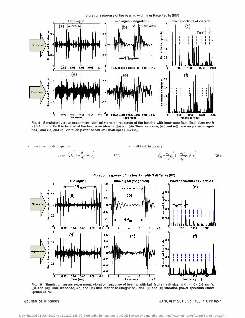
• case frequency

fcage =fr

2�1 −

db

dpcos �� 29�

Here n is the number of balls, fr is the rotor frequency, db is theall diameter, dp is the bearing pitch diameter, and � is the contactngle, which is zero for radial bearings. Given fr=35 Hz, for theearing of Table 1, the bearing frequencies are

f IRF = 189.28 Hz, fORF = 125.72 Hz, fBF

= 166.32 Hz, fcage = 13.96 Hz

igure 9�a� contains simulated vibration signals of accelerationersus time for IRF. Here, fault impact signals are modulated withotor frequency fr because the inner race fault, fixed on the innerace, passes through the load zone at a rate of fr as the inner raceotates. Similar behavior with the same frequency is observed inhe corresponding experimental signals shown in Fig. 9�d�. The

agnified portion of vibration signal plotted in Fig. 9�b� showshe fundamental fault frequencies of the bearing, which is con-rmed by the experiments in Fig. 9�e�. As the IRF passes through

he contact, two impact responses appear in the vibration signal.he fault model of Fig. 3 suggests that the leading and trailingdges of the surface profile dent would cause impacts with thealls in the load zone. The distance between these two impactignals contains information on the size faults. Figures 9�c� and�f� present power spectrum of the vibration signals. Dependingn the frequency range, harmonics of the fault frequencies �indi-ated by dashed lines� might appear in the power spectrum.

Figure 10 shows the vibration signals of a bearing with a singleF. Fault impact signals spaced by the fault frequency timing

1 / fBF� are clearly observed in both simulation and experimentalata. Also, simulated signals are modulated by the cage frequency

fcage. However, in real bearings, three dimensional rotations ofalls can prevent engaging of ball faults with races, causing ran-

Fig. 11 Simulation versus experiment: vibration responÃ1.0 mm2

…. „„a… and „d…… Time response, „„b… and „e…… tispectrum „shaft speed: 35 Hz…

omness in measured signals. This phenomenon generates random

11102-8 / Vol. 133, JANUARY 2011


modulations of vibration signals �see Fig. 10�d��, which can beused to separate ball faults from other types of bearing faults.Another vibration signal feature that agrees with experiments isshape of the impact signals, as shown in Figs. 10�b� and 10�e�. Asshown in the magnified plots, vibration signals due to BF consistof a single impact response signal for each fault, compared withthe IRF and ORF that generate two impacts. The power spectrumof simulated signals �Fig. 10�c�� reveals harmonics of the faultfrequency, which are not very clear in measured signals becauseof three dimensional motions of balls.

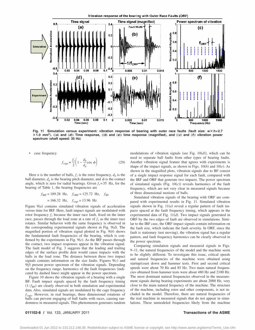
Simulated vibration signals of the bearing with ORF are com-pared with experimental results in Fig. 11. Simulated vibrationsignals shown in Fig. 11�a� reveal a regular pattern of fault im-pacts spaced at the fault frequency timing, which appears in theexperimental data of Fig. 11�d�. Two impact signals generated inORF by the two edges of fault are observed in simulations. Simi-lar to the IRF case, the ORF impact signals contain information onthe fault size, which indicate the fault severity. In ORF, since thefault is stationary �not moving�, the vibration signal has a regularpattern, and fault frequency harmonics can be clearly observed inthe power spectrum.

Comparing simulation signals and measured signals in Figs.9–11, the natural frequencies of the model and the machine seemto be slightly different. To investigate this issue, critical speedsand natural frequencies of the machine were obtained usingstartup/coast down and hammer tests. First and second criticalspeeds were about 70 Hz and 85 Hz. Two main natural frequen-cies obtained from hammer tests were about 480 Hz and 2100 Hz.The most dominant natural frequencies observed in the measure-ment signals during bearing experiments are about 2000 Hz, veryclose to the main natural frequency of the machine. The structureof the machine, including rotor and other components, is not in-cluded in the model. Therefore, there are natural frequencies ofthe real machine in measured signals that do not appear in simu-

of bearing with outer race faults „fault size: wÃh=2.7response „magnified…, and „„c… and „f…… vibration power

seme

lations. These unmodeled frequencies likely from the machine



fic

estfiarnaiw

fsmbtc

FTrc

J

Dow

rame, bearing housing, rotating shaft, couplings, etc., can be eas-ly considered in the model by appended submodels of machineomponents to the bond graph model.

Simulations suggest that information on type and size of faultsxist in the vibration signals from the bearing. However, the realystem has numerous natural frequencies not in the bearing modelhat might mask the original spikes from faults. Tools such as highrequency filters might remove masking signals and retrieve faultnformation in the real system. Also, factors such as imbalancend misalignments can alter the regular patterns of the faults in aeal machine. Interpreting the pattern of damage in real faultseeds more than one snapshot of the signal and some statisticalnalysis to determine the confidence level of the results. This needs more critical in the case of ball faults and inner race faults, inhich faults are moving.The model includes centrifugal forces on balls. To illustrate this

acet, a roller bearing with zero clearance under radial load wasimulated for different shaft speeds. Bearing radial deflections al-ost overlay data of Harris �35� in Fig. 12. The quadratic relation

etween radial deflections and shaft speed in Fig. 12 representshe centrifugal effects in the bearing. The centrifugal force in-reases quadratically with the orbital speed of balls, which in-

ig. 12 Radial deflection versus speed for a roller bearing.he centrifugal force on rollers increases contact loads andadial deflections when shaft speed increases. Simulations areompared with the results of Harris †35‡.

Fig. 13 Vibration response of a bearing with IRF fo2
Ã0.71 „level II…, 2.82Ã1.41 „level I… „mm …, and fr=35 H
ournal of Tribology


creases the contact force and bearing radial deflections. Centrifu-gal effects mainly appear at high speeds and are not significant atlow speeds.

5.3 Fault Severity Test. A model-based diagnostic employs amodel to detect and assess faults, by estimating parameters in themodel associated with faults. Therefore, a parametric study isneeded. Here the effects of type �IRF, BF, and ORF�, size �w�h�, and shape of the fault on vibration responses are studied.Referring to Table 2, faults in three levels corresponding to dif-ferent sizes of w�h are simulated and shown in Figs. 13–15 forIRF, BF, and ORF, respectively. In time waveform and frequencysignals, fundamental fault frequencies �f IRF,FBF,FORF� for alltypes of faults, cage frequency fcage for BF, and rotor frequency frfor IRF are observed. More severe faults with bigger defect sizesgenerate impact with higher amplitudes, for all types of faults. InIRF and ORF cases, vibration signals have a fault-element impactwaveform characterized by two distinct peaks, with distance be-tween these peaks proportional to the fault width, as shown inFigs. 13�b�, 13�e�, and 13�h� and Figs. 15�b�, 15�e�, and 15�h�.However, in the case of BF as shown in Fig. 14, the fault size onlyaffects impact amplitudes rather than the distance between twoimpact peaks.

To investigate the effect of fault shapes on the vibration re-sponse, faults with different size ratios �w /h=5,2 ,1� were simu-lated and results are shown in Fig. 16. For IRF and ORF, increas-ing the fault size ratio w /h enlarges the distance between the twoimpact peaks but does not change the impact amplitude much. ForBF, the vibration response is relatively insensitive to w /h.

To understand dynamics of the contact with faults, detailedsimulations of contacts in the presence of BFs are shown in Fig.17. The contact is within the load zone, but once the fault passesthrough the contact, nonlinear dynamic interactions can inducetransient surface separations. Figures 17�a� and 17�b� show con-tact displacements �solid line� and forces �dashed line� for thecontacts between inner race balls and outer race balls, for BFbetween inner race and ball. Negative force and displacementsdenote compression. Positive displacements denote surface sepa-rations, leading to zero forces. As shown in Fig. 17�a�, the innerrace does not touch the bottom surface of the fault, and ball-raceseparation occurs until the inner race surface hits the trailing cor-ner of the fault, causing the main impact. During this time, asshown in Fig. 17�b� at about 45.1 ms, the contact between ball andouter race unloads, which momentarily separate the surfaces. Justbefore 45.2 ms, a fault impact shock reloads the contact. These

ifferent fault severities: wÃh=1Ã0.5 „level I…, 1.42
r d z
JANUARY 2011, Vol. 133 / 011102-9


0

Dow

Fig. 14 Vibration response of a bearing with BFs for different fault severities: wÃh=1Ã0.5 „level I…, 1.42Ã0.71 „level II…, 2.82Ã1.41 „level I… „mm2

…, and f =35 Hz
r
Fig. 15 Vibration response of a bearing with ORF for different fault severities: wÃh=1Ã0.5 „level I…,2
1.42Ã0.71 „level II…, 2.82Ã1.41 „level I… „mm …, and fr=35 Hz
NormalizedAcceleration

Fig. 16 Vibration responses of faulty bearings „IRF, BF, and ORF… with
different fault shapes, fr=35 Hz
11102-10 / Vol. 133, JANUARY 2011 Transactions of the ASME

nloaded 01 Jun 2012 to 210.212.148.38. Redistribution subject to ASME license or copyright; see http://www.asme.org/terms/Terms_Use.cfm

nfF

6

tcNbtkwvplmpdtop

mbsttmm

N

T

J

Dow

onlinear contact dynamics generate fault impulses, which trans-erred through elements, and generate vibrations, as observed inig. 17�c�.

Summary and ConclusionsA detailed model of rolling element bearings developed in vec-

or bond graphs incorporated multibody dynamics of elements,entrifugal effects, dynamics of contacts, and surface defects.ewton–Euler’s equations for each element were encoded intoond graphs, with dynamics of contacts, traction forces, and rota-ional frictions formulated as constitutive laws of elements. Ainematics-based fault model was introduced. Tribological faultsere modeled as surface profile changes, which generate impulsesia dynamic interactions of faults and bearing elements. Faultarameters define type, size, shape, and locations of faults. Simu-ations for different clearances and radial loads show ability of the

odel to incorporate load zone effects in vibration signals. Ex-eriments for healthy and faulty rolling element bearings vali-ated the model. A parametric study investigated the effects ofype, size, and shape of faults on vibration responses. Dynamicsf contacts under faults demonstrated how fault impulses arehysically generated.

The modular and generic rolling element bearing bond graphodel represent complex dynamics of both normal and defective

earings, for rolling element bearings with different geometry andpecifications. With physical and kinematic parameters assignedo faults, the model can predict bearing response for fault condi-ions, and thus be used in model-based diagnostics of rolling ele-

ent bearings, for information processing necessary for predictiveaintenance of machinery.

omenclatureCS � bearing static load ratingE � modulus of elasticityFi � external force vector acting on the bodyFS � static equivalent load

Fx ,Fy ,Fr ,Fa � forces in x, y, radial, and axial directions,respectively

F� � curvature differenceJ � body rotational inertia matrix

M � body mass matrixT � coordinate transformation matrix

TGB � transformation matrix from the global to thebody coordinate

Tf � rotational resistive torqueTf � fault type indicators �1: IRF, 2: BF, 3:ORF�

load ,Tlub ,Tseal� resistive torques due to contact deformations,lubrications, and rubbing seal

XYZ � global fixed coordinateb � contact damping factor

db � balls diameter

Fig. 17 Faults in rolling element generate imForce and displacement at inner race-ball contcontact, and „c… outer race vibration „ball faulball contact, fr=35 Hz….

dp � bearing pitch diameter

ournal of Tribology


fr � bearing rotational speed in rpmrf � fault size ratiov0 � kinematic viscosity of the lubricantK � contact stiffnessk � equivalent linear stiffness of the bearingn � number of balls in the rolling element bearingr � radius of curvaturer � position vector with respect to the body

coordinates � contact slide-roll ratiox � body position vector with respect to the global

coordinatexiyizi � moving coordinate associated with the body i

xijyijzij � moving contact coordinate between bodies iand j

v � Poisson’s ratiow ,h � width and depth of localized faults

� oil film parameter which is a function of oilfilm thickness

�ij � orientation of the contact coordinate describedin the global coordinate

� f � angular position of the fault defined in bodycoordinate

�� dimensionless deflection factor� � body angular position vector�i � orientation of the body coordinate described in

the global coordinate� � friction coefficient

�bd ,�hd � � under boundary lubrication and hydrody-namic lubrication modes

� � curvature� � external torque vector acting on the body� � bearing contact angle¯ � bar accent assigned to vectors described in the

body coordinate system

References�1� Raison, B., Rostaing, G., Butscher, O., and Maroni, C. S., 2002, “Investiga-

tions of Algorithms for Bearing Fault Detection in Induction Drives,”IECON02, pp. 1696–1701.

�2� Nakhaeinejad, M., and Bryant, M. D., 2010, “Multibody Dynamics of RollingElement Bearings With Faults,” Proceedings of the ASME/STLE InternationalJoint Tribology Conference 2009, pp. 249–251.

�3� Isermann, R., and Balle, P., 1997, “Trends in the Application of Model-BasedFault Detection and Diagnosis of Technical Processes,” Control Eng. Pract.,5�5�, pp. 709–719.

�4� Purdue University, 2003, “Virtual Machine Design Workshop—Defining theRequirements for the Next Generation of Analytical Software for the Design ofRotating Components,” Technical Report.

�5� Jones, A. B., 1960, “A General Theory for Elastically Constrained Ball andRoller Bearing Under Arbitrary Load and Speed Conditions,” ASME J. BasicEng., 82�21�, pp. 309–320.

�6� Gupta, P. K., 1979, “Dynamics of Rolling-Element Bearings.1. CylindricalRoller Bearing Analysis,” Mech. Eng. �Am. Soc. Mech. Eng.�, 101�1�, pp.

ts, which can cause contact separations. „a…, „b… force and displacement at ball-outer raceÃh=1.42Ã0.71 mm2 engaged at inner race-

pacactt: w

95–96.

JANUARY 2011, Vol. 133 / 011102-11


0

Dow

�7� McFadden, P. D., and Smith, J. D., 1984, “Vibration Monitoring of RollingElement Bearings by the High-Frequency Resonance Technique—A Review,”Tribol. Int., 17�1�, pp. 3–10.

�8� Afshari, N., and Loparo, K. A., 1998, “A Model-Based Technique for the FaultDetection of Rolling Element Bearings Using Detection Filter Design andSliding Mode Technique,” Proceedings of the 37th IEEE Conference on De-cision and Control, Vols. 1–4, pp. 2593–2598.

�9� Adams, M. L., 2010, “Rotating Machinery Vibration: From Analysis toTroubleshooting,” 2nd ed., CRC Press, Boca Raton, FL.

�10� Harsha, S. P., 2006, “Nonlinear Dynamic Analysis of Rolling Element Bear-ings Due to Cage Run-Out and Number of Balls,” J. Sound Vib., 289�1–2�,pp. 360–381.

�11� El-Saeidy, F. M. A., and Sticher, F., 2010, “Dynamics of a Rigid Rotor Linear/Nonlinear Bearings System Subject to Rotating Unbalance and Base Excita-tions,” J. Vib. Control, 16�3�, pp. 403–438.

�12� Liew, A., Feng, N., and Hahn, E. J., 2002, “Transient Rotordynamic Modelingof Rolling Element Bearing Systems,” ASME J. Eng. Gas Turbines Power,124�4�, pp. 984–991.

�13� Sopanen, J., and Mikkola, A., 2003, “Dynamic Model of a Deep-Groove BallBearing Including Localized and Distributed Defects. Part 1: Theory,” Pro-ceedings of the Institution of Mechanical Engineers Part K-Journal of Multi-Body Dynamics, 217�3�, pp. 201–211.

�14� Sopanen, J., and Mikkola, A., 2003, “Dynamic Model of a Deep-Groove BallBearing Including Localized and Distributed Defects. Part 2: Implementationand Results,” Proceedings of the Institution of Mechanical Engineers PartK-Journal of Multi-Body Dynamics, 217�3�, pp. 213–223.

�15� Jang, G., and Jeong, S. W., 2004, “Vibration Analysis of a Rotating SystemDue to the Effect of Ball Bearing Waviness,” J. Sound Vib., 269�3–5�, pp.709–726.

�16� Changqing, B., and Qingyu, X., 2006, “Dynamic Model of Ball Bearings WithInternal Clearance and Waviness,” J. Sound Vib., 294�1–2�, pp. 23–48.

�17� Patil, M. S., Mathew, J., Rajendrakumar, P. K., and Desai, S., 2010, “A The-oretical Model to Predict the Effect of Localized Defect on Vibrations Asso-ciated With Ball Bearing,” Int. J. Mech. Sci., 52�9�, pp. 1193–1201.

�18� Wensing, J. A., 1998, “Dynamic Behaviour of Ball Bearings on Vibration TestSpindles,” IMAC, Proceedings of the 16th International Modal Analysis Con-ference, pp. 788–794.

�19� Sassi, S., Badri, B., and Thomas, M., 2007, “A Numerical Model to PredictDamaged Bearing Vibrations,” J. Vib. Control, 13�11�, pp. 1603–1628.

�20� Karkkainen, A., Helfert, M., Aeschlimann, B., and Mikkola, A., 2008, “Dy-

11102-12 / Vol. 133, JANUARY 2011


namic Analysis of Rotor System With Misaligned Retainer Bearings,” ASMEJ. Tribol., 130�2�, p. 021102.

�21� Ashtekar, A., Sadeghi, F., and Stacke, L. E., 2008, “A New Approach toModeling Surface Defects in Bearing Dynamics Simulations,” ASME J. Tri-bol., 130�4�, pp. 041103.

�22� Ashtekar, A., Sadeghi, F., and Stacke, L. E., 2010, “Surface Defects Effects onBearing Dynamics,” Proc. Inst. Mech. Eng., Part J: J. Eng. Tribol., 224, pp.25–35.

�23� Bhattacharyya, K., and Mukherjee, A., 2006, “Modeling and Simulation ofCenterless Grinding of Ball Bearings,” Simul. Model. Pract. Theory, 14�7�,pp. 971–988.

�24� Nakhaeinejad, M., Lee, S. H., and Bryant, M. D., 2010, “Finite Element BondGraphs of Rotors,” Proceeding of Ninth International Conference on BondGraph Modeling & Simulation �ICBGM’ 2010�, Vol. 42, Issue No. 2, pp.164–171.

�25� Harris, T., and Kotzalas, M., 2007, Essential Concepts of Bearing Technology,Taylor & Francis, Boca Raton, FL.

�26� Aktürk, N., Uneeb, M., and Gohar, R., 1997, “The Effects of Number of Ballsand Preload on Vibrations Associated With Ball Bearings,” ASME J. Tribol.,119�4�, pp. 747–753.

�27� Kramer, E., 1993, Dynamics of Rotors and Foundations, Springer, Berlin.�28� Kragselsky, V., Dobychin, N., and Kombalov, S., 1982, Friction and Wear:

Calculated Methods, Pergamon, Elmsford, NY.�29� Gupta, P., 1984, Advanced Dynamic of Rolling Elements, Springer-Verlag,

New York.�30� Palmgren, A., 1959, Ball and Roller Bearing Engineering, SKF Industries,

Inc., Philadelphia.�31� Shin, H., 2004, “Bearing Diagnosis Using Embedded Modeling Method and

System Identification Technique,” Ph.D. thesis, Rensselaer Polytechnic Insti-tute, Troy, NY.

�32� Paynter, H. M., 1961, Analysis and Design of Engineering Systems, MIT,Cambridge, MA.

�33� Karnopp, D. C., Margolis, D. L., and Rosenberg, R. C., 2000, System Dynam-ics: Modeling and Simulation of Mechatronic System, Wiley, New York.

�34� Sinokrot, T., Nakhaeinejad, M., and Shabana, A. A., 2008, “A Velocity Trans-formation Method for the Nonlinear Dynamic Simulation of Railroad VehicleSystems,” Nonlinear Dyn., 51�1–2�, pp. 289–307.

�35� Harris, T., and Kotzalas, M., 2007, Advanced Concepts of Bearing Technology,
Taylor & Francis, Boca Raton, FL.


Dynamic Modeling of Rolling Element Bearings With Surface ... · each element of the rolling...

Documents

Transcript of Dynamic Modeling of Rolling Element Bearings With Surface ... · each element of the rolling...