Dynamic Load Evaluation of Large Dimensioned Casing ... · bottom plug landed on the float collar...
69
Dynamic Load Evaluation of Large Dimensioned Casing Strings at Primary Cementing Master Thesis Author: Volker Jedlitschka Mining University Leoben Chair for Drilling Engineering in cooperation with OMV Industry Advisor University Advisor DI Markus Doschek Univ.-Prof. DI Dr.mont. Gerhard Thonhauser
Transcript of Dynamic Load Evaluation of Large Dimensioned Casing ... · bottom plug landed on the float collar...

Dynamic Load Evaluation of
Large Dimensioned Casing
Strings at Primary Cementing
Master Thesis
Author Volker Jedlitschka
Mining University Leoben
Chair for Drilling Engineering
in cooperation with OMV
Industry Advisor University Advisor
DI Markus Doschek Univ-Prof DI Drmont Gerhard Thonhauser
I declare in lieu of oath that I did this
Masterrsquos thesis in hand by myself using only
literature cited at the end of this volume
______________________________________
Volker Jedlitschka Leoben in March 2007
Table of Contents
1 Acknowledgements 7
2 Zusammenfassung 8
3 Abstract 9
4 Introduction 10
5 Cementing 16rdquo Casing at MQE-1 11
6 Free Falling Cement 15
7 Water Hammer Effect 16 71 What is a Water-Hammer 16 72 Rough Estimation after Budau 16 73 The Elastic Liquid Column 18
731 Pressure Wave 18 732 Pressure and Fluid Velocity Distribution 19 733 Speed of Sound Determination 24 734 Dampening of the pressure waves 27
74 Transients in Horizontal Pipes 29 75 Transients in Vertical Pipes 31 76 Measuring of Pressure Waves 33
8 Water Hammer Simulation 34 81 Simulation with ldquoFluentrdquo 34 82 Simulation with ldquoWanda 3rdquo 36
9 Simulation of Water Hammer at MQE-1 41 91 Defining Boundary Conditions 41
911 U-Tube 41 912 Bonds 42 913 Float Collar 42 914 Free Falling Zone 42 915 Simulation Depth 43 916 Different Phases 43 917 Bulk Modulus 44 918 Cavitation Pressure 45
92 Simulation Execution 45 93 Simulation Results 48 94 Analysis ndash Impact of Different Parameters 55
941 Friction Force 55 942 Fluid Velocity Fluid Density 57 943 Speed of Sound 57
10 Limits of Different Casing Sizes 65
11 Conclusion 67
10 References 69
4
List of Figures
Figure 1 Casing with landing collar lowered into the wellbore 13
Figure 2 Slurry is pumped between top and bottom plug 13
Figure 3 Top plug lands on bottom plug cement job is done 13
Figure 4 Top and bottom plug with float collar 14
Figure 5 Situation when the water hammer possibly occurred 14
Figure 6 Relation between closing time and impact force according Budau 17
Figure 7 Schematic illustration according Budau4 17
Figure 8 Fluid Compression 6 18
Figure 9 Movement of molecules in a harmonic sound wave7 19
Figure 10 Pressure and velocity sequence before the valve4 21
Figure 11 Pressure and velocity sequence behind the valve4 22
Figure 12 Pressure and velocity distribution along the whole pipe4 23
Figure 13 Piston in a liquid filled pipe7 25
Figure 14 Water hammer measured on a quick-acting valve 28
Figure 15 Pressure sequence caused by water hammer in horizontal pipe 30
Figure 16 Water hammer effect behind the valve 31
Figure 17 Total pressure across the valve 31
Figure 18 Pressure sequence at the valve simulated in vertical pipe 32
Figure 19 Pressure sequence behind the valve simulated in vertical pipe 32
Figure 20 Total pressure across the valve in vertical pipe 33
Figure 21 Pressure pulse set up for a pipeline 33
Figure 23 Pressure distribution along the pipe 35
Figure 24 Velocity distribution caused by the water hammer 35
Figure 25 Pressure distribution after valve has closed 36
Figure 26 Wanda operating windows 38
Figure 27 Pressure wave causes change in fluid velocity 38
5
Figure 28 Pressure wave is generated fluid still enters pipe 39
Figure 29 Pressure wave propagates towards the inlet zero fluid velocity behind the wave front39
Figure 30 Wave front has reached inlet zero fluid velocity along the pipe 40
Figure 31 Pressure wave was reflected fluid exits pipe through the inlet 40
Figure 32 Adaption of the plug cementation to the simulation program 41
Figure 33 Free falling evaluation with OptiCem 43
Figure 34 Fluid compression due to external pressure11
44
Figure 35 Fluid properties windows casing fluid on the left annular fluid on the right 47
Figure 36 Input Panel for pipe and valve properties 48
Figure 37 Water hammer effect calculated by Wanda 49
Figure 38 Pressure data transferred into Excel 49
Figure 39 Water hammer effect behind the valve causes a negative pressure wave first 50
Figure 40 Load at the casing 51
Figure 41 Overlapping of the transient data 51
Figure 42 Decreasing Δp acting on the casing 52
Figure 43 Zoom in of figure 40 52
Figure 44 Discharge rate at the casing bond 53
Figure 45 Discharge rate at annular bond 54
Figure 46 Linear pressure increase due to friction force 55
Figure 47 Different bulk moduli affect the slope at the pressure peaks 56
Figure 48 Linear pressure increase on top of pressure peak 56
Figure 49 Water hammer simulated with higher fluid velocity 57
Figure 50 Pipe dimension test 19 (L=400m ID=200mm) 60
Figure 51 Pipe dimension test 29 (L=400m ID=400mm) 60
Figure 52 Pipe dimension test 39 (L=400m ID=600m) 60
Figure 53 Pipe dimension test 49 (L=600m ID=200mm) 61
Figure 54 Pipe dimension test 59 (L=600 ID=400mm) 61
Figure 55 Pipe dimension test 69 (L=600m ID=600mm) 61
Figure 56 Pipe dimension test 79 (L=800m ID=200mm) 62
6
Figure 57 Pipe dimension test 89 (L=800m ID=600mm) 62
Figure 58 Pipe dimension test 99 (L=800m ID=600mm) 62
Figure 59 Pipe dimension test regarding wall thickness 63
Figure 60 Water hammer effect if the well would have been 10000m deep 64
Figure 61 Tendency of the critical flow rate for several casings at certain depths 66
Figure 62 Δp caused by water hammer acting an the casing 67
7
1 Acknowledgements
The author would like to thank Univ-Prof DI Drmont Gerhard THONHAUSER and DI Hermann F SPOumlRKER for their permission to write this thesis Special thanks to DI Markus DOSCHEK from OMV and DI Drtechn Dominik MAYR from the Technical University Graz Austria for their excellent support and valuable comments during preparation of this thesis
Strong appreciation also goes to the institute for hydraulic engineering and water resources management at the Technical University Graz which enabled and supported the simulation with ldquoWandardquo Also thanks to Stefan FUHRMANN Halliburton Company Austria who enabled the use of OPTICEM Simulator and thus provided valuable information for this investigation
8
2 Zusammenfassung
In dieser Diplomarbeit wurde eine Plug-Zementation eines 16 Casing Stranges untersucht bei
der die 2440m lange Verrohrung leck wurde Die Ursache dafuumlr ist ungeklaumlrt jedoch vermutet
man dass ein sogenannter Wasserschlag den Casing beschaumldigte Es wird angenommen
dass der Bottom-Plug das Ruumlckschlagventil in der Landeplatte blockiert hat wodurch die
Zementsaumlule zum abrupten Stillstand gekommen ist In dieser Arbeit wird untersucht ob die
Belastung die durch einen eventuellen Wasserschlag hervorgerufen wurde ausreichen wuumlrde
um eine 16ldquo Verrohrung zu beschaumldigen
Es konnte festgestellt werden dass eine maximale Belastung der Verrohrung von 6153 bar
aufgetreten ist von denen jedoch nur 112 bar auf das Phaumlnomen des Wasserschlages
zuruumlckzufuumlhren sind Diese maximale Belastung ist nicht ausreichend um den 16ldquo Casing zu
beschaumldigen
Weiters wuumlrde nachgewiesen dass im Falle eines Wasserschlages ein groumlszligerer
Rohrdurchmesser nicht zu einer houmlheren Belastung fuumlhrt sondern das Verhaumlltnis
Innendurchmesser (D) zu Wandstaumlrke (t) entscheidend ist Generell fuumlhrt ein groumlszligeres Dt
Verhaumlltnis zu einer Reduktion des Wasserschlages
Fuumlr uumlblich verwendete Casing Groumlszligen wuumlrde im Zuge dieser Arbeit festgestellt dass groumlszligere
weniger gefaumlhrdet sind auf Grund der Belastung eines Wasserschlages zu gebrechen Diese
Tendenz konnte fuumlr verschiedene Laumlngen festgestellt werden
Die Ergebnisse dieser Arbeit wuumlrden mit Hilfe des Simulationsprogrammes Wanda 3 ermittelt
9
3 Abstract
In this thesis a plug cementation of a 16 casing string is investigated What happened was that
during primary cementing of a 16 casing string at a depth of 2440m the string failed It was
assumed that the bottom plug plugged the float valve and thus the cement column was
immediately stopped on its way downhole The phenomenon when fluid flow is immediately
stopped is called ldquowater hammer-effectrdquo Task was to investigate if this water hammer effect
caused a sufficient high load to damage the casing string
It could be figured out that the string faced a maximum load of 6153bar but out of this only
113bar were generated by the water hammer The remaining 503bar were caused due to the
hydrostatic difference between the annulus filled with mud and the casing filled with cement It
is obvious that the calculated load was not sufficient to harm the casing string
Further it could be proved that a larger casing diameter does not compulsorily increase the
impact of a water hammer Concerning pipe dimensions the ratio between wall thickness and
inner diameter is decisive General can be said that a higher Dt ratio reduces the water
hammer impact
Concerning commonly used casing dimensions it could be proved for different lengths that
larger casings are less endangered to fail due to the load caused by a water hammer
The whole study is supported with a simulation software called Wanda 3
10
4 Introduction
Decisive for the topic of this thesis was a certain failure at an OMV well drilled in 2005 What happened was that during primary cementing of a 16rdquo casing string at a depth of 2440m the string failed The reason for this failure is not clear but a certain theory is investigated in this thesis It is assumed that the bottom plug plugged the float valve at the landing collar which caused the moving cement column to be stopped immediately The phenomenon when fluid flow within a pipe is suddenly stopped is called ldquowater hammerrdquo and can lead to significant pipe damage The author investigates the water hammer theory in case of the 16rdquo casing string This study is supported by several simulation programs as ldquoOptiCemrdquo ldquoFluentrdquo and ldquoWandardquo All parameters that influence this water hammer phenomenon are discussed and different casing dimensions are investigated to this effect After a detailed explanation of the occurrences during cementing operations the free falling cement phenomenon is shortly explained and followed by chapters with detailed investigations Task is to find out if the impact of a possible water hammer would be sufficient high to damage the 16rdquo casing string
11
5 Cementing 16rdquo Casing at MQE-1
The 18-12rdquo hole section was drilled to the desired depth of 2444m and the 2440m casing string could be landed with a mandrel hanger into the wellhead with full string weight of 300tons which was indication for a well shaped bore hole without significant drag For the cementing operation two 2rdquo lines from the cement pump to the cementing head where installed The operation was a plug cementation In Figures1-3 this type of cementation is schematically illustrated and in figure 4 a pair of plugs is shown The red plug (bottom plug) is loaded afterwards the black one (top plug) The cementation started by pumping 16m
3 of spacer (105kgl) before the bottom plug was
loaded 136m3 of lead cement (15kgl) and 127m
3 tail slurry (19kgl) followed As the
bottom plug landed on the float collar in time a sudden increase in pump pressure to 120bar was observed An abrupt pressure drop followed and circulation could be regained At this point it was assumed that the pressure peak was caused by the membrane in the bottom plug which normally bursts at a small pressure difference (3-7bar) It was supposed that the cement was now displaced into the annulus as usual passing by float collar and casing shoe At a successful plug cementation the top plug moves downhole and when it reaches the bottom plug a pressure increase is observed at surface because the mud is pumped into a closed system The top plug upon the bottom plug closes the system and usually at this point of time the job is done At OMVrsquos well this expected pressure increase was detected a bit earlier as expected At next the pumps were stopped and it was attempted to re-bump the plug By doing so continuous circulation could be established with return rates and pressure values similar as before A continuous pressure increase could be recorded while the displacement process was continued It has to be mentioned that the displacement was performed with the rig pumps and the pump efficiency was picked wrong as post-analysis had proven As the risk of overdisplacement was given a close look to the mud returns from annulus were taken and unplanned spacer returns have been detected It was planned that spacer and cement will not reach surface The displacement process was stopped by shut-off the pumps and the pressure was released Then the return valve on the pump was opened to check if mud was returning from the casing If the system is tight this should not be the case and the pressure at surface should be zero At this point normally the hydrostatic is the only pressure acting inside the casing after the top plug was landed and the pump pressure is released However mud returned when the return valve at the pump was opened This was an indication that some flow from the annulus entered the casing somewhere downhole It has to be mentioned that a double valve float shoe and a single valve float collar where installed Theoretically two possible scenarios could have been happening Either all three float valves failed or the casing itself became leak At this point it was decided by on-site personnel to attempt displacing the full cement volume back to surface to potentially be able to pull the 16rdquo casing again While further circulating communication was established with the operations office and it was decided not to displace the cement out of the annulus but let as much slurry as possible flow back (natural flow direction was from the annulus into the casing) Indeed the over displaced fluid was able to flow back into the casing string with remarkable returns at surface from inner casing This was an indication for a large leakage or an even parted casing string But after several barrel of return the flow stopped and cement hardening phase started The next step was to examine the tightness of the casing string by running a packer Step by step the packer was lowered and pressure tests were executed Actually below deepest packer setting depth close to the landing collar a leakage could be detected However the packer became stuck close to the landing collar and could not be retrieved any more More and more it seemed that the string had in fact been parted It was decided to go on with a sidetrack because further examination could not change the situation on site After these occurrences the casing manufacturer was inspected by a third party However no lack in quality at the manufacturing process was discovered
12
Analyzing of what happened and searching for explanations the water hammer-theory came up which is graphically illustrated in Figure 5 This theory is based on the assumption that the bottom plug somehow plugged the float valve of the landing collar This can happen either that the membrane of the plug did not burst or the plug faced so much ware on its way downhole that it parted and some rubber elements plugged the valve Theoretically a water hammer could lead to casing burst or slippage of an improper made up casing connection
13
Landing Collar
Casing
Casing Shoe
Back Pressure
Valve
Figure 1 Casing with landing collar lowered into the wellbore
Back Pressure
Valve
Bottom Plug
Top Plug
Cement
Landing Collar
Figure 2 Slurry is pumped between top and bottom plug
Closed System
Figure 3 Top plug lands on bottom plug cement job is done
14
Figure 4 Top and bottom plug with float collar
Depth of
Investigation
Figure 5 Situation when the water hammer possibly occurred
15
6 Free Falling Cement
Before discussing the water hammer effect the free falling cement phenomenon should be contemplated and well understood which also occurred during the plug cementation of the 16rdquo casing It is introduced in this chapter Generally can be said that while cementing we have to deal with several fluids of different densities the initial mud a pre-flush a spacer various densities of cement slurries and at the end some mud again Normally the cement slurry has a higher density as all other fluids pumped into the hole During the cementing process after the plugs are loaded and pumping the cement is started a heavier fluid column is placed above a lighter one Besides the pump pressure this density difference causes an additional driving force due to gravity As pumping continues the cement column gets heavier and might start to speed up on its way downhole Due to its acceleration it loses contact with the surface pump rate This happens if the total friction pressure is exceeded by the hydrostatic pressure difference between the fluid column inside the casing and the fluid column in the annulus
1 These
conditions in the wellbore lead to a phenomenon called ldquofree falling cementrdquo This free falling period of the cement has several consequences and is highly influenced by differences in fluid densities and depth It causes a negative absolute well head pressure which lead to a discontinuous zone between the well head and the free falling column
1
This means the fluids do not occupy the entire pipe diameter any more The free falling cement phenomenon was quite detailed investigated by Beirute
2 in 1987
and by Spoumlrker1 in 1993 In several field studies and simulation runs Spoumlrker analyzed the
cementing head pressures pump rates and return rates versus time and could exactly define when free falling actually occurs and how long this period lasts Spoumlrker monitored that when the well head pressure drops during the cement job the annular return rates exceed the pump rates That means more fluid returns from the annulus as it is pumped into the well Now the free falling period has started Further more it was observed by Spoumlrker that towards the end of the job the situation reverses and it seems that a lost circulation condition occurs At this time when the cement enters the annulus through the casing shoe the fluids create their own equilibrium between friction and hydrostatic forces
1This is called U-tubing As pumping continues this equilibrium will never be a static
one but pump rates have no longer influence on the fluid velocity Concerning the displacement process in the annulus during the cementation job the free falling period itself does not matter that much What matters is that the slow movement of the slurry in the annulus during the later stages avoids satisfying displacement as displacement efficiency is a function of the displacing fluid velocity
1
For this study it is important to understand the free falling phenomenon not because of the displacement efficiency but with regard to the fluid velocities within the pipe
16
7 Water Hammer Effect
Since it is assumed that a kind of water-hammer effect could be the reason for the failure of the 16rdquo casing it is detailed investigated in this chapter
71 What is a Water-Hammer
Water hammer or hydraulic shock is a momentary increase in pressure and is the result of a sudden change in liquid velocity A water hammer usually occurs when a transfer system is quickly started stopped or is forced to make a rapid change in direction Following points are common reasons for a water hammer effect
Valve operations
Pumps switching on or off
Filling up of pipes
Irregular pumping (discontinuous suction of air) The primary cause of water hammer in process applications is the quick closing and opening of a valve A valve is defined as quick acting if it closes before a pressure wave is reflected back from upstream or down stream Symptoms include noise vibration and hammering pipe sounds which can lead to equipment damage A common example of a water hammer in most homes is simply turning off a shower quickly By doing so a thud through the house piping can eventually be recognized The magnitude of the water hammer is mainly influenced by the change of flow The quicker a valve is operated the higher the impact The generated shock wave (transient) is caused by the kinetic energy of the fluid in motion when it is forced to stop suddenly Moving water in a pipe has kinetic energy proportional to the mass of water in a given volume times the square of its velocity
3
kinetic energy = (mass x velocity
2)2
If the velocity becomes zero cause of such reasons mentioned above there is still energy left This energy changes in deformation energy and is transferred to the piping and the medium itself (liquid in this case) For this reason most pipe sizing charts recommend to keep the flow velocity below 15ms
3
72 Rough Estimation after Budau
This estimation considers a liquid column as a rigid body with the mass m 4 The
mechanics of rigid bodies tells us that a change in velocity of a mass causes a force F
dvm Fdt
If the velocity with the initial value of v0 changes to a final value of ve while the valve is closing the integration of Equation (2) delivers
0
0
T
em v m v F dt
In this relation the valve closing time is expressed with T In order to solve Equation (3) the function F(t) has to be known Strictly spoken this function can only be evaluated from the operating characteristic of a valve which describes the change in cross-sectional area
(2)
(1)
(34)
17
while closing For a rough approximation Budau suggests to use a quadratic relation between the force F and the time t (Figure 6)
4
Figure 6 Relation between closing time and impact force according Budau
In a F t - coordinate system the integral
0
T
F dt illustrates the area below the curve and
due to its parabolic shape it can be determined by following relation
max 0
0
2
3
T
eF dt F T m v m v
For a pipe with a length l and a cross sectional area A the mass of the liquid can be defined as
m A l
and from Equation (4)
0max
3 ( )
2
eA l v vF
T
can be evaluated
Figure 7 Schematic illustration according Budau4
(44)
(5)
(6)
18
Since maxmax
FP
A the maximum pressure according Budau is defined by
0max
3 ( )
2
el Q QP
A T
From Equation (7) can be seen that the pressure is higher the smaller Qe is and the shorter the closing time is A longer pipe also leads to a pressure increase However for Trarr0 it would mean that the pressure would become infinite high which is not valid in praxis
73 The Elastic Liquid Column
Considering the elasticity of a fluid column leads to a complete different calculation model which includes the wave character of a pressure change
4
By analyzing what exactly happens during such a water hammer it can be said that a column of liquid either horizontal or vertical acts like a train crashing into a rock side
5 The
back of the train continues forward even though the front can not go any further In Figure 8 fluid compression is illustrated
Figure 8 Fluid Compression
6
Since the water flow is restricted inside the pipe a shock wave travels backward the pipe deflecting everything in its path then forward and back again It is reflected at the open end of the pipe at a wall or at a closed end pipe By acting against the piping and valves very high forces are exerted The pressure wave immediately accelerates to the speed of sound 6
731 Pressure Wave
A pressure wave is nothing else as a sound wave A sound wave is a wave type propagation of pressure and density changes in an elastic medium as gas liquids or solids Pressure waves spread as longitudinal waves A density disturbance propagates by the
(74)
19
interaction between the molecules which oscillate parallel to the direction of expansion Oscillation means that the molecules stay at there place but move around their neutral position
7
Figure 9 shows the movement of air molecules in a harmonic sound wave a) Oscillation of the molecules from their state of equilibrium at a certain time point as a
function of distance The molecules at the points x1 and x3 stay in their state of equilibrium and those at x2 face maximum deflection
b) Some representative molecules in their state of equilibrium before the sound wave is going to deflect them The arrows show the direction of oscillation
c) Position of the molecules after the sound wave met them d) Density of air at this specific time point At the point x3 airrsquos density is at a maximum
and at point x1 at a minimum At both point the oscillation of the molecules is zero e) Change in pressure as a function of distance It can be seen that the pressure curve
(e) and the oscillation curve (a) have a phase difference of 90deg
Figure 9 Movement of molecules in a harmonic sound wave7
In pipes not only the elasticity of water but also the one of the pipe material influences the pressure wave velocity A pressure increase of the liquid column causes an enlargement of the pipe diameter Due to the internal pressure the pipe tends to expand This effect causes a slower wave spreading in pipes as in open water systems
7
732 Pressure and Fluid Velocity Distribution
The following description is illustrated in Figure 10
4 We consider a pipe which is at one
end connected to a bond with water and on the other end a valve is installed In steady state conditions water is flowing at velocity w0 At the time point t=0 the valve is closed
20
abruptly This causes the velocity directly in front of the valve to become 0 The inertia of the following water particles cause a pressure increase which leads to an enlargement of the pipe diameter at the same time This procedure now shifts with the speed of sound from the closed valve towards the pipe inlet The pressure wave reaches the bond at the time
Lta
In the bond the pressure wave is reflected at the liquid surface which is phase boundary to air In hydraulic engineering a liquid surface is considered as a body of infinite inertia This means for a pressure wave a liquid surface acts like a solid medium At this point of time when the wave is reflected an unbalanced situation at the transition zone between the cross sectional area of the pipe and the bond occurs In the pipe the velocity is zero but the pressure is higher as it is in the bond before the transition zone where it is determined by the liquid level inside The consequence of this situation is that the fluid starts to flow from the pipe into the bond From the higher pressurized area to the area with lower pressure Thereby the pressure energy again converts completely into kinetic energy again This procedure again transfers into the pipe and reaches the valve at
2 Lt
a
At this point of time an unbalanced situation occurs at the valve The fluid flow out of the pipe into the bond now causes a suction force at the valve because no more fluid can enter through the closed valve The suction force reduces the pressure which becomes smaller
as it was at steady state flowing conditions at time point 0t Due to the suction force the
pipe is compressed and therefore its diameter is reduced Again this procedure shifts at speed of sound along the pipe and reaches the bond at
3 Lt
a
The unbalanced situation now is characterised as the pressure in the bond is higher as it is in the pipe The conversion of the pressure energy creates again a fluid velocity w0 when the fluid enters the pipe The fluid front and the reflected pressure wave move towards the valve At the time
4 Lt
a
when the fluid reaches the valve with its velocity w0 the same physical state is obtained as
at 0t The described oscillation starts again from the beginning and lasts until the
energy is consumed by friction losses In the following Figures 10 to 12 the described pressure and velocity changes are illustrated Considering what is going on behind the valve a kind of reverse but similar procedure is valid The immediate interruption of fluid flow causes a negative pressure wave behind the valve and the pipe tends to shrink A negative pressure wave means that the pressure is smaller than at steady state conditions whereas it is termed ldquopositiverdquo when the pressure is higher The fluid velocity between the shifting wave and the valve is zero and between wave and the end of the pipe is still the initial w0 When the negative pressure wave reaches the end of the pipe at
Lta
the fluid velocity along the whole pipe is 0 The following process is the same as for the pipe section before the valve It can be noticed that when the water hammer occurs the valve has to withstand a positive pressure upstream and a negative one downstream at the same time
21
Figure 10 Pressure and velocity sequence before the valve4
22
Figure 11 Pressure and velocity sequence behind the valve4
23
Figure 12 Pressure and velocity distribution along the whole pipe4
24
733 Speed of Sound Determination
Pressure waves propagate at the speed of sound which is different in each medium The velocity [ms] of sound in liquids and gases can be determined by following equation
where ρ[kgm
3] is the density of the medium and K[Nm
2] the compression modulus For
liquids instead of K often the bulk modulus B is used but the meaning is the same The compression modulus can easily be explained Itrsquos the ratio between the pressure acting on a medium and its resulting volume change
pK
V V
The speed of sound in a massive stick which represents a special case is determined by replacing the compression modulus K in Equation (8) by Youngs modulus E For a massive stick it is assumed that its diameter is significant smaller than the wave length of sound
So it can be said that the speed of sound and so pressure wave velocity is dependent on media properties as density and compressibility Liquids and solids are relative incompressible therefore they have higher values for the compression modulus which is rather independent of temperature and pressure However gases are strongly compressible and their K-values are much smaller and highly dependent on temperature and pressure The reciprocal of the compression modulus is the compressibility
Equation (8) explains mathematically why the speed of sound in air is lower as it is in steel for example A higher denominator delivers a higher velocity In the table below values for certain media are listed These values are from experimental series only and therefore cannot be seen as exact Looking up these values one gets a different value for each literature source
K
E
1 V V
K p
(97)
(87)
(117)
(107)
25
Table 1 Speed of sound in different mediums8
The range in the table can also be explained easily from the physical side The speed of sound is determined by the elasticity and density of the specific medium Generally can be said that each medium is somehow compressible otherwise it would immediately decompose if any impulse is acting on it Pressure waves propagate through atoms or molecules and they oscillate around their neutral position which is a state of equilibrium
7
What propagates is not the medium itself but the state of movement of the molecules This state is described by energy and impulse Energy and impulse are transferred by the molecules as they bump against each other In steel molecules are arranged very close to each other in a rigid crystalline structure Any movement or change of the crystalline structure would afford high quantities of energy So the energy which faces the molecules is immediately transferred to its neighbors The short distance between the molecules and their stable arrangement are responsible for the high propagation velocity and rather small energy losses
Derivation of pressure wave velocity equation
A horizontal pipe filled with fluid of certain density is considered Figure 13 illustrates the device
Figure 13 Piston in a liquid filled pipe
7
The pipe includes a piston with a cross-sectional area A For a short moment (Δt) the piston is moved to the right which results in a fluid density increase at that point The
Air (20degC) 343 ms
Helium 981 ms
Water 1484 ms
Ice (-4degC) 1402 ms
Oil 1740 ms
Wood 3300 ms
Iron 5170 ms
Steel 5920 ms
Aluminium 6300 ms
Diamond 18000 ms
Wave front with velocity v
Fluid in neutral position
Fluid with velocity u
Piston with cross sectional area A
26
pressure at the left end of the liquid column increases for Δp What happens is that the piston hits the molecules of the fluid and they transmit the bump to their neighboring molecules and so a density disturbance propagates along the pipe Simplifying it is assumed that during Δt the piston moves with a constant velocity u and transfers its velocity to the whole amount of liquid Further more it is supposed that u is much smaller than the propagation velocity v of the generated pressure wave In the time interval Δt the piston moves a distance of Δtu to the right and the pressure wave a distance of Δtv That means that at Δt the pressure wave is Δtv in front of the piston The assumption that the whole amount of liquid at this distance moves with the same velocity u means that we have a rectangular form of the wave The speed of sound can now be calculated if the impulse change of the fluid is compared with the acting force F caused by the pressure at Δt
7
Impulse = FΔt = AΔpΔt [kg ms] According the second Newtonian axiom F=dpdt the impulse is equal the total impulse change during a time interval Δt
9
The mass m of the moved amount of liquid is the product of its density ρ and the volume AvΔt Therefore the impulse change can be defined as following Impulse Change = ρ(A vΔt) u
AΔpΔt = ρ(AvΔt)u
or Δp = ρvu
Equation (15) is similar to the Joukowsky formula
46 where v is displaced by Δv The
Joukowski formula is introduced in a separate chapter An increase in pressure leads to a compression of the liquid volume This relation is expressed by Equation (16) Since compression leads to a reduction of the initial volume ΔV is termed negative
Before the piston is acting the liquid volume is defined by V=AvΔt Due to the piston movement the volume is changed by ΔV= -AuΔt therefore following is valid
and
using Equation (15) results in Ku
vuv
or that is equal to Equation (8)
Kup
v
Kv
Vp K
V
V Au t u
V Av t v
(17
7)
(167)
(147
)
(137)
(127)
(187)
(197)
(207)
(157
)
27
734 Dampening of the pressure waves
If a pressure wave is monitored it can be observed that the amplitude of the wave gets smaller and smaller with time and distance Later in this thesis several simulation runs are documented where this effect can be recognized The decreasing of the wave amplitude can have several reasons which act together Dampening of the pressure waves is caused by
Friction losses
Deformation
Interference
Shut-in-time gt Reflection-time Friction losses occur at the phase border of fluid and pipe wall and are increased with the inner pipe roughness and any inner surface changes A second inhibiting force which is acting is the inner friction It is an energy consumption that occurs as the atoms and molecules of a medium move against each other The inner friction is responsible for the viscosity of a fluid For a fluid particle the external forces as pressure friction and inertia have to be in equilibrium if the system is not accelerated
10
Deformation can be a further reason of decreasing wave intensity It is meant that the system in which the pressure wave propagates yields For example if a pipe expands and the internal diameter increases The situation is a bit different if the deformation is elastic (reversible) because any movement back to the initial state acts like a driving force In any case the pipe absorbs kinetic energy Shut-in time and reflection time are two important parameters for water-hammer calculation As already mentioned if the shut-in time is very short the pressure acting on the valve is higher as it would be in case of a slower closing The highest pressure in the system is obtained if the shut-in time is smaller than the reflection time This is not the case if the valve closing lasts several seconds for instance So if the cross sectional area of a valve is decreased slowly smaller pressure waves are generated continuously as long as the fluid flows This leads to an overlapping of generated and reflected waves This phenomenon is called interference It is distinguished between constructive interference and destructive interference Constructive interference occurs if two sinus waves with same length phase and frequency overlap This would lead to an increase of the amplitude of the final wave If the waves have the same amplitude but a phase difference of 180deg which means that a wave trough meets a wave valley they discharge each other
47
The shape of the pressure peak is dependent on the shut-in time on friction forces along the pipe and on the pressure-loss coefficient of the valve During the closing process the highest pressure increase is generated within the last 20 of closing
4 A valve for
example which is closed in 2 seconds will cause most of the pressure pulse in the last 04 second In Figure 14 pressures vs shut-in time is plotted The longer it takes to close a valve the slower the pressure will increase
28
Figure 14 Water hammer measured on a quick-acting valve
29
74 Transients in Horizontal Pipes
Before applying the information above in combination to the 16rdquo casing cementation letrsquos take first a closer look to the pressure behavior in horizontal pipe systems As a quick acting valve in a pipeline is operated a pressure pulse will be generated The pressure wave will propagate both up-stream and down-stream of the valve The magnitude of such a pressure pulse can be calculated by Joukowsky formula which is only valid if the shut in time is shorter then the reflection time The reflection time is the time the pressure wave takes for twice the distance to the point where it is reflected That means the valve has to be closed before the generated pressure wave returns again at the valve after it was reflected If the closing takes longer Δp is reduced due to wave overlapping This overlapping would be created if the reflected pressure wave meets those waves which are generated continuously at the decreasing cross sectional area of a pipe as the valve closes Joukowsky formula for water hammer calculation
p a u
where ρ(kgm3) is the fluid density Δu (ms) the fluid velocity change and a (ms) the speed of sound in the fluid In other literatures often c (celerity) is used instead of a Since the fluid velocity is decreased to zero Δu is equal to the steady state velocity If a pressure wave propagates through a piping system the pipe properties have a significant influence on the magnitude of the pressure peak As already mentioned pipes tend to enlarge in diameter as a water hammer effect occurs This fact is not unimportant as it influences the wave speed Up to now Equation (8) to determine the speed of sound was introduced In order to consider Youngs modulus diameter and wall thickness of a pipe following equation is used
1
1
F
F P
aD
E t E
where EF = the bulk modulus of the fluid media EP = Youngs modulus of the pipe (21e11 Nm2) D = inner diameter of the pipe t = pipe wall thickness ρF = fluid density
Water-Hammer-Example
Assuming water is flowing with 05ms through a horizontal 100m long pipe with an internal diameter of 300mm and a wall thickness of 20mm After quickly closing the valve the Joukowsky pressure peak can be calculated by applying Equations (21) and (22)
(214)
(224)
30
1
1000 1350 1 03
21 9 002 21 11
a m s
e e
1000 05 1350 676p bar
The resulting pressure increase after Joukowsky is 676bar As already mentioned this calculation is only valid if the valve shut in time is shorter than the pressure wave reflection time This example was also run with a simulation software and the results are illustrated in Figures 15 to 17 From Figure 15 it can be seen that the calculated and simulated value of Δp correspond well The liquid source is a water bond with a liquid level of 100m which is similar to a pump pressure of 981bar This can be seen from the steady state condition within the first five seconds The pressure measurement was directly taken at the valve which has the same cross sectional area as the pipe In the simulation the valve is closed after 5 seconds of continuous flow within in 001 seconds Since the speed of sound in water is about 1480ms the pressure wave takes 0067 seconds for one distance The reflection time is the time the wave needs for one time back and forth Therefore the valve has to be closed within 0135 seconds otherwise the Joukowsky formula would not be valid
Figure 15 Pressure sequence caused by water hammer in horizontal pipe
In Figure 16 the pressure drop behind the valve is shown As soon as the fluid flow is interrupted the inertia of the water forces the liquid to flow a bit further and not to stop immediately A suction effect arises and a negative pressure wave is generated A pressure wave is termed to be positive if its magnitude is above steady state conditions They are generated in front of a closing valve Negative transients appear first after a closing valve and their magnitude is lower as the steady state pressure within a system The Δp of the first pressure peak in Figure 15 and Figure 16 have the same value If for example the inner diameter of the pipe section behind the valve is smaller the Δp in Figure 16 would be higher since the fluid velocity would be increased in a smaller cross-sectional area This will be relevant for the simulation of the 16rdquo casing string within the 204in (average value of caliper measurement) borehole
100m Horizontal Pipe
C500m Horizontal Pipe Testw di 2007 Feb 1 1711 - Wanda 353
Pressure 1 VALVE V1
Time (s)
1514131211109876543210
Pressure 1 (bar)
17
16
15
14
13
12
11
10
9
8
7
6
5
4
3
31
Figure 16 Water hammer effect behind the valve
Figure 17 illustrates the total pressure change across the valve This means the difference between the positive pressure wave before the valve and the negative after or in other words the sum of the two Δp Therefore the graph shows 0 pressure change for the steady state condition in the first five seconds
Figure 17 Total pressure across the valve
75 Transients in Vertical Pipes
In order to investigate the possible water hammer effect at the 16rdquo casing string the difference between a water hammer in a horizontal and in a vertical pipe has to be ascertained The example of the previous chapter is now simulated with a vertical pipe using the same boundary conditions Water is flowing at a speed of 05ms through a 100m vertical pipe with an inner diameter of 300mm and a wall thickness of 20mm Again the water source is a bond on top of the pipe with a liquid level of 100m The results are presented in Figures 18 to 20 It can be clearly seen that in steady state conditions the pressure at the valve is about 196bar This is the sum of the hydrostatic pressure in the
100m Horizontal Pipe Test
C500m Horizontal Pipe Testw di 2007 Feb 1 1711 - Wanda 353
Pressure drop VALVE V1
Time (s)
1514131211109876543210
Pressure drop (bar)
14
12
10
8
6
4
2
0
-2
-4
-6
-8
-10
-12
-14
100m Horizontal Pipe
C500m Horizontal Pipe Testw di 2007 Feb 1 1711 - Wanda 353
Pressure 2 VALVE V1
Time (s)
1514131211109876543210
Pressure 2 (bar)
16
15
14
13
12
11
10
9
8
7
6
5
4
3
32
100m vertical pipe and the hydrostatics the 100m water level in the bond or in other words a pump pressure The following three figures illustrate the pressure behaviour determined directly before and after the valve and the total pressure change across the valve
Figure 18 Pressure sequence at the valve simulated in vertical pipe
Figure 19 Pressure sequence behind the valve simulated in vertical pipe
100m Vertical Pipe
C500m Horizontal Pipe Testw di 2007 Feb 1 1739 - Wanda 353
Pressure 2 VALVE V1
Time (s)
1514131211109876543210
Pressure 2 (bar)
26
25
24
23
22
21
20
19
18
17
16
15
14
13
100m Vertical Pipe
C500m Horizontal Pipe Testw di 2007 Feb 1 1739 - Wanda 353
Pressure 1 VALVE V1
Time (s)
1514131211109876543210
Pressure 1 (bar)
26
25
24
23
22
21
20
19
18
17
16
15
14
13
33
Figure 20 Total pressure across the valve in vertical pipe
The simulation shows that the difference between the pressure peak in a horizontal pipe and in a vertical pipe is the hydrostatic pressure in this case 981bar Another interesting aspect is that even in a vertical pipe the magnitude of a negative pressure wave (Figure 19) behind the valve is not affected by the hydrostatic pressure Therefore the total pressure difference is the same in both cases The reason for choosing a higher inlet pressure as it would be necessary for achieving a fluid velocity of 05ms is that the simulation program has problems with the pressure calculation if the pressure drops below the vaporisation pressure which is 0017bar for water This phenomenon is called cavitation and results in forming ldquogas pocketsrdquo
76 Measuring of Pressure Waves
In the Figure 21 a typical set-up for a pressure pulse experiment is shown The fluid flows from the left to the right At time point 0 the pressure in B is higher than in A otherwise no fluid flow can be generated It shows a quick-acting valve and two pressure transducers A and B upstream of the valve As the quick-acting valve closes it generates a rapid increase in pipe pressure at A and B The pressure wave will arrive at A first than at B The time difference is defined as the time-of-flight Therefore a set-up like this can be used to determine the speed of sound in any liquid or gas-liquid mixtures
Figure 21 Pressure pulse set up for a pipeline
As speed of sound in water is about 1480ms pressure transducers have to be rather sensitive in order to detect those initial pressure values
100m Vertical Pipe
C500m Horizontal Pipe Testw di 2007 Feb 1 1739 - Wanda 353
Pressure drop VALVE V1
Time (s)
1514131211109876543210
Pressure drop (bar)
14
12
10
8
6
4
2
0
-2
-4
-6
-8
-10
-12
-14
34
8 Water Hammer Simulation
The calculation of a water hammer can also be done with several simulation softwares This is quite useful especially if boundary conditions can not be considered that easily For example if a transfer system contains several phases boundary conditions change with time In the previous chapters the task of this thesis and the theoretical background of the water hammer effect were discussed This chapter guides step by step to a final result of the problem Remembering the task is to determine the loading present during 16rdquo casing string primary cementing operation Further more it will be interesting to compare results out of simulation runs with those calculated by the Joukowsky formula The author had the possibility to work with two different software programs called ldquoFluent 63rdquo and ldquoWanda 3rdquo ldquoFluentrdquo is one of the most developed programs in computational fluid determination (CFD) therefore it is also a quite complex software It can be used together with ldquoGambitrdquo ldquoCADrdquo or ldquoSolidWorksrdquo which are design programs that produce the geometry of a problem such as pipes gearboxes or rotors for example The author became aware of this software since it can be used at the University of the Leoben ldquoWanda 3rdquo is an advanced software product to support the hydraulic design process of pipeline systems and can be used for hydraulic analysis of steady and unsteady flow conditions ldquoWanda 3rdquo was developed by ldquoDelft Hydraulicsrdquo The author became aware of this program as he found out that for hydroelectric power stations in Austria the hydraulic engineering design is supported by this software Therefore it seemed that ldquoWandardquo is quite suitable for determining a water hammer effect considering large dimensions All simulation runs using above mentioned programs were performed by the author
81 Simulation with ldquoFluentrdquo
Simulating with ldquoFluentrdquo a steady state flow through a pipe delivered the expected result which is shown in Figure 22 and 23 It can be recognized that the fluid velocity at the pipe wall is zero In Figure 23 the pressure distribution is illustrated As expected it decreases with length
Figure 22 Zoom in of fluid velocity profile in a pipe
35
Figure 23 Pressure distribution along the pipe
In order to simulate a water hammer a valve was installed in the middle of the pipe Introducing the valve into the program turned out to be a little bit complicated At first the fluid flow has to be determined as an unsteady flow in order to interrupt the iteration process Interrupting the iteration process is necessary to change the settings of the boundary conditions The location of the valve is defined as an interface which can be switched from ldquointeriorrdquo to ldquowallrdquo This change let suddenly a wall appear in the middle of the pipe and the iteration process can be continued What happened is shown in Figures 24 and 25
Figure 24 Velocity distribution caused by the water hammer
36
Figure 25 Pressure distribution after valve has closed
In Figure 24 the impact of the suddenly initialized wall on the velocity distribution can be noticed On the left side the initial velocity of 4ms at the inlet can be noticed The fluid flow slows down towards the valve and become zero Directly at the valve the two lighter spots at both sides indicate some whirling It can be seen pretty clear how the fluid flow is ldquocutrdquo in the middle and forced to slow down even after the valve Concerning the pressure distribution in Figure 25 no pressure wave or any linear change in pressure can be detected In ldquoFluentrdquo the user has the possibility to make and save pictures of changes in state of an unsteady process for instance velocity or pressure changes in a system The user defines the time interval and the sequence when the pictures are made At the end of the simulation you have stored so many pictures that it would be possible to create an animation In this case the author tried to catch the pressure wave as it propagates from the valve backwards to the inlet Figure 25 is showing the first picture made but as you can see the pressure distributions in front and after the valve are the same Although after increasing the sequence of the pictures a pressure wave detection was not possible Considering the wave takes 6710
-4 seconds for one meter it
is not surprisingly that the software cannot picture the wave as occurred At the scale in Figure 25 a pressure of -2130bar can be read of and lead to an unrealistic and invalid value While working with ldquoFluentrdquo it turned out that the program had big problems in dealing with the sudden interruption of fluid flow due to an appearing wall in the pipe Most of the time unrealistic results like shown in Figure 25 are delivered Numerical errors of the program are mainly the cause of these wrong results
82 Simulation with ldquoWanda 3rdquo
In this chapter the simulation software ldquoWanda 3rdquo is introduced and its pros and cons from the authorrsquos point of view are discussed ldquoWandardquo is a simple and user friendly two dimensional simulation program A comparison between ldquoFluentrdquo and ldquoWandardquo does not make sense because they have there advantages in complete different applications With ldquoFluentrdquo which can be applied for two and three dimensional problems fluid flow and heat transfer in rather complex geometries can be determined Above these geometries a grid is laid and single cells are obtained Fluent is able to calculate geometries which contain up to several millions cells ldquoWandardquo can be applied for the calculations in different types of piping systems of any dimension like fire fighting systems sewer systems water distribution networks industrial plants or hydroelectric power stations The mathematical model behind is termed ldquoMethod
37
of Characteristicrdquo This method is not discussed in this thesis In Figure 26 the operating surface of the program is illustrated It consists of the diagram window which is the larger one with the white back ground a hydraulic component window and on the right the component property window The component window is a kind of data base which contains a large variety of pipes pumps valves bonds etc By selecting a component from this library and dragging it to the diagram window the user can build a hydraulic model In the property window the single components are defined By clicking on any component its property window is opened automatically In Figure 26 for instance you can see that the pipe in the diagram window is marked and its diameter of 300mm is defined in the property window ldquoWandardquo offers two different calculation mode called ldquoWanda Engineeringrdquo and its extension ldquoWanda Transientrdquo The first one is used for steady state conditions It can be used for flow and pressure balancing for the evaluation of flow capacities and pipe diameters or for hydraulic gradient evaluations ldquoWanda Transientrdquo enables the user to simulate steady and unsteady flow conditions (water hammer) in networks independent of their size For several components actions can be specified such as valve closingopening changes in pump rates or pressures etc The effects of changing boundary conditions can be measured and illustrated with animation In Figure 26 a simple set up for a water hammer calculation is shown It consists of two bonds filled with water at different levels in order to create fluid flow from the left to the right These bonds are connected with two pipes and a valve is placed in-between A special feature of this program is that the liquid levels of the two bonds stay constant therefore the hydrostatic pressure at the bottom of the first bond can be considered as a constant pump pressure It can be seen in the diagram window that the graphical solution of hydraulic modeling is rather simple The valve is closed after 2 seconds and a pressure wave is generated The front window of Figure 26 shows a pressure vs pipe length animation of the marked pipe in the example The orange line illustrates the actual pressure distribution within the pipe whereas the blue and green lines indicate the maximum and minimum pressure values along the pipe Before the valve is operated the orange line is straight and slightly decreasing due to a small pressure difference caused by different liquid levels in the bonds When the valve is closed a water hammer effect occurs at the valve and the generated pressure front shifts backwards towards the inlet As already explained in the previous chapter the fluid velocity after (right side) the pressure wave is zero and ahead the initial steady state condition is present Figure 26 is showing the pressure wave while Figure 27 is showing the velocity distribution at the same moment in time during the simulation run The initial fluid velocity of 1ms drops behind the pressure front immediately to zero and this change shifts towards the inlet as the pressure wave propagates Prior in chapter 532 theoretically discussed pressure and velocity distributions are confirmed by the simulation In the Figures 28 to 31 the same procedure as in Figure 26 is again illustrated by a simulation run In the first window the fluid velocity is displayed which is about 04ms for steady state conditions This value becomes negative if the flowing direction is reversed due to the unbalanced pressure conditions at the valve or at the pipe inlet The second window shows the propagation of the transient along the pipe The third window of each figure shows the pressure vs time relation at the valve or in other words the pressure change at the left end of the pipe The first peak is the so called water hammer The vertical line in this plot which shifts from the left to the right shows how long it takes for the wave to be reflected Concerning pressure or velocity distributions in a pipe the author detected a big disadvantage of ldquoWandardquo namely that it is not possible to illustrate these distributions along a vertical pipe So in case of vertical pipes no animations can be run Only at specific points like at valves pipe inlets or outlets changes in flowing conditions can be displayed
38
Figure 26 Wanda operating windows
Figure 27 Pressure wave causes change in fluid velocity
39
Figure 28 Pressure wave is generated fluid still enters pipe
Figure 29 Pressure wave propagates towards the inlet zero fluid velocity behind the wave front
40
Figure 30 Wave front has reached inlet zero fluid velocity along the pipe
Figure 31 Pressure wave was reflected fluid exits pipe through the inlet
After this introduction to ldquoWanda 3rdquo the different steps in the determination of the water hammer that probable occurred at the 16rdquo casing string are explained next
41
9 Simulation of Water Hammer at MQE-1
One of the greatest challenges during this thesis was to understand and adapt the simulation program ldquoWandardquo to this specific task ldquoWandardquo was neither developed for multiphase flow nor to simulate cement slurries All considerations and determination steps are described in this chapter
91 Defining Boundary Conditions
Figure 32 Adaption of the plug cementation to the simulation program
911 U-Tube
First of all the casing cementation is considered as a U-tube This is a common comparison for a pipe ndash annulus configuration and can also be applied in this case (figure 32) The cross sectional area of the second part of the U-tube is equal the cross sectional area of the annulus For the hole diameter the result of the calibre measurement is used This is an average value of 519mm (2043 in) Therefore the inner diameter for the annulus equivalent pipe is 3228mm (127 in)
2 2 2 2 2
1 2( ) (519 4064 ) 8183854 4
43228 127
AN
AN
A d d mm
Ad mm in
42
912 Bonds
The bonds on top of the U-tube provide the desired flow rate Why a bond with a certain liquid level is used in stead of a pump has the following reason If the valve at the bottom is closed and the pump continuous pumping the pressure would increase infinitely and the pressure peak caused by the water hammer could not clearly be defined Further more the situation on site was different because due to the free falling period the pressure at the pump was 0 The free falling phenomenon caused a phase boundary between vapour and liquid (Chapter 6) This boundary condition is defined by the bond where the liquid level is open to the atmosphere The second bond is necessary because the program requires a kind of vessel at an exit of a pipe In this case the atmospheric conditions exactly correspond to the conditions on site as the annular return rates face surface conditions It was not possible to define exactly the flowing velocity of the cement slurry on its way downhole but cementing engineers suggested from experience a pump rate of 12bblmin in this specific case which means a fluid velocity of 03ms Therefore the liquid levels within the tanks on the top of the U-tube were adjusted to provide a fluid velocity of 03ms The difference of the liquid levels is 46m and thus this hydrostatic difference between the two pipes provides the flow rate In ldquoWandardquo the liquid level in the tanks stays constant and so the flow rate is kept constant
913 Float Collar
In order to simulate how the cement column is immediately stopped when the bottom plug is landing the float collar is replaced by a valve with an internal diameter equal to that of the pipe Although the internal diameter of the float collar is much smaller in reality it is chosen for the simulation this way because the cross sectional area of the bottom plug stopped the fluid column and faced the sudden pressure peak The suddenly plugged single valve float collar can be compared with a quick closing of a valve because the effect for the cement column above is the same In the simulation run the valve is closed after five seconds of continuous flow and the closing takes 005 seconds
914 Free Falling Zone
The free falling phenomenon was already discussed at the beginning of this thesis It is proved that during the plug cementation of the 16rdquo casing string a free falling period occurred but it can not be said exactly how a pressure wave behaves if it meets such a discontinuous zone Simulation runs have shown that if a positive pressure wave meets a negative the magnitude of the positive is reduced by Δp between the pressure at steady state conditions and negative pressure wave This was tested as fluid flow in a pipe was immediately stopped by a closing valve and the pump on the inlet was shut down before the positive pressure wave reached the inlet So the transient which arrived at the inlet was reduced by the magnitude of the negative transient Further more it can not be proved if cavitation took place during the free falling period In this case a simulation across the cavitation zone would not be possible Together with the authors supervisor it was decided not to take the free falling period into account This means the simulated casing length is reduced by the free falling height which existed at the time point when the bottom plug landed With the support of Halliburton the free falling height could be evaluated Therefore the plug cementation was simulated with ldquoOptiCemrdquo which is an advanced software program for cementing operation developed by Halliburton For the certain point in time a free falling height of 345m was determined For the simulation this means the fluid column above the float collar consists of 11908m of lead cement 1114m of tail cement and 3696m of mud In Figure 33 the output of ldquoOptiCemrdquo is displayed The exact value was taken from cement job design report
43
Figure 33 Free falling evaluation with OptiCem
915 Simulation Depth
The casing shoe is situated at a depth of 2440m As discussed before the free falling length is not considered and therefore subtracted The float collar is located two casings above the casing shoe at a depth of 2417m The author decided to take these 23m not into account because they would not influence the magnitude of a pressure wave The final simulation depth is therefore 2072m
916 Different Phases
For a proper simulation the U-tube system is separated into two parts one before and one after the valve It is necessary to find out where are the different phases located when the bottom plug is landed The pumped cement which consists of a lead and a tail slurry is above the bottom plug of course and its column length is about 1302m Further more the mud which is pumped to displace the cement has to be considered The free falling phenomenon has an impact on the pumped mud but even when the free falling height is subtracted there is still a mud column of 3968m left The previous mud and the spacer have already passed the float collar and are located in the second part of the U-tube For the application of ldquoWanda 3rdquo the three phase fluid column above the bottom plug has to be changed into a single phase column For the determination of the average phase properties the volumetric fraction of each phase is attended Remembering Joukowskyrsquos equation the density plays a significant role for the magnitude of a water hammer
Density
The volumetric fractions of the different phases are divided up as follows
44
3
3
3
3
87811
135945
21720
23647
878110371
23647
1359450575
23647
127200053
23647
1180371 1890053 150575 14
Mud
Lead
Tail
Total
Mud
Lead
Tail
V m
V m
V m
V m
F
F
F
kgDensity
l
Kinematik Viscosity
Another input parameter is the kinematik viscosity which is defined as the dynamic viscosity η divided by the density ρ of a fluid
6
2
2
0011785 10
1400
kg NsPa s
m s m
m
s
In our case the kinematik viscosity was determined with 785e-6m2s The volumetric
fraction was also considered for this calculation
917 Bulk Modulus
The bulk modulus is a material property and expresses how much it will compress under a given amount of external pressure (Figure 34) It is defined as the ratio of the change in pressure to the fractional volume compression
11 The reciprocal of the bulk modulus is
called compressibility
Figure 34 Fluid compression due to external pressure11
Other moduli describe the materials response (strain) to other kinds of stresses the shear modulus describes the response to shear and Youngs modulus describes the response to linear strain
12 For a fluid only the bulk modulus is meaningful
(23)
(24)
pB
V
V
45
The author could neither find a value for the bulk modulus of a cement slurry in literature nor in the industry since in civil engineering Youngrsquos modulus of the hardened cement is of importance and not of the slurry In the following table some values from literature are listed Liquids with higher values are less compressible Gases for example have values to the power of 5
Bulk Modulus SI Units (Pa Nm
2) x 10
9 Water 215
Seawater 235
Mercury 285
Glycerine 452
Ethyl Alcohol 106
Table 2 Bulk modulus of different liquids11
According the advice of Prof Heigerth of the Technical University Graz (Austria) the author estimated a value of 24e9Nm
2 for the bulk modulus of a cement slurry
918 Cavitation Pressure
When a volume of liquid faces a sufficiently low pressure the phenomenon of cavitation can be detected Cavitation describes the creation and decomposition of voids or bubbles due to pressure changes in liquids
13 Cavitation is usually divided into two classes the
vapour and the gas cavitation In case of the vapour cavitation the voids contain only little or no gas but vapour of the surrounded liquid These voids collapse due to the higher external pressure and thereby generate shock waves In case of gas cavitation the voids are filled with the dissolved gas of the liquid The voids dissolve slowly since the surrounded liquid starts to diffuse into the gas General spoken cavitation occurs at fast moving objects in water According to Bernulli the pressure in a liquid is lower the higher its velocity If the fluid velocity is so high that the static pressure drops below the vapour pressure of the liquid gas and vapour bubbles are developed
13
At a plug cementation the inertia of the slurry causes a suction force and thus the pressure drops For the simulation the cavitation pressure is a further input parameter in order to define the fluid properties In water cavitation starts at an absolute pressure of 0017bar and this value is also used for the mud plus cement equivalent phase It will turn out that this value has no influence on the result of this study because a pressure of 0017bar is never reached
92 Simulation Execution
After the boundary conditions are defined the simulation can be run The aim is to receive the magnitude of the water hammer which is the first pressure peak in a pressure vs time curve measured at the valve Due to this pressure peak the casing experiences a higher load inside It has to be considered that this load is further increased since the hydrostatic pressure in the annulus is reduced In the worst case the casing would burst if the pressure difference across the casing wall exceeded the burst resistance of the pipe (Equation (25) The reduction of the annular pressure is caused by the inertia of the mud As soon as the fluid flow is abruptly stopped its inertia forces the fluid to flow a bit further A suction force is generated which reduces the steady state flowing pressure This effect causes a negative pressure wave and reduces the annular pressure to even below hydrostatics This was mentioned at Figure 19
(25)
46
Burst Cas Annp p p
where pCas = Pressure inside the casing pAnn = Pressure in the annulus ΔpBurst = Burst Resistance of Casing For casing design calculations a safety factor (SF) is considered and the burst resistance (ΔpBurst) of a pipe in Equation (26) should not be exceeded by the load acting on the casing otherwise it is endangered to fail
( )Burst Cas Annp SF p p
Since for the U-tube simulation the 23m long distance between the float collar and the casing shoe is not taken into account the valve is located at the deepest point of the U-tube and the pressure measured directly behind the valve corresponds to the pressure in the annulus opposite the float collar So the sum of the positive Δp and the negative Δp should not exceed the burst resistance of the 16rdquocasing If the simulation shows that the burst resistance of the pipe is exceeded it can be maintained with high reliability that a water hammer effect caused the casing string to fail Before the simulation can be started another point has to be marked The transients are generated in different fluids One propagates inside the casing where tail lead and mud are changed into a single phase and the other one in the annulus where spacer and the previous mud are located This means if the simulation is run with cement equivalent fluid only the magnitude of the positive pressure wave generated before the valve is valid The value behind the valve would be false as the annulus is filled with a different fluid In order to get a valid value from behind the valve a second run with the mud equivalent fluid has to be performed From the second run the measured pressure data behind the valve is used The different Δp-values of the two runs can only be compared if the boundary conditions stay the same especially fluid velocity For the final result the Δp-values of each graph are added and the sum is the total load the casing finally faced Further when the valve is closed the hydrostatics in the casing and the annulus are different This fact delivers an additional load to the casing It could be seen in the previous pressure vs time plots of water hammer effects that a certain time period passes by till the valve is suddenly closed and the pressure peaks follow This time period shows the constant pressure at steady state conditions which is the same before and behind the valve (Figure18 and 19) It is the hydrostatic pressure of the casing plus the hydrostatic of the liquid level in the bond Now in this case the transient graph behind the valve taken from the second simulation run (mud equivalent fluid) will show a much lower pressure during the steady state conditions as the pressure graph taken from the first run (cement equivalent fluid) before the valve This was expected because the annular fluid has a lower density as the slurry inside the casing As long as the system is open to both sides U-tube is still acting At the point of time when the valve is closed two separated systems had to be considered The hydrostatic in the annulus is less then inside the casing and this difference is the main load on the casing after the displacement process The reason why the casing and the annulus in this U-tube simulation are considered as two different systems can be explained easily First of all it is the only way to simulate the different phases with a one phase simulation program Further more the mud equivalent fluid in the annulus has no contact to the cement equivalent fluid inside the casing when the water hammer happens The two annular fluids have to be changed into a single phase The density difference between the mud (11kgl) and the spacer (10kgl) in the annulus is not so significant that the author decided not to consider the spacer If the spacer would be considered and with
(26)
47
the properties of the mud and the spacer a new single phase would be increased slightly compared to the mud and the delta hydrostatic pressure would be slightly reduced This would lead to a minimum reduction of the pressure wave magnitude This can be proved by applying the Joukowsky formula For this calculation a result which might be one bar higher is less critical than one which is lower In the following the simulation input data and the results are demonstrated In Figure 35 the fluid properties windows in ldquoWandardquo are shown on the left the cement equivalent fluid on the right the mud equivalent fluid
Figure 35 Fluid properties windows casing fluid on the left annular fluid on the right
In Figure 36 the input data windows for the U-tube components casing (P1) ldquoannularrdquo pipe (P3) and valve (V1) are shown The white cells are the input fields and those with the light blue back ground are the output ones The wall roughness for the ldquoannularrdquo pipe (10mm) is chosen as high as the program allows At the input cell ldquolocal losses Xirdquo ldquoTABLErdquo stands for a hidden input array where local pressure losses caused by changes in flow direction can be defined In reality the mud is forced to turn its flow 180 degrees after the casing shoe In the simulated version the 23m between float collar and casing shoe are not considered therefore the 180 degrees turn is defined after the valve The output data show the minimum and maximum values that were calculated by the program Concerning the fluid velocity 05ms instead of 03ms can be read off The reason is that Figure 36 is a screen shot from a further simulation run where the fluid velocity was increased to 05ms This further run with increased fluid velocity was performed because the 12bblgal (=3ms) free falling velocity were a rough estimation from the industry
48
Figure 36 Input Panel for pipe and valve properties
93 Simulation Results
The magnitude of the water hammer which probably occurred at OMVrsquos well is illustrated in Figure 37 The first pressure peak is up to 29574bar and the Δp is 517bar Applying Joukowsky formula and Equation (22) a Δp of 47bar is determined Similar results are obtained by the simulation and the empirical calculation After about 80 seconds the pressure wave shows a stable deviation of +-05bar This behaviour was not expected and could also not be detected at former simulation runs where much smaller pipes were tested A probable explanation is that due to the large pipe diameter and the inner friction of the fluid a complete reduction of the pressure wave magnitude is not determined by the program At the peak itself a linear further pressure increase can be detected during the first 40 seconds afterwards this increase changes to a decrease This effect is caused by friction and will be discusses in the following chapter
49
In ldquoWandardquo it is possible to copy the calculated data into Excel spread sheets This has the advantage that several pressure curves can be overlayed or the scale can be changed as it is done in Figure 38
Figure 37 Water hammer effect calculated by Wanda
Water Hammer-Effect at Float Collar
284
286
288
290
292
294
296
298
0 10 20 30 40 50 60 70 80
Time [s]
Pre
ss
ure
[b
ar]
Figure 38 Pressure data transferred into Excel
The effect behind the float collar is illustrated in Figure 39 The 24023bar correspond to the hydrostatic pressure in the annulus The first negative pressure peak reduces the steady state pressure by 6bar After 80 seconds the amplitude is decreased to zero
Waterhammer-Effect at Float Collar
C2072Casing_Cem_Utubew di 2007 Jan 17 1226 - Wanda 353
Pressure 1 VALVE V1
Time (s)
20019519018518017517016516015515014514013513012512011511010510095908580757065605550454035302520151050
Pre
ssure
1 (
bar)
296
295
294
293
292
291
290
289
288
287
286
50
Water Hammer-Effect behind Float Collar and
Casing
232
234
236
238
240
242
244
246
0 20 40 60 80
Time [s]
Pre
ssu
re [
bar]
Figure 39 Water hammer effect behind the valve causes a negative pressure wave first
The maximum load the casing faced at the float collar is the sum of the two Δp plus the hydrostatic difference between casing and annulus Since the valve is closed the casing and the annulus are two different systems with different hydrostatic The maximum load is determined as follows
29056 24023 5033hydr Chydr Ahydrp p p bar
52 6 112WH C Ap p p bar
5033 112 6153Totalp bar
where pChydr = hydrostatic pressure in casing pAhydr = hydrostatic pressure in annulus Δphydr = hydrostatic pressure difference between casing and annulus ΔpWH = load due to water hammer-effect ΔpC = load due to water hammer-effect inside casing ΔpA = load due to water hammer-effect in annulus ΔpTotal = total pressure difference It is obvious that 6153bar would not cause any harm to pipe body with a burst resistance of 2985bar
14 The major load is caused by the density difference between the cement
equivalent fluid inside the casing and the mud equivalent fluid in the annulus This load stays constant whereas the 112bar of the water hammer-effect decrease with time In Figure 40 the pressure wave sequences in the casing (blue line) and in the annulus (red line) are plotted The amplitudes of the pressure waves decrease with time and the hydrostatic pressure difference between casing and annulus is left If the annulus and the casing would contain the same fluid the two curves would meet again after a certain time
51
Pressure Sequence across Float Collar and Casing
Wall
230
240
250
260
270
280
290
300
0 10 20 30 40 50 60 70 80Time [s]
Pre
ssu
re [
bar]
Figure 40 Load at the casing
In Figure 41 the two amplitude curves of the water hammer are plotted and overlapped on a Δp-scale Hydrostatic is not considered in this plot only the impact of the water hammer to the pipe is shown The magnitude of the first pressure peak of the blue line differs from that of the yellow This leads back to the smaller cross-sectional area of the annulus compared to the casing The black curves connect the peaks and the difference between these two curves is an approximation of the load only caused by the water hammer-effect across the casing wall
ΔP-Calculation
y = 8E-08x4 - 2E-05x
3 + 00018x
2 - 01525x + 63407
y = -5E-11x5 - 2E-07x
4 + 5E-05x
3 - 0005x
2 + 02873x - 85289
-8
-6
-4
-2
0
2
4
6
0 10 20 30 40 50 60 70 80
Time [s]
Pre
ss
re [
ba
r]
Figure 41 Overlapping of the transient data
The total Δp over time across the casing at the depth of the float collar is illustrated in Figure 42 The sum of the positive and negative Δp-values caused by the water hammer decreases with time till the hydrostatic difference of 5033bar is left
Δpmax=6153 bar Δphydr = 5033 bar
Annulus
Casing
52
Pressure Decrease across Casing Wall
50
52
54
56
58
60
62
64
0 10 20 30 40 50 60 70 80
Time [s]
Pre
ssu
re [
bar]
Figure 42 Decreasing Δp acting on the casing
It has to be mentioned that the pressure curve in Figure 42 is an approximation which partly deviates at about 1bar This deviation can be explained if we take a closer look to Figure 41 For example the values after 20th second do not meet the maximum and minimum curve (Figure 43) At this point of time the sum of the positive and negative Δp value is smaller
Figure 43 Zoom in of figure 40
In Figure 44 the simulated fluid rate at the casing bond is plotted For a closer investigation Figure 10 has to be remembered where the pressure wave sequence in a pipe is schematically illustrated and have a closer look to the changing flow direction of the liquid When the pressure wave is generated and propagates through the pipe the fluid still enters the pipe This means that after the valve is closed the cement enters the casing as long as the wave takes to arrive at the bond This time period is calculated by Lc where L is the pipe length and c is the speed of sound Therefore the constant discharge rate at the bond lasts nearly 2 seconds longer after the valve is closed Comparing again with Figure 10 the fluid begins flowing out of the well into the bond when the positive pressure wave starts to travel back down hole In Figure 44 the reversal in flow direction is shown as the positive discharge rate at steady state conditions switches into negative This procedure continues and looses its intensity with time The initial value of 1236m
3h corresponds to the fluid
velocity of 03ms in the 16rdquo casing that has a cross-sectional area of 0114m2 This was
calculated on the base of the 12bblmin free falling rate In reality at the cementation of the 16rdquo casing this phenomenon was probably not detected since the free falling zone of 345m was in between the float collar and the cementing head However on surface at the annular return lines some irregularities in flow must have taken place if this water hammer occurred down hole
53
Figure 44 Discharge rate at the casing bond
In Figure the 45 the discharge rate of the annulus is demonstrated It is a reversal procedure as in Figure 44 As soon as the fluid flow is interrupted the negative pressure wave moves towards the outlet on the surface During this time (Lc) the discharge at the surface stays constant but when the wave arrives at the outlet and the whole amount of fluid stands still for a tiny moment the direction of flow is reversed and the fluid enters the ldquoannularrdquo pipe The fluid flows back into the annulus as long as the pressure wave takes for one time up and down the well This time period is determined by 2Lc (Chapter 732) This process continues and decreases as the amplitude of the pressure wave decreases In Figure 45 the initial negative value of 1236m
3h in the steady state period expresses that
the fluid enters the bond at surface a positive value stand for the reversal After 80 seconds a irregularity can be detected where the wave starts to develop an amplitude again In reality a hose was installed at the wellhead that directed the annular returns to the spider box which is installed between the mud return line and the shale shakers to divert the flow At the outlet of the hose the mud faced atmospheric conditions When now the negative pressure wave passes the well head and reaches the end of the hose it is reflected at the interface of fluid and air When the pressure wave turns the mud inside the hose will be forced to flow back towards the well head and since no mud from the spider box can enter air is sucked into the hose The return rate is interrupted for a duration of 36 seconds The indication at surface would be a repeating break of the return flow and the hose would start to move and vibrate due to the flow and suction sequences Remarkable occurrences like those were not detected on site On the other side in this case it is difficult to estimate the impact on surface equipment and probably since nothing was expected nothing was noticed
Discharge at the Bond
C16Thesisw di 2007 Feb 6 1101 - Wanda 353
Discharge BOUNDH B1
Time (s)
15014514013513012512011511010510095908580757065605550454035302520151050
Dis
charg
e (
m3h
)120
100
80
60
40
20
0
-20
-40
-60
-80
-100
-120
54
Discharge Rate at Annular Bond
-150
-100
-50
0
50
100
150
0 10 20 30 40 50 60 70 80
Time [s]
Dis
ch
rga R
eta
[m
3h
]
Figure 45 Discharge rate at annular bond
55
94 Analysis ndash Impact of Different Parameters
Up to now the water hammer theory at OMVrsquos well was investigated and a final result could be found The maximum load on the casing string was 615bar out of which 112bar were caused by the water hammer-effect itself The next step is to study how single parameters influence the magnitude of a water hammer A rather important question is for example in how far the size of the pipe impacts a water hammer Further more the shape of the pressure curves is investigated Following parameters that determine a water hammer are discussed in this chapter
Friction Force
Fluid Density
Fluid Velocity
Speed of Sound
Bulk Modulus
Pipe Dimension
941 Friction Force
The friction force which is developed due to fluid flow on the pipe wall acts against the direction of flow If the fluid velocity is zero no friction force occurs In case of a water hammer the pressure and velocity sequence within the pipe was investigated in a former chapter and is illustrated in Figure 10 If a pressure wave is generated in a pipe and starts to propagate the fluid velocity between the point of generation and the wave front is zero Therefore the section where no friction force is acting gets longer and longer since the wave front travels towards the pipe inlet This means the magnitude of the initial generated pressure peak is increased linear with time by the amount of the friction force as shown in Figure 46 When the pressure front reaches the inlet no friction is acting since the whole fluid column stands still for a moment The next step is that the wave is reflected and fluid starts to flow out of the pipe Because of the reverse in flow direction a friction force acting towards the valve is generated So the pressure at the valve is further increased linear This effect is responsible for the linear pressure increase at the pressure peak itself The friction at the pipe wall and the inner friction cause a reduction of the fluid velocity Due to this reduction the slope of this linear section is getting smaller with the number of pressure wave cycles
Figure 46 Linear pressure increase due to friction force
Concerning the linear section at the pressure peak it was first assumed that this has to do with the compressibility of the fluid Thatrsquos why several runs with different bulk moduli were performed in order to find out if there is a relation between the fluid compressibility and the slope at the pressure peak The bulk modulus of water (21e9Nm
2) was doubled and
halved for the same boundary conditions The linear section of each result was then plotted in Excel and the different slopes were determined with regression lines Figure 47 illustrates the result In a medium with a lower bulk modulus the speed of sound is much slower and therefore the green line in Figure 47 is the longest A higher speed of sound results in a higher water hammer effect Thatrsquos why the black line is on top Regarding the slopes no relation to the different bulk moduli could be detected
56
Pressure Peak Slope at Different Bulk Moduli
y = 01226x + 1964
y = 00943x + 17349
y = 01582x + 22522
15
16
17
18
19
20
21
22
23
24
25
5 525 55 575 6 625 65
Time [sec]
Pre
ssu
re [
bar]
Figure 47 Different bulk moduli affect the slope at the pressure peaks
The relation between the friction pressure and the shape of the pressure peak was noticed when a water hammer in a 7rdquo casing was simulated In pipes of smaller diameter the friction pressure losses are higher than in those of larger At the 7rdquo casing the shape of the pressure peak was more significant and the pressure difference of the linear section corresponded to the friction pressure losses
Pressure Differnce across 7 Float Collar
-15
-10
-5
0
5
10
15
20
0 10 20 30 40 50
Time [s]
Pre
ssu
re [
bar]
Figure 48 Linear pressure increase on top of pressure peak
The analysis of the next parameters is based on two equations which were already introduced the Joukowsky Formula (21) and the speed of sound Formula (22)
p a u
1
1
F
F P
aD
E t E
(21)
(22)
B=105e9 Nm2
B=42e9 Nm2
B=21e9 Nm2
57
942 Fluid Velocity Fluid Density
The Joukowsky formula shows that by doubling the fluid velocity the Δp before the valve is doubled too This formula only describes the magnitude of the positive pressure wave not the total load across a valve According to Equation (21) the fluid velocity is an important factor If Δu is doubled Δp is doubled also For the simulation of the plug cementation a fluid velocity of 03ms was assumed since 12bblmin can be assumed as free falling velocity In Figure 49 the first two pressure peaks of the 16rdquo casing simulation run with a fluid velocity of 05 and 1ms are presented The remaining boundary conditions were exactly the same It can be seen that the load across the casing and the valve is significantly increased The hydrostatic pressure difference of 503bar is not considered in Figure 49
Water Hammer Magnitude at Different Fluid Velocities
-30
-20
-10
0
10
20
30
40
50
0 5 10 15 20
Time [s]
Pre
ssu
re [
bar]
1ms
05ms
Figure 49 Water hammer simulated with higher fluid velocity
An increase in fluid density causes also a rise of the Joukowsky-Δp although it reduces the speed of sound This behaviour can easily be understood by applying Equations (21) and (22)
943 Speed of Sound
The speed of sound is dependent on several different parameters on the one side the fluid properties density and bulk modulus and on the other side the material properties of the pipe Youngs modulus pipe diameter and wall thickness In the previous paragraph it was mentioned that increasing fluid density reduces the wave speed However the density has a higher power in the Joukowsky equation
Bulk Modulus
Generally water based fluids are considered as incompressible and this is indeed valid since the volume change due to a certain external pressure is rather small In case of pressure waves strictly spoken no material is absolute incompressible Regarding the wave character of pressure changes a complete incompressible medium would be immediately destroyed because the molecules would not be able to absorb any impact In case of a liquid flow which causes a water hammer the speed of sound within the liquid is decisive for the magnitude of the pressure peak In case of a vertical flow a reduction of the liquid column length occurs when the fluid flow is suddenly stopped In hydraulic engineering the impact of this volume reduction is rather small and therefore not considered Concerning this topic the author consulted engineers from the Technical University Graz (Austria)
15 who are responsible for the design of hydroelectric power
58
stations where heads of more than 1000m are not unusual The presumption that in hydraulic engineering processes water is treated as an incompressible medium was confirmed by the institute of hydraulic engineering at the technical university in Graz
15 In
addition to that it was recommended that the bulk modulus of a cement slurry is probably slightly higher as the one of water A cement slurry contains solid particles in suspension and in how far this particles influence a water hammer effect can only be figured out by laboratory experiments A water hammer determination according to Equations (21) and (22) does not consider the fluid compressibility However the bulk modulus of a liquid phase plays a decisive role for the determination It defines the speed of sound in the medium and not the change in liquid volume Also for the simulation with ldquoWandardquo the compression of a fluid is not taken into account In case of the water hammer investigation at the 16rdquo casing the liquid volume change due to pressure can easily be determined by
pB
V
V
where Δp is the pressure increase and ΔV the volume change of the initial volume V The total amount of fluid in the wellbore is 23654m
3 the Δp is 51bar and the bulk modulus is
estimated with 24e9Nm2 The result according to Equation (24) is a volume change of
005m3 which is equal to a fluid column of 05m The same result is obtained by using the
bulk modulus of water (21e9Nm2) This result justifies the neglecting of the fluid
compressibility
351 5 23654005
24 9
p V eV m
B e
Pipe Dimension
The dimension of a pipe is defined by its inner diameter its length and its wall thickness of the pipe Equation (22) for the determination of the speed of sound shows in how far these parameters influence the speed of sound and thus the magnitude of the water hammer The denominator of the equation includes a ratio between the inner diameter and the wall thickness Comparing several sizes of pipes containing the same liquid the speed of sound must be equal for all if the Dt ratio is the same However if the wall thickness stays constant and only the inner diameter is increased the wave velocity would be reduced as the value of the denominator rises A reduction of the speed of sound within a fluid reduces the Δp after Joukowsky Therefore following Equation (22) it can be said that in pipes with a bigger wall thickness the magnitude of a water hammer is smaller A larger diameter does not lead to a stronger water hammer but reduces the pressure wave speed and therefore reduces the water hammer effect This statement is valid if all boundary conditions stay the same also the volumetric ratio between mud and cement Regarding the analysis of the impact of the pipe dimension on the magnitude of the water hammer several pipe sizes were simulated For each pipe length three different diameters were tested whereas all pipes had the same wall thickness The pipes were simulated horizontally and water at a velocity of 05ms is flowing through until a valve is closed within 002 seconds The pipe length listed in Table 3 is the length before and after the valve Recorded is the total pressure difference across the valve
(24)
59
Pipe Length
[m]
Inner Diameter
[mm]
Wall Thickness
[mm]
Δp [bar] after
Joukowsky
400 200 12 671
400 12 627
600 12 592
600 200 12 671
400 12 627
600 12 592
800 200 12 671
400 12 627
600 12 592
Table 3 Simulated pipe dimensions
The results are shown in the following pages Indeed the discussed trend in loading which was based on the Equations (21) and (22) can also be noticed at the different runs At a constant wall thickness an increasing diameter causes a lower Δp across the valve This is valid for each length In order to show that the trend of the simulation is true the fourth column in Table 3 presents the results calculated by Joukowsky In the equation the length does not play a role In the following figures the height of the first pressure peak of those pipes with the same length should be compared
60
L=400m ID=200mm
-15
-12
-9
-6
-3
0
3
6
9
12
15
0 5 10 15 20
Time [s]
Pre
ssu
re [
bar]
Figure 50 Pipe dimension test 19 (L=400m ID=200mm)
L=400m ID=400mm
-15
-12
-9
-6
-3
0
3
6
9
12
15
0 5 10 15 20
Time [s]
Pre
ssu
re [
bar]
Figure 51 Pipe dimension test 29 (L=400m ID=400mm)
L=400m ID=600mm
-15
-12
-9
-6
-3
0
3
6
9
12
15
0 5 10 15 20
Time [s]
Pre
ssu
re [
bar]
Figure 52 Pipe dimension test 39 (L=400m ID=600m)
61
L=600m ID=200mm
-15
-12
-9
-6
-3
0
3
6
9
12
15
0 5 10 15 20
Time [s]
Pre
ssu
re [
bar]
Figure 53 Pipe dimension test 49 (L=600m ID=200mm)
L=600m ID=400mm
-15
-12
-9
-6
-3
0
3
6
9
12
15
0 5 10 15 20
Time [s]
Pre
ss
ure
[b
ar]
Figure 54 Pipe dimension test 59 (L=600 ID=400mm)
L=600m ID=600mm
-15
-12
-9
-6
-3
0
3
6
9
12
15
0 5 10 15 20
Time [s]
Pre
ss
ure
[b
ar]
Figure 55 Pipe dimension test 69 (L=600m ID=600mm)
62
L=800m ID=200mm
-15
-12
-9
-6
-3
0
3
6
9
12
15
0 5 10 15 20
Time [s]
Pre
ssu
re [
bar]
Figure 56 Pipe dimension test 79 (L=800m ID=200mm)
L= 800m ID=400mm
-15
-12
-9
-6
-3
0
3
6
9
12
15
0 5 10 15 20
Time [s]
Pre
ss
ure
[b
ar]
Figure 57 Pipe dimension test 89 (L=800m ID=600mm)
L=800m ID=600mm
-15
-12
-9
-6
-3
0
3
6
9
12
15
0 5 10 15 20
Time [s]
Pre
ssu
re [
bar]
Figure 58 Pipe dimension test 99 (L=800m ID=600mm)
63
Wallthickness Check L=600m ID=600mm
tD ratio equal to L=600m ID=200mm
-15
-12
-9
-6
-3
0
3
6
9
12
15
0 5 10 15 20
Time [s]
Pre
ssu
re [
bar]
Figure 59 Pipe dimension test regarding wall thickness
Figures 53 and 59 with the yellow background further prove the assumption regarding the pipe wall thickness The pipe in Figure 53 has a wall thickness of 12mm equal to the others so its IDt ratio r is
200166
12r
Now the pipe from Figure 59 (ID=600mm) was simulated with the same IDt ratio like the one from Figure 53
600166
359r
The magnitude of the water hammer is in both cases 165bar About the impact of the pipe length no statement was made up to now For the determination after Joukowsky the pipe length does not play any role for the magnitude of the Δp Following this a change length does not influence the water hammer The longer the pipe the longer it takes the pressure wave to travel back and forth This can be seen in Figures 50 to 58 since the single pressure peaks are getting broader Even from the simulation no clear trend in how far the pipe length is related to the height of the pressure peaks can be detected All pipes with the internal diameter of 400mm show the same result illustrated in Figures 5154 and 57 The remaining ones tend to decrease slightly An increase of the water hammer effect with an increase of pipe length at same boundary conditions can not be detected After these investigations the author was interested into an unrealistic but interesting example What would be the result if the 16rdquo casing string was 10000m long The previous simulation set up was changed to a depth of 10000m and the run was simulated with the cement slurry only The result is shown in Figure 60 It can be seen that the load due to the water hammer is far away from endangering the casing to burst The effect of friction can be seen very clearly from the linear section of the pressure peaks
64
Pressure Difference across 16 Float Collar
(Depth 10 000m)
-10
-5
0
5
10
15
20
25
0 50 100 150 200
Time [s]
Pressu
re [
bar]
Figure 60 Water hammer effect if the well would have been 10000m deep
65
10 Limits of Different Casing Sizes
At OMV a water hammer probably occurred during the plug cementation of the 16rdquo casing string The task of this chapter is to find out the limits of common casing sizes for the case that a plug cementation again generates a water hammer due to any defects On base of the previous investigations the relation between pipe size and water hammer magnitude is known Further more all parameters that influence the height of the pressure peak are well known
Fluid density
Fluid velocity
Speed of sound
Bulk modulus
Youngs modulus
Pipe diameter
Wall thickness The question is which parameters are planned ahead and which can be influenced directly In the casing design process the type and size of the string is chosen long before the well is drilled Since the casing is selected the pipe properties Youngs modulus diameter and wall thickness can be considered as constants The bulk modulus of the slurry can also be seen as a constant because it cannot be significantly changed except for foamed slurries Density has a rather high impact on the water hammer phenomenon Concerning the slurry density the author decided to select the same density as it was used for the investigation of the 16rdquo casing cementation The composition of the slurry used was a quite common one and further the value determined for the simulation includes the volumetric ratio of mud lead and tail cement The slurry velocity is equal the free falling velocity which can only be reduced if a back up pressure is provided at the annular return In the following for common casing diameters the maximum allowable flow rate is figured out Above this critical value a water hammer would exceed the burst resistance of the different casings Following casing sizes were tested
OD [in] Weight [lbft] Grade Wall thickness [in] Internal Yield Pressure [psi]
7rdquo 29 TN 95HS 040 9690
9 58rdquo 535 API L80 054 7930
13 38rdquo 807 TN 95HS 058 7210
16rdquo 84 API L80 049 4330
20rdquo 106 API J55 050 2420
Table 4 Tested casing sizes
Size [in] 7rdquo 9 58rdquo 13 38rdquo 16rdquo 20rdquo
Depth [m] Slurry velocity [m3min]
1000 465 155 435 4101 439
2000 36 1218 3371 3218 362
3000 314 1065 2936 2807 3292
4000 29 952 2718 2602 2963
Table 5 Critical slurry velocities for different casing sizes
From Table 5 a decrease of the critical pump rate with increasing depth can be noticed for
66
all casing size This can be explained due to friction forces The deeper the casing the higher is the friction pressure loss For a water hammer calculation this loss again appears as the linear pressure increase on top of the pressure peak itself Concerning the internal yield pressure this additional Δp is high enough to ldquoallowrdquo the fluid velocity to be reduced For the same depth the tendency of different pipe sizes is illustrated in Figure 61 As mentioned before it can be seen that the deeper the well the lower would be the critical flow rate This is valid for all casing sizes Concerning the diameter the critical flow rates above 13 38rdquo casings do not differ that much compared to 7rdquo and 9 58rdquo casings The simulation runs for theses casing size tests were performed as U-tubes The inner diameter of the annular pipe was determined by the ratio of the hole diameter to the outer casing diameter of the 16rdquo casing
Critical Flow Rates for Common Casings at
Different Depths
0
5000
10000
15000
20000
25000
30000
35000
40000
45000
50000
0 5 10 15 20 25
OD [in]
Flo
w R
ate
[l
min
]
Figure 61 Tendency of the critical flow rate for several casings at certain depths
1000m
2000m
3000m
4000m
67
11 Conclusion
First of all why was the water hammer theory taken into consideration A water hammer only occurs if a fluid flow is stopped immediately Concerning the plug cementation it is a realistic assumption that the bottom plug which was made out of rubber faced so much wear on its way downhole that it was decomposed Therefore a plugging of the valve could be possible It is even known that bottom plugs might turn around while they are pumped downhole Of course this is also a question of plug quality
The simulation of the water hammer-effect at the 16rdquo casing delivered a maximum pressure difference of 6153bar across the casing wall whereas 5033bar out of this is caused by the hydrostatic difference between the casing and the annular Only 116bar are generated by the impact of the water hammer and as it can be seen from Figure 62 this is the amount of pressure that is reduced with time It is remarkable that this impact is rather small It is obvious that the total load does not endanger the 16rdquo casing string to burst
Pressure Decrease across Casing Wall
50
52
54
56
58
60
62
64
0 10 20 30 40 50 60 70 80
Time [s]
Pre
ssu
re [
bar]
Figure 62 Δp caused by water hammer acting an the casing
This result seems to be an approach for further investigation of the problem occurred in OMV well during the 16rdquo cement job A special topic like the connection slippage theory would be worth to be studied in detail since it was not included in this thesis Concerning this further theory the impact of the slurry velocity which was shown in Figure 49 has to be pointed out Concerning the casing dimension its impact on the water hammer magnitude could be proved mathematically and by the simulation For a constant wall thickness a larger inner diameter reduces the speed of sound and thus the generated Δp The reverse happens in case of a smaller diameter In pipes of different sizes but with same Dt ratio the magnitude of a water hammer is equal for each diameter It was shown that pipes with a larger wall thickness face a higher load if water hammer occurs Pipe length or depth only indirectly influences the resulting Δp The amount of friction pressure losses in a longer pipe section is higher as in a shorter one of course Friction pressure losses lead to a further but linear increase of the pressure peak with time This means the maximum pressure is reached after the time 2La with L as pipe length and a as speed of sound This behaviour is related to the pressure and velocity sequence in the pipe when the pressure wave is reflected
68
Figure 61 represents the flow rate limit above which common types of casings are endangered to burst when a water hammer occurs at a certain depth Very general spoken in deeper wells the burst resistance of a casing is exceeded at lower fluid velocities as in case of shallower wells The initial assumption that the compressibility of the slurry column has a significant impact on the final water hammer load could not be confirmed by this investigation It was determined that the slurry column length was reduced by half a meter due to liquid compression Following the calculation this rather small impact can be neglected In this context it has to be pointed out that a slurry contains solid particles It is not clear wether these particles influence the compressibility Regarding the simulation it must be said that computational programs strictly follow physical laws and formulas Therefore results are based on ideal conditions The fact that the slurry contains solid particles can not totally be covered by the simulation Slurries viscosity is a known parameter whereof the kinematik viscosity can be determined The viscosity of a liquid is based on the interaction of molecules This interaction causes inner friction since it counteracts on movement and thus is responsible for the shear stress - shear rate relation of a liquid Due to the known viscosity the inner friction of the slurry and its solid particles are considered in the simulation Concerning the pressure wave velocity it is known that small gas bubbles dispersed in a fluid reduced the speed of sound significantly It is assumed that the opposite would be true for solid particles if they were homogeneously arranged and in direct contact to each other
15 Since this is not the case in a suspension the solid particles do not increases the
speed of sound In how far they in fact influence the wave propagation velocity was not investigated during this thesis For the height of the first pressure peak the inner friction is irrelevant but not for the decline of the following pressure peaks The inner friction strongly dampens the pressure wave intensity The simulation delivered a pressure sequence that lasted about 80 seconds In hydraulic engineering at the Technical University Graz (Austria) the experience was made that the duration of a pressure sequence after a water hammer is in reality shorter as it is determined by a simulation However it can only be assumed how long it actually lasted
69
10 References
1 Spoumlrker H ldquoAnalysis of the Free Fall Phenomenon During Primary Cementingrdquo
Thesis Leoben U Austria (1993)
2 Beirute RM ldquoThe Phenomenon of Free Fall During Primary Cementingrdquo SPE
13045 1984 ldquoA Technique for Onsite Diagnosis of Cement Job Problems The
Concept of Job Signaturerdquo SPE 166491987
3 Science and Technology Encyclopedia ldquoWater Hammerrdquo
httpwwwanswerscomtopicwater-hammer 01022007
4 Klasinc R ldquoHydraulic VArdquo Script Technical University Graz Austria
5 Pickford J rdquoAnalysis of Water Surgerdquo 1969 Gordon and Breach Science
Publisher
httpwwwnescwvuedundwcarticlesotWI03Water_Hammerhtml
01022007
6 Repp T ldquoFluiddynamic Waterhammer Simulations with Consideration of Fluid-
Structure Interactionldquo Publication presented at the annular conference of nuclear
science in Karlsruhe Germany Mai 1999
httpwwwfzddepublications002143jb08pdf 01022007
7 Tipler P ldquoPhysikrdquo (2000) p 459-470
8 Wikipedia Encyclopedia ldquoSchallgeschwindigkeitrdquo
httpdewikipediaorgwikiSchallgeschwindigkeit 01022007
9 Tipler P ldquoPhysikrdquo (2000) p 207
10 Wikipedia Encyclopedia ldquoInnere Reibungldquo
httpdewikipediaorgwikiReibungInnere_Reibung 01022007
11 HyperPhysiks Georgia State University
httphyperphysicsphy-astrgsueduhbasepermot3html 01022007
12 Wikipedia Encyclopedia ldquoBulk Modulusrdquo
httpenwikipediaorgwikiBulk_modulus 01022007
13 Wikipedia Encyclopedia ldquoCavitationrdquo
httpenwikipediaorgwikiCavitation 01022007
14 Tenaris Oilfield Services Online Catalogue
httpwwwtenariscomarchivosdocuments2003532pdf 01022007
15 Univ-Prof DI Dr techn Heigerth Guumlnther DI Dr techn Dominik Mayr

4
List of Figures
Figure 1 Casing with landing collar lowered into the wellbore 13
Figure 2 Slurry is pumped between top and bottom plug 13
Figure 3 Top plug lands on bottom plug cement job is done 13
Figure 4 Top and bottom plug with float collar 14
Figure 5 Situation when the water hammer possibly occurred 14
Figure 6 Relation between closing time and impact force according Budau 17
Figure 7 Schematic illustration according Budau4 17
Figure 8 Fluid Compression 6 18
Figure 9 Movement of molecules in a harmonic sound wave7 19
Figure 10 Pressure and velocity sequence before the valve4 21
Figure 11 Pressure and velocity sequence behind the valve4 22
Figure 12 Pressure and velocity distribution along the whole pipe4 23
Figure 13 Piston in a liquid filled pipe7 25
Figure 14 Water hammer measured on a quick-acting valve 28
Figure 15 Pressure sequence caused by water hammer in horizontal pipe 30
Figure 16 Water hammer effect behind the valve 31
Figure 17 Total pressure across the valve 31
Figure 18 Pressure sequence at the valve simulated in vertical pipe 32
Figure 19 Pressure sequence behind the valve simulated in vertical pipe 32
Figure 20 Total pressure across the valve in vertical pipe 33
Figure 21 Pressure pulse set up for a pipeline 33
Figure 23 Pressure distribution along the pipe 35
Figure 24 Velocity distribution caused by the water hammer 35
Figure 25 Pressure distribution after valve has closed 36
Figure 26 Wanda operating windows 38
Figure 27 Pressure wave causes change in fluid velocity 38
5
Figure 28 Pressure wave is generated fluid still enters pipe 39
Figure 29 Pressure wave propagates towards the inlet zero fluid velocity behind the wave front39
Figure 30 Wave front has reached inlet zero fluid velocity along the pipe 40
Figure 31 Pressure wave was reflected fluid exits pipe through the inlet 40
Figure 32 Adaption of the plug cementation to the simulation program 41
Figure 33 Free falling evaluation with OptiCem 43
Figure 34 Fluid compression due to external pressure11
44
Figure 35 Fluid properties windows casing fluid on the left annular fluid on the right 47
Figure 36 Input Panel for pipe and valve properties 48
Figure 37 Water hammer effect calculated by Wanda 49
Figure 38 Pressure data transferred into Excel 49
Figure 39 Water hammer effect behind the valve causes a negative pressure wave first 50
Figure 40 Load at the casing 51
Figure 41 Overlapping of the transient data 51
Figure 42 Decreasing Δp acting on the casing 52
Figure 43 Zoom in of figure 40 52
Figure 44 Discharge rate at the casing bond 53
Figure 45 Discharge rate at annular bond 54
Figure 46 Linear pressure increase due to friction force 55
Figure 47 Different bulk moduli affect the slope at the pressure peaks 56
Figure 48 Linear pressure increase on top of pressure peak 56
Figure 49 Water hammer simulated with higher fluid velocity 57
Figure 50 Pipe dimension test 19 (L=400m ID=200mm) 60
Figure 51 Pipe dimension test 29 (L=400m ID=400mm) 60
Figure 52 Pipe dimension test 39 (L=400m ID=600m) 60
Figure 53 Pipe dimension test 49 (L=600m ID=200mm) 61
Figure 54 Pipe dimension test 59 (L=600 ID=400mm) 61
Figure 55 Pipe dimension test 69 (L=600m ID=600mm) 61
Figure 56 Pipe dimension test 79 (L=800m ID=200mm) 62
6
Figure 57 Pipe dimension test 89 (L=800m ID=600mm) 62
Figure 58 Pipe dimension test 99 (L=800m ID=600mm) 62
Figure 59 Pipe dimension test regarding wall thickness 63
Figure 60 Water hammer effect if the well would have been 10000m deep 64
Figure 61 Tendency of the critical flow rate for several casings at certain depths 66
Figure 62 Δp caused by water hammer acting an the casing 67
7
1 Acknowledgements
The author would like to thank Univ-Prof DI Drmont Gerhard THONHAUSER and DI Hermann F SPOumlRKER for their permission to write this thesis Special thanks to DI Markus DOSCHEK from OMV and DI Drtechn Dominik MAYR from the Technical University Graz Austria for their excellent support and valuable comments during preparation of this thesis
Strong appreciation also goes to the institute for hydraulic engineering and water resources management at the Technical University Graz which enabled and supported the simulation with ldquoWandardquo Also thanks to Stefan FUHRMANN Halliburton Company Austria who enabled the use of OPTICEM Simulator and thus provided valuable information for this investigation
8
2 Zusammenfassung
In dieser Diplomarbeit wurde eine Plug-Zementation eines 16 Casing Stranges untersucht bei
der die 2440m lange Verrohrung leck wurde Die Ursache dafuumlr ist ungeklaumlrt jedoch vermutet
man dass ein sogenannter Wasserschlag den Casing beschaumldigte Es wird angenommen
dass der Bottom-Plug das Ruumlckschlagventil in der Landeplatte blockiert hat wodurch die
Zementsaumlule zum abrupten Stillstand gekommen ist In dieser Arbeit wird untersucht ob die
Belastung die durch einen eventuellen Wasserschlag hervorgerufen wurde ausreichen wuumlrde
um eine 16ldquo Verrohrung zu beschaumldigen
Es konnte festgestellt werden dass eine maximale Belastung der Verrohrung von 6153 bar
aufgetreten ist von denen jedoch nur 112 bar auf das Phaumlnomen des Wasserschlages
zuruumlckzufuumlhren sind Diese maximale Belastung ist nicht ausreichend um den 16ldquo Casing zu
beschaumldigen
Weiters wuumlrde nachgewiesen dass im Falle eines Wasserschlages ein groumlszligerer
Rohrdurchmesser nicht zu einer houmlheren Belastung fuumlhrt sondern das Verhaumlltnis
Innendurchmesser (D) zu Wandstaumlrke (t) entscheidend ist Generell fuumlhrt ein groumlszligeres Dt
Verhaumlltnis zu einer Reduktion des Wasserschlages
Fuumlr uumlblich verwendete Casing Groumlszligen wuumlrde im Zuge dieser Arbeit festgestellt dass groumlszligere
weniger gefaumlhrdet sind auf Grund der Belastung eines Wasserschlages zu gebrechen Diese
Tendenz konnte fuumlr verschiedene Laumlngen festgestellt werden
Die Ergebnisse dieser Arbeit wuumlrden mit Hilfe des Simulationsprogrammes Wanda 3 ermittelt
9
3 Abstract
In this thesis a plug cementation of a 16 casing string is investigated What happened was that
during primary cementing of a 16 casing string at a depth of 2440m the string failed It was
assumed that the bottom plug plugged the float valve and thus the cement column was
immediately stopped on its way downhole The phenomenon when fluid flow is immediately
stopped is called ldquowater hammer-effectrdquo Task was to investigate if this water hammer effect
caused a sufficient high load to damage the casing string
It could be figured out that the string faced a maximum load of 6153bar but out of this only
113bar were generated by the water hammer The remaining 503bar were caused due to the
hydrostatic difference between the annulus filled with mud and the casing filled with cement It
is obvious that the calculated load was not sufficient to harm the casing string
Further it could be proved that a larger casing diameter does not compulsorily increase the
impact of a water hammer Concerning pipe dimensions the ratio between wall thickness and
inner diameter is decisive General can be said that a higher Dt ratio reduces the water
hammer impact
Concerning commonly used casing dimensions it could be proved for different lengths that
larger casings are less endangered to fail due to the load caused by a water hammer
The whole study is supported with a simulation software called Wanda 3
10
4 Introduction
Decisive for the topic of this thesis was a certain failure at an OMV well drilled in 2005 What happened was that during primary cementing of a 16rdquo casing string at a depth of 2440m the string failed The reason for this failure is not clear but a certain theory is investigated in this thesis It is assumed that the bottom plug plugged the float valve at the landing collar which caused the moving cement column to be stopped immediately The phenomenon when fluid flow within a pipe is suddenly stopped is called ldquowater hammerrdquo and can lead to significant pipe damage The author investigates the water hammer theory in case of the 16rdquo casing string This study is supported by several simulation programs as ldquoOptiCemrdquo ldquoFluentrdquo and ldquoWandardquo All parameters that influence this water hammer phenomenon are discussed and different casing dimensions are investigated to this effect After a detailed explanation of the occurrences during cementing operations the free falling cement phenomenon is shortly explained and followed by chapters with detailed investigations Task is to find out if the impact of a possible water hammer would be sufficient high to damage the 16rdquo casing string
11
5 Cementing 16rdquo Casing at MQE-1
The 18-12rdquo hole section was drilled to the desired depth of 2444m and the 2440m casing string could be landed with a mandrel hanger into the wellhead with full string weight of 300tons which was indication for a well shaped bore hole without significant drag For the cementing operation two 2rdquo lines from the cement pump to the cementing head where installed The operation was a plug cementation In Figures1-3 this type of cementation is schematically illustrated and in figure 4 a pair of plugs is shown The red plug (bottom plug) is loaded afterwards the black one (top plug) The cementation started by pumping 16m
3 of spacer (105kgl) before the bottom plug was
loaded 136m3 of lead cement (15kgl) and 127m
3 tail slurry (19kgl) followed As the
bottom plug landed on the float collar in time a sudden increase in pump pressure to 120bar was observed An abrupt pressure drop followed and circulation could be regained At this point it was assumed that the pressure peak was caused by the membrane in the bottom plug which normally bursts at a small pressure difference (3-7bar) It was supposed that the cement was now displaced into the annulus as usual passing by float collar and casing shoe At a successful plug cementation the top plug moves downhole and when it reaches the bottom plug a pressure increase is observed at surface because the mud is pumped into a closed system The top plug upon the bottom plug closes the system and usually at this point of time the job is done At OMVrsquos well this expected pressure increase was detected a bit earlier as expected At next the pumps were stopped and it was attempted to re-bump the plug By doing so continuous circulation could be established with return rates and pressure values similar as before A continuous pressure increase could be recorded while the displacement process was continued It has to be mentioned that the displacement was performed with the rig pumps and the pump efficiency was picked wrong as post-analysis had proven As the risk of overdisplacement was given a close look to the mud returns from annulus were taken and unplanned spacer returns have been detected It was planned that spacer and cement will not reach surface The displacement process was stopped by shut-off the pumps and the pressure was released Then the return valve on the pump was opened to check if mud was returning from the casing If the system is tight this should not be the case and the pressure at surface should be zero At this point normally the hydrostatic is the only pressure acting inside the casing after the top plug was landed and the pump pressure is released However mud returned when the return valve at the pump was opened This was an indication that some flow from the annulus entered the casing somewhere downhole It has to be mentioned that a double valve float shoe and a single valve float collar where installed Theoretically two possible scenarios could have been happening Either all three float valves failed or the casing itself became leak At this point it was decided by on-site personnel to attempt displacing the full cement volume back to surface to potentially be able to pull the 16rdquo casing again While further circulating communication was established with the operations office and it was decided not to displace the cement out of the annulus but let as much slurry as possible flow back (natural flow direction was from the annulus into the casing) Indeed the over displaced fluid was able to flow back into the casing string with remarkable returns at surface from inner casing This was an indication for a large leakage or an even parted casing string But after several barrel of return the flow stopped and cement hardening phase started The next step was to examine the tightness of the casing string by running a packer Step by step the packer was lowered and pressure tests were executed Actually below deepest packer setting depth close to the landing collar a leakage could be detected However the packer became stuck close to the landing collar and could not be retrieved any more More and more it seemed that the string had in fact been parted It was decided to go on with a sidetrack because further examination could not change the situation on site After these occurrences the casing manufacturer was inspected by a third party However no lack in quality at the manufacturing process was discovered
12
Analyzing of what happened and searching for explanations the water hammer-theory came up which is graphically illustrated in Figure 5 This theory is based on the assumption that the bottom plug somehow plugged the float valve of the landing collar This can happen either that the membrane of the plug did not burst or the plug faced so much ware on its way downhole that it parted and some rubber elements plugged the valve Theoretically a water hammer could lead to casing burst or slippage of an improper made up casing connection
13
Landing Collar
Casing
Casing Shoe
Back Pressure
Valve
Figure 1 Casing with landing collar lowered into the wellbore
Back Pressure
Valve
Bottom Plug
Top Plug
Cement
Landing Collar
Figure 2 Slurry is pumped between top and bottom plug
Closed System
Figure 3 Top plug lands on bottom plug cement job is done
14
Figure 4 Top and bottom plug with float collar
Depth of
Investigation
Figure 5 Situation when the water hammer possibly occurred
15
6 Free Falling Cement
Before discussing the water hammer effect the free falling cement phenomenon should be contemplated and well understood which also occurred during the plug cementation of the 16rdquo casing It is introduced in this chapter Generally can be said that while cementing we have to deal with several fluids of different densities the initial mud a pre-flush a spacer various densities of cement slurries and at the end some mud again Normally the cement slurry has a higher density as all other fluids pumped into the hole During the cementing process after the plugs are loaded and pumping the cement is started a heavier fluid column is placed above a lighter one Besides the pump pressure this density difference causes an additional driving force due to gravity As pumping continues the cement column gets heavier and might start to speed up on its way downhole Due to its acceleration it loses contact with the surface pump rate This happens if the total friction pressure is exceeded by the hydrostatic pressure difference between the fluid column inside the casing and the fluid column in the annulus
1 These
conditions in the wellbore lead to a phenomenon called ldquofree falling cementrdquo This free falling period of the cement has several consequences and is highly influenced by differences in fluid densities and depth It causes a negative absolute well head pressure which lead to a discontinuous zone between the well head and the free falling column
1
This means the fluids do not occupy the entire pipe diameter any more The free falling cement phenomenon was quite detailed investigated by Beirute
2 in 1987
and by Spoumlrker1 in 1993 In several field studies and simulation runs Spoumlrker analyzed the
cementing head pressures pump rates and return rates versus time and could exactly define when free falling actually occurs and how long this period lasts Spoumlrker monitored that when the well head pressure drops during the cement job the annular return rates exceed the pump rates That means more fluid returns from the annulus as it is pumped into the well Now the free falling period has started Further more it was observed by Spoumlrker that towards the end of the job the situation reverses and it seems that a lost circulation condition occurs At this time when the cement enters the annulus through the casing shoe the fluids create their own equilibrium between friction and hydrostatic forces
1This is called U-tubing As pumping continues this equilibrium will never be a static
one but pump rates have no longer influence on the fluid velocity Concerning the displacement process in the annulus during the cementation job the free falling period itself does not matter that much What matters is that the slow movement of the slurry in the annulus during the later stages avoids satisfying displacement as displacement efficiency is a function of the displacing fluid velocity
1
For this study it is important to understand the free falling phenomenon not because of the displacement efficiency but with regard to the fluid velocities within the pipe
16
7 Water Hammer Effect
Since it is assumed that a kind of water-hammer effect could be the reason for the failure of the 16rdquo casing it is detailed investigated in this chapter
71 What is a Water-Hammer
Water hammer or hydraulic shock is a momentary increase in pressure and is the result of a sudden change in liquid velocity A water hammer usually occurs when a transfer system is quickly started stopped or is forced to make a rapid change in direction Following points are common reasons for a water hammer effect
Valve operations
Pumps switching on or off
Filling up of pipes
Irregular pumping (discontinuous suction of air) The primary cause of water hammer in process applications is the quick closing and opening of a valve A valve is defined as quick acting if it closes before a pressure wave is reflected back from upstream or down stream Symptoms include noise vibration and hammering pipe sounds which can lead to equipment damage A common example of a water hammer in most homes is simply turning off a shower quickly By doing so a thud through the house piping can eventually be recognized The magnitude of the water hammer is mainly influenced by the change of flow The quicker a valve is operated the higher the impact The generated shock wave (transient) is caused by the kinetic energy of the fluid in motion when it is forced to stop suddenly Moving water in a pipe has kinetic energy proportional to the mass of water in a given volume times the square of its velocity
3
kinetic energy = (mass x velocity
2)2
If the velocity becomes zero cause of such reasons mentioned above there is still energy left This energy changes in deformation energy and is transferred to the piping and the medium itself (liquid in this case) For this reason most pipe sizing charts recommend to keep the flow velocity below 15ms
3
72 Rough Estimation after Budau
This estimation considers a liquid column as a rigid body with the mass m 4 The
mechanics of rigid bodies tells us that a change in velocity of a mass causes a force F
dvm Fdt
If the velocity with the initial value of v0 changes to a final value of ve while the valve is closing the integration of Equation (2) delivers
0
0
T
em v m v F dt
In this relation the valve closing time is expressed with T In order to solve Equation (3) the function F(t) has to be known Strictly spoken this function can only be evaluated from the operating characteristic of a valve which describes the change in cross-sectional area
(2)
(1)
(34)
17
while closing For a rough approximation Budau suggests to use a quadratic relation between the force F and the time t (Figure 6)
4
Figure 6 Relation between closing time and impact force according Budau
In a F t - coordinate system the integral
0
T
F dt illustrates the area below the curve and
due to its parabolic shape it can be determined by following relation
max 0
0
2
3
T
eF dt F T m v m v
For a pipe with a length l and a cross sectional area A the mass of the liquid can be defined as
m A l
and from Equation (4)
0max
3 ( )
2
eA l v vF
T
can be evaluated
Figure 7 Schematic illustration according Budau4
(44)
(5)
(6)
18
Since maxmax
FP
A the maximum pressure according Budau is defined by
0max
3 ( )
2
el Q QP
A T
From Equation (7) can be seen that the pressure is higher the smaller Qe is and the shorter the closing time is A longer pipe also leads to a pressure increase However for Trarr0 it would mean that the pressure would become infinite high which is not valid in praxis
73 The Elastic Liquid Column
Considering the elasticity of a fluid column leads to a complete different calculation model which includes the wave character of a pressure change
4
By analyzing what exactly happens during such a water hammer it can be said that a column of liquid either horizontal or vertical acts like a train crashing into a rock side
5 The
back of the train continues forward even though the front can not go any further In Figure 8 fluid compression is illustrated
Figure 8 Fluid Compression
6
Since the water flow is restricted inside the pipe a shock wave travels backward the pipe deflecting everything in its path then forward and back again It is reflected at the open end of the pipe at a wall or at a closed end pipe By acting against the piping and valves very high forces are exerted The pressure wave immediately accelerates to the speed of sound 6
731 Pressure Wave
A pressure wave is nothing else as a sound wave A sound wave is a wave type propagation of pressure and density changes in an elastic medium as gas liquids or solids Pressure waves spread as longitudinal waves A density disturbance propagates by the
(74)
19
interaction between the molecules which oscillate parallel to the direction of expansion Oscillation means that the molecules stay at there place but move around their neutral position
7
Figure 9 shows the movement of air molecules in a harmonic sound wave a) Oscillation of the molecules from their state of equilibrium at a certain time point as a
function of distance The molecules at the points x1 and x3 stay in their state of equilibrium and those at x2 face maximum deflection
b) Some representative molecules in their state of equilibrium before the sound wave is going to deflect them The arrows show the direction of oscillation
c) Position of the molecules after the sound wave met them d) Density of air at this specific time point At the point x3 airrsquos density is at a maximum
and at point x1 at a minimum At both point the oscillation of the molecules is zero e) Change in pressure as a function of distance It can be seen that the pressure curve
(e) and the oscillation curve (a) have a phase difference of 90deg
Figure 9 Movement of molecules in a harmonic sound wave7
In pipes not only the elasticity of water but also the one of the pipe material influences the pressure wave velocity A pressure increase of the liquid column causes an enlargement of the pipe diameter Due to the internal pressure the pipe tends to expand This effect causes a slower wave spreading in pipes as in open water systems
7
732 Pressure and Fluid Velocity Distribution
The following description is illustrated in Figure 10
4 We consider a pipe which is at one
end connected to a bond with water and on the other end a valve is installed In steady state conditions water is flowing at velocity w0 At the time point t=0 the valve is closed
20
abruptly This causes the velocity directly in front of the valve to become 0 The inertia of the following water particles cause a pressure increase which leads to an enlargement of the pipe diameter at the same time This procedure now shifts with the speed of sound from the closed valve towards the pipe inlet The pressure wave reaches the bond at the time
Lta
In the bond the pressure wave is reflected at the liquid surface which is phase boundary to air In hydraulic engineering a liquid surface is considered as a body of infinite inertia This means for a pressure wave a liquid surface acts like a solid medium At this point of time when the wave is reflected an unbalanced situation at the transition zone between the cross sectional area of the pipe and the bond occurs In the pipe the velocity is zero but the pressure is higher as it is in the bond before the transition zone where it is determined by the liquid level inside The consequence of this situation is that the fluid starts to flow from the pipe into the bond From the higher pressurized area to the area with lower pressure Thereby the pressure energy again converts completely into kinetic energy again This procedure again transfers into the pipe and reaches the valve at
2 Lt
a
At this point of time an unbalanced situation occurs at the valve The fluid flow out of the pipe into the bond now causes a suction force at the valve because no more fluid can enter through the closed valve The suction force reduces the pressure which becomes smaller
as it was at steady state flowing conditions at time point 0t Due to the suction force the
pipe is compressed and therefore its diameter is reduced Again this procedure shifts at speed of sound along the pipe and reaches the bond at
3 Lt
a
The unbalanced situation now is characterised as the pressure in the bond is higher as it is in the pipe The conversion of the pressure energy creates again a fluid velocity w0 when the fluid enters the pipe The fluid front and the reflected pressure wave move towards the valve At the time
4 Lt
a
when the fluid reaches the valve with its velocity w0 the same physical state is obtained as
at 0t The described oscillation starts again from the beginning and lasts until the
energy is consumed by friction losses In the following Figures 10 to 12 the described pressure and velocity changes are illustrated Considering what is going on behind the valve a kind of reverse but similar procedure is valid The immediate interruption of fluid flow causes a negative pressure wave behind the valve and the pipe tends to shrink A negative pressure wave means that the pressure is smaller than at steady state conditions whereas it is termed ldquopositiverdquo when the pressure is higher The fluid velocity between the shifting wave and the valve is zero and between wave and the end of the pipe is still the initial w0 When the negative pressure wave reaches the end of the pipe at
Lta
the fluid velocity along the whole pipe is 0 The following process is the same as for the pipe section before the valve It can be noticed that when the water hammer occurs the valve has to withstand a positive pressure upstream and a negative one downstream at the same time
21
Figure 10 Pressure and velocity sequence before the valve4
22
Figure 11 Pressure and velocity sequence behind the valve4
23
Figure 12 Pressure and velocity distribution along the whole pipe4
24
733 Speed of Sound Determination
Pressure waves propagate at the speed of sound which is different in each medium The velocity [ms] of sound in liquids and gases can be determined by following equation
where ρ[kgm
3] is the density of the medium and K[Nm
2] the compression modulus For
liquids instead of K often the bulk modulus B is used but the meaning is the same The compression modulus can easily be explained Itrsquos the ratio between the pressure acting on a medium and its resulting volume change
pK
V V
The speed of sound in a massive stick which represents a special case is determined by replacing the compression modulus K in Equation (8) by Youngs modulus E For a massive stick it is assumed that its diameter is significant smaller than the wave length of sound
So it can be said that the speed of sound and so pressure wave velocity is dependent on media properties as density and compressibility Liquids and solids are relative incompressible therefore they have higher values for the compression modulus which is rather independent of temperature and pressure However gases are strongly compressible and their K-values are much smaller and highly dependent on temperature and pressure The reciprocal of the compression modulus is the compressibility
Equation (8) explains mathematically why the speed of sound in air is lower as it is in steel for example A higher denominator delivers a higher velocity In the table below values for certain media are listed These values are from experimental series only and therefore cannot be seen as exact Looking up these values one gets a different value for each literature source
K
E
1 V V
K p
(97)
(87)
(117)
(107)
25
Table 1 Speed of sound in different mediums8
The range in the table can also be explained easily from the physical side The speed of sound is determined by the elasticity and density of the specific medium Generally can be said that each medium is somehow compressible otherwise it would immediately decompose if any impulse is acting on it Pressure waves propagate through atoms or molecules and they oscillate around their neutral position which is a state of equilibrium
7
What propagates is not the medium itself but the state of movement of the molecules This state is described by energy and impulse Energy and impulse are transferred by the molecules as they bump against each other In steel molecules are arranged very close to each other in a rigid crystalline structure Any movement or change of the crystalline structure would afford high quantities of energy So the energy which faces the molecules is immediately transferred to its neighbors The short distance between the molecules and their stable arrangement are responsible for the high propagation velocity and rather small energy losses
Derivation of pressure wave velocity equation
A horizontal pipe filled with fluid of certain density is considered Figure 13 illustrates the device
Figure 13 Piston in a liquid filled pipe
7
The pipe includes a piston with a cross-sectional area A For a short moment (Δt) the piston is moved to the right which results in a fluid density increase at that point The
Air (20degC) 343 ms
Helium 981 ms
Water 1484 ms
Ice (-4degC) 1402 ms
Oil 1740 ms
Wood 3300 ms
Iron 5170 ms
Steel 5920 ms
Aluminium 6300 ms
Diamond 18000 ms
Wave front with velocity v
Fluid in neutral position
Fluid with velocity u
Piston with cross sectional area A
26
pressure at the left end of the liquid column increases for Δp What happens is that the piston hits the molecules of the fluid and they transmit the bump to their neighboring molecules and so a density disturbance propagates along the pipe Simplifying it is assumed that during Δt the piston moves with a constant velocity u and transfers its velocity to the whole amount of liquid Further more it is supposed that u is much smaller than the propagation velocity v of the generated pressure wave In the time interval Δt the piston moves a distance of Δtu to the right and the pressure wave a distance of Δtv That means that at Δt the pressure wave is Δtv in front of the piston The assumption that the whole amount of liquid at this distance moves with the same velocity u means that we have a rectangular form of the wave The speed of sound can now be calculated if the impulse change of the fluid is compared with the acting force F caused by the pressure at Δt
7
Impulse = FΔt = AΔpΔt [kg ms] According the second Newtonian axiom F=dpdt the impulse is equal the total impulse change during a time interval Δt
9
The mass m of the moved amount of liquid is the product of its density ρ and the volume AvΔt Therefore the impulse change can be defined as following Impulse Change = ρ(A vΔt) u
AΔpΔt = ρ(AvΔt)u
or Δp = ρvu
Equation (15) is similar to the Joukowsky formula
46 where v is displaced by Δv The
Joukowski formula is introduced in a separate chapter An increase in pressure leads to a compression of the liquid volume This relation is expressed by Equation (16) Since compression leads to a reduction of the initial volume ΔV is termed negative
Before the piston is acting the liquid volume is defined by V=AvΔt Due to the piston movement the volume is changed by ΔV= -AuΔt therefore following is valid
and
using Equation (15) results in Ku
vuv
or that is equal to Equation (8)
Kup
v
Kv
Vp K
V
V Au t u
V Av t v
(17
7)
(167)
(147
)
(137)
(127)
(187)
(197)
(207)
(157
)
27
734 Dampening of the pressure waves
If a pressure wave is monitored it can be observed that the amplitude of the wave gets smaller and smaller with time and distance Later in this thesis several simulation runs are documented where this effect can be recognized The decreasing of the wave amplitude can have several reasons which act together Dampening of the pressure waves is caused by
Friction losses
Deformation
Interference
Shut-in-time gt Reflection-time Friction losses occur at the phase border of fluid and pipe wall and are increased with the inner pipe roughness and any inner surface changes A second inhibiting force which is acting is the inner friction It is an energy consumption that occurs as the atoms and molecules of a medium move against each other The inner friction is responsible for the viscosity of a fluid For a fluid particle the external forces as pressure friction and inertia have to be in equilibrium if the system is not accelerated
10
Deformation can be a further reason of decreasing wave intensity It is meant that the system in which the pressure wave propagates yields For example if a pipe expands and the internal diameter increases The situation is a bit different if the deformation is elastic (reversible) because any movement back to the initial state acts like a driving force In any case the pipe absorbs kinetic energy Shut-in time and reflection time are two important parameters for water-hammer calculation As already mentioned if the shut-in time is very short the pressure acting on the valve is higher as it would be in case of a slower closing The highest pressure in the system is obtained if the shut-in time is smaller than the reflection time This is not the case if the valve closing lasts several seconds for instance So if the cross sectional area of a valve is decreased slowly smaller pressure waves are generated continuously as long as the fluid flows This leads to an overlapping of generated and reflected waves This phenomenon is called interference It is distinguished between constructive interference and destructive interference Constructive interference occurs if two sinus waves with same length phase and frequency overlap This would lead to an increase of the amplitude of the final wave If the waves have the same amplitude but a phase difference of 180deg which means that a wave trough meets a wave valley they discharge each other
47
The shape of the pressure peak is dependent on the shut-in time on friction forces along the pipe and on the pressure-loss coefficient of the valve During the closing process the highest pressure increase is generated within the last 20 of closing
4 A valve for
example which is closed in 2 seconds will cause most of the pressure pulse in the last 04 second In Figure 14 pressures vs shut-in time is plotted The longer it takes to close a valve the slower the pressure will increase
28
Figure 14 Water hammer measured on a quick-acting valve
29
74 Transients in Horizontal Pipes
Before applying the information above in combination to the 16rdquo casing cementation letrsquos take first a closer look to the pressure behavior in horizontal pipe systems As a quick acting valve in a pipeline is operated a pressure pulse will be generated The pressure wave will propagate both up-stream and down-stream of the valve The magnitude of such a pressure pulse can be calculated by Joukowsky formula which is only valid if the shut in time is shorter then the reflection time The reflection time is the time the pressure wave takes for twice the distance to the point where it is reflected That means the valve has to be closed before the generated pressure wave returns again at the valve after it was reflected If the closing takes longer Δp is reduced due to wave overlapping This overlapping would be created if the reflected pressure wave meets those waves which are generated continuously at the decreasing cross sectional area of a pipe as the valve closes Joukowsky formula for water hammer calculation
p a u
where ρ(kgm3) is the fluid density Δu (ms) the fluid velocity change and a (ms) the speed of sound in the fluid In other literatures often c (celerity) is used instead of a Since the fluid velocity is decreased to zero Δu is equal to the steady state velocity If a pressure wave propagates through a piping system the pipe properties have a significant influence on the magnitude of the pressure peak As already mentioned pipes tend to enlarge in diameter as a water hammer effect occurs This fact is not unimportant as it influences the wave speed Up to now Equation (8) to determine the speed of sound was introduced In order to consider Youngs modulus diameter and wall thickness of a pipe following equation is used
1
1
F
F P
aD
E t E
where EF = the bulk modulus of the fluid media EP = Youngs modulus of the pipe (21e11 Nm2) D = inner diameter of the pipe t = pipe wall thickness ρF = fluid density
Water-Hammer-Example
Assuming water is flowing with 05ms through a horizontal 100m long pipe with an internal diameter of 300mm and a wall thickness of 20mm After quickly closing the valve the Joukowsky pressure peak can be calculated by applying Equations (21) and (22)
(214)
(224)
30
1
1000 1350 1 03
21 9 002 21 11
a m s
e e
1000 05 1350 676p bar
The resulting pressure increase after Joukowsky is 676bar As already mentioned this calculation is only valid if the valve shut in time is shorter than the pressure wave reflection time This example was also run with a simulation software and the results are illustrated in Figures 15 to 17 From Figure 15 it can be seen that the calculated and simulated value of Δp correspond well The liquid source is a water bond with a liquid level of 100m which is similar to a pump pressure of 981bar This can be seen from the steady state condition within the first five seconds The pressure measurement was directly taken at the valve which has the same cross sectional area as the pipe In the simulation the valve is closed after 5 seconds of continuous flow within in 001 seconds Since the speed of sound in water is about 1480ms the pressure wave takes 0067 seconds for one distance The reflection time is the time the wave needs for one time back and forth Therefore the valve has to be closed within 0135 seconds otherwise the Joukowsky formula would not be valid
Figure 15 Pressure sequence caused by water hammer in horizontal pipe
In Figure 16 the pressure drop behind the valve is shown As soon as the fluid flow is interrupted the inertia of the water forces the liquid to flow a bit further and not to stop immediately A suction effect arises and a negative pressure wave is generated A pressure wave is termed to be positive if its magnitude is above steady state conditions They are generated in front of a closing valve Negative transients appear first after a closing valve and their magnitude is lower as the steady state pressure within a system The Δp of the first pressure peak in Figure 15 and Figure 16 have the same value If for example the inner diameter of the pipe section behind the valve is smaller the Δp in Figure 16 would be higher since the fluid velocity would be increased in a smaller cross-sectional area This will be relevant for the simulation of the 16rdquo casing string within the 204in (average value of caliper measurement) borehole
100m Horizontal Pipe
C500m Horizontal Pipe Testw di 2007 Feb 1 1711 - Wanda 353
Pressure 1 VALVE V1
Time (s)
1514131211109876543210
Pressure 1 (bar)
17
16
15
14
13
12
11
10
9
8
7
6
5
4
3
31
Figure 16 Water hammer effect behind the valve
Figure 17 illustrates the total pressure change across the valve This means the difference between the positive pressure wave before the valve and the negative after or in other words the sum of the two Δp Therefore the graph shows 0 pressure change for the steady state condition in the first five seconds
Figure 17 Total pressure across the valve
75 Transients in Vertical Pipes
In order to investigate the possible water hammer effect at the 16rdquo casing string the difference between a water hammer in a horizontal and in a vertical pipe has to be ascertained The example of the previous chapter is now simulated with a vertical pipe using the same boundary conditions Water is flowing at a speed of 05ms through a 100m vertical pipe with an inner diameter of 300mm and a wall thickness of 20mm Again the water source is a bond on top of the pipe with a liquid level of 100m The results are presented in Figures 18 to 20 It can be clearly seen that in steady state conditions the pressure at the valve is about 196bar This is the sum of the hydrostatic pressure in the
100m Horizontal Pipe Test
C500m Horizontal Pipe Testw di 2007 Feb 1 1711 - Wanda 353
Pressure drop VALVE V1
Time (s)
1514131211109876543210
Pressure drop (bar)
14
12
10
8
6
4
2
0
-2
-4
-6
-8
-10
-12
-14
100m Horizontal Pipe
C500m Horizontal Pipe Testw di 2007 Feb 1 1711 - Wanda 353
Pressure 2 VALVE V1
Time (s)
1514131211109876543210
Pressure 2 (bar)
16
15
14
13
12
11
10
9
8
7
6
5
4
3
32
100m vertical pipe and the hydrostatics the 100m water level in the bond or in other words a pump pressure The following three figures illustrate the pressure behaviour determined directly before and after the valve and the total pressure change across the valve
Figure 18 Pressure sequence at the valve simulated in vertical pipe
Figure 19 Pressure sequence behind the valve simulated in vertical pipe
100m Vertical Pipe
C500m Horizontal Pipe Testw di 2007 Feb 1 1739 - Wanda 353
Pressure 2 VALVE V1
Time (s)
1514131211109876543210
Pressure 2 (bar)
26
25
24
23
22
21
20
19
18
17
16
15
14
13
100m Vertical Pipe
C500m Horizontal Pipe Testw di 2007 Feb 1 1739 - Wanda 353
Pressure 1 VALVE V1
Time (s)
1514131211109876543210
Pressure 1 (bar)
26
25
24
23
22
21
20
19
18
17
16
15
14
13
33
Figure 20 Total pressure across the valve in vertical pipe
The simulation shows that the difference between the pressure peak in a horizontal pipe and in a vertical pipe is the hydrostatic pressure in this case 981bar Another interesting aspect is that even in a vertical pipe the magnitude of a negative pressure wave (Figure 19) behind the valve is not affected by the hydrostatic pressure Therefore the total pressure difference is the same in both cases The reason for choosing a higher inlet pressure as it would be necessary for achieving a fluid velocity of 05ms is that the simulation program has problems with the pressure calculation if the pressure drops below the vaporisation pressure which is 0017bar for water This phenomenon is called cavitation and results in forming ldquogas pocketsrdquo
76 Measuring of Pressure Waves
In the Figure 21 a typical set-up for a pressure pulse experiment is shown The fluid flows from the left to the right At time point 0 the pressure in B is higher than in A otherwise no fluid flow can be generated It shows a quick-acting valve and two pressure transducers A and B upstream of the valve As the quick-acting valve closes it generates a rapid increase in pipe pressure at A and B The pressure wave will arrive at A first than at B The time difference is defined as the time-of-flight Therefore a set-up like this can be used to determine the speed of sound in any liquid or gas-liquid mixtures
Figure 21 Pressure pulse set up for a pipeline
As speed of sound in water is about 1480ms pressure transducers have to be rather sensitive in order to detect those initial pressure values
100m Vertical Pipe
C500m Horizontal Pipe Testw di 2007 Feb 1 1739 - Wanda 353
Pressure drop VALVE V1
Time (s)
1514131211109876543210
Pressure drop (bar)
14
12
10
8
6
4
2
0
-2
-4
-6
-8
-10
-12
-14
34
8 Water Hammer Simulation
The calculation of a water hammer can also be done with several simulation softwares This is quite useful especially if boundary conditions can not be considered that easily For example if a transfer system contains several phases boundary conditions change with time In the previous chapters the task of this thesis and the theoretical background of the water hammer effect were discussed This chapter guides step by step to a final result of the problem Remembering the task is to determine the loading present during 16rdquo casing string primary cementing operation Further more it will be interesting to compare results out of simulation runs with those calculated by the Joukowsky formula The author had the possibility to work with two different software programs called ldquoFluent 63rdquo and ldquoWanda 3rdquo ldquoFluentrdquo is one of the most developed programs in computational fluid determination (CFD) therefore it is also a quite complex software It can be used together with ldquoGambitrdquo ldquoCADrdquo or ldquoSolidWorksrdquo which are design programs that produce the geometry of a problem such as pipes gearboxes or rotors for example The author became aware of this software since it can be used at the University of the Leoben ldquoWanda 3rdquo is an advanced software product to support the hydraulic design process of pipeline systems and can be used for hydraulic analysis of steady and unsteady flow conditions ldquoWanda 3rdquo was developed by ldquoDelft Hydraulicsrdquo The author became aware of this program as he found out that for hydroelectric power stations in Austria the hydraulic engineering design is supported by this software Therefore it seemed that ldquoWandardquo is quite suitable for determining a water hammer effect considering large dimensions All simulation runs using above mentioned programs were performed by the author
81 Simulation with ldquoFluentrdquo
Simulating with ldquoFluentrdquo a steady state flow through a pipe delivered the expected result which is shown in Figure 22 and 23 It can be recognized that the fluid velocity at the pipe wall is zero In Figure 23 the pressure distribution is illustrated As expected it decreases with length
Figure 22 Zoom in of fluid velocity profile in a pipe
35
Figure 23 Pressure distribution along the pipe
In order to simulate a water hammer a valve was installed in the middle of the pipe Introducing the valve into the program turned out to be a little bit complicated At first the fluid flow has to be determined as an unsteady flow in order to interrupt the iteration process Interrupting the iteration process is necessary to change the settings of the boundary conditions The location of the valve is defined as an interface which can be switched from ldquointeriorrdquo to ldquowallrdquo This change let suddenly a wall appear in the middle of the pipe and the iteration process can be continued What happened is shown in Figures 24 and 25
Figure 24 Velocity distribution caused by the water hammer
36
Figure 25 Pressure distribution after valve has closed
In Figure 24 the impact of the suddenly initialized wall on the velocity distribution can be noticed On the left side the initial velocity of 4ms at the inlet can be noticed The fluid flow slows down towards the valve and become zero Directly at the valve the two lighter spots at both sides indicate some whirling It can be seen pretty clear how the fluid flow is ldquocutrdquo in the middle and forced to slow down even after the valve Concerning the pressure distribution in Figure 25 no pressure wave or any linear change in pressure can be detected In ldquoFluentrdquo the user has the possibility to make and save pictures of changes in state of an unsteady process for instance velocity or pressure changes in a system The user defines the time interval and the sequence when the pictures are made At the end of the simulation you have stored so many pictures that it would be possible to create an animation In this case the author tried to catch the pressure wave as it propagates from the valve backwards to the inlet Figure 25 is showing the first picture made but as you can see the pressure distributions in front and after the valve are the same Although after increasing the sequence of the pictures a pressure wave detection was not possible Considering the wave takes 6710
-4 seconds for one meter it
is not surprisingly that the software cannot picture the wave as occurred At the scale in Figure 25 a pressure of -2130bar can be read of and lead to an unrealistic and invalid value While working with ldquoFluentrdquo it turned out that the program had big problems in dealing with the sudden interruption of fluid flow due to an appearing wall in the pipe Most of the time unrealistic results like shown in Figure 25 are delivered Numerical errors of the program are mainly the cause of these wrong results
82 Simulation with ldquoWanda 3rdquo
In this chapter the simulation software ldquoWanda 3rdquo is introduced and its pros and cons from the authorrsquos point of view are discussed ldquoWandardquo is a simple and user friendly two dimensional simulation program A comparison between ldquoFluentrdquo and ldquoWandardquo does not make sense because they have there advantages in complete different applications With ldquoFluentrdquo which can be applied for two and three dimensional problems fluid flow and heat transfer in rather complex geometries can be determined Above these geometries a grid is laid and single cells are obtained Fluent is able to calculate geometries which contain up to several millions cells ldquoWandardquo can be applied for the calculations in different types of piping systems of any dimension like fire fighting systems sewer systems water distribution networks industrial plants or hydroelectric power stations The mathematical model behind is termed ldquoMethod
37
of Characteristicrdquo This method is not discussed in this thesis In Figure 26 the operating surface of the program is illustrated It consists of the diagram window which is the larger one with the white back ground a hydraulic component window and on the right the component property window The component window is a kind of data base which contains a large variety of pipes pumps valves bonds etc By selecting a component from this library and dragging it to the diagram window the user can build a hydraulic model In the property window the single components are defined By clicking on any component its property window is opened automatically In Figure 26 for instance you can see that the pipe in the diagram window is marked and its diameter of 300mm is defined in the property window ldquoWandardquo offers two different calculation mode called ldquoWanda Engineeringrdquo and its extension ldquoWanda Transientrdquo The first one is used for steady state conditions It can be used for flow and pressure balancing for the evaluation of flow capacities and pipe diameters or for hydraulic gradient evaluations ldquoWanda Transientrdquo enables the user to simulate steady and unsteady flow conditions (water hammer) in networks independent of their size For several components actions can be specified such as valve closingopening changes in pump rates or pressures etc The effects of changing boundary conditions can be measured and illustrated with animation In Figure 26 a simple set up for a water hammer calculation is shown It consists of two bonds filled with water at different levels in order to create fluid flow from the left to the right These bonds are connected with two pipes and a valve is placed in-between A special feature of this program is that the liquid levels of the two bonds stay constant therefore the hydrostatic pressure at the bottom of the first bond can be considered as a constant pump pressure It can be seen in the diagram window that the graphical solution of hydraulic modeling is rather simple The valve is closed after 2 seconds and a pressure wave is generated The front window of Figure 26 shows a pressure vs pipe length animation of the marked pipe in the example The orange line illustrates the actual pressure distribution within the pipe whereas the blue and green lines indicate the maximum and minimum pressure values along the pipe Before the valve is operated the orange line is straight and slightly decreasing due to a small pressure difference caused by different liquid levels in the bonds When the valve is closed a water hammer effect occurs at the valve and the generated pressure front shifts backwards towards the inlet As already explained in the previous chapter the fluid velocity after (right side) the pressure wave is zero and ahead the initial steady state condition is present Figure 26 is showing the pressure wave while Figure 27 is showing the velocity distribution at the same moment in time during the simulation run The initial fluid velocity of 1ms drops behind the pressure front immediately to zero and this change shifts towards the inlet as the pressure wave propagates Prior in chapter 532 theoretically discussed pressure and velocity distributions are confirmed by the simulation In the Figures 28 to 31 the same procedure as in Figure 26 is again illustrated by a simulation run In the first window the fluid velocity is displayed which is about 04ms for steady state conditions This value becomes negative if the flowing direction is reversed due to the unbalanced pressure conditions at the valve or at the pipe inlet The second window shows the propagation of the transient along the pipe The third window of each figure shows the pressure vs time relation at the valve or in other words the pressure change at the left end of the pipe The first peak is the so called water hammer The vertical line in this plot which shifts from the left to the right shows how long it takes for the wave to be reflected Concerning pressure or velocity distributions in a pipe the author detected a big disadvantage of ldquoWandardquo namely that it is not possible to illustrate these distributions along a vertical pipe So in case of vertical pipes no animations can be run Only at specific points like at valves pipe inlets or outlets changes in flowing conditions can be displayed
38
Figure 26 Wanda operating windows
Figure 27 Pressure wave causes change in fluid velocity
39
Figure 28 Pressure wave is generated fluid still enters pipe
Figure 29 Pressure wave propagates towards the inlet zero fluid velocity behind the wave front
40
Figure 30 Wave front has reached inlet zero fluid velocity along the pipe
Figure 31 Pressure wave was reflected fluid exits pipe through the inlet
After this introduction to ldquoWanda 3rdquo the different steps in the determination of the water hammer that probable occurred at the 16rdquo casing string are explained next
41
9 Simulation of Water Hammer at MQE-1
One of the greatest challenges during this thesis was to understand and adapt the simulation program ldquoWandardquo to this specific task ldquoWandardquo was neither developed for multiphase flow nor to simulate cement slurries All considerations and determination steps are described in this chapter
91 Defining Boundary Conditions
Figure 32 Adaption of the plug cementation to the simulation program
911 U-Tube
First of all the casing cementation is considered as a U-tube This is a common comparison for a pipe ndash annulus configuration and can also be applied in this case (figure 32) The cross sectional area of the second part of the U-tube is equal the cross sectional area of the annulus For the hole diameter the result of the calibre measurement is used This is an average value of 519mm (2043 in) Therefore the inner diameter for the annulus equivalent pipe is 3228mm (127 in)
2 2 2 2 2
1 2( ) (519 4064 ) 8183854 4
43228 127
AN
AN
A d d mm
Ad mm in
42
912 Bonds
The bonds on top of the U-tube provide the desired flow rate Why a bond with a certain liquid level is used in stead of a pump has the following reason If the valve at the bottom is closed and the pump continuous pumping the pressure would increase infinitely and the pressure peak caused by the water hammer could not clearly be defined Further more the situation on site was different because due to the free falling period the pressure at the pump was 0 The free falling phenomenon caused a phase boundary between vapour and liquid (Chapter 6) This boundary condition is defined by the bond where the liquid level is open to the atmosphere The second bond is necessary because the program requires a kind of vessel at an exit of a pipe In this case the atmospheric conditions exactly correspond to the conditions on site as the annular return rates face surface conditions It was not possible to define exactly the flowing velocity of the cement slurry on its way downhole but cementing engineers suggested from experience a pump rate of 12bblmin in this specific case which means a fluid velocity of 03ms Therefore the liquid levels within the tanks on the top of the U-tube were adjusted to provide a fluid velocity of 03ms The difference of the liquid levels is 46m and thus this hydrostatic difference between the two pipes provides the flow rate In ldquoWandardquo the liquid level in the tanks stays constant and so the flow rate is kept constant
913 Float Collar
In order to simulate how the cement column is immediately stopped when the bottom plug is landing the float collar is replaced by a valve with an internal diameter equal to that of the pipe Although the internal diameter of the float collar is much smaller in reality it is chosen for the simulation this way because the cross sectional area of the bottom plug stopped the fluid column and faced the sudden pressure peak The suddenly plugged single valve float collar can be compared with a quick closing of a valve because the effect for the cement column above is the same In the simulation run the valve is closed after five seconds of continuous flow and the closing takes 005 seconds
914 Free Falling Zone
The free falling phenomenon was already discussed at the beginning of this thesis It is proved that during the plug cementation of the 16rdquo casing string a free falling period occurred but it can not be said exactly how a pressure wave behaves if it meets such a discontinuous zone Simulation runs have shown that if a positive pressure wave meets a negative the magnitude of the positive is reduced by Δp between the pressure at steady state conditions and negative pressure wave This was tested as fluid flow in a pipe was immediately stopped by a closing valve and the pump on the inlet was shut down before the positive pressure wave reached the inlet So the transient which arrived at the inlet was reduced by the magnitude of the negative transient Further more it can not be proved if cavitation took place during the free falling period In this case a simulation across the cavitation zone would not be possible Together with the authors supervisor it was decided not to take the free falling period into account This means the simulated casing length is reduced by the free falling height which existed at the time point when the bottom plug landed With the support of Halliburton the free falling height could be evaluated Therefore the plug cementation was simulated with ldquoOptiCemrdquo which is an advanced software program for cementing operation developed by Halliburton For the certain point in time a free falling height of 345m was determined For the simulation this means the fluid column above the float collar consists of 11908m of lead cement 1114m of tail cement and 3696m of mud In Figure 33 the output of ldquoOptiCemrdquo is displayed The exact value was taken from cement job design report
43
Figure 33 Free falling evaluation with OptiCem
915 Simulation Depth
The casing shoe is situated at a depth of 2440m As discussed before the free falling length is not considered and therefore subtracted The float collar is located two casings above the casing shoe at a depth of 2417m The author decided to take these 23m not into account because they would not influence the magnitude of a pressure wave The final simulation depth is therefore 2072m
916 Different Phases
For a proper simulation the U-tube system is separated into two parts one before and one after the valve It is necessary to find out where are the different phases located when the bottom plug is landed The pumped cement which consists of a lead and a tail slurry is above the bottom plug of course and its column length is about 1302m Further more the mud which is pumped to displace the cement has to be considered The free falling phenomenon has an impact on the pumped mud but even when the free falling height is subtracted there is still a mud column of 3968m left The previous mud and the spacer have already passed the float collar and are located in the second part of the U-tube For the application of ldquoWanda 3rdquo the three phase fluid column above the bottom plug has to be changed into a single phase column For the determination of the average phase properties the volumetric fraction of each phase is attended Remembering Joukowskyrsquos equation the density plays a significant role for the magnitude of a water hammer
Density
The volumetric fractions of the different phases are divided up as follows
44
3
3
3
3
87811
135945
21720
23647
878110371
23647
1359450575
23647
127200053
23647
1180371 1890053 150575 14
Mud
Lead
Tail
Total
Mud
Lead
Tail
V m
V m
V m
V m
F
F
F
kgDensity
l
Kinematik Viscosity
Another input parameter is the kinematik viscosity which is defined as the dynamic viscosity η divided by the density ρ of a fluid
6
2
2
0011785 10
1400
kg NsPa s
m s m
m
s
In our case the kinematik viscosity was determined with 785e-6m2s The volumetric
fraction was also considered for this calculation
917 Bulk Modulus
The bulk modulus is a material property and expresses how much it will compress under a given amount of external pressure (Figure 34) It is defined as the ratio of the change in pressure to the fractional volume compression
11 The reciprocal of the bulk modulus is
called compressibility
Figure 34 Fluid compression due to external pressure11
Other moduli describe the materials response (strain) to other kinds of stresses the shear modulus describes the response to shear and Youngs modulus describes the response to linear strain
12 For a fluid only the bulk modulus is meaningful
(23)
(24)
pB
V
V
45
The author could neither find a value for the bulk modulus of a cement slurry in literature nor in the industry since in civil engineering Youngrsquos modulus of the hardened cement is of importance and not of the slurry In the following table some values from literature are listed Liquids with higher values are less compressible Gases for example have values to the power of 5
Bulk Modulus SI Units (Pa Nm
2) x 10
9 Water 215
Seawater 235
Mercury 285
Glycerine 452
Ethyl Alcohol 106
Table 2 Bulk modulus of different liquids11
According the advice of Prof Heigerth of the Technical University Graz (Austria) the author estimated a value of 24e9Nm
2 for the bulk modulus of a cement slurry
918 Cavitation Pressure
When a volume of liquid faces a sufficiently low pressure the phenomenon of cavitation can be detected Cavitation describes the creation and decomposition of voids or bubbles due to pressure changes in liquids
13 Cavitation is usually divided into two classes the
vapour and the gas cavitation In case of the vapour cavitation the voids contain only little or no gas but vapour of the surrounded liquid These voids collapse due to the higher external pressure and thereby generate shock waves In case of gas cavitation the voids are filled with the dissolved gas of the liquid The voids dissolve slowly since the surrounded liquid starts to diffuse into the gas General spoken cavitation occurs at fast moving objects in water According to Bernulli the pressure in a liquid is lower the higher its velocity If the fluid velocity is so high that the static pressure drops below the vapour pressure of the liquid gas and vapour bubbles are developed
13
At a plug cementation the inertia of the slurry causes a suction force and thus the pressure drops For the simulation the cavitation pressure is a further input parameter in order to define the fluid properties In water cavitation starts at an absolute pressure of 0017bar and this value is also used for the mud plus cement equivalent phase It will turn out that this value has no influence on the result of this study because a pressure of 0017bar is never reached
92 Simulation Execution
After the boundary conditions are defined the simulation can be run The aim is to receive the magnitude of the water hammer which is the first pressure peak in a pressure vs time curve measured at the valve Due to this pressure peak the casing experiences a higher load inside It has to be considered that this load is further increased since the hydrostatic pressure in the annulus is reduced In the worst case the casing would burst if the pressure difference across the casing wall exceeded the burst resistance of the pipe (Equation (25) The reduction of the annular pressure is caused by the inertia of the mud As soon as the fluid flow is abruptly stopped its inertia forces the fluid to flow a bit further A suction force is generated which reduces the steady state flowing pressure This effect causes a negative pressure wave and reduces the annular pressure to even below hydrostatics This was mentioned at Figure 19
(25)
46
Burst Cas Annp p p
where pCas = Pressure inside the casing pAnn = Pressure in the annulus ΔpBurst = Burst Resistance of Casing For casing design calculations a safety factor (SF) is considered and the burst resistance (ΔpBurst) of a pipe in Equation (26) should not be exceeded by the load acting on the casing otherwise it is endangered to fail
( )Burst Cas Annp SF p p
Since for the U-tube simulation the 23m long distance between the float collar and the casing shoe is not taken into account the valve is located at the deepest point of the U-tube and the pressure measured directly behind the valve corresponds to the pressure in the annulus opposite the float collar So the sum of the positive Δp and the negative Δp should not exceed the burst resistance of the 16rdquocasing If the simulation shows that the burst resistance of the pipe is exceeded it can be maintained with high reliability that a water hammer effect caused the casing string to fail Before the simulation can be started another point has to be marked The transients are generated in different fluids One propagates inside the casing where tail lead and mud are changed into a single phase and the other one in the annulus where spacer and the previous mud are located This means if the simulation is run with cement equivalent fluid only the magnitude of the positive pressure wave generated before the valve is valid The value behind the valve would be false as the annulus is filled with a different fluid In order to get a valid value from behind the valve a second run with the mud equivalent fluid has to be performed From the second run the measured pressure data behind the valve is used The different Δp-values of the two runs can only be compared if the boundary conditions stay the same especially fluid velocity For the final result the Δp-values of each graph are added and the sum is the total load the casing finally faced Further when the valve is closed the hydrostatics in the casing and the annulus are different This fact delivers an additional load to the casing It could be seen in the previous pressure vs time plots of water hammer effects that a certain time period passes by till the valve is suddenly closed and the pressure peaks follow This time period shows the constant pressure at steady state conditions which is the same before and behind the valve (Figure18 and 19) It is the hydrostatic pressure of the casing plus the hydrostatic of the liquid level in the bond Now in this case the transient graph behind the valve taken from the second simulation run (mud equivalent fluid) will show a much lower pressure during the steady state conditions as the pressure graph taken from the first run (cement equivalent fluid) before the valve This was expected because the annular fluid has a lower density as the slurry inside the casing As long as the system is open to both sides U-tube is still acting At the point of time when the valve is closed two separated systems had to be considered The hydrostatic in the annulus is less then inside the casing and this difference is the main load on the casing after the displacement process The reason why the casing and the annulus in this U-tube simulation are considered as two different systems can be explained easily First of all it is the only way to simulate the different phases with a one phase simulation program Further more the mud equivalent fluid in the annulus has no contact to the cement equivalent fluid inside the casing when the water hammer happens The two annular fluids have to be changed into a single phase The density difference between the mud (11kgl) and the spacer (10kgl) in the annulus is not so significant that the author decided not to consider the spacer If the spacer would be considered and with
(26)
47
the properties of the mud and the spacer a new single phase would be increased slightly compared to the mud and the delta hydrostatic pressure would be slightly reduced This would lead to a minimum reduction of the pressure wave magnitude This can be proved by applying the Joukowsky formula For this calculation a result which might be one bar higher is less critical than one which is lower In the following the simulation input data and the results are demonstrated In Figure 35 the fluid properties windows in ldquoWandardquo are shown on the left the cement equivalent fluid on the right the mud equivalent fluid
Figure 35 Fluid properties windows casing fluid on the left annular fluid on the right
In Figure 36 the input data windows for the U-tube components casing (P1) ldquoannularrdquo pipe (P3) and valve (V1) are shown The white cells are the input fields and those with the light blue back ground are the output ones The wall roughness for the ldquoannularrdquo pipe (10mm) is chosen as high as the program allows At the input cell ldquolocal losses Xirdquo ldquoTABLErdquo stands for a hidden input array where local pressure losses caused by changes in flow direction can be defined In reality the mud is forced to turn its flow 180 degrees after the casing shoe In the simulated version the 23m between float collar and casing shoe are not considered therefore the 180 degrees turn is defined after the valve The output data show the minimum and maximum values that were calculated by the program Concerning the fluid velocity 05ms instead of 03ms can be read off The reason is that Figure 36 is a screen shot from a further simulation run where the fluid velocity was increased to 05ms This further run with increased fluid velocity was performed because the 12bblgal (=3ms) free falling velocity were a rough estimation from the industry
48
Figure 36 Input Panel for pipe and valve properties
93 Simulation Results
The magnitude of the water hammer which probably occurred at OMVrsquos well is illustrated in Figure 37 The first pressure peak is up to 29574bar and the Δp is 517bar Applying Joukowsky formula and Equation (22) a Δp of 47bar is determined Similar results are obtained by the simulation and the empirical calculation After about 80 seconds the pressure wave shows a stable deviation of +-05bar This behaviour was not expected and could also not be detected at former simulation runs where much smaller pipes were tested A probable explanation is that due to the large pipe diameter and the inner friction of the fluid a complete reduction of the pressure wave magnitude is not determined by the program At the peak itself a linear further pressure increase can be detected during the first 40 seconds afterwards this increase changes to a decrease This effect is caused by friction and will be discusses in the following chapter
49
In ldquoWandardquo it is possible to copy the calculated data into Excel spread sheets This has the advantage that several pressure curves can be overlayed or the scale can be changed as it is done in Figure 38
Figure 37 Water hammer effect calculated by Wanda
Water Hammer-Effect at Float Collar
284
286
288
290
292
294
296
298
0 10 20 30 40 50 60 70 80
Time [s]
Pre
ss
ure
[b
ar]
Figure 38 Pressure data transferred into Excel
The effect behind the float collar is illustrated in Figure 39 The 24023bar correspond to the hydrostatic pressure in the annulus The first negative pressure peak reduces the steady state pressure by 6bar After 80 seconds the amplitude is decreased to zero
Waterhammer-Effect at Float Collar
C2072Casing_Cem_Utubew di 2007 Jan 17 1226 - Wanda 353
Pressure 1 VALVE V1
Time (s)
20019519018518017517016516015515014514013513012512011511010510095908580757065605550454035302520151050
Pre
ssure
1 (
bar)
296
295
294
293
292
291
290
289
288
287
286
50
Water Hammer-Effect behind Float Collar and
Casing
232
234
236
238
240
242
244
246
0 20 40 60 80
Time [s]
Pre
ssu
re [
bar]
Figure 39 Water hammer effect behind the valve causes a negative pressure wave first
The maximum load the casing faced at the float collar is the sum of the two Δp plus the hydrostatic difference between casing and annulus Since the valve is closed the casing and the annulus are two different systems with different hydrostatic The maximum load is determined as follows
29056 24023 5033hydr Chydr Ahydrp p p bar
52 6 112WH C Ap p p bar
5033 112 6153Totalp bar
where pChydr = hydrostatic pressure in casing pAhydr = hydrostatic pressure in annulus Δphydr = hydrostatic pressure difference between casing and annulus ΔpWH = load due to water hammer-effect ΔpC = load due to water hammer-effect inside casing ΔpA = load due to water hammer-effect in annulus ΔpTotal = total pressure difference It is obvious that 6153bar would not cause any harm to pipe body with a burst resistance of 2985bar
14 The major load is caused by the density difference between the cement
equivalent fluid inside the casing and the mud equivalent fluid in the annulus This load stays constant whereas the 112bar of the water hammer-effect decrease with time In Figure 40 the pressure wave sequences in the casing (blue line) and in the annulus (red line) are plotted The amplitudes of the pressure waves decrease with time and the hydrostatic pressure difference between casing and annulus is left If the annulus and the casing would contain the same fluid the two curves would meet again after a certain time
51
Pressure Sequence across Float Collar and Casing
Wall
230
240
250
260
270
280
290
300
0 10 20 30 40 50 60 70 80Time [s]
Pre
ssu
re [
bar]
Figure 40 Load at the casing
In Figure 41 the two amplitude curves of the water hammer are plotted and overlapped on a Δp-scale Hydrostatic is not considered in this plot only the impact of the water hammer to the pipe is shown The magnitude of the first pressure peak of the blue line differs from that of the yellow This leads back to the smaller cross-sectional area of the annulus compared to the casing The black curves connect the peaks and the difference between these two curves is an approximation of the load only caused by the water hammer-effect across the casing wall
ΔP-Calculation
y = 8E-08x4 - 2E-05x
3 + 00018x
2 - 01525x + 63407
y = -5E-11x5 - 2E-07x
4 + 5E-05x
3 - 0005x
2 + 02873x - 85289
-8
-6
-4
-2
0
2
4
6
0 10 20 30 40 50 60 70 80
Time [s]
Pre
ss
re [
ba
r]
Figure 41 Overlapping of the transient data
The total Δp over time across the casing at the depth of the float collar is illustrated in Figure 42 The sum of the positive and negative Δp-values caused by the water hammer decreases with time till the hydrostatic difference of 5033bar is left
Δpmax=6153 bar Δphydr = 5033 bar
Annulus
Casing
52
Pressure Decrease across Casing Wall
50
52
54
56
58
60
62
64
0 10 20 30 40 50 60 70 80
Time [s]
Pre
ssu
re [
bar]
Figure 42 Decreasing Δp acting on the casing
It has to be mentioned that the pressure curve in Figure 42 is an approximation which partly deviates at about 1bar This deviation can be explained if we take a closer look to Figure 41 For example the values after 20th second do not meet the maximum and minimum curve (Figure 43) At this point of time the sum of the positive and negative Δp value is smaller
Figure 43 Zoom in of figure 40
In Figure 44 the simulated fluid rate at the casing bond is plotted For a closer investigation Figure 10 has to be remembered where the pressure wave sequence in a pipe is schematically illustrated and have a closer look to the changing flow direction of the liquid When the pressure wave is generated and propagates through the pipe the fluid still enters the pipe This means that after the valve is closed the cement enters the casing as long as the wave takes to arrive at the bond This time period is calculated by Lc where L is the pipe length and c is the speed of sound Therefore the constant discharge rate at the bond lasts nearly 2 seconds longer after the valve is closed Comparing again with Figure 10 the fluid begins flowing out of the well into the bond when the positive pressure wave starts to travel back down hole In Figure 44 the reversal in flow direction is shown as the positive discharge rate at steady state conditions switches into negative This procedure continues and looses its intensity with time The initial value of 1236m
3h corresponds to the fluid
velocity of 03ms in the 16rdquo casing that has a cross-sectional area of 0114m2 This was
calculated on the base of the 12bblmin free falling rate In reality at the cementation of the 16rdquo casing this phenomenon was probably not detected since the free falling zone of 345m was in between the float collar and the cementing head However on surface at the annular return lines some irregularities in flow must have taken place if this water hammer occurred down hole
53
Figure 44 Discharge rate at the casing bond
In Figure the 45 the discharge rate of the annulus is demonstrated It is a reversal procedure as in Figure 44 As soon as the fluid flow is interrupted the negative pressure wave moves towards the outlet on the surface During this time (Lc) the discharge at the surface stays constant but when the wave arrives at the outlet and the whole amount of fluid stands still for a tiny moment the direction of flow is reversed and the fluid enters the ldquoannularrdquo pipe The fluid flows back into the annulus as long as the pressure wave takes for one time up and down the well This time period is determined by 2Lc (Chapter 732) This process continues and decreases as the amplitude of the pressure wave decreases In Figure 45 the initial negative value of 1236m
3h in the steady state period expresses that
the fluid enters the bond at surface a positive value stand for the reversal After 80 seconds a irregularity can be detected where the wave starts to develop an amplitude again In reality a hose was installed at the wellhead that directed the annular returns to the spider box which is installed between the mud return line and the shale shakers to divert the flow At the outlet of the hose the mud faced atmospheric conditions When now the negative pressure wave passes the well head and reaches the end of the hose it is reflected at the interface of fluid and air When the pressure wave turns the mud inside the hose will be forced to flow back towards the well head and since no mud from the spider box can enter air is sucked into the hose The return rate is interrupted for a duration of 36 seconds The indication at surface would be a repeating break of the return flow and the hose would start to move and vibrate due to the flow and suction sequences Remarkable occurrences like those were not detected on site On the other side in this case it is difficult to estimate the impact on surface equipment and probably since nothing was expected nothing was noticed
Discharge at the Bond
C16Thesisw di 2007 Feb 6 1101 - Wanda 353
Discharge BOUNDH B1
Time (s)
15014514013513012512011511010510095908580757065605550454035302520151050
Dis
charg
e (
m3h
)120
100
80
60
40
20
0
-20
-40
-60
-80
-100
-120
54
Discharge Rate at Annular Bond
-150
-100
-50
0
50
100
150
0 10 20 30 40 50 60 70 80
Time [s]
Dis
ch
rga R
eta
[m
3h
]
Figure 45 Discharge rate at annular bond
55
94 Analysis ndash Impact of Different Parameters
Up to now the water hammer theory at OMVrsquos well was investigated and a final result could be found The maximum load on the casing string was 615bar out of which 112bar were caused by the water hammer-effect itself The next step is to study how single parameters influence the magnitude of a water hammer A rather important question is for example in how far the size of the pipe impacts a water hammer Further more the shape of the pressure curves is investigated Following parameters that determine a water hammer are discussed in this chapter
Friction Force
Fluid Density
Fluid Velocity
Speed of Sound
Bulk Modulus
Pipe Dimension
941 Friction Force
The friction force which is developed due to fluid flow on the pipe wall acts against the direction of flow If the fluid velocity is zero no friction force occurs In case of a water hammer the pressure and velocity sequence within the pipe was investigated in a former chapter and is illustrated in Figure 10 If a pressure wave is generated in a pipe and starts to propagate the fluid velocity between the point of generation and the wave front is zero Therefore the section where no friction force is acting gets longer and longer since the wave front travels towards the pipe inlet This means the magnitude of the initial generated pressure peak is increased linear with time by the amount of the friction force as shown in Figure 46 When the pressure front reaches the inlet no friction is acting since the whole fluid column stands still for a moment The next step is that the wave is reflected and fluid starts to flow out of the pipe Because of the reverse in flow direction a friction force acting towards the valve is generated So the pressure at the valve is further increased linear This effect is responsible for the linear pressure increase at the pressure peak itself The friction at the pipe wall and the inner friction cause a reduction of the fluid velocity Due to this reduction the slope of this linear section is getting smaller with the number of pressure wave cycles
Figure 46 Linear pressure increase due to friction force
Concerning the linear section at the pressure peak it was first assumed that this has to do with the compressibility of the fluid Thatrsquos why several runs with different bulk moduli were performed in order to find out if there is a relation between the fluid compressibility and the slope at the pressure peak The bulk modulus of water (21e9Nm
2) was doubled and
halved for the same boundary conditions The linear section of each result was then plotted in Excel and the different slopes were determined with regression lines Figure 47 illustrates the result In a medium with a lower bulk modulus the speed of sound is much slower and therefore the green line in Figure 47 is the longest A higher speed of sound results in a higher water hammer effect Thatrsquos why the black line is on top Regarding the slopes no relation to the different bulk moduli could be detected
56
Pressure Peak Slope at Different Bulk Moduli
y = 01226x + 1964
y = 00943x + 17349
y = 01582x + 22522
15
16
17
18
19
20
21
22
23
24
25
5 525 55 575 6 625 65
Time [sec]
Pre
ssu
re [
bar]
Figure 47 Different bulk moduli affect the slope at the pressure peaks
The relation between the friction pressure and the shape of the pressure peak was noticed when a water hammer in a 7rdquo casing was simulated In pipes of smaller diameter the friction pressure losses are higher than in those of larger At the 7rdquo casing the shape of the pressure peak was more significant and the pressure difference of the linear section corresponded to the friction pressure losses
Pressure Differnce across 7 Float Collar
-15
-10
-5
0
5
10
15
20
0 10 20 30 40 50
Time [s]
Pre
ssu
re [
bar]
Figure 48 Linear pressure increase on top of pressure peak
The analysis of the next parameters is based on two equations which were already introduced the Joukowsky Formula (21) and the speed of sound Formula (22)
p a u
1
1
F
F P
aD
E t E
(21)
(22)
B=105e9 Nm2
B=42e9 Nm2
B=21e9 Nm2
57
942 Fluid Velocity Fluid Density
The Joukowsky formula shows that by doubling the fluid velocity the Δp before the valve is doubled too This formula only describes the magnitude of the positive pressure wave not the total load across a valve According to Equation (21) the fluid velocity is an important factor If Δu is doubled Δp is doubled also For the simulation of the plug cementation a fluid velocity of 03ms was assumed since 12bblmin can be assumed as free falling velocity In Figure 49 the first two pressure peaks of the 16rdquo casing simulation run with a fluid velocity of 05 and 1ms are presented The remaining boundary conditions were exactly the same It can be seen that the load across the casing and the valve is significantly increased The hydrostatic pressure difference of 503bar is not considered in Figure 49
Water Hammer Magnitude at Different Fluid Velocities
-30
-20
-10
0
10
20
30
40
50
0 5 10 15 20
Time [s]
Pre
ssu
re [
bar]
1ms
05ms
Figure 49 Water hammer simulated with higher fluid velocity
An increase in fluid density causes also a rise of the Joukowsky-Δp although it reduces the speed of sound This behaviour can easily be understood by applying Equations (21) and (22)
943 Speed of Sound
The speed of sound is dependent on several different parameters on the one side the fluid properties density and bulk modulus and on the other side the material properties of the pipe Youngs modulus pipe diameter and wall thickness In the previous paragraph it was mentioned that increasing fluid density reduces the wave speed However the density has a higher power in the Joukowsky equation
Bulk Modulus
Generally water based fluids are considered as incompressible and this is indeed valid since the volume change due to a certain external pressure is rather small In case of pressure waves strictly spoken no material is absolute incompressible Regarding the wave character of pressure changes a complete incompressible medium would be immediately destroyed because the molecules would not be able to absorb any impact In case of a liquid flow which causes a water hammer the speed of sound within the liquid is decisive for the magnitude of the pressure peak In case of a vertical flow a reduction of the liquid column length occurs when the fluid flow is suddenly stopped In hydraulic engineering the impact of this volume reduction is rather small and therefore not considered Concerning this topic the author consulted engineers from the Technical University Graz (Austria)
15 who are responsible for the design of hydroelectric power
58
stations where heads of more than 1000m are not unusual The presumption that in hydraulic engineering processes water is treated as an incompressible medium was confirmed by the institute of hydraulic engineering at the technical university in Graz
15 In
addition to that it was recommended that the bulk modulus of a cement slurry is probably slightly higher as the one of water A cement slurry contains solid particles in suspension and in how far this particles influence a water hammer effect can only be figured out by laboratory experiments A water hammer determination according to Equations (21) and (22) does not consider the fluid compressibility However the bulk modulus of a liquid phase plays a decisive role for the determination It defines the speed of sound in the medium and not the change in liquid volume Also for the simulation with ldquoWandardquo the compression of a fluid is not taken into account In case of the water hammer investigation at the 16rdquo casing the liquid volume change due to pressure can easily be determined by
pB
V
V
where Δp is the pressure increase and ΔV the volume change of the initial volume V The total amount of fluid in the wellbore is 23654m
3 the Δp is 51bar and the bulk modulus is
estimated with 24e9Nm2 The result according to Equation (24) is a volume change of
005m3 which is equal to a fluid column of 05m The same result is obtained by using the
bulk modulus of water (21e9Nm2) This result justifies the neglecting of the fluid
compressibility
351 5 23654005
24 9
p V eV m
B e
Pipe Dimension
The dimension of a pipe is defined by its inner diameter its length and its wall thickness of the pipe Equation (22) for the determination of the speed of sound shows in how far these parameters influence the speed of sound and thus the magnitude of the water hammer The denominator of the equation includes a ratio between the inner diameter and the wall thickness Comparing several sizes of pipes containing the same liquid the speed of sound must be equal for all if the Dt ratio is the same However if the wall thickness stays constant and only the inner diameter is increased the wave velocity would be reduced as the value of the denominator rises A reduction of the speed of sound within a fluid reduces the Δp after Joukowsky Therefore following Equation (22) it can be said that in pipes with a bigger wall thickness the magnitude of a water hammer is smaller A larger diameter does not lead to a stronger water hammer but reduces the pressure wave speed and therefore reduces the water hammer effect This statement is valid if all boundary conditions stay the same also the volumetric ratio between mud and cement Regarding the analysis of the impact of the pipe dimension on the magnitude of the water hammer several pipe sizes were simulated For each pipe length three different diameters were tested whereas all pipes had the same wall thickness The pipes were simulated horizontally and water at a velocity of 05ms is flowing through until a valve is closed within 002 seconds The pipe length listed in Table 3 is the length before and after the valve Recorded is the total pressure difference across the valve
(24)
59
Pipe Length
[m]
Inner Diameter
[mm]
Wall Thickness
[mm]
Δp [bar] after
Joukowsky
400 200 12 671
400 12 627
600 12 592
600 200 12 671
400 12 627
600 12 592
800 200 12 671
400 12 627
600 12 592
Table 3 Simulated pipe dimensions
The results are shown in the following pages Indeed the discussed trend in loading which was based on the Equations (21) and (22) can also be noticed at the different runs At a constant wall thickness an increasing diameter causes a lower Δp across the valve This is valid for each length In order to show that the trend of the simulation is true the fourth column in Table 3 presents the results calculated by Joukowsky In the equation the length does not play a role In the following figures the height of the first pressure peak of those pipes with the same length should be compared
60
L=400m ID=200mm
-15
-12
-9
-6
-3
0
3
6
9
12
15
0 5 10 15 20
Time [s]
Pre
ssu
re [
bar]
Figure 50 Pipe dimension test 19 (L=400m ID=200mm)
L=400m ID=400mm
-15
-12
-9
-6
-3
0
3
6
9
12
15
0 5 10 15 20
Time [s]
Pre
ssu
re [
bar]
Figure 51 Pipe dimension test 29 (L=400m ID=400mm)
L=400m ID=600mm
-15
-12
-9
-6
-3
0
3
6
9
12
15
0 5 10 15 20
Time [s]
Pre
ssu
re [
bar]
Figure 52 Pipe dimension test 39 (L=400m ID=600m)
61
L=600m ID=200mm
-15
-12
-9
-6
-3
0
3
6
9
12
15
0 5 10 15 20
Time [s]
Pre
ssu
re [
bar]
Figure 53 Pipe dimension test 49 (L=600m ID=200mm)
L=600m ID=400mm
-15
-12
-9
-6
-3
0
3
6
9
12
15
0 5 10 15 20
Time [s]
Pre
ss
ure
[b
ar]
Figure 54 Pipe dimension test 59 (L=600 ID=400mm)
L=600m ID=600mm
-15
-12
-9
-6
-3
0
3
6
9
12
15
0 5 10 15 20
Time [s]
Pre
ss
ure
[b
ar]
Figure 55 Pipe dimension test 69 (L=600m ID=600mm)
62
L=800m ID=200mm
-15
-12
-9
-6
-3
0
3
6
9
12
15
0 5 10 15 20
Time [s]
Pre
ssu
re [
bar]
Figure 56 Pipe dimension test 79 (L=800m ID=200mm)
L= 800m ID=400mm
-15
-12
-9
-6
-3
0
3
6
9
12
15
0 5 10 15 20
Time [s]
Pre
ss
ure
[b
ar]
Figure 57 Pipe dimension test 89 (L=800m ID=600mm)
L=800m ID=600mm
-15
-12
-9
-6
-3
0
3
6
9
12
15
0 5 10 15 20
Time [s]
Pre
ssu
re [
bar]
Figure 58 Pipe dimension test 99 (L=800m ID=600mm)
63
Wallthickness Check L=600m ID=600mm
tD ratio equal to L=600m ID=200mm
-15
-12
-9
-6
-3
0
3
6
9
12
15
0 5 10 15 20
Time [s]
Pre
ssu
re [
bar]
Figure 59 Pipe dimension test regarding wall thickness
Figures 53 and 59 with the yellow background further prove the assumption regarding the pipe wall thickness The pipe in Figure 53 has a wall thickness of 12mm equal to the others so its IDt ratio r is
200166
12r
Now the pipe from Figure 59 (ID=600mm) was simulated with the same IDt ratio like the one from Figure 53
600166
359r
The magnitude of the water hammer is in both cases 165bar About the impact of the pipe length no statement was made up to now For the determination after Joukowsky the pipe length does not play any role for the magnitude of the Δp Following this a change length does not influence the water hammer The longer the pipe the longer it takes the pressure wave to travel back and forth This can be seen in Figures 50 to 58 since the single pressure peaks are getting broader Even from the simulation no clear trend in how far the pipe length is related to the height of the pressure peaks can be detected All pipes with the internal diameter of 400mm show the same result illustrated in Figures 5154 and 57 The remaining ones tend to decrease slightly An increase of the water hammer effect with an increase of pipe length at same boundary conditions can not be detected After these investigations the author was interested into an unrealistic but interesting example What would be the result if the 16rdquo casing string was 10000m long The previous simulation set up was changed to a depth of 10000m and the run was simulated with the cement slurry only The result is shown in Figure 60 It can be seen that the load due to the water hammer is far away from endangering the casing to burst The effect of friction can be seen very clearly from the linear section of the pressure peaks
64
Pressure Difference across 16 Float Collar
(Depth 10 000m)
-10
-5
0
5
10
15
20
25
0 50 100 150 200
Time [s]
Pressu
re [
bar]
Figure 60 Water hammer effect if the well would have been 10000m deep
65
10 Limits of Different Casing Sizes
At OMV a water hammer probably occurred during the plug cementation of the 16rdquo casing string The task of this chapter is to find out the limits of common casing sizes for the case that a plug cementation again generates a water hammer due to any defects On base of the previous investigations the relation between pipe size and water hammer magnitude is known Further more all parameters that influence the height of the pressure peak are well known
Fluid density
Fluid velocity
Speed of sound
Bulk modulus
Youngs modulus
Pipe diameter
Wall thickness The question is which parameters are planned ahead and which can be influenced directly In the casing design process the type and size of the string is chosen long before the well is drilled Since the casing is selected the pipe properties Youngs modulus diameter and wall thickness can be considered as constants The bulk modulus of the slurry can also be seen as a constant because it cannot be significantly changed except for foamed slurries Density has a rather high impact on the water hammer phenomenon Concerning the slurry density the author decided to select the same density as it was used for the investigation of the 16rdquo casing cementation The composition of the slurry used was a quite common one and further the value determined for the simulation includes the volumetric ratio of mud lead and tail cement The slurry velocity is equal the free falling velocity which can only be reduced if a back up pressure is provided at the annular return In the following for common casing diameters the maximum allowable flow rate is figured out Above this critical value a water hammer would exceed the burst resistance of the different casings Following casing sizes were tested
OD [in] Weight [lbft] Grade Wall thickness [in] Internal Yield Pressure [psi]
7rdquo 29 TN 95HS 040 9690
9 58rdquo 535 API L80 054 7930
13 38rdquo 807 TN 95HS 058 7210
16rdquo 84 API L80 049 4330
20rdquo 106 API J55 050 2420
Table 4 Tested casing sizes
Size [in] 7rdquo 9 58rdquo 13 38rdquo 16rdquo 20rdquo
Depth [m] Slurry velocity [m3min]
1000 465 155 435 4101 439
2000 36 1218 3371 3218 362
3000 314 1065 2936 2807 3292
4000 29 952 2718 2602 2963
Table 5 Critical slurry velocities for different casing sizes
From Table 5 a decrease of the critical pump rate with increasing depth can be noticed for
66
all casing size This can be explained due to friction forces The deeper the casing the higher is the friction pressure loss For a water hammer calculation this loss again appears as the linear pressure increase on top of the pressure peak itself Concerning the internal yield pressure this additional Δp is high enough to ldquoallowrdquo the fluid velocity to be reduced For the same depth the tendency of different pipe sizes is illustrated in Figure 61 As mentioned before it can be seen that the deeper the well the lower would be the critical flow rate This is valid for all casing sizes Concerning the diameter the critical flow rates above 13 38rdquo casings do not differ that much compared to 7rdquo and 9 58rdquo casings The simulation runs for theses casing size tests were performed as U-tubes The inner diameter of the annular pipe was determined by the ratio of the hole diameter to the outer casing diameter of the 16rdquo casing
Critical Flow Rates for Common Casings at
Different Depths
0
5000
10000
15000
20000
25000
30000
35000
40000
45000
50000
0 5 10 15 20 25
OD [in]
Flo
w R
ate
[l
min
]
Figure 61 Tendency of the critical flow rate for several casings at certain depths
1000m
2000m
3000m
4000m
67
11 Conclusion
First of all why was the water hammer theory taken into consideration A water hammer only occurs if a fluid flow is stopped immediately Concerning the plug cementation it is a realistic assumption that the bottom plug which was made out of rubber faced so much wear on its way downhole that it was decomposed Therefore a plugging of the valve could be possible It is even known that bottom plugs might turn around while they are pumped downhole Of course this is also a question of plug quality
The simulation of the water hammer-effect at the 16rdquo casing delivered a maximum pressure difference of 6153bar across the casing wall whereas 5033bar out of this is caused by the hydrostatic difference between the casing and the annular Only 116bar are generated by the impact of the water hammer and as it can be seen from Figure 62 this is the amount of pressure that is reduced with time It is remarkable that this impact is rather small It is obvious that the total load does not endanger the 16rdquo casing string to burst
Pressure Decrease across Casing Wall
50
52
54
56
58
60
62
64
0 10 20 30 40 50 60 70 80
Time [s]
Pre
ssu
re [
bar]
Figure 62 Δp caused by water hammer acting an the casing
This result seems to be an approach for further investigation of the problem occurred in OMV well during the 16rdquo cement job A special topic like the connection slippage theory would be worth to be studied in detail since it was not included in this thesis Concerning this further theory the impact of the slurry velocity which was shown in Figure 49 has to be pointed out Concerning the casing dimension its impact on the water hammer magnitude could be proved mathematically and by the simulation For a constant wall thickness a larger inner diameter reduces the speed of sound and thus the generated Δp The reverse happens in case of a smaller diameter In pipes of different sizes but with same Dt ratio the magnitude of a water hammer is equal for each diameter It was shown that pipes with a larger wall thickness face a higher load if water hammer occurs Pipe length or depth only indirectly influences the resulting Δp The amount of friction pressure losses in a longer pipe section is higher as in a shorter one of course Friction pressure losses lead to a further but linear increase of the pressure peak with time This means the maximum pressure is reached after the time 2La with L as pipe length and a as speed of sound This behaviour is related to the pressure and velocity sequence in the pipe when the pressure wave is reflected
68
Figure 61 represents the flow rate limit above which common types of casings are endangered to burst when a water hammer occurs at a certain depth Very general spoken in deeper wells the burst resistance of a casing is exceeded at lower fluid velocities as in case of shallower wells The initial assumption that the compressibility of the slurry column has a significant impact on the final water hammer load could not be confirmed by this investigation It was determined that the slurry column length was reduced by half a meter due to liquid compression Following the calculation this rather small impact can be neglected In this context it has to be pointed out that a slurry contains solid particles It is not clear wether these particles influence the compressibility Regarding the simulation it must be said that computational programs strictly follow physical laws and formulas Therefore results are based on ideal conditions The fact that the slurry contains solid particles can not totally be covered by the simulation Slurries viscosity is a known parameter whereof the kinematik viscosity can be determined The viscosity of a liquid is based on the interaction of molecules This interaction causes inner friction since it counteracts on movement and thus is responsible for the shear stress - shear rate relation of a liquid Due to the known viscosity the inner friction of the slurry and its solid particles are considered in the simulation Concerning the pressure wave velocity it is known that small gas bubbles dispersed in a fluid reduced the speed of sound significantly It is assumed that the opposite would be true for solid particles if they were homogeneously arranged and in direct contact to each other
15 Since this is not the case in a suspension the solid particles do not increases the
speed of sound In how far they in fact influence the wave propagation velocity was not investigated during this thesis For the height of the first pressure peak the inner friction is irrelevant but not for the decline of the following pressure peaks The inner friction strongly dampens the pressure wave intensity The simulation delivered a pressure sequence that lasted about 80 seconds In hydraulic engineering at the Technical University Graz (Austria) the experience was made that the duration of a pressure sequence after a water hammer is in reality shorter as it is determined by a simulation However it can only be assumed how long it actually lasted
69
10 References
1 Spoumlrker H ldquoAnalysis of the Free Fall Phenomenon During Primary Cementingrdquo
Thesis Leoben U Austria (1993)
2 Beirute RM ldquoThe Phenomenon of Free Fall During Primary Cementingrdquo SPE
13045 1984 ldquoA Technique for Onsite Diagnosis of Cement Job Problems The
Concept of Job Signaturerdquo SPE 166491987
3 Science and Technology Encyclopedia ldquoWater Hammerrdquo
httpwwwanswerscomtopicwater-hammer 01022007
4 Klasinc R ldquoHydraulic VArdquo Script Technical University Graz Austria
5 Pickford J rdquoAnalysis of Water Surgerdquo 1969 Gordon and Breach Science
Publisher
httpwwwnescwvuedundwcarticlesotWI03Water_Hammerhtml
01022007
6 Repp T ldquoFluiddynamic Waterhammer Simulations with Consideration of Fluid-
Structure Interactionldquo Publication presented at the annular conference of nuclear
science in Karlsruhe Germany Mai 1999
httpwwwfzddepublications002143jb08pdf 01022007
7 Tipler P ldquoPhysikrdquo (2000) p 459-470
8 Wikipedia Encyclopedia ldquoSchallgeschwindigkeitrdquo
httpdewikipediaorgwikiSchallgeschwindigkeit 01022007
9 Tipler P ldquoPhysikrdquo (2000) p 207
10 Wikipedia Encyclopedia ldquoInnere Reibungldquo
httpdewikipediaorgwikiReibungInnere_Reibung 01022007
11 HyperPhysiks Georgia State University
httphyperphysicsphy-astrgsueduhbasepermot3html 01022007
12 Wikipedia Encyclopedia ldquoBulk Modulusrdquo
httpenwikipediaorgwikiBulk_modulus 01022007
13 Wikipedia Encyclopedia ldquoCavitationrdquo
httpenwikipediaorgwikiCavitation 01022007
14 Tenaris Oilfield Services Online Catalogue
httpwwwtenariscomarchivosdocuments2003532pdf 01022007
15 Univ-Prof DI Dr techn Heigerth Guumlnther DI Dr techn Dominik Mayr

5
Figure 28 Pressure wave is generated fluid still enters pipe 39
Figure 29 Pressure wave propagates towards the inlet zero fluid velocity behind the wave front39
Figure 30 Wave front has reached inlet zero fluid velocity along the pipe 40
Figure 31 Pressure wave was reflected fluid exits pipe through the inlet 40
Figure 32 Adaption of the plug cementation to the simulation program 41
Figure 33 Free falling evaluation with OptiCem 43
Figure 34 Fluid compression due to external pressure11
44
Figure 35 Fluid properties windows casing fluid on the left annular fluid on the right 47
Figure 36 Input Panel for pipe and valve properties 48
Figure 37 Water hammer effect calculated by Wanda 49
Figure 38 Pressure data transferred into Excel 49
Figure 39 Water hammer effect behind the valve causes a negative pressure wave first 50
Figure 40 Load at the casing 51
Figure 41 Overlapping of the transient data 51
Figure 42 Decreasing Δp acting on the casing 52
Figure 43 Zoom in of figure 40 52
Figure 44 Discharge rate at the casing bond 53
Figure 45 Discharge rate at annular bond 54
Figure 46 Linear pressure increase due to friction force 55
Figure 47 Different bulk moduli affect the slope at the pressure peaks 56
Figure 48 Linear pressure increase on top of pressure peak 56
Figure 49 Water hammer simulated with higher fluid velocity 57
Figure 50 Pipe dimension test 19 (L=400m ID=200mm) 60
Figure 51 Pipe dimension test 29 (L=400m ID=400mm) 60
Figure 52 Pipe dimension test 39 (L=400m ID=600m) 60
Figure 53 Pipe dimension test 49 (L=600m ID=200mm) 61
Figure 54 Pipe dimension test 59 (L=600 ID=400mm) 61
Figure 55 Pipe dimension test 69 (L=600m ID=600mm) 61
Figure 56 Pipe dimension test 79 (L=800m ID=200mm) 62
6
Figure 57 Pipe dimension test 89 (L=800m ID=600mm) 62
Figure 58 Pipe dimension test 99 (L=800m ID=600mm) 62
Figure 59 Pipe dimension test regarding wall thickness 63
Figure 60 Water hammer effect if the well would have been 10000m deep 64
Figure 61 Tendency of the critical flow rate for several casings at certain depths 66
Figure 62 Δp caused by water hammer acting an the casing 67
7
1 Acknowledgements
The author would like to thank Univ-Prof DI Drmont Gerhard THONHAUSER and DI Hermann F SPOumlRKER for their permission to write this thesis Special thanks to DI Markus DOSCHEK from OMV and DI Drtechn Dominik MAYR from the Technical University Graz Austria for their excellent support and valuable comments during preparation of this thesis
Strong appreciation also goes to the institute for hydraulic engineering and water resources management at the Technical University Graz which enabled and supported the simulation with ldquoWandardquo Also thanks to Stefan FUHRMANN Halliburton Company Austria who enabled the use of OPTICEM Simulator and thus provided valuable information for this investigation
8
2 Zusammenfassung
In dieser Diplomarbeit wurde eine Plug-Zementation eines 16 Casing Stranges untersucht bei
der die 2440m lange Verrohrung leck wurde Die Ursache dafuumlr ist ungeklaumlrt jedoch vermutet
man dass ein sogenannter Wasserschlag den Casing beschaumldigte Es wird angenommen
dass der Bottom-Plug das Ruumlckschlagventil in der Landeplatte blockiert hat wodurch die
Zementsaumlule zum abrupten Stillstand gekommen ist In dieser Arbeit wird untersucht ob die
Belastung die durch einen eventuellen Wasserschlag hervorgerufen wurde ausreichen wuumlrde
um eine 16ldquo Verrohrung zu beschaumldigen
Es konnte festgestellt werden dass eine maximale Belastung der Verrohrung von 6153 bar
aufgetreten ist von denen jedoch nur 112 bar auf das Phaumlnomen des Wasserschlages
zuruumlckzufuumlhren sind Diese maximale Belastung ist nicht ausreichend um den 16ldquo Casing zu
beschaumldigen
Weiters wuumlrde nachgewiesen dass im Falle eines Wasserschlages ein groumlszligerer
Rohrdurchmesser nicht zu einer houmlheren Belastung fuumlhrt sondern das Verhaumlltnis
Innendurchmesser (D) zu Wandstaumlrke (t) entscheidend ist Generell fuumlhrt ein groumlszligeres Dt
Verhaumlltnis zu einer Reduktion des Wasserschlages
Fuumlr uumlblich verwendete Casing Groumlszligen wuumlrde im Zuge dieser Arbeit festgestellt dass groumlszligere
weniger gefaumlhrdet sind auf Grund der Belastung eines Wasserschlages zu gebrechen Diese
Tendenz konnte fuumlr verschiedene Laumlngen festgestellt werden
Die Ergebnisse dieser Arbeit wuumlrden mit Hilfe des Simulationsprogrammes Wanda 3 ermittelt
9
3 Abstract
In this thesis a plug cementation of a 16 casing string is investigated What happened was that
during primary cementing of a 16 casing string at a depth of 2440m the string failed It was
assumed that the bottom plug plugged the float valve and thus the cement column was
immediately stopped on its way downhole The phenomenon when fluid flow is immediately
stopped is called ldquowater hammer-effectrdquo Task was to investigate if this water hammer effect
caused a sufficient high load to damage the casing string
It could be figured out that the string faced a maximum load of 6153bar but out of this only
113bar were generated by the water hammer The remaining 503bar were caused due to the
hydrostatic difference between the annulus filled with mud and the casing filled with cement It
is obvious that the calculated load was not sufficient to harm the casing string
Further it could be proved that a larger casing diameter does not compulsorily increase the
impact of a water hammer Concerning pipe dimensions the ratio between wall thickness and
inner diameter is decisive General can be said that a higher Dt ratio reduces the water
hammer impact
Concerning commonly used casing dimensions it could be proved for different lengths that
larger casings are less endangered to fail due to the load caused by a water hammer
The whole study is supported with a simulation software called Wanda 3
10
4 Introduction
Decisive for the topic of this thesis was a certain failure at an OMV well drilled in 2005 What happened was that during primary cementing of a 16rdquo casing string at a depth of 2440m the string failed The reason for this failure is not clear but a certain theory is investigated in this thesis It is assumed that the bottom plug plugged the float valve at the landing collar which caused the moving cement column to be stopped immediately The phenomenon when fluid flow within a pipe is suddenly stopped is called ldquowater hammerrdquo and can lead to significant pipe damage The author investigates the water hammer theory in case of the 16rdquo casing string This study is supported by several simulation programs as ldquoOptiCemrdquo ldquoFluentrdquo and ldquoWandardquo All parameters that influence this water hammer phenomenon are discussed and different casing dimensions are investigated to this effect After a detailed explanation of the occurrences during cementing operations the free falling cement phenomenon is shortly explained and followed by chapters with detailed investigations Task is to find out if the impact of a possible water hammer would be sufficient high to damage the 16rdquo casing string
11
5 Cementing 16rdquo Casing at MQE-1
The 18-12rdquo hole section was drilled to the desired depth of 2444m and the 2440m casing string could be landed with a mandrel hanger into the wellhead with full string weight of 300tons which was indication for a well shaped bore hole without significant drag For the cementing operation two 2rdquo lines from the cement pump to the cementing head where installed The operation was a plug cementation In Figures1-3 this type of cementation is schematically illustrated and in figure 4 a pair of plugs is shown The red plug (bottom plug) is loaded afterwards the black one (top plug) The cementation started by pumping 16m
3 of spacer (105kgl) before the bottom plug was
loaded 136m3 of lead cement (15kgl) and 127m
3 tail slurry (19kgl) followed As the
bottom plug landed on the float collar in time a sudden increase in pump pressure to 120bar was observed An abrupt pressure drop followed and circulation could be regained At this point it was assumed that the pressure peak was caused by the membrane in the bottom plug which normally bursts at a small pressure difference (3-7bar) It was supposed that the cement was now displaced into the annulus as usual passing by float collar and casing shoe At a successful plug cementation the top plug moves downhole and when it reaches the bottom plug a pressure increase is observed at surface because the mud is pumped into a closed system The top plug upon the bottom plug closes the system and usually at this point of time the job is done At OMVrsquos well this expected pressure increase was detected a bit earlier as expected At next the pumps were stopped and it was attempted to re-bump the plug By doing so continuous circulation could be established with return rates and pressure values similar as before A continuous pressure increase could be recorded while the displacement process was continued It has to be mentioned that the displacement was performed with the rig pumps and the pump efficiency was picked wrong as post-analysis had proven As the risk of overdisplacement was given a close look to the mud returns from annulus were taken and unplanned spacer returns have been detected It was planned that spacer and cement will not reach surface The displacement process was stopped by shut-off the pumps and the pressure was released Then the return valve on the pump was opened to check if mud was returning from the casing If the system is tight this should not be the case and the pressure at surface should be zero At this point normally the hydrostatic is the only pressure acting inside the casing after the top plug was landed and the pump pressure is released However mud returned when the return valve at the pump was opened This was an indication that some flow from the annulus entered the casing somewhere downhole It has to be mentioned that a double valve float shoe and a single valve float collar where installed Theoretically two possible scenarios could have been happening Either all three float valves failed or the casing itself became leak At this point it was decided by on-site personnel to attempt displacing the full cement volume back to surface to potentially be able to pull the 16rdquo casing again While further circulating communication was established with the operations office and it was decided not to displace the cement out of the annulus but let as much slurry as possible flow back (natural flow direction was from the annulus into the casing) Indeed the over displaced fluid was able to flow back into the casing string with remarkable returns at surface from inner casing This was an indication for a large leakage or an even parted casing string But after several barrel of return the flow stopped and cement hardening phase started The next step was to examine the tightness of the casing string by running a packer Step by step the packer was lowered and pressure tests were executed Actually below deepest packer setting depth close to the landing collar a leakage could be detected However the packer became stuck close to the landing collar and could not be retrieved any more More and more it seemed that the string had in fact been parted It was decided to go on with a sidetrack because further examination could not change the situation on site After these occurrences the casing manufacturer was inspected by a third party However no lack in quality at the manufacturing process was discovered
12
Analyzing of what happened and searching for explanations the water hammer-theory came up which is graphically illustrated in Figure 5 This theory is based on the assumption that the bottom plug somehow plugged the float valve of the landing collar This can happen either that the membrane of the plug did not burst or the plug faced so much ware on its way downhole that it parted and some rubber elements plugged the valve Theoretically a water hammer could lead to casing burst or slippage of an improper made up casing connection
13
Landing Collar
Casing
Casing Shoe
Back Pressure
Valve
Figure 1 Casing with landing collar lowered into the wellbore
Back Pressure
Valve
Bottom Plug
Top Plug
Cement
Landing Collar
Figure 2 Slurry is pumped between top and bottom plug
Closed System
Figure 3 Top plug lands on bottom plug cement job is done
14
Figure 4 Top and bottom plug with float collar
Depth of
Investigation
Figure 5 Situation when the water hammer possibly occurred
15
6 Free Falling Cement
Before discussing the water hammer effect the free falling cement phenomenon should be contemplated and well understood which also occurred during the plug cementation of the 16rdquo casing It is introduced in this chapter Generally can be said that while cementing we have to deal with several fluids of different densities the initial mud a pre-flush a spacer various densities of cement slurries and at the end some mud again Normally the cement slurry has a higher density as all other fluids pumped into the hole During the cementing process after the plugs are loaded and pumping the cement is started a heavier fluid column is placed above a lighter one Besides the pump pressure this density difference causes an additional driving force due to gravity As pumping continues the cement column gets heavier and might start to speed up on its way downhole Due to its acceleration it loses contact with the surface pump rate This happens if the total friction pressure is exceeded by the hydrostatic pressure difference between the fluid column inside the casing and the fluid column in the annulus
1 These
conditions in the wellbore lead to a phenomenon called ldquofree falling cementrdquo This free falling period of the cement has several consequences and is highly influenced by differences in fluid densities and depth It causes a negative absolute well head pressure which lead to a discontinuous zone between the well head and the free falling column
1
This means the fluids do not occupy the entire pipe diameter any more The free falling cement phenomenon was quite detailed investigated by Beirute
2 in 1987
and by Spoumlrker1 in 1993 In several field studies and simulation runs Spoumlrker analyzed the
cementing head pressures pump rates and return rates versus time and could exactly define when free falling actually occurs and how long this period lasts Spoumlrker monitored that when the well head pressure drops during the cement job the annular return rates exceed the pump rates That means more fluid returns from the annulus as it is pumped into the well Now the free falling period has started Further more it was observed by Spoumlrker that towards the end of the job the situation reverses and it seems that a lost circulation condition occurs At this time when the cement enters the annulus through the casing shoe the fluids create their own equilibrium between friction and hydrostatic forces
1This is called U-tubing As pumping continues this equilibrium will never be a static
one but pump rates have no longer influence on the fluid velocity Concerning the displacement process in the annulus during the cementation job the free falling period itself does not matter that much What matters is that the slow movement of the slurry in the annulus during the later stages avoids satisfying displacement as displacement efficiency is a function of the displacing fluid velocity
1
For this study it is important to understand the free falling phenomenon not because of the displacement efficiency but with regard to the fluid velocities within the pipe
16
7 Water Hammer Effect
Since it is assumed that a kind of water-hammer effect could be the reason for the failure of the 16rdquo casing it is detailed investigated in this chapter
71 What is a Water-Hammer
Water hammer or hydraulic shock is a momentary increase in pressure and is the result of a sudden change in liquid velocity A water hammer usually occurs when a transfer system is quickly started stopped or is forced to make a rapid change in direction Following points are common reasons for a water hammer effect
Valve operations
Pumps switching on or off
Filling up of pipes
Irregular pumping (discontinuous suction of air) The primary cause of water hammer in process applications is the quick closing and opening of a valve A valve is defined as quick acting if it closes before a pressure wave is reflected back from upstream or down stream Symptoms include noise vibration and hammering pipe sounds which can lead to equipment damage A common example of a water hammer in most homes is simply turning off a shower quickly By doing so a thud through the house piping can eventually be recognized The magnitude of the water hammer is mainly influenced by the change of flow The quicker a valve is operated the higher the impact The generated shock wave (transient) is caused by the kinetic energy of the fluid in motion when it is forced to stop suddenly Moving water in a pipe has kinetic energy proportional to the mass of water in a given volume times the square of its velocity
3
kinetic energy = (mass x velocity
2)2
If the velocity becomes zero cause of such reasons mentioned above there is still energy left This energy changes in deformation energy and is transferred to the piping and the medium itself (liquid in this case) For this reason most pipe sizing charts recommend to keep the flow velocity below 15ms
3
72 Rough Estimation after Budau
This estimation considers a liquid column as a rigid body with the mass m 4 The
mechanics of rigid bodies tells us that a change in velocity of a mass causes a force F
dvm Fdt
If the velocity with the initial value of v0 changes to a final value of ve while the valve is closing the integration of Equation (2) delivers
0
0
T
em v m v F dt
In this relation the valve closing time is expressed with T In order to solve Equation (3) the function F(t) has to be known Strictly spoken this function can only be evaluated from the operating characteristic of a valve which describes the change in cross-sectional area
(2)
(1)
(34)
17
while closing For a rough approximation Budau suggests to use a quadratic relation between the force F and the time t (Figure 6)
4
Figure 6 Relation between closing time and impact force according Budau
In a F t - coordinate system the integral
0
T
F dt illustrates the area below the curve and
due to its parabolic shape it can be determined by following relation
max 0
0
2
3
T
eF dt F T m v m v
For a pipe with a length l and a cross sectional area A the mass of the liquid can be defined as
m A l
and from Equation (4)
0max
3 ( )
2
eA l v vF
T
can be evaluated
Figure 7 Schematic illustration according Budau4
(44)
(5)
(6)
18
Since maxmax
FP
A the maximum pressure according Budau is defined by
0max
3 ( )
2
el Q QP
A T
From Equation (7) can be seen that the pressure is higher the smaller Qe is and the shorter the closing time is A longer pipe also leads to a pressure increase However for Trarr0 it would mean that the pressure would become infinite high which is not valid in praxis
73 The Elastic Liquid Column
Considering the elasticity of a fluid column leads to a complete different calculation model which includes the wave character of a pressure change
4
By analyzing what exactly happens during such a water hammer it can be said that a column of liquid either horizontal or vertical acts like a train crashing into a rock side
5 The
back of the train continues forward even though the front can not go any further In Figure 8 fluid compression is illustrated
Figure 8 Fluid Compression
6
Since the water flow is restricted inside the pipe a shock wave travels backward the pipe deflecting everything in its path then forward and back again It is reflected at the open end of the pipe at a wall or at a closed end pipe By acting against the piping and valves very high forces are exerted The pressure wave immediately accelerates to the speed of sound 6
731 Pressure Wave
A pressure wave is nothing else as a sound wave A sound wave is a wave type propagation of pressure and density changes in an elastic medium as gas liquids or solids Pressure waves spread as longitudinal waves A density disturbance propagates by the
(74)
19
interaction between the molecules which oscillate parallel to the direction of expansion Oscillation means that the molecules stay at there place but move around their neutral position
7
Figure 9 shows the movement of air molecules in a harmonic sound wave a) Oscillation of the molecules from their state of equilibrium at a certain time point as a
function of distance The molecules at the points x1 and x3 stay in their state of equilibrium and those at x2 face maximum deflection
b) Some representative molecules in their state of equilibrium before the sound wave is going to deflect them The arrows show the direction of oscillation
c) Position of the molecules after the sound wave met them d) Density of air at this specific time point At the point x3 airrsquos density is at a maximum
and at point x1 at a minimum At both point the oscillation of the molecules is zero e) Change in pressure as a function of distance It can be seen that the pressure curve
(e) and the oscillation curve (a) have a phase difference of 90deg
Figure 9 Movement of molecules in a harmonic sound wave7
In pipes not only the elasticity of water but also the one of the pipe material influences the pressure wave velocity A pressure increase of the liquid column causes an enlargement of the pipe diameter Due to the internal pressure the pipe tends to expand This effect causes a slower wave spreading in pipes as in open water systems
7
732 Pressure and Fluid Velocity Distribution
The following description is illustrated in Figure 10
4 We consider a pipe which is at one
end connected to a bond with water and on the other end a valve is installed In steady state conditions water is flowing at velocity w0 At the time point t=0 the valve is closed
20
abruptly This causes the velocity directly in front of the valve to become 0 The inertia of the following water particles cause a pressure increase which leads to an enlargement of the pipe diameter at the same time This procedure now shifts with the speed of sound from the closed valve towards the pipe inlet The pressure wave reaches the bond at the time
Lta
In the bond the pressure wave is reflected at the liquid surface which is phase boundary to air In hydraulic engineering a liquid surface is considered as a body of infinite inertia This means for a pressure wave a liquid surface acts like a solid medium At this point of time when the wave is reflected an unbalanced situation at the transition zone between the cross sectional area of the pipe and the bond occurs In the pipe the velocity is zero but the pressure is higher as it is in the bond before the transition zone where it is determined by the liquid level inside The consequence of this situation is that the fluid starts to flow from the pipe into the bond From the higher pressurized area to the area with lower pressure Thereby the pressure energy again converts completely into kinetic energy again This procedure again transfers into the pipe and reaches the valve at
2 Lt
a
At this point of time an unbalanced situation occurs at the valve The fluid flow out of the pipe into the bond now causes a suction force at the valve because no more fluid can enter through the closed valve The suction force reduces the pressure which becomes smaller
as it was at steady state flowing conditions at time point 0t Due to the suction force the
pipe is compressed and therefore its diameter is reduced Again this procedure shifts at speed of sound along the pipe and reaches the bond at
3 Lt
a
The unbalanced situation now is characterised as the pressure in the bond is higher as it is in the pipe The conversion of the pressure energy creates again a fluid velocity w0 when the fluid enters the pipe The fluid front and the reflected pressure wave move towards the valve At the time
4 Lt
a
when the fluid reaches the valve with its velocity w0 the same physical state is obtained as
at 0t The described oscillation starts again from the beginning and lasts until the
energy is consumed by friction losses In the following Figures 10 to 12 the described pressure and velocity changes are illustrated Considering what is going on behind the valve a kind of reverse but similar procedure is valid The immediate interruption of fluid flow causes a negative pressure wave behind the valve and the pipe tends to shrink A negative pressure wave means that the pressure is smaller than at steady state conditions whereas it is termed ldquopositiverdquo when the pressure is higher The fluid velocity between the shifting wave and the valve is zero and between wave and the end of the pipe is still the initial w0 When the negative pressure wave reaches the end of the pipe at
Lta
the fluid velocity along the whole pipe is 0 The following process is the same as for the pipe section before the valve It can be noticed that when the water hammer occurs the valve has to withstand a positive pressure upstream and a negative one downstream at the same time
21
Figure 10 Pressure and velocity sequence before the valve4
22
Figure 11 Pressure and velocity sequence behind the valve4
23
Figure 12 Pressure and velocity distribution along the whole pipe4
24
733 Speed of Sound Determination
Pressure waves propagate at the speed of sound which is different in each medium The velocity [ms] of sound in liquids and gases can be determined by following equation
where ρ[kgm
3] is the density of the medium and K[Nm
2] the compression modulus For
liquids instead of K often the bulk modulus B is used but the meaning is the same The compression modulus can easily be explained Itrsquos the ratio between the pressure acting on a medium and its resulting volume change
pK
V V
The speed of sound in a massive stick which represents a special case is determined by replacing the compression modulus K in Equation (8) by Youngs modulus E For a massive stick it is assumed that its diameter is significant smaller than the wave length of sound
So it can be said that the speed of sound and so pressure wave velocity is dependent on media properties as density and compressibility Liquids and solids are relative incompressible therefore they have higher values for the compression modulus which is rather independent of temperature and pressure However gases are strongly compressible and their K-values are much smaller and highly dependent on temperature and pressure The reciprocal of the compression modulus is the compressibility
Equation (8) explains mathematically why the speed of sound in air is lower as it is in steel for example A higher denominator delivers a higher velocity In the table below values for certain media are listed These values are from experimental series only and therefore cannot be seen as exact Looking up these values one gets a different value for each literature source
K
E
1 V V
K p
(97)
(87)
(117)
(107)
25
Table 1 Speed of sound in different mediums8
The range in the table can also be explained easily from the physical side The speed of sound is determined by the elasticity and density of the specific medium Generally can be said that each medium is somehow compressible otherwise it would immediately decompose if any impulse is acting on it Pressure waves propagate through atoms or molecules and they oscillate around their neutral position which is a state of equilibrium
7
What propagates is not the medium itself but the state of movement of the molecules This state is described by energy and impulse Energy and impulse are transferred by the molecules as they bump against each other In steel molecules are arranged very close to each other in a rigid crystalline structure Any movement or change of the crystalline structure would afford high quantities of energy So the energy which faces the molecules is immediately transferred to its neighbors The short distance between the molecules and their stable arrangement are responsible for the high propagation velocity and rather small energy losses
Derivation of pressure wave velocity equation
A horizontal pipe filled with fluid of certain density is considered Figure 13 illustrates the device
Figure 13 Piston in a liquid filled pipe
7
The pipe includes a piston with a cross-sectional area A For a short moment (Δt) the piston is moved to the right which results in a fluid density increase at that point The
Air (20degC) 343 ms
Helium 981 ms
Water 1484 ms
Ice (-4degC) 1402 ms
Oil 1740 ms
Wood 3300 ms
Iron 5170 ms
Steel 5920 ms
Aluminium 6300 ms
Diamond 18000 ms
Wave front with velocity v
Fluid in neutral position
Fluid with velocity u
Piston with cross sectional area A
26
pressure at the left end of the liquid column increases for Δp What happens is that the piston hits the molecules of the fluid and they transmit the bump to their neighboring molecules and so a density disturbance propagates along the pipe Simplifying it is assumed that during Δt the piston moves with a constant velocity u and transfers its velocity to the whole amount of liquid Further more it is supposed that u is much smaller than the propagation velocity v of the generated pressure wave In the time interval Δt the piston moves a distance of Δtu to the right and the pressure wave a distance of Δtv That means that at Δt the pressure wave is Δtv in front of the piston The assumption that the whole amount of liquid at this distance moves with the same velocity u means that we have a rectangular form of the wave The speed of sound can now be calculated if the impulse change of the fluid is compared with the acting force F caused by the pressure at Δt
7
Impulse = FΔt = AΔpΔt [kg ms] According the second Newtonian axiom F=dpdt the impulse is equal the total impulse change during a time interval Δt
9
The mass m of the moved amount of liquid is the product of its density ρ and the volume AvΔt Therefore the impulse change can be defined as following Impulse Change = ρ(A vΔt) u
AΔpΔt = ρ(AvΔt)u
or Δp = ρvu
Equation (15) is similar to the Joukowsky formula
46 where v is displaced by Δv The
Joukowski formula is introduced in a separate chapter An increase in pressure leads to a compression of the liquid volume This relation is expressed by Equation (16) Since compression leads to a reduction of the initial volume ΔV is termed negative
Before the piston is acting the liquid volume is defined by V=AvΔt Due to the piston movement the volume is changed by ΔV= -AuΔt therefore following is valid
and
using Equation (15) results in Ku
vuv
or that is equal to Equation (8)
Kup
v
Kv
Vp K
V
V Au t u
V Av t v
(17
7)
(167)
(147
)
(137)
(127)
(187)
(197)
(207)
(157
)
27
734 Dampening of the pressure waves
If a pressure wave is monitored it can be observed that the amplitude of the wave gets smaller and smaller with time and distance Later in this thesis several simulation runs are documented where this effect can be recognized The decreasing of the wave amplitude can have several reasons which act together Dampening of the pressure waves is caused by
Friction losses
Deformation
Interference
Shut-in-time gt Reflection-time Friction losses occur at the phase border of fluid and pipe wall and are increased with the inner pipe roughness and any inner surface changes A second inhibiting force which is acting is the inner friction It is an energy consumption that occurs as the atoms and molecules of a medium move against each other The inner friction is responsible for the viscosity of a fluid For a fluid particle the external forces as pressure friction and inertia have to be in equilibrium if the system is not accelerated
10
Deformation can be a further reason of decreasing wave intensity It is meant that the system in which the pressure wave propagates yields For example if a pipe expands and the internal diameter increases The situation is a bit different if the deformation is elastic (reversible) because any movement back to the initial state acts like a driving force In any case the pipe absorbs kinetic energy Shut-in time and reflection time are two important parameters for water-hammer calculation As already mentioned if the shut-in time is very short the pressure acting on the valve is higher as it would be in case of a slower closing The highest pressure in the system is obtained if the shut-in time is smaller than the reflection time This is not the case if the valve closing lasts several seconds for instance So if the cross sectional area of a valve is decreased slowly smaller pressure waves are generated continuously as long as the fluid flows This leads to an overlapping of generated and reflected waves This phenomenon is called interference It is distinguished between constructive interference and destructive interference Constructive interference occurs if two sinus waves with same length phase and frequency overlap This would lead to an increase of the amplitude of the final wave If the waves have the same amplitude but a phase difference of 180deg which means that a wave trough meets a wave valley they discharge each other
47
The shape of the pressure peak is dependent on the shut-in time on friction forces along the pipe and on the pressure-loss coefficient of the valve During the closing process the highest pressure increase is generated within the last 20 of closing
4 A valve for
example which is closed in 2 seconds will cause most of the pressure pulse in the last 04 second In Figure 14 pressures vs shut-in time is plotted The longer it takes to close a valve the slower the pressure will increase
28
Figure 14 Water hammer measured on a quick-acting valve
29
74 Transients in Horizontal Pipes
Before applying the information above in combination to the 16rdquo casing cementation letrsquos take first a closer look to the pressure behavior in horizontal pipe systems As a quick acting valve in a pipeline is operated a pressure pulse will be generated The pressure wave will propagate both up-stream and down-stream of the valve The magnitude of such a pressure pulse can be calculated by Joukowsky formula which is only valid if the shut in time is shorter then the reflection time The reflection time is the time the pressure wave takes for twice the distance to the point where it is reflected That means the valve has to be closed before the generated pressure wave returns again at the valve after it was reflected If the closing takes longer Δp is reduced due to wave overlapping This overlapping would be created if the reflected pressure wave meets those waves which are generated continuously at the decreasing cross sectional area of a pipe as the valve closes Joukowsky formula for water hammer calculation
p a u
where ρ(kgm3) is the fluid density Δu (ms) the fluid velocity change and a (ms) the speed of sound in the fluid In other literatures often c (celerity) is used instead of a Since the fluid velocity is decreased to zero Δu is equal to the steady state velocity If a pressure wave propagates through a piping system the pipe properties have a significant influence on the magnitude of the pressure peak As already mentioned pipes tend to enlarge in diameter as a water hammer effect occurs This fact is not unimportant as it influences the wave speed Up to now Equation (8) to determine the speed of sound was introduced In order to consider Youngs modulus diameter and wall thickness of a pipe following equation is used
1
1
F
F P
aD
E t E
where EF = the bulk modulus of the fluid media EP = Youngs modulus of the pipe (21e11 Nm2) D = inner diameter of the pipe t = pipe wall thickness ρF = fluid density
Water-Hammer-Example
Assuming water is flowing with 05ms through a horizontal 100m long pipe with an internal diameter of 300mm and a wall thickness of 20mm After quickly closing the valve the Joukowsky pressure peak can be calculated by applying Equations (21) and (22)
(214)
(224)
30
1
1000 1350 1 03
21 9 002 21 11
a m s
e e
1000 05 1350 676p bar
The resulting pressure increase after Joukowsky is 676bar As already mentioned this calculation is only valid if the valve shut in time is shorter than the pressure wave reflection time This example was also run with a simulation software and the results are illustrated in Figures 15 to 17 From Figure 15 it can be seen that the calculated and simulated value of Δp correspond well The liquid source is a water bond with a liquid level of 100m which is similar to a pump pressure of 981bar This can be seen from the steady state condition within the first five seconds The pressure measurement was directly taken at the valve which has the same cross sectional area as the pipe In the simulation the valve is closed after 5 seconds of continuous flow within in 001 seconds Since the speed of sound in water is about 1480ms the pressure wave takes 0067 seconds for one distance The reflection time is the time the wave needs for one time back and forth Therefore the valve has to be closed within 0135 seconds otherwise the Joukowsky formula would not be valid
Figure 15 Pressure sequence caused by water hammer in horizontal pipe
In Figure 16 the pressure drop behind the valve is shown As soon as the fluid flow is interrupted the inertia of the water forces the liquid to flow a bit further and not to stop immediately A suction effect arises and a negative pressure wave is generated A pressure wave is termed to be positive if its magnitude is above steady state conditions They are generated in front of a closing valve Negative transients appear first after a closing valve and their magnitude is lower as the steady state pressure within a system The Δp of the first pressure peak in Figure 15 and Figure 16 have the same value If for example the inner diameter of the pipe section behind the valve is smaller the Δp in Figure 16 would be higher since the fluid velocity would be increased in a smaller cross-sectional area This will be relevant for the simulation of the 16rdquo casing string within the 204in (average value of caliper measurement) borehole
100m Horizontal Pipe
C500m Horizontal Pipe Testw di 2007 Feb 1 1711 - Wanda 353
Pressure 1 VALVE V1
Time (s)
1514131211109876543210
Pressure 1 (bar)
17
16
15
14
13
12
11
10
9
8
7
6
5
4
3
31
Figure 16 Water hammer effect behind the valve
Figure 17 illustrates the total pressure change across the valve This means the difference between the positive pressure wave before the valve and the negative after or in other words the sum of the two Δp Therefore the graph shows 0 pressure change for the steady state condition in the first five seconds
Figure 17 Total pressure across the valve
75 Transients in Vertical Pipes
In order to investigate the possible water hammer effect at the 16rdquo casing string the difference between a water hammer in a horizontal and in a vertical pipe has to be ascertained The example of the previous chapter is now simulated with a vertical pipe using the same boundary conditions Water is flowing at a speed of 05ms through a 100m vertical pipe with an inner diameter of 300mm and a wall thickness of 20mm Again the water source is a bond on top of the pipe with a liquid level of 100m The results are presented in Figures 18 to 20 It can be clearly seen that in steady state conditions the pressure at the valve is about 196bar This is the sum of the hydrostatic pressure in the
100m Horizontal Pipe Test
C500m Horizontal Pipe Testw di 2007 Feb 1 1711 - Wanda 353
Pressure drop VALVE V1
Time (s)
1514131211109876543210
Pressure drop (bar)
14
12
10
8
6
4
2
0
-2
-4
-6
-8
-10
-12
-14
100m Horizontal Pipe
C500m Horizontal Pipe Testw di 2007 Feb 1 1711 - Wanda 353
Pressure 2 VALVE V1
Time (s)
1514131211109876543210
Pressure 2 (bar)
16
15
14
13
12
11
10
9
8
7
6
5
4
3
32
100m vertical pipe and the hydrostatics the 100m water level in the bond or in other words a pump pressure The following three figures illustrate the pressure behaviour determined directly before and after the valve and the total pressure change across the valve
Figure 18 Pressure sequence at the valve simulated in vertical pipe
Figure 19 Pressure sequence behind the valve simulated in vertical pipe
100m Vertical Pipe
C500m Horizontal Pipe Testw di 2007 Feb 1 1739 - Wanda 353
Pressure 2 VALVE V1
Time (s)
1514131211109876543210
Pressure 2 (bar)
26
25
24
23
22
21
20
19
18
17
16
15
14
13
100m Vertical Pipe
C500m Horizontal Pipe Testw di 2007 Feb 1 1739 - Wanda 353
Pressure 1 VALVE V1
Time (s)
1514131211109876543210
Pressure 1 (bar)
26
25
24
23
22
21
20
19
18
17
16
15
14
13
33
Figure 20 Total pressure across the valve in vertical pipe
The simulation shows that the difference between the pressure peak in a horizontal pipe and in a vertical pipe is the hydrostatic pressure in this case 981bar Another interesting aspect is that even in a vertical pipe the magnitude of a negative pressure wave (Figure 19) behind the valve is not affected by the hydrostatic pressure Therefore the total pressure difference is the same in both cases The reason for choosing a higher inlet pressure as it would be necessary for achieving a fluid velocity of 05ms is that the simulation program has problems with the pressure calculation if the pressure drops below the vaporisation pressure which is 0017bar for water This phenomenon is called cavitation and results in forming ldquogas pocketsrdquo
76 Measuring of Pressure Waves
In the Figure 21 a typical set-up for a pressure pulse experiment is shown The fluid flows from the left to the right At time point 0 the pressure in B is higher than in A otherwise no fluid flow can be generated It shows a quick-acting valve and two pressure transducers A and B upstream of the valve As the quick-acting valve closes it generates a rapid increase in pipe pressure at A and B The pressure wave will arrive at A first than at B The time difference is defined as the time-of-flight Therefore a set-up like this can be used to determine the speed of sound in any liquid or gas-liquid mixtures
Figure 21 Pressure pulse set up for a pipeline
As speed of sound in water is about 1480ms pressure transducers have to be rather sensitive in order to detect those initial pressure values
100m Vertical Pipe
C500m Horizontal Pipe Testw di 2007 Feb 1 1739 - Wanda 353
Pressure drop VALVE V1
Time (s)
1514131211109876543210
Pressure drop (bar)
14
12
10
8
6
4
2
0
-2
-4
-6
-8
-10
-12
-14
34
8 Water Hammer Simulation
The calculation of a water hammer can also be done with several simulation softwares This is quite useful especially if boundary conditions can not be considered that easily For example if a transfer system contains several phases boundary conditions change with time In the previous chapters the task of this thesis and the theoretical background of the water hammer effect were discussed This chapter guides step by step to a final result of the problem Remembering the task is to determine the loading present during 16rdquo casing string primary cementing operation Further more it will be interesting to compare results out of simulation runs with those calculated by the Joukowsky formula The author had the possibility to work with two different software programs called ldquoFluent 63rdquo and ldquoWanda 3rdquo ldquoFluentrdquo is one of the most developed programs in computational fluid determination (CFD) therefore it is also a quite complex software It can be used together with ldquoGambitrdquo ldquoCADrdquo or ldquoSolidWorksrdquo which are design programs that produce the geometry of a problem such as pipes gearboxes or rotors for example The author became aware of this software since it can be used at the University of the Leoben ldquoWanda 3rdquo is an advanced software product to support the hydraulic design process of pipeline systems and can be used for hydraulic analysis of steady and unsteady flow conditions ldquoWanda 3rdquo was developed by ldquoDelft Hydraulicsrdquo The author became aware of this program as he found out that for hydroelectric power stations in Austria the hydraulic engineering design is supported by this software Therefore it seemed that ldquoWandardquo is quite suitable for determining a water hammer effect considering large dimensions All simulation runs using above mentioned programs were performed by the author
81 Simulation with ldquoFluentrdquo
Simulating with ldquoFluentrdquo a steady state flow through a pipe delivered the expected result which is shown in Figure 22 and 23 It can be recognized that the fluid velocity at the pipe wall is zero In Figure 23 the pressure distribution is illustrated As expected it decreases with length
Figure 22 Zoom in of fluid velocity profile in a pipe
35
Figure 23 Pressure distribution along the pipe
In order to simulate a water hammer a valve was installed in the middle of the pipe Introducing the valve into the program turned out to be a little bit complicated At first the fluid flow has to be determined as an unsteady flow in order to interrupt the iteration process Interrupting the iteration process is necessary to change the settings of the boundary conditions The location of the valve is defined as an interface which can be switched from ldquointeriorrdquo to ldquowallrdquo This change let suddenly a wall appear in the middle of the pipe and the iteration process can be continued What happened is shown in Figures 24 and 25
Figure 24 Velocity distribution caused by the water hammer
36
Figure 25 Pressure distribution after valve has closed
In Figure 24 the impact of the suddenly initialized wall on the velocity distribution can be noticed On the left side the initial velocity of 4ms at the inlet can be noticed The fluid flow slows down towards the valve and become zero Directly at the valve the two lighter spots at both sides indicate some whirling It can be seen pretty clear how the fluid flow is ldquocutrdquo in the middle and forced to slow down even after the valve Concerning the pressure distribution in Figure 25 no pressure wave or any linear change in pressure can be detected In ldquoFluentrdquo the user has the possibility to make and save pictures of changes in state of an unsteady process for instance velocity or pressure changes in a system The user defines the time interval and the sequence when the pictures are made At the end of the simulation you have stored so many pictures that it would be possible to create an animation In this case the author tried to catch the pressure wave as it propagates from the valve backwards to the inlet Figure 25 is showing the first picture made but as you can see the pressure distributions in front and after the valve are the same Although after increasing the sequence of the pictures a pressure wave detection was not possible Considering the wave takes 6710
-4 seconds for one meter it
is not surprisingly that the software cannot picture the wave as occurred At the scale in Figure 25 a pressure of -2130bar can be read of and lead to an unrealistic and invalid value While working with ldquoFluentrdquo it turned out that the program had big problems in dealing with the sudden interruption of fluid flow due to an appearing wall in the pipe Most of the time unrealistic results like shown in Figure 25 are delivered Numerical errors of the program are mainly the cause of these wrong results
82 Simulation with ldquoWanda 3rdquo
In this chapter the simulation software ldquoWanda 3rdquo is introduced and its pros and cons from the authorrsquos point of view are discussed ldquoWandardquo is a simple and user friendly two dimensional simulation program A comparison between ldquoFluentrdquo and ldquoWandardquo does not make sense because they have there advantages in complete different applications With ldquoFluentrdquo which can be applied for two and three dimensional problems fluid flow and heat transfer in rather complex geometries can be determined Above these geometries a grid is laid and single cells are obtained Fluent is able to calculate geometries which contain up to several millions cells ldquoWandardquo can be applied for the calculations in different types of piping systems of any dimension like fire fighting systems sewer systems water distribution networks industrial plants or hydroelectric power stations The mathematical model behind is termed ldquoMethod
37
of Characteristicrdquo This method is not discussed in this thesis In Figure 26 the operating surface of the program is illustrated It consists of the diagram window which is the larger one with the white back ground a hydraulic component window and on the right the component property window The component window is a kind of data base which contains a large variety of pipes pumps valves bonds etc By selecting a component from this library and dragging it to the diagram window the user can build a hydraulic model In the property window the single components are defined By clicking on any component its property window is opened automatically In Figure 26 for instance you can see that the pipe in the diagram window is marked and its diameter of 300mm is defined in the property window ldquoWandardquo offers two different calculation mode called ldquoWanda Engineeringrdquo and its extension ldquoWanda Transientrdquo The first one is used for steady state conditions It can be used for flow and pressure balancing for the evaluation of flow capacities and pipe diameters or for hydraulic gradient evaluations ldquoWanda Transientrdquo enables the user to simulate steady and unsteady flow conditions (water hammer) in networks independent of their size For several components actions can be specified such as valve closingopening changes in pump rates or pressures etc The effects of changing boundary conditions can be measured and illustrated with animation In Figure 26 a simple set up for a water hammer calculation is shown It consists of two bonds filled with water at different levels in order to create fluid flow from the left to the right These bonds are connected with two pipes and a valve is placed in-between A special feature of this program is that the liquid levels of the two bonds stay constant therefore the hydrostatic pressure at the bottom of the first bond can be considered as a constant pump pressure It can be seen in the diagram window that the graphical solution of hydraulic modeling is rather simple The valve is closed after 2 seconds and a pressure wave is generated The front window of Figure 26 shows a pressure vs pipe length animation of the marked pipe in the example The orange line illustrates the actual pressure distribution within the pipe whereas the blue and green lines indicate the maximum and minimum pressure values along the pipe Before the valve is operated the orange line is straight and slightly decreasing due to a small pressure difference caused by different liquid levels in the bonds When the valve is closed a water hammer effect occurs at the valve and the generated pressure front shifts backwards towards the inlet As already explained in the previous chapter the fluid velocity after (right side) the pressure wave is zero and ahead the initial steady state condition is present Figure 26 is showing the pressure wave while Figure 27 is showing the velocity distribution at the same moment in time during the simulation run The initial fluid velocity of 1ms drops behind the pressure front immediately to zero and this change shifts towards the inlet as the pressure wave propagates Prior in chapter 532 theoretically discussed pressure and velocity distributions are confirmed by the simulation In the Figures 28 to 31 the same procedure as in Figure 26 is again illustrated by a simulation run In the first window the fluid velocity is displayed which is about 04ms for steady state conditions This value becomes negative if the flowing direction is reversed due to the unbalanced pressure conditions at the valve or at the pipe inlet The second window shows the propagation of the transient along the pipe The third window of each figure shows the pressure vs time relation at the valve or in other words the pressure change at the left end of the pipe The first peak is the so called water hammer The vertical line in this plot which shifts from the left to the right shows how long it takes for the wave to be reflected Concerning pressure or velocity distributions in a pipe the author detected a big disadvantage of ldquoWandardquo namely that it is not possible to illustrate these distributions along a vertical pipe So in case of vertical pipes no animations can be run Only at specific points like at valves pipe inlets or outlets changes in flowing conditions can be displayed
38
Figure 26 Wanda operating windows
Figure 27 Pressure wave causes change in fluid velocity
39
Figure 28 Pressure wave is generated fluid still enters pipe
Figure 29 Pressure wave propagates towards the inlet zero fluid velocity behind the wave front
40
Figure 30 Wave front has reached inlet zero fluid velocity along the pipe
Figure 31 Pressure wave was reflected fluid exits pipe through the inlet
After this introduction to ldquoWanda 3rdquo the different steps in the determination of the water hammer that probable occurred at the 16rdquo casing string are explained next
41
9 Simulation of Water Hammer at MQE-1
One of the greatest challenges during this thesis was to understand and adapt the simulation program ldquoWandardquo to this specific task ldquoWandardquo was neither developed for multiphase flow nor to simulate cement slurries All considerations and determination steps are described in this chapter
91 Defining Boundary Conditions
Figure 32 Adaption of the plug cementation to the simulation program
911 U-Tube
First of all the casing cementation is considered as a U-tube This is a common comparison for a pipe ndash annulus configuration and can also be applied in this case (figure 32) The cross sectional area of the second part of the U-tube is equal the cross sectional area of the annulus For the hole diameter the result of the calibre measurement is used This is an average value of 519mm (2043 in) Therefore the inner diameter for the annulus equivalent pipe is 3228mm (127 in)
2 2 2 2 2
1 2( ) (519 4064 ) 8183854 4
43228 127
AN
AN
A d d mm
Ad mm in
42
912 Bonds
The bonds on top of the U-tube provide the desired flow rate Why a bond with a certain liquid level is used in stead of a pump has the following reason If the valve at the bottom is closed and the pump continuous pumping the pressure would increase infinitely and the pressure peak caused by the water hammer could not clearly be defined Further more the situation on site was different because due to the free falling period the pressure at the pump was 0 The free falling phenomenon caused a phase boundary between vapour and liquid (Chapter 6) This boundary condition is defined by the bond where the liquid level is open to the atmosphere The second bond is necessary because the program requires a kind of vessel at an exit of a pipe In this case the atmospheric conditions exactly correspond to the conditions on site as the annular return rates face surface conditions It was not possible to define exactly the flowing velocity of the cement slurry on its way downhole but cementing engineers suggested from experience a pump rate of 12bblmin in this specific case which means a fluid velocity of 03ms Therefore the liquid levels within the tanks on the top of the U-tube were adjusted to provide a fluid velocity of 03ms The difference of the liquid levels is 46m and thus this hydrostatic difference between the two pipes provides the flow rate In ldquoWandardquo the liquid level in the tanks stays constant and so the flow rate is kept constant
913 Float Collar
In order to simulate how the cement column is immediately stopped when the bottom plug is landing the float collar is replaced by a valve with an internal diameter equal to that of the pipe Although the internal diameter of the float collar is much smaller in reality it is chosen for the simulation this way because the cross sectional area of the bottom plug stopped the fluid column and faced the sudden pressure peak The suddenly plugged single valve float collar can be compared with a quick closing of a valve because the effect for the cement column above is the same In the simulation run the valve is closed after five seconds of continuous flow and the closing takes 005 seconds
914 Free Falling Zone
The free falling phenomenon was already discussed at the beginning of this thesis It is proved that during the plug cementation of the 16rdquo casing string a free falling period occurred but it can not be said exactly how a pressure wave behaves if it meets such a discontinuous zone Simulation runs have shown that if a positive pressure wave meets a negative the magnitude of the positive is reduced by Δp between the pressure at steady state conditions and negative pressure wave This was tested as fluid flow in a pipe was immediately stopped by a closing valve and the pump on the inlet was shut down before the positive pressure wave reached the inlet So the transient which arrived at the inlet was reduced by the magnitude of the negative transient Further more it can not be proved if cavitation took place during the free falling period In this case a simulation across the cavitation zone would not be possible Together with the authors supervisor it was decided not to take the free falling period into account This means the simulated casing length is reduced by the free falling height which existed at the time point when the bottom plug landed With the support of Halliburton the free falling height could be evaluated Therefore the plug cementation was simulated with ldquoOptiCemrdquo which is an advanced software program for cementing operation developed by Halliburton For the certain point in time a free falling height of 345m was determined For the simulation this means the fluid column above the float collar consists of 11908m of lead cement 1114m of tail cement and 3696m of mud In Figure 33 the output of ldquoOptiCemrdquo is displayed The exact value was taken from cement job design report
43
Figure 33 Free falling evaluation with OptiCem
915 Simulation Depth
The casing shoe is situated at a depth of 2440m As discussed before the free falling length is not considered and therefore subtracted The float collar is located two casings above the casing shoe at a depth of 2417m The author decided to take these 23m not into account because they would not influence the magnitude of a pressure wave The final simulation depth is therefore 2072m
916 Different Phases
For a proper simulation the U-tube system is separated into two parts one before and one after the valve It is necessary to find out where are the different phases located when the bottom plug is landed The pumped cement which consists of a lead and a tail slurry is above the bottom plug of course and its column length is about 1302m Further more the mud which is pumped to displace the cement has to be considered The free falling phenomenon has an impact on the pumped mud but even when the free falling height is subtracted there is still a mud column of 3968m left The previous mud and the spacer have already passed the float collar and are located in the second part of the U-tube For the application of ldquoWanda 3rdquo the three phase fluid column above the bottom plug has to be changed into a single phase column For the determination of the average phase properties the volumetric fraction of each phase is attended Remembering Joukowskyrsquos equation the density plays a significant role for the magnitude of a water hammer
Density
The volumetric fractions of the different phases are divided up as follows
44
3
3
3
3
87811
135945
21720
23647
878110371
23647
1359450575
23647
127200053
23647
1180371 1890053 150575 14
Mud
Lead
Tail
Total
Mud
Lead
Tail
V m
V m
V m
V m
F
F
F
kgDensity
l
Kinematik Viscosity
Another input parameter is the kinematik viscosity which is defined as the dynamic viscosity η divided by the density ρ of a fluid
6
2
2
0011785 10
1400
kg NsPa s
m s m
m
s
In our case the kinematik viscosity was determined with 785e-6m2s The volumetric
fraction was also considered for this calculation
917 Bulk Modulus
The bulk modulus is a material property and expresses how much it will compress under a given amount of external pressure (Figure 34) It is defined as the ratio of the change in pressure to the fractional volume compression
11 The reciprocal of the bulk modulus is
called compressibility
Figure 34 Fluid compression due to external pressure11
Other moduli describe the materials response (strain) to other kinds of stresses the shear modulus describes the response to shear and Youngs modulus describes the response to linear strain
12 For a fluid only the bulk modulus is meaningful
(23)
(24)
pB
V
V
45
The author could neither find a value for the bulk modulus of a cement slurry in literature nor in the industry since in civil engineering Youngrsquos modulus of the hardened cement is of importance and not of the slurry In the following table some values from literature are listed Liquids with higher values are less compressible Gases for example have values to the power of 5
Bulk Modulus SI Units (Pa Nm
2) x 10
9 Water 215
Seawater 235
Mercury 285
Glycerine 452
Ethyl Alcohol 106
Table 2 Bulk modulus of different liquids11
According the advice of Prof Heigerth of the Technical University Graz (Austria) the author estimated a value of 24e9Nm
2 for the bulk modulus of a cement slurry
918 Cavitation Pressure
When a volume of liquid faces a sufficiently low pressure the phenomenon of cavitation can be detected Cavitation describes the creation and decomposition of voids or bubbles due to pressure changes in liquids
13 Cavitation is usually divided into two classes the
vapour and the gas cavitation In case of the vapour cavitation the voids contain only little or no gas but vapour of the surrounded liquid These voids collapse due to the higher external pressure and thereby generate shock waves In case of gas cavitation the voids are filled with the dissolved gas of the liquid The voids dissolve slowly since the surrounded liquid starts to diffuse into the gas General spoken cavitation occurs at fast moving objects in water According to Bernulli the pressure in a liquid is lower the higher its velocity If the fluid velocity is so high that the static pressure drops below the vapour pressure of the liquid gas and vapour bubbles are developed
13
At a plug cementation the inertia of the slurry causes a suction force and thus the pressure drops For the simulation the cavitation pressure is a further input parameter in order to define the fluid properties In water cavitation starts at an absolute pressure of 0017bar and this value is also used for the mud plus cement equivalent phase It will turn out that this value has no influence on the result of this study because a pressure of 0017bar is never reached
92 Simulation Execution
After the boundary conditions are defined the simulation can be run The aim is to receive the magnitude of the water hammer which is the first pressure peak in a pressure vs time curve measured at the valve Due to this pressure peak the casing experiences a higher load inside It has to be considered that this load is further increased since the hydrostatic pressure in the annulus is reduced In the worst case the casing would burst if the pressure difference across the casing wall exceeded the burst resistance of the pipe (Equation (25) The reduction of the annular pressure is caused by the inertia of the mud As soon as the fluid flow is abruptly stopped its inertia forces the fluid to flow a bit further A suction force is generated which reduces the steady state flowing pressure This effect causes a negative pressure wave and reduces the annular pressure to even below hydrostatics This was mentioned at Figure 19
(25)
46
Burst Cas Annp p p
where pCas = Pressure inside the casing pAnn = Pressure in the annulus ΔpBurst = Burst Resistance of Casing For casing design calculations a safety factor (SF) is considered and the burst resistance (ΔpBurst) of a pipe in Equation (26) should not be exceeded by the load acting on the casing otherwise it is endangered to fail
( )Burst Cas Annp SF p p
Since for the U-tube simulation the 23m long distance between the float collar and the casing shoe is not taken into account the valve is located at the deepest point of the U-tube and the pressure measured directly behind the valve corresponds to the pressure in the annulus opposite the float collar So the sum of the positive Δp and the negative Δp should not exceed the burst resistance of the 16rdquocasing If the simulation shows that the burst resistance of the pipe is exceeded it can be maintained with high reliability that a water hammer effect caused the casing string to fail Before the simulation can be started another point has to be marked The transients are generated in different fluids One propagates inside the casing where tail lead and mud are changed into a single phase and the other one in the annulus where spacer and the previous mud are located This means if the simulation is run with cement equivalent fluid only the magnitude of the positive pressure wave generated before the valve is valid The value behind the valve would be false as the annulus is filled with a different fluid In order to get a valid value from behind the valve a second run with the mud equivalent fluid has to be performed From the second run the measured pressure data behind the valve is used The different Δp-values of the two runs can only be compared if the boundary conditions stay the same especially fluid velocity For the final result the Δp-values of each graph are added and the sum is the total load the casing finally faced Further when the valve is closed the hydrostatics in the casing and the annulus are different This fact delivers an additional load to the casing It could be seen in the previous pressure vs time plots of water hammer effects that a certain time period passes by till the valve is suddenly closed and the pressure peaks follow This time period shows the constant pressure at steady state conditions which is the same before and behind the valve (Figure18 and 19) It is the hydrostatic pressure of the casing plus the hydrostatic of the liquid level in the bond Now in this case the transient graph behind the valve taken from the second simulation run (mud equivalent fluid) will show a much lower pressure during the steady state conditions as the pressure graph taken from the first run (cement equivalent fluid) before the valve This was expected because the annular fluid has a lower density as the slurry inside the casing As long as the system is open to both sides U-tube is still acting At the point of time when the valve is closed two separated systems had to be considered The hydrostatic in the annulus is less then inside the casing and this difference is the main load on the casing after the displacement process The reason why the casing and the annulus in this U-tube simulation are considered as two different systems can be explained easily First of all it is the only way to simulate the different phases with a one phase simulation program Further more the mud equivalent fluid in the annulus has no contact to the cement equivalent fluid inside the casing when the water hammer happens The two annular fluids have to be changed into a single phase The density difference between the mud (11kgl) and the spacer (10kgl) in the annulus is not so significant that the author decided not to consider the spacer If the spacer would be considered and with
(26)
47
the properties of the mud and the spacer a new single phase would be increased slightly compared to the mud and the delta hydrostatic pressure would be slightly reduced This would lead to a minimum reduction of the pressure wave magnitude This can be proved by applying the Joukowsky formula For this calculation a result which might be one bar higher is less critical than one which is lower In the following the simulation input data and the results are demonstrated In Figure 35 the fluid properties windows in ldquoWandardquo are shown on the left the cement equivalent fluid on the right the mud equivalent fluid
Figure 35 Fluid properties windows casing fluid on the left annular fluid on the right
In Figure 36 the input data windows for the U-tube components casing (P1) ldquoannularrdquo pipe (P3) and valve (V1) are shown The white cells are the input fields and those with the light blue back ground are the output ones The wall roughness for the ldquoannularrdquo pipe (10mm) is chosen as high as the program allows At the input cell ldquolocal losses Xirdquo ldquoTABLErdquo stands for a hidden input array where local pressure losses caused by changes in flow direction can be defined In reality the mud is forced to turn its flow 180 degrees after the casing shoe In the simulated version the 23m between float collar and casing shoe are not considered therefore the 180 degrees turn is defined after the valve The output data show the minimum and maximum values that were calculated by the program Concerning the fluid velocity 05ms instead of 03ms can be read off The reason is that Figure 36 is a screen shot from a further simulation run where the fluid velocity was increased to 05ms This further run with increased fluid velocity was performed because the 12bblgal (=3ms) free falling velocity were a rough estimation from the industry
48
Figure 36 Input Panel for pipe and valve properties
93 Simulation Results
The magnitude of the water hammer which probably occurred at OMVrsquos well is illustrated in Figure 37 The first pressure peak is up to 29574bar and the Δp is 517bar Applying Joukowsky formula and Equation (22) a Δp of 47bar is determined Similar results are obtained by the simulation and the empirical calculation After about 80 seconds the pressure wave shows a stable deviation of +-05bar This behaviour was not expected and could also not be detected at former simulation runs where much smaller pipes were tested A probable explanation is that due to the large pipe diameter and the inner friction of the fluid a complete reduction of the pressure wave magnitude is not determined by the program At the peak itself a linear further pressure increase can be detected during the first 40 seconds afterwards this increase changes to a decrease This effect is caused by friction and will be discusses in the following chapter
49
In ldquoWandardquo it is possible to copy the calculated data into Excel spread sheets This has the advantage that several pressure curves can be overlayed or the scale can be changed as it is done in Figure 38
Figure 37 Water hammer effect calculated by Wanda
Water Hammer-Effect at Float Collar
284
286
288
290
292
294
296
298
0 10 20 30 40 50 60 70 80
Time [s]
Pre
ss
ure
[b
ar]
Figure 38 Pressure data transferred into Excel
The effect behind the float collar is illustrated in Figure 39 The 24023bar correspond to the hydrostatic pressure in the annulus The first negative pressure peak reduces the steady state pressure by 6bar After 80 seconds the amplitude is decreased to zero
Waterhammer-Effect at Float Collar
C2072Casing_Cem_Utubew di 2007 Jan 17 1226 - Wanda 353
Pressure 1 VALVE V1
Time (s)
20019519018518017517016516015515014514013513012512011511010510095908580757065605550454035302520151050
Pre
ssure
1 (
bar)
296
295
294
293
292
291
290
289
288
287
286
50
Water Hammer-Effect behind Float Collar and
Casing
232
234
236
238
240
242
244
246
0 20 40 60 80
Time [s]
Pre
ssu
re [
bar]
Figure 39 Water hammer effect behind the valve causes a negative pressure wave first
The maximum load the casing faced at the float collar is the sum of the two Δp plus the hydrostatic difference between casing and annulus Since the valve is closed the casing and the annulus are two different systems with different hydrostatic The maximum load is determined as follows
29056 24023 5033hydr Chydr Ahydrp p p bar
52 6 112WH C Ap p p bar
5033 112 6153Totalp bar
where pChydr = hydrostatic pressure in casing pAhydr = hydrostatic pressure in annulus Δphydr = hydrostatic pressure difference between casing and annulus ΔpWH = load due to water hammer-effect ΔpC = load due to water hammer-effect inside casing ΔpA = load due to water hammer-effect in annulus ΔpTotal = total pressure difference It is obvious that 6153bar would not cause any harm to pipe body with a burst resistance of 2985bar
14 The major load is caused by the density difference between the cement
equivalent fluid inside the casing and the mud equivalent fluid in the annulus This load stays constant whereas the 112bar of the water hammer-effect decrease with time In Figure 40 the pressure wave sequences in the casing (blue line) and in the annulus (red line) are plotted The amplitudes of the pressure waves decrease with time and the hydrostatic pressure difference between casing and annulus is left If the annulus and the casing would contain the same fluid the two curves would meet again after a certain time
51
Pressure Sequence across Float Collar and Casing
Wall
230
240
250
260
270
280
290
300
0 10 20 30 40 50 60 70 80Time [s]
Pre
ssu
re [
bar]
Figure 40 Load at the casing
In Figure 41 the two amplitude curves of the water hammer are plotted and overlapped on a Δp-scale Hydrostatic is not considered in this plot only the impact of the water hammer to the pipe is shown The magnitude of the first pressure peak of the blue line differs from that of the yellow This leads back to the smaller cross-sectional area of the annulus compared to the casing The black curves connect the peaks and the difference between these two curves is an approximation of the load only caused by the water hammer-effect across the casing wall
ΔP-Calculation
y = 8E-08x4 - 2E-05x
3 + 00018x
2 - 01525x + 63407
y = -5E-11x5 - 2E-07x
4 + 5E-05x
3 - 0005x
2 + 02873x - 85289
-8
-6
-4
-2
0
2
4
6
0 10 20 30 40 50 60 70 80
Time [s]
Pre
ss
re [
ba
r]
Figure 41 Overlapping of the transient data
The total Δp over time across the casing at the depth of the float collar is illustrated in Figure 42 The sum of the positive and negative Δp-values caused by the water hammer decreases with time till the hydrostatic difference of 5033bar is left
Δpmax=6153 bar Δphydr = 5033 bar
Annulus
Casing
52
Pressure Decrease across Casing Wall
50
52
54
56
58
60
62
64
0 10 20 30 40 50 60 70 80
Time [s]
Pre
ssu
re [
bar]
Figure 42 Decreasing Δp acting on the casing
It has to be mentioned that the pressure curve in Figure 42 is an approximation which partly deviates at about 1bar This deviation can be explained if we take a closer look to Figure 41 For example the values after 20th second do not meet the maximum and minimum curve (Figure 43) At this point of time the sum of the positive and negative Δp value is smaller
Figure 43 Zoom in of figure 40
In Figure 44 the simulated fluid rate at the casing bond is plotted For a closer investigation Figure 10 has to be remembered where the pressure wave sequence in a pipe is schematically illustrated and have a closer look to the changing flow direction of the liquid When the pressure wave is generated and propagates through the pipe the fluid still enters the pipe This means that after the valve is closed the cement enters the casing as long as the wave takes to arrive at the bond This time period is calculated by Lc where L is the pipe length and c is the speed of sound Therefore the constant discharge rate at the bond lasts nearly 2 seconds longer after the valve is closed Comparing again with Figure 10 the fluid begins flowing out of the well into the bond when the positive pressure wave starts to travel back down hole In Figure 44 the reversal in flow direction is shown as the positive discharge rate at steady state conditions switches into negative This procedure continues and looses its intensity with time The initial value of 1236m
3h corresponds to the fluid
velocity of 03ms in the 16rdquo casing that has a cross-sectional area of 0114m2 This was
calculated on the base of the 12bblmin free falling rate In reality at the cementation of the 16rdquo casing this phenomenon was probably not detected since the free falling zone of 345m was in between the float collar and the cementing head However on surface at the annular return lines some irregularities in flow must have taken place if this water hammer occurred down hole
53
Figure 44 Discharge rate at the casing bond
In Figure the 45 the discharge rate of the annulus is demonstrated It is a reversal procedure as in Figure 44 As soon as the fluid flow is interrupted the negative pressure wave moves towards the outlet on the surface During this time (Lc) the discharge at the surface stays constant but when the wave arrives at the outlet and the whole amount of fluid stands still for a tiny moment the direction of flow is reversed and the fluid enters the ldquoannularrdquo pipe The fluid flows back into the annulus as long as the pressure wave takes for one time up and down the well This time period is determined by 2Lc (Chapter 732) This process continues and decreases as the amplitude of the pressure wave decreases In Figure 45 the initial negative value of 1236m
3h in the steady state period expresses that
the fluid enters the bond at surface a positive value stand for the reversal After 80 seconds a irregularity can be detected where the wave starts to develop an amplitude again In reality a hose was installed at the wellhead that directed the annular returns to the spider box which is installed between the mud return line and the shale shakers to divert the flow At the outlet of the hose the mud faced atmospheric conditions When now the negative pressure wave passes the well head and reaches the end of the hose it is reflected at the interface of fluid and air When the pressure wave turns the mud inside the hose will be forced to flow back towards the well head and since no mud from the spider box can enter air is sucked into the hose The return rate is interrupted for a duration of 36 seconds The indication at surface would be a repeating break of the return flow and the hose would start to move and vibrate due to the flow and suction sequences Remarkable occurrences like those were not detected on site On the other side in this case it is difficult to estimate the impact on surface equipment and probably since nothing was expected nothing was noticed
Discharge at the Bond
C16Thesisw di 2007 Feb 6 1101 - Wanda 353
Discharge BOUNDH B1
Time (s)
15014514013513012512011511010510095908580757065605550454035302520151050
Dis
charg
e (
m3h
)120
100
80
60
40
20
0
-20
-40
-60
-80
-100
-120
54
Discharge Rate at Annular Bond
-150
-100
-50
0
50
100
150
0 10 20 30 40 50 60 70 80
Time [s]
Dis
ch
rga R
eta
[m
3h
]
Figure 45 Discharge rate at annular bond
55
94 Analysis ndash Impact of Different Parameters
Up to now the water hammer theory at OMVrsquos well was investigated and a final result could be found The maximum load on the casing string was 615bar out of which 112bar were caused by the water hammer-effect itself The next step is to study how single parameters influence the magnitude of a water hammer A rather important question is for example in how far the size of the pipe impacts a water hammer Further more the shape of the pressure curves is investigated Following parameters that determine a water hammer are discussed in this chapter
Friction Force
Fluid Density
Fluid Velocity
Speed of Sound
Bulk Modulus
Pipe Dimension
941 Friction Force
The friction force which is developed due to fluid flow on the pipe wall acts against the direction of flow If the fluid velocity is zero no friction force occurs In case of a water hammer the pressure and velocity sequence within the pipe was investigated in a former chapter and is illustrated in Figure 10 If a pressure wave is generated in a pipe and starts to propagate the fluid velocity between the point of generation and the wave front is zero Therefore the section where no friction force is acting gets longer and longer since the wave front travels towards the pipe inlet This means the magnitude of the initial generated pressure peak is increased linear with time by the amount of the friction force as shown in Figure 46 When the pressure front reaches the inlet no friction is acting since the whole fluid column stands still for a moment The next step is that the wave is reflected and fluid starts to flow out of the pipe Because of the reverse in flow direction a friction force acting towards the valve is generated So the pressure at the valve is further increased linear This effect is responsible for the linear pressure increase at the pressure peak itself The friction at the pipe wall and the inner friction cause a reduction of the fluid velocity Due to this reduction the slope of this linear section is getting smaller with the number of pressure wave cycles
Figure 46 Linear pressure increase due to friction force
Concerning the linear section at the pressure peak it was first assumed that this has to do with the compressibility of the fluid Thatrsquos why several runs with different bulk moduli were performed in order to find out if there is a relation between the fluid compressibility and the slope at the pressure peak The bulk modulus of water (21e9Nm
2) was doubled and
halved for the same boundary conditions The linear section of each result was then plotted in Excel and the different slopes were determined with regression lines Figure 47 illustrates the result In a medium with a lower bulk modulus the speed of sound is much slower and therefore the green line in Figure 47 is the longest A higher speed of sound results in a higher water hammer effect Thatrsquos why the black line is on top Regarding the slopes no relation to the different bulk moduli could be detected
56
Pressure Peak Slope at Different Bulk Moduli
y = 01226x + 1964
y = 00943x + 17349
y = 01582x + 22522
15
16
17
18
19
20
21
22
23
24
25
5 525 55 575 6 625 65
Time [sec]
Pre
ssu
re [
bar]
Figure 47 Different bulk moduli affect the slope at the pressure peaks
The relation between the friction pressure and the shape of the pressure peak was noticed when a water hammer in a 7rdquo casing was simulated In pipes of smaller diameter the friction pressure losses are higher than in those of larger At the 7rdquo casing the shape of the pressure peak was more significant and the pressure difference of the linear section corresponded to the friction pressure losses
Pressure Differnce across 7 Float Collar
-15
-10
-5
0
5
10
15
20
0 10 20 30 40 50
Time [s]
Pre
ssu
re [
bar]
Figure 48 Linear pressure increase on top of pressure peak
The analysis of the next parameters is based on two equations which were already introduced the Joukowsky Formula (21) and the speed of sound Formula (22)
p a u
1
1
F
F P
aD
E t E
(21)
(22)
B=105e9 Nm2
B=42e9 Nm2
B=21e9 Nm2
57
942 Fluid Velocity Fluid Density
The Joukowsky formula shows that by doubling the fluid velocity the Δp before the valve is doubled too This formula only describes the magnitude of the positive pressure wave not the total load across a valve According to Equation (21) the fluid velocity is an important factor If Δu is doubled Δp is doubled also For the simulation of the plug cementation a fluid velocity of 03ms was assumed since 12bblmin can be assumed as free falling velocity In Figure 49 the first two pressure peaks of the 16rdquo casing simulation run with a fluid velocity of 05 and 1ms are presented The remaining boundary conditions were exactly the same It can be seen that the load across the casing and the valve is significantly increased The hydrostatic pressure difference of 503bar is not considered in Figure 49
Water Hammer Magnitude at Different Fluid Velocities
-30
-20
-10
0
10
20
30
40
50
0 5 10 15 20
Time [s]
Pre
ssu
re [
bar]
1ms
05ms
Figure 49 Water hammer simulated with higher fluid velocity
An increase in fluid density causes also a rise of the Joukowsky-Δp although it reduces the speed of sound This behaviour can easily be understood by applying Equations (21) and (22)
943 Speed of Sound
The speed of sound is dependent on several different parameters on the one side the fluid properties density and bulk modulus and on the other side the material properties of the pipe Youngs modulus pipe diameter and wall thickness In the previous paragraph it was mentioned that increasing fluid density reduces the wave speed However the density has a higher power in the Joukowsky equation
Bulk Modulus
Generally water based fluids are considered as incompressible and this is indeed valid since the volume change due to a certain external pressure is rather small In case of pressure waves strictly spoken no material is absolute incompressible Regarding the wave character of pressure changes a complete incompressible medium would be immediately destroyed because the molecules would not be able to absorb any impact In case of a liquid flow which causes a water hammer the speed of sound within the liquid is decisive for the magnitude of the pressure peak In case of a vertical flow a reduction of the liquid column length occurs when the fluid flow is suddenly stopped In hydraulic engineering the impact of this volume reduction is rather small and therefore not considered Concerning this topic the author consulted engineers from the Technical University Graz (Austria)
15 who are responsible for the design of hydroelectric power
58
stations where heads of more than 1000m are not unusual The presumption that in hydraulic engineering processes water is treated as an incompressible medium was confirmed by the institute of hydraulic engineering at the technical university in Graz
15 In
addition to that it was recommended that the bulk modulus of a cement slurry is probably slightly higher as the one of water A cement slurry contains solid particles in suspension and in how far this particles influence a water hammer effect can only be figured out by laboratory experiments A water hammer determination according to Equations (21) and (22) does not consider the fluid compressibility However the bulk modulus of a liquid phase plays a decisive role for the determination It defines the speed of sound in the medium and not the change in liquid volume Also for the simulation with ldquoWandardquo the compression of a fluid is not taken into account In case of the water hammer investigation at the 16rdquo casing the liquid volume change due to pressure can easily be determined by
pB
V
V
where Δp is the pressure increase and ΔV the volume change of the initial volume V The total amount of fluid in the wellbore is 23654m
3 the Δp is 51bar and the bulk modulus is
estimated with 24e9Nm2 The result according to Equation (24) is a volume change of
005m3 which is equal to a fluid column of 05m The same result is obtained by using the
bulk modulus of water (21e9Nm2) This result justifies the neglecting of the fluid
compressibility
351 5 23654005
24 9
p V eV m
B e
Pipe Dimension
The dimension of a pipe is defined by its inner diameter its length and its wall thickness of the pipe Equation (22) for the determination of the speed of sound shows in how far these parameters influence the speed of sound and thus the magnitude of the water hammer The denominator of the equation includes a ratio between the inner diameter and the wall thickness Comparing several sizes of pipes containing the same liquid the speed of sound must be equal for all if the Dt ratio is the same However if the wall thickness stays constant and only the inner diameter is increased the wave velocity would be reduced as the value of the denominator rises A reduction of the speed of sound within a fluid reduces the Δp after Joukowsky Therefore following Equation (22) it can be said that in pipes with a bigger wall thickness the magnitude of a water hammer is smaller A larger diameter does not lead to a stronger water hammer but reduces the pressure wave speed and therefore reduces the water hammer effect This statement is valid if all boundary conditions stay the same also the volumetric ratio between mud and cement Regarding the analysis of the impact of the pipe dimension on the magnitude of the water hammer several pipe sizes were simulated For each pipe length three different diameters were tested whereas all pipes had the same wall thickness The pipes were simulated horizontally and water at a velocity of 05ms is flowing through until a valve is closed within 002 seconds The pipe length listed in Table 3 is the length before and after the valve Recorded is the total pressure difference across the valve
(24)
59
Pipe Length
[m]
Inner Diameter
[mm]
Wall Thickness
[mm]
Δp [bar] after
Joukowsky
400 200 12 671
400 12 627
600 12 592
600 200 12 671
400 12 627
600 12 592
800 200 12 671
400 12 627
600 12 592
Table 3 Simulated pipe dimensions
The results are shown in the following pages Indeed the discussed trend in loading which was based on the Equations (21) and (22) can also be noticed at the different runs At a constant wall thickness an increasing diameter causes a lower Δp across the valve This is valid for each length In order to show that the trend of the simulation is true the fourth column in Table 3 presents the results calculated by Joukowsky In the equation the length does not play a role In the following figures the height of the first pressure peak of those pipes with the same length should be compared
60
L=400m ID=200mm
-15
-12
-9
-6
-3
0
3
6
9
12
15
0 5 10 15 20
Time [s]
Pre
ssu
re [
bar]
Figure 50 Pipe dimension test 19 (L=400m ID=200mm)
L=400m ID=400mm
-15
-12
-9
-6
-3
0
3
6
9
12
15
0 5 10 15 20
Time [s]
Pre
ssu
re [
bar]
Figure 51 Pipe dimension test 29 (L=400m ID=400mm)
L=400m ID=600mm
-15
-12
-9
-6
-3
0
3
6
9
12
15
0 5 10 15 20
Time [s]
Pre
ssu
re [
bar]
Figure 52 Pipe dimension test 39 (L=400m ID=600m)
61
L=600m ID=200mm
-15
-12
-9
-6
-3
0
3
6
9
12
15
0 5 10 15 20
Time [s]
Pre
ssu
re [
bar]
Figure 53 Pipe dimension test 49 (L=600m ID=200mm)
L=600m ID=400mm
-15
-12
-9
-6
-3
0
3
6
9
12
15
0 5 10 15 20
Time [s]
Pre
ss
ure
[b
ar]
Figure 54 Pipe dimension test 59 (L=600 ID=400mm)
L=600m ID=600mm
-15
-12
-9
-6
-3
0
3
6
9
12
15
0 5 10 15 20
Time [s]
Pre
ss
ure
[b
ar]
Figure 55 Pipe dimension test 69 (L=600m ID=600mm)
62
L=800m ID=200mm
-15
-12
-9
-6
-3
0
3
6
9
12
15
0 5 10 15 20
Time [s]
Pre
ssu
re [
bar]
Figure 56 Pipe dimension test 79 (L=800m ID=200mm)
L= 800m ID=400mm
-15
-12
-9
-6
-3
0
3
6
9
12
15
0 5 10 15 20
Time [s]
Pre
ss
ure
[b
ar]
Figure 57 Pipe dimension test 89 (L=800m ID=600mm)
L=800m ID=600mm
-15
-12
-9
-6
-3
0
3
6
9
12
15
0 5 10 15 20
Time [s]
Pre
ssu
re [
bar]
Figure 58 Pipe dimension test 99 (L=800m ID=600mm)
63
Wallthickness Check L=600m ID=600mm
tD ratio equal to L=600m ID=200mm
-15
-12
-9
-6
-3
0
3
6
9
12
15
0 5 10 15 20
Time [s]
Pre
ssu
re [
bar]
Figure 59 Pipe dimension test regarding wall thickness
Figures 53 and 59 with the yellow background further prove the assumption regarding the pipe wall thickness The pipe in Figure 53 has a wall thickness of 12mm equal to the others so its IDt ratio r is
200166
12r
Now the pipe from Figure 59 (ID=600mm) was simulated with the same IDt ratio like the one from Figure 53
600166
359r
The magnitude of the water hammer is in both cases 165bar About the impact of the pipe length no statement was made up to now For the determination after Joukowsky the pipe length does not play any role for the magnitude of the Δp Following this a change length does not influence the water hammer The longer the pipe the longer it takes the pressure wave to travel back and forth This can be seen in Figures 50 to 58 since the single pressure peaks are getting broader Even from the simulation no clear trend in how far the pipe length is related to the height of the pressure peaks can be detected All pipes with the internal diameter of 400mm show the same result illustrated in Figures 5154 and 57 The remaining ones tend to decrease slightly An increase of the water hammer effect with an increase of pipe length at same boundary conditions can not be detected After these investigations the author was interested into an unrealistic but interesting example What would be the result if the 16rdquo casing string was 10000m long The previous simulation set up was changed to a depth of 10000m and the run was simulated with the cement slurry only The result is shown in Figure 60 It can be seen that the load due to the water hammer is far away from endangering the casing to burst The effect of friction can be seen very clearly from the linear section of the pressure peaks
64
Pressure Difference across 16 Float Collar
(Depth 10 000m)
-10
-5
0
5
10
15
20
25
0 50 100 150 200
Time [s]
Pressu
re [
bar]
Figure 60 Water hammer effect if the well would have been 10000m deep
65
10 Limits of Different Casing Sizes
At OMV a water hammer probably occurred during the plug cementation of the 16rdquo casing string The task of this chapter is to find out the limits of common casing sizes for the case that a plug cementation again generates a water hammer due to any defects On base of the previous investigations the relation between pipe size and water hammer magnitude is known Further more all parameters that influence the height of the pressure peak are well known
Fluid density
Fluid velocity
Speed of sound
Bulk modulus
Youngs modulus
Pipe diameter
Wall thickness The question is which parameters are planned ahead and which can be influenced directly In the casing design process the type and size of the string is chosen long before the well is drilled Since the casing is selected the pipe properties Youngs modulus diameter and wall thickness can be considered as constants The bulk modulus of the slurry can also be seen as a constant because it cannot be significantly changed except for foamed slurries Density has a rather high impact on the water hammer phenomenon Concerning the slurry density the author decided to select the same density as it was used for the investigation of the 16rdquo casing cementation The composition of the slurry used was a quite common one and further the value determined for the simulation includes the volumetric ratio of mud lead and tail cement The slurry velocity is equal the free falling velocity which can only be reduced if a back up pressure is provided at the annular return In the following for common casing diameters the maximum allowable flow rate is figured out Above this critical value a water hammer would exceed the burst resistance of the different casings Following casing sizes were tested
OD [in] Weight [lbft] Grade Wall thickness [in] Internal Yield Pressure [psi]
7rdquo 29 TN 95HS 040 9690
9 58rdquo 535 API L80 054 7930
13 38rdquo 807 TN 95HS 058 7210
16rdquo 84 API L80 049 4330
20rdquo 106 API J55 050 2420
Table 4 Tested casing sizes
Size [in] 7rdquo 9 58rdquo 13 38rdquo 16rdquo 20rdquo
Depth [m] Slurry velocity [m3min]
1000 465 155 435 4101 439
2000 36 1218 3371 3218 362
3000 314 1065 2936 2807 3292
4000 29 952 2718 2602 2963
Table 5 Critical slurry velocities for different casing sizes
From Table 5 a decrease of the critical pump rate with increasing depth can be noticed for
66
all casing size This can be explained due to friction forces The deeper the casing the higher is the friction pressure loss For a water hammer calculation this loss again appears as the linear pressure increase on top of the pressure peak itself Concerning the internal yield pressure this additional Δp is high enough to ldquoallowrdquo the fluid velocity to be reduced For the same depth the tendency of different pipe sizes is illustrated in Figure 61 As mentioned before it can be seen that the deeper the well the lower would be the critical flow rate This is valid for all casing sizes Concerning the diameter the critical flow rates above 13 38rdquo casings do not differ that much compared to 7rdquo and 9 58rdquo casings The simulation runs for theses casing size tests were performed as U-tubes The inner diameter of the annular pipe was determined by the ratio of the hole diameter to the outer casing diameter of the 16rdquo casing
Critical Flow Rates for Common Casings at
Different Depths
0
5000
10000
15000
20000
25000
30000
35000
40000
45000
50000
0 5 10 15 20 25
OD [in]
Flo
w R
ate
[l
min
]
Figure 61 Tendency of the critical flow rate for several casings at certain depths
1000m
2000m
3000m
4000m
67
11 Conclusion
First of all why was the water hammer theory taken into consideration A water hammer only occurs if a fluid flow is stopped immediately Concerning the plug cementation it is a realistic assumption that the bottom plug which was made out of rubber faced so much wear on its way downhole that it was decomposed Therefore a plugging of the valve could be possible It is even known that bottom plugs might turn around while they are pumped downhole Of course this is also a question of plug quality
The simulation of the water hammer-effect at the 16rdquo casing delivered a maximum pressure difference of 6153bar across the casing wall whereas 5033bar out of this is caused by the hydrostatic difference between the casing and the annular Only 116bar are generated by the impact of the water hammer and as it can be seen from Figure 62 this is the amount of pressure that is reduced with time It is remarkable that this impact is rather small It is obvious that the total load does not endanger the 16rdquo casing string to burst
Pressure Decrease across Casing Wall
50
52
54
56
58
60
62
64
0 10 20 30 40 50 60 70 80
Time [s]
Pre
ssu
re [
bar]
Figure 62 Δp caused by water hammer acting an the casing
This result seems to be an approach for further investigation of the problem occurred in OMV well during the 16rdquo cement job A special topic like the connection slippage theory would be worth to be studied in detail since it was not included in this thesis Concerning this further theory the impact of the slurry velocity which was shown in Figure 49 has to be pointed out Concerning the casing dimension its impact on the water hammer magnitude could be proved mathematically and by the simulation For a constant wall thickness a larger inner diameter reduces the speed of sound and thus the generated Δp The reverse happens in case of a smaller diameter In pipes of different sizes but with same Dt ratio the magnitude of a water hammer is equal for each diameter It was shown that pipes with a larger wall thickness face a higher load if water hammer occurs Pipe length or depth only indirectly influences the resulting Δp The amount of friction pressure losses in a longer pipe section is higher as in a shorter one of course Friction pressure losses lead to a further but linear increase of the pressure peak with time This means the maximum pressure is reached after the time 2La with L as pipe length and a as speed of sound This behaviour is related to the pressure and velocity sequence in the pipe when the pressure wave is reflected
68
Figure 61 represents the flow rate limit above which common types of casings are endangered to burst when a water hammer occurs at a certain depth Very general spoken in deeper wells the burst resistance of a casing is exceeded at lower fluid velocities as in case of shallower wells The initial assumption that the compressibility of the slurry column has a significant impact on the final water hammer load could not be confirmed by this investigation It was determined that the slurry column length was reduced by half a meter due to liquid compression Following the calculation this rather small impact can be neglected In this context it has to be pointed out that a slurry contains solid particles It is not clear wether these particles influence the compressibility Regarding the simulation it must be said that computational programs strictly follow physical laws and formulas Therefore results are based on ideal conditions The fact that the slurry contains solid particles can not totally be covered by the simulation Slurries viscosity is a known parameter whereof the kinematik viscosity can be determined The viscosity of a liquid is based on the interaction of molecules This interaction causes inner friction since it counteracts on movement and thus is responsible for the shear stress - shear rate relation of a liquid Due to the known viscosity the inner friction of the slurry and its solid particles are considered in the simulation Concerning the pressure wave velocity it is known that small gas bubbles dispersed in a fluid reduced the speed of sound significantly It is assumed that the opposite would be true for solid particles if they were homogeneously arranged and in direct contact to each other
15 Since this is not the case in a suspension the solid particles do not increases the
speed of sound In how far they in fact influence the wave propagation velocity was not investigated during this thesis For the height of the first pressure peak the inner friction is irrelevant but not for the decline of the following pressure peaks The inner friction strongly dampens the pressure wave intensity The simulation delivered a pressure sequence that lasted about 80 seconds In hydraulic engineering at the Technical University Graz (Austria) the experience was made that the duration of a pressure sequence after a water hammer is in reality shorter as it is determined by a simulation However it can only be assumed how long it actually lasted
69
10 References
1 Spoumlrker H ldquoAnalysis of the Free Fall Phenomenon During Primary Cementingrdquo
Thesis Leoben U Austria (1993)
2 Beirute RM ldquoThe Phenomenon of Free Fall During Primary Cementingrdquo SPE
13045 1984 ldquoA Technique for Onsite Diagnosis of Cement Job Problems The
Concept of Job Signaturerdquo SPE 166491987
3 Science and Technology Encyclopedia ldquoWater Hammerrdquo
httpwwwanswerscomtopicwater-hammer 01022007
4 Klasinc R ldquoHydraulic VArdquo Script Technical University Graz Austria
5 Pickford J rdquoAnalysis of Water Surgerdquo 1969 Gordon and Breach Science
Publisher
httpwwwnescwvuedundwcarticlesotWI03Water_Hammerhtml
01022007
6 Repp T ldquoFluiddynamic Waterhammer Simulations with Consideration of Fluid-
Structure Interactionldquo Publication presented at the annular conference of nuclear
science in Karlsruhe Germany Mai 1999
httpwwwfzddepublications002143jb08pdf 01022007
7 Tipler P ldquoPhysikrdquo (2000) p 459-470
8 Wikipedia Encyclopedia ldquoSchallgeschwindigkeitrdquo
httpdewikipediaorgwikiSchallgeschwindigkeit 01022007
9 Tipler P ldquoPhysikrdquo (2000) p 207
10 Wikipedia Encyclopedia ldquoInnere Reibungldquo
httpdewikipediaorgwikiReibungInnere_Reibung 01022007
11 HyperPhysiks Georgia State University
httphyperphysicsphy-astrgsueduhbasepermot3html 01022007
12 Wikipedia Encyclopedia ldquoBulk Modulusrdquo
httpenwikipediaorgwikiBulk_modulus 01022007
13 Wikipedia Encyclopedia ldquoCavitationrdquo
httpenwikipediaorgwikiCavitation 01022007
14 Tenaris Oilfield Services Online Catalogue
httpwwwtenariscomarchivosdocuments2003532pdf 01022007
15 Univ-Prof DI Dr techn Heigerth Guumlnther DI Dr techn Dominik Mayr

6
Figure 57 Pipe dimension test 89 (L=800m ID=600mm) 62
Figure 58 Pipe dimension test 99 (L=800m ID=600mm) 62
Figure 59 Pipe dimension test regarding wall thickness 63
Figure 60 Water hammer effect if the well would have been 10000m deep 64
Figure 61 Tendency of the critical flow rate for several casings at certain depths 66
Figure 62 Δp caused by water hammer acting an the casing 67
7
1 Acknowledgements
The author would like to thank Univ-Prof DI Drmont Gerhard THONHAUSER and DI Hermann F SPOumlRKER for their permission to write this thesis Special thanks to DI Markus DOSCHEK from OMV and DI Drtechn Dominik MAYR from the Technical University Graz Austria for their excellent support and valuable comments during preparation of this thesis
Strong appreciation also goes to the institute for hydraulic engineering and water resources management at the Technical University Graz which enabled and supported the simulation with ldquoWandardquo Also thanks to Stefan FUHRMANN Halliburton Company Austria who enabled the use of OPTICEM Simulator and thus provided valuable information for this investigation
8
2 Zusammenfassung
In dieser Diplomarbeit wurde eine Plug-Zementation eines 16 Casing Stranges untersucht bei
der die 2440m lange Verrohrung leck wurde Die Ursache dafuumlr ist ungeklaumlrt jedoch vermutet
man dass ein sogenannter Wasserschlag den Casing beschaumldigte Es wird angenommen
dass der Bottom-Plug das Ruumlckschlagventil in der Landeplatte blockiert hat wodurch die
Zementsaumlule zum abrupten Stillstand gekommen ist In dieser Arbeit wird untersucht ob die
Belastung die durch einen eventuellen Wasserschlag hervorgerufen wurde ausreichen wuumlrde
um eine 16ldquo Verrohrung zu beschaumldigen
Es konnte festgestellt werden dass eine maximale Belastung der Verrohrung von 6153 bar
aufgetreten ist von denen jedoch nur 112 bar auf das Phaumlnomen des Wasserschlages
zuruumlckzufuumlhren sind Diese maximale Belastung ist nicht ausreichend um den 16ldquo Casing zu
beschaumldigen
Weiters wuumlrde nachgewiesen dass im Falle eines Wasserschlages ein groumlszligerer
Rohrdurchmesser nicht zu einer houmlheren Belastung fuumlhrt sondern das Verhaumlltnis
Innendurchmesser (D) zu Wandstaumlrke (t) entscheidend ist Generell fuumlhrt ein groumlszligeres Dt
Verhaumlltnis zu einer Reduktion des Wasserschlages
Fuumlr uumlblich verwendete Casing Groumlszligen wuumlrde im Zuge dieser Arbeit festgestellt dass groumlszligere
weniger gefaumlhrdet sind auf Grund der Belastung eines Wasserschlages zu gebrechen Diese
Tendenz konnte fuumlr verschiedene Laumlngen festgestellt werden
Die Ergebnisse dieser Arbeit wuumlrden mit Hilfe des Simulationsprogrammes Wanda 3 ermittelt
9
3 Abstract
In this thesis a plug cementation of a 16 casing string is investigated What happened was that
during primary cementing of a 16 casing string at a depth of 2440m the string failed It was
assumed that the bottom plug plugged the float valve and thus the cement column was
immediately stopped on its way downhole The phenomenon when fluid flow is immediately
stopped is called ldquowater hammer-effectrdquo Task was to investigate if this water hammer effect
caused a sufficient high load to damage the casing string
It could be figured out that the string faced a maximum load of 6153bar but out of this only
113bar were generated by the water hammer The remaining 503bar were caused due to the
hydrostatic difference between the annulus filled with mud and the casing filled with cement It
is obvious that the calculated load was not sufficient to harm the casing string
Further it could be proved that a larger casing diameter does not compulsorily increase the
impact of a water hammer Concerning pipe dimensions the ratio between wall thickness and
inner diameter is decisive General can be said that a higher Dt ratio reduces the water
hammer impact
Concerning commonly used casing dimensions it could be proved for different lengths that
larger casings are less endangered to fail due to the load caused by a water hammer
The whole study is supported with a simulation software called Wanda 3
10
4 Introduction
Decisive for the topic of this thesis was a certain failure at an OMV well drilled in 2005 What happened was that during primary cementing of a 16rdquo casing string at a depth of 2440m the string failed The reason for this failure is not clear but a certain theory is investigated in this thesis It is assumed that the bottom plug plugged the float valve at the landing collar which caused the moving cement column to be stopped immediately The phenomenon when fluid flow within a pipe is suddenly stopped is called ldquowater hammerrdquo and can lead to significant pipe damage The author investigates the water hammer theory in case of the 16rdquo casing string This study is supported by several simulation programs as ldquoOptiCemrdquo ldquoFluentrdquo and ldquoWandardquo All parameters that influence this water hammer phenomenon are discussed and different casing dimensions are investigated to this effect After a detailed explanation of the occurrences during cementing operations the free falling cement phenomenon is shortly explained and followed by chapters with detailed investigations Task is to find out if the impact of a possible water hammer would be sufficient high to damage the 16rdquo casing string
11
5 Cementing 16rdquo Casing at MQE-1
The 18-12rdquo hole section was drilled to the desired depth of 2444m and the 2440m casing string could be landed with a mandrel hanger into the wellhead with full string weight of 300tons which was indication for a well shaped bore hole without significant drag For the cementing operation two 2rdquo lines from the cement pump to the cementing head where installed The operation was a plug cementation In Figures1-3 this type of cementation is schematically illustrated and in figure 4 a pair of plugs is shown The red plug (bottom plug) is loaded afterwards the black one (top plug) The cementation started by pumping 16m
3 of spacer (105kgl) before the bottom plug was
loaded 136m3 of lead cement (15kgl) and 127m
3 tail slurry (19kgl) followed As the
bottom plug landed on the float collar in time a sudden increase in pump pressure to 120bar was observed An abrupt pressure drop followed and circulation could be regained At this point it was assumed that the pressure peak was caused by the membrane in the bottom plug which normally bursts at a small pressure difference (3-7bar) It was supposed that the cement was now displaced into the annulus as usual passing by float collar and casing shoe At a successful plug cementation the top plug moves downhole and when it reaches the bottom plug a pressure increase is observed at surface because the mud is pumped into a closed system The top plug upon the bottom plug closes the system and usually at this point of time the job is done At OMVrsquos well this expected pressure increase was detected a bit earlier as expected At next the pumps were stopped and it was attempted to re-bump the plug By doing so continuous circulation could be established with return rates and pressure values similar as before A continuous pressure increase could be recorded while the displacement process was continued It has to be mentioned that the displacement was performed with the rig pumps and the pump efficiency was picked wrong as post-analysis had proven As the risk of overdisplacement was given a close look to the mud returns from annulus were taken and unplanned spacer returns have been detected It was planned that spacer and cement will not reach surface The displacement process was stopped by shut-off the pumps and the pressure was released Then the return valve on the pump was opened to check if mud was returning from the casing If the system is tight this should not be the case and the pressure at surface should be zero At this point normally the hydrostatic is the only pressure acting inside the casing after the top plug was landed and the pump pressure is released However mud returned when the return valve at the pump was opened This was an indication that some flow from the annulus entered the casing somewhere downhole It has to be mentioned that a double valve float shoe and a single valve float collar where installed Theoretically two possible scenarios could have been happening Either all three float valves failed or the casing itself became leak At this point it was decided by on-site personnel to attempt displacing the full cement volume back to surface to potentially be able to pull the 16rdquo casing again While further circulating communication was established with the operations office and it was decided not to displace the cement out of the annulus but let as much slurry as possible flow back (natural flow direction was from the annulus into the casing) Indeed the over displaced fluid was able to flow back into the casing string with remarkable returns at surface from inner casing This was an indication for a large leakage or an even parted casing string But after several barrel of return the flow stopped and cement hardening phase started The next step was to examine the tightness of the casing string by running a packer Step by step the packer was lowered and pressure tests were executed Actually below deepest packer setting depth close to the landing collar a leakage could be detected However the packer became stuck close to the landing collar and could not be retrieved any more More and more it seemed that the string had in fact been parted It was decided to go on with a sidetrack because further examination could not change the situation on site After these occurrences the casing manufacturer was inspected by a third party However no lack in quality at the manufacturing process was discovered
12
Analyzing of what happened and searching for explanations the water hammer-theory came up which is graphically illustrated in Figure 5 This theory is based on the assumption that the bottom plug somehow plugged the float valve of the landing collar This can happen either that the membrane of the plug did not burst or the plug faced so much ware on its way downhole that it parted and some rubber elements plugged the valve Theoretically a water hammer could lead to casing burst or slippage of an improper made up casing connection
13
Landing Collar
Casing
Casing Shoe
Back Pressure
Valve
Figure 1 Casing with landing collar lowered into the wellbore
Back Pressure
Valve
Bottom Plug
Top Plug
Cement
Landing Collar
Figure 2 Slurry is pumped between top and bottom plug
Closed System
Figure 3 Top plug lands on bottom plug cement job is done
14
Figure 4 Top and bottom plug with float collar
Depth of
Investigation
Figure 5 Situation when the water hammer possibly occurred
15
6 Free Falling Cement
Before discussing the water hammer effect the free falling cement phenomenon should be contemplated and well understood which also occurred during the plug cementation of the 16rdquo casing It is introduced in this chapter Generally can be said that while cementing we have to deal with several fluids of different densities the initial mud a pre-flush a spacer various densities of cement slurries and at the end some mud again Normally the cement slurry has a higher density as all other fluids pumped into the hole During the cementing process after the plugs are loaded and pumping the cement is started a heavier fluid column is placed above a lighter one Besides the pump pressure this density difference causes an additional driving force due to gravity As pumping continues the cement column gets heavier and might start to speed up on its way downhole Due to its acceleration it loses contact with the surface pump rate This happens if the total friction pressure is exceeded by the hydrostatic pressure difference between the fluid column inside the casing and the fluid column in the annulus
1 These
conditions in the wellbore lead to a phenomenon called ldquofree falling cementrdquo This free falling period of the cement has several consequences and is highly influenced by differences in fluid densities and depth It causes a negative absolute well head pressure which lead to a discontinuous zone between the well head and the free falling column
1
This means the fluids do not occupy the entire pipe diameter any more The free falling cement phenomenon was quite detailed investigated by Beirute
2 in 1987
and by Spoumlrker1 in 1993 In several field studies and simulation runs Spoumlrker analyzed the
cementing head pressures pump rates and return rates versus time and could exactly define when free falling actually occurs and how long this period lasts Spoumlrker monitored that when the well head pressure drops during the cement job the annular return rates exceed the pump rates That means more fluid returns from the annulus as it is pumped into the well Now the free falling period has started Further more it was observed by Spoumlrker that towards the end of the job the situation reverses and it seems that a lost circulation condition occurs At this time when the cement enters the annulus through the casing shoe the fluids create their own equilibrium between friction and hydrostatic forces
1This is called U-tubing As pumping continues this equilibrium will never be a static
one but pump rates have no longer influence on the fluid velocity Concerning the displacement process in the annulus during the cementation job the free falling period itself does not matter that much What matters is that the slow movement of the slurry in the annulus during the later stages avoids satisfying displacement as displacement efficiency is a function of the displacing fluid velocity
1
For this study it is important to understand the free falling phenomenon not because of the displacement efficiency but with regard to the fluid velocities within the pipe
16
7 Water Hammer Effect
Since it is assumed that a kind of water-hammer effect could be the reason for the failure of the 16rdquo casing it is detailed investigated in this chapter
71 What is a Water-Hammer
Water hammer or hydraulic shock is a momentary increase in pressure and is the result of a sudden change in liquid velocity A water hammer usually occurs when a transfer system is quickly started stopped or is forced to make a rapid change in direction Following points are common reasons for a water hammer effect
Valve operations
Pumps switching on or off
Filling up of pipes
Irregular pumping (discontinuous suction of air) The primary cause of water hammer in process applications is the quick closing and opening of a valve A valve is defined as quick acting if it closes before a pressure wave is reflected back from upstream or down stream Symptoms include noise vibration and hammering pipe sounds which can lead to equipment damage A common example of a water hammer in most homes is simply turning off a shower quickly By doing so a thud through the house piping can eventually be recognized The magnitude of the water hammer is mainly influenced by the change of flow The quicker a valve is operated the higher the impact The generated shock wave (transient) is caused by the kinetic energy of the fluid in motion when it is forced to stop suddenly Moving water in a pipe has kinetic energy proportional to the mass of water in a given volume times the square of its velocity
3
kinetic energy = (mass x velocity
2)2
If the velocity becomes zero cause of such reasons mentioned above there is still energy left This energy changes in deformation energy and is transferred to the piping and the medium itself (liquid in this case) For this reason most pipe sizing charts recommend to keep the flow velocity below 15ms
3
72 Rough Estimation after Budau
This estimation considers a liquid column as a rigid body with the mass m 4 The
mechanics of rigid bodies tells us that a change in velocity of a mass causes a force F
dvm Fdt
If the velocity with the initial value of v0 changes to a final value of ve while the valve is closing the integration of Equation (2) delivers
0
0
T
em v m v F dt
In this relation the valve closing time is expressed with T In order to solve Equation (3) the function F(t) has to be known Strictly spoken this function can only be evaluated from the operating characteristic of a valve which describes the change in cross-sectional area
(2)
(1)
(34)
17
while closing For a rough approximation Budau suggests to use a quadratic relation between the force F and the time t (Figure 6)
4
Figure 6 Relation between closing time and impact force according Budau
In a F t - coordinate system the integral
0
T
F dt illustrates the area below the curve and
due to its parabolic shape it can be determined by following relation
max 0
0
2
3
T
eF dt F T m v m v
For a pipe with a length l and a cross sectional area A the mass of the liquid can be defined as
m A l
and from Equation (4)
0max
3 ( )
2
eA l v vF
T
can be evaluated
Figure 7 Schematic illustration according Budau4
(44)
(5)
(6)
18
Since maxmax
FP
A the maximum pressure according Budau is defined by
0max
3 ( )
2
el Q QP
A T
From Equation (7) can be seen that the pressure is higher the smaller Qe is and the shorter the closing time is A longer pipe also leads to a pressure increase However for Trarr0 it would mean that the pressure would become infinite high which is not valid in praxis
73 The Elastic Liquid Column
Considering the elasticity of a fluid column leads to a complete different calculation model which includes the wave character of a pressure change
4
By analyzing what exactly happens during such a water hammer it can be said that a column of liquid either horizontal or vertical acts like a train crashing into a rock side
5 The
back of the train continues forward even though the front can not go any further In Figure 8 fluid compression is illustrated
Figure 8 Fluid Compression
6
Since the water flow is restricted inside the pipe a shock wave travels backward the pipe deflecting everything in its path then forward and back again It is reflected at the open end of the pipe at a wall or at a closed end pipe By acting against the piping and valves very high forces are exerted The pressure wave immediately accelerates to the speed of sound 6
731 Pressure Wave
A pressure wave is nothing else as a sound wave A sound wave is a wave type propagation of pressure and density changes in an elastic medium as gas liquids or solids Pressure waves spread as longitudinal waves A density disturbance propagates by the
(74)
19
interaction between the molecules which oscillate parallel to the direction of expansion Oscillation means that the molecules stay at there place but move around their neutral position
7
Figure 9 shows the movement of air molecules in a harmonic sound wave a) Oscillation of the molecules from their state of equilibrium at a certain time point as a
function of distance The molecules at the points x1 and x3 stay in their state of equilibrium and those at x2 face maximum deflection
b) Some representative molecules in their state of equilibrium before the sound wave is going to deflect them The arrows show the direction of oscillation
c) Position of the molecules after the sound wave met them d) Density of air at this specific time point At the point x3 airrsquos density is at a maximum
and at point x1 at a minimum At both point the oscillation of the molecules is zero e) Change in pressure as a function of distance It can be seen that the pressure curve
(e) and the oscillation curve (a) have a phase difference of 90deg
Figure 9 Movement of molecules in a harmonic sound wave7
In pipes not only the elasticity of water but also the one of the pipe material influences the pressure wave velocity A pressure increase of the liquid column causes an enlargement of the pipe diameter Due to the internal pressure the pipe tends to expand This effect causes a slower wave spreading in pipes as in open water systems
7
732 Pressure and Fluid Velocity Distribution
The following description is illustrated in Figure 10
4 We consider a pipe which is at one
end connected to a bond with water and on the other end a valve is installed In steady state conditions water is flowing at velocity w0 At the time point t=0 the valve is closed
20
abruptly This causes the velocity directly in front of the valve to become 0 The inertia of the following water particles cause a pressure increase which leads to an enlargement of the pipe diameter at the same time This procedure now shifts with the speed of sound from the closed valve towards the pipe inlet The pressure wave reaches the bond at the time
Lta
In the bond the pressure wave is reflected at the liquid surface which is phase boundary to air In hydraulic engineering a liquid surface is considered as a body of infinite inertia This means for a pressure wave a liquid surface acts like a solid medium At this point of time when the wave is reflected an unbalanced situation at the transition zone between the cross sectional area of the pipe and the bond occurs In the pipe the velocity is zero but the pressure is higher as it is in the bond before the transition zone where it is determined by the liquid level inside The consequence of this situation is that the fluid starts to flow from the pipe into the bond From the higher pressurized area to the area with lower pressure Thereby the pressure energy again converts completely into kinetic energy again This procedure again transfers into the pipe and reaches the valve at
2 Lt
a
At this point of time an unbalanced situation occurs at the valve The fluid flow out of the pipe into the bond now causes a suction force at the valve because no more fluid can enter through the closed valve The suction force reduces the pressure which becomes smaller
as it was at steady state flowing conditions at time point 0t Due to the suction force the
pipe is compressed and therefore its diameter is reduced Again this procedure shifts at speed of sound along the pipe and reaches the bond at
3 Lt
a
The unbalanced situation now is characterised as the pressure in the bond is higher as it is in the pipe The conversion of the pressure energy creates again a fluid velocity w0 when the fluid enters the pipe The fluid front and the reflected pressure wave move towards the valve At the time
4 Lt
a
when the fluid reaches the valve with its velocity w0 the same physical state is obtained as
at 0t The described oscillation starts again from the beginning and lasts until the
energy is consumed by friction losses In the following Figures 10 to 12 the described pressure and velocity changes are illustrated Considering what is going on behind the valve a kind of reverse but similar procedure is valid The immediate interruption of fluid flow causes a negative pressure wave behind the valve and the pipe tends to shrink A negative pressure wave means that the pressure is smaller than at steady state conditions whereas it is termed ldquopositiverdquo when the pressure is higher The fluid velocity between the shifting wave and the valve is zero and between wave and the end of the pipe is still the initial w0 When the negative pressure wave reaches the end of the pipe at
Lta
the fluid velocity along the whole pipe is 0 The following process is the same as for the pipe section before the valve It can be noticed that when the water hammer occurs the valve has to withstand a positive pressure upstream and a negative one downstream at the same time
21
Figure 10 Pressure and velocity sequence before the valve4
22
Figure 11 Pressure and velocity sequence behind the valve4
23
Figure 12 Pressure and velocity distribution along the whole pipe4
24
733 Speed of Sound Determination
Pressure waves propagate at the speed of sound which is different in each medium The velocity [ms] of sound in liquids and gases can be determined by following equation
where ρ[kgm
3] is the density of the medium and K[Nm
2] the compression modulus For
liquids instead of K often the bulk modulus B is used but the meaning is the same The compression modulus can easily be explained Itrsquos the ratio between the pressure acting on a medium and its resulting volume change
pK
V V
The speed of sound in a massive stick which represents a special case is determined by replacing the compression modulus K in Equation (8) by Youngs modulus E For a massive stick it is assumed that its diameter is significant smaller than the wave length of sound
So it can be said that the speed of sound and so pressure wave velocity is dependent on media properties as density and compressibility Liquids and solids are relative incompressible therefore they have higher values for the compression modulus which is rather independent of temperature and pressure However gases are strongly compressible and their K-values are much smaller and highly dependent on temperature and pressure The reciprocal of the compression modulus is the compressibility
Equation (8) explains mathematically why the speed of sound in air is lower as it is in steel for example A higher denominator delivers a higher velocity In the table below values for certain media are listed These values are from experimental series only and therefore cannot be seen as exact Looking up these values one gets a different value for each literature source
K
E
1 V V
K p
(97)
(87)
(117)
(107)
25
Table 1 Speed of sound in different mediums8
The range in the table can also be explained easily from the physical side The speed of sound is determined by the elasticity and density of the specific medium Generally can be said that each medium is somehow compressible otherwise it would immediately decompose if any impulse is acting on it Pressure waves propagate through atoms or molecules and they oscillate around their neutral position which is a state of equilibrium
7
What propagates is not the medium itself but the state of movement of the molecules This state is described by energy and impulse Energy and impulse are transferred by the molecules as they bump against each other In steel molecules are arranged very close to each other in a rigid crystalline structure Any movement or change of the crystalline structure would afford high quantities of energy So the energy which faces the molecules is immediately transferred to its neighbors The short distance between the molecules and their stable arrangement are responsible for the high propagation velocity and rather small energy losses
Derivation of pressure wave velocity equation
A horizontal pipe filled with fluid of certain density is considered Figure 13 illustrates the device
Figure 13 Piston in a liquid filled pipe
7
The pipe includes a piston with a cross-sectional area A For a short moment (Δt) the piston is moved to the right which results in a fluid density increase at that point The
Air (20degC) 343 ms
Helium 981 ms
Water 1484 ms
Ice (-4degC) 1402 ms
Oil 1740 ms
Wood 3300 ms
Iron 5170 ms
Steel 5920 ms
Aluminium 6300 ms
Diamond 18000 ms
Wave front with velocity v
Fluid in neutral position
Fluid with velocity u
Piston with cross sectional area A
26
pressure at the left end of the liquid column increases for Δp What happens is that the piston hits the molecules of the fluid and they transmit the bump to their neighboring molecules and so a density disturbance propagates along the pipe Simplifying it is assumed that during Δt the piston moves with a constant velocity u and transfers its velocity to the whole amount of liquid Further more it is supposed that u is much smaller than the propagation velocity v of the generated pressure wave In the time interval Δt the piston moves a distance of Δtu to the right and the pressure wave a distance of Δtv That means that at Δt the pressure wave is Δtv in front of the piston The assumption that the whole amount of liquid at this distance moves with the same velocity u means that we have a rectangular form of the wave The speed of sound can now be calculated if the impulse change of the fluid is compared with the acting force F caused by the pressure at Δt
7
Impulse = FΔt = AΔpΔt [kg ms] According the second Newtonian axiom F=dpdt the impulse is equal the total impulse change during a time interval Δt
9
The mass m of the moved amount of liquid is the product of its density ρ and the volume AvΔt Therefore the impulse change can be defined as following Impulse Change = ρ(A vΔt) u
AΔpΔt = ρ(AvΔt)u
or Δp = ρvu
Equation (15) is similar to the Joukowsky formula
46 where v is displaced by Δv The
Joukowski formula is introduced in a separate chapter An increase in pressure leads to a compression of the liquid volume This relation is expressed by Equation (16) Since compression leads to a reduction of the initial volume ΔV is termed negative
Before the piston is acting the liquid volume is defined by V=AvΔt Due to the piston movement the volume is changed by ΔV= -AuΔt therefore following is valid
and
using Equation (15) results in Ku
vuv
or that is equal to Equation (8)
Kup
v
Kv
Vp K
V
V Au t u
V Av t v
(17
7)
(167)
(147
)
(137)
(127)
(187)
(197)
(207)
(157
)
27
734 Dampening of the pressure waves
If a pressure wave is monitored it can be observed that the amplitude of the wave gets smaller and smaller with time and distance Later in this thesis several simulation runs are documented where this effect can be recognized The decreasing of the wave amplitude can have several reasons which act together Dampening of the pressure waves is caused by
Friction losses
Deformation
Interference
Shut-in-time gt Reflection-time Friction losses occur at the phase border of fluid and pipe wall and are increased with the inner pipe roughness and any inner surface changes A second inhibiting force which is acting is the inner friction It is an energy consumption that occurs as the atoms and molecules of a medium move against each other The inner friction is responsible for the viscosity of a fluid For a fluid particle the external forces as pressure friction and inertia have to be in equilibrium if the system is not accelerated
10
Deformation can be a further reason of decreasing wave intensity It is meant that the system in which the pressure wave propagates yields For example if a pipe expands and the internal diameter increases The situation is a bit different if the deformation is elastic (reversible) because any movement back to the initial state acts like a driving force In any case the pipe absorbs kinetic energy Shut-in time and reflection time are two important parameters for water-hammer calculation As already mentioned if the shut-in time is very short the pressure acting on the valve is higher as it would be in case of a slower closing The highest pressure in the system is obtained if the shut-in time is smaller than the reflection time This is not the case if the valve closing lasts several seconds for instance So if the cross sectional area of a valve is decreased slowly smaller pressure waves are generated continuously as long as the fluid flows This leads to an overlapping of generated and reflected waves This phenomenon is called interference It is distinguished between constructive interference and destructive interference Constructive interference occurs if two sinus waves with same length phase and frequency overlap This would lead to an increase of the amplitude of the final wave If the waves have the same amplitude but a phase difference of 180deg which means that a wave trough meets a wave valley they discharge each other
47
The shape of the pressure peak is dependent on the shut-in time on friction forces along the pipe and on the pressure-loss coefficient of the valve During the closing process the highest pressure increase is generated within the last 20 of closing
4 A valve for
example which is closed in 2 seconds will cause most of the pressure pulse in the last 04 second In Figure 14 pressures vs shut-in time is plotted The longer it takes to close a valve the slower the pressure will increase
28
Figure 14 Water hammer measured on a quick-acting valve
29
74 Transients in Horizontal Pipes
Before applying the information above in combination to the 16rdquo casing cementation letrsquos take first a closer look to the pressure behavior in horizontal pipe systems As a quick acting valve in a pipeline is operated a pressure pulse will be generated The pressure wave will propagate both up-stream and down-stream of the valve The magnitude of such a pressure pulse can be calculated by Joukowsky formula which is only valid if the shut in time is shorter then the reflection time The reflection time is the time the pressure wave takes for twice the distance to the point where it is reflected That means the valve has to be closed before the generated pressure wave returns again at the valve after it was reflected If the closing takes longer Δp is reduced due to wave overlapping This overlapping would be created if the reflected pressure wave meets those waves which are generated continuously at the decreasing cross sectional area of a pipe as the valve closes Joukowsky formula for water hammer calculation
p a u
where ρ(kgm3) is the fluid density Δu (ms) the fluid velocity change and a (ms) the speed of sound in the fluid In other literatures often c (celerity) is used instead of a Since the fluid velocity is decreased to zero Δu is equal to the steady state velocity If a pressure wave propagates through a piping system the pipe properties have a significant influence on the magnitude of the pressure peak As already mentioned pipes tend to enlarge in diameter as a water hammer effect occurs This fact is not unimportant as it influences the wave speed Up to now Equation (8) to determine the speed of sound was introduced In order to consider Youngs modulus diameter and wall thickness of a pipe following equation is used
1
1
F
F P
aD
E t E
where EF = the bulk modulus of the fluid media EP = Youngs modulus of the pipe (21e11 Nm2) D = inner diameter of the pipe t = pipe wall thickness ρF = fluid density
Water-Hammer-Example
Assuming water is flowing with 05ms through a horizontal 100m long pipe with an internal diameter of 300mm and a wall thickness of 20mm After quickly closing the valve the Joukowsky pressure peak can be calculated by applying Equations (21) and (22)
(214)
(224)
30
1
1000 1350 1 03
21 9 002 21 11
a m s
e e
1000 05 1350 676p bar
The resulting pressure increase after Joukowsky is 676bar As already mentioned this calculation is only valid if the valve shut in time is shorter than the pressure wave reflection time This example was also run with a simulation software and the results are illustrated in Figures 15 to 17 From Figure 15 it can be seen that the calculated and simulated value of Δp correspond well The liquid source is a water bond with a liquid level of 100m which is similar to a pump pressure of 981bar This can be seen from the steady state condition within the first five seconds The pressure measurement was directly taken at the valve which has the same cross sectional area as the pipe In the simulation the valve is closed after 5 seconds of continuous flow within in 001 seconds Since the speed of sound in water is about 1480ms the pressure wave takes 0067 seconds for one distance The reflection time is the time the wave needs for one time back and forth Therefore the valve has to be closed within 0135 seconds otherwise the Joukowsky formula would not be valid
Figure 15 Pressure sequence caused by water hammer in horizontal pipe
In Figure 16 the pressure drop behind the valve is shown As soon as the fluid flow is interrupted the inertia of the water forces the liquid to flow a bit further and not to stop immediately A suction effect arises and a negative pressure wave is generated A pressure wave is termed to be positive if its magnitude is above steady state conditions They are generated in front of a closing valve Negative transients appear first after a closing valve and their magnitude is lower as the steady state pressure within a system The Δp of the first pressure peak in Figure 15 and Figure 16 have the same value If for example the inner diameter of the pipe section behind the valve is smaller the Δp in Figure 16 would be higher since the fluid velocity would be increased in a smaller cross-sectional area This will be relevant for the simulation of the 16rdquo casing string within the 204in (average value of caliper measurement) borehole
100m Horizontal Pipe
C500m Horizontal Pipe Testw di 2007 Feb 1 1711 - Wanda 353
Pressure 1 VALVE V1
Time (s)
1514131211109876543210
Pressure 1 (bar)
17
16
15
14
13
12
11
10
9
8
7
6
5
4
3
31
Figure 16 Water hammer effect behind the valve
Figure 17 illustrates the total pressure change across the valve This means the difference between the positive pressure wave before the valve and the negative after or in other words the sum of the two Δp Therefore the graph shows 0 pressure change for the steady state condition in the first five seconds
Figure 17 Total pressure across the valve
75 Transients in Vertical Pipes
In order to investigate the possible water hammer effect at the 16rdquo casing string the difference between a water hammer in a horizontal and in a vertical pipe has to be ascertained The example of the previous chapter is now simulated with a vertical pipe using the same boundary conditions Water is flowing at a speed of 05ms through a 100m vertical pipe with an inner diameter of 300mm and a wall thickness of 20mm Again the water source is a bond on top of the pipe with a liquid level of 100m The results are presented in Figures 18 to 20 It can be clearly seen that in steady state conditions the pressure at the valve is about 196bar This is the sum of the hydrostatic pressure in the
100m Horizontal Pipe Test
C500m Horizontal Pipe Testw di 2007 Feb 1 1711 - Wanda 353
Pressure drop VALVE V1
Time (s)
1514131211109876543210
Pressure drop (bar)
14
12
10
8
6
4
2
0
-2
-4
-6
-8
-10
-12
-14
100m Horizontal Pipe
C500m Horizontal Pipe Testw di 2007 Feb 1 1711 - Wanda 353
Pressure 2 VALVE V1
Time (s)
1514131211109876543210
Pressure 2 (bar)
16
15
14
13
12
11
10
9
8
7
6
5
4
3
32
100m vertical pipe and the hydrostatics the 100m water level in the bond or in other words a pump pressure The following three figures illustrate the pressure behaviour determined directly before and after the valve and the total pressure change across the valve
Figure 18 Pressure sequence at the valve simulated in vertical pipe
Figure 19 Pressure sequence behind the valve simulated in vertical pipe
100m Vertical Pipe
C500m Horizontal Pipe Testw di 2007 Feb 1 1739 - Wanda 353
Pressure 2 VALVE V1
Time (s)
1514131211109876543210
Pressure 2 (bar)
26
25
24
23
22
21
20
19
18
17
16
15
14
13
100m Vertical Pipe
C500m Horizontal Pipe Testw di 2007 Feb 1 1739 - Wanda 353
Pressure 1 VALVE V1
Time (s)
1514131211109876543210
Pressure 1 (bar)
26
25
24
23
22
21
20
19
18
17
16
15
14
13
33
Figure 20 Total pressure across the valve in vertical pipe
The simulation shows that the difference between the pressure peak in a horizontal pipe and in a vertical pipe is the hydrostatic pressure in this case 981bar Another interesting aspect is that even in a vertical pipe the magnitude of a negative pressure wave (Figure 19) behind the valve is not affected by the hydrostatic pressure Therefore the total pressure difference is the same in both cases The reason for choosing a higher inlet pressure as it would be necessary for achieving a fluid velocity of 05ms is that the simulation program has problems with the pressure calculation if the pressure drops below the vaporisation pressure which is 0017bar for water This phenomenon is called cavitation and results in forming ldquogas pocketsrdquo
76 Measuring of Pressure Waves
In the Figure 21 a typical set-up for a pressure pulse experiment is shown The fluid flows from the left to the right At time point 0 the pressure in B is higher than in A otherwise no fluid flow can be generated It shows a quick-acting valve and two pressure transducers A and B upstream of the valve As the quick-acting valve closes it generates a rapid increase in pipe pressure at A and B The pressure wave will arrive at A first than at B The time difference is defined as the time-of-flight Therefore a set-up like this can be used to determine the speed of sound in any liquid or gas-liquid mixtures
Figure 21 Pressure pulse set up for a pipeline
As speed of sound in water is about 1480ms pressure transducers have to be rather sensitive in order to detect those initial pressure values
100m Vertical Pipe
C500m Horizontal Pipe Testw di 2007 Feb 1 1739 - Wanda 353
Pressure drop VALVE V1
Time (s)
1514131211109876543210
Pressure drop (bar)
14
12
10
8
6
4
2
0
-2
-4
-6
-8
-10
-12
-14
34
8 Water Hammer Simulation
The calculation of a water hammer can also be done with several simulation softwares This is quite useful especially if boundary conditions can not be considered that easily For example if a transfer system contains several phases boundary conditions change with time In the previous chapters the task of this thesis and the theoretical background of the water hammer effect were discussed This chapter guides step by step to a final result of the problem Remembering the task is to determine the loading present during 16rdquo casing string primary cementing operation Further more it will be interesting to compare results out of simulation runs with those calculated by the Joukowsky formula The author had the possibility to work with two different software programs called ldquoFluent 63rdquo and ldquoWanda 3rdquo ldquoFluentrdquo is one of the most developed programs in computational fluid determination (CFD) therefore it is also a quite complex software It can be used together with ldquoGambitrdquo ldquoCADrdquo or ldquoSolidWorksrdquo which are design programs that produce the geometry of a problem such as pipes gearboxes or rotors for example The author became aware of this software since it can be used at the University of the Leoben ldquoWanda 3rdquo is an advanced software product to support the hydraulic design process of pipeline systems and can be used for hydraulic analysis of steady and unsteady flow conditions ldquoWanda 3rdquo was developed by ldquoDelft Hydraulicsrdquo The author became aware of this program as he found out that for hydroelectric power stations in Austria the hydraulic engineering design is supported by this software Therefore it seemed that ldquoWandardquo is quite suitable for determining a water hammer effect considering large dimensions All simulation runs using above mentioned programs were performed by the author
81 Simulation with ldquoFluentrdquo
Simulating with ldquoFluentrdquo a steady state flow through a pipe delivered the expected result which is shown in Figure 22 and 23 It can be recognized that the fluid velocity at the pipe wall is zero In Figure 23 the pressure distribution is illustrated As expected it decreases with length
Figure 22 Zoom in of fluid velocity profile in a pipe
35
Figure 23 Pressure distribution along the pipe
In order to simulate a water hammer a valve was installed in the middle of the pipe Introducing the valve into the program turned out to be a little bit complicated At first the fluid flow has to be determined as an unsteady flow in order to interrupt the iteration process Interrupting the iteration process is necessary to change the settings of the boundary conditions The location of the valve is defined as an interface which can be switched from ldquointeriorrdquo to ldquowallrdquo This change let suddenly a wall appear in the middle of the pipe and the iteration process can be continued What happened is shown in Figures 24 and 25
Figure 24 Velocity distribution caused by the water hammer
36
Figure 25 Pressure distribution after valve has closed
In Figure 24 the impact of the suddenly initialized wall on the velocity distribution can be noticed On the left side the initial velocity of 4ms at the inlet can be noticed The fluid flow slows down towards the valve and become zero Directly at the valve the two lighter spots at both sides indicate some whirling It can be seen pretty clear how the fluid flow is ldquocutrdquo in the middle and forced to slow down even after the valve Concerning the pressure distribution in Figure 25 no pressure wave or any linear change in pressure can be detected In ldquoFluentrdquo the user has the possibility to make and save pictures of changes in state of an unsteady process for instance velocity or pressure changes in a system The user defines the time interval and the sequence when the pictures are made At the end of the simulation you have stored so many pictures that it would be possible to create an animation In this case the author tried to catch the pressure wave as it propagates from the valve backwards to the inlet Figure 25 is showing the first picture made but as you can see the pressure distributions in front and after the valve are the same Although after increasing the sequence of the pictures a pressure wave detection was not possible Considering the wave takes 6710
-4 seconds for one meter it
is not surprisingly that the software cannot picture the wave as occurred At the scale in Figure 25 a pressure of -2130bar can be read of and lead to an unrealistic and invalid value While working with ldquoFluentrdquo it turned out that the program had big problems in dealing with the sudden interruption of fluid flow due to an appearing wall in the pipe Most of the time unrealistic results like shown in Figure 25 are delivered Numerical errors of the program are mainly the cause of these wrong results
82 Simulation with ldquoWanda 3rdquo
In this chapter the simulation software ldquoWanda 3rdquo is introduced and its pros and cons from the authorrsquos point of view are discussed ldquoWandardquo is a simple and user friendly two dimensional simulation program A comparison between ldquoFluentrdquo and ldquoWandardquo does not make sense because they have there advantages in complete different applications With ldquoFluentrdquo which can be applied for two and three dimensional problems fluid flow and heat transfer in rather complex geometries can be determined Above these geometries a grid is laid and single cells are obtained Fluent is able to calculate geometries which contain up to several millions cells ldquoWandardquo can be applied for the calculations in different types of piping systems of any dimension like fire fighting systems sewer systems water distribution networks industrial plants or hydroelectric power stations The mathematical model behind is termed ldquoMethod
37
of Characteristicrdquo This method is not discussed in this thesis In Figure 26 the operating surface of the program is illustrated It consists of the diagram window which is the larger one with the white back ground a hydraulic component window and on the right the component property window The component window is a kind of data base which contains a large variety of pipes pumps valves bonds etc By selecting a component from this library and dragging it to the diagram window the user can build a hydraulic model In the property window the single components are defined By clicking on any component its property window is opened automatically In Figure 26 for instance you can see that the pipe in the diagram window is marked and its diameter of 300mm is defined in the property window ldquoWandardquo offers two different calculation mode called ldquoWanda Engineeringrdquo and its extension ldquoWanda Transientrdquo The first one is used for steady state conditions It can be used for flow and pressure balancing for the evaluation of flow capacities and pipe diameters or for hydraulic gradient evaluations ldquoWanda Transientrdquo enables the user to simulate steady and unsteady flow conditions (water hammer) in networks independent of their size For several components actions can be specified such as valve closingopening changes in pump rates or pressures etc The effects of changing boundary conditions can be measured and illustrated with animation In Figure 26 a simple set up for a water hammer calculation is shown It consists of two bonds filled with water at different levels in order to create fluid flow from the left to the right These bonds are connected with two pipes and a valve is placed in-between A special feature of this program is that the liquid levels of the two bonds stay constant therefore the hydrostatic pressure at the bottom of the first bond can be considered as a constant pump pressure It can be seen in the diagram window that the graphical solution of hydraulic modeling is rather simple The valve is closed after 2 seconds and a pressure wave is generated The front window of Figure 26 shows a pressure vs pipe length animation of the marked pipe in the example The orange line illustrates the actual pressure distribution within the pipe whereas the blue and green lines indicate the maximum and minimum pressure values along the pipe Before the valve is operated the orange line is straight and slightly decreasing due to a small pressure difference caused by different liquid levels in the bonds When the valve is closed a water hammer effect occurs at the valve and the generated pressure front shifts backwards towards the inlet As already explained in the previous chapter the fluid velocity after (right side) the pressure wave is zero and ahead the initial steady state condition is present Figure 26 is showing the pressure wave while Figure 27 is showing the velocity distribution at the same moment in time during the simulation run The initial fluid velocity of 1ms drops behind the pressure front immediately to zero and this change shifts towards the inlet as the pressure wave propagates Prior in chapter 532 theoretically discussed pressure and velocity distributions are confirmed by the simulation In the Figures 28 to 31 the same procedure as in Figure 26 is again illustrated by a simulation run In the first window the fluid velocity is displayed which is about 04ms for steady state conditions This value becomes negative if the flowing direction is reversed due to the unbalanced pressure conditions at the valve or at the pipe inlet The second window shows the propagation of the transient along the pipe The third window of each figure shows the pressure vs time relation at the valve or in other words the pressure change at the left end of the pipe The first peak is the so called water hammer The vertical line in this plot which shifts from the left to the right shows how long it takes for the wave to be reflected Concerning pressure or velocity distributions in a pipe the author detected a big disadvantage of ldquoWandardquo namely that it is not possible to illustrate these distributions along a vertical pipe So in case of vertical pipes no animations can be run Only at specific points like at valves pipe inlets or outlets changes in flowing conditions can be displayed
38
Figure 26 Wanda operating windows
Figure 27 Pressure wave causes change in fluid velocity
39
Figure 28 Pressure wave is generated fluid still enters pipe
Figure 29 Pressure wave propagates towards the inlet zero fluid velocity behind the wave front
40
Figure 30 Wave front has reached inlet zero fluid velocity along the pipe
Figure 31 Pressure wave was reflected fluid exits pipe through the inlet
After this introduction to ldquoWanda 3rdquo the different steps in the determination of the water hammer that probable occurred at the 16rdquo casing string are explained next
41
9 Simulation of Water Hammer at MQE-1
One of the greatest challenges during this thesis was to understand and adapt the simulation program ldquoWandardquo to this specific task ldquoWandardquo was neither developed for multiphase flow nor to simulate cement slurries All considerations and determination steps are described in this chapter
91 Defining Boundary Conditions
Figure 32 Adaption of the plug cementation to the simulation program
911 U-Tube
First of all the casing cementation is considered as a U-tube This is a common comparison for a pipe ndash annulus configuration and can also be applied in this case (figure 32) The cross sectional area of the second part of the U-tube is equal the cross sectional area of the annulus For the hole diameter the result of the calibre measurement is used This is an average value of 519mm (2043 in) Therefore the inner diameter for the annulus equivalent pipe is 3228mm (127 in)
2 2 2 2 2
1 2( ) (519 4064 ) 8183854 4
43228 127
AN
AN
A d d mm
Ad mm in
42
912 Bonds
The bonds on top of the U-tube provide the desired flow rate Why a bond with a certain liquid level is used in stead of a pump has the following reason If the valve at the bottom is closed and the pump continuous pumping the pressure would increase infinitely and the pressure peak caused by the water hammer could not clearly be defined Further more the situation on site was different because due to the free falling period the pressure at the pump was 0 The free falling phenomenon caused a phase boundary between vapour and liquid (Chapter 6) This boundary condition is defined by the bond where the liquid level is open to the atmosphere The second bond is necessary because the program requires a kind of vessel at an exit of a pipe In this case the atmospheric conditions exactly correspond to the conditions on site as the annular return rates face surface conditions It was not possible to define exactly the flowing velocity of the cement slurry on its way downhole but cementing engineers suggested from experience a pump rate of 12bblmin in this specific case which means a fluid velocity of 03ms Therefore the liquid levels within the tanks on the top of the U-tube were adjusted to provide a fluid velocity of 03ms The difference of the liquid levels is 46m and thus this hydrostatic difference between the two pipes provides the flow rate In ldquoWandardquo the liquid level in the tanks stays constant and so the flow rate is kept constant
913 Float Collar
In order to simulate how the cement column is immediately stopped when the bottom plug is landing the float collar is replaced by a valve with an internal diameter equal to that of the pipe Although the internal diameter of the float collar is much smaller in reality it is chosen for the simulation this way because the cross sectional area of the bottom plug stopped the fluid column and faced the sudden pressure peak The suddenly plugged single valve float collar can be compared with a quick closing of a valve because the effect for the cement column above is the same In the simulation run the valve is closed after five seconds of continuous flow and the closing takes 005 seconds
914 Free Falling Zone
The free falling phenomenon was already discussed at the beginning of this thesis It is proved that during the plug cementation of the 16rdquo casing string a free falling period occurred but it can not be said exactly how a pressure wave behaves if it meets such a discontinuous zone Simulation runs have shown that if a positive pressure wave meets a negative the magnitude of the positive is reduced by Δp between the pressure at steady state conditions and negative pressure wave This was tested as fluid flow in a pipe was immediately stopped by a closing valve and the pump on the inlet was shut down before the positive pressure wave reached the inlet So the transient which arrived at the inlet was reduced by the magnitude of the negative transient Further more it can not be proved if cavitation took place during the free falling period In this case a simulation across the cavitation zone would not be possible Together with the authors supervisor it was decided not to take the free falling period into account This means the simulated casing length is reduced by the free falling height which existed at the time point when the bottom plug landed With the support of Halliburton the free falling height could be evaluated Therefore the plug cementation was simulated with ldquoOptiCemrdquo which is an advanced software program for cementing operation developed by Halliburton For the certain point in time a free falling height of 345m was determined For the simulation this means the fluid column above the float collar consists of 11908m of lead cement 1114m of tail cement and 3696m of mud In Figure 33 the output of ldquoOptiCemrdquo is displayed The exact value was taken from cement job design report
43
Figure 33 Free falling evaluation with OptiCem
915 Simulation Depth
The casing shoe is situated at a depth of 2440m As discussed before the free falling length is not considered and therefore subtracted The float collar is located two casings above the casing shoe at a depth of 2417m The author decided to take these 23m not into account because they would not influence the magnitude of a pressure wave The final simulation depth is therefore 2072m
916 Different Phases
For a proper simulation the U-tube system is separated into two parts one before and one after the valve It is necessary to find out where are the different phases located when the bottom plug is landed The pumped cement which consists of a lead and a tail slurry is above the bottom plug of course and its column length is about 1302m Further more the mud which is pumped to displace the cement has to be considered The free falling phenomenon has an impact on the pumped mud but even when the free falling height is subtracted there is still a mud column of 3968m left The previous mud and the spacer have already passed the float collar and are located in the second part of the U-tube For the application of ldquoWanda 3rdquo the three phase fluid column above the bottom plug has to be changed into a single phase column For the determination of the average phase properties the volumetric fraction of each phase is attended Remembering Joukowskyrsquos equation the density plays a significant role for the magnitude of a water hammer
Density
The volumetric fractions of the different phases are divided up as follows
44
3
3
3
3
87811
135945
21720
23647
878110371
23647
1359450575
23647
127200053
23647
1180371 1890053 150575 14
Mud
Lead
Tail
Total
Mud
Lead
Tail
V m
V m
V m
V m
F
F
F
kgDensity
l
Kinematik Viscosity
Another input parameter is the kinematik viscosity which is defined as the dynamic viscosity η divided by the density ρ of a fluid
6
2
2
0011785 10
1400
kg NsPa s
m s m
m
s
In our case the kinematik viscosity was determined with 785e-6m2s The volumetric
fraction was also considered for this calculation
917 Bulk Modulus
The bulk modulus is a material property and expresses how much it will compress under a given amount of external pressure (Figure 34) It is defined as the ratio of the change in pressure to the fractional volume compression
11 The reciprocal of the bulk modulus is
called compressibility
Figure 34 Fluid compression due to external pressure11
Other moduli describe the materials response (strain) to other kinds of stresses the shear modulus describes the response to shear and Youngs modulus describes the response to linear strain
12 For a fluid only the bulk modulus is meaningful
(23)
(24)
pB
V
V
45
The author could neither find a value for the bulk modulus of a cement slurry in literature nor in the industry since in civil engineering Youngrsquos modulus of the hardened cement is of importance and not of the slurry In the following table some values from literature are listed Liquids with higher values are less compressible Gases for example have values to the power of 5
Bulk Modulus SI Units (Pa Nm
2) x 10
9 Water 215
Seawater 235
Mercury 285
Glycerine 452
Ethyl Alcohol 106
Table 2 Bulk modulus of different liquids11
According the advice of Prof Heigerth of the Technical University Graz (Austria) the author estimated a value of 24e9Nm
2 for the bulk modulus of a cement slurry
918 Cavitation Pressure
When a volume of liquid faces a sufficiently low pressure the phenomenon of cavitation can be detected Cavitation describes the creation and decomposition of voids or bubbles due to pressure changes in liquids
13 Cavitation is usually divided into two classes the
vapour and the gas cavitation In case of the vapour cavitation the voids contain only little or no gas but vapour of the surrounded liquid These voids collapse due to the higher external pressure and thereby generate shock waves In case of gas cavitation the voids are filled with the dissolved gas of the liquid The voids dissolve slowly since the surrounded liquid starts to diffuse into the gas General spoken cavitation occurs at fast moving objects in water According to Bernulli the pressure in a liquid is lower the higher its velocity If the fluid velocity is so high that the static pressure drops below the vapour pressure of the liquid gas and vapour bubbles are developed
13
At a plug cementation the inertia of the slurry causes a suction force and thus the pressure drops For the simulation the cavitation pressure is a further input parameter in order to define the fluid properties In water cavitation starts at an absolute pressure of 0017bar and this value is also used for the mud plus cement equivalent phase It will turn out that this value has no influence on the result of this study because a pressure of 0017bar is never reached
92 Simulation Execution
After the boundary conditions are defined the simulation can be run The aim is to receive the magnitude of the water hammer which is the first pressure peak in a pressure vs time curve measured at the valve Due to this pressure peak the casing experiences a higher load inside It has to be considered that this load is further increased since the hydrostatic pressure in the annulus is reduced In the worst case the casing would burst if the pressure difference across the casing wall exceeded the burst resistance of the pipe (Equation (25) The reduction of the annular pressure is caused by the inertia of the mud As soon as the fluid flow is abruptly stopped its inertia forces the fluid to flow a bit further A suction force is generated which reduces the steady state flowing pressure This effect causes a negative pressure wave and reduces the annular pressure to even below hydrostatics This was mentioned at Figure 19
(25)
46
Burst Cas Annp p p
where pCas = Pressure inside the casing pAnn = Pressure in the annulus ΔpBurst = Burst Resistance of Casing For casing design calculations a safety factor (SF) is considered and the burst resistance (ΔpBurst) of a pipe in Equation (26) should not be exceeded by the load acting on the casing otherwise it is endangered to fail
( )Burst Cas Annp SF p p
Since for the U-tube simulation the 23m long distance between the float collar and the casing shoe is not taken into account the valve is located at the deepest point of the U-tube and the pressure measured directly behind the valve corresponds to the pressure in the annulus opposite the float collar So the sum of the positive Δp and the negative Δp should not exceed the burst resistance of the 16rdquocasing If the simulation shows that the burst resistance of the pipe is exceeded it can be maintained with high reliability that a water hammer effect caused the casing string to fail Before the simulation can be started another point has to be marked The transients are generated in different fluids One propagates inside the casing where tail lead and mud are changed into a single phase and the other one in the annulus where spacer and the previous mud are located This means if the simulation is run with cement equivalent fluid only the magnitude of the positive pressure wave generated before the valve is valid The value behind the valve would be false as the annulus is filled with a different fluid In order to get a valid value from behind the valve a second run with the mud equivalent fluid has to be performed From the second run the measured pressure data behind the valve is used The different Δp-values of the two runs can only be compared if the boundary conditions stay the same especially fluid velocity For the final result the Δp-values of each graph are added and the sum is the total load the casing finally faced Further when the valve is closed the hydrostatics in the casing and the annulus are different This fact delivers an additional load to the casing It could be seen in the previous pressure vs time plots of water hammer effects that a certain time period passes by till the valve is suddenly closed and the pressure peaks follow This time period shows the constant pressure at steady state conditions which is the same before and behind the valve (Figure18 and 19) It is the hydrostatic pressure of the casing plus the hydrostatic of the liquid level in the bond Now in this case the transient graph behind the valve taken from the second simulation run (mud equivalent fluid) will show a much lower pressure during the steady state conditions as the pressure graph taken from the first run (cement equivalent fluid) before the valve This was expected because the annular fluid has a lower density as the slurry inside the casing As long as the system is open to both sides U-tube is still acting At the point of time when the valve is closed two separated systems had to be considered The hydrostatic in the annulus is less then inside the casing and this difference is the main load on the casing after the displacement process The reason why the casing and the annulus in this U-tube simulation are considered as two different systems can be explained easily First of all it is the only way to simulate the different phases with a one phase simulation program Further more the mud equivalent fluid in the annulus has no contact to the cement equivalent fluid inside the casing when the water hammer happens The two annular fluids have to be changed into a single phase The density difference between the mud (11kgl) and the spacer (10kgl) in the annulus is not so significant that the author decided not to consider the spacer If the spacer would be considered and with
(26)
47
the properties of the mud and the spacer a new single phase would be increased slightly compared to the mud and the delta hydrostatic pressure would be slightly reduced This would lead to a minimum reduction of the pressure wave magnitude This can be proved by applying the Joukowsky formula For this calculation a result which might be one bar higher is less critical than one which is lower In the following the simulation input data and the results are demonstrated In Figure 35 the fluid properties windows in ldquoWandardquo are shown on the left the cement equivalent fluid on the right the mud equivalent fluid
Figure 35 Fluid properties windows casing fluid on the left annular fluid on the right
In Figure 36 the input data windows for the U-tube components casing (P1) ldquoannularrdquo pipe (P3) and valve (V1) are shown The white cells are the input fields and those with the light blue back ground are the output ones The wall roughness for the ldquoannularrdquo pipe (10mm) is chosen as high as the program allows At the input cell ldquolocal losses Xirdquo ldquoTABLErdquo stands for a hidden input array where local pressure losses caused by changes in flow direction can be defined In reality the mud is forced to turn its flow 180 degrees after the casing shoe In the simulated version the 23m between float collar and casing shoe are not considered therefore the 180 degrees turn is defined after the valve The output data show the minimum and maximum values that were calculated by the program Concerning the fluid velocity 05ms instead of 03ms can be read off The reason is that Figure 36 is a screen shot from a further simulation run where the fluid velocity was increased to 05ms This further run with increased fluid velocity was performed because the 12bblgal (=3ms) free falling velocity were a rough estimation from the industry
48
Figure 36 Input Panel for pipe and valve properties
93 Simulation Results
The magnitude of the water hammer which probably occurred at OMVrsquos well is illustrated in Figure 37 The first pressure peak is up to 29574bar and the Δp is 517bar Applying Joukowsky formula and Equation (22) a Δp of 47bar is determined Similar results are obtained by the simulation and the empirical calculation After about 80 seconds the pressure wave shows a stable deviation of +-05bar This behaviour was not expected and could also not be detected at former simulation runs where much smaller pipes were tested A probable explanation is that due to the large pipe diameter and the inner friction of the fluid a complete reduction of the pressure wave magnitude is not determined by the program At the peak itself a linear further pressure increase can be detected during the first 40 seconds afterwards this increase changes to a decrease This effect is caused by friction and will be discusses in the following chapter
49
In ldquoWandardquo it is possible to copy the calculated data into Excel spread sheets This has the advantage that several pressure curves can be overlayed or the scale can be changed as it is done in Figure 38
Figure 37 Water hammer effect calculated by Wanda
Water Hammer-Effect at Float Collar
284
286
288
290
292
294
296
298
0 10 20 30 40 50 60 70 80
Time [s]
Pre
ss
ure
[b
ar]
Figure 38 Pressure data transferred into Excel
The effect behind the float collar is illustrated in Figure 39 The 24023bar correspond to the hydrostatic pressure in the annulus The first negative pressure peak reduces the steady state pressure by 6bar After 80 seconds the amplitude is decreased to zero
Waterhammer-Effect at Float Collar
C2072Casing_Cem_Utubew di 2007 Jan 17 1226 - Wanda 353
Pressure 1 VALVE V1
Time (s)
20019519018518017517016516015515014514013513012512011511010510095908580757065605550454035302520151050
Pre
ssure
1 (
bar)
296
295
294
293
292
291
290
289
288
287
286
50
Water Hammer-Effect behind Float Collar and
Casing
232
234
236
238
240
242
244
246
0 20 40 60 80
Time [s]
Pre
ssu
re [
bar]
Figure 39 Water hammer effect behind the valve causes a negative pressure wave first
The maximum load the casing faced at the float collar is the sum of the two Δp plus the hydrostatic difference between casing and annulus Since the valve is closed the casing and the annulus are two different systems with different hydrostatic The maximum load is determined as follows
29056 24023 5033hydr Chydr Ahydrp p p bar
52 6 112WH C Ap p p bar
5033 112 6153Totalp bar
where pChydr = hydrostatic pressure in casing pAhydr = hydrostatic pressure in annulus Δphydr = hydrostatic pressure difference between casing and annulus ΔpWH = load due to water hammer-effect ΔpC = load due to water hammer-effect inside casing ΔpA = load due to water hammer-effect in annulus ΔpTotal = total pressure difference It is obvious that 6153bar would not cause any harm to pipe body with a burst resistance of 2985bar
14 The major load is caused by the density difference between the cement
equivalent fluid inside the casing and the mud equivalent fluid in the annulus This load stays constant whereas the 112bar of the water hammer-effect decrease with time In Figure 40 the pressure wave sequences in the casing (blue line) and in the annulus (red line) are plotted The amplitudes of the pressure waves decrease with time and the hydrostatic pressure difference between casing and annulus is left If the annulus and the casing would contain the same fluid the two curves would meet again after a certain time
51
Pressure Sequence across Float Collar and Casing
Wall
230
240
250
260
270
280
290
300
0 10 20 30 40 50 60 70 80Time [s]
Pre
ssu
re [
bar]
Figure 40 Load at the casing
In Figure 41 the two amplitude curves of the water hammer are plotted and overlapped on a Δp-scale Hydrostatic is not considered in this plot only the impact of the water hammer to the pipe is shown The magnitude of the first pressure peak of the blue line differs from that of the yellow This leads back to the smaller cross-sectional area of the annulus compared to the casing The black curves connect the peaks and the difference between these two curves is an approximation of the load only caused by the water hammer-effect across the casing wall
ΔP-Calculation
y = 8E-08x4 - 2E-05x
3 + 00018x
2 - 01525x + 63407
y = -5E-11x5 - 2E-07x
4 + 5E-05x
3 - 0005x
2 + 02873x - 85289
-8
-6
-4
-2
0
2
4
6
0 10 20 30 40 50 60 70 80
Time [s]
Pre
ss
re [
ba
r]
Figure 41 Overlapping of the transient data
The total Δp over time across the casing at the depth of the float collar is illustrated in Figure 42 The sum of the positive and negative Δp-values caused by the water hammer decreases with time till the hydrostatic difference of 5033bar is left
Δpmax=6153 bar Δphydr = 5033 bar
Annulus
Casing
52
Pressure Decrease across Casing Wall
50
52
54
56
58
60
62
64
0 10 20 30 40 50 60 70 80
Time [s]
Pre
ssu
re [
bar]
Figure 42 Decreasing Δp acting on the casing
It has to be mentioned that the pressure curve in Figure 42 is an approximation which partly deviates at about 1bar This deviation can be explained if we take a closer look to Figure 41 For example the values after 20th second do not meet the maximum and minimum curve (Figure 43) At this point of time the sum of the positive and negative Δp value is smaller
Figure 43 Zoom in of figure 40
In Figure 44 the simulated fluid rate at the casing bond is plotted For a closer investigation Figure 10 has to be remembered where the pressure wave sequence in a pipe is schematically illustrated and have a closer look to the changing flow direction of the liquid When the pressure wave is generated and propagates through the pipe the fluid still enters the pipe This means that after the valve is closed the cement enters the casing as long as the wave takes to arrive at the bond This time period is calculated by Lc where L is the pipe length and c is the speed of sound Therefore the constant discharge rate at the bond lasts nearly 2 seconds longer after the valve is closed Comparing again with Figure 10 the fluid begins flowing out of the well into the bond when the positive pressure wave starts to travel back down hole In Figure 44 the reversal in flow direction is shown as the positive discharge rate at steady state conditions switches into negative This procedure continues and looses its intensity with time The initial value of 1236m
3h corresponds to the fluid
velocity of 03ms in the 16rdquo casing that has a cross-sectional area of 0114m2 This was
calculated on the base of the 12bblmin free falling rate In reality at the cementation of the 16rdquo casing this phenomenon was probably not detected since the free falling zone of 345m was in between the float collar and the cementing head However on surface at the annular return lines some irregularities in flow must have taken place if this water hammer occurred down hole
53
Figure 44 Discharge rate at the casing bond
In Figure the 45 the discharge rate of the annulus is demonstrated It is a reversal procedure as in Figure 44 As soon as the fluid flow is interrupted the negative pressure wave moves towards the outlet on the surface During this time (Lc) the discharge at the surface stays constant but when the wave arrives at the outlet and the whole amount of fluid stands still for a tiny moment the direction of flow is reversed and the fluid enters the ldquoannularrdquo pipe The fluid flows back into the annulus as long as the pressure wave takes for one time up and down the well This time period is determined by 2Lc (Chapter 732) This process continues and decreases as the amplitude of the pressure wave decreases In Figure 45 the initial negative value of 1236m
3h in the steady state period expresses that
the fluid enters the bond at surface a positive value stand for the reversal After 80 seconds a irregularity can be detected where the wave starts to develop an amplitude again In reality a hose was installed at the wellhead that directed the annular returns to the spider box which is installed between the mud return line and the shale shakers to divert the flow At the outlet of the hose the mud faced atmospheric conditions When now the negative pressure wave passes the well head and reaches the end of the hose it is reflected at the interface of fluid and air When the pressure wave turns the mud inside the hose will be forced to flow back towards the well head and since no mud from the spider box can enter air is sucked into the hose The return rate is interrupted for a duration of 36 seconds The indication at surface would be a repeating break of the return flow and the hose would start to move and vibrate due to the flow and suction sequences Remarkable occurrences like those were not detected on site On the other side in this case it is difficult to estimate the impact on surface equipment and probably since nothing was expected nothing was noticed
Discharge at the Bond
C16Thesisw di 2007 Feb 6 1101 - Wanda 353
Discharge BOUNDH B1
Time (s)
15014514013513012512011511010510095908580757065605550454035302520151050
Dis
charg
e (
m3h
)120
100
80
60
40
20
0
-20
-40
-60
-80
-100
-120
54
Discharge Rate at Annular Bond
-150
-100
-50
0
50
100
150
0 10 20 30 40 50 60 70 80
Time [s]
Dis
ch
rga R
eta
[m
3h
]
Figure 45 Discharge rate at annular bond
55
94 Analysis ndash Impact of Different Parameters
Up to now the water hammer theory at OMVrsquos well was investigated and a final result could be found The maximum load on the casing string was 615bar out of which 112bar were caused by the water hammer-effect itself The next step is to study how single parameters influence the magnitude of a water hammer A rather important question is for example in how far the size of the pipe impacts a water hammer Further more the shape of the pressure curves is investigated Following parameters that determine a water hammer are discussed in this chapter
Friction Force
Fluid Density
Fluid Velocity
Speed of Sound
Bulk Modulus
Pipe Dimension
941 Friction Force
The friction force which is developed due to fluid flow on the pipe wall acts against the direction of flow If the fluid velocity is zero no friction force occurs In case of a water hammer the pressure and velocity sequence within the pipe was investigated in a former chapter and is illustrated in Figure 10 If a pressure wave is generated in a pipe and starts to propagate the fluid velocity between the point of generation and the wave front is zero Therefore the section where no friction force is acting gets longer and longer since the wave front travels towards the pipe inlet This means the magnitude of the initial generated pressure peak is increased linear with time by the amount of the friction force as shown in Figure 46 When the pressure front reaches the inlet no friction is acting since the whole fluid column stands still for a moment The next step is that the wave is reflected and fluid starts to flow out of the pipe Because of the reverse in flow direction a friction force acting towards the valve is generated So the pressure at the valve is further increased linear This effect is responsible for the linear pressure increase at the pressure peak itself The friction at the pipe wall and the inner friction cause a reduction of the fluid velocity Due to this reduction the slope of this linear section is getting smaller with the number of pressure wave cycles
Figure 46 Linear pressure increase due to friction force
Concerning the linear section at the pressure peak it was first assumed that this has to do with the compressibility of the fluid Thatrsquos why several runs with different bulk moduli were performed in order to find out if there is a relation between the fluid compressibility and the slope at the pressure peak The bulk modulus of water (21e9Nm
2) was doubled and
halved for the same boundary conditions The linear section of each result was then plotted in Excel and the different slopes were determined with regression lines Figure 47 illustrates the result In a medium with a lower bulk modulus the speed of sound is much slower and therefore the green line in Figure 47 is the longest A higher speed of sound results in a higher water hammer effect Thatrsquos why the black line is on top Regarding the slopes no relation to the different bulk moduli could be detected
56
Pressure Peak Slope at Different Bulk Moduli
y = 01226x + 1964
y = 00943x + 17349
y = 01582x + 22522
15
16
17
18
19
20
21
22
23
24
25
5 525 55 575 6 625 65
Time [sec]
Pre
ssu
re [
bar]
Figure 47 Different bulk moduli affect the slope at the pressure peaks
The relation between the friction pressure and the shape of the pressure peak was noticed when a water hammer in a 7rdquo casing was simulated In pipes of smaller diameter the friction pressure losses are higher than in those of larger At the 7rdquo casing the shape of the pressure peak was more significant and the pressure difference of the linear section corresponded to the friction pressure losses
Pressure Differnce across 7 Float Collar
-15
-10
-5
0
5
10
15
20
0 10 20 30 40 50
Time [s]
Pre
ssu
re [
bar]
Figure 48 Linear pressure increase on top of pressure peak
The analysis of the next parameters is based on two equations which were already introduced the Joukowsky Formula (21) and the speed of sound Formula (22)
p a u
1
1
F
F P
aD
E t E
(21)
(22)
B=105e9 Nm2
B=42e9 Nm2
B=21e9 Nm2
57
942 Fluid Velocity Fluid Density
The Joukowsky formula shows that by doubling the fluid velocity the Δp before the valve is doubled too This formula only describes the magnitude of the positive pressure wave not the total load across a valve According to Equation (21) the fluid velocity is an important factor If Δu is doubled Δp is doubled also For the simulation of the plug cementation a fluid velocity of 03ms was assumed since 12bblmin can be assumed as free falling velocity In Figure 49 the first two pressure peaks of the 16rdquo casing simulation run with a fluid velocity of 05 and 1ms are presented The remaining boundary conditions were exactly the same It can be seen that the load across the casing and the valve is significantly increased The hydrostatic pressure difference of 503bar is not considered in Figure 49
Water Hammer Magnitude at Different Fluid Velocities
-30
-20
-10
0
10
20
30
40
50
0 5 10 15 20
Time [s]
Pre
ssu
re [
bar]
1ms
05ms
Figure 49 Water hammer simulated with higher fluid velocity
An increase in fluid density causes also a rise of the Joukowsky-Δp although it reduces the speed of sound This behaviour can easily be understood by applying Equations (21) and (22)
943 Speed of Sound
The speed of sound is dependent on several different parameters on the one side the fluid properties density and bulk modulus and on the other side the material properties of the pipe Youngs modulus pipe diameter and wall thickness In the previous paragraph it was mentioned that increasing fluid density reduces the wave speed However the density has a higher power in the Joukowsky equation
Bulk Modulus
Generally water based fluids are considered as incompressible and this is indeed valid since the volume change due to a certain external pressure is rather small In case of pressure waves strictly spoken no material is absolute incompressible Regarding the wave character of pressure changes a complete incompressible medium would be immediately destroyed because the molecules would not be able to absorb any impact In case of a liquid flow which causes a water hammer the speed of sound within the liquid is decisive for the magnitude of the pressure peak In case of a vertical flow a reduction of the liquid column length occurs when the fluid flow is suddenly stopped In hydraulic engineering the impact of this volume reduction is rather small and therefore not considered Concerning this topic the author consulted engineers from the Technical University Graz (Austria)
15 who are responsible for the design of hydroelectric power
58
stations where heads of more than 1000m are not unusual The presumption that in hydraulic engineering processes water is treated as an incompressible medium was confirmed by the institute of hydraulic engineering at the technical university in Graz
15 In
addition to that it was recommended that the bulk modulus of a cement slurry is probably slightly higher as the one of water A cement slurry contains solid particles in suspension and in how far this particles influence a water hammer effect can only be figured out by laboratory experiments A water hammer determination according to Equations (21) and (22) does not consider the fluid compressibility However the bulk modulus of a liquid phase plays a decisive role for the determination It defines the speed of sound in the medium and not the change in liquid volume Also for the simulation with ldquoWandardquo the compression of a fluid is not taken into account In case of the water hammer investigation at the 16rdquo casing the liquid volume change due to pressure can easily be determined by
pB
V
V
where Δp is the pressure increase and ΔV the volume change of the initial volume V The total amount of fluid in the wellbore is 23654m
3 the Δp is 51bar and the bulk modulus is
estimated with 24e9Nm2 The result according to Equation (24) is a volume change of
005m3 which is equal to a fluid column of 05m The same result is obtained by using the
bulk modulus of water (21e9Nm2) This result justifies the neglecting of the fluid
compressibility
351 5 23654005
24 9
p V eV m
B e
Pipe Dimension
The dimension of a pipe is defined by its inner diameter its length and its wall thickness of the pipe Equation (22) for the determination of the speed of sound shows in how far these parameters influence the speed of sound and thus the magnitude of the water hammer The denominator of the equation includes a ratio between the inner diameter and the wall thickness Comparing several sizes of pipes containing the same liquid the speed of sound must be equal for all if the Dt ratio is the same However if the wall thickness stays constant and only the inner diameter is increased the wave velocity would be reduced as the value of the denominator rises A reduction of the speed of sound within a fluid reduces the Δp after Joukowsky Therefore following Equation (22) it can be said that in pipes with a bigger wall thickness the magnitude of a water hammer is smaller A larger diameter does not lead to a stronger water hammer but reduces the pressure wave speed and therefore reduces the water hammer effect This statement is valid if all boundary conditions stay the same also the volumetric ratio between mud and cement Regarding the analysis of the impact of the pipe dimension on the magnitude of the water hammer several pipe sizes were simulated For each pipe length three different diameters were tested whereas all pipes had the same wall thickness The pipes were simulated horizontally and water at a velocity of 05ms is flowing through until a valve is closed within 002 seconds The pipe length listed in Table 3 is the length before and after the valve Recorded is the total pressure difference across the valve
(24)
59
Pipe Length
[m]
Inner Diameter
[mm]
Wall Thickness
[mm]
Δp [bar] after
Joukowsky
400 200 12 671
400 12 627
600 12 592
600 200 12 671
400 12 627
600 12 592
800 200 12 671
400 12 627
600 12 592
Table 3 Simulated pipe dimensions
The results are shown in the following pages Indeed the discussed trend in loading which was based on the Equations (21) and (22) can also be noticed at the different runs At a constant wall thickness an increasing diameter causes a lower Δp across the valve This is valid for each length In order to show that the trend of the simulation is true the fourth column in Table 3 presents the results calculated by Joukowsky In the equation the length does not play a role In the following figures the height of the first pressure peak of those pipes with the same length should be compared
60
L=400m ID=200mm
-15
-12
-9
-6
-3
0
3
6
9
12
15
0 5 10 15 20
Time [s]
Pre
ssu
re [
bar]
Figure 50 Pipe dimension test 19 (L=400m ID=200mm)
L=400m ID=400mm
-15
-12
-9
-6
-3
0
3
6
9
12
15
0 5 10 15 20
Time [s]
Pre
ssu
re [
bar]
Figure 51 Pipe dimension test 29 (L=400m ID=400mm)
L=400m ID=600mm
-15
-12
-9
-6
-3
0
3
6
9
12
15
0 5 10 15 20
Time [s]
Pre
ssu
re [
bar]
Figure 52 Pipe dimension test 39 (L=400m ID=600m)
61
L=600m ID=200mm
-15
-12
-9
-6
-3
0
3
6
9
12
15
0 5 10 15 20
Time [s]
Pre
ssu
re [
bar]
Figure 53 Pipe dimension test 49 (L=600m ID=200mm)
L=600m ID=400mm
-15
-12
-9
-6
-3
0
3
6
9
12
15
0 5 10 15 20
Time [s]
Pre
ss
ure
[b
ar]
Figure 54 Pipe dimension test 59 (L=600 ID=400mm)
L=600m ID=600mm
-15
-12
-9
-6
-3
0
3
6
9
12
15
0 5 10 15 20
Time [s]
Pre
ss
ure
[b
ar]
Figure 55 Pipe dimension test 69 (L=600m ID=600mm)
62
L=800m ID=200mm
-15
-12
-9
-6
-3
0
3
6
9
12
15
0 5 10 15 20
Time [s]
Pre
ssu
re [
bar]
Figure 56 Pipe dimension test 79 (L=800m ID=200mm)
L= 800m ID=400mm
-15
-12
-9
-6
-3
0
3
6
9
12
15
0 5 10 15 20
Time [s]
Pre
ss
ure
[b
ar]
Figure 57 Pipe dimension test 89 (L=800m ID=600mm)
L=800m ID=600mm
-15
-12
-9
-6
-3
0
3
6
9
12
15
0 5 10 15 20
Time [s]
Pre
ssu
re [
bar]
Figure 58 Pipe dimension test 99 (L=800m ID=600mm)
63
Wallthickness Check L=600m ID=600mm
tD ratio equal to L=600m ID=200mm
-15
-12
-9
-6
-3
0
3
6
9
12
15
0 5 10 15 20
Time [s]
Pre
ssu
re [
bar]
Figure 59 Pipe dimension test regarding wall thickness
Figures 53 and 59 with the yellow background further prove the assumption regarding the pipe wall thickness The pipe in Figure 53 has a wall thickness of 12mm equal to the others so its IDt ratio r is
200166
12r
Now the pipe from Figure 59 (ID=600mm) was simulated with the same IDt ratio like the one from Figure 53
600166
359r
The magnitude of the water hammer is in both cases 165bar About the impact of the pipe length no statement was made up to now For the determination after Joukowsky the pipe length does not play any role for the magnitude of the Δp Following this a change length does not influence the water hammer The longer the pipe the longer it takes the pressure wave to travel back and forth This can be seen in Figures 50 to 58 since the single pressure peaks are getting broader Even from the simulation no clear trend in how far the pipe length is related to the height of the pressure peaks can be detected All pipes with the internal diameter of 400mm show the same result illustrated in Figures 5154 and 57 The remaining ones tend to decrease slightly An increase of the water hammer effect with an increase of pipe length at same boundary conditions can not be detected After these investigations the author was interested into an unrealistic but interesting example What would be the result if the 16rdquo casing string was 10000m long The previous simulation set up was changed to a depth of 10000m and the run was simulated with the cement slurry only The result is shown in Figure 60 It can be seen that the load due to the water hammer is far away from endangering the casing to burst The effect of friction can be seen very clearly from the linear section of the pressure peaks
64
Pressure Difference across 16 Float Collar
(Depth 10 000m)
-10
-5
0
5
10
15
20
25
0 50 100 150 200
Time [s]
Pressu
re [
bar]
Figure 60 Water hammer effect if the well would have been 10000m deep
65
10 Limits of Different Casing Sizes
At OMV a water hammer probably occurred during the plug cementation of the 16rdquo casing string The task of this chapter is to find out the limits of common casing sizes for the case that a plug cementation again generates a water hammer due to any defects On base of the previous investigations the relation between pipe size and water hammer magnitude is known Further more all parameters that influence the height of the pressure peak are well known
Fluid density
Fluid velocity
Speed of sound
Bulk modulus
Youngs modulus
Pipe diameter
Wall thickness The question is which parameters are planned ahead and which can be influenced directly In the casing design process the type and size of the string is chosen long before the well is drilled Since the casing is selected the pipe properties Youngs modulus diameter and wall thickness can be considered as constants The bulk modulus of the slurry can also be seen as a constant because it cannot be significantly changed except for foamed slurries Density has a rather high impact on the water hammer phenomenon Concerning the slurry density the author decided to select the same density as it was used for the investigation of the 16rdquo casing cementation The composition of the slurry used was a quite common one and further the value determined for the simulation includes the volumetric ratio of mud lead and tail cement The slurry velocity is equal the free falling velocity which can only be reduced if a back up pressure is provided at the annular return In the following for common casing diameters the maximum allowable flow rate is figured out Above this critical value a water hammer would exceed the burst resistance of the different casings Following casing sizes were tested
OD [in] Weight [lbft] Grade Wall thickness [in] Internal Yield Pressure [psi]
7rdquo 29 TN 95HS 040 9690
9 58rdquo 535 API L80 054 7930
13 38rdquo 807 TN 95HS 058 7210
16rdquo 84 API L80 049 4330
20rdquo 106 API J55 050 2420
Table 4 Tested casing sizes
Size [in] 7rdquo 9 58rdquo 13 38rdquo 16rdquo 20rdquo
Depth [m] Slurry velocity [m3min]
1000 465 155 435 4101 439
2000 36 1218 3371 3218 362
3000 314 1065 2936 2807 3292
4000 29 952 2718 2602 2963
Table 5 Critical slurry velocities for different casing sizes
From Table 5 a decrease of the critical pump rate with increasing depth can be noticed for
66
all casing size This can be explained due to friction forces The deeper the casing the higher is the friction pressure loss For a water hammer calculation this loss again appears as the linear pressure increase on top of the pressure peak itself Concerning the internal yield pressure this additional Δp is high enough to ldquoallowrdquo the fluid velocity to be reduced For the same depth the tendency of different pipe sizes is illustrated in Figure 61 As mentioned before it can be seen that the deeper the well the lower would be the critical flow rate This is valid for all casing sizes Concerning the diameter the critical flow rates above 13 38rdquo casings do not differ that much compared to 7rdquo and 9 58rdquo casings The simulation runs for theses casing size tests were performed as U-tubes The inner diameter of the annular pipe was determined by the ratio of the hole diameter to the outer casing diameter of the 16rdquo casing
Critical Flow Rates for Common Casings at
Different Depths
0
5000
10000
15000
20000
25000
30000
35000
40000
45000
50000
0 5 10 15 20 25
OD [in]
Flo
w R
ate
[l
min
]
Figure 61 Tendency of the critical flow rate for several casings at certain depths
1000m
2000m
3000m
4000m
67
11 Conclusion
First of all why was the water hammer theory taken into consideration A water hammer only occurs if a fluid flow is stopped immediately Concerning the plug cementation it is a realistic assumption that the bottom plug which was made out of rubber faced so much wear on its way downhole that it was decomposed Therefore a plugging of the valve could be possible It is even known that bottom plugs might turn around while they are pumped downhole Of course this is also a question of plug quality
The simulation of the water hammer-effect at the 16rdquo casing delivered a maximum pressure difference of 6153bar across the casing wall whereas 5033bar out of this is caused by the hydrostatic difference between the casing and the annular Only 116bar are generated by the impact of the water hammer and as it can be seen from Figure 62 this is the amount of pressure that is reduced with time It is remarkable that this impact is rather small It is obvious that the total load does not endanger the 16rdquo casing string to burst
Pressure Decrease across Casing Wall
50
52
54
56
58
60
62
64
0 10 20 30 40 50 60 70 80
Time [s]
Pre
ssu
re [
bar]
Figure 62 Δp caused by water hammer acting an the casing
This result seems to be an approach for further investigation of the problem occurred in OMV well during the 16rdquo cement job A special topic like the connection slippage theory would be worth to be studied in detail since it was not included in this thesis Concerning this further theory the impact of the slurry velocity which was shown in Figure 49 has to be pointed out Concerning the casing dimension its impact on the water hammer magnitude could be proved mathematically and by the simulation For a constant wall thickness a larger inner diameter reduces the speed of sound and thus the generated Δp The reverse happens in case of a smaller diameter In pipes of different sizes but with same Dt ratio the magnitude of a water hammer is equal for each diameter It was shown that pipes with a larger wall thickness face a higher load if water hammer occurs Pipe length or depth only indirectly influences the resulting Δp The amount of friction pressure losses in a longer pipe section is higher as in a shorter one of course Friction pressure losses lead to a further but linear increase of the pressure peak with time This means the maximum pressure is reached after the time 2La with L as pipe length and a as speed of sound This behaviour is related to the pressure and velocity sequence in the pipe when the pressure wave is reflected
68
Figure 61 represents the flow rate limit above which common types of casings are endangered to burst when a water hammer occurs at a certain depth Very general spoken in deeper wells the burst resistance of a casing is exceeded at lower fluid velocities as in case of shallower wells The initial assumption that the compressibility of the slurry column has a significant impact on the final water hammer load could not be confirmed by this investigation It was determined that the slurry column length was reduced by half a meter due to liquid compression Following the calculation this rather small impact can be neglected In this context it has to be pointed out that a slurry contains solid particles It is not clear wether these particles influence the compressibility Regarding the simulation it must be said that computational programs strictly follow physical laws and formulas Therefore results are based on ideal conditions The fact that the slurry contains solid particles can not totally be covered by the simulation Slurries viscosity is a known parameter whereof the kinematik viscosity can be determined The viscosity of a liquid is based on the interaction of molecules This interaction causes inner friction since it counteracts on movement and thus is responsible for the shear stress - shear rate relation of a liquid Due to the known viscosity the inner friction of the slurry and its solid particles are considered in the simulation Concerning the pressure wave velocity it is known that small gas bubbles dispersed in a fluid reduced the speed of sound significantly It is assumed that the opposite would be true for solid particles if they were homogeneously arranged and in direct contact to each other
15 Since this is not the case in a suspension the solid particles do not increases the
speed of sound In how far they in fact influence the wave propagation velocity was not investigated during this thesis For the height of the first pressure peak the inner friction is irrelevant but not for the decline of the following pressure peaks The inner friction strongly dampens the pressure wave intensity The simulation delivered a pressure sequence that lasted about 80 seconds In hydraulic engineering at the Technical University Graz (Austria) the experience was made that the duration of a pressure sequence after a water hammer is in reality shorter as it is determined by a simulation However it can only be assumed how long it actually lasted
69
10 References
1 Spoumlrker H ldquoAnalysis of the Free Fall Phenomenon During Primary Cementingrdquo
Thesis Leoben U Austria (1993)
2 Beirute RM ldquoThe Phenomenon of Free Fall During Primary Cementingrdquo SPE
13045 1984 ldquoA Technique for Onsite Diagnosis of Cement Job Problems The
Concept of Job Signaturerdquo SPE 166491987
3 Science and Technology Encyclopedia ldquoWater Hammerrdquo
httpwwwanswerscomtopicwater-hammer 01022007
4 Klasinc R ldquoHydraulic VArdquo Script Technical University Graz Austria
5 Pickford J rdquoAnalysis of Water Surgerdquo 1969 Gordon and Breach Science
Publisher
httpwwwnescwvuedundwcarticlesotWI03Water_Hammerhtml
01022007
6 Repp T ldquoFluiddynamic Waterhammer Simulations with Consideration of Fluid-
Structure Interactionldquo Publication presented at the annular conference of nuclear
science in Karlsruhe Germany Mai 1999
httpwwwfzddepublications002143jb08pdf 01022007
7 Tipler P ldquoPhysikrdquo (2000) p 459-470
8 Wikipedia Encyclopedia ldquoSchallgeschwindigkeitrdquo
httpdewikipediaorgwikiSchallgeschwindigkeit 01022007
9 Tipler P ldquoPhysikrdquo (2000) p 207
10 Wikipedia Encyclopedia ldquoInnere Reibungldquo
httpdewikipediaorgwikiReibungInnere_Reibung 01022007
11 HyperPhysiks Georgia State University
httphyperphysicsphy-astrgsueduhbasepermot3html 01022007
12 Wikipedia Encyclopedia ldquoBulk Modulusrdquo
httpenwikipediaorgwikiBulk_modulus 01022007
13 Wikipedia Encyclopedia ldquoCavitationrdquo
httpenwikipediaorgwikiCavitation 01022007
14 Tenaris Oilfield Services Online Catalogue
httpwwwtenariscomarchivosdocuments2003532pdf 01022007
15 Univ-Prof DI Dr techn Heigerth Guumlnther DI Dr techn Dominik Mayr

7
1 Acknowledgements
The author would like to thank Univ-Prof DI Drmont Gerhard THONHAUSER and DI Hermann F SPOumlRKER for their permission to write this thesis Special thanks to DI Markus DOSCHEK from OMV and DI Drtechn Dominik MAYR from the Technical University Graz Austria for their excellent support and valuable comments during preparation of this thesis
Strong appreciation also goes to the institute for hydraulic engineering and water resources management at the Technical University Graz which enabled and supported the simulation with ldquoWandardquo Also thanks to Stefan FUHRMANN Halliburton Company Austria who enabled the use of OPTICEM Simulator and thus provided valuable information for this investigation
8
2 Zusammenfassung
In dieser Diplomarbeit wurde eine Plug-Zementation eines 16 Casing Stranges untersucht bei
der die 2440m lange Verrohrung leck wurde Die Ursache dafuumlr ist ungeklaumlrt jedoch vermutet
man dass ein sogenannter Wasserschlag den Casing beschaumldigte Es wird angenommen
dass der Bottom-Plug das Ruumlckschlagventil in der Landeplatte blockiert hat wodurch die
Zementsaumlule zum abrupten Stillstand gekommen ist In dieser Arbeit wird untersucht ob die
Belastung die durch einen eventuellen Wasserschlag hervorgerufen wurde ausreichen wuumlrde
um eine 16ldquo Verrohrung zu beschaumldigen
Es konnte festgestellt werden dass eine maximale Belastung der Verrohrung von 6153 bar
aufgetreten ist von denen jedoch nur 112 bar auf das Phaumlnomen des Wasserschlages
zuruumlckzufuumlhren sind Diese maximale Belastung ist nicht ausreichend um den 16ldquo Casing zu
beschaumldigen
Weiters wuumlrde nachgewiesen dass im Falle eines Wasserschlages ein groumlszligerer
Rohrdurchmesser nicht zu einer houmlheren Belastung fuumlhrt sondern das Verhaumlltnis
Innendurchmesser (D) zu Wandstaumlrke (t) entscheidend ist Generell fuumlhrt ein groumlszligeres Dt
Verhaumlltnis zu einer Reduktion des Wasserschlages
Fuumlr uumlblich verwendete Casing Groumlszligen wuumlrde im Zuge dieser Arbeit festgestellt dass groumlszligere
weniger gefaumlhrdet sind auf Grund der Belastung eines Wasserschlages zu gebrechen Diese
Tendenz konnte fuumlr verschiedene Laumlngen festgestellt werden
Die Ergebnisse dieser Arbeit wuumlrden mit Hilfe des Simulationsprogrammes Wanda 3 ermittelt
9
3 Abstract
In this thesis a plug cementation of a 16 casing string is investigated What happened was that
during primary cementing of a 16 casing string at a depth of 2440m the string failed It was
assumed that the bottom plug plugged the float valve and thus the cement column was
immediately stopped on its way downhole The phenomenon when fluid flow is immediately
stopped is called ldquowater hammer-effectrdquo Task was to investigate if this water hammer effect
caused a sufficient high load to damage the casing string
It could be figured out that the string faced a maximum load of 6153bar but out of this only
113bar were generated by the water hammer The remaining 503bar were caused due to the
hydrostatic difference between the annulus filled with mud and the casing filled with cement It
is obvious that the calculated load was not sufficient to harm the casing string
Further it could be proved that a larger casing diameter does not compulsorily increase the
impact of a water hammer Concerning pipe dimensions the ratio between wall thickness and
inner diameter is decisive General can be said that a higher Dt ratio reduces the water
hammer impact
Concerning commonly used casing dimensions it could be proved for different lengths that
larger casings are less endangered to fail due to the load caused by a water hammer
The whole study is supported with a simulation software called Wanda 3
10
4 Introduction
Decisive for the topic of this thesis was a certain failure at an OMV well drilled in 2005 What happened was that during primary cementing of a 16rdquo casing string at a depth of 2440m the string failed The reason for this failure is not clear but a certain theory is investigated in this thesis It is assumed that the bottom plug plugged the float valve at the landing collar which caused the moving cement column to be stopped immediately The phenomenon when fluid flow within a pipe is suddenly stopped is called ldquowater hammerrdquo and can lead to significant pipe damage The author investigates the water hammer theory in case of the 16rdquo casing string This study is supported by several simulation programs as ldquoOptiCemrdquo ldquoFluentrdquo and ldquoWandardquo All parameters that influence this water hammer phenomenon are discussed and different casing dimensions are investigated to this effect After a detailed explanation of the occurrences during cementing operations the free falling cement phenomenon is shortly explained and followed by chapters with detailed investigations Task is to find out if the impact of a possible water hammer would be sufficient high to damage the 16rdquo casing string
11
5 Cementing 16rdquo Casing at MQE-1
The 18-12rdquo hole section was drilled to the desired depth of 2444m and the 2440m casing string could be landed with a mandrel hanger into the wellhead with full string weight of 300tons which was indication for a well shaped bore hole without significant drag For the cementing operation two 2rdquo lines from the cement pump to the cementing head where installed The operation was a plug cementation In Figures1-3 this type of cementation is schematically illustrated and in figure 4 a pair of plugs is shown The red plug (bottom plug) is loaded afterwards the black one (top plug) The cementation started by pumping 16m
3 of spacer (105kgl) before the bottom plug was
loaded 136m3 of lead cement (15kgl) and 127m
3 tail slurry (19kgl) followed As the
bottom plug landed on the float collar in time a sudden increase in pump pressure to 120bar was observed An abrupt pressure drop followed and circulation could be regained At this point it was assumed that the pressure peak was caused by the membrane in the bottom plug which normally bursts at a small pressure difference (3-7bar) It was supposed that the cement was now displaced into the annulus as usual passing by float collar and casing shoe At a successful plug cementation the top plug moves downhole and when it reaches the bottom plug a pressure increase is observed at surface because the mud is pumped into a closed system The top plug upon the bottom plug closes the system and usually at this point of time the job is done At OMVrsquos well this expected pressure increase was detected a bit earlier as expected At next the pumps were stopped and it was attempted to re-bump the plug By doing so continuous circulation could be established with return rates and pressure values similar as before A continuous pressure increase could be recorded while the displacement process was continued It has to be mentioned that the displacement was performed with the rig pumps and the pump efficiency was picked wrong as post-analysis had proven As the risk of overdisplacement was given a close look to the mud returns from annulus were taken and unplanned spacer returns have been detected It was planned that spacer and cement will not reach surface The displacement process was stopped by shut-off the pumps and the pressure was released Then the return valve on the pump was opened to check if mud was returning from the casing If the system is tight this should not be the case and the pressure at surface should be zero At this point normally the hydrostatic is the only pressure acting inside the casing after the top plug was landed and the pump pressure is released However mud returned when the return valve at the pump was opened This was an indication that some flow from the annulus entered the casing somewhere downhole It has to be mentioned that a double valve float shoe and a single valve float collar where installed Theoretically two possible scenarios could have been happening Either all three float valves failed or the casing itself became leak At this point it was decided by on-site personnel to attempt displacing the full cement volume back to surface to potentially be able to pull the 16rdquo casing again While further circulating communication was established with the operations office and it was decided not to displace the cement out of the annulus but let as much slurry as possible flow back (natural flow direction was from the annulus into the casing) Indeed the over displaced fluid was able to flow back into the casing string with remarkable returns at surface from inner casing This was an indication for a large leakage or an even parted casing string But after several barrel of return the flow stopped and cement hardening phase started The next step was to examine the tightness of the casing string by running a packer Step by step the packer was lowered and pressure tests were executed Actually below deepest packer setting depth close to the landing collar a leakage could be detected However the packer became stuck close to the landing collar and could not be retrieved any more More and more it seemed that the string had in fact been parted It was decided to go on with a sidetrack because further examination could not change the situation on site After these occurrences the casing manufacturer was inspected by a third party However no lack in quality at the manufacturing process was discovered
12
Analyzing of what happened and searching for explanations the water hammer-theory came up which is graphically illustrated in Figure 5 This theory is based on the assumption that the bottom plug somehow plugged the float valve of the landing collar This can happen either that the membrane of the plug did not burst or the plug faced so much ware on its way downhole that it parted and some rubber elements plugged the valve Theoretically a water hammer could lead to casing burst or slippage of an improper made up casing connection
13
Landing Collar
Casing
Casing Shoe
Back Pressure
Valve
Figure 1 Casing with landing collar lowered into the wellbore
Back Pressure
Valve
Bottom Plug
Top Plug
Cement
Landing Collar
Figure 2 Slurry is pumped between top and bottom plug
Closed System
Figure 3 Top plug lands on bottom plug cement job is done
14
Figure 4 Top and bottom plug with float collar
Depth of
Investigation
Figure 5 Situation when the water hammer possibly occurred
15
6 Free Falling Cement
Before discussing the water hammer effect the free falling cement phenomenon should be contemplated and well understood which also occurred during the plug cementation of the 16rdquo casing It is introduced in this chapter Generally can be said that while cementing we have to deal with several fluids of different densities the initial mud a pre-flush a spacer various densities of cement slurries and at the end some mud again Normally the cement slurry has a higher density as all other fluids pumped into the hole During the cementing process after the plugs are loaded and pumping the cement is started a heavier fluid column is placed above a lighter one Besides the pump pressure this density difference causes an additional driving force due to gravity As pumping continues the cement column gets heavier and might start to speed up on its way downhole Due to its acceleration it loses contact with the surface pump rate This happens if the total friction pressure is exceeded by the hydrostatic pressure difference between the fluid column inside the casing and the fluid column in the annulus
1 These
conditions in the wellbore lead to a phenomenon called ldquofree falling cementrdquo This free falling period of the cement has several consequences and is highly influenced by differences in fluid densities and depth It causes a negative absolute well head pressure which lead to a discontinuous zone between the well head and the free falling column
1
This means the fluids do not occupy the entire pipe diameter any more The free falling cement phenomenon was quite detailed investigated by Beirute
2 in 1987
and by Spoumlrker1 in 1993 In several field studies and simulation runs Spoumlrker analyzed the
cementing head pressures pump rates and return rates versus time and could exactly define when free falling actually occurs and how long this period lasts Spoumlrker monitored that when the well head pressure drops during the cement job the annular return rates exceed the pump rates That means more fluid returns from the annulus as it is pumped into the well Now the free falling period has started Further more it was observed by Spoumlrker that towards the end of the job the situation reverses and it seems that a lost circulation condition occurs At this time when the cement enters the annulus through the casing shoe the fluids create their own equilibrium between friction and hydrostatic forces
1This is called U-tubing As pumping continues this equilibrium will never be a static
one but pump rates have no longer influence on the fluid velocity Concerning the displacement process in the annulus during the cementation job the free falling period itself does not matter that much What matters is that the slow movement of the slurry in the annulus during the later stages avoids satisfying displacement as displacement efficiency is a function of the displacing fluid velocity
1
For this study it is important to understand the free falling phenomenon not because of the displacement efficiency but with regard to the fluid velocities within the pipe
16
7 Water Hammer Effect
Since it is assumed that a kind of water-hammer effect could be the reason for the failure of the 16rdquo casing it is detailed investigated in this chapter
71 What is a Water-Hammer
Water hammer or hydraulic shock is a momentary increase in pressure and is the result of a sudden change in liquid velocity A water hammer usually occurs when a transfer system is quickly started stopped or is forced to make a rapid change in direction Following points are common reasons for a water hammer effect
Valve operations
Pumps switching on or off
Filling up of pipes
Irregular pumping (discontinuous suction of air) The primary cause of water hammer in process applications is the quick closing and opening of a valve A valve is defined as quick acting if it closes before a pressure wave is reflected back from upstream or down stream Symptoms include noise vibration and hammering pipe sounds which can lead to equipment damage A common example of a water hammer in most homes is simply turning off a shower quickly By doing so a thud through the house piping can eventually be recognized The magnitude of the water hammer is mainly influenced by the change of flow The quicker a valve is operated the higher the impact The generated shock wave (transient) is caused by the kinetic energy of the fluid in motion when it is forced to stop suddenly Moving water in a pipe has kinetic energy proportional to the mass of water in a given volume times the square of its velocity
3
kinetic energy = (mass x velocity
2)2
If the velocity becomes zero cause of such reasons mentioned above there is still energy left This energy changes in deformation energy and is transferred to the piping and the medium itself (liquid in this case) For this reason most pipe sizing charts recommend to keep the flow velocity below 15ms
3
72 Rough Estimation after Budau
This estimation considers a liquid column as a rigid body with the mass m 4 The
mechanics of rigid bodies tells us that a change in velocity of a mass causes a force F
dvm Fdt
If the velocity with the initial value of v0 changes to a final value of ve while the valve is closing the integration of Equation (2) delivers
0
0
T
em v m v F dt
In this relation the valve closing time is expressed with T In order to solve Equation (3) the function F(t) has to be known Strictly spoken this function can only be evaluated from the operating characteristic of a valve which describes the change in cross-sectional area
(2)
(1)
(34)
17
while closing For a rough approximation Budau suggests to use a quadratic relation between the force F and the time t (Figure 6)
4
Figure 6 Relation between closing time and impact force according Budau
In a F t - coordinate system the integral
0
T
F dt illustrates the area below the curve and
due to its parabolic shape it can be determined by following relation
max 0
0
2
3
T
eF dt F T m v m v
For a pipe with a length l and a cross sectional area A the mass of the liquid can be defined as
m A l
and from Equation (4)
0max
3 ( )
2
eA l v vF
T
can be evaluated
Figure 7 Schematic illustration according Budau4
(44)
(5)
(6)
18
Since maxmax
FP
A the maximum pressure according Budau is defined by
0max
3 ( )
2
el Q QP
A T
From Equation (7) can be seen that the pressure is higher the smaller Qe is and the shorter the closing time is A longer pipe also leads to a pressure increase However for Trarr0 it would mean that the pressure would become infinite high which is not valid in praxis
73 The Elastic Liquid Column
Considering the elasticity of a fluid column leads to a complete different calculation model which includes the wave character of a pressure change
4
By analyzing what exactly happens during such a water hammer it can be said that a column of liquid either horizontal or vertical acts like a train crashing into a rock side
5 The
back of the train continues forward even though the front can not go any further In Figure 8 fluid compression is illustrated
Figure 8 Fluid Compression
6
Since the water flow is restricted inside the pipe a shock wave travels backward the pipe deflecting everything in its path then forward and back again It is reflected at the open end of the pipe at a wall or at a closed end pipe By acting against the piping and valves very high forces are exerted The pressure wave immediately accelerates to the speed of sound 6
731 Pressure Wave
A pressure wave is nothing else as a sound wave A sound wave is a wave type propagation of pressure and density changes in an elastic medium as gas liquids or solids Pressure waves spread as longitudinal waves A density disturbance propagates by the
(74)
19
interaction between the molecules which oscillate parallel to the direction of expansion Oscillation means that the molecules stay at there place but move around their neutral position
7
Figure 9 shows the movement of air molecules in a harmonic sound wave a) Oscillation of the molecules from their state of equilibrium at a certain time point as a
function of distance The molecules at the points x1 and x3 stay in their state of equilibrium and those at x2 face maximum deflection
b) Some representative molecules in their state of equilibrium before the sound wave is going to deflect them The arrows show the direction of oscillation
c) Position of the molecules after the sound wave met them d) Density of air at this specific time point At the point x3 airrsquos density is at a maximum
and at point x1 at a minimum At both point the oscillation of the molecules is zero e) Change in pressure as a function of distance It can be seen that the pressure curve
(e) and the oscillation curve (a) have a phase difference of 90deg
Figure 9 Movement of molecules in a harmonic sound wave7
In pipes not only the elasticity of water but also the one of the pipe material influences the pressure wave velocity A pressure increase of the liquid column causes an enlargement of the pipe diameter Due to the internal pressure the pipe tends to expand This effect causes a slower wave spreading in pipes as in open water systems
7
732 Pressure and Fluid Velocity Distribution
The following description is illustrated in Figure 10
4 We consider a pipe which is at one
end connected to a bond with water and on the other end a valve is installed In steady state conditions water is flowing at velocity w0 At the time point t=0 the valve is closed
20
abruptly This causes the velocity directly in front of the valve to become 0 The inertia of the following water particles cause a pressure increase which leads to an enlargement of the pipe diameter at the same time This procedure now shifts with the speed of sound from the closed valve towards the pipe inlet The pressure wave reaches the bond at the time
Lta
In the bond the pressure wave is reflected at the liquid surface which is phase boundary to air In hydraulic engineering a liquid surface is considered as a body of infinite inertia This means for a pressure wave a liquid surface acts like a solid medium At this point of time when the wave is reflected an unbalanced situation at the transition zone between the cross sectional area of the pipe and the bond occurs In the pipe the velocity is zero but the pressure is higher as it is in the bond before the transition zone where it is determined by the liquid level inside The consequence of this situation is that the fluid starts to flow from the pipe into the bond From the higher pressurized area to the area with lower pressure Thereby the pressure energy again converts completely into kinetic energy again This procedure again transfers into the pipe and reaches the valve at
2 Lt
a
At this point of time an unbalanced situation occurs at the valve The fluid flow out of the pipe into the bond now causes a suction force at the valve because no more fluid can enter through the closed valve The suction force reduces the pressure which becomes smaller
as it was at steady state flowing conditions at time point 0t Due to the suction force the
pipe is compressed and therefore its diameter is reduced Again this procedure shifts at speed of sound along the pipe and reaches the bond at
3 Lt
a
The unbalanced situation now is characterised as the pressure in the bond is higher as it is in the pipe The conversion of the pressure energy creates again a fluid velocity w0 when the fluid enters the pipe The fluid front and the reflected pressure wave move towards the valve At the time
4 Lt
a
when the fluid reaches the valve with its velocity w0 the same physical state is obtained as
at 0t The described oscillation starts again from the beginning and lasts until the
energy is consumed by friction losses In the following Figures 10 to 12 the described pressure and velocity changes are illustrated Considering what is going on behind the valve a kind of reverse but similar procedure is valid The immediate interruption of fluid flow causes a negative pressure wave behind the valve and the pipe tends to shrink A negative pressure wave means that the pressure is smaller than at steady state conditions whereas it is termed ldquopositiverdquo when the pressure is higher The fluid velocity between the shifting wave and the valve is zero and between wave and the end of the pipe is still the initial w0 When the negative pressure wave reaches the end of the pipe at
Lta
the fluid velocity along the whole pipe is 0 The following process is the same as for the pipe section before the valve It can be noticed that when the water hammer occurs the valve has to withstand a positive pressure upstream and a negative one downstream at the same time
21
Figure 10 Pressure and velocity sequence before the valve4
22
Figure 11 Pressure and velocity sequence behind the valve4
23
Figure 12 Pressure and velocity distribution along the whole pipe4
24
733 Speed of Sound Determination
Pressure waves propagate at the speed of sound which is different in each medium The velocity [ms] of sound in liquids and gases can be determined by following equation
where ρ[kgm
3] is the density of the medium and K[Nm
2] the compression modulus For
liquids instead of K often the bulk modulus B is used but the meaning is the same The compression modulus can easily be explained Itrsquos the ratio between the pressure acting on a medium and its resulting volume change
pK
V V
The speed of sound in a massive stick which represents a special case is determined by replacing the compression modulus K in Equation (8) by Youngs modulus E For a massive stick it is assumed that its diameter is significant smaller than the wave length of sound
So it can be said that the speed of sound and so pressure wave velocity is dependent on media properties as density and compressibility Liquids and solids are relative incompressible therefore they have higher values for the compression modulus which is rather independent of temperature and pressure However gases are strongly compressible and their K-values are much smaller and highly dependent on temperature and pressure The reciprocal of the compression modulus is the compressibility
Equation (8) explains mathematically why the speed of sound in air is lower as it is in steel for example A higher denominator delivers a higher velocity In the table below values for certain media are listed These values are from experimental series only and therefore cannot be seen as exact Looking up these values one gets a different value for each literature source
K
E
1 V V
K p
(97)
(87)
(117)
(107)
25
Table 1 Speed of sound in different mediums8
The range in the table can also be explained easily from the physical side The speed of sound is determined by the elasticity and density of the specific medium Generally can be said that each medium is somehow compressible otherwise it would immediately decompose if any impulse is acting on it Pressure waves propagate through atoms or molecules and they oscillate around their neutral position which is a state of equilibrium
7
What propagates is not the medium itself but the state of movement of the molecules This state is described by energy and impulse Energy and impulse are transferred by the molecules as they bump against each other In steel molecules are arranged very close to each other in a rigid crystalline structure Any movement or change of the crystalline structure would afford high quantities of energy So the energy which faces the molecules is immediately transferred to its neighbors The short distance between the molecules and their stable arrangement are responsible for the high propagation velocity and rather small energy losses
Derivation of pressure wave velocity equation
A horizontal pipe filled with fluid of certain density is considered Figure 13 illustrates the device
Figure 13 Piston in a liquid filled pipe
7
The pipe includes a piston with a cross-sectional area A For a short moment (Δt) the piston is moved to the right which results in a fluid density increase at that point The
Air (20degC) 343 ms
Helium 981 ms
Water 1484 ms
Ice (-4degC) 1402 ms
Oil 1740 ms
Wood 3300 ms
Iron 5170 ms
Steel 5920 ms
Aluminium 6300 ms
Diamond 18000 ms
Wave front with velocity v
Fluid in neutral position
Fluid with velocity u
Piston with cross sectional area A
26
pressure at the left end of the liquid column increases for Δp What happens is that the piston hits the molecules of the fluid and they transmit the bump to their neighboring molecules and so a density disturbance propagates along the pipe Simplifying it is assumed that during Δt the piston moves with a constant velocity u and transfers its velocity to the whole amount of liquid Further more it is supposed that u is much smaller than the propagation velocity v of the generated pressure wave In the time interval Δt the piston moves a distance of Δtu to the right and the pressure wave a distance of Δtv That means that at Δt the pressure wave is Δtv in front of the piston The assumption that the whole amount of liquid at this distance moves with the same velocity u means that we have a rectangular form of the wave The speed of sound can now be calculated if the impulse change of the fluid is compared with the acting force F caused by the pressure at Δt
7
Impulse = FΔt = AΔpΔt [kg ms] According the second Newtonian axiom F=dpdt the impulse is equal the total impulse change during a time interval Δt
9
The mass m of the moved amount of liquid is the product of its density ρ and the volume AvΔt Therefore the impulse change can be defined as following Impulse Change = ρ(A vΔt) u
AΔpΔt = ρ(AvΔt)u
or Δp = ρvu
Equation (15) is similar to the Joukowsky formula
46 where v is displaced by Δv The
Joukowski formula is introduced in a separate chapter An increase in pressure leads to a compression of the liquid volume This relation is expressed by Equation (16) Since compression leads to a reduction of the initial volume ΔV is termed negative
Before the piston is acting the liquid volume is defined by V=AvΔt Due to the piston movement the volume is changed by ΔV= -AuΔt therefore following is valid
and
using Equation (15) results in Ku
vuv
or that is equal to Equation (8)
Kup
v
Kv
Vp K
V
V Au t u
V Av t v
(17
7)
(167)
(147
)
(137)
(127)
(187)
(197)
(207)
(157
)
27
734 Dampening of the pressure waves
If a pressure wave is monitored it can be observed that the amplitude of the wave gets smaller and smaller with time and distance Later in this thesis several simulation runs are documented where this effect can be recognized The decreasing of the wave amplitude can have several reasons which act together Dampening of the pressure waves is caused by
Friction losses
Deformation
Interference
Shut-in-time gt Reflection-time Friction losses occur at the phase border of fluid and pipe wall and are increased with the inner pipe roughness and any inner surface changes A second inhibiting force which is acting is the inner friction It is an energy consumption that occurs as the atoms and molecules of a medium move against each other The inner friction is responsible for the viscosity of a fluid For a fluid particle the external forces as pressure friction and inertia have to be in equilibrium if the system is not accelerated
10
Deformation can be a further reason of decreasing wave intensity It is meant that the system in which the pressure wave propagates yields For example if a pipe expands and the internal diameter increases The situation is a bit different if the deformation is elastic (reversible) because any movement back to the initial state acts like a driving force In any case the pipe absorbs kinetic energy Shut-in time and reflection time are two important parameters for water-hammer calculation As already mentioned if the shut-in time is very short the pressure acting on the valve is higher as it would be in case of a slower closing The highest pressure in the system is obtained if the shut-in time is smaller than the reflection time This is not the case if the valve closing lasts several seconds for instance So if the cross sectional area of a valve is decreased slowly smaller pressure waves are generated continuously as long as the fluid flows This leads to an overlapping of generated and reflected waves This phenomenon is called interference It is distinguished between constructive interference and destructive interference Constructive interference occurs if two sinus waves with same length phase and frequency overlap This would lead to an increase of the amplitude of the final wave If the waves have the same amplitude but a phase difference of 180deg which means that a wave trough meets a wave valley they discharge each other
47
The shape of the pressure peak is dependent on the shut-in time on friction forces along the pipe and on the pressure-loss coefficient of the valve During the closing process the highest pressure increase is generated within the last 20 of closing
4 A valve for
example which is closed in 2 seconds will cause most of the pressure pulse in the last 04 second In Figure 14 pressures vs shut-in time is plotted The longer it takes to close a valve the slower the pressure will increase
28
Figure 14 Water hammer measured on a quick-acting valve
29
74 Transients in Horizontal Pipes
Before applying the information above in combination to the 16rdquo casing cementation letrsquos take first a closer look to the pressure behavior in horizontal pipe systems As a quick acting valve in a pipeline is operated a pressure pulse will be generated The pressure wave will propagate both up-stream and down-stream of the valve The magnitude of such a pressure pulse can be calculated by Joukowsky formula which is only valid if the shut in time is shorter then the reflection time The reflection time is the time the pressure wave takes for twice the distance to the point where it is reflected That means the valve has to be closed before the generated pressure wave returns again at the valve after it was reflected If the closing takes longer Δp is reduced due to wave overlapping This overlapping would be created if the reflected pressure wave meets those waves which are generated continuously at the decreasing cross sectional area of a pipe as the valve closes Joukowsky formula for water hammer calculation
p a u
where ρ(kgm3) is the fluid density Δu (ms) the fluid velocity change and a (ms) the speed of sound in the fluid In other literatures often c (celerity) is used instead of a Since the fluid velocity is decreased to zero Δu is equal to the steady state velocity If a pressure wave propagates through a piping system the pipe properties have a significant influence on the magnitude of the pressure peak As already mentioned pipes tend to enlarge in diameter as a water hammer effect occurs This fact is not unimportant as it influences the wave speed Up to now Equation (8) to determine the speed of sound was introduced In order to consider Youngs modulus diameter and wall thickness of a pipe following equation is used
1
1
F
F P
aD
E t E
where EF = the bulk modulus of the fluid media EP = Youngs modulus of the pipe (21e11 Nm2) D = inner diameter of the pipe t = pipe wall thickness ρF = fluid density
Water-Hammer-Example
Assuming water is flowing with 05ms through a horizontal 100m long pipe with an internal diameter of 300mm and a wall thickness of 20mm After quickly closing the valve the Joukowsky pressure peak can be calculated by applying Equations (21) and (22)
(214)
(224)
30
1
1000 1350 1 03
21 9 002 21 11
a m s
e e
1000 05 1350 676p bar
The resulting pressure increase after Joukowsky is 676bar As already mentioned this calculation is only valid if the valve shut in time is shorter than the pressure wave reflection time This example was also run with a simulation software and the results are illustrated in Figures 15 to 17 From Figure 15 it can be seen that the calculated and simulated value of Δp correspond well The liquid source is a water bond with a liquid level of 100m which is similar to a pump pressure of 981bar This can be seen from the steady state condition within the first five seconds The pressure measurement was directly taken at the valve which has the same cross sectional area as the pipe In the simulation the valve is closed after 5 seconds of continuous flow within in 001 seconds Since the speed of sound in water is about 1480ms the pressure wave takes 0067 seconds for one distance The reflection time is the time the wave needs for one time back and forth Therefore the valve has to be closed within 0135 seconds otherwise the Joukowsky formula would not be valid
Figure 15 Pressure sequence caused by water hammer in horizontal pipe
In Figure 16 the pressure drop behind the valve is shown As soon as the fluid flow is interrupted the inertia of the water forces the liquid to flow a bit further and not to stop immediately A suction effect arises and a negative pressure wave is generated A pressure wave is termed to be positive if its magnitude is above steady state conditions They are generated in front of a closing valve Negative transients appear first after a closing valve and their magnitude is lower as the steady state pressure within a system The Δp of the first pressure peak in Figure 15 and Figure 16 have the same value If for example the inner diameter of the pipe section behind the valve is smaller the Δp in Figure 16 would be higher since the fluid velocity would be increased in a smaller cross-sectional area This will be relevant for the simulation of the 16rdquo casing string within the 204in (average value of caliper measurement) borehole
100m Horizontal Pipe
C500m Horizontal Pipe Testw di 2007 Feb 1 1711 - Wanda 353
Pressure 1 VALVE V1
Time (s)
1514131211109876543210
Pressure 1 (bar)
17
16
15
14
13
12
11
10
9
8
7
6
5
4
3
31
Figure 16 Water hammer effect behind the valve
Figure 17 illustrates the total pressure change across the valve This means the difference between the positive pressure wave before the valve and the negative after or in other words the sum of the two Δp Therefore the graph shows 0 pressure change for the steady state condition in the first five seconds
Figure 17 Total pressure across the valve
75 Transients in Vertical Pipes
In order to investigate the possible water hammer effect at the 16rdquo casing string the difference between a water hammer in a horizontal and in a vertical pipe has to be ascertained The example of the previous chapter is now simulated with a vertical pipe using the same boundary conditions Water is flowing at a speed of 05ms through a 100m vertical pipe with an inner diameter of 300mm and a wall thickness of 20mm Again the water source is a bond on top of the pipe with a liquid level of 100m The results are presented in Figures 18 to 20 It can be clearly seen that in steady state conditions the pressure at the valve is about 196bar This is the sum of the hydrostatic pressure in the
100m Horizontal Pipe Test
C500m Horizontal Pipe Testw di 2007 Feb 1 1711 - Wanda 353
Pressure drop VALVE V1
Time (s)
1514131211109876543210
Pressure drop (bar)
14
12
10
8
6
4
2
0
-2
-4
-6
-8
-10
-12
-14
100m Horizontal Pipe
C500m Horizontal Pipe Testw di 2007 Feb 1 1711 - Wanda 353
Pressure 2 VALVE V1
Time (s)
1514131211109876543210
Pressure 2 (bar)
16
15
14
13
12
11
10
9
8
7
6
5
4
3
32
100m vertical pipe and the hydrostatics the 100m water level in the bond or in other words a pump pressure The following three figures illustrate the pressure behaviour determined directly before and after the valve and the total pressure change across the valve
Figure 18 Pressure sequence at the valve simulated in vertical pipe
Figure 19 Pressure sequence behind the valve simulated in vertical pipe
100m Vertical Pipe
C500m Horizontal Pipe Testw di 2007 Feb 1 1739 - Wanda 353
Pressure 2 VALVE V1
Time (s)
1514131211109876543210
Pressure 2 (bar)
26
25
24
23
22
21
20
19
18
17
16
15
14
13
100m Vertical Pipe
C500m Horizontal Pipe Testw di 2007 Feb 1 1739 - Wanda 353
Pressure 1 VALVE V1
Time (s)
1514131211109876543210
Pressure 1 (bar)
26
25
24
23
22
21
20
19
18
17
16
15
14
13
33
Figure 20 Total pressure across the valve in vertical pipe
The simulation shows that the difference between the pressure peak in a horizontal pipe and in a vertical pipe is the hydrostatic pressure in this case 981bar Another interesting aspect is that even in a vertical pipe the magnitude of a negative pressure wave (Figure 19) behind the valve is not affected by the hydrostatic pressure Therefore the total pressure difference is the same in both cases The reason for choosing a higher inlet pressure as it would be necessary for achieving a fluid velocity of 05ms is that the simulation program has problems with the pressure calculation if the pressure drops below the vaporisation pressure which is 0017bar for water This phenomenon is called cavitation and results in forming ldquogas pocketsrdquo
76 Measuring of Pressure Waves
In the Figure 21 a typical set-up for a pressure pulse experiment is shown The fluid flows from the left to the right At time point 0 the pressure in B is higher than in A otherwise no fluid flow can be generated It shows a quick-acting valve and two pressure transducers A and B upstream of the valve As the quick-acting valve closes it generates a rapid increase in pipe pressure at A and B The pressure wave will arrive at A first than at B The time difference is defined as the time-of-flight Therefore a set-up like this can be used to determine the speed of sound in any liquid or gas-liquid mixtures
Figure 21 Pressure pulse set up for a pipeline
As speed of sound in water is about 1480ms pressure transducers have to be rather sensitive in order to detect those initial pressure values
100m Vertical Pipe
C500m Horizontal Pipe Testw di 2007 Feb 1 1739 - Wanda 353
Pressure drop VALVE V1
Time (s)
1514131211109876543210
Pressure drop (bar)
14
12
10
8
6
4
2
0
-2
-4
-6
-8
-10
-12
-14
34
8 Water Hammer Simulation
The calculation of a water hammer can also be done with several simulation softwares This is quite useful especially if boundary conditions can not be considered that easily For example if a transfer system contains several phases boundary conditions change with time In the previous chapters the task of this thesis and the theoretical background of the water hammer effect were discussed This chapter guides step by step to a final result of the problem Remembering the task is to determine the loading present during 16rdquo casing string primary cementing operation Further more it will be interesting to compare results out of simulation runs with those calculated by the Joukowsky formula The author had the possibility to work with two different software programs called ldquoFluent 63rdquo and ldquoWanda 3rdquo ldquoFluentrdquo is one of the most developed programs in computational fluid determination (CFD) therefore it is also a quite complex software It can be used together with ldquoGambitrdquo ldquoCADrdquo or ldquoSolidWorksrdquo which are design programs that produce the geometry of a problem such as pipes gearboxes or rotors for example The author became aware of this software since it can be used at the University of the Leoben ldquoWanda 3rdquo is an advanced software product to support the hydraulic design process of pipeline systems and can be used for hydraulic analysis of steady and unsteady flow conditions ldquoWanda 3rdquo was developed by ldquoDelft Hydraulicsrdquo The author became aware of this program as he found out that for hydroelectric power stations in Austria the hydraulic engineering design is supported by this software Therefore it seemed that ldquoWandardquo is quite suitable for determining a water hammer effect considering large dimensions All simulation runs using above mentioned programs were performed by the author
81 Simulation with ldquoFluentrdquo
Simulating with ldquoFluentrdquo a steady state flow through a pipe delivered the expected result which is shown in Figure 22 and 23 It can be recognized that the fluid velocity at the pipe wall is zero In Figure 23 the pressure distribution is illustrated As expected it decreases with length
Figure 22 Zoom in of fluid velocity profile in a pipe
35
Figure 23 Pressure distribution along the pipe
In order to simulate a water hammer a valve was installed in the middle of the pipe Introducing the valve into the program turned out to be a little bit complicated At first the fluid flow has to be determined as an unsteady flow in order to interrupt the iteration process Interrupting the iteration process is necessary to change the settings of the boundary conditions The location of the valve is defined as an interface which can be switched from ldquointeriorrdquo to ldquowallrdquo This change let suddenly a wall appear in the middle of the pipe and the iteration process can be continued What happened is shown in Figures 24 and 25
Figure 24 Velocity distribution caused by the water hammer
36
Figure 25 Pressure distribution after valve has closed
In Figure 24 the impact of the suddenly initialized wall on the velocity distribution can be noticed On the left side the initial velocity of 4ms at the inlet can be noticed The fluid flow slows down towards the valve and become zero Directly at the valve the two lighter spots at both sides indicate some whirling It can be seen pretty clear how the fluid flow is ldquocutrdquo in the middle and forced to slow down even after the valve Concerning the pressure distribution in Figure 25 no pressure wave or any linear change in pressure can be detected In ldquoFluentrdquo the user has the possibility to make and save pictures of changes in state of an unsteady process for instance velocity or pressure changes in a system The user defines the time interval and the sequence when the pictures are made At the end of the simulation you have stored so many pictures that it would be possible to create an animation In this case the author tried to catch the pressure wave as it propagates from the valve backwards to the inlet Figure 25 is showing the first picture made but as you can see the pressure distributions in front and after the valve are the same Although after increasing the sequence of the pictures a pressure wave detection was not possible Considering the wave takes 6710
-4 seconds for one meter it
is not surprisingly that the software cannot picture the wave as occurred At the scale in Figure 25 a pressure of -2130bar can be read of and lead to an unrealistic and invalid value While working with ldquoFluentrdquo it turned out that the program had big problems in dealing with the sudden interruption of fluid flow due to an appearing wall in the pipe Most of the time unrealistic results like shown in Figure 25 are delivered Numerical errors of the program are mainly the cause of these wrong results
82 Simulation with ldquoWanda 3rdquo
In this chapter the simulation software ldquoWanda 3rdquo is introduced and its pros and cons from the authorrsquos point of view are discussed ldquoWandardquo is a simple and user friendly two dimensional simulation program A comparison between ldquoFluentrdquo and ldquoWandardquo does not make sense because they have there advantages in complete different applications With ldquoFluentrdquo which can be applied for two and three dimensional problems fluid flow and heat transfer in rather complex geometries can be determined Above these geometries a grid is laid and single cells are obtained Fluent is able to calculate geometries which contain up to several millions cells ldquoWandardquo can be applied for the calculations in different types of piping systems of any dimension like fire fighting systems sewer systems water distribution networks industrial plants or hydroelectric power stations The mathematical model behind is termed ldquoMethod
37
of Characteristicrdquo This method is not discussed in this thesis In Figure 26 the operating surface of the program is illustrated It consists of the diagram window which is the larger one with the white back ground a hydraulic component window and on the right the component property window The component window is a kind of data base which contains a large variety of pipes pumps valves bonds etc By selecting a component from this library and dragging it to the diagram window the user can build a hydraulic model In the property window the single components are defined By clicking on any component its property window is opened automatically In Figure 26 for instance you can see that the pipe in the diagram window is marked and its diameter of 300mm is defined in the property window ldquoWandardquo offers two different calculation mode called ldquoWanda Engineeringrdquo and its extension ldquoWanda Transientrdquo The first one is used for steady state conditions It can be used for flow and pressure balancing for the evaluation of flow capacities and pipe diameters or for hydraulic gradient evaluations ldquoWanda Transientrdquo enables the user to simulate steady and unsteady flow conditions (water hammer) in networks independent of their size For several components actions can be specified such as valve closingopening changes in pump rates or pressures etc The effects of changing boundary conditions can be measured and illustrated with animation In Figure 26 a simple set up for a water hammer calculation is shown It consists of two bonds filled with water at different levels in order to create fluid flow from the left to the right These bonds are connected with two pipes and a valve is placed in-between A special feature of this program is that the liquid levels of the two bonds stay constant therefore the hydrostatic pressure at the bottom of the first bond can be considered as a constant pump pressure It can be seen in the diagram window that the graphical solution of hydraulic modeling is rather simple The valve is closed after 2 seconds and a pressure wave is generated The front window of Figure 26 shows a pressure vs pipe length animation of the marked pipe in the example The orange line illustrates the actual pressure distribution within the pipe whereas the blue and green lines indicate the maximum and minimum pressure values along the pipe Before the valve is operated the orange line is straight and slightly decreasing due to a small pressure difference caused by different liquid levels in the bonds When the valve is closed a water hammer effect occurs at the valve and the generated pressure front shifts backwards towards the inlet As already explained in the previous chapter the fluid velocity after (right side) the pressure wave is zero and ahead the initial steady state condition is present Figure 26 is showing the pressure wave while Figure 27 is showing the velocity distribution at the same moment in time during the simulation run The initial fluid velocity of 1ms drops behind the pressure front immediately to zero and this change shifts towards the inlet as the pressure wave propagates Prior in chapter 532 theoretically discussed pressure and velocity distributions are confirmed by the simulation In the Figures 28 to 31 the same procedure as in Figure 26 is again illustrated by a simulation run In the first window the fluid velocity is displayed which is about 04ms for steady state conditions This value becomes negative if the flowing direction is reversed due to the unbalanced pressure conditions at the valve or at the pipe inlet The second window shows the propagation of the transient along the pipe The third window of each figure shows the pressure vs time relation at the valve or in other words the pressure change at the left end of the pipe The first peak is the so called water hammer The vertical line in this plot which shifts from the left to the right shows how long it takes for the wave to be reflected Concerning pressure or velocity distributions in a pipe the author detected a big disadvantage of ldquoWandardquo namely that it is not possible to illustrate these distributions along a vertical pipe So in case of vertical pipes no animations can be run Only at specific points like at valves pipe inlets or outlets changes in flowing conditions can be displayed
38
Figure 26 Wanda operating windows
Figure 27 Pressure wave causes change in fluid velocity
39
Figure 28 Pressure wave is generated fluid still enters pipe
Figure 29 Pressure wave propagates towards the inlet zero fluid velocity behind the wave front
40
Figure 30 Wave front has reached inlet zero fluid velocity along the pipe
Figure 31 Pressure wave was reflected fluid exits pipe through the inlet
After this introduction to ldquoWanda 3rdquo the different steps in the determination of the water hammer that probable occurred at the 16rdquo casing string are explained next
41
9 Simulation of Water Hammer at MQE-1
One of the greatest challenges during this thesis was to understand and adapt the simulation program ldquoWandardquo to this specific task ldquoWandardquo was neither developed for multiphase flow nor to simulate cement slurries All considerations and determination steps are described in this chapter
91 Defining Boundary Conditions
Figure 32 Adaption of the plug cementation to the simulation program
911 U-Tube
First of all the casing cementation is considered as a U-tube This is a common comparison for a pipe ndash annulus configuration and can also be applied in this case (figure 32) The cross sectional area of the second part of the U-tube is equal the cross sectional area of the annulus For the hole diameter the result of the calibre measurement is used This is an average value of 519mm (2043 in) Therefore the inner diameter for the annulus equivalent pipe is 3228mm (127 in)
2 2 2 2 2
1 2( ) (519 4064 ) 8183854 4
43228 127
AN
AN
A d d mm
Ad mm in
42
912 Bonds
The bonds on top of the U-tube provide the desired flow rate Why a bond with a certain liquid level is used in stead of a pump has the following reason If the valve at the bottom is closed and the pump continuous pumping the pressure would increase infinitely and the pressure peak caused by the water hammer could not clearly be defined Further more the situation on site was different because due to the free falling period the pressure at the pump was 0 The free falling phenomenon caused a phase boundary between vapour and liquid (Chapter 6) This boundary condition is defined by the bond where the liquid level is open to the atmosphere The second bond is necessary because the program requires a kind of vessel at an exit of a pipe In this case the atmospheric conditions exactly correspond to the conditions on site as the annular return rates face surface conditions It was not possible to define exactly the flowing velocity of the cement slurry on its way downhole but cementing engineers suggested from experience a pump rate of 12bblmin in this specific case which means a fluid velocity of 03ms Therefore the liquid levels within the tanks on the top of the U-tube were adjusted to provide a fluid velocity of 03ms The difference of the liquid levels is 46m and thus this hydrostatic difference between the two pipes provides the flow rate In ldquoWandardquo the liquid level in the tanks stays constant and so the flow rate is kept constant
913 Float Collar
In order to simulate how the cement column is immediately stopped when the bottom plug is landing the float collar is replaced by a valve with an internal diameter equal to that of the pipe Although the internal diameter of the float collar is much smaller in reality it is chosen for the simulation this way because the cross sectional area of the bottom plug stopped the fluid column and faced the sudden pressure peak The suddenly plugged single valve float collar can be compared with a quick closing of a valve because the effect for the cement column above is the same In the simulation run the valve is closed after five seconds of continuous flow and the closing takes 005 seconds
914 Free Falling Zone
The free falling phenomenon was already discussed at the beginning of this thesis It is proved that during the plug cementation of the 16rdquo casing string a free falling period occurred but it can not be said exactly how a pressure wave behaves if it meets such a discontinuous zone Simulation runs have shown that if a positive pressure wave meets a negative the magnitude of the positive is reduced by Δp between the pressure at steady state conditions and negative pressure wave This was tested as fluid flow in a pipe was immediately stopped by a closing valve and the pump on the inlet was shut down before the positive pressure wave reached the inlet So the transient which arrived at the inlet was reduced by the magnitude of the negative transient Further more it can not be proved if cavitation took place during the free falling period In this case a simulation across the cavitation zone would not be possible Together with the authors supervisor it was decided not to take the free falling period into account This means the simulated casing length is reduced by the free falling height which existed at the time point when the bottom plug landed With the support of Halliburton the free falling height could be evaluated Therefore the plug cementation was simulated with ldquoOptiCemrdquo which is an advanced software program for cementing operation developed by Halliburton For the certain point in time a free falling height of 345m was determined For the simulation this means the fluid column above the float collar consists of 11908m of lead cement 1114m of tail cement and 3696m of mud In Figure 33 the output of ldquoOptiCemrdquo is displayed The exact value was taken from cement job design report
43
Figure 33 Free falling evaluation with OptiCem
915 Simulation Depth
The casing shoe is situated at a depth of 2440m As discussed before the free falling length is not considered and therefore subtracted The float collar is located two casings above the casing shoe at a depth of 2417m The author decided to take these 23m not into account because they would not influence the magnitude of a pressure wave The final simulation depth is therefore 2072m
916 Different Phases
For a proper simulation the U-tube system is separated into two parts one before and one after the valve It is necessary to find out where are the different phases located when the bottom plug is landed The pumped cement which consists of a lead and a tail slurry is above the bottom plug of course and its column length is about 1302m Further more the mud which is pumped to displace the cement has to be considered The free falling phenomenon has an impact on the pumped mud but even when the free falling height is subtracted there is still a mud column of 3968m left The previous mud and the spacer have already passed the float collar and are located in the second part of the U-tube For the application of ldquoWanda 3rdquo the three phase fluid column above the bottom plug has to be changed into a single phase column For the determination of the average phase properties the volumetric fraction of each phase is attended Remembering Joukowskyrsquos equation the density plays a significant role for the magnitude of a water hammer
Density
The volumetric fractions of the different phases are divided up as follows
44
3
3
3
3
87811
135945
21720
23647
878110371
23647
1359450575
23647
127200053
23647
1180371 1890053 150575 14
Mud
Lead
Tail
Total
Mud
Lead
Tail
V m
V m
V m
V m
F
F
F
kgDensity
l
Kinematik Viscosity
Another input parameter is the kinematik viscosity which is defined as the dynamic viscosity η divided by the density ρ of a fluid
6
2
2
0011785 10
1400
kg NsPa s
m s m
m
s
In our case the kinematik viscosity was determined with 785e-6m2s The volumetric
fraction was also considered for this calculation
917 Bulk Modulus
The bulk modulus is a material property and expresses how much it will compress under a given amount of external pressure (Figure 34) It is defined as the ratio of the change in pressure to the fractional volume compression
11 The reciprocal of the bulk modulus is
called compressibility
Figure 34 Fluid compression due to external pressure11
Other moduli describe the materials response (strain) to other kinds of stresses the shear modulus describes the response to shear and Youngs modulus describes the response to linear strain
12 For a fluid only the bulk modulus is meaningful
(23)
(24)
pB
V
V
45
The author could neither find a value for the bulk modulus of a cement slurry in literature nor in the industry since in civil engineering Youngrsquos modulus of the hardened cement is of importance and not of the slurry In the following table some values from literature are listed Liquids with higher values are less compressible Gases for example have values to the power of 5
Bulk Modulus SI Units (Pa Nm
2) x 10
9 Water 215
Seawater 235
Mercury 285
Glycerine 452
Ethyl Alcohol 106
Table 2 Bulk modulus of different liquids11
According the advice of Prof Heigerth of the Technical University Graz (Austria) the author estimated a value of 24e9Nm
2 for the bulk modulus of a cement slurry
918 Cavitation Pressure
When a volume of liquid faces a sufficiently low pressure the phenomenon of cavitation can be detected Cavitation describes the creation and decomposition of voids or bubbles due to pressure changes in liquids
13 Cavitation is usually divided into two classes the
vapour and the gas cavitation In case of the vapour cavitation the voids contain only little or no gas but vapour of the surrounded liquid These voids collapse due to the higher external pressure and thereby generate shock waves In case of gas cavitation the voids are filled with the dissolved gas of the liquid The voids dissolve slowly since the surrounded liquid starts to diffuse into the gas General spoken cavitation occurs at fast moving objects in water According to Bernulli the pressure in a liquid is lower the higher its velocity If the fluid velocity is so high that the static pressure drops below the vapour pressure of the liquid gas and vapour bubbles are developed
13
At a plug cementation the inertia of the slurry causes a suction force and thus the pressure drops For the simulation the cavitation pressure is a further input parameter in order to define the fluid properties In water cavitation starts at an absolute pressure of 0017bar and this value is also used for the mud plus cement equivalent phase It will turn out that this value has no influence on the result of this study because a pressure of 0017bar is never reached
92 Simulation Execution
After the boundary conditions are defined the simulation can be run The aim is to receive the magnitude of the water hammer which is the first pressure peak in a pressure vs time curve measured at the valve Due to this pressure peak the casing experiences a higher load inside It has to be considered that this load is further increased since the hydrostatic pressure in the annulus is reduced In the worst case the casing would burst if the pressure difference across the casing wall exceeded the burst resistance of the pipe (Equation (25) The reduction of the annular pressure is caused by the inertia of the mud As soon as the fluid flow is abruptly stopped its inertia forces the fluid to flow a bit further A suction force is generated which reduces the steady state flowing pressure This effect causes a negative pressure wave and reduces the annular pressure to even below hydrostatics This was mentioned at Figure 19
(25)
46
Burst Cas Annp p p
where pCas = Pressure inside the casing pAnn = Pressure in the annulus ΔpBurst = Burst Resistance of Casing For casing design calculations a safety factor (SF) is considered and the burst resistance (ΔpBurst) of a pipe in Equation (26) should not be exceeded by the load acting on the casing otherwise it is endangered to fail
( )Burst Cas Annp SF p p
Since for the U-tube simulation the 23m long distance between the float collar and the casing shoe is not taken into account the valve is located at the deepest point of the U-tube and the pressure measured directly behind the valve corresponds to the pressure in the annulus opposite the float collar So the sum of the positive Δp and the negative Δp should not exceed the burst resistance of the 16rdquocasing If the simulation shows that the burst resistance of the pipe is exceeded it can be maintained with high reliability that a water hammer effect caused the casing string to fail Before the simulation can be started another point has to be marked The transients are generated in different fluids One propagates inside the casing where tail lead and mud are changed into a single phase and the other one in the annulus where spacer and the previous mud are located This means if the simulation is run with cement equivalent fluid only the magnitude of the positive pressure wave generated before the valve is valid The value behind the valve would be false as the annulus is filled with a different fluid In order to get a valid value from behind the valve a second run with the mud equivalent fluid has to be performed From the second run the measured pressure data behind the valve is used The different Δp-values of the two runs can only be compared if the boundary conditions stay the same especially fluid velocity For the final result the Δp-values of each graph are added and the sum is the total load the casing finally faced Further when the valve is closed the hydrostatics in the casing and the annulus are different This fact delivers an additional load to the casing It could be seen in the previous pressure vs time plots of water hammer effects that a certain time period passes by till the valve is suddenly closed and the pressure peaks follow This time period shows the constant pressure at steady state conditions which is the same before and behind the valve (Figure18 and 19) It is the hydrostatic pressure of the casing plus the hydrostatic of the liquid level in the bond Now in this case the transient graph behind the valve taken from the second simulation run (mud equivalent fluid) will show a much lower pressure during the steady state conditions as the pressure graph taken from the first run (cement equivalent fluid) before the valve This was expected because the annular fluid has a lower density as the slurry inside the casing As long as the system is open to both sides U-tube is still acting At the point of time when the valve is closed two separated systems had to be considered The hydrostatic in the annulus is less then inside the casing and this difference is the main load on the casing after the displacement process The reason why the casing and the annulus in this U-tube simulation are considered as two different systems can be explained easily First of all it is the only way to simulate the different phases with a one phase simulation program Further more the mud equivalent fluid in the annulus has no contact to the cement equivalent fluid inside the casing when the water hammer happens The two annular fluids have to be changed into a single phase The density difference between the mud (11kgl) and the spacer (10kgl) in the annulus is not so significant that the author decided not to consider the spacer If the spacer would be considered and with
(26)
47
the properties of the mud and the spacer a new single phase would be increased slightly compared to the mud and the delta hydrostatic pressure would be slightly reduced This would lead to a minimum reduction of the pressure wave magnitude This can be proved by applying the Joukowsky formula For this calculation a result which might be one bar higher is less critical than one which is lower In the following the simulation input data and the results are demonstrated In Figure 35 the fluid properties windows in ldquoWandardquo are shown on the left the cement equivalent fluid on the right the mud equivalent fluid
Figure 35 Fluid properties windows casing fluid on the left annular fluid on the right
In Figure 36 the input data windows for the U-tube components casing (P1) ldquoannularrdquo pipe (P3) and valve (V1) are shown The white cells are the input fields and those with the light blue back ground are the output ones The wall roughness for the ldquoannularrdquo pipe (10mm) is chosen as high as the program allows At the input cell ldquolocal losses Xirdquo ldquoTABLErdquo stands for a hidden input array where local pressure losses caused by changes in flow direction can be defined In reality the mud is forced to turn its flow 180 degrees after the casing shoe In the simulated version the 23m between float collar and casing shoe are not considered therefore the 180 degrees turn is defined after the valve The output data show the minimum and maximum values that were calculated by the program Concerning the fluid velocity 05ms instead of 03ms can be read off The reason is that Figure 36 is a screen shot from a further simulation run where the fluid velocity was increased to 05ms This further run with increased fluid velocity was performed because the 12bblgal (=3ms) free falling velocity were a rough estimation from the industry
48
Figure 36 Input Panel for pipe and valve properties
93 Simulation Results
The magnitude of the water hammer which probably occurred at OMVrsquos well is illustrated in Figure 37 The first pressure peak is up to 29574bar and the Δp is 517bar Applying Joukowsky formula and Equation (22) a Δp of 47bar is determined Similar results are obtained by the simulation and the empirical calculation After about 80 seconds the pressure wave shows a stable deviation of +-05bar This behaviour was not expected and could also not be detected at former simulation runs where much smaller pipes were tested A probable explanation is that due to the large pipe diameter and the inner friction of the fluid a complete reduction of the pressure wave magnitude is not determined by the program At the peak itself a linear further pressure increase can be detected during the first 40 seconds afterwards this increase changes to a decrease This effect is caused by friction and will be discusses in the following chapter
49
In ldquoWandardquo it is possible to copy the calculated data into Excel spread sheets This has the advantage that several pressure curves can be overlayed or the scale can be changed as it is done in Figure 38
Figure 37 Water hammer effect calculated by Wanda
Water Hammer-Effect at Float Collar
284
286
288
290
292
294
296
298
0 10 20 30 40 50 60 70 80
Time [s]
Pre
ss
ure
[b
ar]
Figure 38 Pressure data transferred into Excel
The effect behind the float collar is illustrated in Figure 39 The 24023bar correspond to the hydrostatic pressure in the annulus The first negative pressure peak reduces the steady state pressure by 6bar After 80 seconds the amplitude is decreased to zero
Waterhammer-Effect at Float Collar
C2072Casing_Cem_Utubew di 2007 Jan 17 1226 - Wanda 353
Pressure 1 VALVE V1
Time (s)
20019519018518017517016516015515014514013513012512011511010510095908580757065605550454035302520151050
Pre
ssure
1 (
bar)
296
295
294
293
292
291
290
289
288
287
286
50
Water Hammer-Effect behind Float Collar and
Casing
232
234
236
238
240
242
244
246
0 20 40 60 80
Time [s]
Pre
ssu
re [
bar]
Figure 39 Water hammer effect behind the valve causes a negative pressure wave first
The maximum load the casing faced at the float collar is the sum of the two Δp plus the hydrostatic difference between casing and annulus Since the valve is closed the casing and the annulus are two different systems with different hydrostatic The maximum load is determined as follows
29056 24023 5033hydr Chydr Ahydrp p p bar
52 6 112WH C Ap p p bar
5033 112 6153Totalp bar
where pChydr = hydrostatic pressure in casing pAhydr = hydrostatic pressure in annulus Δphydr = hydrostatic pressure difference between casing and annulus ΔpWH = load due to water hammer-effect ΔpC = load due to water hammer-effect inside casing ΔpA = load due to water hammer-effect in annulus ΔpTotal = total pressure difference It is obvious that 6153bar would not cause any harm to pipe body with a burst resistance of 2985bar
14 The major load is caused by the density difference between the cement
equivalent fluid inside the casing and the mud equivalent fluid in the annulus This load stays constant whereas the 112bar of the water hammer-effect decrease with time In Figure 40 the pressure wave sequences in the casing (blue line) and in the annulus (red line) are plotted The amplitudes of the pressure waves decrease with time and the hydrostatic pressure difference between casing and annulus is left If the annulus and the casing would contain the same fluid the two curves would meet again after a certain time
51
Pressure Sequence across Float Collar and Casing
Wall
230
240
250
260
270
280
290
300
0 10 20 30 40 50 60 70 80Time [s]
Pre
ssu
re [
bar]
Figure 40 Load at the casing
In Figure 41 the two amplitude curves of the water hammer are plotted and overlapped on a Δp-scale Hydrostatic is not considered in this plot only the impact of the water hammer to the pipe is shown The magnitude of the first pressure peak of the blue line differs from that of the yellow This leads back to the smaller cross-sectional area of the annulus compared to the casing The black curves connect the peaks and the difference between these two curves is an approximation of the load only caused by the water hammer-effect across the casing wall
ΔP-Calculation
y = 8E-08x4 - 2E-05x
3 + 00018x
2 - 01525x + 63407
y = -5E-11x5 - 2E-07x
4 + 5E-05x
3 - 0005x
2 + 02873x - 85289
-8
-6
-4
-2
0
2
4
6
0 10 20 30 40 50 60 70 80
Time [s]
Pre
ss
re [
ba
r]
Figure 41 Overlapping of the transient data
The total Δp over time across the casing at the depth of the float collar is illustrated in Figure 42 The sum of the positive and negative Δp-values caused by the water hammer decreases with time till the hydrostatic difference of 5033bar is left
Δpmax=6153 bar Δphydr = 5033 bar
Annulus
Casing
52
Pressure Decrease across Casing Wall
50
52
54
56
58
60
62
64
0 10 20 30 40 50 60 70 80
Time [s]
Pre
ssu
re [
bar]
Figure 42 Decreasing Δp acting on the casing
It has to be mentioned that the pressure curve in Figure 42 is an approximation which partly deviates at about 1bar This deviation can be explained if we take a closer look to Figure 41 For example the values after 20th second do not meet the maximum and minimum curve (Figure 43) At this point of time the sum of the positive and negative Δp value is smaller
Figure 43 Zoom in of figure 40
In Figure 44 the simulated fluid rate at the casing bond is plotted For a closer investigation Figure 10 has to be remembered where the pressure wave sequence in a pipe is schematically illustrated and have a closer look to the changing flow direction of the liquid When the pressure wave is generated and propagates through the pipe the fluid still enters the pipe This means that after the valve is closed the cement enters the casing as long as the wave takes to arrive at the bond This time period is calculated by Lc where L is the pipe length and c is the speed of sound Therefore the constant discharge rate at the bond lasts nearly 2 seconds longer after the valve is closed Comparing again with Figure 10 the fluid begins flowing out of the well into the bond when the positive pressure wave starts to travel back down hole In Figure 44 the reversal in flow direction is shown as the positive discharge rate at steady state conditions switches into negative This procedure continues and looses its intensity with time The initial value of 1236m
3h corresponds to the fluid
velocity of 03ms in the 16rdquo casing that has a cross-sectional area of 0114m2 This was
calculated on the base of the 12bblmin free falling rate In reality at the cementation of the 16rdquo casing this phenomenon was probably not detected since the free falling zone of 345m was in between the float collar and the cementing head However on surface at the annular return lines some irregularities in flow must have taken place if this water hammer occurred down hole
53
Figure 44 Discharge rate at the casing bond
In Figure the 45 the discharge rate of the annulus is demonstrated It is a reversal procedure as in Figure 44 As soon as the fluid flow is interrupted the negative pressure wave moves towards the outlet on the surface During this time (Lc) the discharge at the surface stays constant but when the wave arrives at the outlet and the whole amount of fluid stands still for a tiny moment the direction of flow is reversed and the fluid enters the ldquoannularrdquo pipe The fluid flows back into the annulus as long as the pressure wave takes for one time up and down the well This time period is determined by 2Lc (Chapter 732) This process continues and decreases as the amplitude of the pressure wave decreases In Figure 45 the initial negative value of 1236m
3h in the steady state period expresses that
the fluid enters the bond at surface a positive value stand for the reversal After 80 seconds a irregularity can be detected where the wave starts to develop an amplitude again In reality a hose was installed at the wellhead that directed the annular returns to the spider box which is installed between the mud return line and the shale shakers to divert the flow At the outlet of the hose the mud faced atmospheric conditions When now the negative pressure wave passes the well head and reaches the end of the hose it is reflected at the interface of fluid and air When the pressure wave turns the mud inside the hose will be forced to flow back towards the well head and since no mud from the spider box can enter air is sucked into the hose The return rate is interrupted for a duration of 36 seconds The indication at surface would be a repeating break of the return flow and the hose would start to move and vibrate due to the flow and suction sequences Remarkable occurrences like those were not detected on site On the other side in this case it is difficult to estimate the impact on surface equipment and probably since nothing was expected nothing was noticed
Discharge at the Bond
C16Thesisw di 2007 Feb 6 1101 - Wanda 353
Discharge BOUNDH B1
Time (s)
15014514013513012512011511010510095908580757065605550454035302520151050
Dis
charg
e (
m3h
)120
100
80
60
40
20
0
-20
-40
-60
-80
-100
-120
54
Discharge Rate at Annular Bond
-150
-100
-50
0
50
100
150
0 10 20 30 40 50 60 70 80
Time [s]
Dis
ch
rga R
eta
[m
3h
]
Figure 45 Discharge rate at annular bond
55
94 Analysis ndash Impact of Different Parameters
Up to now the water hammer theory at OMVrsquos well was investigated and a final result could be found The maximum load on the casing string was 615bar out of which 112bar were caused by the water hammer-effect itself The next step is to study how single parameters influence the magnitude of a water hammer A rather important question is for example in how far the size of the pipe impacts a water hammer Further more the shape of the pressure curves is investigated Following parameters that determine a water hammer are discussed in this chapter
Friction Force
Fluid Density
Fluid Velocity
Speed of Sound
Bulk Modulus
Pipe Dimension
941 Friction Force
The friction force which is developed due to fluid flow on the pipe wall acts against the direction of flow If the fluid velocity is zero no friction force occurs In case of a water hammer the pressure and velocity sequence within the pipe was investigated in a former chapter and is illustrated in Figure 10 If a pressure wave is generated in a pipe and starts to propagate the fluid velocity between the point of generation and the wave front is zero Therefore the section where no friction force is acting gets longer and longer since the wave front travels towards the pipe inlet This means the magnitude of the initial generated pressure peak is increased linear with time by the amount of the friction force as shown in Figure 46 When the pressure front reaches the inlet no friction is acting since the whole fluid column stands still for a moment The next step is that the wave is reflected and fluid starts to flow out of the pipe Because of the reverse in flow direction a friction force acting towards the valve is generated So the pressure at the valve is further increased linear This effect is responsible for the linear pressure increase at the pressure peak itself The friction at the pipe wall and the inner friction cause a reduction of the fluid velocity Due to this reduction the slope of this linear section is getting smaller with the number of pressure wave cycles
Figure 46 Linear pressure increase due to friction force
Concerning the linear section at the pressure peak it was first assumed that this has to do with the compressibility of the fluid Thatrsquos why several runs with different bulk moduli were performed in order to find out if there is a relation between the fluid compressibility and the slope at the pressure peak The bulk modulus of water (21e9Nm
2) was doubled and
halved for the same boundary conditions The linear section of each result was then plotted in Excel and the different slopes were determined with regression lines Figure 47 illustrates the result In a medium with a lower bulk modulus the speed of sound is much slower and therefore the green line in Figure 47 is the longest A higher speed of sound results in a higher water hammer effect Thatrsquos why the black line is on top Regarding the slopes no relation to the different bulk moduli could be detected
56
Pressure Peak Slope at Different Bulk Moduli
y = 01226x + 1964
y = 00943x + 17349
y = 01582x + 22522
15
16
17
18
19
20
21
22
23
24
25
5 525 55 575 6 625 65
Time [sec]
Pre
ssu
re [
bar]
Figure 47 Different bulk moduli affect the slope at the pressure peaks
The relation between the friction pressure and the shape of the pressure peak was noticed when a water hammer in a 7rdquo casing was simulated In pipes of smaller diameter the friction pressure losses are higher than in those of larger At the 7rdquo casing the shape of the pressure peak was more significant and the pressure difference of the linear section corresponded to the friction pressure losses
Pressure Differnce across 7 Float Collar
-15
-10
-5
0
5
10
15
20
0 10 20 30 40 50
Time [s]
Pre
ssu
re [
bar]
Figure 48 Linear pressure increase on top of pressure peak
The analysis of the next parameters is based on two equations which were already introduced the Joukowsky Formula (21) and the speed of sound Formula (22)
p a u
1
1
F
F P
aD
E t E
(21)
(22)
B=105e9 Nm2
B=42e9 Nm2
B=21e9 Nm2
57
942 Fluid Velocity Fluid Density
The Joukowsky formula shows that by doubling the fluid velocity the Δp before the valve is doubled too This formula only describes the magnitude of the positive pressure wave not the total load across a valve According to Equation (21) the fluid velocity is an important factor If Δu is doubled Δp is doubled also For the simulation of the plug cementation a fluid velocity of 03ms was assumed since 12bblmin can be assumed as free falling velocity In Figure 49 the first two pressure peaks of the 16rdquo casing simulation run with a fluid velocity of 05 and 1ms are presented The remaining boundary conditions were exactly the same It can be seen that the load across the casing and the valve is significantly increased The hydrostatic pressure difference of 503bar is not considered in Figure 49
Water Hammer Magnitude at Different Fluid Velocities
-30
-20
-10
0
10
20
30
40
50
0 5 10 15 20
Time [s]
Pre
ssu
re [
bar]
1ms
05ms
Figure 49 Water hammer simulated with higher fluid velocity
An increase in fluid density causes also a rise of the Joukowsky-Δp although it reduces the speed of sound This behaviour can easily be understood by applying Equations (21) and (22)
943 Speed of Sound
The speed of sound is dependent on several different parameters on the one side the fluid properties density and bulk modulus and on the other side the material properties of the pipe Youngs modulus pipe diameter and wall thickness In the previous paragraph it was mentioned that increasing fluid density reduces the wave speed However the density has a higher power in the Joukowsky equation
Bulk Modulus
Generally water based fluids are considered as incompressible and this is indeed valid since the volume change due to a certain external pressure is rather small In case of pressure waves strictly spoken no material is absolute incompressible Regarding the wave character of pressure changes a complete incompressible medium would be immediately destroyed because the molecules would not be able to absorb any impact In case of a liquid flow which causes a water hammer the speed of sound within the liquid is decisive for the magnitude of the pressure peak In case of a vertical flow a reduction of the liquid column length occurs when the fluid flow is suddenly stopped In hydraulic engineering the impact of this volume reduction is rather small and therefore not considered Concerning this topic the author consulted engineers from the Technical University Graz (Austria)
15 who are responsible for the design of hydroelectric power
58
stations where heads of more than 1000m are not unusual The presumption that in hydraulic engineering processes water is treated as an incompressible medium was confirmed by the institute of hydraulic engineering at the technical university in Graz
15 In
addition to that it was recommended that the bulk modulus of a cement slurry is probably slightly higher as the one of water A cement slurry contains solid particles in suspension and in how far this particles influence a water hammer effect can only be figured out by laboratory experiments A water hammer determination according to Equations (21) and (22) does not consider the fluid compressibility However the bulk modulus of a liquid phase plays a decisive role for the determination It defines the speed of sound in the medium and not the change in liquid volume Also for the simulation with ldquoWandardquo the compression of a fluid is not taken into account In case of the water hammer investigation at the 16rdquo casing the liquid volume change due to pressure can easily be determined by
pB
V
V
where Δp is the pressure increase and ΔV the volume change of the initial volume V The total amount of fluid in the wellbore is 23654m
3 the Δp is 51bar and the bulk modulus is
estimated with 24e9Nm2 The result according to Equation (24) is a volume change of
005m3 which is equal to a fluid column of 05m The same result is obtained by using the
bulk modulus of water (21e9Nm2) This result justifies the neglecting of the fluid
compressibility
351 5 23654005
24 9
p V eV m
B e
Pipe Dimension
The dimension of a pipe is defined by its inner diameter its length and its wall thickness of the pipe Equation (22) for the determination of the speed of sound shows in how far these parameters influence the speed of sound and thus the magnitude of the water hammer The denominator of the equation includes a ratio between the inner diameter and the wall thickness Comparing several sizes of pipes containing the same liquid the speed of sound must be equal for all if the Dt ratio is the same However if the wall thickness stays constant and only the inner diameter is increased the wave velocity would be reduced as the value of the denominator rises A reduction of the speed of sound within a fluid reduces the Δp after Joukowsky Therefore following Equation (22) it can be said that in pipes with a bigger wall thickness the magnitude of a water hammer is smaller A larger diameter does not lead to a stronger water hammer but reduces the pressure wave speed and therefore reduces the water hammer effect This statement is valid if all boundary conditions stay the same also the volumetric ratio between mud and cement Regarding the analysis of the impact of the pipe dimension on the magnitude of the water hammer several pipe sizes were simulated For each pipe length three different diameters were tested whereas all pipes had the same wall thickness The pipes were simulated horizontally and water at a velocity of 05ms is flowing through until a valve is closed within 002 seconds The pipe length listed in Table 3 is the length before and after the valve Recorded is the total pressure difference across the valve
(24)
59
Pipe Length
[m]
Inner Diameter
[mm]
Wall Thickness
[mm]
Δp [bar] after
Joukowsky
400 200 12 671
400 12 627
600 12 592
600 200 12 671
400 12 627
600 12 592
800 200 12 671
400 12 627
600 12 592
Table 3 Simulated pipe dimensions
The results are shown in the following pages Indeed the discussed trend in loading which was based on the Equations (21) and (22) can also be noticed at the different runs At a constant wall thickness an increasing diameter causes a lower Δp across the valve This is valid for each length In order to show that the trend of the simulation is true the fourth column in Table 3 presents the results calculated by Joukowsky In the equation the length does not play a role In the following figures the height of the first pressure peak of those pipes with the same length should be compared
60
L=400m ID=200mm
-15
-12
-9
-6
-3
0
3
6
9
12
15
0 5 10 15 20
Time [s]
Pre
ssu
re [
bar]
Figure 50 Pipe dimension test 19 (L=400m ID=200mm)
L=400m ID=400mm
-15
-12
-9
-6
-3
0
3
6
9
12
15
0 5 10 15 20
Time [s]
Pre
ssu
re [
bar]
Figure 51 Pipe dimension test 29 (L=400m ID=400mm)
L=400m ID=600mm
-15
-12
-9
-6
-3
0
3
6
9
12
15
0 5 10 15 20
Time [s]
Pre
ssu
re [
bar]
Figure 52 Pipe dimension test 39 (L=400m ID=600m)
61
L=600m ID=200mm
-15
-12
-9
-6
-3
0
3
6
9
12
15
0 5 10 15 20
Time [s]
Pre
ssu
re [
bar]
Figure 53 Pipe dimension test 49 (L=600m ID=200mm)
L=600m ID=400mm
-15
-12
-9
-6
-3
0
3
6
9
12
15
0 5 10 15 20
Time [s]
Pre
ss
ure
[b
ar]
Figure 54 Pipe dimension test 59 (L=600 ID=400mm)
L=600m ID=600mm
-15
-12
-9
-6
-3
0
3
6
9
12
15
0 5 10 15 20
Time [s]
Pre
ss
ure
[b
ar]
Figure 55 Pipe dimension test 69 (L=600m ID=600mm)
62
L=800m ID=200mm
-15
-12
-9
-6
-3
0
3
6
9
12
15
0 5 10 15 20
Time [s]
Pre
ssu
re [
bar]
Figure 56 Pipe dimension test 79 (L=800m ID=200mm)
L= 800m ID=400mm
-15
-12
-9
-6
-3
0
3
6
9
12
15
0 5 10 15 20
Time [s]
Pre
ss
ure
[b
ar]
Figure 57 Pipe dimension test 89 (L=800m ID=600mm)
L=800m ID=600mm
-15
-12
-9
-6
-3
0
3
6
9
12
15
0 5 10 15 20
Time [s]
Pre
ssu
re [
bar]
Figure 58 Pipe dimension test 99 (L=800m ID=600mm)
63
Wallthickness Check L=600m ID=600mm
tD ratio equal to L=600m ID=200mm
-15
-12
-9
-6
-3
0
3
6
9
12
15
0 5 10 15 20
Time [s]
Pre
ssu
re [
bar]
Figure 59 Pipe dimension test regarding wall thickness
Figures 53 and 59 with the yellow background further prove the assumption regarding the pipe wall thickness The pipe in Figure 53 has a wall thickness of 12mm equal to the others so its IDt ratio r is
200166
12r
Now the pipe from Figure 59 (ID=600mm) was simulated with the same IDt ratio like the one from Figure 53
600166
359r
The magnitude of the water hammer is in both cases 165bar About the impact of the pipe length no statement was made up to now For the determination after Joukowsky the pipe length does not play any role for the magnitude of the Δp Following this a change length does not influence the water hammer The longer the pipe the longer it takes the pressure wave to travel back and forth This can be seen in Figures 50 to 58 since the single pressure peaks are getting broader Even from the simulation no clear trend in how far the pipe length is related to the height of the pressure peaks can be detected All pipes with the internal diameter of 400mm show the same result illustrated in Figures 5154 and 57 The remaining ones tend to decrease slightly An increase of the water hammer effect with an increase of pipe length at same boundary conditions can not be detected After these investigations the author was interested into an unrealistic but interesting example What would be the result if the 16rdquo casing string was 10000m long The previous simulation set up was changed to a depth of 10000m and the run was simulated with the cement slurry only The result is shown in Figure 60 It can be seen that the load due to the water hammer is far away from endangering the casing to burst The effect of friction can be seen very clearly from the linear section of the pressure peaks
64
Pressure Difference across 16 Float Collar
(Depth 10 000m)
-10
-5
0
5
10
15
20
25
0 50 100 150 200
Time [s]
Pressu
re [
bar]
Figure 60 Water hammer effect if the well would have been 10000m deep
65
10 Limits of Different Casing Sizes
At OMV a water hammer probably occurred during the plug cementation of the 16rdquo casing string The task of this chapter is to find out the limits of common casing sizes for the case that a plug cementation again generates a water hammer due to any defects On base of the previous investigations the relation between pipe size and water hammer magnitude is known Further more all parameters that influence the height of the pressure peak are well known
Fluid density
Fluid velocity
Speed of sound
Bulk modulus
Youngs modulus
Pipe diameter
Wall thickness The question is which parameters are planned ahead and which can be influenced directly In the casing design process the type and size of the string is chosen long before the well is drilled Since the casing is selected the pipe properties Youngs modulus diameter and wall thickness can be considered as constants The bulk modulus of the slurry can also be seen as a constant because it cannot be significantly changed except for foamed slurries Density has a rather high impact on the water hammer phenomenon Concerning the slurry density the author decided to select the same density as it was used for the investigation of the 16rdquo casing cementation The composition of the slurry used was a quite common one and further the value determined for the simulation includes the volumetric ratio of mud lead and tail cement The slurry velocity is equal the free falling velocity which can only be reduced if a back up pressure is provided at the annular return In the following for common casing diameters the maximum allowable flow rate is figured out Above this critical value a water hammer would exceed the burst resistance of the different casings Following casing sizes were tested
OD [in] Weight [lbft] Grade Wall thickness [in] Internal Yield Pressure [psi]
7rdquo 29 TN 95HS 040 9690
9 58rdquo 535 API L80 054 7930
13 38rdquo 807 TN 95HS 058 7210
16rdquo 84 API L80 049 4330
20rdquo 106 API J55 050 2420
Table 4 Tested casing sizes
Size [in] 7rdquo 9 58rdquo 13 38rdquo 16rdquo 20rdquo
Depth [m] Slurry velocity [m3min]
1000 465 155 435 4101 439
2000 36 1218 3371 3218 362
3000 314 1065 2936 2807 3292
4000 29 952 2718 2602 2963
Table 5 Critical slurry velocities for different casing sizes
From Table 5 a decrease of the critical pump rate with increasing depth can be noticed for
66
all casing size This can be explained due to friction forces The deeper the casing the higher is the friction pressure loss For a water hammer calculation this loss again appears as the linear pressure increase on top of the pressure peak itself Concerning the internal yield pressure this additional Δp is high enough to ldquoallowrdquo the fluid velocity to be reduced For the same depth the tendency of different pipe sizes is illustrated in Figure 61 As mentioned before it can be seen that the deeper the well the lower would be the critical flow rate This is valid for all casing sizes Concerning the diameter the critical flow rates above 13 38rdquo casings do not differ that much compared to 7rdquo and 9 58rdquo casings The simulation runs for theses casing size tests were performed as U-tubes The inner diameter of the annular pipe was determined by the ratio of the hole diameter to the outer casing diameter of the 16rdquo casing
Critical Flow Rates for Common Casings at
Different Depths
0
5000
10000
15000
20000
25000
30000
35000
40000
45000
50000
0 5 10 15 20 25
OD [in]
Flo
w R
ate
[l
min
]
Figure 61 Tendency of the critical flow rate for several casings at certain depths
1000m
2000m
3000m
4000m
67
11 Conclusion
First of all why was the water hammer theory taken into consideration A water hammer only occurs if a fluid flow is stopped immediately Concerning the plug cementation it is a realistic assumption that the bottom plug which was made out of rubber faced so much wear on its way downhole that it was decomposed Therefore a plugging of the valve could be possible It is even known that bottom plugs might turn around while they are pumped downhole Of course this is also a question of plug quality
The simulation of the water hammer-effect at the 16rdquo casing delivered a maximum pressure difference of 6153bar across the casing wall whereas 5033bar out of this is caused by the hydrostatic difference between the casing and the annular Only 116bar are generated by the impact of the water hammer and as it can be seen from Figure 62 this is the amount of pressure that is reduced with time It is remarkable that this impact is rather small It is obvious that the total load does not endanger the 16rdquo casing string to burst
Pressure Decrease across Casing Wall
50
52
54
56
58
60
62
64
0 10 20 30 40 50 60 70 80
Time [s]
Pre
ssu
re [
bar]
Figure 62 Δp caused by water hammer acting an the casing
This result seems to be an approach for further investigation of the problem occurred in OMV well during the 16rdquo cement job A special topic like the connection slippage theory would be worth to be studied in detail since it was not included in this thesis Concerning this further theory the impact of the slurry velocity which was shown in Figure 49 has to be pointed out Concerning the casing dimension its impact on the water hammer magnitude could be proved mathematically and by the simulation For a constant wall thickness a larger inner diameter reduces the speed of sound and thus the generated Δp The reverse happens in case of a smaller diameter In pipes of different sizes but with same Dt ratio the magnitude of a water hammer is equal for each diameter It was shown that pipes with a larger wall thickness face a higher load if water hammer occurs Pipe length or depth only indirectly influences the resulting Δp The amount of friction pressure losses in a longer pipe section is higher as in a shorter one of course Friction pressure losses lead to a further but linear increase of the pressure peak with time This means the maximum pressure is reached after the time 2La with L as pipe length and a as speed of sound This behaviour is related to the pressure and velocity sequence in the pipe when the pressure wave is reflected
68
Figure 61 represents the flow rate limit above which common types of casings are endangered to burst when a water hammer occurs at a certain depth Very general spoken in deeper wells the burst resistance of a casing is exceeded at lower fluid velocities as in case of shallower wells The initial assumption that the compressibility of the slurry column has a significant impact on the final water hammer load could not be confirmed by this investigation It was determined that the slurry column length was reduced by half a meter due to liquid compression Following the calculation this rather small impact can be neglected In this context it has to be pointed out that a slurry contains solid particles It is not clear wether these particles influence the compressibility Regarding the simulation it must be said that computational programs strictly follow physical laws and formulas Therefore results are based on ideal conditions The fact that the slurry contains solid particles can not totally be covered by the simulation Slurries viscosity is a known parameter whereof the kinematik viscosity can be determined The viscosity of a liquid is based on the interaction of molecules This interaction causes inner friction since it counteracts on movement and thus is responsible for the shear stress - shear rate relation of a liquid Due to the known viscosity the inner friction of the slurry and its solid particles are considered in the simulation Concerning the pressure wave velocity it is known that small gas bubbles dispersed in a fluid reduced the speed of sound significantly It is assumed that the opposite would be true for solid particles if they were homogeneously arranged and in direct contact to each other
15 Since this is not the case in a suspension the solid particles do not increases the
speed of sound In how far they in fact influence the wave propagation velocity was not investigated during this thesis For the height of the first pressure peak the inner friction is irrelevant but not for the decline of the following pressure peaks The inner friction strongly dampens the pressure wave intensity The simulation delivered a pressure sequence that lasted about 80 seconds In hydraulic engineering at the Technical University Graz (Austria) the experience was made that the duration of a pressure sequence after a water hammer is in reality shorter as it is determined by a simulation However it can only be assumed how long it actually lasted
69
10 References
1 Spoumlrker H ldquoAnalysis of the Free Fall Phenomenon During Primary Cementingrdquo
Thesis Leoben U Austria (1993)
2 Beirute RM ldquoThe Phenomenon of Free Fall During Primary Cementingrdquo SPE
13045 1984 ldquoA Technique for Onsite Diagnosis of Cement Job Problems The
Concept of Job Signaturerdquo SPE 166491987
3 Science and Technology Encyclopedia ldquoWater Hammerrdquo
httpwwwanswerscomtopicwater-hammer 01022007
4 Klasinc R ldquoHydraulic VArdquo Script Technical University Graz Austria
5 Pickford J rdquoAnalysis of Water Surgerdquo 1969 Gordon and Breach Science
Publisher
httpwwwnescwvuedundwcarticlesotWI03Water_Hammerhtml
01022007
6 Repp T ldquoFluiddynamic Waterhammer Simulations with Consideration of Fluid-
Structure Interactionldquo Publication presented at the annular conference of nuclear
science in Karlsruhe Germany Mai 1999
httpwwwfzddepublications002143jb08pdf 01022007
7 Tipler P ldquoPhysikrdquo (2000) p 459-470
8 Wikipedia Encyclopedia ldquoSchallgeschwindigkeitrdquo
httpdewikipediaorgwikiSchallgeschwindigkeit 01022007
9 Tipler P ldquoPhysikrdquo (2000) p 207
10 Wikipedia Encyclopedia ldquoInnere Reibungldquo
httpdewikipediaorgwikiReibungInnere_Reibung 01022007
11 HyperPhysiks Georgia State University
httphyperphysicsphy-astrgsueduhbasepermot3html 01022007
12 Wikipedia Encyclopedia ldquoBulk Modulusrdquo
httpenwikipediaorgwikiBulk_modulus 01022007
13 Wikipedia Encyclopedia ldquoCavitationrdquo
httpenwikipediaorgwikiCavitation 01022007
14 Tenaris Oilfield Services Online Catalogue
httpwwwtenariscomarchivosdocuments2003532pdf 01022007
15 Univ-Prof DI Dr techn Heigerth Guumlnther DI Dr techn Dominik Mayr

8
2 Zusammenfassung
In dieser Diplomarbeit wurde eine Plug-Zementation eines 16 Casing Stranges untersucht bei
der die 2440m lange Verrohrung leck wurde Die Ursache dafuumlr ist ungeklaumlrt jedoch vermutet
man dass ein sogenannter Wasserschlag den Casing beschaumldigte Es wird angenommen
dass der Bottom-Plug das Ruumlckschlagventil in der Landeplatte blockiert hat wodurch die
Zementsaumlule zum abrupten Stillstand gekommen ist In dieser Arbeit wird untersucht ob die
Belastung die durch einen eventuellen Wasserschlag hervorgerufen wurde ausreichen wuumlrde
um eine 16ldquo Verrohrung zu beschaumldigen
Es konnte festgestellt werden dass eine maximale Belastung der Verrohrung von 6153 bar
aufgetreten ist von denen jedoch nur 112 bar auf das Phaumlnomen des Wasserschlages
zuruumlckzufuumlhren sind Diese maximale Belastung ist nicht ausreichend um den 16ldquo Casing zu
beschaumldigen
Weiters wuumlrde nachgewiesen dass im Falle eines Wasserschlages ein groumlszligerer
Rohrdurchmesser nicht zu einer houmlheren Belastung fuumlhrt sondern das Verhaumlltnis
Innendurchmesser (D) zu Wandstaumlrke (t) entscheidend ist Generell fuumlhrt ein groumlszligeres Dt
Verhaumlltnis zu einer Reduktion des Wasserschlages
Fuumlr uumlblich verwendete Casing Groumlszligen wuumlrde im Zuge dieser Arbeit festgestellt dass groumlszligere
weniger gefaumlhrdet sind auf Grund der Belastung eines Wasserschlages zu gebrechen Diese
Tendenz konnte fuumlr verschiedene Laumlngen festgestellt werden
Die Ergebnisse dieser Arbeit wuumlrden mit Hilfe des Simulationsprogrammes Wanda 3 ermittelt
9
3 Abstract
In this thesis a plug cementation of a 16 casing string is investigated What happened was that
during primary cementing of a 16 casing string at a depth of 2440m the string failed It was
assumed that the bottom plug plugged the float valve and thus the cement column was
immediately stopped on its way downhole The phenomenon when fluid flow is immediately
stopped is called ldquowater hammer-effectrdquo Task was to investigate if this water hammer effect
caused a sufficient high load to damage the casing string
It could be figured out that the string faced a maximum load of 6153bar but out of this only
113bar were generated by the water hammer The remaining 503bar were caused due to the
hydrostatic difference between the annulus filled with mud and the casing filled with cement It
is obvious that the calculated load was not sufficient to harm the casing string
Further it could be proved that a larger casing diameter does not compulsorily increase the
impact of a water hammer Concerning pipe dimensions the ratio between wall thickness and
inner diameter is decisive General can be said that a higher Dt ratio reduces the water
hammer impact
Concerning commonly used casing dimensions it could be proved for different lengths that
larger casings are less endangered to fail due to the load caused by a water hammer
The whole study is supported with a simulation software called Wanda 3
10
4 Introduction
Decisive for the topic of this thesis was a certain failure at an OMV well drilled in 2005 What happened was that during primary cementing of a 16rdquo casing string at a depth of 2440m the string failed The reason for this failure is not clear but a certain theory is investigated in this thesis It is assumed that the bottom plug plugged the float valve at the landing collar which caused the moving cement column to be stopped immediately The phenomenon when fluid flow within a pipe is suddenly stopped is called ldquowater hammerrdquo and can lead to significant pipe damage The author investigates the water hammer theory in case of the 16rdquo casing string This study is supported by several simulation programs as ldquoOptiCemrdquo ldquoFluentrdquo and ldquoWandardquo All parameters that influence this water hammer phenomenon are discussed and different casing dimensions are investigated to this effect After a detailed explanation of the occurrences during cementing operations the free falling cement phenomenon is shortly explained and followed by chapters with detailed investigations Task is to find out if the impact of a possible water hammer would be sufficient high to damage the 16rdquo casing string
11
5 Cementing 16rdquo Casing at MQE-1
The 18-12rdquo hole section was drilled to the desired depth of 2444m and the 2440m casing string could be landed with a mandrel hanger into the wellhead with full string weight of 300tons which was indication for a well shaped bore hole without significant drag For the cementing operation two 2rdquo lines from the cement pump to the cementing head where installed The operation was a plug cementation In Figures1-3 this type of cementation is schematically illustrated and in figure 4 a pair of plugs is shown The red plug (bottom plug) is loaded afterwards the black one (top plug) The cementation started by pumping 16m
3 of spacer (105kgl) before the bottom plug was
loaded 136m3 of lead cement (15kgl) and 127m
3 tail slurry (19kgl) followed As the
bottom plug landed on the float collar in time a sudden increase in pump pressure to 120bar was observed An abrupt pressure drop followed and circulation could be regained At this point it was assumed that the pressure peak was caused by the membrane in the bottom plug which normally bursts at a small pressure difference (3-7bar) It was supposed that the cement was now displaced into the annulus as usual passing by float collar and casing shoe At a successful plug cementation the top plug moves downhole and when it reaches the bottom plug a pressure increase is observed at surface because the mud is pumped into a closed system The top plug upon the bottom plug closes the system and usually at this point of time the job is done At OMVrsquos well this expected pressure increase was detected a bit earlier as expected At next the pumps were stopped and it was attempted to re-bump the plug By doing so continuous circulation could be established with return rates and pressure values similar as before A continuous pressure increase could be recorded while the displacement process was continued It has to be mentioned that the displacement was performed with the rig pumps and the pump efficiency was picked wrong as post-analysis had proven As the risk of overdisplacement was given a close look to the mud returns from annulus were taken and unplanned spacer returns have been detected It was planned that spacer and cement will not reach surface The displacement process was stopped by shut-off the pumps and the pressure was released Then the return valve on the pump was opened to check if mud was returning from the casing If the system is tight this should not be the case and the pressure at surface should be zero At this point normally the hydrostatic is the only pressure acting inside the casing after the top plug was landed and the pump pressure is released However mud returned when the return valve at the pump was opened This was an indication that some flow from the annulus entered the casing somewhere downhole It has to be mentioned that a double valve float shoe and a single valve float collar where installed Theoretically two possible scenarios could have been happening Either all three float valves failed or the casing itself became leak At this point it was decided by on-site personnel to attempt displacing the full cement volume back to surface to potentially be able to pull the 16rdquo casing again While further circulating communication was established with the operations office and it was decided not to displace the cement out of the annulus but let as much slurry as possible flow back (natural flow direction was from the annulus into the casing) Indeed the over displaced fluid was able to flow back into the casing string with remarkable returns at surface from inner casing This was an indication for a large leakage or an even parted casing string But after several barrel of return the flow stopped and cement hardening phase started The next step was to examine the tightness of the casing string by running a packer Step by step the packer was lowered and pressure tests were executed Actually below deepest packer setting depth close to the landing collar a leakage could be detected However the packer became stuck close to the landing collar and could not be retrieved any more More and more it seemed that the string had in fact been parted It was decided to go on with a sidetrack because further examination could not change the situation on site After these occurrences the casing manufacturer was inspected by a third party However no lack in quality at the manufacturing process was discovered
12
Analyzing of what happened and searching for explanations the water hammer-theory came up which is graphically illustrated in Figure 5 This theory is based on the assumption that the bottom plug somehow plugged the float valve of the landing collar This can happen either that the membrane of the plug did not burst or the plug faced so much ware on its way downhole that it parted and some rubber elements plugged the valve Theoretically a water hammer could lead to casing burst or slippage of an improper made up casing connection
13
Landing Collar
Casing
Casing Shoe
Back Pressure
Valve
Figure 1 Casing with landing collar lowered into the wellbore
Back Pressure
Valve
Bottom Plug
Top Plug
Cement
Landing Collar
Figure 2 Slurry is pumped between top and bottom plug
Closed System
Figure 3 Top plug lands on bottom plug cement job is done
14
Figure 4 Top and bottom plug with float collar
Depth of
Investigation
Figure 5 Situation when the water hammer possibly occurred
15
6 Free Falling Cement
Before discussing the water hammer effect the free falling cement phenomenon should be contemplated and well understood which also occurred during the plug cementation of the 16rdquo casing It is introduced in this chapter Generally can be said that while cementing we have to deal with several fluids of different densities the initial mud a pre-flush a spacer various densities of cement slurries and at the end some mud again Normally the cement slurry has a higher density as all other fluids pumped into the hole During the cementing process after the plugs are loaded and pumping the cement is started a heavier fluid column is placed above a lighter one Besides the pump pressure this density difference causes an additional driving force due to gravity As pumping continues the cement column gets heavier and might start to speed up on its way downhole Due to its acceleration it loses contact with the surface pump rate This happens if the total friction pressure is exceeded by the hydrostatic pressure difference between the fluid column inside the casing and the fluid column in the annulus
1 These
conditions in the wellbore lead to a phenomenon called ldquofree falling cementrdquo This free falling period of the cement has several consequences and is highly influenced by differences in fluid densities and depth It causes a negative absolute well head pressure which lead to a discontinuous zone between the well head and the free falling column
1
This means the fluids do not occupy the entire pipe diameter any more The free falling cement phenomenon was quite detailed investigated by Beirute
2 in 1987
and by Spoumlrker1 in 1993 In several field studies and simulation runs Spoumlrker analyzed the
cementing head pressures pump rates and return rates versus time and could exactly define when free falling actually occurs and how long this period lasts Spoumlrker monitored that when the well head pressure drops during the cement job the annular return rates exceed the pump rates That means more fluid returns from the annulus as it is pumped into the well Now the free falling period has started Further more it was observed by Spoumlrker that towards the end of the job the situation reverses and it seems that a lost circulation condition occurs At this time when the cement enters the annulus through the casing shoe the fluids create their own equilibrium between friction and hydrostatic forces
1This is called U-tubing As pumping continues this equilibrium will never be a static
one but pump rates have no longer influence on the fluid velocity Concerning the displacement process in the annulus during the cementation job the free falling period itself does not matter that much What matters is that the slow movement of the slurry in the annulus during the later stages avoids satisfying displacement as displacement efficiency is a function of the displacing fluid velocity
1
For this study it is important to understand the free falling phenomenon not because of the displacement efficiency but with regard to the fluid velocities within the pipe
16
7 Water Hammer Effect
Since it is assumed that a kind of water-hammer effect could be the reason for the failure of the 16rdquo casing it is detailed investigated in this chapter
71 What is a Water-Hammer
Water hammer or hydraulic shock is a momentary increase in pressure and is the result of a sudden change in liquid velocity A water hammer usually occurs when a transfer system is quickly started stopped or is forced to make a rapid change in direction Following points are common reasons for a water hammer effect
Valve operations
Pumps switching on or off
Filling up of pipes
Irregular pumping (discontinuous suction of air) The primary cause of water hammer in process applications is the quick closing and opening of a valve A valve is defined as quick acting if it closes before a pressure wave is reflected back from upstream or down stream Symptoms include noise vibration and hammering pipe sounds which can lead to equipment damage A common example of a water hammer in most homes is simply turning off a shower quickly By doing so a thud through the house piping can eventually be recognized The magnitude of the water hammer is mainly influenced by the change of flow The quicker a valve is operated the higher the impact The generated shock wave (transient) is caused by the kinetic energy of the fluid in motion when it is forced to stop suddenly Moving water in a pipe has kinetic energy proportional to the mass of water in a given volume times the square of its velocity
3
kinetic energy = (mass x velocity
2)2
If the velocity becomes zero cause of such reasons mentioned above there is still energy left This energy changes in deformation energy and is transferred to the piping and the medium itself (liquid in this case) For this reason most pipe sizing charts recommend to keep the flow velocity below 15ms
3
72 Rough Estimation after Budau
This estimation considers a liquid column as a rigid body with the mass m 4 The
mechanics of rigid bodies tells us that a change in velocity of a mass causes a force F
dvm Fdt
If the velocity with the initial value of v0 changes to a final value of ve while the valve is closing the integration of Equation (2) delivers
0
0
T
em v m v F dt
In this relation the valve closing time is expressed with T In order to solve Equation (3) the function F(t) has to be known Strictly spoken this function can only be evaluated from the operating characteristic of a valve which describes the change in cross-sectional area
(2)
(1)
(34)
17
while closing For a rough approximation Budau suggests to use a quadratic relation between the force F and the time t (Figure 6)
4
Figure 6 Relation between closing time and impact force according Budau
In a F t - coordinate system the integral
0
T
F dt illustrates the area below the curve and
due to its parabolic shape it can be determined by following relation
max 0
0
2
3
T
eF dt F T m v m v
For a pipe with a length l and a cross sectional area A the mass of the liquid can be defined as
m A l
and from Equation (4)
0max
3 ( )
2
eA l v vF
T
can be evaluated
Figure 7 Schematic illustration according Budau4
(44)
(5)
(6)
18
Since maxmax
FP
A the maximum pressure according Budau is defined by
0max
3 ( )
2
el Q QP
A T
From Equation (7) can be seen that the pressure is higher the smaller Qe is and the shorter the closing time is A longer pipe also leads to a pressure increase However for Trarr0 it would mean that the pressure would become infinite high which is not valid in praxis
73 The Elastic Liquid Column
Considering the elasticity of a fluid column leads to a complete different calculation model which includes the wave character of a pressure change
4
By analyzing what exactly happens during such a water hammer it can be said that a column of liquid either horizontal or vertical acts like a train crashing into a rock side
5 The
back of the train continues forward even though the front can not go any further In Figure 8 fluid compression is illustrated
Figure 8 Fluid Compression
6
Since the water flow is restricted inside the pipe a shock wave travels backward the pipe deflecting everything in its path then forward and back again It is reflected at the open end of the pipe at a wall or at a closed end pipe By acting against the piping and valves very high forces are exerted The pressure wave immediately accelerates to the speed of sound 6
731 Pressure Wave
A pressure wave is nothing else as a sound wave A sound wave is a wave type propagation of pressure and density changes in an elastic medium as gas liquids or solids Pressure waves spread as longitudinal waves A density disturbance propagates by the
(74)
19
interaction between the molecules which oscillate parallel to the direction of expansion Oscillation means that the molecules stay at there place but move around their neutral position
7
Figure 9 shows the movement of air molecules in a harmonic sound wave a) Oscillation of the molecules from their state of equilibrium at a certain time point as a
function of distance The molecules at the points x1 and x3 stay in their state of equilibrium and those at x2 face maximum deflection
b) Some representative molecules in their state of equilibrium before the sound wave is going to deflect them The arrows show the direction of oscillation
c) Position of the molecules after the sound wave met them d) Density of air at this specific time point At the point x3 airrsquos density is at a maximum
and at point x1 at a minimum At both point the oscillation of the molecules is zero e) Change in pressure as a function of distance It can be seen that the pressure curve
(e) and the oscillation curve (a) have a phase difference of 90deg
Figure 9 Movement of molecules in a harmonic sound wave7
In pipes not only the elasticity of water but also the one of the pipe material influences the pressure wave velocity A pressure increase of the liquid column causes an enlargement of the pipe diameter Due to the internal pressure the pipe tends to expand This effect causes a slower wave spreading in pipes as in open water systems
7
732 Pressure and Fluid Velocity Distribution
The following description is illustrated in Figure 10
4 We consider a pipe which is at one
end connected to a bond with water and on the other end a valve is installed In steady state conditions water is flowing at velocity w0 At the time point t=0 the valve is closed
20
abruptly This causes the velocity directly in front of the valve to become 0 The inertia of the following water particles cause a pressure increase which leads to an enlargement of the pipe diameter at the same time This procedure now shifts with the speed of sound from the closed valve towards the pipe inlet The pressure wave reaches the bond at the time
Lta
In the bond the pressure wave is reflected at the liquid surface which is phase boundary to air In hydraulic engineering a liquid surface is considered as a body of infinite inertia This means for a pressure wave a liquid surface acts like a solid medium At this point of time when the wave is reflected an unbalanced situation at the transition zone between the cross sectional area of the pipe and the bond occurs In the pipe the velocity is zero but the pressure is higher as it is in the bond before the transition zone where it is determined by the liquid level inside The consequence of this situation is that the fluid starts to flow from the pipe into the bond From the higher pressurized area to the area with lower pressure Thereby the pressure energy again converts completely into kinetic energy again This procedure again transfers into the pipe and reaches the valve at
2 Lt
a
At this point of time an unbalanced situation occurs at the valve The fluid flow out of the pipe into the bond now causes a suction force at the valve because no more fluid can enter through the closed valve The suction force reduces the pressure which becomes smaller
as it was at steady state flowing conditions at time point 0t Due to the suction force the
pipe is compressed and therefore its diameter is reduced Again this procedure shifts at speed of sound along the pipe and reaches the bond at
3 Lt
a
The unbalanced situation now is characterised as the pressure in the bond is higher as it is in the pipe The conversion of the pressure energy creates again a fluid velocity w0 when the fluid enters the pipe The fluid front and the reflected pressure wave move towards the valve At the time
4 Lt
a
when the fluid reaches the valve with its velocity w0 the same physical state is obtained as
at 0t The described oscillation starts again from the beginning and lasts until the
energy is consumed by friction losses In the following Figures 10 to 12 the described pressure and velocity changes are illustrated Considering what is going on behind the valve a kind of reverse but similar procedure is valid The immediate interruption of fluid flow causes a negative pressure wave behind the valve and the pipe tends to shrink A negative pressure wave means that the pressure is smaller than at steady state conditions whereas it is termed ldquopositiverdquo when the pressure is higher The fluid velocity between the shifting wave and the valve is zero and between wave and the end of the pipe is still the initial w0 When the negative pressure wave reaches the end of the pipe at
Lta
the fluid velocity along the whole pipe is 0 The following process is the same as for the pipe section before the valve It can be noticed that when the water hammer occurs the valve has to withstand a positive pressure upstream and a negative one downstream at the same time
21
Figure 10 Pressure and velocity sequence before the valve4
22
Figure 11 Pressure and velocity sequence behind the valve4
23
Figure 12 Pressure and velocity distribution along the whole pipe4
24
733 Speed of Sound Determination
Pressure waves propagate at the speed of sound which is different in each medium The velocity [ms] of sound in liquids and gases can be determined by following equation
where ρ[kgm
3] is the density of the medium and K[Nm
2] the compression modulus For
liquids instead of K often the bulk modulus B is used but the meaning is the same The compression modulus can easily be explained Itrsquos the ratio between the pressure acting on a medium and its resulting volume change
pK
V V
The speed of sound in a massive stick which represents a special case is determined by replacing the compression modulus K in Equation (8) by Youngs modulus E For a massive stick it is assumed that its diameter is significant smaller than the wave length of sound
So it can be said that the speed of sound and so pressure wave velocity is dependent on media properties as density and compressibility Liquids and solids are relative incompressible therefore they have higher values for the compression modulus which is rather independent of temperature and pressure However gases are strongly compressible and their K-values are much smaller and highly dependent on temperature and pressure The reciprocal of the compression modulus is the compressibility
Equation (8) explains mathematically why the speed of sound in air is lower as it is in steel for example A higher denominator delivers a higher velocity In the table below values for certain media are listed These values are from experimental series only and therefore cannot be seen as exact Looking up these values one gets a different value for each literature source
K
E
1 V V
K p
(97)
(87)
(117)
(107)
25
Table 1 Speed of sound in different mediums8
The range in the table can also be explained easily from the physical side The speed of sound is determined by the elasticity and density of the specific medium Generally can be said that each medium is somehow compressible otherwise it would immediately decompose if any impulse is acting on it Pressure waves propagate through atoms or molecules and they oscillate around their neutral position which is a state of equilibrium
7
What propagates is not the medium itself but the state of movement of the molecules This state is described by energy and impulse Energy and impulse are transferred by the molecules as they bump against each other In steel molecules are arranged very close to each other in a rigid crystalline structure Any movement or change of the crystalline structure would afford high quantities of energy So the energy which faces the molecules is immediately transferred to its neighbors The short distance between the molecules and their stable arrangement are responsible for the high propagation velocity and rather small energy losses
Derivation of pressure wave velocity equation
A horizontal pipe filled with fluid of certain density is considered Figure 13 illustrates the device
Figure 13 Piston in a liquid filled pipe
7
The pipe includes a piston with a cross-sectional area A For a short moment (Δt) the piston is moved to the right which results in a fluid density increase at that point The
Air (20degC) 343 ms
Helium 981 ms
Water 1484 ms
Ice (-4degC) 1402 ms
Oil 1740 ms
Wood 3300 ms
Iron 5170 ms
Steel 5920 ms
Aluminium 6300 ms
Diamond 18000 ms
Wave front with velocity v
Fluid in neutral position
Fluid with velocity u
Piston with cross sectional area A
26
pressure at the left end of the liquid column increases for Δp What happens is that the piston hits the molecules of the fluid and they transmit the bump to their neighboring molecules and so a density disturbance propagates along the pipe Simplifying it is assumed that during Δt the piston moves with a constant velocity u and transfers its velocity to the whole amount of liquid Further more it is supposed that u is much smaller than the propagation velocity v of the generated pressure wave In the time interval Δt the piston moves a distance of Δtu to the right and the pressure wave a distance of Δtv That means that at Δt the pressure wave is Δtv in front of the piston The assumption that the whole amount of liquid at this distance moves with the same velocity u means that we have a rectangular form of the wave The speed of sound can now be calculated if the impulse change of the fluid is compared with the acting force F caused by the pressure at Δt
7
Impulse = FΔt = AΔpΔt [kg ms] According the second Newtonian axiom F=dpdt the impulse is equal the total impulse change during a time interval Δt
9
The mass m of the moved amount of liquid is the product of its density ρ and the volume AvΔt Therefore the impulse change can be defined as following Impulse Change = ρ(A vΔt) u
AΔpΔt = ρ(AvΔt)u
or Δp = ρvu
Equation (15) is similar to the Joukowsky formula
46 where v is displaced by Δv The
Joukowski formula is introduced in a separate chapter An increase in pressure leads to a compression of the liquid volume This relation is expressed by Equation (16) Since compression leads to a reduction of the initial volume ΔV is termed negative
Before the piston is acting the liquid volume is defined by V=AvΔt Due to the piston movement the volume is changed by ΔV= -AuΔt therefore following is valid
and
using Equation (15) results in Ku
vuv
or that is equal to Equation (8)
Kup
v
Kv
Vp K
V
V Au t u
V Av t v
(17
7)
(167)
(147
)
(137)
(127)
(187)
(197)
(207)
(157
)
27
734 Dampening of the pressure waves
If a pressure wave is monitored it can be observed that the amplitude of the wave gets smaller and smaller with time and distance Later in this thesis several simulation runs are documented where this effect can be recognized The decreasing of the wave amplitude can have several reasons which act together Dampening of the pressure waves is caused by
Friction losses
Deformation
Interference
Shut-in-time gt Reflection-time Friction losses occur at the phase border of fluid and pipe wall and are increased with the inner pipe roughness and any inner surface changes A second inhibiting force which is acting is the inner friction It is an energy consumption that occurs as the atoms and molecules of a medium move against each other The inner friction is responsible for the viscosity of a fluid For a fluid particle the external forces as pressure friction and inertia have to be in equilibrium if the system is not accelerated
10
Deformation can be a further reason of decreasing wave intensity It is meant that the system in which the pressure wave propagates yields For example if a pipe expands and the internal diameter increases The situation is a bit different if the deformation is elastic (reversible) because any movement back to the initial state acts like a driving force In any case the pipe absorbs kinetic energy Shut-in time and reflection time are two important parameters for water-hammer calculation As already mentioned if the shut-in time is very short the pressure acting on the valve is higher as it would be in case of a slower closing The highest pressure in the system is obtained if the shut-in time is smaller than the reflection time This is not the case if the valve closing lasts several seconds for instance So if the cross sectional area of a valve is decreased slowly smaller pressure waves are generated continuously as long as the fluid flows This leads to an overlapping of generated and reflected waves This phenomenon is called interference It is distinguished between constructive interference and destructive interference Constructive interference occurs if two sinus waves with same length phase and frequency overlap This would lead to an increase of the amplitude of the final wave If the waves have the same amplitude but a phase difference of 180deg which means that a wave trough meets a wave valley they discharge each other
47
The shape of the pressure peak is dependent on the shut-in time on friction forces along the pipe and on the pressure-loss coefficient of the valve During the closing process the highest pressure increase is generated within the last 20 of closing
4 A valve for
example which is closed in 2 seconds will cause most of the pressure pulse in the last 04 second In Figure 14 pressures vs shut-in time is plotted The longer it takes to close a valve the slower the pressure will increase
28
Figure 14 Water hammer measured on a quick-acting valve
29
74 Transients in Horizontal Pipes
Before applying the information above in combination to the 16rdquo casing cementation letrsquos take first a closer look to the pressure behavior in horizontal pipe systems As a quick acting valve in a pipeline is operated a pressure pulse will be generated The pressure wave will propagate both up-stream and down-stream of the valve The magnitude of such a pressure pulse can be calculated by Joukowsky formula which is only valid if the shut in time is shorter then the reflection time The reflection time is the time the pressure wave takes for twice the distance to the point where it is reflected That means the valve has to be closed before the generated pressure wave returns again at the valve after it was reflected If the closing takes longer Δp is reduced due to wave overlapping This overlapping would be created if the reflected pressure wave meets those waves which are generated continuously at the decreasing cross sectional area of a pipe as the valve closes Joukowsky formula for water hammer calculation
p a u
where ρ(kgm3) is the fluid density Δu (ms) the fluid velocity change and a (ms) the speed of sound in the fluid In other literatures often c (celerity) is used instead of a Since the fluid velocity is decreased to zero Δu is equal to the steady state velocity If a pressure wave propagates through a piping system the pipe properties have a significant influence on the magnitude of the pressure peak As already mentioned pipes tend to enlarge in diameter as a water hammer effect occurs This fact is not unimportant as it influences the wave speed Up to now Equation (8) to determine the speed of sound was introduced In order to consider Youngs modulus diameter and wall thickness of a pipe following equation is used
1
1
F
F P
aD
E t E
where EF = the bulk modulus of the fluid media EP = Youngs modulus of the pipe (21e11 Nm2) D = inner diameter of the pipe t = pipe wall thickness ρF = fluid density
Water-Hammer-Example
Assuming water is flowing with 05ms through a horizontal 100m long pipe with an internal diameter of 300mm and a wall thickness of 20mm After quickly closing the valve the Joukowsky pressure peak can be calculated by applying Equations (21) and (22)
(214)
(224)
30
1
1000 1350 1 03
21 9 002 21 11
a m s
e e
1000 05 1350 676p bar
The resulting pressure increase after Joukowsky is 676bar As already mentioned this calculation is only valid if the valve shut in time is shorter than the pressure wave reflection time This example was also run with a simulation software and the results are illustrated in Figures 15 to 17 From Figure 15 it can be seen that the calculated and simulated value of Δp correspond well The liquid source is a water bond with a liquid level of 100m which is similar to a pump pressure of 981bar This can be seen from the steady state condition within the first five seconds The pressure measurement was directly taken at the valve which has the same cross sectional area as the pipe In the simulation the valve is closed after 5 seconds of continuous flow within in 001 seconds Since the speed of sound in water is about 1480ms the pressure wave takes 0067 seconds for one distance The reflection time is the time the wave needs for one time back and forth Therefore the valve has to be closed within 0135 seconds otherwise the Joukowsky formula would not be valid
Figure 15 Pressure sequence caused by water hammer in horizontal pipe
In Figure 16 the pressure drop behind the valve is shown As soon as the fluid flow is interrupted the inertia of the water forces the liquid to flow a bit further and not to stop immediately A suction effect arises and a negative pressure wave is generated A pressure wave is termed to be positive if its magnitude is above steady state conditions They are generated in front of a closing valve Negative transients appear first after a closing valve and their magnitude is lower as the steady state pressure within a system The Δp of the first pressure peak in Figure 15 and Figure 16 have the same value If for example the inner diameter of the pipe section behind the valve is smaller the Δp in Figure 16 would be higher since the fluid velocity would be increased in a smaller cross-sectional area This will be relevant for the simulation of the 16rdquo casing string within the 204in (average value of caliper measurement) borehole
100m Horizontal Pipe
C500m Horizontal Pipe Testw di 2007 Feb 1 1711 - Wanda 353
Pressure 1 VALVE V1
Time (s)
1514131211109876543210
Pressure 1 (bar)
17
16
15
14
13
12
11
10
9
8
7
6
5
4
3
31
Figure 16 Water hammer effect behind the valve
Figure 17 illustrates the total pressure change across the valve This means the difference between the positive pressure wave before the valve and the negative after or in other words the sum of the two Δp Therefore the graph shows 0 pressure change for the steady state condition in the first five seconds
Figure 17 Total pressure across the valve
75 Transients in Vertical Pipes
In order to investigate the possible water hammer effect at the 16rdquo casing string the difference between a water hammer in a horizontal and in a vertical pipe has to be ascertained The example of the previous chapter is now simulated with a vertical pipe using the same boundary conditions Water is flowing at a speed of 05ms through a 100m vertical pipe with an inner diameter of 300mm and a wall thickness of 20mm Again the water source is a bond on top of the pipe with a liquid level of 100m The results are presented in Figures 18 to 20 It can be clearly seen that in steady state conditions the pressure at the valve is about 196bar This is the sum of the hydrostatic pressure in the
100m Horizontal Pipe Test
C500m Horizontal Pipe Testw di 2007 Feb 1 1711 - Wanda 353
Pressure drop VALVE V1
Time (s)
1514131211109876543210
Pressure drop (bar)
14
12
10
8
6
4
2
0
-2
-4
-6
-8
-10
-12
-14
100m Horizontal Pipe
C500m Horizontal Pipe Testw di 2007 Feb 1 1711 - Wanda 353
Pressure 2 VALVE V1
Time (s)
1514131211109876543210
Pressure 2 (bar)
16
15
14
13
12
11
10
9
8
7
6
5
4
3
32
100m vertical pipe and the hydrostatics the 100m water level in the bond or in other words a pump pressure The following three figures illustrate the pressure behaviour determined directly before and after the valve and the total pressure change across the valve
Figure 18 Pressure sequence at the valve simulated in vertical pipe
Figure 19 Pressure sequence behind the valve simulated in vertical pipe
100m Vertical Pipe
C500m Horizontal Pipe Testw di 2007 Feb 1 1739 - Wanda 353
Pressure 2 VALVE V1
Time (s)
1514131211109876543210
Pressure 2 (bar)
26
25
24
23
22
21
20
19
18
17
16
15
14
13
100m Vertical Pipe
C500m Horizontal Pipe Testw di 2007 Feb 1 1739 - Wanda 353
Pressure 1 VALVE V1
Time (s)
1514131211109876543210
Pressure 1 (bar)
26
25
24
23
22
21
20
19
18
17
16
15
14
13
33
Figure 20 Total pressure across the valve in vertical pipe
The simulation shows that the difference between the pressure peak in a horizontal pipe and in a vertical pipe is the hydrostatic pressure in this case 981bar Another interesting aspect is that even in a vertical pipe the magnitude of a negative pressure wave (Figure 19) behind the valve is not affected by the hydrostatic pressure Therefore the total pressure difference is the same in both cases The reason for choosing a higher inlet pressure as it would be necessary for achieving a fluid velocity of 05ms is that the simulation program has problems with the pressure calculation if the pressure drops below the vaporisation pressure which is 0017bar for water This phenomenon is called cavitation and results in forming ldquogas pocketsrdquo
76 Measuring of Pressure Waves
In the Figure 21 a typical set-up for a pressure pulse experiment is shown The fluid flows from the left to the right At time point 0 the pressure in B is higher than in A otherwise no fluid flow can be generated It shows a quick-acting valve and two pressure transducers A and B upstream of the valve As the quick-acting valve closes it generates a rapid increase in pipe pressure at A and B The pressure wave will arrive at A first than at B The time difference is defined as the time-of-flight Therefore a set-up like this can be used to determine the speed of sound in any liquid or gas-liquid mixtures
Figure 21 Pressure pulse set up for a pipeline
As speed of sound in water is about 1480ms pressure transducers have to be rather sensitive in order to detect those initial pressure values
100m Vertical Pipe
C500m Horizontal Pipe Testw di 2007 Feb 1 1739 - Wanda 353
Pressure drop VALVE V1
Time (s)
1514131211109876543210
Pressure drop (bar)
14
12
10
8
6
4
2
0
-2
-4
-6
-8
-10
-12
-14
34
8 Water Hammer Simulation
The calculation of a water hammer can also be done with several simulation softwares This is quite useful especially if boundary conditions can not be considered that easily For example if a transfer system contains several phases boundary conditions change with time In the previous chapters the task of this thesis and the theoretical background of the water hammer effect were discussed This chapter guides step by step to a final result of the problem Remembering the task is to determine the loading present during 16rdquo casing string primary cementing operation Further more it will be interesting to compare results out of simulation runs with those calculated by the Joukowsky formula The author had the possibility to work with two different software programs called ldquoFluent 63rdquo and ldquoWanda 3rdquo ldquoFluentrdquo is one of the most developed programs in computational fluid determination (CFD) therefore it is also a quite complex software It can be used together with ldquoGambitrdquo ldquoCADrdquo or ldquoSolidWorksrdquo which are design programs that produce the geometry of a problem such as pipes gearboxes or rotors for example The author became aware of this software since it can be used at the University of the Leoben ldquoWanda 3rdquo is an advanced software product to support the hydraulic design process of pipeline systems and can be used for hydraulic analysis of steady and unsteady flow conditions ldquoWanda 3rdquo was developed by ldquoDelft Hydraulicsrdquo The author became aware of this program as he found out that for hydroelectric power stations in Austria the hydraulic engineering design is supported by this software Therefore it seemed that ldquoWandardquo is quite suitable for determining a water hammer effect considering large dimensions All simulation runs using above mentioned programs were performed by the author
81 Simulation with ldquoFluentrdquo
Simulating with ldquoFluentrdquo a steady state flow through a pipe delivered the expected result which is shown in Figure 22 and 23 It can be recognized that the fluid velocity at the pipe wall is zero In Figure 23 the pressure distribution is illustrated As expected it decreases with length
Figure 22 Zoom in of fluid velocity profile in a pipe
35
Figure 23 Pressure distribution along the pipe
In order to simulate a water hammer a valve was installed in the middle of the pipe Introducing the valve into the program turned out to be a little bit complicated At first the fluid flow has to be determined as an unsteady flow in order to interrupt the iteration process Interrupting the iteration process is necessary to change the settings of the boundary conditions The location of the valve is defined as an interface which can be switched from ldquointeriorrdquo to ldquowallrdquo This change let suddenly a wall appear in the middle of the pipe and the iteration process can be continued What happened is shown in Figures 24 and 25
Figure 24 Velocity distribution caused by the water hammer
36
Figure 25 Pressure distribution after valve has closed
In Figure 24 the impact of the suddenly initialized wall on the velocity distribution can be noticed On the left side the initial velocity of 4ms at the inlet can be noticed The fluid flow slows down towards the valve and become zero Directly at the valve the two lighter spots at both sides indicate some whirling It can be seen pretty clear how the fluid flow is ldquocutrdquo in the middle and forced to slow down even after the valve Concerning the pressure distribution in Figure 25 no pressure wave or any linear change in pressure can be detected In ldquoFluentrdquo the user has the possibility to make and save pictures of changes in state of an unsteady process for instance velocity or pressure changes in a system The user defines the time interval and the sequence when the pictures are made At the end of the simulation you have stored so many pictures that it would be possible to create an animation In this case the author tried to catch the pressure wave as it propagates from the valve backwards to the inlet Figure 25 is showing the first picture made but as you can see the pressure distributions in front and after the valve are the same Although after increasing the sequence of the pictures a pressure wave detection was not possible Considering the wave takes 6710
-4 seconds for one meter it
is not surprisingly that the software cannot picture the wave as occurred At the scale in Figure 25 a pressure of -2130bar can be read of and lead to an unrealistic and invalid value While working with ldquoFluentrdquo it turned out that the program had big problems in dealing with the sudden interruption of fluid flow due to an appearing wall in the pipe Most of the time unrealistic results like shown in Figure 25 are delivered Numerical errors of the program are mainly the cause of these wrong results
82 Simulation with ldquoWanda 3rdquo
In this chapter the simulation software ldquoWanda 3rdquo is introduced and its pros and cons from the authorrsquos point of view are discussed ldquoWandardquo is a simple and user friendly two dimensional simulation program A comparison between ldquoFluentrdquo and ldquoWandardquo does not make sense because they have there advantages in complete different applications With ldquoFluentrdquo which can be applied for two and three dimensional problems fluid flow and heat transfer in rather complex geometries can be determined Above these geometries a grid is laid and single cells are obtained Fluent is able to calculate geometries which contain up to several millions cells ldquoWandardquo can be applied for the calculations in different types of piping systems of any dimension like fire fighting systems sewer systems water distribution networks industrial plants or hydroelectric power stations The mathematical model behind is termed ldquoMethod
37
of Characteristicrdquo This method is not discussed in this thesis In Figure 26 the operating surface of the program is illustrated It consists of the diagram window which is the larger one with the white back ground a hydraulic component window and on the right the component property window The component window is a kind of data base which contains a large variety of pipes pumps valves bonds etc By selecting a component from this library and dragging it to the diagram window the user can build a hydraulic model In the property window the single components are defined By clicking on any component its property window is opened automatically In Figure 26 for instance you can see that the pipe in the diagram window is marked and its diameter of 300mm is defined in the property window ldquoWandardquo offers two different calculation mode called ldquoWanda Engineeringrdquo and its extension ldquoWanda Transientrdquo The first one is used for steady state conditions It can be used for flow and pressure balancing for the evaluation of flow capacities and pipe diameters or for hydraulic gradient evaluations ldquoWanda Transientrdquo enables the user to simulate steady and unsteady flow conditions (water hammer) in networks independent of their size For several components actions can be specified such as valve closingopening changes in pump rates or pressures etc The effects of changing boundary conditions can be measured and illustrated with animation In Figure 26 a simple set up for a water hammer calculation is shown It consists of two bonds filled with water at different levels in order to create fluid flow from the left to the right These bonds are connected with two pipes and a valve is placed in-between A special feature of this program is that the liquid levels of the two bonds stay constant therefore the hydrostatic pressure at the bottom of the first bond can be considered as a constant pump pressure It can be seen in the diagram window that the graphical solution of hydraulic modeling is rather simple The valve is closed after 2 seconds and a pressure wave is generated The front window of Figure 26 shows a pressure vs pipe length animation of the marked pipe in the example The orange line illustrates the actual pressure distribution within the pipe whereas the blue and green lines indicate the maximum and minimum pressure values along the pipe Before the valve is operated the orange line is straight and slightly decreasing due to a small pressure difference caused by different liquid levels in the bonds When the valve is closed a water hammer effect occurs at the valve and the generated pressure front shifts backwards towards the inlet As already explained in the previous chapter the fluid velocity after (right side) the pressure wave is zero and ahead the initial steady state condition is present Figure 26 is showing the pressure wave while Figure 27 is showing the velocity distribution at the same moment in time during the simulation run The initial fluid velocity of 1ms drops behind the pressure front immediately to zero and this change shifts towards the inlet as the pressure wave propagates Prior in chapter 532 theoretically discussed pressure and velocity distributions are confirmed by the simulation In the Figures 28 to 31 the same procedure as in Figure 26 is again illustrated by a simulation run In the first window the fluid velocity is displayed which is about 04ms for steady state conditions This value becomes negative if the flowing direction is reversed due to the unbalanced pressure conditions at the valve or at the pipe inlet The second window shows the propagation of the transient along the pipe The third window of each figure shows the pressure vs time relation at the valve or in other words the pressure change at the left end of the pipe The first peak is the so called water hammer The vertical line in this plot which shifts from the left to the right shows how long it takes for the wave to be reflected Concerning pressure or velocity distributions in a pipe the author detected a big disadvantage of ldquoWandardquo namely that it is not possible to illustrate these distributions along a vertical pipe So in case of vertical pipes no animations can be run Only at specific points like at valves pipe inlets or outlets changes in flowing conditions can be displayed
38
Figure 26 Wanda operating windows
Figure 27 Pressure wave causes change in fluid velocity
39
Figure 28 Pressure wave is generated fluid still enters pipe
Figure 29 Pressure wave propagates towards the inlet zero fluid velocity behind the wave front
40
Figure 30 Wave front has reached inlet zero fluid velocity along the pipe
Figure 31 Pressure wave was reflected fluid exits pipe through the inlet
After this introduction to ldquoWanda 3rdquo the different steps in the determination of the water hammer that probable occurred at the 16rdquo casing string are explained next
41
9 Simulation of Water Hammer at MQE-1
One of the greatest challenges during this thesis was to understand and adapt the simulation program ldquoWandardquo to this specific task ldquoWandardquo was neither developed for multiphase flow nor to simulate cement slurries All considerations and determination steps are described in this chapter
91 Defining Boundary Conditions
Figure 32 Adaption of the plug cementation to the simulation program
911 U-Tube
First of all the casing cementation is considered as a U-tube This is a common comparison for a pipe ndash annulus configuration and can also be applied in this case (figure 32) The cross sectional area of the second part of the U-tube is equal the cross sectional area of the annulus For the hole diameter the result of the calibre measurement is used This is an average value of 519mm (2043 in) Therefore the inner diameter for the annulus equivalent pipe is 3228mm (127 in)
2 2 2 2 2
1 2( ) (519 4064 ) 8183854 4
43228 127
AN
AN
A d d mm
Ad mm in
42
912 Bonds
The bonds on top of the U-tube provide the desired flow rate Why a bond with a certain liquid level is used in stead of a pump has the following reason If the valve at the bottom is closed and the pump continuous pumping the pressure would increase infinitely and the pressure peak caused by the water hammer could not clearly be defined Further more the situation on site was different because due to the free falling period the pressure at the pump was 0 The free falling phenomenon caused a phase boundary between vapour and liquid (Chapter 6) This boundary condition is defined by the bond where the liquid level is open to the atmosphere The second bond is necessary because the program requires a kind of vessel at an exit of a pipe In this case the atmospheric conditions exactly correspond to the conditions on site as the annular return rates face surface conditions It was not possible to define exactly the flowing velocity of the cement slurry on its way downhole but cementing engineers suggested from experience a pump rate of 12bblmin in this specific case which means a fluid velocity of 03ms Therefore the liquid levels within the tanks on the top of the U-tube were adjusted to provide a fluid velocity of 03ms The difference of the liquid levels is 46m and thus this hydrostatic difference between the two pipes provides the flow rate In ldquoWandardquo the liquid level in the tanks stays constant and so the flow rate is kept constant
913 Float Collar
In order to simulate how the cement column is immediately stopped when the bottom plug is landing the float collar is replaced by a valve with an internal diameter equal to that of the pipe Although the internal diameter of the float collar is much smaller in reality it is chosen for the simulation this way because the cross sectional area of the bottom plug stopped the fluid column and faced the sudden pressure peak The suddenly plugged single valve float collar can be compared with a quick closing of a valve because the effect for the cement column above is the same In the simulation run the valve is closed after five seconds of continuous flow and the closing takes 005 seconds
914 Free Falling Zone
The free falling phenomenon was already discussed at the beginning of this thesis It is proved that during the plug cementation of the 16rdquo casing string a free falling period occurred but it can not be said exactly how a pressure wave behaves if it meets such a discontinuous zone Simulation runs have shown that if a positive pressure wave meets a negative the magnitude of the positive is reduced by Δp between the pressure at steady state conditions and negative pressure wave This was tested as fluid flow in a pipe was immediately stopped by a closing valve and the pump on the inlet was shut down before the positive pressure wave reached the inlet So the transient which arrived at the inlet was reduced by the magnitude of the negative transient Further more it can not be proved if cavitation took place during the free falling period In this case a simulation across the cavitation zone would not be possible Together with the authors supervisor it was decided not to take the free falling period into account This means the simulated casing length is reduced by the free falling height which existed at the time point when the bottom plug landed With the support of Halliburton the free falling height could be evaluated Therefore the plug cementation was simulated with ldquoOptiCemrdquo which is an advanced software program for cementing operation developed by Halliburton For the certain point in time a free falling height of 345m was determined For the simulation this means the fluid column above the float collar consists of 11908m of lead cement 1114m of tail cement and 3696m of mud In Figure 33 the output of ldquoOptiCemrdquo is displayed The exact value was taken from cement job design report
43
Figure 33 Free falling evaluation with OptiCem
915 Simulation Depth
The casing shoe is situated at a depth of 2440m As discussed before the free falling length is not considered and therefore subtracted The float collar is located two casings above the casing shoe at a depth of 2417m The author decided to take these 23m not into account because they would not influence the magnitude of a pressure wave The final simulation depth is therefore 2072m
916 Different Phases
For a proper simulation the U-tube system is separated into two parts one before and one after the valve It is necessary to find out where are the different phases located when the bottom plug is landed The pumped cement which consists of a lead and a tail slurry is above the bottom plug of course and its column length is about 1302m Further more the mud which is pumped to displace the cement has to be considered The free falling phenomenon has an impact on the pumped mud but even when the free falling height is subtracted there is still a mud column of 3968m left The previous mud and the spacer have already passed the float collar and are located in the second part of the U-tube For the application of ldquoWanda 3rdquo the three phase fluid column above the bottom plug has to be changed into a single phase column For the determination of the average phase properties the volumetric fraction of each phase is attended Remembering Joukowskyrsquos equation the density plays a significant role for the magnitude of a water hammer
Density
The volumetric fractions of the different phases are divided up as follows
44
3
3
3
3
87811
135945
21720
23647
878110371
23647
1359450575
23647
127200053
23647
1180371 1890053 150575 14
Mud
Lead
Tail
Total
Mud
Lead
Tail
V m
V m
V m
V m
F
F
F
kgDensity
l
Kinematik Viscosity
Another input parameter is the kinematik viscosity which is defined as the dynamic viscosity η divided by the density ρ of a fluid
6
2
2
0011785 10
1400
kg NsPa s
m s m
m
s
In our case the kinematik viscosity was determined with 785e-6m2s The volumetric
fraction was also considered for this calculation
917 Bulk Modulus
The bulk modulus is a material property and expresses how much it will compress under a given amount of external pressure (Figure 34) It is defined as the ratio of the change in pressure to the fractional volume compression
11 The reciprocal of the bulk modulus is
called compressibility
Figure 34 Fluid compression due to external pressure11
Other moduli describe the materials response (strain) to other kinds of stresses the shear modulus describes the response to shear and Youngs modulus describes the response to linear strain
12 For a fluid only the bulk modulus is meaningful
(23)
(24)
pB
V
V
45
The author could neither find a value for the bulk modulus of a cement slurry in literature nor in the industry since in civil engineering Youngrsquos modulus of the hardened cement is of importance and not of the slurry In the following table some values from literature are listed Liquids with higher values are less compressible Gases for example have values to the power of 5
Bulk Modulus SI Units (Pa Nm
2) x 10
9 Water 215
Seawater 235
Mercury 285
Glycerine 452
Ethyl Alcohol 106
Table 2 Bulk modulus of different liquids11
According the advice of Prof Heigerth of the Technical University Graz (Austria) the author estimated a value of 24e9Nm
2 for the bulk modulus of a cement slurry
918 Cavitation Pressure
When a volume of liquid faces a sufficiently low pressure the phenomenon of cavitation can be detected Cavitation describes the creation and decomposition of voids or bubbles due to pressure changes in liquids
13 Cavitation is usually divided into two classes the
vapour and the gas cavitation In case of the vapour cavitation the voids contain only little or no gas but vapour of the surrounded liquid These voids collapse due to the higher external pressure and thereby generate shock waves In case of gas cavitation the voids are filled with the dissolved gas of the liquid The voids dissolve slowly since the surrounded liquid starts to diffuse into the gas General spoken cavitation occurs at fast moving objects in water According to Bernulli the pressure in a liquid is lower the higher its velocity If the fluid velocity is so high that the static pressure drops below the vapour pressure of the liquid gas and vapour bubbles are developed
13
At a plug cementation the inertia of the slurry causes a suction force and thus the pressure drops For the simulation the cavitation pressure is a further input parameter in order to define the fluid properties In water cavitation starts at an absolute pressure of 0017bar and this value is also used for the mud plus cement equivalent phase It will turn out that this value has no influence on the result of this study because a pressure of 0017bar is never reached
92 Simulation Execution
After the boundary conditions are defined the simulation can be run The aim is to receive the magnitude of the water hammer which is the first pressure peak in a pressure vs time curve measured at the valve Due to this pressure peak the casing experiences a higher load inside It has to be considered that this load is further increased since the hydrostatic pressure in the annulus is reduced In the worst case the casing would burst if the pressure difference across the casing wall exceeded the burst resistance of the pipe (Equation (25) The reduction of the annular pressure is caused by the inertia of the mud As soon as the fluid flow is abruptly stopped its inertia forces the fluid to flow a bit further A suction force is generated which reduces the steady state flowing pressure This effect causes a negative pressure wave and reduces the annular pressure to even below hydrostatics This was mentioned at Figure 19
(25)
46
Burst Cas Annp p p
where pCas = Pressure inside the casing pAnn = Pressure in the annulus ΔpBurst = Burst Resistance of Casing For casing design calculations a safety factor (SF) is considered and the burst resistance (ΔpBurst) of a pipe in Equation (26) should not be exceeded by the load acting on the casing otherwise it is endangered to fail
( )Burst Cas Annp SF p p
Since for the U-tube simulation the 23m long distance between the float collar and the casing shoe is not taken into account the valve is located at the deepest point of the U-tube and the pressure measured directly behind the valve corresponds to the pressure in the annulus opposite the float collar So the sum of the positive Δp and the negative Δp should not exceed the burst resistance of the 16rdquocasing If the simulation shows that the burst resistance of the pipe is exceeded it can be maintained with high reliability that a water hammer effect caused the casing string to fail Before the simulation can be started another point has to be marked The transients are generated in different fluids One propagates inside the casing where tail lead and mud are changed into a single phase and the other one in the annulus where spacer and the previous mud are located This means if the simulation is run with cement equivalent fluid only the magnitude of the positive pressure wave generated before the valve is valid The value behind the valve would be false as the annulus is filled with a different fluid In order to get a valid value from behind the valve a second run with the mud equivalent fluid has to be performed From the second run the measured pressure data behind the valve is used The different Δp-values of the two runs can only be compared if the boundary conditions stay the same especially fluid velocity For the final result the Δp-values of each graph are added and the sum is the total load the casing finally faced Further when the valve is closed the hydrostatics in the casing and the annulus are different This fact delivers an additional load to the casing It could be seen in the previous pressure vs time plots of water hammer effects that a certain time period passes by till the valve is suddenly closed and the pressure peaks follow This time period shows the constant pressure at steady state conditions which is the same before and behind the valve (Figure18 and 19) It is the hydrostatic pressure of the casing plus the hydrostatic of the liquid level in the bond Now in this case the transient graph behind the valve taken from the second simulation run (mud equivalent fluid) will show a much lower pressure during the steady state conditions as the pressure graph taken from the first run (cement equivalent fluid) before the valve This was expected because the annular fluid has a lower density as the slurry inside the casing As long as the system is open to both sides U-tube is still acting At the point of time when the valve is closed two separated systems had to be considered The hydrostatic in the annulus is less then inside the casing and this difference is the main load on the casing after the displacement process The reason why the casing and the annulus in this U-tube simulation are considered as two different systems can be explained easily First of all it is the only way to simulate the different phases with a one phase simulation program Further more the mud equivalent fluid in the annulus has no contact to the cement equivalent fluid inside the casing when the water hammer happens The two annular fluids have to be changed into a single phase The density difference between the mud (11kgl) and the spacer (10kgl) in the annulus is not so significant that the author decided not to consider the spacer If the spacer would be considered and with
(26)
47
the properties of the mud and the spacer a new single phase would be increased slightly compared to the mud and the delta hydrostatic pressure would be slightly reduced This would lead to a minimum reduction of the pressure wave magnitude This can be proved by applying the Joukowsky formula For this calculation a result which might be one bar higher is less critical than one which is lower In the following the simulation input data and the results are demonstrated In Figure 35 the fluid properties windows in ldquoWandardquo are shown on the left the cement equivalent fluid on the right the mud equivalent fluid
Figure 35 Fluid properties windows casing fluid on the left annular fluid on the right
In Figure 36 the input data windows for the U-tube components casing (P1) ldquoannularrdquo pipe (P3) and valve (V1) are shown The white cells are the input fields and those with the light blue back ground are the output ones The wall roughness for the ldquoannularrdquo pipe (10mm) is chosen as high as the program allows At the input cell ldquolocal losses Xirdquo ldquoTABLErdquo stands for a hidden input array where local pressure losses caused by changes in flow direction can be defined In reality the mud is forced to turn its flow 180 degrees after the casing shoe In the simulated version the 23m between float collar and casing shoe are not considered therefore the 180 degrees turn is defined after the valve The output data show the minimum and maximum values that were calculated by the program Concerning the fluid velocity 05ms instead of 03ms can be read off The reason is that Figure 36 is a screen shot from a further simulation run where the fluid velocity was increased to 05ms This further run with increased fluid velocity was performed because the 12bblgal (=3ms) free falling velocity were a rough estimation from the industry
48
Figure 36 Input Panel for pipe and valve properties
93 Simulation Results
The magnitude of the water hammer which probably occurred at OMVrsquos well is illustrated in Figure 37 The first pressure peak is up to 29574bar and the Δp is 517bar Applying Joukowsky formula and Equation (22) a Δp of 47bar is determined Similar results are obtained by the simulation and the empirical calculation After about 80 seconds the pressure wave shows a stable deviation of +-05bar This behaviour was not expected and could also not be detected at former simulation runs where much smaller pipes were tested A probable explanation is that due to the large pipe diameter and the inner friction of the fluid a complete reduction of the pressure wave magnitude is not determined by the program At the peak itself a linear further pressure increase can be detected during the first 40 seconds afterwards this increase changes to a decrease This effect is caused by friction and will be discusses in the following chapter
49
In ldquoWandardquo it is possible to copy the calculated data into Excel spread sheets This has the advantage that several pressure curves can be overlayed or the scale can be changed as it is done in Figure 38
Figure 37 Water hammer effect calculated by Wanda
Water Hammer-Effect at Float Collar
284
286
288
290
292
294
296
298
0 10 20 30 40 50 60 70 80
Time [s]
Pre
ss
ure
[b
ar]
Figure 38 Pressure data transferred into Excel
The effect behind the float collar is illustrated in Figure 39 The 24023bar correspond to the hydrostatic pressure in the annulus The first negative pressure peak reduces the steady state pressure by 6bar After 80 seconds the amplitude is decreased to zero
Waterhammer-Effect at Float Collar
C2072Casing_Cem_Utubew di 2007 Jan 17 1226 - Wanda 353
Pressure 1 VALVE V1
Time (s)
20019519018518017517016516015515014514013513012512011511010510095908580757065605550454035302520151050
Pre
ssure
1 (
bar)
296
295
294
293
292
291
290
289
288
287
286
50
Water Hammer-Effect behind Float Collar and
Casing
232
234
236
238
240
242
244
246
0 20 40 60 80
Time [s]
Pre
ssu
re [
bar]
Figure 39 Water hammer effect behind the valve causes a negative pressure wave first
The maximum load the casing faced at the float collar is the sum of the two Δp plus the hydrostatic difference between casing and annulus Since the valve is closed the casing and the annulus are two different systems with different hydrostatic The maximum load is determined as follows
29056 24023 5033hydr Chydr Ahydrp p p bar
52 6 112WH C Ap p p bar
5033 112 6153Totalp bar
where pChydr = hydrostatic pressure in casing pAhydr = hydrostatic pressure in annulus Δphydr = hydrostatic pressure difference between casing and annulus ΔpWH = load due to water hammer-effect ΔpC = load due to water hammer-effect inside casing ΔpA = load due to water hammer-effect in annulus ΔpTotal = total pressure difference It is obvious that 6153bar would not cause any harm to pipe body with a burst resistance of 2985bar
14 The major load is caused by the density difference between the cement
equivalent fluid inside the casing and the mud equivalent fluid in the annulus This load stays constant whereas the 112bar of the water hammer-effect decrease with time In Figure 40 the pressure wave sequences in the casing (blue line) and in the annulus (red line) are plotted The amplitudes of the pressure waves decrease with time and the hydrostatic pressure difference between casing and annulus is left If the annulus and the casing would contain the same fluid the two curves would meet again after a certain time
51
Pressure Sequence across Float Collar and Casing
Wall
230
240
250
260
270
280
290
300
0 10 20 30 40 50 60 70 80Time [s]
Pre
ssu
re [
bar]
Figure 40 Load at the casing
In Figure 41 the two amplitude curves of the water hammer are plotted and overlapped on a Δp-scale Hydrostatic is not considered in this plot only the impact of the water hammer to the pipe is shown The magnitude of the first pressure peak of the blue line differs from that of the yellow This leads back to the smaller cross-sectional area of the annulus compared to the casing The black curves connect the peaks and the difference between these two curves is an approximation of the load only caused by the water hammer-effect across the casing wall
ΔP-Calculation
y = 8E-08x4 - 2E-05x
3 + 00018x
2 - 01525x + 63407
y = -5E-11x5 - 2E-07x
4 + 5E-05x
3 - 0005x
2 + 02873x - 85289
-8
-6
-4
-2
0
2
4
6
0 10 20 30 40 50 60 70 80
Time [s]
Pre
ss
re [
ba
r]
Figure 41 Overlapping of the transient data
The total Δp over time across the casing at the depth of the float collar is illustrated in Figure 42 The sum of the positive and negative Δp-values caused by the water hammer decreases with time till the hydrostatic difference of 5033bar is left
Δpmax=6153 bar Δphydr = 5033 bar
Annulus
Casing
52
Pressure Decrease across Casing Wall
50
52
54
56
58
60
62
64
0 10 20 30 40 50 60 70 80
Time [s]
Pre
ssu
re [
bar]
Figure 42 Decreasing Δp acting on the casing
It has to be mentioned that the pressure curve in Figure 42 is an approximation which partly deviates at about 1bar This deviation can be explained if we take a closer look to Figure 41 For example the values after 20th second do not meet the maximum and minimum curve (Figure 43) At this point of time the sum of the positive and negative Δp value is smaller
Figure 43 Zoom in of figure 40
In Figure 44 the simulated fluid rate at the casing bond is plotted For a closer investigation Figure 10 has to be remembered where the pressure wave sequence in a pipe is schematically illustrated and have a closer look to the changing flow direction of the liquid When the pressure wave is generated and propagates through the pipe the fluid still enters the pipe This means that after the valve is closed the cement enters the casing as long as the wave takes to arrive at the bond This time period is calculated by Lc where L is the pipe length and c is the speed of sound Therefore the constant discharge rate at the bond lasts nearly 2 seconds longer after the valve is closed Comparing again with Figure 10 the fluid begins flowing out of the well into the bond when the positive pressure wave starts to travel back down hole In Figure 44 the reversal in flow direction is shown as the positive discharge rate at steady state conditions switches into negative This procedure continues and looses its intensity with time The initial value of 1236m
3h corresponds to the fluid
velocity of 03ms in the 16rdquo casing that has a cross-sectional area of 0114m2 This was
calculated on the base of the 12bblmin free falling rate In reality at the cementation of the 16rdquo casing this phenomenon was probably not detected since the free falling zone of 345m was in between the float collar and the cementing head However on surface at the annular return lines some irregularities in flow must have taken place if this water hammer occurred down hole
53
Figure 44 Discharge rate at the casing bond
In Figure the 45 the discharge rate of the annulus is demonstrated It is a reversal procedure as in Figure 44 As soon as the fluid flow is interrupted the negative pressure wave moves towards the outlet on the surface During this time (Lc) the discharge at the surface stays constant but when the wave arrives at the outlet and the whole amount of fluid stands still for a tiny moment the direction of flow is reversed and the fluid enters the ldquoannularrdquo pipe The fluid flows back into the annulus as long as the pressure wave takes for one time up and down the well This time period is determined by 2Lc (Chapter 732) This process continues and decreases as the amplitude of the pressure wave decreases In Figure 45 the initial negative value of 1236m
3h in the steady state period expresses that
the fluid enters the bond at surface a positive value stand for the reversal After 80 seconds a irregularity can be detected where the wave starts to develop an amplitude again In reality a hose was installed at the wellhead that directed the annular returns to the spider box which is installed between the mud return line and the shale shakers to divert the flow At the outlet of the hose the mud faced atmospheric conditions When now the negative pressure wave passes the well head and reaches the end of the hose it is reflected at the interface of fluid and air When the pressure wave turns the mud inside the hose will be forced to flow back towards the well head and since no mud from the spider box can enter air is sucked into the hose The return rate is interrupted for a duration of 36 seconds The indication at surface would be a repeating break of the return flow and the hose would start to move and vibrate due to the flow and suction sequences Remarkable occurrences like those were not detected on site On the other side in this case it is difficult to estimate the impact on surface equipment and probably since nothing was expected nothing was noticed
Discharge at the Bond
C16Thesisw di 2007 Feb 6 1101 - Wanda 353
Discharge BOUNDH B1
Time (s)
15014514013513012512011511010510095908580757065605550454035302520151050
Dis
charg
e (
m3h
)120
100
80
60
40
20
0
-20
-40
-60
-80
-100
-120
54
Discharge Rate at Annular Bond
-150
-100
-50
0
50
100
150
0 10 20 30 40 50 60 70 80
Time [s]
Dis
ch
rga R
eta
[m
3h
]
Figure 45 Discharge rate at annular bond
55
94 Analysis ndash Impact of Different Parameters
Up to now the water hammer theory at OMVrsquos well was investigated and a final result could be found The maximum load on the casing string was 615bar out of which 112bar were caused by the water hammer-effect itself The next step is to study how single parameters influence the magnitude of a water hammer A rather important question is for example in how far the size of the pipe impacts a water hammer Further more the shape of the pressure curves is investigated Following parameters that determine a water hammer are discussed in this chapter
Friction Force
Fluid Density
Fluid Velocity
Speed of Sound
Bulk Modulus
Pipe Dimension
941 Friction Force
The friction force which is developed due to fluid flow on the pipe wall acts against the direction of flow If the fluid velocity is zero no friction force occurs In case of a water hammer the pressure and velocity sequence within the pipe was investigated in a former chapter and is illustrated in Figure 10 If a pressure wave is generated in a pipe and starts to propagate the fluid velocity between the point of generation and the wave front is zero Therefore the section where no friction force is acting gets longer and longer since the wave front travels towards the pipe inlet This means the magnitude of the initial generated pressure peak is increased linear with time by the amount of the friction force as shown in Figure 46 When the pressure front reaches the inlet no friction is acting since the whole fluid column stands still for a moment The next step is that the wave is reflected and fluid starts to flow out of the pipe Because of the reverse in flow direction a friction force acting towards the valve is generated So the pressure at the valve is further increased linear This effect is responsible for the linear pressure increase at the pressure peak itself The friction at the pipe wall and the inner friction cause a reduction of the fluid velocity Due to this reduction the slope of this linear section is getting smaller with the number of pressure wave cycles
Figure 46 Linear pressure increase due to friction force
Concerning the linear section at the pressure peak it was first assumed that this has to do with the compressibility of the fluid Thatrsquos why several runs with different bulk moduli were performed in order to find out if there is a relation between the fluid compressibility and the slope at the pressure peak The bulk modulus of water (21e9Nm
2) was doubled and
halved for the same boundary conditions The linear section of each result was then plotted in Excel and the different slopes were determined with regression lines Figure 47 illustrates the result In a medium with a lower bulk modulus the speed of sound is much slower and therefore the green line in Figure 47 is the longest A higher speed of sound results in a higher water hammer effect Thatrsquos why the black line is on top Regarding the slopes no relation to the different bulk moduli could be detected
56
Pressure Peak Slope at Different Bulk Moduli
y = 01226x + 1964
y = 00943x + 17349
y = 01582x + 22522
15
16
17
18
19
20
21
22
23
24
25
5 525 55 575 6 625 65
Time [sec]
Pre
ssu
re [
bar]
Figure 47 Different bulk moduli affect the slope at the pressure peaks
The relation between the friction pressure and the shape of the pressure peak was noticed when a water hammer in a 7rdquo casing was simulated In pipes of smaller diameter the friction pressure losses are higher than in those of larger At the 7rdquo casing the shape of the pressure peak was more significant and the pressure difference of the linear section corresponded to the friction pressure losses
Pressure Differnce across 7 Float Collar
-15
-10
-5
0
5
10
15
20
0 10 20 30 40 50
Time [s]
Pre
ssu
re [
bar]
Figure 48 Linear pressure increase on top of pressure peak
The analysis of the next parameters is based on two equations which were already introduced the Joukowsky Formula (21) and the speed of sound Formula (22)
p a u
1
1
F
F P
aD
E t E
(21)
(22)
B=105e9 Nm2
B=42e9 Nm2
B=21e9 Nm2
57
942 Fluid Velocity Fluid Density
The Joukowsky formula shows that by doubling the fluid velocity the Δp before the valve is doubled too This formula only describes the magnitude of the positive pressure wave not the total load across a valve According to Equation (21) the fluid velocity is an important factor If Δu is doubled Δp is doubled also For the simulation of the plug cementation a fluid velocity of 03ms was assumed since 12bblmin can be assumed as free falling velocity In Figure 49 the first two pressure peaks of the 16rdquo casing simulation run with a fluid velocity of 05 and 1ms are presented The remaining boundary conditions were exactly the same It can be seen that the load across the casing and the valve is significantly increased The hydrostatic pressure difference of 503bar is not considered in Figure 49
Water Hammer Magnitude at Different Fluid Velocities
-30
-20
-10
0
10
20
30
40
50
0 5 10 15 20
Time [s]
Pre
ssu
re [
bar]
1ms
05ms
Figure 49 Water hammer simulated with higher fluid velocity
An increase in fluid density causes also a rise of the Joukowsky-Δp although it reduces the speed of sound This behaviour can easily be understood by applying Equations (21) and (22)
943 Speed of Sound
The speed of sound is dependent on several different parameters on the one side the fluid properties density and bulk modulus and on the other side the material properties of the pipe Youngs modulus pipe diameter and wall thickness In the previous paragraph it was mentioned that increasing fluid density reduces the wave speed However the density has a higher power in the Joukowsky equation
Bulk Modulus
Generally water based fluids are considered as incompressible and this is indeed valid since the volume change due to a certain external pressure is rather small In case of pressure waves strictly spoken no material is absolute incompressible Regarding the wave character of pressure changes a complete incompressible medium would be immediately destroyed because the molecules would not be able to absorb any impact In case of a liquid flow which causes a water hammer the speed of sound within the liquid is decisive for the magnitude of the pressure peak In case of a vertical flow a reduction of the liquid column length occurs when the fluid flow is suddenly stopped In hydraulic engineering the impact of this volume reduction is rather small and therefore not considered Concerning this topic the author consulted engineers from the Technical University Graz (Austria)
15 who are responsible for the design of hydroelectric power
58
stations where heads of more than 1000m are not unusual The presumption that in hydraulic engineering processes water is treated as an incompressible medium was confirmed by the institute of hydraulic engineering at the technical university in Graz
15 In
addition to that it was recommended that the bulk modulus of a cement slurry is probably slightly higher as the one of water A cement slurry contains solid particles in suspension and in how far this particles influence a water hammer effect can only be figured out by laboratory experiments A water hammer determination according to Equations (21) and (22) does not consider the fluid compressibility However the bulk modulus of a liquid phase plays a decisive role for the determination It defines the speed of sound in the medium and not the change in liquid volume Also for the simulation with ldquoWandardquo the compression of a fluid is not taken into account In case of the water hammer investigation at the 16rdquo casing the liquid volume change due to pressure can easily be determined by
pB
V
V
where Δp is the pressure increase and ΔV the volume change of the initial volume V The total amount of fluid in the wellbore is 23654m
3 the Δp is 51bar and the bulk modulus is
estimated with 24e9Nm2 The result according to Equation (24) is a volume change of
005m3 which is equal to a fluid column of 05m The same result is obtained by using the
bulk modulus of water (21e9Nm2) This result justifies the neglecting of the fluid
compressibility
351 5 23654005
24 9
p V eV m
B e
Pipe Dimension
The dimension of a pipe is defined by its inner diameter its length and its wall thickness of the pipe Equation (22) for the determination of the speed of sound shows in how far these parameters influence the speed of sound and thus the magnitude of the water hammer The denominator of the equation includes a ratio between the inner diameter and the wall thickness Comparing several sizes of pipes containing the same liquid the speed of sound must be equal for all if the Dt ratio is the same However if the wall thickness stays constant and only the inner diameter is increased the wave velocity would be reduced as the value of the denominator rises A reduction of the speed of sound within a fluid reduces the Δp after Joukowsky Therefore following Equation (22) it can be said that in pipes with a bigger wall thickness the magnitude of a water hammer is smaller A larger diameter does not lead to a stronger water hammer but reduces the pressure wave speed and therefore reduces the water hammer effect This statement is valid if all boundary conditions stay the same also the volumetric ratio between mud and cement Regarding the analysis of the impact of the pipe dimension on the magnitude of the water hammer several pipe sizes were simulated For each pipe length three different diameters were tested whereas all pipes had the same wall thickness The pipes were simulated horizontally and water at a velocity of 05ms is flowing through until a valve is closed within 002 seconds The pipe length listed in Table 3 is the length before and after the valve Recorded is the total pressure difference across the valve
(24)
59
Pipe Length
[m]
Inner Diameter
[mm]
Wall Thickness
[mm]
Δp [bar] after
Joukowsky
400 200 12 671
400 12 627
600 12 592
600 200 12 671
400 12 627
600 12 592
800 200 12 671
400 12 627
600 12 592
Table 3 Simulated pipe dimensions
The results are shown in the following pages Indeed the discussed trend in loading which was based on the Equations (21) and (22) can also be noticed at the different runs At a constant wall thickness an increasing diameter causes a lower Δp across the valve This is valid for each length In order to show that the trend of the simulation is true the fourth column in Table 3 presents the results calculated by Joukowsky In the equation the length does not play a role In the following figures the height of the first pressure peak of those pipes with the same length should be compared
60
L=400m ID=200mm
-15
-12
-9
-6
-3
0
3
6
9
12
15
0 5 10 15 20
Time [s]
Pre
ssu
re [
bar]
Figure 50 Pipe dimension test 19 (L=400m ID=200mm)
L=400m ID=400mm
-15
-12
-9
-6
-3
0
3
6
9
12
15
0 5 10 15 20
Time [s]
Pre
ssu
re [
bar]
Figure 51 Pipe dimension test 29 (L=400m ID=400mm)
L=400m ID=600mm
-15
-12
-9
-6
-3
0
3
6
9
12
15
0 5 10 15 20
Time [s]
Pre
ssu
re [
bar]
Figure 52 Pipe dimension test 39 (L=400m ID=600m)
61
L=600m ID=200mm
-15
-12
-9
-6
-3
0
3
6
9
12
15
0 5 10 15 20
Time [s]
Pre
ssu
re [
bar]
Figure 53 Pipe dimension test 49 (L=600m ID=200mm)
L=600m ID=400mm
-15
-12
-9
-6
-3
0
3
6
9
12
15
0 5 10 15 20
Time [s]
Pre
ss
ure
[b
ar]
Figure 54 Pipe dimension test 59 (L=600 ID=400mm)
L=600m ID=600mm
-15
-12
-9
-6
-3
0
3
6
9
12
15
0 5 10 15 20
Time [s]
Pre
ss
ure
[b
ar]
Figure 55 Pipe dimension test 69 (L=600m ID=600mm)
62
L=800m ID=200mm
-15
-12
-9
-6
-3
0
3
6
9
12
15
0 5 10 15 20
Time [s]
Pre
ssu
re [
bar]
Figure 56 Pipe dimension test 79 (L=800m ID=200mm)
L= 800m ID=400mm
-15
-12
-9
-6
-3
0
3
6
9
12
15
0 5 10 15 20
Time [s]
Pre
ss
ure
[b
ar]
Figure 57 Pipe dimension test 89 (L=800m ID=600mm)
L=800m ID=600mm
-15
-12
-9
-6
-3
0
3
6
9
12
15
0 5 10 15 20
Time [s]
Pre
ssu
re [
bar]
Figure 58 Pipe dimension test 99 (L=800m ID=600mm)
63
Wallthickness Check L=600m ID=600mm
tD ratio equal to L=600m ID=200mm
-15
-12
-9
-6
-3
0
3
6
9
12
15
0 5 10 15 20
Time [s]
Pre
ssu
re [
bar]
Figure 59 Pipe dimension test regarding wall thickness
Figures 53 and 59 with the yellow background further prove the assumption regarding the pipe wall thickness The pipe in Figure 53 has a wall thickness of 12mm equal to the others so its IDt ratio r is
200166
12r
Now the pipe from Figure 59 (ID=600mm) was simulated with the same IDt ratio like the one from Figure 53
600166
359r
The magnitude of the water hammer is in both cases 165bar About the impact of the pipe length no statement was made up to now For the determination after Joukowsky the pipe length does not play any role for the magnitude of the Δp Following this a change length does not influence the water hammer The longer the pipe the longer it takes the pressure wave to travel back and forth This can be seen in Figures 50 to 58 since the single pressure peaks are getting broader Even from the simulation no clear trend in how far the pipe length is related to the height of the pressure peaks can be detected All pipes with the internal diameter of 400mm show the same result illustrated in Figures 5154 and 57 The remaining ones tend to decrease slightly An increase of the water hammer effect with an increase of pipe length at same boundary conditions can not be detected After these investigations the author was interested into an unrealistic but interesting example What would be the result if the 16rdquo casing string was 10000m long The previous simulation set up was changed to a depth of 10000m and the run was simulated with the cement slurry only The result is shown in Figure 60 It can be seen that the load due to the water hammer is far away from endangering the casing to burst The effect of friction can be seen very clearly from the linear section of the pressure peaks
64
Pressure Difference across 16 Float Collar
(Depth 10 000m)
-10
-5
0
5
10
15
20
25
0 50 100 150 200
Time [s]
Pressu
re [
bar]
Figure 60 Water hammer effect if the well would have been 10000m deep
65
10 Limits of Different Casing Sizes
At OMV a water hammer probably occurred during the plug cementation of the 16rdquo casing string The task of this chapter is to find out the limits of common casing sizes for the case that a plug cementation again generates a water hammer due to any defects On base of the previous investigations the relation between pipe size and water hammer magnitude is known Further more all parameters that influence the height of the pressure peak are well known
Fluid density
Fluid velocity
Speed of sound
Bulk modulus
Youngs modulus
Pipe diameter
Wall thickness The question is which parameters are planned ahead and which can be influenced directly In the casing design process the type and size of the string is chosen long before the well is drilled Since the casing is selected the pipe properties Youngs modulus diameter and wall thickness can be considered as constants The bulk modulus of the slurry can also be seen as a constant because it cannot be significantly changed except for foamed slurries Density has a rather high impact on the water hammer phenomenon Concerning the slurry density the author decided to select the same density as it was used for the investigation of the 16rdquo casing cementation The composition of the slurry used was a quite common one and further the value determined for the simulation includes the volumetric ratio of mud lead and tail cement The slurry velocity is equal the free falling velocity which can only be reduced if a back up pressure is provided at the annular return In the following for common casing diameters the maximum allowable flow rate is figured out Above this critical value a water hammer would exceed the burst resistance of the different casings Following casing sizes were tested
OD [in] Weight [lbft] Grade Wall thickness [in] Internal Yield Pressure [psi]
7rdquo 29 TN 95HS 040 9690
9 58rdquo 535 API L80 054 7930
13 38rdquo 807 TN 95HS 058 7210
16rdquo 84 API L80 049 4330
20rdquo 106 API J55 050 2420
Table 4 Tested casing sizes
Size [in] 7rdquo 9 58rdquo 13 38rdquo 16rdquo 20rdquo
Depth [m] Slurry velocity [m3min]
1000 465 155 435 4101 439
2000 36 1218 3371 3218 362
3000 314 1065 2936 2807 3292
4000 29 952 2718 2602 2963
Table 5 Critical slurry velocities for different casing sizes
From Table 5 a decrease of the critical pump rate with increasing depth can be noticed for
66
all casing size This can be explained due to friction forces The deeper the casing the higher is the friction pressure loss For a water hammer calculation this loss again appears as the linear pressure increase on top of the pressure peak itself Concerning the internal yield pressure this additional Δp is high enough to ldquoallowrdquo the fluid velocity to be reduced For the same depth the tendency of different pipe sizes is illustrated in Figure 61 As mentioned before it can be seen that the deeper the well the lower would be the critical flow rate This is valid for all casing sizes Concerning the diameter the critical flow rates above 13 38rdquo casings do not differ that much compared to 7rdquo and 9 58rdquo casings The simulation runs for theses casing size tests were performed as U-tubes The inner diameter of the annular pipe was determined by the ratio of the hole diameter to the outer casing diameter of the 16rdquo casing
Critical Flow Rates for Common Casings at
Different Depths
0
5000
10000
15000
20000
25000
30000
35000
40000
45000
50000
0 5 10 15 20 25
OD [in]
Flo
w R
ate
[l
min
]
Figure 61 Tendency of the critical flow rate for several casings at certain depths
1000m
2000m
3000m
4000m
67
11 Conclusion
First of all why was the water hammer theory taken into consideration A water hammer only occurs if a fluid flow is stopped immediately Concerning the plug cementation it is a realistic assumption that the bottom plug which was made out of rubber faced so much wear on its way downhole that it was decomposed Therefore a plugging of the valve could be possible It is even known that bottom plugs might turn around while they are pumped downhole Of course this is also a question of plug quality
The simulation of the water hammer-effect at the 16rdquo casing delivered a maximum pressure difference of 6153bar across the casing wall whereas 5033bar out of this is caused by the hydrostatic difference between the casing and the annular Only 116bar are generated by the impact of the water hammer and as it can be seen from Figure 62 this is the amount of pressure that is reduced with time It is remarkable that this impact is rather small It is obvious that the total load does not endanger the 16rdquo casing string to burst
Pressure Decrease across Casing Wall
50
52
54
56
58
60
62
64
0 10 20 30 40 50 60 70 80
Time [s]
Pre
ssu
re [
bar]
Figure 62 Δp caused by water hammer acting an the casing
This result seems to be an approach for further investigation of the problem occurred in OMV well during the 16rdquo cement job A special topic like the connection slippage theory would be worth to be studied in detail since it was not included in this thesis Concerning this further theory the impact of the slurry velocity which was shown in Figure 49 has to be pointed out Concerning the casing dimension its impact on the water hammer magnitude could be proved mathematically and by the simulation For a constant wall thickness a larger inner diameter reduces the speed of sound and thus the generated Δp The reverse happens in case of a smaller diameter In pipes of different sizes but with same Dt ratio the magnitude of a water hammer is equal for each diameter It was shown that pipes with a larger wall thickness face a higher load if water hammer occurs Pipe length or depth only indirectly influences the resulting Δp The amount of friction pressure losses in a longer pipe section is higher as in a shorter one of course Friction pressure losses lead to a further but linear increase of the pressure peak with time This means the maximum pressure is reached after the time 2La with L as pipe length and a as speed of sound This behaviour is related to the pressure and velocity sequence in the pipe when the pressure wave is reflected
68
Figure 61 represents the flow rate limit above which common types of casings are endangered to burst when a water hammer occurs at a certain depth Very general spoken in deeper wells the burst resistance of a casing is exceeded at lower fluid velocities as in case of shallower wells The initial assumption that the compressibility of the slurry column has a significant impact on the final water hammer load could not be confirmed by this investigation It was determined that the slurry column length was reduced by half a meter due to liquid compression Following the calculation this rather small impact can be neglected In this context it has to be pointed out that a slurry contains solid particles It is not clear wether these particles influence the compressibility Regarding the simulation it must be said that computational programs strictly follow physical laws and formulas Therefore results are based on ideal conditions The fact that the slurry contains solid particles can not totally be covered by the simulation Slurries viscosity is a known parameter whereof the kinematik viscosity can be determined The viscosity of a liquid is based on the interaction of molecules This interaction causes inner friction since it counteracts on movement and thus is responsible for the shear stress - shear rate relation of a liquid Due to the known viscosity the inner friction of the slurry and its solid particles are considered in the simulation Concerning the pressure wave velocity it is known that small gas bubbles dispersed in a fluid reduced the speed of sound significantly It is assumed that the opposite would be true for solid particles if they were homogeneously arranged and in direct contact to each other
15 Since this is not the case in a suspension the solid particles do not increases the
speed of sound In how far they in fact influence the wave propagation velocity was not investigated during this thesis For the height of the first pressure peak the inner friction is irrelevant but not for the decline of the following pressure peaks The inner friction strongly dampens the pressure wave intensity The simulation delivered a pressure sequence that lasted about 80 seconds In hydraulic engineering at the Technical University Graz (Austria) the experience was made that the duration of a pressure sequence after a water hammer is in reality shorter as it is determined by a simulation However it can only be assumed how long it actually lasted
69
10 References
1 Spoumlrker H ldquoAnalysis of the Free Fall Phenomenon During Primary Cementingrdquo
Thesis Leoben U Austria (1993)
2 Beirute RM ldquoThe Phenomenon of Free Fall During Primary Cementingrdquo SPE
13045 1984 ldquoA Technique for Onsite Diagnosis of Cement Job Problems The
Concept of Job Signaturerdquo SPE 166491987
3 Science and Technology Encyclopedia ldquoWater Hammerrdquo
httpwwwanswerscomtopicwater-hammer 01022007
4 Klasinc R ldquoHydraulic VArdquo Script Technical University Graz Austria
5 Pickford J rdquoAnalysis of Water Surgerdquo 1969 Gordon and Breach Science
Publisher
httpwwwnescwvuedundwcarticlesotWI03Water_Hammerhtml
01022007
6 Repp T ldquoFluiddynamic Waterhammer Simulations with Consideration of Fluid-
Structure Interactionldquo Publication presented at the annular conference of nuclear
science in Karlsruhe Germany Mai 1999
httpwwwfzddepublications002143jb08pdf 01022007
7 Tipler P ldquoPhysikrdquo (2000) p 459-470
8 Wikipedia Encyclopedia ldquoSchallgeschwindigkeitrdquo
httpdewikipediaorgwikiSchallgeschwindigkeit 01022007
9 Tipler P ldquoPhysikrdquo (2000) p 207
10 Wikipedia Encyclopedia ldquoInnere Reibungldquo
httpdewikipediaorgwikiReibungInnere_Reibung 01022007
11 HyperPhysiks Georgia State University
httphyperphysicsphy-astrgsueduhbasepermot3html 01022007
12 Wikipedia Encyclopedia ldquoBulk Modulusrdquo
httpenwikipediaorgwikiBulk_modulus 01022007
13 Wikipedia Encyclopedia ldquoCavitationrdquo
httpenwikipediaorgwikiCavitation 01022007
14 Tenaris Oilfield Services Online Catalogue
httpwwwtenariscomarchivosdocuments2003532pdf 01022007
15 Univ-Prof DI Dr techn Heigerth Guumlnther DI Dr techn Dominik Mayr

9
3 Abstract
In this thesis a plug cementation of a 16 casing string is investigated What happened was that
during primary cementing of a 16 casing string at a depth of 2440m the string failed It was
assumed that the bottom plug plugged the float valve and thus the cement column was
immediately stopped on its way downhole The phenomenon when fluid flow is immediately
stopped is called ldquowater hammer-effectrdquo Task was to investigate if this water hammer effect
caused a sufficient high load to damage the casing string
It could be figured out that the string faced a maximum load of 6153bar but out of this only
113bar were generated by the water hammer The remaining 503bar were caused due to the
hydrostatic difference between the annulus filled with mud and the casing filled with cement It
is obvious that the calculated load was not sufficient to harm the casing string
Further it could be proved that a larger casing diameter does not compulsorily increase the
impact of a water hammer Concerning pipe dimensions the ratio between wall thickness and
inner diameter is decisive General can be said that a higher Dt ratio reduces the water
hammer impact
Concerning commonly used casing dimensions it could be proved for different lengths that
larger casings are less endangered to fail due to the load caused by a water hammer
The whole study is supported with a simulation software called Wanda 3
10
4 Introduction
Decisive for the topic of this thesis was a certain failure at an OMV well drilled in 2005 What happened was that during primary cementing of a 16rdquo casing string at a depth of 2440m the string failed The reason for this failure is not clear but a certain theory is investigated in this thesis It is assumed that the bottom plug plugged the float valve at the landing collar which caused the moving cement column to be stopped immediately The phenomenon when fluid flow within a pipe is suddenly stopped is called ldquowater hammerrdquo and can lead to significant pipe damage The author investigates the water hammer theory in case of the 16rdquo casing string This study is supported by several simulation programs as ldquoOptiCemrdquo ldquoFluentrdquo and ldquoWandardquo All parameters that influence this water hammer phenomenon are discussed and different casing dimensions are investigated to this effect After a detailed explanation of the occurrences during cementing operations the free falling cement phenomenon is shortly explained and followed by chapters with detailed investigations Task is to find out if the impact of a possible water hammer would be sufficient high to damage the 16rdquo casing string
11
5 Cementing 16rdquo Casing at MQE-1
The 18-12rdquo hole section was drilled to the desired depth of 2444m and the 2440m casing string could be landed with a mandrel hanger into the wellhead with full string weight of 300tons which was indication for a well shaped bore hole without significant drag For the cementing operation two 2rdquo lines from the cement pump to the cementing head where installed The operation was a plug cementation In Figures1-3 this type of cementation is schematically illustrated and in figure 4 a pair of plugs is shown The red plug (bottom plug) is loaded afterwards the black one (top plug) The cementation started by pumping 16m
3 of spacer (105kgl) before the bottom plug was
loaded 136m3 of lead cement (15kgl) and 127m
3 tail slurry (19kgl) followed As the
bottom plug landed on the float collar in time a sudden increase in pump pressure to 120bar was observed An abrupt pressure drop followed and circulation could be regained At this point it was assumed that the pressure peak was caused by the membrane in the bottom plug which normally bursts at a small pressure difference (3-7bar) It was supposed that the cement was now displaced into the annulus as usual passing by float collar and casing shoe At a successful plug cementation the top plug moves downhole and when it reaches the bottom plug a pressure increase is observed at surface because the mud is pumped into a closed system The top plug upon the bottom plug closes the system and usually at this point of time the job is done At OMVrsquos well this expected pressure increase was detected a bit earlier as expected At next the pumps were stopped and it was attempted to re-bump the plug By doing so continuous circulation could be established with return rates and pressure values similar as before A continuous pressure increase could be recorded while the displacement process was continued It has to be mentioned that the displacement was performed with the rig pumps and the pump efficiency was picked wrong as post-analysis had proven As the risk of overdisplacement was given a close look to the mud returns from annulus were taken and unplanned spacer returns have been detected It was planned that spacer and cement will not reach surface The displacement process was stopped by shut-off the pumps and the pressure was released Then the return valve on the pump was opened to check if mud was returning from the casing If the system is tight this should not be the case and the pressure at surface should be zero At this point normally the hydrostatic is the only pressure acting inside the casing after the top plug was landed and the pump pressure is released However mud returned when the return valve at the pump was opened This was an indication that some flow from the annulus entered the casing somewhere downhole It has to be mentioned that a double valve float shoe and a single valve float collar where installed Theoretically two possible scenarios could have been happening Either all three float valves failed or the casing itself became leak At this point it was decided by on-site personnel to attempt displacing the full cement volume back to surface to potentially be able to pull the 16rdquo casing again While further circulating communication was established with the operations office and it was decided not to displace the cement out of the annulus but let as much slurry as possible flow back (natural flow direction was from the annulus into the casing) Indeed the over displaced fluid was able to flow back into the casing string with remarkable returns at surface from inner casing This was an indication for a large leakage or an even parted casing string But after several barrel of return the flow stopped and cement hardening phase started The next step was to examine the tightness of the casing string by running a packer Step by step the packer was lowered and pressure tests were executed Actually below deepest packer setting depth close to the landing collar a leakage could be detected However the packer became stuck close to the landing collar and could not be retrieved any more More and more it seemed that the string had in fact been parted It was decided to go on with a sidetrack because further examination could not change the situation on site After these occurrences the casing manufacturer was inspected by a third party However no lack in quality at the manufacturing process was discovered
12
Analyzing of what happened and searching for explanations the water hammer-theory came up which is graphically illustrated in Figure 5 This theory is based on the assumption that the bottom plug somehow plugged the float valve of the landing collar This can happen either that the membrane of the plug did not burst or the plug faced so much ware on its way downhole that it parted and some rubber elements plugged the valve Theoretically a water hammer could lead to casing burst or slippage of an improper made up casing connection
13
Landing Collar
Casing
Casing Shoe
Back Pressure
Valve
Figure 1 Casing with landing collar lowered into the wellbore
Back Pressure
Valve
Bottom Plug
Top Plug
Cement
Landing Collar
Figure 2 Slurry is pumped between top and bottom plug
Closed System
Figure 3 Top plug lands on bottom plug cement job is done
14
Figure 4 Top and bottom plug with float collar
Depth of
Investigation
Figure 5 Situation when the water hammer possibly occurred
15
6 Free Falling Cement
Before discussing the water hammer effect the free falling cement phenomenon should be contemplated and well understood which also occurred during the plug cementation of the 16rdquo casing It is introduced in this chapter Generally can be said that while cementing we have to deal with several fluids of different densities the initial mud a pre-flush a spacer various densities of cement slurries and at the end some mud again Normally the cement slurry has a higher density as all other fluids pumped into the hole During the cementing process after the plugs are loaded and pumping the cement is started a heavier fluid column is placed above a lighter one Besides the pump pressure this density difference causes an additional driving force due to gravity As pumping continues the cement column gets heavier and might start to speed up on its way downhole Due to its acceleration it loses contact with the surface pump rate This happens if the total friction pressure is exceeded by the hydrostatic pressure difference between the fluid column inside the casing and the fluid column in the annulus
1 These
conditions in the wellbore lead to a phenomenon called ldquofree falling cementrdquo This free falling period of the cement has several consequences and is highly influenced by differences in fluid densities and depth It causes a negative absolute well head pressure which lead to a discontinuous zone between the well head and the free falling column
1
This means the fluids do not occupy the entire pipe diameter any more The free falling cement phenomenon was quite detailed investigated by Beirute
2 in 1987
and by Spoumlrker1 in 1993 In several field studies and simulation runs Spoumlrker analyzed the
cementing head pressures pump rates and return rates versus time and could exactly define when free falling actually occurs and how long this period lasts Spoumlrker monitored that when the well head pressure drops during the cement job the annular return rates exceed the pump rates That means more fluid returns from the annulus as it is pumped into the well Now the free falling period has started Further more it was observed by Spoumlrker that towards the end of the job the situation reverses and it seems that a lost circulation condition occurs At this time when the cement enters the annulus through the casing shoe the fluids create their own equilibrium between friction and hydrostatic forces
1This is called U-tubing As pumping continues this equilibrium will never be a static
one but pump rates have no longer influence on the fluid velocity Concerning the displacement process in the annulus during the cementation job the free falling period itself does not matter that much What matters is that the slow movement of the slurry in the annulus during the later stages avoids satisfying displacement as displacement efficiency is a function of the displacing fluid velocity
1
For this study it is important to understand the free falling phenomenon not because of the displacement efficiency but with regard to the fluid velocities within the pipe
16
7 Water Hammer Effect
Since it is assumed that a kind of water-hammer effect could be the reason for the failure of the 16rdquo casing it is detailed investigated in this chapter
71 What is a Water-Hammer
Water hammer or hydraulic shock is a momentary increase in pressure and is the result of a sudden change in liquid velocity A water hammer usually occurs when a transfer system is quickly started stopped or is forced to make a rapid change in direction Following points are common reasons for a water hammer effect
Valve operations
Pumps switching on or off
Filling up of pipes
Irregular pumping (discontinuous suction of air) The primary cause of water hammer in process applications is the quick closing and opening of a valve A valve is defined as quick acting if it closes before a pressure wave is reflected back from upstream or down stream Symptoms include noise vibration and hammering pipe sounds which can lead to equipment damage A common example of a water hammer in most homes is simply turning off a shower quickly By doing so a thud through the house piping can eventually be recognized The magnitude of the water hammer is mainly influenced by the change of flow The quicker a valve is operated the higher the impact The generated shock wave (transient) is caused by the kinetic energy of the fluid in motion when it is forced to stop suddenly Moving water in a pipe has kinetic energy proportional to the mass of water in a given volume times the square of its velocity
3
kinetic energy = (mass x velocity
2)2
If the velocity becomes zero cause of such reasons mentioned above there is still energy left This energy changes in deformation energy and is transferred to the piping and the medium itself (liquid in this case) For this reason most pipe sizing charts recommend to keep the flow velocity below 15ms
3
72 Rough Estimation after Budau
This estimation considers a liquid column as a rigid body with the mass m 4 The
mechanics of rigid bodies tells us that a change in velocity of a mass causes a force F
dvm Fdt
If the velocity with the initial value of v0 changes to a final value of ve while the valve is closing the integration of Equation (2) delivers
0
0
T
em v m v F dt
In this relation the valve closing time is expressed with T In order to solve Equation (3) the function F(t) has to be known Strictly spoken this function can only be evaluated from the operating characteristic of a valve which describes the change in cross-sectional area
(2)
(1)
(34)
17
while closing For a rough approximation Budau suggests to use a quadratic relation between the force F and the time t (Figure 6)
4
Figure 6 Relation between closing time and impact force according Budau
In a F t - coordinate system the integral
0
T
F dt illustrates the area below the curve and
due to its parabolic shape it can be determined by following relation
max 0
0
2
3
T
eF dt F T m v m v
For a pipe with a length l and a cross sectional area A the mass of the liquid can be defined as
m A l
and from Equation (4)
0max
3 ( )
2
eA l v vF
T
can be evaluated
Figure 7 Schematic illustration according Budau4
(44)
(5)
(6)
18
Since maxmax
FP
A the maximum pressure according Budau is defined by
0max
3 ( )
2
el Q QP
A T
From Equation (7) can be seen that the pressure is higher the smaller Qe is and the shorter the closing time is A longer pipe also leads to a pressure increase However for Trarr0 it would mean that the pressure would become infinite high which is not valid in praxis
73 The Elastic Liquid Column
Considering the elasticity of a fluid column leads to a complete different calculation model which includes the wave character of a pressure change
4
By analyzing what exactly happens during such a water hammer it can be said that a column of liquid either horizontal or vertical acts like a train crashing into a rock side
5 The
back of the train continues forward even though the front can not go any further In Figure 8 fluid compression is illustrated
Figure 8 Fluid Compression
6
Since the water flow is restricted inside the pipe a shock wave travels backward the pipe deflecting everything in its path then forward and back again It is reflected at the open end of the pipe at a wall or at a closed end pipe By acting against the piping and valves very high forces are exerted The pressure wave immediately accelerates to the speed of sound 6
731 Pressure Wave
A pressure wave is nothing else as a sound wave A sound wave is a wave type propagation of pressure and density changes in an elastic medium as gas liquids or solids Pressure waves spread as longitudinal waves A density disturbance propagates by the
(74)
19
interaction between the molecules which oscillate parallel to the direction of expansion Oscillation means that the molecules stay at there place but move around their neutral position
7
Figure 9 shows the movement of air molecules in a harmonic sound wave a) Oscillation of the molecules from their state of equilibrium at a certain time point as a
function of distance The molecules at the points x1 and x3 stay in their state of equilibrium and those at x2 face maximum deflection
b) Some representative molecules in their state of equilibrium before the sound wave is going to deflect them The arrows show the direction of oscillation
c) Position of the molecules after the sound wave met them d) Density of air at this specific time point At the point x3 airrsquos density is at a maximum
and at point x1 at a minimum At both point the oscillation of the molecules is zero e) Change in pressure as a function of distance It can be seen that the pressure curve
(e) and the oscillation curve (a) have a phase difference of 90deg
Figure 9 Movement of molecules in a harmonic sound wave7
In pipes not only the elasticity of water but also the one of the pipe material influences the pressure wave velocity A pressure increase of the liquid column causes an enlargement of the pipe diameter Due to the internal pressure the pipe tends to expand This effect causes a slower wave spreading in pipes as in open water systems
7
732 Pressure and Fluid Velocity Distribution
The following description is illustrated in Figure 10
4 We consider a pipe which is at one
end connected to a bond with water and on the other end a valve is installed In steady state conditions water is flowing at velocity w0 At the time point t=0 the valve is closed
20
abruptly This causes the velocity directly in front of the valve to become 0 The inertia of the following water particles cause a pressure increase which leads to an enlargement of the pipe diameter at the same time This procedure now shifts with the speed of sound from the closed valve towards the pipe inlet The pressure wave reaches the bond at the time
Lta
In the bond the pressure wave is reflected at the liquid surface which is phase boundary to air In hydraulic engineering a liquid surface is considered as a body of infinite inertia This means for a pressure wave a liquid surface acts like a solid medium At this point of time when the wave is reflected an unbalanced situation at the transition zone between the cross sectional area of the pipe and the bond occurs In the pipe the velocity is zero but the pressure is higher as it is in the bond before the transition zone where it is determined by the liquid level inside The consequence of this situation is that the fluid starts to flow from the pipe into the bond From the higher pressurized area to the area with lower pressure Thereby the pressure energy again converts completely into kinetic energy again This procedure again transfers into the pipe and reaches the valve at
2 Lt
a
At this point of time an unbalanced situation occurs at the valve The fluid flow out of the pipe into the bond now causes a suction force at the valve because no more fluid can enter through the closed valve The suction force reduces the pressure which becomes smaller
as it was at steady state flowing conditions at time point 0t Due to the suction force the
pipe is compressed and therefore its diameter is reduced Again this procedure shifts at speed of sound along the pipe and reaches the bond at
3 Lt
a
The unbalanced situation now is characterised as the pressure in the bond is higher as it is in the pipe The conversion of the pressure energy creates again a fluid velocity w0 when the fluid enters the pipe The fluid front and the reflected pressure wave move towards the valve At the time
4 Lt
a
when the fluid reaches the valve with its velocity w0 the same physical state is obtained as
at 0t The described oscillation starts again from the beginning and lasts until the
energy is consumed by friction losses In the following Figures 10 to 12 the described pressure and velocity changes are illustrated Considering what is going on behind the valve a kind of reverse but similar procedure is valid The immediate interruption of fluid flow causes a negative pressure wave behind the valve and the pipe tends to shrink A negative pressure wave means that the pressure is smaller than at steady state conditions whereas it is termed ldquopositiverdquo when the pressure is higher The fluid velocity between the shifting wave and the valve is zero and between wave and the end of the pipe is still the initial w0 When the negative pressure wave reaches the end of the pipe at
Lta
the fluid velocity along the whole pipe is 0 The following process is the same as for the pipe section before the valve It can be noticed that when the water hammer occurs the valve has to withstand a positive pressure upstream and a negative one downstream at the same time
21
Figure 10 Pressure and velocity sequence before the valve4
22
Figure 11 Pressure and velocity sequence behind the valve4
23
Figure 12 Pressure and velocity distribution along the whole pipe4
24
733 Speed of Sound Determination
Pressure waves propagate at the speed of sound which is different in each medium The velocity [ms] of sound in liquids and gases can be determined by following equation
where ρ[kgm
3] is the density of the medium and K[Nm
2] the compression modulus For
liquids instead of K often the bulk modulus B is used but the meaning is the same The compression modulus can easily be explained Itrsquos the ratio between the pressure acting on a medium and its resulting volume change
pK
V V
The speed of sound in a massive stick which represents a special case is determined by replacing the compression modulus K in Equation (8) by Youngs modulus E For a massive stick it is assumed that its diameter is significant smaller than the wave length of sound
So it can be said that the speed of sound and so pressure wave velocity is dependent on media properties as density and compressibility Liquids and solids are relative incompressible therefore they have higher values for the compression modulus which is rather independent of temperature and pressure However gases are strongly compressible and their K-values are much smaller and highly dependent on temperature and pressure The reciprocal of the compression modulus is the compressibility
Equation (8) explains mathematically why the speed of sound in air is lower as it is in steel for example A higher denominator delivers a higher velocity In the table below values for certain media are listed These values are from experimental series only and therefore cannot be seen as exact Looking up these values one gets a different value for each literature source
K
E
1 V V
K p
(97)
(87)
(117)
(107)
25
Table 1 Speed of sound in different mediums8
The range in the table can also be explained easily from the physical side The speed of sound is determined by the elasticity and density of the specific medium Generally can be said that each medium is somehow compressible otherwise it would immediately decompose if any impulse is acting on it Pressure waves propagate through atoms or molecules and they oscillate around their neutral position which is a state of equilibrium
7
What propagates is not the medium itself but the state of movement of the molecules This state is described by energy and impulse Energy and impulse are transferred by the molecules as they bump against each other In steel molecules are arranged very close to each other in a rigid crystalline structure Any movement or change of the crystalline structure would afford high quantities of energy So the energy which faces the molecules is immediately transferred to its neighbors The short distance between the molecules and their stable arrangement are responsible for the high propagation velocity and rather small energy losses
Derivation of pressure wave velocity equation
A horizontal pipe filled with fluid of certain density is considered Figure 13 illustrates the device
Figure 13 Piston in a liquid filled pipe
7
The pipe includes a piston with a cross-sectional area A For a short moment (Δt) the piston is moved to the right which results in a fluid density increase at that point The
Air (20degC) 343 ms
Helium 981 ms
Water 1484 ms
Ice (-4degC) 1402 ms
Oil 1740 ms
Wood 3300 ms
Iron 5170 ms
Steel 5920 ms
Aluminium 6300 ms
Diamond 18000 ms
Wave front with velocity v
Fluid in neutral position
Fluid with velocity u
Piston with cross sectional area A
26
pressure at the left end of the liquid column increases for Δp What happens is that the piston hits the molecules of the fluid and they transmit the bump to their neighboring molecules and so a density disturbance propagates along the pipe Simplifying it is assumed that during Δt the piston moves with a constant velocity u and transfers its velocity to the whole amount of liquid Further more it is supposed that u is much smaller than the propagation velocity v of the generated pressure wave In the time interval Δt the piston moves a distance of Δtu to the right and the pressure wave a distance of Δtv That means that at Δt the pressure wave is Δtv in front of the piston The assumption that the whole amount of liquid at this distance moves with the same velocity u means that we have a rectangular form of the wave The speed of sound can now be calculated if the impulse change of the fluid is compared with the acting force F caused by the pressure at Δt
7
Impulse = FΔt = AΔpΔt [kg ms] According the second Newtonian axiom F=dpdt the impulse is equal the total impulse change during a time interval Δt
9
The mass m of the moved amount of liquid is the product of its density ρ and the volume AvΔt Therefore the impulse change can be defined as following Impulse Change = ρ(A vΔt) u
AΔpΔt = ρ(AvΔt)u
or Δp = ρvu
Equation (15) is similar to the Joukowsky formula
46 where v is displaced by Δv The
Joukowski formula is introduced in a separate chapter An increase in pressure leads to a compression of the liquid volume This relation is expressed by Equation (16) Since compression leads to a reduction of the initial volume ΔV is termed negative
Before the piston is acting the liquid volume is defined by V=AvΔt Due to the piston movement the volume is changed by ΔV= -AuΔt therefore following is valid
and
using Equation (15) results in Ku
vuv
or that is equal to Equation (8)
Kup
v
Kv
Vp K
V
V Au t u
V Av t v
(17
7)
(167)
(147
)
(137)
(127)
(187)
(197)
(207)
(157
)
27
734 Dampening of the pressure waves
If a pressure wave is monitored it can be observed that the amplitude of the wave gets smaller and smaller with time and distance Later in this thesis several simulation runs are documented where this effect can be recognized The decreasing of the wave amplitude can have several reasons which act together Dampening of the pressure waves is caused by
Friction losses
Deformation
Interference
Shut-in-time gt Reflection-time Friction losses occur at the phase border of fluid and pipe wall and are increased with the inner pipe roughness and any inner surface changes A second inhibiting force which is acting is the inner friction It is an energy consumption that occurs as the atoms and molecules of a medium move against each other The inner friction is responsible for the viscosity of a fluid For a fluid particle the external forces as pressure friction and inertia have to be in equilibrium if the system is not accelerated
10
Deformation can be a further reason of decreasing wave intensity It is meant that the system in which the pressure wave propagates yields For example if a pipe expands and the internal diameter increases The situation is a bit different if the deformation is elastic (reversible) because any movement back to the initial state acts like a driving force In any case the pipe absorbs kinetic energy Shut-in time and reflection time are two important parameters for water-hammer calculation As already mentioned if the shut-in time is very short the pressure acting on the valve is higher as it would be in case of a slower closing The highest pressure in the system is obtained if the shut-in time is smaller than the reflection time This is not the case if the valve closing lasts several seconds for instance So if the cross sectional area of a valve is decreased slowly smaller pressure waves are generated continuously as long as the fluid flows This leads to an overlapping of generated and reflected waves This phenomenon is called interference It is distinguished between constructive interference and destructive interference Constructive interference occurs if two sinus waves with same length phase and frequency overlap This would lead to an increase of the amplitude of the final wave If the waves have the same amplitude but a phase difference of 180deg which means that a wave trough meets a wave valley they discharge each other
47
The shape of the pressure peak is dependent on the shut-in time on friction forces along the pipe and on the pressure-loss coefficient of the valve During the closing process the highest pressure increase is generated within the last 20 of closing
4 A valve for
example which is closed in 2 seconds will cause most of the pressure pulse in the last 04 second In Figure 14 pressures vs shut-in time is plotted The longer it takes to close a valve the slower the pressure will increase
28
Figure 14 Water hammer measured on a quick-acting valve
29
74 Transients in Horizontal Pipes
Before applying the information above in combination to the 16rdquo casing cementation letrsquos take first a closer look to the pressure behavior in horizontal pipe systems As a quick acting valve in a pipeline is operated a pressure pulse will be generated The pressure wave will propagate both up-stream and down-stream of the valve The magnitude of such a pressure pulse can be calculated by Joukowsky formula which is only valid if the shut in time is shorter then the reflection time The reflection time is the time the pressure wave takes for twice the distance to the point where it is reflected That means the valve has to be closed before the generated pressure wave returns again at the valve after it was reflected If the closing takes longer Δp is reduced due to wave overlapping This overlapping would be created if the reflected pressure wave meets those waves which are generated continuously at the decreasing cross sectional area of a pipe as the valve closes Joukowsky formula for water hammer calculation
p a u
where ρ(kgm3) is the fluid density Δu (ms) the fluid velocity change and a (ms) the speed of sound in the fluid In other literatures often c (celerity) is used instead of a Since the fluid velocity is decreased to zero Δu is equal to the steady state velocity If a pressure wave propagates through a piping system the pipe properties have a significant influence on the magnitude of the pressure peak As already mentioned pipes tend to enlarge in diameter as a water hammer effect occurs This fact is not unimportant as it influences the wave speed Up to now Equation (8) to determine the speed of sound was introduced In order to consider Youngs modulus diameter and wall thickness of a pipe following equation is used
1
1
F
F P
aD
E t E
where EF = the bulk modulus of the fluid media EP = Youngs modulus of the pipe (21e11 Nm2) D = inner diameter of the pipe t = pipe wall thickness ρF = fluid density
Water-Hammer-Example
Assuming water is flowing with 05ms through a horizontal 100m long pipe with an internal diameter of 300mm and a wall thickness of 20mm After quickly closing the valve the Joukowsky pressure peak can be calculated by applying Equations (21) and (22)
(214)
(224)
30
1
1000 1350 1 03
21 9 002 21 11
a m s
e e
1000 05 1350 676p bar
The resulting pressure increase after Joukowsky is 676bar As already mentioned this calculation is only valid if the valve shut in time is shorter than the pressure wave reflection time This example was also run with a simulation software and the results are illustrated in Figures 15 to 17 From Figure 15 it can be seen that the calculated and simulated value of Δp correspond well The liquid source is a water bond with a liquid level of 100m which is similar to a pump pressure of 981bar This can be seen from the steady state condition within the first five seconds The pressure measurement was directly taken at the valve which has the same cross sectional area as the pipe In the simulation the valve is closed after 5 seconds of continuous flow within in 001 seconds Since the speed of sound in water is about 1480ms the pressure wave takes 0067 seconds for one distance The reflection time is the time the wave needs for one time back and forth Therefore the valve has to be closed within 0135 seconds otherwise the Joukowsky formula would not be valid
Figure 15 Pressure sequence caused by water hammer in horizontal pipe
In Figure 16 the pressure drop behind the valve is shown As soon as the fluid flow is interrupted the inertia of the water forces the liquid to flow a bit further and not to stop immediately A suction effect arises and a negative pressure wave is generated A pressure wave is termed to be positive if its magnitude is above steady state conditions They are generated in front of a closing valve Negative transients appear first after a closing valve and their magnitude is lower as the steady state pressure within a system The Δp of the first pressure peak in Figure 15 and Figure 16 have the same value If for example the inner diameter of the pipe section behind the valve is smaller the Δp in Figure 16 would be higher since the fluid velocity would be increased in a smaller cross-sectional area This will be relevant for the simulation of the 16rdquo casing string within the 204in (average value of caliper measurement) borehole
100m Horizontal Pipe
C500m Horizontal Pipe Testw di 2007 Feb 1 1711 - Wanda 353
Pressure 1 VALVE V1
Time (s)
1514131211109876543210
Pressure 1 (bar)
17
16
15
14
13
12
11
10
9
8
7
6
5
4
3
31
Figure 16 Water hammer effect behind the valve
Figure 17 illustrates the total pressure change across the valve This means the difference between the positive pressure wave before the valve and the negative after or in other words the sum of the two Δp Therefore the graph shows 0 pressure change for the steady state condition in the first five seconds
Figure 17 Total pressure across the valve
75 Transients in Vertical Pipes
In order to investigate the possible water hammer effect at the 16rdquo casing string the difference between a water hammer in a horizontal and in a vertical pipe has to be ascertained The example of the previous chapter is now simulated with a vertical pipe using the same boundary conditions Water is flowing at a speed of 05ms through a 100m vertical pipe with an inner diameter of 300mm and a wall thickness of 20mm Again the water source is a bond on top of the pipe with a liquid level of 100m The results are presented in Figures 18 to 20 It can be clearly seen that in steady state conditions the pressure at the valve is about 196bar This is the sum of the hydrostatic pressure in the
100m Horizontal Pipe Test
C500m Horizontal Pipe Testw di 2007 Feb 1 1711 - Wanda 353
Pressure drop VALVE V1
Time (s)
1514131211109876543210
Pressure drop (bar)
14
12
10
8
6
4
2
0
-2
-4
-6
-8
-10
-12
-14
100m Horizontal Pipe
C500m Horizontal Pipe Testw di 2007 Feb 1 1711 - Wanda 353
Pressure 2 VALVE V1
Time (s)
1514131211109876543210
Pressure 2 (bar)
16
15
14
13
12
11
10
9
8
7
6
5
4
3
32
100m vertical pipe and the hydrostatics the 100m water level in the bond or in other words a pump pressure The following three figures illustrate the pressure behaviour determined directly before and after the valve and the total pressure change across the valve
Figure 18 Pressure sequence at the valve simulated in vertical pipe
Figure 19 Pressure sequence behind the valve simulated in vertical pipe
100m Vertical Pipe
C500m Horizontal Pipe Testw di 2007 Feb 1 1739 - Wanda 353
Pressure 2 VALVE V1
Time (s)
1514131211109876543210
Pressure 2 (bar)
26
25
24
23
22
21
20
19
18
17
16
15
14
13
100m Vertical Pipe
C500m Horizontal Pipe Testw di 2007 Feb 1 1739 - Wanda 353
Pressure 1 VALVE V1
Time (s)
1514131211109876543210
Pressure 1 (bar)
26
25
24
23
22
21
20
19
18
17
16
15
14
13
33
Figure 20 Total pressure across the valve in vertical pipe
The simulation shows that the difference between the pressure peak in a horizontal pipe and in a vertical pipe is the hydrostatic pressure in this case 981bar Another interesting aspect is that even in a vertical pipe the magnitude of a negative pressure wave (Figure 19) behind the valve is not affected by the hydrostatic pressure Therefore the total pressure difference is the same in both cases The reason for choosing a higher inlet pressure as it would be necessary for achieving a fluid velocity of 05ms is that the simulation program has problems with the pressure calculation if the pressure drops below the vaporisation pressure which is 0017bar for water This phenomenon is called cavitation and results in forming ldquogas pocketsrdquo
76 Measuring of Pressure Waves
In the Figure 21 a typical set-up for a pressure pulse experiment is shown The fluid flows from the left to the right At time point 0 the pressure in B is higher than in A otherwise no fluid flow can be generated It shows a quick-acting valve and two pressure transducers A and B upstream of the valve As the quick-acting valve closes it generates a rapid increase in pipe pressure at A and B The pressure wave will arrive at A first than at B The time difference is defined as the time-of-flight Therefore a set-up like this can be used to determine the speed of sound in any liquid or gas-liquid mixtures
Figure 21 Pressure pulse set up for a pipeline
As speed of sound in water is about 1480ms pressure transducers have to be rather sensitive in order to detect those initial pressure values
100m Vertical Pipe
C500m Horizontal Pipe Testw di 2007 Feb 1 1739 - Wanda 353
Pressure drop VALVE V1
Time (s)
1514131211109876543210
Pressure drop (bar)
14
12
10
8
6
4
2
0
-2
-4
-6
-8
-10
-12
-14
34
8 Water Hammer Simulation
The calculation of a water hammer can also be done with several simulation softwares This is quite useful especially if boundary conditions can not be considered that easily For example if a transfer system contains several phases boundary conditions change with time In the previous chapters the task of this thesis and the theoretical background of the water hammer effect were discussed This chapter guides step by step to a final result of the problem Remembering the task is to determine the loading present during 16rdquo casing string primary cementing operation Further more it will be interesting to compare results out of simulation runs with those calculated by the Joukowsky formula The author had the possibility to work with two different software programs called ldquoFluent 63rdquo and ldquoWanda 3rdquo ldquoFluentrdquo is one of the most developed programs in computational fluid determination (CFD) therefore it is also a quite complex software It can be used together with ldquoGambitrdquo ldquoCADrdquo or ldquoSolidWorksrdquo which are design programs that produce the geometry of a problem such as pipes gearboxes or rotors for example The author became aware of this software since it can be used at the University of the Leoben ldquoWanda 3rdquo is an advanced software product to support the hydraulic design process of pipeline systems and can be used for hydraulic analysis of steady and unsteady flow conditions ldquoWanda 3rdquo was developed by ldquoDelft Hydraulicsrdquo The author became aware of this program as he found out that for hydroelectric power stations in Austria the hydraulic engineering design is supported by this software Therefore it seemed that ldquoWandardquo is quite suitable for determining a water hammer effect considering large dimensions All simulation runs using above mentioned programs were performed by the author
81 Simulation with ldquoFluentrdquo
Simulating with ldquoFluentrdquo a steady state flow through a pipe delivered the expected result which is shown in Figure 22 and 23 It can be recognized that the fluid velocity at the pipe wall is zero In Figure 23 the pressure distribution is illustrated As expected it decreases with length
Figure 22 Zoom in of fluid velocity profile in a pipe
35
Figure 23 Pressure distribution along the pipe
In order to simulate a water hammer a valve was installed in the middle of the pipe Introducing the valve into the program turned out to be a little bit complicated At first the fluid flow has to be determined as an unsteady flow in order to interrupt the iteration process Interrupting the iteration process is necessary to change the settings of the boundary conditions The location of the valve is defined as an interface which can be switched from ldquointeriorrdquo to ldquowallrdquo This change let suddenly a wall appear in the middle of the pipe and the iteration process can be continued What happened is shown in Figures 24 and 25
Figure 24 Velocity distribution caused by the water hammer
36
Figure 25 Pressure distribution after valve has closed
In Figure 24 the impact of the suddenly initialized wall on the velocity distribution can be noticed On the left side the initial velocity of 4ms at the inlet can be noticed The fluid flow slows down towards the valve and become zero Directly at the valve the two lighter spots at both sides indicate some whirling It can be seen pretty clear how the fluid flow is ldquocutrdquo in the middle and forced to slow down even after the valve Concerning the pressure distribution in Figure 25 no pressure wave or any linear change in pressure can be detected In ldquoFluentrdquo the user has the possibility to make and save pictures of changes in state of an unsteady process for instance velocity or pressure changes in a system The user defines the time interval and the sequence when the pictures are made At the end of the simulation you have stored so many pictures that it would be possible to create an animation In this case the author tried to catch the pressure wave as it propagates from the valve backwards to the inlet Figure 25 is showing the first picture made but as you can see the pressure distributions in front and after the valve are the same Although after increasing the sequence of the pictures a pressure wave detection was not possible Considering the wave takes 6710
-4 seconds for one meter it
is not surprisingly that the software cannot picture the wave as occurred At the scale in Figure 25 a pressure of -2130bar can be read of and lead to an unrealistic and invalid value While working with ldquoFluentrdquo it turned out that the program had big problems in dealing with the sudden interruption of fluid flow due to an appearing wall in the pipe Most of the time unrealistic results like shown in Figure 25 are delivered Numerical errors of the program are mainly the cause of these wrong results
82 Simulation with ldquoWanda 3rdquo
In this chapter the simulation software ldquoWanda 3rdquo is introduced and its pros and cons from the authorrsquos point of view are discussed ldquoWandardquo is a simple and user friendly two dimensional simulation program A comparison between ldquoFluentrdquo and ldquoWandardquo does not make sense because they have there advantages in complete different applications With ldquoFluentrdquo which can be applied for two and three dimensional problems fluid flow and heat transfer in rather complex geometries can be determined Above these geometries a grid is laid and single cells are obtained Fluent is able to calculate geometries which contain up to several millions cells ldquoWandardquo can be applied for the calculations in different types of piping systems of any dimension like fire fighting systems sewer systems water distribution networks industrial plants or hydroelectric power stations The mathematical model behind is termed ldquoMethod
37
of Characteristicrdquo This method is not discussed in this thesis In Figure 26 the operating surface of the program is illustrated It consists of the diagram window which is the larger one with the white back ground a hydraulic component window and on the right the component property window The component window is a kind of data base which contains a large variety of pipes pumps valves bonds etc By selecting a component from this library and dragging it to the diagram window the user can build a hydraulic model In the property window the single components are defined By clicking on any component its property window is opened automatically In Figure 26 for instance you can see that the pipe in the diagram window is marked and its diameter of 300mm is defined in the property window ldquoWandardquo offers two different calculation mode called ldquoWanda Engineeringrdquo and its extension ldquoWanda Transientrdquo The first one is used for steady state conditions It can be used for flow and pressure balancing for the evaluation of flow capacities and pipe diameters or for hydraulic gradient evaluations ldquoWanda Transientrdquo enables the user to simulate steady and unsteady flow conditions (water hammer) in networks independent of their size For several components actions can be specified such as valve closingopening changes in pump rates or pressures etc The effects of changing boundary conditions can be measured and illustrated with animation In Figure 26 a simple set up for a water hammer calculation is shown It consists of two bonds filled with water at different levels in order to create fluid flow from the left to the right These bonds are connected with two pipes and a valve is placed in-between A special feature of this program is that the liquid levels of the two bonds stay constant therefore the hydrostatic pressure at the bottom of the first bond can be considered as a constant pump pressure It can be seen in the diagram window that the graphical solution of hydraulic modeling is rather simple The valve is closed after 2 seconds and a pressure wave is generated The front window of Figure 26 shows a pressure vs pipe length animation of the marked pipe in the example The orange line illustrates the actual pressure distribution within the pipe whereas the blue and green lines indicate the maximum and minimum pressure values along the pipe Before the valve is operated the orange line is straight and slightly decreasing due to a small pressure difference caused by different liquid levels in the bonds When the valve is closed a water hammer effect occurs at the valve and the generated pressure front shifts backwards towards the inlet As already explained in the previous chapter the fluid velocity after (right side) the pressure wave is zero and ahead the initial steady state condition is present Figure 26 is showing the pressure wave while Figure 27 is showing the velocity distribution at the same moment in time during the simulation run The initial fluid velocity of 1ms drops behind the pressure front immediately to zero and this change shifts towards the inlet as the pressure wave propagates Prior in chapter 532 theoretically discussed pressure and velocity distributions are confirmed by the simulation In the Figures 28 to 31 the same procedure as in Figure 26 is again illustrated by a simulation run In the first window the fluid velocity is displayed which is about 04ms for steady state conditions This value becomes negative if the flowing direction is reversed due to the unbalanced pressure conditions at the valve or at the pipe inlet The second window shows the propagation of the transient along the pipe The third window of each figure shows the pressure vs time relation at the valve or in other words the pressure change at the left end of the pipe The first peak is the so called water hammer The vertical line in this plot which shifts from the left to the right shows how long it takes for the wave to be reflected Concerning pressure or velocity distributions in a pipe the author detected a big disadvantage of ldquoWandardquo namely that it is not possible to illustrate these distributions along a vertical pipe So in case of vertical pipes no animations can be run Only at specific points like at valves pipe inlets or outlets changes in flowing conditions can be displayed
38
Figure 26 Wanda operating windows
Figure 27 Pressure wave causes change in fluid velocity
39
Figure 28 Pressure wave is generated fluid still enters pipe
Figure 29 Pressure wave propagates towards the inlet zero fluid velocity behind the wave front
40
Figure 30 Wave front has reached inlet zero fluid velocity along the pipe
Figure 31 Pressure wave was reflected fluid exits pipe through the inlet
After this introduction to ldquoWanda 3rdquo the different steps in the determination of the water hammer that probable occurred at the 16rdquo casing string are explained next
41
9 Simulation of Water Hammer at MQE-1
One of the greatest challenges during this thesis was to understand and adapt the simulation program ldquoWandardquo to this specific task ldquoWandardquo was neither developed for multiphase flow nor to simulate cement slurries All considerations and determination steps are described in this chapter
91 Defining Boundary Conditions
Figure 32 Adaption of the plug cementation to the simulation program
911 U-Tube
First of all the casing cementation is considered as a U-tube This is a common comparison for a pipe ndash annulus configuration and can also be applied in this case (figure 32) The cross sectional area of the second part of the U-tube is equal the cross sectional area of the annulus For the hole diameter the result of the calibre measurement is used This is an average value of 519mm (2043 in) Therefore the inner diameter for the annulus equivalent pipe is 3228mm (127 in)
2 2 2 2 2
1 2( ) (519 4064 ) 8183854 4
43228 127
AN
AN
A d d mm
Ad mm in
42
912 Bonds
The bonds on top of the U-tube provide the desired flow rate Why a bond with a certain liquid level is used in stead of a pump has the following reason If the valve at the bottom is closed and the pump continuous pumping the pressure would increase infinitely and the pressure peak caused by the water hammer could not clearly be defined Further more the situation on site was different because due to the free falling period the pressure at the pump was 0 The free falling phenomenon caused a phase boundary between vapour and liquid (Chapter 6) This boundary condition is defined by the bond where the liquid level is open to the atmosphere The second bond is necessary because the program requires a kind of vessel at an exit of a pipe In this case the atmospheric conditions exactly correspond to the conditions on site as the annular return rates face surface conditions It was not possible to define exactly the flowing velocity of the cement slurry on its way downhole but cementing engineers suggested from experience a pump rate of 12bblmin in this specific case which means a fluid velocity of 03ms Therefore the liquid levels within the tanks on the top of the U-tube were adjusted to provide a fluid velocity of 03ms The difference of the liquid levels is 46m and thus this hydrostatic difference between the two pipes provides the flow rate In ldquoWandardquo the liquid level in the tanks stays constant and so the flow rate is kept constant
913 Float Collar
In order to simulate how the cement column is immediately stopped when the bottom plug is landing the float collar is replaced by a valve with an internal diameter equal to that of the pipe Although the internal diameter of the float collar is much smaller in reality it is chosen for the simulation this way because the cross sectional area of the bottom plug stopped the fluid column and faced the sudden pressure peak The suddenly plugged single valve float collar can be compared with a quick closing of a valve because the effect for the cement column above is the same In the simulation run the valve is closed after five seconds of continuous flow and the closing takes 005 seconds
914 Free Falling Zone
The free falling phenomenon was already discussed at the beginning of this thesis It is proved that during the plug cementation of the 16rdquo casing string a free falling period occurred but it can not be said exactly how a pressure wave behaves if it meets such a discontinuous zone Simulation runs have shown that if a positive pressure wave meets a negative the magnitude of the positive is reduced by Δp between the pressure at steady state conditions and negative pressure wave This was tested as fluid flow in a pipe was immediately stopped by a closing valve and the pump on the inlet was shut down before the positive pressure wave reached the inlet So the transient which arrived at the inlet was reduced by the magnitude of the negative transient Further more it can not be proved if cavitation took place during the free falling period In this case a simulation across the cavitation zone would not be possible Together with the authors supervisor it was decided not to take the free falling period into account This means the simulated casing length is reduced by the free falling height which existed at the time point when the bottom plug landed With the support of Halliburton the free falling height could be evaluated Therefore the plug cementation was simulated with ldquoOptiCemrdquo which is an advanced software program for cementing operation developed by Halliburton For the certain point in time a free falling height of 345m was determined For the simulation this means the fluid column above the float collar consists of 11908m of lead cement 1114m of tail cement and 3696m of mud In Figure 33 the output of ldquoOptiCemrdquo is displayed The exact value was taken from cement job design report
43
Figure 33 Free falling evaluation with OptiCem
915 Simulation Depth
The casing shoe is situated at a depth of 2440m As discussed before the free falling length is not considered and therefore subtracted The float collar is located two casings above the casing shoe at a depth of 2417m The author decided to take these 23m not into account because they would not influence the magnitude of a pressure wave The final simulation depth is therefore 2072m
916 Different Phases
For a proper simulation the U-tube system is separated into two parts one before and one after the valve It is necessary to find out where are the different phases located when the bottom plug is landed The pumped cement which consists of a lead and a tail slurry is above the bottom plug of course and its column length is about 1302m Further more the mud which is pumped to displace the cement has to be considered The free falling phenomenon has an impact on the pumped mud but even when the free falling height is subtracted there is still a mud column of 3968m left The previous mud and the spacer have already passed the float collar and are located in the second part of the U-tube For the application of ldquoWanda 3rdquo the three phase fluid column above the bottom plug has to be changed into a single phase column For the determination of the average phase properties the volumetric fraction of each phase is attended Remembering Joukowskyrsquos equation the density plays a significant role for the magnitude of a water hammer
Density
The volumetric fractions of the different phases are divided up as follows
44
3
3
3
3
87811
135945
21720
23647
878110371
23647
1359450575
23647
127200053
23647
1180371 1890053 150575 14
Mud
Lead
Tail
Total
Mud
Lead
Tail
V m
V m
V m
V m
F
F
F
kgDensity
l
Kinematik Viscosity
Another input parameter is the kinematik viscosity which is defined as the dynamic viscosity η divided by the density ρ of a fluid
6
2
2
0011785 10
1400
kg NsPa s
m s m
m
s
In our case the kinematik viscosity was determined with 785e-6m2s The volumetric
fraction was also considered for this calculation
917 Bulk Modulus
The bulk modulus is a material property and expresses how much it will compress under a given amount of external pressure (Figure 34) It is defined as the ratio of the change in pressure to the fractional volume compression
11 The reciprocal of the bulk modulus is
called compressibility
Figure 34 Fluid compression due to external pressure11
Other moduli describe the materials response (strain) to other kinds of stresses the shear modulus describes the response to shear and Youngs modulus describes the response to linear strain
12 For a fluid only the bulk modulus is meaningful
(23)
(24)
pB
V
V
45
The author could neither find a value for the bulk modulus of a cement slurry in literature nor in the industry since in civil engineering Youngrsquos modulus of the hardened cement is of importance and not of the slurry In the following table some values from literature are listed Liquids with higher values are less compressible Gases for example have values to the power of 5
Bulk Modulus SI Units (Pa Nm
2) x 10
9 Water 215
Seawater 235
Mercury 285
Glycerine 452
Ethyl Alcohol 106
Table 2 Bulk modulus of different liquids11
According the advice of Prof Heigerth of the Technical University Graz (Austria) the author estimated a value of 24e9Nm
2 for the bulk modulus of a cement slurry
918 Cavitation Pressure
When a volume of liquid faces a sufficiently low pressure the phenomenon of cavitation can be detected Cavitation describes the creation and decomposition of voids or bubbles due to pressure changes in liquids
13 Cavitation is usually divided into two classes the
vapour and the gas cavitation In case of the vapour cavitation the voids contain only little or no gas but vapour of the surrounded liquid These voids collapse due to the higher external pressure and thereby generate shock waves In case of gas cavitation the voids are filled with the dissolved gas of the liquid The voids dissolve slowly since the surrounded liquid starts to diffuse into the gas General spoken cavitation occurs at fast moving objects in water According to Bernulli the pressure in a liquid is lower the higher its velocity If the fluid velocity is so high that the static pressure drops below the vapour pressure of the liquid gas and vapour bubbles are developed
13
At a plug cementation the inertia of the slurry causes a suction force and thus the pressure drops For the simulation the cavitation pressure is a further input parameter in order to define the fluid properties In water cavitation starts at an absolute pressure of 0017bar and this value is also used for the mud plus cement equivalent phase It will turn out that this value has no influence on the result of this study because a pressure of 0017bar is never reached
92 Simulation Execution
After the boundary conditions are defined the simulation can be run The aim is to receive the magnitude of the water hammer which is the first pressure peak in a pressure vs time curve measured at the valve Due to this pressure peak the casing experiences a higher load inside It has to be considered that this load is further increased since the hydrostatic pressure in the annulus is reduced In the worst case the casing would burst if the pressure difference across the casing wall exceeded the burst resistance of the pipe (Equation (25) The reduction of the annular pressure is caused by the inertia of the mud As soon as the fluid flow is abruptly stopped its inertia forces the fluid to flow a bit further A suction force is generated which reduces the steady state flowing pressure This effect causes a negative pressure wave and reduces the annular pressure to even below hydrostatics This was mentioned at Figure 19
(25)
46
Burst Cas Annp p p
where pCas = Pressure inside the casing pAnn = Pressure in the annulus ΔpBurst = Burst Resistance of Casing For casing design calculations a safety factor (SF) is considered and the burst resistance (ΔpBurst) of a pipe in Equation (26) should not be exceeded by the load acting on the casing otherwise it is endangered to fail
( )Burst Cas Annp SF p p
Since for the U-tube simulation the 23m long distance between the float collar and the casing shoe is not taken into account the valve is located at the deepest point of the U-tube and the pressure measured directly behind the valve corresponds to the pressure in the annulus opposite the float collar So the sum of the positive Δp and the negative Δp should not exceed the burst resistance of the 16rdquocasing If the simulation shows that the burst resistance of the pipe is exceeded it can be maintained with high reliability that a water hammer effect caused the casing string to fail Before the simulation can be started another point has to be marked The transients are generated in different fluids One propagates inside the casing where tail lead and mud are changed into a single phase and the other one in the annulus where spacer and the previous mud are located This means if the simulation is run with cement equivalent fluid only the magnitude of the positive pressure wave generated before the valve is valid The value behind the valve would be false as the annulus is filled with a different fluid In order to get a valid value from behind the valve a second run with the mud equivalent fluid has to be performed From the second run the measured pressure data behind the valve is used The different Δp-values of the two runs can only be compared if the boundary conditions stay the same especially fluid velocity For the final result the Δp-values of each graph are added and the sum is the total load the casing finally faced Further when the valve is closed the hydrostatics in the casing and the annulus are different This fact delivers an additional load to the casing It could be seen in the previous pressure vs time plots of water hammer effects that a certain time period passes by till the valve is suddenly closed and the pressure peaks follow This time period shows the constant pressure at steady state conditions which is the same before and behind the valve (Figure18 and 19) It is the hydrostatic pressure of the casing plus the hydrostatic of the liquid level in the bond Now in this case the transient graph behind the valve taken from the second simulation run (mud equivalent fluid) will show a much lower pressure during the steady state conditions as the pressure graph taken from the first run (cement equivalent fluid) before the valve This was expected because the annular fluid has a lower density as the slurry inside the casing As long as the system is open to both sides U-tube is still acting At the point of time when the valve is closed two separated systems had to be considered The hydrostatic in the annulus is less then inside the casing and this difference is the main load on the casing after the displacement process The reason why the casing and the annulus in this U-tube simulation are considered as two different systems can be explained easily First of all it is the only way to simulate the different phases with a one phase simulation program Further more the mud equivalent fluid in the annulus has no contact to the cement equivalent fluid inside the casing when the water hammer happens The two annular fluids have to be changed into a single phase The density difference between the mud (11kgl) and the spacer (10kgl) in the annulus is not so significant that the author decided not to consider the spacer If the spacer would be considered and with
(26)
47
the properties of the mud and the spacer a new single phase would be increased slightly compared to the mud and the delta hydrostatic pressure would be slightly reduced This would lead to a minimum reduction of the pressure wave magnitude This can be proved by applying the Joukowsky formula For this calculation a result which might be one bar higher is less critical than one which is lower In the following the simulation input data and the results are demonstrated In Figure 35 the fluid properties windows in ldquoWandardquo are shown on the left the cement equivalent fluid on the right the mud equivalent fluid
Figure 35 Fluid properties windows casing fluid on the left annular fluid on the right
In Figure 36 the input data windows for the U-tube components casing (P1) ldquoannularrdquo pipe (P3) and valve (V1) are shown The white cells are the input fields and those with the light blue back ground are the output ones The wall roughness for the ldquoannularrdquo pipe (10mm) is chosen as high as the program allows At the input cell ldquolocal losses Xirdquo ldquoTABLErdquo stands for a hidden input array where local pressure losses caused by changes in flow direction can be defined In reality the mud is forced to turn its flow 180 degrees after the casing shoe In the simulated version the 23m between float collar and casing shoe are not considered therefore the 180 degrees turn is defined after the valve The output data show the minimum and maximum values that were calculated by the program Concerning the fluid velocity 05ms instead of 03ms can be read off The reason is that Figure 36 is a screen shot from a further simulation run where the fluid velocity was increased to 05ms This further run with increased fluid velocity was performed because the 12bblgal (=3ms) free falling velocity were a rough estimation from the industry
48
Figure 36 Input Panel for pipe and valve properties
93 Simulation Results
The magnitude of the water hammer which probably occurred at OMVrsquos well is illustrated in Figure 37 The first pressure peak is up to 29574bar and the Δp is 517bar Applying Joukowsky formula and Equation (22) a Δp of 47bar is determined Similar results are obtained by the simulation and the empirical calculation After about 80 seconds the pressure wave shows a stable deviation of +-05bar This behaviour was not expected and could also not be detected at former simulation runs where much smaller pipes were tested A probable explanation is that due to the large pipe diameter and the inner friction of the fluid a complete reduction of the pressure wave magnitude is not determined by the program At the peak itself a linear further pressure increase can be detected during the first 40 seconds afterwards this increase changes to a decrease This effect is caused by friction and will be discusses in the following chapter
49
In ldquoWandardquo it is possible to copy the calculated data into Excel spread sheets This has the advantage that several pressure curves can be overlayed or the scale can be changed as it is done in Figure 38
Figure 37 Water hammer effect calculated by Wanda
Water Hammer-Effect at Float Collar
284
286
288
290
292
294
296
298
0 10 20 30 40 50 60 70 80
Time [s]
Pre
ss
ure
[b
ar]
Figure 38 Pressure data transferred into Excel
The effect behind the float collar is illustrated in Figure 39 The 24023bar correspond to the hydrostatic pressure in the annulus The first negative pressure peak reduces the steady state pressure by 6bar After 80 seconds the amplitude is decreased to zero
Waterhammer-Effect at Float Collar
C2072Casing_Cem_Utubew di 2007 Jan 17 1226 - Wanda 353
Pressure 1 VALVE V1
Time (s)
20019519018518017517016516015515014514013513012512011511010510095908580757065605550454035302520151050
Pre
ssure
1 (
bar)
296
295
294
293
292
291
290
289
288
287
286
50
Water Hammer-Effect behind Float Collar and
Casing
232
234
236
238
240
242
244
246
0 20 40 60 80
Time [s]
Pre
ssu
re [
bar]
Figure 39 Water hammer effect behind the valve causes a negative pressure wave first
The maximum load the casing faced at the float collar is the sum of the two Δp plus the hydrostatic difference between casing and annulus Since the valve is closed the casing and the annulus are two different systems with different hydrostatic The maximum load is determined as follows
29056 24023 5033hydr Chydr Ahydrp p p bar
52 6 112WH C Ap p p bar
5033 112 6153Totalp bar
where pChydr = hydrostatic pressure in casing pAhydr = hydrostatic pressure in annulus Δphydr = hydrostatic pressure difference between casing and annulus ΔpWH = load due to water hammer-effect ΔpC = load due to water hammer-effect inside casing ΔpA = load due to water hammer-effect in annulus ΔpTotal = total pressure difference It is obvious that 6153bar would not cause any harm to pipe body with a burst resistance of 2985bar
14 The major load is caused by the density difference between the cement
equivalent fluid inside the casing and the mud equivalent fluid in the annulus This load stays constant whereas the 112bar of the water hammer-effect decrease with time In Figure 40 the pressure wave sequences in the casing (blue line) and in the annulus (red line) are plotted The amplitudes of the pressure waves decrease with time and the hydrostatic pressure difference between casing and annulus is left If the annulus and the casing would contain the same fluid the two curves would meet again after a certain time
51
Pressure Sequence across Float Collar and Casing
Wall
230
240
250
260
270
280
290
300
0 10 20 30 40 50 60 70 80Time [s]
Pre
ssu
re [
bar]
Figure 40 Load at the casing
In Figure 41 the two amplitude curves of the water hammer are plotted and overlapped on a Δp-scale Hydrostatic is not considered in this plot only the impact of the water hammer to the pipe is shown The magnitude of the first pressure peak of the blue line differs from that of the yellow This leads back to the smaller cross-sectional area of the annulus compared to the casing The black curves connect the peaks and the difference between these two curves is an approximation of the load only caused by the water hammer-effect across the casing wall
ΔP-Calculation
y = 8E-08x4 - 2E-05x
3 + 00018x
2 - 01525x + 63407
y = -5E-11x5 - 2E-07x
4 + 5E-05x
3 - 0005x
2 + 02873x - 85289
-8
-6
-4
-2
0
2
4
6
0 10 20 30 40 50 60 70 80
Time [s]
Pre
ss
re [
ba
r]
Figure 41 Overlapping of the transient data
The total Δp over time across the casing at the depth of the float collar is illustrated in Figure 42 The sum of the positive and negative Δp-values caused by the water hammer decreases with time till the hydrostatic difference of 5033bar is left
Δpmax=6153 bar Δphydr = 5033 bar
Annulus
Casing
52
Pressure Decrease across Casing Wall
50
52
54
56
58
60
62
64
0 10 20 30 40 50 60 70 80
Time [s]
Pre
ssu
re [
bar]
Figure 42 Decreasing Δp acting on the casing
It has to be mentioned that the pressure curve in Figure 42 is an approximation which partly deviates at about 1bar This deviation can be explained if we take a closer look to Figure 41 For example the values after 20th second do not meet the maximum and minimum curve (Figure 43) At this point of time the sum of the positive and negative Δp value is smaller
Figure 43 Zoom in of figure 40
In Figure 44 the simulated fluid rate at the casing bond is plotted For a closer investigation Figure 10 has to be remembered where the pressure wave sequence in a pipe is schematically illustrated and have a closer look to the changing flow direction of the liquid When the pressure wave is generated and propagates through the pipe the fluid still enters the pipe This means that after the valve is closed the cement enters the casing as long as the wave takes to arrive at the bond This time period is calculated by Lc where L is the pipe length and c is the speed of sound Therefore the constant discharge rate at the bond lasts nearly 2 seconds longer after the valve is closed Comparing again with Figure 10 the fluid begins flowing out of the well into the bond when the positive pressure wave starts to travel back down hole In Figure 44 the reversal in flow direction is shown as the positive discharge rate at steady state conditions switches into negative This procedure continues and looses its intensity with time The initial value of 1236m
3h corresponds to the fluid
velocity of 03ms in the 16rdquo casing that has a cross-sectional area of 0114m2 This was
calculated on the base of the 12bblmin free falling rate In reality at the cementation of the 16rdquo casing this phenomenon was probably not detected since the free falling zone of 345m was in between the float collar and the cementing head However on surface at the annular return lines some irregularities in flow must have taken place if this water hammer occurred down hole
53
Figure 44 Discharge rate at the casing bond
In Figure the 45 the discharge rate of the annulus is demonstrated It is a reversal procedure as in Figure 44 As soon as the fluid flow is interrupted the negative pressure wave moves towards the outlet on the surface During this time (Lc) the discharge at the surface stays constant but when the wave arrives at the outlet and the whole amount of fluid stands still for a tiny moment the direction of flow is reversed and the fluid enters the ldquoannularrdquo pipe The fluid flows back into the annulus as long as the pressure wave takes for one time up and down the well This time period is determined by 2Lc (Chapter 732) This process continues and decreases as the amplitude of the pressure wave decreases In Figure 45 the initial negative value of 1236m
3h in the steady state period expresses that
the fluid enters the bond at surface a positive value stand for the reversal After 80 seconds a irregularity can be detected where the wave starts to develop an amplitude again In reality a hose was installed at the wellhead that directed the annular returns to the spider box which is installed between the mud return line and the shale shakers to divert the flow At the outlet of the hose the mud faced atmospheric conditions When now the negative pressure wave passes the well head and reaches the end of the hose it is reflected at the interface of fluid and air When the pressure wave turns the mud inside the hose will be forced to flow back towards the well head and since no mud from the spider box can enter air is sucked into the hose The return rate is interrupted for a duration of 36 seconds The indication at surface would be a repeating break of the return flow and the hose would start to move and vibrate due to the flow and suction sequences Remarkable occurrences like those were not detected on site On the other side in this case it is difficult to estimate the impact on surface equipment and probably since nothing was expected nothing was noticed
Discharge at the Bond
C16Thesisw di 2007 Feb 6 1101 - Wanda 353
Discharge BOUNDH B1
Time (s)
15014514013513012512011511010510095908580757065605550454035302520151050
Dis
charg
e (
m3h
)120
100
80
60
40
20
0
-20
-40
-60
-80
-100
-120
54
Discharge Rate at Annular Bond
-150
-100
-50
0
50
100
150
0 10 20 30 40 50 60 70 80
Time [s]
Dis
ch
rga R
eta
[m
3h
]
Figure 45 Discharge rate at annular bond
55
94 Analysis ndash Impact of Different Parameters
Up to now the water hammer theory at OMVrsquos well was investigated and a final result could be found The maximum load on the casing string was 615bar out of which 112bar were caused by the water hammer-effect itself The next step is to study how single parameters influence the magnitude of a water hammer A rather important question is for example in how far the size of the pipe impacts a water hammer Further more the shape of the pressure curves is investigated Following parameters that determine a water hammer are discussed in this chapter
Friction Force
Fluid Density
Fluid Velocity
Speed of Sound
Bulk Modulus
Pipe Dimension
941 Friction Force
The friction force which is developed due to fluid flow on the pipe wall acts against the direction of flow If the fluid velocity is zero no friction force occurs In case of a water hammer the pressure and velocity sequence within the pipe was investigated in a former chapter and is illustrated in Figure 10 If a pressure wave is generated in a pipe and starts to propagate the fluid velocity between the point of generation and the wave front is zero Therefore the section where no friction force is acting gets longer and longer since the wave front travels towards the pipe inlet This means the magnitude of the initial generated pressure peak is increased linear with time by the amount of the friction force as shown in Figure 46 When the pressure front reaches the inlet no friction is acting since the whole fluid column stands still for a moment The next step is that the wave is reflected and fluid starts to flow out of the pipe Because of the reverse in flow direction a friction force acting towards the valve is generated So the pressure at the valve is further increased linear This effect is responsible for the linear pressure increase at the pressure peak itself The friction at the pipe wall and the inner friction cause a reduction of the fluid velocity Due to this reduction the slope of this linear section is getting smaller with the number of pressure wave cycles
Figure 46 Linear pressure increase due to friction force
Concerning the linear section at the pressure peak it was first assumed that this has to do with the compressibility of the fluid Thatrsquos why several runs with different bulk moduli were performed in order to find out if there is a relation between the fluid compressibility and the slope at the pressure peak The bulk modulus of water (21e9Nm
2) was doubled and
halved for the same boundary conditions The linear section of each result was then plotted in Excel and the different slopes were determined with regression lines Figure 47 illustrates the result In a medium with a lower bulk modulus the speed of sound is much slower and therefore the green line in Figure 47 is the longest A higher speed of sound results in a higher water hammer effect Thatrsquos why the black line is on top Regarding the slopes no relation to the different bulk moduli could be detected
56
Pressure Peak Slope at Different Bulk Moduli
y = 01226x + 1964
y = 00943x + 17349
y = 01582x + 22522
15
16
17
18
19
20
21
22
23
24
25
5 525 55 575 6 625 65
Time [sec]
Pre
ssu
re [
bar]
Figure 47 Different bulk moduli affect the slope at the pressure peaks
The relation between the friction pressure and the shape of the pressure peak was noticed when a water hammer in a 7rdquo casing was simulated In pipes of smaller diameter the friction pressure losses are higher than in those of larger At the 7rdquo casing the shape of the pressure peak was more significant and the pressure difference of the linear section corresponded to the friction pressure losses
Pressure Differnce across 7 Float Collar
-15
-10
-5
0
5
10
15
20
0 10 20 30 40 50
Time [s]
Pre
ssu
re [
bar]
Figure 48 Linear pressure increase on top of pressure peak
The analysis of the next parameters is based on two equations which were already introduced the Joukowsky Formula (21) and the speed of sound Formula (22)
p a u
1
1
F
F P
aD
E t E
(21)
(22)
B=105e9 Nm2
B=42e9 Nm2
B=21e9 Nm2
57
942 Fluid Velocity Fluid Density
The Joukowsky formula shows that by doubling the fluid velocity the Δp before the valve is doubled too This formula only describes the magnitude of the positive pressure wave not the total load across a valve According to Equation (21) the fluid velocity is an important factor If Δu is doubled Δp is doubled also For the simulation of the plug cementation a fluid velocity of 03ms was assumed since 12bblmin can be assumed as free falling velocity In Figure 49 the first two pressure peaks of the 16rdquo casing simulation run with a fluid velocity of 05 and 1ms are presented The remaining boundary conditions were exactly the same It can be seen that the load across the casing and the valve is significantly increased The hydrostatic pressure difference of 503bar is not considered in Figure 49
Water Hammer Magnitude at Different Fluid Velocities
-30
-20
-10
0
10
20
30
40
50
0 5 10 15 20
Time [s]
Pre
ssu
re [
bar]
1ms
05ms
Figure 49 Water hammer simulated with higher fluid velocity
An increase in fluid density causes also a rise of the Joukowsky-Δp although it reduces the speed of sound This behaviour can easily be understood by applying Equations (21) and (22)
943 Speed of Sound
The speed of sound is dependent on several different parameters on the one side the fluid properties density and bulk modulus and on the other side the material properties of the pipe Youngs modulus pipe diameter and wall thickness In the previous paragraph it was mentioned that increasing fluid density reduces the wave speed However the density has a higher power in the Joukowsky equation
Bulk Modulus
Generally water based fluids are considered as incompressible and this is indeed valid since the volume change due to a certain external pressure is rather small In case of pressure waves strictly spoken no material is absolute incompressible Regarding the wave character of pressure changes a complete incompressible medium would be immediately destroyed because the molecules would not be able to absorb any impact In case of a liquid flow which causes a water hammer the speed of sound within the liquid is decisive for the magnitude of the pressure peak In case of a vertical flow a reduction of the liquid column length occurs when the fluid flow is suddenly stopped In hydraulic engineering the impact of this volume reduction is rather small and therefore not considered Concerning this topic the author consulted engineers from the Technical University Graz (Austria)
15 who are responsible for the design of hydroelectric power
58
stations where heads of more than 1000m are not unusual The presumption that in hydraulic engineering processes water is treated as an incompressible medium was confirmed by the institute of hydraulic engineering at the technical university in Graz
15 In
addition to that it was recommended that the bulk modulus of a cement slurry is probably slightly higher as the one of water A cement slurry contains solid particles in suspension and in how far this particles influence a water hammer effect can only be figured out by laboratory experiments A water hammer determination according to Equations (21) and (22) does not consider the fluid compressibility However the bulk modulus of a liquid phase plays a decisive role for the determination It defines the speed of sound in the medium and not the change in liquid volume Also for the simulation with ldquoWandardquo the compression of a fluid is not taken into account In case of the water hammer investigation at the 16rdquo casing the liquid volume change due to pressure can easily be determined by
pB
V
V
where Δp is the pressure increase and ΔV the volume change of the initial volume V The total amount of fluid in the wellbore is 23654m
3 the Δp is 51bar and the bulk modulus is
estimated with 24e9Nm2 The result according to Equation (24) is a volume change of
005m3 which is equal to a fluid column of 05m The same result is obtained by using the
bulk modulus of water (21e9Nm2) This result justifies the neglecting of the fluid
compressibility
351 5 23654005
24 9
p V eV m
B e
Pipe Dimension
The dimension of a pipe is defined by its inner diameter its length and its wall thickness of the pipe Equation (22) for the determination of the speed of sound shows in how far these parameters influence the speed of sound and thus the magnitude of the water hammer The denominator of the equation includes a ratio between the inner diameter and the wall thickness Comparing several sizes of pipes containing the same liquid the speed of sound must be equal for all if the Dt ratio is the same However if the wall thickness stays constant and only the inner diameter is increased the wave velocity would be reduced as the value of the denominator rises A reduction of the speed of sound within a fluid reduces the Δp after Joukowsky Therefore following Equation (22) it can be said that in pipes with a bigger wall thickness the magnitude of a water hammer is smaller A larger diameter does not lead to a stronger water hammer but reduces the pressure wave speed and therefore reduces the water hammer effect This statement is valid if all boundary conditions stay the same also the volumetric ratio between mud and cement Regarding the analysis of the impact of the pipe dimension on the magnitude of the water hammer several pipe sizes were simulated For each pipe length three different diameters were tested whereas all pipes had the same wall thickness The pipes were simulated horizontally and water at a velocity of 05ms is flowing through until a valve is closed within 002 seconds The pipe length listed in Table 3 is the length before and after the valve Recorded is the total pressure difference across the valve
(24)
59
Pipe Length
[m]
Inner Diameter
[mm]
Wall Thickness
[mm]
Δp [bar] after
Joukowsky
400 200 12 671
400 12 627
600 12 592
600 200 12 671
400 12 627
600 12 592
800 200 12 671
400 12 627
600 12 592
Table 3 Simulated pipe dimensions
The results are shown in the following pages Indeed the discussed trend in loading which was based on the Equations (21) and (22) can also be noticed at the different runs At a constant wall thickness an increasing diameter causes a lower Δp across the valve This is valid for each length In order to show that the trend of the simulation is true the fourth column in Table 3 presents the results calculated by Joukowsky In the equation the length does not play a role In the following figures the height of the first pressure peak of those pipes with the same length should be compared
60
L=400m ID=200mm
-15
-12
-9
-6
-3
0
3
6
9
12
15
0 5 10 15 20
Time [s]
Pre
ssu
re [
bar]
Figure 50 Pipe dimension test 19 (L=400m ID=200mm)
L=400m ID=400mm
-15
-12
-9
-6
-3
0
3
6
9
12
15
0 5 10 15 20
Time [s]
Pre
ssu
re [
bar]
Figure 51 Pipe dimension test 29 (L=400m ID=400mm)
L=400m ID=600mm
-15
-12
-9
-6
-3
0
3
6
9
12
15
0 5 10 15 20
Time [s]
Pre
ssu
re [
bar]
Figure 52 Pipe dimension test 39 (L=400m ID=600m)
61
L=600m ID=200mm
-15
-12
-9
-6
-3
0
3
6
9
12
15
0 5 10 15 20
Time [s]
Pre
ssu
re [
bar]
Figure 53 Pipe dimension test 49 (L=600m ID=200mm)
L=600m ID=400mm
-15
-12
-9
-6
-3
0
3
6
9
12
15
0 5 10 15 20
Time [s]
Pre
ss
ure
[b
ar]
Figure 54 Pipe dimension test 59 (L=600 ID=400mm)
L=600m ID=600mm
-15
-12
-9
-6
-3
0
3
6
9
12
15
0 5 10 15 20
Time [s]
Pre
ss
ure
[b
ar]
Figure 55 Pipe dimension test 69 (L=600m ID=600mm)
62
L=800m ID=200mm
-15
-12
-9
-6
-3
0
3
6
9
12
15
0 5 10 15 20
Time [s]
Pre
ssu
re [
bar]
Figure 56 Pipe dimension test 79 (L=800m ID=200mm)
L= 800m ID=400mm
-15
-12
-9
-6
-3
0
3
6
9
12
15
0 5 10 15 20
Time [s]
Pre
ss
ure
[b
ar]
Figure 57 Pipe dimension test 89 (L=800m ID=600mm)
L=800m ID=600mm
-15
-12
-9
-6
-3
0
3
6
9
12
15
0 5 10 15 20
Time [s]
Pre
ssu
re [
bar]
Figure 58 Pipe dimension test 99 (L=800m ID=600mm)
63
Wallthickness Check L=600m ID=600mm
tD ratio equal to L=600m ID=200mm
-15
-12
-9
-6
-3
0
3
6
9
12
15
0 5 10 15 20
Time [s]
Pre
ssu
re [
bar]
Figure 59 Pipe dimension test regarding wall thickness
Figures 53 and 59 with the yellow background further prove the assumption regarding the pipe wall thickness The pipe in Figure 53 has a wall thickness of 12mm equal to the others so its IDt ratio r is
200166
12r
Now the pipe from Figure 59 (ID=600mm) was simulated with the same IDt ratio like the one from Figure 53
600166
359r
The magnitude of the water hammer is in both cases 165bar About the impact of the pipe length no statement was made up to now For the determination after Joukowsky the pipe length does not play any role for the magnitude of the Δp Following this a change length does not influence the water hammer The longer the pipe the longer it takes the pressure wave to travel back and forth This can be seen in Figures 50 to 58 since the single pressure peaks are getting broader Even from the simulation no clear trend in how far the pipe length is related to the height of the pressure peaks can be detected All pipes with the internal diameter of 400mm show the same result illustrated in Figures 5154 and 57 The remaining ones tend to decrease slightly An increase of the water hammer effect with an increase of pipe length at same boundary conditions can not be detected After these investigations the author was interested into an unrealistic but interesting example What would be the result if the 16rdquo casing string was 10000m long The previous simulation set up was changed to a depth of 10000m and the run was simulated with the cement slurry only The result is shown in Figure 60 It can be seen that the load due to the water hammer is far away from endangering the casing to burst The effect of friction can be seen very clearly from the linear section of the pressure peaks
64
Pressure Difference across 16 Float Collar
(Depth 10 000m)
-10
-5
0
5
10
15
20
25
0 50 100 150 200
Time [s]
Pressu
re [
bar]
Figure 60 Water hammer effect if the well would have been 10000m deep
65
10 Limits of Different Casing Sizes
At OMV a water hammer probably occurred during the plug cementation of the 16rdquo casing string The task of this chapter is to find out the limits of common casing sizes for the case that a plug cementation again generates a water hammer due to any defects On base of the previous investigations the relation between pipe size and water hammer magnitude is known Further more all parameters that influence the height of the pressure peak are well known
Fluid density
Fluid velocity
Speed of sound
Bulk modulus
Youngs modulus
Pipe diameter
Wall thickness The question is which parameters are planned ahead and which can be influenced directly In the casing design process the type and size of the string is chosen long before the well is drilled Since the casing is selected the pipe properties Youngs modulus diameter and wall thickness can be considered as constants The bulk modulus of the slurry can also be seen as a constant because it cannot be significantly changed except for foamed slurries Density has a rather high impact on the water hammer phenomenon Concerning the slurry density the author decided to select the same density as it was used for the investigation of the 16rdquo casing cementation The composition of the slurry used was a quite common one and further the value determined for the simulation includes the volumetric ratio of mud lead and tail cement The slurry velocity is equal the free falling velocity which can only be reduced if a back up pressure is provided at the annular return In the following for common casing diameters the maximum allowable flow rate is figured out Above this critical value a water hammer would exceed the burst resistance of the different casings Following casing sizes were tested
OD [in] Weight [lbft] Grade Wall thickness [in] Internal Yield Pressure [psi]
7rdquo 29 TN 95HS 040 9690
9 58rdquo 535 API L80 054 7930
13 38rdquo 807 TN 95HS 058 7210
16rdquo 84 API L80 049 4330
20rdquo 106 API J55 050 2420
Table 4 Tested casing sizes
Size [in] 7rdquo 9 58rdquo 13 38rdquo 16rdquo 20rdquo
Depth [m] Slurry velocity [m3min]
1000 465 155 435 4101 439
2000 36 1218 3371 3218 362
3000 314 1065 2936 2807 3292
4000 29 952 2718 2602 2963
Table 5 Critical slurry velocities for different casing sizes
From Table 5 a decrease of the critical pump rate with increasing depth can be noticed for
66
all casing size This can be explained due to friction forces The deeper the casing the higher is the friction pressure loss For a water hammer calculation this loss again appears as the linear pressure increase on top of the pressure peak itself Concerning the internal yield pressure this additional Δp is high enough to ldquoallowrdquo the fluid velocity to be reduced For the same depth the tendency of different pipe sizes is illustrated in Figure 61 As mentioned before it can be seen that the deeper the well the lower would be the critical flow rate This is valid for all casing sizes Concerning the diameter the critical flow rates above 13 38rdquo casings do not differ that much compared to 7rdquo and 9 58rdquo casings The simulation runs for theses casing size tests were performed as U-tubes The inner diameter of the annular pipe was determined by the ratio of the hole diameter to the outer casing diameter of the 16rdquo casing
Critical Flow Rates for Common Casings at
Different Depths
0
5000
10000
15000
20000
25000
30000
35000
40000
45000
50000
0 5 10 15 20 25
OD [in]
Flo
w R
ate
[l
min
]
Figure 61 Tendency of the critical flow rate for several casings at certain depths
1000m
2000m
3000m
4000m
67
11 Conclusion
First of all why was the water hammer theory taken into consideration A water hammer only occurs if a fluid flow is stopped immediately Concerning the plug cementation it is a realistic assumption that the bottom plug which was made out of rubber faced so much wear on its way downhole that it was decomposed Therefore a plugging of the valve could be possible It is even known that bottom plugs might turn around while they are pumped downhole Of course this is also a question of plug quality
The simulation of the water hammer-effect at the 16rdquo casing delivered a maximum pressure difference of 6153bar across the casing wall whereas 5033bar out of this is caused by the hydrostatic difference between the casing and the annular Only 116bar are generated by the impact of the water hammer and as it can be seen from Figure 62 this is the amount of pressure that is reduced with time It is remarkable that this impact is rather small It is obvious that the total load does not endanger the 16rdquo casing string to burst
Pressure Decrease across Casing Wall
50
52
54
56
58
60
62
64
0 10 20 30 40 50 60 70 80
Time [s]
Pre
ssu
re [
bar]
Figure 62 Δp caused by water hammer acting an the casing
This result seems to be an approach for further investigation of the problem occurred in OMV well during the 16rdquo cement job A special topic like the connection slippage theory would be worth to be studied in detail since it was not included in this thesis Concerning this further theory the impact of the slurry velocity which was shown in Figure 49 has to be pointed out Concerning the casing dimension its impact on the water hammer magnitude could be proved mathematically and by the simulation For a constant wall thickness a larger inner diameter reduces the speed of sound and thus the generated Δp The reverse happens in case of a smaller diameter In pipes of different sizes but with same Dt ratio the magnitude of a water hammer is equal for each diameter It was shown that pipes with a larger wall thickness face a higher load if water hammer occurs Pipe length or depth only indirectly influences the resulting Δp The amount of friction pressure losses in a longer pipe section is higher as in a shorter one of course Friction pressure losses lead to a further but linear increase of the pressure peak with time This means the maximum pressure is reached after the time 2La with L as pipe length and a as speed of sound This behaviour is related to the pressure and velocity sequence in the pipe when the pressure wave is reflected
68
Figure 61 represents the flow rate limit above which common types of casings are endangered to burst when a water hammer occurs at a certain depth Very general spoken in deeper wells the burst resistance of a casing is exceeded at lower fluid velocities as in case of shallower wells The initial assumption that the compressibility of the slurry column has a significant impact on the final water hammer load could not be confirmed by this investigation It was determined that the slurry column length was reduced by half a meter due to liquid compression Following the calculation this rather small impact can be neglected In this context it has to be pointed out that a slurry contains solid particles It is not clear wether these particles influence the compressibility Regarding the simulation it must be said that computational programs strictly follow physical laws and formulas Therefore results are based on ideal conditions The fact that the slurry contains solid particles can not totally be covered by the simulation Slurries viscosity is a known parameter whereof the kinematik viscosity can be determined The viscosity of a liquid is based on the interaction of molecules This interaction causes inner friction since it counteracts on movement and thus is responsible for the shear stress - shear rate relation of a liquid Due to the known viscosity the inner friction of the slurry and its solid particles are considered in the simulation Concerning the pressure wave velocity it is known that small gas bubbles dispersed in a fluid reduced the speed of sound significantly It is assumed that the opposite would be true for solid particles if they were homogeneously arranged and in direct contact to each other
15 Since this is not the case in a suspension the solid particles do not increases the
speed of sound In how far they in fact influence the wave propagation velocity was not investigated during this thesis For the height of the first pressure peak the inner friction is irrelevant but not for the decline of the following pressure peaks The inner friction strongly dampens the pressure wave intensity The simulation delivered a pressure sequence that lasted about 80 seconds In hydraulic engineering at the Technical University Graz (Austria) the experience was made that the duration of a pressure sequence after a water hammer is in reality shorter as it is determined by a simulation However it can only be assumed how long it actually lasted
69
10 References
1 Spoumlrker H ldquoAnalysis of the Free Fall Phenomenon During Primary Cementingrdquo
Thesis Leoben U Austria (1993)
2 Beirute RM ldquoThe Phenomenon of Free Fall During Primary Cementingrdquo SPE
13045 1984 ldquoA Technique for Onsite Diagnosis of Cement Job Problems The
Concept of Job Signaturerdquo SPE 166491987
3 Science and Technology Encyclopedia ldquoWater Hammerrdquo
httpwwwanswerscomtopicwater-hammer 01022007
4 Klasinc R ldquoHydraulic VArdquo Script Technical University Graz Austria
5 Pickford J rdquoAnalysis of Water Surgerdquo 1969 Gordon and Breach Science
Publisher
httpwwwnescwvuedundwcarticlesotWI03Water_Hammerhtml
01022007
6 Repp T ldquoFluiddynamic Waterhammer Simulations with Consideration of Fluid-
Structure Interactionldquo Publication presented at the annular conference of nuclear
science in Karlsruhe Germany Mai 1999
httpwwwfzddepublications002143jb08pdf 01022007
7 Tipler P ldquoPhysikrdquo (2000) p 459-470
8 Wikipedia Encyclopedia ldquoSchallgeschwindigkeitrdquo
httpdewikipediaorgwikiSchallgeschwindigkeit 01022007
9 Tipler P ldquoPhysikrdquo (2000) p 207
10 Wikipedia Encyclopedia ldquoInnere Reibungldquo
httpdewikipediaorgwikiReibungInnere_Reibung 01022007
11 HyperPhysiks Georgia State University
httphyperphysicsphy-astrgsueduhbasepermot3html 01022007
12 Wikipedia Encyclopedia ldquoBulk Modulusrdquo
httpenwikipediaorgwikiBulk_modulus 01022007
13 Wikipedia Encyclopedia ldquoCavitationrdquo
httpenwikipediaorgwikiCavitation 01022007
14 Tenaris Oilfield Services Online Catalogue
httpwwwtenariscomarchivosdocuments2003532pdf 01022007
15 Univ-Prof DI Dr techn Heigerth Guumlnther DI Dr techn Dominik Mayr

10
4 Introduction
Decisive for the topic of this thesis was a certain failure at an OMV well drilled in 2005 What happened was that during primary cementing of a 16rdquo casing string at a depth of 2440m the string failed The reason for this failure is not clear but a certain theory is investigated in this thesis It is assumed that the bottom plug plugged the float valve at the landing collar which caused the moving cement column to be stopped immediately The phenomenon when fluid flow within a pipe is suddenly stopped is called ldquowater hammerrdquo and can lead to significant pipe damage The author investigates the water hammer theory in case of the 16rdquo casing string This study is supported by several simulation programs as ldquoOptiCemrdquo ldquoFluentrdquo and ldquoWandardquo All parameters that influence this water hammer phenomenon are discussed and different casing dimensions are investigated to this effect After a detailed explanation of the occurrences during cementing operations the free falling cement phenomenon is shortly explained and followed by chapters with detailed investigations Task is to find out if the impact of a possible water hammer would be sufficient high to damage the 16rdquo casing string
11
5 Cementing 16rdquo Casing at MQE-1
The 18-12rdquo hole section was drilled to the desired depth of 2444m and the 2440m casing string could be landed with a mandrel hanger into the wellhead with full string weight of 300tons which was indication for a well shaped bore hole without significant drag For the cementing operation two 2rdquo lines from the cement pump to the cementing head where installed The operation was a plug cementation In Figures1-3 this type of cementation is schematically illustrated and in figure 4 a pair of plugs is shown The red plug (bottom plug) is loaded afterwards the black one (top plug) The cementation started by pumping 16m
3 of spacer (105kgl) before the bottom plug was
loaded 136m3 of lead cement (15kgl) and 127m
3 tail slurry (19kgl) followed As the
bottom plug landed on the float collar in time a sudden increase in pump pressure to 120bar was observed An abrupt pressure drop followed and circulation could be regained At this point it was assumed that the pressure peak was caused by the membrane in the bottom plug which normally bursts at a small pressure difference (3-7bar) It was supposed that the cement was now displaced into the annulus as usual passing by float collar and casing shoe At a successful plug cementation the top plug moves downhole and when it reaches the bottom plug a pressure increase is observed at surface because the mud is pumped into a closed system The top plug upon the bottom plug closes the system and usually at this point of time the job is done At OMVrsquos well this expected pressure increase was detected a bit earlier as expected At next the pumps were stopped and it was attempted to re-bump the plug By doing so continuous circulation could be established with return rates and pressure values similar as before A continuous pressure increase could be recorded while the displacement process was continued It has to be mentioned that the displacement was performed with the rig pumps and the pump efficiency was picked wrong as post-analysis had proven As the risk of overdisplacement was given a close look to the mud returns from annulus were taken and unplanned spacer returns have been detected It was planned that spacer and cement will not reach surface The displacement process was stopped by shut-off the pumps and the pressure was released Then the return valve on the pump was opened to check if mud was returning from the casing If the system is tight this should not be the case and the pressure at surface should be zero At this point normally the hydrostatic is the only pressure acting inside the casing after the top plug was landed and the pump pressure is released However mud returned when the return valve at the pump was opened This was an indication that some flow from the annulus entered the casing somewhere downhole It has to be mentioned that a double valve float shoe and a single valve float collar where installed Theoretically two possible scenarios could have been happening Either all three float valves failed or the casing itself became leak At this point it was decided by on-site personnel to attempt displacing the full cement volume back to surface to potentially be able to pull the 16rdquo casing again While further circulating communication was established with the operations office and it was decided not to displace the cement out of the annulus but let as much slurry as possible flow back (natural flow direction was from the annulus into the casing) Indeed the over displaced fluid was able to flow back into the casing string with remarkable returns at surface from inner casing This was an indication for a large leakage or an even parted casing string But after several barrel of return the flow stopped and cement hardening phase started The next step was to examine the tightness of the casing string by running a packer Step by step the packer was lowered and pressure tests were executed Actually below deepest packer setting depth close to the landing collar a leakage could be detected However the packer became stuck close to the landing collar and could not be retrieved any more More and more it seemed that the string had in fact been parted It was decided to go on with a sidetrack because further examination could not change the situation on site After these occurrences the casing manufacturer was inspected by a third party However no lack in quality at the manufacturing process was discovered
12
Analyzing of what happened and searching for explanations the water hammer-theory came up which is graphically illustrated in Figure 5 This theory is based on the assumption that the bottom plug somehow plugged the float valve of the landing collar This can happen either that the membrane of the plug did not burst or the plug faced so much ware on its way downhole that it parted and some rubber elements plugged the valve Theoretically a water hammer could lead to casing burst or slippage of an improper made up casing connection
13
Landing Collar
Casing
Casing Shoe
Back Pressure
Valve
Figure 1 Casing with landing collar lowered into the wellbore
Back Pressure
Valve
Bottom Plug
Top Plug
Cement
Landing Collar
Figure 2 Slurry is pumped between top and bottom plug
Closed System
Figure 3 Top plug lands on bottom plug cement job is done
14
Figure 4 Top and bottom plug with float collar
Depth of
Investigation
Figure 5 Situation when the water hammer possibly occurred
15
6 Free Falling Cement
Before discussing the water hammer effect the free falling cement phenomenon should be contemplated and well understood which also occurred during the plug cementation of the 16rdquo casing It is introduced in this chapter Generally can be said that while cementing we have to deal with several fluids of different densities the initial mud a pre-flush a spacer various densities of cement slurries and at the end some mud again Normally the cement slurry has a higher density as all other fluids pumped into the hole During the cementing process after the plugs are loaded and pumping the cement is started a heavier fluid column is placed above a lighter one Besides the pump pressure this density difference causes an additional driving force due to gravity As pumping continues the cement column gets heavier and might start to speed up on its way downhole Due to its acceleration it loses contact with the surface pump rate This happens if the total friction pressure is exceeded by the hydrostatic pressure difference between the fluid column inside the casing and the fluid column in the annulus
1 These
conditions in the wellbore lead to a phenomenon called ldquofree falling cementrdquo This free falling period of the cement has several consequences and is highly influenced by differences in fluid densities and depth It causes a negative absolute well head pressure which lead to a discontinuous zone between the well head and the free falling column
1
This means the fluids do not occupy the entire pipe diameter any more The free falling cement phenomenon was quite detailed investigated by Beirute
2 in 1987
and by Spoumlrker1 in 1993 In several field studies and simulation runs Spoumlrker analyzed the
cementing head pressures pump rates and return rates versus time and could exactly define when free falling actually occurs and how long this period lasts Spoumlrker monitored that when the well head pressure drops during the cement job the annular return rates exceed the pump rates That means more fluid returns from the annulus as it is pumped into the well Now the free falling period has started Further more it was observed by Spoumlrker that towards the end of the job the situation reverses and it seems that a lost circulation condition occurs At this time when the cement enters the annulus through the casing shoe the fluids create their own equilibrium between friction and hydrostatic forces
1This is called U-tubing As pumping continues this equilibrium will never be a static
one but pump rates have no longer influence on the fluid velocity Concerning the displacement process in the annulus during the cementation job the free falling period itself does not matter that much What matters is that the slow movement of the slurry in the annulus during the later stages avoids satisfying displacement as displacement efficiency is a function of the displacing fluid velocity
1
For this study it is important to understand the free falling phenomenon not because of the displacement efficiency but with regard to the fluid velocities within the pipe
16
7 Water Hammer Effect
Since it is assumed that a kind of water-hammer effect could be the reason for the failure of the 16rdquo casing it is detailed investigated in this chapter
71 What is a Water-Hammer
Water hammer or hydraulic shock is a momentary increase in pressure and is the result of a sudden change in liquid velocity A water hammer usually occurs when a transfer system is quickly started stopped or is forced to make a rapid change in direction Following points are common reasons for a water hammer effect
Valve operations
Pumps switching on or off
Filling up of pipes
Irregular pumping (discontinuous suction of air) The primary cause of water hammer in process applications is the quick closing and opening of a valve A valve is defined as quick acting if it closes before a pressure wave is reflected back from upstream or down stream Symptoms include noise vibration and hammering pipe sounds which can lead to equipment damage A common example of a water hammer in most homes is simply turning off a shower quickly By doing so a thud through the house piping can eventually be recognized The magnitude of the water hammer is mainly influenced by the change of flow The quicker a valve is operated the higher the impact The generated shock wave (transient) is caused by the kinetic energy of the fluid in motion when it is forced to stop suddenly Moving water in a pipe has kinetic energy proportional to the mass of water in a given volume times the square of its velocity
3
kinetic energy = (mass x velocity
2)2
If the velocity becomes zero cause of such reasons mentioned above there is still energy left This energy changes in deformation energy and is transferred to the piping and the medium itself (liquid in this case) For this reason most pipe sizing charts recommend to keep the flow velocity below 15ms
3
72 Rough Estimation after Budau
This estimation considers a liquid column as a rigid body with the mass m 4 The
mechanics of rigid bodies tells us that a change in velocity of a mass causes a force F
dvm Fdt
If the velocity with the initial value of v0 changes to a final value of ve while the valve is closing the integration of Equation (2) delivers
0
0
T
em v m v F dt
In this relation the valve closing time is expressed with T In order to solve Equation (3) the function F(t) has to be known Strictly spoken this function can only be evaluated from the operating characteristic of a valve which describes the change in cross-sectional area
(2)
(1)
(34)
17
while closing For a rough approximation Budau suggests to use a quadratic relation between the force F and the time t (Figure 6)
4
Figure 6 Relation between closing time and impact force according Budau
In a F t - coordinate system the integral
0
T
F dt illustrates the area below the curve and
due to its parabolic shape it can be determined by following relation
max 0
0
2
3
T
eF dt F T m v m v
For a pipe with a length l and a cross sectional area A the mass of the liquid can be defined as
m A l
and from Equation (4)
0max
3 ( )
2
eA l v vF
T
can be evaluated
Figure 7 Schematic illustration according Budau4
(44)
(5)
(6)
18
Since maxmax
FP
A the maximum pressure according Budau is defined by
0max
3 ( )
2
el Q QP
A T
From Equation (7) can be seen that the pressure is higher the smaller Qe is and the shorter the closing time is A longer pipe also leads to a pressure increase However for Trarr0 it would mean that the pressure would become infinite high which is not valid in praxis
73 The Elastic Liquid Column
Considering the elasticity of a fluid column leads to a complete different calculation model which includes the wave character of a pressure change
4
By analyzing what exactly happens during such a water hammer it can be said that a column of liquid either horizontal or vertical acts like a train crashing into a rock side
5 The
back of the train continues forward even though the front can not go any further In Figure 8 fluid compression is illustrated
Figure 8 Fluid Compression
6
Since the water flow is restricted inside the pipe a shock wave travels backward the pipe deflecting everything in its path then forward and back again It is reflected at the open end of the pipe at a wall or at a closed end pipe By acting against the piping and valves very high forces are exerted The pressure wave immediately accelerates to the speed of sound 6
731 Pressure Wave
A pressure wave is nothing else as a sound wave A sound wave is a wave type propagation of pressure and density changes in an elastic medium as gas liquids or solids Pressure waves spread as longitudinal waves A density disturbance propagates by the
(74)
19
interaction between the molecules which oscillate parallel to the direction of expansion Oscillation means that the molecules stay at there place but move around their neutral position
7
Figure 9 shows the movement of air molecules in a harmonic sound wave a) Oscillation of the molecules from their state of equilibrium at a certain time point as a
function of distance The molecules at the points x1 and x3 stay in their state of equilibrium and those at x2 face maximum deflection
b) Some representative molecules in their state of equilibrium before the sound wave is going to deflect them The arrows show the direction of oscillation
c) Position of the molecules after the sound wave met them d) Density of air at this specific time point At the point x3 airrsquos density is at a maximum
and at point x1 at a minimum At both point the oscillation of the molecules is zero e) Change in pressure as a function of distance It can be seen that the pressure curve
(e) and the oscillation curve (a) have a phase difference of 90deg
Figure 9 Movement of molecules in a harmonic sound wave7
In pipes not only the elasticity of water but also the one of the pipe material influences the pressure wave velocity A pressure increase of the liquid column causes an enlargement of the pipe diameter Due to the internal pressure the pipe tends to expand This effect causes a slower wave spreading in pipes as in open water systems
7
732 Pressure and Fluid Velocity Distribution
The following description is illustrated in Figure 10
4 We consider a pipe which is at one
end connected to a bond with water and on the other end a valve is installed In steady state conditions water is flowing at velocity w0 At the time point t=0 the valve is closed
20
abruptly This causes the velocity directly in front of the valve to become 0 The inertia of the following water particles cause a pressure increase which leads to an enlargement of the pipe diameter at the same time This procedure now shifts with the speed of sound from the closed valve towards the pipe inlet The pressure wave reaches the bond at the time
Lta
In the bond the pressure wave is reflected at the liquid surface which is phase boundary to air In hydraulic engineering a liquid surface is considered as a body of infinite inertia This means for a pressure wave a liquid surface acts like a solid medium At this point of time when the wave is reflected an unbalanced situation at the transition zone between the cross sectional area of the pipe and the bond occurs In the pipe the velocity is zero but the pressure is higher as it is in the bond before the transition zone where it is determined by the liquid level inside The consequence of this situation is that the fluid starts to flow from the pipe into the bond From the higher pressurized area to the area with lower pressure Thereby the pressure energy again converts completely into kinetic energy again This procedure again transfers into the pipe and reaches the valve at
2 Lt
a
At this point of time an unbalanced situation occurs at the valve The fluid flow out of the pipe into the bond now causes a suction force at the valve because no more fluid can enter through the closed valve The suction force reduces the pressure which becomes smaller
as it was at steady state flowing conditions at time point 0t Due to the suction force the
pipe is compressed and therefore its diameter is reduced Again this procedure shifts at speed of sound along the pipe and reaches the bond at
3 Lt
a
The unbalanced situation now is characterised as the pressure in the bond is higher as it is in the pipe The conversion of the pressure energy creates again a fluid velocity w0 when the fluid enters the pipe The fluid front and the reflected pressure wave move towards the valve At the time
4 Lt
a
when the fluid reaches the valve with its velocity w0 the same physical state is obtained as
at 0t The described oscillation starts again from the beginning and lasts until the
energy is consumed by friction losses In the following Figures 10 to 12 the described pressure and velocity changes are illustrated Considering what is going on behind the valve a kind of reverse but similar procedure is valid The immediate interruption of fluid flow causes a negative pressure wave behind the valve and the pipe tends to shrink A negative pressure wave means that the pressure is smaller than at steady state conditions whereas it is termed ldquopositiverdquo when the pressure is higher The fluid velocity between the shifting wave and the valve is zero and between wave and the end of the pipe is still the initial w0 When the negative pressure wave reaches the end of the pipe at
Lta
the fluid velocity along the whole pipe is 0 The following process is the same as for the pipe section before the valve It can be noticed that when the water hammer occurs the valve has to withstand a positive pressure upstream and a negative one downstream at the same time
21
Figure 10 Pressure and velocity sequence before the valve4
22
Figure 11 Pressure and velocity sequence behind the valve4
23
Figure 12 Pressure and velocity distribution along the whole pipe4
24
733 Speed of Sound Determination
Pressure waves propagate at the speed of sound which is different in each medium The velocity [ms] of sound in liquids and gases can be determined by following equation
where ρ[kgm
3] is the density of the medium and K[Nm
2] the compression modulus For
liquids instead of K often the bulk modulus B is used but the meaning is the same The compression modulus can easily be explained Itrsquos the ratio between the pressure acting on a medium and its resulting volume change
pK
V V
The speed of sound in a massive stick which represents a special case is determined by replacing the compression modulus K in Equation (8) by Youngs modulus E For a massive stick it is assumed that its diameter is significant smaller than the wave length of sound
So it can be said that the speed of sound and so pressure wave velocity is dependent on media properties as density and compressibility Liquids and solids are relative incompressible therefore they have higher values for the compression modulus which is rather independent of temperature and pressure However gases are strongly compressible and their K-values are much smaller and highly dependent on temperature and pressure The reciprocal of the compression modulus is the compressibility
Equation (8) explains mathematically why the speed of sound in air is lower as it is in steel for example A higher denominator delivers a higher velocity In the table below values for certain media are listed These values are from experimental series only and therefore cannot be seen as exact Looking up these values one gets a different value for each literature source
K
E
1 V V
K p
(97)
(87)
(117)
(107)
25
Table 1 Speed of sound in different mediums8
The range in the table can also be explained easily from the physical side The speed of sound is determined by the elasticity and density of the specific medium Generally can be said that each medium is somehow compressible otherwise it would immediately decompose if any impulse is acting on it Pressure waves propagate through atoms or molecules and they oscillate around their neutral position which is a state of equilibrium
7
What propagates is not the medium itself but the state of movement of the molecules This state is described by energy and impulse Energy and impulse are transferred by the molecules as they bump against each other In steel molecules are arranged very close to each other in a rigid crystalline structure Any movement or change of the crystalline structure would afford high quantities of energy So the energy which faces the molecules is immediately transferred to its neighbors The short distance between the molecules and their stable arrangement are responsible for the high propagation velocity and rather small energy losses
Derivation of pressure wave velocity equation
A horizontal pipe filled with fluid of certain density is considered Figure 13 illustrates the device
Figure 13 Piston in a liquid filled pipe
7
The pipe includes a piston with a cross-sectional area A For a short moment (Δt) the piston is moved to the right which results in a fluid density increase at that point The
Air (20degC) 343 ms
Helium 981 ms
Water 1484 ms
Ice (-4degC) 1402 ms
Oil 1740 ms
Wood 3300 ms
Iron 5170 ms
Steel 5920 ms
Aluminium 6300 ms
Diamond 18000 ms
Wave front with velocity v
Fluid in neutral position
Fluid with velocity u
Piston with cross sectional area A
26
pressure at the left end of the liquid column increases for Δp What happens is that the piston hits the molecules of the fluid and they transmit the bump to their neighboring molecules and so a density disturbance propagates along the pipe Simplifying it is assumed that during Δt the piston moves with a constant velocity u and transfers its velocity to the whole amount of liquid Further more it is supposed that u is much smaller than the propagation velocity v of the generated pressure wave In the time interval Δt the piston moves a distance of Δtu to the right and the pressure wave a distance of Δtv That means that at Δt the pressure wave is Δtv in front of the piston The assumption that the whole amount of liquid at this distance moves with the same velocity u means that we have a rectangular form of the wave The speed of sound can now be calculated if the impulse change of the fluid is compared with the acting force F caused by the pressure at Δt
7
Impulse = FΔt = AΔpΔt [kg ms] According the second Newtonian axiom F=dpdt the impulse is equal the total impulse change during a time interval Δt
9
The mass m of the moved amount of liquid is the product of its density ρ and the volume AvΔt Therefore the impulse change can be defined as following Impulse Change = ρ(A vΔt) u
AΔpΔt = ρ(AvΔt)u
or Δp = ρvu
Equation (15) is similar to the Joukowsky formula
46 where v is displaced by Δv The
Joukowski formula is introduced in a separate chapter An increase in pressure leads to a compression of the liquid volume This relation is expressed by Equation (16) Since compression leads to a reduction of the initial volume ΔV is termed negative
Before the piston is acting the liquid volume is defined by V=AvΔt Due to the piston movement the volume is changed by ΔV= -AuΔt therefore following is valid
and
using Equation (15) results in Ku
vuv
or that is equal to Equation (8)
Kup
v
Kv
Vp K
V
V Au t u
V Av t v
(17
7)
(167)
(147
)
(137)
(127)
(187)
(197)
(207)
(157
)
27
734 Dampening of the pressure waves
If a pressure wave is monitored it can be observed that the amplitude of the wave gets smaller and smaller with time and distance Later in this thesis several simulation runs are documented where this effect can be recognized The decreasing of the wave amplitude can have several reasons which act together Dampening of the pressure waves is caused by
Friction losses
Deformation
Interference
Shut-in-time gt Reflection-time Friction losses occur at the phase border of fluid and pipe wall and are increased with the inner pipe roughness and any inner surface changes A second inhibiting force which is acting is the inner friction It is an energy consumption that occurs as the atoms and molecules of a medium move against each other The inner friction is responsible for the viscosity of a fluid For a fluid particle the external forces as pressure friction and inertia have to be in equilibrium if the system is not accelerated
10
Deformation can be a further reason of decreasing wave intensity It is meant that the system in which the pressure wave propagates yields For example if a pipe expands and the internal diameter increases The situation is a bit different if the deformation is elastic (reversible) because any movement back to the initial state acts like a driving force In any case the pipe absorbs kinetic energy Shut-in time and reflection time are two important parameters for water-hammer calculation As already mentioned if the shut-in time is very short the pressure acting on the valve is higher as it would be in case of a slower closing The highest pressure in the system is obtained if the shut-in time is smaller than the reflection time This is not the case if the valve closing lasts several seconds for instance So if the cross sectional area of a valve is decreased slowly smaller pressure waves are generated continuously as long as the fluid flows This leads to an overlapping of generated and reflected waves This phenomenon is called interference It is distinguished between constructive interference and destructive interference Constructive interference occurs if two sinus waves with same length phase and frequency overlap This would lead to an increase of the amplitude of the final wave If the waves have the same amplitude but a phase difference of 180deg which means that a wave trough meets a wave valley they discharge each other
47
The shape of the pressure peak is dependent on the shut-in time on friction forces along the pipe and on the pressure-loss coefficient of the valve During the closing process the highest pressure increase is generated within the last 20 of closing
4 A valve for
example which is closed in 2 seconds will cause most of the pressure pulse in the last 04 second In Figure 14 pressures vs shut-in time is plotted The longer it takes to close a valve the slower the pressure will increase
28
Figure 14 Water hammer measured on a quick-acting valve
29
74 Transients in Horizontal Pipes
Before applying the information above in combination to the 16rdquo casing cementation letrsquos take first a closer look to the pressure behavior in horizontal pipe systems As a quick acting valve in a pipeline is operated a pressure pulse will be generated The pressure wave will propagate both up-stream and down-stream of the valve The magnitude of such a pressure pulse can be calculated by Joukowsky formula which is only valid if the shut in time is shorter then the reflection time The reflection time is the time the pressure wave takes for twice the distance to the point where it is reflected That means the valve has to be closed before the generated pressure wave returns again at the valve after it was reflected If the closing takes longer Δp is reduced due to wave overlapping This overlapping would be created if the reflected pressure wave meets those waves which are generated continuously at the decreasing cross sectional area of a pipe as the valve closes Joukowsky formula for water hammer calculation
p a u
where ρ(kgm3) is the fluid density Δu (ms) the fluid velocity change and a (ms) the speed of sound in the fluid In other literatures often c (celerity) is used instead of a Since the fluid velocity is decreased to zero Δu is equal to the steady state velocity If a pressure wave propagates through a piping system the pipe properties have a significant influence on the magnitude of the pressure peak As already mentioned pipes tend to enlarge in diameter as a water hammer effect occurs This fact is not unimportant as it influences the wave speed Up to now Equation (8) to determine the speed of sound was introduced In order to consider Youngs modulus diameter and wall thickness of a pipe following equation is used
1
1
F
F P
aD
E t E
where EF = the bulk modulus of the fluid media EP = Youngs modulus of the pipe (21e11 Nm2) D = inner diameter of the pipe t = pipe wall thickness ρF = fluid density
Water-Hammer-Example
Assuming water is flowing with 05ms through a horizontal 100m long pipe with an internal diameter of 300mm and a wall thickness of 20mm After quickly closing the valve the Joukowsky pressure peak can be calculated by applying Equations (21) and (22)
(214)
(224)
30
1
1000 1350 1 03
21 9 002 21 11
a m s
e e
1000 05 1350 676p bar
The resulting pressure increase after Joukowsky is 676bar As already mentioned this calculation is only valid if the valve shut in time is shorter than the pressure wave reflection time This example was also run with a simulation software and the results are illustrated in Figures 15 to 17 From Figure 15 it can be seen that the calculated and simulated value of Δp correspond well The liquid source is a water bond with a liquid level of 100m which is similar to a pump pressure of 981bar This can be seen from the steady state condition within the first five seconds The pressure measurement was directly taken at the valve which has the same cross sectional area as the pipe In the simulation the valve is closed after 5 seconds of continuous flow within in 001 seconds Since the speed of sound in water is about 1480ms the pressure wave takes 0067 seconds for one distance The reflection time is the time the wave needs for one time back and forth Therefore the valve has to be closed within 0135 seconds otherwise the Joukowsky formula would not be valid
Figure 15 Pressure sequence caused by water hammer in horizontal pipe
In Figure 16 the pressure drop behind the valve is shown As soon as the fluid flow is interrupted the inertia of the water forces the liquid to flow a bit further and not to stop immediately A suction effect arises and a negative pressure wave is generated A pressure wave is termed to be positive if its magnitude is above steady state conditions They are generated in front of a closing valve Negative transients appear first after a closing valve and their magnitude is lower as the steady state pressure within a system The Δp of the first pressure peak in Figure 15 and Figure 16 have the same value If for example the inner diameter of the pipe section behind the valve is smaller the Δp in Figure 16 would be higher since the fluid velocity would be increased in a smaller cross-sectional area This will be relevant for the simulation of the 16rdquo casing string within the 204in (average value of caliper measurement) borehole
100m Horizontal Pipe
C500m Horizontal Pipe Testw di 2007 Feb 1 1711 - Wanda 353
Pressure 1 VALVE V1
Time (s)
1514131211109876543210
Pressure 1 (bar)
17
16
15
14
13
12
11
10
9
8
7
6
5
4
3
31
Figure 16 Water hammer effect behind the valve
Figure 17 illustrates the total pressure change across the valve This means the difference between the positive pressure wave before the valve and the negative after or in other words the sum of the two Δp Therefore the graph shows 0 pressure change for the steady state condition in the first five seconds
Figure 17 Total pressure across the valve
75 Transients in Vertical Pipes
In order to investigate the possible water hammer effect at the 16rdquo casing string the difference between a water hammer in a horizontal and in a vertical pipe has to be ascertained The example of the previous chapter is now simulated with a vertical pipe using the same boundary conditions Water is flowing at a speed of 05ms through a 100m vertical pipe with an inner diameter of 300mm and a wall thickness of 20mm Again the water source is a bond on top of the pipe with a liquid level of 100m The results are presented in Figures 18 to 20 It can be clearly seen that in steady state conditions the pressure at the valve is about 196bar This is the sum of the hydrostatic pressure in the
100m Horizontal Pipe Test
C500m Horizontal Pipe Testw di 2007 Feb 1 1711 - Wanda 353
Pressure drop VALVE V1
Time (s)
1514131211109876543210
Pressure drop (bar)
14
12
10
8
6
4
2
0
-2
-4
-6
-8
-10
-12
-14
100m Horizontal Pipe
C500m Horizontal Pipe Testw di 2007 Feb 1 1711 - Wanda 353
Pressure 2 VALVE V1
Time (s)
1514131211109876543210
Pressure 2 (bar)
16
15
14
13
12
11
10
9
8
7
6
5
4
3
32
100m vertical pipe and the hydrostatics the 100m water level in the bond or in other words a pump pressure The following three figures illustrate the pressure behaviour determined directly before and after the valve and the total pressure change across the valve
Figure 18 Pressure sequence at the valve simulated in vertical pipe
Figure 19 Pressure sequence behind the valve simulated in vertical pipe
100m Vertical Pipe
C500m Horizontal Pipe Testw di 2007 Feb 1 1739 - Wanda 353
Pressure 2 VALVE V1
Time (s)
1514131211109876543210
Pressure 2 (bar)
26
25
24
23
22
21
20
19
18
17
16
15
14
13
100m Vertical Pipe
C500m Horizontal Pipe Testw di 2007 Feb 1 1739 - Wanda 353
Pressure 1 VALVE V1
Time (s)
1514131211109876543210
Pressure 1 (bar)
26
25
24
23
22
21
20
19
18
17
16
15
14
13
33
Figure 20 Total pressure across the valve in vertical pipe
The simulation shows that the difference between the pressure peak in a horizontal pipe and in a vertical pipe is the hydrostatic pressure in this case 981bar Another interesting aspect is that even in a vertical pipe the magnitude of a negative pressure wave (Figure 19) behind the valve is not affected by the hydrostatic pressure Therefore the total pressure difference is the same in both cases The reason for choosing a higher inlet pressure as it would be necessary for achieving a fluid velocity of 05ms is that the simulation program has problems with the pressure calculation if the pressure drops below the vaporisation pressure which is 0017bar for water This phenomenon is called cavitation and results in forming ldquogas pocketsrdquo
76 Measuring of Pressure Waves
In the Figure 21 a typical set-up for a pressure pulse experiment is shown The fluid flows from the left to the right At time point 0 the pressure in B is higher than in A otherwise no fluid flow can be generated It shows a quick-acting valve and two pressure transducers A and B upstream of the valve As the quick-acting valve closes it generates a rapid increase in pipe pressure at A and B The pressure wave will arrive at A first than at B The time difference is defined as the time-of-flight Therefore a set-up like this can be used to determine the speed of sound in any liquid or gas-liquid mixtures
Figure 21 Pressure pulse set up for a pipeline
As speed of sound in water is about 1480ms pressure transducers have to be rather sensitive in order to detect those initial pressure values
100m Vertical Pipe
C500m Horizontal Pipe Testw di 2007 Feb 1 1739 - Wanda 353
Pressure drop VALVE V1
Time (s)
1514131211109876543210
Pressure drop (bar)
14
12
10
8
6
4
2
0
-2
-4
-6
-8
-10
-12
-14
34
8 Water Hammer Simulation
The calculation of a water hammer can also be done with several simulation softwares This is quite useful especially if boundary conditions can not be considered that easily For example if a transfer system contains several phases boundary conditions change with time In the previous chapters the task of this thesis and the theoretical background of the water hammer effect were discussed This chapter guides step by step to a final result of the problem Remembering the task is to determine the loading present during 16rdquo casing string primary cementing operation Further more it will be interesting to compare results out of simulation runs with those calculated by the Joukowsky formula The author had the possibility to work with two different software programs called ldquoFluent 63rdquo and ldquoWanda 3rdquo ldquoFluentrdquo is one of the most developed programs in computational fluid determination (CFD) therefore it is also a quite complex software It can be used together with ldquoGambitrdquo ldquoCADrdquo or ldquoSolidWorksrdquo which are design programs that produce the geometry of a problem such as pipes gearboxes or rotors for example The author became aware of this software since it can be used at the University of the Leoben ldquoWanda 3rdquo is an advanced software product to support the hydraulic design process of pipeline systems and can be used for hydraulic analysis of steady and unsteady flow conditions ldquoWanda 3rdquo was developed by ldquoDelft Hydraulicsrdquo The author became aware of this program as he found out that for hydroelectric power stations in Austria the hydraulic engineering design is supported by this software Therefore it seemed that ldquoWandardquo is quite suitable for determining a water hammer effect considering large dimensions All simulation runs using above mentioned programs were performed by the author
81 Simulation with ldquoFluentrdquo
Simulating with ldquoFluentrdquo a steady state flow through a pipe delivered the expected result which is shown in Figure 22 and 23 It can be recognized that the fluid velocity at the pipe wall is zero In Figure 23 the pressure distribution is illustrated As expected it decreases with length
Figure 22 Zoom in of fluid velocity profile in a pipe
35
Figure 23 Pressure distribution along the pipe
In order to simulate a water hammer a valve was installed in the middle of the pipe Introducing the valve into the program turned out to be a little bit complicated At first the fluid flow has to be determined as an unsteady flow in order to interrupt the iteration process Interrupting the iteration process is necessary to change the settings of the boundary conditions The location of the valve is defined as an interface which can be switched from ldquointeriorrdquo to ldquowallrdquo This change let suddenly a wall appear in the middle of the pipe and the iteration process can be continued What happened is shown in Figures 24 and 25
Figure 24 Velocity distribution caused by the water hammer
36
Figure 25 Pressure distribution after valve has closed
In Figure 24 the impact of the suddenly initialized wall on the velocity distribution can be noticed On the left side the initial velocity of 4ms at the inlet can be noticed The fluid flow slows down towards the valve and become zero Directly at the valve the two lighter spots at both sides indicate some whirling It can be seen pretty clear how the fluid flow is ldquocutrdquo in the middle and forced to slow down even after the valve Concerning the pressure distribution in Figure 25 no pressure wave or any linear change in pressure can be detected In ldquoFluentrdquo the user has the possibility to make and save pictures of changes in state of an unsteady process for instance velocity or pressure changes in a system The user defines the time interval and the sequence when the pictures are made At the end of the simulation you have stored so many pictures that it would be possible to create an animation In this case the author tried to catch the pressure wave as it propagates from the valve backwards to the inlet Figure 25 is showing the first picture made but as you can see the pressure distributions in front and after the valve are the same Although after increasing the sequence of the pictures a pressure wave detection was not possible Considering the wave takes 6710
-4 seconds for one meter it
is not surprisingly that the software cannot picture the wave as occurred At the scale in Figure 25 a pressure of -2130bar can be read of and lead to an unrealistic and invalid value While working with ldquoFluentrdquo it turned out that the program had big problems in dealing with the sudden interruption of fluid flow due to an appearing wall in the pipe Most of the time unrealistic results like shown in Figure 25 are delivered Numerical errors of the program are mainly the cause of these wrong results
82 Simulation with ldquoWanda 3rdquo
In this chapter the simulation software ldquoWanda 3rdquo is introduced and its pros and cons from the authorrsquos point of view are discussed ldquoWandardquo is a simple and user friendly two dimensional simulation program A comparison between ldquoFluentrdquo and ldquoWandardquo does not make sense because they have there advantages in complete different applications With ldquoFluentrdquo which can be applied for two and three dimensional problems fluid flow and heat transfer in rather complex geometries can be determined Above these geometries a grid is laid and single cells are obtained Fluent is able to calculate geometries which contain up to several millions cells ldquoWandardquo can be applied for the calculations in different types of piping systems of any dimension like fire fighting systems sewer systems water distribution networks industrial plants or hydroelectric power stations The mathematical model behind is termed ldquoMethod
37
of Characteristicrdquo This method is not discussed in this thesis In Figure 26 the operating surface of the program is illustrated It consists of the diagram window which is the larger one with the white back ground a hydraulic component window and on the right the component property window The component window is a kind of data base which contains a large variety of pipes pumps valves bonds etc By selecting a component from this library and dragging it to the diagram window the user can build a hydraulic model In the property window the single components are defined By clicking on any component its property window is opened automatically In Figure 26 for instance you can see that the pipe in the diagram window is marked and its diameter of 300mm is defined in the property window ldquoWandardquo offers two different calculation mode called ldquoWanda Engineeringrdquo and its extension ldquoWanda Transientrdquo The first one is used for steady state conditions It can be used for flow and pressure balancing for the evaluation of flow capacities and pipe diameters or for hydraulic gradient evaluations ldquoWanda Transientrdquo enables the user to simulate steady and unsteady flow conditions (water hammer) in networks independent of their size For several components actions can be specified such as valve closingopening changes in pump rates or pressures etc The effects of changing boundary conditions can be measured and illustrated with animation In Figure 26 a simple set up for a water hammer calculation is shown It consists of two bonds filled with water at different levels in order to create fluid flow from the left to the right These bonds are connected with two pipes and a valve is placed in-between A special feature of this program is that the liquid levels of the two bonds stay constant therefore the hydrostatic pressure at the bottom of the first bond can be considered as a constant pump pressure It can be seen in the diagram window that the graphical solution of hydraulic modeling is rather simple The valve is closed after 2 seconds and a pressure wave is generated The front window of Figure 26 shows a pressure vs pipe length animation of the marked pipe in the example The orange line illustrates the actual pressure distribution within the pipe whereas the blue and green lines indicate the maximum and minimum pressure values along the pipe Before the valve is operated the orange line is straight and slightly decreasing due to a small pressure difference caused by different liquid levels in the bonds When the valve is closed a water hammer effect occurs at the valve and the generated pressure front shifts backwards towards the inlet As already explained in the previous chapter the fluid velocity after (right side) the pressure wave is zero and ahead the initial steady state condition is present Figure 26 is showing the pressure wave while Figure 27 is showing the velocity distribution at the same moment in time during the simulation run The initial fluid velocity of 1ms drops behind the pressure front immediately to zero and this change shifts towards the inlet as the pressure wave propagates Prior in chapter 532 theoretically discussed pressure and velocity distributions are confirmed by the simulation In the Figures 28 to 31 the same procedure as in Figure 26 is again illustrated by a simulation run In the first window the fluid velocity is displayed which is about 04ms for steady state conditions This value becomes negative if the flowing direction is reversed due to the unbalanced pressure conditions at the valve or at the pipe inlet The second window shows the propagation of the transient along the pipe The third window of each figure shows the pressure vs time relation at the valve or in other words the pressure change at the left end of the pipe The first peak is the so called water hammer The vertical line in this plot which shifts from the left to the right shows how long it takes for the wave to be reflected Concerning pressure or velocity distributions in a pipe the author detected a big disadvantage of ldquoWandardquo namely that it is not possible to illustrate these distributions along a vertical pipe So in case of vertical pipes no animations can be run Only at specific points like at valves pipe inlets or outlets changes in flowing conditions can be displayed
38
Figure 26 Wanda operating windows
Figure 27 Pressure wave causes change in fluid velocity
39
Figure 28 Pressure wave is generated fluid still enters pipe
Figure 29 Pressure wave propagates towards the inlet zero fluid velocity behind the wave front
40
Figure 30 Wave front has reached inlet zero fluid velocity along the pipe
Figure 31 Pressure wave was reflected fluid exits pipe through the inlet
After this introduction to ldquoWanda 3rdquo the different steps in the determination of the water hammer that probable occurred at the 16rdquo casing string are explained next
41
9 Simulation of Water Hammer at MQE-1
One of the greatest challenges during this thesis was to understand and adapt the simulation program ldquoWandardquo to this specific task ldquoWandardquo was neither developed for multiphase flow nor to simulate cement slurries All considerations and determination steps are described in this chapter
91 Defining Boundary Conditions
Figure 32 Adaption of the plug cementation to the simulation program
911 U-Tube
First of all the casing cementation is considered as a U-tube This is a common comparison for a pipe ndash annulus configuration and can also be applied in this case (figure 32) The cross sectional area of the second part of the U-tube is equal the cross sectional area of the annulus For the hole diameter the result of the calibre measurement is used This is an average value of 519mm (2043 in) Therefore the inner diameter for the annulus equivalent pipe is 3228mm (127 in)
2 2 2 2 2
1 2( ) (519 4064 ) 8183854 4
43228 127
AN
AN
A d d mm
Ad mm in
42
912 Bonds
The bonds on top of the U-tube provide the desired flow rate Why a bond with a certain liquid level is used in stead of a pump has the following reason If the valve at the bottom is closed and the pump continuous pumping the pressure would increase infinitely and the pressure peak caused by the water hammer could not clearly be defined Further more the situation on site was different because due to the free falling period the pressure at the pump was 0 The free falling phenomenon caused a phase boundary between vapour and liquid (Chapter 6) This boundary condition is defined by the bond where the liquid level is open to the atmosphere The second bond is necessary because the program requires a kind of vessel at an exit of a pipe In this case the atmospheric conditions exactly correspond to the conditions on site as the annular return rates face surface conditions It was not possible to define exactly the flowing velocity of the cement slurry on its way downhole but cementing engineers suggested from experience a pump rate of 12bblmin in this specific case which means a fluid velocity of 03ms Therefore the liquid levels within the tanks on the top of the U-tube were adjusted to provide a fluid velocity of 03ms The difference of the liquid levels is 46m and thus this hydrostatic difference between the two pipes provides the flow rate In ldquoWandardquo the liquid level in the tanks stays constant and so the flow rate is kept constant
913 Float Collar
In order to simulate how the cement column is immediately stopped when the bottom plug is landing the float collar is replaced by a valve with an internal diameter equal to that of the pipe Although the internal diameter of the float collar is much smaller in reality it is chosen for the simulation this way because the cross sectional area of the bottom plug stopped the fluid column and faced the sudden pressure peak The suddenly plugged single valve float collar can be compared with a quick closing of a valve because the effect for the cement column above is the same In the simulation run the valve is closed after five seconds of continuous flow and the closing takes 005 seconds
914 Free Falling Zone
The free falling phenomenon was already discussed at the beginning of this thesis It is proved that during the plug cementation of the 16rdquo casing string a free falling period occurred but it can not be said exactly how a pressure wave behaves if it meets such a discontinuous zone Simulation runs have shown that if a positive pressure wave meets a negative the magnitude of the positive is reduced by Δp between the pressure at steady state conditions and negative pressure wave This was tested as fluid flow in a pipe was immediately stopped by a closing valve and the pump on the inlet was shut down before the positive pressure wave reached the inlet So the transient which arrived at the inlet was reduced by the magnitude of the negative transient Further more it can not be proved if cavitation took place during the free falling period In this case a simulation across the cavitation zone would not be possible Together with the authors supervisor it was decided not to take the free falling period into account This means the simulated casing length is reduced by the free falling height which existed at the time point when the bottom plug landed With the support of Halliburton the free falling height could be evaluated Therefore the plug cementation was simulated with ldquoOptiCemrdquo which is an advanced software program for cementing operation developed by Halliburton For the certain point in time a free falling height of 345m was determined For the simulation this means the fluid column above the float collar consists of 11908m of lead cement 1114m of tail cement and 3696m of mud In Figure 33 the output of ldquoOptiCemrdquo is displayed The exact value was taken from cement job design report
43
Figure 33 Free falling evaluation with OptiCem
915 Simulation Depth
The casing shoe is situated at a depth of 2440m As discussed before the free falling length is not considered and therefore subtracted The float collar is located two casings above the casing shoe at a depth of 2417m The author decided to take these 23m not into account because they would not influence the magnitude of a pressure wave The final simulation depth is therefore 2072m
916 Different Phases
For a proper simulation the U-tube system is separated into two parts one before and one after the valve It is necessary to find out where are the different phases located when the bottom plug is landed The pumped cement which consists of a lead and a tail slurry is above the bottom plug of course and its column length is about 1302m Further more the mud which is pumped to displace the cement has to be considered The free falling phenomenon has an impact on the pumped mud but even when the free falling height is subtracted there is still a mud column of 3968m left The previous mud and the spacer have already passed the float collar and are located in the second part of the U-tube For the application of ldquoWanda 3rdquo the three phase fluid column above the bottom plug has to be changed into a single phase column For the determination of the average phase properties the volumetric fraction of each phase is attended Remembering Joukowskyrsquos equation the density plays a significant role for the magnitude of a water hammer
Density
The volumetric fractions of the different phases are divided up as follows
44
3
3
3
3
87811
135945
21720
23647
878110371
23647
1359450575
23647
127200053
23647
1180371 1890053 150575 14
Mud
Lead
Tail
Total
Mud
Lead
Tail
V m
V m
V m
V m
F
F
F
kgDensity
l
Kinematik Viscosity
Another input parameter is the kinematik viscosity which is defined as the dynamic viscosity η divided by the density ρ of a fluid
6
2
2
0011785 10
1400
kg NsPa s
m s m
m
s
In our case the kinematik viscosity was determined with 785e-6m2s The volumetric
fraction was also considered for this calculation
917 Bulk Modulus
The bulk modulus is a material property and expresses how much it will compress under a given amount of external pressure (Figure 34) It is defined as the ratio of the change in pressure to the fractional volume compression
11 The reciprocal of the bulk modulus is
called compressibility
Figure 34 Fluid compression due to external pressure11
Other moduli describe the materials response (strain) to other kinds of stresses the shear modulus describes the response to shear and Youngs modulus describes the response to linear strain
12 For a fluid only the bulk modulus is meaningful
(23)
(24)
pB
V
V
45
The author could neither find a value for the bulk modulus of a cement slurry in literature nor in the industry since in civil engineering Youngrsquos modulus of the hardened cement is of importance and not of the slurry In the following table some values from literature are listed Liquids with higher values are less compressible Gases for example have values to the power of 5
Bulk Modulus SI Units (Pa Nm
2) x 10
9 Water 215
Seawater 235
Mercury 285
Glycerine 452
Ethyl Alcohol 106
Table 2 Bulk modulus of different liquids11
According the advice of Prof Heigerth of the Technical University Graz (Austria) the author estimated a value of 24e9Nm
2 for the bulk modulus of a cement slurry
918 Cavitation Pressure
When a volume of liquid faces a sufficiently low pressure the phenomenon of cavitation can be detected Cavitation describes the creation and decomposition of voids or bubbles due to pressure changes in liquids
13 Cavitation is usually divided into two classes the
vapour and the gas cavitation In case of the vapour cavitation the voids contain only little or no gas but vapour of the surrounded liquid These voids collapse due to the higher external pressure and thereby generate shock waves In case of gas cavitation the voids are filled with the dissolved gas of the liquid The voids dissolve slowly since the surrounded liquid starts to diffuse into the gas General spoken cavitation occurs at fast moving objects in water According to Bernulli the pressure in a liquid is lower the higher its velocity If the fluid velocity is so high that the static pressure drops below the vapour pressure of the liquid gas and vapour bubbles are developed
13
At a plug cementation the inertia of the slurry causes a suction force and thus the pressure drops For the simulation the cavitation pressure is a further input parameter in order to define the fluid properties In water cavitation starts at an absolute pressure of 0017bar and this value is also used for the mud plus cement equivalent phase It will turn out that this value has no influence on the result of this study because a pressure of 0017bar is never reached
92 Simulation Execution
After the boundary conditions are defined the simulation can be run The aim is to receive the magnitude of the water hammer which is the first pressure peak in a pressure vs time curve measured at the valve Due to this pressure peak the casing experiences a higher load inside It has to be considered that this load is further increased since the hydrostatic pressure in the annulus is reduced In the worst case the casing would burst if the pressure difference across the casing wall exceeded the burst resistance of the pipe (Equation (25) The reduction of the annular pressure is caused by the inertia of the mud As soon as the fluid flow is abruptly stopped its inertia forces the fluid to flow a bit further A suction force is generated which reduces the steady state flowing pressure This effect causes a negative pressure wave and reduces the annular pressure to even below hydrostatics This was mentioned at Figure 19
(25)
46
Burst Cas Annp p p
where pCas = Pressure inside the casing pAnn = Pressure in the annulus ΔpBurst = Burst Resistance of Casing For casing design calculations a safety factor (SF) is considered and the burst resistance (ΔpBurst) of a pipe in Equation (26) should not be exceeded by the load acting on the casing otherwise it is endangered to fail
( )Burst Cas Annp SF p p
Since for the U-tube simulation the 23m long distance between the float collar and the casing shoe is not taken into account the valve is located at the deepest point of the U-tube and the pressure measured directly behind the valve corresponds to the pressure in the annulus opposite the float collar So the sum of the positive Δp and the negative Δp should not exceed the burst resistance of the 16rdquocasing If the simulation shows that the burst resistance of the pipe is exceeded it can be maintained with high reliability that a water hammer effect caused the casing string to fail Before the simulation can be started another point has to be marked The transients are generated in different fluids One propagates inside the casing where tail lead and mud are changed into a single phase and the other one in the annulus where spacer and the previous mud are located This means if the simulation is run with cement equivalent fluid only the magnitude of the positive pressure wave generated before the valve is valid The value behind the valve would be false as the annulus is filled with a different fluid In order to get a valid value from behind the valve a second run with the mud equivalent fluid has to be performed From the second run the measured pressure data behind the valve is used The different Δp-values of the two runs can only be compared if the boundary conditions stay the same especially fluid velocity For the final result the Δp-values of each graph are added and the sum is the total load the casing finally faced Further when the valve is closed the hydrostatics in the casing and the annulus are different This fact delivers an additional load to the casing It could be seen in the previous pressure vs time plots of water hammer effects that a certain time period passes by till the valve is suddenly closed and the pressure peaks follow This time period shows the constant pressure at steady state conditions which is the same before and behind the valve (Figure18 and 19) It is the hydrostatic pressure of the casing plus the hydrostatic of the liquid level in the bond Now in this case the transient graph behind the valve taken from the second simulation run (mud equivalent fluid) will show a much lower pressure during the steady state conditions as the pressure graph taken from the first run (cement equivalent fluid) before the valve This was expected because the annular fluid has a lower density as the slurry inside the casing As long as the system is open to both sides U-tube is still acting At the point of time when the valve is closed two separated systems had to be considered The hydrostatic in the annulus is less then inside the casing and this difference is the main load on the casing after the displacement process The reason why the casing and the annulus in this U-tube simulation are considered as two different systems can be explained easily First of all it is the only way to simulate the different phases with a one phase simulation program Further more the mud equivalent fluid in the annulus has no contact to the cement equivalent fluid inside the casing when the water hammer happens The two annular fluids have to be changed into a single phase The density difference between the mud (11kgl) and the spacer (10kgl) in the annulus is not so significant that the author decided not to consider the spacer If the spacer would be considered and with
(26)
47
the properties of the mud and the spacer a new single phase would be increased slightly compared to the mud and the delta hydrostatic pressure would be slightly reduced This would lead to a minimum reduction of the pressure wave magnitude This can be proved by applying the Joukowsky formula For this calculation a result which might be one bar higher is less critical than one which is lower In the following the simulation input data and the results are demonstrated In Figure 35 the fluid properties windows in ldquoWandardquo are shown on the left the cement equivalent fluid on the right the mud equivalent fluid
Figure 35 Fluid properties windows casing fluid on the left annular fluid on the right
In Figure 36 the input data windows for the U-tube components casing (P1) ldquoannularrdquo pipe (P3) and valve (V1) are shown The white cells are the input fields and those with the light blue back ground are the output ones The wall roughness for the ldquoannularrdquo pipe (10mm) is chosen as high as the program allows At the input cell ldquolocal losses Xirdquo ldquoTABLErdquo stands for a hidden input array where local pressure losses caused by changes in flow direction can be defined In reality the mud is forced to turn its flow 180 degrees after the casing shoe In the simulated version the 23m between float collar and casing shoe are not considered therefore the 180 degrees turn is defined after the valve The output data show the minimum and maximum values that were calculated by the program Concerning the fluid velocity 05ms instead of 03ms can be read off The reason is that Figure 36 is a screen shot from a further simulation run where the fluid velocity was increased to 05ms This further run with increased fluid velocity was performed because the 12bblgal (=3ms) free falling velocity were a rough estimation from the industry
48
Figure 36 Input Panel for pipe and valve properties
93 Simulation Results
The magnitude of the water hammer which probably occurred at OMVrsquos well is illustrated in Figure 37 The first pressure peak is up to 29574bar and the Δp is 517bar Applying Joukowsky formula and Equation (22) a Δp of 47bar is determined Similar results are obtained by the simulation and the empirical calculation After about 80 seconds the pressure wave shows a stable deviation of +-05bar This behaviour was not expected and could also not be detected at former simulation runs where much smaller pipes were tested A probable explanation is that due to the large pipe diameter and the inner friction of the fluid a complete reduction of the pressure wave magnitude is not determined by the program At the peak itself a linear further pressure increase can be detected during the first 40 seconds afterwards this increase changes to a decrease This effect is caused by friction and will be discusses in the following chapter
49
In ldquoWandardquo it is possible to copy the calculated data into Excel spread sheets This has the advantage that several pressure curves can be overlayed or the scale can be changed as it is done in Figure 38
Figure 37 Water hammer effect calculated by Wanda
Water Hammer-Effect at Float Collar
284
286
288
290
292
294
296
298
0 10 20 30 40 50 60 70 80
Time [s]
Pre
ss
ure
[b
ar]
Figure 38 Pressure data transferred into Excel
The effect behind the float collar is illustrated in Figure 39 The 24023bar correspond to the hydrostatic pressure in the annulus The first negative pressure peak reduces the steady state pressure by 6bar After 80 seconds the amplitude is decreased to zero
Waterhammer-Effect at Float Collar
C2072Casing_Cem_Utubew di 2007 Jan 17 1226 - Wanda 353
Pressure 1 VALVE V1
Time (s)
20019519018518017517016516015515014514013513012512011511010510095908580757065605550454035302520151050
Pre
ssure
1 (
bar)
296
295
294
293
292
291
290
289
288
287
286
50
Water Hammer-Effect behind Float Collar and
Casing
232
234
236
238
240
242
244
246
0 20 40 60 80
Time [s]
Pre
ssu
re [
bar]
Figure 39 Water hammer effect behind the valve causes a negative pressure wave first
The maximum load the casing faced at the float collar is the sum of the two Δp plus the hydrostatic difference between casing and annulus Since the valve is closed the casing and the annulus are two different systems with different hydrostatic The maximum load is determined as follows
29056 24023 5033hydr Chydr Ahydrp p p bar
52 6 112WH C Ap p p bar
5033 112 6153Totalp bar
where pChydr = hydrostatic pressure in casing pAhydr = hydrostatic pressure in annulus Δphydr = hydrostatic pressure difference between casing and annulus ΔpWH = load due to water hammer-effect ΔpC = load due to water hammer-effect inside casing ΔpA = load due to water hammer-effect in annulus ΔpTotal = total pressure difference It is obvious that 6153bar would not cause any harm to pipe body with a burst resistance of 2985bar
14 The major load is caused by the density difference between the cement
equivalent fluid inside the casing and the mud equivalent fluid in the annulus This load stays constant whereas the 112bar of the water hammer-effect decrease with time In Figure 40 the pressure wave sequences in the casing (blue line) and in the annulus (red line) are plotted The amplitudes of the pressure waves decrease with time and the hydrostatic pressure difference between casing and annulus is left If the annulus and the casing would contain the same fluid the two curves would meet again after a certain time
51
Pressure Sequence across Float Collar and Casing
Wall
230
240
250
260
270
280
290
300
0 10 20 30 40 50 60 70 80Time [s]
Pre
ssu
re [
bar]
Figure 40 Load at the casing
In Figure 41 the two amplitude curves of the water hammer are plotted and overlapped on a Δp-scale Hydrostatic is not considered in this plot only the impact of the water hammer to the pipe is shown The magnitude of the first pressure peak of the blue line differs from that of the yellow This leads back to the smaller cross-sectional area of the annulus compared to the casing The black curves connect the peaks and the difference between these two curves is an approximation of the load only caused by the water hammer-effect across the casing wall
ΔP-Calculation
y = 8E-08x4 - 2E-05x
3 + 00018x
2 - 01525x + 63407
y = -5E-11x5 - 2E-07x
4 + 5E-05x
3 - 0005x
2 + 02873x - 85289
-8
-6
-4
-2
0
2
4
6
0 10 20 30 40 50 60 70 80
Time [s]
Pre
ss
re [
ba
r]
Figure 41 Overlapping of the transient data
The total Δp over time across the casing at the depth of the float collar is illustrated in Figure 42 The sum of the positive and negative Δp-values caused by the water hammer decreases with time till the hydrostatic difference of 5033bar is left
Δpmax=6153 bar Δphydr = 5033 bar
Annulus
Casing
52
Pressure Decrease across Casing Wall
50
52
54
56
58
60
62
64
0 10 20 30 40 50 60 70 80
Time [s]
Pre
ssu
re [
bar]
Figure 42 Decreasing Δp acting on the casing
It has to be mentioned that the pressure curve in Figure 42 is an approximation which partly deviates at about 1bar This deviation can be explained if we take a closer look to Figure 41 For example the values after 20th second do not meet the maximum and minimum curve (Figure 43) At this point of time the sum of the positive and negative Δp value is smaller
Figure 43 Zoom in of figure 40
In Figure 44 the simulated fluid rate at the casing bond is plotted For a closer investigation Figure 10 has to be remembered where the pressure wave sequence in a pipe is schematically illustrated and have a closer look to the changing flow direction of the liquid When the pressure wave is generated and propagates through the pipe the fluid still enters the pipe This means that after the valve is closed the cement enters the casing as long as the wave takes to arrive at the bond This time period is calculated by Lc where L is the pipe length and c is the speed of sound Therefore the constant discharge rate at the bond lasts nearly 2 seconds longer after the valve is closed Comparing again with Figure 10 the fluid begins flowing out of the well into the bond when the positive pressure wave starts to travel back down hole In Figure 44 the reversal in flow direction is shown as the positive discharge rate at steady state conditions switches into negative This procedure continues and looses its intensity with time The initial value of 1236m
3h corresponds to the fluid
velocity of 03ms in the 16rdquo casing that has a cross-sectional area of 0114m2 This was
calculated on the base of the 12bblmin free falling rate In reality at the cementation of the 16rdquo casing this phenomenon was probably not detected since the free falling zone of 345m was in between the float collar and the cementing head However on surface at the annular return lines some irregularities in flow must have taken place if this water hammer occurred down hole
53
Figure 44 Discharge rate at the casing bond
In Figure the 45 the discharge rate of the annulus is demonstrated It is a reversal procedure as in Figure 44 As soon as the fluid flow is interrupted the negative pressure wave moves towards the outlet on the surface During this time (Lc) the discharge at the surface stays constant but when the wave arrives at the outlet and the whole amount of fluid stands still for a tiny moment the direction of flow is reversed and the fluid enters the ldquoannularrdquo pipe The fluid flows back into the annulus as long as the pressure wave takes for one time up and down the well This time period is determined by 2Lc (Chapter 732) This process continues and decreases as the amplitude of the pressure wave decreases In Figure 45 the initial negative value of 1236m
3h in the steady state period expresses that
the fluid enters the bond at surface a positive value stand for the reversal After 80 seconds a irregularity can be detected where the wave starts to develop an amplitude again In reality a hose was installed at the wellhead that directed the annular returns to the spider box which is installed between the mud return line and the shale shakers to divert the flow At the outlet of the hose the mud faced atmospheric conditions When now the negative pressure wave passes the well head and reaches the end of the hose it is reflected at the interface of fluid and air When the pressure wave turns the mud inside the hose will be forced to flow back towards the well head and since no mud from the spider box can enter air is sucked into the hose The return rate is interrupted for a duration of 36 seconds The indication at surface would be a repeating break of the return flow and the hose would start to move and vibrate due to the flow and suction sequences Remarkable occurrences like those were not detected on site On the other side in this case it is difficult to estimate the impact on surface equipment and probably since nothing was expected nothing was noticed
Discharge at the Bond
C16Thesisw di 2007 Feb 6 1101 - Wanda 353
Discharge BOUNDH B1
Time (s)
15014514013513012512011511010510095908580757065605550454035302520151050
Dis
charg
e (
m3h
)120
100
80
60
40
20
0
-20
-40
-60
-80
-100
-120
54
Discharge Rate at Annular Bond
-150
-100
-50
0
50
100
150
0 10 20 30 40 50 60 70 80
Time [s]
Dis
ch
rga R
eta
[m
3h
]
Figure 45 Discharge rate at annular bond
55
94 Analysis ndash Impact of Different Parameters
Up to now the water hammer theory at OMVrsquos well was investigated and a final result could be found The maximum load on the casing string was 615bar out of which 112bar were caused by the water hammer-effect itself The next step is to study how single parameters influence the magnitude of a water hammer A rather important question is for example in how far the size of the pipe impacts a water hammer Further more the shape of the pressure curves is investigated Following parameters that determine a water hammer are discussed in this chapter
Friction Force
Fluid Density
Fluid Velocity
Speed of Sound
Bulk Modulus
Pipe Dimension
941 Friction Force
The friction force which is developed due to fluid flow on the pipe wall acts against the direction of flow If the fluid velocity is zero no friction force occurs In case of a water hammer the pressure and velocity sequence within the pipe was investigated in a former chapter and is illustrated in Figure 10 If a pressure wave is generated in a pipe and starts to propagate the fluid velocity between the point of generation and the wave front is zero Therefore the section where no friction force is acting gets longer and longer since the wave front travels towards the pipe inlet This means the magnitude of the initial generated pressure peak is increased linear with time by the amount of the friction force as shown in Figure 46 When the pressure front reaches the inlet no friction is acting since the whole fluid column stands still for a moment The next step is that the wave is reflected and fluid starts to flow out of the pipe Because of the reverse in flow direction a friction force acting towards the valve is generated So the pressure at the valve is further increased linear This effect is responsible for the linear pressure increase at the pressure peak itself The friction at the pipe wall and the inner friction cause a reduction of the fluid velocity Due to this reduction the slope of this linear section is getting smaller with the number of pressure wave cycles
Figure 46 Linear pressure increase due to friction force
Concerning the linear section at the pressure peak it was first assumed that this has to do with the compressibility of the fluid Thatrsquos why several runs with different bulk moduli were performed in order to find out if there is a relation between the fluid compressibility and the slope at the pressure peak The bulk modulus of water (21e9Nm
2) was doubled and
halved for the same boundary conditions The linear section of each result was then plotted in Excel and the different slopes were determined with regression lines Figure 47 illustrates the result In a medium with a lower bulk modulus the speed of sound is much slower and therefore the green line in Figure 47 is the longest A higher speed of sound results in a higher water hammer effect Thatrsquos why the black line is on top Regarding the slopes no relation to the different bulk moduli could be detected
56
Pressure Peak Slope at Different Bulk Moduli
y = 01226x + 1964
y = 00943x + 17349
y = 01582x + 22522
15
16
17
18
19
20
21
22
23
24
25
5 525 55 575 6 625 65
Time [sec]
Pre
ssu
re [
bar]
Figure 47 Different bulk moduli affect the slope at the pressure peaks
The relation between the friction pressure and the shape of the pressure peak was noticed when a water hammer in a 7rdquo casing was simulated In pipes of smaller diameter the friction pressure losses are higher than in those of larger At the 7rdquo casing the shape of the pressure peak was more significant and the pressure difference of the linear section corresponded to the friction pressure losses
Pressure Differnce across 7 Float Collar
-15
-10
-5
0
5
10
15
20
0 10 20 30 40 50
Time [s]
Pre
ssu
re [
bar]
Figure 48 Linear pressure increase on top of pressure peak
The analysis of the next parameters is based on two equations which were already introduced the Joukowsky Formula (21) and the speed of sound Formula (22)
p a u
1
1
F
F P
aD
E t E
(21)
(22)
B=105e9 Nm2
B=42e9 Nm2
B=21e9 Nm2
57
942 Fluid Velocity Fluid Density
The Joukowsky formula shows that by doubling the fluid velocity the Δp before the valve is doubled too This formula only describes the magnitude of the positive pressure wave not the total load across a valve According to Equation (21) the fluid velocity is an important factor If Δu is doubled Δp is doubled also For the simulation of the plug cementation a fluid velocity of 03ms was assumed since 12bblmin can be assumed as free falling velocity In Figure 49 the first two pressure peaks of the 16rdquo casing simulation run with a fluid velocity of 05 and 1ms are presented The remaining boundary conditions were exactly the same It can be seen that the load across the casing and the valve is significantly increased The hydrostatic pressure difference of 503bar is not considered in Figure 49
Water Hammer Magnitude at Different Fluid Velocities
-30
-20
-10
0
10
20
30
40
50
0 5 10 15 20
Time [s]
Pre
ssu
re [
bar]
1ms
05ms
Figure 49 Water hammer simulated with higher fluid velocity
An increase in fluid density causes also a rise of the Joukowsky-Δp although it reduces the speed of sound This behaviour can easily be understood by applying Equations (21) and (22)
943 Speed of Sound
The speed of sound is dependent on several different parameters on the one side the fluid properties density and bulk modulus and on the other side the material properties of the pipe Youngs modulus pipe diameter and wall thickness In the previous paragraph it was mentioned that increasing fluid density reduces the wave speed However the density has a higher power in the Joukowsky equation
Bulk Modulus
Generally water based fluids are considered as incompressible and this is indeed valid since the volume change due to a certain external pressure is rather small In case of pressure waves strictly spoken no material is absolute incompressible Regarding the wave character of pressure changes a complete incompressible medium would be immediately destroyed because the molecules would not be able to absorb any impact In case of a liquid flow which causes a water hammer the speed of sound within the liquid is decisive for the magnitude of the pressure peak In case of a vertical flow a reduction of the liquid column length occurs when the fluid flow is suddenly stopped In hydraulic engineering the impact of this volume reduction is rather small and therefore not considered Concerning this topic the author consulted engineers from the Technical University Graz (Austria)
15 who are responsible for the design of hydroelectric power
58
stations where heads of more than 1000m are not unusual The presumption that in hydraulic engineering processes water is treated as an incompressible medium was confirmed by the institute of hydraulic engineering at the technical university in Graz
15 In
addition to that it was recommended that the bulk modulus of a cement slurry is probably slightly higher as the one of water A cement slurry contains solid particles in suspension and in how far this particles influence a water hammer effect can only be figured out by laboratory experiments A water hammer determination according to Equations (21) and (22) does not consider the fluid compressibility However the bulk modulus of a liquid phase plays a decisive role for the determination It defines the speed of sound in the medium and not the change in liquid volume Also for the simulation with ldquoWandardquo the compression of a fluid is not taken into account In case of the water hammer investigation at the 16rdquo casing the liquid volume change due to pressure can easily be determined by
pB
V
V
where Δp is the pressure increase and ΔV the volume change of the initial volume V The total amount of fluid in the wellbore is 23654m
3 the Δp is 51bar and the bulk modulus is
estimated with 24e9Nm2 The result according to Equation (24) is a volume change of
005m3 which is equal to a fluid column of 05m The same result is obtained by using the
bulk modulus of water (21e9Nm2) This result justifies the neglecting of the fluid
compressibility
351 5 23654005
24 9
p V eV m
B e
Pipe Dimension
The dimension of a pipe is defined by its inner diameter its length and its wall thickness of the pipe Equation (22) for the determination of the speed of sound shows in how far these parameters influence the speed of sound and thus the magnitude of the water hammer The denominator of the equation includes a ratio between the inner diameter and the wall thickness Comparing several sizes of pipes containing the same liquid the speed of sound must be equal for all if the Dt ratio is the same However if the wall thickness stays constant and only the inner diameter is increased the wave velocity would be reduced as the value of the denominator rises A reduction of the speed of sound within a fluid reduces the Δp after Joukowsky Therefore following Equation (22) it can be said that in pipes with a bigger wall thickness the magnitude of a water hammer is smaller A larger diameter does not lead to a stronger water hammer but reduces the pressure wave speed and therefore reduces the water hammer effect This statement is valid if all boundary conditions stay the same also the volumetric ratio between mud and cement Regarding the analysis of the impact of the pipe dimension on the magnitude of the water hammer several pipe sizes were simulated For each pipe length three different diameters were tested whereas all pipes had the same wall thickness The pipes were simulated horizontally and water at a velocity of 05ms is flowing through until a valve is closed within 002 seconds The pipe length listed in Table 3 is the length before and after the valve Recorded is the total pressure difference across the valve
(24)
59
Pipe Length
[m]
Inner Diameter
[mm]
Wall Thickness
[mm]
Δp [bar] after
Joukowsky
400 200 12 671
400 12 627
600 12 592
600 200 12 671
400 12 627
600 12 592
800 200 12 671
400 12 627
600 12 592
Table 3 Simulated pipe dimensions
The results are shown in the following pages Indeed the discussed trend in loading which was based on the Equations (21) and (22) can also be noticed at the different runs At a constant wall thickness an increasing diameter causes a lower Δp across the valve This is valid for each length In order to show that the trend of the simulation is true the fourth column in Table 3 presents the results calculated by Joukowsky In the equation the length does not play a role In the following figures the height of the first pressure peak of those pipes with the same length should be compared
60
L=400m ID=200mm
-15
-12
-9
-6
-3
0
3
6
9
12
15
0 5 10 15 20
Time [s]
Pre
ssu
re [
bar]
Figure 50 Pipe dimension test 19 (L=400m ID=200mm)
L=400m ID=400mm
-15
-12
-9
-6
-3
0
3
6
9
12
15
0 5 10 15 20
Time [s]
Pre
ssu
re [
bar]
Figure 51 Pipe dimension test 29 (L=400m ID=400mm)
L=400m ID=600mm
-15
-12
-9
-6
-3
0
3
6
9
12
15
0 5 10 15 20
Time [s]
Pre
ssu
re [
bar]
Figure 52 Pipe dimension test 39 (L=400m ID=600m)
61
L=600m ID=200mm
-15
-12
-9
-6
-3
0
3
6
9
12
15
0 5 10 15 20
Time [s]
Pre
ssu
re [
bar]
Figure 53 Pipe dimension test 49 (L=600m ID=200mm)
L=600m ID=400mm
-15
-12
-9
-6
-3
0
3
6
9
12
15
0 5 10 15 20
Time [s]
Pre
ss
ure
[b
ar]
Figure 54 Pipe dimension test 59 (L=600 ID=400mm)
L=600m ID=600mm
-15
-12
-9
-6
-3
0
3
6
9
12
15
0 5 10 15 20
Time [s]
Pre
ss
ure
[b
ar]
Figure 55 Pipe dimension test 69 (L=600m ID=600mm)
62
L=800m ID=200mm
-15
-12
-9
-6
-3
0
3
6
9
12
15
0 5 10 15 20
Time [s]
Pre
ssu
re [
bar]
Figure 56 Pipe dimension test 79 (L=800m ID=200mm)
L= 800m ID=400mm
-15
-12
-9
-6
-3
0
3
6
9
12
15
0 5 10 15 20
Time [s]
Pre
ss
ure
[b
ar]
Figure 57 Pipe dimension test 89 (L=800m ID=600mm)
L=800m ID=600mm
-15
-12
-9
-6
-3
0
3
6
9
12
15
0 5 10 15 20
Time [s]
Pre
ssu
re [
bar]
Figure 58 Pipe dimension test 99 (L=800m ID=600mm)
63
Wallthickness Check L=600m ID=600mm
tD ratio equal to L=600m ID=200mm
-15
-12
-9
-6
-3
0
3
6
9
12
15
0 5 10 15 20
Time [s]
Pre
ssu
re [
bar]
Figure 59 Pipe dimension test regarding wall thickness
Figures 53 and 59 with the yellow background further prove the assumption regarding the pipe wall thickness The pipe in Figure 53 has a wall thickness of 12mm equal to the others so its IDt ratio r is
200166
12r
Now the pipe from Figure 59 (ID=600mm) was simulated with the same IDt ratio like the one from Figure 53
600166
359r
The magnitude of the water hammer is in both cases 165bar About the impact of the pipe length no statement was made up to now For the determination after Joukowsky the pipe length does not play any role for the magnitude of the Δp Following this a change length does not influence the water hammer The longer the pipe the longer it takes the pressure wave to travel back and forth This can be seen in Figures 50 to 58 since the single pressure peaks are getting broader Even from the simulation no clear trend in how far the pipe length is related to the height of the pressure peaks can be detected All pipes with the internal diameter of 400mm show the same result illustrated in Figures 5154 and 57 The remaining ones tend to decrease slightly An increase of the water hammer effect with an increase of pipe length at same boundary conditions can not be detected After these investigations the author was interested into an unrealistic but interesting example What would be the result if the 16rdquo casing string was 10000m long The previous simulation set up was changed to a depth of 10000m and the run was simulated with the cement slurry only The result is shown in Figure 60 It can be seen that the load due to the water hammer is far away from endangering the casing to burst The effect of friction can be seen very clearly from the linear section of the pressure peaks
64
Pressure Difference across 16 Float Collar
(Depth 10 000m)
-10
-5
0
5
10
15
20
25
0 50 100 150 200
Time [s]
Pressu
re [
bar]
Figure 60 Water hammer effect if the well would have been 10000m deep
65
10 Limits of Different Casing Sizes
At OMV a water hammer probably occurred during the plug cementation of the 16rdquo casing string The task of this chapter is to find out the limits of common casing sizes for the case that a plug cementation again generates a water hammer due to any defects On base of the previous investigations the relation between pipe size and water hammer magnitude is known Further more all parameters that influence the height of the pressure peak are well known
Fluid density
Fluid velocity
Speed of sound
Bulk modulus
Youngs modulus
Pipe diameter
Wall thickness The question is which parameters are planned ahead and which can be influenced directly In the casing design process the type and size of the string is chosen long before the well is drilled Since the casing is selected the pipe properties Youngs modulus diameter and wall thickness can be considered as constants The bulk modulus of the slurry can also be seen as a constant because it cannot be significantly changed except for foamed slurries Density has a rather high impact on the water hammer phenomenon Concerning the slurry density the author decided to select the same density as it was used for the investigation of the 16rdquo casing cementation The composition of the slurry used was a quite common one and further the value determined for the simulation includes the volumetric ratio of mud lead and tail cement The slurry velocity is equal the free falling velocity which can only be reduced if a back up pressure is provided at the annular return In the following for common casing diameters the maximum allowable flow rate is figured out Above this critical value a water hammer would exceed the burst resistance of the different casings Following casing sizes were tested
OD [in] Weight [lbft] Grade Wall thickness [in] Internal Yield Pressure [psi]
7rdquo 29 TN 95HS 040 9690
9 58rdquo 535 API L80 054 7930
13 38rdquo 807 TN 95HS 058 7210
16rdquo 84 API L80 049 4330
20rdquo 106 API J55 050 2420
Table 4 Tested casing sizes
Size [in] 7rdquo 9 58rdquo 13 38rdquo 16rdquo 20rdquo
Depth [m] Slurry velocity [m3min]
1000 465 155 435 4101 439
2000 36 1218 3371 3218 362
3000 314 1065 2936 2807 3292
4000 29 952 2718 2602 2963
Table 5 Critical slurry velocities for different casing sizes
From Table 5 a decrease of the critical pump rate with increasing depth can be noticed for
66
all casing size This can be explained due to friction forces The deeper the casing the higher is the friction pressure loss For a water hammer calculation this loss again appears as the linear pressure increase on top of the pressure peak itself Concerning the internal yield pressure this additional Δp is high enough to ldquoallowrdquo the fluid velocity to be reduced For the same depth the tendency of different pipe sizes is illustrated in Figure 61 As mentioned before it can be seen that the deeper the well the lower would be the critical flow rate This is valid for all casing sizes Concerning the diameter the critical flow rates above 13 38rdquo casings do not differ that much compared to 7rdquo and 9 58rdquo casings The simulation runs for theses casing size tests were performed as U-tubes The inner diameter of the annular pipe was determined by the ratio of the hole diameter to the outer casing diameter of the 16rdquo casing
Critical Flow Rates for Common Casings at
Different Depths
0
5000
10000
15000
20000
25000
30000
35000
40000
45000
50000
0 5 10 15 20 25
OD [in]
Flo
w R
ate
[l
min
]
Figure 61 Tendency of the critical flow rate for several casings at certain depths
1000m
2000m
3000m
4000m
67
11 Conclusion
First of all why was the water hammer theory taken into consideration A water hammer only occurs if a fluid flow is stopped immediately Concerning the plug cementation it is a realistic assumption that the bottom plug which was made out of rubber faced so much wear on its way downhole that it was decomposed Therefore a plugging of the valve could be possible It is even known that bottom plugs might turn around while they are pumped downhole Of course this is also a question of plug quality
The simulation of the water hammer-effect at the 16rdquo casing delivered a maximum pressure difference of 6153bar across the casing wall whereas 5033bar out of this is caused by the hydrostatic difference between the casing and the annular Only 116bar are generated by the impact of the water hammer and as it can be seen from Figure 62 this is the amount of pressure that is reduced with time It is remarkable that this impact is rather small It is obvious that the total load does not endanger the 16rdquo casing string to burst
Pressure Decrease across Casing Wall
50
52
54
56
58
60
62
64
0 10 20 30 40 50 60 70 80
Time [s]
Pre
ssu
re [
bar]
Figure 62 Δp caused by water hammer acting an the casing
This result seems to be an approach for further investigation of the problem occurred in OMV well during the 16rdquo cement job A special topic like the connection slippage theory would be worth to be studied in detail since it was not included in this thesis Concerning this further theory the impact of the slurry velocity which was shown in Figure 49 has to be pointed out Concerning the casing dimension its impact on the water hammer magnitude could be proved mathematically and by the simulation For a constant wall thickness a larger inner diameter reduces the speed of sound and thus the generated Δp The reverse happens in case of a smaller diameter In pipes of different sizes but with same Dt ratio the magnitude of a water hammer is equal for each diameter It was shown that pipes with a larger wall thickness face a higher load if water hammer occurs Pipe length or depth only indirectly influences the resulting Δp The amount of friction pressure losses in a longer pipe section is higher as in a shorter one of course Friction pressure losses lead to a further but linear increase of the pressure peak with time This means the maximum pressure is reached after the time 2La with L as pipe length and a as speed of sound This behaviour is related to the pressure and velocity sequence in the pipe when the pressure wave is reflected
68
Figure 61 represents the flow rate limit above which common types of casings are endangered to burst when a water hammer occurs at a certain depth Very general spoken in deeper wells the burst resistance of a casing is exceeded at lower fluid velocities as in case of shallower wells The initial assumption that the compressibility of the slurry column has a significant impact on the final water hammer load could not be confirmed by this investigation It was determined that the slurry column length was reduced by half a meter due to liquid compression Following the calculation this rather small impact can be neglected In this context it has to be pointed out that a slurry contains solid particles It is not clear wether these particles influence the compressibility Regarding the simulation it must be said that computational programs strictly follow physical laws and formulas Therefore results are based on ideal conditions The fact that the slurry contains solid particles can not totally be covered by the simulation Slurries viscosity is a known parameter whereof the kinematik viscosity can be determined The viscosity of a liquid is based on the interaction of molecules This interaction causes inner friction since it counteracts on movement and thus is responsible for the shear stress - shear rate relation of a liquid Due to the known viscosity the inner friction of the slurry and its solid particles are considered in the simulation Concerning the pressure wave velocity it is known that small gas bubbles dispersed in a fluid reduced the speed of sound significantly It is assumed that the opposite would be true for solid particles if they were homogeneously arranged and in direct contact to each other
15 Since this is not the case in a suspension the solid particles do not increases the
speed of sound In how far they in fact influence the wave propagation velocity was not investigated during this thesis For the height of the first pressure peak the inner friction is irrelevant but not for the decline of the following pressure peaks The inner friction strongly dampens the pressure wave intensity The simulation delivered a pressure sequence that lasted about 80 seconds In hydraulic engineering at the Technical University Graz (Austria) the experience was made that the duration of a pressure sequence after a water hammer is in reality shorter as it is determined by a simulation However it can only be assumed how long it actually lasted
69
10 References
1 Spoumlrker H ldquoAnalysis of the Free Fall Phenomenon During Primary Cementingrdquo
Thesis Leoben U Austria (1993)
2 Beirute RM ldquoThe Phenomenon of Free Fall During Primary Cementingrdquo SPE
13045 1984 ldquoA Technique for Onsite Diagnosis of Cement Job Problems The
Concept of Job Signaturerdquo SPE 166491987
3 Science and Technology Encyclopedia ldquoWater Hammerrdquo
httpwwwanswerscomtopicwater-hammer 01022007
4 Klasinc R ldquoHydraulic VArdquo Script Technical University Graz Austria
5 Pickford J rdquoAnalysis of Water Surgerdquo 1969 Gordon and Breach Science
Publisher
httpwwwnescwvuedundwcarticlesotWI03Water_Hammerhtml
01022007
6 Repp T ldquoFluiddynamic Waterhammer Simulations with Consideration of Fluid-
Structure Interactionldquo Publication presented at the annular conference of nuclear
science in Karlsruhe Germany Mai 1999
httpwwwfzddepublications002143jb08pdf 01022007
7 Tipler P ldquoPhysikrdquo (2000) p 459-470
8 Wikipedia Encyclopedia ldquoSchallgeschwindigkeitrdquo
httpdewikipediaorgwikiSchallgeschwindigkeit 01022007
9 Tipler P ldquoPhysikrdquo (2000) p 207
10 Wikipedia Encyclopedia ldquoInnere Reibungldquo
httpdewikipediaorgwikiReibungInnere_Reibung 01022007
11 HyperPhysiks Georgia State University
httphyperphysicsphy-astrgsueduhbasepermot3html 01022007
12 Wikipedia Encyclopedia ldquoBulk Modulusrdquo
httpenwikipediaorgwikiBulk_modulus 01022007
13 Wikipedia Encyclopedia ldquoCavitationrdquo
httpenwikipediaorgwikiCavitation 01022007
14 Tenaris Oilfield Services Online Catalogue
httpwwwtenariscomarchivosdocuments2003532pdf 01022007
15 Univ-Prof DI Dr techn Heigerth Guumlnther DI Dr techn Dominik Mayr

11
5 Cementing 16rdquo Casing at MQE-1
The 18-12rdquo hole section was drilled to the desired depth of 2444m and the 2440m casing string could be landed with a mandrel hanger into the wellhead with full string weight of 300tons which was indication for a well shaped bore hole without significant drag For the cementing operation two 2rdquo lines from the cement pump to the cementing head where installed The operation was a plug cementation In Figures1-3 this type of cementation is schematically illustrated and in figure 4 a pair of plugs is shown The red plug (bottom plug) is loaded afterwards the black one (top plug) The cementation started by pumping 16m
3 of spacer (105kgl) before the bottom plug was
loaded 136m3 of lead cement (15kgl) and 127m
3 tail slurry (19kgl) followed As the
bottom plug landed on the float collar in time a sudden increase in pump pressure to 120bar was observed An abrupt pressure drop followed and circulation could be regained At this point it was assumed that the pressure peak was caused by the membrane in the bottom plug which normally bursts at a small pressure difference (3-7bar) It was supposed that the cement was now displaced into the annulus as usual passing by float collar and casing shoe At a successful plug cementation the top plug moves downhole and when it reaches the bottom plug a pressure increase is observed at surface because the mud is pumped into a closed system The top plug upon the bottom plug closes the system and usually at this point of time the job is done At OMVrsquos well this expected pressure increase was detected a bit earlier as expected At next the pumps were stopped and it was attempted to re-bump the plug By doing so continuous circulation could be established with return rates and pressure values similar as before A continuous pressure increase could be recorded while the displacement process was continued It has to be mentioned that the displacement was performed with the rig pumps and the pump efficiency was picked wrong as post-analysis had proven As the risk of overdisplacement was given a close look to the mud returns from annulus were taken and unplanned spacer returns have been detected It was planned that spacer and cement will not reach surface The displacement process was stopped by shut-off the pumps and the pressure was released Then the return valve on the pump was opened to check if mud was returning from the casing If the system is tight this should not be the case and the pressure at surface should be zero At this point normally the hydrostatic is the only pressure acting inside the casing after the top plug was landed and the pump pressure is released However mud returned when the return valve at the pump was opened This was an indication that some flow from the annulus entered the casing somewhere downhole It has to be mentioned that a double valve float shoe and a single valve float collar where installed Theoretically two possible scenarios could have been happening Either all three float valves failed or the casing itself became leak At this point it was decided by on-site personnel to attempt displacing the full cement volume back to surface to potentially be able to pull the 16rdquo casing again While further circulating communication was established with the operations office and it was decided not to displace the cement out of the annulus but let as much slurry as possible flow back (natural flow direction was from the annulus into the casing) Indeed the over displaced fluid was able to flow back into the casing string with remarkable returns at surface from inner casing This was an indication for a large leakage or an even parted casing string But after several barrel of return the flow stopped and cement hardening phase started The next step was to examine the tightness of the casing string by running a packer Step by step the packer was lowered and pressure tests were executed Actually below deepest packer setting depth close to the landing collar a leakage could be detected However the packer became stuck close to the landing collar and could not be retrieved any more More and more it seemed that the string had in fact been parted It was decided to go on with a sidetrack because further examination could not change the situation on site After these occurrences the casing manufacturer was inspected by a third party However no lack in quality at the manufacturing process was discovered
12
Analyzing of what happened and searching for explanations the water hammer-theory came up which is graphically illustrated in Figure 5 This theory is based on the assumption that the bottom plug somehow plugged the float valve of the landing collar This can happen either that the membrane of the plug did not burst or the plug faced so much ware on its way downhole that it parted and some rubber elements plugged the valve Theoretically a water hammer could lead to casing burst or slippage of an improper made up casing connection
13
Landing Collar
Casing
Casing Shoe
Back Pressure
Valve
Figure 1 Casing with landing collar lowered into the wellbore
Back Pressure
Valve
Bottom Plug
Top Plug
Cement
Landing Collar
Figure 2 Slurry is pumped between top and bottom plug
Closed System
Figure 3 Top plug lands on bottom plug cement job is done
14
Figure 4 Top and bottom plug with float collar
Depth of
Investigation
Figure 5 Situation when the water hammer possibly occurred
15
6 Free Falling Cement
Before discussing the water hammer effect the free falling cement phenomenon should be contemplated and well understood which also occurred during the plug cementation of the 16rdquo casing It is introduced in this chapter Generally can be said that while cementing we have to deal with several fluids of different densities the initial mud a pre-flush a spacer various densities of cement slurries and at the end some mud again Normally the cement slurry has a higher density as all other fluids pumped into the hole During the cementing process after the plugs are loaded and pumping the cement is started a heavier fluid column is placed above a lighter one Besides the pump pressure this density difference causes an additional driving force due to gravity As pumping continues the cement column gets heavier and might start to speed up on its way downhole Due to its acceleration it loses contact with the surface pump rate This happens if the total friction pressure is exceeded by the hydrostatic pressure difference between the fluid column inside the casing and the fluid column in the annulus
1 These
conditions in the wellbore lead to a phenomenon called ldquofree falling cementrdquo This free falling period of the cement has several consequences and is highly influenced by differences in fluid densities and depth It causes a negative absolute well head pressure which lead to a discontinuous zone between the well head and the free falling column
1
This means the fluids do not occupy the entire pipe diameter any more The free falling cement phenomenon was quite detailed investigated by Beirute
2 in 1987
and by Spoumlrker1 in 1993 In several field studies and simulation runs Spoumlrker analyzed the
cementing head pressures pump rates and return rates versus time and could exactly define when free falling actually occurs and how long this period lasts Spoumlrker monitored that when the well head pressure drops during the cement job the annular return rates exceed the pump rates That means more fluid returns from the annulus as it is pumped into the well Now the free falling period has started Further more it was observed by Spoumlrker that towards the end of the job the situation reverses and it seems that a lost circulation condition occurs At this time when the cement enters the annulus through the casing shoe the fluids create their own equilibrium between friction and hydrostatic forces
1This is called U-tubing As pumping continues this equilibrium will never be a static
one but pump rates have no longer influence on the fluid velocity Concerning the displacement process in the annulus during the cementation job the free falling period itself does not matter that much What matters is that the slow movement of the slurry in the annulus during the later stages avoids satisfying displacement as displacement efficiency is a function of the displacing fluid velocity
1
For this study it is important to understand the free falling phenomenon not because of the displacement efficiency but with regard to the fluid velocities within the pipe
16
7 Water Hammer Effect
Since it is assumed that a kind of water-hammer effect could be the reason for the failure of the 16rdquo casing it is detailed investigated in this chapter
71 What is a Water-Hammer
Water hammer or hydraulic shock is a momentary increase in pressure and is the result of a sudden change in liquid velocity A water hammer usually occurs when a transfer system is quickly started stopped or is forced to make a rapid change in direction Following points are common reasons for a water hammer effect
Valve operations
Pumps switching on or off
Filling up of pipes
Irregular pumping (discontinuous suction of air) The primary cause of water hammer in process applications is the quick closing and opening of a valve A valve is defined as quick acting if it closes before a pressure wave is reflected back from upstream or down stream Symptoms include noise vibration and hammering pipe sounds which can lead to equipment damage A common example of a water hammer in most homes is simply turning off a shower quickly By doing so a thud through the house piping can eventually be recognized The magnitude of the water hammer is mainly influenced by the change of flow The quicker a valve is operated the higher the impact The generated shock wave (transient) is caused by the kinetic energy of the fluid in motion when it is forced to stop suddenly Moving water in a pipe has kinetic energy proportional to the mass of water in a given volume times the square of its velocity
3
kinetic energy = (mass x velocity
2)2
If the velocity becomes zero cause of such reasons mentioned above there is still energy left This energy changes in deformation energy and is transferred to the piping and the medium itself (liquid in this case) For this reason most pipe sizing charts recommend to keep the flow velocity below 15ms
3
72 Rough Estimation after Budau
This estimation considers a liquid column as a rigid body with the mass m 4 The
mechanics of rigid bodies tells us that a change in velocity of a mass causes a force F
dvm Fdt
If the velocity with the initial value of v0 changes to a final value of ve while the valve is closing the integration of Equation (2) delivers
0
0
T
em v m v F dt
In this relation the valve closing time is expressed with T In order to solve Equation (3) the function F(t) has to be known Strictly spoken this function can only be evaluated from the operating characteristic of a valve which describes the change in cross-sectional area
(2)
(1)
(34)
17
while closing For a rough approximation Budau suggests to use a quadratic relation between the force F and the time t (Figure 6)
4
Figure 6 Relation between closing time and impact force according Budau
In a F t - coordinate system the integral
0
T
F dt illustrates the area below the curve and
due to its parabolic shape it can be determined by following relation
max 0
0
2
3
T
eF dt F T m v m v
For a pipe with a length l and a cross sectional area A the mass of the liquid can be defined as
m A l
and from Equation (4)
0max
3 ( )
2
eA l v vF
T
can be evaluated
Figure 7 Schematic illustration according Budau4
(44)
(5)
(6)
18
Since maxmax
FP
A the maximum pressure according Budau is defined by
0max
3 ( )
2
el Q QP
A T
From Equation (7) can be seen that the pressure is higher the smaller Qe is and the shorter the closing time is A longer pipe also leads to a pressure increase However for Trarr0 it would mean that the pressure would become infinite high which is not valid in praxis
73 The Elastic Liquid Column
Considering the elasticity of a fluid column leads to a complete different calculation model which includes the wave character of a pressure change
4
By analyzing what exactly happens during such a water hammer it can be said that a column of liquid either horizontal or vertical acts like a train crashing into a rock side
5 The
back of the train continues forward even though the front can not go any further In Figure 8 fluid compression is illustrated
Figure 8 Fluid Compression
6
Since the water flow is restricted inside the pipe a shock wave travels backward the pipe deflecting everything in its path then forward and back again It is reflected at the open end of the pipe at a wall or at a closed end pipe By acting against the piping and valves very high forces are exerted The pressure wave immediately accelerates to the speed of sound 6
731 Pressure Wave
A pressure wave is nothing else as a sound wave A sound wave is a wave type propagation of pressure and density changes in an elastic medium as gas liquids or solids Pressure waves spread as longitudinal waves A density disturbance propagates by the
(74)
19
interaction between the molecules which oscillate parallel to the direction of expansion Oscillation means that the molecules stay at there place but move around their neutral position
7
Figure 9 shows the movement of air molecules in a harmonic sound wave a) Oscillation of the molecules from their state of equilibrium at a certain time point as a
function of distance The molecules at the points x1 and x3 stay in their state of equilibrium and those at x2 face maximum deflection
b) Some representative molecules in their state of equilibrium before the sound wave is going to deflect them The arrows show the direction of oscillation
c) Position of the molecules after the sound wave met them d) Density of air at this specific time point At the point x3 airrsquos density is at a maximum
and at point x1 at a minimum At both point the oscillation of the molecules is zero e) Change in pressure as a function of distance It can be seen that the pressure curve
(e) and the oscillation curve (a) have a phase difference of 90deg
Figure 9 Movement of molecules in a harmonic sound wave7
In pipes not only the elasticity of water but also the one of the pipe material influences the pressure wave velocity A pressure increase of the liquid column causes an enlargement of the pipe diameter Due to the internal pressure the pipe tends to expand This effect causes a slower wave spreading in pipes as in open water systems
7
732 Pressure and Fluid Velocity Distribution
The following description is illustrated in Figure 10
4 We consider a pipe which is at one
end connected to a bond with water and on the other end a valve is installed In steady state conditions water is flowing at velocity w0 At the time point t=0 the valve is closed
20
abruptly This causes the velocity directly in front of the valve to become 0 The inertia of the following water particles cause a pressure increase which leads to an enlargement of the pipe diameter at the same time This procedure now shifts with the speed of sound from the closed valve towards the pipe inlet The pressure wave reaches the bond at the time
Lta
In the bond the pressure wave is reflected at the liquid surface which is phase boundary to air In hydraulic engineering a liquid surface is considered as a body of infinite inertia This means for a pressure wave a liquid surface acts like a solid medium At this point of time when the wave is reflected an unbalanced situation at the transition zone between the cross sectional area of the pipe and the bond occurs In the pipe the velocity is zero but the pressure is higher as it is in the bond before the transition zone where it is determined by the liquid level inside The consequence of this situation is that the fluid starts to flow from the pipe into the bond From the higher pressurized area to the area with lower pressure Thereby the pressure energy again converts completely into kinetic energy again This procedure again transfers into the pipe and reaches the valve at
2 Lt
a
At this point of time an unbalanced situation occurs at the valve The fluid flow out of the pipe into the bond now causes a suction force at the valve because no more fluid can enter through the closed valve The suction force reduces the pressure which becomes smaller
as it was at steady state flowing conditions at time point 0t Due to the suction force the
pipe is compressed and therefore its diameter is reduced Again this procedure shifts at speed of sound along the pipe and reaches the bond at
3 Lt
a
The unbalanced situation now is characterised as the pressure in the bond is higher as it is in the pipe The conversion of the pressure energy creates again a fluid velocity w0 when the fluid enters the pipe The fluid front and the reflected pressure wave move towards the valve At the time
4 Lt
a
when the fluid reaches the valve with its velocity w0 the same physical state is obtained as
at 0t The described oscillation starts again from the beginning and lasts until the
energy is consumed by friction losses In the following Figures 10 to 12 the described pressure and velocity changes are illustrated Considering what is going on behind the valve a kind of reverse but similar procedure is valid The immediate interruption of fluid flow causes a negative pressure wave behind the valve and the pipe tends to shrink A negative pressure wave means that the pressure is smaller than at steady state conditions whereas it is termed ldquopositiverdquo when the pressure is higher The fluid velocity between the shifting wave and the valve is zero and between wave and the end of the pipe is still the initial w0 When the negative pressure wave reaches the end of the pipe at
Lta
the fluid velocity along the whole pipe is 0 The following process is the same as for the pipe section before the valve It can be noticed that when the water hammer occurs the valve has to withstand a positive pressure upstream and a negative one downstream at the same time
21
Figure 10 Pressure and velocity sequence before the valve4
22
Figure 11 Pressure and velocity sequence behind the valve4
23
Figure 12 Pressure and velocity distribution along the whole pipe4
24
733 Speed of Sound Determination
Pressure waves propagate at the speed of sound which is different in each medium The velocity [ms] of sound in liquids and gases can be determined by following equation
where ρ[kgm
3] is the density of the medium and K[Nm
2] the compression modulus For
liquids instead of K often the bulk modulus B is used but the meaning is the same The compression modulus can easily be explained Itrsquos the ratio between the pressure acting on a medium and its resulting volume change
pK
V V
The speed of sound in a massive stick which represents a special case is determined by replacing the compression modulus K in Equation (8) by Youngs modulus E For a massive stick it is assumed that its diameter is significant smaller than the wave length of sound
So it can be said that the speed of sound and so pressure wave velocity is dependent on media properties as density and compressibility Liquids and solids are relative incompressible therefore they have higher values for the compression modulus which is rather independent of temperature and pressure However gases are strongly compressible and their K-values are much smaller and highly dependent on temperature and pressure The reciprocal of the compression modulus is the compressibility
Equation (8) explains mathematically why the speed of sound in air is lower as it is in steel for example A higher denominator delivers a higher velocity In the table below values for certain media are listed These values are from experimental series only and therefore cannot be seen as exact Looking up these values one gets a different value for each literature source
K
E
1 V V
K p
(97)
(87)
(117)
(107)
25
Table 1 Speed of sound in different mediums8
The range in the table can also be explained easily from the physical side The speed of sound is determined by the elasticity and density of the specific medium Generally can be said that each medium is somehow compressible otherwise it would immediately decompose if any impulse is acting on it Pressure waves propagate through atoms or molecules and they oscillate around their neutral position which is a state of equilibrium
7
What propagates is not the medium itself but the state of movement of the molecules This state is described by energy and impulse Energy and impulse are transferred by the molecules as they bump against each other In steel molecules are arranged very close to each other in a rigid crystalline structure Any movement or change of the crystalline structure would afford high quantities of energy So the energy which faces the molecules is immediately transferred to its neighbors The short distance between the molecules and their stable arrangement are responsible for the high propagation velocity and rather small energy losses
Derivation of pressure wave velocity equation
A horizontal pipe filled with fluid of certain density is considered Figure 13 illustrates the device
Figure 13 Piston in a liquid filled pipe
7
The pipe includes a piston with a cross-sectional area A For a short moment (Δt) the piston is moved to the right which results in a fluid density increase at that point The
Air (20degC) 343 ms
Helium 981 ms
Water 1484 ms
Ice (-4degC) 1402 ms
Oil 1740 ms
Wood 3300 ms
Iron 5170 ms
Steel 5920 ms
Aluminium 6300 ms
Diamond 18000 ms
Wave front with velocity v
Fluid in neutral position
Fluid with velocity u
Piston with cross sectional area A
26
pressure at the left end of the liquid column increases for Δp What happens is that the piston hits the molecules of the fluid and they transmit the bump to their neighboring molecules and so a density disturbance propagates along the pipe Simplifying it is assumed that during Δt the piston moves with a constant velocity u and transfers its velocity to the whole amount of liquid Further more it is supposed that u is much smaller than the propagation velocity v of the generated pressure wave In the time interval Δt the piston moves a distance of Δtu to the right and the pressure wave a distance of Δtv That means that at Δt the pressure wave is Δtv in front of the piston The assumption that the whole amount of liquid at this distance moves with the same velocity u means that we have a rectangular form of the wave The speed of sound can now be calculated if the impulse change of the fluid is compared with the acting force F caused by the pressure at Δt
7
Impulse = FΔt = AΔpΔt [kg ms] According the second Newtonian axiom F=dpdt the impulse is equal the total impulse change during a time interval Δt
9
The mass m of the moved amount of liquid is the product of its density ρ and the volume AvΔt Therefore the impulse change can be defined as following Impulse Change = ρ(A vΔt) u
AΔpΔt = ρ(AvΔt)u
or Δp = ρvu
Equation (15) is similar to the Joukowsky formula
46 where v is displaced by Δv The
Joukowski formula is introduced in a separate chapter An increase in pressure leads to a compression of the liquid volume This relation is expressed by Equation (16) Since compression leads to a reduction of the initial volume ΔV is termed negative
Before the piston is acting the liquid volume is defined by V=AvΔt Due to the piston movement the volume is changed by ΔV= -AuΔt therefore following is valid
and
using Equation (15) results in Ku
vuv
or that is equal to Equation (8)
Kup
v
Kv
Vp K
V
V Au t u
V Av t v
(17
7)
(167)
(147
)
(137)
(127)
(187)
(197)
(207)
(157
)
27
734 Dampening of the pressure waves
If a pressure wave is monitored it can be observed that the amplitude of the wave gets smaller and smaller with time and distance Later in this thesis several simulation runs are documented where this effect can be recognized The decreasing of the wave amplitude can have several reasons which act together Dampening of the pressure waves is caused by
Friction losses
Deformation
Interference
Shut-in-time gt Reflection-time Friction losses occur at the phase border of fluid and pipe wall and are increased with the inner pipe roughness and any inner surface changes A second inhibiting force which is acting is the inner friction It is an energy consumption that occurs as the atoms and molecules of a medium move against each other The inner friction is responsible for the viscosity of a fluid For a fluid particle the external forces as pressure friction and inertia have to be in equilibrium if the system is not accelerated
10
Deformation can be a further reason of decreasing wave intensity It is meant that the system in which the pressure wave propagates yields For example if a pipe expands and the internal diameter increases The situation is a bit different if the deformation is elastic (reversible) because any movement back to the initial state acts like a driving force In any case the pipe absorbs kinetic energy Shut-in time and reflection time are two important parameters for water-hammer calculation As already mentioned if the shut-in time is very short the pressure acting on the valve is higher as it would be in case of a slower closing The highest pressure in the system is obtained if the shut-in time is smaller than the reflection time This is not the case if the valve closing lasts several seconds for instance So if the cross sectional area of a valve is decreased slowly smaller pressure waves are generated continuously as long as the fluid flows This leads to an overlapping of generated and reflected waves This phenomenon is called interference It is distinguished between constructive interference and destructive interference Constructive interference occurs if two sinus waves with same length phase and frequency overlap This would lead to an increase of the amplitude of the final wave If the waves have the same amplitude but a phase difference of 180deg which means that a wave trough meets a wave valley they discharge each other
47
The shape of the pressure peak is dependent on the shut-in time on friction forces along the pipe and on the pressure-loss coefficient of the valve During the closing process the highest pressure increase is generated within the last 20 of closing
4 A valve for
example which is closed in 2 seconds will cause most of the pressure pulse in the last 04 second In Figure 14 pressures vs shut-in time is plotted The longer it takes to close a valve the slower the pressure will increase
28
Figure 14 Water hammer measured on a quick-acting valve
29
74 Transients in Horizontal Pipes
Before applying the information above in combination to the 16rdquo casing cementation letrsquos take first a closer look to the pressure behavior in horizontal pipe systems As a quick acting valve in a pipeline is operated a pressure pulse will be generated The pressure wave will propagate both up-stream and down-stream of the valve The magnitude of such a pressure pulse can be calculated by Joukowsky formula which is only valid if the shut in time is shorter then the reflection time The reflection time is the time the pressure wave takes for twice the distance to the point where it is reflected That means the valve has to be closed before the generated pressure wave returns again at the valve after it was reflected If the closing takes longer Δp is reduced due to wave overlapping This overlapping would be created if the reflected pressure wave meets those waves which are generated continuously at the decreasing cross sectional area of a pipe as the valve closes Joukowsky formula for water hammer calculation
p a u
where ρ(kgm3) is the fluid density Δu (ms) the fluid velocity change and a (ms) the speed of sound in the fluid In other literatures often c (celerity) is used instead of a Since the fluid velocity is decreased to zero Δu is equal to the steady state velocity If a pressure wave propagates through a piping system the pipe properties have a significant influence on the magnitude of the pressure peak As already mentioned pipes tend to enlarge in diameter as a water hammer effect occurs This fact is not unimportant as it influences the wave speed Up to now Equation (8) to determine the speed of sound was introduced In order to consider Youngs modulus diameter and wall thickness of a pipe following equation is used
1
1
F
F P
aD
E t E
where EF = the bulk modulus of the fluid media EP = Youngs modulus of the pipe (21e11 Nm2) D = inner diameter of the pipe t = pipe wall thickness ρF = fluid density
Water-Hammer-Example
Assuming water is flowing with 05ms through a horizontal 100m long pipe with an internal diameter of 300mm and a wall thickness of 20mm After quickly closing the valve the Joukowsky pressure peak can be calculated by applying Equations (21) and (22)
(214)
(224)
30
1
1000 1350 1 03
21 9 002 21 11
a m s
e e
1000 05 1350 676p bar
The resulting pressure increase after Joukowsky is 676bar As already mentioned this calculation is only valid if the valve shut in time is shorter than the pressure wave reflection time This example was also run with a simulation software and the results are illustrated in Figures 15 to 17 From Figure 15 it can be seen that the calculated and simulated value of Δp correspond well The liquid source is a water bond with a liquid level of 100m which is similar to a pump pressure of 981bar This can be seen from the steady state condition within the first five seconds The pressure measurement was directly taken at the valve which has the same cross sectional area as the pipe In the simulation the valve is closed after 5 seconds of continuous flow within in 001 seconds Since the speed of sound in water is about 1480ms the pressure wave takes 0067 seconds for one distance The reflection time is the time the wave needs for one time back and forth Therefore the valve has to be closed within 0135 seconds otherwise the Joukowsky formula would not be valid
Figure 15 Pressure sequence caused by water hammer in horizontal pipe
In Figure 16 the pressure drop behind the valve is shown As soon as the fluid flow is interrupted the inertia of the water forces the liquid to flow a bit further and not to stop immediately A suction effect arises and a negative pressure wave is generated A pressure wave is termed to be positive if its magnitude is above steady state conditions They are generated in front of a closing valve Negative transients appear first after a closing valve and their magnitude is lower as the steady state pressure within a system The Δp of the first pressure peak in Figure 15 and Figure 16 have the same value If for example the inner diameter of the pipe section behind the valve is smaller the Δp in Figure 16 would be higher since the fluid velocity would be increased in a smaller cross-sectional area This will be relevant for the simulation of the 16rdquo casing string within the 204in (average value of caliper measurement) borehole
100m Horizontal Pipe
C500m Horizontal Pipe Testw di 2007 Feb 1 1711 - Wanda 353
Pressure 1 VALVE V1
Time (s)
1514131211109876543210
Pressure 1 (bar)
17
16
15
14
13
12
11
10
9
8
7
6
5
4
3
31
Figure 16 Water hammer effect behind the valve
Figure 17 illustrates the total pressure change across the valve This means the difference between the positive pressure wave before the valve and the negative after or in other words the sum of the two Δp Therefore the graph shows 0 pressure change for the steady state condition in the first five seconds
Figure 17 Total pressure across the valve
75 Transients in Vertical Pipes
In order to investigate the possible water hammer effect at the 16rdquo casing string the difference between a water hammer in a horizontal and in a vertical pipe has to be ascertained The example of the previous chapter is now simulated with a vertical pipe using the same boundary conditions Water is flowing at a speed of 05ms through a 100m vertical pipe with an inner diameter of 300mm and a wall thickness of 20mm Again the water source is a bond on top of the pipe with a liquid level of 100m The results are presented in Figures 18 to 20 It can be clearly seen that in steady state conditions the pressure at the valve is about 196bar This is the sum of the hydrostatic pressure in the
100m Horizontal Pipe Test
C500m Horizontal Pipe Testw di 2007 Feb 1 1711 - Wanda 353
Pressure drop VALVE V1
Time (s)
1514131211109876543210
Pressure drop (bar)
14
12
10
8
6
4
2
0
-2
-4
-6
-8
-10
-12
-14
100m Horizontal Pipe
C500m Horizontal Pipe Testw di 2007 Feb 1 1711 - Wanda 353
Pressure 2 VALVE V1
Time (s)
1514131211109876543210
Pressure 2 (bar)
16
15
14
13
12
11
10
9
8
7
6
5
4
3
32
100m vertical pipe and the hydrostatics the 100m water level in the bond or in other words a pump pressure The following three figures illustrate the pressure behaviour determined directly before and after the valve and the total pressure change across the valve
Figure 18 Pressure sequence at the valve simulated in vertical pipe
Figure 19 Pressure sequence behind the valve simulated in vertical pipe
100m Vertical Pipe
C500m Horizontal Pipe Testw di 2007 Feb 1 1739 - Wanda 353
Pressure 2 VALVE V1
Time (s)
1514131211109876543210
Pressure 2 (bar)
26
25
24
23
22
21
20
19
18
17
16
15
14
13
100m Vertical Pipe
C500m Horizontal Pipe Testw di 2007 Feb 1 1739 - Wanda 353
Pressure 1 VALVE V1
Time (s)
1514131211109876543210
Pressure 1 (bar)
26
25
24
23
22
21
20
19
18
17
16
15
14
13
33
Figure 20 Total pressure across the valve in vertical pipe
The simulation shows that the difference between the pressure peak in a horizontal pipe and in a vertical pipe is the hydrostatic pressure in this case 981bar Another interesting aspect is that even in a vertical pipe the magnitude of a negative pressure wave (Figure 19) behind the valve is not affected by the hydrostatic pressure Therefore the total pressure difference is the same in both cases The reason for choosing a higher inlet pressure as it would be necessary for achieving a fluid velocity of 05ms is that the simulation program has problems with the pressure calculation if the pressure drops below the vaporisation pressure which is 0017bar for water This phenomenon is called cavitation and results in forming ldquogas pocketsrdquo
76 Measuring of Pressure Waves
In the Figure 21 a typical set-up for a pressure pulse experiment is shown The fluid flows from the left to the right At time point 0 the pressure in B is higher than in A otherwise no fluid flow can be generated It shows a quick-acting valve and two pressure transducers A and B upstream of the valve As the quick-acting valve closes it generates a rapid increase in pipe pressure at A and B The pressure wave will arrive at A first than at B The time difference is defined as the time-of-flight Therefore a set-up like this can be used to determine the speed of sound in any liquid or gas-liquid mixtures
Figure 21 Pressure pulse set up for a pipeline
As speed of sound in water is about 1480ms pressure transducers have to be rather sensitive in order to detect those initial pressure values
100m Vertical Pipe
C500m Horizontal Pipe Testw di 2007 Feb 1 1739 - Wanda 353
Pressure drop VALVE V1
Time (s)
1514131211109876543210
Pressure drop (bar)
14
12
10
8
6
4
2
0
-2
-4
-6
-8
-10
-12
-14
34
8 Water Hammer Simulation
The calculation of a water hammer can also be done with several simulation softwares This is quite useful especially if boundary conditions can not be considered that easily For example if a transfer system contains several phases boundary conditions change with time In the previous chapters the task of this thesis and the theoretical background of the water hammer effect were discussed This chapter guides step by step to a final result of the problem Remembering the task is to determine the loading present during 16rdquo casing string primary cementing operation Further more it will be interesting to compare results out of simulation runs with those calculated by the Joukowsky formula The author had the possibility to work with two different software programs called ldquoFluent 63rdquo and ldquoWanda 3rdquo ldquoFluentrdquo is one of the most developed programs in computational fluid determination (CFD) therefore it is also a quite complex software It can be used together with ldquoGambitrdquo ldquoCADrdquo or ldquoSolidWorksrdquo which are design programs that produce the geometry of a problem such as pipes gearboxes or rotors for example The author became aware of this software since it can be used at the University of the Leoben ldquoWanda 3rdquo is an advanced software product to support the hydraulic design process of pipeline systems and can be used for hydraulic analysis of steady and unsteady flow conditions ldquoWanda 3rdquo was developed by ldquoDelft Hydraulicsrdquo The author became aware of this program as he found out that for hydroelectric power stations in Austria the hydraulic engineering design is supported by this software Therefore it seemed that ldquoWandardquo is quite suitable for determining a water hammer effect considering large dimensions All simulation runs using above mentioned programs were performed by the author
81 Simulation with ldquoFluentrdquo
Simulating with ldquoFluentrdquo a steady state flow through a pipe delivered the expected result which is shown in Figure 22 and 23 It can be recognized that the fluid velocity at the pipe wall is zero In Figure 23 the pressure distribution is illustrated As expected it decreases with length
Figure 22 Zoom in of fluid velocity profile in a pipe
35
Figure 23 Pressure distribution along the pipe
In order to simulate a water hammer a valve was installed in the middle of the pipe Introducing the valve into the program turned out to be a little bit complicated At first the fluid flow has to be determined as an unsteady flow in order to interrupt the iteration process Interrupting the iteration process is necessary to change the settings of the boundary conditions The location of the valve is defined as an interface which can be switched from ldquointeriorrdquo to ldquowallrdquo This change let suddenly a wall appear in the middle of the pipe and the iteration process can be continued What happened is shown in Figures 24 and 25
Figure 24 Velocity distribution caused by the water hammer
36
Figure 25 Pressure distribution after valve has closed
In Figure 24 the impact of the suddenly initialized wall on the velocity distribution can be noticed On the left side the initial velocity of 4ms at the inlet can be noticed The fluid flow slows down towards the valve and become zero Directly at the valve the two lighter spots at both sides indicate some whirling It can be seen pretty clear how the fluid flow is ldquocutrdquo in the middle and forced to slow down even after the valve Concerning the pressure distribution in Figure 25 no pressure wave or any linear change in pressure can be detected In ldquoFluentrdquo the user has the possibility to make and save pictures of changes in state of an unsteady process for instance velocity or pressure changes in a system The user defines the time interval and the sequence when the pictures are made At the end of the simulation you have stored so many pictures that it would be possible to create an animation In this case the author tried to catch the pressure wave as it propagates from the valve backwards to the inlet Figure 25 is showing the first picture made but as you can see the pressure distributions in front and after the valve are the same Although after increasing the sequence of the pictures a pressure wave detection was not possible Considering the wave takes 6710
-4 seconds for one meter it
is not surprisingly that the software cannot picture the wave as occurred At the scale in Figure 25 a pressure of -2130bar can be read of and lead to an unrealistic and invalid value While working with ldquoFluentrdquo it turned out that the program had big problems in dealing with the sudden interruption of fluid flow due to an appearing wall in the pipe Most of the time unrealistic results like shown in Figure 25 are delivered Numerical errors of the program are mainly the cause of these wrong results
82 Simulation with ldquoWanda 3rdquo
In this chapter the simulation software ldquoWanda 3rdquo is introduced and its pros and cons from the authorrsquos point of view are discussed ldquoWandardquo is a simple and user friendly two dimensional simulation program A comparison between ldquoFluentrdquo and ldquoWandardquo does not make sense because they have there advantages in complete different applications With ldquoFluentrdquo which can be applied for two and three dimensional problems fluid flow and heat transfer in rather complex geometries can be determined Above these geometries a grid is laid and single cells are obtained Fluent is able to calculate geometries which contain up to several millions cells ldquoWandardquo can be applied for the calculations in different types of piping systems of any dimension like fire fighting systems sewer systems water distribution networks industrial plants or hydroelectric power stations The mathematical model behind is termed ldquoMethod
37
of Characteristicrdquo This method is not discussed in this thesis In Figure 26 the operating surface of the program is illustrated It consists of the diagram window which is the larger one with the white back ground a hydraulic component window and on the right the component property window The component window is a kind of data base which contains a large variety of pipes pumps valves bonds etc By selecting a component from this library and dragging it to the diagram window the user can build a hydraulic model In the property window the single components are defined By clicking on any component its property window is opened automatically In Figure 26 for instance you can see that the pipe in the diagram window is marked and its diameter of 300mm is defined in the property window ldquoWandardquo offers two different calculation mode called ldquoWanda Engineeringrdquo and its extension ldquoWanda Transientrdquo The first one is used for steady state conditions It can be used for flow and pressure balancing for the evaluation of flow capacities and pipe diameters or for hydraulic gradient evaluations ldquoWanda Transientrdquo enables the user to simulate steady and unsteady flow conditions (water hammer) in networks independent of their size For several components actions can be specified such as valve closingopening changes in pump rates or pressures etc The effects of changing boundary conditions can be measured and illustrated with animation In Figure 26 a simple set up for a water hammer calculation is shown It consists of two bonds filled with water at different levels in order to create fluid flow from the left to the right These bonds are connected with two pipes and a valve is placed in-between A special feature of this program is that the liquid levels of the two bonds stay constant therefore the hydrostatic pressure at the bottom of the first bond can be considered as a constant pump pressure It can be seen in the diagram window that the graphical solution of hydraulic modeling is rather simple The valve is closed after 2 seconds and a pressure wave is generated The front window of Figure 26 shows a pressure vs pipe length animation of the marked pipe in the example The orange line illustrates the actual pressure distribution within the pipe whereas the blue and green lines indicate the maximum and minimum pressure values along the pipe Before the valve is operated the orange line is straight and slightly decreasing due to a small pressure difference caused by different liquid levels in the bonds When the valve is closed a water hammer effect occurs at the valve and the generated pressure front shifts backwards towards the inlet As already explained in the previous chapter the fluid velocity after (right side) the pressure wave is zero and ahead the initial steady state condition is present Figure 26 is showing the pressure wave while Figure 27 is showing the velocity distribution at the same moment in time during the simulation run The initial fluid velocity of 1ms drops behind the pressure front immediately to zero and this change shifts towards the inlet as the pressure wave propagates Prior in chapter 532 theoretically discussed pressure and velocity distributions are confirmed by the simulation In the Figures 28 to 31 the same procedure as in Figure 26 is again illustrated by a simulation run In the first window the fluid velocity is displayed which is about 04ms for steady state conditions This value becomes negative if the flowing direction is reversed due to the unbalanced pressure conditions at the valve or at the pipe inlet The second window shows the propagation of the transient along the pipe The third window of each figure shows the pressure vs time relation at the valve or in other words the pressure change at the left end of the pipe The first peak is the so called water hammer The vertical line in this plot which shifts from the left to the right shows how long it takes for the wave to be reflected Concerning pressure or velocity distributions in a pipe the author detected a big disadvantage of ldquoWandardquo namely that it is not possible to illustrate these distributions along a vertical pipe So in case of vertical pipes no animations can be run Only at specific points like at valves pipe inlets or outlets changes in flowing conditions can be displayed
38
Figure 26 Wanda operating windows
Figure 27 Pressure wave causes change in fluid velocity
39
Figure 28 Pressure wave is generated fluid still enters pipe
Figure 29 Pressure wave propagates towards the inlet zero fluid velocity behind the wave front
40
Figure 30 Wave front has reached inlet zero fluid velocity along the pipe
Figure 31 Pressure wave was reflected fluid exits pipe through the inlet
After this introduction to ldquoWanda 3rdquo the different steps in the determination of the water hammer that probable occurred at the 16rdquo casing string are explained next
41
9 Simulation of Water Hammer at MQE-1
One of the greatest challenges during this thesis was to understand and adapt the simulation program ldquoWandardquo to this specific task ldquoWandardquo was neither developed for multiphase flow nor to simulate cement slurries All considerations and determination steps are described in this chapter
91 Defining Boundary Conditions
Figure 32 Adaption of the plug cementation to the simulation program
911 U-Tube
First of all the casing cementation is considered as a U-tube This is a common comparison for a pipe ndash annulus configuration and can also be applied in this case (figure 32) The cross sectional area of the second part of the U-tube is equal the cross sectional area of the annulus For the hole diameter the result of the calibre measurement is used This is an average value of 519mm (2043 in) Therefore the inner diameter for the annulus equivalent pipe is 3228mm (127 in)
2 2 2 2 2
1 2( ) (519 4064 ) 8183854 4
43228 127
AN
AN
A d d mm
Ad mm in
42
912 Bonds
The bonds on top of the U-tube provide the desired flow rate Why a bond with a certain liquid level is used in stead of a pump has the following reason If the valve at the bottom is closed and the pump continuous pumping the pressure would increase infinitely and the pressure peak caused by the water hammer could not clearly be defined Further more the situation on site was different because due to the free falling period the pressure at the pump was 0 The free falling phenomenon caused a phase boundary between vapour and liquid (Chapter 6) This boundary condition is defined by the bond where the liquid level is open to the atmosphere The second bond is necessary because the program requires a kind of vessel at an exit of a pipe In this case the atmospheric conditions exactly correspond to the conditions on site as the annular return rates face surface conditions It was not possible to define exactly the flowing velocity of the cement slurry on its way downhole but cementing engineers suggested from experience a pump rate of 12bblmin in this specific case which means a fluid velocity of 03ms Therefore the liquid levels within the tanks on the top of the U-tube were adjusted to provide a fluid velocity of 03ms The difference of the liquid levels is 46m and thus this hydrostatic difference between the two pipes provides the flow rate In ldquoWandardquo the liquid level in the tanks stays constant and so the flow rate is kept constant
913 Float Collar
In order to simulate how the cement column is immediately stopped when the bottom plug is landing the float collar is replaced by a valve with an internal diameter equal to that of the pipe Although the internal diameter of the float collar is much smaller in reality it is chosen for the simulation this way because the cross sectional area of the bottom plug stopped the fluid column and faced the sudden pressure peak The suddenly plugged single valve float collar can be compared with a quick closing of a valve because the effect for the cement column above is the same In the simulation run the valve is closed after five seconds of continuous flow and the closing takes 005 seconds
914 Free Falling Zone
The free falling phenomenon was already discussed at the beginning of this thesis It is proved that during the plug cementation of the 16rdquo casing string a free falling period occurred but it can not be said exactly how a pressure wave behaves if it meets such a discontinuous zone Simulation runs have shown that if a positive pressure wave meets a negative the magnitude of the positive is reduced by Δp between the pressure at steady state conditions and negative pressure wave This was tested as fluid flow in a pipe was immediately stopped by a closing valve and the pump on the inlet was shut down before the positive pressure wave reached the inlet So the transient which arrived at the inlet was reduced by the magnitude of the negative transient Further more it can not be proved if cavitation took place during the free falling period In this case a simulation across the cavitation zone would not be possible Together with the authors supervisor it was decided not to take the free falling period into account This means the simulated casing length is reduced by the free falling height which existed at the time point when the bottom plug landed With the support of Halliburton the free falling height could be evaluated Therefore the plug cementation was simulated with ldquoOptiCemrdquo which is an advanced software program for cementing operation developed by Halliburton For the certain point in time a free falling height of 345m was determined For the simulation this means the fluid column above the float collar consists of 11908m of lead cement 1114m of tail cement and 3696m of mud In Figure 33 the output of ldquoOptiCemrdquo is displayed The exact value was taken from cement job design report
43
Figure 33 Free falling evaluation with OptiCem
915 Simulation Depth
The casing shoe is situated at a depth of 2440m As discussed before the free falling length is not considered and therefore subtracted The float collar is located two casings above the casing shoe at a depth of 2417m The author decided to take these 23m not into account because they would not influence the magnitude of a pressure wave The final simulation depth is therefore 2072m
916 Different Phases
For a proper simulation the U-tube system is separated into two parts one before and one after the valve It is necessary to find out where are the different phases located when the bottom plug is landed The pumped cement which consists of a lead and a tail slurry is above the bottom plug of course and its column length is about 1302m Further more the mud which is pumped to displace the cement has to be considered The free falling phenomenon has an impact on the pumped mud but even when the free falling height is subtracted there is still a mud column of 3968m left The previous mud and the spacer have already passed the float collar and are located in the second part of the U-tube For the application of ldquoWanda 3rdquo the three phase fluid column above the bottom plug has to be changed into a single phase column For the determination of the average phase properties the volumetric fraction of each phase is attended Remembering Joukowskyrsquos equation the density plays a significant role for the magnitude of a water hammer
Density
The volumetric fractions of the different phases are divided up as follows
44
3
3
3
3
87811
135945
21720
23647
878110371
23647
1359450575
23647
127200053
23647
1180371 1890053 150575 14
Mud
Lead
Tail
Total
Mud
Lead
Tail
V m
V m
V m
V m
F
F
F
kgDensity
l
Kinematik Viscosity
Another input parameter is the kinematik viscosity which is defined as the dynamic viscosity η divided by the density ρ of a fluid
6
2
2
0011785 10
1400
kg NsPa s
m s m
m
s
In our case the kinematik viscosity was determined with 785e-6m2s The volumetric
fraction was also considered for this calculation
917 Bulk Modulus
The bulk modulus is a material property and expresses how much it will compress under a given amount of external pressure (Figure 34) It is defined as the ratio of the change in pressure to the fractional volume compression
11 The reciprocal of the bulk modulus is
called compressibility
Figure 34 Fluid compression due to external pressure11
Other moduli describe the materials response (strain) to other kinds of stresses the shear modulus describes the response to shear and Youngs modulus describes the response to linear strain
12 For a fluid only the bulk modulus is meaningful
(23)
(24)
pB
V
V
45
The author could neither find a value for the bulk modulus of a cement slurry in literature nor in the industry since in civil engineering Youngrsquos modulus of the hardened cement is of importance and not of the slurry In the following table some values from literature are listed Liquids with higher values are less compressible Gases for example have values to the power of 5
Bulk Modulus SI Units (Pa Nm
2) x 10
9 Water 215
Seawater 235
Mercury 285
Glycerine 452
Ethyl Alcohol 106
Table 2 Bulk modulus of different liquids11
According the advice of Prof Heigerth of the Technical University Graz (Austria) the author estimated a value of 24e9Nm
2 for the bulk modulus of a cement slurry
918 Cavitation Pressure
When a volume of liquid faces a sufficiently low pressure the phenomenon of cavitation can be detected Cavitation describes the creation and decomposition of voids or bubbles due to pressure changes in liquids
13 Cavitation is usually divided into two classes the
vapour and the gas cavitation In case of the vapour cavitation the voids contain only little or no gas but vapour of the surrounded liquid These voids collapse due to the higher external pressure and thereby generate shock waves In case of gas cavitation the voids are filled with the dissolved gas of the liquid The voids dissolve slowly since the surrounded liquid starts to diffuse into the gas General spoken cavitation occurs at fast moving objects in water According to Bernulli the pressure in a liquid is lower the higher its velocity If the fluid velocity is so high that the static pressure drops below the vapour pressure of the liquid gas and vapour bubbles are developed
13
At a plug cementation the inertia of the slurry causes a suction force and thus the pressure drops For the simulation the cavitation pressure is a further input parameter in order to define the fluid properties In water cavitation starts at an absolute pressure of 0017bar and this value is also used for the mud plus cement equivalent phase It will turn out that this value has no influence on the result of this study because a pressure of 0017bar is never reached
92 Simulation Execution
After the boundary conditions are defined the simulation can be run The aim is to receive the magnitude of the water hammer which is the first pressure peak in a pressure vs time curve measured at the valve Due to this pressure peak the casing experiences a higher load inside It has to be considered that this load is further increased since the hydrostatic pressure in the annulus is reduced In the worst case the casing would burst if the pressure difference across the casing wall exceeded the burst resistance of the pipe (Equation (25) The reduction of the annular pressure is caused by the inertia of the mud As soon as the fluid flow is abruptly stopped its inertia forces the fluid to flow a bit further A suction force is generated which reduces the steady state flowing pressure This effect causes a negative pressure wave and reduces the annular pressure to even below hydrostatics This was mentioned at Figure 19
(25)
46
Burst Cas Annp p p
where pCas = Pressure inside the casing pAnn = Pressure in the annulus ΔpBurst = Burst Resistance of Casing For casing design calculations a safety factor (SF) is considered and the burst resistance (ΔpBurst) of a pipe in Equation (26) should not be exceeded by the load acting on the casing otherwise it is endangered to fail
( )Burst Cas Annp SF p p
Since for the U-tube simulation the 23m long distance between the float collar and the casing shoe is not taken into account the valve is located at the deepest point of the U-tube and the pressure measured directly behind the valve corresponds to the pressure in the annulus opposite the float collar So the sum of the positive Δp and the negative Δp should not exceed the burst resistance of the 16rdquocasing If the simulation shows that the burst resistance of the pipe is exceeded it can be maintained with high reliability that a water hammer effect caused the casing string to fail Before the simulation can be started another point has to be marked The transients are generated in different fluids One propagates inside the casing where tail lead and mud are changed into a single phase and the other one in the annulus where spacer and the previous mud are located This means if the simulation is run with cement equivalent fluid only the magnitude of the positive pressure wave generated before the valve is valid The value behind the valve would be false as the annulus is filled with a different fluid In order to get a valid value from behind the valve a second run with the mud equivalent fluid has to be performed From the second run the measured pressure data behind the valve is used The different Δp-values of the two runs can only be compared if the boundary conditions stay the same especially fluid velocity For the final result the Δp-values of each graph are added and the sum is the total load the casing finally faced Further when the valve is closed the hydrostatics in the casing and the annulus are different This fact delivers an additional load to the casing It could be seen in the previous pressure vs time plots of water hammer effects that a certain time period passes by till the valve is suddenly closed and the pressure peaks follow This time period shows the constant pressure at steady state conditions which is the same before and behind the valve (Figure18 and 19) It is the hydrostatic pressure of the casing plus the hydrostatic of the liquid level in the bond Now in this case the transient graph behind the valve taken from the second simulation run (mud equivalent fluid) will show a much lower pressure during the steady state conditions as the pressure graph taken from the first run (cement equivalent fluid) before the valve This was expected because the annular fluid has a lower density as the slurry inside the casing As long as the system is open to both sides U-tube is still acting At the point of time when the valve is closed two separated systems had to be considered The hydrostatic in the annulus is less then inside the casing and this difference is the main load on the casing after the displacement process The reason why the casing and the annulus in this U-tube simulation are considered as two different systems can be explained easily First of all it is the only way to simulate the different phases with a one phase simulation program Further more the mud equivalent fluid in the annulus has no contact to the cement equivalent fluid inside the casing when the water hammer happens The two annular fluids have to be changed into a single phase The density difference between the mud (11kgl) and the spacer (10kgl) in the annulus is not so significant that the author decided not to consider the spacer If the spacer would be considered and with
(26)
47
the properties of the mud and the spacer a new single phase would be increased slightly compared to the mud and the delta hydrostatic pressure would be slightly reduced This would lead to a minimum reduction of the pressure wave magnitude This can be proved by applying the Joukowsky formula For this calculation a result which might be one bar higher is less critical than one which is lower In the following the simulation input data and the results are demonstrated In Figure 35 the fluid properties windows in ldquoWandardquo are shown on the left the cement equivalent fluid on the right the mud equivalent fluid
Figure 35 Fluid properties windows casing fluid on the left annular fluid on the right
In Figure 36 the input data windows for the U-tube components casing (P1) ldquoannularrdquo pipe (P3) and valve (V1) are shown The white cells are the input fields and those with the light blue back ground are the output ones The wall roughness for the ldquoannularrdquo pipe (10mm) is chosen as high as the program allows At the input cell ldquolocal losses Xirdquo ldquoTABLErdquo stands for a hidden input array where local pressure losses caused by changes in flow direction can be defined In reality the mud is forced to turn its flow 180 degrees after the casing shoe In the simulated version the 23m between float collar and casing shoe are not considered therefore the 180 degrees turn is defined after the valve The output data show the minimum and maximum values that were calculated by the program Concerning the fluid velocity 05ms instead of 03ms can be read off The reason is that Figure 36 is a screen shot from a further simulation run where the fluid velocity was increased to 05ms This further run with increased fluid velocity was performed because the 12bblgal (=3ms) free falling velocity were a rough estimation from the industry
48
Figure 36 Input Panel for pipe and valve properties
93 Simulation Results
The magnitude of the water hammer which probably occurred at OMVrsquos well is illustrated in Figure 37 The first pressure peak is up to 29574bar and the Δp is 517bar Applying Joukowsky formula and Equation (22) a Δp of 47bar is determined Similar results are obtained by the simulation and the empirical calculation After about 80 seconds the pressure wave shows a stable deviation of +-05bar This behaviour was not expected and could also not be detected at former simulation runs where much smaller pipes were tested A probable explanation is that due to the large pipe diameter and the inner friction of the fluid a complete reduction of the pressure wave magnitude is not determined by the program At the peak itself a linear further pressure increase can be detected during the first 40 seconds afterwards this increase changes to a decrease This effect is caused by friction and will be discusses in the following chapter
49
In ldquoWandardquo it is possible to copy the calculated data into Excel spread sheets This has the advantage that several pressure curves can be overlayed or the scale can be changed as it is done in Figure 38
Figure 37 Water hammer effect calculated by Wanda
Water Hammer-Effect at Float Collar
284
286
288
290
292
294
296
298
0 10 20 30 40 50 60 70 80
Time [s]
Pre
ss
ure
[b
ar]
Figure 38 Pressure data transferred into Excel
The effect behind the float collar is illustrated in Figure 39 The 24023bar correspond to the hydrostatic pressure in the annulus The first negative pressure peak reduces the steady state pressure by 6bar After 80 seconds the amplitude is decreased to zero
Waterhammer-Effect at Float Collar
C2072Casing_Cem_Utubew di 2007 Jan 17 1226 - Wanda 353
Pressure 1 VALVE V1
Time (s)
20019519018518017517016516015515014514013513012512011511010510095908580757065605550454035302520151050
Pre
ssure
1 (
bar)
296
295
294
293
292
291
290
289
288
287
286
50
Water Hammer-Effect behind Float Collar and
Casing
232
234
236
238
240
242
244
246
0 20 40 60 80
Time [s]
Pre
ssu
re [
bar]
Figure 39 Water hammer effect behind the valve causes a negative pressure wave first
The maximum load the casing faced at the float collar is the sum of the two Δp plus the hydrostatic difference between casing and annulus Since the valve is closed the casing and the annulus are two different systems with different hydrostatic The maximum load is determined as follows
29056 24023 5033hydr Chydr Ahydrp p p bar
52 6 112WH C Ap p p bar
5033 112 6153Totalp bar
where pChydr = hydrostatic pressure in casing pAhydr = hydrostatic pressure in annulus Δphydr = hydrostatic pressure difference between casing and annulus ΔpWH = load due to water hammer-effect ΔpC = load due to water hammer-effect inside casing ΔpA = load due to water hammer-effect in annulus ΔpTotal = total pressure difference It is obvious that 6153bar would not cause any harm to pipe body with a burst resistance of 2985bar
14 The major load is caused by the density difference between the cement
equivalent fluid inside the casing and the mud equivalent fluid in the annulus This load stays constant whereas the 112bar of the water hammer-effect decrease with time In Figure 40 the pressure wave sequences in the casing (blue line) and in the annulus (red line) are plotted The amplitudes of the pressure waves decrease with time and the hydrostatic pressure difference between casing and annulus is left If the annulus and the casing would contain the same fluid the two curves would meet again after a certain time
51
Pressure Sequence across Float Collar and Casing
Wall
230
240
250
260
270
280
290
300
0 10 20 30 40 50 60 70 80Time [s]
Pre
ssu
re [
bar]
Figure 40 Load at the casing
In Figure 41 the two amplitude curves of the water hammer are plotted and overlapped on a Δp-scale Hydrostatic is not considered in this plot only the impact of the water hammer to the pipe is shown The magnitude of the first pressure peak of the blue line differs from that of the yellow This leads back to the smaller cross-sectional area of the annulus compared to the casing The black curves connect the peaks and the difference between these two curves is an approximation of the load only caused by the water hammer-effect across the casing wall
ΔP-Calculation
y = 8E-08x4 - 2E-05x
3 + 00018x
2 - 01525x + 63407
y = -5E-11x5 - 2E-07x
4 + 5E-05x
3 - 0005x
2 + 02873x - 85289
-8
-6
-4
-2
0
2
4
6
0 10 20 30 40 50 60 70 80
Time [s]
Pre
ss
re [
ba
r]
Figure 41 Overlapping of the transient data
The total Δp over time across the casing at the depth of the float collar is illustrated in Figure 42 The sum of the positive and negative Δp-values caused by the water hammer decreases with time till the hydrostatic difference of 5033bar is left
Δpmax=6153 bar Δphydr = 5033 bar
Annulus
Casing
52
Pressure Decrease across Casing Wall
50
52
54
56
58
60
62
64
0 10 20 30 40 50 60 70 80
Time [s]
Pre
ssu
re [
bar]
Figure 42 Decreasing Δp acting on the casing
It has to be mentioned that the pressure curve in Figure 42 is an approximation which partly deviates at about 1bar This deviation can be explained if we take a closer look to Figure 41 For example the values after 20th second do not meet the maximum and minimum curve (Figure 43) At this point of time the sum of the positive and negative Δp value is smaller
Figure 43 Zoom in of figure 40
In Figure 44 the simulated fluid rate at the casing bond is plotted For a closer investigation Figure 10 has to be remembered where the pressure wave sequence in a pipe is schematically illustrated and have a closer look to the changing flow direction of the liquid When the pressure wave is generated and propagates through the pipe the fluid still enters the pipe This means that after the valve is closed the cement enters the casing as long as the wave takes to arrive at the bond This time period is calculated by Lc where L is the pipe length and c is the speed of sound Therefore the constant discharge rate at the bond lasts nearly 2 seconds longer after the valve is closed Comparing again with Figure 10 the fluid begins flowing out of the well into the bond when the positive pressure wave starts to travel back down hole In Figure 44 the reversal in flow direction is shown as the positive discharge rate at steady state conditions switches into negative This procedure continues and looses its intensity with time The initial value of 1236m
3h corresponds to the fluid
velocity of 03ms in the 16rdquo casing that has a cross-sectional area of 0114m2 This was
calculated on the base of the 12bblmin free falling rate In reality at the cementation of the 16rdquo casing this phenomenon was probably not detected since the free falling zone of 345m was in between the float collar and the cementing head However on surface at the annular return lines some irregularities in flow must have taken place if this water hammer occurred down hole
53
Figure 44 Discharge rate at the casing bond
In Figure the 45 the discharge rate of the annulus is demonstrated It is a reversal procedure as in Figure 44 As soon as the fluid flow is interrupted the negative pressure wave moves towards the outlet on the surface During this time (Lc) the discharge at the surface stays constant but when the wave arrives at the outlet and the whole amount of fluid stands still for a tiny moment the direction of flow is reversed and the fluid enters the ldquoannularrdquo pipe The fluid flows back into the annulus as long as the pressure wave takes for one time up and down the well This time period is determined by 2Lc (Chapter 732) This process continues and decreases as the amplitude of the pressure wave decreases In Figure 45 the initial negative value of 1236m
3h in the steady state period expresses that
the fluid enters the bond at surface a positive value stand for the reversal After 80 seconds a irregularity can be detected where the wave starts to develop an amplitude again In reality a hose was installed at the wellhead that directed the annular returns to the spider box which is installed between the mud return line and the shale shakers to divert the flow At the outlet of the hose the mud faced atmospheric conditions When now the negative pressure wave passes the well head and reaches the end of the hose it is reflected at the interface of fluid and air When the pressure wave turns the mud inside the hose will be forced to flow back towards the well head and since no mud from the spider box can enter air is sucked into the hose The return rate is interrupted for a duration of 36 seconds The indication at surface would be a repeating break of the return flow and the hose would start to move and vibrate due to the flow and suction sequences Remarkable occurrences like those were not detected on site On the other side in this case it is difficult to estimate the impact on surface equipment and probably since nothing was expected nothing was noticed
Discharge at the Bond
C16Thesisw di 2007 Feb 6 1101 - Wanda 353
Discharge BOUNDH B1
Time (s)
15014514013513012512011511010510095908580757065605550454035302520151050
Dis
charg
e (
m3h
)120
100
80
60
40
20
0
-20
-40
-60
-80
-100
-120
54
Discharge Rate at Annular Bond
-150
-100
-50
0
50
100
150
0 10 20 30 40 50 60 70 80
Time [s]
Dis
ch
rga R
eta
[m
3h
]
Figure 45 Discharge rate at annular bond
55
94 Analysis ndash Impact of Different Parameters
Up to now the water hammer theory at OMVrsquos well was investigated and a final result could be found The maximum load on the casing string was 615bar out of which 112bar were caused by the water hammer-effect itself The next step is to study how single parameters influence the magnitude of a water hammer A rather important question is for example in how far the size of the pipe impacts a water hammer Further more the shape of the pressure curves is investigated Following parameters that determine a water hammer are discussed in this chapter
Friction Force
Fluid Density
Fluid Velocity
Speed of Sound
Bulk Modulus
Pipe Dimension
941 Friction Force
The friction force which is developed due to fluid flow on the pipe wall acts against the direction of flow If the fluid velocity is zero no friction force occurs In case of a water hammer the pressure and velocity sequence within the pipe was investigated in a former chapter and is illustrated in Figure 10 If a pressure wave is generated in a pipe and starts to propagate the fluid velocity between the point of generation and the wave front is zero Therefore the section where no friction force is acting gets longer and longer since the wave front travels towards the pipe inlet This means the magnitude of the initial generated pressure peak is increased linear with time by the amount of the friction force as shown in Figure 46 When the pressure front reaches the inlet no friction is acting since the whole fluid column stands still for a moment The next step is that the wave is reflected and fluid starts to flow out of the pipe Because of the reverse in flow direction a friction force acting towards the valve is generated So the pressure at the valve is further increased linear This effect is responsible for the linear pressure increase at the pressure peak itself The friction at the pipe wall and the inner friction cause a reduction of the fluid velocity Due to this reduction the slope of this linear section is getting smaller with the number of pressure wave cycles
Figure 46 Linear pressure increase due to friction force
Concerning the linear section at the pressure peak it was first assumed that this has to do with the compressibility of the fluid Thatrsquos why several runs with different bulk moduli were performed in order to find out if there is a relation between the fluid compressibility and the slope at the pressure peak The bulk modulus of water (21e9Nm
2) was doubled and
halved for the same boundary conditions The linear section of each result was then plotted in Excel and the different slopes were determined with regression lines Figure 47 illustrates the result In a medium with a lower bulk modulus the speed of sound is much slower and therefore the green line in Figure 47 is the longest A higher speed of sound results in a higher water hammer effect Thatrsquos why the black line is on top Regarding the slopes no relation to the different bulk moduli could be detected
56
Pressure Peak Slope at Different Bulk Moduli
y = 01226x + 1964
y = 00943x + 17349
y = 01582x + 22522
15
16
17
18
19
20
21
22
23
24
25
5 525 55 575 6 625 65
Time [sec]
Pre
ssu
re [
bar]
Figure 47 Different bulk moduli affect the slope at the pressure peaks
The relation between the friction pressure and the shape of the pressure peak was noticed when a water hammer in a 7rdquo casing was simulated In pipes of smaller diameter the friction pressure losses are higher than in those of larger At the 7rdquo casing the shape of the pressure peak was more significant and the pressure difference of the linear section corresponded to the friction pressure losses
Pressure Differnce across 7 Float Collar
-15
-10
-5
0
5
10
15
20
0 10 20 30 40 50
Time [s]
Pre
ssu
re [
bar]
Figure 48 Linear pressure increase on top of pressure peak
The analysis of the next parameters is based on two equations which were already introduced the Joukowsky Formula (21) and the speed of sound Formula (22)
p a u
1
1
F
F P
aD
E t E
(21)
(22)
B=105e9 Nm2
B=42e9 Nm2
B=21e9 Nm2
57
942 Fluid Velocity Fluid Density
The Joukowsky formula shows that by doubling the fluid velocity the Δp before the valve is doubled too This formula only describes the magnitude of the positive pressure wave not the total load across a valve According to Equation (21) the fluid velocity is an important factor If Δu is doubled Δp is doubled also For the simulation of the plug cementation a fluid velocity of 03ms was assumed since 12bblmin can be assumed as free falling velocity In Figure 49 the first two pressure peaks of the 16rdquo casing simulation run with a fluid velocity of 05 and 1ms are presented The remaining boundary conditions were exactly the same It can be seen that the load across the casing and the valve is significantly increased The hydrostatic pressure difference of 503bar is not considered in Figure 49
Water Hammer Magnitude at Different Fluid Velocities
-30
-20
-10
0
10
20
30
40
50
0 5 10 15 20
Time [s]
Pre
ssu
re [
bar]
1ms
05ms
Figure 49 Water hammer simulated with higher fluid velocity
An increase in fluid density causes also a rise of the Joukowsky-Δp although it reduces the speed of sound This behaviour can easily be understood by applying Equations (21) and (22)
943 Speed of Sound
The speed of sound is dependent on several different parameters on the one side the fluid properties density and bulk modulus and on the other side the material properties of the pipe Youngs modulus pipe diameter and wall thickness In the previous paragraph it was mentioned that increasing fluid density reduces the wave speed However the density has a higher power in the Joukowsky equation
Bulk Modulus
Generally water based fluids are considered as incompressible and this is indeed valid since the volume change due to a certain external pressure is rather small In case of pressure waves strictly spoken no material is absolute incompressible Regarding the wave character of pressure changes a complete incompressible medium would be immediately destroyed because the molecules would not be able to absorb any impact In case of a liquid flow which causes a water hammer the speed of sound within the liquid is decisive for the magnitude of the pressure peak In case of a vertical flow a reduction of the liquid column length occurs when the fluid flow is suddenly stopped In hydraulic engineering the impact of this volume reduction is rather small and therefore not considered Concerning this topic the author consulted engineers from the Technical University Graz (Austria)
15 who are responsible for the design of hydroelectric power
58
stations where heads of more than 1000m are not unusual The presumption that in hydraulic engineering processes water is treated as an incompressible medium was confirmed by the institute of hydraulic engineering at the technical university in Graz
15 In
addition to that it was recommended that the bulk modulus of a cement slurry is probably slightly higher as the one of water A cement slurry contains solid particles in suspension and in how far this particles influence a water hammer effect can only be figured out by laboratory experiments A water hammer determination according to Equations (21) and (22) does not consider the fluid compressibility However the bulk modulus of a liquid phase plays a decisive role for the determination It defines the speed of sound in the medium and not the change in liquid volume Also for the simulation with ldquoWandardquo the compression of a fluid is not taken into account In case of the water hammer investigation at the 16rdquo casing the liquid volume change due to pressure can easily be determined by
pB
V
V
where Δp is the pressure increase and ΔV the volume change of the initial volume V The total amount of fluid in the wellbore is 23654m
3 the Δp is 51bar and the bulk modulus is
estimated with 24e9Nm2 The result according to Equation (24) is a volume change of
005m3 which is equal to a fluid column of 05m The same result is obtained by using the
bulk modulus of water (21e9Nm2) This result justifies the neglecting of the fluid
compressibility
351 5 23654005
24 9
p V eV m
B e
Pipe Dimension
The dimension of a pipe is defined by its inner diameter its length and its wall thickness of the pipe Equation (22) for the determination of the speed of sound shows in how far these parameters influence the speed of sound and thus the magnitude of the water hammer The denominator of the equation includes a ratio between the inner diameter and the wall thickness Comparing several sizes of pipes containing the same liquid the speed of sound must be equal for all if the Dt ratio is the same However if the wall thickness stays constant and only the inner diameter is increased the wave velocity would be reduced as the value of the denominator rises A reduction of the speed of sound within a fluid reduces the Δp after Joukowsky Therefore following Equation (22) it can be said that in pipes with a bigger wall thickness the magnitude of a water hammer is smaller A larger diameter does not lead to a stronger water hammer but reduces the pressure wave speed and therefore reduces the water hammer effect This statement is valid if all boundary conditions stay the same also the volumetric ratio between mud and cement Regarding the analysis of the impact of the pipe dimension on the magnitude of the water hammer several pipe sizes were simulated For each pipe length three different diameters were tested whereas all pipes had the same wall thickness The pipes were simulated horizontally and water at a velocity of 05ms is flowing through until a valve is closed within 002 seconds The pipe length listed in Table 3 is the length before and after the valve Recorded is the total pressure difference across the valve
(24)
59
Pipe Length
[m]
Inner Diameter
[mm]
Wall Thickness
[mm]
Δp [bar] after
Joukowsky
400 200 12 671
400 12 627
600 12 592
600 200 12 671
400 12 627
600 12 592
800 200 12 671
400 12 627
600 12 592
Table 3 Simulated pipe dimensions
The results are shown in the following pages Indeed the discussed trend in loading which was based on the Equations (21) and (22) can also be noticed at the different runs At a constant wall thickness an increasing diameter causes a lower Δp across the valve This is valid for each length In order to show that the trend of the simulation is true the fourth column in Table 3 presents the results calculated by Joukowsky In the equation the length does not play a role In the following figures the height of the first pressure peak of those pipes with the same length should be compared
60
L=400m ID=200mm
-15
-12
-9
-6
-3
0
3
6
9
12
15
0 5 10 15 20
Time [s]
Pre
ssu
re [
bar]
Figure 50 Pipe dimension test 19 (L=400m ID=200mm)
L=400m ID=400mm
-15
-12
-9
-6
-3
0
3
6
9
12
15
0 5 10 15 20
Time [s]
Pre
ssu
re [
bar]
Figure 51 Pipe dimension test 29 (L=400m ID=400mm)
L=400m ID=600mm
-15
-12
-9
-6
-3
0
3
6
9
12
15
0 5 10 15 20
Time [s]
Pre
ssu
re [
bar]
Figure 52 Pipe dimension test 39 (L=400m ID=600m)
61
L=600m ID=200mm
-15
-12
-9
-6
-3
0
3
6
9
12
15
0 5 10 15 20
Time [s]
Pre
ssu
re [
bar]
Figure 53 Pipe dimension test 49 (L=600m ID=200mm)
L=600m ID=400mm
-15
-12
-9
-6
-3
0
3
6
9
12
15
0 5 10 15 20
Time [s]
Pre
ss
ure
[b
ar]
Figure 54 Pipe dimension test 59 (L=600 ID=400mm)
L=600m ID=600mm
-15
-12
-9
-6
-3
0
3
6
9
12
15
0 5 10 15 20
Time [s]
Pre
ss
ure
[b
ar]
Figure 55 Pipe dimension test 69 (L=600m ID=600mm)
62
L=800m ID=200mm
-15
-12
-9
-6
-3
0
3
6
9
12
15
0 5 10 15 20
Time [s]
Pre
ssu
re [
bar]
Figure 56 Pipe dimension test 79 (L=800m ID=200mm)
L= 800m ID=400mm
-15
-12
-9
-6
-3
0
3
6
9
12
15
0 5 10 15 20
Time [s]
Pre
ss
ure
[b
ar]
Figure 57 Pipe dimension test 89 (L=800m ID=600mm)
L=800m ID=600mm
-15
-12
-9
-6
-3
0
3
6
9
12
15
0 5 10 15 20
Time [s]
Pre
ssu
re [
bar]
Figure 58 Pipe dimension test 99 (L=800m ID=600mm)
63
Wallthickness Check L=600m ID=600mm
tD ratio equal to L=600m ID=200mm
-15
-12
-9
-6
-3
0
3
6
9
12
15
0 5 10 15 20
Time [s]
Pre
ssu
re [
bar]
Figure 59 Pipe dimension test regarding wall thickness
Figures 53 and 59 with the yellow background further prove the assumption regarding the pipe wall thickness The pipe in Figure 53 has a wall thickness of 12mm equal to the others so its IDt ratio r is
200166
12r
Now the pipe from Figure 59 (ID=600mm) was simulated with the same IDt ratio like the one from Figure 53
600166
359r
The magnitude of the water hammer is in both cases 165bar About the impact of the pipe length no statement was made up to now For the determination after Joukowsky the pipe length does not play any role for the magnitude of the Δp Following this a change length does not influence the water hammer The longer the pipe the longer it takes the pressure wave to travel back and forth This can be seen in Figures 50 to 58 since the single pressure peaks are getting broader Even from the simulation no clear trend in how far the pipe length is related to the height of the pressure peaks can be detected All pipes with the internal diameter of 400mm show the same result illustrated in Figures 5154 and 57 The remaining ones tend to decrease slightly An increase of the water hammer effect with an increase of pipe length at same boundary conditions can not be detected After these investigations the author was interested into an unrealistic but interesting example What would be the result if the 16rdquo casing string was 10000m long The previous simulation set up was changed to a depth of 10000m and the run was simulated with the cement slurry only The result is shown in Figure 60 It can be seen that the load due to the water hammer is far away from endangering the casing to burst The effect of friction can be seen very clearly from the linear section of the pressure peaks
64
Pressure Difference across 16 Float Collar
(Depth 10 000m)
-10
-5
0
5
10
15
20
25
0 50 100 150 200
Time [s]
Pressu
re [
bar]
Figure 60 Water hammer effect if the well would have been 10000m deep
65
10 Limits of Different Casing Sizes
At OMV a water hammer probably occurred during the plug cementation of the 16rdquo casing string The task of this chapter is to find out the limits of common casing sizes for the case that a plug cementation again generates a water hammer due to any defects On base of the previous investigations the relation between pipe size and water hammer magnitude is known Further more all parameters that influence the height of the pressure peak are well known
Fluid density
Fluid velocity
Speed of sound
Bulk modulus
Youngs modulus
Pipe diameter
Wall thickness The question is which parameters are planned ahead and which can be influenced directly In the casing design process the type and size of the string is chosen long before the well is drilled Since the casing is selected the pipe properties Youngs modulus diameter and wall thickness can be considered as constants The bulk modulus of the slurry can also be seen as a constant because it cannot be significantly changed except for foamed slurries Density has a rather high impact on the water hammer phenomenon Concerning the slurry density the author decided to select the same density as it was used for the investigation of the 16rdquo casing cementation The composition of the slurry used was a quite common one and further the value determined for the simulation includes the volumetric ratio of mud lead and tail cement The slurry velocity is equal the free falling velocity which can only be reduced if a back up pressure is provided at the annular return In the following for common casing diameters the maximum allowable flow rate is figured out Above this critical value a water hammer would exceed the burst resistance of the different casings Following casing sizes were tested
OD [in] Weight [lbft] Grade Wall thickness [in] Internal Yield Pressure [psi]
7rdquo 29 TN 95HS 040 9690
9 58rdquo 535 API L80 054 7930
13 38rdquo 807 TN 95HS 058 7210
16rdquo 84 API L80 049 4330
20rdquo 106 API J55 050 2420
Table 4 Tested casing sizes
Size [in] 7rdquo 9 58rdquo 13 38rdquo 16rdquo 20rdquo
Depth [m] Slurry velocity [m3min]
1000 465 155 435 4101 439
2000 36 1218 3371 3218 362
3000 314 1065 2936 2807 3292
4000 29 952 2718 2602 2963
Table 5 Critical slurry velocities for different casing sizes
From Table 5 a decrease of the critical pump rate with increasing depth can be noticed for
66
all casing size This can be explained due to friction forces The deeper the casing the higher is the friction pressure loss For a water hammer calculation this loss again appears as the linear pressure increase on top of the pressure peak itself Concerning the internal yield pressure this additional Δp is high enough to ldquoallowrdquo the fluid velocity to be reduced For the same depth the tendency of different pipe sizes is illustrated in Figure 61 As mentioned before it can be seen that the deeper the well the lower would be the critical flow rate This is valid for all casing sizes Concerning the diameter the critical flow rates above 13 38rdquo casings do not differ that much compared to 7rdquo and 9 58rdquo casings The simulation runs for theses casing size tests were performed as U-tubes The inner diameter of the annular pipe was determined by the ratio of the hole diameter to the outer casing diameter of the 16rdquo casing
Critical Flow Rates for Common Casings at
Different Depths
0
5000
10000
15000
20000
25000
30000
35000
40000
45000
50000
0 5 10 15 20 25
OD [in]
Flo
w R
ate
[l
min
]
Figure 61 Tendency of the critical flow rate for several casings at certain depths
1000m
2000m
3000m
4000m
67
11 Conclusion
First of all why was the water hammer theory taken into consideration A water hammer only occurs if a fluid flow is stopped immediately Concerning the plug cementation it is a realistic assumption that the bottom plug which was made out of rubber faced so much wear on its way downhole that it was decomposed Therefore a plugging of the valve could be possible It is even known that bottom plugs might turn around while they are pumped downhole Of course this is also a question of plug quality
The simulation of the water hammer-effect at the 16rdquo casing delivered a maximum pressure difference of 6153bar across the casing wall whereas 5033bar out of this is caused by the hydrostatic difference between the casing and the annular Only 116bar are generated by the impact of the water hammer and as it can be seen from Figure 62 this is the amount of pressure that is reduced with time It is remarkable that this impact is rather small It is obvious that the total load does not endanger the 16rdquo casing string to burst
Pressure Decrease across Casing Wall
50
52
54
56
58
60
62
64
0 10 20 30 40 50 60 70 80
Time [s]
Pre
ssu
re [
bar]
Figure 62 Δp caused by water hammer acting an the casing
This result seems to be an approach for further investigation of the problem occurred in OMV well during the 16rdquo cement job A special topic like the connection slippage theory would be worth to be studied in detail since it was not included in this thesis Concerning this further theory the impact of the slurry velocity which was shown in Figure 49 has to be pointed out Concerning the casing dimension its impact on the water hammer magnitude could be proved mathematically and by the simulation For a constant wall thickness a larger inner diameter reduces the speed of sound and thus the generated Δp The reverse happens in case of a smaller diameter In pipes of different sizes but with same Dt ratio the magnitude of a water hammer is equal for each diameter It was shown that pipes with a larger wall thickness face a higher load if water hammer occurs Pipe length or depth only indirectly influences the resulting Δp The amount of friction pressure losses in a longer pipe section is higher as in a shorter one of course Friction pressure losses lead to a further but linear increase of the pressure peak with time This means the maximum pressure is reached after the time 2La with L as pipe length and a as speed of sound This behaviour is related to the pressure and velocity sequence in the pipe when the pressure wave is reflected
68
Figure 61 represents the flow rate limit above which common types of casings are endangered to burst when a water hammer occurs at a certain depth Very general spoken in deeper wells the burst resistance of a casing is exceeded at lower fluid velocities as in case of shallower wells The initial assumption that the compressibility of the slurry column has a significant impact on the final water hammer load could not be confirmed by this investigation It was determined that the slurry column length was reduced by half a meter due to liquid compression Following the calculation this rather small impact can be neglected In this context it has to be pointed out that a slurry contains solid particles It is not clear wether these particles influence the compressibility Regarding the simulation it must be said that computational programs strictly follow physical laws and formulas Therefore results are based on ideal conditions The fact that the slurry contains solid particles can not totally be covered by the simulation Slurries viscosity is a known parameter whereof the kinematik viscosity can be determined The viscosity of a liquid is based on the interaction of molecules This interaction causes inner friction since it counteracts on movement and thus is responsible for the shear stress - shear rate relation of a liquid Due to the known viscosity the inner friction of the slurry and its solid particles are considered in the simulation Concerning the pressure wave velocity it is known that small gas bubbles dispersed in a fluid reduced the speed of sound significantly It is assumed that the opposite would be true for solid particles if they were homogeneously arranged and in direct contact to each other
15 Since this is not the case in a suspension the solid particles do not increases the
speed of sound In how far they in fact influence the wave propagation velocity was not investigated during this thesis For the height of the first pressure peak the inner friction is irrelevant but not for the decline of the following pressure peaks The inner friction strongly dampens the pressure wave intensity The simulation delivered a pressure sequence that lasted about 80 seconds In hydraulic engineering at the Technical University Graz (Austria) the experience was made that the duration of a pressure sequence after a water hammer is in reality shorter as it is determined by a simulation However it can only be assumed how long it actually lasted
69
10 References
1 Spoumlrker H ldquoAnalysis of the Free Fall Phenomenon During Primary Cementingrdquo
Thesis Leoben U Austria (1993)
2 Beirute RM ldquoThe Phenomenon of Free Fall During Primary Cementingrdquo SPE
13045 1984 ldquoA Technique for Onsite Diagnosis of Cement Job Problems The
Concept of Job Signaturerdquo SPE 166491987
3 Science and Technology Encyclopedia ldquoWater Hammerrdquo
httpwwwanswerscomtopicwater-hammer 01022007
4 Klasinc R ldquoHydraulic VArdquo Script Technical University Graz Austria
5 Pickford J rdquoAnalysis of Water Surgerdquo 1969 Gordon and Breach Science
Publisher
httpwwwnescwvuedundwcarticlesotWI03Water_Hammerhtml
01022007
6 Repp T ldquoFluiddynamic Waterhammer Simulations with Consideration of Fluid-
Structure Interactionldquo Publication presented at the annular conference of nuclear
science in Karlsruhe Germany Mai 1999
httpwwwfzddepublications002143jb08pdf 01022007
7 Tipler P ldquoPhysikrdquo (2000) p 459-470
8 Wikipedia Encyclopedia ldquoSchallgeschwindigkeitrdquo
httpdewikipediaorgwikiSchallgeschwindigkeit 01022007
9 Tipler P ldquoPhysikrdquo (2000) p 207
10 Wikipedia Encyclopedia ldquoInnere Reibungldquo
httpdewikipediaorgwikiReibungInnere_Reibung 01022007
11 HyperPhysiks Georgia State University
httphyperphysicsphy-astrgsueduhbasepermot3html 01022007
12 Wikipedia Encyclopedia ldquoBulk Modulusrdquo
httpenwikipediaorgwikiBulk_modulus 01022007
13 Wikipedia Encyclopedia ldquoCavitationrdquo
httpenwikipediaorgwikiCavitation 01022007
14 Tenaris Oilfield Services Online Catalogue
httpwwwtenariscomarchivosdocuments2003532pdf 01022007
15 Univ-Prof DI Dr techn Heigerth Guumlnther DI Dr techn Dominik Mayr

12
Analyzing of what happened and searching for explanations the water hammer-theory came up which is graphically illustrated in Figure 5 This theory is based on the assumption that the bottom plug somehow plugged the float valve of the landing collar This can happen either that the membrane of the plug did not burst or the plug faced so much ware on its way downhole that it parted and some rubber elements plugged the valve Theoretically a water hammer could lead to casing burst or slippage of an improper made up casing connection
13
Landing Collar
Casing
Casing Shoe
Back Pressure
Valve
Figure 1 Casing with landing collar lowered into the wellbore
Back Pressure
Valve
Bottom Plug
Top Plug
Cement
Landing Collar
Figure 2 Slurry is pumped between top and bottom plug
Closed System
Figure 3 Top plug lands on bottom plug cement job is done
14
Figure 4 Top and bottom plug with float collar
Depth of
Investigation
Figure 5 Situation when the water hammer possibly occurred
15
6 Free Falling Cement
Before discussing the water hammer effect the free falling cement phenomenon should be contemplated and well understood which also occurred during the plug cementation of the 16rdquo casing It is introduced in this chapter Generally can be said that while cementing we have to deal with several fluids of different densities the initial mud a pre-flush a spacer various densities of cement slurries and at the end some mud again Normally the cement slurry has a higher density as all other fluids pumped into the hole During the cementing process after the plugs are loaded and pumping the cement is started a heavier fluid column is placed above a lighter one Besides the pump pressure this density difference causes an additional driving force due to gravity As pumping continues the cement column gets heavier and might start to speed up on its way downhole Due to its acceleration it loses contact with the surface pump rate This happens if the total friction pressure is exceeded by the hydrostatic pressure difference between the fluid column inside the casing and the fluid column in the annulus
1 These
conditions in the wellbore lead to a phenomenon called ldquofree falling cementrdquo This free falling period of the cement has several consequences and is highly influenced by differences in fluid densities and depth It causes a negative absolute well head pressure which lead to a discontinuous zone between the well head and the free falling column
1
This means the fluids do not occupy the entire pipe diameter any more The free falling cement phenomenon was quite detailed investigated by Beirute
2 in 1987
and by Spoumlrker1 in 1993 In several field studies and simulation runs Spoumlrker analyzed the
cementing head pressures pump rates and return rates versus time and could exactly define when free falling actually occurs and how long this period lasts Spoumlrker monitored that when the well head pressure drops during the cement job the annular return rates exceed the pump rates That means more fluid returns from the annulus as it is pumped into the well Now the free falling period has started Further more it was observed by Spoumlrker that towards the end of the job the situation reverses and it seems that a lost circulation condition occurs At this time when the cement enters the annulus through the casing shoe the fluids create their own equilibrium between friction and hydrostatic forces
1This is called U-tubing As pumping continues this equilibrium will never be a static
one but pump rates have no longer influence on the fluid velocity Concerning the displacement process in the annulus during the cementation job the free falling period itself does not matter that much What matters is that the slow movement of the slurry in the annulus during the later stages avoids satisfying displacement as displacement efficiency is a function of the displacing fluid velocity
1
For this study it is important to understand the free falling phenomenon not because of the displacement efficiency but with regard to the fluid velocities within the pipe
16
7 Water Hammer Effect
Since it is assumed that a kind of water-hammer effect could be the reason for the failure of the 16rdquo casing it is detailed investigated in this chapter
71 What is a Water-Hammer
Water hammer or hydraulic shock is a momentary increase in pressure and is the result of a sudden change in liquid velocity A water hammer usually occurs when a transfer system is quickly started stopped or is forced to make a rapid change in direction Following points are common reasons for a water hammer effect
Valve operations
Pumps switching on or off
Filling up of pipes
Irregular pumping (discontinuous suction of air) The primary cause of water hammer in process applications is the quick closing and opening of a valve A valve is defined as quick acting if it closes before a pressure wave is reflected back from upstream or down stream Symptoms include noise vibration and hammering pipe sounds which can lead to equipment damage A common example of a water hammer in most homes is simply turning off a shower quickly By doing so a thud through the house piping can eventually be recognized The magnitude of the water hammer is mainly influenced by the change of flow The quicker a valve is operated the higher the impact The generated shock wave (transient) is caused by the kinetic energy of the fluid in motion when it is forced to stop suddenly Moving water in a pipe has kinetic energy proportional to the mass of water in a given volume times the square of its velocity
3
kinetic energy = (mass x velocity
2)2
If the velocity becomes zero cause of such reasons mentioned above there is still energy left This energy changes in deformation energy and is transferred to the piping and the medium itself (liquid in this case) For this reason most pipe sizing charts recommend to keep the flow velocity below 15ms
3
72 Rough Estimation after Budau
This estimation considers a liquid column as a rigid body with the mass m 4 The
mechanics of rigid bodies tells us that a change in velocity of a mass causes a force F
dvm Fdt
If the velocity with the initial value of v0 changes to a final value of ve while the valve is closing the integration of Equation (2) delivers
0
0
T
em v m v F dt
In this relation the valve closing time is expressed with T In order to solve Equation (3) the function F(t) has to be known Strictly spoken this function can only be evaluated from the operating characteristic of a valve which describes the change in cross-sectional area
(2)
(1)
(34)
17
while closing For a rough approximation Budau suggests to use a quadratic relation between the force F and the time t (Figure 6)
4
Figure 6 Relation between closing time and impact force according Budau
In a F t - coordinate system the integral
0
T
F dt illustrates the area below the curve and
due to its parabolic shape it can be determined by following relation
max 0
0
2
3
T
eF dt F T m v m v
For a pipe with a length l and a cross sectional area A the mass of the liquid can be defined as
m A l
and from Equation (4)
0max
3 ( )
2
eA l v vF
T
can be evaluated
Figure 7 Schematic illustration according Budau4
(44)
(5)
(6)
18
Since maxmax
FP
A the maximum pressure according Budau is defined by
0max
3 ( )
2
el Q QP
A T
From Equation (7) can be seen that the pressure is higher the smaller Qe is and the shorter the closing time is A longer pipe also leads to a pressure increase However for Trarr0 it would mean that the pressure would become infinite high which is not valid in praxis
73 The Elastic Liquid Column
Considering the elasticity of a fluid column leads to a complete different calculation model which includes the wave character of a pressure change
4
By analyzing what exactly happens during such a water hammer it can be said that a column of liquid either horizontal or vertical acts like a train crashing into a rock side
5 The
back of the train continues forward even though the front can not go any further In Figure 8 fluid compression is illustrated
Figure 8 Fluid Compression
6
Since the water flow is restricted inside the pipe a shock wave travels backward the pipe deflecting everything in its path then forward and back again It is reflected at the open end of the pipe at a wall or at a closed end pipe By acting against the piping and valves very high forces are exerted The pressure wave immediately accelerates to the speed of sound 6
731 Pressure Wave
A pressure wave is nothing else as a sound wave A sound wave is a wave type propagation of pressure and density changes in an elastic medium as gas liquids or solids Pressure waves spread as longitudinal waves A density disturbance propagates by the
(74)
19
interaction between the molecules which oscillate parallel to the direction of expansion Oscillation means that the molecules stay at there place but move around their neutral position
7
Figure 9 shows the movement of air molecules in a harmonic sound wave a) Oscillation of the molecules from their state of equilibrium at a certain time point as a
function of distance The molecules at the points x1 and x3 stay in their state of equilibrium and those at x2 face maximum deflection
b) Some representative molecules in their state of equilibrium before the sound wave is going to deflect them The arrows show the direction of oscillation
c) Position of the molecules after the sound wave met them d) Density of air at this specific time point At the point x3 airrsquos density is at a maximum
and at point x1 at a minimum At both point the oscillation of the molecules is zero e) Change in pressure as a function of distance It can be seen that the pressure curve
(e) and the oscillation curve (a) have a phase difference of 90deg
Figure 9 Movement of molecules in a harmonic sound wave7
In pipes not only the elasticity of water but also the one of the pipe material influences the pressure wave velocity A pressure increase of the liquid column causes an enlargement of the pipe diameter Due to the internal pressure the pipe tends to expand This effect causes a slower wave spreading in pipes as in open water systems
7
732 Pressure and Fluid Velocity Distribution
The following description is illustrated in Figure 10
4 We consider a pipe which is at one
end connected to a bond with water and on the other end a valve is installed In steady state conditions water is flowing at velocity w0 At the time point t=0 the valve is closed
20
abruptly This causes the velocity directly in front of the valve to become 0 The inertia of the following water particles cause a pressure increase which leads to an enlargement of the pipe diameter at the same time This procedure now shifts with the speed of sound from the closed valve towards the pipe inlet The pressure wave reaches the bond at the time
Lta
In the bond the pressure wave is reflected at the liquid surface which is phase boundary to air In hydraulic engineering a liquid surface is considered as a body of infinite inertia This means for a pressure wave a liquid surface acts like a solid medium At this point of time when the wave is reflected an unbalanced situation at the transition zone between the cross sectional area of the pipe and the bond occurs In the pipe the velocity is zero but the pressure is higher as it is in the bond before the transition zone where it is determined by the liquid level inside The consequence of this situation is that the fluid starts to flow from the pipe into the bond From the higher pressurized area to the area with lower pressure Thereby the pressure energy again converts completely into kinetic energy again This procedure again transfers into the pipe and reaches the valve at
2 Lt
a
At this point of time an unbalanced situation occurs at the valve The fluid flow out of the pipe into the bond now causes a suction force at the valve because no more fluid can enter through the closed valve The suction force reduces the pressure which becomes smaller
as it was at steady state flowing conditions at time point 0t Due to the suction force the
pipe is compressed and therefore its diameter is reduced Again this procedure shifts at speed of sound along the pipe and reaches the bond at
3 Lt
a
The unbalanced situation now is characterised as the pressure in the bond is higher as it is in the pipe The conversion of the pressure energy creates again a fluid velocity w0 when the fluid enters the pipe The fluid front and the reflected pressure wave move towards the valve At the time
4 Lt
a
when the fluid reaches the valve with its velocity w0 the same physical state is obtained as
at 0t The described oscillation starts again from the beginning and lasts until the
energy is consumed by friction losses In the following Figures 10 to 12 the described pressure and velocity changes are illustrated Considering what is going on behind the valve a kind of reverse but similar procedure is valid The immediate interruption of fluid flow causes a negative pressure wave behind the valve and the pipe tends to shrink A negative pressure wave means that the pressure is smaller than at steady state conditions whereas it is termed ldquopositiverdquo when the pressure is higher The fluid velocity between the shifting wave and the valve is zero and between wave and the end of the pipe is still the initial w0 When the negative pressure wave reaches the end of the pipe at
Lta
the fluid velocity along the whole pipe is 0 The following process is the same as for the pipe section before the valve It can be noticed that when the water hammer occurs the valve has to withstand a positive pressure upstream and a negative one downstream at the same time
21
Figure 10 Pressure and velocity sequence before the valve4
22
Figure 11 Pressure and velocity sequence behind the valve4
23
Figure 12 Pressure and velocity distribution along the whole pipe4
24
733 Speed of Sound Determination
Pressure waves propagate at the speed of sound which is different in each medium The velocity [ms] of sound in liquids and gases can be determined by following equation
where ρ[kgm
3] is the density of the medium and K[Nm
2] the compression modulus For
liquids instead of K often the bulk modulus B is used but the meaning is the same The compression modulus can easily be explained Itrsquos the ratio between the pressure acting on a medium and its resulting volume change
pK
V V
The speed of sound in a massive stick which represents a special case is determined by replacing the compression modulus K in Equation (8) by Youngs modulus E For a massive stick it is assumed that its diameter is significant smaller than the wave length of sound
So it can be said that the speed of sound and so pressure wave velocity is dependent on media properties as density and compressibility Liquids and solids are relative incompressible therefore they have higher values for the compression modulus which is rather independent of temperature and pressure However gases are strongly compressible and their K-values are much smaller and highly dependent on temperature and pressure The reciprocal of the compression modulus is the compressibility
Equation (8) explains mathematically why the speed of sound in air is lower as it is in steel for example A higher denominator delivers a higher velocity In the table below values for certain media are listed These values are from experimental series only and therefore cannot be seen as exact Looking up these values one gets a different value for each literature source
K
E
1 V V
K p
(97)
(87)
(117)
(107)
25
Table 1 Speed of sound in different mediums8
The range in the table can also be explained easily from the physical side The speed of sound is determined by the elasticity and density of the specific medium Generally can be said that each medium is somehow compressible otherwise it would immediately decompose if any impulse is acting on it Pressure waves propagate through atoms or molecules and they oscillate around their neutral position which is a state of equilibrium
7
What propagates is not the medium itself but the state of movement of the molecules This state is described by energy and impulse Energy and impulse are transferred by the molecules as they bump against each other In steel molecules are arranged very close to each other in a rigid crystalline structure Any movement or change of the crystalline structure would afford high quantities of energy So the energy which faces the molecules is immediately transferred to its neighbors The short distance between the molecules and their stable arrangement are responsible for the high propagation velocity and rather small energy losses
Derivation of pressure wave velocity equation
A horizontal pipe filled with fluid of certain density is considered Figure 13 illustrates the device
Figure 13 Piston in a liquid filled pipe
7
The pipe includes a piston with a cross-sectional area A For a short moment (Δt) the piston is moved to the right which results in a fluid density increase at that point The
Air (20degC) 343 ms
Helium 981 ms
Water 1484 ms
Ice (-4degC) 1402 ms
Oil 1740 ms
Wood 3300 ms
Iron 5170 ms
Steel 5920 ms
Aluminium 6300 ms
Diamond 18000 ms
Wave front with velocity v
Fluid in neutral position
Fluid with velocity u
Piston with cross sectional area A
26
pressure at the left end of the liquid column increases for Δp What happens is that the piston hits the molecules of the fluid and they transmit the bump to their neighboring molecules and so a density disturbance propagates along the pipe Simplifying it is assumed that during Δt the piston moves with a constant velocity u and transfers its velocity to the whole amount of liquid Further more it is supposed that u is much smaller than the propagation velocity v of the generated pressure wave In the time interval Δt the piston moves a distance of Δtu to the right and the pressure wave a distance of Δtv That means that at Δt the pressure wave is Δtv in front of the piston The assumption that the whole amount of liquid at this distance moves with the same velocity u means that we have a rectangular form of the wave The speed of sound can now be calculated if the impulse change of the fluid is compared with the acting force F caused by the pressure at Δt
7
Impulse = FΔt = AΔpΔt [kg ms] According the second Newtonian axiom F=dpdt the impulse is equal the total impulse change during a time interval Δt
9
The mass m of the moved amount of liquid is the product of its density ρ and the volume AvΔt Therefore the impulse change can be defined as following Impulse Change = ρ(A vΔt) u
AΔpΔt = ρ(AvΔt)u
or Δp = ρvu
Equation (15) is similar to the Joukowsky formula
46 where v is displaced by Δv The
Joukowski formula is introduced in a separate chapter An increase in pressure leads to a compression of the liquid volume This relation is expressed by Equation (16) Since compression leads to a reduction of the initial volume ΔV is termed negative
Before the piston is acting the liquid volume is defined by V=AvΔt Due to the piston movement the volume is changed by ΔV= -AuΔt therefore following is valid
and
using Equation (15) results in Ku
vuv
or that is equal to Equation (8)
Kup
v
Kv
Vp K
V
V Au t u
V Av t v
(17
7)
(167)
(147
)
(137)
(127)
(187)
(197)
(207)
(157
)
27
734 Dampening of the pressure waves
If a pressure wave is monitored it can be observed that the amplitude of the wave gets smaller and smaller with time and distance Later in this thesis several simulation runs are documented where this effect can be recognized The decreasing of the wave amplitude can have several reasons which act together Dampening of the pressure waves is caused by
Friction losses
Deformation
Interference
Shut-in-time gt Reflection-time Friction losses occur at the phase border of fluid and pipe wall and are increased with the inner pipe roughness and any inner surface changes A second inhibiting force which is acting is the inner friction It is an energy consumption that occurs as the atoms and molecules of a medium move against each other The inner friction is responsible for the viscosity of a fluid For a fluid particle the external forces as pressure friction and inertia have to be in equilibrium if the system is not accelerated
10
Deformation can be a further reason of decreasing wave intensity It is meant that the system in which the pressure wave propagates yields For example if a pipe expands and the internal diameter increases The situation is a bit different if the deformation is elastic (reversible) because any movement back to the initial state acts like a driving force In any case the pipe absorbs kinetic energy Shut-in time and reflection time are two important parameters for water-hammer calculation As already mentioned if the shut-in time is very short the pressure acting on the valve is higher as it would be in case of a slower closing The highest pressure in the system is obtained if the shut-in time is smaller than the reflection time This is not the case if the valve closing lasts several seconds for instance So if the cross sectional area of a valve is decreased slowly smaller pressure waves are generated continuously as long as the fluid flows This leads to an overlapping of generated and reflected waves This phenomenon is called interference It is distinguished between constructive interference and destructive interference Constructive interference occurs if two sinus waves with same length phase and frequency overlap This would lead to an increase of the amplitude of the final wave If the waves have the same amplitude but a phase difference of 180deg which means that a wave trough meets a wave valley they discharge each other
47
The shape of the pressure peak is dependent on the shut-in time on friction forces along the pipe and on the pressure-loss coefficient of the valve During the closing process the highest pressure increase is generated within the last 20 of closing
4 A valve for
example which is closed in 2 seconds will cause most of the pressure pulse in the last 04 second In Figure 14 pressures vs shut-in time is plotted The longer it takes to close a valve the slower the pressure will increase
28
Figure 14 Water hammer measured on a quick-acting valve
29
74 Transients in Horizontal Pipes
Before applying the information above in combination to the 16rdquo casing cementation letrsquos take first a closer look to the pressure behavior in horizontal pipe systems As a quick acting valve in a pipeline is operated a pressure pulse will be generated The pressure wave will propagate both up-stream and down-stream of the valve The magnitude of such a pressure pulse can be calculated by Joukowsky formula which is only valid if the shut in time is shorter then the reflection time The reflection time is the time the pressure wave takes for twice the distance to the point where it is reflected That means the valve has to be closed before the generated pressure wave returns again at the valve after it was reflected If the closing takes longer Δp is reduced due to wave overlapping This overlapping would be created if the reflected pressure wave meets those waves which are generated continuously at the decreasing cross sectional area of a pipe as the valve closes Joukowsky formula for water hammer calculation
p a u
where ρ(kgm3) is the fluid density Δu (ms) the fluid velocity change and a (ms) the speed of sound in the fluid In other literatures often c (celerity) is used instead of a Since the fluid velocity is decreased to zero Δu is equal to the steady state velocity If a pressure wave propagates through a piping system the pipe properties have a significant influence on the magnitude of the pressure peak As already mentioned pipes tend to enlarge in diameter as a water hammer effect occurs This fact is not unimportant as it influences the wave speed Up to now Equation (8) to determine the speed of sound was introduced In order to consider Youngs modulus diameter and wall thickness of a pipe following equation is used
1
1
F
F P
aD
E t E
where EF = the bulk modulus of the fluid media EP = Youngs modulus of the pipe (21e11 Nm2) D = inner diameter of the pipe t = pipe wall thickness ρF = fluid density
Water-Hammer-Example
Assuming water is flowing with 05ms through a horizontal 100m long pipe with an internal diameter of 300mm and a wall thickness of 20mm After quickly closing the valve the Joukowsky pressure peak can be calculated by applying Equations (21) and (22)
(214)
(224)
30
1
1000 1350 1 03
21 9 002 21 11
a m s
e e
1000 05 1350 676p bar
The resulting pressure increase after Joukowsky is 676bar As already mentioned this calculation is only valid if the valve shut in time is shorter than the pressure wave reflection time This example was also run with a simulation software and the results are illustrated in Figures 15 to 17 From Figure 15 it can be seen that the calculated and simulated value of Δp correspond well The liquid source is a water bond with a liquid level of 100m which is similar to a pump pressure of 981bar This can be seen from the steady state condition within the first five seconds The pressure measurement was directly taken at the valve which has the same cross sectional area as the pipe In the simulation the valve is closed after 5 seconds of continuous flow within in 001 seconds Since the speed of sound in water is about 1480ms the pressure wave takes 0067 seconds for one distance The reflection time is the time the wave needs for one time back and forth Therefore the valve has to be closed within 0135 seconds otherwise the Joukowsky formula would not be valid
Figure 15 Pressure sequence caused by water hammer in horizontal pipe
In Figure 16 the pressure drop behind the valve is shown As soon as the fluid flow is interrupted the inertia of the water forces the liquid to flow a bit further and not to stop immediately A suction effect arises and a negative pressure wave is generated A pressure wave is termed to be positive if its magnitude is above steady state conditions They are generated in front of a closing valve Negative transients appear first after a closing valve and their magnitude is lower as the steady state pressure within a system The Δp of the first pressure peak in Figure 15 and Figure 16 have the same value If for example the inner diameter of the pipe section behind the valve is smaller the Δp in Figure 16 would be higher since the fluid velocity would be increased in a smaller cross-sectional area This will be relevant for the simulation of the 16rdquo casing string within the 204in (average value of caliper measurement) borehole
100m Horizontal Pipe
C500m Horizontal Pipe Testw di 2007 Feb 1 1711 - Wanda 353
Pressure 1 VALVE V1
Time (s)
1514131211109876543210
Pressure 1 (bar)
17
16
15
14
13
12
11
10
9
8
7
6
5
4
3
31
Figure 16 Water hammer effect behind the valve
Figure 17 illustrates the total pressure change across the valve This means the difference between the positive pressure wave before the valve and the negative after or in other words the sum of the two Δp Therefore the graph shows 0 pressure change for the steady state condition in the first five seconds
Figure 17 Total pressure across the valve
75 Transients in Vertical Pipes
In order to investigate the possible water hammer effect at the 16rdquo casing string the difference between a water hammer in a horizontal and in a vertical pipe has to be ascertained The example of the previous chapter is now simulated with a vertical pipe using the same boundary conditions Water is flowing at a speed of 05ms through a 100m vertical pipe with an inner diameter of 300mm and a wall thickness of 20mm Again the water source is a bond on top of the pipe with a liquid level of 100m The results are presented in Figures 18 to 20 It can be clearly seen that in steady state conditions the pressure at the valve is about 196bar This is the sum of the hydrostatic pressure in the
100m Horizontal Pipe Test
C500m Horizontal Pipe Testw di 2007 Feb 1 1711 - Wanda 353
Pressure drop VALVE V1
Time (s)
1514131211109876543210
Pressure drop (bar)
14
12
10
8
6
4
2
0
-2
-4
-6
-8
-10
-12
-14
100m Horizontal Pipe
C500m Horizontal Pipe Testw di 2007 Feb 1 1711 - Wanda 353
Pressure 2 VALVE V1
Time (s)
1514131211109876543210
Pressure 2 (bar)
16
15
14
13
12
11
10
9
8
7
6
5
4
3
32
100m vertical pipe and the hydrostatics the 100m water level in the bond or in other words a pump pressure The following three figures illustrate the pressure behaviour determined directly before and after the valve and the total pressure change across the valve
Figure 18 Pressure sequence at the valve simulated in vertical pipe
Figure 19 Pressure sequence behind the valve simulated in vertical pipe
100m Vertical Pipe
C500m Horizontal Pipe Testw di 2007 Feb 1 1739 - Wanda 353
Pressure 2 VALVE V1
Time (s)
1514131211109876543210
Pressure 2 (bar)
26
25
24
23
22
21
20
19
18
17
16
15
14
13
100m Vertical Pipe
C500m Horizontal Pipe Testw di 2007 Feb 1 1739 - Wanda 353
Pressure 1 VALVE V1
Time (s)
1514131211109876543210
Pressure 1 (bar)
26
25
24
23
22
21
20
19
18
17
16
15
14
13
33
Figure 20 Total pressure across the valve in vertical pipe
The simulation shows that the difference between the pressure peak in a horizontal pipe and in a vertical pipe is the hydrostatic pressure in this case 981bar Another interesting aspect is that even in a vertical pipe the magnitude of a negative pressure wave (Figure 19) behind the valve is not affected by the hydrostatic pressure Therefore the total pressure difference is the same in both cases The reason for choosing a higher inlet pressure as it would be necessary for achieving a fluid velocity of 05ms is that the simulation program has problems with the pressure calculation if the pressure drops below the vaporisation pressure which is 0017bar for water This phenomenon is called cavitation and results in forming ldquogas pocketsrdquo
76 Measuring of Pressure Waves
In the Figure 21 a typical set-up for a pressure pulse experiment is shown The fluid flows from the left to the right At time point 0 the pressure in B is higher than in A otherwise no fluid flow can be generated It shows a quick-acting valve and two pressure transducers A and B upstream of the valve As the quick-acting valve closes it generates a rapid increase in pipe pressure at A and B The pressure wave will arrive at A first than at B The time difference is defined as the time-of-flight Therefore a set-up like this can be used to determine the speed of sound in any liquid or gas-liquid mixtures
Figure 21 Pressure pulse set up for a pipeline
As speed of sound in water is about 1480ms pressure transducers have to be rather sensitive in order to detect those initial pressure values
100m Vertical Pipe
C500m Horizontal Pipe Testw di 2007 Feb 1 1739 - Wanda 353
Pressure drop VALVE V1
Time (s)
1514131211109876543210
Pressure drop (bar)
14
12
10
8
6
4
2
0
-2
-4
-6
-8
-10
-12
-14
34
8 Water Hammer Simulation
The calculation of a water hammer can also be done with several simulation softwares This is quite useful especially if boundary conditions can not be considered that easily For example if a transfer system contains several phases boundary conditions change with time In the previous chapters the task of this thesis and the theoretical background of the water hammer effect were discussed This chapter guides step by step to a final result of the problem Remembering the task is to determine the loading present during 16rdquo casing string primary cementing operation Further more it will be interesting to compare results out of simulation runs with those calculated by the Joukowsky formula The author had the possibility to work with two different software programs called ldquoFluent 63rdquo and ldquoWanda 3rdquo ldquoFluentrdquo is one of the most developed programs in computational fluid determination (CFD) therefore it is also a quite complex software It can be used together with ldquoGambitrdquo ldquoCADrdquo or ldquoSolidWorksrdquo which are design programs that produce the geometry of a problem such as pipes gearboxes or rotors for example The author became aware of this software since it can be used at the University of the Leoben ldquoWanda 3rdquo is an advanced software product to support the hydraulic design process of pipeline systems and can be used for hydraulic analysis of steady and unsteady flow conditions ldquoWanda 3rdquo was developed by ldquoDelft Hydraulicsrdquo The author became aware of this program as he found out that for hydroelectric power stations in Austria the hydraulic engineering design is supported by this software Therefore it seemed that ldquoWandardquo is quite suitable for determining a water hammer effect considering large dimensions All simulation runs using above mentioned programs were performed by the author
81 Simulation with ldquoFluentrdquo
Simulating with ldquoFluentrdquo a steady state flow through a pipe delivered the expected result which is shown in Figure 22 and 23 It can be recognized that the fluid velocity at the pipe wall is zero In Figure 23 the pressure distribution is illustrated As expected it decreases with length
Figure 22 Zoom in of fluid velocity profile in a pipe
35
Figure 23 Pressure distribution along the pipe
In order to simulate a water hammer a valve was installed in the middle of the pipe Introducing the valve into the program turned out to be a little bit complicated At first the fluid flow has to be determined as an unsteady flow in order to interrupt the iteration process Interrupting the iteration process is necessary to change the settings of the boundary conditions The location of the valve is defined as an interface which can be switched from ldquointeriorrdquo to ldquowallrdquo This change let suddenly a wall appear in the middle of the pipe and the iteration process can be continued What happened is shown in Figures 24 and 25
Figure 24 Velocity distribution caused by the water hammer
36
Figure 25 Pressure distribution after valve has closed
In Figure 24 the impact of the suddenly initialized wall on the velocity distribution can be noticed On the left side the initial velocity of 4ms at the inlet can be noticed The fluid flow slows down towards the valve and become zero Directly at the valve the two lighter spots at both sides indicate some whirling It can be seen pretty clear how the fluid flow is ldquocutrdquo in the middle and forced to slow down even after the valve Concerning the pressure distribution in Figure 25 no pressure wave or any linear change in pressure can be detected In ldquoFluentrdquo the user has the possibility to make and save pictures of changes in state of an unsteady process for instance velocity or pressure changes in a system The user defines the time interval and the sequence when the pictures are made At the end of the simulation you have stored so many pictures that it would be possible to create an animation In this case the author tried to catch the pressure wave as it propagates from the valve backwards to the inlet Figure 25 is showing the first picture made but as you can see the pressure distributions in front and after the valve are the same Although after increasing the sequence of the pictures a pressure wave detection was not possible Considering the wave takes 6710
-4 seconds for one meter it
is not surprisingly that the software cannot picture the wave as occurred At the scale in Figure 25 a pressure of -2130bar can be read of and lead to an unrealistic and invalid value While working with ldquoFluentrdquo it turned out that the program had big problems in dealing with the sudden interruption of fluid flow due to an appearing wall in the pipe Most of the time unrealistic results like shown in Figure 25 are delivered Numerical errors of the program are mainly the cause of these wrong results
82 Simulation with ldquoWanda 3rdquo
In this chapter the simulation software ldquoWanda 3rdquo is introduced and its pros and cons from the authorrsquos point of view are discussed ldquoWandardquo is a simple and user friendly two dimensional simulation program A comparison between ldquoFluentrdquo and ldquoWandardquo does not make sense because they have there advantages in complete different applications With ldquoFluentrdquo which can be applied for two and three dimensional problems fluid flow and heat transfer in rather complex geometries can be determined Above these geometries a grid is laid and single cells are obtained Fluent is able to calculate geometries which contain up to several millions cells ldquoWandardquo can be applied for the calculations in different types of piping systems of any dimension like fire fighting systems sewer systems water distribution networks industrial plants or hydroelectric power stations The mathematical model behind is termed ldquoMethod
37
of Characteristicrdquo This method is not discussed in this thesis In Figure 26 the operating surface of the program is illustrated It consists of the diagram window which is the larger one with the white back ground a hydraulic component window and on the right the component property window The component window is a kind of data base which contains a large variety of pipes pumps valves bonds etc By selecting a component from this library and dragging it to the diagram window the user can build a hydraulic model In the property window the single components are defined By clicking on any component its property window is opened automatically In Figure 26 for instance you can see that the pipe in the diagram window is marked and its diameter of 300mm is defined in the property window ldquoWandardquo offers two different calculation mode called ldquoWanda Engineeringrdquo and its extension ldquoWanda Transientrdquo The first one is used for steady state conditions It can be used for flow and pressure balancing for the evaluation of flow capacities and pipe diameters or for hydraulic gradient evaluations ldquoWanda Transientrdquo enables the user to simulate steady and unsteady flow conditions (water hammer) in networks independent of their size For several components actions can be specified such as valve closingopening changes in pump rates or pressures etc The effects of changing boundary conditions can be measured and illustrated with animation In Figure 26 a simple set up for a water hammer calculation is shown It consists of two bonds filled with water at different levels in order to create fluid flow from the left to the right These bonds are connected with two pipes and a valve is placed in-between A special feature of this program is that the liquid levels of the two bonds stay constant therefore the hydrostatic pressure at the bottom of the first bond can be considered as a constant pump pressure It can be seen in the diagram window that the graphical solution of hydraulic modeling is rather simple The valve is closed after 2 seconds and a pressure wave is generated The front window of Figure 26 shows a pressure vs pipe length animation of the marked pipe in the example The orange line illustrates the actual pressure distribution within the pipe whereas the blue and green lines indicate the maximum and minimum pressure values along the pipe Before the valve is operated the orange line is straight and slightly decreasing due to a small pressure difference caused by different liquid levels in the bonds When the valve is closed a water hammer effect occurs at the valve and the generated pressure front shifts backwards towards the inlet As already explained in the previous chapter the fluid velocity after (right side) the pressure wave is zero and ahead the initial steady state condition is present Figure 26 is showing the pressure wave while Figure 27 is showing the velocity distribution at the same moment in time during the simulation run The initial fluid velocity of 1ms drops behind the pressure front immediately to zero and this change shifts towards the inlet as the pressure wave propagates Prior in chapter 532 theoretically discussed pressure and velocity distributions are confirmed by the simulation In the Figures 28 to 31 the same procedure as in Figure 26 is again illustrated by a simulation run In the first window the fluid velocity is displayed which is about 04ms for steady state conditions This value becomes negative if the flowing direction is reversed due to the unbalanced pressure conditions at the valve or at the pipe inlet The second window shows the propagation of the transient along the pipe The third window of each figure shows the pressure vs time relation at the valve or in other words the pressure change at the left end of the pipe The first peak is the so called water hammer The vertical line in this plot which shifts from the left to the right shows how long it takes for the wave to be reflected Concerning pressure or velocity distributions in a pipe the author detected a big disadvantage of ldquoWandardquo namely that it is not possible to illustrate these distributions along a vertical pipe So in case of vertical pipes no animations can be run Only at specific points like at valves pipe inlets or outlets changes in flowing conditions can be displayed
38
Figure 26 Wanda operating windows
Figure 27 Pressure wave causes change in fluid velocity
39
Figure 28 Pressure wave is generated fluid still enters pipe
Figure 29 Pressure wave propagates towards the inlet zero fluid velocity behind the wave front
40
Figure 30 Wave front has reached inlet zero fluid velocity along the pipe
Figure 31 Pressure wave was reflected fluid exits pipe through the inlet
After this introduction to ldquoWanda 3rdquo the different steps in the determination of the water hammer that probable occurred at the 16rdquo casing string are explained next
41
9 Simulation of Water Hammer at MQE-1
One of the greatest challenges during this thesis was to understand and adapt the simulation program ldquoWandardquo to this specific task ldquoWandardquo was neither developed for multiphase flow nor to simulate cement slurries All considerations and determination steps are described in this chapter
91 Defining Boundary Conditions
Figure 32 Adaption of the plug cementation to the simulation program
911 U-Tube
First of all the casing cementation is considered as a U-tube This is a common comparison for a pipe ndash annulus configuration and can also be applied in this case (figure 32) The cross sectional area of the second part of the U-tube is equal the cross sectional area of the annulus For the hole diameter the result of the calibre measurement is used This is an average value of 519mm (2043 in) Therefore the inner diameter for the annulus equivalent pipe is 3228mm (127 in)
2 2 2 2 2
1 2( ) (519 4064 ) 8183854 4
43228 127
AN
AN
A d d mm
Ad mm in
42
912 Bonds
The bonds on top of the U-tube provide the desired flow rate Why a bond with a certain liquid level is used in stead of a pump has the following reason If the valve at the bottom is closed and the pump continuous pumping the pressure would increase infinitely and the pressure peak caused by the water hammer could not clearly be defined Further more the situation on site was different because due to the free falling period the pressure at the pump was 0 The free falling phenomenon caused a phase boundary between vapour and liquid (Chapter 6) This boundary condition is defined by the bond where the liquid level is open to the atmosphere The second bond is necessary because the program requires a kind of vessel at an exit of a pipe In this case the atmospheric conditions exactly correspond to the conditions on site as the annular return rates face surface conditions It was not possible to define exactly the flowing velocity of the cement slurry on its way downhole but cementing engineers suggested from experience a pump rate of 12bblmin in this specific case which means a fluid velocity of 03ms Therefore the liquid levels within the tanks on the top of the U-tube were adjusted to provide a fluid velocity of 03ms The difference of the liquid levels is 46m and thus this hydrostatic difference between the two pipes provides the flow rate In ldquoWandardquo the liquid level in the tanks stays constant and so the flow rate is kept constant
913 Float Collar
In order to simulate how the cement column is immediately stopped when the bottom plug is landing the float collar is replaced by a valve with an internal diameter equal to that of the pipe Although the internal diameter of the float collar is much smaller in reality it is chosen for the simulation this way because the cross sectional area of the bottom plug stopped the fluid column and faced the sudden pressure peak The suddenly plugged single valve float collar can be compared with a quick closing of a valve because the effect for the cement column above is the same In the simulation run the valve is closed after five seconds of continuous flow and the closing takes 005 seconds
914 Free Falling Zone
The free falling phenomenon was already discussed at the beginning of this thesis It is proved that during the plug cementation of the 16rdquo casing string a free falling period occurred but it can not be said exactly how a pressure wave behaves if it meets such a discontinuous zone Simulation runs have shown that if a positive pressure wave meets a negative the magnitude of the positive is reduced by Δp between the pressure at steady state conditions and negative pressure wave This was tested as fluid flow in a pipe was immediately stopped by a closing valve and the pump on the inlet was shut down before the positive pressure wave reached the inlet So the transient which arrived at the inlet was reduced by the magnitude of the negative transient Further more it can not be proved if cavitation took place during the free falling period In this case a simulation across the cavitation zone would not be possible Together with the authors supervisor it was decided not to take the free falling period into account This means the simulated casing length is reduced by the free falling height which existed at the time point when the bottom plug landed With the support of Halliburton the free falling height could be evaluated Therefore the plug cementation was simulated with ldquoOptiCemrdquo which is an advanced software program for cementing operation developed by Halliburton For the certain point in time a free falling height of 345m was determined For the simulation this means the fluid column above the float collar consists of 11908m of lead cement 1114m of tail cement and 3696m of mud In Figure 33 the output of ldquoOptiCemrdquo is displayed The exact value was taken from cement job design report
43
Figure 33 Free falling evaluation with OptiCem
915 Simulation Depth
The casing shoe is situated at a depth of 2440m As discussed before the free falling length is not considered and therefore subtracted The float collar is located two casings above the casing shoe at a depth of 2417m The author decided to take these 23m not into account because they would not influence the magnitude of a pressure wave The final simulation depth is therefore 2072m
916 Different Phases
For a proper simulation the U-tube system is separated into two parts one before and one after the valve It is necessary to find out where are the different phases located when the bottom plug is landed The pumped cement which consists of a lead and a tail slurry is above the bottom plug of course and its column length is about 1302m Further more the mud which is pumped to displace the cement has to be considered The free falling phenomenon has an impact on the pumped mud but even when the free falling height is subtracted there is still a mud column of 3968m left The previous mud and the spacer have already passed the float collar and are located in the second part of the U-tube For the application of ldquoWanda 3rdquo the three phase fluid column above the bottom plug has to be changed into a single phase column For the determination of the average phase properties the volumetric fraction of each phase is attended Remembering Joukowskyrsquos equation the density plays a significant role for the magnitude of a water hammer
Density
The volumetric fractions of the different phases are divided up as follows
44
3
3
3
3
87811
135945
21720
23647
878110371
23647
1359450575
23647
127200053
23647
1180371 1890053 150575 14
Mud
Lead
Tail
Total
Mud
Lead
Tail
V m
V m
V m
V m
F
F
F
kgDensity
l
Kinematik Viscosity
Another input parameter is the kinematik viscosity which is defined as the dynamic viscosity η divided by the density ρ of a fluid
6
2
2
0011785 10
1400
kg NsPa s
m s m
m
s
In our case the kinematik viscosity was determined with 785e-6m2s The volumetric
fraction was also considered for this calculation
917 Bulk Modulus
The bulk modulus is a material property and expresses how much it will compress under a given amount of external pressure (Figure 34) It is defined as the ratio of the change in pressure to the fractional volume compression
11 The reciprocal of the bulk modulus is
called compressibility
Figure 34 Fluid compression due to external pressure11
Other moduli describe the materials response (strain) to other kinds of stresses the shear modulus describes the response to shear and Youngs modulus describes the response to linear strain
12 For a fluid only the bulk modulus is meaningful
(23)
(24)
pB
V
V
45
The author could neither find a value for the bulk modulus of a cement slurry in literature nor in the industry since in civil engineering Youngrsquos modulus of the hardened cement is of importance and not of the slurry In the following table some values from literature are listed Liquids with higher values are less compressible Gases for example have values to the power of 5
Bulk Modulus SI Units (Pa Nm
2) x 10
9 Water 215
Seawater 235
Mercury 285
Glycerine 452
Ethyl Alcohol 106
Table 2 Bulk modulus of different liquids11
According the advice of Prof Heigerth of the Technical University Graz (Austria) the author estimated a value of 24e9Nm
2 for the bulk modulus of a cement slurry
918 Cavitation Pressure
When a volume of liquid faces a sufficiently low pressure the phenomenon of cavitation can be detected Cavitation describes the creation and decomposition of voids or bubbles due to pressure changes in liquids
13 Cavitation is usually divided into two classes the
vapour and the gas cavitation In case of the vapour cavitation the voids contain only little or no gas but vapour of the surrounded liquid These voids collapse due to the higher external pressure and thereby generate shock waves In case of gas cavitation the voids are filled with the dissolved gas of the liquid The voids dissolve slowly since the surrounded liquid starts to diffuse into the gas General spoken cavitation occurs at fast moving objects in water According to Bernulli the pressure in a liquid is lower the higher its velocity If the fluid velocity is so high that the static pressure drops below the vapour pressure of the liquid gas and vapour bubbles are developed
13
At a plug cementation the inertia of the slurry causes a suction force and thus the pressure drops For the simulation the cavitation pressure is a further input parameter in order to define the fluid properties In water cavitation starts at an absolute pressure of 0017bar and this value is also used for the mud plus cement equivalent phase It will turn out that this value has no influence on the result of this study because a pressure of 0017bar is never reached
92 Simulation Execution
After the boundary conditions are defined the simulation can be run The aim is to receive the magnitude of the water hammer which is the first pressure peak in a pressure vs time curve measured at the valve Due to this pressure peak the casing experiences a higher load inside It has to be considered that this load is further increased since the hydrostatic pressure in the annulus is reduced In the worst case the casing would burst if the pressure difference across the casing wall exceeded the burst resistance of the pipe (Equation (25) The reduction of the annular pressure is caused by the inertia of the mud As soon as the fluid flow is abruptly stopped its inertia forces the fluid to flow a bit further A suction force is generated which reduces the steady state flowing pressure This effect causes a negative pressure wave and reduces the annular pressure to even below hydrostatics This was mentioned at Figure 19
(25)
46
Burst Cas Annp p p
where pCas = Pressure inside the casing pAnn = Pressure in the annulus ΔpBurst = Burst Resistance of Casing For casing design calculations a safety factor (SF) is considered and the burst resistance (ΔpBurst) of a pipe in Equation (26) should not be exceeded by the load acting on the casing otherwise it is endangered to fail
( )Burst Cas Annp SF p p
Since for the U-tube simulation the 23m long distance between the float collar and the casing shoe is not taken into account the valve is located at the deepest point of the U-tube and the pressure measured directly behind the valve corresponds to the pressure in the annulus opposite the float collar So the sum of the positive Δp and the negative Δp should not exceed the burst resistance of the 16rdquocasing If the simulation shows that the burst resistance of the pipe is exceeded it can be maintained with high reliability that a water hammer effect caused the casing string to fail Before the simulation can be started another point has to be marked The transients are generated in different fluids One propagates inside the casing where tail lead and mud are changed into a single phase and the other one in the annulus where spacer and the previous mud are located This means if the simulation is run with cement equivalent fluid only the magnitude of the positive pressure wave generated before the valve is valid The value behind the valve would be false as the annulus is filled with a different fluid In order to get a valid value from behind the valve a second run with the mud equivalent fluid has to be performed From the second run the measured pressure data behind the valve is used The different Δp-values of the two runs can only be compared if the boundary conditions stay the same especially fluid velocity For the final result the Δp-values of each graph are added and the sum is the total load the casing finally faced Further when the valve is closed the hydrostatics in the casing and the annulus are different This fact delivers an additional load to the casing It could be seen in the previous pressure vs time plots of water hammer effects that a certain time period passes by till the valve is suddenly closed and the pressure peaks follow This time period shows the constant pressure at steady state conditions which is the same before and behind the valve (Figure18 and 19) It is the hydrostatic pressure of the casing plus the hydrostatic of the liquid level in the bond Now in this case the transient graph behind the valve taken from the second simulation run (mud equivalent fluid) will show a much lower pressure during the steady state conditions as the pressure graph taken from the first run (cement equivalent fluid) before the valve This was expected because the annular fluid has a lower density as the slurry inside the casing As long as the system is open to both sides U-tube is still acting At the point of time when the valve is closed two separated systems had to be considered The hydrostatic in the annulus is less then inside the casing and this difference is the main load on the casing after the displacement process The reason why the casing and the annulus in this U-tube simulation are considered as two different systems can be explained easily First of all it is the only way to simulate the different phases with a one phase simulation program Further more the mud equivalent fluid in the annulus has no contact to the cement equivalent fluid inside the casing when the water hammer happens The two annular fluids have to be changed into a single phase The density difference between the mud (11kgl) and the spacer (10kgl) in the annulus is not so significant that the author decided not to consider the spacer If the spacer would be considered and with
(26)
47
the properties of the mud and the spacer a new single phase would be increased slightly compared to the mud and the delta hydrostatic pressure would be slightly reduced This would lead to a minimum reduction of the pressure wave magnitude This can be proved by applying the Joukowsky formula For this calculation a result which might be one bar higher is less critical than one which is lower In the following the simulation input data and the results are demonstrated In Figure 35 the fluid properties windows in ldquoWandardquo are shown on the left the cement equivalent fluid on the right the mud equivalent fluid
Figure 35 Fluid properties windows casing fluid on the left annular fluid on the right
In Figure 36 the input data windows for the U-tube components casing (P1) ldquoannularrdquo pipe (P3) and valve (V1) are shown The white cells are the input fields and those with the light blue back ground are the output ones The wall roughness for the ldquoannularrdquo pipe (10mm) is chosen as high as the program allows At the input cell ldquolocal losses Xirdquo ldquoTABLErdquo stands for a hidden input array where local pressure losses caused by changes in flow direction can be defined In reality the mud is forced to turn its flow 180 degrees after the casing shoe In the simulated version the 23m between float collar and casing shoe are not considered therefore the 180 degrees turn is defined after the valve The output data show the minimum and maximum values that were calculated by the program Concerning the fluid velocity 05ms instead of 03ms can be read off The reason is that Figure 36 is a screen shot from a further simulation run where the fluid velocity was increased to 05ms This further run with increased fluid velocity was performed because the 12bblgal (=3ms) free falling velocity were a rough estimation from the industry
48
Figure 36 Input Panel for pipe and valve properties
93 Simulation Results
The magnitude of the water hammer which probably occurred at OMVrsquos well is illustrated in Figure 37 The first pressure peak is up to 29574bar and the Δp is 517bar Applying Joukowsky formula and Equation (22) a Δp of 47bar is determined Similar results are obtained by the simulation and the empirical calculation After about 80 seconds the pressure wave shows a stable deviation of +-05bar This behaviour was not expected and could also not be detected at former simulation runs where much smaller pipes were tested A probable explanation is that due to the large pipe diameter and the inner friction of the fluid a complete reduction of the pressure wave magnitude is not determined by the program At the peak itself a linear further pressure increase can be detected during the first 40 seconds afterwards this increase changes to a decrease This effect is caused by friction and will be discusses in the following chapter
49
In ldquoWandardquo it is possible to copy the calculated data into Excel spread sheets This has the advantage that several pressure curves can be overlayed or the scale can be changed as it is done in Figure 38
Figure 37 Water hammer effect calculated by Wanda
Water Hammer-Effect at Float Collar
284
286
288
290
292
294
296
298
0 10 20 30 40 50 60 70 80
Time [s]
Pre
ss
ure
[b
ar]
Figure 38 Pressure data transferred into Excel
The effect behind the float collar is illustrated in Figure 39 The 24023bar correspond to the hydrostatic pressure in the annulus The first negative pressure peak reduces the steady state pressure by 6bar After 80 seconds the amplitude is decreased to zero
Waterhammer-Effect at Float Collar
C2072Casing_Cem_Utubew di 2007 Jan 17 1226 - Wanda 353
Pressure 1 VALVE V1
Time (s)
20019519018518017517016516015515014514013513012512011511010510095908580757065605550454035302520151050
Pre
ssure
1 (
bar)
296
295
294
293
292
291
290
289
288
287
286
50
Water Hammer-Effect behind Float Collar and
Casing
232
234
236
238
240
242
244
246
0 20 40 60 80
Time [s]
Pre
ssu
re [
bar]
Figure 39 Water hammer effect behind the valve causes a negative pressure wave first
The maximum load the casing faced at the float collar is the sum of the two Δp plus the hydrostatic difference between casing and annulus Since the valve is closed the casing and the annulus are two different systems with different hydrostatic The maximum load is determined as follows
29056 24023 5033hydr Chydr Ahydrp p p bar
52 6 112WH C Ap p p bar
5033 112 6153Totalp bar
where pChydr = hydrostatic pressure in casing pAhydr = hydrostatic pressure in annulus Δphydr = hydrostatic pressure difference between casing and annulus ΔpWH = load due to water hammer-effect ΔpC = load due to water hammer-effect inside casing ΔpA = load due to water hammer-effect in annulus ΔpTotal = total pressure difference It is obvious that 6153bar would not cause any harm to pipe body with a burst resistance of 2985bar
14 The major load is caused by the density difference between the cement
equivalent fluid inside the casing and the mud equivalent fluid in the annulus This load stays constant whereas the 112bar of the water hammer-effect decrease with time In Figure 40 the pressure wave sequences in the casing (blue line) and in the annulus (red line) are plotted The amplitudes of the pressure waves decrease with time and the hydrostatic pressure difference between casing and annulus is left If the annulus and the casing would contain the same fluid the two curves would meet again after a certain time
51
Pressure Sequence across Float Collar and Casing
Wall
230
240
250
260
270
280
290
300
0 10 20 30 40 50 60 70 80Time [s]
Pre
ssu
re [
bar]
Figure 40 Load at the casing
In Figure 41 the two amplitude curves of the water hammer are plotted and overlapped on a Δp-scale Hydrostatic is not considered in this plot only the impact of the water hammer to the pipe is shown The magnitude of the first pressure peak of the blue line differs from that of the yellow This leads back to the smaller cross-sectional area of the annulus compared to the casing The black curves connect the peaks and the difference between these two curves is an approximation of the load only caused by the water hammer-effect across the casing wall
ΔP-Calculation
y = 8E-08x4 - 2E-05x
3 + 00018x
2 - 01525x + 63407
y = -5E-11x5 - 2E-07x
4 + 5E-05x
3 - 0005x
2 + 02873x - 85289
-8
-6
-4
-2
0
2
4
6
0 10 20 30 40 50 60 70 80
Time [s]
Pre
ss
re [
ba
r]
Figure 41 Overlapping of the transient data
The total Δp over time across the casing at the depth of the float collar is illustrated in Figure 42 The sum of the positive and negative Δp-values caused by the water hammer decreases with time till the hydrostatic difference of 5033bar is left
Δpmax=6153 bar Δphydr = 5033 bar
Annulus
Casing
52
Pressure Decrease across Casing Wall
50
52
54
56
58
60
62
64
0 10 20 30 40 50 60 70 80
Time [s]
Pre
ssu
re [
bar]
Figure 42 Decreasing Δp acting on the casing
It has to be mentioned that the pressure curve in Figure 42 is an approximation which partly deviates at about 1bar This deviation can be explained if we take a closer look to Figure 41 For example the values after 20th second do not meet the maximum and minimum curve (Figure 43) At this point of time the sum of the positive and negative Δp value is smaller
Figure 43 Zoom in of figure 40
In Figure 44 the simulated fluid rate at the casing bond is plotted For a closer investigation Figure 10 has to be remembered where the pressure wave sequence in a pipe is schematically illustrated and have a closer look to the changing flow direction of the liquid When the pressure wave is generated and propagates through the pipe the fluid still enters the pipe This means that after the valve is closed the cement enters the casing as long as the wave takes to arrive at the bond This time period is calculated by Lc where L is the pipe length and c is the speed of sound Therefore the constant discharge rate at the bond lasts nearly 2 seconds longer after the valve is closed Comparing again with Figure 10 the fluid begins flowing out of the well into the bond when the positive pressure wave starts to travel back down hole In Figure 44 the reversal in flow direction is shown as the positive discharge rate at steady state conditions switches into negative This procedure continues and looses its intensity with time The initial value of 1236m
3h corresponds to the fluid
velocity of 03ms in the 16rdquo casing that has a cross-sectional area of 0114m2 This was
calculated on the base of the 12bblmin free falling rate In reality at the cementation of the 16rdquo casing this phenomenon was probably not detected since the free falling zone of 345m was in between the float collar and the cementing head However on surface at the annular return lines some irregularities in flow must have taken place if this water hammer occurred down hole
53
Figure 44 Discharge rate at the casing bond
In Figure the 45 the discharge rate of the annulus is demonstrated It is a reversal procedure as in Figure 44 As soon as the fluid flow is interrupted the negative pressure wave moves towards the outlet on the surface During this time (Lc) the discharge at the surface stays constant but when the wave arrives at the outlet and the whole amount of fluid stands still for a tiny moment the direction of flow is reversed and the fluid enters the ldquoannularrdquo pipe The fluid flows back into the annulus as long as the pressure wave takes for one time up and down the well This time period is determined by 2Lc (Chapter 732) This process continues and decreases as the amplitude of the pressure wave decreases In Figure 45 the initial negative value of 1236m
3h in the steady state period expresses that
the fluid enters the bond at surface a positive value stand for the reversal After 80 seconds a irregularity can be detected where the wave starts to develop an amplitude again In reality a hose was installed at the wellhead that directed the annular returns to the spider box which is installed between the mud return line and the shale shakers to divert the flow At the outlet of the hose the mud faced atmospheric conditions When now the negative pressure wave passes the well head and reaches the end of the hose it is reflected at the interface of fluid and air When the pressure wave turns the mud inside the hose will be forced to flow back towards the well head and since no mud from the spider box can enter air is sucked into the hose The return rate is interrupted for a duration of 36 seconds The indication at surface would be a repeating break of the return flow and the hose would start to move and vibrate due to the flow and suction sequences Remarkable occurrences like those were not detected on site On the other side in this case it is difficult to estimate the impact on surface equipment and probably since nothing was expected nothing was noticed
Discharge at the Bond
C16Thesisw di 2007 Feb 6 1101 - Wanda 353
Discharge BOUNDH B1
Time (s)
15014514013513012512011511010510095908580757065605550454035302520151050
Dis
charg
e (
m3h
)120
100
80
60
40
20
0
-20
-40
-60
-80
-100
-120
54
Discharge Rate at Annular Bond
-150
-100
-50
0
50
100
150
0 10 20 30 40 50 60 70 80
Time [s]
Dis
ch
rga R
eta
[m
3h
]
Figure 45 Discharge rate at annular bond
55
94 Analysis ndash Impact of Different Parameters
Up to now the water hammer theory at OMVrsquos well was investigated and a final result could be found The maximum load on the casing string was 615bar out of which 112bar were caused by the water hammer-effect itself The next step is to study how single parameters influence the magnitude of a water hammer A rather important question is for example in how far the size of the pipe impacts a water hammer Further more the shape of the pressure curves is investigated Following parameters that determine a water hammer are discussed in this chapter
Friction Force
Fluid Density
Fluid Velocity
Speed of Sound
Bulk Modulus
Pipe Dimension
941 Friction Force
The friction force which is developed due to fluid flow on the pipe wall acts against the direction of flow If the fluid velocity is zero no friction force occurs In case of a water hammer the pressure and velocity sequence within the pipe was investigated in a former chapter and is illustrated in Figure 10 If a pressure wave is generated in a pipe and starts to propagate the fluid velocity between the point of generation and the wave front is zero Therefore the section where no friction force is acting gets longer and longer since the wave front travels towards the pipe inlet This means the magnitude of the initial generated pressure peak is increased linear with time by the amount of the friction force as shown in Figure 46 When the pressure front reaches the inlet no friction is acting since the whole fluid column stands still for a moment The next step is that the wave is reflected and fluid starts to flow out of the pipe Because of the reverse in flow direction a friction force acting towards the valve is generated So the pressure at the valve is further increased linear This effect is responsible for the linear pressure increase at the pressure peak itself The friction at the pipe wall and the inner friction cause a reduction of the fluid velocity Due to this reduction the slope of this linear section is getting smaller with the number of pressure wave cycles
Figure 46 Linear pressure increase due to friction force
Concerning the linear section at the pressure peak it was first assumed that this has to do with the compressibility of the fluid Thatrsquos why several runs with different bulk moduli were performed in order to find out if there is a relation between the fluid compressibility and the slope at the pressure peak The bulk modulus of water (21e9Nm
2) was doubled and
halved for the same boundary conditions The linear section of each result was then plotted in Excel and the different slopes were determined with regression lines Figure 47 illustrates the result In a medium with a lower bulk modulus the speed of sound is much slower and therefore the green line in Figure 47 is the longest A higher speed of sound results in a higher water hammer effect Thatrsquos why the black line is on top Regarding the slopes no relation to the different bulk moduli could be detected
56
Pressure Peak Slope at Different Bulk Moduli
y = 01226x + 1964
y = 00943x + 17349
y = 01582x + 22522
15
16
17
18
19
20
21
22
23
24
25
5 525 55 575 6 625 65
Time [sec]
Pre
ssu
re [
bar]
Figure 47 Different bulk moduli affect the slope at the pressure peaks
The relation between the friction pressure and the shape of the pressure peak was noticed when a water hammer in a 7rdquo casing was simulated In pipes of smaller diameter the friction pressure losses are higher than in those of larger At the 7rdquo casing the shape of the pressure peak was more significant and the pressure difference of the linear section corresponded to the friction pressure losses
Pressure Differnce across 7 Float Collar
-15
-10
-5
0
5
10
15
20
0 10 20 30 40 50
Time [s]
Pre
ssu
re [
bar]
Figure 48 Linear pressure increase on top of pressure peak
The analysis of the next parameters is based on two equations which were already introduced the Joukowsky Formula (21) and the speed of sound Formula (22)
p a u
1
1
F
F P
aD
E t E
(21)
(22)
B=105e9 Nm2
B=42e9 Nm2
B=21e9 Nm2
57
942 Fluid Velocity Fluid Density
The Joukowsky formula shows that by doubling the fluid velocity the Δp before the valve is doubled too This formula only describes the magnitude of the positive pressure wave not the total load across a valve According to Equation (21) the fluid velocity is an important factor If Δu is doubled Δp is doubled also For the simulation of the plug cementation a fluid velocity of 03ms was assumed since 12bblmin can be assumed as free falling velocity In Figure 49 the first two pressure peaks of the 16rdquo casing simulation run with a fluid velocity of 05 and 1ms are presented The remaining boundary conditions were exactly the same It can be seen that the load across the casing and the valve is significantly increased The hydrostatic pressure difference of 503bar is not considered in Figure 49
Water Hammer Magnitude at Different Fluid Velocities
-30
-20
-10
0
10
20
30
40
50
0 5 10 15 20
Time [s]
Pre
ssu
re [
bar]
1ms
05ms
Figure 49 Water hammer simulated with higher fluid velocity
An increase in fluid density causes also a rise of the Joukowsky-Δp although it reduces the speed of sound This behaviour can easily be understood by applying Equations (21) and (22)
943 Speed of Sound
The speed of sound is dependent on several different parameters on the one side the fluid properties density and bulk modulus and on the other side the material properties of the pipe Youngs modulus pipe diameter and wall thickness In the previous paragraph it was mentioned that increasing fluid density reduces the wave speed However the density has a higher power in the Joukowsky equation
Bulk Modulus
Generally water based fluids are considered as incompressible and this is indeed valid since the volume change due to a certain external pressure is rather small In case of pressure waves strictly spoken no material is absolute incompressible Regarding the wave character of pressure changes a complete incompressible medium would be immediately destroyed because the molecules would not be able to absorb any impact In case of a liquid flow which causes a water hammer the speed of sound within the liquid is decisive for the magnitude of the pressure peak In case of a vertical flow a reduction of the liquid column length occurs when the fluid flow is suddenly stopped In hydraulic engineering the impact of this volume reduction is rather small and therefore not considered Concerning this topic the author consulted engineers from the Technical University Graz (Austria)
15 who are responsible for the design of hydroelectric power
58
stations where heads of more than 1000m are not unusual The presumption that in hydraulic engineering processes water is treated as an incompressible medium was confirmed by the institute of hydraulic engineering at the technical university in Graz
15 In
addition to that it was recommended that the bulk modulus of a cement slurry is probably slightly higher as the one of water A cement slurry contains solid particles in suspension and in how far this particles influence a water hammer effect can only be figured out by laboratory experiments A water hammer determination according to Equations (21) and (22) does not consider the fluid compressibility However the bulk modulus of a liquid phase plays a decisive role for the determination It defines the speed of sound in the medium and not the change in liquid volume Also for the simulation with ldquoWandardquo the compression of a fluid is not taken into account In case of the water hammer investigation at the 16rdquo casing the liquid volume change due to pressure can easily be determined by
pB
V
V
where Δp is the pressure increase and ΔV the volume change of the initial volume V The total amount of fluid in the wellbore is 23654m
3 the Δp is 51bar and the bulk modulus is
estimated with 24e9Nm2 The result according to Equation (24) is a volume change of
005m3 which is equal to a fluid column of 05m The same result is obtained by using the
bulk modulus of water (21e9Nm2) This result justifies the neglecting of the fluid
compressibility
351 5 23654005
24 9
p V eV m
B e
Pipe Dimension
The dimension of a pipe is defined by its inner diameter its length and its wall thickness of the pipe Equation (22) for the determination of the speed of sound shows in how far these parameters influence the speed of sound and thus the magnitude of the water hammer The denominator of the equation includes a ratio between the inner diameter and the wall thickness Comparing several sizes of pipes containing the same liquid the speed of sound must be equal for all if the Dt ratio is the same However if the wall thickness stays constant and only the inner diameter is increased the wave velocity would be reduced as the value of the denominator rises A reduction of the speed of sound within a fluid reduces the Δp after Joukowsky Therefore following Equation (22) it can be said that in pipes with a bigger wall thickness the magnitude of a water hammer is smaller A larger diameter does not lead to a stronger water hammer but reduces the pressure wave speed and therefore reduces the water hammer effect This statement is valid if all boundary conditions stay the same also the volumetric ratio between mud and cement Regarding the analysis of the impact of the pipe dimension on the magnitude of the water hammer several pipe sizes were simulated For each pipe length three different diameters were tested whereas all pipes had the same wall thickness The pipes were simulated horizontally and water at a velocity of 05ms is flowing through until a valve is closed within 002 seconds The pipe length listed in Table 3 is the length before and after the valve Recorded is the total pressure difference across the valve
(24)
59
Pipe Length
[m]
Inner Diameter
[mm]
Wall Thickness
[mm]
Δp [bar] after
Joukowsky
400 200 12 671
400 12 627
600 12 592
600 200 12 671
400 12 627
600 12 592
800 200 12 671
400 12 627
600 12 592
Table 3 Simulated pipe dimensions
The results are shown in the following pages Indeed the discussed trend in loading which was based on the Equations (21) and (22) can also be noticed at the different runs At a constant wall thickness an increasing diameter causes a lower Δp across the valve This is valid for each length In order to show that the trend of the simulation is true the fourth column in Table 3 presents the results calculated by Joukowsky In the equation the length does not play a role In the following figures the height of the first pressure peak of those pipes with the same length should be compared
60
L=400m ID=200mm
-15
-12
-9
-6
-3
0
3
6
9
12
15
0 5 10 15 20
Time [s]
Pre
ssu
re [
bar]
Figure 50 Pipe dimension test 19 (L=400m ID=200mm)
L=400m ID=400mm
-15
-12
-9
-6
-3
0
3
6
9
12
15
0 5 10 15 20
Time [s]
Pre
ssu
re [
bar]
Figure 51 Pipe dimension test 29 (L=400m ID=400mm)
L=400m ID=600mm
-15
-12
-9
-6
-3
0
3
6
9
12
15
0 5 10 15 20
Time [s]
Pre
ssu
re [
bar]
Figure 52 Pipe dimension test 39 (L=400m ID=600m)
61
L=600m ID=200mm
-15
-12
-9
-6
-3
0
3
6
9
12
15
0 5 10 15 20
Time [s]
Pre
ssu
re [
bar]
Figure 53 Pipe dimension test 49 (L=600m ID=200mm)
L=600m ID=400mm
-15
-12
-9
-6
-3
0
3
6
9
12
15
0 5 10 15 20
Time [s]
Pre
ss
ure
[b
ar]
Figure 54 Pipe dimension test 59 (L=600 ID=400mm)
L=600m ID=600mm
-15
-12
-9
-6
-3
0
3
6
9
12
15
0 5 10 15 20
Time [s]
Pre
ss
ure
[b
ar]
Figure 55 Pipe dimension test 69 (L=600m ID=600mm)
62
L=800m ID=200mm
-15
-12
-9
-6
-3
0
3
6
9
12
15
0 5 10 15 20
Time [s]
Pre
ssu
re [
bar]
Figure 56 Pipe dimension test 79 (L=800m ID=200mm)
L= 800m ID=400mm
-15
-12
-9
-6
-3
0
3
6
9
12
15
0 5 10 15 20
Time [s]
Pre
ss
ure
[b
ar]
Figure 57 Pipe dimension test 89 (L=800m ID=600mm)
L=800m ID=600mm
-15
-12
-9
-6
-3
0
3
6
9
12
15
0 5 10 15 20
Time [s]
Pre
ssu
re [
bar]
Figure 58 Pipe dimension test 99 (L=800m ID=600mm)
63
Wallthickness Check L=600m ID=600mm
tD ratio equal to L=600m ID=200mm
-15
-12
-9
-6
-3
0
3
6
9
12
15
0 5 10 15 20
Time [s]
Pre
ssu
re [
bar]
Figure 59 Pipe dimension test regarding wall thickness
Figures 53 and 59 with the yellow background further prove the assumption regarding the pipe wall thickness The pipe in Figure 53 has a wall thickness of 12mm equal to the others so its IDt ratio r is
200166
12r
Now the pipe from Figure 59 (ID=600mm) was simulated with the same IDt ratio like the one from Figure 53
600166
359r
The magnitude of the water hammer is in both cases 165bar About the impact of the pipe length no statement was made up to now For the determination after Joukowsky the pipe length does not play any role for the magnitude of the Δp Following this a change length does not influence the water hammer The longer the pipe the longer it takes the pressure wave to travel back and forth This can be seen in Figures 50 to 58 since the single pressure peaks are getting broader Even from the simulation no clear trend in how far the pipe length is related to the height of the pressure peaks can be detected All pipes with the internal diameter of 400mm show the same result illustrated in Figures 5154 and 57 The remaining ones tend to decrease slightly An increase of the water hammer effect with an increase of pipe length at same boundary conditions can not be detected After these investigations the author was interested into an unrealistic but interesting example What would be the result if the 16rdquo casing string was 10000m long The previous simulation set up was changed to a depth of 10000m and the run was simulated with the cement slurry only The result is shown in Figure 60 It can be seen that the load due to the water hammer is far away from endangering the casing to burst The effect of friction can be seen very clearly from the linear section of the pressure peaks
64
Pressure Difference across 16 Float Collar
(Depth 10 000m)
-10
-5
0
5
10
15
20
25
0 50 100 150 200
Time [s]
Pressu
re [
bar]
Figure 60 Water hammer effect if the well would have been 10000m deep
65
10 Limits of Different Casing Sizes
At OMV a water hammer probably occurred during the plug cementation of the 16rdquo casing string The task of this chapter is to find out the limits of common casing sizes for the case that a plug cementation again generates a water hammer due to any defects On base of the previous investigations the relation between pipe size and water hammer magnitude is known Further more all parameters that influence the height of the pressure peak are well known
Fluid density
Fluid velocity
Speed of sound
Bulk modulus
Youngs modulus
Pipe diameter
Wall thickness The question is which parameters are planned ahead and which can be influenced directly In the casing design process the type and size of the string is chosen long before the well is drilled Since the casing is selected the pipe properties Youngs modulus diameter and wall thickness can be considered as constants The bulk modulus of the slurry can also be seen as a constant because it cannot be significantly changed except for foamed slurries Density has a rather high impact on the water hammer phenomenon Concerning the slurry density the author decided to select the same density as it was used for the investigation of the 16rdquo casing cementation The composition of the slurry used was a quite common one and further the value determined for the simulation includes the volumetric ratio of mud lead and tail cement The slurry velocity is equal the free falling velocity which can only be reduced if a back up pressure is provided at the annular return In the following for common casing diameters the maximum allowable flow rate is figured out Above this critical value a water hammer would exceed the burst resistance of the different casings Following casing sizes were tested
OD [in] Weight [lbft] Grade Wall thickness [in] Internal Yield Pressure [psi]
7rdquo 29 TN 95HS 040 9690
9 58rdquo 535 API L80 054 7930
13 38rdquo 807 TN 95HS 058 7210
16rdquo 84 API L80 049 4330
20rdquo 106 API J55 050 2420
Table 4 Tested casing sizes
Size [in] 7rdquo 9 58rdquo 13 38rdquo 16rdquo 20rdquo
Depth [m] Slurry velocity [m3min]
1000 465 155 435 4101 439
2000 36 1218 3371 3218 362
3000 314 1065 2936 2807 3292
4000 29 952 2718 2602 2963
Table 5 Critical slurry velocities for different casing sizes
From Table 5 a decrease of the critical pump rate with increasing depth can be noticed for
66
all casing size This can be explained due to friction forces The deeper the casing the higher is the friction pressure loss For a water hammer calculation this loss again appears as the linear pressure increase on top of the pressure peak itself Concerning the internal yield pressure this additional Δp is high enough to ldquoallowrdquo the fluid velocity to be reduced For the same depth the tendency of different pipe sizes is illustrated in Figure 61 As mentioned before it can be seen that the deeper the well the lower would be the critical flow rate This is valid for all casing sizes Concerning the diameter the critical flow rates above 13 38rdquo casings do not differ that much compared to 7rdquo and 9 58rdquo casings The simulation runs for theses casing size tests were performed as U-tubes The inner diameter of the annular pipe was determined by the ratio of the hole diameter to the outer casing diameter of the 16rdquo casing
Critical Flow Rates for Common Casings at
Different Depths
0
5000
10000
15000
20000
25000
30000
35000
40000
45000
50000
0 5 10 15 20 25
OD [in]
Flo
w R
ate
[l
min
]
Figure 61 Tendency of the critical flow rate for several casings at certain depths
1000m
2000m
3000m
4000m
67
11 Conclusion
First of all why was the water hammer theory taken into consideration A water hammer only occurs if a fluid flow is stopped immediately Concerning the plug cementation it is a realistic assumption that the bottom plug which was made out of rubber faced so much wear on its way downhole that it was decomposed Therefore a plugging of the valve could be possible It is even known that bottom plugs might turn around while they are pumped downhole Of course this is also a question of plug quality
The simulation of the water hammer-effect at the 16rdquo casing delivered a maximum pressure difference of 6153bar across the casing wall whereas 5033bar out of this is caused by the hydrostatic difference between the casing and the annular Only 116bar are generated by the impact of the water hammer and as it can be seen from Figure 62 this is the amount of pressure that is reduced with time It is remarkable that this impact is rather small It is obvious that the total load does not endanger the 16rdquo casing string to burst
Pressure Decrease across Casing Wall
50
52
54
56
58
60
62
64
0 10 20 30 40 50 60 70 80
Time [s]
Pre
ssu
re [
bar]
Figure 62 Δp caused by water hammer acting an the casing
This result seems to be an approach for further investigation of the problem occurred in OMV well during the 16rdquo cement job A special topic like the connection slippage theory would be worth to be studied in detail since it was not included in this thesis Concerning this further theory the impact of the slurry velocity which was shown in Figure 49 has to be pointed out Concerning the casing dimension its impact on the water hammer magnitude could be proved mathematically and by the simulation For a constant wall thickness a larger inner diameter reduces the speed of sound and thus the generated Δp The reverse happens in case of a smaller diameter In pipes of different sizes but with same Dt ratio the magnitude of a water hammer is equal for each diameter It was shown that pipes with a larger wall thickness face a higher load if water hammer occurs Pipe length or depth only indirectly influences the resulting Δp The amount of friction pressure losses in a longer pipe section is higher as in a shorter one of course Friction pressure losses lead to a further but linear increase of the pressure peak with time This means the maximum pressure is reached after the time 2La with L as pipe length and a as speed of sound This behaviour is related to the pressure and velocity sequence in the pipe when the pressure wave is reflected
68
Figure 61 represents the flow rate limit above which common types of casings are endangered to burst when a water hammer occurs at a certain depth Very general spoken in deeper wells the burst resistance of a casing is exceeded at lower fluid velocities as in case of shallower wells The initial assumption that the compressibility of the slurry column has a significant impact on the final water hammer load could not be confirmed by this investigation It was determined that the slurry column length was reduced by half a meter due to liquid compression Following the calculation this rather small impact can be neglected In this context it has to be pointed out that a slurry contains solid particles It is not clear wether these particles influence the compressibility Regarding the simulation it must be said that computational programs strictly follow physical laws and formulas Therefore results are based on ideal conditions The fact that the slurry contains solid particles can not totally be covered by the simulation Slurries viscosity is a known parameter whereof the kinematik viscosity can be determined The viscosity of a liquid is based on the interaction of molecules This interaction causes inner friction since it counteracts on movement and thus is responsible for the shear stress - shear rate relation of a liquid Due to the known viscosity the inner friction of the slurry and its solid particles are considered in the simulation Concerning the pressure wave velocity it is known that small gas bubbles dispersed in a fluid reduced the speed of sound significantly It is assumed that the opposite would be true for solid particles if they were homogeneously arranged and in direct contact to each other
15 Since this is not the case in a suspension the solid particles do not increases the
speed of sound In how far they in fact influence the wave propagation velocity was not investigated during this thesis For the height of the first pressure peak the inner friction is irrelevant but not for the decline of the following pressure peaks The inner friction strongly dampens the pressure wave intensity The simulation delivered a pressure sequence that lasted about 80 seconds In hydraulic engineering at the Technical University Graz (Austria) the experience was made that the duration of a pressure sequence after a water hammer is in reality shorter as it is determined by a simulation However it can only be assumed how long it actually lasted
69
10 References
1 Spoumlrker H ldquoAnalysis of the Free Fall Phenomenon During Primary Cementingrdquo
Thesis Leoben U Austria (1993)
2 Beirute RM ldquoThe Phenomenon of Free Fall During Primary Cementingrdquo SPE
13045 1984 ldquoA Technique for Onsite Diagnosis of Cement Job Problems The
Concept of Job Signaturerdquo SPE 166491987
3 Science and Technology Encyclopedia ldquoWater Hammerrdquo
httpwwwanswerscomtopicwater-hammer 01022007
4 Klasinc R ldquoHydraulic VArdquo Script Technical University Graz Austria
5 Pickford J rdquoAnalysis of Water Surgerdquo 1969 Gordon and Breach Science
Publisher
httpwwwnescwvuedundwcarticlesotWI03Water_Hammerhtml
01022007
6 Repp T ldquoFluiddynamic Waterhammer Simulations with Consideration of Fluid-
Structure Interactionldquo Publication presented at the annular conference of nuclear
science in Karlsruhe Germany Mai 1999
httpwwwfzddepublications002143jb08pdf 01022007
7 Tipler P ldquoPhysikrdquo (2000) p 459-470
8 Wikipedia Encyclopedia ldquoSchallgeschwindigkeitrdquo
httpdewikipediaorgwikiSchallgeschwindigkeit 01022007
9 Tipler P ldquoPhysikrdquo (2000) p 207
10 Wikipedia Encyclopedia ldquoInnere Reibungldquo
httpdewikipediaorgwikiReibungInnere_Reibung 01022007
11 HyperPhysiks Georgia State University
httphyperphysicsphy-astrgsueduhbasepermot3html 01022007
12 Wikipedia Encyclopedia ldquoBulk Modulusrdquo
httpenwikipediaorgwikiBulk_modulus 01022007
13 Wikipedia Encyclopedia ldquoCavitationrdquo
httpenwikipediaorgwikiCavitation 01022007
14 Tenaris Oilfield Services Online Catalogue
httpwwwtenariscomarchivosdocuments2003532pdf 01022007
15 Univ-Prof DI Dr techn Heigerth Guumlnther DI Dr techn Dominik Mayr

13
Landing Collar
Casing
Casing Shoe
Back Pressure
Valve
Figure 1 Casing with landing collar lowered into the wellbore
Back Pressure
Valve
Bottom Plug
Top Plug
Cement
Landing Collar
Figure 2 Slurry is pumped between top and bottom plug
Closed System
Figure 3 Top plug lands on bottom plug cement job is done
14
Figure 4 Top and bottom plug with float collar
Depth of
Investigation
Figure 5 Situation when the water hammer possibly occurred
15
6 Free Falling Cement
Before discussing the water hammer effect the free falling cement phenomenon should be contemplated and well understood which also occurred during the plug cementation of the 16rdquo casing It is introduced in this chapter Generally can be said that while cementing we have to deal with several fluids of different densities the initial mud a pre-flush a spacer various densities of cement slurries and at the end some mud again Normally the cement slurry has a higher density as all other fluids pumped into the hole During the cementing process after the plugs are loaded and pumping the cement is started a heavier fluid column is placed above a lighter one Besides the pump pressure this density difference causes an additional driving force due to gravity As pumping continues the cement column gets heavier and might start to speed up on its way downhole Due to its acceleration it loses contact with the surface pump rate This happens if the total friction pressure is exceeded by the hydrostatic pressure difference between the fluid column inside the casing and the fluid column in the annulus
1 These
conditions in the wellbore lead to a phenomenon called ldquofree falling cementrdquo This free falling period of the cement has several consequences and is highly influenced by differences in fluid densities and depth It causes a negative absolute well head pressure which lead to a discontinuous zone between the well head and the free falling column
1
This means the fluids do not occupy the entire pipe diameter any more The free falling cement phenomenon was quite detailed investigated by Beirute
2 in 1987
and by Spoumlrker1 in 1993 In several field studies and simulation runs Spoumlrker analyzed the
cementing head pressures pump rates and return rates versus time and could exactly define when free falling actually occurs and how long this period lasts Spoumlrker monitored that when the well head pressure drops during the cement job the annular return rates exceed the pump rates That means more fluid returns from the annulus as it is pumped into the well Now the free falling period has started Further more it was observed by Spoumlrker that towards the end of the job the situation reverses and it seems that a lost circulation condition occurs At this time when the cement enters the annulus through the casing shoe the fluids create their own equilibrium between friction and hydrostatic forces
1This is called U-tubing As pumping continues this equilibrium will never be a static
one but pump rates have no longer influence on the fluid velocity Concerning the displacement process in the annulus during the cementation job the free falling period itself does not matter that much What matters is that the slow movement of the slurry in the annulus during the later stages avoids satisfying displacement as displacement efficiency is a function of the displacing fluid velocity
1
For this study it is important to understand the free falling phenomenon not because of the displacement efficiency but with regard to the fluid velocities within the pipe
16
7 Water Hammer Effect
Since it is assumed that a kind of water-hammer effect could be the reason for the failure of the 16rdquo casing it is detailed investigated in this chapter
71 What is a Water-Hammer
Water hammer or hydraulic shock is a momentary increase in pressure and is the result of a sudden change in liquid velocity A water hammer usually occurs when a transfer system is quickly started stopped or is forced to make a rapid change in direction Following points are common reasons for a water hammer effect
Valve operations
Pumps switching on or off
Filling up of pipes
Irregular pumping (discontinuous suction of air) The primary cause of water hammer in process applications is the quick closing and opening of a valve A valve is defined as quick acting if it closes before a pressure wave is reflected back from upstream or down stream Symptoms include noise vibration and hammering pipe sounds which can lead to equipment damage A common example of a water hammer in most homes is simply turning off a shower quickly By doing so a thud through the house piping can eventually be recognized The magnitude of the water hammer is mainly influenced by the change of flow The quicker a valve is operated the higher the impact The generated shock wave (transient) is caused by the kinetic energy of the fluid in motion when it is forced to stop suddenly Moving water in a pipe has kinetic energy proportional to the mass of water in a given volume times the square of its velocity
3
kinetic energy = (mass x velocity
2)2
If the velocity becomes zero cause of such reasons mentioned above there is still energy left This energy changes in deformation energy and is transferred to the piping and the medium itself (liquid in this case) For this reason most pipe sizing charts recommend to keep the flow velocity below 15ms
3
72 Rough Estimation after Budau
This estimation considers a liquid column as a rigid body with the mass m 4 The
mechanics of rigid bodies tells us that a change in velocity of a mass causes a force F
dvm Fdt
If the velocity with the initial value of v0 changes to a final value of ve while the valve is closing the integration of Equation (2) delivers
0
0
T
em v m v F dt
In this relation the valve closing time is expressed with T In order to solve Equation (3) the function F(t) has to be known Strictly spoken this function can only be evaluated from the operating characteristic of a valve which describes the change in cross-sectional area
(2)
(1)
(34)
17
while closing For a rough approximation Budau suggests to use a quadratic relation between the force F and the time t (Figure 6)
4
Figure 6 Relation between closing time and impact force according Budau
In a F t - coordinate system the integral
0
T
F dt illustrates the area below the curve and
due to its parabolic shape it can be determined by following relation
max 0
0
2
3
T
eF dt F T m v m v
For a pipe with a length l and a cross sectional area A the mass of the liquid can be defined as
m A l
and from Equation (4)
0max
3 ( )
2
eA l v vF
T
can be evaluated
Figure 7 Schematic illustration according Budau4
(44)
(5)
(6)
18
Since maxmax
FP
A the maximum pressure according Budau is defined by
0max
3 ( )
2
el Q QP
A T
From Equation (7) can be seen that the pressure is higher the smaller Qe is and the shorter the closing time is A longer pipe also leads to a pressure increase However for Trarr0 it would mean that the pressure would become infinite high which is not valid in praxis
73 The Elastic Liquid Column
Considering the elasticity of a fluid column leads to a complete different calculation model which includes the wave character of a pressure change
4
By analyzing what exactly happens during such a water hammer it can be said that a column of liquid either horizontal or vertical acts like a train crashing into a rock side
5 The
back of the train continues forward even though the front can not go any further In Figure 8 fluid compression is illustrated
Figure 8 Fluid Compression
6
Since the water flow is restricted inside the pipe a shock wave travels backward the pipe deflecting everything in its path then forward and back again It is reflected at the open end of the pipe at a wall or at a closed end pipe By acting against the piping and valves very high forces are exerted The pressure wave immediately accelerates to the speed of sound 6
731 Pressure Wave
A pressure wave is nothing else as a sound wave A sound wave is a wave type propagation of pressure and density changes in an elastic medium as gas liquids or solids Pressure waves spread as longitudinal waves A density disturbance propagates by the
(74)
19
interaction between the molecules which oscillate parallel to the direction of expansion Oscillation means that the molecules stay at there place but move around their neutral position
7
Figure 9 shows the movement of air molecules in a harmonic sound wave a) Oscillation of the molecules from their state of equilibrium at a certain time point as a
function of distance The molecules at the points x1 and x3 stay in their state of equilibrium and those at x2 face maximum deflection
b) Some representative molecules in their state of equilibrium before the sound wave is going to deflect them The arrows show the direction of oscillation
c) Position of the molecules after the sound wave met them d) Density of air at this specific time point At the point x3 airrsquos density is at a maximum
and at point x1 at a minimum At both point the oscillation of the molecules is zero e) Change in pressure as a function of distance It can be seen that the pressure curve
(e) and the oscillation curve (a) have a phase difference of 90deg
Figure 9 Movement of molecules in a harmonic sound wave7
In pipes not only the elasticity of water but also the one of the pipe material influences the pressure wave velocity A pressure increase of the liquid column causes an enlargement of the pipe diameter Due to the internal pressure the pipe tends to expand This effect causes a slower wave spreading in pipes as in open water systems
7
732 Pressure and Fluid Velocity Distribution
The following description is illustrated in Figure 10
4 We consider a pipe which is at one
end connected to a bond with water and on the other end a valve is installed In steady state conditions water is flowing at velocity w0 At the time point t=0 the valve is closed
20
abruptly This causes the velocity directly in front of the valve to become 0 The inertia of the following water particles cause a pressure increase which leads to an enlargement of the pipe diameter at the same time This procedure now shifts with the speed of sound from the closed valve towards the pipe inlet The pressure wave reaches the bond at the time
Lta
In the bond the pressure wave is reflected at the liquid surface which is phase boundary to air In hydraulic engineering a liquid surface is considered as a body of infinite inertia This means for a pressure wave a liquid surface acts like a solid medium At this point of time when the wave is reflected an unbalanced situation at the transition zone between the cross sectional area of the pipe and the bond occurs In the pipe the velocity is zero but the pressure is higher as it is in the bond before the transition zone where it is determined by the liquid level inside The consequence of this situation is that the fluid starts to flow from the pipe into the bond From the higher pressurized area to the area with lower pressure Thereby the pressure energy again converts completely into kinetic energy again This procedure again transfers into the pipe and reaches the valve at
2 Lt
a
At this point of time an unbalanced situation occurs at the valve The fluid flow out of the pipe into the bond now causes a suction force at the valve because no more fluid can enter through the closed valve The suction force reduces the pressure which becomes smaller
as it was at steady state flowing conditions at time point 0t Due to the suction force the
pipe is compressed and therefore its diameter is reduced Again this procedure shifts at speed of sound along the pipe and reaches the bond at
3 Lt
a
The unbalanced situation now is characterised as the pressure in the bond is higher as it is in the pipe The conversion of the pressure energy creates again a fluid velocity w0 when the fluid enters the pipe The fluid front and the reflected pressure wave move towards the valve At the time
4 Lt
a
when the fluid reaches the valve with its velocity w0 the same physical state is obtained as
at 0t The described oscillation starts again from the beginning and lasts until the
energy is consumed by friction losses In the following Figures 10 to 12 the described pressure and velocity changes are illustrated Considering what is going on behind the valve a kind of reverse but similar procedure is valid The immediate interruption of fluid flow causes a negative pressure wave behind the valve and the pipe tends to shrink A negative pressure wave means that the pressure is smaller than at steady state conditions whereas it is termed ldquopositiverdquo when the pressure is higher The fluid velocity between the shifting wave and the valve is zero and between wave and the end of the pipe is still the initial w0 When the negative pressure wave reaches the end of the pipe at
Lta
the fluid velocity along the whole pipe is 0 The following process is the same as for the pipe section before the valve It can be noticed that when the water hammer occurs the valve has to withstand a positive pressure upstream and a negative one downstream at the same time
21
Figure 10 Pressure and velocity sequence before the valve4
22
Figure 11 Pressure and velocity sequence behind the valve4
23
Figure 12 Pressure and velocity distribution along the whole pipe4
24
733 Speed of Sound Determination
Pressure waves propagate at the speed of sound which is different in each medium The velocity [ms] of sound in liquids and gases can be determined by following equation
where ρ[kgm
3] is the density of the medium and K[Nm
2] the compression modulus For
liquids instead of K often the bulk modulus B is used but the meaning is the same The compression modulus can easily be explained Itrsquos the ratio between the pressure acting on a medium and its resulting volume change
pK
V V
The speed of sound in a massive stick which represents a special case is determined by replacing the compression modulus K in Equation (8) by Youngs modulus E For a massive stick it is assumed that its diameter is significant smaller than the wave length of sound
So it can be said that the speed of sound and so pressure wave velocity is dependent on media properties as density and compressibility Liquids and solids are relative incompressible therefore they have higher values for the compression modulus which is rather independent of temperature and pressure However gases are strongly compressible and their K-values are much smaller and highly dependent on temperature and pressure The reciprocal of the compression modulus is the compressibility
Equation (8) explains mathematically why the speed of sound in air is lower as it is in steel for example A higher denominator delivers a higher velocity In the table below values for certain media are listed These values are from experimental series only and therefore cannot be seen as exact Looking up these values one gets a different value for each literature source
K
E
1 V V
K p
(97)
(87)
(117)
(107)
25
Table 1 Speed of sound in different mediums8
The range in the table can also be explained easily from the physical side The speed of sound is determined by the elasticity and density of the specific medium Generally can be said that each medium is somehow compressible otherwise it would immediately decompose if any impulse is acting on it Pressure waves propagate through atoms or molecules and they oscillate around their neutral position which is a state of equilibrium
7
What propagates is not the medium itself but the state of movement of the molecules This state is described by energy and impulse Energy and impulse are transferred by the molecules as they bump against each other In steel molecules are arranged very close to each other in a rigid crystalline structure Any movement or change of the crystalline structure would afford high quantities of energy So the energy which faces the molecules is immediately transferred to its neighbors The short distance between the molecules and their stable arrangement are responsible for the high propagation velocity and rather small energy losses
Derivation of pressure wave velocity equation
A horizontal pipe filled with fluid of certain density is considered Figure 13 illustrates the device
Figure 13 Piston in a liquid filled pipe
7
The pipe includes a piston with a cross-sectional area A For a short moment (Δt) the piston is moved to the right which results in a fluid density increase at that point The
Air (20degC) 343 ms
Helium 981 ms
Water 1484 ms
Ice (-4degC) 1402 ms
Oil 1740 ms
Wood 3300 ms
Iron 5170 ms
Steel 5920 ms
Aluminium 6300 ms
Diamond 18000 ms
Wave front with velocity v
Fluid in neutral position
Fluid with velocity u
Piston with cross sectional area A
26
pressure at the left end of the liquid column increases for Δp What happens is that the piston hits the molecules of the fluid and they transmit the bump to their neighboring molecules and so a density disturbance propagates along the pipe Simplifying it is assumed that during Δt the piston moves with a constant velocity u and transfers its velocity to the whole amount of liquid Further more it is supposed that u is much smaller than the propagation velocity v of the generated pressure wave In the time interval Δt the piston moves a distance of Δtu to the right and the pressure wave a distance of Δtv That means that at Δt the pressure wave is Δtv in front of the piston The assumption that the whole amount of liquid at this distance moves with the same velocity u means that we have a rectangular form of the wave The speed of sound can now be calculated if the impulse change of the fluid is compared with the acting force F caused by the pressure at Δt
7
Impulse = FΔt = AΔpΔt [kg ms] According the second Newtonian axiom F=dpdt the impulse is equal the total impulse change during a time interval Δt
9
The mass m of the moved amount of liquid is the product of its density ρ and the volume AvΔt Therefore the impulse change can be defined as following Impulse Change = ρ(A vΔt) u
AΔpΔt = ρ(AvΔt)u
or Δp = ρvu
Equation (15) is similar to the Joukowsky formula
46 where v is displaced by Δv The
Joukowski formula is introduced in a separate chapter An increase in pressure leads to a compression of the liquid volume This relation is expressed by Equation (16) Since compression leads to a reduction of the initial volume ΔV is termed negative
Before the piston is acting the liquid volume is defined by V=AvΔt Due to the piston movement the volume is changed by ΔV= -AuΔt therefore following is valid
and
using Equation (15) results in Ku
vuv
or that is equal to Equation (8)
Kup
v
Kv
Vp K
V
V Au t u
V Av t v
(17
7)
(167)
(147
)
(137)
(127)
(187)
(197)
(207)
(157
)
27
734 Dampening of the pressure waves
If a pressure wave is monitored it can be observed that the amplitude of the wave gets smaller and smaller with time and distance Later in this thesis several simulation runs are documented where this effect can be recognized The decreasing of the wave amplitude can have several reasons which act together Dampening of the pressure waves is caused by
Friction losses
Deformation
Interference
Shut-in-time gt Reflection-time Friction losses occur at the phase border of fluid and pipe wall and are increased with the inner pipe roughness and any inner surface changes A second inhibiting force which is acting is the inner friction It is an energy consumption that occurs as the atoms and molecules of a medium move against each other The inner friction is responsible for the viscosity of a fluid For a fluid particle the external forces as pressure friction and inertia have to be in equilibrium if the system is not accelerated
10
Deformation can be a further reason of decreasing wave intensity It is meant that the system in which the pressure wave propagates yields For example if a pipe expands and the internal diameter increases The situation is a bit different if the deformation is elastic (reversible) because any movement back to the initial state acts like a driving force In any case the pipe absorbs kinetic energy Shut-in time and reflection time are two important parameters for water-hammer calculation As already mentioned if the shut-in time is very short the pressure acting on the valve is higher as it would be in case of a slower closing The highest pressure in the system is obtained if the shut-in time is smaller than the reflection time This is not the case if the valve closing lasts several seconds for instance So if the cross sectional area of a valve is decreased slowly smaller pressure waves are generated continuously as long as the fluid flows This leads to an overlapping of generated and reflected waves This phenomenon is called interference It is distinguished between constructive interference and destructive interference Constructive interference occurs if two sinus waves with same length phase and frequency overlap This would lead to an increase of the amplitude of the final wave If the waves have the same amplitude but a phase difference of 180deg which means that a wave trough meets a wave valley they discharge each other
47
The shape of the pressure peak is dependent on the shut-in time on friction forces along the pipe and on the pressure-loss coefficient of the valve During the closing process the highest pressure increase is generated within the last 20 of closing
4 A valve for
example which is closed in 2 seconds will cause most of the pressure pulse in the last 04 second In Figure 14 pressures vs shut-in time is plotted The longer it takes to close a valve the slower the pressure will increase
28
Figure 14 Water hammer measured on a quick-acting valve
29
74 Transients in Horizontal Pipes
Before applying the information above in combination to the 16rdquo casing cementation letrsquos take first a closer look to the pressure behavior in horizontal pipe systems As a quick acting valve in a pipeline is operated a pressure pulse will be generated The pressure wave will propagate both up-stream and down-stream of the valve The magnitude of such a pressure pulse can be calculated by Joukowsky formula which is only valid if the shut in time is shorter then the reflection time The reflection time is the time the pressure wave takes for twice the distance to the point where it is reflected That means the valve has to be closed before the generated pressure wave returns again at the valve after it was reflected If the closing takes longer Δp is reduced due to wave overlapping This overlapping would be created if the reflected pressure wave meets those waves which are generated continuously at the decreasing cross sectional area of a pipe as the valve closes Joukowsky formula for water hammer calculation
p a u
where ρ(kgm3) is the fluid density Δu (ms) the fluid velocity change and a (ms) the speed of sound in the fluid In other literatures often c (celerity) is used instead of a Since the fluid velocity is decreased to zero Δu is equal to the steady state velocity If a pressure wave propagates through a piping system the pipe properties have a significant influence on the magnitude of the pressure peak As already mentioned pipes tend to enlarge in diameter as a water hammer effect occurs This fact is not unimportant as it influences the wave speed Up to now Equation (8) to determine the speed of sound was introduced In order to consider Youngs modulus diameter and wall thickness of a pipe following equation is used
1
1
F
F P
aD
E t E
where EF = the bulk modulus of the fluid media EP = Youngs modulus of the pipe (21e11 Nm2) D = inner diameter of the pipe t = pipe wall thickness ρF = fluid density
Water-Hammer-Example
Assuming water is flowing with 05ms through a horizontal 100m long pipe with an internal diameter of 300mm and a wall thickness of 20mm After quickly closing the valve the Joukowsky pressure peak can be calculated by applying Equations (21) and (22)
(214)
(224)
30
1
1000 1350 1 03
21 9 002 21 11
a m s
e e
1000 05 1350 676p bar
The resulting pressure increase after Joukowsky is 676bar As already mentioned this calculation is only valid if the valve shut in time is shorter than the pressure wave reflection time This example was also run with a simulation software and the results are illustrated in Figures 15 to 17 From Figure 15 it can be seen that the calculated and simulated value of Δp correspond well The liquid source is a water bond with a liquid level of 100m which is similar to a pump pressure of 981bar This can be seen from the steady state condition within the first five seconds The pressure measurement was directly taken at the valve which has the same cross sectional area as the pipe In the simulation the valve is closed after 5 seconds of continuous flow within in 001 seconds Since the speed of sound in water is about 1480ms the pressure wave takes 0067 seconds for one distance The reflection time is the time the wave needs for one time back and forth Therefore the valve has to be closed within 0135 seconds otherwise the Joukowsky formula would not be valid
Figure 15 Pressure sequence caused by water hammer in horizontal pipe
In Figure 16 the pressure drop behind the valve is shown As soon as the fluid flow is interrupted the inertia of the water forces the liquid to flow a bit further and not to stop immediately A suction effect arises and a negative pressure wave is generated A pressure wave is termed to be positive if its magnitude is above steady state conditions They are generated in front of a closing valve Negative transients appear first after a closing valve and their magnitude is lower as the steady state pressure within a system The Δp of the first pressure peak in Figure 15 and Figure 16 have the same value If for example the inner diameter of the pipe section behind the valve is smaller the Δp in Figure 16 would be higher since the fluid velocity would be increased in a smaller cross-sectional area This will be relevant for the simulation of the 16rdquo casing string within the 204in (average value of caliper measurement) borehole
100m Horizontal Pipe
C500m Horizontal Pipe Testw di 2007 Feb 1 1711 - Wanda 353
Pressure 1 VALVE V1
Time (s)
1514131211109876543210
Pressure 1 (bar)
17
16
15
14
13
12
11
10
9
8
7
6
5
4
3
31
Figure 16 Water hammer effect behind the valve
Figure 17 illustrates the total pressure change across the valve This means the difference between the positive pressure wave before the valve and the negative after or in other words the sum of the two Δp Therefore the graph shows 0 pressure change for the steady state condition in the first five seconds
Figure 17 Total pressure across the valve
75 Transients in Vertical Pipes
In order to investigate the possible water hammer effect at the 16rdquo casing string the difference between a water hammer in a horizontal and in a vertical pipe has to be ascertained The example of the previous chapter is now simulated with a vertical pipe using the same boundary conditions Water is flowing at a speed of 05ms through a 100m vertical pipe with an inner diameter of 300mm and a wall thickness of 20mm Again the water source is a bond on top of the pipe with a liquid level of 100m The results are presented in Figures 18 to 20 It can be clearly seen that in steady state conditions the pressure at the valve is about 196bar This is the sum of the hydrostatic pressure in the
100m Horizontal Pipe Test
C500m Horizontal Pipe Testw di 2007 Feb 1 1711 - Wanda 353
Pressure drop VALVE V1
Time (s)
1514131211109876543210
Pressure drop (bar)
14
12
10
8
6
4
2
0
-2
-4
-6
-8
-10
-12
-14
100m Horizontal Pipe
C500m Horizontal Pipe Testw di 2007 Feb 1 1711 - Wanda 353
Pressure 2 VALVE V1
Time (s)
1514131211109876543210
Pressure 2 (bar)
16
15
14
13
12
11
10
9
8
7
6
5
4
3
32
100m vertical pipe and the hydrostatics the 100m water level in the bond or in other words a pump pressure The following three figures illustrate the pressure behaviour determined directly before and after the valve and the total pressure change across the valve
Figure 18 Pressure sequence at the valve simulated in vertical pipe
Figure 19 Pressure sequence behind the valve simulated in vertical pipe
100m Vertical Pipe
C500m Horizontal Pipe Testw di 2007 Feb 1 1739 - Wanda 353
Pressure 2 VALVE V1
Time (s)
1514131211109876543210
Pressure 2 (bar)
26
25
24
23
22
21
20
19
18
17
16
15
14
13
100m Vertical Pipe
C500m Horizontal Pipe Testw di 2007 Feb 1 1739 - Wanda 353
Pressure 1 VALVE V1
Time (s)
1514131211109876543210
Pressure 1 (bar)
26
25
24
23
22
21
20
19
18
17
16
15
14
13
33
Figure 20 Total pressure across the valve in vertical pipe
The simulation shows that the difference between the pressure peak in a horizontal pipe and in a vertical pipe is the hydrostatic pressure in this case 981bar Another interesting aspect is that even in a vertical pipe the magnitude of a negative pressure wave (Figure 19) behind the valve is not affected by the hydrostatic pressure Therefore the total pressure difference is the same in both cases The reason for choosing a higher inlet pressure as it would be necessary for achieving a fluid velocity of 05ms is that the simulation program has problems with the pressure calculation if the pressure drops below the vaporisation pressure which is 0017bar for water This phenomenon is called cavitation and results in forming ldquogas pocketsrdquo
76 Measuring of Pressure Waves
In the Figure 21 a typical set-up for a pressure pulse experiment is shown The fluid flows from the left to the right At time point 0 the pressure in B is higher than in A otherwise no fluid flow can be generated It shows a quick-acting valve and two pressure transducers A and B upstream of the valve As the quick-acting valve closes it generates a rapid increase in pipe pressure at A and B The pressure wave will arrive at A first than at B The time difference is defined as the time-of-flight Therefore a set-up like this can be used to determine the speed of sound in any liquid or gas-liquid mixtures
Figure 21 Pressure pulse set up for a pipeline
As speed of sound in water is about 1480ms pressure transducers have to be rather sensitive in order to detect those initial pressure values
100m Vertical Pipe
C500m Horizontal Pipe Testw di 2007 Feb 1 1739 - Wanda 353
Pressure drop VALVE V1
Time (s)
1514131211109876543210
Pressure drop (bar)
14
12
10
8
6
4
2
0
-2
-4
-6
-8
-10
-12
-14
34
8 Water Hammer Simulation
The calculation of a water hammer can also be done with several simulation softwares This is quite useful especially if boundary conditions can not be considered that easily For example if a transfer system contains several phases boundary conditions change with time In the previous chapters the task of this thesis and the theoretical background of the water hammer effect were discussed This chapter guides step by step to a final result of the problem Remembering the task is to determine the loading present during 16rdquo casing string primary cementing operation Further more it will be interesting to compare results out of simulation runs with those calculated by the Joukowsky formula The author had the possibility to work with two different software programs called ldquoFluent 63rdquo and ldquoWanda 3rdquo ldquoFluentrdquo is one of the most developed programs in computational fluid determination (CFD) therefore it is also a quite complex software It can be used together with ldquoGambitrdquo ldquoCADrdquo or ldquoSolidWorksrdquo which are design programs that produce the geometry of a problem such as pipes gearboxes or rotors for example The author became aware of this software since it can be used at the University of the Leoben ldquoWanda 3rdquo is an advanced software product to support the hydraulic design process of pipeline systems and can be used for hydraulic analysis of steady and unsteady flow conditions ldquoWanda 3rdquo was developed by ldquoDelft Hydraulicsrdquo The author became aware of this program as he found out that for hydroelectric power stations in Austria the hydraulic engineering design is supported by this software Therefore it seemed that ldquoWandardquo is quite suitable for determining a water hammer effect considering large dimensions All simulation runs using above mentioned programs were performed by the author
81 Simulation with ldquoFluentrdquo
Simulating with ldquoFluentrdquo a steady state flow through a pipe delivered the expected result which is shown in Figure 22 and 23 It can be recognized that the fluid velocity at the pipe wall is zero In Figure 23 the pressure distribution is illustrated As expected it decreases with length
Figure 22 Zoom in of fluid velocity profile in a pipe
35
Figure 23 Pressure distribution along the pipe
In order to simulate a water hammer a valve was installed in the middle of the pipe Introducing the valve into the program turned out to be a little bit complicated At first the fluid flow has to be determined as an unsteady flow in order to interrupt the iteration process Interrupting the iteration process is necessary to change the settings of the boundary conditions The location of the valve is defined as an interface which can be switched from ldquointeriorrdquo to ldquowallrdquo This change let suddenly a wall appear in the middle of the pipe and the iteration process can be continued What happened is shown in Figures 24 and 25
Figure 24 Velocity distribution caused by the water hammer
36
Figure 25 Pressure distribution after valve has closed
In Figure 24 the impact of the suddenly initialized wall on the velocity distribution can be noticed On the left side the initial velocity of 4ms at the inlet can be noticed The fluid flow slows down towards the valve and become zero Directly at the valve the two lighter spots at both sides indicate some whirling It can be seen pretty clear how the fluid flow is ldquocutrdquo in the middle and forced to slow down even after the valve Concerning the pressure distribution in Figure 25 no pressure wave or any linear change in pressure can be detected In ldquoFluentrdquo the user has the possibility to make and save pictures of changes in state of an unsteady process for instance velocity or pressure changes in a system The user defines the time interval and the sequence when the pictures are made At the end of the simulation you have stored so many pictures that it would be possible to create an animation In this case the author tried to catch the pressure wave as it propagates from the valve backwards to the inlet Figure 25 is showing the first picture made but as you can see the pressure distributions in front and after the valve are the same Although after increasing the sequence of the pictures a pressure wave detection was not possible Considering the wave takes 6710
-4 seconds for one meter it
is not surprisingly that the software cannot picture the wave as occurred At the scale in Figure 25 a pressure of -2130bar can be read of and lead to an unrealistic and invalid value While working with ldquoFluentrdquo it turned out that the program had big problems in dealing with the sudden interruption of fluid flow due to an appearing wall in the pipe Most of the time unrealistic results like shown in Figure 25 are delivered Numerical errors of the program are mainly the cause of these wrong results
82 Simulation with ldquoWanda 3rdquo
In this chapter the simulation software ldquoWanda 3rdquo is introduced and its pros and cons from the authorrsquos point of view are discussed ldquoWandardquo is a simple and user friendly two dimensional simulation program A comparison between ldquoFluentrdquo and ldquoWandardquo does not make sense because they have there advantages in complete different applications With ldquoFluentrdquo which can be applied for two and three dimensional problems fluid flow and heat transfer in rather complex geometries can be determined Above these geometries a grid is laid and single cells are obtained Fluent is able to calculate geometries which contain up to several millions cells ldquoWandardquo can be applied for the calculations in different types of piping systems of any dimension like fire fighting systems sewer systems water distribution networks industrial plants or hydroelectric power stations The mathematical model behind is termed ldquoMethod
37
of Characteristicrdquo This method is not discussed in this thesis In Figure 26 the operating surface of the program is illustrated It consists of the diagram window which is the larger one with the white back ground a hydraulic component window and on the right the component property window The component window is a kind of data base which contains a large variety of pipes pumps valves bonds etc By selecting a component from this library and dragging it to the diagram window the user can build a hydraulic model In the property window the single components are defined By clicking on any component its property window is opened automatically In Figure 26 for instance you can see that the pipe in the diagram window is marked and its diameter of 300mm is defined in the property window ldquoWandardquo offers two different calculation mode called ldquoWanda Engineeringrdquo and its extension ldquoWanda Transientrdquo The first one is used for steady state conditions It can be used for flow and pressure balancing for the evaluation of flow capacities and pipe diameters or for hydraulic gradient evaluations ldquoWanda Transientrdquo enables the user to simulate steady and unsteady flow conditions (water hammer) in networks independent of their size For several components actions can be specified such as valve closingopening changes in pump rates or pressures etc The effects of changing boundary conditions can be measured and illustrated with animation In Figure 26 a simple set up for a water hammer calculation is shown It consists of two bonds filled with water at different levels in order to create fluid flow from the left to the right These bonds are connected with two pipes and a valve is placed in-between A special feature of this program is that the liquid levels of the two bonds stay constant therefore the hydrostatic pressure at the bottom of the first bond can be considered as a constant pump pressure It can be seen in the diagram window that the graphical solution of hydraulic modeling is rather simple The valve is closed after 2 seconds and a pressure wave is generated The front window of Figure 26 shows a pressure vs pipe length animation of the marked pipe in the example The orange line illustrates the actual pressure distribution within the pipe whereas the blue and green lines indicate the maximum and minimum pressure values along the pipe Before the valve is operated the orange line is straight and slightly decreasing due to a small pressure difference caused by different liquid levels in the bonds When the valve is closed a water hammer effect occurs at the valve and the generated pressure front shifts backwards towards the inlet As already explained in the previous chapter the fluid velocity after (right side) the pressure wave is zero and ahead the initial steady state condition is present Figure 26 is showing the pressure wave while Figure 27 is showing the velocity distribution at the same moment in time during the simulation run The initial fluid velocity of 1ms drops behind the pressure front immediately to zero and this change shifts towards the inlet as the pressure wave propagates Prior in chapter 532 theoretically discussed pressure and velocity distributions are confirmed by the simulation In the Figures 28 to 31 the same procedure as in Figure 26 is again illustrated by a simulation run In the first window the fluid velocity is displayed which is about 04ms for steady state conditions This value becomes negative if the flowing direction is reversed due to the unbalanced pressure conditions at the valve or at the pipe inlet The second window shows the propagation of the transient along the pipe The third window of each figure shows the pressure vs time relation at the valve or in other words the pressure change at the left end of the pipe The first peak is the so called water hammer The vertical line in this plot which shifts from the left to the right shows how long it takes for the wave to be reflected Concerning pressure or velocity distributions in a pipe the author detected a big disadvantage of ldquoWandardquo namely that it is not possible to illustrate these distributions along a vertical pipe So in case of vertical pipes no animations can be run Only at specific points like at valves pipe inlets or outlets changes in flowing conditions can be displayed
38
Figure 26 Wanda operating windows
Figure 27 Pressure wave causes change in fluid velocity
39
Figure 28 Pressure wave is generated fluid still enters pipe
Figure 29 Pressure wave propagates towards the inlet zero fluid velocity behind the wave front
40
Figure 30 Wave front has reached inlet zero fluid velocity along the pipe
Figure 31 Pressure wave was reflected fluid exits pipe through the inlet
After this introduction to ldquoWanda 3rdquo the different steps in the determination of the water hammer that probable occurred at the 16rdquo casing string are explained next
41
9 Simulation of Water Hammer at MQE-1
One of the greatest challenges during this thesis was to understand and adapt the simulation program ldquoWandardquo to this specific task ldquoWandardquo was neither developed for multiphase flow nor to simulate cement slurries All considerations and determination steps are described in this chapter
91 Defining Boundary Conditions
Figure 32 Adaption of the plug cementation to the simulation program
911 U-Tube
First of all the casing cementation is considered as a U-tube This is a common comparison for a pipe ndash annulus configuration and can also be applied in this case (figure 32) The cross sectional area of the second part of the U-tube is equal the cross sectional area of the annulus For the hole diameter the result of the calibre measurement is used This is an average value of 519mm (2043 in) Therefore the inner diameter for the annulus equivalent pipe is 3228mm (127 in)
2 2 2 2 2
1 2( ) (519 4064 ) 8183854 4
43228 127
AN
AN
A d d mm
Ad mm in
42
912 Bonds
The bonds on top of the U-tube provide the desired flow rate Why a bond with a certain liquid level is used in stead of a pump has the following reason If the valve at the bottom is closed and the pump continuous pumping the pressure would increase infinitely and the pressure peak caused by the water hammer could not clearly be defined Further more the situation on site was different because due to the free falling period the pressure at the pump was 0 The free falling phenomenon caused a phase boundary between vapour and liquid (Chapter 6) This boundary condition is defined by the bond where the liquid level is open to the atmosphere The second bond is necessary because the program requires a kind of vessel at an exit of a pipe In this case the atmospheric conditions exactly correspond to the conditions on site as the annular return rates face surface conditions It was not possible to define exactly the flowing velocity of the cement slurry on its way downhole but cementing engineers suggested from experience a pump rate of 12bblmin in this specific case which means a fluid velocity of 03ms Therefore the liquid levels within the tanks on the top of the U-tube were adjusted to provide a fluid velocity of 03ms The difference of the liquid levels is 46m and thus this hydrostatic difference between the two pipes provides the flow rate In ldquoWandardquo the liquid level in the tanks stays constant and so the flow rate is kept constant
913 Float Collar
In order to simulate how the cement column is immediately stopped when the bottom plug is landing the float collar is replaced by a valve with an internal diameter equal to that of the pipe Although the internal diameter of the float collar is much smaller in reality it is chosen for the simulation this way because the cross sectional area of the bottom plug stopped the fluid column and faced the sudden pressure peak The suddenly plugged single valve float collar can be compared with a quick closing of a valve because the effect for the cement column above is the same In the simulation run the valve is closed after five seconds of continuous flow and the closing takes 005 seconds
914 Free Falling Zone
The free falling phenomenon was already discussed at the beginning of this thesis It is proved that during the plug cementation of the 16rdquo casing string a free falling period occurred but it can not be said exactly how a pressure wave behaves if it meets such a discontinuous zone Simulation runs have shown that if a positive pressure wave meets a negative the magnitude of the positive is reduced by Δp between the pressure at steady state conditions and negative pressure wave This was tested as fluid flow in a pipe was immediately stopped by a closing valve and the pump on the inlet was shut down before the positive pressure wave reached the inlet So the transient which arrived at the inlet was reduced by the magnitude of the negative transient Further more it can not be proved if cavitation took place during the free falling period In this case a simulation across the cavitation zone would not be possible Together with the authors supervisor it was decided not to take the free falling period into account This means the simulated casing length is reduced by the free falling height which existed at the time point when the bottom plug landed With the support of Halliburton the free falling height could be evaluated Therefore the plug cementation was simulated with ldquoOptiCemrdquo which is an advanced software program for cementing operation developed by Halliburton For the certain point in time a free falling height of 345m was determined For the simulation this means the fluid column above the float collar consists of 11908m of lead cement 1114m of tail cement and 3696m of mud In Figure 33 the output of ldquoOptiCemrdquo is displayed The exact value was taken from cement job design report
43
Figure 33 Free falling evaluation with OptiCem
915 Simulation Depth
The casing shoe is situated at a depth of 2440m As discussed before the free falling length is not considered and therefore subtracted The float collar is located two casings above the casing shoe at a depth of 2417m The author decided to take these 23m not into account because they would not influence the magnitude of a pressure wave The final simulation depth is therefore 2072m
916 Different Phases
For a proper simulation the U-tube system is separated into two parts one before and one after the valve It is necessary to find out where are the different phases located when the bottom plug is landed The pumped cement which consists of a lead and a tail slurry is above the bottom plug of course and its column length is about 1302m Further more the mud which is pumped to displace the cement has to be considered The free falling phenomenon has an impact on the pumped mud but even when the free falling height is subtracted there is still a mud column of 3968m left The previous mud and the spacer have already passed the float collar and are located in the second part of the U-tube For the application of ldquoWanda 3rdquo the three phase fluid column above the bottom plug has to be changed into a single phase column For the determination of the average phase properties the volumetric fraction of each phase is attended Remembering Joukowskyrsquos equation the density plays a significant role for the magnitude of a water hammer
Density
The volumetric fractions of the different phases are divided up as follows
44
3
3
3
3
87811
135945
21720
23647
878110371
23647
1359450575
23647
127200053
23647
1180371 1890053 150575 14
Mud
Lead
Tail
Total
Mud
Lead
Tail
V m
V m
V m
V m
F
F
F
kgDensity
l
Kinematik Viscosity
Another input parameter is the kinematik viscosity which is defined as the dynamic viscosity η divided by the density ρ of a fluid
6
2
2
0011785 10
1400
kg NsPa s
m s m
m
s
In our case the kinematik viscosity was determined with 785e-6m2s The volumetric
fraction was also considered for this calculation
917 Bulk Modulus
The bulk modulus is a material property and expresses how much it will compress under a given amount of external pressure (Figure 34) It is defined as the ratio of the change in pressure to the fractional volume compression
11 The reciprocal of the bulk modulus is
called compressibility
Figure 34 Fluid compression due to external pressure11
Other moduli describe the materials response (strain) to other kinds of stresses the shear modulus describes the response to shear and Youngs modulus describes the response to linear strain
12 For a fluid only the bulk modulus is meaningful
(23)
(24)
pB
V
V
45
The author could neither find a value for the bulk modulus of a cement slurry in literature nor in the industry since in civil engineering Youngrsquos modulus of the hardened cement is of importance and not of the slurry In the following table some values from literature are listed Liquids with higher values are less compressible Gases for example have values to the power of 5
Bulk Modulus SI Units (Pa Nm
2) x 10
9 Water 215
Seawater 235
Mercury 285
Glycerine 452
Ethyl Alcohol 106
Table 2 Bulk modulus of different liquids11
According the advice of Prof Heigerth of the Technical University Graz (Austria) the author estimated a value of 24e9Nm
2 for the bulk modulus of a cement slurry
918 Cavitation Pressure
When a volume of liquid faces a sufficiently low pressure the phenomenon of cavitation can be detected Cavitation describes the creation and decomposition of voids or bubbles due to pressure changes in liquids
13 Cavitation is usually divided into two classes the
vapour and the gas cavitation In case of the vapour cavitation the voids contain only little or no gas but vapour of the surrounded liquid These voids collapse due to the higher external pressure and thereby generate shock waves In case of gas cavitation the voids are filled with the dissolved gas of the liquid The voids dissolve slowly since the surrounded liquid starts to diffuse into the gas General spoken cavitation occurs at fast moving objects in water According to Bernulli the pressure in a liquid is lower the higher its velocity If the fluid velocity is so high that the static pressure drops below the vapour pressure of the liquid gas and vapour bubbles are developed
13
At a plug cementation the inertia of the slurry causes a suction force and thus the pressure drops For the simulation the cavitation pressure is a further input parameter in order to define the fluid properties In water cavitation starts at an absolute pressure of 0017bar and this value is also used for the mud plus cement equivalent phase It will turn out that this value has no influence on the result of this study because a pressure of 0017bar is never reached
92 Simulation Execution
After the boundary conditions are defined the simulation can be run The aim is to receive the magnitude of the water hammer which is the first pressure peak in a pressure vs time curve measured at the valve Due to this pressure peak the casing experiences a higher load inside It has to be considered that this load is further increased since the hydrostatic pressure in the annulus is reduced In the worst case the casing would burst if the pressure difference across the casing wall exceeded the burst resistance of the pipe (Equation (25) The reduction of the annular pressure is caused by the inertia of the mud As soon as the fluid flow is abruptly stopped its inertia forces the fluid to flow a bit further A suction force is generated which reduces the steady state flowing pressure This effect causes a negative pressure wave and reduces the annular pressure to even below hydrostatics This was mentioned at Figure 19
(25)
46
Burst Cas Annp p p
where pCas = Pressure inside the casing pAnn = Pressure in the annulus ΔpBurst = Burst Resistance of Casing For casing design calculations a safety factor (SF) is considered and the burst resistance (ΔpBurst) of a pipe in Equation (26) should not be exceeded by the load acting on the casing otherwise it is endangered to fail
( )Burst Cas Annp SF p p
Since for the U-tube simulation the 23m long distance between the float collar and the casing shoe is not taken into account the valve is located at the deepest point of the U-tube and the pressure measured directly behind the valve corresponds to the pressure in the annulus opposite the float collar So the sum of the positive Δp and the negative Δp should not exceed the burst resistance of the 16rdquocasing If the simulation shows that the burst resistance of the pipe is exceeded it can be maintained with high reliability that a water hammer effect caused the casing string to fail Before the simulation can be started another point has to be marked The transients are generated in different fluids One propagates inside the casing where tail lead and mud are changed into a single phase and the other one in the annulus where spacer and the previous mud are located This means if the simulation is run with cement equivalent fluid only the magnitude of the positive pressure wave generated before the valve is valid The value behind the valve would be false as the annulus is filled with a different fluid In order to get a valid value from behind the valve a second run with the mud equivalent fluid has to be performed From the second run the measured pressure data behind the valve is used The different Δp-values of the two runs can only be compared if the boundary conditions stay the same especially fluid velocity For the final result the Δp-values of each graph are added and the sum is the total load the casing finally faced Further when the valve is closed the hydrostatics in the casing and the annulus are different This fact delivers an additional load to the casing It could be seen in the previous pressure vs time plots of water hammer effects that a certain time period passes by till the valve is suddenly closed and the pressure peaks follow This time period shows the constant pressure at steady state conditions which is the same before and behind the valve (Figure18 and 19) It is the hydrostatic pressure of the casing plus the hydrostatic of the liquid level in the bond Now in this case the transient graph behind the valve taken from the second simulation run (mud equivalent fluid) will show a much lower pressure during the steady state conditions as the pressure graph taken from the first run (cement equivalent fluid) before the valve This was expected because the annular fluid has a lower density as the slurry inside the casing As long as the system is open to both sides U-tube is still acting At the point of time when the valve is closed two separated systems had to be considered The hydrostatic in the annulus is less then inside the casing and this difference is the main load on the casing after the displacement process The reason why the casing and the annulus in this U-tube simulation are considered as two different systems can be explained easily First of all it is the only way to simulate the different phases with a one phase simulation program Further more the mud equivalent fluid in the annulus has no contact to the cement equivalent fluid inside the casing when the water hammer happens The two annular fluids have to be changed into a single phase The density difference between the mud (11kgl) and the spacer (10kgl) in the annulus is not so significant that the author decided not to consider the spacer If the spacer would be considered and with
(26)
47
the properties of the mud and the spacer a new single phase would be increased slightly compared to the mud and the delta hydrostatic pressure would be slightly reduced This would lead to a minimum reduction of the pressure wave magnitude This can be proved by applying the Joukowsky formula For this calculation a result which might be one bar higher is less critical than one which is lower In the following the simulation input data and the results are demonstrated In Figure 35 the fluid properties windows in ldquoWandardquo are shown on the left the cement equivalent fluid on the right the mud equivalent fluid
Figure 35 Fluid properties windows casing fluid on the left annular fluid on the right
In Figure 36 the input data windows for the U-tube components casing (P1) ldquoannularrdquo pipe (P3) and valve (V1) are shown The white cells are the input fields and those with the light blue back ground are the output ones The wall roughness for the ldquoannularrdquo pipe (10mm) is chosen as high as the program allows At the input cell ldquolocal losses Xirdquo ldquoTABLErdquo stands for a hidden input array where local pressure losses caused by changes in flow direction can be defined In reality the mud is forced to turn its flow 180 degrees after the casing shoe In the simulated version the 23m between float collar and casing shoe are not considered therefore the 180 degrees turn is defined after the valve The output data show the minimum and maximum values that were calculated by the program Concerning the fluid velocity 05ms instead of 03ms can be read off The reason is that Figure 36 is a screen shot from a further simulation run where the fluid velocity was increased to 05ms This further run with increased fluid velocity was performed because the 12bblgal (=3ms) free falling velocity were a rough estimation from the industry
48
Figure 36 Input Panel for pipe and valve properties
93 Simulation Results
The magnitude of the water hammer which probably occurred at OMVrsquos well is illustrated in Figure 37 The first pressure peak is up to 29574bar and the Δp is 517bar Applying Joukowsky formula and Equation (22) a Δp of 47bar is determined Similar results are obtained by the simulation and the empirical calculation After about 80 seconds the pressure wave shows a stable deviation of +-05bar This behaviour was not expected and could also not be detected at former simulation runs where much smaller pipes were tested A probable explanation is that due to the large pipe diameter and the inner friction of the fluid a complete reduction of the pressure wave magnitude is not determined by the program At the peak itself a linear further pressure increase can be detected during the first 40 seconds afterwards this increase changes to a decrease This effect is caused by friction and will be discusses in the following chapter
49
In ldquoWandardquo it is possible to copy the calculated data into Excel spread sheets This has the advantage that several pressure curves can be overlayed or the scale can be changed as it is done in Figure 38
Figure 37 Water hammer effect calculated by Wanda
Water Hammer-Effect at Float Collar
284
286
288
290
292
294
296
298
0 10 20 30 40 50 60 70 80
Time [s]
Pre
ss
ure
[b
ar]
Figure 38 Pressure data transferred into Excel
The effect behind the float collar is illustrated in Figure 39 The 24023bar correspond to the hydrostatic pressure in the annulus The first negative pressure peak reduces the steady state pressure by 6bar After 80 seconds the amplitude is decreased to zero
Waterhammer-Effect at Float Collar
C2072Casing_Cem_Utubew di 2007 Jan 17 1226 - Wanda 353
Pressure 1 VALVE V1
Time (s)
20019519018518017517016516015515014514013513012512011511010510095908580757065605550454035302520151050
Pre
ssure
1 (
bar)
296
295
294
293
292
291
290
289
288
287
286
50
Water Hammer-Effect behind Float Collar and
Casing
232
234
236
238
240
242
244
246
0 20 40 60 80
Time [s]
Pre
ssu
re [
bar]
Figure 39 Water hammer effect behind the valve causes a negative pressure wave first
The maximum load the casing faced at the float collar is the sum of the two Δp plus the hydrostatic difference between casing and annulus Since the valve is closed the casing and the annulus are two different systems with different hydrostatic The maximum load is determined as follows
29056 24023 5033hydr Chydr Ahydrp p p bar
52 6 112WH C Ap p p bar
5033 112 6153Totalp bar
where pChydr = hydrostatic pressure in casing pAhydr = hydrostatic pressure in annulus Δphydr = hydrostatic pressure difference between casing and annulus ΔpWH = load due to water hammer-effect ΔpC = load due to water hammer-effect inside casing ΔpA = load due to water hammer-effect in annulus ΔpTotal = total pressure difference It is obvious that 6153bar would not cause any harm to pipe body with a burst resistance of 2985bar
14 The major load is caused by the density difference between the cement
equivalent fluid inside the casing and the mud equivalent fluid in the annulus This load stays constant whereas the 112bar of the water hammer-effect decrease with time In Figure 40 the pressure wave sequences in the casing (blue line) and in the annulus (red line) are plotted The amplitudes of the pressure waves decrease with time and the hydrostatic pressure difference between casing and annulus is left If the annulus and the casing would contain the same fluid the two curves would meet again after a certain time
51
Pressure Sequence across Float Collar and Casing
Wall
230
240
250
260
270
280
290
300
0 10 20 30 40 50 60 70 80Time [s]
Pre
ssu
re [
bar]
Figure 40 Load at the casing
In Figure 41 the two amplitude curves of the water hammer are plotted and overlapped on a Δp-scale Hydrostatic is not considered in this plot only the impact of the water hammer to the pipe is shown The magnitude of the first pressure peak of the blue line differs from that of the yellow This leads back to the smaller cross-sectional area of the annulus compared to the casing The black curves connect the peaks and the difference between these two curves is an approximation of the load only caused by the water hammer-effect across the casing wall
ΔP-Calculation
y = 8E-08x4 - 2E-05x
3 + 00018x
2 - 01525x + 63407
y = -5E-11x5 - 2E-07x
4 + 5E-05x
3 - 0005x
2 + 02873x - 85289
-8
-6
-4
-2
0
2
4
6
0 10 20 30 40 50 60 70 80
Time [s]
Pre
ss
re [
ba
r]
Figure 41 Overlapping of the transient data
The total Δp over time across the casing at the depth of the float collar is illustrated in Figure 42 The sum of the positive and negative Δp-values caused by the water hammer decreases with time till the hydrostatic difference of 5033bar is left
Δpmax=6153 bar Δphydr = 5033 bar
Annulus
Casing
52
Pressure Decrease across Casing Wall
50
52
54
56
58
60
62
64
0 10 20 30 40 50 60 70 80
Time [s]
Pre
ssu
re [
bar]
Figure 42 Decreasing Δp acting on the casing
It has to be mentioned that the pressure curve in Figure 42 is an approximation which partly deviates at about 1bar This deviation can be explained if we take a closer look to Figure 41 For example the values after 20th second do not meet the maximum and minimum curve (Figure 43) At this point of time the sum of the positive and negative Δp value is smaller
Figure 43 Zoom in of figure 40
In Figure 44 the simulated fluid rate at the casing bond is plotted For a closer investigation Figure 10 has to be remembered where the pressure wave sequence in a pipe is schematically illustrated and have a closer look to the changing flow direction of the liquid When the pressure wave is generated and propagates through the pipe the fluid still enters the pipe This means that after the valve is closed the cement enters the casing as long as the wave takes to arrive at the bond This time period is calculated by Lc where L is the pipe length and c is the speed of sound Therefore the constant discharge rate at the bond lasts nearly 2 seconds longer after the valve is closed Comparing again with Figure 10 the fluid begins flowing out of the well into the bond when the positive pressure wave starts to travel back down hole In Figure 44 the reversal in flow direction is shown as the positive discharge rate at steady state conditions switches into negative This procedure continues and looses its intensity with time The initial value of 1236m
3h corresponds to the fluid
velocity of 03ms in the 16rdquo casing that has a cross-sectional area of 0114m2 This was
calculated on the base of the 12bblmin free falling rate In reality at the cementation of the 16rdquo casing this phenomenon was probably not detected since the free falling zone of 345m was in between the float collar and the cementing head However on surface at the annular return lines some irregularities in flow must have taken place if this water hammer occurred down hole
53
Figure 44 Discharge rate at the casing bond
In Figure the 45 the discharge rate of the annulus is demonstrated It is a reversal procedure as in Figure 44 As soon as the fluid flow is interrupted the negative pressure wave moves towards the outlet on the surface During this time (Lc) the discharge at the surface stays constant but when the wave arrives at the outlet and the whole amount of fluid stands still for a tiny moment the direction of flow is reversed and the fluid enters the ldquoannularrdquo pipe The fluid flows back into the annulus as long as the pressure wave takes for one time up and down the well This time period is determined by 2Lc (Chapter 732) This process continues and decreases as the amplitude of the pressure wave decreases In Figure 45 the initial negative value of 1236m
3h in the steady state period expresses that
the fluid enters the bond at surface a positive value stand for the reversal After 80 seconds a irregularity can be detected where the wave starts to develop an amplitude again In reality a hose was installed at the wellhead that directed the annular returns to the spider box which is installed between the mud return line and the shale shakers to divert the flow At the outlet of the hose the mud faced atmospheric conditions When now the negative pressure wave passes the well head and reaches the end of the hose it is reflected at the interface of fluid and air When the pressure wave turns the mud inside the hose will be forced to flow back towards the well head and since no mud from the spider box can enter air is sucked into the hose The return rate is interrupted for a duration of 36 seconds The indication at surface would be a repeating break of the return flow and the hose would start to move and vibrate due to the flow and suction sequences Remarkable occurrences like those were not detected on site On the other side in this case it is difficult to estimate the impact on surface equipment and probably since nothing was expected nothing was noticed
Discharge at the Bond
C16Thesisw di 2007 Feb 6 1101 - Wanda 353
Discharge BOUNDH B1
Time (s)
15014514013513012512011511010510095908580757065605550454035302520151050
Dis
charg
e (
m3h
)120
100
80
60
40
20
0
-20
-40
-60
-80
-100
-120
54
Discharge Rate at Annular Bond
-150
-100
-50
0
50
100
150
0 10 20 30 40 50 60 70 80
Time [s]
Dis
ch
rga R
eta
[m
3h
]
Figure 45 Discharge rate at annular bond
55
94 Analysis ndash Impact of Different Parameters
Up to now the water hammer theory at OMVrsquos well was investigated and a final result could be found The maximum load on the casing string was 615bar out of which 112bar were caused by the water hammer-effect itself The next step is to study how single parameters influence the magnitude of a water hammer A rather important question is for example in how far the size of the pipe impacts a water hammer Further more the shape of the pressure curves is investigated Following parameters that determine a water hammer are discussed in this chapter
Friction Force
Fluid Density
Fluid Velocity
Speed of Sound
Bulk Modulus
Pipe Dimension
941 Friction Force
The friction force which is developed due to fluid flow on the pipe wall acts against the direction of flow If the fluid velocity is zero no friction force occurs In case of a water hammer the pressure and velocity sequence within the pipe was investigated in a former chapter and is illustrated in Figure 10 If a pressure wave is generated in a pipe and starts to propagate the fluid velocity between the point of generation and the wave front is zero Therefore the section where no friction force is acting gets longer and longer since the wave front travels towards the pipe inlet This means the magnitude of the initial generated pressure peak is increased linear with time by the amount of the friction force as shown in Figure 46 When the pressure front reaches the inlet no friction is acting since the whole fluid column stands still for a moment The next step is that the wave is reflected and fluid starts to flow out of the pipe Because of the reverse in flow direction a friction force acting towards the valve is generated So the pressure at the valve is further increased linear This effect is responsible for the linear pressure increase at the pressure peak itself The friction at the pipe wall and the inner friction cause a reduction of the fluid velocity Due to this reduction the slope of this linear section is getting smaller with the number of pressure wave cycles
Figure 46 Linear pressure increase due to friction force
Concerning the linear section at the pressure peak it was first assumed that this has to do with the compressibility of the fluid Thatrsquos why several runs with different bulk moduli were performed in order to find out if there is a relation between the fluid compressibility and the slope at the pressure peak The bulk modulus of water (21e9Nm
2) was doubled and
halved for the same boundary conditions The linear section of each result was then plotted in Excel and the different slopes were determined with regression lines Figure 47 illustrates the result In a medium with a lower bulk modulus the speed of sound is much slower and therefore the green line in Figure 47 is the longest A higher speed of sound results in a higher water hammer effect Thatrsquos why the black line is on top Regarding the slopes no relation to the different bulk moduli could be detected
56
Pressure Peak Slope at Different Bulk Moduli
y = 01226x + 1964
y = 00943x + 17349
y = 01582x + 22522
15
16
17
18
19
20
21
22
23
24
25
5 525 55 575 6 625 65
Time [sec]
Pre
ssu
re [
bar]
Figure 47 Different bulk moduli affect the slope at the pressure peaks
The relation between the friction pressure and the shape of the pressure peak was noticed when a water hammer in a 7rdquo casing was simulated In pipes of smaller diameter the friction pressure losses are higher than in those of larger At the 7rdquo casing the shape of the pressure peak was more significant and the pressure difference of the linear section corresponded to the friction pressure losses
Pressure Differnce across 7 Float Collar
-15
-10
-5
0
5
10
15
20
0 10 20 30 40 50
Time [s]
Pre
ssu
re [
bar]
Figure 48 Linear pressure increase on top of pressure peak
The analysis of the next parameters is based on two equations which were already introduced the Joukowsky Formula (21) and the speed of sound Formula (22)
p a u
1
1
F
F P
aD
E t E
(21)
(22)
B=105e9 Nm2
B=42e9 Nm2
B=21e9 Nm2
57
942 Fluid Velocity Fluid Density
The Joukowsky formula shows that by doubling the fluid velocity the Δp before the valve is doubled too This formula only describes the magnitude of the positive pressure wave not the total load across a valve According to Equation (21) the fluid velocity is an important factor If Δu is doubled Δp is doubled also For the simulation of the plug cementation a fluid velocity of 03ms was assumed since 12bblmin can be assumed as free falling velocity In Figure 49 the first two pressure peaks of the 16rdquo casing simulation run with a fluid velocity of 05 and 1ms are presented The remaining boundary conditions were exactly the same It can be seen that the load across the casing and the valve is significantly increased The hydrostatic pressure difference of 503bar is not considered in Figure 49
Water Hammer Magnitude at Different Fluid Velocities
-30
-20
-10
0
10
20
30
40
50
0 5 10 15 20
Time [s]
Pre
ssu
re [
bar]
1ms
05ms
Figure 49 Water hammer simulated with higher fluid velocity
An increase in fluid density causes also a rise of the Joukowsky-Δp although it reduces the speed of sound This behaviour can easily be understood by applying Equations (21) and (22)
943 Speed of Sound
The speed of sound is dependent on several different parameters on the one side the fluid properties density and bulk modulus and on the other side the material properties of the pipe Youngs modulus pipe diameter and wall thickness In the previous paragraph it was mentioned that increasing fluid density reduces the wave speed However the density has a higher power in the Joukowsky equation
Bulk Modulus
Generally water based fluids are considered as incompressible and this is indeed valid since the volume change due to a certain external pressure is rather small In case of pressure waves strictly spoken no material is absolute incompressible Regarding the wave character of pressure changes a complete incompressible medium would be immediately destroyed because the molecules would not be able to absorb any impact In case of a liquid flow which causes a water hammer the speed of sound within the liquid is decisive for the magnitude of the pressure peak In case of a vertical flow a reduction of the liquid column length occurs when the fluid flow is suddenly stopped In hydraulic engineering the impact of this volume reduction is rather small and therefore not considered Concerning this topic the author consulted engineers from the Technical University Graz (Austria)
15 who are responsible for the design of hydroelectric power
58
stations where heads of more than 1000m are not unusual The presumption that in hydraulic engineering processes water is treated as an incompressible medium was confirmed by the institute of hydraulic engineering at the technical university in Graz
15 In
addition to that it was recommended that the bulk modulus of a cement slurry is probably slightly higher as the one of water A cement slurry contains solid particles in suspension and in how far this particles influence a water hammer effect can only be figured out by laboratory experiments A water hammer determination according to Equations (21) and (22) does not consider the fluid compressibility However the bulk modulus of a liquid phase plays a decisive role for the determination It defines the speed of sound in the medium and not the change in liquid volume Also for the simulation with ldquoWandardquo the compression of a fluid is not taken into account In case of the water hammer investigation at the 16rdquo casing the liquid volume change due to pressure can easily be determined by
pB
V
V
where Δp is the pressure increase and ΔV the volume change of the initial volume V The total amount of fluid in the wellbore is 23654m
3 the Δp is 51bar and the bulk modulus is
estimated with 24e9Nm2 The result according to Equation (24) is a volume change of
005m3 which is equal to a fluid column of 05m The same result is obtained by using the
bulk modulus of water (21e9Nm2) This result justifies the neglecting of the fluid
compressibility
351 5 23654005
24 9
p V eV m
B e
Pipe Dimension
The dimension of a pipe is defined by its inner diameter its length and its wall thickness of the pipe Equation (22) for the determination of the speed of sound shows in how far these parameters influence the speed of sound and thus the magnitude of the water hammer The denominator of the equation includes a ratio between the inner diameter and the wall thickness Comparing several sizes of pipes containing the same liquid the speed of sound must be equal for all if the Dt ratio is the same However if the wall thickness stays constant and only the inner diameter is increased the wave velocity would be reduced as the value of the denominator rises A reduction of the speed of sound within a fluid reduces the Δp after Joukowsky Therefore following Equation (22) it can be said that in pipes with a bigger wall thickness the magnitude of a water hammer is smaller A larger diameter does not lead to a stronger water hammer but reduces the pressure wave speed and therefore reduces the water hammer effect This statement is valid if all boundary conditions stay the same also the volumetric ratio between mud and cement Regarding the analysis of the impact of the pipe dimension on the magnitude of the water hammer several pipe sizes were simulated For each pipe length three different diameters were tested whereas all pipes had the same wall thickness The pipes were simulated horizontally and water at a velocity of 05ms is flowing through until a valve is closed within 002 seconds The pipe length listed in Table 3 is the length before and after the valve Recorded is the total pressure difference across the valve
(24)
59
Pipe Length
[m]
Inner Diameter
[mm]
Wall Thickness
[mm]
Δp [bar] after
Joukowsky
400 200 12 671
400 12 627
600 12 592
600 200 12 671
400 12 627
600 12 592
800 200 12 671
400 12 627
600 12 592
Table 3 Simulated pipe dimensions
The results are shown in the following pages Indeed the discussed trend in loading which was based on the Equations (21) and (22) can also be noticed at the different runs At a constant wall thickness an increasing diameter causes a lower Δp across the valve This is valid for each length In order to show that the trend of the simulation is true the fourth column in Table 3 presents the results calculated by Joukowsky In the equation the length does not play a role In the following figures the height of the first pressure peak of those pipes with the same length should be compared
60
L=400m ID=200mm
-15
-12
-9
-6
-3
0
3
6
9
12
15
0 5 10 15 20
Time [s]
Pre
ssu
re [
bar]
Figure 50 Pipe dimension test 19 (L=400m ID=200mm)
L=400m ID=400mm
-15
-12
-9
-6
-3
0
3
6
9
12
15
0 5 10 15 20
Time [s]
Pre
ssu
re [
bar]
Figure 51 Pipe dimension test 29 (L=400m ID=400mm)
L=400m ID=600mm
-15
-12
-9
-6
-3
0
3
6
9
12
15
0 5 10 15 20
Time [s]
Pre
ssu
re [
bar]
Figure 52 Pipe dimension test 39 (L=400m ID=600m)
61
L=600m ID=200mm
-15
-12
-9
-6
-3
0
3
6
9
12
15
0 5 10 15 20
Time [s]
Pre
ssu
re [
bar]
Figure 53 Pipe dimension test 49 (L=600m ID=200mm)
L=600m ID=400mm
-15
-12
-9
-6
-3
0
3
6
9
12
15
0 5 10 15 20
Time [s]
Pre
ss
ure
[b
ar]
Figure 54 Pipe dimension test 59 (L=600 ID=400mm)
L=600m ID=600mm
-15
-12
-9
-6
-3
0
3
6
9
12
15
0 5 10 15 20
Time [s]
Pre
ss
ure
[b
ar]
Figure 55 Pipe dimension test 69 (L=600m ID=600mm)
62
L=800m ID=200mm
-15
-12
-9
-6
-3
0
3
6
9
12
15
0 5 10 15 20
Time [s]
Pre
ssu
re [
bar]
Figure 56 Pipe dimension test 79 (L=800m ID=200mm)
L= 800m ID=400mm
-15
-12
-9
-6
-3
0
3
6
9
12
15
0 5 10 15 20
Time [s]
Pre
ss
ure
[b
ar]
Figure 57 Pipe dimension test 89 (L=800m ID=600mm)
L=800m ID=600mm
-15
-12
-9
-6
-3
0
3
6
9
12
15
0 5 10 15 20
Time [s]
Pre
ssu
re [
bar]
Figure 58 Pipe dimension test 99 (L=800m ID=600mm)
63
Wallthickness Check L=600m ID=600mm
tD ratio equal to L=600m ID=200mm
-15
-12
-9
-6
-3
0
3
6
9
12
15
0 5 10 15 20
Time [s]
Pre
ssu
re [
bar]
Figure 59 Pipe dimension test regarding wall thickness
Figures 53 and 59 with the yellow background further prove the assumption regarding the pipe wall thickness The pipe in Figure 53 has a wall thickness of 12mm equal to the others so its IDt ratio r is
200166
12r
Now the pipe from Figure 59 (ID=600mm) was simulated with the same IDt ratio like the one from Figure 53
600166
359r
The magnitude of the water hammer is in both cases 165bar About the impact of the pipe length no statement was made up to now For the determination after Joukowsky the pipe length does not play any role for the magnitude of the Δp Following this a change length does not influence the water hammer The longer the pipe the longer it takes the pressure wave to travel back and forth This can be seen in Figures 50 to 58 since the single pressure peaks are getting broader Even from the simulation no clear trend in how far the pipe length is related to the height of the pressure peaks can be detected All pipes with the internal diameter of 400mm show the same result illustrated in Figures 5154 and 57 The remaining ones tend to decrease slightly An increase of the water hammer effect with an increase of pipe length at same boundary conditions can not be detected After these investigations the author was interested into an unrealistic but interesting example What would be the result if the 16rdquo casing string was 10000m long The previous simulation set up was changed to a depth of 10000m and the run was simulated with the cement slurry only The result is shown in Figure 60 It can be seen that the load due to the water hammer is far away from endangering the casing to burst The effect of friction can be seen very clearly from the linear section of the pressure peaks
64
Pressure Difference across 16 Float Collar
(Depth 10 000m)
-10
-5
0
5
10
15
20
25
0 50 100 150 200
Time [s]
Pressu
re [
bar]
Figure 60 Water hammer effect if the well would have been 10000m deep
65
10 Limits of Different Casing Sizes
At OMV a water hammer probably occurred during the plug cementation of the 16rdquo casing string The task of this chapter is to find out the limits of common casing sizes for the case that a plug cementation again generates a water hammer due to any defects On base of the previous investigations the relation between pipe size and water hammer magnitude is known Further more all parameters that influence the height of the pressure peak are well known
Fluid density
Fluid velocity
Speed of sound
Bulk modulus
Youngs modulus
Pipe diameter
Wall thickness The question is which parameters are planned ahead and which can be influenced directly In the casing design process the type and size of the string is chosen long before the well is drilled Since the casing is selected the pipe properties Youngs modulus diameter and wall thickness can be considered as constants The bulk modulus of the slurry can also be seen as a constant because it cannot be significantly changed except for foamed slurries Density has a rather high impact on the water hammer phenomenon Concerning the slurry density the author decided to select the same density as it was used for the investigation of the 16rdquo casing cementation The composition of the slurry used was a quite common one and further the value determined for the simulation includes the volumetric ratio of mud lead and tail cement The slurry velocity is equal the free falling velocity which can only be reduced if a back up pressure is provided at the annular return In the following for common casing diameters the maximum allowable flow rate is figured out Above this critical value a water hammer would exceed the burst resistance of the different casings Following casing sizes were tested
OD [in] Weight [lbft] Grade Wall thickness [in] Internal Yield Pressure [psi]
7rdquo 29 TN 95HS 040 9690
9 58rdquo 535 API L80 054 7930
13 38rdquo 807 TN 95HS 058 7210
16rdquo 84 API L80 049 4330
20rdquo 106 API J55 050 2420
Table 4 Tested casing sizes
Size [in] 7rdquo 9 58rdquo 13 38rdquo 16rdquo 20rdquo
Depth [m] Slurry velocity [m3min]
1000 465 155 435 4101 439
2000 36 1218 3371 3218 362
3000 314 1065 2936 2807 3292
4000 29 952 2718 2602 2963
Table 5 Critical slurry velocities for different casing sizes
From Table 5 a decrease of the critical pump rate with increasing depth can be noticed for
66
all casing size This can be explained due to friction forces The deeper the casing the higher is the friction pressure loss For a water hammer calculation this loss again appears as the linear pressure increase on top of the pressure peak itself Concerning the internal yield pressure this additional Δp is high enough to ldquoallowrdquo the fluid velocity to be reduced For the same depth the tendency of different pipe sizes is illustrated in Figure 61 As mentioned before it can be seen that the deeper the well the lower would be the critical flow rate This is valid for all casing sizes Concerning the diameter the critical flow rates above 13 38rdquo casings do not differ that much compared to 7rdquo and 9 58rdquo casings The simulation runs for theses casing size tests were performed as U-tubes The inner diameter of the annular pipe was determined by the ratio of the hole diameter to the outer casing diameter of the 16rdquo casing
Critical Flow Rates for Common Casings at
Different Depths
0
5000
10000
15000
20000
25000
30000
35000
40000
45000
50000
0 5 10 15 20 25
OD [in]
Flo
w R
ate
[l
min
]
Figure 61 Tendency of the critical flow rate for several casings at certain depths
1000m
2000m
3000m
4000m
67
11 Conclusion
First of all why was the water hammer theory taken into consideration A water hammer only occurs if a fluid flow is stopped immediately Concerning the plug cementation it is a realistic assumption that the bottom plug which was made out of rubber faced so much wear on its way downhole that it was decomposed Therefore a plugging of the valve could be possible It is even known that bottom plugs might turn around while they are pumped downhole Of course this is also a question of plug quality
The simulation of the water hammer-effect at the 16rdquo casing delivered a maximum pressure difference of 6153bar across the casing wall whereas 5033bar out of this is caused by the hydrostatic difference between the casing and the annular Only 116bar are generated by the impact of the water hammer and as it can be seen from Figure 62 this is the amount of pressure that is reduced with time It is remarkable that this impact is rather small It is obvious that the total load does not endanger the 16rdquo casing string to burst
Pressure Decrease across Casing Wall
50
52
54
56
58
60
62
64
0 10 20 30 40 50 60 70 80
Time [s]
Pre
ssu
re [
bar]
Figure 62 Δp caused by water hammer acting an the casing
This result seems to be an approach for further investigation of the problem occurred in OMV well during the 16rdquo cement job A special topic like the connection slippage theory would be worth to be studied in detail since it was not included in this thesis Concerning this further theory the impact of the slurry velocity which was shown in Figure 49 has to be pointed out Concerning the casing dimension its impact on the water hammer magnitude could be proved mathematically and by the simulation For a constant wall thickness a larger inner diameter reduces the speed of sound and thus the generated Δp The reverse happens in case of a smaller diameter In pipes of different sizes but with same Dt ratio the magnitude of a water hammer is equal for each diameter It was shown that pipes with a larger wall thickness face a higher load if water hammer occurs Pipe length or depth only indirectly influences the resulting Δp The amount of friction pressure losses in a longer pipe section is higher as in a shorter one of course Friction pressure losses lead to a further but linear increase of the pressure peak with time This means the maximum pressure is reached after the time 2La with L as pipe length and a as speed of sound This behaviour is related to the pressure and velocity sequence in the pipe when the pressure wave is reflected
68
Figure 61 represents the flow rate limit above which common types of casings are endangered to burst when a water hammer occurs at a certain depth Very general spoken in deeper wells the burst resistance of a casing is exceeded at lower fluid velocities as in case of shallower wells The initial assumption that the compressibility of the slurry column has a significant impact on the final water hammer load could not be confirmed by this investigation It was determined that the slurry column length was reduced by half a meter due to liquid compression Following the calculation this rather small impact can be neglected In this context it has to be pointed out that a slurry contains solid particles It is not clear wether these particles influence the compressibility Regarding the simulation it must be said that computational programs strictly follow physical laws and formulas Therefore results are based on ideal conditions The fact that the slurry contains solid particles can not totally be covered by the simulation Slurries viscosity is a known parameter whereof the kinematik viscosity can be determined The viscosity of a liquid is based on the interaction of molecules This interaction causes inner friction since it counteracts on movement and thus is responsible for the shear stress - shear rate relation of a liquid Due to the known viscosity the inner friction of the slurry and its solid particles are considered in the simulation Concerning the pressure wave velocity it is known that small gas bubbles dispersed in a fluid reduced the speed of sound significantly It is assumed that the opposite would be true for solid particles if they were homogeneously arranged and in direct contact to each other
15 Since this is not the case in a suspension the solid particles do not increases the
speed of sound In how far they in fact influence the wave propagation velocity was not investigated during this thesis For the height of the first pressure peak the inner friction is irrelevant but not for the decline of the following pressure peaks The inner friction strongly dampens the pressure wave intensity The simulation delivered a pressure sequence that lasted about 80 seconds In hydraulic engineering at the Technical University Graz (Austria) the experience was made that the duration of a pressure sequence after a water hammer is in reality shorter as it is determined by a simulation However it can only be assumed how long it actually lasted
69
10 References
1 Spoumlrker H ldquoAnalysis of the Free Fall Phenomenon During Primary Cementingrdquo
Thesis Leoben U Austria (1993)
2 Beirute RM ldquoThe Phenomenon of Free Fall During Primary Cementingrdquo SPE
13045 1984 ldquoA Technique for Onsite Diagnosis of Cement Job Problems The
Concept of Job Signaturerdquo SPE 166491987
3 Science and Technology Encyclopedia ldquoWater Hammerrdquo
httpwwwanswerscomtopicwater-hammer 01022007
4 Klasinc R ldquoHydraulic VArdquo Script Technical University Graz Austria
5 Pickford J rdquoAnalysis of Water Surgerdquo 1969 Gordon and Breach Science
Publisher
httpwwwnescwvuedundwcarticlesotWI03Water_Hammerhtml
01022007
6 Repp T ldquoFluiddynamic Waterhammer Simulations with Consideration of Fluid-
Structure Interactionldquo Publication presented at the annular conference of nuclear
science in Karlsruhe Germany Mai 1999
httpwwwfzddepublications002143jb08pdf 01022007
7 Tipler P ldquoPhysikrdquo (2000) p 459-470
8 Wikipedia Encyclopedia ldquoSchallgeschwindigkeitrdquo
httpdewikipediaorgwikiSchallgeschwindigkeit 01022007
9 Tipler P ldquoPhysikrdquo (2000) p 207
10 Wikipedia Encyclopedia ldquoInnere Reibungldquo
httpdewikipediaorgwikiReibungInnere_Reibung 01022007
11 HyperPhysiks Georgia State University
httphyperphysicsphy-astrgsueduhbasepermot3html 01022007
12 Wikipedia Encyclopedia ldquoBulk Modulusrdquo
httpenwikipediaorgwikiBulk_modulus 01022007
13 Wikipedia Encyclopedia ldquoCavitationrdquo
httpenwikipediaorgwikiCavitation 01022007
14 Tenaris Oilfield Services Online Catalogue
httpwwwtenariscomarchivosdocuments2003532pdf 01022007
15 Univ-Prof DI Dr techn Heigerth Guumlnther DI Dr techn Dominik Mayr

14
Figure 4 Top and bottom plug with float collar
Depth of
Investigation
Figure 5 Situation when the water hammer possibly occurred
15
6 Free Falling Cement
Before discussing the water hammer effect the free falling cement phenomenon should be contemplated and well understood which also occurred during the plug cementation of the 16rdquo casing It is introduced in this chapter Generally can be said that while cementing we have to deal with several fluids of different densities the initial mud a pre-flush a spacer various densities of cement slurries and at the end some mud again Normally the cement slurry has a higher density as all other fluids pumped into the hole During the cementing process after the plugs are loaded and pumping the cement is started a heavier fluid column is placed above a lighter one Besides the pump pressure this density difference causes an additional driving force due to gravity As pumping continues the cement column gets heavier and might start to speed up on its way downhole Due to its acceleration it loses contact with the surface pump rate This happens if the total friction pressure is exceeded by the hydrostatic pressure difference between the fluid column inside the casing and the fluid column in the annulus
1 These
conditions in the wellbore lead to a phenomenon called ldquofree falling cementrdquo This free falling period of the cement has several consequences and is highly influenced by differences in fluid densities and depth It causes a negative absolute well head pressure which lead to a discontinuous zone between the well head and the free falling column
1
This means the fluids do not occupy the entire pipe diameter any more The free falling cement phenomenon was quite detailed investigated by Beirute
2 in 1987
and by Spoumlrker1 in 1993 In several field studies and simulation runs Spoumlrker analyzed the
cementing head pressures pump rates and return rates versus time and could exactly define when free falling actually occurs and how long this period lasts Spoumlrker monitored that when the well head pressure drops during the cement job the annular return rates exceed the pump rates That means more fluid returns from the annulus as it is pumped into the well Now the free falling period has started Further more it was observed by Spoumlrker that towards the end of the job the situation reverses and it seems that a lost circulation condition occurs At this time when the cement enters the annulus through the casing shoe the fluids create their own equilibrium between friction and hydrostatic forces
1This is called U-tubing As pumping continues this equilibrium will never be a static
one but pump rates have no longer influence on the fluid velocity Concerning the displacement process in the annulus during the cementation job the free falling period itself does not matter that much What matters is that the slow movement of the slurry in the annulus during the later stages avoids satisfying displacement as displacement efficiency is a function of the displacing fluid velocity
1
For this study it is important to understand the free falling phenomenon not because of the displacement efficiency but with regard to the fluid velocities within the pipe
16
7 Water Hammer Effect
Since it is assumed that a kind of water-hammer effect could be the reason for the failure of the 16rdquo casing it is detailed investigated in this chapter
71 What is a Water-Hammer
Water hammer or hydraulic shock is a momentary increase in pressure and is the result of a sudden change in liquid velocity A water hammer usually occurs when a transfer system is quickly started stopped or is forced to make a rapid change in direction Following points are common reasons for a water hammer effect
Valve operations
Pumps switching on or off
Filling up of pipes
Irregular pumping (discontinuous suction of air) The primary cause of water hammer in process applications is the quick closing and opening of a valve A valve is defined as quick acting if it closes before a pressure wave is reflected back from upstream or down stream Symptoms include noise vibration and hammering pipe sounds which can lead to equipment damage A common example of a water hammer in most homes is simply turning off a shower quickly By doing so a thud through the house piping can eventually be recognized The magnitude of the water hammer is mainly influenced by the change of flow The quicker a valve is operated the higher the impact The generated shock wave (transient) is caused by the kinetic energy of the fluid in motion when it is forced to stop suddenly Moving water in a pipe has kinetic energy proportional to the mass of water in a given volume times the square of its velocity
3
kinetic energy = (mass x velocity
2)2
If the velocity becomes zero cause of such reasons mentioned above there is still energy left This energy changes in deformation energy and is transferred to the piping and the medium itself (liquid in this case) For this reason most pipe sizing charts recommend to keep the flow velocity below 15ms
3
72 Rough Estimation after Budau
This estimation considers a liquid column as a rigid body with the mass m 4 The
mechanics of rigid bodies tells us that a change in velocity of a mass causes a force F
dvm Fdt
If the velocity with the initial value of v0 changes to a final value of ve while the valve is closing the integration of Equation (2) delivers
0
0
T
em v m v F dt
In this relation the valve closing time is expressed with T In order to solve Equation (3) the function F(t) has to be known Strictly spoken this function can only be evaluated from the operating characteristic of a valve which describes the change in cross-sectional area
(2)
(1)
(34)
17
while closing For a rough approximation Budau suggests to use a quadratic relation between the force F and the time t (Figure 6)
4
Figure 6 Relation between closing time and impact force according Budau
In a F t - coordinate system the integral
0
T
F dt illustrates the area below the curve and
due to its parabolic shape it can be determined by following relation
max 0
0
2
3
T
eF dt F T m v m v
For a pipe with a length l and a cross sectional area A the mass of the liquid can be defined as
m A l
and from Equation (4)
0max
3 ( )
2
eA l v vF
T
can be evaluated
Figure 7 Schematic illustration according Budau4
(44)
(5)
(6)
18
Since maxmax
FP
A the maximum pressure according Budau is defined by
0max
3 ( )
2
el Q QP
A T
From Equation (7) can be seen that the pressure is higher the smaller Qe is and the shorter the closing time is A longer pipe also leads to a pressure increase However for Trarr0 it would mean that the pressure would become infinite high which is not valid in praxis
73 The Elastic Liquid Column
Considering the elasticity of a fluid column leads to a complete different calculation model which includes the wave character of a pressure change
4
By analyzing what exactly happens during such a water hammer it can be said that a column of liquid either horizontal or vertical acts like a train crashing into a rock side
5 The
back of the train continues forward even though the front can not go any further In Figure 8 fluid compression is illustrated
Figure 8 Fluid Compression
6
Since the water flow is restricted inside the pipe a shock wave travels backward the pipe deflecting everything in its path then forward and back again It is reflected at the open end of the pipe at a wall or at a closed end pipe By acting against the piping and valves very high forces are exerted The pressure wave immediately accelerates to the speed of sound 6
731 Pressure Wave
A pressure wave is nothing else as a sound wave A sound wave is a wave type propagation of pressure and density changes in an elastic medium as gas liquids or solids Pressure waves spread as longitudinal waves A density disturbance propagates by the
(74)
19
interaction between the molecules which oscillate parallel to the direction of expansion Oscillation means that the molecules stay at there place but move around their neutral position
7
Figure 9 shows the movement of air molecules in a harmonic sound wave a) Oscillation of the molecules from their state of equilibrium at a certain time point as a
function of distance The molecules at the points x1 and x3 stay in their state of equilibrium and those at x2 face maximum deflection
b) Some representative molecules in their state of equilibrium before the sound wave is going to deflect them The arrows show the direction of oscillation
c) Position of the molecules after the sound wave met them d) Density of air at this specific time point At the point x3 airrsquos density is at a maximum
and at point x1 at a minimum At both point the oscillation of the molecules is zero e) Change in pressure as a function of distance It can be seen that the pressure curve
(e) and the oscillation curve (a) have a phase difference of 90deg
Figure 9 Movement of molecules in a harmonic sound wave7
In pipes not only the elasticity of water but also the one of the pipe material influences the pressure wave velocity A pressure increase of the liquid column causes an enlargement of the pipe diameter Due to the internal pressure the pipe tends to expand This effect causes a slower wave spreading in pipes as in open water systems
7
732 Pressure and Fluid Velocity Distribution
The following description is illustrated in Figure 10
4 We consider a pipe which is at one
end connected to a bond with water and on the other end a valve is installed In steady state conditions water is flowing at velocity w0 At the time point t=0 the valve is closed
20
abruptly This causes the velocity directly in front of the valve to become 0 The inertia of the following water particles cause a pressure increase which leads to an enlargement of the pipe diameter at the same time This procedure now shifts with the speed of sound from the closed valve towards the pipe inlet The pressure wave reaches the bond at the time
Lta
In the bond the pressure wave is reflected at the liquid surface which is phase boundary to air In hydraulic engineering a liquid surface is considered as a body of infinite inertia This means for a pressure wave a liquid surface acts like a solid medium At this point of time when the wave is reflected an unbalanced situation at the transition zone between the cross sectional area of the pipe and the bond occurs In the pipe the velocity is zero but the pressure is higher as it is in the bond before the transition zone where it is determined by the liquid level inside The consequence of this situation is that the fluid starts to flow from the pipe into the bond From the higher pressurized area to the area with lower pressure Thereby the pressure energy again converts completely into kinetic energy again This procedure again transfers into the pipe and reaches the valve at
2 Lt
a
At this point of time an unbalanced situation occurs at the valve The fluid flow out of the pipe into the bond now causes a suction force at the valve because no more fluid can enter through the closed valve The suction force reduces the pressure which becomes smaller
as it was at steady state flowing conditions at time point 0t Due to the suction force the
pipe is compressed and therefore its diameter is reduced Again this procedure shifts at speed of sound along the pipe and reaches the bond at
3 Lt
a
The unbalanced situation now is characterised as the pressure in the bond is higher as it is in the pipe The conversion of the pressure energy creates again a fluid velocity w0 when the fluid enters the pipe The fluid front and the reflected pressure wave move towards the valve At the time
4 Lt
a
when the fluid reaches the valve with its velocity w0 the same physical state is obtained as
at 0t The described oscillation starts again from the beginning and lasts until the
energy is consumed by friction losses In the following Figures 10 to 12 the described pressure and velocity changes are illustrated Considering what is going on behind the valve a kind of reverse but similar procedure is valid The immediate interruption of fluid flow causes a negative pressure wave behind the valve and the pipe tends to shrink A negative pressure wave means that the pressure is smaller than at steady state conditions whereas it is termed ldquopositiverdquo when the pressure is higher The fluid velocity between the shifting wave and the valve is zero and between wave and the end of the pipe is still the initial w0 When the negative pressure wave reaches the end of the pipe at
Lta
the fluid velocity along the whole pipe is 0 The following process is the same as for the pipe section before the valve It can be noticed that when the water hammer occurs the valve has to withstand a positive pressure upstream and a negative one downstream at the same time
21
Figure 10 Pressure and velocity sequence before the valve4
22
Figure 11 Pressure and velocity sequence behind the valve4
23
Figure 12 Pressure and velocity distribution along the whole pipe4
24
733 Speed of Sound Determination
Pressure waves propagate at the speed of sound which is different in each medium The velocity [ms] of sound in liquids and gases can be determined by following equation
where ρ[kgm
3] is the density of the medium and K[Nm
2] the compression modulus For
liquids instead of K often the bulk modulus B is used but the meaning is the same The compression modulus can easily be explained Itrsquos the ratio between the pressure acting on a medium and its resulting volume change
pK
V V
The speed of sound in a massive stick which represents a special case is determined by replacing the compression modulus K in Equation (8) by Youngs modulus E For a massive stick it is assumed that its diameter is significant smaller than the wave length of sound
So it can be said that the speed of sound and so pressure wave velocity is dependent on media properties as density and compressibility Liquids and solids are relative incompressible therefore they have higher values for the compression modulus which is rather independent of temperature and pressure However gases are strongly compressible and their K-values are much smaller and highly dependent on temperature and pressure The reciprocal of the compression modulus is the compressibility
Equation (8) explains mathematically why the speed of sound in air is lower as it is in steel for example A higher denominator delivers a higher velocity In the table below values for certain media are listed These values are from experimental series only and therefore cannot be seen as exact Looking up these values one gets a different value for each literature source
K
E
1 V V
K p
(97)
(87)
(117)
(107)
25
Table 1 Speed of sound in different mediums8
The range in the table can also be explained easily from the physical side The speed of sound is determined by the elasticity and density of the specific medium Generally can be said that each medium is somehow compressible otherwise it would immediately decompose if any impulse is acting on it Pressure waves propagate through atoms or molecules and they oscillate around their neutral position which is a state of equilibrium
7
What propagates is not the medium itself but the state of movement of the molecules This state is described by energy and impulse Energy and impulse are transferred by the molecules as they bump against each other In steel molecules are arranged very close to each other in a rigid crystalline structure Any movement or change of the crystalline structure would afford high quantities of energy So the energy which faces the molecules is immediately transferred to its neighbors The short distance between the molecules and their stable arrangement are responsible for the high propagation velocity and rather small energy losses
Derivation of pressure wave velocity equation
A horizontal pipe filled with fluid of certain density is considered Figure 13 illustrates the device
Figure 13 Piston in a liquid filled pipe
7
The pipe includes a piston with a cross-sectional area A For a short moment (Δt) the piston is moved to the right which results in a fluid density increase at that point The
Air (20degC) 343 ms
Helium 981 ms
Water 1484 ms
Ice (-4degC) 1402 ms
Oil 1740 ms
Wood 3300 ms
Iron 5170 ms
Steel 5920 ms
Aluminium 6300 ms
Diamond 18000 ms
Wave front with velocity v
Fluid in neutral position
Fluid with velocity u
Piston with cross sectional area A
26
pressure at the left end of the liquid column increases for Δp What happens is that the piston hits the molecules of the fluid and they transmit the bump to their neighboring molecules and so a density disturbance propagates along the pipe Simplifying it is assumed that during Δt the piston moves with a constant velocity u and transfers its velocity to the whole amount of liquid Further more it is supposed that u is much smaller than the propagation velocity v of the generated pressure wave In the time interval Δt the piston moves a distance of Δtu to the right and the pressure wave a distance of Δtv That means that at Δt the pressure wave is Δtv in front of the piston The assumption that the whole amount of liquid at this distance moves with the same velocity u means that we have a rectangular form of the wave The speed of sound can now be calculated if the impulse change of the fluid is compared with the acting force F caused by the pressure at Δt
7
Impulse = FΔt = AΔpΔt [kg ms] According the second Newtonian axiom F=dpdt the impulse is equal the total impulse change during a time interval Δt
9
The mass m of the moved amount of liquid is the product of its density ρ and the volume AvΔt Therefore the impulse change can be defined as following Impulse Change = ρ(A vΔt) u
AΔpΔt = ρ(AvΔt)u
or Δp = ρvu
Equation (15) is similar to the Joukowsky formula
46 where v is displaced by Δv The
Joukowski formula is introduced in a separate chapter An increase in pressure leads to a compression of the liquid volume This relation is expressed by Equation (16) Since compression leads to a reduction of the initial volume ΔV is termed negative
Before the piston is acting the liquid volume is defined by V=AvΔt Due to the piston movement the volume is changed by ΔV= -AuΔt therefore following is valid
and
using Equation (15) results in Ku
vuv
or that is equal to Equation (8)
Kup
v
Kv
Vp K
V
V Au t u
V Av t v
(17
7)
(167)
(147
)
(137)
(127)
(187)
(197)
(207)
(157
)
27
734 Dampening of the pressure waves
If a pressure wave is monitored it can be observed that the amplitude of the wave gets smaller and smaller with time and distance Later in this thesis several simulation runs are documented where this effect can be recognized The decreasing of the wave amplitude can have several reasons which act together Dampening of the pressure waves is caused by
Friction losses
Deformation
Interference
Shut-in-time gt Reflection-time Friction losses occur at the phase border of fluid and pipe wall and are increased with the inner pipe roughness and any inner surface changes A second inhibiting force which is acting is the inner friction It is an energy consumption that occurs as the atoms and molecules of a medium move against each other The inner friction is responsible for the viscosity of a fluid For a fluid particle the external forces as pressure friction and inertia have to be in equilibrium if the system is not accelerated
10
Deformation can be a further reason of decreasing wave intensity It is meant that the system in which the pressure wave propagates yields For example if a pipe expands and the internal diameter increases The situation is a bit different if the deformation is elastic (reversible) because any movement back to the initial state acts like a driving force In any case the pipe absorbs kinetic energy Shut-in time and reflection time are two important parameters for water-hammer calculation As already mentioned if the shut-in time is very short the pressure acting on the valve is higher as it would be in case of a slower closing The highest pressure in the system is obtained if the shut-in time is smaller than the reflection time This is not the case if the valve closing lasts several seconds for instance So if the cross sectional area of a valve is decreased slowly smaller pressure waves are generated continuously as long as the fluid flows This leads to an overlapping of generated and reflected waves This phenomenon is called interference It is distinguished between constructive interference and destructive interference Constructive interference occurs if two sinus waves with same length phase and frequency overlap This would lead to an increase of the amplitude of the final wave If the waves have the same amplitude but a phase difference of 180deg which means that a wave trough meets a wave valley they discharge each other
47
The shape of the pressure peak is dependent on the shut-in time on friction forces along the pipe and on the pressure-loss coefficient of the valve During the closing process the highest pressure increase is generated within the last 20 of closing
4 A valve for
example which is closed in 2 seconds will cause most of the pressure pulse in the last 04 second In Figure 14 pressures vs shut-in time is plotted The longer it takes to close a valve the slower the pressure will increase
28
Figure 14 Water hammer measured on a quick-acting valve
29
74 Transients in Horizontal Pipes
Before applying the information above in combination to the 16rdquo casing cementation letrsquos take first a closer look to the pressure behavior in horizontal pipe systems As a quick acting valve in a pipeline is operated a pressure pulse will be generated The pressure wave will propagate both up-stream and down-stream of the valve The magnitude of such a pressure pulse can be calculated by Joukowsky formula which is only valid if the shut in time is shorter then the reflection time The reflection time is the time the pressure wave takes for twice the distance to the point where it is reflected That means the valve has to be closed before the generated pressure wave returns again at the valve after it was reflected If the closing takes longer Δp is reduced due to wave overlapping This overlapping would be created if the reflected pressure wave meets those waves which are generated continuously at the decreasing cross sectional area of a pipe as the valve closes Joukowsky formula for water hammer calculation
p a u
where ρ(kgm3) is the fluid density Δu (ms) the fluid velocity change and a (ms) the speed of sound in the fluid In other literatures often c (celerity) is used instead of a Since the fluid velocity is decreased to zero Δu is equal to the steady state velocity If a pressure wave propagates through a piping system the pipe properties have a significant influence on the magnitude of the pressure peak As already mentioned pipes tend to enlarge in diameter as a water hammer effect occurs This fact is not unimportant as it influences the wave speed Up to now Equation (8) to determine the speed of sound was introduced In order to consider Youngs modulus diameter and wall thickness of a pipe following equation is used
1
1
F
F P
aD
E t E
where EF = the bulk modulus of the fluid media EP = Youngs modulus of the pipe (21e11 Nm2) D = inner diameter of the pipe t = pipe wall thickness ρF = fluid density
Water-Hammer-Example
Assuming water is flowing with 05ms through a horizontal 100m long pipe with an internal diameter of 300mm and a wall thickness of 20mm After quickly closing the valve the Joukowsky pressure peak can be calculated by applying Equations (21) and (22)
(214)
(224)
30
1
1000 1350 1 03
21 9 002 21 11
a m s
e e
1000 05 1350 676p bar
The resulting pressure increase after Joukowsky is 676bar As already mentioned this calculation is only valid if the valve shut in time is shorter than the pressure wave reflection time This example was also run with a simulation software and the results are illustrated in Figures 15 to 17 From Figure 15 it can be seen that the calculated and simulated value of Δp correspond well The liquid source is a water bond with a liquid level of 100m which is similar to a pump pressure of 981bar This can be seen from the steady state condition within the first five seconds The pressure measurement was directly taken at the valve which has the same cross sectional area as the pipe In the simulation the valve is closed after 5 seconds of continuous flow within in 001 seconds Since the speed of sound in water is about 1480ms the pressure wave takes 0067 seconds for one distance The reflection time is the time the wave needs for one time back and forth Therefore the valve has to be closed within 0135 seconds otherwise the Joukowsky formula would not be valid
Figure 15 Pressure sequence caused by water hammer in horizontal pipe
In Figure 16 the pressure drop behind the valve is shown As soon as the fluid flow is interrupted the inertia of the water forces the liquid to flow a bit further and not to stop immediately A suction effect arises and a negative pressure wave is generated A pressure wave is termed to be positive if its magnitude is above steady state conditions They are generated in front of a closing valve Negative transients appear first after a closing valve and their magnitude is lower as the steady state pressure within a system The Δp of the first pressure peak in Figure 15 and Figure 16 have the same value If for example the inner diameter of the pipe section behind the valve is smaller the Δp in Figure 16 would be higher since the fluid velocity would be increased in a smaller cross-sectional area This will be relevant for the simulation of the 16rdquo casing string within the 204in (average value of caliper measurement) borehole
100m Horizontal Pipe
C500m Horizontal Pipe Testw di 2007 Feb 1 1711 - Wanda 353
Pressure 1 VALVE V1
Time (s)
1514131211109876543210
Pressure 1 (bar)
17
16
15
14
13
12
11
10
9
8
7
6
5
4
3
31
Figure 16 Water hammer effect behind the valve
Figure 17 illustrates the total pressure change across the valve This means the difference between the positive pressure wave before the valve and the negative after or in other words the sum of the two Δp Therefore the graph shows 0 pressure change for the steady state condition in the first five seconds
Figure 17 Total pressure across the valve
75 Transients in Vertical Pipes
In order to investigate the possible water hammer effect at the 16rdquo casing string the difference between a water hammer in a horizontal and in a vertical pipe has to be ascertained The example of the previous chapter is now simulated with a vertical pipe using the same boundary conditions Water is flowing at a speed of 05ms through a 100m vertical pipe with an inner diameter of 300mm and a wall thickness of 20mm Again the water source is a bond on top of the pipe with a liquid level of 100m The results are presented in Figures 18 to 20 It can be clearly seen that in steady state conditions the pressure at the valve is about 196bar This is the sum of the hydrostatic pressure in the
100m Horizontal Pipe Test
C500m Horizontal Pipe Testw di 2007 Feb 1 1711 - Wanda 353
Pressure drop VALVE V1
Time (s)
1514131211109876543210
Pressure drop (bar)
14
12
10
8
6
4
2
0
-2
-4
-6
-8
-10
-12
-14
100m Horizontal Pipe
C500m Horizontal Pipe Testw di 2007 Feb 1 1711 - Wanda 353
Pressure 2 VALVE V1
Time (s)
1514131211109876543210
Pressure 2 (bar)
16
15
14
13
12
11
10
9
8
7
6
5
4
3
32
100m vertical pipe and the hydrostatics the 100m water level in the bond or in other words a pump pressure The following three figures illustrate the pressure behaviour determined directly before and after the valve and the total pressure change across the valve
Figure 18 Pressure sequence at the valve simulated in vertical pipe
Figure 19 Pressure sequence behind the valve simulated in vertical pipe
100m Vertical Pipe
C500m Horizontal Pipe Testw di 2007 Feb 1 1739 - Wanda 353
Pressure 2 VALVE V1
Time (s)
1514131211109876543210
Pressure 2 (bar)
26
25
24
23
22
21
20
19
18
17
16
15
14
13
100m Vertical Pipe
C500m Horizontal Pipe Testw di 2007 Feb 1 1739 - Wanda 353
Pressure 1 VALVE V1
Time (s)
1514131211109876543210
Pressure 1 (bar)
26
25
24
23
22
21
20
19
18
17
16
15
14
13
33
Figure 20 Total pressure across the valve in vertical pipe
The simulation shows that the difference between the pressure peak in a horizontal pipe and in a vertical pipe is the hydrostatic pressure in this case 981bar Another interesting aspect is that even in a vertical pipe the magnitude of a negative pressure wave (Figure 19) behind the valve is not affected by the hydrostatic pressure Therefore the total pressure difference is the same in both cases The reason for choosing a higher inlet pressure as it would be necessary for achieving a fluid velocity of 05ms is that the simulation program has problems with the pressure calculation if the pressure drops below the vaporisation pressure which is 0017bar for water This phenomenon is called cavitation and results in forming ldquogas pocketsrdquo
76 Measuring of Pressure Waves
In the Figure 21 a typical set-up for a pressure pulse experiment is shown The fluid flows from the left to the right At time point 0 the pressure in B is higher than in A otherwise no fluid flow can be generated It shows a quick-acting valve and two pressure transducers A and B upstream of the valve As the quick-acting valve closes it generates a rapid increase in pipe pressure at A and B The pressure wave will arrive at A first than at B The time difference is defined as the time-of-flight Therefore a set-up like this can be used to determine the speed of sound in any liquid or gas-liquid mixtures
Figure 21 Pressure pulse set up for a pipeline
As speed of sound in water is about 1480ms pressure transducers have to be rather sensitive in order to detect those initial pressure values
100m Vertical Pipe
C500m Horizontal Pipe Testw di 2007 Feb 1 1739 - Wanda 353
Pressure drop VALVE V1
Time (s)
1514131211109876543210
Pressure drop (bar)
14
12
10
8
6
4
2
0
-2
-4
-6
-8
-10
-12
-14
34
8 Water Hammer Simulation
The calculation of a water hammer can also be done with several simulation softwares This is quite useful especially if boundary conditions can not be considered that easily For example if a transfer system contains several phases boundary conditions change with time In the previous chapters the task of this thesis and the theoretical background of the water hammer effect were discussed This chapter guides step by step to a final result of the problem Remembering the task is to determine the loading present during 16rdquo casing string primary cementing operation Further more it will be interesting to compare results out of simulation runs with those calculated by the Joukowsky formula The author had the possibility to work with two different software programs called ldquoFluent 63rdquo and ldquoWanda 3rdquo ldquoFluentrdquo is one of the most developed programs in computational fluid determination (CFD) therefore it is also a quite complex software It can be used together with ldquoGambitrdquo ldquoCADrdquo or ldquoSolidWorksrdquo which are design programs that produce the geometry of a problem such as pipes gearboxes or rotors for example The author became aware of this software since it can be used at the University of the Leoben ldquoWanda 3rdquo is an advanced software product to support the hydraulic design process of pipeline systems and can be used for hydraulic analysis of steady and unsteady flow conditions ldquoWanda 3rdquo was developed by ldquoDelft Hydraulicsrdquo The author became aware of this program as he found out that for hydroelectric power stations in Austria the hydraulic engineering design is supported by this software Therefore it seemed that ldquoWandardquo is quite suitable for determining a water hammer effect considering large dimensions All simulation runs using above mentioned programs were performed by the author
81 Simulation with ldquoFluentrdquo
Simulating with ldquoFluentrdquo a steady state flow through a pipe delivered the expected result which is shown in Figure 22 and 23 It can be recognized that the fluid velocity at the pipe wall is zero In Figure 23 the pressure distribution is illustrated As expected it decreases with length
Figure 22 Zoom in of fluid velocity profile in a pipe
35
Figure 23 Pressure distribution along the pipe
In order to simulate a water hammer a valve was installed in the middle of the pipe Introducing the valve into the program turned out to be a little bit complicated At first the fluid flow has to be determined as an unsteady flow in order to interrupt the iteration process Interrupting the iteration process is necessary to change the settings of the boundary conditions The location of the valve is defined as an interface which can be switched from ldquointeriorrdquo to ldquowallrdquo This change let suddenly a wall appear in the middle of the pipe and the iteration process can be continued What happened is shown in Figures 24 and 25
Figure 24 Velocity distribution caused by the water hammer
36
Figure 25 Pressure distribution after valve has closed
In Figure 24 the impact of the suddenly initialized wall on the velocity distribution can be noticed On the left side the initial velocity of 4ms at the inlet can be noticed The fluid flow slows down towards the valve and become zero Directly at the valve the two lighter spots at both sides indicate some whirling It can be seen pretty clear how the fluid flow is ldquocutrdquo in the middle and forced to slow down even after the valve Concerning the pressure distribution in Figure 25 no pressure wave or any linear change in pressure can be detected In ldquoFluentrdquo the user has the possibility to make and save pictures of changes in state of an unsteady process for instance velocity or pressure changes in a system The user defines the time interval and the sequence when the pictures are made At the end of the simulation you have stored so many pictures that it would be possible to create an animation In this case the author tried to catch the pressure wave as it propagates from the valve backwards to the inlet Figure 25 is showing the first picture made but as you can see the pressure distributions in front and after the valve are the same Although after increasing the sequence of the pictures a pressure wave detection was not possible Considering the wave takes 6710
-4 seconds for one meter it
is not surprisingly that the software cannot picture the wave as occurred At the scale in Figure 25 a pressure of -2130bar can be read of and lead to an unrealistic and invalid value While working with ldquoFluentrdquo it turned out that the program had big problems in dealing with the sudden interruption of fluid flow due to an appearing wall in the pipe Most of the time unrealistic results like shown in Figure 25 are delivered Numerical errors of the program are mainly the cause of these wrong results
82 Simulation with ldquoWanda 3rdquo
In this chapter the simulation software ldquoWanda 3rdquo is introduced and its pros and cons from the authorrsquos point of view are discussed ldquoWandardquo is a simple and user friendly two dimensional simulation program A comparison between ldquoFluentrdquo and ldquoWandardquo does not make sense because they have there advantages in complete different applications With ldquoFluentrdquo which can be applied for two and three dimensional problems fluid flow and heat transfer in rather complex geometries can be determined Above these geometries a grid is laid and single cells are obtained Fluent is able to calculate geometries which contain up to several millions cells ldquoWandardquo can be applied for the calculations in different types of piping systems of any dimension like fire fighting systems sewer systems water distribution networks industrial plants or hydroelectric power stations The mathematical model behind is termed ldquoMethod
37
of Characteristicrdquo This method is not discussed in this thesis In Figure 26 the operating surface of the program is illustrated It consists of the diagram window which is the larger one with the white back ground a hydraulic component window and on the right the component property window The component window is a kind of data base which contains a large variety of pipes pumps valves bonds etc By selecting a component from this library and dragging it to the diagram window the user can build a hydraulic model In the property window the single components are defined By clicking on any component its property window is opened automatically In Figure 26 for instance you can see that the pipe in the diagram window is marked and its diameter of 300mm is defined in the property window ldquoWandardquo offers two different calculation mode called ldquoWanda Engineeringrdquo and its extension ldquoWanda Transientrdquo The first one is used for steady state conditions It can be used for flow and pressure balancing for the evaluation of flow capacities and pipe diameters or for hydraulic gradient evaluations ldquoWanda Transientrdquo enables the user to simulate steady and unsteady flow conditions (water hammer) in networks independent of their size For several components actions can be specified such as valve closingopening changes in pump rates or pressures etc The effects of changing boundary conditions can be measured and illustrated with animation In Figure 26 a simple set up for a water hammer calculation is shown It consists of two bonds filled with water at different levels in order to create fluid flow from the left to the right These bonds are connected with two pipes and a valve is placed in-between A special feature of this program is that the liquid levels of the two bonds stay constant therefore the hydrostatic pressure at the bottom of the first bond can be considered as a constant pump pressure It can be seen in the diagram window that the graphical solution of hydraulic modeling is rather simple The valve is closed after 2 seconds and a pressure wave is generated The front window of Figure 26 shows a pressure vs pipe length animation of the marked pipe in the example The orange line illustrates the actual pressure distribution within the pipe whereas the blue and green lines indicate the maximum and minimum pressure values along the pipe Before the valve is operated the orange line is straight and slightly decreasing due to a small pressure difference caused by different liquid levels in the bonds When the valve is closed a water hammer effect occurs at the valve and the generated pressure front shifts backwards towards the inlet As already explained in the previous chapter the fluid velocity after (right side) the pressure wave is zero and ahead the initial steady state condition is present Figure 26 is showing the pressure wave while Figure 27 is showing the velocity distribution at the same moment in time during the simulation run The initial fluid velocity of 1ms drops behind the pressure front immediately to zero and this change shifts towards the inlet as the pressure wave propagates Prior in chapter 532 theoretically discussed pressure and velocity distributions are confirmed by the simulation In the Figures 28 to 31 the same procedure as in Figure 26 is again illustrated by a simulation run In the first window the fluid velocity is displayed which is about 04ms for steady state conditions This value becomes negative if the flowing direction is reversed due to the unbalanced pressure conditions at the valve or at the pipe inlet The second window shows the propagation of the transient along the pipe The third window of each figure shows the pressure vs time relation at the valve or in other words the pressure change at the left end of the pipe The first peak is the so called water hammer The vertical line in this plot which shifts from the left to the right shows how long it takes for the wave to be reflected Concerning pressure or velocity distributions in a pipe the author detected a big disadvantage of ldquoWandardquo namely that it is not possible to illustrate these distributions along a vertical pipe So in case of vertical pipes no animations can be run Only at specific points like at valves pipe inlets or outlets changes in flowing conditions can be displayed
38
Figure 26 Wanda operating windows
Figure 27 Pressure wave causes change in fluid velocity
39
Figure 28 Pressure wave is generated fluid still enters pipe
Figure 29 Pressure wave propagates towards the inlet zero fluid velocity behind the wave front
40
Figure 30 Wave front has reached inlet zero fluid velocity along the pipe
Figure 31 Pressure wave was reflected fluid exits pipe through the inlet
After this introduction to ldquoWanda 3rdquo the different steps in the determination of the water hammer that probable occurred at the 16rdquo casing string are explained next
41
9 Simulation of Water Hammer at MQE-1
One of the greatest challenges during this thesis was to understand and adapt the simulation program ldquoWandardquo to this specific task ldquoWandardquo was neither developed for multiphase flow nor to simulate cement slurries All considerations and determination steps are described in this chapter
91 Defining Boundary Conditions
Figure 32 Adaption of the plug cementation to the simulation program
911 U-Tube
First of all the casing cementation is considered as a U-tube This is a common comparison for a pipe ndash annulus configuration and can also be applied in this case (figure 32) The cross sectional area of the second part of the U-tube is equal the cross sectional area of the annulus For the hole diameter the result of the calibre measurement is used This is an average value of 519mm (2043 in) Therefore the inner diameter for the annulus equivalent pipe is 3228mm (127 in)
2 2 2 2 2
1 2( ) (519 4064 ) 8183854 4
43228 127
AN
AN
A d d mm
Ad mm in
42
912 Bonds
The bonds on top of the U-tube provide the desired flow rate Why a bond with a certain liquid level is used in stead of a pump has the following reason If the valve at the bottom is closed and the pump continuous pumping the pressure would increase infinitely and the pressure peak caused by the water hammer could not clearly be defined Further more the situation on site was different because due to the free falling period the pressure at the pump was 0 The free falling phenomenon caused a phase boundary between vapour and liquid (Chapter 6) This boundary condition is defined by the bond where the liquid level is open to the atmosphere The second bond is necessary because the program requires a kind of vessel at an exit of a pipe In this case the atmospheric conditions exactly correspond to the conditions on site as the annular return rates face surface conditions It was not possible to define exactly the flowing velocity of the cement slurry on its way downhole but cementing engineers suggested from experience a pump rate of 12bblmin in this specific case which means a fluid velocity of 03ms Therefore the liquid levels within the tanks on the top of the U-tube were adjusted to provide a fluid velocity of 03ms The difference of the liquid levels is 46m and thus this hydrostatic difference between the two pipes provides the flow rate In ldquoWandardquo the liquid level in the tanks stays constant and so the flow rate is kept constant
913 Float Collar
In order to simulate how the cement column is immediately stopped when the bottom plug is landing the float collar is replaced by a valve with an internal diameter equal to that of the pipe Although the internal diameter of the float collar is much smaller in reality it is chosen for the simulation this way because the cross sectional area of the bottom plug stopped the fluid column and faced the sudden pressure peak The suddenly plugged single valve float collar can be compared with a quick closing of a valve because the effect for the cement column above is the same In the simulation run the valve is closed after five seconds of continuous flow and the closing takes 005 seconds
914 Free Falling Zone
The free falling phenomenon was already discussed at the beginning of this thesis It is proved that during the plug cementation of the 16rdquo casing string a free falling period occurred but it can not be said exactly how a pressure wave behaves if it meets such a discontinuous zone Simulation runs have shown that if a positive pressure wave meets a negative the magnitude of the positive is reduced by Δp between the pressure at steady state conditions and negative pressure wave This was tested as fluid flow in a pipe was immediately stopped by a closing valve and the pump on the inlet was shut down before the positive pressure wave reached the inlet So the transient which arrived at the inlet was reduced by the magnitude of the negative transient Further more it can not be proved if cavitation took place during the free falling period In this case a simulation across the cavitation zone would not be possible Together with the authors supervisor it was decided not to take the free falling period into account This means the simulated casing length is reduced by the free falling height which existed at the time point when the bottom plug landed With the support of Halliburton the free falling height could be evaluated Therefore the plug cementation was simulated with ldquoOptiCemrdquo which is an advanced software program for cementing operation developed by Halliburton For the certain point in time a free falling height of 345m was determined For the simulation this means the fluid column above the float collar consists of 11908m of lead cement 1114m of tail cement and 3696m of mud In Figure 33 the output of ldquoOptiCemrdquo is displayed The exact value was taken from cement job design report
43
Figure 33 Free falling evaluation with OptiCem
915 Simulation Depth
The casing shoe is situated at a depth of 2440m As discussed before the free falling length is not considered and therefore subtracted The float collar is located two casings above the casing shoe at a depth of 2417m The author decided to take these 23m not into account because they would not influence the magnitude of a pressure wave The final simulation depth is therefore 2072m
916 Different Phases
For a proper simulation the U-tube system is separated into two parts one before and one after the valve It is necessary to find out where are the different phases located when the bottom plug is landed The pumped cement which consists of a lead and a tail slurry is above the bottom plug of course and its column length is about 1302m Further more the mud which is pumped to displace the cement has to be considered The free falling phenomenon has an impact on the pumped mud but even when the free falling height is subtracted there is still a mud column of 3968m left The previous mud and the spacer have already passed the float collar and are located in the second part of the U-tube For the application of ldquoWanda 3rdquo the three phase fluid column above the bottom plug has to be changed into a single phase column For the determination of the average phase properties the volumetric fraction of each phase is attended Remembering Joukowskyrsquos equation the density plays a significant role for the magnitude of a water hammer
Density
The volumetric fractions of the different phases are divided up as follows
44
3
3
3
3
87811
135945
21720
23647
878110371
23647
1359450575
23647
127200053
23647
1180371 1890053 150575 14
Mud
Lead
Tail
Total
Mud
Lead
Tail
V m
V m
V m
V m
F
F
F
kgDensity
l
Kinematik Viscosity
Another input parameter is the kinematik viscosity which is defined as the dynamic viscosity η divided by the density ρ of a fluid
6
2
2
0011785 10
1400
kg NsPa s
m s m
m
s
In our case the kinematik viscosity was determined with 785e-6m2s The volumetric
fraction was also considered for this calculation
917 Bulk Modulus
The bulk modulus is a material property and expresses how much it will compress under a given amount of external pressure (Figure 34) It is defined as the ratio of the change in pressure to the fractional volume compression
11 The reciprocal of the bulk modulus is
called compressibility
Figure 34 Fluid compression due to external pressure11
Other moduli describe the materials response (strain) to other kinds of stresses the shear modulus describes the response to shear and Youngs modulus describes the response to linear strain
12 For a fluid only the bulk modulus is meaningful
(23)
(24)
pB
V
V
45
The author could neither find a value for the bulk modulus of a cement slurry in literature nor in the industry since in civil engineering Youngrsquos modulus of the hardened cement is of importance and not of the slurry In the following table some values from literature are listed Liquids with higher values are less compressible Gases for example have values to the power of 5
Bulk Modulus SI Units (Pa Nm
2) x 10
9 Water 215
Seawater 235
Mercury 285
Glycerine 452
Ethyl Alcohol 106
Table 2 Bulk modulus of different liquids11
According the advice of Prof Heigerth of the Technical University Graz (Austria) the author estimated a value of 24e9Nm
2 for the bulk modulus of a cement slurry
918 Cavitation Pressure
When a volume of liquid faces a sufficiently low pressure the phenomenon of cavitation can be detected Cavitation describes the creation and decomposition of voids or bubbles due to pressure changes in liquids
13 Cavitation is usually divided into two classes the
vapour and the gas cavitation In case of the vapour cavitation the voids contain only little or no gas but vapour of the surrounded liquid These voids collapse due to the higher external pressure and thereby generate shock waves In case of gas cavitation the voids are filled with the dissolved gas of the liquid The voids dissolve slowly since the surrounded liquid starts to diffuse into the gas General spoken cavitation occurs at fast moving objects in water According to Bernulli the pressure in a liquid is lower the higher its velocity If the fluid velocity is so high that the static pressure drops below the vapour pressure of the liquid gas and vapour bubbles are developed
13
At a plug cementation the inertia of the slurry causes a suction force and thus the pressure drops For the simulation the cavitation pressure is a further input parameter in order to define the fluid properties In water cavitation starts at an absolute pressure of 0017bar and this value is also used for the mud plus cement equivalent phase It will turn out that this value has no influence on the result of this study because a pressure of 0017bar is never reached
92 Simulation Execution
After the boundary conditions are defined the simulation can be run The aim is to receive the magnitude of the water hammer which is the first pressure peak in a pressure vs time curve measured at the valve Due to this pressure peak the casing experiences a higher load inside It has to be considered that this load is further increased since the hydrostatic pressure in the annulus is reduced In the worst case the casing would burst if the pressure difference across the casing wall exceeded the burst resistance of the pipe (Equation (25) The reduction of the annular pressure is caused by the inertia of the mud As soon as the fluid flow is abruptly stopped its inertia forces the fluid to flow a bit further A suction force is generated which reduces the steady state flowing pressure This effect causes a negative pressure wave and reduces the annular pressure to even below hydrostatics This was mentioned at Figure 19
(25)
46
Burst Cas Annp p p
where pCas = Pressure inside the casing pAnn = Pressure in the annulus ΔpBurst = Burst Resistance of Casing For casing design calculations a safety factor (SF) is considered and the burst resistance (ΔpBurst) of a pipe in Equation (26) should not be exceeded by the load acting on the casing otherwise it is endangered to fail
( )Burst Cas Annp SF p p
Since for the U-tube simulation the 23m long distance between the float collar and the casing shoe is not taken into account the valve is located at the deepest point of the U-tube and the pressure measured directly behind the valve corresponds to the pressure in the annulus opposite the float collar So the sum of the positive Δp and the negative Δp should not exceed the burst resistance of the 16rdquocasing If the simulation shows that the burst resistance of the pipe is exceeded it can be maintained with high reliability that a water hammer effect caused the casing string to fail Before the simulation can be started another point has to be marked The transients are generated in different fluids One propagates inside the casing where tail lead and mud are changed into a single phase and the other one in the annulus where spacer and the previous mud are located This means if the simulation is run with cement equivalent fluid only the magnitude of the positive pressure wave generated before the valve is valid The value behind the valve would be false as the annulus is filled with a different fluid In order to get a valid value from behind the valve a second run with the mud equivalent fluid has to be performed From the second run the measured pressure data behind the valve is used The different Δp-values of the two runs can only be compared if the boundary conditions stay the same especially fluid velocity For the final result the Δp-values of each graph are added and the sum is the total load the casing finally faced Further when the valve is closed the hydrostatics in the casing and the annulus are different This fact delivers an additional load to the casing It could be seen in the previous pressure vs time plots of water hammer effects that a certain time period passes by till the valve is suddenly closed and the pressure peaks follow This time period shows the constant pressure at steady state conditions which is the same before and behind the valve (Figure18 and 19) It is the hydrostatic pressure of the casing plus the hydrostatic of the liquid level in the bond Now in this case the transient graph behind the valve taken from the second simulation run (mud equivalent fluid) will show a much lower pressure during the steady state conditions as the pressure graph taken from the first run (cement equivalent fluid) before the valve This was expected because the annular fluid has a lower density as the slurry inside the casing As long as the system is open to both sides U-tube is still acting At the point of time when the valve is closed two separated systems had to be considered The hydrostatic in the annulus is less then inside the casing and this difference is the main load on the casing after the displacement process The reason why the casing and the annulus in this U-tube simulation are considered as two different systems can be explained easily First of all it is the only way to simulate the different phases with a one phase simulation program Further more the mud equivalent fluid in the annulus has no contact to the cement equivalent fluid inside the casing when the water hammer happens The two annular fluids have to be changed into a single phase The density difference between the mud (11kgl) and the spacer (10kgl) in the annulus is not so significant that the author decided not to consider the spacer If the spacer would be considered and with
(26)
47
the properties of the mud and the spacer a new single phase would be increased slightly compared to the mud and the delta hydrostatic pressure would be slightly reduced This would lead to a minimum reduction of the pressure wave magnitude This can be proved by applying the Joukowsky formula For this calculation a result which might be one bar higher is less critical than one which is lower In the following the simulation input data and the results are demonstrated In Figure 35 the fluid properties windows in ldquoWandardquo are shown on the left the cement equivalent fluid on the right the mud equivalent fluid
Figure 35 Fluid properties windows casing fluid on the left annular fluid on the right
In Figure 36 the input data windows for the U-tube components casing (P1) ldquoannularrdquo pipe (P3) and valve (V1) are shown The white cells are the input fields and those with the light blue back ground are the output ones The wall roughness for the ldquoannularrdquo pipe (10mm) is chosen as high as the program allows At the input cell ldquolocal losses Xirdquo ldquoTABLErdquo stands for a hidden input array where local pressure losses caused by changes in flow direction can be defined In reality the mud is forced to turn its flow 180 degrees after the casing shoe In the simulated version the 23m between float collar and casing shoe are not considered therefore the 180 degrees turn is defined after the valve The output data show the minimum and maximum values that were calculated by the program Concerning the fluid velocity 05ms instead of 03ms can be read off The reason is that Figure 36 is a screen shot from a further simulation run where the fluid velocity was increased to 05ms This further run with increased fluid velocity was performed because the 12bblgal (=3ms) free falling velocity were a rough estimation from the industry
48
Figure 36 Input Panel for pipe and valve properties
93 Simulation Results
The magnitude of the water hammer which probably occurred at OMVrsquos well is illustrated in Figure 37 The first pressure peak is up to 29574bar and the Δp is 517bar Applying Joukowsky formula and Equation (22) a Δp of 47bar is determined Similar results are obtained by the simulation and the empirical calculation After about 80 seconds the pressure wave shows a stable deviation of +-05bar This behaviour was not expected and could also not be detected at former simulation runs where much smaller pipes were tested A probable explanation is that due to the large pipe diameter and the inner friction of the fluid a complete reduction of the pressure wave magnitude is not determined by the program At the peak itself a linear further pressure increase can be detected during the first 40 seconds afterwards this increase changes to a decrease This effect is caused by friction and will be discusses in the following chapter
49
In ldquoWandardquo it is possible to copy the calculated data into Excel spread sheets This has the advantage that several pressure curves can be overlayed or the scale can be changed as it is done in Figure 38
Figure 37 Water hammer effect calculated by Wanda
Water Hammer-Effect at Float Collar
284
286
288
290
292
294
296
298
0 10 20 30 40 50 60 70 80
Time [s]
Pre
ss
ure
[b
ar]
Figure 38 Pressure data transferred into Excel
The effect behind the float collar is illustrated in Figure 39 The 24023bar correspond to the hydrostatic pressure in the annulus The first negative pressure peak reduces the steady state pressure by 6bar After 80 seconds the amplitude is decreased to zero
Waterhammer-Effect at Float Collar
C2072Casing_Cem_Utubew di 2007 Jan 17 1226 - Wanda 353
Pressure 1 VALVE V1
Time (s)
20019519018518017517016516015515014514013513012512011511010510095908580757065605550454035302520151050
Pre
ssure
1 (
bar)
296
295
294
293
292
291
290
289
288
287
286
50
Water Hammer-Effect behind Float Collar and
Casing
232
234
236
238
240
242
244
246
0 20 40 60 80
Time [s]
Pre
ssu
re [
bar]
Figure 39 Water hammer effect behind the valve causes a negative pressure wave first
The maximum load the casing faced at the float collar is the sum of the two Δp plus the hydrostatic difference between casing and annulus Since the valve is closed the casing and the annulus are two different systems with different hydrostatic The maximum load is determined as follows
29056 24023 5033hydr Chydr Ahydrp p p bar
52 6 112WH C Ap p p bar
5033 112 6153Totalp bar
where pChydr = hydrostatic pressure in casing pAhydr = hydrostatic pressure in annulus Δphydr = hydrostatic pressure difference between casing and annulus ΔpWH = load due to water hammer-effect ΔpC = load due to water hammer-effect inside casing ΔpA = load due to water hammer-effect in annulus ΔpTotal = total pressure difference It is obvious that 6153bar would not cause any harm to pipe body with a burst resistance of 2985bar
14 The major load is caused by the density difference between the cement
equivalent fluid inside the casing and the mud equivalent fluid in the annulus This load stays constant whereas the 112bar of the water hammer-effect decrease with time In Figure 40 the pressure wave sequences in the casing (blue line) and in the annulus (red line) are plotted The amplitudes of the pressure waves decrease with time and the hydrostatic pressure difference between casing and annulus is left If the annulus and the casing would contain the same fluid the two curves would meet again after a certain time
51
Pressure Sequence across Float Collar and Casing
Wall
230
240
250
260
270
280
290
300
0 10 20 30 40 50 60 70 80Time [s]
Pre
ssu
re [
bar]
Figure 40 Load at the casing
In Figure 41 the two amplitude curves of the water hammer are plotted and overlapped on a Δp-scale Hydrostatic is not considered in this plot only the impact of the water hammer to the pipe is shown The magnitude of the first pressure peak of the blue line differs from that of the yellow This leads back to the smaller cross-sectional area of the annulus compared to the casing The black curves connect the peaks and the difference between these two curves is an approximation of the load only caused by the water hammer-effect across the casing wall
ΔP-Calculation
y = 8E-08x4 - 2E-05x
3 + 00018x
2 - 01525x + 63407
y = -5E-11x5 - 2E-07x
4 + 5E-05x
3 - 0005x
2 + 02873x - 85289
-8
-6
-4
-2
0
2
4
6
0 10 20 30 40 50 60 70 80
Time [s]
Pre
ss
re [
ba
r]
Figure 41 Overlapping of the transient data
The total Δp over time across the casing at the depth of the float collar is illustrated in Figure 42 The sum of the positive and negative Δp-values caused by the water hammer decreases with time till the hydrostatic difference of 5033bar is left
Δpmax=6153 bar Δphydr = 5033 bar
Annulus
Casing
52
Pressure Decrease across Casing Wall
50
52
54
56
58
60
62
64
0 10 20 30 40 50 60 70 80
Time [s]
Pre
ssu
re [
bar]
Figure 42 Decreasing Δp acting on the casing
It has to be mentioned that the pressure curve in Figure 42 is an approximation which partly deviates at about 1bar This deviation can be explained if we take a closer look to Figure 41 For example the values after 20th second do not meet the maximum and minimum curve (Figure 43) At this point of time the sum of the positive and negative Δp value is smaller
Figure 43 Zoom in of figure 40
In Figure 44 the simulated fluid rate at the casing bond is plotted For a closer investigation Figure 10 has to be remembered where the pressure wave sequence in a pipe is schematically illustrated and have a closer look to the changing flow direction of the liquid When the pressure wave is generated and propagates through the pipe the fluid still enters the pipe This means that after the valve is closed the cement enters the casing as long as the wave takes to arrive at the bond This time period is calculated by Lc where L is the pipe length and c is the speed of sound Therefore the constant discharge rate at the bond lasts nearly 2 seconds longer after the valve is closed Comparing again with Figure 10 the fluid begins flowing out of the well into the bond when the positive pressure wave starts to travel back down hole In Figure 44 the reversal in flow direction is shown as the positive discharge rate at steady state conditions switches into negative This procedure continues and looses its intensity with time The initial value of 1236m
3h corresponds to the fluid
velocity of 03ms in the 16rdquo casing that has a cross-sectional area of 0114m2 This was
calculated on the base of the 12bblmin free falling rate In reality at the cementation of the 16rdquo casing this phenomenon was probably not detected since the free falling zone of 345m was in between the float collar and the cementing head However on surface at the annular return lines some irregularities in flow must have taken place if this water hammer occurred down hole
53
Figure 44 Discharge rate at the casing bond
In Figure the 45 the discharge rate of the annulus is demonstrated It is a reversal procedure as in Figure 44 As soon as the fluid flow is interrupted the negative pressure wave moves towards the outlet on the surface During this time (Lc) the discharge at the surface stays constant but when the wave arrives at the outlet and the whole amount of fluid stands still for a tiny moment the direction of flow is reversed and the fluid enters the ldquoannularrdquo pipe The fluid flows back into the annulus as long as the pressure wave takes for one time up and down the well This time period is determined by 2Lc (Chapter 732) This process continues and decreases as the amplitude of the pressure wave decreases In Figure 45 the initial negative value of 1236m
3h in the steady state period expresses that
the fluid enters the bond at surface a positive value stand for the reversal After 80 seconds a irregularity can be detected where the wave starts to develop an amplitude again In reality a hose was installed at the wellhead that directed the annular returns to the spider box which is installed between the mud return line and the shale shakers to divert the flow At the outlet of the hose the mud faced atmospheric conditions When now the negative pressure wave passes the well head and reaches the end of the hose it is reflected at the interface of fluid and air When the pressure wave turns the mud inside the hose will be forced to flow back towards the well head and since no mud from the spider box can enter air is sucked into the hose The return rate is interrupted for a duration of 36 seconds The indication at surface would be a repeating break of the return flow and the hose would start to move and vibrate due to the flow and suction sequences Remarkable occurrences like those were not detected on site On the other side in this case it is difficult to estimate the impact on surface equipment and probably since nothing was expected nothing was noticed
Discharge at the Bond
C16Thesisw di 2007 Feb 6 1101 - Wanda 353
Discharge BOUNDH B1
Time (s)
15014514013513012512011511010510095908580757065605550454035302520151050
Dis
charg
e (
m3h
)120
100
80
60
40
20
0
-20
-40
-60
-80
-100
-120
54
Discharge Rate at Annular Bond
-150
-100
-50
0
50
100
150
0 10 20 30 40 50 60 70 80
Time [s]
Dis
ch
rga R
eta
[m
3h
]
Figure 45 Discharge rate at annular bond
55
94 Analysis ndash Impact of Different Parameters
Up to now the water hammer theory at OMVrsquos well was investigated and a final result could be found The maximum load on the casing string was 615bar out of which 112bar were caused by the water hammer-effect itself The next step is to study how single parameters influence the magnitude of a water hammer A rather important question is for example in how far the size of the pipe impacts a water hammer Further more the shape of the pressure curves is investigated Following parameters that determine a water hammer are discussed in this chapter
Friction Force
Fluid Density
Fluid Velocity
Speed of Sound
Bulk Modulus
Pipe Dimension
941 Friction Force
The friction force which is developed due to fluid flow on the pipe wall acts against the direction of flow If the fluid velocity is zero no friction force occurs In case of a water hammer the pressure and velocity sequence within the pipe was investigated in a former chapter and is illustrated in Figure 10 If a pressure wave is generated in a pipe and starts to propagate the fluid velocity between the point of generation and the wave front is zero Therefore the section where no friction force is acting gets longer and longer since the wave front travels towards the pipe inlet This means the magnitude of the initial generated pressure peak is increased linear with time by the amount of the friction force as shown in Figure 46 When the pressure front reaches the inlet no friction is acting since the whole fluid column stands still for a moment The next step is that the wave is reflected and fluid starts to flow out of the pipe Because of the reverse in flow direction a friction force acting towards the valve is generated So the pressure at the valve is further increased linear This effect is responsible for the linear pressure increase at the pressure peak itself The friction at the pipe wall and the inner friction cause a reduction of the fluid velocity Due to this reduction the slope of this linear section is getting smaller with the number of pressure wave cycles
Figure 46 Linear pressure increase due to friction force
Concerning the linear section at the pressure peak it was first assumed that this has to do with the compressibility of the fluid Thatrsquos why several runs with different bulk moduli were performed in order to find out if there is a relation between the fluid compressibility and the slope at the pressure peak The bulk modulus of water (21e9Nm
2) was doubled and
halved for the same boundary conditions The linear section of each result was then plotted in Excel and the different slopes were determined with regression lines Figure 47 illustrates the result In a medium with a lower bulk modulus the speed of sound is much slower and therefore the green line in Figure 47 is the longest A higher speed of sound results in a higher water hammer effect Thatrsquos why the black line is on top Regarding the slopes no relation to the different bulk moduli could be detected
56
Pressure Peak Slope at Different Bulk Moduli
y = 01226x + 1964
y = 00943x + 17349
y = 01582x + 22522
15
16
17
18
19
20
21
22
23
24
25
5 525 55 575 6 625 65
Time [sec]
Pre
ssu
re [
bar]
Figure 47 Different bulk moduli affect the slope at the pressure peaks
The relation between the friction pressure and the shape of the pressure peak was noticed when a water hammer in a 7rdquo casing was simulated In pipes of smaller diameter the friction pressure losses are higher than in those of larger At the 7rdquo casing the shape of the pressure peak was more significant and the pressure difference of the linear section corresponded to the friction pressure losses
Pressure Differnce across 7 Float Collar
-15
-10
-5
0
5
10
15
20
0 10 20 30 40 50
Time [s]
Pre
ssu
re [
bar]
Figure 48 Linear pressure increase on top of pressure peak
The analysis of the next parameters is based on two equations which were already introduced the Joukowsky Formula (21) and the speed of sound Formula (22)
p a u
1
1
F
F P
aD
E t E
(21)
(22)
B=105e9 Nm2
B=42e9 Nm2
B=21e9 Nm2
57
942 Fluid Velocity Fluid Density
The Joukowsky formula shows that by doubling the fluid velocity the Δp before the valve is doubled too This formula only describes the magnitude of the positive pressure wave not the total load across a valve According to Equation (21) the fluid velocity is an important factor If Δu is doubled Δp is doubled also For the simulation of the plug cementation a fluid velocity of 03ms was assumed since 12bblmin can be assumed as free falling velocity In Figure 49 the first two pressure peaks of the 16rdquo casing simulation run with a fluid velocity of 05 and 1ms are presented The remaining boundary conditions were exactly the same It can be seen that the load across the casing and the valve is significantly increased The hydrostatic pressure difference of 503bar is not considered in Figure 49
Water Hammer Magnitude at Different Fluid Velocities
-30
-20
-10
0
10
20
30
40
50
0 5 10 15 20
Time [s]
Pre
ssu
re [
bar]
1ms
05ms
Figure 49 Water hammer simulated with higher fluid velocity
An increase in fluid density causes also a rise of the Joukowsky-Δp although it reduces the speed of sound This behaviour can easily be understood by applying Equations (21) and (22)
943 Speed of Sound
The speed of sound is dependent on several different parameters on the one side the fluid properties density and bulk modulus and on the other side the material properties of the pipe Youngs modulus pipe diameter and wall thickness In the previous paragraph it was mentioned that increasing fluid density reduces the wave speed However the density has a higher power in the Joukowsky equation
Bulk Modulus
Generally water based fluids are considered as incompressible and this is indeed valid since the volume change due to a certain external pressure is rather small In case of pressure waves strictly spoken no material is absolute incompressible Regarding the wave character of pressure changes a complete incompressible medium would be immediately destroyed because the molecules would not be able to absorb any impact In case of a liquid flow which causes a water hammer the speed of sound within the liquid is decisive for the magnitude of the pressure peak In case of a vertical flow a reduction of the liquid column length occurs when the fluid flow is suddenly stopped In hydraulic engineering the impact of this volume reduction is rather small and therefore not considered Concerning this topic the author consulted engineers from the Technical University Graz (Austria)
15 who are responsible for the design of hydroelectric power
58
stations where heads of more than 1000m are not unusual The presumption that in hydraulic engineering processes water is treated as an incompressible medium was confirmed by the institute of hydraulic engineering at the technical university in Graz
15 In
addition to that it was recommended that the bulk modulus of a cement slurry is probably slightly higher as the one of water A cement slurry contains solid particles in suspension and in how far this particles influence a water hammer effect can only be figured out by laboratory experiments A water hammer determination according to Equations (21) and (22) does not consider the fluid compressibility However the bulk modulus of a liquid phase plays a decisive role for the determination It defines the speed of sound in the medium and not the change in liquid volume Also for the simulation with ldquoWandardquo the compression of a fluid is not taken into account In case of the water hammer investigation at the 16rdquo casing the liquid volume change due to pressure can easily be determined by
pB
V
V
where Δp is the pressure increase and ΔV the volume change of the initial volume V The total amount of fluid in the wellbore is 23654m
3 the Δp is 51bar and the bulk modulus is
estimated with 24e9Nm2 The result according to Equation (24) is a volume change of
005m3 which is equal to a fluid column of 05m The same result is obtained by using the
bulk modulus of water (21e9Nm2) This result justifies the neglecting of the fluid
compressibility
351 5 23654005
24 9
p V eV m
B e
Pipe Dimension
The dimension of a pipe is defined by its inner diameter its length and its wall thickness of the pipe Equation (22) for the determination of the speed of sound shows in how far these parameters influence the speed of sound and thus the magnitude of the water hammer The denominator of the equation includes a ratio between the inner diameter and the wall thickness Comparing several sizes of pipes containing the same liquid the speed of sound must be equal for all if the Dt ratio is the same However if the wall thickness stays constant and only the inner diameter is increased the wave velocity would be reduced as the value of the denominator rises A reduction of the speed of sound within a fluid reduces the Δp after Joukowsky Therefore following Equation (22) it can be said that in pipes with a bigger wall thickness the magnitude of a water hammer is smaller A larger diameter does not lead to a stronger water hammer but reduces the pressure wave speed and therefore reduces the water hammer effect This statement is valid if all boundary conditions stay the same also the volumetric ratio between mud and cement Regarding the analysis of the impact of the pipe dimension on the magnitude of the water hammer several pipe sizes were simulated For each pipe length three different diameters were tested whereas all pipes had the same wall thickness The pipes were simulated horizontally and water at a velocity of 05ms is flowing through until a valve is closed within 002 seconds The pipe length listed in Table 3 is the length before and after the valve Recorded is the total pressure difference across the valve
(24)
59
Pipe Length
[m]
Inner Diameter
[mm]
Wall Thickness
[mm]
Δp [bar] after
Joukowsky
400 200 12 671
400 12 627
600 12 592
600 200 12 671
400 12 627
600 12 592
800 200 12 671
400 12 627
600 12 592
Table 3 Simulated pipe dimensions
The results are shown in the following pages Indeed the discussed trend in loading which was based on the Equations (21) and (22) can also be noticed at the different runs At a constant wall thickness an increasing diameter causes a lower Δp across the valve This is valid for each length In order to show that the trend of the simulation is true the fourth column in Table 3 presents the results calculated by Joukowsky In the equation the length does not play a role In the following figures the height of the first pressure peak of those pipes with the same length should be compared
60
L=400m ID=200mm
-15
-12
-9
-6
-3
0
3
6
9
12
15
0 5 10 15 20
Time [s]
Pre
ssu
re [
bar]
Figure 50 Pipe dimension test 19 (L=400m ID=200mm)
L=400m ID=400mm
-15
-12
-9
-6
-3
0
3
6
9
12
15
0 5 10 15 20
Time [s]
Pre
ssu
re [
bar]
Figure 51 Pipe dimension test 29 (L=400m ID=400mm)
L=400m ID=600mm
-15
-12
-9
-6
-3
0
3
6
9
12
15
0 5 10 15 20
Time [s]
Pre
ssu
re [
bar]
Figure 52 Pipe dimension test 39 (L=400m ID=600m)
61
L=600m ID=200mm
-15
-12
-9
-6
-3
0
3
6
9
12
15
0 5 10 15 20
Time [s]
Pre
ssu
re [
bar]
Figure 53 Pipe dimension test 49 (L=600m ID=200mm)
L=600m ID=400mm
-15
-12
-9
-6
-3
0
3
6
9
12
15
0 5 10 15 20
Time [s]
Pre
ss
ure
[b
ar]
Figure 54 Pipe dimension test 59 (L=600 ID=400mm)
L=600m ID=600mm
-15
-12
-9
-6
-3
0
3
6
9
12
15
0 5 10 15 20
Time [s]
Pre
ss
ure
[b
ar]
Figure 55 Pipe dimension test 69 (L=600m ID=600mm)
62
L=800m ID=200mm
-15
-12
-9
-6
-3
0
3
6
9
12
15
0 5 10 15 20
Time [s]
Pre
ssu
re [
bar]
Figure 56 Pipe dimension test 79 (L=800m ID=200mm)
L= 800m ID=400mm
-15
-12
-9
-6
-3
0
3
6
9
12
15
0 5 10 15 20
Time [s]
Pre
ss
ure
[b
ar]
Figure 57 Pipe dimension test 89 (L=800m ID=600mm)
L=800m ID=600mm
-15
-12
-9
-6
-3
0
3
6
9
12
15
0 5 10 15 20
Time [s]
Pre
ssu
re [
bar]
Figure 58 Pipe dimension test 99 (L=800m ID=600mm)
63
Wallthickness Check L=600m ID=600mm
tD ratio equal to L=600m ID=200mm
-15
-12
-9
-6
-3
0
3
6
9
12
15
0 5 10 15 20
Time [s]
Pre
ssu
re [
bar]
Figure 59 Pipe dimension test regarding wall thickness
Figures 53 and 59 with the yellow background further prove the assumption regarding the pipe wall thickness The pipe in Figure 53 has a wall thickness of 12mm equal to the others so its IDt ratio r is
200166
12r
Now the pipe from Figure 59 (ID=600mm) was simulated with the same IDt ratio like the one from Figure 53
600166
359r
The magnitude of the water hammer is in both cases 165bar About the impact of the pipe length no statement was made up to now For the determination after Joukowsky the pipe length does not play any role for the magnitude of the Δp Following this a change length does not influence the water hammer The longer the pipe the longer it takes the pressure wave to travel back and forth This can be seen in Figures 50 to 58 since the single pressure peaks are getting broader Even from the simulation no clear trend in how far the pipe length is related to the height of the pressure peaks can be detected All pipes with the internal diameter of 400mm show the same result illustrated in Figures 5154 and 57 The remaining ones tend to decrease slightly An increase of the water hammer effect with an increase of pipe length at same boundary conditions can not be detected After these investigations the author was interested into an unrealistic but interesting example What would be the result if the 16rdquo casing string was 10000m long The previous simulation set up was changed to a depth of 10000m and the run was simulated with the cement slurry only The result is shown in Figure 60 It can be seen that the load due to the water hammer is far away from endangering the casing to burst The effect of friction can be seen very clearly from the linear section of the pressure peaks
64
Pressure Difference across 16 Float Collar
(Depth 10 000m)
-10
-5
0
5
10
15
20
25
0 50 100 150 200
Time [s]
Pressu
re [
bar]
Figure 60 Water hammer effect if the well would have been 10000m deep
65
10 Limits of Different Casing Sizes
At OMV a water hammer probably occurred during the plug cementation of the 16rdquo casing string The task of this chapter is to find out the limits of common casing sizes for the case that a plug cementation again generates a water hammer due to any defects On base of the previous investigations the relation between pipe size and water hammer magnitude is known Further more all parameters that influence the height of the pressure peak are well known
Fluid density
Fluid velocity
Speed of sound
Bulk modulus
Youngs modulus
Pipe diameter
Wall thickness The question is which parameters are planned ahead and which can be influenced directly In the casing design process the type and size of the string is chosen long before the well is drilled Since the casing is selected the pipe properties Youngs modulus diameter and wall thickness can be considered as constants The bulk modulus of the slurry can also be seen as a constant because it cannot be significantly changed except for foamed slurries Density has a rather high impact on the water hammer phenomenon Concerning the slurry density the author decided to select the same density as it was used for the investigation of the 16rdquo casing cementation The composition of the slurry used was a quite common one and further the value determined for the simulation includes the volumetric ratio of mud lead and tail cement The slurry velocity is equal the free falling velocity which can only be reduced if a back up pressure is provided at the annular return In the following for common casing diameters the maximum allowable flow rate is figured out Above this critical value a water hammer would exceed the burst resistance of the different casings Following casing sizes were tested
OD [in] Weight [lbft] Grade Wall thickness [in] Internal Yield Pressure [psi]
7rdquo 29 TN 95HS 040 9690
9 58rdquo 535 API L80 054 7930
13 38rdquo 807 TN 95HS 058 7210
16rdquo 84 API L80 049 4330
20rdquo 106 API J55 050 2420
Table 4 Tested casing sizes
Size [in] 7rdquo 9 58rdquo 13 38rdquo 16rdquo 20rdquo
Depth [m] Slurry velocity [m3min]
1000 465 155 435 4101 439
2000 36 1218 3371 3218 362
3000 314 1065 2936 2807 3292
4000 29 952 2718 2602 2963
Table 5 Critical slurry velocities for different casing sizes
From Table 5 a decrease of the critical pump rate with increasing depth can be noticed for
66
all casing size This can be explained due to friction forces The deeper the casing the higher is the friction pressure loss For a water hammer calculation this loss again appears as the linear pressure increase on top of the pressure peak itself Concerning the internal yield pressure this additional Δp is high enough to ldquoallowrdquo the fluid velocity to be reduced For the same depth the tendency of different pipe sizes is illustrated in Figure 61 As mentioned before it can be seen that the deeper the well the lower would be the critical flow rate This is valid for all casing sizes Concerning the diameter the critical flow rates above 13 38rdquo casings do not differ that much compared to 7rdquo and 9 58rdquo casings The simulation runs for theses casing size tests were performed as U-tubes The inner diameter of the annular pipe was determined by the ratio of the hole diameter to the outer casing diameter of the 16rdquo casing
Critical Flow Rates for Common Casings at
Different Depths
0
5000
10000
15000
20000
25000
30000
35000
40000
45000
50000
0 5 10 15 20 25
OD [in]
Flo
w R
ate
[l
min
]
Figure 61 Tendency of the critical flow rate for several casings at certain depths
1000m
2000m
3000m
4000m
67
11 Conclusion
First of all why was the water hammer theory taken into consideration A water hammer only occurs if a fluid flow is stopped immediately Concerning the plug cementation it is a realistic assumption that the bottom plug which was made out of rubber faced so much wear on its way downhole that it was decomposed Therefore a plugging of the valve could be possible It is even known that bottom plugs might turn around while they are pumped downhole Of course this is also a question of plug quality
The simulation of the water hammer-effect at the 16rdquo casing delivered a maximum pressure difference of 6153bar across the casing wall whereas 5033bar out of this is caused by the hydrostatic difference between the casing and the annular Only 116bar are generated by the impact of the water hammer and as it can be seen from Figure 62 this is the amount of pressure that is reduced with time It is remarkable that this impact is rather small It is obvious that the total load does not endanger the 16rdquo casing string to burst
Pressure Decrease across Casing Wall
50
52
54
56
58
60
62
64
0 10 20 30 40 50 60 70 80
Time [s]
Pre
ssu
re [
bar]
Figure 62 Δp caused by water hammer acting an the casing
This result seems to be an approach for further investigation of the problem occurred in OMV well during the 16rdquo cement job A special topic like the connection slippage theory would be worth to be studied in detail since it was not included in this thesis Concerning this further theory the impact of the slurry velocity which was shown in Figure 49 has to be pointed out Concerning the casing dimension its impact on the water hammer magnitude could be proved mathematically and by the simulation For a constant wall thickness a larger inner diameter reduces the speed of sound and thus the generated Δp The reverse happens in case of a smaller diameter In pipes of different sizes but with same Dt ratio the magnitude of a water hammer is equal for each diameter It was shown that pipes with a larger wall thickness face a higher load if water hammer occurs Pipe length or depth only indirectly influences the resulting Δp The amount of friction pressure losses in a longer pipe section is higher as in a shorter one of course Friction pressure losses lead to a further but linear increase of the pressure peak with time This means the maximum pressure is reached after the time 2La with L as pipe length and a as speed of sound This behaviour is related to the pressure and velocity sequence in the pipe when the pressure wave is reflected
68
Figure 61 represents the flow rate limit above which common types of casings are endangered to burst when a water hammer occurs at a certain depth Very general spoken in deeper wells the burst resistance of a casing is exceeded at lower fluid velocities as in case of shallower wells The initial assumption that the compressibility of the slurry column has a significant impact on the final water hammer load could not be confirmed by this investigation It was determined that the slurry column length was reduced by half a meter due to liquid compression Following the calculation this rather small impact can be neglected In this context it has to be pointed out that a slurry contains solid particles It is not clear wether these particles influence the compressibility Regarding the simulation it must be said that computational programs strictly follow physical laws and formulas Therefore results are based on ideal conditions The fact that the slurry contains solid particles can not totally be covered by the simulation Slurries viscosity is a known parameter whereof the kinematik viscosity can be determined The viscosity of a liquid is based on the interaction of molecules This interaction causes inner friction since it counteracts on movement and thus is responsible for the shear stress - shear rate relation of a liquid Due to the known viscosity the inner friction of the slurry and its solid particles are considered in the simulation Concerning the pressure wave velocity it is known that small gas bubbles dispersed in a fluid reduced the speed of sound significantly It is assumed that the opposite would be true for solid particles if they were homogeneously arranged and in direct contact to each other
15 Since this is not the case in a suspension the solid particles do not increases the
speed of sound In how far they in fact influence the wave propagation velocity was not investigated during this thesis For the height of the first pressure peak the inner friction is irrelevant but not for the decline of the following pressure peaks The inner friction strongly dampens the pressure wave intensity The simulation delivered a pressure sequence that lasted about 80 seconds In hydraulic engineering at the Technical University Graz (Austria) the experience was made that the duration of a pressure sequence after a water hammer is in reality shorter as it is determined by a simulation However it can only be assumed how long it actually lasted
69
10 References
1 Spoumlrker H ldquoAnalysis of the Free Fall Phenomenon During Primary Cementingrdquo
Thesis Leoben U Austria (1993)
2 Beirute RM ldquoThe Phenomenon of Free Fall During Primary Cementingrdquo SPE
13045 1984 ldquoA Technique for Onsite Diagnosis of Cement Job Problems The
Concept of Job Signaturerdquo SPE 166491987
3 Science and Technology Encyclopedia ldquoWater Hammerrdquo
httpwwwanswerscomtopicwater-hammer 01022007
4 Klasinc R ldquoHydraulic VArdquo Script Technical University Graz Austria
5 Pickford J rdquoAnalysis of Water Surgerdquo 1969 Gordon and Breach Science
Publisher
httpwwwnescwvuedundwcarticlesotWI03Water_Hammerhtml
01022007
6 Repp T ldquoFluiddynamic Waterhammer Simulations with Consideration of Fluid-
Structure Interactionldquo Publication presented at the annular conference of nuclear
science in Karlsruhe Germany Mai 1999
httpwwwfzddepublications002143jb08pdf 01022007
7 Tipler P ldquoPhysikrdquo (2000) p 459-470
8 Wikipedia Encyclopedia ldquoSchallgeschwindigkeitrdquo
httpdewikipediaorgwikiSchallgeschwindigkeit 01022007
9 Tipler P ldquoPhysikrdquo (2000) p 207
10 Wikipedia Encyclopedia ldquoInnere Reibungldquo
httpdewikipediaorgwikiReibungInnere_Reibung 01022007
11 HyperPhysiks Georgia State University
httphyperphysicsphy-astrgsueduhbasepermot3html 01022007
12 Wikipedia Encyclopedia ldquoBulk Modulusrdquo
httpenwikipediaorgwikiBulk_modulus 01022007
13 Wikipedia Encyclopedia ldquoCavitationrdquo
httpenwikipediaorgwikiCavitation 01022007
14 Tenaris Oilfield Services Online Catalogue
httpwwwtenariscomarchivosdocuments2003532pdf 01022007
15 Univ-Prof DI Dr techn Heigerth Guumlnther DI Dr techn Dominik Mayr

15
6 Free Falling Cement
Before discussing the water hammer effect the free falling cement phenomenon should be contemplated and well understood which also occurred during the plug cementation of the 16rdquo casing It is introduced in this chapter Generally can be said that while cementing we have to deal with several fluids of different densities the initial mud a pre-flush a spacer various densities of cement slurries and at the end some mud again Normally the cement slurry has a higher density as all other fluids pumped into the hole During the cementing process after the plugs are loaded and pumping the cement is started a heavier fluid column is placed above a lighter one Besides the pump pressure this density difference causes an additional driving force due to gravity As pumping continues the cement column gets heavier and might start to speed up on its way downhole Due to its acceleration it loses contact with the surface pump rate This happens if the total friction pressure is exceeded by the hydrostatic pressure difference between the fluid column inside the casing and the fluid column in the annulus
1 These
conditions in the wellbore lead to a phenomenon called ldquofree falling cementrdquo This free falling period of the cement has several consequences and is highly influenced by differences in fluid densities and depth It causes a negative absolute well head pressure which lead to a discontinuous zone between the well head and the free falling column
1
This means the fluids do not occupy the entire pipe diameter any more The free falling cement phenomenon was quite detailed investigated by Beirute
2 in 1987
and by Spoumlrker1 in 1993 In several field studies and simulation runs Spoumlrker analyzed the
cementing head pressures pump rates and return rates versus time and could exactly define when free falling actually occurs and how long this period lasts Spoumlrker monitored that when the well head pressure drops during the cement job the annular return rates exceed the pump rates That means more fluid returns from the annulus as it is pumped into the well Now the free falling period has started Further more it was observed by Spoumlrker that towards the end of the job the situation reverses and it seems that a lost circulation condition occurs At this time when the cement enters the annulus through the casing shoe the fluids create their own equilibrium between friction and hydrostatic forces
1This is called U-tubing As pumping continues this equilibrium will never be a static
one but pump rates have no longer influence on the fluid velocity Concerning the displacement process in the annulus during the cementation job the free falling period itself does not matter that much What matters is that the slow movement of the slurry in the annulus during the later stages avoids satisfying displacement as displacement efficiency is a function of the displacing fluid velocity
1
For this study it is important to understand the free falling phenomenon not because of the displacement efficiency but with regard to the fluid velocities within the pipe
16
7 Water Hammer Effect
Since it is assumed that a kind of water-hammer effect could be the reason for the failure of the 16rdquo casing it is detailed investigated in this chapter
71 What is a Water-Hammer
Water hammer or hydraulic shock is a momentary increase in pressure and is the result of a sudden change in liquid velocity A water hammer usually occurs when a transfer system is quickly started stopped or is forced to make a rapid change in direction Following points are common reasons for a water hammer effect
Valve operations
Pumps switching on or off
Filling up of pipes
Irregular pumping (discontinuous suction of air) The primary cause of water hammer in process applications is the quick closing and opening of a valve A valve is defined as quick acting if it closes before a pressure wave is reflected back from upstream or down stream Symptoms include noise vibration and hammering pipe sounds which can lead to equipment damage A common example of a water hammer in most homes is simply turning off a shower quickly By doing so a thud through the house piping can eventually be recognized The magnitude of the water hammer is mainly influenced by the change of flow The quicker a valve is operated the higher the impact The generated shock wave (transient) is caused by the kinetic energy of the fluid in motion when it is forced to stop suddenly Moving water in a pipe has kinetic energy proportional to the mass of water in a given volume times the square of its velocity
3
kinetic energy = (mass x velocity
2)2
If the velocity becomes zero cause of such reasons mentioned above there is still energy left This energy changes in deformation energy and is transferred to the piping and the medium itself (liquid in this case) For this reason most pipe sizing charts recommend to keep the flow velocity below 15ms
3
72 Rough Estimation after Budau
This estimation considers a liquid column as a rigid body with the mass m 4 The
mechanics of rigid bodies tells us that a change in velocity of a mass causes a force F
dvm Fdt
If the velocity with the initial value of v0 changes to a final value of ve while the valve is closing the integration of Equation (2) delivers
0
0
T
em v m v F dt
In this relation the valve closing time is expressed with T In order to solve Equation (3) the function F(t) has to be known Strictly spoken this function can only be evaluated from the operating characteristic of a valve which describes the change in cross-sectional area
(2)
(1)
(34)
17
while closing For a rough approximation Budau suggests to use a quadratic relation between the force F and the time t (Figure 6)
4
Figure 6 Relation between closing time and impact force according Budau
In a F t - coordinate system the integral
0
T
F dt illustrates the area below the curve and
due to its parabolic shape it can be determined by following relation
max 0
0
2
3
T
eF dt F T m v m v
For a pipe with a length l and a cross sectional area A the mass of the liquid can be defined as
m A l
and from Equation (4)
0max
3 ( )
2
eA l v vF
T
can be evaluated
Figure 7 Schematic illustration according Budau4
(44)
(5)
(6)
18
Since maxmax
FP
A the maximum pressure according Budau is defined by
0max
3 ( )
2
el Q QP
A T
From Equation (7) can be seen that the pressure is higher the smaller Qe is and the shorter the closing time is A longer pipe also leads to a pressure increase However for Trarr0 it would mean that the pressure would become infinite high which is not valid in praxis
73 The Elastic Liquid Column
Considering the elasticity of a fluid column leads to a complete different calculation model which includes the wave character of a pressure change
4
By analyzing what exactly happens during such a water hammer it can be said that a column of liquid either horizontal or vertical acts like a train crashing into a rock side
5 The
back of the train continues forward even though the front can not go any further In Figure 8 fluid compression is illustrated
Figure 8 Fluid Compression
6
Since the water flow is restricted inside the pipe a shock wave travels backward the pipe deflecting everything in its path then forward and back again It is reflected at the open end of the pipe at a wall or at a closed end pipe By acting against the piping and valves very high forces are exerted The pressure wave immediately accelerates to the speed of sound 6
731 Pressure Wave
A pressure wave is nothing else as a sound wave A sound wave is a wave type propagation of pressure and density changes in an elastic medium as gas liquids or solids Pressure waves spread as longitudinal waves A density disturbance propagates by the
(74)
19
interaction between the molecules which oscillate parallel to the direction of expansion Oscillation means that the molecules stay at there place but move around their neutral position
7
Figure 9 shows the movement of air molecules in a harmonic sound wave a) Oscillation of the molecules from their state of equilibrium at a certain time point as a
function of distance The molecules at the points x1 and x3 stay in their state of equilibrium and those at x2 face maximum deflection
b) Some representative molecules in their state of equilibrium before the sound wave is going to deflect them The arrows show the direction of oscillation
c) Position of the molecules after the sound wave met them d) Density of air at this specific time point At the point x3 airrsquos density is at a maximum
and at point x1 at a minimum At both point the oscillation of the molecules is zero e) Change in pressure as a function of distance It can be seen that the pressure curve
(e) and the oscillation curve (a) have a phase difference of 90deg
Figure 9 Movement of molecules in a harmonic sound wave7
In pipes not only the elasticity of water but also the one of the pipe material influences the pressure wave velocity A pressure increase of the liquid column causes an enlargement of the pipe diameter Due to the internal pressure the pipe tends to expand This effect causes a slower wave spreading in pipes as in open water systems
7
732 Pressure and Fluid Velocity Distribution
The following description is illustrated in Figure 10
4 We consider a pipe which is at one
end connected to a bond with water and on the other end a valve is installed In steady state conditions water is flowing at velocity w0 At the time point t=0 the valve is closed
20
abruptly This causes the velocity directly in front of the valve to become 0 The inertia of the following water particles cause a pressure increase which leads to an enlargement of the pipe diameter at the same time This procedure now shifts with the speed of sound from the closed valve towards the pipe inlet The pressure wave reaches the bond at the time
Lta
In the bond the pressure wave is reflected at the liquid surface which is phase boundary to air In hydraulic engineering a liquid surface is considered as a body of infinite inertia This means for a pressure wave a liquid surface acts like a solid medium At this point of time when the wave is reflected an unbalanced situation at the transition zone between the cross sectional area of the pipe and the bond occurs In the pipe the velocity is zero but the pressure is higher as it is in the bond before the transition zone where it is determined by the liquid level inside The consequence of this situation is that the fluid starts to flow from the pipe into the bond From the higher pressurized area to the area with lower pressure Thereby the pressure energy again converts completely into kinetic energy again This procedure again transfers into the pipe and reaches the valve at
2 Lt
a
At this point of time an unbalanced situation occurs at the valve The fluid flow out of the pipe into the bond now causes a suction force at the valve because no more fluid can enter through the closed valve The suction force reduces the pressure which becomes smaller
as it was at steady state flowing conditions at time point 0t Due to the suction force the
pipe is compressed and therefore its diameter is reduced Again this procedure shifts at speed of sound along the pipe and reaches the bond at
3 Lt
a
The unbalanced situation now is characterised as the pressure in the bond is higher as it is in the pipe The conversion of the pressure energy creates again a fluid velocity w0 when the fluid enters the pipe The fluid front and the reflected pressure wave move towards the valve At the time
4 Lt
a
when the fluid reaches the valve with its velocity w0 the same physical state is obtained as
at 0t The described oscillation starts again from the beginning and lasts until the
energy is consumed by friction losses In the following Figures 10 to 12 the described pressure and velocity changes are illustrated Considering what is going on behind the valve a kind of reverse but similar procedure is valid The immediate interruption of fluid flow causes a negative pressure wave behind the valve and the pipe tends to shrink A negative pressure wave means that the pressure is smaller than at steady state conditions whereas it is termed ldquopositiverdquo when the pressure is higher The fluid velocity between the shifting wave and the valve is zero and between wave and the end of the pipe is still the initial w0 When the negative pressure wave reaches the end of the pipe at
Lta
the fluid velocity along the whole pipe is 0 The following process is the same as for the pipe section before the valve It can be noticed that when the water hammer occurs the valve has to withstand a positive pressure upstream and a negative one downstream at the same time
21
Figure 10 Pressure and velocity sequence before the valve4
22
Figure 11 Pressure and velocity sequence behind the valve4
23
Figure 12 Pressure and velocity distribution along the whole pipe4
24
733 Speed of Sound Determination
Pressure waves propagate at the speed of sound which is different in each medium The velocity [ms] of sound in liquids and gases can be determined by following equation
where ρ[kgm
3] is the density of the medium and K[Nm
2] the compression modulus For
liquids instead of K often the bulk modulus B is used but the meaning is the same The compression modulus can easily be explained Itrsquos the ratio between the pressure acting on a medium and its resulting volume change
pK
V V
The speed of sound in a massive stick which represents a special case is determined by replacing the compression modulus K in Equation (8) by Youngs modulus E For a massive stick it is assumed that its diameter is significant smaller than the wave length of sound
So it can be said that the speed of sound and so pressure wave velocity is dependent on media properties as density and compressibility Liquids and solids are relative incompressible therefore they have higher values for the compression modulus which is rather independent of temperature and pressure However gases are strongly compressible and their K-values are much smaller and highly dependent on temperature and pressure The reciprocal of the compression modulus is the compressibility
Equation (8) explains mathematically why the speed of sound in air is lower as it is in steel for example A higher denominator delivers a higher velocity In the table below values for certain media are listed These values are from experimental series only and therefore cannot be seen as exact Looking up these values one gets a different value for each literature source
K
E
1 V V
K p
(97)
(87)
(117)
(107)
25
Table 1 Speed of sound in different mediums8
The range in the table can also be explained easily from the physical side The speed of sound is determined by the elasticity and density of the specific medium Generally can be said that each medium is somehow compressible otherwise it would immediately decompose if any impulse is acting on it Pressure waves propagate through atoms or molecules and they oscillate around their neutral position which is a state of equilibrium
7
What propagates is not the medium itself but the state of movement of the molecules This state is described by energy and impulse Energy and impulse are transferred by the molecules as they bump against each other In steel molecules are arranged very close to each other in a rigid crystalline structure Any movement or change of the crystalline structure would afford high quantities of energy So the energy which faces the molecules is immediately transferred to its neighbors The short distance between the molecules and their stable arrangement are responsible for the high propagation velocity and rather small energy losses
Derivation of pressure wave velocity equation
A horizontal pipe filled with fluid of certain density is considered Figure 13 illustrates the device
Figure 13 Piston in a liquid filled pipe
7
The pipe includes a piston with a cross-sectional area A For a short moment (Δt) the piston is moved to the right which results in a fluid density increase at that point The
Air (20degC) 343 ms
Helium 981 ms
Water 1484 ms
Ice (-4degC) 1402 ms
Oil 1740 ms
Wood 3300 ms
Iron 5170 ms
Steel 5920 ms
Aluminium 6300 ms
Diamond 18000 ms
Wave front with velocity v
Fluid in neutral position
Fluid with velocity u
Piston with cross sectional area A
26
pressure at the left end of the liquid column increases for Δp What happens is that the piston hits the molecules of the fluid and they transmit the bump to their neighboring molecules and so a density disturbance propagates along the pipe Simplifying it is assumed that during Δt the piston moves with a constant velocity u and transfers its velocity to the whole amount of liquid Further more it is supposed that u is much smaller than the propagation velocity v of the generated pressure wave In the time interval Δt the piston moves a distance of Δtu to the right and the pressure wave a distance of Δtv That means that at Δt the pressure wave is Δtv in front of the piston The assumption that the whole amount of liquid at this distance moves with the same velocity u means that we have a rectangular form of the wave The speed of sound can now be calculated if the impulse change of the fluid is compared with the acting force F caused by the pressure at Δt
7
Impulse = FΔt = AΔpΔt [kg ms] According the second Newtonian axiom F=dpdt the impulse is equal the total impulse change during a time interval Δt
9
The mass m of the moved amount of liquid is the product of its density ρ and the volume AvΔt Therefore the impulse change can be defined as following Impulse Change = ρ(A vΔt) u
AΔpΔt = ρ(AvΔt)u
or Δp = ρvu
Equation (15) is similar to the Joukowsky formula
46 where v is displaced by Δv The
Joukowski formula is introduced in a separate chapter An increase in pressure leads to a compression of the liquid volume This relation is expressed by Equation (16) Since compression leads to a reduction of the initial volume ΔV is termed negative
Before the piston is acting the liquid volume is defined by V=AvΔt Due to the piston movement the volume is changed by ΔV= -AuΔt therefore following is valid
and
using Equation (15) results in Ku
vuv
or that is equal to Equation (8)
Kup
v
Kv
Vp K
V
V Au t u
V Av t v
(17
7)
(167)
(147
)
(137)
(127)
(187)
(197)
(207)
(157
)
27
734 Dampening of the pressure waves
If a pressure wave is monitored it can be observed that the amplitude of the wave gets smaller and smaller with time and distance Later in this thesis several simulation runs are documented where this effect can be recognized The decreasing of the wave amplitude can have several reasons which act together Dampening of the pressure waves is caused by
Friction losses
Deformation
Interference
Shut-in-time gt Reflection-time Friction losses occur at the phase border of fluid and pipe wall and are increased with the inner pipe roughness and any inner surface changes A second inhibiting force which is acting is the inner friction It is an energy consumption that occurs as the atoms and molecules of a medium move against each other The inner friction is responsible for the viscosity of a fluid For a fluid particle the external forces as pressure friction and inertia have to be in equilibrium if the system is not accelerated
10
Deformation can be a further reason of decreasing wave intensity It is meant that the system in which the pressure wave propagates yields For example if a pipe expands and the internal diameter increases The situation is a bit different if the deformation is elastic (reversible) because any movement back to the initial state acts like a driving force In any case the pipe absorbs kinetic energy Shut-in time and reflection time are two important parameters for water-hammer calculation As already mentioned if the shut-in time is very short the pressure acting on the valve is higher as it would be in case of a slower closing The highest pressure in the system is obtained if the shut-in time is smaller than the reflection time This is not the case if the valve closing lasts several seconds for instance So if the cross sectional area of a valve is decreased slowly smaller pressure waves are generated continuously as long as the fluid flows This leads to an overlapping of generated and reflected waves This phenomenon is called interference It is distinguished between constructive interference and destructive interference Constructive interference occurs if two sinus waves with same length phase and frequency overlap This would lead to an increase of the amplitude of the final wave If the waves have the same amplitude but a phase difference of 180deg which means that a wave trough meets a wave valley they discharge each other
47
The shape of the pressure peak is dependent on the shut-in time on friction forces along the pipe and on the pressure-loss coefficient of the valve During the closing process the highest pressure increase is generated within the last 20 of closing
4 A valve for
example which is closed in 2 seconds will cause most of the pressure pulse in the last 04 second In Figure 14 pressures vs shut-in time is plotted The longer it takes to close a valve the slower the pressure will increase
28
Figure 14 Water hammer measured on a quick-acting valve
29
74 Transients in Horizontal Pipes
Before applying the information above in combination to the 16rdquo casing cementation letrsquos take first a closer look to the pressure behavior in horizontal pipe systems As a quick acting valve in a pipeline is operated a pressure pulse will be generated The pressure wave will propagate both up-stream and down-stream of the valve The magnitude of such a pressure pulse can be calculated by Joukowsky formula which is only valid if the shut in time is shorter then the reflection time The reflection time is the time the pressure wave takes for twice the distance to the point where it is reflected That means the valve has to be closed before the generated pressure wave returns again at the valve after it was reflected If the closing takes longer Δp is reduced due to wave overlapping This overlapping would be created if the reflected pressure wave meets those waves which are generated continuously at the decreasing cross sectional area of a pipe as the valve closes Joukowsky formula for water hammer calculation
p a u
where ρ(kgm3) is the fluid density Δu (ms) the fluid velocity change and a (ms) the speed of sound in the fluid In other literatures often c (celerity) is used instead of a Since the fluid velocity is decreased to zero Δu is equal to the steady state velocity If a pressure wave propagates through a piping system the pipe properties have a significant influence on the magnitude of the pressure peak As already mentioned pipes tend to enlarge in diameter as a water hammer effect occurs This fact is not unimportant as it influences the wave speed Up to now Equation (8) to determine the speed of sound was introduced In order to consider Youngs modulus diameter and wall thickness of a pipe following equation is used
1
1
F
F P
aD
E t E
where EF = the bulk modulus of the fluid media EP = Youngs modulus of the pipe (21e11 Nm2) D = inner diameter of the pipe t = pipe wall thickness ρF = fluid density
Water-Hammer-Example
Assuming water is flowing with 05ms through a horizontal 100m long pipe with an internal diameter of 300mm and a wall thickness of 20mm After quickly closing the valve the Joukowsky pressure peak can be calculated by applying Equations (21) and (22)
(214)
(224)
30
1
1000 1350 1 03
21 9 002 21 11
a m s
e e
1000 05 1350 676p bar
The resulting pressure increase after Joukowsky is 676bar As already mentioned this calculation is only valid if the valve shut in time is shorter than the pressure wave reflection time This example was also run with a simulation software and the results are illustrated in Figures 15 to 17 From Figure 15 it can be seen that the calculated and simulated value of Δp correspond well The liquid source is a water bond with a liquid level of 100m which is similar to a pump pressure of 981bar This can be seen from the steady state condition within the first five seconds The pressure measurement was directly taken at the valve which has the same cross sectional area as the pipe In the simulation the valve is closed after 5 seconds of continuous flow within in 001 seconds Since the speed of sound in water is about 1480ms the pressure wave takes 0067 seconds for one distance The reflection time is the time the wave needs for one time back and forth Therefore the valve has to be closed within 0135 seconds otherwise the Joukowsky formula would not be valid
Figure 15 Pressure sequence caused by water hammer in horizontal pipe
In Figure 16 the pressure drop behind the valve is shown As soon as the fluid flow is interrupted the inertia of the water forces the liquid to flow a bit further and not to stop immediately A suction effect arises and a negative pressure wave is generated A pressure wave is termed to be positive if its magnitude is above steady state conditions They are generated in front of a closing valve Negative transients appear first after a closing valve and their magnitude is lower as the steady state pressure within a system The Δp of the first pressure peak in Figure 15 and Figure 16 have the same value If for example the inner diameter of the pipe section behind the valve is smaller the Δp in Figure 16 would be higher since the fluid velocity would be increased in a smaller cross-sectional area This will be relevant for the simulation of the 16rdquo casing string within the 204in (average value of caliper measurement) borehole
100m Horizontal Pipe
C500m Horizontal Pipe Testw di 2007 Feb 1 1711 - Wanda 353
Pressure 1 VALVE V1
Time (s)
1514131211109876543210
Pressure 1 (bar)
17
16
15
14
13
12
11
10
9
8
7
6
5
4
3
31
Figure 16 Water hammer effect behind the valve
Figure 17 illustrates the total pressure change across the valve This means the difference between the positive pressure wave before the valve and the negative after or in other words the sum of the two Δp Therefore the graph shows 0 pressure change for the steady state condition in the first five seconds
Figure 17 Total pressure across the valve
75 Transients in Vertical Pipes
In order to investigate the possible water hammer effect at the 16rdquo casing string the difference between a water hammer in a horizontal and in a vertical pipe has to be ascertained The example of the previous chapter is now simulated with a vertical pipe using the same boundary conditions Water is flowing at a speed of 05ms through a 100m vertical pipe with an inner diameter of 300mm and a wall thickness of 20mm Again the water source is a bond on top of the pipe with a liquid level of 100m The results are presented in Figures 18 to 20 It can be clearly seen that in steady state conditions the pressure at the valve is about 196bar This is the sum of the hydrostatic pressure in the
100m Horizontal Pipe Test
C500m Horizontal Pipe Testw di 2007 Feb 1 1711 - Wanda 353
Pressure drop VALVE V1
Time (s)
1514131211109876543210
Pressure drop (bar)
14
12
10
8
6
4
2
0
-2
-4
-6
-8
-10
-12
-14
100m Horizontal Pipe
C500m Horizontal Pipe Testw di 2007 Feb 1 1711 - Wanda 353
Pressure 2 VALVE V1
Time (s)
1514131211109876543210
Pressure 2 (bar)
16
15
14
13
12
11
10
9
8
7
6
5
4
3
32
100m vertical pipe and the hydrostatics the 100m water level in the bond or in other words a pump pressure The following three figures illustrate the pressure behaviour determined directly before and after the valve and the total pressure change across the valve
Figure 18 Pressure sequence at the valve simulated in vertical pipe
Figure 19 Pressure sequence behind the valve simulated in vertical pipe
100m Vertical Pipe
C500m Horizontal Pipe Testw di 2007 Feb 1 1739 - Wanda 353
Pressure 2 VALVE V1
Time (s)
1514131211109876543210
Pressure 2 (bar)
26
25
24
23
22
21
20
19
18
17
16
15
14
13
100m Vertical Pipe
C500m Horizontal Pipe Testw di 2007 Feb 1 1739 - Wanda 353
Pressure 1 VALVE V1
Time (s)
1514131211109876543210
Pressure 1 (bar)
26
25
24
23
22
21
20
19
18
17
16
15
14
13
33
Figure 20 Total pressure across the valve in vertical pipe
The simulation shows that the difference between the pressure peak in a horizontal pipe and in a vertical pipe is the hydrostatic pressure in this case 981bar Another interesting aspect is that even in a vertical pipe the magnitude of a negative pressure wave (Figure 19) behind the valve is not affected by the hydrostatic pressure Therefore the total pressure difference is the same in both cases The reason for choosing a higher inlet pressure as it would be necessary for achieving a fluid velocity of 05ms is that the simulation program has problems with the pressure calculation if the pressure drops below the vaporisation pressure which is 0017bar for water This phenomenon is called cavitation and results in forming ldquogas pocketsrdquo
76 Measuring of Pressure Waves
In the Figure 21 a typical set-up for a pressure pulse experiment is shown The fluid flows from the left to the right At time point 0 the pressure in B is higher than in A otherwise no fluid flow can be generated It shows a quick-acting valve and two pressure transducers A and B upstream of the valve As the quick-acting valve closes it generates a rapid increase in pipe pressure at A and B The pressure wave will arrive at A first than at B The time difference is defined as the time-of-flight Therefore a set-up like this can be used to determine the speed of sound in any liquid or gas-liquid mixtures
Figure 21 Pressure pulse set up for a pipeline
As speed of sound in water is about 1480ms pressure transducers have to be rather sensitive in order to detect those initial pressure values
100m Vertical Pipe
C500m Horizontal Pipe Testw di 2007 Feb 1 1739 - Wanda 353
Pressure drop VALVE V1
Time (s)
1514131211109876543210
Pressure drop (bar)
14
12
10
8
6
4
2
0
-2
-4
-6
-8
-10
-12
-14
34
8 Water Hammer Simulation
The calculation of a water hammer can also be done with several simulation softwares This is quite useful especially if boundary conditions can not be considered that easily For example if a transfer system contains several phases boundary conditions change with time In the previous chapters the task of this thesis and the theoretical background of the water hammer effect were discussed This chapter guides step by step to a final result of the problem Remembering the task is to determine the loading present during 16rdquo casing string primary cementing operation Further more it will be interesting to compare results out of simulation runs with those calculated by the Joukowsky formula The author had the possibility to work with two different software programs called ldquoFluent 63rdquo and ldquoWanda 3rdquo ldquoFluentrdquo is one of the most developed programs in computational fluid determination (CFD) therefore it is also a quite complex software It can be used together with ldquoGambitrdquo ldquoCADrdquo or ldquoSolidWorksrdquo which are design programs that produce the geometry of a problem such as pipes gearboxes or rotors for example The author became aware of this software since it can be used at the University of the Leoben ldquoWanda 3rdquo is an advanced software product to support the hydraulic design process of pipeline systems and can be used for hydraulic analysis of steady and unsteady flow conditions ldquoWanda 3rdquo was developed by ldquoDelft Hydraulicsrdquo The author became aware of this program as he found out that for hydroelectric power stations in Austria the hydraulic engineering design is supported by this software Therefore it seemed that ldquoWandardquo is quite suitable for determining a water hammer effect considering large dimensions All simulation runs using above mentioned programs were performed by the author
81 Simulation with ldquoFluentrdquo
Simulating with ldquoFluentrdquo a steady state flow through a pipe delivered the expected result which is shown in Figure 22 and 23 It can be recognized that the fluid velocity at the pipe wall is zero In Figure 23 the pressure distribution is illustrated As expected it decreases with length
Figure 22 Zoom in of fluid velocity profile in a pipe
35
Figure 23 Pressure distribution along the pipe
In order to simulate a water hammer a valve was installed in the middle of the pipe Introducing the valve into the program turned out to be a little bit complicated At first the fluid flow has to be determined as an unsteady flow in order to interrupt the iteration process Interrupting the iteration process is necessary to change the settings of the boundary conditions The location of the valve is defined as an interface which can be switched from ldquointeriorrdquo to ldquowallrdquo This change let suddenly a wall appear in the middle of the pipe and the iteration process can be continued What happened is shown in Figures 24 and 25
Figure 24 Velocity distribution caused by the water hammer
36
Figure 25 Pressure distribution after valve has closed
In Figure 24 the impact of the suddenly initialized wall on the velocity distribution can be noticed On the left side the initial velocity of 4ms at the inlet can be noticed The fluid flow slows down towards the valve and become zero Directly at the valve the two lighter spots at both sides indicate some whirling It can be seen pretty clear how the fluid flow is ldquocutrdquo in the middle and forced to slow down even after the valve Concerning the pressure distribution in Figure 25 no pressure wave or any linear change in pressure can be detected In ldquoFluentrdquo the user has the possibility to make and save pictures of changes in state of an unsteady process for instance velocity or pressure changes in a system The user defines the time interval and the sequence when the pictures are made At the end of the simulation you have stored so many pictures that it would be possible to create an animation In this case the author tried to catch the pressure wave as it propagates from the valve backwards to the inlet Figure 25 is showing the first picture made but as you can see the pressure distributions in front and after the valve are the same Although after increasing the sequence of the pictures a pressure wave detection was not possible Considering the wave takes 6710
-4 seconds for one meter it
is not surprisingly that the software cannot picture the wave as occurred At the scale in Figure 25 a pressure of -2130bar can be read of and lead to an unrealistic and invalid value While working with ldquoFluentrdquo it turned out that the program had big problems in dealing with the sudden interruption of fluid flow due to an appearing wall in the pipe Most of the time unrealistic results like shown in Figure 25 are delivered Numerical errors of the program are mainly the cause of these wrong results
82 Simulation with ldquoWanda 3rdquo
In this chapter the simulation software ldquoWanda 3rdquo is introduced and its pros and cons from the authorrsquos point of view are discussed ldquoWandardquo is a simple and user friendly two dimensional simulation program A comparison between ldquoFluentrdquo and ldquoWandardquo does not make sense because they have there advantages in complete different applications With ldquoFluentrdquo which can be applied for two and three dimensional problems fluid flow and heat transfer in rather complex geometries can be determined Above these geometries a grid is laid and single cells are obtained Fluent is able to calculate geometries which contain up to several millions cells ldquoWandardquo can be applied for the calculations in different types of piping systems of any dimension like fire fighting systems sewer systems water distribution networks industrial plants or hydroelectric power stations The mathematical model behind is termed ldquoMethod
37
of Characteristicrdquo This method is not discussed in this thesis In Figure 26 the operating surface of the program is illustrated It consists of the diagram window which is the larger one with the white back ground a hydraulic component window and on the right the component property window The component window is a kind of data base which contains a large variety of pipes pumps valves bonds etc By selecting a component from this library and dragging it to the diagram window the user can build a hydraulic model In the property window the single components are defined By clicking on any component its property window is opened automatically In Figure 26 for instance you can see that the pipe in the diagram window is marked and its diameter of 300mm is defined in the property window ldquoWandardquo offers two different calculation mode called ldquoWanda Engineeringrdquo and its extension ldquoWanda Transientrdquo The first one is used for steady state conditions It can be used for flow and pressure balancing for the evaluation of flow capacities and pipe diameters or for hydraulic gradient evaluations ldquoWanda Transientrdquo enables the user to simulate steady and unsteady flow conditions (water hammer) in networks independent of their size For several components actions can be specified such as valve closingopening changes in pump rates or pressures etc The effects of changing boundary conditions can be measured and illustrated with animation In Figure 26 a simple set up for a water hammer calculation is shown It consists of two bonds filled with water at different levels in order to create fluid flow from the left to the right These bonds are connected with two pipes and a valve is placed in-between A special feature of this program is that the liquid levels of the two bonds stay constant therefore the hydrostatic pressure at the bottom of the first bond can be considered as a constant pump pressure It can be seen in the diagram window that the graphical solution of hydraulic modeling is rather simple The valve is closed after 2 seconds and a pressure wave is generated The front window of Figure 26 shows a pressure vs pipe length animation of the marked pipe in the example The orange line illustrates the actual pressure distribution within the pipe whereas the blue and green lines indicate the maximum and minimum pressure values along the pipe Before the valve is operated the orange line is straight and slightly decreasing due to a small pressure difference caused by different liquid levels in the bonds When the valve is closed a water hammer effect occurs at the valve and the generated pressure front shifts backwards towards the inlet As already explained in the previous chapter the fluid velocity after (right side) the pressure wave is zero and ahead the initial steady state condition is present Figure 26 is showing the pressure wave while Figure 27 is showing the velocity distribution at the same moment in time during the simulation run The initial fluid velocity of 1ms drops behind the pressure front immediately to zero and this change shifts towards the inlet as the pressure wave propagates Prior in chapter 532 theoretically discussed pressure and velocity distributions are confirmed by the simulation In the Figures 28 to 31 the same procedure as in Figure 26 is again illustrated by a simulation run In the first window the fluid velocity is displayed which is about 04ms for steady state conditions This value becomes negative if the flowing direction is reversed due to the unbalanced pressure conditions at the valve or at the pipe inlet The second window shows the propagation of the transient along the pipe The third window of each figure shows the pressure vs time relation at the valve or in other words the pressure change at the left end of the pipe The first peak is the so called water hammer The vertical line in this plot which shifts from the left to the right shows how long it takes for the wave to be reflected Concerning pressure or velocity distributions in a pipe the author detected a big disadvantage of ldquoWandardquo namely that it is not possible to illustrate these distributions along a vertical pipe So in case of vertical pipes no animations can be run Only at specific points like at valves pipe inlets or outlets changes in flowing conditions can be displayed
38
Figure 26 Wanda operating windows
Figure 27 Pressure wave causes change in fluid velocity
39
Figure 28 Pressure wave is generated fluid still enters pipe
Figure 29 Pressure wave propagates towards the inlet zero fluid velocity behind the wave front
40
Figure 30 Wave front has reached inlet zero fluid velocity along the pipe
Figure 31 Pressure wave was reflected fluid exits pipe through the inlet
After this introduction to ldquoWanda 3rdquo the different steps in the determination of the water hammer that probable occurred at the 16rdquo casing string are explained next
41
9 Simulation of Water Hammer at MQE-1
One of the greatest challenges during this thesis was to understand and adapt the simulation program ldquoWandardquo to this specific task ldquoWandardquo was neither developed for multiphase flow nor to simulate cement slurries All considerations and determination steps are described in this chapter
91 Defining Boundary Conditions
Figure 32 Adaption of the plug cementation to the simulation program
911 U-Tube
First of all the casing cementation is considered as a U-tube This is a common comparison for a pipe ndash annulus configuration and can also be applied in this case (figure 32) The cross sectional area of the second part of the U-tube is equal the cross sectional area of the annulus For the hole diameter the result of the calibre measurement is used This is an average value of 519mm (2043 in) Therefore the inner diameter for the annulus equivalent pipe is 3228mm (127 in)
2 2 2 2 2
1 2( ) (519 4064 ) 8183854 4
43228 127
AN
AN
A d d mm
Ad mm in
42
912 Bonds
The bonds on top of the U-tube provide the desired flow rate Why a bond with a certain liquid level is used in stead of a pump has the following reason If the valve at the bottom is closed and the pump continuous pumping the pressure would increase infinitely and the pressure peak caused by the water hammer could not clearly be defined Further more the situation on site was different because due to the free falling period the pressure at the pump was 0 The free falling phenomenon caused a phase boundary between vapour and liquid (Chapter 6) This boundary condition is defined by the bond where the liquid level is open to the atmosphere The second bond is necessary because the program requires a kind of vessel at an exit of a pipe In this case the atmospheric conditions exactly correspond to the conditions on site as the annular return rates face surface conditions It was not possible to define exactly the flowing velocity of the cement slurry on its way downhole but cementing engineers suggested from experience a pump rate of 12bblmin in this specific case which means a fluid velocity of 03ms Therefore the liquid levels within the tanks on the top of the U-tube were adjusted to provide a fluid velocity of 03ms The difference of the liquid levels is 46m and thus this hydrostatic difference between the two pipes provides the flow rate In ldquoWandardquo the liquid level in the tanks stays constant and so the flow rate is kept constant
913 Float Collar
In order to simulate how the cement column is immediately stopped when the bottom plug is landing the float collar is replaced by a valve with an internal diameter equal to that of the pipe Although the internal diameter of the float collar is much smaller in reality it is chosen for the simulation this way because the cross sectional area of the bottom plug stopped the fluid column and faced the sudden pressure peak The suddenly plugged single valve float collar can be compared with a quick closing of a valve because the effect for the cement column above is the same In the simulation run the valve is closed after five seconds of continuous flow and the closing takes 005 seconds
914 Free Falling Zone
The free falling phenomenon was already discussed at the beginning of this thesis It is proved that during the plug cementation of the 16rdquo casing string a free falling period occurred but it can not be said exactly how a pressure wave behaves if it meets such a discontinuous zone Simulation runs have shown that if a positive pressure wave meets a negative the magnitude of the positive is reduced by Δp between the pressure at steady state conditions and negative pressure wave This was tested as fluid flow in a pipe was immediately stopped by a closing valve and the pump on the inlet was shut down before the positive pressure wave reached the inlet So the transient which arrived at the inlet was reduced by the magnitude of the negative transient Further more it can not be proved if cavitation took place during the free falling period In this case a simulation across the cavitation zone would not be possible Together with the authors supervisor it was decided not to take the free falling period into account This means the simulated casing length is reduced by the free falling height which existed at the time point when the bottom plug landed With the support of Halliburton the free falling height could be evaluated Therefore the plug cementation was simulated with ldquoOptiCemrdquo which is an advanced software program for cementing operation developed by Halliburton For the certain point in time a free falling height of 345m was determined For the simulation this means the fluid column above the float collar consists of 11908m of lead cement 1114m of tail cement and 3696m of mud In Figure 33 the output of ldquoOptiCemrdquo is displayed The exact value was taken from cement job design report
43
Figure 33 Free falling evaluation with OptiCem
915 Simulation Depth
The casing shoe is situated at a depth of 2440m As discussed before the free falling length is not considered and therefore subtracted The float collar is located two casings above the casing shoe at a depth of 2417m The author decided to take these 23m not into account because they would not influence the magnitude of a pressure wave The final simulation depth is therefore 2072m
916 Different Phases
For a proper simulation the U-tube system is separated into two parts one before and one after the valve It is necessary to find out where are the different phases located when the bottom plug is landed The pumped cement which consists of a lead and a tail slurry is above the bottom plug of course and its column length is about 1302m Further more the mud which is pumped to displace the cement has to be considered The free falling phenomenon has an impact on the pumped mud but even when the free falling height is subtracted there is still a mud column of 3968m left The previous mud and the spacer have already passed the float collar and are located in the second part of the U-tube For the application of ldquoWanda 3rdquo the three phase fluid column above the bottom plug has to be changed into a single phase column For the determination of the average phase properties the volumetric fraction of each phase is attended Remembering Joukowskyrsquos equation the density plays a significant role for the magnitude of a water hammer
Density
The volumetric fractions of the different phases are divided up as follows
44
3
3
3
3
87811
135945
21720
23647
878110371
23647
1359450575
23647
127200053
23647
1180371 1890053 150575 14
Mud
Lead
Tail
Total
Mud
Lead
Tail
V m
V m
V m
V m
F
F
F
kgDensity
l
Kinematik Viscosity
Another input parameter is the kinematik viscosity which is defined as the dynamic viscosity η divided by the density ρ of a fluid
6
2
2
0011785 10
1400
kg NsPa s
m s m
m
s
In our case the kinematik viscosity was determined with 785e-6m2s The volumetric
fraction was also considered for this calculation
917 Bulk Modulus
The bulk modulus is a material property and expresses how much it will compress under a given amount of external pressure (Figure 34) It is defined as the ratio of the change in pressure to the fractional volume compression
11 The reciprocal of the bulk modulus is
called compressibility
Figure 34 Fluid compression due to external pressure11
Other moduli describe the materials response (strain) to other kinds of stresses the shear modulus describes the response to shear and Youngs modulus describes the response to linear strain
12 For a fluid only the bulk modulus is meaningful
(23)
(24)
pB
V
V
45
The author could neither find a value for the bulk modulus of a cement slurry in literature nor in the industry since in civil engineering Youngrsquos modulus of the hardened cement is of importance and not of the slurry In the following table some values from literature are listed Liquids with higher values are less compressible Gases for example have values to the power of 5
Bulk Modulus SI Units (Pa Nm
2) x 10
9 Water 215
Seawater 235
Mercury 285
Glycerine 452
Ethyl Alcohol 106
Table 2 Bulk modulus of different liquids11
According the advice of Prof Heigerth of the Technical University Graz (Austria) the author estimated a value of 24e9Nm
2 for the bulk modulus of a cement slurry
918 Cavitation Pressure
When a volume of liquid faces a sufficiently low pressure the phenomenon of cavitation can be detected Cavitation describes the creation and decomposition of voids or bubbles due to pressure changes in liquids
13 Cavitation is usually divided into two classes the
vapour and the gas cavitation In case of the vapour cavitation the voids contain only little or no gas but vapour of the surrounded liquid These voids collapse due to the higher external pressure and thereby generate shock waves In case of gas cavitation the voids are filled with the dissolved gas of the liquid The voids dissolve slowly since the surrounded liquid starts to diffuse into the gas General spoken cavitation occurs at fast moving objects in water According to Bernulli the pressure in a liquid is lower the higher its velocity If the fluid velocity is so high that the static pressure drops below the vapour pressure of the liquid gas and vapour bubbles are developed
13
At a plug cementation the inertia of the slurry causes a suction force and thus the pressure drops For the simulation the cavitation pressure is a further input parameter in order to define the fluid properties In water cavitation starts at an absolute pressure of 0017bar and this value is also used for the mud plus cement equivalent phase It will turn out that this value has no influence on the result of this study because a pressure of 0017bar is never reached
92 Simulation Execution
After the boundary conditions are defined the simulation can be run The aim is to receive the magnitude of the water hammer which is the first pressure peak in a pressure vs time curve measured at the valve Due to this pressure peak the casing experiences a higher load inside It has to be considered that this load is further increased since the hydrostatic pressure in the annulus is reduced In the worst case the casing would burst if the pressure difference across the casing wall exceeded the burst resistance of the pipe (Equation (25) The reduction of the annular pressure is caused by the inertia of the mud As soon as the fluid flow is abruptly stopped its inertia forces the fluid to flow a bit further A suction force is generated which reduces the steady state flowing pressure This effect causes a negative pressure wave and reduces the annular pressure to even below hydrostatics This was mentioned at Figure 19
(25)
46
Burst Cas Annp p p
where pCas = Pressure inside the casing pAnn = Pressure in the annulus ΔpBurst = Burst Resistance of Casing For casing design calculations a safety factor (SF) is considered and the burst resistance (ΔpBurst) of a pipe in Equation (26) should not be exceeded by the load acting on the casing otherwise it is endangered to fail
( )Burst Cas Annp SF p p
Since for the U-tube simulation the 23m long distance between the float collar and the casing shoe is not taken into account the valve is located at the deepest point of the U-tube and the pressure measured directly behind the valve corresponds to the pressure in the annulus opposite the float collar So the sum of the positive Δp and the negative Δp should not exceed the burst resistance of the 16rdquocasing If the simulation shows that the burst resistance of the pipe is exceeded it can be maintained with high reliability that a water hammer effect caused the casing string to fail Before the simulation can be started another point has to be marked The transients are generated in different fluids One propagates inside the casing where tail lead and mud are changed into a single phase and the other one in the annulus where spacer and the previous mud are located This means if the simulation is run with cement equivalent fluid only the magnitude of the positive pressure wave generated before the valve is valid The value behind the valve would be false as the annulus is filled with a different fluid In order to get a valid value from behind the valve a second run with the mud equivalent fluid has to be performed From the second run the measured pressure data behind the valve is used The different Δp-values of the two runs can only be compared if the boundary conditions stay the same especially fluid velocity For the final result the Δp-values of each graph are added and the sum is the total load the casing finally faced Further when the valve is closed the hydrostatics in the casing and the annulus are different This fact delivers an additional load to the casing It could be seen in the previous pressure vs time plots of water hammer effects that a certain time period passes by till the valve is suddenly closed and the pressure peaks follow This time period shows the constant pressure at steady state conditions which is the same before and behind the valve (Figure18 and 19) It is the hydrostatic pressure of the casing plus the hydrostatic of the liquid level in the bond Now in this case the transient graph behind the valve taken from the second simulation run (mud equivalent fluid) will show a much lower pressure during the steady state conditions as the pressure graph taken from the first run (cement equivalent fluid) before the valve This was expected because the annular fluid has a lower density as the slurry inside the casing As long as the system is open to both sides U-tube is still acting At the point of time when the valve is closed two separated systems had to be considered The hydrostatic in the annulus is less then inside the casing and this difference is the main load on the casing after the displacement process The reason why the casing and the annulus in this U-tube simulation are considered as two different systems can be explained easily First of all it is the only way to simulate the different phases with a one phase simulation program Further more the mud equivalent fluid in the annulus has no contact to the cement equivalent fluid inside the casing when the water hammer happens The two annular fluids have to be changed into a single phase The density difference between the mud (11kgl) and the spacer (10kgl) in the annulus is not so significant that the author decided not to consider the spacer If the spacer would be considered and with
(26)
47
the properties of the mud and the spacer a new single phase would be increased slightly compared to the mud and the delta hydrostatic pressure would be slightly reduced This would lead to a minimum reduction of the pressure wave magnitude This can be proved by applying the Joukowsky formula For this calculation a result which might be one bar higher is less critical than one which is lower In the following the simulation input data and the results are demonstrated In Figure 35 the fluid properties windows in ldquoWandardquo are shown on the left the cement equivalent fluid on the right the mud equivalent fluid
Figure 35 Fluid properties windows casing fluid on the left annular fluid on the right
In Figure 36 the input data windows for the U-tube components casing (P1) ldquoannularrdquo pipe (P3) and valve (V1) are shown The white cells are the input fields and those with the light blue back ground are the output ones The wall roughness for the ldquoannularrdquo pipe (10mm) is chosen as high as the program allows At the input cell ldquolocal losses Xirdquo ldquoTABLErdquo stands for a hidden input array where local pressure losses caused by changes in flow direction can be defined In reality the mud is forced to turn its flow 180 degrees after the casing shoe In the simulated version the 23m between float collar and casing shoe are not considered therefore the 180 degrees turn is defined after the valve The output data show the minimum and maximum values that were calculated by the program Concerning the fluid velocity 05ms instead of 03ms can be read off The reason is that Figure 36 is a screen shot from a further simulation run where the fluid velocity was increased to 05ms This further run with increased fluid velocity was performed because the 12bblgal (=3ms) free falling velocity were a rough estimation from the industry
48
Figure 36 Input Panel for pipe and valve properties
93 Simulation Results
The magnitude of the water hammer which probably occurred at OMVrsquos well is illustrated in Figure 37 The first pressure peak is up to 29574bar and the Δp is 517bar Applying Joukowsky formula and Equation (22) a Δp of 47bar is determined Similar results are obtained by the simulation and the empirical calculation After about 80 seconds the pressure wave shows a stable deviation of +-05bar This behaviour was not expected and could also not be detected at former simulation runs where much smaller pipes were tested A probable explanation is that due to the large pipe diameter and the inner friction of the fluid a complete reduction of the pressure wave magnitude is not determined by the program At the peak itself a linear further pressure increase can be detected during the first 40 seconds afterwards this increase changes to a decrease This effect is caused by friction and will be discusses in the following chapter
49
In ldquoWandardquo it is possible to copy the calculated data into Excel spread sheets This has the advantage that several pressure curves can be overlayed or the scale can be changed as it is done in Figure 38
Figure 37 Water hammer effect calculated by Wanda
Water Hammer-Effect at Float Collar
284
286
288
290
292
294
296
298
0 10 20 30 40 50 60 70 80
Time [s]
Pre
ss
ure
[b
ar]
Figure 38 Pressure data transferred into Excel
The effect behind the float collar is illustrated in Figure 39 The 24023bar correspond to the hydrostatic pressure in the annulus The first negative pressure peak reduces the steady state pressure by 6bar After 80 seconds the amplitude is decreased to zero
Waterhammer-Effect at Float Collar
C2072Casing_Cem_Utubew di 2007 Jan 17 1226 - Wanda 353
Pressure 1 VALVE V1
Time (s)
20019519018518017517016516015515014514013513012512011511010510095908580757065605550454035302520151050
Pre
ssure
1 (
bar)
296
295
294
293
292
291
290
289
288
287
286
50
Water Hammer-Effect behind Float Collar and
Casing
232
234
236
238
240
242
244
246
0 20 40 60 80
Time [s]
Pre
ssu
re [
bar]
Figure 39 Water hammer effect behind the valve causes a negative pressure wave first
The maximum load the casing faced at the float collar is the sum of the two Δp plus the hydrostatic difference between casing and annulus Since the valve is closed the casing and the annulus are two different systems with different hydrostatic The maximum load is determined as follows
29056 24023 5033hydr Chydr Ahydrp p p bar
52 6 112WH C Ap p p bar
5033 112 6153Totalp bar
where pChydr = hydrostatic pressure in casing pAhydr = hydrostatic pressure in annulus Δphydr = hydrostatic pressure difference between casing and annulus ΔpWH = load due to water hammer-effect ΔpC = load due to water hammer-effect inside casing ΔpA = load due to water hammer-effect in annulus ΔpTotal = total pressure difference It is obvious that 6153bar would not cause any harm to pipe body with a burst resistance of 2985bar
14 The major load is caused by the density difference between the cement
equivalent fluid inside the casing and the mud equivalent fluid in the annulus This load stays constant whereas the 112bar of the water hammer-effect decrease with time In Figure 40 the pressure wave sequences in the casing (blue line) and in the annulus (red line) are plotted The amplitudes of the pressure waves decrease with time and the hydrostatic pressure difference between casing and annulus is left If the annulus and the casing would contain the same fluid the two curves would meet again after a certain time
51
Pressure Sequence across Float Collar and Casing
Wall
230
240
250
260
270
280
290
300
0 10 20 30 40 50 60 70 80Time [s]
Pre
ssu
re [
bar]
Figure 40 Load at the casing
In Figure 41 the two amplitude curves of the water hammer are plotted and overlapped on a Δp-scale Hydrostatic is not considered in this plot only the impact of the water hammer to the pipe is shown The magnitude of the first pressure peak of the blue line differs from that of the yellow This leads back to the smaller cross-sectional area of the annulus compared to the casing The black curves connect the peaks and the difference between these two curves is an approximation of the load only caused by the water hammer-effect across the casing wall
ΔP-Calculation
y = 8E-08x4 - 2E-05x
3 + 00018x
2 - 01525x + 63407
y = -5E-11x5 - 2E-07x
4 + 5E-05x
3 - 0005x
2 + 02873x - 85289
-8
-6
-4
-2
0
2
4
6
0 10 20 30 40 50 60 70 80
Time [s]
Pre
ss
re [
ba
r]
Figure 41 Overlapping of the transient data
The total Δp over time across the casing at the depth of the float collar is illustrated in Figure 42 The sum of the positive and negative Δp-values caused by the water hammer decreases with time till the hydrostatic difference of 5033bar is left
Δpmax=6153 bar Δphydr = 5033 bar
Annulus
Casing
52
Pressure Decrease across Casing Wall
50
52
54
56
58
60
62
64
0 10 20 30 40 50 60 70 80
Time [s]
Pre
ssu
re [
bar]
Figure 42 Decreasing Δp acting on the casing
It has to be mentioned that the pressure curve in Figure 42 is an approximation which partly deviates at about 1bar This deviation can be explained if we take a closer look to Figure 41 For example the values after 20th second do not meet the maximum and minimum curve (Figure 43) At this point of time the sum of the positive and negative Δp value is smaller
Figure 43 Zoom in of figure 40
In Figure 44 the simulated fluid rate at the casing bond is plotted For a closer investigation Figure 10 has to be remembered where the pressure wave sequence in a pipe is schematically illustrated and have a closer look to the changing flow direction of the liquid When the pressure wave is generated and propagates through the pipe the fluid still enters the pipe This means that after the valve is closed the cement enters the casing as long as the wave takes to arrive at the bond This time period is calculated by Lc where L is the pipe length and c is the speed of sound Therefore the constant discharge rate at the bond lasts nearly 2 seconds longer after the valve is closed Comparing again with Figure 10 the fluid begins flowing out of the well into the bond when the positive pressure wave starts to travel back down hole In Figure 44 the reversal in flow direction is shown as the positive discharge rate at steady state conditions switches into negative This procedure continues and looses its intensity with time The initial value of 1236m
3h corresponds to the fluid
velocity of 03ms in the 16rdquo casing that has a cross-sectional area of 0114m2 This was
calculated on the base of the 12bblmin free falling rate In reality at the cementation of the 16rdquo casing this phenomenon was probably not detected since the free falling zone of 345m was in between the float collar and the cementing head However on surface at the annular return lines some irregularities in flow must have taken place if this water hammer occurred down hole
53
Figure 44 Discharge rate at the casing bond
In Figure the 45 the discharge rate of the annulus is demonstrated It is a reversal procedure as in Figure 44 As soon as the fluid flow is interrupted the negative pressure wave moves towards the outlet on the surface During this time (Lc) the discharge at the surface stays constant but when the wave arrives at the outlet and the whole amount of fluid stands still for a tiny moment the direction of flow is reversed and the fluid enters the ldquoannularrdquo pipe The fluid flows back into the annulus as long as the pressure wave takes for one time up and down the well This time period is determined by 2Lc (Chapter 732) This process continues and decreases as the amplitude of the pressure wave decreases In Figure 45 the initial negative value of 1236m
3h in the steady state period expresses that
the fluid enters the bond at surface a positive value stand for the reversal After 80 seconds a irregularity can be detected where the wave starts to develop an amplitude again In reality a hose was installed at the wellhead that directed the annular returns to the spider box which is installed between the mud return line and the shale shakers to divert the flow At the outlet of the hose the mud faced atmospheric conditions When now the negative pressure wave passes the well head and reaches the end of the hose it is reflected at the interface of fluid and air When the pressure wave turns the mud inside the hose will be forced to flow back towards the well head and since no mud from the spider box can enter air is sucked into the hose The return rate is interrupted for a duration of 36 seconds The indication at surface would be a repeating break of the return flow and the hose would start to move and vibrate due to the flow and suction sequences Remarkable occurrences like those were not detected on site On the other side in this case it is difficult to estimate the impact on surface equipment and probably since nothing was expected nothing was noticed
Discharge at the Bond
C16Thesisw di 2007 Feb 6 1101 - Wanda 353
Discharge BOUNDH B1
Time (s)
15014514013513012512011511010510095908580757065605550454035302520151050
Dis
charg
e (
m3h
)120
100
80
60
40
20
0
-20
-40
-60
-80
-100
-120
54
Discharge Rate at Annular Bond
-150
-100
-50
0
50
100
150
0 10 20 30 40 50 60 70 80
Time [s]
Dis
ch
rga R
eta
[m
3h
]
Figure 45 Discharge rate at annular bond
55
94 Analysis ndash Impact of Different Parameters
Up to now the water hammer theory at OMVrsquos well was investigated and a final result could be found The maximum load on the casing string was 615bar out of which 112bar were caused by the water hammer-effect itself The next step is to study how single parameters influence the magnitude of a water hammer A rather important question is for example in how far the size of the pipe impacts a water hammer Further more the shape of the pressure curves is investigated Following parameters that determine a water hammer are discussed in this chapter
Friction Force
Fluid Density
Fluid Velocity
Speed of Sound
Bulk Modulus
Pipe Dimension
941 Friction Force
The friction force which is developed due to fluid flow on the pipe wall acts against the direction of flow If the fluid velocity is zero no friction force occurs In case of a water hammer the pressure and velocity sequence within the pipe was investigated in a former chapter and is illustrated in Figure 10 If a pressure wave is generated in a pipe and starts to propagate the fluid velocity between the point of generation and the wave front is zero Therefore the section where no friction force is acting gets longer and longer since the wave front travels towards the pipe inlet This means the magnitude of the initial generated pressure peak is increased linear with time by the amount of the friction force as shown in Figure 46 When the pressure front reaches the inlet no friction is acting since the whole fluid column stands still for a moment The next step is that the wave is reflected and fluid starts to flow out of the pipe Because of the reverse in flow direction a friction force acting towards the valve is generated So the pressure at the valve is further increased linear This effect is responsible for the linear pressure increase at the pressure peak itself The friction at the pipe wall and the inner friction cause a reduction of the fluid velocity Due to this reduction the slope of this linear section is getting smaller with the number of pressure wave cycles
Figure 46 Linear pressure increase due to friction force
Concerning the linear section at the pressure peak it was first assumed that this has to do with the compressibility of the fluid Thatrsquos why several runs with different bulk moduli were performed in order to find out if there is a relation between the fluid compressibility and the slope at the pressure peak The bulk modulus of water (21e9Nm
2) was doubled and
halved for the same boundary conditions The linear section of each result was then plotted in Excel and the different slopes were determined with regression lines Figure 47 illustrates the result In a medium with a lower bulk modulus the speed of sound is much slower and therefore the green line in Figure 47 is the longest A higher speed of sound results in a higher water hammer effect Thatrsquos why the black line is on top Regarding the slopes no relation to the different bulk moduli could be detected
56
Pressure Peak Slope at Different Bulk Moduli
y = 01226x + 1964
y = 00943x + 17349
y = 01582x + 22522
15
16
17
18
19
20
21
22
23
24
25
5 525 55 575 6 625 65
Time [sec]
Pre
ssu
re [
bar]
Figure 47 Different bulk moduli affect the slope at the pressure peaks
The relation between the friction pressure and the shape of the pressure peak was noticed when a water hammer in a 7rdquo casing was simulated In pipes of smaller diameter the friction pressure losses are higher than in those of larger At the 7rdquo casing the shape of the pressure peak was more significant and the pressure difference of the linear section corresponded to the friction pressure losses
Pressure Differnce across 7 Float Collar
-15
-10
-5
0
5
10
15
20
0 10 20 30 40 50
Time [s]
Pre
ssu
re [
bar]
Figure 48 Linear pressure increase on top of pressure peak
The analysis of the next parameters is based on two equations which were already introduced the Joukowsky Formula (21) and the speed of sound Formula (22)
p a u
1
1
F
F P
aD
E t E
(21)
(22)
B=105e9 Nm2
B=42e9 Nm2
B=21e9 Nm2
57
942 Fluid Velocity Fluid Density
The Joukowsky formula shows that by doubling the fluid velocity the Δp before the valve is doubled too This formula only describes the magnitude of the positive pressure wave not the total load across a valve According to Equation (21) the fluid velocity is an important factor If Δu is doubled Δp is doubled also For the simulation of the plug cementation a fluid velocity of 03ms was assumed since 12bblmin can be assumed as free falling velocity In Figure 49 the first two pressure peaks of the 16rdquo casing simulation run with a fluid velocity of 05 and 1ms are presented The remaining boundary conditions were exactly the same It can be seen that the load across the casing and the valve is significantly increased The hydrostatic pressure difference of 503bar is not considered in Figure 49
Water Hammer Magnitude at Different Fluid Velocities
-30
-20
-10
0
10
20
30
40
50
0 5 10 15 20
Time [s]
Pre
ssu
re [
bar]
1ms
05ms
Figure 49 Water hammer simulated with higher fluid velocity
An increase in fluid density causes also a rise of the Joukowsky-Δp although it reduces the speed of sound This behaviour can easily be understood by applying Equations (21) and (22)
943 Speed of Sound
The speed of sound is dependent on several different parameters on the one side the fluid properties density and bulk modulus and on the other side the material properties of the pipe Youngs modulus pipe diameter and wall thickness In the previous paragraph it was mentioned that increasing fluid density reduces the wave speed However the density has a higher power in the Joukowsky equation
Bulk Modulus
Generally water based fluids are considered as incompressible and this is indeed valid since the volume change due to a certain external pressure is rather small In case of pressure waves strictly spoken no material is absolute incompressible Regarding the wave character of pressure changes a complete incompressible medium would be immediately destroyed because the molecules would not be able to absorb any impact In case of a liquid flow which causes a water hammer the speed of sound within the liquid is decisive for the magnitude of the pressure peak In case of a vertical flow a reduction of the liquid column length occurs when the fluid flow is suddenly stopped In hydraulic engineering the impact of this volume reduction is rather small and therefore not considered Concerning this topic the author consulted engineers from the Technical University Graz (Austria)
15 who are responsible for the design of hydroelectric power
58
stations where heads of more than 1000m are not unusual The presumption that in hydraulic engineering processes water is treated as an incompressible medium was confirmed by the institute of hydraulic engineering at the technical university in Graz
15 In
addition to that it was recommended that the bulk modulus of a cement slurry is probably slightly higher as the one of water A cement slurry contains solid particles in suspension and in how far this particles influence a water hammer effect can only be figured out by laboratory experiments A water hammer determination according to Equations (21) and (22) does not consider the fluid compressibility However the bulk modulus of a liquid phase plays a decisive role for the determination It defines the speed of sound in the medium and not the change in liquid volume Also for the simulation with ldquoWandardquo the compression of a fluid is not taken into account In case of the water hammer investigation at the 16rdquo casing the liquid volume change due to pressure can easily be determined by
pB
V
V
where Δp is the pressure increase and ΔV the volume change of the initial volume V The total amount of fluid in the wellbore is 23654m
3 the Δp is 51bar and the bulk modulus is
estimated with 24e9Nm2 The result according to Equation (24) is a volume change of
005m3 which is equal to a fluid column of 05m The same result is obtained by using the
bulk modulus of water (21e9Nm2) This result justifies the neglecting of the fluid
compressibility
351 5 23654005
24 9
p V eV m
B e
Pipe Dimension
The dimension of a pipe is defined by its inner diameter its length and its wall thickness of the pipe Equation (22) for the determination of the speed of sound shows in how far these parameters influence the speed of sound and thus the magnitude of the water hammer The denominator of the equation includes a ratio between the inner diameter and the wall thickness Comparing several sizes of pipes containing the same liquid the speed of sound must be equal for all if the Dt ratio is the same However if the wall thickness stays constant and only the inner diameter is increased the wave velocity would be reduced as the value of the denominator rises A reduction of the speed of sound within a fluid reduces the Δp after Joukowsky Therefore following Equation (22) it can be said that in pipes with a bigger wall thickness the magnitude of a water hammer is smaller A larger diameter does not lead to a stronger water hammer but reduces the pressure wave speed and therefore reduces the water hammer effect This statement is valid if all boundary conditions stay the same also the volumetric ratio between mud and cement Regarding the analysis of the impact of the pipe dimension on the magnitude of the water hammer several pipe sizes were simulated For each pipe length three different diameters were tested whereas all pipes had the same wall thickness The pipes were simulated horizontally and water at a velocity of 05ms is flowing through until a valve is closed within 002 seconds The pipe length listed in Table 3 is the length before and after the valve Recorded is the total pressure difference across the valve
(24)
59
Pipe Length
[m]
Inner Diameter
[mm]
Wall Thickness
[mm]
Δp [bar] after
Joukowsky
400 200 12 671
400 12 627
600 12 592
600 200 12 671
400 12 627
600 12 592
800 200 12 671
400 12 627
600 12 592
Table 3 Simulated pipe dimensions
The results are shown in the following pages Indeed the discussed trend in loading which was based on the Equations (21) and (22) can also be noticed at the different runs At a constant wall thickness an increasing diameter causes a lower Δp across the valve This is valid for each length In order to show that the trend of the simulation is true the fourth column in Table 3 presents the results calculated by Joukowsky In the equation the length does not play a role In the following figures the height of the first pressure peak of those pipes with the same length should be compared
60
L=400m ID=200mm
-15
-12
-9
-6
-3
0
3
6
9
12
15
0 5 10 15 20
Time [s]
Pre
ssu
re [
bar]
Figure 50 Pipe dimension test 19 (L=400m ID=200mm)
L=400m ID=400mm
-15
-12
-9
-6
-3
0
3
6
9
12
15
0 5 10 15 20
Time [s]
Pre
ssu
re [
bar]
Figure 51 Pipe dimension test 29 (L=400m ID=400mm)
L=400m ID=600mm
-15
-12
-9
-6
-3
0
3
6
9
12
15
0 5 10 15 20
Time [s]
Pre
ssu
re [
bar]
Figure 52 Pipe dimension test 39 (L=400m ID=600m)
61
L=600m ID=200mm
-15
-12
-9
-6
-3
0
3
6
9
12
15
0 5 10 15 20
Time [s]
Pre
ssu
re [
bar]
Figure 53 Pipe dimension test 49 (L=600m ID=200mm)
L=600m ID=400mm
-15
-12
-9
-6
-3
0
3
6
9
12
15
0 5 10 15 20
Time [s]
Pre
ss
ure
[b
ar]
Figure 54 Pipe dimension test 59 (L=600 ID=400mm)
L=600m ID=600mm
-15
-12
-9
-6
-3
0
3
6
9
12
15
0 5 10 15 20
Time [s]
Pre
ss
ure
[b
ar]
Figure 55 Pipe dimension test 69 (L=600m ID=600mm)
62
L=800m ID=200mm
-15
-12
-9
-6
-3
0
3
6
9
12
15
0 5 10 15 20
Time [s]
Pre
ssu
re [
bar]
Figure 56 Pipe dimension test 79 (L=800m ID=200mm)
L= 800m ID=400mm
-15
-12
-9
-6
-3
0
3
6
9
12
15
0 5 10 15 20
Time [s]
Pre
ss
ure
[b
ar]
Figure 57 Pipe dimension test 89 (L=800m ID=600mm)
L=800m ID=600mm
-15
-12
-9
-6
-3
0
3
6
9
12
15
0 5 10 15 20
Time [s]
Pre
ssu
re [
bar]
Figure 58 Pipe dimension test 99 (L=800m ID=600mm)
63
Wallthickness Check L=600m ID=600mm
tD ratio equal to L=600m ID=200mm
-15
-12
-9
-6
-3
0
3
6
9
12
15
0 5 10 15 20
Time [s]
Pre
ssu
re [
bar]
Figure 59 Pipe dimension test regarding wall thickness
Figures 53 and 59 with the yellow background further prove the assumption regarding the pipe wall thickness The pipe in Figure 53 has a wall thickness of 12mm equal to the others so its IDt ratio r is
200166
12r
Now the pipe from Figure 59 (ID=600mm) was simulated with the same IDt ratio like the one from Figure 53
600166
359r
The magnitude of the water hammer is in both cases 165bar About the impact of the pipe length no statement was made up to now For the determination after Joukowsky the pipe length does not play any role for the magnitude of the Δp Following this a change length does not influence the water hammer The longer the pipe the longer it takes the pressure wave to travel back and forth This can be seen in Figures 50 to 58 since the single pressure peaks are getting broader Even from the simulation no clear trend in how far the pipe length is related to the height of the pressure peaks can be detected All pipes with the internal diameter of 400mm show the same result illustrated in Figures 5154 and 57 The remaining ones tend to decrease slightly An increase of the water hammer effect with an increase of pipe length at same boundary conditions can not be detected After these investigations the author was interested into an unrealistic but interesting example What would be the result if the 16rdquo casing string was 10000m long The previous simulation set up was changed to a depth of 10000m and the run was simulated with the cement slurry only The result is shown in Figure 60 It can be seen that the load due to the water hammer is far away from endangering the casing to burst The effect of friction can be seen very clearly from the linear section of the pressure peaks
64
Pressure Difference across 16 Float Collar
(Depth 10 000m)
-10
-5
0
5
10
15
20
25
0 50 100 150 200
Time [s]
Pressu
re [
bar]
Figure 60 Water hammer effect if the well would have been 10000m deep
65
10 Limits of Different Casing Sizes
At OMV a water hammer probably occurred during the plug cementation of the 16rdquo casing string The task of this chapter is to find out the limits of common casing sizes for the case that a plug cementation again generates a water hammer due to any defects On base of the previous investigations the relation between pipe size and water hammer magnitude is known Further more all parameters that influence the height of the pressure peak are well known
Fluid density
Fluid velocity
Speed of sound
Bulk modulus
Youngs modulus
Pipe diameter
Wall thickness The question is which parameters are planned ahead and which can be influenced directly In the casing design process the type and size of the string is chosen long before the well is drilled Since the casing is selected the pipe properties Youngs modulus diameter and wall thickness can be considered as constants The bulk modulus of the slurry can also be seen as a constant because it cannot be significantly changed except for foamed slurries Density has a rather high impact on the water hammer phenomenon Concerning the slurry density the author decided to select the same density as it was used for the investigation of the 16rdquo casing cementation The composition of the slurry used was a quite common one and further the value determined for the simulation includes the volumetric ratio of mud lead and tail cement The slurry velocity is equal the free falling velocity which can only be reduced if a back up pressure is provided at the annular return In the following for common casing diameters the maximum allowable flow rate is figured out Above this critical value a water hammer would exceed the burst resistance of the different casings Following casing sizes were tested
OD [in] Weight [lbft] Grade Wall thickness [in] Internal Yield Pressure [psi]
7rdquo 29 TN 95HS 040 9690
9 58rdquo 535 API L80 054 7930
13 38rdquo 807 TN 95HS 058 7210
16rdquo 84 API L80 049 4330
20rdquo 106 API J55 050 2420
Table 4 Tested casing sizes
Size [in] 7rdquo 9 58rdquo 13 38rdquo 16rdquo 20rdquo
Depth [m] Slurry velocity [m3min]
1000 465 155 435 4101 439
2000 36 1218 3371 3218 362
3000 314 1065 2936 2807 3292
4000 29 952 2718 2602 2963
Table 5 Critical slurry velocities for different casing sizes
From Table 5 a decrease of the critical pump rate with increasing depth can be noticed for
66
all casing size This can be explained due to friction forces The deeper the casing the higher is the friction pressure loss For a water hammer calculation this loss again appears as the linear pressure increase on top of the pressure peak itself Concerning the internal yield pressure this additional Δp is high enough to ldquoallowrdquo the fluid velocity to be reduced For the same depth the tendency of different pipe sizes is illustrated in Figure 61 As mentioned before it can be seen that the deeper the well the lower would be the critical flow rate This is valid for all casing sizes Concerning the diameter the critical flow rates above 13 38rdquo casings do not differ that much compared to 7rdquo and 9 58rdquo casings The simulation runs for theses casing size tests were performed as U-tubes The inner diameter of the annular pipe was determined by the ratio of the hole diameter to the outer casing diameter of the 16rdquo casing
Critical Flow Rates for Common Casings at
Different Depths
0
5000
10000
15000
20000
25000
30000
35000
40000
45000
50000
0 5 10 15 20 25
OD [in]
Flo
w R
ate
[l
min
]
Figure 61 Tendency of the critical flow rate for several casings at certain depths
1000m
2000m
3000m
4000m
67
11 Conclusion
First of all why was the water hammer theory taken into consideration A water hammer only occurs if a fluid flow is stopped immediately Concerning the plug cementation it is a realistic assumption that the bottom plug which was made out of rubber faced so much wear on its way downhole that it was decomposed Therefore a plugging of the valve could be possible It is even known that bottom plugs might turn around while they are pumped downhole Of course this is also a question of plug quality
The simulation of the water hammer-effect at the 16rdquo casing delivered a maximum pressure difference of 6153bar across the casing wall whereas 5033bar out of this is caused by the hydrostatic difference between the casing and the annular Only 116bar are generated by the impact of the water hammer and as it can be seen from Figure 62 this is the amount of pressure that is reduced with time It is remarkable that this impact is rather small It is obvious that the total load does not endanger the 16rdquo casing string to burst
Pressure Decrease across Casing Wall
50
52
54
56
58
60
62
64
0 10 20 30 40 50 60 70 80
Time [s]
Pre
ssu
re [
bar]
Figure 62 Δp caused by water hammer acting an the casing
This result seems to be an approach for further investigation of the problem occurred in OMV well during the 16rdquo cement job A special topic like the connection slippage theory would be worth to be studied in detail since it was not included in this thesis Concerning this further theory the impact of the slurry velocity which was shown in Figure 49 has to be pointed out Concerning the casing dimension its impact on the water hammer magnitude could be proved mathematically and by the simulation For a constant wall thickness a larger inner diameter reduces the speed of sound and thus the generated Δp The reverse happens in case of a smaller diameter In pipes of different sizes but with same Dt ratio the magnitude of a water hammer is equal for each diameter It was shown that pipes with a larger wall thickness face a higher load if water hammer occurs Pipe length or depth only indirectly influences the resulting Δp The amount of friction pressure losses in a longer pipe section is higher as in a shorter one of course Friction pressure losses lead to a further but linear increase of the pressure peak with time This means the maximum pressure is reached after the time 2La with L as pipe length and a as speed of sound This behaviour is related to the pressure and velocity sequence in the pipe when the pressure wave is reflected
68
Figure 61 represents the flow rate limit above which common types of casings are endangered to burst when a water hammer occurs at a certain depth Very general spoken in deeper wells the burst resistance of a casing is exceeded at lower fluid velocities as in case of shallower wells The initial assumption that the compressibility of the slurry column has a significant impact on the final water hammer load could not be confirmed by this investigation It was determined that the slurry column length was reduced by half a meter due to liquid compression Following the calculation this rather small impact can be neglected In this context it has to be pointed out that a slurry contains solid particles It is not clear wether these particles influence the compressibility Regarding the simulation it must be said that computational programs strictly follow physical laws and formulas Therefore results are based on ideal conditions The fact that the slurry contains solid particles can not totally be covered by the simulation Slurries viscosity is a known parameter whereof the kinematik viscosity can be determined The viscosity of a liquid is based on the interaction of molecules This interaction causes inner friction since it counteracts on movement and thus is responsible for the shear stress - shear rate relation of a liquid Due to the known viscosity the inner friction of the slurry and its solid particles are considered in the simulation Concerning the pressure wave velocity it is known that small gas bubbles dispersed in a fluid reduced the speed of sound significantly It is assumed that the opposite would be true for solid particles if they were homogeneously arranged and in direct contact to each other
15 Since this is not the case in a suspension the solid particles do not increases the
speed of sound In how far they in fact influence the wave propagation velocity was not investigated during this thesis For the height of the first pressure peak the inner friction is irrelevant but not for the decline of the following pressure peaks The inner friction strongly dampens the pressure wave intensity The simulation delivered a pressure sequence that lasted about 80 seconds In hydraulic engineering at the Technical University Graz (Austria) the experience was made that the duration of a pressure sequence after a water hammer is in reality shorter as it is determined by a simulation However it can only be assumed how long it actually lasted
69
10 References
1 Spoumlrker H ldquoAnalysis of the Free Fall Phenomenon During Primary Cementingrdquo
Thesis Leoben U Austria (1993)
2 Beirute RM ldquoThe Phenomenon of Free Fall During Primary Cementingrdquo SPE
13045 1984 ldquoA Technique for Onsite Diagnosis of Cement Job Problems The
Concept of Job Signaturerdquo SPE 166491987
3 Science and Technology Encyclopedia ldquoWater Hammerrdquo
httpwwwanswerscomtopicwater-hammer 01022007
4 Klasinc R ldquoHydraulic VArdquo Script Technical University Graz Austria
5 Pickford J rdquoAnalysis of Water Surgerdquo 1969 Gordon and Breach Science
Publisher
httpwwwnescwvuedundwcarticlesotWI03Water_Hammerhtml
01022007
6 Repp T ldquoFluiddynamic Waterhammer Simulations with Consideration of Fluid-
Structure Interactionldquo Publication presented at the annular conference of nuclear
science in Karlsruhe Germany Mai 1999
httpwwwfzddepublications002143jb08pdf 01022007
7 Tipler P ldquoPhysikrdquo (2000) p 459-470
8 Wikipedia Encyclopedia ldquoSchallgeschwindigkeitrdquo
httpdewikipediaorgwikiSchallgeschwindigkeit 01022007
9 Tipler P ldquoPhysikrdquo (2000) p 207
10 Wikipedia Encyclopedia ldquoInnere Reibungldquo
httpdewikipediaorgwikiReibungInnere_Reibung 01022007
11 HyperPhysiks Georgia State University
httphyperphysicsphy-astrgsueduhbasepermot3html 01022007
12 Wikipedia Encyclopedia ldquoBulk Modulusrdquo
httpenwikipediaorgwikiBulk_modulus 01022007
13 Wikipedia Encyclopedia ldquoCavitationrdquo
httpenwikipediaorgwikiCavitation 01022007
14 Tenaris Oilfield Services Online Catalogue
httpwwwtenariscomarchivosdocuments2003532pdf 01022007
15 Univ-Prof DI Dr techn Heigerth Guumlnther DI Dr techn Dominik Mayr

16
7 Water Hammer Effect
Since it is assumed that a kind of water-hammer effect could be the reason for the failure of the 16rdquo casing it is detailed investigated in this chapter
71 What is a Water-Hammer
Water hammer or hydraulic shock is a momentary increase in pressure and is the result of a sudden change in liquid velocity A water hammer usually occurs when a transfer system is quickly started stopped or is forced to make a rapid change in direction Following points are common reasons for a water hammer effect
Valve operations
Pumps switching on or off
Filling up of pipes
Irregular pumping (discontinuous suction of air) The primary cause of water hammer in process applications is the quick closing and opening of a valve A valve is defined as quick acting if it closes before a pressure wave is reflected back from upstream or down stream Symptoms include noise vibration and hammering pipe sounds which can lead to equipment damage A common example of a water hammer in most homes is simply turning off a shower quickly By doing so a thud through the house piping can eventually be recognized The magnitude of the water hammer is mainly influenced by the change of flow The quicker a valve is operated the higher the impact The generated shock wave (transient) is caused by the kinetic energy of the fluid in motion when it is forced to stop suddenly Moving water in a pipe has kinetic energy proportional to the mass of water in a given volume times the square of its velocity
3
kinetic energy = (mass x velocity
2)2
If the velocity becomes zero cause of such reasons mentioned above there is still energy left This energy changes in deformation energy and is transferred to the piping and the medium itself (liquid in this case) For this reason most pipe sizing charts recommend to keep the flow velocity below 15ms
3
72 Rough Estimation after Budau
This estimation considers a liquid column as a rigid body with the mass m 4 The
mechanics of rigid bodies tells us that a change in velocity of a mass causes a force F
dvm Fdt
If the velocity with the initial value of v0 changes to a final value of ve while the valve is closing the integration of Equation (2) delivers
0
0
T
em v m v F dt
In this relation the valve closing time is expressed with T In order to solve Equation (3) the function F(t) has to be known Strictly spoken this function can only be evaluated from the operating characteristic of a valve which describes the change in cross-sectional area
(2)
(1)
(34)
17
while closing For a rough approximation Budau suggests to use a quadratic relation between the force F and the time t (Figure 6)
4
Figure 6 Relation between closing time and impact force according Budau
In a F t - coordinate system the integral
0
T
F dt illustrates the area below the curve and
due to its parabolic shape it can be determined by following relation
max 0
0
2
3
T
eF dt F T m v m v
For a pipe with a length l and a cross sectional area A the mass of the liquid can be defined as
m A l
and from Equation (4)
0max
3 ( )
2
eA l v vF
T
can be evaluated
Figure 7 Schematic illustration according Budau4
(44)
(5)
(6)
18
Since maxmax
FP
A the maximum pressure according Budau is defined by
0max
3 ( )
2
el Q QP
A T
From Equation (7) can be seen that the pressure is higher the smaller Qe is and the shorter the closing time is A longer pipe also leads to a pressure increase However for Trarr0 it would mean that the pressure would become infinite high which is not valid in praxis
73 The Elastic Liquid Column
Considering the elasticity of a fluid column leads to a complete different calculation model which includes the wave character of a pressure change
4
By analyzing what exactly happens during such a water hammer it can be said that a column of liquid either horizontal or vertical acts like a train crashing into a rock side
5 The
back of the train continues forward even though the front can not go any further In Figure 8 fluid compression is illustrated
Figure 8 Fluid Compression
6
Since the water flow is restricted inside the pipe a shock wave travels backward the pipe deflecting everything in its path then forward and back again It is reflected at the open end of the pipe at a wall or at a closed end pipe By acting against the piping and valves very high forces are exerted The pressure wave immediately accelerates to the speed of sound 6
731 Pressure Wave
A pressure wave is nothing else as a sound wave A sound wave is a wave type propagation of pressure and density changes in an elastic medium as gas liquids or solids Pressure waves spread as longitudinal waves A density disturbance propagates by the
(74)
19
interaction between the molecules which oscillate parallel to the direction of expansion Oscillation means that the molecules stay at there place but move around their neutral position
7
Figure 9 shows the movement of air molecules in a harmonic sound wave a) Oscillation of the molecules from their state of equilibrium at a certain time point as a
function of distance The molecules at the points x1 and x3 stay in their state of equilibrium and those at x2 face maximum deflection
b) Some representative molecules in their state of equilibrium before the sound wave is going to deflect them The arrows show the direction of oscillation
c) Position of the molecules after the sound wave met them d) Density of air at this specific time point At the point x3 airrsquos density is at a maximum
and at point x1 at a minimum At both point the oscillation of the molecules is zero e) Change in pressure as a function of distance It can be seen that the pressure curve
(e) and the oscillation curve (a) have a phase difference of 90deg
Figure 9 Movement of molecules in a harmonic sound wave7
In pipes not only the elasticity of water but also the one of the pipe material influences the pressure wave velocity A pressure increase of the liquid column causes an enlargement of the pipe diameter Due to the internal pressure the pipe tends to expand This effect causes a slower wave spreading in pipes as in open water systems
7
732 Pressure and Fluid Velocity Distribution
The following description is illustrated in Figure 10
4 We consider a pipe which is at one
end connected to a bond with water and on the other end a valve is installed In steady state conditions water is flowing at velocity w0 At the time point t=0 the valve is closed
20
abruptly This causes the velocity directly in front of the valve to become 0 The inertia of the following water particles cause a pressure increase which leads to an enlargement of the pipe diameter at the same time This procedure now shifts with the speed of sound from the closed valve towards the pipe inlet The pressure wave reaches the bond at the time
Lta
In the bond the pressure wave is reflected at the liquid surface which is phase boundary to air In hydraulic engineering a liquid surface is considered as a body of infinite inertia This means for a pressure wave a liquid surface acts like a solid medium At this point of time when the wave is reflected an unbalanced situation at the transition zone between the cross sectional area of the pipe and the bond occurs In the pipe the velocity is zero but the pressure is higher as it is in the bond before the transition zone where it is determined by the liquid level inside The consequence of this situation is that the fluid starts to flow from the pipe into the bond From the higher pressurized area to the area with lower pressure Thereby the pressure energy again converts completely into kinetic energy again This procedure again transfers into the pipe and reaches the valve at
2 Lt
a
At this point of time an unbalanced situation occurs at the valve The fluid flow out of the pipe into the bond now causes a suction force at the valve because no more fluid can enter through the closed valve The suction force reduces the pressure which becomes smaller
as it was at steady state flowing conditions at time point 0t Due to the suction force the
pipe is compressed and therefore its diameter is reduced Again this procedure shifts at speed of sound along the pipe and reaches the bond at
3 Lt
a
The unbalanced situation now is characterised as the pressure in the bond is higher as it is in the pipe The conversion of the pressure energy creates again a fluid velocity w0 when the fluid enters the pipe The fluid front and the reflected pressure wave move towards the valve At the time
4 Lt
a
when the fluid reaches the valve with its velocity w0 the same physical state is obtained as
at 0t The described oscillation starts again from the beginning and lasts until the
energy is consumed by friction losses In the following Figures 10 to 12 the described pressure and velocity changes are illustrated Considering what is going on behind the valve a kind of reverse but similar procedure is valid The immediate interruption of fluid flow causes a negative pressure wave behind the valve and the pipe tends to shrink A negative pressure wave means that the pressure is smaller than at steady state conditions whereas it is termed ldquopositiverdquo when the pressure is higher The fluid velocity between the shifting wave and the valve is zero and between wave and the end of the pipe is still the initial w0 When the negative pressure wave reaches the end of the pipe at
Lta
the fluid velocity along the whole pipe is 0 The following process is the same as for the pipe section before the valve It can be noticed that when the water hammer occurs the valve has to withstand a positive pressure upstream and a negative one downstream at the same time
21
Figure 10 Pressure and velocity sequence before the valve4
22
Figure 11 Pressure and velocity sequence behind the valve4
23
Figure 12 Pressure and velocity distribution along the whole pipe4
24
733 Speed of Sound Determination
Pressure waves propagate at the speed of sound which is different in each medium The velocity [ms] of sound in liquids and gases can be determined by following equation
where ρ[kgm
3] is the density of the medium and K[Nm
2] the compression modulus For
liquids instead of K often the bulk modulus B is used but the meaning is the same The compression modulus can easily be explained Itrsquos the ratio between the pressure acting on a medium and its resulting volume change
pK
V V
The speed of sound in a massive stick which represents a special case is determined by replacing the compression modulus K in Equation (8) by Youngs modulus E For a massive stick it is assumed that its diameter is significant smaller than the wave length of sound
So it can be said that the speed of sound and so pressure wave velocity is dependent on media properties as density and compressibility Liquids and solids are relative incompressible therefore they have higher values for the compression modulus which is rather independent of temperature and pressure However gases are strongly compressible and their K-values are much smaller and highly dependent on temperature and pressure The reciprocal of the compression modulus is the compressibility
Equation (8) explains mathematically why the speed of sound in air is lower as it is in steel for example A higher denominator delivers a higher velocity In the table below values for certain media are listed These values are from experimental series only and therefore cannot be seen as exact Looking up these values one gets a different value for each literature source
K
E
1 V V
K p
(97)
(87)
(117)
(107)
25
Table 1 Speed of sound in different mediums8
The range in the table can also be explained easily from the physical side The speed of sound is determined by the elasticity and density of the specific medium Generally can be said that each medium is somehow compressible otherwise it would immediately decompose if any impulse is acting on it Pressure waves propagate through atoms or molecules and they oscillate around their neutral position which is a state of equilibrium
7
What propagates is not the medium itself but the state of movement of the molecules This state is described by energy and impulse Energy and impulse are transferred by the molecules as they bump against each other In steel molecules are arranged very close to each other in a rigid crystalline structure Any movement or change of the crystalline structure would afford high quantities of energy So the energy which faces the molecules is immediately transferred to its neighbors The short distance between the molecules and their stable arrangement are responsible for the high propagation velocity and rather small energy losses
Derivation of pressure wave velocity equation
A horizontal pipe filled with fluid of certain density is considered Figure 13 illustrates the device
Figure 13 Piston in a liquid filled pipe
7
The pipe includes a piston with a cross-sectional area A For a short moment (Δt) the piston is moved to the right which results in a fluid density increase at that point The
Air (20degC) 343 ms
Helium 981 ms
Water 1484 ms
Ice (-4degC) 1402 ms
Oil 1740 ms
Wood 3300 ms
Iron 5170 ms
Steel 5920 ms
Aluminium 6300 ms
Diamond 18000 ms
Wave front with velocity v
Fluid in neutral position
Fluid with velocity u
Piston with cross sectional area A
26
pressure at the left end of the liquid column increases for Δp What happens is that the piston hits the molecules of the fluid and they transmit the bump to their neighboring molecules and so a density disturbance propagates along the pipe Simplifying it is assumed that during Δt the piston moves with a constant velocity u and transfers its velocity to the whole amount of liquid Further more it is supposed that u is much smaller than the propagation velocity v of the generated pressure wave In the time interval Δt the piston moves a distance of Δtu to the right and the pressure wave a distance of Δtv That means that at Δt the pressure wave is Δtv in front of the piston The assumption that the whole amount of liquid at this distance moves with the same velocity u means that we have a rectangular form of the wave The speed of sound can now be calculated if the impulse change of the fluid is compared with the acting force F caused by the pressure at Δt
7
Impulse = FΔt = AΔpΔt [kg ms] According the second Newtonian axiom F=dpdt the impulse is equal the total impulse change during a time interval Δt
9
The mass m of the moved amount of liquid is the product of its density ρ and the volume AvΔt Therefore the impulse change can be defined as following Impulse Change = ρ(A vΔt) u
AΔpΔt = ρ(AvΔt)u
or Δp = ρvu
Equation (15) is similar to the Joukowsky formula
46 where v is displaced by Δv The
Joukowski formula is introduced in a separate chapter An increase in pressure leads to a compression of the liquid volume This relation is expressed by Equation (16) Since compression leads to a reduction of the initial volume ΔV is termed negative
Before the piston is acting the liquid volume is defined by V=AvΔt Due to the piston movement the volume is changed by ΔV= -AuΔt therefore following is valid
and
using Equation (15) results in Ku
vuv
or that is equal to Equation (8)
Kup
v
Kv
Vp K
V
V Au t u
V Av t v
(17
7)
(167)
(147
)
(137)
(127)
(187)
(197)
(207)
(157
)
27
734 Dampening of the pressure waves
If a pressure wave is monitored it can be observed that the amplitude of the wave gets smaller and smaller with time and distance Later in this thesis several simulation runs are documented where this effect can be recognized The decreasing of the wave amplitude can have several reasons which act together Dampening of the pressure waves is caused by
Friction losses
Deformation
Interference
Shut-in-time gt Reflection-time Friction losses occur at the phase border of fluid and pipe wall and are increased with the inner pipe roughness and any inner surface changes A second inhibiting force which is acting is the inner friction It is an energy consumption that occurs as the atoms and molecules of a medium move against each other The inner friction is responsible for the viscosity of a fluid For a fluid particle the external forces as pressure friction and inertia have to be in equilibrium if the system is not accelerated
10
Deformation can be a further reason of decreasing wave intensity It is meant that the system in which the pressure wave propagates yields For example if a pipe expands and the internal diameter increases The situation is a bit different if the deformation is elastic (reversible) because any movement back to the initial state acts like a driving force In any case the pipe absorbs kinetic energy Shut-in time and reflection time are two important parameters for water-hammer calculation As already mentioned if the shut-in time is very short the pressure acting on the valve is higher as it would be in case of a slower closing The highest pressure in the system is obtained if the shut-in time is smaller than the reflection time This is not the case if the valve closing lasts several seconds for instance So if the cross sectional area of a valve is decreased slowly smaller pressure waves are generated continuously as long as the fluid flows This leads to an overlapping of generated and reflected waves This phenomenon is called interference It is distinguished between constructive interference and destructive interference Constructive interference occurs if two sinus waves with same length phase and frequency overlap This would lead to an increase of the amplitude of the final wave If the waves have the same amplitude but a phase difference of 180deg which means that a wave trough meets a wave valley they discharge each other
47
The shape of the pressure peak is dependent on the shut-in time on friction forces along the pipe and on the pressure-loss coefficient of the valve During the closing process the highest pressure increase is generated within the last 20 of closing
4 A valve for
example which is closed in 2 seconds will cause most of the pressure pulse in the last 04 second In Figure 14 pressures vs shut-in time is plotted The longer it takes to close a valve the slower the pressure will increase
28
Figure 14 Water hammer measured on a quick-acting valve
29
74 Transients in Horizontal Pipes
Before applying the information above in combination to the 16rdquo casing cementation letrsquos take first a closer look to the pressure behavior in horizontal pipe systems As a quick acting valve in a pipeline is operated a pressure pulse will be generated The pressure wave will propagate both up-stream and down-stream of the valve The magnitude of such a pressure pulse can be calculated by Joukowsky formula which is only valid if the shut in time is shorter then the reflection time The reflection time is the time the pressure wave takes for twice the distance to the point where it is reflected That means the valve has to be closed before the generated pressure wave returns again at the valve after it was reflected If the closing takes longer Δp is reduced due to wave overlapping This overlapping would be created if the reflected pressure wave meets those waves which are generated continuously at the decreasing cross sectional area of a pipe as the valve closes Joukowsky formula for water hammer calculation
p a u
where ρ(kgm3) is the fluid density Δu (ms) the fluid velocity change and a (ms) the speed of sound in the fluid In other literatures often c (celerity) is used instead of a Since the fluid velocity is decreased to zero Δu is equal to the steady state velocity If a pressure wave propagates through a piping system the pipe properties have a significant influence on the magnitude of the pressure peak As already mentioned pipes tend to enlarge in diameter as a water hammer effect occurs This fact is not unimportant as it influences the wave speed Up to now Equation (8) to determine the speed of sound was introduced In order to consider Youngs modulus diameter and wall thickness of a pipe following equation is used
1
1
F
F P
aD
E t E
where EF = the bulk modulus of the fluid media EP = Youngs modulus of the pipe (21e11 Nm2) D = inner diameter of the pipe t = pipe wall thickness ρF = fluid density
Water-Hammer-Example
Assuming water is flowing with 05ms through a horizontal 100m long pipe with an internal diameter of 300mm and a wall thickness of 20mm After quickly closing the valve the Joukowsky pressure peak can be calculated by applying Equations (21) and (22)
(214)
(224)
30
1
1000 1350 1 03
21 9 002 21 11
a m s
e e
1000 05 1350 676p bar
The resulting pressure increase after Joukowsky is 676bar As already mentioned this calculation is only valid if the valve shut in time is shorter than the pressure wave reflection time This example was also run with a simulation software and the results are illustrated in Figures 15 to 17 From Figure 15 it can be seen that the calculated and simulated value of Δp correspond well The liquid source is a water bond with a liquid level of 100m which is similar to a pump pressure of 981bar This can be seen from the steady state condition within the first five seconds The pressure measurement was directly taken at the valve which has the same cross sectional area as the pipe In the simulation the valve is closed after 5 seconds of continuous flow within in 001 seconds Since the speed of sound in water is about 1480ms the pressure wave takes 0067 seconds for one distance The reflection time is the time the wave needs for one time back and forth Therefore the valve has to be closed within 0135 seconds otherwise the Joukowsky formula would not be valid
Figure 15 Pressure sequence caused by water hammer in horizontal pipe
In Figure 16 the pressure drop behind the valve is shown As soon as the fluid flow is interrupted the inertia of the water forces the liquid to flow a bit further and not to stop immediately A suction effect arises and a negative pressure wave is generated A pressure wave is termed to be positive if its magnitude is above steady state conditions They are generated in front of a closing valve Negative transients appear first after a closing valve and their magnitude is lower as the steady state pressure within a system The Δp of the first pressure peak in Figure 15 and Figure 16 have the same value If for example the inner diameter of the pipe section behind the valve is smaller the Δp in Figure 16 would be higher since the fluid velocity would be increased in a smaller cross-sectional area This will be relevant for the simulation of the 16rdquo casing string within the 204in (average value of caliper measurement) borehole
100m Horizontal Pipe
C500m Horizontal Pipe Testw di 2007 Feb 1 1711 - Wanda 353
Pressure 1 VALVE V1
Time (s)
1514131211109876543210
Pressure 1 (bar)
17
16
15
14
13
12
11
10
9
8
7
6
5
4
3
31
Figure 16 Water hammer effect behind the valve
Figure 17 illustrates the total pressure change across the valve This means the difference between the positive pressure wave before the valve and the negative after or in other words the sum of the two Δp Therefore the graph shows 0 pressure change for the steady state condition in the first five seconds
Figure 17 Total pressure across the valve
75 Transients in Vertical Pipes
In order to investigate the possible water hammer effect at the 16rdquo casing string the difference between a water hammer in a horizontal and in a vertical pipe has to be ascertained The example of the previous chapter is now simulated with a vertical pipe using the same boundary conditions Water is flowing at a speed of 05ms through a 100m vertical pipe with an inner diameter of 300mm and a wall thickness of 20mm Again the water source is a bond on top of the pipe with a liquid level of 100m The results are presented in Figures 18 to 20 It can be clearly seen that in steady state conditions the pressure at the valve is about 196bar This is the sum of the hydrostatic pressure in the
100m Horizontal Pipe Test
C500m Horizontal Pipe Testw di 2007 Feb 1 1711 - Wanda 353
Pressure drop VALVE V1
Time (s)
1514131211109876543210
Pressure drop (bar)
14
12
10
8
6
4
2
0
-2
-4
-6
-8
-10
-12
-14
100m Horizontal Pipe
C500m Horizontal Pipe Testw di 2007 Feb 1 1711 - Wanda 353
Pressure 2 VALVE V1
Time (s)
1514131211109876543210
Pressure 2 (bar)
16
15
14
13
12
11
10
9
8
7
6
5
4
3
32
100m vertical pipe and the hydrostatics the 100m water level in the bond or in other words a pump pressure The following three figures illustrate the pressure behaviour determined directly before and after the valve and the total pressure change across the valve
Figure 18 Pressure sequence at the valve simulated in vertical pipe
Figure 19 Pressure sequence behind the valve simulated in vertical pipe
100m Vertical Pipe
C500m Horizontal Pipe Testw di 2007 Feb 1 1739 - Wanda 353
Pressure 2 VALVE V1
Time (s)
1514131211109876543210
Pressure 2 (bar)
26
25
24
23
22
21
20
19
18
17
16
15
14
13
100m Vertical Pipe
C500m Horizontal Pipe Testw di 2007 Feb 1 1739 - Wanda 353
Pressure 1 VALVE V1
Time (s)
1514131211109876543210
Pressure 1 (bar)
26
25
24
23
22
21
20
19
18
17
16
15
14
13
33
Figure 20 Total pressure across the valve in vertical pipe
The simulation shows that the difference between the pressure peak in a horizontal pipe and in a vertical pipe is the hydrostatic pressure in this case 981bar Another interesting aspect is that even in a vertical pipe the magnitude of a negative pressure wave (Figure 19) behind the valve is not affected by the hydrostatic pressure Therefore the total pressure difference is the same in both cases The reason for choosing a higher inlet pressure as it would be necessary for achieving a fluid velocity of 05ms is that the simulation program has problems with the pressure calculation if the pressure drops below the vaporisation pressure which is 0017bar for water This phenomenon is called cavitation and results in forming ldquogas pocketsrdquo
76 Measuring of Pressure Waves
In the Figure 21 a typical set-up for a pressure pulse experiment is shown The fluid flows from the left to the right At time point 0 the pressure in B is higher than in A otherwise no fluid flow can be generated It shows a quick-acting valve and two pressure transducers A and B upstream of the valve As the quick-acting valve closes it generates a rapid increase in pipe pressure at A and B The pressure wave will arrive at A first than at B The time difference is defined as the time-of-flight Therefore a set-up like this can be used to determine the speed of sound in any liquid or gas-liquid mixtures
Figure 21 Pressure pulse set up for a pipeline
As speed of sound in water is about 1480ms pressure transducers have to be rather sensitive in order to detect those initial pressure values
100m Vertical Pipe
C500m Horizontal Pipe Testw di 2007 Feb 1 1739 - Wanda 353
Pressure drop VALVE V1
Time (s)
1514131211109876543210
Pressure drop (bar)
14
12
10
8
6
4
2
0
-2
-4
-6
-8
-10
-12
-14
34
8 Water Hammer Simulation
The calculation of a water hammer can also be done with several simulation softwares This is quite useful especially if boundary conditions can not be considered that easily For example if a transfer system contains several phases boundary conditions change with time In the previous chapters the task of this thesis and the theoretical background of the water hammer effect were discussed This chapter guides step by step to a final result of the problem Remembering the task is to determine the loading present during 16rdquo casing string primary cementing operation Further more it will be interesting to compare results out of simulation runs with those calculated by the Joukowsky formula The author had the possibility to work with two different software programs called ldquoFluent 63rdquo and ldquoWanda 3rdquo ldquoFluentrdquo is one of the most developed programs in computational fluid determination (CFD) therefore it is also a quite complex software It can be used together with ldquoGambitrdquo ldquoCADrdquo or ldquoSolidWorksrdquo which are design programs that produce the geometry of a problem such as pipes gearboxes or rotors for example The author became aware of this software since it can be used at the University of the Leoben ldquoWanda 3rdquo is an advanced software product to support the hydraulic design process of pipeline systems and can be used for hydraulic analysis of steady and unsteady flow conditions ldquoWanda 3rdquo was developed by ldquoDelft Hydraulicsrdquo The author became aware of this program as he found out that for hydroelectric power stations in Austria the hydraulic engineering design is supported by this software Therefore it seemed that ldquoWandardquo is quite suitable for determining a water hammer effect considering large dimensions All simulation runs using above mentioned programs were performed by the author
81 Simulation with ldquoFluentrdquo
Simulating with ldquoFluentrdquo a steady state flow through a pipe delivered the expected result which is shown in Figure 22 and 23 It can be recognized that the fluid velocity at the pipe wall is zero In Figure 23 the pressure distribution is illustrated As expected it decreases with length
Figure 22 Zoom in of fluid velocity profile in a pipe
35
Figure 23 Pressure distribution along the pipe
In order to simulate a water hammer a valve was installed in the middle of the pipe Introducing the valve into the program turned out to be a little bit complicated At first the fluid flow has to be determined as an unsteady flow in order to interrupt the iteration process Interrupting the iteration process is necessary to change the settings of the boundary conditions The location of the valve is defined as an interface which can be switched from ldquointeriorrdquo to ldquowallrdquo This change let suddenly a wall appear in the middle of the pipe and the iteration process can be continued What happened is shown in Figures 24 and 25
Figure 24 Velocity distribution caused by the water hammer
36
Figure 25 Pressure distribution after valve has closed
In Figure 24 the impact of the suddenly initialized wall on the velocity distribution can be noticed On the left side the initial velocity of 4ms at the inlet can be noticed The fluid flow slows down towards the valve and become zero Directly at the valve the two lighter spots at both sides indicate some whirling It can be seen pretty clear how the fluid flow is ldquocutrdquo in the middle and forced to slow down even after the valve Concerning the pressure distribution in Figure 25 no pressure wave or any linear change in pressure can be detected In ldquoFluentrdquo the user has the possibility to make and save pictures of changes in state of an unsteady process for instance velocity or pressure changes in a system The user defines the time interval and the sequence when the pictures are made At the end of the simulation you have stored so many pictures that it would be possible to create an animation In this case the author tried to catch the pressure wave as it propagates from the valve backwards to the inlet Figure 25 is showing the first picture made but as you can see the pressure distributions in front and after the valve are the same Although after increasing the sequence of the pictures a pressure wave detection was not possible Considering the wave takes 6710
-4 seconds for one meter it
is not surprisingly that the software cannot picture the wave as occurred At the scale in Figure 25 a pressure of -2130bar can be read of and lead to an unrealistic and invalid value While working with ldquoFluentrdquo it turned out that the program had big problems in dealing with the sudden interruption of fluid flow due to an appearing wall in the pipe Most of the time unrealistic results like shown in Figure 25 are delivered Numerical errors of the program are mainly the cause of these wrong results
82 Simulation with ldquoWanda 3rdquo
In this chapter the simulation software ldquoWanda 3rdquo is introduced and its pros and cons from the authorrsquos point of view are discussed ldquoWandardquo is a simple and user friendly two dimensional simulation program A comparison between ldquoFluentrdquo and ldquoWandardquo does not make sense because they have there advantages in complete different applications With ldquoFluentrdquo which can be applied for two and three dimensional problems fluid flow and heat transfer in rather complex geometries can be determined Above these geometries a grid is laid and single cells are obtained Fluent is able to calculate geometries which contain up to several millions cells ldquoWandardquo can be applied for the calculations in different types of piping systems of any dimension like fire fighting systems sewer systems water distribution networks industrial plants or hydroelectric power stations The mathematical model behind is termed ldquoMethod
37
of Characteristicrdquo This method is not discussed in this thesis In Figure 26 the operating surface of the program is illustrated It consists of the diagram window which is the larger one with the white back ground a hydraulic component window and on the right the component property window The component window is a kind of data base which contains a large variety of pipes pumps valves bonds etc By selecting a component from this library and dragging it to the diagram window the user can build a hydraulic model In the property window the single components are defined By clicking on any component its property window is opened automatically In Figure 26 for instance you can see that the pipe in the diagram window is marked and its diameter of 300mm is defined in the property window ldquoWandardquo offers two different calculation mode called ldquoWanda Engineeringrdquo and its extension ldquoWanda Transientrdquo The first one is used for steady state conditions It can be used for flow and pressure balancing for the evaluation of flow capacities and pipe diameters or for hydraulic gradient evaluations ldquoWanda Transientrdquo enables the user to simulate steady and unsteady flow conditions (water hammer) in networks independent of their size For several components actions can be specified such as valve closingopening changes in pump rates or pressures etc The effects of changing boundary conditions can be measured and illustrated with animation In Figure 26 a simple set up for a water hammer calculation is shown It consists of two bonds filled with water at different levels in order to create fluid flow from the left to the right These bonds are connected with two pipes and a valve is placed in-between A special feature of this program is that the liquid levels of the two bonds stay constant therefore the hydrostatic pressure at the bottom of the first bond can be considered as a constant pump pressure It can be seen in the diagram window that the graphical solution of hydraulic modeling is rather simple The valve is closed after 2 seconds and a pressure wave is generated The front window of Figure 26 shows a pressure vs pipe length animation of the marked pipe in the example The orange line illustrates the actual pressure distribution within the pipe whereas the blue and green lines indicate the maximum and minimum pressure values along the pipe Before the valve is operated the orange line is straight and slightly decreasing due to a small pressure difference caused by different liquid levels in the bonds When the valve is closed a water hammer effect occurs at the valve and the generated pressure front shifts backwards towards the inlet As already explained in the previous chapter the fluid velocity after (right side) the pressure wave is zero and ahead the initial steady state condition is present Figure 26 is showing the pressure wave while Figure 27 is showing the velocity distribution at the same moment in time during the simulation run The initial fluid velocity of 1ms drops behind the pressure front immediately to zero and this change shifts towards the inlet as the pressure wave propagates Prior in chapter 532 theoretically discussed pressure and velocity distributions are confirmed by the simulation In the Figures 28 to 31 the same procedure as in Figure 26 is again illustrated by a simulation run In the first window the fluid velocity is displayed which is about 04ms for steady state conditions This value becomes negative if the flowing direction is reversed due to the unbalanced pressure conditions at the valve or at the pipe inlet The second window shows the propagation of the transient along the pipe The third window of each figure shows the pressure vs time relation at the valve or in other words the pressure change at the left end of the pipe The first peak is the so called water hammer The vertical line in this plot which shifts from the left to the right shows how long it takes for the wave to be reflected Concerning pressure or velocity distributions in a pipe the author detected a big disadvantage of ldquoWandardquo namely that it is not possible to illustrate these distributions along a vertical pipe So in case of vertical pipes no animations can be run Only at specific points like at valves pipe inlets or outlets changes in flowing conditions can be displayed
38
Figure 26 Wanda operating windows
Figure 27 Pressure wave causes change in fluid velocity
39
Figure 28 Pressure wave is generated fluid still enters pipe
Figure 29 Pressure wave propagates towards the inlet zero fluid velocity behind the wave front
40
Figure 30 Wave front has reached inlet zero fluid velocity along the pipe
Figure 31 Pressure wave was reflected fluid exits pipe through the inlet
After this introduction to ldquoWanda 3rdquo the different steps in the determination of the water hammer that probable occurred at the 16rdquo casing string are explained next
41
9 Simulation of Water Hammer at MQE-1
One of the greatest challenges during this thesis was to understand and adapt the simulation program ldquoWandardquo to this specific task ldquoWandardquo was neither developed for multiphase flow nor to simulate cement slurries All considerations and determination steps are described in this chapter
91 Defining Boundary Conditions
Figure 32 Adaption of the plug cementation to the simulation program
911 U-Tube
First of all the casing cementation is considered as a U-tube This is a common comparison for a pipe ndash annulus configuration and can also be applied in this case (figure 32) The cross sectional area of the second part of the U-tube is equal the cross sectional area of the annulus For the hole diameter the result of the calibre measurement is used This is an average value of 519mm (2043 in) Therefore the inner diameter for the annulus equivalent pipe is 3228mm (127 in)
2 2 2 2 2
1 2( ) (519 4064 ) 8183854 4
43228 127
AN
AN
A d d mm
Ad mm in
42
912 Bonds
The bonds on top of the U-tube provide the desired flow rate Why a bond with a certain liquid level is used in stead of a pump has the following reason If the valve at the bottom is closed and the pump continuous pumping the pressure would increase infinitely and the pressure peak caused by the water hammer could not clearly be defined Further more the situation on site was different because due to the free falling period the pressure at the pump was 0 The free falling phenomenon caused a phase boundary between vapour and liquid (Chapter 6) This boundary condition is defined by the bond where the liquid level is open to the atmosphere The second bond is necessary because the program requires a kind of vessel at an exit of a pipe In this case the atmospheric conditions exactly correspond to the conditions on site as the annular return rates face surface conditions It was not possible to define exactly the flowing velocity of the cement slurry on its way downhole but cementing engineers suggested from experience a pump rate of 12bblmin in this specific case which means a fluid velocity of 03ms Therefore the liquid levels within the tanks on the top of the U-tube were adjusted to provide a fluid velocity of 03ms The difference of the liquid levels is 46m and thus this hydrostatic difference between the two pipes provides the flow rate In ldquoWandardquo the liquid level in the tanks stays constant and so the flow rate is kept constant
913 Float Collar
In order to simulate how the cement column is immediately stopped when the bottom plug is landing the float collar is replaced by a valve with an internal diameter equal to that of the pipe Although the internal diameter of the float collar is much smaller in reality it is chosen for the simulation this way because the cross sectional area of the bottom plug stopped the fluid column and faced the sudden pressure peak The suddenly plugged single valve float collar can be compared with a quick closing of a valve because the effect for the cement column above is the same In the simulation run the valve is closed after five seconds of continuous flow and the closing takes 005 seconds
914 Free Falling Zone
The free falling phenomenon was already discussed at the beginning of this thesis It is proved that during the plug cementation of the 16rdquo casing string a free falling period occurred but it can not be said exactly how a pressure wave behaves if it meets such a discontinuous zone Simulation runs have shown that if a positive pressure wave meets a negative the magnitude of the positive is reduced by Δp between the pressure at steady state conditions and negative pressure wave This was tested as fluid flow in a pipe was immediately stopped by a closing valve and the pump on the inlet was shut down before the positive pressure wave reached the inlet So the transient which arrived at the inlet was reduced by the magnitude of the negative transient Further more it can not be proved if cavitation took place during the free falling period In this case a simulation across the cavitation zone would not be possible Together with the authors supervisor it was decided not to take the free falling period into account This means the simulated casing length is reduced by the free falling height which existed at the time point when the bottom plug landed With the support of Halliburton the free falling height could be evaluated Therefore the plug cementation was simulated with ldquoOptiCemrdquo which is an advanced software program for cementing operation developed by Halliburton For the certain point in time a free falling height of 345m was determined For the simulation this means the fluid column above the float collar consists of 11908m of lead cement 1114m of tail cement and 3696m of mud In Figure 33 the output of ldquoOptiCemrdquo is displayed The exact value was taken from cement job design report
43
Figure 33 Free falling evaluation with OptiCem
915 Simulation Depth
The casing shoe is situated at a depth of 2440m As discussed before the free falling length is not considered and therefore subtracted The float collar is located two casings above the casing shoe at a depth of 2417m The author decided to take these 23m not into account because they would not influence the magnitude of a pressure wave The final simulation depth is therefore 2072m
916 Different Phases
For a proper simulation the U-tube system is separated into two parts one before and one after the valve It is necessary to find out where are the different phases located when the bottom plug is landed The pumped cement which consists of a lead and a tail slurry is above the bottom plug of course and its column length is about 1302m Further more the mud which is pumped to displace the cement has to be considered The free falling phenomenon has an impact on the pumped mud but even when the free falling height is subtracted there is still a mud column of 3968m left The previous mud and the spacer have already passed the float collar and are located in the second part of the U-tube For the application of ldquoWanda 3rdquo the three phase fluid column above the bottom plug has to be changed into a single phase column For the determination of the average phase properties the volumetric fraction of each phase is attended Remembering Joukowskyrsquos equation the density plays a significant role for the magnitude of a water hammer
Density
The volumetric fractions of the different phases are divided up as follows
44
3
3
3
3
87811
135945
21720
23647
878110371
23647
1359450575
23647
127200053
23647
1180371 1890053 150575 14
Mud
Lead
Tail
Total
Mud
Lead
Tail
V m
V m
V m
V m
F
F
F
kgDensity
l
Kinematik Viscosity
Another input parameter is the kinematik viscosity which is defined as the dynamic viscosity η divided by the density ρ of a fluid
6
2
2
0011785 10
1400
kg NsPa s
m s m
m
s
In our case the kinematik viscosity was determined with 785e-6m2s The volumetric
fraction was also considered for this calculation
917 Bulk Modulus
The bulk modulus is a material property and expresses how much it will compress under a given amount of external pressure (Figure 34) It is defined as the ratio of the change in pressure to the fractional volume compression
11 The reciprocal of the bulk modulus is
called compressibility
Figure 34 Fluid compression due to external pressure11
Other moduli describe the materials response (strain) to other kinds of stresses the shear modulus describes the response to shear and Youngs modulus describes the response to linear strain
12 For a fluid only the bulk modulus is meaningful
(23)
(24)
pB
V
V
45
The author could neither find a value for the bulk modulus of a cement slurry in literature nor in the industry since in civil engineering Youngrsquos modulus of the hardened cement is of importance and not of the slurry In the following table some values from literature are listed Liquids with higher values are less compressible Gases for example have values to the power of 5
Bulk Modulus SI Units (Pa Nm
2) x 10
9 Water 215
Seawater 235
Mercury 285
Glycerine 452
Ethyl Alcohol 106
Table 2 Bulk modulus of different liquids11
According the advice of Prof Heigerth of the Technical University Graz (Austria) the author estimated a value of 24e9Nm
2 for the bulk modulus of a cement slurry
918 Cavitation Pressure
When a volume of liquid faces a sufficiently low pressure the phenomenon of cavitation can be detected Cavitation describes the creation and decomposition of voids or bubbles due to pressure changes in liquids
13 Cavitation is usually divided into two classes the
vapour and the gas cavitation In case of the vapour cavitation the voids contain only little or no gas but vapour of the surrounded liquid These voids collapse due to the higher external pressure and thereby generate shock waves In case of gas cavitation the voids are filled with the dissolved gas of the liquid The voids dissolve slowly since the surrounded liquid starts to diffuse into the gas General spoken cavitation occurs at fast moving objects in water According to Bernulli the pressure in a liquid is lower the higher its velocity If the fluid velocity is so high that the static pressure drops below the vapour pressure of the liquid gas and vapour bubbles are developed
13
At a plug cementation the inertia of the slurry causes a suction force and thus the pressure drops For the simulation the cavitation pressure is a further input parameter in order to define the fluid properties In water cavitation starts at an absolute pressure of 0017bar and this value is also used for the mud plus cement equivalent phase It will turn out that this value has no influence on the result of this study because a pressure of 0017bar is never reached
92 Simulation Execution
After the boundary conditions are defined the simulation can be run The aim is to receive the magnitude of the water hammer which is the first pressure peak in a pressure vs time curve measured at the valve Due to this pressure peak the casing experiences a higher load inside It has to be considered that this load is further increased since the hydrostatic pressure in the annulus is reduced In the worst case the casing would burst if the pressure difference across the casing wall exceeded the burst resistance of the pipe (Equation (25) The reduction of the annular pressure is caused by the inertia of the mud As soon as the fluid flow is abruptly stopped its inertia forces the fluid to flow a bit further A suction force is generated which reduces the steady state flowing pressure This effect causes a negative pressure wave and reduces the annular pressure to even below hydrostatics This was mentioned at Figure 19
(25)
46
Burst Cas Annp p p
where pCas = Pressure inside the casing pAnn = Pressure in the annulus ΔpBurst = Burst Resistance of Casing For casing design calculations a safety factor (SF) is considered and the burst resistance (ΔpBurst) of a pipe in Equation (26) should not be exceeded by the load acting on the casing otherwise it is endangered to fail
( )Burst Cas Annp SF p p
Since for the U-tube simulation the 23m long distance between the float collar and the casing shoe is not taken into account the valve is located at the deepest point of the U-tube and the pressure measured directly behind the valve corresponds to the pressure in the annulus opposite the float collar So the sum of the positive Δp and the negative Δp should not exceed the burst resistance of the 16rdquocasing If the simulation shows that the burst resistance of the pipe is exceeded it can be maintained with high reliability that a water hammer effect caused the casing string to fail Before the simulation can be started another point has to be marked The transients are generated in different fluids One propagates inside the casing where tail lead and mud are changed into a single phase and the other one in the annulus where spacer and the previous mud are located This means if the simulation is run with cement equivalent fluid only the magnitude of the positive pressure wave generated before the valve is valid The value behind the valve would be false as the annulus is filled with a different fluid In order to get a valid value from behind the valve a second run with the mud equivalent fluid has to be performed From the second run the measured pressure data behind the valve is used The different Δp-values of the two runs can only be compared if the boundary conditions stay the same especially fluid velocity For the final result the Δp-values of each graph are added and the sum is the total load the casing finally faced Further when the valve is closed the hydrostatics in the casing and the annulus are different This fact delivers an additional load to the casing It could be seen in the previous pressure vs time plots of water hammer effects that a certain time period passes by till the valve is suddenly closed and the pressure peaks follow This time period shows the constant pressure at steady state conditions which is the same before and behind the valve (Figure18 and 19) It is the hydrostatic pressure of the casing plus the hydrostatic of the liquid level in the bond Now in this case the transient graph behind the valve taken from the second simulation run (mud equivalent fluid) will show a much lower pressure during the steady state conditions as the pressure graph taken from the first run (cement equivalent fluid) before the valve This was expected because the annular fluid has a lower density as the slurry inside the casing As long as the system is open to both sides U-tube is still acting At the point of time when the valve is closed two separated systems had to be considered The hydrostatic in the annulus is less then inside the casing and this difference is the main load on the casing after the displacement process The reason why the casing and the annulus in this U-tube simulation are considered as two different systems can be explained easily First of all it is the only way to simulate the different phases with a one phase simulation program Further more the mud equivalent fluid in the annulus has no contact to the cement equivalent fluid inside the casing when the water hammer happens The two annular fluids have to be changed into a single phase The density difference between the mud (11kgl) and the spacer (10kgl) in the annulus is not so significant that the author decided not to consider the spacer If the spacer would be considered and with
(26)
47
the properties of the mud and the spacer a new single phase would be increased slightly compared to the mud and the delta hydrostatic pressure would be slightly reduced This would lead to a minimum reduction of the pressure wave magnitude This can be proved by applying the Joukowsky formula For this calculation a result which might be one bar higher is less critical than one which is lower In the following the simulation input data and the results are demonstrated In Figure 35 the fluid properties windows in ldquoWandardquo are shown on the left the cement equivalent fluid on the right the mud equivalent fluid
Figure 35 Fluid properties windows casing fluid on the left annular fluid on the right
In Figure 36 the input data windows for the U-tube components casing (P1) ldquoannularrdquo pipe (P3) and valve (V1) are shown The white cells are the input fields and those with the light blue back ground are the output ones The wall roughness for the ldquoannularrdquo pipe (10mm) is chosen as high as the program allows At the input cell ldquolocal losses Xirdquo ldquoTABLErdquo stands for a hidden input array where local pressure losses caused by changes in flow direction can be defined In reality the mud is forced to turn its flow 180 degrees after the casing shoe In the simulated version the 23m between float collar and casing shoe are not considered therefore the 180 degrees turn is defined after the valve The output data show the minimum and maximum values that were calculated by the program Concerning the fluid velocity 05ms instead of 03ms can be read off The reason is that Figure 36 is a screen shot from a further simulation run where the fluid velocity was increased to 05ms This further run with increased fluid velocity was performed because the 12bblgal (=3ms) free falling velocity were a rough estimation from the industry
48
Figure 36 Input Panel for pipe and valve properties
93 Simulation Results
The magnitude of the water hammer which probably occurred at OMVrsquos well is illustrated in Figure 37 The first pressure peak is up to 29574bar and the Δp is 517bar Applying Joukowsky formula and Equation (22) a Δp of 47bar is determined Similar results are obtained by the simulation and the empirical calculation After about 80 seconds the pressure wave shows a stable deviation of +-05bar This behaviour was not expected and could also not be detected at former simulation runs where much smaller pipes were tested A probable explanation is that due to the large pipe diameter and the inner friction of the fluid a complete reduction of the pressure wave magnitude is not determined by the program At the peak itself a linear further pressure increase can be detected during the first 40 seconds afterwards this increase changes to a decrease This effect is caused by friction and will be discusses in the following chapter
49
In ldquoWandardquo it is possible to copy the calculated data into Excel spread sheets This has the advantage that several pressure curves can be overlayed or the scale can be changed as it is done in Figure 38
Figure 37 Water hammer effect calculated by Wanda
Water Hammer-Effect at Float Collar
284
286
288
290
292
294
296
298
0 10 20 30 40 50 60 70 80
Time [s]
Pre
ss
ure
[b
ar]
Figure 38 Pressure data transferred into Excel
The effect behind the float collar is illustrated in Figure 39 The 24023bar correspond to the hydrostatic pressure in the annulus The first negative pressure peak reduces the steady state pressure by 6bar After 80 seconds the amplitude is decreased to zero
Waterhammer-Effect at Float Collar
C2072Casing_Cem_Utubew di 2007 Jan 17 1226 - Wanda 353
Pressure 1 VALVE V1
Time (s)
20019519018518017517016516015515014514013513012512011511010510095908580757065605550454035302520151050
Pre
ssure
1 (
bar)
296
295
294
293
292
291
290
289
288
287
286
50
Water Hammer-Effect behind Float Collar and
Casing
232
234
236
238
240
242
244
246
0 20 40 60 80
Time [s]
Pre
ssu
re [
bar]
Figure 39 Water hammer effect behind the valve causes a negative pressure wave first
The maximum load the casing faced at the float collar is the sum of the two Δp plus the hydrostatic difference between casing and annulus Since the valve is closed the casing and the annulus are two different systems with different hydrostatic The maximum load is determined as follows
29056 24023 5033hydr Chydr Ahydrp p p bar
52 6 112WH C Ap p p bar
5033 112 6153Totalp bar
where pChydr = hydrostatic pressure in casing pAhydr = hydrostatic pressure in annulus Δphydr = hydrostatic pressure difference between casing and annulus ΔpWH = load due to water hammer-effect ΔpC = load due to water hammer-effect inside casing ΔpA = load due to water hammer-effect in annulus ΔpTotal = total pressure difference It is obvious that 6153bar would not cause any harm to pipe body with a burst resistance of 2985bar
14 The major load is caused by the density difference between the cement
equivalent fluid inside the casing and the mud equivalent fluid in the annulus This load stays constant whereas the 112bar of the water hammer-effect decrease with time In Figure 40 the pressure wave sequences in the casing (blue line) and in the annulus (red line) are plotted The amplitudes of the pressure waves decrease with time and the hydrostatic pressure difference between casing and annulus is left If the annulus and the casing would contain the same fluid the two curves would meet again after a certain time
51
Pressure Sequence across Float Collar and Casing
Wall
230
240
250
260
270
280
290
300
0 10 20 30 40 50 60 70 80Time [s]
Pre
ssu
re [
bar]
Figure 40 Load at the casing
In Figure 41 the two amplitude curves of the water hammer are plotted and overlapped on a Δp-scale Hydrostatic is not considered in this plot only the impact of the water hammer to the pipe is shown The magnitude of the first pressure peak of the blue line differs from that of the yellow This leads back to the smaller cross-sectional area of the annulus compared to the casing The black curves connect the peaks and the difference between these two curves is an approximation of the load only caused by the water hammer-effect across the casing wall
ΔP-Calculation
y = 8E-08x4 - 2E-05x
3 + 00018x
2 - 01525x + 63407
y = -5E-11x5 - 2E-07x
4 + 5E-05x
3 - 0005x
2 + 02873x - 85289
-8
-6
-4
-2
0
2
4
6
0 10 20 30 40 50 60 70 80
Time [s]
Pre
ss
re [
ba
r]
Figure 41 Overlapping of the transient data
The total Δp over time across the casing at the depth of the float collar is illustrated in Figure 42 The sum of the positive and negative Δp-values caused by the water hammer decreases with time till the hydrostatic difference of 5033bar is left
Δpmax=6153 bar Δphydr = 5033 bar
Annulus
Casing
52
Pressure Decrease across Casing Wall
50
52
54
56
58
60
62
64
0 10 20 30 40 50 60 70 80
Time [s]
Pre
ssu
re [
bar]
Figure 42 Decreasing Δp acting on the casing
It has to be mentioned that the pressure curve in Figure 42 is an approximation which partly deviates at about 1bar This deviation can be explained if we take a closer look to Figure 41 For example the values after 20th second do not meet the maximum and minimum curve (Figure 43) At this point of time the sum of the positive and negative Δp value is smaller
Figure 43 Zoom in of figure 40
In Figure 44 the simulated fluid rate at the casing bond is plotted For a closer investigation Figure 10 has to be remembered where the pressure wave sequence in a pipe is schematically illustrated and have a closer look to the changing flow direction of the liquid When the pressure wave is generated and propagates through the pipe the fluid still enters the pipe This means that after the valve is closed the cement enters the casing as long as the wave takes to arrive at the bond This time period is calculated by Lc where L is the pipe length and c is the speed of sound Therefore the constant discharge rate at the bond lasts nearly 2 seconds longer after the valve is closed Comparing again with Figure 10 the fluid begins flowing out of the well into the bond when the positive pressure wave starts to travel back down hole In Figure 44 the reversal in flow direction is shown as the positive discharge rate at steady state conditions switches into negative This procedure continues and looses its intensity with time The initial value of 1236m
3h corresponds to the fluid
velocity of 03ms in the 16rdquo casing that has a cross-sectional area of 0114m2 This was
calculated on the base of the 12bblmin free falling rate In reality at the cementation of the 16rdquo casing this phenomenon was probably not detected since the free falling zone of 345m was in between the float collar and the cementing head However on surface at the annular return lines some irregularities in flow must have taken place if this water hammer occurred down hole
53
Figure 44 Discharge rate at the casing bond
In Figure the 45 the discharge rate of the annulus is demonstrated It is a reversal procedure as in Figure 44 As soon as the fluid flow is interrupted the negative pressure wave moves towards the outlet on the surface During this time (Lc) the discharge at the surface stays constant but when the wave arrives at the outlet and the whole amount of fluid stands still for a tiny moment the direction of flow is reversed and the fluid enters the ldquoannularrdquo pipe The fluid flows back into the annulus as long as the pressure wave takes for one time up and down the well This time period is determined by 2Lc (Chapter 732) This process continues and decreases as the amplitude of the pressure wave decreases In Figure 45 the initial negative value of 1236m
3h in the steady state period expresses that
the fluid enters the bond at surface a positive value stand for the reversal After 80 seconds a irregularity can be detected where the wave starts to develop an amplitude again In reality a hose was installed at the wellhead that directed the annular returns to the spider box which is installed between the mud return line and the shale shakers to divert the flow At the outlet of the hose the mud faced atmospheric conditions When now the negative pressure wave passes the well head and reaches the end of the hose it is reflected at the interface of fluid and air When the pressure wave turns the mud inside the hose will be forced to flow back towards the well head and since no mud from the spider box can enter air is sucked into the hose The return rate is interrupted for a duration of 36 seconds The indication at surface would be a repeating break of the return flow and the hose would start to move and vibrate due to the flow and suction sequences Remarkable occurrences like those were not detected on site On the other side in this case it is difficult to estimate the impact on surface equipment and probably since nothing was expected nothing was noticed
Discharge at the Bond
C16Thesisw di 2007 Feb 6 1101 - Wanda 353
Discharge BOUNDH B1
Time (s)
15014514013513012512011511010510095908580757065605550454035302520151050
Dis
charg
e (
m3h
)120
100
80
60
40
20
0
-20
-40
-60
-80
-100
-120
54
Discharge Rate at Annular Bond
-150
-100
-50
0
50
100
150
0 10 20 30 40 50 60 70 80
Time [s]
Dis
ch
rga R
eta
[m
3h
]
Figure 45 Discharge rate at annular bond
55
94 Analysis ndash Impact of Different Parameters
Up to now the water hammer theory at OMVrsquos well was investigated and a final result could be found The maximum load on the casing string was 615bar out of which 112bar were caused by the water hammer-effect itself The next step is to study how single parameters influence the magnitude of a water hammer A rather important question is for example in how far the size of the pipe impacts a water hammer Further more the shape of the pressure curves is investigated Following parameters that determine a water hammer are discussed in this chapter
Friction Force
Fluid Density
Fluid Velocity
Speed of Sound
Bulk Modulus
Pipe Dimension
941 Friction Force
The friction force which is developed due to fluid flow on the pipe wall acts against the direction of flow If the fluid velocity is zero no friction force occurs In case of a water hammer the pressure and velocity sequence within the pipe was investigated in a former chapter and is illustrated in Figure 10 If a pressure wave is generated in a pipe and starts to propagate the fluid velocity between the point of generation and the wave front is zero Therefore the section where no friction force is acting gets longer and longer since the wave front travels towards the pipe inlet This means the magnitude of the initial generated pressure peak is increased linear with time by the amount of the friction force as shown in Figure 46 When the pressure front reaches the inlet no friction is acting since the whole fluid column stands still for a moment The next step is that the wave is reflected and fluid starts to flow out of the pipe Because of the reverse in flow direction a friction force acting towards the valve is generated So the pressure at the valve is further increased linear This effect is responsible for the linear pressure increase at the pressure peak itself The friction at the pipe wall and the inner friction cause a reduction of the fluid velocity Due to this reduction the slope of this linear section is getting smaller with the number of pressure wave cycles
Figure 46 Linear pressure increase due to friction force
Concerning the linear section at the pressure peak it was first assumed that this has to do with the compressibility of the fluid Thatrsquos why several runs with different bulk moduli were performed in order to find out if there is a relation between the fluid compressibility and the slope at the pressure peak The bulk modulus of water (21e9Nm
2) was doubled and
halved for the same boundary conditions The linear section of each result was then plotted in Excel and the different slopes were determined with regression lines Figure 47 illustrates the result In a medium with a lower bulk modulus the speed of sound is much slower and therefore the green line in Figure 47 is the longest A higher speed of sound results in a higher water hammer effect Thatrsquos why the black line is on top Regarding the slopes no relation to the different bulk moduli could be detected
56
Pressure Peak Slope at Different Bulk Moduli
y = 01226x + 1964
y = 00943x + 17349
y = 01582x + 22522
15
16
17
18
19
20
21
22
23
24
25
5 525 55 575 6 625 65
Time [sec]
Pre
ssu
re [
bar]
Figure 47 Different bulk moduli affect the slope at the pressure peaks
The relation between the friction pressure and the shape of the pressure peak was noticed when a water hammer in a 7rdquo casing was simulated In pipes of smaller diameter the friction pressure losses are higher than in those of larger At the 7rdquo casing the shape of the pressure peak was more significant and the pressure difference of the linear section corresponded to the friction pressure losses
Pressure Differnce across 7 Float Collar
-15
-10
-5
0
5
10
15
20
0 10 20 30 40 50
Time [s]
Pre
ssu
re [
bar]
Figure 48 Linear pressure increase on top of pressure peak
The analysis of the next parameters is based on two equations which were already introduced the Joukowsky Formula (21) and the speed of sound Formula (22)
p a u
1
1
F
F P
aD
E t E
(21)
(22)
B=105e9 Nm2
B=42e9 Nm2
B=21e9 Nm2
57
942 Fluid Velocity Fluid Density
The Joukowsky formula shows that by doubling the fluid velocity the Δp before the valve is doubled too This formula only describes the magnitude of the positive pressure wave not the total load across a valve According to Equation (21) the fluid velocity is an important factor If Δu is doubled Δp is doubled also For the simulation of the plug cementation a fluid velocity of 03ms was assumed since 12bblmin can be assumed as free falling velocity In Figure 49 the first two pressure peaks of the 16rdquo casing simulation run with a fluid velocity of 05 and 1ms are presented The remaining boundary conditions were exactly the same It can be seen that the load across the casing and the valve is significantly increased The hydrostatic pressure difference of 503bar is not considered in Figure 49
Water Hammer Magnitude at Different Fluid Velocities
-30
-20
-10
0
10
20
30
40
50
0 5 10 15 20
Time [s]
Pre
ssu
re [
bar]
1ms
05ms
Figure 49 Water hammer simulated with higher fluid velocity
An increase in fluid density causes also a rise of the Joukowsky-Δp although it reduces the speed of sound This behaviour can easily be understood by applying Equations (21) and (22)
943 Speed of Sound
The speed of sound is dependent on several different parameters on the one side the fluid properties density and bulk modulus and on the other side the material properties of the pipe Youngs modulus pipe diameter and wall thickness In the previous paragraph it was mentioned that increasing fluid density reduces the wave speed However the density has a higher power in the Joukowsky equation
Bulk Modulus
Generally water based fluids are considered as incompressible and this is indeed valid since the volume change due to a certain external pressure is rather small In case of pressure waves strictly spoken no material is absolute incompressible Regarding the wave character of pressure changes a complete incompressible medium would be immediately destroyed because the molecules would not be able to absorb any impact In case of a liquid flow which causes a water hammer the speed of sound within the liquid is decisive for the magnitude of the pressure peak In case of a vertical flow a reduction of the liquid column length occurs when the fluid flow is suddenly stopped In hydraulic engineering the impact of this volume reduction is rather small and therefore not considered Concerning this topic the author consulted engineers from the Technical University Graz (Austria)
15 who are responsible for the design of hydroelectric power
58
stations where heads of more than 1000m are not unusual The presumption that in hydraulic engineering processes water is treated as an incompressible medium was confirmed by the institute of hydraulic engineering at the technical university in Graz
15 In
addition to that it was recommended that the bulk modulus of a cement slurry is probably slightly higher as the one of water A cement slurry contains solid particles in suspension and in how far this particles influence a water hammer effect can only be figured out by laboratory experiments A water hammer determination according to Equations (21) and (22) does not consider the fluid compressibility However the bulk modulus of a liquid phase plays a decisive role for the determination It defines the speed of sound in the medium and not the change in liquid volume Also for the simulation with ldquoWandardquo the compression of a fluid is not taken into account In case of the water hammer investigation at the 16rdquo casing the liquid volume change due to pressure can easily be determined by
pB
V
V
where Δp is the pressure increase and ΔV the volume change of the initial volume V The total amount of fluid in the wellbore is 23654m
3 the Δp is 51bar and the bulk modulus is
estimated with 24e9Nm2 The result according to Equation (24) is a volume change of
005m3 which is equal to a fluid column of 05m The same result is obtained by using the
bulk modulus of water (21e9Nm2) This result justifies the neglecting of the fluid
compressibility
351 5 23654005
24 9
p V eV m
B e
Pipe Dimension
The dimension of a pipe is defined by its inner diameter its length and its wall thickness of the pipe Equation (22) for the determination of the speed of sound shows in how far these parameters influence the speed of sound and thus the magnitude of the water hammer The denominator of the equation includes a ratio between the inner diameter and the wall thickness Comparing several sizes of pipes containing the same liquid the speed of sound must be equal for all if the Dt ratio is the same However if the wall thickness stays constant and only the inner diameter is increased the wave velocity would be reduced as the value of the denominator rises A reduction of the speed of sound within a fluid reduces the Δp after Joukowsky Therefore following Equation (22) it can be said that in pipes with a bigger wall thickness the magnitude of a water hammer is smaller A larger diameter does not lead to a stronger water hammer but reduces the pressure wave speed and therefore reduces the water hammer effect This statement is valid if all boundary conditions stay the same also the volumetric ratio between mud and cement Regarding the analysis of the impact of the pipe dimension on the magnitude of the water hammer several pipe sizes were simulated For each pipe length three different diameters were tested whereas all pipes had the same wall thickness The pipes were simulated horizontally and water at a velocity of 05ms is flowing through until a valve is closed within 002 seconds The pipe length listed in Table 3 is the length before and after the valve Recorded is the total pressure difference across the valve
(24)
59
Pipe Length
[m]
Inner Diameter
[mm]
Wall Thickness
[mm]
Δp [bar] after
Joukowsky
400 200 12 671
400 12 627
600 12 592
600 200 12 671
400 12 627
600 12 592
800 200 12 671
400 12 627
600 12 592
Table 3 Simulated pipe dimensions
The results are shown in the following pages Indeed the discussed trend in loading which was based on the Equations (21) and (22) can also be noticed at the different runs At a constant wall thickness an increasing diameter causes a lower Δp across the valve This is valid for each length In order to show that the trend of the simulation is true the fourth column in Table 3 presents the results calculated by Joukowsky In the equation the length does not play a role In the following figures the height of the first pressure peak of those pipes with the same length should be compared
60
L=400m ID=200mm
-15
-12
-9
-6
-3
0
3
6
9
12
15
0 5 10 15 20
Time [s]
Pre
ssu
re [
bar]
Figure 50 Pipe dimension test 19 (L=400m ID=200mm)
L=400m ID=400mm
-15
-12
-9
-6
-3
0
3
6
9
12
15
0 5 10 15 20
Time [s]
Pre
ssu
re [
bar]
Figure 51 Pipe dimension test 29 (L=400m ID=400mm)
L=400m ID=600mm
-15
-12
-9
-6
-3
0
3
6
9
12
15
0 5 10 15 20
Time [s]
Pre
ssu
re [
bar]
Figure 52 Pipe dimension test 39 (L=400m ID=600m)
61
L=600m ID=200mm
-15
-12
-9
-6
-3
0
3
6
9
12
15
0 5 10 15 20
Time [s]
Pre
ssu
re [
bar]
Figure 53 Pipe dimension test 49 (L=600m ID=200mm)
L=600m ID=400mm
-15
-12
-9
-6
-3
0
3
6
9
12
15
0 5 10 15 20
Time [s]
Pre
ss
ure
[b
ar]
Figure 54 Pipe dimension test 59 (L=600 ID=400mm)
L=600m ID=600mm
-15
-12
-9
-6
-3
0
3
6
9
12
15
0 5 10 15 20
Time [s]
Pre
ss
ure
[b
ar]
Figure 55 Pipe dimension test 69 (L=600m ID=600mm)
62
L=800m ID=200mm
-15
-12
-9
-6
-3
0
3
6
9
12
15
0 5 10 15 20
Time [s]
Pre
ssu
re [
bar]
Figure 56 Pipe dimension test 79 (L=800m ID=200mm)
L= 800m ID=400mm
-15
-12
-9
-6
-3
0
3
6
9
12
15
0 5 10 15 20
Time [s]
Pre
ss
ure
[b
ar]
Figure 57 Pipe dimension test 89 (L=800m ID=600mm)
L=800m ID=600mm
-15
-12
-9
-6
-3
0
3
6
9
12
15
0 5 10 15 20
Time [s]
Pre
ssu
re [
bar]
Figure 58 Pipe dimension test 99 (L=800m ID=600mm)
63
Wallthickness Check L=600m ID=600mm
tD ratio equal to L=600m ID=200mm
-15
-12
-9
-6
-3
0
3
6
9
12
15
0 5 10 15 20
Time [s]
Pre
ssu
re [
bar]
Figure 59 Pipe dimension test regarding wall thickness
Figures 53 and 59 with the yellow background further prove the assumption regarding the pipe wall thickness The pipe in Figure 53 has a wall thickness of 12mm equal to the others so its IDt ratio r is
200166
12r
Now the pipe from Figure 59 (ID=600mm) was simulated with the same IDt ratio like the one from Figure 53
600166
359r
The magnitude of the water hammer is in both cases 165bar About the impact of the pipe length no statement was made up to now For the determination after Joukowsky the pipe length does not play any role for the magnitude of the Δp Following this a change length does not influence the water hammer The longer the pipe the longer it takes the pressure wave to travel back and forth This can be seen in Figures 50 to 58 since the single pressure peaks are getting broader Even from the simulation no clear trend in how far the pipe length is related to the height of the pressure peaks can be detected All pipes with the internal diameter of 400mm show the same result illustrated in Figures 5154 and 57 The remaining ones tend to decrease slightly An increase of the water hammer effect with an increase of pipe length at same boundary conditions can not be detected After these investigations the author was interested into an unrealistic but interesting example What would be the result if the 16rdquo casing string was 10000m long The previous simulation set up was changed to a depth of 10000m and the run was simulated with the cement slurry only The result is shown in Figure 60 It can be seen that the load due to the water hammer is far away from endangering the casing to burst The effect of friction can be seen very clearly from the linear section of the pressure peaks
64
Pressure Difference across 16 Float Collar
(Depth 10 000m)
-10
-5
0
5
10
15
20
25
0 50 100 150 200
Time [s]
Pressu
re [
bar]
Figure 60 Water hammer effect if the well would have been 10000m deep
65
10 Limits of Different Casing Sizes
At OMV a water hammer probably occurred during the plug cementation of the 16rdquo casing string The task of this chapter is to find out the limits of common casing sizes for the case that a plug cementation again generates a water hammer due to any defects On base of the previous investigations the relation between pipe size and water hammer magnitude is known Further more all parameters that influence the height of the pressure peak are well known
Fluid density
Fluid velocity
Speed of sound
Bulk modulus
Youngs modulus
Pipe diameter
Wall thickness The question is which parameters are planned ahead and which can be influenced directly In the casing design process the type and size of the string is chosen long before the well is drilled Since the casing is selected the pipe properties Youngs modulus diameter and wall thickness can be considered as constants The bulk modulus of the slurry can also be seen as a constant because it cannot be significantly changed except for foamed slurries Density has a rather high impact on the water hammer phenomenon Concerning the slurry density the author decided to select the same density as it was used for the investigation of the 16rdquo casing cementation The composition of the slurry used was a quite common one and further the value determined for the simulation includes the volumetric ratio of mud lead and tail cement The slurry velocity is equal the free falling velocity which can only be reduced if a back up pressure is provided at the annular return In the following for common casing diameters the maximum allowable flow rate is figured out Above this critical value a water hammer would exceed the burst resistance of the different casings Following casing sizes were tested
OD [in] Weight [lbft] Grade Wall thickness [in] Internal Yield Pressure [psi]
7rdquo 29 TN 95HS 040 9690
9 58rdquo 535 API L80 054 7930
13 38rdquo 807 TN 95HS 058 7210
16rdquo 84 API L80 049 4330
20rdquo 106 API J55 050 2420
Table 4 Tested casing sizes
Size [in] 7rdquo 9 58rdquo 13 38rdquo 16rdquo 20rdquo
Depth [m] Slurry velocity [m3min]
1000 465 155 435 4101 439
2000 36 1218 3371 3218 362
3000 314 1065 2936 2807 3292
4000 29 952 2718 2602 2963
Table 5 Critical slurry velocities for different casing sizes
From Table 5 a decrease of the critical pump rate with increasing depth can be noticed for
66
all casing size This can be explained due to friction forces The deeper the casing the higher is the friction pressure loss For a water hammer calculation this loss again appears as the linear pressure increase on top of the pressure peak itself Concerning the internal yield pressure this additional Δp is high enough to ldquoallowrdquo the fluid velocity to be reduced For the same depth the tendency of different pipe sizes is illustrated in Figure 61 As mentioned before it can be seen that the deeper the well the lower would be the critical flow rate This is valid for all casing sizes Concerning the diameter the critical flow rates above 13 38rdquo casings do not differ that much compared to 7rdquo and 9 58rdquo casings The simulation runs for theses casing size tests were performed as U-tubes The inner diameter of the annular pipe was determined by the ratio of the hole diameter to the outer casing diameter of the 16rdquo casing
Critical Flow Rates for Common Casings at
Different Depths
0
5000
10000
15000
20000
25000
30000
35000
40000
45000
50000
0 5 10 15 20 25
OD [in]
Flo
w R
ate
[l
min
]
Figure 61 Tendency of the critical flow rate for several casings at certain depths
1000m
2000m
3000m
4000m
67
11 Conclusion
First of all why was the water hammer theory taken into consideration A water hammer only occurs if a fluid flow is stopped immediately Concerning the plug cementation it is a realistic assumption that the bottom plug which was made out of rubber faced so much wear on its way downhole that it was decomposed Therefore a plugging of the valve could be possible It is even known that bottom plugs might turn around while they are pumped downhole Of course this is also a question of plug quality
The simulation of the water hammer-effect at the 16rdquo casing delivered a maximum pressure difference of 6153bar across the casing wall whereas 5033bar out of this is caused by the hydrostatic difference between the casing and the annular Only 116bar are generated by the impact of the water hammer and as it can be seen from Figure 62 this is the amount of pressure that is reduced with time It is remarkable that this impact is rather small It is obvious that the total load does not endanger the 16rdquo casing string to burst
Pressure Decrease across Casing Wall
50
52
54
56
58
60
62
64
0 10 20 30 40 50 60 70 80
Time [s]
Pre
ssu
re [
bar]
Figure 62 Δp caused by water hammer acting an the casing
This result seems to be an approach for further investigation of the problem occurred in OMV well during the 16rdquo cement job A special topic like the connection slippage theory would be worth to be studied in detail since it was not included in this thesis Concerning this further theory the impact of the slurry velocity which was shown in Figure 49 has to be pointed out Concerning the casing dimension its impact on the water hammer magnitude could be proved mathematically and by the simulation For a constant wall thickness a larger inner diameter reduces the speed of sound and thus the generated Δp The reverse happens in case of a smaller diameter In pipes of different sizes but with same Dt ratio the magnitude of a water hammer is equal for each diameter It was shown that pipes with a larger wall thickness face a higher load if water hammer occurs Pipe length or depth only indirectly influences the resulting Δp The amount of friction pressure losses in a longer pipe section is higher as in a shorter one of course Friction pressure losses lead to a further but linear increase of the pressure peak with time This means the maximum pressure is reached after the time 2La with L as pipe length and a as speed of sound This behaviour is related to the pressure and velocity sequence in the pipe when the pressure wave is reflected
68
Figure 61 represents the flow rate limit above which common types of casings are endangered to burst when a water hammer occurs at a certain depth Very general spoken in deeper wells the burst resistance of a casing is exceeded at lower fluid velocities as in case of shallower wells The initial assumption that the compressibility of the slurry column has a significant impact on the final water hammer load could not be confirmed by this investigation It was determined that the slurry column length was reduced by half a meter due to liquid compression Following the calculation this rather small impact can be neglected In this context it has to be pointed out that a slurry contains solid particles It is not clear wether these particles influence the compressibility Regarding the simulation it must be said that computational programs strictly follow physical laws and formulas Therefore results are based on ideal conditions The fact that the slurry contains solid particles can not totally be covered by the simulation Slurries viscosity is a known parameter whereof the kinematik viscosity can be determined The viscosity of a liquid is based on the interaction of molecules This interaction causes inner friction since it counteracts on movement and thus is responsible for the shear stress - shear rate relation of a liquid Due to the known viscosity the inner friction of the slurry and its solid particles are considered in the simulation Concerning the pressure wave velocity it is known that small gas bubbles dispersed in a fluid reduced the speed of sound significantly It is assumed that the opposite would be true for solid particles if they were homogeneously arranged and in direct contact to each other
15 Since this is not the case in a suspension the solid particles do not increases the
speed of sound In how far they in fact influence the wave propagation velocity was not investigated during this thesis For the height of the first pressure peak the inner friction is irrelevant but not for the decline of the following pressure peaks The inner friction strongly dampens the pressure wave intensity The simulation delivered a pressure sequence that lasted about 80 seconds In hydraulic engineering at the Technical University Graz (Austria) the experience was made that the duration of a pressure sequence after a water hammer is in reality shorter as it is determined by a simulation However it can only be assumed how long it actually lasted
69
10 References
1 Spoumlrker H ldquoAnalysis of the Free Fall Phenomenon During Primary Cementingrdquo
Thesis Leoben U Austria (1993)
2 Beirute RM ldquoThe Phenomenon of Free Fall During Primary Cementingrdquo SPE
13045 1984 ldquoA Technique for Onsite Diagnosis of Cement Job Problems The
Concept of Job Signaturerdquo SPE 166491987
3 Science and Technology Encyclopedia ldquoWater Hammerrdquo
httpwwwanswerscomtopicwater-hammer 01022007
4 Klasinc R ldquoHydraulic VArdquo Script Technical University Graz Austria
5 Pickford J rdquoAnalysis of Water Surgerdquo 1969 Gordon and Breach Science
Publisher
httpwwwnescwvuedundwcarticlesotWI03Water_Hammerhtml
01022007
6 Repp T ldquoFluiddynamic Waterhammer Simulations with Consideration of Fluid-
Structure Interactionldquo Publication presented at the annular conference of nuclear
science in Karlsruhe Germany Mai 1999
httpwwwfzddepublications002143jb08pdf 01022007
7 Tipler P ldquoPhysikrdquo (2000) p 459-470
8 Wikipedia Encyclopedia ldquoSchallgeschwindigkeitrdquo
httpdewikipediaorgwikiSchallgeschwindigkeit 01022007
9 Tipler P ldquoPhysikrdquo (2000) p 207
10 Wikipedia Encyclopedia ldquoInnere Reibungldquo
httpdewikipediaorgwikiReibungInnere_Reibung 01022007
11 HyperPhysiks Georgia State University
httphyperphysicsphy-astrgsueduhbasepermot3html 01022007
12 Wikipedia Encyclopedia ldquoBulk Modulusrdquo
httpenwikipediaorgwikiBulk_modulus 01022007
13 Wikipedia Encyclopedia ldquoCavitationrdquo
httpenwikipediaorgwikiCavitation 01022007
14 Tenaris Oilfield Services Online Catalogue
httpwwwtenariscomarchivosdocuments2003532pdf 01022007
15 Univ-Prof DI Dr techn Heigerth Guumlnther DI Dr techn Dominik Mayr

17
while closing For a rough approximation Budau suggests to use a quadratic relation between the force F and the time t (Figure 6)
4
Figure 6 Relation between closing time and impact force according Budau
In a F t - coordinate system the integral
0
T
F dt illustrates the area below the curve and
due to its parabolic shape it can be determined by following relation
max 0
0
2
3
T
eF dt F T m v m v
For a pipe with a length l and a cross sectional area A the mass of the liquid can be defined as
m A l
and from Equation (4)
0max
3 ( )
2
eA l v vF
T
can be evaluated
Figure 7 Schematic illustration according Budau4
(44)
(5)
(6)
18
Since maxmax
FP
A the maximum pressure according Budau is defined by
0max
3 ( )
2
el Q QP
A T
From Equation (7) can be seen that the pressure is higher the smaller Qe is and the shorter the closing time is A longer pipe also leads to a pressure increase However for Trarr0 it would mean that the pressure would become infinite high which is not valid in praxis
73 The Elastic Liquid Column
Considering the elasticity of a fluid column leads to a complete different calculation model which includes the wave character of a pressure change
4
By analyzing what exactly happens during such a water hammer it can be said that a column of liquid either horizontal or vertical acts like a train crashing into a rock side
5 The
back of the train continues forward even though the front can not go any further In Figure 8 fluid compression is illustrated
Figure 8 Fluid Compression
6
Since the water flow is restricted inside the pipe a shock wave travels backward the pipe deflecting everything in its path then forward and back again It is reflected at the open end of the pipe at a wall or at a closed end pipe By acting against the piping and valves very high forces are exerted The pressure wave immediately accelerates to the speed of sound 6
731 Pressure Wave
A pressure wave is nothing else as a sound wave A sound wave is a wave type propagation of pressure and density changes in an elastic medium as gas liquids or solids Pressure waves spread as longitudinal waves A density disturbance propagates by the
(74)
19
interaction between the molecules which oscillate parallel to the direction of expansion Oscillation means that the molecules stay at there place but move around their neutral position
7
Figure 9 shows the movement of air molecules in a harmonic sound wave a) Oscillation of the molecules from their state of equilibrium at a certain time point as a
function of distance The molecules at the points x1 and x3 stay in their state of equilibrium and those at x2 face maximum deflection
b) Some representative molecules in their state of equilibrium before the sound wave is going to deflect them The arrows show the direction of oscillation
c) Position of the molecules after the sound wave met them d) Density of air at this specific time point At the point x3 airrsquos density is at a maximum
and at point x1 at a minimum At both point the oscillation of the molecules is zero e) Change in pressure as a function of distance It can be seen that the pressure curve
(e) and the oscillation curve (a) have a phase difference of 90deg
Figure 9 Movement of molecules in a harmonic sound wave7
In pipes not only the elasticity of water but also the one of the pipe material influences the pressure wave velocity A pressure increase of the liquid column causes an enlargement of the pipe diameter Due to the internal pressure the pipe tends to expand This effect causes a slower wave spreading in pipes as in open water systems
7
732 Pressure and Fluid Velocity Distribution
The following description is illustrated in Figure 10
4 We consider a pipe which is at one
end connected to a bond with water and on the other end a valve is installed In steady state conditions water is flowing at velocity w0 At the time point t=0 the valve is closed
20
abruptly This causes the velocity directly in front of the valve to become 0 The inertia of the following water particles cause a pressure increase which leads to an enlargement of the pipe diameter at the same time This procedure now shifts with the speed of sound from the closed valve towards the pipe inlet The pressure wave reaches the bond at the time
Lta
In the bond the pressure wave is reflected at the liquid surface which is phase boundary to air In hydraulic engineering a liquid surface is considered as a body of infinite inertia This means for a pressure wave a liquid surface acts like a solid medium At this point of time when the wave is reflected an unbalanced situation at the transition zone between the cross sectional area of the pipe and the bond occurs In the pipe the velocity is zero but the pressure is higher as it is in the bond before the transition zone where it is determined by the liquid level inside The consequence of this situation is that the fluid starts to flow from the pipe into the bond From the higher pressurized area to the area with lower pressure Thereby the pressure energy again converts completely into kinetic energy again This procedure again transfers into the pipe and reaches the valve at
2 Lt
a
At this point of time an unbalanced situation occurs at the valve The fluid flow out of the pipe into the bond now causes a suction force at the valve because no more fluid can enter through the closed valve The suction force reduces the pressure which becomes smaller
as it was at steady state flowing conditions at time point 0t Due to the suction force the
pipe is compressed and therefore its diameter is reduced Again this procedure shifts at speed of sound along the pipe and reaches the bond at
3 Lt
a
The unbalanced situation now is characterised as the pressure in the bond is higher as it is in the pipe The conversion of the pressure energy creates again a fluid velocity w0 when the fluid enters the pipe The fluid front and the reflected pressure wave move towards the valve At the time
4 Lt
a
when the fluid reaches the valve with its velocity w0 the same physical state is obtained as
at 0t The described oscillation starts again from the beginning and lasts until the
energy is consumed by friction losses In the following Figures 10 to 12 the described pressure and velocity changes are illustrated Considering what is going on behind the valve a kind of reverse but similar procedure is valid The immediate interruption of fluid flow causes a negative pressure wave behind the valve and the pipe tends to shrink A negative pressure wave means that the pressure is smaller than at steady state conditions whereas it is termed ldquopositiverdquo when the pressure is higher The fluid velocity between the shifting wave and the valve is zero and between wave and the end of the pipe is still the initial w0 When the negative pressure wave reaches the end of the pipe at
Lta
the fluid velocity along the whole pipe is 0 The following process is the same as for the pipe section before the valve It can be noticed that when the water hammer occurs the valve has to withstand a positive pressure upstream and a negative one downstream at the same time
21
Figure 10 Pressure and velocity sequence before the valve4
22
Figure 11 Pressure and velocity sequence behind the valve4
23
Figure 12 Pressure and velocity distribution along the whole pipe4
24
733 Speed of Sound Determination
Pressure waves propagate at the speed of sound which is different in each medium The velocity [ms] of sound in liquids and gases can be determined by following equation
where ρ[kgm
3] is the density of the medium and K[Nm
2] the compression modulus For
liquids instead of K often the bulk modulus B is used but the meaning is the same The compression modulus can easily be explained Itrsquos the ratio between the pressure acting on a medium and its resulting volume change
pK
V V
The speed of sound in a massive stick which represents a special case is determined by replacing the compression modulus K in Equation (8) by Youngs modulus E For a massive stick it is assumed that its diameter is significant smaller than the wave length of sound
So it can be said that the speed of sound and so pressure wave velocity is dependent on media properties as density and compressibility Liquids and solids are relative incompressible therefore they have higher values for the compression modulus which is rather independent of temperature and pressure However gases are strongly compressible and their K-values are much smaller and highly dependent on temperature and pressure The reciprocal of the compression modulus is the compressibility
Equation (8) explains mathematically why the speed of sound in air is lower as it is in steel for example A higher denominator delivers a higher velocity In the table below values for certain media are listed These values are from experimental series only and therefore cannot be seen as exact Looking up these values one gets a different value for each literature source
K
E
1 V V
K p
(97)
(87)
(117)
(107)
25
Table 1 Speed of sound in different mediums8
The range in the table can also be explained easily from the physical side The speed of sound is determined by the elasticity and density of the specific medium Generally can be said that each medium is somehow compressible otherwise it would immediately decompose if any impulse is acting on it Pressure waves propagate through atoms or molecules and they oscillate around their neutral position which is a state of equilibrium
7
What propagates is not the medium itself but the state of movement of the molecules This state is described by energy and impulse Energy and impulse are transferred by the molecules as they bump against each other In steel molecules are arranged very close to each other in a rigid crystalline structure Any movement or change of the crystalline structure would afford high quantities of energy So the energy which faces the molecules is immediately transferred to its neighbors The short distance between the molecules and their stable arrangement are responsible for the high propagation velocity and rather small energy losses
Derivation of pressure wave velocity equation
A horizontal pipe filled with fluid of certain density is considered Figure 13 illustrates the device
Figure 13 Piston in a liquid filled pipe
7
The pipe includes a piston with a cross-sectional area A For a short moment (Δt) the piston is moved to the right which results in a fluid density increase at that point The
Air (20degC) 343 ms
Helium 981 ms
Water 1484 ms
Ice (-4degC) 1402 ms
Oil 1740 ms
Wood 3300 ms
Iron 5170 ms
Steel 5920 ms
Aluminium 6300 ms
Diamond 18000 ms
Wave front with velocity v
Fluid in neutral position
Fluid with velocity u
Piston with cross sectional area A
26
pressure at the left end of the liquid column increases for Δp What happens is that the piston hits the molecules of the fluid and they transmit the bump to their neighboring molecules and so a density disturbance propagates along the pipe Simplifying it is assumed that during Δt the piston moves with a constant velocity u and transfers its velocity to the whole amount of liquid Further more it is supposed that u is much smaller than the propagation velocity v of the generated pressure wave In the time interval Δt the piston moves a distance of Δtu to the right and the pressure wave a distance of Δtv That means that at Δt the pressure wave is Δtv in front of the piston The assumption that the whole amount of liquid at this distance moves with the same velocity u means that we have a rectangular form of the wave The speed of sound can now be calculated if the impulse change of the fluid is compared with the acting force F caused by the pressure at Δt
7
Impulse = FΔt = AΔpΔt [kg ms] According the second Newtonian axiom F=dpdt the impulse is equal the total impulse change during a time interval Δt
9
The mass m of the moved amount of liquid is the product of its density ρ and the volume AvΔt Therefore the impulse change can be defined as following Impulse Change = ρ(A vΔt) u
AΔpΔt = ρ(AvΔt)u
or Δp = ρvu
Equation (15) is similar to the Joukowsky formula
46 where v is displaced by Δv The
Joukowski formula is introduced in a separate chapter An increase in pressure leads to a compression of the liquid volume This relation is expressed by Equation (16) Since compression leads to a reduction of the initial volume ΔV is termed negative
Before the piston is acting the liquid volume is defined by V=AvΔt Due to the piston movement the volume is changed by ΔV= -AuΔt therefore following is valid
and
using Equation (15) results in Ku
vuv
or that is equal to Equation (8)
Kup
v
Kv
Vp K
V
V Au t u
V Av t v
(17
7)
(167)
(147
)
(137)
(127)
(187)
(197)
(207)
(157
)
27
734 Dampening of the pressure waves
If a pressure wave is monitored it can be observed that the amplitude of the wave gets smaller and smaller with time and distance Later in this thesis several simulation runs are documented where this effect can be recognized The decreasing of the wave amplitude can have several reasons which act together Dampening of the pressure waves is caused by
Friction losses
Deformation
Interference
Shut-in-time gt Reflection-time Friction losses occur at the phase border of fluid and pipe wall and are increased with the inner pipe roughness and any inner surface changes A second inhibiting force which is acting is the inner friction It is an energy consumption that occurs as the atoms and molecules of a medium move against each other The inner friction is responsible for the viscosity of a fluid For a fluid particle the external forces as pressure friction and inertia have to be in equilibrium if the system is not accelerated
10
Deformation can be a further reason of decreasing wave intensity It is meant that the system in which the pressure wave propagates yields For example if a pipe expands and the internal diameter increases The situation is a bit different if the deformation is elastic (reversible) because any movement back to the initial state acts like a driving force In any case the pipe absorbs kinetic energy Shut-in time and reflection time are two important parameters for water-hammer calculation As already mentioned if the shut-in time is very short the pressure acting on the valve is higher as it would be in case of a slower closing The highest pressure in the system is obtained if the shut-in time is smaller than the reflection time This is not the case if the valve closing lasts several seconds for instance So if the cross sectional area of a valve is decreased slowly smaller pressure waves are generated continuously as long as the fluid flows This leads to an overlapping of generated and reflected waves This phenomenon is called interference It is distinguished between constructive interference and destructive interference Constructive interference occurs if two sinus waves with same length phase and frequency overlap This would lead to an increase of the amplitude of the final wave If the waves have the same amplitude but a phase difference of 180deg which means that a wave trough meets a wave valley they discharge each other
47
The shape of the pressure peak is dependent on the shut-in time on friction forces along the pipe and on the pressure-loss coefficient of the valve During the closing process the highest pressure increase is generated within the last 20 of closing
4 A valve for
example which is closed in 2 seconds will cause most of the pressure pulse in the last 04 second In Figure 14 pressures vs shut-in time is plotted The longer it takes to close a valve the slower the pressure will increase
28
Figure 14 Water hammer measured on a quick-acting valve
29
74 Transients in Horizontal Pipes
Before applying the information above in combination to the 16rdquo casing cementation letrsquos take first a closer look to the pressure behavior in horizontal pipe systems As a quick acting valve in a pipeline is operated a pressure pulse will be generated The pressure wave will propagate both up-stream and down-stream of the valve The magnitude of such a pressure pulse can be calculated by Joukowsky formula which is only valid if the shut in time is shorter then the reflection time The reflection time is the time the pressure wave takes for twice the distance to the point where it is reflected That means the valve has to be closed before the generated pressure wave returns again at the valve after it was reflected If the closing takes longer Δp is reduced due to wave overlapping This overlapping would be created if the reflected pressure wave meets those waves which are generated continuously at the decreasing cross sectional area of a pipe as the valve closes Joukowsky formula for water hammer calculation
p a u
where ρ(kgm3) is the fluid density Δu (ms) the fluid velocity change and a (ms) the speed of sound in the fluid In other literatures often c (celerity) is used instead of a Since the fluid velocity is decreased to zero Δu is equal to the steady state velocity If a pressure wave propagates through a piping system the pipe properties have a significant influence on the magnitude of the pressure peak As already mentioned pipes tend to enlarge in diameter as a water hammer effect occurs This fact is not unimportant as it influences the wave speed Up to now Equation (8) to determine the speed of sound was introduced In order to consider Youngs modulus diameter and wall thickness of a pipe following equation is used
1
1
F
F P
aD
E t E
where EF = the bulk modulus of the fluid media EP = Youngs modulus of the pipe (21e11 Nm2) D = inner diameter of the pipe t = pipe wall thickness ρF = fluid density
Water-Hammer-Example
Assuming water is flowing with 05ms through a horizontal 100m long pipe with an internal diameter of 300mm and a wall thickness of 20mm After quickly closing the valve the Joukowsky pressure peak can be calculated by applying Equations (21) and (22)
(214)
(224)
30
1
1000 1350 1 03
21 9 002 21 11
a m s
e e
1000 05 1350 676p bar
The resulting pressure increase after Joukowsky is 676bar As already mentioned this calculation is only valid if the valve shut in time is shorter than the pressure wave reflection time This example was also run with a simulation software and the results are illustrated in Figures 15 to 17 From Figure 15 it can be seen that the calculated and simulated value of Δp correspond well The liquid source is a water bond with a liquid level of 100m which is similar to a pump pressure of 981bar This can be seen from the steady state condition within the first five seconds The pressure measurement was directly taken at the valve which has the same cross sectional area as the pipe In the simulation the valve is closed after 5 seconds of continuous flow within in 001 seconds Since the speed of sound in water is about 1480ms the pressure wave takes 0067 seconds for one distance The reflection time is the time the wave needs for one time back and forth Therefore the valve has to be closed within 0135 seconds otherwise the Joukowsky formula would not be valid
Figure 15 Pressure sequence caused by water hammer in horizontal pipe
In Figure 16 the pressure drop behind the valve is shown As soon as the fluid flow is interrupted the inertia of the water forces the liquid to flow a bit further and not to stop immediately A suction effect arises and a negative pressure wave is generated A pressure wave is termed to be positive if its magnitude is above steady state conditions They are generated in front of a closing valve Negative transients appear first after a closing valve and their magnitude is lower as the steady state pressure within a system The Δp of the first pressure peak in Figure 15 and Figure 16 have the same value If for example the inner diameter of the pipe section behind the valve is smaller the Δp in Figure 16 would be higher since the fluid velocity would be increased in a smaller cross-sectional area This will be relevant for the simulation of the 16rdquo casing string within the 204in (average value of caliper measurement) borehole
100m Horizontal Pipe
C500m Horizontal Pipe Testw di 2007 Feb 1 1711 - Wanda 353
Pressure 1 VALVE V1
Time (s)
1514131211109876543210
Pressure 1 (bar)
17
16
15
14
13
12
11
10
9
8
7
6
5
4
3
31
Figure 16 Water hammer effect behind the valve
Figure 17 illustrates the total pressure change across the valve This means the difference between the positive pressure wave before the valve and the negative after or in other words the sum of the two Δp Therefore the graph shows 0 pressure change for the steady state condition in the first five seconds
Figure 17 Total pressure across the valve
75 Transients in Vertical Pipes
In order to investigate the possible water hammer effect at the 16rdquo casing string the difference between a water hammer in a horizontal and in a vertical pipe has to be ascertained The example of the previous chapter is now simulated with a vertical pipe using the same boundary conditions Water is flowing at a speed of 05ms through a 100m vertical pipe with an inner diameter of 300mm and a wall thickness of 20mm Again the water source is a bond on top of the pipe with a liquid level of 100m The results are presented in Figures 18 to 20 It can be clearly seen that in steady state conditions the pressure at the valve is about 196bar This is the sum of the hydrostatic pressure in the
100m Horizontal Pipe Test
C500m Horizontal Pipe Testw di 2007 Feb 1 1711 - Wanda 353
Pressure drop VALVE V1
Time (s)
1514131211109876543210
Pressure drop (bar)
14
12
10
8
6
4
2
0
-2
-4
-6
-8
-10
-12
-14
100m Horizontal Pipe
C500m Horizontal Pipe Testw di 2007 Feb 1 1711 - Wanda 353
Pressure 2 VALVE V1
Time (s)
1514131211109876543210
Pressure 2 (bar)
16
15
14
13
12
11
10
9
8
7
6
5
4
3
32
100m vertical pipe and the hydrostatics the 100m water level in the bond or in other words a pump pressure The following three figures illustrate the pressure behaviour determined directly before and after the valve and the total pressure change across the valve
Figure 18 Pressure sequence at the valve simulated in vertical pipe
Figure 19 Pressure sequence behind the valve simulated in vertical pipe
100m Vertical Pipe
C500m Horizontal Pipe Testw di 2007 Feb 1 1739 - Wanda 353
Pressure 2 VALVE V1
Time (s)
1514131211109876543210
Pressure 2 (bar)
26
25
24
23
22
21
20
19
18
17
16
15
14
13
100m Vertical Pipe
C500m Horizontal Pipe Testw di 2007 Feb 1 1739 - Wanda 353
Pressure 1 VALVE V1
Time (s)
1514131211109876543210
Pressure 1 (bar)
26
25
24
23
22
21
20
19
18
17
16
15
14
13
33
Figure 20 Total pressure across the valve in vertical pipe
The simulation shows that the difference between the pressure peak in a horizontal pipe and in a vertical pipe is the hydrostatic pressure in this case 981bar Another interesting aspect is that even in a vertical pipe the magnitude of a negative pressure wave (Figure 19) behind the valve is not affected by the hydrostatic pressure Therefore the total pressure difference is the same in both cases The reason for choosing a higher inlet pressure as it would be necessary for achieving a fluid velocity of 05ms is that the simulation program has problems with the pressure calculation if the pressure drops below the vaporisation pressure which is 0017bar for water This phenomenon is called cavitation and results in forming ldquogas pocketsrdquo
76 Measuring of Pressure Waves
In the Figure 21 a typical set-up for a pressure pulse experiment is shown The fluid flows from the left to the right At time point 0 the pressure in B is higher than in A otherwise no fluid flow can be generated It shows a quick-acting valve and two pressure transducers A and B upstream of the valve As the quick-acting valve closes it generates a rapid increase in pipe pressure at A and B The pressure wave will arrive at A first than at B The time difference is defined as the time-of-flight Therefore a set-up like this can be used to determine the speed of sound in any liquid or gas-liquid mixtures
Figure 21 Pressure pulse set up for a pipeline
As speed of sound in water is about 1480ms pressure transducers have to be rather sensitive in order to detect those initial pressure values
100m Vertical Pipe
C500m Horizontal Pipe Testw di 2007 Feb 1 1739 - Wanda 353
Pressure drop VALVE V1
Time (s)
1514131211109876543210
Pressure drop (bar)
14
12
10
8
6
4
2
0
-2
-4
-6
-8
-10
-12
-14
34
8 Water Hammer Simulation
The calculation of a water hammer can also be done with several simulation softwares This is quite useful especially if boundary conditions can not be considered that easily For example if a transfer system contains several phases boundary conditions change with time In the previous chapters the task of this thesis and the theoretical background of the water hammer effect were discussed This chapter guides step by step to a final result of the problem Remembering the task is to determine the loading present during 16rdquo casing string primary cementing operation Further more it will be interesting to compare results out of simulation runs with those calculated by the Joukowsky formula The author had the possibility to work with two different software programs called ldquoFluent 63rdquo and ldquoWanda 3rdquo ldquoFluentrdquo is one of the most developed programs in computational fluid determination (CFD) therefore it is also a quite complex software It can be used together with ldquoGambitrdquo ldquoCADrdquo or ldquoSolidWorksrdquo which are design programs that produce the geometry of a problem such as pipes gearboxes or rotors for example The author became aware of this software since it can be used at the University of the Leoben ldquoWanda 3rdquo is an advanced software product to support the hydraulic design process of pipeline systems and can be used for hydraulic analysis of steady and unsteady flow conditions ldquoWanda 3rdquo was developed by ldquoDelft Hydraulicsrdquo The author became aware of this program as he found out that for hydroelectric power stations in Austria the hydraulic engineering design is supported by this software Therefore it seemed that ldquoWandardquo is quite suitable for determining a water hammer effect considering large dimensions All simulation runs using above mentioned programs were performed by the author
81 Simulation with ldquoFluentrdquo
Simulating with ldquoFluentrdquo a steady state flow through a pipe delivered the expected result which is shown in Figure 22 and 23 It can be recognized that the fluid velocity at the pipe wall is zero In Figure 23 the pressure distribution is illustrated As expected it decreases with length
Figure 22 Zoom in of fluid velocity profile in a pipe
35
Figure 23 Pressure distribution along the pipe
In order to simulate a water hammer a valve was installed in the middle of the pipe Introducing the valve into the program turned out to be a little bit complicated At first the fluid flow has to be determined as an unsteady flow in order to interrupt the iteration process Interrupting the iteration process is necessary to change the settings of the boundary conditions The location of the valve is defined as an interface which can be switched from ldquointeriorrdquo to ldquowallrdquo This change let suddenly a wall appear in the middle of the pipe and the iteration process can be continued What happened is shown in Figures 24 and 25
Figure 24 Velocity distribution caused by the water hammer
36
Figure 25 Pressure distribution after valve has closed
In Figure 24 the impact of the suddenly initialized wall on the velocity distribution can be noticed On the left side the initial velocity of 4ms at the inlet can be noticed The fluid flow slows down towards the valve and become zero Directly at the valve the two lighter spots at both sides indicate some whirling It can be seen pretty clear how the fluid flow is ldquocutrdquo in the middle and forced to slow down even after the valve Concerning the pressure distribution in Figure 25 no pressure wave or any linear change in pressure can be detected In ldquoFluentrdquo the user has the possibility to make and save pictures of changes in state of an unsteady process for instance velocity or pressure changes in a system The user defines the time interval and the sequence when the pictures are made At the end of the simulation you have stored so many pictures that it would be possible to create an animation In this case the author tried to catch the pressure wave as it propagates from the valve backwards to the inlet Figure 25 is showing the first picture made but as you can see the pressure distributions in front and after the valve are the same Although after increasing the sequence of the pictures a pressure wave detection was not possible Considering the wave takes 6710
-4 seconds for one meter it
is not surprisingly that the software cannot picture the wave as occurred At the scale in Figure 25 a pressure of -2130bar can be read of and lead to an unrealistic and invalid value While working with ldquoFluentrdquo it turned out that the program had big problems in dealing with the sudden interruption of fluid flow due to an appearing wall in the pipe Most of the time unrealistic results like shown in Figure 25 are delivered Numerical errors of the program are mainly the cause of these wrong results
82 Simulation with ldquoWanda 3rdquo
In this chapter the simulation software ldquoWanda 3rdquo is introduced and its pros and cons from the authorrsquos point of view are discussed ldquoWandardquo is a simple and user friendly two dimensional simulation program A comparison between ldquoFluentrdquo and ldquoWandardquo does not make sense because they have there advantages in complete different applications With ldquoFluentrdquo which can be applied for two and three dimensional problems fluid flow and heat transfer in rather complex geometries can be determined Above these geometries a grid is laid and single cells are obtained Fluent is able to calculate geometries which contain up to several millions cells ldquoWandardquo can be applied for the calculations in different types of piping systems of any dimension like fire fighting systems sewer systems water distribution networks industrial plants or hydroelectric power stations The mathematical model behind is termed ldquoMethod
37
of Characteristicrdquo This method is not discussed in this thesis In Figure 26 the operating surface of the program is illustrated It consists of the diagram window which is the larger one with the white back ground a hydraulic component window and on the right the component property window The component window is a kind of data base which contains a large variety of pipes pumps valves bonds etc By selecting a component from this library and dragging it to the diagram window the user can build a hydraulic model In the property window the single components are defined By clicking on any component its property window is opened automatically In Figure 26 for instance you can see that the pipe in the diagram window is marked and its diameter of 300mm is defined in the property window ldquoWandardquo offers two different calculation mode called ldquoWanda Engineeringrdquo and its extension ldquoWanda Transientrdquo The first one is used for steady state conditions It can be used for flow and pressure balancing for the evaluation of flow capacities and pipe diameters or for hydraulic gradient evaluations ldquoWanda Transientrdquo enables the user to simulate steady and unsteady flow conditions (water hammer) in networks independent of their size For several components actions can be specified such as valve closingopening changes in pump rates or pressures etc The effects of changing boundary conditions can be measured and illustrated with animation In Figure 26 a simple set up for a water hammer calculation is shown It consists of two bonds filled with water at different levels in order to create fluid flow from the left to the right These bonds are connected with two pipes and a valve is placed in-between A special feature of this program is that the liquid levels of the two bonds stay constant therefore the hydrostatic pressure at the bottom of the first bond can be considered as a constant pump pressure It can be seen in the diagram window that the graphical solution of hydraulic modeling is rather simple The valve is closed after 2 seconds and a pressure wave is generated The front window of Figure 26 shows a pressure vs pipe length animation of the marked pipe in the example The orange line illustrates the actual pressure distribution within the pipe whereas the blue and green lines indicate the maximum and minimum pressure values along the pipe Before the valve is operated the orange line is straight and slightly decreasing due to a small pressure difference caused by different liquid levels in the bonds When the valve is closed a water hammer effect occurs at the valve and the generated pressure front shifts backwards towards the inlet As already explained in the previous chapter the fluid velocity after (right side) the pressure wave is zero and ahead the initial steady state condition is present Figure 26 is showing the pressure wave while Figure 27 is showing the velocity distribution at the same moment in time during the simulation run The initial fluid velocity of 1ms drops behind the pressure front immediately to zero and this change shifts towards the inlet as the pressure wave propagates Prior in chapter 532 theoretically discussed pressure and velocity distributions are confirmed by the simulation In the Figures 28 to 31 the same procedure as in Figure 26 is again illustrated by a simulation run In the first window the fluid velocity is displayed which is about 04ms for steady state conditions This value becomes negative if the flowing direction is reversed due to the unbalanced pressure conditions at the valve or at the pipe inlet The second window shows the propagation of the transient along the pipe The third window of each figure shows the pressure vs time relation at the valve or in other words the pressure change at the left end of the pipe The first peak is the so called water hammer The vertical line in this plot which shifts from the left to the right shows how long it takes for the wave to be reflected Concerning pressure or velocity distributions in a pipe the author detected a big disadvantage of ldquoWandardquo namely that it is not possible to illustrate these distributions along a vertical pipe So in case of vertical pipes no animations can be run Only at specific points like at valves pipe inlets or outlets changes in flowing conditions can be displayed
38
Figure 26 Wanda operating windows
Figure 27 Pressure wave causes change in fluid velocity
39
Figure 28 Pressure wave is generated fluid still enters pipe
Figure 29 Pressure wave propagates towards the inlet zero fluid velocity behind the wave front
40
Figure 30 Wave front has reached inlet zero fluid velocity along the pipe
Figure 31 Pressure wave was reflected fluid exits pipe through the inlet
After this introduction to ldquoWanda 3rdquo the different steps in the determination of the water hammer that probable occurred at the 16rdquo casing string are explained next
41
9 Simulation of Water Hammer at MQE-1
One of the greatest challenges during this thesis was to understand and adapt the simulation program ldquoWandardquo to this specific task ldquoWandardquo was neither developed for multiphase flow nor to simulate cement slurries All considerations and determination steps are described in this chapter
91 Defining Boundary Conditions
Figure 32 Adaption of the plug cementation to the simulation program
911 U-Tube
First of all the casing cementation is considered as a U-tube This is a common comparison for a pipe ndash annulus configuration and can also be applied in this case (figure 32) The cross sectional area of the second part of the U-tube is equal the cross sectional area of the annulus For the hole diameter the result of the calibre measurement is used This is an average value of 519mm (2043 in) Therefore the inner diameter for the annulus equivalent pipe is 3228mm (127 in)
2 2 2 2 2
1 2( ) (519 4064 ) 8183854 4
43228 127
AN
AN
A d d mm
Ad mm in
42
912 Bonds
The bonds on top of the U-tube provide the desired flow rate Why a bond with a certain liquid level is used in stead of a pump has the following reason If the valve at the bottom is closed and the pump continuous pumping the pressure would increase infinitely and the pressure peak caused by the water hammer could not clearly be defined Further more the situation on site was different because due to the free falling period the pressure at the pump was 0 The free falling phenomenon caused a phase boundary between vapour and liquid (Chapter 6) This boundary condition is defined by the bond where the liquid level is open to the atmosphere The second bond is necessary because the program requires a kind of vessel at an exit of a pipe In this case the atmospheric conditions exactly correspond to the conditions on site as the annular return rates face surface conditions It was not possible to define exactly the flowing velocity of the cement slurry on its way downhole but cementing engineers suggested from experience a pump rate of 12bblmin in this specific case which means a fluid velocity of 03ms Therefore the liquid levels within the tanks on the top of the U-tube were adjusted to provide a fluid velocity of 03ms The difference of the liquid levels is 46m and thus this hydrostatic difference between the two pipes provides the flow rate In ldquoWandardquo the liquid level in the tanks stays constant and so the flow rate is kept constant
913 Float Collar
In order to simulate how the cement column is immediately stopped when the bottom plug is landing the float collar is replaced by a valve with an internal diameter equal to that of the pipe Although the internal diameter of the float collar is much smaller in reality it is chosen for the simulation this way because the cross sectional area of the bottom plug stopped the fluid column and faced the sudden pressure peak The suddenly plugged single valve float collar can be compared with a quick closing of a valve because the effect for the cement column above is the same In the simulation run the valve is closed after five seconds of continuous flow and the closing takes 005 seconds
914 Free Falling Zone
The free falling phenomenon was already discussed at the beginning of this thesis It is proved that during the plug cementation of the 16rdquo casing string a free falling period occurred but it can not be said exactly how a pressure wave behaves if it meets such a discontinuous zone Simulation runs have shown that if a positive pressure wave meets a negative the magnitude of the positive is reduced by Δp between the pressure at steady state conditions and negative pressure wave This was tested as fluid flow in a pipe was immediately stopped by a closing valve and the pump on the inlet was shut down before the positive pressure wave reached the inlet So the transient which arrived at the inlet was reduced by the magnitude of the negative transient Further more it can not be proved if cavitation took place during the free falling period In this case a simulation across the cavitation zone would not be possible Together with the authors supervisor it was decided not to take the free falling period into account This means the simulated casing length is reduced by the free falling height which existed at the time point when the bottom plug landed With the support of Halliburton the free falling height could be evaluated Therefore the plug cementation was simulated with ldquoOptiCemrdquo which is an advanced software program for cementing operation developed by Halliburton For the certain point in time a free falling height of 345m was determined For the simulation this means the fluid column above the float collar consists of 11908m of lead cement 1114m of tail cement and 3696m of mud In Figure 33 the output of ldquoOptiCemrdquo is displayed The exact value was taken from cement job design report
43
Figure 33 Free falling evaluation with OptiCem
915 Simulation Depth
The casing shoe is situated at a depth of 2440m As discussed before the free falling length is not considered and therefore subtracted The float collar is located two casings above the casing shoe at a depth of 2417m The author decided to take these 23m not into account because they would not influence the magnitude of a pressure wave The final simulation depth is therefore 2072m
916 Different Phases
For a proper simulation the U-tube system is separated into two parts one before and one after the valve It is necessary to find out where are the different phases located when the bottom plug is landed The pumped cement which consists of a lead and a tail slurry is above the bottom plug of course and its column length is about 1302m Further more the mud which is pumped to displace the cement has to be considered The free falling phenomenon has an impact on the pumped mud but even when the free falling height is subtracted there is still a mud column of 3968m left The previous mud and the spacer have already passed the float collar and are located in the second part of the U-tube For the application of ldquoWanda 3rdquo the three phase fluid column above the bottom plug has to be changed into a single phase column For the determination of the average phase properties the volumetric fraction of each phase is attended Remembering Joukowskyrsquos equation the density plays a significant role for the magnitude of a water hammer
Density
The volumetric fractions of the different phases are divided up as follows
44
3
3
3
3
87811
135945
21720
23647
878110371
23647
1359450575
23647
127200053
23647
1180371 1890053 150575 14
Mud
Lead
Tail
Total
Mud
Lead
Tail
V m
V m
V m
V m
F
F
F
kgDensity
l
Kinematik Viscosity
Another input parameter is the kinematik viscosity which is defined as the dynamic viscosity η divided by the density ρ of a fluid
6
2
2
0011785 10
1400
kg NsPa s
m s m
m
s
In our case the kinematik viscosity was determined with 785e-6m2s The volumetric
fraction was also considered for this calculation
917 Bulk Modulus
The bulk modulus is a material property and expresses how much it will compress under a given amount of external pressure (Figure 34) It is defined as the ratio of the change in pressure to the fractional volume compression
11 The reciprocal of the bulk modulus is
called compressibility
Figure 34 Fluid compression due to external pressure11
Other moduli describe the materials response (strain) to other kinds of stresses the shear modulus describes the response to shear and Youngs modulus describes the response to linear strain
12 For a fluid only the bulk modulus is meaningful
(23)
(24)
pB
V
V
45
The author could neither find a value for the bulk modulus of a cement slurry in literature nor in the industry since in civil engineering Youngrsquos modulus of the hardened cement is of importance and not of the slurry In the following table some values from literature are listed Liquids with higher values are less compressible Gases for example have values to the power of 5
Bulk Modulus SI Units (Pa Nm
2) x 10
9 Water 215
Seawater 235
Mercury 285
Glycerine 452
Ethyl Alcohol 106
Table 2 Bulk modulus of different liquids11
According the advice of Prof Heigerth of the Technical University Graz (Austria) the author estimated a value of 24e9Nm
2 for the bulk modulus of a cement slurry
918 Cavitation Pressure
When a volume of liquid faces a sufficiently low pressure the phenomenon of cavitation can be detected Cavitation describes the creation and decomposition of voids or bubbles due to pressure changes in liquids
13 Cavitation is usually divided into two classes the
vapour and the gas cavitation In case of the vapour cavitation the voids contain only little or no gas but vapour of the surrounded liquid These voids collapse due to the higher external pressure and thereby generate shock waves In case of gas cavitation the voids are filled with the dissolved gas of the liquid The voids dissolve slowly since the surrounded liquid starts to diffuse into the gas General spoken cavitation occurs at fast moving objects in water According to Bernulli the pressure in a liquid is lower the higher its velocity If the fluid velocity is so high that the static pressure drops below the vapour pressure of the liquid gas and vapour bubbles are developed
13
At a plug cementation the inertia of the slurry causes a suction force and thus the pressure drops For the simulation the cavitation pressure is a further input parameter in order to define the fluid properties In water cavitation starts at an absolute pressure of 0017bar and this value is also used for the mud plus cement equivalent phase It will turn out that this value has no influence on the result of this study because a pressure of 0017bar is never reached
92 Simulation Execution
After the boundary conditions are defined the simulation can be run The aim is to receive the magnitude of the water hammer which is the first pressure peak in a pressure vs time curve measured at the valve Due to this pressure peak the casing experiences a higher load inside It has to be considered that this load is further increased since the hydrostatic pressure in the annulus is reduced In the worst case the casing would burst if the pressure difference across the casing wall exceeded the burst resistance of the pipe (Equation (25) The reduction of the annular pressure is caused by the inertia of the mud As soon as the fluid flow is abruptly stopped its inertia forces the fluid to flow a bit further A suction force is generated which reduces the steady state flowing pressure This effect causes a negative pressure wave and reduces the annular pressure to even below hydrostatics This was mentioned at Figure 19
(25)
46
Burst Cas Annp p p
where pCas = Pressure inside the casing pAnn = Pressure in the annulus ΔpBurst = Burst Resistance of Casing For casing design calculations a safety factor (SF) is considered and the burst resistance (ΔpBurst) of a pipe in Equation (26) should not be exceeded by the load acting on the casing otherwise it is endangered to fail
( )Burst Cas Annp SF p p
Since for the U-tube simulation the 23m long distance between the float collar and the casing shoe is not taken into account the valve is located at the deepest point of the U-tube and the pressure measured directly behind the valve corresponds to the pressure in the annulus opposite the float collar So the sum of the positive Δp and the negative Δp should not exceed the burst resistance of the 16rdquocasing If the simulation shows that the burst resistance of the pipe is exceeded it can be maintained with high reliability that a water hammer effect caused the casing string to fail Before the simulation can be started another point has to be marked The transients are generated in different fluids One propagates inside the casing where tail lead and mud are changed into a single phase and the other one in the annulus where spacer and the previous mud are located This means if the simulation is run with cement equivalent fluid only the magnitude of the positive pressure wave generated before the valve is valid The value behind the valve would be false as the annulus is filled with a different fluid In order to get a valid value from behind the valve a second run with the mud equivalent fluid has to be performed From the second run the measured pressure data behind the valve is used The different Δp-values of the two runs can only be compared if the boundary conditions stay the same especially fluid velocity For the final result the Δp-values of each graph are added and the sum is the total load the casing finally faced Further when the valve is closed the hydrostatics in the casing and the annulus are different This fact delivers an additional load to the casing It could be seen in the previous pressure vs time plots of water hammer effects that a certain time period passes by till the valve is suddenly closed and the pressure peaks follow This time period shows the constant pressure at steady state conditions which is the same before and behind the valve (Figure18 and 19) It is the hydrostatic pressure of the casing plus the hydrostatic of the liquid level in the bond Now in this case the transient graph behind the valve taken from the second simulation run (mud equivalent fluid) will show a much lower pressure during the steady state conditions as the pressure graph taken from the first run (cement equivalent fluid) before the valve This was expected because the annular fluid has a lower density as the slurry inside the casing As long as the system is open to both sides U-tube is still acting At the point of time when the valve is closed two separated systems had to be considered The hydrostatic in the annulus is less then inside the casing and this difference is the main load on the casing after the displacement process The reason why the casing and the annulus in this U-tube simulation are considered as two different systems can be explained easily First of all it is the only way to simulate the different phases with a one phase simulation program Further more the mud equivalent fluid in the annulus has no contact to the cement equivalent fluid inside the casing when the water hammer happens The two annular fluids have to be changed into a single phase The density difference between the mud (11kgl) and the spacer (10kgl) in the annulus is not so significant that the author decided not to consider the spacer If the spacer would be considered and with
(26)
47
the properties of the mud and the spacer a new single phase would be increased slightly compared to the mud and the delta hydrostatic pressure would be slightly reduced This would lead to a minimum reduction of the pressure wave magnitude This can be proved by applying the Joukowsky formula For this calculation a result which might be one bar higher is less critical than one which is lower In the following the simulation input data and the results are demonstrated In Figure 35 the fluid properties windows in ldquoWandardquo are shown on the left the cement equivalent fluid on the right the mud equivalent fluid
Figure 35 Fluid properties windows casing fluid on the left annular fluid on the right
In Figure 36 the input data windows for the U-tube components casing (P1) ldquoannularrdquo pipe (P3) and valve (V1) are shown The white cells are the input fields and those with the light blue back ground are the output ones The wall roughness for the ldquoannularrdquo pipe (10mm) is chosen as high as the program allows At the input cell ldquolocal losses Xirdquo ldquoTABLErdquo stands for a hidden input array where local pressure losses caused by changes in flow direction can be defined In reality the mud is forced to turn its flow 180 degrees after the casing shoe In the simulated version the 23m between float collar and casing shoe are not considered therefore the 180 degrees turn is defined after the valve The output data show the minimum and maximum values that were calculated by the program Concerning the fluid velocity 05ms instead of 03ms can be read off The reason is that Figure 36 is a screen shot from a further simulation run where the fluid velocity was increased to 05ms This further run with increased fluid velocity was performed because the 12bblgal (=3ms) free falling velocity were a rough estimation from the industry
48
Figure 36 Input Panel for pipe and valve properties
93 Simulation Results
The magnitude of the water hammer which probably occurred at OMVrsquos well is illustrated in Figure 37 The first pressure peak is up to 29574bar and the Δp is 517bar Applying Joukowsky formula and Equation (22) a Δp of 47bar is determined Similar results are obtained by the simulation and the empirical calculation After about 80 seconds the pressure wave shows a stable deviation of +-05bar This behaviour was not expected and could also not be detected at former simulation runs where much smaller pipes were tested A probable explanation is that due to the large pipe diameter and the inner friction of the fluid a complete reduction of the pressure wave magnitude is not determined by the program At the peak itself a linear further pressure increase can be detected during the first 40 seconds afterwards this increase changes to a decrease This effect is caused by friction and will be discusses in the following chapter
49
In ldquoWandardquo it is possible to copy the calculated data into Excel spread sheets This has the advantage that several pressure curves can be overlayed or the scale can be changed as it is done in Figure 38
Figure 37 Water hammer effect calculated by Wanda
Water Hammer-Effect at Float Collar
284
286
288
290
292
294
296
298
0 10 20 30 40 50 60 70 80
Time [s]
Pre
ss
ure
[b
ar]
Figure 38 Pressure data transferred into Excel
The effect behind the float collar is illustrated in Figure 39 The 24023bar correspond to the hydrostatic pressure in the annulus The first negative pressure peak reduces the steady state pressure by 6bar After 80 seconds the amplitude is decreased to zero
Waterhammer-Effect at Float Collar
C2072Casing_Cem_Utubew di 2007 Jan 17 1226 - Wanda 353
Pressure 1 VALVE V1
Time (s)
20019519018518017517016516015515014514013513012512011511010510095908580757065605550454035302520151050
Pre
ssure
1 (
bar)
296
295
294
293
292
291
290
289
288
287
286
50
Water Hammer-Effect behind Float Collar and
Casing
232
234
236
238
240
242
244
246
0 20 40 60 80
Time [s]
Pre
ssu
re [
bar]
Figure 39 Water hammer effect behind the valve causes a negative pressure wave first
The maximum load the casing faced at the float collar is the sum of the two Δp plus the hydrostatic difference between casing and annulus Since the valve is closed the casing and the annulus are two different systems with different hydrostatic The maximum load is determined as follows
29056 24023 5033hydr Chydr Ahydrp p p bar
52 6 112WH C Ap p p bar
5033 112 6153Totalp bar
where pChydr = hydrostatic pressure in casing pAhydr = hydrostatic pressure in annulus Δphydr = hydrostatic pressure difference between casing and annulus ΔpWH = load due to water hammer-effect ΔpC = load due to water hammer-effect inside casing ΔpA = load due to water hammer-effect in annulus ΔpTotal = total pressure difference It is obvious that 6153bar would not cause any harm to pipe body with a burst resistance of 2985bar
14 The major load is caused by the density difference between the cement
equivalent fluid inside the casing and the mud equivalent fluid in the annulus This load stays constant whereas the 112bar of the water hammer-effect decrease with time In Figure 40 the pressure wave sequences in the casing (blue line) and in the annulus (red line) are plotted The amplitudes of the pressure waves decrease with time and the hydrostatic pressure difference between casing and annulus is left If the annulus and the casing would contain the same fluid the two curves would meet again after a certain time
51
Pressure Sequence across Float Collar and Casing
Wall
230
240
250
260
270
280
290
300
0 10 20 30 40 50 60 70 80Time [s]
Pre
ssu
re [
bar]
Figure 40 Load at the casing
In Figure 41 the two amplitude curves of the water hammer are plotted and overlapped on a Δp-scale Hydrostatic is not considered in this plot only the impact of the water hammer to the pipe is shown The magnitude of the first pressure peak of the blue line differs from that of the yellow This leads back to the smaller cross-sectional area of the annulus compared to the casing The black curves connect the peaks and the difference between these two curves is an approximation of the load only caused by the water hammer-effect across the casing wall
ΔP-Calculation
y = 8E-08x4 - 2E-05x
3 + 00018x
2 - 01525x + 63407
y = -5E-11x5 - 2E-07x
4 + 5E-05x
3 - 0005x
2 + 02873x - 85289
-8
-6
-4
-2
0
2
4
6
0 10 20 30 40 50 60 70 80
Time [s]
Pre
ss
re [
ba
r]
Figure 41 Overlapping of the transient data
The total Δp over time across the casing at the depth of the float collar is illustrated in Figure 42 The sum of the positive and negative Δp-values caused by the water hammer decreases with time till the hydrostatic difference of 5033bar is left
Δpmax=6153 bar Δphydr = 5033 bar
Annulus
Casing
52
Pressure Decrease across Casing Wall
50
52
54
56
58
60
62
64
0 10 20 30 40 50 60 70 80
Time [s]
Pre
ssu
re [
bar]
Figure 42 Decreasing Δp acting on the casing
It has to be mentioned that the pressure curve in Figure 42 is an approximation which partly deviates at about 1bar This deviation can be explained if we take a closer look to Figure 41 For example the values after 20th second do not meet the maximum and minimum curve (Figure 43) At this point of time the sum of the positive and negative Δp value is smaller
Figure 43 Zoom in of figure 40
In Figure 44 the simulated fluid rate at the casing bond is plotted For a closer investigation Figure 10 has to be remembered where the pressure wave sequence in a pipe is schematically illustrated and have a closer look to the changing flow direction of the liquid When the pressure wave is generated and propagates through the pipe the fluid still enters the pipe This means that after the valve is closed the cement enters the casing as long as the wave takes to arrive at the bond This time period is calculated by Lc where L is the pipe length and c is the speed of sound Therefore the constant discharge rate at the bond lasts nearly 2 seconds longer after the valve is closed Comparing again with Figure 10 the fluid begins flowing out of the well into the bond when the positive pressure wave starts to travel back down hole In Figure 44 the reversal in flow direction is shown as the positive discharge rate at steady state conditions switches into negative This procedure continues and looses its intensity with time The initial value of 1236m
3h corresponds to the fluid
velocity of 03ms in the 16rdquo casing that has a cross-sectional area of 0114m2 This was
calculated on the base of the 12bblmin free falling rate In reality at the cementation of the 16rdquo casing this phenomenon was probably not detected since the free falling zone of 345m was in between the float collar and the cementing head However on surface at the annular return lines some irregularities in flow must have taken place if this water hammer occurred down hole
53
Figure 44 Discharge rate at the casing bond
In Figure the 45 the discharge rate of the annulus is demonstrated It is a reversal procedure as in Figure 44 As soon as the fluid flow is interrupted the negative pressure wave moves towards the outlet on the surface During this time (Lc) the discharge at the surface stays constant but when the wave arrives at the outlet and the whole amount of fluid stands still for a tiny moment the direction of flow is reversed and the fluid enters the ldquoannularrdquo pipe The fluid flows back into the annulus as long as the pressure wave takes for one time up and down the well This time period is determined by 2Lc (Chapter 732) This process continues and decreases as the amplitude of the pressure wave decreases In Figure 45 the initial negative value of 1236m
3h in the steady state period expresses that
the fluid enters the bond at surface a positive value stand for the reversal After 80 seconds a irregularity can be detected where the wave starts to develop an amplitude again In reality a hose was installed at the wellhead that directed the annular returns to the spider box which is installed between the mud return line and the shale shakers to divert the flow At the outlet of the hose the mud faced atmospheric conditions When now the negative pressure wave passes the well head and reaches the end of the hose it is reflected at the interface of fluid and air When the pressure wave turns the mud inside the hose will be forced to flow back towards the well head and since no mud from the spider box can enter air is sucked into the hose The return rate is interrupted for a duration of 36 seconds The indication at surface would be a repeating break of the return flow and the hose would start to move and vibrate due to the flow and suction sequences Remarkable occurrences like those were not detected on site On the other side in this case it is difficult to estimate the impact on surface equipment and probably since nothing was expected nothing was noticed
Discharge at the Bond
C16Thesisw di 2007 Feb 6 1101 - Wanda 353
Discharge BOUNDH B1
Time (s)
15014514013513012512011511010510095908580757065605550454035302520151050
Dis
charg
e (
m3h
)120
100
80
60
40
20
0
-20
-40
-60
-80
-100
-120
54
Discharge Rate at Annular Bond
-150
-100
-50
0
50
100
150
0 10 20 30 40 50 60 70 80
Time [s]
Dis
ch
rga R
eta
[m
3h
]
Figure 45 Discharge rate at annular bond
55
94 Analysis ndash Impact of Different Parameters
Up to now the water hammer theory at OMVrsquos well was investigated and a final result could be found The maximum load on the casing string was 615bar out of which 112bar were caused by the water hammer-effect itself The next step is to study how single parameters influence the magnitude of a water hammer A rather important question is for example in how far the size of the pipe impacts a water hammer Further more the shape of the pressure curves is investigated Following parameters that determine a water hammer are discussed in this chapter
Friction Force
Fluid Density
Fluid Velocity
Speed of Sound
Bulk Modulus
Pipe Dimension
941 Friction Force
The friction force which is developed due to fluid flow on the pipe wall acts against the direction of flow If the fluid velocity is zero no friction force occurs In case of a water hammer the pressure and velocity sequence within the pipe was investigated in a former chapter and is illustrated in Figure 10 If a pressure wave is generated in a pipe and starts to propagate the fluid velocity between the point of generation and the wave front is zero Therefore the section where no friction force is acting gets longer and longer since the wave front travels towards the pipe inlet This means the magnitude of the initial generated pressure peak is increased linear with time by the amount of the friction force as shown in Figure 46 When the pressure front reaches the inlet no friction is acting since the whole fluid column stands still for a moment The next step is that the wave is reflected and fluid starts to flow out of the pipe Because of the reverse in flow direction a friction force acting towards the valve is generated So the pressure at the valve is further increased linear This effect is responsible for the linear pressure increase at the pressure peak itself The friction at the pipe wall and the inner friction cause a reduction of the fluid velocity Due to this reduction the slope of this linear section is getting smaller with the number of pressure wave cycles
Figure 46 Linear pressure increase due to friction force
Concerning the linear section at the pressure peak it was first assumed that this has to do with the compressibility of the fluid Thatrsquos why several runs with different bulk moduli were performed in order to find out if there is a relation between the fluid compressibility and the slope at the pressure peak The bulk modulus of water (21e9Nm
2) was doubled and
halved for the same boundary conditions The linear section of each result was then plotted in Excel and the different slopes were determined with regression lines Figure 47 illustrates the result In a medium with a lower bulk modulus the speed of sound is much slower and therefore the green line in Figure 47 is the longest A higher speed of sound results in a higher water hammer effect Thatrsquos why the black line is on top Regarding the slopes no relation to the different bulk moduli could be detected
56
Pressure Peak Slope at Different Bulk Moduli
y = 01226x + 1964
y = 00943x + 17349
y = 01582x + 22522
15
16
17
18
19
20
21
22
23
24
25
5 525 55 575 6 625 65
Time [sec]
Pre
ssu
re [
bar]
Figure 47 Different bulk moduli affect the slope at the pressure peaks
The relation between the friction pressure and the shape of the pressure peak was noticed when a water hammer in a 7rdquo casing was simulated In pipes of smaller diameter the friction pressure losses are higher than in those of larger At the 7rdquo casing the shape of the pressure peak was more significant and the pressure difference of the linear section corresponded to the friction pressure losses
Pressure Differnce across 7 Float Collar
-15
-10
-5
0
5
10
15
20
0 10 20 30 40 50
Time [s]
Pre
ssu
re [
bar]
Figure 48 Linear pressure increase on top of pressure peak
The analysis of the next parameters is based on two equations which were already introduced the Joukowsky Formula (21) and the speed of sound Formula (22)
p a u
1
1
F
F P
aD
E t E
(21)
(22)
B=105e9 Nm2
B=42e9 Nm2
B=21e9 Nm2
57
942 Fluid Velocity Fluid Density
The Joukowsky formula shows that by doubling the fluid velocity the Δp before the valve is doubled too This formula only describes the magnitude of the positive pressure wave not the total load across a valve According to Equation (21) the fluid velocity is an important factor If Δu is doubled Δp is doubled also For the simulation of the plug cementation a fluid velocity of 03ms was assumed since 12bblmin can be assumed as free falling velocity In Figure 49 the first two pressure peaks of the 16rdquo casing simulation run with a fluid velocity of 05 and 1ms are presented The remaining boundary conditions were exactly the same It can be seen that the load across the casing and the valve is significantly increased The hydrostatic pressure difference of 503bar is not considered in Figure 49
Water Hammer Magnitude at Different Fluid Velocities
-30
-20
-10
0
10
20
30
40
50
0 5 10 15 20
Time [s]
Pre
ssu
re [
bar]
1ms
05ms
Figure 49 Water hammer simulated with higher fluid velocity
An increase in fluid density causes also a rise of the Joukowsky-Δp although it reduces the speed of sound This behaviour can easily be understood by applying Equations (21) and (22)
943 Speed of Sound
The speed of sound is dependent on several different parameters on the one side the fluid properties density and bulk modulus and on the other side the material properties of the pipe Youngs modulus pipe diameter and wall thickness In the previous paragraph it was mentioned that increasing fluid density reduces the wave speed However the density has a higher power in the Joukowsky equation
Bulk Modulus
Generally water based fluids are considered as incompressible and this is indeed valid since the volume change due to a certain external pressure is rather small In case of pressure waves strictly spoken no material is absolute incompressible Regarding the wave character of pressure changes a complete incompressible medium would be immediately destroyed because the molecules would not be able to absorb any impact In case of a liquid flow which causes a water hammer the speed of sound within the liquid is decisive for the magnitude of the pressure peak In case of a vertical flow a reduction of the liquid column length occurs when the fluid flow is suddenly stopped In hydraulic engineering the impact of this volume reduction is rather small and therefore not considered Concerning this topic the author consulted engineers from the Technical University Graz (Austria)
15 who are responsible for the design of hydroelectric power
58
stations where heads of more than 1000m are not unusual The presumption that in hydraulic engineering processes water is treated as an incompressible medium was confirmed by the institute of hydraulic engineering at the technical university in Graz
15 In
addition to that it was recommended that the bulk modulus of a cement slurry is probably slightly higher as the one of water A cement slurry contains solid particles in suspension and in how far this particles influence a water hammer effect can only be figured out by laboratory experiments A water hammer determination according to Equations (21) and (22) does not consider the fluid compressibility However the bulk modulus of a liquid phase plays a decisive role for the determination It defines the speed of sound in the medium and not the change in liquid volume Also for the simulation with ldquoWandardquo the compression of a fluid is not taken into account In case of the water hammer investigation at the 16rdquo casing the liquid volume change due to pressure can easily be determined by
pB
V
V
where Δp is the pressure increase and ΔV the volume change of the initial volume V The total amount of fluid in the wellbore is 23654m
3 the Δp is 51bar and the bulk modulus is
estimated with 24e9Nm2 The result according to Equation (24) is a volume change of
005m3 which is equal to a fluid column of 05m The same result is obtained by using the
bulk modulus of water (21e9Nm2) This result justifies the neglecting of the fluid
compressibility
351 5 23654005
24 9
p V eV m
B e
Pipe Dimension
The dimension of a pipe is defined by its inner diameter its length and its wall thickness of the pipe Equation (22) for the determination of the speed of sound shows in how far these parameters influence the speed of sound and thus the magnitude of the water hammer The denominator of the equation includes a ratio between the inner diameter and the wall thickness Comparing several sizes of pipes containing the same liquid the speed of sound must be equal for all if the Dt ratio is the same However if the wall thickness stays constant and only the inner diameter is increased the wave velocity would be reduced as the value of the denominator rises A reduction of the speed of sound within a fluid reduces the Δp after Joukowsky Therefore following Equation (22) it can be said that in pipes with a bigger wall thickness the magnitude of a water hammer is smaller A larger diameter does not lead to a stronger water hammer but reduces the pressure wave speed and therefore reduces the water hammer effect This statement is valid if all boundary conditions stay the same also the volumetric ratio between mud and cement Regarding the analysis of the impact of the pipe dimension on the magnitude of the water hammer several pipe sizes were simulated For each pipe length three different diameters were tested whereas all pipes had the same wall thickness The pipes were simulated horizontally and water at a velocity of 05ms is flowing through until a valve is closed within 002 seconds The pipe length listed in Table 3 is the length before and after the valve Recorded is the total pressure difference across the valve
(24)
59
Pipe Length
[m]
Inner Diameter
[mm]
Wall Thickness
[mm]
Δp [bar] after
Joukowsky
400 200 12 671
400 12 627
600 12 592
600 200 12 671
400 12 627
600 12 592
800 200 12 671
400 12 627
600 12 592
Table 3 Simulated pipe dimensions
The results are shown in the following pages Indeed the discussed trend in loading which was based on the Equations (21) and (22) can also be noticed at the different runs At a constant wall thickness an increasing diameter causes a lower Δp across the valve This is valid for each length In order to show that the trend of the simulation is true the fourth column in Table 3 presents the results calculated by Joukowsky In the equation the length does not play a role In the following figures the height of the first pressure peak of those pipes with the same length should be compared
60
L=400m ID=200mm
-15
-12
-9
-6
-3
0
3
6
9
12
15
0 5 10 15 20
Time [s]
Pre
ssu
re [
bar]
Figure 50 Pipe dimension test 19 (L=400m ID=200mm)
L=400m ID=400mm
-15
-12
-9
-6
-3
0
3
6
9
12
15
0 5 10 15 20
Time [s]
Pre
ssu
re [
bar]
Figure 51 Pipe dimension test 29 (L=400m ID=400mm)
L=400m ID=600mm
-15
-12
-9
-6
-3
0
3
6
9
12
15
0 5 10 15 20
Time [s]
Pre
ssu
re [
bar]
Figure 52 Pipe dimension test 39 (L=400m ID=600m)
61
L=600m ID=200mm
-15
-12
-9
-6
-3
0
3
6
9
12
15
0 5 10 15 20
Time [s]
Pre
ssu
re [
bar]
Figure 53 Pipe dimension test 49 (L=600m ID=200mm)
L=600m ID=400mm
-15
-12
-9
-6
-3
0
3
6
9
12
15
0 5 10 15 20
Time [s]
Pre
ss
ure
[b
ar]
Figure 54 Pipe dimension test 59 (L=600 ID=400mm)
L=600m ID=600mm
-15
-12
-9
-6
-3
0
3
6
9
12
15
0 5 10 15 20
Time [s]
Pre
ss
ure
[b
ar]
Figure 55 Pipe dimension test 69 (L=600m ID=600mm)
62
L=800m ID=200mm
-15
-12
-9
-6
-3
0
3
6
9
12
15
0 5 10 15 20
Time [s]
Pre
ssu
re [
bar]
Figure 56 Pipe dimension test 79 (L=800m ID=200mm)
L= 800m ID=400mm
-15
-12
-9
-6
-3
0
3
6
9
12
15
0 5 10 15 20
Time [s]
Pre
ss
ure
[b
ar]
Figure 57 Pipe dimension test 89 (L=800m ID=600mm)
L=800m ID=600mm
-15
-12
-9
-6
-3
0
3
6
9
12
15
0 5 10 15 20
Time [s]
Pre
ssu
re [
bar]
Figure 58 Pipe dimension test 99 (L=800m ID=600mm)
63
Wallthickness Check L=600m ID=600mm
tD ratio equal to L=600m ID=200mm
-15
-12
-9
-6
-3
0
3
6
9
12
15
0 5 10 15 20
Time [s]
Pre
ssu
re [
bar]
Figure 59 Pipe dimension test regarding wall thickness
Figures 53 and 59 with the yellow background further prove the assumption regarding the pipe wall thickness The pipe in Figure 53 has a wall thickness of 12mm equal to the others so its IDt ratio r is
200166
12r
Now the pipe from Figure 59 (ID=600mm) was simulated with the same IDt ratio like the one from Figure 53
600166
359r
The magnitude of the water hammer is in both cases 165bar About the impact of the pipe length no statement was made up to now For the determination after Joukowsky the pipe length does not play any role for the magnitude of the Δp Following this a change length does not influence the water hammer The longer the pipe the longer it takes the pressure wave to travel back and forth This can be seen in Figures 50 to 58 since the single pressure peaks are getting broader Even from the simulation no clear trend in how far the pipe length is related to the height of the pressure peaks can be detected All pipes with the internal diameter of 400mm show the same result illustrated in Figures 5154 and 57 The remaining ones tend to decrease slightly An increase of the water hammer effect with an increase of pipe length at same boundary conditions can not be detected After these investigations the author was interested into an unrealistic but interesting example What would be the result if the 16rdquo casing string was 10000m long The previous simulation set up was changed to a depth of 10000m and the run was simulated with the cement slurry only The result is shown in Figure 60 It can be seen that the load due to the water hammer is far away from endangering the casing to burst The effect of friction can be seen very clearly from the linear section of the pressure peaks
64
Pressure Difference across 16 Float Collar
(Depth 10 000m)
-10
-5
0
5
10
15
20
25
0 50 100 150 200
Time [s]
Pressu
re [
bar]
Figure 60 Water hammer effect if the well would have been 10000m deep
65
10 Limits of Different Casing Sizes
At OMV a water hammer probably occurred during the plug cementation of the 16rdquo casing string The task of this chapter is to find out the limits of common casing sizes for the case that a plug cementation again generates a water hammer due to any defects On base of the previous investigations the relation between pipe size and water hammer magnitude is known Further more all parameters that influence the height of the pressure peak are well known
Fluid density
Fluid velocity
Speed of sound
Bulk modulus
Youngs modulus
Pipe diameter
Wall thickness The question is which parameters are planned ahead and which can be influenced directly In the casing design process the type and size of the string is chosen long before the well is drilled Since the casing is selected the pipe properties Youngs modulus diameter and wall thickness can be considered as constants The bulk modulus of the slurry can also be seen as a constant because it cannot be significantly changed except for foamed slurries Density has a rather high impact on the water hammer phenomenon Concerning the slurry density the author decided to select the same density as it was used for the investigation of the 16rdquo casing cementation The composition of the slurry used was a quite common one and further the value determined for the simulation includes the volumetric ratio of mud lead and tail cement The slurry velocity is equal the free falling velocity which can only be reduced if a back up pressure is provided at the annular return In the following for common casing diameters the maximum allowable flow rate is figured out Above this critical value a water hammer would exceed the burst resistance of the different casings Following casing sizes were tested
OD [in] Weight [lbft] Grade Wall thickness [in] Internal Yield Pressure [psi]
7rdquo 29 TN 95HS 040 9690
9 58rdquo 535 API L80 054 7930
13 38rdquo 807 TN 95HS 058 7210
16rdquo 84 API L80 049 4330
20rdquo 106 API J55 050 2420
Table 4 Tested casing sizes
Size [in] 7rdquo 9 58rdquo 13 38rdquo 16rdquo 20rdquo
Depth [m] Slurry velocity [m3min]
1000 465 155 435 4101 439
2000 36 1218 3371 3218 362
3000 314 1065 2936 2807 3292
4000 29 952 2718 2602 2963
Table 5 Critical slurry velocities for different casing sizes
From Table 5 a decrease of the critical pump rate with increasing depth can be noticed for
66
all casing size This can be explained due to friction forces The deeper the casing the higher is the friction pressure loss For a water hammer calculation this loss again appears as the linear pressure increase on top of the pressure peak itself Concerning the internal yield pressure this additional Δp is high enough to ldquoallowrdquo the fluid velocity to be reduced For the same depth the tendency of different pipe sizes is illustrated in Figure 61 As mentioned before it can be seen that the deeper the well the lower would be the critical flow rate This is valid for all casing sizes Concerning the diameter the critical flow rates above 13 38rdquo casings do not differ that much compared to 7rdquo and 9 58rdquo casings The simulation runs for theses casing size tests were performed as U-tubes The inner diameter of the annular pipe was determined by the ratio of the hole diameter to the outer casing diameter of the 16rdquo casing
Critical Flow Rates for Common Casings at
Different Depths
0
5000
10000
15000
20000
25000
30000
35000
40000
45000
50000
0 5 10 15 20 25
OD [in]
Flo
w R
ate
[l
min
]
Figure 61 Tendency of the critical flow rate for several casings at certain depths
1000m
2000m
3000m
4000m
67
11 Conclusion
First of all why was the water hammer theory taken into consideration A water hammer only occurs if a fluid flow is stopped immediately Concerning the plug cementation it is a realistic assumption that the bottom plug which was made out of rubber faced so much wear on its way downhole that it was decomposed Therefore a plugging of the valve could be possible It is even known that bottom plugs might turn around while they are pumped downhole Of course this is also a question of plug quality
The simulation of the water hammer-effect at the 16rdquo casing delivered a maximum pressure difference of 6153bar across the casing wall whereas 5033bar out of this is caused by the hydrostatic difference between the casing and the annular Only 116bar are generated by the impact of the water hammer and as it can be seen from Figure 62 this is the amount of pressure that is reduced with time It is remarkable that this impact is rather small It is obvious that the total load does not endanger the 16rdquo casing string to burst
Pressure Decrease across Casing Wall
50
52
54
56
58
60
62
64
0 10 20 30 40 50 60 70 80
Time [s]
Pre
ssu
re [
bar]
Figure 62 Δp caused by water hammer acting an the casing
This result seems to be an approach for further investigation of the problem occurred in OMV well during the 16rdquo cement job A special topic like the connection slippage theory would be worth to be studied in detail since it was not included in this thesis Concerning this further theory the impact of the slurry velocity which was shown in Figure 49 has to be pointed out Concerning the casing dimension its impact on the water hammer magnitude could be proved mathematically and by the simulation For a constant wall thickness a larger inner diameter reduces the speed of sound and thus the generated Δp The reverse happens in case of a smaller diameter In pipes of different sizes but with same Dt ratio the magnitude of a water hammer is equal for each diameter It was shown that pipes with a larger wall thickness face a higher load if water hammer occurs Pipe length or depth only indirectly influences the resulting Δp The amount of friction pressure losses in a longer pipe section is higher as in a shorter one of course Friction pressure losses lead to a further but linear increase of the pressure peak with time This means the maximum pressure is reached after the time 2La with L as pipe length and a as speed of sound This behaviour is related to the pressure and velocity sequence in the pipe when the pressure wave is reflected
68
Figure 61 represents the flow rate limit above which common types of casings are endangered to burst when a water hammer occurs at a certain depth Very general spoken in deeper wells the burst resistance of a casing is exceeded at lower fluid velocities as in case of shallower wells The initial assumption that the compressibility of the slurry column has a significant impact on the final water hammer load could not be confirmed by this investigation It was determined that the slurry column length was reduced by half a meter due to liquid compression Following the calculation this rather small impact can be neglected In this context it has to be pointed out that a slurry contains solid particles It is not clear wether these particles influence the compressibility Regarding the simulation it must be said that computational programs strictly follow physical laws and formulas Therefore results are based on ideal conditions The fact that the slurry contains solid particles can not totally be covered by the simulation Slurries viscosity is a known parameter whereof the kinematik viscosity can be determined The viscosity of a liquid is based on the interaction of molecules This interaction causes inner friction since it counteracts on movement and thus is responsible for the shear stress - shear rate relation of a liquid Due to the known viscosity the inner friction of the slurry and its solid particles are considered in the simulation Concerning the pressure wave velocity it is known that small gas bubbles dispersed in a fluid reduced the speed of sound significantly It is assumed that the opposite would be true for solid particles if they were homogeneously arranged and in direct contact to each other
15 Since this is not the case in a suspension the solid particles do not increases the
speed of sound In how far they in fact influence the wave propagation velocity was not investigated during this thesis For the height of the first pressure peak the inner friction is irrelevant but not for the decline of the following pressure peaks The inner friction strongly dampens the pressure wave intensity The simulation delivered a pressure sequence that lasted about 80 seconds In hydraulic engineering at the Technical University Graz (Austria) the experience was made that the duration of a pressure sequence after a water hammer is in reality shorter as it is determined by a simulation However it can only be assumed how long it actually lasted
69
10 References
1 Spoumlrker H ldquoAnalysis of the Free Fall Phenomenon During Primary Cementingrdquo
Thesis Leoben U Austria (1993)
2 Beirute RM ldquoThe Phenomenon of Free Fall During Primary Cementingrdquo SPE
13045 1984 ldquoA Technique for Onsite Diagnosis of Cement Job Problems The
Concept of Job Signaturerdquo SPE 166491987
3 Science and Technology Encyclopedia ldquoWater Hammerrdquo
httpwwwanswerscomtopicwater-hammer 01022007
4 Klasinc R ldquoHydraulic VArdquo Script Technical University Graz Austria
5 Pickford J rdquoAnalysis of Water Surgerdquo 1969 Gordon and Breach Science
Publisher
httpwwwnescwvuedundwcarticlesotWI03Water_Hammerhtml
01022007
6 Repp T ldquoFluiddynamic Waterhammer Simulations with Consideration of Fluid-
Structure Interactionldquo Publication presented at the annular conference of nuclear
science in Karlsruhe Germany Mai 1999
httpwwwfzddepublications002143jb08pdf 01022007
7 Tipler P ldquoPhysikrdquo (2000) p 459-470
8 Wikipedia Encyclopedia ldquoSchallgeschwindigkeitrdquo
httpdewikipediaorgwikiSchallgeschwindigkeit 01022007
9 Tipler P ldquoPhysikrdquo (2000) p 207
10 Wikipedia Encyclopedia ldquoInnere Reibungldquo
httpdewikipediaorgwikiReibungInnere_Reibung 01022007
11 HyperPhysiks Georgia State University
httphyperphysicsphy-astrgsueduhbasepermot3html 01022007
12 Wikipedia Encyclopedia ldquoBulk Modulusrdquo
httpenwikipediaorgwikiBulk_modulus 01022007
13 Wikipedia Encyclopedia ldquoCavitationrdquo
httpenwikipediaorgwikiCavitation 01022007
14 Tenaris Oilfield Services Online Catalogue
httpwwwtenariscomarchivosdocuments2003532pdf 01022007
15 Univ-Prof DI Dr techn Heigerth Guumlnther DI Dr techn Dominik Mayr

18
Since maxmax
FP
A the maximum pressure according Budau is defined by
0max
3 ( )
2
el Q QP
A T
From Equation (7) can be seen that the pressure is higher the smaller Qe is and the shorter the closing time is A longer pipe also leads to a pressure increase However for Trarr0 it would mean that the pressure would become infinite high which is not valid in praxis
73 The Elastic Liquid Column
Considering the elasticity of a fluid column leads to a complete different calculation model which includes the wave character of a pressure change
4
By analyzing what exactly happens during such a water hammer it can be said that a column of liquid either horizontal or vertical acts like a train crashing into a rock side
5 The
back of the train continues forward even though the front can not go any further In Figure 8 fluid compression is illustrated
Figure 8 Fluid Compression
6
Since the water flow is restricted inside the pipe a shock wave travels backward the pipe deflecting everything in its path then forward and back again It is reflected at the open end of the pipe at a wall or at a closed end pipe By acting against the piping and valves very high forces are exerted The pressure wave immediately accelerates to the speed of sound 6
731 Pressure Wave
A pressure wave is nothing else as a sound wave A sound wave is a wave type propagation of pressure and density changes in an elastic medium as gas liquids or solids Pressure waves spread as longitudinal waves A density disturbance propagates by the
(74)
19
interaction between the molecules which oscillate parallel to the direction of expansion Oscillation means that the molecules stay at there place but move around their neutral position
7
Figure 9 shows the movement of air molecules in a harmonic sound wave a) Oscillation of the molecules from their state of equilibrium at a certain time point as a
function of distance The molecules at the points x1 and x3 stay in their state of equilibrium and those at x2 face maximum deflection
b) Some representative molecules in their state of equilibrium before the sound wave is going to deflect them The arrows show the direction of oscillation
c) Position of the molecules after the sound wave met them d) Density of air at this specific time point At the point x3 airrsquos density is at a maximum
and at point x1 at a minimum At both point the oscillation of the molecules is zero e) Change in pressure as a function of distance It can be seen that the pressure curve
(e) and the oscillation curve (a) have a phase difference of 90deg
Figure 9 Movement of molecules in a harmonic sound wave7
In pipes not only the elasticity of water but also the one of the pipe material influences the pressure wave velocity A pressure increase of the liquid column causes an enlargement of the pipe diameter Due to the internal pressure the pipe tends to expand This effect causes a slower wave spreading in pipes as in open water systems
7
732 Pressure and Fluid Velocity Distribution
The following description is illustrated in Figure 10
4 We consider a pipe which is at one
end connected to a bond with water and on the other end a valve is installed In steady state conditions water is flowing at velocity w0 At the time point t=0 the valve is closed
20
abruptly This causes the velocity directly in front of the valve to become 0 The inertia of the following water particles cause a pressure increase which leads to an enlargement of the pipe diameter at the same time This procedure now shifts with the speed of sound from the closed valve towards the pipe inlet The pressure wave reaches the bond at the time
Lta
In the bond the pressure wave is reflected at the liquid surface which is phase boundary to air In hydraulic engineering a liquid surface is considered as a body of infinite inertia This means for a pressure wave a liquid surface acts like a solid medium At this point of time when the wave is reflected an unbalanced situation at the transition zone between the cross sectional area of the pipe and the bond occurs In the pipe the velocity is zero but the pressure is higher as it is in the bond before the transition zone where it is determined by the liquid level inside The consequence of this situation is that the fluid starts to flow from the pipe into the bond From the higher pressurized area to the area with lower pressure Thereby the pressure energy again converts completely into kinetic energy again This procedure again transfers into the pipe and reaches the valve at
2 Lt
a
At this point of time an unbalanced situation occurs at the valve The fluid flow out of the pipe into the bond now causes a suction force at the valve because no more fluid can enter through the closed valve The suction force reduces the pressure which becomes smaller
as it was at steady state flowing conditions at time point 0t Due to the suction force the
pipe is compressed and therefore its diameter is reduced Again this procedure shifts at speed of sound along the pipe and reaches the bond at
3 Lt
a
The unbalanced situation now is characterised as the pressure in the bond is higher as it is in the pipe The conversion of the pressure energy creates again a fluid velocity w0 when the fluid enters the pipe The fluid front and the reflected pressure wave move towards the valve At the time
4 Lt
a
when the fluid reaches the valve with its velocity w0 the same physical state is obtained as
at 0t The described oscillation starts again from the beginning and lasts until the
energy is consumed by friction losses In the following Figures 10 to 12 the described pressure and velocity changes are illustrated Considering what is going on behind the valve a kind of reverse but similar procedure is valid The immediate interruption of fluid flow causes a negative pressure wave behind the valve and the pipe tends to shrink A negative pressure wave means that the pressure is smaller than at steady state conditions whereas it is termed ldquopositiverdquo when the pressure is higher The fluid velocity between the shifting wave and the valve is zero and between wave and the end of the pipe is still the initial w0 When the negative pressure wave reaches the end of the pipe at
Lta
the fluid velocity along the whole pipe is 0 The following process is the same as for the pipe section before the valve It can be noticed that when the water hammer occurs the valve has to withstand a positive pressure upstream and a negative one downstream at the same time
21
Figure 10 Pressure and velocity sequence before the valve4
22
Figure 11 Pressure and velocity sequence behind the valve4
23
Figure 12 Pressure and velocity distribution along the whole pipe4
24
733 Speed of Sound Determination
Pressure waves propagate at the speed of sound which is different in each medium The velocity [ms] of sound in liquids and gases can be determined by following equation
where ρ[kgm
3] is the density of the medium and K[Nm
2] the compression modulus For
liquids instead of K often the bulk modulus B is used but the meaning is the same The compression modulus can easily be explained Itrsquos the ratio between the pressure acting on a medium and its resulting volume change
pK
V V
The speed of sound in a massive stick which represents a special case is determined by replacing the compression modulus K in Equation (8) by Youngs modulus E For a massive stick it is assumed that its diameter is significant smaller than the wave length of sound
So it can be said that the speed of sound and so pressure wave velocity is dependent on media properties as density and compressibility Liquids and solids are relative incompressible therefore they have higher values for the compression modulus which is rather independent of temperature and pressure However gases are strongly compressible and their K-values are much smaller and highly dependent on temperature and pressure The reciprocal of the compression modulus is the compressibility
Equation (8) explains mathematically why the speed of sound in air is lower as it is in steel for example A higher denominator delivers a higher velocity In the table below values for certain media are listed These values are from experimental series only and therefore cannot be seen as exact Looking up these values one gets a different value for each literature source
K
E
1 V V
K p
(97)
(87)
(117)
(107)
25
Table 1 Speed of sound in different mediums8
The range in the table can also be explained easily from the physical side The speed of sound is determined by the elasticity and density of the specific medium Generally can be said that each medium is somehow compressible otherwise it would immediately decompose if any impulse is acting on it Pressure waves propagate through atoms or molecules and they oscillate around their neutral position which is a state of equilibrium
7
What propagates is not the medium itself but the state of movement of the molecules This state is described by energy and impulse Energy and impulse are transferred by the molecules as they bump against each other In steel molecules are arranged very close to each other in a rigid crystalline structure Any movement or change of the crystalline structure would afford high quantities of energy So the energy which faces the molecules is immediately transferred to its neighbors The short distance between the molecules and their stable arrangement are responsible for the high propagation velocity and rather small energy losses
Derivation of pressure wave velocity equation
A horizontal pipe filled with fluid of certain density is considered Figure 13 illustrates the device
Figure 13 Piston in a liquid filled pipe
7
The pipe includes a piston with a cross-sectional area A For a short moment (Δt) the piston is moved to the right which results in a fluid density increase at that point The
Air (20degC) 343 ms
Helium 981 ms
Water 1484 ms
Ice (-4degC) 1402 ms
Oil 1740 ms
Wood 3300 ms
Iron 5170 ms
Steel 5920 ms
Aluminium 6300 ms
Diamond 18000 ms
Wave front with velocity v
Fluid in neutral position
Fluid with velocity u
Piston with cross sectional area A
26
pressure at the left end of the liquid column increases for Δp What happens is that the piston hits the molecules of the fluid and they transmit the bump to their neighboring molecules and so a density disturbance propagates along the pipe Simplifying it is assumed that during Δt the piston moves with a constant velocity u and transfers its velocity to the whole amount of liquid Further more it is supposed that u is much smaller than the propagation velocity v of the generated pressure wave In the time interval Δt the piston moves a distance of Δtu to the right and the pressure wave a distance of Δtv That means that at Δt the pressure wave is Δtv in front of the piston The assumption that the whole amount of liquid at this distance moves with the same velocity u means that we have a rectangular form of the wave The speed of sound can now be calculated if the impulse change of the fluid is compared with the acting force F caused by the pressure at Δt
7
Impulse = FΔt = AΔpΔt [kg ms] According the second Newtonian axiom F=dpdt the impulse is equal the total impulse change during a time interval Δt
9
The mass m of the moved amount of liquid is the product of its density ρ and the volume AvΔt Therefore the impulse change can be defined as following Impulse Change = ρ(A vΔt) u
AΔpΔt = ρ(AvΔt)u
or Δp = ρvu
Equation (15) is similar to the Joukowsky formula
46 where v is displaced by Δv The
Joukowski formula is introduced in a separate chapter An increase in pressure leads to a compression of the liquid volume This relation is expressed by Equation (16) Since compression leads to a reduction of the initial volume ΔV is termed negative
Before the piston is acting the liquid volume is defined by V=AvΔt Due to the piston movement the volume is changed by ΔV= -AuΔt therefore following is valid
and
using Equation (15) results in Ku
vuv
or that is equal to Equation (8)
Kup
v
Kv
Vp K
V
V Au t u
V Av t v
(17
7)
(167)
(147
)
(137)
(127)
(187)
(197)
(207)
(157
)
27
734 Dampening of the pressure waves
If a pressure wave is monitored it can be observed that the amplitude of the wave gets smaller and smaller with time and distance Later in this thesis several simulation runs are documented where this effect can be recognized The decreasing of the wave amplitude can have several reasons which act together Dampening of the pressure waves is caused by
Friction losses
Deformation
Interference
Shut-in-time gt Reflection-time Friction losses occur at the phase border of fluid and pipe wall and are increased with the inner pipe roughness and any inner surface changes A second inhibiting force which is acting is the inner friction It is an energy consumption that occurs as the atoms and molecules of a medium move against each other The inner friction is responsible for the viscosity of a fluid For a fluid particle the external forces as pressure friction and inertia have to be in equilibrium if the system is not accelerated
10
Deformation can be a further reason of decreasing wave intensity It is meant that the system in which the pressure wave propagates yields For example if a pipe expands and the internal diameter increases The situation is a bit different if the deformation is elastic (reversible) because any movement back to the initial state acts like a driving force In any case the pipe absorbs kinetic energy Shut-in time and reflection time are two important parameters for water-hammer calculation As already mentioned if the shut-in time is very short the pressure acting on the valve is higher as it would be in case of a slower closing The highest pressure in the system is obtained if the shut-in time is smaller than the reflection time This is not the case if the valve closing lasts several seconds for instance So if the cross sectional area of a valve is decreased slowly smaller pressure waves are generated continuously as long as the fluid flows This leads to an overlapping of generated and reflected waves This phenomenon is called interference It is distinguished between constructive interference and destructive interference Constructive interference occurs if two sinus waves with same length phase and frequency overlap This would lead to an increase of the amplitude of the final wave If the waves have the same amplitude but a phase difference of 180deg which means that a wave trough meets a wave valley they discharge each other
47
The shape of the pressure peak is dependent on the shut-in time on friction forces along the pipe and on the pressure-loss coefficient of the valve During the closing process the highest pressure increase is generated within the last 20 of closing
4 A valve for
example which is closed in 2 seconds will cause most of the pressure pulse in the last 04 second In Figure 14 pressures vs shut-in time is plotted The longer it takes to close a valve the slower the pressure will increase
28
Figure 14 Water hammer measured on a quick-acting valve
29
74 Transients in Horizontal Pipes
Before applying the information above in combination to the 16rdquo casing cementation letrsquos take first a closer look to the pressure behavior in horizontal pipe systems As a quick acting valve in a pipeline is operated a pressure pulse will be generated The pressure wave will propagate both up-stream and down-stream of the valve The magnitude of such a pressure pulse can be calculated by Joukowsky formula which is only valid if the shut in time is shorter then the reflection time The reflection time is the time the pressure wave takes for twice the distance to the point where it is reflected That means the valve has to be closed before the generated pressure wave returns again at the valve after it was reflected If the closing takes longer Δp is reduced due to wave overlapping This overlapping would be created if the reflected pressure wave meets those waves which are generated continuously at the decreasing cross sectional area of a pipe as the valve closes Joukowsky formula for water hammer calculation
p a u
where ρ(kgm3) is the fluid density Δu (ms) the fluid velocity change and a (ms) the speed of sound in the fluid In other literatures often c (celerity) is used instead of a Since the fluid velocity is decreased to zero Δu is equal to the steady state velocity If a pressure wave propagates through a piping system the pipe properties have a significant influence on the magnitude of the pressure peak As already mentioned pipes tend to enlarge in diameter as a water hammer effect occurs This fact is not unimportant as it influences the wave speed Up to now Equation (8) to determine the speed of sound was introduced In order to consider Youngs modulus diameter and wall thickness of a pipe following equation is used
1
1
F
F P
aD
E t E
where EF = the bulk modulus of the fluid media EP = Youngs modulus of the pipe (21e11 Nm2) D = inner diameter of the pipe t = pipe wall thickness ρF = fluid density
Water-Hammer-Example
Assuming water is flowing with 05ms through a horizontal 100m long pipe with an internal diameter of 300mm and a wall thickness of 20mm After quickly closing the valve the Joukowsky pressure peak can be calculated by applying Equations (21) and (22)
(214)
(224)
30
1
1000 1350 1 03
21 9 002 21 11
a m s
e e
1000 05 1350 676p bar
The resulting pressure increase after Joukowsky is 676bar As already mentioned this calculation is only valid if the valve shut in time is shorter than the pressure wave reflection time This example was also run with a simulation software and the results are illustrated in Figures 15 to 17 From Figure 15 it can be seen that the calculated and simulated value of Δp correspond well The liquid source is a water bond with a liquid level of 100m which is similar to a pump pressure of 981bar This can be seen from the steady state condition within the first five seconds The pressure measurement was directly taken at the valve which has the same cross sectional area as the pipe In the simulation the valve is closed after 5 seconds of continuous flow within in 001 seconds Since the speed of sound in water is about 1480ms the pressure wave takes 0067 seconds for one distance The reflection time is the time the wave needs for one time back and forth Therefore the valve has to be closed within 0135 seconds otherwise the Joukowsky formula would not be valid
Figure 15 Pressure sequence caused by water hammer in horizontal pipe
In Figure 16 the pressure drop behind the valve is shown As soon as the fluid flow is interrupted the inertia of the water forces the liquid to flow a bit further and not to stop immediately A suction effect arises and a negative pressure wave is generated A pressure wave is termed to be positive if its magnitude is above steady state conditions They are generated in front of a closing valve Negative transients appear first after a closing valve and their magnitude is lower as the steady state pressure within a system The Δp of the first pressure peak in Figure 15 and Figure 16 have the same value If for example the inner diameter of the pipe section behind the valve is smaller the Δp in Figure 16 would be higher since the fluid velocity would be increased in a smaller cross-sectional area This will be relevant for the simulation of the 16rdquo casing string within the 204in (average value of caliper measurement) borehole
100m Horizontal Pipe
C500m Horizontal Pipe Testw di 2007 Feb 1 1711 - Wanda 353
Pressure 1 VALVE V1
Time (s)
1514131211109876543210
Pressure 1 (bar)
17
16
15
14
13
12
11
10
9
8
7
6
5
4
3
31
Figure 16 Water hammer effect behind the valve
Figure 17 illustrates the total pressure change across the valve This means the difference between the positive pressure wave before the valve and the negative after or in other words the sum of the two Δp Therefore the graph shows 0 pressure change for the steady state condition in the first five seconds
Figure 17 Total pressure across the valve
75 Transients in Vertical Pipes
In order to investigate the possible water hammer effect at the 16rdquo casing string the difference between a water hammer in a horizontal and in a vertical pipe has to be ascertained The example of the previous chapter is now simulated with a vertical pipe using the same boundary conditions Water is flowing at a speed of 05ms through a 100m vertical pipe with an inner diameter of 300mm and a wall thickness of 20mm Again the water source is a bond on top of the pipe with a liquid level of 100m The results are presented in Figures 18 to 20 It can be clearly seen that in steady state conditions the pressure at the valve is about 196bar This is the sum of the hydrostatic pressure in the
100m Horizontal Pipe Test
C500m Horizontal Pipe Testw di 2007 Feb 1 1711 - Wanda 353
Pressure drop VALVE V1
Time (s)
1514131211109876543210
Pressure drop (bar)
14
12
10
8
6
4
2
0
-2
-4
-6
-8
-10
-12
-14
100m Horizontal Pipe
C500m Horizontal Pipe Testw di 2007 Feb 1 1711 - Wanda 353
Pressure 2 VALVE V1
Time (s)
1514131211109876543210
Pressure 2 (bar)
16
15
14
13
12
11
10
9
8
7
6
5
4
3
32
100m vertical pipe and the hydrostatics the 100m water level in the bond or in other words a pump pressure The following three figures illustrate the pressure behaviour determined directly before and after the valve and the total pressure change across the valve
Figure 18 Pressure sequence at the valve simulated in vertical pipe
Figure 19 Pressure sequence behind the valve simulated in vertical pipe
100m Vertical Pipe
C500m Horizontal Pipe Testw di 2007 Feb 1 1739 - Wanda 353
Pressure 2 VALVE V1
Time (s)
1514131211109876543210
Pressure 2 (bar)
26
25
24
23
22
21
20
19
18
17
16
15
14
13
100m Vertical Pipe
C500m Horizontal Pipe Testw di 2007 Feb 1 1739 - Wanda 353
Pressure 1 VALVE V1
Time (s)
1514131211109876543210
Pressure 1 (bar)
26
25
24
23
22
21
20
19
18
17
16
15
14
13
33
Figure 20 Total pressure across the valve in vertical pipe
The simulation shows that the difference between the pressure peak in a horizontal pipe and in a vertical pipe is the hydrostatic pressure in this case 981bar Another interesting aspect is that even in a vertical pipe the magnitude of a negative pressure wave (Figure 19) behind the valve is not affected by the hydrostatic pressure Therefore the total pressure difference is the same in both cases The reason for choosing a higher inlet pressure as it would be necessary for achieving a fluid velocity of 05ms is that the simulation program has problems with the pressure calculation if the pressure drops below the vaporisation pressure which is 0017bar for water This phenomenon is called cavitation and results in forming ldquogas pocketsrdquo
76 Measuring of Pressure Waves
In the Figure 21 a typical set-up for a pressure pulse experiment is shown The fluid flows from the left to the right At time point 0 the pressure in B is higher than in A otherwise no fluid flow can be generated It shows a quick-acting valve and two pressure transducers A and B upstream of the valve As the quick-acting valve closes it generates a rapid increase in pipe pressure at A and B The pressure wave will arrive at A first than at B The time difference is defined as the time-of-flight Therefore a set-up like this can be used to determine the speed of sound in any liquid or gas-liquid mixtures
Figure 21 Pressure pulse set up for a pipeline
As speed of sound in water is about 1480ms pressure transducers have to be rather sensitive in order to detect those initial pressure values
100m Vertical Pipe
C500m Horizontal Pipe Testw di 2007 Feb 1 1739 - Wanda 353
Pressure drop VALVE V1
Time (s)
1514131211109876543210
Pressure drop (bar)
14
12
10
8
6
4
2
0
-2
-4
-6
-8
-10
-12
-14
34
8 Water Hammer Simulation
The calculation of a water hammer can also be done with several simulation softwares This is quite useful especially if boundary conditions can not be considered that easily For example if a transfer system contains several phases boundary conditions change with time In the previous chapters the task of this thesis and the theoretical background of the water hammer effect were discussed This chapter guides step by step to a final result of the problem Remembering the task is to determine the loading present during 16rdquo casing string primary cementing operation Further more it will be interesting to compare results out of simulation runs with those calculated by the Joukowsky formula The author had the possibility to work with two different software programs called ldquoFluent 63rdquo and ldquoWanda 3rdquo ldquoFluentrdquo is one of the most developed programs in computational fluid determination (CFD) therefore it is also a quite complex software It can be used together with ldquoGambitrdquo ldquoCADrdquo or ldquoSolidWorksrdquo which are design programs that produce the geometry of a problem such as pipes gearboxes or rotors for example The author became aware of this software since it can be used at the University of the Leoben ldquoWanda 3rdquo is an advanced software product to support the hydraulic design process of pipeline systems and can be used for hydraulic analysis of steady and unsteady flow conditions ldquoWanda 3rdquo was developed by ldquoDelft Hydraulicsrdquo The author became aware of this program as he found out that for hydroelectric power stations in Austria the hydraulic engineering design is supported by this software Therefore it seemed that ldquoWandardquo is quite suitable for determining a water hammer effect considering large dimensions All simulation runs using above mentioned programs were performed by the author
81 Simulation with ldquoFluentrdquo
Simulating with ldquoFluentrdquo a steady state flow through a pipe delivered the expected result which is shown in Figure 22 and 23 It can be recognized that the fluid velocity at the pipe wall is zero In Figure 23 the pressure distribution is illustrated As expected it decreases with length
Figure 22 Zoom in of fluid velocity profile in a pipe
35
Figure 23 Pressure distribution along the pipe
In order to simulate a water hammer a valve was installed in the middle of the pipe Introducing the valve into the program turned out to be a little bit complicated At first the fluid flow has to be determined as an unsteady flow in order to interrupt the iteration process Interrupting the iteration process is necessary to change the settings of the boundary conditions The location of the valve is defined as an interface which can be switched from ldquointeriorrdquo to ldquowallrdquo This change let suddenly a wall appear in the middle of the pipe and the iteration process can be continued What happened is shown in Figures 24 and 25
Figure 24 Velocity distribution caused by the water hammer
36
Figure 25 Pressure distribution after valve has closed
In Figure 24 the impact of the suddenly initialized wall on the velocity distribution can be noticed On the left side the initial velocity of 4ms at the inlet can be noticed The fluid flow slows down towards the valve and become zero Directly at the valve the two lighter spots at both sides indicate some whirling It can be seen pretty clear how the fluid flow is ldquocutrdquo in the middle and forced to slow down even after the valve Concerning the pressure distribution in Figure 25 no pressure wave or any linear change in pressure can be detected In ldquoFluentrdquo the user has the possibility to make and save pictures of changes in state of an unsteady process for instance velocity or pressure changes in a system The user defines the time interval and the sequence when the pictures are made At the end of the simulation you have stored so many pictures that it would be possible to create an animation In this case the author tried to catch the pressure wave as it propagates from the valve backwards to the inlet Figure 25 is showing the first picture made but as you can see the pressure distributions in front and after the valve are the same Although after increasing the sequence of the pictures a pressure wave detection was not possible Considering the wave takes 6710
-4 seconds for one meter it
is not surprisingly that the software cannot picture the wave as occurred At the scale in Figure 25 a pressure of -2130bar can be read of and lead to an unrealistic and invalid value While working with ldquoFluentrdquo it turned out that the program had big problems in dealing with the sudden interruption of fluid flow due to an appearing wall in the pipe Most of the time unrealistic results like shown in Figure 25 are delivered Numerical errors of the program are mainly the cause of these wrong results
82 Simulation with ldquoWanda 3rdquo
In this chapter the simulation software ldquoWanda 3rdquo is introduced and its pros and cons from the authorrsquos point of view are discussed ldquoWandardquo is a simple and user friendly two dimensional simulation program A comparison between ldquoFluentrdquo and ldquoWandardquo does not make sense because they have there advantages in complete different applications With ldquoFluentrdquo which can be applied for two and three dimensional problems fluid flow and heat transfer in rather complex geometries can be determined Above these geometries a grid is laid and single cells are obtained Fluent is able to calculate geometries which contain up to several millions cells ldquoWandardquo can be applied for the calculations in different types of piping systems of any dimension like fire fighting systems sewer systems water distribution networks industrial plants or hydroelectric power stations The mathematical model behind is termed ldquoMethod
37
of Characteristicrdquo This method is not discussed in this thesis In Figure 26 the operating surface of the program is illustrated It consists of the diagram window which is the larger one with the white back ground a hydraulic component window and on the right the component property window The component window is a kind of data base which contains a large variety of pipes pumps valves bonds etc By selecting a component from this library and dragging it to the diagram window the user can build a hydraulic model In the property window the single components are defined By clicking on any component its property window is opened automatically In Figure 26 for instance you can see that the pipe in the diagram window is marked and its diameter of 300mm is defined in the property window ldquoWandardquo offers two different calculation mode called ldquoWanda Engineeringrdquo and its extension ldquoWanda Transientrdquo The first one is used for steady state conditions It can be used for flow and pressure balancing for the evaluation of flow capacities and pipe diameters or for hydraulic gradient evaluations ldquoWanda Transientrdquo enables the user to simulate steady and unsteady flow conditions (water hammer) in networks independent of their size For several components actions can be specified such as valve closingopening changes in pump rates or pressures etc The effects of changing boundary conditions can be measured and illustrated with animation In Figure 26 a simple set up for a water hammer calculation is shown It consists of two bonds filled with water at different levels in order to create fluid flow from the left to the right These bonds are connected with two pipes and a valve is placed in-between A special feature of this program is that the liquid levels of the two bonds stay constant therefore the hydrostatic pressure at the bottom of the first bond can be considered as a constant pump pressure It can be seen in the diagram window that the graphical solution of hydraulic modeling is rather simple The valve is closed after 2 seconds and a pressure wave is generated The front window of Figure 26 shows a pressure vs pipe length animation of the marked pipe in the example The orange line illustrates the actual pressure distribution within the pipe whereas the blue and green lines indicate the maximum and minimum pressure values along the pipe Before the valve is operated the orange line is straight and slightly decreasing due to a small pressure difference caused by different liquid levels in the bonds When the valve is closed a water hammer effect occurs at the valve and the generated pressure front shifts backwards towards the inlet As already explained in the previous chapter the fluid velocity after (right side) the pressure wave is zero and ahead the initial steady state condition is present Figure 26 is showing the pressure wave while Figure 27 is showing the velocity distribution at the same moment in time during the simulation run The initial fluid velocity of 1ms drops behind the pressure front immediately to zero and this change shifts towards the inlet as the pressure wave propagates Prior in chapter 532 theoretically discussed pressure and velocity distributions are confirmed by the simulation In the Figures 28 to 31 the same procedure as in Figure 26 is again illustrated by a simulation run In the first window the fluid velocity is displayed which is about 04ms for steady state conditions This value becomes negative if the flowing direction is reversed due to the unbalanced pressure conditions at the valve or at the pipe inlet The second window shows the propagation of the transient along the pipe The third window of each figure shows the pressure vs time relation at the valve or in other words the pressure change at the left end of the pipe The first peak is the so called water hammer The vertical line in this plot which shifts from the left to the right shows how long it takes for the wave to be reflected Concerning pressure or velocity distributions in a pipe the author detected a big disadvantage of ldquoWandardquo namely that it is not possible to illustrate these distributions along a vertical pipe So in case of vertical pipes no animations can be run Only at specific points like at valves pipe inlets or outlets changes in flowing conditions can be displayed
38
Figure 26 Wanda operating windows
Figure 27 Pressure wave causes change in fluid velocity
39
Figure 28 Pressure wave is generated fluid still enters pipe
Figure 29 Pressure wave propagates towards the inlet zero fluid velocity behind the wave front
40
Figure 30 Wave front has reached inlet zero fluid velocity along the pipe
Figure 31 Pressure wave was reflected fluid exits pipe through the inlet
After this introduction to ldquoWanda 3rdquo the different steps in the determination of the water hammer that probable occurred at the 16rdquo casing string are explained next
41
9 Simulation of Water Hammer at MQE-1
One of the greatest challenges during this thesis was to understand and adapt the simulation program ldquoWandardquo to this specific task ldquoWandardquo was neither developed for multiphase flow nor to simulate cement slurries All considerations and determination steps are described in this chapter
91 Defining Boundary Conditions
Figure 32 Adaption of the plug cementation to the simulation program
911 U-Tube
First of all the casing cementation is considered as a U-tube This is a common comparison for a pipe ndash annulus configuration and can also be applied in this case (figure 32) The cross sectional area of the second part of the U-tube is equal the cross sectional area of the annulus For the hole diameter the result of the calibre measurement is used This is an average value of 519mm (2043 in) Therefore the inner diameter for the annulus equivalent pipe is 3228mm (127 in)
2 2 2 2 2
1 2( ) (519 4064 ) 8183854 4
43228 127
AN
AN
A d d mm
Ad mm in
42
912 Bonds
The bonds on top of the U-tube provide the desired flow rate Why a bond with a certain liquid level is used in stead of a pump has the following reason If the valve at the bottom is closed and the pump continuous pumping the pressure would increase infinitely and the pressure peak caused by the water hammer could not clearly be defined Further more the situation on site was different because due to the free falling period the pressure at the pump was 0 The free falling phenomenon caused a phase boundary between vapour and liquid (Chapter 6) This boundary condition is defined by the bond where the liquid level is open to the atmosphere The second bond is necessary because the program requires a kind of vessel at an exit of a pipe In this case the atmospheric conditions exactly correspond to the conditions on site as the annular return rates face surface conditions It was not possible to define exactly the flowing velocity of the cement slurry on its way downhole but cementing engineers suggested from experience a pump rate of 12bblmin in this specific case which means a fluid velocity of 03ms Therefore the liquid levels within the tanks on the top of the U-tube were adjusted to provide a fluid velocity of 03ms The difference of the liquid levels is 46m and thus this hydrostatic difference between the two pipes provides the flow rate In ldquoWandardquo the liquid level in the tanks stays constant and so the flow rate is kept constant
913 Float Collar
In order to simulate how the cement column is immediately stopped when the bottom plug is landing the float collar is replaced by a valve with an internal diameter equal to that of the pipe Although the internal diameter of the float collar is much smaller in reality it is chosen for the simulation this way because the cross sectional area of the bottom plug stopped the fluid column and faced the sudden pressure peak The suddenly plugged single valve float collar can be compared with a quick closing of a valve because the effect for the cement column above is the same In the simulation run the valve is closed after five seconds of continuous flow and the closing takes 005 seconds
914 Free Falling Zone
The free falling phenomenon was already discussed at the beginning of this thesis It is proved that during the plug cementation of the 16rdquo casing string a free falling period occurred but it can not be said exactly how a pressure wave behaves if it meets such a discontinuous zone Simulation runs have shown that if a positive pressure wave meets a negative the magnitude of the positive is reduced by Δp between the pressure at steady state conditions and negative pressure wave This was tested as fluid flow in a pipe was immediately stopped by a closing valve and the pump on the inlet was shut down before the positive pressure wave reached the inlet So the transient which arrived at the inlet was reduced by the magnitude of the negative transient Further more it can not be proved if cavitation took place during the free falling period In this case a simulation across the cavitation zone would not be possible Together with the authors supervisor it was decided not to take the free falling period into account This means the simulated casing length is reduced by the free falling height which existed at the time point when the bottom plug landed With the support of Halliburton the free falling height could be evaluated Therefore the plug cementation was simulated with ldquoOptiCemrdquo which is an advanced software program for cementing operation developed by Halliburton For the certain point in time a free falling height of 345m was determined For the simulation this means the fluid column above the float collar consists of 11908m of lead cement 1114m of tail cement and 3696m of mud In Figure 33 the output of ldquoOptiCemrdquo is displayed The exact value was taken from cement job design report
43
Figure 33 Free falling evaluation with OptiCem
915 Simulation Depth
The casing shoe is situated at a depth of 2440m As discussed before the free falling length is not considered and therefore subtracted The float collar is located two casings above the casing shoe at a depth of 2417m The author decided to take these 23m not into account because they would not influence the magnitude of a pressure wave The final simulation depth is therefore 2072m
916 Different Phases
For a proper simulation the U-tube system is separated into two parts one before and one after the valve It is necessary to find out where are the different phases located when the bottom plug is landed The pumped cement which consists of a lead and a tail slurry is above the bottom plug of course and its column length is about 1302m Further more the mud which is pumped to displace the cement has to be considered The free falling phenomenon has an impact on the pumped mud but even when the free falling height is subtracted there is still a mud column of 3968m left The previous mud and the spacer have already passed the float collar and are located in the second part of the U-tube For the application of ldquoWanda 3rdquo the three phase fluid column above the bottom plug has to be changed into a single phase column For the determination of the average phase properties the volumetric fraction of each phase is attended Remembering Joukowskyrsquos equation the density plays a significant role for the magnitude of a water hammer
Density
The volumetric fractions of the different phases are divided up as follows
44
3
3
3
3
87811
135945
21720
23647
878110371
23647
1359450575
23647
127200053
23647
1180371 1890053 150575 14
Mud
Lead
Tail
Total
Mud
Lead
Tail
V m
V m
V m
V m
F
F
F
kgDensity
l
Kinematik Viscosity
Another input parameter is the kinematik viscosity which is defined as the dynamic viscosity η divided by the density ρ of a fluid
6
2
2
0011785 10
1400
kg NsPa s
m s m
m
s
In our case the kinematik viscosity was determined with 785e-6m2s The volumetric
fraction was also considered for this calculation
917 Bulk Modulus
The bulk modulus is a material property and expresses how much it will compress under a given amount of external pressure (Figure 34) It is defined as the ratio of the change in pressure to the fractional volume compression
11 The reciprocal of the bulk modulus is
called compressibility
Figure 34 Fluid compression due to external pressure11
Other moduli describe the materials response (strain) to other kinds of stresses the shear modulus describes the response to shear and Youngs modulus describes the response to linear strain
12 For a fluid only the bulk modulus is meaningful
(23)
(24)
pB
V
V
45
The author could neither find a value for the bulk modulus of a cement slurry in literature nor in the industry since in civil engineering Youngrsquos modulus of the hardened cement is of importance and not of the slurry In the following table some values from literature are listed Liquids with higher values are less compressible Gases for example have values to the power of 5
Bulk Modulus SI Units (Pa Nm
2) x 10
9 Water 215
Seawater 235
Mercury 285
Glycerine 452
Ethyl Alcohol 106
Table 2 Bulk modulus of different liquids11
According the advice of Prof Heigerth of the Technical University Graz (Austria) the author estimated a value of 24e9Nm
2 for the bulk modulus of a cement slurry
918 Cavitation Pressure
When a volume of liquid faces a sufficiently low pressure the phenomenon of cavitation can be detected Cavitation describes the creation and decomposition of voids or bubbles due to pressure changes in liquids
13 Cavitation is usually divided into two classes the
vapour and the gas cavitation In case of the vapour cavitation the voids contain only little or no gas but vapour of the surrounded liquid These voids collapse due to the higher external pressure and thereby generate shock waves In case of gas cavitation the voids are filled with the dissolved gas of the liquid The voids dissolve slowly since the surrounded liquid starts to diffuse into the gas General spoken cavitation occurs at fast moving objects in water According to Bernulli the pressure in a liquid is lower the higher its velocity If the fluid velocity is so high that the static pressure drops below the vapour pressure of the liquid gas and vapour bubbles are developed
13
At a plug cementation the inertia of the slurry causes a suction force and thus the pressure drops For the simulation the cavitation pressure is a further input parameter in order to define the fluid properties In water cavitation starts at an absolute pressure of 0017bar and this value is also used for the mud plus cement equivalent phase It will turn out that this value has no influence on the result of this study because a pressure of 0017bar is never reached
92 Simulation Execution
After the boundary conditions are defined the simulation can be run The aim is to receive the magnitude of the water hammer which is the first pressure peak in a pressure vs time curve measured at the valve Due to this pressure peak the casing experiences a higher load inside It has to be considered that this load is further increased since the hydrostatic pressure in the annulus is reduced In the worst case the casing would burst if the pressure difference across the casing wall exceeded the burst resistance of the pipe (Equation (25) The reduction of the annular pressure is caused by the inertia of the mud As soon as the fluid flow is abruptly stopped its inertia forces the fluid to flow a bit further A suction force is generated which reduces the steady state flowing pressure This effect causes a negative pressure wave and reduces the annular pressure to even below hydrostatics This was mentioned at Figure 19
(25)
46
Burst Cas Annp p p
where pCas = Pressure inside the casing pAnn = Pressure in the annulus ΔpBurst = Burst Resistance of Casing For casing design calculations a safety factor (SF) is considered and the burst resistance (ΔpBurst) of a pipe in Equation (26) should not be exceeded by the load acting on the casing otherwise it is endangered to fail
( )Burst Cas Annp SF p p
Since for the U-tube simulation the 23m long distance between the float collar and the casing shoe is not taken into account the valve is located at the deepest point of the U-tube and the pressure measured directly behind the valve corresponds to the pressure in the annulus opposite the float collar So the sum of the positive Δp and the negative Δp should not exceed the burst resistance of the 16rdquocasing If the simulation shows that the burst resistance of the pipe is exceeded it can be maintained with high reliability that a water hammer effect caused the casing string to fail Before the simulation can be started another point has to be marked The transients are generated in different fluids One propagates inside the casing where tail lead and mud are changed into a single phase and the other one in the annulus where spacer and the previous mud are located This means if the simulation is run with cement equivalent fluid only the magnitude of the positive pressure wave generated before the valve is valid The value behind the valve would be false as the annulus is filled with a different fluid In order to get a valid value from behind the valve a second run with the mud equivalent fluid has to be performed From the second run the measured pressure data behind the valve is used The different Δp-values of the two runs can only be compared if the boundary conditions stay the same especially fluid velocity For the final result the Δp-values of each graph are added and the sum is the total load the casing finally faced Further when the valve is closed the hydrostatics in the casing and the annulus are different This fact delivers an additional load to the casing It could be seen in the previous pressure vs time plots of water hammer effects that a certain time period passes by till the valve is suddenly closed and the pressure peaks follow This time period shows the constant pressure at steady state conditions which is the same before and behind the valve (Figure18 and 19) It is the hydrostatic pressure of the casing plus the hydrostatic of the liquid level in the bond Now in this case the transient graph behind the valve taken from the second simulation run (mud equivalent fluid) will show a much lower pressure during the steady state conditions as the pressure graph taken from the first run (cement equivalent fluid) before the valve This was expected because the annular fluid has a lower density as the slurry inside the casing As long as the system is open to both sides U-tube is still acting At the point of time when the valve is closed two separated systems had to be considered The hydrostatic in the annulus is less then inside the casing and this difference is the main load on the casing after the displacement process The reason why the casing and the annulus in this U-tube simulation are considered as two different systems can be explained easily First of all it is the only way to simulate the different phases with a one phase simulation program Further more the mud equivalent fluid in the annulus has no contact to the cement equivalent fluid inside the casing when the water hammer happens The two annular fluids have to be changed into a single phase The density difference between the mud (11kgl) and the spacer (10kgl) in the annulus is not so significant that the author decided not to consider the spacer If the spacer would be considered and with
(26)
47
the properties of the mud and the spacer a new single phase would be increased slightly compared to the mud and the delta hydrostatic pressure would be slightly reduced This would lead to a minimum reduction of the pressure wave magnitude This can be proved by applying the Joukowsky formula For this calculation a result which might be one bar higher is less critical than one which is lower In the following the simulation input data and the results are demonstrated In Figure 35 the fluid properties windows in ldquoWandardquo are shown on the left the cement equivalent fluid on the right the mud equivalent fluid
Figure 35 Fluid properties windows casing fluid on the left annular fluid on the right
In Figure 36 the input data windows for the U-tube components casing (P1) ldquoannularrdquo pipe (P3) and valve (V1) are shown The white cells are the input fields and those with the light blue back ground are the output ones The wall roughness for the ldquoannularrdquo pipe (10mm) is chosen as high as the program allows At the input cell ldquolocal losses Xirdquo ldquoTABLErdquo stands for a hidden input array where local pressure losses caused by changes in flow direction can be defined In reality the mud is forced to turn its flow 180 degrees after the casing shoe In the simulated version the 23m between float collar and casing shoe are not considered therefore the 180 degrees turn is defined after the valve The output data show the minimum and maximum values that were calculated by the program Concerning the fluid velocity 05ms instead of 03ms can be read off The reason is that Figure 36 is a screen shot from a further simulation run where the fluid velocity was increased to 05ms This further run with increased fluid velocity was performed because the 12bblgal (=3ms) free falling velocity were a rough estimation from the industry
48
Figure 36 Input Panel for pipe and valve properties
93 Simulation Results
The magnitude of the water hammer which probably occurred at OMVrsquos well is illustrated in Figure 37 The first pressure peak is up to 29574bar and the Δp is 517bar Applying Joukowsky formula and Equation (22) a Δp of 47bar is determined Similar results are obtained by the simulation and the empirical calculation After about 80 seconds the pressure wave shows a stable deviation of +-05bar This behaviour was not expected and could also not be detected at former simulation runs where much smaller pipes were tested A probable explanation is that due to the large pipe diameter and the inner friction of the fluid a complete reduction of the pressure wave magnitude is not determined by the program At the peak itself a linear further pressure increase can be detected during the first 40 seconds afterwards this increase changes to a decrease This effect is caused by friction and will be discusses in the following chapter
49
In ldquoWandardquo it is possible to copy the calculated data into Excel spread sheets This has the advantage that several pressure curves can be overlayed or the scale can be changed as it is done in Figure 38
Figure 37 Water hammer effect calculated by Wanda
Water Hammer-Effect at Float Collar
284
286
288
290
292
294
296
298
0 10 20 30 40 50 60 70 80
Time [s]
Pre
ss
ure
[b
ar]
Figure 38 Pressure data transferred into Excel
The effect behind the float collar is illustrated in Figure 39 The 24023bar correspond to the hydrostatic pressure in the annulus The first negative pressure peak reduces the steady state pressure by 6bar After 80 seconds the amplitude is decreased to zero
Waterhammer-Effect at Float Collar
C2072Casing_Cem_Utubew di 2007 Jan 17 1226 - Wanda 353
Pressure 1 VALVE V1
Time (s)
20019519018518017517016516015515014514013513012512011511010510095908580757065605550454035302520151050
Pre
ssure
1 (
bar)
296
295
294
293
292
291
290
289
288
287
286
50
Water Hammer-Effect behind Float Collar and
Casing
232
234
236
238
240
242
244
246
0 20 40 60 80
Time [s]
Pre
ssu
re [
bar]
Figure 39 Water hammer effect behind the valve causes a negative pressure wave first
The maximum load the casing faced at the float collar is the sum of the two Δp plus the hydrostatic difference between casing and annulus Since the valve is closed the casing and the annulus are two different systems with different hydrostatic The maximum load is determined as follows
29056 24023 5033hydr Chydr Ahydrp p p bar
52 6 112WH C Ap p p bar
5033 112 6153Totalp bar
where pChydr = hydrostatic pressure in casing pAhydr = hydrostatic pressure in annulus Δphydr = hydrostatic pressure difference between casing and annulus ΔpWH = load due to water hammer-effect ΔpC = load due to water hammer-effect inside casing ΔpA = load due to water hammer-effect in annulus ΔpTotal = total pressure difference It is obvious that 6153bar would not cause any harm to pipe body with a burst resistance of 2985bar
14 The major load is caused by the density difference between the cement
equivalent fluid inside the casing and the mud equivalent fluid in the annulus This load stays constant whereas the 112bar of the water hammer-effect decrease with time In Figure 40 the pressure wave sequences in the casing (blue line) and in the annulus (red line) are plotted The amplitudes of the pressure waves decrease with time and the hydrostatic pressure difference between casing and annulus is left If the annulus and the casing would contain the same fluid the two curves would meet again after a certain time
51
Pressure Sequence across Float Collar and Casing
Wall
230
240
250
260
270
280
290
300
0 10 20 30 40 50 60 70 80Time [s]
Pre
ssu
re [
bar]
Figure 40 Load at the casing
In Figure 41 the two amplitude curves of the water hammer are plotted and overlapped on a Δp-scale Hydrostatic is not considered in this plot only the impact of the water hammer to the pipe is shown The magnitude of the first pressure peak of the blue line differs from that of the yellow This leads back to the smaller cross-sectional area of the annulus compared to the casing The black curves connect the peaks and the difference between these two curves is an approximation of the load only caused by the water hammer-effect across the casing wall
ΔP-Calculation
y = 8E-08x4 - 2E-05x
3 + 00018x
2 - 01525x + 63407
y = -5E-11x5 - 2E-07x
4 + 5E-05x
3 - 0005x
2 + 02873x - 85289
-8
-6
-4
-2
0
2
4
6
0 10 20 30 40 50 60 70 80
Time [s]
Pre
ss
re [
ba
r]
Figure 41 Overlapping of the transient data
The total Δp over time across the casing at the depth of the float collar is illustrated in Figure 42 The sum of the positive and negative Δp-values caused by the water hammer decreases with time till the hydrostatic difference of 5033bar is left
Δpmax=6153 bar Δphydr = 5033 bar
Annulus
Casing
52
Pressure Decrease across Casing Wall
50
52
54
56
58
60
62
64
0 10 20 30 40 50 60 70 80
Time [s]
Pre
ssu
re [
bar]
Figure 42 Decreasing Δp acting on the casing
It has to be mentioned that the pressure curve in Figure 42 is an approximation which partly deviates at about 1bar This deviation can be explained if we take a closer look to Figure 41 For example the values after 20th second do not meet the maximum and minimum curve (Figure 43) At this point of time the sum of the positive and negative Δp value is smaller
Figure 43 Zoom in of figure 40
In Figure 44 the simulated fluid rate at the casing bond is plotted For a closer investigation Figure 10 has to be remembered where the pressure wave sequence in a pipe is schematically illustrated and have a closer look to the changing flow direction of the liquid When the pressure wave is generated and propagates through the pipe the fluid still enters the pipe This means that after the valve is closed the cement enters the casing as long as the wave takes to arrive at the bond This time period is calculated by Lc where L is the pipe length and c is the speed of sound Therefore the constant discharge rate at the bond lasts nearly 2 seconds longer after the valve is closed Comparing again with Figure 10 the fluid begins flowing out of the well into the bond when the positive pressure wave starts to travel back down hole In Figure 44 the reversal in flow direction is shown as the positive discharge rate at steady state conditions switches into negative This procedure continues and looses its intensity with time The initial value of 1236m
3h corresponds to the fluid
velocity of 03ms in the 16rdquo casing that has a cross-sectional area of 0114m2 This was
calculated on the base of the 12bblmin free falling rate In reality at the cementation of the 16rdquo casing this phenomenon was probably not detected since the free falling zone of 345m was in between the float collar and the cementing head However on surface at the annular return lines some irregularities in flow must have taken place if this water hammer occurred down hole
53
Figure 44 Discharge rate at the casing bond
In Figure the 45 the discharge rate of the annulus is demonstrated It is a reversal procedure as in Figure 44 As soon as the fluid flow is interrupted the negative pressure wave moves towards the outlet on the surface During this time (Lc) the discharge at the surface stays constant but when the wave arrives at the outlet and the whole amount of fluid stands still for a tiny moment the direction of flow is reversed and the fluid enters the ldquoannularrdquo pipe The fluid flows back into the annulus as long as the pressure wave takes for one time up and down the well This time period is determined by 2Lc (Chapter 732) This process continues and decreases as the amplitude of the pressure wave decreases In Figure 45 the initial negative value of 1236m
3h in the steady state period expresses that
the fluid enters the bond at surface a positive value stand for the reversal After 80 seconds a irregularity can be detected where the wave starts to develop an amplitude again In reality a hose was installed at the wellhead that directed the annular returns to the spider box which is installed between the mud return line and the shale shakers to divert the flow At the outlet of the hose the mud faced atmospheric conditions When now the negative pressure wave passes the well head and reaches the end of the hose it is reflected at the interface of fluid and air When the pressure wave turns the mud inside the hose will be forced to flow back towards the well head and since no mud from the spider box can enter air is sucked into the hose The return rate is interrupted for a duration of 36 seconds The indication at surface would be a repeating break of the return flow and the hose would start to move and vibrate due to the flow and suction sequences Remarkable occurrences like those were not detected on site On the other side in this case it is difficult to estimate the impact on surface equipment and probably since nothing was expected nothing was noticed
Discharge at the Bond
C16Thesisw di 2007 Feb 6 1101 - Wanda 353
Discharge BOUNDH B1
Time (s)
15014514013513012512011511010510095908580757065605550454035302520151050
Dis
charg
e (
m3h
)120
100
80
60
40
20
0
-20
-40
-60
-80
-100
-120
54
Discharge Rate at Annular Bond
-150
-100
-50
0
50
100
150
0 10 20 30 40 50 60 70 80
Time [s]
Dis
ch
rga R
eta
[m
3h
]
Figure 45 Discharge rate at annular bond
55
94 Analysis ndash Impact of Different Parameters
Up to now the water hammer theory at OMVrsquos well was investigated and a final result could be found The maximum load on the casing string was 615bar out of which 112bar were caused by the water hammer-effect itself The next step is to study how single parameters influence the magnitude of a water hammer A rather important question is for example in how far the size of the pipe impacts a water hammer Further more the shape of the pressure curves is investigated Following parameters that determine a water hammer are discussed in this chapter
Friction Force
Fluid Density
Fluid Velocity
Speed of Sound
Bulk Modulus
Pipe Dimension
941 Friction Force
The friction force which is developed due to fluid flow on the pipe wall acts against the direction of flow If the fluid velocity is zero no friction force occurs In case of a water hammer the pressure and velocity sequence within the pipe was investigated in a former chapter and is illustrated in Figure 10 If a pressure wave is generated in a pipe and starts to propagate the fluid velocity between the point of generation and the wave front is zero Therefore the section where no friction force is acting gets longer and longer since the wave front travels towards the pipe inlet This means the magnitude of the initial generated pressure peak is increased linear with time by the amount of the friction force as shown in Figure 46 When the pressure front reaches the inlet no friction is acting since the whole fluid column stands still for a moment The next step is that the wave is reflected and fluid starts to flow out of the pipe Because of the reverse in flow direction a friction force acting towards the valve is generated So the pressure at the valve is further increased linear This effect is responsible for the linear pressure increase at the pressure peak itself The friction at the pipe wall and the inner friction cause a reduction of the fluid velocity Due to this reduction the slope of this linear section is getting smaller with the number of pressure wave cycles
Figure 46 Linear pressure increase due to friction force
Concerning the linear section at the pressure peak it was first assumed that this has to do with the compressibility of the fluid Thatrsquos why several runs with different bulk moduli were performed in order to find out if there is a relation between the fluid compressibility and the slope at the pressure peak The bulk modulus of water (21e9Nm
2) was doubled and
halved for the same boundary conditions The linear section of each result was then plotted in Excel and the different slopes were determined with regression lines Figure 47 illustrates the result In a medium with a lower bulk modulus the speed of sound is much slower and therefore the green line in Figure 47 is the longest A higher speed of sound results in a higher water hammer effect Thatrsquos why the black line is on top Regarding the slopes no relation to the different bulk moduli could be detected
56
Pressure Peak Slope at Different Bulk Moduli
y = 01226x + 1964
y = 00943x + 17349
y = 01582x + 22522
15
16
17
18
19
20
21
22
23
24
25
5 525 55 575 6 625 65
Time [sec]
Pre
ssu
re [
bar]
Figure 47 Different bulk moduli affect the slope at the pressure peaks
The relation between the friction pressure and the shape of the pressure peak was noticed when a water hammer in a 7rdquo casing was simulated In pipes of smaller diameter the friction pressure losses are higher than in those of larger At the 7rdquo casing the shape of the pressure peak was more significant and the pressure difference of the linear section corresponded to the friction pressure losses
Pressure Differnce across 7 Float Collar
-15
-10
-5
0
5
10
15
20
0 10 20 30 40 50
Time [s]
Pre
ssu
re [
bar]
Figure 48 Linear pressure increase on top of pressure peak
The analysis of the next parameters is based on two equations which were already introduced the Joukowsky Formula (21) and the speed of sound Formula (22)
p a u
1
1
F
F P
aD
E t E
(21)
(22)
B=105e9 Nm2
B=42e9 Nm2
B=21e9 Nm2
57
942 Fluid Velocity Fluid Density
The Joukowsky formula shows that by doubling the fluid velocity the Δp before the valve is doubled too This formula only describes the magnitude of the positive pressure wave not the total load across a valve According to Equation (21) the fluid velocity is an important factor If Δu is doubled Δp is doubled also For the simulation of the plug cementation a fluid velocity of 03ms was assumed since 12bblmin can be assumed as free falling velocity In Figure 49 the first two pressure peaks of the 16rdquo casing simulation run with a fluid velocity of 05 and 1ms are presented The remaining boundary conditions were exactly the same It can be seen that the load across the casing and the valve is significantly increased The hydrostatic pressure difference of 503bar is not considered in Figure 49
Water Hammer Magnitude at Different Fluid Velocities
-30
-20
-10
0
10
20
30
40
50
0 5 10 15 20
Time [s]
Pre
ssu
re [
bar]
1ms
05ms
Figure 49 Water hammer simulated with higher fluid velocity
An increase in fluid density causes also a rise of the Joukowsky-Δp although it reduces the speed of sound This behaviour can easily be understood by applying Equations (21) and (22)
943 Speed of Sound
The speed of sound is dependent on several different parameters on the one side the fluid properties density and bulk modulus and on the other side the material properties of the pipe Youngs modulus pipe diameter and wall thickness In the previous paragraph it was mentioned that increasing fluid density reduces the wave speed However the density has a higher power in the Joukowsky equation
Bulk Modulus
Generally water based fluids are considered as incompressible and this is indeed valid since the volume change due to a certain external pressure is rather small In case of pressure waves strictly spoken no material is absolute incompressible Regarding the wave character of pressure changes a complete incompressible medium would be immediately destroyed because the molecules would not be able to absorb any impact In case of a liquid flow which causes a water hammer the speed of sound within the liquid is decisive for the magnitude of the pressure peak In case of a vertical flow a reduction of the liquid column length occurs when the fluid flow is suddenly stopped In hydraulic engineering the impact of this volume reduction is rather small and therefore not considered Concerning this topic the author consulted engineers from the Technical University Graz (Austria)
15 who are responsible for the design of hydroelectric power
58
stations where heads of more than 1000m are not unusual The presumption that in hydraulic engineering processes water is treated as an incompressible medium was confirmed by the institute of hydraulic engineering at the technical university in Graz
15 In
addition to that it was recommended that the bulk modulus of a cement slurry is probably slightly higher as the one of water A cement slurry contains solid particles in suspension and in how far this particles influence a water hammer effect can only be figured out by laboratory experiments A water hammer determination according to Equations (21) and (22) does not consider the fluid compressibility However the bulk modulus of a liquid phase plays a decisive role for the determination It defines the speed of sound in the medium and not the change in liquid volume Also for the simulation with ldquoWandardquo the compression of a fluid is not taken into account In case of the water hammer investigation at the 16rdquo casing the liquid volume change due to pressure can easily be determined by
pB
V
V
where Δp is the pressure increase and ΔV the volume change of the initial volume V The total amount of fluid in the wellbore is 23654m
3 the Δp is 51bar and the bulk modulus is
estimated with 24e9Nm2 The result according to Equation (24) is a volume change of
005m3 which is equal to a fluid column of 05m The same result is obtained by using the
bulk modulus of water (21e9Nm2) This result justifies the neglecting of the fluid
compressibility
351 5 23654005
24 9
p V eV m
B e
Pipe Dimension
The dimension of a pipe is defined by its inner diameter its length and its wall thickness of the pipe Equation (22) for the determination of the speed of sound shows in how far these parameters influence the speed of sound and thus the magnitude of the water hammer The denominator of the equation includes a ratio between the inner diameter and the wall thickness Comparing several sizes of pipes containing the same liquid the speed of sound must be equal for all if the Dt ratio is the same However if the wall thickness stays constant and only the inner diameter is increased the wave velocity would be reduced as the value of the denominator rises A reduction of the speed of sound within a fluid reduces the Δp after Joukowsky Therefore following Equation (22) it can be said that in pipes with a bigger wall thickness the magnitude of a water hammer is smaller A larger diameter does not lead to a stronger water hammer but reduces the pressure wave speed and therefore reduces the water hammer effect This statement is valid if all boundary conditions stay the same also the volumetric ratio between mud and cement Regarding the analysis of the impact of the pipe dimension on the magnitude of the water hammer several pipe sizes were simulated For each pipe length three different diameters were tested whereas all pipes had the same wall thickness The pipes were simulated horizontally and water at a velocity of 05ms is flowing through until a valve is closed within 002 seconds The pipe length listed in Table 3 is the length before and after the valve Recorded is the total pressure difference across the valve
(24)
59
Pipe Length
[m]
Inner Diameter
[mm]
Wall Thickness
[mm]
Δp [bar] after
Joukowsky
400 200 12 671
400 12 627
600 12 592
600 200 12 671
400 12 627
600 12 592
800 200 12 671
400 12 627
600 12 592
Table 3 Simulated pipe dimensions
The results are shown in the following pages Indeed the discussed trend in loading which was based on the Equations (21) and (22) can also be noticed at the different runs At a constant wall thickness an increasing diameter causes a lower Δp across the valve This is valid for each length In order to show that the trend of the simulation is true the fourth column in Table 3 presents the results calculated by Joukowsky In the equation the length does not play a role In the following figures the height of the first pressure peak of those pipes with the same length should be compared
60
L=400m ID=200mm
-15
-12
-9
-6
-3
0
3
6
9
12
15
0 5 10 15 20
Time [s]
Pre
ssu
re [
bar]
Figure 50 Pipe dimension test 19 (L=400m ID=200mm)
L=400m ID=400mm
-15
-12
-9
-6
-3
0
3
6
9
12
15
0 5 10 15 20
Time [s]
Pre
ssu
re [
bar]
Figure 51 Pipe dimension test 29 (L=400m ID=400mm)
L=400m ID=600mm
-15
-12
-9
-6
-3
0
3
6
9
12
15
0 5 10 15 20
Time [s]
Pre
ssu
re [
bar]
Figure 52 Pipe dimension test 39 (L=400m ID=600m)
61
L=600m ID=200mm
-15
-12
-9
-6
-3
0
3
6
9
12
15
0 5 10 15 20
Time [s]
Pre
ssu
re [
bar]
Figure 53 Pipe dimension test 49 (L=600m ID=200mm)
L=600m ID=400mm
-15
-12
-9
-6
-3
0
3
6
9
12
15
0 5 10 15 20
Time [s]
Pre
ss
ure
[b
ar]
Figure 54 Pipe dimension test 59 (L=600 ID=400mm)
L=600m ID=600mm
-15
-12
-9
-6
-3
0
3
6
9
12
15
0 5 10 15 20
Time [s]
Pre
ss
ure
[b
ar]
Figure 55 Pipe dimension test 69 (L=600m ID=600mm)
62
L=800m ID=200mm
-15
-12
-9
-6
-3
0
3
6
9
12
15
0 5 10 15 20
Time [s]
Pre
ssu
re [
bar]
Figure 56 Pipe dimension test 79 (L=800m ID=200mm)
L= 800m ID=400mm
-15
-12
-9
-6
-3
0
3
6
9
12
15
0 5 10 15 20
Time [s]
Pre
ss
ure
[b
ar]
Figure 57 Pipe dimension test 89 (L=800m ID=600mm)
L=800m ID=600mm
-15
-12
-9
-6
-3
0
3
6
9
12
15
0 5 10 15 20
Time [s]
Pre
ssu
re [
bar]
Figure 58 Pipe dimension test 99 (L=800m ID=600mm)
63
Wallthickness Check L=600m ID=600mm
tD ratio equal to L=600m ID=200mm
-15
-12
-9
-6
-3
0
3
6
9
12
15
0 5 10 15 20
Time [s]
Pre
ssu
re [
bar]
Figure 59 Pipe dimension test regarding wall thickness
Figures 53 and 59 with the yellow background further prove the assumption regarding the pipe wall thickness The pipe in Figure 53 has a wall thickness of 12mm equal to the others so its IDt ratio r is
200166
12r
Now the pipe from Figure 59 (ID=600mm) was simulated with the same IDt ratio like the one from Figure 53
600166
359r
The magnitude of the water hammer is in both cases 165bar About the impact of the pipe length no statement was made up to now For the determination after Joukowsky the pipe length does not play any role for the magnitude of the Δp Following this a change length does not influence the water hammer The longer the pipe the longer it takes the pressure wave to travel back and forth This can be seen in Figures 50 to 58 since the single pressure peaks are getting broader Even from the simulation no clear trend in how far the pipe length is related to the height of the pressure peaks can be detected All pipes with the internal diameter of 400mm show the same result illustrated in Figures 5154 and 57 The remaining ones tend to decrease slightly An increase of the water hammer effect with an increase of pipe length at same boundary conditions can not be detected After these investigations the author was interested into an unrealistic but interesting example What would be the result if the 16rdquo casing string was 10000m long The previous simulation set up was changed to a depth of 10000m and the run was simulated with the cement slurry only The result is shown in Figure 60 It can be seen that the load due to the water hammer is far away from endangering the casing to burst The effect of friction can be seen very clearly from the linear section of the pressure peaks
64
Pressure Difference across 16 Float Collar
(Depth 10 000m)
-10
-5
0
5
10
15
20
25
0 50 100 150 200
Time [s]
Pressu
re [
bar]
Figure 60 Water hammer effect if the well would have been 10000m deep
65
10 Limits of Different Casing Sizes
At OMV a water hammer probably occurred during the plug cementation of the 16rdquo casing string The task of this chapter is to find out the limits of common casing sizes for the case that a plug cementation again generates a water hammer due to any defects On base of the previous investigations the relation between pipe size and water hammer magnitude is known Further more all parameters that influence the height of the pressure peak are well known
Fluid density
Fluid velocity
Speed of sound
Bulk modulus
Youngs modulus
Pipe diameter
Wall thickness The question is which parameters are planned ahead and which can be influenced directly In the casing design process the type and size of the string is chosen long before the well is drilled Since the casing is selected the pipe properties Youngs modulus diameter and wall thickness can be considered as constants The bulk modulus of the slurry can also be seen as a constant because it cannot be significantly changed except for foamed slurries Density has a rather high impact on the water hammer phenomenon Concerning the slurry density the author decided to select the same density as it was used for the investigation of the 16rdquo casing cementation The composition of the slurry used was a quite common one and further the value determined for the simulation includes the volumetric ratio of mud lead and tail cement The slurry velocity is equal the free falling velocity which can only be reduced if a back up pressure is provided at the annular return In the following for common casing diameters the maximum allowable flow rate is figured out Above this critical value a water hammer would exceed the burst resistance of the different casings Following casing sizes were tested
OD [in] Weight [lbft] Grade Wall thickness [in] Internal Yield Pressure [psi]
7rdquo 29 TN 95HS 040 9690
9 58rdquo 535 API L80 054 7930
13 38rdquo 807 TN 95HS 058 7210
16rdquo 84 API L80 049 4330
20rdquo 106 API J55 050 2420
Table 4 Tested casing sizes
Size [in] 7rdquo 9 58rdquo 13 38rdquo 16rdquo 20rdquo
Depth [m] Slurry velocity [m3min]
1000 465 155 435 4101 439
2000 36 1218 3371 3218 362
3000 314 1065 2936 2807 3292
4000 29 952 2718 2602 2963
Table 5 Critical slurry velocities for different casing sizes
From Table 5 a decrease of the critical pump rate with increasing depth can be noticed for
66
all casing size This can be explained due to friction forces The deeper the casing the higher is the friction pressure loss For a water hammer calculation this loss again appears as the linear pressure increase on top of the pressure peak itself Concerning the internal yield pressure this additional Δp is high enough to ldquoallowrdquo the fluid velocity to be reduced For the same depth the tendency of different pipe sizes is illustrated in Figure 61 As mentioned before it can be seen that the deeper the well the lower would be the critical flow rate This is valid for all casing sizes Concerning the diameter the critical flow rates above 13 38rdquo casings do not differ that much compared to 7rdquo and 9 58rdquo casings The simulation runs for theses casing size tests were performed as U-tubes The inner diameter of the annular pipe was determined by the ratio of the hole diameter to the outer casing diameter of the 16rdquo casing
Critical Flow Rates for Common Casings at
Different Depths
0
5000
10000
15000
20000
25000
30000
35000
40000
45000
50000
0 5 10 15 20 25
OD [in]
Flo
w R
ate
[l
min
]
Figure 61 Tendency of the critical flow rate for several casings at certain depths
1000m
2000m
3000m
4000m
67
11 Conclusion
First of all why was the water hammer theory taken into consideration A water hammer only occurs if a fluid flow is stopped immediately Concerning the plug cementation it is a realistic assumption that the bottom plug which was made out of rubber faced so much wear on its way downhole that it was decomposed Therefore a plugging of the valve could be possible It is even known that bottom plugs might turn around while they are pumped downhole Of course this is also a question of plug quality
The simulation of the water hammer-effect at the 16rdquo casing delivered a maximum pressure difference of 6153bar across the casing wall whereas 5033bar out of this is caused by the hydrostatic difference between the casing and the annular Only 116bar are generated by the impact of the water hammer and as it can be seen from Figure 62 this is the amount of pressure that is reduced with time It is remarkable that this impact is rather small It is obvious that the total load does not endanger the 16rdquo casing string to burst
Pressure Decrease across Casing Wall
50
52
54
56
58
60
62
64
0 10 20 30 40 50 60 70 80
Time [s]
Pre
ssu
re [
bar]
Figure 62 Δp caused by water hammer acting an the casing
This result seems to be an approach for further investigation of the problem occurred in OMV well during the 16rdquo cement job A special topic like the connection slippage theory would be worth to be studied in detail since it was not included in this thesis Concerning this further theory the impact of the slurry velocity which was shown in Figure 49 has to be pointed out Concerning the casing dimension its impact on the water hammer magnitude could be proved mathematically and by the simulation For a constant wall thickness a larger inner diameter reduces the speed of sound and thus the generated Δp The reverse happens in case of a smaller diameter In pipes of different sizes but with same Dt ratio the magnitude of a water hammer is equal for each diameter It was shown that pipes with a larger wall thickness face a higher load if water hammer occurs Pipe length or depth only indirectly influences the resulting Δp The amount of friction pressure losses in a longer pipe section is higher as in a shorter one of course Friction pressure losses lead to a further but linear increase of the pressure peak with time This means the maximum pressure is reached after the time 2La with L as pipe length and a as speed of sound This behaviour is related to the pressure and velocity sequence in the pipe when the pressure wave is reflected
68
Figure 61 represents the flow rate limit above which common types of casings are endangered to burst when a water hammer occurs at a certain depth Very general spoken in deeper wells the burst resistance of a casing is exceeded at lower fluid velocities as in case of shallower wells The initial assumption that the compressibility of the slurry column has a significant impact on the final water hammer load could not be confirmed by this investigation It was determined that the slurry column length was reduced by half a meter due to liquid compression Following the calculation this rather small impact can be neglected In this context it has to be pointed out that a slurry contains solid particles It is not clear wether these particles influence the compressibility Regarding the simulation it must be said that computational programs strictly follow physical laws and formulas Therefore results are based on ideal conditions The fact that the slurry contains solid particles can not totally be covered by the simulation Slurries viscosity is a known parameter whereof the kinematik viscosity can be determined The viscosity of a liquid is based on the interaction of molecules This interaction causes inner friction since it counteracts on movement and thus is responsible for the shear stress - shear rate relation of a liquid Due to the known viscosity the inner friction of the slurry and its solid particles are considered in the simulation Concerning the pressure wave velocity it is known that small gas bubbles dispersed in a fluid reduced the speed of sound significantly It is assumed that the opposite would be true for solid particles if they were homogeneously arranged and in direct contact to each other
15 Since this is not the case in a suspension the solid particles do not increases the
speed of sound In how far they in fact influence the wave propagation velocity was not investigated during this thesis For the height of the first pressure peak the inner friction is irrelevant but not for the decline of the following pressure peaks The inner friction strongly dampens the pressure wave intensity The simulation delivered a pressure sequence that lasted about 80 seconds In hydraulic engineering at the Technical University Graz (Austria) the experience was made that the duration of a pressure sequence after a water hammer is in reality shorter as it is determined by a simulation However it can only be assumed how long it actually lasted
69
10 References
1 Spoumlrker H ldquoAnalysis of the Free Fall Phenomenon During Primary Cementingrdquo
Thesis Leoben U Austria (1993)
2 Beirute RM ldquoThe Phenomenon of Free Fall During Primary Cementingrdquo SPE
13045 1984 ldquoA Technique for Onsite Diagnosis of Cement Job Problems The
Concept of Job Signaturerdquo SPE 166491987
3 Science and Technology Encyclopedia ldquoWater Hammerrdquo
httpwwwanswerscomtopicwater-hammer 01022007
4 Klasinc R ldquoHydraulic VArdquo Script Technical University Graz Austria
5 Pickford J rdquoAnalysis of Water Surgerdquo 1969 Gordon and Breach Science
Publisher
httpwwwnescwvuedundwcarticlesotWI03Water_Hammerhtml
01022007
6 Repp T ldquoFluiddynamic Waterhammer Simulations with Consideration of Fluid-
Structure Interactionldquo Publication presented at the annular conference of nuclear
science in Karlsruhe Germany Mai 1999
httpwwwfzddepublications002143jb08pdf 01022007
7 Tipler P ldquoPhysikrdquo (2000) p 459-470
8 Wikipedia Encyclopedia ldquoSchallgeschwindigkeitrdquo
httpdewikipediaorgwikiSchallgeschwindigkeit 01022007
9 Tipler P ldquoPhysikrdquo (2000) p 207
10 Wikipedia Encyclopedia ldquoInnere Reibungldquo
httpdewikipediaorgwikiReibungInnere_Reibung 01022007
11 HyperPhysiks Georgia State University
httphyperphysicsphy-astrgsueduhbasepermot3html 01022007
12 Wikipedia Encyclopedia ldquoBulk Modulusrdquo
httpenwikipediaorgwikiBulk_modulus 01022007
13 Wikipedia Encyclopedia ldquoCavitationrdquo
httpenwikipediaorgwikiCavitation 01022007
14 Tenaris Oilfield Services Online Catalogue
httpwwwtenariscomarchivosdocuments2003532pdf 01022007
15 Univ-Prof DI Dr techn Heigerth Guumlnther DI Dr techn Dominik Mayr

19
interaction between the molecules which oscillate parallel to the direction of expansion Oscillation means that the molecules stay at there place but move around their neutral position
7
Figure 9 shows the movement of air molecules in a harmonic sound wave a) Oscillation of the molecules from their state of equilibrium at a certain time point as a
function of distance The molecules at the points x1 and x3 stay in their state of equilibrium and those at x2 face maximum deflection
b) Some representative molecules in their state of equilibrium before the sound wave is going to deflect them The arrows show the direction of oscillation
c) Position of the molecules after the sound wave met them d) Density of air at this specific time point At the point x3 airrsquos density is at a maximum
and at point x1 at a minimum At both point the oscillation of the molecules is zero e) Change in pressure as a function of distance It can be seen that the pressure curve
(e) and the oscillation curve (a) have a phase difference of 90deg
Figure 9 Movement of molecules in a harmonic sound wave7
In pipes not only the elasticity of water but also the one of the pipe material influences the pressure wave velocity A pressure increase of the liquid column causes an enlargement of the pipe diameter Due to the internal pressure the pipe tends to expand This effect causes a slower wave spreading in pipes as in open water systems
7
732 Pressure and Fluid Velocity Distribution
The following description is illustrated in Figure 10
4 We consider a pipe which is at one
end connected to a bond with water and on the other end a valve is installed In steady state conditions water is flowing at velocity w0 At the time point t=0 the valve is closed
20
abruptly This causes the velocity directly in front of the valve to become 0 The inertia of the following water particles cause a pressure increase which leads to an enlargement of the pipe diameter at the same time This procedure now shifts with the speed of sound from the closed valve towards the pipe inlet The pressure wave reaches the bond at the time
Lta
In the bond the pressure wave is reflected at the liquid surface which is phase boundary to air In hydraulic engineering a liquid surface is considered as a body of infinite inertia This means for a pressure wave a liquid surface acts like a solid medium At this point of time when the wave is reflected an unbalanced situation at the transition zone between the cross sectional area of the pipe and the bond occurs In the pipe the velocity is zero but the pressure is higher as it is in the bond before the transition zone where it is determined by the liquid level inside The consequence of this situation is that the fluid starts to flow from the pipe into the bond From the higher pressurized area to the area with lower pressure Thereby the pressure energy again converts completely into kinetic energy again This procedure again transfers into the pipe and reaches the valve at
2 Lt
a
At this point of time an unbalanced situation occurs at the valve The fluid flow out of the pipe into the bond now causes a suction force at the valve because no more fluid can enter through the closed valve The suction force reduces the pressure which becomes smaller
as it was at steady state flowing conditions at time point 0t Due to the suction force the
pipe is compressed and therefore its diameter is reduced Again this procedure shifts at speed of sound along the pipe and reaches the bond at
3 Lt
a
The unbalanced situation now is characterised as the pressure in the bond is higher as it is in the pipe The conversion of the pressure energy creates again a fluid velocity w0 when the fluid enters the pipe The fluid front and the reflected pressure wave move towards the valve At the time
4 Lt
a
when the fluid reaches the valve with its velocity w0 the same physical state is obtained as
at 0t The described oscillation starts again from the beginning and lasts until the
energy is consumed by friction losses In the following Figures 10 to 12 the described pressure and velocity changes are illustrated Considering what is going on behind the valve a kind of reverse but similar procedure is valid The immediate interruption of fluid flow causes a negative pressure wave behind the valve and the pipe tends to shrink A negative pressure wave means that the pressure is smaller than at steady state conditions whereas it is termed ldquopositiverdquo when the pressure is higher The fluid velocity between the shifting wave and the valve is zero and between wave and the end of the pipe is still the initial w0 When the negative pressure wave reaches the end of the pipe at
Lta
the fluid velocity along the whole pipe is 0 The following process is the same as for the pipe section before the valve It can be noticed that when the water hammer occurs the valve has to withstand a positive pressure upstream and a negative one downstream at the same time
21
Figure 10 Pressure and velocity sequence before the valve4
22
Figure 11 Pressure and velocity sequence behind the valve4
23
Figure 12 Pressure and velocity distribution along the whole pipe4
24
733 Speed of Sound Determination
Pressure waves propagate at the speed of sound which is different in each medium The velocity [ms] of sound in liquids and gases can be determined by following equation
where ρ[kgm
3] is the density of the medium and K[Nm
2] the compression modulus For
liquids instead of K often the bulk modulus B is used but the meaning is the same The compression modulus can easily be explained Itrsquos the ratio between the pressure acting on a medium and its resulting volume change
pK
V V
The speed of sound in a massive stick which represents a special case is determined by replacing the compression modulus K in Equation (8) by Youngs modulus E For a massive stick it is assumed that its diameter is significant smaller than the wave length of sound
So it can be said that the speed of sound and so pressure wave velocity is dependent on media properties as density and compressibility Liquids and solids are relative incompressible therefore they have higher values for the compression modulus which is rather independent of temperature and pressure However gases are strongly compressible and their K-values are much smaller and highly dependent on temperature and pressure The reciprocal of the compression modulus is the compressibility
Equation (8) explains mathematically why the speed of sound in air is lower as it is in steel for example A higher denominator delivers a higher velocity In the table below values for certain media are listed These values are from experimental series only and therefore cannot be seen as exact Looking up these values one gets a different value for each literature source
K
E
1 V V
K p
(97)
(87)
(117)
(107)
25
Table 1 Speed of sound in different mediums8
The range in the table can also be explained easily from the physical side The speed of sound is determined by the elasticity and density of the specific medium Generally can be said that each medium is somehow compressible otherwise it would immediately decompose if any impulse is acting on it Pressure waves propagate through atoms or molecules and they oscillate around their neutral position which is a state of equilibrium
7
What propagates is not the medium itself but the state of movement of the molecules This state is described by energy and impulse Energy and impulse are transferred by the molecules as they bump against each other In steel molecules are arranged very close to each other in a rigid crystalline structure Any movement or change of the crystalline structure would afford high quantities of energy So the energy which faces the molecules is immediately transferred to its neighbors The short distance between the molecules and their stable arrangement are responsible for the high propagation velocity and rather small energy losses
Derivation of pressure wave velocity equation
A horizontal pipe filled with fluid of certain density is considered Figure 13 illustrates the device
Figure 13 Piston in a liquid filled pipe
7
The pipe includes a piston with a cross-sectional area A For a short moment (Δt) the piston is moved to the right which results in a fluid density increase at that point The
Air (20degC) 343 ms
Helium 981 ms
Water 1484 ms
Ice (-4degC) 1402 ms
Oil 1740 ms
Wood 3300 ms
Iron 5170 ms
Steel 5920 ms
Aluminium 6300 ms
Diamond 18000 ms
Wave front with velocity v
Fluid in neutral position
Fluid with velocity u
Piston with cross sectional area A
26
pressure at the left end of the liquid column increases for Δp What happens is that the piston hits the molecules of the fluid and they transmit the bump to their neighboring molecules and so a density disturbance propagates along the pipe Simplifying it is assumed that during Δt the piston moves with a constant velocity u and transfers its velocity to the whole amount of liquid Further more it is supposed that u is much smaller than the propagation velocity v of the generated pressure wave In the time interval Δt the piston moves a distance of Δtu to the right and the pressure wave a distance of Δtv That means that at Δt the pressure wave is Δtv in front of the piston The assumption that the whole amount of liquid at this distance moves with the same velocity u means that we have a rectangular form of the wave The speed of sound can now be calculated if the impulse change of the fluid is compared with the acting force F caused by the pressure at Δt
7
Impulse = FΔt = AΔpΔt [kg ms] According the second Newtonian axiom F=dpdt the impulse is equal the total impulse change during a time interval Δt
9
The mass m of the moved amount of liquid is the product of its density ρ and the volume AvΔt Therefore the impulse change can be defined as following Impulse Change = ρ(A vΔt) u
AΔpΔt = ρ(AvΔt)u
or Δp = ρvu
Equation (15) is similar to the Joukowsky formula
46 where v is displaced by Δv The
Joukowski formula is introduced in a separate chapter An increase in pressure leads to a compression of the liquid volume This relation is expressed by Equation (16) Since compression leads to a reduction of the initial volume ΔV is termed negative
Before the piston is acting the liquid volume is defined by V=AvΔt Due to the piston movement the volume is changed by ΔV= -AuΔt therefore following is valid
and
using Equation (15) results in Ku
vuv
or that is equal to Equation (8)
Kup
v
Kv
Vp K
V
V Au t u
V Av t v
(17
7)
(167)
(147
)
(137)
(127)
(187)
(197)
(207)
(157
)
27
734 Dampening of the pressure waves
If a pressure wave is monitored it can be observed that the amplitude of the wave gets smaller and smaller with time and distance Later in this thesis several simulation runs are documented where this effect can be recognized The decreasing of the wave amplitude can have several reasons which act together Dampening of the pressure waves is caused by
Friction losses
Deformation
Interference
Shut-in-time gt Reflection-time Friction losses occur at the phase border of fluid and pipe wall and are increased with the inner pipe roughness and any inner surface changes A second inhibiting force which is acting is the inner friction It is an energy consumption that occurs as the atoms and molecules of a medium move against each other The inner friction is responsible for the viscosity of a fluid For a fluid particle the external forces as pressure friction and inertia have to be in equilibrium if the system is not accelerated
10
Deformation can be a further reason of decreasing wave intensity It is meant that the system in which the pressure wave propagates yields For example if a pipe expands and the internal diameter increases The situation is a bit different if the deformation is elastic (reversible) because any movement back to the initial state acts like a driving force In any case the pipe absorbs kinetic energy Shut-in time and reflection time are two important parameters for water-hammer calculation As already mentioned if the shut-in time is very short the pressure acting on the valve is higher as it would be in case of a slower closing The highest pressure in the system is obtained if the shut-in time is smaller than the reflection time This is not the case if the valve closing lasts several seconds for instance So if the cross sectional area of a valve is decreased slowly smaller pressure waves are generated continuously as long as the fluid flows This leads to an overlapping of generated and reflected waves This phenomenon is called interference It is distinguished between constructive interference and destructive interference Constructive interference occurs if two sinus waves with same length phase and frequency overlap This would lead to an increase of the amplitude of the final wave If the waves have the same amplitude but a phase difference of 180deg which means that a wave trough meets a wave valley they discharge each other
47
The shape of the pressure peak is dependent on the shut-in time on friction forces along the pipe and on the pressure-loss coefficient of the valve During the closing process the highest pressure increase is generated within the last 20 of closing
4 A valve for
example which is closed in 2 seconds will cause most of the pressure pulse in the last 04 second In Figure 14 pressures vs shut-in time is plotted The longer it takes to close a valve the slower the pressure will increase
28
Figure 14 Water hammer measured on a quick-acting valve
29
74 Transients in Horizontal Pipes
Before applying the information above in combination to the 16rdquo casing cementation letrsquos take first a closer look to the pressure behavior in horizontal pipe systems As a quick acting valve in a pipeline is operated a pressure pulse will be generated The pressure wave will propagate both up-stream and down-stream of the valve The magnitude of such a pressure pulse can be calculated by Joukowsky formula which is only valid if the shut in time is shorter then the reflection time The reflection time is the time the pressure wave takes for twice the distance to the point where it is reflected That means the valve has to be closed before the generated pressure wave returns again at the valve after it was reflected If the closing takes longer Δp is reduced due to wave overlapping This overlapping would be created if the reflected pressure wave meets those waves which are generated continuously at the decreasing cross sectional area of a pipe as the valve closes Joukowsky formula for water hammer calculation
p a u
where ρ(kgm3) is the fluid density Δu (ms) the fluid velocity change and a (ms) the speed of sound in the fluid In other literatures often c (celerity) is used instead of a Since the fluid velocity is decreased to zero Δu is equal to the steady state velocity If a pressure wave propagates through a piping system the pipe properties have a significant influence on the magnitude of the pressure peak As already mentioned pipes tend to enlarge in diameter as a water hammer effect occurs This fact is not unimportant as it influences the wave speed Up to now Equation (8) to determine the speed of sound was introduced In order to consider Youngs modulus diameter and wall thickness of a pipe following equation is used
1
1
F
F P
aD
E t E
where EF = the bulk modulus of the fluid media EP = Youngs modulus of the pipe (21e11 Nm2) D = inner diameter of the pipe t = pipe wall thickness ρF = fluid density
Water-Hammer-Example
Assuming water is flowing with 05ms through a horizontal 100m long pipe with an internal diameter of 300mm and a wall thickness of 20mm After quickly closing the valve the Joukowsky pressure peak can be calculated by applying Equations (21) and (22)
(214)
(224)
30
1
1000 1350 1 03
21 9 002 21 11
a m s
e e
1000 05 1350 676p bar
The resulting pressure increase after Joukowsky is 676bar As already mentioned this calculation is only valid if the valve shut in time is shorter than the pressure wave reflection time This example was also run with a simulation software and the results are illustrated in Figures 15 to 17 From Figure 15 it can be seen that the calculated and simulated value of Δp correspond well The liquid source is a water bond with a liquid level of 100m which is similar to a pump pressure of 981bar This can be seen from the steady state condition within the first five seconds The pressure measurement was directly taken at the valve which has the same cross sectional area as the pipe In the simulation the valve is closed after 5 seconds of continuous flow within in 001 seconds Since the speed of sound in water is about 1480ms the pressure wave takes 0067 seconds for one distance The reflection time is the time the wave needs for one time back and forth Therefore the valve has to be closed within 0135 seconds otherwise the Joukowsky formula would not be valid
Figure 15 Pressure sequence caused by water hammer in horizontal pipe
In Figure 16 the pressure drop behind the valve is shown As soon as the fluid flow is interrupted the inertia of the water forces the liquid to flow a bit further and not to stop immediately A suction effect arises and a negative pressure wave is generated A pressure wave is termed to be positive if its magnitude is above steady state conditions They are generated in front of a closing valve Negative transients appear first after a closing valve and their magnitude is lower as the steady state pressure within a system The Δp of the first pressure peak in Figure 15 and Figure 16 have the same value If for example the inner diameter of the pipe section behind the valve is smaller the Δp in Figure 16 would be higher since the fluid velocity would be increased in a smaller cross-sectional area This will be relevant for the simulation of the 16rdquo casing string within the 204in (average value of caliper measurement) borehole
100m Horizontal Pipe
C500m Horizontal Pipe Testw di 2007 Feb 1 1711 - Wanda 353
Pressure 1 VALVE V1
Time (s)
1514131211109876543210
Pressure 1 (bar)
17
16
15
14
13
12
11
10
9
8
7
6
5
4
3
31
Figure 16 Water hammer effect behind the valve
Figure 17 illustrates the total pressure change across the valve This means the difference between the positive pressure wave before the valve and the negative after or in other words the sum of the two Δp Therefore the graph shows 0 pressure change for the steady state condition in the first five seconds
Figure 17 Total pressure across the valve
75 Transients in Vertical Pipes
In order to investigate the possible water hammer effect at the 16rdquo casing string the difference between a water hammer in a horizontal and in a vertical pipe has to be ascertained The example of the previous chapter is now simulated with a vertical pipe using the same boundary conditions Water is flowing at a speed of 05ms through a 100m vertical pipe with an inner diameter of 300mm and a wall thickness of 20mm Again the water source is a bond on top of the pipe with a liquid level of 100m The results are presented in Figures 18 to 20 It can be clearly seen that in steady state conditions the pressure at the valve is about 196bar This is the sum of the hydrostatic pressure in the
100m Horizontal Pipe Test
C500m Horizontal Pipe Testw di 2007 Feb 1 1711 - Wanda 353
Pressure drop VALVE V1
Time (s)
1514131211109876543210
Pressure drop (bar)
14
12
10
8
6
4
2
0
-2
-4
-6
-8
-10
-12
-14
100m Horizontal Pipe
C500m Horizontal Pipe Testw di 2007 Feb 1 1711 - Wanda 353
Pressure 2 VALVE V1
Time (s)
1514131211109876543210
Pressure 2 (bar)
16
15
14
13
12
11
10
9
8
7
6
5
4
3
32
100m vertical pipe and the hydrostatics the 100m water level in the bond or in other words a pump pressure The following three figures illustrate the pressure behaviour determined directly before and after the valve and the total pressure change across the valve
Figure 18 Pressure sequence at the valve simulated in vertical pipe
Figure 19 Pressure sequence behind the valve simulated in vertical pipe
100m Vertical Pipe
C500m Horizontal Pipe Testw di 2007 Feb 1 1739 - Wanda 353
Pressure 2 VALVE V1
Time (s)
1514131211109876543210
Pressure 2 (bar)
26
25
24
23
22
21
20
19
18
17
16
15
14
13
100m Vertical Pipe
C500m Horizontal Pipe Testw di 2007 Feb 1 1739 - Wanda 353
Pressure 1 VALVE V1
Time (s)
1514131211109876543210
Pressure 1 (bar)
26
25
24
23
22
21
20
19
18
17
16
15
14
13
33
Figure 20 Total pressure across the valve in vertical pipe
The simulation shows that the difference between the pressure peak in a horizontal pipe and in a vertical pipe is the hydrostatic pressure in this case 981bar Another interesting aspect is that even in a vertical pipe the magnitude of a negative pressure wave (Figure 19) behind the valve is not affected by the hydrostatic pressure Therefore the total pressure difference is the same in both cases The reason for choosing a higher inlet pressure as it would be necessary for achieving a fluid velocity of 05ms is that the simulation program has problems with the pressure calculation if the pressure drops below the vaporisation pressure which is 0017bar for water This phenomenon is called cavitation and results in forming ldquogas pocketsrdquo
76 Measuring of Pressure Waves
In the Figure 21 a typical set-up for a pressure pulse experiment is shown The fluid flows from the left to the right At time point 0 the pressure in B is higher than in A otherwise no fluid flow can be generated It shows a quick-acting valve and two pressure transducers A and B upstream of the valve As the quick-acting valve closes it generates a rapid increase in pipe pressure at A and B The pressure wave will arrive at A first than at B The time difference is defined as the time-of-flight Therefore a set-up like this can be used to determine the speed of sound in any liquid or gas-liquid mixtures
Figure 21 Pressure pulse set up for a pipeline
As speed of sound in water is about 1480ms pressure transducers have to be rather sensitive in order to detect those initial pressure values
100m Vertical Pipe
C500m Horizontal Pipe Testw di 2007 Feb 1 1739 - Wanda 353
Pressure drop VALVE V1
Time (s)
1514131211109876543210
Pressure drop (bar)
14
12
10
8
6
4
2
0
-2
-4
-6
-8
-10
-12
-14
34
8 Water Hammer Simulation
The calculation of a water hammer can also be done with several simulation softwares This is quite useful especially if boundary conditions can not be considered that easily For example if a transfer system contains several phases boundary conditions change with time In the previous chapters the task of this thesis and the theoretical background of the water hammer effect were discussed This chapter guides step by step to a final result of the problem Remembering the task is to determine the loading present during 16rdquo casing string primary cementing operation Further more it will be interesting to compare results out of simulation runs with those calculated by the Joukowsky formula The author had the possibility to work with two different software programs called ldquoFluent 63rdquo and ldquoWanda 3rdquo ldquoFluentrdquo is one of the most developed programs in computational fluid determination (CFD) therefore it is also a quite complex software It can be used together with ldquoGambitrdquo ldquoCADrdquo or ldquoSolidWorksrdquo which are design programs that produce the geometry of a problem such as pipes gearboxes or rotors for example The author became aware of this software since it can be used at the University of the Leoben ldquoWanda 3rdquo is an advanced software product to support the hydraulic design process of pipeline systems and can be used for hydraulic analysis of steady and unsteady flow conditions ldquoWanda 3rdquo was developed by ldquoDelft Hydraulicsrdquo The author became aware of this program as he found out that for hydroelectric power stations in Austria the hydraulic engineering design is supported by this software Therefore it seemed that ldquoWandardquo is quite suitable for determining a water hammer effect considering large dimensions All simulation runs using above mentioned programs were performed by the author
81 Simulation with ldquoFluentrdquo
Simulating with ldquoFluentrdquo a steady state flow through a pipe delivered the expected result which is shown in Figure 22 and 23 It can be recognized that the fluid velocity at the pipe wall is zero In Figure 23 the pressure distribution is illustrated As expected it decreases with length
Figure 22 Zoom in of fluid velocity profile in a pipe
35
Figure 23 Pressure distribution along the pipe
In order to simulate a water hammer a valve was installed in the middle of the pipe Introducing the valve into the program turned out to be a little bit complicated At first the fluid flow has to be determined as an unsteady flow in order to interrupt the iteration process Interrupting the iteration process is necessary to change the settings of the boundary conditions The location of the valve is defined as an interface which can be switched from ldquointeriorrdquo to ldquowallrdquo This change let suddenly a wall appear in the middle of the pipe and the iteration process can be continued What happened is shown in Figures 24 and 25
Figure 24 Velocity distribution caused by the water hammer
36
Figure 25 Pressure distribution after valve has closed
In Figure 24 the impact of the suddenly initialized wall on the velocity distribution can be noticed On the left side the initial velocity of 4ms at the inlet can be noticed The fluid flow slows down towards the valve and become zero Directly at the valve the two lighter spots at both sides indicate some whirling It can be seen pretty clear how the fluid flow is ldquocutrdquo in the middle and forced to slow down even after the valve Concerning the pressure distribution in Figure 25 no pressure wave or any linear change in pressure can be detected In ldquoFluentrdquo the user has the possibility to make and save pictures of changes in state of an unsteady process for instance velocity or pressure changes in a system The user defines the time interval and the sequence when the pictures are made At the end of the simulation you have stored so many pictures that it would be possible to create an animation In this case the author tried to catch the pressure wave as it propagates from the valve backwards to the inlet Figure 25 is showing the first picture made but as you can see the pressure distributions in front and after the valve are the same Although after increasing the sequence of the pictures a pressure wave detection was not possible Considering the wave takes 6710
-4 seconds for one meter it
is not surprisingly that the software cannot picture the wave as occurred At the scale in Figure 25 a pressure of -2130bar can be read of and lead to an unrealistic and invalid value While working with ldquoFluentrdquo it turned out that the program had big problems in dealing with the sudden interruption of fluid flow due to an appearing wall in the pipe Most of the time unrealistic results like shown in Figure 25 are delivered Numerical errors of the program are mainly the cause of these wrong results
82 Simulation with ldquoWanda 3rdquo
In this chapter the simulation software ldquoWanda 3rdquo is introduced and its pros and cons from the authorrsquos point of view are discussed ldquoWandardquo is a simple and user friendly two dimensional simulation program A comparison between ldquoFluentrdquo and ldquoWandardquo does not make sense because they have there advantages in complete different applications With ldquoFluentrdquo which can be applied for two and three dimensional problems fluid flow and heat transfer in rather complex geometries can be determined Above these geometries a grid is laid and single cells are obtained Fluent is able to calculate geometries which contain up to several millions cells ldquoWandardquo can be applied for the calculations in different types of piping systems of any dimension like fire fighting systems sewer systems water distribution networks industrial plants or hydroelectric power stations The mathematical model behind is termed ldquoMethod
37
of Characteristicrdquo This method is not discussed in this thesis In Figure 26 the operating surface of the program is illustrated It consists of the diagram window which is the larger one with the white back ground a hydraulic component window and on the right the component property window The component window is a kind of data base which contains a large variety of pipes pumps valves bonds etc By selecting a component from this library and dragging it to the diagram window the user can build a hydraulic model In the property window the single components are defined By clicking on any component its property window is opened automatically In Figure 26 for instance you can see that the pipe in the diagram window is marked and its diameter of 300mm is defined in the property window ldquoWandardquo offers two different calculation mode called ldquoWanda Engineeringrdquo and its extension ldquoWanda Transientrdquo The first one is used for steady state conditions It can be used for flow and pressure balancing for the evaluation of flow capacities and pipe diameters or for hydraulic gradient evaluations ldquoWanda Transientrdquo enables the user to simulate steady and unsteady flow conditions (water hammer) in networks independent of their size For several components actions can be specified such as valve closingopening changes in pump rates or pressures etc The effects of changing boundary conditions can be measured and illustrated with animation In Figure 26 a simple set up for a water hammer calculation is shown It consists of two bonds filled with water at different levels in order to create fluid flow from the left to the right These bonds are connected with two pipes and a valve is placed in-between A special feature of this program is that the liquid levels of the two bonds stay constant therefore the hydrostatic pressure at the bottom of the first bond can be considered as a constant pump pressure It can be seen in the diagram window that the graphical solution of hydraulic modeling is rather simple The valve is closed after 2 seconds and a pressure wave is generated The front window of Figure 26 shows a pressure vs pipe length animation of the marked pipe in the example The orange line illustrates the actual pressure distribution within the pipe whereas the blue and green lines indicate the maximum and minimum pressure values along the pipe Before the valve is operated the orange line is straight and slightly decreasing due to a small pressure difference caused by different liquid levels in the bonds When the valve is closed a water hammer effect occurs at the valve and the generated pressure front shifts backwards towards the inlet As already explained in the previous chapter the fluid velocity after (right side) the pressure wave is zero and ahead the initial steady state condition is present Figure 26 is showing the pressure wave while Figure 27 is showing the velocity distribution at the same moment in time during the simulation run The initial fluid velocity of 1ms drops behind the pressure front immediately to zero and this change shifts towards the inlet as the pressure wave propagates Prior in chapter 532 theoretically discussed pressure and velocity distributions are confirmed by the simulation In the Figures 28 to 31 the same procedure as in Figure 26 is again illustrated by a simulation run In the first window the fluid velocity is displayed which is about 04ms for steady state conditions This value becomes negative if the flowing direction is reversed due to the unbalanced pressure conditions at the valve or at the pipe inlet The second window shows the propagation of the transient along the pipe The third window of each figure shows the pressure vs time relation at the valve or in other words the pressure change at the left end of the pipe The first peak is the so called water hammer The vertical line in this plot which shifts from the left to the right shows how long it takes for the wave to be reflected Concerning pressure or velocity distributions in a pipe the author detected a big disadvantage of ldquoWandardquo namely that it is not possible to illustrate these distributions along a vertical pipe So in case of vertical pipes no animations can be run Only at specific points like at valves pipe inlets or outlets changes in flowing conditions can be displayed
38
Figure 26 Wanda operating windows
Figure 27 Pressure wave causes change in fluid velocity
39
Figure 28 Pressure wave is generated fluid still enters pipe
Figure 29 Pressure wave propagates towards the inlet zero fluid velocity behind the wave front
40
Figure 30 Wave front has reached inlet zero fluid velocity along the pipe
Figure 31 Pressure wave was reflected fluid exits pipe through the inlet
After this introduction to ldquoWanda 3rdquo the different steps in the determination of the water hammer that probable occurred at the 16rdquo casing string are explained next
41
9 Simulation of Water Hammer at MQE-1
One of the greatest challenges during this thesis was to understand and adapt the simulation program ldquoWandardquo to this specific task ldquoWandardquo was neither developed for multiphase flow nor to simulate cement slurries All considerations and determination steps are described in this chapter
91 Defining Boundary Conditions
Figure 32 Adaption of the plug cementation to the simulation program
911 U-Tube
First of all the casing cementation is considered as a U-tube This is a common comparison for a pipe ndash annulus configuration and can also be applied in this case (figure 32) The cross sectional area of the second part of the U-tube is equal the cross sectional area of the annulus For the hole diameter the result of the calibre measurement is used This is an average value of 519mm (2043 in) Therefore the inner diameter for the annulus equivalent pipe is 3228mm (127 in)
2 2 2 2 2
1 2( ) (519 4064 ) 8183854 4
43228 127
AN
AN
A d d mm
Ad mm in
42
912 Bonds
The bonds on top of the U-tube provide the desired flow rate Why a bond with a certain liquid level is used in stead of a pump has the following reason If the valve at the bottom is closed and the pump continuous pumping the pressure would increase infinitely and the pressure peak caused by the water hammer could not clearly be defined Further more the situation on site was different because due to the free falling period the pressure at the pump was 0 The free falling phenomenon caused a phase boundary between vapour and liquid (Chapter 6) This boundary condition is defined by the bond where the liquid level is open to the atmosphere The second bond is necessary because the program requires a kind of vessel at an exit of a pipe In this case the atmospheric conditions exactly correspond to the conditions on site as the annular return rates face surface conditions It was not possible to define exactly the flowing velocity of the cement slurry on its way downhole but cementing engineers suggested from experience a pump rate of 12bblmin in this specific case which means a fluid velocity of 03ms Therefore the liquid levels within the tanks on the top of the U-tube were adjusted to provide a fluid velocity of 03ms The difference of the liquid levels is 46m and thus this hydrostatic difference between the two pipes provides the flow rate In ldquoWandardquo the liquid level in the tanks stays constant and so the flow rate is kept constant
913 Float Collar
In order to simulate how the cement column is immediately stopped when the bottom plug is landing the float collar is replaced by a valve with an internal diameter equal to that of the pipe Although the internal diameter of the float collar is much smaller in reality it is chosen for the simulation this way because the cross sectional area of the bottom plug stopped the fluid column and faced the sudden pressure peak The suddenly plugged single valve float collar can be compared with a quick closing of a valve because the effect for the cement column above is the same In the simulation run the valve is closed after five seconds of continuous flow and the closing takes 005 seconds
914 Free Falling Zone
The free falling phenomenon was already discussed at the beginning of this thesis It is proved that during the plug cementation of the 16rdquo casing string a free falling period occurred but it can not be said exactly how a pressure wave behaves if it meets such a discontinuous zone Simulation runs have shown that if a positive pressure wave meets a negative the magnitude of the positive is reduced by Δp between the pressure at steady state conditions and negative pressure wave This was tested as fluid flow in a pipe was immediately stopped by a closing valve and the pump on the inlet was shut down before the positive pressure wave reached the inlet So the transient which arrived at the inlet was reduced by the magnitude of the negative transient Further more it can not be proved if cavitation took place during the free falling period In this case a simulation across the cavitation zone would not be possible Together with the authors supervisor it was decided not to take the free falling period into account This means the simulated casing length is reduced by the free falling height which existed at the time point when the bottom plug landed With the support of Halliburton the free falling height could be evaluated Therefore the plug cementation was simulated with ldquoOptiCemrdquo which is an advanced software program for cementing operation developed by Halliburton For the certain point in time a free falling height of 345m was determined For the simulation this means the fluid column above the float collar consists of 11908m of lead cement 1114m of tail cement and 3696m of mud In Figure 33 the output of ldquoOptiCemrdquo is displayed The exact value was taken from cement job design report
43
Figure 33 Free falling evaluation with OptiCem
915 Simulation Depth
The casing shoe is situated at a depth of 2440m As discussed before the free falling length is not considered and therefore subtracted The float collar is located two casings above the casing shoe at a depth of 2417m The author decided to take these 23m not into account because they would not influence the magnitude of a pressure wave The final simulation depth is therefore 2072m
916 Different Phases
For a proper simulation the U-tube system is separated into two parts one before and one after the valve It is necessary to find out where are the different phases located when the bottom plug is landed The pumped cement which consists of a lead and a tail slurry is above the bottom plug of course and its column length is about 1302m Further more the mud which is pumped to displace the cement has to be considered The free falling phenomenon has an impact on the pumped mud but even when the free falling height is subtracted there is still a mud column of 3968m left The previous mud and the spacer have already passed the float collar and are located in the second part of the U-tube For the application of ldquoWanda 3rdquo the three phase fluid column above the bottom plug has to be changed into a single phase column For the determination of the average phase properties the volumetric fraction of each phase is attended Remembering Joukowskyrsquos equation the density plays a significant role for the magnitude of a water hammer
Density
The volumetric fractions of the different phases are divided up as follows
44
3
3
3
3
87811
135945
21720
23647
878110371
23647
1359450575
23647
127200053
23647
1180371 1890053 150575 14
Mud
Lead
Tail
Total
Mud
Lead
Tail
V m
V m
V m
V m
F
F
F
kgDensity
l
Kinematik Viscosity
Another input parameter is the kinematik viscosity which is defined as the dynamic viscosity η divided by the density ρ of a fluid
6
2
2
0011785 10
1400
kg NsPa s
m s m
m
s
In our case the kinematik viscosity was determined with 785e-6m2s The volumetric
fraction was also considered for this calculation
917 Bulk Modulus
The bulk modulus is a material property and expresses how much it will compress under a given amount of external pressure (Figure 34) It is defined as the ratio of the change in pressure to the fractional volume compression
11 The reciprocal of the bulk modulus is
called compressibility
Figure 34 Fluid compression due to external pressure11
Other moduli describe the materials response (strain) to other kinds of stresses the shear modulus describes the response to shear and Youngs modulus describes the response to linear strain
12 For a fluid only the bulk modulus is meaningful
(23)
(24)
pB
V
V
45
The author could neither find a value for the bulk modulus of a cement slurry in literature nor in the industry since in civil engineering Youngrsquos modulus of the hardened cement is of importance and not of the slurry In the following table some values from literature are listed Liquids with higher values are less compressible Gases for example have values to the power of 5
Bulk Modulus SI Units (Pa Nm
2) x 10
9 Water 215
Seawater 235
Mercury 285
Glycerine 452
Ethyl Alcohol 106
Table 2 Bulk modulus of different liquids11
According the advice of Prof Heigerth of the Technical University Graz (Austria) the author estimated a value of 24e9Nm
2 for the bulk modulus of a cement slurry
918 Cavitation Pressure
When a volume of liquid faces a sufficiently low pressure the phenomenon of cavitation can be detected Cavitation describes the creation and decomposition of voids or bubbles due to pressure changes in liquids
13 Cavitation is usually divided into two classes the
vapour and the gas cavitation In case of the vapour cavitation the voids contain only little or no gas but vapour of the surrounded liquid These voids collapse due to the higher external pressure and thereby generate shock waves In case of gas cavitation the voids are filled with the dissolved gas of the liquid The voids dissolve slowly since the surrounded liquid starts to diffuse into the gas General spoken cavitation occurs at fast moving objects in water According to Bernulli the pressure in a liquid is lower the higher its velocity If the fluid velocity is so high that the static pressure drops below the vapour pressure of the liquid gas and vapour bubbles are developed
13
At a plug cementation the inertia of the slurry causes a suction force and thus the pressure drops For the simulation the cavitation pressure is a further input parameter in order to define the fluid properties In water cavitation starts at an absolute pressure of 0017bar and this value is also used for the mud plus cement equivalent phase It will turn out that this value has no influence on the result of this study because a pressure of 0017bar is never reached
92 Simulation Execution
After the boundary conditions are defined the simulation can be run The aim is to receive the magnitude of the water hammer which is the first pressure peak in a pressure vs time curve measured at the valve Due to this pressure peak the casing experiences a higher load inside It has to be considered that this load is further increased since the hydrostatic pressure in the annulus is reduced In the worst case the casing would burst if the pressure difference across the casing wall exceeded the burst resistance of the pipe (Equation (25) The reduction of the annular pressure is caused by the inertia of the mud As soon as the fluid flow is abruptly stopped its inertia forces the fluid to flow a bit further A suction force is generated which reduces the steady state flowing pressure This effect causes a negative pressure wave and reduces the annular pressure to even below hydrostatics This was mentioned at Figure 19
(25)
46
Burst Cas Annp p p
where pCas = Pressure inside the casing pAnn = Pressure in the annulus ΔpBurst = Burst Resistance of Casing For casing design calculations a safety factor (SF) is considered and the burst resistance (ΔpBurst) of a pipe in Equation (26) should not be exceeded by the load acting on the casing otherwise it is endangered to fail
( )Burst Cas Annp SF p p
Since for the U-tube simulation the 23m long distance between the float collar and the casing shoe is not taken into account the valve is located at the deepest point of the U-tube and the pressure measured directly behind the valve corresponds to the pressure in the annulus opposite the float collar So the sum of the positive Δp and the negative Δp should not exceed the burst resistance of the 16rdquocasing If the simulation shows that the burst resistance of the pipe is exceeded it can be maintained with high reliability that a water hammer effect caused the casing string to fail Before the simulation can be started another point has to be marked The transients are generated in different fluids One propagates inside the casing where tail lead and mud are changed into a single phase and the other one in the annulus where spacer and the previous mud are located This means if the simulation is run with cement equivalent fluid only the magnitude of the positive pressure wave generated before the valve is valid The value behind the valve would be false as the annulus is filled with a different fluid In order to get a valid value from behind the valve a second run with the mud equivalent fluid has to be performed From the second run the measured pressure data behind the valve is used The different Δp-values of the two runs can only be compared if the boundary conditions stay the same especially fluid velocity For the final result the Δp-values of each graph are added and the sum is the total load the casing finally faced Further when the valve is closed the hydrostatics in the casing and the annulus are different This fact delivers an additional load to the casing It could be seen in the previous pressure vs time plots of water hammer effects that a certain time period passes by till the valve is suddenly closed and the pressure peaks follow This time period shows the constant pressure at steady state conditions which is the same before and behind the valve (Figure18 and 19) It is the hydrostatic pressure of the casing plus the hydrostatic of the liquid level in the bond Now in this case the transient graph behind the valve taken from the second simulation run (mud equivalent fluid) will show a much lower pressure during the steady state conditions as the pressure graph taken from the first run (cement equivalent fluid) before the valve This was expected because the annular fluid has a lower density as the slurry inside the casing As long as the system is open to both sides U-tube is still acting At the point of time when the valve is closed two separated systems had to be considered The hydrostatic in the annulus is less then inside the casing and this difference is the main load on the casing after the displacement process The reason why the casing and the annulus in this U-tube simulation are considered as two different systems can be explained easily First of all it is the only way to simulate the different phases with a one phase simulation program Further more the mud equivalent fluid in the annulus has no contact to the cement equivalent fluid inside the casing when the water hammer happens The two annular fluids have to be changed into a single phase The density difference between the mud (11kgl) and the spacer (10kgl) in the annulus is not so significant that the author decided not to consider the spacer If the spacer would be considered and with
(26)
47
the properties of the mud and the spacer a new single phase would be increased slightly compared to the mud and the delta hydrostatic pressure would be slightly reduced This would lead to a minimum reduction of the pressure wave magnitude This can be proved by applying the Joukowsky formula For this calculation a result which might be one bar higher is less critical than one which is lower In the following the simulation input data and the results are demonstrated In Figure 35 the fluid properties windows in ldquoWandardquo are shown on the left the cement equivalent fluid on the right the mud equivalent fluid
Figure 35 Fluid properties windows casing fluid on the left annular fluid on the right
In Figure 36 the input data windows for the U-tube components casing (P1) ldquoannularrdquo pipe (P3) and valve (V1) are shown The white cells are the input fields and those with the light blue back ground are the output ones The wall roughness for the ldquoannularrdquo pipe (10mm) is chosen as high as the program allows At the input cell ldquolocal losses Xirdquo ldquoTABLErdquo stands for a hidden input array where local pressure losses caused by changes in flow direction can be defined In reality the mud is forced to turn its flow 180 degrees after the casing shoe In the simulated version the 23m between float collar and casing shoe are not considered therefore the 180 degrees turn is defined after the valve The output data show the minimum and maximum values that were calculated by the program Concerning the fluid velocity 05ms instead of 03ms can be read off The reason is that Figure 36 is a screen shot from a further simulation run where the fluid velocity was increased to 05ms This further run with increased fluid velocity was performed because the 12bblgal (=3ms) free falling velocity were a rough estimation from the industry
48
Figure 36 Input Panel for pipe and valve properties
93 Simulation Results
The magnitude of the water hammer which probably occurred at OMVrsquos well is illustrated in Figure 37 The first pressure peak is up to 29574bar and the Δp is 517bar Applying Joukowsky formula and Equation (22) a Δp of 47bar is determined Similar results are obtained by the simulation and the empirical calculation After about 80 seconds the pressure wave shows a stable deviation of +-05bar This behaviour was not expected and could also not be detected at former simulation runs where much smaller pipes were tested A probable explanation is that due to the large pipe diameter and the inner friction of the fluid a complete reduction of the pressure wave magnitude is not determined by the program At the peak itself a linear further pressure increase can be detected during the first 40 seconds afterwards this increase changes to a decrease This effect is caused by friction and will be discusses in the following chapter
49
In ldquoWandardquo it is possible to copy the calculated data into Excel spread sheets This has the advantage that several pressure curves can be overlayed or the scale can be changed as it is done in Figure 38
Figure 37 Water hammer effect calculated by Wanda
Water Hammer-Effect at Float Collar
284
286
288
290
292
294
296
298
0 10 20 30 40 50 60 70 80
Time [s]
Pre
ss
ure
[b
ar]
Figure 38 Pressure data transferred into Excel
The effect behind the float collar is illustrated in Figure 39 The 24023bar correspond to the hydrostatic pressure in the annulus The first negative pressure peak reduces the steady state pressure by 6bar After 80 seconds the amplitude is decreased to zero
Waterhammer-Effect at Float Collar
C2072Casing_Cem_Utubew di 2007 Jan 17 1226 - Wanda 353
Pressure 1 VALVE V1
Time (s)
20019519018518017517016516015515014514013513012512011511010510095908580757065605550454035302520151050
Pre
ssure
1 (
bar)
296
295
294
293
292
291
290
289
288
287
286
50
Water Hammer-Effect behind Float Collar and
Casing
232
234
236
238
240
242
244
246
0 20 40 60 80
Time [s]
Pre
ssu
re [
bar]
Figure 39 Water hammer effect behind the valve causes a negative pressure wave first
The maximum load the casing faced at the float collar is the sum of the two Δp plus the hydrostatic difference between casing and annulus Since the valve is closed the casing and the annulus are two different systems with different hydrostatic The maximum load is determined as follows
29056 24023 5033hydr Chydr Ahydrp p p bar
52 6 112WH C Ap p p bar
5033 112 6153Totalp bar
where pChydr = hydrostatic pressure in casing pAhydr = hydrostatic pressure in annulus Δphydr = hydrostatic pressure difference between casing and annulus ΔpWH = load due to water hammer-effect ΔpC = load due to water hammer-effect inside casing ΔpA = load due to water hammer-effect in annulus ΔpTotal = total pressure difference It is obvious that 6153bar would not cause any harm to pipe body with a burst resistance of 2985bar
14 The major load is caused by the density difference between the cement
equivalent fluid inside the casing and the mud equivalent fluid in the annulus This load stays constant whereas the 112bar of the water hammer-effect decrease with time In Figure 40 the pressure wave sequences in the casing (blue line) and in the annulus (red line) are plotted The amplitudes of the pressure waves decrease with time and the hydrostatic pressure difference between casing and annulus is left If the annulus and the casing would contain the same fluid the two curves would meet again after a certain time
51
Pressure Sequence across Float Collar and Casing
Wall
230
240
250
260
270
280
290
300
0 10 20 30 40 50 60 70 80Time [s]
Pre
ssu
re [
bar]
Figure 40 Load at the casing
In Figure 41 the two amplitude curves of the water hammer are plotted and overlapped on a Δp-scale Hydrostatic is not considered in this plot only the impact of the water hammer to the pipe is shown The magnitude of the first pressure peak of the blue line differs from that of the yellow This leads back to the smaller cross-sectional area of the annulus compared to the casing The black curves connect the peaks and the difference between these two curves is an approximation of the load only caused by the water hammer-effect across the casing wall
ΔP-Calculation
y = 8E-08x4 - 2E-05x
3 + 00018x
2 - 01525x + 63407
y = -5E-11x5 - 2E-07x
4 + 5E-05x
3 - 0005x
2 + 02873x - 85289
-8
-6
-4
-2
0
2
4
6
0 10 20 30 40 50 60 70 80
Time [s]
Pre
ss
re [
ba
r]
Figure 41 Overlapping of the transient data
The total Δp over time across the casing at the depth of the float collar is illustrated in Figure 42 The sum of the positive and negative Δp-values caused by the water hammer decreases with time till the hydrostatic difference of 5033bar is left
Δpmax=6153 bar Δphydr = 5033 bar
Annulus
Casing
52
Pressure Decrease across Casing Wall
50
52
54
56
58
60
62
64
0 10 20 30 40 50 60 70 80
Time [s]
Pre
ssu
re [
bar]
Figure 42 Decreasing Δp acting on the casing
It has to be mentioned that the pressure curve in Figure 42 is an approximation which partly deviates at about 1bar This deviation can be explained if we take a closer look to Figure 41 For example the values after 20th second do not meet the maximum and minimum curve (Figure 43) At this point of time the sum of the positive and negative Δp value is smaller
Figure 43 Zoom in of figure 40
In Figure 44 the simulated fluid rate at the casing bond is plotted For a closer investigation Figure 10 has to be remembered where the pressure wave sequence in a pipe is schematically illustrated and have a closer look to the changing flow direction of the liquid When the pressure wave is generated and propagates through the pipe the fluid still enters the pipe This means that after the valve is closed the cement enters the casing as long as the wave takes to arrive at the bond This time period is calculated by Lc where L is the pipe length and c is the speed of sound Therefore the constant discharge rate at the bond lasts nearly 2 seconds longer after the valve is closed Comparing again with Figure 10 the fluid begins flowing out of the well into the bond when the positive pressure wave starts to travel back down hole In Figure 44 the reversal in flow direction is shown as the positive discharge rate at steady state conditions switches into negative This procedure continues and looses its intensity with time The initial value of 1236m
3h corresponds to the fluid
velocity of 03ms in the 16rdquo casing that has a cross-sectional area of 0114m2 This was
calculated on the base of the 12bblmin free falling rate In reality at the cementation of the 16rdquo casing this phenomenon was probably not detected since the free falling zone of 345m was in between the float collar and the cementing head However on surface at the annular return lines some irregularities in flow must have taken place if this water hammer occurred down hole
53
Figure 44 Discharge rate at the casing bond
In Figure the 45 the discharge rate of the annulus is demonstrated It is a reversal procedure as in Figure 44 As soon as the fluid flow is interrupted the negative pressure wave moves towards the outlet on the surface During this time (Lc) the discharge at the surface stays constant but when the wave arrives at the outlet and the whole amount of fluid stands still for a tiny moment the direction of flow is reversed and the fluid enters the ldquoannularrdquo pipe The fluid flows back into the annulus as long as the pressure wave takes for one time up and down the well This time period is determined by 2Lc (Chapter 732) This process continues and decreases as the amplitude of the pressure wave decreases In Figure 45 the initial negative value of 1236m
3h in the steady state period expresses that
the fluid enters the bond at surface a positive value stand for the reversal After 80 seconds a irregularity can be detected where the wave starts to develop an amplitude again In reality a hose was installed at the wellhead that directed the annular returns to the spider box which is installed between the mud return line and the shale shakers to divert the flow At the outlet of the hose the mud faced atmospheric conditions When now the negative pressure wave passes the well head and reaches the end of the hose it is reflected at the interface of fluid and air When the pressure wave turns the mud inside the hose will be forced to flow back towards the well head and since no mud from the spider box can enter air is sucked into the hose The return rate is interrupted for a duration of 36 seconds The indication at surface would be a repeating break of the return flow and the hose would start to move and vibrate due to the flow and suction sequences Remarkable occurrences like those were not detected on site On the other side in this case it is difficult to estimate the impact on surface equipment and probably since nothing was expected nothing was noticed
Discharge at the Bond
C16Thesisw di 2007 Feb 6 1101 - Wanda 353
Discharge BOUNDH B1
Time (s)
15014514013513012512011511010510095908580757065605550454035302520151050
Dis
charg
e (
m3h
)120
100
80
60
40
20
0
-20
-40
-60
-80
-100
-120
54
Discharge Rate at Annular Bond
-150
-100
-50
0
50
100
150
0 10 20 30 40 50 60 70 80
Time [s]
Dis
ch
rga R
eta
[m
3h
]
Figure 45 Discharge rate at annular bond
55
94 Analysis ndash Impact of Different Parameters
Up to now the water hammer theory at OMVrsquos well was investigated and a final result could be found The maximum load on the casing string was 615bar out of which 112bar were caused by the water hammer-effect itself The next step is to study how single parameters influence the magnitude of a water hammer A rather important question is for example in how far the size of the pipe impacts a water hammer Further more the shape of the pressure curves is investigated Following parameters that determine a water hammer are discussed in this chapter
Friction Force
Fluid Density
Fluid Velocity
Speed of Sound
Bulk Modulus
Pipe Dimension
941 Friction Force
The friction force which is developed due to fluid flow on the pipe wall acts against the direction of flow If the fluid velocity is zero no friction force occurs In case of a water hammer the pressure and velocity sequence within the pipe was investigated in a former chapter and is illustrated in Figure 10 If a pressure wave is generated in a pipe and starts to propagate the fluid velocity between the point of generation and the wave front is zero Therefore the section where no friction force is acting gets longer and longer since the wave front travels towards the pipe inlet This means the magnitude of the initial generated pressure peak is increased linear with time by the amount of the friction force as shown in Figure 46 When the pressure front reaches the inlet no friction is acting since the whole fluid column stands still for a moment The next step is that the wave is reflected and fluid starts to flow out of the pipe Because of the reverse in flow direction a friction force acting towards the valve is generated So the pressure at the valve is further increased linear This effect is responsible for the linear pressure increase at the pressure peak itself The friction at the pipe wall and the inner friction cause a reduction of the fluid velocity Due to this reduction the slope of this linear section is getting smaller with the number of pressure wave cycles
Figure 46 Linear pressure increase due to friction force
Concerning the linear section at the pressure peak it was first assumed that this has to do with the compressibility of the fluid Thatrsquos why several runs with different bulk moduli were performed in order to find out if there is a relation between the fluid compressibility and the slope at the pressure peak The bulk modulus of water (21e9Nm
2) was doubled and
halved for the same boundary conditions The linear section of each result was then plotted in Excel and the different slopes were determined with regression lines Figure 47 illustrates the result In a medium with a lower bulk modulus the speed of sound is much slower and therefore the green line in Figure 47 is the longest A higher speed of sound results in a higher water hammer effect Thatrsquos why the black line is on top Regarding the slopes no relation to the different bulk moduli could be detected
56
Pressure Peak Slope at Different Bulk Moduli
y = 01226x + 1964
y = 00943x + 17349
y = 01582x + 22522
15
16
17
18
19
20
21
22
23
24
25
5 525 55 575 6 625 65
Time [sec]
Pre
ssu
re [
bar]
Figure 47 Different bulk moduli affect the slope at the pressure peaks
The relation between the friction pressure and the shape of the pressure peak was noticed when a water hammer in a 7rdquo casing was simulated In pipes of smaller diameter the friction pressure losses are higher than in those of larger At the 7rdquo casing the shape of the pressure peak was more significant and the pressure difference of the linear section corresponded to the friction pressure losses
Pressure Differnce across 7 Float Collar
-15
-10
-5
0
5
10
15
20
0 10 20 30 40 50
Time [s]
Pre
ssu
re [
bar]
Figure 48 Linear pressure increase on top of pressure peak
The analysis of the next parameters is based on two equations which were already introduced the Joukowsky Formula (21) and the speed of sound Formula (22)
p a u
1
1
F
F P
aD
E t E
(21)
(22)
B=105e9 Nm2
B=42e9 Nm2
B=21e9 Nm2
57
942 Fluid Velocity Fluid Density
The Joukowsky formula shows that by doubling the fluid velocity the Δp before the valve is doubled too This formula only describes the magnitude of the positive pressure wave not the total load across a valve According to Equation (21) the fluid velocity is an important factor If Δu is doubled Δp is doubled also For the simulation of the plug cementation a fluid velocity of 03ms was assumed since 12bblmin can be assumed as free falling velocity In Figure 49 the first two pressure peaks of the 16rdquo casing simulation run with a fluid velocity of 05 and 1ms are presented The remaining boundary conditions were exactly the same It can be seen that the load across the casing and the valve is significantly increased The hydrostatic pressure difference of 503bar is not considered in Figure 49
Water Hammer Magnitude at Different Fluid Velocities
-30
-20
-10
0
10
20
30
40
50
0 5 10 15 20
Time [s]
Pre
ssu
re [
bar]
1ms
05ms
Figure 49 Water hammer simulated with higher fluid velocity
An increase in fluid density causes also a rise of the Joukowsky-Δp although it reduces the speed of sound This behaviour can easily be understood by applying Equations (21) and (22)
943 Speed of Sound
The speed of sound is dependent on several different parameters on the one side the fluid properties density and bulk modulus and on the other side the material properties of the pipe Youngs modulus pipe diameter and wall thickness In the previous paragraph it was mentioned that increasing fluid density reduces the wave speed However the density has a higher power in the Joukowsky equation
Bulk Modulus
Generally water based fluids are considered as incompressible and this is indeed valid since the volume change due to a certain external pressure is rather small In case of pressure waves strictly spoken no material is absolute incompressible Regarding the wave character of pressure changes a complete incompressible medium would be immediately destroyed because the molecules would not be able to absorb any impact In case of a liquid flow which causes a water hammer the speed of sound within the liquid is decisive for the magnitude of the pressure peak In case of a vertical flow a reduction of the liquid column length occurs when the fluid flow is suddenly stopped In hydraulic engineering the impact of this volume reduction is rather small and therefore not considered Concerning this topic the author consulted engineers from the Technical University Graz (Austria)
15 who are responsible for the design of hydroelectric power
58
stations where heads of more than 1000m are not unusual The presumption that in hydraulic engineering processes water is treated as an incompressible medium was confirmed by the institute of hydraulic engineering at the technical university in Graz
15 In
addition to that it was recommended that the bulk modulus of a cement slurry is probably slightly higher as the one of water A cement slurry contains solid particles in suspension and in how far this particles influence a water hammer effect can only be figured out by laboratory experiments A water hammer determination according to Equations (21) and (22) does not consider the fluid compressibility However the bulk modulus of a liquid phase plays a decisive role for the determination It defines the speed of sound in the medium and not the change in liquid volume Also for the simulation with ldquoWandardquo the compression of a fluid is not taken into account In case of the water hammer investigation at the 16rdquo casing the liquid volume change due to pressure can easily be determined by
pB
V
V
where Δp is the pressure increase and ΔV the volume change of the initial volume V The total amount of fluid in the wellbore is 23654m
3 the Δp is 51bar and the bulk modulus is
estimated with 24e9Nm2 The result according to Equation (24) is a volume change of
005m3 which is equal to a fluid column of 05m The same result is obtained by using the
bulk modulus of water (21e9Nm2) This result justifies the neglecting of the fluid
compressibility
351 5 23654005
24 9
p V eV m
B e
Pipe Dimension
The dimension of a pipe is defined by its inner diameter its length and its wall thickness of the pipe Equation (22) for the determination of the speed of sound shows in how far these parameters influence the speed of sound and thus the magnitude of the water hammer The denominator of the equation includes a ratio between the inner diameter and the wall thickness Comparing several sizes of pipes containing the same liquid the speed of sound must be equal for all if the Dt ratio is the same However if the wall thickness stays constant and only the inner diameter is increased the wave velocity would be reduced as the value of the denominator rises A reduction of the speed of sound within a fluid reduces the Δp after Joukowsky Therefore following Equation (22) it can be said that in pipes with a bigger wall thickness the magnitude of a water hammer is smaller A larger diameter does not lead to a stronger water hammer but reduces the pressure wave speed and therefore reduces the water hammer effect This statement is valid if all boundary conditions stay the same also the volumetric ratio between mud and cement Regarding the analysis of the impact of the pipe dimension on the magnitude of the water hammer several pipe sizes were simulated For each pipe length three different diameters were tested whereas all pipes had the same wall thickness The pipes were simulated horizontally and water at a velocity of 05ms is flowing through until a valve is closed within 002 seconds The pipe length listed in Table 3 is the length before and after the valve Recorded is the total pressure difference across the valve
(24)
59
Pipe Length
[m]
Inner Diameter
[mm]
Wall Thickness
[mm]
Δp [bar] after
Joukowsky
400 200 12 671
400 12 627
600 12 592
600 200 12 671
400 12 627
600 12 592
800 200 12 671
400 12 627
600 12 592
Table 3 Simulated pipe dimensions
The results are shown in the following pages Indeed the discussed trend in loading which was based on the Equations (21) and (22) can also be noticed at the different runs At a constant wall thickness an increasing diameter causes a lower Δp across the valve This is valid for each length In order to show that the trend of the simulation is true the fourth column in Table 3 presents the results calculated by Joukowsky In the equation the length does not play a role In the following figures the height of the first pressure peak of those pipes with the same length should be compared
60
L=400m ID=200mm
-15
-12
-9
-6
-3
0
3
6
9
12
15
0 5 10 15 20
Time [s]
Pre
ssu
re [
bar]
Figure 50 Pipe dimension test 19 (L=400m ID=200mm)
L=400m ID=400mm
-15
-12
-9
-6
-3
0
3
6
9
12
15
0 5 10 15 20
Time [s]
Pre
ssu
re [
bar]
Figure 51 Pipe dimension test 29 (L=400m ID=400mm)
L=400m ID=600mm
-15
-12
-9
-6
-3
0
3
6
9
12
15
0 5 10 15 20
Time [s]
Pre
ssu
re [
bar]
Figure 52 Pipe dimension test 39 (L=400m ID=600m)
61
L=600m ID=200mm
-15
-12
-9
-6
-3
0
3
6
9
12
15
0 5 10 15 20
Time [s]
Pre
ssu
re [
bar]
Figure 53 Pipe dimension test 49 (L=600m ID=200mm)
L=600m ID=400mm
-15
-12
-9
-6
-3
0
3
6
9
12
15
0 5 10 15 20
Time [s]
Pre
ss
ure
[b
ar]
Figure 54 Pipe dimension test 59 (L=600 ID=400mm)
L=600m ID=600mm
-15
-12
-9
-6
-3
0
3
6
9
12
15
0 5 10 15 20
Time [s]
Pre
ss
ure
[b
ar]
Figure 55 Pipe dimension test 69 (L=600m ID=600mm)
62
L=800m ID=200mm
-15
-12
-9
-6
-3
0
3
6
9
12
15
0 5 10 15 20
Time [s]
Pre
ssu
re [
bar]
Figure 56 Pipe dimension test 79 (L=800m ID=200mm)
L= 800m ID=400mm
-15
-12
-9
-6
-3
0
3
6
9
12
15
0 5 10 15 20
Time [s]
Pre
ss
ure
[b
ar]
Figure 57 Pipe dimension test 89 (L=800m ID=600mm)
L=800m ID=600mm
-15
-12
-9
-6
-3
0
3
6
9
12
15
0 5 10 15 20
Time [s]
Pre
ssu
re [
bar]
Figure 58 Pipe dimension test 99 (L=800m ID=600mm)
63
Wallthickness Check L=600m ID=600mm
tD ratio equal to L=600m ID=200mm
-15
-12
-9
-6
-3
0
3
6
9
12
15
0 5 10 15 20
Time [s]
Pre
ssu
re [
bar]
Figure 59 Pipe dimension test regarding wall thickness
Figures 53 and 59 with the yellow background further prove the assumption regarding the pipe wall thickness The pipe in Figure 53 has a wall thickness of 12mm equal to the others so its IDt ratio r is
200166
12r
Now the pipe from Figure 59 (ID=600mm) was simulated with the same IDt ratio like the one from Figure 53
600166
359r
The magnitude of the water hammer is in both cases 165bar About the impact of the pipe length no statement was made up to now For the determination after Joukowsky the pipe length does not play any role for the magnitude of the Δp Following this a change length does not influence the water hammer The longer the pipe the longer it takes the pressure wave to travel back and forth This can be seen in Figures 50 to 58 since the single pressure peaks are getting broader Even from the simulation no clear trend in how far the pipe length is related to the height of the pressure peaks can be detected All pipes with the internal diameter of 400mm show the same result illustrated in Figures 5154 and 57 The remaining ones tend to decrease slightly An increase of the water hammer effect with an increase of pipe length at same boundary conditions can not be detected After these investigations the author was interested into an unrealistic but interesting example What would be the result if the 16rdquo casing string was 10000m long The previous simulation set up was changed to a depth of 10000m and the run was simulated with the cement slurry only The result is shown in Figure 60 It can be seen that the load due to the water hammer is far away from endangering the casing to burst The effect of friction can be seen very clearly from the linear section of the pressure peaks
64
Pressure Difference across 16 Float Collar
(Depth 10 000m)
-10
-5
0
5
10
15
20
25
0 50 100 150 200
Time [s]
Pressu
re [
bar]
Figure 60 Water hammer effect if the well would have been 10000m deep
65
10 Limits of Different Casing Sizes
At OMV a water hammer probably occurred during the plug cementation of the 16rdquo casing string The task of this chapter is to find out the limits of common casing sizes for the case that a plug cementation again generates a water hammer due to any defects On base of the previous investigations the relation between pipe size and water hammer magnitude is known Further more all parameters that influence the height of the pressure peak are well known
Fluid density
Fluid velocity
Speed of sound
Bulk modulus
Youngs modulus
Pipe diameter
Wall thickness The question is which parameters are planned ahead and which can be influenced directly In the casing design process the type and size of the string is chosen long before the well is drilled Since the casing is selected the pipe properties Youngs modulus diameter and wall thickness can be considered as constants The bulk modulus of the slurry can also be seen as a constant because it cannot be significantly changed except for foamed slurries Density has a rather high impact on the water hammer phenomenon Concerning the slurry density the author decided to select the same density as it was used for the investigation of the 16rdquo casing cementation The composition of the slurry used was a quite common one and further the value determined for the simulation includes the volumetric ratio of mud lead and tail cement The slurry velocity is equal the free falling velocity which can only be reduced if a back up pressure is provided at the annular return In the following for common casing diameters the maximum allowable flow rate is figured out Above this critical value a water hammer would exceed the burst resistance of the different casings Following casing sizes were tested
OD [in] Weight [lbft] Grade Wall thickness [in] Internal Yield Pressure [psi]
7rdquo 29 TN 95HS 040 9690
9 58rdquo 535 API L80 054 7930
13 38rdquo 807 TN 95HS 058 7210
16rdquo 84 API L80 049 4330
20rdquo 106 API J55 050 2420
Table 4 Tested casing sizes
Size [in] 7rdquo 9 58rdquo 13 38rdquo 16rdquo 20rdquo
Depth [m] Slurry velocity [m3min]
1000 465 155 435 4101 439
2000 36 1218 3371 3218 362
3000 314 1065 2936 2807 3292
4000 29 952 2718 2602 2963
Table 5 Critical slurry velocities for different casing sizes
From Table 5 a decrease of the critical pump rate with increasing depth can be noticed for
66
all casing size This can be explained due to friction forces The deeper the casing the higher is the friction pressure loss For a water hammer calculation this loss again appears as the linear pressure increase on top of the pressure peak itself Concerning the internal yield pressure this additional Δp is high enough to ldquoallowrdquo the fluid velocity to be reduced For the same depth the tendency of different pipe sizes is illustrated in Figure 61 As mentioned before it can be seen that the deeper the well the lower would be the critical flow rate This is valid for all casing sizes Concerning the diameter the critical flow rates above 13 38rdquo casings do not differ that much compared to 7rdquo and 9 58rdquo casings The simulation runs for theses casing size tests were performed as U-tubes The inner diameter of the annular pipe was determined by the ratio of the hole diameter to the outer casing diameter of the 16rdquo casing
Critical Flow Rates for Common Casings at
Different Depths
0
5000
10000
15000
20000
25000
30000
35000
40000
45000
50000
0 5 10 15 20 25
OD [in]
Flo
w R
ate
[l
min
]
Figure 61 Tendency of the critical flow rate for several casings at certain depths
1000m
2000m
3000m
4000m
67
11 Conclusion
First of all why was the water hammer theory taken into consideration A water hammer only occurs if a fluid flow is stopped immediately Concerning the plug cementation it is a realistic assumption that the bottom plug which was made out of rubber faced so much wear on its way downhole that it was decomposed Therefore a plugging of the valve could be possible It is even known that bottom plugs might turn around while they are pumped downhole Of course this is also a question of plug quality
The simulation of the water hammer-effect at the 16rdquo casing delivered a maximum pressure difference of 6153bar across the casing wall whereas 5033bar out of this is caused by the hydrostatic difference between the casing and the annular Only 116bar are generated by the impact of the water hammer and as it can be seen from Figure 62 this is the amount of pressure that is reduced with time It is remarkable that this impact is rather small It is obvious that the total load does not endanger the 16rdquo casing string to burst
Pressure Decrease across Casing Wall
50
52
54
56
58
60
62
64
0 10 20 30 40 50 60 70 80
Time [s]
Pre
ssu
re [
bar]
Figure 62 Δp caused by water hammer acting an the casing
This result seems to be an approach for further investigation of the problem occurred in OMV well during the 16rdquo cement job A special topic like the connection slippage theory would be worth to be studied in detail since it was not included in this thesis Concerning this further theory the impact of the slurry velocity which was shown in Figure 49 has to be pointed out Concerning the casing dimension its impact on the water hammer magnitude could be proved mathematically and by the simulation For a constant wall thickness a larger inner diameter reduces the speed of sound and thus the generated Δp The reverse happens in case of a smaller diameter In pipes of different sizes but with same Dt ratio the magnitude of a water hammer is equal for each diameter It was shown that pipes with a larger wall thickness face a higher load if water hammer occurs Pipe length or depth only indirectly influences the resulting Δp The amount of friction pressure losses in a longer pipe section is higher as in a shorter one of course Friction pressure losses lead to a further but linear increase of the pressure peak with time This means the maximum pressure is reached after the time 2La with L as pipe length and a as speed of sound This behaviour is related to the pressure and velocity sequence in the pipe when the pressure wave is reflected
68
Figure 61 represents the flow rate limit above which common types of casings are endangered to burst when a water hammer occurs at a certain depth Very general spoken in deeper wells the burst resistance of a casing is exceeded at lower fluid velocities as in case of shallower wells The initial assumption that the compressibility of the slurry column has a significant impact on the final water hammer load could not be confirmed by this investigation It was determined that the slurry column length was reduced by half a meter due to liquid compression Following the calculation this rather small impact can be neglected In this context it has to be pointed out that a slurry contains solid particles It is not clear wether these particles influence the compressibility Regarding the simulation it must be said that computational programs strictly follow physical laws and formulas Therefore results are based on ideal conditions The fact that the slurry contains solid particles can not totally be covered by the simulation Slurries viscosity is a known parameter whereof the kinematik viscosity can be determined The viscosity of a liquid is based on the interaction of molecules This interaction causes inner friction since it counteracts on movement and thus is responsible for the shear stress - shear rate relation of a liquid Due to the known viscosity the inner friction of the slurry and its solid particles are considered in the simulation Concerning the pressure wave velocity it is known that small gas bubbles dispersed in a fluid reduced the speed of sound significantly It is assumed that the opposite would be true for solid particles if they were homogeneously arranged and in direct contact to each other
15 Since this is not the case in a suspension the solid particles do not increases the
speed of sound In how far they in fact influence the wave propagation velocity was not investigated during this thesis For the height of the first pressure peak the inner friction is irrelevant but not for the decline of the following pressure peaks The inner friction strongly dampens the pressure wave intensity The simulation delivered a pressure sequence that lasted about 80 seconds In hydraulic engineering at the Technical University Graz (Austria) the experience was made that the duration of a pressure sequence after a water hammer is in reality shorter as it is determined by a simulation However it can only be assumed how long it actually lasted
69
10 References
1 Spoumlrker H ldquoAnalysis of the Free Fall Phenomenon During Primary Cementingrdquo
Thesis Leoben U Austria (1993)
2 Beirute RM ldquoThe Phenomenon of Free Fall During Primary Cementingrdquo SPE
13045 1984 ldquoA Technique for Onsite Diagnosis of Cement Job Problems The
Concept of Job Signaturerdquo SPE 166491987
3 Science and Technology Encyclopedia ldquoWater Hammerrdquo
httpwwwanswerscomtopicwater-hammer 01022007
4 Klasinc R ldquoHydraulic VArdquo Script Technical University Graz Austria
5 Pickford J rdquoAnalysis of Water Surgerdquo 1969 Gordon and Breach Science
Publisher
httpwwwnescwvuedundwcarticlesotWI03Water_Hammerhtml
01022007
6 Repp T ldquoFluiddynamic Waterhammer Simulations with Consideration of Fluid-
Structure Interactionldquo Publication presented at the annular conference of nuclear
science in Karlsruhe Germany Mai 1999
httpwwwfzddepublications002143jb08pdf 01022007
7 Tipler P ldquoPhysikrdquo (2000) p 459-470
8 Wikipedia Encyclopedia ldquoSchallgeschwindigkeitrdquo
httpdewikipediaorgwikiSchallgeschwindigkeit 01022007
9 Tipler P ldquoPhysikrdquo (2000) p 207
10 Wikipedia Encyclopedia ldquoInnere Reibungldquo
httpdewikipediaorgwikiReibungInnere_Reibung 01022007
11 HyperPhysiks Georgia State University
httphyperphysicsphy-astrgsueduhbasepermot3html 01022007
12 Wikipedia Encyclopedia ldquoBulk Modulusrdquo
httpenwikipediaorgwikiBulk_modulus 01022007
13 Wikipedia Encyclopedia ldquoCavitationrdquo
httpenwikipediaorgwikiCavitation 01022007
14 Tenaris Oilfield Services Online Catalogue
httpwwwtenariscomarchivosdocuments2003532pdf 01022007
15 Univ-Prof DI Dr techn Heigerth Guumlnther DI Dr techn Dominik Mayr

20
abruptly This causes the velocity directly in front of the valve to become 0 The inertia of the following water particles cause a pressure increase which leads to an enlargement of the pipe diameter at the same time This procedure now shifts with the speed of sound from the closed valve towards the pipe inlet The pressure wave reaches the bond at the time
Lta
In the bond the pressure wave is reflected at the liquid surface which is phase boundary to air In hydraulic engineering a liquid surface is considered as a body of infinite inertia This means for a pressure wave a liquid surface acts like a solid medium At this point of time when the wave is reflected an unbalanced situation at the transition zone between the cross sectional area of the pipe and the bond occurs In the pipe the velocity is zero but the pressure is higher as it is in the bond before the transition zone where it is determined by the liquid level inside The consequence of this situation is that the fluid starts to flow from the pipe into the bond From the higher pressurized area to the area with lower pressure Thereby the pressure energy again converts completely into kinetic energy again This procedure again transfers into the pipe and reaches the valve at
2 Lt
a
At this point of time an unbalanced situation occurs at the valve The fluid flow out of the pipe into the bond now causes a suction force at the valve because no more fluid can enter through the closed valve The suction force reduces the pressure which becomes smaller
as it was at steady state flowing conditions at time point 0t Due to the suction force the
pipe is compressed and therefore its diameter is reduced Again this procedure shifts at speed of sound along the pipe and reaches the bond at
3 Lt
a
The unbalanced situation now is characterised as the pressure in the bond is higher as it is in the pipe The conversion of the pressure energy creates again a fluid velocity w0 when the fluid enters the pipe The fluid front and the reflected pressure wave move towards the valve At the time
4 Lt
a
when the fluid reaches the valve with its velocity w0 the same physical state is obtained as
at 0t The described oscillation starts again from the beginning and lasts until the
energy is consumed by friction losses In the following Figures 10 to 12 the described pressure and velocity changes are illustrated Considering what is going on behind the valve a kind of reverse but similar procedure is valid The immediate interruption of fluid flow causes a negative pressure wave behind the valve and the pipe tends to shrink A negative pressure wave means that the pressure is smaller than at steady state conditions whereas it is termed ldquopositiverdquo when the pressure is higher The fluid velocity between the shifting wave and the valve is zero and between wave and the end of the pipe is still the initial w0 When the negative pressure wave reaches the end of the pipe at
Lta
the fluid velocity along the whole pipe is 0 The following process is the same as for the pipe section before the valve It can be noticed that when the water hammer occurs the valve has to withstand a positive pressure upstream and a negative one downstream at the same time
21
Figure 10 Pressure and velocity sequence before the valve4
22
Figure 11 Pressure and velocity sequence behind the valve4
23
Figure 12 Pressure and velocity distribution along the whole pipe4
24
733 Speed of Sound Determination
Pressure waves propagate at the speed of sound which is different in each medium The velocity [ms] of sound in liquids and gases can be determined by following equation
where ρ[kgm
3] is the density of the medium and K[Nm
2] the compression modulus For
liquids instead of K often the bulk modulus B is used but the meaning is the same The compression modulus can easily be explained Itrsquos the ratio between the pressure acting on a medium and its resulting volume change
pK
V V
The speed of sound in a massive stick which represents a special case is determined by replacing the compression modulus K in Equation (8) by Youngs modulus E For a massive stick it is assumed that its diameter is significant smaller than the wave length of sound
So it can be said that the speed of sound and so pressure wave velocity is dependent on media properties as density and compressibility Liquids and solids are relative incompressible therefore they have higher values for the compression modulus which is rather independent of temperature and pressure However gases are strongly compressible and their K-values are much smaller and highly dependent on temperature and pressure The reciprocal of the compression modulus is the compressibility
Equation (8) explains mathematically why the speed of sound in air is lower as it is in steel for example A higher denominator delivers a higher velocity In the table below values for certain media are listed These values are from experimental series only and therefore cannot be seen as exact Looking up these values one gets a different value for each literature source
K
E
1 V V
K p
(97)
(87)
(117)
(107)
25
Table 1 Speed of sound in different mediums8
The range in the table can also be explained easily from the physical side The speed of sound is determined by the elasticity and density of the specific medium Generally can be said that each medium is somehow compressible otherwise it would immediately decompose if any impulse is acting on it Pressure waves propagate through atoms or molecules and they oscillate around their neutral position which is a state of equilibrium
7
What propagates is not the medium itself but the state of movement of the molecules This state is described by energy and impulse Energy and impulse are transferred by the molecules as they bump against each other In steel molecules are arranged very close to each other in a rigid crystalline structure Any movement or change of the crystalline structure would afford high quantities of energy So the energy which faces the molecules is immediately transferred to its neighbors The short distance between the molecules and their stable arrangement are responsible for the high propagation velocity and rather small energy losses
Derivation of pressure wave velocity equation
A horizontal pipe filled with fluid of certain density is considered Figure 13 illustrates the device
Figure 13 Piston in a liquid filled pipe
7
The pipe includes a piston with a cross-sectional area A For a short moment (Δt) the piston is moved to the right which results in a fluid density increase at that point The
Air (20degC) 343 ms
Helium 981 ms
Water 1484 ms
Ice (-4degC) 1402 ms
Oil 1740 ms
Wood 3300 ms
Iron 5170 ms
Steel 5920 ms
Aluminium 6300 ms
Diamond 18000 ms
Wave front with velocity v
Fluid in neutral position
Fluid with velocity u
Piston with cross sectional area A
26
pressure at the left end of the liquid column increases for Δp What happens is that the piston hits the molecules of the fluid and they transmit the bump to their neighboring molecules and so a density disturbance propagates along the pipe Simplifying it is assumed that during Δt the piston moves with a constant velocity u and transfers its velocity to the whole amount of liquid Further more it is supposed that u is much smaller than the propagation velocity v of the generated pressure wave In the time interval Δt the piston moves a distance of Δtu to the right and the pressure wave a distance of Δtv That means that at Δt the pressure wave is Δtv in front of the piston The assumption that the whole amount of liquid at this distance moves with the same velocity u means that we have a rectangular form of the wave The speed of sound can now be calculated if the impulse change of the fluid is compared with the acting force F caused by the pressure at Δt
7
Impulse = FΔt = AΔpΔt [kg ms] According the second Newtonian axiom F=dpdt the impulse is equal the total impulse change during a time interval Δt
9
The mass m of the moved amount of liquid is the product of its density ρ and the volume AvΔt Therefore the impulse change can be defined as following Impulse Change = ρ(A vΔt) u
AΔpΔt = ρ(AvΔt)u
or Δp = ρvu
Equation (15) is similar to the Joukowsky formula
46 where v is displaced by Δv The
Joukowski formula is introduced in a separate chapter An increase in pressure leads to a compression of the liquid volume This relation is expressed by Equation (16) Since compression leads to a reduction of the initial volume ΔV is termed negative
Before the piston is acting the liquid volume is defined by V=AvΔt Due to the piston movement the volume is changed by ΔV= -AuΔt therefore following is valid
and
using Equation (15) results in Ku
vuv
or that is equal to Equation (8)
Kup
v
Kv
Vp K
V
V Au t u
V Av t v
(17
7)
(167)
(147
)
(137)
(127)
(187)
(197)
(207)
(157
)
27
734 Dampening of the pressure waves
If a pressure wave is monitored it can be observed that the amplitude of the wave gets smaller and smaller with time and distance Later in this thesis several simulation runs are documented where this effect can be recognized The decreasing of the wave amplitude can have several reasons which act together Dampening of the pressure waves is caused by
Friction losses
Deformation
Interference
Shut-in-time gt Reflection-time Friction losses occur at the phase border of fluid and pipe wall and are increased with the inner pipe roughness and any inner surface changes A second inhibiting force which is acting is the inner friction It is an energy consumption that occurs as the atoms and molecules of a medium move against each other The inner friction is responsible for the viscosity of a fluid For a fluid particle the external forces as pressure friction and inertia have to be in equilibrium if the system is not accelerated
10
Deformation can be a further reason of decreasing wave intensity It is meant that the system in which the pressure wave propagates yields For example if a pipe expands and the internal diameter increases The situation is a bit different if the deformation is elastic (reversible) because any movement back to the initial state acts like a driving force In any case the pipe absorbs kinetic energy Shut-in time and reflection time are two important parameters for water-hammer calculation As already mentioned if the shut-in time is very short the pressure acting on the valve is higher as it would be in case of a slower closing The highest pressure in the system is obtained if the shut-in time is smaller than the reflection time This is not the case if the valve closing lasts several seconds for instance So if the cross sectional area of a valve is decreased slowly smaller pressure waves are generated continuously as long as the fluid flows This leads to an overlapping of generated and reflected waves This phenomenon is called interference It is distinguished between constructive interference and destructive interference Constructive interference occurs if two sinus waves with same length phase and frequency overlap This would lead to an increase of the amplitude of the final wave If the waves have the same amplitude but a phase difference of 180deg which means that a wave trough meets a wave valley they discharge each other
47
The shape of the pressure peak is dependent on the shut-in time on friction forces along the pipe and on the pressure-loss coefficient of the valve During the closing process the highest pressure increase is generated within the last 20 of closing
4 A valve for
example which is closed in 2 seconds will cause most of the pressure pulse in the last 04 second In Figure 14 pressures vs shut-in time is plotted The longer it takes to close a valve the slower the pressure will increase
28
Figure 14 Water hammer measured on a quick-acting valve
29
74 Transients in Horizontal Pipes
Before applying the information above in combination to the 16rdquo casing cementation letrsquos take first a closer look to the pressure behavior in horizontal pipe systems As a quick acting valve in a pipeline is operated a pressure pulse will be generated The pressure wave will propagate both up-stream and down-stream of the valve The magnitude of such a pressure pulse can be calculated by Joukowsky formula which is only valid if the shut in time is shorter then the reflection time The reflection time is the time the pressure wave takes for twice the distance to the point where it is reflected That means the valve has to be closed before the generated pressure wave returns again at the valve after it was reflected If the closing takes longer Δp is reduced due to wave overlapping This overlapping would be created if the reflected pressure wave meets those waves which are generated continuously at the decreasing cross sectional area of a pipe as the valve closes Joukowsky formula for water hammer calculation
p a u
where ρ(kgm3) is the fluid density Δu (ms) the fluid velocity change and a (ms) the speed of sound in the fluid In other literatures often c (celerity) is used instead of a Since the fluid velocity is decreased to zero Δu is equal to the steady state velocity If a pressure wave propagates through a piping system the pipe properties have a significant influence on the magnitude of the pressure peak As already mentioned pipes tend to enlarge in diameter as a water hammer effect occurs This fact is not unimportant as it influences the wave speed Up to now Equation (8) to determine the speed of sound was introduced In order to consider Youngs modulus diameter and wall thickness of a pipe following equation is used
1
1
F
F P
aD
E t E
where EF = the bulk modulus of the fluid media EP = Youngs modulus of the pipe (21e11 Nm2) D = inner diameter of the pipe t = pipe wall thickness ρF = fluid density
Water-Hammer-Example
Assuming water is flowing with 05ms through a horizontal 100m long pipe with an internal diameter of 300mm and a wall thickness of 20mm After quickly closing the valve the Joukowsky pressure peak can be calculated by applying Equations (21) and (22)
(214)
(224)
30
1
1000 1350 1 03
21 9 002 21 11
a m s
e e
1000 05 1350 676p bar
The resulting pressure increase after Joukowsky is 676bar As already mentioned this calculation is only valid if the valve shut in time is shorter than the pressure wave reflection time This example was also run with a simulation software and the results are illustrated in Figures 15 to 17 From Figure 15 it can be seen that the calculated and simulated value of Δp correspond well The liquid source is a water bond with a liquid level of 100m which is similar to a pump pressure of 981bar This can be seen from the steady state condition within the first five seconds The pressure measurement was directly taken at the valve which has the same cross sectional area as the pipe In the simulation the valve is closed after 5 seconds of continuous flow within in 001 seconds Since the speed of sound in water is about 1480ms the pressure wave takes 0067 seconds for one distance The reflection time is the time the wave needs for one time back and forth Therefore the valve has to be closed within 0135 seconds otherwise the Joukowsky formula would not be valid
Figure 15 Pressure sequence caused by water hammer in horizontal pipe
In Figure 16 the pressure drop behind the valve is shown As soon as the fluid flow is interrupted the inertia of the water forces the liquid to flow a bit further and not to stop immediately A suction effect arises and a negative pressure wave is generated A pressure wave is termed to be positive if its magnitude is above steady state conditions They are generated in front of a closing valve Negative transients appear first after a closing valve and their magnitude is lower as the steady state pressure within a system The Δp of the first pressure peak in Figure 15 and Figure 16 have the same value If for example the inner diameter of the pipe section behind the valve is smaller the Δp in Figure 16 would be higher since the fluid velocity would be increased in a smaller cross-sectional area This will be relevant for the simulation of the 16rdquo casing string within the 204in (average value of caliper measurement) borehole
100m Horizontal Pipe
C500m Horizontal Pipe Testw di 2007 Feb 1 1711 - Wanda 353
Pressure 1 VALVE V1
Time (s)
1514131211109876543210
Pressure 1 (bar)
17
16
15
14
13
12
11
10
9
8
7
6
5
4
3
31
Figure 16 Water hammer effect behind the valve
Figure 17 illustrates the total pressure change across the valve This means the difference between the positive pressure wave before the valve and the negative after or in other words the sum of the two Δp Therefore the graph shows 0 pressure change for the steady state condition in the first five seconds
Figure 17 Total pressure across the valve
75 Transients in Vertical Pipes
In order to investigate the possible water hammer effect at the 16rdquo casing string the difference between a water hammer in a horizontal and in a vertical pipe has to be ascertained The example of the previous chapter is now simulated with a vertical pipe using the same boundary conditions Water is flowing at a speed of 05ms through a 100m vertical pipe with an inner diameter of 300mm and a wall thickness of 20mm Again the water source is a bond on top of the pipe with a liquid level of 100m The results are presented in Figures 18 to 20 It can be clearly seen that in steady state conditions the pressure at the valve is about 196bar This is the sum of the hydrostatic pressure in the
100m Horizontal Pipe Test
C500m Horizontal Pipe Testw di 2007 Feb 1 1711 - Wanda 353
Pressure drop VALVE V1
Time (s)
1514131211109876543210
Pressure drop (bar)
14
12
10
8
6
4
2
0
-2
-4
-6
-8
-10
-12
-14
100m Horizontal Pipe
C500m Horizontal Pipe Testw di 2007 Feb 1 1711 - Wanda 353
Pressure 2 VALVE V1
Time (s)
1514131211109876543210
Pressure 2 (bar)
16
15
14
13
12
11
10
9
8
7
6
5
4
3
32
100m vertical pipe and the hydrostatics the 100m water level in the bond or in other words a pump pressure The following three figures illustrate the pressure behaviour determined directly before and after the valve and the total pressure change across the valve
Figure 18 Pressure sequence at the valve simulated in vertical pipe
Figure 19 Pressure sequence behind the valve simulated in vertical pipe
100m Vertical Pipe
C500m Horizontal Pipe Testw di 2007 Feb 1 1739 - Wanda 353
Pressure 2 VALVE V1
Time (s)
1514131211109876543210
Pressure 2 (bar)
26
25
24
23
22
21
20
19
18
17
16
15
14
13
100m Vertical Pipe
C500m Horizontal Pipe Testw di 2007 Feb 1 1739 - Wanda 353
Pressure 1 VALVE V1
Time (s)
1514131211109876543210
Pressure 1 (bar)
26
25
24
23
22
21
20
19
18
17
16
15
14
13
33
Figure 20 Total pressure across the valve in vertical pipe
The simulation shows that the difference between the pressure peak in a horizontal pipe and in a vertical pipe is the hydrostatic pressure in this case 981bar Another interesting aspect is that even in a vertical pipe the magnitude of a negative pressure wave (Figure 19) behind the valve is not affected by the hydrostatic pressure Therefore the total pressure difference is the same in both cases The reason for choosing a higher inlet pressure as it would be necessary for achieving a fluid velocity of 05ms is that the simulation program has problems with the pressure calculation if the pressure drops below the vaporisation pressure which is 0017bar for water This phenomenon is called cavitation and results in forming ldquogas pocketsrdquo
76 Measuring of Pressure Waves
In the Figure 21 a typical set-up for a pressure pulse experiment is shown The fluid flows from the left to the right At time point 0 the pressure in B is higher than in A otherwise no fluid flow can be generated It shows a quick-acting valve and two pressure transducers A and B upstream of the valve As the quick-acting valve closes it generates a rapid increase in pipe pressure at A and B The pressure wave will arrive at A first than at B The time difference is defined as the time-of-flight Therefore a set-up like this can be used to determine the speed of sound in any liquid or gas-liquid mixtures
Figure 21 Pressure pulse set up for a pipeline
As speed of sound in water is about 1480ms pressure transducers have to be rather sensitive in order to detect those initial pressure values
100m Vertical Pipe
C500m Horizontal Pipe Testw di 2007 Feb 1 1739 - Wanda 353
Pressure drop VALVE V1
Time (s)
1514131211109876543210
Pressure drop (bar)
14
12
10
8
6
4
2
0
-2
-4
-6
-8
-10
-12
-14
34
8 Water Hammer Simulation
The calculation of a water hammer can also be done with several simulation softwares This is quite useful especially if boundary conditions can not be considered that easily For example if a transfer system contains several phases boundary conditions change with time In the previous chapters the task of this thesis and the theoretical background of the water hammer effect were discussed This chapter guides step by step to a final result of the problem Remembering the task is to determine the loading present during 16rdquo casing string primary cementing operation Further more it will be interesting to compare results out of simulation runs with those calculated by the Joukowsky formula The author had the possibility to work with two different software programs called ldquoFluent 63rdquo and ldquoWanda 3rdquo ldquoFluentrdquo is one of the most developed programs in computational fluid determination (CFD) therefore it is also a quite complex software It can be used together with ldquoGambitrdquo ldquoCADrdquo or ldquoSolidWorksrdquo which are design programs that produce the geometry of a problem such as pipes gearboxes or rotors for example The author became aware of this software since it can be used at the University of the Leoben ldquoWanda 3rdquo is an advanced software product to support the hydraulic design process of pipeline systems and can be used for hydraulic analysis of steady and unsteady flow conditions ldquoWanda 3rdquo was developed by ldquoDelft Hydraulicsrdquo The author became aware of this program as he found out that for hydroelectric power stations in Austria the hydraulic engineering design is supported by this software Therefore it seemed that ldquoWandardquo is quite suitable for determining a water hammer effect considering large dimensions All simulation runs using above mentioned programs were performed by the author
81 Simulation with ldquoFluentrdquo
Simulating with ldquoFluentrdquo a steady state flow through a pipe delivered the expected result which is shown in Figure 22 and 23 It can be recognized that the fluid velocity at the pipe wall is zero In Figure 23 the pressure distribution is illustrated As expected it decreases with length
Figure 22 Zoom in of fluid velocity profile in a pipe
35
Figure 23 Pressure distribution along the pipe
In order to simulate a water hammer a valve was installed in the middle of the pipe Introducing the valve into the program turned out to be a little bit complicated At first the fluid flow has to be determined as an unsteady flow in order to interrupt the iteration process Interrupting the iteration process is necessary to change the settings of the boundary conditions The location of the valve is defined as an interface which can be switched from ldquointeriorrdquo to ldquowallrdquo This change let suddenly a wall appear in the middle of the pipe and the iteration process can be continued What happened is shown in Figures 24 and 25
Figure 24 Velocity distribution caused by the water hammer
36
Figure 25 Pressure distribution after valve has closed
In Figure 24 the impact of the suddenly initialized wall on the velocity distribution can be noticed On the left side the initial velocity of 4ms at the inlet can be noticed The fluid flow slows down towards the valve and become zero Directly at the valve the two lighter spots at both sides indicate some whirling It can be seen pretty clear how the fluid flow is ldquocutrdquo in the middle and forced to slow down even after the valve Concerning the pressure distribution in Figure 25 no pressure wave or any linear change in pressure can be detected In ldquoFluentrdquo the user has the possibility to make and save pictures of changes in state of an unsteady process for instance velocity or pressure changes in a system The user defines the time interval and the sequence when the pictures are made At the end of the simulation you have stored so many pictures that it would be possible to create an animation In this case the author tried to catch the pressure wave as it propagates from the valve backwards to the inlet Figure 25 is showing the first picture made but as you can see the pressure distributions in front and after the valve are the same Although after increasing the sequence of the pictures a pressure wave detection was not possible Considering the wave takes 6710
-4 seconds for one meter it
is not surprisingly that the software cannot picture the wave as occurred At the scale in Figure 25 a pressure of -2130bar can be read of and lead to an unrealistic and invalid value While working with ldquoFluentrdquo it turned out that the program had big problems in dealing with the sudden interruption of fluid flow due to an appearing wall in the pipe Most of the time unrealistic results like shown in Figure 25 are delivered Numerical errors of the program are mainly the cause of these wrong results
82 Simulation with ldquoWanda 3rdquo
In this chapter the simulation software ldquoWanda 3rdquo is introduced and its pros and cons from the authorrsquos point of view are discussed ldquoWandardquo is a simple and user friendly two dimensional simulation program A comparison between ldquoFluentrdquo and ldquoWandardquo does not make sense because they have there advantages in complete different applications With ldquoFluentrdquo which can be applied for two and three dimensional problems fluid flow and heat transfer in rather complex geometries can be determined Above these geometries a grid is laid and single cells are obtained Fluent is able to calculate geometries which contain up to several millions cells ldquoWandardquo can be applied for the calculations in different types of piping systems of any dimension like fire fighting systems sewer systems water distribution networks industrial plants or hydroelectric power stations The mathematical model behind is termed ldquoMethod
37
of Characteristicrdquo This method is not discussed in this thesis In Figure 26 the operating surface of the program is illustrated It consists of the diagram window which is the larger one with the white back ground a hydraulic component window and on the right the component property window The component window is a kind of data base which contains a large variety of pipes pumps valves bonds etc By selecting a component from this library and dragging it to the diagram window the user can build a hydraulic model In the property window the single components are defined By clicking on any component its property window is opened automatically In Figure 26 for instance you can see that the pipe in the diagram window is marked and its diameter of 300mm is defined in the property window ldquoWandardquo offers two different calculation mode called ldquoWanda Engineeringrdquo and its extension ldquoWanda Transientrdquo The first one is used for steady state conditions It can be used for flow and pressure balancing for the evaluation of flow capacities and pipe diameters or for hydraulic gradient evaluations ldquoWanda Transientrdquo enables the user to simulate steady and unsteady flow conditions (water hammer) in networks independent of their size For several components actions can be specified such as valve closingopening changes in pump rates or pressures etc The effects of changing boundary conditions can be measured and illustrated with animation In Figure 26 a simple set up for a water hammer calculation is shown It consists of two bonds filled with water at different levels in order to create fluid flow from the left to the right These bonds are connected with two pipes and a valve is placed in-between A special feature of this program is that the liquid levels of the two bonds stay constant therefore the hydrostatic pressure at the bottom of the first bond can be considered as a constant pump pressure It can be seen in the diagram window that the graphical solution of hydraulic modeling is rather simple The valve is closed after 2 seconds and a pressure wave is generated The front window of Figure 26 shows a pressure vs pipe length animation of the marked pipe in the example The orange line illustrates the actual pressure distribution within the pipe whereas the blue and green lines indicate the maximum and minimum pressure values along the pipe Before the valve is operated the orange line is straight and slightly decreasing due to a small pressure difference caused by different liquid levels in the bonds When the valve is closed a water hammer effect occurs at the valve and the generated pressure front shifts backwards towards the inlet As already explained in the previous chapter the fluid velocity after (right side) the pressure wave is zero and ahead the initial steady state condition is present Figure 26 is showing the pressure wave while Figure 27 is showing the velocity distribution at the same moment in time during the simulation run The initial fluid velocity of 1ms drops behind the pressure front immediately to zero and this change shifts towards the inlet as the pressure wave propagates Prior in chapter 532 theoretically discussed pressure and velocity distributions are confirmed by the simulation In the Figures 28 to 31 the same procedure as in Figure 26 is again illustrated by a simulation run In the first window the fluid velocity is displayed which is about 04ms for steady state conditions This value becomes negative if the flowing direction is reversed due to the unbalanced pressure conditions at the valve or at the pipe inlet The second window shows the propagation of the transient along the pipe The third window of each figure shows the pressure vs time relation at the valve or in other words the pressure change at the left end of the pipe The first peak is the so called water hammer The vertical line in this plot which shifts from the left to the right shows how long it takes for the wave to be reflected Concerning pressure or velocity distributions in a pipe the author detected a big disadvantage of ldquoWandardquo namely that it is not possible to illustrate these distributions along a vertical pipe So in case of vertical pipes no animations can be run Only at specific points like at valves pipe inlets or outlets changes in flowing conditions can be displayed
38
Figure 26 Wanda operating windows
Figure 27 Pressure wave causes change in fluid velocity
39
Figure 28 Pressure wave is generated fluid still enters pipe
Figure 29 Pressure wave propagates towards the inlet zero fluid velocity behind the wave front
40
Figure 30 Wave front has reached inlet zero fluid velocity along the pipe
Figure 31 Pressure wave was reflected fluid exits pipe through the inlet
After this introduction to ldquoWanda 3rdquo the different steps in the determination of the water hammer that probable occurred at the 16rdquo casing string are explained next
41
9 Simulation of Water Hammer at MQE-1
One of the greatest challenges during this thesis was to understand and adapt the simulation program ldquoWandardquo to this specific task ldquoWandardquo was neither developed for multiphase flow nor to simulate cement slurries All considerations and determination steps are described in this chapter
91 Defining Boundary Conditions
Figure 32 Adaption of the plug cementation to the simulation program
911 U-Tube
First of all the casing cementation is considered as a U-tube This is a common comparison for a pipe ndash annulus configuration and can also be applied in this case (figure 32) The cross sectional area of the second part of the U-tube is equal the cross sectional area of the annulus For the hole diameter the result of the calibre measurement is used This is an average value of 519mm (2043 in) Therefore the inner diameter for the annulus equivalent pipe is 3228mm (127 in)
2 2 2 2 2
1 2( ) (519 4064 ) 8183854 4
43228 127
AN
AN
A d d mm
Ad mm in
42
912 Bonds
The bonds on top of the U-tube provide the desired flow rate Why a bond with a certain liquid level is used in stead of a pump has the following reason If the valve at the bottom is closed and the pump continuous pumping the pressure would increase infinitely and the pressure peak caused by the water hammer could not clearly be defined Further more the situation on site was different because due to the free falling period the pressure at the pump was 0 The free falling phenomenon caused a phase boundary between vapour and liquid (Chapter 6) This boundary condition is defined by the bond where the liquid level is open to the atmosphere The second bond is necessary because the program requires a kind of vessel at an exit of a pipe In this case the atmospheric conditions exactly correspond to the conditions on site as the annular return rates face surface conditions It was not possible to define exactly the flowing velocity of the cement slurry on its way downhole but cementing engineers suggested from experience a pump rate of 12bblmin in this specific case which means a fluid velocity of 03ms Therefore the liquid levels within the tanks on the top of the U-tube were adjusted to provide a fluid velocity of 03ms The difference of the liquid levels is 46m and thus this hydrostatic difference between the two pipes provides the flow rate In ldquoWandardquo the liquid level in the tanks stays constant and so the flow rate is kept constant
913 Float Collar
In order to simulate how the cement column is immediately stopped when the bottom plug is landing the float collar is replaced by a valve with an internal diameter equal to that of the pipe Although the internal diameter of the float collar is much smaller in reality it is chosen for the simulation this way because the cross sectional area of the bottom plug stopped the fluid column and faced the sudden pressure peak The suddenly plugged single valve float collar can be compared with a quick closing of a valve because the effect for the cement column above is the same In the simulation run the valve is closed after five seconds of continuous flow and the closing takes 005 seconds
914 Free Falling Zone
The free falling phenomenon was already discussed at the beginning of this thesis It is proved that during the plug cementation of the 16rdquo casing string a free falling period occurred but it can not be said exactly how a pressure wave behaves if it meets such a discontinuous zone Simulation runs have shown that if a positive pressure wave meets a negative the magnitude of the positive is reduced by Δp between the pressure at steady state conditions and negative pressure wave This was tested as fluid flow in a pipe was immediately stopped by a closing valve and the pump on the inlet was shut down before the positive pressure wave reached the inlet So the transient which arrived at the inlet was reduced by the magnitude of the negative transient Further more it can not be proved if cavitation took place during the free falling period In this case a simulation across the cavitation zone would not be possible Together with the authors supervisor it was decided not to take the free falling period into account This means the simulated casing length is reduced by the free falling height which existed at the time point when the bottom plug landed With the support of Halliburton the free falling height could be evaluated Therefore the plug cementation was simulated with ldquoOptiCemrdquo which is an advanced software program for cementing operation developed by Halliburton For the certain point in time a free falling height of 345m was determined For the simulation this means the fluid column above the float collar consists of 11908m of lead cement 1114m of tail cement and 3696m of mud In Figure 33 the output of ldquoOptiCemrdquo is displayed The exact value was taken from cement job design report
43
Figure 33 Free falling evaluation with OptiCem
915 Simulation Depth
The casing shoe is situated at a depth of 2440m As discussed before the free falling length is not considered and therefore subtracted The float collar is located two casings above the casing shoe at a depth of 2417m The author decided to take these 23m not into account because they would not influence the magnitude of a pressure wave The final simulation depth is therefore 2072m
916 Different Phases
For a proper simulation the U-tube system is separated into two parts one before and one after the valve It is necessary to find out where are the different phases located when the bottom plug is landed The pumped cement which consists of a lead and a tail slurry is above the bottom plug of course and its column length is about 1302m Further more the mud which is pumped to displace the cement has to be considered The free falling phenomenon has an impact on the pumped mud but even when the free falling height is subtracted there is still a mud column of 3968m left The previous mud and the spacer have already passed the float collar and are located in the second part of the U-tube For the application of ldquoWanda 3rdquo the three phase fluid column above the bottom plug has to be changed into a single phase column For the determination of the average phase properties the volumetric fraction of each phase is attended Remembering Joukowskyrsquos equation the density plays a significant role for the magnitude of a water hammer
Density
The volumetric fractions of the different phases are divided up as follows
44
3
3
3
3
87811
135945
21720
23647
878110371
23647
1359450575
23647
127200053
23647
1180371 1890053 150575 14
Mud
Lead
Tail
Total
Mud
Lead
Tail
V m
V m
V m
V m
F
F
F
kgDensity
l
Kinematik Viscosity
Another input parameter is the kinematik viscosity which is defined as the dynamic viscosity η divided by the density ρ of a fluid
6
2
2
0011785 10
1400
kg NsPa s
m s m
m
s
In our case the kinematik viscosity was determined with 785e-6m2s The volumetric
fraction was also considered for this calculation
917 Bulk Modulus
The bulk modulus is a material property and expresses how much it will compress under a given amount of external pressure (Figure 34) It is defined as the ratio of the change in pressure to the fractional volume compression
11 The reciprocal of the bulk modulus is
called compressibility
Figure 34 Fluid compression due to external pressure11
Other moduli describe the materials response (strain) to other kinds of stresses the shear modulus describes the response to shear and Youngs modulus describes the response to linear strain
12 For a fluid only the bulk modulus is meaningful
(23)
(24)
pB
V
V
45
The author could neither find a value for the bulk modulus of a cement slurry in literature nor in the industry since in civil engineering Youngrsquos modulus of the hardened cement is of importance and not of the slurry In the following table some values from literature are listed Liquids with higher values are less compressible Gases for example have values to the power of 5
Bulk Modulus SI Units (Pa Nm
2) x 10
9 Water 215
Seawater 235
Mercury 285
Glycerine 452
Ethyl Alcohol 106
Table 2 Bulk modulus of different liquids11
According the advice of Prof Heigerth of the Technical University Graz (Austria) the author estimated a value of 24e9Nm
2 for the bulk modulus of a cement slurry
918 Cavitation Pressure
When a volume of liquid faces a sufficiently low pressure the phenomenon of cavitation can be detected Cavitation describes the creation and decomposition of voids or bubbles due to pressure changes in liquids
13 Cavitation is usually divided into two classes the
vapour and the gas cavitation In case of the vapour cavitation the voids contain only little or no gas but vapour of the surrounded liquid These voids collapse due to the higher external pressure and thereby generate shock waves In case of gas cavitation the voids are filled with the dissolved gas of the liquid The voids dissolve slowly since the surrounded liquid starts to diffuse into the gas General spoken cavitation occurs at fast moving objects in water According to Bernulli the pressure in a liquid is lower the higher its velocity If the fluid velocity is so high that the static pressure drops below the vapour pressure of the liquid gas and vapour bubbles are developed
13
At a plug cementation the inertia of the slurry causes a suction force and thus the pressure drops For the simulation the cavitation pressure is a further input parameter in order to define the fluid properties In water cavitation starts at an absolute pressure of 0017bar and this value is also used for the mud plus cement equivalent phase It will turn out that this value has no influence on the result of this study because a pressure of 0017bar is never reached
92 Simulation Execution
After the boundary conditions are defined the simulation can be run The aim is to receive the magnitude of the water hammer which is the first pressure peak in a pressure vs time curve measured at the valve Due to this pressure peak the casing experiences a higher load inside It has to be considered that this load is further increased since the hydrostatic pressure in the annulus is reduced In the worst case the casing would burst if the pressure difference across the casing wall exceeded the burst resistance of the pipe (Equation (25) The reduction of the annular pressure is caused by the inertia of the mud As soon as the fluid flow is abruptly stopped its inertia forces the fluid to flow a bit further A suction force is generated which reduces the steady state flowing pressure This effect causes a negative pressure wave and reduces the annular pressure to even below hydrostatics This was mentioned at Figure 19
(25)
46
Burst Cas Annp p p
where pCas = Pressure inside the casing pAnn = Pressure in the annulus ΔpBurst = Burst Resistance of Casing For casing design calculations a safety factor (SF) is considered and the burst resistance (ΔpBurst) of a pipe in Equation (26) should not be exceeded by the load acting on the casing otherwise it is endangered to fail
( )Burst Cas Annp SF p p
Since for the U-tube simulation the 23m long distance between the float collar and the casing shoe is not taken into account the valve is located at the deepest point of the U-tube and the pressure measured directly behind the valve corresponds to the pressure in the annulus opposite the float collar So the sum of the positive Δp and the negative Δp should not exceed the burst resistance of the 16rdquocasing If the simulation shows that the burst resistance of the pipe is exceeded it can be maintained with high reliability that a water hammer effect caused the casing string to fail Before the simulation can be started another point has to be marked The transients are generated in different fluids One propagates inside the casing where tail lead and mud are changed into a single phase and the other one in the annulus where spacer and the previous mud are located This means if the simulation is run with cement equivalent fluid only the magnitude of the positive pressure wave generated before the valve is valid The value behind the valve would be false as the annulus is filled with a different fluid In order to get a valid value from behind the valve a second run with the mud equivalent fluid has to be performed From the second run the measured pressure data behind the valve is used The different Δp-values of the two runs can only be compared if the boundary conditions stay the same especially fluid velocity For the final result the Δp-values of each graph are added and the sum is the total load the casing finally faced Further when the valve is closed the hydrostatics in the casing and the annulus are different This fact delivers an additional load to the casing It could be seen in the previous pressure vs time plots of water hammer effects that a certain time period passes by till the valve is suddenly closed and the pressure peaks follow This time period shows the constant pressure at steady state conditions which is the same before and behind the valve (Figure18 and 19) It is the hydrostatic pressure of the casing plus the hydrostatic of the liquid level in the bond Now in this case the transient graph behind the valve taken from the second simulation run (mud equivalent fluid) will show a much lower pressure during the steady state conditions as the pressure graph taken from the first run (cement equivalent fluid) before the valve This was expected because the annular fluid has a lower density as the slurry inside the casing As long as the system is open to both sides U-tube is still acting At the point of time when the valve is closed two separated systems had to be considered The hydrostatic in the annulus is less then inside the casing and this difference is the main load on the casing after the displacement process The reason why the casing and the annulus in this U-tube simulation are considered as two different systems can be explained easily First of all it is the only way to simulate the different phases with a one phase simulation program Further more the mud equivalent fluid in the annulus has no contact to the cement equivalent fluid inside the casing when the water hammer happens The two annular fluids have to be changed into a single phase The density difference between the mud (11kgl) and the spacer (10kgl) in the annulus is not so significant that the author decided not to consider the spacer If the spacer would be considered and with
(26)
47
the properties of the mud and the spacer a new single phase would be increased slightly compared to the mud and the delta hydrostatic pressure would be slightly reduced This would lead to a minimum reduction of the pressure wave magnitude This can be proved by applying the Joukowsky formula For this calculation a result which might be one bar higher is less critical than one which is lower In the following the simulation input data and the results are demonstrated In Figure 35 the fluid properties windows in ldquoWandardquo are shown on the left the cement equivalent fluid on the right the mud equivalent fluid
Figure 35 Fluid properties windows casing fluid on the left annular fluid on the right
In Figure 36 the input data windows for the U-tube components casing (P1) ldquoannularrdquo pipe (P3) and valve (V1) are shown The white cells are the input fields and those with the light blue back ground are the output ones The wall roughness for the ldquoannularrdquo pipe (10mm) is chosen as high as the program allows At the input cell ldquolocal losses Xirdquo ldquoTABLErdquo stands for a hidden input array where local pressure losses caused by changes in flow direction can be defined In reality the mud is forced to turn its flow 180 degrees after the casing shoe In the simulated version the 23m between float collar and casing shoe are not considered therefore the 180 degrees turn is defined after the valve The output data show the minimum and maximum values that were calculated by the program Concerning the fluid velocity 05ms instead of 03ms can be read off The reason is that Figure 36 is a screen shot from a further simulation run where the fluid velocity was increased to 05ms This further run with increased fluid velocity was performed because the 12bblgal (=3ms) free falling velocity were a rough estimation from the industry
48
Figure 36 Input Panel for pipe and valve properties
93 Simulation Results
The magnitude of the water hammer which probably occurred at OMVrsquos well is illustrated in Figure 37 The first pressure peak is up to 29574bar and the Δp is 517bar Applying Joukowsky formula and Equation (22) a Δp of 47bar is determined Similar results are obtained by the simulation and the empirical calculation After about 80 seconds the pressure wave shows a stable deviation of +-05bar This behaviour was not expected and could also not be detected at former simulation runs where much smaller pipes were tested A probable explanation is that due to the large pipe diameter and the inner friction of the fluid a complete reduction of the pressure wave magnitude is not determined by the program At the peak itself a linear further pressure increase can be detected during the first 40 seconds afterwards this increase changes to a decrease This effect is caused by friction and will be discusses in the following chapter
49
In ldquoWandardquo it is possible to copy the calculated data into Excel spread sheets This has the advantage that several pressure curves can be overlayed or the scale can be changed as it is done in Figure 38
Figure 37 Water hammer effect calculated by Wanda
Water Hammer-Effect at Float Collar
284
286
288
290
292
294
296
298
0 10 20 30 40 50 60 70 80
Time [s]
Pre
ss
ure
[b
ar]
Figure 38 Pressure data transferred into Excel
The effect behind the float collar is illustrated in Figure 39 The 24023bar correspond to the hydrostatic pressure in the annulus The first negative pressure peak reduces the steady state pressure by 6bar After 80 seconds the amplitude is decreased to zero
Waterhammer-Effect at Float Collar
C2072Casing_Cem_Utubew di 2007 Jan 17 1226 - Wanda 353
Pressure 1 VALVE V1
Time (s)
20019519018518017517016516015515014514013513012512011511010510095908580757065605550454035302520151050
Pre
ssure
1 (
bar)
296
295
294
293
292
291
290
289
288
287
286
50
Water Hammer-Effect behind Float Collar and
Casing
232
234
236
238
240
242
244
246
0 20 40 60 80
Time [s]
Pre
ssu
re [
bar]
Figure 39 Water hammer effect behind the valve causes a negative pressure wave first
The maximum load the casing faced at the float collar is the sum of the two Δp plus the hydrostatic difference between casing and annulus Since the valve is closed the casing and the annulus are two different systems with different hydrostatic The maximum load is determined as follows
29056 24023 5033hydr Chydr Ahydrp p p bar
52 6 112WH C Ap p p bar
5033 112 6153Totalp bar
where pChydr = hydrostatic pressure in casing pAhydr = hydrostatic pressure in annulus Δphydr = hydrostatic pressure difference between casing and annulus ΔpWH = load due to water hammer-effect ΔpC = load due to water hammer-effect inside casing ΔpA = load due to water hammer-effect in annulus ΔpTotal = total pressure difference It is obvious that 6153bar would not cause any harm to pipe body with a burst resistance of 2985bar
14 The major load is caused by the density difference between the cement
equivalent fluid inside the casing and the mud equivalent fluid in the annulus This load stays constant whereas the 112bar of the water hammer-effect decrease with time In Figure 40 the pressure wave sequences in the casing (blue line) and in the annulus (red line) are plotted The amplitudes of the pressure waves decrease with time and the hydrostatic pressure difference between casing and annulus is left If the annulus and the casing would contain the same fluid the two curves would meet again after a certain time
51
Pressure Sequence across Float Collar and Casing
Wall
230
240
250
260
270
280
290
300
0 10 20 30 40 50 60 70 80Time [s]
Pre
ssu
re [
bar]
Figure 40 Load at the casing
In Figure 41 the two amplitude curves of the water hammer are plotted and overlapped on a Δp-scale Hydrostatic is not considered in this plot only the impact of the water hammer to the pipe is shown The magnitude of the first pressure peak of the blue line differs from that of the yellow This leads back to the smaller cross-sectional area of the annulus compared to the casing The black curves connect the peaks and the difference between these two curves is an approximation of the load only caused by the water hammer-effect across the casing wall
ΔP-Calculation
y = 8E-08x4 - 2E-05x
3 + 00018x
2 - 01525x + 63407
y = -5E-11x5 - 2E-07x
4 + 5E-05x
3 - 0005x
2 + 02873x - 85289
-8
-6
-4
-2
0
2
4
6
0 10 20 30 40 50 60 70 80
Time [s]
Pre
ss
re [
ba
r]
Figure 41 Overlapping of the transient data
The total Δp over time across the casing at the depth of the float collar is illustrated in Figure 42 The sum of the positive and negative Δp-values caused by the water hammer decreases with time till the hydrostatic difference of 5033bar is left
Δpmax=6153 bar Δphydr = 5033 bar
Annulus
Casing
52
Pressure Decrease across Casing Wall
50
52
54
56
58
60
62
64
0 10 20 30 40 50 60 70 80
Time [s]
Pre
ssu
re [
bar]
Figure 42 Decreasing Δp acting on the casing
It has to be mentioned that the pressure curve in Figure 42 is an approximation which partly deviates at about 1bar This deviation can be explained if we take a closer look to Figure 41 For example the values after 20th second do not meet the maximum and minimum curve (Figure 43) At this point of time the sum of the positive and negative Δp value is smaller
Figure 43 Zoom in of figure 40
In Figure 44 the simulated fluid rate at the casing bond is plotted For a closer investigation Figure 10 has to be remembered where the pressure wave sequence in a pipe is schematically illustrated and have a closer look to the changing flow direction of the liquid When the pressure wave is generated and propagates through the pipe the fluid still enters the pipe This means that after the valve is closed the cement enters the casing as long as the wave takes to arrive at the bond This time period is calculated by Lc where L is the pipe length and c is the speed of sound Therefore the constant discharge rate at the bond lasts nearly 2 seconds longer after the valve is closed Comparing again with Figure 10 the fluid begins flowing out of the well into the bond when the positive pressure wave starts to travel back down hole In Figure 44 the reversal in flow direction is shown as the positive discharge rate at steady state conditions switches into negative This procedure continues and looses its intensity with time The initial value of 1236m
3h corresponds to the fluid
velocity of 03ms in the 16rdquo casing that has a cross-sectional area of 0114m2 This was
calculated on the base of the 12bblmin free falling rate In reality at the cementation of the 16rdquo casing this phenomenon was probably not detected since the free falling zone of 345m was in between the float collar and the cementing head However on surface at the annular return lines some irregularities in flow must have taken place if this water hammer occurred down hole
53
Figure 44 Discharge rate at the casing bond
In Figure the 45 the discharge rate of the annulus is demonstrated It is a reversal procedure as in Figure 44 As soon as the fluid flow is interrupted the negative pressure wave moves towards the outlet on the surface During this time (Lc) the discharge at the surface stays constant but when the wave arrives at the outlet and the whole amount of fluid stands still for a tiny moment the direction of flow is reversed and the fluid enters the ldquoannularrdquo pipe The fluid flows back into the annulus as long as the pressure wave takes for one time up and down the well This time period is determined by 2Lc (Chapter 732) This process continues and decreases as the amplitude of the pressure wave decreases In Figure 45 the initial negative value of 1236m
3h in the steady state period expresses that
the fluid enters the bond at surface a positive value stand for the reversal After 80 seconds a irregularity can be detected where the wave starts to develop an amplitude again In reality a hose was installed at the wellhead that directed the annular returns to the spider box which is installed between the mud return line and the shale shakers to divert the flow At the outlet of the hose the mud faced atmospheric conditions When now the negative pressure wave passes the well head and reaches the end of the hose it is reflected at the interface of fluid and air When the pressure wave turns the mud inside the hose will be forced to flow back towards the well head and since no mud from the spider box can enter air is sucked into the hose The return rate is interrupted for a duration of 36 seconds The indication at surface would be a repeating break of the return flow and the hose would start to move and vibrate due to the flow and suction sequences Remarkable occurrences like those were not detected on site On the other side in this case it is difficult to estimate the impact on surface equipment and probably since nothing was expected nothing was noticed
Discharge at the Bond
C16Thesisw di 2007 Feb 6 1101 - Wanda 353
Discharge BOUNDH B1
Time (s)
15014514013513012512011511010510095908580757065605550454035302520151050
Dis
charg
e (
m3h
)120
100
80
60
40
20
0
-20
-40
-60
-80
-100
-120
54
Discharge Rate at Annular Bond
-150
-100
-50
0
50
100
150
0 10 20 30 40 50 60 70 80
Time [s]
Dis
ch
rga R
eta
[m
3h
]
Figure 45 Discharge rate at annular bond
55
94 Analysis ndash Impact of Different Parameters
Up to now the water hammer theory at OMVrsquos well was investigated and a final result could be found The maximum load on the casing string was 615bar out of which 112bar were caused by the water hammer-effect itself The next step is to study how single parameters influence the magnitude of a water hammer A rather important question is for example in how far the size of the pipe impacts a water hammer Further more the shape of the pressure curves is investigated Following parameters that determine a water hammer are discussed in this chapter
Friction Force
Fluid Density
Fluid Velocity
Speed of Sound
Bulk Modulus
Pipe Dimension
941 Friction Force
The friction force which is developed due to fluid flow on the pipe wall acts against the direction of flow If the fluid velocity is zero no friction force occurs In case of a water hammer the pressure and velocity sequence within the pipe was investigated in a former chapter and is illustrated in Figure 10 If a pressure wave is generated in a pipe and starts to propagate the fluid velocity between the point of generation and the wave front is zero Therefore the section where no friction force is acting gets longer and longer since the wave front travels towards the pipe inlet This means the magnitude of the initial generated pressure peak is increased linear with time by the amount of the friction force as shown in Figure 46 When the pressure front reaches the inlet no friction is acting since the whole fluid column stands still for a moment The next step is that the wave is reflected and fluid starts to flow out of the pipe Because of the reverse in flow direction a friction force acting towards the valve is generated So the pressure at the valve is further increased linear This effect is responsible for the linear pressure increase at the pressure peak itself The friction at the pipe wall and the inner friction cause a reduction of the fluid velocity Due to this reduction the slope of this linear section is getting smaller with the number of pressure wave cycles
Figure 46 Linear pressure increase due to friction force
Concerning the linear section at the pressure peak it was first assumed that this has to do with the compressibility of the fluid Thatrsquos why several runs with different bulk moduli were performed in order to find out if there is a relation between the fluid compressibility and the slope at the pressure peak The bulk modulus of water (21e9Nm
2) was doubled and
halved for the same boundary conditions The linear section of each result was then plotted in Excel and the different slopes were determined with regression lines Figure 47 illustrates the result In a medium with a lower bulk modulus the speed of sound is much slower and therefore the green line in Figure 47 is the longest A higher speed of sound results in a higher water hammer effect Thatrsquos why the black line is on top Regarding the slopes no relation to the different bulk moduli could be detected
56
Pressure Peak Slope at Different Bulk Moduli
y = 01226x + 1964
y = 00943x + 17349
y = 01582x + 22522
15
16
17
18
19
20
21
22
23
24
25
5 525 55 575 6 625 65
Time [sec]
Pre
ssu
re [
bar]
Figure 47 Different bulk moduli affect the slope at the pressure peaks
The relation between the friction pressure and the shape of the pressure peak was noticed when a water hammer in a 7rdquo casing was simulated In pipes of smaller diameter the friction pressure losses are higher than in those of larger At the 7rdquo casing the shape of the pressure peak was more significant and the pressure difference of the linear section corresponded to the friction pressure losses
Pressure Differnce across 7 Float Collar
-15
-10
-5
0
5
10
15
20
0 10 20 30 40 50
Time [s]
Pre
ssu
re [
bar]
Figure 48 Linear pressure increase on top of pressure peak
The analysis of the next parameters is based on two equations which were already introduced the Joukowsky Formula (21) and the speed of sound Formula (22)
p a u
1
1
F
F P
aD
E t E
(21)
(22)
B=105e9 Nm2
B=42e9 Nm2
B=21e9 Nm2
57
942 Fluid Velocity Fluid Density
The Joukowsky formula shows that by doubling the fluid velocity the Δp before the valve is doubled too This formula only describes the magnitude of the positive pressure wave not the total load across a valve According to Equation (21) the fluid velocity is an important factor If Δu is doubled Δp is doubled also For the simulation of the plug cementation a fluid velocity of 03ms was assumed since 12bblmin can be assumed as free falling velocity In Figure 49 the first two pressure peaks of the 16rdquo casing simulation run with a fluid velocity of 05 and 1ms are presented The remaining boundary conditions were exactly the same It can be seen that the load across the casing and the valve is significantly increased The hydrostatic pressure difference of 503bar is not considered in Figure 49
Water Hammer Magnitude at Different Fluid Velocities
-30
-20
-10
0
10
20
30
40
50
0 5 10 15 20
Time [s]
Pre
ssu
re [
bar]
1ms
05ms
Figure 49 Water hammer simulated with higher fluid velocity
An increase in fluid density causes also a rise of the Joukowsky-Δp although it reduces the speed of sound This behaviour can easily be understood by applying Equations (21) and (22)
943 Speed of Sound
The speed of sound is dependent on several different parameters on the one side the fluid properties density and bulk modulus and on the other side the material properties of the pipe Youngs modulus pipe diameter and wall thickness In the previous paragraph it was mentioned that increasing fluid density reduces the wave speed However the density has a higher power in the Joukowsky equation
Bulk Modulus
Generally water based fluids are considered as incompressible and this is indeed valid since the volume change due to a certain external pressure is rather small In case of pressure waves strictly spoken no material is absolute incompressible Regarding the wave character of pressure changes a complete incompressible medium would be immediately destroyed because the molecules would not be able to absorb any impact In case of a liquid flow which causes a water hammer the speed of sound within the liquid is decisive for the magnitude of the pressure peak In case of a vertical flow a reduction of the liquid column length occurs when the fluid flow is suddenly stopped In hydraulic engineering the impact of this volume reduction is rather small and therefore not considered Concerning this topic the author consulted engineers from the Technical University Graz (Austria)
15 who are responsible for the design of hydroelectric power
58
stations where heads of more than 1000m are not unusual The presumption that in hydraulic engineering processes water is treated as an incompressible medium was confirmed by the institute of hydraulic engineering at the technical university in Graz
15 In
addition to that it was recommended that the bulk modulus of a cement slurry is probably slightly higher as the one of water A cement slurry contains solid particles in suspension and in how far this particles influence a water hammer effect can only be figured out by laboratory experiments A water hammer determination according to Equations (21) and (22) does not consider the fluid compressibility However the bulk modulus of a liquid phase plays a decisive role for the determination It defines the speed of sound in the medium and not the change in liquid volume Also for the simulation with ldquoWandardquo the compression of a fluid is not taken into account In case of the water hammer investigation at the 16rdquo casing the liquid volume change due to pressure can easily be determined by
pB
V
V
where Δp is the pressure increase and ΔV the volume change of the initial volume V The total amount of fluid in the wellbore is 23654m
3 the Δp is 51bar and the bulk modulus is
estimated with 24e9Nm2 The result according to Equation (24) is a volume change of
005m3 which is equal to a fluid column of 05m The same result is obtained by using the
bulk modulus of water (21e9Nm2) This result justifies the neglecting of the fluid
compressibility
351 5 23654005
24 9
p V eV m
B e
Pipe Dimension
The dimension of a pipe is defined by its inner diameter its length and its wall thickness of the pipe Equation (22) for the determination of the speed of sound shows in how far these parameters influence the speed of sound and thus the magnitude of the water hammer The denominator of the equation includes a ratio between the inner diameter and the wall thickness Comparing several sizes of pipes containing the same liquid the speed of sound must be equal for all if the Dt ratio is the same However if the wall thickness stays constant and only the inner diameter is increased the wave velocity would be reduced as the value of the denominator rises A reduction of the speed of sound within a fluid reduces the Δp after Joukowsky Therefore following Equation (22) it can be said that in pipes with a bigger wall thickness the magnitude of a water hammer is smaller A larger diameter does not lead to a stronger water hammer but reduces the pressure wave speed and therefore reduces the water hammer effect This statement is valid if all boundary conditions stay the same also the volumetric ratio between mud and cement Regarding the analysis of the impact of the pipe dimension on the magnitude of the water hammer several pipe sizes were simulated For each pipe length three different diameters were tested whereas all pipes had the same wall thickness The pipes were simulated horizontally and water at a velocity of 05ms is flowing through until a valve is closed within 002 seconds The pipe length listed in Table 3 is the length before and after the valve Recorded is the total pressure difference across the valve
(24)
59
Pipe Length
[m]
Inner Diameter
[mm]
Wall Thickness
[mm]
Δp [bar] after
Joukowsky
400 200 12 671
400 12 627
600 12 592
600 200 12 671
400 12 627
600 12 592
800 200 12 671
400 12 627
600 12 592
Table 3 Simulated pipe dimensions
The results are shown in the following pages Indeed the discussed trend in loading which was based on the Equations (21) and (22) can also be noticed at the different runs At a constant wall thickness an increasing diameter causes a lower Δp across the valve This is valid for each length In order to show that the trend of the simulation is true the fourth column in Table 3 presents the results calculated by Joukowsky In the equation the length does not play a role In the following figures the height of the first pressure peak of those pipes with the same length should be compared
60
L=400m ID=200mm
-15
-12
-9
-6
-3
0
3
6
9
12
15
0 5 10 15 20
Time [s]
Pre
ssu
re [
bar]
Figure 50 Pipe dimension test 19 (L=400m ID=200mm)
L=400m ID=400mm
-15
-12
-9
-6
-3
0
3
6
9
12
15
0 5 10 15 20
Time [s]
Pre
ssu
re [
bar]
Figure 51 Pipe dimension test 29 (L=400m ID=400mm)
L=400m ID=600mm
-15
-12
-9
-6
-3
0
3
6
9
12
15
0 5 10 15 20
Time [s]
Pre
ssu
re [
bar]
Figure 52 Pipe dimension test 39 (L=400m ID=600m)
61
L=600m ID=200mm
-15
-12
-9
-6
-3
0
3
6
9
12
15
0 5 10 15 20
Time [s]
Pre
ssu
re [
bar]
Figure 53 Pipe dimension test 49 (L=600m ID=200mm)
L=600m ID=400mm
-15
-12
-9
-6
-3
0
3
6
9
12
15
0 5 10 15 20
Time [s]
Pre
ss
ure
[b
ar]
Figure 54 Pipe dimension test 59 (L=600 ID=400mm)
L=600m ID=600mm
-15
-12
-9
-6
-3
0
3
6
9
12
15
0 5 10 15 20
Time [s]
Pre
ss
ure
[b
ar]
Figure 55 Pipe dimension test 69 (L=600m ID=600mm)
62
L=800m ID=200mm
-15
-12
-9
-6
-3
0
3
6
9
12
15
0 5 10 15 20
Time [s]
Pre
ssu
re [
bar]
Figure 56 Pipe dimension test 79 (L=800m ID=200mm)
L= 800m ID=400mm
-15
-12
-9
-6
-3
0
3
6
9
12
15
0 5 10 15 20
Time [s]
Pre
ss
ure
[b
ar]
Figure 57 Pipe dimension test 89 (L=800m ID=600mm)
L=800m ID=600mm
-15
-12
-9
-6
-3
0
3
6
9
12
15
0 5 10 15 20
Time [s]
Pre
ssu
re [
bar]
Figure 58 Pipe dimension test 99 (L=800m ID=600mm)
63
Wallthickness Check L=600m ID=600mm
tD ratio equal to L=600m ID=200mm
-15
-12
-9
-6
-3
0
3
6
9
12
15
0 5 10 15 20
Time [s]
Pre
ssu
re [
bar]
Figure 59 Pipe dimension test regarding wall thickness
Figures 53 and 59 with the yellow background further prove the assumption regarding the pipe wall thickness The pipe in Figure 53 has a wall thickness of 12mm equal to the others so its IDt ratio r is
200166
12r
Now the pipe from Figure 59 (ID=600mm) was simulated with the same IDt ratio like the one from Figure 53
600166
359r
The magnitude of the water hammer is in both cases 165bar About the impact of the pipe length no statement was made up to now For the determination after Joukowsky the pipe length does not play any role for the magnitude of the Δp Following this a change length does not influence the water hammer The longer the pipe the longer it takes the pressure wave to travel back and forth This can be seen in Figures 50 to 58 since the single pressure peaks are getting broader Even from the simulation no clear trend in how far the pipe length is related to the height of the pressure peaks can be detected All pipes with the internal diameter of 400mm show the same result illustrated in Figures 5154 and 57 The remaining ones tend to decrease slightly An increase of the water hammer effect with an increase of pipe length at same boundary conditions can not be detected After these investigations the author was interested into an unrealistic but interesting example What would be the result if the 16rdquo casing string was 10000m long The previous simulation set up was changed to a depth of 10000m and the run was simulated with the cement slurry only The result is shown in Figure 60 It can be seen that the load due to the water hammer is far away from endangering the casing to burst The effect of friction can be seen very clearly from the linear section of the pressure peaks
64
Pressure Difference across 16 Float Collar
(Depth 10 000m)
-10
-5
0
5
10
15
20
25
0 50 100 150 200
Time [s]
Pressu
re [
bar]
Figure 60 Water hammer effect if the well would have been 10000m deep
65
10 Limits of Different Casing Sizes
At OMV a water hammer probably occurred during the plug cementation of the 16rdquo casing string The task of this chapter is to find out the limits of common casing sizes for the case that a plug cementation again generates a water hammer due to any defects On base of the previous investigations the relation between pipe size and water hammer magnitude is known Further more all parameters that influence the height of the pressure peak are well known
Fluid density
Fluid velocity
Speed of sound
Bulk modulus
Youngs modulus
Pipe diameter
Wall thickness The question is which parameters are planned ahead and which can be influenced directly In the casing design process the type and size of the string is chosen long before the well is drilled Since the casing is selected the pipe properties Youngs modulus diameter and wall thickness can be considered as constants The bulk modulus of the slurry can also be seen as a constant because it cannot be significantly changed except for foamed slurries Density has a rather high impact on the water hammer phenomenon Concerning the slurry density the author decided to select the same density as it was used for the investigation of the 16rdquo casing cementation The composition of the slurry used was a quite common one and further the value determined for the simulation includes the volumetric ratio of mud lead and tail cement The slurry velocity is equal the free falling velocity which can only be reduced if a back up pressure is provided at the annular return In the following for common casing diameters the maximum allowable flow rate is figured out Above this critical value a water hammer would exceed the burst resistance of the different casings Following casing sizes were tested
OD [in] Weight [lbft] Grade Wall thickness [in] Internal Yield Pressure [psi]
7rdquo 29 TN 95HS 040 9690
9 58rdquo 535 API L80 054 7930
13 38rdquo 807 TN 95HS 058 7210
16rdquo 84 API L80 049 4330
20rdquo 106 API J55 050 2420
Table 4 Tested casing sizes
Size [in] 7rdquo 9 58rdquo 13 38rdquo 16rdquo 20rdquo
Depth [m] Slurry velocity [m3min]
1000 465 155 435 4101 439
2000 36 1218 3371 3218 362
3000 314 1065 2936 2807 3292
4000 29 952 2718 2602 2963
Table 5 Critical slurry velocities for different casing sizes
From Table 5 a decrease of the critical pump rate with increasing depth can be noticed for
66
all casing size This can be explained due to friction forces The deeper the casing the higher is the friction pressure loss For a water hammer calculation this loss again appears as the linear pressure increase on top of the pressure peak itself Concerning the internal yield pressure this additional Δp is high enough to ldquoallowrdquo the fluid velocity to be reduced For the same depth the tendency of different pipe sizes is illustrated in Figure 61 As mentioned before it can be seen that the deeper the well the lower would be the critical flow rate This is valid for all casing sizes Concerning the diameter the critical flow rates above 13 38rdquo casings do not differ that much compared to 7rdquo and 9 58rdquo casings The simulation runs for theses casing size tests were performed as U-tubes The inner diameter of the annular pipe was determined by the ratio of the hole diameter to the outer casing diameter of the 16rdquo casing
Critical Flow Rates for Common Casings at
Different Depths
0
5000
10000
15000
20000
25000
30000
35000
40000
45000
50000
0 5 10 15 20 25
OD [in]
Flo
w R
ate
[l
min
]
Figure 61 Tendency of the critical flow rate for several casings at certain depths
1000m
2000m
3000m
4000m
67
11 Conclusion
First of all why was the water hammer theory taken into consideration A water hammer only occurs if a fluid flow is stopped immediately Concerning the plug cementation it is a realistic assumption that the bottom plug which was made out of rubber faced so much wear on its way downhole that it was decomposed Therefore a plugging of the valve could be possible It is even known that bottom plugs might turn around while they are pumped downhole Of course this is also a question of plug quality
The simulation of the water hammer-effect at the 16rdquo casing delivered a maximum pressure difference of 6153bar across the casing wall whereas 5033bar out of this is caused by the hydrostatic difference between the casing and the annular Only 116bar are generated by the impact of the water hammer and as it can be seen from Figure 62 this is the amount of pressure that is reduced with time It is remarkable that this impact is rather small It is obvious that the total load does not endanger the 16rdquo casing string to burst
Pressure Decrease across Casing Wall
50
52
54
56
58
60
62
64
0 10 20 30 40 50 60 70 80
Time [s]
Pre
ssu
re [
bar]
Figure 62 Δp caused by water hammer acting an the casing
This result seems to be an approach for further investigation of the problem occurred in OMV well during the 16rdquo cement job A special topic like the connection slippage theory would be worth to be studied in detail since it was not included in this thesis Concerning this further theory the impact of the slurry velocity which was shown in Figure 49 has to be pointed out Concerning the casing dimension its impact on the water hammer magnitude could be proved mathematically and by the simulation For a constant wall thickness a larger inner diameter reduces the speed of sound and thus the generated Δp The reverse happens in case of a smaller diameter In pipes of different sizes but with same Dt ratio the magnitude of a water hammer is equal for each diameter It was shown that pipes with a larger wall thickness face a higher load if water hammer occurs Pipe length or depth only indirectly influences the resulting Δp The amount of friction pressure losses in a longer pipe section is higher as in a shorter one of course Friction pressure losses lead to a further but linear increase of the pressure peak with time This means the maximum pressure is reached after the time 2La with L as pipe length and a as speed of sound This behaviour is related to the pressure and velocity sequence in the pipe when the pressure wave is reflected
68
Figure 61 represents the flow rate limit above which common types of casings are endangered to burst when a water hammer occurs at a certain depth Very general spoken in deeper wells the burst resistance of a casing is exceeded at lower fluid velocities as in case of shallower wells The initial assumption that the compressibility of the slurry column has a significant impact on the final water hammer load could not be confirmed by this investigation It was determined that the slurry column length was reduced by half a meter due to liquid compression Following the calculation this rather small impact can be neglected In this context it has to be pointed out that a slurry contains solid particles It is not clear wether these particles influence the compressibility Regarding the simulation it must be said that computational programs strictly follow physical laws and formulas Therefore results are based on ideal conditions The fact that the slurry contains solid particles can not totally be covered by the simulation Slurries viscosity is a known parameter whereof the kinematik viscosity can be determined The viscosity of a liquid is based on the interaction of molecules This interaction causes inner friction since it counteracts on movement and thus is responsible for the shear stress - shear rate relation of a liquid Due to the known viscosity the inner friction of the slurry and its solid particles are considered in the simulation Concerning the pressure wave velocity it is known that small gas bubbles dispersed in a fluid reduced the speed of sound significantly It is assumed that the opposite would be true for solid particles if they were homogeneously arranged and in direct contact to each other
15 Since this is not the case in a suspension the solid particles do not increases the
speed of sound In how far they in fact influence the wave propagation velocity was not investigated during this thesis For the height of the first pressure peak the inner friction is irrelevant but not for the decline of the following pressure peaks The inner friction strongly dampens the pressure wave intensity The simulation delivered a pressure sequence that lasted about 80 seconds In hydraulic engineering at the Technical University Graz (Austria) the experience was made that the duration of a pressure sequence after a water hammer is in reality shorter as it is determined by a simulation However it can only be assumed how long it actually lasted
69
10 References
1 Spoumlrker H ldquoAnalysis of the Free Fall Phenomenon During Primary Cementingrdquo
Thesis Leoben U Austria (1993)
2 Beirute RM ldquoThe Phenomenon of Free Fall During Primary Cementingrdquo SPE
13045 1984 ldquoA Technique for Onsite Diagnosis of Cement Job Problems The
Concept of Job Signaturerdquo SPE 166491987
3 Science and Technology Encyclopedia ldquoWater Hammerrdquo
httpwwwanswerscomtopicwater-hammer 01022007
4 Klasinc R ldquoHydraulic VArdquo Script Technical University Graz Austria
5 Pickford J rdquoAnalysis of Water Surgerdquo 1969 Gordon and Breach Science
Publisher
httpwwwnescwvuedundwcarticlesotWI03Water_Hammerhtml
01022007
6 Repp T ldquoFluiddynamic Waterhammer Simulations with Consideration of Fluid-
Structure Interactionldquo Publication presented at the annular conference of nuclear
science in Karlsruhe Germany Mai 1999
httpwwwfzddepublications002143jb08pdf 01022007
7 Tipler P ldquoPhysikrdquo (2000) p 459-470
8 Wikipedia Encyclopedia ldquoSchallgeschwindigkeitrdquo
httpdewikipediaorgwikiSchallgeschwindigkeit 01022007
9 Tipler P ldquoPhysikrdquo (2000) p 207
10 Wikipedia Encyclopedia ldquoInnere Reibungldquo
httpdewikipediaorgwikiReibungInnere_Reibung 01022007
11 HyperPhysiks Georgia State University
httphyperphysicsphy-astrgsueduhbasepermot3html 01022007
12 Wikipedia Encyclopedia ldquoBulk Modulusrdquo
httpenwikipediaorgwikiBulk_modulus 01022007
13 Wikipedia Encyclopedia ldquoCavitationrdquo
httpenwikipediaorgwikiCavitation 01022007
14 Tenaris Oilfield Services Online Catalogue
httpwwwtenariscomarchivosdocuments2003532pdf 01022007
15 Univ-Prof DI Dr techn Heigerth Guumlnther DI Dr techn Dominik Mayr

21
Figure 10 Pressure and velocity sequence before the valve4
22
Figure 11 Pressure and velocity sequence behind the valve4
23
Figure 12 Pressure and velocity distribution along the whole pipe4
24
733 Speed of Sound Determination
Pressure waves propagate at the speed of sound which is different in each medium The velocity [ms] of sound in liquids and gases can be determined by following equation
where ρ[kgm
3] is the density of the medium and K[Nm
2] the compression modulus For
liquids instead of K often the bulk modulus B is used but the meaning is the same The compression modulus can easily be explained Itrsquos the ratio between the pressure acting on a medium and its resulting volume change
pK
V V
The speed of sound in a massive stick which represents a special case is determined by replacing the compression modulus K in Equation (8) by Youngs modulus E For a massive stick it is assumed that its diameter is significant smaller than the wave length of sound
So it can be said that the speed of sound and so pressure wave velocity is dependent on media properties as density and compressibility Liquids and solids are relative incompressible therefore they have higher values for the compression modulus which is rather independent of temperature and pressure However gases are strongly compressible and their K-values are much smaller and highly dependent on temperature and pressure The reciprocal of the compression modulus is the compressibility
Equation (8) explains mathematically why the speed of sound in air is lower as it is in steel for example A higher denominator delivers a higher velocity In the table below values for certain media are listed These values are from experimental series only and therefore cannot be seen as exact Looking up these values one gets a different value for each literature source
K
E
1 V V
K p
(97)
(87)
(117)
(107)
25
Table 1 Speed of sound in different mediums8
The range in the table can also be explained easily from the physical side The speed of sound is determined by the elasticity and density of the specific medium Generally can be said that each medium is somehow compressible otherwise it would immediately decompose if any impulse is acting on it Pressure waves propagate through atoms or molecules and they oscillate around their neutral position which is a state of equilibrium
7
What propagates is not the medium itself but the state of movement of the molecules This state is described by energy and impulse Energy and impulse are transferred by the molecules as they bump against each other In steel molecules are arranged very close to each other in a rigid crystalline structure Any movement or change of the crystalline structure would afford high quantities of energy So the energy which faces the molecules is immediately transferred to its neighbors The short distance between the molecules and their stable arrangement are responsible for the high propagation velocity and rather small energy losses
Derivation of pressure wave velocity equation
A horizontal pipe filled with fluid of certain density is considered Figure 13 illustrates the device
Figure 13 Piston in a liquid filled pipe
7
The pipe includes a piston with a cross-sectional area A For a short moment (Δt) the piston is moved to the right which results in a fluid density increase at that point The
Air (20degC) 343 ms
Helium 981 ms
Water 1484 ms
Ice (-4degC) 1402 ms
Oil 1740 ms
Wood 3300 ms
Iron 5170 ms
Steel 5920 ms
Aluminium 6300 ms
Diamond 18000 ms
Wave front with velocity v
Fluid in neutral position
Fluid with velocity u
Piston with cross sectional area A
26
pressure at the left end of the liquid column increases for Δp What happens is that the piston hits the molecules of the fluid and they transmit the bump to their neighboring molecules and so a density disturbance propagates along the pipe Simplifying it is assumed that during Δt the piston moves with a constant velocity u and transfers its velocity to the whole amount of liquid Further more it is supposed that u is much smaller than the propagation velocity v of the generated pressure wave In the time interval Δt the piston moves a distance of Δtu to the right and the pressure wave a distance of Δtv That means that at Δt the pressure wave is Δtv in front of the piston The assumption that the whole amount of liquid at this distance moves with the same velocity u means that we have a rectangular form of the wave The speed of sound can now be calculated if the impulse change of the fluid is compared with the acting force F caused by the pressure at Δt
7
Impulse = FΔt = AΔpΔt [kg ms] According the second Newtonian axiom F=dpdt the impulse is equal the total impulse change during a time interval Δt
9
The mass m of the moved amount of liquid is the product of its density ρ and the volume AvΔt Therefore the impulse change can be defined as following Impulse Change = ρ(A vΔt) u
AΔpΔt = ρ(AvΔt)u
or Δp = ρvu
Equation (15) is similar to the Joukowsky formula
46 where v is displaced by Δv The
Joukowski formula is introduced in a separate chapter An increase in pressure leads to a compression of the liquid volume This relation is expressed by Equation (16) Since compression leads to a reduction of the initial volume ΔV is termed negative
Before the piston is acting the liquid volume is defined by V=AvΔt Due to the piston movement the volume is changed by ΔV= -AuΔt therefore following is valid
and
using Equation (15) results in Ku
vuv
or that is equal to Equation (8)
Kup
v
Kv
Vp K
V
V Au t u
V Av t v
(17
7)
(167)
(147
)
(137)
(127)
(187)
(197)
(207)
(157
)
27
734 Dampening of the pressure waves
If a pressure wave is monitored it can be observed that the amplitude of the wave gets smaller and smaller with time and distance Later in this thesis several simulation runs are documented where this effect can be recognized The decreasing of the wave amplitude can have several reasons which act together Dampening of the pressure waves is caused by
Friction losses
Deformation
Interference
Shut-in-time gt Reflection-time Friction losses occur at the phase border of fluid and pipe wall and are increased with the inner pipe roughness and any inner surface changes A second inhibiting force which is acting is the inner friction It is an energy consumption that occurs as the atoms and molecules of a medium move against each other The inner friction is responsible for the viscosity of a fluid For a fluid particle the external forces as pressure friction and inertia have to be in equilibrium if the system is not accelerated
10
Deformation can be a further reason of decreasing wave intensity It is meant that the system in which the pressure wave propagates yields For example if a pipe expands and the internal diameter increases The situation is a bit different if the deformation is elastic (reversible) because any movement back to the initial state acts like a driving force In any case the pipe absorbs kinetic energy Shut-in time and reflection time are two important parameters for water-hammer calculation As already mentioned if the shut-in time is very short the pressure acting on the valve is higher as it would be in case of a slower closing The highest pressure in the system is obtained if the shut-in time is smaller than the reflection time This is not the case if the valve closing lasts several seconds for instance So if the cross sectional area of a valve is decreased slowly smaller pressure waves are generated continuously as long as the fluid flows This leads to an overlapping of generated and reflected waves This phenomenon is called interference It is distinguished between constructive interference and destructive interference Constructive interference occurs if two sinus waves with same length phase and frequency overlap This would lead to an increase of the amplitude of the final wave If the waves have the same amplitude but a phase difference of 180deg which means that a wave trough meets a wave valley they discharge each other
47
The shape of the pressure peak is dependent on the shut-in time on friction forces along the pipe and on the pressure-loss coefficient of the valve During the closing process the highest pressure increase is generated within the last 20 of closing
4 A valve for
example which is closed in 2 seconds will cause most of the pressure pulse in the last 04 second In Figure 14 pressures vs shut-in time is plotted The longer it takes to close a valve the slower the pressure will increase
28
Figure 14 Water hammer measured on a quick-acting valve
29
74 Transients in Horizontal Pipes
Before applying the information above in combination to the 16rdquo casing cementation letrsquos take first a closer look to the pressure behavior in horizontal pipe systems As a quick acting valve in a pipeline is operated a pressure pulse will be generated The pressure wave will propagate both up-stream and down-stream of the valve The magnitude of such a pressure pulse can be calculated by Joukowsky formula which is only valid if the shut in time is shorter then the reflection time The reflection time is the time the pressure wave takes for twice the distance to the point where it is reflected That means the valve has to be closed before the generated pressure wave returns again at the valve after it was reflected If the closing takes longer Δp is reduced due to wave overlapping This overlapping would be created if the reflected pressure wave meets those waves which are generated continuously at the decreasing cross sectional area of a pipe as the valve closes Joukowsky formula for water hammer calculation
p a u
where ρ(kgm3) is the fluid density Δu (ms) the fluid velocity change and a (ms) the speed of sound in the fluid In other literatures often c (celerity) is used instead of a Since the fluid velocity is decreased to zero Δu is equal to the steady state velocity If a pressure wave propagates through a piping system the pipe properties have a significant influence on the magnitude of the pressure peak As already mentioned pipes tend to enlarge in diameter as a water hammer effect occurs This fact is not unimportant as it influences the wave speed Up to now Equation (8) to determine the speed of sound was introduced In order to consider Youngs modulus diameter and wall thickness of a pipe following equation is used
1
1
F
F P
aD
E t E
where EF = the bulk modulus of the fluid media EP = Youngs modulus of the pipe (21e11 Nm2) D = inner diameter of the pipe t = pipe wall thickness ρF = fluid density
Water-Hammer-Example
Assuming water is flowing with 05ms through a horizontal 100m long pipe with an internal diameter of 300mm and a wall thickness of 20mm After quickly closing the valve the Joukowsky pressure peak can be calculated by applying Equations (21) and (22)
(214)
(224)
30
1
1000 1350 1 03
21 9 002 21 11
a m s
e e
1000 05 1350 676p bar
The resulting pressure increase after Joukowsky is 676bar As already mentioned this calculation is only valid if the valve shut in time is shorter than the pressure wave reflection time This example was also run with a simulation software and the results are illustrated in Figures 15 to 17 From Figure 15 it can be seen that the calculated and simulated value of Δp correspond well The liquid source is a water bond with a liquid level of 100m which is similar to a pump pressure of 981bar This can be seen from the steady state condition within the first five seconds The pressure measurement was directly taken at the valve which has the same cross sectional area as the pipe In the simulation the valve is closed after 5 seconds of continuous flow within in 001 seconds Since the speed of sound in water is about 1480ms the pressure wave takes 0067 seconds for one distance The reflection time is the time the wave needs for one time back and forth Therefore the valve has to be closed within 0135 seconds otherwise the Joukowsky formula would not be valid
Figure 15 Pressure sequence caused by water hammer in horizontal pipe
In Figure 16 the pressure drop behind the valve is shown As soon as the fluid flow is interrupted the inertia of the water forces the liquid to flow a bit further and not to stop immediately A suction effect arises and a negative pressure wave is generated A pressure wave is termed to be positive if its magnitude is above steady state conditions They are generated in front of a closing valve Negative transients appear first after a closing valve and their magnitude is lower as the steady state pressure within a system The Δp of the first pressure peak in Figure 15 and Figure 16 have the same value If for example the inner diameter of the pipe section behind the valve is smaller the Δp in Figure 16 would be higher since the fluid velocity would be increased in a smaller cross-sectional area This will be relevant for the simulation of the 16rdquo casing string within the 204in (average value of caliper measurement) borehole
100m Horizontal Pipe
C500m Horizontal Pipe Testw di 2007 Feb 1 1711 - Wanda 353
Pressure 1 VALVE V1
Time (s)
1514131211109876543210
Pressure 1 (bar)
17
16
15
14
13
12
11
10
9
8
7
6
5
4
3
31
Figure 16 Water hammer effect behind the valve
Figure 17 illustrates the total pressure change across the valve This means the difference between the positive pressure wave before the valve and the negative after or in other words the sum of the two Δp Therefore the graph shows 0 pressure change for the steady state condition in the first five seconds
Figure 17 Total pressure across the valve
75 Transients in Vertical Pipes
In order to investigate the possible water hammer effect at the 16rdquo casing string the difference between a water hammer in a horizontal and in a vertical pipe has to be ascertained The example of the previous chapter is now simulated with a vertical pipe using the same boundary conditions Water is flowing at a speed of 05ms through a 100m vertical pipe with an inner diameter of 300mm and a wall thickness of 20mm Again the water source is a bond on top of the pipe with a liquid level of 100m The results are presented in Figures 18 to 20 It can be clearly seen that in steady state conditions the pressure at the valve is about 196bar This is the sum of the hydrostatic pressure in the
100m Horizontal Pipe Test
C500m Horizontal Pipe Testw di 2007 Feb 1 1711 - Wanda 353
Pressure drop VALVE V1
Time (s)
1514131211109876543210
Pressure drop (bar)
14
12
10
8
6
4
2
0
-2
-4
-6
-8
-10
-12
-14
100m Horizontal Pipe
C500m Horizontal Pipe Testw di 2007 Feb 1 1711 - Wanda 353
Pressure 2 VALVE V1
Time (s)
1514131211109876543210
Pressure 2 (bar)
16
15
14
13
12
11
10
9
8
7
6
5
4
3
32
100m vertical pipe and the hydrostatics the 100m water level in the bond or in other words a pump pressure The following three figures illustrate the pressure behaviour determined directly before and after the valve and the total pressure change across the valve
Figure 18 Pressure sequence at the valve simulated in vertical pipe
Figure 19 Pressure sequence behind the valve simulated in vertical pipe
100m Vertical Pipe
C500m Horizontal Pipe Testw di 2007 Feb 1 1739 - Wanda 353
Pressure 2 VALVE V1
Time (s)
1514131211109876543210
Pressure 2 (bar)
26
25
24
23
22
21
20
19
18
17
16
15
14
13
100m Vertical Pipe
C500m Horizontal Pipe Testw di 2007 Feb 1 1739 - Wanda 353
Pressure 1 VALVE V1
Time (s)
1514131211109876543210
Pressure 1 (bar)
26
25
24
23
22
21
20
19
18
17
16
15
14
13
33
Figure 20 Total pressure across the valve in vertical pipe
The simulation shows that the difference between the pressure peak in a horizontal pipe and in a vertical pipe is the hydrostatic pressure in this case 981bar Another interesting aspect is that even in a vertical pipe the magnitude of a negative pressure wave (Figure 19) behind the valve is not affected by the hydrostatic pressure Therefore the total pressure difference is the same in both cases The reason for choosing a higher inlet pressure as it would be necessary for achieving a fluid velocity of 05ms is that the simulation program has problems with the pressure calculation if the pressure drops below the vaporisation pressure which is 0017bar for water This phenomenon is called cavitation and results in forming ldquogas pocketsrdquo
76 Measuring of Pressure Waves
In the Figure 21 a typical set-up for a pressure pulse experiment is shown The fluid flows from the left to the right At time point 0 the pressure in B is higher than in A otherwise no fluid flow can be generated It shows a quick-acting valve and two pressure transducers A and B upstream of the valve As the quick-acting valve closes it generates a rapid increase in pipe pressure at A and B The pressure wave will arrive at A first than at B The time difference is defined as the time-of-flight Therefore a set-up like this can be used to determine the speed of sound in any liquid or gas-liquid mixtures
Figure 21 Pressure pulse set up for a pipeline
As speed of sound in water is about 1480ms pressure transducers have to be rather sensitive in order to detect those initial pressure values
100m Vertical Pipe
C500m Horizontal Pipe Testw di 2007 Feb 1 1739 - Wanda 353
Pressure drop VALVE V1
Time (s)
1514131211109876543210
Pressure drop (bar)
14
12
10
8
6
4
2
0
-2
-4
-6
-8
-10
-12
-14
34
8 Water Hammer Simulation
The calculation of a water hammer can also be done with several simulation softwares This is quite useful especially if boundary conditions can not be considered that easily For example if a transfer system contains several phases boundary conditions change with time In the previous chapters the task of this thesis and the theoretical background of the water hammer effect were discussed This chapter guides step by step to a final result of the problem Remembering the task is to determine the loading present during 16rdquo casing string primary cementing operation Further more it will be interesting to compare results out of simulation runs with those calculated by the Joukowsky formula The author had the possibility to work with two different software programs called ldquoFluent 63rdquo and ldquoWanda 3rdquo ldquoFluentrdquo is one of the most developed programs in computational fluid determination (CFD) therefore it is also a quite complex software It can be used together with ldquoGambitrdquo ldquoCADrdquo or ldquoSolidWorksrdquo which are design programs that produce the geometry of a problem such as pipes gearboxes or rotors for example The author became aware of this software since it can be used at the University of the Leoben ldquoWanda 3rdquo is an advanced software product to support the hydraulic design process of pipeline systems and can be used for hydraulic analysis of steady and unsteady flow conditions ldquoWanda 3rdquo was developed by ldquoDelft Hydraulicsrdquo The author became aware of this program as he found out that for hydroelectric power stations in Austria the hydraulic engineering design is supported by this software Therefore it seemed that ldquoWandardquo is quite suitable for determining a water hammer effect considering large dimensions All simulation runs using above mentioned programs were performed by the author
81 Simulation with ldquoFluentrdquo
Simulating with ldquoFluentrdquo a steady state flow through a pipe delivered the expected result which is shown in Figure 22 and 23 It can be recognized that the fluid velocity at the pipe wall is zero In Figure 23 the pressure distribution is illustrated As expected it decreases with length
Figure 22 Zoom in of fluid velocity profile in a pipe
35
Figure 23 Pressure distribution along the pipe
In order to simulate a water hammer a valve was installed in the middle of the pipe Introducing the valve into the program turned out to be a little bit complicated At first the fluid flow has to be determined as an unsteady flow in order to interrupt the iteration process Interrupting the iteration process is necessary to change the settings of the boundary conditions The location of the valve is defined as an interface which can be switched from ldquointeriorrdquo to ldquowallrdquo This change let suddenly a wall appear in the middle of the pipe and the iteration process can be continued What happened is shown in Figures 24 and 25
Figure 24 Velocity distribution caused by the water hammer
36
Figure 25 Pressure distribution after valve has closed
In Figure 24 the impact of the suddenly initialized wall on the velocity distribution can be noticed On the left side the initial velocity of 4ms at the inlet can be noticed The fluid flow slows down towards the valve and become zero Directly at the valve the two lighter spots at both sides indicate some whirling It can be seen pretty clear how the fluid flow is ldquocutrdquo in the middle and forced to slow down even after the valve Concerning the pressure distribution in Figure 25 no pressure wave or any linear change in pressure can be detected In ldquoFluentrdquo the user has the possibility to make and save pictures of changes in state of an unsteady process for instance velocity or pressure changes in a system The user defines the time interval and the sequence when the pictures are made At the end of the simulation you have stored so many pictures that it would be possible to create an animation In this case the author tried to catch the pressure wave as it propagates from the valve backwards to the inlet Figure 25 is showing the first picture made but as you can see the pressure distributions in front and after the valve are the same Although after increasing the sequence of the pictures a pressure wave detection was not possible Considering the wave takes 6710
-4 seconds for one meter it
is not surprisingly that the software cannot picture the wave as occurred At the scale in Figure 25 a pressure of -2130bar can be read of and lead to an unrealistic and invalid value While working with ldquoFluentrdquo it turned out that the program had big problems in dealing with the sudden interruption of fluid flow due to an appearing wall in the pipe Most of the time unrealistic results like shown in Figure 25 are delivered Numerical errors of the program are mainly the cause of these wrong results
82 Simulation with ldquoWanda 3rdquo
In this chapter the simulation software ldquoWanda 3rdquo is introduced and its pros and cons from the authorrsquos point of view are discussed ldquoWandardquo is a simple and user friendly two dimensional simulation program A comparison between ldquoFluentrdquo and ldquoWandardquo does not make sense because they have there advantages in complete different applications With ldquoFluentrdquo which can be applied for two and three dimensional problems fluid flow and heat transfer in rather complex geometries can be determined Above these geometries a grid is laid and single cells are obtained Fluent is able to calculate geometries which contain up to several millions cells ldquoWandardquo can be applied for the calculations in different types of piping systems of any dimension like fire fighting systems sewer systems water distribution networks industrial plants or hydroelectric power stations The mathematical model behind is termed ldquoMethod
37
of Characteristicrdquo This method is not discussed in this thesis In Figure 26 the operating surface of the program is illustrated It consists of the diagram window which is the larger one with the white back ground a hydraulic component window and on the right the component property window The component window is a kind of data base which contains a large variety of pipes pumps valves bonds etc By selecting a component from this library and dragging it to the diagram window the user can build a hydraulic model In the property window the single components are defined By clicking on any component its property window is opened automatically In Figure 26 for instance you can see that the pipe in the diagram window is marked and its diameter of 300mm is defined in the property window ldquoWandardquo offers two different calculation mode called ldquoWanda Engineeringrdquo and its extension ldquoWanda Transientrdquo The first one is used for steady state conditions It can be used for flow and pressure balancing for the evaluation of flow capacities and pipe diameters or for hydraulic gradient evaluations ldquoWanda Transientrdquo enables the user to simulate steady and unsteady flow conditions (water hammer) in networks independent of their size For several components actions can be specified such as valve closingopening changes in pump rates or pressures etc The effects of changing boundary conditions can be measured and illustrated with animation In Figure 26 a simple set up for a water hammer calculation is shown It consists of two bonds filled with water at different levels in order to create fluid flow from the left to the right These bonds are connected with two pipes and a valve is placed in-between A special feature of this program is that the liquid levels of the two bonds stay constant therefore the hydrostatic pressure at the bottom of the first bond can be considered as a constant pump pressure It can be seen in the diagram window that the graphical solution of hydraulic modeling is rather simple The valve is closed after 2 seconds and a pressure wave is generated The front window of Figure 26 shows a pressure vs pipe length animation of the marked pipe in the example The orange line illustrates the actual pressure distribution within the pipe whereas the blue and green lines indicate the maximum and minimum pressure values along the pipe Before the valve is operated the orange line is straight and slightly decreasing due to a small pressure difference caused by different liquid levels in the bonds When the valve is closed a water hammer effect occurs at the valve and the generated pressure front shifts backwards towards the inlet As already explained in the previous chapter the fluid velocity after (right side) the pressure wave is zero and ahead the initial steady state condition is present Figure 26 is showing the pressure wave while Figure 27 is showing the velocity distribution at the same moment in time during the simulation run The initial fluid velocity of 1ms drops behind the pressure front immediately to zero and this change shifts towards the inlet as the pressure wave propagates Prior in chapter 532 theoretically discussed pressure and velocity distributions are confirmed by the simulation In the Figures 28 to 31 the same procedure as in Figure 26 is again illustrated by a simulation run In the first window the fluid velocity is displayed which is about 04ms for steady state conditions This value becomes negative if the flowing direction is reversed due to the unbalanced pressure conditions at the valve or at the pipe inlet The second window shows the propagation of the transient along the pipe The third window of each figure shows the pressure vs time relation at the valve or in other words the pressure change at the left end of the pipe The first peak is the so called water hammer The vertical line in this plot which shifts from the left to the right shows how long it takes for the wave to be reflected Concerning pressure or velocity distributions in a pipe the author detected a big disadvantage of ldquoWandardquo namely that it is not possible to illustrate these distributions along a vertical pipe So in case of vertical pipes no animations can be run Only at specific points like at valves pipe inlets or outlets changes in flowing conditions can be displayed
38
Figure 26 Wanda operating windows
Figure 27 Pressure wave causes change in fluid velocity
39
Figure 28 Pressure wave is generated fluid still enters pipe
Figure 29 Pressure wave propagates towards the inlet zero fluid velocity behind the wave front
40
Figure 30 Wave front has reached inlet zero fluid velocity along the pipe
Figure 31 Pressure wave was reflected fluid exits pipe through the inlet
After this introduction to ldquoWanda 3rdquo the different steps in the determination of the water hammer that probable occurred at the 16rdquo casing string are explained next
41
9 Simulation of Water Hammer at MQE-1
One of the greatest challenges during this thesis was to understand and adapt the simulation program ldquoWandardquo to this specific task ldquoWandardquo was neither developed for multiphase flow nor to simulate cement slurries All considerations and determination steps are described in this chapter
91 Defining Boundary Conditions
Figure 32 Adaption of the plug cementation to the simulation program
911 U-Tube
First of all the casing cementation is considered as a U-tube This is a common comparison for a pipe ndash annulus configuration and can also be applied in this case (figure 32) The cross sectional area of the second part of the U-tube is equal the cross sectional area of the annulus For the hole diameter the result of the calibre measurement is used This is an average value of 519mm (2043 in) Therefore the inner diameter for the annulus equivalent pipe is 3228mm (127 in)
2 2 2 2 2
1 2( ) (519 4064 ) 8183854 4
43228 127
AN
AN
A d d mm
Ad mm in
42
912 Bonds
The bonds on top of the U-tube provide the desired flow rate Why a bond with a certain liquid level is used in stead of a pump has the following reason If the valve at the bottom is closed and the pump continuous pumping the pressure would increase infinitely and the pressure peak caused by the water hammer could not clearly be defined Further more the situation on site was different because due to the free falling period the pressure at the pump was 0 The free falling phenomenon caused a phase boundary between vapour and liquid (Chapter 6) This boundary condition is defined by the bond where the liquid level is open to the atmosphere The second bond is necessary because the program requires a kind of vessel at an exit of a pipe In this case the atmospheric conditions exactly correspond to the conditions on site as the annular return rates face surface conditions It was not possible to define exactly the flowing velocity of the cement slurry on its way downhole but cementing engineers suggested from experience a pump rate of 12bblmin in this specific case which means a fluid velocity of 03ms Therefore the liquid levels within the tanks on the top of the U-tube were adjusted to provide a fluid velocity of 03ms The difference of the liquid levels is 46m and thus this hydrostatic difference between the two pipes provides the flow rate In ldquoWandardquo the liquid level in the tanks stays constant and so the flow rate is kept constant
913 Float Collar
In order to simulate how the cement column is immediately stopped when the bottom plug is landing the float collar is replaced by a valve with an internal diameter equal to that of the pipe Although the internal diameter of the float collar is much smaller in reality it is chosen for the simulation this way because the cross sectional area of the bottom plug stopped the fluid column and faced the sudden pressure peak The suddenly plugged single valve float collar can be compared with a quick closing of a valve because the effect for the cement column above is the same In the simulation run the valve is closed after five seconds of continuous flow and the closing takes 005 seconds
914 Free Falling Zone
The free falling phenomenon was already discussed at the beginning of this thesis It is proved that during the plug cementation of the 16rdquo casing string a free falling period occurred but it can not be said exactly how a pressure wave behaves if it meets such a discontinuous zone Simulation runs have shown that if a positive pressure wave meets a negative the magnitude of the positive is reduced by Δp between the pressure at steady state conditions and negative pressure wave This was tested as fluid flow in a pipe was immediately stopped by a closing valve and the pump on the inlet was shut down before the positive pressure wave reached the inlet So the transient which arrived at the inlet was reduced by the magnitude of the negative transient Further more it can not be proved if cavitation took place during the free falling period In this case a simulation across the cavitation zone would not be possible Together with the authors supervisor it was decided not to take the free falling period into account This means the simulated casing length is reduced by the free falling height which existed at the time point when the bottom plug landed With the support of Halliburton the free falling height could be evaluated Therefore the plug cementation was simulated with ldquoOptiCemrdquo which is an advanced software program for cementing operation developed by Halliburton For the certain point in time a free falling height of 345m was determined For the simulation this means the fluid column above the float collar consists of 11908m of lead cement 1114m of tail cement and 3696m of mud In Figure 33 the output of ldquoOptiCemrdquo is displayed The exact value was taken from cement job design report
43
Figure 33 Free falling evaluation with OptiCem
915 Simulation Depth
The casing shoe is situated at a depth of 2440m As discussed before the free falling length is not considered and therefore subtracted The float collar is located two casings above the casing shoe at a depth of 2417m The author decided to take these 23m not into account because they would not influence the magnitude of a pressure wave The final simulation depth is therefore 2072m
916 Different Phases
For a proper simulation the U-tube system is separated into two parts one before and one after the valve It is necessary to find out where are the different phases located when the bottom plug is landed The pumped cement which consists of a lead and a tail slurry is above the bottom plug of course and its column length is about 1302m Further more the mud which is pumped to displace the cement has to be considered The free falling phenomenon has an impact on the pumped mud but even when the free falling height is subtracted there is still a mud column of 3968m left The previous mud and the spacer have already passed the float collar and are located in the second part of the U-tube For the application of ldquoWanda 3rdquo the three phase fluid column above the bottom plug has to be changed into a single phase column For the determination of the average phase properties the volumetric fraction of each phase is attended Remembering Joukowskyrsquos equation the density plays a significant role for the magnitude of a water hammer
Density
The volumetric fractions of the different phases are divided up as follows
44
3
3
3
3
87811
135945
21720
23647
878110371
23647
1359450575
23647
127200053
23647
1180371 1890053 150575 14
Mud
Lead
Tail
Total
Mud
Lead
Tail
V m
V m
V m
V m
F
F
F
kgDensity
l
Kinematik Viscosity
Another input parameter is the kinematik viscosity which is defined as the dynamic viscosity η divided by the density ρ of a fluid
6
2
2
0011785 10
1400
kg NsPa s
m s m
m
s
In our case the kinematik viscosity was determined with 785e-6m2s The volumetric
fraction was also considered for this calculation
917 Bulk Modulus
The bulk modulus is a material property and expresses how much it will compress under a given amount of external pressure (Figure 34) It is defined as the ratio of the change in pressure to the fractional volume compression
11 The reciprocal of the bulk modulus is
called compressibility
Figure 34 Fluid compression due to external pressure11
Other moduli describe the materials response (strain) to other kinds of stresses the shear modulus describes the response to shear and Youngs modulus describes the response to linear strain
12 For a fluid only the bulk modulus is meaningful
(23)
(24)
pB
V
V
45
The author could neither find a value for the bulk modulus of a cement slurry in literature nor in the industry since in civil engineering Youngrsquos modulus of the hardened cement is of importance and not of the slurry In the following table some values from literature are listed Liquids with higher values are less compressible Gases for example have values to the power of 5
Bulk Modulus SI Units (Pa Nm
2) x 10
9 Water 215
Seawater 235
Mercury 285
Glycerine 452
Ethyl Alcohol 106
Table 2 Bulk modulus of different liquids11
According the advice of Prof Heigerth of the Technical University Graz (Austria) the author estimated a value of 24e9Nm
2 for the bulk modulus of a cement slurry
918 Cavitation Pressure
When a volume of liquid faces a sufficiently low pressure the phenomenon of cavitation can be detected Cavitation describes the creation and decomposition of voids or bubbles due to pressure changes in liquids
13 Cavitation is usually divided into two classes the
vapour and the gas cavitation In case of the vapour cavitation the voids contain only little or no gas but vapour of the surrounded liquid These voids collapse due to the higher external pressure and thereby generate shock waves In case of gas cavitation the voids are filled with the dissolved gas of the liquid The voids dissolve slowly since the surrounded liquid starts to diffuse into the gas General spoken cavitation occurs at fast moving objects in water According to Bernulli the pressure in a liquid is lower the higher its velocity If the fluid velocity is so high that the static pressure drops below the vapour pressure of the liquid gas and vapour bubbles are developed
13
At a plug cementation the inertia of the slurry causes a suction force and thus the pressure drops For the simulation the cavitation pressure is a further input parameter in order to define the fluid properties In water cavitation starts at an absolute pressure of 0017bar and this value is also used for the mud plus cement equivalent phase It will turn out that this value has no influence on the result of this study because a pressure of 0017bar is never reached
92 Simulation Execution
After the boundary conditions are defined the simulation can be run The aim is to receive the magnitude of the water hammer which is the first pressure peak in a pressure vs time curve measured at the valve Due to this pressure peak the casing experiences a higher load inside It has to be considered that this load is further increased since the hydrostatic pressure in the annulus is reduced In the worst case the casing would burst if the pressure difference across the casing wall exceeded the burst resistance of the pipe (Equation (25) The reduction of the annular pressure is caused by the inertia of the mud As soon as the fluid flow is abruptly stopped its inertia forces the fluid to flow a bit further A suction force is generated which reduces the steady state flowing pressure This effect causes a negative pressure wave and reduces the annular pressure to even below hydrostatics This was mentioned at Figure 19
(25)
46
Burst Cas Annp p p
where pCas = Pressure inside the casing pAnn = Pressure in the annulus ΔpBurst = Burst Resistance of Casing For casing design calculations a safety factor (SF) is considered and the burst resistance (ΔpBurst) of a pipe in Equation (26) should not be exceeded by the load acting on the casing otherwise it is endangered to fail
( )Burst Cas Annp SF p p
Since for the U-tube simulation the 23m long distance between the float collar and the casing shoe is not taken into account the valve is located at the deepest point of the U-tube and the pressure measured directly behind the valve corresponds to the pressure in the annulus opposite the float collar So the sum of the positive Δp and the negative Δp should not exceed the burst resistance of the 16rdquocasing If the simulation shows that the burst resistance of the pipe is exceeded it can be maintained with high reliability that a water hammer effect caused the casing string to fail Before the simulation can be started another point has to be marked The transients are generated in different fluids One propagates inside the casing where tail lead and mud are changed into a single phase and the other one in the annulus where spacer and the previous mud are located This means if the simulation is run with cement equivalent fluid only the magnitude of the positive pressure wave generated before the valve is valid The value behind the valve would be false as the annulus is filled with a different fluid In order to get a valid value from behind the valve a second run with the mud equivalent fluid has to be performed From the second run the measured pressure data behind the valve is used The different Δp-values of the two runs can only be compared if the boundary conditions stay the same especially fluid velocity For the final result the Δp-values of each graph are added and the sum is the total load the casing finally faced Further when the valve is closed the hydrostatics in the casing and the annulus are different This fact delivers an additional load to the casing It could be seen in the previous pressure vs time plots of water hammer effects that a certain time period passes by till the valve is suddenly closed and the pressure peaks follow This time period shows the constant pressure at steady state conditions which is the same before and behind the valve (Figure18 and 19) It is the hydrostatic pressure of the casing plus the hydrostatic of the liquid level in the bond Now in this case the transient graph behind the valve taken from the second simulation run (mud equivalent fluid) will show a much lower pressure during the steady state conditions as the pressure graph taken from the first run (cement equivalent fluid) before the valve This was expected because the annular fluid has a lower density as the slurry inside the casing As long as the system is open to both sides U-tube is still acting At the point of time when the valve is closed two separated systems had to be considered The hydrostatic in the annulus is less then inside the casing and this difference is the main load on the casing after the displacement process The reason why the casing and the annulus in this U-tube simulation are considered as two different systems can be explained easily First of all it is the only way to simulate the different phases with a one phase simulation program Further more the mud equivalent fluid in the annulus has no contact to the cement equivalent fluid inside the casing when the water hammer happens The two annular fluids have to be changed into a single phase The density difference between the mud (11kgl) and the spacer (10kgl) in the annulus is not so significant that the author decided not to consider the spacer If the spacer would be considered and with
(26)
47
the properties of the mud and the spacer a new single phase would be increased slightly compared to the mud and the delta hydrostatic pressure would be slightly reduced This would lead to a minimum reduction of the pressure wave magnitude This can be proved by applying the Joukowsky formula For this calculation a result which might be one bar higher is less critical than one which is lower In the following the simulation input data and the results are demonstrated In Figure 35 the fluid properties windows in ldquoWandardquo are shown on the left the cement equivalent fluid on the right the mud equivalent fluid
Figure 35 Fluid properties windows casing fluid on the left annular fluid on the right
In Figure 36 the input data windows for the U-tube components casing (P1) ldquoannularrdquo pipe (P3) and valve (V1) are shown The white cells are the input fields and those with the light blue back ground are the output ones The wall roughness for the ldquoannularrdquo pipe (10mm) is chosen as high as the program allows At the input cell ldquolocal losses Xirdquo ldquoTABLErdquo stands for a hidden input array where local pressure losses caused by changes in flow direction can be defined In reality the mud is forced to turn its flow 180 degrees after the casing shoe In the simulated version the 23m between float collar and casing shoe are not considered therefore the 180 degrees turn is defined after the valve The output data show the minimum and maximum values that were calculated by the program Concerning the fluid velocity 05ms instead of 03ms can be read off The reason is that Figure 36 is a screen shot from a further simulation run where the fluid velocity was increased to 05ms This further run with increased fluid velocity was performed because the 12bblgal (=3ms) free falling velocity were a rough estimation from the industry
48
Figure 36 Input Panel for pipe and valve properties
93 Simulation Results
The magnitude of the water hammer which probably occurred at OMVrsquos well is illustrated in Figure 37 The first pressure peak is up to 29574bar and the Δp is 517bar Applying Joukowsky formula and Equation (22) a Δp of 47bar is determined Similar results are obtained by the simulation and the empirical calculation After about 80 seconds the pressure wave shows a stable deviation of +-05bar This behaviour was not expected and could also not be detected at former simulation runs where much smaller pipes were tested A probable explanation is that due to the large pipe diameter and the inner friction of the fluid a complete reduction of the pressure wave magnitude is not determined by the program At the peak itself a linear further pressure increase can be detected during the first 40 seconds afterwards this increase changes to a decrease This effect is caused by friction and will be discusses in the following chapter
49
In ldquoWandardquo it is possible to copy the calculated data into Excel spread sheets This has the advantage that several pressure curves can be overlayed or the scale can be changed as it is done in Figure 38
Figure 37 Water hammer effect calculated by Wanda
Water Hammer-Effect at Float Collar
284
286
288
290
292
294
296
298
0 10 20 30 40 50 60 70 80
Time [s]
Pre
ss
ure
[b
ar]
Figure 38 Pressure data transferred into Excel
The effect behind the float collar is illustrated in Figure 39 The 24023bar correspond to the hydrostatic pressure in the annulus The first negative pressure peak reduces the steady state pressure by 6bar After 80 seconds the amplitude is decreased to zero
Waterhammer-Effect at Float Collar
C2072Casing_Cem_Utubew di 2007 Jan 17 1226 - Wanda 353
Pressure 1 VALVE V1
Time (s)
20019519018518017517016516015515014514013513012512011511010510095908580757065605550454035302520151050
Pre
ssure
1 (
bar)
296
295
294
293
292
291
290
289
288
287
286
50
Water Hammer-Effect behind Float Collar and
Casing
232
234
236
238
240
242
244
246
0 20 40 60 80
Time [s]
Pre
ssu
re [
bar]
Figure 39 Water hammer effect behind the valve causes a negative pressure wave first
The maximum load the casing faced at the float collar is the sum of the two Δp plus the hydrostatic difference between casing and annulus Since the valve is closed the casing and the annulus are two different systems with different hydrostatic The maximum load is determined as follows
29056 24023 5033hydr Chydr Ahydrp p p bar
52 6 112WH C Ap p p bar
5033 112 6153Totalp bar
where pChydr = hydrostatic pressure in casing pAhydr = hydrostatic pressure in annulus Δphydr = hydrostatic pressure difference between casing and annulus ΔpWH = load due to water hammer-effect ΔpC = load due to water hammer-effect inside casing ΔpA = load due to water hammer-effect in annulus ΔpTotal = total pressure difference It is obvious that 6153bar would not cause any harm to pipe body with a burst resistance of 2985bar
14 The major load is caused by the density difference between the cement
equivalent fluid inside the casing and the mud equivalent fluid in the annulus This load stays constant whereas the 112bar of the water hammer-effect decrease with time In Figure 40 the pressure wave sequences in the casing (blue line) and in the annulus (red line) are plotted The amplitudes of the pressure waves decrease with time and the hydrostatic pressure difference between casing and annulus is left If the annulus and the casing would contain the same fluid the two curves would meet again after a certain time
51
Pressure Sequence across Float Collar and Casing
Wall
230
240
250
260
270
280
290
300
0 10 20 30 40 50 60 70 80Time [s]
Pre
ssu
re [
bar]
Figure 40 Load at the casing
In Figure 41 the two amplitude curves of the water hammer are plotted and overlapped on a Δp-scale Hydrostatic is not considered in this plot only the impact of the water hammer to the pipe is shown The magnitude of the first pressure peak of the blue line differs from that of the yellow This leads back to the smaller cross-sectional area of the annulus compared to the casing The black curves connect the peaks and the difference between these two curves is an approximation of the load only caused by the water hammer-effect across the casing wall
ΔP-Calculation
y = 8E-08x4 - 2E-05x
3 + 00018x
2 - 01525x + 63407
y = -5E-11x5 - 2E-07x
4 + 5E-05x
3 - 0005x
2 + 02873x - 85289
-8
-6
-4
-2
0
2
4
6
0 10 20 30 40 50 60 70 80
Time [s]
Pre
ss
re [
ba
r]
Figure 41 Overlapping of the transient data
The total Δp over time across the casing at the depth of the float collar is illustrated in Figure 42 The sum of the positive and negative Δp-values caused by the water hammer decreases with time till the hydrostatic difference of 5033bar is left
Δpmax=6153 bar Δphydr = 5033 bar
Annulus
Casing
52
Pressure Decrease across Casing Wall
50
52
54
56
58
60
62
64
0 10 20 30 40 50 60 70 80
Time [s]
Pre
ssu
re [
bar]
Figure 42 Decreasing Δp acting on the casing
It has to be mentioned that the pressure curve in Figure 42 is an approximation which partly deviates at about 1bar This deviation can be explained if we take a closer look to Figure 41 For example the values after 20th second do not meet the maximum and minimum curve (Figure 43) At this point of time the sum of the positive and negative Δp value is smaller
Figure 43 Zoom in of figure 40
In Figure 44 the simulated fluid rate at the casing bond is plotted For a closer investigation Figure 10 has to be remembered where the pressure wave sequence in a pipe is schematically illustrated and have a closer look to the changing flow direction of the liquid When the pressure wave is generated and propagates through the pipe the fluid still enters the pipe This means that after the valve is closed the cement enters the casing as long as the wave takes to arrive at the bond This time period is calculated by Lc where L is the pipe length and c is the speed of sound Therefore the constant discharge rate at the bond lasts nearly 2 seconds longer after the valve is closed Comparing again with Figure 10 the fluid begins flowing out of the well into the bond when the positive pressure wave starts to travel back down hole In Figure 44 the reversal in flow direction is shown as the positive discharge rate at steady state conditions switches into negative This procedure continues and looses its intensity with time The initial value of 1236m
3h corresponds to the fluid
velocity of 03ms in the 16rdquo casing that has a cross-sectional area of 0114m2 This was
calculated on the base of the 12bblmin free falling rate In reality at the cementation of the 16rdquo casing this phenomenon was probably not detected since the free falling zone of 345m was in between the float collar and the cementing head However on surface at the annular return lines some irregularities in flow must have taken place if this water hammer occurred down hole
53
Figure 44 Discharge rate at the casing bond
In Figure the 45 the discharge rate of the annulus is demonstrated It is a reversal procedure as in Figure 44 As soon as the fluid flow is interrupted the negative pressure wave moves towards the outlet on the surface During this time (Lc) the discharge at the surface stays constant but when the wave arrives at the outlet and the whole amount of fluid stands still for a tiny moment the direction of flow is reversed and the fluid enters the ldquoannularrdquo pipe The fluid flows back into the annulus as long as the pressure wave takes for one time up and down the well This time period is determined by 2Lc (Chapter 732) This process continues and decreases as the amplitude of the pressure wave decreases In Figure 45 the initial negative value of 1236m
3h in the steady state period expresses that
the fluid enters the bond at surface a positive value stand for the reversal After 80 seconds a irregularity can be detected where the wave starts to develop an amplitude again In reality a hose was installed at the wellhead that directed the annular returns to the spider box which is installed between the mud return line and the shale shakers to divert the flow At the outlet of the hose the mud faced atmospheric conditions When now the negative pressure wave passes the well head and reaches the end of the hose it is reflected at the interface of fluid and air When the pressure wave turns the mud inside the hose will be forced to flow back towards the well head and since no mud from the spider box can enter air is sucked into the hose The return rate is interrupted for a duration of 36 seconds The indication at surface would be a repeating break of the return flow and the hose would start to move and vibrate due to the flow and suction sequences Remarkable occurrences like those were not detected on site On the other side in this case it is difficult to estimate the impact on surface equipment and probably since nothing was expected nothing was noticed
Discharge at the Bond
C16Thesisw di 2007 Feb 6 1101 - Wanda 353
Discharge BOUNDH B1
Time (s)
15014514013513012512011511010510095908580757065605550454035302520151050
Dis
charg
e (
m3h
)120
100
80
60
40
20
0
-20
-40
-60
-80
-100
-120
54
Discharge Rate at Annular Bond
-150
-100
-50
0
50
100
150
0 10 20 30 40 50 60 70 80
Time [s]
Dis
ch
rga R
eta
[m
3h
]
Figure 45 Discharge rate at annular bond
55
94 Analysis ndash Impact of Different Parameters
Up to now the water hammer theory at OMVrsquos well was investigated and a final result could be found The maximum load on the casing string was 615bar out of which 112bar were caused by the water hammer-effect itself The next step is to study how single parameters influence the magnitude of a water hammer A rather important question is for example in how far the size of the pipe impacts a water hammer Further more the shape of the pressure curves is investigated Following parameters that determine a water hammer are discussed in this chapter
Friction Force
Fluid Density
Fluid Velocity
Speed of Sound
Bulk Modulus
Pipe Dimension
941 Friction Force
The friction force which is developed due to fluid flow on the pipe wall acts against the direction of flow If the fluid velocity is zero no friction force occurs In case of a water hammer the pressure and velocity sequence within the pipe was investigated in a former chapter and is illustrated in Figure 10 If a pressure wave is generated in a pipe and starts to propagate the fluid velocity between the point of generation and the wave front is zero Therefore the section where no friction force is acting gets longer and longer since the wave front travels towards the pipe inlet This means the magnitude of the initial generated pressure peak is increased linear with time by the amount of the friction force as shown in Figure 46 When the pressure front reaches the inlet no friction is acting since the whole fluid column stands still for a moment The next step is that the wave is reflected and fluid starts to flow out of the pipe Because of the reverse in flow direction a friction force acting towards the valve is generated So the pressure at the valve is further increased linear This effect is responsible for the linear pressure increase at the pressure peak itself The friction at the pipe wall and the inner friction cause a reduction of the fluid velocity Due to this reduction the slope of this linear section is getting smaller with the number of pressure wave cycles
Figure 46 Linear pressure increase due to friction force
Concerning the linear section at the pressure peak it was first assumed that this has to do with the compressibility of the fluid Thatrsquos why several runs with different bulk moduli were performed in order to find out if there is a relation between the fluid compressibility and the slope at the pressure peak The bulk modulus of water (21e9Nm
2) was doubled and
halved for the same boundary conditions The linear section of each result was then plotted in Excel and the different slopes were determined with regression lines Figure 47 illustrates the result In a medium with a lower bulk modulus the speed of sound is much slower and therefore the green line in Figure 47 is the longest A higher speed of sound results in a higher water hammer effect Thatrsquos why the black line is on top Regarding the slopes no relation to the different bulk moduli could be detected
56
Pressure Peak Slope at Different Bulk Moduli
y = 01226x + 1964
y = 00943x + 17349
y = 01582x + 22522
15
16
17
18
19
20
21
22
23
24
25
5 525 55 575 6 625 65
Time [sec]
Pre
ssu
re [
bar]
Figure 47 Different bulk moduli affect the slope at the pressure peaks
The relation between the friction pressure and the shape of the pressure peak was noticed when a water hammer in a 7rdquo casing was simulated In pipes of smaller diameter the friction pressure losses are higher than in those of larger At the 7rdquo casing the shape of the pressure peak was more significant and the pressure difference of the linear section corresponded to the friction pressure losses
Pressure Differnce across 7 Float Collar
-15
-10
-5
0
5
10
15
20
0 10 20 30 40 50
Time [s]
Pre
ssu
re [
bar]
Figure 48 Linear pressure increase on top of pressure peak
The analysis of the next parameters is based on two equations which were already introduced the Joukowsky Formula (21) and the speed of sound Formula (22)
p a u
1
1
F
F P
aD
E t E
(21)
(22)
B=105e9 Nm2
B=42e9 Nm2
B=21e9 Nm2
57
942 Fluid Velocity Fluid Density
The Joukowsky formula shows that by doubling the fluid velocity the Δp before the valve is doubled too This formula only describes the magnitude of the positive pressure wave not the total load across a valve According to Equation (21) the fluid velocity is an important factor If Δu is doubled Δp is doubled also For the simulation of the plug cementation a fluid velocity of 03ms was assumed since 12bblmin can be assumed as free falling velocity In Figure 49 the first two pressure peaks of the 16rdquo casing simulation run with a fluid velocity of 05 and 1ms are presented The remaining boundary conditions were exactly the same It can be seen that the load across the casing and the valve is significantly increased The hydrostatic pressure difference of 503bar is not considered in Figure 49
Water Hammer Magnitude at Different Fluid Velocities
-30
-20
-10
0
10
20
30
40
50
0 5 10 15 20
Time [s]
Pre
ssu
re [
bar]
1ms
05ms
Figure 49 Water hammer simulated with higher fluid velocity
An increase in fluid density causes also a rise of the Joukowsky-Δp although it reduces the speed of sound This behaviour can easily be understood by applying Equations (21) and (22)
943 Speed of Sound
The speed of sound is dependent on several different parameters on the one side the fluid properties density and bulk modulus and on the other side the material properties of the pipe Youngs modulus pipe diameter and wall thickness In the previous paragraph it was mentioned that increasing fluid density reduces the wave speed However the density has a higher power in the Joukowsky equation
Bulk Modulus
Generally water based fluids are considered as incompressible and this is indeed valid since the volume change due to a certain external pressure is rather small In case of pressure waves strictly spoken no material is absolute incompressible Regarding the wave character of pressure changes a complete incompressible medium would be immediately destroyed because the molecules would not be able to absorb any impact In case of a liquid flow which causes a water hammer the speed of sound within the liquid is decisive for the magnitude of the pressure peak In case of a vertical flow a reduction of the liquid column length occurs when the fluid flow is suddenly stopped In hydraulic engineering the impact of this volume reduction is rather small and therefore not considered Concerning this topic the author consulted engineers from the Technical University Graz (Austria)
15 who are responsible for the design of hydroelectric power
58
stations where heads of more than 1000m are not unusual The presumption that in hydraulic engineering processes water is treated as an incompressible medium was confirmed by the institute of hydraulic engineering at the technical university in Graz
15 In
addition to that it was recommended that the bulk modulus of a cement slurry is probably slightly higher as the one of water A cement slurry contains solid particles in suspension and in how far this particles influence a water hammer effect can only be figured out by laboratory experiments A water hammer determination according to Equations (21) and (22) does not consider the fluid compressibility However the bulk modulus of a liquid phase plays a decisive role for the determination It defines the speed of sound in the medium and not the change in liquid volume Also for the simulation with ldquoWandardquo the compression of a fluid is not taken into account In case of the water hammer investigation at the 16rdquo casing the liquid volume change due to pressure can easily be determined by
pB
V
V
where Δp is the pressure increase and ΔV the volume change of the initial volume V The total amount of fluid in the wellbore is 23654m
3 the Δp is 51bar and the bulk modulus is
estimated with 24e9Nm2 The result according to Equation (24) is a volume change of
005m3 which is equal to a fluid column of 05m The same result is obtained by using the
bulk modulus of water (21e9Nm2) This result justifies the neglecting of the fluid
compressibility
351 5 23654005
24 9
p V eV m
B e
Pipe Dimension
The dimension of a pipe is defined by its inner diameter its length and its wall thickness of the pipe Equation (22) for the determination of the speed of sound shows in how far these parameters influence the speed of sound and thus the magnitude of the water hammer The denominator of the equation includes a ratio between the inner diameter and the wall thickness Comparing several sizes of pipes containing the same liquid the speed of sound must be equal for all if the Dt ratio is the same However if the wall thickness stays constant and only the inner diameter is increased the wave velocity would be reduced as the value of the denominator rises A reduction of the speed of sound within a fluid reduces the Δp after Joukowsky Therefore following Equation (22) it can be said that in pipes with a bigger wall thickness the magnitude of a water hammer is smaller A larger diameter does not lead to a stronger water hammer but reduces the pressure wave speed and therefore reduces the water hammer effect This statement is valid if all boundary conditions stay the same also the volumetric ratio between mud and cement Regarding the analysis of the impact of the pipe dimension on the magnitude of the water hammer several pipe sizes were simulated For each pipe length three different diameters were tested whereas all pipes had the same wall thickness The pipes were simulated horizontally and water at a velocity of 05ms is flowing through until a valve is closed within 002 seconds The pipe length listed in Table 3 is the length before and after the valve Recorded is the total pressure difference across the valve
(24)
59
Pipe Length
[m]
Inner Diameter
[mm]
Wall Thickness
[mm]
Δp [bar] after
Joukowsky
400 200 12 671
400 12 627
600 12 592
600 200 12 671
400 12 627
600 12 592
800 200 12 671
400 12 627
600 12 592
Table 3 Simulated pipe dimensions
The results are shown in the following pages Indeed the discussed trend in loading which was based on the Equations (21) and (22) can also be noticed at the different runs At a constant wall thickness an increasing diameter causes a lower Δp across the valve This is valid for each length In order to show that the trend of the simulation is true the fourth column in Table 3 presents the results calculated by Joukowsky In the equation the length does not play a role In the following figures the height of the first pressure peak of those pipes with the same length should be compared
60
L=400m ID=200mm
-15
-12
-9
-6
-3
0
3
6
9
12
15
0 5 10 15 20
Time [s]
Pre
ssu
re [
bar]
Figure 50 Pipe dimension test 19 (L=400m ID=200mm)
L=400m ID=400mm
-15
-12
-9
-6
-3
0
3
6
9
12
15
0 5 10 15 20
Time [s]
Pre
ssu
re [
bar]
Figure 51 Pipe dimension test 29 (L=400m ID=400mm)
L=400m ID=600mm
-15
-12
-9
-6
-3
0
3
6
9
12
15
0 5 10 15 20
Time [s]
Pre
ssu
re [
bar]
Figure 52 Pipe dimension test 39 (L=400m ID=600m)
61
L=600m ID=200mm
-15
-12
-9
-6
-3
0
3
6
9
12
15
0 5 10 15 20
Time [s]
Pre
ssu
re [
bar]
Figure 53 Pipe dimension test 49 (L=600m ID=200mm)
L=600m ID=400mm
-15
-12
-9
-6
-3
0
3
6
9
12
15
0 5 10 15 20
Time [s]
Pre
ss
ure
[b
ar]
Figure 54 Pipe dimension test 59 (L=600 ID=400mm)
L=600m ID=600mm
-15
-12
-9
-6
-3
0
3
6
9
12
15
0 5 10 15 20
Time [s]
Pre
ss
ure
[b
ar]
Figure 55 Pipe dimension test 69 (L=600m ID=600mm)
62
L=800m ID=200mm
-15
-12
-9
-6
-3
0
3
6
9
12
15
0 5 10 15 20
Time [s]
Pre
ssu
re [
bar]
Figure 56 Pipe dimension test 79 (L=800m ID=200mm)
L= 800m ID=400mm
-15
-12
-9
-6
-3
0
3
6
9
12
15
0 5 10 15 20
Time [s]
Pre
ss
ure
[b
ar]
Figure 57 Pipe dimension test 89 (L=800m ID=600mm)
L=800m ID=600mm
-15
-12
-9
-6
-3
0
3
6
9
12
15
0 5 10 15 20
Time [s]
Pre
ssu
re [
bar]
Figure 58 Pipe dimension test 99 (L=800m ID=600mm)
63
Wallthickness Check L=600m ID=600mm
tD ratio equal to L=600m ID=200mm
-15
-12
-9
-6
-3
0
3
6
9
12
15
0 5 10 15 20
Time [s]
Pre
ssu
re [
bar]
Figure 59 Pipe dimension test regarding wall thickness
Figures 53 and 59 with the yellow background further prove the assumption regarding the pipe wall thickness The pipe in Figure 53 has a wall thickness of 12mm equal to the others so its IDt ratio r is
200166
12r
Now the pipe from Figure 59 (ID=600mm) was simulated with the same IDt ratio like the one from Figure 53
600166
359r
The magnitude of the water hammer is in both cases 165bar About the impact of the pipe length no statement was made up to now For the determination after Joukowsky the pipe length does not play any role for the magnitude of the Δp Following this a change length does not influence the water hammer The longer the pipe the longer it takes the pressure wave to travel back and forth This can be seen in Figures 50 to 58 since the single pressure peaks are getting broader Even from the simulation no clear trend in how far the pipe length is related to the height of the pressure peaks can be detected All pipes with the internal diameter of 400mm show the same result illustrated in Figures 5154 and 57 The remaining ones tend to decrease slightly An increase of the water hammer effect with an increase of pipe length at same boundary conditions can not be detected After these investigations the author was interested into an unrealistic but interesting example What would be the result if the 16rdquo casing string was 10000m long The previous simulation set up was changed to a depth of 10000m and the run was simulated with the cement slurry only The result is shown in Figure 60 It can be seen that the load due to the water hammer is far away from endangering the casing to burst The effect of friction can be seen very clearly from the linear section of the pressure peaks
64
Pressure Difference across 16 Float Collar
(Depth 10 000m)
-10
-5
0
5
10
15
20
25
0 50 100 150 200
Time [s]
Pressu
re [
bar]
Figure 60 Water hammer effect if the well would have been 10000m deep
65
10 Limits of Different Casing Sizes
At OMV a water hammer probably occurred during the plug cementation of the 16rdquo casing string The task of this chapter is to find out the limits of common casing sizes for the case that a plug cementation again generates a water hammer due to any defects On base of the previous investigations the relation between pipe size and water hammer magnitude is known Further more all parameters that influence the height of the pressure peak are well known
Fluid density
Fluid velocity
Speed of sound
Bulk modulus
Youngs modulus
Pipe diameter
Wall thickness The question is which parameters are planned ahead and which can be influenced directly In the casing design process the type and size of the string is chosen long before the well is drilled Since the casing is selected the pipe properties Youngs modulus diameter and wall thickness can be considered as constants The bulk modulus of the slurry can also be seen as a constant because it cannot be significantly changed except for foamed slurries Density has a rather high impact on the water hammer phenomenon Concerning the slurry density the author decided to select the same density as it was used for the investigation of the 16rdquo casing cementation The composition of the slurry used was a quite common one and further the value determined for the simulation includes the volumetric ratio of mud lead and tail cement The slurry velocity is equal the free falling velocity which can only be reduced if a back up pressure is provided at the annular return In the following for common casing diameters the maximum allowable flow rate is figured out Above this critical value a water hammer would exceed the burst resistance of the different casings Following casing sizes were tested
OD [in] Weight [lbft] Grade Wall thickness [in] Internal Yield Pressure [psi]
7rdquo 29 TN 95HS 040 9690
9 58rdquo 535 API L80 054 7930
13 38rdquo 807 TN 95HS 058 7210
16rdquo 84 API L80 049 4330
20rdquo 106 API J55 050 2420
Table 4 Tested casing sizes
Size [in] 7rdquo 9 58rdquo 13 38rdquo 16rdquo 20rdquo
Depth [m] Slurry velocity [m3min]
1000 465 155 435 4101 439
2000 36 1218 3371 3218 362
3000 314 1065 2936 2807 3292
4000 29 952 2718 2602 2963
Table 5 Critical slurry velocities for different casing sizes
From Table 5 a decrease of the critical pump rate with increasing depth can be noticed for
66
all casing size This can be explained due to friction forces The deeper the casing the higher is the friction pressure loss For a water hammer calculation this loss again appears as the linear pressure increase on top of the pressure peak itself Concerning the internal yield pressure this additional Δp is high enough to ldquoallowrdquo the fluid velocity to be reduced For the same depth the tendency of different pipe sizes is illustrated in Figure 61 As mentioned before it can be seen that the deeper the well the lower would be the critical flow rate This is valid for all casing sizes Concerning the diameter the critical flow rates above 13 38rdquo casings do not differ that much compared to 7rdquo and 9 58rdquo casings The simulation runs for theses casing size tests were performed as U-tubes The inner diameter of the annular pipe was determined by the ratio of the hole diameter to the outer casing diameter of the 16rdquo casing
Critical Flow Rates for Common Casings at
Different Depths
0
5000
10000
15000
20000
25000
30000
35000
40000
45000
50000
0 5 10 15 20 25
OD [in]
Flo
w R
ate
[l
min
]
Figure 61 Tendency of the critical flow rate for several casings at certain depths
1000m
2000m
3000m
4000m
67
11 Conclusion
First of all why was the water hammer theory taken into consideration A water hammer only occurs if a fluid flow is stopped immediately Concerning the plug cementation it is a realistic assumption that the bottom plug which was made out of rubber faced so much wear on its way downhole that it was decomposed Therefore a plugging of the valve could be possible It is even known that bottom plugs might turn around while they are pumped downhole Of course this is also a question of plug quality
The simulation of the water hammer-effect at the 16rdquo casing delivered a maximum pressure difference of 6153bar across the casing wall whereas 5033bar out of this is caused by the hydrostatic difference between the casing and the annular Only 116bar are generated by the impact of the water hammer and as it can be seen from Figure 62 this is the amount of pressure that is reduced with time It is remarkable that this impact is rather small It is obvious that the total load does not endanger the 16rdquo casing string to burst
Pressure Decrease across Casing Wall
50
52
54
56
58
60
62
64
0 10 20 30 40 50 60 70 80
Time [s]
Pre
ssu
re [
bar]
Figure 62 Δp caused by water hammer acting an the casing
This result seems to be an approach for further investigation of the problem occurred in OMV well during the 16rdquo cement job A special topic like the connection slippage theory would be worth to be studied in detail since it was not included in this thesis Concerning this further theory the impact of the slurry velocity which was shown in Figure 49 has to be pointed out Concerning the casing dimension its impact on the water hammer magnitude could be proved mathematically and by the simulation For a constant wall thickness a larger inner diameter reduces the speed of sound and thus the generated Δp The reverse happens in case of a smaller diameter In pipes of different sizes but with same Dt ratio the magnitude of a water hammer is equal for each diameter It was shown that pipes with a larger wall thickness face a higher load if water hammer occurs Pipe length or depth only indirectly influences the resulting Δp The amount of friction pressure losses in a longer pipe section is higher as in a shorter one of course Friction pressure losses lead to a further but linear increase of the pressure peak with time This means the maximum pressure is reached after the time 2La with L as pipe length and a as speed of sound This behaviour is related to the pressure and velocity sequence in the pipe when the pressure wave is reflected
68
Figure 61 represents the flow rate limit above which common types of casings are endangered to burst when a water hammer occurs at a certain depth Very general spoken in deeper wells the burst resistance of a casing is exceeded at lower fluid velocities as in case of shallower wells The initial assumption that the compressibility of the slurry column has a significant impact on the final water hammer load could not be confirmed by this investigation It was determined that the slurry column length was reduced by half a meter due to liquid compression Following the calculation this rather small impact can be neglected In this context it has to be pointed out that a slurry contains solid particles It is not clear wether these particles influence the compressibility Regarding the simulation it must be said that computational programs strictly follow physical laws and formulas Therefore results are based on ideal conditions The fact that the slurry contains solid particles can not totally be covered by the simulation Slurries viscosity is a known parameter whereof the kinematik viscosity can be determined The viscosity of a liquid is based on the interaction of molecules This interaction causes inner friction since it counteracts on movement and thus is responsible for the shear stress - shear rate relation of a liquid Due to the known viscosity the inner friction of the slurry and its solid particles are considered in the simulation Concerning the pressure wave velocity it is known that small gas bubbles dispersed in a fluid reduced the speed of sound significantly It is assumed that the opposite would be true for solid particles if they were homogeneously arranged and in direct contact to each other
15 Since this is not the case in a suspension the solid particles do not increases the
speed of sound In how far they in fact influence the wave propagation velocity was not investigated during this thesis For the height of the first pressure peak the inner friction is irrelevant but not for the decline of the following pressure peaks The inner friction strongly dampens the pressure wave intensity The simulation delivered a pressure sequence that lasted about 80 seconds In hydraulic engineering at the Technical University Graz (Austria) the experience was made that the duration of a pressure sequence after a water hammer is in reality shorter as it is determined by a simulation However it can only be assumed how long it actually lasted
69
10 References
1 Spoumlrker H ldquoAnalysis of the Free Fall Phenomenon During Primary Cementingrdquo
Thesis Leoben U Austria (1993)
2 Beirute RM ldquoThe Phenomenon of Free Fall During Primary Cementingrdquo SPE
13045 1984 ldquoA Technique for Onsite Diagnosis of Cement Job Problems The
Concept of Job Signaturerdquo SPE 166491987
3 Science and Technology Encyclopedia ldquoWater Hammerrdquo
httpwwwanswerscomtopicwater-hammer 01022007
4 Klasinc R ldquoHydraulic VArdquo Script Technical University Graz Austria
5 Pickford J rdquoAnalysis of Water Surgerdquo 1969 Gordon and Breach Science
Publisher
httpwwwnescwvuedundwcarticlesotWI03Water_Hammerhtml
01022007
6 Repp T ldquoFluiddynamic Waterhammer Simulations with Consideration of Fluid-
Structure Interactionldquo Publication presented at the annular conference of nuclear
science in Karlsruhe Germany Mai 1999
httpwwwfzddepublications002143jb08pdf 01022007
7 Tipler P ldquoPhysikrdquo (2000) p 459-470
8 Wikipedia Encyclopedia ldquoSchallgeschwindigkeitrdquo
httpdewikipediaorgwikiSchallgeschwindigkeit 01022007
9 Tipler P ldquoPhysikrdquo (2000) p 207
10 Wikipedia Encyclopedia ldquoInnere Reibungldquo
httpdewikipediaorgwikiReibungInnere_Reibung 01022007
11 HyperPhysiks Georgia State University
httphyperphysicsphy-astrgsueduhbasepermot3html 01022007
12 Wikipedia Encyclopedia ldquoBulk Modulusrdquo
httpenwikipediaorgwikiBulk_modulus 01022007
13 Wikipedia Encyclopedia ldquoCavitationrdquo
httpenwikipediaorgwikiCavitation 01022007
14 Tenaris Oilfield Services Online Catalogue
httpwwwtenariscomarchivosdocuments2003532pdf 01022007
15 Univ-Prof DI Dr techn Heigerth Guumlnther DI Dr techn Dominik Mayr

22
Figure 11 Pressure and velocity sequence behind the valve4
23
Figure 12 Pressure and velocity distribution along the whole pipe4
24
733 Speed of Sound Determination
Pressure waves propagate at the speed of sound which is different in each medium The velocity [ms] of sound in liquids and gases can be determined by following equation
where ρ[kgm
3] is the density of the medium and K[Nm
2] the compression modulus For
liquids instead of K often the bulk modulus B is used but the meaning is the same The compression modulus can easily be explained Itrsquos the ratio between the pressure acting on a medium and its resulting volume change
pK
V V
The speed of sound in a massive stick which represents a special case is determined by replacing the compression modulus K in Equation (8) by Youngs modulus E For a massive stick it is assumed that its diameter is significant smaller than the wave length of sound
So it can be said that the speed of sound and so pressure wave velocity is dependent on media properties as density and compressibility Liquids and solids are relative incompressible therefore they have higher values for the compression modulus which is rather independent of temperature and pressure However gases are strongly compressible and their K-values are much smaller and highly dependent on temperature and pressure The reciprocal of the compression modulus is the compressibility
Equation (8) explains mathematically why the speed of sound in air is lower as it is in steel for example A higher denominator delivers a higher velocity In the table below values for certain media are listed These values are from experimental series only and therefore cannot be seen as exact Looking up these values one gets a different value for each literature source
K
E
1 V V
K p
(97)
(87)
(117)
(107)
25
Table 1 Speed of sound in different mediums8
The range in the table can also be explained easily from the physical side The speed of sound is determined by the elasticity and density of the specific medium Generally can be said that each medium is somehow compressible otherwise it would immediately decompose if any impulse is acting on it Pressure waves propagate through atoms or molecules and they oscillate around their neutral position which is a state of equilibrium
7
What propagates is not the medium itself but the state of movement of the molecules This state is described by energy and impulse Energy and impulse are transferred by the molecules as they bump against each other In steel molecules are arranged very close to each other in a rigid crystalline structure Any movement or change of the crystalline structure would afford high quantities of energy So the energy which faces the molecules is immediately transferred to its neighbors The short distance between the molecules and their stable arrangement are responsible for the high propagation velocity and rather small energy losses
Derivation of pressure wave velocity equation
A horizontal pipe filled with fluid of certain density is considered Figure 13 illustrates the device
Figure 13 Piston in a liquid filled pipe
7
The pipe includes a piston with a cross-sectional area A For a short moment (Δt) the piston is moved to the right which results in a fluid density increase at that point The
Air (20degC) 343 ms
Helium 981 ms
Water 1484 ms
Ice (-4degC) 1402 ms
Oil 1740 ms
Wood 3300 ms
Iron 5170 ms
Steel 5920 ms
Aluminium 6300 ms
Diamond 18000 ms
Wave front with velocity v
Fluid in neutral position
Fluid with velocity u
Piston with cross sectional area A
26
pressure at the left end of the liquid column increases for Δp What happens is that the piston hits the molecules of the fluid and they transmit the bump to their neighboring molecules and so a density disturbance propagates along the pipe Simplifying it is assumed that during Δt the piston moves with a constant velocity u and transfers its velocity to the whole amount of liquid Further more it is supposed that u is much smaller than the propagation velocity v of the generated pressure wave In the time interval Δt the piston moves a distance of Δtu to the right and the pressure wave a distance of Δtv That means that at Δt the pressure wave is Δtv in front of the piston The assumption that the whole amount of liquid at this distance moves with the same velocity u means that we have a rectangular form of the wave The speed of sound can now be calculated if the impulse change of the fluid is compared with the acting force F caused by the pressure at Δt
7
Impulse = FΔt = AΔpΔt [kg ms] According the second Newtonian axiom F=dpdt the impulse is equal the total impulse change during a time interval Δt
9
The mass m of the moved amount of liquid is the product of its density ρ and the volume AvΔt Therefore the impulse change can be defined as following Impulse Change = ρ(A vΔt) u
AΔpΔt = ρ(AvΔt)u
or Δp = ρvu
Equation (15) is similar to the Joukowsky formula
46 where v is displaced by Δv The
Joukowski formula is introduced in a separate chapter An increase in pressure leads to a compression of the liquid volume This relation is expressed by Equation (16) Since compression leads to a reduction of the initial volume ΔV is termed negative
Before the piston is acting the liquid volume is defined by V=AvΔt Due to the piston movement the volume is changed by ΔV= -AuΔt therefore following is valid
and
using Equation (15) results in Ku
vuv
or that is equal to Equation (8)
Kup
v
Kv
Vp K
V
V Au t u
V Av t v
(17
7)
(167)
(147
)
(137)
(127)
(187)
(197)
(207)
(157
)
27
734 Dampening of the pressure waves
If a pressure wave is monitored it can be observed that the amplitude of the wave gets smaller and smaller with time and distance Later in this thesis several simulation runs are documented where this effect can be recognized The decreasing of the wave amplitude can have several reasons which act together Dampening of the pressure waves is caused by
Friction losses
Deformation
Interference
Shut-in-time gt Reflection-time Friction losses occur at the phase border of fluid and pipe wall and are increased with the inner pipe roughness and any inner surface changes A second inhibiting force which is acting is the inner friction It is an energy consumption that occurs as the atoms and molecules of a medium move against each other The inner friction is responsible for the viscosity of a fluid For a fluid particle the external forces as pressure friction and inertia have to be in equilibrium if the system is not accelerated
10
Deformation can be a further reason of decreasing wave intensity It is meant that the system in which the pressure wave propagates yields For example if a pipe expands and the internal diameter increases The situation is a bit different if the deformation is elastic (reversible) because any movement back to the initial state acts like a driving force In any case the pipe absorbs kinetic energy Shut-in time and reflection time are two important parameters for water-hammer calculation As already mentioned if the shut-in time is very short the pressure acting on the valve is higher as it would be in case of a slower closing The highest pressure in the system is obtained if the shut-in time is smaller than the reflection time This is not the case if the valve closing lasts several seconds for instance So if the cross sectional area of a valve is decreased slowly smaller pressure waves are generated continuously as long as the fluid flows This leads to an overlapping of generated and reflected waves This phenomenon is called interference It is distinguished between constructive interference and destructive interference Constructive interference occurs if two sinus waves with same length phase and frequency overlap This would lead to an increase of the amplitude of the final wave If the waves have the same amplitude but a phase difference of 180deg which means that a wave trough meets a wave valley they discharge each other
47
The shape of the pressure peak is dependent on the shut-in time on friction forces along the pipe and on the pressure-loss coefficient of the valve During the closing process the highest pressure increase is generated within the last 20 of closing
4 A valve for
example which is closed in 2 seconds will cause most of the pressure pulse in the last 04 second In Figure 14 pressures vs shut-in time is plotted The longer it takes to close a valve the slower the pressure will increase
28
Figure 14 Water hammer measured on a quick-acting valve
29
74 Transients in Horizontal Pipes
Before applying the information above in combination to the 16rdquo casing cementation letrsquos take first a closer look to the pressure behavior in horizontal pipe systems As a quick acting valve in a pipeline is operated a pressure pulse will be generated The pressure wave will propagate both up-stream and down-stream of the valve The magnitude of such a pressure pulse can be calculated by Joukowsky formula which is only valid if the shut in time is shorter then the reflection time The reflection time is the time the pressure wave takes for twice the distance to the point where it is reflected That means the valve has to be closed before the generated pressure wave returns again at the valve after it was reflected If the closing takes longer Δp is reduced due to wave overlapping This overlapping would be created if the reflected pressure wave meets those waves which are generated continuously at the decreasing cross sectional area of a pipe as the valve closes Joukowsky formula for water hammer calculation
p a u
where ρ(kgm3) is the fluid density Δu (ms) the fluid velocity change and a (ms) the speed of sound in the fluid In other literatures often c (celerity) is used instead of a Since the fluid velocity is decreased to zero Δu is equal to the steady state velocity If a pressure wave propagates through a piping system the pipe properties have a significant influence on the magnitude of the pressure peak As already mentioned pipes tend to enlarge in diameter as a water hammer effect occurs This fact is not unimportant as it influences the wave speed Up to now Equation (8) to determine the speed of sound was introduced In order to consider Youngs modulus diameter and wall thickness of a pipe following equation is used
1
1
F
F P
aD
E t E
where EF = the bulk modulus of the fluid media EP = Youngs modulus of the pipe (21e11 Nm2) D = inner diameter of the pipe t = pipe wall thickness ρF = fluid density
Water-Hammer-Example
Assuming water is flowing with 05ms through a horizontal 100m long pipe with an internal diameter of 300mm and a wall thickness of 20mm After quickly closing the valve the Joukowsky pressure peak can be calculated by applying Equations (21) and (22)
(214)
(224)
30
1
1000 1350 1 03
21 9 002 21 11
a m s
e e
1000 05 1350 676p bar
The resulting pressure increase after Joukowsky is 676bar As already mentioned this calculation is only valid if the valve shut in time is shorter than the pressure wave reflection time This example was also run with a simulation software and the results are illustrated in Figures 15 to 17 From Figure 15 it can be seen that the calculated and simulated value of Δp correspond well The liquid source is a water bond with a liquid level of 100m which is similar to a pump pressure of 981bar This can be seen from the steady state condition within the first five seconds The pressure measurement was directly taken at the valve which has the same cross sectional area as the pipe In the simulation the valve is closed after 5 seconds of continuous flow within in 001 seconds Since the speed of sound in water is about 1480ms the pressure wave takes 0067 seconds for one distance The reflection time is the time the wave needs for one time back and forth Therefore the valve has to be closed within 0135 seconds otherwise the Joukowsky formula would not be valid
Figure 15 Pressure sequence caused by water hammer in horizontal pipe
In Figure 16 the pressure drop behind the valve is shown As soon as the fluid flow is interrupted the inertia of the water forces the liquid to flow a bit further and not to stop immediately A suction effect arises and a negative pressure wave is generated A pressure wave is termed to be positive if its magnitude is above steady state conditions They are generated in front of a closing valve Negative transients appear first after a closing valve and their magnitude is lower as the steady state pressure within a system The Δp of the first pressure peak in Figure 15 and Figure 16 have the same value If for example the inner diameter of the pipe section behind the valve is smaller the Δp in Figure 16 would be higher since the fluid velocity would be increased in a smaller cross-sectional area This will be relevant for the simulation of the 16rdquo casing string within the 204in (average value of caliper measurement) borehole
100m Horizontal Pipe
C500m Horizontal Pipe Testw di 2007 Feb 1 1711 - Wanda 353
Pressure 1 VALVE V1
Time (s)
1514131211109876543210
Pressure 1 (bar)
17
16
15
14
13
12
11
10
9
8
7
6
5
4
3
31
Figure 16 Water hammer effect behind the valve
Figure 17 illustrates the total pressure change across the valve This means the difference between the positive pressure wave before the valve and the negative after or in other words the sum of the two Δp Therefore the graph shows 0 pressure change for the steady state condition in the first five seconds
Figure 17 Total pressure across the valve
75 Transients in Vertical Pipes
In order to investigate the possible water hammer effect at the 16rdquo casing string the difference between a water hammer in a horizontal and in a vertical pipe has to be ascertained The example of the previous chapter is now simulated with a vertical pipe using the same boundary conditions Water is flowing at a speed of 05ms through a 100m vertical pipe with an inner diameter of 300mm and a wall thickness of 20mm Again the water source is a bond on top of the pipe with a liquid level of 100m The results are presented in Figures 18 to 20 It can be clearly seen that in steady state conditions the pressure at the valve is about 196bar This is the sum of the hydrostatic pressure in the
100m Horizontal Pipe Test
C500m Horizontal Pipe Testw di 2007 Feb 1 1711 - Wanda 353
Pressure drop VALVE V1
Time (s)
1514131211109876543210
Pressure drop (bar)
14
12
10
8
6
4
2
0
-2
-4
-6
-8
-10
-12
-14
100m Horizontal Pipe
C500m Horizontal Pipe Testw di 2007 Feb 1 1711 - Wanda 353
Pressure 2 VALVE V1
Time (s)
1514131211109876543210
Pressure 2 (bar)
16
15
14
13
12
11
10
9
8
7
6
5
4
3
32
100m vertical pipe and the hydrostatics the 100m water level in the bond or in other words a pump pressure The following three figures illustrate the pressure behaviour determined directly before and after the valve and the total pressure change across the valve
Figure 18 Pressure sequence at the valve simulated in vertical pipe
Figure 19 Pressure sequence behind the valve simulated in vertical pipe
100m Vertical Pipe
C500m Horizontal Pipe Testw di 2007 Feb 1 1739 - Wanda 353
Pressure 2 VALVE V1
Time (s)
1514131211109876543210
Pressure 2 (bar)
26
25
24
23
22
21
20
19
18
17
16
15
14
13
100m Vertical Pipe
C500m Horizontal Pipe Testw di 2007 Feb 1 1739 - Wanda 353
Pressure 1 VALVE V1
Time (s)
1514131211109876543210
Pressure 1 (bar)
26
25
24
23
22
21
20
19
18
17
16
15
14
13
33
Figure 20 Total pressure across the valve in vertical pipe
The simulation shows that the difference between the pressure peak in a horizontal pipe and in a vertical pipe is the hydrostatic pressure in this case 981bar Another interesting aspect is that even in a vertical pipe the magnitude of a negative pressure wave (Figure 19) behind the valve is not affected by the hydrostatic pressure Therefore the total pressure difference is the same in both cases The reason for choosing a higher inlet pressure as it would be necessary for achieving a fluid velocity of 05ms is that the simulation program has problems with the pressure calculation if the pressure drops below the vaporisation pressure which is 0017bar for water This phenomenon is called cavitation and results in forming ldquogas pocketsrdquo
76 Measuring of Pressure Waves
In the Figure 21 a typical set-up for a pressure pulse experiment is shown The fluid flows from the left to the right At time point 0 the pressure in B is higher than in A otherwise no fluid flow can be generated It shows a quick-acting valve and two pressure transducers A and B upstream of the valve As the quick-acting valve closes it generates a rapid increase in pipe pressure at A and B The pressure wave will arrive at A first than at B The time difference is defined as the time-of-flight Therefore a set-up like this can be used to determine the speed of sound in any liquid or gas-liquid mixtures
Figure 21 Pressure pulse set up for a pipeline
As speed of sound in water is about 1480ms pressure transducers have to be rather sensitive in order to detect those initial pressure values
100m Vertical Pipe
C500m Horizontal Pipe Testw di 2007 Feb 1 1739 - Wanda 353
Pressure drop VALVE V1
Time (s)
1514131211109876543210
Pressure drop (bar)
14
12
10
8
6
4
2
0
-2
-4
-6
-8
-10
-12
-14
34
8 Water Hammer Simulation
The calculation of a water hammer can also be done with several simulation softwares This is quite useful especially if boundary conditions can not be considered that easily For example if a transfer system contains several phases boundary conditions change with time In the previous chapters the task of this thesis and the theoretical background of the water hammer effect were discussed This chapter guides step by step to a final result of the problem Remembering the task is to determine the loading present during 16rdquo casing string primary cementing operation Further more it will be interesting to compare results out of simulation runs with those calculated by the Joukowsky formula The author had the possibility to work with two different software programs called ldquoFluent 63rdquo and ldquoWanda 3rdquo ldquoFluentrdquo is one of the most developed programs in computational fluid determination (CFD) therefore it is also a quite complex software It can be used together with ldquoGambitrdquo ldquoCADrdquo or ldquoSolidWorksrdquo which are design programs that produce the geometry of a problem such as pipes gearboxes or rotors for example The author became aware of this software since it can be used at the University of the Leoben ldquoWanda 3rdquo is an advanced software product to support the hydraulic design process of pipeline systems and can be used for hydraulic analysis of steady and unsteady flow conditions ldquoWanda 3rdquo was developed by ldquoDelft Hydraulicsrdquo The author became aware of this program as he found out that for hydroelectric power stations in Austria the hydraulic engineering design is supported by this software Therefore it seemed that ldquoWandardquo is quite suitable for determining a water hammer effect considering large dimensions All simulation runs using above mentioned programs were performed by the author
81 Simulation with ldquoFluentrdquo
Simulating with ldquoFluentrdquo a steady state flow through a pipe delivered the expected result which is shown in Figure 22 and 23 It can be recognized that the fluid velocity at the pipe wall is zero In Figure 23 the pressure distribution is illustrated As expected it decreases with length
Figure 22 Zoom in of fluid velocity profile in a pipe
35
Figure 23 Pressure distribution along the pipe
In order to simulate a water hammer a valve was installed in the middle of the pipe Introducing the valve into the program turned out to be a little bit complicated At first the fluid flow has to be determined as an unsteady flow in order to interrupt the iteration process Interrupting the iteration process is necessary to change the settings of the boundary conditions The location of the valve is defined as an interface which can be switched from ldquointeriorrdquo to ldquowallrdquo This change let suddenly a wall appear in the middle of the pipe and the iteration process can be continued What happened is shown in Figures 24 and 25
Figure 24 Velocity distribution caused by the water hammer
36
Figure 25 Pressure distribution after valve has closed
In Figure 24 the impact of the suddenly initialized wall on the velocity distribution can be noticed On the left side the initial velocity of 4ms at the inlet can be noticed The fluid flow slows down towards the valve and become zero Directly at the valve the two lighter spots at both sides indicate some whirling It can be seen pretty clear how the fluid flow is ldquocutrdquo in the middle and forced to slow down even after the valve Concerning the pressure distribution in Figure 25 no pressure wave or any linear change in pressure can be detected In ldquoFluentrdquo the user has the possibility to make and save pictures of changes in state of an unsteady process for instance velocity or pressure changes in a system The user defines the time interval and the sequence when the pictures are made At the end of the simulation you have stored so many pictures that it would be possible to create an animation In this case the author tried to catch the pressure wave as it propagates from the valve backwards to the inlet Figure 25 is showing the first picture made but as you can see the pressure distributions in front and after the valve are the same Although after increasing the sequence of the pictures a pressure wave detection was not possible Considering the wave takes 6710
-4 seconds for one meter it
is not surprisingly that the software cannot picture the wave as occurred At the scale in Figure 25 a pressure of -2130bar can be read of and lead to an unrealistic and invalid value While working with ldquoFluentrdquo it turned out that the program had big problems in dealing with the sudden interruption of fluid flow due to an appearing wall in the pipe Most of the time unrealistic results like shown in Figure 25 are delivered Numerical errors of the program are mainly the cause of these wrong results
82 Simulation with ldquoWanda 3rdquo
In this chapter the simulation software ldquoWanda 3rdquo is introduced and its pros and cons from the authorrsquos point of view are discussed ldquoWandardquo is a simple and user friendly two dimensional simulation program A comparison between ldquoFluentrdquo and ldquoWandardquo does not make sense because they have there advantages in complete different applications With ldquoFluentrdquo which can be applied for two and three dimensional problems fluid flow and heat transfer in rather complex geometries can be determined Above these geometries a grid is laid and single cells are obtained Fluent is able to calculate geometries which contain up to several millions cells ldquoWandardquo can be applied for the calculations in different types of piping systems of any dimension like fire fighting systems sewer systems water distribution networks industrial plants or hydroelectric power stations The mathematical model behind is termed ldquoMethod
37
of Characteristicrdquo This method is not discussed in this thesis In Figure 26 the operating surface of the program is illustrated It consists of the diagram window which is the larger one with the white back ground a hydraulic component window and on the right the component property window The component window is a kind of data base which contains a large variety of pipes pumps valves bonds etc By selecting a component from this library and dragging it to the diagram window the user can build a hydraulic model In the property window the single components are defined By clicking on any component its property window is opened automatically In Figure 26 for instance you can see that the pipe in the diagram window is marked and its diameter of 300mm is defined in the property window ldquoWandardquo offers two different calculation mode called ldquoWanda Engineeringrdquo and its extension ldquoWanda Transientrdquo The first one is used for steady state conditions It can be used for flow and pressure balancing for the evaluation of flow capacities and pipe diameters or for hydraulic gradient evaluations ldquoWanda Transientrdquo enables the user to simulate steady and unsteady flow conditions (water hammer) in networks independent of their size For several components actions can be specified such as valve closingopening changes in pump rates or pressures etc The effects of changing boundary conditions can be measured and illustrated with animation In Figure 26 a simple set up for a water hammer calculation is shown It consists of two bonds filled with water at different levels in order to create fluid flow from the left to the right These bonds are connected with two pipes and a valve is placed in-between A special feature of this program is that the liquid levels of the two bonds stay constant therefore the hydrostatic pressure at the bottom of the first bond can be considered as a constant pump pressure It can be seen in the diagram window that the graphical solution of hydraulic modeling is rather simple The valve is closed after 2 seconds and a pressure wave is generated The front window of Figure 26 shows a pressure vs pipe length animation of the marked pipe in the example The orange line illustrates the actual pressure distribution within the pipe whereas the blue and green lines indicate the maximum and minimum pressure values along the pipe Before the valve is operated the orange line is straight and slightly decreasing due to a small pressure difference caused by different liquid levels in the bonds When the valve is closed a water hammer effect occurs at the valve and the generated pressure front shifts backwards towards the inlet As already explained in the previous chapter the fluid velocity after (right side) the pressure wave is zero and ahead the initial steady state condition is present Figure 26 is showing the pressure wave while Figure 27 is showing the velocity distribution at the same moment in time during the simulation run The initial fluid velocity of 1ms drops behind the pressure front immediately to zero and this change shifts towards the inlet as the pressure wave propagates Prior in chapter 532 theoretically discussed pressure and velocity distributions are confirmed by the simulation In the Figures 28 to 31 the same procedure as in Figure 26 is again illustrated by a simulation run In the first window the fluid velocity is displayed which is about 04ms for steady state conditions This value becomes negative if the flowing direction is reversed due to the unbalanced pressure conditions at the valve or at the pipe inlet The second window shows the propagation of the transient along the pipe The third window of each figure shows the pressure vs time relation at the valve or in other words the pressure change at the left end of the pipe The first peak is the so called water hammer The vertical line in this plot which shifts from the left to the right shows how long it takes for the wave to be reflected Concerning pressure or velocity distributions in a pipe the author detected a big disadvantage of ldquoWandardquo namely that it is not possible to illustrate these distributions along a vertical pipe So in case of vertical pipes no animations can be run Only at specific points like at valves pipe inlets or outlets changes in flowing conditions can be displayed
38
Figure 26 Wanda operating windows
Figure 27 Pressure wave causes change in fluid velocity
39
Figure 28 Pressure wave is generated fluid still enters pipe
Figure 29 Pressure wave propagates towards the inlet zero fluid velocity behind the wave front
40
Figure 30 Wave front has reached inlet zero fluid velocity along the pipe
Figure 31 Pressure wave was reflected fluid exits pipe through the inlet
After this introduction to ldquoWanda 3rdquo the different steps in the determination of the water hammer that probable occurred at the 16rdquo casing string are explained next
41
9 Simulation of Water Hammer at MQE-1
One of the greatest challenges during this thesis was to understand and adapt the simulation program ldquoWandardquo to this specific task ldquoWandardquo was neither developed for multiphase flow nor to simulate cement slurries All considerations and determination steps are described in this chapter
91 Defining Boundary Conditions
Figure 32 Adaption of the plug cementation to the simulation program
911 U-Tube
First of all the casing cementation is considered as a U-tube This is a common comparison for a pipe ndash annulus configuration and can also be applied in this case (figure 32) The cross sectional area of the second part of the U-tube is equal the cross sectional area of the annulus For the hole diameter the result of the calibre measurement is used This is an average value of 519mm (2043 in) Therefore the inner diameter for the annulus equivalent pipe is 3228mm (127 in)
2 2 2 2 2
1 2( ) (519 4064 ) 8183854 4
43228 127
AN
AN
A d d mm
Ad mm in
42
912 Bonds
The bonds on top of the U-tube provide the desired flow rate Why a bond with a certain liquid level is used in stead of a pump has the following reason If the valve at the bottom is closed and the pump continuous pumping the pressure would increase infinitely and the pressure peak caused by the water hammer could not clearly be defined Further more the situation on site was different because due to the free falling period the pressure at the pump was 0 The free falling phenomenon caused a phase boundary between vapour and liquid (Chapter 6) This boundary condition is defined by the bond where the liquid level is open to the atmosphere The second bond is necessary because the program requires a kind of vessel at an exit of a pipe In this case the atmospheric conditions exactly correspond to the conditions on site as the annular return rates face surface conditions It was not possible to define exactly the flowing velocity of the cement slurry on its way downhole but cementing engineers suggested from experience a pump rate of 12bblmin in this specific case which means a fluid velocity of 03ms Therefore the liquid levels within the tanks on the top of the U-tube were adjusted to provide a fluid velocity of 03ms The difference of the liquid levels is 46m and thus this hydrostatic difference between the two pipes provides the flow rate In ldquoWandardquo the liquid level in the tanks stays constant and so the flow rate is kept constant
913 Float Collar
In order to simulate how the cement column is immediately stopped when the bottom plug is landing the float collar is replaced by a valve with an internal diameter equal to that of the pipe Although the internal diameter of the float collar is much smaller in reality it is chosen for the simulation this way because the cross sectional area of the bottom plug stopped the fluid column and faced the sudden pressure peak The suddenly plugged single valve float collar can be compared with a quick closing of a valve because the effect for the cement column above is the same In the simulation run the valve is closed after five seconds of continuous flow and the closing takes 005 seconds
914 Free Falling Zone
The free falling phenomenon was already discussed at the beginning of this thesis It is proved that during the plug cementation of the 16rdquo casing string a free falling period occurred but it can not be said exactly how a pressure wave behaves if it meets such a discontinuous zone Simulation runs have shown that if a positive pressure wave meets a negative the magnitude of the positive is reduced by Δp between the pressure at steady state conditions and negative pressure wave This was tested as fluid flow in a pipe was immediately stopped by a closing valve and the pump on the inlet was shut down before the positive pressure wave reached the inlet So the transient which arrived at the inlet was reduced by the magnitude of the negative transient Further more it can not be proved if cavitation took place during the free falling period In this case a simulation across the cavitation zone would not be possible Together with the authors supervisor it was decided not to take the free falling period into account This means the simulated casing length is reduced by the free falling height which existed at the time point when the bottom plug landed With the support of Halliburton the free falling height could be evaluated Therefore the plug cementation was simulated with ldquoOptiCemrdquo which is an advanced software program for cementing operation developed by Halliburton For the certain point in time a free falling height of 345m was determined For the simulation this means the fluid column above the float collar consists of 11908m of lead cement 1114m of tail cement and 3696m of mud In Figure 33 the output of ldquoOptiCemrdquo is displayed The exact value was taken from cement job design report
43
Figure 33 Free falling evaluation with OptiCem
915 Simulation Depth
The casing shoe is situated at a depth of 2440m As discussed before the free falling length is not considered and therefore subtracted The float collar is located two casings above the casing shoe at a depth of 2417m The author decided to take these 23m not into account because they would not influence the magnitude of a pressure wave The final simulation depth is therefore 2072m
916 Different Phases
For a proper simulation the U-tube system is separated into two parts one before and one after the valve It is necessary to find out where are the different phases located when the bottom plug is landed The pumped cement which consists of a lead and a tail slurry is above the bottom plug of course and its column length is about 1302m Further more the mud which is pumped to displace the cement has to be considered The free falling phenomenon has an impact on the pumped mud but even when the free falling height is subtracted there is still a mud column of 3968m left The previous mud and the spacer have already passed the float collar and are located in the second part of the U-tube For the application of ldquoWanda 3rdquo the three phase fluid column above the bottom plug has to be changed into a single phase column For the determination of the average phase properties the volumetric fraction of each phase is attended Remembering Joukowskyrsquos equation the density plays a significant role for the magnitude of a water hammer
Density
The volumetric fractions of the different phases are divided up as follows
44
3
3
3
3
87811
135945
21720
23647
878110371
23647
1359450575
23647
127200053
23647
1180371 1890053 150575 14
Mud
Lead
Tail
Total
Mud
Lead
Tail
V m
V m
V m
V m
F
F
F
kgDensity
l
Kinematik Viscosity
Another input parameter is the kinematik viscosity which is defined as the dynamic viscosity η divided by the density ρ of a fluid
6
2
2
0011785 10
1400
kg NsPa s
m s m
m
s
In our case the kinematik viscosity was determined with 785e-6m2s The volumetric
fraction was also considered for this calculation
917 Bulk Modulus
The bulk modulus is a material property and expresses how much it will compress under a given amount of external pressure (Figure 34) It is defined as the ratio of the change in pressure to the fractional volume compression
11 The reciprocal of the bulk modulus is
called compressibility
Figure 34 Fluid compression due to external pressure11
Other moduli describe the materials response (strain) to other kinds of stresses the shear modulus describes the response to shear and Youngs modulus describes the response to linear strain
12 For a fluid only the bulk modulus is meaningful
(23)
(24)
pB
V
V
45
The author could neither find a value for the bulk modulus of a cement slurry in literature nor in the industry since in civil engineering Youngrsquos modulus of the hardened cement is of importance and not of the slurry In the following table some values from literature are listed Liquids with higher values are less compressible Gases for example have values to the power of 5
Bulk Modulus SI Units (Pa Nm
2) x 10
9 Water 215
Seawater 235
Mercury 285
Glycerine 452
Ethyl Alcohol 106
Table 2 Bulk modulus of different liquids11
According the advice of Prof Heigerth of the Technical University Graz (Austria) the author estimated a value of 24e9Nm
2 for the bulk modulus of a cement slurry
918 Cavitation Pressure
When a volume of liquid faces a sufficiently low pressure the phenomenon of cavitation can be detected Cavitation describes the creation and decomposition of voids or bubbles due to pressure changes in liquids
13 Cavitation is usually divided into two classes the
vapour and the gas cavitation In case of the vapour cavitation the voids contain only little or no gas but vapour of the surrounded liquid These voids collapse due to the higher external pressure and thereby generate shock waves In case of gas cavitation the voids are filled with the dissolved gas of the liquid The voids dissolve slowly since the surrounded liquid starts to diffuse into the gas General spoken cavitation occurs at fast moving objects in water According to Bernulli the pressure in a liquid is lower the higher its velocity If the fluid velocity is so high that the static pressure drops below the vapour pressure of the liquid gas and vapour bubbles are developed
13
At a plug cementation the inertia of the slurry causes a suction force and thus the pressure drops For the simulation the cavitation pressure is a further input parameter in order to define the fluid properties In water cavitation starts at an absolute pressure of 0017bar and this value is also used for the mud plus cement equivalent phase It will turn out that this value has no influence on the result of this study because a pressure of 0017bar is never reached
92 Simulation Execution
After the boundary conditions are defined the simulation can be run The aim is to receive the magnitude of the water hammer which is the first pressure peak in a pressure vs time curve measured at the valve Due to this pressure peak the casing experiences a higher load inside It has to be considered that this load is further increased since the hydrostatic pressure in the annulus is reduced In the worst case the casing would burst if the pressure difference across the casing wall exceeded the burst resistance of the pipe (Equation (25) The reduction of the annular pressure is caused by the inertia of the mud As soon as the fluid flow is abruptly stopped its inertia forces the fluid to flow a bit further A suction force is generated which reduces the steady state flowing pressure This effect causes a negative pressure wave and reduces the annular pressure to even below hydrostatics This was mentioned at Figure 19
(25)
46
Burst Cas Annp p p
where pCas = Pressure inside the casing pAnn = Pressure in the annulus ΔpBurst = Burst Resistance of Casing For casing design calculations a safety factor (SF) is considered and the burst resistance (ΔpBurst) of a pipe in Equation (26) should not be exceeded by the load acting on the casing otherwise it is endangered to fail
( )Burst Cas Annp SF p p
Since for the U-tube simulation the 23m long distance between the float collar and the casing shoe is not taken into account the valve is located at the deepest point of the U-tube and the pressure measured directly behind the valve corresponds to the pressure in the annulus opposite the float collar So the sum of the positive Δp and the negative Δp should not exceed the burst resistance of the 16rdquocasing If the simulation shows that the burst resistance of the pipe is exceeded it can be maintained with high reliability that a water hammer effect caused the casing string to fail Before the simulation can be started another point has to be marked The transients are generated in different fluids One propagates inside the casing where tail lead and mud are changed into a single phase and the other one in the annulus where spacer and the previous mud are located This means if the simulation is run with cement equivalent fluid only the magnitude of the positive pressure wave generated before the valve is valid The value behind the valve would be false as the annulus is filled with a different fluid In order to get a valid value from behind the valve a second run with the mud equivalent fluid has to be performed From the second run the measured pressure data behind the valve is used The different Δp-values of the two runs can only be compared if the boundary conditions stay the same especially fluid velocity For the final result the Δp-values of each graph are added and the sum is the total load the casing finally faced Further when the valve is closed the hydrostatics in the casing and the annulus are different This fact delivers an additional load to the casing It could be seen in the previous pressure vs time plots of water hammer effects that a certain time period passes by till the valve is suddenly closed and the pressure peaks follow This time period shows the constant pressure at steady state conditions which is the same before and behind the valve (Figure18 and 19) It is the hydrostatic pressure of the casing plus the hydrostatic of the liquid level in the bond Now in this case the transient graph behind the valve taken from the second simulation run (mud equivalent fluid) will show a much lower pressure during the steady state conditions as the pressure graph taken from the first run (cement equivalent fluid) before the valve This was expected because the annular fluid has a lower density as the slurry inside the casing As long as the system is open to both sides U-tube is still acting At the point of time when the valve is closed two separated systems had to be considered The hydrostatic in the annulus is less then inside the casing and this difference is the main load on the casing after the displacement process The reason why the casing and the annulus in this U-tube simulation are considered as two different systems can be explained easily First of all it is the only way to simulate the different phases with a one phase simulation program Further more the mud equivalent fluid in the annulus has no contact to the cement equivalent fluid inside the casing when the water hammer happens The two annular fluids have to be changed into a single phase The density difference between the mud (11kgl) and the spacer (10kgl) in the annulus is not so significant that the author decided not to consider the spacer If the spacer would be considered and with
(26)
47
the properties of the mud and the spacer a new single phase would be increased slightly compared to the mud and the delta hydrostatic pressure would be slightly reduced This would lead to a minimum reduction of the pressure wave magnitude This can be proved by applying the Joukowsky formula For this calculation a result which might be one bar higher is less critical than one which is lower In the following the simulation input data and the results are demonstrated In Figure 35 the fluid properties windows in ldquoWandardquo are shown on the left the cement equivalent fluid on the right the mud equivalent fluid
Figure 35 Fluid properties windows casing fluid on the left annular fluid on the right
In Figure 36 the input data windows for the U-tube components casing (P1) ldquoannularrdquo pipe (P3) and valve (V1) are shown The white cells are the input fields and those with the light blue back ground are the output ones The wall roughness for the ldquoannularrdquo pipe (10mm) is chosen as high as the program allows At the input cell ldquolocal losses Xirdquo ldquoTABLErdquo stands for a hidden input array where local pressure losses caused by changes in flow direction can be defined In reality the mud is forced to turn its flow 180 degrees after the casing shoe In the simulated version the 23m between float collar and casing shoe are not considered therefore the 180 degrees turn is defined after the valve The output data show the minimum and maximum values that were calculated by the program Concerning the fluid velocity 05ms instead of 03ms can be read off The reason is that Figure 36 is a screen shot from a further simulation run where the fluid velocity was increased to 05ms This further run with increased fluid velocity was performed because the 12bblgal (=3ms) free falling velocity were a rough estimation from the industry
48
Figure 36 Input Panel for pipe and valve properties
93 Simulation Results
The magnitude of the water hammer which probably occurred at OMVrsquos well is illustrated in Figure 37 The first pressure peak is up to 29574bar and the Δp is 517bar Applying Joukowsky formula and Equation (22) a Δp of 47bar is determined Similar results are obtained by the simulation and the empirical calculation After about 80 seconds the pressure wave shows a stable deviation of +-05bar This behaviour was not expected and could also not be detected at former simulation runs where much smaller pipes were tested A probable explanation is that due to the large pipe diameter and the inner friction of the fluid a complete reduction of the pressure wave magnitude is not determined by the program At the peak itself a linear further pressure increase can be detected during the first 40 seconds afterwards this increase changes to a decrease This effect is caused by friction and will be discusses in the following chapter
49
In ldquoWandardquo it is possible to copy the calculated data into Excel spread sheets This has the advantage that several pressure curves can be overlayed or the scale can be changed as it is done in Figure 38
Figure 37 Water hammer effect calculated by Wanda
Water Hammer-Effect at Float Collar
284
286
288
290
292
294
296
298
0 10 20 30 40 50 60 70 80
Time [s]
Pre
ss
ure
[b
ar]
Figure 38 Pressure data transferred into Excel
The effect behind the float collar is illustrated in Figure 39 The 24023bar correspond to the hydrostatic pressure in the annulus The first negative pressure peak reduces the steady state pressure by 6bar After 80 seconds the amplitude is decreased to zero
Waterhammer-Effect at Float Collar
C2072Casing_Cem_Utubew di 2007 Jan 17 1226 - Wanda 353
Pressure 1 VALVE V1
Time (s)
20019519018518017517016516015515014514013513012512011511010510095908580757065605550454035302520151050
Pre
ssure
1 (
bar)
296
295
294
293
292
291
290
289
288
287
286
50
Water Hammer-Effect behind Float Collar and
Casing
232
234
236
238
240
242
244
246
0 20 40 60 80
Time [s]
Pre
ssu
re [
bar]
Figure 39 Water hammer effect behind the valve causes a negative pressure wave first
The maximum load the casing faced at the float collar is the sum of the two Δp plus the hydrostatic difference between casing and annulus Since the valve is closed the casing and the annulus are two different systems with different hydrostatic The maximum load is determined as follows
29056 24023 5033hydr Chydr Ahydrp p p bar
52 6 112WH C Ap p p bar
5033 112 6153Totalp bar
where pChydr = hydrostatic pressure in casing pAhydr = hydrostatic pressure in annulus Δphydr = hydrostatic pressure difference between casing and annulus ΔpWH = load due to water hammer-effect ΔpC = load due to water hammer-effect inside casing ΔpA = load due to water hammer-effect in annulus ΔpTotal = total pressure difference It is obvious that 6153bar would not cause any harm to pipe body with a burst resistance of 2985bar
14 The major load is caused by the density difference between the cement
equivalent fluid inside the casing and the mud equivalent fluid in the annulus This load stays constant whereas the 112bar of the water hammer-effect decrease with time In Figure 40 the pressure wave sequences in the casing (blue line) and in the annulus (red line) are plotted The amplitudes of the pressure waves decrease with time and the hydrostatic pressure difference between casing and annulus is left If the annulus and the casing would contain the same fluid the two curves would meet again after a certain time
51
Pressure Sequence across Float Collar and Casing
Wall
230
240
250
260
270
280
290
300
0 10 20 30 40 50 60 70 80Time [s]
Pre
ssu
re [
bar]
Figure 40 Load at the casing
In Figure 41 the two amplitude curves of the water hammer are plotted and overlapped on a Δp-scale Hydrostatic is not considered in this plot only the impact of the water hammer to the pipe is shown The magnitude of the first pressure peak of the blue line differs from that of the yellow This leads back to the smaller cross-sectional area of the annulus compared to the casing The black curves connect the peaks and the difference between these two curves is an approximation of the load only caused by the water hammer-effect across the casing wall
ΔP-Calculation
y = 8E-08x4 - 2E-05x
3 + 00018x
2 - 01525x + 63407
y = -5E-11x5 - 2E-07x
4 + 5E-05x
3 - 0005x
2 + 02873x - 85289
-8
-6
-4
-2
0
2
4
6
0 10 20 30 40 50 60 70 80
Time [s]
Pre
ss
re [
ba
r]
Figure 41 Overlapping of the transient data
The total Δp over time across the casing at the depth of the float collar is illustrated in Figure 42 The sum of the positive and negative Δp-values caused by the water hammer decreases with time till the hydrostatic difference of 5033bar is left
Δpmax=6153 bar Δphydr = 5033 bar
Annulus
Casing
52
Pressure Decrease across Casing Wall
50
52
54
56
58
60
62
64
0 10 20 30 40 50 60 70 80
Time [s]
Pre
ssu
re [
bar]
Figure 42 Decreasing Δp acting on the casing
It has to be mentioned that the pressure curve in Figure 42 is an approximation which partly deviates at about 1bar This deviation can be explained if we take a closer look to Figure 41 For example the values after 20th second do not meet the maximum and minimum curve (Figure 43) At this point of time the sum of the positive and negative Δp value is smaller
Figure 43 Zoom in of figure 40
In Figure 44 the simulated fluid rate at the casing bond is plotted For a closer investigation Figure 10 has to be remembered where the pressure wave sequence in a pipe is schematically illustrated and have a closer look to the changing flow direction of the liquid When the pressure wave is generated and propagates through the pipe the fluid still enters the pipe This means that after the valve is closed the cement enters the casing as long as the wave takes to arrive at the bond This time period is calculated by Lc where L is the pipe length and c is the speed of sound Therefore the constant discharge rate at the bond lasts nearly 2 seconds longer after the valve is closed Comparing again with Figure 10 the fluid begins flowing out of the well into the bond when the positive pressure wave starts to travel back down hole In Figure 44 the reversal in flow direction is shown as the positive discharge rate at steady state conditions switches into negative This procedure continues and looses its intensity with time The initial value of 1236m
3h corresponds to the fluid
velocity of 03ms in the 16rdquo casing that has a cross-sectional area of 0114m2 This was
calculated on the base of the 12bblmin free falling rate In reality at the cementation of the 16rdquo casing this phenomenon was probably not detected since the free falling zone of 345m was in between the float collar and the cementing head However on surface at the annular return lines some irregularities in flow must have taken place if this water hammer occurred down hole
53
Figure 44 Discharge rate at the casing bond
In Figure the 45 the discharge rate of the annulus is demonstrated It is a reversal procedure as in Figure 44 As soon as the fluid flow is interrupted the negative pressure wave moves towards the outlet on the surface During this time (Lc) the discharge at the surface stays constant but when the wave arrives at the outlet and the whole amount of fluid stands still for a tiny moment the direction of flow is reversed and the fluid enters the ldquoannularrdquo pipe The fluid flows back into the annulus as long as the pressure wave takes for one time up and down the well This time period is determined by 2Lc (Chapter 732) This process continues and decreases as the amplitude of the pressure wave decreases In Figure 45 the initial negative value of 1236m
3h in the steady state period expresses that
the fluid enters the bond at surface a positive value stand for the reversal After 80 seconds a irregularity can be detected where the wave starts to develop an amplitude again In reality a hose was installed at the wellhead that directed the annular returns to the spider box which is installed between the mud return line and the shale shakers to divert the flow At the outlet of the hose the mud faced atmospheric conditions When now the negative pressure wave passes the well head and reaches the end of the hose it is reflected at the interface of fluid and air When the pressure wave turns the mud inside the hose will be forced to flow back towards the well head and since no mud from the spider box can enter air is sucked into the hose The return rate is interrupted for a duration of 36 seconds The indication at surface would be a repeating break of the return flow and the hose would start to move and vibrate due to the flow and suction sequences Remarkable occurrences like those were not detected on site On the other side in this case it is difficult to estimate the impact on surface equipment and probably since nothing was expected nothing was noticed
Discharge at the Bond
C16Thesisw di 2007 Feb 6 1101 - Wanda 353
Discharge BOUNDH B1
Time (s)
15014514013513012512011511010510095908580757065605550454035302520151050
Dis
charg
e (
m3h
)120
100
80
60
40
20
0
-20
-40
-60
-80
-100
-120
54
Discharge Rate at Annular Bond
-150
-100
-50
0
50
100
150
0 10 20 30 40 50 60 70 80
Time [s]
Dis
ch
rga R
eta
[m
3h
]
Figure 45 Discharge rate at annular bond
55
94 Analysis ndash Impact of Different Parameters
Up to now the water hammer theory at OMVrsquos well was investigated and a final result could be found The maximum load on the casing string was 615bar out of which 112bar were caused by the water hammer-effect itself The next step is to study how single parameters influence the magnitude of a water hammer A rather important question is for example in how far the size of the pipe impacts a water hammer Further more the shape of the pressure curves is investigated Following parameters that determine a water hammer are discussed in this chapter
Friction Force
Fluid Density
Fluid Velocity
Speed of Sound
Bulk Modulus
Pipe Dimension
941 Friction Force
The friction force which is developed due to fluid flow on the pipe wall acts against the direction of flow If the fluid velocity is zero no friction force occurs In case of a water hammer the pressure and velocity sequence within the pipe was investigated in a former chapter and is illustrated in Figure 10 If a pressure wave is generated in a pipe and starts to propagate the fluid velocity between the point of generation and the wave front is zero Therefore the section where no friction force is acting gets longer and longer since the wave front travels towards the pipe inlet This means the magnitude of the initial generated pressure peak is increased linear with time by the amount of the friction force as shown in Figure 46 When the pressure front reaches the inlet no friction is acting since the whole fluid column stands still for a moment The next step is that the wave is reflected and fluid starts to flow out of the pipe Because of the reverse in flow direction a friction force acting towards the valve is generated So the pressure at the valve is further increased linear This effect is responsible for the linear pressure increase at the pressure peak itself The friction at the pipe wall and the inner friction cause a reduction of the fluid velocity Due to this reduction the slope of this linear section is getting smaller with the number of pressure wave cycles
Figure 46 Linear pressure increase due to friction force
Concerning the linear section at the pressure peak it was first assumed that this has to do with the compressibility of the fluid Thatrsquos why several runs with different bulk moduli were performed in order to find out if there is a relation between the fluid compressibility and the slope at the pressure peak The bulk modulus of water (21e9Nm
2) was doubled and
halved for the same boundary conditions The linear section of each result was then plotted in Excel and the different slopes were determined with regression lines Figure 47 illustrates the result In a medium with a lower bulk modulus the speed of sound is much slower and therefore the green line in Figure 47 is the longest A higher speed of sound results in a higher water hammer effect Thatrsquos why the black line is on top Regarding the slopes no relation to the different bulk moduli could be detected
56
Pressure Peak Slope at Different Bulk Moduli
y = 01226x + 1964
y = 00943x + 17349
y = 01582x + 22522
15
16
17
18
19
20
21
22
23
24
25
5 525 55 575 6 625 65
Time [sec]
Pre
ssu
re [
bar]
Figure 47 Different bulk moduli affect the slope at the pressure peaks
The relation between the friction pressure and the shape of the pressure peak was noticed when a water hammer in a 7rdquo casing was simulated In pipes of smaller diameter the friction pressure losses are higher than in those of larger At the 7rdquo casing the shape of the pressure peak was more significant and the pressure difference of the linear section corresponded to the friction pressure losses
Pressure Differnce across 7 Float Collar
-15
-10
-5
0
5
10
15
20
0 10 20 30 40 50
Time [s]
Pre
ssu
re [
bar]
Figure 48 Linear pressure increase on top of pressure peak
The analysis of the next parameters is based on two equations which were already introduced the Joukowsky Formula (21) and the speed of sound Formula (22)
p a u
1
1
F
F P
aD
E t E
(21)
(22)
B=105e9 Nm2
B=42e9 Nm2
B=21e9 Nm2
57
942 Fluid Velocity Fluid Density
The Joukowsky formula shows that by doubling the fluid velocity the Δp before the valve is doubled too This formula only describes the magnitude of the positive pressure wave not the total load across a valve According to Equation (21) the fluid velocity is an important factor If Δu is doubled Δp is doubled also For the simulation of the plug cementation a fluid velocity of 03ms was assumed since 12bblmin can be assumed as free falling velocity In Figure 49 the first two pressure peaks of the 16rdquo casing simulation run with a fluid velocity of 05 and 1ms are presented The remaining boundary conditions were exactly the same It can be seen that the load across the casing and the valve is significantly increased The hydrostatic pressure difference of 503bar is not considered in Figure 49
Water Hammer Magnitude at Different Fluid Velocities
-30
-20
-10
0
10
20
30
40
50
0 5 10 15 20
Time [s]
Pre
ssu
re [
bar]
1ms
05ms
Figure 49 Water hammer simulated with higher fluid velocity
An increase in fluid density causes also a rise of the Joukowsky-Δp although it reduces the speed of sound This behaviour can easily be understood by applying Equations (21) and (22)
943 Speed of Sound
The speed of sound is dependent on several different parameters on the one side the fluid properties density and bulk modulus and on the other side the material properties of the pipe Youngs modulus pipe diameter and wall thickness In the previous paragraph it was mentioned that increasing fluid density reduces the wave speed However the density has a higher power in the Joukowsky equation
Bulk Modulus
Generally water based fluids are considered as incompressible and this is indeed valid since the volume change due to a certain external pressure is rather small In case of pressure waves strictly spoken no material is absolute incompressible Regarding the wave character of pressure changes a complete incompressible medium would be immediately destroyed because the molecules would not be able to absorb any impact In case of a liquid flow which causes a water hammer the speed of sound within the liquid is decisive for the magnitude of the pressure peak In case of a vertical flow a reduction of the liquid column length occurs when the fluid flow is suddenly stopped In hydraulic engineering the impact of this volume reduction is rather small and therefore not considered Concerning this topic the author consulted engineers from the Technical University Graz (Austria)
15 who are responsible for the design of hydroelectric power
58
stations where heads of more than 1000m are not unusual The presumption that in hydraulic engineering processes water is treated as an incompressible medium was confirmed by the institute of hydraulic engineering at the technical university in Graz
15 In
addition to that it was recommended that the bulk modulus of a cement slurry is probably slightly higher as the one of water A cement slurry contains solid particles in suspension and in how far this particles influence a water hammer effect can only be figured out by laboratory experiments A water hammer determination according to Equations (21) and (22) does not consider the fluid compressibility However the bulk modulus of a liquid phase plays a decisive role for the determination It defines the speed of sound in the medium and not the change in liquid volume Also for the simulation with ldquoWandardquo the compression of a fluid is not taken into account In case of the water hammer investigation at the 16rdquo casing the liquid volume change due to pressure can easily be determined by
pB
V
V
where Δp is the pressure increase and ΔV the volume change of the initial volume V The total amount of fluid in the wellbore is 23654m
3 the Δp is 51bar and the bulk modulus is
estimated with 24e9Nm2 The result according to Equation (24) is a volume change of
005m3 which is equal to a fluid column of 05m The same result is obtained by using the
bulk modulus of water (21e9Nm2) This result justifies the neglecting of the fluid
compressibility
351 5 23654005
24 9
p V eV m
B e
Pipe Dimension
The dimension of a pipe is defined by its inner diameter its length and its wall thickness of the pipe Equation (22) for the determination of the speed of sound shows in how far these parameters influence the speed of sound and thus the magnitude of the water hammer The denominator of the equation includes a ratio between the inner diameter and the wall thickness Comparing several sizes of pipes containing the same liquid the speed of sound must be equal for all if the Dt ratio is the same However if the wall thickness stays constant and only the inner diameter is increased the wave velocity would be reduced as the value of the denominator rises A reduction of the speed of sound within a fluid reduces the Δp after Joukowsky Therefore following Equation (22) it can be said that in pipes with a bigger wall thickness the magnitude of a water hammer is smaller A larger diameter does not lead to a stronger water hammer but reduces the pressure wave speed and therefore reduces the water hammer effect This statement is valid if all boundary conditions stay the same also the volumetric ratio between mud and cement Regarding the analysis of the impact of the pipe dimension on the magnitude of the water hammer several pipe sizes were simulated For each pipe length three different diameters were tested whereas all pipes had the same wall thickness The pipes were simulated horizontally and water at a velocity of 05ms is flowing through until a valve is closed within 002 seconds The pipe length listed in Table 3 is the length before and after the valve Recorded is the total pressure difference across the valve
(24)
59
Pipe Length
[m]
Inner Diameter
[mm]
Wall Thickness
[mm]
Δp [bar] after
Joukowsky
400 200 12 671
400 12 627
600 12 592
600 200 12 671
400 12 627
600 12 592
800 200 12 671
400 12 627
600 12 592
Table 3 Simulated pipe dimensions
The results are shown in the following pages Indeed the discussed trend in loading which was based on the Equations (21) and (22) can also be noticed at the different runs At a constant wall thickness an increasing diameter causes a lower Δp across the valve This is valid for each length In order to show that the trend of the simulation is true the fourth column in Table 3 presents the results calculated by Joukowsky In the equation the length does not play a role In the following figures the height of the first pressure peak of those pipes with the same length should be compared
60
L=400m ID=200mm
-15
-12
-9
-6
-3
0
3
6
9
12
15
0 5 10 15 20
Time [s]
Pre
ssu
re [
bar]
Figure 50 Pipe dimension test 19 (L=400m ID=200mm)
L=400m ID=400mm
-15
-12
-9
-6
-3
0
3
6
9
12
15
0 5 10 15 20
Time [s]
Pre
ssu
re [
bar]
Figure 51 Pipe dimension test 29 (L=400m ID=400mm)
L=400m ID=600mm
-15
-12
-9
-6
-3
0
3
6
9
12
15
0 5 10 15 20
Time [s]
Pre
ssu
re [
bar]
Figure 52 Pipe dimension test 39 (L=400m ID=600m)
61
L=600m ID=200mm
-15
-12
-9
-6
-3
0
3
6
9
12
15
0 5 10 15 20
Time [s]
Pre
ssu
re [
bar]
Figure 53 Pipe dimension test 49 (L=600m ID=200mm)
L=600m ID=400mm
-15
-12
-9
-6
-3
0
3
6
9
12
15
0 5 10 15 20
Time [s]
Pre
ss
ure
[b
ar]
Figure 54 Pipe dimension test 59 (L=600 ID=400mm)
L=600m ID=600mm
-15
-12
-9
-6
-3
0
3
6
9
12
15
0 5 10 15 20
Time [s]
Pre
ss
ure
[b
ar]
Figure 55 Pipe dimension test 69 (L=600m ID=600mm)
62
L=800m ID=200mm
-15
-12
-9
-6
-3
0
3
6
9
12
15
0 5 10 15 20
Time [s]
Pre
ssu
re [
bar]
Figure 56 Pipe dimension test 79 (L=800m ID=200mm)
L= 800m ID=400mm
-15
-12
-9
-6
-3
0
3
6
9
12
15
0 5 10 15 20
Time [s]
Pre
ss
ure
[b
ar]
Figure 57 Pipe dimension test 89 (L=800m ID=600mm)
L=800m ID=600mm
-15
-12
-9
-6
-3
0
3
6
9
12
15
0 5 10 15 20
Time [s]
Pre
ssu
re [
bar]
Figure 58 Pipe dimension test 99 (L=800m ID=600mm)
63
Wallthickness Check L=600m ID=600mm
tD ratio equal to L=600m ID=200mm
-15
-12
-9
-6
-3
0
3
6
9
12
15
0 5 10 15 20
Time [s]
Pre
ssu
re [
bar]
Figure 59 Pipe dimension test regarding wall thickness
Figures 53 and 59 with the yellow background further prove the assumption regarding the pipe wall thickness The pipe in Figure 53 has a wall thickness of 12mm equal to the others so its IDt ratio r is
200166
12r
Now the pipe from Figure 59 (ID=600mm) was simulated with the same IDt ratio like the one from Figure 53
600166
359r
The magnitude of the water hammer is in both cases 165bar About the impact of the pipe length no statement was made up to now For the determination after Joukowsky the pipe length does not play any role for the magnitude of the Δp Following this a change length does not influence the water hammer The longer the pipe the longer it takes the pressure wave to travel back and forth This can be seen in Figures 50 to 58 since the single pressure peaks are getting broader Even from the simulation no clear trend in how far the pipe length is related to the height of the pressure peaks can be detected All pipes with the internal diameter of 400mm show the same result illustrated in Figures 5154 and 57 The remaining ones tend to decrease slightly An increase of the water hammer effect with an increase of pipe length at same boundary conditions can not be detected After these investigations the author was interested into an unrealistic but interesting example What would be the result if the 16rdquo casing string was 10000m long The previous simulation set up was changed to a depth of 10000m and the run was simulated with the cement slurry only The result is shown in Figure 60 It can be seen that the load due to the water hammer is far away from endangering the casing to burst The effect of friction can be seen very clearly from the linear section of the pressure peaks
64
Pressure Difference across 16 Float Collar
(Depth 10 000m)
-10
-5
0
5
10
15
20
25
0 50 100 150 200
Time [s]
Pressu
re [
bar]
Figure 60 Water hammer effect if the well would have been 10000m deep
65
10 Limits of Different Casing Sizes
At OMV a water hammer probably occurred during the plug cementation of the 16rdquo casing string The task of this chapter is to find out the limits of common casing sizes for the case that a plug cementation again generates a water hammer due to any defects On base of the previous investigations the relation between pipe size and water hammer magnitude is known Further more all parameters that influence the height of the pressure peak are well known
Fluid density
Fluid velocity
Speed of sound
Bulk modulus
Youngs modulus
Pipe diameter
Wall thickness The question is which parameters are planned ahead and which can be influenced directly In the casing design process the type and size of the string is chosen long before the well is drilled Since the casing is selected the pipe properties Youngs modulus diameter and wall thickness can be considered as constants The bulk modulus of the slurry can also be seen as a constant because it cannot be significantly changed except for foamed slurries Density has a rather high impact on the water hammer phenomenon Concerning the slurry density the author decided to select the same density as it was used for the investigation of the 16rdquo casing cementation The composition of the slurry used was a quite common one and further the value determined for the simulation includes the volumetric ratio of mud lead and tail cement The slurry velocity is equal the free falling velocity which can only be reduced if a back up pressure is provided at the annular return In the following for common casing diameters the maximum allowable flow rate is figured out Above this critical value a water hammer would exceed the burst resistance of the different casings Following casing sizes were tested
OD [in] Weight [lbft] Grade Wall thickness [in] Internal Yield Pressure [psi]
7rdquo 29 TN 95HS 040 9690
9 58rdquo 535 API L80 054 7930
13 38rdquo 807 TN 95HS 058 7210
16rdquo 84 API L80 049 4330
20rdquo 106 API J55 050 2420
Table 4 Tested casing sizes
Size [in] 7rdquo 9 58rdquo 13 38rdquo 16rdquo 20rdquo
Depth [m] Slurry velocity [m3min]
1000 465 155 435 4101 439
2000 36 1218 3371 3218 362
3000 314 1065 2936 2807 3292
4000 29 952 2718 2602 2963
Table 5 Critical slurry velocities for different casing sizes
From Table 5 a decrease of the critical pump rate with increasing depth can be noticed for
66
all casing size This can be explained due to friction forces The deeper the casing the higher is the friction pressure loss For a water hammer calculation this loss again appears as the linear pressure increase on top of the pressure peak itself Concerning the internal yield pressure this additional Δp is high enough to ldquoallowrdquo the fluid velocity to be reduced For the same depth the tendency of different pipe sizes is illustrated in Figure 61 As mentioned before it can be seen that the deeper the well the lower would be the critical flow rate This is valid for all casing sizes Concerning the diameter the critical flow rates above 13 38rdquo casings do not differ that much compared to 7rdquo and 9 58rdquo casings The simulation runs for theses casing size tests were performed as U-tubes The inner diameter of the annular pipe was determined by the ratio of the hole diameter to the outer casing diameter of the 16rdquo casing
Critical Flow Rates for Common Casings at
Different Depths
0
5000
10000
15000
20000
25000
30000
35000
40000
45000
50000
0 5 10 15 20 25
OD [in]
Flo
w R
ate
[l
min
]
Figure 61 Tendency of the critical flow rate for several casings at certain depths
1000m
2000m
3000m
4000m
67
11 Conclusion
First of all why was the water hammer theory taken into consideration A water hammer only occurs if a fluid flow is stopped immediately Concerning the plug cementation it is a realistic assumption that the bottom plug which was made out of rubber faced so much wear on its way downhole that it was decomposed Therefore a plugging of the valve could be possible It is even known that bottom plugs might turn around while they are pumped downhole Of course this is also a question of plug quality
The simulation of the water hammer-effect at the 16rdquo casing delivered a maximum pressure difference of 6153bar across the casing wall whereas 5033bar out of this is caused by the hydrostatic difference between the casing and the annular Only 116bar are generated by the impact of the water hammer and as it can be seen from Figure 62 this is the amount of pressure that is reduced with time It is remarkable that this impact is rather small It is obvious that the total load does not endanger the 16rdquo casing string to burst
Pressure Decrease across Casing Wall
50
52
54
56
58
60
62
64
0 10 20 30 40 50 60 70 80
Time [s]
Pre
ssu
re [
bar]
Figure 62 Δp caused by water hammer acting an the casing
This result seems to be an approach for further investigation of the problem occurred in OMV well during the 16rdquo cement job A special topic like the connection slippage theory would be worth to be studied in detail since it was not included in this thesis Concerning this further theory the impact of the slurry velocity which was shown in Figure 49 has to be pointed out Concerning the casing dimension its impact on the water hammer magnitude could be proved mathematically and by the simulation For a constant wall thickness a larger inner diameter reduces the speed of sound and thus the generated Δp The reverse happens in case of a smaller diameter In pipes of different sizes but with same Dt ratio the magnitude of a water hammer is equal for each diameter It was shown that pipes with a larger wall thickness face a higher load if water hammer occurs Pipe length or depth only indirectly influences the resulting Δp The amount of friction pressure losses in a longer pipe section is higher as in a shorter one of course Friction pressure losses lead to a further but linear increase of the pressure peak with time This means the maximum pressure is reached after the time 2La with L as pipe length and a as speed of sound This behaviour is related to the pressure and velocity sequence in the pipe when the pressure wave is reflected
68
Figure 61 represents the flow rate limit above which common types of casings are endangered to burst when a water hammer occurs at a certain depth Very general spoken in deeper wells the burst resistance of a casing is exceeded at lower fluid velocities as in case of shallower wells The initial assumption that the compressibility of the slurry column has a significant impact on the final water hammer load could not be confirmed by this investigation It was determined that the slurry column length was reduced by half a meter due to liquid compression Following the calculation this rather small impact can be neglected In this context it has to be pointed out that a slurry contains solid particles It is not clear wether these particles influence the compressibility Regarding the simulation it must be said that computational programs strictly follow physical laws and formulas Therefore results are based on ideal conditions The fact that the slurry contains solid particles can not totally be covered by the simulation Slurries viscosity is a known parameter whereof the kinematik viscosity can be determined The viscosity of a liquid is based on the interaction of molecules This interaction causes inner friction since it counteracts on movement and thus is responsible for the shear stress - shear rate relation of a liquid Due to the known viscosity the inner friction of the slurry and its solid particles are considered in the simulation Concerning the pressure wave velocity it is known that small gas bubbles dispersed in a fluid reduced the speed of sound significantly It is assumed that the opposite would be true for solid particles if they were homogeneously arranged and in direct contact to each other
15 Since this is not the case in a suspension the solid particles do not increases the
speed of sound In how far they in fact influence the wave propagation velocity was not investigated during this thesis For the height of the first pressure peak the inner friction is irrelevant but not for the decline of the following pressure peaks The inner friction strongly dampens the pressure wave intensity The simulation delivered a pressure sequence that lasted about 80 seconds In hydraulic engineering at the Technical University Graz (Austria) the experience was made that the duration of a pressure sequence after a water hammer is in reality shorter as it is determined by a simulation However it can only be assumed how long it actually lasted
69
10 References
1 Spoumlrker H ldquoAnalysis of the Free Fall Phenomenon During Primary Cementingrdquo
Thesis Leoben U Austria (1993)
2 Beirute RM ldquoThe Phenomenon of Free Fall During Primary Cementingrdquo SPE
13045 1984 ldquoA Technique for Onsite Diagnosis of Cement Job Problems The
Concept of Job Signaturerdquo SPE 166491987
3 Science and Technology Encyclopedia ldquoWater Hammerrdquo
httpwwwanswerscomtopicwater-hammer 01022007
4 Klasinc R ldquoHydraulic VArdquo Script Technical University Graz Austria
5 Pickford J rdquoAnalysis of Water Surgerdquo 1969 Gordon and Breach Science
Publisher
httpwwwnescwvuedundwcarticlesotWI03Water_Hammerhtml
01022007
6 Repp T ldquoFluiddynamic Waterhammer Simulations with Consideration of Fluid-
Structure Interactionldquo Publication presented at the annular conference of nuclear
science in Karlsruhe Germany Mai 1999
httpwwwfzddepublications002143jb08pdf 01022007
7 Tipler P ldquoPhysikrdquo (2000) p 459-470
8 Wikipedia Encyclopedia ldquoSchallgeschwindigkeitrdquo
httpdewikipediaorgwikiSchallgeschwindigkeit 01022007
9 Tipler P ldquoPhysikrdquo (2000) p 207
10 Wikipedia Encyclopedia ldquoInnere Reibungldquo
httpdewikipediaorgwikiReibungInnere_Reibung 01022007
11 HyperPhysiks Georgia State University
httphyperphysicsphy-astrgsueduhbasepermot3html 01022007
12 Wikipedia Encyclopedia ldquoBulk Modulusrdquo
httpenwikipediaorgwikiBulk_modulus 01022007
13 Wikipedia Encyclopedia ldquoCavitationrdquo
httpenwikipediaorgwikiCavitation 01022007
14 Tenaris Oilfield Services Online Catalogue
httpwwwtenariscomarchivosdocuments2003532pdf 01022007
15 Univ-Prof DI Dr techn Heigerth Guumlnther DI Dr techn Dominik Mayr

23
Figure 12 Pressure and velocity distribution along the whole pipe4
24
733 Speed of Sound Determination
Pressure waves propagate at the speed of sound which is different in each medium The velocity [ms] of sound in liquids and gases can be determined by following equation
where ρ[kgm
3] is the density of the medium and K[Nm
2] the compression modulus For
liquids instead of K often the bulk modulus B is used but the meaning is the same The compression modulus can easily be explained Itrsquos the ratio between the pressure acting on a medium and its resulting volume change
pK
V V
The speed of sound in a massive stick which represents a special case is determined by replacing the compression modulus K in Equation (8) by Youngs modulus E For a massive stick it is assumed that its diameter is significant smaller than the wave length of sound
So it can be said that the speed of sound and so pressure wave velocity is dependent on media properties as density and compressibility Liquids and solids are relative incompressible therefore they have higher values for the compression modulus which is rather independent of temperature and pressure However gases are strongly compressible and their K-values are much smaller and highly dependent on temperature and pressure The reciprocal of the compression modulus is the compressibility
Equation (8) explains mathematically why the speed of sound in air is lower as it is in steel for example A higher denominator delivers a higher velocity In the table below values for certain media are listed These values are from experimental series only and therefore cannot be seen as exact Looking up these values one gets a different value for each literature source
K
E
1 V V
K p
(97)
(87)
(117)
(107)
25
Table 1 Speed of sound in different mediums8
The range in the table can also be explained easily from the physical side The speed of sound is determined by the elasticity and density of the specific medium Generally can be said that each medium is somehow compressible otherwise it would immediately decompose if any impulse is acting on it Pressure waves propagate through atoms or molecules and they oscillate around their neutral position which is a state of equilibrium
7
What propagates is not the medium itself but the state of movement of the molecules This state is described by energy and impulse Energy and impulse are transferred by the molecules as they bump against each other In steel molecules are arranged very close to each other in a rigid crystalline structure Any movement or change of the crystalline structure would afford high quantities of energy So the energy which faces the molecules is immediately transferred to its neighbors The short distance between the molecules and their stable arrangement are responsible for the high propagation velocity and rather small energy losses
Derivation of pressure wave velocity equation
A horizontal pipe filled with fluid of certain density is considered Figure 13 illustrates the device
Figure 13 Piston in a liquid filled pipe
7
The pipe includes a piston with a cross-sectional area A For a short moment (Δt) the piston is moved to the right which results in a fluid density increase at that point The
Air (20degC) 343 ms
Helium 981 ms
Water 1484 ms
Ice (-4degC) 1402 ms
Oil 1740 ms
Wood 3300 ms
Iron 5170 ms
Steel 5920 ms
Aluminium 6300 ms
Diamond 18000 ms
Wave front with velocity v
Fluid in neutral position
Fluid with velocity u
Piston with cross sectional area A
26
pressure at the left end of the liquid column increases for Δp What happens is that the piston hits the molecules of the fluid and they transmit the bump to their neighboring molecules and so a density disturbance propagates along the pipe Simplifying it is assumed that during Δt the piston moves with a constant velocity u and transfers its velocity to the whole amount of liquid Further more it is supposed that u is much smaller than the propagation velocity v of the generated pressure wave In the time interval Δt the piston moves a distance of Δtu to the right and the pressure wave a distance of Δtv That means that at Δt the pressure wave is Δtv in front of the piston The assumption that the whole amount of liquid at this distance moves with the same velocity u means that we have a rectangular form of the wave The speed of sound can now be calculated if the impulse change of the fluid is compared with the acting force F caused by the pressure at Δt
7
Impulse = FΔt = AΔpΔt [kg ms] According the second Newtonian axiom F=dpdt the impulse is equal the total impulse change during a time interval Δt
9
The mass m of the moved amount of liquid is the product of its density ρ and the volume AvΔt Therefore the impulse change can be defined as following Impulse Change = ρ(A vΔt) u
AΔpΔt = ρ(AvΔt)u
or Δp = ρvu
Equation (15) is similar to the Joukowsky formula
46 where v is displaced by Δv The
Joukowski formula is introduced in a separate chapter An increase in pressure leads to a compression of the liquid volume This relation is expressed by Equation (16) Since compression leads to a reduction of the initial volume ΔV is termed negative
Before the piston is acting the liquid volume is defined by V=AvΔt Due to the piston movement the volume is changed by ΔV= -AuΔt therefore following is valid
and
using Equation (15) results in Ku
vuv
or that is equal to Equation (8)
Kup
v
Kv
Vp K
V
V Au t u
V Av t v
(17
7)
(167)
(147
)
(137)
(127)
(187)
(197)
(207)
(157
)
27
734 Dampening of the pressure waves
If a pressure wave is monitored it can be observed that the amplitude of the wave gets smaller and smaller with time and distance Later in this thesis several simulation runs are documented where this effect can be recognized The decreasing of the wave amplitude can have several reasons which act together Dampening of the pressure waves is caused by
Friction losses
Deformation
Interference
Shut-in-time gt Reflection-time Friction losses occur at the phase border of fluid and pipe wall and are increased with the inner pipe roughness and any inner surface changes A second inhibiting force which is acting is the inner friction It is an energy consumption that occurs as the atoms and molecules of a medium move against each other The inner friction is responsible for the viscosity of a fluid For a fluid particle the external forces as pressure friction and inertia have to be in equilibrium if the system is not accelerated
10
Deformation can be a further reason of decreasing wave intensity It is meant that the system in which the pressure wave propagates yields For example if a pipe expands and the internal diameter increases The situation is a bit different if the deformation is elastic (reversible) because any movement back to the initial state acts like a driving force In any case the pipe absorbs kinetic energy Shut-in time and reflection time are two important parameters for water-hammer calculation As already mentioned if the shut-in time is very short the pressure acting on the valve is higher as it would be in case of a slower closing The highest pressure in the system is obtained if the shut-in time is smaller than the reflection time This is not the case if the valve closing lasts several seconds for instance So if the cross sectional area of a valve is decreased slowly smaller pressure waves are generated continuously as long as the fluid flows This leads to an overlapping of generated and reflected waves This phenomenon is called interference It is distinguished between constructive interference and destructive interference Constructive interference occurs if two sinus waves with same length phase and frequency overlap This would lead to an increase of the amplitude of the final wave If the waves have the same amplitude but a phase difference of 180deg which means that a wave trough meets a wave valley they discharge each other
47
The shape of the pressure peak is dependent on the shut-in time on friction forces along the pipe and on the pressure-loss coefficient of the valve During the closing process the highest pressure increase is generated within the last 20 of closing
4 A valve for
example which is closed in 2 seconds will cause most of the pressure pulse in the last 04 second In Figure 14 pressures vs shut-in time is plotted The longer it takes to close a valve the slower the pressure will increase
28
Figure 14 Water hammer measured on a quick-acting valve
29
74 Transients in Horizontal Pipes
Before applying the information above in combination to the 16rdquo casing cementation letrsquos take first a closer look to the pressure behavior in horizontal pipe systems As a quick acting valve in a pipeline is operated a pressure pulse will be generated The pressure wave will propagate both up-stream and down-stream of the valve The magnitude of such a pressure pulse can be calculated by Joukowsky formula which is only valid if the shut in time is shorter then the reflection time The reflection time is the time the pressure wave takes for twice the distance to the point where it is reflected That means the valve has to be closed before the generated pressure wave returns again at the valve after it was reflected If the closing takes longer Δp is reduced due to wave overlapping This overlapping would be created if the reflected pressure wave meets those waves which are generated continuously at the decreasing cross sectional area of a pipe as the valve closes Joukowsky formula for water hammer calculation
p a u
where ρ(kgm3) is the fluid density Δu (ms) the fluid velocity change and a (ms) the speed of sound in the fluid In other literatures often c (celerity) is used instead of a Since the fluid velocity is decreased to zero Δu is equal to the steady state velocity If a pressure wave propagates through a piping system the pipe properties have a significant influence on the magnitude of the pressure peak As already mentioned pipes tend to enlarge in diameter as a water hammer effect occurs This fact is not unimportant as it influences the wave speed Up to now Equation (8) to determine the speed of sound was introduced In order to consider Youngs modulus diameter and wall thickness of a pipe following equation is used
1
1
F
F P
aD
E t E
where EF = the bulk modulus of the fluid media EP = Youngs modulus of the pipe (21e11 Nm2) D = inner diameter of the pipe t = pipe wall thickness ρF = fluid density
Water-Hammer-Example
Assuming water is flowing with 05ms through a horizontal 100m long pipe with an internal diameter of 300mm and a wall thickness of 20mm After quickly closing the valve the Joukowsky pressure peak can be calculated by applying Equations (21) and (22)
(214)
(224)
30
1
1000 1350 1 03
21 9 002 21 11
a m s
e e
1000 05 1350 676p bar
The resulting pressure increase after Joukowsky is 676bar As already mentioned this calculation is only valid if the valve shut in time is shorter than the pressure wave reflection time This example was also run with a simulation software and the results are illustrated in Figures 15 to 17 From Figure 15 it can be seen that the calculated and simulated value of Δp correspond well The liquid source is a water bond with a liquid level of 100m which is similar to a pump pressure of 981bar This can be seen from the steady state condition within the first five seconds The pressure measurement was directly taken at the valve which has the same cross sectional area as the pipe In the simulation the valve is closed after 5 seconds of continuous flow within in 001 seconds Since the speed of sound in water is about 1480ms the pressure wave takes 0067 seconds for one distance The reflection time is the time the wave needs for one time back and forth Therefore the valve has to be closed within 0135 seconds otherwise the Joukowsky formula would not be valid
Figure 15 Pressure sequence caused by water hammer in horizontal pipe
In Figure 16 the pressure drop behind the valve is shown As soon as the fluid flow is interrupted the inertia of the water forces the liquid to flow a bit further and not to stop immediately A suction effect arises and a negative pressure wave is generated A pressure wave is termed to be positive if its magnitude is above steady state conditions They are generated in front of a closing valve Negative transients appear first after a closing valve and their magnitude is lower as the steady state pressure within a system The Δp of the first pressure peak in Figure 15 and Figure 16 have the same value If for example the inner diameter of the pipe section behind the valve is smaller the Δp in Figure 16 would be higher since the fluid velocity would be increased in a smaller cross-sectional area This will be relevant for the simulation of the 16rdquo casing string within the 204in (average value of caliper measurement) borehole
100m Horizontal Pipe
C500m Horizontal Pipe Testw di 2007 Feb 1 1711 - Wanda 353
Pressure 1 VALVE V1
Time (s)
1514131211109876543210
Pressure 1 (bar)
17
16
15
14
13
12
11
10
9
8
7
6
5
4
3
31
Figure 16 Water hammer effect behind the valve
Figure 17 illustrates the total pressure change across the valve This means the difference between the positive pressure wave before the valve and the negative after or in other words the sum of the two Δp Therefore the graph shows 0 pressure change for the steady state condition in the first five seconds
Figure 17 Total pressure across the valve
75 Transients in Vertical Pipes
In order to investigate the possible water hammer effect at the 16rdquo casing string the difference between a water hammer in a horizontal and in a vertical pipe has to be ascertained The example of the previous chapter is now simulated with a vertical pipe using the same boundary conditions Water is flowing at a speed of 05ms through a 100m vertical pipe with an inner diameter of 300mm and a wall thickness of 20mm Again the water source is a bond on top of the pipe with a liquid level of 100m The results are presented in Figures 18 to 20 It can be clearly seen that in steady state conditions the pressure at the valve is about 196bar This is the sum of the hydrostatic pressure in the
100m Horizontal Pipe Test
C500m Horizontal Pipe Testw di 2007 Feb 1 1711 - Wanda 353
Pressure drop VALVE V1
Time (s)
1514131211109876543210
Pressure drop (bar)
14
12
10
8
6
4
2
0
-2
-4
-6
-8
-10
-12
-14
100m Horizontal Pipe
C500m Horizontal Pipe Testw di 2007 Feb 1 1711 - Wanda 353
Pressure 2 VALVE V1
Time (s)
1514131211109876543210
Pressure 2 (bar)
16
15
14
13
12
11
10
9
8
7
6
5
4
3
32
100m vertical pipe and the hydrostatics the 100m water level in the bond or in other words a pump pressure The following three figures illustrate the pressure behaviour determined directly before and after the valve and the total pressure change across the valve
Figure 18 Pressure sequence at the valve simulated in vertical pipe
Figure 19 Pressure sequence behind the valve simulated in vertical pipe
100m Vertical Pipe
C500m Horizontal Pipe Testw di 2007 Feb 1 1739 - Wanda 353
Pressure 2 VALVE V1
Time (s)
1514131211109876543210
Pressure 2 (bar)
26
25
24
23
22
21
20
19
18
17
16
15
14
13
100m Vertical Pipe
C500m Horizontal Pipe Testw di 2007 Feb 1 1739 - Wanda 353
Pressure 1 VALVE V1
Time (s)
1514131211109876543210
Pressure 1 (bar)
26
25
24
23
22
21
20
19
18
17
16
15
14
13
33
Figure 20 Total pressure across the valve in vertical pipe
The simulation shows that the difference between the pressure peak in a horizontal pipe and in a vertical pipe is the hydrostatic pressure in this case 981bar Another interesting aspect is that even in a vertical pipe the magnitude of a negative pressure wave (Figure 19) behind the valve is not affected by the hydrostatic pressure Therefore the total pressure difference is the same in both cases The reason for choosing a higher inlet pressure as it would be necessary for achieving a fluid velocity of 05ms is that the simulation program has problems with the pressure calculation if the pressure drops below the vaporisation pressure which is 0017bar for water This phenomenon is called cavitation and results in forming ldquogas pocketsrdquo
76 Measuring of Pressure Waves
In the Figure 21 a typical set-up for a pressure pulse experiment is shown The fluid flows from the left to the right At time point 0 the pressure in B is higher than in A otherwise no fluid flow can be generated It shows a quick-acting valve and two pressure transducers A and B upstream of the valve As the quick-acting valve closes it generates a rapid increase in pipe pressure at A and B The pressure wave will arrive at A first than at B The time difference is defined as the time-of-flight Therefore a set-up like this can be used to determine the speed of sound in any liquid or gas-liquid mixtures
Figure 21 Pressure pulse set up for a pipeline
As speed of sound in water is about 1480ms pressure transducers have to be rather sensitive in order to detect those initial pressure values
100m Vertical Pipe
C500m Horizontal Pipe Testw di 2007 Feb 1 1739 - Wanda 353
Pressure drop VALVE V1
Time (s)
1514131211109876543210
Pressure drop (bar)
14
12
10
8
6
4
2
0
-2
-4
-6
-8
-10
-12
-14
34
8 Water Hammer Simulation
The calculation of a water hammer can also be done with several simulation softwares This is quite useful especially if boundary conditions can not be considered that easily For example if a transfer system contains several phases boundary conditions change with time In the previous chapters the task of this thesis and the theoretical background of the water hammer effect were discussed This chapter guides step by step to a final result of the problem Remembering the task is to determine the loading present during 16rdquo casing string primary cementing operation Further more it will be interesting to compare results out of simulation runs with those calculated by the Joukowsky formula The author had the possibility to work with two different software programs called ldquoFluent 63rdquo and ldquoWanda 3rdquo ldquoFluentrdquo is one of the most developed programs in computational fluid determination (CFD) therefore it is also a quite complex software It can be used together with ldquoGambitrdquo ldquoCADrdquo or ldquoSolidWorksrdquo which are design programs that produce the geometry of a problem such as pipes gearboxes or rotors for example The author became aware of this software since it can be used at the University of the Leoben ldquoWanda 3rdquo is an advanced software product to support the hydraulic design process of pipeline systems and can be used for hydraulic analysis of steady and unsteady flow conditions ldquoWanda 3rdquo was developed by ldquoDelft Hydraulicsrdquo The author became aware of this program as he found out that for hydroelectric power stations in Austria the hydraulic engineering design is supported by this software Therefore it seemed that ldquoWandardquo is quite suitable for determining a water hammer effect considering large dimensions All simulation runs using above mentioned programs were performed by the author
81 Simulation with ldquoFluentrdquo
Simulating with ldquoFluentrdquo a steady state flow through a pipe delivered the expected result which is shown in Figure 22 and 23 It can be recognized that the fluid velocity at the pipe wall is zero In Figure 23 the pressure distribution is illustrated As expected it decreases with length
Figure 22 Zoom in of fluid velocity profile in a pipe
35
Figure 23 Pressure distribution along the pipe
In order to simulate a water hammer a valve was installed in the middle of the pipe Introducing the valve into the program turned out to be a little bit complicated At first the fluid flow has to be determined as an unsteady flow in order to interrupt the iteration process Interrupting the iteration process is necessary to change the settings of the boundary conditions The location of the valve is defined as an interface which can be switched from ldquointeriorrdquo to ldquowallrdquo This change let suddenly a wall appear in the middle of the pipe and the iteration process can be continued What happened is shown in Figures 24 and 25
Figure 24 Velocity distribution caused by the water hammer
36
Figure 25 Pressure distribution after valve has closed
In Figure 24 the impact of the suddenly initialized wall on the velocity distribution can be noticed On the left side the initial velocity of 4ms at the inlet can be noticed The fluid flow slows down towards the valve and become zero Directly at the valve the two lighter spots at both sides indicate some whirling It can be seen pretty clear how the fluid flow is ldquocutrdquo in the middle and forced to slow down even after the valve Concerning the pressure distribution in Figure 25 no pressure wave or any linear change in pressure can be detected In ldquoFluentrdquo the user has the possibility to make and save pictures of changes in state of an unsteady process for instance velocity or pressure changes in a system The user defines the time interval and the sequence when the pictures are made At the end of the simulation you have stored so many pictures that it would be possible to create an animation In this case the author tried to catch the pressure wave as it propagates from the valve backwards to the inlet Figure 25 is showing the first picture made but as you can see the pressure distributions in front and after the valve are the same Although after increasing the sequence of the pictures a pressure wave detection was not possible Considering the wave takes 6710
-4 seconds for one meter it
is not surprisingly that the software cannot picture the wave as occurred At the scale in Figure 25 a pressure of -2130bar can be read of and lead to an unrealistic and invalid value While working with ldquoFluentrdquo it turned out that the program had big problems in dealing with the sudden interruption of fluid flow due to an appearing wall in the pipe Most of the time unrealistic results like shown in Figure 25 are delivered Numerical errors of the program are mainly the cause of these wrong results
82 Simulation with ldquoWanda 3rdquo
In this chapter the simulation software ldquoWanda 3rdquo is introduced and its pros and cons from the authorrsquos point of view are discussed ldquoWandardquo is a simple and user friendly two dimensional simulation program A comparison between ldquoFluentrdquo and ldquoWandardquo does not make sense because they have there advantages in complete different applications With ldquoFluentrdquo which can be applied for two and three dimensional problems fluid flow and heat transfer in rather complex geometries can be determined Above these geometries a grid is laid and single cells are obtained Fluent is able to calculate geometries which contain up to several millions cells ldquoWandardquo can be applied for the calculations in different types of piping systems of any dimension like fire fighting systems sewer systems water distribution networks industrial plants or hydroelectric power stations The mathematical model behind is termed ldquoMethod
37
of Characteristicrdquo This method is not discussed in this thesis In Figure 26 the operating surface of the program is illustrated It consists of the diagram window which is the larger one with the white back ground a hydraulic component window and on the right the component property window The component window is a kind of data base which contains a large variety of pipes pumps valves bonds etc By selecting a component from this library and dragging it to the diagram window the user can build a hydraulic model In the property window the single components are defined By clicking on any component its property window is opened automatically In Figure 26 for instance you can see that the pipe in the diagram window is marked and its diameter of 300mm is defined in the property window ldquoWandardquo offers two different calculation mode called ldquoWanda Engineeringrdquo and its extension ldquoWanda Transientrdquo The first one is used for steady state conditions It can be used for flow and pressure balancing for the evaluation of flow capacities and pipe diameters or for hydraulic gradient evaluations ldquoWanda Transientrdquo enables the user to simulate steady and unsteady flow conditions (water hammer) in networks independent of their size For several components actions can be specified such as valve closingopening changes in pump rates or pressures etc The effects of changing boundary conditions can be measured and illustrated with animation In Figure 26 a simple set up for a water hammer calculation is shown It consists of two bonds filled with water at different levels in order to create fluid flow from the left to the right These bonds are connected with two pipes and a valve is placed in-between A special feature of this program is that the liquid levels of the two bonds stay constant therefore the hydrostatic pressure at the bottom of the first bond can be considered as a constant pump pressure It can be seen in the diagram window that the graphical solution of hydraulic modeling is rather simple The valve is closed after 2 seconds and a pressure wave is generated The front window of Figure 26 shows a pressure vs pipe length animation of the marked pipe in the example The orange line illustrates the actual pressure distribution within the pipe whereas the blue and green lines indicate the maximum and minimum pressure values along the pipe Before the valve is operated the orange line is straight and slightly decreasing due to a small pressure difference caused by different liquid levels in the bonds When the valve is closed a water hammer effect occurs at the valve and the generated pressure front shifts backwards towards the inlet As already explained in the previous chapter the fluid velocity after (right side) the pressure wave is zero and ahead the initial steady state condition is present Figure 26 is showing the pressure wave while Figure 27 is showing the velocity distribution at the same moment in time during the simulation run The initial fluid velocity of 1ms drops behind the pressure front immediately to zero and this change shifts towards the inlet as the pressure wave propagates Prior in chapter 532 theoretically discussed pressure and velocity distributions are confirmed by the simulation In the Figures 28 to 31 the same procedure as in Figure 26 is again illustrated by a simulation run In the first window the fluid velocity is displayed which is about 04ms for steady state conditions This value becomes negative if the flowing direction is reversed due to the unbalanced pressure conditions at the valve or at the pipe inlet The second window shows the propagation of the transient along the pipe The third window of each figure shows the pressure vs time relation at the valve or in other words the pressure change at the left end of the pipe The first peak is the so called water hammer The vertical line in this plot which shifts from the left to the right shows how long it takes for the wave to be reflected Concerning pressure or velocity distributions in a pipe the author detected a big disadvantage of ldquoWandardquo namely that it is not possible to illustrate these distributions along a vertical pipe So in case of vertical pipes no animations can be run Only at specific points like at valves pipe inlets or outlets changes in flowing conditions can be displayed
38
Figure 26 Wanda operating windows
Figure 27 Pressure wave causes change in fluid velocity
39
Figure 28 Pressure wave is generated fluid still enters pipe
Figure 29 Pressure wave propagates towards the inlet zero fluid velocity behind the wave front
40
Figure 30 Wave front has reached inlet zero fluid velocity along the pipe
Figure 31 Pressure wave was reflected fluid exits pipe through the inlet
After this introduction to ldquoWanda 3rdquo the different steps in the determination of the water hammer that probable occurred at the 16rdquo casing string are explained next
41
9 Simulation of Water Hammer at MQE-1
One of the greatest challenges during this thesis was to understand and adapt the simulation program ldquoWandardquo to this specific task ldquoWandardquo was neither developed for multiphase flow nor to simulate cement slurries All considerations and determination steps are described in this chapter
91 Defining Boundary Conditions
Figure 32 Adaption of the plug cementation to the simulation program
911 U-Tube
First of all the casing cementation is considered as a U-tube This is a common comparison for a pipe ndash annulus configuration and can also be applied in this case (figure 32) The cross sectional area of the second part of the U-tube is equal the cross sectional area of the annulus For the hole diameter the result of the calibre measurement is used This is an average value of 519mm (2043 in) Therefore the inner diameter for the annulus equivalent pipe is 3228mm (127 in)
2 2 2 2 2
1 2( ) (519 4064 ) 8183854 4
43228 127
AN
AN
A d d mm
Ad mm in
42
912 Bonds
The bonds on top of the U-tube provide the desired flow rate Why a bond with a certain liquid level is used in stead of a pump has the following reason If the valve at the bottom is closed and the pump continuous pumping the pressure would increase infinitely and the pressure peak caused by the water hammer could not clearly be defined Further more the situation on site was different because due to the free falling period the pressure at the pump was 0 The free falling phenomenon caused a phase boundary between vapour and liquid (Chapter 6) This boundary condition is defined by the bond where the liquid level is open to the atmosphere The second bond is necessary because the program requires a kind of vessel at an exit of a pipe In this case the atmospheric conditions exactly correspond to the conditions on site as the annular return rates face surface conditions It was not possible to define exactly the flowing velocity of the cement slurry on its way downhole but cementing engineers suggested from experience a pump rate of 12bblmin in this specific case which means a fluid velocity of 03ms Therefore the liquid levels within the tanks on the top of the U-tube were adjusted to provide a fluid velocity of 03ms The difference of the liquid levels is 46m and thus this hydrostatic difference between the two pipes provides the flow rate In ldquoWandardquo the liquid level in the tanks stays constant and so the flow rate is kept constant
913 Float Collar
In order to simulate how the cement column is immediately stopped when the bottom plug is landing the float collar is replaced by a valve with an internal diameter equal to that of the pipe Although the internal diameter of the float collar is much smaller in reality it is chosen for the simulation this way because the cross sectional area of the bottom plug stopped the fluid column and faced the sudden pressure peak The suddenly plugged single valve float collar can be compared with a quick closing of a valve because the effect for the cement column above is the same In the simulation run the valve is closed after five seconds of continuous flow and the closing takes 005 seconds
914 Free Falling Zone
The free falling phenomenon was already discussed at the beginning of this thesis It is proved that during the plug cementation of the 16rdquo casing string a free falling period occurred but it can not be said exactly how a pressure wave behaves if it meets such a discontinuous zone Simulation runs have shown that if a positive pressure wave meets a negative the magnitude of the positive is reduced by Δp between the pressure at steady state conditions and negative pressure wave This was tested as fluid flow in a pipe was immediately stopped by a closing valve and the pump on the inlet was shut down before the positive pressure wave reached the inlet So the transient which arrived at the inlet was reduced by the magnitude of the negative transient Further more it can not be proved if cavitation took place during the free falling period In this case a simulation across the cavitation zone would not be possible Together with the authors supervisor it was decided not to take the free falling period into account This means the simulated casing length is reduced by the free falling height which existed at the time point when the bottom plug landed With the support of Halliburton the free falling height could be evaluated Therefore the plug cementation was simulated with ldquoOptiCemrdquo which is an advanced software program for cementing operation developed by Halliburton For the certain point in time a free falling height of 345m was determined For the simulation this means the fluid column above the float collar consists of 11908m of lead cement 1114m of tail cement and 3696m of mud In Figure 33 the output of ldquoOptiCemrdquo is displayed The exact value was taken from cement job design report
43
Figure 33 Free falling evaluation with OptiCem
915 Simulation Depth
The casing shoe is situated at a depth of 2440m As discussed before the free falling length is not considered and therefore subtracted The float collar is located two casings above the casing shoe at a depth of 2417m The author decided to take these 23m not into account because they would not influence the magnitude of a pressure wave The final simulation depth is therefore 2072m
916 Different Phases
For a proper simulation the U-tube system is separated into two parts one before and one after the valve It is necessary to find out where are the different phases located when the bottom plug is landed The pumped cement which consists of a lead and a tail slurry is above the bottom plug of course and its column length is about 1302m Further more the mud which is pumped to displace the cement has to be considered The free falling phenomenon has an impact on the pumped mud but even when the free falling height is subtracted there is still a mud column of 3968m left The previous mud and the spacer have already passed the float collar and are located in the second part of the U-tube For the application of ldquoWanda 3rdquo the three phase fluid column above the bottom plug has to be changed into a single phase column For the determination of the average phase properties the volumetric fraction of each phase is attended Remembering Joukowskyrsquos equation the density plays a significant role for the magnitude of a water hammer
Density
The volumetric fractions of the different phases are divided up as follows
44
3
3
3
3
87811
135945
21720
23647
878110371
23647
1359450575
23647
127200053
23647
1180371 1890053 150575 14
Mud
Lead
Tail
Total
Mud
Lead
Tail
V m
V m
V m
V m
F
F
F
kgDensity
l
Kinematik Viscosity
Another input parameter is the kinematik viscosity which is defined as the dynamic viscosity η divided by the density ρ of a fluid
6
2
2
0011785 10
1400
kg NsPa s
m s m
m
s
In our case the kinematik viscosity was determined with 785e-6m2s The volumetric
fraction was also considered for this calculation
917 Bulk Modulus
The bulk modulus is a material property and expresses how much it will compress under a given amount of external pressure (Figure 34) It is defined as the ratio of the change in pressure to the fractional volume compression
11 The reciprocal of the bulk modulus is
called compressibility
Figure 34 Fluid compression due to external pressure11
Other moduli describe the materials response (strain) to other kinds of stresses the shear modulus describes the response to shear and Youngs modulus describes the response to linear strain
12 For a fluid only the bulk modulus is meaningful
(23)
(24)
pB
V
V
45
The author could neither find a value for the bulk modulus of a cement slurry in literature nor in the industry since in civil engineering Youngrsquos modulus of the hardened cement is of importance and not of the slurry In the following table some values from literature are listed Liquids with higher values are less compressible Gases for example have values to the power of 5
Bulk Modulus SI Units (Pa Nm
2) x 10
9 Water 215
Seawater 235
Mercury 285
Glycerine 452
Ethyl Alcohol 106
Table 2 Bulk modulus of different liquids11
According the advice of Prof Heigerth of the Technical University Graz (Austria) the author estimated a value of 24e9Nm
2 for the bulk modulus of a cement slurry
918 Cavitation Pressure
When a volume of liquid faces a sufficiently low pressure the phenomenon of cavitation can be detected Cavitation describes the creation and decomposition of voids or bubbles due to pressure changes in liquids
13 Cavitation is usually divided into two classes the
vapour and the gas cavitation In case of the vapour cavitation the voids contain only little or no gas but vapour of the surrounded liquid These voids collapse due to the higher external pressure and thereby generate shock waves In case of gas cavitation the voids are filled with the dissolved gas of the liquid The voids dissolve slowly since the surrounded liquid starts to diffuse into the gas General spoken cavitation occurs at fast moving objects in water According to Bernulli the pressure in a liquid is lower the higher its velocity If the fluid velocity is so high that the static pressure drops below the vapour pressure of the liquid gas and vapour bubbles are developed
13
At a plug cementation the inertia of the slurry causes a suction force and thus the pressure drops For the simulation the cavitation pressure is a further input parameter in order to define the fluid properties In water cavitation starts at an absolute pressure of 0017bar and this value is also used for the mud plus cement equivalent phase It will turn out that this value has no influence on the result of this study because a pressure of 0017bar is never reached
92 Simulation Execution
After the boundary conditions are defined the simulation can be run The aim is to receive the magnitude of the water hammer which is the first pressure peak in a pressure vs time curve measured at the valve Due to this pressure peak the casing experiences a higher load inside It has to be considered that this load is further increased since the hydrostatic pressure in the annulus is reduced In the worst case the casing would burst if the pressure difference across the casing wall exceeded the burst resistance of the pipe (Equation (25) The reduction of the annular pressure is caused by the inertia of the mud As soon as the fluid flow is abruptly stopped its inertia forces the fluid to flow a bit further A suction force is generated which reduces the steady state flowing pressure This effect causes a negative pressure wave and reduces the annular pressure to even below hydrostatics This was mentioned at Figure 19
(25)
46
Burst Cas Annp p p
where pCas = Pressure inside the casing pAnn = Pressure in the annulus ΔpBurst = Burst Resistance of Casing For casing design calculations a safety factor (SF) is considered and the burst resistance (ΔpBurst) of a pipe in Equation (26) should not be exceeded by the load acting on the casing otherwise it is endangered to fail
( )Burst Cas Annp SF p p
Since for the U-tube simulation the 23m long distance between the float collar and the casing shoe is not taken into account the valve is located at the deepest point of the U-tube and the pressure measured directly behind the valve corresponds to the pressure in the annulus opposite the float collar So the sum of the positive Δp and the negative Δp should not exceed the burst resistance of the 16rdquocasing If the simulation shows that the burst resistance of the pipe is exceeded it can be maintained with high reliability that a water hammer effect caused the casing string to fail Before the simulation can be started another point has to be marked The transients are generated in different fluids One propagates inside the casing where tail lead and mud are changed into a single phase and the other one in the annulus where spacer and the previous mud are located This means if the simulation is run with cement equivalent fluid only the magnitude of the positive pressure wave generated before the valve is valid The value behind the valve would be false as the annulus is filled with a different fluid In order to get a valid value from behind the valve a second run with the mud equivalent fluid has to be performed From the second run the measured pressure data behind the valve is used The different Δp-values of the two runs can only be compared if the boundary conditions stay the same especially fluid velocity For the final result the Δp-values of each graph are added and the sum is the total load the casing finally faced Further when the valve is closed the hydrostatics in the casing and the annulus are different This fact delivers an additional load to the casing It could be seen in the previous pressure vs time plots of water hammer effects that a certain time period passes by till the valve is suddenly closed and the pressure peaks follow This time period shows the constant pressure at steady state conditions which is the same before and behind the valve (Figure18 and 19) It is the hydrostatic pressure of the casing plus the hydrostatic of the liquid level in the bond Now in this case the transient graph behind the valve taken from the second simulation run (mud equivalent fluid) will show a much lower pressure during the steady state conditions as the pressure graph taken from the first run (cement equivalent fluid) before the valve This was expected because the annular fluid has a lower density as the slurry inside the casing As long as the system is open to both sides U-tube is still acting At the point of time when the valve is closed two separated systems had to be considered The hydrostatic in the annulus is less then inside the casing and this difference is the main load on the casing after the displacement process The reason why the casing and the annulus in this U-tube simulation are considered as two different systems can be explained easily First of all it is the only way to simulate the different phases with a one phase simulation program Further more the mud equivalent fluid in the annulus has no contact to the cement equivalent fluid inside the casing when the water hammer happens The two annular fluids have to be changed into a single phase The density difference between the mud (11kgl) and the spacer (10kgl) in the annulus is not so significant that the author decided not to consider the spacer If the spacer would be considered and with
(26)
47
the properties of the mud and the spacer a new single phase would be increased slightly compared to the mud and the delta hydrostatic pressure would be slightly reduced This would lead to a minimum reduction of the pressure wave magnitude This can be proved by applying the Joukowsky formula For this calculation a result which might be one bar higher is less critical than one which is lower In the following the simulation input data and the results are demonstrated In Figure 35 the fluid properties windows in ldquoWandardquo are shown on the left the cement equivalent fluid on the right the mud equivalent fluid
Figure 35 Fluid properties windows casing fluid on the left annular fluid on the right
In Figure 36 the input data windows for the U-tube components casing (P1) ldquoannularrdquo pipe (P3) and valve (V1) are shown The white cells are the input fields and those with the light blue back ground are the output ones The wall roughness for the ldquoannularrdquo pipe (10mm) is chosen as high as the program allows At the input cell ldquolocal losses Xirdquo ldquoTABLErdquo stands for a hidden input array where local pressure losses caused by changes in flow direction can be defined In reality the mud is forced to turn its flow 180 degrees after the casing shoe In the simulated version the 23m between float collar and casing shoe are not considered therefore the 180 degrees turn is defined after the valve The output data show the minimum and maximum values that were calculated by the program Concerning the fluid velocity 05ms instead of 03ms can be read off The reason is that Figure 36 is a screen shot from a further simulation run where the fluid velocity was increased to 05ms This further run with increased fluid velocity was performed because the 12bblgal (=3ms) free falling velocity were a rough estimation from the industry
48
Figure 36 Input Panel for pipe and valve properties
93 Simulation Results
The magnitude of the water hammer which probably occurred at OMVrsquos well is illustrated in Figure 37 The first pressure peak is up to 29574bar and the Δp is 517bar Applying Joukowsky formula and Equation (22) a Δp of 47bar is determined Similar results are obtained by the simulation and the empirical calculation After about 80 seconds the pressure wave shows a stable deviation of +-05bar This behaviour was not expected and could also not be detected at former simulation runs where much smaller pipes were tested A probable explanation is that due to the large pipe diameter and the inner friction of the fluid a complete reduction of the pressure wave magnitude is not determined by the program At the peak itself a linear further pressure increase can be detected during the first 40 seconds afterwards this increase changes to a decrease This effect is caused by friction and will be discusses in the following chapter
49
In ldquoWandardquo it is possible to copy the calculated data into Excel spread sheets This has the advantage that several pressure curves can be overlayed or the scale can be changed as it is done in Figure 38
Figure 37 Water hammer effect calculated by Wanda
Water Hammer-Effect at Float Collar
284
286
288
290
292
294
296
298
0 10 20 30 40 50 60 70 80
Time [s]
Pre
ss
ure
[b
ar]
Figure 38 Pressure data transferred into Excel
The effect behind the float collar is illustrated in Figure 39 The 24023bar correspond to the hydrostatic pressure in the annulus The first negative pressure peak reduces the steady state pressure by 6bar After 80 seconds the amplitude is decreased to zero
Waterhammer-Effect at Float Collar
C2072Casing_Cem_Utubew di 2007 Jan 17 1226 - Wanda 353
Pressure 1 VALVE V1
Time (s)
20019519018518017517016516015515014514013513012512011511010510095908580757065605550454035302520151050
Pre
ssure
1 (
bar)
296
295
294
293
292
291
290
289
288
287
286
50
Water Hammer-Effect behind Float Collar and
Casing
232
234
236
238
240
242
244
246
0 20 40 60 80
Time [s]
Pre
ssu
re [
bar]
Figure 39 Water hammer effect behind the valve causes a negative pressure wave first
The maximum load the casing faced at the float collar is the sum of the two Δp plus the hydrostatic difference between casing and annulus Since the valve is closed the casing and the annulus are two different systems with different hydrostatic The maximum load is determined as follows
29056 24023 5033hydr Chydr Ahydrp p p bar
52 6 112WH C Ap p p bar
5033 112 6153Totalp bar
where pChydr = hydrostatic pressure in casing pAhydr = hydrostatic pressure in annulus Δphydr = hydrostatic pressure difference between casing and annulus ΔpWH = load due to water hammer-effect ΔpC = load due to water hammer-effect inside casing ΔpA = load due to water hammer-effect in annulus ΔpTotal = total pressure difference It is obvious that 6153bar would not cause any harm to pipe body with a burst resistance of 2985bar
14 The major load is caused by the density difference between the cement
equivalent fluid inside the casing and the mud equivalent fluid in the annulus This load stays constant whereas the 112bar of the water hammer-effect decrease with time In Figure 40 the pressure wave sequences in the casing (blue line) and in the annulus (red line) are plotted The amplitudes of the pressure waves decrease with time and the hydrostatic pressure difference between casing and annulus is left If the annulus and the casing would contain the same fluid the two curves would meet again after a certain time
51
Pressure Sequence across Float Collar and Casing
Wall
230
240
250
260
270
280
290
300
0 10 20 30 40 50 60 70 80Time [s]
Pre
ssu
re [
bar]
Figure 40 Load at the casing
In Figure 41 the two amplitude curves of the water hammer are plotted and overlapped on a Δp-scale Hydrostatic is not considered in this plot only the impact of the water hammer to the pipe is shown The magnitude of the first pressure peak of the blue line differs from that of the yellow This leads back to the smaller cross-sectional area of the annulus compared to the casing The black curves connect the peaks and the difference between these two curves is an approximation of the load only caused by the water hammer-effect across the casing wall
ΔP-Calculation
y = 8E-08x4 - 2E-05x
3 + 00018x
2 - 01525x + 63407
y = -5E-11x5 - 2E-07x
4 + 5E-05x
3 - 0005x
2 + 02873x - 85289
-8
-6
-4
-2
0
2
4
6
0 10 20 30 40 50 60 70 80
Time [s]
Pre
ss
re [
ba
r]
Figure 41 Overlapping of the transient data
The total Δp over time across the casing at the depth of the float collar is illustrated in Figure 42 The sum of the positive and negative Δp-values caused by the water hammer decreases with time till the hydrostatic difference of 5033bar is left
Δpmax=6153 bar Δphydr = 5033 bar
Annulus
Casing
52
Pressure Decrease across Casing Wall
50
52
54
56
58
60
62
64
0 10 20 30 40 50 60 70 80
Time [s]
Pre
ssu
re [
bar]
Figure 42 Decreasing Δp acting on the casing
It has to be mentioned that the pressure curve in Figure 42 is an approximation which partly deviates at about 1bar This deviation can be explained if we take a closer look to Figure 41 For example the values after 20th second do not meet the maximum and minimum curve (Figure 43) At this point of time the sum of the positive and negative Δp value is smaller
Figure 43 Zoom in of figure 40
In Figure 44 the simulated fluid rate at the casing bond is plotted For a closer investigation Figure 10 has to be remembered where the pressure wave sequence in a pipe is schematically illustrated and have a closer look to the changing flow direction of the liquid When the pressure wave is generated and propagates through the pipe the fluid still enters the pipe This means that after the valve is closed the cement enters the casing as long as the wave takes to arrive at the bond This time period is calculated by Lc where L is the pipe length and c is the speed of sound Therefore the constant discharge rate at the bond lasts nearly 2 seconds longer after the valve is closed Comparing again with Figure 10 the fluid begins flowing out of the well into the bond when the positive pressure wave starts to travel back down hole In Figure 44 the reversal in flow direction is shown as the positive discharge rate at steady state conditions switches into negative This procedure continues and looses its intensity with time The initial value of 1236m
3h corresponds to the fluid
velocity of 03ms in the 16rdquo casing that has a cross-sectional area of 0114m2 This was
calculated on the base of the 12bblmin free falling rate In reality at the cementation of the 16rdquo casing this phenomenon was probably not detected since the free falling zone of 345m was in between the float collar and the cementing head However on surface at the annular return lines some irregularities in flow must have taken place if this water hammer occurred down hole
53
Figure 44 Discharge rate at the casing bond
In Figure the 45 the discharge rate of the annulus is demonstrated It is a reversal procedure as in Figure 44 As soon as the fluid flow is interrupted the negative pressure wave moves towards the outlet on the surface During this time (Lc) the discharge at the surface stays constant but when the wave arrives at the outlet and the whole amount of fluid stands still for a tiny moment the direction of flow is reversed and the fluid enters the ldquoannularrdquo pipe The fluid flows back into the annulus as long as the pressure wave takes for one time up and down the well This time period is determined by 2Lc (Chapter 732) This process continues and decreases as the amplitude of the pressure wave decreases In Figure 45 the initial negative value of 1236m
3h in the steady state period expresses that
the fluid enters the bond at surface a positive value stand for the reversal After 80 seconds a irregularity can be detected where the wave starts to develop an amplitude again In reality a hose was installed at the wellhead that directed the annular returns to the spider box which is installed between the mud return line and the shale shakers to divert the flow At the outlet of the hose the mud faced atmospheric conditions When now the negative pressure wave passes the well head and reaches the end of the hose it is reflected at the interface of fluid and air When the pressure wave turns the mud inside the hose will be forced to flow back towards the well head and since no mud from the spider box can enter air is sucked into the hose The return rate is interrupted for a duration of 36 seconds The indication at surface would be a repeating break of the return flow and the hose would start to move and vibrate due to the flow and suction sequences Remarkable occurrences like those were not detected on site On the other side in this case it is difficult to estimate the impact on surface equipment and probably since nothing was expected nothing was noticed
Discharge at the Bond
C16Thesisw di 2007 Feb 6 1101 - Wanda 353
Discharge BOUNDH B1
Time (s)
15014514013513012512011511010510095908580757065605550454035302520151050
Dis
charg
e (
m3h
)120
100
80
60
40
20
0
-20
-40
-60
-80
-100
-120
54
Discharge Rate at Annular Bond
-150
-100
-50
0
50
100
150
0 10 20 30 40 50 60 70 80
Time [s]
Dis
ch
rga R
eta
[m
3h
]
Figure 45 Discharge rate at annular bond
55
94 Analysis ndash Impact of Different Parameters
Up to now the water hammer theory at OMVrsquos well was investigated and a final result could be found The maximum load on the casing string was 615bar out of which 112bar were caused by the water hammer-effect itself The next step is to study how single parameters influence the magnitude of a water hammer A rather important question is for example in how far the size of the pipe impacts a water hammer Further more the shape of the pressure curves is investigated Following parameters that determine a water hammer are discussed in this chapter
Friction Force
Fluid Density
Fluid Velocity
Speed of Sound
Bulk Modulus
Pipe Dimension
941 Friction Force
The friction force which is developed due to fluid flow on the pipe wall acts against the direction of flow If the fluid velocity is zero no friction force occurs In case of a water hammer the pressure and velocity sequence within the pipe was investigated in a former chapter and is illustrated in Figure 10 If a pressure wave is generated in a pipe and starts to propagate the fluid velocity between the point of generation and the wave front is zero Therefore the section where no friction force is acting gets longer and longer since the wave front travels towards the pipe inlet This means the magnitude of the initial generated pressure peak is increased linear with time by the amount of the friction force as shown in Figure 46 When the pressure front reaches the inlet no friction is acting since the whole fluid column stands still for a moment The next step is that the wave is reflected and fluid starts to flow out of the pipe Because of the reverse in flow direction a friction force acting towards the valve is generated So the pressure at the valve is further increased linear This effect is responsible for the linear pressure increase at the pressure peak itself The friction at the pipe wall and the inner friction cause a reduction of the fluid velocity Due to this reduction the slope of this linear section is getting smaller with the number of pressure wave cycles
Figure 46 Linear pressure increase due to friction force
Concerning the linear section at the pressure peak it was first assumed that this has to do with the compressibility of the fluid Thatrsquos why several runs with different bulk moduli were performed in order to find out if there is a relation between the fluid compressibility and the slope at the pressure peak The bulk modulus of water (21e9Nm
2) was doubled and
halved for the same boundary conditions The linear section of each result was then plotted in Excel and the different slopes were determined with regression lines Figure 47 illustrates the result In a medium with a lower bulk modulus the speed of sound is much slower and therefore the green line in Figure 47 is the longest A higher speed of sound results in a higher water hammer effect Thatrsquos why the black line is on top Regarding the slopes no relation to the different bulk moduli could be detected
56
Pressure Peak Slope at Different Bulk Moduli
y = 01226x + 1964
y = 00943x + 17349
y = 01582x + 22522
15
16
17
18
19
20
21
22
23
24
25
5 525 55 575 6 625 65
Time [sec]
Pre
ssu
re [
bar]
Figure 47 Different bulk moduli affect the slope at the pressure peaks
The relation between the friction pressure and the shape of the pressure peak was noticed when a water hammer in a 7rdquo casing was simulated In pipes of smaller diameter the friction pressure losses are higher than in those of larger At the 7rdquo casing the shape of the pressure peak was more significant and the pressure difference of the linear section corresponded to the friction pressure losses
Pressure Differnce across 7 Float Collar
-15
-10
-5
0
5
10
15
20
0 10 20 30 40 50
Time [s]
Pre
ssu
re [
bar]
Figure 48 Linear pressure increase on top of pressure peak
The analysis of the next parameters is based on two equations which were already introduced the Joukowsky Formula (21) and the speed of sound Formula (22)
p a u
1
1
F
F P
aD
E t E
(21)
(22)
B=105e9 Nm2
B=42e9 Nm2
B=21e9 Nm2
57
942 Fluid Velocity Fluid Density
The Joukowsky formula shows that by doubling the fluid velocity the Δp before the valve is doubled too This formula only describes the magnitude of the positive pressure wave not the total load across a valve According to Equation (21) the fluid velocity is an important factor If Δu is doubled Δp is doubled also For the simulation of the plug cementation a fluid velocity of 03ms was assumed since 12bblmin can be assumed as free falling velocity In Figure 49 the first two pressure peaks of the 16rdquo casing simulation run with a fluid velocity of 05 and 1ms are presented The remaining boundary conditions were exactly the same It can be seen that the load across the casing and the valve is significantly increased The hydrostatic pressure difference of 503bar is not considered in Figure 49
Water Hammer Magnitude at Different Fluid Velocities
-30
-20
-10
0
10
20
30
40
50
0 5 10 15 20
Time [s]
Pre
ssu
re [
bar]
1ms
05ms
Figure 49 Water hammer simulated with higher fluid velocity
An increase in fluid density causes also a rise of the Joukowsky-Δp although it reduces the speed of sound This behaviour can easily be understood by applying Equations (21) and (22)
943 Speed of Sound
The speed of sound is dependent on several different parameters on the one side the fluid properties density and bulk modulus and on the other side the material properties of the pipe Youngs modulus pipe diameter and wall thickness In the previous paragraph it was mentioned that increasing fluid density reduces the wave speed However the density has a higher power in the Joukowsky equation
Bulk Modulus
Generally water based fluids are considered as incompressible and this is indeed valid since the volume change due to a certain external pressure is rather small In case of pressure waves strictly spoken no material is absolute incompressible Regarding the wave character of pressure changes a complete incompressible medium would be immediately destroyed because the molecules would not be able to absorb any impact In case of a liquid flow which causes a water hammer the speed of sound within the liquid is decisive for the magnitude of the pressure peak In case of a vertical flow a reduction of the liquid column length occurs when the fluid flow is suddenly stopped In hydraulic engineering the impact of this volume reduction is rather small and therefore not considered Concerning this topic the author consulted engineers from the Technical University Graz (Austria)
15 who are responsible for the design of hydroelectric power
58
stations where heads of more than 1000m are not unusual The presumption that in hydraulic engineering processes water is treated as an incompressible medium was confirmed by the institute of hydraulic engineering at the technical university in Graz
15 In
addition to that it was recommended that the bulk modulus of a cement slurry is probably slightly higher as the one of water A cement slurry contains solid particles in suspension and in how far this particles influence a water hammer effect can only be figured out by laboratory experiments A water hammer determination according to Equations (21) and (22) does not consider the fluid compressibility However the bulk modulus of a liquid phase plays a decisive role for the determination It defines the speed of sound in the medium and not the change in liquid volume Also for the simulation with ldquoWandardquo the compression of a fluid is not taken into account In case of the water hammer investigation at the 16rdquo casing the liquid volume change due to pressure can easily be determined by
pB
V
V
where Δp is the pressure increase and ΔV the volume change of the initial volume V The total amount of fluid in the wellbore is 23654m
3 the Δp is 51bar and the bulk modulus is
estimated with 24e9Nm2 The result according to Equation (24) is a volume change of
005m3 which is equal to a fluid column of 05m The same result is obtained by using the
bulk modulus of water (21e9Nm2) This result justifies the neglecting of the fluid
compressibility
351 5 23654005
24 9
p V eV m
B e
Pipe Dimension
The dimension of a pipe is defined by its inner diameter its length and its wall thickness of the pipe Equation (22) for the determination of the speed of sound shows in how far these parameters influence the speed of sound and thus the magnitude of the water hammer The denominator of the equation includes a ratio between the inner diameter and the wall thickness Comparing several sizes of pipes containing the same liquid the speed of sound must be equal for all if the Dt ratio is the same However if the wall thickness stays constant and only the inner diameter is increased the wave velocity would be reduced as the value of the denominator rises A reduction of the speed of sound within a fluid reduces the Δp after Joukowsky Therefore following Equation (22) it can be said that in pipes with a bigger wall thickness the magnitude of a water hammer is smaller A larger diameter does not lead to a stronger water hammer but reduces the pressure wave speed and therefore reduces the water hammer effect This statement is valid if all boundary conditions stay the same also the volumetric ratio between mud and cement Regarding the analysis of the impact of the pipe dimension on the magnitude of the water hammer several pipe sizes were simulated For each pipe length three different diameters were tested whereas all pipes had the same wall thickness The pipes were simulated horizontally and water at a velocity of 05ms is flowing through until a valve is closed within 002 seconds The pipe length listed in Table 3 is the length before and after the valve Recorded is the total pressure difference across the valve
(24)
59
Pipe Length
[m]
Inner Diameter
[mm]
Wall Thickness
[mm]
Δp [bar] after
Joukowsky
400 200 12 671
400 12 627
600 12 592
600 200 12 671
400 12 627
600 12 592
800 200 12 671
400 12 627
600 12 592
Table 3 Simulated pipe dimensions
The results are shown in the following pages Indeed the discussed trend in loading which was based on the Equations (21) and (22) can also be noticed at the different runs At a constant wall thickness an increasing diameter causes a lower Δp across the valve This is valid for each length In order to show that the trend of the simulation is true the fourth column in Table 3 presents the results calculated by Joukowsky In the equation the length does not play a role In the following figures the height of the first pressure peak of those pipes with the same length should be compared
60
L=400m ID=200mm
-15
-12
-9
-6
-3
0
3
6
9
12
15
0 5 10 15 20
Time [s]
Pre
ssu
re [
bar]
Figure 50 Pipe dimension test 19 (L=400m ID=200mm)
L=400m ID=400mm
-15
-12
-9
-6
-3
0
3
6
9
12
15
0 5 10 15 20
Time [s]
Pre
ssu
re [
bar]
Figure 51 Pipe dimension test 29 (L=400m ID=400mm)
L=400m ID=600mm
-15
-12
-9
-6
-3
0
3
6
9
12
15
0 5 10 15 20
Time [s]
Pre
ssu
re [
bar]
Figure 52 Pipe dimension test 39 (L=400m ID=600m)
61
L=600m ID=200mm
-15
-12
-9
-6
-3
0
3
6
9
12
15
0 5 10 15 20
Time [s]
Pre
ssu
re [
bar]
Figure 53 Pipe dimension test 49 (L=600m ID=200mm)
L=600m ID=400mm
-15
-12
-9
-6
-3
0
3
6
9
12
15
0 5 10 15 20
Time [s]
Pre
ss
ure
[b
ar]
Figure 54 Pipe dimension test 59 (L=600 ID=400mm)
L=600m ID=600mm
-15
-12
-9
-6
-3
0
3
6
9
12
15
0 5 10 15 20
Time [s]
Pre
ss
ure
[b
ar]
Figure 55 Pipe dimension test 69 (L=600m ID=600mm)
62
L=800m ID=200mm
-15
-12
-9
-6
-3
0
3
6
9
12
15
0 5 10 15 20
Time [s]
Pre
ssu
re [
bar]
Figure 56 Pipe dimension test 79 (L=800m ID=200mm)
L= 800m ID=400mm
-15
-12
-9
-6
-3
0
3
6
9
12
15
0 5 10 15 20
Time [s]
Pre
ss
ure
[b
ar]
Figure 57 Pipe dimension test 89 (L=800m ID=600mm)
L=800m ID=600mm
-15
-12
-9
-6
-3
0
3
6
9
12
15
0 5 10 15 20
Time [s]
Pre
ssu
re [
bar]
Figure 58 Pipe dimension test 99 (L=800m ID=600mm)
63
Wallthickness Check L=600m ID=600mm
tD ratio equal to L=600m ID=200mm
-15
-12
-9
-6
-3
0
3
6
9
12
15
0 5 10 15 20
Time [s]
Pre
ssu
re [
bar]
Figure 59 Pipe dimension test regarding wall thickness
Figures 53 and 59 with the yellow background further prove the assumption regarding the pipe wall thickness The pipe in Figure 53 has a wall thickness of 12mm equal to the others so its IDt ratio r is
200166
12r
Now the pipe from Figure 59 (ID=600mm) was simulated with the same IDt ratio like the one from Figure 53
600166
359r
The magnitude of the water hammer is in both cases 165bar About the impact of the pipe length no statement was made up to now For the determination after Joukowsky the pipe length does not play any role for the magnitude of the Δp Following this a change length does not influence the water hammer The longer the pipe the longer it takes the pressure wave to travel back and forth This can be seen in Figures 50 to 58 since the single pressure peaks are getting broader Even from the simulation no clear trend in how far the pipe length is related to the height of the pressure peaks can be detected All pipes with the internal diameter of 400mm show the same result illustrated in Figures 5154 and 57 The remaining ones tend to decrease slightly An increase of the water hammer effect with an increase of pipe length at same boundary conditions can not be detected After these investigations the author was interested into an unrealistic but interesting example What would be the result if the 16rdquo casing string was 10000m long The previous simulation set up was changed to a depth of 10000m and the run was simulated with the cement slurry only The result is shown in Figure 60 It can be seen that the load due to the water hammer is far away from endangering the casing to burst The effect of friction can be seen very clearly from the linear section of the pressure peaks
64
Pressure Difference across 16 Float Collar
(Depth 10 000m)
-10
-5
0
5
10
15
20
25
0 50 100 150 200
Time [s]
Pressu
re [
bar]
Figure 60 Water hammer effect if the well would have been 10000m deep
65
10 Limits of Different Casing Sizes
At OMV a water hammer probably occurred during the plug cementation of the 16rdquo casing string The task of this chapter is to find out the limits of common casing sizes for the case that a plug cementation again generates a water hammer due to any defects On base of the previous investigations the relation between pipe size and water hammer magnitude is known Further more all parameters that influence the height of the pressure peak are well known
Fluid density
Fluid velocity
Speed of sound
Bulk modulus
Youngs modulus
Pipe diameter
Wall thickness The question is which parameters are planned ahead and which can be influenced directly In the casing design process the type and size of the string is chosen long before the well is drilled Since the casing is selected the pipe properties Youngs modulus diameter and wall thickness can be considered as constants The bulk modulus of the slurry can also be seen as a constant because it cannot be significantly changed except for foamed slurries Density has a rather high impact on the water hammer phenomenon Concerning the slurry density the author decided to select the same density as it was used for the investigation of the 16rdquo casing cementation The composition of the slurry used was a quite common one and further the value determined for the simulation includes the volumetric ratio of mud lead and tail cement The slurry velocity is equal the free falling velocity which can only be reduced if a back up pressure is provided at the annular return In the following for common casing diameters the maximum allowable flow rate is figured out Above this critical value a water hammer would exceed the burst resistance of the different casings Following casing sizes were tested
OD [in] Weight [lbft] Grade Wall thickness [in] Internal Yield Pressure [psi]
7rdquo 29 TN 95HS 040 9690
9 58rdquo 535 API L80 054 7930
13 38rdquo 807 TN 95HS 058 7210
16rdquo 84 API L80 049 4330
20rdquo 106 API J55 050 2420
Table 4 Tested casing sizes
Size [in] 7rdquo 9 58rdquo 13 38rdquo 16rdquo 20rdquo
Depth [m] Slurry velocity [m3min]
1000 465 155 435 4101 439
2000 36 1218 3371 3218 362
3000 314 1065 2936 2807 3292
4000 29 952 2718 2602 2963
Table 5 Critical slurry velocities for different casing sizes
From Table 5 a decrease of the critical pump rate with increasing depth can be noticed for
66
all casing size This can be explained due to friction forces The deeper the casing the higher is the friction pressure loss For a water hammer calculation this loss again appears as the linear pressure increase on top of the pressure peak itself Concerning the internal yield pressure this additional Δp is high enough to ldquoallowrdquo the fluid velocity to be reduced For the same depth the tendency of different pipe sizes is illustrated in Figure 61 As mentioned before it can be seen that the deeper the well the lower would be the critical flow rate This is valid for all casing sizes Concerning the diameter the critical flow rates above 13 38rdquo casings do not differ that much compared to 7rdquo and 9 58rdquo casings The simulation runs for theses casing size tests were performed as U-tubes The inner diameter of the annular pipe was determined by the ratio of the hole diameter to the outer casing diameter of the 16rdquo casing
Critical Flow Rates for Common Casings at
Different Depths
0
5000
10000
15000
20000
25000
30000
35000
40000
45000
50000
0 5 10 15 20 25
OD [in]
Flo
w R
ate
[l
min
]
Figure 61 Tendency of the critical flow rate for several casings at certain depths
1000m
2000m
3000m
4000m
67
11 Conclusion
First of all why was the water hammer theory taken into consideration A water hammer only occurs if a fluid flow is stopped immediately Concerning the plug cementation it is a realistic assumption that the bottom plug which was made out of rubber faced so much wear on its way downhole that it was decomposed Therefore a plugging of the valve could be possible It is even known that bottom plugs might turn around while they are pumped downhole Of course this is also a question of plug quality
The simulation of the water hammer-effect at the 16rdquo casing delivered a maximum pressure difference of 6153bar across the casing wall whereas 5033bar out of this is caused by the hydrostatic difference between the casing and the annular Only 116bar are generated by the impact of the water hammer and as it can be seen from Figure 62 this is the amount of pressure that is reduced with time It is remarkable that this impact is rather small It is obvious that the total load does not endanger the 16rdquo casing string to burst
Pressure Decrease across Casing Wall
50
52
54
56
58
60
62
64
0 10 20 30 40 50 60 70 80
Time [s]
Pre
ssu
re [
bar]
Figure 62 Δp caused by water hammer acting an the casing
This result seems to be an approach for further investigation of the problem occurred in OMV well during the 16rdquo cement job A special topic like the connection slippage theory would be worth to be studied in detail since it was not included in this thesis Concerning this further theory the impact of the slurry velocity which was shown in Figure 49 has to be pointed out Concerning the casing dimension its impact on the water hammer magnitude could be proved mathematically and by the simulation For a constant wall thickness a larger inner diameter reduces the speed of sound and thus the generated Δp The reverse happens in case of a smaller diameter In pipes of different sizes but with same Dt ratio the magnitude of a water hammer is equal for each diameter It was shown that pipes with a larger wall thickness face a higher load if water hammer occurs Pipe length or depth only indirectly influences the resulting Δp The amount of friction pressure losses in a longer pipe section is higher as in a shorter one of course Friction pressure losses lead to a further but linear increase of the pressure peak with time This means the maximum pressure is reached after the time 2La with L as pipe length and a as speed of sound This behaviour is related to the pressure and velocity sequence in the pipe when the pressure wave is reflected
68
Figure 61 represents the flow rate limit above which common types of casings are endangered to burst when a water hammer occurs at a certain depth Very general spoken in deeper wells the burst resistance of a casing is exceeded at lower fluid velocities as in case of shallower wells The initial assumption that the compressibility of the slurry column has a significant impact on the final water hammer load could not be confirmed by this investigation It was determined that the slurry column length was reduced by half a meter due to liquid compression Following the calculation this rather small impact can be neglected In this context it has to be pointed out that a slurry contains solid particles It is not clear wether these particles influence the compressibility Regarding the simulation it must be said that computational programs strictly follow physical laws and formulas Therefore results are based on ideal conditions The fact that the slurry contains solid particles can not totally be covered by the simulation Slurries viscosity is a known parameter whereof the kinematik viscosity can be determined The viscosity of a liquid is based on the interaction of molecules This interaction causes inner friction since it counteracts on movement and thus is responsible for the shear stress - shear rate relation of a liquid Due to the known viscosity the inner friction of the slurry and its solid particles are considered in the simulation Concerning the pressure wave velocity it is known that small gas bubbles dispersed in a fluid reduced the speed of sound significantly It is assumed that the opposite would be true for solid particles if they were homogeneously arranged and in direct contact to each other
15 Since this is not the case in a suspension the solid particles do not increases the
speed of sound In how far they in fact influence the wave propagation velocity was not investigated during this thesis For the height of the first pressure peak the inner friction is irrelevant but not for the decline of the following pressure peaks The inner friction strongly dampens the pressure wave intensity The simulation delivered a pressure sequence that lasted about 80 seconds In hydraulic engineering at the Technical University Graz (Austria) the experience was made that the duration of a pressure sequence after a water hammer is in reality shorter as it is determined by a simulation However it can only be assumed how long it actually lasted
69
10 References
1 Spoumlrker H ldquoAnalysis of the Free Fall Phenomenon During Primary Cementingrdquo
Thesis Leoben U Austria (1993)
2 Beirute RM ldquoThe Phenomenon of Free Fall During Primary Cementingrdquo SPE
13045 1984 ldquoA Technique for Onsite Diagnosis of Cement Job Problems The
Concept of Job Signaturerdquo SPE 166491987
3 Science and Technology Encyclopedia ldquoWater Hammerrdquo
httpwwwanswerscomtopicwater-hammer 01022007
4 Klasinc R ldquoHydraulic VArdquo Script Technical University Graz Austria
5 Pickford J rdquoAnalysis of Water Surgerdquo 1969 Gordon and Breach Science
Publisher
httpwwwnescwvuedundwcarticlesotWI03Water_Hammerhtml
01022007
6 Repp T ldquoFluiddynamic Waterhammer Simulations with Consideration of Fluid-
Structure Interactionldquo Publication presented at the annular conference of nuclear
science in Karlsruhe Germany Mai 1999
httpwwwfzddepublications002143jb08pdf 01022007
7 Tipler P ldquoPhysikrdquo (2000) p 459-470
8 Wikipedia Encyclopedia ldquoSchallgeschwindigkeitrdquo
httpdewikipediaorgwikiSchallgeschwindigkeit 01022007
9 Tipler P ldquoPhysikrdquo (2000) p 207
10 Wikipedia Encyclopedia ldquoInnere Reibungldquo
httpdewikipediaorgwikiReibungInnere_Reibung 01022007
11 HyperPhysiks Georgia State University
httphyperphysicsphy-astrgsueduhbasepermot3html 01022007
12 Wikipedia Encyclopedia ldquoBulk Modulusrdquo
httpenwikipediaorgwikiBulk_modulus 01022007
13 Wikipedia Encyclopedia ldquoCavitationrdquo
httpenwikipediaorgwikiCavitation 01022007
14 Tenaris Oilfield Services Online Catalogue
httpwwwtenariscomarchivosdocuments2003532pdf 01022007
15 Univ-Prof DI Dr techn Heigerth Guumlnther DI Dr techn Dominik Mayr

24
733 Speed of Sound Determination
Pressure waves propagate at the speed of sound which is different in each medium The velocity [ms] of sound in liquids and gases can be determined by following equation
where ρ[kgm
3] is the density of the medium and K[Nm
2] the compression modulus For
liquids instead of K often the bulk modulus B is used but the meaning is the same The compression modulus can easily be explained Itrsquos the ratio between the pressure acting on a medium and its resulting volume change
pK
V V
The speed of sound in a massive stick which represents a special case is determined by replacing the compression modulus K in Equation (8) by Youngs modulus E For a massive stick it is assumed that its diameter is significant smaller than the wave length of sound
So it can be said that the speed of sound and so pressure wave velocity is dependent on media properties as density and compressibility Liquids and solids are relative incompressible therefore they have higher values for the compression modulus which is rather independent of temperature and pressure However gases are strongly compressible and their K-values are much smaller and highly dependent on temperature and pressure The reciprocal of the compression modulus is the compressibility
Equation (8) explains mathematically why the speed of sound in air is lower as it is in steel for example A higher denominator delivers a higher velocity In the table below values for certain media are listed These values are from experimental series only and therefore cannot be seen as exact Looking up these values one gets a different value for each literature source
K
E
1 V V
K p
(97)
(87)
(117)
(107)
25
Table 1 Speed of sound in different mediums8
The range in the table can also be explained easily from the physical side The speed of sound is determined by the elasticity and density of the specific medium Generally can be said that each medium is somehow compressible otherwise it would immediately decompose if any impulse is acting on it Pressure waves propagate through atoms or molecules and they oscillate around their neutral position which is a state of equilibrium
7
What propagates is not the medium itself but the state of movement of the molecules This state is described by energy and impulse Energy and impulse are transferred by the molecules as they bump against each other In steel molecules are arranged very close to each other in a rigid crystalline structure Any movement or change of the crystalline structure would afford high quantities of energy So the energy which faces the molecules is immediately transferred to its neighbors The short distance between the molecules and their stable arrangement are responsible for the high propagation velocity and rather small energy losses
Derivation of pressure wave velocity equation
A horizontal pipe filled with fluid of certain density is considered Figure 13 illustrates the device
Figure 13 Piston in a liquid filled pipe
7
The pipe includes a piston with a cross-sectional area A For a short moment (Δt) the piston is moved to the right which results in a fluid density increase at that point The
Air (20degC) 343 ms
Helium 981 ms
Water 1484 ms
Ice (-4degC) 1402 ms
Oil 1740 ms
Wood 3300 ms
Iron 5170 ms
Steel 5920 ms
Aluminium 6300 ms
Diamond 18000 ms
Wave front with velocity v
Fluid in neutral position
Fluid with velocity u
Piston with cross sectional area A
26
pressure at the left end of the liquid column increases for Δp What happens is that the piston hits the molecules of the fluid and they transmit the bump to their neighboring molecules and so a density disturbance propagates along the pipe Simplifying it is assumed that during Δt the piston moves with a constant velocity u and transfers its velocity to the whole amount of liquid Further more it is supposed that u is much smaller than the propagation velocity v of the generated pressure wave In the time interval Δt the piston moves a distance of Δtu to the right and the pressure wave a distance of Δtv That means that at Δt the pressure wave is Δtv in front of the piston The assumption that the whole amount of liquid at this distance moves with the same velocity u means that we have a rectangular form of the wave The speed of sound can now be calculated if the impulse change of the fluid is compared with the acting force F caused by the pressure at Δt
7
Impulse = FΔt = AΔpΔt [kg ms] According the second Newtonian axiom F=dpdt the impulse is equal the total impulse change during a time interval Δt
9
The mass m of the moved amount of liquid is the product of its density ρ and the volume AvΔt Therefore the impulse change can be defined as following Impulse Change = ρ(A vΔt) u
AΔpΔt = ρ(AvΔt)u
or Δp = ρvu
Equation (15) is similar to the Joukowsky formula
46 where v is displaced by Δv The
Joukowski formula is introduced in a separate chapter An increase in pressure leads to a compression of the liquid volume This relation is expressed by Equation (16) Since compression leads to a reduction of the initial volume ΔV is termed negative
Before the piston is acting the liquid volume is defined by V=AvΔt Due to the piston movement the volume is changed by ΔV= -AuΔt therefore following is valid
and
using Equation (15) results in Ku
vuv
or that is equal to Equation (8)
Kup
v
Kv
Vp K
V
V Au t u
V Av t v
(17
7)
(167)
(147
)
(137)
(127)
(187)
(197)
(207)
(157
)
27
734 Dampening of the pressure waves
If a pressure wave is monitored it can be observed that the amplitude of the wave gets smaller and smaller with time and distance Later in this thesis several simulation runs are documented where this effect can be recognized The decreasing of the wave amplitude can have several reasons which act together Dampening of the pressure waves is caused by
Friction losses
Deformation
Interference
Shut-in-time gt Reflection-time Friction losses occur at the phase border of fluid and pipe wall and are increased with the inner pipe roughness and any inner surface changes A second inhibiting force which is acting is the inner friction It is an energy consumption that occurs as the atoms and molecules of a medium move against each other The inner friction is responsible for the viscosity of a fluid For a fluid particle the external forces as pressure friction and inertia have to be in equilibrium if the system is not accelerated
10
Deformation can be a further reason of decreasing wave intensity It is meant that the system in which the pressure wave propagates yields For example if a pipe expands and the internal diameter increases The situation is a bit different if the deformation is elastic (reversible) because any movement back to the initial state acts like a driving force In any case the pipe absorbs kinetic energy Shut-in time and reflection time are two important parameters for water-hammer calculation As already mentioned if the shut-in time is very short the pressure acting on the valve is higher as it would be in case of a slower closing The highest pressure in the system is obtained if the shut-in time is smaller than the reflection time This is not the case if the valve closing lasts several seconds for instance So if the cross sectional area of a valve is decreased slowly smaller pressure waves are generated continuously as long as the fluid flows This leads to an overlapping of generated and reflected waves This phenomenon is called interference It is distinguished between constructive interference and destructive interference Constructive interference occurs if two sinus waves with same length phase and frequency overlap This would lead to an increase of the amplitude of the final wave If the waves have the same amplitude but a phase difference of 180deg which means that a wave trough meets a wave valley they discharge each other
47
The shape of the pressure peak is dependent on the shut-in time on friction forces along the pipe and on the pressure-loss coefficient of the valve During the closing process the highest pressure increase is generated within the last 20 of closing
4 A valve for
example which is closed in 2 seconds will cause most of the pressure pulse in the last 04 second In Figure 14 pressures vs shut-in time is plotted The longer it takes to close a valve the slower the pressure will increase
28
Figure 14 Water hammer measured on a quick-acting valve
29
74 Transients in Horizontal Pipes
Before applying the information above in combination to the 16rdquo casing cementation letrsquos take first a closer look to the pressure behavior in horizontal pipe systems As a quick acting valve in a pipeline is operated a pressure pulse will be generated The pressure wave will propagate both up-stream and down-stream of the valve The magnitude of such a pressure pulse can be calculated by Joukowsky formula which is only valid if the shut in time is shorter then the reflection time The reflection time is the time the pressure wave takes for twice the distance to the point where it is reflected That means the valve has to be closed before the generated pressure wave returns again at the valve after it was reflected If the closing takes longer Δp is reduced due to wave overlapping This overlapping would be created if the reflected pressure wave meets those waves which are generated continuously at the decreasing cross sectional area of a pipe as the valve closes Joukowsky formula for water hammer calculation
p a u
where ρ(kgm3) is the fluid density Δu (ms) the fluid velocity change and a (ms) the speed of sound in the fluid In other literatures often c (celerity) is used instead of a Since the fluid velocity is decreased to zero Δu is equal to the steady state velocity If a pressure wave propagates through a piping system the pipe properties have a significant influence on the magnitude of the pressure peak As already mentioned pipes tend to enlarge in diameter as a water hammer effect occurs This fact is not unimportant as it influences the wave speed Up to now Equation (8) to determine the speed of sound was introduced In order to consider Youngs modulus diameter and wall thickness of a pipe following equation is used
1
1
F
F P
aD
E t E
where EF = the bulk modulus of the fluid media EP = Youngs modulus of the pipe (21e11 Nm2) D = inner diameter of the pipe t = pipe wall thickness ρF = fluid density
Water-Hammer-Example
Assuming water is flowing with 05ms through a horizontal 100m long pipe with an internal diameter of 300mm and a wall thickness of 20mm After quickly closing the valve the Joukowsky pressure peak can be calculated by applying Equations (21) and (22)
(214)
(224)
30
1
1000 1350 1 03
21 9 002 21 11
a m s
e e
1000 05 1350 676p bar
The resulting pressure increase after Joukowsky is 676bar As already mentioned this calculation is only valid if the valve shut in time is shorter than the pressure wave reflection time This example was also run with a simulation software and the results are illustrated in Figures 15 to 17 From Figure 15 it can be seen that the calculated and simulated value of Δp correspond well The liquid source is a water bond with a liquid level of 100m which is similar to a pump pressure of 981bar This can be seen from the steady state condition within the first five seconds The pressure measurement was directly taken at the valve which has the same cross sectional area as the pipe In the simulation the valve is closed after 5 seconds of continuous flow within in 001 seconds Since the speed of sound in water is about 1480ms the pressure wave takes 0067 seconds for one distance The reflection time is the time the wave needs for one time back and forth Therefore the valve has to be closed within 0135 seconds otherwise the Joukowsky formula would not be valid
Figure 15 Pressure sequence caused by water hammer in horizontal pipe
In Figure 16 the pressure drop behind the valve is shown As soon as the fluid flow is interrupted the inertia of the water forces the liquid to flow a bit further and not to stop immediately A suction effect arises and a negative pressure wave is generated A pressure wave is termed to be positive if its magnitude is above steady state conditions They are generated in front of a closing valve Negative transients appear first after a closing valve and their magnitude is lower as the steady state pressure within a system The Δp of the first pressure peak in Figure 15 and Figure 16 have the same value If for example the inner diameter of the pipe section behind the valve is smaller the Δp in Figure 16 would be higher since the fluid velocity would be increased in a smaller cross-sectional area This will be relevant for the simulation of the 16rdquo casing string within the 204in (average value of caliper measurement) borehole
100m Horizontal Pipe
C500m Horizontal Pipe Testw di 2007 Feb 1 1711 - Wanda 353
Pressure 1 VALVE V1
Time (s)
1514131211109876543210
Pressure 1 (bar)
17
16
15
14
13
12
11
10
9
8
7
6
5
4
3
31
Figure 16 Water hammer effect behind the valve
Figure 17 illustrates the total pressure change across the valve This means the difference between the positive pressure wave before the valve and the negative after or in other words the sum of the two Δp Therefore the graph shows 0 pressure change for the steady state condition in the first five seconds
Figure 17 Total pressure across the valve
75 Transients in Vertical Pipes
In order to investigate the possible water hammer effect at the 16rdquo casing string the difference between a water hammer in a horizontal and in a vertical pipe has to be ascertained The example of the previous chapter is now simulated with a vertical pipe using the same boundary conditions Water is flowing at a speed of 05ms through a 100m vertical pipe with an inner diameter of 300mm and a wall thickness of 20mm Again the water source is a bond on top of the pipe with a liquid level of 100m The results are presented in Figures 18 to 20 It can be clearly seen that in steady state conditions the pressure at the valve is about 196bar This is the sum of the hydrostatic pressure in the
100m Horizontal Pipe Test
C500m Horizontal Pipe Testw di 2007 Feb 1 1711 - Wanda 353
Pressure drop VALVE V1
Time (s)
1514131211109876543210
Pressure drop (bar)
14
12
10
8
6
4
2
0
-2
-4
-6
-8
-10
-12
-14
100m Horizontal Pipe
C500m Horizontal Pipe Testw di 2007 Feb 1 1711 - Wanda 353
Pressure 2 VALVE V1
Time (s)
1514131211109876543210
Pressure 2 (bar)
16
15
14
13
12
11
10
9
8
7
6
5
4
3
32
100m vertical pipe and the hydrostatics the 100m water level in the bond or in other words a pump pressure The following three figures illustrate the pressure behaviour determined directly before and after the valve and the total pressure change across the valve
Figure 18 Pressure sequence at the valve simulated in vertical pipe
Figure 19 Pressure sequence behind the valve simulated in vertical pipe
100m Vertical Pipe
C500m Horizontal Pipe Testw di 2007 Feb 1 1739 - Wanda 353
Pressure 2 VALVE V1
Time (s)
1514131211109876543210
Pressure 2 (bar)
26
25
24
23
22
21
20
19
18
17
16
15
14
13
100m Vertical Pipe
C500m Horizontal Pipe Testw di 2007 Feb 1 1739 - Wanda 353
Pressure 1 VALVE V1
Time (s)
1514131211109876543210
Pressure 1 (bar)
26
25
24
23
22
21
20
19
18
17
16
15
14
13
33
Figure 20 Total pressure across the valve in vertical pipe
The simulation shows that the difference between the pressure peak in a horizontal pipe and in a vertical pipe is the hydrostatic pressure in this case 981bar Another interesting aspect is that even in a vertical pipe the magnitude of a negative pressure wave (Figure 19) behind the valve is not affected by the hydrostatic pressure Therefore the total pressure difference is the same in both cases The reason for choosing a higher inlet pressure as it would be necessary for achieving a fluid velocity of 05ms is that the simulation program has problems with the pressure calculation if the pressure drops below the vaporisation pressure which is 0017bar for water This phenomenon is called cavitation and results in forming ldquogas pocketsrdquo
76 Measuring of Pressure Waves
In the Figure 21 a typical set-up for a pressure pulse experiment is shown The fluid flows from the left to the right At time point 0 the pressure in B is higher than in A otherwise no fluid flow can be generated It shows a quick-acting valve and two pressure transducers A and B upstream of the valve As the quick-acting valve closes it generates a rapid increase in pipe pressure at A and B The pressure wave will arrive at A first than at B The time difference is defined as the time-of-flight Therefore a set-up like this can be used to determine the speed of sound in any liquid or gas-liquid mixtures
Figure 21 Pressure pulse set up for a pipeline
As speed of sound in water is about 1480ms pressure transducers have to be rather sensitive in order to detect those initial pressure values
100m Vertical Pipe
C500m Horizontal Pipe Testw di 2007 Feb 1 1739 - Wanda 353
Pressure drop VALVE V1
Time (s)
1514131211109876543210
Pressure drop (bar)
14
12
10
8
6
4
2
0
-2
-4
-6
-8
-10
-12
-14
34
8 Water Hammer Simulation
The calculation of a water hammer can also be done with several simulation softwares This is quite useful especially if boundary conditions can not be considered that easily For example if a transfer system contains several phases boundary conditions change with time In the previous chapters the task of this thesis and the theoretical background of the water hammer effect were discussed This chapter guides step by step to a final result of the problem Remembering the task is to determine the loading present during 16rdquo casing string primary cementing operation Further more it will be interesting to compare results out of simulation runs with those calculated by the Joukowsky formula The author had the possibility to work with two different software programs called ldquoFluent 63rdquo and ldquoWanda 3rdquo ldquoFluentrdquo is one of the most developed programs in computational fluid determination (CFD) therefore it is also a quite complex software It can be used together with ldquoGambitrdquo ldquoCADrdquo or ldquoSolidWorksrdquo which are design programs that produce the geometry of a problem such as pipes gearboxes or rotors for example The author became aware of this software since it can be used at the University of the Leoben ldquoWanda 3rdquo is an advanced software product to support the hydraulic design process of pipeline systems and can be used for hydraulic analysis of steady and unsteady flow conditions ldquoWanda 3rdquo was developed by ldquoDelft Hydraulicsrdquo The author became aware of this program as he found out that for hydroelectric power stations in Austria the hydraulic engineering design is supported by this software Therefore it seemed that ldquoWandardquo is quite suitable for determining a water hammer effect considering large dimensions All simulation runs using above mentioned programs were performed by the author
81 Simulation with ldquoFluentrdquo
Simulating with ldquoFluentrdquo a steady state flow through a pipe delivered the expected result which is shown in Figure 22 and 23 It can be recognized that the fluid velocity at the pipe wall is zero In Figure 23 the pressure distribution is illustrated As expected it decreases with length
Figure 22 Zoom in of fluid velocity profile in a pipe
35
Figure 23 Pressure distribution along the pipe
In order to simulate a water hammer a valve was installed in the middle of the pipe Introducing the valve into the program turned out to be a little bit complicated At first the fluid flow has to be determined as an unsteady flow in order to interrupt the iteration process Interrupting the iteration process is necessary to change the settings of the boundary conditions The location of the valve is defined as an interface which can be switched from ldquointeriorrdquo to ldquowallrdquo This change let suddenly a wall appear in the middle of the pipe and the iteration process can be continued What happened is shown in Figures 24 and 25
Figure 24 Velocity distribution caused by the water hammer
36
Figure 25 Pressure distribution after valve has closed
In Figure 24 the impact of the suddenly initialized wall on the velocity distribution can be noticed On the left side the initial velocity of 4ms at the inlet can be noticed The fluid flow slows down towards the valve and become zero Directly at the valve the two lighter spots at both sides indicate some whirling It can be seen pretty clear how the fluid flow is ldquocutrdquo in the middle and forced to slow down even after the valve Concerning the pressure distribution in Figure 25 no pressure wave or any linear change in pressure can be detected In ldquoFluentrdquo the user has the possibility to make and save pictures of changes in state of an unsteady process for instance velocity or pressure changes in a system The user defines the time interval and the sequence when the pictures are made At the end of the simulation you have stored so many pictures that it would be possible to create an animation In this case the author tried to catch the pressure wave as it propagates from the valve backwards to the inlet Figure 25 is showing the first picture made but as you can see the pressure distributions in front and after the valve are the same Although after increasing the sequence of the pictures a pressure wave detection was not possible Considering the wave takes 6710
-4 seconds for one meter it
is not surprisingly that the software cannot picture the wave as occurred At the scale in Figure 25 a pressure of -2130bar can be read of and lead to an unrealistic and invalid value While working with ldquoFluentrdquo it turned out that the program had big problems in dealing with the sudden interruption of fluid flow due to an appearing wall in the pipe Most of the time unrealistic results like shown in Figure 25 are delivered Numerical errors of the program are mainly the cause of these wrong results
82 Simulation with ldquoWanda 3rdquo
In this chapter the simulation software ldquoWanda 3rdquo is introduced and its pros and cons from the authorrsquos point of view are discussed ldquoWandardquo is a simple and user friendly two dimensional simulation program A comparison between ldquoFluentrdquo and ldquoWandardquo does not make sense because they have there advantages in complete different applications With ldquoFluentrdquo which can be applied for two and three dimensional problems fluid flow and heat transfer in rather complex geometries can be determined Above these geometries a grid is laid and single cells are obtained Fluent is able to calculate geometries which contain up to several millions cells ldquoWandardquo can be applied for the calculations in different types of piping systems of any dimension like fire fighting systems sewer systems water distribution networks industrial plants or hydroelectric power stations The mathematical model behind is termed ldquoMethod
37
of Characteristicrdquo This method is not discussed in this thesis In Figure 26 the operating surface of the program is illustrated It consists of the diagram window which is the larger one with the white back ground a hydraulic component window and on the right the component property window The component window is a kind of data base which contains a large variety of pipes pumps valves bonds etc By selecting a component from this library and dragging it to the diagram window the user can build a hydraulic model In the property window the single components are defined By clicking on any component its property window is opened automatically In Figure 26 for instance you can see that the pipe in the diagram window is marked and its diameter of 300mm is defined in the property window ldquoWandardquo offers two different calculation mode called ldquoWanda Engineeringrdquo and its extension ldquoWanda Transientrdquo The first one is used for steady state conditions It can be used for flow and pressure balancing for the evaluation of flow capacities and pipe diameters or for hydraulic gradient evaluations ldquoWanda Transientrdquo enables the user to simulate steady and unsteady flow conditions (water hammer) in networks independent of their size For several components actions can be specified such as valve closingopening changes in pump rates or pressures etc The effects of changing boundary conditions can be measured and illustrated with animation In Figure 26 a simple set up for a water hammer calculation is shown It consists of two bonds filled with water at different levels in order to create fluid flow from the left to the right These bonds are connected with two pipes and a valve is placed in-between A special feature of this program is that the liquid levels of the two bonds stay constant therefore the hydrostatic pressure at the bottom of the first bond can be considered as a constant pump pressure It can be seen in the diagram window that the graphical solution of hydraulic modeling is rather simple The valve is closed after 2 seconds and a pressure wave is generated The front window of Figure 26 shows a pressure vs pipe length animation of the marked pipe in the example The orange line illustrates the actual pressure distribution within the pipe whereas the blue and green lines indicate the maximum and minimum pressure values along the pipe Before the valve is operated the orange line is straight and slightly decreasing due to a small pressure difference caused by different liquid levels in the bonds When the valve is closed a water hammer effect occurs at the valve and the generated pressure front shifts backwards towards the inlet As already explained in the previous chapter the fluid velocity after (right side) the pressure wave is zero and ahead the initial steady state condition is present Figure 26 is showing the pressure wave while Figure 27 is showing the velocity distribution at the same moment in time during the simulation run The initial fluid velocity of 1ms drops behind the pressure front immediately to zero and this change shifts towards the inlet as the pressure wave propagates Prior in chapter 532 theoretically discussed pressure and velocity distributions are confirmed by the simulation In the Figures 28 to 31 the same procedure as in Figure 26 is again illustrated by a simulation run In the first window the fluid velocity is displayed which is about 04ms for steady state conditions This value becomes negative if the flowing direction is reversed due to the unbalanced pressure conditions at the valve or at the pipe inlet The second window shows the propagation of the transient along the pipe The third window of each figure shows the pressure vs time relation at the valve or in other words the pressure change at the left end of the pipe The first peak is the so called water hammer The vertical line in this plot which shifts from the left to the right shows how long it takes for the wave to be reflected Concerning pressure or velocity distributions in a pipe the author detected a big disadvantage of ldquoWandardquo namely that it is not possible to illustrate these distributions along a vertical pipe So in case of vertical pipes no animations can be run Only at specific points like at valves pipe inlets or outlets changes in flowing conditions can be displayed
38
Figure 26 Wanda operating windows
Figure 27 Pressure wave causes change in fluid velocity
39
Figure 28 Pressure wave is generated fluid still enters pipe
Figure 29 Pressure wave propagates towards the inlet zero fluid velocity behind the wave front
40
Figure 30 Wave front has reached inlet zero fluid velocity along the pipe
Figure 31 Pressure wave was reflected fluid exits pipe through the inlet
After this introduction to ldquoWanda 3rdquo the different steps in the determination of the water hammer that probable occurred at the 16rdquo casing string are explained next
41
9 Simulation of Water Hammer at MQE-1
One of the greatest challenges during this thesis was to understand and adapt the simulation program ldquoWandardquo to this specific task ldquoWandardquo was neither developed for multiphase flow nor to simulate cement slurries All considerations and determination steps are described in this chapter
91 Defining Boundary Conditions
Figure 32 Adaption of the plug cementation to the simulation program
911 U-Tube
First of all the casing cementation is considered as a U-tube This is a common comparison for a pipe ndash annulus configuration and can also be applied in this case (figure 32) The cross sectional area of the second part of the U-tube is equal the cross sectional area of the annulus For the hole diameter the result of the calibre measurement is used This is an average value of 519mm (2043 in) Therefore the inner diameter for the annulus equivalent pipe is 3228mm (127 in)
2 2 2 2 2
1 2( ) (519 4064 ) 8183854 4
43228 127
AN
AN
A d d mm
Ad mm in
42
912 Bonds
The bonds on top of the U-tube provide the desired flow rate Why a bond with a certain liquid level is used in stead of a pump has the following reason If the valve at the bottom is closed and the pump continuous pumping the pressure would increase infinitely and the pressure peak caused by the water hammer could not clearly be defined Further more the situation on site was different because due to the free falling period the pressure at the pump was 0 The free falling phenomenon caused a phase boundary between vapour and liquid (Chapter 6) This boundary condition is defined by the bond where the liquid level is open to the atmosphere The second bond is necessary because the program requires a kind of vessel at an exit of a pipe In this case the atmospheric conditions exactly correspond to the conditions on site as the annular return rates face surface conditions It was not possible to define exactly the flowing velocity of the cement slurry on its way downhole but cementing engineers suggested from experience a pump rate of 12bblmin in this specific case which means a fluid velocity of 03ms Therefore the liquid levels within the tanks on the top of the U-tube were adjusted to provide a fluid velocity of 03ms The difference of the liquid levels is 46m and thus this hydrostatic difference between the two pipes provides the flow rate In ldquoWandardquo the liquid level in the tanks stays constant and so the flow rate is kept constant
913 Float Collar
In order to simulate how the cement column is immediately stopped when the bottom plug is landing the float collar is replaced by a valve with an internal diameter equal to that of the pipe Although the internal diameter of the float collar is much smaller in reality it is chosen for the simulation this way because the cross sectional area of the bottom plug stopped the fluid column and faced the sudden pressure peak The suddenly plugged single valve float collar can be compared with a quick closing of a valve because the effect for the cement column above is the same In the simulation run the valve is closed after five seconds of continuous flow and the closing takes 005 seconds
914 Free Falling Zone
The free falling phenomenon was already discussed at the beginning of this thesis It is proved that during the plug cementation of the 16rdquo casing string a free falling period occurred but it can not be said exactly how a pressure wave behaves if it meets such a discontinuous zone Simulation runs have shown that if a positive pressure wave meets a negative the magnitude of the positive is reduced by Δp between the pressure at steady state conditions and negative pressure wave This was tested as fluid flow in a pipe was immediately stopped by a closing valve and the pump on the inlet was shut down before the positive pressure wave reached the inlet So the transient which arrived at the inlet was reduced by the magnitude of the negative transient Further more it can not be proved if cavitation took place during the free falling period In this case a simulation across the cavitation zone would not be possible Together with the authors supervisor it was decided not to take the free falling period into account This means the simulated casing length is reduced by the free falling height which existed at the time point when the bottom plug landed With the support of Halliburton the free falling height could be evaluated Therefore the plug cementation was simulated with ldquoOptiCemrdquo which is an advanced software program for cementing operation developed by Halliburton For the certain point in time a free falling height of 345m was determined For the simulation this means the fluid column above the float collar consists of 11908m of lead cement 1114m of tail cement and 3696m of mud In Figure 33 the output of ldquoOptiCemrdquo is displayed The exact value was taken from cement job design report
43
Figure 33 Free falling evaluation with OptiCem
915 Simulation Depth
The casing shoe is situated at a depth of 2440m As discussed before the free falling length is not considered and therefore subtracted The float collar is located two casings above the casing shoe at a depth of 2417m The author decided to take these 23m not into account because they would not influence the magnitude of a pressure wave The final simulation depth is therefore 2072m
916 Different Phases
For a proper simulation the U-tube system is separated into two parts one before and one after the valve It is necessary to find out where are the different phases located when the bottom plug is landed The pumped cement which consists of a lead and a tail slurry is above the bottom plug of course and its column length is about 1302m Further more the mud which is pumped to displace the cement has to be considered The free falling phenomenon has an impact on the pumped mud but even when the free falling height is subtracted there is still a mud column of 3968m left The previous mud and the spacer have already passed the float collar and are located in the second part of the U-tube For the application of ldquoWanda 3rdquo the three phase fluid column above the bottom plug has to be changed into a single phase column For the determination of the average phase properties the volumetric fraction of each phase is attended Remembering Joukowskyrsquos equation the density plays a significant role for the magnitude of a water hammer
Density
The volumetric fractions of the different phases are divided up as follows
44
3
3
3
3
87811
135945
21720
23647
878110371
23647
1359450575
23647
127200053
23647
1180371 1890053 150575 14
Mud
Lead
Tail
Total
Mud
Lead
Tail
V m
V m
V m
V m
F
F
F
kgDensity
l
Kinematik Viscosity
Another input parameter is the kinematik viscosity which is defined as the dynamic viscosity η divided by the density ρ of a fluid
6
2
2
0011785 10
1400
kg NsPa s
m s m
m
s
In our case the kinematik viscosity was determined with 785e-6m2s The volumetric
fraction was also considered for this calculation
917 Bulk Modulus
The bulk modulus is a material property and expresses how much it will compress under a given amount of external pressure (Figure 34) It is defined as the ratio of the change in pressure to the fractional volume compression
11 The reciprocal of the bulk modulus is
called compressibility
Figure 34 Fluid compression due to external pressure11
Other moduli describe the materials response (strain) to other kinds of stresses the shear modulus describes the response to shear and Youngs modulus describes the response to linear strain
12 For a fluid only the bulk modulus is meaningful
(23)
(24)
pB
V
V
45
The author could neither find a value for the bulk modulus of a cement slurry in literature nor in the industry since in civil engineering Youngrsquos modulus of the hardened cement is of importance and not of the slurry In the following table some values from literature are listed Liquids with higher values are less compressible Gases for example have values to the power of 5
Bulk Modulus SI Units (Pa Nm
2) x 10
9 Water 215
Seawater 235
Mercury 285
Glycerine 452
Ethyl Alcohol 106
Table 2 Bulk modulus of different liquids11
According the advice of Prof Heigerth of the Technical University Graz (Austria) the author estimated a value of 24e9Nm
2 for the bulk modulus of a cement slurry
918 Cavitation Pressure
When a volume of liquid faces a sufficiently low pressure the phenomenon of cavitation can be detected Cavitation describes the creation and decomposition of voids or bubbles due to pressure changes in liquids
13 Cavitation is usually divided into two classes the
vapour and the gas cavitation In case of the vapour cavitation the voids contain only little or no gas but vapour of the surrounded liquid These voids collapse due to the higher external pressure and thereby generate shock waves In case of gas cavitation the voids are filled with the dissolved gas of the liquid The voids dissolve slowly since the surrounded liquid starts to diffuse into the gas General spoken cavitation occurs at fast moving objects in water According to Bernulli the pressure in a liquid is lower the higher its velocity If the fluid velocity is so high that the static pressure drops below the vapour pressure of the liquid gas and vapour bubbles are developed
13
At a plug cementation the inertia of the slurry causes a suction force and thus the pressure drops For the simulation the cavitation pressure is a further input parameter in order to define the fluid properties In water cavitation starts at an absolute pressure of 0017bar and this value is also used for the mud plus cement equivalent phase It will turn out that this value has no influence on the result of this study because a pressure of 0017bar is never reached
92 Simulation Execution
After the boundary conditions are defined the simulation can be run The aim is to receive the magnitude of the water hammer which is the first pressure peak in a pressure vs time curve measured at the valve Due to this pressure peak the casing experiences a higher load inside It has to be considered that this load is further increased since the hydrostatic pressure in the annulus is reduced In the worst case the casing would burst if the pressure difference across the casing wall exceeded the burst resistance of the pipe (Equation (25) The reduction of the annular pressure is caused by the inertia of the mud As soon as the fluid flow is abruptly stopped its inertia forces the fluid to flow a bit further A suction force is generated which reduces the steady state flowing pressure This effect causes a negative pressure wave and reduces the annular pressure to even below hydrostatics This was mentioned at Figure 19
(25)
46
Burst Cas Annp p p
where pCas = Pressure inside the casing pAnn = Pressure in the annulus ΔpBurst = Burst Resistance of Casing For casing design calculations a safety factor (SF) is considered and the burst resistance (ΔpBurst) of a pipe in Equation (26) should not be exceeded by the load acting on the casing otherwise it is endangered to fail
( )Burst Cas Annp SF p p
Since for the U-tube simulation the 23m long distance between the float collar and the casing shoe is not taken into account the valve is located at the deepest point of the U-tube and the pressure measured directly behind the valve corresponds to the pressure in the annulus opposite the float collar So the sum of the positive Δp and the negative Δp should not exceed the burst resistance of the 16rdquocasing If the simulation shows that the burst resistance of the pipe is exceeded it can be maintained with high reliability that a water hammer effect caused the casing string to fail Before the simulation can be started another point has to be marked The transients are generated in different fluids One propagates inside the casing where tail lead and mud are changed into a single phase and the other one in the annulus where spacer and the previous mud are located This means if the simulation is run with cement equivalent fluid only the magnitude of the positive pressure wave generated before the valve is valid The value behind the valve would be false as the annulus is filled with a different fluid In order to get a valid value from behind the valve a second run with the mud equivalent fluid has to be performed From the second run the measured pressure data behind the valve is used The different Δp-values of the two runs can only be compared if the boundary conditions stay the same especially fluid velocity For the final result the Δp-values of each graph are added and the sum is the total load the casing finally faced Further when the valve is closed the hydrostatics in the casing and the annulus are different This fact delivers an additional load to the casing It could be seen in the previous pressure vs time plots of water hammer effects that a certain time period passes by till the valve is suddenly closed and the pressure peaks follow This time period shows the constant pressure at steady state conditions which is the same before and behind the valve (Figure18 and 19) It is the hydrostatic pressure of the casing plus the hydrostatic of the liquid level in the bond Now in this case the transient graph behind the valve taken from the second simulation run (mud equivalent fluid) will show a much lower pressure during the steady state conditions as the pressure graph taken from the first run (cement equivalent fluid) before the valve This was expected because the annular fluid has a lower density as the slurry inside the casing As long as the system is open to both sides U-tube is still acting At the point of time when the valve is closed two separated systems had to be considered The hydrostatic in the annulus is less then inside the casing and this difference is the main load on the casing after the displacement process The reason why the casing and the annulus in this U-tube simulation are considered as two different systems can be explained easily First of all it is the only way to simulate the different phases with a one phase simulation program Further more the mud equivalent fluid in the annulus has no contact to the cement equivalent fluid inside the casing when the water hammer happens The two annular fluids have to be changed into a single phase The density difference between the mud (11kgl) and the spacer (10kgl) in the annulus is not so significant that the author decided not to consider the spacer If the spacer would be considered and with
(26)
47
the properties of the mud and the spacer a new single phase would be increased slightly compared to the mud and the delta hydrostatic pressure would be slightly reduced This would lead to a minimum reduction of the pressure wave magnitude This can be proved by applying the Joukowsky formula For this calculation a result which might be one bar higher is less critical than one which is lower In the following the simulation input data and the results are demonstrated In Figure 35 the fluid properties windows in ldquoWandardquo are shown on the left the cement equivalent fluid on the right the mud equivalent fluid
Figure 35 Fluid properties windows casing fluid on the left annular fluid on the right
In Figure 36 the input data windows for the U-tube components casing (P1) ldquoannularrdquo pipe (P3) and valve (V1) are shown The white cells are the input fields and those with the light blue back ground are the output ones The wall roughness for the ldquoannularrdquo pipe (10mm) is chosen as high as the program allows At the input cell ldquolocal losses Xirdquo ldquoTABLErdquo stands for a hidden input array where local pressure losses caused by changes in flow direction can be defined In reality the mud is forced to turn its flow 180 degrees after the casing shoe In the simulated version the 23m between float collar and casing shoe are not considered therefore the 180 degrees turn is defined after the valve The output data show the minimum and maximum values that were calculated by the program Concerning the fluid velocity 05ms instead of 03ms can be read off The reason is that Figure 36 is a screen shot from a further simulation run where the fluid velocity was increased to 05ms This further run with increased fluid velocity was performed because the 12bblgal (=3ms) free falling velocity were a rough estimation from the industry
48
Figure 36 Input Panel for pipe and valve properties
93 Simulation Results
The magnitude of the water hammer which probably occurred at OMVrsquos well is illustrated in Figure 37 The first pressure peak is up to 29574bar and the Δp is 517bar Applying Joukowsky formula and Equation (22) a Δp of 47bar is determined Similar results are obtained by the simulation and the empirical calculation After about 80 seconds the pressure wave shows a stable deviation of +-05bar This behaviour was not expected and could also not be detected at former simulation runs where much smaller pipes were tested A probable explanation is that due to the large pipe diameter and the inner friction of the fluid a complete reduction of the pressure wave magnitude is not determined by the program At the peak itself a linear further pressure increase can be detected during the first 40 seconds afterwards this increase changes to a decrease This effect is caused by friction and will be discusses in the following chapter
49
In ldquoWandardquo it is possible to copy the calculated data into Excel spread sheets This has the advantage that several pressure curves can be overlayed or the scale can be changed as it is done in Figure 38
Figure 37 Water hammer effect calculated by Wanda
Water Hammer-Effect at Float Collar
284
286
288
290
292
294
296
298
0 10 20 30 40 50 60 70 80
Time [s]
Pre
ss
ure
[b
ar]
Figure 38 Pressure data transferred into Excel
The effect behind the float collar is illustrated in Figure 39 The 24023bar correspond to the hydrostatic pressure in the annulus The first negative pressure peak reduces the steady state pressure by 6bar After 80 seconds the amplitude is decreased to zero
Waterhammer-Effect at Float Collar
C2072Casing_Cem_Utubew di 2007 Jan 17 1226 - Wanda 353
Pressure 1 VALVE V1
Time (s)
20019519018518017517016516015515014514013513012512011511010510095908580757065605550454035302520151050
Pre
ssure
1 (
bar)
296
295
294
293
292
291
290
289
288
287
286
50
Water Hammer-Effect behind Float Collar and
Casing
232
234
236
238
240
242
244
246
0 20 40 60 80
Time [s]
Pre
ssu
re [
bar]
Figure 39 Water hammer effect behind the valve causes a negative pressure wave first
The maximum load the casing faced at the float collar is the sum of the two Δp plus the hydrostatic difference between casing and annulus Since the valve is closed the casing and the annulus are two different systems with different hydrostatic The maximum load is determined as follows
29056 24023 5033hydr Chydr Ahydrp p p bar
52 6 112WH C Ap p p bar
5033 112 6153Totalp bar
where pChydr = hydrostatic pressure in casing pAhydr = hydrostatic pressure in annulus Δphydr = hydrostatic pressure difference between casing and annulus ΔpWH = load due to water hammer-effect ΔpC = load due to water hammer-effect inside casing ΔpA = load due to water hammer-effect in annulus ΔpTotal = total pressure difference It is obvious that 6153bar would not cause any harm to pipe body with a burst resistance of 2985bar
14 The major load is caused by the density difference between the cement
equivalent fluid inside the casing and the mud equivalent fluid in the annulus This load stays constant whereas the 112bar of the water hammer-effect decrease with time In Figure 40 the pressure wave sequences in the casing (blue line) and in the annulus (red line) are plotted The amplitudes of the pressure waves decrease with time and the hydrostatic pressure difference between casing and annulus is left If the annulus and the casing would contain the same fluid the two curves would meet again after a certain time
51
Pressure Sequence across Float Collar and Casing
Wall
230
240
250
260
270
280
290
300
0 10 20 30 40 50 60 70 80Time [s]
Pre
ssu
re [
bar]
Figure 40 Load at the casing
In Figure 41 the two amplitude curves of the water hammer are plotted and overlapped on a Δp-scale Hydrostatic is not considered in this plot only the impact of the water hammer to the pipe is shown The magnitude of the first pressure peak of the blue line differs from that of the yellow This leads back to the smaller cross-sectional area of the annulus compared to the casing The black curves connect the peaks and the difference between these two curves is an approximation of the load only caused by the water hammer-effect across the casing wall
ΔP-Calculation
y = 8E-08x4 - 2E-05x
3 + 00018x
2 - 01525x + 63407
y = -5E-11x5 - 2E-07x
4 + 5E-05x
3 - 0005x
2 + 02873x - 85289
-8
-6
-4
-2
0
2
4
6
0 10 20 30 40 50 60 70 80
Time [s]
Pre
ss
re [
ba
r]
Figure 41 Overlapping of the transient data
The total Δp over time across the casing at the depth of the float collar is illustrated in Figure 42 The sum of the positive and negative Δp-values caused by the water hammer decreases with time till the hydrostatic difference of 5033bar is left
Δpmax=6153 bar Δphydr = 5033 bar
Annulus
Casing
52
Pressure Decrease across Casing Wall
50
52
54
56
58
60
62
64
0 10 20 30 40 50 60 70 80
Time [s]
Pre
ssu
re [
bar]
Figure 42 Decreasing Δp acting on the casing
It has to be mentioned that the pressure curve in Figure 42 is an approximation which partly deviates at about 1bar This deviation can be explained if we take a closer look to Figure 41 For example the values after 20th second do not meet the maximum and minimum curve (Figure 43) At this point of time the sum of the positive and negative Δp value is smaller
Figure 43 Zoom in of figure 40
In Figure 44 the simulated fluid rate at the casing bond is plotted For a closer investigation Figure 10 has to be remembered where the pressure wave sequence in a pipe is schematically illustrated and have a closer look to the changing flow direction of the liquid When the pressure wave is generated and propagates through the pipe the fluid still enters the pipe This means that after the valve is closed the cement enters the casing as long as the wave takes to arrive at the bond This time period is calculated by Lc where L is the pipe length and c is the speed of sound Therefore the constant discharge rate at the bond lasts nearly 2 seconds longer after the valve is closed Comparing again with Figure 10 the fluid begins flowing out of the well into the bond when the positive pressure wave starts to travel back down hole In Figure 44 the reversal in flow direction is shown as the positive discharge rate at steady state conditions switches into negative This procedure continues and looses its intensity with time The initial value of 1236m
3h corresponds to the fluid
velocity of 03ms in the 16rdquo casing that has a cross-sectional area of 0114m2 This was
calculated on the base of the 12bblmin free falling rate In reality at the cementation of the 16rdquo casing this phenomenon was probably not detected since the free falling zone of 345m was in between the float collar and the cementing head However on surface at the annular return lines some irregularities in flow must have taken place if this water hammer occurred down hole
53
Figure 44 Discharge rate at the casing bond
In Figure the 45 the discharge rate of the annulus is demonstrated It is a reversal procedure as in Figure 44 As soon as the fluid flow is interrupted the negative pressure wave moves towards the outlet on the surface During this time (Lc) the discharge at the surface stays constant but when the wave arrives at the outlet and the whole amount of fluid stands still for a tiny moment the direction of flow is reversed and the fluid enters the ldquoannularrdquo pipe The fluid flows back into the annulus as long as the pressure wave takes for one time up and down the well This time period is determined by 2Lc (Chapter 732) This process continues and decreases as the amplitude of the pressure wave decreases In Figure 45 the initial negative value of 1236m
3h in the steady state period expresses that
the fluid enters the bond at surface a positive value stand for the reversal After 80 seconds a irregularity can be detected where the wave starts to develop an amplitude again In reality a hose was installed at the wellhead that directed the annular returns to the spider box which is installed between the mud return line and the shale shakers to divert the flow At the outlet of the hose the mud faced atmospheric conditions When now the negative pressure wave passes the well head and reaches the end of the hose it is reflected at the interface of fluid and air When the pressure wave turns the mud inside the hose will be forced to flow back towards the well head and since no mud from the spider box can enter air is sucked into the hose The return rate is interrupted for a duration of 36 seconds The indication at surface would be a repeating break of the return flow and the hose would start to move and vibrate due to the flow and suction sequences Remarkable occurrences like those were not detected on site On the other side in this case it is difficult to estimate the impact on surface equipment and probably since nothing was expected nothing was noticed
Discharge at the Bond
C16Thesisw di 2007 Feb 6 1101 - Wanda 353
Discharge BOUNDH B1
Time (s)
15014514013513012512011511010510095908580757065605550454035302520151050
Dis
charg
e (
m3h
)120
100
80
60
40
20
0
-20
-40
-60
-80
-100
-120
54
Discharge Rate at Annular Bond
-150
-100
-50
0
50
100
150
0 10 20 30 40 50 60 70 80
Time [s]
Dis
ch
rga R
eta
[m
3h
]
Figure 45 Discharge rate at annular bond
55
94 Analysis ndash Impact of Different Parameters
Up to now the water hammer theory at OMVrsquos well was investigated and a final result could be found The maximum load on the casing string was 615bar out of which 112bar were caused by the water hammer-effect itself The next step is to study how single parameters influence the magnitude of a water hammer A rather important question is for example in how far the size of the pipe impacts a water hammer Further more the shape of the pressure curves is investigated Following parameters that determine a water hammer are discussed in this chapter
Friction Force
Fluid Density
Fluid Velocity
Speed of Sound
Bulk Modulus
Pipe Dimension
941 Friction Force
The friction force which is developed due to fluid flow on the pipe wall acts against the direction of flow If the fluid velocity is zero no friction force occurs In case of a water hammer the pressure and velocity sequence within the pipe was investigated in a former chapter and is illustrated in Figure 10 If a pressure wave is generated in a pipe and starts to propagate the fluid velocity between the point of generation and the wave front is zero Therefore the section where no friction force is acting gets longer and longer since the wave front travels towards the pipe inlet This means the magnitude of the initial generated pressure peak is increased linear with time by the amount of the friction force as shown in Figure 46 When the pressure front reaches the inlet no friction is acting since the whole fluid column stands still for a moment The next step is that the wave is reflected and fluid starts to flow out of the pipe Because of the reverse in flow direction a friction force acting towards the valve is generated So the pressure at the valve is further increased linear This effect is responsible for the linear pressure increase at the pressure peak itself The friction at the pipe wall and the inner friction cause a reduction of the fluid velocity Due to this reduction the slope of this linear section is getting smaller with the number of pressure wave cycles
Figure 46 Linear pressure increase due to friction force
Concerning the linear section at the pressure peak it was first assumed that this has to do with the compressibility of the fluid Thatrsquos why several runs with different bulk moduli were performed in order to find out if there is a relation between the fluid compressibility and the slope at the pressure peak The bulk modulus of water (21e9Nm
2) was doubled and
halved for the same boundary conditions The linear section of each result was then plotted in Excel and the different slopes were determined with regression lines Figure 47 illustrates the result In a medium with a lower bulk modulus the speed of sound is much slower and therefore the green line in Figure 47 is the longest A higher speed of sound results in a higher water hammer effect Thatrsquos why the black line is on top Regarding the slopes no relation to the different bulk moduli could be detected
56
Pressure Peak Slope at Different Bulk Moduli
y = 01226x + 1964
y = 00943x + 17349
y = 01582x + 22522
15
16
17
18
19
20
21
22
23
24
25
5 525 55 575 6 625 65
Time [sec]
Pre
ssu
re [
bar]
Figure 47 Different bulk moduli affect the slope at the pressure peaks
The relation between the friction pressure and the shape of the pressure peak was noticed when a water hammer in a 7rdquo casing was simulated In pipes of smaller diameter the friction pressure losses are higher than in those of larger At the 7rdquo casing the shape of the pressure peak was more significant and the pressure difference of the linear section corresponded to the friction pressure losses
Pressure Differnce across 7 Float Collar
-15
-10
-5
0
5
10
15
20
0 10 20 30 40 50
Time [s]
Pre
ssu
re [
bar]
Figure 48 Linear pressure increase on top of pressure peak
The analysis of the next parameters is based on two equations which were already introduced the Joukowsky Formula (21) and the speed of sound Formula (22)
p a u
1
1
F
F P
aD
E t E
(21)
(22)
B=105e9 Nm2
B=42e9 Nm2
B=21e9 Nm2
57
942 Fluid Velocity Fluid Density
The Joukowsky formula shows that by doubling the fluid velocity the Δp before the valve is doubled too This formula only describes the magnitude of the positive pressure wave not the total load across a valve According to Equation (21) the fluid velocity is an important factor If Δu is doubled Δp is doubled also For the simulation of the plug cementation a fluid velocity of 03ms was assumed since 12bblmin can be assumed as free falling velocity In Figure 49 the first two pressure peaks of the 16rdquo casing simulation run with a fluid velocity of 05 and 1ms are presented The remaining boundary conditions were exactly the same It can be seen that the load across the casing and the valve is significantly increased The hydrostatic pressure difference of 503bar is not considered in Figure 49
Water Hammer Magnitude at Different Fluid Velocities
-30
-20
-10
0
10
20
30
40
50
0 5 10 15 20
Time [s]
Pre
ssu
re [
bar]
1ms
05ms
Figure 49 Water hammer simulated with higher fluid velocity
An increase in fluid density causes also a rise of the Joukowsky-Δp although it reduces the speed of sound This behaviour can easily be understood by applying Equations (21) and (22)
943 Speed of Sound
The speed of sound is dependent on several different parameters on the one side the fluid properties density and bulk modulus and on the other side the material properties of the pipe Youngs modulus pipe diameter and wall thickness In the previous paragraph it was mentioned that increasing fluid density reduces the wave speed However the density has a higher power in the Joukowsky equation
Bulk Modulus
Generally water based fluids are considered as incompressible and this is indeed valid since the volume change due to a certain external pressure is rather small In case of pressure waves strictly spoken no material is absolute incompressible Regarding the wave character of pressure changes a complete incompressible medium would be immediately destroyed because the molecules would not be able to absorb any impact In case of a liquid flow which causes a water hammer the speed of sound within the liquid is decisive for the magnitude of the pressure peak In case of a vertical flow a reduction of the liquid column length occurs when the fluid flow is suddenly stopped In hydraulic engineering the impact of this volume reduction is rather small and therefore not considered Concerning this topic the author consulted engineers from the Technical University Graz (Austria)
15 who are responsible for the design of hydroelectric power
58
stations where heads of more than 1000m are not unusual The presumption that in hydraulic engineering processes water is treated as an incompressible medium was confirmed by the institute of hydraulic engineering at the technical university in Graz
15 In
addition to that it was recommended that the bulk modulus of a cement slurry is probably slightly higher as the one of water A cement slurry contains solid particles in suspension and in how far this particles influence a water hammer effect can only be figured out by laboratory experiments A water hammer determination according to Equations (21) and (22) does not consider the fluid compressibility However the bulk modulus of a liquid phase plays a decisive role for the determination It defines the speed of sound in the medium and not the change in liquid volume Also for the simulation with ldquoWandardquo the compression of a fluid is not taken into account In case of the water hammer investigation at the 16rdquo casing the liquid volume change due to pressure can easily be determined by
pB
V
V
where Δp is the pressure increase and ΔV the volume change of the initial volume V The total amount of fluid in the wellbore is 23654m
3 the Δp is 51bar and the bulk modulus is
estimated with 24e9Nm2 The result according to Equation (24) is a volume change of
005m3 which is equal to a fluid column of 05m The same result is obtained by using the
bulk modulus of water (21e9Nm2) This result justifies the neglecting of the fluid
compressibility
351 5 23654005
24 9
p V eV m
B e
Pipe Dimension
The dimension of a pipe is defined by its inner diameter its length and its wall thickness of the pipe Equation (22) for the determination of the speed of sound shows in how far these parameters influence the speed of sound and thus the magnitude of the water hammer The denominator of the equation includes a ratio between the inner diameter and the wall thickness Comparing several sizes of pipes containing the same liquid the speed of sound must be equal for all if the Dt ratio is the same However if the wall thickness stays constant and only the inner diameter is increased the wave velocity would be reduced as the value of the denominator rises A reduction of the speed of sound within a fluid reduces the Δp after Joukowsky Therefore following Equation (22) it can be said that in pipes with a bigger wall thickness the magnitude of a water hammer is smaller A larger diameter does not lead to a stronger water hammer but reduces the pressure wave speed and therefore reduces the water hammer effect This statement is valid if all boundary conditions stay the same also the volumetric ratio between mud and cement Regarding the analysis of the impact of the pipe dimension on the magnitude of the water hammer several pipe sizes were simulated For each pipe length three different diameters were tested whereas all pipes had the same wall thickness The pipes were simulated horizontally and water at a velocity of 05ms is flowing through until a valve is closed within 002 seconds The pipe length listed in Table 3 is the length before and after the valve Recorded is the total pressure difference across the valve
(24)
59
Pipe Length
[m]
Inner Diameter
[mm]
Wall Thickness
[mm]
Δp [bar] after
Joukowsky
400 200 12 671
400 12 627
600 12 592
600 200 12 671
400 12 627
600 12 592
800 200 12 671
400 12 627
600 12 592
Table 3 Simulated pipe dimensions
The results are shown in the following pages Indeed the discussed trend in loading which was based on the Equations (21) and (22) can also be noticed at the different runs At a constant wall thickness an increasing diameter causes a lower Δp across the valve This is valid for each length In order to show that the trend of the simulation is true the fourth column in Table 3 presents the results calculated by Joukowsky In the equation the length does not play a role In the following figures the height of the first pressure peak of those pipes with the same length should be compared
60
L=400m ID=200mm
-15
-12
-9
-6
-3
0
3
6
9
12
15
0 5 10 15 20
Time [s]
Pre
ssu
re [
bar]
Figure 50 Pipe dimension test 19 (L=400m ID=200mm)
L=400m ID=400mm
-15
-12
-9
-6
-3
0
3
6
9
12
15
0 5 10 15 20
Time [s]
Pre
ssu
re [
bar]
Figure 51 Pipe dimension test 29 (L=400m ID=400mm)
L=400m ID=600mm
-15
-12
-9
-6
-3
0
3
6
9
12
15
0 5 10 15 20
Time [s]
Pre
ssu
re [
bar]
Figure 52 Pipe dimension test 39 (L=400m ID=600m)
61
L=600m ID=200mm
-15
-12
-9
-6
-3
0
3
6
9
12
15
0 5 10 15 20
Time [s]
Pre
ssu
re [
bar]
Figure 53 Pipe dimension test 49 (L=600m ID=200mm)
L=600m ID=400mm
-15
-12
-9
-6
-3
0
3
6
9
12
15
0 5 10 15 20
Time [s]
Pre
ss
ure
[b
ar]
Figure 54 Pipe dimension test 59 (L=600 ID=400mm)
L=600m ID=600mm
-15
-12
-9
-6
-3
0
3
6
9
12
15
0 5 10 15 20
Time [s]
Pre
ss
ure
[b
ar]
Figure 55 Pipe dimension test 69 (L=600m ID=600mm)
62
L=800m ID=200mm
-15
-12
-9
-6
-3
0
3
6
9
12
15
0 5 10 15 20
Time [s]
Pre
ssu
re [
bar]
Figure 56 Pipe dimension test 79 (L=800m ID=200mm)
L= 800m ID=400mm
-15
-12
-9
-6
-3
0
3
6
9
12
15
0 5 10 15 20
Time [s]
Pre
ss
ure
[b
ar]
Figure 57 Pipe dimension test 89 (L=800m ID=600mm)
L=800m ID=600mm
-15
-12
-9
-6
-3
0
3
6
9
12
15
0 5 10 15 20
Time [s]
Pre
ssu
re [
bar]
Figure 58 Pipe dimension test 99 (L=800m ID=600mm)
63
Wallthickness Check L=600m ID=600mm
tD ratio equal to L=600m ID=200mm
-15
-12
-9
-6
-3
0
3
6
9
12
15
0 5 10 15 20
Time [s]
Pre
ssu
re [
bar]
Figure 59 Pipe dimension test regarding wall thickness
Figures 53 and 59 with the yellow background further prove the assumption regarding the pipe wall thickness The pipe in Figure 53 has a wall thickness of 12mm equal to the others so its IDt ratio r is
200166
12r
Now the pipe from Figure 59 (ID=600mm) was simulated with the same IDt ratio like the one from Figure 53
600166
359r
The magnitude of the water hammer is in both cases 165bar About the impact of the pipe length no statement was made up to now For the determination after Joukowsky the pipe length does not play any role for the magnitude of the Δp Following this a change length does not influence the water hammer The longer the pipe the longer it takes the pressure wave to travel back and forth This can be seen in Figures 50 to 58 since the single pressure peaks are getting broader Even from the simulation no clear trend in how far the pipe length is related to the height of the pressure peaks can be detected All pipes with the internal diameter of 400mm show the same result illustrated in Figures 5154 and 57 The remaining ones tend to decrease slightly An increase of the water hammer effect with an increase of pipe length at same boundary conditions can not be detected After these investigations the author was interested into an unrealistic but interesting example What would be the result if the 16rdquo casing string was 10000m long The previous simulation set up was changed to a depth of 10000m and the run was simulated with the cement slurry only The result is shown in Figure 60 It can be seen that the load due to the water hammer is far away from endangering the casing to burst The effect of friction can be seen very clearly from the linear section of the pressure peaks
64
Pressure Difference across 16 Float Collar
(Depth 10 000m)
-10
-5
0
5
10
15
20
25
0 50 100 150 200
Time [s]
Pressu
re [
bar]
Figure 60 Water hammer effect if the well would have been 10000m deep
65
10 Limits of Different Casing Sizes
At OMV a water hammer probably occurred during the plug cementation of the 16rdquo casing string The task of this chapter is to find out the limits of common casing sizes for the case that a plug cementation again generates a water hammer due to any defects On base of the previous investigations the relation between pipe size and water hammer magnitude is known Further more all parameters that influence the height of the pressure peak are well known
Fluid density
Fluid velocity
Speed of sound
Bulk modulus
Youngs modulus
Pipe diameter
Wall thickness The question is which parameters are planned ahead and which can be influenced directly In the casing design process the type and size of the string is chosen long before the well is drilled Since the casing is selected the pipe properties Youngs modulus diameter and wall thickness can be considered as constants The bulk modulus of the slurry can also be seen as a constant because it cannot be significantly changed except for foamed slurries Density has a rather high impact on the water hammer phenomenon Concerning the slurry density the author decided to select the same density as it was used for the investigation of the 16rdquo casing cementation The composition of the slurry used was a quite common one and further the value determined for the simulation includes the volumetric ratio of mud lead and tail cement The slurry velocity is equal the free falling velocity which can only be reduced if a back up pressure is provided at the annular return In the following for common casing diameters the maximum allowable flow rate is figured out Above this critical value a water hammer would exceed the burst resistance of the different casings Following casing sizes were tested
OD [in] Weight [lbft] Grade Wall thickness [in] Internal Yield Pressure [psi]
7rdquo 29 TN 95HS 040 9690
9 58rdquo 535 API L80 054 7930
13 38rdquo 807 TN 95HS 058 7210
16rdquo 84 API L80 049 4330
20rdquo 106 API J55 050 2420
Table 4 Tested casing sizes
Size [in] 7rdquo 9 58rdquo 13 38rdquo 16rdquo 20rdquo
Depth [m] Slurry velocity [m3min]
1000 465 155 435 4101 439
2000 36 1218 3371 3218 362
3000 314 1065 2936 2807 3292
4000 29 952 2718 2602 2963
Table 5 Critical slurry velocities for different casing sizes
From Table 5 a decrease of the critical pump rate with increasing depth can be noticed for
66
all casing size This can be explained due to friction forces The deeper the casing the higher is the friction pressure loss For a water hammer calculation this loss again appears as the linear pressure increase on top of the pressure peak itself Concerning the internal yield pressure this additional Δp is high enough to ldquoallowrdquo the fluid velocity to be reduced For the same depth the tendency of different pipe sizes is illustrated in Figure 61 As mentioned before it can be seen that the deeper the well the lower would be the critical flow rate This is valid for all casing sizes Concerning the diameter the critical flow rates above 13 38rdquo casings do not differ that much compared to 7rdquo and 9 58rdquo casings The simulation runs for theses casing size tests were performed as U-tubes The inner diameter of the annular pipe was determined by the ratio of the hole diameter to the outer casing diameter of the 16rdquo casing
Critical Flow Rates for Common Casings at
Different Depths
0
5000
10000
15000
20000
25000
30000
35000
40000
45000
50000
0 5 10 15 20 25
OD [in]
Flo
w R
ate
[l
min
]
Figure 61 Tendency of the critical flow rate for several casings at certain depths
1000m
2000m
3000m
4000m
67
11 Conclusion
First of all why was the water hammer theory taken into consideration A water hammer only occurs if a fluid flow is stopped immediately Concerning the plug cementation it is a realistic assumption that the bottom plug which was made out of rubber faced so much wear on its way downhole that it was decomposed Therefore a plugging of the valve could be possible It is even known that bottom plugs might turn around while they are pumped downhole Of course this is also a question of plug quality
The simulation of the water hammer-effect at the 16rdquo casing delivered a maximum pressure difference of 6153bar across the casing wall whereas 5033bar out of this is caused by the hydrostatic difference between the casing and the annular Only 116bar are generated by the impact of the water hammer and as it can be seen from Figure 62 this is the amount of pressure that is reduced with time It is remarkable that this impact is rather small It is obvious that the total load does not endanger the 16rdquo casing string to burst
Pressure Decrease across Casing Wall
50
52
54
56
58
60
62
64
0 10 20 30 40 50 60 70 80
Time [s]
Pre
ssu
re [
bar]
Figure 62 Δp caused by water hammer acting an the casing
This result seems to be an approach for further investigation of the problem occurred in OMV well during the 16rdquo cement job A special topic like the connection slippage theory would be worth to be studied in detail since it was not included in this thesis Concerning this further theory the impact of the slurry velocity which was shown in Figure 49 has to be pointed out Concerning the casing dimension its impact on the water hammer magnitude could be proved mathematically and by the simulation For a constant wall thickness a larger inner diameter reduces the speed of sound and thus the generated Δp The reverse happens in case of a smaller diameter In pipes of different sizes but with same Dt ratio the magnitude of a water hammer is equal for each diameter It was shown that pipes with a larger wall thickness face a higher load if water hammer occurs Pipe length or depth only indirectly influences the resulting Δp The amount of friction pressure losses in a longer pipe section is higher as in a shorter one of course Friction pressure losses lead to a further but linear increase of the pressure peak with time This means the maximum pressure is reached after the time 2La with L as pipe length and a as speed of sound This behaviour is related to the pressure and velocity sequence in the pipe when the pressure wave is reflected
68
Figure 61 represents the flow rate limit above which common types of casings are endangered to burst when a water hammer occurs at a certain depth Very general spoken in deeper wells the burst resistance of a casing is exceeded at lower fluid velocities as in case of shallower wells The initial assumption that the compressibility of the slurry column has a significant impact on the final water hammer load could not be confirmed by this investigation It was determined that the slurry column length was reduced by half a meter due to liquid compression Following the calculation this rather small impact can be neglected In this context it has to be pointed out that a slurry contains solid particles It is not clear wether these particles influence the compressibility Regarding the simulation it must be said that computational programs strictly follow physical laws and formulas Therefore results are based on ideal conditions The fact that the slurry contains solid particles can not totally be covered by the simulation Slurries viscosity is a known parameter whereof the kinematik viscosity can be determined The viscosity of a liquid is based on the interaction of molecules This interaction causes inner friction since it counteracts on movement and thus is responsible for the shear stress - shear rate relation of a liquid Due to the known viscosity the inner friction of the slurry and its solid particles are considered in the simulation Concerning the pressure wave velocity it is known that small gas bubbles dispersed in a fluid reduced the speed of sound significantly It is assumed that the opposite would be true for solid particles if they were homogeneously arranged and in direct contact to each other
15 Since this is not the case in a suspension the solid particles do not increases the
speed of sound In how far they in fact influence the wave propagation velocity was not investigated during this thesis For the height of the first pressure peak the inner friction is irrelevant but not for the decline of the following pressure peaks The inner friction strongly dampens the pressure wave intensity The simulation delivered a pressure sequence that lasted about 80 seconds In hydraulic engineering at the Technical University Graz (Austria) the experience was made that the duration of a pressure sequence after a water hammer is in reality shorter as it is determined by a simulation However it can only be assumed how long it actually lasted
69
10 References
1 Spoumlrker H ldquoAnalysis of the Free Fall Phenomenon During Primary Cementingrdquo
Thesis Leoben U Austria (1993)
2 Beirute RM ldquoThe Phenomenon of Free Fall During Primary Cementingrdquo SPE
13045 1984 ldquoA Technique for Onsite Diagnosis of Cement Job Problems The
Concept of Job Signaturerdquo SPE 166491987
3 Science and Technology Encyclopedia ldquoWater Hammerrdquo
httpwwwanswerscomtopicwater-hammer 01022007
4 Klasinc R ldquoHydraulic VArdquo Script Technical University Graz Austria
5 Pickford J rdquoAnalysis of Water Surgerdquo 1969 Gordon and Breach Science
Publisher
httpwwwnescwvuedundwcarticlesotWI03Water_Hammerhtml
01022007
6 Repp T ldquoFluiddynamic Waterhammer Simulations with Consideration of Fluid-
Structure Interactionldquo Publication presented at the annular conference of nuclear
science in Karlsruhe Germany Mai 1999
httpwwwfzddepublications002143jb08pdf 01022007
7 Tipler P ldquoPhysikrdquo (2000) p 459-470
8 Wikipedia Encyclopedia ldquoSchallgeschwindigkeitrdquo
httpdewikipediaorgwikiSchallgeschwindigkeit 01022007
9 Tipler P ldquoPhysikrdquo (2000) p 207
10 Wikipedia Encyclopedia ldquoInnere Reibungldquo
httpdewikipediaorgwikiReibungInnere_Reibung 01022007
11 HyperPhysiks Georgia State University
httphyperphysicsphy-astrgsueduhbasepermot3html 01022007
12 Wikipedia Encyclopedia ldquoBulk Modulusrdquo
httpenwikipediaorgwikiBulk_modulus 01022007
13 Wikipedia Encyclopedia ldquoCavitationrdquo
httpenwikipediaorgwikiCavitation 01022007
14 Tenaris Oilfield Services Online Catalogue
httpwwwtenariscomarchivosdocuments2003532pdf 01022007
15 Univ-Prof DI Dr techn Heigerth Guumlnther DI Dr techn Dominik Mayr

25
Table 1 Speed of sound in different mediums8
The range in the table can also be explained easily from the physical side The speed of sound is determined by the elasticity and density of the specific medium Generally can be said that each medium is somehow compressible otherwise it would immediately decompose if any impulse is acting on it Pressure waves propagate through atoms or molecules and they oscillate around their neutral position which is a state of equilibrium
7
What propagates is not the medium itself but the state of movement of the molecules This state is described by energy and impulse Energy and impulse are transferred by the molecules as they bump against each other In steel molecules are arranged very close to each other in a rigid crystalline structure Any movement or change of the crystalline structure would afford high quantities of energy So the energy which faces the molecules is immediately transferred to its neighbors The short distance between the molecules and their stable arrangement are responsible for the high propagation velocity and rather small energy losses
Derivation of pressure wave velocity equation
A horizontal pipe filled with fluid of certain density is considered Figure 13 illustrates the device
Figure 13 Piston in a liquid filled pipe
7
The pipe includes a piston with a cross-sectional area A For a short moment (Δt) the piston is moved to the right which results in a fluid density increase at that point The
Air (20degC) 343 ms
Helium 981 ms
Water 1484 ms
Ice (-4degC) 1402 ms
Oil 1740 ms
Wood 3300 ms
Iron 5170 ms
Steel 5920 ms
Aluminium 6300 ms
Diamond 18000 ms
Wave front with velocity v
Fluid in neutral position
Fluid with velocity u
Piston with cross sectional area A
26
pressure at the left end of the liquid column increases for Δp What happens is that the piston hits the molecules of the fluid and they transmit the bump to their neighboring molecules and so a density disturbance propagates along the pipe Simplifying it is assumed that during Δt the piston moves with a constant velocity u and transfers its velocity to the whole amount of liquid Further more it is supposed that u is much smaller than the propagation velocity v of the generated pressure wave In the time interval Δt the piston moves a distance of Δtu to the right and the pressure wave a distance of Δtv That means that at Δt the pressure wave is Δtv in front of the piston The assumption that the whole amount of liquid at this distance moves with the same velocity u means that we have a rectangular form of the wave The speed of sound can now be calculated if the impulse change of the fluid is compared with the acting force F caused by the pressure at Δt
7
Impulse = FΔt = AΔpΔt [kg ms] According the second Newtonian axiom F=dpdt the impulse is equal the total impulse change during a time interval Δt
9
The mass m of the moved amount of liquid is the product of its density ρ and the volume AvΔt Therefore the impulse change can be defined as following Impulse Change = ρ(A vΔt) u
AΔpΔt = ρ(AvΔt)u
or Δp = ρvu
Equation (15) is similar to the Joukowsky formula
46 where v is displaced by Δv The
Joukowski formula is introduced in a separate chapter An increase in pressure leads to a compression of the liquid volume This relation is expressed by Equation (16) Since compression leads to a reduction of the initial volume ΔV is termed negative
Before the piston is acting the liquid volume is defined by V=AvΔt Due to the piston movement the volume is changed by ΔV= -AuΔt therefore following is valid
and
using Equation (15) results in Ku
vuv
or that is equal to Equation (8)
Kup
v
Kv
Vp K
V
V Au t u
V Av t v
(17
7)
(167)
(147
)
(137)
(127)
(187)
(197)
(207)
(157
)
27
734 Dampening of the pressure waves
If a pressure wave is monitored it can be observed that the amplitude of the wave gets smaller and smaller with time and distance Later in this thesis several simulation runs are documented where this effect can be recognized The decreasing of the wave amplitude can have several reasons which act together Dampening of the pressure waves is caused by
Friction losses
Deformation
Interference
Shut-in-time gt Reflection-time Friction losses occur at the phase border of fluid and pipe wall and are increased with the inner pipe roughness and any inner surface changes A second inhibiting force which is acting is the inner friction It is an energy consumption that occurs as the atoms and molecules of a medium move against each other The inner friction is responsible for the viscosity of a fluid For a fluid particle the external forces as pressure friction and inertia have to be in equilibrium if the system is not accelerated
10
Deformation can be a further reason of decreasing wave intensity It is meant that the system in which the pressure wave propagates yields For example if a pipe expands and the internal diameter increases The situation is a bit different if the deformation is elastic (reversible) because any movement back to the initial state acts like a driving force In any case the pipe absorbs kinetic energy Shut-in time and reflection time are two important parameters for water-hammer calculation As already mentioned if the shut-in time is very short the pressure acting on the valve is higher as it would be in case of a slower closing The highest pressure in the system is obtained if the shut-in time is smaller than the reflection time This is not the case if the valve closing lasts several seconds for instance So if the cross sectional area of a valve is decreased slowly smaller pressure waves are generated continuously as long as the fluid flows This leads to an overlapping of generated and reflected waves This phenomenon is called interference It is distinguished between constructive interference and destructive interference Constructive interference occurs if two sinus waves with same length phase and frequency overlap This would lead to an increase of the amplitude of the final wave If the waves have the same amplitude but a phase difference of 180deg which means that a wave trough meets a wave valley they discharge each other
47
The shape of the pressure peak is dependent on the shut-in time on friction forces along the pipe and on the pressure-loss coefficient of the valve During the closing process the highest pressure increase is generated within the last 20 of closing
4 A valve for
example which is closed in 2 seconds will cause most of the pressure pulse in the last 04 second In Figure 14 pressures vs shut-in time is plotted The longer it takes to close a valve the slower the pressure will increase
28
Figure 14 Water hammer measured on a quick-acting valve
29
74 Transients in Horizontal Pipes
Before applying the information above in combination to the 16rdquo casing cementation letrsquos take first a closer look to the pressure behavior in horizontal pipe systems As a quick acting valve in a pipeline is operated a pressure pulse will be generated The pressure wave will propagate both up-stream and down-stream of the valve The magnitude of such a pressure pulse can be calculated by Joukowsky formula which is only valid if the shut in time is shorter then the reflection time The reflection time is the time the pressure wave takes for twice the distance to the point where it is reflected That means the valve has to be closed before the generated pressure wave returns again at the valve after it was reflected If the closing takes longer Δp is reduced due to wave overlapping This overlapping would be created if the reflected pressure wave meets those waves which are generated continuously at the decreasing cross sectional area of a pipe as the valve closes Joukowsky formula for water hammer calculation
p a u
where ρ(kgm3) is the fluid density Δu (ms) the fluid velocity change and a (ms) the speed of sound in the fluid In other literatures often c (celerity) is used instead of a Since the fluid velocity is decreased to zero Δu is equal to the steady state velocity If a pressure wave propagates through a piping system the pipe properties have a significant influence on the magnitude of the pressure peak As already mentioned pipes tend to enlarge in diameter as a water hammer effect occurs This fact is not unimportant as it influences the wave speed Up to now Equation (8) to determine the speed of sound was introduced In order to consider Youngs modulus diameter and wall thickness of a pipe following equation is used
1
1
F
F P
aD
E t E
where EF = the bulk modulus of the fluid media EP = Youngs modulus of the pipe (21e11 Nm2) D = inner diameter of the pipe t = pipe wall thickness ρF = fluid density
Water-Hammer-Example
Assuming water is flowing with 05ms through a horizontal 100m long pipe with an internal diameter of 300mm and a wall thickness of 20mm After quickly closing the valve the Joukowsky pressure peak can be calculated by applying Equations (21) and (22)
(214)
(224)
30
1
1000 1350 1 03
21 9 002 21 11
a m s
e e
1000 05 1350 676p bar
The resulting pressure increase after Joukowsky is 676bar As already mentioned this calculation is only valid if the valve shut in time is shorter than the pressure wave reflection time This example was also run with a simulation software and the results are illustrated in Figures 15 to 17 From Figure 15 it can be seen that the calculated and simulated value of Δp correspond well The liquid source is a water bond with a liquid level of 100m which is similar to a pump pressure of 981bar This can be seen from the steady state condition within the first five seconds The pressure measurement was directly taken at the valve which has the same cross sectional area as the pipe In the simulation the valve is closed after 5 seconds of continuous flow within in 001 seconds Since the speed of sound in water is about 1480ms the pressure wave takes 0067 seconds for one distance The reflection time is the time the wave needs for one time back and forth Therefore the valve has to be closed within 0135 seconds otherwise the Joukowsky formula would not be valid
Figure 15 Pressure sequence caused by water hammer in horizontal pipe
In Figure 16 the pressure drop behind the valve is shown As soon as the fluid flow is interrupted the inertia of the water forces the liquid to flow a bit further and not to stop immediately A suction effect arises and a negative pressure wave is generated A pressure wave is termed to be positive if its magnitude is above steady state conditions They are generated in front of a closing valve Negative transients appear first after a closing valve and their magnitude is lower as the steady state pressure within a system The Δp of the first pressure peak in Figure 15 and Figure 16 have the same value If for example the inner diameter of the pipe section behind the valve is smaller the Δp in Figure 16 would be higher since the fluid velocity would be increased in a smaller cross-sectional area This will be relevant for the simulation of the 16rdquo casing string within the 204in (average value of caliper measurement) borehole
100m Horizontal Pipe
C500m Horizontal Pipe Testw di 2007 Feb 1 1711 - Wanda 353
Pressure 1 VALVE V1
Time (s)
1514131211109876543210
Pressure 1 (bar)
17
16
15
14
13
12
11
10
9
8
7
6
5
4
3
31
Figure 16 Water hammer effect behind the valve
Figure 17 illustrates the total pressure change across the valve This means the difference between the positive pressure wave before the valve and the negative after or in other words the sum of the two Δp Therefore the graph shows 0 pressure change for the steady state condition in the first five seconds
Figure 17 Total pressure across the valve
75 Transients in Vertical Pipes
In order to investigate the possible water hammer effect at the 16rdquo casing string the difference between a water hammer in a horizontal and in a vertical pipe has to be ascertained The example of the previous chapter is now simulated with a vertical pipe using the same boundary conditions Water is flowing at a speed of 05ms through a 100m vertical pipe with an inner diameter of 300mm and a wall thickness of 20mm Again the water source is a bond on top of the pipe with a liquid level of 100m The results are presented in Figures 18 to 20 It can be clearly seen that in steady state conditions the pressure at the valve is about 196bar This is the sum of the hydrostatic pressure in the
100m Horizontal Pipe Test
C500m Horizontal Pipe Testw di 2007 Feb 1 1711 - Wanda 353
Pressure drop VALVE V1
Time (s)
1514131211109876543210
Pressure drop (bar)
14
12
10
8
6
4
2
0
-2
-4
-6
-8
-10
-12
-14
100m Horizontal Pipe
C500m Horizontal Pipe Testw di 2007 Feb 1 1711 - Wanda 353
Pressure 2 VALVE V1
Time (s)
1514131211109876543210
Pressure 2 (bar)
16
15
14
13
12
11
10
9
8
7
6
5
4
3
32
100m vertical pipe and the hydrostatics the 100m water level in the bond or in other words a pump pressure The following three figures illustrate the pressure behaviour determined directly before and after the valve and the total pressure change across the valve
Figure 18 Pressure sequence at the valve simulated in vertical pipe
Figure 19 Pressure sequence behind the valve simulated in vertical pipe
100m Vertical Pipe
C500m Horizontal Pipe Testw di 2007 Feb 1 1739 - Wanda 353
Pressure 2 VALVE V1
Time (s)
1514131211109876543210
Pressure 2 (bar)
26
25
24
23
22
21
20
19
18
17
16
15
14
13
100m Vertical Pipe
C500m Horizontal Pipe Testw di 2007 Feb 1 1739 - Wanda 353
Pressure 1 VALVE V1
Time (s)
1514131211109876543210
Pressure 1 (bar)
26
25
24
23
22
21
20
19
18
17
16
15
14
13
33
Figure 20 Total pressure across the valve in vertical pipe
The simulation shows that the difference between the pressure peak in a horizontal pipe and in a vertical pipe is the hydrostatic pressure in this case 981bar Another interesting aspect is that even in a vertical pipe the magnitude of a negative pressure wave (Figure 19) behind the valve is not affected by the hydrostatic pressure Therefore the total pressure difference is the same in both cases The reason for choosing a higher inlet pressure as it would be necessary for achieving a fluid velocity of 05ms is that the simulation program has problems with the pressure calculation if the pressure drops below the vaporisation pressure which is 0017bar for water This phenomenon is called cavitation and results in forming ldquogas pocketsrdquo
76 Measuring of Pressure Waves
In the Figure 21 a typical set-up for a pressure pulse experiment is shown The fluid flows from the left to the right At time point 0 the pressure in B is higher than in A otherwise no fluid flow can be generated It shows a quick-acting valve and two pressure transducers A and B upstream of the valve As the quick-acting valve closes it generates a rapid increase in pipe pressure at A and B The pressure wave will arrive at A first than at B The time difference is defined as the time-of-flight Therefore a set-up like this can be used to determine the speed of sound in any liquid or gas-liquid mixtures
Figure 21 Pressure pulse set up for a pipeline
As speed of sound in water is about 1480ms pressure transducers have to be rather sensitive in order to detect those initial pressure values
100m Vertical Pipe
C500m Horizontal Pipe Testw di 2007 Feb 1 1739 - Wanda 353
Pressure drop VALVE V1
Time (s)
1514131211109876543210
Pressure drop (bar)
14
12
10
8
6
4
2
0
-2
-4
-6
-8
-10
-12
-14
34
8 Water Hammer Simulation
The calculation of a water hammer can also be done with several simulation softwares This is quite useful especially if boundary conditions can not be considered that easily For example if a transfer system contains several phases boundary conditions change with time In the previous chapters the task of this thesis and the theoretical background of the water hammer effect were discussed This chapter guides step by step to a final result of the problem Remembering the task is to determine the loading present during 16rdquo casing string primary cementing operation Further more it will be interesting to compare results out of simulation runs with those calculated by the Joukowsky formula The author had the possibility to work with two different software programs called ldquoFluent 63rdquo and ldquoWanda 3rdquo ldquoFluentrdquo is one of the most developed programs in computational fluid determination (CFD) therefore it is also a quite complex software It can be used together with ldquoGambitrdquo ldquoCADrdquo or ldquoSolidWorksrdquo which are design programs that produce the geometry of a problem such as pipes gearboxes or rotors for example The author became aware of this software since it can be used at the University of the Leoben ldquoWanda 3rdquo is an advanced software product to support the hydraulic design process of pipeline systems and can be used for hydraulic analysis of steady and unsteady flow conditions ldquoWanda 3rdquo was developed by ldquoDelft Hydraulicsrdquo The author became aware of this program as he found out that for hydroelectric power stations in Austria the hydraulic engineering design is supported by this software Therefore it seemed that ldquoWandardquo is quite suitable for determining a water hammer effect considering large dimensions All simulation runs using above mentioned programs were performed by the author
81 Simulation with ldquoFluentrdquo
Simulating with ldquoFluentrdquo a steady state flow through a pipe delivered the expected result which is shown in Figure 22 and 23 It can be recognized that the fluid velocity at the pipe wall is zero In Figure 23 the pressure distribution is illustrated As expected it decreases with length
Figure 22 Zoom in of fluid velocity profile in a pipe
35
Figure 23 Pressure distribution along the pipe
In order to simulate a water hammer a valve was installed in the middle of the pipe Introducing the valve into the program turned out to be a little bit complicated At first the fluid flow has to be determined as an unsteady flow in order to interrupt the iteration process Interrupting the iteration process is necessary to change the settings of the boundary conditions The location of the valve is defined as an interface which can be switched from ldquointeriorrdquo to ldquowallrdquo This change let suddenly a wall appear in the middle of the pipe and the iteration process can be continued What happened is shown in Figures 24 and 25
Figure 24 Velocity distribution caused by the water hammer
36
Figure 25 Pressure distribution after valve has closed
In Figure 24 the impact of the suddenly initialized wall on the velocity distribution can be noticed On the left side the initial velocity of 4ms at the inlet can be noticed The fluid flow slows down towards the valve and become zero Directly at the valve the two lighter spots at both sides indicate some whirling It can be seen pretty clear how the fluid flow is ldquocutrdquo in the middle and forced to slow down even after the valve Concerning the pressure distribution in Figure 25 no pressure wave or any linear change in pressure can be detected In ldquoFluentrdquo the user has the possibility to make and save pictures of changes in state of an unsteady process for instance velocity or pressure changes in a system The user defines the time interval and the sequence when the pictures are made At the end of the simulation you have stored so many pictures that it would be possible to create an animation In this case the author tried to catch the pressure wave as it propagates from the valve backwards to the inlet Figure 25 is showing the first picture made but as you can see the pressure distributions in front and after the valve are the same Although after increasing the sequence of the pictures a pressure wave detection was not possible Considering the wave takes 6710
-4 seconds for one meter it
is not surprisingly that the software cannot picture the wave as occurred At the scale in Figure 25 a pressure of -2130bar can be read of and lead to an unrealistic and invalid value While working with ldquoFluentrdquo it turned out that the program had big problems in dealing with the sudden interruption of fluid flow due to an appearing wall in the pipe Most of the time unrealistic results like shown in Figure 25 are delivered Numerical errors of the program are mainly the cause of these wrong results
82 Simulation with ldquoWanda 3rdquo
In this chapter the simulation software ldquoWanda 3rdquo is introduced and its pros and cons from the authorrsquos point of view are discussed ldquoWandardquo is a simple and user friendly two dimensional simulation program A comparison between ldquoFluentrdquo and ldquoWandardquo does not make sense because they have there advantages in complete different applications With ldquoFluentrdquo which can be applied for two and three dimensional problems fluid flow and heat transfer in rather complex geometries can be determined Above these geometries a grid is laid and single cells are obtained Fluent is able to calculate geometries which contain up to several millions cells ldquoWandardquo can be applied for the calculations in different types of piping systems of any dimension like fire fighting systems sewer systems water distribution networks industrial plants or hydroelectric power stations The mathematical model behind is termed ldquoMethod
37
of Characteristicrdquo This method is not discussed in this thesis In Figure 26 the operating surface of the program is illustrated It consists of the diagram window which is the larger one with the white back ground a hydraulic component window and on the right the component property window The component window is a kind of data base which contains a large variety of pipes pumps valves bonds etc By selecting a component from this library and dragging it to the diagram window the user can build a hydraulic model In the property window the single components are defined By clicking on any component its property window is opened automatically In Figure 26 for instance you can see that the pipe in the diagram window is marked and its diameter of 300mm is defined in the property window ldquoWandardquo offers two different calculation mode called ldquoWanda Engineeringrdquo and its extension ldquoWanda Transientrdquo The first one is used for steady state conditions It can be used for flow and pressure balancing for the evaluation of flow capacities and pipe diameters or for hydraulic gradient evaluations ldquoWanda Transientrdquo enables the user to simulate steady and unsteady flow conditions (water hammer) in networks independent of their size For several components actions can be specified such as valve closingopening changes in pump rates or pressures etc The effects of changing boundary conditions can be measured and illustrated with animation In Figure 26 a simple set up for a water hammer calculation is shown It consists of two bonds filled with water at different levels in order to create fluid flow from the left to the right These bonds are connected with two pipes and a valve is placed in-between A special feature of this program is that the liquid levels of the two bonds stay constant therefore the hydrostatic pressure at the bottom of the first bond can be considered as a constant pump pressure It can be seen in the diagram window that the graphical solution of hydraulic modeling is rather simple The valve is closed after 2 seconds and a pressure wave is generated The front window of Figure 26 shows a pressure vs pipe length animation of the marked pipe in the example The orange line illustrates the actual pressure distribution within the pipe whereas the blue and green lines indicate the maximum and minimum pressure values along the pipe Before the valve is operated the orange line is straight and slightly decreasing due to a small pressure difference caused by different liquid levels in the bonds When the valve is closed a water hammer effect occurs at the valve and the generated pressure front shifts backwards towards the inlet As already explained in the previous chapter the fluid velocity after (right side) the pressure wave is zero and ahead the initial steady state condition is present Figure 26 is showing the pressure wave while Figure 27 is showing the velocity distribution at the same moment in time during the simulation run The initial fluid velocity of 1ms drops behind the pressure front immediately to zero and this change shifts towards the inlet as the pressure wave propagates Prior in chapter 532 theoretically discussed pressure and velocity distributions are confirmed by the simulation In the Figures 28 to 31 the same procedure as in Figure 26 is again illustrated by a simulation run In the first window the fluid velocity is displayed which is about 04ms for steady state conditions This value becomes negative if the flowing direction is reversed due to the unbalanced pressure conditions at the valve or at the pipe inlet The second window shows the propagation of the transient along the pipe The third window of each figure shows the pressure vs time relation at the valve or in other words the pressure change at the left end of the pipe The first peak is the so called water hammer The vertical line in this plot which shifts from the left to the right shows how long it takes for the wave to be reflected Concerning pressure or velocity distributions in a pipe the author detected a big disadvantage of ldquoWandardquo namely that it is not possible to illustrate these distributions along a vertical pipe So in case of vertical pipes no animations can be run Only at specific points like at valves pipe inlets or outlets changes in flowing conditions can be displayed
38
Figure 26 Wanda operating windows
Figure 27 Pressure wave causes change in fluid velocity
39
Figure 28 Pressure wave is generated fluid still enters pipe
Figure 29 Pressure wave propagates towards the inlet zero fluid velocity behind the wave front
40
Figure 30 Wave front has reached inlet zero fluid velocity along the pipe
Figure 31 Pressure wave was reflected fluid exits pipe through the inlet
After this introduction to ldquoWanda 3rdquo the different steps in the determination of the water hammer that probable occurred at the 16rdquo casing string are explained next
41
9 Simulation of Water Hammer at MQE-1
One of the greatest challenges during this thesis was to understand and adapt the simulation program ldquoWandardquo to this specific task ldquoWandardquo was neither developed for multiphase flow nor to simulate cement slurries All considerations and determination steps are described in this chapter
91 Defining Boundary Conditions
Figure 32 Adaption of the plug cementation to the simulation program
911 U-Tube
First of all the casing cementation is considered as a U-tube This is a common comparison for a pipe ndash annulus configuration and can also be applied in this case (figure 32) The cross sectional area of the second part of the U-tube is equal the cross sectional area of the annulus For the hole diameter the result of the calibre measurement is used This is an average value of 519mm (2043 in) Therefore the inner diameter for the annulus equivalent pipe is 3228mm (127 in)
2 2 2 2 2
1 2( ) (519 4064 ) 8183854 4
43228 127
AN
AN
A d d mm
Ad mm in
42
912 Bonds
The bonds on top of the U-tube provide the desired flow rate Why a bond with a certain liquid level is used in stead of a pump has the following reason If the valve at the bottom is closed and the pump continuous pumping the pressure would increase infinitely and the pressure peak caused by the water hammer could not clearly be defined Further more the situation on site was different because due to the free falling period the pressure at the pump was 0 The free falling phenomenon caused a phase boundary between vapour and liquid (Chapter 6) This boundary condition is defined by the bond where the liquid level is open to the atmosphere The second bond is necessary because the program requires a kind of vessel at an exit of a pipe In this case the atmospheric conditions exactly correspond to the conditions on site as the annular return rates face surface conditions It was not possible to define exactly the flowing velocity of the cement slurry on its way downhole but cementing engineers suggested from experience a pump rate of 12bblmin in this specific case which means a fluid velocity of 03ms Therefore the liquid levels within the tanks on the top of the U-tube were adjusted to provide a fluid velocity of 03ms The difference of the liquid levels is 46m and thus this hydrostatic difference between the two pipes provides the flow rate In ldquoWandardquo the liquid level in the tanks stays constant and so the flow rate is kept constant
913 Float Collar
In order to simulate how the cement column is immediately stopped when the bottom plug is landing the float collar is replaced by a valve with an internal diameter equal to that of the pipe Although the internal diameter of the float collar is much smaller in reality it is chosen for the simulation this way because the cross sectional area of the bottom plug stopped the fluid column and faced the sudden pressure peak The suddenly plugged single valve float collar can be compared with a quick closing of a valve because the effect for the cement column above is the same In the simulation run the valve is closed after five seconds of continuous flow and the closing takes 005 seconds
914 Free Falling Zone
The free falling phenomenon was already discussed at the beginning of this thesis It is proved that during the plug cementation of the 16rdquo casing string a free falling period occurred but it can not be said exactly how a pressure wave behaves if it meets such a discontinuous zone Simulation runs have shown that if a positive pressure wave meets a negative the magnitude of the positive is reduced by Δp between the pressure at steady state conditions and negative pressure wave This was tested as fluid flow in a pipe was immediately stopped by a closing valve and the pump on the inlet was shut down before the positive pressure wave reached the inlet So the transient which arrived at the inlet was reduced by the magnitude of the negative transient Further more it can not be proved if cavitation took place during the free falling period In this case a simulation across the cavitation zone would not be possible Together with the authors supervisor it was decided not to take the free falling period into account This means the simulated casing length is reduced by the free falling height which existed at the time point when the bottom plug landed With the support of Halliburton the free falling height could be evaluated Therefore the plug cementation was simulated with ldquoOptiCemrdquo which is an advanced software program for cementing operation developed by Halliburton For the certain point in time a free falling height of 345m was determined For the simulation this means the fluid column above the float collar consists of 11908m of lead cement 1114m of tail cement and 3696m of mud In Figure 33 the output of ldquoOptiCemrdquo is displayed The exact value was taken from cement job design report
43
Figure 33 Free falling evaluation with OptiCem
915 Simulation Depth
The casing shoe is situated at a depth of 2440m As discussed before the free falling length is not considered and therefore subtracted The float collar is located two casings above the casing shoe at a depth of 2417m The author decided to take these 23m not into account because they would not influence the magnitude of a pressure wave The final simulation depth is therefore 2072m
916 Different Phases
For a proper simulation the U-tube system is separated into two parts one before and one after the valve It is necessary to find out where are the different phases located when the bottom plug is landed The pumped cement which consists of a lead and a tail slurry is above the bottom plug of course and its column length is about 1302m Further more the mud which is pumped to displace the cement has to be considered The free falling phenomenon has an impact on the pumped mud but even when the free falling height is subtracted there is still a mud column of 3968m left The previous mud and the spacer have already passed the float collar and are located in the second part of the U-tube For the application of ldquoWanda 3rdquo the three phase fluid column above the bottom plug has to be changed into a single phase column For the determination of the average phase properties the volumetric fraction of each phase is attended Remembering Joukowskyrsquos equation the density plays a significant role for the magnitude of a water hammer
Density
The volumetric fractions of the different phases are divided up as follows
44
3
3
3
3
87811
135945
21720
23647
878110371
23647
1359450575
23647
127200053
23647
1180371 1890053 150575 14
Mud
Lead
Tail
Total
Mud
Lead
Tail
V m
V m
V m
V m
F
F
F
kgDensity
l
Kinematik Viscosity
Another input parameter is the kinematik viscosity which is defined as the dynamic viscosity η divided by the density ρ of a fluid
6
2
2
0011785 10
1400
kg NsPa s
m s m
m
s
In our case the kinematik viscosity was determined with 785e-6m2s The volumetric
fraction was also considered for this calculation
917 Bulk Modulus
The bulk modulus is a material property and expresses how much it will compress under a given amount of external pressure (Figure 34) It is defined as the ratio of the change in pressure to the fractional volume compression
11 The reciprocal of the bulk modulus is
called compressibility
Figure 34 Fluid compression due to external pressure11
Other moduli describe the materials response (strain) to other kinds of stresses the shear modulus describes the response to shear and Youngs modulus describes the response to linear strain
12 For a fluid only the bulk modulus is meaningful
(23)
(24)
pB
V
V
45
The author could neither find a value for the bulk modulus of a cement slurry in literature nor in the industry since in civil engineering Youngrsquos modulus of the hardened cement is of importance and not of the slurry In the following table some values from literature are listed Liquids with higher values are less compressible Gases for example have values to the power of 5
Bulk Modulus SI Units (Pa Nm
2) x 10
9 Water 215
Seawater 235
Mercury 285
Glycerine 452
Ethyl Alcohol 106
Table 2 Bulk modulus of different liquids11
According the advice of Prof Heigerth of the Technical University Graz (Austria) the author estimated a value of 24e9Nm
2 for the bulk modulus of a cement slurry
918 Cavitation Pressure
When a volume of liquid faces a sufficiently low pressure the phenomenon of cavitation can be detected Cavitation describes the creation and decomposition of voids or bubbles due to pressure changes in liquids
13 Cavitation is usually divided into two classes the
vapour and the gas cavitation In case of the vapour cavitation the voids contain only little or no gas but vapour of the surrounded liquid These voids collapse due to the higher external pressure and thereby generate shock waves In case of gas cavitation the voids are filled with the dissolved gas of the liquid The voids dissolve slowly since the surrounded liquid starts to diffuse into the gas General spoken cavitation occurs at fast moving objects in water According to Bernulli the pressure in a liquid is lower the higher its velocity If the fluid velocity is so high that the static pressure drops below the vapour pressure of the liquid gas and vapour bubbles are developed
13
At a plug cementation the inertia of the slurry causes a suction force and thus the pressure drops For the simulation the cavitation pressure is a further input parameter in order to define the fluid properties In water cavitation starts at an absolute pressure of 0017bar and this value is also used for the mud plus cement equivalent phase It will turn out that this value has no influence on the result of this study because a pressure of 0017bar is never reached
92 Simulation Execution
After the boundary conditions are defined the simulation can be run The aim is to receive the magnitude of the water hammer which is the first pressure peak in a pressure vs time curve measured at the valve Due to this pressure peak the casing experiences a higher load inside It has to be considered that this load is further increased since the hydrostatic pressure in the annulus is reduced In the worst case the casing would burst if the pressure difference across the casing wall exceeded the burst resistance of the pipe (Equation (25) The reduction of the annular pressure is caused by the inertia of the mud As soon as the fluid flow is abruptly stopped its inertia forces the fluid to flow a bit further A suction force is generated which reduces the steady state flowing pressure This effect causes a negative pressure wave and reduces the annular pressure to even below hydrostatics This was mentioned at Figure 19
(25)
46
Burst Cas Annp p p
where pCas = Pressure inside the casing pAnn = Pressure in the annulus ΔpBurst = Burst Resistance of Casing For casing design calculations a safety factor (SF) is considered and the burst resistance (ΔpBurst) of a pipe in Equation (26) should not be exceeded by the load acting on the casing otherwise it is endangered to fail
( )Burst Cas Annp SF p p
Since for the U-tube simulation the 23m long distance between the float collar and the casing shoe is not taken into account the valve is located at the deepest point of the U-tube and the pressure measured directly behind the valve corresponds to the pressure in the annulus opposite the float collar So the sum of the positive Δp and the negative Δp should not exceed the burst resistance of the 16rdquocasing If the simulation shows that the burst resistance of the pipe is exceeded it can be maintained with high reliability that a water hammer effect caused the casing string to fail Before the simulation can be started another point has to be marked The transients are generated in different fluids One propagates inside the casing where tail lead and mud are changed into a single phase and the other one in the annulus where spacer and the previous mud are located This means if the simulation is run with cement equivalent fluid only the magnitude of the positive pressure wave generated before the valve is valid The value behind the valve would be false as the annulus is filled with a different fluid In order to get a valid value from behind the valve a second run with the mud equivalent fluid has to be performed From the second run the measured pressure data behind the valve is used The different Δp-values of the two runs can only be compared if the boundary conditions stay the same especially fluid velocity For the final result the Δp-values of each graph are added and the sum is the total load the casing finally faced Further when the valve is closed the hydrostatics in the casing and the annulus are different This fact delivers an additional load to the casing It could be seen in the previous pressure vs time plots of water hammer effects that a certain time period passes by till the valve is suddenly closed and the pressure peaks follow This time period shows the constant pressure at steady state conditions which is the same before and behind the valve (Figure18 and 19) It is the hydrostatic pressure of the casing plus the hydrostatic of the liquid level in the bond Now in this case the transient graph behind the valve taken from the second simulation run (mud equivalent fluid) will show a much lower pressure during the steady state conditions as the pressure graph taken from the first run (cement equivalent fluid) before the valve This was expected because the annular fluid has a lower density as the slurry inside the casing As long as the system is open to both sides U-tube is still acting At the point of time when the valve is closed two separated systems had to be considered The hydrostatic in the annulus is less then inside the casing and this difference is the main load on the casing after the displacement process The reason why the casing and the annulus in this U-tube simulation are considered as two different systems can be explained easily First of all it is the only way to simulate the different phases with a one phase simulation program Further more the mud equivalent fluid in the annulus has no contact to the cement equivalent fluid inside the casing when the water hammer happens The two annular fluids have to be changed into a single phase The density difference between the mud (11kgl) and the spacer (10kgl) in the annulus is not so significant that the author decided not to consider the spacer If the spacer would be considered and with
(26)
47
the properties of the mud and the spacer a new single phase would be increased slightly compared to the mud and the delta hydrostatic pressure would be slightly reduced This would lead to a minimum reduction of the pressure wave magnitude This can be proved by applying the Joukowsky formula For this calculation a result which might be one bar higher is less critical than one which is lower In the following the simulation input data and the results are demonstrated In Figure 35 the fluid properties windows in ldquoWandardquo are shown on the left the cement equivalent fluid on the right the mud equivalent fluid
Figure 35 Fluid properties windows casing fluid on the left annular fluid on the right
In Figure 36 the input data windows for the U-tube components casing (P1) ldquoannularrdquo pipe (P3) and valve (V1) are shown The white cells are the input fields and those with the light blue back ground are the output ones The wall roughness for the ldquoannularrdquo pipe (10mm) is chosen as high as the program allows At the input cell ldquolocal losses Xirdquo ldquoTABLErdquo stands for a hidden input array where local pressure losses caused by changes in flow direction can be defined In reality the mud is forced to turn its flow 180 degrees after the casing shoe In the simulated version the 23m between float collar and casing shoe are not considered therefore the 180 degrees turn is defined after the valve The output data show the minimum and maximum values that were calculated by the program Concerning the fluid velocity 05ms instead of 03ms can be read off The reason is that Figure 36 is a screen shot from a further simulation run where the fluid velocity was increased to 05ms This further run with increased fluid velocity was performed because the 12bblgal (=3ms) free falling velocity were a rough estimation from the industry
48
Figure 36 Input Panel for pipe and valve properties
93 Simulation Results
The magnitude of the water hammer which probably occurred at OMVrsquos well is illustrated in Figure 37 The first pressure peak is up to 29574bar and the Δp is 517bar Applying Joukowsky formula and Equation (22) a Δp of 47bar is determined Similar results are obtained by the simulation and the empirical calculation After about 80 seconds the pressure wave shows a stable deviation of +-05bar This behaviour was not expected and could also not be detected at former simulation runs where much smaller pipes were tested A probable explanation is that due to the large pipe diameter and the inner friction of the fluid a complete reduction of the pressure wave magnitude is not determined by the program At the peak itself a linear further pressure increase can be detected during the first 40 seconds afterwards this increase changes to a decrease This effect is caused by friction and will be discusses in the following chapter
49
In ldquoWandardquo it is possible to copy the calculated data into Excel spread sheets This has the advantage that several pressure curves can be overlayed or the scale can be changed as it is done in Figure 38
Figure 37 Water hammer effect calculated by Wanda
Water Hammer-Effect at Float Collar
284
286
288
290
292
294
296
298
0 10 20 30 40 50 60 70 80
Time [s]
Pre
ss
ure
[b
ar]
Figure 38 Pressure data transferred into Excel
The effect behind the float collar is illustrated in Figure 39 The 24023bar correspond to the hydrostatic pressure in the annulus The first negative pressure peak reduces the steady state pressure by 6bar After 80 seconds the amplitude is decreased to zero
Waterhammer-Effect at Float Collar
C2072Casing_Cem_Utubew di 2007 Jan 17 1226 - Wanda 353
Pressure 1 VALVE V1
Time (s)
20019519018518017517016516015515014514013513012512011511010510095908580757065605550454035302520151050
Pre
ssure
1 (
bar)
296
295
294
293
292
291
290
289
288
287
286
50
Water Hammer-Effect behind Float Collar and
Casing
232
234
236
238
240
242
244
246
0 20 40 60 80
Time [s]
Pre
ssu
re [
bar]
Figure 39 Water hammer effect behind the valve causes a negative pressure wave first
The maximum load the casing faced at the float collar is the sum of the two Δp plus the hydrostatic difference between casing and annulus Since the valve is closed the casing and the annulus are two different systems with different hydrostatic The maximum load is determined as follows
29056 24023 5033hydr Chydr Ahydrp p p bar
52 6 112WH C Ap p p bar
5033 112 6153Totalp bar
where pChydr = hydrostatic pressure in casing pAhydr = hydrostatic pressure in annulus Δphydr = hydrostatic pressure difference between casing and annulus ΔpWH = load due to water hammer-effect ΔpC = load due to water hammer-effect inside casing ΔpA = load due to water hammer-effect in annulus ΔpTotal = total pressure difference It is obvious that 6153bar would not cause any harm to pipe body with a burst resistance of 2985bar
14 The major load is caused by the density difference between the cement
equivalent fluid inside the casing and the mud equivalent fluid in the annulus This load stays constant whereas the 112bar of the water hammer-effect decrease with time In Figure 40 the pressure wave sequences in the casing (blue line) and in the annulus (red line) are plotted The amplitudes of the pressure waves decrease with time and the hydrostatic pressure difference between casing and annulus is left If the annulus and the casing would contain the same fluid the two curves would meet again after a certain time
51
Pressure Sequence across Float Collar and Casing
Wall
230
240
250
260
270
280
290
300
0 10 20 30 40 50 60 70 80Time [s]
Pre
ssu
re [
bar]
Figure 40 Load at the casing
In Figure 41 the two amplitude curves of the water hammer are plotted and overlapped on a Δp-scale Hydrostatic is not considered in this plot only the impact of the water hammer to the pipe is shown The magnitude of the first pressure peak of the blue line differs from that of the yellow This leads back to the smaller cross-sectional area of the annulus compared to the casing The black curves connect the peaks and the difference between these two curves is an approximation of the load only caused by the water hammer-effect across the casing wall
ΔP-Calculation
y = 8E-08x4 - 2E-05x
3 + 00018x
2 - 01525x + 63407
y = -5E-11x5 - 2E-07x
4 + 5E-05x
3 - 0005x
2 + 02873x - 85289
-8
-6
-4
-2
0
2
4
6
0 10 20 30 40 50 60 70 80
Time [s]
Pre
ss
re [
ba
r]
Figure 41 Overlapping of the transient data
The total Δp over time across the casing at the depth of the float collar is illustrated in Figure 42 The sum of the positive and negative Δp-values caused by the water hammer decreases with time till the hydrostatic difference of 5033bar is left
Δpmax=6153 bar Δphydr = 5033 bar
Annulus
Casing
52
Pressure Decrease across Casing Wall
50
52
54
56
58
60
62
64
0 10 20 30 40 50 60 70 80
Time [s]
Pre
ssu
re [
bar]
Figure 42 Decreasing Δp acting on the casing
It has to be mentioned that the pressure curve in Figure 42 is an approximation which partly deviates at about 1bar This deviation can be explained if we take a closer look to Figure 41 For example the values after 20th second do not meet the maximum and minimum curve (Figure 43) At this point of time the sum of the positive and negative Δp value is smaller
Figure 43 Zoom in of figure 40
In Figure 44 the simulated fluid rate at the casing bond is plotted For a closer investigation Figure 10 has to be remembered where the pressure wave sequence in a pipe is schematically illustrated and have a closer look to the changing flow direction of the liquid When the pressure wave is generated and propagates through the pipe the fluid still enters the pipe This means that after the valve is closed the cement enters the casing as long as the wave takes to arrive at the bond This time period is calculated by Lc where L is the pipe length and c is the speed of sound Therefore the constant discharge rate at the bond lasts nearly 2 seconds longer after the valve is closed Comparing again with Figure 10 the fluid begins flowing out of the well into the bond when the positive pressure wave starts to travel back down hole In Figure 44 the reversal in flow direction is shown as the positive discharge rate at steady state conditions switches into negative This procedure continues and looses its intensity with time The initial value of 1236m
3h corresponds to the fluid
velocity of 03ms in the 16rdquo casing that has a cross-sectional area of 0114m2 This was
calculated on the base of the 12bblmin free falling rate In reality at the cementation of the 16rdquo casing this phenomenon was probably not detected since the free falling zone of 345m was in between the float collar and the cementing head However on surface at the annular return lines some irregularities in flow must have taken place if this water hammer occurred down hole
53
Figure 44 Discharge rate at the casing bond
In Figure the 45 the discharge rate of the annulus is demonstrated It is a reversal procedure as in Figure 44 As soon as the fluid flow is interrupted the negative pressure wave moves towards the outlet on the surface During this time (Lc) the discharge at the surface stays constant but when the wave arrives at the outlet and the whole amount of fluid stands still for a tiny moment the direction of flow is reversed and the fluid enters the ldquoannularrdquo pipe The fluid flows back into the annulus as long as the pressure wave takes for one time up and down the well This time period is determined by 2Lc (Chapter 732) This process continues and decreases as the amplitude of the pressure wave decreases In Figure 45 the initial negative value of 1236m
3h in the steady state period expresses that
the fluid enters the bond at surface a positive value stand for the reversal After 80 seconds a irregularity can be detected where the wave starts to develop an amplitude again In reality a hose was installed at the wellhead that directed the annular returns to the spider box which is installed between the mud return line and the shale shakers to divert the flow At the outlet of the hose the mud faced atmospheric conditions When now the negative pressure wave passes the well head and reaches the end of the hose it is reflected at the interface of fluid and air When the pressure wave turns the mud inside the hose will be forced to flow back towards the well head and since no mud from the spider box can enter air is sucked into the hose The return rate is interrupted for a duration of 36 seconds The indication at surface would be a repeating break of the return flow and the hose would start to move and vibrate due to the flow and suction sequences Remarkable occurrences like those were not detected on site On the other side in this case it is difficult to estimate the impact on surface equipment and probably since nothing was expected nothing was noticed
Discharge at the Bond
C16Thesisw di 2007 Feb 6 1101 - Wanda 353
Discharge BOUNDH B1
Time (s)
15014514013513012512011511010510095908580757065605550454035302520151050
Dis
charg
e (
m3h
)120
100
80
60
40
20
0
-20
-40
-60
-80
-100
-120
54
Discharge Rate at Annular Bond
-150
-100
-50
0
50
100
150
0 10 20 30 40 50 60 70 80
Time [s]
Dis
ch
rga R
eta
[m
3h
]
Figure 45 Discharge rate at annular bond
55
94 Analysis ndash Impact of Different Parameters
Up to now the water hammer theory at OMVrsquos well was investigated and a final result could be found The maximum load on the casing string was 615bar out of which 112bar were caused by the water hammer-effect itself The next step is to study how single parameters influence the magnitude of a water hammer A rather important question is for example in how far the size of the pipe impacts a water hammer Further more the shape of the pressure curves is investigated Following parameters that determine a water hammer are discussed in this chapter
Friction Force
Fluid Density
Fluid Velocity
Speed of Sound
Bulk Modulus
Pipe Dimension
941 Friction Force
The friction force which is developed due to fluid flow on the pipe wall acts against the direction of flow If the fluid velocity is zero no friction force occurs In case of a water hammer the pressure and velocity sequence within the pipe was investigated in a former chapter and is illustrated in Figure 10 If a pressure wave is generated in a pipe and starts to propagate the fluid velocity between the point of generation and the wave front is zero Therefore the section where no friction force is acting gets longer and longer since the wave front travels towards the pipe inlet This means the magnitude of the initial generated pressure peak is increased linear with time by the amount of the friction force as shown in Figure 46 When the pressure front reaches the inlet no friction is acting since the whole fluid column stands still for a moment The next step is that the wave is reflected and fluid starts to flow out of the pipe Because of the reverse in flow direction a friction force acting towards the valve is generated So the pressure at the valve is further increased linear This effect is responsible for the linear pressure increase at the pressure peak itself The friction at the pipe wall and the inner friction cause a reduction of the fluid velocity Due to this reduction the slope of this linear section is getting smaller with the number of pressure wave cycles
Figure 46 Linear pressure increase due to friction force
Concerning the linear section at the pressure peak it was first assumed that this has to do with the compressibility of the fluid Thatrsquos why several runs with different bulk moduli were performed in order to find out if there is a relation between the fluid compressibility and the slope at the pressure peak The bulk modulus of water (21e9Nm
2) was doubled and
halved for the same boundary conditions The linear section of each result was then plotted in Excel and the different slopes were determined with regression lines Figure 47 illustrates the result In a medium with a lower bulk modulus the speed of sound is much slower and therefore the green line in Figure 47 is the longest A higher speed of sound results in a higher water hammer effect Thatrsquos why the black line is on top Regarding the slopes no relation to the different bulk moduli could be detected
56
Pressure Peak Slope at Different Bulk Moduli
y = 01226x + 1964
y = 00943x + 17349
y = 01582x + 22522
15
16
17
18
19
20
21
22
23
24
25
5 525 55 575 6 625 65
Time [sec]
Pre
ssu
re [
bar]
Figure 47 Different bulk moduli affect the slope at the pressure peaks
The relation between the friction pressure and the shape of the pressure peak was noticed when a water hammer in a 7rdquo casing was simulated In pipes of smaller diameter the friction pressure losses are higher than in those of larger At the 7rdquo casing the shape of the pressure peak was more significant and the pressure difference of the linear section corresponded to the friction pressure losses
Pressure Differnce across 7 Float Collar
-15
-10
-5
0
5
10
15
20
0 10 20 30 40 50
Time [s]
Pre
ssu
re [
bar]
Figure 48 Linear pressure increase on top of pressure peak
The analysis of the next parameters is based on two equations which were already introduced the Joukowsky Formula (21) and the speed of sound Formula (22)
p a u
1
1
F
F P
aD
E t E
(21)
(22)
B=105e9 Nm2
B=42e9 Nm2
B=21e9 Nm2
57
942 Fluid Velocity Fluid Density
The Joukowsky formula shows that by doubling the fluid velocity the Δp before the valve is doubled too This formula only describes the magnitude of the positive pressure wave not the total load across a valve According to Equation (21) the fluid velocity is an important factor If Δu is doubled Δp is doubled also For the simulation of the plug cementation a fluid velocity of 03ms was assumed since 12bblmin can be assumed as free falling velocity In Figure 49 the first two pressure peaks of the 16rdquo casing simulation run with a fluid velocity of 05 and 1ms are presented The remaining boundary conditions were exactly the same It can be seen that the load across the casing and the valve is significantly increased The hydrostatic pressure difference of 503bar is not considered in Figure 49
Water Hammer Magnitude at Different Fluid Velocities
-30
-20
-10
0
10
20
30
40
50
0 5 10 15 20
Time [s]
Pre
ssu
re [
bar]
1ms
05ms
Figure 49 Water hammer simulated with higher fluid velocity
An increase in fluid density causes also a rise of the Joukowsky-Δp although it reduces the speed of sound This behaviour can easily be understood by applying Equations (21) and (22)
943 Speed of Sound
The speed of sound is dependent on several different parameters on the one side the fluid properties density and bulk modulus and on the other side the material properties of the pipe Youngs modulus pipe diameter and wall thickness In the previous paragraph it was mentioned that increasing fluid density reduces the wave speed However the density has a higher power in the Joukowsky equation
Bulk Modulus
Generally water based fluids are considered as incompressible and this is indeed valid since the volume change due to a certain external pressure is rather small In case of pressure waves strictly spoken no material is absolute incompressible Regarding the wave character of pressure changes a complete incompressible medium would be immediately destroyed because the molecules would not be able to absorb any impact In case of a liquid flow which causes a water hammer the speed of sound within the liquid is decisive for the magnitude of the pressure peak In case of a vertical flow a reduction of the liquid column length occurs when the fluid flow is suddenly stopped In hydraulic engineering the impact of this volume reduction is rather small and therefore not considered Concerning this topic the author consulted engineers from the Technical University Graz (Austria)
15 who are responsible for the design of hydroelectric power
58
stations where heads of more than 1000m are not unusual The presumption that in hydraulic engineering processes water is treated as an incompressible medium was confirmed by the institute of hydraulic engineering at the technical university in Graz
15 In
addition to that it was recommended that the bulk modulus of a cement slurry is probably slightly higher as the one of water A cement slurry contains solid particles in suspension and in how far this particles influence a water hammer effect can only be figured out by laboratory experiments A water hammer determination according to Equations (21) and (22) does not consider the fluid compressibility However the bulk modulus of a liquid phase plays a decisive role for the determination It defines the speed of sound in the medium and not the change in liquid volume Also for the simulation with ldquoWandardquo the compression of a fluid is not taken into account In case of the water hammer investigation at the 16rdquo casing the liquid volume change due to pressure can easily be determined by
pB
V
V
where Δp is the pressure increase and ΔV the volume change of the initial volume V The total amount of fluid in the wellbore is 23654m
3 the Δp is 51bar and the bulk modulus is
estimated with 24e9Nm2 The result according to Equation (24) is a volume change of
005m3 which is equal to a fluid column of 05m The same result is obtained by using the
bulk modulus of water (21e9Nm2) This result justifies the neglecting of the fluid
compressibility
351 5 23654005
24 9
p V eV m
B e
Pipe Dimension
The dimension of a pipe is defined by its inner diameter its length and its wall thickness of the pipe Equation (22) for the determination of the speed of sound shows in how far these parameters influence the speed of sound and thus the magnitude of the water hammer The denominator of the equation includes a ratio between the inner diameter and the wall thickness Comparing several sizes of pipes containing the same liquid the speed of sound must be equal for all if the Dt ratio is the same However if the wall thickness stays constant and only the inner diameter is increased the wave velocity would be reduced as the value of the denominator rises A reduction of the speed of sound within a fluid reduces the Δp after Joukowsky Therefore following Equation (22) it can be said that in pipes with a bigger wall thickness the magnitude of a water hammer is smaller A larger diameter does not lead to a stronger water hammer but reduces the pressure wave speed and therefore reduces the water hammer effect This statement is valid if all boundary conditions stay the same also the volumetric ratio between mud and cement Regarding the analysis of the impact of the pipe dimension on the magnitude of the water hammer several pipe sizes were simulated For each pipe length three different diameters were tested whereas all pipes had the same wall thickness The pipes were simulated horizontally and water at a velocity of 05ms is flowing through until a valve is closed within 002 seconds The pipe length listed in Table 3 is the length before and after the valve Recorded is the total pressure difference across the valve
(24)
59
Pipe Length
[m]
Inner Diameter
[mm]
Wall Thickness
[mm]
Δp [bar] after
Joukowsky
400 200 12 671
400 12 627
600 12 592
600 200 12 671
400 12 627
600 12 592
800 200 12 671
400 12 627
600 12 592
Table 3 Simulated pipe dimensions
The results are shown in the following pages Indeed the discussed trend in loading which was based on the Equations (21) and (22) can also be noticed at the different runs At a constant wall thickness an increasing diameter causes a lower Δp across the valve This is valid for each length In order to show that the trend of the simulation is true the fourth column in Table 3 presents the results calculated by Joukowsky In the equation the length does not play a role In the following figures the height of the first pressure peak of those pipes with the same length should be compared
60
L=400m ID=200mm
-15
-12
-9
-6
-3
0
3
6
9
12
15
0 5 10 15 20
Time [s]
Pre
ssu
re [
bar]
Figure 50 Pipe dimension test 19 (L=400m ID=200mm)
L=400m ID=400mm
-15
-12
-9
-6
-3
0
3
6
9
12
15
0 5 10 15 20
Time [s]
Pre
ssu
re [
bar]
Figure 51 Pipe dimension test 29 (L=400m ID=400mm)
L=400m ID=600mm
-15
-12
-9
-6
-3
0
3
6
9
12
15
0 5 10 15 20
Time [s]
Pre
ssu
re [
bar]
Figure 52 Pipe dimension test 39 (L=400m ID=600m)
61
L=600m ID=200mm
-15
-12
-9
-6
-3
0
3
6
9
12
15
0 5 10 15 20
Time [s]
Pre
ssu
re [
bar]
Figure 53 Pipe dimension test 49 (L=600m ID=200mm)
L=600m ID=400mm
-15
-12
-9
-6
-3
0
3
6
9
12
15
0 5 10 15 20
Time [s]
Pre
ss
ure
[b
ar]
Figure 54 Pipe dimension test 59 (L=600 ID=400mm)
L=600m ID=600mm
-15
-12
-9
-6
-3
0
3
6
9
12
15
0 5 10 15 20
Time [s]
Pre
ss
ure
[b
ar]
Figure 55 Pipe dimension test 69 (L=600m ID=600mm)
62
L=800m ID=200mm
-15
-12
-9
-6
-3
0
3
6
9
12
15
0 5 10 15 20
Time [s]
Pre
ssu
re [
bar]
Figure 56 Pipe dimension test 79 (L=800m ID=200mm)
L= 800m ID=400mm
-15
-12
-9
-6
-3
0
3
6
9
12
15
0 5 10 15 20
Time [s]
Pre
ss
ure
[b
ar]
Figure 57 Pipe dimension test 89 (L=800m ID=600mm)
L=800m ID=600mm
-15
-12
-9
-6
-3
0
3
6
9
12
15
0 5 10 15 20
Time [s]
Pre
ssu
re [
bar]
Figure 58 Pipe dimension test 99 (L=800m ID=600mm)
63
Wallthickness Check L=600m ID=600mm
tD ratio equal to L=600m ID=200mm
-15
-12
-9
-6
-3
0
3
6
9
12
15
0 5 10 15 20
Time [s]
Pre
ssu
re [
bar]
Figure 59 Pipe dimension test regarding wall thickness
Figures 53 and 59 with the yellow background further prove the assumption regarding the pipe wall thickness The pipe in Figure 53 has a wall thickness of 12mm equal to the others so its IDt ratio r is
200166
12r
Now the pipe from Figure 59 (ID=600mm) was simulated with the same IDt ratio like the one from Figure 53
600166
359r
The magnitude of the water hammer is in both cases 165bar About the impact of the pipe length no statement was made up to now For the determination after Joukowsky the pipe length does not play any role for the magnitude of the Δp Following this a change length does not influence the water hammer The longer the pipe the longer it takes the pressure wave to travel back and forth This can be seen in Figures 50 to 58 since the single pressure peaks are getting broader Even from the simulation no clear trend in how far the pipe length is related to the height of the pressure peaks can be detected All pipes with the internal diameter of 400mm show the same result illustrated in Figures 5154 and 57 The remaining ones tend to decrease slightly An increase of the water hammer effect with an increase of pipe length at same boundary conditions can not be detected After these investigations the author was interested into an unrealistic but interesting example What would be the result if the 16rdquo casing string was 10000m long The previous simulation set up was changed to a depth of 10000m and the run was simulated with the cement slurry only The result is shown in Figure 60 It can be seen that the load due to the water hammer is far away from endangering the casing to burst The effect of friction can be seen very clearly from the linear section of the pressure peaks
64
Pressure Difference across 16 Float Collar
(Depth 10 000m)
-10
-5
0
5
10
15
20
25
0 50 100 150 200
Time [s]
Pressu
re [
bar]
Figure 60 Water hammer effect if the well would have been 10000m deep
65
10 Limits of Different Casing Sizes
At OMV a water hammer probably occurred during the plug cementation of the 16rdquo casing string The task of this chapter is to find out the limits of common casing sizes for the case that a plug cementation again generates a water hammer due to any defects On base of the previous investigations the relation between pipe size and water hammer magnitude is known Further more all parameters that influence the height of the pressure peak are well known
Fluid density
Fluid velocity
Speed of sound
Bulk modulus
Youngs modulus
Pipe diameter
Wall thickness The question is which parameters are planned ahead and which can be influenced directly In the casing design process the type and size of the string is chosen long before the well is drilled Since the casing is selected the pipe properties Youngs modulus diameter and wall thickness can be considered as constants The bulk modulus of the slurry can also be seen as a constant because it cannot be significantly changed except for foamed slurries Density has a rather high impact on the water hammer phenomenon Concerning the slurry density the author decided to select the same density as it was used for the investigation of the 16rdquo casing cementation The composition of the slurry used was a quite common one and further the value determined for the simulation includes the volumetric ratio of mud lead and tail cement The slurry velocity is equal the free falling velocity which can only be reduced if a back up pressure is provided at the annular return In the following for common casing diameters the maximum allowable flow rate is figured out Above this critical value a water hammer would exceed the burst resistance of the different casings Following casing sizes were tested
OD [in] Weight [lbft] Grade Wall thickness [in] Internal Yield Pressure [psi]
7rdquo 29 TN 95HS 040 9690
9 58rdquo 535 API L80 054 7930
13 38rdquo 807 TN 95HS 058 7210
16rdquo 84 API L80 049 4330
20rdquo 106 API J55 050 2420
Table 4 Tested casing sizes
Size [in] 7rdquo 9 58rdquo 13 38rdquo 16rdquo 20rdquo
Depth [m] Slurry velocity [m3min]
1000 465 155 435 4101 439
2000 36 1218 3371 3218 362
3000 314 1065 2936 2807 3292
4000 29 952 2718 2602 2963
Table 5 Critical slurry velocities for different casing sizes
From Table 5 a decrease of the critical pump rate with increasing depth can be noticed for
66
all casing size This can be explained due to friction forces The deeper the casing the higher is the friction pressure loss For a water hammer calculation this loss again appears as the linear pressure increase on top of the pressure peak itself Concerning the internal yield pressure this additional Δp is high enough to ldquoallowrdquo the fluid velocity to be reduced For the same depth the tendency of different pipe sizes is illustrated in Figure 61 As mentioned before it can be seen that the deeper the well the lower would be the critical flow rate This is valid for all casing sizes Concerning the diameter the critical flow rates above 13 38rdquo casings do not differ that much compared to 7rdquo and 9 58rdquo casings The simulation runs for theses casing size tests were performed as U-tubes The inner diameter of the annular pipe was determined by the ratio of the hole diameter to the outer casing diameter of the 16rdquo casing
Critical Flow Rates for Common Casings at
Different Depths
0
5000
10000
15000
20000
25000
30000
35000
40000
45000
50000
0 5 10 15 20 25
OD [in]
Flo
w R
ate
[l
min
]
Figure 61 Tendency of the critical flow rate for several casings at certain depths
1000m
2000m
3000m
4000m
67
11 Conclusion
First of all why was the water hammer theory taken into consideration A water hammer only occurs if a fluid flow is stopped immediately Concerning the plug cementation it is a realistic assumption that the bottom plug which was made out of rubber faced so much wear on its way downhole that it was decomposed Therefore a plugging of the valve could be possible It is even known that bottom plugs might turn around while they are pumped downhole Of course this is also a question of plug quality
The simulation of the water hammer-effect at the 16rdquo casing delivered a maximum pressure difference of 6153bar across the casing wall whereas 5033bar out of this is caused by the hydrostatic difference between the casing and the annular Only 116bar are generated by the impact of the water hammer and as it can be seen from Figure 62 this is the amount of pressure that is reduced with time It is remarkable that this impact is rather small It is obvious that the total load does not endanger the 16rdquo casing string to burst
Pressure Decrease across Casing Wall
50
52
54
56
58
60
62
64
0 10 20 30 40 50 60 70 80
Time [s]
Pre
ssu
re [
bar]
Figure 62 Δp caused by water hammer acting an the casing
This result seems to be an approach for further investigation of the problem occurred in OMV well during the 16rdquo cement job A special topic like the connection slippage theory would be worth to be studied in detail since it was not included in this thesis Concerning this further theory the impact of the slurry velocity which was shown in Figure 49 has to be pointed out Concerning the casing dimension its impact on the water hammer magnitude could be proved mathematically and by the simulation For a constant wall thickness a larger inner diameter reduces the speed of sound and thus the generated Δp The reverse happens in case of a smaller diameter In pipes of different sizes but with same Dt ratio the magnitude of a water hammer is equal for each diameter It was shown that pipes with a larger wall thickness face a higher load if water hammer occurs Pipe length or depth only indirectly influences the resulting Δp The amount of friction pressure losses in a longer pipe section is higher as in a shorter one of course Friction pressure losses lead to a further but linear increase of the pressure peak with time This means the maximum pressure is reached after the time 2La with L as pipe length and a as speed of sound This behaviour is related to the pressure and velocity sequence in the pipe when the pressure wave is reflected
68
Figure 61 represents the flow rate limit above which common types of casings are endangered to burst when a water hammer occurs at a certain depth Very general spoken in deeper wells the burst resistance of a casing is exceeded at lower fluid velocities as in case of shallower wells The initial assumption that the compressibility of the slurry column has a significant impact on the final water hammer load could not be confirmed by this investigation It was determined that the slurry column length was reduced by half a meter due to liquid compression Following the calculation this rather small impact can be neglected In this context it has to be pointed out that a slurry contains solid particles It is not clear wether these particles influence the compressibility Regarding the simulation it must be said that computational programs strictly follow physical laws and formulas Therefore results are based on ideal conditions The fact that the slurry contains solid particles can not totally be covered by the simulation Slurries viscosity is a known parameter whereof the kinematik viscosity can be determined The viscosity of a liquid is based on the interaction of molecules This interaction causes inner friction since it counteracts on movement and thus is responsible for the shear stress - shear rate relation of a liquid Due to the known viscosity the inner friction of the slurry and its solid particles are considered in the simulation Concerning the pressure wave velocity it is known that small gas bubbles dispersed in a fluid reduced the speed of sound significantly It is assumed that the opposite would be true for solid particles if they were homogeneously arranged and in direct contact to each other
15 Since this is not the case in a suspension the solid particles do not increases the
speed of sound In how far they in fact influence the wave propagation velocity was not investigated during this thesis For the height of the first pressure peak the inner friction is irrelevant but not for the decline of the following pressure peaks The inner friction strongly dampens the pressure wave intensity The simulation delivered a pressure sequence that lasted about 80 seconds In hydraulic engineering at the Technical University Graz (Austria) the experience was made that the duration of a pressure sequence after a water hammer is in reality shorter as it is determined by a simulation However it can only be assumed how long it actually lasted
69
10 References
1 Spoumlrker H ldquoAnalysis of the Free Fall Phenomenon During Primary Cementingrdquo
Thesis Leoben U Austria (1993)
2 Beirute RM ldquoThe Phenomenon of Free Fall During Primary Cementingrdquo SPE
13045 1984 ldquoA Technique for Onsite Diagnosis of Cement Job Problems The
Concept of Job Signaturerdquo SPE 166491987
3 Science and Technology Encyclopedia ldquoWater Hammerrdquo
httpwwwanswerscomtopicwater-hammer 01022007
4 Klasinc R ldquoHydraulic VArdquo Script Technical University Graz Austria
5 Pickford J rdquoAnalysis of Water Surgerdquo 1969 Gordon and Breach Science
Publisher
httpwwwnescwvuedundwcarticlesotWI03Water_Hammerhtml
01022007
6 Repp T ldquoFluiddynamic Waterhammer Simulations with Consideration of Fluid-
Structure Interactionldquo Publication presented at the annular conference of nuclear
science in Karlsruhe Germany Mai 1999
httpwwwfzddepublications002143jb08pdf 01022007
7 Tipler P ldquoPhysikrdquo (2000) p 459-470
8 Wikipedia Encyclopedia ldquoSchallgeschwindigkeitrdquo
httpdewikipediaorgwikiSchallgeschwindigkeit 01022007
9 Tipler P ldquoPhysikrdquo (2000) p 207
10 Wikipedia Encyclopedia ldquoInnere Reibungldquo
httpdewikipediaorgwikiReibungInnere_Reibung 01022007
11 HyperPhysiks Georgia State University
httphyperphysicsphy-astrgsueduhbasepermot3html 01022007
12 Wikipedia Encyclopedia ldquoBulk Modulusrdquo
httpenwikipediaorgwikiBulk_modulus 01022007
13 Wikipedia Encyclopedia ldquoCavitationrdquo
httpenwikipediaorgwikiCavitation 01022007
14 Tenaris Oilfield Services Online Catalogue
httpwwwtenariscomarchivosdocuments2003532pdf 01022007
15 Univ-Prof DI Dr techn Heigerth Guumlnther DI Dr techn Dominik Mayr

26
pressure at the left end of the liquid column increases for Δp What happens is that the piston hits the molecules of the fluid and they transmit the bump to their neighboring molecules and so a density disturbance propagates along the pipe Simplifying it is assumed that during Δt the piston moves with a constant velocity u and transfers its velocity to the whole amount of liquid Further more it is supposed that u is much smaller than the propagation velocity v of the generated pressure wave In the time interval Δt the piston moves a distance of Δtu to the right and the pressure wave a distance of Δtv That means that at Δt the pressure wave is Δtv in front of the piston The assumption that the whole amount of liquid at this distance moves with the same velocity u means that we have a rectangular form of the wave The speed of sound can now be calculated if the impulse change of the fluid is compared with the acting force F caused by the pressure at Δt
7
Impulse = FΔt = AΔpΔt [kg ms] According the second Newtonian axiom F=dpdt the impulse is equal the total impulse change during a time interval Δt
9
The mass m of the moved amount of liquid is the product of its density ρ and the volume AvΔt Therefore the impulse change can be defined as following Impulse Change = ρ(A vΔt) u
AΔpΔt = ρ(AvΔt)u
or Δp = ρvu
Equation (15) is similar to the Joukowsky formula
46 where v is displaced by Δv The
Joukowski formula is introduced in a separate chapter An increase in pressure leads to a compression of the liquid volume This relation is expressed by Equation (16) Since compression leads to a reduction of the initial volume ΔV is termed negative
Before the piston is acting the liquid volume is defined by V=AvΔt Due to the piston movement the volume is changed by ΔV= -AuΔt therefore following is valid
and
using Equation (15) results in Ku
vuv
or that is equal to Equation (8)
Kup
v
Kv
Vp K
V
V Au t u
V Av t v
(17
7)
(167)
(147
)
(137)
(127)
(187)
(197)
(207)
(157
)
27
734 Dampening of the pressure waves
If a pressure wave is monitored it can be observed that the amplitude of the wave gets smaller and smaller with time and distance Later in this thesis several simulation runs are documented where this effect can be recognized The decreasing of the wave amplitude can have several reasons which act together Dampening of the pressure waves is caused by
Friction losses
Deformation
Interference
Shut-in-time gt Reflection-time Friction losses occur at the phase border of fluid and pipe wall and are increased with the inner pipe roughness and any inner surface changes A second inhibiting force which is acting is the inner friction It is an energy consumption that occurs as the atoms and molecules of a medium move against each other The inner friction is responsible for the viscosity of a fluid For a fluid particle the external forces as pressure friction and inertia have to be in equilibrium if the system is not accelerated
10
Deformation can be a further reason of decreasing wave intensity It is meant that the system in which the pressure wave propagates yields For example if a pipe expands and the internal diameter increases The situation is a bit different if the deformation is elastic (reversible) because any movement back to the initial state acts like a driving force In any case the pipe absorbs kinetic energy Shut-in time and reflection time are two important parameters for water-hammer calculation As already mentioned if the shut-in time is very short the pressure acting on the valve is higher as it would be in case of a slower closing The highest pressure in the system is obtained if the shut-in time is smaller than the reflection time This is not the case if the valve closing lasts several seconds for instance So if the cross sectional area of a valve is decreased slowly smaller pressure waves are generated continuously as long as the fluid flows This leads to an overlapping of generated and reflected waves This phenomenon is called interference It is distinguished between constructive interference and destructive interference Constructive interference occurs if two sinus waves with same length phase and frequency overlap This would lead to an increase of the amplitude of the final wave If the waves have the same amplitude but a phase difference of 180deg which means that a wave trough meets a wave valley they discharge each other
47
The shape of the pressure peak is dependent on the shut-in time on friction forces along the pipe and on the pressure-loss coefficient of the valve During the closing process the highest pressure increase is generated within the last 20 of closing
4 A valve for
example which is closed in 2 seconds will cause most of the pressure pulse in the last 04 second In Figure 14 pressures vs shut-in time is plotted The longer it takes to close a valve the slower the pressure will increase
28
Figure 14 Water hammer measured on a quick-acting valve
29
74 Transients in Horizontal Pipes
Before applying the information above in combination to the 16rdquo casing cementation letrsquos take first a closer look to the pressure behavior in horizontal pipe systems As a quick acting valve in a pipeline is operated a pressure pulse will be generated The pressure wave will propagate both up-stream and down-stream of the valve The magnitude of such a pressure pulse can be calculated by Joukowsky formula which is only valid if the shut in time is shorter then the reflection time The reflection time is the time the pressure wave takes for twice the distance to the point where it is reflected That means the valve has to be closed before the generated pressure wave returns again at the valve after it was reflected If the closing takes longer Δp is reduced due to wave overlapping This overlapping would be created if the reflected pressure wave meets those waves which are generated continuously at the decreasing cross sectional area of a pipe as the valve closes Joukowsky formula for water hammer calculation
p a u
where ρ(kgm3) is the fluid density Δu (ms) the fluid velocity change and a (ms) the speed of sound in the fluid In other literatures often c (celerity) is used instead of a Since the fluid velocity is decreased to zero Δu is equal to the steady state velocity If a pressure wave propagates through a piping system the pipe properties have a significant influence on the magnitude of the pressure peak As already mentioned pipes tend to enlarge in diameter as a water hammer effect occurs This fact is not unimportant as it influences the wave speed Up to now Equation (8) to determine the speed of sound was introduced In order to consider Youngs modulus diameter and wall thickness of a pipe following equation is used
1
1
F
F P
aD
E t E
where EF = the bulk modulus of the fluid media EP = Youngs modulus of the pipe (21e11 Nm2) D = inner diameter of the pipe t = pipe wall thickness ρF = fluid density
Water-Hammer-Example
Assuming water is flowing with 05ms through a horizontal 100m long pipe with an internal diameter of 300mm and a wall thickness of 20mm After quickly closing the valve the Joukowsky pressure peak can be calculated by applying Equations (21) and (22)
(214)
(224)
30
1
1000 1350 1 03
21 9 002 21 11
a m s
e e
1000 05 1350 676p bar
The resulting pressure increase after Joukowsky is 676bar As already mentioned this calculation is only valid if the valve shut in time is shorter than the pressure wave reflection time This example was also run with a simulation software and the results are illustrated in Figures 15 to 17 From Figure 15 it can be seen that the calculated and simulated value of Δp correspond well The liquid source is a water bond with a liquid level of 100m which is similar to a pump pressure of 981bar This can be seen from the steady state condition within the first five seconds The pressure measurement was directly taken at the valve which has the same cross sectional area as the pipe In the simulation the valve is closed after 5 seconds of continuous flow within in 001 seconds Since the speed of sound in water is about 1480ms the pressure wave takes 0067 seconds for one distance The reflection time is the time the wave needs for one time back and forth Therefore the valve has to be closed within 0135 seconds otherwise the Joukowsky formula would not be valid
Figure 15 Pressure sequence caused by water hammer in horizontal pipe
In Figure 16 the pressure drop behind the valve is shown As soon as the fluid flow is interrupted the inertia of the water forces the liquid to flow a bit further and not to stop immediately A suction effect arises and a negative pressure wave is generated A pressure wave is termed to be positive if its magnitude is above steady state conditions They are generated in front of a closing valve Negative transients appear first after a closing valve and their magnitude is lower as the steady state pressure within a system The Δp of the first pressure peak in Figure 15 and Figure 16 have the same value If for example the inner diameter of the pipe section behind the valve is smaller the Δp in Figure 16 would be higher since the fluid velocity would be increased in a smaller cross-sectional area This will be relevant for the simulation of the 16rdquo casing string within the 204in (average value of caliper measurement) borehole
100m Horizontal Pipe
C500m Horizontal Pipe Testw di 2007 Feb 1 1711 - Wanda 353
Pressure 1 VALVE V1
Time (s)
1514131211109876543210
Pressure 1 (bar)
17
16
15
14
13
12
11
10
9
8
7
6
5
4
3
31
Figure 16 Water hammer effect behind the valve
Figure 17 illustrates the total pressure change across the valve This means the difference between the positive pressure wave before the valve and the negative after or in other words the sum of the two Δp Therefore the graph shows 0 pressure change for the steady state condition in the first five seconds
Figure 17 Total pressure across the valve
75 Transients in Vertical Pipes
In order to investigate the possible water hammer effect at the 16rdquo casing string the difference between a water hammer in a horizontal and in a vertical pipe has to be ascertained The example of the previous chapter is now simulated with a vertical pipe using the same boundary conditions Water is flowing at a speed of 05ms through a 100m vertical pipe with an inner diameter of 300mm and a wall thickness of 20mm Again the water source is a bond on top of the pipe with a liquid level of 100m The results are presented in Figures 18 to 20 It can be clearly seen that in steady state conditions the pressure at the valve is about 196bar This is the sum of the hydrostatic pressure in the
100m Horizontal Pipe Test
C500m Horizontal Pipe Testw di 2007 Feb 1 1711 - Wanda 353
Pressure drop VALVE V1
Time (s)
1514131211109876543210
Pressure drop (bar)
14
12
10
8
6
4
2
0
-2
-4
-6
-8
-10
-12
-14
100m Horizontal Pipe
C500m Horizontal Pipe Testw di 2007 Feb 1 1711 - Wanda 353
Pressure 2 VALVE V1
Time (s)
1514131211109876543210
Pressure 2 (bar)
16
15
14
13
12
11
10
9
8
7
6
5
4
3
32
100m vertical pipe and the hydrostatics the 100m water level in the bond or in other words a pump pressure The following three figures illustrate the pressure behaviour determined directly before and after the valve and the total pressure change across the valve
Figure 18 Pressure sequence at the valve simulated in vertical pipe
Figure 19 Pressure sequence behind the valve simulated in vertical pipe
100m Vertical Pipe
C500m Horizontal Pipe Testw di 2007 Feb 1 1739 - Wanda 353
Pressure 2 VALVE V1
Time (s)
1514131211109876543210
Pressure 2 (bar)
26
25
24
23
22
21
20
19
18
17
16
15
14
13
100m Vertical Pipe
C500m Horizontal Pipe Testw di 2007 Feb 1 1739 - Wanda 353
Pressure 1 VALVE V1
Time (s)
1514131211109876543210
Pressure 1 (bar)
26
25
24
23
22
21
20
19
18
17
16
15
14
13
33
Figure 20 Total pressure across the valve in vertical pipe
The simulation shows that the difference between the pressure peak in a horizontal pipe and in a vertical pipe is the hydrostatic pressure in this case 981bar Another interesting aspect is that even in a vertical pipe the magnitude of a negative pressure wave (Figure 19) behind the valve is not affected by the hydrostatic pressure Therefore the total pressure difference is the same in both cases The reason for choosing a higher inlet pressure as it would be necessary for achieving a fluid velocity of 05ms is that the simulation program has problems with the pressure calculation if the pressure drops below the vaporisation pressure which is 0017bar for water This phenomenon is called cavitation and results in forming ldquogas pocketsrdquo
76 Measuring of Pressure Waves
In the Figure 21 a typical set-up for a pressure pulse experiment is shown The fluid flows from the left to the right At time point 0 the pressure in B is higher than in A otherwise no fluid flow can be generated It shows a quick-acting valve and two pressure transducers A and B upstream of the valve As the quick-acting valve closes it generates a rapid increase in pipe pressure at A and B The pressure wave will arrive at A first than at B The time difference is defined as the time-of-flight Therefore a set-up like this can be used to determine the speed of sound in any liquid or gas-liquid mixtures
Figure 21 Pressure pulse set up for a pipeline
As speed of sound in water is about 1480ms pressure transducers have to be rather sensitive in order to detect those initial pressure values
100m Vertical Pipe
C500m Horizontal Pipe Testw di 2007 Feb 1 1739 - Wanda 353
Pressure drop VALVE V1
Time (s)
1514131211109876543210
Pressure drop (bar)
14
12
10
8
6
4
2
0
-2
-4
-6
-8
-10
-12
-14
34
8 Water Hammer Simulation
The calculation of a water hammer can also be done with several simulation softwares This is quite useful especially if boundary conditions can not be considered that easily For example if a transfer system contains several phases boundary conditions change with time In the previous chapters the task of this thesis and the theoretical background of the water hammer effect were discussed This chapter guides step by step to a final result of the problem Remembering the task is to determine the loading present during 16rdquo casing string primary cementing operation Further more it will be interesting to compare results out of simulation runs with those calculated by the Joukowsky formula The author had the possibility to work with two different software programs called ldquoFluent 63rdquo and ldquoWanda 3rdquo ldquoFluentrdquo is one of the most developed programs in computational fluid determination (CFD) therefore it is also a quite complex software It can be used together with ldquoGambitrdquo ldquoCADrdquo or ldquoSolidWorksrdquo which are design programs that produce the geometry of a problem such as pipes gearboxes or rotors for example The author became aware of this software since it can be used at the University of the Leoben ldquoWanda 3rdquo is an advanced software product to support the hydraulic design process of pipeline systems and can be used for hydraulic analysis of steady and unsteady flow conditions ldquoWanda 3rdquo was developed by ldquoDelft Hydraulicsrdquo The author became aware of this program as he found out that for hydroelectric power stations in Austria the hydraulic engineering design is supported by this software Therefore it seemed that ldquoWandardquo is quite suitable for determining a water hammer effect considering large dimensions All simulation runs using above mentioned programs were performed by the author
81 Simulation with ldquoFluentrdquo
Simulating with ldquoFluentrdquo a steady state flow through a pipe delivered the expected result which is shown in Figure 22 and 23 It can be recognized that the fluid velocity at the pipe wall is zero In Figure 23 the pressure distribution is illustrated As expected it decreases with length
Figure 22 Zoom in of fluid velocity profile in a pipe
35
Figure 23 Pressure distribution along the pipe
In order to simulate a water hammer a valve was installed in the middle of the pipe Introducing the valve into the program turned out to be a little bit complicated At first the fluid flow has to be determined as an unsteady flow in order to interrupt the iteration process Interrupting the iteration process is necessary to change the settings of the boundary conditions The location of the valve is defined as an interface which can be switched from ldquointeriorrdquo to ldquowallrdquo This change let suddenly a wall appear in the middle of the pipe and the iteration process can be continued What happened is shown in Figures 24 and 25
Figure 24 Velocity distribution caused by the water hammer
36
Figure 25 Pressure distribution after valve has closed
In Figure 24 the impact of the suddenly initialized wall on the velocity distribution can be noticed On the left side the initial velocity of 4ms at the inlet can be noticed The fluid flow slows down towards the valve and become zero Directly at the valve the two lighter spots at both sides indicate some whirling It can be seen pretty clear how the fluid flow is ldquocutrdquo in the middle and forced to slow down even after the valve Concerning the pressure distribution in Figure 25 no pressure wave or any linear change in pressure can be detected In ldquoFluentrdquo the user has the possibility to make and save pictures of changes in state of an unsteady process for instance velocity or pressure changes in a system The user defines the time interval and the sequence when the pictures are made At the end of the simulation you have stored so many pictures that it would be possible to create an animation In this case the author tried to catch the pressure wave as it propagates from the valve backwards to the inlet Figure 25 is showing the first picture made but as you can see the pressure distributions in front and after the valve are the same Although after increasing the sequence of the pictures a pressure wave detection was not possible Considering the wave takes 6710
-4 seconds for one meter it
is not surprisingly that the software cannot picture the wave as occurred At the scale in Figure 25 a pressure of -2130bar can be read of and lead to an unrealistic and invalid value While working with ldquoFluentrdquo it turned out that the program had big problems in dealing with the sudden interruption of fluid flow due to an appearing wall in the pipe Most of the time unrealistic results like shown in Figure 25 are delivered Numerical errors of the program are mainly the cause of these wrong results
82 Simulation with ldquoWanda 3rdquo
In this chapter the simulation software ldquoWanda 3rdquo is introduced and its pros and cons from the authorrsquos point of view are discussed ldquoWandardquo is a simple and user friendly two dimensional simulation program A comparison between ldquoFluentrdquo and ldquoWandardquo does not make sense because they have there advantages in complete different applications With ldquoFluentrdquo which can be applied for two and three dimensional problems fluid flow and heat transfer in rather complex geometries can be determined Above these geometries a grid is laid and single cells are obtained Fluent is able to calculate geometries which contain up to several millions cells ldquoWandardquo can be applied for the calculations in different types of piping systems of any dimension like fire fighting systems sewer systems water distribution networks industrial plants or hydroelectric power stations The mathematical model behind is termed ldquoMethod
37
of Characteristicrdquo This method is not discussed in this thesis In Figure 26 the operating surface of the program is illustrated It consists of the diagram window which is the larger one with the white back ground a hydraulic component window and on the right the component property window The component window is a kind of data base which contains a large variety of pipes pumps valves bonds etc By selecting a component from this library and dragging it to the diagram window the user can build a hydraulic model In the property window the single components are defined By clicking on any component its property window is opened automatically In Figure 26 for instance you can see that the pipe in the diagram window is marked and its diameter of 300mm is defined in the property window ldquoWandardquo offers two different calculation mode called ldquoWanda Engineeringrdquo and its extension ldquoWanda Transientrdquo The first one is used for steady state conditions It can be used for flow and pressure balancing for the evaluation of flow capacities and pipe diameters or for hydraulic gradient evaluations ldquoWanda Transientrdquo enables the user to simulate steady and unsteady flow conditions (water hammer) in networks independent of their size For several components actions can be specified such as valve closingopening changes in pump rates or pressures etc The effects of changing boundary conditions can be measured and illustrated with animation In Figure 26 a simple set up for a water hammer calculation is shown It consists of two bonds filled with water at different levels in order to create fluid flow from the left to the right These bonds are connected with two pipes and a valve is placed in-between A special feature of this program is that the liquid levels of the two bonds stay constant therefore the hydrostatic pressure at the bottom of the first bond can be considered as a constant pump pressure It can be seen in the diagram window that the graphical solution of hydraulic modeling is rather simple The valve is closed after 2 seconds and a pressure wave is generated The front window of Figure 26 shows a pressure vs pipe length animation of the marked pipe in the example The orange line illustrates the actual pressure distribution within the pipe whereas the blue and green lines indicate the maximum and minimum pressure values along the pipe Before the valve is operated the orange line is straight and slightly decreasing due to a small pressure difference caused by different liquid levels in the bonds When the valve is closed a water hammer effect occurs at the valve and the generated pressure front shifts backwards towards the inlet As already explained in the previous chapter the fluid velocity after (right side) the pressure wave is zero and ahead the initial steady state condition is present Figure 26 is showing the pressure wave while Figure 27 is showing the velocity distribution at the same moment in time during the simulation run The initial fluid velocity of 1ms drops behind the pressure front immediately to zero and this change shifts towards the inlet as the pressure wave propagates Prior in chapter 532 theoretically discussed pressure and velocity distributions are confirmed by the simulation In the Figures 28 to 31 the same procedure as in Figure 26 is again illustrated by a simulation run In the first window the fluid velocity is displayed which is about 04ms for steady state conditions This value becomes negative if the flowing direction is reversed due to the unbalanced pressure conditions at the valve or at the pipe inlet The second window shows the propagation of the transient along the pipe The third window of each figure shows the pressure vs time relation at the valve or in other words the pressure change at the left end of the pipe The first peak is the so called water hammer The vertical line in this plot which shifts from the left to the right shows how long it takes for the wave to be reflected Concerning pressure or velocity distributions in a pipe the author detected a big disadvantage of ldquoWandardquo namely that it is not possible to illustrate these distributions along a vertical pipe So in case of vertical pipes no animations can be run Only at specific points like at valves pipe inlets or outlets changes in flowing conditions can be displayed
38
Figure 26 Wanda operating windows
Figure 27 Pressure wave causes change in fluid velocity
39
Figure 28 Pressure wave is generated fluid still enters pipe
Figure 29 Pressure wave propagates towards the inlet zero fluid velocity behind the wave front
40
Figure 30 Wave front has reached inlet zero fluid velocity along the pipe
Figure 31 Pressure wave was reflected fluid exits pipe through the inlet
After this introduction to ldquoWanda 3rdquo the different steps in the determination of the water hammer that probable occurred at the 16rdquo casing string are explained next
41
9 Simulation of Water Hammer at MQE-1
One of the greatest challenges during this thesis was to understand and adapt the simulation program ldquoWandardquo to this specific task ldquoWandardquo was neither developed for multiphase flow nor to simulate cement slurries All considerations and determination steps are described in this chapter
91 Defining Boundary Conditions
Figure 32 Adaption of the plug cementation to the simulation program
911 U-Tube
First of all the casing cementation is considered as a U-tube This is a common comparison for a pipe ndash annulus configuration and can also be applied in this case (figure 32) The cross sectional area of the second part of the U-tube is equal the cross sectional area of the annulus For the hole diameter the result of the calibre measurement is used This is an average value of 519mm (2043 in) Therefore the inner diameter for the annulus equivalent pipe is 3228mm (127 in)
2 2 2 2 2
1 2( ) (519 4064 ) 8183854 4
43228 127
AN
AN
A d d mm
Ad mm in
42
912 Bonds
The bonds on top of the U-tube provide the desired flow rate Why a bond with a certain liquid level is used in stead of a pump has the following reason If the valve at the bottom is closed and the pump continuous pumping the pressure would increase infinitely and the pressure peak caused by the water hammer could not clearly be defined Further more the situation on site was different because due to the free falling period the pressure at the pump was 0 The free falling phenomenon caused a phase boundary between vapour and liquid (Chapter 6) This boundary condition is defined by the bond where the liquid level is open to the atmosphere The second bond is necessary because the program requires a kind of vessel at an exit of a pipe In this case the atmospheric conditions exactly correspond to the conditions on site as the annular return rates face surface conditions It was not possible to define exactly the flowing velocity of the cement slurry on its way downhole but cementing engineers suggested from experience a pump rate of 12bblmin in this specific case which means a fluid velocity of 03ms Therefore the liquid levels within the tanks on the top of the U-tube were adjusted to provide a fluid velocity of 03ms The difference of the liquid levels is 46m and thus this hydrostatic difference between the two pipes provides the flow rate In ldquoWandardquo the liquid level in the tanks stays constant and so the flow rate is kept constant
913 Float Collar
In order to simulate how the cement column is immediately stopped when the bottom plug is landing the float collar is replaced by a valve with an internal diameter equal to that of the pipe Although the internal diameter of the float collar is much smaller in reality it is chosen for the simulation this way because the cross sectional area of the bottom plug stopped the fluid column and faced the sudden pressure peak The suddenly plugged single valve float collar can be compared with a quick closing of a valve because the effect for the cement column above is the same In the simulation run the valve is closed after five seconds of continuous flow and the closing takes 005 seconds
914 Free Falling Zone
The free falling phenomenon was already discussed at the beginning of this thesis It is proved that during the plug cementation of the 16rdquo casing string a free falling period occurred but it can not be said exactly how a pressure wave behaves if it meets such a discontinuous zone Simulation runs have shown that if a positive pressure wave meets a negative the magnitude of the positive is reduced by Δp between the pressure at steady state conditions and negative pressure wave This was tested as fluid flow in a pipe was immediately stopped by a closing valve and the pump on the inlet was shut down before the positive pressure wave reached the inlet So the transient which arrived at the inlet was reduced by the magnitude of the negative transient Further more it can not be proved if cavitation took place during the free falling period In this case a simulation across the cavitation zone would not be possible Together with the authors supervisor it was decided not to take the free falling period into account This means the simulated casing length is reduced by the free falling height which existed at the time point when the bottom plug landed With the support of Halliburton the free falling height could be evaluated Therefore the plug cementation was simulated with ldquoOptiCemrdquo which is an advanced software program for cementing operation developed by Halliburton For the certain point in time a free falling height of 345m was determined For the simulation this means the fluid column above the float collar consists of 11908m of lead cement 1114m of tail cement and 3696m of mud In Figure 33 the output of ldquoOptiCemrdquo is displayed The exact value was taken from cement job design report
43
Figure 33 Free falling evaluation with OptiCem
915 Simulation Depth
The casing shoe is situated at a depth of 2440m As discussed before the free falling length is not considered and therefore subtracted The float collar is located two casings above the casing shoe at a depth of 2417m The author decided to take these 23m not into account because they would not influence the magnitude of a pressure wave The final simulation depth is therefore 2072m
916 Different Phases
For a proper simulation the U-tube system is separated into two parts one before and one after the valve It is necessary to find out where are the different phases located when the bottom plug is landed The pumped cement which consists of a lead and a tail slurry is above the bottom plug of course and its column length is about 1302m Further more the mud which is pumped to displace the cement has to be considered The free falling phenomenon has an impact on the pumped mud but even when the free falling height is subtracted there is still a mud column of 3968m left The previous mud and the spacer have already passed the float collar and are located in the second part of the U-tube For the application of ldquoWanda 3rdquo the three phase fluid column above the bottom plug has to be changed into a single phase column For the determination of the average phase properties the volumetric fraction of each phase is attended Remembering Joukowskyrsquos equation the density plays a significant role for the magnitude of a water hammer
Density
The volumetric fractions of the different phases are divided up as follows
44
3
3
3
3
87811
135945
21720
23647
878110371
23647
1359450575
23647
127200053
23647
1180371 1890053 150575 14
Mud
Lead
Tail
Total
Mud
Lead
Tail
V m
V m
V m
V m
F
F
F
kgDensity
l
Kinematik Viscosity
Another input parameter is the kinematik viscosity which is defined as the dynamic viscosity η divided by the density ρ of a fluid
6
2
2
0011785 10
1400
kg NsPa s
m s m
m
s
In our case the kinematik viscosity was determined with 785e-6m2s The volumetric
fraction was also considered for this calculation
917 Bulk Modulus
The bulk modulus is a material property and expresses how much it will compress under a given amount of external pressure (Figure 34) It is defined as the ratio of the change in pressure to the fractional volume compression
11 The reciprocal of the bulk modulus is
called compressibility
Figure 34 Fluid compression due to external pressure11
Other moduli describe the materials response (strain) to other kinds of stresses the shear modulus describes the response to shear and Youngs modulus describes the response to linear strain
12 For a fluid only the bulk modulus is meaningful
(23)
(24)
pB
V
V
45
The author could neither find a value for the bulk modulus of a cement slurry in literature nor in the industry since in civil engineering Youngrsquos modulus of the hardened cement is of importance and not of the slurry In the following table some values from literature are listed Liquids with higher values are less compressible Gases for example have values to the power of 5
Bulk Modulus SI Units (Pa Nm
2) x 10
9 Water 215
Seawater 235
Mercury 285
Glycerine 452
Ethyl Alcohol 106
Table 2 Bulk modulus of different liquids11
According the advice of Prof Heigerth of the Technical University Graz (Austria) the author estimated a value of 24e9Nm
2 for the bulk modulus of a cement slurry
918 Cavitation Pressure
When a volume of liquid faces a sufficiently low pressure the phenomenon of cavitation can be detected Cavitation describes the creation and decomposition of voids or bubbles due to pressure changes in liquids
13 Cavitation is usually divided into two classes the
vapour and the gas cavitation In case of the vapour cavitation the voids contain only little or no gas but vapour of the surrounded liquid These voids collapse due to the higher external pressure and thereby generate shock waves In case of gas cavitation the voids are filled with the dissolved gas of the liquid The voids dissolve slowly since the surrounded liquid starts to diffuse into the gas General spoken cavitation occurs at fast moving objects in water According to Bernulli the pressure in a liquid is lower the higher its velocity If the fluid velocity is so high that the static pressure drops below the vapour pressure of the liquid gas and vapour bubbles are developed
13
At a plug cementation the inertia of the slurry causes a suction force and thus the pressure drops For the simulation the cavitation pressure is a further input parameter in order to define the fluid properties In water cavitation starts at an absolute pressure of 0017bar and this value is also used for the mud plus cement equivalent phase It will turn out that this value has no influence on the result of this study because a pressure of 0017bar is never reached
92 Simulation Execution
After the boundary conditions are defined the simulation can be run The aim is to receive the magnitude of the water hammer which is the first pressure peak in a pressure vs time curve measured at the valve Due to this pressure peak the casing experiences a higher load inside It has to be considered that this load is further increased since the hydrostatic pressure in the annulus is reduced In the worst case the casing would burst if the pressure difference across the casing wall exceeded the burst resistance of the pipe (Equation (25) The reduction of the annular pressure is caused by the inertia of the mud As soon as the fluid flow is abruptly stopped its inertia forces the fluid to flow a bit further A suction force is generated which reduces the steady state flowing pressure This effect causes a negative pressure wave and reduces the annular pressure to even below hydrostatics This was mentioned at Figure 19
(25)
46
Burst Cas Annp p p
where pCas = Pressure inside the casing pAnn = Pressure in the annulus ΔpBurst = Burst Resistance of Casing For casing design calculations a safety factor (SF) is considered and the burst resistance (ΔpBurst) of a pipe in Equation (26) should not be exceeded by the load acting on the casing otherwise it is endangered to fail
( )Burst Cas Annp SF p p
Since for the U-tube simulation the 23m long distance between the float collar and the casing shoe is not taken into account the valve is located at the deepest point of the U-tube and the pressure measured directly behind the valve corresponds to the pressure in the annulus opposite the float collar So the sum of the positive Δp and the negative Δp should not exceed the burst resistance of the 16rdquocasing If the simulation shows that the burst resistance of the pipe is exceeded it can be maintained with high reliability that a water hammer effect caused the casing string to fail Before the simulation can be started another point has to be marked The transients are generated in different fluids One propagates inside the casing where tail lead and mud are changed into a single phase and the other one in the annulus where spacer and the previous mud are located This means if the simulation is run with cement equivalent fluid only the magnitude of the positive pressure wave generated before the valve is valid The value behind the valve would be false as the annulus is filled with a different fluid In order to get a valid value from behind the valve a second run with the mud equivalent fluid has to be performed From the second run the measured pressure data behind the valve is used The different Δp-values of the two runs can only be compared if the boundary conditions stay the same especially fluid velocity For the final result the Δp-values of each graph are added and the sum is the total load the casing finally faced Further when the valve is closed the hydrostatics in the casing and the annulus are different This fact delivers an additional load to the casing It could be seen in the previous pressure vs time plots of water hammer effects that a certain time period passes by till the valve is suddenly closed and the pressure peaks follow This time period shows the constant pressure at steady state conditions which is the same before and behind the valve (Figure18 and 19) It is the hydrostatic pressure of the casing plus the hydrostatic of the liquid level in the bond Now in this case the transient graph behind the valve taken from the second simulation run (mud equivalent fluid) will show a much lower pressure during the steady state conditions as the pressure graph taken from the first run (cement equivalent fluid) before the valve This was expected because the annular fluid has a lower density as the slurry inside the casing As long as the system is open to both sides U-tube is still acting At the point of time when the valve is closed two separated systems had to be considered The hydrostatic in the annulus is less then inside the casing and this difference is the main load on the casing after the displacement process The reason why the casing and the annulus in this U-tube simulation are considered as two different systems can be explained easily First of all it is the only way to simulate the different phases with a one phase simulation program Further more the mud equivalent fluid in the annulus has no contact to the cement equivalent fluid inside the casing when the water hammer happens The two annular fluids have to be changed into a single phase The density difference between the mud (11kgl) and the spacer (10kgl) in the annulus is not so significant that the author decided not to consider the spacer If the spacer would be considered and with
(26)
47
the properties of the mud and the spacer a new single phase would be increased slightly compared to the mud and the delta hydrostatic pressure would be slightly reduced This would lead to a minimum reduction of the pressure wave magnitude This can be proved by applying the Joukowsky formula For this calculation a result which might be one bar higher is less critical than one which is lower In the following the simulation input data and the results are demonstrated In Figure 35 the fluid properties windows in ldquoWandardquo are shown on the left the cement equivalent fluid on the right the mud equivalent fluid
Figure 35 Fluid properties windows casing fluid on the left annular fluid on the right
In Figure 36 the input data windows for the U-tube components casing (P1) ldquoannularrdquo pipe (P3) and valve (V1) are shown The white cells are the input fields and those with the light blue back ground are the output ones The wall roughness for the ldquoannularrdquo pipe (10mm) is chosen as high as the program allows At the input cell ldquolocal losses Xirdquo ldquoTABLErdquo stands for a hidden input array where local pressure losses caused by changes in flow direction can be defined In reality the mud is forced to turn its flow 180 degrees after the casing shoe In the simulated version the 23m between float collar and casing shoe are not considered therefore the 180 degrees turn is defined after the valve The output data show the minimum and maximum values that were calculated by the program Concerning the fluid velocity 05ms instead of 03ms can be read off The reason is that Figure 36 is a screen shot from a further simulation run where the fluid velocity was increased to 05ms This further run with increased fluid velocity was performed because the 12bblgal (=3ms) free falling velocity were a rough estimation from the industry
48
Figure 36 Input Panel for pipe and valve properties
93 Simulation Results
The magnitude of the water hammer which probably occurred at OMVrsquos well is illustrated in Figure 37 The first pressure peak is up to 29574bar and the Δp is 517bar Applying Joukowsky formula and Equation (22) a Δp of 47bar is determined Similar results are obtained by the simulation and the empirical calculation After about 80 seconds the pressure wave shows a stable deviation of +-05bar This behaviour was not expected and could also not be detected at former simulation runs where much smaller pipes were tested A probable explanation is that due to the large pipe diameter and the inner friction of the fluid a complete reduction of the pressure wave magnitude is not determined by the program At the peak itself a linear further pressure increase can be detected during the first 40 seconds afterwards this increase changes to a decrease This effect is caused by friction and will be discusses in the following chapter
49
In ldquoWandardquo it is possible to copy the calculated data into Excel spread sheets This has the advantage that several pressure curves can be overlayed or the scale can be changed as it is done in Figure 38
Figure 37 Water hammer effect calculated by Wanda
Water Hammer-Effect at Float Collar
284
286
288
290
292
294
296
298
0 10 20 30 40 50 60 70 80
Time [s]
Pre
ss
ure
[b
ar]
Figure 38 Pressure data transferred into Excel
The effect behind the float collar is illustrated in Figure 39 The 24023bar correspond to the hydrostatic pressure in the annulus The first negative pressure peak reduces the steady state pressure by 6bar After 80 seconds the amplitude is decreased to zero
Waterhammer-Effect at Float Collar
C2072Casing_Cem_Utubew di 2007 Jan 17 1226 - Wanda 353
Pressure 1 VALVE V1
Time (s)
20019519018518017517016516015515014514013513012512011511010510095908580757065605550454035302520151050
Pre
ssure
1 (
bar)
296
295
294
293
292
291
290
289
288
287
286
50
Water Hammer-Effect behind Float Collar and
Casing
232
234
236
238
240
242
244
246
0 20 40 60 80
Time [s]
Pre
ssu
re [
bar]
Figure 39 Water hammer effect behind the valve causes a negative pressure wave first
The maximum load the casing faced at the float collar is the sum of the two Δp plus the hydrostatic difference between casing and annulus Since the valve is closed the casing and the annulus are two different systems with different hydrostatic The maximum load is determined as follows
29056 24023 5033hydr Chydr Ahydrp p p bar
52 6 112WH C Ap p p bar
5033 112 6153Totalp bar
where pChydr = hydrostatic pressure in casing pAhydr = hydrostatic pressure in annulus Δphydr = hydrostatic pressure difference between casing and annulus ΔpWH = load due to water hammer-effect ΔpC = load due to water hammer-effect inside casing ΔpA = load due to water hammer-effect in annulus ΔpTotal = total pressure difference It is obvious that 6153bar would not cause any harm to pipe body with a burst resistance of 2985bar
14 The major load is caused by the density difference between the cement
equivalent fluid inside the casing and the mud equivalent fluid in the annulus This load stays constant whereas the 112bar of the water hammer-effect decrease with time In Figure 40 the pressure wave sequences in the casing (blue line) and in the annulus (red line) are plotted The amplitudes of the pressure waves decrease with time and the hydrostatic pressure difference between casing and annulus is left If the annulus and the casing would contain the same fluid the two curves would meet again after a certain time
51
Pressure Sequence across Float Collar and Casing
Wall
230
240
250
260
270
280
290
300
0 10 20 30 40 50 60 70 80Time [s]
Pre
ssu
re [
bar]
Figure 40 Load at the casing
In Figure 41 the two amplitude curves of the water hammer are plotted and overlapped on a Δp-scale Hydrostatic is not considered in this plot only the impact of the water hammer to the pipe is shown The magnitude of the first pressure peak of the blue line differs from that of the yellow This leads back to the smaller cross-sectional area of the annulus compared to the casing The black curves connect the peaks and the difference between these two curves is an approximation of the load only caused by the water hammer-effect across the casing wall
ΔP-Calculation
y = 8E-08x4 - 2E-05x
3 + 00018x
2 - 01525x + 63407
y = -5E-11x5 - 2E-07x
4 + 5E-05x
3 - 0005x
2 + 02873x - 85289
-8
-6
-4
-2
0
2
4
6
0 10 20 30 40 50 60 70 80
Time [s]
Pre
ss
re [
ba
r]
Figure 41 Overlapping of the transient data
The total Δp over time across the casing at the depth of the float collar is illustrated in Figure 42 The sum of the positive and negative Δp-values caused by the water hammer decreases with time till the hydrostatic difference of 5033bar is left
Δpmax=6153 bar Δphydr = 5033 bar
Annulus
Casing
52
Pressure Decrease across Casing Wall
50
52
54
56
58
60
62
64
0 10 20 30 40 50 60 70 80
Time [s]
Pre
ssu
re [
bar]
Figure 42 Decreasing Δp acting on the casing
It has to be mentioned that the pressure curve in Figure 42 is an approximation which partly deviates at about 1bar This deviation can be explained if we take a closer look to Figure 41 For example the values after 20th second do not meet the maximum and minimum curve (Figure 43) At this point of time the sum of the positive and negative Δp value is smaller
Figure 43 Zoom in of figure 40
In Figure 44 the simulated fluid rate at the casing bond is plotted For a closer investigation Figure 10 has to be remembered where the pressure wave sequence in a pipe is schematically illustrated and have a closer look to the changing flow direction of the liquid When the pressure wave is generated and propagates through the pipe the fluid still enters the pipe This means that after the valve is closed the cement enters the casing as long as the wave takes to arrive at the bond This time period is calculated by Lc where L is the pipe length and c is the speed of sound Therefore the constant discharge rate at the bond lasts nearly 2 seconds longer after the valve is closed Comparing again with Figure 10 the fluid begins flowing out of the well into the bond when the positive pressure wave starts to travel back down hole In Figure 44 the reversal in flow direction is shown as the positive discharge rate at steady state conditions switches into negative This procedure continues and looses its intensity with time The initial value of 1236m
3h corresponds to the fluid
velocity of 03ms in the 16rdquo casing that has a cross-sectional area of 0114m2 This was
calculated on the base of the 12bblmin free falling rate In reality at the cementation of the 16rdquo casing this phenomenon was probably not detected since the free falling zone of 345m was in between the float collar and the cementing head However on surface at the annular return lines some irregularities in flow must have taken place if this water hammer occurred down hole
53
Figure 44 Discharge rate at the casing bond
In Figure the 45 the discharge rate of the annulus is demonstrated It is a reversal procedure as in Figure 44 As soon as the fluid flow is interrupted the negative pressure wave moves towards the outlet on the surface During this time (Lc) the discharge at the surface stays constant but when the wave arrives at the outlet and the whole amount of fluid stands still for a tiny moment the direction of flow is reversed and the fluid enters the ldquoannularrdquo pipe The fluid flows back into the annulus as long as the pressure wave takes for one time up and down the well This time period is determined by 2Lc (Chapter 732) This process continues and decreases as the amplitude of the pressure wave decreases In Figure 45 the initial negative value of 1236m
3h in the steady state period expresses that
the fluid enters the bond at surface a positive value stand for the reversal After 80 seconds a irregularity can be detected where the wave starts to develop an amplitude again In reality a hose was installed at the wellhead that directed the annular returns to the spider box which is installed between the mud return line and the shale shakers to divert the flow At the outlet of the hose the mud faced atmospheric conditions When now the negative pressure wave passes the well head and reaches the end of the hose it is reflected at the interface of fluid and air When the pressure wave turns the mud inside the hose will be forced to flow back towards the well head and since no mud from the spider box can enter air is sucked into the hose The return rate is interrupted for a duration of 36 seconds The indication at surface would be a repeating break of the return flow and the hose would start to move and vibrate due to the flow and suction sequences Remarkable occurrences like those were not detected on site On the other side in this case it is difficult to estimate the impact on surface equipment and probably since nothing was expected nothing was noticed
Discharge at the Bond
C16Thesisw di 2007 Feb 6 1101 - Wanda 353
Discharge BOUNDH B1
Time (s)
15014514013513012512011511010510095908580757065605550454035302520151050
Dis
charg
e (
m3h
)120
100
80
60
40
20
0
-20
-40
-60
-80
-100
-120
54
Discharge Rate at Annular Bond
-150
-100
-50
0
50
100
150
0 10 20 30 40 50 60 70 80
Time [s]
Dis
ch
rga R
eta
[m
3h
]
Figure 45 Discharge rate at annular bond
55
94 Analysis ndash Impact of Different Parameters
Up to now the water hammer theory at OMVrsquos well was investigated and a final result could be found The maximum load on the casing string was 615bar out of which 112bar were caused by the water hammer-effect itself The next step is to study how single parameters influence the magnitude of a water hammer A rather important question is for example in how far the size of the pipe impacts a water hammer Further more the shape of the pressure curves is investigated Following parameters that determine a water hammer are discussed in this chapter
Friction Force
Fluid Density
Fluid Velocity
Speed of Sound
Bulk Modulus
Pipe Dimension
941 Friction Force
The friction force which is developed due to fluid flow on the pipe wall acts against the direction of flow If the fluid velocity is zero no friction force occurs In case of a water hammer the pressure and velocity sequence within the pipe was investigated in a former chapter and is illustrated in Figure 10 If a pressure wave is generated in a pipe and starts to propagate the fluid velocity between the point of generation and the wave front is zero Therefore the section where no friction force is acting gets longer and longer since the wave front travels towards the pipe inlet This means the magnitude of the initial generated pressure peak is increased linear with time by the amount of the friction force as shown in Figure 46 When the pressure front reaches the inlet no friction is acting since the whole fluid column stands still for a moment The next step is that the wave is reflected and fluid starts to flow out of the pipe Because of the reverse in flow direction a friction force acting towards the valve is generated So the pressure at the valve is further increased linear This effect is responsible for the linear pressure increase at the pressure peak itself The friction at the pipe wall and the inner friction cause a reduction of the fluid velocity Due to this reduction the slope of this linear section is getting smaller with the number of pressure wave cycles
Figure 46 Linear pressure increase due to friction force
Concerning the linear section at the pressure peak it was first assumed that this has to do with the compressibility of the fluid Thatrsquos why several runs with different bulk moduli were performed in order to find out if there is a relation between the fluid compressibility and the slope at the pressure peak The bulk modulus of water (21e9Nm
2) was doubled and
halved for the same boundary conditions The linear section of each result was then plotted in Excel and the different slopes were determined with regression lines Figure 47 illustrates the result In a medium with a lower bulk modulus the speed of sound is much slower and therefore the green line in Figure 47 is the longest A higher speed of sound results in a higher water hammer effect Thatrsquos why the black line is on top Regarding the slopes no relation to the different bulk moduli could be detected
56
Pressure Peak Slope at Different Bulk Moduli
y = 01226x + 1964
y = 00943x + 17349
y = 01582x + 22522
15
16
17
18
19
20
21
22
23
24
25
5 525 55 575 6 625 65
Time [sec]
Pre
ssu
re [
bar]
Figure 47 Different bulk moduli affect the slope at the pressure peaks
The relation between the friction pressure and the shape of the pressure peak was noticed when a water hammer in a 7rdquo casing was simulated In pipes of smaller diameter the friction pressure losses are higher than in those of larger At the 7rdquo casing the shape of the pressure peak was more significant and the pressure difference of the linear section corresponded to the friction pressure losses
Pressure Differnce across 7 Float Collar
-15
-10
-5
0
5
10
15
20
0 10 20 30 40 50
Time [s]
Pre
ssu
re [
bar]
Figure 48 Linear pressure increase on top of pressure peak
The analysis of the next parameters is based on two equations which were already introduced the Joukowsky Formula (21) and the speed of sound Formula (22)
p a u
1
1
F
F P
aD
E t E
(21)
(22)
B=105e9 Nm2
B=42e9 Nm2
B=21e9 Nm2
57
942 Fluid Velocity Fluid Density
The Joukowsky formula shows that by doubling the fluid velocity the Δp before the valve is doubled too This formula only describes the magnitude of the positive pressure wave not the total load across a valve According to Equation (21) the fluid velocity is an important factor If Δu is doubled Δp is doubled also For the simulation of the plug cementation a fluid velocity of 03ms was assumed since 12bblmin can be assumed as free falling velocity In Figure 49 the first two pressure peaks of the 16rdquo casing simulation run with a fluid velocity of 05 and 1ms are presented The remaining boundary conditions were exactly the same It can be seen that the load across the casing and the valve is significantly increased The hydrostatic pressure difference of 503bar is not considered in Figure 49
Water Hammer Magnitude at Different Fluid Velocities
-30
-20
-10
0
10
20
30
40
50
0 5 10 15 20
Time [s]
Pre
ssu
re [
bar]
1ms
05ms
Figure 49 Water hammer simulated with higher fluid velocity
An increase in fluid density causes also a rise of the Joukowsky-Δp although it reduces the speed of sound This behaviour can easily be understood by applying Equations (21) and (22)
943 Speed of Sound
The speed of sound is dependent on several different parameters on the one side the fluid properties density and bulk modulus and on the other side the material properties of the pipe Youngs modulus pipe diameter and wall thickness In the previous paragraph it was mentioned that increasing fluid density reduces the wave speed However the density has a higher power in the Joukowsky equation
Bulk Modulus
Generally water based fluids are considered as incompressible and this is indeed valid since the volume change due to a certain external pressure is rather small In case of pressure waves strictly spoken no material is absolute incompressible Regarding the wave character of pressure changes a complete incompressible medium would be immediately destroyed because the molecules would not be able to absorb any impact In case of a liquid flow which causes a water hammer the speed of sound within the liquid is decisive for the magnitude of the pressure peak In case of a vertical flow a reduction of the liquid column length occurs when the fluid flow is suddenly stopped In hydraulic engineering the impact of this volume reduction is rather small and therefore not considered Concerning this topic the author consulted engineers from the Technical University Graz (Austria)
15 who are responsible for the design of hydroelectric power
58
stations where heads of more than 1000m are not unusual The presumption that in hydraulic engineering processes water is treated as an incompressible medium was confirmed by the institute of hydraulic engineering at the technical university in Graz
15 In
addition to that it was recommended that the bulk modulus of a cement slurry is probably slightly higher as the one of water A cement slurry contains solid particles in suspension and in how far this particles influence a water hammer effect can only be figured out by laboratory experiments A water hammer determination according to Equations (21) and (22) does not consider the fluid compressibility However the bulk modulus of a liquid phase plays a decisive role for the determination It defines the speed of sound in the medium and not the change in liquid volume Also for the simulation with ldquoWandardquo the compression of a fluid is not taken into account In case of the water hammer investigation at the 16rdquo casing the liquid volume change due to pressure can easily be determined by
pB
V
V
where Δp is the pressure increase and ΔV the volume change of the initial volume V The total amount of fluid in the wellbore is 23654m
3 the Δp is 51bar and the bulk modulus is
estimated with 24e9Nm2 The result according to Equation (24) is a volume change of
005m3 which is equal to a fluid column of 05m The same result is obtained by using the
bulk modulus of water (21e9Nm2) This result justifies the neglecting of the fluid
compressibility
351 5 23654005
24 9
p V eV m
B e
Pipe Dimension
The dimension of a pipe is defined by its inner diameter its length and its wall thickness of the pipe Equation (22) for the determination of the speed of sound shows in how far these parameters influence the speed of sound and thus the magnitude of the water hammer The denominator of the equation includes a ratio between the inner diameter and the wall thickness Comparing several sizes of pipes containing the same liquid the speed of sound must be equal for all if the Dt ratio is the same However if the wall thickness stays constant and only the inner diameter is increased the wave velocity would be reduced as the value of the denominator rises A reduction of the speed of sound within a fluid reduces the Δp after Joukowsky Therefore following Equation (22) it can be said that in pipes with a bigger wall thickness the magnitude of a water hammer is smaller A larger diameter does not lead to a stronger water hammer but reduces the pressure wave speed and therefore reduces the water hammer effect This statement is valid if all boundary conditions stay the same also the volumetric ratio between mud and cement Regarding the analysis of the impact of the pipe dimension on the magnitude of the water hammer several pipe sizes were simulated For each pipe length three different diameters were tested whereas all pipes had the same wall thickness The pipes were simulated horizontally and water at a velocity of 05ms is flowing through until a valve is closed within 002 seconds The pipe length listed in Table 3 is the length before and after the valve Recorded is the total pressure difference across the valve
(24)
59
Pipe Length
[m]
Inner Diameter
[mm]
Wall Thickness
[mm]
Δp [bar] after
Joukowsky
400 200 12 671
400 12 627
600 12 592
600 200 12 671
400 12 627
600 12 592
800 200 12 671
400 12 627
600 12 592
Table 3 Simulated pipe dimensions
The results are shown in the following pages Indeed the discussed trend in loading which was based on the Equations (21) and (22) can also be noticed at the different runs At a constant wall thickness an increasing diameter causes a lower Δp across the valve This is valid for each length In order to show that the trend of the simulation is true the fourth column in Table 3 presents the results calculated by Joukowsky In the equation the length does not play a role In the following figures the height of the first pressure peak of those pipes with the same length should be compared
60
L=400m ID=200mm
-15
-12
-9
-6
-3
0
3
6
9
12
15
0 5 10 15 20
Time [s]
Pre
ssu
re [
bar]
Figure 50 Pipe dimension test 19 (L=400m ID=200mm)
L=400m ID=400mm
-15
-12
-9
-6
-3
0
3
6
9
12
15
0 5 10 15 20
Time [s]
Pre
ssu
re [
bar]
Figure 51 Pipe dimension test 29 (L=400m ID=400mm)
L=400m ID=600mm
-15
-12
-9
-6
-3
0
3
6
9
12
15
0 5 10 15 20
Time [s]
Pre
ssu
re [
bar]
Figure 52 Pipe dimension test 39 (L=400m ID=600m)
61
L=600m ID=200mm
-15
-12
-9
-6
-3
0
3
6
9
12
15
0 5 10 15 20
Time [s]
Pre
ssu
re [
bar]
Figure 53 Pipe dimension test 49 (L=600m ID=200mm)
L=600m ID=400mm
-15
-12
-9
-6
-3
0
3
6
9
12
15
0 5 10 15 20
Time [s]
Pre
ss
ure
[b
ar]
Figure 54 Pipe dimension test 59 (L=600 ID=400mm)
L=600m ID=600mm
-15
-12
-9
-6
-3
0
3
6
9
12
15
0 5 10 15 20
Time [s]
Pre
ss
ure
[b
ar]
Figure 55 Pipe dimension test 69 (L=600m ID=600mm)
62
L=800m ID=200mm
-15
-12
-9
-6
-3
0
3
6
9
12
15
0 5 10 15 20
Time [s]
Pre
ssu
re [
bar]
Figure 56 Pipe dimension test 79 (L=800m ID=200mm)
L= 800m ID=400mm
-15
-12
-9
-6
-3
0
3
6
9
12
15
0 5 10 15 20
Time [s]
Pre
ss
ure
[b
ar]
Figure 57 Pipe dimension test 89 (L=800m ID=600mm)
L=800m ID=600mm
-15
-12
-9
-6
-3
0
3
6
9
12
15
0 5 10 15 20
Time [s]
Pre
ssu
re [
bar]
Figure 58 Pipe dimension test 99 (L=800m ID=600mm)
63
Wallthickness Check L=600m ID=600mm
tD ratio equal to L=600m ID=200mm
-15
-12
-9
-6
-3
0
3
6
9
12
15
0 5 10 15 20
Time [s]
Pre
ssu
re [
bar]
Figure 59 Pipe dimension test regarding wall thickness
Figures 53 and 59 with the yellow background further prove the assumption regarding the pipe wall thickness The pipe in Figure 53 has a wall thickness of 12mm equal to the others so its IDt ratio r is
200166
12r
Now the pipe from Figure 59 (ID=600mm) was simulated with the same IDt ratio like the one from Figure 53
600166
359r
The magnitude of the water hammer is in both cases 165bar About the impact of the pipe length no statement was made up to now For the determination after Joukowsky the pipe length does not play any role for the magnitude of the Δp Following this a change length does not influence the water hammer The longer the pipe the longer it takes the pressure wave to travel back and forth This can be seen in Figures 50 to 58 since the single pressure peaks are getting broader Even from the simulation no clear trend in how far the pipe length is related to the height of the pressure peaks can be detected All pipes with the internal diameter of 400mm show the same result illustrated in Figures 5154 and 57 The remaining ones tend to decrease slightly An increase of the water hammer effect with an increase of pipe length at same boundary conditions can not be detected After these investigations the author was interested into an unrealistic but interesting example What would be the result if the 16rdquo casing string was 10000m long The previous simulation set up was changed to a depth of 10000m and the run was simulated with the cement slurry only The result is shown in Figure 60 It can be seen that the load due to the water hammer is far away from endangering the casing to burst The effect of friction can be seen very clearly from the linear section of the pressure peaks
64
Pressure Difference across 16 Float Collar
(Depth 10 000m)
-10
-5
0
5
10
15
20
25
0 50 100 150 200
Time [s]
Pressu
re [
bar]
Figure 60 Water hammer effect if the well would have been 10000m deep
65
10 Limits of Different Casing Sizes
At OMV a water hammer probably occurred during the plug cementation of the 16rdquo casing string The task of this chapter is to find out the limits of common casing sizes for the case that a plug cementation again generates a water hammer due to any defects On base of the previous investigations the relation between pipe size and water hammer magnitude is known Further more all parameters that influence the height of the pressure peak are well known
Fluid density
Fluid velocity
Speed of sound
Bulk modulus
Youngs modulus
Pipe diameter
Wall thickness The question is which parameters are planned ahead and which can be influenced directly In the casing design process the type and size of the string is chosen long before the well is drilled Since the casing is selected the pipe properties Youngs modulus diameter and wall thickness can be considered as constants The bulk modulus of the slurry can also be seen as a constant because it cannot be significantly changed except for foamed slurries Density has a rather high impact on the water hammer phenomenon Concerning the slurry density the author decided to select the same density as it was used for the investigation of the 16rdquo casing cementation The composition of the slurry used was a quite common one and further the value determined for the simulation includes the volumetric ratio of mud lead and tail cement The slurry velocity is equal the free falling velocity which can only be reduced if a back up pressure is provided at the annular return In the following for common casing diameters the maximum allowable flow rate is figured out Above this critical value a water hammer would exceed the burst resistance of the different casings Following casing sizes were tested
OD [in] Weight [lbft] Grade Wall thickness [in] Internal Yield Pressure [psi]
7rdquo 29 TN 95HS 040 9690
9 58rdquo 535 API L80 054 7930
13 38rdquo 807 TN 95HS 058 7210
16rdquo 84 API L80 049 4330
20rdquo 106 API J55 050 2420
Table 4 Tested casing sizes
Size [in] 7rdquo 9 58rdquo 13 38rdquo 16rdquo 20rdquo
Depth [m] Slurry velocity [m3min]
1000 465 155 435 4101 439
2000 36 1218 3371 3218 362
3000 314 1065 2936 2807 3292
4000 29 952 2718 2602 2963
Table 5 Critical slurry velocities for different casing sizes
From Table 5 a decrease of the critical pump rate with increasing depth can be noticed for
66
all casing size This can be explained due to friction forces The deeper the casing the higher is the friction pressure loss For a water hammer calculation this loss again appears as the linear pressure increase on top of the pressure peak itself Concerning the internal yield pressure this additional Δp is high enough to ldquoallowrdquo the fluid velocity to be reduced For the same depth the tendency of different pipe sizes is illustrated in Figure 61 As mentioned before it can be seen that the deeper the well the lower would be the critical flow rate This is valid for all casing sizes Concerning the diameter the critical flow rates above 13 38rdquo casings do not differ that much compared to 7rdquo and 9 58rdquo casings The simulation runs for theses casing size tests were performed as U-tubes The inner diameter of the annular pipe was determined by the ratio of the hole diameter to the outer casing diameter of the 16rdquo casing
Critical Flow Rates for Common Casings at
Different Depths
0
5000
10000
15000
20000
25000
30000
35000
40000
45000
50000
0 5 10 15 20 25
OD [in]
Flo
w R
ate
[l
min
]
Figure 61 Tendency of the critical flow rate for several casings at certain depths
1000m
2000m
3000m
4000m
67
11 Conclusion
First of all why was the water hammer theory taken into consideration A water hammer only occurs if a fluid flow is stopped immediately Concerning the plug cementation it is a realistic assumption that the bottom plug which was made out of rubber faced so much wear on its way downhole that it was decomposed Therefore a plugging of the valve could be possible It is even known that bottom plugs might turn around while they are pumped downhole Of course this is also a question of plug quality
The simulation of the water hammer-effect at the 16rdquo casing delivered a maximum pressure difference of 6153bar across the casing wall whereas 5033bar out of this is caused by the hydrostatic difference between the casing and the annular Only 116bar are generated by the impact of the water hammer and as it can be seen from Figure 62 this is the amount of pressure that is reduced with time It is remarkable that this impact is rather small It is obvious that the total load does not endanger the 16rdquo casing string to burst
Pressure Decrease across Casing Wall
50
52
54
56
58
60
62
64
0 10 20 30 40 50 60 70 80
Time [s]
Pre
ssu
re [
bar]
Figure 62 Δp caused by water hammer acting an the casing
This result seems to be an approach for further investigation of the problem occurred in OMV well during the 16rdquo cement job A special topic like the connection slippage theory would be worth to be studied in detail since it was not included in this thesis Concerning this further theory the impact of the slurry velocity which was shown in Figure 49 has to be pointed out Concerning the casing dimension its impact on the water hammer magnitude could be proved mathematically and by the simulation For a constant wall thickness a larger inner diameter reduces the speed of sound and thus the generated Δp The reverse happens in case of a smaller diameter In pipes of different sizes but with same Dt ratio the magnitude of a water hammer is equal for each diameter It was shown that pipes with a larger wall thickness face a higher load if water hammer occurs Pipe length or depth only indirectly influences the resulting Δp The amount of friction pressure losses in a longer pipe section is higher as in a shorter one of course Friction pressure losses lead to a further but linear increase of the pressure peak with time This means the maximum pressure is reached after the time 2La with L as pipe length and a as speed of sound This behaviour is related to the pressure and velocity sequence in the pipe when the pressure wave is reflected
68
Figure 61 represents the flow rate limit above which common types of casings are endangered to burst when a water hammer occurs at a certain depth Very general spoken in deeper wells the burst resistance of a casing is exceeded at lower fluid velocities as in case of shallower wells The initial assumption that the compressibility of the slurry column has a significant impact on the final water hammer load could not be confirmed by this investigation It was determined that the slurry column length was reduced by half a meter due to liquid compression Following the calculation this rather small impact can be neglected In this context it has to be pointed out that a slurry contains solid particles It is not clear wether these particles influence the compressibility Regarding the simulation it must be said that computational programs strictly follow physical laws and formulas Therefore results are based on ideal conditions The fact that the slurry contains solid particles can not totally be covered by the simulation Slurries viscosity is a known parameter whereof the kinematik viscosity can be determined The viscosity of a liquid is based on the interaction of molecules This interaction causes inner friction since it counteracts on movement and thus is responsible for the shear stress - shear rate relation of a liquid Due to the known viscosity the inner friction of the slurry and its solid particles are considered in the simulation Concerning the pressure wave velocity it is known that small gas bubbles dispersed in a fluid reduced the speed of sound significantly It is assumed that the opposite would be true for solid particles if they were homogeneously arranged and in direct contact to each other
15 Since this is not the case in a suspension the solid particles do not increases the
speed of sound In how far they in fact influence the wave propagation velocity was not investigated during this thesis For the height of the first pressure peak the inner friction is irrelevant but not for the decline of the following pressure peaks The inner friction strongly dampens the pressure wave intensity The simulation delivered a pressure sequence that lasted about 80 seconds In hydraulic engineering at the Technical University Graz (Austria) the experience was made that the duration of a pressure sequence after a water hammer is in reality shorter as it is determined by a simulation However it can only be assumed how long it actually lasted
69
10 References
1 Spoumlrker H ldquoAnalysis of the Free Fall Phenomenon During Primary Cementingrdquo
Thesis Leoben U Austria (1993)
2 Beirute RM ldquoThe Phenomenon of Free Fall During Primary Cementingrdquo SPE
13045 1984 ldquoA Technique for Onsite Diagnosis of Cement Job Problems The
Concept of Job Signaturerdquo SPE 166491987
3 Science and Technology Encyclopedia ldquoWater Hammerrdquo
httpwwwanswerscomtopicwater-hammer 01022007
4 Klasinc R ldquoHydraulic VArdquo Script Technical University Graz Austria
5 Pickford J rdquoAnalysis of Water Surgerdquo 1969 Gordon and Breach Science
Publisher
httpwwwnescwvuedundwcarticlesotWI03Water_Hammerhtml
01022007
6 Repp T ldquoFluiddynamic Waterhammer Simulations with Consideration of Fluid-
Structure Interactionldquo Publication presented at the annular conference of nuclear
science in Karlsruhe Germany Mai 1999
httpwwwfzddepublications002143jb08pdf 01022007
7 Tipler P ldquoPhysikrdquo (2000) p 459-470
8 Wikipedia Encyclopedia ldquoSchallgeschwindigkeitrdquo
httpdewikipediaorgwikiSchallgeschwindigkeit 01022007
9 Tipler P ldquoPhysikrdquo (2000) p 207
10 Wikipedia Encyclopedia ldquoInnere Reibungldquo
httpdewikipediaorgwikiReibungInnere_Reibung 01022007
11 HyperPhysiks Georgia State University
httphyperphysicsphy-astrgsueduhbasepermot3html 01022007
12 Wikipedia Encyclopedia ldquoBulk Modulusrdquo
httpenwikipediaorgwikiBulk_modulus 01022007
13 Wikipedia Encyclopedia ldquoCavitationrdquo
httpenwikipediaorgwikiCavitation 01022007
14 Tenaris Oilfield Services Online Catalogue
httpwwwtenariscomarchivosdocuments2003532pdf 01022007
15 Univ-Prof DI Dr techn Heigerth Guumlnther DI Dr techn Dominik Mayr

30
1
1000 1350 1 03
21 9 002 21 11
a m s
e e
1000 05 1350 676p bar
The resulting pressure increase after Joukowsky is 676bar As already mentioned this calculation is only valid if the valve shut in time is shorter than the pressure wave reflection time This example was also run with a simulation software and the results are illustrated in Figures 15 to 17 From Figure 15 it can be seen that the calculated and simulated value of Δp correspond well The liquid source is a water bond with a liquid level of 100m which is similar to a pump pressure of 981bar This can be seen from the steady state condition within the first five seconds The pressure measurement was directly taken at the valve which has the same cross sectional area as the pipe In the simulation the valve is closed after 5 seconds of continuous flow within in 001 seconds Since the speed of sound in water is about 1480ms the pressure wave takes 0067 seconds for one distance The reflection time is the time the wave needs for one time back and forth Therefore the valve has to be closed within 0135 seconds otherwise the Joukowsky formula would not be valid
Figure 15 Pressure sequence caused by water hammer in horizontal pipe
In Figure 16 the pressure drop behind the valve is shown As soon as the fluid flow is interrupted the inertia of the water forces the liquid to flow a bit further and not to stop immediately A suction effect arises and a negative pressure wave is generated A pressure wave is termed to be positive if its magnitude is above steady state conditions They are generated in front of a closing valve Negative transients appear first after a closing valve and their magnitude is lower as the steady state pressure within a system The Δp of the first pressure peak in Figure 15 and Figure 16 have the same value If for example the inner diameter of the pipe section behind the valve is smaller the Δp in Figure 16 would be higher since the fluid velocity would be increased in a smaller cross-sectional area This will be relevant for the simulation of the 16rdquo casing string within the 204in (average value of caliper measurement) borehole
100m Horizontal Pipe
C500m Horizontal Pipe Testw di 2007 Feb 1 1711 - Wanda 353
Pressure 1 VALVE V1
Time (s)
1514131211109876543210
Pressure 1 (bar)
17
16
15
14
13
12
11
10
9
8
7
6
5
4
3
31
Figure 16 Water hammer effect behind the valve
Figure 17 illustrates the total pressure change across the valve This means the difference between the positive pressure wave before the valve and the negative after or in other words the sum of the two Δp Therefore the graph shows 0 pressure change for the steady state condition in the first five seconds
Figure 17 Total pressure across the valve
75 Transients in Vertical Pipes
In order to investigate the possible water hammer effect at the 16rdquo casing string the difference between a water hammer in a horizontal and in a vertical pipe has to be ascertained The example of the previous chapter is now simulated with a vertical pipe using the same boundary conditions Water is flowing at a speed of 05ms through a 100m vertical pipe with an inner diameter of 300mm and a wall thickness of 20mm Again the water source is a bond on top of the pipe with a liquid level of 100m The results are presented in Figures 18 to 20 It can be clearly seen that in steady state conditions the pressure at the valve is about 196bar This is the sum of the hydrostatic pressure in the
100m Horizontal Pipe Test
C500m Horizontal Pipe Testw di 2007 Feb 1 1711 - Wanda 353
Pressure drop VALVE V1
Time (s)
1514131211109876543210
Pressure drop (bar)
14
12
10
8
6
4
2
0
-2
-4
-6
-8
-10
-12
-14
100m Horizontal Pipe
C500m Horizontal Pipe Testw di 2007 Feb 1 1711 - Wanda 353
Pressure 2 VALVE V1
Time (s)
1514131211109876543210
Pressure 2 (bar)
16
15
14
13
12
11
10
9
8
7
6
5
4
3
32
100m vertical pipe and the hydrostatics the 100m water level in the bond or in other words a pump pressure The following three figures illustrate the pressure behaviour determined directly before and after the valve and the total pressure change across the valve
Figure 18 Pressure sequence at the valve simulated in vertical pipe
Figure 19 Pressure sequence behind the valve simulated in vertical pipe
100m Vertical Pipe
C500m Horizontal Pipe Testw di 2007 Feb 1 1739 - Wanda 353
Pressure 2 VALVE V1
Time (s)
1514131211109876543210
Pressure 2 (bar)
26
25
24
23
22
21
20
19
18
17
16
15
14
13
100m Vertical Pipe
C500m Horizontal Pipe Testw di 2007 Feb 1 1739 - Wanda 353
Pressure 1 VALVE V1
Time (s)
1514131211109876543210
Pressure 1 (bar)
26
25
24
23
22
21
20
19
18
17
16
15
14
13
33
Figure 20 Total pressure across the valve in vertical pipe
The simulation shows that the difference between the pressure peak in a horizontal pipe and in a vertical pipe is the hydrostatic pressure in this case 981bar Another interesting aspect is that even in a vertical pipe the magnitude of a negative pressure wave (Figure 19) behind the valve is not affected by the hydrostatic pressure Therefore the total pressure difference is the same in both cases The reason for choosing a higher inlet pressure as it would be necessary for achieving a fluid velocity of 05ms is that the simulation program has problems with the pressure calculation if the pressure drops below the vaporisation pressure which is 0017bar for water This phenomenon is called cavitation and results in forming ldquogas pocketsrdquo
76 Measuring of Pressure Waves
In the Figure 21 a typical set-up for a pressure pulse experiment is shown The fluid flows from the left to the right At time point 0 the pressure in B is higher than in A otherwise no fluid flow can be generated It shows a quick-acting valve and two pressure transducers A and B upstream of the valve As the quick-acting valve closes it generates a rapid increase in pipe pressure at A and B The pressure wave will arrive at A first than at B The time difference is defined as the time-of-flight Therefore a set-up like this can be used to determine the speed of sound in any liquid or gas-liquid mixtures
Figure 21 Pressure pulse set up for a pipeline
As speed of sound in water is about 1480ms pressure transducers have to be rather sensitive in order to detect those initial pressure values
100m Vertical Pipe
C500m Horizontal Pipe Testw di 2007 Feb 1 1739 - Wanda 353
Pressure drop VALVE V1
Time (s)
1514131211109876543210
Pressure drop (bar)
14
12
10
8
6
4
2
0
-2
-4
-6
-8
-10
-12
-14
34
8 Water Hammer Simulation
The calculation of a water hammer can also be done with several simulation softwares This is quite useful especially if boundary conditions can not be considered that easily For example if a transfer system contains several phases boundary conditions change with time In the previous chapters the task of this thesis and the theoretical background of the water hammer effect were discussed This chapter guides step by step to a final result of the problem Remembering the task is to determine the loading present during 16rdquo casing string primary cementing operation Further more it will be interesting to compare results out of simulation runs with those calculated by the Joukowsky formula The author had the possibility to work with two different software programs called ldquoFluent 63rdquo and ldquoWanda 3rdquo ldquoFluentrdquo is one of the most developed programs in computational fluid determination (CFD) therefore it is also a quite complex software It can be used together with ldquoGambitrdquo ldquoCADrdquo or ldquoSolidWorksrdquo which are design programs that produce the geometry of a problem such as pipes gearboxes or rotors for example The author became aware of this software since it can be used at the University of the Leoben ldquoWanda 3rdquo is an advanced software product to support the hydraulic design process of pipeline systems and can be used for hydraulic analysis of steady and unsteady flow conditions ldquoWanda 3rdquo was developed by ldquoDelft Hydraulicsrdquo The author became aware of this program as he found out that for hydroelectric power stations in Austria the hydraulic engineering design is supported by this software Therefore it seemed that ldquoWandardquo is quite suitable for determining a water hammer effect considering large dimensions All simulation runs using above mentioned programs were performed by the author
81 Simulation with ldquoFluentrdquo
Simulating with ldquoFluentrdquo a steady state flow through a pipe delivered the expected result which is shown in Figure 22 and 23 It can be recognized that the fluid velocity at the pipe wall is zero In Figure 23 the pressure distribution is illustrated As expected it decreases with length
Figure 22 Zoom in of fluid velocity profile in a pipe
35
Figure 23 Pressure distribution along the pipe
In order to simulate a water hammer a valve was installed in the middle of the pipe Introducing the valve into the program turned out to be a little bit complicated At first the fluid flow has to be determined as an unsteady flow in order to interrupt the iteration process Interrupting the iteration process is necessary to change the settings of the boundary conditions The location of the valve is defined as an interface which can be switched from ldquointeriorrdquo to ldquowallrdquo This change let suddenly a wall appear in the middle of the pipe and the iteration process can be continued What happened is shown in Figures 24 and 25
Figure 24 Velocity distribution caused by the water hammer
36
Figure 25 Pressure distribution after valve has closed
In Figure 24 the impact of the suddenly initialized wall on the velocity distribution can be noticed On the left side the initial velocity of 4ms at the inlet can be noticed The fluid flow slows down towards the valve and become zero Directly at the valve the two lighter spots at both sides indicate some whirling It can be seen pretty clear how the fluid flow is ldquocutrdquo in the middle and forced to slow down even after the valve Concerning the pressure distribution in Figure 25 no pressure wave or any linear change in pressure can be detected In ldquoFluentrdquo the user has the possibility to make and save pictures of changes in state of an unsteady process for instance velocity or pressure changes in a system The user defines the time interval and the sequence when the pictures are made At the end of the simulation you have stored so many pictures that it would be possible to create an animation In this case the author tried to catch the pressure wave as it propagates from the valve backwards to the inlet Figure 25 is showing the first picture made but as you can see the pressure distributions in front and after the valve are the same Although after increasing the sequence of the pictures a pressure wave detection was not possible Considering the wave takes 6710
-4 seconds for one meter it
is not surprisingly that the software cannot picture the wave as occurred At the scale in Figure 25 a pressure of -2130bar can be read of and lead to an unrealistic and invalid value While working with ldquoFluentrdquo it turned out that the program had big problems in dealing with the sudden interruption of fluid flow due to an appearing wall in the pipe Most of the time unrealistic results like shown in Figure 25 are delivered Numerical errors of the program are mainly the cause of these wrong results
82 Simulation with ldquoWanda 3rdquo
In this chapter the simulation software ldquoWanda 3rdquo is introduced and its pros and cons from the authorrsquos point of view are discussed ldquoWandardquo is a simple and user friendly two dimensional simulation program A comparison between ldquoFluentrdquo and ldquoWandardquo does not make sense because they have there advantages in complete different applications With ldquoFluentrdquo which can be applied for two and three dimensional problems fluid flow and heat transfer in rather complex geometries can be determined Above these geometries a grid is laid and single cells are obtained Fluent is able to calculate geometries which contain up to several millions cells ldquoWandardquo can be applied for the calculations in different types of piping systems of any dimension like fire fighting systems sewer systems water distribution networks industrial plants or hydroelectric power stations The mathematical model behind is termed ldquoMethod
37
of Characteristicrdquo This method is not discussed in this thesis In Figure 26 the operating surface of the program is illustrated It consists of the diagram window which is the larger one with the white back ground a hydraulic component window and on the right the component property window The component window is a kind of data base which contains a large variety of pipes pumps valves bonds etc By selecting a component from this library and dragging it to the diagram window the user can build a hydraulic model In the property window the single components are defined By clicking on any component its property window is opened automatically In Figure 26 for instance you can see that the pipe in the diagram window is marked and its diameter of 300mm is defined in the property window ldquoWandardquo offers two different calculation mode called ldquoWanda Engineeringrdquo and its extension ldquoWanda Transientrdquo The first one is used for steady state conditions It can be used for flow and pressure balancing for the evaluation of flow capacities and pipe diameters or for hydraulic gradient evaluations ldquoWanda Transientrdquo enables the user to simulate steady and unsteady flow conditions (water hammer) in networks independent of their size For several components actions can be specified such as valve closingopening changes in pump rates or pressures etc The effects of changing boundary conditions can be measured and illustrated with animation In Figure 26 a simple set up for a water hammer calculation is shown It consists of two bonds filled with water at different levels in order to create fluid flow from the left to the right These bonds are connected with two pipes and a valve is placed in-between A special feature of this program is that the liquid levels of the two bonds stay constant therefore the hydrostatic pressure at the bottom of the first bond can be considered as a constant pump pressure It can be seen in the diagram window that the graphical solution of hydraulic modeling is rather simple The valve is closed after 2 seconds and a pressure wave is generated The front window of Figure 26 shows a pressure vs pipe length animation of the marked pipe in the example The orange line illustrates the actual pressure distribution within the pipe whereas the blue and green lines indicate the maximum and minimum pressure values along the pipe Before the valve is operated the orange line is straight and slightly decreasing due to a small pressure difference caused by different liquid levels in the bonds When the valve is closed a water hammer effect occurs at the valve and the generated pressure front shifts backwards towards the inlet As already explained in the previous chapter the fluid velocity after (right side) the pressure wave is zero and ahead the initial steady state condition is present Figure 26 is showing the pressure wave while Figure 27 is showing the velocity distribution at the same moment in time during the simulation run The initial fluid velocity of 1ms drops behind the pressure front immediately to zero and this change shifts towards the inlet as the pressure wave propagates Prior in chapter 532 theoretically discussed pressure and velocity distributions are confirmed by the simulation In the Figures 28 to 31 the same procedure as in Figure 26 is again illustrated by a simulation run In the first window the fluid velocity is displayed which is about 04ms for steady state conditions This value becomes negative if the flowing direction is reversed due to the unbalanced pressure conditions at the valve or at the pipe inlet The second window shows the propagation of the transient along the pipe The third window of each figure shows the pressure vs time relation at the valve or in other words the pressure change at the left end of the pipe The first peak is the so called water hammer The vertical line in this plot which shifts from the left to the right shows how long it takes for the wave to be reflected Concerning pressure or velocity distributions in a pipe the author detected a big disadvantage of ldquoWandardquo namely that it is not possible to illustrate these distributions along a vertical pipe So in case of vertical pipes no animations can be run Only at specific points like at valves pipe inlets or outlets changes in flowing conditions can be displayed
38
Figure 26 Wanda operating windows
Figure 27 Pressure wave causes change in fluid velocity
39
Figure 28 Pressure wave is generated fluid still enters pipe
Figure 29 Pressure wave propagates towards the inlet zero fluid velocity behind the wave front
40
Figure 30 Wave front has reached inlet zero fluid velocity along the pipe
Figure 31 Pressure wave was reflected fluid exits pipe through the inlet
After this introduction to ldquoWanda 3rdquo the different steps in the determination of the water hammer that probable occurred at the 16rdquo casing string are explained next
41
9 Simulation of Water Hammer at MQE-1
One of the greatest challenges during this thesis was to understand and adapt the simulation program ldquoWandardquo to this specific task ldquoWandardquo was neither developed for multiphase flow nor to simulate cement slurries All considerations and determination steps are described in this chapter
91 Defining Boundary Conditions
Figure 32 Adaption of the plug cementation to the simulation program
911 U-Tube
First of all the casing cementation is considered as a U-tube This is a common comparison for a pipe ndash annulus configuration and can also be applied in this case (figure 32) The cross sectional area of the second part of the U-tube is equal the cross sectional area of the annulus For the hole diameter the result of the calibre measurement is used This is an average value of 519mm (2043 in) Therefore the inner diameter for the annulus equivalent pipe is 3228mm (127 in)
2 2 2 2 2
1 2( ) (519 4064 ) 8183854 4
43228 127
AN
AN
A d d mm
Ad mm in
42
912 Bonds
The bonds on top of the U-tube provide the desired flow rate Why a bond with a certain liquid level is used in stead of a pump has the following reason If the valve at the bottom is closed and the pump continuous pumping the pressure would increase infinitely and the pressure peak caused by the water hammer could not clearly be defined Further more the situation on site was different because due to the free falling period the pressure at the pump was 0 The free falling phenomenon caused a phase boundary between vapour and liquid (Chapter 6) This boundary condition is defined by the bond where the liquid level is open to the atmosphere The second bond is necessary because the program requires a kind of vessel at an exit of a pipe In this case the atmospheric conditions exactly correspond to the conditions on site as the annular return rates face surface conditions It was not possible to define exactly the flowing velocity of the cement slurry on its way downhole but cementing engineers suggested from experience a pump rate of 12bblmin in this specific case which means a fluid velocity of 03ms Therefore the liquid levels within the tanks on the top of the U-tube were adjusted to provide a fluid velocity of 03ms The difference of the liquid levels is 46m and thus this hydrostatic difference between the two pipes provides the flow rate In ldquoWandardquo the liquid level in the tanks stays constant and so the flow rate is kept constant
913 Float Collar
In order to simulate how the cement column is immediately stopped when the bottom plug is landing the float collar is replaced by a valve with an internal diameter equal to that of the pipe Although the internal diameter of the float collar is much smaller in reality it is chosen for the simulation this way because the cross sectional area of the bottom plug stopped the fluid column and faced the sudden pressure peak The suddenly plugged single valve float collar can be compared with a quick closing of a valve because the effect for the cement column above is the same In the simulation run the valve is closed after five seconds of continuous flow and the closing takes 005 seconds
914 Free Falling Zone
The free falling phenomenon was already discussed at the beginning of this thesis It is proved that during the plug cementation of the 16rdquo casing string a free falling period occurred but it can not be said exactly how a pressure wave behaves if it meets such a discontinuous zone Simulation runs have shown that if a positive pressure wave meets a negative the magnitude of the positive is reduced by Δp between the pressure at steady state conditions and negative pressure wave This was tested as fluid flow in a pipe was immediately stopped by a closing valve and the pump on the inlet was shut down before the positive pressure wave reached the inlet So the transient which arrived at the inlet was reduced by the magnitude of the negative transient Further more it can not be proved if cavitation took place during the free falling period In this case a simulation across the cavitation zone would not be possible Together with the authors supervisor it was decided not to take the free falling period into account This means the simulated casing length is reduced by the free falling height which existed at the time point when the bottom plug landed With the support of Halliburton the free falling height could be evaluated Therefore the plug cementation was simulated with ldquoOptiCemrdquo which is an advanced software program for cementing operation developed by Halliburton For the certain point in time a free falling height of 345m was determined For the simulation this means the fluid column above the float collar consists of 11908m of lead cement 1114m of tail cement and 3696m of mud In Figure 33 the output of ldquoOptiCemrdquo is displayed The exact value was taken from cement job design report
43
Figure 33 Free falling evaluation with OptiCem
915 Simulation Depth
The casing shoe is situated at a depth of 2440m As discussed before the free falling length is not considered and therefore subtracted The float collar is located two casings above the casing shoe at a depth of 2417m The author decided to take these 23m not into account because they would not influence the magnitude of a pressure wave The final simulation depth is therefore 2072m
916 Different Phases
For a proper simulation the U-tube system is separated into two parts one before and one after the valve It is necessary to find out where are the different phases located when the bottom plug is landed The pumped cement which consists of a lead and a tail slurry is above the bottom plug of course and its column length is about 1302m Further more the mud which is pumped to displace the cement has to be considered The free falling phenomenon has an impact on the pumped mud but even when the free falling height is subtracted there is still a mud column of 3968m left The previous mud and the spacer have already passed the float collar and are located in the second part of the U-tube For the application of ldquoWanda 3rdquo the three phase fluid column above the bottom plug has to be changed into a single phase column For the determination of the average phase properties the volumetric fraction of each phase is attended Remembering Joukowskyrsquos equation the density plays a significant role for the magnitude of a water hammer
Density
The volumetric fractions of the different phases are divided up as follows
44
3
3
3
3
87811
135945
21720
23647
878110371
23647
1359450575
23647
127200053
23647
1180371 1890053 150575 14
Mud
Lead
Tail
Total
Mud
Lead
Tail
V m
V m
V m
V m
F
F
F
kgDensity
l
Kinematik Viscosity
Another input parameter is the kinematik viscosity which is defined as the dynamic viscosity η divided by the density ρ of a fluid
6
2
2
0011785 10
1400
kg NsPa s
m s m
m
s
In our case the kinematik viscosity was determined with 785e-6m2s The volumetric
fraction was also considered for this calculation
917 Bulk Modulus
The bulk modulus is a material property and expresses how much it will compress under a given amount of external pressure (Figure 34) It is defined as the ratio of the change in pressure to the fractional volume compression
11 The reciprocal of the bulk modulus is
called compressibility
Figure 34 Fluid compression due to external pressure11
Other moduli describe the materials response (strain) to other kinds of stresses the shear modulus describes the response to shear and Youngs modulus describes the response to linear strain
12 For a fluid only the bulk modulus is meaningful
(23)
(24)
pB
V
V
45
The author could neither find a value for the bulk modulus of a cement slurry in literature nor in the industry since in civil engineering Youngrsquos modulus of the hardened cement is of importance and not of the slurry In the following table some values from literature are listed Liquids with higher values are less compressible Gases for example have values to the power of 5
Bulk Modulus SI Units (Pa Nm
2) x 10
9 Water 215
Seawater 235
Mercury 285
Glycerine 452
Ethyl Alcohol 106
Table 2 Bulk modulus of different liquids11
According the advice of Prof Heigerth of the Technical University Graz (Austria) the author estimated a value of 24e9Nm
2 for the bulk modulus of a cement slurry
918 Cavitation Pressure
When a volume of liquid faces a sufficiently low pressure the phenomenon of cavitation can be detected Cavitation describes the creation and decomposition of voids or bubbles due to pressure changes in liquids
13 Cavitation is usually divided into two classes the
vapour and the gas cavitation In case of the vapour cavitation the voids contain only little or no gas but vapour of the surrounded liquid These voids collapse due to the higher external pressure and thereby generate shock waves In case of gas cavitation the voids are filled with the dissolved gas of the liquid The voids dissolve slowly since the surrounded liquid starts to diffuse into the gas General spoken cavitation occurs at fast moving objects in water According to Bernulli the pressure in a liquid is lower the higher its velocity If the fluid velocity is so high that the static pressure drops below the vapour pressure of the liquid gas and vapour bubbles are developed
13
At a plug cementation the inertia of the slurry causes a suction force and thus the pressure drops For the simulation the cavitation pressure is a further input parameter in order to define the fluid properties In water cavitation starts at an absolute pressure of 0017bar and this value is also used for the mud plus cement equivalent phase It will turn out that this value has no influence on the result of this study because a pressure of 0017bar is never reached
92 Simulation Execution
After the boundary conditions are defined the simulation can be run The aim is to receive the magnitude of the water hammer which is the first pressure peak in a pressure vs time curve measured at the valve Due to this pressure peak the casing experiences a higher load inside It has to be considered that this load is further increased since the hydrostatic pressure in the annulus is reduced In the worst case the casing would burst if the pressure difference across the casing wall exceeded the burst resistance of the pipe (Equation (25) The reduction of the annular pressure is caused by the inertia of the mud As soon as the fluid flow is abruptly stopped its inertia forces the fluid to flow a bit further A suction force is generated which reduces the steady state flowing pressure This effect causes a negative pressure wave and reduces the annular pressure to even below hydrostatics This was mentioned at Figure 19
(25)
46
Burst Cas Annp p p
where pCas = Pressure inside the casing pAnn = Pressure in the annulus ΔpBurst = Burst Resistance of Casing For casing design calculations a safety factor (SF) is considered and the burst resistance (ΔpBurst) of a pipe in Equation (26) should not be exceeded by the load acting on the casing otherwise it is endangered to fail
( )Burst Cas Annp SF p p
Since for the U-tube simulation the 23m long distance between the float collar and the casing shoe is not taken into account the valve is located at the deepest point of the U-tube and the pressure measured directly behind the valve corresponds to the pressure in the annulus opposite the float collar So the sum of the positive Δp and the negative Δp should not exceed the burst resistance of the 16rdquocasing If the simulation shows that the burst resistance of the pipe is exceeded it can be maintained with high reliability that a water hammer effect caused the casing string to fail Before the simulation can be started another point has to be marked The transients are generated in different fluids One propagates inside the casing where tail lead and mud are changed into a single phase and the other one in the annulus where spacer and the previous mud are located This means if the simulation is run with cement equivalent fluid only the magnitude of the positive pressure wave generated before the valve is valid The value behind the valve would be false as the annulus is filled with a different fluid In order to get a valid value from behind the valve a second run with the mud equivalent fluid has to be performed From the second run the measured pressure data behind the valve is used The different Δp-values of the two runs can only be compared if the boundary conditions stay the same especially fluid velocity For the final result the Δp-values of each graph are added and the sum is the total load the casing finally faced Further when the valve is closed the hydrostatics in the casing and the annulus are different This fact delivers an additional load to the casing It could be seen in the previous pressure vs time plots of water hammer effects that a certain time period passes by till the valve is suddenly closed and the pressure peaks follow This time period shows the constant pressure at steady state conditions which is the same before and behind the valve (Figure18 and 19) It is the hydrostatic pressure of the casing plus the hydrostatic of the liquid level in the bond Now in this case the transient graph behind the valve taken from the second simulation run (mud equivalent fluid) will show a much lower pressure during the steady state conditions as the pressure graph taken from the first run (cement equivalent fluid) before the valve This was expected because the annular fluid has a lower density as the slurry inside the casing As long as the system is open to both sides U-tube is still acting At the point of time when the valve is closed two separated systems had to be considered The hydrostatic in the annulus is less then inside the casing and this difference is the main load on the casing after the displacement process The reason why the casing and the annulus in this U-tube simulation are considered as two different systems can be explained easily First of all it is the only way to simulate the different phases with a one phase simulation program Further more the mud equivalent fluid in the annulus has no contact to the cement equivalent fluid inside the casing when the water hammer happens The two annular fluids have to be changed into a single phase The density difference between the mud (11kgl) and the spacer (10kgl) in the annulus is not so significant that the author decided not to consider the spacer If the spacer would be considered and with
(26)
47
the properties of the mud and the spacer a new single phase would be increased slightly compared to the mud and the delta hydrostatic pressure would be slightly reduced This would lead to a minimum reduction of the pressure wave magnitude This can be proved by applying the Joukowsky formula For this calculation a result which might be one bar higher is less critical than one which is lower In the following the simulation input data and the results are demonstrated In Figure 35 the fluid properties windows in ldquoWandardquo are shown on the left the cement equivalent fluid on the right the mud equivalent fluid
Figure 35 Fluid properties windows casing fluid on the left annular fluid on the right
In Figure 36 the input data windows for the U-tube components casing (P1) ldquoannularrdquo pipe (P3) and valve (V1) are shown The white cells are the input fields and those with the light blue back ground are the output ones The wall roughness for the ldquoannularrdquo pipe (10mm) is chosen as high as the program allows At the input cell ldquolocal losses Xirdquo ldquoTABLErdquo stands for a hidden input array where local pressure losses caused by changes in flow direction can be defined In reality the mud is forced to turn its flow 180 degrees after the casing shoe In the simulated version the 23m between float collar and casing shoe are not considered therefore the 180 degrees turn is defined after the valve The output data show the minimum and maximum values that were calculated by the program Concerning the fluid velocity 05ms instead of 03ms can be read off The reason is that Figure 36 is a screen shot from a further simulation run where the fluid velocity was increased to 05ms This further run with increased fluid velocity was performed because the 12bblgal (=3ms) free falling velocity were a rough estimation from the industry
48
Figure 36 Input Panel for pipe and valve properties
93 Simulation Results
The magnitude of the water hammer which probably occurred at OMVrsquos well is illustrated in Figure 37 The first pressure peak is up to 29574bar and the Δp is 517bar Applying Joukowsky formula and Equation (22) a Δp of 47bar is determined Similar results are obtained by the simulation and the empirical calculation After about 80 seconds the pressure wave shows a stable deviation of +-05bar This behaviour was not expected and could also not be detected at former simulation runs where much smaller pipes were tested A probable explanation is that due to the large pipe diameter and the inner friction of the fluid a complete reduction of the pressure wave magnitude is not determined by the program At the peak itself a linear further pressure increase can be detected during the first 40 seconds afterwards this increase changes to a decrease This effect is caused by friction and will be discusses in the following chapter
49
In ldquoWandardquo it is possible to copy the calculated data into Excel spread sheets This has the advantage that several pressure curves can be overlayed or the scale can be changed as it is done in Figure 38
Figure 37 Water hammer effect calculated by Wanda
Water Hammer-Effect at Float Collar
284
286
288
290
292
294
296
298
0 10 20 30 40 50 60 70 80
Time [s]
Pre
ss
ure
[b
ar]
Figure 38 Pressure data transferred into Excel
The effect behind the float collar is illustrated in Figure 39 The 24023bar correspond to the hydrostatic pressure in the annulus The first negative pressure peak reduces the steady state pressure by 6bar After 80 seconds the amplitude is decreased to zero
Waterhammer-Effect at Float Collar
C2072Casing_Cem_Utubew di 2007 Jan 17 1226 - Wanda 353
Pressure 1 VALVE V1
Time (s)
20019519018518017517016516015515014514013513012512011511010510095908580757065605550454035302520151050
Pre
ssure
1 (
bar)
296
295
294
293
292
291
290
289
288
287
286
50
Water Hammer-Effect behind Float Collar and
Casing
232
234
236
238
240
242
244
246
0 20 40 60 80
Time [s]
Pre
ssu
re [
bar]
Figure 39 Water hammer effect behind the valve causes a negative pressure wave first
The maximum load the casing faced at the float collar is the sum of the two Δp plus the hydrostatic difference between casing and annulus Since the valve is closed the casing and the annulus are two different systems with different hydrostatic The maximum load is determined as follows
29056 24023 5033hydr Chydr Ahydrp p p bar
52 6 112WH C Ap p p bar
5033 112 6153Totalp bar
where pChydr = hydrostatic pressure in casing pAhydr = hydrostatic pressure in annulus Δphydr = hydrostatic pressure difference between casing and annulus ΔpWH = load due to water hammer-effect ΔpC = load due to water hammer-effect inside casing ΔpA = load due to water hammer-effect in annulus ΔpTotal = total pressure difference It is obvious that 6153bar would not cause any harm to pipe body with a burst resistance of 2985bar
14 The major load is caused by the density difference between the cement
equivalent fluid inside the casing and the mud equivalent fluid in the annulus This load stays constant whereas the 112bar of the water hammer-effect decrease with time In Figure 40 the pressure wave sequences in the casing (blue line) and in the annulus (red line) are plotted The amplitudes of the pressure waves decrease with time and the hydrostatic pressure difference between casing and annulus is left If the annulus and the casing would contain the same fluid the two curves would meet again after a certain time
51
Pressure Sequence across Float Collar and Casing
Wall
230
240
250
260
270
280
290
300
0 10 20 30 40 50 60 70 80Time [s]
Pre
ssu
re [
bar]
Figure 40 Load at the casing
In Figure 41 the two amplitude curves of the water hammer are plotted and overlapped on a Δp-scale Hydrostatic is not considered in this plot only the impact of the water hammer to the pipe is shown The magnitude of the first pressure peak of the blue line differs from that of the yellow This leads back to the smaller cross-sectional area of the annulus compared to the casing The black curves connect the peaks and the difference between these two curves is an approximation of the load only caused by the water hammer-effect across the casing wall
ΔP-Calculation
y = 8E-08x4 - 2E-05x
3 + 00018x
2 - 01525x + 63407
y = -5E-11x5 - 2E-07x
4 + 5E-05x
3 - 0005x
2 + 02873x - 85289
-8
-6
-4
-2
0
2
4
6
0 10 20 30 40 50 60 70 80
Time [s]
Pre
ss
re [
ba
r]
Figure 41 Overlapping of the transient data
The total Δp over time across the casing at the depth of the float collar is illustrated in Figure 42 The sum of the positive and negative Δp-values caused by the water hammer decreases with time till the hydrostatic difference of 5033bar is left
Δpmax=6153 bar Δphydr = 5033 bar
Annulus
Casing
52
Pressure Decrease across Casing Wall
50
52
54
56
58
60
62
64
0 10 20 30 40 50 60 70 80
Time [s]
Pre
ssu
re [
bar]
Figure 42 Decreasing Δp acting on the casing
It has to be mentioned that the pressure curve in Figure 42 is an approximation which partly deviates at about 1bar This deviation can be explained if we take a closer look to Figure 41 For example the values after 20th second do not meet the maximum and minimum curve (Figure 43) At this point of time the sum of the positive and negative Δp value is smaller
Figure 43 Zoom in of figure 40
In Figure 44 the simulated fluid rate at the casing bond is plotted For a closer investigation Figure 10 has to be remembered where the pressure wave sequence in a pipe is schematically illustrated and have a closer look to the changing flow direction of the liquid When the pressure wave is generated and propagates through the pipe the fluid still enters the pipe This means that after the valve is closed the cement enters the casing as long as the wave takes to arrive at the bond This time period is calculated by Lc where L is the pipe length and c is the speed of sound Therefore the constant discharge rate at the bond lasts nearly 2 seconds longer after the valve is closed Comparing again with Figure 10 the fluid begins flowing out of the well into the bond when the positive pressure wave starts to travel back down hole In Figure 44 the reversal in flow direction is shown as the positive discharge rate at steady state conditions switches into negative This procedure continues and looses its intensity with time The initial value of 1236m
3h corresponds to the fluid
velocity of 03ms in the 16rdquo casing that has a cross-sectional area of 0114m2 This was
calculated on the base of the 12bblmin free falling rate In reality at the cementation of the 16rdquo casing this phenomenon was probably not detected since the free falling zone of 345m was in between the float collar and the cementing head However on surface at the annular return lines some irregularities in flow must have taken place if this water hammer occurred down hole
53
Figure 44 Discharge rate at the casing bond
In Figure the 45 the discharge rate of the annulus is demonstrated It is a reversal procedure as in Figure 44 As soon as the fluid flow is interrupted the negative pressure wave moves towards the outlet on the surface During this time (Lc) the discharge at the surface stays constant but when the wave arrives at the outlet and the whole amount of fluid stands still for a tiny moment the direction of flow is reversed and the fluid enters the ldquoannularrdquo pipe The fluid flows back into the annulus as long as the pressure wave takes for one time up and down the well This time period is determined by 2Lc (Chapter 732) This process continues and decreases as the amplitude of the pressure wave decreases In Figure 45 the initial negative value of 1236m
3h in the steady state period expresses that
the fluid enters the bond at surface a positive value stand for the reversal After 80 seconds a irregularity can be detected where the wave starts to develop an amplitude again In reality a hose was installed at the wellhead that directed the annular returns to the spider box which is installed between the mud return line and the shale shakers to divert the flow At the outlet of the hose the mud faced atmospheric conditions When now the negative pressure wave passes the well head and reaches the end of the hose it is reflected at the interface of fluid and air When the pressure wave turns the mud inside the hose will be forced to flow back towards the well head and since no mud from the spider box can enter air is sucked into the hose The return rate is interrupted for a duration of 36 seconds The indication at surface would be a repeating break of the return flow and the hose would start to move and vibrate due to the flow and suction sequences Remarkable occurrences like those were not detected on site On the other side in this case it is difficult to estimate the impact on surface equipment and probably since nothing was expected nothing was noticed
Discharge at the Bond
C16Thesisw di 2007 Feb 6 1101 - Wanda 353
Discharge BOUNDH B1
Time (s)
15014514013513012512011511010510095908580757065605550454035302520151050
Dis
charg
e (
m3h
)120
100
80
60
40
20
0
-20
-40
-60
-80
-100
-120
54
Discharge Rate at Annular Bond
-150
-100
-50
0
50
100
150
0 10 20 30 40 50 60 70 80
Time [s]
Dis
ch
rga R
eta
[m
3h
]
Figure 45 Discharge rate at annular bond
55
94 Analysis ndash Impact of Different Parameters
Up to now the water hammer theory at OMVrsquos well was investigated and a final result could be found The maximum load on the casing string was 615bar out of which 112bar were caused by the water hammer-effect itself The next step is to study how single parameters influence the magnitude of a water hammer A rather important question is for example in how far the size of the pipe impacts a water hammer Further more the shape of the pressure curves is investigated Following parameters that determine a water hammer are discussed in this chapter
Friction Force
Fluid Density
Fluid Velocity
Speed of Sound
Bulk Modulus
Pipe Dimension
941 Friction Force
The friction force which is developed due to fluid flow on the pipe wall acts against the direction of flow If the fluid velocity is zero no friction force occurs In case of a water hammer the pressure and velocity sequence within the pipe was investigated in a former chapter and is illustrated in Figure 10 If a pressure wave is generated in a pipe and starts to propagate the fluid velocity between the point of generation and the wave front is zero Therefore the section where no friction force is acting gets longer and longer since the wave front travels towards the pipe inlet This means the magnitude of the initial generated pressure peak is increased linear with time by the amount of the friction force as shown in Figure 46 When the pressure front reaches the inlet no friction is acting since the whole fluid column stands still for a moment The next step is that the wave is reflected and fluid starts to flow out of the pipe Because of the reverse in flow direction a friction force acting towards the valve is generated So the pressure at the valve is further increased linear This effect is responsible for the linear pressure increase at the pressure peak itself The friction at the pipe wall and the inner friction cause a reduction of the fluid velocity Due to this reduction the slope of this linear section is getting smaller with the number of pressure wave cycles
Figure 46 Linear pressure increase due to friction force
Concerning the linear section at the pressure peak it was first assumed that this has to do with the compressibility of the fluid Thatrsquos why several runs with different bulk moduli were performed in order to find out if there is a relation between the fluid compressibility and the slope at the pressure peak The bulk modulus of water (21e9Nm
2) was doubled and
halved for the same boundary conditions The linear section of each result was then plotted in Excel and the different slopes were determined with regression lines Figure 47 illustrates the result In a medium with a lower bulk modulus the speed of sound is much slower and therefore the green line in Figure 47 is the longest A higher speed of sound results in a higher water hammer effect Thatrsquos why the black line is on top Regarding the slopes no relation to the different bulk moduli could be detected
56
Pressure Peak Slope at Different Bulk Moduli
y = 01226x + 1964
y = 00943x + 17349
y = 01582x + 22522
15
16
17
18
19
20
21
22
23
24
25
5 525 55 575 6 625 65
Time [sec]
Pre
ssu
re [
bar]
Figure 47 Different bulk moduli affect the slope at the pressure peaks
The relation between the friction pressure and the shape of the pressure peak was noticed when a water hammer in a 7rdquo casing was simulated In pipes of smaller diameter the friction pressure losses are higher than in those of larger At the 7rdquo casing the shape of the pressure peak was more significant and the pressure difference of the linear section corresponded to the friction pressure losses
Pressure Differnce across 7 Float Collar
-15
-10
-5
0
5
10
15
20
0 10 20 30 40 50
Time [s]
Pre
ssu
re [
bar]
Figure 48 Linear pressure increase on top of pressure peak
The analysis of the next parameters is based on two equations which were already introduced the Joukowsky Formula (21) and the speed of sound Formula (22)
p a u
1
1
F
F P
aD
E t E
(21)
(22)
B=105e9 Nm2
B=42e9 Nm2
B=21e9 Nm2
57
942 Fluid Velocity Fluid Density
The Joukowsky formula shows that by doubling the fluid velocity the Δp before the valve is doubled too This formula only describes the magnitude of the positive pressure wave not the total load across a valve According to Equation (21) the fluid velocity is an important factor If Δu is doubled Δp is doubled also For the simulation of the plug cementation a fluid velocity of 03ms was assumed since 12bblmin can be assumed as free falling velocity In Figure 49 the first two pressure peaks of the 16rdquo casing simulation run with a fluid velocity of 05 and 1ms are presented The remaining boundary conditions were exactly the same It can be seen that the load across the casing and the valve is significantly increased The hydrostatic pressure difference of 503bar is not considered in Figure 49
Water Hammer Magnitude at Different Fluid Velocities
-30
-20
-10
0
10
20
30
40
50
0 5 10 15 20
Time [s]
Pre
ssu
re [
bar]
1ms
05ms
Figure 49 Water hammer simulated with higher fluid velocity
An increase in fluid density causes also a rise of the Joukowsky-Δp although it reduces the speed of sound This behaviour can easily be understood by applying Equations (21) and (22)
943 Speed of Sound
The speed of sound is dependent on several different parameters on the one side the fluid properties density and bulk modulus and on the other side the material properties of the pipe Youngs modulus pipe diameter and wall thickness In the previous paragraph it was mentioned that increasing fluid density reduces the wave speed However the density has a higher power in the Joukowsky equation
Bulk Modulus
Generally water based fluids are considered as incompressible and this is indeed valid since the volume change due to a certain external pressure is rather small In case of pressure waves strictly spoken no material is absolute incompressible Regarding the wave character of pressure changes a complete incompressible medium would be immediately destroyed because the molecules would not be able to absorb any impact In case of a liquid flow which causes a water hammer the speed of sound within the liquid is decisive for the magnitude of the pressure peak In case of a vertical flow a reduction of the liquid column length occurs when the fluid flow is suddenly stopped In hydraulic engineering the impact of this volume reduction is rather small and therefore not considered Concerning this topic the author consulted engineers from the Technical University Graz (Austria)
15 who are responsible for the design of hydroelectric power
58
stations where heads of more than 1000m are not unusual The presumption that in hydraulic engineering processes water is treated as an incompressible medium was confirmed by the institute of hydraulic engineering at the technical university in Graz
15 In
addition to that it was recommended that the bulk modulus of a cement slurry is probably slightly higher as the one of water A cement slurry contains solid particles in suspension and in how far this particles influence a water hammer effect can only be figured out by laboratory experiments A water hammer determination according to Equations (21) and (22) does not consider the fluid compressibility However the bulk modulus of a liquid phase plays a decisive role for the determination It defines the speed of sound in the medium and not the change in liquid volume Also for the simulation with ldquoWandardquo the compression of a fluid is not taken into account In case of the water hammer investigation at the 16rdquo casing the liquid volume change due to pressure can easily be determined by
pB
V
V
where Δp is the pressure increase and ΔV the volume change of the initial volume V The total amount of fluid in the wellbore is 23654m
3 the Δp is 51bar and the bulk modulus is
estimated with 24e9Nm2 The result according to Equation (24) is a volume change of
005m3 which is equal to a fluid column of 05m The same result is obtained by using the
bulk modulus of water (21e9Nm2) This result justifies the neglecting of the fluid
compressibility
351 5 23654005
24 9
p V eV m
B e
Pipe Dimension
The dimension of a pipe is defined by its inner diameter its length and its wall thickness of the pipe Equation (22) for the determination of the speed of sound shows in how far these parameters influence the speed of sound and thus the magnitude of the water hammer The denominator of the equation includes a ratio between the inner diameter and the wall thickness Comparing several sizes of pipes containing the same liquid the speed of sound must be equal for all if the Dt ratio is the same However if the wall thickness stays constant and only the inner diameter is increased the wave velocity would be reduced as the value of the denominator rises A reduction of the speed of sound within a fluid reduces the Δp after Joukowsky Therefore following Equation (22) it can be said that in pipes with a bigger wall thickness the magnitude of a water hammer is smaller A larger diameter does not lead to a stronger water hammer but reduces the pressure wave speed and therefore reduces the water hammer effect This statement is valid if all boundary conditions stay the same also the volumetric ratio between mud and cement Regarding the analysis of the impact of the pipe dimension on the magnitude of the water hammer several pipe sizes were simulated For each pipe length three different diameters were tested whereas all pipes had the same wall thickness The pipes were simulated horizontally and water at a velocity of 05ms is flowing through until a valve is closed within 002 seconds The pipe length listed in Table 3 is the length before and after the valve Recorded is the total pressure difference across the valve
(24)
59
Pipe Length
[m]
Inner Diameter
[mm]
Wall Thickness
[mm]
Δp [bar] after
Joukowsky
400 200 12 671
400 12 627
600 12 592
600 200 12 671
400 12 627
600 12 592
800 200 12 671
400 12 627
600 12 592
Table 3 Simulated pipe dimensions
The results are shown in the following pages Indeed the discussed trend in loading which was based on the Equations (21) and (22) can also be noticed at the different runs At a constant wall thickness an increasing diameter causes a lower Δp across the valve This is valid for each length In order to show that the trend of the simulation is true the fourth column in Table 3 presents the results calculated by Joukowsky In the equation the length does not play a role In the following figures the height of the first pressure peak of those pipes with the same length should be compared
60
L=400m ID=200mm
-15
-12
-9
-6
-3
0
3
6
9
12
15
0 5 10 15 20
Time [s]
Pre
ssu
re [
bar]
Figure 50 Pipe dimension test 19 (L=400m ID=200mm)
L=400m ID=400mm
-15
-12
-9
-6
-3
0
3
6
9
12
15
0 5 10 15 20
Time [s]
Pre
ssu
re [
bar]
Figure 51 Pipe dimension test 29 (L=400m ID=400mm)
L=400m ID=600mm
-15
-12
-9
-6
-3
0
3
6
9
12
15
0 5 10 15 20
Time [s]
Pre
ssu
re [
bar]
Figure 52 Pipe dimension test 39 (L=400m ID=600m)
61
L=600m ID=200mm
-15
-12
-9
-6
-3
0
3
6
9
12
15
0 5 10 15 20
Time [s]
Pre
ssu
re [
bar]
Figure 53 Pipe dimension test 49 (L=600m ID=200mm)
L=600m ID=400mm
-15
-12
-9
-6
-3
0
3
6
9
12
15
0 5 10 15 20
Time [s]
Pre
ss
ure
[b
ar]
Figure 54 Pipe dimension test 59 (L=600 ID=400mm)
L=600m ID=600mm
-15
-12
-9
-6
-3
0
3
6
9
12
15
0 5 10 15 20
Time [s]
Pre
ss
ure
[b
ar]
Figure 55 Pipe dimension test 69 (L=600m ID=600mm)
62
L=800m ID=200mm
-15
-12
-9
-6
-3
0
3
6
9
12
15
0 5 10 15 20
Time [s]
Pre
ssu
re [
bar]
Figure 56 Pipe dimension test 79 (L=800m ID=200mm)
L= 800m ID=400mm
-15
-12
-9
-6
-3
0
3
6
9
12
15
0 5 10 15 20
Time [s]
Pre
ss
ure
[b
ar]
Figure 57 Pipe dimension test 89 (L=800m ID=600mm)
L=800m ID=600mm
-15
-12
-9
-6
-3
0
3
6
9
12
15
0 5 10 15 20
Time [s]
Pre
ssu
re [
bar]
Figure 58 Pipe dimension test 99 (L=800m ID=600mm)
63
Wallthickness Check L=600m ID=600mm
tD ratio equal to L=600m ID=200mm
-15
-12
-9
-6
-3
0
3
6
9
12
15
0 5 10 15 20
Time [s]
Pre
ssu
re [
bar]
Figure 59 Pipe dimension test regarding wall thickness
Figures 53 and 59 with the yellow background further prove the assumption regarding the pipe wall thickness The pipe in Figure 53 has a wall thickness of 12mm equal to the others so its IDt ratio r is
200166
12r
Now the pipe from Figure 59 (ID=600mm) was simulated with the same IDt ratio like the one from Figure 53
600166
359r
The magnitude of the water hammer is in both cases 165bar About the impact of the pipe length no statement was made up to now For the determination after Joukowsky the pipe length does not play any role for the magnitude of the Δp Following this a change length does not influence the water hammer The longer the pipe the longer it takes the pressure wave to travel back and forth This can be seen in Figures 50 to 58 since the single pressure peaks are getting broader Even from the simulation no clear trend in how far the pipe length is related to the height of the pressure peaks can be detected All pipes with the internal diameter of 400mm show the same result illustrated in Figures 5154 and 57 The remaining ones tend to decrease slightly An increase of the water hammer effect with an increase of pipe length at same boundary conditions can not be detected After these investigations the author was interested into an unrealistic but interesting example What would be the result if the 16rdquo casing string was 10000m long The previous simulation set up was changed to a depth of 10000m and the run was simulated with the cement slurry only The result is shown in Figure 60 It can be seen that the load due to the water hammer is far away from endangering the casing to burst The effect of friction can be seen very clearly from the linear section of the pressure peaks
64
Pressure Difference across 16 Float Collar
(Depth 10 000m)
-10
-5
0
5
10
15
20
25
0 50 100 150 200
Time [s]
Pressu
re [
bar]
Figure 60 Water hammer effect if the well would have been 10000m deep
65
10 Limits of Different Casing Sizes
At OMV a water hammer probably occurred during the plug cementation of the 16rdquo casing string The task of this chapter is to find out the limits of common casing sizes for the case that a plug cementation again generates a water hammer due to any defects On base of the previous investigations the relation between pipe size and water hammer magnitude is known Further more all parameters that influence the height of the pressure peak are well known
Fluid density
Fluid velocity
Speed of sound
Bulk modulus
Youngs modulus
Pipe diameter
Wall thickness The question is which parameters are planned ahead and which can be influenced directly In the casing design process the type and size of the string is chosen long before the well is drilled Since the casing is selected the pipe properties Youngs modulus diameter and wall thickness can be considered as constants The bulk modulus of the slurry can also be seen as a constant because it cannot be significantly changed except for foamed slurries Density has a rather high impact on the water hammer phenomenon Concerning the slurry density the author decided to select the same density as it was used for the investigation of the 16rdquo casing cementation The composition of the slurry used was a quite common one and further the value determined for the simulation includes the volumetric ratio of mud lead and tail cement The slurry velocity is equal the free falling velocity which can only be reduced if a back up pressure is provided at the annular return In the following for common casing diameters the maximum allowable flow rate is figured out Above this critical value a water hammer would exceed the burst resistance of the different casings Following casing sizes were tested
OD [in] Weight [lbft] Grade Wall thickness [in] Internal Yield Pressure [psi]
7rdquo 29 TN 95HS 040 9690
9 58rdquo 535 API L80 054 7930
13 38rdquo 807 TN 95HS 058 7210
16rdquo 84 API L80 049 4330
20rdquo 106 API J55 050 2420
Table 4 Tested casing sizes
Size [in] 7rdquo 9 58rdquo 13 38rdquo 16rdquo 20rdquo
Depth [m] Slurry velocity [m3min]
1000 465 155 435 4101 439
2000 36 1218 3371 3218 362
3000 314 1065 2936 2807 3292
4000 29 952 2718 2602 2963
Table 5 Critical slurry velocities for different casing sizes
From Table 5 a decrease of the critical pump rate with increasing depth can be noticed for
66
all casing size This can be explained due to friction forces The deeper the casing the higher is the friction pressure loss For a water hammer calculation this loss again appears as the linear pressure increase on top of the pressure peak itself Concerning the internal yield pressure this additional Δp is high enough to ldquoallowrdquo the fluid velocity to be reduced For the same depth the tendency of different pipe sizes is illustrated in Figure 61 As mentioned before it can be seen that the deeper the well the lower would be the critical flow rate This is valid for all casing sizes Concerning the diameter the critical flow rates above 13 38rdquo casings do not differ that much compared to 7rdquo and 9 58rdquo casings The simulation runs for theses casing size tests were performed as U-tubes The inner diameter of the annular pipe was determined by the ratio of the hole diameter to the outer casing diameter of the 16rdquo casing
Critical Flow Rates for Common Casings at
Different Depths
0
5000
10000
15000
20000
25000
30000
35000
40000
45000
50000
0 5 10 15 20 25
OD [in]
Flo
w R
ate
[l
min
]
Figure 61 Tendency of the critical flow rate for several casings at certain depths
1000m
2000m
3000m
4000m
67
11 Conclusion
First of all why was the water hammer theory taken into consideration A water hammer only occurs if a fluid flow is stopped immediately Concerning the plug cementation it is a realistic assumption that the bottom plug which was made out of rubber faced so much wear on its way downhole that it was decomposed Therefore a plugging of the valve could be possible It is even known that bottom plugs might turn around while they are pumped downhole Of course this is also a question of plug quality
The simulation of the water hammer-effect at the 16rdquo casing delivered a maximum pressure difference of 6153bar across the casing wall whereas 5033bar out of this is caused by the hydrostatic difference between the casing and the annular Only 116bar are generated by the impact of the water hammer and as it can be seen from Figure 62 this is the amount of pressure that is reduced with time It is remarkable that this impact is rather small It is obvious that the total load does not endanger the 16rdquo casing string to burst
Pressure Decrease across Casing Wall
50
52
54
56
58
60
62
64
0 10 20 30 40 50 60 70 80
Time [s]
Pre
ssu
re [
bar]
Figure 62 Δp caused by water hammer acting an the casing
This result seems to be an approach for further investigation of the problem occurred in OMV well during the 16rdquo cement job A special topic like the connection slippage theory would be worth to be studied in detail since it was not included in this thesis Concerning this further theory the impact of the slurry velocity which was shown in Figure 49 has to be pointed out Concerning the casing dimension its impact on the water hammer magnitude could be proved mathematically and by the simulation For a constant wall thickness a larger inner diameter reduces the speed of sound and thus the generated Δp The reverse happens in case of a smaller diameter In pipes of different sizes but with same Dt ratio the magnitude of a water hammer is equal for each diameter It was shown that pipes with a larger wall thickness face a higher load if water hammer occurs Pipe length or depth only indirectly influences the resulting Δp The amount of friction pressure losses in a longer pipe section is higher as in a shorter one of course Friction pressure losses lead to a further but linear increase of the pressure peak with time This means the maximum pressure is reached after the time 2La with L as pipe length and a as speed of sound This behaviour is related to the pressure and velocity sequence in the pipe when the pressure wave is reflected
68
Figure 61 represents the flow rate limit above which common types of casings are endangered to burst when a water hammer occurs at a certain depth Very general spoken in deeper wells the burst resistance of a casing is exceeded at lower fluid velocities as in case of shallower wells The initial assumption that the compressibility of the slurry column has a significant impact on the final water hammer load could not be confirmed by this investigation It was determined that the slurry column length was reduced by half a meter due to liquid compression Following the calculation this rather small impact can be neglected In this context it has to be pointed out that a slurry contains solid particles It is not clear wether these particles influence the compressibility Regarding the simulation it must be said that computational programs strictly follow physical laws and formulas Therefore results are based on ideal conditions The fact that the slurry contains solid particles can not totally be covered by the simulation Slurries viscosity is a known parameter whereof the kinematik viscosity can be determined The viscosity of a liquid is based on the interaction of molecules This interaction causes inner friction since it counteracts on movement and thus is responsible for the shear stress - shear rate relation of a liquid Due to the known viscosity the inner friction of the slurry and its solid particles are considered in the simulation Concerning the pressure wave velocity it is known that small gas bubbles dispersed in a fluid reduced the speed of sound significantly It is assumed that the opposite would be true for solid particles if they were homogeneously arranged and in direct contact to each other
15 Since this is not the case in a suspension the solid particles do not increases the
speed of sound In how far they in fact influence the wave propagation velocity was not investigated during this thesis For the height of the first pressure peak the inner friction is irrelevant but not for the decline of the following pressure peaks The inner friction strongly dampens the pressure wave intensity The simulation delivered a pressure sequence that lasted about 80 seconds In hydraulic engineering at the Technical University Graz (Austria) the experience was made that the duration of a pressure sequence after a water hammer is in reality shorter as it is determined by a simulation However it can only be assumed how long it actually lasted
69
10 References
1 Spoumlrker H ldquoAnalysis of the Free Fall Phenomenon During Primary Cementingrdquo
Thesis Leoben U Austria (1993)
2 Beirute RM ldquoThe Phenomenon of Free Fall During Primary Cementingrdquo SPE
13045 1984 ldquoA Technique for Onsite Diagnosis of Cement Job Problems The
Concept of Job Signaturerdquo SPE 166491987
3 Science and Technology Encyclopedia ldquoWater Hammerrdquo
httpwwwanswerscomtopicwater-hammer 01022007
4 Klasinc R ldquoHydraulic VArdquo Script Technical University Graz Austria
5 Pickford J rdquoAnalysis of Water Surgerdquo 1969 Gordon and Breach Science
Publisher
httpwwwnescwvuedundwcarticlesotWI03Water_Hammerhtml
01022007
6 Repp T ldquoFluiddynamic Waterhammer Simulations with Consideration of Fluid-
Structure Interactionldquo Publication presented at the annular conference of nuclear
science in Karlsruhe Germany Mai 1999
httpwwwfzddepublications002143jb08pdf 01022007
7 Tipler P ldquoPhysikrdquo (2000) p 459-470
8 Wikipedia Encyclopedia ldquoSchallgeschwindigkeitrdquo
httpdewikipediaorgwikiSchallgeschwindigkeit 01022007
9 Tipler P ldquoPhysikrdquo (2000) p 207
10 Wikipedia Encyclopedia ldquoInnere Reibungldquo
httpdewikipediaorgwikiReibungInnere_Reibung 01022007
11 HyperPhysiks Georgia State University
httphyperphysicsphy-astrgsueduhbasepermot3html 01022007
12 Wikipedia Encyclopedia ldquoBulk Modulusrdquo
httpenwikipediaorgwikiBulk_modulus 01022007
13 Wikipedia Encyclopedia ldquoCavitationrdquo
httpenwikipediaorgwikiCavitation 01022007
14 Tenaris Oilfield Services Online Catalogue
httpwwwtenariscomarchivosdocuments2003532pdf 01022007
15 Univ-Prof DI Dr techn Heigerth Guumlnther DI Dr techn Dominik Mayr

40
Figure 30 Wave front has reached inlet zero fluid velocity along the pipe
Figure 31 Pressure wave was reflected fluid exits pipe through the inlet
After this introduction to ldquoWanda 3rdquo the different steps in the determination of the water hammer that probable occurred at the 16rdquo casing string are explained next
41
9 Simulation of Water Hammer at MQE-1
One of the greatest challenges during this thesis was to understand and adapt the simulation program ldquoWandardquo to this specific task ldquoWandardquo was neither developed for multiphase flow nor to simulate cement slurries All considerations and determination steps are described in this chapter
91 Defining Boundary Conditions
Figure 32 Adaption of the plug cementation to the simulation program
911 U-Tube
First of all the casing cementation is considered as a U-tube This is a common comparison for a pipe ndash annulus configuration and can also be applied in this case (figure 32) The cross sectional area of the second part of the U-tube is equal the cross sectional area of the annulus For the hole diameter the result of the calibre measurement is used This is an average value of 519mm (2043 in) Therefore the inner diameter for the annulus equivalent pipe is 3228mm (127 in)
2 2 2 2 2
1 2( ) (519 4064 ) 8183854 4
43228 127
AN
AN
A d d mm
Ad mm in
42
912 Bonds
The bonds on top of the U-tube provide the desired flow rate Why a bond with a certain liquid level is used in stead of a pump has the following reason If the valve at the bottom is closed and the pump continuous pumping the pressure would increase infinitely and the pressure peak caused by the water hammer could not clearly be defined Further more the situation on site was different because due to the free falling period the pressure at the pump was 0 The free falling phenomenon caused a phase boundary between vapour and liquid (Chapter 6) This boundary condition is defined by the bond where the liquid level is open to the atmosphere The second bond is necessary because the program requires a kind of vessel at an exit of a pipe In this case the atmospheric conditions exactly correspond to the conditions on site as the annular return rates face surface conditions It was not possible to define exactly the flowing velocity of the cement slurry on its way downhole but cementing engineers suggested from experience a pump rate of 12bblmin in this specific case which means a fluid velocity of 03ms Therefore the liquid levels within the tanks on the top of the U-tube were adjusted to provide a fluid velocity of 03ms The difference of the liquid levels is 46m and thus this hydrostatic difference between the two pipes provides the flow rate In ldquoWandardquo the liquid level in the tanks stays constant and so the flow rate is kept constant
913 Float Collar
In order to simulate how the cement column is immediately stopped when the bottom plug is landing the float collar is replaced by a valve with an internal diameter equal to that of the pipe Although the internal diameter of the float collar is much smaller in reality it is chosen for the simulation this way because the cross sectional area of the bottom plug stopped the fluid column and faced the sudden pressure peak The suddenly plugged single valve float collar can be compared with a quick closing of a valve because the effect for the cement column above is the same In the simulation run the valve is closed after five seconds of continuous flow and the closing takes 005 seconds
914 Free Falling Zone
The free falling phenomenon was already discussed at the beginning of this thesis It is proved that during the plug cementation of the 16rdquo casing string a free falling period occurred but it can not be said exactly how a pressure wave behaves if it meets such a discontinuous zone Simulation runs have shown that if a positive pressure wave meets a negative the magnitude of the positive is reduced by Δp between the pressure at steady state conditions and negative pressure wave This was tested as fluid flow in a pipe was immediately stopped by a closing valve and the pump on the inlet was shut down before the positive pressure wave reached the inlet So the transient which arrived at the inlet was reduced by the magnitude of the negative transient Further more it can not be proved if cavitation took place during the free falling period In this case a simulation across the cavitation zone would not be possible Together with the authors supervisor it was decided not to take the free falling period into account This means the simulated casing length is reduced by the free falling height which existed at the time point when the bottom plug landed With the support of Halliburton the free falling height could be evaluated Therefore the plug cementation was simulated with ldquoOptiCemrdquo which is an advanced software program for cementing operation developed by Halliburton For the certain point in time a free falling height of 345m was determined For the simulation this means the fluid column above the float collar consists of 11908m of lead cement 1114m of tail cement and 3696m of mud In Figure 33 the output of ldquoOptiCemrdquo is displayed The exact value was taken from cement job design report
43
Figure 33 Free falling evaluation with OptiCem
915 Simulation Depth
The casing shoe is situated at a depth of 2440m As discussed before the free falling length is not considered and therefore subtracted The float collar is located two casings above the casing shoe at a depth of 2417m The author decided to take these 23m not into account because they would not influence the magnitude of a pressure wave The final simulation depth is therefore 2072m
916 Different Phases
For a proper simulation the U-tube system is separated into two parts one before and one after the valve It is necessary to find out where are the different phases located when the bottom plug is landed The pumped cement which consists of a lead and a tail slurry is above the bottom plug of course and its column length is about 1302m Further more the mud which is pumped to displace the cement has to be considered The free falling phenomenon has an impact on the pumped mud but even when the free falling height is subtracted there is still a mud column of 3968m left The previous mud and the spacer have already passed the float collar and are located in the second part of the U-tube For the application of ldquoWanda 3rdquo the three phase fluid column above the bottom plug has to be changed into a single phase column For the determination of the average phase properties the volumetric fraction of each phase is attended Remembering Joukowskyrsquos equation the density plays a significant role for the magnitude of a water hammer
Density
The volumetric fractions of the different phases are divided up as follows
44
3
3
3
3
87811
135945
21720
23647
878110371
23647
1359450575
23647
127200053
23647
1180371 1890053 150575 14
Mud
Lead
Tail
Total
Mud
Lead
Tail
V m
V m
V m
V m
F
F
F
kgDensity
l
Kinematik Viscosity
Another input parameter is the kinematik viscosity which is defined as the dynamic viscosity η divided by the density ρ of a fluid
6
2
2
0011785 10
1400
kg NsPa s
m s m
m
s
In our case the kinematik viscosity was determined with 785e-6m2s The volumetric
fraction was also considered for this calculation
917 Bulk Modulus
The bulk modulus is a material property and expresses how much it will compress under a given amount of external pressure (Figure 34) It is defined as the ratio of the change in pressure to the fractional volume compression
11 The reciprocal of the bulk modulus is
called compressibility
Figure 34 Fluid compression due to external pressure11
Other moduli describe the materials response (strain) to other kinds of stresses the shear modulus describes the response to shear and Youngs modulus describes the response to linear strain
12 For a fluid only the bulk modulus is meaningful
(23)
(24)
pB
V
V
45
The author could neither find a value for the bulk modulus of a cement slurry in literature nor in the industry since in civil engineering Youngrsquos modulus of the hardened cement is of importance and not of the slurry In the following table some values from literature are listed Liquids with higher values are less compressible Gases for example have values to the power of 5
Bulk Modulus SI Units (Pa Nm
2) x 10
9 Water 215
Seawater 235
Mercury 285
Glycerine 452
Ethyl Alcohol 106
Table 2 Bulk modulus of different liquids11
According the advice of Prof Heigerth of the Technical University Graz (Austria) the author estimated a value of 24e9Nm
2 for the bulk modulus of a cement slurry
918 Cavitation Pressure
When a volume of liquid faces a sufficiently low pressure the phenomenon of cavitation can be detected Cavitation describes the creation and decomposition of voids or bubbles due to pressure changes in liquids
13 Cavitation is usually divided into two classes the
vapour and the gas cavitation In case of the vapour cavitation the voids contain only little or no gas but vapour of the surrounded liquid These voids collapse due to the higher external pressure and thereby generate shock waves In case of gas cavitation the voids are filled with the dissolved gas of the liquid The voids dissolve slowly since the surrounded liquid starts to diffuse into the gas General spoken cavitation occurs at fast moving objects in water According to Bernulli the pressure in a liquid is lower the higher its velocity If the fluid velocity is so high that the static pressure drops below the vapour pressure of the liquid gas and vapour bubbles are developed
13
At a plug cementation the inertia of the slurry causes a suction force and thus the pressure drops For the simulation the cavitation pressure is a further input parameter in order to define the fluid properties In water cavitation starts at an absolute pressure of 0017bar and this value is also used for the mud plus cement equivalent phase It will turn out that this value has no influence on the result of this study because a pressure of 0017bar is never reached
92 Simulation Execution
After the boundary conditions are defined the simulation can be run The aim is to receive the magnitude of the water hammer which is the first pressure peak in a pressure vs time curve measured at the valve Due to this pressure peak the casing experiences a higher load inside It has to be considered that this load is further increased since the hydrostatic pressure in the annulus is reduced In the worst case the casing would burst if the pressure difference across the casing wall exceeded the burst resistance of the pipe (Equation (25) The reduction of the annular pressure is caused by the inertia of the mud As soon as the fluid flow is abruptly stopped its inertia forces the fluid to flow a bit further A suction force is generated which reduces the steady state flowing pressure This effect causes a negative pressure wave and reduces the annular pressure to even below hydrostatics This was mentioned at Figure 19
(25)
46
Burst Cas Annp p p
where pCas = Pressure inside the casing pAnn = Pressure in the annulus ΔpBurst = Burst Resistance of Casing For casing design calculations a safety factor (SF) is considered and the burst resistance (ΔpBurst) of a pipe in Equation (26) should not be exceeded by the load acting on the casing otherwise it is endangered to fail
( )Burst Cas Annp SF p p
Since for the U-tube simulation the 23m long distance between the float collar and the casing shoe is not taken into account the valve is located at the deepest point of the U-tube and the pressure measured directly behind the valve corresponds to the pressure in the annulus opposite the float collar So the sum of the positive Δp and the negative Δp should not exceed the burst resistance of the 16rdquocasing If the simulation shows that the burst resistance of the pipe is exceeded it can be maintained with high reliability that a water hammer effect caused the casing string to fail Before the simulation can be started another point has to be marked The transients are generated in different fluids One propagates inside the casing where tail lead and mud are changed into a single phase and the other one in the annulus where spacer and the previous mud are located This means if the simulation is run with cement equivalent fluid only the magnitude of the positive pressure wave generated before the valve is valid The value behind the valve would be false as the annulus is filled with a different fluid In order to get a valid value from behind the valve a second run with the mud equivalent fluid has to be performed From the second run the measured pressure data behind the valve is used The different Δp-values of the two runs can only be compared if the boundary conditions stay the same especially fluid velocity For the final result the Δp-values of each graph are added and the sum is the total load the casing finally faced Further when the valve is closed the hydrostatics in the casing and the annulus are different This fact delivers an additional load to the casing It could be seen in the previous pressure vs time plots of water hammer effects that a certain time period passes by till the valve is suddenly closed and the pressure peaks follow This time period shows the constant pressure at steady state conditions which is the same before and behind the valve (Figure18 and 19) It is the hydrostatic pressure of the casing plus the hydrostatic of the liquid level in the bond Now in this case the transient graph behind the valve taken from the second simulation run (mud equivalent fluid) will show a much lower pressure during the steady state conditions as the pressure graph taken from the first run (cement equivalent fluid) before the valve This was expected because the annular fluid has a lower density as the slurry inside the casing As long as the system is open to both sides U-tube is still acting At the point of time when the valve is closed two separated systems had to be considered The hydrostatic in the annulus is less then inside the casing and this difference is the main load on the casing after the displacement process The reason why the casing and the annulus in this U-tube simulation are considered as two different systems can be explained easily First of all it is the only way to simulate the different phases with a one phase simulation program Further more the mud equivalent fluid in the annulus has no contact to the cement equivalent fluid inside the casing when the water hammer happens The two annular fluids have to be changed into a single phase The density difference between the mud (11kgl) and the spacer (10kgl) in the annulus is not so significant that the author decided not to consider the spacer If the spacer would be considered and with
(26)
47
the properties of the mud and the spacer a new single phase would be increased slightly compared to the mud and the delta hydrostatic pressure would be slightly reduced This would lead to a minimum reduction of the pressure wave magnitude This can be proved by applying the Joukowsky formula For this calculation a result which might be one bar higher is less critical than one which is lower In the following the simulation input data and the results are demonstrated In Figure 35 the fluid properties windows in ldquoWandardquo are shown on the left the cement equivalent fluid on the right the mud equivalent fluid
Figure 35 Fluid properties windows casing fluid on the left annular fluid on the right
In Figure 36 the input data windows for the U-tube components casing (P1) ldquoannularrdquo pipe (P3) and valve (V1) are shown The white cells are the input fields and those with the light blue back ground are the output ones The wall roughness for the ldquoannularrdquo pipe (10mm) is chosen as high as the program allows At the input cell ldquolocal losses Xirdquo ldquoTABLErdquo stands for a hidden input array where local pressure losses caused by changes in flow direction can be defined In reality the mud is forced to turn its flow 180 degrees after the casing shoe In the simulated version the 23m between float collar and casing shoe are not considered therefore the 180 degrees turn is defined after the valve The output data show the minimum and maximum values that were calculated by the program Concerning the fluid velocity 05ms instead of 03ms can be read off The reason is that Figure 36 is a screen shot from a further simulation run where the fluid velocity was increased to 05ms This further run with increased fluid velocity was performed because the 12bblgal (=3ms) free falling velocity were a rough estimation from the industry
48
Figure 36 Input Panel for pipe and valve properties
93 Simulation Results
The magnitude of the water hammer which probably occurred at OMVrsquos well is illustrated in Figure 37 The first pressure peak is up to 29574bar and the Δp is 517bar Applying Joukowsky formula and Equation (22) a Δp of 47bar is determined Similar results are obtained by the simulation and the empirical calculation After about 80 seconds the pressure wave shows a stable deviation of +-05bar This behaviour was not expected and could also not be detected at former simulation runs where much smaller pipes were tested A probable explanation is that due to the large pipe diameter and the inner friction of the fluid a complete reduction of the pressure wave magnitude is not determined by the program At the peak itself a linear further pressure increase can be detected during the first 40 seconds afterwards this increase changes to a decrease This effect is caused by friction and will be discusses in the following chapter
49
In ldquoWandardquo it is possible to copy the calculated data into Excel spread sheets This has the advantage that several pressure curves can be overlayed or the scale can be changed as it is done in Figure 38
Figure 37 Water hammer effect calculated by Wanda
Water Hammer-Effect at Float Collar
284
286
288
290
292
294
296
298
0 10 20 30 40 50 60 70 80
Time [s]
Pre
ss
ure
[b
ar]
Figure 38 Pressure data transferred into Excel
The effect behind the float collar is illustrated in Figure 39 The 24023bar correspond to the hydrostatic pressure in the annulus The first negative pressure peak reduces the steady state pressure by 6bar After 80 seconds the amplitude is decreased to zero
Waterhammer-Effect at Float Collar
C2072Casing_Cem_Utubew di 2007 Jan 17 1226 - Wanda 353
Pressure 1 VALVE V1
Time (s)
20019519018518017517016516015515014514013513012512011511010510095908580757065605550454035302520151050
Pre
ssure
1 (
bar)
296
295
294
293
292
291
290
289
288
287
286
50
Water Hammer-Effect behind Float Collar and
Casing
232
234
236
238
240
242
244
246
0 20 40 60 80
Time [s]
Pre
ssu
re [
bar]
Figure 39 Water hammer effect behind the valve causes a negative pressure wave first
The maximum load the casing faced at the float collar is the sum of the two Δp plus the hydrostatic difference between casing and annulus Since the valve is closed the casing and the annulus are two different systems with different hydrostatic The maximum load is determined as follows
29056 24023 5033hydr Chydr Ahydrp p p bar
52 6 112WH C Ap p p bar
5033 112 6153Totalp bar
where pChydr = hydrostatic pressure in casing pAhydr = hydrostatic pressure in annulus Δphydr = hydrostatic pressure difference between casing and annulus ΔpWH = load due to water hammer-effect ΔpC = load due to water hammer-effect inside casing ΔpA = load due to water hammer-effect in annulus ΔpTotal = total pressure difference It is obvious that 6153bar would not cause any harm to pipe body with a burst resistance of 2985bar
14 The major load is caused by the density difference between the cement
equivalent fluid inside the casing and the mud equivalent fluid in the annulus This load stays constant whereas the 112bar of the water hammer-effect decrease with time In Figure 40 the pressure wave sequences in the casing (blue line) and in the annulus (red line) are plotted The amplitudes of the pressure waves decrease with time and the hydrostatic pressure difference between casing and annulus is left If the annulus and the casing would contain the same fluid the two curves would meet again after a certain time
51
Pressure Sequence across Float Collar and Casing
Wall
230
240
250
260
270
280
290
300
0 10 20 30 40 50 60 70 80Time [s]
Pre
ssu
re [
bar]
Figure 40 Load at the casing
In Figure 41 the two amplitude curves of the water hammer are plotted and overlapped on a Δp-scale Hydrostatic is not considered in this plot only the impact of the water hammer to the pipe is shown The magnitude of the first pressure peak of the blue line differs from that of the yellow This leads back to the smaller cross-sectional area of the annulus compared to the casing The black curves connect the peaks and the difference between these two curves is an approximation of the load only caused by the water hammer-effect across the casing wall
ΔP-Calculation
y = 8E-08x4 - 2E-05x
3 + 00018x
2 - 01525x + 63407
y = -5E-11x5 - 2E-07x
4 + 5E-05x
3 - 0005x
2 + 02873x - 85289
-8
-6
-4
-2
0
2
4
6
0 10 20 30 40 50 60 70 80
Time [s]
Pre
ss
re [
ba
r]
Figure 41 Overlapping of the transient data
The total Δp over time across the casing at the depth of the float collar is illustrated in Figure 42 The sum of the positive and negative Δp-values caused by the water hammer decreases with time till the hydrostatic difference of 5033bar is left
Δpmax=6153 bar Δphydr = 5033 bar
Annulus
Casing
52
Pressure Decrease across Casing Wall
50
52
54
56
58
60
62
64
0 10 20 30 40 50 60 70 80
Time [s]
Pre
ssu
re [
bar]
Figure 42 Decreasing Δp acting on the casing
It has to be mentioned that the pressure curve in Figure 42 is an approximation which partly deviates at about 1bar This deviation can be explained if we take a closer look to Figure 41 For example the values after 20th second do not meet the maximum and minimum curve (Figure 43) At this point of time the sum of the positive and negative Δp value is smaller
Figure 43 Zoom in of figure 40
In Figure 44 the simulated fluid rate at the casing bond is plotted For a closer investigation Figure 10 has to be remembered where the pressure wave sequence in a pipe is schematically illustrated and have a closer look to the changing flow direction of the liquid When the pressure wave is generated and propagates through the pipe the fluid still enters the pipe This means that after the valve is closed the cement enters the casing as long as the wave takes to arrive at the bond This time period is calculated by Lc where L is the pipe length and c is the speed of sound Therefore the constant discharge rate at the bond lasts nearly 2 seconds longer after the valve is closed Comparing again with Figure 10 the fluid begins flowing out of the well into the bond when the positive pressure wave starts to travel back down hole In Figure 44 the reversal in flow direction is shown as the positive discharge rate at steady state conditions switches into negative This procedure continues and looses its intensity with time The initial value of 1236m
3h corresponds to the fluid
velocity of 03ms in the 16rdquo casing that has a cross-sectional area of 0114m2 This was
calculated on the base of the 12bblmin free falling rate In reality at the cementation of the 16rdquo casing this phenomenon was probably not detected since the free falling zone of 345m was in between the float collar and the cementing head However on surface at the annular return lines some irregularities in flow must have taken place if this water hammer occurred down hole
53
Figure 44 Discharge rate at the casing bond
In Figure the 45 the discharge rate of the annulus is demonstrated It is a reversal procedure as in Figure 44 As soon as the fluid flow is interrupted the negative pressure wave moves towards the outlet on the surface During this time (Lc) the discharge at the surface stays constant but when the wave arrives at the outlet and the whole amount of fluid stands still for a tiny moment the direction of flow is reversed and the fluid enters the ldquoannularrdquo pipe The fluid flows back into the annulus as long as the pressure wave takes for one time up and down the well This time period is determined by 2Lc (Chapter 732) This process continues and decreases as the amplitude of the pressure wave decreases In Figure 45 the initial negative value of 1236m
3h in the steady state period expresses that
the fluid enters the bond at surface a positive value stand for the reversal After 80 seconds a irregularity can be detected where the wave starts to develop an amplitude again In reality a hose was installed at the wellhead that directed the annular returns to the spider box which is installed between the mud return line and the shale shakers to divert the flow At the outlet of the hose the mud faced atmospheric conditions When now the negative pressure wave passes the well head and reaches the end of the hose it is reflected at the interface of fluid and air When the pressure wave turns the mud inside the hose will be forced to flow back towards the well head and since no mud from the spider box can enter air is sucked into the hose The return rate is interrupted for a duration of 36 seconds The indication at surface would be a repeating break of the return flow and the hose would start to move and vibrate due to the flow and suction sequences Remarkable occurrences like those were not detected on site On the other side in this case it is difficult to estimate the impact on surface equipment and probably since nothing was expected nothing was noticed
Discharge at the Bond
C16Thesisw di 2007 Feb 6 1101 - Wanda 353
Discharge BOUNDH B1
Time (s)
15014514013513012512011511010510095908580757065605550454035302520151050
Dis
charg
e (
m3h
)120
100
80
60
40
20
0
-20
-40
-60
-80
-100
-120
54
Discharge Rate at Annular Bond
-150
-100
-50
0
50
100
150
0 10 20 30 40 50 60 70 80
Time [s]
Dis
ch
rga R
eta
[m
3h
]
Figure 45 Discharge rate at annular bond
55
94 Analysis ndash Impact of Different Parameters
Up to now the water hammer theory at OMVrsquos well was investigated and a final result could be found The maximum load on the casing string was 615bar out of which 112bar were caused by the water hammer-effect itself The next step is to study how single parameters influence the magnitude of a water hammer A rather important question is for example in how far the size of the pipe impacts a water hammer Further more the shape of the pressure curves is investigated Following parameters that determine a water hammer are discussed in this chapter
Friction Force
Fluid Density
Fluid Velocity
Speed of Sound
Bulk Modulus
Pipe Dimension
941 Friction Force
The friction force which is developed due to fluid flow on the pipe wall acts against the direction of flow If the fluid velocity is zero no friction force occurs In case of a water hammer the pressure and velocity sequence within the pipe was investigated in a former chapter and is illustrated in Figure 10 If a pressure wave is generated in a pipe and starts to propagate the fluid velocity between the point of generation and the wave front is zero Therefore the section where no friction force is acting gets longer and longer since the wave front travels towards the pipe inlet This means the magnitude of the initial generated pressure peak is increased linear with time by the amount of the friction force as shown in Figure 46 When the pressure front reaches the inlet no friction is acting since the whole fluid column stands still for a moment The next step is that the wave is reflected and fluid starts to flow out of the pipe Because of the reverse in flow direction a friction force acting towards the valve is generated So the pressure at the valve is further increased linear This effect is responsible for the linear pressure increase at the pressure peak itself The friction at the pipe wall and the inner friction cause a reduction of the fluid velocity Due to this reduction the slope of this linear section is getting smaller with the number of pressure wave cycles
Figure 46 Linear pressure increase due to friction force
Concerning the linear section at the pressure peak it was first assumed that this has to do with the compressibility of the fluid Thatrsquos why several runs with different bulk moduli were performed in order to find out if there is a relation between the fluid compressibility and the slope at the pressure peak The bulk modulus of water (21e9Nm
2) was doubled and
halved for the same boundary conditions The linear section of each result was then plotted in Excel and the different slopes were determined with regression lines Figure 47 illustrates the result In a medium with a lower bulk modulus the speed of sound is much slower and therefore the green line in Figure 47 is the longest A higher speed of sound results in a higher water hammer effect Thatrsquos why the black line is on top Regarding the slopes no relation to the different bulk moduli could be detected
56
Pressure Peak Slope at Different Bulk Moduli
y = 01226x + 1964
y = 00943x + 17349
y = 01582x + 22522
15
16
17
18
19
20
21
22
23
24
25
5 525 55 575 6 625 65
Time [sec]
Pre
ssu
re [
bar]
Figure 47 Different bulk moduli affect the slope at the pressure peaks
The relation between the friction pressure and the shape of the pressure peak was noticed when a water hammer in a 7rdquo casing was simulated In pipes of smaller diameter the friction pressure losses are higher than in those of larger At the 7rdquo casing the shape of the pressure peak was more significant and the pressure difference of the linear section corresponded to the friction pressure losses
Pressure Differnce across 7 Float Collar
-15
-10
-5
0
5
10
15
20
0 10 20 30 40 50
Time [s]
Pre
ssu
re [
bar]
Figure 48 Linear pressure increase on top of pressure peak
The analysis of the next parameters is based on two equations which were already introduced the Joukowsky Formula (21) and the speed of sound Formula (22)
p a u
1
1
F
F P
aD
E t E
(21)
(22)
B=105e9 Nm2
B=42e9 Nm2
B=21e9 Nm2
57
942 Fluid Velocity Fluid Density
The Joukowsky formula shows that by doubling the fluid velocity the Δp before the valve is doubled too This formula only describes the magnitude of the positive pressure wave not the total load across a valve According to Equation (21) the fluid velocity is an important factor If Δu is doubled Δp is doubled also For the simulation of the plug cementation a fluid velocity of 03ms was assumed since 12bblmin can be assumed as free falling velocity In Figure 49 the first two pressure peaks of the 16rdquo casing simulation run with a fluid velocity of 05 and 1ms are presented The remaining boundary conditions were exactly the same It can be seen that the load across the casing and the valve is significantly increased The hydrostatic pressure difference of 503bar is not considered in Figure 49
Water Hammer Magnitude at Different Fluid Velocities
-30
-20
-10
0
10
20
30
40
50
0 5 10 15 20
Time [s]
Pre
ssu
re [
bar]
1ms
05ms
Figure 49 Water hammer simulated with higher fluid velocity
An increase in fluid density causes also a rise of the Joukowsky-Δp although it reduces the speed of sound This behaviour can easily be understood by applying Equations (21) and (22)
943 Speed of Sound
The speed of sound is dependent on several different parameters on the one side the fluid properties density and bulk modulus and on the other side the material properties of the pipe Youngs modulus pipe diameter and wall thickness In the previous paragraph it was mentioned that increasing fluid density reduces the wave speed However the density has a higher power in the Joukowsky equation
Bulk Modulus
Generally water based fluids are considered as incompressible and this is indeed valid since the volume change due to a certain external pressure is rather small In case of pressure waves strictly spoken no material is absolute incompressible Regarding the wave character of pressure changes a complete incompressible medium would be immediately destroyed because the molecules would not be able to absorb any impact In case of a liquid flow which causes a water hammer the speed of sound within the liquid is decisive for the magnitude of the pressure peak In case of a vertical flow a reduction of the liquid column length occurs when the fluid flow is suddenly stopped In hydraulic engineering the impact of this volume reduction is rather small and therefore not considered Concerning this topic the author consulted engineers from the Technical University Graz (Austria)
15 who are responsible for the design of hydroelectric power
58
stations where heads of more than 1000m are not unusual The presumption that in hydraulic engineering processes water is treated as an incompressible medium was confirmed by the institute of hydraulic engineering at the technical university in Graz
15 In
addition to that it was recommended that the bulk modulus of a cement slurry is probably slightly higher as the one of water A cement slurry contains solid particles in suspension and in how far this particles influence a water hammer effect can only be figured out by laboratory experiments A water hammer determination according to Equations (21) and (22) does not consider the fluid compressibility However the bulk modulus of a liquid phase plays a decisive role for the determination It defines the speed of sound in the medium and not the change in liquid volume Also for the simulation with ldquoWandardquo the compression of a fluid is not taken into account In case of the water hammer investigation at the 16rdquo casing the liquid volume change due to pressure can easily be determined by
pB
V
V
where Δp is the pressure increase and ΔV the volume change of the initial volume V The total amount of fluid in the wellbore is 23654m
3 the Δp is 51bar and the bulk modulus is
estimated with 24e9Nm2 The result according to Equation (24) is a volume change of
005m3 which is equal to a fluid column of 05m The same result is obtained by using the
bulk modulus of water (21e9Nm2) This result justifies the neglecting of the fluid
compressibility
351 5 23654005
24 9
p V eV m
B e
Pipe Dimension
The dimension of a pipe is defined by its inner diameter its length and its wall thickness of the pipe Equation (22) for the determination of the speed of sound shows in how far these parameters influence the speed of sound and thus the magnitude of the water hammer The denominator of the equation includes a ratio between the inner diameter and the wall thickness Comparing several sizes of pipes containing the same liquid the speed of sound must be equal for all if the Dt ratio is the same However if the wall thickness stays constant and only the inner diameter is increased the wave velocity would be reduced as the value of the denominator rises A reduction of the speed of sound within a fluid reduces the Δp after Joukowsky Therefore following Equation (22) it can be said that in pipes with a bigger wall thickness the magnitude of a water hammer is smaller A larger diameter does not lead to a stronger water hammer but reduces the pressure wave speed and therefore reduces the water hammer effect This statement is valid if all boundary conditions stay the same also the volumetric ratio between mud and cement Regarding the analysis of the impact of the pipe dimension on the magnitude of the water hammer several pipe sizes were simulated For each pipe length three different diameters were tested whereas all pipes had the same wall thickness The pipes were simulated horizontally and water at a velocity of 05ms is flowing through until a valve is closed within 002 seconds The pipe length listed in Table 3 is the length before and after the valve Recorded is the total pressure difference across the valve
(24)
59
Pipe Length
[m]
Inner Diameter
[mm]
Wall Thickness
[mm]
Δp [bar] after
Joukowsky
400 200 12 671
400 12 627
600 12 592
600 200 12 671
400 12 627
600 12 592
800 200 12 671
400 12 627
600 12 592
Table 3 Simulated pipe dimensions
The results are shown in the following pages Indeed the discussed trend in loading which was based on the Equations (21) and (22) can also be noticed at the different runs At a constant wall thickness an increasing diameter causes a lower Δp across the valve This is valid for each length In order to show that the trend of the simulation is true the fourth column in Table 3 presents the results calculated by Joukowsky In the equation the length does not play a role In the following figures the height of the first pressure peak of those pipes with the same length should be compared
60
L=400m ID=200mm
-15
-12
-9
-6
-3
0
3
6
9
12
15
0 5 10 15 20
Time [s]
Pre
ssu
re [
bar]
Figure 50 Pipe dimension test 19 (L=400m ID=200mm)
L=400m ID=400mm
-15
-12
-9
-6
-3
0
3
6
9
12
15
0 5 10 15 20
Time [s]
Pre
ssu
re [
bar]
Figure 51 Pipe dimension test 29 (L=400m ID=400mm)
L=400m ID=600mm
-15
-12
-9
-6
-3
0
3
6
9
12
15
0 5 10 15 20
Time [s]
Pre
ssu
re [
bar]
Figure 52 Pipe dimension test 39 (L=400m ID=600m)
61
L=600m ID=200mm
-15
-12
-9
-6
-3
0
3
6
9
12
15
0 5 10 15 20
Time [s]
Pre
ssu
re [
bar]
Figure 53 Pipe dimension test 49 (L=600m ID=200mm)
L=600m ID=400mm
-15
-12
-9
-6
-3
0
3
6
9
12
15
0 5 10 15 20
Time [s]
Pre
ss
ure
[b
ar]
Figure 54 Pipe dimension test 59 (L=600 ID=400mm)
L=600m ID=600mm
-15
-12
-9
-6
-3
0
3
6
9
12
15
0 5 10 15 20
Time [s]
Pre
ss
ure
[b
ar]
Figure 55 Pipe dimension test 69 (L=600m ID=600mm)
62
L=800m ID=200mm
-15
-12
-9
-6
-3
0
3
6
9
12
15
0 5 10 15 20
Time [s]
Pre
ssu
re [
bar]
Figure 56 Pipe dimension test 79 (L=800m ID=200mm)
L= 800m ID=400mm
-15
-12
-9
-6
-3
0
3
6
9
12
15
0 5 10 15 20
Time [s]
Pre
ss
ure
[b
ar]
Figure 57 Pipe dimension test 89 (L=800m ID=600mm)
L=800m ID=600mm
-15
-12
-9
-6
-3
0
3
6
9
12
15
0 5 10 15 20
Time [s]
Pre
ssu
re [
bar]
Figure 58 Pipe dimension test 99 (L=800m ID=600mm)
63
Wallthickness Check L=600m ID=600mm
tD ratio equal to L=600m ID=200mm
-15
-12
-9
-6
-3
0
3
6
9
12
15
0 5 10 15 20
Time [s]
Pre
ssu
re [
bar]
Figure 59 Pipe dimension test regarding wall thickness
Figures 53 and 59 with the yellow background further prove the assumption regarding the pipe wall thickness The pipe in Figure 53 has a wall thickness of 12mm equal to the others so its IDt ratio r is
200166
12r
Now the pipe from Figure 59 (ID=600mm) was simulated with the same IDt ratio like the one from Figure 53
600166
359r
The magnitude of the water hammer is in both cases 165bar About the impact of the pipe length no statement was made up to now For the determination after Joukowsky the pipe length does not play any role for the magnitude of the Δp Following this a change length does not influence the water hammer The longer the pipe the longer it takes the pressure wave to travel back and forth This can be seen in Figures 50 to 58 since the single pressure peaks are getting broader Even from the simulation no clear trend in how far the pipe length is related to the height of the pressure peaks can be detected All pipes with the internal diameter of 400mm show the same result illustrated in Figures 5154 and 57 The remaining ones tend to decrease slightly An increase of the water hammer effect with an increase of pipe length at same boundary conditions can not be detected After these investigations the author was interested into an unrealistic but interesting example What would be the result if the 16rdquo casing string was 10000m long The previous simulation set up was changed to a depth of 10000m and the run was simulated with the cement slurry only The result is shown in Figure 60 It can be seen that the load due to the water hammer is far away from endangering the casing to burst The effect of friction can be seen very clearly from the linear section of the pressure peaks
64
Pressure Difference across 16 Float Collar
(Depth 10 000m)
-10
-5
0
5
10
15
20
25
0 50 100 150 200
Time [s]
Pressu
re [
bar]
Figure 60 Water hammer effect if the well would have been 10000m deep
65
10 Limits of Different Casing Sizes
At OMV a water hammer probably occurred during the plug cementation of the 16rdquo casing string The task of this chapter is to find out the limits of common casing sizes for the case that a plug cementation again generates a water hammer due to any defects On base of the previous investigations the relation between pipe size and water hammer magnitude is known Further more all parameters that influence the height of the pressure peak are well known
Fluid density
Fluid velocity
Speed of sound
Bulk modulus
Youngs modulus
Pipe diameter
Wall thickness The question is which parameters are planned ahead and which can be influenced directly In the casing design process the type and size of the string is chosen long before the well is drilled Since the casing is selected the pipe properties Youngs modulus diameter and wall thickness can be considered as constants The bulk modulus of the slurry can also be seen as a constant because it cannot be significantly changed except for foamed slurries Density has a rather high impact on the water hammer phenomenon Concerning the slurry density the author decided to select the same density as it was used for the investigation of the 16rdquo casing cementation The composition of the slurry used was a quite common one and further the value determined for the simulation includes the volumetric ratio of mud lead and tail cement The slurry velocity is equal the free falling velocity which can only be reduced if a back up pressure is provided at the annular return In the following for common casing diameters the maximum allowable flow rate is figured out Above this critical value a water hammer would exceed the burst resistance of the different casings Following casing sizes were tested
OD [in] Weight [lbft] Grade Wall thickness [in] Internal Yield Pressure [psi]
7rdquo 29 TN 95HS 040 9690
9 58rdquo 535 API L80 054 7930
13 38rdquo 807 TN 95HS 058 7210
16rdquo 84 API L80 049 4330
20rdquo 106 API J55 050 2420
Table 4 Tested casing sizes
Size [in] 7rdquo 9 58rdquo 13 38rdquo 16rdquo 20rdquo
Depth [m] Slurry velocity [m3min]
1000 465 155 435 4101 439
2000 36 1218 3371 3218 362
3000 314 1065 2936 2807 3292
4000 29 952 2718 2602 2963
Table 5 Critical slurry velocities for different casing sizes
From Table 5 a decrease of the critical pump rate with increasing depth can be noticed for
66
all casing size This can be explained due to friction forces The deeper the casing the higher is the friction pressure loss For a water hammer calculation this loss again appears as the linear pressure increase on top of the pressure peak itself Concerning the internal yield pressure this additional Δp is high enough to ldquoallowrdquo the fluid velocity to be reduced For the same depth the tendency of different pipe sizes is illustrated in Figure 61 As mentioned before it can be seen that the deeper the well the lower would be the critical flow rate This is valid for all casing sizes Concerning the diameter the critical flow rates above 13 38rdquo casings do not differ that much compared to 7rdquo and 9 58rdquo casings The simulation runs for theses casing size tests were performed as U-tubes The inner diameter of the annular pipe was determined by the ratio of the hole diameter to the outer casing diameter of the 16rdquo casing
Critical Flow Rates for Common Casings at
Different Depths
0
5000
10000
15000
20000
25000
30000
35000
40000
45000
50000
0 5 10 15 20 25
OD [in]
Flo
w R
ate
[l
min
]
Figure 61 Tendency of the critical flow rate for several casings at certain depths
1000m
2000m
3000m
4000m
67
11 Conclusion
First of all why was the water hammer theory taken into consideration A water hammer only occurs if a fluid flow is stopped immediately Concerning the plug cementation it is a realistic assumption that the bottom plug which was made out of rubber faced so much wear on its way downhole that it was decomposed Therefore a plugging of the valve could be possible It is even known that bottom plugs might turn around while they are pumped downhole Of course this is also a question of plug quality
The simulation of the water hammer-effect at the 16rdquo casing delivered a maximum pressure difference of 6153bar across the casing wall whereas 5033bar out of this is caused by the hydrostatic difference between the casing and the annular Only 116bar are generated by the impact of the water hammer and as it can be seen from Figure 62 this is the amount of pressure that is reduced with time It is remarkable that this impact is rather small It is obvious that the total load does not endanger the 16rdquo casing string to burst
Pressure Decrease across Casing Wall
50
52
54
56
58
60
62
64
0 10 20 30 40 50 60 70 80
Time [s]
Pre
ssu
re [
bar]
Figure 62 Δp caused by water hammer acting an the casing
This result seems to be an approach for further investigation of the problem occurred in OMV well during the 16rdquo cement job A special topic like the connection slippage theory would be worth to be studied in detail since it was not included in this thesis Concerning this further theory the impact of the slurry velocity which was shown in Figure 49 has to be pointed out Concerning the casing dimension its impact on the water hammer magnitude could be proved mathematically and by the simulation For a constant wall thickness a larger inner diameter reduces the speed of sound and thus the generated Δp The reverse happens in case of a smaller diameter In pipes of different sizes but with same Dt ratio the magnitude of a water hammer is equal for each diameter It was shown that pipes with a larger wall thickness face a higher load if water hammer occurs Pipe length or depth only indirectly influences the resulting Δp The amount of friction pressure losses in a longer pipe section is higher as in a shorter one of course Friction pressure losses lead to a further but linear increase of the pressure peak with time This means the maximum pressure is reached after the time 2La with L as pipe length and a as speed of sound This behaviour is related to the pressure and velocity sequence in the pipe when the pressure wave is reflected
68
Figure 61 represents the flow rate limit above which common types of casings are endangered to burst when a water hammer occurs at a certain depth Very general spoken in deeper wells the burst resistance of a casing is exceeded at lower fluid velocities as in case of shallower wells The initial assumption that the compressibility of the slurry column has a significant impact on the final water hammer load could not be confirmed by this investigation It was determined that the slurry column length was reduced by half a meter due to liquid compression Following the calculation this rather small impact can be neglected In this context it has to be pointed out that a slurry contains solid particles It is not clear wether these particles influence the compressibility Regarding the simulation it must be said that computational programs strictly follow physical laws and formulas Therefore results are based on ideal conditions The fact that the slurry contains solid particles can not totally be covered by the simulation Slurries viscosity is a known parameter whereof the kinematik viscosity can be determined The viscosity of a liquid is based on the interaction of molecules This interaction causes inner friction since it counteracts on movement and thus is responsible for the shear stress - shear rate relation of a liquid Due to the known viscosity the inner friction of the slurry and its solid particles are considered in the simulation Concerning the pressure wave velocity it is known that small gas bubbles dispersed in a fluid reduced the speed of sound significantly It is assumed that the opposite would be true for solid particles if they were homogeneously arranged and in direct contact to each other
15 Since this is not the case in a suspension the solid particles do not increases the
speed of sound In how far they in fact influence the wave propagation velocity was not investigated during this thesis For the height of the first pressure peak the inner friction is irrelevant but not for the decline of the following pressure peaks The inner friction strongly dampens the pressure wave intensity The simulation delivered a pressure sequence that lasted about 80 seconds In hydraulic engineering at the Technical University Graz (Austria) the experience was made that the duration of a pressure sequence after a water hammer is in reality shorter as it is determined by a simulation However it can only be assumed how long it actually lasted
69
10 References
1 Spoumlrker H ldquoAnalysis of the Free Fall Phenomenon During Primary Cementingrdquo
Thesis Leoben U Austria (1993)
2 Beirute RM ldquoThe Phenomenon of Free Fall During Primary Cementingrdquo SPE
13045 1984 ldquoA Technique for Onsite Diagnosis of Cement Job Problems The
Concept of Job Signaturerdquo SPE 166491987
3 Science and Technology Encyclopedia ldquoWater Hammerrdquo
httpwwwanswerscomtopicwater-hammer 01022007
4 Klasinc R ldquoHydraulic VArdquo Script Technical University Graz Austria
5 Pickford J rdquoAnalysis of Water Surgerdquo 1969 Gordon and Breach Science
Publisher
httpwwwnescwvuedundwcarticlesotWI03Water_Hammerhtml
01022007
6 Repp T ldquoFluiddynamic Waterhammer Simulations with Consideration of Fluid-
Structure Interactionldquo Publication presented at the annular conference of nuclear
science in Karlsruhe Germany Mai 1999
httpwwwfzddepublications002143jb08pdf 01022007
7 Tipler P ldquoPhysikrdquo (2000) p 459-470
8 Wikipedia Encyclopedia ldquoSchallgeschwindigkeitrdquo
httpdewikipediaorgwikiSchallgeschwindigkeit 01022007
9 Tipler P ldquoPhysikrdquo (2000) p 207
10 Wikipedia Encyclopedia ldquoInnere Reibungldquo
httpdewikipediaorgwikiReibungInnere_Reibung 01022007
11 HyperPhysiks Georgia State University
httphyperphysicsphy-astrgsueduhbasepermot3html 01022007
12 Wikipedia Encyclopedia ldquoBulk Modulusrdquo
httpenwikipediaorgwikiBulk_modulus 01022007
13 Wikipedia Encyclopedia ldquoCavitationrdquo
httpenwikipediaorgwikiCavitation 01022007
14 Tenaris Oilfield Services Online Catalogue
httpwwwtenariscomarchivosdocuments2003532pdf 01022007
15 Univ-Prof DI Dr techn Heigerth Guumlnther DI Dr techn Dominik Mayr

50
Water Hammer-Effect behind Float Collar and
Casing
232
234
236
238
240
242
244
246
0 20 40 60 80
Time [s]
Pre
ssu
re [
bar]
Figure 39 Water hammer effect behind the valve causes a negative pressure wave first
The maximum load the casing faced at the float collar is the sum of the two Δp plus the hydrostatic difference between casing and annulus Since the valve is closed the casing and the annulus are two different systems with different hydrostatic The maximum load is determined as follows
29056 24023 5033hydr Chydr Ahydrp p p bar
52 6 112WH C Ap p p bar
5033 112 6153Totalp bar
where pChydr = hydrostatic pressure in casing pAhydr = hydrostatic pressure in annulus Δphydr = hydrostatic pressure difference between casing and annulus ΔpWH = load due to water hammer-effect ΔpC = load due to water hammer-effect inside casing ΔpA = load due to water hammer-effect in annulus ΔpTotal = total pressure difference It is obvious that 6153bar would not cause any harm to pipe body with a burst resistance of 2985bar
14 The major load is caused by the density difference between the cement
equivalent fluid inside the casing and the mud equivalent fluid in the annulus This load stays constant whereas the 112bar of the water hammer-effect decrease with time In Figure 40 the pressure wave sequences in the casing (blue line) and in the annulus (red line) are plotted The amplitudes of the pressure waves decrease with time and the hydrostatic pressure difference between casing and annulus is left If the annulus and the casing would contain the same fluid the two curves would meet again after a certain time
51
Pressure Sequence across Float Collar and Casing
Wall
230
240
250
260
270
280
290
300
0 10 20 30 40 50 60 70 80Time [s]
Pre
ssu
re [
bar]
Figure 40 Load at the casing
In Figure 41 the two amplitude curves of the water hammer are plotted and overlapped on a Δp-scale Hydrostatic is not considered in this plot only the impact of the water hammer to the pipe is shown The magnitude of the first pressure peak of the blue line differs from that of the yellow This leads back to the smaller cross-sectional area of the annulus compared to the casing The black curves connect the peaks and the difference between these two curves is an approximation of the load only caused by the water hammer-effect across the casing wall
ΔP-Calculation
y = 8E-08x4 - 2E-05x
3 + 00018x
2 - 01525x + 63407
y = -5E-11x5 - 2E-07x
4 + 5E-05x
3 - 0005x
2 + 02873x - 85289
-8
-6
-4
-2
0
2
4
6
0 10 20 30 40 50 60 70 80
Time [s]
Pre
ss
re [
ba
r]
Figure 41 Overlapping of the transient data
The total Δp over time across the casing at the depth of the float collar is illustrated in Figure 42 The sum of the positive and negative Δp-values caused by the water hammer decreases with time till the hydrostatic difference of 5033bar is left
Δpmax=6153 bar Δphydr = 5033 bar
Annulus
Casing
52
Pressure Decrease across Casing Wall
50
52
54
56
58
60
62
64
0 10 20 30 40 50 60 70 80
Time [s]
Pre
ssu
re [
bar]
Figure 42 Decreasing Δp acting on the casing
It has to be mentioned that the pressure curve in Figure 42 is an approximation which partly deviates at about 1bar This deviation can be explained if we take a closer look to Figure 41 For example the values after 20th second do not meet the maximum and minimum curve (Figure 43) At this point of time the sum of the positive and negative Δp value is smaller
Figure 43 Zoom in of figure 40
In Figure 44 the simulated fluid rate at the casing bond is plotted For a closer investigation Figure 10 has to be remembered where the pressure wave sequence in a pipe is schematically illustrated and have a closer look to the changing flow direction of the liquid When the pressure wave is generated and propagates through the pipe the fluid still enters the pipe This means that after the valve is closed the cement enters the casing as long as the wave takes to arrive at the bond This time period is calculated by Lc where L is the pipe length and c is the speed of sound Therefore the constant discharge rate at the bond lasts nearly 2 seconds longer after the valve is closed Comparing again with Figure 10 the fluid begins flowing out of the well into the bond when the positive pressure wave starts to travel back down hole In Figure 44 the reversal in flow direction is shown as the positive discharge rate at steady state conditions switches into negative This procedure continues and looses its intensity with time The initial value of 1236m
3h corresponds to the fluid
velocity of 03ms in the 16rdquo casing that has a cross-sectional area of 0114m2 This was
calculated on the base of the 12bblmin free falling rate In reality at the cementation of the 16rdquo casing this phenomenon was probably not detected since the free falling zone of 345m was in between the float collar and the cementing head However on surface at the annular return lines some irregularities in flow must have taken place if this water hammer occurred down hole
53
Figure 44 Discharge rate at the casing bond
In Figure the 45 the discharge rate of the annulus is demonstrated It is a reversal procedure as in Figure 44 As soon as the fluid flow is interrupted the negative pressure wave moves towards the outlet on the surface During this time (Lc) the discharge at the surface stays constant but when the wave arrives at the outlet and the whole amount of fluid stands still for a tiny moment the direction of flow is reversed and the fluid enters the ldquoannularrdquo pipe The fluid flows back into the annulus as long as the pressure wave takes for one time up and down the well This time period is determined by 2Lc (Chapter 732) This process continues and decreases as the amplitude of the pressure wave decreases In Figure 45 the initial negative value of 1236m
3h in the steady state period expresses that
the fluid enters the bond at surface a positive value stand for the reversal After 80 seconds a irregularity can be detected where the wave starts to develop an amplitude again In reality a hose was installed at the wellhead that directed the annular returns to the spider box which is installed between the mud return line and the shale shakers to divert the flow At the outlet of the hose the mud faced atmospheric conditions When now the negative pressure wave passes the well head and reaches the end of the hose it is reflected at the interface of fluid and air When the pressure wave turns the mud inside the hose will be forced to flow back towards the well head and since no mud from the spider box can enter air is sucked into the hose The return rate is interrupted for a duration of 36 seconds The indication at surface would be a repeating break of the return flow and the hose would start to move and vibrate due to the flow and suction sequences Remarkable occurrences like those were not detected on site On the other side in this case it is difficult to estimate the impact on surface equipment and probably since nothing was expected nothing was noticed
Discharge at the Bond
C16Thesisw di 2007 Feb 6 1101 - Wanda 353
Discharge BOUNDH B1
Time (s)
15014514013513012512011511010510095908580757065605550454035302520151050
Dis
charg
e (
m3h
)120
100
80
60
40
20
0
-20
-40
-60
-80
-100
-120
54
Discharge Rate at Annular Bond
-150
-100
-50
0
50
100
150
0 10 20 30 40 50 60 70 80
Time [s]
Dis
ch
rga R
eta
[m
3h
]
Figure 45 Discharge rate at annular bond
55
94 Analysis ndash Impact of Different Parameters
Up to now the water hammer theory at OMVrsquos well was investigated and a final result could be found The maximum load on the casing string was 615bar out of which 112bar were caused by the water hammer-effect itself The next step is to study how single parameters influence the magnitude of a water hammer A rather important question is for example in how far the size of the pipe impacts a water hammer Further more the shape of the pressure curves is investigated Following parameters that determine a water hammer are discussed in this chapter
Friction Force
Fluid Density
Fluid Velocity
Speed of Sound
Bulk Modulus
Pipe Dimension
941 Friction Force
The friction force which is developed due to fluid flow on the pipe wall acts against the direction of flow If the fluid velocity is zero no friction force occurs In case of a water hammer the pressure and velocity sequence within the pipe was investigated in a former chapter and is illustrated in Figure 10 If a pressure wave is generated in a pipe and starts to propagate the fluid velocity between the point of generation and the wave front is zero Therefore the section where no friction force is acting gets longer and longer since the wave front travels towards the pipe inlet This means the magnitude of the initial generated pressure peak is increased linear with time by the amount of the friction force as shown in Figure 46 When the pressure front reaches the inlet no friction is acting since the whole fluid column stands still for a moment The next step is that the wave is reflected and fluid starts to flow out of the pipe Because of the reverse in flow direction a friction force acting towards the valve is generated So the pressure at the valve is further increased linear This effect is responsible for the linear pressure increase at the pressure peak itself The friction at the pipe wall and the inner friction cause a reduction of the fluid velocity Due to this reduction the slope of this linear section is getting smaller with the number of pressure wave cycles
Figure 46 Linear pressure increase due to friction force
Concerning the linear section at the pressure peak it was first assumed that this has to do with the compressibility of the fluid Thatrsquos why several runs with different bulk moduli were performed in order to find out if there is a relation between the fluid compressibility and the slope at the pressure peak The bulk modulus of water (21e9Nm
2) was doubled and
halved for the same boundary conditions The linear section of each result was then plotted in Excel and the different slopes were determined with regression lines Figure 47 illustrates the result In a medium with a lower bulk modulus the speed of sound is much slower and therefore the green line in Figure 47 is the longest A higher speed of sound results in a higher water hammer effect Thatrsquos why the black line is on top Regarding the slopes no relation to the different bulk moduli could be detected
56
Pressure Peak Slope at Different Bulk Moduli
y = 01226x + 1964
y = 00943x + 17349
y = 01582x + 22522
15
16
17
18
19
20
21
22
23
24
25
5 525 55 575 6 625 65
Time [sec]
Pre
ssu
re [
bar]
Figure 47 Different bulk moduli affect the slope at the pressure peaks
The relation between the friction pressure and the shape of the pressure peak was noticed when a water hammer in a 7rdquo casing was simulated In pipes of smaller diameter the friction pressure losses are higher than in those of larger At the 7rdquo casing the shape of the pressure peak was more significant and the pressure difference of the linear section corresponded to the friction pressure losses
Pressure Differnce across 7 Float Collar
-15
-10
-5
0
5
10
15
20
0 10 20 30 40 50
Time [s]
Pre
ssu
re [
bar]
Figure 48 Linear pressure increase on top of pressure peak
The analysis of the next parameters is based on two equations which were already introduced the Joukowsky Formula (21) and the speed of sound Formula (22)
p a u
1
1
F
F P
aD
E t E
(21)
(22)
B=105e9 Nm2
B=42e9 Nm2
B=21e9 Nm2
57
942 Fluid Velocity Fluid Density
The Joukowsky formula shows that by doubling the fluid velocity the Δp before the valve is doubled too This formula only describes the magnitude of the positive pressure wave not the total load across a valve According to Equation (21) the fluid velocity is an important factor If Δu is doubled Δp is doubled also For the simulation of the plug cementation a fluid velocity of 03ms was assumed since 12bblmin can be assumed as free falling velocity In Figure 49 the first two pressure peaks of the 16rdquo casing simulation run with a fluid velocity of 05 and 1ms are presented The remaining boundary conditions were exactly the same It can be seen that the load across the casing and the valve is significantly increased The hydrostatic pressure difference of 503bar is not considered in Figure 49
Water Hammer Magnitude at Different Fluid Velocities
-30
-20
-10
0
10
20
30
40
50
0 5 10 15 20
Time [s]
Pre
ssu
re [
bar]
1ms
05ms
Figure 49 Water hammer simulated with higher fluid velocity
An increase in fluid density causes also a rise of the Joukowsky-Δp although it reduces the speed of sound This behaviour can easily be understood by applying Equations (21) and (22)
943 Speed of Sound
The speed of sound is dependent on several different parameters on the one side the fluid properties density and bulk modulus and on the other side the material properties of the pipe Youngs modulus pipe diameter and wall thickness In the previous paragraph it was mentioned that increasing fluid density reduces the wave speed However the density has a higher power in the Joukowsky equation
Bulk Modulus
Generally water based fluids are considered as incompressible and this is indeed valid since the volume change due to a certain external pressure is rather small In case of pressure waves strictly spoken no material is absolute incompressible Regarding the wave character of pressure changes a complete incompressible medium would be immediately destroyed because the molecules would not be able to absorb any impact In case of a liquid flow which causes a water hammer the speed of sound within the liquid is decisive for the magnitude of the pressure peak In case of a vertical flow a reduction of the liquid column length occurs when the fluid flow is suddenly stopped In hydraulic engineering the impact of this volume reduction is rather small and therefore not considered Concerning this topic the author consulted engineers from the Technical University Graz (Austria)
15 who are responsible for the design of hydroelectric power
58
stations where heads of more than 1000m are not unusual The presumption that in hydraulic engineering processes water is treated as an incompressible medium was confirmed by the institute of hydraulic engineering at the technical university in Graz
15 In
addition to that it was recommended that the bulk modulus of a cement slurry is probably slightly higher as the one of water A cement slurry contains solid particles in suspension and in how far this particles influence a water hammer effect can only be figured out by laboratory experiments A water hammer determination according to Equations (21) and (22) does not consider the fluid compressibility However the bulk modulus of a liquid phase plays a decisive role for the determination It defines the speed of sound in the medium and not the change in liquid volume Also for the simulation with ldquoWandardquo the compression of a fluid is not taken into account In case of the water hammer investigation at the 16rdquo casing the liquid volume change due to pressure can easily be determined by
pB
V
V
where Δp is the pressure increase and ΔV the volume change of the initial volume V The total amount of fluid in the wellbore is 23654m
3 the Δp is 51bar and the bulk modulus is
estimated with 24e9Nm2 The result according to Equation (24) is a volume change of
005m3 which is equal to a fluid column of 05m The same result is obtained by using the
bulk modulus of water (21e9Nm2) This result justifies the neglecting of the fluid
compressibility
351 5 23654005
24 9
p V eV m
B e
Pipe Dimension
The dimension of a pipe is defined by its inner diameter its length and its wall thickness of the pipe Equation (22) for the determination of the speed of sound shows in how far these parameters influence the speed of sound and thus the magnitude of the water hammer The denominator of the equation includes a ratio between the inner diameter and the wall thickness Comparing several sizes of pipes containing the same liquid the speed of sound must be equal for all if the Dt ratio is the same However if the wall thickness stays constant and only the inner diameter is increased the wave velocity would be reduced as the value of the denominator rises A reduction of the speed of sound within a fluid reduces the Δp after Joukowsky Therefore following Equation (22) it can be said that in pipes with a bigger wall thickness the magnitude of a water hammer is smaller A larger diameter does not lead to a stronger water hammer but reduces the pressure wave speed and therefore reduces the water hammer effect This statement is valid if all boundary conditions stay the same also the volumetric ratio between mud and cement Regarding the analysis of the impact of the pipe dimension on the magnitude of the water hammer several pipe sizes were simulated For each pipe length three different diameters were tested whereas all pipes had the same wall thickness The pipes were simulated horizontally and water at a velocity of 05ms is flowing through until a valve is closed within 002 seconds The pipe length listed in Table 3 is the length before and after the valve Recorded is the total pressure difference across the valve
(24)
59
Pipe Length
[m]
Inner Diameter
[mm]
Wall Thickness
[mm]
Δp [bar] after
Joukowsky
400 200 12 671
400 12 627
600 12 592
600 200 12 671
400 12 627
600 12 592
800 200 12 671
400 12 627
600 12 592
Table 3 Simulated pipe dimensions
The results are shown in the following pages Indeed the discussed trend in loading which was based on the Equations (21) and (22) can also be noticed at the different runs At a constant wall thickness an increasing diameter causes a lower Δp across the valve This is valid for each length In order to show that the trend of the simulation is true the fourth column in Table 3 presents the results calculated by Joukowsky In the equation the length does not play a role In the following figures the height of the first pressure peak of those pipes with the same length should be compared
60
L=400m ID=200mm
-15
-12
-9
-6
-3
0
3
6
9
12
15
0 5 10 15 20
Time [s]
Pre
ssu
re [
bar]
Figure 50 Pipe dimension test 19 (L=400m ID=200mm)
L=400m ID=400mm
-15
-12
-9
-6
-3
0
3
6
9
12
15
0 5 10 15 20
Time [s]
Pre
ssu
re [
bar]
Figure 51 Pipe dimension test 29 (L=400m ID=400mm)
L=400m ID=600mm
-15
-12
-9
-6
-3
0
3
6
9
12
15
0 5 10 15 20
Time [s]
Pre
ssu
re [
bar]
Figure 52 Pipe dimension test 39 (L=400m ID=600m)
61
L=600m ID=200mm
-15
-12
-9
-6
-3
0
3
6
9
12
15
0 5 10 15 20
Time [s]
Pre
ssu
re [
bar]
Figure 53 Pipe dimension test 49 (L=600m ID=200mm)
L=600m ID=400mm
-15
-12
-9
-6
-3
0
3
6
9
12
15
0 5 10 15 20
Time [s]
Pre
ss
ure
[b
ar]
Figure 54 Pipe dimension test 59 (L=600 ID=400mm)
L=600m ID=600mm
-15
-12
-9
-6
-3
0
3
6
9
12
15
0 5 10 15 20
Time [s]
Pre
ss
ure
[b
ar]
Figure 55 Pipe dimension test 69 (L=600m ID=600mm)
62
L=800m ID=200mm
-15
-12
-9
-6
-3
0
3
6
9
12
15
0 5 10 15 20
Time [s]
Pre
ssu
re [
bar]
Figure 56 Pipe dimension test 79 (L=800m ID=200mm)
L= 800m ID=400mm
-15
-12
-9
-6
-3
0
3
6
9
12
15
0 5 10 15 20
Time [s]
Pre
ss
ure
[b
ar]
Figure 57 Pipe dimension test 89 (L=800m ID=600mm)
L=800m ID=600mm
-15
-12
-9
-6
-3
0
3
6
9
12
15
0 5 10 15 20
Time [s]
Pre
ssu
re [
bar]
Figure 58 Pipe dimension test 99 (L=800m ID=600mm)
63
Wallthickness Check L=600m ID=600mm
tD ratio equal to L=600m ID=200mm
-15
-12
-9
-6
-3
0
3
6
9
12
15
0 5 10 15 20
Time [s]
Pre
ssu
re [
bar]
Figure 59 Pipe dimension test regarding wall thickness
Figures 53 and 59 with the yellow background further prove the assumption regarding the pipe wall thickness The pipe in Figure 53 has a wall thickness of 12mm equal to the others so its IDt ratio r is
200166
12r
Now the pipe from Figure 59 (ID=600mm) was simulated with the same IDt ratio like the one from Figure 53
600166
359r
The magnitude of the water hammer is in both cases 165bar About the impact of the pipe length no statement was made up to now For the determination after Joukowsky the pipe length does not play any role for the magnitude of the Δp Following this a change length does not influence the water hammer The longer the pipe the longer it takes the pressure wave to travel back and forth This can be seen in Figures 50 to 58 since the single pressure peaks are getting broader Even from the simulation no clear trend in how far the pipe length is related to the height of the pressure peaks can be detected All pipes with the internal diameter of 400mm show the same result illustrated in Figures 5154 and 57 The remaining ones tend to decrease slightly An increase of the water hammer effect with an increase of pipe length at same boundary conditions can not be detected After these investigations the author was interested into an unrealistic but interesting example What would be the result if the 16rdquo casing string was 10000m long The previous simulation set up was changed to a depth of 10000m and the run was simulated with the cement slurry only The result is shown in Figure 60 It can be seen that the load due to the water hammer is far away from endangering the casing to burst The effect of friction can be seen very clearly from the linear section of the pressure peaks
64
Pressure Difference across 16 Float Collar
(Depth 10 000m)
-10
-5
0
5
10
15
20
25
0 50 100 150 200
Time [s]
Pressu
re [
bar]
Figure 60 Water hammer effect if the well would have been 10000m deep
65
10 Limits of Different Casing Sizes
At OMV a water hammer probably occurred during the plug cementation of the 16rdquo casing string The task of this chapter is to find out the limits of common casing sizes for the case that a plug cementation again generates a water hammer due to any defects On base of the previous investigations the relation between pipe size and water hammer magnitude is known Further more all parameters that influence the height of the pressure peak are well known
Fluid density
Fluid velocity
Speed of sound
Bulk modulus
Youngs modulus
Pipe diameter
Wall thickness The question is which parameters are planned ahead and which can be influenced directly In the casing design process the type and size of the string is chosen long before the well is drilled Since the casing is selected the pipe properties Youngs modulus diameter and wall thickness can be considered as constants The bulk modulus of the slurry can also be seen as a constant because it cannot be significantly changed except for foamed slurries Density has a rather high impact on the water hammer phenomenon Concerning the slurry density the author decided to select the same density as it was used for the investigation of the 16rdquo casing cementation The composition of the slurry used was a quite common one and further the value determined for the simulation includes the volumetric ratio of mud lead and tail cement The slurry velocity is equal the free falling velocity which can only be reduced if a back up pressure is provided at the annular return In the following for common casing diameters the maximum allowable flow rate is figured out Above this critical value a water hammer would exceed the burst resistance of the different casings Following casing sizes were tested
OD [in] Weight [lbft] Grade Wall thickness [in] Internal Yield Pressure [psi]
7rdquo 29 TN 95HS 040 9690
9 58rdquo 535 API L80 054 7930
13 38rdquo 807 TN 95HS 058 7210
16rdquo 84 API L80 049 4330
20rdquo 106 API J55 050 2420
Table 4 Tested casing sizes
Size [in] 7rdquo 9 58rdquo 13 38rdquo 16rdquo 20rdquo
Depth [m] Slurry velocity [m3min]
1000 465 155 435 4101 439
2000 36 1218 3371 3218 362
3000 314 1065 2936 2807 3292
4000 29 952 2718 2602 2963
Table 5 Critical slurry velocities for different casing sizes
From Table 5 a decrease of the critical pump rate with increasing depth can be noticed for
66
all casing size This can be explained due to friction forces The deeper the casing the higher is the friction pressure loss For a water hammer calculation this loss again appears as the linear pressure increase on top of the pressure peak itself Concerning the internal yield pressure this additional Δp is high enough to ldquoallowrdquo the fluid velocity to be reduced For the same depth the tendency of different pipe sizes is illustrated in Figure 61 As mentioned before it can be seen that the deeper the well the lower would be the critical flow rate This is valid for all casing sizes Concerning the diameter the critical flow rates above 13 38rdquo casings do not differ that much compared to 7rdquo and 9 58rdquo casings The simulation runs for theses casing size tests were performed as U-tubes The inner diameter of the annular pipe was determined by the ratio of the hole diameter to the outer casing diameter of the 16rdquo casing
Critical Flow Rates for Common Casings at
Different Depths
0
5000
10000
15000
20000
25000
30000
35000
40000
45000
50000
0 5 10 15 20 25
OD [in]
Flo
w R
ate
[l
min
]
Figure 61 Tendency of the critical flow rate for several casings at certain depths
1000m
2000m
3000m
4000m
67
11 Conclusion
First of all why was the water hammer theory taken into consideration A water hammer only occurs if a fluid flow is stopped immediately Concerning the plug cementation it is a realistic assumption that the bottom plug which was made out of rubber faced so much wear on its way downhole that it was decomposed Therefore a plugging of the valve could be possible It is even known that bottom plugs might turn around while they are pumped downhole Of course this is also a question of plug quality
The simulation of the water hammer-effect at the 16rdquo casing delivered a maximum pressure difference of 6153bar across the casing wall whereas 5033bar out of this is caused by the hydrostatic difference between the casing and the annular Only 116bar are generated by the impact of the water hammer and as it can be seen from Figure 62 this is the amount of pressure that is reduced with time It is remarkable that this impact is rather small It is obvious that the total load does not endanger the 16rdquo casing string to burst
Pressure Decrease across Casing Wall
50
52
54
56
58
60
62
64
0 10 20 30 40 50 60 70 80
Time [s]
Pre
ssu
re [
bar]
Figure 62 Δp caused by water hammer acting an the casing
This result seems to be an approach for further investigation of the problem occurred in OMV well during the 16rdquo cement job A special topic like the connection slippage theory would be worth to be studied in detail since it was not included in this thesis Concerning this further theory the impact of the slurry velocity which was shown in Figure 49 has to be pointed out Concerning the casing dimension its impact on the water hammer magnitude could be proved mathematically and by the simulation For a constant wall thickness a larger inner diameter reduces the speed of sound and thus the generated Δp The reverse happens in case of a smaller diameter In pipes of different sizes but with same Dt ratio the magnitude of a water hammer is equal for each diameter It was shown that pipes with a larger wall thickness face a higher load if water hammer occurs Pipe length or depth only indirectly influences the resulting Δp The amount of friction pressure losses in a longer pipe section is higher as in a shorter one of course Friction pressure losses lead to a further but linear increase of the pressure peak with time This means the maximum pressure is reached after the time 2La with L as pipe length and a as speed of sound This behaviour is related to the pressure and velocity sequence in the pipe when the pressure wave is reflected
68
Figure 61 represents the flow rate limit above which common types of casings are endangered to burst when a water hammer occurs at a certain depth Very general spoken in deeper wells the burst resistance of a casing is exceeded at lower fluid velocities as in case of shallower wells The initial assumption that the compressibility of the slurry column has a significant impact on the final water hammer load could not be confirmed by this investigation It was determined that the slurry column length was reduced by half a meter due to liquid compression Following the calculation this rather small impact can be neglected In this context it has to be pointed out that a slurry contains solid particles It is not clear wether these particles influence the compressibility Regarding the simulation it must be said that computational programs strictly follow physical laws and formulas Therefore results are based on ideal conditions The fact that the slurry contains solid particles can not totally be covered by the simulation Slurries viscosity is a known parameter whereof the kinematik viscosity can be determined The viscosity of a liquid is based on the interaction of molecules This interaction causes inner friction since it counteracts on movement and thus is responsible for the shear stress - shear rate relation of a liquid Due to the known viscosity the inner friction of the slurry and its solid particles are considered in the simulation Concerning the pressure wave velocity it is known that small gas bubbles dispersed in a fluid reduced the speed of sound significantly It is assumed that the opposite would be true for solid particles if they were homogeneously arranged and in direct contact to each other
15 Since this is not the case in a suspension the solid particles do not increases the
speed of sound In how far they in fact influence the wave propagation velocity was not investigated during this thesis For the height of the first pressure peak the inner friction is irrelevant but not for the decline of the following pressure peaks The inner friction strongly dampens the pressure wave intensity The simulation delivered a pressure sequence that lasted about 80 seconds In hydraulic engineering at the Technical University Graz (Austria) the experience was made that the duration of a pressure sequence after a water hammer is in reality shorter as it is determined by a simulation However it can only be assumed how long it actually lasted
69
10 References
1 Spoumlrker H ldquoAnalysis of the Free Fall Phenomenon During Primary Cementingrdquo
Thesis Leoben U Austria (1993)
2 Beirute RM ldquoThe Phenomenon of Free Fall During Primary Cementingrdquo SPE
13045 1984 ldquoA Technique for Onsite Diagnosis of Cement Job Problems The
Concept of Job Signaturerdquo SPE 166491987
3 Science and Technology Encyclopedia ldquoWater Hammerrdquo
httpwwwanswerscomtopicwater-hammer 01022007
4 Klasinc R ldquoHydraulic VArdquo Script Technical University Graz Austria
5 Pickford J rdquoAnalysis of Water Surgerdquo 1969 Gordon and Breach Science
Publisher
httpwwwnescwvuedundwcarticlesotWI03Water_Hammerhtml
01022007
6 Repp T ldquoFluiddynamic Waterhammer Simulations with Consideration of Fluid-
Structure Interactionldquo Publication presented at the annular conference of nuclear
science in Karlsruhe Germany Mai 1999
httpwwwfzddepublications002143jb08pdf 01022007
7 Tipler P ldquoPhysikrdquo (2000) p 459-470
8 Wikipedia Encyclopedia ldquoSchallgeschwindigkeitrdquo
httpdewikipediaorgwikiSchallgeschwindigkeit 01022007
9 Tipler P ldquoPhysikrdquo (2000) p 207
10 Wikipedia Encyclopedia ldquoInnere Reibungldquo
httpdewikipediaorgwikiReibungInnere_Reibung 01022007
11 HyperPhysiks Georgia State University
httphyperphysicsphy-astrgsueduhbasepermot3html 01022007
12 Wikipedia Encyclopedia ldquoBulk Modulusrdquo
httpenwikipediaorgwikiBulk_modulus 01022007
13 Wikipedia Encyclopedia ldquoCavitationrdquo
httpenwikipediaorgwikiCavitation 01022007
14 Tenaris Oilfield Services Online Catalogue
httpwwwtenariscomarchivosdocuments2003532pdf 01022007
15 Univ-Prof DI Dr techn Heigerth Guumlnther DI Dr techn Dominik Mayr
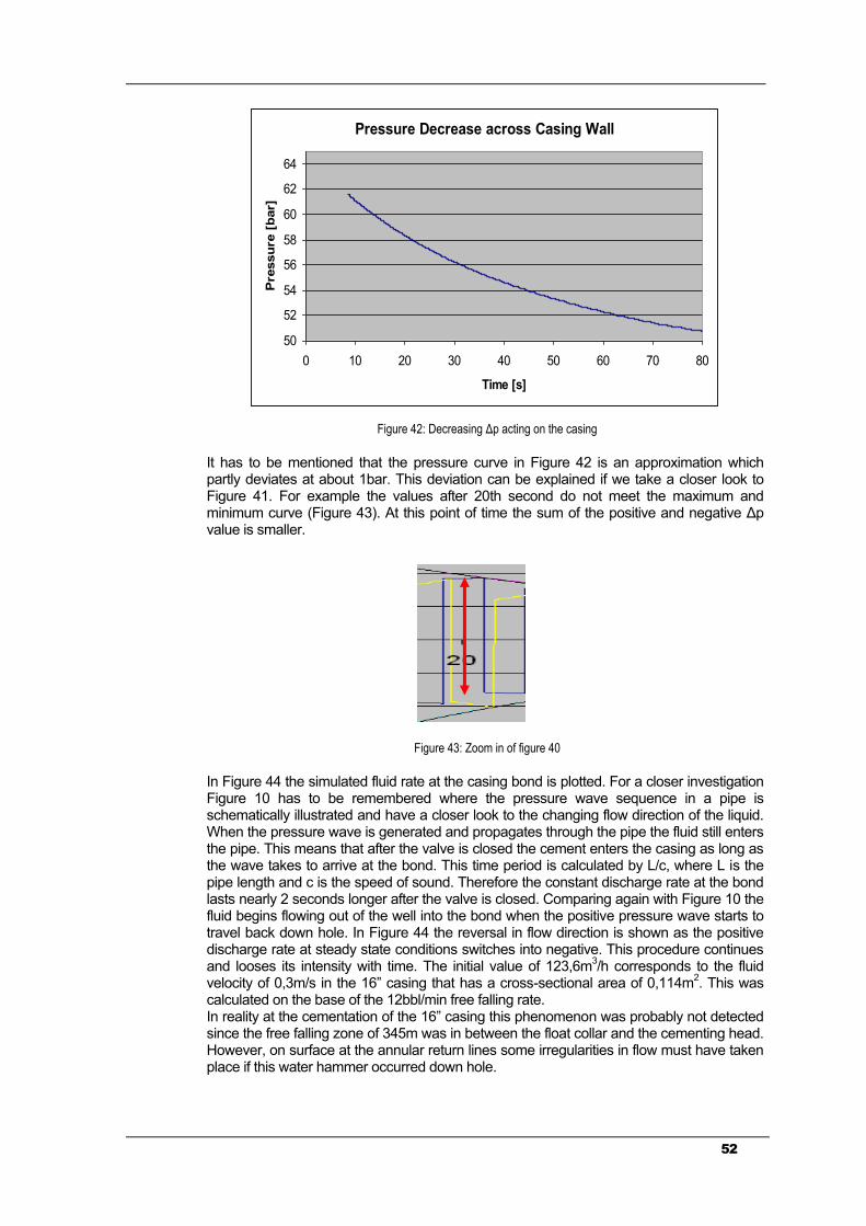
52
Pressure Decrease across Casing Wall
50
52
54
56
58
60
62
64
0 10 20 30 40 50 60 70 80
Time [s]
Pre
ssu
re [
bar]
Figure 42 Decreasing Δp acting on the casing
It has to be mentioned that the pressure curve in Figure 42 is an approximation which partly deviates at about 1bar This deviation can be explained if we take a closer look to Figure 41 For example the values after 20th second do not meet the maximum and minimum curve (Figure 43) At this point of time the sum of the positive and negative Δp value is smaller
Figure 43 Zoom in of figure 40
In Figure 44 the simulated fluid rate at the casing bond is plotted For a closer investigation Figure 10 has to be remembered where the pressure wave sequence in a pipe is schematically illustrated and have a closer look to the changing flow direction of the liquid When the pressure wave is generated and propagates through the pipe the fluid still enters the pipe This means that after the valve is closed the cement enters the casing as long as the wave takes to arrive at the bond This time period is calculated by Lc where L is the pipe length and c is the speed of sound Therefore the constant discharge rate at the bond lasts nearly 2 seconds longer after the valve is closed Comparing again with Figure 10 the fluid begins flowing out of the well into the bond when the positive pressure wave starts to travel back down hole In Figure 44 the reversal in flow direction is shown as the positive discharge rate at steady state conditions switches into negative This procedure continues and looses its intensity with time The initial value of 1236m
3h corresponds to the fluid
velocity of 03ms in the 16rdquo casing that has a cross-sectional area of 0114m2 This was
calculated on the base of the 12bblmin free falling rate In reality at the cementation of the 16rdquo casing this phenomenon was probably not detected since the free falling zone of 345m was in between the float collar and the cementing head However on surface at the annular return lines some irregularities in flow must have taken place if this water hammer occurred down hole
53
Figure 44 Discharge rate at the casing bond
In Figure the 45 the discharge rate of the annulus is demonstrated It is a reversal procedure as in Figure 44 As soon as the fluid flow is interrupted the negative pressure wave moves towards the outlet on the surface During this time (Lc) the discharge at the surface stays constant but when the wave arrives at the outlet and the whole amount of fluid stands still for a tiny moment the direction of flow is reversed and the fluid enters the ldquoannularrdquo pipe The fluid flows back into the annulus as long as the pressure wave takes for one time up and down the well This time period is determined by 2Lc (Chapter 732) This process continues and decreases as the amplitude of the pressure wave decreases In Figure 45 the initial negative value of 1236m
3h in the steady state period expresses that
the fluid enters the bond at surface a positive value stand for the reversal After 80 seconds a irregularity can be detected where the wave starts to develop an amplitude again In reality a hose was installed at the wellhead that directed the annular returns to the spider box which is installed between the mud return line and the shale shakers to divert the flow At the outlet of the hose the mud faced atmospheric conditions When now the negative pressure wave passes the well head and reaches the end of the hose it is reflected at the interface of fluid and air When the pressure wave turns the mud inside the hose will be forced to flow back towards the well head and since no mud from the spider box can enter air is sucked into the hose The return rate is interrupted for a duration of 36 seconds The indication at surface would be a repeating break of the return flow and the hose would start to move and vibrate due to the flow and suction sequences Remarkable occurrences like those were not detected on site On the other side in this case it is difficult to estimate the impact on surface equipment and probably since nothing was expected nothing was noticed
Discharge at the Bond
C16Thesisw di 2007 Feb 6 1101 - Wanda 353
Discharge BOUNDH B1
Time (s)
15014514013513012512011511010510095908580757065605550454035302520151050
Dis
charg
e (
m3h
)120
100
80
60
40
20
0
-20
-40
-60
-80
-100
-120
54
Discharge Rate at Annular Bond
-150
-100
-50
0
50
100
150
0 10 20 30 40 50 60 70 80
Time [s]
Dis
ch
rga R
eta
[m
3h
]
Figure 45 Discharge rate at annular bond
55
94 Analysis ndash Impact of Different Parameters
Up to now the water hammer theory at OMVrsquos well was investigated and a final result could be found The maximum load on the casing string was 615bar out of which 112bar were caused by the water hammer-effect itself The next step is to study how single parameters influence the magnitude of a water hammer A rather important question is for example in how far the size of the pipe impacts a water hammer Further more the shape of the pressure curves is investigated Following parameters that determine a water hammer are discussed in this chapter
Friction Force
Fluid Density
Fluid Velocity
Speed of Sound
Bulk Modulus
Pipe Dimension
941 Friction Force
The friction force which is developed due to fluid flow on the pipe wall acts against the direction of flow If the fluid velocity is zero no friction force occurs In case of a water hammer the pressure and velocity sequence within the pipe was investigated in a former chapter and is illustrated in Figure 10 If a pressure wave is generated in a pipe and starts to propagate the fluid velocity between the point of generation and the wave front is zero Therefore the section where no friction force is acting gets longer and longer since the wave front travels towards the pipe inlet This means the magnitude of the initial generated pressure peak is increased linear with time by the amount of the friction force as shown in Figure 46 When the pressure front reaches the inlet no friction is acting since the whole fluid column stands still for a moment The next step is that the wave is reflected and fluid starts to flow out of the pipe Because of the reverse in flow direction a friction force acting towards the valve is generated So the pressure at the valve is further increased linear This effect is responsible for the linear pressure increase at the pressure peak itself The friction at the pipe wall and the inner friction cause a reduction of the fluid velocity Due to this reduction the slope of this linear section is getting smaller with the number of pressure wave cycles
Figure 46 Linear pressure increase due to friction force
Concerning the linear section at the pressure peak it was first assumed that this has to do with the compressibility of the fluid Thatrsquos why several runs with different bulk moduli were performed in order to find out if there is a relation between the fluid compressibility and the slope at the pressure peak The bulk modulus of water (21e9Nm
2) was doubled and
halved for the same boundary conditions The linear section of each result was then plotted in Excel and the different slopes were determined with regression lines Figure 47 illustrates the result In a medium with a lower bulk modulus the speed of sound is much slower and therefore the green line in Figure 47 is the longest A higher speed of sound results in a higher water hammer effect Thatrsquos why the black line is on top Regarding the slopes no relation to the different bulk moduli could be detected
56
Pressure Peak Slope at Different Bulk Moduli
y = 01226x + 1964
y = 00943x + 17349
y = 01582x + 22522
15
16
17
18
19
20
21
22
23
24
25
5 525 55 575 6 625 65
Time [sec]
Pre
ssu
re [
bar]
Figure 47 Different bulk moduli affect the slope at the pressure peaks
The relation between the friction pressure and the shape of the pressure peak was noticed when a water hammer in a 7rdquo casing was simulated In pipes of smaller diameter the friction pressure losses are higher than in those of larger At the 7rdquo casing the shape of the pressure peak was more significant and the pressure difference of the linear section corresponded to the friction pressure losses
Pressure Differnce across 7 Float Collar
-15
-10
-5
0
5
10
15
20
0 10 20 30 40 50
Time [s]
Pre
ssu
re [
bar]
Figure 48 Linear pressure increase on top of pressure peak
The analysis of the next parameters is based on two equations which were already introduced the Joukowsky Formula (21) and the speed of sound Formula (22)
p a u
1
1
F
F P
aD
E t E
(21)
(22)
B=105e9 Nm2
B=42e9 Nm2
B=21e9 Nm2
57
942 Fluid Velocity Fluid Density
The Joukowsky formula shows that by doubling the fluid velocity the Δp before the valve is doubled too This formula only describes the magnitude of the positive pressure wave not the total load across a valve According to Equation (21) the fluid velocity is an important factor If Δu is doubled Δp is doubled also For the simulation of the plug cementation a fluid velocity of 03ms was assumed since 12bblmin can be assumed as free falling velocity In Figure 49 the first two pressure peaks of the 16rdquo casing simulation run with a fluid velocity of 05 and 1ms are presented The remaining boundary conditions were exactly the same It can be seen that the load across the casing and the valve is significantly increased The hydrostatic pressure difference of 503bar is not considered in Figure 49
Water Hammer Magnitude at Different Fluid Velocities
-30
-20
-10
0
10
20
30
40
50
0 5 10 15 20
Time [s]
Pre
ssu
re [
bar]
1ms
05ms
Figure 49 Water hammer simulated with higher fluid velocity
An increase in fluid density causes also a rise of the Joukowsky-Δp although it reduces the speed of sound This behaviour can easily be understood by applying Equations (21) and (22)
943 Speed of Sound
The speed of sound is dependent on several different parameters on the one side the fluid properties density and bulk modulus and on the other side the material properties of the pipe Youngs modulus pipe diameter and wall thickness In the previous paragraph it was mentioned that increasing fluid density reduces the wave speed However the density has a higher power in the Joukowsky equation
Bulk Modulus
Generally water based fluids are considered as incompressible and this is indeed valid since the volume change due to a certain external pressure is rather small In case of pressure waves strictly spoken no material is absolute incompressible Regarding the wave character of pressure changes a complete incompressible medium would be immediately destroyed because the molecules would not be able to absorb any impact In case of a liquid flow which causes a water hammer the speed of sound within the liquid is decisive for the magnitude of the pressure peak In case of a vertical flow a reduction of the liquid column length occurs when the fluid flow is suddenly stopped In hydraulic engineering the impact of this volume reduction is rather small and therefore not considered Concerning this topic the author consulted engineers from the Technical University Graz (Austria)
15 who are responsible for the design of hydroelectric power
58
stations where heads of more than 1000m are not unusual The presumption that in hydraulic engineering processes water is treated as an incompressible medium was confirmed by the institute of hydraulic engineering at the technical university in Graz
15 In
addition to that it was recommended that the bulk modulus of a cement slurry is probably slightly higher as the one of water A cement slurry contains solid particles in suspension and in how far this particles influence a water hammer effect can only be figured out by laboratory experiments A water hammer determination according to Equations (21) and (22) does not consider the fluid compressibility However the bulk modulus of a liquid phase plays a decisive role for the determination It defines the speed of sound in the medium and not the change in liquid volume Also for the simulation with ldquoWandardquo the compression of a fluid is not taken into account In case of the water hammer investigation at the 16rdquo casing the liquid volume change due to pressure can easily be determined by
pB
V
V
where Δp is the pressure increase and ΔV the volume change of the initial volume V The total amount of fluid in the wellbore is 23654m
3 the Δp is 51bar and the bulk modulus is
estimated with 24e9Nm2 The result according to Equation (24) is a volume change of
005m3 which is equal to a fluid column of 05m The same result is obtained by using the
bulk modulus of water (21e9Nm2) This result justifies the neglecting of the fluid
compressibility
351 5 23654005
24 9
p V eV m
B e
Pipe Dimension
The dimension of a pipe is defined by its inner diameter its length and its wall thickness of the pipe Equation (22) for the determination of the speed of sound shows in how far these parameters influence the speed of sound and thus the magnitude of the water hammer The denominator of the equation includes a ratio between the inner diameter and the wall thickness Comparing several sizes of pipes containing the same liquid the speed of sound must be equal for all if the Dt ratio is the same However if the wall thickness stays constant and only the inner diameter is increased the wave velocity would be reduced as the value of the denominator rises A reduction of the speed of sound within a fluid reduces the Δp after Joukowsky Therefore following Equation (22) it can be said that in pipes with a bigger wall thickness the magnitude of a water hammer is smaller A larger diameter does not lead to a stronger water hammer but reduces the pressure wave speed and therefore reduces the water hammer effect This statement is valid if all boundary conditions stay the same also the volumetric ratio between mud and cement Regarding the analysis of the impact of the pipe dimension on the magnitude of the water hammer several pipe sizes were simulated For each pipe length three different diameters were tested whereas all pipes had the same wall thickness The pipes were simulated horizontally and water at a velocity of 05ms is flowing through until a valve is closed within 002 seconds The pipe length listed in Table 3 is the length before and after the valve Recorded is the total pressure difference across the valve
(24)
59
Pipe Length
[m]
Inner Diameter
[mm]
Wall Thickness
[mm]
Δp [bar] after
Joukowsky
400 200 12 671
400 12 627
600 12 592
600 200 12 671
400 12 627
600 12 592
800 200 12 671
400 12 627
600 12 592
Table 3 Simulated pipe dimensions
The results are shown in the following pages Indeed the discussed trend in loading which was based on the Equations (21) and (22) can also be noticed at the different runs At a constant wall thickness an increasing diameter causes a lower Δp across the valve This is valid for each length In order to show that the trend of the simulation is true the fourth column in Table 3 presents the results calculated by Joukowsky In the equation the length does not play a role In the following figures the height of the first pressure peak of those pipes with the same length should be compared
60
L=400m ID=200mm
-15
-12
-9
-6
-3
0
3
6
9
12
15
0 5 10 15 20
Time [s]
Pre
ssu
re [
bar]
Figure 50 Pipe dimension test 19 (L=400m ID=200mm)
L=400m ID=400mm
-15
-12
-9
-6
-3
0
3
6
9
12
15
0 5 10 15 20
Time [s]
Pre
ssu
re [
bar]
Figure 51 Pipe dimension test 29 (L=400m ID=400mm)
L=400m ID=600mm
-15
-12
-9
-6
-3
0
3
6
9
12
15
0 5 10 15 20
Time [s]
Pre
ssu
re [
bar]
Figure 52 Pipe dimension test 39 (L=400m ID=600m)
61
L=600m ID=200mm
-15
-12
-9
-6
-3
0
3
6
9
12
15
0 5 10 15 20
Time [s]
Pre
ssu
re [
bar]
Figure 53 Pipe dimension test 49 (L=600m ID=200mm)
L=600m ID=400mm
-15
-12
-9
-6
-3
0
3
6
9
12
15
0 5 10 15 20
Time [s]
Pre
ss
ure
[b
ar]
Figure 54 Pipe dimension test 59 (L=600 ID=400mm)
L=600m ID=600mm
-15
-12
-9
-6
-3
0
3
6
9
12
15
0 5 10 15 20
Time [s]
Pre
ss
ure
[b
ar]
Figure 55 Pipe dimension test 69 (L=600m ID=600mm)
62
L=800m ID=200mm
-15
-12
-9
-6
-3
0
3
6
9
12
15
0 5 10 15 20
Time [s]
Pre
ssu
re [
bar]
Figure 56 Pipe dimension test 79 (L=800m ID=200mm)
L= 800m ID=400mm
-15
-12
-9
-6
-3
0
3
6
9
12
15
0 5 10 15 20
Time [s]
Pre
ss
ure
[b
ar]
Figure 57 Pipe dimension test 89 (L=800m ID=600mm)
L=800m ID=600mm
-15
-12
-9
-6
-3
0
3
6
9
12
15
0 5 10 15 20
Time [s]
Pre
ssu
re [
bar]
Figure 58 Pipe dimension test 99 (L=800m ID=600mm)
63
Wallthickness Check L=600m ID=600mm
tD ratio equal to L=600m ID=200mm
-15
-12
-9
-6
-3
0
3
6
9
12
15
0 5 10 15 20
Time [s]
Pre
ssu
re [
bar]
Figure 59 Pipe dimension test regarding wall thickness
Figures 53 and 59 with the yellow background further prove the assumption regarding the pipe wall thickness The pipe in Figure 53 has a wall thickness of 12mm equal to the others so its IDt ratio r is
200166
12r
Now the pipe from Figure 59 (ID=600mm) was simulated with the same IDt ratio like the one from Figure 53
600166
359r
The magnitude of the water hammer is in both cases 165bar About the impact of the pipe length no statement was made up to now For the determination after Joukowsky the pipe length does not play any role for the magnitude of the Δp Following this a change length does not influence the water hammer The longer the pipe the longer it takes the pressure wave to travel back and forth This can be seen in Figures 50 to 58 since the single pressure peaks are getting broader Even from the simulation no clear trend in how far the pipe length is related to the height of the pressure peaks can be detected All pipes with the internal diameter of 400mm show the same result illustrated in Figures 5154 and 57 The remaining ones tend to decrease slightly An increase of the water hammer effect with an increase of pipe length at same boundary conditions can not be detected After these investigations the author was interested into an unrealistic but interesting example What would be the result if the 16rdquo casing string was 10000m long The previous simulation set up was changed to a depth of 10000m and the run was simulated with the cement slurry only The result is shown in Figure 60 It can be seen that the load due to the water hammer is far away from endangering the casing to burst The effect of friction can be seen very clearly from the linear section of the pressure peaks
64
Pressure Difference across 16 Float Collar
(Depth 10 000m)
-10
-5
0
5
10
15
20
25
0 50 100 150 200
Time [s]
Pressu
re [
bar]
Figure 60 Water hammer effect if the well would have been 10000m deep
65
10 Limits of Different Casing Sizes
At OMV a water hammer probably occurred during the plug cementation of the 16rdquo casing string The task of this chapter is to find out the limits of common casing sizes for the case that a plug cementation again generates a water hammer due to any defects On base of the previous investigations the relation between pipe size and water hammer magnitude is known Further more all parameters that influence the height of the pressure peak are well known
Fluid density
Fluid velocity
Speed of sound
Bulk modulus
Youngs modulus
Pipe diameter
Wall thickness The question is which parameters are planned ahead and which can be influenced directly In the casing design process the type and size of the string is chosen long before the well is drilled Since the casing is selected the pipe properties Youngs modulus diameter and wall thickness can be considered as constants The bulk modulus of the slurry can also be seen as a constant because it cannot be significantly changed except for foamed slurries Density has a rather high impact on the water hammer phenomenon Concerning the slurry density the author decided to select the same density as it was used for the investigation of the 16rdquo casing cementation The composition of the slurry used was a quite common one and further the value determined for the simulation includes the volumetric ratio of mud lead and tail cement The slurry velocity is equal the free falling velocity which can only be reduced if a back up pressure is provided at the annular return In the following for common casing diameters the maximum allowable flow rate is figured out Above this critical value a water hammer would exceed the burst resistance of the different casings Following casing sizes were tested
OD [in] Weight [lbft] Grade Wall thickness [in] Internal Yield Pressure [psi]
7rdquo 29 TN 95HS 040 9690
9 58rdquo 535 API L80 054 7930
13 38rdquo 807 TN 95HS 058 7210
16rdquo 84 API L80 049 4330
20rdquo 106 API J55 050 2420
Table 4 Tested casing sizes
Size [in] 7rdquo 9 58rdquo 13 38rdquo 16rdquo 20rdquo
Depth [m] Slurry velocity [m3min]
1000 465 155 435 4101 439
2000 36 1218 3371 3218 362
3000 314 1065 2936 2807 3292
4000 29 952 2718 2602 2963
Table 5 Critical slurry velocities for different casing sizes
From Table 5 a decrease of the critical pump rate with increasing depth can be noticed for
66
all casing size This can be explained due to friction forces The deeper the casing the higher is the friction pressure loss For a water hammer calculation this loss again appears as the linear pressure increase on top of the pressure peak itself Concerning the internal yield pressure this additional Δp is high enough to ldquoallowrdquo the fluid velocity to be reduced For the same depth the tendency of different pipe sizes is illustrated in Figure 61 As mentioned before it can be seen that the deeper the well the lower would be the critical flow rate This is valid for all casing sizes Concerning the diameter the critical flow rates above 13 38rdquo casings do not differ that much compared to 7rdquo and 9 58rdquo casings The simulation runs for theses casing size tests were performed as U-tubes The inner diameter of the annular pipe was determined by the ratio of the hole diameter to the outer casing diameter of the 16rdquo casing
Critical Flow Rates for Common Casings at
Different Depths
0
5000
10000
15000
20000
25000
30000
35000
40000
45000
50000
0 5 10 15 20 25
OD [in]
Flo
w R
ate
[l
min
]
Figure 61 Tendency of the critical flow rate for several casings at certain depths
1000m
2000m
3000m
4000m
67
11 Conclusion
First of all why was the water hammer theory taken into consideration A water hammer only occurs if a fluid flow is stopped immediately Concerning the plug cementation it is a realistic assumption that the bottom plug which was made out of rubber faced so much wear on its way downhole that it was decomposed Therefore a plugging of the valve could be possible It is even known that bottom plugs might turn around while they are pumped downhole Of course this is also a question of plug quality
The simulation of the water hammer-effect at the 16rdquo casing delivered a maximum pressure difference of 6153bar across the casing wall whereas 5033bar out of this is caused by the hydrostatic difference between the casing and the annular Only 116bar are generated by the impact of the water hammer and as it can be seen from Figure 62 this is the amount of pressure that is reduced with time It is remarkable that this impact is rather small It is obvious that the total load does not endanger the 16rdquo casing string to burst
Pressure Decrease across Casing Wall
50
52
54
56
58
60
62
64
0 10 20 30 40 50 60 70 80
Time [s]
Pre
ssu
re [
bar]
Figure 62 Δp caused by water hammer acting an the casing
This result seems to be an approach for further investigation of the problem occurred in OMV well during the 16rdquo cement job A special topic like the connection slippage theory would be worth to be studied in detail since it was not included in this thesis Concerning this further theory the impact of the slurry velocity which was shown in Figure 49 has to be pointed out Concerning the casing dimension its impact on the water hammer magnitude could be proved mathematically and by the simulation For a constant wall thickness a larger inner diameter reduces the speed of sound and thus the generated Δp The reverse happens in case of a smaller diameter In pipes of different sizes but with same Dt ratio the magnitude of a water hammer is equal for each diameter It was shown that pipes with a larger wall thickness face a higher load if water hammer occurs Pipe length or depth only indirectly influences the resulting Δp The amount of friction pressure losses in a longer pipe section is higher as in a shorter one of course Friction pressure losses lead to a further but linear increase of the pressure peak with time This means the maximum pressure is reached after the time 2La with L as pipe length and a as speed of sound This behaviour is related to the pressure and velocity sequence in the pipe when the pressure wave is reflected
68
Figure 61 represents the flow rate limit above which common types of casings are endangered to burst when a water hammer occurs at a certain depth Very general spoken in deeper wells the burst resistance of a casing is exceeded at lower fluid velocities as in case of shallower wells The initial assumption that the compressibility of the slurry column has a significant impact on the final water hammer load could not be confirmed by this investigation It was determined that the slurry column length was reduced by half a meter due to liquid compression Following the calculation this rather small impact can be neglected In this context it has to be pointed out that a slurry contains solid particles It is not clear wether these particles influence the compressibility Regarding the simulation it must be said that computational programs strictly follow physical laws and formulas Therefore results are based on ideal conditions The fact that the slurry contains solid particles can not totally be covered by the simulation Slurries viscosity is a known parameter whereof the kinematik viscosity can be determined The viscosity of a liquid is based on the interaction of molecules This interaction causes inner friction since it counteracts on movement and thus is responsible for the shear stress - shear rate relation of a liquid Due to the known viscosity the inner friction of the slurry and its solid particles are considered in the simulation Concerning the pressure wave velocity it is known that small gas bubbles dispersed in a fluid reduced the speed of sound significantly It is assumed that the opposite would be true for solid particles if they were homogeneously arranged and in direct contact to each other
15 Since this is not the case in a suspension the solid particles do not increases the
speed of sound In how far they in fact influence the wave propagation velocity was not investigated during this thesis For the height of the first pressure peak the inner friction is irrelevant but not for the decline of the following pressure peaks The inner friction strongly dampens the pressure wave intensity The simulation delivered a pressure sequence that lasted about 80 seconds In hydraulic engineering at the Technical University Graz (Austria) the experience was made that the duration of a pressure sequence after a water hammer is in reality shorter as it is determined by a simulation However it can only be assumed how long it actually lasted
69
10 References
1 Spoumlrker H ldquoAnalysis of the Free Fall Phenomenon During Primary Cementingrdquo
Thesis Leoben U Austria (1993)
2 Beirute RM ldquoThe Phenomenon of Free Fall During Primary Cementingrdquo SPE
13045 1984 ldquoA Technique for Onsite Diagnosis of Cement Job Problems The
Concept of Job Signaturerdquo SPE 166491987
3 Science and Technology Encyclopedia ldquoWater Hammerrdquo
httpwwwanswerscomtopicwater-hammer 01022007
4 Klasinc R ldquoHydraulic VArdquo Script Technical University Graz Austria
5 Pickford J rdquoAnalysis of Water Surgerdquo 1969 Gordon and Breach Science
Publisher
httpwwwnescwvuedundwcarticlesotWI03Water_Hammerhtml
01022007
6 Repp T ldquoFluiddynamic Waterhammer Simulations with Consideration of Fluid-
Structure Interactionldquo Publication presented at the annular conference of nuclear
science in Karlsruhe Germany Mai 1999
httpwwwfzddepublications002143jb08pdf 01022007
7 Tipler P ldquoPhysikrdquo (2000) p 459-470
8 Wikipedia Encyclopedia ldquoSchallgeschwindigkeitrdquo
httpdewikipediaorgwikiSchallgeschwindigkeit 01022007
9 Tipler P ldquoPhysikrdquo (2000) p 207
10 Wikipedia Encyclopedia ldquoInnere Reibungldquo
httpdewikipediaorgwikiReibungInnere_Reibung 01022007
11 HyperPhysiks Georgia State University
httphyperphysicsphy-astrgsueduhbasepermot3html 01022007
12 Wikipedia Encyclopedia ldquoBulk Modulusrdquo
httpenwikipediaorgwikiBulk_modulus 01022007
13 Wikipedia Encyclopedia ldquoCavitationrdquo
httpenwikipediaorgwikiCavitation 01022007
14 Tenaris Oilfield Services Online Catalogue
httpwwwtenariscomarchivosdocuments2003532pdf 01022007
15 Univ-Prof DI Dr techn Heigerth Guumlnther DI Dr techn Dominik Mayr

54
Discharge Rate at Annular Bond
-150
-100
-50
0
50
100
150
0 10 20 30 40 50 60 70 80
Time [s]
Dis
ch
rga R
eta
[m
3h
]
Figure 45 Discharge rate at annular bond
55
94 Analysis ndash Impact of Different Parameters
Up to now the water hammer theory at OMVrsquos well was investigated and a final result could be found The maximum load on the casing string was 615bar out of which 112bar were caused by the water hammer-effect itself The next step is to study how single parameters influence the magnitude of a water hammer A rather important question is for example in how far the size of the pipe impacts a water hammer Further more the shape of the pressure curves is investigated Following parameters that determine a water hammer are discussed in this chapter
Friction Force
Fluid Density
Fluid Velocity
Speed of Sound
Bulk Modulus
Pipe Dimension
941 Friction Force
The friction force which is developed due to fluid flow on the pipe wall acts against the direction of flow If the fluid velocity is zero no friction force occurs In case of a water hammer the pressure and velocity sequence within the pipe was investigated in a former chapter and is illustrated in Figure 10 If a pressure wave is generated in a pipe and starts to propagate the fluid velocity between the point of generation and the wave front is zero Therefore the section where no friction force is acting gets longer and longer since the wave front travels towards the pipe inlet This means the magnitude of the initial generated pressure peak is increased linear with time by the amount of the friction force as shown in Figure 46 When the pressure front reaches the inlet no friction is acting since the whole fluid column stands still for a moment The next step is that the wave is reflected and fluid starts to flow out of the pipe Because of the reverse in flow direction a friction force acting towards the valve is generated So the pressure at the valve is further increased linear This effect is responsible for the linear pressure increase at the pressure peak itself The friction at the pipe wall and the inner friction cause a reduction of the fluid velocity Due to this reduction the slope of this linear section is getting smaller with the number of pressure wave cycles
Figure 46 Linear pressure increase due to friction force
Concerning the linear section at the pressure peak it was first assumed that this has to do with the compressibility of the fluid Thatrsquos why several runs with different bulk moduli were performed in order to find out if there is a relation between the fluid compressibility and the slope at the pressure peak The bulk modulus of water (21e9Nm
2) was doubled and
halved for the same boundary conditions The linear section of each result was then plotted in Excel and the different slopes were determined with regression lines Figure 47 illustrates the result In a medium with a lower bulk modulus the speed of sound is much slower and therefore the green line in Figure 47 is the longest A higher speed of sound results in a higher water hammer effect Thatrsquos why the black line is on top Regarding the slopes no relation to the different bulk moduli could be detected
56
Pressure Peak Slope at Different Bulk Moduli
y = 01226x + 1964
y = 00943x + 17349
y = 01582x + 22522
15
16
17
18
19
20
21
22
23
24
25
5 525 55 575 6 625 65
Time [sec]
Pre
ssu
re [
bar]
Figure 47 Different bulk moduli affect the slope at the pressure peaks
The relation between the friction pressure and the shape of the pressure peak was noticed when a water hammer in a 7rdquo casing was simulated In pipes of smaller diameter the friction pressure losses are higher than in those of larger At the 7rdquo casing the shape of the pressure peak was more significant and the pressure difference of the linear section corresponded to the friction pressure losses
Pressure Differnce across 7 Float Collar
-15
-10
-5
0
5
10
15
20
0 10 20 30 40 50
Time [s]
Pre
ssu
re [
bar]
Figure 48 Linear pressure increase on top of pressure peak
The analysis of the next parameters is based on two equations which were already introduced the Joukowsky Formula (21) and the speed of sound Formula (22)
p a u
1
1
F
F P
aD
E t E
(21)
(22)
B=105e9 Nm2
B=42e9 Nm2
B=21e9 Nm2
57
942 Fluid Velocity Fluid Density
The Joukowsky formula shows that by doubling the fluid velocity the Δp before the valve is doubled too This formula only describes the magnitude of the positive pressure wave not the total load across a valve According to Equation (21) the fluid velocity is an important factor If Δu is doubled Δp is doubled also For the simulation of the plug cementation a fluid velocity of 03ms was assumed since 12bblmin can be assumed as free falling velocity In Figure 49 the first two pressure peaks of the 16rdquo casing simulation run with a fluid velocity of 05 and 1ms are presented The remaining boundary conditions were exactly the same It can be seen that the load across the casing and the valve is significantly increased The hydrostatic pressure difference of 503bar is not considered in Figure 49
Water Hammer Magnitude at Different Fluid Velocities
-30
-20
-10
0
10
20
30
40
50
0 5 10 15 20
Time [s]
Pre
ssu
re [
bar]
1ms
05ms
Figure 49 Water hammer simulated with higher fluid velocity
An increase in fluid density causes also a rise of the Joukowsky-Δp although it reduces the speed of sound This behaviour can easily be understood by applying Equations (21) and (22)
943 Speed of Sound
The speed of sound is dependent on several different parameters on the one side the fluid properties density and bulk modulus and on the other side the material properties of the pipe Youngs modulus pipe diameter and wall thickness In the previous paragraph it was mentioned that increasing fluid density reduces the wave speed However the density has a higher power in the Joukowsky equation
Bulk Modulus
Generally water based fluids are considered as incompressible and this is indeed valid since the volume change due to a certain external pressure is rather small In case of pressure waves strictly spoken no material is absolute incompressible Regarding the wave character of pressure changes a complete incompressible medium would be immediately destroyed because the molecules would not be able to absorb any impact In case of a liquid flow which causes a water hammer the speed of sound within the liquid is decisive for the magnitude of the pressure peak In case of a vertical flow a reduction of the liquid column length occurs when the fluid flow is suddenly stopped In hydraulic engineering the impact of this volume reduction is rather small and therefore not considered Concerning this topic the author consulted engineers from the Technical University Graz (Austria)
15 who are responsible for the design of hydroelectric power
58
stations where heads of more than 1000m are not unusual The presumption that in hydraulic engineering processes water is treated as an incompressible medium was confirmed by the institute of hydraulic engineering at the technical university in Graz
15 In
addition to that it was recommended that the bulk modulus of a cement slurry is probably slightly higher as the one of water A cement slurry contains solid particles in suspension and in how far this particles influence a water hammer effect can only be figured out by laboratory experiments A water hammer determination according to Equations (21) and (22) does not consider the fluid compressibility However the bulk modulus of a liquid phase plays a decisive role for the determination It defines the speed of sound in the medium and not the change in liquid volume Also for the simulation with ldquoWandardquo the compression of a fluid is not taken into account In case of the water hammer investigation at the 16rdquo casing the liquid volume change due to pressure can easily be determined by
pB
V
V
where Δp is the pressure increase and ΔV the volume change of the initial volume V The total amount of fluid in the wellbore is 23654m
3 the Δp is 51bar and the bulk modulus is
estimated with 24e9Nm2 The result according to Equation (24) is a volume change of
005m3 which is equal to a fluid column of 05m The same result is obtained by using the
bulk modulus of water (21e9Nm2) This result justifies the neglecting of the fluid
compressibility
351 5 23654005
24 9
p V eV m
B e
Pipe Dimension
The dimension of a pipe is defined by its inner diameter its length and its wall thickness of the pipe Equation (22) for the determination of the speed of sound shows in how far these parameters influence the speed of sound and thus the magnitude of the water hammer The denominator of the equation includes a ratio between the inner diameter and the wall thickness Comparing several sizes of pipes containing the same liquid the speed of sound must be equal for all if the Dt ratio is the same However if the wall thickness stays constant and only the inner diameter is increased the wave velocity would be reduced as the value of the denominator rises A reduction of the speed of sound within a fluid reduces the Δp after Joukowsky Therefore following Equation (22) it can be said that in pipes with a bigger wall thickness the magnitude of a water hammer is smaller A larger diameter does not lead to a stronger water hammer but reduces the pressure wave speed and therefore reduces the water hammer effect This statement is valid if all boundary conditions stay the same also the volumetric ratio between mud and cement Regarding the analysis of the impact of the pipe dimension on the magnitude of the water hammer several pipe sizes were simulated For each pipe length three different diameters were tested whereas all pipes had the same wall thickness The pipes were simulated horizontally and water at a velocity of 05ms is flowing through until a valve is closed within 002 seconds The pipe length listed in Table 3 is the length before and after the valve Recorded is the total pressure difference across the valve
(24)
59
Pipe Length
[m]
Inner Diameter
[mm]
Wall Thickness
[mm]
Δp [bar] after
Joukowsky
400 200 12 671
400 12 627
600 12 592
600 200 12 671
400 12 627
600 12 592
800 200 12 671
400 12 627
600 12 592
Table 3 Simulated pipe dimensions
The results are shown in the following pages Indeed the discussed trend in loading which was based on the Equations (21) and (22) can also be noticed at the different runs At a constant wall thickness an increasing diameter causes a lower Δp across the valve This is valid for each length In order to show that the trend of the simulation is true the fourth column in Table 3 presents the results calculated by Joukowsky In the equation the length does not play a role In the following figures the height of the first pressure peak of those pipes with the same length should be compared
60
L=400m ID=200mm
-15
-12
-9
-6
-3
0
3
6
9
12
15
0 5 10 15 20
Time [s]
Pre
ssu
re [
bar]
Figure 50 Pipe dimension test 19 (L=400m ID=200mm)
L=400m ID=400mm
-15
-12
-9
-6
-3
0
3
6
9
12
15
0 5 10 15 20
Time [s]
Pre
ssu
re [
bar]
Figure 51 Pipe dimension test 29 (L=400m ID=400mm)
L=400m ID=600mm
-15
-12
-9
-6
-3
0
3
6
9
12
15
0 5 10 15 20
Time [s]
Pre
ssu
re [
bar]
Figure 52 Pipe dimension test 39 (L=400m ID=600m)
61
L=600m ID=200mm
-15
-12
-9
-6
-3
0
3
6
9
12
15
0 5 10 15 20
Time [s]
Pre
ssu
re [
bar]
Figure 53 Pipe dimension test 49 (L=600m ID=200mm)
L=600m ID=400mm
-15
-12
-9
-6
-3
0
3
6
9
12
15
0 5 10 15 20
Time [s]
Pre
ss
ure
[b
ar]
Figure 54 Pipe dimension test 59 (L=600 ID=400mm)
L=600m ID=600mm
-15
-12
-9
-6
-3
0
3
6
9
12
15
0 5 10 15 20
Time [s]
Pre
ss
ure
[b
ar]
Figure 55 Pipe dimension test 69 (L=600m ID=600mm)
62
L=800m ID=200mm
-15
-12
-9
-6
-3
0
3
6
9
12
15
0 5 10 15 20
Time [s]
Pre
ssu
re [
bar]
Figure 56 Pipe dimension test 79 (L=800m ID=200mm)
L= 800m ID=400mm
-15
-12
-9
-6
-3
0
3
6
9
12
15
0 5 10 15 20
Time [s]
Pre
ss
ure
[b
ar]
Figure 57 Pipe dimension test 89 (L=800m ID=600mm)
L=800m ID=600mm
-15
-12
-9
-6
-3
0
3
6
9
12
15
0 5 10 15 20
Time [s]
Pre
ssu
re [
bar]
Figure 58 Pipe dimension test 99 (L=800m ID=600mm)
63
Wallthickness Check L=600m ID=600mm
tD ratio equal to L=600m ID=200mm
-15
-12
-9
-6
-3
0
3
6
9
12
15
0 5 10 15 20
Time [s]
Pre
ssu
re [
bar]
Figure 59 Pipe dimension test regarding wall thickness
Figures 53 and 59 with the yellow background further prove the assumption regarding the pipe wall thickness The pipe in Figure 53 has a wall thickness of 12mm equal to the others so its IDt ratio r is
200166
12r
Now the pipe from Figure 59 (ID=600mm) was simulated with the same IDt ratio like the one from Figure 53
600166
359r
The magnitude of the water hammer is in both cases 165bar About the impact of the pipe length no statement was made up to now For the determination after Joukowsky the pipe length does not play any role for the magnitude of the Δp Following this a change length does not influence the water hammer The longer the pipe the longer it takes the pressure wave to travel back and forth This can be seen in Figures 50 to 58 since the single pressure peaks are getting broader Even from the simulation no clear trend in how far the pipe length is related to the height of the pressure peaks can be detected All pipes with the internal diameter of 400mm show the same result illustrated in Figures 5154 and 57 The remaining ones tend to decrease slightly An increase of the water hammer effect with an increase of pipe length at same boundary conditions can not be detected After these investigations the author was interested into an unrealistic but interesting example What would be the result if the 16rdquo casing string was 10000m long The previous simulation set up was changed to a depth of 10000m and the run was simulated with the cement slurry only The result is shown in Figure 60 It can be seen that the load due to the water hammer is far away from endangering the casing to burst The effect of friction can be seen very clearly from the linear section of the pressure peaks
64
Pressure Difference across 16 Float Collar
(Depth 10 000m)
-10
-5
0
5
10
15
20
25
0 50 100 150 200
Time [s]
Pressu
re [
bar]
Figure 60 Water hammer effect if the well would have been 10000m deep
65
10 Limits of Different Casing Sizes
At OMV a water hammer probably occurred during the plug cementation of the 16rdquo casing string The task of this chapter is to find out the limits of common casing sizes for the case that a plug cementation again generates a water hammer due to any defects On base of the previous investigations the relation between pipe size and water hammer magnitude is known Further more all parameters that influence the height of the pressure peak are well known
Fluid density
Fluid velocity
Speed of sound
Bulk modulus
Youngs modulus
Pipe diameter
Wall thickness The question is which parameters are planned ahead and which can be influenced directly In the casing design process the type and size of the string is chosen long before the well is drilled Since the casing is selected the pipe properties Youngs modulus diameter and wall thickness can be considered as constants The bulk modulus of the slurry can also be seen as a constant because it cannot be significantly changed except for foamed slurries Density has a rather high impact on the water hammer phenomenon Concerning the slurry density the author decided to select the same density as it was used for the investigation of the 16rdquo casing cementation The composition of the slurry used was a quite common one and further the value determined for the simulation includes the volumetric ratio of mud lead and tail cement The slurry velocity is equal the free falling velocity which can only be reduced if a back up pressure is provided at the annular return In the following for common casing diameters the maximum allowable flow rate is figured out Above this critical value a water hammer would exceed the burst resistance of the different casings Following casing sizes were tested
OD [in] Weight [lbft] Grade Wall thickness [in] Internal Yield Pressure [psi]
7rdquo 29 TN 95HS 040 9690
9 58rdquo 535 API L80 054 7930
13 38rdquo 807 TN 95HS 058 7210
16rdquo 84 API L80 049 4330
20rdquo 106 API J55 050 2420
Table 4 Tested casing sizes
Size [in] 7rdquo 9 58rdquo 13 38rdquo 16rdquo 20rdquo
Depth [m] Slurry velocity [m3min]
1000 465 155 435 4101 439
2000 36 1218 3371 3218 362
3000 314 1065 2936 2807 3292
4000 29 952 2718 2602 2963
Table 5 Critical slurry velocities for different casing sizes
From Table 5 a decrease of the critical pump rate with increasing depth can be noticed for
66
all casing size This can be explained due to friction forces The deeper the casing the higher is the friction pressure loss For a water hammer calculation this loss again appears as the linear pressure increase on top of the pressure peak itself Concerning the internal yield pressure this additional Δp is high enough to ldquoallowrdquo the fluid velocity to be reduced For the same depth the tendency of different pipe sizes is illustrated in Figure 61 As mentioned before it can be seen that the deeper the well the lower would be the critical flow rate This is valid for all casing sizes Concerning the diameter the critical flow rates above 13 38rdquo casings do not differ that much compared to 7rdquo and 9 58rdquo casings The simulation runs for theses casing size tests were performed as U-tubes The inner diameter of the annular pipe was determined by the ratio of the hole diameter to the outer casing diameter of the 16rdquo casing
Critical Flow Rates for Common Casings at
Different Depths
0
5000
10000
15000
20000
25000
30000
35000
40000
45000
50000
0 5 10 15 20 25
OD [in]
Flo
w R
ate
[l
min
]
Figure 61 Tendency of the critical flow rate for several casings at certain depths
1000m
2000m
3000m
4000m
67
11 Conclusion
First of all why was the water hammer theory taken into consideration A water hammer only occurs if a fluid flow is stopped immediately Concerning the plug cementation it is a realistic assumption that the bottom plug which was made out of rubber faced so much wear on its way downhole that it was decomposed Therefore a plugging of the valve could be possible It is even known that bottom plugs might turn around while they are pumped downhole Of course this is also a question of plug quality
The simulation of the water hammer-effect at the 16rdquo casing delivered a maximum pressure difference of 6153bar across the casing wall whereas 5033bar out of this is caused by the hydrostatic difference between the casing and the annular Only 116bar are generated by the impact of the water hammer and as it can be seen from Figure 62 this is the amount of pressure that is reduced with time It is remarkable that this impact is rather small It is obvious that the total load does not endanger the 16rdquo casing string to burst
Pressure Decrease across Casing Wall
50
52
54
56
58
60
62
64
0 10 20 30 40 50 60 70 80
Time [s]
Pre
ssu
re [
bar]
Figure 62 Δp caused by water hammer acting an the casing
This result seems to be an approach for further investigation of the problem occurred in OMV well during the 16rdquo cement job A special topic like the connection slippage theory would be worth to be studied in detail since it was not included in this thesis Concerning this further theory the impact of the slurry velocity which was shown in Figure 49 has to be pointed out Concerning the casing dimension its impact on the water hammer magnitude could be proved mathematically and by the simulation For a constant wall thickness a larger inner diameter reduces the speed of sound and thus the generated Δp The reverse happens in case of a smaller diameter In pipes of different sizes but with same Dt ratio the magnitude of a water hammer is equal for each diameter It was shown that pipes with a larger wall thickness face a higher load if water hammer occurs Pipe length or depth only indirectly influences the resulting Δp The amount of friction pressure losses in a longer pipe section is higher as in a shorter one of course Friction pressure losses lead to a further but linear increase of the pressure peak with time This means the maximum pressure is reached after the time 2La with L as pipe length and a as speed of sound This behaviour is related to the pressure and velocity sequence in the pipe when the pressure wave is reflected
68
Figure 61 represents the flow rate limit above which common types of casings are endangered to burst when a water hammer occurs at a certain depth Very general spoken in deeper wells the burst resistance of a casing is exceeded at lower fluid velocities as in case of shallower wells The initial assumption that the compressibility of the slurry column has a significant impact on the final water hammer load could not be confirmed by this investigation It was determined that the slurry column length was reduced by half a meter due to liquid compression Following the calculation this rather small impact can be neglected In this context it has to be pointed out that a slurry contains solid particles It is not clear wether these particles influence the compressibility Regarding the simulation it must be said that computational programs strictly follow physical laws and formulas Therefore results are based on ideal conditions The fact that the slurry contains solid particles can not totally be covered by the simulation Slurries viscosity is a known parameter whereof the kinematik viscosity can be determined The viscosity of a liquid is based on the interaction of molecules This interaction causes inner friction since it counteracts on movement and thus is responsible for the shear stress - shear rate relation of a liquid Due to the known viscosity the inner friction of the slurry and its solid particles are considered in the simulation Concerning the pressure wave velocity it is known that small gas bubbles dispersed in a fluid reduced the speed of sound significantly It is assumed that the opposite would be true for solid particles if they were homogeneously arranged and in direct contact to each other
15 Since this is not the case in a suspension the solid particles do not increases the
speed of sound In how far they in fact influence the wave propagation velocity was not investigated during this thesis For the height of the first pressure peak the inner friction is irrelevant but not for the decline of the following pressure peaks The inner friction strongly dampens the pressure wave intensity The simulation delivered a pressure sequence that lasted about 80 seconds In hydraulic engineering at the Technical University Graz (Austria) the experience was made that the duration of a pressure sequence after a water hammer is in reality shorter as it is determined by a simulation However it can only be assumed how long it actually lasted
69
10 References
1 Spoumlrker H ldquoAnalysis of the Free Fall Phenomenon During Primary Cementingrdquo
Thesis Leoben U Austria (1993)
2 Beirute RM ldquoThe Phenomenon of Free Fall During Primary Cementingrdquo SPE
13045 1984 ldquoA Technique for Onsite Diagnosis of Cement Job Problems The
Concept of Job Signaturerdquo SPE 166491987
3 Science and Technology Encyclopedia ldquoWater Hammerrdquo
httpwwwanswerscomtopicwater-hammer 01022007
4 Klasinc R ldquoHydraulic VArdquo Script Technical University Graz Austria
5 Pickford J rdquoAnalysis of Water Surgerdquo 1969 Gordon and Breach Science
Publisher
httpwwwnescwvuedundwcarticlesotWI03Water_Hammerhtml
01022007
6 Repp T ldquoFluiddynamic Waterhammer Simulations with Consideration of Fluid-
Structure Interactionldquo Publication presented at the annular conference of nuclear
science in Karlsruhe Germany Mai 1999
httpwwwfzddepublications002143jb08pdf 01022007
7 Tipler P ldquoPhysikrdquo (2000) p 459-470
8 Wikipedia Encyclopedia ldquoSchallgeschwindigkeitrdquo
httpdewikipediaorgwikiSchallgeschwindigkeit 01022007
9 Tipler P ldquoPhysikrdquo (2000) p 207
10 Wikipedia Encyclopedia ldquoInnere Reibungldquo
httpdewikipediaorgwikiReibungInnere_Reibung 01022007
11 HyperPhysiks Georgia State University
httphyperphysicsphy-astrgsueduhbasepermot3html 01022007
12 Wikipedia Encyclopedia ldquoBulk Modulusrdquo
httpenwikipediaorgwikiBulk_modulus 01022007
13 Wikipedia Encyclopedia ldquoCavitationrdquo
httpenwikipediaorgwikiCavitation 01022007
14 Tenaris Oilfield Services Online Catalogue
httpwwwtenariscomarchivosdocuments2003532pdf 01022007
15 Univ-Prof DI Dr techn Heigerth Guumlnther DI Dr techn Dominik Mayr

56
Pressure Peak Slope at Different Bulk Moduli
y = 01226x + 1964
y = 00943x + 17349
y = 01582x + 22522
15
16
17
18
19
20
21
22
23
24
25
5 525 55 575 6 625 65
Time [sec]
Pre
ssu
re [
bar]
Figure 47 Different bulk moduli affect the slope at the pressure peaks
The relation between the friction pressure and the shape of the pressure peak was noticed when a water hammer in a 7rdquo casing was simulated In pipes of smaller diameter the friction pressure losses are higher than in those of larger At the 7rdquo casing the shape of the pressure peak was more significant and the pressure difference of the linear section corresponded to the friction pressure losses
Pressure Differnce across 7 Float Collar
-15
-10
-5
0
5
10
15
20
0 10 20 30 40 50
Time [s]
Pre
ssu
re [
bar]
Figure 48 Linear pressure increase on top of pressure peak
The analysis of the next parameters is based on two equations which were already introduced the Joukowsky Formula (21) and the speed of sound Formula (22)
p a u
1
1
F
F P
aD
E t E
(21)
(22)
B=105e9 Nm2
B=42e9 Nm2
B=21e9 Nm2
57
942 Fluid Velocity Fluid Density
The Joukowsky formula shows that by doubling the fluid velocity the Δp before the valve is doubled too This formula only describes the magnitude of the positive pressure wave not the total load across a valve According to Equation (21) the fluid velocity is an important factor If Δu is doubled Δp is doubled also For the simulation of the plug cementation a fluid velocity of 03ms was assumed since 12bblmin can be assumed as free falling velocity In Figure 49 the first two pressure peaks of the 16rdquo casing simulation run with a fluid velocity of 05 and 1ms are presented The remaining boundary conditions were exactly the same It can be seen that the load across the casing and the valve is significantly increased The hydrostatic pressure difference of 503bar is not considered in Figure 49
Water Hammer Magnitude at Different Fluid Velocities
-30
-20
-10
0
10
20
30
40
50
0 5 10 15 20
Time [s]
Pre
ssu
re [
bar]
1ms
05ms
Figure 49 Water hammer simulated with higher fluid velocity
An increase in fluid density causes also a rise of the Joukowsky-Δp although it reduces the speed of sound This behaviour can easily be understood by applying Equations (21) and (22)
943 Speed of Sound
The speed of sound is dependent on several different parameters on the one side the fluid properties density and bulk modulus and on the other side the material properties of the pipe Youngs modulus pipe diameter and wall thickness In the previous paragraph it was mentioned that increasing fluid density reduces the wave speed However the density has a higher power in the Joukowsky equation
Bulk Modulus
Generally water based fluids are considered as incompressible and this is indeed valid since the volume change due to a certain external pressure is rather small In case of pressure waves strictly spoken no material is absolute incompressible Regarding the wave character of pressure changes a complete incompressible medium would be immediately destroyed because the molecules would not be able to absorb any impact In case of a liquid flow which causes a water hammer the speed of sound within the liquid is decisive for the magnitude of the pressure peak In case of a vertical flow a reduction of the liquid column length occurs when the fluid flow is suddenly stopped In hydraulic engineering the impact of this volume reduction is rather small and therefore not considered Concerning this topic the author consulted engineers from the Technical University Graz (Austria)
15 who are responsible for the design of hydroelectric power
58
stations where heads of more than 1000m are not unusual The presumption that in hydraulic engineering processes water is treated as an incompressible medium was confirmed by the institute of hydraulic engineering at the technical university in Graz
15 In
addition to that it was recommended that the bulk modulus of a cement slurry is probably slightly higher as the one of water A cement slurry contains solid particles in suspension and in how far this particles influence a water hammer effect can only be figured out by laboratory experiments A water hammer determination according to Equations (21) and (22) does not consider the fluid compressibility However the bulk modulus of a liquid phase plays a decisive role for the determination It defines the speed of sound in the medium and not the change in liquid volume Also for the simulation with ldquoWandardquo the compression of a fluid is not taken into account In case of the water hammer investigation at the 16rdquo casing the liquid volume change due to pressure can easily be determined by
pB
V
V
where Δp is the pressure increase and ΔV the volume change of the initial volume V The total amount of fluid in the wellbore is 23654m
3 the Δp is 51bar and the bulk modulus is
estimated with 24e9Nm2 The result according to Equation (24) is a volume change of
005m3 which is equal to a fluid column of 05m The same result is obtained by using the
bulk modulus of water (21e9Nm2) This result justifies the neglecting of the fluid
compressibility
351 5 23654005
24 9
p V eV m
B e
Pipe Dimension
The dimension of a pipe is defined by its inner diameter its length and its wall thickness of the pipe Equation (22) for the determination of the speed of sound shows in how far these parameters influence the speed of sound and thus the magnitude of the water hammer The denominator of the equation includes a ratio between the inner diameter and the wall thickness Comparing several sizes of pipes containing the same liquid the speed of sound must be equal for all if the Dt ratio is the same However if the wall thickness stays constant and only the inner diameter is increased the wave velocity would be reduced as the value of the denominator rises A reduction of the speed of sound within a fluid reduces the Δp after Joukowsky Therefore following Equation (22) it can be said that in pipes with a bigger wall thickness the magnitude of a water hammer is smaller A larger diameter does not lead to a stronger water hammer but reduces the pressure wave speed and therefore reduces the water hammer effect This statement is valid if all boundary conditions stay the same also the volumetric ratio between mud and cement Regarding the analysis of the impact of the pipe dimension on the magnitude of the water hammer several pipe sizes were simulated For each pipe length three different diameters were tested whereas all pipes had the same wall thickness The pipes were simulated horizontally and water at a velocity of 05ms is flowing through until a valve is closed within 002 seconds The pipe length listed in Table 3 is the length before and after the valve Recorded is the total pressure difference across the valve
(24)
59
Pipe Length
[m]
Inner Diameter
[mm]
Wall Thickness
[mm]
Δp [bar] after
Joukowsky
400 200 12 671
400 12 627
600 12 592
600 200 12 671
400 12 627
600 12 592
800 200 12 671
400 12 627
600 12 592
Table 3 Simulated pipe dimensions
The results are shown in the following pages Indeed the discussed trend in loading which was based on the Equations (21) and (22) can also be noticed at the different runs At a constant wall thickness an increasing diameter causes a lower Δp across the valve This is valid for each length In order to show that the trend of the simulation is true the fourth column in Table 3 presents the results calculated by Joukowsky In the equation the length does not play a role In the following figures the height of the first pressure peak of those pipes with the same length should be compared
60
L=400m ID=200mm
-15
-12
-9
-6
-3
0
3
6
9
12
15
0 5 10 15 20
Time [s]
Pre
ssu
re [
bar]
Figure 50 Pipe dimension test 19 (L=400m ID=200mm)
L=400m ID=400mm
-15
-12
-9
-6
-3
0
3
6
9
12
15
0 5 10 15 20
Time [s]
Pre
ssu
re [
bar]
Figure 51 Pipe dimension test 29 (L=400m ID=400mm)
L=400m ID=600mm
-15
-12
-9
-6
-3
0
3
6
9
12
15
0 5 10 15 20
Time [s]
Pre
ssu
re [
bar]
Figure 52 Pipe dimension test 39 (L=400m ID=600m)
61
L=600m ID=200mm
-15
-12
-9
-6
-3
0
3
6
9
12
15
0 5 10 15 20
Time [s]
Pre
ssu
re [
bar]
Figure 53 Pipe dimension test 49 (L=600m ID=200mm)
L=600m ID=400mm
-15
-12
-9
-6
-3
0
3
6
9
12
15
0 5 10 15 20
Time [s]
Pre
ss
ure
[b
ar]
Figure 54 Pipe dimension test 59 (L=600 ID=400mm)
L=600m ID=600mm
-15
-12
-9
-6
-3
0
3
6
9
12
15
0 5 10 15 20
Time [s]
Pre
ss
ure
[b
ar]
Figure 55 Pipe dimension test 69 (L=600m ID=600mm)
62
L=800m ID=200mm
-15
-12
-9
-6
-3
0
3
6
9
12
15
0 5 10 15 20
Time [s]
Pre
ssu
re [
bar]
Figure 56 Pipe dimension test 79 (L=800m ID=200mm)
L= 800m ID=400mm
-15
-12
-9
-6
-3
0
3
6
9
12
15
0 5 10 15 20
Time [s]
Pre
ss
ure
[b
ar]
Figure 57 Pipe dimension test 89 (L=800m ID=600mm)
L=800m ID=600mm
-15
-12
-9
-6
-3
0
3
6
9
12
15
0 5 10 15 20
Time [s]
Pre
ssu
re [
bar]
Figure 58 Pipe dimension test 99 (L=800m ID=600mm)
63
Wallthickness Check L=600m ID=600mm
tD ratio equal to L=600m ID=200mm
-15
-12
-9
-6
-3
0
3
6
9
12
15
0 5 10 15 20
Time [s]
Pre
ssu
re [
bar]
Figure 59 Pipe dimension test regarding wall thickness
Figures 53 and 59 with the yellow background further prove the assumption regarding the pipe wall thickness The pipe in Figure 53 has a wall thickness of 12mm equal to the others so its IDt ratio r is
200166
12r
Now the pipe from Figure 59 (ID=600mm) was simulated with the same IDt ratio like the one from Figure 53
600166
359r
The magnitude of the water hammer is in both cases 165bar About the impact of the pipe length no statement was made up to now For the determination after Joukowsky the pipe length does not play any role for the magnitude of the Δp Following this a change length does not influence the water hammer The longer the pipe the longer it takes the pressure wave to travel back and forth This can be seen in Figures 50 to 58 since the single pressure peaks are getting broader Even from the simulation no clear trend in how far the pipe length is related to the height of the pressure peaks can be detected All pipes with the internal diameter of 400mm show the same result illustrated in Figures 5154 and 57 The remaining ones tend to decrease slightly An increase of the water hammer effect with an increase of pipe length at same boundary conditions can not be detected After these investigations the author was interested into an unrealistic but interesting example What would be the result if the 16rdquo casing string was 10000m long The previous simulation set up was changed to a depth of 10000m and the run was simulated with the cement slurry only The result is shown in Figure 60 It can be seen that the load due to the water hammer is far away from endangering the casing to burst The effect of friction can be seen very clearly from the linear section of the pressure peaks
64
Pressure Difference across 16 Float Collar
(Depth 10 000m)
-10
-5
0
5
10
15
20
25
0 50 100 150 200
Time [s]
Pressu
re [
bar]
Figure 60 Water hammer effect if the well would have been 10000m deep
65
10 Limits of Different Casing Sizes
At OMV a water hammer probably occurred during the plug cementation of the 16rdquo casing string The task of this chapter is to find out the limits of common casing sizes for the case that a plug cementation again generates a water hammer due to any defects On base of the previous investigations the relation between pipe size and water hammer magnitude is known Further more all parameters that influence the height of the pressure peak are well known
Fluid density
Fluid velocity
Speed of sound
Bulk modulus
Youngs modulus
Pipe diameter
Wall thickness The question is which parameters are planned ahead and which can be influenced directly In the casing design process the type and size of the string is chosen long before the well is drilled Since the casing is selected the pipe properties Youngs modulus diameter and wall thickness can be considered as constants The bulk modulus of the slurry can also be seen as a constant because it cannot be significantly changed except for foamed slurries Density has a rather high impact on the water hammer phenomenon Concerning the slurry density the author decided to select the same density as it was used for the investigation of the 16rdquo casing cementation The composition of the slurry used was a quite common one and further the value determined for the simulation includes the volumetric ratio of mud lead and tail cement The slurry velocity is equal the free falling velocity which can only be reduced if a back up pressure is provided at the annular return In the following for common casing diameters the maximum allowable flow rate is figured out Above this critical value a water hammer would exceed the burst resistance of the different casings Following casing sizes were tested
OD [in] Weight [lbft] Grade Wall thickness [in] Internal Yield Pressure [psi]
7rdquo 29 TN 95HS 040 9690
9 58rdquo 535 API L80 054 7930
13 38rdquo 807 TN 95HS 058 7210
16rdquo 84 API L80 049 4330
20rdquo 106 API J55 050 2420
Table 4 Tested casing sizes
Size [in] 7rdquo 9 58rdquo 13 38rdquo 16rdquo 20rdquo
Depth [m] Slurry velocity [m3min]
1000 465 155 435 4101 439
2000 36 1218 3371 3218 362
3000 314 1065 2936 2807 3292
4000 29 952 2718 2602 2963
Table 5 Critical slurry velocities for different casing sizes
From Table 5 a decrease of the critical pump rate with increasing depth can be noticed for
66
all casing size This can be explained due to friction forces The deeper the casing the higher is the friction pressure loss For a water hammer calculation this loss again appears as the linear pressure increase on top of the pressure peak itself Concerning the internal yield pressure this additional Δp is high enough to ldquoallowrdquo the fluid velocity to be reduced For the same depth the tendency of different pipe sizes is illustrated in Figure 61 As mentioned before it can be seen that the deeper the well the lower would be the critical flow rate This is valid for all casing sizes Concerning the diameter the critical flow rates above 13 38rdquo casings do not differ that much compared to 7rdquo and 9 58rdquo casings The simulation runs for theses casing size tests were performed as U-tubes The inner diameter of the annular pipe was determined by the ratio of the hole diameter to the outer casing diameter of the 16rdquo casing
Critical Flow Rates for Common Casings at
Different Depths
0
5000
10000
15000
20000
25000
30000
35000
40000
45000
50000
0 5 10 15 20 25
OD [in]
Flo
w R
ate
[l
min
]
Figure 61 Tendency of the critical flow rate for several casings at certain depths
1000m
2000m
3000m
4000m
67
11 Conclusion
First of all why was the water hammer theory taken into consideration A water hammer only occurs if a fluid flow is stopped immediately Concerning the plug cementation it is a realistic assumption that the bottom plug which was made out of rubber faced so much wear on its way downhole that it was decomposed Therefore a plugging of the valve could be possible It is even known that bottom plugs might turn around while they are pumped downhole Of course this is also a question of plug quality
The simulation of the water hammer-effect at the 16rdquo casing delivered a maximum pressure difference of 6153bar across the casing wall whereas 5033bar out of this is caused by the hydrostatic difference between the casing and the annular Only 116bar are generated by the impact of the water hammer and as it can be seen from Figure 62 this is the amount of pressure that is reduced with time It is remarkable that this impact is rather small It is obvious that the total load does not endanger the 16rdquo casing string to burst
Pressure Decrease across Casing Wall
50
52
54
56
58
60
62
64
0 10 20 30 40 50 60 70 80
Time [s]
Pre
ssu
re [
bar]
Figure 62 Δp caused by water hammer acting an the casing
This result seems to be an approach for further investigation of the problem occurred in OMV well during the 16rdquo cement job A special topic like the connection slippage theory would be worth to be studied in detail since it was not included in this thesis Concerning this further theory the impact of the slurry velocity which was shown in Figure 49 has to be pointed out Concerning the casing dimension its impact on the water hammer magnitude could be proved mathematically and by the simulation For a constant wall thickness a larger inner diameter reduces the speed of sound and thus the generated Δp The reverse happens in case of a smaller diameter In pipes of different sizes but with same Dt ratio the magnitude of a water hammer is equal for each diameter It was shown that pipes with a larger wall thickness face a higher load if water hammer occurs Pipe length or depth only indirectly influences the resulting Δp The amount of friction pressure losses in a longer pipe section is higher as in a shorter one of course Friction pressure losses lead to a further but linear increase of the pressure peak with time This means the maximum pressure is reached after the time 2La with L as pipe length and a as speed of sound This behaviour is related to the pressure and velocity sequence in the pipe when the pressure wave is reflected
68
Figure 61 represents the flow rate limit above which common types of casings are endangered to burst when a water hammer occurs at a certain depth Very general spoken in deeper wells the burst resistance of a casing is exceeded at lower fluid velocities as in case of shallower wells The initial assumption that the compressibility of the slurry column has a significant impact on the final water hammer load could not be confirmed by this investigation It was determined that the slurry column length was reduced by half a meter due to liquid compression Following the calculation this rather small impact can be neglected In this context it has to be pointed out that a slurry contains solid particles It is not clear wether these particles influence the compressibility Regarding the simulation it must be said that computational programs strictly follow physical laws and formulas Therefore results are based on ideal conditions The fact that the slurry contains solid particles can not totally be covered by the simulation Slurries viscosity is a known parameter whereof the kinematik viscosity can be determined The viscosity of a liquid is based on the interaction of molecules This interaction causes inner friction since it counteracts on movement and thus is responsible for the shear stress - shear rate relation of a liquid Due to the known viscosity the inner friction of the slurry and its solid particles are considered in the simulation Concerning the pressure wave velocity it is known that small gas bubbles dispersed in a fluid reduced the speed of sound significantly It is assumed that the opposite would be true for solid particles if they were homogeneously arranged and in direct contact to each other
15 Since this is not the case in a suspension the solid particles do not increases the
speed of sound In how far they in fact influence the wave propagation velocity was not investigated during this thesis For the height of the first pressure peak the inner friction is irrelevant but not for the decline of the following pressure peaks The inner friction strongly dampens the pressure wave intensity The simulation delivered a pressure sequence that lasted about 80 seconds In hydraulic engineering at the Technical University Graz (Austria) the experience was made that the duration of a pressure sequence after a water hammer is in reality shorter as it is determined by a simulation However it can only be assumed how long it actually lasted
69
10 References
1 Spoumlrker H ldquoAnalysis of the Free Fall Phenomenon During Primary Cementingrdquo
Thesis Leoben U Austria (1993)
2 Beirute RM ldquoThe Phenomenon of Free Fall During Primary Cementingrdquo SPE
13045 1984 ldquoA Technique for Onsite Diagnosis of Cement Job Problems The
Concept of Job Signaturerdquo SPE 166491987
3 Science and Technology Encyclopedia ldquoWater Hammerrdquo
httpwwwanswerscomtopicwater-hammer 01022007
4 Klasinc R ldquoHydraulic VArdquo Script Technical University Graz Austria
5 Pickford J rdquoAnalysis of Water Surgerdquo 1969 Gordon and Breach Science
Publisher
httpwwwnescwvuedundwcarticlesotWI03Water_Hammerhtml
01022007
6 Repp T ldquoFluiddynamic Waterhammer Simulations with Consideration of Fluid-
Structure Interactionldquo Publication presented at the annular conference of nuclear
science in Karlsruhe Germany Mai 1999
httpwwwfzddepublications002143jb08pdf 01022007
7 Tipler P ldquoPhysikrdquo (2000) p 459-470
8 Wikipedia Encyclopedia ldquoSchallgeschwindigkeitrdquo
httpdewikipediaorgwikiSchallgeschwindigkeit 01022007
9 Tipler P ldquoPhysikrdquo (2000) p 207
10 Wikipedia Encyclopedia ldquoInnere Reibungldquo
httpdewikipediaorgwikiReibungInnere_Reibung 01022007
11 HyperPhysiks Georgia State University
httphyperphysicsphy-astrgsueduhbasepermot3html 01022007
12 Wikipedia Encyclopedia ldquoBulk Modulusrdquo
httpenwikipediaorgwikiBulk_modulus 01022007
13 Wikipedia Encyclopedia ldquoCavitationrdquo
httpenwikipediaorgwikiCavitation 01022007
14 Tenaris Oilfield Services Online Catalogue
httpwwwtenariscomarchivosdocuments2003532pdf 01022007
15 Univ-Prof DI Dr techn Heigerth Guumlnther DI Dr techn Dominik Mayr

58
stations where heads of more than 1000m are not unusual The presumption that in hydraulic engineering processes water is treated as an incompressible medium was confirmed by the institute of hydraulic engineering at the technical university in Graz
15 In
addition to that it was recommended that the bulk modulus of a cement slurry is probably slightly higher as the one of water A cement slurry contains solid particles in suspension and in how far this particles influence a water hammer effect can only be figured out by laboratory experiments A water hammer determination according to Equations (21) and (22) does not consider the fluid compressibility However the bulk modulus of a liquid phase plays a decisive role for the determination It defines the speed of sound in the medium and not the change in liquid volume Also for the simulation with ldquoWandardquo the compression of a fluid is not taken into account In case of the water hammer investigation at the 16rdquo casing the liquid volume change due to pressure can easily be determined by
pB
V
V
where Δp is the pressure increase and ΔV the volume change of the initial volume V The total amount of fluid in the wellbore is 23654m
3 the Δp is 51bar and the bulk modulus is
estimated with 24e9Nm2 The result according to Equation (24) is a volume change of
005m3 which is equal to a fluid column of 05m The same result is obtained by using the
bulk modulus of water (21e9Nm2) This result justifies the neglecting of the fluid
compressibility
351 5 23654005
24 9
p V eV m
B e
Pipe Dimension
The dimension of a pipe is defined by its inner diameter its length and its wall thickness of the pipe Equation (22) for the determination of the speed of sound shows in how far these parameters influence the speed of sound and thus the magnitude of the water hammer The denominator of the equation includes a ratio between the inner diameter and the wall thickness Comparing several sizes of pipes containing the same liquid the speed of sound must be equal for all if the Dt ratio is the same However if the wall thickness stays constant and only the inner diameter is increased the wave velocity would be reduced as the value of the denominator rises A reduction of the speed of sound within a fluid reduces the Δp after Joukowsky Therefore following Equation (22) it can be said that in pipes with a bigger wall thickness the magnitude of a water hammer is smaller A larger diameter does not lead to a stronger water hammer but reduces the pressure wave speed and therefore reduces the water hammer effect This statement is valid if all boundary conditions stay the same also the volumetric ratio between mud and cement Regarding the analysis of the impact of the pipe dimension on the magnitude of the water hammer several pipe sizes were simulated For each pipe length three different diameters were tested whereas all pipes had the same wall thickness The pipes were simulated horizontally and water at a velocity of 05ms is flowing through until a valve is closed within 002 seconds The pipe length listed in Table 3 is the length before and after the valve Recorded is the total pressure difference across the valve
(24)
59
Pipe Length
[m]
Inner Diameter
[mm]
Wall Thickness
[mm]
Δp [bar] after
Joukowsky
400 200 12 671
400 12 627
600 12 592
600 200 12 671
400 12 627
600 12 592
800 200 12 671
400 12 627
600 12 592
Table 3 Simulated pipe dimensions
The results are shown in the following pages Indeed the discussed trend in loading which was based on the Equations (21) and (22) can also be noticed at the different runs At a constant wall thickness an increasing diameter causes a lower Δp across the valve This is valid for each length In order to show that the trend of the simulation is true the fourth column in Table 3 presents the results calculated by Joukowsky In the equation the length does not play a role In the following figures the height of the first pressure peak of those pipes with the same length should be compared
60
L=400m ID=200mm
-15
-12
-9
-6
-3
0
3
6
9
12
15
0 5 10 15 20
Time [s]
Pre
ssu
re [
bar]
Figure 50 Pipe dimension test 19 (L=400m ID=200mm)
L=400m ID=400mm
-15
-12
-9
-6
-3
0
3
6
9
12
15
0 5 10 15 20
Time [s]
Pre
ssu
re [
bar]
Figure 51 Pipe dimension test 29 (L=400m ID=400mm)
L=400m ID=600mm
-15
-12
-9
-6
-3
0
3
6
9
12
15
0 5 10 15 20
Time [s]
Pre
ssu
re [
bar]
Figure 52 Pipe dimension test 39 (L=400m ID=600m)
61
L=600m ID=200mm
-15
-12
-9
-6
-3
0
3
6
9
12
15
0 5 10 15 20
Time [s]
Pre
ssu
re [
bar]
Figure 53 Pipe dimension test 49 (L=600m ID=200mm)
L=600m ID=400mm
-15
-12
-9
-6
-3
0
3
6
9
12
15
0 5 10 15 20
Time [s]
Pre
ss
ure
[b
ar]
Figure 54 Pipe dimension test 59 (L=600 ID=400mm)
L=600m ID=600mm
-15
-12
-9
-6
-3
0
3
6
9
12
15
0 5 10 15 20
Time [s]
Pre
ss
ure
[b
ar]
Figure 55 Pipe dimension test 69 (L=600m ID=600mm)
62
L=800m ID=200mm
-15
-12
-9
-6
-3
0
3
6
9
12
15
0 5 10 15 20
Time [s]
Pre
ssu
re [
bar]
Figure 56 Pipe dimension test 79 (L=800m ID=200mm)
L= 800m ID=400mm
-15
-12
-9
-6
-3
0
3
6
9
12
15
0 5 10 15 20
Time [s]
Pre
ss
ure
[b
ar]
Figure 57 Pipe dimension test 89 (L=800m ID=600mm)
L=800m ID=600mm
-15
-12
-9
-6
-3
0
3
6
9
12
15
0 5 10 15 20
Time [s]
Pre
ssu
re [
bar]
Figure 58 Pipe dimension test 99 (L=800m ID=600mm)
63
Wallthickness Check L=600m ID=600mm
tD ratio equal to L=600m ID=200mm
-15
-12
-9
-6
-3
0
3
6
9
12
15
0 5 10 15 20
Time [s]
Pre
ssu
re [
bar]
Figure 59 Pipe dimension test regarding wall thickness
Figures 53 and 59 with the yellow background further prove the assumption regarding the pipe wall thickness The pipe in Figure 53 has a wall thickness of 12mm equal to the others so its IDt ratio r is
200166
12r
Now the pipe from Figure 59 (ID=600mm) was simulated with the same IDt ratio like the one from Figure 53
600166
359r
The magnitude of the water hammer is in both cases 165bar About the impact of the pipe length no statement was made up to now For the determination after Joukowsky the pipe length does not play any role for the magnitude of the Δp Following this a change length does not influence the water hammer The longer the pipe the longer it takes the pressure wave to travel back and forth This can be seen in Figures 50 to 58 since the single pressure peaks are getting broader Even from the simulation no clear trend in how far the pipe length is related to the height of the pressure peaks can be detected All pipes with the internal diameter of 400mm show the same result illustrated in Figures 5154 and 57 The remaining ones tend to decrease slightly An increase of the water hammer effect with an increase of pipe length at same boundary conditions can not be detected After these investigations the author was interested into an unrealistic but interesting example What would be the result if the 16rdquo casing string was 10000m long The previous simulation set up was changed to a depth of 10000m and the run was simulated with the cement slurry only The result is shown in Figure 60 It can be seen that the load due to the water hammer is far away from endangering the casing to burst The effect of friction can be seen very clearly from the linear section of the pressure peaks
64
Pressure Difference across 16 Float Collar
(Depth 10 000m)
-10
-5
0
5
10
15
20
25
0 50 100 150 200
Time [s]
Pressu
re [
bar]
Figure 60 Water hammer effect if the well would have been 10000m deep
65
10 Limits of Different Casing Sizes
At OMV a water hammer probably occurred during the plug cementation of the 16rdquo casing string The task of this chapter is to find out the limits of common casing sizes for the case that a plug cementation again generates a water hammer due to any defects On base of the previous investigations the relation between pipe size and water hammer magnitude is known Further more all parameters that influence the height of the pressure peak are well known
Fluid density
Fluid velocity
Speed of sound
Bulk modulus
Youngs modulus
Pipe diameter
Wall thickness The question is which parameters are planned ahead and which can be influenced directly In the casing design process the type and size of the string is chosen long before the well is drilled Since the casing is selected the pipe properties Youngs modulus diameter and wall thickness can be considered as constants The bulk modulus of the slurry can also be seen as a constant because it cannot be significantly changed except for foamed slurries Density has a rather high impact on the water hammer phenomenon Concerning the slurry density the author decided to select the same density as it was used for the investigation of the 16rdquo casing cementation The composition of the slurry used was a quite common one and further the value determined for the simulation includes the volumetric ratio of mud lead and tail cement The slurry velocity is equal the free falling velocity which can only be reduced if a back up pressure is provided at the annular return In the following for common casing diameters the maximum allowable flow rate is figured out Above this critical value a water hammer would exceed the burst resistance of the different casings Following casing sizes were tested
OD [in] Weight [lbft] Grade Wall thickness [in] Internal Yield Pressure [psi]
7rdquo 29 TN 95HS 040 9690
9 58rdquo 535 API L80 054 7930
13 38rdquo 807 TN 95HS 058 7210
16rdquo 84 API L80 049 4330
20rdquo 106 API J55 050 2420
Table 4 Tested casing sizes
Size [in] 7rdquo 9 58rdquo 13 38rdquo 16rdquo 20rdquo
Depth [m] Slurry velocity [m3min]
1000 465 155 435 4101 439
2000 36 1218 3371 3218 362
3000 314 1065 2936 2807 3292
4000 29 952 2718 2602 2963
Table 5 Critical slurry velocities for different casing sizes
From Table 5 a decrease of the critical pump rate with increasing depth can be noticed for
66
all casing size This can be explained due to friction forces The deeper the casing the higher is the friction pressure loss For a water hammer calculation this loss again appears as the linear pressure increase on top of the pressure peak itself Concerning the internal yield pressure this additional Δp is high enough to ldquoallowrdquo the fluid velocity to be reduced For the same depth the tendency of different pipe sizes is illustrated in Figure 61 As mentioned before it can be seen that the deeper the well the lower would be the critical flow rate This is valid for all casing sizes Concerning the diameter the critical flow rates above 13 38rdquo casings do not differ that much compared to 7rdquo and 9 58rdquo casings The simulation runs for theses casing size tests were performed as U-tubes The inner diameter of the annular pipe was determined by the ratio of the hole diameter to the outer casing diameter of the 16rdquo casing
Critical Flow Rates for Common Casings at
Different Depths
0
5000
10000
15000
20000
25000
30000
35000
40000
45000
50000
0 5 10 15 20 25
OD [in]
Flo
w R
ate
[l
min
]
Figure 61 Tendency of the critical flow rate for several casings at certain depths
1000m
2000m
3000m
4000m
67
11 Conclusion
First of all why was the water hammer theory taken into consideration A water hammer only occurs if a fluid flow is stopped immediately Concerning the plug cementation it is a realistic assumption that the bottom plug which was made out of rubber faced so much wear on its way downhole that it was decomposed Therefore a plugging of the valve could be possible It is even known that bottom plugs might turn around while they are pumped downhole Of course this is also a question of plug quality
The simulation of the water hammer-effect at the 16rdquo casing delivered a maximum pressure difference of 6153bar across the casing wall whereas 5033bar out of this is caused by the hydrostatic difference between the casing and the annular Only 116bar are generated by the impact of the water hammer and as it can be seen from Figure 62 this is the amount of pressure that is reduced with time It is remarkable that this impact is rather small It is obvious that the total load does not endanger the 16rdquo casing string to burst
Pressure Decrease across Casing Wall
50
52
54
56
58
60
62
64
0 10 20 30 40 50 60 70 80
Time [s]
Pre
ssu
re [
bar]
Figure 62 Δp caused by water hammer acting an the casing
This result seems to be an approach for further investigation of the problem occurred in OMV well during the 16rdquo cement job A special topic like the connection slippage theory would be worth to be studied in detail since it was not included in this thesis Concerning this further theory the impact of the slurry velocity which was shown in Figure 49 has to be pointed out Concerning the casing dimension its impact on the water hammer magnitude could be proved mathematically and by the simulation For a constant wall thickness a larger inner diameter reduces the speed of sound and thus the generated Δp The reverse happens in case of a smaller diameter In pipes of different sizes but with same Dt ratio the magnitude of a water hammer is equal for each diameter It was shown that pipes with a larger wall thickness face a higher load if water hammer occurs Pipe length or depth only indirectly influences the resulting Δp The amount of friction pressure losses in a longer pipe section is higher as in a shorter one of course Friction pressure losses lead to a further but linear increase of the pressure peak with time This means the maximum pressure is reached after the time 2La with L as pipe length and a as speed of sound This behaviour is related to the pressure and velocity sequence in the pipe when the pressure wave is reflected
68
Figure 61 represents the flow rate limit above which common types of casings are endangered to burst when a water hammer occurs at a certain depth Very general spoken in deeper wells the burst resistance of a casing is exceeded at lower fluid velocities as in case of shallower wells The initial assumption that the compressibility of the slurry column has a significant impact on the final water hammer load could not be confirmed by this investigation It was determined that the slurry column length was reduced by half a meter due to liquid compression Following the calculation this rather small impact can be neglected In this context it has to be pointed out that a slurry contains solid particles It is not clear wether these particles influence the compressibility Regarding the simulation it must be said that computational programs strictly follow physical laws and formulas Therefore results are based on ideal conditions The fact that the slurry contains solid particles can not totally be covered by the simulation Slurries viscosity is a known parameter whereof the kinematik viscosity can be determined The viscosity of a liquid is based on the interaction of molecules This interaction causes inner friction since it counteracts on movement and thus is responsible for the shear stress - shear rate relation of a liquid Due to the known viscosity the inner friction of the slurry and its solid particles are considered in the simulation Concerning the pressure wave velocity it is known that small gas bubbles dispersed in a fluid reduced the speed of sound significantly It is assumed that the opposite would be true for solid particles if they were homogeneously arranged and in direct contact to each other
15 Since this is not the case in a suspension the solid particles do not increases the
speed of sound In how far they in fact influence the wave propagation velocity was not investigated during this thesis For the height of the first pressure peak the inner friction is irrelevant but not for the decline of the following pressure peaks The inner friction strongly dampens the pressure wave intensity The simulation delivered a pressure sequence that lasted about 80 seconds In hydraulic engineering at the Technical University Graz (Austria) the experience was made that the duration of a pressure sequence after a water hammer is in reality shorter as it is determined by a simulation However it can only be assumed how long it actually lasted
69
10 References
1 Spoumlrker H ldquoAnalysis of the Free Fall Phenomenon During Primary Cementingrdquo
Thesis Leoben U Austria (1993)
2 Beirute RM ldquoThe Phenomenon of Free Fall During Primary Cementingrdquo SPE
13045 1984 ldquoA Technique for Onsite Diagnosis of Cement Job Problems The
Concept of Job Signaturerdquo SPE 166491987
3 Science and Technology Encyclopedia ldquoWater Hammerrdquo
httpwwwanswerscomtopicwater-hammer 01022007
4 Klasinc R ldquoHydraulic VArdquo Script Technical University Graz Austria
5 Pickford J rdquoAnalysis of Water Surgerdquo 1969 Gordon and Breach Science
Publisher
httpwwwnescwvuedundwcarticlesotWI03Water_Hammerhtml
01022007
6 Repp T ldquoFluiddynamic Waterhammer Simulations with Consideration of Fluid-
Structure Interactionldquo Publication presented at the annular conference of nuclear
science in Karlsruhe Germany Mai 1999
httpwwwfzddepublications002143jb08pdf 01022007
7 Tipler P ldquoPhysikrdquo (2000) p 459-470
8 Wikipedia Encyclopedia ldquoSchallgeschwindigkeitrdquo
httpdewikipediaorgwikiSchallgeschwindigkeit 01022007
9 Tipler P ldquoPhysikrdquo (2000) p 207
10 Wikipedia Encyclopedia ldquoInnere Reibungldquo
httpdewikipediaorgwikiReibungInnere_Reibung 01022007
11 HyperPhysiks Georgia State University
httphyperphysicsphy-astrgsueduhbasepermot3html 01022007
12 Wikipedia Encyclopedia ldquoBulk Modulusrdquo
httpenwikipediaorgwikiBulk_modulus 01022007
13 Wikipedia Encyclopedia ldquoCavitationrdquo
httpenwikipediaorgwikiCavitation 01022007
14 Tenaris Oilfield Services Online Catalogue
httpwwwtenariscomarchivosdocuments2003532pdf 01022007
15 Univ-Prof DI Dr techn Heigerth Guumlnther DI Dr techn Dominik Mayr

60
L=400m ID=200mm
-15
-12
-9
-6
-3
0
3
6
9
12
15
0 5 10 15 20
Time [s]
Pre
ssu
re [
bar]
Figure 50 Pipe dimension test 19 (L=400m ID=200mm)
L=400m ID=400mm
-15
-12
-9
-6
-3
0
3
6
9
12
15
0 5 10 15 20
Time [s]
Pre
ssu
re [
bar]
Figure 51 Pipe dimension test 29 (L=400m ID=400mm)
L=400m ID=600mm
-15
-12
-9
-6
-3
0
3
6
9
12
15
0 5 10 15 20
Time [s]
Pre
ssu
re [
bar]
Figure 52 Pipe dimension test 39 (L=400m ID=600m)
61
L=600m ID=200mm
-15
-12
-9
-6
-3
0
3
6
9
12
15
0 5 10 15 20
Time [s]
Pre
ssu
re [
bar]
Figure 53 Pipe dimension test 49 (L=600m ID=200mm)
L=600m ID=400mm
-15
-12
-9
-6
-3
0
3
6
9
12
15
0 5 10 15 20
Time [s]
Pre
ss
ure
[b
ar]
Figure 54 Pipe dimension test 59 (L=600 ID=400mm)
L=600m ID=600mm
-15
-12
-9
-6
-3
0
3
6
9
12
15
0 5 10 15 20
Time [s]
Pre
ss
ure
[b
ar]
Figure 55 Pipe dimension test 69 (L=600m ID=600mm)
62
L=800m ID=200mm
-15
-12
-9
-6
-3
0
3
6
9
12
15
0 5 10 15 20
Time [s]
Pre
ssu
re [
bar]
Figure 56 Pipe dimension test 79 (L=800m ID=200mm)
L= 800m ID=400mm
-15
-12
-9
-6
-3
0
3
6
9
12
15
0 5 10 15 20
Time [s]
Pre
ss
ure
[b
ar]
Figure 57 Pipe dimension test 89 (L=800m ID=600mm)
L=800m ID=600mm
-15
-12
-9
-6
-3
0
3
6
9
12
15
0 5 10 15 20
Time [s]
Pre
ssu
re [
bar]
Figure 58 Pipe dimension test 99 (L=800m ID=600mm)
63
Wallthickness Check L=600m ID=600mm
tD ratio equal to L=600m ID=200mm
-15
-12
-9
-6
-3
0
3
6
9
12
15
0 5 10 15 20
Time [s]
Pre
ssu
re [
bar]
Figure 59 Pipe dimension test regarding wall thickness
Figures 53 and 59 with the yellow background further prove the assumption regarding the pipe wall thickness The pipe in Figure 53 has a wall thickness of 12mm equal to the others so its IDt ratio r is
200166
12r
Now the pipe from Figure 59 (ID=600mm) was simulated with the same IDt ratio like the one from Figure 53
600166
359r
The magnitude of the water hammer is in both cases 165bar About the impact of the pipe length no statement was made up to now For the determination after Joukowsky the pipe length does not play any role for the magnitude of the Δp Following this a change length does not influence the water hammer The longer the pipe the longer it takes the pressure wave to travel back and forth This can be seen in Figures 50 to 58 since the single pressure peaks are getting broader Even from the simulation no clear trend in how far the pipe length is related to the height of the pressure peaks can be detected All pipes with the internal diameter of 400mm show the same result illustrated in Figures 5154 and 57 The remaining ones tend to decrease slightly An increase of the water hammer effect with an increase of pipe length at same boundary conditions can not be detected After these investigations the author was interested into an unrealistic but interesting example What would be the result if the 16rdquo casing string was 10000m long The previous simulation set up was changed to a depth of 10000m and the run was simulated with the cement slurry only The result is shown in Figure 60 It can be seen that the load due to the water hammer is far away from endangering the casing to burst The effect of friction can be seen very clearly from the linear section of the pressure peaks
64
Pressure Difference across 16 Float Collar
(Depth 10 000m)
-10
-5
0
5
10
15
20
25
0 50 100 150 200
Time [s]
Pressu
re [
bar]
Figure 60 Water hammer effect if the well would have been 10000m deep
65
10 Limits of Different Casing Sizes
At OMV a water hammer probably occurred during the plug cementation of the 16rdquo casing string The task of this chapter is to find out the limits of common casing sizes for the case that a plug cementation again generates a water hammer due to any defects On base of the previous investigations the relation between pipe size and water hammer magnitude is known Further more all parameters that influence the height of the pressure peak are well known
Fluid density
Fluid velocity
Speed of sound
Bulk modulus
Youngs modulus
Pipe diameter
Wall thickness The question is which parameters are planned ahead and which can be influenced directly In the casing design process the type and size of the string is chosen long before the well is drilled Since the casing is selected the pipe properties Youngs modulus diameter and wall thickness can be considered as constants The bulk modulus of the slurry can also be seen as a constant because it cannot be significantly changed except for foamed slurries Density has a rather high impact on the water hammer phenomenon Concerning the slurry density the author decided to select the same density as it was used for the investigation of the 16rdquo casing cementation The composition of the slurry used was a quite common one and further the value determined for the simulation includes the volumetric ratio of mud lead and tail cement The slurry velocity is equal the free falling velocity which can only be reduced if a back up pressure is provided at the annular return In the following for common casing diameters the maximum allowable flow rate is figured out Above this critical value a water hammer would exceed the burst resistance of the different casings Following casing sizes were tested
OD [in] Weight [lbft] Grade Wall thickness [in] Internal Yield Pressure [psi]
7rdquo 29 TN 95HS 040 9690
9 58rdquo 535 API L80 054 7930
13 38rdquo 807 TN 95HS 058 7210
16rdquo 84 API L80 049 4330
20rdquo 106 API J55 050 2420
Table 4 Tested casing sizes
Size [in] 7rdquo 9 58rdquo 13 38rdquo 16rdquo 20rdquo
Depth [m] Slurry velocity [m3min]
1000 465 155 435 4101 439
2000 36 1218 3371 3218 362
3000 314 1065 2936 2807 3292
4000 29 952 2718 2602 2963
Table 5 Critical slurry velocities for different casing sizes
From Table 5 a decrease of the critical pump rate with increasing depth can be noticed for
66
all casing size This can be explained due to friction forces The deeper the casing the higher is the friction pressure loss For a water hammer calculation this loss again appears as the linear pressure increase on top of the pressure peak itself Concerning the internal yield pressure this additional Δp is high enough to ldquoallowrdquo the fluid velocity to be reduced For the same depth the tendency of different pipe sizes is illustrated in Figure 61 As mentioned before it can be seen that the deeper the well the lower would be the critical flow rate This is valid for all casing sizes Concerning the diameter the critical flow rates above 13 38rdquo casings do not differ that much compared to 7rdquo and 9 58rdquo casings The simulation runs for theses casing size tests were performed as U-tubes The inner diameter of the annular pipe was determined by the ratio of the hole diameter to the outer casing diameter of the 16rdquo casing
Critical Flow Rates for Common Casings at
Different Depths
0
5000
10000
15000
20000
25000
30000
35000
40000
45000
50000
0 5 10 15 20 25
OD [in]
Flo
w R
ate
[l
min
]
Figure 61 Tendency of the critical flow rate for several casings at certain depths
1000m
2000m
3000m
4000m
67
11 Conclusion
First of all why was the water hammer theory taken into consideration A water hammer only occurs if a fluid flow is stopped immediately Concerning the plug cementation it is a realistic assumption that the bottom plug which was made out of rubber faced so much wear on its way downhole that it was decomposed Therefore a plugging of the valve could be possible It is even known that bottom plugs might turn around while they are pumped downhole Of course this is also a question of plug quality
The simulation of the water hammer-effect at the 16rdquo casing delivered a maximum pressure difference of 6153bar across the casing wall whereas 5033bar out of this is caused by the hydrostatic difference between the casing and the annular Only 116bar are generated by the impact of the water hammer and as it can be seen from Figure 62 this is the amount of pressure that is reduced with time It is remarkable that this impact is rather small It is obvious that the total load does not endanger the 16rdquo casing string to burst
Pressure Decrease across Casing Wall
50
52
54
56
58
60
62
64
0 10 20 30 40 50 60 70 80
Time [s]
Pre
ssu
re [
bar]
Figure 62 Δp caused by water hammer acting an the casing
This result seems to be an approach for further investigation of the problem occurred in OMV well during the 16rdquo cement job A special topic like the connection slippage theory would be worth to be studied in detail since it was not included in this thesis Concerning this further theory the impact of the slurry velocity which was shown in Figure 49 has to be pointed out Concerning the casing dimension its impact on the water hammer magnitude could be proved mathematically and by the simulation For a constant wall thickness a larger inner diameter reduces the speed of sound and thus the generated Δp The reverse happens in case of a smaller diameter In pipes of different sizes but with same Dt ratio the magnitude of a water hammer is equal for each diameter It was shown that pipes with a larger wall thickness face a higher load if water hammer occurs Pipe length or depth only indirectly influences the resulting Δp The amount of friction pressure losses in a longer pipe section is higher as in a shorter one of course Friction pressure losses lead to a further but linear increase of the pressure peak with time This means the maximum pressure is reached after the time 2La with L as pipe length and a as speed of sound This behaviour is related to the pressure and velocity sequence in the pipe when the pressure wave is reflected
68
Figure 61 represents the flow rate limit above which common types of casings are endangered to burst when a water hammer occurs at a certain depth Very general spoken in deeper wells the burst resistance of a casing is exceeded at lower fluid velocities as in case of shallower wells The initial assumption that the compressibility of the slurry column has a significant impact on the final water hammer load could not be confirmed by this investigation It was determined that the slurry column length was reduced by half a meter due to liquid compression Following the calculation this rather small impact can be neglected In this context it has to be pointed out that a slurry contains solid particles It is not clear wether these particles influence the compressibility Regarding the simulation it must be said that computational programs strictly follow physical laws and formulas Therefore results are based on ideal conditions The fact that the slurry contains solid particles can not totally be covered by the simulation Slurries viscosity is a known parameter whereof the kinematik viscosity can be determined The viscosity of a liquid is based on the interaction of molecules This interaction causes inner friction since it counteracts on movement and thus is responsible for the shear stress - shear rate relation of a liquid Due to the known viscosity the inner friction of the slurry and its solid particles are considered in the simulation Concerning the pressure wave velocity it is known that small gas bubbles dispersed in a fluid reduced the speed of sound significantly It is assumed that the opposite would be true for solid particles if they were homogeneously arranged and in direct contact to each other
15 Since this is not the case in a suspension the solid particles do not increases the
speed of sound In how far they in fact influence the wave propagation velocity was not investigated during this thesis For the height of the first pressure peak the inner friction is irrelevant but not for the decline of the following pressure peaks The inner friction strongly dampens the pressure wave intensity The simulation delivered a pressure sequence that lasted about 80 seconds In hydraulic engineering at the Technical University Graz (Austria) the experience was made that the duration of a pressure sequence after a water hammer is in reality shorter as it is determined by a simulation However it can only be assumed how long it actually lasted
69
10 References
1 Spoumlrker H ldquoAnalysis of the Free Fall Phenomenon During Primary Cementingrdquo
Thesis Leoben U Austria (1993)
2 Beirute RM ldquoThe Phenomenon of Free Fall During Primary Cementingrdquo SPE
13045 1984 ldquoA Technique for Onsite Diagnosis of Cement Job Problems The
Concept of Job Signaturerdquo SPE 166491987
3 Science and Technology Encyclopedia ldquoWater Hammerrdquo
httpwwwanswerscomtopicwater-hammer 01022007
4 Klasinc R ldquoHydraulic VArdquo Script Technical University Graz Austria
5 Pickford J rdquoAnalysis of Water Surgerdquo 1969 Gordon and Breach Science
Publisher
httpwwwnescwvuedundwcarticlesotWI03Water_Hammerhtml
01022007
6 Repp T ldquoFluiddynamic Waterhammer Simulations with Consideration of Fluid-
Structure Interactionldquo Publication presented at the annular conference of nuclear
science in Karlsruhe Germany Mai 1999
httpwwwfzddepublications002143jb08pdf 01022007
7 Tipler P ldquoPhysikrdquo (2000) p 459-470
8 Wikipedia Encyclopedia ldquoSchallgeschwindigkeitrdquo
httpdewikipediaorgwikiSchallgeschwindigkeit 01022007
9 Tipler P ldquoPhysikrdquo (2000) p 207
10 Wikipedia Encyclopedia ldquoInnere Reibungldquo
httpdewikipediaorgwikiReibungInnere_Reibung 01022007
11 HyperPhysiks Georgia State University
httphyperphysicsphy-astrgsueduhbasepermot3html 01022007
12 Wikipedia Encyclopedia ldquoBulk Modulusrdquo
httpenwikipediaorgwikiBulk_modulus 01022007
13 Wikipedia Encyclopedia ldquoCavitationrdquo
httpenwikipediaorgwikiCavitation 01022007
14 Tenaris Oilfield Services Online Catalogue
httpwwwtenariscomarchivosdocuments2003532pdf 01022007
15 Univ-Prof DI Dr techn Heigerth Guumlnther DI Dr techn Dominik Mayr

62
L=800m ID=200mm
-15
-12
-9
-6
-3
0
3
6
9
12
15
0 5 10 15 20
Time [s]
Pre
ssu
re [
bar]
Figure 56 Pipe dimension test 79 (L=800m ID=200mm)
L= 800m ID=400mm
-15
-12
-9
-6
-3
0
3
6
9
12
15
0 5 10 15 20
Time [s]
Pre
ss
ure
[b
ar]
Figure 57 Pipe dimension test 89 (L=800m ID=600mm)
L=800m ID=600mm
-15
-12
-9
-6
-3
0
3
6
9
12
15
0 5 10 15 20
Time [s]
Pre
ssu
re [
bar]
Figure 58 Pipe dimension test 99 (L=800m ID=600mm)
63
Wallthickness Check L=600m ID=600mm
tD ratio equal to L=600m ID=200mm
-15
-12
-9
-6
-3
0
3
6
9
12
15
0 5 10 15 20
Time [s]
Pre
ssu
re [
bar]
Figure 59 Pipe dimension test regarding wall thickness
Figures 53 and 59 with the yellow background further prove the assumption regarding the pipe wall thickness The pipe in Figure 53 has a wall thickness of 12mm equal to the others so its IDt ratio r is
200166
12r
Now the pipe from Figure 59 (ID=600mm) was simulated with the same IDt ratio like the one from Figure 53
600166
359r
The magnitude of the water hammer is in both cases 165bar About the impact of the pipe length no statement was made up to now For the determination after Joukowsky the pipe length does not play any role for the magnitude of the Δp Following this a change length does not influence the water hammer The longer the pipe the longer it takes the pressure wave to travel back and forth This can be seen in Figures 50 to 58 since the single pressure peaks are getting broader Even from the simulation no clear trend in how far the pipe length is related to the height of the pressure peaks can be detected All pipes with the internal diameter of 400mm show the same result illustrated in Figures 5154 and 57 The remaining ones tend to decrease slightly An increase of the water hammer effect with an increase of pipe length at same boundary conditions can not be detected After these investigations the author was interested into an unrealistic but interesting example What would be the result if the 16rdquo casing string was 10000m long The previous simulation set up was changed to a depth of 10000m and the run was simulated with the cement slurry only The result is shown in Figure 60 It can be seen that the load due to the water hammer is far away from endangering the casing to burst The effect of friction can be seen very clearly from the linear section of the pressure peaks
64
Pressure Difference across 16 Float Collar
(Depth 10 000m)
-10
-5
0
5
10
15
20
25
0 50 100 150 200
Time [s]
Pressu
re [
bar]
Figure 60 Water hammer effect if the well would have been 10000m deep
65
10 Limits of Different Casing Sizes
At OMV a water hammer probably occurred during the plug cementation of the 16rdquo casing string The task of this chapter is to find out the limits of common casing sizes for the case that a plug cementation again generates a water hammer due to any defects On base of the previous investigations the relation between pipe size and water hammer magnitude is known Further more all parameters that influence the height of the pressure peak are well known
Fluid density
Fluid velocity
Speed of sound
Bulk modulus
Youngs modulus
Pipe diameter
Wall thickness The question is which parameters are planned ahead and which can be influenced directly In the casing design process the type and size of the string is chosen long before the well is drilled Since the casing is selected the pipe properties Youngs modulus diameter and wall thickness can be considered as constants The bulk modulus of the slurry can also be seen as a constant because it cannot be significantly changed except for foamed slurries Density has a rather high impact on the water hammer phenomenon Concerning the slurry density the author decided to select the same density as it was used for the investigation of the 16rdquo casing cementation The composition of the slurry used was a quite common one and further the value determined for the simulation includes the volumetric ratio of mud lead and tail cement The slurry velocity is equal the free falling velocity which can only be reduced if a back up pressure is provided at the annular return In the following for common casing diameters the maximum allowable flow rate is figured out Above this critical value a water hammer would exceed the burst resistance of the different casings Following casing sizes were tested
OD [in] Weight [lbft] Grade Wall thickness [in] Internal Yield Pressure [psi]
7rdquo 29 TN 95HS 040 9690
9 58rdquo 535 API L80 054 7930
13 38rdquo 807 TN 95HS 058 7210
16rdquo 84 API L80 049 4330
20rdquo 106 API J55 050 2420
Table 4 Tested casing sizes
Size [in] 7rdquo 9 58rdquo 13 38rdquo 16rdquo 20rdquo
Depth [m] Slurry velocity [m3min]
1000 465 155 435 4101 439
2000 36 1218 3371 3218 362
3000 314 1065 2936 2807 3292
4000 29 952 2718 2602 2963
Table 5 Critical slurry velocities for different casing sizes
From Table 5 a decrease of the critical pump rate with increasing depth can be noticed for
66
all casing size This can be explained due to friction forces The deeper the casing the higher is the friction pressure loss For a water hammer calculation this loss again appears as the linear pressure increase on top of the pressure peak itself Concerning the internal yield pressure this additional Δp is high enough to ldquoallowrdquo the fluid velocity to be reduced For the same depth the tendency of different pipe sizes is illustrated in Figure 61 As mentioned before it can be seen that the deeper the well the lower would be the critical flow rate This is valid for all casing sizes Concerning the diameter the critical flow rates above 13 38rdquo casings do not differ that much compared to 7rdquo and 9 58rdquo casings The simulation runs for theses casing size tests were performed as U-tubes The inner diameter of the annular pipe was determined by the ratio of the hole diameter to the outer casing diameter of the 16rdquo casing
Critical Flow Rates for Common Casings at
Different Depths
0
5000
10000
15000
20000
25000
30000
35000
40000
45000
50000
0 5 10 15 20 25
OD [in]
Flo
w R
ate
[l
min
]
Figure 61 Tendency of the critical flow rate for several casings at certain depths
1000m
2000m
3000m
4000m
67
11 Conclusion
First of all why was the water hammer theory taken into consideration A water hammer only occurs if a fluid flow is stopped immediately Concerning the plug cementation it is a realistic assumption that the bottom plug which was made out of rubber faced so much wear on its way downhole that it was decomposed Therefore a plugging of the valve could be possible It is even known that bottom plugs might turn around while they are pumped downhole Of course this is also a question of plug quality
The simulation of the water hammer-effect at the 16rdquo casing delivered a maximum pressure difference of 6153bar across the casing wall whereas 5033bar out of this is caused by the hydrostatic difference between the casing and the annular Only 116bar are generated by the impact of the water hammer and as it can be seen from Figure 62 this is the amount of pressure that is reduced with time It is remarkable that this impact is rather small It is obvious that the total load does not endanger the 16rdquo casing string to burst
Pressure Decrease across Casing Wall
50
52
54
56
58
60
62
64
0 10 20 30 40 50 60 70 80
Time [s]
Pre
ssu
re [
bar]
Figure 62 Δp caused by water hammer acting an the casing
This result seems to be an approach for further investigation of the problem occurred in OMV well during the 16rdquo cement job A special topic like the connection slippage theory would be worth to be studied in detail since it was not included in this thesis Concerning this further theory the impact of the slurry velocity which was shown in Figure 49 has to be pointed out Concerning the casing dimension its impact on the water hammer magnitude could be proved mathematically and by the simulation For a constant wall thickness a larger inner diameter reduces the speed of sound and thus the generated Δp The reverse happens in case of a smaller diameter In pipes of different sizes but with same Dt ratio the magnitude of a water hammer is equal for each diameter It was shown that pipes with a larger wall thickness face a higher load if water hammer occurs Pipe length or depth only indirectly influences the resulting Δp The amount of friction pressure losses in a longer pipe section is higher as in a shorter one of course Friction pressure losses lead to a further but linear increase of the pressure peak with time This means the maximum pressure is reached after the time 2La with L as pipe length and a as speed of sound This behaviour is related to the pressure and velocity sequence in the pipe when the pressure wave is reflected
68
Figure 61 represents the flow rate limit above which common types of casings are endangered to burst when a water hammer occurs at a certain depth Very general spoken in deeper wells the burst resistance of a casing is exceeded at lower fluid velocities as in case of shallower wells The initial assumption that the compressibility of the slurry column has a significant impact on the final water hammer load could not be confirmed by this investigation It was determined that the slurry column length was reduced by half a meter due to liquid compression Following the calculation this rather small impact can be neglected In this context it has to be pointed out that a slurry contains solid particles It is not clear wether these particles influence the compressibility Regarding the simulation it must be said that computational programs strictly follow physical laws and formulas Therefore results are based on ideal conditions The fact that the slurry contains solid particles can not totally be covered by the simulation Slurries viscosity is a known parameter whereof the kinematik viscosity can be determined The viscosity of a liquid is based on the interaction of molecules This interaction causes inner friction since it counteracts on movement and thus is responsible for the shear stress - shear rate relation of a liquid Due to the known viscosity the inner friction of the slurry and its solid particles are considered in the simulation Concerning the pressure wave velocity it is known that small gas bubbles dispersed in a fluid reduced the speed of sound significantly It is assumed that the opposite would be true for solid particles if they were homogeneously arranged and in direct contact to each other
15 Since this is not the case in a suspension the solid particles do not increases the
speed of sound In how far they in fact influence the wave propagation velocity was not investigated during this thesis For the height of the first pressure peak the inner friction is irrelevant but not for the decline of the following pressure peaks The inner friction strongly dampens the pressure wave intensity The simulation delivered a pressure sequence that lasted about 80 seconds In hydraulic engineering at the Technical University Graz (Austria) the experience was made that the duration of a pressure sequence after a water hammer is in reality shorter as it is determined by a simulation However it can only be assumed how long it actually lasted
69
10 References
1 Spoumlrker H ldquoAnalysis of the Free Fall Phenomenon During Primary Cementingrdquo
Thesis Leoben U Austria (1993)
2 Beirute RM ldquoThe Phenomenon of Free Fall During Primary Cementingrdquo SPE
13045 1984 ldquoA Technique for Onsite Diagnosis of Cement Job Problems The
Concept of Job Signaturerdquo SPE 166491987
3 Science and Technology Encyclopedia ldquoWater Hammerrdquo
httpwwwanswerscomtopicwater-hammer 01022007
4 Klasinc R ldquoHydraulic VArdquo Script Technical University Graz Austria
5 Pickford J rdquoAnalysis of Water Surgerdquo 1969 Gordon and Breach Science
Publisher
httpwwwnescwvuedundwcarticlesotWI03Water_Hammerhtml
01022007
6 Repp T ldquoFluiddynamic Waterhammer Simulations with Consideration of Fluid-
Structure Interactionldquo Publication presented at the annular conference of nuclear
science in Karlsruhe Germany Mai 1999
httpwwwfzddepublications002143jb08pdf 01022007
7 Tipler P ldquoPhysikrdquo (2000) p 459-470
8 Wikipedia Encyclopedia ldquoSchallgeschwindigkeitrdquo
httpdewikipediaorgwikiSchallgeschwindigkeit 01022007
9 Tipler P ldquoPhysikrdquo (2000) p 207
10 Wikipedia Encyclopedia ldquoInnere Reibungldquo
httpdewikipediaorgwikiReibungInnere_Reibung 01022007
11 HyperPhysiks Georgia State University
httphyperphysicsphy-astrgsueduhbasepermot3html 01022007
12 Wikipedia Encyclopedia ldquoBulk Modulusrdquo
httpenwikipediaorgwikiBulk_modulus 01022007
13 Wikipedia Encyclopedia ldquoCavitationrdquo
httpenwikipediaorgwikiCavitation 01022007
14 Tenaris Oilfield Services Online Catalogue
httpwwwtenariscomarchivosdocuments2003532pdf 01022007
15 Univ-Prof DI Dr techn Heigerth Guumlnther DI Dr techn Dominik Mayr

64
Pressure Difference across 16 Float Collar
(Depth 10 000m)
-10
-5
0
5
10
15
20
25
0 50 100 150 200
Time [s]
Pressu
re [
bar]
Figure 60 Water hammer effect if the well would have been 10000m deep
65
10 Limits of Different Casing Sizes
At OMV a water hammer probably occurred during the plug cementation of the 16rdquo casing string The task of this chapter is to find out the limits of common casing sizes for the case that a plug cementation again generates a water hammer due to any defects On base of the previous investigations the relation between pipe size and water hammer magnitude is known Further more all parameters that influence the height of the pressure peak are well known
Fluid density
Fluid velocity
Speed of sound
Bulk modulus
Youngs modulus
Pipe diameter
Wall thickness The question is which parameters are planned ahead and which can be influenced directly In the casing design process the type and size of the string is chosen long before the well is drilled Since the casing is selected the pipe properties Youngs modulus diameter and wall thickness can be considered as constants The bulk modulus of the slurry can also be seen as a constant because it cannot be significantly changed except for foamed slurries Density has a rather high impact on the water hammer phenomenon Concerning the slurry density the author decided to select the same density as it was used for the investigation of the 16rdquo casing cementation The composition of the slurry used was a quite common one and further the value determined for the simulation includes the volumetric ratio of mud lead and tail cement The slurry velocity is equal the free falling velocity which can only be reduced if a back up pressure is provided at the annular return In the following for common casing diameters the maximum allowable flow rate is figured out Above this critical value a water hammer would exceed the burst resistance of the different casings Following casing sizes were tested
OD [in] Weight [lbft] Grade Wall thickness [in] Internal Yield Pressure [psi]
7rdquo 29 TN 95HS 040 9690
9 58rdquo 535 API L80 054 7930
13 38rdquo 807 TN 95HS 058 7210
16rdquo 84 API L80 049 4330
20rdquo 106 API J55 050 2420
Table 4 Tested casing sizes
Size [in] 7rdquo 9 58rdquo 13 38rdquo 16rdquo 20rdquo
Depth [m] Slurry velocity [m3min]
1000 465 155 435 4101 439
2000 36 1218 3371 3218 362
3000 314 1065 2936 2807 3292
4000 29 952 2718 2602 2963
Table 5 Critical slurry velocities for different casing sizes
From Table 5 a decrease of the critical pump rate with increasing depth can be noticed for
66
all casing size This can be explained due to friction forces The deeper the casing the higher is the friction pressure loss For a water hammer calculation this loss again appears as the linear pressure increase on top of the pressure peak itself Concerning the internal yield pressure this additional Δp is high enough to ldquoallowrdquo the fluid velocity to be reduced For the same depth the tendency of different pipe sizes is illustrated in Figure 61 As mentioned before it can be seen that the deeper the well the lower would be the critical flow rate This is valid for all casing sizes Concerning the diameter the critical flow rates above 13 38rdquo casings do not differ that much compared to 7rdquo and 9 58rdquo casings The simulation runs for theses casing size tests were performed as U-tubes The inner diameter of the annular pipe was determined by the ratio of the hole diameter to the outer casing diameter of the 16rdquo casing
Critical Flow Rates for Common Casings at
Different Depths
0
5000
10000
15000
20000
25000
30000
35000
40000
45000
50000
0 5 10 15 20 25
OD [in]
Flo
w R
ate
[l
min
]
Figure 61 Tendency of the critical flow rate for several casings at certain depths
1000m
2000m
3000m
4000m
67
11 Conclusion
First of all why was the water hammer theory taken into consideration A water hammer only occurs if a fluid flow is stopped immediately Concerning the plug cementation it is a realistic assumption that the bottom plug which was made out of rubber faced so much wear on its way downhole that it was decomposed Therefore a plugging of the valve could be possible It is even known that bottom plugs might turn around while they are pumped downhole Of course this is also a question of plug quality
The simulation of the water hammer-effect at the 16rdquo casing delivered a maximum pressure difference of 6153bar across the casing wall whereas 5033bar out of this is caused by the hydrostatic difference between the casing and the annular Only 116bar are generated by the impact of the water hammer and as it can be seen from Figure 62 this is the amount of pressure that is reduced with time It is remarkable that this impact is rather small It is obvious that the total load does not endanger the 16rdquo casing string to burst
Pressure Decrease across Casing Wall
50
52
54
56
58
60
62
64
0 10 20 30 40 50 60 70 80
Time [s]
Pre
ssu
re [
bar]
Figure 62 Δp caused by water hammer acting an the casing
This result seems to be an approach for further investigation of the problem occurred in OMV well during the 16rdquo cement job A special topic like the connection slippage theory would be worth to be studied in detail since it was not included in this thesis Concerning this further theory the impact of the slurry velocity which was shown in Figure 49 has to be pointed out Concerning the casing dimension its impact on the water hammer magnitude could be proved mathematically and by the simulation For a constant wall thickness a larger inner diameter reduces the speed of sound and thus the generated Δp The reverse happens in case of a smaller diameter In pipes of different sizes but with same Dt ratio the magnitude of a water hammer is equal for each diameter It was shown that pipes with a larger wall thickness face a higher load if water hammer occurs Pipe length or depth only indirectly influences the resulting Δp The amount of friction pressure losses in a longer pipe section is higher as in a shorter one of course Friction pressure losses lead to a further but linear increase of the pressure peak with time This means the maximum pressure is reached after the time 2La with L as pipe length and a as speed of sound This behaviour is related to the pressure and velocity sequence in the pipe when the pressure wave is reflected
68
Figure 61 represents the flow rate limit above which common types of casings are endangered to burst when a water hammer occurs at a certain depth Very general spoken in deeper wells the burst resistance of a casing is exceeded at lower fluid velocities as in case of shallower wells The initial assumption that the compressibility of the slurry column has a significant impact on the final water hammer load could not be confirmed by this investigation It was determined that the slurry column length was reduced by half a meter due to liquid compression Following the calculation this rather small impact can be neglected In this context it has to be pointed out that a slurry contains solid particles It is not clear wether these particles influence the compressibility Regarding the simulation it must be said that computational programs strictly follow physical laws and formulas Therefore results are based on ideal conditions The fact that the slurry contains solid particles can not totally be covered by the simulation Slurries viscosity is a known parameter whereof the kinematik viscosity can be determined The viscosity of a liquid is based on the interaction of molecules This interaction causes inner friction since it counteracts on movement and thus is responsible for the shear stress - shear rate relation of a liquid Due to the known viscosity the inner friction of the slurry and its solid particles are considered in the simulation Concerning the pressure wave velocity it is known that small gas bubbles dispersed in a fluid reduced the speed of sound significantly It is assumed that the opposite would be true for solid particles if they were homogeneously arranged and in direct contact to each other
15 Since this is not the case in a suspension the solid particles do not increases the
speed of sound In how far they in fact influence the wave propagation velocity was not investigated during this thesis For the height of the first pressure peak the inner friction is irrelevant but not for the decline of the following pressure peaks The inner friction strongly dampens the pressure wave intensity The simulation delivered a pressure sequence that lasted about 80 seconds In hydraulic engineering at the Technical University Graz (Austria) the experience was made that the duration of a pressure sequence after a water hammer is in reality shorter as it is determined by a simulation However it can only be assumed how long it actually lasted
69
10 References
1 Spoumlrker H ldquoAnalysis of the Free Fall Phenomenon During Primary Cementingrdquo
Thesis Leoben U Austria (1993)
2 Beirute RM ldquoThe Phenomenon of Free Fall During Primary Cementingrdquo SPE
13045 1984 ldquoA Technique for Onsite Diagnosis of Cement Job Problems The
Concept of Job Signaturerdquo SPE 166491987
3 Science and Technology Encyclopedia ldquoWater Hammerrdquo
httpwwwanswerscomtopicwater-hammer 01022007
4 Klasinc R ldquoHydraulic VArdquo Script Technical University Graz Austria
5 Pickford J rdquoAnalysis of Water Surgerdquo 1969 Gordon and Breach Science
Publisher
httpwwwnescwvuedundwcarticlesotWI03Water_Hammerhtml
01022007
6 Repp T ldquoFluiddynamic Waterhammer Simulations with Consideration of Fluid-
Structure Interactionldquo Publication presented at the annular conference of nuclear
science in Karlsruhe Germany Mai 1999
httpwwwfzddepublications002143jb08pdf 01022007
7 Tipler P ldquoPhysikrdquo (2000) p 459-470
8 Wikipedia Encyclopedia ldquoSchallgeschwindigkeitrdquo
httpdewikipediaorgwikiSchallgeschwindigkeit 01022007
9 Tipler P ldquoPhysikrdquo (2000) p 207
10 Wikipedia Encyclopedia ldquoInnere Reibungldquo
httpdewikipediaorgwikiReibungInnere_Reibung 01022007
11 HyperPhysiks Georgia State University
httphyperphysicsphy-astrgsueduhbasepermot3html 01022007
12 Wikipedia Encyclopedia ldquoBulk Modulusrdquo
httpenwikipediaorgwikiBulk_modulus 01022007
13 Wikipedia Encyclopedia ldquoCavitationrdquo
httpenwikipediaorgwikiCavitation 01022007
14 Tenaris Oilfield Services Online Catalogue
httpwwwtenariscomarchivosdocuments2003532pdf 01022007
15 Univ-Prof DI Dr techn Heigerth Guumlnther DI Dr techn Dominik Mayr

![REVISION D DESIGNED & DIMENSIONED ACP-22-XX-X …suddendocs.samtec.com/prints/acp-22-xx-x-xx.xx-x-xx-p-x-mkt.pdf · designed & dimensioned in millimeters[inches] this product manufactured](https://static.fdocuments.in/doc/165x107/5aa47cfd7f8b9a185d8c1528/revision-d-designed-dimensioned-acp-22-xx-x-dimensioned-in-millimetersinches.jpg)