Munich Personal RePEc Archive

Dynamic linkages between tourism,

transportation, growth and carbon

emission in the USA: evidence from

partial and multiple wavelet coherence

Mishra, Shekhar and Sinha, Avik and Sharif, Arshian and

Mohd Suki, Norazah

C.V. Raman College of Engineering, Bhubaneswar, India, Goa

Institute of Management, India, University Utara Malaysia, Sintok,

Malaysia

2020

Online at https://mpra.ub.uni-muenchen.de/99984/

MPRA Paper No. 99984, posted 03 May 2020 14:40 UTC

Dynamic linkages between Tourism, Transportation, Growth and Carbon Emission in the

USA: Evidence from partial and multiple wavelet coherence

Abstract: The present paper endeavors to analyze and provide fresh insights from the dynamic

association between tourism, transportation, economic growth and carbon emission in the United

States. The analysis employs a novel Morlet’s Wavelet Approach. Precisely, the paper

implements Partial and Multiple Wavelet Coherence techniques to the monthly data spanning

from 2001-2017. From the frequency domain point of view, the study discovers remarkable

wavelet coherence and robust lead and lag linkages. The analysis discovers significant progress

in variables over frequency and time. The variables display strong but inconsistent associations

between them. There exist a strong co-movement among the variables considered, which is not

equal across the time scales. The study may help the policymakers and regulars to devise

strategies and formulate policies pertaining to tourism development, which can contribute

towards environmentally sustainable economic growth.

Keywords: Tourism; Transportation; CO2 Emissions; Partial Wavelet Coherence; Multiple

Wavelet Coherence

1. Introduction

Since last few decades, Tourism has earned the distinction of being a major socio-

economic activity in the global economic scenario (Sharif et al. 2017; Raza et al. 2017). Being a

major service sector, tourism is having a far-reaching contribution towards economic growth,

trade, investments, employment generation, and development of society, and therefore,

researchers designate it as a panacea for unemployment and economic decline (Isik and Shahbaz,

2015; Ertrugul et. al. 2016; Isik et. al. 2017a, 2017b). The decreasing travel costs and easy

availability of information about the destinations have led the tourism industry to become one of

the rapidly growing industries in the world. The development of tourism sector has now been

recognized as a significant driving force for the global economic growth.

Driven by this growth in tourism sector, energy and environmental economists have

turned their attention towards discovering the possible link between tourism development,

energy consumption, and climate change (Katircioglu et al. 2014; Raza et al. 2017; Sharif et al.

2017). Researchers have identified various channels through, which tourism stimulates the

increase in energy demand (Becken et al., 2003, 2011). From transportation to accommodation,

growth in each aspect of tourism and allied activities, energy is consumed through both direct

and indirect forms. The World Tourism Organization (UNWTO) postulated that 4.6% of global

warming and 5% of global CO2 emissions is due to the tourism sector. Peeters et al. (2007) and

Nielsen et al. (2010) have identified the same for the European countries and Switzerland,

respectively. Apart from increasing the level of CO2 emissions in ambient atmosphere, tourism

industry also contributes to environmental degradation through construction of hotels and tourist

facilities, and thereby, encroaching green space (Gossling, 2002; Day et al. 2012). Development

of tourism infrastructure might also lead to significant land alteration process, which also leads

to deterioration of environmental quality (IPCC, 2001).

Despite being one of the top three tourist destinations in the world, the tourism industry

in the United States of America (USA) is also facing these issues. During last decade, the USA

has experienced two contradicting scenarios in the tourism industry. On one hand, the

recessionary pressure in the economy led to slump in the tourist footfall, and on the other, the

share of ecotourism in the USA tourism industry has grown to nearly 60 percent (Fetters, 2017).

This rise in the ecotourism has led to the changes in ecosystems and faster depletion of natural

resources, thereby, causing more harm to the ecological quality. Moreover, even at the time of

slump, the USA has accounted the world’s highest carbon footprint from tourism, and this very

phenomenon can be characterized by the dependence of tourism on transportation (Lenzen et al.,

2018). In this view, sustainability of the tourism industry in the USA might be questioned, within

the purview of its present outlook. Therefore, from the perspective of sustainable tourism, we

intend to assess the interaction between tourism development, transportation, economic growth,

and climate change in the context of the USA, in the present study.

Methodologically speaking, in the present study, we have employed the partial and

multiple wavelet coherence method by Aguiar-Conraria et al. (2008, 2012) to investigate the

association between tourism development, transportation, economic growth, and CO2 emissions.1

Following Dima et al. (2015), Balli et al. (2018), Das and Kumar (2018) and Singh et al. (2018),

This approach allows to examine the wavelet coherence of different time series, while

controlling for their mutual related factors described by the effect of multiple predictor variables

(Ng and Chan, 2012). Assuming the possible complication of the hypothesized association, this

method can suggest inclusive outcomes about the interactions both in time and frequency realm.

Given the present issues being faced by the tourism industry in the USA, this study has

its contributions both theoretically and methodologically. As the world has ushered in the regime

of Sustainable Development Goals (SDGs), it is the responsibility of every nation to look into the

1 Kumar et al. (2018) and Suresh and Tiwari (2018) are the earliest ones to apply wavelet analysis in the area of tourism, and our methodology is adopted from their studies.

contributing sectors and assure the sustainability of that sector in keeping with the global socio-

ecological balance. From the perspective of sustainable tourism, assessment of the linkage

between tourism development, transportation, economic growth, and CO2 emissions might turn

out to be important for the USA, as the futuristic sustainable policy design should incorporate not

only the tourism sector, but also the demand and supply sides of the sector in augmenting the

level of environmental degradation. Methodologically, multiple wavelet analysis offers full and

distinct consideration to the time and frequency domain association among the model

parameters, while discovering undisclosed information through frequency-level disintegration

(Aguiar-Conraria et al. 2008). Additionally, the partial and multiple wavelet analysis have

noteworthy power during the standard time series models, predominantly when the time series in

research are not stationary (Roueff and Von-Sach, 2011).2 Lastly, through wavelet analysis, we

can visualize the degree of association among the model parameters, how such a connection

progress with the time, and the lead-lag position of variables in short, medium and long-run.

The rest of the paper is set as follows: section 2 elaborates the literature review of the

study, section 3 discusses the methodology of partial wavelet coherence and multiple wavelet

coherence, section 4 explains and discusses outcomes and findings, and the final section provides

the conclusions and major policy implications of our findings.

2. Literature Review

A number of researchers have endeavored to examine the relationship between energy

consumption and tourism. Becken et al. (2003) observed how different transport choices add up

the total energy bill of international and domestic tourists in New Zealand. The authors found

energy usage by international tourists to be four times greater than that of their domestic

counterparts. Lai et al. (2011) assessed the relationship between electricity consumption, tourism

and other control variables in China. The authors employed Johansen cointegration and Granger

2 The motivation for selecting Morlet wavelet is ―yields information on the amplitude and phase, both essential to study synchronism between different time-series‖ (Aguiar-Conraria and Soares, 2011).

Causality Test to assess the relationship and failed to found any significant role of tourism in

China’s electricity consumption. Tiwari et al. (2013) examined the association between energy

consumption, tourism and CO2 emissions in a trivariate panel Vector Auto Regression setup for

OECD countries, and found significant positive impact of tourism on energy consumption. This

result contradicts the findings of Lai et al. (2011).

In Turkey, Katircioglu (2014a) adopted Bounds Testing Approach to Cointegration,

Impulse Response Function, and Variance Decomposition Analysis to analyze the relationship

between energy consumption, tourism, CO2 emission and economic growth. Besides observing

cointegration among the variables, the authors found unidirectional causality running from

tourism to energy consumption. Similar findings were also obtained in Singapore by Katircioglu

(2014b) which was further substantiated by the analysis done by Yorucu and Mehmet (2015) in

Turkey. Katircioglu (2014) employed a similar approach to examine whether tourism

development stimulates energy consumption and/or CO2 emissions in Cyprus and found long run

relationship among the variables under study. The author’s analysis further observed

bidirectional causality between tourism and energy consumption and found tourism having a

direct influence on long-term energy consumption in Cyprus. In India, Tang et al. (2016) on

Bounds Test Approach and Gregory-Hansen Test for Cointegration with Structural Break

observed cointegration among energy consumption, tourism and economic growth. The authors

found tourism and economic growth strongly affecting energy consumption in India.

During the last few years, many researchers have examined the tourism on CO2 emission.

Lee and Brahmasarene (2013) employed Im-Pesaran-Shin (IPS) and Levin-Lin-Chu (LLC) Panel

Unit Root Test, along with Johansen Cointegration and OLS estimator on a panel of European

Union countries to examine the impact of tourism for the period 1988-2009. In their study, the

authors observed a negative influence on tourism on CO2 emission. On the contrary, in Cyprus,

Katricioglu (2014) statistically positive influence of tourism on CO2 emission along with energy.

Katricioglu (2015) also observed the significant role of tourism on environmental degradation in

Turkey. While analyzing the linkage between tourism development and CO2 emission in

Malaysia, Solarin (2014) observed the long-run relationship between the variables under study.

The author found the existence of positive unidirectional causality running from tourism

development to the level of CO2 emission. In Mauritius, Durbarry and Seetanah (2014) on

employing Autoregressive Distributed Lag (ARDL) approach confirmed tourist arrivals having a

significant positive influence on CO2 emission both in a long and short run. Dogan et al. (2015)

used cross-sectionally augmented IPS (CIPS) and cross-sectionally augmented Dickey-Fuller

(CADF) unit root tests, Lagrange multiplier (LM) Bootstrap cointegration test, dynamic ordinary

least square (OLS), and Dumitrescu-Hurlin causality test to analyze the long-run relationship

between tourism, CO2 emission, energy consumption and real GDP for OECD countries over

1995-2010. In their study, the authors observed from tourism to CO2 emission, tourism to energy

consumption and from tourism to economic growth. Similarly, Zaman et al. (2016) on employing

two-stage technique and Dumitrescu- Hurlin Causality Method observed unidirectional causality

running from tourism to CO2 emission and energy consumption to CO2 emission in East Asia

and Pacific, The European Union, and high income OECD and non-OECD economies. Sharif et

al. (2017) on investigating the relationship between CO2 emission and growth of tourism in

Pakistan confirmed the existence of unidirectional causality running from tourist arrival to CO2

emission.

Many researchers have also examined the influence of tourism arrival and departure on

pollution caused by transportation industry termed to be the major mode of tourism movement

(Byrnes and Wanken, 2006; Gossling, 2002; Howitt et al., 2010; Scott et al., 2010). Gossling

(2002) termed the transportation sector to be responsible for nearly 94% of the total contribution

of tourism towards greenhouse gas emission. In Australia, Byrnes and Warnken (2006) found

total greenhouse gas emitted by tour boat operations to be 0.1% of the transport industry.

However, Peeters et al. (2007) found intercontinental and air transportation tourism to be

responsible for enhanced air pollution. In Switzerland. Perch-Nielsen et al. (2009) found a share

of air transport at 80% to be highest in Greenhouse Gas emission. Howitt et al. (2010) while

analyzing the cause and effect relationship between CO2 emission and to-and-fro journey by

cruise ship in New Zealand found a ship to travel to be the more greenhouse gas emitting

approach of international travel as compared to a flight. Lin (2010) while investigating the CO2

emission of five different national parks in Taiwan to examine the role of road vehicles in

greenhouse gas emission found CO2 emitted by tourist using private cars to be extraordinarily

high. Wei et al. (2012) in his study observed a significant increase in CO2 emissions due to

China’s tourism transport during the last three decades.

Limited studies have also employed Wavelet methodology to investigate the causality

between tourism development, energy consumption, and CO2 emission. Raza et al. (2017)

employed a wavelet approach to analyzing the causality between tourism development and

environmental degradation in the United States. In their study, the authors concluded that

tourists’ arrival exerts a significant positive impact on CO2 emission in short, medium and long

run. The authors also suggested the existence of unidirectional causality between tourism

development and CO2 emission in the United States.

The review of the literature has elucidated us about the studies conducted on the

association between tourism development, transportation, economic growth, and CO2 emissions.

However, any definitive direction regarding the sustainable future of the tourism industry in the

USA has not emerged out of the review, and there lies the focus of our study. By means of the

wavelet coherence method, we have analyzed the short-run, medium run, and long run scenarios

for the aforementioned association in the USA. From the perspective of sustainable tourism

policy design, this study contributes to the literature by addressing the recent issues being faced

by the USA and recommending the suitable policies for the same.

3. Data and Variables

The present study employs monthly observations of tourism development, transportation service

index, energy consumption and CO2 emissions of the USA for 2001 (M1)-2017 (M12). The data

of tourist arrivals have been collected from the National Travel and Tourism Office3. The data on

CO2 emissions are collected from U.S. Energy Information Administration. Data of

transportation service index and industrial production index are collected from FRED| ST.

LOUIS FED4. The data have been converted into a logarithmic difference series for obtaining the

return series and ensure its stationarity.

4. Methodology

4.1. The Wavelet Coherence

The present paper employs Wavelet Coherence to encircle the relationship between Tourism

Development, transportation service index, economic growth and CO2 emission across the time

scales. The Wavelet Coherence approach is popularly used irrespective of time series. Initially,

we need to define cross wavelet transform and cross-wavelet power. According to Torrence and

Compo (1998), the framework for cross wavelet transform between two-time sequences x(t) and

y(t) can be formulated as follows: ( ) ( ) ( ) (2) ( ) and ( ) represent cross wavelet transform of x(t) and y(t) separately. The

location index is represented by m and n denotes the measure. The sign * represents the

composite conjugate. The cross-wavelet power is calculated by cross wavelet to transform as | ( )|. In the time-frequency domain, the regions of intense energy concentration defined as

cumulus of confined variance relative to the considered time series are isolated by the cross-

wavelet power spectra.

3 https://travel.trade.gov/research/monthly/arrivals/index.asp 4 https://fred.stlouisfed.org/series/TSITTL

The wavelet coherence in a particular time-frequency domain identifies those areas where

abrupt and significant variations happen in the co-movement pattern of the given time series.

Torrence and Webster (1999) formulated the coefficient for adjusted wavelet coherence as

follows:

( ) | ( ( )| ( | ( )| ) ( | ( )| ) (3)

The range of squared wavelet coherence coefficient is represented as follows: ( ) (4)

The value close to zero signifies the absence of correlation. On the contrary, when the value is

close to unity, it implies the presence of a high level of correlation. The Wavelet Coherence in

the present study is examined through Monte Carlo methods.

4.2. The Partial Wavelet Coherence

The partial wavelet coherence is a unique approach that can be utilized in a simple correlation

theory. Using the wavelet approach, we can attain this with the support of partial wavelet

coherence. The method lets one detect the wavelet coherence among two time series x2 and x1

after eliminating the influence of another time series y. Therefore, coherence among x1 and x2, x1

and y and x2 and y is transcribed as: ( ) ( ) √ ( ) ( ) ; (5)

( ) ( ) ( ) (6) ( )= ( ) √ ( ) ( ) ; (7)

( ) ( ) ( ) (8) ( )= ( ) √ ( ) ( ) ; (9)

( ) ( ) ( ) (10)

4.3. The Multiple Wavelet Coherence

The Multiple Wavelet Coherence (MWC) is similar to multiple correlations and is suitable when

we need to analyze the coherence of multiple dependent variables on the dependent variable. The

framework for MWC can be formulated as follows: ( ) ( ) ( ) ( ) ( ) ( ) ( ) (11)

Eq. (11) represents the resulting wavelet coherence squared that derives the proportion of

wavelet power of dependent time series y understood by two independent time series x1 and x2 at

a given frequency domain. The Monte Carlo methods are employed to estimate the significance

level of MWC. The significance tests are derived from the generated from the huge set of

surrogate data having the same AR(1) coefficients as the input datasets. The Cone of Influence

(COI) represented by lighter shade splitting the high-power region from the rest is the region of

the wavelet spectrum with important edge effects (Torrence and Compo, 1998). The values

outside the COI ascertains the significance level of each scale of Wavelet Coherence.

5. Empirical Analysis

5.1. Stationarity test and cointegration

The present paper endeavors to analyze the time-frequency causality between Tourism

development, economic growth, Transportation service index and CO2 emission. Prior to the

empirical analysis, Descriptive Statistics is conducted to understand and analyze the univariate

characteristics of the variables under study. Apart from descriptive statistics, the stationarity

properties of the data under study are also ascertained by employing Ng and Perron (2001) unit

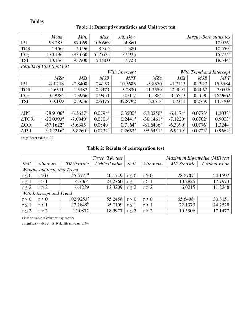
root test. Descriptive statistics and the results of unit root test are presented in Table 1.

<Insert Table 1 here>

From the information on descriptive statistics presented in Table 1, it can be observed

that mean value of CO2 emission is maximum experiencing the highest degree of volatility

owing to maximum standard deviation as compared to other variables under study. The Jarque

Bera Test reveals the non-normal nature of all the variables under study.

The results of unit root test show that the variables are stationary at first order difference.

Therefore, it can be said that the variables under study are integrated to first order, i.e. I (1).5

Further, the long run relationship between the variables is estimated with the Johansen and

Juselius (1990) cointegration test. Results are presented in Table 2, and they show the presence

of cointegrating vectors is visible for both the cases of trace and maximum eigenvalue. It denotes

the presence of cointegrating association among tourism development, transportation, economic

growth, and CO2 emissions.

<Insert Table 2 here>

5.2. Wavelet Decomposition

From the literature, it can be observed that a very limited number of researchers have worked on

analyzing the relationship between the variables under study, within the wavelet framework. The

dataset comprising of a number of different variables has several periods, and all are needed to

explain the proper time scales in the specific analysis (Gallegati et al. 2011). This necessitates

analyzing the relationship between the variables at various time horizons in different time series

data sets with time frequency-based methods, generally referred to ―Wavelets‖. The Wavelets

method considers nonstationarity as the intrinsic property of data and is not required to be sorted

out with pre-processing of the data. The Multiresolution analysis (MRA) of the pattern, J=6 for

all the time series data under study, viz. IPI, TOR, CO2 and TSI employing the MODWT based

Daubechies (1992) Least Asymmetric (LA) Wavelet Filter is illustrated in Figure 1(a-d).

According to Daubechies (1992), the LA Wavelet Filter is the widely used wavelet, as it

provides the most accurate time-alignment between wavelet coefficients at various scales and the

original time series, and it is applicable to wide variety of data types. In Figures 1 (a-d), we plot

the orthogonal components (D1, D2 …, D6) which details the different frequency components of

the original series and a smoothed component (S6). From the figures, we observe high

5 Hylleberg et al. (1990) seasonal unit root test results (see Appendix 2) show no unit root in various frequencies.

frequencies in the short period of the time series under study, with the variations becoming stable

in the longer periods.

<Insert Figure 1 here>

After decomposing the wavelet time series data of the variables under study, we examine

the association between the variables, by employing MODWT based wavelet covariance

analysis, which analyses the covariance between two variables in a particular timescale. Apart

from Wavelet Covariance Analysis, we also employ Wavelet Correlation Analysis to analyze the

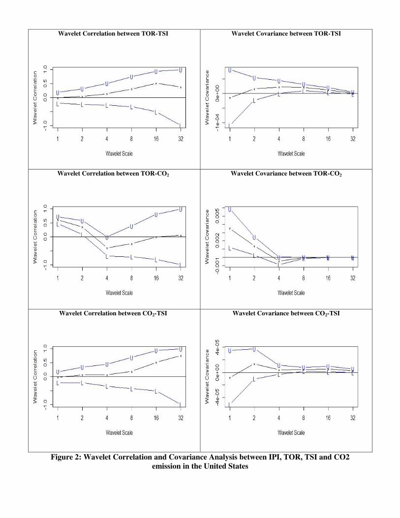
correlation between the variables under study. Figure 2 illustrates the outcome of the Wavelet

Covariance and Correlation between Industrial Production Index, Tourism, Transportation Index

and CO2 emission in the United States. From Figure 2, we can observe positive covariance and

correlation between Industrial Production Index and Tourism development in the United States

in very short, short, medium and long run. Similarly, there exists a positive covariance and

correlation between Industrial Production Index and Transportation Index and CO2 emission.

The tourism development also has a positive influence on Transportation level in the United

States as observed from the Wavelet Correlation and Covariance Analysis. However, Tourism

development is not having a significant influence on CO2 emission. In short and medium run,

there exists a negative correlation between Tourism Development and CO2 emission. In a

medium, long and very long run, there does not exist any covariance between Tourism

Development and CO2 emission in the United States. There exist a positive correlation and

covariance between CO2 emission and Transportation Index in the United States as observed

from Wavelet Correlation and Covariance analysis between the variables under study.

The present paper further employs Continuous Wavelet Analysis on the relationship

between the variables under study to evaluate the findings of MODWT based approach. The

Continuous Wavelet Power Spectrum of all the time series under study is presented in Figure 3.

The Continuous Wavelet Power Spectrum illustrates the movement of the series in a three-

dimension contour plot i.e. time, frequency and color code. From Figure 3, we can very well

witness the different characteristics of IPI, TOR, CO2, and TSI in different time-frequency

domains. The figure indicates that for tourism, there exists a stable variance in a long and very

long run as compared short and medium run. In case of CO2 emission, the variances remain

stable for medium, long and very long run. There exists a strong variance in short and medium

and run for tourism and short run for CO2 emission. The variances remain strong in short and

very long run but remain stable in a medium run for Industrial Production Index. However, for

the Transportation Index, the variances remain strong enough across all time periods.

<Insert Figure 2 here>

<Insert Figure 3 here>

5.3. Wavelets Coherence Transform (WTC)

The outcome of the Wavelet Coherence Transform illustrating the sectors where the two-time

series exhibit co-movement in time and frequency domain is presented in Figure 4. The WTC for

IPI-TOR (Figure 4a) shows that in the period 1-4 and 4-8 months’ cycle during the year 2000 to

the year 2012, the arrows are either right side up or left side down, indicating that IPI and TOR

are in phase presenting the cyclic effect with TOR leading. However, during the year 2013 and

2014, the arrows are in anti-phase. Similarly, during the medium period cycle of 8 to 16 months

also, we find TOR leading during the years of 2005, 2006 and 2010.

<Insert Figure 4 here>

However, in 2014 and 2015, we observe IPI leading. In the long period of 16-32 months’

cycle, TOR leads from the year 2004 to 2007. From the year 2008 to the year 2012, the arrows

point towards the right direction showing the time series data in phase. In the very long period of

32-64 months’ cycle also, the give time series data are in phase. The outcome of WTC for IPI

with CO2 emission (Figure 4b) show that during the year 2013 and 2014, with arrows right side

up, CO2 emission leads in 1-4 months’ cycle. A similar scenario is also observed during the

months of 2001, 2002 2003 and 2004. In the short period of 4 to 8 months’ cycle, IPI lags during

the months of the year 2004. In the long period and very long period of 16 to 32 months’ and 32

to 64 months’ cycle, the time series data remain in phase and IPI leading. Also during the very

long period, CO2 emission leads suggesting that in the case of IPI-CO2 emission, both the

variables are leading each other. In many instances during the long and very long period, we find

strong co-movement between the variables.

For WTC results of IPI-TSI (Figure 4c), we observe both the variables i.e. IPI and TSI

leading each other in the very short period of 0 to 4 months’ cycle. Similarly, in the short period

and medium period also, both the variables are leading each other. During the long and very long

period, we do find strong co-movement between IPI-TSI variables. In the case of TOR-CO2

emission (Figure 4d), TOR leads during 0 to 4 months’ cycle during whole time span under

study. On the contrary, the CO2 emission is observed to be leading in the medium period of 8 to

16 months’ cycle. In the months of the year 2008, 2009, 2010 and 2012, the TOR is observed to

be leading and CO2 emission lagging in the long period of 16 to 32 months’ cycle. In the long

run period, with the arrows pointing towards the right, the variables are observed in phase with

strong co-movement among the variables.

For TOR-TSI, we observe both TOR and TSI (Figure 4e), leading each other, in the very

short period of 1-4 months. In the short period, during the months of the year 2004, we observe

TOR leading and TSI lagging. In the long and very long run period, the variables exhibit strong

co-movements among them. A similar situation is also observed in WTC for CO2 emission and

TSI during the very long period (Figure 4f). In the long period, the CO2 emission is observed to

be leading and TSI lagging. No significant relationship is observed among the variables during

the medium period. In the short and very short period of 1-4 months’ cycle and 4-8 months’

cycle, we observe CO2 emission and TSI leading other.

5.4. Partial and Multiple Wavelet Coherence

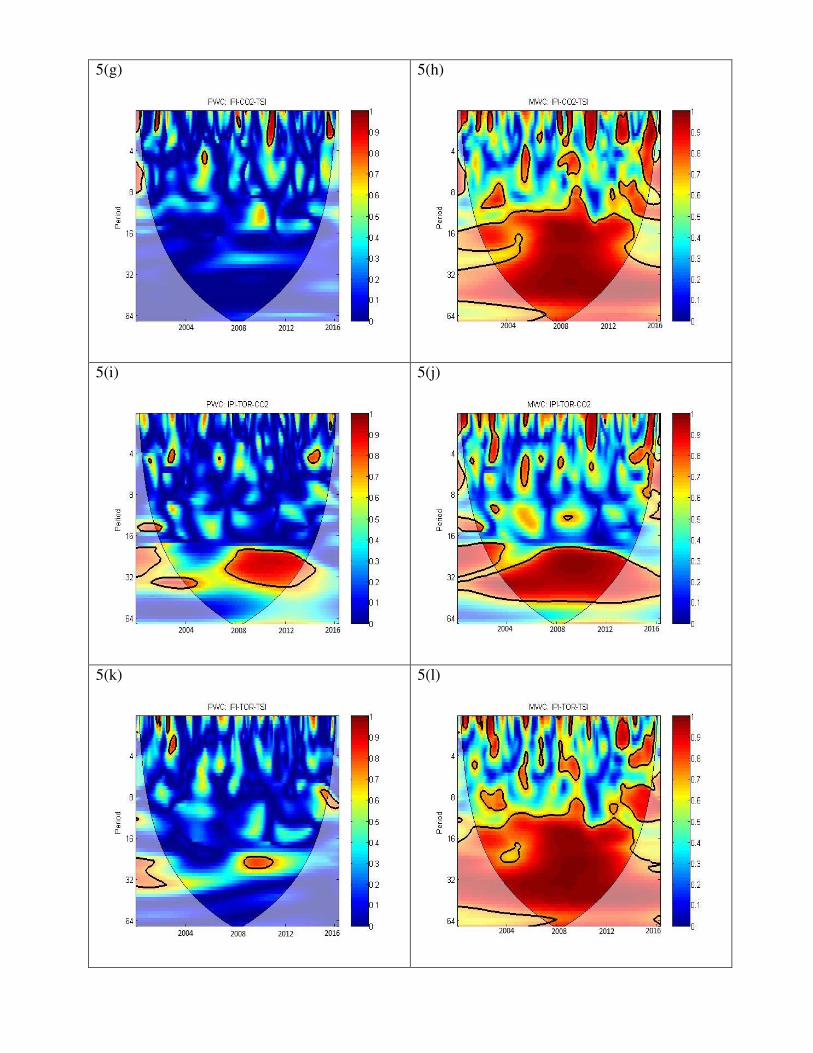
The outcome of Partial and Multiple Wavelet Coherence explaining the coherence plots between

IPI, TOR, CO2, and TSI in the United States presented in Figure 5. The results of Partial Wavelet

Coherence (PWC) is presented on the left-hand side, whereas that of Multiple Wavelet

Coherence (MWC) in Right Hand Side. Figure (5a) presents the partial wavelet coherence

among CO2 emission and Industrial Production Index (IPI) after canceling out the Tourism

(TOR). The correlation is observed to be weak with very few numbers of small red color

significant islands identified across the different horizons. We observe one small island in a very

short period of 0 to 4 months’ cycle in between 2008 and 2012 and one during the months of

2015 and 2016. One small red color significant island is observed in the short period of 4-8

months’ cycle during 2015. Similarly, very few significant islands are observed in medium, the

long and very long horizon of 8-16 months’ cycle, 16-32 months’ cycle and 32 to 64 months’

cycle respectively during the respective months of 2007-2008, 2013-2014 and 2005-2006. When

TOR is considered in the relationship between CO2 emission and IPI, a strong co-movement

among the variables is observed in 1-4 months’ cycle and 4-8 months’ cycle with a remarkable

number of the red color significant island across different time horizons from 2004 to 2016. The

correlation ranges from 0.8 to 1. In the medium run, on the island for a whole 8 - 16 months’

cycle stretching from 2004 to 2015 with correlation range 0.9 to 1 is observed. For the long and

very long period, one red color significant island of correlation ranges 0.7 to 0.9 stretch from, the

year 2005 to the year 2013. From figure 5(a) and 5(b) illustrating the PWC and MWC between,

CO2, IPI, and TOR, we can observe the robust effect of Tourism in examining the relationship

between CO2 emission, Industrial Production Index, and Tourism.

Figure 5(c) illustrates the Partial Wavelet Coherence between CO2 emission and TOR

after canceling out the Transportation Index (TSI). In the frequency bands of 1-4 months’ cycle

and 4-8 months’ cycle, we observe significant red color islands with correlation ranging from 0.8

to 0.9 during the sub-period ranging from 2004 to 2007, 2008 to 2010 and 2012. In the medium

frequency band of 8-16 months’ cycle, we observe one significant red color island as a whole

stretching from 2004 to 2016. The correlation at this medium period ranges from 0.8 to 1. In

MWC, when we consider TSI in examining the relationship between CO2 and TOR, along with

low and medium frequency band, we observe significant red color island in a high-frequency

band covering a long period of 16 – 32 months’ cycle and very long period of 32-64 months’

cycle. In very short, short and medium period, the correlation ranges from 0.8 to 1. However, in

the long and very long period, the correlation ranges from 0.7 to 0.9.

<Insert Figure 5 here>

The Partial Wavelet Coherence between CO2 and TSI on canceling out IPI is shown in

Figure 5(e). From the given PWC, we observe three significant red color islands depicting the

strong co-movement in the frequency band of the very short period 1-4 months’ cycle during

2004, 2009 and 2015. Here the correlation ranges from 0.9 to 1. In a short period of 4-8 months’

cycle, we observe islands during the sub-period of 2004 and 2010. However, the correlation with

a range between 0.6 and 0.7 is not much significant. On considering IPI, in explaining the

relationship between CO2 and TSI (Figure 5f), we observe significant red color islands in the

frequency band of very short period 1-4 months’ cycle during the sub-period of 2003 to 2004,

2005, 2008, 2010 to 2012, and 2015 to 2016. Here the correlation ranges from 0.9 to 1. In a short

period of 4-8 months’ cycle, few islands could be observed, but the correlation ranges from 0.6

to 0.8. In the frequency band of medium period 8 to 16 months, one island is observed in the sub-

period of 2009. Here the correlation is about 0.6. In the long and very long period of 16-32

months’ cycle and 32-64 months’ cycle respectively, we observe one red color significant island

stretching from the sub-period 2004 to 2012 with the correlation ranging from 0.8 to 1.

Figure 5g and figure 5k depicts the partial wavelet coherence between IPI and CO2

emission and IPI and TOR respectively, canceling out TSI from both. In IPI-CO2 relation we

observe small significant red color island depicting strong correlation during sub-period of 2005,

2008, 2010 and 2015. In the frequency band of 4-8 months’ cycle, we observe one significant

island with a correlation of about 0.7 during the sub-period of 2006. In the PWC of IPI and TOR,

we observe three significant red color islands formed during the sub-period of 2004-2005 in the

frequency band of 1-4 months’ cycle. Here the correlation ranges between 0.8 to 1. One small

island is formed in the frequency band of 16-32 months’ cycle with the correlation range

between 0.7-0.9. When we consider TSI, the scenario in the relationship between IPI and CO2

emission and IPI and TOR (Figure 5h and Figure 5l) becomes different. We detect a strong co-

movement in the short, medium and long run of IPI-CO2-TSI and IPI-TOR-TSI. In figure 5h we

observe significant red color islands formed in 2003, 2004, between 2008 and 2011, 2012, and

between 2014 and 2016. The correlation ranges from 0.8 to 1. In the frequency band of 4-8

months’ cycle islands with correlation range from 0.7 to 0.8 are formed between 2008 and 2008

and during 2009. In the frequency band of 8-16 months’ cycle, one island of correlation of about

0.8 is formed in 2004. Apart from them, a single island covering the frequency bands of 8-16

months’, 16-32 months’ and 32-64 months’ cycle is formed which spans from the period 2004 to

2016. Here the correlation ranges from 0.7 to 1. The similar scenario is also observed in figure

5l. The presence of islands formed in frequency bands of 1-4 months’ cycle between 2004 to

2012 in MWC for IPI-TOR-TSI we strong co-movements between the time series. In 4-8months’

cycle islands with correlation range between 0.7 to 0.9 suggest co-movements between the

variables during 2003, between 2004 and 2008 and between 2015 and 2016. A single island with

correlation range between 0.9 and 1 covering all the sub-periods stretches from frequency band

8-16 months’ cycle to 32-64 months’ cycle.

The PWC depicting the relationship between IPI and TOR, TOR and TSI, and TSI and

IPI on canceling the CO2 emission is illustrated in figure 5i, figure 5o and figure 5u. In PWC

between IPI and TOR, as observed in figure 5i, the co-movement between the variables exist

with the formation of islands in the frequency band of 4-8 months’ cycle between 2004 and 2008

and 2012 and 2016. Here the correlation is within the range of 0.7 to 0.9. A very small island

bearing the correlation of about 0.7 is formed in the frequency band of 8 to 16 months’ cycle and

16 to 32 months’ cycle during 2004. Apart from that formation of the single significant red color

island of correlation between 0.9 and 1 in the frequency band of 16-32 months’ cycle indicates

strong co-movement in the long period between 2008-2012. A similar scenario is also observed

in the PWC between TOR and TSI (figure 5o). Here few significant red color islands in the

frequency bands of 4-8 months’ and 8-16 months’ of correlation of about 0.8 indicate strong

movement between the variables between 2004 and 2008. In the frequency band of 32-64

months’ cycle, the red color significant island of correlation about 0.9 is formed between 2012-

2016 showing the co-movement between the variables. In case of PWC between TSI and IPI

(figure 5u), strong co-movement between the variables is observed with the formation of

significant red color islands bearing correlation in the range of 0.8 to 1 in the frequency bands of

1-4 months’ cycle, 4-8 months’ cycle and 8-16 months’ cycle between 2012-2016. Strong co-

movements between the variables also exist between the sub-period 2004 and 2012 in the

frequency band of 16-32 months’ cycle and 32-64 months’ cycle due to presence island bearing

the correlation of the range 0.9 to 1. When CO2 emission is considered in analyzing the

relationship between IPI-TOR-CO2, TOR-TSI-CO2 and TSI-IPI-CO2, the scenario is

significantly different. In case of IPI-TOR-CO2 (figure 5j), due to the formation of significant

red color islands in the very short and short period of 1-4 months’ cycle and 4-8 months’ cycle

respectively, the significant co-movement among the variables is observed between the sub-

period 2004-2008 and 2012-2016. Here the correlation ranges between 0.8 and 1. In between the

sub-period 2004 and 2005, two islands bearing the correlation of range 0.7 to 0.9 are formed in

the frequency band of 16-32 months’ cycle. In the frequency bands of 16-32 months’ cycle and

32-64 months’ cycle, two significant red color islands are formed of correlation ranging between

0.9-1 indicating significant co-movement between the variables in the sub-period between 2004

and 2012. Similarly, when CO2 emission is considered in analyzing the relation between TOR

and TSI (Figure 5p), with the formation of islands between 2003 and 2015, a strong correlation

between the variables exist in the frequency band of 1-4 and 4-8 months’ cycle. Here the

correlation is between 0.9 and 1. Similarly, strong correlation of range 0.8-1 exists between the

time range between 2003 and 2013, in frequency bands of 8-16 months’ cycle, 16-32 months’

cycle, and 32-64 months’ cycle. In the case of MWC between TSI-IPI-CO2 (Figure 5v), strong

correlation ranging between 0.9-1 exist across time horizon in all the frequency bands.

Figure 5m and figure 5q analyses the PWC between TOR and CO2, and TOR and TSI on

canceling the influence of IPI on it. In the PWC analysis of TOR-CO2 as observed in figure 5m

strong correlation of range 0.9-1, exist between the variables in the short period of 1-4 months’

cycle with the presence of islands in the time period between 2004 and 2006, 2008, 2012 and

2015. In the frequency band of 4-8 months’ cycle islands of correlation, range 0.8-1 are formed

during 2004, 2007 and 2012. In the frequency band of 8-16 months’ cycle and the single island is

formed of correlation range 0.9-1 across the time horizon of 2004 to 2016. However, when we

consider the influence of IPI and analyze the relation between TOR-CO2-IPI, we find a strong

correlation among the variables across the time period in all the frequency bands. In the case of

PWC between TOR-TSI, we find a strong correlation between the variables, with only three

small islands formed during 2005, 2009 and 2015 in the frequency band of 1-4 months’ cycle. In

the frequency band of 4-8 months’ cycle, we observe only two small islands of correlation range

0.9-1 formed between 2003 and 2005. When we consider the influence of IPI and analyze the

relation between TOR-TSI-IPI (figure 5r), we observe the formation of islands of correlation

range 0.8-1 between 2003 and 2005, 2008 and between 2010 and 2012 in the short period of 1-4

months’ cycle. We observe very few significant islands formed in the frequency band of 4-8

months’ cycle formed during 2004 and 2008. However, in the frequency band stretching between

16-32 months’ cycle and 32-64 months’ cycle we observe a significant island of correlation

range 0.9-1 formed across the time period 2004-2012.

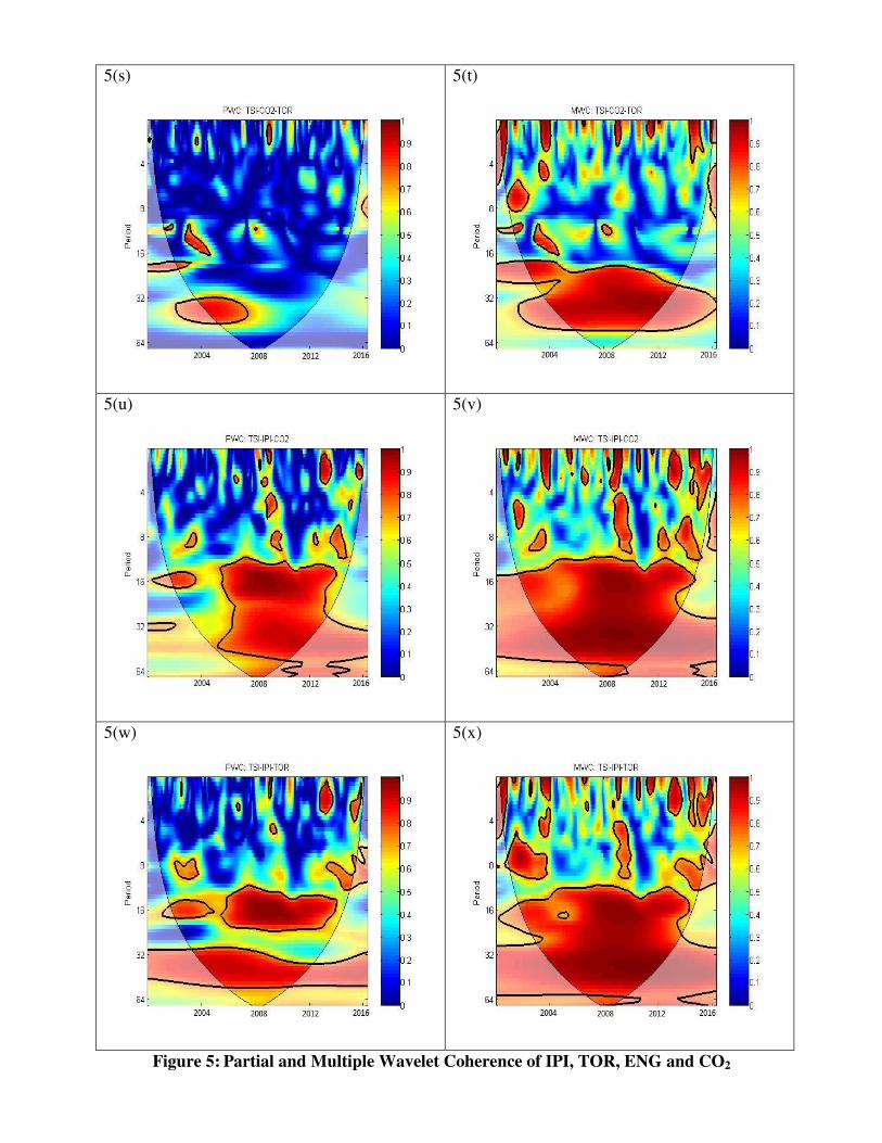
Figure 5s and figure 5w analyze the PWC between TSI-CO2 and TSI-IPI respectively on

canceling the influence of TOR. In the PWC of TSI-CO2 (figure 5s) we observe only one island

of strong correlation formed in the frequency band of 1-4 months’ cycle in the sub-period

between 2008 and 2012. Similarly, in the frequency bands of 8-16 months’ cycle, 16-32 months’

cycle and 32-64 months’ cycle only one island of correlation range 0.9-1 is formed between 2004

and 2006. When we consider the influence of TOR in analyzing the TSI-CO2-TOR relation

(figure 5t), we observe few islands of correlation range 0.8-1 formed between 2004-2006, 2008-

2012 and 2012-2015 in the very short period of 1-4 months’ cycle. In the frequency band of 4-8

months’ cycle and 8-16 months’ cycle, we find few small significant red color islands formed

between 2004 and 2008. However, in the frequency band stretching from 16-32 months’ cycle

and 32-64 months’ cycle, we find a single significant red color island formed across the time

period 2004-2012. Here the correlation ranges between 0.8-1. The presence of this single island

indicates the existence of strong co-movement between the variables in the long and very long

period. Figure 5w illustrates the PWC between TSI-IPI on canceling the effect of TOR. In the

figure 5w, we observe significant red color islands of correlation 0.9-1, formed between 2012-

2016 in the frequency band of 1-4 months’ cycle. In the frequency band of 8-16 months’, 16-32

months, and 32-64 months’ cycle we observe a strong correlation among the variables between

the time period 2006-2012. When we consider the influence of TOR in analyzing TSI-IPI-TOR

relation (Figure 5x), we observe with the presence of small islands formed in the frequency band

of 1-4 months’ cycle between the period 2001-2004 and 2015 indicating the correlation of range

0.8-1. In the frequency band of 4-8 months’ cycle, we few islands formed between the period

2004-2006, 2008-2010 and 2013-2016. Here the correlation ranges between 0.8-1. In the

frequency band stretching from 16-32 months’ cycle to 32-64 months’, the cycle we observe a

single significant red color island formed across 2004-2012. Here the correlation range is 0.9-1.

This indicates the presence of intense co-movement between the variables in the long and very

long period.

As a final step of the analysis, following Lehkonen and Heimonen (2014), Mensi et al.

(2016) and Gupta et al. (2018), we have conducted the Granger causality tests on the original and

wavelet-decomposed data. The causality test results on the original data show the existence of

bidirectional causal association between CO2 emissions and tourism development. Alongside

this, industrial production and transportation service are found to have respective causal impacts

on tourism development. However, the results of causality results on frequency-decomposed data

reveal the existence of the bidirectional casual associations between CO2 emissions and tourism

development, industrial production and tourism development, and transportation service and

tourism development, respectively. In light of this new evidence, we can conclude that the co-

movements among the model parameters discovered through the wavelet coherence analysis are

subsequently validated by the results of causality analysis. Therefore, we can infer that in the

short run, while having a co-movement among the variables, significant causal association

among the variables can also be found.

6. Conclusion and Policy Recommendations

The present paper employs wavelets transform approach to analyze the relation between tourism

development, transportation, economic growth, and CO2 emissions. The approach decomposes

the time series into a number of time frequencies and presents the outcomes specific to these

frequencies based on very short, short, medium, long and very long run. The study employs

MODWT, wavelet covariance, wavelet correlation, continuous wavelet power spectrum, wavelet

coherence transform, partial and multiple wavelet coherence, and wavelet-based Granger

causality tests to analyze the association between the variables in the USA. The paper uses the

monthly data from January 2001 to December 2017.

The wavelet approach employed in the present study explains the way the association

between the model variables develops over time and frequencies. The wavelet decomposition

analysis indicates the frequency of the variables becoming stable in the long run, whereas

wavelet covariance and correlation analysis indicate positive correlation and covariance between

them. As revealed by the wavelet coherence transform, wavelet coherence and robust lead-lag

relationship exist among the variables. For the temporal domain, we observe a heterogeneous

association between the variables. Co-movements of the variables are observed to be unequal

across the time periods. Partial and multiple wavelet coherence analysis divulge significant

association among the model variables. Moreover, the results of wavelet-based Granger causality

analysis divulge bidirectional causal links between CO2 emissions and tourism development,

industrial production and tourism development, and transportation service and tourism

development, respectively.

The outcome of the analysis calls for significant policy implications for the sustainable

tourism development in the USA. As the ecotourism in the USA is on a rise, the policymakers

should invest the revenue generated from tourism in educating the tourists about maintaining the

ecological quality, so that ecosystem can remain unharmed. Along with investing for increasing

the awareness among the tourists, the policymakers should also preserve the natural resources,

while limiting the expansion in the ecotourism activities. Soft ecotourists should be encouraged

more over the hard ecotourists, as the engagement of soft ecotourists with the environment is

less, and therefore, the possibility and volume of environmentally degrading activities reduce.

Rising level of environmental awareness will also make the hard ecotourists inherently comply

with the directives for the preservation of ecological quality, and it will eventually help the USA

to earn more revenue from ecotourism.

While saying this, it should also be mentioned that the mode of transportation used in the

tourism industry needs a thorough reassessment. The mode of transportation used in the tourism

sector is not only responsible for the ambient air pollution, but also the shift in ecological

balance through displacement of the wildlife. Owing to the negative impact of transportation

sector on environmental quality, policymakers need to promote clean energy policies, which

might help the US in promoting sustainable tourism. In this pursuit, policymakers may promote

hybrid engines, electrical transport or carbon neutral transport solutions for land transport. At the

same time, it is also needed to enhance their investment in R&D activities towards development

fuel efficient and cleaner technologies especially thriving upon the renewable sources of energy,

which will help in reducing pollution in the long-run. Now, shifting the fuel sources from

nonrenewable to renewable at one go might harm the economic growth pattern significantly, as

well as the growth in tourism sector. Owing to the high implementation cost of renewable energy

solutions, the policymakers need to carry out a phase-wise shift of fuel sources. Alternate fuels

for transport might be implemented in the places with low tourist penetration to start with, and

with graduation of acceptance among the users and communities, implementation might be

carried out towards the areas with high tourist penetration. While carrying this out, the

policymakers should also think of encouraging the people-public-private partnerships for making

the transition smoother. Along with these policies, the policymakers should also need to be

careful about the use of transportation in the deeper regions of the forests, as the increased use of

transportation by hard ecotourists might create ecological imbalance. Therefore, while carrying

out cleaner energy policies, the policymakers should also think about restricting the use of

transportation in the deep forest areas.

As future scope of research, the study could also employ daily and weekly data to get a

more detailed outcome. Moreover, from the contextual perspective, scope of the study could be

further extended to other nations like France, China, Germany, Spain etc. which have not only

witnessed huge tourism development but also experienced economic growth.

Appendix

Appendix 1: Results of Seasonal unit root test at level

3 Months 6 Months 12 Months

IPI -2.606c -5.990a -4.637a TOR -2.795c -6.747a -3.895a CO2 -3.088b -10.001a -5.453a TSI -2.179b -5.217a -4.080a

a significant value at 1%, b significant value at 5%, c significant value at 10%

Tables

Table 1: Descriptive statistics and Unit root test

Mean Min. Max. Std. Dev. Jarque-Bera statistics IPI 98.285 87.069 106.663 4.860 10.976a TOR 4.456 2.096 8.365 1.380 10.550a CO2 470.196 383.660 557.625 37.925 15.774a TSI 110.156 93.900 124.800 7.728 18.544a Results of Unit Root test

With Intercept With Trend and Intercept

MZa MZt MSB MPT MZa MZt MSB MPT

IPI -2.0218 -0.8408 0.4159 10.5685 -5.8570 -1.7113 0.2922 15.5584 TOR -4.6511 -1.5487 0.3479 5.2830 -11.3550 -2.4091 0.2062 7.0556 CO2 -0.3984 -0.3966 0.9954 50.017 -1.1884 -0.5573 0.4690 46.9662 TSI 0.9199 0.5956 0.6475 32.8792 -6.2513 -1.7311 0.2769 14.5709 ∆IPI -78.9106a -6.2627a 0.0794a 0.3500a -83.0250a -6.4174a 0.0773a 1.2033a ∆TOR -20.0393a -7.0849a 0.0706a 0.2441a -30.1461a -7.1220a 0.0702a 0.9003a ∆CO2 -67.1622a -5.6385a 0.0840a 0.7164a -81.6436a -6.3390a 0.0776a 1.3244a ∆TSI -93.2216a -6.8260a 0.0732a 0.2653a -95.6451a -6.9119a 0.0723a 0.9662a

a significant value at 1%

Table 2: Results of cointegration test

Trace (TR) test Maximum Eigenvalue (ME) test

Null Alternate TR Statistic Critical value Null Alternate ME Statistic Critical value

Without Intercept and Trend r ≤ 0 r > 0 45.5771a 40.1749 r ≤ 0 r > 0 28.8707a 24.1592 r ≤ 1 r > 1 16.7064 24.2760 r ≤ 1 r > 1 10.2825 17.7973 r ≤ 2 r > 2 6.4239 12.3209 r ≤ 2 r > 2 6.0215 11.2248 With Intercept and Trend

r ≤ 0 r > 0 102.9253a 55.2458 r ≤ 0 r > 0 65.6408a 30.8151 r ≤ 1 r > 1 37.2845b 35.0109 r ≤ 1 r > 1 22.1973 24.2520 r ≤ 2 r > 2 15.0872 18.3977 r ≤ 2 r > 2 10.5906 17.1477

r is the number of cointegrating vectors

a significant value at 1%, b significant value at 5%

Table 3: Results of Wavelet-based Granger Causality tests

Frequency Domains Dependent Variables Independent Variables

IPI TOR CO2 TSI

D1

IPI - 16.9273b 1.2567 21.9575a TOR 31.3103a - 21.0715a 19.5302a CO2 26.3759a 15.8762a - 10.2930b TSI 7.2386c 3.5154c 11.8731b -

D2

IPI - 3.1974c 0.3839 7.7511a TOR 23.8193a - 21.0857a 16.2776a CO2 17.9916b 7.9488a - 15.2727b TSI 13.1979a 2.6391 8.7834c -

D3

IPI - 15.1958b 1.8753 28.4359a TOR 21.9815a - 24.1255a 16.4274a CO2 23.5337a 215.3583a - 22.7770a TSI 14.3971a 12.8440b 13.7680a -

D4

IPI - 18.8371b 5.4995b 6.0557b TOR 16.6077a - 5.9843b 21.4189a CO2 15.0956a 54.0960a - 32.1816a TSI 4.2164b 21.2484a 13.5562a -

D5

IPI - 7.1338b 9.2638a 18.7076a TOR 74.6382a - 24.4549a 3.7064c CO2 12.3198a 23.3502a - 25.2039a TSI 6.3580b 27.7620a 15.9180a -

D6

IPI - 16.7368a 26.3779a 96.5913a TOR 41.3161a - 6.0611b 32.4846a CO2 73.6162a 52.5378a - 22.7352a TSI 119.2425a 26.4918a 13.2017b -

Original

IPI - 2.2588 0.0837 15.1129a TOR 24.0120a - 13.1949a 20.0705a CO2 0.2335 22.0946a - 18.5468b TSI 9.6929a 3.9371 1.8737 -

Note: Asymptotic Chi-square values are reported

a significant value at 1%, b significant value at 5%, c significant at 10%

Figures

Figure 1(a)

Figure 1(b)

Figure 1 (c)

Figure 1(d)

Figure 1: MODWT decomposition of variables on J = 6 Wavelet Levels

Wavelet Correlation between IPI-TOR

Wavelet Covariance between IPI-TOR

Wavelet Correlation between IPI-TSI

Wavelet Covariance between IPI-TSI

Wavelet Correlation between IPI-CO2

Wavelet Covariance between IPI-CO2

Wavelet Correlation between TOR-TSI

Wavelet Covariance between TOR-TSI

Wavelet Correlation between TOR-CO2

Wavelet Covariance between TOR-CO2

Wavelet Correlation between CO2-TSI

Wavelet Covariance between CO2-TSI

Figure 2: Wavelet Correlation and Covariance Analysis between IPI, TOR, TSI and CO2

emission in the United States

3(a)

3(b)

3(c)

3(d)

Figure 3: Continuous Wavelet Transform of IPI, TOR, CO2 & TSI

4(a)

4(b)

4(c)

4(d)

4(e)

4(f)

Figure 4: Wavelet Coherence of IPI, TOR, CO2 & TSI

5(a)

5(b)

5(c)

5(d)

5(e)

5(f)

5(g)

5(h)

5(i)

5(j)

5(k)

5(l)

5(m)

5(n)

5(o)

5(p)

5(q)

5(r)

5(s)

5(t)

5(u)

5(v)

5(w)

5(x)

Figure 5: Partial and Multiple Wavelet Coherence of IPI, TOR, ENG and CO2

References

Aguiar-Conraria, L., Azevedo, N., Soares, M.J., 2008. Using wavelets to decompose the time-frequency effects of monetary policy. Physica A: Statistical mechanics and its Applications, 387(12), 2863-2878.

Aguiar-Conraria, L., Soares, M.J., 2011. Oil and the macroeconomy: using wavelets to analyze old issues. Empirical Economics, 40(3), 645-655.

Aguiar-Conraria, L., Martins, M.M., Soares, M.J., 2012. The yield curve and the macro-economy across time and frequencies. Journal of Economic Dynamics and Control, 36(12), 1950-1970.

Al-Mulali, U., Fereidouni, H.G., Janice Y.M. L. Mohammed, A.H., 2014. Estimating the tourism-led growth hypothesis: A case study of the Middle East countries, Anatolia. 25(2), 290-298.

Asif, M., Muneer, T., 2007. Energy supply, its demand and security issues for developed and emerging economies, Renewable and Sustainable Energy Reviews, 11(7), 1388-1413.

Balli, F., Shahzad, S.J.H., Uddin, G.S., 2018. A tale of two shocks: What do we learn from the impacts of economic policy uncertainties on tourism? Tourism Management, 68, 470-475.

Basarir, C., and Cakir, Y. N., 2015. Causal interactions between CO2 emissions, financial development, energy and tourism, Asian Economic and Financial Review, 5(11), 1227-1238.

Becken, S., 2011. Oil, the global economy and tourism, Tourism Review, 66(3), 65-72. Becken, S., Simmons, D.G., Frampton, C., 2003. Energy use associated with different travel

choices, Tourism Management, 24(3), 267-277. Boden, T.A., Marland, G., Andres. R.J., 2011, Global, Regional, and National Fossil-Fuel CO2

Emissions. Carbon Dioxide Information Analysis Center, Oak Ridge National Laboratory, U.S. Department of Energy, Oak Ridge, Tenn., U.S.A.

Byrnes, T.A., Warnken, J., 2006, Greenhouse gas emissions from marine tours: A case study of Australian tour boat operators, Journal of Sustainable Tourism, 14, 255–270.

Crouch, G.I., Ritchie, B.J.R., 1999. Tourism, Competitiveness, and Societal Prosperity, Journal of Business Research, 44, 137–152.

Das, D., Kumar, S.B., 2018. International economic policy uncertainty and stock prices revisited: Multiple and Partial wavelet approach. Economics Letters, 164, 100-108.

Day, J., Cai, L.P., 2012. Environmental and energy-related challenges to sustainable tourism in the United States and China, International Journal of Sustainable Development and World Ecology, 19(5), 379-388.

Dima, B., Dima, Ş.M., Barna, F., 2015. A wavelet analysis of capital markets’ integration in Latin America. Applied Economics, 47(10), 1019-1036.

Dogan, E., Seker, F., 2016, The influence of real output, renewable and non-renewable energy, trade and financial development on carbon emissions in the top renewable energy countries, Renewable and Sustainable Energy Reviews, 60, 1074-1085.

Dogan, E., Seker, F., Bulbul, S., 2017. Investigating the impacts of energy consumption, real GDP, tourism and trade on CO2 emissions by accounting for cross-sectional dependence: A panel study of OECD countries, Current Issues in Tourism, 20(16), 1701-1719.

Dubois, G., Ceron, J.P., 2006. Tourism/leisure greenhouse gas emissions forecasts for 2050: Factors for change in France, Journal of Sustainable Tourism, 14(2), 172-191.

Durbarry, R., Seetanah, B., 2015. The Impact of Long Haul Destinations on Carbon Emissions: The Case of Mauritius, Journal of Hospitality Marketing & Management, 24(4), 401-410.

Ertugrul, H.M., Cetin, M., Seker, F., Dogan, E., 2016. The impact of trade openness on global carbon dioxide emissions: Evidence from the top ten emitters among developing countries, Ecological Indicators, 67, 543-555.

Fetters, A.K., 2017. Why Ecotourism Is Booming. U.S. News and World Report. Available at: https://travel.usnews.com/features/why-ecotourism-is-booming

Gössling, S., 2002. Global environmental consequences of tourism, Global Environmental Change, 12(4), 283-302.

Gupta, S., Das, D., Hasim, H., Tiwari, A.K., 2018. The dynamic relationship between stock returns and trading volume revisited: A MODWT-VAR approach. Finance Research Letters, 27, 91-98.

Howitt, O.J.A., Revol, V.G.N., Smith, I.J., Rodger, C.J., 2010. Carbon emissions from international cruise ship passengers’ travel to and from New Zealand. Energy Policy, 38(5), 2552-2560.

Hylleberg, S., Engle, R.F., Granger, C.W., Yoo, B.S., 1990. Seasonal integration and cointegration. Journal of Econometrics, 44(1-2), 215-238.

Işik, C., Doğan, E., Ongan, S., 2017. Analyzing the Tourism–Energy–Growth Nexus for the Top 10 Most-Visited Countries. Economics, 5(40), 1-13.

Isik, C., 2012. The USA’s international travel demand and economic growth in Turkey: A causality analysis: (1990–2008). Tourismos: An International Multidisciplinary Journal of Tourism, 7, 235–252.

Isik, C., 2013. The importance of creating a competitive advantage and investing in information technology for modern economies: An ARDL test approach from Turkey. Journal of the Knowledge Economy, 4, 387–405.

Isik, C., Shahbaz, M., 2015. Energy Consumption and Economic Growth: A Panel Data Approach to OECD Countries. International Journal of Energy Science, 5, 1–5.

Isik, C., Radulescu, M., 2017a. Investigation of the Relationship between Renewable Energy, Tourism Receipts and Economic Growth in Europe. Statıstıka-Statıstıcs and Economy Journal, 97, 85–94.

Isik, C., Radulescu, M., 2017b. Electricity–Growth Nexus in Turkey: The Importance of Capital and Labor. Revista Română de Statistică, 6, 230–244.

Johansen, S., Juselius, K., 1990. Maximum likelihood estimation and inference on cointegration—with applications to the demand for money. Oxford Bulletin of Economics and Statistics, 52(2), 169-210.

Katircioglu, S.T., Feridun, M., Kilinc, C., 2014. Estimating tourism-induced energy consumption and CO2 emissions: The case of Cyprus. Renewable and Sustainable Energy Reviews, 29, 634-640.

Katircioglu, S., 2014a. International tourism, energy consumption, and environmental pollution: The case of Turkey. Renewable and Sustainable Energy Reviews, 36, 180-187.

Katircioglu, S., 2014b. Testing the tourism-induced EKC hypothesis: The case of Singapore. Economic Modelling, 41, 383-391.

Kumar, M., Prashar, S., Jana, R.K., 2019. Does international tourism spur international trade and output? Evidence from wavelet analysis. Tourism Economics, 25(1), 22-33.

Lai, T.M., To, W.M., Lo, W.C., Choy, Y.S., Lam, K.H., 2011. The causal relationship between electricity consumption and economic growth in a Gaming and Tourism Center: The case of Macao SAR, the People’s Republic of China. Energy, 36(2), 1134-1142.

Lee, J.W., Brahmasrene, T., 2013. Investigating the influence of tourism on economic growth and carbon emissions: Evidence from panel analysis of the European Union. Tourism Management, 38, 69-76.

Lehkonen, H., Heimonen, K., 2014. Timescale-dependent stock market comovement: BRICs vs. developed markets. Journal of Empirical Finance, 28, 90-103.

Lenzen, M., Sun, Y.Y., Faturay, F., Ting, Y.P., Geschke, A., Malik, A., 2018. The carbon footprint of global tourism. Nature Climate Change, 8(6), 522-528.

Lin, T.P., 2010. Carbon dioxide emissions from transport in Taiwan’s national parks. Tourism Management, 31(2), 285-290

Liu, J., Feng, T., Yang, X., 2011. The energy requirements and carbon dioxide emissions of the tourism industry of Western China: A case of Chengdu city. Renewable and Sustainable Energy Reviews, 15(6), 2887-2894.

Mensi, W., Hammoudeh, S., Tiwari, A.K., 2016. New evidence on hedges and safe havens for Gulf stock markets using the wavelet-based quantile. Emerging Markets Review, 28, 155-183.

Nepal, S.K., 2008. Tourism induced rural energy consumption in the Annapurna region of Nepal. Tourism Management, 29, 89-100.

Ng, E.K., Chan, J.C., 2012. Geophysical applications of partial wavelet coherence and multiple wavelet coherence. Journal of Atmospheric and Oceanic Technology, 29(12), 1845-1853.

Nielsen, S.P., Sesartic, A., Stucki, M., 2010. The greenhouse gas intensity of the tourism sector: The case of Switzerland. Environmental Science and Policy, 13(2), 131-140.

Peeters, P., Szimba, E., Duijnisveld, M., 2007. Major environmental impacts of European tourist transport. Journal of Transport Geography, 15(2), 83-93.

Perch-Nielsen, S., Sesartic, A., Stucki, M., 2010. The greenhouse gas intensity of the tourism sector: The case of Switzerland. Environmental Science and Policy, 13(2), 131-140.

Raza, S.A., Sharif, A., Wong, W.K., Karim, M.Z.A., 2017. Tourism development and environmental degradation in the United States: evidence from the wavelet-based analysis. Current Issues in Tourism, 20(16), 1768-1790.

Roueff, F., Von Sachs, R., 2011. Locally stationary long memory estimation. Stochastic Processes and their Applications, 121(4), 813-844.

Sharif, A., Afshan, S., Nisha, N., 2017. Impact of tourism on CO2 emission: evidence from Pakistan, Asia Pacific Journal of Tourism Research, 22(4), 408-421.

Scott, D., 2011. Why sustainable tourism must address climate change? Journal of Sustainable Tourism, 19, 17-34.

Singh, R., Das, D., Jana, R.K., Tiwari, A.K., 2018. A wavelet analysis for exploring the relationship between economic policy uncertainty and tourist footfalls in the USA. Current Issues in Tourism, 1-8.

Solarin, S.A., 2014. Tourist arrivals and macroeconomic determinants of CO2 emissions in Malaysia. Anatolia, 25(2), 228-241.

Suresh, K.G., Tiwari, A.K., 2018. Does international tourism affect international trade and economic growth? The Indian experience. Empirical Economics, 54(3), 945-957.

Tang, C.F., Tiwari A.K., Shahbaz, M., 2016. Dynamic inter-relationships among tourism, economic growth, and energy consumption in India. Geosystem Engineering, 19(4), 158-169.

Tiwari, A.K., Ozturk, I., Aruna, M., 2013. Tourism, energy consumption and climate change in OECD countries. International Journal of Energy Economics and Policy, 3, 247-261.

UNWTO, 2008. Climate Change and Tourism: Responding to Global Challenges. World Tourism Organisation, Madrid.

Wu, P., Shi, P.J., 2011. An estimation of energy consumption and CO2 emissions in the tourism sector of China, Journal of Geographical Science, 21(4), 733-745.

Wei, Y.X., Sun, G.N., Ma, L.J., 2012. Estimating the carbon emissions and regional differences of tourism transport in China. Journal of Shanxi Normal University, 40(2), 76-84.

Yorucu, V., Mehmet, O., 2015. Modeling energy consumption for growth in an open economy: ARDL and causality analysis for Turkey. International Journal of Green Energy, 12, 1197- 1205.

Zaman, K., Shahbaz, M., Loganathan, N., Raza, S.A., 2016. Tourism development, energy consumption and Environmental Kuznets Curve: Trivariate analysis in the panel of developed and developing countries. Tourism Management, 54, 275-283.