Dynamic fMRI brain connectivity -...

Master’s Thesis

Dynamic fMRI brain connectivity:A study of the brain’s large-scale network dynamics

Author: Supervisors:Per Brantefors William Hedley [email protected] Peter Fransson

Examiner:Anders Eklund

Karolinska InstitutetDepartment of Clinical NeurosienceMaster’s Thesis Engineering PhysicsAcademic Year 2015/2016, January 18, 2016

Abstract

Approximately 20% of the body’s energy consumption is ongoingly consumedby the brain, where the main part is due to the neural activity, which is onlyincreased slightly when doing a demanding task. This ongoingly neural activityare studied with the so called resting-state fMRI, which mean that the neuralactivity in the brain is measured for participants with no specific task. Thesestudies have been useful to understand the neural function and how the neuralnetworks are constructed and cooperate. This have also been helpful in severalclinical research, for example have differences been identified between bipolardisorder and major depressive disorder [1]. Recent research has focused on tem-poral properties of the ongoing activity and it is well known that neural activityoccurs in bursts. In this study, resting-state fMRI data and temporal graphtheory is used to develop a point based method (PBM) to quantify these burstsat a nodal level. By doing this, the bursty pattern can be further investigatedand the nodes showing the most bursty pattern (i.e hubs) can be identified. Themethod developed shows a robustness regarding several different aspects. In themethod is two different variance threshold algorithms suggested. One local vari-ance threshold (LVT) based on the individual variance of the edge time-seriesand one global variance threshold (GVT) based on the variance of all edgestime-series, where the GVT shows the highest robustness. However, the choiceof threshold needs to be adapted for the aims of the current study. Finally, thismethod ends up in a new measure to quantify this bursty pattern named burstycentrality. The derived temporal graph theoretical measure was correlated withtraditional static graph properties used in resting state and showed a low butsignificant correlation. By applying this method on resting-state fMRI data for32 young adults was it possible to identify regions of the brain that showed themost dynamic properties, these regions differed between the two thresholdingalgorithms.

i

Sammanfattning

Ungefär 20% av kroppens energikonsumtion konsumeras ständigt av hjärnan,där huvudelen av enegin går åt till den neurala aktiviteten, som bara ökar nå-got vid en pågående arbetesuppgift. Denna pågående neurala aktiviteten stud-eras med fMRI i vilande tillstånd, vilket innebär att den neurala aktiviteten ihjärnan mäts när testdeltagaren inte har någon specifik uppgift. Dessa studierhar varit viktiga för att få förståelse för de neurala funktionerna och hur deneurala nätverken är uppbyggda och sammarbetar. Detta har också varit tillnytta i flertalet kliniska projekt, till exempel har skillnader identifierats mellanbipolära personer och personer med allvarlig depression [1]. Senare forskning harfokuserat på de temporala egenskaperna av den pågående neurala aktivitetenoch det är nu allmänt känt att den neurala aktiviteten sker i skurar. I den härstudien används data från fMRI i vilande tillstånd och temporal grafteori att föratt utveckla en punkt baserad metod (PBM) för att kvantifiera dessa skurar pånodnivå. Genom denna metod kan man ytterligare undersöka detta mönster ochde noder som uppvisar den högsta graden av skurar (s.k hubar) kan identifieras.Metoden som har utvecklats uppvisar en robusthet i flera olika avseenden. Imetoden presenteras även två olika algoritmer för varianströskling. En lokal var-ianströskel (LVT) som baseras på den individuella variansen för varje kopplingstidsserie och en global varianströskel (GVT) som utgår från den globala vari-ansen för alla kopplingars tidsserier, där GVT uppvisar den bästa robustheten.Men valet av trösklings algoritm måste anpassas för målet man har med studien.Slutligen presenteras ett nytt mått för att kvantifiera detta mönster på nodnivå,bursty centrality. Det utvecklade temporala grafiteori måttet korrelerades sedanmed traditionella statiska grafteori mått som ofta används för fMRI i vilandetillstånd och visade en svag men signifikant korrelation. Genom att sedan an-vända denna metod på data från fMRI i vilande tillstånd från 32 unga vuxna vardet möjligt att identifiera områden i hjärnan som visade de största dynamiskaegenskaperna, dessa områden varierade för de olika trökslings algoritmerna.

ii

Commonly Used Acronyms

MRI Magnetic Resonance ImagingfMRI functional Magnetic Resonance ImagingTR Repetition Time; indicating the temporal resolution of MRI

imagesHb Oxygenated hemoglobindHb Deoxygenated hemoglobinBOLD Blood-Oxygen-Level-DependentMNI Atlas of brain coordinates produced by Montreal Neurolog-

ical InstituteAAL Automated Anatomical LabelingBA Brodmann areaPBM Point based methodROI Region of interestPower Power 164 atlasHO Harvard-Oxford atlasPCA Principle component analysisDMN Default mode networkSMN Somato-motor networkVis Visual networkFPN Frontal parietal networkSAN Salience networkCON Cingulo opercular networkAU Auditory networkSub Subcortical networkVAN Ventral attention networkDAN Dorsal attention networkETPS Edge time-point scalingGTPS Global time-point scalingLVT Local variance thresholdGVT Global variance thresholdISI Inter spike intervalminL Minimum length of a burst

iv

Dynamic fMRI brain connectivity: Contents

Contents1 Introduction 1

1.1 Background . . . . . . . . . . . . . . . . . . . . . . . . . . . . . . 11.2 Aims . . . . . . . . . . . . . . . . . . . . . . . . . . . . . . . . . . 21.3 Limitations . . . . . . . . . . . . . . . . . . . . . . . . . . . . . . 2

2 Theory 32.1 Imaging . . . . . . . . . . . . . . . . . . . . . . . . . . . . . . . . 3

2.1.1 Magnetic Resonance Imaging . . . . . . . . . . . . . . . . 32.1.2 Functional Magnetic Resonance Imaging . . . . . . . . . . 42.1.3 Spatial resolution . . . . . . . . . . . . . . . . . . . . . . . 52.1.4 Temporal resolution . . . . . . . . . . . . . . . . . . . . . 5

2.2 Neuroanatomy and neural networks . . . . . . . . . . . . . . . . . 62.2.1 Neurons . . . . . . . . . . . . . . . . . . . . . . . . . . . . 62.2.2 Neural networks . . . . . . . . . . . . . . . . . . . . . . . 6

2.3 Graph theory in neuroscience . . . . . . . . . . . . . . . . . . . . 8

3 Method 103.1 Data . . . . . . . . . . . . . . . . . . . . . . . . . . . . . . . . . . 103.2 Preprocessing - SPM12 . . . . . . . . . . . . . . . . . . . . . . . . 10

3.2.1 Head motion correction . . . . . . . . . . . . . . . . . . . 103.2.2 Coregistration . . . . . . . . . . . . . . . . . . . . . . . . 113.2.3 Segmentation . . . . . . . . . . . . . . . . . . . . . . . . . 113.2.4 Normalization . . . . . . . . . . . . . . . . . . . . . . . . . 113.2.5 Smoothing . . . . . . . . . . . . . . . . . . . . . . . . . . 12

3.3 Postprocessing - CONN . . . . . . . . . . . . . . . . . . . . . . . 123.4 MRIcron . . . . . . . . . . . . . . . . . . . . . . . . . . . . . . . . 133.5 BrainNet Viewer . . . . . . . . . . . . . . . . . . . . . . . . . . . 133.6 Power 264 atlas . . . . . . . . . . . . . . . . . . . . . . . . . . . . 133.7 Harvard-Oxford atlas . . . . . . . . . . . . . . . . . . . . . . . . . 143.8 Principal Component Analysis . . . . . . . . . . . . . . . . . . . 143.9 K-means clustering . . . . . . . . . . . . . . . . . . . . . . . . . . 153.10 State-Graphlets and Temporal-Graphlets . . . . . . . . . . . . . . 173.11 Weighting . . . . . . . . . . . . . . . . . . . . . . . . . . . . . . . 18

3.11.1 Global time-point scaling . . . . . . . . . . . . . . . . . . 193.11.2 Edge time-point scaling . . . . . . . . . . . . . . . . . . . 19

3.12 Thresholding . . . . . . . . . . . . . . . . . . . . . . . . . . . . . 203.12.1 Local Variance Threshold . . . . . . . . . . . . . . . . . . 213.12.2 Global Variance Threshold . . . . . . . . . . . . . . . . . 22

3.13 Bursty centrality . . . . . . . . . . . . . . . . . . . . . . . . . . . 23

4 Results 244.1 Dependence of thresholding algorithm . . . . . . . . . . . . . . . 244.2 Comparison between atlases . . . . . . . . . . . . . . . . . . . . . 274.3 Dependence of k-value . . . . . . . . . . . . . . . . . . . . . . . . 284.4 Dependence of weighting algorithm . . . . . . . . . . . . . . . . . 294.5 Comparison between datasets . . . . . . . . . . . . . . . . . . . . 304.6 Comparison with other measures . . . . . . . . . . . . . . . . . . 31

v

Dynamic fMRI brain connectivity: Contents

5 Discussion 335.1 Clustering . . . . . . . . . . . . . . . . . . . . . . . . . . . . . . . 335.2 Weighting . . . . . . . . . . . . . . . . . . . . . . . . . . . . . . . 335.3 Atlases . . . . . . . . . . . . . . . . . . . . . . . . . . . . . . . . . 335.4 Datasets . . . . . . . . . . . . . . . . . . . . . . . . . . . . . . . . 345.5 Thresholding . . . . . . . . . . . . . . . . . . . . . . . . . . . . . 345.6 Inter spike interval and minimum length . . . . . . . . . . . . . . 345.7 Robustness of the method . . . . . . . . . . . . . . . . . . . . . . 355.8 Bursty Centrality . . . . . . . . . . . . . . . . . . . . . . . . . . . 355.9 Future Work . . . . . . . . . . . . . . . . . . . . . . . . . . . . . 36

6 Conclusion 37

A Appendix A 40

B Appendix B 42

C Appendix C 46

vi

Dynamic fMRI brain connectivity: 1 Introduction

1 Introduction

1.1 Background

There are several ways to investigate the neural activity in the brain, for exampleelectroencephalography (EEG), magnetoencephalography (MEG) and the oneused in this project, functional magnetic resonance imaging (fMRI).

In the beginning, the majority of the fMRI studies in neuroscience have beenfocusing on the brain response to a certain task or a stimuli [2]. These studieshave linked certain regions of the brain to specific tasks or a specific stimuli.Based on responses to tasks and stimuli, the neural structure have been di-vided into several functional networks. It has also been noted that there issome intrinsic fluctuating neural activity in the brain even during resting stateconditions (i.e when no task are performed and no stimuli is applied), which isthe reason for the resting-state fMRI studies. These resting-state studies haveidentified a region of brain activities active during resting conditions, whichhas been named the default mode network (DMN). Before Biswal in 1995 firststudied these spontaneous fluctuations in neural activity [3] were these consid-ered to be noise, but due to several reasons, these fluctuations is important tostudy further. Firstly, the brain accounts for approximately 20% of the total en-ergy consumption during resting state but it weighs only about 2% of the bodyweight. Most of the energy consumption in the brain is due to neural activity [2].The increase in metabolism during a task is usually less then 5% compared tothe resting state consumption. This increase is very small because the activityis increased in a very small part of the brain. To get a better knowledge of howthe brain operates, the spontaneous neural activity has to be studied, which iswhat is isolated during rest. Studies have also shown that these spontaneousactivities are not random, one example of this is the higher activation in theDMN during resting state, another is the fact that left somatomotor cortex isspecifically correlated with the right somatomotor cortex during resting state[3]. The neural fluctuation during resting-state condition is therefore importantto study further, which was done for 10 resting-state networks in this study.

In earlier studies have a bursty pattern in the neural activity been suggested[4]. It was also suggested that the bursty pattern are stronger between networkswhile the connectivity within a network displays both a bursty and a periodicpattern of connectivity [4]. However, these studies only shows that there is abursty pattern in the neural activity and not which nodes or networks that arethe most bursty ones. Now, the temporal properties of resting-state connectivityis being investigated, for example the fact that the connectivity increases in abursty pattern in large scale connectivity. To do this, temporal graph theoryhave been applied were the brain is seen as a mathematical system consisting ofseveral items called nodes and connection between them called edges and a setof nodes and edges is called network. This will hopefully identify certain regions(i.e nodes) that are more important for the dissemination of information in thebrain. Further, also a simultaneously activation in different nodes indicate thatthe information is sent between these nodes. This can indicate whether thereis a specific node that is important for sending information within the networkrespectively between the networks. Once a methods to quantify the dynamicnature of the spontaneous neural activity are in place, they can be applied in,for example, clinical settings where traditionally resting state activity has beenuse [5]. However, to do this, the first thing needed to be done is to develop a

1

Dynamic fMRI brain connectivity: 1 Introduction

method and a measure for this quantification on a smaller level (i.e node level)in the brain.

1.2 Aims

The main goal of this project is to in a graph theoretical way study the burstypattern in the resting-state fMRI data shown by Thompson and Fransson in thearticle Bursty and persistent properties of a large-scale brain networks revealedwith a point-based method for dynamic functional connectivity [4]. The methodused in the said article will form the foundation of this work but will be extendedin several ways. In the end, the main goal is to quantify the burstiness on anodal level by introducing a new graph theoretical measure. The purpose ofthis measure is to quantify which nodes and which networks that shows themost bursty pattern and thus have an important role in the dissemination ofinformation in the brain.

1.3 Limitations

All the analysis in this project is limited to a graph theoretical approach and thedevelopment of the method will be performed only in Matlab and Matlab-basedprograms. The data used to develop the method are limited to resting-statefMRI eyes open data of 56 healthy adults found in the Oulu A dataset, butalso the Oulu B dataset including 47 healthy adults will be used in the end toconfirm the results.

2

Dynamic fMRI brain connectivity: 2 Theory

2 Theory

2.1 Imaging

2.1.1 Magnetic Resonance Imaging

Functional Magnetic Resonance Imaging (fMRI) is a powerful tool to measurethe neural activity in the brain. It is based on Magnetic Resonance Imaging(MRI) which uses the properties of the hydrogen nucleus to create a image of anobject. The body consists of a large amount of water molecules and each watermolecule contain two hydrogen nuclei. Since the hydrogen nucleus consists ofa single proton which have an intrinsic spin, a magnetic field is produced, alsocalled a magnetic moment. Due to this, all the hydrogen atoms will align to thestrong external magnetic field (B0) applied in the MRI-scanner [6] according tothe Bloch equation

dM(t)

dt= γM(t)×B(t) (1)

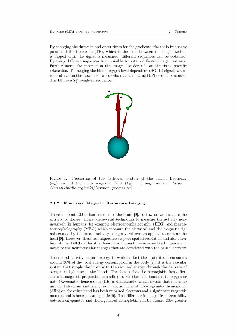
where M is the magnetization and γ is the gyromagnetic ratio. The gyromag-netic ratio for protons is equal to 2.7 × 108 rad/sT or 42.57 MHzT−1 [7]. Infact, the protons aligned with the magnetic field will also be rotating slightlyaround the external magnetic field. This is called precessing, and the pressesionrate is termed Larmor frequency, ωL, see figure 1. The Larmor frequency isrelated to the magnetic field according to the Larmor equation below

ωL = γB0 (2)

When a radio frequency pulse at the Larmor frequency is applied, the atomswill flip into a higher energy state and the magnetization of the hydrogen nu-clei will tilt to the transverse plan orthogonal to B0. The magnetization willas a reaction go back to the equilibrium state along B0. Thus, the absorbedenergy will be emitted as radio frequency signal when flipping back to the lowenergy state [6]. The time it takes for the magnetization to align to B0 afterthe excitation is tissue specific and called spin-lattice relaxation, T1. Initiallyall the protons precesses will be in phase. But due to interactions between thehydrogen atoms the protons will begin to dephase, this leads to a decrease inmagnetization over time and is known as the spin-spin relaxation, T2. But dueto inhomogeneities in the magnetic field and the magnetic susceptibility an ad-ditional dephasing called T ∗2 will occur. The magnitude of the radio frequencywaves emitted during the relaxation is proportional to the transverse compo-nent of the net magnetization and is detected by the radio frequency coil in thescanner.

To localize the signal, three magnetic gradients are used. By applying a gradientfield, a linear variation in the magnetization is created which as a result willproduce variations in the resonance frequency in the direction of the gradientfield. This means that the radio waves with a certain frequency only will fulfillthe resonance condition in equation 2 at a certain plane perpendicular to thegradient field, this is called slice selection [6]. To localize the signal in the slicethe so called phase encoding gradient and the frequency encoding gradients areapplied. The phase encoding gradient rendering different phases of the mag-netization and the frequency encoding gradient rendering different frequenciesin the slice [8]. By combining the phase and frequency at a specific time eachspatial location in the slice can be localized.

3


By changing the duration and onset times for the gradients, the radio frequencypulse and the time-echo (TE), which is the time between the magnetizationis flipped until the signal is measured, different sequences can be obtained.By using different sequences is it possible to obtain different image contrasts.Further more, the contrast in the image also depends on the tissue specificrelaxation. To imaging the blood oxygen level dependent (BOLD) signal, whichis of interest in this case, a so called echo planar imaging (EPI) sequence is used.The EPI is a T ∗2 weighted sequence.

Figure 1: Precessing of the hydrogen proton at the larmor frequency(ωL) around the main magnetic field (B0). (Image source: https ://en.wikipedia.org/wiki/Larmor_precession)

2.1.2 Functional Magnetic Resonance Imaging

There is about 100 billion neurons in the brain [9], so how do we measure theactivity of those? There are several techniques to measure the activity non-invasively in humans, for example electroencephalography (EEG) and magne-toencephalography (MEG) which measure the electrical and the magnetic sig-nals caused by the neural activity using several sensors applied to or near thehead [9]. However, these techniques have a poor spatial resolution and also otherlimitations. fMRI on the other hand is an indirect measurement technique whichmeasure the neurovascular changes that are correlated with the neural activity.

The neural activity require energy to work, in fact the brain it self consumesaround 20% of the total energy consumption in the body [2]. It is the vascularsystem that supply the brain with the required energy through the delivery ofoxygen and glucose in the blood. The fact is that the hemoglobin has differ-ences in magnetic properties depending on whether it is bounded to oxygen ornot. Oxygenated hemoglobin (Hb) is diamagnetic which means that it has nounpaired electrons and hence no magnetic moment. Deoxygenated hemoglobin(dHb) on the other hand has both unpaired electrons and a significant magneticmoment and is hence paramagnetic [9]. The difference in magnetic susceptibilitybetween oxygenated and deoxygenated hemoglobin can be around 20% greater

4


for the deoxygenated hemoglobin. This is the physological property which isused in the fMRI scanner [9]. The paramagnetic hemoglobin will affect themagnetic field, also nearby protons will be affected and as a result precess atdifferent frequencies. This will result in a shorter T ∗2 which leads to the oxy-genated blood will have a stronger MR signal for a T ∗2 sensitive sequence thanthe deoxygenated blood will have. This signal is called the blood-oxygen-level-dependent (BOLD) contrast.

2.1.3 Spatial resolution

The spatial resolution of fMRI data is often stated as voxel size which is de-termined by the three scanner parameters: field of view, matrix size and slicethickness. When studying the entire brain using fMRI a voxel size of around4 × 4 × 4 mm is common, while a quite smaller one, approximately 1 × 1 × 1mm, is used when studying a single region of the brain. For anatomical imagesa voxel size of approximately 1×1×1 mm is used [9]. To make it easier to visu-alize the results is it common to use a anatomical scan to display the functionaldata upon. So why do one often use such a large voxel size for the functionaldata? There are mainly two reasons. First, a smaller voxel size will decrease thesignal-to-noise-ratio of the BOLD signal. This is because the total amount ofdeoxygenated hemoglobin within a voxel affect the BOLD signal. This meansthat when reducing the voxel size by half also the BOLD signal changes willbe reduced by half, which results in a smaller signal which leads to a smallersignal-to-noise ratio [9]. The second reason for not using a smaller voxel sizeis the scanning time, which leads to a reduced temporal resolution. For exam-ple when decreasing the slice thickness by half, twice as many slices is neededwhich of course will double the acquisition time. Also the slice resolution affectthe scanning time. A typical scanner, for example, could acquire 16 slides persecond at a resolution of 4× 4× 4 mm and only 1 slice per second at 1× 1× 1mm resolution.

2.1.4 Temporal resolution

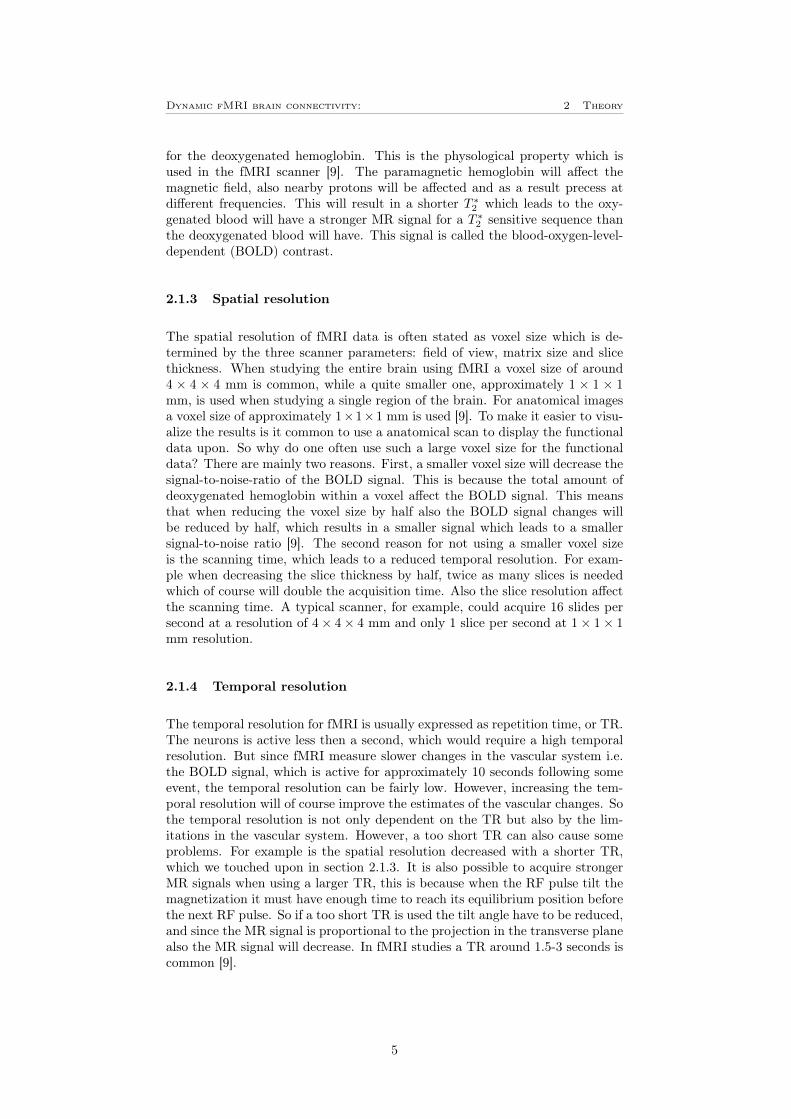
The temporal resolution for fMRI is usually expressed as repetition time, or TR.The neurons is active less then a second, which would require a high temporalresolution. But since fMRI measure slower changes in the vascular system i.e.the BOLD signal, which is active for approximately 10 seconds following someevent, the temporal resolution can be fairly low. However, increasing the tem-poral resolution will of course improve the estimates of the vascular changes. Sothe temporal resolution is not only dependent on the TR but also by the lim-itations in the vascular system. However, a too short TR can also cause someproblems. For example is the spatial resolution decreased with a shorter TR,which we touched upon in section 2.1.3. It is also possible to acquire strongerMR signals when using a larger TR, this is because when the RF pulse tilt themagnetization it must have enough time to reach its equilibrium position beforethe next RF pulse. So if a too short TR is used the tilt angle have to be reduced,and since the MR signal is proportional to the projection in the transverse planealso the MR signal will decrease. In fMRI studies a TR around 1.5-3 seconds iscommon [9].

5


2.2 Neuroanatomy and neural networks

2.2.1 Neurons

The central nervous system (CNS) consists of the spinal cord and the brain.Further, the CNS is composed of several cellular elements including the neuronswhich are the principal information processing cells. The neurons consists of cellbodies, axons and dendrites. The axon is the connection to other neurons andthe dendrites is the connection to other cells. The brain can be divided into threedifferent structures; gray matter, which primarily consists of cell bodies, whitematter, which primarily consists of axons and the cerebrospinal fluid (CSF),which is a colorless liquid [9]. Since the BOLD signal is derived from the graymatter is this the interesting part when studying the neural activity using fMRI.

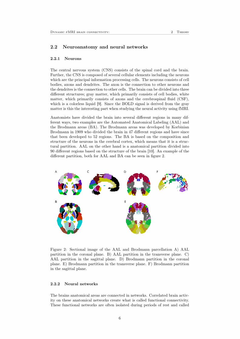
Anatomists have divided the brain into several different regions in many dif-ferent ways, two examples are the Automated Anatomical Labeling (AAL) andthe Brodmann areas (BA). The Brodmann areas was developed by KorbinianBrodmann in 1909 who divided the brain in 47 different regions and have sincethat been developed to 52 regions. The BA is based on the composition andstructure of the neurons in the cerebral cortex, which means that it is a struc-tural partition. AAL on the other hand is a anatomical partition divided into90 different regions based on the structure of the brain [10]. An example of thedifferent partition, both for AAL and BA can be seen in figure 2.

Figure 2: Sectional image of the AAL and Brodmann parcellation A) AALpartition in the coronal plane. B) AAL partition in the transverse plane. C)AAL partition in the sagittal plane. D) Brodmann partition in the coronalplane. E) Brodmann partition in the transverse plane. F) Brodmann partitionin the sagittal plane.

2.2.2 Neural networks

The brains anatomical areas are connected in networks. Correlated brain activ-ity on these anatomical networks create what is called functional connectivity.These functional networks are often isolated during periods of rest and called

6


resting state networks (RSNs). In this study, these networks are derived using atemplate (Power 264 atlas, see section 3.6), into 10 RSNs. Since the purpose ofthis study together with many other studies is to mapping the brain’s functionalnetwork, there is still some uncertainties exactly what each of these neural net-works do but below is a short summary of each of the 10 resting-state networksused in this study. In figure 3 an illustration of the networks is given.

Somato-Motor (SM)The first identified networks and is mainly linked to sensory perceptionand movement of the body.

Cingulo-Opercular (CO)Have been hard to functionally characterize but it seems to bee related tothe maintenance activity that spans over the whole task [11].

Auditory (AU)Linked to hearing and processing sound input.

Default mode network (DMN)Connected to self and social cognition and is the part of the brain thatare hypothesized to be inactive during a task and are more active duringresting state conditions [12].

Visual (VIS)Linked to process visual information.

Frontal parietal (FPN)Supports phasic components of attentional control (adaption after errors,task-switching).

Salience (SA)Supports introspective awareness and autonomic processes, for examplebreathing, blood circulation etc.

Subcortical (SUB)A collection of the areas which not is located in cortex. These areas isimportant for biological functions such as hunger and temperature regu-lation. It also have an important role for relaying the incoming signals tothe other parts of the brain.

Ventral Attention (VA)Related to unvoluntary attention and consciousness. This area supportsthe detecting of unexpected or unattended stimuli.

Dorsal Attention (DA)Related to voluntary attention and consciousness and supports selectiveattention in the visual and spatial domains [13].

Undefined (U)Contains nodes that could not be included in any of the networks or pos-sibly belong to multiple networks and therefore were hard to classify.

7


Figure 3: The resting-state network partitions used in this study.

2.3 Graph theory in neuroscience

To study resting-state fMRI many different methods can be used. One of themost powerful, and the one used in this project is the graph theoretical approach.In the graph theoretical approach a mathematical system consisting of items andpairwise relationship between the items describes a complex system. The itemsare called nodes, the relationships between them are called edges and a set ofnodes and their edges are called a network [14]. From these is often a so calledconnectivity matrix, Ai,j (or adjacency matrix) created, where i and j is nodesand A representing the connectivity between the nodes (i.e edges), see figure 4.By using this approach is it possible to identify and quantify substructures andhierarchy within a network, identify hubs and critical nodes and see how theinformation in the network is distributed [14]. Another main advantage of usinggraph theory is the simplicity to model the systems in different levels such asthe entire graph, subgraphs (i.e. networks) and individual nodes. An extensionof graph theory is quantifying the changes in connectivity during time, temporalgraph theory [15].

Graph theory is useful to consider the connections of multiple brain areas. Andalso use different graph theoretical measures, for example betweenness centrality,CB . Betweenness centrality is a measure of the fraction of shortest paths in anetwork that contain a specific node. A high betweenness centrality value thusmeans that the current node participate in many shortest paths [15], and thusindicates that the node is important for information dissemination. Betweenness

8


centrality can also be described with the following formula.

CB(i) =Σi 6=j 6=kvi(j, k)

Σi 6=j 6=kv(j, k)(3)

Where v(j, k) is the number of paths between j and k and vi(j, k) is the numberof shortest paths between k and j that goes through i.

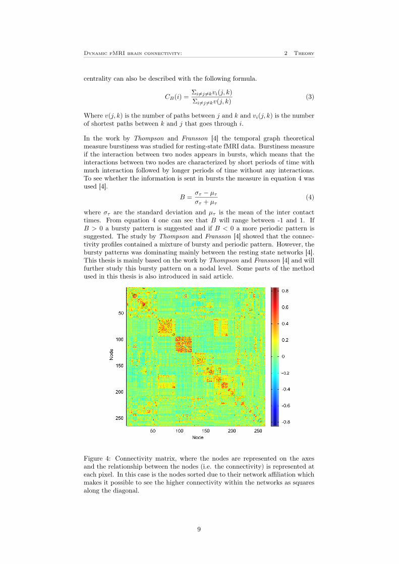
In the work by Thompson and Fransson [4] the temporal graph theoreticalmeasure burstiness was studied for resting-state fMRI data. Burstiness measureif the interaction between two nodes appears in bursts, which means that theinteractions between two nodes are characterized by short periods of time withmuch interaction followed by longer periods of time without any interactions.To see whether the information is sent in bursts the measure in equation 4 wasused [4].

B =στ − µτστ + µτ

(4)

where στ are the standard deviation and µτ is the mean of the inter contacttimes. From equation 4 one can see that B will range between -1 and 1. IfB > 0 a bursty pattern is suggested and if B < 0 a more periodic pattern issuggested. The study by Thompson and Fransson [4] showed that the connec-tivity profiles contained a mixture of bursty and periodic pattern. However, thebursty patterns was dominating mainly between the resting state networks [4].This thesis is mainly based on the work by Thompson and Fransson [4] and willfurther study this bursty pattern on a nodal level. Some parts of the methodused in this thesis is also introduced in said article.

Figure 4: Connectivity matrix, where the nodes are represented on the axesand the relationship between the nodes (i.e. the connectivity) is represented ateach pixel. In this case is the nodes sorted due to their network affiliation whichmakes it possible to see the higher connectivity within the networks as squaresalong the diagonal.

9

Dynamic fMRI brain connectivity: 3 Method

3 Method

3.1 Data

The analysis was performed on resting-state fMRI data included in the Oulu Adata set taken from the 1000 functional connectomes [16]. The data was col-lected during resting-state with eyes open using a fixation cross for 56 healthysubjects at the age ranging 20 − 22 years old. There were 23 males and 33females. The images included the cerebellum which sometimes led to the topparts of the brain being missing which led to some of the subject had to be re-jected after the preprocessing (see section 3.2) due to incomplete data. A totalof 24 subjects were rejected yielding that 32 subjects remained in the study.The age of the remaining subjects ranged from 21 − 22 years old including 8males and 24 females.

To verify the results was also the Oulu B data set used, also taken from the1000 functional connectomes [16]. This consists of 47 healthy subjects at theage ranging 20− 23 years old. There was 14 males and 33 females. Due to thesame reason as for Oulu A was 18 subjects rejected yielding that 29 subjectsremained. The age of the remaining subject ranged from 20− 22 old, there was8 males and 21 females.

The fMRI data was in both cases collected on a 1.5T scanner with an repe-tition time (TR) of 1800 ms and 28 oblique axial slices at 245 time-points. Thisdata was selected since it was found to have little sleep artifacts which can bea problem with resting state data [17].

3.2 Preprocessing - SPM12

To assemble the functional and anatomical data and to make the different sub-jects comparable, preprocessing was necessary. This was done by the Matlabbased program SPM12. The preprocessing was done in five steps, head motioncorrection, coregistration, segmentation, normalisation and smoothing. Belowwill these steps be described in brief, for more information about SPM12 seeSPM12 Manual [18].

3.2.1 Head motion correction

The most important step in the preprocessing is to correct for head motionsduring the scan. Since the voxels are defined by their position in the scannerand not their position in the brain, head movements can result in some hugeerrors if they are not corrected. For example, if the subject moves his or herhead inside the scanner the scanner will record the activation in a specific spa-tial locations in different voxels at different time-points.

Since the head movement in a fMRI scan often are quite small, the changein shape or size are also very small and can therefore be ignored. Because ofthis SPM12 consider the head to be a rigid body. The motions of this rigidbody can be described by six variables, z which is defined along the magneticfield, thus runs from the feet to the top of the head of the subject. The x-axis

10


runs through the subjects ears, from left to right, and the y-axis runs from theback of the head and exits the forehead. Yaw is the rotation around the z-axis,pitch the rotation around the x-axis and roll is the rotation around the y-axis.

To do these head motion corrections SPM12 uses the BOLD response of oneimage, selected by the user, as reference and then correct all the other imagesat each time-points as good as possible at each coordinate. This assumes thatthe BOLD signal is exactly the same for all time-points which of course notis the case. However we expect that the activation in the most voxels will beroughly the same for the functional data through all the time-points which isused to do the correction as good as possible [19].

3.2.2 Coregistration

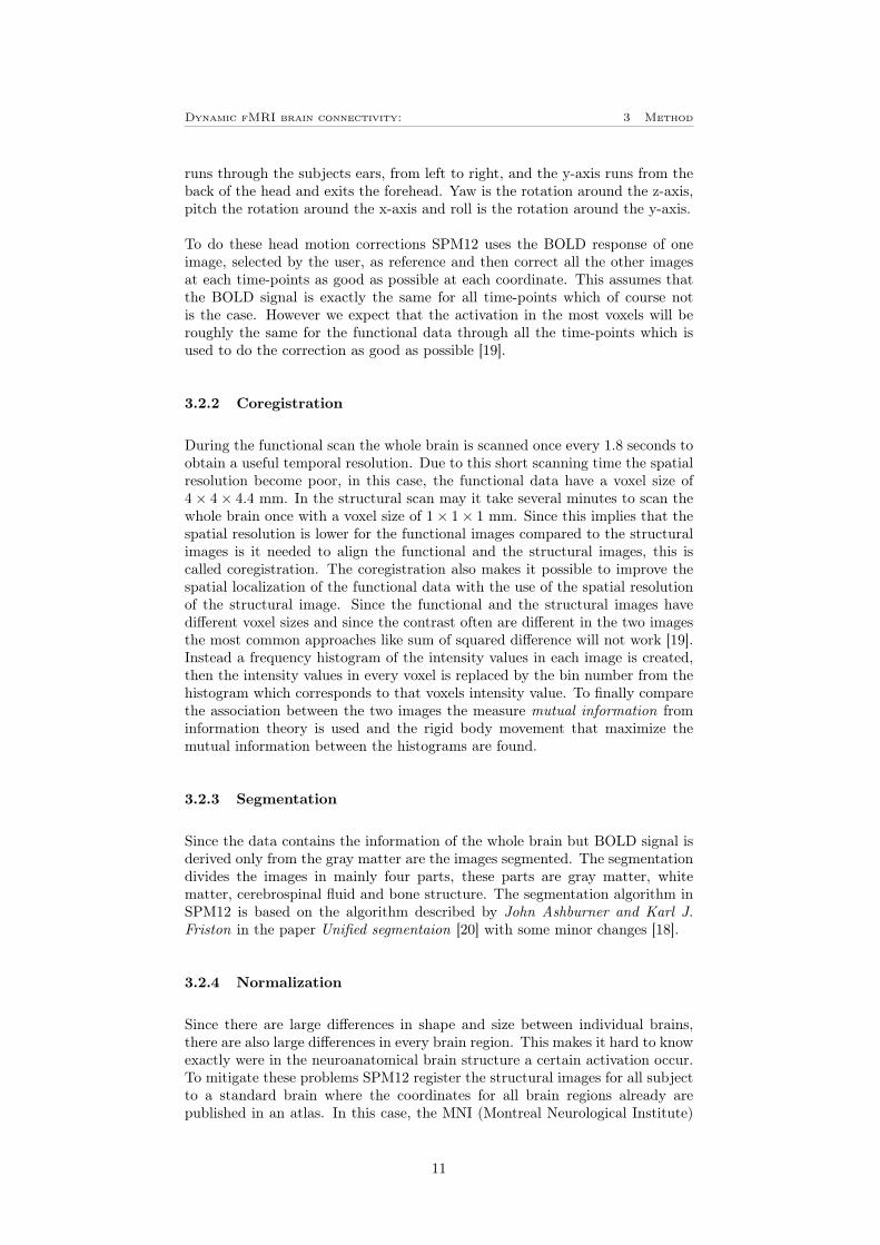
During the functional scan the whole brain is scanned once every 1.8 seconds toobtain a useful temporal resolution. Due to this short scanning time the spatialresolution become poor, in this case, the functional data have a voxel size of4× 4× 4.4 mm. In the structural scan may it take several minutes to scan thewhole brain once with a voxel size of 1× 1× 1 mm. Since this implies that thespatial resolution is lower for the functional images compared to the structuralimages is it needed to align the functional and the structural images, this iscalled coregistration. The coregistration also makes it possible to improve thespatial localization of the functional data with the use of the spatial resolutionof the structural image. Since the functional and the structural images havedifferent voxel sizes and since the contrast often are different in the two imagesthe most common approaches like sum of squared difference will not work [19].Instead a frequency histogram of the intensity values in each image is created,then the intensity values in every voxel is replaced by the bin number from thehistogram which corresponds to that voxels intensity value. To finally comparethe association between the two images the measure mutual information frominformation theory is used and the rigid body movement that maximize themutual information between the histograms are found.

3.2.3 Segmentation

Since the data contains the information of the whole brain but BOLD signal isderived only from the gray matter are the images segmented. The segmentationdivides the images in mainly four parts, these parts are gray matter, whitematter, cerebrospinal fluid and bone structure. The segmentation algorithm inSPM12 is based on the algorithm described by John Ashburner and Karl J.Friston in the paper Unified segmentaion [20] with some minor changes [18].

3.2.4 Normalization

Since there are large differences in shape and size between individual brains,there are also large differences in every brain region. This makes it hard to knowexactly were in the neuroanatomical brain structure a certain activation occur.To mitigate these problems SPM12 register the structural images for all subjectto a standard brain where the coordinates for all brain regions already arepublished in an atlas. In this case, the MNI (Montreal Neurological Institute)

11


atlas have been used. The MNI atlas is an average of 152 different brains [19].To do this the first step is to align the image so that it will be in the samelocation, orientation and size as the reference, this is done by a linear affinetransformation [19]. The affine transformation include translation, rotation,scaling and shearing transformations. The main difference remaining now isdue to local differences between the image and the reference. To align thesedifferences a non-linear transformation is used to perform local changes likeshrinking, stretching, spatial movements etc. However, due to these changes allthe voxels will no longer be the same size and not rectangular and thereforeit is necessary to redefine the voxels. To do this, interpolation is required toestimate the intensity value in the redefined voxels. For further informationabout the normalization algorithm see the SPM12 Manual [18] or the articleUnified segmentation [20] which presenting the algorithm SPM12 used as a basefor their algorithm. Due to the normalization is it now possible to report andinterpret spatial locations in a consistent manner across subjects. Results canbe compared across studies, averaged across subjects and generalized to largerpopulations. But there are of course also some disadvantages, for example isthe spatial resolution reduced and errors may be introduced in the data.

3.2.5 Smoothing

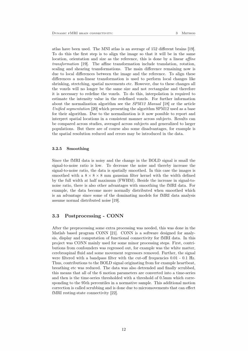
Since the fMRI data is noisy and the change in the BOLD signal is small thesignal-to-noise ratio is low. To decrease the noise and thereby increase thesignal-to-noise ratio, the data is spatially smoothed. In this case the images issmoothed with a 8 × 8 × 8 mm gaussian filter kernel with the width definedby the full width at half maximum (FWHM). Beside the increase in signal-to-noise ratio, there is also other advantages with smoothing the fMRI data. Forexample, the data become more normally distributed when smoothed whichis an advantage since some of the dominating models for fMRI data analysisassume normal distributed noise [19].

3.3 Postprocessing - CONN

After the preprocessing some extra processing was needed, this was done in theMatlab based program CONN [21]. CONN is a software designed for analy-sis, display and computation of functional connectivity for fMRI data. In thisproject was CONN mainly used for some minor processing steps. First, contri-butions from confounders was regressed out, for example was the white matter,cerebrospinal fluid and some movement regressors removed. Further, the signalwere filtered with a bandpass filter with the cut-off frequencies 0.01 - 0.1 Hz.Thus, contributions to the BOLD signal originating from for example heartbeat,breathing etc was reduced. The data was also detrended and finally scrubbed,this means that all of the 6 motion parameters are converted into a time-seriesand then is the time-series thresholded with a threshold of 0.5mm which corre-sponding to the 95th percentiles in a normative sample. This additional motioncorrection is called scrubbing and is done due to micromovements that can effectfMRI resting-state connectivity [22].

12


3.4 MRIcron

As was said in section 2.2.1 can the brain be parcellated into several subparts.In this project two of the most common parcellations was used, the AutomatedAnatomical Labeling (AAL) and Brodmann area (BA). MRIcron is a visualiza-tion and region drawing software for neuroimaging developed by Chris Rorden[23] which uses the MNI coordinates to look up which of the AAL or Brodmannareas a specific node belongs to. This can be used to identify specific brainregions (e.g. which brain region a node from Power 264 atlas belongs to, seesection 3.6). It also makes the results easier to comprehend and to comparewith other studies which may have used other sets of nodes or even not a pointbased method which is used in this study and will be further described in thesection 3.6.

3.5 BrainNet Viewer

BrainNet Viewer [24] is a simple Matlab-based program for visualization ofstructural and functional brain networks and is suitable when using an graphtheoretical approach. In BrainNet Viewer, a template of a brain is loaded asa surface and further the brain connectivity data is loaded. The data can beloaded as a volume, nodes or as edges. There is also possible to do some plottingsettings in BrainNet Viewer such as thresholding, color coding, size coding etc.This makes it possible to visualize the results in a distinctly and easy way.

3.6 Power 264 atlas

After the processing steps, the nodes was created. One standard method issimply define each voxel as a node. But since this project investigate functionalareas on a macroscopic level a point based method was used, this means thatseveral region of interests (ROI) is extracted. The set of ROIs extracted isthe set Power et al first defined in the article Functional Network Organizationof the Human Brain [14]. This gives 264 ROIs covering the cerebral cortex,subcortical structures and cerebellum. Each ROI was in this case a sphere witha 10 mm radius which was defined as one node. Since the ROI cover severalvoxels, the mean value of the BOLD signals for all these voxels was used. Thiswill of course reduce the spatial resolution. The reason to extract the ROIsusing Power 264 atlas is because it also divided the ROIs into the networksdescribed in section 2.2.2 based on the connectivity between them [14]. All theROIs are shown in figure 5 where the color indicates their network affiliation,these can also be seen in figure 3 in section 3. Out of the total 264 ROIs is 58in the DMN, 35 in SM, 31 in Vis, 24 in FP, 18 in Sa, 14 in CO, 13 in Au, 13 inSub, 11 in DA, 9 in VA and 38 nodes are undefined with respect to resting-statenetwork.

13


Figure 5: Parcellation of the brain using the Power 264 nodes where the colorshows there network affiliation, the white nodes is the ones with an undefinednetwork affiliation. (Image source: Bursty and persistent properties of a large-scale brain networks revealed with a point-based method for dynamic functionalconnectivity [4])

3.7 Harvard-Oxford atlas

To check how the results depends of the chosen Power 264 atlas described above,also another atlas was used during some parts of the project. This atlas is calledthe Harvard-Oxford atlas (HO-atlas). The HO-atlas cover the whole cortexand also some subcortical regions and consists of 57 brain areas but splittingmany of the structures into left and right hemisphere ended up in 106 differentregions. This parcellation was taken from CONN toolbox. To make it easierto evaluate the results, these region were also divided into networks by theuse of the code infomap developed by Roswall and Bergström and available athttp://www.mapequation.org/code.html [25]. This resulted in 17 different sub-networks where many of them contained only a few number of regions. All of thenetworks containing less then five regions were put together into one network,this resulted in a total of 7 networks which can be seen in figure 6 below.

Figure 6: The network parcellation for the Harvard Oxford atlas. This consistsof 7 networks, showed by the color

3.8 Principal Component Analysis

Principal component analysis (PCA) is a multivariate statistical technique anda common technique for data reduction. PCA finds a linear transform which

14


represent as much as possible of the variance in the data in fewer dimensions.The bases of the transformed data is the eigenvectors and the eigenvalues rep-resent the variance [19]. When the variance is represented in a few dimensions,the new data in the PCA dimension is sorted starting with the one containingthe highest variance. By then keeping the most prominent PCA dimensions,i.e the PCA dimensions with the highest variance, the data can be reduced butstill keep much of the important information. PCA can also be used to reducenoise since the noise often are characterized by a low variance. This is done byonly retain very few of the PCA dimensions with the highest variance but italso result in dynamics to be lost.

In this case data reduction was the purpose of the PCA since k-means clustering(see section 3.9) will be more efficient with a lower number of dimensions in thedata. All of the 264 ROIs time-series was transformed into PCA-space anddescribed along 264 PCA dimensions sorted due to how much of the varianceeach PCA dimension explains of the data. In this case, 90% of the variance,corresponding to 104 out of the 264 PCA dimensions was kept. These 104 PCAdimensions was later used in the k-means clustering in section 3.9. From thePCA also a weight called loadings is obtained, this weight describes the originaldata in terms of the PCA-dimensions, which is described in equation 5.

y = xl (5)

Where y is the original data x is the data in PCA-space and l is the loadings.This will be further used in section 3.11.2.

3.9 K-means clustering

Each ROI is now represented along 104 PCA dimensions which is used in the k-means clustering. The aim of this is to divide the BOLD fMRI signal time-seriesinto several clusters based on their co-activation pattern in their spatial dimen-sions regardless of their temporal location. An example for a two node systemof this can be seen in figure 8A. K-mean is a iterative clustering algorithm com-monly used in neuroscience [26], which divide the data into k number of cluster,where k is decided by the user. The method first places k number of centroidsat random locations. Then all the data points, in this case all the time-pointsin each of the 104 PCA-dimension, finds the nearest centroid and assign thetime-point to that specific cluster. A new location for all the centroids is thencalculated by taking the mean position of all the data-points within the cluster.Since the centroid now is in a new position new time-points will be assigned tothat cluster. This is then repeated until all the clusters are unchanged. To getan even better result, independent of the initial position of the centroids, all thisis then replicated several times, every time with a new random initial positionfor the centroids. Finally the result with the lowest sum of point-to-centroiddistances is selected as the final result. There are also several other ways tocalculate the new position of the centroids, the one described above is calledthe squared Euclidian distance and is considered to be the standard method.

The k-mean clustering was performed for k-values between 1 and 30. The clus-tering was performed up to 1000 iterations for each k-value to attain convergenceand each k-value was repeated 20 times to reduce the influence of the initialcondition and to obtain the best possible result. The centroid position fromthe different data-points was calculated using the squared Euclidian distance.

15


Finally to know which k-value to use equation 6 was used.

s(i) =b(i)− a(i)

a(i) + b(i)(6)

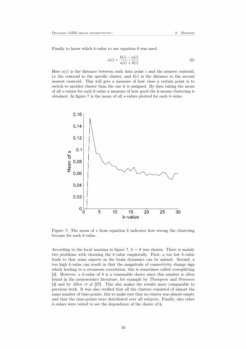
Here a(i) is the distance between each data point i and the nearest centroid,i.e the centroid to the specific cluster, and b(i) is the distance to the secondnearest centroid. This will give a measure of how close a certain point is toswitch to another cluster than the one it is assigned. By then taking the meanof all s-values for each k-value a measure of how good the k-means clustering isobtained. In figure 7 is the mean of all s-values plotted for each k-value.

Figure 7: The mean of s from equation 6 indicates how strong the clusteringbecome for each k-value.

According to the local maxima in figure 7, k = 8 was chosen. There is mainlytwo problems with choosing the k-value empirically. First, a too low k-valueleads to that some aspects in the brain dynamics can be missed. Second, atoo high k-value can result in that the magnitude of connectivity change signwhich leading to a erroneous correlation, this is sometimes called oversplitting[4]. However, a k-value of 8 is a reasonable choice since this number is oftenfound in the neuroscience literature, for example by Thompson and Fransson[4] and by Allen et al [27]. This also makes the results more comparable toprevious work. It was also verified that all the clusters consisted of almost thesame number of time-points, this to make sure that no cluster was almost emptyand that the time-points were distributed over all subjects. Finally, also otherk-values were tested to see the dependence of the choice of k.

16


3.10 State-Graphlets and Temporal-Graphlets

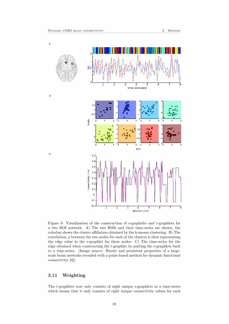
To correlating time-points at each cluster between each ROI-combination (edge),the Spearman correlation was used. This was used since it is robust to potentialoutliers that might occur due to the clustering process. For the Power 264 atlas,this resulted in one 264×264 connectivity matrix (106×106 for the HO-atlas) foreach cluster with a specific connectivity value, ρ for each edge. These matricesare called state-graphlets or s-graphlets. In figure 8 A-B, an example of the stepfrom a PCA time-series to the creation of a s-graphlets are visualized.

By representing every time-point with their respective s-graphlets in a time-series of connectivity matrices a temporal-graphlets or t-graphlets is created[4]. Thus the dynamics of the resting-state networks such as burstiness can becomputed on the t-graphlets. In figure 8, an example of the construction ofs-graphlets and t-graphlets is shown for a two ROI network.

17


Figure 8: Visualization of the construction of s-graphelts and t-graphlets fora two ROI network. A) The two ROIs and their time-series are shown, thecolorbar shows the cluster affiliation obtained by the k-means clustering. B) Thecorrelation, ρ between the two nodes for each of the clusters is then representingthe edge value in the s-graphlet for these nodes. C) The time-series for theedge obtained when constructing the t-graphlet by putting the s-graphlets backto a time-series. (Image source: Bursty and persistent properties of a large-scale brain networks revealed with a point-based method for dynamic functionalconnectivity [4]).

3.11 Weighting

The t-graphlets now only consists of eight unique s-graphlets in a time-serieswhich means that it only consists of eight unique connectivity values for each

18


edge. This is not ideal as we would like unique connectivity estimates per time-point. To get a unique value for each edge at each time-point the t-graphlets areweighted. To do this, two different weighting strategies have been developed.Both weighting schemes aims to consider two variables, the s-graphlet and thedistance from the cluster centroid. Given these considerations, the time-seriesshall be manipulated to consist of unique connectivity values for each edge. Byconsidering each s-graphlet as representative of the connectivity for time-pointsclustered to that centroid and assume that points closer to the centroid reflectthe connectivity better than points further away. This assumes that there issome linearity between the distance to a cluster’s centroid and how much theconnectivity is represented by the said cluster. The two weighting schemesstarting from the same equation 7

TGi,j,t =k∑s=1

SGi,j,swi,j,s,t (7)

which is simply that the edge, i, j at the time, t for a t-graphlet, TG is theweighted mean of all the s-graphlets, SG were the weight, w is specific for thecluster, s and time-point, t. The difference between the two methods is of coursethe weight which is described below.

3.11.1 Global time-point scaling

In the first method called global time-point scaling (GTPS), the weight is derivedfrom the distance to each centroid as:

wi,j,s,t =d−αs,tk∑sd−αs,t

(8)

where ds,t is the euclidean distance from a time-point to a centroid of cluster, sat the time point, t. Since d is identical for every edge in a specific s-graphlet,the weight, w will be a scalar applied to every edge and α is some scaling value,in this study α = 4 was used. A higher value of α will increase the significanceof nearer clusters and when α increase to infinity, the value will become theclosest unweighted t-graphlet. This weighting scheme is very quick and easy toimplement but it effectively scales all edges of a t-graphlet by an equal amount.This seem unreasonable since every edge may display its peak of connectivityat a specific time-point and having every connection increase or decrease basedon the time-point does not seem biologically plausible.

3.11.2 Edge time-point scaling

The second weighting scheme is called edge time-point scaling (ETPS) andis similar to the first one in the idea of constructing weights derived from s-graphlets and distance from centroids. However this method aims to deriveweights for each edge, instead of each s-graphlet.

The distance from each centroid is expressed along 104 PCA dimensions, mean-ing some time-points with the same Euclidean distance from a cluster in theprevious method could vary along different PCA dimensions. Some of thesePCA dimensions will then have a greater importance for the edge. For each

19


time-point and each edge, this approach considers to which extent, the PCA di-mensions that the clustering was based upon explain the variance for the nodesthe edge connects. This builds upon the idea that if a time-point is identicalin distance from two centroids except for one PCA dimension, but this PCAdimension explains none of the variance for two nodes in a s-graphlet, then theweights for this edge should be identical. Distance for each edge becomes basedon the distance of the relevant PCA components for a nodes-pairing, givingunique scalars, per time-point, per edge.

PCA express the original data, y, in PCA dimensions, x and loadings l, which isused in this weighting scheme. The loadings represent the weight to transformthe PCA dimensions back to the original spatial dimensions. Hence can theoriginal data be obtained by the following formula

y = xl (9)

First, the eucldiean distance to a cluster’s centroid, C for each PCA dimensionis calculated, instead of the shortest distance used in GTPS. This is describedin the following equation

dc,s,t = |Cc,s − xc,t| (10)

Where dc,s,t is the distance in each of the 104 PCA-component, c, for eachcluster, s and for every time-point, t. Cc,s is the centroid and xc,t is the dataexpressed in the PCA dimensions. But since this method aims to obtain aspecific weight for each edge is the loadings for the nodes which is connected bythe current edge summed for every state as can be seen in equation 11 below

lec,i,j = lc,i + lc,j (11)

Where lec,i,j is the loading in each PCA dimension, c for the edge between thenodes, i and j. For simplicity negative loadings are set to zero. Otherwise acorrelation at a s-graphlet may effect a correlation negatively, this is describedin the equation below.

lec,i,j =

®lec,i,j if lec,i,j > 0

0 if lec,i,j ≤ 0(12)

To obtain the weight is the edge-loadings and the distance multiplied and trans-formed into percent. Finally are also the weight scaled into percent in the sameway as in equation 8. This is described in equation 13.

wi,j,s,t =

Çdc,s,tl

ec,i,j∑

c

dc,s,tlec,i,j

å−1k∑s

Çdc,s,tl

ec,i,j∑

s

dc,s,tlec,i,j

å−1 (13)

Where wi,j,c,t is the final weight for the edge between the nodes, i and j, forevery cluster, s and for all the time-points, t. This is then used in equation 7to obtain the weighted t-graphlet.

3.12 Thresholding

Since it is unreasonable to assume that every region of the brain is connectedat every time-point is the t-graphlets thresholded and since only the number of

20


bursts and not the magnitude of the connectivity during a burst is of interestthe t-graphlets are made binary. For the binary t-graphlets are 1 representinga present connectivity at the edge and 0 representing a absent connectivity atthe edge.

In the article The mean– variance relationship reveals two possible strategiesfor dynamic brain connectivity analysis in fMRI [28] a negative correlation be-tween the mean and the variance for each edge time-serie is suggested. Thislead too mainly two possible types of thresholds. These are variance thresh-old and magnitude threshold. Since the connectivity is higher within restingstate networks also the mean will be higher, this implies that the variance willbe lower according to the negative scaling [28]. This lead to that the variancebased threshold is more sensitive to the between resting state network connec-tivity. While the magnitude threshold is more sensitive to the within restingstate network connectivity [28]. Considering this projects aims to calculate theintegration of information across the entire brain, the magnitude threshold wasnot used, as it would results in far more bursts within network nodes comparedto between network connectivity. This would lead the method to be biased bythe size of each resting-state network, which is not what the goal is. Insteadwas the variance threshold used, which is described in section 3.12.1. Also anew threshold, the global variance threshold was developed, this is describedin section 3.12.2. But before thresholding the data is demeaned along the timedimension and subjects dimension, so that the connectivity will be around zerofor all time-series. This is done to make sure that every node will be treatedindependent of the magnitude of the mean, why this is important will soon bediscussed.

3.12.1 Local Variance Threshold

The local variance threshold (LVT) is very straight forward. The edge is rejected(i.e set to zero) if the connectivity value is lower then two standard deviationsfor the current edges time-series. And if it is over two standard deviations itis set to 1. This thresholding strategy entails that every edge will have someactivity that excedes the threshold. This may add noisy connections but at thesame time does not bias the edge selection. In figure 9 is an example showinghow the LVT thresholds the time-series.

21


Figure 9: Example of how the LVT thresholds two different time-series.

3.12.2 Global Variance Threshold

The global variance threshold (GVT) is more complicated. First a so called null-s-graphlets is created. The difference between the null-s-graphlet and the origi-nal s-graphlet is that one of the dimensions order of the time-points clustered ina s-graphlet was flipped. This means that the null-s-graphlets mainly consistsof noise and any effects due to an autocorrelation. Next, the null-s-graphlets gothrough the same step as the s-graphlets to become a null-t-graphlet i.e weight-ing and demeaning. Every edge from the null-t-graphlets are combined to createa distribution of correlations which we can compare the t-graphlet values againstto see if the t-graphlet correlations are large enough in magnitude to be con-sidered relevant. The threshold is then set so that the edge is accepted if itsconnectivity is higher than 99% (p < 0.01) of the edges in the null-t-graphlet.Since this will end up in just a single number, the demeaning is very important,without this would this threshold become a magnitude threshold. An exam-ple of the GVT can be seen in figure 10. This thresholding attempt reducesthe number of noisy edges having time-points marked as relevant connectivity.However, this will lead to the edges with the highest variance to have moretime-points marked as relevant (see figure 11E).

22


Figure 10: Example of how the GVT thresholds two different time-series.

3.13 Bursty centrality

With bursts being increases in connectivity under a short time-period. Burstycentrality aims to, for every node, quantify how many bursts occur throughoutthe time-series. To do this, the number of bursts exists within a connectivitytime-series needs to be determined. For doing this automatically, two parame-ters is needed: one define the minimum length of a burst (minL), i.e the numberof ones that a burst must include. And one, inter spike interval (ISI), whichdefine how many consecutive time-points with zero connectivity are allowedbetween connectivity time-points to still be considered a burst.

In this project mainly ISI = 2 and minL = 1 was used, but also other values ofthese parameters were tested and compared, for example ISI = 0 andminL = 1(figure 18). By the use of these settings could now the number of bursts for everyedge be calculated, this is defined as counts. By then taking the mean of this forevery node is the bursty centrality, BC obtained, this is described in equation14

BCi =1

n

∑j

Ci,j (14)

Where Ci,j is the number of bursts in the edge between the nodes, i, j and n isthe number of nodes. To make it easier to compare bursty centrality to othergraph theoretical measures, the bursty centrality is scaled between 0 and 1, thiscan be seen in the equation below.

BC∗i =BCi −min[BCi]

max[BCi]−min[BCi](15)

Where BC∗i is the scaled bursty centrality for each node, i.

23

Dynamic fMRI brain connectivity: 4 Results

4 Results

As can be seen in the method in section 3, the methods robustness is challengedfor several different options, for example the choice of atlas (i.e Power 264 orHarvard-Oxford), weighting method (i.e the GTPS or ETPS) and k-value. Butthere is also a choice of thresholding algorithm that have to be customizedaccording to the present study. The dependence of all these are studied andis presented in this section. The method was also tested for a new datasetto see whether there is any common patterns or common nodes that are themost bursty across these datasets. Finally was also the bursty centrality cor-related with other graph theoretical measures such as betweenness centralityand temporal centrality. If nothing else is stated, the different parameters werecomputed with Oulu A dataset, Power 264 atlas parcellation, ETPS and withk = 8.

4.1 Dependence of thresholding algorithm

To replicate the findings in The mean– variance relationship reveals two possi-ble strategies for dynamic brain connectivity analysis in fMRI [28], which wasdiscussed in section 3.12 was the mean plotted versus the variance (figure 11A).This plot was the foundation for the two different thresholding algorithms. How-ever, in this case, there is no linear correlation between the mean and the vari-ance, but a similar dissociation between edges with high mean and high varianceexists. Still it is important to understand how the different thresholding algo-rithms thresholds the data. For both the LVT and GVT algorithms is thenumber of counts (i.e number of bursts in every edge) almost the same regard-less of the mean (figure 11B for LVT and figure 11D for GVT). However, inthe GVT algorithm a clear relationship can be seen between the counts and thevariance (figure 11E) which does not exist with the mean (figure 11D). SinceGVT uses the global variance as a threshold for every edge is this a quite obviousbehavior.

24


Figure 11: A) Mean versus variance of the edges time-series. B) Shows that thereis no clear dependence between the number of counts (i.e number of bursts inevery edge) for the LVT and the mean for the edge time-series. C) Shows thatthere is no clear dependence between the number of counts for the LVT and thevariance for the edge time-series. D) Shows that there is no clear dependencebetween the number of counts for the GVT and the mean for the edge time-series. E) Shows a clear positive dependence between the number of counts andvariance of the edge time-series when using the GVT.

We have established that the different thresholding algorithms will allow differ-ent edges to pass the threshold and it is of interest to see which nodes in thebrain that is the most bursty. The bursty centrality was calculated for eachnode (figure 12A for the LVT and figure 12B for the GTV). The nodes withthe highest bursty centrality were classed as candidates to be dynamic hubs.A threshold at 15% (40 nodes) was chosen, which is the yellow part in figure12 A and B and the colorbar along the x-axis show the network correspondingto each node. These 40 nodes corresponds to approximately 23% of the totalnumber of bursts for the LVT and 32% for the GVT.

Using BrainNet viewer were these 40 nodes plotted for both the LVT (figure12C)) and for the GVT (figure 12D). The size of the ROIs corresponds to thenumber of bursts and the color corresponds to the network affiliation. Thesefigures shows that for the LVT, the most bursty nodes are located in the frontalparts of the brain, the most bursty node is left thalamus in the subcorticalnetwork. In table 1 in appendix A can a complete list of the 40 most burstynodes be found. Worth mentioning is that the DMN is by far the most burstynetwork where 14 of the 40 most bursty nodes are located. For the GVT on theother hand is there mainly the dorsal regions that are bursty, the most burstyone is left precuneus in the somato-motor network. For this threshold the visualand the DMN that are dominating with 13 respective 11 nodes of the 40 mostbursty. The complete list of this can be found in table 2 in appendix A.

25


Figure 12: A-B) Bursty centrality for the (A) LVT and (B) GVT. The colorbarshows the network affiliation and the yellow part shows the 40 nodes (15%)with highest bursty centrality. C-D) The 40 nodes with highest bursty centralityplotted using BrainNet viewer, for (C) LVT and (D) GVT. The size of the nodesindicates the bursty centrality and the color shows the network affiliation

26


4.2 Comparison between atlases

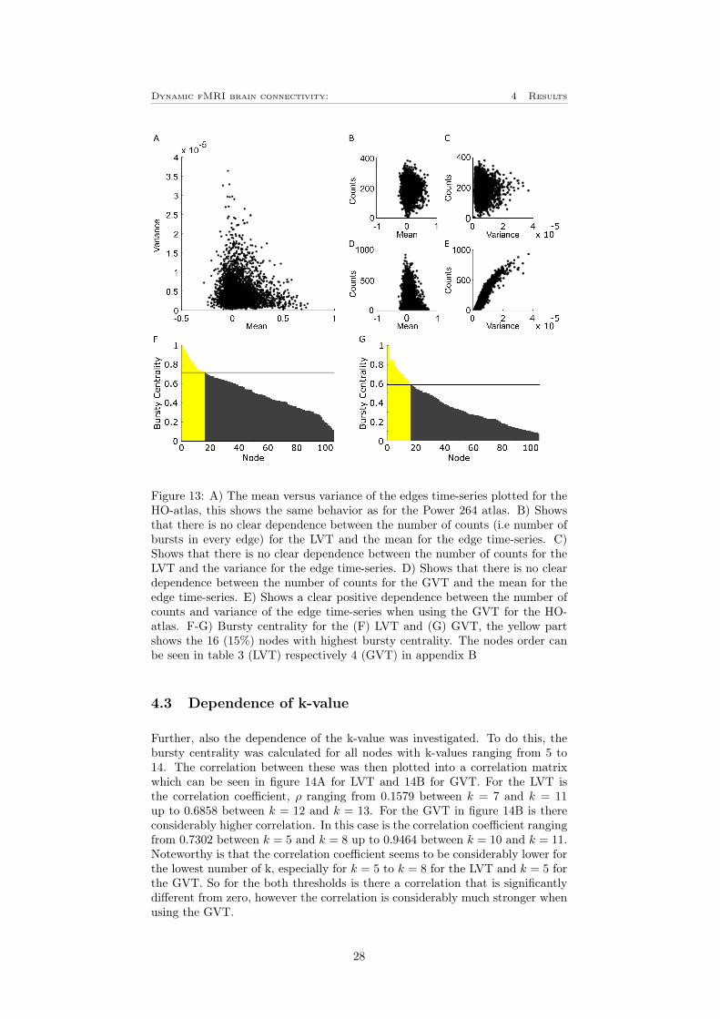
To investigate how the result will depend on the choice of atlas, the plots cor-responding to figure 11 and 12 A and B were also plotted for the HO-atlasdescribed in section 3.7, these can be seen in figure 13. Since the network clas-sification in the HO-atlas only are based on mutual information and not furtherinvestigated as in the case for the Power 264 atlas is there no colorbar in figure13 F and G. Instead, the nodes are listed in table 3 for the LVT in figure 13Fand table 4 for the GVT in figure 13G, these tables can be found in appendixB. By comparing figure 13 to figure 11 can it be observed that the mean versusvariance plot is very similar for the both atlases. It can also be seen that thethresholds treats the data in the same way as previously. Also the distributionof bursts following the same shape in both cases, for the HO-atlas correspondsthe 15% (i.e 16 nodes) most bursty nodes for approximately 17% of the totalnumber of bursts for the LVT, where left heschl’s gyrus have the highest burstycentrality. For the GVT have frontal medial cortex the highest bursty centralityand the 16 most bursty nodes corresponds for approximately 31% of the totalnumber of bursts.

27


Figure 13: A) The mean versus variance of the edges time-series plotted for theHO-atlas, this shows the same behavior as for the Power 264 atlas. B) Showsthat there is no clear dependence between the number of counts (i.e number ofbursts in every edge) for the LVT and the mean for the edge time-series. C)Shows that there is no clear dependence between the number of counts for theLVT and the variance for the edge time-series. D) Shows that there is no cleardependence between the number of counts for the GVT and the mean for theedge time-series. E) Shows a clear positive dependence between the number ofcounts and variance of the edge time-series when using the GVT for the HO-atlas. F-G) Bursty centrality for the (F) LVT and (G) GVT, the yellow partshows the 16 (15%) nodes with highest bursty centrality. The nodes order canbe seen in table 3 (LVT) respectively 4 (GVT) in appendix B

4.3 Dependence of k-value

Further, also the dependence of the k-value was investigated. To do this, thebursty centrality was calculated for all nodes with k-values ranging from 5 to14. The correlation between these was then plotted into a correlation matrixwhich can be seen in figure 14A for LVT and 14B for GVT. For the LVT isthe correlation coefficient, ρ ranging from 0.1579 between k = 7 and k = 11up to 0.6858 between k = 12 and k = 13. For the GVT in figure 14B is thereconsiderably higher correlation. In this case is the correlation coefficient rangingfrom 0.7302 between k = 5 and k = 8 up to 0.9464 between k = 10 and k = 11.Noteworthy is that the correlation coefficient seems to be considerably lower forthe lowest number of k, especially for k = 5 to k = 8 for the LVT and k = 5 forthe GVT. So for the both thresholds is there a correlation that is significantlydifferent from zero, however the correlation is considerably much stronger whenusing the GVT.

28


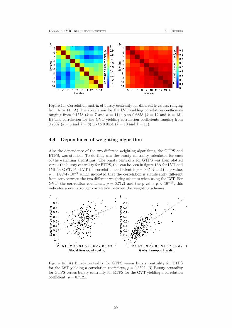
Figure 14: Correlation matrix of bursty centrality for different k-values, rangingfrom 5 to 14. A) The correlation for the LVT yielding correlation coefficientsranging from 0.1578 (k = 7 and k = 11) up to 0.6858 (k = 12 and k = 13).B) The correlation for the GVT yielding correlation coefficients ranging from0.7302 (k = 5 and k = 8) up to 0.9464 (k = 10 and k = 11).

4.4 Dependence of weighting algorithm

Also the dependence of the two different weighting algorithms, the GTPS andETPS, was studied. To do this, was the bursty centrality calculated for eachof the weighting algorithms. The bursty centrality for GTPS was then plottedversus the bursty centrality for ETPS, this can be seen in figure 15A for LVT and15B for GVT. For LVT the correlation coefficient is ρ = 0.3592 and the p-value,p = 1.8574 · 10−9 which indicated that the correlation is significantly differentfrom zero between the two different weighting schemes when using the LVT. ForGVT, the correlation coefficient, ρ = 0.7121 and the p-value p < 10−10, thisindicates a even stronger correlation between the weighting schemes.

Figure 15: A) Bursty centrality for GTPS versus bursty centrality for ETPSfor the LVT yielding a correlation coefficient, ρ = 0.3592. B) Bursty centralityfor GTPS versus bursty centrality for ETPS for the GVT yielding a correlationcoefficient, ρ = 0.7121.

29


4.5 Comparison between datasets

To see how the result will differ between different datasets, the bursty centralitywas calculated for the Oulu B dataset. This result was then correlated with theresult for Oulu A, this can be seen in figure 16A and 16B. One can see thatthere is a positive correlation for both the LVT and the GVT. For the LVT(figure 16A) is the correlation coefficient, ρ = 0.2493 and p = 4.1917 · 10−5.For the GVT (figure 16B), the correlation is a bit higher and the correlationcoefficient is in this case ρ = 0.6255 and p < 10−10. This means that for boththe different thresholds, the correlation between the two datasets is significantlydifferent from zero. Also in this case was the 40 nodes with the highest burstycentrality identified for both datasets. In figure 16C is the nodes that appearsin the 40 most bursty nodes for both Oulu A and Oulu B shown. For the LVTwhich is the blue nodes in the figure, there are 11 nodes that appear in the40 most bursty nodes for both Oulu A and Oulu B, these can also be seen intable 5 in appendix C. One can see that it is mainly nodes located in thalamusthat is common for the two datasets. For GVT there are 26 nodes that appearsfor both Oulu A and Oulu B, these are shown as the green nodes in figure16C and can also be seen in table 6 in appendix C. For this is it mainly theDMN and visual network dominating with precuneus as the most common AALarea. Noteworthy is that both the ROIs with the highest bursty centrality (leftthalamus for LVT and left precuneus for GVT) have a high bursty centrality forboth of the two datasets. This shows that bursty centrality is a measure whichleads to results on two independent datasets and can capture general attributesof dynamic functional connectivity.

30


Figure 16: A) Bursty centrality for Oulu A versus Oulu B for the LVT yieldinga correlation coefficient, ρ = 0.2493. B) Bursty centrality for Oulu A versusOulu B for the GVT yielding a correlation coefficient, ρ = 0.6255. C) Showsthe nodes that are the 40 nodes (15%) with the highest bursty centrality forboth the data sets (Oulu A and Oulu B). The blue nodes shows the commonnodes for the LVT and the green nodes shows the common nodes for the GVT.

4.6 Comparison with other measures

Finally was the bursty centrality also correlated with other graph theoreticalmeasures. In figure 17 is the bursty centrality correlated with the static be-tweenness centrality described in section 2.3. To make them comparable, alsobetweenness centrality is scaled between 0 and 1 in the same way as for burstycentrality. As can be seen in the figure there is a negative correlation for theLVT with a correlation coefficient, ρ = −0.2246 and p = 2.3416 · 10−4. Forthe GVT on the other hand is there a positive correlation with the correlationvalue, ρ = 0.2180 and p = 3.5880 · 10−4. This shows that measures of dynamicconnectivity correlate with the functional level. However, due to the issue ofthresholding, this relationship can vary. This emphazises the importance ofadjust the thresholding algorithm for the study.

31


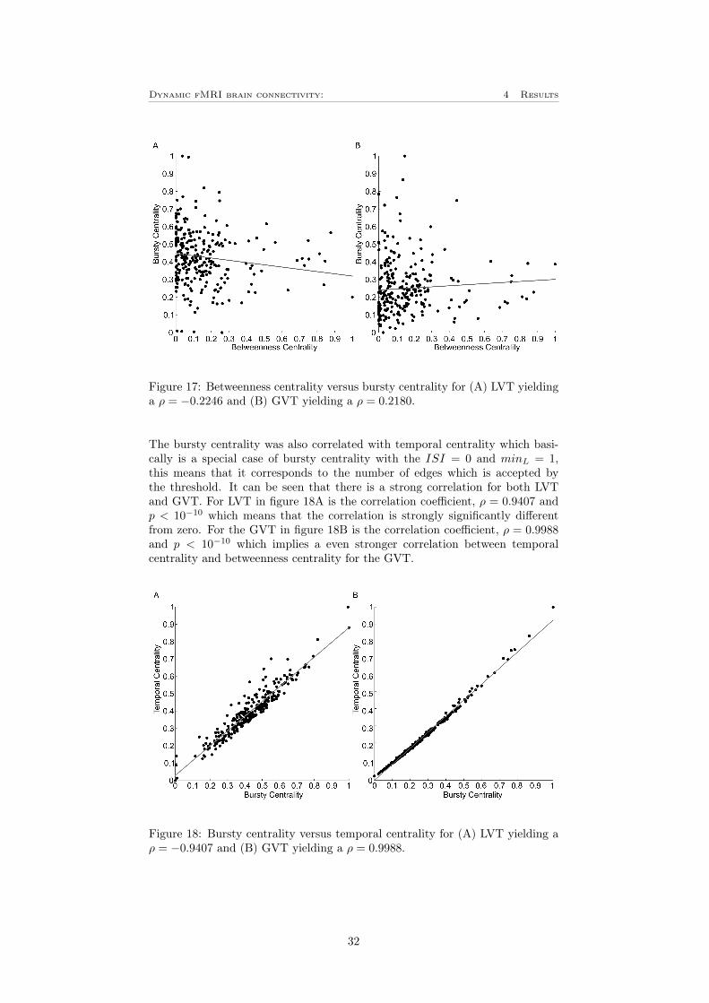
Figure 17: Betweenness centrality versus bursty centrality for (A) LVT yieldinga ρ = −0.2246 and (B) GVT yielding a ρ = 0.2180.

The bursty centrality was also correlated with temporal centrality which basi-cally is a special case of bursty centrality with the ISI = 0 and minL = 1,this means that it corresponds to the number of edges which is accepted bythe threshold. It can be seen that there is a strong correlation for both LVTand GVT. For LVT in figure 18A is the correlation coefficient, ρ = 0.9407 andp < 10−10 which means that the correlation is strongly significantly differentfrom zero. For the GVT in figure 18B is the correlation coefficient, ρ = 0.9988and p < 10−10 which implies a even stronger correlation between temporalcentrality and betweenness centrality for the GVT.

Figure 18: Bursty centrality versus temporal centrality for (A) LVT yielding aρ = −0.9407 and (B) GVT yielding a ρ = 0.9988.

32

Dynamic fMRI brain connectivity: 5 Discussion

5 Discussion

The point based method used in this study is mainly built upon the methodpresented by Thompson and Fransson [4]. As was discussed in the said article,this is a very suitable method to investigate temporal dynamics of the resting-state fMRI data for several reasons. The most important is that the wholetime-series is used in the analysis and therefore all the dynamical connectivitychanges over time is considered. Further, connectivity profiles for each statefrom the clustering is represented in the s-graphlets which then is assembled ina time-series called t-graphlets. The t-graphlets allow temporal analysis of theconnectivity by use of temporal graph theory which is suitable when introducingthe bursty centrality measure [4].

5.1 Clustering

However, as was seen in section 4 were many different options tested to investi-gate the robustness of the method, which all had influence on the result. Firstof all, which not was compared in section 4, is the choice of clustering method.In fact there are several other clustering algorithm that could have been usedinstead. In this case, k-means clustering was used because of its simplicity andit is also a common choice in fMRI studies. The main problem with the k-meansalgorithm is the choice of k-value. The choice k = 8 in this thesis was based onthe local maximum in figure 7 and it is also a common choice in other studies,for example by Thompson and Fransson [4] and by Allen et al [27]. Also severalother choices of k-values were tested and correlated with each other and thisindicated a rather high correlation for several of the choices, especially for theGVT. This indicates that the choice of k-value is not critical for the results.

5.2 Weighting

Also the choice of weighting algorithm have to be selected. In this study twodifferent algorithms were studied (i.e GTPS and ETPS) but there are probablymany other ways to weight the data. However the two algorithm tested in thisstudy correlated well, which indicates that both of them at least are fairly good,but this could probably be further developed.

5.3 Atlases

The choice of atlas is more dependent on the intent of the study. In this studywas two different atlases tested (Power 264 and Harvard-Oxford) and it wasshown that both of them yielded similar results. However is it hard to comparethe bursty centrality between the two atlases because of the differences in thenodes construction. For example, the Power 264 atlas consists of 264 smallspherical nodes which is scattered across the brain while the HO-atlas consistsof 106 differently shaped volumes which together cover the whole brain exceptcerebellum.

33


5.4 Datasets

Obviously also the choice of dataset depend on the specific study, it can behealthy adults as in this case, it can be children, persons with a specific diseaseor injury. Regardless of this is it important to show that the same behavior alsocan be seen in other datasets, and it is always good to increase the number ofdata to reduce the influence of coincidence. As can be seen in figure 16 andin the tables 5 and 6 in appendix C, many of the nodes with a high burstycentrality are common for both the datasets. This indicates that the result aresimilar for both the datasets.

5.5 Thresholding

The choice of threshold is probably the biggest issue, in this thesis, two differentthresholding algorithms are suggested, but of course, there are also many otherpossible thresholds that could be used. The two thresholds suggested are bothvariance based thresholds, one global and one local.

By studying the plots in figure 11B and 11D it was noted that both thresholds(LVT and GVT) treats the data independently of the mean of the edge time-series. This is obvious since the data was demeaned before the thresholding.In figure 11C and 11E was another dependence observed. Figure 11C showedthat the LVT also treated the data independently of the variance of the edgetime-series. Also this can be seen as obvious since the threshold is based onthe variance for the specific time-series for each edge and thus the thresholdis different for each edge. However, figure 11E shows that the variance have apositive dependence on the counts for the GVT. Since all the time-series aredemeaned and the GVT thresholds the data with the same threshold for alledges, the edges with the highest variance will also gain the most number ofcounts. Further in figures 14, 15, 16 and 18 can be observed that the correlationis higher for the GVT then for the LVT, this indicates that the GVT at leastdecreases the dependence of the other choices in the method. However thetwo thresholds can provide different results which can be seen in the figures12, 16 and the tables in appendix A, B and C. This is of course due to thedifferent characteristics of the LVT and the GVT. The LVT accepts all time-points in the edge time-series that exceed two standard deviations of the currentedge time-series. Here, it will measure how often a time-series have a highmagnitude compared to its own time-series. The GVT threshold on the otherhand accepts the time-points when the variance in the BOLD-signal in the nodeexceed a certain value calculated by the global variance of all edges time-series.Thus, this will give a measure of which nodes that often have oscillations ofhigh magnitude compared to other edges. As a result of these differences is itimpossible to suggest only one of the threshold methods, instead the one thatis suitable for the specific study have to be selected. And as was said before,there are also many other possible thresholds that maybe are even more suitabledepending on the situation.

5.6 Inter spike interval and minimum length

Also the parameters for counting the number of bursts can be changed. Thishave to be chosen dependent on what characteristics that are of interest in the

34


specific study. First, the parameter ISI (inter spike interval) have to be chosen.ISI determined the limit of how many zeros that was needed to end a burst. Andthe second was minL (minimum length) which is the minimum number of onesthat is needed to be considered as a burst. In this thesis was ISI set to 2 andminL to 1 which is a pretty generous choice. The reason to this generous choicewas to obtain many bursts which will make it easier to evaluate the results.

5.7 Robustness of the method

Since there are several choices that have to be made depending on the situationand the intentions of the study it is also many things that can challenge therobustness of the method. However, it is shown that many of these choices leadsto quite small differences (i.e altas, k-value, weighting method, dataset, ISI andminL) in the results which indicates that the method can be considered to bequite robust. However, it is very important to be careful with the choices thathave to be made and customize these for the current study. The one parametersthat, as expected, led to different results was the thresholding algorithm. Thisemphasises the points raised in The mean- variance relationship reveals twopossible strategies for dynamic brain connectivity analysis in fMRI [28] aboutthe importance of the thresholding algorithm.

5.8 Bursty Centrality

Bursts in single neurons can actually be traced back to 1973 in the study Studieson single neurons in dorsal hippocampal formation and septum in unrestrainedrats. [29]. And the bursty pattern in temporal properties of large scale brainnetworks were later shown by Thompson and Fransson [4]. In this work, amethod to quantify these bursts in single nodes of the brain is developed whichresulted in a new measure, bursty centrality. However, bursty centrality isdependent on the two thresholding algorithm suggested in this work (LVT andGVT). This showed that the most bursty region using LVT is thalamus whichis expected since thalamus have a coordinating role between different brainregions, which makes it important in the information dissemination in the brainand therefore it is logical that this part shows a high bursty centrality. As alsowas noted is the DMN dominating for this threshold which also can be seen aslogical since this is the most active network during resting state condition. Forthe GVT was precuneus the node with the highest bursty centrality. Precuneusis for example related to self-consciousness, self-awareness and memory and hasbeen considered an important hub of brain activity [30]. During the resting-statefMRI scan it is intended that the participants shall think of nothing specific.This is really hard and it is common that the participants end up in thoughtsabout different memories which makes it logical that precuneus have a highactivity. For the GVT had also the DMN a high bursty centrality as expected,but also the visual network, this is probably because it was a resting-state fMRIscan with eyes open which will activate the visual network. If it was a resting-state fMRI scan with eyes closed, the visual network would probably have aconsiderably much lower bursty centrality.

Since bursty centrality is a completely new measure for the dynamic connec-tivity of a node, was it compared with two traditionally measures. First thebetweenness centrality which is a stationary network measure, and is one of the

35


most common graph theoretical measures used when investigating static brainconnectivity. It was expected that there should be some relation between thedynamic connectivity level and the functional connectivity level. This showed asmall negative correlation for the LVT and a small positive correlation for theGVT, see figure 17. These small correlations and the fact that one is negativeand one is positive makes it difficult to draw any conclusions. However, it showsthat it at least is some kind of correlation between the betweenness centralityon the functional level and the bursty centrality on the dynamic level. It alsoshows that this correlation is strongly dependent on the thresholding algorithm,this further emphasizing the importance to consider which thresholding algo-rithm is used in dynamic connectivity studies. Second, the bursty centrality wasalso correlated with temporal centrality, which is a measure in dynamic networkstudies [15], however it has not to our knowledge been applied to the brain. Thiscorrelation can be seen in figure 18. This showed a very strong correlation forboth LVT and GVT which not is surprising since the temporal centrality justis a special case of the bursty centrality with ISI = 0 and minL = 1. However,there are still several reasons for using bursty centrality over temporal centrality.First, it is easier to compare bursty centrality between different datasets withdifferent TR, since the temporal resolution will be different. It is also possiblethat the length of the burst will vary between different persons, tasks etc whichwould be possible to investigate with bursty centrality.

5.9 Future Work

As was said in the section 5.7 is the method shown to be robust, however itis probably possible to make it even better. The main part to concentrate onwould be the thresholding, but also the weighting may be possible to developfurther. Apart from developing the method further would it be interestingto investigate which nodes that mainly sends information within the networkand which mainly send it between networks. This would give an even furtherknowledge of how the information propagates through the brain’s networks. Itis also needed to decoding the content of the information transmitted in bursts.Further could this also be applied in several clinical research, for example itcould be interesting to see if there is any difference in bursty centrality between,for example healthy subjects and subjects with bipolar disorder.

36

Dynamic fMRI brain connectivity: 6 Conclusion

6 Conclusion

This work extends and further develop the findings presented by Thompson andFransson [4] where they, by the use of temporal graph theory showed a burstypattern in the connectivity, mainly between resting state networks. The aim ofthis work was to establish a method that could quantify a dynamic property ona nodal level. The achieved method uses the full time-series of the resting-statefMRI which resulted in a robust method for several tested parameters. How-ever, in this work was two threshold algorithms suggested. One local variancethreshold (LVT) which thresholds the time-points according to the standard de-viation of the current edges time-series. The other threshold is a global variancethreshold (GVT) and thresholds the time-point according to the global varianceof all edges in the system. By compare these two thresholding algorithms wasit found that the GVT increased the robustness of the study compared to theLVT. However, because of the different methods in the thresholding will it alsoemphasize different dynamic properties. This makes it very important to adjustchoice of thresholding algorithm for the intent of current study. Also the pa-rameters ISI (inter spike interval) and minL (minimum length) can be modifiedto fit the current study and to obtain the most suitable result.

Further was the bursts quantified on a nodal level with the measure namedbursty centrality. This was correlated with betweenness centrality resulting in asignificant correlation for both the LVT and the GVT. However, the correlationwas negative for the LVT and positive for the GVT which indicate that thecorrelation is strongly dependent on the choice of thresholding algorithm. Thismeasure resulted in the highest value of bursty centrality for thalamus and theDMN when using the LVT. For the GVT is precuneus the node with the highestbursty centrality and the visual network and DMN are the networks with thehighest bursty centrality value. All this results seems to be reasonable comparedto the different tasks these nodes and networks corresponds to.

37

Dynamic fMRI brain connectivity: References

References

[1] Hao He, Qingbao Yu, Yuhui Du, Victor Vergara, Teresa A. Victor, WayneC. Drevets, Jonathan B. Savitz, Tianzi Jiang, Jing Sui, Vince D. Calhoun.(2015) "Resting-state functional network connectivity in prefrontal regionsdiffers between unmedicated patients with bipolar and major depressivedisorders" J Affect Disord. 2015 Oct 31;190:483-493.

[2] Michael D. Fox and Marcus E. Raichle, (2007) "Spontaneous fluctuationsin brain activity observed with functional magnetic resonance imaging"Nature Reviews Neuroscience 8, 700-711

[3] Bharat Biswal, F. Zerrin Yetkin, Victor M. Haughton, James S. Hyde.(1995) "Functional Connectivity in the Motor Cortex of Resting HumanBrain Using Echo-Planar MRI" Magn Reson Med. 1995 Oct;34(4):537-41.

[4] WH. Thompson and P. Fransson. (Submitted 2015) "Bursty and persis-tent properties of a large-scale brain networks revealed with a point-basedmethod for dynamic functional connectivity".

[5] Michael D. Fox and Michael Greicius. (2010) "Clinical Applications of Rest-ing State Functional Connectivity". Front Syst Neurosci. 2010; 4: 19.

[6] L. G. Hanson. (2005) “Introduction to Magnetic Resonance ImagingTechniques” Danish Research Centre for Magnetic Resonance (DRCMR),Copenhagen, Denmark, Tech. Rep.

[7] McRobbie, Donald W., Moore, Elizabeth A., Graves, Martin J., Prince,Martin R. (2007) "MRI From Picture to Proton", 2nd ed. 2007

[8] Pär Flodin. (2015) "Intrinsic brain activity in health and disease" Karolin-ska Institutet.

[9] Scott A. Huettel, Allen W. Song and Gregory McCarthy. (2009) "Func-tional Magnetic Resonance Imaging", 2nd ed. 2009

[10] Tzourio-Mazoyer N, Landeau B, Papathanassiou D, Crivello F, Etard O,Delcroix N, Mazoyer B, Joliot M. (2002) "Automated Anatomical Labelingof Activations in SPM Using a Macroscopic Anatomical Parcellationof theMNI MRI Single-Subject Brain" Neuroimage. 2002 Jan;15(1):273-89.

[11] Dosenbach NU, Fair DA, Cohen AL, Schlaggar BL, Petersen SE. (2008) "Adual-networks architecture of top-down control". Trends Cogn Sci. 2008Mar;12(3):99-105.

[12] Damoiseaux JS, Rombouts SA, Barkhof F, Scheltens P, Stam CJ, SmithSM, Beckmann CF. (2006) "Consistent resting-state networks acrosshealthy subjects" Proc Natl Acad Sci U S A. 2006 Sep 12;103(37):13848-53.

[13] S. Vossel, Joy J. Geng and Gereon R. Fink. (2014) "Dorsal and VentralAttention Systems Distinct Neural Circuits but Collaborative Roles" Neu-roscientist, April 2014 vol. 20 no. 2 150-159

[14] Jonathan D. Power, Alexander L. Cohen, Steven M. Nelson, Gagan S.Wig, Kelly Anne Barnes, Jessica A. Church, Alecia C. Vogel, Timothy O.Laumann, Fran M. Miezin, Bradley L. Schlaggar, and Steven E. Petersen.(2011) "Functional Network Organization of the Human Brain" Neuron,Volume 72, Issue 4, 17 November 2011, Pages 665–678

38

Dynamic fMRI brain connectivity: References

[15] P. Holme and J. Saramaki. (2011) "Temporal Networks".

[16] Neuroimaging Informatics Tools and Resources Clearinghouse (NI-TRC). http : //fcon_1000.projects.nitrc.org/fcpClassic/FcpTable.html(Downloaded 2015-08-20)

[17] E. Tagliazucchi and H. Laufs. (2014) "Decoding Wakefulness Levels fromTypical fMRI Resting-State Data Reveals Reliable Drifts between Wake-fulness and Sleep". Neuron. 2014 May 7;82(3):695-708.

[18] J. Ashburner, G. Barnes, CC. Chen J. Daunizeau, G. Flandin, K. Friston, S.Kiebel, J. Kilner, V. Litvak, R. Moran, W. Penny, K. Stephan, P. Zeidman,D. Gitelman, R. Henson, C. Hutton, V. Glauche J. Mattout and C. Phillips.(2015). "SPM12 Manual" Functional Imaging Laboratory Wellcome TrustCentre for Neuroimaging Institute of Neurology, UCL. [Online]. Avaliable:http://www.fil.ion.ucl.ac.uk/spm/doc/manual.pdf

[19] F. Gregory Ashby. (2011) "Statistical Analysis of fMRI Data".

[20] J. Ashburner and K.J. Friston. (2005) "Unified segmentation". Neuroimage.2005 Jul 1;26(3):839-51.

[21] Whitfield-Gabrieli S, Nieto-Castanon A. (2012) "Conn: a functional con-nectivity toolbox for correlated and anticorrelated brain networks". BrainConnect. 2012;2(3):125-41.

[22] Power J.D, Barnes K, Snyder A.Z, Schlaggar B.L, Petersen S.E. (2012)"Spurious but systematic correlations in functional connectivity MRI net-woks arise from subject motion." Neuroimage. 2012 Feb 1;59(3):2142-54.

[23] Chris Rorden. www.mricro.com (Loaded 2015-12-16)

[24] Mingrui Xia , Jinhui Wang, Yong He. (2013) "BrainNet Viewer: A NetworkVisualization Tool for Human Brain Connectomics" PLoS One. 2013 Jul4;8(7).

[25] Martin Rosvall and Carl T. Bergstrom. (2007) "Maps of random walks oncomplex networks reveal community structure". Proc Natl Acad Sci U S A.2008 Jan 29;105(4):1118-23

[26] Xiao Liu and Jeff H. Duyn. (2013) "Time-varying functional network infor-mation extracted from brief instances of spontaneous brain activity". ProcNatl Acad Sci U S A. 2013 Mar 12;110(11):4392-7.

[27] Allen EA, Damaraju E, Plis SM, Erhardt EB, Eichele T, Calhoun VD.(2014) "Tracking whole-brain connectivity dynamics in the resting state."Cereb Cortex. 2014 Mar;24(3):663-76.

[28] WH. Thompson and P. Fransson. (2015) "The mean– variance relationshipreveals two possible strategies for dynamic brain connectivity analysis infMRI". Front Hum Neurosci. 2015 Jul 14;9:398.

[29] James B. Ranck Jr. (1973) "Studies on single neurons in dorsal hippocam-pal formation and septum in unrestrained rats. I. Behavioral correlates andfiring repertoires". Experimental Neurology Volume 41, Issue 2, November1973, Pages 462–531

[30] Peter Fransson, Guillaume Marrelec. (2008) "The precuneus/posterior cin-gulate cortex plays a pivotal role in the default mode network: Evidencefrom a partial correlation network analysis". Volume 42, Issue 3, September2008, Pages 1178–1184

39

Dynamic fMRI brain connectivity: A Appendix A

A Appendix A

Table 1: Scaled bursty centrality (BC∗), brodmann areas, AAL ar-eas and network affiliation for the 40 nodes (15%) with the highestbursty centrality for the local variance threshold (LVT) using thePower 264 atlas. For the nodes with an undefined Brodmann areas(i.e BA=0) is the closest brodmann area stated in the parentheses.

BC∗ Brodmann area AAL Network1 0 (23) Thalamus L Subcortical0.9943 10 Frontal Med Orb R DMN0.8201 9 Frontal Sup R DMN0.7944 18 Lingual R Undefined0.7708 44 Frontal Inf Oper L FPN0.7512 20 Temporal Pole Mid L DMN0.7472 0 (25) Thalamus R Subcortical0.7445 30 ParaHippocampal L Undefined0.7084 21 Temporal Mid L DMN0.7012 0 (30) ParaHippocampal R Undefiened0.6947 4 Postcentral L Somato-motor0.6756 0 (48) Thalamus R Subcortical0.6729 37 ParaHippocampal L DMN0.6715 20 Fusifrom L Undefined0.6627 11 Frontal Med Orb L DMN0.6601 20 Fusiform L Undefined0.6505 48 Heschl L Auditory0.6476 9 Frontal Sup R DMN0.6441 48 Frontal Mid R SAN0.6436 37 Temporal Mid R DAN0.6347 8 Frontal Sup L DMN0.6291 32 Cingulum Ant L DMN0.6271 48 Insula R Somato-motor0.6264 37 Fusiform L DMN0.6158 20 Temporal Inf R Undefined0.6069 46 Frontal Mid R SAN0.5995 4 Precentral R Somato-motor0.5959 39 Occipital Mid L DMN0.5951 0 (27) Thalamus R Subcortical0.5927 6 Precentral L FPN0.5920 20 Fusiform R Undefined0.5835 10 Cingulum Ant L DMN0.5834 18 Occipital Mid L Visual0.5834 19 Occipital Mid L Visual0.5819 0 (27) Cerebelum 4 5 L Subcortical0.5719 9 Frontal Sup R DMN0.5718 0 (24) Cingulum Mid L CON0.5693 9 Frontal Sup L DMN0.5692 48 Heschl R Auditory0.5658 0 (18) Cerebelum Crus2 R Undefined

40

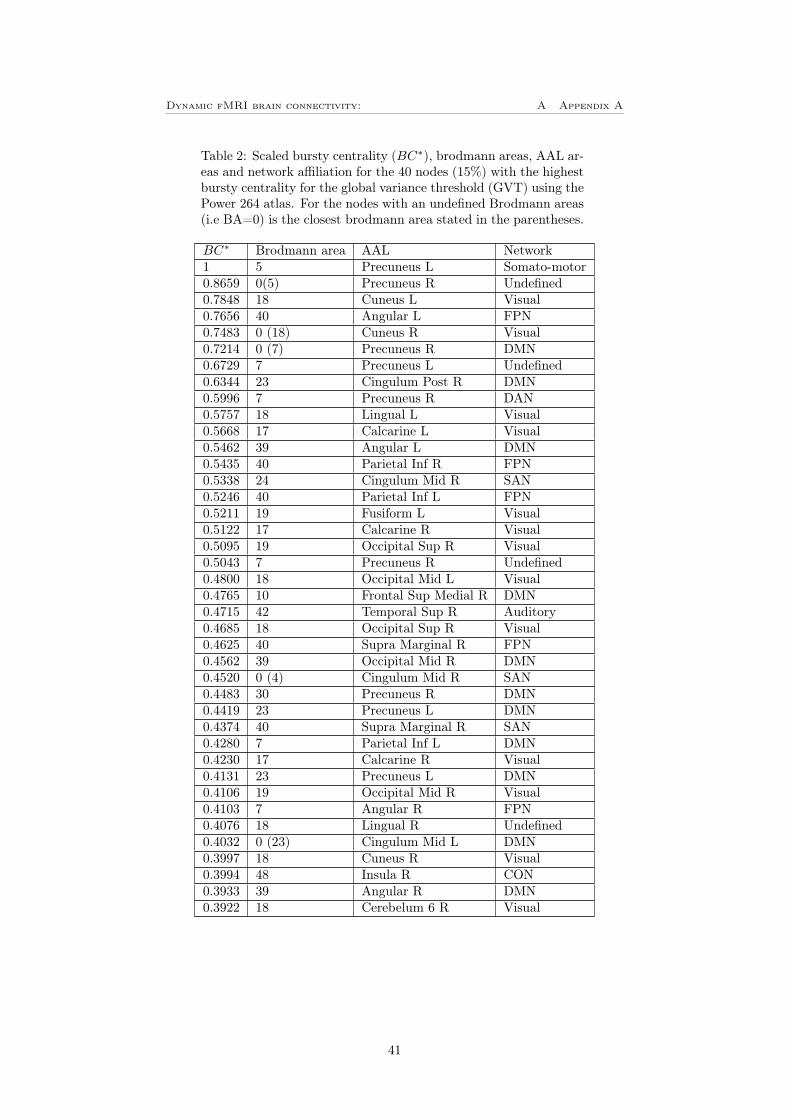
Dynamic fMRI brain connectivity: A Appendix A

Table 2: Scaled bursty centrality (BC∗), brodmann areas, AAL ar-eas and network affiliation for the 40 nodes (15%) with the highestbursty centrality for the global variance threshold (GVT) using thePower 264 atlas. For the nodes with an undefined Brodmann areas(i.e BA=0) is the closest brodmann area stated in the parentheses.

BC∗ Brodmann area AAL Network1 5 Precuneus L Somato-motor0.8659 0(5) Precuneus R Undefined0.7848 18 Cuneus L Visual0.7656 40 Angular L FPN0.7483 0 (18) Cuneus R Visual0.7214 0 (7) Precuneus R DMN0.6729 7 Precuneus L Undefined0.6344 23 Cingulum Post R DMN0.5996 7 Precuneus R DAN0.5757 18 Lingual L Visual0.5668 17 Calcarine L Visual0.5462 39 Angular L DMN0.5435 40 Parietal Inf R FPN0.5338 24 Cingulum Mid R SAN0.5246 40 Parietal Inf L FPN0.5211 19 Fusiform L Visual0.5122 17 Calcarine R Visual0.5095 19 Occipital Sup R Visual0.5043 7 Precuneus R Undefined0.4800 18 Occipital Mid L Visual0.4765 10 Frontal Sup Medial R DMN0.4715 42 Temporal Sup R Auditory0.4685 18 Occipital Sup R Visual0.4625 40 Supra Marginal R FPN0.4562 39 Occipital Mid R DMN0.4520 0 (4) Cingulum Mid R SAN0.4483 30 Precuneus R DMN0.4419 23 Precuneus L DMN0.4374 40 Supra Marginal R SAN0.4280 7 Parietal Inf L DMN0.4230 17 Calcarine R Visual0.4131 23 Precuneus L DMN0.4106 19 Occipital Mid R Visual0.4103 7 Angular R FPN0.4076 18 Lingual R Undefined0.4032 0 (23) Cingulum Mid L DMN0.3997 18 Cuneus R Visual0.3994 48 Insula R CON0.3933 39 Angular R DMN0.3922 18 Cerebelum 6 R Visual

41

Dynamic fMRI brain connectivity: B Appendix B

B Appendix B

Table 3: Scaled bursty centrality (BC∗) for 106 Harvard-Oxfordatlas brain regions for the local variance threshold (LVT) plottedin figure 13F.

BC∗ Brain region BC∗ Brain region1 Heschl’s Gyrus Left 0.4899 Superior Frontal Gyrus Right0.9541 Superior Temporal Gyrus, poste-

rior division Left0.4881 Middle Frontal Gyrus Left

0.9248 Supramarginal Gyrus, anteriordivision Right

0.4843 Planum Temporale Right

0.8909 Superior Temporal Gyrus, ante-rior division Right

0.4808 Amygdala r

0.8593 Planum Temporale Left 0.4746 Lateral Occipital Cortex, inferiordivision Right

0.8402 Temporal Occipital FusiformCortex Right

0.4652 Parahippocampal Gyrus, ante-rior division Right

0.8256 Parahippocampal Gyrus, ante-rior division Left

0.4560 Parahippocampal Gyrus, poste-rior division Left

0.8144 Heschl’s Gyrus Right 0.4548 Subcallosal Cortex0.7810 Insular Cortex Left 0.4425 Occipital Fusiform Gyrus Left0.7527 Putamen r 0.4333 Lateral Occipital Cortex, super-

oir division Right0.7405 Inferior Frontal Gyrus, pars op-

ercularis Right0.4303 Inferior Temporal Gyrus, poste-

rior division Right0.7400 Superior Temporal Gyrus, ante-

rior division Left0.4275 Precuneous Cortex

0.7329 Inferior Frontal Gyrus, pars tri-angularis Right

0.4247 Postcentral Gyrus Left

0.7262 Precentral Gyrus Left 0.4244 Temporal Fusiform Cortex, pos-terior division Right

0.7214 Inferior Temporal Gyrus, ante-rior division Left

0.4237 Insular Cortex Right

0.7165 Cingulate Gyrus, anterior divi-sion

0.4165 Insular Cortex Right

0.7107 Inferior Frontal Gyrus, pars tri-angularis Left

0.4158 Planum Polare Right

0.6956 Accumbens r 0.4155 Temporal Pole Right0.6877 Inferior Frontal Gyrus, pars op-

ercularis Left0.4089 Superior Temporal Gyrus, poste-

rior division Right0.6821 Frontal Operculum Cortex Left 0.4050 Supramarginal Gyrus, posterior

division Left0.6809 Central Opercular Cortex Left 0.3847 Frontal Pole Left0.6747 Precentral Gyrus Right 0.3724 Inferior Temporal Gyrus, tem-

porooccipital part Left0.6574 Postcentral Gyrus Right 0.3717 Lingual Gyrus Left0.6569 Hippocampus r 0.3699 Superior Parietal Lobule Left0.6564 Supracalcarine Cortex Right 0.3653 Intracalcarine Cortex Left0.6518 Supramarginal Gyrus, anterior

division Left0.3630 Superior Frontal Gyrus Left

0.6459 Middle Temporal Gyrus, poste-rior division Right

0.3497 Thalamus l

42


0.6449 Temporal Occipital FusiformCortex Left

0.3454 Inferior Temporal Gyrus, poste-rior division Left

0.6421 Parietal Operculum CortexRight

0.3426 Middle Temporal Gyrus, poste-rior division Left

0.6314 Occipital Fusiform Gyrus Right 0.3357 Middle Frontal Gyrus Right0.6306 Occipital Pole Right 0.3306 Cuneal Cortex Left0.6253 Intracalcarine Cortex Right 0.3286 Middle Temporal Gyrus, ante-

rior division Right0.6179 Parietal Operculum Cortex Left 0.3191 Accumbens l0.6166 Supramarginal Gyrus, posterior

division Right0.3189 Occipital Pole Left

0.6097 Paracingulate Gyrus Left 0.3174 Caudate l0.6036 Temporal Fusiform Cortex, ante-

rior division Left0.3158 Temporal Fusiform Cortex, ante-

rior division Right0.6026 Hippocampus l 0.3112 Temporal Fusiform Cortex, pos-

terior division Left0.5893 Frontal Orbital Cortex Left 0.3107 Superior Parietal Lobule Right0.5886 Pallidum l 0.2901 Brain-Stem0.5769 Parahippocampal Gyrus, poste-

rior division Right0.2850 Central Opercular Cortex Right

0.5761 Temporal Pole Left 0.2842 Lateral Occipital Cortex, inferiordivision Left

0.5702 Amygdala l 0.2522 Middle Temporal Gyrus, ante-rior division Left

0.5664 Juxtapositional Lobule Cortex -formerly Supplementary MotorCortex- Right

0.2738 Angular Gyrus Right

0.5422 Frontal Operculum Cortex Right 0.2508 Middle Temporal Gyrus, tem-porooccipital part Right

0.5414 Putamen l 0.2190 Inferior Temporal Gyrus, ante-rior division Right

0.5407 Inferior Temporal Gyrus, tem-porooccipital part Right

0.2014 Lingual Gyrus Right

0.5396 Cuneal Cortex Right 0.1960 Supracalcarine Cortex Left0.5343 Frontal Orbital Cortex Right 0.1853 Cingulate Gyrus, posterior divi-

sion0.5157 Lateral Occipital Cortex, super-

oir division Left0.1642 Thalamus r

0.5055 Frontal Pole Right 0.1552 Caudate r0.4991 Pallidum r 0.1364 Frontal Medial Cortex0.4981 Planum Polare Left 0.1165 Middle Temporal Gyrus, tem-

porooccipital part Left0.4902 Paracingulate Gyrus Right 0 Angular Gyrus Left

43


Table 4: Scaled bursty centrality (BC) for 106 Harvard-Oxfordatlas brain regions for the global variance threshold (GVT) plottedin figure 13G.

BC∗ Brain region BC∗ Brain region1 Frontal Medial Cortex 0.3088 Precentral Gyrus Left0.8536 Superior Frontal Gyrus Right 0.2950 Temporal Pole Left0.8479 Planum Temporale Right 0.2881 Thalamus l0.8391 Lingual Gyrus Left 0.2786 Occipital Pole Left0.7945 Lateral Occipital Cortex, super-

oir division Right0.2773 Temporal Pole Right

0.7874 Precuneous Cortex 0.2773 Superior Parietal Lobule Right0.7564 Frontal Orbital Cortex Right 0.2735 Inferior Temporal Gyrus, ante-

rior division Right0.7244 Frontal Pole Right 0.2708 Inferior Temporal Gyrus, tem-

porooccipital part Right0.7089 Middle Temporal Gyrus, poste-

rior division Right0.2677 Hippocampus l

0.7082 Frontal Orbital Cortex Left 0.2668 Frontal Operculum Cortex Right0.6994 Lingual Gyrus Right 0.2624 Planum Polare Left0.6639 Middle Frontal Gyrus Right 0.2604 Amygdala r0.6562 Lateral Occipital Cortex, super-

oir division Left0.2537 Central Opercular Cortex Right

0.6314 Temporal Occipital FusiformCortex Left

0.2443 Juxtapositional Lobule Cortex -formerly Supplementary MotorCortex- Left

0.6135 Middle Frontal Gyrus Left 0.2401 Inferior Temporal Gyrus, poste-rior division Left

0.5890 Inferior Frontal Gyrus, pars op-ercularis Right

0.2341 Putamen l

0.5803 Frontal Pole Left 0.2332 Supramarginal Gyrus, posteriordivision Left

0.5761 Planum Temporale Left 0.2327 Superior Temporal Gyrus, ante-rior division Right

0.5674 Superior Frontal Gyrus Left 0.2313 Parahippocampal Gyrus, poste-rior division Left

0.5436 Middle Temporal Gyrus, poste-rior division Left

0.2308 Parahippocampal Gyrus, poste-rior division Right

0.5405 Cingulate Gyrus, posterior divi-sion

0.2287 Middle Temporal Gyrus, tem-porooccipital part Left

0.5396 Cuneal Cortex Right 0.2272 Supracalcarine Cortex Left0.5233 Supracalcarine Cortex Right 0.2234 Parietal Operculum Cortex Left0.5225 Intracalcarine Cortex Right 0.2148 Parahippocampal Gyrus, ante-

rior division Left0.5097 Insular Cortex Left 0.2055 Inferior Temporal Gyrus, ante-

rior division Left0.5046 Middle Temporal Gyrus, ante-

rior division Left0.1924 Putamen r

0.5042 Cuneal Cortex Left 0.1824 Postcentral Gyrus Right0.4960 Lateral Occipital Cortex, inferior

division Left0.1814 Hippocampus r

0.4945 Middle Temporal Gyrus, tem-porooccipital part Right

0.1756 Supramarginal Gyrus, anteriordivision Right

44


0.4829 Intracalcarine Cortex Left 0.1690 Inferior Temporal Gyrus, tem-porooccipital part Left

0.4793 Occipital Fusiform Gyrus Right 0.1576 Superior Temporal Gyrus, ante-rior division Left

0.4681 Paracingulate Gyrus Right 0.1564 Pallidum l0.4554 Inferior Frontal Gyrus, pars tri-

angularis Right0.1517 Central Opercular Cortex Left

0.4471 Occipital Fusiform Gyrus Left 0.1467 Superior Parietal Lobule Left0.4387 Parietal Operculum Cortex

Right0.1408 Temporal Fusiform Cortex, pos-

terior division Right0.4269 Paracingulate Gyrus Left 0.1313 Frontal Operculum Cortex Left0.4150 Inferior Frontal Gyrus, pars op-

ercularis Left0.1313 Occipital Pole Right

0.4055 Angular Gyrus Right 0.1307 Caudate l0.3963 Lateral Occipital Cortex, inferior

division Right0.1262 Superior Temporal Gyrus, poste-

rior division Right0.3844 Middle Temporal Gyrus, ante-

rior division Right0.1230 Caudate r

0.3842 Temporal Occipital FusiformCortex Right

0.1183 Postcentral Gyrus Left

0.3773 Juxtapositional Lobule Cortex -formerly Supplementary MotorCortex- Right

0.1181 Accumbens r

0.3643 Inferior Frontal Gyrus, pars tri-angularis Left

0.1131 Planum Polare Right

0.3547 Supramarginal Gyrus, posteriordivision Right

0.1086 Heschl’s Gyrus Left

0.3523 Insular Cortex Right 0.1069 Supramarginal Gyrus, anteriordivision Left

0.3454 Parahippocampal Gyrus, ante-rior division Right

0.1064 Accumbens l

0.3395 Subcallosal Cortex 0.0972 Temporal Fusiform Cortex, pos-terior division Left

0.3362 Cingulate Gyrus, anterior divi-sion

0.0951 Pallidum r

0.3331 Thalamus r 0.0902 Brain-Stem0.3259 Precentral Gyrus Right 0.0857 Amygdala l0.3219 Angular Gyrus Left 0.0846 Superior Temporal Gyrus, poste-

rior division Left0.3124 Temporal Fusiform Cortex, ante-

rior division Left0.0731 Inferior Temporal Gyrus, poste-

rior division Right0.3117 Temporal Fusiform Cortex, ante-

rior division Right0 Heschl’s Gyrus Right

45

Dynamic fMRI brain connectivity: C Appendix C

C Appendix C

Table 5: The AAL areas, brodmann areas and network affiliationfor the 11 nodes which occurring in the top 40 nodes (15%) withthe highest bursty centrality for both Oulu A and Oulu B with thelocal variance threshold (LVT). These are also shown as blue nodesin figure 16C. For the nodes with an undefined Brodmann area (i.eBA=0) is the closest brodmann area stated in the parentheses.

AAL Brodmann area NetworkParaHippocampal L 30 UndefinedParaHippocampal R 39 UndefinedInsula R 48 Somato-motorOccipital Mid L 0 (30) DMNFrontal Sup R 9 DMNPrecentral L 6 FPNThalamus R 0 (27) SubcorticalThalamus L 0 (23) SubcorticalThalamus R 0 (25) SubcorticalFusiform R 20 UndefinedTemporal Mid R 37 DAN

46

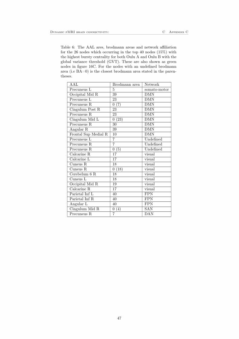
Dynamic fMRI brain connectivity: C Appendix C

Table 6: The AAL ares, brodmann areas and network affiliationfor the 26 nodes which occurring in the top 40 nodes (15%) withthe highest bursty centrality for both Oulu A and Oulu B with theglobal variance threshold (GVT). These are also shown as greennodes in figure 16C. For the nodes with an undefined brodmannarea (i.e BA=0) is the closest brodmann area stated in the paren-theses.

AAL Brodmann area NetworkPrecuneus L 5 somato-motorOccipital Mid R 39 DMNPrecuneus L 23 DMNPrecuneus R 0 (7) DMNCingulum Post R 23 DMNPrecuneus R 23 DMNCingulum Mid L 0 (23) DMNPrecuneus R 30 DMNAngular R 39 DMNFrontal Sup Medial R 10 DMNPrecuneus L 7 UndefinedPrecuneus R 7 UndefinedPrecuneus R 0 (5) UndefinedCalcarine R 17 visualCalcarine L 17 visualCuneus R 18 visualCuneus R 0 (18) visualCerebelum 6 R 18 visualCuneus L 18 visualOccipital Mid R 19 visualCalcarine R 17 visualParietal Inf L 40 FPNParietal Inf R 40 FPNAngular L 40 FPNCingulum Mid R 0 (4) SANPrecuneus R 7 DAN

47

Dynamic fMRI brain connectivity -...

Documents

Transcript of Dynamic fMRI brain connectivity -...