
Dynamic Feedbacks Between Vegetation and Hydrology in the ...
137
Dynamic Feedbacks Between Vegetation and Hydrology in the Long Term Dissertation der Mathematisch-Naturwissenschaftlichen Fakultät der Eberhard Karls Universität Tübingen zur Erlangung des Grades eines Doktors der Naturwissenschaften (Dr. rer. nat.) vorgelegt von Shanghua Li aus Luoyang/China Tübingen 2020
Transcript of Dynamic Feedbacks Between Vegetation and Hydrology in the ...

Dynamic Feedbacks Between Vegetation and Hydrology in
the Long Term
Dissertation
der Mathematisch-Naturwissenschaftlichen Fakultät
der Eberhard Karls Universität Tübingen
zur Erlangung des Grades eines
Doktors der Naturwissenschaften
(Dr. rer. nat.)
vorgelegt von
Shanghua Li
aus Luoyang/China
Tübingen
2020

Gedruckt mit Genehmigung der Mathematisch-Naturwissenschaftlichen Fakultät der Eberhard
Karls Universität Tübingen.
Tag der mündlichen Qualifikation: 30.10.2020
Stellvertretender Dekan: Prof. Dr. József Fortágh
1. Berichterstatter: Prof. Dr. Katja Tielbörger
2. Berichterstatter: Dr. Sebastian Gayler

I
Abstract
The interaction and feedback between vegetation and hydrology plays an important role in the
soil-plant-atmosphere system. The challenge of simulating the dynamic interactions between
vegetation and hydrology using either hydrological models or ecological models alone have
been gradually recognized as an issue in both hydrology and ecology. Most current hydrological
models simulated plants without or with only little dynamics of its own. Vice-versa, most
current plant ecological models simplify hydrological conditions and ignore the temporal
dynamics of spatially distributed hydraulic conditions. Pre-defining hydrological or ecological
components would hinder the ability of models for a ‘close-to-reality’ simulation of the
dynamics feedbacks between hydrology and vegetation, which may seriously modify the
modelled system behavior.
This dissertation focuses on exploring the dynamic feedbacks between the hydrological
processes and vegetation under different climate conditions on a long-term time scale. In
particular, it identifies the conditions under which one should use a coupled vegetation-
hydrological model for a better representation of the reality. Models used in this study include
a fully integrated surface and subsurface flow model HydroGeoSphere (HGS) that is
dynamically coupled with a highly flexible plant model (PLANTHeR). The hydrological model
solves the diffusive wave equation on the surface and the Richards equation in the subsurface
domain, with an exchange water flux term that couples the surface and subsurface. The
PLANTHeR model is an individual-based model designed for simulating composition and
structure of plant functional types (PFTs) in a plant community under the entire possible range
of hydrological conditions, i.e. from permanently flooded to completely dry. The coupling of
the 2-D PLANTHeR model to the 3-D HGS model allows for a better representation of dynamic
relationships between the hydrology and vegetation for the scenarios investigated in this study.
The coupled PLANTHeR-HGS model was used to evaluate three main questions:
1) Why is it important to use the PLANTHeR-HGS model instead of the uncoupled
PLANTHeR and HGS models to simulate the hydrological processes and plant community
dynamics, and which hydrological or plant community variables match better with empirical
values from literature, when using the PLANTHeR-HGS model?
2) Under which climate conditions - dry climates or wet climates - it matters the most to use
the coupled PLANTHeR-HGS model instead of the uncoupled PLANTHeR or HGS models?
II
3) Does high plant diversity increase ecosystem stability under extreme climate events in
drylands?
To address the first question, the PLANTHeR model was coupled to the HGS model at a plot-
scale with a year-to-year feedback. By comparing the results between the PLANTHeR-HGS
model and the uncoupled HGS model over 1000 years, it was found that the PLANTHeR-HGS
model led to lower transpiration and higher evaporation than those runs resulting from the
uncoupled HGS model. Besides, variation of plants simulated with the PLANTHeR-HGS
model greatly influenced the soil water content under drought stress conditions, while
implementing static plant components in the uncoupled HGS model led to an unrealistically
dryer hydrological state. Vice-versa, by comparing the results between the PLANTHeR-HGS
model and the uncoupled PLANTHeR model, it was found that the coupled PLANTHeR-HGS
model resulted in a lower mean Shannon index and lower PFT richness, as well as lower mean
aboveground biomass than those simulated with the uncoupled PLANTHeR model. Increased
spatial soil water resource heterogeneity did not decrease plant community diversity and
richness but decreased mean aboveground biomass. The results show that the hydrological
conditions and the plant community structure differ meaningfully when the two dynamic
models are coupled.
To address the second question, the PLANTHeR model was coupled to the HGS model on a
seasonal timestep and at a hillslope scale. The dynamic relationships along a hydroclimatic
gradient, from the semi-arid climate, to the sub-humid climate, and to the humid climate, were
investigated. The results show that better results can be obtained by using the coupled
PLANTHeR-HGS model to quantify transpiration, soil water content and surface runoff, as
well as plant community richness and annual aboveground biomass in a drier climate. When
quantifying evaporation and the plant community diversity (through the Shannon index), using
the coupled PLANTHeR-HGS model gives best results in a wetter climate.
To address the third question, the seasonally coupled PLANTHeR-HGS model is used to
explore the biodiversity-stability relationships under three extreme climates in drylands.
Namely, extreme drought climates, extreme flood climates, and extreme drought and heavy
rainfall climates were investigated. Results show that increasing diversity increased plant
community stability under extreme flood climatic events, and under extreme drought and heavy
rainfall events. But increasing diversity did not increase plant community stability under

III
extreme drought events, due to a non-significant diversity impact on resistance against extreme
drought events.
Concluding, the importance of dynamically considering both ecological and hydrological
processes in dedicated models of the respective disciplines could be shown, especially for
extreme conditions and for long-term approaches.
IV
Zusammenfassung
Die Interaktion zwischen Vegetation und Hydrologie spielt eine wichtige Rolle im System
Boden-Pflanze-Atmosphäre. Die Herausforderung, die dynamischen Interaktion zwischen
Vegetation und Hydrologie entweder nur mit hydrologischen oder nur mit ökologischen
Modellen zu simulieren, wurde in der Hydrologie sowohl in der Ökologie als Problem erkannt.
Die meisten aktuellen hydrologischen Modelle simulieren Pflanzen ohne oder nur mit geringer
Eigendynamik. Gleichzeitig vereinfachen die meisten verfügbaren ökologischen Modelle die
hydrologischen Bedingungen, oder ignorieren die räumlich-zeitlich Dynamik der
hydrologischen Prozesse. Eine Vordefinition hydrologischer oder ökologischer Komponenten
würde die Fähigkeit von Modellen zu einer "realitätsnahen" Simulation der dynamischen
Rückkopplungen zwischen Hydrologie und Vegetation behindern, was das modellierte
Systemverhalten stark verändern würde.
In dieser Dissertation geht es darum, die dynamische Interaktion zwischen der Hydrologie und
der Vegetation unter verschiedenen Klimabedingungen auf einer langfristigen Zeitskala zu
untersuchen und die Bedingungen zu identifizieren, unter denen man ein gekoppeltes
vegetations-hydrologisches Modell für eine bessere Darstellung der Realität verwenden sollte.
Die in dieser Studie verwendeten Modelle umfassen ein vollständig integriertes Oberflächen-
und Untergrundströmungsmodell HydroGeoSphere (HGS), das dynamisch mit einem
hochflexiblen Pflanzenmodell (PLANTHeR) gekoppelt ist. Das hydrologische Modell HGS
löst die Diffusionswellengleichung an der Oberfläche und die Richards-Gleichung im Bereich
des Untergrundes und verbindet diese mit einem Term für den Austausch zwischen Oberfläche
und Untergrund. Das Modell PLANTHeR ist ein individuenbasiertes Modell zur Simulation
der Zusammensetzung und Struktur von Pflanzenfunktionstypen (PFTs) in einer
Pflanzengemeinschaft unter der gesamten möglichen Bandbreite hydrologischer Konditionen,
d.h. von permanenter Überflutung bis hin zur völligen Austrocknung. Die Kopplung des 2-D
PLANTHeR-Modells mit dem 3-D HGS-Modell ermöglicht eine bessere Darstellung der
dynamischen Beziehungen zwischen Hydrologie und Vegetation, für die in dieser Studie
untersuchten Szenarien. Das gekoppelte PLANTHeR-HGS-Modell wurde zur Bewertung von
drei Hauptfragen verwendet:
1) Warum ist es wichtig, zur Simulation der hydrologischen Prozesse und der Dynamik von
Pflanzengemeinschaften das PLANTHeR-HGS-Modell anstelle der ungekoppelten

V
PLANTHeR- und HGS-Modelle zu verwenden, und welche hydrologischen oder okologischen
Variablen zur Beschreibung der Pflanzengemeinschaften- würden bei der Verwendung des
PLANTHeR-HGS-Modells realitätsnäher beschrieben?
2) Unter welchen Klimabedingungen - trockenes Klima oder feuchtes Klima - ist es am
entscheidensten, das gekoppelte Modell PLANTHeR-HGS anstelle der entkoppelten Modelle
PLANTHeR und HGS zu verwenden?
3) Erhöht eine hohe Diversität von Pflanzengemeinschaften die Stabilität von Ökosystemen
beim Vorkommen von extremen Klimaereignissen in Trockengebieten?
Um die erste Frage zu beantworten, wurde das PLANTHeR-Modell an das HGS-Modell auf
der Feldskala und mit einem Austausch von Jahr zu Jahr gekoppelt. Durch den Vergleich der
Ergebnisse zwischen dem PLANTHeR-HGS-Modell und dem entkoppelten HGS-Modell über
1000 Jahre konnte gezeigt werden, dass das PLANTHeR-HGS-Modell zu geringerer
Transpiration und höherer Verdunstung führte und dass die Pflanzendynamik, die mit dem
PLANTHeR-HGS-Modell simuliert wurden, den Bodenwassergehalt unter
Trockenstressbedingungen stark beeinflussen. Während die Implementierung statischer
Pflanzenkomponenten in das entkoppelte HGS-Modell zu einem unrealistischen trockeneren
hydrologischen Zustand führte, führte die Simulation mit dem HGS-Modell zu einer geringeren
Transpiration und höherer Verdunstung. Zugleich konnte beim Vergleich der Ergebnisse
zwischen dem PLANTHeR-HGS-Modell und dem ungekoppelten PLANTHeR-Modell
festgestellt werden, dass das gekoppelte PLANTHeR-HGS-Modell zu einem niedrigeren
mittleren Shannon-Index und PFT-Reichtum, sowie zu einer Verringerung der mittleren
oberirdischen Biomasse führte als mit dem ungekoppelten PLANTheR-Modell. Eine Zunahme
der räumlichen Heterogenität der Bodenwasserressourcen führte nicht zu einer Abnahme der
Vielfalt und des Reichtums der Pflanzengemeinschaften, sondern zu einer Abnahme der
mittleren oberirdischen Biomasse. Die Ergebnisse zeigen, dass sich die hydrologischen
Bedingungen und die Struktur der Pflanzengemeinschaften deutlich unterscheiden, wenn die
beiden dynamischen Modelle gekoppelt werden.
Um die zweite Frage zu beantworten, wurde das PLANTHeR-Modell mit dem HGS-Modell
saisonal und auf einer Hangskala gekoppelt, und die dynamischen Beziehungen entlang eines
hydroklimatischen Gradienten untersucht, vom semi-ariden Klima zum sub-humiden Klima
und weiter zum feuchten Klima. Die Ergebnisse zeigen, dass die Nutzung des gekoppelten
PLANTHeR-HGS-Modells einen wesentlichen Unterschied zur Quantifizierung der

VI
Transpiration, des Bodenwassergehalts und des Oberflächenabflusses sowie des Reichtums an
Pflanzengemeinschaften und der jährlichen oberirdischen Biomasse in einem trockeneren
Klima macht. Für ein feuchteres Klima ergeben sich die besten Ergebnisse für das gekoppelte
Modell PLANTHeR-HGS zur Quantifizierung der Verdunstung und der Vielfalt der
Pflanzengemeinschaften mit Hilfe des Shannon-Index. Um die dritte Frage zu beantworten,
wurde PLANTHeR-HGS auf der saisonalen Zeitskala verwendet, um die Biodiversitäts-
Stabilitäts-Beziehungen unter drei extremen Klimaten in Trockengebieten zu untersuchen, und
zwar für extreme Dürreklimate, extrem feuchte Klimate und extreme Dürre- und
Starkregenklimata. Die Ergebnisse zeigen, dass eine größere Vielfalt die Stabilität von
Pflanzengemeinschaften unter klimatisch extrem feuchten Bedingungen und extremen Dürre-
und Starkregenklimaten erhöht. Die erhöhte funktionelle Vielfalt erhöhte jedoch nicht die
Stabilität der Pflanzengemeinschaft gegenüber extremen Dürreereignissen, da die
Auswirkungen der Diversität auf die Resistenz nicht signifikant waren.
Zusammenfassend konnte die Wichtigkeit der dynamischen Einbeziehung von ökologischen
Prozessen in Modelle der jeweiligen Disziplinen gezeigt werden, insbesondere für
Extrembedingungen und langjährige Betrachtungen.

VII
Acknowledgements
My thesis would not be the same without the support from all my supervisors. I would like to
thank all the professors, post-docs, teachers, colleagues, administration staff and my families
for their support during my Ph.D journey. First, I would like to thank all my supervisors, Katja
Tielbörger, Sebastian Gayler, Nandita Basu, and Claus Haslauer. I want to thank you all for
your patience, guidance, inspiration, and continuous support over all these years. I would like
to express my great appreciation to my supervisor Katja Tielbörger, who was there guide me
into the fascinating world of ecology, trained me with scientific ways of thinking, and support
me until the end of my Ph.D. I want to especially thank Claus Haslauer, that even though not
being not officially my supervisor in the end, he still guided me, supported me, encouraged me
and had many intensive discussions with me from the very beginning of my Ph.D until the end.
I also want to express my great appreciation to Maximiliane Herberich, who contributed her
plant model to my research, helped me with the understanding of her model, and gave me many
constructive comments and suggestions.
I want to personally thank all my research group colleagues, I will never forget those interesting,
warm, and meaningful memories with you guys. I want to thank Prof. Olaf Cirpka, who gave
me the opportunity to join the International Research Training Group (IRTG) and supported me
through this long journey. Special thanks to Nandita Basu and her working group in Canada,
who welcomed and enriched my staying time in Canada, and even though it was short, you
guys gave me such a great and memorable time. I am deeply grateful for the support from Ms.
Monika Jekelius, who helped me with numerous paperwork and administrative issues, which
won’t have been easy without her. I would like to thank the German Research Foundation
(DFG) for their financial support within the International Research Training Groups (IRTG)
project.
At the end, I want to especially thank my families. My family in Germany, my husband, who
supported me and encouraged me through all these years, who believed in me even though I
did not sometimes. My son, who gives me endless energy, and makes my every single day
cheerful and colorful. My family in China, who are far away but still there for me, whenever I
need them. Without you, my families, life won’t be worth fighting for.

VIII
Contents
Abstract ....................................................................................................................................... I
Zusammenfassung .................................................................................................................... IV
Acknowledgements ................................................................................................................. VII
Contents ................................................................................................................................. VIII
Declaration of my own contribution ....................................................................................... XII
List of Figures ....................................................................................................................... XIII
List of Tables .......................................................................................................................... XV
Introduction ................................................................................................................................ 1
1.1 Motivation ........................................................................................................................ 1
1.2 Objective and structure of the thesis ................................................................................ 4
2. Methods .................................................................................................................................. 6
2.1 Introduction to HydroGeoSphere (HGS) ......................................................................... 6
2.1.1 Evapotranspiration .................................................................................................... 6
2.1.2 Surface-subsurface coupling ..................................................................................... 8
2.2 The plant model PLANTHeR .......................................................................................... 8
2.2.1 Competition for water in the PLANTHeR model ................................................... 10
2.2.2 Zone of Influence (ZOI) .......................................................................................... 10
2.2.3 Shannon Index and PFT Richness ........................................................................... 11
2.3 Coupling of the HGS model with the PLANTHeR model ............................................. 11
2.3.1 The coupling interface between the HGS and PLANTHeR models ....................... 11
2.3.2 Parameters exchanged between the PLANTHeR model and the HGS model ........ 13
2.3.3 Initial conditions and soil texture in the PLANTHeR-HGS model ........................ 17
3. Modification of the Classic Modelling Approach for Interactions Between Vegetation and
Hydrology by Dynamic Coupling ............................................................................................ 18
3.1 Introduction .................................................................................................................... 18

IX
3.2 Coupling the PLANTHeR model with the HGS model ................................................. 21
3.2.1 The PLANTHeR-HGS model domain .................................................................... 22
3.2.2 Initial conditions ...................................................................................................... 23
3.3 Simulation scenarios ...................................................................................................... 23
3.3.1 The PLANTHeR-HGS model and the uncoupled HGS model simulations ........... 24
3.3.2 The PLANTHeR-HGS model and the uncoupled PLANTHeR model simulations 24
3.3.3 Statistical analysis ................................................................................................... 25
3.4 Results ............................................................................................................................ 25
3.4.1 Simulation of hydrologic fluxes using the uncoupled HGS model vs. the
PLANTHeR-HGS model ................................................................................................. 25
3.4.2 Response of plant community attributes to model coupling ................................... 30
3.5 Discussion ...................................................................................................................... 33
3.5.1 Influence of model coupling on hydrological processes ......................................... 33
3.5.2 Response of plant community attributes to model coupling ................................... 35
3.6 Conclusion ...................................................................................................................... 37
4. Comparison of the Coupled Hydrological and Ecological Model for the Assessment of Plant-
Water Interactions between Wet and Dry Climates ................................................................. 39
4.1 Introduction .................................................................................................................... 39
4.2. Coupling the PLANTHeR model to the HGS model at seasonal time scales ............... 42
4.2.1 Climate scenarios and climate forcing parameters .................................................. 43
4.2.2 The PLANTHeR-HGS model domain and initial conditions ................................. 47
4.2.3 Input and output parameters of the PLANTHeR-HGS model ................................ 48
4.2.4 Simulation scenarios ............................................................................................... 52
4.2.5 Statistical analysis ................................................................................................... 52
4.3 Results ............................................................................................................................ 53
4.3.1 Impact of using the PLANTHeR-HGS model versus the uncoupled HGS model to
simulate the hydrological processes along a hydroclimate gradient ................................ 53

X
4.3.2 Impact of using the PLANTHeR-HGS model in comparison to the uncoupled
PLANTHeR model to simulate plant community richness and diversity, and plant
community aboveground biomass along a hydroclimate gradient ................................... 57
4.4 Discussion ...................................................................................................................... 60
4.4.1 Comparison of the impact of using the PLANTHeR-HGS model and using the
uncoupled HGS model on hydrological processes simulations among different climate
scenarios ........................................................................................................................... 60
4.4.2 Comparison of the impact of using the PLANTHeR-HGS model and using the
uncoupled PLANTHeR model on plant community dynamics simulations under three
different climate scenarios ............................................................................................... 62
4.5. Conclusion ..................................................................................................................... 65
5. The Impact of Plant Species Richness on Dryland Ecosystem Stability under Extreme
Climates .................................................................................................................................... 66
5.1. Introduction ................................................................................................................... 66
5.2 Climate scenarios and parameters definition ................................................................. 70
5.2.1 Extreme climate scenarios ....................................................................................... 70
5.2.2 Ecological parameters definition ............................................................................. 72
5.2.3 Different PFTs diversity groups and its abilities to water stress tolerance ............. 74
5.2.4 Statistical analysis ................................................................................................... 75
5.3. Results ........................................................................................................................... 75
5.3.1 Biodiversity-ecosystem stability relationship under different extreme climate
scenarios ........................................................................................................................... 75
5.3.2 Impact of drought and heavy rainfall vs. drought or flood events on the mean annual
aboveground biomass in each diversity group ................................................................. 78
5.4 Discussion ...................................................................................................................... 79
5.4.1 Biodiversity-stability relationship under different climate scenarios ..................... 79
5.4.3 Comparisons between dual impacts of extreme drought and heavy rainfall and
extreme drought or flood events on annual aboveground biomass .................................. 81

XI
5.5 Conclusion ...................................................................................................................... 82
6. General Conclusions ............................................................................................................ 83
7. References ............................................................................................................................ 86
Appendix ................................................................................................................................ 107

XII
Declaration of my own contribution
I declare that I have developed the enclosed dissertation completely by myself and I have not
used sources or means without declaration in the text.
My work presented in this thesis was supervised by Prof. Dr. Katja Tielbörger. Dr. Sebastian
Gayler, Dr. Claus Haslauer, and Associate Professor Nandita Basu. Together with all my
supervisors, I developed the general ideas about the coupling methods and structures of my
Ph.D work. I wrote and tested the coupling scripts. Furthermore, I designed the modelling
scenarios and implemented the coupling schemes and model runs. I processed and analyzed the
model output including statistical tests and designed the figures. Furthermore, I wrote the
dissertation in its entirety by myself.
The plant model PLANTHeR was contributed by Dr. Maximiliane Herberich. I modified her
model to make it fit for my Ph.D work by myself. Besides, Dr. Maximiliane Herberich
contributed the Fig. 1 in Chapter 2 and gave advices regarding the usage of the plant model. Dr.
Claus Haslauer contributed python functions related to post-processing of the hydrological
model output and python functions for calculating the heterogeneity of soil matric potential.
Dr. Sebastian Gayler gave constructive suggestions and helped with the ideas of model
coupling. Associate Professor. Nandita Basu contributed a Poisson distribution script in Chapter
4, which I modified accordingly for the purposes of this Ph.D work. Prof. Dr. Katja Tielbörger,
Dr. Sebastian Gayler, and Dr. Claus Haslauer gave many valuable inputs for improving the
structure and the storylines of Chapter 3 and 4. Furthermore, Chapter 3 and Chapter 4 received
suggestions and comments from Associate Professor. Nandita Basu. Dr. Maximiliane Herberich
gave useful comments regarding the results related to the plant model in Chapter 3 and Chapter
4. Prof. Dr. Katja Tielbörger gave a valuable input also concerning the improvement of storyline
and structures of Chapter 5. Furthermore, an advanced draft of the entire thesis received
suggestions and comments from Dr. Sebastian Gayler.

XIII
List of Figures
Fig. 1. Yearly life cycle of individual plants in the model.. ....................................................... 9
Fig. 2. The coupling interface between the HGS model and the PLANTHeR model ............. 12
Fig. 3. The coupling interface between the HGS model and the PLANTHeR model at the yearly
time scale .................................................................................................................................. 21
Fig. 4. The plot scale PLANTHeR-HGS model ...................................................................... 23
Fig. 5. Soil matric potential with different heterogeneity.. ...................................................... 25
Fig. 6. Comparison of evaporation and transpiration between the PLANTHeR-HGS model and
the uncoupled HGS model with 20 replicates.. ........................................................................ 26
Fig. 7. Distribution of evaporation and transpiration at the top surface at year 2 and year 1000
simulated with the PLANTHeR-HGS- model ......................................................................... 27
Fig. 8. Distribution of LAI at different years simulated with the PLANTHeR-HGS model and
the uncoupled HGS model of one simulation .......................................................................... 27
Fig. 9. Plant distribution simulated with the PLANTHeR-HGS model and the uncoupled HGS
model.. ...................................................................................................................................... 28
Fig. 10. Spatial distribution of soil water saturation within the root zone simulated with the
PLANTHeR-HGS model and the uncoupled HGS model at the initial year, year 2 and year
1000.. ........................................................................................................................................ 29
Fig. 11. Mean soil water saturation along the model y-axis simulated with the PLANTHeR-
HGS model of 20 independent replicates (S1-S20) and the uncoupled HGS model at the initial
year, year 2 and year 1000 ....................................................................................................... 29
Fig. 12. Comparison of Shannon Index (a) and PFT richness (b) simulated among the
spatiotemporal heterogeneous smp scenario, the spatial heterogeneous smp scenario, and the
homogeneous smp scenario of 20 independent replicates. ...................................................... 30
Fig. 13. Comparison of mean annual total aboveground biomass of 20 independent replicates
simulated among the spatiotemporal heterogeneous smp scenario, the spatial heterogeneous
smp scenario, and the homogeneous smp scenario. ................................................................. 31
Fig. 14. Plant distribution simulated with the spatiotemporal heterogeneous smp scenarios, and
spatial heterogeneous smp scenarios, as well as the homogeneous smp scenarios... ............... 32
Fig. 15. Coupling the PLANTHeR-HGS model at seasonal time scales ................................. 43
Fig. 16. The PLANTHeR-HGS model at the seasonal time scale ........................................... 48
XIV
Fig. 17. The relative differences of transpiration (a), evaporation (b), and surface runoff (c) of
5 replicates simulated between the PLANTHeR-HGS model and the uncoupled HGS model
among semi-arid, sub-humid and humid climates.. ................................................................. 54
Fig. 18. Relationship between yearly mean actual evapotranspiration and yearly potential
evapotranspiration in the humid climate (a), relationship between the yearly mean transpiration
and yearly mean LAI in the humid climate (b), relationships between the yearly mean actual
evapotranspiration and yearly rainfall amount in the sub-humid (c) and in the semi-arid
climates (d). .............................................................................................................................. 55
Fig. 19. Comparison of relative differences of the soil saturation gradient (a) and soil water
saturation within the root depth (b) simulated between the PLANTHeR-HGS model and the
uncoupled HGS model among three climates. ......................................................................... 56
Fig. 20. Critical water potentials of surviving PFTs at year 1000 simulated with the
PLANTHeR-HGS model in semi-arid, sub-humid and humid climates .................................. 58
Fig. 21. Comparison of relative differences of PFTs critical water potentials simulated between
PLANTHeR-HGS and the uncoupled PLANTHeR models in semi-arid, sub-humid and humid
climates.. ................................................................................................................................... 58
Fig. 22. The relative differences of Shannon index (a), PFT richness (b) and annual
aboveground biomass (c) simulated between the PLANTHeR-HGS mode and the uncoupled
PLANTHeR model in semi-arid, sub-humid and humid climates ........................................... 59
Fig. 23. Plant community resistance and resilience under extreme drought climate scenarios (a-
b), under extreme flood climate scenarios (c-d), and under extreme drought and heavy rainfall
climate scenarios (e-f) at different diversity levels. ................................................................. 77
Fig. 24. Biodiversity-stability relationships under extreme drought climate scenarios (a), under
extreme flood climate scenarios (b), and under extreme drought and heavy rainfall climate
scenarios (c) .............................................................................................................................. 78
Fig. 25. The relative differences of biomass simulated between extreme drought climates and
the reference climates, between extreme flood climates and the reference climates, between
extreme drought and heavy rainfall climates and the reference climates at the event years. ... 79

XV
List of Tables
Table. 1. Number of richness in each diversity groups before and after the pre-run .............. 74

1
Introduction
1.1 Motivation
Vegetation plays an important role in hydrological fluxes of the terrestrial-atmosphere system
(Peel, 2009; 2010), especially through its role of partitioning rainfall into runoff and
evapotranspiration (ET) through canopy transpiration and interception loss (Vertessy, 2001).
On the one hand, without vegetation, the whole world’s mean water and energy cycle would be
much slower due to the decreased evapotranspiration and precipitation rates (Fraedrich et al.,
1999). The spatial and temporal distribution of soil water extraction by plants depends on
climatic factors, soil water availability and the characteristics of respective types of vegetation.
On the other hand, plants cannot survive without water supply (Asbjornsen et al., 2011). The
spatiotemporal dynamics of soil water availability have a strong influence over the distribution
and composition as well as the structure of plant communities (Asbjornsen et al., 2011). These
interrelationships are expected to vary under varying hydrological conditions (e.g. different soil
availability in different landscapes) and under varying driving forces (e.g. climate change).
Due to the recognized vital role played by plants in many hydrological processes, different
attempts have been made by both ecologists and hydrologists, to deepen and refine the
understanding of water fluxes, and its complex interplay with plant dynamics within these
respective disciplines (Asbjornsen et al., 2011). During the last decades, ecohydrology has been
recognized as a useful interdisciplinary field to bridge the ecological and hydrological process
studies (e.g. Smettem, 2008). In this field, several models have been developed to explore the
role of plant communities in hydrological processes and their response to water stress (Laio et
al., 2001a, 2001b; Rodriguez-Iturbe et al., 1999a, 1999b, 2001; Van Wijk and Rodriguez-Iturbe,
2002), as well as the emergence and shifts of vegetation patterns induced by soil moisture
changes (Okayasu and Aizawa, 2001; Rietkerk et al., 2004; von Hardenberg et al., 2001).
Although these point-scale studies are able to help to distinguish the main influencing factor
and study the system sensitivity with respect to them (Ivanov, 2002), the approaches used in
these studies often have simplified assumptions and did not incorporate the complex feedbacks
underlining the hydrology and vegetation natural systems, which can be crucial in determining
system dynamics (Ivanov, 2002). Furthermore, these local studies have simplified or ignored at
least one of the following processes: plant-plant spatial interactions, temporal evolutionary
dynamics of the vegetation system or the lateral flow of water fluxes (e.g. surface runoff).

2
However, plant-plant spatial interaction, competition and facilitation can shape the plant
communities (Bertness and Callaway, 1994; Callaway, 1995), which in turn can greatly
influence surface runoff and soil water dynamics (Barbier et al., 2008). Simplifying or ignoring
these important processes will greatly modify the results of water dynamics. Also, it is highly
unrealistic when the temporal evolutionary dynamics of the vegetation system, such as
vegetation properties, LAI or rooting depth, do not change in time or do not change with
changing climate (Wegehenkel, 2009). It is well known that many plant physiological and
morphological features affecting water transport are plastically or adaptively changing between
seasons, years and climatic conditions (Schöb et al., 2013; Xu et al., 2009). Besides, vegetation
plays a significant role in partitioning rainfall into vertical and lateral water fluxes through
regulating evapotranspiration, infiltration capacity (HilleRisLambers et al., 2001; Walker et al.,
1981), and surface roughness (Bartley et al., 2006). The transpiration process varies with
physiological (stomatal conductance), and structural properties, mainly leaf area index (LAI,
Granier et al., 2000) and the root water ability, which is largely affected by plant properties, the
root distribution of the plant, soil hydraulic conductivity and climate conditions (Feddes et al.,
2001; Jackson et al., 2000). Thus, changes in LAI and the root system (e.g. root depth) will
directly affect transpiration and evaporation processes and consequently change soil moisture.
In addition, lateral fluxes like surface runoff can be generated due to topographic slope during
heavy rainfall events (Hallema et al., 2016). Concluding the above, ignoring the lateral water
fluxes may affect the output of other water balance components, like evaporation, transpiration,
and soil water content, via modified rainfall partitioning processes.
At the same time, for plant physiologists and ecologists, many studies ignored the impact of
spatial and temporal water resource heterogeneity on plant growth (Hutchings et al., 2003) and
treated water as a constant input without spatiotemporal features. This is not realistic because
homogeneous environments rarely exist outside the laboratory and glasshouse (Hutchings et
al., 2003). A homogeneous environment would not be able to represent the complex
heterogeneity of resources existing in space and time, and thus would not be able to depict the
influence of a prevalent force, e.g. competition for resources, in structuring plant communities
(Craine and Dybzinski, 2013). Furthermore, it is well-known that plants tend to distribute in the
landscape according to water availability (Rodriguez-Iturbe et al., 1999b; Riis et al., 2001; van
de Koppel et al., 2002). Without considering the feedback between plant species distribution
and soil water availability in ecological or hydrological models, plants may distribute randomly

3
in the system rather than according to the soil water availability. This is highly unrealistic from
an ecological point of view, e.g. plants would distribute in landscape not according to the
hydrological niche segregation (Silvertown et al., 2015), and competition for water would
generate regular resources pattern (Craine and Dybzinski, 2013). Consequently, simplifying or
ignoring one or more of these ecological and hydrological dynamic behaviors in vegetation-
hydrology modelling would hinder the ability for ecohydrological models to fully investigate
the behavior of the natural system (Ivanov, 2002). Thus, a model with a proper spatial scale
that can incorporate the plant-plant interactions, temporal evolutionary dynamics of the
vegetation system as well as the spatiotemporal dynamic changes in water resources are needed
for a better representation of the interactions between the ‘green’ and ‘blue’ world, such as a
the coupled model introduced in this study.
Water is an essential part of all ecosystems; thus, it can be argued that water controls all
ecosystems to some extent. But the exact mechanisms underlying the interplay between plants
and water fluxes, which may vary greatly between water-limited ecosystems and the water-
abundant ecosystems (Asbjornsen et al., 2011). In water-limited ecosystems, like arid and semi-
arid areas, are often characterized by highly variably rainfall distribution and recurrent but
unpredictable droughts (Farooq and Siddique, 2016). In these ecosystems, soil moisture
significantly differs not only between wet and dry years, but also between bare soil and
vegetated soil patches, with a complex and great seasonal and annual variability in response to
water pulses (e.g. Breshears et al., 2009; Loik et al., 2004). In turn, the spatiotemporal soil water
dynamics strongly influence plant community productivity, growth, species composition and
structures. Different from the dryland, humid ecosystems are often characterized by excessive
water resources or saturated soil, such as in wetlands, and ecosystem functions are strongly
influenced by complex interactions between vegetation properties, water table fluctuations,
rainfall regime and successional dynamics (Asbjornsen et al., 2011; Rodriguez-Iturbe et al.,
2007). Decreases in the water table below the root zone can negatively affect vegetation growth
through increasing water stress and thus causing mortality (Scott et al., 1999, 2000a; Sperry et
al., 2002). On the contrary, a high water level and excessive amounts of water can result in an
anoxic environment and thus affect transpiration (Asbjornsen et al., 2011), such as decreased
sap flow in mangroves in response to flooding (Krauss et al., 2007).
Understanding the contrasting sensitivities and responses to environmental perturbations in the
water-limited and water-abundant ecosystems (Asbjornsen et al., 2011) under climate change,
4
requires a model that is flexible enough to incorporate different mechanisms and processes that
underlined in these ecosystems, such as the coupled model introduced in this study. Meanwhile,
temporal scales required for climate change impact studies are often long-term time scales
(decades, hundreds of years) (e.g. Cao et al., 2011; Sarr, 2012), and using a coupled model for
this type of analysis is often complex and computationally expensive. Thus, it is desirable to
identify the climate conditions as well as variables for hydrological processes and plant
community dynamics, where more reliable results could be predicted by using a coupled
hydrological and ecological model, and for which satisfactory results could be obtained by
using an uncoupled hydrological or ecological model only. With this, not only the sensitive
hydrological and vegetational variables that are subject to changes in plant-water interactions
would be recognized, but the computational time required for quantifying certain parameters
would be also significantly decreased. Furthermore, with the identification of sensitive
ecosystems that would have a better depiction with a coupled model, important ecological
questions, such as whether biodiversity buffers ecosystem functions against climatic extremes
(De Boeck et al., 2018), can be analyzed.
1.2 Objective and structure of the thesis
This dissertation, therefore, 1) attempts to contribute a new and state-of-the-art coupled
hydrology and vegetation model approach to improve the understanding of the complex
relationship between vegetation dynamics and hydrological processes, tackling the problems
existing in the current hydrological models and vegetation models described above, 2) gives a
direct comparison under which climate conditions one should use this coupled hydrological and
vegetation model, and under which conditions one can use simpler uncoupled models giving
reasonably good results, and 3) explores the biodiversity-stability relationships under different
extreme climates.
The model used in this thesis is composed of the spatially-explicit individual-based 2D model
PLANTHeR (PLAnt fuNctional Traits Hydrological Regimes, Herberich et al., 2017), coupled
to the fully integrated surface and subsurface flow model HydroGeoSphere (HGS, Therrien,
2006). The innovation of this coupled PLANTHeR-HGS model is that these two models have
never been coupled before. The PLANTHeR model uses traits to represent plant species, thus
the coupled PLANTHeR-HGS model has a high flexibility to simulate different types of
ecosystems, and allows for fully dynamic interactions between the hydrological and vegetation

5
processes occurring at a fine space-time resolution (0.05 m in space, seasonal time scale). The
complete model description and the detailed coupling processes are presented in the following
chapter 2.
In chapter 3, the advantages and challenges of using the PLANTHeR-HGS model instead of
using the uncoupled HGS or PLANTHeR models to quantify the hydrological processes and
plant community dynamics, as well as hydrological and plant components that are sensitive to
the absence of the PLANTHeR-HGS model, are being investigated and discussed. The impacts
of heterogeneity on plant community diversity and aboveground biomass are discussed in this
chapter as well.
After evaluating the importance and benefit of using the PLANTHeR-HGS model, chapter 4
investigates when to use the PLANTHeR-HGS model, and here specifically, under which type
of climate it makes the largest difference to use the PLANTHeR-HGS model instead of using
the uncoupled HGS or the uncoupled PLANTHeR models for a better representation of the
dynamic feedbacks. Three types of climate characterized by different mean annual precipitation
and different interannual coefficient of variation of the precipitation are being investigated.
After finding the climate type and the sensitive vegetation and hydrological components that
matter the most to use the PLANTHeR-HGS model based on chapter 4, the biodiversity-
stability relationships under different extreme climate scenarios is being examined in chapter
5. This chapter also compares the effects of extreme climate on plant community biomass using
the coupled model approach.
Finally, in chapter 6, conclusions over the outcomes of the investigations from this dissertation
are drawn, and an outlook on possible future research is given.

6
2. Methods
2.1 Introduction to HydroGeoSphere (HGS)
The hydrological model used in this study is HydroGeoSphere (HGS, Therrien, (2006);
Therrien et al., (2010)). HGS is a process-based, three-dimensional, fully integrated surface and
subsurface flow model. Rainfall partitioning is simulated in a physically based manner into
surface flow, evaporation, transpiration, groundwater recharge, while considering subsurface
discharge into rivers and lakes (Brunner and Simmons, 2012).
2.1.1 Evapotranspiration
The HGS model simulates interception, transpiration, and evaporation separately, following the
model of Kristensen and Jensen (1975) and Therrien et al. (2010). I assume the initial
interception storage is zero in this study. Evapotranspiration (ET) is modelled as a combination
of plant transpiration and evaporation, and they affect both surface and subsurface flow
domains.
2.1.1.1 Transpiration
Transpiration is modelled as a function of soil moisture, potential evapotranspiration (PET),
evaporation from the canopy layer, root depth, and LAI.
𝑇𝑝 = 𝑓1(𝐿𝐴𝐼)𝑓2(𝜃)𝑅𝐷𝐹[𝑃𝐸𝑇 − 𝐸𝑐𝑎𝑛] (1)
where 𝑓1(𝐿𝐴𝐼) is a function of leaf area index, 𝑓2(𝜃) is a function of nodal water content
[dimensionless], RDF is the time-varying root distribution function and 𝐸𝑐𝑎𝑛 is the canopy
evaporation. 𝐸𝑐𝑎𝑛 represents the amount of water evaporating from the intercepted precipitation
from leaves, branches and stems of vegetation surfaces (Therrien et al., 2010), and it varies
between different plant types due to differences in LAI and canopy storage capacity.
The vegetation term is expressed as:
𝑓1(𝐿𝐴𝐼) = 𝑚𝑎𝑥{0,𝑚𝑖𝑛[1, (𝐶2 + 𝐶1𝐿𝐴𝐼)]} (2)
The moisture content dependence term is expressed as

7
𝑓2 (𝜃) =
{
0 𝑓𝑜𝑟 0 ≤ 𝜃 ≤ 𝜃𝑤𝑝
1 − (𝜃𝑓𝑐 − 𝜃
𝜃𝑓𝑐 − 𝜃𝑤𝑝)𝐶3 𝑓𝑜𝑟 𝜃𝑤𝑝 < 𝜃 < 𝜃𝑓𝑐
1 𝑓𝑜𝑟 𝜃𝑓𝑐 < 𝜃 ≤ 𝜃𝑜
(𝜃𝑎𝑛 − 𝜃
𝜃𝑎𝑛 − 𝜃𝑜)𝐶3 𝑓𝑜𝑟 𝜃𝑜 < 𝜃 < 𝜃𝑎𝑛
0 𝑓𝑜𝑟 𝜃𝑎𝑛 ≤ 𝜃
(3)
where C1, C2, C3 are dimensionless fitting parameters, 𝜃𝑤𝑝 is the moisture content at the wilting
point, 𝜃𝑓𝑐 is the moisture content at field capacity, 𝜃𝑜 is the moisture content at the oxic limit,
𝜃𝑎𝑛is the moisture content at the anoxic limit. The function f1 correlates the transpiration (Tp)
with the leaf area index (LAI) linearly. The function f2 is a simplified root processes function.
It describes the correlation of Tp with the moisture status in the root zone (Kristensen and
Jensen, 1975). Transpiration is zero when soil moisture is below the wilting point, and will
increase to a maximum when soil moisture reaches field capacity. Between the field capacity
and the oxic moisture content, transpiration stays at maximum. When the soil water content
exceeds the oxic limit, transpiration decreases and then reaches zero when moisture reaches the
anoxic limit. With that, water stress increases from oxic to anoxic water contents because the
roots are inactive due to the lack of aeration (Feddes et al., 1978).
2.1.1.2 Evaporation
Actual evaporation is a function of soil moisture and PET after subtracting evaporation from
the canopy layer. This study assumes that evaporation occurs along with transpiration, resulting
from energy that penetrates the vegetation cover (Therrien et al., 2010) and is expressed as
𝐸𝑠 = 𝛼∗(𝑃𝐸𝑇 − 𝐸𝑐𝑎𝑛)[1 − 𝑓1(𝐿𝐴𝐼)]𝐸𝐷𝐹 (4)
where 𝛼∗ is a wetness factor given by
𝛼∗ =
{
𝜃 − 𝜃𝑒2𝜃𝑒1 − 𝜃𝑒2
𝑓𝑜𝑟 𝜃𝑒2 ≤ 𝜃 ≤ 𝜃𝑒1
1 𝑓𝑜𝑟 𝜃 > 𝜃𝑒1 0 𝑓𝑜𝑟 𝜃 < 𝜃𝑒2
(5)
where 𝜃𝑒1 is the moisture content at the end of the energy-limiting stage (above which
evaporation can occur) and 𝜃𝑒2 is the limiting moisture content below which evaporation is zero
(Allen et al., 1998). The term EDF in equation (4) is a function of the root distribution function,
which decreases with depth.

8
Transpiration and evaporation are assumed to be zero below a certain saturation limit which is
chosen from the soil retention curve in this study. The spatial distribution of evaporation
depends on available moisture and the root distribution function (EDF).
2.1.2 Surface-subsurface coupling
The surface-subsurface coupling is driven by a dual-node approach. The exchange water flux
between the surface and subsurface domains is a function of the head differences between
surface water and subsurface medium, relative permeabilities, and the coupling length (Therrien
et al., 2010). The coupling length describes the connectivity between the surface and subsurface
domain (von Gunten et al., 2015).
2.2 The plant model PLANTHeR
The plant model used in this study is the PLANTHeR model (Herberich et al., 2017). Here,
only a brief description of the model is given, more details of the PLANTHeR model can be
found in Herberich et al. (2017). The PLANTHeR model is an individual-based model designed
for simulating composition and structure of plant functional types (PFTs) in a plant community
under the entire possible range of hydrological conditions, i.e. from permanently flooded to
completely dry. Plant functional types are nonphylogenetic group of species that response to
environment perturbations similarly because their shared response mechanisms (PFTs, Gitay
and Noble, 1997). Using plant functional types to represent species in an ecosystem is a more
general and better approach, because it constitutes more than merely number of species (Tilman
et al., 1997). The vegetation composition, structure, and vegetation cover in the PLANTHeR
model responds to current water availability and varies over time. The model simulates the
vegetation life cycle from seed survival, seed germination, seed establishment, adult growth,
seed production and dispersal to adult mortality (see Fig. 1). The model lets plant functional
traits ‘evolve’ as a function of hydrological disturbances and competition among the plants
without assuming any trade-offs.

9
Fig. 1. Yearly life cycle of individual plants in the model. Dashed line – seed production; § – stages in which the
individual outcome is affected by its interaction withneighbors; Ψ– stages in which the individual outcome is
affected by the individual’s water availability FΨ (from Herberich et al., 2017).
The meta-PFT based approaches, where only two to three general meta-plant functional types
(meta-PFTs), namely woody plants, perennial grasses, and annual grasses (e.g., Blaum et al.,
2009; Tietjen et al., 2009a; Wasiolka et al., 2010), assumes that trait variability within PFTs
can be neglected compared to the trait variability between different PFTs (Guo et al., 2016).
But this neglected trait variability within PFTs may help explain variations in ecosystem
functioning on different scales (Flynn et al., 2011; Guo et al., 2016; Schumacher and Roscher,
2009; Weiss et al., 2014). Unlike meta-PFT based approaches used in other ecological models,
the PLANTHeR model uses multiple plant traits-based plant functional types (PTFs). This
approach increases the vegetation model’s ability to give a better representation of the
vegetation composition and variation of ecosystem properties (Esther et al., 2011; van
Bodegom et al., 2014; Weiss et al., 2014; Guo et al., 2016). Besides, the PLANTHeR model
does not define a priori any fixed PTFs but rather lets the PFTs and plant traits ‘evolve’ in
response to particular hydrological conditions. The reason for not defining a priori fixed PFTs
is because a priori trade-offs based niche theories do not provide a general explanation for
species relative abundance (Tilman, 2004) and vegetation structure (Herberich et al. 2017). The
PLANTHeR model simulates six general functional traits. ‘Each functional trait is represented

10
by two opposing strategies: perennial(P)/annual(a) life form, high(T)/low(t) water stress
tolerance, long(D)/short(d) seed dispersal distance, long(S)/short-term(s) seed dormancy,
strong(C)/weak(c) seeding competitive ability, and high(G)/low(g) maximum growth rate’ (in
Herberich et al., 2017).
2.2.1 Competition for water in the PLANTHeR model
The competition for water in the PLANTHeR model is size symmetric due to the non-
preemptable distribution of soil water (Schulte et al. 2013). The water uptake by roots of each
individual depends on given hydrological conditions. The root extraction process can be
suppressed during non-optimal water condition periods and is represented by a reduction
function 𝑓(𝛹) (Herberich et al., 2017). This reduction function (dimensionless) is calculated
based on the Feddes function (Feddes et al., 1978), which uses four critical soil water pressure
values Ψ1 - Ψ𝑃𝑊𝑃 [mm]. Root water uptake is set to zero when water potential is below |Ψ1|
(oxygen deficiency, Yang and Jong, 1971) or above |Ψ𝑃𝑊𝑃| (permanent wilting point). Root
water uptake is at maximum between |Ψ2| and |Ψ3|, because of the optimal soil water conditions.
A linear relationship is assumed when soil matric potential is varying between |Ψ1| and |Ψ2| or
between |Ψ3| and |Ψ𝑃𝑊𝑃| (Eq. (6)) (see Herberich et al., 2017).
𝑓(𝛹) =
{
0 𝑖f Ψ < Ψ𝑝𝑤𝑝
Ψ − ΨPWPΨ3 − ΨPWP
𝑖𝑓 Ψ𝑝𝑤𝑝 ≤ Ψ < Ψ3
1 𝑖𝑓 Ψ3 ≤ Ψ < Ψ2Ψ1 − Ψ
Ψ1 − Ψ2 𝑖𝑓 Ψ2 ≤ Ψ < Ψ1
0 𝑖𝑓 Ψ1 ≤ Ψ
(6)
Values of Ψ1 - ΨPWP are available in various publications (Wesseling, 1991; Bittner et al., 2010).
The high water stress tolerance represents high tolerance to dry conditions but low tolerance to
wet conditions and the opposite being true for the low water stress tolerance (Herberich et al.,
2017).
2.2.2 Zone of Influence (ZOI)
The zone of influence (ZOI) (see Herberich et al., 2017) is modelled as a circular area and is
allometrically related to the aboveground biomass of plant species, ZOI (cm2)~B2/3[mg]
(Weiner et al., 2001; West et al., 1999; Herberich et al., 2017). In this ZOI, individuals could

11
potentially take up water and compete for the water resources in the overlapping ZOI areas
(Herberich et al., 2017). According to this, individual plants can acquire water within and
outside their habitat cells, as long as it is within the distance dependent ZOI (Czárán, 1998).
The ZOI of one plant represents a resource depletion zone (Lehsten and Kleyer, 2007). This
approach has been used for different ecosystems to assess competition or community dynamics
(e.g. Casper et al., 2003; May et al., 2009), and it has the potential to increase the accuracy of
characterizing ecohydrological feedbacks in arid to semiarid ecosystems (Tietjen, 2016).
2.2.3 Shannon Index and PFT Richness
The Shannon diversity index (H) is a commonly used index for characterizing species diversity
in a plant community. Shannon's index accounts for both abundance and evenness of the species
present (Magurran, 1988; Rosenzweig, 1995). Shannon index is estimated using the equation
(7) (Beisel and Moreteau, 1997; Peet, 1974) :
H = −∑(𝑞𝑖𝑄) ln (
𝑞𝑖𝑄)
𝑆
𝑖=1
(7)
where S is species richness, 𝑞𝑖is the number of individuals in the ith species, and
𝑄 =∑𝑞𝑖
𝑆
𝑖=1
(8)
i.e. the total number of individuals (Beisel and Moreteau, 1997).
Plant functional types (PFT) richness is the number of coexisting PFT in the whole simulation
area (Herberich et al., 2017).
2.3 Coupling of the HGS model with the PLANTHeR model
2.3.1 The coupling interface between the HGS and PLANTHeR models
The main function of the coupling interface is that the PLANTHeR model and HGS model can
dynamically communicate with each other. This means that the output from one model can be
used as input for the other model, as shown in Fig. 2.
The plant community composition and structure changes in the PLANTHeR model under given
hydrological conditions, namely with soil water potential Ψ [mm]. This value can be calculated

12
based on the hydraulic head value from the HGS model. The evapotranspiration calculation in
the HGS model depends on the LAI values and the root depth value. The surface flow in the
HGS model is calculated based on the surface roughness, which depends on the plant height,
plant density and the plant distribution. The LAI, root depth, plant height and density, as well
as the grid cells that have plants can be derived from the Zone of Influence, biomass, and the
plant distribution, which are the calculation output from the PLANTHeR model. The
calculation details can be found in the following paragraphs.
The coupling interface was developed by using R (3.1.0) and python (3.3), in connection with
numpy (1.1.2).
Fig. 2. The coupling interface between the HGS model and the PLANTHeR model

13
2.3.2 Parameters exchanged between the PLANTHeR model and the HGS model
The PLANTHeR model was slightly modified to communicate with the HGS model. Namely,
several new modules were included, for example, for reading the value of soil matric potential
per cell (in a heterogeneous pattern) instead of treating soil matric potential as static
homogeneous inputs, as well as additional calculations (e.g. root depth, plant height) that can
transfer the parameters between the PLANTHeR model and the HGS model. The main
parameters that exchanged between the two models are the hydraulic head, the soil matric
potential, LAI and root depth, plant biomass, plant height as well as plant distribution.
2.3.3.1 Weighted soil matric potential (ΨT ) calculation
Because it is only focused on water transport in this work, solute potential and air pressure
potential can be neglected. Hence, the soil water potential, ΨT can be expressed as (Hillel,
2004):
Ψ𝑇 = Ψ𝑝 +Ψ𝑧 (N
m2) (9)
where Ψ𝑝 is the pressure potential, and Ψ𝑧is the gravitational potential.
Pressure potential can be both negative and positive. Positive values Ψ𝑝 occur when the soil is
saturated, and often denoted as the pressure potential. If the soil is unsaturated, then Ψ𝑝 is
negative, and is denoted as the matric potential Ψ𝑚 (Hillel, 2004).
In order to calculate the soil matric potential for each cell (2D) as water potential input for the
PLANTHeR model, the soil matric potential in each 3D element in the HGS model is calculated
from the corresponding nodal water potential value. Then the mean soil matric potential over
the root zone (3D) is calculated as the final soil matric potential input (2D). The depth of the
root zone in the HGS model is defined as the difference between the surface layer and the
bottom boundary of the layer where the maximum root depth extends to. In this work, the
weighted mean soil potential over the root zone was calculated as the mean soil matric potential.
The weighted mean soil matric potential over the root zone is calculated based on the
relationship between root distribution function RDF (from HGS output) and soil matric
potential (𝜑𝑖) at each layer:

14
Ѱ𝑚𝑎𝑡𝑟𝑖𝑐 = ∑𝑅𝐷𝐹𝑖
∑ 𝑅𝐷𝐹𝑖𝑛𝑖=1
𝜑𝑖
max𝑟𝑜𝑜𝑡𝑑𝑒𝑝𝑡ℎ
𝑖=1
(10)
where ∑ 𝑅𝐷𝐹𝑖𝑛𝑖=1 = 1.
Both trees and grass generally located more roots in the shallow soil layers, and root density is
negatively correlated to the soil moisture (February and Higgins, 2010). Thus, soil moisture at
the shallow root depth is depleted faster (negative soil matric potential) than the soil moisture
at the deeper root depth. Besides, species with fast resources acquisition strategies, i.e. thin
roots, are able to capitalize soil water resources within short time in shallow soil, while species
with conservative root strategies, i.e. coarse roots, are advantaged during low water availability
period by consuming less water (Fort et al., 2017). Thus, using the weighted soil matric
potential, the water use strategies as well as the water uptake characteristic of shallow-rooted
plants like grass, and deep-rooted plants like trees, can be captured.
2.3.3.2 Manning’s roughness coefficient
Manning’s roughness coefficient n is being used to calculate the surface flow in the HGS model.
Instead of giving the same roughness value for all the grid cells in the HGS model, the
roughness coefficient n is calculated in each grid cell.
This value either equals to the value of bare soil roughness (Chow, 1959) if no plants are present
in the grid cell, or it equals to the value calculated with equation (11) if there are any plant
functional types present in the grid cell, based on the mean plant height from all the plants that
occupy the same cell in the PLANTHeR model. Manning coefficients for the coupled model
were calculated based on the equation (Arcement and Schneider ,1989):
𝑛 = 𝑛0√1 + (𝐶∗∑𝐴𝑖2𝑔𝐴𝐿
) (1.49
𝑛0)2
𝑅43 (11)
where no is the Manning boundary roughness coefficient, excluding the effect of the vegetation
(see Appendix Section 1).
C* = effective-drag coefficient for the vegetation in the direction of flow [-]
∑𝐴𝑖 = the total frontal area of vegetation blocking the flow in the reach [m²]
g = the gravitational constant [m/s²]

15
A= the cross-sectional area of flow [m²]
L=the length of channel reach being considered [m]
R=the hydraulic radius, equal to cross-sectional area of flow divided by the wetted perimeter.
In this study we assume this value equal to the depth of flow [m]
∑𝐴𝑖 𝐴𝐿⁄ is the vegetation characteristics, which is the vegetation density in the cross section.
The vegetation density is expressed as (Arcement and Schneider, 1989):
𝑉𝑒𝑔𝑑 =∑𝐴𝑖𝐴𝐿
=ℎ∑𝑛𝑖𝑑𝑖ℎ𝑤𝑙
(12)
Where ∑𝑛𝑖𝑑𝑖= the sum of number of plants multiplied by plant diameter [m]
h= depth of water [m]
w= width of sample area [m], and
l=length of sample area [m]
2.3.3.3 Leaf area index (LAI)
In this study, it was assumed that the ZOI of each plant in the PLANTHeR model is equal to its
own canopy area (Caplat et al., 2008). Evapotranspiration values are calculated per grid cell
based on the LAI value of this grid cell. The grid cell size used in the PLANTHeR model is 5
cm × 5 cm, which corresponds to the size of an average adult herbaceous plants, typical for
much of the temperate herbaceous vegetation (Schippers et al., 2001).
Leaf area index (LAI) is defined as ‘the one-sided green leaf area per unit ground surface area’
(Watson, 1947). In the PLANTHeR model, each plant can occupy multiply cells within its own
ZOI area. The ZOI of different plants can overlap over the same grid cell. The LAI per grid cell
is calculated as the number of ZOI from different plants overlapping on the same cell.
𝐿𝐴𝐼 =∑𝑖
𝑛
𝑖=1
(13)
where i is the number of ZOI from different plants overlapping on the same cell.

16
2.3.3.4 Rooting depth
The root depth used for calculating the evapotranspiration in the HGS model is the maximum
root depth of all the plants in a same grid cell. Instead of calculating root depth according to the
plant type, a universal scaling law to calculate root depth regardless of its PFTs was used. Root
depth of an individual plant is calculated using an allometric scaling law for the biomass
allocation, which describes most of the size-related variations and the biomass of different parts
as allometric relationships (Enquist and Niklas, 2002; Niklas, 2004, 2005; Savage et al., 2008;
Snell, 1892; West et al., 1999):
𝑌 = 𝑌𝑂𝑀𝑏 (14)
where Y is the variable of interest, Yo is a normalization constant, M is the body mass and b is
the scaling exponent. The scaling exponent for the relationship between a plant height and its
biomass equals to 0.264±0.019 across all species (Niklas and Enquist, 2001). In this study, the
statistically verified value of 1/4 scaling exponent was used (Chen and Li, 2003; Niklas, 1994;
Niklas and Enquist, 2001; West et al., 1999).
Plant height can give a rough estimate of root penetration depth (Foxx, 1984). The study of
Foxx (1984) reveals that for the United States - including semiarid or arid regions - in most
cases the root depth to plant height ratio (d/h) of trees is less than 1.1. Trees that are less than
305 cm tall have a ratio of 0.22. Shrubs have a d/h ratio of 1.2, forbs have a value of 1.7 and
grasses have a ratio of 2.0. With this, an approximate average value of 1.0 as the ratio of the
root depth to a plant height was used in this study.
𝑅𝑜𝑜𝑡 𝑑𝑒𝑝𝑡ℎ = 1.0 ∗ 𝑝𝑙𝑎𝑛𝑡 ℎ𝑒𝑖𝑔ℎ𝑡 = 𝑌𝑂′ ∗ M
14 (15)
where 𝑌𝑂′ is a constant that may be characteristic of a given taxon (Price et al., 2007), and M is
the aboveground biomass derived from the PLANTHeR model [kg]. The value of 𝑌𝑂′ was
around 0.9 for an exponent equal to 1/4 (Niklas and Enquist, 2001), and it can vary from 0.75
to 2.78 from worldwide herbaceous to tree-size monocots, when the exponent varied between
0.245 and 0.283 (Niklas and Enquist, 2001). In this study, the value of 1 was chosen.
Based on previous findings that the maximum plant height with an annual precipitation of
300mm is estimated at around 10m (Moles et al., 2009), the maximum root depth of savanna at
around 15.0±5.4 m, that of desert at around 9.5±2.4 m and that of tropical ecosystems at around
7.3±2.8 m (Canadell et al., 1996), it was assumed for this work that the maximum values of
root depth and the plant height is equal to 10m.

17
2.3.3 Initial conditions and soil texture in the PLANTHeR-HGS model
The soil texture used in both PLANTHeR-HGS and uncouple HGS models was homogeneous
silt to silty loam. The soil water potentials at wilting point and field capacity were -1500kPa
and -33.3kPa, respectively. The soil moisture saturation values used as transpiration-limiting
parameters in the HGS model were taken from the water retention curve according to the
parameters of the unsaturated zone from the van Genuchten (1980) model of different soil types
(Carsel and Parrish, 1988).
In order to create initial conditions for the HGS model, the HGS model was started at fully
saturated hydrological conditions and repeated years with the same constant climate forcing
were simulated until the hydrography and the hydraulic heads achieve a dynamic steady state
(i.e., the temporal fluctuations were nearly identical from one simulation year to the next).
Before coupling the PLANTHeR model to the HGS model, the plant community status in the
PLANTHeR model, such as mean LAI and mean root depth, should be like the status used in
the HGS steady state model. Therefore, the PLANTHeR model was pre-run until the variables
with direct impact on evapotranspiration (LAI, root depth) reached similar values as those used
in the steady state HGS model. Then, after the PLANTHeR model spin up, the outputs (LAI,
root depth, plant height and plant distribution) were used as input parameters for the first year
PLANTHeR- HGS model. After running the steady state HGS model, the hydraulic head
conditions at the last time step were used as the initial hydraulic head conditions for the first
year coupled PLANTHeR-HGS model. A cell in the PLANTHeR-HGS model was
characterized either by bare soil without plants, by one large individual plant, or by multiple
small individual plants.

18
3. Modification of the Classic Modelling Approach for Interactions
Between Vegetation and Hydrology by Dynamic Coupling
3.1 Introduction
The challenge explicitly representing and simulating the complex interactions between
vegetation and hydrology using either hydrological models or ecological models alone have
been gradually recognized as an issue in both hydrology and ecology (Rodriguez-Iturbe et al.,
1999a, 1999b; Tietjen et al., 2007, 2009a; Ivanov et al., 2008a). This is because the terrestrial,
biological and hydrological processes are intrinsically coupled (Ivanov et al., 2008a), and this
coupling implies that studying one part requires the simultaneous treatment of the other one in
order to capture the key processes and feedbacks (Band et al., 1993; Ivanov et al., 2008a). Thus,
models that are capable of treating both hydrology and vegetation components as dynamic
features rather than static ‘green’ (vegetation) or a ‘blue’ (hydrology) layers may be superior in
analyzing the complex hydrology-vegetation dynamics under climate change.
Several studies have used different approaches to account for distinct vegetation dynamics in
hydrological models, such as including vegetation models or modules to the land surface
models (e.g. Jiao et al., 2017; Wegehenkel, 2009), or partially including vegetation dynamics
(e.g. LAI at different time scales, daily, monthly, seasonally) (Guillevic et al., 2002; Williams
and Albertson, 2005; Tang et al., 2012). These attempts of trying to capture the essential
vegetation characteristics by either pre-defining plant species types, or simulating few plant
functional types only (Herberich et al., 2017), would not be able to capture the concurrent
variation of characteristics of species response to a changing environment, and thus limiting
their explanatory power (e.g. Bonan et al. 2002; Lapola et al. 2008; Herberich et al., 2017). In
addition, results from these previous coupled vegetation and land surface models showed
inconsistencies in the time scale at which fluxes are influenced by the temporal vegetation
dynamics (Williams and Albertson, 2005). For example, Guillevic et al. (2002) find that
monthly and annual evapotranspiration are sensitive to interannual variability in sparsely
vegetated or mesic areas, but are much less sensitive when vegetation density is high or in semi-
arid and arid areas. Williams and Albertson (2005) showed that daily water fluxes were
sensitive to the vegetation dynamics only during periods of high soil water, and annual and
long-term scale water fluxes were lacking a response to vegetation dynamics in a water-limited
ecosystem. Differently, annual and long-term time scale evaporation, transpiration, runoff, and

19
soil moisture content have been shown to be highly sensitive to changes in monthly or yearly
vegetation from dry to wet climates (e.g. Wegehenkel, 2009; Tesemma et al., 2015; Jiao et al.,
2017). Thus, the time scale at which fluxes are influenced by the temporal vegetation dynamics
still need to be investigated.
The relationship between heterogeneity and diversity is one of the principal concepts in ecology
(Tamme et al., 2010), and was believed to be positive until recently (Allouche et al., 2012).
Some studies postulate that soil resources heterogeneity can reduce interspecies competition
through increasing niche availability and niche differences, thus promoting species coexistence
and diversity (Grime, 1974; Harrison et al., 2010). Others argue that when the scale of resource
patches is smaller than the size of plant individuals, increase spatial heterogeneity may have
negative or no impacts (Gazol et al., 2013; Lundholm, 2009; Tamme et al., 2010). Tamme et
al. (2010) propose to treat the term heterogeneity as a separate niche axis, because some species
may performs better under heterogeneous environments by exhibiting competitive advantage.
Gazol et al. (2013) hypothesized a negative heterogeneity-diversity relationship can be
explained by heterogeneity as a separate niche axis theory. Indeed, Gazol et al. (2013) found
increasing small-scale soil resource heterogeneity decreased diversity due to asymmetric
competition belowground, and advantaged species with better foraging abilities were able to
deplete resource-rich patches and thereby outcompete others. Thus, small-scale heterogeneous
(high heterogeneity) soil resources may lower diversity compared with large-scale
heterogeneous water sources (low heterogeneity). In a recent study conducted by Allouche et
al. (2012), they argue that the outcome of the heterogeneity-diversity relationship may be
influenced by the properties of the species and the spatiotemporal scale of the analysis.
Besides the controversial results on the heterogeneity-diversity relationship, the impact of water
heterogeneity on plant productivity (e.g. plant biomass) showed inconsistencies as well. Several
studies find that plant biomass tends to decrease under heterogeneous water supply (high
temporal variability) compared to homogeneous water supply (low temporal variability), even
when the same amount of water has been supplied under both regimes (Heisler-White et al.,
2008; Hagiwara et al., 2010). Similar results that increased water temporal heterogeneity
decreasing plant biomass were also found by Fay et al. (2003), Knapp et al. (2002) and Nippert
et al. (2006) under low soil water availability. In contrast, Maestre and Reynolds (2007) found
that increased water heterogeneity increased biomass, while Lundholm and Larson (2004)
found no clear impact of increased water heterogeneity on the productivity under low soil water

20
availability. This discrepancy could be due to different performances of pre-defined species
evolving in these studies in a heterogeneous environment. Because studies with a prior species
have been argued to have limited explanatory power (Bonan et al. 2002; Lapola et al. 2008;
Herberich et al., 2017), an approach with no pre-defined species, such as for the coupled
PLANTHeR-HGS model in this work, might be helpful in identifying the relationship between
the biomass productivity and temporal heterogeneity of water availability.
Another issue that possibly hinders comparisons and extrapolation across diversity-
heterogeneity research, are the ambiguous definitions of heterogeneity across studies (Stein et
al., 2014). For example, some studies contained more than one term, while some used multiple
synonymous terms, or remained without any specification or delimitation in a single study (e.g.
Poggio et al., 2010). Besides spatial heterogeneity, plant species also differ in their response to
temporal heterogeneity, especially when the resource is in short supply (Grime, 1994).
However, compare to the spatial heterogeneity-diversity studies, research on temporal and
especially spatiotemporal richness patterns on ecological time scales, are still rare (White et al.,
2010). The coupled hydrological and vegetation model in this thesis is able to address both
spatial and temporal soil water heterogeneity impacts at a long-term time scale.
Therefore, in this chapter, I addressed the above research gaps and issues. I applied a
dynamically coupled PLANTHeR-HGS model to study the dynamic feedbacks between
vegetation and hydrological processes at a plot scale (100 m2). By comparing the PLANTHeR-
HGS model with the uncoupled HGS and PLANTHeR models, it is hypothesized that: 1) The
PLANTHeR-HGS model performs better than the uncoupled models in terms of simulating
more ‘close-to-reality’ hydrological processes and plant community dynamics. 2) Increasing
spatial heterogeneity of water resources decreases plant diversity and richness due to water
resource distribution being small-scaled; 3) An increase in the temporal heterogeneity of soil
matric potential decreases plant aboveground biomass.
All these hypotheses are then being subsumed in addressing the question whether including the
dynamic feedbacks between hydrology and ecology is imperative in improving predictions of
hydrology and vegetation dynamics.
The climate scenarios analyzed in this chapter represent a semi-arid climate, where plant species
are under water stress due to the low soil water availability. Wet climate scenarios are not
presented here, as no obvious differences between the PLANTHeR-HGS model and the

21
uncoupled HGS and PLANTHeR models were detected when all plants have sufficient water
supply.
3.2 Coupling the PLANTHeR model with the HGS model
The coupling of the PLANTHeR model with the HGS model was at first done on a yearly time
scale by exchanging the parameters between these two models once for every modelled year.
The soil matric potential, which was calculated based on the mean hydraulic head, is used as
input in the PLANTHeR model. Then, based on the given soil matric potentials, individual
plants and seeds were simulated through their life cycle in the PLANTHeR model and variables,
such as LAI, maximum root depth, biomass, were created. Based on these variables,
evapotranspiration, surface flow, and the hydraulic head were calculated within the HGS model
in the next year, as shown in Fig. 3.
Fig. 3. The coupling interface between the HGS model and the PLANTHeR model at the yearly time scale

22
3.2.1 The PLANTHeR-HGS model domain
The resulting PLANTHeR-HGS model is composed of the plant model for surface vegetation
processes coupled to the unsaturated zone hydrological model (Fig. 4). The PLANTHeR-HGS
model was characterized by a cell size with 5 cm × 5 cm, which corresponds to an average
typical size of the temperate herbaceous vegetation (Schippers et al., 2001). The PLANTHeR
model landscape consisted of 200 × 200 grid cells with periodic boundaries to avoid boundary
effects (Herberich et al., 2017). Both HGS and PLANTHeR models have the same grid cell size
so parameters per grid cell value calculated in one model can be directly used in the other model.
The PLANTHeR model is two dimensional, with each grid cell driven only by one state
variable, namely soil matric potential (ΨT). Four different values of water potential Ψ1 - ΨPWP
[mm] are used in this study (see Appendix; Table. A2), for an even stronger differentiation of
the reduction functions between high and low drought stress tolerance PFTs (Fig. A1), in
comparison to Herberich et al. (2017) (Table. A1). The value of the Shannon index varied
between 0 and 6, and PFT richness value varied between 0 and 64 for the PLANTHeR-HGS
model at a yearly coupling time scale.
The HGS model is a three-dimensional model with a spatial scale of 10 m × 10 m in x-y
direction (Fig. 4). It was assumed that the ground surface equals to zero meter. In order to exert
a strong differentiation of soil water potentials and obvious impact on vegetation dynamic (e.g.
in Ivanov et al., 2008b) between low and high model slopes, the model surface was designed
with a slope of 31º. On the left side of the model was the low slope side with an elevation of 10
m in the z-direction, and on the right side was the high slope side with an elevation of 16 m
(Fig. 4). The water could leave the domain by evapotranspiration and by surface flow at the
downslope boundary of the surface domain. No-flow boundary conditions were assumed at the
bottom boundary and at the sides of the subsurface domain.
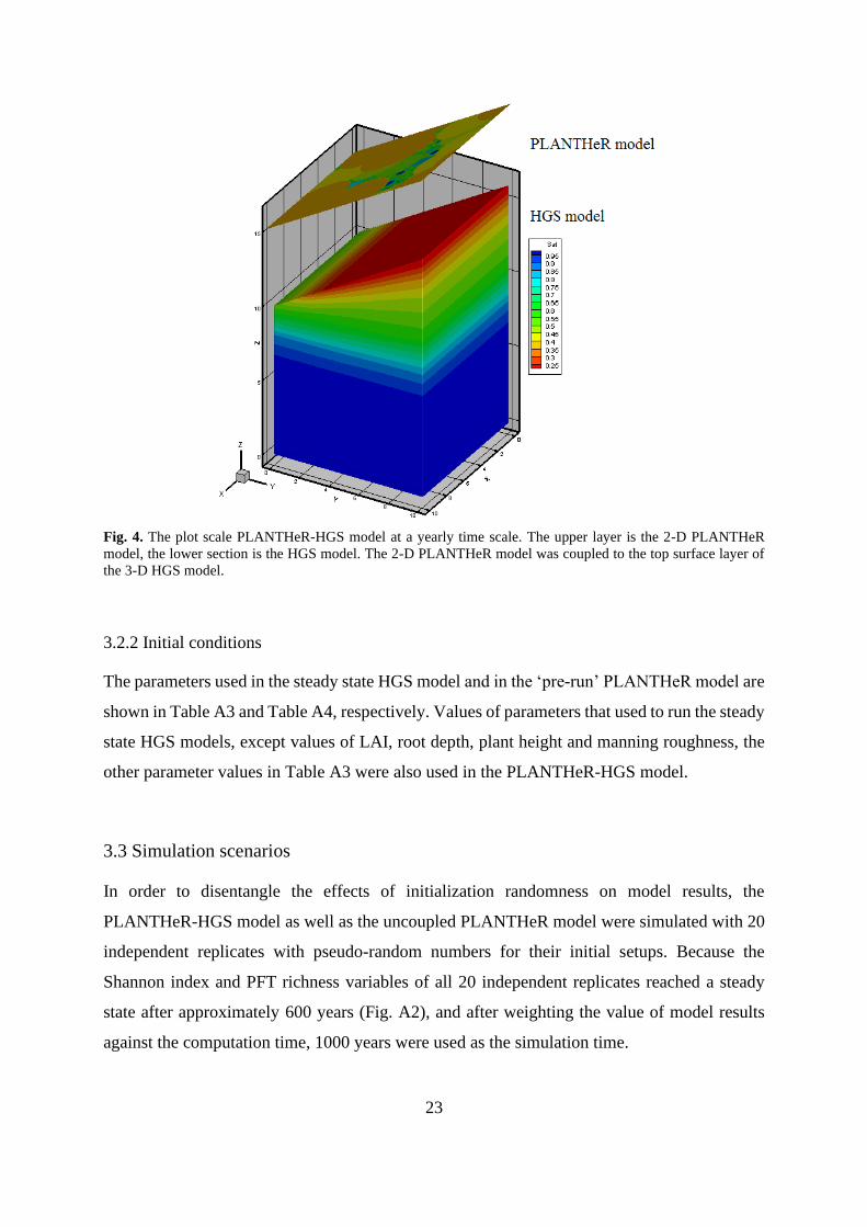
23
Fig. 4. The plot scale PLANTHeR-HGS model at a yearly time scale. The upper layer is the 2-D PLANTHeR
model, the lower section is the HGS model. The 2-D PLANTHeR model was coupled to the top surface layer of
the 3-D HGS model.
3.2.2 Initial conditions
The parameters used in the steady state HGS model and in the ‘pre-run’ PLANTHeR model are
shown in Table A3 and Table A4, respectively. Values of parameters that used to run the steady
state HGS models, except values of LAI, root depth, plant height and manning roughness, the
other parameter values in Table A3 were also used in the PLANTHeR-HGS model.
3.3 Simulation scenarios
In order to disentangle the effects of initialization randomness on model results, the
PLANTHeR-HGS model as well as the uncoupled PLANTHeR model were simulated with 20
independent replicates with pseudo-random numbers for their initial setups. Because the
Shannon index and PFT richness variables of all 20 independent replicates reached a steady
state after approximately 600 years (Fig. A2), and after weighting the value of model results
against the computation time, 1000 years were used as the simulation time.

24
3.3.1 The PLANTHeR-HGS model and the uncoupled HGS model simulations
The impact on the hydrological processes between the PLANTHeR-HGS model and the
uncoupled HGS model was compared. Due to the annual feedback between the HGS model and
the PLANTHeR model, the plant’s structural properties (LAI, root depth and plant height) as
well as the plant distribution simulated in the PLANTHeR-HGS model were different each
year, while in the uncoupled HGS model, each cell was characterized by constant values of
LAI, root depth and plant height for all the simulation years.
3.3.2 The PLANTHeR-HGS model and the uncoupled PLANTHeR model simulations
Likewise, the impact on the plant community richness and diversity was compared between the
PLANTHeR-HGS model and the uncoupled PLANTHeR model. In order to analyze the impact
of spatiotemporal heterogeneity on the PFT richness and diversity, three different types of
heterogeneity were compared. The first type of heterogeneity was the soil matric potential with
spatiotemporal heterogeneity (named as the spatiotemporal heterogeneous smp in the following
context), which was generated due to the dynamic feedbacks in the PLANTHeR-HGS model.
In the spatiotemporal heterogeneous smp, each cell was filled with a different soil matric
potential compared to its neighbor (Fig. 5a). The second type of heterogeneity was the soil
matric potential (smp) characterized by spatial heterogeneity, which did not change over time
(named as the spatial heterogeneous smp) (Fig. 5b). The third type was the homogeneous soil
matric potential with no spatial and no temporal heterogeneity (named as the homogeneous
smp) (Fig. 5c). Both, spatial heterogeneous smp and homogeneous smp have the same mean
value. The spatial heterogeneous smp and homogeneous smp were applied in the uncoupled
PLANTHeR model.
The soil matric potential heterogeneity was analyzed by the variogram method. The variogram
is a discrete function calculated using a measure of variability between pairs of points at various
distances (Deutsch and Journel, 1998). In this study, heterogeneity was quantified as the
Pearson correlation of a pair of points at various distances from distance of 1 grid cell up to 50
grid cells in both horizontal direction and vertical direction. Then, yearly heterogeneity was
calculated as the sum of correlation coefficients in horizontal and vertical directions. The soil
matric potential heterogeneity in three heterogeneity scenarios see Fig. A3.

25
Fig. 5. Soil matric potential with different heterogeneity. From a) to c) are soil matric potential with spatiotemporal
heterogeneity, soil matric potential with spatial heterogeneity, and soil matric potential with no heterogeneity,
respectively.
3.3.3 Statistical analysis
To test whether the PLANTHeR-HGS model simulated different transpiration, evaporation and
soil water saturation compared to the uncoupled HGS model, a two-tailed T-test was used. To
test the heterogeneity decreased mean Shannon index, PFT richness, biomass hypotheses, a
linear regression was used to explore the relationships between soil matric potential
heterogeneity and Shannon index, PFT richness, as well as the relationship between soil matric
potential temporal heterogeneity and plant aboveground biomass.
In addition, a one-way ANOVA test was used to examine the differences of mean Shannon
index, PFT richness, and mean biomass simulated among the three different types of soil matric
potential heterogeneity (P values only showed in the context but not in Figures). The statistical
analyses were performed in R (3.5.2).
3.4 Results
3.4.1 Simulation of hydrologic fluxes using the uncoupled HGS model vs. the PLANTHeR-
HGS model
3.4.1.1 Evaporation and transpiration
When compared with the uncoupled HGS model, the PLANTHeR-HGS model led to
differences regarding the annual and the long-term time scale evaporation and transpiration.
The PLANTHeR-HGS model resulted in overall lower mean transpiration but higher mean

26
evaporation (Fig. 6), when compared with the uncoupled HGS model simulations.
Transpiration and evaporation simulated with the uncoupled HGS model stayed unchanged
over the entire simulation period, while transpiration and evaporation simulated with the
PLANTHeR-HGS model changed annually.
In order to have a closer look at the influence of dynamic feedback between the HGS model
and the PLANTHeR model on evaporation and transpiration, the spatial distribution of
evaporation and transpiration was examined (Fig. 7). The dynamic feedbacks in the
PLANTHeR-HGS model created unique spatial distribution patterns of evaporation and
transpiration in different years, while the uncoupled HGS model did not create any spatial
pattern (Fig. 7).
A clear effect of plant distribution on the spatial distributions of evaporation and transpiration
was found in the simulations with the PLANTHeR-HGS model (Fig. 7 and Fig. 9). Furthermore,
a high LAI occurred when plant density was high (Fig. 8 and Fig. 9), and high transpiration but
low evaporate rates occurred in the next year where LAI was high (Fig. 7). These relationships
could not be observed for the simulations with the uncoupled HGS model (Fig. 7- Fig. 9).
Fig. 6. Comparison of evaporation and transpiration between the PLANTHeR-HGS model (mean ± 95%CI, mean±
standard deviation) and the uncoupled HGS model with 20 replicates. CI=confidence intervals. CI indicated by

27
light blue color for both evaporation and transpiration, standard deviation indicated by light red shadow for
transpiration and by light grey color for evaporation. Mean values simulated with the PLANTHeR-HGS model of
20 independent replicates indicated by the solid red (transpiration) and solid black (evaporation) lines. Values
simulated with the uncoupled HGS model indicated by the dashed lines for both evaporation and transpiration.
The P value here indicates a two tailed T-test P value. p<0.05*, p<0.01**, p<0.001***
Fig. 7. Distribution of evaporation and transpiration at the top surface at year 2 and year 1000 simulated with the
PLANTHeR-HGS model. Numbers on x- and y-axes are the cell number.
Fig. 8. Distribution of LAI at different years simulated with the PLANTHeR-HGS model and the uncoupled HGS
model of one simulation. Numbers on x- and y-axes are cell numbers.

28
Fig. 9. Plant distribution simulated with the PLANTHeR-HGS model and the uncoupled HGS model. Numbers
on x- and y-axes are cell numbers.
3.4.1.2 Soil water saturation
Even though the PLANTHeR-HGS model and the uncoupled HGS model started with the same
initial soil water saturation, the PLANTHeR-HGS model created a unique spatial pattern of soil
water saturation in both horizontal and vertical dimensions of the surface domain (Fig. 10). Soil
water saturation simulated with the PLANTHeR-HGS model developed towards a more
homogeneous pattern within the ZOI areas of large adult plants (Fig. 10). Meanwhile, areas
occupied by young plants with high density showed to decrease soil water saturation and created
unevenly distributed soil moisture patterns (Fig. 10).
However, for the uncoupled HGS model, the most obvious change was that soil water saturation
decreased at year 1000 (Fig. 11). The soil water saturation gradient between the high and the
low slopes of the PLANTHeR-HGS model and the uncoupled HGS model were both intensified
at year 1000 compared with the gradient at the initial year (Fig. 11).

29
Fig. 10. Spatial distribution of soil water saturation within the root zone simulated with the PLANTHeR-HGS model and the
uncoupled HGS model at the initial year, year 2 and year 1000. Numbers on x- and y-axes are cell numbers.
Fig. 11. Mean soil water saturation along the model y-axis (from downslope to upslope, elevation from 10m to
16m) simulated with the PLANTHeR-HGS model (mean ± 95% CI, mean± standard deviation) of 20 independent
replicates (S1-S20) and the uncoupled HGS model at the initial year, year 2 and year 1000. CI=confidence
intervals. CI indicated by light blue shadow; standard deviation indicated by light red shadow. The P value here
indicates a two tailed T-test P value. ns: not significant. p<0.05*, p<0.01**, p<0.001***

30
3.4.2 Response of plant community attributes to model coupling
3.4.2.1 Community diversity
Three different heterogeneities of soil matric potential led to significant differences of mean
Shannon index and PFT richness (ANOVA test, P<0.0001 not shown) (Fig. 12). Among the
three heterogeneity types, the spatiotemporal heterogeneity soil matric potential resulted in the
lowest mean Shannon index and mean PFT richness over the simulation years (Fig. 12a), while
the homogeneous soil matric potential resulted in the highest mean Shannon index and mean
PFT richness (Fig. 12b). Meanwhile, no negative relationships were found between
heterogeneity and mean Shannon index (P=0.09), mean PFT richness (P=0.05) (Fig. 12).
Fig. 12. Comparison of Shannon Index (a) and PFT richness (b) (mean ± 95%CI) simulated among the
spatiotemporal heterogeneous smp scenario (named as spatiotemporal in legend, the red color), the spatial
heterogeneous smp scenario (named as spatial in legend, the grey color), and the homogeneous smp scenario
(named as homogeneous in legend, the blue color), of 20 independent replicates. P values here indicate the
significance level of regression analysis. p<0.05*, p<0.01**, p<0.001***
3.4.2.2 Plant aboveground biomass
Like the mean Shannon index and PFT richness, significant differences of mean annual
aboveground biomass among three different soil matric potential heterogeneities were found
(ANOVA test, P<0.01 not shown) (Fig. 13). Among the three heterogeneity types, the
spatiotemporal heterogeneous soil matric potential led to the lowest mean total aboveground

31
biomass, while the homogeneous soil matric potential resulted in the highest mean total
aboveground biomass (Fig. 13). Besides, a significant negative relationship between temporal
variability and mean aboveground biomass was found (P=0.006) (Fig. 13).
Fig. 13. Comparison of mean annual total aboveground biomass (mean ± 95% CI) of 20 independent replicates
simulated among the spatiotemporal heterogeneous smp scenario (named as spatiotemporal in legend, the red
color), the spatial heterogeneous smp scenario (named as spatial in legend, the grey color), and the homogeneous
smp scenario (named as homogeneous in legend, the blue color). The variability means the temporal variation of
soil matric potentials. P values here indicate the significance level of regression analysis. p<0.05*, p<0.01**,
p<0.001***
3.4.2.3 Plant distribution
A clear response of plant distribution to soil matric potential spatial variation was found in the
spatiotemporal heterogeneous soil matric potential scenarios (Fig. 14a), however, this response
were not found in the spatial heterogeneous and homogeneous soil matric potential scenarios
(Fig. 14b and Fig. 14c).

32
Fig. 14. Plant distribution simulated with the spatiotemporal heterogeneous smp scenarios, and spatial
heterogeneous smp scenarios, as well as the homogeneous smp scenarios. The SMP distribution means the soil
matric potential distribution. Numbers on x- and y-axes are cell numbers.

33
3.5 Discussion
The differences of transpiration and evaporation as well as plant distribution and dynamics
simulated between the PLANTHeR-HGS model and uncoupled HGS models were statistically
significant.
Increased heterogeneity did not decrease mean Shannon index and mean PFT richness, but
decreased mean aboveground biomass.
3.5.1 Influence of model coupling on hydrological processes
3.5.1.1 Evaporation and transpiration simulated with the PLANTHeR-HGS model and the
uncoupled HGS model
The ratio of transpiration to actual evapotranspiration simulated with the PLANTHeR-HGS
model found in this study is consistent with the modelled value of 70 ± 9% for the T to ET ratio
from Fatichi and Pappas (2017). Also, the mean LAI simulated with the PLANTHeR-HGS
model is in line with the observation values found in a similar dry climate from previous studies
(e.g. Asner et al., 2003; Sprintsin et al., 2011). Besides, the PLANTHeR-HGS model fits the
assumption of the Budyko’s curve, which showed that in arid conditions, the long-term average
evapotranspiration converges towards precipitation when the hydrological conditions are in
steady state (no significant inputs of groundwater, losses or storage changes) (Freund and
Kirchner, 2017). This implies that the actual evapotranspiration in dry areas is limited by the
total amount of water available (Freund and Kirchner, 2017). With this, the results of this study,
where the total amount of actual evapotranspiration is balanced by precipitation in both the
PLANTHeR-HGS model and the uncoupled HGS model simulations support Budyko’s
assumption (Budyko, 1958;1974) that evapotranspiration is limited by the amount of available
water in dry conditions.
Without considering plant growth and its influence on evapotranspiration processes in the
uncoupled HGS model, the constant spatial distribution of plants with its constant LAI and root
depth led to constant evaporation and transpiration in the HGS model simulations. On the
contrary, due to the dynamic features of plant growth and its interaction with evapotranspiration
processes was simulated in the PLANTHeR-HGS model, mean annual transpiration and
evaporation amount as well as their spatial distribution varied significantly. This reveals the
importance of including vegetation dynamics into hydrological models, especially for the

34
studies that quantify transpiration and evaporation processes separately. Wegehenkel (2009)
and Tang et al. (2012) shared a similar conclusion that representing dynamic vegetation in
hydrological models can simulate different magnitudes of transpiration and evaporation,
compared to those hydrological models with static plant properties that are independent from
environmental conditions. The results in the present study also indicated that annual vegetation
dynamics influenced the annual and long-term transpiration and evaporation, which agrees with
previous modelling studies in semi-arid climates (Tesemma et al., 2015; Jiao et al., 2017),
suggesting that annual and long-term evaporation and transpiration were sensitive to yearly
vegetation dynamics in water-limited environments.
Grasses have long been hypothesized to be superior competitors in taking advantage of soil
water during small rainfall event periods in dryland areas, owing to their distributed dense roots
at the top of the soil surface providing them with good access to soil water as it enters the soil
(Walter, 1971; Sankaran et al., 2004; Donzelli et al., 2013). In this study, it was found that large
plants in the PLANTHeR-HGS model transpired less water than the small plants with high
density per square meter, because large plants were estimated to have deeper roots than small
plants. But for smaller plants a higher leaf area per square meter was demonstrated, and this
higher leaf area led to higher transpiration per square meter. These results agree with previous
observation and modelling studies suggesting that per unit area, grasses transpire more water
than trees in a water-limited environment, but individually, trees transpire more water than
grasses at an annual scale (Grady et al., 1998; Mazzacavallo and Kulmatiski, 2015). Also,
results of the present work indicate that dense and shallow roots system can take up water more
efficiently than deep-rooted system (Tron et al. 2015).
3.5.1.2 Influence of model coupling on soil water dynamics
In the PLANTHeR-HGS model simulations, for those areas occupied by plants with high
density, but with shallow root depth, most water was transpired, leaving less water stored in the
root zone. For the areas being occupied by large adult plants with low plant density but deeper
root depth, less amount of water was being transpired, and more water was stored within the
root zone. This result of increased leaf area and towards more deeply rooted vegetation
increasing annual transpiration and soil water storage in the PLANTHeR-HGS model was also
found in previous modelling studies on Mediterranean tree-grass ecosystems (Joffre and
Rambal, 1993), and was also observed in savanna ecosystems (Baldocchi et al., 2004). The

35
areas with extremely low water availability led to bare areas, which were then occupied by other
plants (Cornet et al., 1988; Dunkerley, 1997), and these plants started to grow when the soil
water condition become favorable, thus showing that plants are distributed spatially according
to soil water availability (Rodriguez-Iturbe et al., 1999b; Riis et al., 2001; van de Koppel et al.,
2002) in the PLANTHeR-HGS model. However, the uncoupled HGS model was not able to
simulate the ‘two-way’ active interactions between plant distribution and soil water saturation
variation, but only a ‘one-way’ impact of constant plant distribution and their properties on soil
water saturation was considered.
The dynamic interplay between plant structure properties (LAI and root depth) and hydrological
components (transpiration, evaporation and soil water content) suggested that the ‘realistic
vegetation’ simulated with the PLANTHeR-HGS model played an active role in influencing
the water balance, while at the same time being influenced by the dry climate conditions and
the resulting water stress. This result illustrates that the coupled PLANTHeR-HGS model was
able to reproduce the special role plants play in ecosystem dynamics (Rodriguez-Iturbe et al,
2001).
In general, the hydrological processes simulated with the PLANTHeR-HGS model was more
meaningful compared to the uncoupled HGS model.
3.5.2 Response of plant community attributes to model coupling
3.5.2.1 Plant community attributes with model coupling
The dynamic feedbacks between the PLANTHeR model and the HGS model created a more
stressful environment for plant communities than the uncoupled PLANTHeR model, thus
lowering the mean Shannon index, mean PFT richness and mean aboveground biomass
compared to those simulations with the uncoupled PLANTHeR model. The results agree with
previous modelling studies that diversity and richness decreases in areas with high
environmental severity (Yang et al., 2015), and increased plant water stress in response to
increased soil water resource variation led to a reduction in the primary productivity in water-
limited environments (Fay et al., 2003). The high spatiotemporal variation of soil water
resources simulated in the PLANTHeR model created a higher environment severity than the
environment in the uncoupled PLANTHeR model, due to no temporal and spatial soil water
variation simulated in the uncoupled PLANTHeR model. In addition, three different soil matric

36
potential heterogeneity scenarios all led to only one type of PFT succeeding after the plant
community reached the steady state, which were perennial PFTs with a high adult growth rate,
strong seedling competitive ability, short seed dispersal distance, short-term seed dormancy,
and high drought stress tolerance. This type of PFT efficiently and rapidly occupied all the
space by its high adult growth rate and by producing a large number of vigorously growing
offspring in its vicinity, and by short-term seed dormancy, and thus high seed germination rate.
This type of plant is similar to an invasive “master-of-all-traits” plant type described by Pyšek
et al. (2007). This invasive species is characterized by extremely high fecundity, raid growth
rate, an extended germination period through a short-term persistent seed bank, and high
germination rate (Pyšek et al., 2007).
Clear differences of plant distribution patterns in the PLANTHeR-HGS model and in the
uncoupled PLANTHeR model showed that, without considering the feedback impact between
vegetation status and water status in the uncoupled PLANTHeR model, plants distributed in the
system in a random way. This is not consistent with the hydrological niche segregation
hypothesis (Silvertown et al., 2015). Also, no spatial changes of soil matric potential in the
spatial heterogeneous and homogeneous soil matric potential simulations were observed despite
clear changes of plant species distribution patterns. This do not follow the general finding that
competition for resources among plants would generate stress for plants and is an importance
processes determining the distribution of species (Craine and Dybzinki, 2013).
Thus, the PLANTHeR-HGS model simulated more ‘close-to-reality’ plant distribution and
dynamics comparable to the uncoupled PLANTHeR model.
3.5.2.2 Relationship between heterogeneity and plant community attributes
The relationships between the heterogeneity and richness, and heterogeneity and diversity did
not agree with previous experimental studies (Gazol et al., 2013; Tamme et al., 2010), where
an increased small-scale resource heterogeneity decreased with plant community diversity. This
is probably due to the heterogeneity in the present study including the effect of temporal
heterogeneity, while other studies often simply included spatial heterogeneity only. Stein et al.
(2014) pointed out that temporal and spatial heterogeneities have fundamental differences. The
temporal heterogeneity can be the result of interannual and seasonal variations of soil water
availability and long-term climate fluctuations (Stein et al., 2014). The relationship between
temporal heterogeneity and species richness is often assumed to be negative (Stein et al., 2014).

37
Indeed, considering the temporal heterogeneity in the PLANTHeR-HGS model decreased the
mean Shannon index and mean PFT richness values compared to those simulations with
homogeneous or spatial soil matric potential heterogeneity.
The finding of increased soil matric potential temporal heterogeneity decreased mean
aboveground biomass is consistent with previous field experiment studies on herbaceous plants
in semi-arid climates (Heisler-White et al., 2008; Novoplansky and Goldberg, 2001). This was
probably due to the homogeneous soil matric potential having allowed plants to take up water
more steadily than the heterogeneous environment, thus increasing root water uptake efficiency
through promoting plant root systems and thereby allowing continuous plant growth
(Novoplansky and Goldberg, 2001; Hagiwara et al., 2012).
3.6 Conclusion
By comparing the PLANTHeR-HGS model and the uncoupled HGS model and the uncoupled
PLANTHeR model, examples were presented stressing the importance of including year-to-
year dynamic feedbacks between the hydrological and the plant models for quantifying
evapotranspiration and plant community dynamics.
On the one hand, not considering the dynamic plant properties in hydrological models,
including temporal dynamics of LAI and root depth, may lead to the estimation of an
unrealistically hydrological state (too dry or too wet). This is especially true when the study is
focusing on using the hydrological model to simulate transpiration and evaporation processes.
Besides, the realistic vegetation pattern simulated the feedbacks between vegetation dynamics
and soil water status in the PLANTHeR-HGS model homogenized soil water content within its
root zone, while only considering static vegetation failed to simulate this part realistically. On
the other hand, increased small-scale spatial soil-resource heterogeneity did not have a
significant negative impact on the plant community diversity or richness. But increased
heterogeneity in soil water resources decreased mean aboveground biomass. Only using the
uncoupled PLANTHeR model would not be able to simulate the ‘actual’ stressed environment,
because when ignoring the spatially distributed soil water dynamics in the plant model, plants
would tend to distribute randomly in the model rather than distribute according to soil water
availability. This is unrealistic from an ecological point of view, e.g., no hydrological niche
segregation, or competition for water would generate regular water resources patterns.

38
The results of the present thesis suggest that the PLANTHeR-HGS model was able to give a
more explicit representation of the complex relationship between vegetation and hydrological
processes than the uncoupled HGS model or the PLANTHeR model alone. Thus, when
modelling the interactions between hydrological processes and plant communities it should be
considered to include the impact of the year-to-year dynamic feedbacks between hydrological
processes and the plant life cycle.

39
4. Comparison of the Coupled Hydrological and Ecological Model for
the Assessment of Plant-Water Interactions between Wet and Dry
Climates
4.1 Introduction
Precipitation is a crucial environmental factor in determining ecosystem productivity (Reich et
al, 2014) because of the direct and indirect influence of moisture availability on growth and
biomass (Epstein et al., 2002; Vogel et al., 2008), seed germination (Rivas-Arancibia et al.,
2006; Quevedo-Robledo et al., 2010), and seedling growth and survival (Padilla and Pugnaire,
2007), thereby altering the productivity (Miranda et al., 2009a) and species richness (Brown,
2003) across different biomes. Overall, since water is probably the most important resource
driving plant metabolism, it is not surprising that a myriad of studies exist that have shown the
great impact of precipitation on plant productivity (e.g. Knapp and Smith, 2001; Huxman et al.,
2004a; Swemmer et al., 2007). However, studies of precipitation effects on productivity ranging
from desert to Mediterranean ecosystems have reported mixed results. Some studies (Lauenroth
and Sala, 1992; Miranda et al., 2009b) suggested a positive relationship between productivity
and precipitation in arid/semi-arid areas. For example, the total aboveground biomass of a
Tibetan alpine meadow was found to increase with increasing annual precipitation (Zhang et
al., 2013). A global scale study (Huxman et al., 2004a) suggested increased mean annual
precipitation increase productivity for the mean annual precipitation varying between 0 mm to
3000 mm. However, Xia et al. (2010) found the summer aboveground net primary production
of annuals were poorly correlated with summer precipitation in a Chihuahuan Desert grassland.
Sankaran et al. (2005) reported an asymptotic relationship between the woody cover and the
mean annual precipitation in African savannas. Another experiment from a California annual
grassland ecosystem even found that the annual aboveground biomass decreased with high total
rainfall (Salve et al., 2011).
Besides the inconsistency in the precipitation amount effect among different ecosystems, due
to variations in canopy structure, rooting depth and the ability of species to tolerate water stress
among different ecosystems (Porporato et al., 2001), impacts of changes in the rainfall
variability on plant productivity are also likely to differ, such as between water-limited and
water-abundant ecosystems (Ross et al., 2012). Some studies in mesic ecosystems have shown
that increased plant water stress in response to increased precipitation variability can lead to a

40
reduction in the primary productivity in grasslands (Fay et al., 2003; Heisler-White et al., 2009;
Knapp et al., 2002). On the contrary, studies in arid ecosystems suggest that productivity may
increase due to reduced soil moisture stress caused by increased precipitation variability, as the
‘amplification of soil water dynamics’ during the large rainfall events would allow high
infiltration into deeper soil, thus maintaining the soil moisture above drought stress thresholds
for longer periods (Knapp et al., 2008). Indeed, Thomey et al. (2011) reported a decreased soil
moisture deficit with a concomitated increase in aboveground net primary productivity (ANPP)
in an arid grassland with increasing precipitation variability. Therefore, despite the obvious and
apparently trivial importance of water for plant growth, it seems still far away from a general
understanding of water-productivity relationships in different ecosystems.
The temporal variation in precipitation has a strong impact not only on plant productivity, but
also on plant community structure, species richness and diversity (Yan et al., 2015).This is
especially true for water-limited environments, such as arid, semi-arid, deserts, grasslands and
savanna areas, where the ecosystems are often sensitive and prone to change because of water
limitations (Robinson et al., 2013; Schöb et al., 2013). Understanding the impact of seasonal
variations in resources availability on plant community structures and dynamic, including plant
growth, their interaction, and survival mechanisms across different ecosystems, is one of the
main goals in ecological studies (Resco et al., 2008). Studies from Ayanlade (2009), Bagayoko
et al (2006), Vezzoli et al. (2008) demonstrate that, the seasonality in the rainfall regime is a
strong driver of ecosystem structure and function changes in dryland areas. For example,
species richness of summer annuals was found to be positively correlated with summer
precipitation in desert Chihuahuan grasslands (Xia et al., 2010). Likewise, species richness
increased with increasing average available water content in the western Negev Desert during
the growing seasons (Kidron, 2014). Increased rainfall interannual variation has been shown to
increase plant diversity in water-limited environments (e.g. Gherardi and Sala, 2015). For
water-abundant ecosystems, many studies showed that the interannual fluctuations in rainfall
strongly drives temporal stem growth variation (Schippers et al., 2015) and the tree annual
growth in rainforests (Brienen and Zuidema, 2005; Dunisch et al., 2003; Worbes, 1999).
Species richness has been shown to be positively correlated to the mean annual rainfall across
a hydroclimate gradient with rainfall varying from 500mm to 2000mm (Harrison et al., 2020).
As for diversity, studies have reported positive relationships between species diversity and

41
biomass in a rainforest (Day et al., 2013), and between diversity and soil water content in a
mesic grassland (Knapp et al., 2002).
Furthermore, the leaf area index (LAI), as having a center role connecting hydrology, ecology
and climatology, is reported to vary strongly to the dynamics of soil water availability in
response to rainfall variation in drylands (Davoodi et al., 2017; Kahiu and Hanan, 2018; Musau
et al., 2016). The leaf area index is often characterized by high seasonality in water-limited
ecosystems. Studies show that the seasonal coefficient of variation (CV) of LAI can range from
30% (Tian et al., 2004) to 70% for savanna plants (Kahiu and Hanan, 2018) and to 80% for
fine-leafed savanna and shrubland (Mayr and Samimi, 2015; Scholes et al., 2004). The
interannual CV of LAI is around 70% for deserts biomes (Asner et al., 2003; Kahiu and Hanan,
2018). In contrast to water-limited ecosystems, in water-abundant ecosystems, e.g. biomes with
sufficient annual precipitation (>1500 mm), the LAI does not always increase with a further
increase in annual precipitation (Li et al., 2017; Musau et al., 2016), because it can also be
limited by other factors (Gower, 2003; Körner, 2015). For example, soil fertility affects the LAI
in combination with air temperature and precipitation levels (Battaglia et al., 1998; Reich et al.,
1997; Waring et al., 1978). The leaf area index in water-abundant ecosystems is often
characterized by a low seasonality. For example, the seasonal CV of tropical rainforest LAI
ranges from 3% to 6% (De Wasseige et al., 2003; Malhado et al., 2009). At the same time, there
are studies showing that the interannual CV of evergreen forest LAI can range from 11%
(Sumida et al., 2018) to 35% (Asner et al., 2003; Scurlock et al., 2001).
Overall, these different findings for wet compared to dry ecosystems suggest that from a
hydrological modelling perspective, plants should not be simulated as a “constant green plant
layer” in hydrological models in drylands because of the high LAI and root depth variation as
well as its associated spatially distributed soil water dynamics. Vice-versa, in humid climates,
due to the low LAI variation in response to the low rainfall variability, such a “constant green
layer-approach” could be useful in hydrological models because variation in plant dynamics is
small and thus a more complex integration into hydrological models would only inflate their
complexity. Several previous studies have developed certain dynamic ecohydrological models,
for example Ivanov (2002) developed a vegetation-water-energy dynamics model, and Tietjen
et al. (2009a) developed a coupled water-vegetation model to explore the effects of climate
change on soil moisture and vegetation cover. Both of these coupled water-vegetation models
have been designed and applied specifically for drylands (e.g. Ivanov et al., 2008a, 2008b;

42
Tietjen et al., 2009b; Guo et al., 2016). Thus, there are still no studies testing the sensitivity of
coupled vs. uncoupled models across ecosystems with largely different hydrological conditions.
Hence, it is hypothesized that comparing wet and dry ecosystems, coupling plant and
hydrological models should have large effects for simulating hydrology and vegetation
dynamics in dry ecosystems, whereas in wet ecosystems, the coupling would not make much
difference. For this assessment, the coupled PLANTHeR-HGS model is used and its outcome
is compared to the uncoupled HGS model for testing this hypothesis.
For this, vegetation dynamics and hydrological processes are compared along a hydroclimatic
gradient (from arid climate to humid climates) at a long-term timescale (1000 years). Three
different climate scenarios, the semi-arid climate, the dry sub-humid climate, and the humid
climate, are simulated in this study. It is aimed specifically at investigating the following
research questions: 1) For which hydrological variables, or plant community attributes the using
of the PLANTHeR-HGS model is favorable for its estimation compared to the uncoupled
models? 2) Under which climate, coupled models instead of uncoupled ones should be used to
simulate the plant community dynamics and hydrological processes? The hypothesis to be
tested in this context is, as stated above, that using a coupled model matters the most for dry
climatic conditions.
4.2. Coupling the PLANTHeR model to the HGS model at seasonal time scales
Plant growth phases in the PLANTHeR model are divided into four main growth phases,
namely, seed germination, adult plant growth, seed production and dispersal, as well as adult
plant mortality (Fig. 15). Each plant growth phase is affected by the soil matric potential given
in the modelled system; therefore, these four plant growth phases are used as the seasonal
coupling time steps. For this, each phase responded to one season. Coupling the PLANTHeR-
HGS model at seasonal time scales offered the opportunity to analyze the impact of inter-
seasonal rainfall changes on the plant community structure and composition. The daily
precipitation is generated based on the Poisson distribution (based on Rodriguez-Iturbe et al.,
1999a), and the monthly potential evapotranspiration (PET) is generated using the
Thornthwaite method with an effective temperature. Both, daily precipitation and monthly PET
are generated with the programming tool MATLAB.

43
Fig. 15. Coupling the PLANTHeR-HGS model at seasonal time scales
4.2.1 Climate scenarios and climate forcing parameters
The current study includes three different type of climates, namely the semi-arid climate, the
sub-humid climate, and the humid climate. The precipitation in each climate is defined based
on the rainfall amount, the rainfall intensity and frequency found in the literature as described
below. The MATLAB codes that were used to generate the precipitation and PET data for each

44
climate scenario are listed in the Appendix, Section 2, and the Poisson parameters are listed in
Appendix, Table A5.
4.2.1.1 Precipitation
According to UNEP (1992,1997), UNCCD (1994) and Le Houérou (1996), the semi-arid zones
are defined with an Aridity Index (AI=P/PET) of 0.2 <=AI <0.5, the dry sub-humid climate
with 0.5 <= AI <0.65 and the humid climate with AI >= 0.75. The semi-arid and the dry sub-
humid climates are characterized with raining and non-raining seasons (Vezzoli et al., 2008;
Shimola and Krishnaveni, 2014), where the growing season corresponds to the raining season
(Rishmawi et al., 2016). The humid climate is characterized by low variation in inter-annual
precipitation and temperature (Kumagai et al., 2004; Malhi and Wright, 2004). According to
the previous studies, in semi-arid climates, 80-90% of the total rainfall amount falls in the
raining season (Laio et al., 2001a; Porporato et al., 2002) and in the sub-humid climate around
70% of rain falls in the raining season (Fernandez-Illescas and Rodriguez-Iturbe, 2003).
Rainfall in arid regions can be modelled by a marked Poisson distribution because of it often
occurs as high intensity convective storms with short duration (Laio et al., 2001b).
The interannual coefficient of variation (CV) of rainfall in the semi-arid climate has been found
to be between 30% to 50% with the mean annual precipitation between 300 mm to 400mm
(Dasci and Merchan, 2010; Tielbörger et al., 2014). The dry sub-humid climate has been found
to be characterized by an interannual CV between 30% to 40% and with the mean annual
precipitation between 500 mm to 700 mm (Jemai et al., 2013; Smerdon et al., 2008; Tielbörger
et al., 2014). The humid climate is found to be characterized by an interannual rainfall CV of
14% with the mean annual precipitation over 2000mm (Kumagai et al., 2005; Sun et al., 2019).
A study shows that when the coefficient of variation (CV) (%) is greater than 30% in rainfall
data series, it indicates massive variability in rainfall amounts and distributional patterns (Araya
and Stroosnijder, 2011). Therefore, for the present work, the interannual variation in the semi-
arid climate is defined to be around 50%, in the sub-humid climate to be around 30%, and in
the humid climate to be around 10%. The mean annual precipitation (MAP) in the semi-arid
climate (AI=0.34), the dry sub-humid climate (AI=0.55) and the humid climate (AI=1.32) were
defined for the present study as 358 mm/year, 625 mm/year and 2100 mm/year, respectively.

45
4.2.1.2 Potential evapotranspiration (PET)
The most common method to calculate potential evapotranspiration is the Penman-Monteith
equation (Allen et al., 1998), which is suitable for different climates (Fooladmand and
Haghighat, 2007). However, this method requires many input variables, such as minimum and
maximum relative humidity, minimum and maximum air temperature, sunshine hours, and
wind speed. In areas with remote access, such as developing regions, it is difficult to acquire
all these parameters, thus limiting its applicability (Ahmadi and Fooladmand, 2008; Pereira and
Pruitt, 2004). A simpler alternative is the Thornthwaite method (Wilm, 1944; Thornthwaite,
1948), which requires only temperature as the input data.
Previous studies (Ahmadi and Fooladmand, 2008; Chen et al., 2005; Maeda et al., 2011)
showed that the Thornthwaite method underestimates PET under arid conditions (Hashemi and
Habibian, 1979) and overestimates PET in the equatorial humid climate of the Amazon region
(Camargo et al., 1999). Camargo et al. (1999) proposed using an effective temperature instead
of monthly average temperature in the Thornthwaite method. Using this modified Thornthwaite
method has been shown to be able to produce reliable PET estimates (Ahmadi and Fooladmand,
2008; Camargo et al. 1999; Pereira and Pruitt, 2004) and even can be a better option to estimate
PET compared to the Penman-Monteith method (Sentelhas et al., 2010), when only temperature
data are available. The Thornthwaite method also shown to be able to produce satisfying results
for the long-term period potential evapotranspiration (Grace and Quick, 1988). Therefore, the
modified Thornthwaite method is used to simulate the long-term (1000 years) PET.
The Thornthwaite model (Thornthwaite, 1948) is based on an empirical relationship between
PET and mean air temperature T. For mean temperatures above 26.5º, Willmott et al. (1985)
proposed another equation to calculate the PET (Pereira and Pruitt, 2004; Sentelhas et al., 2010).
The value of 𝑃𝐸𝑇𝑚 (monthly PET) for a standard month of 30 days, as a function of the monthly
average temperature 𝑇𝑚𝑒𝑎𝑛 is given by the following equations:
𝑃𝐸𝑇𝑚 = 16 × (10𝑇𝑚𝑒𝑎𝑛𝐼
)𝑎
0° ≤ 𝑇𝑚𝑒𝑎𝑛 ≤ 26.5° 𝐶 (16)
𝑃𝐸𝑇𝑚 = −415.85 + 32.24𝑇𝑚𝑒𝑎𝑛 − 0.43𝑇𝑚𝑒𝑎𝑛2 𝑇𝑚𝑒𝑎𝑛 > 26.5°𝐶 (17)
𝐼 = ∑(𝑇𝑚𝑒𝑎𝑛𝑖
5)1.514
12
𝑖=1
(18)

46
𝛼 = 67.5 × 10⁻⁸𝐼3 − 7.71 × 10⁻⁶𝐼2 + 0.01791𝐼 + 0.492 (19)
where I is the thermal index imposed by the local normal climatic temperature regime (Maeda
et al., 2011). 𝑃𝐸𝑇𝑚 is the standard 30-day evapotranspiration (mm 30 days-1), considering N=12
T.
Then the 𝑃𝐸𝑇𝑑 (daily) is calculated by using the following expression:
𝑃𝐸𝑇𝑑 = 𝑃𝐸𝑇𝑚
30⁄ × 𝑁 12⁄ (20)
where N is maximum number of sunshine hours for a given day.
Camargo et al. (1999) propose to use the effective temperature instead of monthly mean
temperature to estimate PET in arid and very humid conditions. For that, the average 𝑇𝑚𝑒𝑎𝑛 is
replaced by the effective temperature (𝑇𝑒𝑓𝑓 ) in the 𝑃𝐸𝑇𝑚 calculation, given by:
𝐴 = 𝑇𝑚𝑎𝑥 − 𝑇𝑚𝑖𝑛 (21)
𝑇𝑒𝑓𝑓 = 𝑘(𝑇𝑎𝑣𝑒 + 𝐴) =1
2𝑘(3𝑇𝑚𝑎𝑥 − 𝑇𝑚𝑖𝑛) (22)
where 𝑇𝑚𝑖𝑛and 𝑇𝑚𝑎𝑥 are the minimum and maximum monthly temperatures, respectively, and
k is the calibration coefficient. The value of k = 0.72 (Camargo et al., 1999) is seen as the
statistically best value for estimating 𝑃𝐸𝑇𝑚 (Pereira and Pruitt, 2004), while the value of k =
0.69 (Pereira and Pruitt, 2004) was also reported to give a reasonable performance. For this
study, the value of 0.72 was used.
With the effective temperature, the monthly 𝑃𝐸𝑇𝑚 is given by the following equations:
𝑃𝐸𝑇𝑚 = 16 × (10𝑇𝑒𝑓𝑓
𝐼)𝑎
0° ≤ 𝑇𝑒𝑓𝑓 ≤ 26.5° 𝐶 (23)
𝑃𝐸𝑇𝑚 = −415.85 + 32.24𝑇𝑒𝑓𝑓 − 0.43𝑇𝑒𝑓𝑓2 𝑇𝑒𝑓𝑓 > 26.5°𝐶 (24)
The monthly average temperature is used instead of the effective temperature for calculating
the thermal index (I) in Eq. (23) (Pereira and Pruitt, 2004). To estimate the PET in all three
climates in this study, the Eq. (23) was used when the mean monthly temperature was lower
than 26.5 °𝐶, and Eq. (24) was used when the mean monthly temperature was higher than
26.5 °𝐶.

47
The daily temperature for each climate was produced with MATLAB code (see Appendix
section 2.2) based on the maximum temperature and minimum temperature for each climate
according to the literature (Table. A6). The mean annual PET estimated in the semi-arid
climate, the dry sub-humid climate and humid climate were 1085 mm/year, 1127 mm/year and
1582 mm/year, respectively. The semi-arid climates were defined according to the savannas
climates in South Africa (Laio et al., 2001a; Rodriguez-Iturbe et al., 1999; Kaseke et al., 2016),
semi-arid climates in Israel (Tietjen et al., 2009a), and semi-arid climates in South Texas
(D’Odorico et al., 2000; Fernandez-Illescas and Rodriguez-Iturbe, 2003). The sub-humid
climate data are simulated according to the climates in the sub-humid regions in Asia, Africa
and in USA (Ayanlade, 2018; Fernandez-Illescas and Rodriguez-Iturbe., 2003; Geng et al.,
2014; Ogolo, 2011; Rishmawi et al., 2016). The humid climate datasets are estimated according
to the tropical rainforest climates in Asia, Africa and at the Amazon (Kumagai et al., 2004;
Malhi and Wright, 2004; Maeda et al. 2017) (Table. A3). The parameters like rainfall intensity
and frequency, minimum and maximum temperatures, that are used to generate climate data in
semi-arid, sub-humid and humid climates, are the mean values of those parameters that were
used to simulate drylands in Asia, Africa and America (Huang et al., 2016), and tropical
rainforest climates globally (Malhi and Wright, 2004). These semi-arid and dry sub-humid areas
are experiencing the highest climate transitions, e.g. from sub-humid/humid to semi-arid, and
semi-arid to arid areas, which make these regions fragile and sensitive to climate change (Huang
et al., 2016). Additionally, most of these areas have long systematic studies (e.g. Rodriguez-
Iturbe et al., 1999a), thus allowing for powerful and systematic analyses across sites, which
makes these regions important benchmarks in dryland studies.
4.2.2 The PLANTHeR-HGS model domain and initial conditions
4.2.2.1 The PLANTHeR-HGS model domain size
The PLANTHeR-HGS domain size in the current study is 10 m × 100 m in x-y direction
(Fig. 16) for all climate scenarios. It is assumed that the ground surface equals to zero meter,
and the vertical direction was designed to be 25 m at the downslope end side and 85 m on the
upslope end side with a surface slope of 37º. The PLANTHeR model landscape consisted of
200 × 2000 grid cells with a cell size of 5 cm × 5 cm and with no periodic boundaries. The cell
size in the HGS model was 1 m × 1 m with 10 × 100 cells in x-y direction. Water could leave
the domain by evapotranspiration and by surface flow at the downslope boundary of the surface
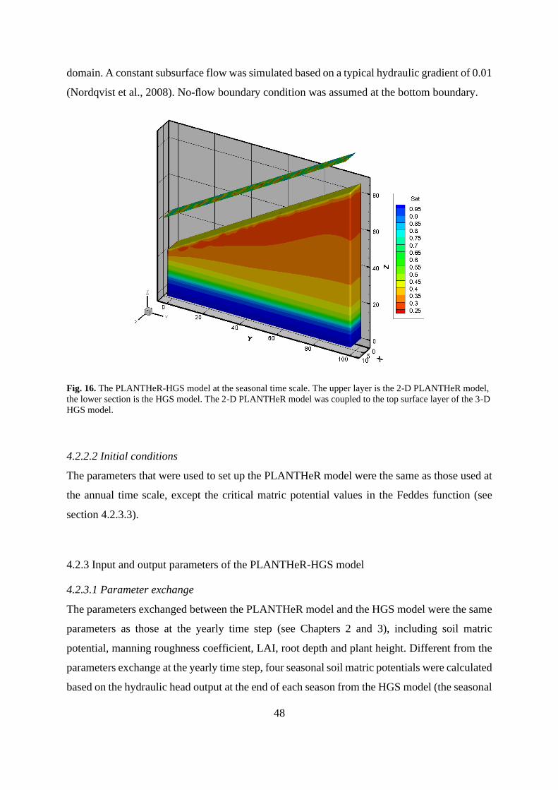
48
domain. A constant subsurface flow was simulated based on a typical hydraulic gradient of 0.01
(Nordqvist et al., 2008). No-flow boundary condition was assumed at the bottom boundary.
Fig. 16. The PLANTHeR-HGS model at the seasonal time scale. The upper layer is the 2-D PLANTHeR model,
the lower section is the HGS model. The 2-D PLANTHeR model was coupled to the top surface layer of the 3-D
HGS model.
4.2.2.2 Initial conditions
The parameters that were used to set up the PLANTHeR model were the same as those used at
the annual time scale, except the critical matric potential values in the Feddes function (see
section 4.2.3.3).
4.2.3 Input and output parameters of the PLANTHeR-HGS model
4.2.3.1 Parameter exchange
The parameters exchanged between the PLANTHeR model and the HGS model were the same
parameters as those at the yearly time step (see Chapters 2 and 3), including soil matric
potential, manning roughness coefficient, LAI, root depth and plant height. Different from the
parameters exchange at the yearly time step, four seasonal soil matric potentials were calculated
based on the hydraulic head output at the end of each season from the HGS model (the seasonal

49
length for each climate scenario; see Table. A7). These four soil matric potentials were given
to the PLANTHeR model as the seasonal soil matric potential inputs. Due to the cell size in the
HGS model being different from the PLANTHeR model, the parameters that exchanged
between the HGS model and the PLANTHeR model were transformed in the following way:
Parameters used in the HGS model were calculated based on the output parameters from the
PLANTHeR model ( 1 𝑐𝑒𝑙𝑙𝐻𝐺𝑆 = 1 𝑚 × 1 𝑚 , 1 𝑐𝑒𝑙𝑙𝑃𝐿𝐴𝑁𝑇𝐻𝑒𝑅 = 0.05 𝑚 × 0.05 𝑚 , thus
1 𝑐𝑒𝑙𝑙𝐻𝐺𝑆 = 20 × 20 𝑐𝑒𝑙𝑙𝑠𝑃𝐿𝐴𝑁𝑇𝐻𝑒𝑅):
𝐿𝐴𝐼𝐻𝐺𝑆 =1
400∑∑𝐿𝐴𝐼𝑃𝐿𝐴𝑁𝑇𝐻𝑒𝑅,𝑖𝑗
20
𝑗=1
20
𝑖=1
(25)
𝑅𝑜𝑜𝑡 𝑑𝑒𝑝𝑡ℎ𝐻𝐺𝑆 = 𝑚𝑎𝑥{𝑅𝑜𝑜𝑡 𝑑𝑒𝑝𝑡ℎ𝑃𝐿𝐴𝑁𝑇𝐻𝑒𝑅,𝑖𝑗|𝑖 = 1,… 20; 𝑗 = 1, …20} (26)
𝐻𝑒𝑖𝑔ℎ𝑡𝐻𝐺𝑆 = 𝑚𝑒𝑎𝑛{𝐻𝑒𝑖𝑔ℎ𝑡𝑃𝐿𝐴𝑁𝑇𝐻𝑒𝑅,𝑖𝑗|𝑖 = 1, …20; 𝑗 = 1,… 20} (27)
𝑃𝑙𝑎𝑛𝑡 𝐷𝑒𝑛𝑠𝑖𝑡𝑦 𝐻𝐺𝑆 =∑∑𝑁𝑃𝐿𝐴𝑁𝑇𝐻𝑒𝑅,𝑖𝑗
20
𝑗=1
20
𝑖=1
(28)
𝑁 is the number of plants in the PLANTHeR model on one cell
𝑃𝑙𝑎𝑛𝑡 𝑇𝑦𝑝𝑒𝐻𝐺𝑆 = {𝑃𝑙𝑎𝑛𝑡 𝑡𝑦𝑝𝑒𝑃𝐿𝐴𝑁𝑇𝐻𝑒𝑅,𝑖𝑗|𝑖 = 1, …20; 𝑗 = 1, … 20} (29)
-If all the 20 × 20 cells only presented perennial plants, then the plant type on the
correspondent cell in the HGS model was a perennial plant;
-If all the 20 × 20 cells only presented annual plants, then the plant type on the correspondent
cell in the HGS model was an annual plant;
-If all the 20 × 20 cells presented both perennial and annual plants, then the plant type on the
correspondent cell in the HGS model was the perennial and annual plant mixture;
-If all the 20 × 20 cells did not have any perennial and annual plants, then the plant type on
the correspondent cell in the HGS model was bare soil.
The LAI values within one year were calculated based on the plant type present in each cell.
For example, it was assumed that the LAI of perennial plants does not change within one year.
The LAI value of annual plants varied within one year following a Gaussian curve. The LAI of
mixed communities varied also like a Gaussian curve within one year but with a higher

50
variance. The LAI of bare soil equaled to zero. It was assumed that plants would have the
highest LAI value after the growing season, so the LAI value per cell of the HGS model was
calculated as:
𝐿𝐴𝐼𝐻𝐺𝑆 = 𝑠𝐿𝐴𝐼 ∗ 𝑚𝑎𝑥 {𝐿𝐴𝐼𝑃𝐿𝐴𝑁𝑇𝐻𝑒𝑅,𝑖𝑗|𝑖 = 1, …20; 𝑗 = 1,… 20} (30)
where 𝑠𝐿𝐴𝐼is the scaling factor within one year (see Fig. A8), the maximum 𝐿𝐴𝐼𝑃𝐿𝐴𝑁𝑇𝐻𝑒𝑅 equals
to the maximum LAI value over 400 grid cells after the growing season in the PLANTHeR
model.
Soil matric potential inputs used in the PLANTHeR model were calculated from the HGS
model:
𝑆𝑀𝑃𝑃𝐿𝐴𝑁𝑇𝐻𝑒𝑅,𝑖,𝑗|𝑖 = 1,… 20; 𝑗 = 1,… 20 = 𝑆𝑀𝑃𝐻𝐺𝑆 (31)
where 𝑆𝑀𝑃 is the soil matric potential. The soil matric potential values of 400 grid cells in the
PLANTHeR model equal to the soil matric potential value on the correspondent cell in the HGS
model.
4.2.3.2 Number of plant functional types (PFTs) in the PLANTHeR model simulated at the
seasonal time scale
Instead of having two opposing plant functional type (PFTs) strategies for water stress tolerant
plants, namely the high drought stress tolerance PFTs and the low drought stress tolerance
PFTs, as simulated in the PLANTHeR-HGS model at the yearly time scale. The PLANTHeR
model at the seasonal time scale did not define the opposing high and low drought stress
tolerance plants, instead, the modelled system lets the given hydrological conditions ‘choose’
the best adapted plants (see 4.2.3.3). With this, instead of a total 64 PFTs in the PLANTHeR
model, in total 32 PFTs with the combination of four flexible critical matric potentials were
simulated at the seasonal time scale. The 32 PFTs consisted of five plant traits with opposite
strategies, including perennial and annual life forms, short-term and long-term seed dormancy,
short and long seed dispersal distance, high and low seedling competitive ability and high and
low adult growth rate.

51
4.2.3.3 Critical matric potential values for PFTs simulated in three climate scenarios
The permanent wilting point is defined as ‘the amount of water per unit weight or per unit soil
bulk volume in the soil, expressed in percent, that is held so tightly by the soil matrix that roots
cannot absorb this water and a plant will wilt’ (Kirkham, 2005). Briggs and Shantz (1912)
defined the “wilting coefficient” (wilting point) as “the moisture content of the soil (expressed
as a percentage of the dry weight) at the time when the leaves of the plant growing in that soil
first undergo a permanent reduction in their moisture content as the result of a deficiency in the
soil-moisture supply”.
The maximum and minimum values for each matric potential are chosen based on the potential
values of plants in water-insufficient and in water-abundant environment (Wesseling, 1991;
Veenhof and McBride, 1994; Scholes and Archer, 1997; Laio et al., 2001b; Bittner et al., 2010).
The value ranges for the four matric potentials were the same in all three climates. In this way,
the PFTs with the most suitable matric potentials combinations will eventually survive under
the given hydrological conditions in each climate scenario.
-150 < 𝛹1 ≤ 0
-300 < 𝛹2 ≤ -10
-10000 < 𝛹3 ≤ -1000
-1000000 < 𝛹4 ≤ -20000
𝛹1: oxygen deficiency potential (mm), 𝛹2: field capacity (mm), 𝛹3: reduction point matric
potential (mm), 𝛹4:wilting point potential (mm).
4.2.3.4 Seed dispersal distance in the PLANTHeR model
Instead of based on the habitat domain size used at the annual coupling time scale, the seed
dispersal distance in the PLANTHeR model was now calculated based on the mean seed
dispersal distance with the PFT’s specific value. In this study, the mean seed dispersal distance
for long-distance seed dispersal of 15 meter was used, which is based on a log-normal dispersal
kernel of mature trees (Wagner, 1997; Stoyan and Wagner, 2001), and the mean seed dispersal
distance for a short seed dispersal distance of 2 meter was used based on the study of Cain et
al. (2000).

52
4.2.4 Simulation scenarios
In order to disentangle the effects of initialization randomness on model results, the
PLANTHeR-HGS model, as well as the uncoupled PLANTHeR model simulated with 5
independent replicates with random initial setups for each climate scenario.
4.2.4.1 The PLANTHeR-HGS Model and the uncoupled HGS Model Simulations
The impact of using the PLANTHeR-HGS model and using the uncoupled HGS model to
simulate the hydrological processes along a hydroclimate gradient were compared. The
uncoupled HGS model was characterized by a constant seasonal LAI, root depth and plant
height values, which equaled to the mean values of those parameters from the PLANTHeR-
HGS model.
4.2.4.2 The PLANTHeR-HGS Model and the uncoupled PLANTHeR Model Simulations
The impact of using the PLANTHeR-HGS model and using the uncoupled PLANTHeR model
to simulate the plants community diversity, richness and the mean annual aboveground biomass
along a hydroclimate gradient was compared. Three types of soil matric potential were applied
in each climate scenario, one was the soil matric potential with the spatiotemporal heterogeneity
(named as the spatiotemporal heterogeneous smp in the following context) (Fig. A9- Fig. A11,
a1 to a4), which was generated due to the dynamic feedbacks in the PLANTHeR-HGS model.
The second type was the soil matric potential (smp) characterized by only the spatial
heterogeneity (named as the spatial heterogeneous smp in the text) (Fig. A9 to Fig. A11, b1-
b4). The last type was the soil matric potential with no spatial and no temporal heterogeneity
(named as the homogeneous smp in the text) (Fig. A9 to Fig. A11, c1-c4). The spatial
heterogeneous smp and the homogeneous smp were used in the uncoupled PLANTHeR model.
The mean of all three types of soil matric potential were the same within each climate (Fig.
A12).
4.2.5 Statistical analysis
To test the hypothesis, a two-tailed T-test was used to examine the presence of significant
differences for absolute values of transpiration, evaporation, surface runoff, soil saturation,

53
critical water potentials, the Shannon index, PFT richness and above ground biomass between
the PLANTHeR-HGS and the uncoupled models in three climates.
Linear regression tests were used to explore the relationships between actual evapotranspiration
and potential evapotranspiration, mean transpiration and leaf area index in the humid climate,
as well as relationships between actual evapotranspiration and mean annual rainfall in dry
climates (semi-arid and sub-humid climates). A one-way ANOVA test was used to test the
significant differences of matric potentials simulated among three different climates.
The statistical analyses were performed in R (3.5.2) and Python (3.7).
4.3 Results
4.3.1 Impact of using the PLANTHeR-HGS model versus the uncoupled HGS model to
simulate the hydrological processes along a hydroclimate gradient
4.3.1.1 Comparison of model coupling impact on evaporation and transpiration in different
climates
The PLANTHeR-HGS model simulated significantly different transpiration, evaporation and
surface runoff than the uncoupled HGS model for all climates (Fig. 17, P<0.001***). The
PLANTHeR-HGS model generally produced higher transpiration values, but lower surface
runoff in all climate scenarios compared with the uncoupled HGS model (Fig. 17a and Fig. 17c,
absolute values see Fig. A13). The semi-arid climate led to the highest relative difference of
transpiration (5.5%) and surface runoff (-1%) between the PLANTHeR-HGS model and the
uncoupled HGS model (Fig. 17a, 17c). At the same time, for the evaporation values, the
PLANTHeR-HGS model simulated a lower evaporation than the uncoupled HGS model in both
semi-arid and humid climates (Fig. 17b, absolute values see Fig. A13). The highest difference
of evaporation (-3.7%) simulated between the PLANTHeR-HGS model and the uncoupled
HGS model was found in the humid climate (Fig. 17b). Meanwhile, strong positive correlations
between the mean actual evapotranspiration and the potential evapotranspiration, and between
the mean transpiration and the mean LAI were found in the humid climate (Fig. 18a and
Fig.18b). Different from the correlations in the humid climate, the mean actual
evapotranspiration in the sub-humid climate and in the semi-arid climate were found to be
strongly correlated to the mean annual precipitation (Fig. 18c and Fig. 18d).

54
Fig. 17. The relative differences of transpiration (a), evaporation (b), and surface runoff (c) (mean ± 95%CI) of 5
replicates simulated between the PLANTHeR-HGS model and the uncoupled HGS model among semi-arid (MAP
=358mm, interannual CV=48%) (the red color), sub-humid (MAP =625mm, interannual CV=33%) (the green
color), and humid climates (MAP =2100 mm, interannual CV=12%) (the blue color). The differences of
transpiration, evaporation and surface runoff in each climate = (variables (the PLANTHeR-HGS model) - variables
(the HGS model)) / MAP. P values are for a two tailed T-test. P<0.05*, p<0.01**, p<0.001***.

55
Fig. 18. Relationship between yearly mean actual evapotranspiration and yearly potential evapotranspiration in
the humid climate (a), relationship between the yearly mean transpiration and yearly mean LAI in the humid
climate (b), relationships between the yearly mean actual evapotranspiration and yearly rainfall amount in the sub-
humid (c) and in the semi-arid climates (d). P values indicate significances of the linear relationships
4.3.1.2 Comparison of model coupling impact on soil water saturation gradient and the mean
soil water saturation within the root depth in different climates
Generally speaking, using the PLANTHeR-HGS model simulated significant differences in soil
saturation gradients for semi-arid and humid climates (P<0.05*, Fig. 19a), and the PLANTHeR-
HGS model and the HGS model simulated significant differences of soil water saturation within
the root zone in all climates (P<0.001***, Fig. 19b).

56
The semi-arid climate had the highest relative difference of change in the soil saturation
gradient (222%) simulated between the PLANTHeR-HGS model and the HGS model, while
the sub-humid climate had the smallest relative difference of change in the saturation gradient
(-6%) simulated between the two models (Fig. 19a).
Besides, among the three different climate scenarios, the semi-arid climate had the highest
relative difference of the soil water saturation simulated between the PLANTHeR-HGS model
and the HGS model (4.26%), while sub-humid (0.92%) and humid (-0.96%) climates resulted
in similar relative differences of soil water saturation between the models (Fig. 19b). In general,
the PLANTHeR-HGS model led to higher mean soil water saturation within the root depth in
drier climates (semi-arid and sub-humid climates), but in lower soil water saturation in the
humid climate (Fig. 19b).
Fig. 19. Comparison of relative differences of the soil saturation gradient (a) and soil water saturation within the
root depth (b) simulated between the PLANTHeR-HGS model and the uncoupled HGS model among three
climates. Changes of soil saturation gradient between year 1000 and year initial = (saturation gradient at year 1000-
saturation gradient at year initial) / saturation gradient at year initial. The relative difference of saturation =
(saturation simulated with the PLANTHeR-HGS model - saturation simulated with the HGS model) / saturation
simulated with the HGS model. P values are for a two tailed T-test. P<0.05*, p<0.01**, p<0.001***, ns means non-
significant.

57
4.3.2 Impact of using the PLANTHeR-HGS model in comparison to the uncoupled
PLANTHeR model to simulate plant community richness and diversity, and plant community
aboveground biomass along a hydroclimate gradient
4.3.2.1 The critical matric potentials of PFTs surviving under different climates at end of the
simulation year
The three different climates, from dry climates to wet climates, resulted in different PFTs with
different water stress tolerance abilities at year 1000 (Fig. 20). Significant differences of the
wilting point potential Ψ4 simulated with the PLANTHeR-HGS model were found among the
three climates. The semi-arid climate resulted in the most negative wilting point Ψ4 thus PFTs
with the highest drought stress tolerance ability, while for the humid the PFTs with lowest
drought stress tolerance ability were observed (less negative value of Ψ4 ) (Fig. 20).
By comparing the relative differences of water potentials of surviving plant functional types
between the PLANTHeR-HGS model and the uncoupled PLANTHeR model in each climate,
it was found that, using the PLANTHeR-HGS model led to a significant relative difference of
oxygen deficient potential Ψ1 (-89%), reduction water potential Ψ3 (-20%) and wilting point
potential Ψ4 (13%) compared to the uncoupled PLANTHeR model in the humid climate
(Fig. 21), (P<0.05*). In the semi-arid climate, using the PLANTHeR-HGS model led to the
significant relative difference wilting point potential Ψ4 compared to the uncoupled
PLANTHeR model (P<0.01**, Fig. 21), while in the sub-humid climate no significant
difference of critical water potential between the PLANTHeR-HGS model and the uncoupled
PLANTHeR model was found (Fig. 21, P > 0.05).

58
Fig. 20. Critical water potentials (mean ± 95% CI) of surviving PFTs at year 1000 simulated with the PLANTHeR-
HGS model in semi-arid (MAP =358mm, interannual CV=48%, the red color), sub-humid (MAP =625mm,
interannual CV=33%, the green color) and humid climates (MAP =2100 mm, interannual CV=12%, the blue
color). P values are for a one-way ANOVA test. P<0.05*, p<0.01**, p<0.001***, ns means non-significant.
Fig. 21. Comparison of relative differences of PFTs critical water potentials (mean ± 95% CI) simulated between
PLANTHeR-HGS and the uncoupled PLANTHeR models in semi-arid (MAP =358mm, interannual CV=48%, the
red color), sub-humid (MAP =625mm, interannual CV=33%, the green color) and humid climates (MAP =2100
mm, interannual CV=12%, the blue color). P values are for a two tailed T-test. P<0.05*, p<0.01**, p<0.001***, ns
means non-significant.

59
4.3.2.2 Comparison of relative differences of plant community variables simulated between the
spatiotemporal heterogeneous smp and the spatial heterogeneous smp
The PLANTHeR-HGS model resulted in significant lower mean PFT richness and mean
aboveground biomass in the semi-arid climate compared to the uncoupled PLANTHeR model
(Fig. 22b and Fig. 22c, P<0.01**). In the humid climate, the PLANTHeR-HGS model resulted
in a significantly higher mean aboveground biomass compared to the uncoupled PLANTHeR
model (P<0.001*** in Fig. 22c, absolute values see Fig. A14).
Among the three climates, the mean PFT richness being the plant community variable that has
the highest relative difference simulated between the PLANTHeR-HGS model and the
uncoupled PLANTHeR model (Fig. 22). The relative difference of mean PFT richness in the
semi-arid climate (-34.57%) was almost 3 times as high as the relative difference in the humid
climate (11.56%), and was 15 times as high as the relative difference value in the sub-humid
climate (-2.33%) (Fig. 22b).
When comparing the relative difference of mean Shannon index simulated between the
PLANTHeR-HGS model and the uncoupled PLANTHeR model, the humid climate simulated
the highest relative difference (-9.99%) compared to those in the sub-humid (2.65%) and semi-
arid climates (0.85%) (Fig. 22a). For the relative difference of mean annual aboveground
biomass simulated between the PLANTHeR-HGS model and the uncoupled PLANTHeR
model, the highest relative difference was found in the semi-arid climate (- 26.54%), while the
lowest relative difference value was found in the sub-humid climate (1.28%) (Fig. 22c).
Fig. 22. The relative differences (mean ± 95%CI) of Shannon index (a), PFT richness (b) and annual aboveground
biomass (c) simulated between the PLANTHeR-HGS mode and the uncoupled PLANTHeR model in semi-arid
(MAP =358mm, interannual CV=48%, the red color), sub-humid (MAP =625mm, interannual CV=33%, the green
color) and humid climates (MAP =2100 mm, interannual CV=12%, the blue color). The relative differences of

60
variables in each climate = (variables (PLANTHeR-HGS model) - variables (uncoupled PLANTHeR model)) /
variables (the uncoupled PLANTHeR model). P values are for a two tailed T-test. P<0.05*, p<0.01**, p<0.001***,
ns means non-significant.
4.4 Discussion
It was found that the coupled PLANTHeR-HGS model simulated significant different values
of hydrologocal and plant community variables compare to the uncoupled models. And my
results generally indicated that not using the PLANTHeR-HGS model had a larger impact on
the semi-arid climate than on the humid climate.
4.4.1 Comparison of the impact of using the PLANTHeR-HGS model and using the uncoupled
HGS model on hydrological processes simulations among different climate scenarios
4.4.1.1 Comparison of hydrological processes for different climate scenarios
The T to ET ratios simulated with the PLANTHeR-HGS model in all climates are consistent
with the T to ET ratio values found from previous global observation and modelling studies
(Coenders-Gerrits et al., 2014; Wang et al., 2014; Fatichi and Pappas., 2017). The transpiration
and evapotranspiration values simulated with the PLANTHeR-HGS model in the humid climate
were comparable to those value in humid tropical forests reported by Bruijnzeel (1990), where
an average of 1045mm in annual transpiration and an annual value of 1500 mm for
evapotranspiration were estimated. The low estimations of transpiration values and T to ET
ratios for all climates were probably caused by the uncoupled HGS model not having plant
cover dynamics in response to changing hydrological conditions included. Vegetation cover is
adapted to maximize its exploitation of all available water resources possible (e.g., Beer et al.,
2009; Xue et al., 2015), but for models like the uncoupled HGS model, not simulating the
dynamics feedback between plant-water system these mechanisms cannot be simulated. The
high T to ET ratio from the PLANTHeR-HGS model in this study shows the strong control of
vegetation on ET partitioning in the semi-arid climate (e.g., Good et al., 2014; Schlesinger and
Jasechko, 2014). A high T to ET ratio from the PLANTHeR-HGS model with the mean annual
rainfall amount below 400 mm in the semi-arid climate found in this study is intuitive, because
without such a high T to ET ratio, the vegetation productivity could not be sustained in a dry
climate, which would then become almost or completely desert (Fatichi and Pappas, 2017).
Thus, the PLANTHeR-HGS model contributes to a better characterization of T:ET.
61
For the surface runoff, both the PLANTHeR-HGS model and the uncoupled HGS model
simulated lower surface runoff to mean annual rainfall amount ratios in the semi-arid and sub-
humid climates compared to previous modelling studies in dry climates (Deus et al., 2011;
Oroud, 2015). This is because, the hydraulic conditions simulated in the semi-arid climate for
both the PLANTHeR-HGS and the HGS models was so dry that almost all the rainfall (98% of
the annual rainfall) in the system is being transpired and evaporated immediately, and left only
a small amount of water available for surface runoff. The ratios of surface runoff to the mean
annal rainfall simulated for the humid climate from both the PLANTHeR-HGS and the
uncoupled HGS models were comparable to the ratio measured in a similar humid climate (e.g.
Jansson and Strömberg, 2004). However, this ratio was considerably higher than the estimated
ratio obtained by Leopoldo et al. (1995) using the water-balance method based on measured
data. The reason could be that the study of Leopoldo et al. (1995) considered the interception
loss in the water balance, while the interception loss was counted as zero in this present study
for numerical reasons. Therefore, it should be considered, when using the water balance method
to estimate the surface runoff, that the resulting surface runoff value may be affected by the
interception loss value.
Overall, the coupled PLANTHeR-HGS model performed better than the uncoupled model
considering empirical observations, especially for the T to ET ratio, transpiration and
evaporation estimations.
4.4.1.2 The relative differences of hydrological processes in different climates
When looking at transpiration and soil water content, the hypothesis could be confirmed that
the PLANTHeR-HGS model shows largest differences in the drier climate. Namely,
transpiration and soil saturation within the root zone were much closer to realistic values in the
PLANTHeR-HGS model than the uncoupled HGS model. The reason for this finding is that the
PLANTHeR-HGS model was able to simulate the high seasonal and interannual dynamics of
LAI and root zone in response to the high interannual rainfall variation in drylands (Noy-Meir,
1973; Zeppel et al., 2014; Ratzmann et al., 2016). Compared to the drier climate, seasonal and
interannual variation of LAI was lower due to the low interannual rainfall variation in the humid
climate. Changes in leaf area and vegetation cover have been shown to influence the
transpiration value (Baldocchi et al., 2004), and the soil moisture dynamics (Yang et al., 2018)
through influencing the root uptake water ability in dry areas (Feddes et al., 2001; Wang and

62
Smith, 2004). Increased vegetation cover and evapotranspiration rate during the wetter period
in the semi-arid climate reduced the amount of runoff (e.g. Mostert et al., 1993). Therefore,
when the uncoupled HGS model was unable to simulate this dynamic features of plant
structures, high differences between the realistic plant structures (LAI, root depth, in the
PLANTHeR-HGS model) and the constant plant structures (in the HGS model) led to large
differences of simulated transpiration and soil saturation values in drier climates.
Surprisingly, the results for evaporation was opposite to my expectation, with larger relative
difference output between the PLANTHeR-HGS model and the uncoupled HGS model in the
humid climate. This is probably caused by the humid climate having the highest plant richness
and the highest mean LAI values compared with the semi-arid and sub-humid climates.
Increased PFT richness and increased leaf area simulated with the PLANTHeR-HGS model in
the humid climate decreased evaporation (Milcu et al., 2016) because of increased shading by
the canopy (Rosenkranz et al., 2012), while constant LAI values in the uncoupled HGS model
led to constant evaporation values over the simulation years. Therefore, the highest difference
of evaporation values simulated between the PLANTHeR-HGS model and the uncoupled
model was found in the humid climate.
4.4.2 Comparison of the impact of using the PLANTHeR-HGS model and using the uncoupled
PLANTHeR model on plant community dynamics simulations under three different climate
scenarios
4.4.2.1 Comparison plant community dynamics in different climate scenarios
Given that generally plants with high drought stress tolerance exist in drier climates (e.g.
Wesseling, 1991; Basu et al., 2016), while plants with low drought stress tolerance but high
flood stress exist in wetter climates (e.g., Bittner et al., 2010), both the PLANTHeR-HGS and
the uncoupled PLANTHeR models simulated close-to-reality wilting point values of plant
functional types found in dry climates (MacMahon and Schimpf, 1981; Scholes, 1993; Laio et
al., 2001a). However, in the humid climate, both PLANTHeR-HGS and uncoupled
PLANTHeR models simulated plant functional types with more negative wilting point potential
values than those generally observed in a wet climate (Meir et al., 2015). This was because a
drier hydrological environment was simulated in the humid climate compared to other wet
climates from previous studies (Taylor and Gaylen, 1972; Hillel, 2013; Ohashi et al., 2014;
Kirkham, 2014), despite the high rainfall amount. Probably due to the high rainfall amount in
63
the model was not able to raise the water table because of a fixed head boundary conditions in
the subsurface flow. Thus, only plant functional types that were able to cope with the low water
availability eventually survived in the humid climate. The low relative differences of water
potentials between the PLANTHeR-HGS and the uncoupled HGS models indicated that, when
estimating the water potential values of plant functional types in dry climates, using the
uncoupled PLANTHeR model is sufficient. But when estimating water potentials of plant
functional types in wet climates, it is recommended to use a different subsurface flow boundary
condition in the PLANTHeR-HGS model.
The plant community richness simulated with the PLANTHeR-HGS model in the semi-arid and
dry sub-humid climates was similar to the richness values measured in grassland ecosystems in
similar dry climates (Yan et al., 2015; Xia et al., 2010). The diversity simulated with both the
PLANTHeR-HGS and the uncoupled PLANTHeR models in semi-arid and sub-humid climates
was comparable to values found from previous experimental study on grassland (Zhou et al.,
2006) and observational study on mixed grass and shrub ecosystems (Li et al., 2018) in similar
dry climates. For the humid climate, both the PLANTHeR-HGS and the uncoupled
PLANTHeR models simulated lower richness and diversity values than those observed from
previous study on mangrove forest in a similar climate (Osland et al., 2017), owing to a more
stressed environment caused by low soil water availability in this study compared to previous
studies.
The annal aboveground biomass simulated in the semi-arid climate is higher than the one
measured from natural and experimental grassland ecosystems in similar climates (Xia et al.,
2010; Zhou et al., 2006) This is probably caused by most of the species having existed and
survived under the dry climates each year as ‘best-adapted’ drought stress tolerance plant
functional types, and thus do not experience negative growth impact from the water stress. Even
though only this type of plant species simulated in both models for all climates, compared to
the uncoupled PLANTHeR model, the PLANTHeR-HGS model estimated relatively more
close to reality biomass in both dry (Xia et al., 2010; Zhou et al., 2006) and wet climates (Day
et al., 2013).
Therefore, the PLANTHeR-HGS model is relatively superior in approximating reality in
general in estimating the plant community dynamics.

64
4.4.2.2 Relative differences of plant community dynamics in different climates
When quantifying the PFT richness and mean annual aboveground biomass in the semi-arid
climate, it can be stated that using the PLANTHeR-HGS model instead of using the uncoupled
PLANTHeR model matters the most in the drier climate. Namely, the PFT richness and the
mean annual aboveground biomass values simulated with the PLANTHeR-HGS model are
much closer to realistic values than those simulated with the uncoupled PLANTHeR model in
the semi-arid climate. One explanation is that because water is the primary limiting resource in
semi-arid areas (Noy-Meir, 1973; Sala et al., 1988), and timing and quantity of the rainfall is
generally considered to be the main influencing factor structing plant communities (Nafus et
al., 2017), i.e. temporal variations of precipitation affect seed germination (Rivas-Arancibia et
al, 2006; Quevedo-Robledo et al., 2010), plant richness (Adler and Levine, 2007; Xia et al.,
2010) as well as aboveground biomass (Yan et al., 2015; Ma et al., 2010) via modified soil
water content in semi-arid areas. Since the uncoupled PLANTHeR model is not equipped with
the spatial and temporal variation of soil moisture in response to precipitation, differences
between dynamics water availability for the PLANTHeR-HGS model and the constant water
availability cause large differences of plant richness and aboveground biomass between the
PLANTHeR-HGS model and the uncoupled PLANTHeR model in the semi-arid climate.
At the same time, the results for plant diversity are opposite to the hypothesis, as a larger
difference between the PLANTHeR-HGS model and the uncoupled PLANTHeR model was
found in the humid climate. This is because the mathematical property of plant community
diversity is not only affected by the richness, but also is affected by the total number of
individual plants. For the humid climate the lowest relative difference of total amount of plants
was observed, while the semi-arid climate was found to have the highest relative change in the
number of plants between the PLANTHeR-HGS model and the uncoupled PLANTHeR model.
This is owing to plant abundance shown to be influenced by the soil moisture in both dry (Li et
al., 2009) and wet climates (Touré et al., 2015). With larger change in plant abundance in
response to changes in soil moisture in the semi-arid climate compared to plant abundance
changes in the other two climates, the effects of changes in PFT richness and abundance
balanced out. While in the humid climate, the effect of moderate increase of PFTs and small
decrease of plant abundance in the PLANTHeR-HGS model resulted in the highest change of
Shannon index.

65
4.5. Conclusion
It could be shown that the PLANTHeR-HGS model performed better than the uncoupled HGS
and PLANTHeR models for quantifying transpiration, evaporation, T to ET ratio, plant
community richness and plant aboveground biomass in both dry and wet climates, in the way
that these variables when simulated with the PLANTHeR-HGS model are more close to
empirical data from previous studies.
This study revealed that when quantifying transpiration and soil water content, as well as plant
community richness and annual aboveground biomass, it is most useful to use the PLANTHeR-
HGS model for the drier climate. Meanwhile, it can be also important for the humid climate to
use the PLANTHeR-HGS model, especially when a study aims to quantify the evaporation
process or the diversity of the plant community by using the Shannon index. At the same time,
it is sufficient to use only the uncoupled HGS model to evaluate surface runoff in both dry and
wet climates, and to use the uncoupled PLANTHeR model for estimating water potential values
of plant functional types in dry climates.

66
5. The Impact of Plant Species Richness on Dryland Ecosystem
Stability under Extreme Climates
5.1. Introduction
Studies have shown that climate change will not only lead to global warming or an alteration
of mean precipitation (Easterling, 2000b; Trenberth et al., 2007), but also lead to dramatic
changes in rainfall frequency, intensity, duration and the frequency of extreme weather events
(IPCC, 2013). Indeed, not only climate models but also global precipitation observation studies
have reported worldwide cases of increased extreme precipitation events (Marvel and Bonfils,
2013; Trenberth et al., 2003), which is the result of an evidenced global water-cycle
intensification (Huntington, 2006). These extreme climates, including persistent long-term
drought, rainfall years exceeding the historical-record, and modified rainfall patterns within
growing/non-growing seasons, have been observed worldwide (Knapp et al., 2015). The latter
are characterized by heavy rainfall within a short period of time, less individual events and
longer dry spells (Easterling et al., 2000b; Groisman et al., 2005; Janssen et al., 2014; Knapp et
al., 2015). These extreme climates have been mostly felt in water-limited ecosystems, such as
arid and semi-arid regions (Feng et al., 2013; Weltzin and Tissue, 2003), where water is the
limiting factor and its availability and timing have a strong control over plant productivity
(Huxman et al., 2004b) through influencing plant growth and reproduction (Singh et al., 2005;
Walther et al., 2002). Extreme events like severe drought and short periods of heavy rainfall
may cause strong effects in plant physiology, species diversity and ecosystem structure (Reyer
et al., 2013; Smith, 2011). The worldwide ecosystem degradation processes, especially in
drylands, would be accelerated by extreme weather events. Thus, concerns have raised
regarding potential effects of biodiversity loss may have on ecosystem functions and ecosystem
services (Cardinale et al., 2012; Hooper et al., 2005). Therefore, understanding the potential
impact of these changes on ecosystem stability and functions is a critical task (Cardinale et al.
2012; Loreau et al. 2001) for environmental protection. However, the stochastic nature of
extreme climates as well as unknown aspects of threshold behavior that determine the
ecosystems in response to climate extremes, make the analysis of extreme events more
challenging (De Boeck et al., 2018; Kayler et al., 2015).
Projections of future precipitation patterns simulated from climate models show large variations
(Huang et al., 2017), partly due to the uncertainties and internal variability in regional

67
precipitation (Zhao and Dai, 2016). For example, an analysis of multi-model projections
showed that the annual changes of precipitation can range from -30% to 40% over drylands
(Bates et al., 2008; Zhao et al., 2014; Zhao and Dai, 2016). Other climate models suggest that
dryland countries are likely to experience more extended periods of dry days but decreasing
consecutive wet days (Marigi et al., 2016), more intense flood conditions (Shongwe et al.,
2011), or a combination of both (Vaghefi et al., 2019). Thus, based on these previous studies,
it seems that drylands are likely to experience drought (Jiménez et al., 2011; Marigi et al., 2016;
Orlowsky and Seneviratne, 2013; Western et al., 2015), more heavy rainfall events, and/or
longer dry spells (Tebaldi et al., 2006; Ye et al., 2016). Drought and prolonged heavy rainfall
can influence plant species through modified soil moisture (Kreyling et al., 2008b), and
decrease in soil water availability can lead to increase in plants water stress (Kreyling et al.,
2008b). In contrast, excessive water can create an anoxia environment and thus negatively
affect plant growth via increased fine root mortality (Crawford and Braendle, 1996). Thus, if
certain processes are above certain tolerances threshold, both mechanisms are capable of
causing dramatic negative impact on productivity and even result in high mortality rates of plant
species (Kreyling et al., 2008b). Therefore, as both extreme events, drought and heavy rainfall
can both generate stressful conditions, an increase in the frequency of this type of extreme
climatic event can have a dual impact on aboveground productivity during the growing season
(Kreyling et al., 2008b). However, the combined effects of extreme drought and flood events,
as well as extreme flood event at temporal intra-annual scales in dryland areas, especially in
arid and semi-arid regions, have not been thoroughly studied simultaneously (Vaghefi et al.,
2019), probably because of the general notion that droughts are the key factors in drylands. Yet
the combined impacts on root anatomy (Jaiphong et al., 2016) and thus plant growth could be
severe (Baruch and Mérida, 1995). Besides, despite the increased interests in extreme weather
events, studies that investigate the impact of multiple extreme drivers instead of single-driver
climate indices in arid and semi-arid regions are still lacking (Vaghefi et al., 2019). This is
regrettable because it is clear that climate change involves many different climatic variables
simultaneously.
Ecosystem stability, e.g. in response to an extreme event, is often measured as resistance (i.e.
the ability to “remain essentially unchanged” when facing disturbance(s), Grimm and Wissel,
1997) and/or resilience (“the capacity to restore pre-disturbance structure and function”,
Herrero and Zamora, 2014), which is analogous to ‘engineering resilience’ (Holling, 1996).

68
Hodgson et al. (2015) argue that the resilience can include effects of resistance, or recovery, or
a combination of both. Resilience generally is measured as the ability of ecosystems to return
to a pre-disturbance status following the disturbance (Webster et al., 1975), and resistance often
measures the ability of ecosystems maintaining its status in the face of a disturbance (Harrison,
1979). Over the last decades, there is a growing number of researchers who studied the impact
of extreme events on different ecosystems, including grassland communities (De Boeck et al.,
2016; Hoover et al., 2014; Jentsch et al., 2011), temperate forest ecosystems (Breda et al.,
2006), Mediterranean mountain ecosystems (Herrero and Zamora, 2014), and mixed semi-arid
grass and woody ecosystems (Holmgren et al., 2006; Jiménez et al., 2011). However, these
studies have reported mixed results regarding the magnitude of effects of climate extremes on
ecosystems functions, ranging from minimal (e.g. Jentsch et al., 2011) to major effects (e.g. De
Boeck et al., 2016; Holmgren et al., 2006). Frank et al. (2015) and Smith (2011) hypothesized
the lack of consistency in ecosystem responses to climate extremes could be attributed to
different ecosystems in question or characteristics of climate extremes. De Boeck et al. (2018)
hypothesized that levels of biodiversity (Isbell et al., 2015) may have played an important role
in influencing the outcomes of ecosystem functions studies. Evidence shows that the temporal
stability of communities, which often is measured as temporal variability in community
properties (e.g. biomass, productivity, etc.), generally increases with biodiversity (Campbell et
al. 2011; McCann, 2000; Tilman et al., 2006). Thus, this potential stabilizing effect of
biodiversity on ecosystems stability would help ecosystems to buffer against severe
environmental variations like extreme climate events, and its loss may impair the ecosystem
functions and services it provides (Loreau and de Mazancourt, 2013).
Although many studies have investigated the diversity-stability relationships, the exact
mechanisms underlying diversity–stability relationships have been the subject of a long-
standing debate in ecology (Grman et al., 2010; Loreau et al. 2002; McCann, 2000; Pimm,
1984). Multi-species ecosystems are hypothesized to have an ‘insured’ stability due to the
higher probability of containing species that can buffer ecosystem functioning if others fail
(“Insurance Hypothesis”, Yachi and Loreau, 1999), thus, more diverse plant communities may
offer a greater range of sensitivities (De Boeck et al., 2018). Although the general consensus is
that more diverse community have a higher temporal stability (Wang and Loreau, 2016),
research on climate extremes effects on the diversity-stability relationship is less common and
only gained more attentions recently (De Boeck et al., 2018).

69
Among previous biodiversity-stability studies, the complex interplay between biodiversity,
ecosystem stability and productivity yields conflicting results. Kahmen et al. (2005) and
Kreyling et al. (2008a) found positive effects of diversity on below-ground productivity, while
Bloor and Bardgett (2012) reported a positive effect of diversity on above-ground productivity.
Lanta et al. (2012) found positive diversity effects on productivity, but negative diversity effects
on stability. In recent studies, Isbell et al. (2015) reported positive richness effects on resistance
and stability but richness effects on resilience differ across different ecosystems, while the study
of Kreyling et al. (2017) suggested species richness only promoted recovery, but not resistance,
in grassland mesocosms across different climate zones. Therefore, diversity may affect
resilience and resistance differently, thus studies that analyzing diversity–stability relationships
should investigate the resistance and resilience separately (De Boeck et al., 2018). Also, studies
exploring biodiversity-stability relationships are found to quantify biodiversity using different
indices, such as richness or a diversity index. Some studies hypothesized the absence of positive
diversity effects would be due to the lack of functional groups or traits diversity (e.g. Carter and
Blair, 2012; Kennedy et al., 2003), because of that evenness may play a role in the biodiversity-
stability relationship (De Boeck et al., 2018). Thus, diversity, instead of richness, may be a
more appropriate index for quantifying the biodiversity-stability relationship (De Boeck et al.,
2018; Kahmen et al., 2005). In addition, most of these biodiversity-stability studies have mainly
focused on temperate areas with an annual precipitation larger than 600mm, and only few
studies have covered drylands (e.g. García-Palacios et al., 2018; Isbell et al., 2015; Kennedy et
al., 2003). However, compared to other regions, drylands are not only particularly vulnerable
ecosystems under the impact of climate change (Huang et al., 2017), but also are the ecosystems
where changes in one system, such as biological, geomorphological, and hydrological, could
cause dramatic effects on the other via feedback loops, increasing chances of ecosystems at risk
(Graetz, 1991; Zimmerer, 2014). Therefore, studies that investigate the impact of extreme
climate on dryland ecosystem stability are highly needed.
In this chapter, the biodiversity-stability relationship under different extreme climate scenarios
in a semi-arid climate using a plant functional diversity approach is explored. I did so because
the diversity index includes the effect of evenness (De Boeck et al., 2018). This study will not
only quantify the ecosystem stability, but also will explicitly quantify separately the constituent
elements of stability, resistance and resilience. This study uses a state-of-the-art approach,
namely, the dynamically coupled hydrological-ecological PLANTHeR-HGS model, to explore

70
the relationship between plant functional richness and ecosystem stability under extreme
climate scenarios. Different from previous biodiversity-stability relationship studies, the time-
scale in my study is 100 years as opposed to the short-time scales (days, months or few years)
in previous studies (Hector et al., 1999; Kreyling et al., 2017; Tilman et al., 1997; Tilman et al.,
2001). Based on the study from Ummenhofer and Meehl (2017), extreme climate events are
likely to affect ecosystem dynamics at a scale from few months up to 100 years (Leonard et al.,
2014; Sheehan, 1995). It is hypothesized that 1) increasing species diversity would increase
plant community stability under extreme climatic events (drought vs. flood vs. drought and
heavy rainfall) by increasing resistance and resilience in a manner consistent with the insurance
hypothesis; 2) the impact of extreme drought and heavy rainfall on aboveground biomass would
be greater than the impact of drought or flood events alone at the extreme event year.
5.2 Climate scenarios and parameters definition
5.2.1 Extreme climate scenarios
‘A climate extreme occurs when the value of a weather or climate variable such as temperature
or precipitation exceeds (or falls below) a threshold value near the upper (or lower) end of the
range of observed values of the variable’ (IPCC, 2013). Statistical thresholds for defining
climate extremes generally varied among the 10th (Easterling et al., 2000a,b), 5th (Smith, 2011),
and 1st percentile (Jentsch et al., 2007). Here, by considering the occurrence probability of
extreme climatic events, the extreme events definition proposed by Knapp et al. (2015) was
used, which is ‘defined statistically as 10th percentile or less of the distribution from a long-
term reference time-period’. Due to a 10-years return time of wet days/years being found in
drylands (Shongwe et al., 2011; Vaghefi et al., 2019), and an extreme climate return time of
one in 10 years is recommended for extreme weather studies (De Boeck et al., 2018; Knapp et
al., 2015), in total 10 extreme event years for each extreme climate scenario were simulated.
The total rainfall amount at an extreme drought year is defined as 99th percentile of the dry
years during the 100-years rainfall scenario, and the total rainfall amount at an extreme flood
year is defined as 90th percentile of the flood years during the 100-years rainfall scenario.
At first, based on the rainfall intensity, frequency, annual rainfall amount, and interannual
coefficient of variation (CV%) in semi-arid climates in previous studies (Laio et al., 2001a;
Porporato et al., 2002; Fernandez-Illescas and Rodriguez-Iturbe., 2003; Tielbörger et al., 2014;

71
Western et al., 2015), a 100-year time-series for a semi-arid climate (daily rainfall and monthly
potential evapotranspiration) is generated. This climate has two purposes. First, this climate
scenario is being used to ‘pre-run’ the PLANTHeR-HGS model, so that after the ‘pre-run’, a
temporal steady-state plant community is generated for further use (based on previous chapters,
the plant community generally reaches a temporal steady state at year 90±5 in a semi-arid
climate). Then, this plant state can be used in four other climate scenarios as initial plant
community state. Using the year of the temporal plant community steady state instead of the
initial model set-up year as a starting year, over- or under-estimation of the plant community
results can be avoided (Pearcy, 1999). Second, this climate is used to define extreme climates
(extreme drought events and extreme flood events). The extreme drought events are simulated
by increasing the number of extreme consecutive dry days (number of dry periods that exceed
in length (days) the 95th percentile of all dry period in the 100-year record, which was 20 days
in this study) and by decreasing the number of precipitation events (number of days with
precipitation >= 0.3 mm), at the same time reducing the extremely large daily events, and
increasing the period of time between events (following Knapp et al., 2015). The extreme flood
events are simulated by increasing the number of extreme events (number of events per year
when the daily precipitation amount exceeded the 99th percentile of daily precipitation amount
for the entire 100-year record, which was 44 mm/day in this study) (following Knapp et al.,
2015). These attributes, namely the number of extreme consecutive dry days, the number of
extreme events, the period of time between events and the number of precipitation events, were
used because they are able to capture key characteristics of extreme precipitation years, based
on previous assessments and observations of extreme weather climates and rainfall regimes
changes (Frich et al., 2002; IPCC, 2013).
Based on the above definitions of extreme climates, one reference climate and three extreme
climate scenarios are used in this study:
1. The first climate scenario is the reference rainfall scenario. This climate scenario is
based on the prediction that rainfall amount will generally decrease in drylands due to
high frequency of summer droughts (Marigi et al., 2016; Zhao et al., 2014). The rainfall
amount decreased consistently over 100 years in this scenario (mean annual rainfall =
158 mm/year).
2. The second climate scenario is the extreme drought climate scenario. This climate
scenario is characterized by an annually decreasing rainfall and a recurrent extreme

72
drought year with a return time of 1 in 10 years. The drought year is characterized by
the decreased annual rainfall amount and long periods with consecutive dry days during
growing seasons (mean annual rainfall is 151 mm/year).
3. The third climate scenario is the extreme flood climate scenario. This climate scenario
is characterized by an annually decreasing rainfall and a recurrent extreme flood year
with a return time of 1 in 10 years. The extreme flood year is characterized by a
decreasing annual rainfall amount and heavy rainfall during growing seasons (mean
annual rainfall is 190 mm/year).
4. The fourth climate scenario is the extreme drought and heavy rainfall climate scenario.
This climate scenario is characterized by an annually decreasing rainfall and a recurrent
extreme climate year with a return time 1 in 10 years. As well, the extreme flood and
drought year is characterized by the decreasing amount in annual rainfall and a
combination of long periods with consecutive dry days and a short-period of heavy
rainfall during growing seasons (mean annual rainfall is 165 mm/year).
5.2.2 Ecological parameters definition
The plant ecology parameters quantified in this study are explained in the following context.
Here, pre-drought/pre-flood, drought/flood year and post-drought/post-flood productivity as
response variable are used to test the hypotheses, such as in most previous studies (Fischer et
al., 2016; Isbell et al., 2015).
5.2.2.1 Ecosystem stability
The ecosystem stability is defined as the stability of plant community biomass over time and
was calculated as the ratio of the temporal mean (here: mean aboveground biomass) to the
standard deviation (Tilman et al., 2006). This dimensionless ecosystem stability measures allow
direct comparison among studies with different levels of productivity (Isbell et al., 2015). The
ecosystem stability has two components, ecosystem resistance and ecosystem resilience (Díaz
and Cabido, 2001).

73
5.2.2.2 Resistance
Resistance is the ability to persist in the same state in the face of a perturbation (Díaz and
Cabido, 2001). It is calculated as the proportional changes in plant community aboveground
biomass from one year to the next,
Ω =Yn̅̅ ̅
|Ye − Yn̅̅ ̅| (32)
after Isbell et al. (2015), where Yn̅̅ ̅ and Ye are the expected ecosystem productivities during
normal years (mean across all non-extreme climate event years), and during years with extreme
climate events (mean of all years with extreme climate events), respectively. Resistance
indicates the proximity of productivity to normal levels during a climate event (Isbell et al.,
2015). For example, if productivity is reduced during a drought to half its normal level, then Ω
= 2. If biomass losses or gains of 100%, this results in a resistance value of 1 (Fischer et al.,
2016). If productivity is not affected by the disturbance, then the value of resistance would be
approaching infinity.
5.2.2.3 Resilience
The resilience is the ability of an ecosystem returns to its former level following a perturbation
(Díaz and Cabido, 2001). It is calculated as the proportional change in plant community
aboveground biomass from one year to the next,
Δ =|Ye − Yn̅̅ ̅|
|Ye+1 − Yn̅̅ ̅| (33)
after Isbell et al. (2015), where Yn̅̅ ̅, Ye+1, Ye are the expected ecosystem productivity during
normal years (mean across all non-extreme climate event years), during the year after an
extreme climate event, and during the year of an extreme climate event, respectively.
If the productivity is lowered during the extreme events and then a higher growth rate happened
following the events, this would lead to a higher resilience until the productivity is fully
recovered to its former state during the year after the events (which would approach infinity)
(Isbell et al., 2015). A higher biomass growth rate than this can result in low resistance values
because productivity ‘overshoots its normal level’ (Isbell et al., 2015). Due to the absolute terms
in the equation, this means, e.g. that if the productivity recovers from 50% to 75% during the
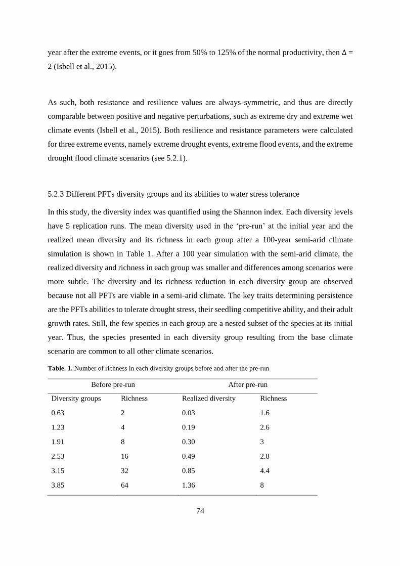
74
year after the extreme events, or it goes from 50% to 125% of the normal productivity, then Δ =
2 (Isbell et al., 2015).
As such, both resistance and resilience values are always symmetric, and thus are directly
comparable between positive and negative perturbations, such as extreme dry and extreme wet
climate events (Isbell et al., 2015). Both resilience and resistance parameters were calculated
for three extreme events, namely extreme drought events, extreme flood events, and the extreme
drought flood climate scenarios (see 5.2.1).
5.2.3 Different PFTs diversity groups and its abilities to water stress tolerance
In this study, the diversity index was quantified using the Shannon index. Each diversity levels
have 5 replication runs. The mean diversity used in the ‘pre-run’ at the initial year and the
realized mean diversity and its richness in each group after a 100-year semi-arid climate
simulation is shown in Table 1. After a 100 year simulation with the semi-arid climate, the
realized diversity and richness in each group was smaller and differences among scenarios were
more subtle. The diversity and its richness reduction in each diversity group are observed
because not all PFTs are viable in a semi-arid climate. The key traits determining persistence
are the PFTs abilities to tolerate drought stress, their seedling competitive ability, and their adult
growth rates. Still, the few species in each group are a nested subset of the species at its initial
year. Thus, the species presented in each diversity group resulting from the base climate
scenario are common to all other climate scenarios.
Table. 1. Number of richness in each diversity groups before and after the pre-run
Before pre-run After pre-run
Diversity groups Richness Realized diversity Richness
0.63 2 0.03 1.6
1.23 4 0.19 2.6
1.91 8 0.30 3
2.53 16 0.49 2.8
3.15 32 0.85 4.4
3.85 64 1.36 8

75
The matric potential values, namely oxygen deficiency potential Ψ1, field capacity Ψ2, reduction
point matric potential Ψ3, wilting point potential Ψ4, of the high and low drought stress tolerance
ability of PFTs were defined based on the matric potential values of plant functional types that
eventually survived under a semi-arid climate (based on previous assessments, see Chapter 4).
The values of high drought water stress tolerance plant functional types are -80 mm, -180 mm,
-600000 mm, -1000000 mm for Ψ1, Ψ2, Ψ3, Ψ4, respectively. The potential values of the low
drought water stress tolerance PFTs are -80 mm, -150 mm, -7000 mm, and -60000 mm for Ψ1,
Ψ2, Ψ3, Ψ4, respectively. The values of Ψ1, Ψ2, Ψ3 of the low drought stress tolerance plant
functional types were defined based on the critical matric potential values found in literatures
(Bittner et al., 2010; Laio et al., 2001a; Scholes and Archer, 1997;Veenhof and McBride, 1994;
Wesseling, 1991).
5.2.4 Statistical analysis
In order to test whether there is a positive relationship between the resistance and diversity,
between resilience and diversity, as well as between the ecosystem stability and diversity under
different extreme climate scenarios, linear regression tests were used. To test whether the
impact of extreme drought and heavy rainfall on aboveground biomass is greater than the
impact of drought or flood events alone at the extreme event year, a one-way ANOVA test was
used to compare the effects of the three extreme climates (dual impact of drought and heavy
rainfall, extreme drought or extreme heavy rainfall) on the mean aboveground biomass. The
statistical analyses were performed in R (3.5.2).
5.3. Results
5.3.1 Biodiversity-ecosystem stability relationship under different extreme climate scenarios
Increased diversity had different impacts on the resilience and resistance under extreme wet
and dry climate scenarios (Fig. 23). Under extreme drought climates, no positive relationship
between resistance and diversity was found, but increased diversity increased resilience (Fig.
23a, Fig. 23b). Under extreme flood climate events, increased diversity increased resistance but
decreased resilience (Fig. 23c and Fig. 23d). Similar to the extreme flood climates, increased
diversity increased resistance, but decreased resilience under extreme drought and heavy
rainfall extreme climate (Fig. 23e, Fig. 23f).

76
Increased diversity increased mean biomass stability under both extreme flood (Fig. 24b) and
extreme drought and heavy rainfall climate scenarios (Fig. 24c). But increased diversity did not
have a significant impact on the mean biomass stability under the extreme drought climate
scenarios (Fig. 24a).

77
Fig. 23. Plant community resistance and resilience (mean ± 95% CI) under extreme drought climate scenarios (a-
b), under extreme flood climate scenarios (c-d), and under extreme drought and heavy rainfall climate scenarios
(e-f) at different diversity levels. Each climate scenarios have 6 levels of diversity, and each diversity level have
5 replications. p<0.05*, p<0.01**, p<0.001***

78
Fig. 24. Biodiversity-stability relationships (mean ± 95% CI) under extreme drought climate scenarios (a), under extreme flood climate scenarios (b), and under extreme drought and heavy rainfall climate scenarios (c). Each
climate scenarios have 6 levels of diversity, and each diversity level have 5 replications. p<0.05*, p<0.01**,
p<0.001***
5.3.2 Impact of drought and heavy rainfall vs. drought or flood events on the mean annual
aboveground biomass in each diversity group
An impact of different climate extremes on the mean annual aboveground biomass for the event
year was found (Fig. 25). Drought climate extremes decreased the mean annual biomass, while
extreme flood and extreme drought and heavy rainfall climate increased mean annual
aboveground biomass compared to the biomass simulated in the reference climate at the event
year. And this different effect of extreme climates on aboveground biomass was significant for
low diversity groups for the event year. However, no significant extreme climates effects on
aboveground biomass in high diversity levels were found for the event year. Among the three
climate extremes, extreme flood climate had the highest positive impact on mean aboveground
biomass compared to the reference climate biomass.

79
Fig. 25. The relative differences of biomass simulated between extreme drought climates and the reference
climates (DRY to REF, the red color), between extreme flood climates and the reference climates (WET to REF,
the blue color), between extreme drought and heavy rainfall climates and the reference climates (the BOTH to
REF, green color) at the event years. The relative biomass differences (%) was calculated as (biomass (DRY;
WET; BOTH) - biomass (REF)) / biomass (REF). The P values from left to right indicated the significant
differences of effect on biomass among DRY to REF, WET to REF, BOTH to REF at different diversity levels.
Each climate scenarios have 6 levels of diversity, and each diversity level have 5 replications.
5.4 Discussion
The results reveal that the “Insurance Hypothesis” does not apply to all climate extremes.
Besides, the impact of an extreme flood climate on mean annual aboveground biomass was
greater than the dual impact of extreme drought and heavy rainfall at event years.
5.4.1 Biodiversity-stability relationship under different climate scenarios
The results show positive relationships between increased diversity and ecosystem stability in
both extreme flood events and dual drought and flood extreme events. Such diversity-stability
relationships agree with previous findings that increased diversity increases stability, as shown
in field experimental and observational studies on grassland in semi-arid climates (e.g. Isbell et
al., 2011; Polley et al., 2013) and in a general stochastic modelling study (Yachi and Loreau,
1999). In response to extreme flood climates, resistance and resilience behaved differently with

80
increased diversity. Increasing diversity increased resistance under flood extremes owing to the
low diversity community containing fast-growing species that can take advantage of the water
resources (Reich, 2003; Wright et al., 2015) during flood extremes, e.g. annual plants with
short-term seed dormancy and high adult growth rate, thus results in a large biomass deviation
compared to non-flood years. This finding supports the assumptions from previous studies that
low-diversity plant community have a high probability to contain a higher proportion of fast-
growing species that are often sensitive and vulnerable to extreme events, such as to extreme
drought events (Huston, 1997; Ouédraogo et al, 2013). Besides, the high diversity plant
communities generally have higher mean LAI, root depth and plant height than the low diversity
plant communities, and these types of plants tend to be able to survive and tolerate the flood
stress (Striker, 2012). Conversely, increased diversity decreased resilience under conditions of
extreme flood events. This result agrees with results found in semi-arid climate in a review
study on grassland communities, where it was shown that diversity has a negative effect on
resilience under wet climate events (Isbell et al., 2015). This is probably due to the impact of
biomass recovery being greater than the biomass gain during the year after the flood events for
high diversity communities. The deep roots in the high diversity community allow them to store
more water during extreme flood events, and later use these water resources during the year
after the flood for regaining biomass (Fischer et al., 2016).
Similar to the extreme flood events, increasing diversity also increased resistance, but decreased
resilience under conditions of drought and heavy rainfall. Increasing diversity led to increased
resistance under extreme drought and flood climates was probably because the high diversity
communities included different types of plant functional types, which allowed them to use the
same resources at different times or different points in space (Hooper et al., 2005). For example,
the high proportional drought-tolerance and slow-growing subordinate species in high diversity
communities may buffered ecosystem against extreme drought events (Lepš et al., 1982; Yachi
and Loreau, 1999), and the tall plants with large LAI in high diversity communities tolerated
flood stress during heavy rainfall (Striker, 2012). The negative impact on resilience in drought
and heavy rainfall conditions was caused by a greater impact of biomass gain at event years
than the biomass recovery during the year after the events in low diversity communities. This
is probably due to fast-growing annual species in low diversity groups rapidly utilized the
increased water resources (Reich, 2003) and thus increased its biomass during the heavy rainfall
period at extreme event years.

81
The lack of positive effects of diversity on biomass stability under extreme drought climate was
due to the absence of a positive diversity effect on resistance, despite a positive diversity effect
on resilience was observed. This finding is not consistent with previous findings on grassland
in semi-arid climates (Isbell et al., 2011), but consistent with the experimental finding from
Kreyling et al. (2017), who showed that species richness of temperate and Mediterranean
grassland did not affect resistance but promoted recovery under extreme drought events. The
non-significant effect of diversity on biomass resistance was probably due to drought events
reduced biomass production similarly at both the 0.85 and 1.36 diversity levels, because of the
dominating drought-tolerance species in these two diversity levels. The positive diversity
effects on resilience under extreme drought climates was driven by community productivity.
This could be because some of the low diversity communities were dominated by slow-growing
species with low productivity, such as perennial plants with low adult growth rates, which were
less able to take advantage of increased resource availability after the end of the drought events
(Lepš et al. 1982; Reich, 2003).
Thus, the findings in this work generally support the insurance hypothesis, but only for extreme
wet events and not for extreme dry events. This could be due to the different natures of the
climate extreme events triggering different diversity effects on resilience and resistance.
Namely, increasing diversity generally increases resistance, and increasing diversity decreases
resilience under extreme wet conditions but increases resilience under extreme dry conditions.
5.4.3 Comparisons between dual impacts of extreme drought and heavy rainfall and extreme
drought or flood events on annual aboveground biomass
The highest impact on biomass coming from extreme flood events did not support the stated
hypothesis. This pattern is especially obvious at low diversity groups. Drought extreme events
caused high stress for plant growth due to decreased water availability and had a negative
impact on productivity. Conversely, the flood disturbance did not increase stress on plant
growth, but rather alleviated the drought stress because of increased water resources, and
thereby allowing plant growth and thus an increase in productivity. This effect was especially
observed in the low diversity group where fast-growing species are able to take advantage of
these resources and thus being able to increase their aboveground biomass (Reich, 2003). This
positive effect of extreme flood events on biomass agrees with previous experimental study on
a California grassland in a similar climate, where a sudden very wet weather in a usually dry

82
areas evokes growth and thus have a positive effect on productivity (De Boeck et al., 2018;
Harpole et al., 2007). Compared to positive effects of extreme flood events, the drought and
heavy rainfall extremes had a lower positive effect on productivity. This is the case because the
conversed positive and negative effects between heavy rainfall and drought extremes lowered
the general positive effect on productivity. Therefore, extreme flood events had a greater
positive impact on plant productivity than the impact of dual drought and heavy rainfall.
5.5 Conclusion
The results revealed that increased functional diversity does not necessarily increase plant
community stability against extreme drought events, due to a non-significant impact on
resistance. Increased diversity increased plant community stability under extreme flood events,
and under extreme drought and heavy rainfall events, by increasing resistance but decreasing
resilience.
Results suggest that resilience and resistance can behave differently under different climate
extremes, because the different natures of the climate events may trigger different responses
and behaviors from different plant communities. Increased diversity generally increases
resistance, and increasing diversity increases resilience under extreme dry events but decreases
resilience under extreme wet events.
Furthermore, the impact of dual drought and heavy rainfall extremes on plants aboveground
productivity is not larger than the single type of climate extremes and is not necessarily
negative. Rather, drought and heavy rainfall extremes can alleviate drought stress and trigger
growth increases due to an increase of water availability in dry environments.

83
6. General Conclusions
This dissertation identified the lack of flexible coupled hydrological and vegetation models that
are able to depict the dynamic feedbacks between plant and water at different spatial and
temporal scales as a research gap. It examines whether using a coupled hydrology and
vegetation model is superior than uncoupled models in quantifying hydrological processes and
plant community attributes in different climates, as well as the role that biodiversity plays in
ecosystem functioning under climate extremes. To address these gaps, two models, the
HydroGeoSphere (HGS) model and PLAnt fuNctional Traits Hydrological Regimes model
(PLANTHeR), have been coupled for the first time, and this coupled model was applied to
examine and analyze the hydrology-vegetation, heterogeneity-diversity and biodiversity-
stability relationships.
First, a hydrological HGS model was coupled to the individual-based PLANTHeR model at a
plot scale on a yearly basis (Chapter 3). Besides examining its suitability and advantage over
the uncoupled HGS or PLANTHeR models in quantifying the hydrological processes and plant
community dynamics, a heterogeneity-richness relationship was explored. The PLANTHeR-
HGS model was found to be superior in simulating transpiration, evaporation, plant community
diversity and richness compared to the uncoupled models. To be more specific, that the ‘realistic
vegetation’ in the PLANTHeR-HGS model is able to simulate a ‘two-way’ impact between
plant LAI, density, root depth dynamics and the variation of transpiration, evaporation, or soil
water content. The consideration of dynamic plants homogenized soil water content within its
root zone and patterns of soil water availability determined the spatial distribution of plant
species. This emphasizes the importance of including vegetation dynamics in hydrological
models as well as considering the spatiotemporal water availability in plant models.
Furthermore, increased spatial heterogeneity of small sized soil water resources did not
decrease plant richness and diversity, but increased temporal variability of soil water resources
and decreased mean aboveground biomass.
Secondly, the differences of using the PLANTHeR-HGS model in quantifying the hydrological
processes and plant community dynamics among three climates, spanning from dry to wet
climates, were compared to simulations with the uncoupled models (Chapter 4). Due to the high
variability of rainfall in dry climates and low rainfall variability in wet climates, it was expected
that it matters the most to use the PLANTHeR-HGS model for a dry climate. As expected,

84
transpiration, soil saturation within the root depth, plant community richness and aboveground
biomass had larger differences when using the coupled PLANTHeR-HGS model in drier
climates. However, surprisingly, evaporation and the plant community diversity (the Shannon
index) were found to have larger differences between the PLANTheR-HGS and the uncoupled
models in a wetter climate. The larger difference of evaporation in wet climate was the result
of a high leaf area index, which lowered evaporation because of increased shading by the
canopy. The larger difference in the diversity (quantified by the Shannon index) in a wetter
climate was because of the mathematical property of the Shannon index, which is positively
related to richness but negatively related to plant abundance. Thus, a combination of low
relative change of plant abundance in response to low variation of soil saturation and a moderate
increase in PFTs richness resulted in a larger deviation of the Shannon index in a wetter climate.
Third, it was shown that high diversity of plant communities increases their temporal stability
under extreme wet climate events, but not under extreme dry climate events (Chapter 5). Under
the current rapid change of climate extremes, ecosystems in drylands are increasingly
threatened by ecosystem degradation as well as losses in biodiversity, ecosystem functions and
services. Ecosystems with more diverse species are generally considered to have higher
resistance and resilience against extreme climates because of a high probability of containing
species that are able to tolerate stress and recover from the disturbance. Since extreme climates,
like prolonged consecutive dry days or heavy rainfall or a combination of both, have been
frequently observed in drylands, it was expected that high diversity would buffer the ecosystem
against these extreme conditions in dry climates. Indeed, high diversity increased biomass
stability under extreme flood events, but not under extreme drought climate events. This was
due to two high diversity level groups behaving similarly in biomass changes during the
extreme drought events, which resulted in a non-significant relationship between diversity and
resistance under extreme drought climate events. Although resistance has been found to
generally increases with increased diversity, resilience behaved differently in extreme dry vs.
wet events. Resilience decreased under extreme wet climates but increased under extreme dry
climates with increasing diversity. Thus, the “Insurance-Hypothesis” did not apply to the
extreme drought events in this study.
The simulation results in Chapter 3 to Chapter 5 not only enhanced our understanding of the
dynamic feedbacks between hydrology and vegetation at different spatial and temporal scales,
and the biodiversity-stability relationships under extreme climate events, but also identified

85
sensitive variables for hydrology and vegetation in different climates with regards to using a
dynamically coupled vegetation-hydrology model. The PLANTHeR-HGS model is generally
able to give a better and meaningful representation of the ‘close-to-reality’ hydrology-
vegetation feedbacks than uncoupled models at both yearly and seasonal time scales, and at plot
and hillslope spatial scales. Future work may consider upscaling the PLANTHeR-HGS model
to a catchment scale, where the effects of changing hydroclimatic conditions in a dry climate,
such as a semi-arid region, on the evolution of a specific plant community can be explored.
Besides, soil texture can indirectly affect plant growth through influencing soil water supply,
and homogenous soil texture is rarely existing in natural environments, thus future work should
consider the effects of different soil textures, i.e., different water folding capacities, in the
PLANTHeR-HGS model when applying it at a large spatial scale (e.g. the catchment scale). In
addition, including an anthropogenic factor to the PLANTHeR-HGS model would contribute
to the current understanding of the impact of anthropogenic climate change on ecosystem
functions, since most of natural ecosystems have been modified directly and indirectly by
anthropogenic activities.
In summary, it was shown that the PLANTHeR-HGS model was generally superior to the
uncoupled HGS and PLANTHeR models in quantifying hydrological processes (transpiration,
evaporation, soil water saturation) and plant community attributes (diversity, richness, and
aboveground biomass). Plant and water are intricately linked together and studying one system
requires to simultaneously consider the other. The results in this thesis suggest that the
hydrological conditions and the plant community structures differed meaningfully when the
two models were coupled. Thus, based on the outcomes of this study, the application of dynamic
coupling of vegetation and hydrological models instead of modeling these two compartments
in isolation is advocated.

86
7. References
Adler, P.B., Levine, J.M., 2007. Contrasting relationships between precipitation and species richness in
space and time. Oikos. 116, 221-232.
Ahmadi, S. H., Fooladmand, H.R., 2008. Spatially distributed monthly reference evapotranspiration
derived from the calibration of Thornthwaite equation: a case study, South of Iran. Irrigation
Science. 26(4), 303-312.
Aldridge, B.N., Garrett, J.M., 1973. Roughness coefficients for stream channels in Arizona: U.S.
Geological Survey Open-File Report.
Allen, R.G., Pereira, L.S., Raes, D., Smith, M. 1998. Chapter 3 - Meteorological data from Crop
evapotranspiration - guidelines for computing crop water requirements. FAO Irrigation and
drainage paper 56. Food and Agriculture Organization, Rome
Allouche, O., Kalyuzhny, M., Moreno-Rueda, G., Pizarro, M., Kadmon, R., 2012. Area–heterogeneity
tradeoff and the diversity of ecological communities. PNAS. 109 (43), 17495-17500.
Araya A, Stroosnijder L, 2011. Assessing drought risk and irrigation need in Northern Ethiopia.
Agricultural and Forest Meteorology. 151(4), 425–436.
Arcement, Jr, J.G., Schneider, V.R., 1989. Guide for selecting Manning's roughness coefficients for
natural channels and flood plains. Geological Survey (U.S.).
Asbjornsen, H., Goldsmith, G R., Alvarado-Barrientos, M S., Rebel, K., Osch, F.P.V., Rietkerk, M.,
Chen, J., Gotsch, S., Tobón, C., Geissert, D.R., Gómez-Tagle, A., Vache, K., Dawson, T.E., 2011.
Ecohydrological advances and applications in plant–water relations research: a review. Journal
of Plant Ecology. 4(1-2), 3-22.
Asner, G.Y., Scurlock, J.M.O., Hicke, J.A., 2003. Global synthesis of leaf area index observations:
implications for ecological and remote sensing studies. Global Ecology and Biogeography.12,
191–205.
Ayanlade, A., 2009. Seasonal rainfall variability in Guinea Savanna part of Nigeria: a GIS approach,
International Journal of Climate Change Strategies and Management. 1(3), 282-296.
Ayanlade, A., 2018. Rainfall variability and drought characteristics in two agro-climatic zones, an
assessment of climate change challenges in Africa. Science of the Total Environment. 630, 728–
737.
Bagayoko, F., Yonkeu, S., van de Giesen, N.C., 2006. Effect of seasonal dynamics of vegetation cover
on land surface models: a case study of NOAH LSM over a savanna farm land in eastern Burkina
Faso, West Africa. Hydrology and Earth System Sciences Discussions. 3(5), 2757–2788.
Baldocchi, D.D., Xu, L.K., Kiang, N., 2004. How plant functional-type, weather, seasonal drought, and
soil physical properties alter water and energy fluxes of an oak–grass savanna and an annual
grassland. Agricultural and Forest Meteorology. 123(1–2), 13–39.
Band, L.E., Patterson, P., Nemani, R., Running, S.W., 1993. Forest ecosystem processes at the
watershed scale - incorporating hillslope hydrology, Agricultural and Forest Meteorology. 63(1-
2), 93-126.
Barbier, N., Couteron, P., Lefever, R, Deblauwe, V., Lejeune, O., 2008. Spatial decoupling of
facilitation and competition at origin of gapped vegetation patterns. Ecology. 89(6), 1521-1531.
Bartley, R., Roth, C.H., Ludwig, J., McJannet, D., Liedloff, A., Corfield, J, Hawdon, A., Abbott, B.,
2006. Runoff and erosion from Australia’s tropical semi-arid range-lands: influence of ground
cover for differing space and time scales. Hydrological Processes. 20(15), 3317-3333.
Baruch Z., Mérida. T., 1995. Effects of drought and flooding on root anatomy in four tropical forage
grasses. International Journal of Plant Sciences. 156(4), 514-521.

87
Basu, S., Ramegowda, V., Kumar, A., Pereira, A. 2016. Plants adaptation to drought stress [version 1;
peer review: 3 approved]. F1000Research, 5(F1000 Faculty Rev):1554
Battaglia, M., Cherry, M. L., Beadle, C. L., Sands, P. J., Hingston, A., 1998. Prediction of leaf area
index in eucalypt plantations: effects of water stress and temperature. Tree Physiology. 18(8-9),
521–528.
Bates, B. C., Kundzewicz, Z. W., Wu, S., Palutikof, J.P., Eds., 2008. Climate Change and Water:
Technical Paper of the Intergovernmental Panel on Climate Change. IPCC Secretariat, Geneva,
210 pp.
Beer, C.P., Ciais.P., Reichstein, M., Baldocchi, D., Law, B.E., Papale, D., Soussana, J.-F., Ammann, C.,
Buchmann, N., Frank, D., Gianelle, D., Janssens, I.A., Knohl, A., Köstner, B., Moors, E.,
Roupsard, O., Verbeeck, H., Vesala, T., Williams, C.A., Wohlfahrt, G., 2009. Temporal and
among-site variability of inherent water use efficiency at the ecosystem level, Global
Biogeochemical Cycles. 23(2), GB2018. 1-13.
Beisel, J.N., Moreteau, J.C., 1997. A simple formula for calculating the lower limit of Shannon’s
diversity index. Ecological Modelling. 99(2-3), 289-292.
Bertness, M. D., Callaway, R. M., 1994. Positive interactions in communities, Trends in Ecology and
Evolution. 9(5), 191–193.
Bittner, S., Talkner, U., Krämer, I., Beese, F., Hölscher, D., Priesack, E., 2010. Modeling stand water
budgets of mixed temperate broad-leaved forest stands by considering variations in species
specific drought response. Agricultural and Forest Meteorology. 150(10), 1347–1357.
Blaum, N., Seymour, C., Rossmanith, E., Schwager, M., Jeltsch, F., 2009. Changes in arthropod
diversity along a land use driven gradient of shrub cover in savanna rangelands: identification of
suitable indicators. Biodiversity and Conservation. 18, 1187-1199.
Bloor J. M.G., Bardgett, R.D., 2012. Stability of above-ground and below-ground processes to extreme
drought in model grassland ecosystems: Interactions with plant species diversity and soil nitrogen
availability. Perspectives in Plant Ecology Evolution and Systematics. 14, 193–204.
Bonan, G.B., Levis, S., Kergoat, L., Oleson, K.W., 2002. Landscapes as patches of plant functional
types: An integrating concept for climate and ecosystem models. Global Biogeochemical Cycles.
16(2), 5-1-5-23.
Brunner, P., Simmons, C.T., 2012. HydroGeoSphere: A Fully Integrated, Physically Based hydrological
Model. Ground Water. 50(2), 170-176.
Breda, N., Huc, R., Granier, A., Dreyer, E., 2006. Temperate forest trees and stands under severe drought:
A review of ecophysiological responses, adaptation processes and long-term consequences.
Annals of Forest Science. 63, 625–644.
Breshears, D.D., Myers, O.B., Barnes, F.J., 2009. Horizontal heterogeneity in the frequency of plant-
available water with woodland intercanopy-canopy vegetation patch type rivals that occuring
vertically by soil depth. Ecohydrology. 2, 503–19.
Brienen, R.J.W., Zuidema, P.A., 2005. Relating tree growth to rainfall in Bolivian rain forests: a test for
six species using tree ring analysis. Oecologia. 146, 1–12.
Briggs, L.J., Shantz, H.L., 1912. The Wilting Coefficient and Its Indirect Determination. Botanical
Gazette. 53(1), 20–37.
Brown, G. 2003. Species richness, diversity and biomass production of desert annuals in an ungrazed
Rhanterium epapposum community over three growth seasons in Kuwait. Plant Ecology. 165,
53–68.
Bruijnzeel, L.A., 1990. Hydrology of Moist Tropical Forests and Effects of Conversion: A State of
Knowledge Review. International Hydrological Programme, UNESCO.pp. 224.
Budyko, M. I., 1958. The heat balance of the earth’s surface, U.S. Dept.of Commerce, Washington,
1958.

88
Budyko, M.I., 1974. Climate and Life. Academic Press, New York.
Cain, M.L., Milligan, B.G., Strand, A.E., 2000. Long-distance seed dispersal in plant populations.
American Journal of Botany. 87(9), 1217–1227.
Callaway, R.M., 1995. Positive interactions among plants, Botanical Review, 61(4), 306–349.
Campbell, V., Murphy, G., Romanuk, T.N., 2011. Experimental design and the outcome and
interpretation of diversity–stability relations. Oikos. 120(3), 399–408.
Camargo, A.P., Marin, F.R., Sentelhas, P.C., Picini, A.G., 1999. Adjust of the Thornthwaite’s method
to estimate the potential evapotranspiration for arid and superhumid climates, based on daily
temperature amplitude. Revista Brasileira de Agrometeorologica. 7, 251–257.
Canadell, J., Jackson, R.B., Ehleringer, J.B., Mooney, H.A., Sala, O.E., Schulze, E.D., 1996. Maximum
rooting depth of vegetation types at the global scale. Oecologia. 108, 583–595.
Cao, L., Zhang, Y., Shi, Y., 2011. Climate change effect on hydrological processes over the Yangtze
River basin. Quaternary International. 244, 202-210.
Caplat, P., Anand, M., Bauch, C., 2008. Symmetric competition causes population oscillations in an
individual-based model of forest dynamics. Ecological modelling. 211(3), 491-500.
Cardinale, B. J., Duffy, J. E., Gonzalez, A., Hooper, D.U., Perrings, C., Venail, P., Narwani, A., Mace,
G., Tilman, D., Wardle, D., Kinzig, A., Daily, G., Loreau, M., Grace, J., Larigauderie, A.,
Srivastava, D., Naeem, S., 2012. Biodiversity loss and its impact on humanity. Nature. 486, 59–
67.
Carsel, R.F., Parrish, R.S., 1988. Developing joint probability distributions of soil water retention
characteristics. Water Resources Research. 24(5), 755–769.
Carter, D.L., Blair, J.M., 2012. High richness and dense seeding enhance grassland restoration
establishment but have little effect on drought response. Ecological Applications. 22(4), 1308–
1319.
Casper, B.B., Schenk, H.J., Jackson, R.B., 2003. Defining a plant’s belowground zone of influence.
Ecology. 84(9), 2313-2321.
Chen, X., Li, B.L., 2003. Testing the allometric scaling relationships with seedlings of two tree species.
Acta Oecologica. 24(3). 125–129.
Chen, D., Gao G., Xu, C.Y., Guo, J., Ren, G., 2005. Comparison of the Thornthwaite method and pan
data with the standard Penman-Monteith estimates of reference evapotranspiration in China.
Climate research. 28, 123–132.
Chow, V.T., 1959. Open channel hydraulic. MaGraw-Hill Book Company.
Cornet, A.F., Delhoume, J.P. Montana, C., 1988. Dynamics of striped vegetation patterns and water
balance in the Chihuahuan Desert. In: During, H.J., Werger, M.J.A. & Willems, H.J. (Eds),
Diversity and Pattern in Plant Communities, pp. 221–231. The Hague: SPB Academic. 278 pp.
Coenders-Gerrits, A.M.J., van der Ent, R.J., Bogaard, T.A., Wang-Erlandsson, L., Hrachowitz, M., H
Savenije, H.H.G., 2014. Uncertainties in transpiration estimates, Nature. 506(7487), E1–E2.
Craine, J.M., Dybzinski, R., 2013. Mechanisms of plant competition for nutrients, water and light.
Functional Ecology. 27(4). 833-840.
Crawford, R.M.M., Braendle, R., 1996. Oxygen deprivation stress in a changing environment. Journal
of Experimental Botany. 47(2). 145–159.
Czárán, T., 1998. Spatiotemporal models of population and community dynamics. Volume 21 of
Population and Community Biology Series. first ed. Chapman and Hall. London. ISSN 1367-5257
Dasci, M., Koc, S.A., Comakli, B., Güllap, M.K., Cengiz, M.M., Erkovan, H.I., 2010. Importance of
annual and seasonal precipitation variations for the sustainable use of rangelands in semi-arid
regions with high altitude. African Journal of Agricultural Research, 5(16), 2184-2191.

89
Davoodi, E., Ghasemieh, H., Batelaan, O., Abdollahi, K., 2017. Spatial-Temporal Simulation of LAI on
Basis of Rainfall and Growing Degree Days. Remote Sensing. 9(12), [1207].17pages.
Day, M., Baldauf, C., Rutishauser, E., Sunderland, T.C.H., 2013. Relationships between tree species
diversity and above-ground biomass in Central African rainforests: implications for REDD.
Environmental Conservation. 41, (1), 64–72.
De Boeck, H.J., Bassin, S., Verlinden, M., Zeiter, M., Hiltbrunner, E., 2016. Simulated heat waves
affected alpine grassland only in combination with drought. New Phytologist. 209(2), 531–541.
De Boeck, H.J., Bloor, J.M.G., Kreyling, J., Ransijn, J.C.G., Nijs, I., Jentsch, A., Zeiter, M., 2018.
Patterns and drivers of biodiversity–stability relationships under climate extremes. Journal of
Ecology. 106(3). 1320-1320.
De Wasseige, C., Bastin, D., Defourny, P., 2003. Seasonal variation of tropical forest LAI based on field
measurements in Central African Republic. Agricultural and Forest Meteorology.119(3),181-194.
Deus, D., Gloaguen, R., Krause, P., 2011. Water balance modelling in a semi-arid environment with
limited in-situ data: remote sensing coupled with satellite gravimetry, Lake Manyara, East
African Rift, Tanzania. Hydrology and Earth System Sciences Discussions. 8(5), 8737–8792.
Deutsch, C.V., Journel, A.G., 1998. GSLIB Geostatistical Software Library and User's Guide, 2nd
Edition, Applied Geostatistics Series, Oxford University Press, Inc. New York, NY.
Díaz, S., Cabido, M., Vive la différence: 2011. Plant functional diversity matters to ecosystem processes.
Trends in Ecology and Evolution. 16(11). 646-655.
D’Odorico, P., Ridolfi, L., Porporato, A., Rodriguez-Iturbe, I., 2000. Preferential states of seasonal soil
moisture: the impact of climate fluctuations. Water Resources Research. 36(8), 2209–19.
Donzelli, D., De Michele, C., Scholes, R.J., 2013. Competition between trees and grasses for both soil
water and mineral nitrogen in dry savannas. Journal of Theoretical Biology. 332,181–90.
Dunisch, O., Montoia, V.R., Bauch, J., 2003. Dendroecological investigations on Swietenia macrophylla
King and Cedrela odorata L. (Meliaceae) in the central Amazon. Trees- Structure and Function.
17, 244–250.
Dunkerley, D.L., 1997. Banded vegetation: survival under drought and grazing pressure based on a
simple cellular automaton model. Journal of Arid Environments. 35(3), 419–428.
Easterling, D.R., Meehl, G.A., Parmesan, C., Changnon, S.A., Karl, T.R., Mearns, L.O., 2000a. Climate
extremes: observations, modeling, and impacts. Science, 289, 2068–2074.
Easterling, D.R., Evans, J.L., Groisman, P.Y., Karl, T.R., Kunkel, K.E., Ambenje, P., 2000b. Observed
variability and trends in extreme climate events: a brief review. Bulletin of the American
Meteorological Society. 81(3), 417–425.
Ebel, B.A., Mirus, B.B., Heppner, C.S., VanderKwaak, J.E., Loague, K., 2009. First-order exchange
coefficient coupling for simulating surface water–groundwater interactions parameter sensitivity
and consistency with a physics-based approach. Hydrological Processes. 23(13), 1949–1959.
Enquist, B. J., Niklas. K.J., 2002. Global allocation rules for patterns of biomass partitioning in seed
plants. Science. 295, 1517 – 1520.
Epstein, H. E., Burke, I. C., Lauenroth, W. K., 2002. Regional patterns of decomposition and primary
production rates in the US Great Plains. Ecology. 83, 320–327.
Esther, A., Groeneveld, J., Enright, N.J., Miller, B.P., Lamont, B.B., Perry, G.L.W., Tietjen, B., Jeltsch,
F., 2011. Low-dimensional trade-offs fail to explain richness and structure in species-rich plant
communities. Theoretical Ecology. 4(4), 495-511.
Farooq, M., Siddique, K., 2016. Chapter 2: Research and developmental issues in dryland agriculture.
In Book Innovations in Dryland Agriculture. Springer International Publishing. 10.1007/978-3-
319-47928-6. 31-46
90
Fatichi, S., Pappas, C., 2017. Constrained variability of modeled T:ET ratio across biomes. Geophysical
Research Letters. 44(13), 6795–6803.
Fay, P.A., Carlisle, J.D., Knapp, A.K., Blair, J.M., Collins, S.L., 2003. Productivity responses to altered
rainfall patterns in a C4-dominated grassland. Oecologia. 137(2), 245–251.
February, E.C., Higgins, S.I., 2010. The distribution of tree and grass roots in savannas in relation to
soil nitrogen and water. South African Journal of Botany. 76(3). 517–523
Feddes, R.A., Kowalik, P.J., Zaradny, H., 1978. Simulation of field water use and crop yield. Pudoc,
Wageningen. Simulation Monographs.
Feddes, R.A., Hoff, H., Bruen, M., Dawson, T., de Rosnay, P., Dirmeyer, P., Jackson, R.B., Kabat, P.,
Kleidon, A., Lilly. A., Pitman, A.J., 2001. Modeling root water uptake in hydrological and climate
models. Bulletin of the American Meteorological Society. 82(12), 2797–2809.
Feng, S., Fu, Q., 2013, Expansion of global drylands under a warming climate, Atmospheric Chemistry
and Physics, 13(19), 10081–10094.
Fernandez-Illescas, C.P., Rodriguez-Iturbe, I., 2003. Hydrological driven hierarchical compettion-
colonization models: the impact of interannual climate fluxtuations. Ecological Monographs.
73(2), 207-222.
Fischer, F.M., Wright, A.J., Eisenhauer, N., Ebeling, A., Roscher, C., Wagg, C., Weigelt, A., Weisser,
W.W., Pillar, V.D., 2016. Plant species richness and functional traits affect community stability
after a flood event. Philosophical Transactions of The Royal Society B Biological Sciences. 371:
20150276.
Flynn, D.F.B., Mirotchnick, N., Jain, M., Palmer, M.I., Naeem, S., 2011. Functional and phylogenetic
diversity as predictors of biodiversity-ecosystem-function relationships. Ecology. 92(8), 1573-
1581.
Fooladmand, H.R., Haghighat, M., 2007. Spatial and temporal calibration of Hargreaves equation for
calculating monthly ETo based on penman-monteith method. Irrigation and Drainage. 56(4).
439–449.
Fort, F., Volaire, F., Guilioni, L., Barkaoui, K., Navas, M.L., Roumet, C., 2017. Root traits are related
to plant water-use among rangeland Mediterranean species. Functional Ecology.31,1700–1709.
Foxx, T.S., Tierney, G.D., Williams, J.M., 1984. Rooting Depths of Plants to Biological and
Environmental Factors. Los Alamos National Laboratory report. LA-10254-MS.
Fraedrich, K., Kleidon, A., Lunkeit, F., 1999. A Green Planet versus a Desert World: Estimating the
Effect of Vegetation Extremes on the Atmosphere. Journal of Climate.12(10), 3156-3163.
Frank, D., Reichstein, M., Bahn, M., Thonicke, K., Frank, D., Mahecha, M. D., Smith, P., van der Velde,
M., Vicca, S., Badst, F., Beer, C., Buchmann, N., Canadell, J.G., Ciais, P., Cramer, W., Ibrom,
A., Miglietta, F., Poulter, B., Ramming, A., Seneviratne, S.I., Walz, A., Wattenbach, M., Zavala,
M.A., Zscheischler, J., 2015. Effects of climate extremes on the terrestrial carbon cycle: Concepts,
processes and potential future impacts. Global Change Biology, 21, 2861–2880.
Freund, E.R., Kirchner, J.W., 2017. A budyko frame work for estimating how spatial heterogeneity and
lateral moisture redistribution affect average evapotranspiration rates as seen from the atmosphere.
Hydrology and Earth System Sciences. 21, 217–233.
Frich, P., Alexander, L.V., Della-Marta, P.M., Gleason, B.E., Haylock, M.R., Klein Tank, A.M.G.,
Peterson, T., 2002. Observed coherent changes in climatic extremes during the second half of the
twentieth century. Climate Research. 19(3), 193–212.
García-Palacios, P., Groass, N., Gaitán, J., Maestre, F.T., 2018. Climate mediates the biodiversity–
ecosystem stability relationship globally. PNAS. 115(33). 8400-8405.
Gazol, A., Tamme, R., Price, J.N., Hiiesalu, I., Laanisto, L., Pärtel, M., 2013. A negative heterogeneity-
diversity relationship found in experimental grassland communities. Oecologia. 173(2), 545-555.

91
Geng, Q.L., Wu, P.T., Zhao, X.N., Wang, Y.B., 2014. Comparison of classification methods for the
divisions of wet/dry climate regions in Northwest China. International Journal of Climatology.
34(7), 2163–2174.
Gherardi, L.A., Sala, O.E., 2015. Enhanced interannual precipitation variability increases plant
functional diversity that in turn ameliorates negative impact on productivity. Ecology Letters. 18:
1293–1300.
Gitay, H., Noble, I.R., 1997. What are functional types and how should we seek them? In Smith, T.M.,
Shugart, H.H. and Woodward, F.I., editors, Plant functional types, Cambridge: Cambridge
University Press, 3–19.
Gower, S. T., 2003. Patterns and mechanisms of the forest carbon cycle. Annual Review of Environment
and Resources. 28, 169–204.
Good, S. P., Soderberg, K., Guan, K., King, E.G., Scalon, T.M., Caylor, K. K., 2014. δ2H isotopic flux
partitioning of evapotranspiration over a grass field following a water pulse and subsequent dry
down, Water Resources Research. 50(2), 1410–1432.
Grace, B., Quick, B., 1988. A Comparison of Methods for the Calculation of Potential
Evapotranspiration Under the Windy Semi-arid Conditions of Southern Alberta , Canadian. Water
Resources Journal, 13:1, 9-19.
Grady, A. P. O’., Eamus, D., Hutley, L.B., 1998. Transpiration increases during the dry season: patterns
of tree water use in eucalypt open-forests of northern Australia. Tree Physiology, 19, 591-597.
Graetz, R.D., 1991. Desertification: A tale of two feedbacks, in Ecosystem Experiments, In: Mooney,
H.A.;=International Council of Scientific Unions. Scientific Committee on Problems of the
Environment (eds.), editor/s. Ecosystem Experiments. Chichester: John Wiley & Sons Ltd;
1991. 59-87.
Granier, A., Loustau, D., Bréda, N., 2000. A generic model of forest canopy conductance dependent on
climate, soil water availability and leaf area index. Annals of Forest Science. 57(8), 755-765.
Grime, J.P., 1974. Vegetation classification by reference to strategies. Nature. 250, 26–31.
Grime, J.P., 1994. The role of plasticity in exploiting environmental heterogeneity. In: Caldwell MM
(ed) Exploitation of environmental heterogeneity by plants: ecophysiological processes above-
and belowground. Academic Press, San Diego, pp 1–19
Grimm, V., Wissel, C., 1997. Babel, or the ecological stability discussions: an inventory and analysis of
terminology and a guide for avoiding confusion. Oecologia. 109(3): 323–334.
Groisman, P.Y., Knight, R.W., Easterling, D.R., Karl, T.R., Hegerl, G.C., Razuvaev, V.N., 2005. Trends
in intense precipitation in the climate record. Journal of Climate. 18, 1326–1350.
Grman, E., Lau, J.A., Schoolmaster, D.R.Jr, Gross, K.L., 2010. Mechanisms contributing to stability in
ecosystem function depend on the environmental context. Ecology Letters, 13(11), 1400–1410.
Guillevic, P., Koster, R.D., Suarez, M.J., Bounoua, L., Collatz, G.J., Los, S.O., Mahanama, S.P.P., 2002,
Influence of the interannual variability of vegetation on the surface energy balance - A global
sensitivity study, Journal of Hydrometeorology. 3.617-629.
Guo, T., Lohmann, D., Ratzmann, G., Tietjen, B., 2016. Response of semi-arid savanna vegetation
composition towards grazing along a precipitation gradient-The effects of including plant
heterogeneity into an ecohydrologcal savanna model. Ecological Modelling. 325, 47-56
Hagiwara, Y., Kachi, N., Suzuki, J-I., 2010. Effects of temporal heterogeneity of water supply on the
growth of Perilla frutescens depend on plant density. Annals of Botany. 106(1), 173–181.
Hallema, D.W., Moussa, R., Sun, G., McNulty, S.G., Surface storm flow prediction on hillslopes based
on topography and hydrologic connectivity. Ecological Processes, 5, 13.
Harpole, W.S., Potts, D.L., Suding, K.N., 2007. Ecosystem responses to water and nitrogen amendment
in a California grassland. Global Change Biology, 13, 2341–2348.

92
Harrison, G.W., 1979. Stability under environmental stress: resistance, resilience, persistence, and
variability. American Naturalist. 113(5), 659–669.
Harrison, S., Cornell, H., Moore, K.A., 2010. Spatial niches and coexistence: testing theory with
tarweeds. Ecology. 91, 2141–2150.
Harrison, S., Spasojevic, M.J., Li, D.J., 2020. Climate and plant community diversity in space and time.
PNAS,117(9). 4464–4470.
Hashemi, F., Habibian, M.T., 1979. Limitations of temperature-based methods in estimating crop
evapotranspiration in arid-zone agricultural projects. Agricultural Meteorology. 20(3), 237–247.
Hector, A., Schmid, B., Beierkuhnlein, C., Caldeira, M.C., Diemer, M., Dimitrakopoulos, P.G., Finn, J.
A., Freitas, H., Giller, P. S., Good, J., Harris, R., Högberg, P., Huss-Danell, K., Joshi, J.,
Jumpponen, A., Körner, C., Leadley, P.W., Loreau, M., Minns, A., Mulder, C.P.H., O’Donovan,
G., Otway, S. J., Pereira, J. S., Prinz, A., Read, D.J., Scherer-Lorenzen, M., Schulze, E.-D.,
Siamantziouras, A.-S.D., Spehn E.M., Terry, A.C., Troumbis, A.Y., Woodward, F.I., Yachi, S.,
Lawton, J.H., 1999. Plant diversity and productivity experiments in european grasslands. Science,
286, 1123–1127.
Heisler-White, J.L., Knapp, A.K., Kelly, E.F., 2008. Increasing precipitation event size increases
aboveground net primary productivity in a semi-arid grassland. Oecologia. 158, 129–140.
Heisler-White, J.L., Blair, J.M., Kelly, E.F., Harmoney, K., Knapp, A.K., 2009. Contingent productivity
responses to more extreme rainfall regimes across a grassland biome. Global Change Biology. 15
(12), 2894–2904.
Herberich, M. M., Sebastian, G., Anand, M., Tielbörger, K., 2017. Hydrological niche segregation of
plant functions traits in an individual-based model. Ecological Modelling. 356, 14–24
Herrero, A., Zamora, R., 2014. Plant Responses to Extreme Climatic Events: A Field Test of Resilience
Capacity at the Southern Range Edge. PLoS ONE, 9(1): e87842.
Hillel, D., 2004. Introduction to Environmental Soil Physics. Elsevier Academic Press. Amsterdam.
Hillel, Daniel. Fundamentals of soil physics. Academic press, 2013. (Book link)
HilleRisLambers, R., Rietkerk, M., van den Bosch, F., Prins, H.H.T., de Kroon, H., 2001. Vegetation
pattern formation in semi-arid grazing systems. Ecology. 82, 50-61
Hodgson, D., McDonald, J.L., Hosken, D. J., 2015. What do you mean, ‘resilient’? Trends in Ecology
and Evolution, 30, 503–506.
Holling, C.S., 1996. Engineering resilience versus ecological resilience. In: Schulze P, editor.
Engineering within ecological constraints. Washington: National Academy. pp. 31–44.
Hölting, B. 1995, Hydrogeologie, 5. edn, Spektrum Akademischer Verlag, Stuttgart.
Holmgren M, Paul Stapp, Chris R. Dickman, Carlos Gracia, Sonia Graham,Julio R. Gutiérrez, Christine
Hice, Fabián Jaksic, Douglas A. Kelt, Mike Letnic, MauricioLima, Bernat C. López, Peter L.
Meserve, W. Bryan Milstead, Gary A. Polis, M. AndreaPrevitali, Michael Richter, Santi Sabaté
and Francisco A. Squeo. 2006. Extreme Climatic Events Shape Arid and Semiarid Ecosystems.
Frontiers in Ecology and the Environment, 4(2), 87-95.
Hooper, D.U., Chapin, F.S.III, Ewel, J.J., Hector, A., Inchausti, P., Lavorel, S., Lawton, J.H., Lodge,
D.M., Loreau, M., Naeem, S., Schmid, B., Setälä, H., Symstad, A.J., Vandermeer, J., Wardle, D.
A., 2005. Effects of biodiversity on ecosystem functioning: A consensus of current knowledge.
Ecological Monographs. 75(1), 3–35.
Hoover, D.L., Knapp, A.K., Smith, M.D., 2014. Resistance and resilience of a grassland ecosystem to
climate extremes. Ecology. 95, 2646–2656.
Huang, J.P., Ji, M.X., Xie, Y.K., Wang, S.S., He, Y.L., Ran, J.J., 2016. Global semi-arid climate change
over last 60 years. Climate Dynamics. 46, 1131-1150.

93
Huang, J., Li, Y., Chen, F., Fu, Q., Dai, A., Shinoda, M., Ma, Z., Guo, W., Li, Z., Zhang, L., Liu, Y.,
Yu, H., He, Y., Xie, Y., Guan, X., Ji, M., Lin, L., Wang, S., Yan, H., Wang, G., 2017. Dryland
climate change: Recent progress and challenges. Reviews of Geophysics, 55, 719–778,
Huntington, T.G., 2006. Evidence for intensification of the global water cycle: review and synthesis.
Journal of Hydrology, 319, 83–95.
Huston, M.A., 1997. Hidden treatments in ecological experiments: Re-evaluating the ecosystem
function of biodiversity. Oecologia, 110, 449–460.
Hutchings, M.J., John, E.A., Wijesinghe, D.K., 2003.Toward understanding the consequences of soil
heterogeneity for plant populations and communities. Ecology. 84(9), 2322–2334.
Huxman, T.E., Smith, M.D., Fay, P.A., Knapp, A.K., Shaw, M.R., Loik, M.E., Smith, S.D., Tissue, D.T.,
Zak, J.C., Weltzin, J.F., Pockman, W.T., Sala, O.E., Haddad, Brent.M., Harte, J., Koch, G.W.,
Susan, S., Small, E.E., Williams, David.G., 2004a. Convergence across biomes to a common rain-
use efficiency. Nature. 429: 651–654. PMID: 15190350
Huxman, T. E. Snyder, K.A., Tissue, D., Leffler, A.J., Ogle, K., Pockman, W.T., Sandquist, D.R., Potts,
D.L., Schwinning, S., 2004b. Precipitation pulses and carbon fluxes in semiarid and arid
ecosystems. Oecologia,141, 254–268.
IPCC, 2013. Climate Change 2013: The Physical Science Basis. Contribution of Working Group 1 to
the Fifth Assessment Report of the Intergovernmental Panel on Climate Change (eds Stocker TF,
Qing D, Plattner G-K, Tingor M, Allen SK, Boschung J, Nauels A, Xia Y, Bex V, Midgley PM),
Cambridge University Press, Cambridge, UK, and New York, NY, USA.
Isbell, F., Calcagno, V., Hector, A., Connolly, J., Harpole, W.S., Reich, P.B., Scherer-Lorenzen, M.,
Schmid, B., Tilman, D., van Ruijven, J., Weigelt, A., Wilsey, J.B., Zavaleta, E., Loreau, M.,
2011. High plant diversity is needed to maintain ecosystem services. Nature. 477, 199-203.
Isbell, F., Craven, D., Connolly, J., Loreau, M., Schmid, B., Beierkuhnlein, C., Bezemer, T.M., Bonin,
C., Bruelheide, H., de Luca, E., Ebeling, A., Griffin, J.N., Guo, Q., Hautier, Y., Hector, A., Jentsch,
A., Kreyling, J., Lanta, V., Manning, P., Meyer, S.T., Mori, A.S., Naeem, S., Niklaus, P.A., Polley,
W.H., Reich, P.B., Roscher, C., Seabloom, E.W., Smith, M.D., Thakur, M.P., Tilman, D., Tracy,
B.F., van der Putten, W.H., van Ruijven, J., Weigelt, A., Weisser,W.W., Wilsey, B., Eisenhauer,
N., 2015. Biodiversity increases the resistance of ecosystem productivity to climate extremes.
Nature, 526, 574–577.
Ivanov, V.Y., 2002. Effects of Dynamic Vegetation and Topography on Hydrological Processes in
Semi-Arid Areas. Doctoral thesis. Russia
Ivanov, V.Y., Bras, R.L., Vivoni, E.R., 2008a. Vegetation-hydrology dynamics in complex terrain of
semiarid areas: 1. A mechanistic approach to modeling dynamic feedbacks. Water Resource
Research, 44, W03429
Ivanov, V.Y., Bras, R.L., Vivoni, E.R., 2008b. Vegetation‐hydrology dynamics in complex terrain of
semiarid areas: 2. Energy‐water controls of vegetation spatiotemporal dynamics and topographic
niches of favorability. Water Resource Research,44, W03430
Jackson, R.B., Sperry, J.S., Dawson, T.E., 2000. Root water uptake and transport: using physiological
processes in global predictions. Trends in Plant Science, 5(11), 482–488.
Jaiphong, T., Tominaga, J., Watanabe, K., Nakabaru, M., Takaragawa, H., Suwa, R., Ueno, M.,
Kawamitsu, Y., 2016. Effects of duration and combination of drought and flood conditions on
leaf photosynthesis, growth and sugar content in sugarcane, Plant Production Science. 19(3), 427-
437
Janssen, E., Wuebbles, D.J., Kunkel, K.E., Olsen, S.C., Goodman, A., 2014. Observational and model-
based trends and projections of extreme precipitation over the contiguous United States. Earth’s
Future. 2, 99–113
Jansson, M.B., Strömberg, K., 2004. Surface runoff and soil loss in tropical rainforest and pasture, Costa
Rica and indices explaining their variation. Zeitschrift für Geomorphologie. 48(1), 25 - 51

94
Jemai, I., Aissa, B.N., Guirat, B.S., Ben-Hammouda, M., Gallali, T., 2013. Impact of three and seven
years of no-till age on the soil water storage, in the plant root zone, under a dry sub-humid
Tunisian climate. Soil and Tillage Research. 126, 26-33
Jentsch, A., Kreyling, J., Beierkuhnlein, C., 2007. A new generation of climate- change experiments:
events, not trends. Frontiers in Ecology and the Environment. 5(7), 365–374.
Jentsch, A., Kreyling, J., Elmer, M., Gellesch, E., Glaser, B., Grant, K., Hein, R., Lara, M., Mirzae, H.,
Nadler, S.E., Nagy, L., Otieno, D., Pritsch, K., Rascher, U., Schädler, M., Schloter, M., Singh,
B.K., Stadler, J., Walter, J., Wellstein, C., Wöllecke, J., Beierkuhnlein, C., 2011. Climate
extremes initiate ecosystem-regulating functions while maintaining productivity. Journal of
Ecology, 99(3), 689–702.
Jiao, Y., Lei, H.M., Yang, D.W., Huang, M.Y., Liu, D.F., Yu, X., 2017. Impact of vegetation dynamics
on hydrological processes in a semi-arid basin by using a land surface-hydrology coupled model.
Journal of Hydrology. 551. 116–131
Jiménez, M., Jaksic, F., Armesto, J., Gaxiola, A., Meserve, P., Kelt, D., Gutiérrez, J., 2011. Extreme
climatic events change the dynamics and invasibility of semi-arid annual plant communities.
Ecology Letters. 14(12), 1227–1235.
Joffre, R., Rambal S., 1993. How tree cover influences the water balance of Mediterranean rangelands.
Ecology,74, 570–582.
Kahiu, M.N., Hanan, N.P., 2018. Estimation of woody and herbaceous leaf area index in Sub-Saharan
Africa using MODIS data. Journal of Geophysical Research: Biogeosciences, 123(1), 3–17.
Kahmen, A., Perner, J., Buchmann, N., 2005. Diversity-dependent productivity in semi-natural
grasslands following climate perturbations. Functional Ecology, 19, 594–601.
Kaseke, K.F., Wang, L., Wanke, H., Turewicz, V., Koeniger, P., 2016. An Analysis of Precipitation
Isotope Distributions across Namibia Using Historical Data. PLoS ONE, 11(5): e0154598.
Kayler, Z.E., De Boeck, H.J., Fatichi, S., Grünzweig, J.M., Merbold, L., Beier, C., McDowell, N., Dukes,
J.S., 2015. Experiments to confront the environmental extremes of climate change. Frontiers in
Ecology and the Environment, 13, 219–225.
Kennedy, A.D., Biggs, H., Zambatis, N., 2003. Relationship between grass species richness and
ecosystem stability in Kruger National Park, South Africa. African Journal of Ecology, 41, 131–
140.
Kidron, G.J., 2014. The negative effect of biocrusts upon annual-plant growth on sand dunes during
extreme droughts. Journal of Hydrology.508, 128–136.
Kirkham, M.B., in Principles of Soil and Plant Water Relations, 2005. Chapter 8. Field Capacity, Wilting
Point, Available Water, and the Non-Limiting Water Range
Kirkham, M.B, 2014. Chapter 10 - Field Capacity, Wilting Point, Available Water, and the Nonlimiting
Water Rang. Principles of Soil and Plant Water Relations. Academic Press. ISBN 978-0-12-
420022-7. Page 150-170.
Knapp, A. K., Smith, M.D., 2001, Variation among biomes in temporal dynamics of aboveground
primary production, Science, 291, 481–484.
Knapp, A.K., Fay, P.A., Blair, J.M., Collins, S.L., Smith, M.D., Carlisle, J.D., Harper, C.W., Danner,
B.T., Lett, M.S., McCarron, J.K., 2002. Rainfall variability, carbon cycling, and plant species
diversity in a mesic grassland. Science. 298, 2202 –2205.
Knapp, A. K., Beier, C., Briske, D. D., Classen, A. T., Luo, Y., Reichstein, M., Smith, M. D., Smith, S.
D., Bell, J. E., Fay, P. A., Heisler, J. L., Leavitt, S. W., Sherry, R., Smith, B., Weng, E., 2008.
Consequences of more extreme precipitation regimes for terrestrial ecosystems, Bioscience, 58,
811–821.
Knapp, A.K., Hoover, D.L., Wilcox, K.R., Avolio, M.L., Koerner, S.E., La Pierre, K.J., Loik, M.E., Luo,
Y., Sala, O.E., Smith, M.D., 2015. Characterizing differences in precipitation regimes of extreme

95
wet and dry years: Implications for climate change experiments. Global Change Biology, 21,
2624–2633.
Körner, C. 2015.Paradigm shift in plant growth control. Current Opinion Plant Biology. 25, 107–114.
Krauss, K.W., Young, P.J., Chambers, J.L., Doyle, T.W., Twilley, R.R., 2007. Sap flow characteristics
of neotropical mangroves in flooded and drained soils. Tree Physiology. 27(5), 775–83.
Kreyling, J., Beierkuhnlein, C., Elmer, M., Pritsch, K., Radovski, M., Schloter, M., Wöllecke, J., Jentsch,
A. 2008a. Soil biotic processes remain remarkably stable after 100-year extreme weather events
in experimental grassland and heath. Plant and Soil, 308, 175–188.
Kreyling, J., Wenigmann, M., Beierkujnilein, C., Jentsch, A., 2008b. Effects of extreme weather events
on plant productivity and tissue die-back are modified by community composition. Ecosystems.
11: 752–763.
Kreyling, J., Dengler, J., Walter, J., Velev, N., Ugurlu, E., Sopotlieva, D., Ransijn, J., Picon‐Cochard,
Catherine., Nijs, I., Hernandez, P., Güler, B., von Gillhaussen, P., De Boeck, H.J., Bloor, J.M.G.,
Berwaers, S., Beierkuhnlein, C., Arfin Khan, M.A.S, Apostolova, I., Altan, Y., Zeiter, M.,
Wellstein, C., Sternberg, M., Stampfli, A., Campetella, G., Bartha, S., Bahn, M., Jentsch, A. 2017.
Species richness effects on grassland recovery from drought depend on community productivity
in a multi-site experiment. Ecology Letters, 20: 1405–1413
Kristensen, K.J., Jensen, S.E., 1975. A model for estimating actual evapotranspiration from potential
evapotranspiration. Nordic Hydrology, 6, 1975, 170-188.
Kumagai, T., Katul, G.G., Saitoh, T.M., Sato, Y., Manfroi, O.J.,Morooka, T., Ichie, T., Kuraji, K.,
Suzuki, M., Porporato, A., 2004. Water cycling in a Bornean tropical rain forest under current
and projected precipitation scenarios. Water Resource Research. 40(1), W01104,
Kumagai, T., Saitoh, M,T., Sato, Y., Takahashi, H., Manfroi, O.J., Morooka, T., Kuraji, K., Suzuki, M.,
Yasunari, T., Komatsu, H., 2005. Annual water balance and seasonality of evapotranspiration in
a Bornean tropical rainforest. Agricultural and Forest Meteorology, 128. 81–92
Laio, F., Porporato, A., Ridolfi, L., Rodriguez-Iturbe, I., 2001a. Plants in water-controlled ecosystems:
Active role in hydrologic processes and response to water stress, II, Probabilistic soil moisture
dynamics, Advances in Water Resources. 24(7), 707–724.
Laio, F., Porporato, A., Fernandez-Illescas, C.P., Rodriguez-Iturbe, I., 2001b. Plants in water-controlled
ecosystems: active role in hydrologic processes and response to water stress - IV. Discussion of
real cases. Advances in Water Resources. 24(7), 745-762.
Lapola, D.M., Oyama, M.D., Nobre, C.A., Sampaio, G., 2008. A new world natural vegetation map for
global change studies. Anais da Academia Brasileira de Ciências, 80, 397-408.
Lanta, V., Doležal, J., Zemková, L., Lepš, L., 2012. Communities of different plant diversity respond
similarly to drought stress: experimental evidence from field non-weeded and greenhouse
conditions. Naturwissenschaften, 99, 473–482.
Lauenroth, W.K., Sala, O.E., 1992. Long-term forage production of North American shortgrass steppe.
Ecological Applications. 2, 397–403.
Le Houérou, H.N., 1996. Climate change, drought and desertification. Journal of Arid Environments.
34(2), 133–185.
Lehsten, V., Kleyer, M., 2007. Turnover of plant trait hierarchies in simulated community assembly in
response to fertility and disturbance. Ecological Modelling, 203(3):270-278
Leonard, M., Westra, Seth., Phatak, Aloke., Lambert, Martin., van den Hurk, Bart., McInnes, Kathleen.,
Risbey, James., Schuster, Sandra., Jakob, Doerte., Stafford‐Smith, Mark., 2014. A compound
event framework for understanding extreme impacts. WIREs Climate Change. 5(1), 113–128.
Leopoldo, P.R., Franken, W.K., Villa Vova, N.A., 1995. Real evapotranspiration and transpiration
through a tropical rainforest in central Amazonia as estimated by the water balance method.
Forest Ecology and Management. 73(1-3), 185-195.

96
Lepš, J., Osbornovakosinova, J. Rejmanek, M., 1982. Community stability, complexity and species life-
history strategies. Vegetatio, 50, 53–63.
Li, Q., Unger, A., Sudicky, E., Kassenaar, D., Wexler, E., Shikaze, S., 2008. Simulating the multi-
seasonal response of a large-scale watershed with a 3D physically-based hydrologic model.
Journal of Hydrology. 357(3-4), 317–336.
Li, X.R., Tan, H.J., He, M.Z., Wang, X.P., Li, X.J., 2009. Patterns of shrub species richness and
abundance in relation to environmental factors on the Alxa Plateau: Prerequisites for conserving
shrub diversity in extreme arid desert regions. Science in China Series D Earth Sciences. 52(5).
669-680
Li, L.H., Wang, Y.P., Beringer, J., Shi, H., Cleverly, J., Cheng, L., Eamus, D., Heute, A., Hutley, L.,
Lu, X.J., Piao, S.L., Zhang, L., Zhang, Y.Q., Yu, Q., 2017. Responses of LAI to rainfall explain
contrasting sensitivities to carbon uptake between forest and non-forest ecosystems in Australia.
Scientific Reports, 7:11720
Li , S., Su, P., Zhang, H., Zhou, Z., Xie, T., Shi, R., Gou, W., 2018. Distribution patterns of desert plant
diversity and relationship to soil properties in the Heihe River Basin, China. Ecosphere.
9(7):e02355.
Loik, M.E., Breshears, D.D., Lauenroth, W.K., Belnap, J., 2004. A multi-scale perspective of water
pulses in dryland ecosystems: climatology and ecohydrology of the western USA. Oecologia,
141, 269–81.
Loreau, M., Naeem, S., Inchausti, P., Bengtsson, J., Grime, J.P., Hector, A., Hooper, D.U., Huston, M.
A., Raffaelli, D., Schmid, B., Tilman, D., Wardle, D.A., 2001. Biodiversity and ecosystem
functioning: current knowledge and future challenges. Science, 294 (5543), 804–808.
Loreau, M., Downing, J.A., Emmerson, M., Gonzalez, A., Hughes, J., Inchausti, P., Joshi, J., Norberg,
J., Sala, O., 2002a. A new look at the relationship between diversity and stability. Pages 294 in
M. Loreau, S. Naeem, and P. Inchausti, editors. Biodiversity and ecosystem functioning: synthesis
and perspectives. Oxford University Press, Oxford, UK.
Loreau, M., de Mazancourt, C., 2013. Biodiversity and ecosystem stability: A synthesis of underlying
mechanisms. Ecology Letters, 16, 106–115.
Lundholm, J.T., Larson, D.W., 2004. Experimental separation of resource quantity from temporal
variability: seedling responses to water pulses. Oecologia. 141(2), 346–352.
Lundholm, J.T., 2009. Plant species diversity and environmental heterogeneity: spatial scale and
competing hypotheses. Journal of Vegetation Science. 20(3), 377–391.
Ma, W., Liu, Z., Wang, Z., Wang, W., Liang, C., Tang, Y., He, J-S., Fang, J., 2010. Climate change
alters interannual variation of grassland aboveground productivity: evidence from a 22-year
measurement series in the Inner Mongolian grassland. Journal of Plant Research. 123(4), 509-
517.
MacMahon, J.A., Schimpf, D.J., 1981. Water as a factor in the biology of North American plants. In:
Evans D D, Thames J L., Stroudburg Pa, editors. Water in desert ecosystem. USA: Dowden,
Hutch-inson Ross.
Maeda, E.E., Wiberg, D.A., Pellikka, P.K.E., 2011. Estimating reference evapotranspiration using
remote sensing and empirical models in a region with limited ground data availability in Kenya.
Applied Geography, 31(1). 251-258
Maestre, F.T., Reynolds, J.F., 2007. Amount or pattern? Grassland responses to the heterogeneity and
availability of two key resources. Ecology. 88(2), 501–511.
Maeda E.E., Ma, X., Wanger, H.F., Kim, H., Oki, T., Eamus, D., Heute, A., 2017. Evapotranspiration
seasonality across the Amazon Basin. Earth System Dynamics, 8(2), 439–454.
Malhi, Y., Wright, J., 2004. Spatial patterns and recent trends in the climate of tropical rainforest regions,
Philosophical Transactions of the Royal Society B. 359(1443), 311–329.
97
Magurran, A.E., 1988. Ecological Diversity and its Measurement. Princeton University Press, Princeton,
NJ.
Malhado, A., Costa, M., de Lima, F., Portilho, K., Figueireda, D., 2009. Seasonal leaf dynamics in an
Amazonian tropical forest. Forest Ecology and Management, 258, 1161-1165.
Marigi, S.N., Njogu, A.K. Githungo, W.N., 2016. Trends of Extreme Temperature and Rainfall Indices
for Arid and Semi-Arid Lands of South Eastern Kenya. Journal of Geoscience and Environment
Protection, 4(12), 158-171.
Marvel, K., Bonfils, C., 2013. Identifying external influences on global precipitation. Proceedings of
the National Academy of Sciences, 110(48), 19301–19306.
May, F., Grimm, V., Jeltsch, F., 2009. Reversed effects of grazing on plant diversity: the role of below-
ground competition and size symmetry. Oikos. 118(12), 1830-1843.
Mayr, M.J., Samimi, C., 2015. Comparing the Dry Season In-Situ Leaf Area Index (LAI) Derived from
High-Resolution RapidEye Imagery with MODIS LAI in a Namibian Savanna. Remote Sensing.
7(4), 4834-4857.
Mazzacavallo, M.G., Kulmatiski, A., 2015. Modelling Water Uptake Provides a New Perspective on
Grass and Tree Coexistence. PLoS ONE, 10(12):e0144300.
McCann, K.S., 2000. The diversity–stability debate. Nature, 405, 228–233.
Meir, P., Wood, T.E., Galbraith, D.R., Brando, P.M., Da Costa, A.C.L., Rowland, L., Ferreira, L.V.,
2015. Threshold responses to soil moisture deficit by trees and soil in tropical rain forests: insight
from field experiments. BioScience. 65(9), 882-892
Milcu, A., Eugster, W., Bachmann, D., Guderle, M., Roscher, C., Gockele, A., Landais, D., Ravel, O.,
Gessler, A., Lange, M., Ebeling, A., Weisser, W.W., Roy, J., Hildebrandt, A., Buchmann, N.,
2016. Plant functional diversity increases grassland productivity‐related water vapor fluxes: An
ecotron and modeling approach. Ecology, 97(8), 2044–2054.
Miranda, J.D., Padilla, F.M., Pugnaire, F.I. 2009a. Response of a Mediterranean semi-arid community
to changing patterns of water supply, Perspectives in Plant Ecology, Evolution and Systematics,
11(4), 255–266.
Miranda, J.de.D., Padilla, F.M, Lázaro, R., Pugnaire, F.I., 2009b. Do changes in rainfall patterns affect
semiarid annual plant communities? Journal of Vegetation Science. 20(2), 269–276.
Moles, A.T., Warton, D.L., Warman, L., Swenson, N.G., 2009. Global patterns in plant height. Journal
of Ecology. 97(5), 923–932.
Mostert, A., McKenzie, R., Crerar, S., 1993. A rainfall/runoff model for ephemeral rivers in an arid or
semi-arid environment, 6th South African National Hydrology Symposium, Pietermaritzburg,
219–224.
Musau, J., Patil, S., Sheffield, J., Marshall, M., 2016. Spatio-temporal vegetation dynamics and
relationship with climate over East Africa. Hydrology and Earth System Discussions, 502.pp22
Nafus, M.G., Tuberville, T.D., Buhlmann, K.A., Todd, B.D., 2017. Precipitation quantity and timing
affect native plant production and growth of a key herbivore, the desert tortoise, in the Mojave
Desert. Climate Change Responses. 4:4. pp10.
Niklas, K.J., 1994. Plant Allometry: The Scaling of Form and Process. Univ. of Chicago Press, Chicago.
Niklas, K.J., Enquist, B.J., 2001. Invariant scaling relationships for interspecific plant biomass
production rates and body size. PNAS. 98. 52922–2927.
Niklas, K.J., 2004. Plant allometry: is there a grand unifying theory? Biological Reviews, 79(4), 871 –
889.
Niklas, K.J., 2005. Modelling below- and above-ground biomass for nonwoody and woody plants.
Annals of Botany. 95(2), 315 – 321.

98
Nippert, J.B., Knapp, A.K., Briggs, J. M., 2006. Intra-annual rainfall variability and grassland
productivity: Can the past predict the future? Plant Ecology. 184(1), 65–74.
Nordqvist, R., Gustafsson, E., Andersson, P., Thur, P., Geosignma, A.B., 2008. Groundwater flow and
hydraulic gradients in fractures and fracture zones at Forsmark and Oskarshamn. ISSN.1402-3091.
SKB Rapport R-08-103.
Novoplansky, A., Goldberg, D.E., 2001. Effects of water pulsing on individual performance and
competitive hierarchies in plants. Journal of Vegetation Science. 12(2), 199–208.
Noy-Meir, I. 1973. Desert ecosystems: Environments and producers. Annual Review of Ecology and
Systematics, 4, 25–51.
Ogolo, E.O., 2011. Regional trend of analysis of pan evapotranspiration in Nigeria. Journal of
Geography and Regional Planning. 4(10), 566-577,
Ohashi, S., Okada, N., Abdul Azim, A.A., Siripatanadilok, S., Veenin, T., Yahya, A.Z., Nobuchi, T.,
2014. Vessel feature changes as a tool for detecting annual rings in tropical trees. Tree. 28, 137-
149.
Okayasu, T., Aizawa, Y., 2001. Systematic analysis of periodic vegetation patterns. Progress of
Theoretical Physics, 106(4), 705-720.
Orlowsky, B. Seneviratne, S.I., 2013. Elusive drought: uncertainty in observed trends and short- and
long-term CMIP5 projections. Hydrology and Earth System Sciences. 17, 1765–1781.
Oroud, I.M., 2015. Water budget assessment within a Typical semiarid watershed in the eastern
Mediterranean. Environmental processes. 2:395-409.
Osland, M.J., Feher, L.C., Griffith, K.T., Cavanaugh, K.C., Enwright, N.M., Day, R.H., Stagg, C.L.,
Krauss, K.W., Howard, R.J., Grace, J.B., Rogers, K., 2017. Climatic controls on the global
distribution, abundance, and species richness of mangrove forests. Ecological Monographs, 87(2),
341–359
Ouédraogo, D.Y., Mortier, F., Gourlet-Fleury, S., Picard, N., 2013. Slow-growing species cope best
with drought: Evidence from long-term measurements in a tropical semi-deciduousmoist forest
of Central Africa. Journal of Ecology, 101, 1459–1470.
Padilla, F.M., Pugnaire, F.I., 2007. Rooting depth and soil moisture control Mediterranean woody
seedling survival during drought. Functional Ecology. 21(3), 489–495.
Panday, S., Huyakorn, P.S., 2004. A fully coupled physically-based spatially-distributed model for
evaluating surface/subsurface flow. Advances in Water Resources. 27(4), 361–382.
Pearcy, R.W., 1999. Responses of plants to heterogeneous light environments. In: Pugnaire FI and
Valladares F (eds). Handbook of functional plant ecology. ISBN; 0-8247-1950-6. Marcel Dekker,
New York. 269-314
Reich, P.B., 2014. The world-wide ‘fast-slow’ plant economics spectrum: a traits manifesto. Journal of
Ecology, 102(2), 275–301.
Peel, M.C., 2009. Hydrology: catchment vegetation and runoff. Progress in Physical Geography. 33(6),
837–844.
Peel, M.C., McMahon, T.A., Finlayson, B.L., 2010. Vegetation impact on mean annual
evapotranspiration at a global catchment scale. Water Resource Research, 46(9), W09508.pp16
Peet, R.K., 1974. The measurement of species diversity. Annual Review of Ecology and Systematics. 5.
285-307.
Pereira, A.R., Pruitt W.O., 2004. Adaptation of the Thornthwaite scheme for estimating daily reference
evapotranspiration. Agricultural Water Management, 66(3), 251–257.
Pimm, S.L., 1984. The complexity and stability of ecosystems. Nature, 307(5949), 321–326.

99
Poggio, S.L., Chaneton, E.J., Ghersa, C.M., 2010. Landscape complexity differentially affects alpha,
beta, and gamma diversities of plants occurring in fencerows and crop fields. Biological
Conservation, 143(11), 2477–2486.
Polley, H.W., Isbell, F.I., Wilsey, B.J., 2013. Plant functional traits improve diversity-based predictions
of temporal stability of grassland productivity. Oikos, 122(9), 1275–1282.
Porporato, A., Laio, F., Ridolfi, L., Rodriguez-Iturbe, I., 2001. Plants in water-controlled ecosystems:
active role in hydrologic processes and response to water stress- III. Vegetation water stress.
Advances in Water Resources. 24(7), 725-744
Porporato, A., D’Odorico, P., Laio, F., Ridolfi, L., Rodriguez-Iturbe, I., 2002. Ecohydrology of water-
controlled ecosystems. Advances in Water Resources, 25, 1335–1348.
Porporato, A.L., Rodriguez-Iturbe, I. 2002. Ecohydrology - a challenging multidisciplinary research
perspective, Hydrological Sciences Journal, 47(5), 811-821.
Price, C.A., Enquist, B.J., Savage, V.M., 2007. A general model for allometric covariation in botanical
form and function. PNAS. 104 (32), 13204–13209.
Pyšek, P., Cock, M.J.W., Nentwig, W., Ravn. H.P., 2007. Master of all traits: Can we successfully fight
giant hogweed? – In: Pyšek P., Cock M. J. W., Nentwig W. & Ravn H. P. (eds), Ecology and
management of giant hogweed (Heracleum mantegazzianum), p. 297–312, CAB International,
Wallingford, UK.
Quevedo-Robledo, L., Pucheta, E., Ribas-Fernández, Y., 2010. Influences of interyear rainfall
variability and microhabitat on the germinable seed bank of annual plants in a sandy Monte Desert.
Journal of Arid Environments. 74(2). 167–172.
Ratzmann, G., Gangkofner, U., Tietjen, B., Fensholt, R., 2016. Dryland Vegetation Functional Response
to Altered Rainfall Amounts and Variability Derived from Satellite Time Series Data. Remote
Sensing. 8(12), 1026
Reich, P.B., Grigal, D.F., Aber, J.D. Gower, S.T., 1997. Nitrogen mineralization and productivity in 50
hardwood and conifer stands on diverse soils. Ecology. 78, 335–347.
Reich, P.B., Luo, Y.J., Bradford, J.B., Poorter, H., Perry, C.H., Oleksyn, J., 2014. Temperature drives
global patterns in forest biomass distribution in leaves, stems, and roots. Proceedings of the
National Academy of Sciences. 111(38), 13721–13726 .
Reich, P.B., Wright, I.J., Cavender-Bares, J., Craine, J.M., Oleksyn, J., Westoby, M. Walters, M.B.
2003.The evolution of plant functional variation: traits, spectra, and strategies. International
Journal of Plant Sciences, 164, S143–S164.
Resco, V., Ignace, D.D., Sun, W., Huxman, T.E,, Weltzin, J.F., Williams, D.G., 2008. Chlorophyll
fluorescence, predawn water potential and photosynthesis in precipitation pulse driven
ecosystems – implications for ecological studies. Functional Ecology. 22, 479–483.
Reyer, C.P., Leuzinger, S., Rammig, A., Wolf, A., Bartholomeus, R.P., Bonfante, A., de Lorenzi, F.,
Dury, M., Gloning, P., Jaoudé, A.R., Klein, T., Kuster, T.M., Martins, M., Niedrist, G., Riccardi,
M., Wohlfahrt, G., de Angelis, P., de Dato, G., François, L., Menzel, A., Pereira, M., 2013. A
plant’s perspective of extremes: Terrestrial plant responses to changing climatic variability.
Global Change Biology. 19(1), 75–89.
Rietkerk, M., Dekker S.C., de Ruiter P.C., van de Koppel, J., 2004. Self-organized patchiness and
catastrophic shifts in ecosystems. Science. 305, 1926–1929.
Riis, T., Sand-Jensen, K., Larsen, S.E., 2001. Plant distribution and abundance in relation to physical
conditions and location within Danish stream systems. Hydrobiologia, 448(1), 217–228.
Rishmawi, K., Prince, S.D., Xue, Y., 2016. Vegetation responses to climate variability in the northern
arid to sub-humid zones of Sub-Saharan Africa. Remote Sensing, 8(11), 910.

100
Rivas-Arancibia, S.P., Montaña, C., Velasco-Hernández, J.X., Zavala-Hurtado, J.A., 2006. Germination
responses of annual plants to substrate type, rainfall, and temperature in a semi-arid inter-tropical
region in Mexico. Journal of Arid Environments. 67(3), 416–427.
Robinson, T.M.P., Pierre, K.J.La., Vadeboncoeur, M.A., Byrne, K.M., Thomey, M.L., Colby, S.E., 2013.
Seasonal, not annual precipitation drives community productivity across ecosystems. Oikos,
122(5), 727–738.
Rodriguez-Iturbe, I., Porporato, A., Ridolfi, L., Isham, V., Cox, D.R. 1999a. Probabilistic modelling of
water balance at a point: the role of climate, soil and vegetation, Proceedings of the Royal Society
of London Series a Mathematical Physical and Engineering Sciences, 455(1990), 3789-3805.
Rodriguez-Iturbe, I., D'Odorico, P., Porporato, A., Ridolfi, L. 1999b. On the spatial and temporal links
between vegetation, climate, and soil moisture, Water Resources Research, 35(12), 3709-3722.
Rodriguez-Iturbe, I., Porporato, A., Laio, F., Ridolfi, L. 2001. Plants in water-controlled ecosystems:
active role in hydrologic processes and response to water stress- I. Scope and general outline,
Advances in Water Resources, 24(7), 695-705.
Rodriguez-Iturbe, I., D’Odorico, P., Laio, F., Ridolfi, L., Tamea, S., 2007. Challenges in humid land
ecohydrology: Interactions of water table and unsaturated zone with climate, soil, and vegetation,
Water Resources Research, 43, W09301.
Rosenkranz, S., Wilcke, W., Eisenhauer, N., Oelmann, Y., 2012. Net ammonification as influenced by
plant diversity in experimental grasslands. Soil Biology and Biochemistry, 48, 78–87.
Rosenzweig, M.L., 1995. Species Diversity in Space and Time. first ed. Cambridge University Press,
New York.
Ross, I., Mission, L., Rambal, S., Arneth, A., Scott, R.L., Carrara, A., Cescatti, A., Genesio, L., 2012.
How do variations in the temporal distribution of rainfall events affect ecosystem fluxes in
seasonally water-limited Northern Hemisphere shrublands and forests? Biogeosciences, 9, 1007–
1024
Sala, O.E., Parton, W.J., Joyce, L.A., Lauenroth, W.K., 1988. Primary production of the central
grassland region of the United States. Ecology, 69: 40-45.
Salve, R., Sudderth, E.A., St. Clair, S.B., Torn, M.S., 2011. Effect of grassland vegetation type on the
responses of hydrological processes to seasonal precipitation patterns. Journal of Hydrology.
410(1-2), 51–61.
Sankaran, M., Ratnam, J., Hanan, N.P., 2004. Tree-grass coexistence in savannas revisited—insights
from an examination of assumptions and mechanisms invoked in existing models. Ecology Letters.
7(6), 480–90.
Sankaran, M., Hanan, N.P., Scholes, R.J., Ratnam, J., Augustine, D.J., Cade, B.S., Gignoux, J., Higgins,
S.I., Le Roux, X., Ludwig, F., Ardo, J., Banyikwa, F., Bronn, A., Bucini, G., Caylor, K.K.,
Coughenour, M.B., Diouf, A., Ekaya, W., Feral, C.J., February, E.C., Forst, P.G.H., Hiernaux, P.,
Hrabar, H., Metzger, K.L., Prins, H.H.T., Ringrose, S., Sea, W., Tews, J., Worden, J., Zambatis,
N., 2005. Determinants of woody cover in African savannas. Nature, 438, 846–849.
Sarr, B., 2012. Present and future climate change in the semi‐arid region of West Africa: a crucial input
for practical adaptation in agriculture. Atmospheric Science Letters. 13(2), 108–112.
Savage, V. M., Deeds, E. J., Fontana, W., 2008. Sizing up allometric scaling theory. PLoS
Computational Biology. 4(9), 1-17.
Schippers, P., Van Groenendael, J.M., Vleeshouwers, L.M., Hunt, R., 2001. Herbaceous plant strategies
in disturbed habitats. Oikos. 95, 198–210.
Schippers, P., Sterck, F., Vlam, M., Zuidema, P.A., 2015. Tree growth variation in the tropical forest:
understanding effects of temperature, rainfall and CO2. Global Change Biology, 21, 2749–2761.
Schlesinger, W.H., Jasechko, S., 2014, Transpiration in the global water cycle, Agricultural and Forest
Meteorology, 189–190, 115–117.

101
Scholes, R.J., Walker, B.H., 1993. An African savanna. Cambridge, UK: Cambridge University Press.
Scholes, R.J., Archer, S.R., 1997. Tree-Grass Interactions in Savannas. Annual Review of Ecological
and Systematics, 28, 517–544.
Scholes, R.J., Frost, P.G.H., Tian, Y., 2004. Canopy structure in savannas along a moisture gradient on
Kalahari sands. Global Change Biology, 10(3), 292–302.
Schöb, C., Armas, C., Guler, M., Prieto, I., Pugnaire, F.I., 2013. Variability in functional traits mediates
plant interactions along stress gradients. Journal of Ecology, 101, 753-762.
Schulte, M.J.D., Matyssek, R., Gayler, S., Priesack, E., Grams, T.E., 2013. Mode of competition for
light and water amongst juvenile beech and spruce trees under ambient and elevated levels of O3
and CO2. Trees, 27, 1763–1773.
Schumacher, J., Roscher, C., 2009. Differential effects of functional traits on above-ground biomass in
semi-natural grasslands. Oikos. 118, 1659–1668.
Scott, M.L., Shafroth, P.B., Auble, G.T., 1999. Responses of riparian cottonwoods to alluvial water table
declines. Environmental Management, 23(3), 347–58.
Scott, M.L., Lines, G.C., Auble, G.T., 2000a. Channel incision and patterns of cottonwood stress and
mortality along the Mojave River, California. Journal of Arid Environments. 44(4), 399–414.
Scurlock, J.M.O., Asner, G.P., Gower, S.T., 2001. Worldwide historical estimates of leaf area index,
1932-2000. ORNL/TM-2001/268. Oak Ridge National Laboratory, Oak Ridge, USA.
Sentelhas, P.C., Gillespie, T.J., Santos, E.A., 2010. Evaluation of FAO Penman–Monteith and
alternative methods for estimating reference evapotranspiration with missing data in Southern
Ontario, Canada. Agricultural Water Management, 97(5), 635–644.
Sheehan, P., 1995. Assessments of ecological impacts on a regional scale. In SCOPE 53—Methods to
assess the effects of chemicals on ecosystems.
Shimola, K., Krishnaveni, M., 2014. A study on rainfall variability and its pattern in a semi-arid basin,
Tamil Nadu, India, Disaster Advances. 7(5), 1-8.
Shongwe, M.E., Oldenborgh, G.J.V., Hurk, B.V.E., 2011. Projected Changes in Mean and extreme
precipitation in Africa under Global Warming. Part II: East Africa. Journal of Climate. 24. 3718-
3733
Silvertown, J., Araya, Y., Gowing, D., 2015. Hydrological niches in terrestrial plant communities: a
review. Journal of Ecology. 103(1), 93–108.
Singh, K.P., Kushwaha, C.P., 2005. Emerging paradigms of tree phenology in dry tropics. Current
Science. 89(6), 964–975.
Smettem, K.R.J., 2008. Welcome address for the new ’Ecohydrology’ Journal. Ecohydrology, 1(1),1–2.
Smerdon, B.D., Mendoza, C.A., Devito, K.J., 2008. Influence of subhumid climate and water table depth
on groundwater recharge in shallow outwash aquifers. Water Resources Research, 44(8),
W08427
Smith, M.D., 2011. The ecological role of climate extremes: Current understanding and future prospects.
Journal of Ecology, 99(3), 651–655.
Snell, O., 1892. "Die Abhängigkeit des Hirngewichts von dem Körpergewicht und den geistigen
Fähigkeiten". Arch. Psychiatry. 23(2). 436–446.
Sperry, J.S., Hacke, U.G., Oren, R., Comstock, J.P., 2002. Water deficits and hydraulic limits to leaf
water supply. Plant Cell Environment, 25(2), 251-263.
Sprintsin, M., Cohen, S., Maseyk, K., Rotenberg, E., Grünzweig, J., Karnieli, A., Berliner, P., Yakir, D.,
2011. Long term and seasonal courses of leaf area index in a semi-arid forest plantation.
Agricultural and Forest Meteorology. 151, 565–574.
Stein, A., Gerstner, K., Kreft, H., 2014. Environmental heterogeneity as a universal driver of species
richness across taxa, biomes and spatial scales. Ecology Letters. 17(7), 866-880.

102
Stoyan, D., Wagner, S., 2001. Estimating the fruit dispersion of anemochorous forest trees. Ecological
Modelling. 145, 35-47.
Striker, G.G., 2012. Flooding stress on plants: anatomical, morphological and physiological responses.
Botany, Dr. John Mworia (Ed.), ISBN: 978-953-51-0355-4, InTech, Available from:
http://www.intechopen.com/books/botany/flooding-stress-on-plants-anatomical-morphological-
andphysiological-responses
Sumida, A., Watanabe, T., Miyaura, T., 2018. Interannual variability of leaf area index of an evergreen
conifer stand was affected by carry-over effects from recent climate conditions. Scientific Reports.
8(1).13590
Sun, L., Baker, J.C.A., Gloor, E., Spracklen, D., Boesch, H., Somkuti, P., Maeda, E., Buermann, W.,
2019. Seasonal and Inter-annual Variation of Evapotranspiration in Amazonia Based on
Precipitation, River Discharge and Gravity Anomaly Data. Frontiers in Earth Science. 7:32.
Swemmer, A.M., Knapp, A.K., Snyman, H.A., 2007. Intra-seasonal precipitation patterns and above-
ground productivity in three perennial grasslands. Journal of Ecology. 95, 780–788.
Tamme, R., Hiiesalu, I., Laanisto, L., Szava-Kovats, R., Partel, M., 2010. Environmental heterogeneity,
species diversity and co-existence at different spatial scales. Journal of Vegetation Science. 21(4),
796-801.
Tang, Q., Vivoni, E.R., Muñoz-Arriola, F., Lettenmaier, D.P., 2012. Predictability of evapotranspiration
patterns using remotely sensed vegetation dynamics during the North American Monsoon.
Journal of Hydrometeorology. 13(1), 103-121.
Taylor, S.A., Ashcroft, L.G., 1972. Physical edaphology. The physics of irrigated and nonirrigated soils.
W.H. Freeman. 0716708183, 9780716708186.pp, 533.
Tebaldi, C., Hayhoe, K., Arblaster, J.M., Meehl, G.A., 2006. Going to the extremes: an intercomparison
of model-simulated historical and future changes in extreme events. Climate Change. 79, 185-
211.
Tesemma, Z.K., Wie, Y., Peel, M.C., Western, A.W., 2015. The effect of year-to-year variability of leaf
area index on Variable Infiltration Capacity model performance and simulation of runoff.
Advances in Water Resources. 83, 310–322.
Therrien, R., 2006. HydroGeoSphere – A Three-Dimensional Numerical Model Describing Fully-
Integrated Subsurface and Surface Flow and Solute Transport. Ph.D. thesis, Université Laval and
University of Waterloo.
Therrien, R., McLaren, R., Sudicky, E., Panday, S., 2010. HydroGeoSphere: AThree-dimensional
Numerical Model Describing Fully-integrated Subsurface and Surface Flow and Solute Transport
– User Manual, University of Waterloo.
Tian, Y., Dickinson, R.E., Zhou, L., Zeng, X., Dai, Y., Myneni, R.B., Knyazikhin, Y., Zhang, X., Friedl,
M., Yu, H., Wu, W., Shaikh, M., 2004. Comparison of seasonal and spatial variations of leaf area
index and fraction of absorbed photosynthetically active radiation from Moderate Resolution
Imaging Spectroradiometer (MODIS) and Common Land Model. Journal of geophysical
research. 109, D01103.
Tielbörger, K., Bilton, M.C., Metz, J., Kigel.J., Holzapfel, C., Lebrija-Trejos, L., Konsen, I., Parag, H.A.,
Sternberg, M., 2014. Middle-Eastern plant communities tolerate 9 years of drought in a multi-site
climate manipulation experiment. Nature Communications. 5:5102.
Tietjen, B., Jeltsch, F., 2007. Semi-arid grazing systems and climate change: a survey of presenting
modelling potential and future need. Journal of Applied Ecology. 44(2), 425-434.
Tietjen, B., Zehe, E., Jeltsch, F., 2009a. Simulating plant water availability in drylands under climate
change—a generic model of two soil layers. Water Resources Research, 45: W01418

103
Tietjen B., Jeltsch, F., Zehe, E., Classen, N., Groengroeft, A., Schiffers, K., Oldeland, J., 2009b. Effects
of climate change on the coupled dynamics of water and vegetation in drylands. Ecohydrology.
3(2), 226-237.
Tietjen, B., 2016. Same rainfall amount different vegetation –how environmental conditions and their
interactions influence savanna dynamics. Ecological Modelling. 326, 13-22.
Tilman, D., Knops, J., Wedin, D., Reich, P., Ritchie, M., Siemann, E., 1997. The Influence of Functional
Diversity and Composition on Ecosystem Processes. Science, 277, 1300–1302.
Tilman, D., Reich, P.B., Knops, J., Wedin, D., Mielke, T. Lehman, C., 2001. Science, 294, 843–845.
Tilman, D., 2004. Niche tradeoffs, neutrality and community structure: a stochastic theory of resource
competition, invasion and community assembly. PNAS. 101 (30), 0854-10861.
Tilman, D., Reich, P.B., Knops, J.M.H., 2006. Biodiversity and ecosystem stability in a decade-long
grassland experiment. Nature, 441, 629–632.
Trenberth, K.E., Dai, A., Rasmussen, R.M., Parsons, D.B., 2003. The changing character of precipitation.
Bulletin of the American Meteorological Society, 84, 1205–1217.
Trenberth, K.E., P.D. Jones, P. Ambenje, R. Bojariu, D. Easterling, A. Klein Tank, D. Parker, F.
Rahimzadeh, J.A. Renwick, M. Rusticucci, B. Soden and P. Zhai, 2007: Observations: Surface
and Atmospheric Climate Change. In: Climate Change 2007: The Physical Science Basis.
Contribution of Working Group I to the Fourth Assessment Report of the Intergovernmental Panel
on Climate Change [Solomon, S., D. Qin, M. Manning, Z. Chen, M. Marquis, K.B. Averyt, M.
Tignor and H.L. Miller (eds.)]. Cambridge University Press, Cambridge, United Kingdom and
New York, NY, USA.
Thomey, M.L., Collins, S.L., Vargas, R., Johnson, J.E., Brown, R.F., Natvig, D.O., Friggens, M.T.,
2011. Effect of precipitation variability on net primary production and soil respiration in a
Chihuahuan Desert grassland. Global Change Biology. 17, 1505–1515.
Thornthwaite, C.W., 1948. An Approach toward a Rational Classification of Climate. Geographical
Review, 38(1), 55-94.
Touré, D., Ge, J.W., Zhou, J.W., 2015. Interactions between soil characteristics, environmental factors,
and plant species abundance: A case study in the karst mountains of Longhushan Nature Reserve,
southwest China. Article in Journal of Mountain Science. 12(4). 943-960.
Tron, S., Bodner, G., Laio, F., Ridolfi, L., Leitner, D., 2015. Can diversity in root architecture explain
plant water use efficiency? A modeling study. Ecological Modelling, 312, 200–210.
Ummenhofer, C.C., Meehl, G.A., 2017. Extreme weather and climate events with ecological relevance:
a review. Philosophical Transactions of the Royal Society B, 372 (1723), 20160135.
UNCCD: 1994, United Nations Convention to Combat Desertification,United Nations, Geneva,
Switzerland, 58 pp.
UNEP, 1992. World atlas of desertification, 1st edn. Middleton N (coordinating ed) Edward Arnold,
Nairobi
UNEP, 1997. World atlas of desertification, 2nd edn. Middleton N, Thomas D (coordinating eds)
Edward Arnold, London
Vaghefi, S.A., Keykhai, M., Jahanbakhshi, F., Sheikholeslami, J., Ahmadi, A, Yang, H., Abbaspour, K.
C., 2019. The future of extreme climate in Iran. Scientific report. 9(1), 1464.
Van Bodegom, P.M., Douma, J.C., Verheijen, L.M., 2014. A fully traits-based approach to modeling
global vegetation distribution. PNAS.111, 13733–13738,
van de Koppel, J., Rietkerk, M., van Langevelde, F., Kumar, L., Klausmeier, C. A., Fryxell, J.M., Hearne,
J.W., van Andel, J., de Ridder, N., Skidmore, A., Stroosnijder, L., Prins, H. H.T. 2002. Spatial
heterogeneity and irreversible vegetation change in semiarid grazing systems, The American
Naturalist, 159(2), 209– 218.

104
van Genuchten, M.T., 1980. A closed-form equation for predicting the hydraulic conductivity in
unsaturated soils. Soil Science Society of America Journal. 44, 892–898.
Van Wijk, M.T., Rodriguez-Iturbe, I., 2002. Tree-grass competition in space and time: Insights from a
simple cellular automata model based on ecohydrological dynamics, Water Resources Research,
38(9).
Veenhof, D.W. McBride, R.A., 1994. A preliminary performance evaluation of a soil water balance
model (SWATRE) on corn producing croplands in the R.M. of Haldimand-Norfolk. In:McBride,
R.A. ed. Soil compaction susceptibility and compaction risk assessment for corn production.
Centre for Land and Biological Resources Research AAFC, Ottawa, 112-142. Soil Quality
Evaluation Program Report no. 3.
Vertessy, R.A., Watson, F.G.R., O’ Sullivan, S.K., 2001. Factors determining relations between stand
age and catchment water balance in mountain ash forests. Forest Ecology and Management.
143:13–26.
Vezzoli, R., De Michele, C., Pavlopoulos, H., Scholes, R.J., 2008. Dryland ecosystems: The coupled
stochastic dynamics of soil water and vegetation and the role of rainfall seasonality. Physical
Review, E 77, 5.
Vogel, J. G., Bond-Lambery, B., Schuur, E.A.G., Gower, S.T., Mack, M.C., O'connell, K.E.B.,
Valentine D.W., Ruess, R.W., 2008. Carbon allocation in boreal black spruce forests across
regions varying in soil temperature and precipitation. Global Change Biology. 14, 1503–1516.
Von Gunten, D., Wöhling, T., Haslauer, C.P., Merchán. D., Causapé. J., Cirpka, O.A., 2014. Efficient
calibration of a distributed pde-based hydrological model using grid coarsening. Journal of
Hydrology. 519, 3290–3304.
Von Gunten, D., Wöhling, T., Haslauer, C.P., Merchán. D., Causapé. J., Cirpka, O.A., 2015. Estimating
climate change effects on a Mediterranean catchment under various irrigation conditions. Journal
of Hydrology: Regional studies. 4, 550-570.
von Hardenberg, J., Meron, E., Shachak, M., Zarmi, Y., 2001. Diversity of vegetation patterns and
desertification. Physical Review Letters. 87(19), 198101-1-198101-4,
Wagner, S., 1997. A model describing the fruit dispersal of ash (Fraxinus excelsior) taking into account
directionality. Allgemeine Forst- und Jagdezeitung. 168, 149–155.
Walker, B.H., Ludwig, D., Holling, C.S., Peterman, R.M., 1981. Stability of semi-arid savanna grazing
systems, Journal of Ecology. 69(2), 473–498.
Walter, H., 1971. Ecology of Tropical and Subtropical Vegetation. Edinburgh: Oliver and Boyd.
Walther, G-R., Post, E., Convey, P., Menzel, A., Parmesan, C., Beebee, T.J.C., Fromentin, J-M., Hoegh-
Guldberg, O., Bairlein, F., 2002. Ecological responses to recent climate change. Nature. 416,
389–395.
Wang, E., Smith, C.J., 2004. Modeling the growth and water uptake function of plant root systems: a
review. Australian Journal of Agricultural Research, 55, 501-523.
Wang, L., Good, S.P., Caylor, K.K., 2014. Global synthesis of vegetation control on evapotranspiration
partitioning, Geophysical Research Letters, 41(19), 6753–6757,
Wang, S.P., Loreau, M., 2016. Biodiversity and ecosystem stability across scales in metacommunities.
Ecology Letters, 19, 510–518.
Waring, R.H., Emmingham, W.H., Gholz, H.L., Grier, C.C., 1978. Variation in maximum leaf area of
coniferous forest in Oregon and its ecological significance. Forest Science. 24(1), 131–140.
Wasiolka, B., Jeltsch, F., Henschel, J., Blaum, N., 2010. Space use of the spotted sand lizard (Pedioplans
I Lineoocellata) under different degradation states. African Journal of Ecology. 18. 96-104.
Watson, D.J., 1947. Comparative physiological studies on the growth of field crops: I. Variation in net
assimilation rate and leaf area between species and varieties and within and between years. Annals
of Botany, 11, 41-76.

105
Webster, J.R., Waide, J.B., Patten, B.C., 1975. Nutrient recycling and the stability of ecosystems. Pages
1–27 in F. G. Horwell, J. B. Gentry, and M. H. Smith, editors. Mineral cycling in southeastern
ecosystems. National Technical Information Service, Springfield, Virginia, USA.
Wegehenkel. M., 2009. Modeling of vegetation dynamics in hydrological models for the assessment of
the effects of climate change on evapotranspiration and groundwater recharge. Advances in
Geosciences. 21, 109–115.
Weiner, J., Stoll, P., Muller‐Landau, H., Jasentuliyana, A. 2001. The effects of density, spatial pattern,
and competitive symmetry on size variation in simulated plant populations. The American
Naturalist, 158(4), 438-450.
Weiss, L., Pfestorf, H., May, F., Korner, K., Boch, S., Fischer, M., Muller, J., Prati, D., Socher, S.A.,
Jeltsch, F., 2014. Grazing response patterns indicate isolation of semi-natural European
grasslands. Oikos. 123, 599-612.
Weltzin, J.F., Tissue, D.T., 2003. Resource pulses in arid environments—Patterns of rain, patterns of
life, New Phytologist, 157(2), 171–173.
Wesseling, J.G., 1991. Meerjarige simulatie van grondwaterstroming voor verschillende
bodemprofielen, grondwatertrappen en gewassen met het model SWATRE. DLO-Staring
Centrum, Wageningen. Rapport / DLO-Staring Centrum no. 152.
West, G.B., Brown, J.H., Enquist, B.J., 1999. A general model for the structure and allometry of plant
vascular systems. Nature, 400(6745), 664-667.
Western, D., Mose, V.N., Worden, J., Maitumo, D., 2015. Predicting Extreme Droughts in Savannah
Africa: A Comparison of Proxy and Direct Measures in Detecting Biomass Fluctuations, Trends
and Their Causes. PLoS ONE, 10(8): e0136516.
White, E.P., Morgan Ernst, S.K., Adler, P.B., Hurlbert, A.H., Lyons, S.K., 2010. Integrating spatial and
temporal approaches to understanding species richness. Philosophical Transactions of the Royal
Society B, 365(1558), 3633–3643.
Wilm, H.G., Thornthwaite, C.W., Colman, E.A., Cummings, N.W., Croft, A.R., Gisborne, H.T.,
Harding, S.T., Hendrickson, A.H., Hoover, M.D., Houk, I.E., Kittredge, J., Lee, C.H., Rossby,
C.‐G., Saville, T., Taylor, C.A., 1944, "Report of the Committee on Transpiration and
Evaporation, 1943-44." Eos. Transactions, American Geophysical Union, 25(5), 686-693.
Williams, C.A., Albertson, J.D., 2005. Contrasting short- and long-timescale effects of vegetation
dynamics on water and carbon fluxes in water-limited ecosystems, Water Resources Research,
41(6).
Willmott, C.J., Rowe, C.M., Mintz, Y., 1985. Climatology of the terrestrial seasonal water cycle.
Journal of Climatology. 5(6), 589–606.
Wright, A.J., Ebeling, A., de Kroon, H., Roscher, C., Weigelt, A., Buchmann, N., Buchmann, T., Fischer,
C., Hacker, N., Hildebrandt, A., Leimer, S., Mommer, L., Oelmann, Y., Scheu, S., Steinauer, K.,
Strecker, T.,Weisser, W., Wilcke, W., Eisenhauer, N., 2015. Flooding disturbances increase
resource availability and productivity but reduce stability in diverse plant communities. Nature
Communications. 6, 6092.
Worbes, M., 1999. Annual growth rings, rainfall-dependent growth and long-term growth patterns of
tropical trees from the Caparo Forest Reserve in Venezuela. Journal of Ecology. 87, 391–403
Xia, Y., Moore, D.I., Collins, S.L., Muldavin, E.H., 2010. Aboveground production and species richness
of annuals in Chihuahuan Desert grassland and shrubland plant communities. Journal of Arid
Environments. 74(3), 378–385.
Xu, F., Guo, W.H., Xu, W.H., Wei, Y.H., Wang, R.Q., 2009. Leaf morphology correlates with water
and light availability: What consequences for simple and compound leaves? Progress in Natural
Science.19,1789–1798.

106
Xue, B.L., Guo, Q., Otto, A., Xiao, J., Tao, S., Li, L., 2015, Global patterns, trends, and drivers of water
use efficiency from 2000 to 2013. Ecosphere. 6, 174.
Yachi, S., Loreau, M., 1999. Biodiversity and ecosystem productivity in a fluctuating environment: The
insurance hypothesis. Proceedings of the National Academy of Sciences of the United States of
America. 96, 1463–1468.
Yan, H., Liang, C., Li, Z., Liu, Z., Miao, B., He, C., Sheng, L., 2015. Impact of Precipitation Patterns
on Biomass and Species Richness of Annuals in a Dry Steppe. PLoS ONE. 10(4): e0125300.
Yang, S.J., Jong, E.D., 1971. Effect of soil water potential and bulk density on water uptake patterns
and resistance to flow of water in wheat plants. Canadian journal of soil science. 51(2), 211-220.
Yang, Z.Y., Liu, X.Q., Zhou, M.H., Ai, D.X.C., Wang, G., Wang, Y.S., Chu, C.J., Lundholm, J.T., 2015.
The effect of environmental heterogeneity on species richness depends on community position
along the environmental gradient. Scientific Reports. 5:15723
Yang, T., Ala, M., Zhang, Y., Wu, J., Wang, A., Guan, D., 2018. Characteristics of soil moisture under
different vegetation coverage in Horqin Sandy Land, northern China. PLoS ONE, 13(6):
e0198805.
Ye, J.S., Reynolds, J.F., Maestre, F.T., Li, F.M., 2016. Hydrological and ecological responses of
ecosystems to extreme precipitation regimes: A test of empirical-based hypotheses with an
ecosystem model. Perspectives in Plant Ecology, Evolution and Systematics. 22, 36–46
Zeppel, M.J.B., Wilks J.V., Lewis J.D., 2014. Impacts of extreme precipitation and seasonal changes in
precipitation on plants. Biogeosciences. 11, 3083-3093
Zimmerer J., 2014. Climate change, environmental violence and genocide, The International Journal of
Human Rights. 18(3), 265-280.
Zhang, B., Cao, J., Bai, Y., Zhou, X., Ning, Z., Yang, S., Hu, L.,2013. Effects of rainfall amount and
frequency on vegetation growth in a Tibetan alpine meadow. Climatic Change.118, 197–212.
Zhao, T., Chen, L., Ma, Z., 2014, Simulation of historical and projected climate change in arid and
semiarid areas by CMIP5 models, Chinese Science Bulletin. 59, 414–429.
Zhao, T., Dai, A., 2016. Uncertainties in historical changes and future projections of drought, Part II:
Model-simulated historical and future drought changes, Climatic Change. 144(3), 535-548.
Zhou, Z., Sun, O.J., Huang, J., Gao, Y., Han, X., 2006. Land Use Affects the Relationship between
Species Diversity and Productivity at the Local Scale in a Semi-Arid Steppe Ecosystem.
Functional Ecology. 20(5),753-762

107
Appendix
1. Manning coefficient used in the PLANTHeR-HGS model
An effective-drag coefficient can be selected from a graph of effective-drag coefficient for
verified n values against the hydraulic radius of densely wooded flood plains (Arcement and
Schneider, 1989):
no = (nb + n1 + n2 + n3 + n4′ )m (A.1)
where no = Manning boundary roughness coefficient
nb = base value of n in natural materials bare soil surface
n1 = a correction factor for the effect of surface irregularities,
n2 = a value for variations in shape and size of the channel cross section,
n3 = a value for obstructions,
n4’= a value for vegetation and flow conditions, and
m =a correction factor for meandering of the channel.
The value nb is used as 0.02 (Arcement and Schneider (1989), modified from Aldridge and
Garrett, 1973), while n1, n2, n3 are equal to zero (Arcement and Schneider (1989), modified from
Aldridge and Garrett, 1973). The adjustment value m for meandering is set to a value of 1.0
because there is no meandering channel in the coupled model. The maximum manning
roughness coefficient in natural streams with dense trees is 0.2, so the maximum manning
roughness coefficient was set at 0.2 (Chow, 1959).
2. MATLAB code to generate precipitation and PET at seasonal coupling time
scale
2.1 Poisson distribution for generating precipitation
interval = poissrnd (poisson_L,1,1);
rainday = 1+interval;
while rainday <= length
raindays_ind(counter) = rainday;
interval = poissrnd(poisson_L,1,1) ;
rainday = rainday+interval;
counter = counter+1;
nrain = counter – 1; % number of rain days
rain = zeros(1,length); % initialize output array (default rain = 0)
rain(raindays_ind)=exprnd(avg_P,1,nrain);

108
the parameters that change among different climates are
poisson_L: rainfall frequency;
avg_P: rainfall intensity, average rainfall in one day, in [mm];
length: raining days within one year.
2.2 MATLAB code to generate precipitation and PET at the seasonal coupling time scale
function [TEM] = Temperature_generator(days, amp,T_mean,T_std)
random_temp = T_std* randn(days,1) + T_mean
Tem_base = abs(amp*0.4*sin((1:days)*pi/365))+25 (Humid)
Tem_base = abs(amp*sin((1:days)*pi/365))+21 (Sub-humid)
Tem_base = abs(amp*sin((1:days)*pi/365))+14 (Semi-arid)
reduction = random_temp(1:days)/(T_mean+T_std) (Humid and Sub-humid)
reduction = random_temp(1:days)/(T_mean+0.5*T_std) (Semi-arid)
TEM = max(0, Tem_base .* reduction');
3. Tables
Table. A1. Critical potentials Ψi [mm] of water uptake governing the reduction function f(Ψ) for plant functional types with
high water stress tolerance (T) and low water stress tolerance (t) in the original PLANTHeR model. (Herberich et al., 2017)
Ψi Water stress tolerance high (T) Water stress tolerance low (t)
Ψ1 -150 -1
Ψ2 -300 -10
Ψ3 -10000 -2000
ΨPWP -240000 -80000
Table. A2. Altered value of critical potentials Ψi [mm] in the current study
Ψi Water stress tolerance high (T) Water stress tolerance low (t)
Ψ1 -150 -1
Ψ2 -300 -10
Ψ3 -5000 -2000
ΨPWP -240000 -30000

109
Table. A3. Parameters used in the steady state HGS model
Parameter
name Units Value Role References
P mm/yr 400 precipitation
Fernandez-Illescas and
Rodriguez-Iturbe (2003) ; Laio
et al. (2011a) : Rodriguez-Iturbe
et al., (1999)
PET mm/yr 1000 potential evapotranspiration von Gunten (2014)
Ɵa - 0.9 Saturation at anoxic limit Panday and Huyakorn (2004)
Ɵ0 - 0.8 Saturation at oxic limit Panday and Huyakorn (2004)
θwp - 0.209 Saturation at wilting point from soil retention curve
θfc - 0.569 Saturation at field capacity from soil retention curve
θe2 - 0.209 Saturation below which
evaporation is zero from soil retention curve
θe1 - 0.569 Saturation above which full
evaporation can occur from soil retention curve
Cint 0 Canopy storage parameter -
S0int 0 Initial interception storage -
LAI cm2/cm2 1.5 Leaf area index
equal to the mean value
calculated from plant model
with static water potential
root depth M 2 Maximum root depth -
C1 - 0.31 Coefficient C1 Li et al. (2008); Kristensen and
Jensen (1975)
C2 - 0.2 Coefficient C2 Li et al. (2008); Panday and
Huyakorn (2004);
C3 - 3.7 Coefficient C3 Li et al. (2008); Therrien et al.
(2010)
Evaporation
depth M 0.05 Maximum evaporation depth von Gunten (2014)
k isotropic m/s 1e-05 Saturated Hydraulic
conductivity
Carsel and Parrish (1988);
Hölting (1995)
Ss 1/m 1e-4 Specific storage von Gunten (2014)
θs - 0.455 porosity Carsel and Parrish (1988)
Swr - 0.1 Residual water saturation Carsel and Parrish (1988)
α - 1.5 Power index alpha Carsel and Parrish (1988)
β - 1.39 Power index beta Carsel and Parrish (1988)
nx, ny - 0.2 Manning roughness coefficients
in the x and y direction Chow (1959)

110
Hd M 0.01
Average height of the soil
depressions for roughness
coefficient
von Gunten et al (2014)
Ho M 2
Average height of the
vegetation for roughness
coefficient
-
lexch M 0.01 Coupling between surface and
subsurface Ebel et al (2009)
Table. A4. Parameters used in the PLANTHeR model setup (The references: Herberich et al., 2017)
Parameter name Units Value Role
Vacancy -
A random value
range between 0
and 1
Represent whether plants are presents in
the cell or not
patch vacancy 0 = Individual present, 1 =
vacant
ZOI cells 1 The potential area that plant can grow
Biomass mg 125 Plant biomass
Stem cells 0.08 Radius of the plant trunk
Totalwater 1
Total water availability of an individual
plants and reduction function summed
over its ZOI
ZOI radius cells 0.56 Radius of ZOI
Age year 1 Plant age, including seed and adults
plants
RadiusZOImax cells 100 Maximum radius of ZOI
Seed Dispersal distance max cells 100 Depends on the model size
Maximum seed amount numbers 20 Maximum seed amount that individual
plants can produce
Minimum seed amount numbers 1 Minimum seed amount that individual
plants can produce
Maximum growth rate - 1 PFT specific maximum growth rate
Seed survival probability - New seeds (0.5)
dormant seeds[0, 1) Seeds survival probability
Mo - 0.8 Probability of mortality at zero growth of
perennial plants
Md - 0.08 decay of growth- dependent mortality of
perennial plants
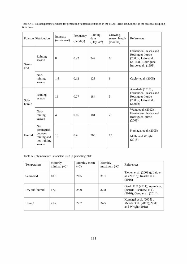
111
Table A 5. Poisson parameters used for generating rainfall distribution in the PLANTHeR-HGS model at the seasonal coupling
time scale
Poisson Distribution Intensity
(mm/event)
Frequency
(per day)
Raining
days
(Day.yr-1)
Growing
season length
(months)
References
Semi-
arid
Raining
season 8
0.22
242 6
Fernandez-Illescas and
Rodriguez-Iturbe
(2003) ; Laio et al.
(2011a) ; Rodriguez-
Iturbe et al., (1999)
Non-
raining
season
1.6 0.12 123 6 Caylor et al. (2005)
Sub-
humid
Raining
season
13 0.27 184 5
Ayanlade (2018) ;
Fernandez-Illescas and
Rodriguez-Iturbe
(2003) ; Laio et al.,
(2001b)
Non-
raining
season
4
0.16
181 7
Wang et al. (2012) ;
Fernandez-Illescas and
Rodriguez-Iturbe
(2003)
Humid
No
distinguish
between
raining and
non-raining
season
16 0.4 365 12
Kumagai et al. (2005)
Malhi and Wright
(2018)
Table A 6. Temperature Parameters used in generating PET
Temperature Monthly
minimal (◦C)
Monthly mean
(◦C)
Monthly
maximum (◦C) References
Semi-arid 10.6 20.5 31.1
Tietjen et al. (2009a); Laio et
al. (2001b); Kaseke et al.
(2016)
Dry sub-humid 17.0 25.0 32.8
Ogolo E.O (2011); Ayanlade,
(2018); Rishmawi et al.
(2016); Geng et al. (2014)
Humid 21.2 27.7 34.5
Kumagai et al. (2005) ;
Meada et al. (2017); Malhi
and Wright (2018)

112
Table A 7. Time step output in the HGS model for different climate scenarios at the seasonal coupling time scale
Output time
Season 1
(days of the
year)
Season 2
(days of the
year)
Season 3
(days of the
year)
Season 4
(days of the
year)
Growing
season length
Semi-arid 61 181 61 62 6 months
Dry sub-humid 59 153 91 62 5 months
Humid 90 91 92 92 12 months
Table A 8. The HGS model steady state time and the PLANTHeR model spin up time for each climate scenario
Parameters LAI (m2/m2) Root depth (m) References
Semi-arid 1.5 5 Sprintsin et al. (2011) ; Canadell et al. (1996)
Asner et al. (2003) ; Caylor et al 2005
Sub-humid 1.7 3.5 Asner et al. (2003) ; Canadell et al. (1996)
Rishmawi et al 2016
Humid 5 2 Asner et al. (2003), Canadell et al. (1996)
Kumagai et al (2005)
4. Figures
Fig. A1. Compare the reduction function between original critical potentials (dash line, Table A1, Herberich et al., 2017) and
in this study (solid line, Table A2)

113
Fig. A2. Shannon index and PFT richness of 20 replications over 1000 years simulated with three types of soil matric potentials,
namely spatiotemporal heterogenous smp (the red color), spatial heterogeneous smp scenarios (the black color) as well as the
homogeneous smp scenarios (the blue color).
Fig. A3. Soil matric potential heterogeneity in spatiotemporal heterogeneous smp scenarios (the red color), in spatial
heterogeneous smp scenarios (the black color) as well as in homogeneous smp scenarios (the blue color).

114
Fig. A4. Comparison of mean LAI and mean root depth between the PLANTHeR-HGS model (mean ± 95%CI, mean± standard
deviation) and the uncoupled HGS of 20 replicates. CI=confidence intervals. CI indicated by light blue shadow, standard
deviation indicated by light orange shadow for LAI and by light grey shadow for root depth. Mean values simulated with the
PLANTHeR-HGS model of 20 independent replicates indicated by the solid red (LAI) and black lines (root depth). Values
simulated with the uncoupled HGS model indicated by the black dash lines for both LAI and root depth.

115
Fig. A5. Plant composition simulated with the spatiotemporal heterogeneous soil matric potential (the PLANTHeR-HGS
model) of 20 independent replicates (mean ± standard deviation).

116
Fig. A6. Plant composition simulated with the spatial heterogeneous soil matric potential (the uncoupled PLANTHeR model)
of 20 independent replicates (mean ± standard deviation).
Fig. A7. Plant composition simulated with the homogeneous soil matric potential (the uncoupled PLANTHeR model) of 20
independent replicates (mean ± standard deviation).

117
Fig. A8. Scaling factor of LAI variation over one year for different types of plants
Fig. A 9.The soil matric potential used in humid climate for the PLANTHeR-HGS model and the uncoupled PLANTHeR
model
0.00
0.20
0.40
0.60
0.80
1.00
1.20
0 50 100 150 200 250 300 350 400
Sca
ling f
acto
r
Time (days)
annual annual and perennial perennial

118
Fig. A 10. The soil matric potential used in sub-humid climate for the PLANTHeR-HGS model and the uncoupled PLANTHeR
model
Fig. A 11. The soil matric potential used in semi-arid climate for the PLANTHeR-HGS model and the uncoupled PLANTHeR
model

119
Fig. A12. Mean soil matric potential used in the spatiotemporal heterogeneous smp (the PLANTHeR-HGS model) simulations
(a), and in the spatial heterogeneous smp as well as in the homogeneous smp simulations (b) (the uncoupled PLANTHeR
model) under humid (the blue color), sub-humid (the green color) and semi-arid (the red color) climate scenarios.
Fig. A13. Comparison of the mean transpiration, mean evaporation, mean surface runoff, and the mean change of soil water
storage of 1000 years simulated between the PLANTHeR-HGS model (mean ± 95% CI of 5 replicates) and the uncoupled HGS
model in the humid climate (a), the sub-humid climate (b) and the semi-arid climate (c).Values simulated with the PLANTHeR-
HGS model of 5 independent replicates are indicated by the blue, green and red color, respectively. Values simulated with the
uncoupled HGS model indicated by the black color.

120
Fig. A14. Mean Shannon index and PFT richness (Mean ± 95CI) from year 200 to year 1000 of 5 replications simulated with
the spatiotemporal heterogeneous smp, the spatial heterogeneous smp and the homogeneous smp in the humid climate (a), in
the sub-humid climate(b) and in the semi-arid climate (c). P value here indicate the significance of a one-way ANOVA test of
differences of different variables (diversity, richness, aboveground biomass) simulated among the spatiotemporal
heterogeneous smp (the PLANTHeR-HGS model), the homogeneous smp and the spatial heterogeneous smp (the uncoupled
PLANTHeR model). P<0.05*, p<0.01**, p<0.001***


