
Dynamic Equations on Time Scales - University of …apeterson1/sample_book.pdf · ·...
69
Dynamic Equations on Time Scales An Introduction with Applications Martin Bohner Allan Peterson PRELIMINARY FINAL Version from May 4, 2001 Author address: Department of Mathematics, University of Missouri–Rolla, Rolla, Missouri 65409-0020 E-mail address : [email protected] URL: http://www.umr.edu/~bohner Department of Mathematics, University of Nebraska–Lincoln, Lin- coln, Nebraska 68588-0323 E-mail address : [email protected] URL: http://www.math.unl.edu/~apeterso
Transcript of Dynamic Equations on Time Scales - University of …apeterson1/sample_book.pdf · ·...

Dynamic Equations on Time Scales
An Introduction with Applications
Martin Bohner
Allan Peterson
PRELIMINARY FINAL Version from May 4, 2001
Author address:
Department of Mathematics, University of Missouri–Rolla, Rolla,
Missouri 65409-0020
E-mail address: [email protected]
URL: http://www.umr.edu/~bohner
Department of Mathematics, University of Nebraska–Lincoln, Lin-
coln, Nebraska 68588-0323
E-mail address: [email protected]
URL: http://www.math.unl.edu/~apeterso

Dedicated to
Monika and Albert
and
Tina, Carla, David, and Carrie
with
{
(
sin(2t)sin(3t)
)
: 0 ≤ t ≤ π}
.
Contents
Preface v
Chapter 1. The Time Scales Calculus 1
1.1. Basic Definitions 1
1.2. Differentiation 5
1.3. Examples and Applications 13
1.4. Integration 22
1.5. Chain Rules 31
1.6. Polynomials 37
1.7. Further Basic Results 46
1.8. Notes and References 49
Chapter 2. First Order Linear Equations 51
2.1. Hilger’s Complex Plane 51
2.2. The Exponential Function 58
2.3. Examples of Exponential Functions 69
2.4. Initial Value Problems 75
2.5. Notes and References 78
Chapter 3. Second Order Linear Equations 81
3.1. Wronskians 81
3.2. Hyperbolic and Trigonometric Functions 87
3.3. Reduction of Order 93
3.4. Method of Factoring 96
3.5. Nonconstant Coefficients 98
3.6. Hyperbolic and Trigonometric Functions II 101
3.7. Euler–Cauchy Equations 108
3.8. Variation of Parameters 113
3.9. Annihilator Method 116
3.10. Laplace Transform 118
3.11. Notes and References 133
Chapter 4. Self-Adjoint Equations 135
4.1. Preliminaries and Examples 135
iii

iv CONTENTS
4.2. The Riccati Equation 147
4.3. Disconjugacy 156
4.4. Boundary Value Problems and Green’s Function 164
4.5. Eigenvalue Problems 177
4.6. Notes and References 186
Chapter 5. Linear Systems and Higher Order Equations 189
5.1. Regressive Matrices 189
5.2. Constant Coefficients 198
5.3. Self-Adjoint Matrix Equations 204
5.4. Asymptotic Behavior of Solutions 224
5.5. Higher Order Linear Dynamic Equations 238
5.6. Notes and References 253
Chapter 6. Dynamic Inequalities 255
6.1. Gronwall’s Inequality 255
6.2. Holder’s and Minkowski’s Inequalities 259
6.3. Jensen’s Inequality 261
6.4. Opial Inequalities 263
6.5. Lyapunov Inequalities 271
6.6. Upper and Lower Solutions 279
6.7. Notes and References 287
Chapter 7. Linear Symplectic Dynamic Systems 289
7.1. Symplectic Systems and Special Cases 289
7.2. Conjoined Bases 299
7.3. Transformation Theory and Trigonometric Systems 306
7.4. Notes and References 314
Chapter 8. Extensions 315
8.1. Measure Chains 315
8.2. Nonlinear Theory 321
8.3. Alpha Derivatives 326
8.4. Nabla Derivatives 331
8.5. Notes and References 336
Solutions to Selected Problems 337
Bibliography 343
Index 355

Preface
On becoming familiar with difference equations and their close re-lation to differential equations, I was in hopes that the theory ofdifference equations could be brought completely abreast with thatfor ordinary differential equations.
[Hugh L. Turrittin, “My Mathematical Expectations”,Springer Lecture Notes 312 (page 10), 1973]
A major task of mathematics today is to harmonize the continuousand the discrete, to include them in one comprehensive mathematics,and to eliminate obscurity from both.
[E. T. Bell, “Men of Mathematics”,Simon and Schuster, New York (page 13/14), 1937]
The theory of time scales, which has recently received a lot of attention, wasintroduced by Stefan Hilger in his PhD thesis [159] in 1988 (supervised by BerndAulbach) in order to unify continuous and discrete analysis. This book is an intro-duction to the study of dynamic equations on time scales. Many results concerningdifferential equations carry over quite easily to corresponding results for differenceequations, while other results seem to be completely different in nature from theircontinuous counterparts. The study of dynamic equations on time scales revealssuch discrepancies, and helps avoid proving results twice, once for differential equa-tions and once for difference equations. The general idea is to prove a result for adynamic equation where the domain of the unknown function is a so-called timescale, which is an arbitrary closed subset of the reals. By choosing the time scaleto be the set of real numbers, the general result yields a result concerning an ordi-nary differential equation as studied in a first course in differential equations, andby choosing the time scale to be the set of integers, the same general result yieldsa result for difference equations. However, since there are many other time scalesthan just the set of real numbers or the set of integers, one has a much more generalresult. We may summarize the above and state that
Unification and Extension
are the two main features of the time scales calculus.
The time scales calculus has a tremendous potential for applications. For exam-ple, it can model insect populations that are continuous while in season (and mayfollow a difference scheme with variable step-size), die out in (say) winter, whiletheir eggs are incubating or dormant, and then hatch in a new season, giving riseto a nonoverlapping population.
The audience for this book is as follows:
v

vi PREFACE
1. Most parts of this book are appropriate for students who have had a first coursein both calculus and linear algebra. Usually, a first course in differential equationsdoes not even consider the discrete case, which students encounter in numer-ous applications, for example in biology, engineering, economics, physics, neuralnetworks, social sciences and so on. A course taught out of this book would si-multaneously teach the continuous and the discrete theory, which would betterprepare students for these applications. The first four chapters can be used foran introductory course on time scales. They contain plenty of exercises, and weincluded many of the solutions at the end of the book. Altogether, this bookcontains 212 exercises, many of them consisting of several separate parts.
2. The last four chapters can be used for an advanced course on time scales at thebeginning graduate level. Also, a special topics course is appropriate. Thesechapters also contain many exercises, however, most of their answers are notincluded in the solutions section at the end of the book.
3. A third group of audience for this book might be graduate students who areinterested in the subject for a thesis project at the masters or doctoral level.Some of the exercises describe open problems that can be used as a starting pointfor such a project. The “Notes and References” sections at the end of each chapteralso point out directions of further possible research.
4. Finally, researchers with a knowledge of differential or difference equations, whowant a rather complete introduction into the time scales calculus without goingthrough all the current literature, may also find this book very useful.
Most of the results given in this book have recently been investigated by StefanHilger and by the authors of this book (together with their research collaboratorsR. P. Agarwal, C. Ahlbrandt, E. Akın, S. Clark, O. Dosly, P. Eloe, L. Erbe, B. Kay-makcalan, D. Lutz, and R. Mathsen). Other results presented or results relatedto the presented ones have been obtained by D. Anderson, F. Atıcı, B. Aulbach,J. Davis, G. Guseinov, J. Henderson, R. Hilscher, S. Keller, V. Lakshmikantham,C. Potzsche, Z. Pospısil, S. Siegmund, and S. Sivasundaram. Many of these re-sults are presented in this book at a level that will be easy for an undergraduatemathematics student to understand.
In Chapter 1 the calculus on time scales as developed in [160] by Stefan Hilger isintroduced. A time scale T is an arbitrary closed subset of the reals. For functionsf : T → R we introduce a derivative and an integral. Fundamental results, e.g.,the product rule and the quotient rule, are presented. Further results concerningdifferentiability and integrability, which have been previously unpublished but areeasy to derive, are given as they are needed in the remaining parts of the book.Important examples of time scales, which we will consider frequently throughoutthe book, are given in this chapter. Such examples contain of course R (the setof all real numbers, which gives rise to differential equations) and Z (the set of allintegers, which gives rise to difference equations), but also the set of all integermultiples of a number h > 0 and the set of all integer powers of a number q > 1,including 0 (this time scale gives rise to so-called q-difference equations, see e.g.,[58, 247, 253]). Other examples are sets of disjoint closed intervals (which haveapplications e.g., in population dynamics) or even “exotic” time scales such as theCantor set. After discussing these examples, we also derive analogues of the chainrule. Taylor’s formula is presented, which is helpful in the study of boundary valueproblems.

PREFACE vii
In Chapter 2 we introduce the Hilger complex plane, following closely StefanHilger’s paper [164]. We use the so-called cylinder transformation to introduce theexponential function on time scales. This exponential function is then shown tosatisfy an initial value problem involving a first order linear dynamic equation. Wederive many properties of the exponential function and use it to solve all initial valueproblems involving first order linear dynamic equations. For the nonhomogeneouscases we utilize a variation of constants technique.
Next, we consider second order linear dynamic equations in Chapter 3. Again,there are several kinds of second order linear homogeneous equations, which wesolve (in the constant coefficient case) using hyperbolic and trigonometric functions.Wronskian determinants are introduced and Abel’s theorem is used to develop areduction of order technique to find a second solution in case one solution is alreadyknown. Certain dynamic equations of second order with nonconstant coefficients(e.g., the Euler–Cauchy equation) are also considered. We also present a variationof constants formula that helps in solving nonhomogeneous second order linear dy-namic equations. The Laplace transformation on a general time scale is introducedand many of its properties are derived.
Next, in Chapter 4, we study self-adjoint dynamic equations on time scales. Suchequations have been well studied in the continuous case (where they are also calledSturm–Liouville equations) and in the discrete case (where they are called Sturm–Liouville difference equations). In this chapter we only consider such equations ofsecond order. We investigate disconjugacy of self-adjoint equations and use thecorresponding Green’s function to study boundary value problems. Also the theoryof Riccati equations is developed in the general setting of time scales, and we presenta characterization of disconjugacy in terms of a certain quadratic functional. Ananalogue of the classical Prufer transformation, which has proved to be a usefultool in oscillation theory of Sturm–Liouville equations, is given as well. In the lastsection, we examine eigenvalue problems on time scales. For the case of separatedboundary conditions we present an oscillation result on the number of zeros ofthe kth eigenfunction. Such a result goes back to Sturm in the continuous case,and its discrete counterpart is contained in the book by Kelley and Peterson [191,Theorem 7.6]. Further results on eigenvalue problems contain a comparison theoremand Rayleigh’s principle.
Chapter 5 is concerned with linear systems of dynamic equations on a timescale. Uniqueness and existence theorems are presented, and the matrix exponentialon a time scale is introduced. We also examine fundamental systems and theirWronskian determinants and give a variation of constants formula. The case ofconstant coefficient matrices is also investigated, and a Putzer algorithm from [31]is presented. This chapter contains a section on self-adjoint vector equations. Suchequations are a special case of symplectic systems as discussed in Chapter 7. Theyare closely connected to certain matrix Riccati equations, and in this section we alsodiscuss oscillation results for those systems. Further results contain a discussion onasymptotic behavior of solutions of linear systems of dynamic equations. Relatedresults are time scales versions of Levinson’s perturbation lemma and the Hartman–Wintner theorem. Finally we study higher order linear dynamic equations on a timescale. We give conditions that imply that corresponding initial value problems haveunique solutions. Abel’s formula is given, and the notion of a generalized zero of asolution is introduced.
viii PREFACE
Chapter 6 is concerned with dynamic inequalities on time scales. Analoguesof Gronwall’s inequality, Holder’s inequality, and Jensen’s inequality are presented.We also derive Opial’s inequality and point out its applications in the study of initialor boundary value problems. Opial inequalities have proved to be a useful tool indifferential equations and in difference equations, and in fact there is an entire book[19] devoted to them. Next, we prove Lyapunov’s inequality for Sturm–Liouvilleequations of second order with positive coefficients. It can be used to give sufficientconditions for disconjugacy. We also offer an extension of Lyapunov’s inequalityto the case of linear Hamiltonian dynamic systems. Further results in this sectionconcern upper and lower solutions of boundary value problems and are containedin the article [32] by Akın.
In Chapter 7 we consider linear symplectic dynamic systems on time scales.This is a very general class of systems that contains for example linear Hamilton-ian dynamic systems which in turn contain Sturm–Liouville dynamic equations ofhigher order (and hence of course also of order two) and self-adjoint vector dynamicequations. We derive a Wronskian identity for such systems as well as a close con-nection to certain matrix Riccati dynamic equations. Disconjugacy of symplecticsystems is introduced as well. Some of the results in this chapter are due to RomanHilscher, who considered Hamiltonian systems on time scales in [166, 167, 168].Other results are contained in a paper by Ondrej Dosly and Roman Hilscher [121].
Chapter 8 contains several possible extensions of the time scales calculus. Inthe first section we present an introduction to the concept of measure chains asintroduced by Stefan Hilger in [159]. The second section contains the proofs of themain local and global existence theorems, that are needed throughout the book.Another extension, which is considered in this last chapter, concerns alpha deriva-tives. The time scales calculus as presented in this book is a special case of thisconcept.
Parts or earlier versions of this book have been proofread by D. Anderson,R. Avery, R. Chiquet, C. J. Chyan, L. Cole, J. Davis, L. Erbe, K. Fick, J. Hen-derson, J. Hoffacker, K. Howard, N. Hummel, B. Karna, R. Mathsen, K. Messer,A. Rosidian, P. Singh, and W. Yin. In particular, we would like to thank ElvanAkın, Roman Hilscher, Billur Kaymakcalan, and Stefan Siegmund for proofreadingthe entire manuscript. Finally, we wish to express our appreciation to “BirkhauserBoston”, in particular to Ann Kostant, for their accomplished handling of thismanuscript.
Martin Bohner and Allan Peterson

CHAPTER 1
The Time Scales Calculus
1.1. Basic Definitions
A time scale (which is a special case of a measure chain, see Chapter 8) is anarbitrary nonempty closed subset of the real numbers. Thus
R, Z, N, N0,
i.e., the real numbers, the integers, the natural numbers, and the nonnegativeintegers are examples of time scales, as are
[0, 1] ∪ [2, 3], [0, 1] ∪ N, and the Cantor set,
while
Q, R \Q, C, (0, 1),
i.e., the rational numbers, the irrational numbers, the complex numbers, and theopen interval between 0 and 1, are not time scales. Throughout this book we willdenote a time scale by the symbol T. We assume throughout that a time scale T
has the topology that it inherits from the real numbers with the standard topology.
The calculus of time scales was initiated by Stefan Hilger in his PhD thesis [159]in order to create a theory that can unify discrete and continuous analysis. Indeed,below we will introduce the delta derivative f∆ for a function f defined on T, andit turns out that
(i) f∆ = f ′ is the usual derivative if T = R and(ii) f∆ = ∆f is the usual forward difference operator if T = Z.
In this section we introduce the basic notions connected to time scales anddifferentiability of functions on them, and we offer the above two cases as examples.However, the general theory is of course applicable to many more time scales T,and we will give some examples of such time scales in Section 1.3 and many moreexamples throughout the rest of this book. Let us start by defining the forwardand backward jump operators.
Definition 1.1. Let T be a time scale. For t ∈ T we define the forward jump
operator σ : T → T by
σ(t) := inf{s ∈ T : s > t},while the backward jump operator ρ : T → T is defined by
ρ(t) := sup{s ∈ T : s < t}.In this definition we put inf ∅ = sup T (i.e., σ(t) = t if T has a maximum t) andsup ∅ = inf T (i.e., ρ(t) = t if T has a minimum t), where ∅ denotes the emptyset. If σ(t) > t, we say that t is right-scattered, while if ρ(t) < t we say that t isleft-scattered. Points that are right-scattered and left-scattered at the same time
1

2 1. THE TIME SCALES CALCULUS
Table 1.1. Classification of Points
t right-scattered t < σ(t)
t right-dense t = σ(t)
t left-scattered ρ(t) < t
t left-dense ρ(t) = t
t isolated ρ(t) < t < σ(t)
t dense ρ(t) = t = σ(t)
Figure 1.1. Classifications of Points
..........................................................................................................................................................................................................................................................................................................................................................................................................................................................r
t1
t1 is left-dense and right-dense
.....................................................................................................................................................................................................................................
rr
t2
t2 is left-dense and right-scattered
......................................................................................................................................................................................................................
.......
.......
.r r
t3
t3 is left-scattered and right-dense
.......
.......
.rr r
t4
t4 is left-scattered and right-scattered
(t1 is dense and t4 is isolated)
are called isolated. Also, if t < sup T and σ(t) = t, then t is called right-dense, andif t > inf T and ρ(t) = t, then t is called left-dense. Points that are right-denseand left-dense at the same time are called dense. Finally, the graininess function
µ : T → [0,∞) is defined byµ(t) := σ(t)− t.
See Table 1.1 for a classification and Figure 1.1 for a schematic classification ofpoints in T. Note that in the definition above both σ(t) and ρ(t) are in T whent ∈ T. This is because of our assumption that T is a closed subset of R. We alsoneed below the set Tκ which is derived from the time scale T as follows: If T has aleft-scattered maximum m, then Tκ = T− {m}. Otherwise, Tκ = T. In summary,
Tκ =
{
T \ (ρ(sup T), sup T] if sup T < ∞T if sup T = ∞.
Finally, if f : T → R is a function, then we define the function fσ : T → R by
fσ(t) = f(σ(t)) for all t ∈ T,
i.e., fσ = f ◦ σ.

1.1. BASIC DEFINITIONS 3
Example 1.2. Let us briefly consider the two examples T = R and T = Z.
(i) If T = R, then we have for any t ∈ R
σ(t) = inf{s ∈ R : s > t} = inf(t,∞) = t
and similarly ρ(t) = t. Hence every point t ∈ R is dense. The graininessfunction µ turns out to be
µ(t) ≡ 0 for all t ∈ T.
(ii) If T = Z, then we have for any t ∈ Z
σ(t) = inf{s ∈ Z : s > t} = inf{t + 1, t + 2, t + 3, . . . } = t + 1
and similarly ρ(t) = t−1. Hence every point t ∈ Z is isolated. The graininessfunction µ in this case is
µ(t) ≡ 1 for all t ∈ T.
For the two cases discussed above, the graininess function is a constant function.We will see below that the graininess function plays a central role in the analysison time scales. For the general case, many formulae will have some term containingthe factor µ(t). This term is there in case T = Z since µ(t) ≡ 1. However, for thecase T = R this term disappears since µ(t) ≡ 0 in this case. In various cases thisfact is the reason for certain differences between the continuous and the discretecase. One of the many examples of this that we will see later is the so-called scalarRiccati equation on a general time scale T (see formula (4.18))
z∆ + q(t) +z2
p(t) + µ(t)z= 0.
Note that if T = R, then we get the well-known Riccati differential equation
z′ + q(t) +1
p(t)z2 = 0,
and if T = Z, then we get the Riccati difference equation (see [191, Chapter 6])
∆z + q(t) +z2
p(t) + z= 0.
Of course, for the case of a general time scale, the graininess function might verywell be a function of t ∈ T, as the reader can verify in the next exercise. For moresuch examples we refer to Section 1.3.
Exercise 1.3. For each of the following time scales T, find σ, ρ, and µ, and classifyeach point t ∈ T as left-dense, left-scattered, right-dense, or right-scattered:
(i) T = {2n : n ∈ Z} ∪ {0};(ii) T =
{
1n
: n ∈ N}
∪ {0};(iii) T =
{
n2 : n ∈ N0
}
;
(iv) T = {√n : n ∈ N0};(v) T = { 3
√n : n ∈ N0}.
Exercise 1.4. Give examples of time scales T and points t ∈ T such that thefollowing equations are not true. Also determine the conditions on t under whichthose equations are true:
(i) σ(ρ(t)) = t;(ii) ρ(σ(t)) = t.
4 1. THE TIME SCALES CALCULUS
Exercise 1.5. Is σ : T → T one-to-one? Is it onto? If it is not onto, determine therange σ(T) of σ. How about ρ : T → T? This exercise was suggested by RomanHilscher.
Exercise 1.6. If T consists of finitely many points, calculate∑
t∈Tµ(t).
Throughout this book we make the blanket assumption that a and b are pointsin T. Often we assume a ≤ b. We then define the interval [a, b] in T by
[a, b] := {t ∈ T : a ≤ t ≤ b} .
Open intervals and half-open intervals etc. are defined accordingly. Note that[a, b]κ = [a, b] if b is left-dense and [a, b]κ = [a, b) = [a, ρ(b)] if b is left-scattered.
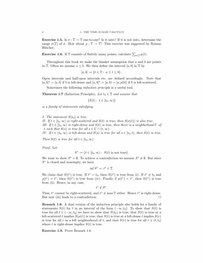
Sometimes the following induction principle is a useful tool.
Theorem 1.7 (Induction Principle). Let t0 ∈ T and assume that
{S(t) : t ∈ [t0,∞)}is a family of statements satisfying:
I. The statement S(t0) is true.
II. If t ∈ [t0,∞) is right-scattered and S(t) is true, then S(σ(t)) is also true.
III. If t ∈ [t0,∞) is right-dense and S(t) is true, then there is a neighborhood U of
t such that S(s) is true for all s ∈ U ∩ (t,∞).IV. If t ∈ (t0,∞) is left-dense and S(s) is true for all s ∈ [t0, t), then S(t) is true.
Then S(t) is true for all t ∈ [t0,∞).
Proof. Let
S∗ := {t ∈ [t0,∞) : S(t) is not true}.We want to show S∗ = ∅. To achieve a contradiction we assume S∗ 6= ∅. But sinceS∗ is closed and nonempty, we have
inf S∗ =: t∗ ∈ T.
We claim that S(t∗) is true. If t∗ = t0, then S(t∗) is true from (i). If t∗ 6= t0 andρ(t∗) = t∗, then S(t∗) is true from (iv). Finally if ρ(t∗) < t∗, then S(t∗) is truefrom (ii). Hence, in any case,
t∗ 6∈ S∗.
Thus, t∗ cannot be right-scattered, and t∗ 6= max T either. Hence t∗ is right-dense.But now (iii) leads to a contradiction.
Remark 1.8. A dual version of the induction principle also holds for a family ofstatements S(t) for t in an interval of the form (−∞, t0]: To show that S(t) istrue for all t ∈ (−∞, t0] we have to show that S(t0) is true, that S(t) is true at aleft-scattered t implies S(ρ(t)) is true, that S(t) is true at a left-dense t implies S(r)is true for all r in a left neighborhood of t, and that S(r) is true for all r ∈ (t, t0]where t is right-dense implies S(t) is true.
Exercise 1.9. Prove Remark 1.8.
1.2. DIFFERENTIATION 5
1.2. Differentiation
Now we consider a function f : T → R and define the so-called delta (or Hilger)derivative of f at a point t ∈ Tκ.
Definition 1.10. Assume f : T → R is a function and let t ∈ Tκ. Then we definef∆(t) to be the number (provided it exists) with the property that given any ε > 0,there is a neighborhood U of t (i.e., U = (t− δ, t + δ)∩T for some δ > 0) such that
∣
∣[f(σ(t))− f(s)]− f∆(t)[σ(t)− s]∣
∣ ≤ ε |σ(t)− s| for all s ∈ U.
We call f∆(t) the delta (or Hilger) derivative of f at t.
Moreover, we say that f is delta (or Hilger) differentiable (or in short: differen-
tiable) on Tκ provided f∆(t) exists for all t ∈ Tκ. The function f∆ : Tκ → R isthen called the (delta) derivative of f on Tκ.
Exercise 1.11. Prove that the delta derivative is well defined.
Exercise 1.12. Sometimes it is convenient to have f∆(t) also defined at a pointt ∈ T \ Tκ. At such a point we use the same definition as given in Definition 1.10.Prove that an f : T → R has any α ∈ R as its derivative at points t ∈ T \ Tκ.
Example 1.13. (i) If f : T → R is defined by f(t) = α for all t ∈ T, whereα ∈ R is constant, then f∆(t) ≡ 0. This is clear because for any ε > 0,
|f(σ(t))− f(s)− 0 · [σ(t)− s]| = |α− α| = 0 ≤ ε|σ(t)− s|holds for all s ∈ T.
(ii) If f : T → R is defined by f(t) = t for all t ∈ T, then f∆(t) ≡ 1. Thisfollows since for any ε > 0,
|f(σ(t))− f(s)− 1 · [σ(t)− s]| = |σ(t)− s− (σ(t)− s)| = 0 ≤ ε|σ(t)− s|holds for all s ∈ T.
Exercise 1.14. (i) Define f : T → R by f(t) = t2 for all t ∈ T. Find f∆.(ii) Define g by g(t) =
√t for all t ∈ T with t > 0. Find g∆.
Exercise 1.15. Using Definition 1.10 show that if t ∈ Tκ (t 6= min T) satisfiesρ(t) = t < σ(t), then the jump operator σ is not delta differentiable at t.
Some easy and useful relationships concerning the delta derivative are givennext.
Theorem 1.16. Assume f : T → R is a function and let t ∈ Tκ. Then we have
the following:
(i) If f is differentiable at t, then f is continuous at t.(ii) If f is continuous at t and t is right-scattered, then f is differentiable at t
with
f∆(t) =f(σ(t))− f(t)
µ(t).
(iii) If t is right-dense, then f is differentiable at t iff the limit
lims→t
f(t)− f(s)
t− s
6 1. THE TIME SCALES CALCULUS
exists as a finite number. In this case
f∆(t) = lims→t
f(t)− f(s)
t− s.
(iv) If f is differentiable at t, then
f(σ(t)) = f(t) + µ(t)f∆(t).
Proof. Part (i). Assume that f is differentiable at t. Let ε ∈ (0, 1). Define
ε∗ = ε[1 + |f∆(t)|+ 2µ(t)]−1.
Then ε∗ ∈ (0, 1). By Definition 1.10 there exists a neighborhood U of t such that
|f(σ(t))− f(s)− [σ(t)− s]f∆(t)| ≤ ε∗|σ(t)− s| for all s ∈ U.
Therefore we have for all s ∈ U ∩ (t− ε∗, t + ε∗)
|f(t)− f(s)| =∣
∣{f(σ(t))− f(s)− f∆(t)[σ(t)− s]}−{f(σ(t))− f(t)− µ(t)f∆(t)}+ (t− s)f∆(t)
∣
∣
≤ ε∗|σ(t)− s|+ ε∗µ(t) + |t− s||f∆(t)|≤ ε∗[µ(t) + |t− s|+ µ(t) + |f∆(t)|]< ε∗[1 + |f∆(t)|+ 2µ(t)]
= ε.
It follows that f is continuous at t.
Part (ii). Assume f is continuous at t and t is right-scattered. By continuity
lims→t
f(σ(t))− f(s)
σ(t)− s=
f(σ(t))− f(t)
σ(t)− t=
f(σ(t))− f(t)
µ(t).
Hence, given ε > 0, there is a neighborhood U of t such that∣
∣
∣
∣
f(σ(t))− f(s)
σ(t)− s− f(σ(t))− f(t)
µ(t)
∣
∣
∣
∣
≤ ε
for all s ∈ U . It follows that∣
∣
∣
∣
[f(σ(t))− f(s)]− f(σ(t))− f(t)
µ(t)[σ(t)− s]
∣
∣
∣
∣
≤ ε|σ(t)− s|
for all s ∈ U . Hence we get the desired result
f∆(t) =f(σ(t))− f(t)
µ(t).
Part (iii). Assume f is differentiable at t and t is right-dense. Let ε > 0 begiven. Since f is differentiable at t, there is a neighborhood U of t such that
|[f(σ(t))− f(s)]− f∆(t)[σ(t)− s]| ≤ ε|σ(t)− s|for all s ∈ U . Since σ(t) = t we have that
|[f(t)− f(s)]− f∆(t)(t− s)| ≤ ε|t− s|for all s ∈ U . It follows that
∣
∣
∣
∣
f(t)− f(s)
t− s− f∆(t)
∣
∣
∣
∣
≤ ε
1.2. DIFFERENTIATION 7
for all s ∈ U , s 6= t. Therefore we get the desired result
f∆(t) = lims→t
f(t)− f(s)
t− s.
The remaining part of the proof of part (iii) is Exercise 1.17.
Part (iv). If σ(t) = t, then µ(t) = 0 and we have that
f(σ(t)) = f(t) = f(t) + µ(t)f∆(t).
On the other hand if σ(t) > t, then by (ii)
f(σ(t)) = f(t) + µ(t) · f(σ(t))− f(t)
µ(t)
= f(t) + µ(t)f∆(t),
and the proof of part (iv) is complete.
Exercise 1.17. Prove the converse part of the statement in Theorem 1.16 (iii):Let t ∈ Tκ be right-dense. If
lims→t
f(t)− f(s)
t− sexists as a finite number, then f is differentiable at t and
f∆(t) = lims→t
f(t)− f(s)
t− s.
Example 1.18. Again we consider the two cases T = R and T = Z.
(i) If T = R, then Theorem 1.16 (iii) yields that f : R → R is delta differentiableat t ∈ R iff
f ′(t) = lims→t
f(t)− f(s)
t− sexists,
i.e., iff f is differentiable (in the ordinary sense) at t. In this case we thenhave
f∆(t) = lims→t
f(t)− f(s)
t− s= f ′(t)
by Theorem 1.16 (iii).(ii) If T = Z, then Theorem 1.16 (ii) yields that f : Z → R is delta differentiable
at t ∈ Z with
f∆(t) =f(σ(t))− f(t)
µ(t)=
f(t + 1)− f(t)
1= f(t + 1)− f(t) = ∆f(t),
where ∆ is the usual forward difference operator defined by the last equationabove.
Exercise 1.19. For each of the following functions f : T → R, use Theorem 1.16to find f∆. Write your final answer in terms of t ∈ T:
(i) f(t) = σ(t) for t ∈ T := { 1n
: n ∈ N} ∪ {0};(ii) f(t) = t2 for t ∈ T := N
120 := {√n : n ∈ N0};
(iii) f(t) = t2 for t ∈ T := {n2 : n ∈ N0};
(iv) f(t) = t3 for t ∈ T := N130 := { 3
√n : n ∈ N0}.
Next, we would like to be able to find the derivatives of sums, products, andquotients of differentiable functions. This is possible according to the followingtheorem.

8 1. THE TIME SCALES CALCULUS
Theorem 1.20. Assume f, g : T → R are differentiable at t ∈ Tκ. Then:
(i) The sum f + g : T → R is differentiable at t with
(f + g)∆(t) = f∆(t) + g∆(t).
(ii) For any constant α, αf : T → R is differentiable at t with
(αf)∆(t) = αf∆(t).
(iii) The product fg : T → R is differentiable at t with
(fg)∆(t) = f∆(t)g(t) + f(σ(t))g∆(t) = f(t)g∆(t) + f∆(t)g(σ(t)).
(iv) If f(t)f(σ(t)) 6= 0, then 1f
is differentiable at t with
(
1
f
)∆
(t) = − f∆(t)
f(t)f(σ(t)).
(v) If g(t)g(σ(t)) 6= 0, then fg
is differentiable at t and
(
f
g
)∆
(t) =f∆(t)g(t)− f(t)g∆(t)
g(t)g(σ(t)).
Proof. Assume that f and g are delta differentiable at t ∈ Tκ.
Part (i). Let ε > 0. Then there exist neighborhoods U1 and U2 of t with
|f(σ(t))− f(s)− f∆(t)(σ(t)− s)| ≤ ε
2|σ(t)− s| for all s ∈ U1
and
|g(σ(t))− g(s)− g∆(t)(σ(t)− s)| ≤ ε
2|σ(t)− s| for all s ∈ U2.
Let U = U1 ∩ U2. Then we have for all s ∈ U
|(f + g)(σ(t))− (f + g)(s)− [f∆(t) + g∆(t)](σ(t)− s)|= |f(σ(t))− f(s)− f∆(t)(σ(t)− s) + g(σ(t))− g(s)− g∆(t)(σ(t)− s)|≤ |f(σ(t))− f(s)− f∆(t)(σ(t)− s)|+ |g(σ(t))− g(s)− g∆(t)(σ(t)− s)|≤ ε
2|σ(t)− s|+ ε
2|σ(t)− s|
= ε|σ(t)− s|.Therefore f + g is differentiable at t and (f + g)∆ = f∆ + g∆ holds at t.
Part (iii). Let ε ∈ (0, 1). Define ε∗ = ε[1 + |f(t)|+ |g(σ(t))|+ |g∆(t)|]−1. Thenε∗ ∈ (0, 1) and hence there exist neighborhoods U1, U2, and U3 of t such that
|f(σ(t))− f(s)− f∆(t)(σ(t)− s)| ≤ ε∗|σ(t)− s| for all s ∈ U1,
|g(σ(t))− g(s)− g∆(t)(σ(t)− s)| ≤ ε∗|σ(t)− s| for all s ∈ U2,
and (from Theorem 1.16 (i))
|f(t)− f(s)| ≤ ε∗ for all s ∈ U3.
1.2. DIFFERENTIATION 9
Put U = U1 ∩ U2 ∩ U3 and let s ∈ U . Then∣
∣(fg)(σ(t))− (fg)(s)− [f∆(t)g(σ(t)) + f(t)g∆(t)](σ(t)− s)∣
∣
=∣
∣[f(σ(t))− f(s)− f∆(t)(σ(t)− s)]g(σ(t))
+[g(σ(t))− g(s)− g∆(t)(σ(t)− s)]f(t)
+[g(σ(t))− g(s)− g∆(t)(σ(t)− s)][f(s)− f(t)]
+(σ(t)− s)g∆(t)[f(s)− f(t)]∣
∣
≤ ε∗|σ(t)− s||g(σ(t))|+ ε∗|σ(t)− s||f(t)|+ε∗ε∗|σ(t)− s|+ ε∗|σ(t)− s||g∆(t)|
= ε∗|σ(t)− s|[|g(σ(t))|+ |f(t)|+ ε∗ + |g∆(t)|]≤ ε∗|σ(t)− s|[1 + |f(t)|+ |g(σ(t))|+ |g∆(t)|]= ε|σ(t)− s|.
Thus (fg)∆ = f∆gσ + fg∆ holds at t. The other product rule in part (iii) of thistheorem follows from this last equation by interchanging the functions f and g.
For the quotient formula (v), we use (ii) and (iv) to calculate
(
f
g
)∆
(t) =
(
f · 1
g
)∆
(t)
= f(t)
(
1
g
)∆
(t) + f∆(t)1
g(σ(t))
= −f(t)g∆(t)
g(t)g(σ(t))+ f∆(t)
1
g(σ(t))
=f∆(t)g(t)− f(t)g∆(t)
g(t)g(σ(t)).
The reader is asked in Exercise 1.21 to prove (ii) and (iv).
Exercise 1.21. Prove parts (ii) and (iv) of Theorem 1.20.
Exercise 1.22. Prove that if x, y, and z are delta differentiable at t, then
(xyz)∆ = x∆yz + xσy∆z + xσyσz∆
holds at t. Write down the generalization of this formula for n functions.
Exercise 1.23. We have by Theorem 1.20 (iii)
(f2)∆ = (f · f)∆ = f∆f + fσf∆ = (f + fσ)f∆.(1.1)
Give the generalization of this formula for the derivative of the (n + 1)st power off , n ∈ N, i.e., for (fn+1)∆.
Theorem 1.24. Let α be constant and m ∈ N.
(i) For f defined by f(t) = (t− α)m we have
f∆(t) =
m−1∑
ν=0
(σ(t)− α)ν(t− α)m−1−ν .

10 1. THE TIME SCALES CALCULUS
(ii) For g defined by g(t) = 1(t−α)m we have
g∆(t) = −m−1∑
ν=0
1
(σ(t)− α)m−ν(t− α)ν+1,
provided (t− α)(σ(t)− α) 6= 0.
Proof. We will prove the first formula by induction. If m = 1, then f(t) = t − α,and clearly f∆(t) = 1 holds by Example 1.13 (i), (ii), and Theorem 1.20 (i). Nowwe assume that
f∆(t) =
m−1∑
ν=0
(σ(t)− α)ν(t− α)m−1−ν
holds for f(t) = (t − α)m and let F (t) = (t − α)m+1 = (t − α)f(t). We use theproduct rule (Theorem 1.20 (iii)) to obtain
F∆(t) = f(σ(t)) + (t− α)f∆(t)
= (σ(t)− α)m + (t− α)
m−1∑
ν=0
(σ(t)− α)ν(t− α)m−1−ν
= (σ(t)− α)m +m−1∑
ν=0
(σ(t)− α)ν(t− α)m−ν
=
m∑
ν=0
(σ(t)− α)ν(t− α)m−ν .
Hence, by mathematical induction, part (i) holds.
Next, for g(t) = 1(t−α)m = 1
f(t) we apply Theorem 1.20 (iv) to obtain
g∆(t) = − f∆(t)
f(t)fσ(t)
= −∑m−1
ν=0 (σ(t)− α)ν(t− α)m−1−ν
(t− α)m(σ(t)− α)m
= −m−1∑
ν=0
1
(t− α)ν+1(σ(t)− α)m−ν,
provided (t− α)(σ(t)− α) 6= 0.
Example 1.25. The derivative of t2 is
t + σ(t).
The derivative of 1/t is
− 1
tσ(t).
Exercise 1.26. Use Theorem 1.24 to find the derivatives in Exercise 1.19.
We define higher order derivatives of functions on time scales in the usual way.

1.2. DIFFERENTIATION 11
Definition 1.27. For a function f : T → R we shall talk about the sec-
ond derivative f∆∆ provided f∆ is differentiable on Tκ2
= (Tκ)κ with deriv-
ative f∆∆ = (f∆)∆ : Tκ2 → R. Similarly we define higher order derivativesf∆n
: Tκn → R. Finally, for t ∈ T, we denote σ2(t) = σ(σ(t)) and ρ2(t) = ρ(ρ(t)),and σn(t) and ρn(t) for n ∈ N are defined accordingly. For convenience we also put
ρ0(t) = σ0(t) = t, f∆0
= f, and Tκ0
= T.
Exercise 1.28. Find the second derivative of each of the functions given in Exercise1.19.
Exercise 1.29. Find the second derivative of f on an arbitrary time scale:
(i) f(t) ≡ 1;(ii) f(t) = t;(iii) f(t) = t2.
Exercise 1.30. For an arbitrary time scale, try to find a function f such thatf∆∆ = 1.
Example 1.31. In general, fg is not twice differentiable even if both f and g aretwice differentiable. We have
(fg)∆ = f∆g + fσg∆.
If f and g are twice differentiable and if fσ is differentiable, then
(fg)∆ = (f∆g + fσg∆)∆
= f∆∆g + f∆σ
g∆ + fσ∆
g∆ + fσσ
g∆∆
= f∆∆g + (f∆σ + fσ∆)g∆ + fσσg∆∆,
where we wrote f∆σ for f∆σ
etc.; we shall also use such notation in the sequel forcombinations of more than two “exponents” of the form ∆ or σ. The formula forthe nth derivative under certain conditions is given in the following result.
Theorem 1.32 (Leibniz Formula). Let S(n)k be the set consisting of all possible
strings of length n, containing exactly k times σ and n− k times ∆. If
fΛ exists for all Λ ∈ S(n)k ,
then
(fg)∆n
=
n∑
k=0
(
∑
Λ∈S(n)k
fΛ
)
g∆k
(1.2)
holds for all n ∈ N.
Proof. We will show (1.2) by induction. First, if n = 1, then (1.2) is true byExample 1.31. (With the convention that
∑
Λ∈∅ fΛ = f , (1.2) also holds for n = 0.)Next, we assume that (1.2) is true for n = m ∈ N. Then, using Theorem 1.20 (i)

12 1. THE TIME SCALES CALCULUS
and (iii), we obtain
(fg)∆m+1
=
m∑
k=0
(
∑
Λ∈S(m)k
fΛ
)
g∆k
∆
=
m∑
k=0
(
∑
Λ∈S(m)k
fΛ
)σ
g∆k+1
+
(
∑
Λ∈S(m)k
fΛ
)∆
g∆k
=m+1∑
k=1
(
∑
Λ∈S(m)k−1
fΛσ
)
g∆k
+m∑
k=0
(
∑
Λ∈S(m)k
fΛ∆
)
g∆k
=
(
∑
Λ∈S(m)m
fΛσ
)
g∆m+1
+
(
∑
Λ∈S(m)0
fΛ∆
)
g
+m∑
k=1
(
∑
Λ∈S(m)k−1
fΛσ +∑
Λ∈S(m)k
fΛ∆
)
g∆k
=
(
∑
Λ∈S(m+1)m+1
fΛ
)
g∆m+1
+
(
∑
Λ∈S(m+1)0
fΛ
)
g +
m∑
k=1
(
∑
Λ∈S(m+1)k
fΛ
)
g∆k
=
m+1∑
k=0
(
∑
Λ∈S(m+1)k
fΛ
)
g∆k
so that (1.2) holds for n = m+1. By the principle of mathematical induction, (1.2)holds for all n ∈ N0.
Example 1.33. If T = R, then
fΛ = f (n−k) for all Λ ∈ S(n)k ,
where f (n) denotes the nth (usual) derivative of f , if it exists, and since
∣
∣
∣S
(n)k
∣
∣
∣=
(
n
k
)
,
where |M | denotes the cardinality of the set M , we have
∑
Λ∈S(n)k
fΛ =∑
Λ∈S(n)k
f (n−k) = f (n−k)∑
Λ∈S(n)k
1 =
(
n
k
)
f (n−k)
and therefore
(fg)∆n
=
n∑
k=0
(
∑
Λ∈S(n)k
fΛ
)
g∆k
=
n∑
k=0
(
n
k
)
f (n−k)g(k).
This is the usual Leibniz formula from calculus.
Exercise 1.34. Use Theorem 1.32 to find ∆n(fg), i.e., (fg)∆n
if T = Z.

1.3. EXAMPLES AND APPLICATIONS 13
Exercise 1.35. Show that in general, even if both f∆σ
and fσ∆
exist,
f∆σ
= fσ∆
(1.3)
does not hold. Is (1.3) true for T = R and T = Z? Give a sufficient condition thatguarantees that (1.3) holds.
Exercise 1.36. Suppose µ is differentiable.
(i) If f∆σ
and fσ∆
both exist, give a formula that actually relates these twofunctions.
(ii) Give a similar formula that relates the functions (if they exist) fσσ∆, fσ∆σ,and f∆σσ.
(iii) Give the corresponding formula that relates the functions (if they exist)fσn∆ and f∆σn
, n ∈ N.
1.3. Examples and Applications
In this section we will discuss some examples of time scales that are consideredthroughout this book.
Example 1.37. Let h > 0 and
T = hZ = {hk : k ∈ Z} .
Then we have for t ∈ T
σ(t) = inf{s ∈ T : s > t} = inf{t + nh : n ∈ N} = t + h
and similarly ρ(t) = t− h. Hence every point t ∈ T is isolated and
µ(t) = σ(t)− t = t + h− t ≡ h for all t ∈ T
so that µ in this example is constant. For a function f : T → R we have
f∆(t) =f(σ(t))− f(t)
µ(t)=
f(t + h)− f(t)
hfor all t ∈ T.
Next,
f∆∆(t) =f∆(σ(t))− f∆(t)
µ(t)
=f∆(t + h)− f∆(t)
h
=f(t+2h)−f(t+h)
h− f(t+h)−f(t)
h
h
=f(t + 2h)− f(t + h)− f(t + h) + f(t)
h2
=f(t + 2h)− 2f(t + h) + f(t)
h2.
It would be too tedious to calculate f∆n
(t) in a similar way, so we consider anotherapproach. First, note that
σn(t) = t + nh and ρn(t) = t− nh for all n ∈ N0.
We now introduce an operator ∆h by
∆h =1
h(σ − I), I being the identity operator.
14 1. THE TIME SCALES CALCULUS
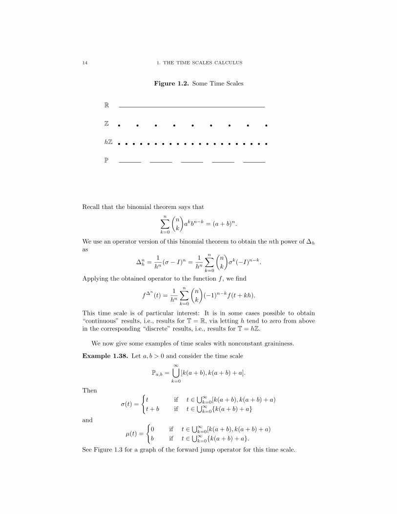
Figure 1.2. Some Time Scales
R ..........................................................................................................................................................................................................................................................................................................................................................................................................................................................................................................................................................................................
Z r r r r r r r r r
hZ r r r r r r r r r r r r r r r r r r r r r
P ...................................................................................... ...................................................................................... ...................................................................................... ...................................................................................... ......................................................................................
Recall that the binomial theorem says that
n∑
k=0
(
n
k
)
akbn−k = (a + b)n.
We use an operator version of this binomial theorem to obtain the nth power of ∆h
as
∆nh =
1
hn(σ − I)n =
1
hn
n∑
k=0
(
n
k
)
σk(−I)n−k.
Applying the obtained operator to the function f , we find
f∆n
(t) =1
hn
n∑
k=0
(
n
k
)
(−1)n−kf(t + kh).
This time scale is of particular interest: It is in some cases possible to obtain“continuous” results, i.e., results for T = R, via letting h tend to zero from abovein the corresponding “discrete” results, i.e., results for T = hZ.
We now give some examples of time scales with nonconstant graininess.
Example 1.38. Let a, b > 0 and consider the time scale
Pa,b =∞⋃
k=0
[k(a + b), k(a + b) + a].
Then
σ(t) =
{
t if t ∈ ⋃∞k=0[k(a + b), k(a + b) + a)
t + b if t ∈ ⋃∞k=0{k(a + b) + a}and
µ(t) =
{
0 if t ∈ ⋃∞k=0[k(a + b), k(a + b) + a)
b if t ∈ ⋃∞k=0{k(a + b) + a}.See Figure 1.3 for a graph of the forward jump operator for this time scale.
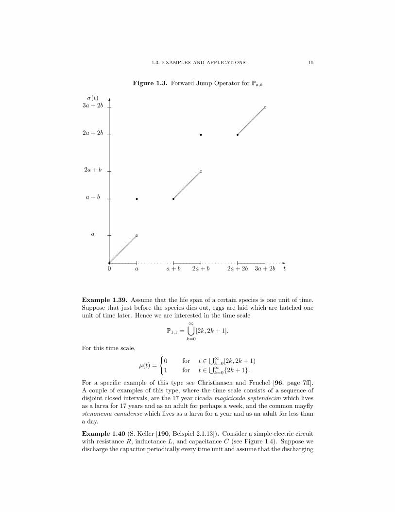
1.3. EXAMPLES AND APPLICATIONS 15
Figure 1.3. Forward Jump Operator for Pa,b
.......
.......
................
0 a...............
.......
.......
.
a + b 2a + b...............
.......
.......
.
2a + 2b 3a + 2b
6
...............a
...............a + b
...............2a + b
...............2a + 2b
...............3a + 2bσ(t)
.......................................................................................................................................................
.......................................................................................................................................................
.......................................................................................................................................................
r
r
b
r
r
b
r
b
-. . . . . . . . . . . . . . . . . . . . . . . . . . . . . . . . . . . . . . . . . . . . . . . . . . . . . . .
t
Example 1.39. Assume that the life span of a certain species is one unit of time.Suppose that just before the species dies out, eggs are laid which are hatched oneunit of time later. Hence we are interested in the time scale
P1,1 =
∞⋃
k=0
[2k, 2k + 1].
For this time scale,
µ(t) =
{
0 for t ∈ ⋃∞k=0[2k, 2k + 1)
1 for t ∈ ⋃∞k=0{2k + 1}.
For a specific example of this type see Christiansen and Fenchel [96, page 7ff].A couple of examples of this type, where the time scale consists of a sequence ofdisjoint closed intervals, are the 17 year cicada magicicada septendecim which livesas a larva for 17 years and as an adult for perhaps a week, and the common mayflystenonema canadense which lives as a larva for a year and as an adult for less thana day.
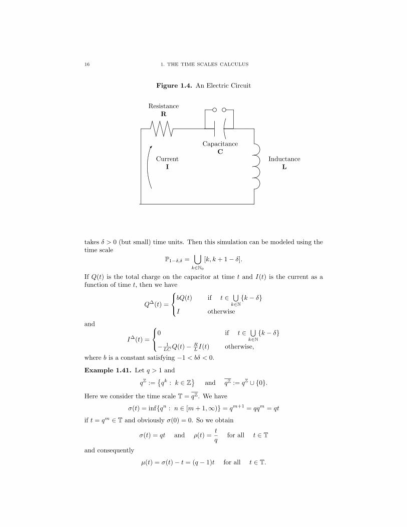
Example 1.40 (S. Keller [190, Beispiel 2.1.13]). Consider a simple electric circuitwith resistance R, inductance L, and capacitance C (see Figure 1.4). Suppose wedischarge the capacitor periodically every time unit and assume that the discharging
16 1. THE TIME SCALES CALCULUS
Figure 1.4. An Electric Circuit
........................................................................................................................................................................................................................................................................................................................................................................................................................................................................................................................................................................................................................................................................................................................................................................................................................................
.............................................................................................
......................................................................................................................
......................................................................................................................
..............................................................................................................................................................................................................................
.......
.......
.......
.......
.......
.......
.......
.......
.......
................................
.......
.......
.......
.......
.......
.......
.......
.......
..................................................................................................................................................................................................................................................................................
....................... ........
.....................................
.......
.......
.......
.......
.......
.......
.......
.......
.
........................................
.......
.......
.......
...................
.......................................................
.................... ............
............................................................... .....
......................................................
................ ......................................................
............................................................................................................................................................................
�
ResistanceR
CapacitanceC
InductanceL
CurrentI
takes δ > 0 (but small) time units. Then this simulation can be modeled using thetime scale
P1−δ,δ =⋃
k∈N0
[k, k + 1− δ].
If Q(t) is the total charge on the capacitor at time t and I(t) is the current as afunction of time t, then we have
Q∆(t) =
bQ(t) if t ∈ ⋃
k∈N
{k − δ}
I otherwise
and
I∆(t) =
0 if t ∈ ⋃
k∈N
{k − δ}
− 1LC
Q(t)− RL
I(t) otherwise,
where b is a constant satisfying −1 < bδ < 0.
Example 1.41. Let q > 1 and
qZ :={
qk : k ∈ Z}
and qZ := qZ ∪ {0}.
Here we consider the time scale T = qZ. We have
σ(t) = inf{qn : n ∈ [m + 1,∞)} = qm+1 = qqm = qt
if t = qm ∈ T and obviously σ(0) = 0. So we obtain
σ(t) = qt and ρ(t) =t
qfor all t ∈ T
and consequently
µ(t) = σ(t)− t = (q − 1)t for all t ∈ T.

1.3. EXAMPLES AND APPLICATIONS 17
Hence 0 is a right-dense minimum and every other point in T is isolated. For afunction f : T → R we have
f∆(t) =f(σ(t))− f(t)
µ(t)=
f(qt)− f(t)
(q − 1)tfor all t ∈ T \ {0}
and
f∆(0) = lims→0
f(0)− f(s)
0− s= lim
s→0
f(s)− f(0)
sprovided this limit exists. Now we calculate the second derivative of f at t 6= 0(refer to Definition 1.27 for how f∆∆ is defined) as
f∆∆(t) =f∆(σ(t))− f∆(t)
µ(t)
=f∆(qt)− f∆(t)
(q − 1)t
=
f(q2t)−f(qt)q(q−1)t − f(qt)−f(t)
(q−1)t
(q − 1)t
=f(q2t)− f(qt)− qf(qt) + qf(t)
q(q − 1)2t2
=f(q2t)− (q + 1)f(qt) + qf(t)
q(q − 1)2t2.
Notice that µ(t) = t above in the particular case q = 2.
Exercise 1.42. Let q > 1. For the time scale T = qZ, evaluate
(i) σ∆;(ii) µ∆.
Exercise 1.43. Find f∆3
for the time scale T = qZ. Find f∆4
and finally find aformula for f∆n
for any natural number n.
Example 1.44. Consider the time scale
T = N20 = {n2 : n ∈ N0}.
We have σ(n2) = (n + 1)2 for n ∈ N0 and
µ(n2) = σ(n2)− n2 = (n + 1)2 − n2 = 2n + 1.
Henceσ(t) = (
√t + 1)2 and µ(t) = 1 + 2
√t for t ∈ T.
Example 1.45. Let Hn be the so-called harmonic numbers
H0 = 0 and Hn =
n∑
k=1
1
kfor n ∈ N.
Consider the time scaleT = {Hn : n ∈ N0}.
We have σ(Hn) = Hn+1 for all n ∈ N0, ρ(Hn) = Hn−1 when n ∈ N, and ρ(H0) =H0. The graininess is given by
µ(Hn) = σ(Hn)−Hn = Hn+1 −Hn =1
n + 1

18 1. THE TIME SCALES CALCULUS
Table 1.2. Examples of Time Scales
T µ(t) σ(t) ρ(t)
R 0 t t
Z 1 t + 1 t− 1
hZ h t + h t− h
qN (q − 1)t qt tq
2N t 2t t2
N20 2
√t + 1 (
√t + 1)2 (
√t− 1)2
for all n ∈ N0. If f : T → R is a function, then
f∆(Hn) =f(Hn+1)− f(Hn)
µ(Hn)= (n + 1)∆f(Hn).
Example 1.46. We let {αn}n∈N0be a sequence of real numbers with αn > 0 for
all n ∈ N and put
tn =n−1∑
k=0
αk.
Consider the time scaleT = {tn : n ∈ N}
if∑∞
k=0 αk = ∞ orT = {tn : n ∈ N} ∪ {L}
if∑∞
k=0 αk = L converges. We have
σ(tn) = tn+1 and µ(tn) = αn
for all n ∈ N. For a function y : T → R we find
y∆(tn) =y(tn+1)− y(tn)
αn
=∆y(tn)
αn
for all n ∈ N.
We remark that using the harmonic series above corresponds to Example 1.45,while using the geometric series corresponds to Example 1.41.
Example 1.47 (The Cantor Set). Consider K0 = [0, 1]. We obtain a subset K1 ofK0 by removing the open “middle third” of K0, i.e., the open interval (1/3, 2/3),from K0. K2 is obtained by removing the two open middle thirds of K1, i.e., thetwo open intervals (1/9, 2/9) and (7/9, 8/9) from K1. Proceeding in this manner,we obtain a sequence {Kn}n∈N0
of subsets of [0, 1]. See Figure 1.5 for K0, K1, K2,and K3. The Cantor set C is now defined as
C =∞⋂
n=0
Kn
1.3. EXAMPLES AND APPLICATIONS 19
and hence is closed. Therefore T = C is a time scale. Each x ∈ [0, 1] can berepresented in its ternary expansion as
x =
∞∑
k=1
ak
3k, where ak ∈ {0, 1, 2} for each k ∈ N.
It is known that a number x is an element of C if and only if it can be representedby a ternary expansion, where the ak are either 0 or 2 (see e.g., [142, page 38]).Let L denote the set of all the left-hand end points of the open intervals removed,i.e.,
L =
{
m∑
k=1
ak
3k+
1
3m+1: m ∈ N and ak ∈ {0, 2} for all 1 ≤ k ≤ m
}
.
Then L ⊂ T. The set of all right-hand end points of the open intervals removed isgiven by
R =
{
m∑
k=1
ak
3k+
2
3m+1: m ∈ N and ak ∈ {0, 2} for all 1 ≤ k ≤ m
}
,
and we also have R ⊂ T. It follows that
σ(t) = t +1
3m+1whenever t =
m∑
k=1
ak
3k+
1
3m+1∈ L.
Each point t ∈ T \ L has other points of T in any neighborhood of t, and thereforesatisfies σ(t) = t. Altogether,
σ(t) =
{
t + 13m+1 if t =
∑mk=1
ak
3k + 13m+1 ∈ L
t if t ∈ T \ L
and similarly
ρ(t) =
{
t− 13m+1 if t =
∑mk=1
ak
3k + 23m+1 ∈ R
t if t ∈ T \R.
Now we obtain the graininess function µ of the Cantor set as
µ(t) =
{
13m+1 if t =
∑mk=1
ak
3k + 13m+1 ∈ L
0 if t ∈ T \ L.
Hence L consists of the right-scattered elements of T, and R consists of the left-scattered elements of T. Thus, T does not contain any isolated points.
We now discuss some examples for the time scale T = Z.
Definition 1.48. Let t ∈ C (i.e., t is a complex number) and k ∈ Z. The factorial
function t(k) is defined as follows:
(i) If k ∈ N, then
t(k) = t(t− 1) · · · (t− k + 1).
(ii) If k = 0, then
t(0) = 1.

20 1. THE TIME SCALES CALCULUS
Figure 1.5. The Cantor Set
................................................................................................................................................................................................................................................................................................................................................................................................................................................................................................................................................................................................................................................................................................................................................................................................. K0r
0
r
1
................................................................................................................................................................................................................................................................. ................................................................................................................................................................................................................................................................. K1r
0
r
13
r
23
r
1
...................................................................................... ...................................................................................... ...................................................................................... ...................................................................................... K2r
0
r
19
r
29
r
13
r
23
r
79
r
89
r
1
............................. ............................. ............................. ............................. ............................. ............................. ............................. ............................. K3r
0
r
127
r
227
r
19
r
29
r
727
r
827
r
13
r
23
r
1927
r
2027
r
79
r
89
r
2527
r
2627
r
1
(iii) If −k ∈ N, then
t(k) =1
(t + 1)(t + 2) · · · (t− k)
for t 6= −1,−2, · · · , k.
In general
t(k) :=Γ(t + 1)
Γ(t− k + 1)(1.4)
for all t, k ∈ C such that the right-hand side of (1.4) makes sense, where Γ is thegamma function. See [191] for some results concerning the gamma and factorialfunctions.
Exercise 1.49. Show that the general definition (1.4) of the factorial function t(k)
gives parts (i), (ii), and (iii) in Definition 1.48 as special cases.
Exercise 1.50. Show that for any constant c
u(t) = cat Γ(t− t1)Γ(t− t2) · · ·Γ(t− tn)
Γ(t− s1)Γ(t− s2) · · ·Γ(t− sm)
is a solution of the recurrence relation
u(t + 1) = a(t− t1)(t− t2) · · · (t− tn)
(t− s1)(t− s2) · · · (t− sm)u(t),
where a, t1, . . . , tn, s1, . . . , sm are real constants and n,m ∈ N. Use this to solvethe difference equations
(i) ∆u = 4t+6t2+5t+6u, where t ∈ N;
(ii) ∆u = 2t+52t+1u, where t ∈ N0.
Next we define a general binomial coefficient(
αβ
)
.
Definition 1.51. We define the binomial coefficient(
αβ
)
by(
α
β
)
=α(β)
Γ(β + 1)
1.3. EXAMPLES AND APPLICATIONS 21
for all α, β ∈ C such that the right-hand side of this equation makes sense.
Exercise 1.52. Assume α, k ∈ C and ∆ is differentiation with respect to t on thetime scale T = Z. Show that
(i)[
(t + α)(k)]∆
= k(t + α)(k−1);
(ii) (αt)∆ = (α− 1)αt;
(iii)(
tα
)∆=(
tα−1
)
.
Exercise 1.53. Prove the following well-known formula concerning binomial coef-ficients:
(
α
β
)
+
(
α
β + 1
)
=
(
α + 1
β + 1
)
.
Exercise 1.54. Introduce some of the above concepts for the time scale T = hZ
and prove some of the above results for this time scale.
We conclude this section by giving some examples concerning the jump operator.
Example 1.55 (σ is in general not continuous). In Figure 1.3 we already haveseen an example of a time scale T whose jump function σ : T → T is not continuousat points t ∈ T which are left-dense and right-scattered at the same time. Here wepresent another such example. This example is due to Douglas Anderson. Let
T = {tn = −1/n : n ∈ N} ∪ N0.
Then
σ(tn) = tn+1 = − 1
n + 1→ 0 6= 1 = σ(0), n →∞,
and hence lims→0 σ(s) 6= σ(0) so σ is not continuous at 0. According to Theorem1.16 (i), σ is not differentiable at 0 either, and this can also be shown directly inthis case using the definition of differentiability (Definition 1.10). However, notethat σ is continuous at right-dense points and that lims→t− σ(s) exists at left-densepoints t ∈ T.
Example 1.56 (σ is in general not differentiable). Here we present an example ofa time scale T whose jump function σ : T → T is continuous but not differentiableat a right-dense point t ∈ T. Let
T ={
tn = (1/2)2n
: n ∈ N0
}
∪ {0,−1}.Then
σ(tn) = tn−1 → 0 = σ(0), n →∞,
and hence lims→0 σ(s) = σ(0) so σ is continuous at 0. But
lims→0
σ(σ(0))− σ(s)
σ(0)− s= lim
s→0
σ(s)
s
= lims→0
√s
s
= lims→0
1√s
= ∞so that σ is not differentiable at 0 (regardless, in fact, whether 0 is left-dense orleft-scattered). Note that t is twice differentiable at 0 (see Example 1.13) whilet · t = t2 is not.

22 1. THE TIME SCALES CALCULUS
1.4. Integration
In order to describe classes of functions that are “integrable”, we introduce thefollowing two concepts.
Definition 1.57. A function f : T → R is called regulated provided its right-sidedlimits exist (finite) at all right-dense points in T and its left-sided limits exist (finite)at all left-dense points in T.
Definition 1.58. A function f : T → R is called rd-continuous provided it iscontinuous at right-dense points in T and its left-sided limits exist (finite) at left-dense points in T. The set of rd-continuous functions f : T → R will be denoted inthis book by
Crd = Crd(T) = Crd(T, R).
The set of functions f : T → R that are differentiable and whose derivative isrd-continuous is denoted by
C1rd = C1
rd(T) = C1rd(T, R).
Exercise 1.59. Are the operators σ, ρ, and µ
(i) continuous;(ii) rd-continuous;(iii) regulated?
Some results concerning rd-continuous and regulated functions are contained inthe following theorem.
Theorem 1.60. Assume f : T → R.
(i) If f is continuous, then f is rd-continuous.
(ii) If f is rd-continuous, then f is regulated.
(iii) The jump operator σ is rd-continuous.
(iv) If f is regulated or rd-continuous, then so is fσ.
(v) Assume f is continuous. If g : T → R is regulated or rd-continuous, then
f ◦ g has that property too.
Exercise 1.61. Prove Theorem 1.60.
Definition 1.62. A continuous function f : T → R is called pre-differentiable with(region of differentiation) D, provided D ⊂ Tκ, Tκ \ D is countable and containsno right-scattered elements of T, and f is differentiable at each t ∈ D.
Example 1.63. Let T := P2,1 and let f : T → R be defined by
f(t) =
{
0 if t ∈ ⋃∞k=0[3k, 3k + 1]
t− 3k − 1 if t ∈ [3k + 1, 3k + 2], k ∈ N0.
Then f is pre-differentiable with
D := T \∞⋃
k=0
{3k + 1}.
Exercise 1.64. For each of the following determine if f is regulated on T, if f isrd-continuous on T, and if f is pre-differentiable. If f is pre-differentiable, find itsregion of differentiability D.

1.4. INTEGRATION 23
(i) The function f is defined on a time scale T and every point t ∈ T is isolated.(ii) Assume T = R and
f(t) =
{
0 if t = 01t
if t ∈ R \ {0}.(iii) Assume T = N0 ∪ {1− 1/n : n ∈ N} and
f(t) =
{
0 if t ∈ N
t otherwise.
(iv) Assume T = R and f(t) = |t|, t ∈ R.(v) Assume T = P1,1 and
f(t) =
{
0 if t = 2k + 1, k ∈ N0
t− 2k if t ∈ [2k, 2k + 1), k ∈ N0.
(vi) Assume T = P1,1 and
f(t) = k, t ∈ [2k, 2k + 1], k ∈ N0.
Theorem 1.65. Every regulated function on a compact interval is bounded.
Proof. Assume f : [a, b] → R is unbounded, i.e., for each n ∈ N there existstn ∈ [a, b] with |f(tn)| > n. Since
{tn : n ∈ N} ⊂ [a, b],
there exists a convergent subsequence {tnk}k∈N, i.e.,
limk→∞
tnk= t0 for some t0 ∈ [a, b].(1.5)
Note that t0 ∈ T since {tnk: k ∈ N} ⊂ T and T is closed. By (1.5), t0 cannot
be isolated, and there exists either a subsequence that tends to t0 from above or asubsequence that tends to t0 from below, and in any case the limit of f(t) as t → t0has to be finite according to regularity, a contradiction.
Remark 1.66. If f is regulated or even if f ∈ Crd, maxa≤t≤b f(t) andmina≤t≤b f(t) need not exist. See Exercise 1.64 (iii) for an example of a functionwhich is rd-continuous but does not attain its supremum on [0, 1].
The following mean value theorem holds for pre-differentiable functions and willbe used to prove the main existence theorems for pre-antiderivatives and antideriva-tives later on in this section. Its proof is an application of the induction principle.
Theorem 1.67 (Mean Value Theorem). Let f and g be real-valued functions de-
fined on T, both pre-differentiable with D. Then
|f∆(t)| ≤ g∆(t) for all t ∈ D
implies
|f(s)− f(r)| ≤ g(s)− g(r) for all r, s ∈ T, r ≤ s.
Proof. Let r, s ∈ T with r ≤ s and denote [r, s) \D = {tn : n ∈ N}. Let ε > 0. Wenow show by induction that
S(t) : |f(t)− f(r)| ≤ g(t)− g(r) + ε
(
t− r +∑
tn<t
2−n
)
24 1. THE TIME SCALES CALCULUS
holds for all t ∈ [r, s]. Note that once we have shown this, the claim of the meanvalue theorem follows. We now check the four conditions given in Theorem 1.7.
I. The statement S(r) is trivially satisfied.II. Let t be right-scattered and assume that S(t) holds. Then t ∈ D and
|f(σ(t))− f(r)| = |f(t) + µ(t)f∆(t)− f(r)|≤ µ(t)|f∆(t)|+ |f(t)− f(r)|
≤ µ(t)g∆(t) + g(t)− g(r) + ε
(
t− r +∑
tn<t
2−n
)
= g(σ(t))− g(r) + ε
(
t− r +∑
tn<σ(t)
2−n
)
< g(σ(t))− g(r) + ε
(
σ(t)− r +∑
tn<σ(t)
2−n
)
.
Therefore S(σ(t)) holds.III. Suppose S(t) holds and t 6= s is right-dense, i.e., σ(t) = t. We consider twocases, namely t ∈ D and t 6∈ D. First of all, suppose t ∈ D. Then f and g aredifferentiable at t and hence there exists a neighborhood U of t with
|f(t)− f(τ)− f∆(t)(t− τ)| ≤ ε
2|t− τ | for all τ ∈ U
and
|g(t)− g(τ)− g∆(t)(t− τ)| ≤ ε
2|t− τ | for all τ ∈ U.
Thus
|f(t)− f(τ)| ≤[
|f∆(t)|+ ε
2
]
|t− τ | for all τ ∈ U
and
g(τ)− g(t)− g∆(t)(τ − t) ≥ − ε
2|t− τ | for all τ ∈ U.
Hence we have for all τ ∈ U ∩ (t,∞)
|f(τ)− f(r)| ≤ |f(τ)− f(t)|+ |f(t)− f(r)|≤
[
|f∆(t)|+ ε
2
]
|t− τ |+ |f(t)− f(r)|
≤[
g∆(t) +ε
2
]
|t− τ |+ g(t)− g(r) + ε
(
t− r +∑
tn<t
2−n
)
= g∆(t)(τ − t) +ε
2(τ − t) + g(t)− g(r) + ε(t− r) + ε
∑
tn<t
2−n
≤ g(τ)− g(t) +ε
2|t− τ |+ ε
2(τ − t) + g(t)− g(r)
+ε(t− r) + ε∑
tn<t
2−n
= g(τ)− g(r) + ε
(
τ − r +∑
tn<τ
2−n
)
so that S(τ) follows for all τ ∈ U ∩ (t,∞).

1.4. INTEGRATION 25
For the second case, suppose t 6∈ D. Then t = tm for some m ∈ N. Sincef and g are pre-differentiable, they both are continuous and hence there exists aneighborhood U of t with
|f(τ)− f(t)| ≤ ε
22−m for all τ ∈ U
and
|g(τ)− g(t)| ≤ ε
22−m for all τ ∈ U.
Therefore
g(τ)− g(t) ≥ − ε
22−m for all τ ∈ U
and hence
|f(τ)− f(r)| ≤ |f(τ)− f(t)|+ |f(t)− f(r)|
≤ ε
22−m + g(t)− g(r) + ε
(
t− r +∑
tn<t
2−n
)
≤ ε
22−m + g(τ) +
ε
22−m − g(r) + ε
(
τ − r +∑
tn<t
2−n
)
= ε2−m + g(τ)− g(r) + ε
(
τ − r +∑
tn<t
2−n
)
≤ g(τ)− g(r) + ε
(
τ − r +∑
tn<τ
2−n
)
so that again S(τ) follows for all τ ∈ U ∩ (t,∞).IV. Now let t be left-dense and suppose S(τ) is true for all τ < t. Then
limτ→t−
|f(τ)− f(r)| ≤ limτ→t−
{
g(τ)− g(r) + ε
(
τ − r +∑
tn<τ
2−n
)
}
≤ limτ→t−
{
g(τ)− g(r) + ε
(
τ − r +∑
tn<t
2−n
)
}
implies S(t) as both f and g are continuous at t.
An application of Theorem 1.7 finishes the proof.
Corollary 1.68. Suppose f and g are pre-differentiable with D.
(i) If U is a compact interval with endpoints r, s ∈ T, then
|f(s)− f(r)| ≤{
supt∈Uκ∩D
|f∆(t)|}
|s− r|.
(ii) If f∆(t) = 0 for all t ∈ D, then f is a constant function.
(iii) If f∆(t) = g∆(t) for all t ∈ D, then
g(t) = f(t) + C for all t ∈ T,
where C is a constant.
26 1. THE TIME SCALES CALCULUS
Proof. Suppose f is pre-differentiable with D and let r, s ∈ T with r ≤ s. If wedefine
g(t) :=
{
supτ∈[r,s]κ∩D
|f∆(τ)|}
(t− r) for t ∈ T,
then
g∆(t) = supτ∈[r,s]κ∩D
|f∆(τ)| ≥ |f∆(t)| for all t ∈ D ∩ [r, s]κ.
By Theorem 1.67,
g(t)− g(r) ≥ |f(t)− f(r)| for all t ∈ [r, s]
so that
|f(s)− f(r)| ≤ g(s)− g(r) = g(s) =
{
supτ∈[r,s]κ∩D
|f∆(τ)|}
(s− r).
This completes the proof of part (i). Part (ii) follows immediately from (i), and(iii) follows from (ii).
Exercise 1.69. Prove Theorem 1.68 (ii) and (iii).
The main existence theorem for pre-antiderivatives now reads as follows. Wewill prove this theorem in a more general form in Chapter 8.
Theorem 1.70 (Existence of Pre-Antiderivatives). Let f be regulated. Then there
exists a function F which is pre-differentiable with region of differentiation D such
that
F∆(t) = f(t) holds for all t ∈ D.
Proof. See the proof of Theorem 8.13.
Definition 1.71. Assume f : T → R is a regulated function. Any function F as inTheorem 1.70 is called a pre-antiderivative of f . We define the indefinite integral
of a regulated function f by∫
f(t)∆t = F (t) + C,
where C is an arbitrary constant and F is a pre-antiderivative of f . We define theCauchy integral by
∫ s
r
f(t)∆t = F (s)− F (r) for all r, s ∈ T.
A function F : T → R is called an antiderivative of f : T → R provided
F∆(t) = f(t) holds for all t ∈ Tκ.
Example 1.72. If T = Z, evaluate the indefinite integral∫
at∆t,
where a 6= 1 is a constant. Since(
at
a− 1
)∆
= ∆
(
at
a− 1
)
=at+1 − at
a− 1= at,

1.4. INTEGRATION 27
we get that∫
at∆t =at
a− 1+ C,
where C is an arbitrary constant.
Exercise 1.73. Show that if T = Z, k 6= −1, and α ∈ R, then
(i)∫
(t + α)(k)∆t = (t+α)(k+1)
k+1 + C;
(ii)∫ (
tα
)
∆t =(
tα+1
)
+ C.
Theorem 1.74 (Existence of Antiderivatives). Every rd-continuous function has
an antiderivative. In particular if t0 ∈ T, then F defined by
F (t) :=
∫ t
t0
f(τ)∆τ for t ∈ T
is an antiderivative of f .
Proof. Suppose f is an rd-continuous function. By Theorem 1.60 (ii), f is regu-lated. Let F be a function guaranteed to exist by Theorem 1.70, together with D,satisfying
F∆(t) = f(t) for all t ∈ D.
This F is pre-differentiable with D. We have to show that F ∆(t) = f(t) holds forall t ∈ Tκ (this, of course, includes all points in Tκ \D). So let t ∈ Tκ \D. Then tis right-dense because Tκ \D cannot contain any right-scattered points accordingto Definition 1.62. Since f is rd-continuous, it is continuous at t. Let ε > 0. Thenthere exists a neighborhood U of t with
|f(s)− f(t)| ≤ ε for all s ∈ U.
Define
h(τ) := F (τ)− f(t)(τ − t0) for τ ∈ T.
Then h is pre-differentiable with D and we have
h∆(τ) = F∆(τ)− f(t) = f(τ)− f(t) for all τ ∈ D.
Hence
|h∆(s)| = |f(s)− f(t)| ≤ ε for all s ∈ D ∩ U.
Therefore
sups∈D∩U
|h∆(s)| ≤ ε.
Thus, by Corollary 1.68, we have for r ∈ U
|F (t)− F (r)− f(t)(t− r)| = |h(t) + f(t)(t− t0)− [h(r) + f(t)(r − t0)]
−f(t)(t− r)|= |h(t)− h(r)|
≤{
sups∈D∩U
|h∆(s)|}
|t− r|
≤ ε|t− r|.But this shows that F is differentiable at t with F ∆(t) = f(t).
28 1. THE TIME SCALES CALCULUS
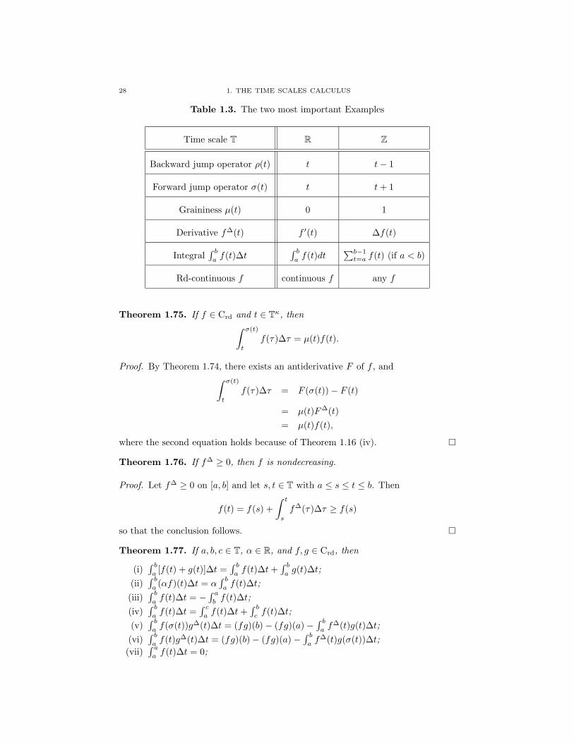
Table 1.3. The two most important Examples
Time scale T R Z
Backward jump operator ρ(t) t t− 1
Forward jump operator σ(t) t t + 1
Graininess µ(t) 0 1
Derivative f∆(t) f ′(t) ∆f(t)
Integral∫ b
af(t)∆t
∫ b
af(t)dt
∑b−1t=a f(t) (if a < b)
Rd-continuous f continuous f any f
Theorem 1.75. If f ∈ Crd and t ∈ Tκ, then
∫ σ(t)
t
f(τ)∆τ = µ(t)f(t).
Proof. By Theorem 1.74, there exists an antiderivative F of f , and∫ σ(t)
t
f(τ)∆τ = F (σ(t))− F (t)
= µ(t)F∆(t)
= µ(t)f(t),
where the second equation holds because of Theorem 1.16 (iv).
Theorem 1.76. If f∆ ≥ 0, then f is nondecreasing.
Proof. Let f∆ ≥ 0 on [a, b] and let s, t ∈ T with a ≤ s ≤ t ≤ b. Then
f(t) = f(s) +
∫ t
s
f∆(τ)∆τ ≥ f(s)
so that the conclusion follows.
Theorem 1.77. If a, b, c ∈ T, α ∈ R, and f, g ∈ Crd, then
(i)∫ b
a[f(t) + g(t)]∆t =
∫ b
af(t)∆t +
∫ b
ag(t)∆t;
(ii)∫ b
a(αf)(t)∆t = α
∫ b
af(t)∆t;
(iii)∫ b
af(t)∆t = −
∫ a
bf(t)∆t;
(iv)∫ b
af(t)∆t =
∫ c
af(t)∆t +
∫ b
cf(t)∆t;
(v)∫ b
af(σ(t))g∆(t)∆t = (fg)(b)− (fg)(a)−
∫ b
af∆(t)g(t)∆t;
(vi)∫ b
af(t)g∆(t)∆t = (fg)(b)− (fg)(a)−
∫ b
af∆(t)g(σ(t))∆t;
(vii)∫ a
af(t)∆t = 0;
1.4. INTEGRATION 29
(viii) if |f(t)| ≤ g(t) on [a, b), then∣
∣
∣
∣
∣
∫ b
a
f(t)∆t
∣
∣
∣
∣
∣
≤∫ b
a
g(t)∆t;
(ix) if f(t) ≥ 0 for all a ≤ t < b, then∫ b
af(t)∆t ≥ 0.
Proof. These results follow easily from Definition 1.71, Theorem 1.20, and Theorem1.67. We only prove (i), (iv), and (v), and leave the rest of the proof as an exercise(see Exercise 1.78). Since f and g are rd-continuous, they possess antiderivatives Fand G by Theorem 1.74. By Theorem 1.20 (i), F + G is an antiderivative of f + gso that
∫ b
a
(f + g)(t)∆t = (F + G)(b)− (F + G)(a)
= F (b)− F (a) + G(b)−G(a)
=
∫ b
a
f(t)∆t +
∫ b
a
g(t)∆t.
Also∫ b
a
f(t)∆t = F (b)− F (a)
= F (c)− F (a) + F (b)− F (c)
=
∫ c
a
f(t)∆t +
∫ b
c
f(t)∆t.
Finally, since fg is an antiderivative of fσg∆ + f∆g,∫ b
a
(
fσg∆ + f∆g)
(t)∆t = (fg)(b)− (fg)(a),
so that (v) follows by using (i).
Note that the formulas in Theorem 1.77 (v) and (vi) are called integration by
parts formulas. Also note that all of the formulas given in Theorem 1.77 also holdfor the case that f and g are only regulated functions.
Exercise 1.78. Finish the proof of Theorem 1.77. Also prove each item of Theorem1.77 assuming that the functions f and g are merely regulated rather than rd-continuous.
Theorem 1.79. Let a, b ∈ T and f ∈ Crd.
(i) If T = R, then∫ b
a
f(t)∆t =
∫ b
a
f(t)dt,
where the integral on the right is the usual Riemann integral from calculus.
(ii) If [a, b] consists of only isolated points, then
∫ b
a
f(t)∆t =
∑
t∈[a,b) µ(t)f(t) if a < b
0 if a = b
−∑t∈[b,a) µ(t)f(t) if a > b.

30 1. THE TIME SCALES CALCULUS
(iii) If T = hZ = {hk : k ∈ Z}, where h > 0, then
∫ b
a
f(t)∆t =
∑
bh−1
k= ah
f(kh)h if a < b
0 if a = b
−∑ah−1
k= bh
f(kh)h if a > b.
(iv) If T = Z, then
∫ b
a
f(t)∆t =
∑b−1t=a f(t) if a < b
0 if a = b
−∑a−1t=b f(t) if a > b.
Proof. Part (i) follows from Example 1.18 (i) and the standard fundamental the-orem of calculus. We now prove (ii). First note that [a, b] contains only finitelymany points since each point in [a, b] is isolated. Assume that a < b and let[a, b] = {t0, t1, . . . , tn}, where
a = t0 < t1 < t2 < · · · < tn = b.
By Theorem 1.77 (iv),∫ b
a
f(t)∆t =n−1∑
i=0
∫ ti+1
ti
f(t)∆t
=
n−1∑
i=0
∫ σ(ti)
ti
f(t)∆t
=
n−1∑
i=0
µ(ti)f(ti)
=∑
t∈[a,b)
µ(t)f(t),
where the third equation above follows from Theorem 1.75. If b < a, then theresult follows from what we just proved and Theorem 1.77 (iii). If a = b, then∫ b
af(t)∆t = 0 by Theorem 1.77 (vii). Parts (iii) and (iv) are special cases of (ii)
(see Exercise 1.80).
Exercise 1.80. Prove that Theorem 1.79 (iii) and (iv) follow from Theorem 1.79(ii).
Exercise 1.81. Let a ∈ T, where T is an arbitrary time scale and evaluate∫ t
a1∆s.
Also evaluate∫ t
0s∆s for t ∈ T, for T = R, for T = Z, for T = hZ, and for
T = [0, 1] ∪ [2, 3].
We next define the improper integral∫∞
af(t)∆t as one would expect.
Definition 1.82. If a ∈ T, sup T = ∞, and f is rd-continuous on [a,∞), then wedefine the improper integral by
∫ ∞
a
f(t)∆t := limb→∞
∫ b
a
f(t)∆t
provided this limit exists, and we say that the improper integral converges in thiscase. If this limit does not exist, then we say that the improper integral diverges.
1.5. CHAIN RULES 31
We now give two exercises concerning improper integrals.
Exercise 1.83. Evaluate the integral∫ ∞
1
1
t2∆t
if T = qN0 , where q > 1.
Exercise 1.84. Assume a ∈ T, a > 0 and sup T = ∞. Evaluate∫ ∞
a
1
tσ(t)∆t.
1.5. Chain Rules
If f, g : R → R, then the chain rule from calculus is that if g is differentiable att and if f is differentiable at g(t), then
(f ◦ g)′(t) = f ′ (g(t)) g′(t).
The next example shows that the chain rule as we know it in calculus does not holdfor all time scales.
Example 1.85. Assume f, g : Z → Z are defined by f(t) = t2, g(t) = 2t and ourtime scale is T = Z. It is easy to see that
(f ◦ g)∆(t) = 8t + 4 6= 8t + 2 = f∆ (g(t)) g∆(t) for all t ∈ Z.
Hence the chain rule as we know it in calculus does not hold in this setting.
Exercise 1.86. Assume that T = Z and f(t) = g(t) = t2. Show that for all t 6= 0,
(f ◦ g)∆(t) 6= f∆ (g(t)) g∆(t).
Sometimes the following substitute of the “continuous” chain rule is useful.
Theorem 1.87 (Chain Rule). Assume g : R → R is continuous, g : T → R is
delta differentiable on Tκ, and f : R → R is continuously differentiable. Then there
exists c in the real interval [t, σ(t)] with
(f ◦ g)∆(t) = f ′ (g(c)) g∆(t).(1.6)
Proof. Fix t ∈ Tκ. First we consider the case where t is right-scattered. In thiscase
(f ◦ g)∆(t) =f (g(σ(t)))− f (g(t))
µ(t).
If g(σ(t)) = g(t), then we get (f ◦ g)∆(t) = 0 and g∆(t) = 0 and so (1.6) holds forany c in the real interval [t, σ(t)]. Hence we can assume g(σ(t)) 6= g(t). Then
(f ◦ g)∆(t) =f (g(σ(t)))− f (g(t))
g (σ(t))− g(t)· g (σ(t))− g(t)
µ(t)
= f ′(ξ)g∆(t)
by the mean value theorem, where ξ is between g(t) and g (σ(t)). Since g : R → R
is continuous, there is c ∈ [t, σ(t)] such that g(c) = ξ, which gives us the desiredresult.

32 1. THE TIME SCALES CALCULUS
It remains to consider the case when t is right-dense. In this case
(f ◦ g)∆(t) = lims→t
f (g(t))− f (g(s))
t− s
= lims→t
{
f ′(ξs) ·g(t)− g(s)
t− s
}
by the mean value theorem in calculus, where ξs is between g(s) and g(t). By thecontinuity of g we get that lims→t ξs = g(t) which gives us the desired result.
Example 1.88. Given T = Z, f(t) = t2, g(t) = 2t, find directly the value cguaranteed by Theorem 1.87 so that
(f ◦ g)∆(3) = f ′ (g(c)) g∆(3)
and show that c is in the interval guaranteed by Theorem 1.87. Using the calcula-tions we made in Example 1.85 we get that this last equation becomes
28 = (4c)2.
Solving for c we get that c = 72 which is in the real interval [3, σ(3)] = [3, 4] as we
are guaranteed by Theorem 1.87.
Exercise 1.89. Assume that T = Z and f(t) = g(t) = t2. Find directly the cguaranteed by Theorem 1.87 so that (f ◦ g)∆(2) = f ′ (g(c)) g∆(2) and be sure tonote that c is in the interval guaranteed by Theorem 1.87.
Now we present a chain rule which calculates (f ◦ g)∆, where
g : T → R and f : R → R.
This chain rule is due to Christian Potzsche, who derived it first in 1998 (see alsoStefan Keller’s PhD thesis [190] and [234]).
Theorem 1.90 (Chain Rule). Let f : R → R be continuously differentiable and
suppose g : T → R is delta differentiable. Then f ◦ g : T → R is delta differentiable
and the formula
(f ◦ g)∆(t) =
{∫ 1
0
f ′(
g(t) + hµ(t)g∆(t))
dh
}
g∆(t)
holds.
Proof. First of all we apply the ordinary substitution rule from calculus to find
f(g(σ(t)))− f(g(s)) =
∫ g(σ(t))
g(s)
f ′(τ)dτ
= [g(σ(t))− g(s)]
∫ 1
0
f ′(hg(σ(t)) + (1− h)g(s))dh.
Let t ∈ Tκ and ε > 0 be given. Since g is differentiable at t, there exists aneighborhood U1 of t such that
|g(σ(t))− g(s)− g∆(t)(σ(t)− s)| ≤ ε∗|σ(t)− s| for all s ∈ U1,
where
ε∗ =ε
1 + 2∫ 1
0|f ′(hg(σ(t)) + (1− h)g(t))|dh
.

1.5. CHAIN RULES 33
Moreover, f ′ is continuous on R, and therefore it is uniformly continuous on closedsubsets of R, and (observe also that g is continuous as it is differentiable, seeTheorem 1.16 (i)) hence there exists a neighborhood U2 of t such that
|f ′(hg(σ(t)) + (1− h)g(s))− f ′(hg(σ(t)) + (1− h)g(t))| ≤ ε
2(ε∗ + |g∆(t)|)
for all s ∈ U2. To see this, note also that
|hg(σ(t)) + (1− h)g(s)− (hg(σ(t)) + (1− h)g(t))| = (1− h)|g(s)− g(t)|≤ |g(s)− g(t)|
holds for all 0 ≤ h ≤ 1. We then define U = U1∩U2 and let s ∈ U . For conveniencewe put
α = hg(σ(t)) + (1− h)g(s) and β = hg(σ(t)) + (1− h)g(t).
Then we have∣
∣
∣
∣
(f ◦ g)(σ(t))− (f ◦ g)(s)− (σ(t)− s)g∆(t)
∫ 1
0
f ′(β)dh
∣
∣
∣
∣
=
∣
∣
∣
∣
[g(σ(t))− g(s)]
∫ 1
0
f ′(α)dh− (σ(t)− s)g∆(t)
∫ 1
0
f ′(β)dh
∣
∣
∣
∣
=
∣
∣
∣
∣
[g(σ(t))− g(s)− (σ(t)− s)g∆(t)]
∫ 1
0
f ′(α)dh
+(σ(t)− s)g∆(t)
∫ 1
0
(f ′(α)− f ′(β))dh
∣
∣
∣
∣
≤ |g(σ(t))− g(s)− (σ(t)− s)g∆(t)|∫ 1
0
|f ′(α)|dh
+|σ(t)− s||g∆(t)|∫ 1
0
|f ′(α)− f ′(β)|dh
≤ ε∗|σ(t)− s|∫ 1
0
|f ′(α)|dh + |σ(t)− s||g∆(t)|∫ 1
0
|f ′(α)− f ′(β)|dh
≤ ε∗|σ(t)− s|∫ 1
0
|f ′(β)|dh + [ε∗ + |g∆(t)|]|σ(t)− s|∫ 1
0
|f ′(α)− f ′(β)|dh
≤ ε
2|σ(t)− s|+ ε
2|σ(t)− s|
= ε|σ(t)− s|.
Therefore f ◦ g is differentiable at t and the derivative is as claimed above.
Example 1.91. We define g : Z → R and f : R → R by
g(t) = t2 and f(x) = exp(x).
Then
g∆(t) = (t + 1)2 − t2 = 2t + 1 and f ′(x) = exp(x).

34 1. THE TIME SCALES CALCULUS
Hence we have by Theorem 1.90
(f ◦ g)∆(t) =
{∫ 1
0
f ′(
g(t) + hµ(t)g∆(t))
dh
}
g∆(t)
= (2t + 1)
∫ 1
0
exp(t2 + h(2t + 1))dh
= (2t + 1) exp(t2)
∫ 1
0
exp(h(2t + 1))dh
= (2t + 1) exp(t2)1
2t + 1[exp(h(2t + 1))]
h=1h=0
= (2t + 1) exp(t2)1
2t + 1(exp(2t + 1)− 1)
= exp(t2)(exp(2t + 1)− 1).
On the other hand, it is easy to check that we have indeed
∆f(g(t)) = f(g(t + 1))− f(g(t))
= exp((t + 1)2)− exp(t2)
= exp(t2 + 2t + 1)− exp(t2)
= exp(t2)(exp(2t + 1)− 1).
In the remainder of this section we present some results related to results in thepaper by C. D. Ahlbrandt, M. Bohner, and J. Ridenhour [24]. Let T be a time
scale and ν : T → R be a strictly increasing function such that T = ν(T) is also
a time scale. By σ we denote the jump function on T and by ∆ we denote thederivative on T. Then ν ◦ σ = σ ◦ ν.
Exercise 1.92. Prove that ν ◦ σ = σ ◦ ν under the hypotheses of the above para-graph.
Theorem 1.93 (Chain Rule). Assume ν : T → R is strictly increasing and T :=
ν(T) is a time scale. Let w : T → R. If ν∆(t) and w∆(ν(t)) exist for t ∈ Tκ, then
(w ◦ ν)∆ = (w∆ ◦ ν)ν∆.
Proof. Let 0 < ε < 1 be given and define ε∗ = ε[
1 + |ν∆(t)|+ |w∆(ν(t))|]−1
. Note
that 0 < ε∗ < 1. According to the assumptions, there exist neighborhoods N1 of tand N2 of ν(t) such that
|ν(σ(t))− ν(s)− (σ(t)− s)ν∆(t)| ≤ ε∗|σ(t)− s| for all s ∈ N1
and
|w(σ(ν(t)))− w(r)− (σ(ν(t))− r)w∆(ν(t))| ≤ ε∗|σ(ν(t))− r|, r ∈ N2.

1.5. CHAIN RULES 35
Put N = N1 ∩ ν−1(N2) and let s ∈ N . Then s ∈ N1 and ν(s) ∈ N2 and
|w(ν(σ(t)))− w(ν(s))− (σ(t)− s)[w∆(ν(t))ν∆(t)]|= |w(ν(σ(t)))− w(ν(s))− (σ(ν(t))− ν(s))w∆(ν(t))
+[σ(ν(t))− ν(s)− (σ(t)− s)ν∆(t)]w∆(ν(t))|≤ ε∗|σ(ν(t))− ν(s)|+ ε∗|σ(t)− s||w∆(ν(t))|≤ ε∗
{
|σ(ν(t))− ν(s)− (σ(t)− s)ν∆(t)|+ |σ(t)− s||ν∆(t)|+|σ(t)− s||w∆(ν(t))|
}
≤ ε∗{
ε∗|σ(t)− s|+ |σ(t)− s||ν∆(t)|+ |σ(t)− s||w∆(ν(t))|}
= ε∗|σ(t)− s|{
ε∗ + |ν∆(t)|+ |w∆(ν(t))|}
≤ ε∗{
1 + |ν∆(t)|+ |w∆(ν(t))|}
|σ(t)− s|= ε|σ(t)− s|.
This proves the claim.
Example 1.94. Let T = N0 and ν(t) = 4t + 1. Hence
T = ν(T) = {4n + 1 : n ∈ N0} = {1, 5, 9, 13, . . . }.Moreover, let w : T → R be defined by w(t) = t2. Then
(w ◦ ν)(t) = w(ν(t)) = w(4t + 1) = (4t + 1)2
and hence
(w ◦ ν)∆(t) = [4(t + 1) + 1]2 − (4t + 1)2
= (4t + 5)2 − (4t + 1)2
= 16t2 + 40t + 25− 16t2 − 8t− 1
= 32t + 24.
Now we apply Theorem 1.93 to obtain the derivative of this composite function.We first calculate ν∆(t) ≡ 4 and then
w∆(t) =w(σ(t))− w(t)
σ(t)− t=
(t + 4)2 − t2
t + 4− t=
8t + 16
4= 2t + 4
and therefore
(w∆ ◦ ν)(t) = w∆(ν(t)) = w∆(4t + 1) = 2(4t + 1) + 4 = 8t + 6.
Thus we obtain
[(w∆ ◦ ν)ν∆](t) = (8t + 6)4 = 32t + 24 = (w ◦ ν)∆(t).
Exercise 1.95. Let T = N0, ν(t) = t2, T = ν(T), and w(t) = 2t2 + 3. Showdirectly as in Example 1.94 that
(w ◦ ν)∆ = (w∆ ◦ ν)ν∆.
Exercise 1.96. Find a time scale T and a strictly increasing function ν : T → R
such that ν(T) is not a time scale.
36 1. THE TIME SCALES CALCULUS
As a consequence of Theorem 1.93 we can now write down a formula for thederivative of the inverse function.
Theorem 1.97 (Derivative of the Inverse). Assume ν : T → R is strictly increasing
and T := ν(T) is a time scale. Then
1
ν∆= (ν−1)∆ ◦ ν
at points where ν∆ is different from zero.
Proof. Let w = ν−1 : T → T in the previous theorem.
Another consequence of Theorem 1.93 is the substitution rule for integrals.
Theorem 1.98 (Substitution). Assume ν : T → R is strictly increasing and
T := ν(T) is a time scale. If f : T → R is an rd-continuous function and ν is
differentiable with rd-continuous derivative, then for a, b ∈ T,∫ b
a
f(t)ν∆(t)∆t =
∫ ν(b)
ν(a)
(f ◦ ν−1)(s)∆s.
Proof. Since fν∆ is an rd-continuous function, it possesses an antiderivative F byTheorem 1.74, i.e., F∆ = fν∆, and
∫ b
a
f(t)ν∆(t)∆t =
∫ b
a
F∆(t)∆t
= F (b)− F (a)
= (F ◦ ν−1)(ν(b))− (F ◦ ν−1)(ν(a))
=
∫ ν(b)
ν(a)
(F ◦ ν−1)∆(s)∆s
=
∫ ν(b)
ν(a)
(F∆ ◦ ν−1)(s)(ν−1)∆(s)∆s
=
∫ ν(b)
ν(a)
((fν∆) ◦ ν−1)(s)(ν−1)∆(s)∆s
=
∫ ν(b)
ν(a)
(f ◦ ν−1)(s)[(ν∆ ◦ ν−1)(ν−1)∆](s)∆s
=
∫ ν(b)
ν(a)
(f ◦ ν−1)(s)∆s,
where for the fifth equal sign we have used Theorem 1.93 and in the last step wehave used Theorem 1.97.
Example 1.99. In this example we use the method of substitution (Theorem 1.98)to evaluate the integral
∫ t
0
(
√
τ2 + 1 + τ)
3τ2
∆τ
for t ∈ T := N120 = {√n : n ∈ N0}. We take
ν(t) = t2
1.6. POLYNOMIALS 37
for t ∈ N120 . Then ν : N
120 → R is strictly increasing and ν
(
N120
)
= N0 is a time
scale. From Exercise 1.19 we get that
ν∆(t) =√
t2 + 1 + t.
Hence if f(t) := 3t2 , we get from Theorem 1.98 that∫ t
0
(
√
τ2 + 1 + τ)
3τ2
∆τ =
∫ t
0
f(τ)ν∆(τ)∆τ
=
∫ t2
0
f(√
s)∆s
=
∫ t2
0
3s∆s
=
[
1
23s
]s=t2
s=0
=1
2(3t2 − 1).
Exercise 1.100. Evaluate the integral∫ t
0
2τ(2τ − 1)∆τ
for t ∈ T := {n2 : n ∈ N0} by applying Theorem 1.98 with ν(t) = 2t.
Exercise 1.101. Evaluate the integral∫ t
0
[
(τ3 + 1)23 + τ(τ3 + 1)
13 + τ2
]
2τ3
∆τ
for t ∈ T := { 3√
n : n ∈ N0}.
1.6. Polynomials
An antiderivative of 0 is 1, an antiderivative of 1 is t, but it is not possible to finda closed formula (for an arbitrary time scale) of an antiderivative of t. Certainlyt2/2 is not the solution, as the derivative of t2/2 is
t + σ(t)
2= t +
µ(t)
2
which is, as we know, e.g., by Example 1.56, not even necessarily a differentiablefunction (although it is the product of two differentiable functions). Similarly,none of the “classical” polynomials are necessarily more than once differentiable,see Theorem 1.24. So the question arises which function plays the role of e.g., t2/2,in the time scales calculus. It could be either
∫ t
0
σ(τ)∆τ or
∫ t
0
τ∆τ.
In fact, if we define
g2(t, s) =
∫ t
s
(σ(τ)− s)∆τ and h2(t, s) =
∫ t
s
(τ − s)∆τ,
38 1. THE TIME SCALES CALCULUS
then we find the following relation between g2 and h2:
g2(t, s) =
∫ t
s
(σ(τ)− s)∆τ
=
∫ t
s
(σ(τ) + τ)∆τ −∫ t
s
τ∆τ −∫ t
s
s∆τ
=
∫ t
s
(τ2)∆∆τ +
∫ s
t
τ∆τ − s(t− s)
=
∫ s
t
τ∆τ + t2 − s2 − s(t− s)
=
∫ s
t
(τ − t)∆τ
= h2(s, t).
In this section we give a Taylor’s formula for functions on a general time scale.Many of the results in this section can be found in R. P. Agarwal and M. Bohner[9]. The generalized polynomials, that also occur in Taylor’s formula, are thefunctions gk, hk : T2 → R, k ∈ N0, defined recursively as follows: The functions g0
and h0 are
g0(t, s) = h0(t, s) ≡ 1 for all s, t ∈ T,(1.7)
and, given gk and hk for k ∈ N0, the functions gk+1 and hk+1 are
gk+1(t, s) =
∫ t
s
gk(σ(τ), s)∆τ for all s, t ∈ T(1.8)
and
hk+1(t, s) =
∫ t
s
hk(τ, s)∆τ for all s, t ∈ T.(1.9)
Note that the functions gk and hk are all well defined according to Theorem 1.60and Theorem 1.74. If we let h∆
k (t, s) denote for each fixed s the derivative of hk(t, s)with respect to t, then
h∆k (t, s) = hk−1(t, s) for k ∈ N, t ∈ Tκ.
Similarly
g∆k (t, s) = gk−1(σ(t), s) for k ∈ N, t ∈ Tκ.
The above definitions obviously imply
g1(t, s) = h1(t, s) = t− s for all s, t ∈ T.
However, finding gk and hk for k > 1 is not easy in general. But for a particulargiven time scale it might be easy to find these functions. We will consider severalexamples first before we present Taylor’s formula in general.
Example 1.102. For the cases T = R and T = Z it is easy to find the functionsgk and hk:

1.6. POLYNOMIALS 39
(i) First, consider T = R. Then σ(t) = t for t ∈ R so that gk = hk for k ∈ N0. Wehave
g2(t, s) = h2(t, s)
=
∫ t
s
(τ − s)dτ
=(τ − s)2
2
∣
∣
∣
∣
τ=t
τ=s
=(t− s)2
2.
We claim that for k ∈ N0
gk(t, s) = hk(t, s) =(t− s)k
k!for all s, t ∈ R(1.10)
as we will now show using the principle of mathematical induction: Obviously(1.10) holds for k = 0. Assume that (1.10) holds with k replaced by some m ∈ N0.Then
gm+1(t, s) = hm+1(t, s)
=
∫ t
s
(τ − s)m
m!dτ
=(τ − s)m+1
(m + 1)!
∣
∣
∣
∣
τ=t
τ=s
=(t− s)m+1
(m + 1)!,
i.e., (1.10) holds with k replaced by m + 1. We note that, for an n times differen-tiable function f : R → R, the following well-known Taylor’s formula holds: Letα ∈ R be arbitrary. Then, for all t ∈ R, the representations
f(t) =n−1∑
k=0
(t− α)k
k!f (k)(α) +
1
(n− 1)!
∫ t
α
(t− τ)n−1f (n)(τ)dτ
=
n−1∑
k=0
hk(t, α)f (k)(α) +
∫ t
α
hn−1(t, σ(τ))f (n)(τ)dτ(1.11)
=
n−1∑
k=0
(−1)kgk(α, t)f (k)(α) +
∫ t
α
(−1)n−1gn−1(σ(τ), t)f (n)(τ)dτ(1.12)
are valid, where f (k) denotes as usual the kth derivative of f . Above we have usedthe relationship
(−1)kgk(s, t) = (−1)k (s− t)k
k!=
(t− s)k
k!= hk(t, s),(1.13)
which holds for all k ∈ N0.

40 1. THE TIME SCALES CALCULUS
(ii) Next, consider T = Z. Then σ(t) = t + 1 for t ∈ Z. We have for s, t ∈ Z
h2(t, s) =
∫ t
s
h1(τ, s)∆s
=
[
(τ − s)(2)
2
]τ=t
τ=s
=
(
t− s
2
)
.
We claim that for k ∈ N0 we have
hk(t, s) =(t− s)(k)
k!=
(
t− s
k
)
for all s, t ∈ Z.(1.14)
Assume (1.14) holds for k replaced by m. Then
hm+1(t, s) =
∫ t
s
hm(τ, s)∆τ
=
∫ t
s
(τ − s)(m)
m!∆τ
=(t− s)(m+1)
(m + 1)!,
which is (1.14) with k replaced by m + 1. Hence by mathematical induction weget that (1.14) holds for all k ∈ N0. Similarly it is possible to show that
gk(t, s) =(t− s + k − 1)(k)
k!for all s, t ∈ Z(1.15)
holds for all k ∈ N0. As before we observe that the relationship
(−1)kgk(s, t) = (−1)k (s− t + k − 1)(k)
k!(1.16)
= (−1)k (s− t + k − 1)(s− t + k − 2) · · · (s− t)
k!
=(t− s) · · · (t− s + 2− k)(t− s + 1− k)
k!
=(t− s)(k)
k!= hk(t, s)
holds for all k ∈ N0. The well-known discrete version of Taylor’s formula (seee.g. [5]) reads as follows: Let f : Z → R be a function, and let α ∈ Z. Then, forall t ∈ Z with t > α + n, the representations
f(t) =
n−1∑
k=0
(t− α)(k)
k!∆kf(α) +
1
(n− 1)!
t−n∑
τ=α
(t− τ − 1)(n−1)∆nf(τ)
=
n−1∑
k=0
hk(t, α)∆kf(α) +
t−n∑
τ=α
hn−1(t, σ(τ))∆nf(τ)(1.17)
=
n−1∑
k=0
(−1)kgk(α, t)∆kf(α) +
t−n∑
τ=α
(−1)n−1gn−1(σ(τ), t)∆nf(τ)(1.18)
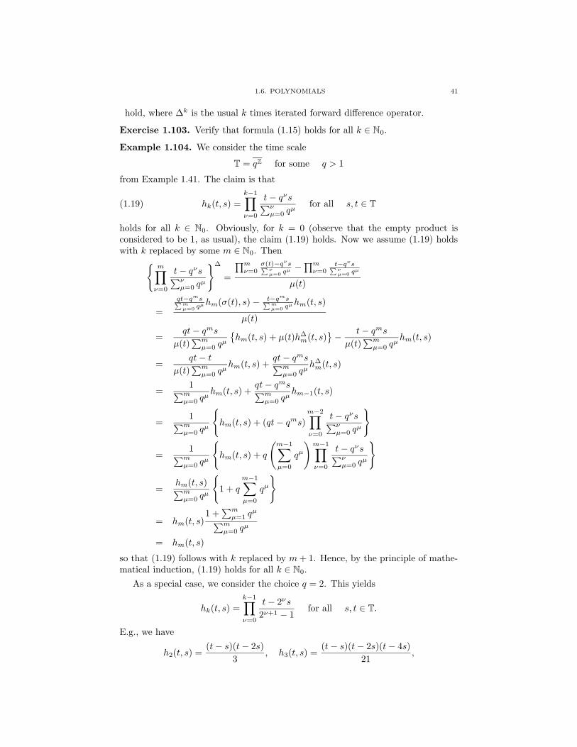
1.6. POLYNOMIALS 41
hold, where ∆k is the usual k times iterated forward difference operator.
Exercise 1.103. Verify that formula (1.15) holds for all k ∈ N0.
Example 1.104. We consider the time scale
T = qZ for some q > 1
from Example 1.41. The claim is that
hk(t, s) =
k−1∏
ν=0
t− qνs∑ν
µ=0 qµfor all s, t ∈ T(1.19)
holds for all k ∈ N0. Obviously, for k = 0 (observe that the empty product isconsidered to be 1, as usual), the claim (1.19) holds. Now we assume (1.19) holdswith k replaced by some m ∈ N0. Then
{
m∏
ν=0
t− qνs∑ν
µ=0 qµ
}∆
=
∏mν=0
σ(t)−qνs∑
νµ=0 qµ −
∏mν=0
t−qνs∑
νµ=0 qµ
µ(t)
=
qt−qms∑
mµ=0 qµ hm(σ(t), s)− t−qms
∑
mµ=0 qµ hm(t, s)
µ(t)
=qt− qms
µ(t)∑m
µ=0 qµ
{
hm(t, s) + µ(t)h∆m(t, s)
}
− t− qms
µ(t)∑m
µ=0 qµhm(t, s)
=qt− t
µ(t)∑m
µ=0 qµhm(t, s) +
qt− qms∑m
µ=0 qµh∆
m(t, s)
=1
∑mµ=0 qµ
hm(t, s) +qt− qms∑m
µ=0 qµhm−1(t, s)
=1
∑mµ=0 qµ
{
hm(t, s) + (qt− qms)
m−2∏
ν=0
t− qνs∑ν
µ=0 qµ
}
=1
∑mµ=0 qµ
{
hm(t, s) + q
(
m−1∑
µ=0
qµ
)
m−1∏
ν=0
t− qνs∑ν
µ=0 qµ
}
=hm(t, s)∑m
µ=0 qµ
{
1 + qm−1∑
µ=0
qµ
}
= hm(t, s)1 +
∑mµ=1 qµ
∑mµ=0 qµ
= hm(t, s)
so that (1.19) follows with k replaced by m + 1. Hence, by the principle of mathe-matical induction, (1.19) holds for all k ∈ N0.
As a special case, we consider the choice q = 2. This yields
hk(t, s) =
k−1∏
ν=0
t− 2νs
2ν+1 − 1for all s, t ∈ T.
E.g., we have
h2(t, s) =(t− s)(t− 2s)
3, h3(t, s) =
(t− s)(t− 2s)(t− 4s)
21,

42 1. THE TIME SCALES CALCULUS
and
h4(t, s) =(t− s)(t− 2s)(t− 4s)(t− 8s)
315.
Exercise 1.105. Find the functions gk for k ∈ N0, where T is the time scaleconsidered in Example 1.104.
Exercise 1.106. Let T = qZ for some q > 1. For n ∈ N, evaluate∫ t
0
sn∆s.
Exercise 1.107. Find the functions hk(·, 0), for k = 0, 1, 2, 3 if T := [0, 1] ∪ [3, 4].
Now we will present and prove Taylor’s formula for the case of a general timescale T. First we need three preliminary results.
Lemma 1.108. Let n ∈ N. Suppose f is n times differentiable and pk, 0 ≤ k ≤n− 1, are differentiable at some t ∈ T with
p∆k+1(t) = pσ
k(t) for all 0 ≤ k ≤ n− 2.(1.20)
Then we have at t[
n−1∑
k=0
(−1)kf∆k
pk
]∆
= (−1)n−1f∆n
pσn−1 + fp∆
0 .
Proof. Using Theorem 1.20 (i), (ii), (iii), and (1.20) we find that[
n−1∑
k=0
(−1)kf∆k
pk
]∆
=
n−1∑
k=0
(−1)k[
f∆k
pk
]∆
=
n−1∑
k=0
(−1)k[
f∆k+1
pσk + f∆k
p∆k
]
=n−2∑
k=0
(−1)kf∆k+1
pσk + (−1)n−1f∆n
pσn−1 +
n−1∑
k=1
(−1)kf∆k
p∆k + fp∆
0
=
n−2∑
k=0
(−1)kf∆k+1
pσk + (−1)n−1f∆n
pσn−1 −
n−2∑
k=0
(−1)kf∆k+1
p∆k+1 + fp∆
0
= (−1)n−1f∆n
pσn−1 + fp∆
0
holds at t. This proves the lemma.
Lemma 1.109. The functions gk defined in (1.7) and (1.8) satisfy for all t ∈ T
gn(ρk(t), t) = 0 for all n ∈ N and all 0 ≤ k ≤ n− 1.
Proof. We prove this result by induction. First, for k = 0, we have
gn(ρ0(t), t) = gn(t, t) = 0.
To complete the induction it suffices to show that
gn−1(ρk(t), t) = gn(ρk(t), t) = 0 with 0 ≤ k < n
implies thatgn(ρk+1(t), t) = 0.

1.6. POLYNOMIALS 43
First, if ρk(t) is left-dense, then ρk+1(t) = ρk(t) so that
gn(ρk+1(t), t) = gn(ρk(t), t) = 0.
If ρk(t) is not left-dense, then it is left-scattered, and σ(ρk+1(t)) = ρk(t) so that byTheorem 1.16 (iv) and (1.8)
gn(ρk+1(t), t) = gn(σ(ρk+1(t)), t)− µ(ρk+1(t))g∆n (ρk+1(t), t)
= gn(ρk(t), t)− µ(ρk+1(t))gn−1(σ(ρk+1(t)), t)
= gn(ρk(t), t)− µ(ρk+1(t))gn−1(ρk(t), t)
= 0
(observe n 6= 1). This proves our claim.
Lemma 1.110. Let n ∈ N, t ∈ T, and suppose that f is (n−1) times differentiable
at ρn−1(t). Then we have
n−1∑
k=0
(−1)kf∆k
(ρn−1(t))gk(ρn−1(t), t) = f(t),(1.21)
where the functions gk are defined by (1.7) and (1.8).
Proof. First of all we have
(−1)0f∆0
(ρ0(t))g0(ρ0(t), t) = f(t)g0(t, t) = f(t)
so that (1.21) is true for n = 1. Suppose now that (1.21) holds with n replacedby some m ∈ N. Then we consider two cases. First, if ρm−1(t) is left-dense, thenρm(t) = ρm−1(t) and hence
m∑
k=0
(−1)kf∆k
(ρm(t))gk(ρm(t), t) =
m−1∑
k=0
(−1)kf∆k
(ρm(t))gk(ρm(t), t)
+(−1)mf∆m
(ρm(t))gm(ρm(t), t)
=
m−1∑
k=0
(−1)kf∆k
(ρm−1(t))gk(ρm−1(t), t) + (−1)mf∆m
(ρm−1(t))gm(ρm−1(t), t)
= f(t) + (−1)mf∆m
(ρm−1(t))gm(ρm−1(t), t)
= f(t),
where we used Lemma 1.109 to obtain the last equation. Hence (1.21) holds with nreplaced by m + 1. We have to draw the same conclusion for the case that ρm−1(t)is left-scattered. In this case we have σ(ρm(t)) = ρm−1(t) and hence by Theorem1.16 (iv) and (1.8) for k ∈ N
gk(ρm−1(t), t) = gk(σ(ρm(t)), t)
= gk(ρm(t), t) + µ(ρm(t))g∆k (ρm(t), t)
= gk(ρm(t), t) + µ(ρm(t))gk−1(σ(ρm(t)), t)
= gk(ρm(t), t) + µ(ρm(t))gk−1(ρm−1(t), t).
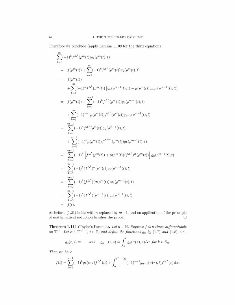
44 1. THE TIME SCALES CALCULUS
Therefore we conclude (apply Lemma 1.109 for the third equation)
m∑
k=0
(−1)kf∆k
(ρm(t))gk(ρm(t), t)
= f(ρm(t)) +
m∑
k=1
(−1)kf∆k
(ρm(t))gk(ρm(t), t)
= f(ρm(t))
+m∑
k=1
(−1)kf∆k
(ρm(t))[
gk(ρm−1(t), t)− µ(ρm(t))gk−1(ρm−1(t), t)
]
= f(ρm(t)) +
m−1∑
k=1
(−1)kf∆k
(ρm(t))gk(ρm−1(t), t)
+
m∑
k=1
(−1)k−1µ(ρm(t))f∆k
(ρm(t))gk−1(ρm−1(t), t)
=
m−1∑
k=0
(−1)kf∆k
(ρm(t))gk(ρm−1(t), t)
+m−1∑
k=0
(−1)kµ(ρm(t))f∆k+1
(ρm(t))gk(ρm−1(t), t)
=
m−1∑
k=0
(−1)k[
f∆k
(ρm(t)) + µ(ρm(t))(f∆k
)∆(ρm(t))]
gk(ρm−1(t), t)
=
m−1∑
k=0
(−1)k(f∆k
)σ(ρm(t))gk(ρm−1(t), t)
=m−1∑
k=0
(−1)k(f∆k
)(σ(ρm(t)))gk(ρm−1(t), t)
=
m−1∑
k=0
(−1)k(f∆k
)(ρm−1(t))gk(ρm−1(t), t)
= f(t).
As before, (1.21) holds with n replaced by m+1, and an application of the principleof mathematical induction finishes the proof.
Theorem 1.111 (Taylor’s Formula). Let n ∈ N. Suppose f is n times differentiable
on Tκn
. Let α ∈ Tκn−1
, t ∈ T, and define the functions gk by (1.7) and (1.8), i.e.,
g0(r, s) ≡ 1 and gk+1(r, s) =
∫ r
s
gk(σ(τ), s)∆τ for k ∈ N0.
Then we have
f(t) =
n−1∑
k=0
(−1)kgk(α, t)f∆k
(α) +
∫ ρn−1(t)
α
(−1)n−1gn−1(σ(τ), t)f∆n
(τ)∆τ.
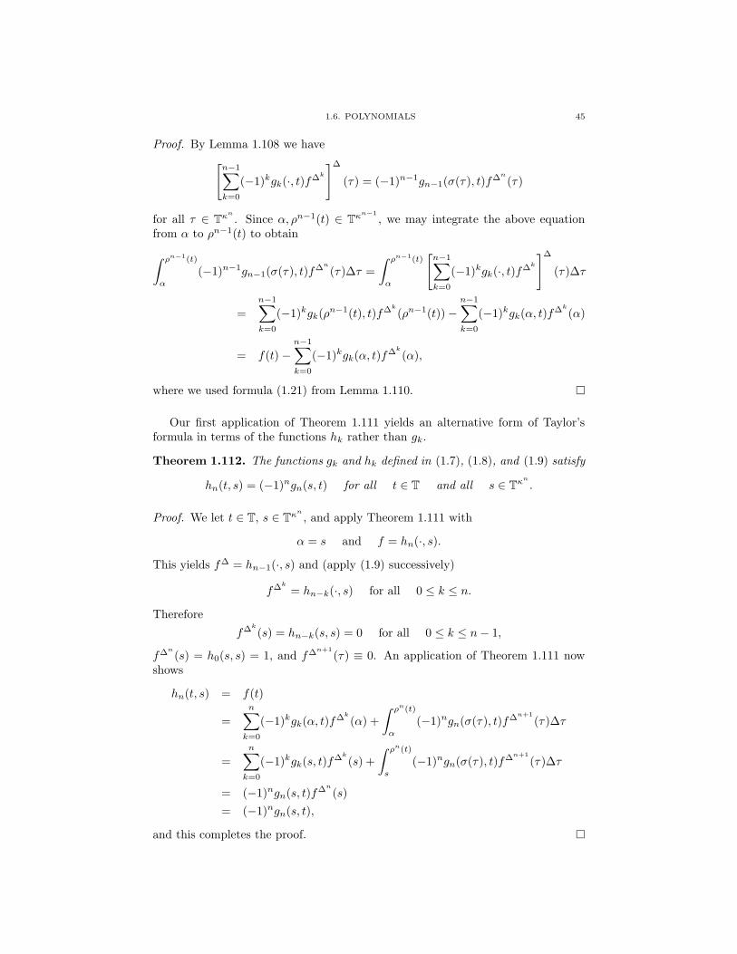
1.6. POLYNOMIALS 45
Proof. By Lemma 1.108 we have
[
n−1∑
k=0
(−1)kgk(·, t)f∆k
]∆
(τ) = (−1)n−1gn−1(σ(τ), t)f∆n
(τ)
for all τ ∈ Tκn
. Since α, ρn−1(t) ∈ Tκn−1
, we may integrate the above equationfrom α to ρn−1(t) to obtain
∫ ρn−1(t)
α
(−1)n−1gn−1(σ(τ), t)f∆n
(τ)∆τ =
∫ ρn−1(t)
α
[
n−1∑
k=0
(−1)kgk(·, t)f∆k
]∆
(τ)∆τ
=n−1∑
k=0
(−1)kgk(ρn−1(t), t)f∆k
(ρn−1(t))−n−1∑
k=0
(−1)kgk(α, t)f∆k
(α)
= f(t)−n−1∑
k=0
(−1)kgk(α, t)f∆k
(α),
where we used formula (1.21) from Lemma 1.110.
Our first application of Theorem 1.111 yields an alternative form of Taylor’sformula in terms of the functions hk rather than gk.
Theorem 1.112. The functions gk and hk defined in (1.7), (1.8), and (1.9) satisfy
hn(t, s) = (−1)ngn(s, t) for all t ∈ T and all s ∈ Tκn
.
Proof. We let t ∈ T, s ∈ Tκn
, and apply Theorem 1.111 with
α = s and f = hn(·, s).
This yields f∆ = hn−1(·, s) and (apply (1.9) successively)
f∆k
= hn−k(·, s) for all 0 ≤ k ≤ n.
Therefore
f∆k
(s) = hn−k(s, s) = 0 for all 0 ≤ k ≤ n− 1,
f∆n
(s) = h0(s, s) = 1, and f∆n+1
(τ) ≡ 0. An application of Theorem 1.111 nowshows
hn(t, s) = f(t)
=n∑
k=0
(−1)kgk(α, t)f∆k
(α) +
∫ ρn(t)
α
(−1)ngn(σ(τ), t)f∆n+1
(τ)∆τ
=n∑
k=0
(−1)kgk(s, t)f∆k
(s) +
∫ ρn(t)
s
(−1)ngn(σ(τ), t)f∆n+1
(τ)∆τ
= (−1)ngn(s, t)f∆n
(s)
= (−1)ngn(s, t),
and this completes the proof.
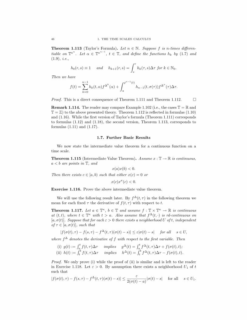
46 1. THE TIME SCALES CALCULUS
Theorem 1.113 (Taylor’s Formula). Let n ∈ N. Suppose f is n-times differen-
tiable on Tκn
. Let α ∈ Tκn−1
, t ∈ T, and define the functions hk by (1.7) and
(1.9), i.e.,
h0(r, s) ≡ 1 and hk+1(r, s) =
∫ r
s
hk(τ, s)∆τ for k ∈ N0.
Then we have
f(t) =
n−1∑
k=0
hk(t, α)f∆k
(α) +
∫ ρn−1(t)
α
hn−1(t, σ(τ))f∆n
(τ)∆τ.
Proof. This is a direct consequence of Theorem 1.111 and Theorem 1.112.
Remark 1.114. The reader may compare Example 1.102 (i.e., the cases T = R andT = Z) to the above presented theory. Theorem 1.112 is reflected in formulas (1.10)and (1.16). While the first version of Taylor’s formula (Theorem 1.111) correspondsto formulas (1.12) and (1.18), the second version, Theorem 1.113, corresponds toformulas (1.11) and (1.17).
1.7. Further Basic Results
We now state the intermediate value theorem for a continuous function on atime scale.
Theorem 1.115 (Intermediate Value Theorem). Assume x : T → R is continuous,
a < b are points in T, and
x(a)x(b) < 0.
Then there exists c ∈ [a, b) such that either x(c) = 0 or
x(c)xσ(c) < 0.
Exercise 1.116. Prove the above intermediate value theorem.
We will use the following result later. By f∆(t, τ) in the following theorem wemean for each fixed τ the derivative of f(t, τ) with respect to t.
Theorem 1.117. Let a ∈ Tκ, b ∈ T and assume f : T × Tκ → R is continuous
at (t, t), where t ∈ Tκ with t > a. Also assume that f∆(t, ·) is rd-continuous on
[a, σ(t)]. Suppose that for each ε > 0 there exists a neighborhood U of t, independent
of τ ∈ [a, σ(t)], such that
|f(σ(t), τ)− f(s, τ)− f∆(t, τ)(σ(t)− s)| ≤ ε|σ(t)− s| for all s ∈ U,
where f∆ denotes the derivative of f with respect to the first variable. Then
(i) g(t) :=∫ t
af(t, τ)∆τ implies g∆(t) =
∫ t
af∆(t, τ)∆τ + f(σ(t), t);
(ii) h(t) :=∫ b
tf(t, τ)∆τ implies h∆(t) =
∫ b
tf∆(t, τ)∆τ − f(σ(t), t).
Proof. We only prove (i) while the proof of (ii) is similar and is left to the readerin Exercise 1.118. Let ε > 0. By assumption there exists a neighborhood U1 of tsuch that
|f(σ(t), τ)− f(s, τ)− f∆(t, τ)(σ(t)− s)| ≤ ε
2(σ(t)− a)|σ(t)− s| for all s ∈ U1.

1.7. FURTHER BASIC RESULTS 47
Since f is continuous at (t, t), there exists a neighborhood U2 of t such that
|f(s, τ)− f(t, t)| ≤ ε
2whenever s, τ ∈ U2.
Now define U = U1 ∩ U2 and let s ∈ U . Then∣
∣
∣
∣
g(σ(t))− g(s)−[
f(σ(t), t) +
∫ t
a
f∆(t, τ)∆τ
]
(σ(t)− s)
∣
∣
∣
∣
=
∣
∣
∣
∣
∣
∫ σ(t)
a
f(σ(t), τ)∆τ −∫ s
a
f(s, τ)∆τ − (σ(t)− s)f(σ(t), t)
−(σ(t)− s)
∫ t
a
f∆(t, τ)∆τ
∣
∣
∣
∣
=
∣
∣
∣
∣
∣
∫ σ(t)
a
[
f(σ(t), τ)− f(s, τ)− f∆(t, τ)(σ(t)− s)]
∆τ
−∫ s
σ(t)
f(s, τ)∆τ − (σ(t)− s)f(σ(t), t)− (σ(t)− s)
∫ t
σ(t)
f∆(t, τ)∆τ
∣
∣
∣
∣
∣
=
∣
∣
∣
∣
∣
∫ σ(t)
a
[
f(σ(t), τ)− f(s, τ)− f∆(t, τ)(σ(t)− s)]
∆τ
−∫ s
σ(t)
f(s, τ)∆τ − (σ(t)− s)f(σ(t), t) + (σ(t)− s)µ(t)f∆(t, t)
∣
∣
∣
∣
∣
=
∣
∣
∣
∣
∣
∫ σ(t)
a
[
f(σ(t), τ)− f(s, τ)− f∆(t, τ)(σ(t)− s)]
∆τ
+
∫ σ(t)
s
f(s, τ)∆τ − (σ(t)− s)f(t, t)
∣
∣
∣
∣
∣
=
∣
∣
∣
∣
∣
∫ σ(t)
a
[
f(σ(t), τ)− f(s, τ)− f∆(t, τ)(σ(t)− s)]
∆τ
+
∫ σ(t)
s
[f(s, τ)− f(t, t)]∆τ
∣
∣
∣
∣
∣
≤∫ σ(t)
a
∣
∣f(σ(t), τ)− f(s, τ)− f∆(t, τ)(σ(t)− s)∣
∣∆τ
+
∣
∣
∣
∣
∣
∫ σ(t)
s
|f(s, τ)− f(t, t)|∆τ
∣
∣
∣
∣
∣
≤∫ σ(t)
a
ε
2(σ(t)− a)|σ(t)− s|∆τ +
∣
∣
∣
∣
∣
∫ σ(t)
s
ε
2∆τ
∣
∣
∣
∣
∣
=ε
2|σ(t)− s|+ ε
2|σ(t)− s|
= ε|σ(t)− s|,where we also have used Theorem 1.75 and Theorem 1.16 (iv).
Exercise 1.118. Prove Theorem 1.117 (ii).
48 1. THE TIME SCALES CALCULUS
Finally, we present several versions of L’Hospital’s rule. We let
T = T ∪ {sup T} ∪ {inf T} .
If ∞ ∈ T, we call ∞ left-dense, and −∞ is called right-dense provided −∞ ∈ T.For any left-dense t0 ∈ T and any ε > 0, the set
Lε(t0) = {t ∈ T : 0 < t0 − t < ε}is nonempty, and so is Lε(∞) =
{
t ∈ T : t > 1ε
}
if ∞ ∈ T. The sets Rε(t0) for
right-dense t0 ∈ T and ε > 0 are defined accordingly. For a function h : T → R wedefine
lim inft→t−0
h(t) = limε→0+
inft∈Lε(t0)
h(t) for left-dense t0 ∈ T,
and lim inft→t+0h(t), lim supt→t−0
h(t), lim supt→t+0h(t) are defined analogously.
Theorem 1.119 (L’Hospital’s Rule). Assume f and g are differentiable on T with
limt→t−0
f(t) = limt→t−0
g(t) = 0 for some left-dense t0 ∈ T.(1.22)
Suppose there exists ε > 0 with
g(t) > 0, g∆(t) < 0 for all t ∈ Lε(t0).(1.23)
Then we have
lim inft→t−0
f∆(t)
g∆(t)≤ lim inf
t→t−0
f(t)
g(t)≤ lim sup
t→t−0
f(t)
g(t)≤ lim sup
t→t−0
f∆(t)
g∆(t).
Proof. Let δ ∈ (0, ε] and put α = infτ∈Lδ(t0)f∆(τ)g∆(τ)
, β = supτ∈Lδ(t0)f∆(τ)g∆(τ)
. Then
αg∆(τ) ≥ f∆(τ) ≥ βg∆(τ) for all τ ∈ Lδ(t0)
by (1.23) and hence by Theorem 1.77 (vii)∫ t
s
αg∆(τ)∆τ ≥∫ t
s
f∆(τ)∆τ ≥∫ t
s
βg∆(τ)∆τ for all s, t ∈ Lδ(t0), s < t
so that
αg(t)− αg(s) ≥ f(t)− f(s) ≥ βg(t)− βg(s) for all s, t ∈ Lδ(t0), s < t.
Now, letting t → t−0 , we find from (1.22)
−αg(s) ≥ −f(s) ≥ −βg(s) for all s ∈ Lδ(t0)
and hence by (1.23)
infτ∈Lδ(t0)
f∆(τ)
g∆(τ)= α ≤ inf
s∈Lδ(t0)
f(s)
g(s)≤ sup
s∈Lδ(t0)
f(s)
g(s)≤ β = sup
τ∈Lδ(t0)
f∆(τ)
g∆(τ).
Letting δ → 0+ yields our desired result.
Theorem 1.120 (L’Hospital’s Rule). Assume f and g are differentiable on T with
limt→t−0
g(t) = ∞ for some left-dense t0 ∈ T.(1.24)
Suppose there exists ε > 0 with
g(t) > 0, g∆(t) > 0 for all t ∈ Lε(t0).(1.25)
Then limt→t−
0
f∆(t)g∆(t) = r ∈ R implies limt→t
−
0
f(t)g(t) = r.
1.8. NOTES AND REFERENCES 49
Proof. First suppose r ∈ R. Let c > 0. Then there exists δ ∈ (0, ε] such that∣
∣
∣
∣
f∆(τ)
g∆(τ)− r
∣
∣
∣
∣
≤ c for all τ ∈ Lδ(t0)
and hence by (1.25)
−cg∆(τ) ≤ f∆(τ)− rg∆(τ) ≤ cg∆(τ) for all τ ∈ Lδ(t0).
We integrate as in the proof of Theorem 1.119 and use (1.25) to obtain
(r − c)
(
1− g(s)
g(t)
)
≤ f(t)
g(t)− f(s)
g(t)≤ (r + c)
(
1− g(s)
g(t)
)
for all s, t ∈ Lδ(t0); s < t.
Letting t → t−0 and applying (1.24) yields
r − c ≤ lim inft→t−0
f(t)
g(t)≤ lim sup
t→t−0
f(t)
g(t)≤ r + c.
Now we let c → 0+ to see that limt→t−0
f(t)g(t) exists and equals r.
Next, if r = ∞ (and similarly if r = −∞), let c > 0. Then there exists δ ∈ (0, ε]with
f∆(τ)
g∆(τ)≥ 1
cfor all τ ∈ Lδ(t0)
and hence by (1.25)
f∆(τ) ≥ 1
cg∆(τ) for all τ ∈ Lδ(t0).
We integrate again to get
f(t)
g(t)− f(s)
g(t)≥ 1
c
(
1− g(s)
g(t)
)
for all s, t ∈ Lδ(t0); s < t.
Thus, letting t → t−0 and applying (1.24), we find lim inf t→t−
0
f(t)g(t) ≥ 1
c, and then,
letting c → 0+, we obtain limt→t−0
f(t)g(t) = ∞ = r.
1.8. Notes and References
The calculus of measure chains originated in 1988, when Stefan Hilger completedhis PhD thesis [159] “Ein Maßkettenkalkul mit Anwendung auf Zentrumsmannig-faltigkeiten” at Universitat Wurzburg, Germany, under the supervision of BerndAulbach. The first publications on the subject of measure chains are Hilger [160]and Aulbach and Hilger [49, 50].
The basic definitions of jump operators and delta differentiation are due toStefan Hilger. We have included some previously unpublished but easy examplesin the section on differentiation, e.g., the derivatives of tk for k ∈ Z in Theorem1.24 and the Leibniz formula for the nth derivative of a product of two functionsin Theorem 1.32. This first section also contains the induction principle on timescales. It is essentially contained in Dieudonne [110]. For the proofs of some ofthe main existence results, this induction principle is utilized, while the remainingresults presented in this book can be derived without using this induction principle.The induction principle requires distinction of several cases, depending on whetherthe point under consideration is left-dense, left-scattered, right-dense, or right-scattered. However, it is one of the key features of the time scales calculus to unify

50 1. THE TIME SCALES CALCULUS
proofs for the continuous and the discrete cases, and hence it should, whereverpossible, be avoided to start discussing those several cases independently. For thatpurpose it is helpful to have formulas available that are valid at each element ofthe time scale, as e.g., in Theorem 1.16 (iv) or the product and quotient rules inTheorem 1.20.
Section 1.3 contains many examples that are considered throughout this book.Concerning the two main examples of the time scales calculus, we refer to theclassical books [103, 152, 237] for differential equations and [5, 125, 191, 200,
216] for difference equations. Other examples discussed in this section contain theinteger multiples of a number h > 0, denoted by hZ; the union of closed intervals,
denoted by P; the integer powers of a number q > 1, denoted by qZ; the integersquares, denoted by Z2; the harmonic numbers, denoted by Hn; and the Cantorset. Many of these examples are considered in this book for the first time or arecontained in [90]. The example on the electric circuit is taken from Stefan Keller’sPhD thesis [190], 1999, at Universitat Augsburg, Germany, under the supervisionof Bernd Aulbach.
In the section on integration we define the two crucial notions of rd-continuityand regularity. These are classes of functions that possess an antiderivative and apre-antiderivative, respectively. We present the corresponding existence theorems;however, delay most of their proofs to the last chapter in a more general setting.A rather weak form of an integral, the Cauchy integral, is defined in terms ofantiderivatives. It would be of interest to derive an integral for a more generalclass of functions than the ones presented here, and this might be one direction offuture research. Theorem 1.65 has been discussed with Roman Hilscher and RonaldMathsen.
Section 1.5 contains several versions of the chain rule, which, in the time scalessetting, does not appear in its usual form. Theorem 1.90 is due to ChristianPotzsche [234], and it also appears in Stefan Keller’s PhD thesis [190]. The chainrule given in Theorem 1.93 originated in the study of so-called alpha derivatives.These alpha derivatives are introduced in Calvin Ahlbrandt, Martin Bohner, andJerry Ridenhour [24], and some related results are presented in the last chapter.This topic on alpha derivatives could become a future area of research.
The time scales versions of L’Hospital’s rules given in the last section are takenfrom Ravi Agarwal and Martin Bohner [9]. Most of the results presented in thesection on polynomials are contained in [9] as well. The functions gk and hk arethe time scales “substitutes” for the usual polynomials. There are two of them, andthat is why there are also two versions of Taylor’s theorem, one using the functionsgk and the other one using the functions hk as coefficients. The functions gk andhk could also be used when expressing functions defined on time scales in terms of“power” series, but this question is not addressed in this book. It also remains anopen area of future research, and one could investigate how solutions of dynamicequations (see the next chapter) may be expressible in terms of such “power” series.

Bibliography
[1] R. Agarwal, C. Ahlbrandt, M. Bohner, and A. Peterson. Discrete linear Hamiltonian sys-
tems: A survey. Dynam. Systems Appl., 8(3-4):307–333, 1999. Special Issue on “Discrete
and Continuous Hamiltonian Systems”, edited by R. P. Agarwal and M. Bohner.
[2] R. Agarwal, M. Bohner, D. O’Regan, and A. Peterson. Dynamic equations on time scales:
A survey. J. Comput. Appl. Math., 2001. Special Issue on “Dynamic Equations on TimeScales”, edited by R. P. Agarwal, M. Bohner, and D. O’Regan. To appear.
[3] R. Agarwal, M. Bohner, and A. Peterson. Inequalities on time scales: A survey. 2001.Submitted.
[4] R. P. Agarwal. Difference calculus with applications to difference equations. In W. Walter,editor, International Series of Numerical Mathematics, volume 71, pages 95–110, Basel,
1984. Birkhauser. General Inequalities 4, Oberwolfach.[5] R. P. Agarwal. Difference Equations and Inequalities. Marcel Dekker, Inc., New York, 1992.[6] R. P. Agarwal. Continuous and discrete maximum principles and their applications to bound-
ary value problems. In G. S. Ladde and M. Sambandham, editors, Proceedings of DynamicSystems and Applications, volume 2, pages 11–18, Atlanta, 1996. Dynamic Publishers. Sec-
ond International Conference on Dynamic Systems and Applications.[7] R. P. Agarwal. Focal Boundary Value Problems for Differential and Difference Equations,
volume 436 of MIA. Kluwer Academic Publishers, Dordrecht, 1998.[8] R. P. Agarwal and M. Bohner. Quadratic functionals for second order matrix equations on
time scales. Nonlinear Anal., 33:675–692, 1998.
[9] R. P. Agarwal and M. Bohner. Basic calculus on time scales and some of its applications.Results Math., 35(1-2):3–22, 1999.
[10] R. P. Agarwal, M. Bohner, and D. O’Regan. Time scale boundary value problems on infiniteintervals. J. Comput. Appl. Math., 2001. Special Issue on “Dynamic Equations on Time
Scales”, edited by R. P. Agarwal, M. Bohner, and D. O’Regan. To appear.[11] R. P. Agarwal, M. Bohner, and D. O’Regan. Time scale systems on infinite intervals. Non-
linear Anal., 2001. To appear.
[12] R. P. Agarwal, M. Bohner, and P. J. Y. Wong. Eigenvalues and eigenfunctions of discreteconjugate boundary value problems. Comput. Math. Appl., 38(3-4):159–183, 1999.
[13] R. P. Agarwal, M. Bohner, and P. J. Y. Wong. Positive solutions and eigenvalues of conjugateboundary value problems. Proc. Edinburgh Math. Soc., 42:349–374, 1999.
[14] R. P. Agarwal, M. Bohner, and P. J. Y. Wong. Sturm–Liouville eigenvalue problems on time
scales. Appl. Math. Comput., 99:153–166, 1999.
[15] R. P. Agarwal, S. R. Grace, and D. O’Regan. Oscillation Theory for Difference and Func-
tional Differential Equations. Kluwer Academic Publishers, Dordrecht, 2000.
[16] R. P. Agarwal and D. O’Regan. Triple solutions to boundary value problems on time scales.Appl. Math. Lett., 13(4):7–11, 2000.
[17] R. P. Agarwal and D. O’Regan. Nonlinear boundary value problems on time scales. NonlinearAnal., 2001. To appear.
[18] R. P. Agarwal, D. O’Regan, and P. J. Y. Wong. Positive Solutions of Differential, Difference
and Integral Equations. Kluwer Academic Publishers, Dordrecht, 1999.
[19] R. P. Agarwal and P. Y. H. Pang. Opial Inequalities with Applications in Differential and
Difference Equations. Kluwer Academic Publishers, Dordrecht, 1995.[20] R. P. Agarwal and P. J. Y. Wong. Advanced Topics in Difference Equations. Kluwer Aca-
demic Publishers, Dordrecht, 1997.
343

344 BIBLIOGRAPHY
[21] C. Ahlbrandt and C. Morian. Partial differential equations on time scales. J. Comput. Appl.
Math., 2001. Special Issue on “Dynamic Equations on Time Scales”, edited by R. P. Agarwal,
M. Bohner, and D. O’Regan. To appear.
[22] C. D. Ahlbrandt. Continued fraction representations of maximal and minimal solutions of
a discrete matrix Riccati equation. SIAM J. Math. Anal., 24(6):1597–1621, 1993.
[23] C. D. Ahlbrandt. Equivalence of discrete Euler equations and discrete Hamiltonian systems.
J. Math. Anal. Appl., 180:498–517, 1993.
[24] C. D. Ahlbrandt, M. Bohner, and J. Ridenhour. Hamiltonian systems on time scales. J.
Math. Anal. Appl., 250:561–578, 2000.
[25] C. D. Ahlbrandt, M. Bohner, and T. Voepel. Variable change for Sturm–Liouville differential
operators on time scales. 1999. In preparation.
[26] C. D. Ahlbrandt and M. Heifetz. Discrete Riccati equations of filtering and control. In
S. Elaydi, J. Graef, G. Ladas, and A. Peterson, editors, Conference Proceedings of the First
International Conference on Difference Equations, pages 1–16, San Antonio, 1994. Gordon
and Breach.
[27] C. D. Ahlbrandt, M. Heifetz, J. W. Hooker, and W. T. Patula. Asymptotics of discrete timeRiccati equations, robust control, and discrete linear Hamiltonian systems. Panamer. Math.J., 5:1–39, 1996.
[28] C. D. Ahlbrandt and J. W. Hooker. Riccati matrix difference equations and disconjugacy ofdiscrete linear systems. SIAM J. Math. Anal., 19(5):1183–1197, 1988.
[29] C. D. Ahlbrandt and A. Peterson. The (n, n)-disconjugacy of a 2nth order linear differenceequation. Comput. Math. Appl., 28:1–9, 1994.
[30] C. D. Ahlbrandt and A. C. Peterson. Discrete Hamiltonian Systems: Difference Equations,
Continued Fractions, and Riccati Equations, volume 16 of Kluwer Texts in the MathematicalSciences. Kluwer Academic Publishers, Boston, 1996.
[31] C. D. Ahlbrandt and J. Ridenhour. Putzer algorithms for matrix exponentials, matrix pow-
ers, and matrix logarithms. 2000. In preparation.[32] E. Akın. Boundary value problems for a differential equation on a measure chain. Panamer.
Math. J., 10(3):17–30, 2000.[33] E. Akın. Boundary value problems, oscillation theory, and the Cauchy functions for dynamic
equations on a measure chain. PhD thesis, University of Nebraska–Lincoln, 2000.[34] E. Akın, M. Bohner, L. Erbe, and A. Peterson. Existence of bounded solutions for second
order dynamic equationso. 2001. In preparation.[35] E. Akın, L. Erbe, B. Kaymakcalan, and A. Peterson. Oscillation results for a dynamic
equation on a time scale. J. Differ. Equations Appl., 2001. To appear.[36] D. Anderson. Discrete Hamiltonian systems. PhD thesis, University of Nebraska–Lincoln,
1997.[37] D. Anderson. Discrete trigonometric matrix functions. Panamer. Math. J., 7(1):39–54, 1997.
[38] D. Anderson. Normalized prepared bases for symplectic matrix systems. Dynam. SystemsAppl., 8(3-4):335–344, 1999. Special Issue on “Discrete and Continuous Hamiltonian Sys-tems”, edited by R. P. Agarwal and M. Bohner.
[39] D. Anderson. Positivity of Green’s function for an n-point right focal boundary value prob-lem on measure chains. Math. Comput. Modelling, 31(6-7):29–50, 2000.
[40] D. Anderson. Eigenvalue intervals for a two-point boundary value problem on a measure
chain. J. Comput. Appl. Math., 2001. Special Issue on “Dynamic Equations on Time Scales”,edited by R. P. Agarwal, M. Bohner, and D. O’Regan. To appear.
[41] D. Anderson and R. Avery. Existence of three positive solutions to a second-order boundary
value problem on a measure chain. J. Comput. Appl. Math., 2001. Special Issue on “Dynamic
Equations on Time Scales”, edited by R. P. Agarwal, M. Bohner, and D. O’Regan. To appear.
[42] D. Anderson and A. Peterson. Asymptotic properties of solutions of a 2nth-order differentialequation on a time scale. Math. Comput. Modelling, 32(5-6):653–660, 2000. Boundary value
problems and related topics.[43] F. M. Atıcı and G. Sh. Guseinov. On Green’s functions and positive solutions for boundary
value problems on time scales. J. Comput. Appl. Math., 2001. Special Issue on “Dynamic
Equations on Time Scales”, edited by R. P. Agarwal, M. Bohner, and D. O’Regan. To
appear.
[44] F. M. Atıcı, G. Sh. Guseinov, and B. Kaymakcalan. On Lyapunov inequality in stability
theory for Hill’s equation on time scales. J. Inequal. Appl., 5:603–620, 2000.
BIBLIOGRAPHY 345
[45] F. M. Atıcı, G. Sh. Guseinov, and B. Kaymakcalan. Stability criteria for dynamic equations
on time scales with periodic coefficients. In Conference Proceedings of the Third Interna-
tional Conference on Dynamic Systems and Applications, Atlanta, 2001. Dynamic publish-
ers. To appear.
[46] F. V. Atkinson. Discrete and Continuous Boundary Problems. Academic Press, New York,
1964.
[47] B. Aulbach. Continuous and Discrete Dynamics Near Manifolds of Equilibria, volume 1058
of Lecture Notes in Mathematics. Springer-Verlag, Berlin, 1984.
[48] B. Aulbach. Analysis auf Zeitmengen. Universitat Augsburg, Augsburg, 1990. Lecture notes.
[49] B. Aulbach and S. Hilger. A unified approach to continuous and discrete dynamics. In
Qualitative Theory of Differential Equations (Szeged, 1988), volume 53 of Colloq. Math.
Soc. Janos Bolyai, pages 37–56. North-Holland, Amsterdam, 1990.
[50] B. Aulbach and S. Hilger. Linear dynamic processes with inhomogeneous time scale. In
Nonlinear Dynamics and Quantum Dynamical Systems (Gaussig, 1990), volume 59 of Math.
Res., pages 9–20. Akademie Verlag, Berlin, 1990.
[51] B. Aulbach and C. Potzsche. Reducibility of linear dynamic equations on measure chains. J.Comput. Appl. Math., 2001. Special Issue on “Dynamic Equations on Time Scales”, editedby R. P. Agarwal, M. Bohner, and D. O’Regan. To appear.
[52] J. H. Barrett. A Prufer transformation for matrix differential equations. Proc. Amer. Math.Soc., 8:510–518, 1957.
[53] G. Baur. An oscillation theorem for the Sturm–Liouville problem with self-adjoint boundaryconditions. Math. Nachr., 138:189–194, 1988.
[54] G. Baur and W. Kratz. A general oscillation theorem for self-adjoint differential systems
with applications to Sturm–Liouville eigenvalue problems and quadratic functionals. Rend.Circ. Mat. Palermo, 38(2):329–370, 1989.
[55] R. Bellman and K. L. Cooke. Differential-Difference Equations. Academic Press, New York,
1963.[56] A. Ben-Israel and T. N. E. Greville. Generalized Inverses: Theory and Applications. John
Wiley & Sons, Inc., New York, 1974.[57] Z. Benzaid and D. A. Lutz. Asymptotic representation of solutions of perturbed systems of
linear difference equations. Stud. Appl. Math., 77:195–221, 1987.[58] J. P. Bezivin. Sur les equations fonctionnelles aux q-differences. Aequationes Math., 43:159–
176, 1993.[59] T. G. Bhaskar. Comparison theorem for a nonlinear boundary value problem on time scales.
J. Comput. Appl. Math., 2001. Special Issue on “Dynamic Equations on Time Scales”, editedby R. P. Agarwal, M. Bohner, and D. O’Regan. To appear.
[60] G. D. Birkhoff. Existence and oscillation theorem for a certain boundary value problem.Trans. Amer. Math. Soc., 10:259–270, 1909.
[61] M. Bohner. Controllability and disconjugacy for linear Hamiltonian difference systems. InS. Elaydi, J. Graef, G. Ladas, and A. Peterson, editors, Conference Proceedings of the FirstInternational Conference on Difference Equations, pages 65–77, San Antonio, 1994. Gordon
and Breach.[62] M. Bohner. Zur Positivitat diskreter quadratischer Funktionale. PhD thesis, Universitat
Ulm, 1995. English Edition: On positivity of discrete quadratic functionals.
[63] M. Bohner. An oscillation theorem for a Sturm–Liouville eigenvalue problem. Math. Nachr.,182:67–72, 1996.
[64] M. Bohner. Linear Hamiltonian difference systems: disconjugacy and Jacobi-type conditions.
J. Math. Anal. Appl., 199(3):804–826, 1996.
[65] M. Bohner. On disconjugacy for Sturm–Liouville difference equations. J. Differ. Equations
Appl., 2(2):227–237, 1996.[66] M. Bohner. Riccati matrix difference equations and linear Hamiltonian difference systems.
Dynam. Contin. Discrete Impuls. Systems, 2(2):147–159, 1996.[67] M. Bohner. Inhomogeneous discrete variational problems. In S. Elaydi, I. Gyori, and
G. Ladas, editors, Conference Proceedings of the Second International Conference on Dif-
ference Equations (Veszprem, 1995), pages 89–97, Amsterdam, 1997. Gordon and Breach.
[68] M. Bohner. Positive definiteness of discrete quadratic functionals. In C. Bandle, editor,
General Inequalities, 7 (Oberwolfach, 1995), volume 123 of Internat. Ser. Numer. Math.,
pages 55–60, Basel, 1997. Birkhauser.

346 BIBLIOGRAPHY
[69] M. Bohner. Symplectic systems and related discrete quadratic functionals. Facta Univ. Ser.
Math. Inform., 12:143–156, 1997.
[70] M. Bohner. Asymptotic behavior of discretized Sturm–Liouville eigenvalue problems. J.
Differ. Equations Appl., 3:289–295, 1998.
[71] M. Bohner. Discrete linear Hamiltonian eigenvalue problems. Comput. Math. Appl., 36(10-
12):179–192, 1998.
[72] M. Bohner. Discrete Sturmian Theory. Math. Inequal. Appl., 1(3):375–383, 1998.
[73] M. Bohner. Calculus of variations on time scales. 2000. In preparation.
[74] M. Bohner and J. Castillo. Mimetic methods on measure chains. Comput. Math. Appl.,
2001. To appear.
[75] M. Bohner, S. Clark, and J. Ridenhour. Lyapunov inequalities on time scales. J. Inequal.
Appl., 2001. To appear.
[76] M. Bohner and O. Dosly. Disconjugacy and transformations for symplectic systems. Rocky
Mountain J. Math., 27(3):707–743, 1997.
[77] M. Bohner and O. Dosly. Positivity of block tridiagonal matrices. SIAM J. Matrix Anal.
Appl., 20(1):182–195, 1998.[78] M. Bohner and O. Dosly. Trigonometric transformations of symplectic difference systems.
J. Differential Equations, 163:113–129, 2000.[79] M. Bohner and O. Dosly. The discrete Prufer transformation. Proc. Amer. Math. Soc., 2001.
To appear.[80] M. Bohner and O. Dosly. Trigonometric systems in oscillation theory of difference equations.
In Conference Proceedings of the Third International Conference on Dynamic Systems andApplications, Atlanta, 2001. Dynamic publishers. To appear.
[81] M. Bohner, O. Dosly, and R. Hilscher. Linear Hamiltonian dynamic systems on time scales:Sturmian property of the principal solution. Nonlinear Anal., 2001. To appear.
[82] M. Bohner, O. Dosly, and W. Kratz. Inequalities and asymptotics for Riccati matrix differ-
ence operators. J. Math. Anal. Appl., 221(1):262–286, 1998.[83] M. Bohner, O. Dosly, and W. Kratz. A Sturmian theorem for recessive solutions of linear
Hamiltonian difference systems. Appl. Math. Lett., 12:101–106, 1999.[84] M. Bohner, O. Dosly, and W. Kratz. Discrete Reid roundabout theorems. Dynam. Sys-
tems Appl., 8(3-4):345–352, 1999. Special Issue on “Discrete and Continuous HamiltonianSystems”, edited by R. P. Agarwal and M. Bohner.
[85] M. Bohner and P. W. Eloe. Higher order dynamic equations on measure chains: Wronskians,disconjugacy, and interpolating families of functions. J. Math. Anal. Appl., 246:639–656,
2000.[86] M. Bohner and R. Hilscher. An eigenvalue problem for linear Hamiltonian systems on time
scales. 2000. In preparation.[87] M. Bohner and B. Kaymakcalan. Opial inequalities on time scales. Ann. Polon. Math., 2001.
To appear.[88] M. Bohner and D. A. Lutz. Asymptotic behavior of dynamic equations on time scales. J.
Differ. Equations Appl., 7(1):21–50, 2001.
[89] M. Bohner and A. Peterson. A survey of exponential functions on time scales. Rev. CuboMat. Educ., 2001. To appear.
[90] M. Bohner and A. Peterson. First and second order linear dynamic equations on measure
chains. J. Differ. Equations Appl., 2001. To appear.[91] M. Bohner and A. Peterson. Laplace transform and Z-transform: Unification and extension.
2001. Submitted.
[92] J. E. Castillo, J. M Hyman, M. J. Shashkov, and S. Steinberg. High-order mimetic finite
difference methods on nonuniform grids. Houston J. Math., 1996. ICOSAHOM 95.
[93] S. Chen. Lyapunov inequalities for differential and difference equations. Fasc. Math., 23:25–41, 1991.
[94] S. Chen. Disconjugacy, disfocality, and oscillation of second order difference equations. J.Differential Equations, 107:383–394, 1994.
[95] S. Chen and L. Erbe. Oscillation and nonoscillation for systems of self-adjoint second-order
difference equations. SIAM J. Math. Anal., 20(4):939–949, 1989.
[96] F. B. Christiansen and T. M. Fenchel. Theories of Populations in Biological Communities,
volume 20 of Lecture Notes in Ecological Studies. Springer-Verlag, Berlin, 1977.

BIBLIOGRAPHY 347
[97] C. J. Chyan, J. M. Davis, J. Henderson, and W. K. C. Yin. Eigenvalue comparisons for
differential equations on a measure chain. Electron. J. Differential Equations, 35:1–7, 1998.
[98] C. J. Chyan and J. Henderson. Eigenvalue problems for nonlinear differential equations on
a measure chain. J. Math. Anal. Appl., 245:547–559, 2000.
[99] C. J. Chyan and J. Henderson. Twin solutions of boundary value problems for differential
equations on measure chains. J. Comput. Appl. Math., 2001. Special Issue on “Dynamic
Equations on Time Scales”, edited by R. P. Agarwal, M. Bohner, and D. O’Regan. To
appear.
[100] C. J. Chyan, J. Henderson, and H. C. Lo. Positive solutions in an annulus for nonlinear
differential equations on a measure chain. Tamkang J. Math., 30(3):231–240, 1999.
[101] S. Clark and D. B. Hinton. A Lyapunov inequality for linear Hamiltonian systems. Math.
Inequal. Appl., 1(2):201–209, 1998.
[102] S. Clark and D. B. Hinton. Discrete Lyapunov inequalities. Dynam. Systems Appl., 8(3-
4):369–380, 1999. Special Issue on “Discrete and Continuous Hamiltonian Systems”, edited
by R. P. Agarwal and M. Bohner.
[103] E. A. Coddington and N. Levinson. Theory of Ordinary Differential Equations. McGraw-HillBook Company, Inc., New York, 1955.
[104] W. A. Coppel. Stability and Asymptotic Behavior of Differential Equations. D. C. Heathand Company, Boston, 1965.
[105] W. A. Coppel. Disconjugacy, volume 220 of Lecture Notes in Mathematics. Springer-Verlag,Berlin, 1971.
[106] J. M. Davis, J. Henderson, and K. R. Prasad. Upper and lower bounds for the solution of thegeneral matrix Riccati differential equation on a time scale. J. Comput. Appl. Math., 2001.
Special Issue on “Dynamic Equations on Time Scales”, edited by R. P. Agarwal, M. Bohner,and D. O’Regan. To appear.
[107] J. M. Davis, J. Henderson, K. R. Prasad, and W. Yin. Solvability of a nonlinear second
order conjugate eigenvalue problem on a time scale. Abstr. Appl. Anal., 2001. To appear.[108] J. M. Davis, J. Henderson, and D. T. Reid. Right focal eigenvalue problems on a measure
chain. Math. Sci. Res. Hot-Line, 3(4):23–32, 1999.[109] G. Derfel, E. Romanenko, and A. Sharkovsky. Long-time properties of solutions of simplest
nonlinear q-difference equations. J. Differ. Equations Appl., 6(5):485–511, 2000.[110] J. Dieudonne. Foundations of Modern Analysis. Prentice Hall, New Jersey, 1966.
[111] R. Donahue. The development of a transform method for use in solving difference equations.Honors thesis, University of Dayton, 1987.
[112] O. Dosly. Principal and nonprincipal solutions of symplectic dynamic systems on time scales.In Proceedings of the 6th Colloquium on the Qualitative Theory of Differential Equations
(Szeged, 1999), pages No. 5, 14 pp. (electronic). Electron. J. Qual. Theory Differ. Equ.,Szeged, 2000.
[113] O. Dosly. On some properties of trigonometric matrices. Cas. Pest. Mat., 112:188–196, 1987.[114] O. Dosly. On transformations of self-adjoint linear differential systems and their reciprocals.
Ann. Polon. Math., 50:223–234, 1990.
[115] O. Dosly. Oscillation criteria and the discreteness of the spectrum of self-adjoint, even order,differential operators. Proc. Roy. Soc. Edinburgh, 119A:219–232, 1991.
[116] O. Dosly. Oscillation theory of self-adjoint equations and some its applications. Tatra Mt.
Math. Publ., 4:39–48, 1994.[117] O. Dosly. Transformations of linear Hamiltonian difference systems and some of their ap-
plications. J. Math. Anal. Appl., 191:250–265, 1995.
[118] O. Dosly. Factorization of disconjugate higher order Sturm–Liouville difference operators.
Comput. Math. Appl., 36(4):227–234, 1998.
[119] O. Dosly and S. Hilger. A necessary and sufficient condition for oscillation of the Sturm–Liouville dynamic equation on time scales. J. Comput. Appl. Math., 2001. Special Issue on
“Dynamic Equations on Time Scales”, edited by R. P. Agarwal, M. Bohner, and D. O’Regan.To appear.
[120] O. Dosly and R. Hilscher. Linear Hamiltonian difference systems: Transformations, recessive
solutions, generalized reciprocity. Dynam. Systems Appl., 8(3-4):401–420, 1999. Special Issue
on “Discrete and Continuous Hamiltonian Systems”, edited by R. P. Agarwal and M. Bohner.
[121] O. Dosly and R. Hilscher. Disconjugacy, transformations and quadratic functionals for sym-
plectic dynamic systems on time scales. J. Differ. Equations Appl., 2001. To appear.
348 BIBLIOGRAPHY
[122] Z. Drici. Practical stability of large-scale uncertain control systems on time scales. J. Differ.
Equations Appl., 2(2):139–159, 1996.
[123] Z. Drici and V. Lakshmikantham. Stability of conditionally invariant sets and controlled
uncertain systems on time scales. Mathematical Problems in Engineering, 1:1–10, 1995.
[124] M. S. P. Eastham. The Asymptotic Solution of Linear Differential Systems. Applications of
the Levinson Theorem. Oxford University Press, Oxford, 1989.
[125] S. Elaydi. An Introduction to Difference Equations. Undergraduate Texts in Mathematics.
Springer-Verlag, New York, 1996.
[126] P. Eloe. The method of quasilinearization and dynamic equations on compact measure
chains. J. Comput. Appl. Math., 2001. Special Issue on “Dynamic Equations on Time
Scales”, edited by R. P. Agarwal, M. Bohner, and D. O’Regan. To appear.
[127] P. W. Eloe and J. Henderson. Analogues of Fekete and Decartes systems of solutions for
difference equations. J. Approx. Theory, 59:38–52, 1989.
[128] L. Erbe and S. Hilger. Sturmian theory on measure chains. Differential Equations Dynam.
Systems, 1(3):223–244, 1993.
[129] L. Erbe, R. Mathsen, and A. Peterson. Existence, multiplicity, and nonexistence of positivesolutions to a differential equation on a measure chain. J. Comput. Appl. Math., 113(1-2):365–380, 2000.
[130] L. Erbe, R. Mathsen, and A. Peterson. Factoring linear differential operators on measurechains. J. Inequal. Appl., 2001. To appear.
[131] L. Erbe and A. Peterson. Green’s functions and comparison theorems for differential equa-tions on measure chains. Dynam. Contin. Discrete Impuls. Systems, 6(1):121–137, 1999.
[132] L. Erbe and A. Peterson. Eigenvalue conditions and positive solutions. J. Differ. Equa-
tions Appl., 6(2):165–191, 2000. Special Issue on “Fixed point theory with applications innonlinear analysis”, edited by R. P. Agarwal and D. O.’Regan.
[133] L. Erbe and A. Peterson. Positive solutions for a nonlinear differential equation on a mea-
sure chain. Math. Comput. Modelling, 32(5-6):571–585, 2000. Boundary value problems andrelated topics.
[134] L. Erbe and A. Peterson. Averaging techniques for self-adjoint matrix equations on a measurechain. 2001. Submitted.
[135] L. Erbe and A. Peterson. Oscillation criteria for second order matrix dynamic equations ona time scale. J. Comput. Appl. Math., 2001. Special Issue on “Dynamic Equations on Time
Scales”, edited by R. P. Agarwal, M. Bohner, and D. O’Regan. To appear.[136] L. Erbe and A. Peterson. Riccati equations on a measure chain. Dynam. Systems Appl.,
2001. To appear.[137] L. Erbe and P. Yan. Disconjugacy for linear Hamiltonian difference systems. J. Math. Anal.
Appl., 167:355–367, 1992.[138] L. Erbe and P. Yan. Qualitative properties of Hamiltonian difference systems. J. Math. Anal.
Appl., 171:334–345, 1992.[139] L. Erbe and P. Yan. Oscillation criteria for Hamiltonian matrix difference systems. Proc.
Amer. Math. Soc., 119(2):525–533, 1993.
[140] L. Erbe and P. Yan. On the discrete Riccati equation and its applications to discrete Hamil-tonian systems. Rocky Mountain J. Math., 25(1):167–178, 1995.
[141] L. Erbe and B. G. Zhang. Oscillation of second order linear difference equations. Chinese
J. Math., 16(4):239–252, 1988.[142] G. Folland. Real Analysis: Modern Techniques and Their Applications. John Wiley & Sons,
Inc., New York, second edition, 1999.
[143] F. R. Gantmacher. The Theory of Matrices, volume 1. Chelsea Publishing Company, New
York, 1959. Originally published in Moscow 1954.
[144] I. M. Gelfand and S. V. Fomin. Calculus of Variations. Prentice Hall, Inc., Englewood Cliffs,1963.
[145] G. Sh. Guseinov and B. Kaymakcalan. On a disconjugacy criterion for second order dy-namic equations on time scales. J. Comput. Appl. Math., 2001. Special Issue on “Dynamic
Equations on Time Scales”, edited by R. P. Agarwal, M. Bohner, and D. O’Regan. To
appear.
[146] D. Hankerson. Right and left disconjugacy in difference equations. Rocky Mountain J. Math.,
20(4):987–995, 1990.
BIBLIOGRAPHY 349
[147] G. H. Hardy, J. E. Littlewood, and G. Polya. Inequalities. Cambridge University Press,
Cambridge, 1959.
[148] B. Harris, R. J. Krueger, and W. F. Trench. Trench’s canonical form for a disconjugate nth
order linear difference equation. Panamer. Math. J., 8:55–71, 1998.
[149] W. A. Harris and D. A. Lutz. On the asymptotic integration of linear differential systems.
J. Math. Anal. Appl., 48(1):1–16, 1974.
[150] W. A. Harris and D. A. Lutz. Asymptotic integration of adiabatic oscillators. J. Math. Anal.
Appl., 51(1):76–93, 1975.
[151] W. A. Harris and D. A. Lutz. A unified theory of asymptotic integration. J. Math. Anal.
Appl., 57(3):571–586, 1977.
[152] P. Hartman. Ordinary Differential Equations. John Wiley & Sons, Inc., New York, 1964.
[153] P. Hartman. Difference equations: disconjugacy, principal solutions, Green’s functions, com-
plete monotonicity. Trans. Amer. Math. Soc., 246:1–30, 1978.
[154] J. Henderson. Countably many solutions for a boundary value problems on a measure chain.
J. Differ. Equations Appl., 6:363–367, 2000.
[155] J. Henderson. Multiple solutions for 2mth order Sturm–Liouville boundary value problemson a measure chain. J. Differ. Equations Appl., 6:417–429, 2000.
[156] J. Henderson and K. R. Prasad. Comparison of eigenvalues for Lidstone boundary valueproblems on a measure chain. Comput. Math. Appl., 38(11-12):55–62, 1999.
[157] J. Henderson and K. R. Prasad. Existence and uniqueness of solutions of three-point bound-ary value problems on time scales by solution matching. Nonlinear Stud., 38(11-12):55–62,1999.
[158] J. Henderson and W. K. C. Yin. Existence of solutions for third order boundary value
problems on a time scale. 2001. Submitted.[159] S. Hilger. Ein Maßkettenkalkul mit Anwendung auf Zentrumsmannigfaltigkeiten. PhD the-
sis, Universitat Wurzburg, 1988.
[160] S. Hilger. Analysis on measure chains – a unified approach to continuous and discrete cal-culus. Results Math., 18:18–56, 1990.
[161] S. Hilger. Smoothness of invariant manifolds. J. Funct. Anal., 106:95–129, 1992.[162] S. Hilger. Generalized theorem of Hartman–Grobman on measure chains. J. Austral. Math.
Soc. Ser. A, 60(2):157–191, 1996.[163] S. Hilger. Differential and difference calculus – unified! Nonlinear Anal., 30(5):2683–2694,
1997.[164] S. Hilger. Special functions, Laplace and Fourier transform on measure chains. Dynam.
Systems Appl., 8(3-4):471–488, 1999. Special Issue on “Discrete and Continuous HamiltonianSystems”, edited by R. P. Agarwal and M. Bohner.
[165] S. Hilger. Matrix Lie theory and measure chains. J. Comput. Appl. Math., 2001. SpecialIssue on “Dynamic Equations on Time Scales”, edited by R. P. Agarwal, M. Bohner, and
D. O’Regan. To appear.[166] R. Hilscher. Linear Hamiltonian systems on time scales: Transformations. Dynam. Sys-
tems Appl., 8(3-4):489–501, 1999. Special Issue on “Discrete and Continuous Hamiltonian
Systems”, edited by R. P. Agarwal and M. Bohner.[167] R. Hilscher. Linear Hamiltonian systems on time scales: Positivity of quadratic functionals.
Math. Comput. Modelling, 32(5-6):507–527, 2000. Boundary value problems and related
topics.[168] R. Hilscher. On disconjugacy for vector linear Hamiltonian systems on time scales. In Com-
munications in difference equations (Poznan, 1998), pages 181–188. Gordon and Breach,
Amsterdam, 2000.
[169] R. Hilscher. A time scales version of a Wirtinger type inequality and applications. J. Com-
put. Appl. Math., 2001. Special Issue on “Dynamic Equations on Time Scales”, edited byR. P. Agarwal, M. Bohner, and D. O’Regan. To appear.
[170] R. Hilscher. Inhomogeneous quadratic functionals on time scales. J. Math. Anal. Appl.,253(2):473–481, 2001.
[171] R. Hilscher. Positivity of quadratic functionals on time scales: Necessity. Math. Nachr.,
2001. To appear.
[172] R. Hilscher. Reid roundabout theorem for symplectic dynamic systems on time scales. Appl.
Math. Optim., 2001. To appear.

350 BIBLIOGRAPHY
[173] R. Hilscher and V. Zeidan. Discrete optimal control: the accessory problem and necessary
optimality conditions. J. Math. Anal. Appl., 243(2):429–452, 2000.
[174] J. W. Hooker, M. K. Kwong, and W. T. Patula. Oscillatory second order linear difference
equations and Riccati equations. SIAM J. Math. Anal., 18(1):54–63, 1987.
[175] J. W. Hooker and W. T. Patula. Riccati type transformations for second-order linear differ-
ence equations. J. Math. Anal. Appl., 82:451–462, 1981.
[176] R. A. Horn and C. R. Johnson. Matrix Analysis. Cambridge University Press, Cambridge,
1991.
[177] R. A. Horn and C. R. Johnson. Topics in Matrix Analysis. Cambridge University Press,
Cambridge, 1991.
[178] E. Jury. Theory and Applications of the z-transform. John Wiley & Sons, Inc., New York,
1964.
[179] E. R. Kaufmann. Smoothness of solutions of conjugate boundary value problems on a mea-
sure chain. Electron. J. Differential Equations, pages No. 54, 10 pp. (electronic), 2000.
[180] B. Kaymakcalan. A survey of dynamic systems on measure chains. Funct. Differ. Equ.,
6(1-2):125–135, 1999.[181] B. Kaymakcalan. Lyapunov stability theory for dynamic systems on time scales. J. Appl.
Math. Stochastic Anal., 5(3):275–281, 1992.[182] B. Kaymakcalan. Existence and comparison results for dynamic systems on time scales. J.
Math. Anal. Appl., 172(1):243–255, 1993.[183] B. Kaymakcalan. Monotone iterative method for dynamic systems on time scales. Dynam.
Systems Appl., 2:213–220, 1993.[184] B. Kaymakcalan. Stability analysis in terms of two measures for dynamic systems on time
scales. J. Appl. Math. Stochastic Anal., 6(5):325–344, 1993.[185] B. Kaymakcalan, V. Lakshmikantham, and S. Sivasundaram. Dynamic Systems on Measure
Chains, volume 370 of Mathematics and its Applications. Kluwer Academic Publishers,
Dordrecht, 1996.[186] B. Kaymakcalan and S. Leela. A survey of dynamic systems on time scales. Nonlinear Times
Digest, 1:37–60, 1994.[187] B. Kaymakcalan, S. A. Ozgun, and A. Zafer. Gronwall and Bihari type inequalities on time
scales. In Conference Proceedings of the Second International Conference on DifferenceEquations (Veszprem, 1995), pages 481–490, Amsterdam, 1997. Gordon and Breach.
[188] B. Kaymakcalan, S. A. Ozgun, and A. Zafer. Asymptotic behavior of higher-order nonlin-
ear equations on time scales. Comput. Math. Appl., 36(10-12):299–306, 1998. Advances indifference equations, II.
[189] B. Kaymakcalan and L. Rangarajan. Variation of Lyapunov’s method for dynamic systemson time scales. J. Math. Anal. Appl., 185(2):356–366, 1994.
[190] S. Keller. Asymptotisches Verhalten invarianter Faserbundel bei Diskretisierung und Mit-telwertbildung im Rahmen der Analysis auf Zeitskalen. PhD thesis, Universitat Augsburg,1999.
[191] W. G. Kelley and A. C. Peterson. Difference Equations: An Introduction with Applications.
Academic Press, San Diego, second edition, 2001.[192] W. Kratz. An oscillation theorem for self-adjoint differential systems and an index result for
corresponding Riccati matrix differential equations. Math. Proc. Cambridge Philos. Soc.,
118:351–361, 1995.
[193] W. Kratz. Quadratic Functionals in Variational Analysis and Control Theory, volume 6 ofMathematical Topics. Akademie Verlag, Berlin, 1995.
[194] W. Kratz. An inequality for finite differences via asymptotics for Riccati matrix differenceequations. J. Differ. Equations Appl., 4:229–246, 1998.
[195] W. Kratz. Sturm–Liouville difference equations and banded matrices. Arch. Math. (Brno),
36, 2000.
[196] W. Kratz and A. Peyerimhoff. An elementary treatment of the theory of Sturmian eigenvalue
problems. Analysis, 4:73–85, 1984.[197] W. Kratz and A. Peyerimhoff. A treatment of Sturm–Liouville eigenvalue problems via
Picone’s identity. Analysis, 5:97–152, 1985.
[198] V. Lakshmikantham and B. Kaymakcalan. Monotone flows and fixed points for dynamic
systems on time scales. Comput. Math. Appl., 28(1-3):185–189, 1994.
BIBLIOGRAPHY 351
[199] V. Lakshmikantham and S. Sivasundaram. Stability of moving invariant sets and uncertain
dynamic systems on time scales. Comput. Math. Appl., 36(10-12):339–346, 1998. Advances
in difference equations, II.
[200] V. Lakshmikantham and D. Trigiante. Theory of Difference Equations: Numerical Methods
and Applications. Academic Press, New York, 1988.
[201] V. Lakshmikantham and A. S. Vatsala. Hybrid systems on time scales. J. Comput. Appl.
Math., 2001. Special Issue on “Dynamic Equations on Time Scales”, edited by R. P. Agarwal,
M. Bohner, and D. O’Regan. To appear.
[202] V. Laksmikantham. Monotone flows and fixed points for dynamic systems on time scales in
a Banach space. Appl. Anal., 56(1-2):175–184, 1995.
[203] V. Laksmikantham, D. D. Bainov, and P. S. Simeonov. Theory of Impulsive Differential
Equations. World Scientific Publishing Co., Singapore, 1989.
[204] V. Laksmikantham and S. Leela. Differential and Integral Inequalities, Vol. I. Academic
Press, New York, 1969.
[205] V. Laksmikantham, N. Shahzad, and S. Sivasundaram. Nonlinear variation of parameters
formula for dynamical systems on measure chains. Dynam. Contin. Discrete Impuls. Sys-tems, 1(2):255–265, 1995.
[206] V. Laksmikantham and S. Sivasundaram. Stability of moving invariant sets and uncertaindynamic systems on time scales. In First International Conference on Nonlinear Problemsin Aviation and Aerospace (Daytona Beach, FL, 1996), pages 331–340. Embry-Riddle Aero-naut. Univ. Press, Daytona Beach, FL, 1996.
[207] A. Lasota. A discrete boundary value problem. Ann. Polon. Math., 20:183–190, 1968.[208] B. Lawrence. A variety of differentiability results for a multi-point boundary value problem.
J. Comput. Appl. Math., 2001. Special Issue on “Dynamic Equations on Time Scales”, editedby R. P. Agarwal, M. Bohner, and D. O’Regan. To appear.
[209] S. Leela. Uncertain dynamic systems on time scales. Mem. Differential Equations Math.
Phys., 12:142–148, 1997. International Symposium on Differential Equations and Mathe-matical Physics (Tbilisi, 1997).
[210] S. Leela and S. Sivasundaram. Dynamic systems on time scales and superlinear conver-gence of iterative process. In Inequalities and Applications, pages 431–436. World Scientific
Publishing Co., River Edge, NJ, 1994.[211] S. Leela and A. S. Vatsala. Dynamic systems on time scales and generalized quasilineariza-
tion. Nonlinear Stud., 3(2):179–186, 1996.[212] S. Leela and A. S. Vatsala. Generalized quasilinearization for dynamics systems on time
scales and superlinear convergence. In G. S. Ladde and M. Sambandham, editors, Proceed-ings of Dynamic Systems and Applications (Atlanta, GA, 1995), volume 2, pages 333–339,
Atlanta, 1996. Dynamic Publishers. Second International Conference on Dynamic Systemsand Applications.
[213] A. Levin. Nonoscillation of solutions of the equation x(n) + p1(t)x(n−1) + · · · + pnx = 0.Uzbek Mat. Zh., 24(2):43–96, 1969.
[214] N. Levinson. The asymptotic nature of solutions of linear differential equations. Duke Math.
J., 15:111–126, 1948.[215] A. M. Lyapunov. Probleme general de la stabilite du mouvement. Ann. Fac. Sci. Toulouse
Math., 9:203–474, 1907.
[216] R. E. Mickens. Difference Equations: Theory and Applications. Van Nostrand Reinhold Co.,New York, second edition, 1990.
[217] R. E. Mickens. Nonstandard Finite Difference Models of Differential Equations. World Sci-
entific Publishing Co., River Edge, NJ, second edition, 1994.
[218] M. Morelli and A. Peterson. A third-order differential equation on a time scale. Math.
Comput. Modelling, 32(5-6):565–570, 2000. Boundary value problems and related topics.[219] K. N. Murty and G. V. S. R. Deekshitulu. Nonlinear Lyapunov type matrix system on time
scales – existence uniqueness and sensitivity analysis. Dynam. Systems Appl., 7(4):451–460,1998.
[220] K. N. Murty and Y. S. Rao. Two-point boundary value problems in homogeneous time-scale
linear dynamic process. J. Math. Anal. Appl., 184(1):22–34, 1994.
[221] Z. Opial. Sur une inegalite. Ann. Polon. Math., 8:29–32, 1960.
[222] T. Peil and A. Peterson. Criteria for C-disfocality of a self-adjoint vector difference equation.
J. Math. Anal. Appl., 179(2):512–524, 1993.
352 BIBLIOGRAPHY
[223] A. Peterson. Boundary value problems for an nth order linear difference equation. SIAM J.
Math. Anal., 15(1):124–132, 1984.
[224] A. Peterson. C-disfocality for linear Hamiltonian difference systems. J. Differential Equa-
tions, 110(1):53–66, 1994.
[225] A. Peterson and J. Ridenhour. Atkinson’s superlinear oscillation theorem for matrix differ-
ence equations. SIAM J. Math. Anal., 22(3):774–784, 1991.
[226] A. Peterson and J. Ridenhour. Oscillation of second order linear matrix difference equations.
J. Differential Equations, 89:69–88, 1991.
[227] A. Peterson and J. Ridenhour. A disconjugacy criterion of W.T. Reid for difference equations.
Proc. Amer. Math. Soc., 114(2):459–468, 1992.
[228] A. Peterson and J. Ridenhour. A disfocality criterion for an nth order difference equation.
In S. Elaydi, J. Graef, G. Ladas, and A. Peterson, editors, Conference Proceedings of the
First International Conference on Difference Equations, pages 411–418, San Antonio, 1994.
Gordon and Breach.
[229] A. Peterson and J. Ridenhour. The (2, 2)-disconjugacy of a fourth order difference equation.
J. Differ. Equations Appl., 1(1):87–93, 1995.[230] M. Picone. Sulle autosoluzione e sulle formule di maggiorazione per gli integrali delle
equazioni differenziali lineari ordinarie autoaggiunte. Math. Z., 28:519–555, 1928.[231] G. Polya. On the mean-value theorem corresponding to a given linear homogeneous differ-
ential equation. Trans. Amer. Math. Soc., 24:312–324, 1922.[232] J. Popenda. Oscillation and nonoscillation theorems for second-order difference equations.
J. Math. Anal. Appl., 123:34–38, 1987.[233] Z. Pospısil. Hyperbolic sine and cosine functions on measure chains. Nonlinear Anal., 2001.
To appear.[234] C. Potzsche. Chain rule and invariance principle on measure chains. J. Comput. Appl. Math.,
2001. Special Issue on “Dynamic Equations on Time Scales”, edited by R. P. Agarwal,
M. Bohner, and D. O’Regan. To appear.[235] H. Prufer. Neue Herleitung der Sturm–Liouvilleschen Reihenentwicklung stetiger Funktio-
nen. Math. Ann., 95:499–518, 1926.[236] W. T. Reid. A Prufer transformation for differential systems. Pacific J. Math., 8:575–584,
1958.[237] W. T. Reid. Ordinary Differential Equations. John Wiley & Sons, Inc., New York, 1971.
[238] W. T. Reid. Sturmian Theory for Ordinary Differential Equations. Springer-Verlag, NewYork, 1980.
[239] R. J. Sacker and G. R. Sell. A spectral theory for linear differential systems. J. DifferentialEquations, 27:320–358, 1978.
[240] J. Schinas. On the asymptotic equivalence of linear difference equations. Riv. Math. Univ.Parma, 4(3):111–118, 1977.
[241] S. Siegmund. A spectral notion for dynamic equations on time scales. J. Comput. Appl.Math., 2001. Special Issue on “Dynamic Equations on Time Scales”, edited by R. P. Agarwal,M. Bohner, and D. O’Regan. To appear.
[242] S. Sivasundaram. Method of mixed monotony for dynamic systems on time scales. NonlinearDifferential Equations Appl., 1(1-2):93–102, 1995.
[243] S. Sivasundaram. Convex dependence of solutions of dynamic systems on time scales rela-
tive to initial data. Stability Control Theory Methods Appl., 5:329–334, 1997. Advances inNonlinear Dynamics.
[244] G. W. Stewart. Introduction to Matrix Computations. Academic Press, New York, 1973.
[245] C. Sturm. Sur les equations differentielles lineaires du second ordre. J. Math. Pures Appl.,
1:106–186, 1836.
[246] W. F. Trench. Canonical forms and principal systems for general disconjugate equations.Trans. Amer. Math. Soc., 189:319–327, 1974.
[247] W. J. Trijtzinsky. Analytic theory of linear q-difference equations. Acta Math., 61:1–38,1933.
[248] A. S. Vatsala. Strict stability criteria for dynamic systems on time scales. J. Differ. Equations
Appl., 3(3-4):267–276, 1998.
[249] P. Rehak. Half-linear discrete oscillation theory. PhD thesis, Masaryk University Brno, 2000.
[250] W. Wasow. Asymptotic Expansions for Ordinary Differential Equations. John Wiley & Sons,
Inc., New York, 1965.
BIBLIOGRAPHY 353
[251] P. J. Y. Wong. Optimal Abel–Gontscharoff interpolation error bounds on measure chains. J.
Comput. Appl. Math., 2001. Special Issue on “Dynamic Equations on Time Scales”, edited
by R. P. Agarwal, M. Bohner, and D. O’Regan. To appear.
[252] B. G. Zhang. Oscillation and asymptotic behavior of second order difference equations. J.
Math. Anal. Appl., 173:58–68, 1993.
[253] C. Zhang. Sur la sommabilite des series entieres solutions d’equations aux q-differences, I.
C. R. Acad. Sci. Paris Ser. I Math., 327:349–352, 1998.


![HANGING SCALES/CRANE SCALES - Aviga HFO 159 page 166 1020,-from € Hanging scales/Crane scales Lisa Mayer Product specialist Hanging scales/Crane scales Tel. +49 [0] 7433 9933 - 219](https://static.fdocuments.in/doc/165x107/5afd22507f8b9a68498c727e/hanging-scalescrane-scales-hfo-159-page-166-1020-from-hanging-scalescrane.jpg)