DYNAMIC EFFECTS OF RAILWAY TRAFFIC DUE TO...

COMPDYN 20113rd ECCOMAS Thematic Conference on

Computational Methods in Structural Dynamics and Earthquake EngineeringM. Papadrakakis, M. Fragiadakis, V. Plevris (eds.)

Corfu, Greece, 25-28 May 2011

DYNAMIC EFFECTS OF RAILWAY TRAFFIC DUE TO LATERALMOTION IN LONG VIADUCTS WITH HIGH PIERS

Jos M. Goicolea and Pablo Antolın

Dept. of Mechanics and Structures, School of Civil EngineeringTechnical University of Madrid

e-mail: [email protected]

Keywords: Instructions, ECCOMAS Thematic Conference, Structural Dynamics, EarthquakeEngineering, Proceedings.

Abstract. The layout of new high-speed railway lines often requires long slender viaducts, in-cluding continuous decks with lengths of 1000 m or more, and high piers or arches with heightsover 70 m. These structures generally exhibit a high lateral compliance. The fundamental modeof vibration usually corresponds to this lateral motion, with frequencies lower than 1 Hz andassociated to long wavelengths. Current experience on lateral behavior of bridges under trafficincludes research work carried out by ERRI D181 committee [1], which considered problemsin European bridges for conventional rail with steel open decks, and of much shorter length anddeformation wavelengths. According to the conclusions from ERRI minimum lateral vibrationfrequencies of spans are required to be higher than 1.2 Hz in the new design codes [2]. How-ever, this case does not correspond to the high speed rail viaducts described above, for whichthere is so far not enough evidence on the behavior nor sufficient knowledge of the relevantmechanisms. In this work we present newly developed models for considering the coupled dy-namic behavior of vehicles and structure in railway viaducts. The structure is discretised withfinite elements of beam and shell type, and vehicles are considered with 3D multibody mod-els, within ABAQUS [3]. A novel technique for considering contact between wheels and railshas been developed. This model includes both vertical and lateral contact, incorporating animplementation of Kalker’s FASTSIM solution technique [4], providing adequate simulation oflateral nosing motion of railway vehicles.

The models developed are applied to a representative case, the “Arroyo de Las Piedras”viaduct [5] with a total length of 1209 m and piers of 94m height. Several simulation scenar-ios are compared, considering track alignment irregularities or not as well as full interactionmodels or simpler moving load models.

1

J.M. Goicolea and P. Antolın

1 INTRODUCTION

A considerable investment has been done in new high speed railway lines in Spain, havingin operation as of today over 2000 km of new lines with UIC gauge. Due to the orographyin the Iberian peninsula, often these lines have to cross deep valleys, necessitating tunnels andviaducts. Generally these viaducts must be supported on tall piers or arches, of the order of100 m or more, and will consist of long continuous decks, of the order of 1000 m or more.As a consequence they will generally have very low lateral stiffness and associated low naturalfrequencies of vibration.

Figure 1: Viaducto “Arroyo las Piedras” in Cordoba–Malaga HS line: first mode of vibration 0.313 Hz

In some cases bridges with low lateral frequencies have been seen to develop considerablevibrations, causing concern for the safety of circulation of railway vehicles. Addressing thisproblem was the objective of the ERRI committee D181 [1], whose work included a numberof European bridges. These bridges were generally steel structures with open decks and lowlateral bending stiffness. Following the conclusions of this work several limitations for lateraldeformability of decks and minimum natural frequencies have been introduced in the Eurocodes[2] and national codes [6].

In principle the types of bridges considered in the ERRI report are not of the same type hereconsidered. Although the lateral compliance is high in both cases, the long and tall viaductstypical of high speed lines have a much longer wavelength of deformation and of vibrationmodes, of the order of several hundreds of meters or more, whereas the ERRI bridges hadlateral deformation wavelengths of the order of tens of meters. It may be expected that withthese latter wavelengths it is possible to produce some resonance or dynamic amplification ofthe vehicles lateral movement, whose kinematic wavelengths are also in this order of magnitude.On the other hand, for a long wavelength which will be generally longer than the complete trainit may be more unlikely to obtain synchronous amplification in all vehicles, as well as withnosing motion.

However, there remain important uncertainties as the lateral dynamic coupled vibrations ofvehicles and bridges have not been throughly studied and the possibilities of obtaining highamplifications or resonance may lead to tragic results for the safety of passengers. Furthermore,external actions such as high lateral winds or earthquake may make these matters worse.

In this work we present a description of a model to consider in a realistic manner vehicle-bridge interaction models, in order to apply to the type of long tall slender viaducts as describedabove. As will be described below, models for coupled lateral dynamics of railway vehicle–bridge interaction are considerable more complex in nature than those for vertical dynamicactions, due to the specific nature of the wheel–rail contact which admits some lateral relativemovement.

2


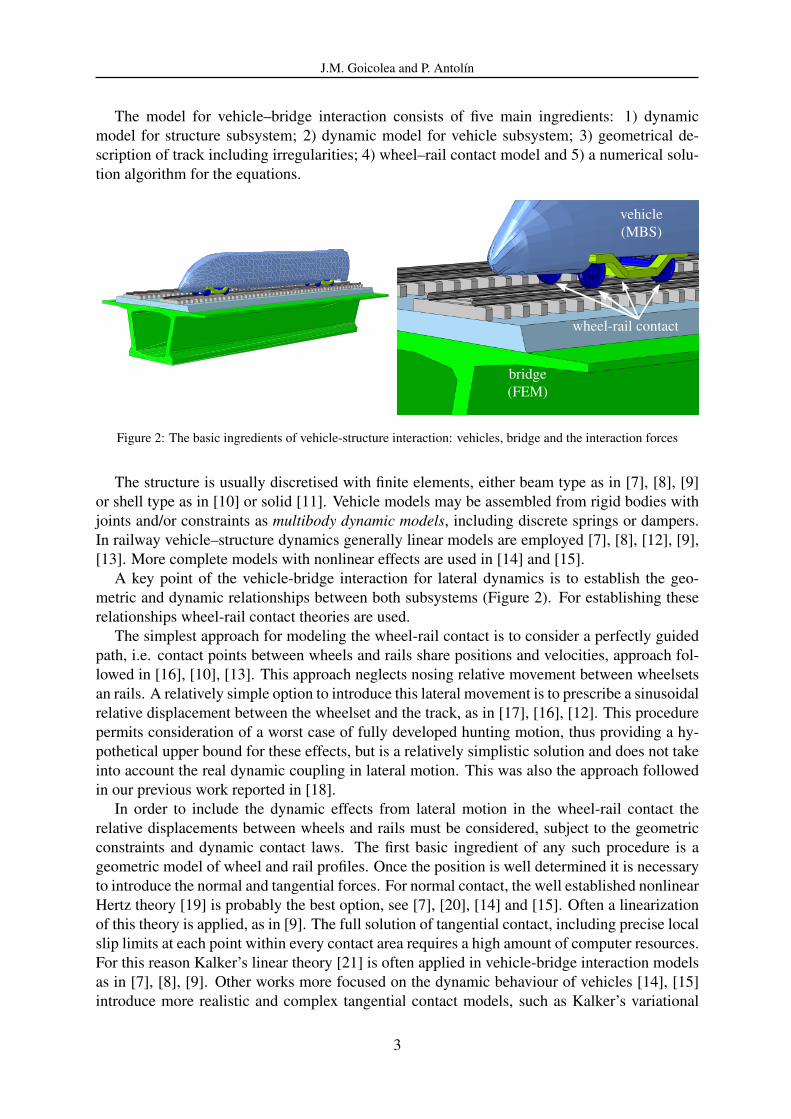
The model for vehicle–bridge interaction consists of five main ingredients: 1) dynamicmodel for structure subsystem; 2) dynamic model for vehicle subsystem; 3) geometrical de-scription of track including irregularities; 4) wheel–rail contact model and 5) a numerical solu-tion algorithm for the equations.

Z

YX

vehicle(MBS)

wheel-rail contact

bridge(FEM)

Figure 2: The basic ingredients of vehicle-structure interaction: vehicles, bridge and the interaction forces

The structure is usually discretised with finite elements, either beam type as in [7], [8], [9]or shell type as in [10] or solid [11]. Vehicle models may be assembled from rigid bodies withjoints and/or constraints as multibody dynamic models, including discrete springs or dampers.In railway vehicle–structure dynamics generally linear models are employed [7], [8], [12], [9],[13]. More complete models with nonlinear effects are used in [14] and [15].

A key point of the vehicle-bridge interaction for lateral dynamics is to establish the geo-metric and dynamic relationships between both subsystems (Figure 2). For establishing theserelationships wheel-rail contact theories are used.

The simplest approach for modeling the wheel-rail contact is to consider a perfectly guidedpath, i.e. contact points between wheels and rails share positions and velocities, approach fol-lowed in [16], [10], [13]. This approach neglects nosing relative movement between wheelsetsan rails. A relatively simple option to introduce this lateral movement is to prescribe a sinusoidalrelative displacement between the wheelset and the track, as in [17], [16], [12]. This procedurepermits consideration of a worst case of fully developed hunting motion, thus providing a hy-pothetical upper bound for these effects, but is a relatively simplistic solution and does not takeinto account the real dynamic coupling in lateral motion. This was also the approach followedin our previous work reported in [18].

In order to include the dynamic effects from lateral motion in the wheel-rail contact therelative displacements between wheels and rails must be considered, subject to the geometricconstraints and dynamic contact laws. The first basic ingredient of any such procedure is ageometric model of wheel and rail profiles. Once the position is well determined it is necessaryto introduce the normal and tangential forces. For normal contact, the well established nonlinearHertz theory [19] is probably the best option, see [7], [20], [14] and [15]. Often a linearizationof this theory is applied, as in [9]. The full solution of tangential contact, including precise localslip limits at each point within every contact area requires a high amount of computer resources.For this reason Kalker’s linear theory [21] is often applied in vehicle-bridge interaction modelsas in [7], [8], [9]. Other works more focused on the dynamic behaviour of vehicles [14], [15]introduce more realistic and complex tangential contact models, such as Kalker’s variational

3


theory [22] or the simplification of this in FASTSIM [4]. A practical alternative is the USETABtables [23], is based on Kalker Variational Theory [22], which is the approach followed in thiswork.

In addition, it must be considered that tracks do not follow perfectly the ideal geometry. Thealignment irregularities are an essential ingredient for excitation of laterl vibrations of vehicles.For considering a hypothetical upper bound scenario Irregularity profiles can be generated usingpower spectral density functions as defined in [24]. This approach is followed in [9], [18] andalso in this work. Another option is of course to employ irregularity profiles measured directlyfrom the track, as in [17], [8] and [16].

The last ingredient for the model is the strategy for numerical solutiona t each time-step.An option is to integrate separately both subsystems and establish at each time-step an iterationloop for achieving force and displacement compatibility at contact points, as in [17], [9], [25]and [26]. Another option is to form a global set of coupled equations including both subsystemscan be solved directly, as in [8], [16], [12], [13] and [27]. In this work the approach followedis similar to this latter option, including both subsystems within the same dynamic model, withspecial emphasis on the contact interface.

In the remaining of this work firstly the details of the numerical model employed will be dis-cussed. Following, this will be applied for the Las Piedras viaduct [5] in the spanish high-speedrailway Cordoba–Malaga, which has piers of 94 m and length of 1209 m. The results obtainedshow that, for the scenarios considered, no adverse lateral vibration effects are foreseable.

2 NUMERICAL MODEL

The vehicle-bridge interaction system is composed of the vehicle and bridge subsystemsand the contact interface between them. The model is constructed within ABAQUS simulationsystem [3], employing multibody capabilities for the vehicles, finite elements for the bridge,and user-developed algorithms for the compatibility between both and the contact interface.

Common cartesian coordinates are used in both subsystems: x along the bridge’s lontigudinaldirection, z pointing upwards and y laterally. The corresponding rotations around each of theseaxes will be called θx, θy and θz (Figure 3).

2.1 Vehicle model

The vehicle is considered as a multibody system. Car body, bogies and wheelsets are con-sidered as rigid bodies. The primary and secondary suspensions are defined using linear springsand dampers (figure 4). Anti-yaw dampers are included in the model with appropriate definitionof viscoelastic properties. For the vehicle model, the following assumptions are considered:

(A1) Small displacements are considered here (except for the wheel-rail contact interface).However this is not a limitation of the model, there is no restriction for nonlinear multi-body dynamics effects should they be necessary, as a full nonlinear solution is performedat each time-step.

(A2) The train is supposed to cross the bridge at a constant speed v.

(A3) The train is composed of independent cars: no connection between cars is considered.

(A4) A constant velocity v along the x axis is considered for all the bodies of each car, thereforethe degrees of freedom of car-bodies and bogies are y, z, θx, θy and θz. For wheelsets, θyis prescribed as θy = v/r0, being r0 the nominal rolling radius of wheels.

4


z

x

θy

H

T 2 T 1

W4

2d1 2d12d2

x

yθz

r0

h3

h2

h1

W3 W2 W1

Figure 3: Vehicle schema and coordinates.

Figure 4: Multibody model showing vehicle box and bogies

(A5) The coordinates used for each of the rigid bodies are absolute inertial coordinates, notrelative coordinates with respect to the bridge.

The multibody capabilities within ABAQUS program [3] are employed in this work to obtainthe vehicle multibody dynamic models.

2.2 Bridge model

The bridge is modeled with finite elements through the finite element library provided withinABAQUS [3]. In general, any type of finite elements can be employed (continuum, shell, beamor truss). In this case the model has been built using 3D beam elements for the deck and thepiers of the viaduct. The assumptions that have been made are:

(A6) Small displacements and linear elastic materials are considered in this case (except forthe wheel-rail contact interface). However this is not a limitation of the model, there isno restriction for nonlinear effects should they be necessary, as a full nonlinear solutionis performed at each time-step.

5


y

z

θx

ey

ez

T

D

Z

Y X

XY

Z

Figure 5: Schematic representation of bridge deck and 3D beam finite elements.

Figure 6: Kinematic constraints for wheelset position on bridge deck: schema and deformed view of rigid contactsurfaces

(A7) The rails are supposed to be rigidly attached to the deck section, with the appropriateoffsets and eccentricities.

(A8) Elastic effects for rail deformation are neglected.

The points on the rails corresponding to each wheelset are derived by interpolation and kine-matical constraints with the beam degrees of freedom. For this purpose, special rigid contactsurfaces are defined in the finite element model, linked kinematically to the structural beams(figure 6).

2.3 Track alignment irregularities

An essential ingredient for proper consideration of the vehicle dynamic effects are the trackirregularities. For this work irregularities for horizontal alignment and vertical profile wereconsidered as these will be the most important for lateral dynamics. In order to provide prob-abilistic upper bounds, irregularities were generated from a power spectral density spectrumadjusted to upper bounds of deviations to be expected in the wavelength between 3 and 25 mfrom maintenance operations (figure 7). The procedure used here is similar to that followed in[24]

6


0 10 20 30 40 50 60 70 80 90 100

−2

0

2

x [m]

Γ y,

Γ z[m

m]

ΓyΓz

1e-11

1e-10

1e-09

1e-08

1e-07

1e-06

1e-05

0.0001

0.01 0.1 1 10 100

PS

D [m

3 /cic

lo]

Frequency [rad/m]

PSD, from dataPSD, analytic

Figure 7: Profile of generated alignment irregularities and check for fit to PSD spectrum

2.4 Vehicle-bridge interaction

The final ingredient are the forces for establishing the interaction between the vehicle andthe structure. This is achieved through contact models, including geometric and dynamic com-ponents. The coupled system of equations may be represented as:(

MV 00 MB

){XV

XB

}(CV 00 CB

){XV

XB

}(KV 00 KB

){XV

XB

}=

{FV +FV

cFB +FB

c

}, (1)

where superscripts (·)V and (·)B refer to the vehicle and bridge subsystems respectively. Ad-ditionally, FV

c is the vector of forces applied on the vehicle as a consequence of the interactionwith the structure, and FB

c , on the structure, which will be computed from the vehicle and bridgedisplacements, velocities and time. The components of the contact forces are described in Sec-tion 2.5.

Equation (1) will be solved directly in time using the HHT Method [28], which is an implicitalgorithm. The tangent matrices of contact forces are needed for the numerical solution:

Kc =dFcdX

, Cc =dFc

dX, (2)

where Fc = (FVc ,FB

c )T. The expressions of the tangential forces applied in this work do not have

analytical derivatives and hence the tangent matrices are computed using numerical jacobians.

2.5 Nonlinear contact forces

The wheel-rail contact forces are developed in this Section. Considering some assumptions,that are expossed below, this problem can be split in three main parts:

Geometric problem: it consists on computing the main geometric variables which depend onthe relative displacements between wheel and rail.

Normal problem: considering the geometric variables obtained before, the contact ellipse di-mensions and the normal stress distribution is calculated using the Hertz theory [19].

Tangential problem: the tangential forces, which depend on the contact geometry, normalstresses and relative velocities between wheel and rail, are computed.

7


According to [22], if the wheel and rail materials have the same mechanical properties, thethree problems can be studied separately: geometric problem is solved firstly, normal problemsecondly and tangential problem thirdly.

2.5.1 Geometric contact problem

For obtaining the main geometric variables of the contact problems serveral assumptions aremade:

(A9) Separations between wheel and rail are not allowed.

(A10) The wheel-rail contact appears only in one area.

(A11) Only rigid body movements perpendicular to x axis are considered for the wheelset andthe track.

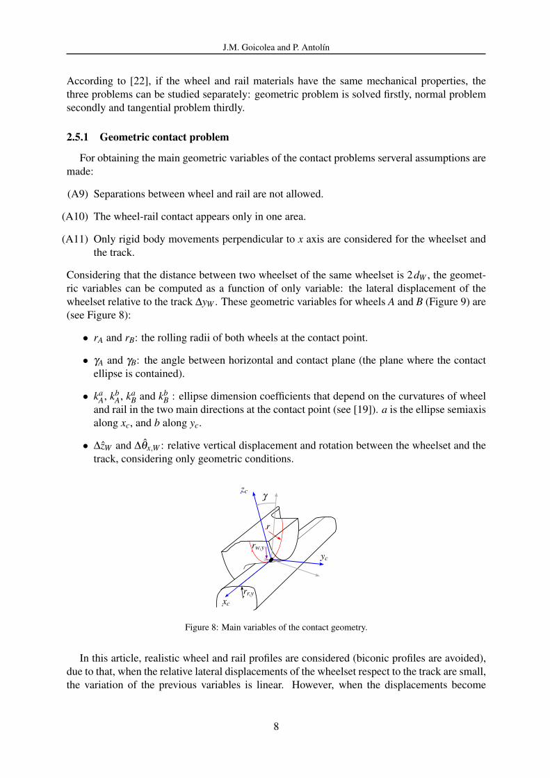
Considering that the distance between two wheelset of the same wheelset is 2dW , the geomet-ric variables can be computed as a function of only variable: the lateral displacement of thewheelset relative to the track ∆yW . These geometric variables for wheels A and B (Figure 9) are(see Figure 8):

• rA and rB: the rolling radii of both wheels at the contact point.

• γA and γB: the angle between horizontal and contact plane (the plane where the contactellipse is contained).

• kaA, kb

A, kaB and kb

B : ellipse dimension coefficients that depend on the curvatures of wheeland rail in the two main directions at the contact point (see [19]). a is the ellipse semiaxisalong xc, and b along yc.

• ∆zW and ∆θx,W : relative vertical displacement and rotation between the wheelset and thetrack, considering only geometric conditions.

zc γ

xc

yc

rr,y

r

rw,y

Figure 8: Main variables of the contact geometry.

In this article, realistic wheel and rail profiles are considered (biconic profiles are avoided),due to that, when the relative lateral displacements of the wheelset respect to the track are small,the variation of the previous variables is linear. However, when the displacements become

8


larger, contact between the flange of the wheel and the rail occurs, and the variation becomesnonlinear.

The relative displacements of the wheelset of vehicle respect to the track are:

∆yW = yW − yBT (x) , (3a)

∆zW = zW − zBT (x) , (3b)

∆θx,W = θx,W −θ Bx,T (x) , (3c)

∆θz,W = θz,W −θ Bz,T (x) , (3d)

being yW , zW , θx,W and θz,W the absolute displacements and rotations of the wheelset.

2.5.2 Normal contact problem

The Hertz theory [19], for solving the shape and dimensions of the contact surface and thenormal stress distribution, take into consideration the following assumptions:

(A12) At contact point, contact surfaces are continuous and nonconformal.

(A13) No plastic deformation is considered and strains are supposed to be small and elastic.

(A14) Stresses are neglected far from contact point.

(A15) Friction between surfaces does not affect to normal problem.

(A16) Quadratic functions of two variables can be used to define the wheel and rail surfacesnear to contact point.

With these assumptions, contact area is considered an ellipse and normal stress distribution anellipsoid.

The ellipse semiaxes can be computed as:

ak = kak(∆yW )

(1−ν

GNk

)1/3

(4a)

bk = kbk(∆yW )

(1−ν

GNk

)1/3

(4b)

where k = {A,B}, G is the shear stress modulus, ν the Poisson coefficient of wheels and railsand Nk the contact normal force in wheel-rail pair (it is explained below how to compute thesenormal forces). The coefficients ka

k and kbk , which depend on ∆yW , are computed before the

calculation and depend on the main curvatures of wheel and rail at contact point (see [4]).

2.5.3 Tangential contact problem

In this problem the tangential contact forces are computed. They appear as a consequence ofa rolling and sliding motion between wheels and rails. In each point of the contact surface theshear stress value can not be greater than the normal stress times friction coefficient. Thus, inthe contact ellipse adhesion and slip areas could appear.

9


The main variables of the tangential contact are the creepages, which are defined as thenon dimensional relative velocities between wheel and rail. ζ k

x , ζ ky and ζ k

R are, respectively,longitudinal, lateral and rotational creepages of wheel-rail pair k and can be expressed as:

ζ kx = 1− rk

r0± ∆θz,W

vdW (5a)

ζ ky =

1v

[(∆yW +∆θx,W rk

)cosγk

+(∆zW ±∆θx,W dW

)sinγk

] (5b)

ζ kR =−sinγk

r0(5c)

where the upper sign of ± and ∓ in the above equations corresponds to the wheel-rail pair A,and the lower, to B (see Figure 9).

Depending on the assumed hypothesis, different methods for solving tangential contact exist.The Kalker Variational Method [22] is a very accurate method for computing tangential forces,however, due to it is computationally very expensive, it can not be applied in an analysis likethat. The USETAB approximation [23], proposed by Kalker, is used in this work. This methodobtains the tangential forces in a pre-calculated table whose input variables are the contactnormal force, the ellipse semiaxes, the friction coefficient and the creepages, and the outputvariables are the tangential forces in longitudinal T k

x and lateral T ky local directions and moment

around normal direction Mkz . The values of this table have been computed using the Kalker

Variational method for different values of the input variables.

2.5.4 Vehicle-structure interaction forces

As it has been seen above, vertical relative displacement ∆zW and relative rotation ∆θx,Wcan be computed as geometric variables, without regard to dynamic aspects. Thus, the relativedisplacements computed as geometric variables and those obtained from the dynamic responseof vehicle and structure must be equal:

∆zW = ∆zW (∆yW ) , (6a)

∆θx,W = ∆θx,W (∆yW ) . (6b)

For imposing these constraints, a penalty force and moment are introduced in wheelsets gravitycentre:

Fzc = kz (∆zW (∆yW )−∆zW )3/2 , (7a)

Mxc = kθ

(∆θx,W (∆yW )−∆θx,W

)3/2. (7b)

These nonlinear penalty expresions derive from the approach expression bewtween two bodiesof the Hertz theory. Stiffness coefficients kz and kθ depend on ∆yW and Nk

W , but in order tosimplify the equations, they are computed considering only the train own weight in a static caseand ∆yW = 0.

10


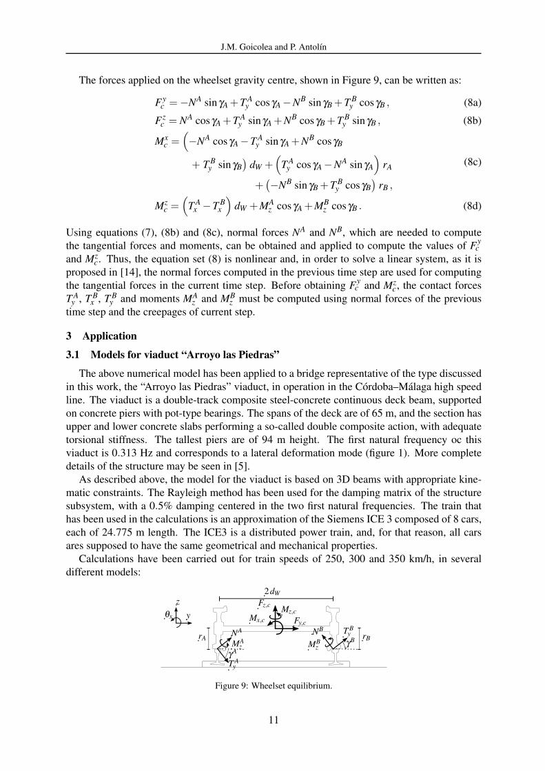
The forces applied on the wheelset gravity centre, shown in Figure 9, can be written as:

Fyc =−NA sinγA +T A

y cosγA−NB sinγB +T By cosγB , (8a)

Fzc = NA cosγA +T A

y sinγA +NB cosγB +T By sinγB , (8b)

Mxc =

(−NA cosγA−T A

y sinγA +NB cosγB

+ T By sinγB

)dW +

(T A

y cosγA−NA sinγA

)rA

+(−NB sinγB +T B

y cosγB)

rB ,

(8c)

Mzc =

(T A

x −T Bx

)dW +MA

z cosγA +MBz cosγB . (8d)

Using equations (7), (8b) and (8c), normal forces NA and NB, which are needed to computethe tangential forces and moments, can be obtained and applied to compute the values of Fy

cand Mz

c. Thus, the equation set (8) is nonlinear and, in order to solve a linear system, as it isproposed in [14], the normal forces computed in the previous time step are used for computingthe tangential forces in the current time step. Before obtaining Fy

c and Mzc, the contact forces

T Ay , T B

x , T By and moments MA

z and MBz must be computed using normal forces of the previous

time step and the creepages of current step.

3 Application

3.1 Models for viaduct “Arroyo las Piedras”

The above numerical model has been applied to a bridge representative of the type discussedin this work, the “Arroyo las Piedras” viaduct, in operation in the Cordoba–Malaga high speedline. The viaduct is a double-track composite steel-concrete continuous deck beam, supportedon concrete piers with pot-type bearings. The spans of the deck are of 65 m, and the section hasupper and lower concrete slabs performing a so-called double composite action, with adequatetorsional stiffness. The tallest piers are of 94 m height. The first natural frequency oc thisviaduct is 0.313 Hz and corresponds to a lateral deformation mode (figure 1). More completedetails of the structure may be seen in [5].

As described above, the model for the viaduct is based on 3D beams with appropriate kine-matic constraints. The Rayleigh method has been used for the damping matrix of the structuresubsystem, with a 0.5% damping centered in the two first natural frequencies. The train thathas been used in the calculations is an approximation of the Siemens ICE 3 composed of 8 cars,each of 24.775 m length. The ICE3 is a distributed power train, and, for that reason, all carsares supposed to have the same geometrical and mechanical properties.

Calculations have been carried out for train speeds of 250, 300 and 350 km/h, in severaldifferent models:

2dW

Fz,c Mz,cFy,c

Mx,c

MAz

γAγB rBrA

NA

T Ay

NB T By

MBz

z

yθx

Figure 9: Wheelset equilibrium.

11


(1) Bridge only model with moving loads, consisting only of the bridge dynamic subsystem,with the vehicle wheelsets simplified as moving loads of fixed magnitude. This amountsto neglecting the dynamic effects of vehicle vibration, and serves as a basic result withwhich to compare the influence of the vehicle vibration on the results. It also serves thepurpose of obtaining a so-called virtual path for the wheelsets of the vehicles, which canbe later applied to these in a decoupled approach to the vehicle-bridge dynamics: thebridge history of displacements is obtained in a first step, and these histories are thenapplied in a second step to the vehicle wheelsets to obtain the response of the train.

(2) Vehicle model, consisting only of the vehicle subsystem, in two different scenarios:

(a) Vehicle on rigid platform (i.e. no bridge) with prescribed profiles of irregularities.This model will enable to compare the influence of the bridge deformation on thevibrations of the vehicle.

(b) Vehicle on virtual path, as described above, this path results from previous analysisof the bridge with moving loads. The geometric track irregularities are added to thevirtual path in order to consider their effect on the vehicle.

(3) Bridge-Vehicle model, performing the calculation for the global system with the wheel-rail contact interaction. In this case, two scenarios have been considered:

(a) Model with interaction but without track irregularities

(b) Model with interaction and with track irregularities

3.2 Results for bridge and vehicle response

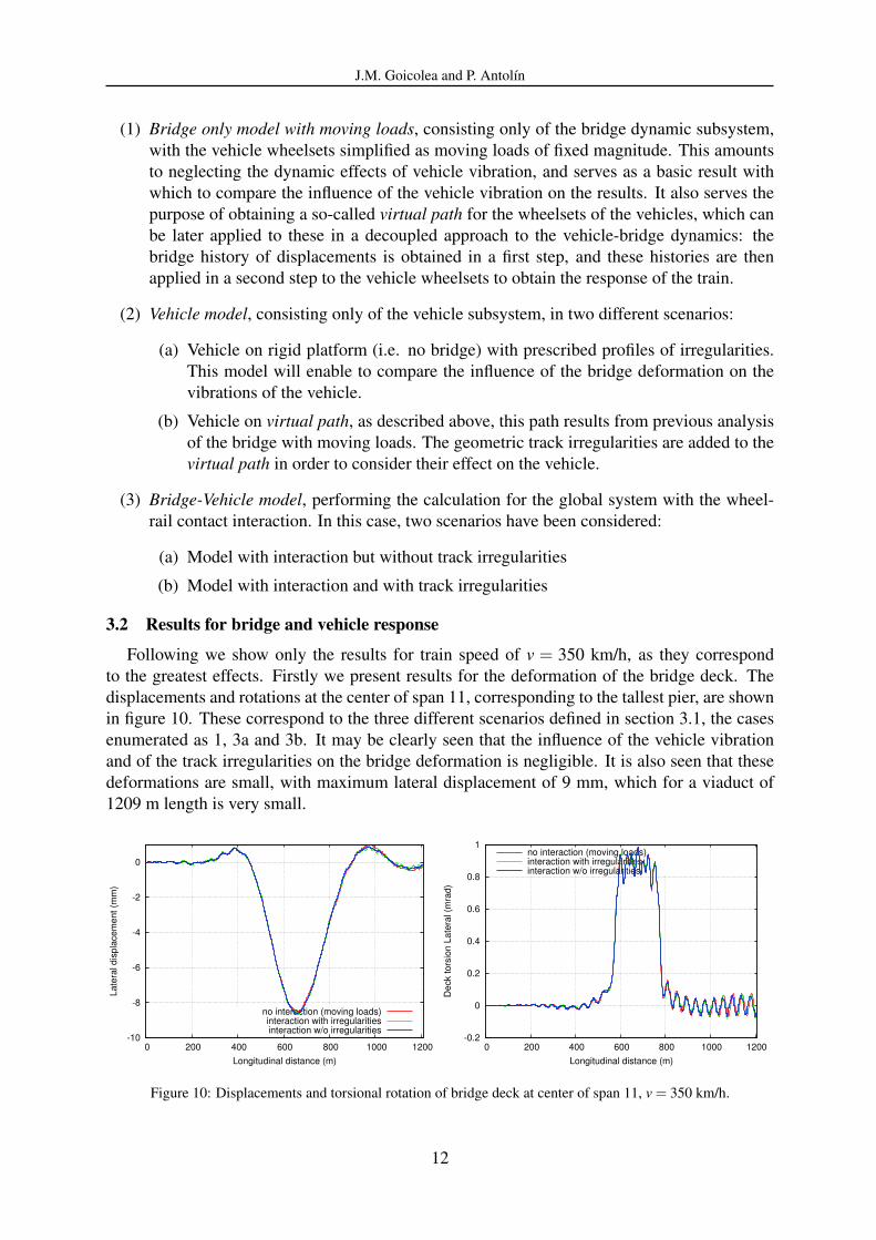
Following we show only the results for train speed of v = 350 km/h, as they correspondto the greatest effects. Firstly we present results for the deformation of the bridge deck. Thedisplacements and rotations at the center of span 11, corresponding to the tallest pier, are shownin figure 10. These correspond to the three different scenarios defined in section 3.1, the casesenumerated as 1, 3a and 3b. It may be clearly seen that the influence of the vehicle vibrationand of the track irregularities on the bridge deformation is negligible. It is also seen that thesedeformations are small, with maximum lateral displacement of 9 mm, which for a viaduct of1209 m length is very small.

-10

-8

-6

-4

-2

0

0 200 400 600 800 1000 1200

La

tera

l d

isp

lace

me

nt

(mm

)

Longitudinal distance (m)

no interaction (moving loads)interaction with irregularitiesinteraction w/o irregularities

-0.2

0

0.2

0.4

0.6

0.8

1

0 200 400 600 800 1000 1200

De

ck t

ors

ion

La

tera

l (m

rad

)


no interaction (moving loads)interaction with irregularitiesinteraction w/o irregularities

Figure 10: Displacements and torsional rotation of bridge deck at center of span 11, v = 350 km/h.

12


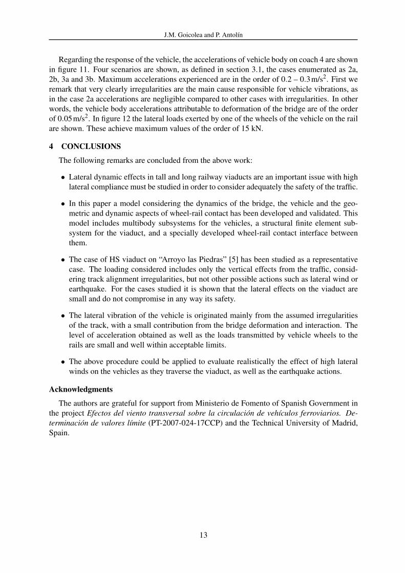
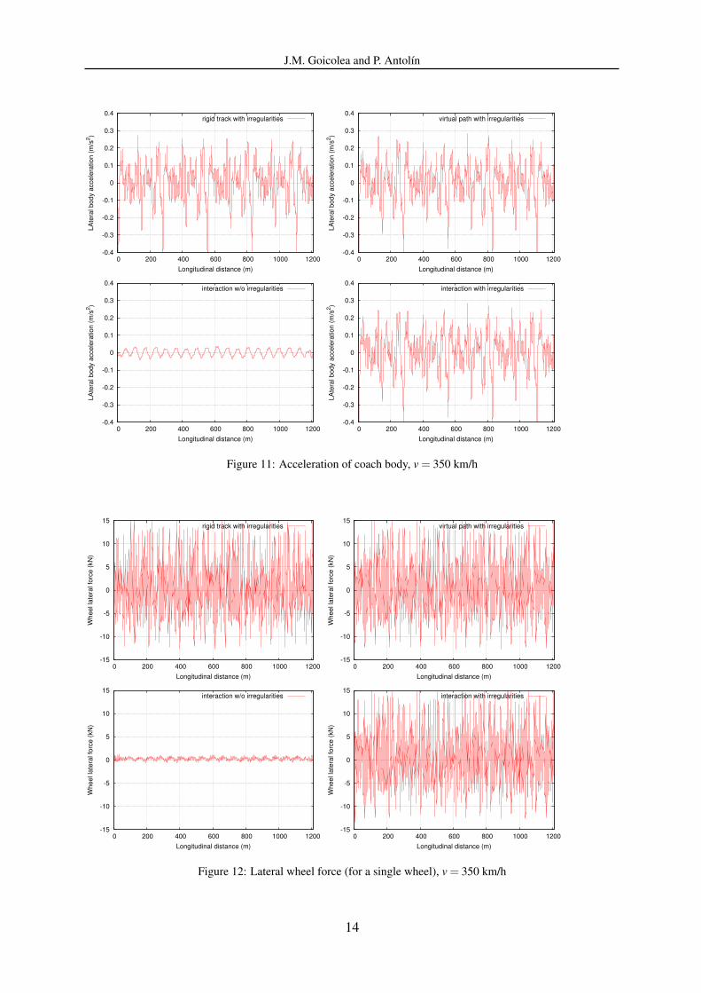
Regarding the response of the vehicle, the accelerations of vehicle body on coach 4 are shownin figure 11. Four scenarios are shown, as defined in section 3.1, the cases enumerated as 2a,2b, 3a and 3b. Maximum accelerations experienced are in the order of 0.2 – 0.3m/s2. First weremark that very clearly irregularities are the main cause responsible for vehicle vibrations, asin the case 2a accelerations are negligible compared to other cases with irregularities. In otherwords, the vehicle body accelerations attributable to deformation of the bridge are of the orderof 0.05m/s2. In figure 12 the lateral loads exerted by one of the wheels of the vehicle on the railare shown. These achieve maximum values of the order of 15 kN.

4 CONCLUSIONS

The following remarks are concluded from the above work:

• Lateral dynamic effects in tall and long railway viaducts are an important issue with highlateral compliance must be studied in order to consider adequately the safety of the traffic.

• In this paper a model considering the dynamics of the bridge, the vehicle and the geo-metric and dynamic aspects of wheel-rail contact has been developed and validated. Thismodel includes multibody subsystems for the vehicles, a structural finite element sub-system for the viaduct, and a specially developed wheel-rail contact interface betweenthem.

• The case of HS viaduct on “Arroyo las Piedras” [5] has been studied as a representativecase. The loading considered includes only the vertical effects from the traffic, consid-ering track alignment irregularities, but not other possible actions such as lateral wind orearthquake. For the cases studied it is shown that the lateral effects on the viaduct aresmall and do not compromise in any way its safety.

• The lateral vibration of the vehicle is originated mainly from the assumed irregularitiesof the track, with a small contribution from the bridge deformation and interaction. Thelevel of acceleration obtained as well as the loads transmitted by vehicle wheels to therails are small and well within acceptable limits.

• The above procedure could be applied to evaluate realistically the effect of high lateralwinds on the vehicles as they traverse the viaduct, as well as the earthquake actions.

Acknowledgments

The authors are grateful for support from Ministerio de Fomento of Spanish Government inthe project Efectos del viento transversal sobre la circulacion de vehıculos ferroviarios. De-terminacion de valores lımite (PT-2007-024-17CCP) and the Technical University of Madrid,Spain.

13


-0.4

-0.3

-0.2

-0.1

0

0.1

0.2

0.3

0.4

0 200 400 600 800 1000 1200

LA

tera

l b

od

y a

cce

lera

tio

n (

m/s

2)


rigid track with irregularities

-0.4

-0.3

-0.2

-0.1

0

0.1

0.2

0.3

0.4

0 200 400 600 800 1000 1200

LA

tera

l b

od

y a

cce

lera

tio

n (

m/s

2)


virtual path with irregularities

-0.4

-0.3

-0.2

-0.1

0

0.1

0.2

0.3

0.4

0 200 400 600 800 1000 1200

LA

tera

l b

od

y a

cce

lera

tio

n (

m/s

2)


interaction w/o irregularities

-0.4

-0.3

-0.2

-0.1

0

0.1

0.2

0.3

0.4

0 200 400 600 800 1000 1200

LA

tera

l b

od

y a

cce

lera

tio

n (

m/s

2)


interaction with irregularities

Figure 11: Acceleration of coach body, v = 350 km/h

-15

-10

-5

0

5

10

15

0 200 400 600 800 1000 1200

Wh

ee

l la

tera

l fo

rce

(kN

)


rigid track with irregularities

-15

-10

-5

0

5

10

15

0 200 400 600 800 1000 1200

Wh

ee

l la

tera

l fo

rce

(kN

)


virtual path with irregularities

-15

-10

-5

0

5

10

15

0 200 400 600 800 1000 1200

Wh

ee

l la

tera

l fo

rce

(kN

)


interaction w/o irregularities

-15

-10

-5

0

5

10

15

0 200 400 600 800 1000 1200

Wh

ee

l la

tera

l fo

rce

(kN

)


interaction with irregularities

Figure 12: Lateral wheel force (for a single wheel), v = 350 km/h

14


REFERENCES

[1] ERRI, Forces Laterales sur les Ponts Ferroviaires. Rapport final RP6, European RailwayResearch Institute, 1996.

[2] European Committee for Standardization, EN1990-A1: EUROCODE 0 – Basis of Struc-tural Design, Ammendment A1: Annex A2, Application for bridges, European Union,2005.

[3] SIMULIA, 166 Valley Street Providence, RI 02909 USA, Abaqus/Standard 6.9, 2010,www.simulia.com.

[4] J J Kalker, Three-Dimensional Elastic Bodies in Rolling Contact (Solid Mechanics andIts Applications), Springer, 1990.

[5] F. Millanes, J. Pascual, and M. Ortega, “’Arroyo las Piedras’ viaduct: The first compositesteel–concrete high speed railway bridge in spain,” Structural Engineering International,vol. 17, no. 4, pp. 292–297, 2007.

[6] Ministerio de Fomento, IAPF-07: Instruccion sobre las acciones a considerar en elproyecto de puentes de ferrocarril, Government of Spain, 2007.

[7] M Tanabe, H Wakui, N Matsumoto, H Okuda, M Sogabe, and S Komiya, “Computationalmodel of a Shinkansen train running on the railway structure and the industrial applica-tions,” Journal of Materials Processing Technology, vol. 140, no. 1-3, pp. 705–710, 2003.

[8] N Zhang, H Xia, W W Guo, and G De Roeck, “A Vehicle-Bridge Linear InteractionModel and Its Validation,” International Journal of Structural Stability and Dynamics,vol. 10, no. 02, pp. 335, 2010.

[9] D V Nguyen, K D Kim, and P Warnitchai, “Simulation procedure for vehicle-substructuredynamic interactions and wheel movements using linearized wheelrail interfaces,” FiniteElements in Analysis and Design, vol. 45, no. 5, pp. 341–356, 2009.

[10] M K Song, H C Noh, and C K Choi, “New three-dimensional finite element analysismodel of high-speed train-bridge,” Engineering Structures, vol. 25, pp. 1611–1626, 2003.

[11] L Kwasniewski, H Li, J Wekezer, and J Malachowski, “Finite element analysis of vehicle-bridge interaction,” Finite Elements in Analysis and Design, vol. 42, no. 11, pp. 950–959,2006.

[12] H Xia and N Zhang, Dynamic Interaction of Vehicles and Structures, Science Press,Beijing, China, 2nd edition, 2005.

[13] Y B Yang and J D Yau, “Vehicle-bridge interaction element for dynamic analysis,” Journalof Sound and Vibration, vol. 123, no. 11, pp. 1512–1518, 1997.

[14] A A Shabana, K E Zaazaa, and H Sugiyama, Railroad Vehicle Dynamics: A Computa-tional Approach, CRC Press, 2008.

[15] K Popp and W Schiehlen, Ground Vehicle Dynamics, Springer Berlin Heidelberg, Chen-nai, 1st edition, 2010.

15


[16] H Xia, N Zhang, and G D Roeck, “Dynamic analysis of high speed railway bridge underarticulated trains,” Computers & Structures, vol. 81, pp. 2467–2478, 2003.

[17] N Zhang, H Xia, and W Guo, “Vehicle-bridge interaction analysis under high-speedtrains,” Journal of Sound and Vibration, vol. 309, no. 3-5, pp. 407–425, 2008.

[18] R. Dias, J.M. Goicolea, F. Gabaldon, M. Cuadrado, J. Nasarre, and P. Gonzalez, “Astudy of the lateral dynamic behaviour of high speed railway viaducts and its effect onvehicle ride comfort and stability,” in Bridge Maintenance, Safety, Management, HealthMonitoring and Informatics, Koh & Frangopol, Ed., Seoul, 14-16 jul 2008, IABMAS08:Fourth International Conference on Bridge Maintenance, Safety and Management, pp.724–735, Taylor & Francis Group London, ISBN 978-0-415-46844-2.

[19] H Hertz, “Uber die beruhrung fester elasticher korper and uber die hartean,” J. fur reineund agewandte Mathematik, vol. 92, pp. 156–171, 1882.

[20] D V Nguyen, K D Kim, and P Warnitchai, “Dynamic analysis of three-dimensional bridge-high-speed train interactions using a wheelrail contact model,” Engineering Structures,vol. 31, no. 12, pp. 3090–3106, 2009.

[21] J J Kalker, On the rolling contact of two elastic bodies in the presence of dry friction,Ph.D. thesis, Delft Unversity of Technology, 1967.

[22] J J Kalker, “The computation of three-dimensional rolling contact with dry friction,”International Journal for Numerical Methods in Engineering, vol. 14, no. 9, pp. 1293–1307, 1979.

[23] J J Kalker, “Book of tables for the Hertzian creep-force law,” in Proceedings of the 2ndMini Conference on Contact Mechanics and Wear of Wheel/Rail Systems, I Zobory, Ed.,Budapest: Technical University of Budapest, 1996, pp. 11–20.

[24] H Claus and W Schiehlen, “Modeling and Simulation of Railway Bogie Structural Vibra-tions,” Vehicle System Dynamics, vol. 29, no. 1, pp. 538–552, Aug. 1997.

[25] Y L Xu, N Zhang, and H Xia, “Vibration of coupled train and cable-stayed bridge systemsin cross winds,” Engineering Structures, vol. 26, pp. 1389–1406, 2004.

[26] G De Roeck, J Maeck, and A Teughels, “Train-bridge interaction: Validation of numericalmodels by experiments on high-speed railway bridge in Antoing,” in TIVC’2001, Beijing,2001, pp. 283–294.

[27] J D Yau and Y B Yang, “Vibration reduction for cable-stayed bridges traveled by high-speed trains,” Finite Elements in Analysis and Design, vol. 40, pp. 341–359, 2004.

[28] H M Hilber, T J R Hughes, and R L Taylor, “Improved numerical dissipation for timeintegration algorithms in structural dynamics,” Earthquake Engineering & Structural Dy-namics, vol. 5, pp. 283–292, 1977.

16

DYNAMIC EFFECTS OF RAILWAY TRAFFIC DUE TO...

Documents

Transcript of DYNAMIC EFFECTS OF RAILWAY TRAFFIC DUE TO...