Dynamic Crack Initiation Toughness: Experiments and ... · Dynamic Crack Initiation Toughness:...

SANDIA REPORTSAND2009-7217Unlimited ReleasePrinted October 2009

Dynamic Crack Initiation Toughness:Experiments and PeridynamicModeling

John T. Foster

Prepared bySandia National LaboratoriesAlbuquerque, New Mexico 87185 and Livermore, California 94550

Sandia is a multiprogram laboratory operated by Sandia Corporation,a Lockheed Martin Company, for the United States Department of Energy’sNational Nuclear Security Administration under Contract DE-AC04-94-AL85000.

Approved for public release; further dissemination unlimited.

Issued by Sandia National Laboratories, operated for the United States Department of Energy

by Sandia Corporation.

NOTICE: This report was prepared as an account of work sponsored by an agency of the United

States Government. Neither the United States Government, nor any agency thereof, nor any

of their employees, nor any of their contractors, subcontractors, or their employees, make any

warranty, express or implied, or assume any legal liability or responsibility for the accuracy,

completeness, or usefulness of any information, apparatus, product, or process disclosed, or rep-

resent that its use would not infringe privately owned rights. Reference herein to any specific

commercial product, process, or service by trade name, trademark, manufacturer, or otherwise,

does not necessarily constitute or imply its endorsement, recommendation, or favoring by the

United States Government, any agency thereof, or any of their contractors or subcontractors.

The views and opinions expressed herein do not necessarily state or reflect those of the United

States Government, any agency thereof, or any of their contractors.

Printed in the United States of America. This report has been reproduced directly from the best

available copy.

Available to DOE and DOE contractors fromU.S. Department of Energy

Office of Scientific and Technical Information

P.O. Box 62

Oak Ridge, TN 37831

Telephone: (865) 576-8401

Facsimile: (865) 576-5728

E-Mail: [email protected]

Online ordering: http://www.osti.gov/bridge

Available to the public fromU.S. Department of Commerce

National Technical Information Service

5285 Port Royal Rd

Springfield, VA 22161

Telephone: (800) 553-6847

Facsimile: (703) 605-6900

E-Mail: [email protected]

Online ordering: http://www.ntis.gov/help/ordermethods.asp?loc=7-4-0#online

DEP

ARTMENT OF ENERGY

• • UN

ITED

STATES OF AM

ERI C

A

2

SAND2009-7217SAND200 9-XXXXUnlimited Release

Printed October 2009

Dynamic Crack Initiation Toughness: Experiments and

Peridynamic Modeling

John T. Foster

Abstract

This is a dissertation on research conducted studying the dynamic crack initiation toughnessof a 4340 steel. Researchers have been conducting experimental testing of dynamic crackinitiation toughness, KIc, for many years, using many experimental techniques with vastlydifferent trends in the results when reporting KIc as a function of loading rate. The dis-sertation describes a novel experimental technique for measuring KIc in metals using theKolsky bar. The method borrows from improvements made in recent years in traditionalKolsky bar testing by using pulse shaping techniques to ensure a constant loading rate ap-plied to the sample before crack initiation. Dynamic crack initiation measurements werereported on a 4340 steel at two different loading rates. The steel was shown to exhibit arate dependence, with the recorded values of KIc being much higher at the higher loadingrate. Using the knowledge of this rate dependence as a motivation in attempting to modelthe fracture events, a viscoplastic constitutive model was implemented into a peridynamiccomputational mechanics code. Peridynamics is a newly developed theory in solid mechanicsthat replaces the classical partial differential equations of motion with integral-differentialequations which do not require the existence of spacial derivatives in the displacement field.This allows for the straightforward modeling of unguided crack initiation and growth. Todate, peridynamic implementations have used severely restricted constitutive models. Thisresearch represents the first implementation of a complex material model and its validation.After showing results comparing deformations to experimental Taylor anvil impact for theviscoplastic material model, a novel failure criterion is introduced to model the dynamiccrack initiation toughness experiments. The failure model is based on an energy criterionand uses the KIc values recorded experimentally as an input. The failure model is thenvalidated against one class of problems showing good agreement with experimental results.

3

Acknowledgement

I would like to acknowledge the support and guidance of my committee chair Prof. WeinongW. Chen; thanks for the countless hours of insightful conversation, which seeded many ofthe ideas that are further developed in this work.

I would like to give a very gracious acknowledgement to the brilliant yet most humble,Dr. Stewart A. Silling, for serving on my committee and fostering many ideas involving theperidynamic theory of solid mechanics.

A special appreciation is given to Mr. Robert C. Anderson, Dr. Brad L. Boyce, Mr. DavidC. Craft, Mr. Thomas B. Crenshaw, Ms. Gloria L. Lloyd, and Dr. Bo Song for their help inlaboratory, Dr. Paul A. Taylor for his conversations regarding peridynamics and computa-tional mechanics, and Dr. Joseph E. Bishop for his constant questioning which challengedme to further explore many ideas.

Additional thanks is given to my current manager at Sandia National Laboratories,Mr. Douglas A. Dederman, for allowing me the time and opportunity to complete this work.Thanks for fighting for my acceptance into the University Part Time Program and allowingme to telecommute for my work responsibilities during the time I was at Purdue.

Appreciation is also give to the remaining members of my advisory committee, Prof. R.Byron Pipes and Prof. Chin-Teh Sun, for their time and effort; and Dr. Vincent K. Lukand the MOU Joint Munitions Program and to the Sandia University Programs office fortheir funding of this research. Sandia is a multiprogram laboratory operated by SandiaCorporation, a Lockheed Martin Company, for the United States Department of Energy’sNational Nuclear Security Administration under contract DE-AC04-94AL85000.

Finally and most importantly, I would like to thank my wife Lisa for allowing me to beaway from home while at Purdue, on travel in support of this research, or just simply stayinglate in the lab or office. Thank you for all your love and support.

4

Contents

Preface 11

1 Introduction 13

1.1 Dynamic Fracture . . . . . . . . . . . . . . . . . . . . . . . . . . . . . . . . . . . . . . . . . . . . . . . . . 13

1.2 Peridynamics . . . . . . . . . . . . . . . . . . . . . . . . . . . . . . . . . . . . . . . . . . . . . . . . . . . . 16

2 Literature Review 19

2.1 Dynamic Fracture Experiments . . . . . . . . . . . . . . . . . . . . . . . . . . . . . . . . . . . . . . 19

2.1.1 Stress Wave Loading Techniques . . . . . . . . . . . . . . . . . . . . . . . . . . . . . . . 19

Electromagnetic Loading . . . . . . . . . . . . . . . . . . . . . . . . . . . . . . . . . . . . . 20

Kolsky Bar Loading . . . . . . . . . . . . . . . . . . . . . . . . . . . . . . . . . . . . . . . . . 20

2.2 Peridynamics . . . . . . . . . . . . . . . . . . . . . . . . . . . . . . . . . . . . . . . . . . . . . . . . . . . . 28

3 Experimental Procedure 31

3.1 Introduction . . . . . . . . . . . . . . . . . . . . . . . . . . . . . . . . . . . . . . . . . . . . . . . . . . . . . 31

3.2 Sample Preparation . . . . . . . . . . . . . . . . . . . . . . . . . . . . . . . . . . . . . . . . . . . . . . . 31

3.3 Fatigue Cracking . . . . . . . . . . . . . . . . . . . . . . . . . . . . . . . . . . . . . . . . . . . . . . . . . 33

3.4 Apparatus . . . . . . . . . . . . . . . . . . . . . . . . . . . . . . . . . . . . . . . . . . . . . . . . . . . . . . . 35

3.5 Crack Initiation Time Detection . . . . . . . . . . . . . . . . . . . . . . . . . . . . . . . . . . . . . 38

3.6 Data Reduction . . . . . . . . . . . . . . . . . . . . . . . . . . . . . . . . . . . . . . . . . . . . . . . . . . 41

3.6.1 Wave Speed Calculation . . . . . . . . . . . . . . . . . . . . . . . . . . . . . . . . . . . . . . 41

5

3.6.2 Strain Conversion . . . . . . . . . . . . . . . . . . . . . . . . . . . . . . . . . . . . . . . . . . . 42

3.6.3 Force Equilibrium Verification . . . . . . . . . . . . . . . . . . . . . . . . . . . . . . . . . 43

3.6.4 Sample Boundary Velocity . . . . . . . . . . . . . . . . . . . . . . . . . . . . . . . . . . . . 47

3.6.5 Crack Length Measurement . . . . . . . . . . . . . . . . . . . . . . . . . . . . . . . . . . . 48

3.6.6 Stress Intensity Factor and Dynamic Crack Initiation Toughness . . . . . 48

3.7 Results and Discussion . . . . . . . . . . . . . . . . . . . . . . . . . . . . . . . . . . . . . . . . . . . . . 48

3.8 Camera Data . . . . . . . . . . . . . . . . . . . . . . . . . . . . . . . . . . . . . . . . . . . . . . . . . . . . 51

3.9 Scanning Electron Microscopy . . . . . . . . . . . . . . . . . . . . . . . . . . . . . . . . . . . . . . . 52

3.10 Concluding Remarks . . . . . . . . . . . . . . . . . . . . . . . . . . . . . . . . . . . . . . . . . . . . . . 52

4 Viscoplasticity Using Peridynamics 57

4.1 Introduction . . . . . . . . . . . . . . . . . . . . . . . . . . . . . . . . . . . . . . . . . . . . . . . . . . . . . 57

4.2 Peridynamic Kinematics . . . . . . . . . . . . . . . . . . . . . . . . . . . . . . . . . . . . . . . . . . . 58

4.3 Principal of Material Frame Indifference . . . . . . . . . . . . . . . . . . . . . . . . . . . . . . . 61

4.4 Stress to Peridynamic State Conversion . . . . . . . . . . . . . . . . . . . . . . . . . . . . . . . 62

4.5 von Mises Plasticity . . . . . . . . . . . . . . . . . . . . . . . . . . . . . . . . . . . . . . . . . . . . . . . 62

4.6 Yield Surface Determination . . . . . . . . . . . . . . . . . . . . . . . . . . . . . . . . . . . . . . . . 64

4.7 Evaluation of Stress Tensor . . . . . . . . . . . . . . . . . . . . . . . . . . . . . . . . . . . . . . . . . 66

4.8 Evaluation of Equivalent Plastic Strain . . . . . . . . . . . . . . . . . . . . . . . . . . . . . . . 67

4.9 Constitutive Model . . . . . . . . . . . . . . . . . . . . . . . . . . . . . . . . . . . . . . . . . . . . . . . . 68

4.10 Numerical Simulations . . . . . . . . . . . . . . . . . . . . . . . . . . . . . . . . . . . . . . . . . . . . . 69


5 Fracture Model and Numerical Simulation 73

5.1 Introduction . . . . . . . . . . . . . . . . . . . . . . . . . . . . . . . . . . . . . . . . . . . . . . . . . . . . . 73

5.2 Failure Model . . . . . . . . . . . . . . . . . . . . . . . . . . . . . . . . . . . . . . . . . . . . . . . . . . . . 73

5.3 Numerical Simulations . . . . . . . . . . . . . . . . . . . . . . . . . . . . . . . . . . . . . . . . . . . . . 78

6


6 Summary and Recomendations 87

References 90

Appendix

A Loading Rate 1 97

B Loading Rate 2 103

C Machine Drawings 109

D Sample Dimensions 113

E Sequenced Images of Crack Initiation and Propagation in Beam 115

F Additional Derivations of Peridynamic Notions 129

G Hole in a Plate Problem 133

7

List of Figures

1.1 Crack opening modes. . . . . . . . . . . . . . . . . . . . . . . . . . . . . . . . . . . . . . . . . . . . . . 14

1.2 Single-edge notched specimen. . . . . . . . . . . . . . . . . . . . . . . . . . . . . . . . . . . . . . . . 14

1.3 Schematic of peridynamic representations. . . . . . . . . . . . . . . . . . . . . . . . . . . . . . 17

2.1 Schematic of Kolsky bar. . . . . . . . . . . . . . . . . . . . . . . . . . . . . . . . . . . . . . . . . . . . 21

2.2 Comparison of experimental results from Klepaczko and Owen. . . . . . . . . . . . . 26

2.3 Schematic of Jiang three point bend setup. . . . . . . . . . . . . . . . . . . . . . . . . . . . . 28

3.1 Four point bend beam. . . . . . . . . . . . . . . . . . . . . . . . . . . . . . . . . . . . . . . . . . . . . . 32

3.2 Four point bend fixture, sample, and microscope camera. . . . . . . . . . . . . . . . . . 36

3.3 Digital microscope monitoring fatigue crack growth. . . . . . . . . . . . . . . . . . . . . . 36

3.4 Schematic of modified Kolsky bar. . . . . . . . . . . . . . . . . . . . . . . . . . . . . . . . . . . . 37

3.5 Sacrificial strain gage placed near crack tip. . . . . . . . . . . . . . . . . . . . . . . . . . . . . 40

3.6 Strain gage post-fracture showing relation to fatigue precrack. . . . . . . . . . . . . . 40

3.7 Typical signal from sacrificial strain gage. . . . . . . . . . . . . . . . . . . . . . . . . . . . . . 41

3.8 Wave speed calculation. . . . . . . . . . . . . . . . . . . . . . . . . . . . . . . . . . . . . . . . . . . . . 42

3.9 Uncorrected force equilibrium. . . . . . . . . . . . . . . . . . . . . . . . . . . . . . . . . . . . . . . . 44

3.10 Compressive stress wave progression. . . . . . . . . . . . . . . . . . . . . . . . . . . . . . . . . . 45

3.11 Pressure profiles from CTH simulation. . . . . . . . . . . . . . . . . . . . . . . . . . . . . . . . 46

3.12 Corrected force equilibrium plot. . . . . . . . . . . . . . . . . . . . . . . . . . . . . . . . . . . . . . 47

8

3.13 Results from a typical dynamic crack initiation toughness test using the mod-ified Kolsky bar. . . . . . . . . . . . . . . . . . . . . . . . . . . . . . . . . . . . . . . . . . . . . . . . . . . 50

3.14 Dynamic crack initiation toughness as a function of loading rate. . . . . . . . . . . 51

3.15 Single frame from Cordin camera taken after crack initiation. . . . . . . . . . . . . . 53

3.16 SEM image taken from fracture surface initiation point. . . . . . . . . . . . . . . . . . . 54

4.1 Illustration of key difference between deformation gradient and deformationvector-state. . . . . . . . . . . . . . . . . . . . . . . . . . . . . . . . . . . . . . . . . . . . . . . . . . . . . . 59

4.2 Notional curve for ∆λ root. . . . . . . . . . . . . . . . . . . . . . . . . . . . . . . . . . . . . . . . . . 67

4.3 Comparison of experimental data with numerical simulation at nominal engi-neering strain rate of 8300/s. . . . . . . . . . . . . . . . . . . . . . . . . . . . . . . . . . . . . . . . . 70

4.4 Normalized length comparison. . . . . . . . . . . . . . . . . . . . . . . . . . . . . . . . . . . . . . . 71

4.5 Normalized diameter comparison. . . . . . . . . . . . . . . . . . . . . . . . . . . . . . . . . . . . . 71

4.6 Qualitative comparison of post test deformation from DSL image with numer-ical simulation at 289m/s impact speed. . . . . . . . . . . . . . . . . . . . . . . . . . . . . . . 72

5.1 Illustration of relationship between state-forces and “bond.” . . . . . . . . . . . . . . 74

5.2 Schematic of bond kinematics. . . . . . . . . . . . . . . . . . . . . . . . . . . . . . . . . . . . . . . 75

5.3 Example of equivalent wξ and different η(tfinal) for two relative displacementrates. . . . . . . . . . . . . . . . . . . . . . . . . . . . . . . . . . . . . . . . . . . . . . . . . . . . . . . . . . . . 76

5.4 Schematic of fracture surface. . . . . . . . . . . . . . . . . . . . . . . . . . . . . . . . . . . . . . . . 77

5.5 Comparison of data to simulation at strain rates of 1150/s and 2900/s. . . . . . 78

5.6 Boundary regions. . . . . . . . . . . . . . . . . . . . . . . . . . . . . . . . . . . . . . . . . . . . . . . . . . 80

5.7 Sample boundary velocities from test T36. . . . . . . . . . . . . . . . . . . . . . . . . . . . . . 81

5.8 Comparison of time-to-fracture from experiment and simulation. . . . . . . . . . . . 82

5.9 Simulation results showing crack initiation and propagation. . . . . . . . . . . . . . . 83

5.10 Comparison of simulation to experimental camera data. . . . . . . . . . . . . . . . . . . 85

6.1 Ogive and flat nose penetration of aluminum plate. . . . . . . . . . . . . . . . . . . . . . . 89

9

List of Tables

2.1 Stress wave loading schemes and respective loading rates. . . . . . . . . . . . . . . . . 20

3.1 Nominal sample dimensions. . . . . . . . . . . . . . . . . . . . . . . . . . . . . . . . . . . . . . . . . 32

10

Preface

This document is a reproduction of a Ph.D. dissertation submitted to the faculty of PurdueUniversity. It has been reformatted here as a SAND report for archival within SandiaNational Laboratories.

The focus of the research in this dissertation is separated into two main areas, experi-ments and numerical simulation. Each of the first two chapters, Introduction and LiteratureReview, will be divided into two main sections, separately describing each of these areas.Chapter 3 describes, in detail, the experimental procedure for measuring dynamic crackinitiation at high loading rates and reports a selection of data for 4340 steel. Chapter 4describes the theory and numerical implementation of a viscoplastic material model into acomputational mechanics code using the peridynamic theory of solid mechanics. Chapter 5describes a novel energy based failure criterion, its numerical implementation, and a selectionof simulations and comparisons to experimental results. The final chapter summarizes theaccomplishments of this research and gives suggestions for further investigation.

11

1 Introduction

1.1 Dynamic Fracture

Failure of engineering materials has been at the forefront of research for scientists and en-gineers for centuries. The pioneering work of Griffith [24] during the first part of the 20th

century steered material failure research towards a crack-dominated analysis and the field offracture mechanics was born. Irwin’s [30, 31] work introduced us to the idea that the stressfield near a crack could be modeled in a linear elastic fashion with only a small plastic zonenear the crack tip. This idea of small scale yielding led to a parameter that could be usedto describe the state of stress near the crack tip, called the stress intensity factor, K, withunits of stress times square root of length, typically given in MPa

√m or ksi

√in.

The rest of the 20th century was filled with subsequent analysis of crack tip stress and initi-ation, mostly formulated within this framework of linear elastic fracture mechanics (LEFM).Many parameters such as strain energy release rate, the J-integral [51, 54], and crack tipopening displacement (CTOD) have been related to the stress intensity factor. These manyforms of analysis allowed experimentalists freedom and creativity in designing experimentsto determine a crack’s stress intensity factor. It was discovered through this experimentationthat there is a limiting value of stress intensity factor that when exceeded will cause a crackto grow. This limiting value is called the fracture toughness and denoted by Kc. A material’sfracture toughness is considered a material property, meaning it is constant irrespective ofsample size or geometry. It is typically presented with respect to the opening mode of thecrack as KIc, KIIc, or KIIIc. Figure 1.1 illustrates these opening modes.

In 1970 the American Society for Testing and Materials (ASTM) International publishedthe original standard for finding the linear-elastic plane-strain fracture toughness, KIc, formetallic materials [29]. This standard is designated E 399 and the current revision at thetime of this writing is 2006. ASTM has also developed standards for finding the fracturetoughness for other types of engineering materials such as ceramics and polymers. All ofthese well defined procedures are only valid for quasi-static loading rates.

High-rate loads are encountered in many engineering applications and it is importantto understand how these loading regimes affect the fundamental fracture mechanisms inorder to assure the integrity of the material. Generally, high-rate loading is defined by the

13

(a) Opening mode I. (b) Sliding mode II. (c) Tearing mode III.

Figure 1.1: Crack opening modes.

v

Figure 1.2: Single-edge notched specimen.

need to analyze the stress wave propagation in a material to fully understand its behavior.This stress wave phenomenon’s action on crack propagation can be easily illustrated withan example taken abridged from Ravi-Chandar[49]: consider a single-edge notched specimenillustrated in Figure 1.2, let the load be applied by a tup, falling at a speed v and impactingon the specimen. The impact generates a stress wave that travels into the specimen, interactswith the crack and reflects from the far end. If the impact speed is sufficiently high, it ispossible to initiate the fracture event before the arrival of the stress wave at the supportingposts. If the crack does not initiate upon the first pass of the stress wave, the wave willsubsequently reflect between the top and bottom surfaces of the specimen and eventuallyput the beam into oscillatory motion. If the stress wave build up causes fracture to occurafter the sample has obtained a dynamic equilibrium state, then this situation is analogousto the quasi-static regime and analysis can proceed according to the laws of elastostatics.It should be obvious that if the crack propagates with the first pass of the stress wave thena more complex analysis is needed. These types of crack initiation and propagation eventswhere stress waves must be taken into consideration fall into the realm of dynamic fracturemechanics.

As with LEFM in the quasi-static regime, the literature on the subject of dynamic frac-ture is vast. There have been many analytic, numerical, and experimental investigations

14

in the area. Under high-rate loading the stress intensity factor is used as the near cracktip stress field characterization, but is called the dynamic stress intensity factor, K(t), as itcarries a time-dependence. Dynamic fracture criterion is typically separated into three partscrack initiation, crack growth, and crack arrest and each criterion is imposed independentlyon a growing crack. Corresponding to each criterion, dynamic crack initiation toughness,dynamic crack growth toughness, and dynamic crack arrest toughness are defined as materialproperties.

Dynamic crack initiation toughness is similar to the quasi-static fracture toughness inthat it is the critical value of the dynamic stress intensity factor that when exceeded willcause a crack to start propagating. The dynamic crack initiation toughness is postulatedas a function of both temperature and loading rate, Kc(K, T ), where the loading rate, K,is the time derivative of stress intensity factor. The temperature dependence, T , is noticedas a change in ductility from explicitly heating or cooling the sample and/or adiabatic heatgenerated from the inelastic deformation at the crack tip. The rate dependence most likelyarises from the inelastic material response at the crack tip or the inertial nature of thestress field development near the crack tip process zone. The crack tip process zone, alsocalled the crack tip plastic zone, is the area around the crack tip where inelastic processesoccur influencing the initiation and growth of a crack. These inelastic processes could bedislocations, void nucleation, microcrack coalescence, etc. The whole field of LEFM is builton the idea of small scale yielding, this concept, while somewhat abstract, refers to theidea that if the crack tip process zone is “small” relative to the crack length, then Kc

will adequately describe the stress field at the crack tip. The word “small” is technicallyundefined but a general guideline is shown in the following relationship:

(

Kc

σY

)2

<< a (1.1)

where, σY is the yield strength of the material and a is the crack length. If this equation issatisfied then small scale yielding is assumed valid.

Once the stress intensity factor has exceeded the value of crack initiation toughnessthen subsequent crack growth is governed by a separate material property called the crackgrowth toughness, Kc(K, T, a). The crack growth toughness is postulated as a function oftemperature, loading rate and crack speed, a, which is the time derivative of the crack tipdisplacement. A third material parameter governs the arrest of a propagating crack. Thiscrack arrest toughness is the smallest values of the dynamic stress intensity factor for whicha moving crack cannot be maintained.

Of the three toughness parameters, the most interesting to engineers is the dynamiccrack initiation toughness also sometimes referred to in literature simply as the dynamicfracture toughness. This is most important to engineers because ordinarily we only analyzethe structural integrity of designs up to the onset of crack propagation. Once a crack hasbegun to propagate we usually consider the design failed. This is not always true, of course;for example, aircraft engineers have great interest in crack propagation as well as arrest.

In this dissertation, Chapter 2 will investigate the experimental work that has been

15

done to date in attempts to find different engineering materials’ dynamic crack initiationtoughness. Chapter 3 will present a novel experimental investigation of our own, followedby Chapter 4 and Chapter 5 which present peridynamic modeling of crack initiation.

1.2 Peridynamics

The peridynamic model [56, 57, 61] is a continuum reformulation of the classical partialdifferential equation of motion (conservation of momentum). It has been most notably usedto model the deformation of bodies in which discontinuities (e.g., cracks) occur spontaneously.The basic equations are applicable even when singularities appear in the deformation field.These discontinuous deformations would lead to an inability to evaluate spatial derivativesin the classical formulation and special techniques would be required to analyze the problem.Recalling from classical continuum theory the conservation of momentum equation shown inEquation 1.21

ρu[x, t] = ∇ · σ[x, t] + b[x, t] (1.2)

where, ρ, u, b are statistically defined quantities representing continuum notions of massdensity, vector valued displacement, and body force density, respectively. σ is a secondorder tensor which satisfies the equation, typically called the first Piola-Kirchhoff stresstensor. The independent variables x and t are defined as a position vector in the referenceconfiguration and time, respectively.

In the peridynamic model, the second term on the right hand side of Equation 1.2, calledthe divergence of the stress tensor, is replaced with an integral functional. The functionalrelates pairwise forces or “bonds” between material particles in a continuum and is validover any body without restriction on displacements (e.g., continuity, differentiability). Theperidynamic equation of motion is given in Equation 1.3

ρu[x, t] =

∫

H

f(u[x′, t] − u[x, t],x′ − x)dVx′ + b[x, t] (1.3)

where x′ is the position vector of some neighboring material location with respect to xand dVx′ is the differential volume of x′. H describes the family of continuum points x′ withrespect to x. H is typically defined by a sphere of radius δ with center at x. Figure 1.3a showsan illustration of a peridynamic continuum body, B. It has been shown that if the analyst isonly interested in the bulk response of the material then the choice of δ is essentially arbitrary[56]. However, if length scale is important, δ can be chosen appropriately, for example, toaccount for van der Waals forces in molecular dynamics modeling. It has also been proven[61] that Equation 1.3 reduces to the classical continuum partial differential equation in thelimit as δ → 0, assuming a certain smoothness of the displacement field as required for theexistence of partial derivatives.

1Notation convention: Throughout this dissertation tensor quantities will be denoted by boldface type.First order tensors may be referred to in the text as vectors. States are denoted by uppercase bold letterswith an underscore.

16

x

x′

Body B

H

δ

ξ

(a) Continuum.

xj

xi

Body B

H

δ

ξ

(b) Discrete.

Figure 1.3: Schematic of peridynamic representations.

Equation 1.3 was the original formulation of the peridynamic theory, which carried afew significant shortcomings; mainly, it is an oversimplification to assume that any pair ofparticles interacts with each other only through a central force potential that is independentof all other local conditions. Therefore, for an isotropic, linear material there will alwaysbe an effective Poisson’s ratio of 1/4, similar to Navier’s original elasticity theory. Anotherdrawback to this particular model is the requirement to completely recast the constitutivebehavior of a material in terms of a pairwise force function when, traditionally, materialbehavior has been formulated in terms of a stress tensor. Finally, although plasticity canbe included in the bond-based theory by permitting permanent deformation of individualbonds, this results in permanent deformation of a material undergoing volumetric strain(without shear). Experimental observations of the behavior of metals have suggested thatonly shear deformations can involve plastic response.

With the need to address these issues, Silling et al. [59] reformulated the peridynamictheory to be more general. The resulting “state-based” peridynamic equation of motion2 isgiven in Equation 1.4

ρu[x, t] =

∫

H

T[x, t]〈x′ − x〉 −T[x′, t]〈x − x′〉dVx′ + b[x, t] (1.4)

where all the definitions for Equation 1.3 hold, and T is defined as the peridynamic force-vector state. The concept of vector states is similar to that of a second order tensor in thatthey both map vectors into vectors, but vector states do not have to be linear or continuousfunctions. The angle brackets, 〈〉, in Equation 1.4 indicate the vector on which the stateoperates. T maps a deformation-vector state into a force-vector state for each material pointwithin H. This generalization essentially allows for neighboring bonds to interact with each

2The formal derivation of this equation appears in Appendix F.

17

other and eliminates all of the shortcomings described above. Using this methodology thereis a straightforward manner in which the analyst can take classical constitutive models (e.g.,Hooke’s Law) and convert them into force-vector state descriptions [59]. Equation 1.4 hasalso been shown to reduce to Equation 1.2 in the limit as δ → 0, again assuming a certainsmoothness of the displacement field [60].

In order to solve general problems in solid mechanics Equation 1.4 is discretized and theintegral is replaced with a finite sum. The resulting formula is shown in Equation 1.5

ρu[xi, t] =

k∑

j=1

T[xi, t]〈xj − xi〉 −T[xj , t]〈xi − xj〉Vj + b[xi, t] ∀ i = 1, 2, . . . ,N (1.5)

where xi represents a discrete material particle, or node, and xj represents a single nodewithin the horizon, H. k represents the total number of nodes within H, and N representsthe total number of nodes within the peridynamic body of interest. Vj is the volume of the xj

node. Figure 1.3b shows an illustration of a discretized peridynamic body B. Figure 1.3b isshown with a structured grid of material points, however this is just for illustrative purposesas the grid could be completely random. This process is described in detail in Silling etal. [58], and results in a mesh free method of solving complex mechanics problems. Anexplicit time integration scheme is used to solve these equations for dynamic problems inthe Sandia National Laboratories code, Emu. Emu discretizes a continuum body into nodes,each with a known volume in the reference configuration; this results in a meshfree methodin the sense that there are no elements or geometric connectivities between the nodes. Emuhas been used to solve many problems of interest for engineering communities who deal withprojectile penetration and perforation, fragmentation, etc.

The common particle based numerical implementation of peridynamics often incorrectlydraws comparisons with other particle methods [48, 13, 21], most notably the smooth par-ticle hydrodynamics (SPH) method [45, 27]. These comparisons are generally a confusionof the numerical implementation with the underlying theory. Peridynamics is a completecontinuum reformulation of the classical theory which provides significant advantages in themodeling of discontinuous displacements and problems involving length scale (because of thenon-locality). The common comparison to SPH most likely results because of the appear-ance of an integral in the equations. In SPH, the material properties are smeared over asmoothing length, but the motion of the particles is still governed by partial differential equa-tions; whereas, in peridynamics the motion of the particles is governed by intego-differentialequations. Additionally the numerical implementation of peridynamics does not exhibit thetensile instability of SPH.

In this dissertation, we will use the state-based peridynamic method along with a novelfailure model using dynamic crack initiation toughness measurements, implemented in Emu,to replicate the fracturing characteristics of a high-strength 4340 steel. Comparisons of thesimulations are made to experiments.

18

2 Literature Review

2.1 Dynamic Fracture Experiments

In order to obtain an experimental measurement of a material’s dynamic crack initiationtoughness a few essential elements are required. First, we obviously need a specimen witha sharp initial crack. This is typically done by growing a fatigue crack from the root of asharp notch, sometimes called a precrack. ASTM E399 [29] outlines a typical procedure forgenerating the fatigue crack to ensure the “sharpness” of the crack tip. The next requirementis a method of generating a well controlled stress wave loading scheme. The final require-ment is a way of instrumenting the specimen to gather information to reduce the dynamicstress intensity factor and also the time at which fracture occurs. The subsequent sectionsreview a selection of the techniques in which other investigators have fulfilled these last tworequirements.

2.1.1 Stress Wave Loading Techniques

Many experimental techniques have been used to generate loading at rates from essentiallyzero to around 108 MPa

√m/s. The near zero loading rate schemes are typically called quasi-

static tests and most commonly utilize precracked beams in bending or tension tests. Theseare generally carried out on a standard test apparatus (e.g., MTS R© Machine) that hasclosed-loop feedback control to ensure the loading rate is constant. Static equations are thenused to reduced the data to find the fracture toughness of the material.

Since there are not ASTM standards that govern the measurement of dynamic crackinitiation toughness, experimentalists have tried many different techniques to generate thedynamic loading. The techniques include drop-weight tower, projectile impact testing, Kol-sky bar methods, explosive loading, and electromagnetic loading schemes. In most of thesetechniques it can be difficult to accurately control the stress wave loading pulse. The tech-niques that offer the most control of the shape and duration of the loading pulse are theKolsky bar methods and the electromagnetic scheme. Table 2.1 provides a summary of themode I loading rates that each of these methods are capable of achieving and the approx-imate time to fracture, tf , for each method. The Kolsky bar methods are included within

19

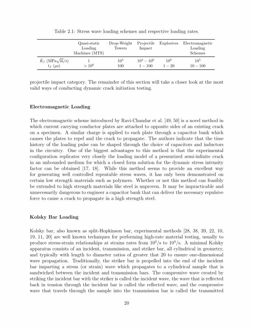
Table 2.1: Stress wave loading schemes and respective loading rates.

Quasi-static Drop-Weight Projectile Explosives ElectromagneticLoading Towers Impact Loading

Machines (MTS) Schemes

KI (MPa√

m/s) 1 104 104 − 106 108 105

tf (µs) > 106 100 1 − 100 1 − 20 10 − 100

projectile impact category. The remainder of this section will take a closer look at the mostvalid ways of conducting dynamic crack initiation testing.

Electromagnetic Loading

The electromagnetic scheme introduced by Ravi-Chandar et al. [49, 50] is a novel method inwhich current carrying conductor plates are attached to opposite sides of an existing crackon a specimen. A similar charge is applied to each plate through a capacitor bank whichcauses the plates to repel and the crack to propagate. The authors indicate that the timehistory of the loading pulse can be shaped through the choice of capacitors and inductorsin the circuitry. One of the biggest advantages to this method is that the experimentalconfiguration replicates very closely the loading model of a pressurized semi-infinite crackin an unbounded medium for which a closed form solution for the dynamic stress intensityfactor can be obtained [17, 18]. While this method seems to provide an excellent wayfor generating well controlled repeatable stress waves, it has only been demonstrated oncertain low strength materials such as polymers. Whether or not this method can feasiblybe extended to high strength materials like steel is unproven. It may be impracticable andunnecessarily dangerous to engineer a capacitor bank that can deliver the necessary repulsiveforce to cause a crack to propagate in a high strength steel.

Kolsky Bar Loading

Kolsky bar, also known as split-Hopkinson bar, experimental methods [28, 38, 39, 22, 10,19, 11, 20] are well known techniques for performing high-rate material testing, usually toproduce stress-strain relationships at strains rates from 102/s to 104/s. A minimal Kolskyapparatus consists of an incident, transmission, and striker bar, all cylindrical in geometry,and typically with length to diameter ratios of greater that 20 to ensure one-dimensionalwave propagation. Traditionally, the striker bar is propelled into the end of the incidentbar imparting a stress (or strain) wave which propagates to a cylindrical sample that issandwiched between the incident and transmission bars. The compressive wave created bystriking the incident bar with the striker is called the incident wave, the wave that is reflectedback in tension through the incident bar is called the reflected wave, and the compressivewave that travels through the sample into the transmission bar is called the transmitted

20

wave. Figure 2.1 shows a schematic of a Kolsky bar. Strain gages are typically placed onthe surface of the incident and transmission bars and the measured strains can be related tomaterial properties in the sample. The material properties of interest in a traditional Kolskybar test are typically curves showing stress as a function of strain at known strain rates. Thefollowing equations will derive how these measures are arrived at in a traditional test. First,we know that engineering strain, ε, is typically defined as follows:

ε(t) =Lf (t) − L

L(2.1)

where, Lf (t) and L are final and initial lengths, respectively. If we refer to Figure 2.1 anddefine x1(t) and x2(t) as the positions of locations 1 and 2 then at any time t, Lf(t) =x2(t) − x1(t). Substituting this relationship into Equation 2.1 we have:

ε(t) =x2(t) − x1(t) − L

L=

x2(t) − x1(t)

L− 1 (2.2)

By taking the first derivative with respect to time of Equation 2.2 we can define the engi-neering strain rate as follows:

ε(t) =x2(t) − x1(t)

L=

v2(t) − v1(t)

L(2.3)

where, v1 and v2 are the velocities of locations 1 and 2 in Figure 2.1. We wish to relate thesevelocities to the measured values of strain recorded in the strain gages on each bar. Fromone-dimensional wave theory [39, 22, 43] we know the following relationship for the particlevelocity, Up, in a one-dimensional rod:

Up = cε (2.4)

where, c is the wave speed and ε is the strain in the bar. Therefore, at interfaces 1 and 2 wehave the following:

1 → v1(t) = c0(εI(t) − εR(t)) (2.5)

2 → v2(t) = c0εT (t) (2.6)

V A0, ρ0, c0

Striker Incident Bar Transmission Bar

1 2

L

Sample w/ A, ρ, c

Figure 2.1: Schematic of Kolsky bar.

21

where, c0 is the wave speed of the incident and transmission bars, εI refers to the measuredstrain from the incident strain wave, εR refers to the measured strain from the reflected strainwave, and εT refers to the transmitted strain wave. The reason the (εI −εR) term appears inEquation 2.5 is because there is an impedance mismatch at the interface of the incident barand the sample which causes some of the strain wave to propagate into the sample and someto be reflected back. We can now substitute Equation 2.5 and Equation 2.6 into Equation 2.3and simplify to get the following relationship for engineering strain rate:

ε(t) =c0

L(εI(t) − εR(t) − εT (t)) (2.7)

Equation 2.7 can now be integrated over time to find the engineering strain in the sampleas shown in Equation 2.8.

ε(t) =c0

L

∫ t

0

(εI(t) − εR(t) − εT (t)) dt (2.8)

In order to find the stress we will assume equilibrium over the entire sample, therefore thestress can be found in terms of the force on each end of the sample as follows:

σ(t) =P1(t) + P2(t)

2A(2.9)

where, σ is the stress in the sample, P1 and P2 are the force applied to the sample at theinterface, and A is the cross sectional area of the sample. The forces can be evaluated fromthe incident and transmission bar strains at the interfaces as follows:

1 → P1(t) = A0E0 (εI + εR) (2.10)

2 → P2(t) = A0E0εT (2.11)

where, A0 is the cross-sectional area of the bars and E0 is the elastic modulus of the bars.Substituting Equation 2.10 and Equation 2.11 into Equation 2.9 results in Equation 2.12.

σ(t) =A0E0

2A(εI(t) + εR(t) + εT (t)) (2.12)

But, for equilibrium, P1 = P2 and therefore εI + εR = εT . If we substitute this back intoEquation 2.7, Equation 2.8, and Equation 2.12 we can get the final equations used to reducestress-strain relationships from Kolsky bar experiments. These equations are shown below:

σ(t) = E0A0

AεT (t) (2.13)

ε(t) = −2c0

LεR(t) (2.14)

ε(t) = −2c0

L

∫ t

0

εR(t)dt (2.15)

These are the standard equations found in many texts and typically presented in literaturewithout derivation.

22

In the last thirty years the Kolsky bar testing methods have been extended to dynamicfracture testing. Researchers have used one, three, and four point bend specimens in amultitude of configurations. Many have used novel specimen designs in tension, compressionand wedging tests. The remainder of this section will be dedicated to reviewing a selectionof relevant research using the Kolsky bar.

One of the earliest adaptations of the Kolsky bar technique for fracture testing was devel-oped by Costin et al. [12]. A 25.4mm diameter bar with a fatigued radial notch was loadedwith a tensile stress pulse originating from an explosive detonation. Using the standardequations for Kolsky bar data reduction the average stress at the crack tip was calculated.Crack tip opening displacement was also measured with a moire optical method thus yieldinga load displacement record of the fracture event. The authors used this method to determinethe rate dependence of the dynamic crack initiation toughness at loading rates on the orderof 106 MPa

√m/s for SAE 4340 steel and 1020 cold-rolled steel. One issue noticed in this

paper related to the reporting of loading rates as constant values, because of the explosiveloading scheme the load-time history is parabolic in nature at the onset of the load. For anear constant loading rate the load-time history should be near linear. Overall this workproduced reasonable data and showed the Kolsky bar as a viable resource for dynamic frac-ture testing. The use of explosives and the advent of newer loading methods would determost researchers from replicating these procedures exactly.

Rittel et al. [52] used a Kolsky bar setup with a novel specimen design called the compactcompression specimen which was placed in between the incident and transmission bars ofthe Kolsky apparatus. The compact compression specimen allowed for the crack to openwhen impacted with a compressive incident wave. Specimens were made of 1035 steel with aprecrack cut with a diamond wire. The root radius of the crack was reported as 0.17mm. Afracture gage (timing wire) was painted using conductive silver paint very close to the cracktip and sequenced with the incident stress pulse in order to get the time-to-fracture. Theauthors realized that although the compact compression specimen allowed for a simple testprocedure, it induces asymmetries in the the loading process, therefore the specimen was notin dynamic equilibrium and mixed mode I and II opening also occurred during fracture. Sincea quasi-static analysis was not valid, a procedure for finding the dynamic crack initiationtoughness was used. Analysis taken from [7] shows that for a non-propagating side crackof length, a, in an semi-infinite two dimensional body, S, for a linear-elastic material theauthors define the H-integral as shown in Equation 2.16.

H :=1

2

∫

S

T[u] ∗ ∂v

∂adS =

1 − ν2

EKu

I ∗ Kv

I (2.16)

where u is the displacement field in S to which the dynamic load T[u] is applied. v is areference field and ∗ is the time convolution product1. Ku

I and Kv

I are defined as the dynamicstress intensity factors associated with u and v respectively. u and T[u] are determinedexperimentally for each test performed. v and Kv

I are determined numerically througha finite element model (FEM) simulation that only needs to be done once. Finally, analgorithm is used to solve the linear convolution equation for Ku

I , at the time of fracture

1f(t) ∗ g(t) =∫

∞

−∞f(τ) · g(t − τ)dτ

23

Ku

I = KIc. The authors report a dynamic crack initiation toughness for the 1035 steel of180MPa

√m, but recognize this number to most likely be incorrect because of the relatively

blunt crack tip. The most apparent drawback of this method in the need to calculate vand Kv

Ic via FEM. Using this procedure the accuracy of KIc is based on the accuracy of theFEM results. Most likely in order to obtain accurate FEM calculations one would need tohave an extremely high mesh density in the crack tip region which could prove to be toocomputationally expensive to be practical. The authors also describe “filtering” out of themode II stress intensity factor, but do not go into detail about the procedure used.

Klepaczko [37] provides a detailed review of many experimental procedures used in dy-namic crack initiation testing in including a method of his own design using the wedge loadedcompact tension (WLCT) specimen. This method attaches a compressive wedge to the in-cident bar and places the WLCT specimen between the wedge and the transmission bar.Estimates were made for the transverse inertia of the WLCT specimen during loading aswell as frictional effects. It was concluded through this analysis that as long as the fracturetime was longer than the initial rise time of the incident pulse the inertia and frictional effectsessentially canceled each other out. One issue to note was that the frictional force was mod-eled with a simple Coulomb friction law which may not be adequate in this dynamic loadingregime and could introduce errors into the calculation of KIc. It appears that Klepaczkocalculates the time-to-fracture simply by inspecting the reflected strain data recorded onthe oscilloscope looking for what he calls “pop-in” points. The author reports results fromWLCT tests on aluminum alloys conducted over seven decades of loading rate. The resultsshow a drop in KIc at KI ≈ 102 MPa

√m/s.

A different set of dynamic crack initiation toughness experiments on 2024-T3 aluminumwas conducted by Owen et al. [46]. The authors used thin aluminum sheets in both aMTS R© load frame for KI < 102 MPa

√m/s and a Kolsky tension bar test configuration

for KI > 105 MPa√

m/s. The specimens were cut with wire electrical discharge machining(EDM) before being fatigued in a MTS R© machine to produce a sharp crack. The values ofKIc were found via the standard quasi-static means for the MTS R© machine experiments.For the Kolsky tension bar tests four-angle steel tabs where attached to each side and atboth ends of the specimen. The specimen was then placed in mating fixtures which werethreaded into the end of each bar. The authors report that the specimen did not slip withrespect to the steel tabs during the test. The tensile stress in the specimen is calculatedvia standard Kolsky bar techniques using the transmitted strain signal and related to thedynamic stress intensity factor by Equation 2.17 taken from [1]:

KI(t) =σ(t)W√

W

√

2 tan(

π a2W

)

cos(

πa2W

)

×[

0.752 + 2.02( a

W

)

+ 0.37(

1 − sin( π a

2W

))3]

(2.17)

where W is the width of the sample, and σ(t) is the applied stress. KI was calculated usinga least squares fit to the KI(t) curve and the dynamic crack initiation toughness, KIc, wastaken as the point where a line having a slope of 0.95KI intersected the KI(t) curve. This

24

is the same procedure used for finding the fracture toughness in quasi-static tests [29].

Equation 2.17 was derived without taking inertia effects into consideration, therefore tosimply replace the quasi-static stress, σ, with a time dependent load, σ(t), is only valid ifthe sample is shown to be in dynamic stress equilibrium. Owen et al. used an independentlocal measurement on one test to help validate the use of the time varying boundary loadresults. They used an optical method to measure the local crack tip opening displacement(CTOD). The J-Integral was evaluated using a relationship given by Shih [54]. When theCTOD is measured at the intersection of two lines at 45 with respect to the crack line therelationship is shown in Equation 2.18,

CTOD = dn(ε0, α, n)J

σ0(2.18)

where, the parameter dn is a function of the reference strain, ε0, constitutive parameters, αand n, and stress state, σ0. Equation 2.18 can be solved for J and then the J-Integral canbe related to the fracture toughness by the well known equation for plane stress shown inEquation 2.19.

J =K2

I

E(2.19)

A limitation of this technique is that in order to extend it to the dynamic regime you mustknow the correct high-rate constitutive parameters contained in dn to be able to calculateJ accurately. The data is then reported for KIc as a function of KI . The local CTODvalues for KIc are overlaid with associated boundary load KIc measurements. Owen et al.make the statement that for times greater than 20 µs there is good comparison between thetwo calculated values. One key flaw in this approach is with the method of calculating thedynamic crack initiation toughness. The investigators in this paper use a 5% offset valuefrom a linear line drawn though the rise of the loading pulse. This is how KIc is calculated inquasi-static testing per ASTM E399. In dynamic testing an accurate time-to-fracture shouldbe calculated experimentally because inertia in either the sample or the loading fixture cancause the recorded load to continue rising after crack initiation. Additionally, the constantapproximation for loading in this case was not accurate because the KI(t) curve oscillatedbefore the fracture time. This state of constant loading is assumed when they generate a plotof KIc as a function of KI . The highest loading rates were on the order of 106 MPa

√m/s;

at these rates there is a drastic increase in dynamic crack initiation toughness. This isin stark contrast to the observations of Klepaczko whose work showed a decrease in KIc

at the highest rates. The two experimental results are compared in Figure 2.2 GrantedKlepaczko’s experiments where close to plane strain loading whereas Owen et al. was closeto plane stress, and the aluminum used in each respective test are not the exact same alloy.One would expect to get different values of KIc in these two experiments, but the opposingtrends in rate dependence are somewhat alarming.

Yokoyama et al. [69, 68] used a modified Kolsky bar assembly to conduct three point benddynamic crack initiation experiments. Two transmission bars where used as the supportsfor a precracked beam and the incident bar was used to apply the dynamic load. The time-to-fracture is found by mounting a semiconductor strain gage on the specimen and using the

25

0

25

50

75

100

10−1 101 103 105 107

KIc

(MPa√

m)

KI (MPa√

m/s)

Klepaczko (PA6 Aluminum)Owen (2024-T3 Aluminum)

Figure 2.2: Comparison of experimental results from Klepaczko and Owen.

peak strain as the time when the crack initiates. The boundary load histories are then inputinto a finite element model and combined with the time-to-fracture information to extractthe dynamic crack initiation toughness. Like other methods that use FEM to extract KI(t),they are only valid if you have an accurate FEM model.

Popelar et al. [47] used a very well instrumented modification of a Hopkinson bar inthree point bend tests of a precracked beam. The dynamic load was applied through theincident bar which records the incident pulse. The samples were instrumented with straingages to monitor the sample contact with the support pins to ensure the beam was not setinto resonance and “jump” off the supports. An eddy current sensor was used to monitorCTOD. There is also a crack ladder gage to measure time-to-fracture and give a discretemeasurement of crack growth speed. The authors use what they call a quasi-dynamic modelto extract the dynamic stress intensity factor from the CTOD data. Their model comes froma solution for the CTOD produced by Tada et al. [65] for a propagating crack. For brevitythese equations are omitted here, however in calculating the dynamic stress intensity factor,and in turn its critical value, KIc, from these equations for a propagating crack they arefailing to consider the dynamic crack initiation toughness and dynamic crack propagationtoughness as independent material properties as suggested by other researchers [49, 18].

Jiang et al. [32] used a Kolsky pressure bar in modified Charpy impact tests to find thedynamic crack initiation toughness of steel specimens. The specimen is supported by ananvil and loaded with the incident bar from the Kolsky apparatus. The authors use a modelbased on a simple spring-mass system to provide an equation for the dynamic motion of

26

the precracked beam. They model the beam as three point bending and use a linear elasticmechanics approach to solve for the stiffness of the beam and in turn derive an expression forthe dynamic stress intensity factor. The final expression they used is shown in Equation 2.20.

KI(t) =3S

√a

2BW 2Y( a

W

)

ω1

∫ t

0

P (τ) sin ω1 (t − τ) dτ (2.20)

Where, a is the crack length, W is the width of the specimen, B is the thickness of thespecimen, S is the distance between the supports, and Y

(

aW

)

is a compliance function takenfrom Srawley [63]. P (τ) is the recorded boundary load from the incident bar strain gage andω1 is the natural frequency of vibration which is a function of the calculated stiffness K(a).Equation 2.20 is then integrated and combined with the measured time-to-fracture from theexperiment to find KIc. The details of this procedure are laid out in [32]. Rokach, in hisrebuttal to Jiang et al.’s paper [53] noticed an error in these approximations. The averagetime-to-fracture in the reported experiments was less than 13µs which is faster than thetime is takes a dilatational wave to travel from the impact boundary to the supports andreturn to the crack tip. Therefore the crack does not even see the effect of the supports, thisis generally referred to as one point bending. Due to the conditions of one point bending,the analysis Jiang et al. used to determine the dynamic stress intensity factor is not validbecause it was derived based on three point bending.

More recently, Weerasooriya et al. [67] used a four point bend technique to determinethe dynamic crack initiation toughness in ceramics. They used a modified Kolsky setupwith the specimen loaded in four point bending between the incident and transmission bars.They used a pulse shaping technique [19, 20] to carefully control the loading pulse to ensurenot only constant loading rate, but dynamic equilibrium of the sample as well. Quartz forcetransducers where imbedded in the ends of the incident and transmission bars to measure thesample in equilibrium. Because the sample was shown to be in dynamic stress equilibrium,quasi-static analysis was used to find the dynamic crack initiation toughness. These exper-iments were performed at loading rates of 4 × 104 MPa

√m/s and 1.5 × 105 MPa

√m/s, and

showed dynamic crack initiation toughness measurements of 5.5MPa√

m and 9.5MPa√

m,respectively.

In one of the most recent works to date, Jiang et al. [34] have devised a new experimentaltechnique using a what they call two-bar/three point bending. This is a much improvedtechnique over the incident bar Charpy scheme by the same authors reviewed earlier. Similarto work by Weerasooriya et al. these investigators use a traditional two bar Kolsky apparatusexperimental setup with a three point bending mechanism attached to the incident andtransmission bars. Figure 2.3 shows a schematic of the gage section between the incidentand transmission that facilitates the three point bending. They use pulse shaping techniquesto control the incidence pulse and investigate the loss of contact issue between the impactpins and the specimen. They use a clever voltage scheme to monitor the contact at thepins and show that the loss of contact occurs well after the crack initiates in the sample.The authors do not actually report any calculated values for dynamic stress intensity factor,but show this techniques applicability for use in dynamic crack initiation testing of bothsteel and aluminum samples. Dynamic stress equilibrium is verified with the 1-wave 2-wave

27

Figure 2.3: Schematic of Jiang three point bend setup.

technique. The only possible issue noted with this work has to do with the possibility of nothaving pure mode I opening. The authors provide a sample of high-speed photographs asvalidation of their voltage contact measurement and in these photographs the crack does notappear to propagate straight across the sample. This “turning” action exhibited by the crackpropagation indicates that mixed mode opening is occurring. However this could possiblybe due to slight misalignment and easily corrected.

In what is most likely the most recent published work, Jiang et al. [33] modified theexperimental technique described in the last paragraph to employ four point bending insteadof three. All other aspects of the setup were essentially the same. The four point bendingshould eliminate any misalignment issues and ensure pure mode I opening during crackinitiation. However, they did not report any actual experimental values of dynamic crackinitiation toughness, they only evaluated the experimental technique.

In this research, a similar method to those described by Jiang et al. and Weerasooriyaet al., is used to record the dynamic crack initiation toughness measurements of a 4340 steelat two different nominal loading rates.

2.2 Peridynamics

The peridynamic theory of solid mechanics is a relatively new development in continuummodeling. There have been only 15-20 papers written on the subject, several of which arecited elsewhere in this dissertation. The following few paragraphs review some of the keyarticles written on the subject as well as other techniques in computational modeling ofmaterial failure.

The original paper on peridynamics was published by Silling in the year 2000 [56]. Thispaper introduced what is now called “bond” based peridynamics, introduced several proto-type material models, and compared several mathematical notions to their analogs in classicalmechanics (partial differential equation) theory. The paper demonstrated the straightfor-ward emergence and modeling of discontinuities (e.g., cracks) without the need for special,sometimes artificial, mathematical models to handle them.

28

A paper that examined some interesting behavior of the peridynamic theory was pub-lished by Silling et al. [61]. In this paper the authors analyzed the deformation fields in aone dimensional infinite peridynamic bar. Some interesting phenomenon was shown that isnot realized in the classical theory. For instance, the equilibrium solution of the bar for thedisplacement field has the same smoothness as the body force field being applied to the bar.In the classical theory of elasticity the displacement field would be two orders smoother (i.e.,continuously differentiable) than the body force field.

The first publication on the numerical implementation of peridynamics was authored bySilling and Askari [58]. In this paper, the authors discretize and numerically implementthe peridynamic continuum model, give an example of a prototype microelastic constitutivemodel, and present example problems where discontinuities arise naturally as part of thedeformation. This paper also presented a derivation of a failure criterion based on energyrelease rate that arrives at a critical bond stretch at which a bond will fail irreversibly onceexceeded.

In order to address the shortcomings described in Chapter 1 of the “bond” based peri-dynamic model, a generalization was done and published by Silling et al. [59]. The outcomeof this paper is what is now referred to as “state” based peridynamics. This generalizationintroduced the notion of peridynamic vector-states which allows for more complex materialmodels while retaining the ability to model complex and even discontinuous deformations.The theory presented in this paper was later shown by Silling and Lehoucq [60] to convergeto the classical theory in the sense of a limit as the non-local horizon tends to zero. Thisconvergence is based on several assumptions including a homogenous, smooth deformationfield.

Because the numerical implementation of peridynamics is a Lagrangian formulation thatrepresents each discrete material point as a particle, it often draws comparisons to other socalled particle methods from the classical theory. These include smooth-particle hydrody-namics (SPH) [45, 27], element-free Galerkin (EFG) methods [4, 41, 5, 6], and reproducing-kernel particle method (RKPM) [40, 9]. It is important to remember that these othernumerical techniques arise from the weak form of the classical partial differential equationsand require special mathematical techniques to account for the spontaneous evolution ofdiscontinuities. In the use of the finite element method for crack propagation, artificial nu-merical “trickery” is sometimes resorted to in order to handle discontinuities. These includeelement death (deletion), element-to-particle conversion [36], cohesive zone elements [16],and extended finite elements (XFEM) [44, 64]. While all of the aforementioned methodshave been demonstrated to varying degrees of accuracy with respect to their application onproblems of fracture, all of them require the application of an external model, not inherentto the fundamental equations, to describe these material failures.

To illustrate the versatility of the peridynamic theory, please allow the use of the follow-ing analogy:2 Assume there are a set of equations which accurately describe the atmosphericweather on most days, including sunny days, raining days, snow days, etc., but are inca-

2Credit is respectfully give to Dr. Stewart A. Silling for the originality of this analogy.

29

pable of describing truly adverse weather such as tornadoes, hurricanes, and blizzards. Nowassume that these equations are implemented into a numerical code using the finite elementmethod and the finite element code could replicate the physics of the underlying equationsby predicting the weather on most days, but in order to model adverse weather, the analysthad to employ the use of “special” elements, e.g., tornado elements. This is equivalent tothe idea of using cohesive zone elements (and other special numerical techniques) to modelfracture. Even though they perform adequately, they represent a significant departure fromthe underlying theory. The peridynamic theory circumvents the need for external equationsto model the adverse events, such as fracture. The peridynamic theory of solid mechanicscaptures all of this while showing significant tiebacks to the classical theory and retainingthe ability to model more conventional continuous deformations.

30

3 Experimental Procedure

3.1 Introduction

This chapter introduces the technique used to experimentally determine the dynamic crackinitiation toughness of a 4340 steel. While the technique is not entirely novel [33, 34, 67],this is the first time it has been presented in this exact configuration. At the outset of thisresearch one goal was to achieve a standard technique for establishing the crack initiationtoughness of metallic materials at dynamic loading rates in a similar fashion to the ASTMstandard E399 for finding fracture toughness in metals at quasi-static loading rates. Theresearch presented herein provides an approach that the author believes is an improvementon other techniques found in literature, it can be used to provide accurate results at knowndynamic loading rates, but still has a few shortcomings to be improved upon in futureiterations. These shortcomings do not involve accuracy of the results only the ease in whichthe experiments can be conducted and the data reduced, all of which will be mentioned alongwith suggestions for further improvement. This chapter includes detailed descriptions of theprocesses of sample preparation, fatigue precracking, and fracture time detection which areoften overlooked or presented as trivial issues in the dynamic fracture literature. A detaileddescription of the modified Kolsky bar and data reduction techniques is also provided in thischapter.

3.2 Sample Preparation

ASTM E399 provides guidelines for the sample preparation of compact tension specimens,notched tensile specimens, and three point bend beam specimens for the purpose of ex-perimentally detecting quasi-static fracture toughness values. For dynamic crack initiationtoughness testing, we have established in Section 2.1.1 that the most common method andeasiest way to deliver controlled dynamic loading is the Kolsky apparatus. For this reasonand others to be elaborated on subsequently, the Kolsky bar was the method we chose toapply the dynamic loading in the dynamic crack initiation tests. In an attempt to followthe spirit of ASTM E399, the bend beam sample was chosen as the sample configuration.However the experiments we conducted were a four point bend configuration as opposed to

31

Wa

L

B

Figure 3.1: Four point bend beam.

a three point bend. This was done because alignment is not as critical in a four point bendtest. In a three point bend test even the smallest misalignment of the striking tup with thecrack can cause mixed mode opening of the crack tip which is undesirable when attemptingto capture KIc. When doing quasi-static tests, alignment is not very hard to achieve becausethe tests are generally done in a standard test apparatus (e.g., MTS R©) where the sample,supports, and striking tup all sit in a vertical orientation, respectively. In the Kolsky barthe striking tup is on the incident bar end and the sample is supported only by a smallamount of friction between the tup and supports and arranged in a horizontal fashion. Thisarrangement lends itself to the possibility of slippage between the sample and supports. Aslong as the potential slippage is small and the crack tip remains between the two strikingtups, the sample will experience pure bending and mode I opening will be ensured. Thishorizontal arrangement was also the reason why the compact tension specimen was not con-sidered, since the size of the sample is much too large to be held in place only by the frictionof the supports and tups. The notched tensile specimen could be considered for use in theKolsky apparatus, but the additional and unnecessary complication of a tensile Kolsky barwas the reason that sample was not considered.

Figure 3.1 shows an illustration of a four point bend precracked beam with descriptivelabels for relevant geometries. ASTM E399 states that the relationship between the samplethickness, B, and sample width, W , should be B = W/2±0.010W and the length, L, shouldbe a minimum of 4.2W . The total length of the crack, a, which includes the total dimension ofthe starter notch and the fatigue generated precrack should be between 0.45 ≤ a/W ≤ 0.55.The generation of the fatigue precrack is discussed in detail in Section 3.3. Based on theASTM E399 guidelines the nominal sample dimensions used in the Kolsky bar tests areshown in Table 3.1. Machine drawings for the samples are included in Appendix C, and the

Table 3.1: Nominal sample dimensions.

W B L a

15mm 7.5mm 63.5mm 7.5mm

32

actual measured dimensions of each sample used for testing is included in Appendix D.

Each sample was machined from 4340 plate stock that originally had rough dimensionsof approximately 130mm× 80mm × 10mm. Before machining the plates were heat treatedwith the following procedure:

1. Annealing: Heat at 680C for 8 hours, air cool

2. Strengthening: 845C ± 10C for 1 hour at temperature, oil quench

3. Temper: 200C ± 10C for 1 hour at temperature, air cool

After heat treatment the samples were machined using a wire EDM to the final dimensions.A starter notch was cut to a depth of 5mm, the thinnest possible width (maximum of 2mm),and perpendicular to the edge within 2 to facilitate fatigue cracking. The front and backfaces where finally machine ground to a surface finish of 3.2µm. This process resulted insamples with Rockwell C50-C55 hardness.

The final step of sample preparation was to polish one side of the sample to a mirrorfinish and label each with a serial number. The mirror finish allowed for easy visibility ofthe fatigue crack under the microscope during the fatigue crack growth process.

3.3 Fatigue Cracking

ASTM standard E399 states that even the narrowest practical machined notch cannot simu-late a natural crack well enough to provide a satisfactory measurement of KIc. Therefore, itis necessary to artificially create a sharp crack by initiating and growing a fatigue crack fromthe root of a narrow machined notch before attempting any KIc measurements. To ensurethe crack is sufficiently “sharp”, ASTM E399 gives guidelines for so called K-calibration.ASTM E399 also gives guidelines for the appropriate crack length and approximate numberof cycles it should take to grow the fatigue crack. A summary of these guidelines are givenas follows:

• The maximum stress intensity factor, Kmax, during any stage of fatigue crack growthshall not exceed 80% of the resulting KIc.

1

• For the terminal stage of fatigue cracking (the final 2.5% of the intended crack size,a), Kmax shall not exceed 60% of the resulting KIc.

• The final crack length, a, should be between 0.45W and 0.55W .

1For the first test of a new material, KIc may be unknown; therefore, an estimation may have to beused, and if the resulting KIc > 1.2Kmax, the fatigue process and experiment will have to be repeated withcorrections in order for KIc to be assumed valid.

33

• The total number of cycles to generate the fatigue crack should be between 104 and106.

The load for the fatigue cracking procedure was generated using a four point bend fixturein an 4.5 kN MTS R© servo-hydraulic test frame, Model 312.21. The K-calibration was doneby running the load frame in force control mode, cycling the appropriate load. In order tocalculate the appropriate load levels for sufficient K-calibration we must first solve for theload, P , from the stress intensity factor definition. For a four point bend beam in mode Iloading, the stress intensity factor is calculated by Equation 3.1 [65]

KI =6M

BW 2

√πa · β

( a

W

)

(3.1)

where, the definitions from the Section 3.2 hold, and M is the applied moment defined by:

M = pd (3.2)

and the compliance function, β, is defined by:

β( a

W

)

= 1.22 − 1.40a

W+ 7.33

( a

W

)2

− 13.08( a

W

)3

+ 14.00( a

W

)4

(3.3)

In Equation 3.2, p refers to the force applied at each of the four support locations and d isthe span between the four point bend supports. Defining the force at each of the supportsin terms of the force measured by the MTS R© test frame, P , we have,

p =P

2(3.4)

Now substituting Equation 3.4 into Equation 3.2 and then that result into Equation 3.1 andsolving for P we have the following relationship:

P =KIBW 2

3d√

πa · β(

aW

) (3.5)

Following the guidelines listed earlier in this section, at no stage during fatigue crack growthdid KI in Equation 3.5 exceed Kmax = 0.8KIc. The assumption was made that the dynamiccrack initiation toughness was greater in magnitude than the quasi-static fracture toughness.For most heat treatments of 4340 steel the reported fracture toughness, KIc, is approximately65MPa

√m. Rounding down to be conservative Kmax = 50MPa

√m was used for the fatigue

crack initiation. For the terminal growth of the fatigue crack, Kmax = 39MPa√

m wasused. In order to calculate the load, P , the crack length, a, corresponding to the expectedfinal length of approximately 7.5mm was used. This added additional conservatism to thecalculation of P because initially the crack length was smaller than 7.5mm; therefore, theactual value of KI was initially lower and increased to the value of Kmax as the crack wasgrown. Using the nominal sample dimensions described in Section 3.2 and d = 17.33mm,the initial and terminal values of P were calculated to be 9.34 kN and 7.12 kN, respectively.

34

In order to initiate the fatigue crack, the MTS R© test frame was placed in force controlmode and cycled between 0 and 9.34 kN at a rate of 50Hz. A KEYENCE digital microscopewith integrated imaging, Model VHX 100K, was used to monitor the fatigue crack initiationand growth. Figure 3.2 shows the four point bend fixture in the MTS R© test frame withthe sample in place and the microscope camera lense. Figure 3.3 shows a fatigue crackbeing monitored. The mirror surface finish on the sample allowed the fatigue crack to beclearly monitored during growth. The blue line to the left of the growing crack in Figure 3.3represents a distance of nominally 2mm. Once the fatigue crack initiated the force waslowered to cycle between 0 and 7.12 kN, once again at a rate of 50Hz until the crack lengthwas near the overall desired length of nominally 7.5mm. The entire fatigue crack initiationand growth took approximately 15 minutes per sample, and resulted in approximately 45 000cycles. The fatigue crack initiation and growth was a very repeatable process. The fatiguecrack growth rate was easily controlled by gradually lowering the force as the crack nearedthe desired length; which, resulted in a very “sharp” crack tip of nearly equal length for allsamples.

3.4 Apparatus

To apply the dynamic loading for these experiments a modified Kolsky bar, also known as asplit-Hopkinson pressure bar (SHPB), at Sandia National Laboratories was used. The Kol-sky bar is an apparatus consisting of two long cylindrical bars, identified as the incident andtransmission bars respectively, and a striker bar. It is typically used for the characterization(i.e., stress-strain data) of engineering materials at high strain rate. This is done by placinga small specimen, between the incident and transmission bars and firing the striker bar intothe incident bar. A stress wave will travel through the incident bar in a one-dimensionalfashion (if the bars are sufficiently long); upon reaching the sample, part of the incidentstress wave will be reflected back into the incident bar and part of the incident stress wavewill be transmitted through the sample into the transmission bar. This phenomenon oc-curs because of a mechanical impedance mismatch between the sample and the bars and iswell documented in literature. The incident, reflected, and transmitted stress waves are thenused to deduce the sample’s mechanical response by using one-dimensional wave propagationtheory. The Kolsky bar has also been used in various configurations to conduct dynamic frac-ture experiments. A modified version used to conduct dynamic fracture initiation toughnessexperiments is described below.

A standard Kolsky bar with a nominal incident bar length, LI , of 305 cm and nominaltransmission bar length, LT , of 149 cm was modified to accept a double impact tup anddouble support to facilitate the four point bending in the sample region. Machine drawingsof the impact tup and support are provided in Appendix C. Both bars are nominally 19mmin diameter and manufactured from C350 martensitic aging steel. A schematic of the setupis shown in Figure 3.4.

Strain gauges were placed at 232.1 cm and 44.5 cm from the sample ends of the incident

35

Figure 3.2: Four point bend fixture, sample, and microscope camera.

Figure 3.3: Digital microscope monitoring fatigue crack growth.

36

Whea

tsto

ne

Bri

dge

Diff

eren

tial

Am

plifier

tim

eDiv

:

5m

s/div

Chan

nel

A:

1V/div

Chan

nel

B:

1V/div

XY

OFF

add:

ON

Offse

tB

0

Offse

tC

0

Offse

tA

0

Gas

Gun/S

trik

erIn

ciden

tB

arTra

nsm

ission

Bar

Osc

illo

scop

e

Str

ain

Gag

es

Cop

per

Pulse

Shap

er

Fat

igue

Pre

crac

k

Fig

ure

3.4:

Sch

emat

icof

modifi

edK

olsk

ybar

.

37

and transmission bars, respectively. The strain signals were used to determine the loadingtime history on the sample and to verify dynamic equilibrium during the experiment.

Annealed copper pulse shapers [19, 20] were used to generate ramp incident pulses. Whenimpacted by the striker, the copper disk flows plastically, which increases its diameter andallows the striker momentum to transfer through the disk into the incident bar creatinga ramp-like stress pulse with increasing amplitude. With proper selection of thickness anddiameter of the pulse shaper and striker velocity magnitude, the shape of the increasing rampstress pulse can be controlled. In this set of experiments the stress pulse was near linear.A ramp pulse was chosen because we wish to have a constant mode I stress intensity factorrate, KI . Because the equation used to calculate the stress intensity factor (Equation 3.1) isessentially a constant times the load, by making the load linearly increasing we can ensurethat KI will be linearly increasing as well. The copper pulse shapers, by lengthening therise-time of the incident stress wave, also allow the sample to come into dynamic equilibriumbefore the crack initiates. If the crack were to initiate before the sample is in equilibriumthen we would not be able to use quasi-static analysis to calculate the stress intensity factor.Stress equilibrium will be discussed further in Section 3.6.

3.5 Crack Initiation Time Detection

The most important measurement in dynamic crack initiation toughness testing is the crackinitiation time. In quasi-static tests the stress intensity factor gradually increases at thecrack tip over a very long period of time (e.g., minutes); the crack initiates and the loadgenerally falls off very sharply allowing the experimentalist to easily detect the value of KIc

directly from the load history without the need for special fiduciary timing tools to identifycrack initiation. Furthermore, when the loading rate is quasi-static, the time-to-fracture, ison the order of 104 s and misdetection of the initiation by even several seconds will oftenlead to an undetectable difference in the reported value of KIc. However, we will see inour dynamic crack initiation experiments the time-to-fracture is on the order of 10−6 s andmisdetection by even as little as 1µs can cause large differences in the reported value of KIc.

Several methods for detecting crack initiation were attempted in the course of this re-search, including using Vishay R© Micro-Measurements R© CD-02-10 single wire crack detec-tion gages, a modified potential drop method for high rate crack propagation, and the use ofa strain gage near the crack tip to detect the rise and fall of strain which signals unloadingand crack initiation. The crack detection gages worked well when they stayed laminatedto the surface of the sample; however, even though the Vishay R© gages used a process ofadhesion similar to the method for placing a strain gage on the sample, the gages tended todelaminate during the crack initiation process. This did not happen nearly as often when astrain gage was simply placed near or in front of the crack tip.

The potential drop method uses the knowledge that when a constant current is passedthrough a sample, a drop in the measured electric potential across the crack can be detected

38

by the crack advancement causing a resistance change in the sample. Using a modifiedmethod with a constant alternating current, it was discovered that an electrical potentialdrop could actually be detected when the two faces of the fatigue precrack simply opened,but before the crack initiated. This method showed promise, but in the end it was not usedbecause of its need for sensitivity calibration and its general complication.

Crack initiation can be detected to a certain degree of accuracy by placing a strain gagenear the crack tip and monitoring the strain. During loading the strain will increase andthen drop off sharply when the crack initiates and the strain near the crack tip is relieved.The problem with this method is that the strain information takes time to propagate fromthe crack tip to the strain gages, which could cause a delay in the initiation detection time.

As a result of the knowledge gained by trying these other methods it was finally decidedto use a sacrificial strain gage placed directly in front of the crack tip as a crack detectiongage. This was done because the strain gages rarely delaminated even when being torn inhalf by the advancing crack. To prepare the strain gage, any excess substrate extendingoutside of the outermost wire was cut away to allow the first wire along the edge of the gageto be placed as near the crack tip as possible. The gages were then placed in front of thecrack under a microscope which resulting in the gages being on the order of ≈ 0.1 mm fromthe tip. Figure 3.5 shows the sacrificial strain gage on the surface of a precracked sample.The fatigue precrack is difficult to see, but the removal of the excess substrate is easilyidentified in the photograph. Figure 3.6 shows a sample that was broken; the relationship ofthe strain gage to the crack tip can be observed in this photograph.

By placing the strain gage directly in front of the crack tip, one can easily distinguishthe time-to-fracture. The load on the sample increases causing large strain in front of thecrack, then when the crack initiates it splits the strain gage in half, breaking the circuitwithin the gage. Figure 3.7 shows a typical measurement as viewed on the oscilloscope fromthe sacrificial strain gage. In order to ensure the integrity of each measurement, a post-testvisual inspection was done of each sample. If the sacrificial strain gage was not seen to havecleanly split in half or any signs of delamination were indicated, the test was consideredinvalid and the data not recorded.

A simple algorithm was used to detect the exact point where the circuit was broken andthis fiduciary mark was then adjusted to allow it to correspond with the other measurementsignals that indicate the load on the sample. This adjustment procedure will be discussedin detail in Section 3.6.

39

Figure 3.5: Sacrificial strain gage placed near crack tip.

Figure 3.6: Strain gage post-fracture showing relation to fatigue precrack.

40

−1

−0.5

0

0.5

1

1000 1050 1100 1150 1200

Ele

ctri

cPot

enti

al(V

)

Time (µs)

Figure 3.7: Typical signal from sacrificial strain gage.

3.6 Data Reduction

3.6.1 Wave Speed Calculation

The first step in valid data reduction for a Kolsky bar experiment is to have an accuratemeasure of the wave speed in the bars. This can be measured by removing the transmissionbar from the Kolsky apparatus and striking the incident bar with a striker. The compressivestress wave imparted on the incident bar by the striker will travel down the bar to the freesurface at the other end and reflect back as a tensile wave. By recording the time-of-arrivalof both the incident and reflected waves at the incident bar strain gage, and knowing thelength between the strain gage and the end of the bar, the bar wave speed can be accuratelycalculated.

The wave speed experiment described in the last paragraph was conducted for the Kolskybar at Sandia National Laboratories. Since it is very difficult to detect the exact moment thestress wave arrives by inspection, a simple algorithm was written to search the compressiveincident wave for the time when the amplitude of the strain (indicated by electric potentialon the oscilloscope) reached 0.2 V. This time is indicated in Figure 3.8 as t1. There isnothing especially particular about the value 0.2V other than the fact that it was larger inmagnitude than any conceivable noise in the strain signal. The same search was done onthe tensile wave for an amplitude of −0.2V. This time is indicated in Figure 3.8 as t2. Toremove any high-frequency noise from the strain gage signal that might influence the search

41

−1

−0.5

0

0.5

1

0 500 1000 1500 2000

Ele

ctri

cPot

enti

al(V

)

Time (µs)

t1 = 610µs t2 = 1555µs

Figure 3.8: Wave speed calculation.

algorithm, the strain signal was first filtered with a 4-pole Butterworth low-pass filter witha cutoff frequency of 40 000Hz. Measuring the length between the incident bar strain gageand the end of the bar, LIg, to be 2.3209m, the wave speed in the bar was calculated withEquation 3.6.

cb =2LIg

t2 − t1=

2 · 2.3209m

1555µs − 610µs≈ 4912m/s (3.6)

3.6.2 Strain Conversion

In the following subsections, references will be made to measured strain, ε. The signalactually measured on the oscilloscope from the strain gages is electric potential and must beconverted to strain. The incident and transmission bars in the Kolsky apparatus both usestrain gages configured in a half Wheatstone bridge. The electric potential measurementsare converted to strain with Equation 3.7.

ε =1

2

Vout

Vin · GF(3.7)

Where, Vout is the electric potential measured on the oscilloscope, Vin is the electric potentialapplied across the strain gage, and GF is the gage factor of the strain gages. All gages usedin these experiments were Vishay R© Micro Measurements 1000Ω gages from lot numberK60FD13 with GF = 2.06 ± 0.3% and and Vin = 28V.

42

3.6.3 Force Equilibrium Verification

The next step for valid data reduction in a Kolsky bar experiment is to ensure that thesample is in dynamic stress equilibrium during the time of interest for the test. For dynamiccrack initiation toughness tests it is required that the sample be in equilibrium before thecrack initiates; otherwise, quasi-static equations would not be valid for data reduction. Onceagain, this is why copper pulse shapers are needed to lengthen the rise-time of the incidentstress wave allowing the sample to equilibrate. In order to check for dynamic equilibrium,a “one-wave, two-wave” technique is used. This is a common method of analysis used tocheck equilibrium in a Kolsky bar experiment. This requires knowing the time-of-arrivalof both the incident and reflected wave on the incident bar strain gage and also the timeof arrival of the transmitted wave on the transmission bar strain gage. In a conventionalKolsky bar test, measurements of the distance between the incident bar strain gage and theend of the incident bar, LIg, the length of the sample, Ls, the distance between the end ofthe transmission bar and the transmission bar strain gage, LTg, and the sample wave speed,cs, would be made. The time-of-arrival of the incident wave, tI , is then chosen either byinspection or with a numerical algorithm and the time-of-arrival of the reflected wave, tR,and the transmitted wave, tT , can then be calculated with Equation 3.8 and Equation 3.9,respectively.

tR = tI +2LIg

cb

(3.8)

tT = tI +LIg + LTg

cb+

Ls

cs(3.9)

The force on the end of the incident bar (and therefore applied to the incident side ofthe sample) is calculated with Equation 3.10.

P1 = EbAb (εI + εR) (3.10)

Where, Eb is the elastic (Young’s) modulus of the bar which is either known beforehand orcalculated with Equation 3.11,

Eb = c2bρb (3.11)

with ρb being the density of the bars, Ab is the cross-sectional area of the bars and εI andεR are the incident and reflected strain measures taken from the incident bar strain gageand indexed from the respective times-of-arrival, tI and tR. The force on the end of thetransmission bar (and therefore applied to the transmission side of the sample) is calculatedwith Equation 3.12.

P2 = EbAbεT (3.12)

Where, εT is the transmitted strain measured on the transmission bar strain gage indexedfrom the time-of-arrival, tT . P1 and P2 are then plotted against each other to check fordynamic equilibrium. If the two curves nearly overlap then the sample is said to be inequilibrium.

The analysis presented above assumes one-dimensional wave propagation through thesample. In the modified Kolsky bar experiments outlined in Section 3.4 the entire gage

43

−100

0

100

200

300

0 50 100 150 200

For

ce(k

N)

Time (µs)

P1P2

Figure 3.9: Uncorrected force equilibrium.

section is modified to accept the incident impact tups and transmitter supports. In addition,the sample is not a cylinder, but a prismatic beam. Under these conditions one-dimensionalwave propagation through the gage section is invalid. If the time-of-arrival of the transmittedstress wave is calculated as in Equation 3.9 there will be significant error when attemptingto plot P1 and P2 to verify equilibrium. This is demonstrated in Figure 3.9, where thetransmitted stress wave is delayed by approximately 35µs. In order to correct for this, anestimate of the time for the stress wave to propagate through the gage section was made.This was performed2 by employing the Sandia National Laboratories Eulerian hydrocodeCTH [25], which was used to model the wave propagation through a shortened incidentbar, the gage section, and a shortened transmission bar. The incident bar was impactedby a striker at 8m/s and three probe locations were placed at the incident side of thegage section, the crack tip location, and the transmission side of the gage section. Theselocations are labeled, p3, p2, and p1, respectively, and illustrated in Figure 3.10a. Figure 3.10graphically illustrates the stress wave propagation through the gage section with snapshotsof the compressive stress wave taken at appropriate times of interest. Only the compressivewave is shown for visual tractability, but there are many tensile reflections occurring at thedifferent interfaces.

The probe locations were used to record the stress wave passing through these points.The goal of these numerical experiments was not an attempt to simulate any deflection orcrack initiation in the sample or even to match the amplitudes of the stress waves. Theonly measure of interest taken from these simulations was the time of arrival of the stress

2Acknowledgment is respectfully given to Dr. Paul A. Taylor for his help in performing this analysis.

44

101

102

Str

ess

(MPa)

sp3

sp2

sp1

(a) Initial.

101

102

Str

ess

(MPa)

(b) Impact.

101

102Str

ess

(MPa)

(c) p3 arrival.

101

102

Str

ess

(MPa)

(d) p2 arrival.

101

102

Str

ess

(MPa)

(e) Propagation into supports.

101

102

Str

ess

(MPa)

(f) p1 arrival.

Figure 3.10: Compressive stress wave progression.

45

−1

−0.5

0

0.5

1

0 25 50 75 100

Str

ess

(GPa)

Time (µs)

tp3tp2

tp1

p1p2p3

Figure 3.11: Pressure profiles from CTH simulation.

waves. The data recorded at the three probe locations is shown in Figure 3.11. The threetimes-of-arrival corresponding to the locations, p1, p2, and p3 are indicated in Figure 3.11 astp1

, tp2, and tp3

, respectively. The time-of-arrival tp3was found to be approximately 25µs,

tp2was found to be approximately 37µs, and tp1

was found to be 60µs. If we define the timefor the stress wave to propagate through the gage section to be ∆tg, it can be calculatedusing Equation 3.13

∆tg = tp1− tp3

(3.13)

The delayed transmitted stress can now be corrected by replacing the last term in Equa-tion 3.9 with ∆tg from Equation 3.13. This results in Equation 3.14.

tT = tI +LIg + LTg

cb+ ∆tg (3.14)

Correcting the data shown in Figure 3.9 in this fashion results in the data shown in Fig-ure 3.12.

The time-to-fracture, tf , was also corrected and indexed with the incident and transmit-ted bar signals is a similar fashion. If we define ∆tSG as the time for the stress wave topropagate from the incident bar side of the gage section to the strain gage place near thecrack tip at the center of the sample we have the following:

∆tSG = tp2− tp3

(3.15)

Using Equation 3.15 we can calculate the time-of-arrival of the stress wave at the crack tip,

46

−100

0

100

200

300

0 50 100 150 200

For

ce(k

N)

Time (µs)

tf ≈ 27µsP1P2

Figure 3.12: Corrected force equilibrium plot.

tt0, using Equation 3.16.

tf0 = tI +LIg

cb+ ∆tSG (3.16)

When the crack tip strain gage signal is indexed with the stress wave times-of-arrival fromthe incident and transmission bar signals, the actual time-to-fracture can be overlayed withthe force equilibrium plots. This is also illustrated in Figure 3.12. Consequently, it is shownin Figure 3.12 that the sample is within a reasonable state of equilibrium through the time-to-fracture, tf ; this will be discussed in more detail in Section 3.7.

3.6.4 Sample Boundary Velocity

A measure of interest not typically reported in Kolsky bar experiments, but can be readilycalculated, is the bar end velocity. In a Kolsky bar experiment, the incident bar end movesat a higher velocity than the end of the transmission bar. This is caused by the addition ofthe compressive incident wave and the tensile reflected stress wave. The difference in relativemotion of the two bar ends causes the sample to deform. The reason the bar end velocitieswere of interest in these experiments was their use in providing boundary conditions for thenumerical simulations to be described in Chapter 5. The velocities of the incident bar endand the transmission bar end, v1 and v2, respectively are calculated using Equation 3.17 andEquation 3.18

v1 = cb (εI − εR) (3.17)

47

v2 = cbεT (3.18)

Where, of course, each respective strain measure is indexed from the appropriate time loca-tions described in the preceding subsection.

3.6.5 Crack Length Measurement

The last measurement needed before calculating the dynamic crack initiation toughness isthe crack length, a. This is easily measure after the samples have been broken by examiningthe length of the fatigue crack under a microscope. One method of doing this is by usinga microscope with a translating stage and a digital readout that describes the stage dis-placement. Following ASTM E399 we take measurements at three locations along the crackface. One in the center, and two each corresponding to distances of approximately 1/3W foreach face of the sample. These three measurements are averaged to come up the the cracklength used in calculating KIc. All crack length measurements are shown in Table D.1 inAppendix D.

3.6.6 Stress Intensity Factor and Dynamic Crack Initiation Tough-

ness

Finally, the stress intensity factor and dynamic crack initiation toughness were calculated.Essentially the same procedure is used as was described in the K-calibration for the fatigueprecrack in Section 3.3. However, in dynamic tests the load P is now a function of time,P (t). This time dependent load replaces the quasi-static value in Equation 3.4 resulting inthe stress intensity factor being a function of time. Following the substitution of Equation 3.4into Equation 3.2 and that result into Equation 3.1 the following equation is used to findthe stress intensity factor as a function of time, KI(t):

KI(t) =3dP (t)

BW 2

√πa · β

( a

W

)

(3.19)

where, all definitions for Section 3.3 hold. The dynamic crack initiation toughness, KIc isthen found by evaluating Equation 3.19 at the time-to-fracture, tf , as shown in Equation 3.20.

KIc =3dP (tf)

BW 2

√πa · β

( a

W

)

(3.20)

3.7 Results and Discussion

Initially, 30 samples where prepared and fatigue precracked following the procedures inSection 3.2 and Section 3.3. Of these initially prepared samples about one-half were sacrificedevaluating the different techniques used to capture accurate time-to-fracture measurements.

48

The remaining samples were used to conduct dynamic fracture initiation toughness tests at2 different loading rates. These resulted in 9 valid experiments, 4 at a nominal loading rateof 2.3 × 106 MPa

√m/s and 5 at a nominal loading rate of 5.4 × 106 MPa

√m/s.

The nominal loading rates, expressed in terms of mode I stress intensity factor rate,KI , were calculated by dividing the average dynamic crack initiation toughness, KIc, by theaverage time-to-fracture tf . Each of the two loading conditions were created by changing thegas gun pressure and the copper pulse shaper size in the Kolsky apparatus. The calculationgives a reasonable estimate of the loading rates without the need to curve fit because therise time of the load was near linear.

Complete results from a typical test are shown in Figure 3.13. The raw data is shownin Figure 3.13a, just as observed on the oscilloscope. All of the other subfigures shown wereprocessed as described in Section 3.6 after being digitally filtered with a 4-pole Butterworthlow-pass filter with a cutoff frequency of 40 000Hz. This was done to remove the very highfrequency bit noise that overlays the strain signals and resulted in robust algorithms fordetecting the stress wave times-of-arrival robust. The results from all tests are included inAppendix A and Appendix B.

It is shown in Figure 3.13d that the sample is in a state of dynamic force equilibriumthrough the time-to-fracture. After the crack initiates, sample equilibrium appears to di-verge, but it is unknown if this is what is actually happening because the equilibrium cal-culation is done from the incident and transmission bar strain gages assuming a constantpropagation of stress from the impacting tups and supports; after crack initiation the beamsample begins to slide along the supports and it is unknown how this phenomenon affects thestress wave propagation. However, since only the crack initiation toughness is the desiredmeasurement, only force equilibrium through time-to-fracture is required.

Figure 3.13e shows the sample boundary velocities as a function of time. In a similarfashion to the force equilibrium plot, unknown boundary conditions after crack initiationcause uncertainty in the velocities after tf .

Figure 3.13f shows the stress intensity factor as a function of time. To evaluate the crackinitiation toughness the stress intensity factor is evaluated at the time-to-fracture. The stressintensity factor is shown to keep increasing after crack initiation in the plot; however, allstress intensity factor data to the right of the vertical line (∀t > tf ) is invalid because atthat point the crack length, a, is now increasing and the stress intensity factor becomes afunction of the moving crack’s speed, a. This process is typically identified in literature asthe crack growth toughness. Crack growth toughness is outside the scope of this research,therefore, crack speed was not measured.

Each sample was visually inspected post fracture to ensure that the crack detection straingage was in place on each fractured beam sample half. If one side or both sides were notcohesively intact, the test was invalidated. Figure 3.14 shows the results from all the validtests.

The nominal loading rate of 2.3 × 106 MPa√

m/s was created by setting the Kolsky bar

49

−1

−0.5

0

0.5

1

0 500 1000 1500 2000

Ele

ctri

cPot

enti

al(V

)

Time (µs)

IncidentTransmitted

Crack Detection

(a) Raw data.

−1

−0.5

0

0.5

1

0 500 1000 1500 2000

Ele

ctri

cPot

enti

al(V

)

Time (µs)

tI tR

(b) Incident signal.

−0.2

−0.1

0

0.1

0.2

0 500 1000 1500 2000

Ele

ctri

cPot

enti

al(V

)

Time (µs)

tT

(c) Transmitted signal.

−100

0

100

200

300

0 50 100 150 200

For

ce(k

N)

Time (µs)

tf ≈ 27µsP1P2

(d) Force equilibrium.

−100

0

100

200

300

0 50 100 150 200

Vel

oci

ty(m

/s)

Time (µs)

tf ≈ 27µsv1v2

(e) Sample boundary velocity.

0

35

70

105

140

0 15 30 45 60

KI

(MPa√

m)

Time (µs)

tf ≈ 27µs

KIc ≈ 65MPa√

m

(f) Stress intensity factor.

Figure 3.13: Results from a typical dynamic crack initiation toughness test using the modifiedKolsky bar.

50

0

50

100

150

200

1 × 106 2.5 × 106 4 × 106 5.5 × 106 7 × 106

KIc

(MPa√

m)

KI (MPa√

m/s)

Figure 3.14: Dynamic crack initiation toughness as a function of loading rate.

gas gun pressure to 275.79MPa and using an annealed copper pulse shaper of 1.32mmthickness by 7.33mm diameter. At this loading rate, the experiments showed excellent re-peatability with all of the tests resulting in a dynamic crack initiation toughness value ofapproximately 65MPa

√m. The time-to-fracture value for this nominal loading rate was

approximately 27µs for each test. The KIc value of approximately 65MPa√

m is roughlywhat the reported quasi-static value is for 4340 steels with approximately the same heattreatment. This implies that at this nominal loading rate there is no difference betweenthe quasi-static and dynamic crack initiation toughness. The second nominal loading rateof 5.3 × 106 MPa

√m/s was produced by using a Kolsky apparatus gas gun pressure of

413.69MPa and an annealed copper pulse shaper of 1.32mm thickness by 8.33mm di-ameter. At this loading rate the experiments were less reproducible with dynamic crackinitiation toughness values ranging from 139MPa

√m to 165MPa

√m and time-to-fracture

measurements ranging from 25µs to 32µs. The actual loading rates in this range were from4.34 × 106 MPa

√m/s to 6.32 × 106 MPa

√m/s. It was noticed that the measured values of

dynamic crack initiation toughness were much higher at the higher nominal loading rate.

3.8 Camera Data

A subset of dynamic crack initiation toughness experiments were conducted on a similarmodified Kolsky bar at Purdue University. The sample preparation for these experimentswas not as well controlled as the experiments reported above. These experiments were done

51

to initially evaluate the viability of conducting controlled loading experiments in the Kolskyapparatus. For this reason, the samples were not machined or heat treated to the tolerancesreported in Section 3.2, and are not included as valid test data in Figure 3.14. However,the experiments initially conducted at Purdue did include the use of a Cordin high-speedrotating mirror camera. The Cordin camera at Purdue has 32 charge-coupled devices (CCDs)capable of frame rates up to 2 million frames per second. The desire in these experimentswas to capture the entire event from the onset of loading, through crack initiation andpropagation. In order to capture the desired events the camera was run at a nominal framerate of 250 000 frames per second resulting in a total recording time of approximately 128 µs.With a sample period of roughly 4 µs the frame rate was not fast enough to accurately resolvetime-to-fracture measurements; therefore, the camera was ultimately abandoned, but doesoffer some qualitative comparisons that will used in Chapter 5 to compare against simulationresults. More images will be shown in those comparisons, but Figure 3.15 offers a view of asingle frame taken from the Cordin camera just after crack initiation in one of the tests.

3.9 Scanning Electron Microscopy

A selection of fractured samples were taken to the lab for scanning electron microscope (SEM)imaging. This was done to evaluate any microstructural differences that may account for, orexplain the loading rate dependence of, the measured values of crack initiation toughness.One might expect that for the crack initiation toughness to be higher at one loading ratecould be a result of an increase in ductility at the crack tip. One hypothesis proposedwas that this increase in ductility was caused by adiabatic heating in the crack tip plasticzone. However, the SEM images shown in Figure 3.16 at the two different nominal loadingrates does not show any evidence to confirm this hypothesis. Both images were taken at amagnification of 1500X at a location very near the crack initiation in what most fractureanalysts would call the process zone. Even to the untrained eye, it is easy to see that neitherimage shows a distinguishable difference from the other. One might expect to see muchlarger voids or evidence of void coalescence if more ductility were occurring due to adiabaticheating.

3.10 Concluding Remarks

This chapter describes in detail the design of a dynamic crack initiation toughness specimen,the fatigue cracking process, a method for experimentally capturing the time-to-fracture,a novel experimental technique for capturing dynamic crack initiation toughness, and thecomplete method of data reduction. We also reported values of dynamic crack initiationtoughness for a 4340 steel specimen at two different near constant nominal loading rates.

A future iteration of this experimental procedure might attempt to either design thesample smaller to fit within the diameter of the incident and transmission bars or possibly

52

Figure 3.15: Single frame from Cordin camera taken after crack initiation.

use larger diameter bars; if the impacting tups and supports could be embedded directly inthe end of the bars, it would minimize the departure from one dimensional wave propagationand perhaps eliminate the need for the special procedure that corrects the timing for thetwo dimensional wave propagation that manifests in this design. Both of these suggestionscause additional difficulties that would have to be overcome in order for the experiment to bevalid. If the sample is too small the crack tip plastic zone may interfere with the boundariescausing the measure of KIc to be invalid because the idea of small scale yielding will nothold. Making bars with diameters large enough to embed the impacting tups and supports inthe ends may require that the bars be very long for one dimensional wave propagation to bevalid. Very long, large diameter bars are difficult and expensive to machine and supportingthem in a fashion that minimizes friction can also be very difficult.

Additional work should also be put into accurately capturing the time-to-fracture mea-surement. This is possibly the most important measurement in the dynamic crack initiation

53

(a) 2.36 × 106 MPa√

m/s nominal loading rate.

(b) 5.3 × 106 MPa√

m/s nominal loading rate.

Figure 3.16: SEM image taken from fracture surface initiation point.

54

toughness process yet is typically skipped over in literature as a trivial exercise. The po-tential drop method briefly described earlier could possibly be the best way to capture thismeasurement. It has been well established for fatigue crack measurements and could possi-bly be extended to measure not only the crack initiation time but also crack propagation athigh loading rates with further research.

55

4 Viscoplasticity Using Peridynamics

4.1 Introduction

The culmination of the work reported in the preceding chapter are the results publishedin Figure 3.14 showing a rate dependence of the dynamic crack initiation toughness for a4340 steel. A minimal amount of investigation was done at the microstructural level to lookfor clues which might explain the rate dependence. A material scientist might undertakea more thorough investigation looking at grain size effects, additional scanning electronmicroscopy, and transmission electron microscopy. As engineers, we will simply make use ofthe knowledge that the steel exhibits a rate dependence without further investigation intothe microstructural evolution and mechanics. Using the knowledge of rate dependent crackinitiation, we will attempt to develop simulations at the continuum level which result insimilar observations as the experiments.

We will start by choosing an appropriate constitutive model and implementing it theperidynamic framework. The peridynamic theory of solid mechanics was introduced in Sec-tion 1.2. To date, only material models with severe restrictions such as the 1/4 Poisson’sratio artifact, also discussed in Section 1.2 have been utilized within this framework. It hasbeen demonstrated that peridynamics has many positive features for modeling failure dueto its lack of dependence on spacial derivatives. We choose to implement a rate sensitiveplasticity model into the peridynamic framework in order to take advantage of the straight-forward ability to capture material failure and still model deformations in a more realisticsense. A viscoplastic model was chosen because of the desire to model both rate depen-dence and strain hardening of the material. The model is implemented by taking a classic(stress-strain) model and converting it to be used with peridynamic force-vector states. Weadopt this approach as a convenience to avoid having to hypothesize and test a constitutivemodel formulated exclusively in terms of force-vector states. This chapter explains how theconstitutive model was implemented into the peridynamic framework and then validates themodel with experimental data. A great deal of the information presented in this chapter ispublished in Foster et al. [15].

57

4.2 Peridynamic Kinematics

The first step in numerically implementing a traditional (formulated in terms of stress andstrain) constitutive model into the state-based peridynamic framework is finding an approx-imation to the local deformation gradient, F, for each node. Recall from classical continuummechanics that the deformation gradient is a defined by Equation 4.1

F = I + u∇x1 (4.1)

where I is the identity tensor and ∇x is the gradient operator with respect to x in the referenceconfiguration. In order for F to be defined, all of the partial derivatives contained in u∇x

must exist. This requires the displacement field to be continuously differentiable. In otherforms of computational mechanics (e.g., Finite Element Method) these partial derivativesmust only be defined in a weak sense in order for F to exist; however, we will not make thisrestriction in the peridynamic formulation [3]. We will use the true deformation, defined bya deformation-vector state Y〈ξ〉 (Equation 4.2), to approximate F

Y[x, t]〈ξ〉 = ξ + η (4.2)

where ξ is the relative position between two material points

ξ = x′ − x (4.3)

and η is the relative displacement,

η = u[x′, t] − u[x, t] (4.4)

Y〈ξ〉 is a vector function that associates any bond ξ with the deformed image of the bond.Figure 4.1 illustrates the key differences between F and Y. Because F is a second ordertensor it is only capable of mapping a circle into an ellipse (sphere into an ellipsoid inthree dimensions), whereas, Y is capable of mapping a circle into any conceivable shapeand includes discontinuous deformations or even replacement, as shown by the reversal ofmaterial at locations A and B in Figure 4.1b.

To approximate the deformation gradient from the true deformation via the deformationvector-state we start by defining a non-local shape tensor with the following integral:

K[x, t] =

∫

H

ω (|ξ|) (ξ ⊗ ξ) dVx′ (4.5)

where ⊗ is the dyadic product operator, and ω is defined as an influence function, whichis scalar valued and dependent on |ξ|. In this implementation, ω is always either 0 or 1,which corresponds to whether the bond is “broken” or not. Broken bonds are the method inwhich material failure is introduced in the peridynamic theory, and while this is one of theprimary advantages of the theory its discussion will be postponed until Chapter 5. ω could

1Fij = δij + ∂ui

∂xjusing indicial notation.

58

A B

A

B

F

(a) Deformation gradient.

A B

A

B

Y

(b) Deformation vector-state.

Figure 4.1: Illustration of key difference between deformation gradient and deformationvector-state.

59

also be used as a distributable influence function where certain material neighbors have moreinfluence than others. To date, only constant influence functions have been studied with noapparent negative effects (instabilities, etc.) The integral in Equation 4.5 results in a positivedefinite tensor when evaluated; therefore, K will always be invertible. For a discrete system,we can represent the non-local shape tensor for a node with the following sum:

K[xi, t] ≈k∑

j=1

ω (|ξ|) (ξ ⊗ ξ)Vj (4.6)

where ξ is nowξ = xj − xi (4.7)

It can likewise be shown that the discrete K in Equation 4.6 will be invertible as long asthree non-coplanar vectors ξ are used in the formulation.

Knowing the shape tensor, the approximated deformation gradient, F, at a material pointx is given by Equation 4.8.

F[x, t] =

[∫

H

ω (|ξ|) (Y〈ξ〉 ⊗ ξ) dVx′

]

K−1 (4.8)

Similarly, in discrete form:

F[xi, t] ≈[

k∑

j=1

ω (|ξ|) (Y〈ξ〉 ⊗ ξ) Vj

]

K−1 (4.9)

The deformation gradient can be shown to be exact for a constant deformation. This is alwaystrue irrespective of the location of a material point within a body, even along boundaries ornear discontinuities. If we assume a constant deformation-vector state, Yi = Fipξp, then theproof follows:

Fij =

[∫

H

ω (ξ)FipξpξkdVξ

]

K−1kj

= Fip

[∫

H

ω (ξ) ξpξkdVξ

]

K−1kj

= FipKpkK−1kj

= Fipδpj

= Fij

With the deformation gradient in hand, the rest of the kinematics follow the standarddefinitions laid out in many texts. Included here for completeness, will be the foundationused to find the unrotated rate of deformation tensor, d. First, the velocity gradient tensoris given by Equation 4.10.

L = F F−1 (4.10)

60

Since F is defined in material (Lagrangian) coordinates, F is the material time derivative ofF. The velocity gradient can be decomposed into symmetric and skew-symmetric parts. Thesymmetric part is referred to as the rate of deformation tensor and is shown in Equation 4.11.

D =1

2

[

L + LT]

(4.11)

If the polar decomposition theorem is applied to F, we have

F = VR = RU (4.12)

where R is a orthogonal tensor describing a rigid body rotation. The tensor R is calculatedin the incremental formulation outlined by Taylor and Flanagan [14]. V and U are the leftand right stretch tensors, respectively. Now we can use the right polar decomposition fromEquation 4.12 and substitute it into Equation 4.10 to define the velocity gradient in thefollowing way:

L = RRT + RUU−1 RT (4.13)

where we have made use of the fact that R−1 = RT for orthogonal tensors. The termRRT in Equation 4.13 is skew symmetric and represents a rate of rotation. The sym-metric part of UU−1 is referred to as the unrotated rate of deformation tensor. Equatingwith Equation 4.11, the unrotated rate of deformation tensor can be described as shown inEquation 4.14.

d =1

2

[

UU−1 + U−1 U]

= RT DR (4.14)

4.3 Principal of Material Frame Indifference

The Principal of Material Frame Indifference (also referred to as objectivity) states that aconstitutive law must be invariant to a change of observer reference frame in the absenceof external fields, such as magnetic fields, that would define a preferred direction in space.Therefore, only objective quantities can be used in a constitutive equation. For this reasonwe will formulate our constitutive relationship involving the Cauchy stress in the unrotatedconfiguration. The reason for this choice will be made clear in the following paragraphs. Theunrotated Cauchy stress, τ , is related to the rotated Cauchy stress or true stress, T , withthe rotation tensor R by the following:

τ = RTT R (4.15)

Because numerical techniques require the integration of constitutive equations involving thestress rate, we require that the stress rate be objective. Johnson and Bammann [35] buildingon the work of Green and Naghdi [23], showed if a motion is considered that differs from agiven motion only by a superimposed rigid body motion, i.e.,

z∗ = a(t) + M(t) z (4.16)

61

where a is a vector function of t that can be interpreted as a rigid body translation and Mis a proper orthogonal tensor function of t that can be interpreted as a rotation, when themotion prescribed in Equation 4.16 is applied to the unrotated and rotated Cauchy stressrate tensors, the following results:

τ ∗ = τ (4.17)

T∗

= MT MT + M T MT + MT MT (4.18)

From Equations 4.17 and 4.18 it is clear that the unrotated Cauchy stress rate is objectivewhereas the Cauchy stress rate in the rotated configuration is not. In the subsequent sectionsdescribing our implementation of the constitutive model, all stress quantities will be assumedto be in the unrotated configuration to ensure compliance with the Principal of MaterialFrame Indifference.

4.4 Stress to Peridynamic State Conversion

If we assume the unrotated Cauchy stress tensor is a known quantity we can rotate backinto the deformed configuration using the rotation tensor from the polar decomposition asfollows:

T = R τ RT (4.19)

We can now convert the rotated Cauchy stress tensor into the first Piola-Kirchhoff stresstensor, σ, with the relationship

σ = det(F) T F−T (4.20)

and the first Piola-Kirchhoff stress tensor can be converted into the force-vector state withthe following relationship2 [59]:

T〈ξ〉 = ω(|ξ|) σ K−1 ξ (4.21)

The force-vector state, T〈ξ〉, can then be substituted back into Equation 1.5 and numericallyintegrated to find the displacements at the next time step. Then the process is repeated forthe desired number of time steps to get a final solution. This method is purely meshlessLagrangian in that it produces all spatial information (displacement, velocity, acceleration,stress, strain) at each node for each time step without the need for Gauss integration pointsand interpolation of nodal values.

4.5 von Mises Plasticity

Data used to determine constitutive model parameters is usually collected during a uniaxialtension test. We need a way to use this information to model arbitrary deformations. Thetheory we adopt here is well developed in many texts [26, 42] and is commonly referred to as

2The full derivation of this relationship is included in Appendix F

62

von Mises plasticity theory. It has been observed experimentally that, as a first approxima-tion, metals yield as a result of shear deformations (independent of hydrostatic pressure). Ifthis assumption of pressure independence is valid, it follows that yielding depends only onthe deviatoric stress, which is defined in Equation 4.22

S = τ − 1

3tr(τ ) I (4.22)

where τ is the unrotated Cauchy stress tensor and tr(τ ) = τ11 + τ22 + τ33 and I is theidentity tensor. The second term in Equation 4.22 represents the hydrostatic pressure, andby subtracting it from the Cauchy stress only the stress as a result of shear deformation isleft. If we assume that the state of stress as measured during a uniaxial tension test at theonset of yielding is defined by a stress, G, then it follows,

τ =

G 0 00 0 00 0 0

(4.23)

the deviatoric stress tensor corresponding to this state of stress is defined by

S =

23G 0 00 −1

3G 0

0 0 −13G

(4.24)

and the magnitude3 of the deviatoric stress tensor is defined as

S = |S| =

√

2

3G (4.25)

The term√

2/3G represents the extent of the yield surface in stress space. Stress space is athree-dimensional space where the axes represent the principal stresses. In von Mises plas-ticity theory the yield surface is always a cylinder with the central axis along the hydrostat,defined by the line σI = σII = σIII , where σI , σII , and σIII are the principal stresses. A stateof stress can never be outside the yield surface, but can sit on the yield surface indefinitely,and the yield surface can change in size, depending on G.

Once the value of the deviatoric stress magnitude has exceeded G the material is said tobe yielded and deforms according to the flow rule, which describes the plastic deformation.To begin the discussion of the flow rule, we will define the total (unrotated) deviatoric strainrate to be as follows:

e = d− 1

3tr(d) I (4.26)

We will assume that the total deviatoric strain rate, e, can be additively decomposed intopurely elastic and plastic parts as shown in Equation 4.27.

e = ee + ep (4.27)

3The magnitude of a tensor A is defined by |A| =√

AijAij using Einstein indicial summation.

63

We assume that the elastic part, ee, is fully recoverable and the plastic part, ep, results inpermanent strain. The elastic part of the deviatoric strain rate tensor can then be writtenaccording to Hooke’s law for stress and strain rates as follows:

ee =S

2µ(4.28)

where µ is the shear modulus. In order to define the plastic part of the deviatoric strain ratetensor we will assume a flow rule of the form:

ep = λQ (4.29)

where λ is a yet undetermined scalar and Q is a unit tensor in the direction of deviatoricstress defined in Equation 4.30.

Q =S

S(4.30)

Equation 4.29 is called an associated flow rule because the direction of plastic flow is associ-ated with the direction of deviatoric stress. This is one of the most common flow rules andis almost always used to model plasticity in metals that deform with pressure invariance.

4.6 Yield Surface Determination

At each time step and for each peridynamic node, we must calculate the scalar value rep-resenting the extent of the yield surface. If we assume a yielded stress magnitude, G, thatis defined as a function of equivalent plastic strain and its time derivative equivalent plasticstrain rate (εp and εp, respectively), or in notational form:

G = f (εp, εp) (4.31)

In order to define G at a time, t, in our numerical solution scheme, we must decide whichvalues of εp and εp to use. The most straightforward method is to use a backward explicitscheme which defines G as in Equation 4.32:

Gt = f

(

εpt−∆t,

εpt−∆t − εp

t−2∆t

∆t

)

(4.32)

where ∆t is a constant time step increment. The constant time step assumption is usedhere to keep the notation tractable, but in general is not a requirement. While this isa straightforward method for defining Gt, stability calculations performed by Silling [55]have shown this method to be unstable for all but trivial cases. A different approach wasdetermined by the same stability calculations to be stable without additional restriction ontime step size beyond that for traditional explicit finite differencing methods. This approachis adopted here and is a backward implicit definition of the form:

Gt = f

(

εpt−∆t,

εpt − εp

t−∆t

∆t

)

(4.33)

64

Here, Gt is implicit in εpt and therefore not a straightforward a calculation. The following

steps describe how we will solve for Gt by casting the problem in a framework involving onlyscalars for simplicity. First, we will define the equivalent plastic strain rate, εp, to be

εp =

√

2

3|ep| (4.34)

The√

2/3 term appears by convention similar to that which results in Equation 4.25 becauseεp is the plastic strain rate that would be measured in a uniaxial tension test. If we substituteEquation 4.29 into Equation 4.34, remembering that Q is a unit tensor we have the following:

εp =

√

2

3λ (4.35)

Now we define a scalar, e, which is the projection of the total deviatoric strain rate tensorin the direction of deviatoric stress we have4:

e = e :Q (4.36)

where, : is the tensor dot product operator. Now we apply a similar relationship to ee

ee = ee :Q (4.37)

If we combine Equations 4.29, 4.36, and 4.37 with Equation 4.27, we have the relationshipthat follows:

e = ee + λ (4.38)

Substituting Equation 4.28 into Equation 4.37 we find that the magnitude of elastic devia-toric strain rate can be described as shown in Equation 4.39.

ee =S

2µ(4.39)

where S is the time derivative of the deviatoric stress magnitude, S = |S|. Next we substituteEquation 4.39 into Equation 4.38 and multiply the result by ∆t in order to convert the rateterms into increments, which results in the following:

∆e =∆S

2µ+ ∆λ (4.40)

If we assume that ∆t represents a time increment between times t and t − ∆t, we can ex-pand the deviatoric strain increment and slightly rearrange Equation 4.40 to provide Equa-tion 4.41,

∆et−∆t/2 −St − St−∆t

2µ− ∆λt−∆t/2 = 0 (4.41)

Assuming the material is yielded at the time t, we can substitute Equation 4.25 into Equa-tion 4.41 to have:

∆et−∆t/2 −√

2/3Gt − St−∆t

2µ− ∆λt−∆t/2 = 0 (4.42)

4A : B = AijBij

65

If we multiply Equation 4.35 by ∆t to once again convert rates into increment values, wecan substitute the result into Equation 4.33 to redefine our yield function as follows:

Gt = f

(

εpt−∆t,

√

2

3

∆λt−∆t/2

∆t

)

(4.43)

Finally we substitute Equation 4.43 into Equation 4.42 to get

∆et−∆t/2 − ∆λt−∆t/2 −1

2µ

[

√

2

3f

(

εpt−∆t,

√

2

3

∆λt−∆t/2

∆t

)

− St−∆t

]

= 0 (4.44)

Equation 4.44 involves only terms that are defined from the previous time step t − ∆t,except for ∆λ, which can be solved with a numerical root solver. If the left-hand side(LHS) of Equation 4.44 is continuous, it can be differentiated with respect to ∆λ therefore,a Newton-Raphson method can be used if desired. However, the LHS of Equation 4.44 is amonotonically decreasing function of ∆λ, and as ∆λ → 0, the slope of this function becomesinfinity and Newton’s method will not converge. A notional curve representing the LHS ofEquation 4.44 as a function of ∆λ is presented in Figure 4.2 to illustrate this idea. Therefore,for the simulations that will be shown in subsequent sections, a bisection method was usedto solve for ∆λ. Generally, ∆λ is a very small positive number much less than 1. Therefore,the root was assumed to be 0 < ∆λ < 1 and has converged in all test cases. Perhaps anumerical root solver such as Brent’s Method would be the most efficient algorithm to usebecause it guarantees convergence if the root is bounded and also converges faster than thebisection method alone, but we found the bisection method to be sufficient for our purposes.

Once ∆λ is known, the current value of the yield surface, Gt, can be found by substituting∆λ into the relationship shown in Equation 4.43.

4.7 Evaluation of Stress Tensor

Once Gt is known, we can decide whether a node has yielded or not by comparing themagnitude of the deviatoric stress with the scalar value indicating the extent of the yieldsurface. First we assume a “trial” deviatoric stress by considering only an elastic deformationincrement across a time step as follows:

Strt = St−∆t + 2µ∆et−∆t/2 (4.45)

Now we can define the deviatoric stress at a time step, t, according to the following:

St =

Strt |Str

t | <√

2/3Gt√

2/3Gt Qtrt |Str

t | ≥√

2/3Gt

(4.46)

Geometrically, the second part of Equation 4.46 represents a “radial return to the yieldsurface,” which ensures that any stress state lies within or on the yield surface for all time.

66

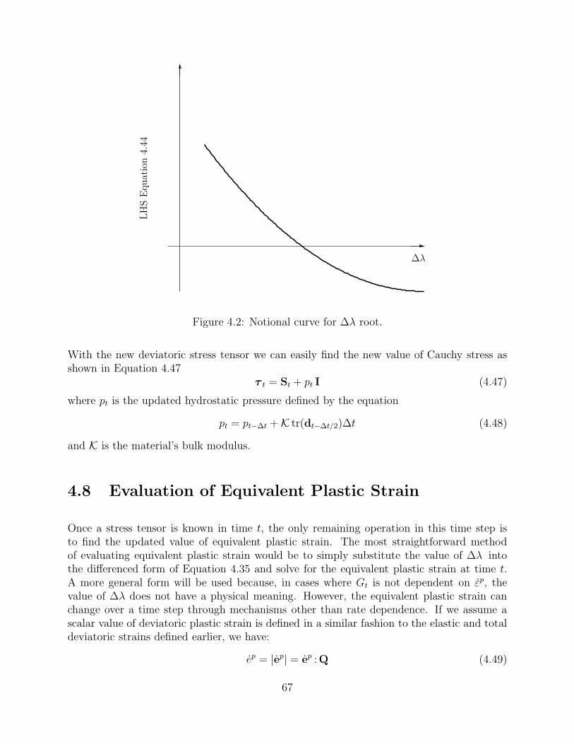
LH

SE

quat

ion

4.44

∆λ

Figure 4.2: Notional curve for ∆λ root.

With the new deviatoric stress tensor we can easily find the new value of Cauchy stress asshown in Equation 4.47

τ t = St + pt I (4.47)

where pt is the updated hydrostatic pressure defined by the equation

pt = pt−∆t + K tr(dt−∆t/2)∆t (4.48)

and K is the material’s bulk modulus.

4.8 Evaluation of Equivalent Plastic Strain

Once a stress tensor is known in time t, the only remaining operation in this time step isto find the updated value of equivalent plastic strain. The most straightforward methodof evaluating equivalent plastic strain would be to simply substitute the value of ∆λ intothe differenced form of Equation 4.35 and solve for the equivalent plastic strain at time t.A more general form will be used because, in cases where Gt is not dependent on εp, thevalue of ∆λ does not have a physical meaning. However, the equivalent plastic strain canchange over a time step through mechanisms other than rate dependence. If we assume ascalar value of deviatoric plastic strain is defined in a similar fashion to the elastic and totaldeviatoric strains defined earlier, we have:

ep = |ep| = ep :Q (4.49)

67

If we solve Equation 4.27 for ep and substitute into Equation 4.49, we have

ep = (e − ee) :Q (4.50)

then we substitute Equation 4.39 into Equation 4.50 to yield the following:

ep =

(

e − S

2µ

)

:Q (4.51)

Finally, we will take Equation 4.51 and substitute it into Equation 4.35, take the differencedform by multiplying through by ∆t, and solve for εp

t to give the following result:

εpt = εp

t−∆t +

√

2

3

(

∆et−∆t/2 −St − St−∆t

2µ

)

:Qt−∆t/2 (4.52)

where,

Qt−∆t/2 =Qt + Qt−∆t

2(4.53)

The current value of equivalent plastic strain, εp, can now be solved for by using Equa-tion 4.52.

4.9 Constitutive Model

With the fundamental theory in hand, we will turn to the numerical implementation of theconstitutive model. The viscoplastic constitutive law we adopted was used in Camacho andOrtiz [8] and modified by Warren and Tabbara [66] to ignore temperature effects resultingin the form shown in Equation 4.54

G = g

(

1 +εp

εp0

)1/m

(4.54)

where εp is the equivalent plastic strain rate, εp0 is a reference equivalent plastic strain rate,

m is the strain-rate exponent, and g defines the work hardening component of the modeland is given by Equation 4.55

g = Y

(

1 +εp

εp0

)1/n

(4.55)

where, Y is the quasi-static yield stress, εp is the equivalent plastic strain, εp0 is the reference

equivalent plastic strain, and n is a strain hardening parameter. This model is phenomenolog-ical in nature with n, m, εp

0, and εp0 being curve fit parameters determined from experimental

data.

Momentarily returning to Equation 4.44, we show the relationship that we will use tonumerically find ∆λ. If we use the constitutive model of Equation 4.54 as the yield function,

68

Equation 4.44 becomes

∆et−∆t/2 − ∆λt−∆t/2

− 1

2µ

√

2

3Y

(

1 +εp

t−∆t

εp0

)1/n(

1 +

√

2

3

∆λt−∆t/2

∆t εp0

)1/m

− St−∆t

= 0 (4.56)

And it follows that the yield surface Gt will be defined by:

Gt = Y

(

1 +εp

t−∆t

εp0

)1/n(

1 +

√

2

3

∆λt−∆t/2

∆t εp0

)1/m

(4.57)

4.10 Numerical Simulations

The viscoplastic constitutive model presented in the previous section was implemented intothe explicit peridynamics code Emu. In a typical finite element code, when a new modelis introduced, it is customary to run a uniaxial stress test on a single element in order toverify that the constitutive response reproduces the experimental data. In the peridynamicframework, a single node simulation will not suffice because a minimum number of nodes isnecessary to calculate a stress tensor. Instead, a model consisting of 3825 nodes representinga cylindrical tensile test specimen was simulated for comparison to experimental data. Thesimulation was run at an engineering strain rate of 8300/s. Boundary conditions are appliedby giving a region of nodes on either ends of the bar a constant velocity. This could also beachieved by applying a prescribed displacement or body force density to a region of nodes.The material parameters used correspond to a data fit to 6061-T6 aluminum provided inSong et. al [62]. The experiments were conducted using pulse shaped Kolsky bar experimentsto ensure a constant engineering strain rate of 8300/s. The constitutive parameters are asfollows: E = 68.9 GPa, ν = 0.333, Y = 276 MPa, n = 13.5, m = 44.0, εp

0 = 0.001/s, and εp0 =

1000/s. Figure 4.3 shows true stress as a function of Lagrangian strain for the simulations.The strain measurement from the simulation was calculated by using the Green-St.Venantformulation from the approximate deformation gradient as shown in Equation 4.58.

E =1

2

(

FT F− I)

(4.58)

The numerical implementation of the constitutive model matches the experimental data verywell. Currently, the constitutive model is only implemented in the explicit peridynamicscode, Emu, which makes running the simulation at quasi-static rates nearly impossible dueto conditions which require a very small time step; consequently, only a comparison at thehigh rate was done.

In order to validate5 the numerical implementation of the viscoplastic constitutive modelinto Emu, Taylor impact experimental results were simulated. A set of Taylor impact tests

5Additional validation was done on an elastic constitutive model, comparing simulations to analyticssolutions. This work is included in Appendix G.

69

were conducted on 6061-T6 aluminum by Anderson et. al [2]. This data included normalizedlength and diameter measurements as well as a selection of Dynamic Structured Light (DSL)images of the deformed specimens. The test specimens were 3.175 cm long with a diameterof 6.35mm (L/D = 5). The tests were conducted at impact speeds between 26 and 440m/s;however, at an impact speed of 363m/s and above, post test examination of the Taylorimpact specimens showed significant “mushrooming” and failure at the impact end. Whilefailure can be modeled with peridynamics and Emu it is beyond the scope of this validationexercise; therefore, these experiments were not attempted in numerical simulation. The Emusimulations were performed with a resolution of 40 nodes across the diameter of the specimen,resulting in 252,800 total nodes. The length scale parameter, δ, was chosen to be 3.05 · ∆xwhere ∆x is the distance between adjacent material particles. Simulations were also ran atδ = 4 · ∆x and δ = 5 · ∆x to investigate the length scale effect. As expected because thesesimulations where intended to investigate bulk response (change in length/diameter), thechange in δ had little to no effect on the simulation results. Figure 4.4 shows the normalizedlength (final length divided by initial length) for the Taylor impact experiments and thenumerical simulations using the Emu code with our viscoplastic model. Figure 4.5 showsthe normalized diameter at the impact face for the Taylor experiments and the numericalsimulations. Both the length and diameter calculations match the experimental data well.For a qualitative comparison of deformation, one of the Emu simulations is shown next tothe DSL Image from tests conducted at 289m/s impact speed in Figure 4.6. Here again wesee a good qualitative comparison of the deformation.

0

112.5

225

337.5

450

0 0.05 0.1 0.15 0.2

Tru

eStr

ess

(MPa)

Lagrangian Strain (m/m)

Emu Simulation6061-T6 Data (Song 2002)

Figure 4.3: Comparison of experimental data with numerical simulation at nominal engi-neering strain rate of 8300/s.

70

0.5

0.625

0.75

0.875

1

0 125 250 375 500

Lf/L

0

Impact Speed (m/s)

6061-T6 Data (Anderson 2008)Emu Simulations

Figure 4.4: Normalized length comparison.

1

1.75

2.5

3.25

4

0 125 250 375 500

Df/D

0

Impact Speed (m/s)

6061-T6 Data (Anderson 2008)Emu Simulations

Figure 4.5: Normalized diameter comparison.

71

DSL Image

Emu Simulation

Figure 4.6: Qualitative comparison of post test deformation from DSL image with numericalsimulation at 289m/s impact speed.

These simulations suggest the viability of using peridynamics to model materials thatexhibit viscoplasticity with hardening.


In this chapter, an elastic, viscoplastic constitutive relationship is implemented into a peri-dynamic numerical analysis code with the use of force-vector states. The model is phe-nomenological and uses parameters fit to experimental data. The model was fit to highstrain-rate constitutive data taken from Kolsky bar experiments on 6061-T6 aluminum. Themodel is then used to reproduce experimental results from Taylor impact tests of aluminum.The normalized length and diameter results from the calculations match the experimentalresults very well, and qualitative comparisons of post test deformation also compare well.This chapter demonstrates the ability to utilize conventional constitutive models within thestate-based peridynamic framework. More importantly, this model will be extremely usefulin our modeling of the inelastic and failure response of our 4340 steel samples as describedin the next chapter.

72

5 Fracture Model and Numerical Sim-ulation

5.1 Introduction

In Chapter 3, experiments were reported that showed a rate dependence of the dynamiccrack initiation of a 4340 steel. An engineering analyst would use the knowledge of this ratedependence in order to predict material failure in structures that have high-rate deformationssuch as blast and impact. The fist step to model these scenarios is to have a rate dependentconstitutive model; a method for implementing such a model into a peridynamic explicitdynamics code was described in Chapter 4. The next step is to implement a failure criterioninto the peridynamic framework that can use the knowledge of the rate dependent crackinitiation toughness as an input to the model. A novel failure criterion and explanation ofit’s implementation along with validation simulations is presented in this chapter.

5.2 Failure Model

The method of damage (failure, cracks, etc.) nucleation, coalescence, and propagation withinthe peridynamic model is through the permanent breaking of “bonds”. The word “bond”is used loosely in this context only to describe the relationship between two material pointsand can be thought of abstractly as an interaction potential; there is not necessarily anotion of direct connectivity such as a spring-like force. This is especially the case withinthe state-based peridynamic framework where the state-forces could potentially act in anyconceivable direction, not just colinear with the position vector, and certainly not in anequal-and-opposite fashion such is the case in bond-based peridynamics. Figure 5.1 showsa notional illustration of this relationship where, following the notation from Chapter 1, ξ

represents the “bond” and the T’s are the force-vector states.

In the numerical simulation of fracture many methods have been utilized to characterizewhen a material might fail. A few examples are the plastic strain to failure, stress triaxiality,lode angle dependence, etc. Most of these methods have some dependence on either the stressor strain histories. Since peridynamics is cast in a form that does not require the notion

73

x

x′ξT[x, t]〈x′ − x〉

T[x′, t]〈x − x′〉

Figure 5.1: Illustration of relationship between state-forces and “bond.”

of stress (although we used stress as a convenience for material modeling in Chapter 4),we wish to develop a failure criterion derived not from any stress or strain criterion, butinstead using thermodynamic notions of work or energy. We can calculate the amount ofenergy density stored a bond1, wξ, by projecting the force vector-states onto the relativedisplacement vector. The calculation is performed by Equation 5.1.

wξ =

∫ η(tfinal)

0

T[x, t]〈x′ − x〉 −T[x′, t]〈x − x′〉 · dη (5.1)

where the integrand of Equation 5.1 is known as the dual force density. Recall from Chapter 4that the relative displacement vector η is defined by Equation 5.2

η = u[x′, t] − u[x, t] (5.2)

A schematic of the bond kinematics is shown in Figure 5.2. Equation 5.1 defines wξ as havingunits of energy per unit volume squared. It represents an amount of work density done on abond due to displacing the two material points x and x′ relative to one another from zero tosome final scalar value of displacement, η(tfinal), which is a function of time. This projectionneglects any work done on the points due to rigid body translation. The motivation for thisidea comes from the well known physics equation where the work done to a body is the forceacting on it, f , integrated over the path length, s, as shown in Equation 5.3

W =

∫

f · ds (5.3)

However, in this case the work is actually an energy density, the force is the dual forcedensity, and the path is the relative displacement.

Although, the formal proof is not attempted here, it is hypothesized that by integratingwξ over the entire volume of the non-local horizon, H, of radius δ, we could expect the

1We will drop the quotation marks from the word bond henceforth, but we maintain the same notion ofinteraction as described in the first paragraph of Section 5.2

74

x

x′ξ

y

y′

ξ + η

u[x, t]

u[x′, t]

Figure 5.2: Schematic of bond kinematics.

result to converge in the limit as δ → 0 to the classic notion of strain energy density, w, asillustrated in Equation 5.4.

w =

∫

σ : dε = limδ→0

∫

H

wξdVξ (5.4)

Of course, we would expect this to be true only if we assume a smooth deformation for theexistence of the partial derivatives contained in the strain tensor, ε.

Figure 5.3 shows an example of how a viscoplastic material could potentially reach thesame bond energy density with different levels of relative displacement at tfinal. The valuesof η and t’s represent some scalar projection of the vector values shown in Equation 5.1,possibly the projection of the vectors onto the axial direction in a standard tensile testexperiment. In this idealized example, wξ1 = wξ2 even though the relative displacements, η1

and η2, have different ultimate values. This is because the material behaves differently (e.g.,exhibits rate dependence) when displaced at the two different rates, η1 and η2.

We will assume that the energy density contained in a bond is fully recoverable2 byreversing the deformation, unless it exceeds some critical energy density, wc. Let us attemptto define wc in terms of material property that can be experimentally determined. Referringto Figure 5.4, let us consider all points A along the dashed line, 0 < z < δ, connected toall points B across a fracture plane of unit area and within a spherical cap of radius δ withrespect to A (the shaded area in Figure 5.4). If we assume there is a critical energy density,wc, associated with moving each point A relative to each point B, that when exceeded willcause the removal of any potential between the two points (irreversible bond breakage), thenwe can sum up all of these energy densities through integration and equate the result with

2The bond energy density will only be fully recoverable if we assume a classicly hyperelastic materialmodel, if we assume a dissipative material model then then some of the work done on the bond may bepermanent.

75

t[x,t

]〈ξ〉−

t[x′ ,

t]〈−

ξ〉

η

wξ1

wξ2

η1

η2

Figure 5.3: Example of equivalent wξ and different η(tfinal) for two relative displacementrates.

the energy release rate, Gf . That is, the energy required to open a new fracture surface ofunit area. This equation is as follows:

Gf =

∫ δ

0

∫ 2π

0

∫ δ

z

∫ cos−1 z/ξ

0

wcξ2 sin φ dφdξdθdz (5.5)

When evaluated and solved for wc, Equation 5.5 reduces to:

wc =4Gf

πδ4(5.6)

Now we have a critical value of energy density that is based solely on material properties(recall that δ is considered a material property). We can compare this critical energy densityto the individual bond energy densities calculated via Equation 5.1 to determine when thebonds will individually fail. Cracks will nucleate and grow when a number of bond failurescoalescence into a surface and propagate. This phenomenon will emerge naturally withoutthe need to specify when and where the cracks will appear through some external criterion.Another advantage to the peridynamic model and allowing the bonds to break in this fashionis that it leads to an unambiguous notion of damage. The percentage of material damage acontinuum point has undergone is simply the percentage of broken bonds. For example, ifone material point interacts with one hundred others and one bond is broken, the materialpoint is considered 1% damaged.

To numerically implement this failure criterion with the constitutive model described inChapter 4, we will activate bond breakage through the use of the influence function contained

76

Fracture Surface

cos−1“

zξ

”

φ ξ

δz

θ

A

B

Figure 5.4: Schematic of fracture surface.

in the deformation gradient and shape tensors. Recall the formula for approximating thedeformation gradient from Chapter 4 reproduced here as Equation 5.7.

F[x, t] =

[∫

H

ω (|ξ|) (Y〈ξ〉 ⊗ ξ) dVx′

]

K−1 (5.7)

The term ω (|ξ|) was defined as an influence function. It can be used to assign a weight tothe amount of influence each bond within the horizon exerts on the point x. We can use it toimplement damage by setting the influence to zero for the bonds that are broken. Therefore,the failure criterion expressed mathematically is as follows:

ω (|ξ|) =

0 wξ > wc

1 otherwise(5.8)

When numerically implemented into the explicit dynamics code Emu, we calculate wξ forevery bond at each time step in the simulation and compare it to wc. If wξ exceeds wc, thenthe influence function is set to zero for that bond, and the bond is effectively left out of thecalculation of the deformation gradient at the next time step. The force that was exerted onthe point x by the broken bond will now have to be assumed by the remaining intact bonds.This additional load on the intact bonds may cause them to subsequently break therebymimicing damage propagation throughout the structure.

77

0

550

1100

1650

2200

0 0.03 0.06 0.09 0.12

Tru

eStr

ess

(MPa)

Lagrangian Strain (m/m)

ε = 1150/s

ε = 2900/s

Data (Frew et al.)Emu Simulation

Figure 5.5: Comparison of data to simulation at strain rates of 1150/s and 2900/s.

5.3 Numerical Simulations

The failure criterion described in Section 5.2 was implemented into the peridynamic com-putational mechanics code Emu and a selection of experiments from Chapter 3 were simu-lated. Because the samples consisted of 4340 steel, the constitutive response for this materialneeded to be validated. The constitutive model described in Chapter 4 was fit to experimen-tal data for 4340 with a similar heat treatment and Rockwell hardness published by Frewet al. [20]. The fitted constitutive parameters for the 4340 steel are E = 210GPa, ν = 0.29,Y = 1116MPa, n = 65, m = 27.5, εp

0 = 5.417 × 10−3 m/m, and εp0 = 5.940 × 10−3/s. The

model fit is demonstrated along with reported data at two different strain rates in Figure 5.5.

The experiments reported in Chapter 3 were done to detect the dynamic crack initiationtoughness of the 4340 steel samples. In order to use KIc as an input to this failure model, wehave to resort to the relationship from plane strain linear elastic fracture mechanics shownin Equation 5.9

Gf =K2

Ic

E

(

1 − ν2)

(5.9)

where, E is the elastic (Young’s) modulus and ν is Poisson’s Ratio, which results in thefailure criterion based on KIc shown in Equation 5.10.

wc =4K2

Ic

πEδ4

(

1 − ν2)

(5.10)

78

Now someone may pose the question, “Why are we resorting to linear elastic fracturemechanics (LEFM) when the peridynamic theory does not exhibit a crack tip stress singu-larity (recall that the singular stress field in the classical theory is the reason one uses KIc)?”The answer to this question has to do with our shortcomings as experimentalists, not fromthe peridynamic theory or the failure model. We use KIc here as a convenience because itis the easiest of the crack tip physics variables to measure. If we possessed measurementsof G or the J-Integral directly (which would not limit us to LEFM) we could use them asinputs to the failure model and proceed with modeling any failure (e.g., elastic-plastic) in astraightforward fashion.

The boundary conditions we applied in the simulations come from the boundary velocitymeasurements in the Kolsky experiments. The measured velocities are applied as initialconditions to a four point bend beam that has been discretized into peridynamic nodes.Figure 5.6 shows the boundary regions where the velocities were applied. Notice that onlya single row of nodes was segmented out and made into boundary regions. This was doneas not to impart any moments in the region where the boundary conditions were applied.Also, note that the velocity vectors all point in the same direction; therefore moving theentire sample to the left during the simulation The deformation comes from the v1 velocitiesbeing much higher in magnitude than the v2 velocities. This is shown to be obvious byreexamining the sample boundary velocities reported in Chapter 3 shown here in Figure 5.7.The boundary condition applied to boundary region 5 shown in Figure 5.6 was a conditionapplied to the entire body that restricts displacements in the direction normal to the planeof the sample. This was done in order to mimic plane strain conditions without the needto actually model a very thick sample. The resulting sample has 5 nodes in the thicknessdirection, 50 nodes across the sample width, and 214 nodes along the sample length, resultingin 53 500 total nodes.

For test number T36 shown in Figure 5.7, the time-to-fracture was approximately 27 µs.The measure of comparison for the simulation is the time-to-fracture, therefore, the simu-lation was only run out to around 50µs. After this time, the boundary conditions becomeless realistic since the sample begins to slide along the supports after crack initiation andthis motion is not modeled in the simulation. Any comparisons to crack propagation canonly be qualitative because of the simplified boundary condition not imposed in the simula-tions which does not represent the experiment exactly. Furthermore, no robust experimentalmeasurements were made on the propagation speed.

Because the peridynamic model allows for arbitrary crack growth through the accumu-lation of broken bonds without specifying when or where the cracks will nucleate and grow,it can be difficult to quantitatively track crack propagation in complex structures. However,because the sample modeled here is fairly simple and it is known from experimental obser-vations where the crack will initiate, a simple algorithm was written to detect when roughly50% of the bonds are broken thereby representing a crack.3 A selection of the experiments

3The 50% damage criterion comes from the fact that for a node to be on the surface of a crack roughlyhalf of the bonds across the failure plane will be irreversibly broken, and roughly half the bonds will still beconnected to the interior of the body

79

Boundary

Reg

ion

v2

v2

v1

v1

1

5

2

3

4

-6

x1

x2

(a) Boundary regions.

(b) Boundary region 2 zoom.

Figure 5.6: Boundary regions.

80

−100

0

100

200

300

0 50 100 150 200

Vel

oci

ty(m

/s)

Time (µs)

tf ≈ 27µsv1v2

Figure 5.7: Sample boundary velocities from test T36.

were modeled, resulting in good agreement with the times-to-fracture for each experiment.Results from two different simulated loading rates are compared to the experimental crackinitiation times-to-fracture in Figure 5.8. The vertical dashed line in the figures representsthe experimentally measured times-to-fracture. The solid line represents the tracking of thecrack tip position in the simulations. Because the coordinate system origin (shown in Fig-ure 5.6) is on the right hand boundary of the sample, the maximum of the ordinate axesin the figures represents the place where the crack would break the sample in half. Theinitial value of the crack tip position represents the initial length of the crack taken from theexperimental measurements. Figure 5.8a uses the value of KIc = 65MPa

√m as an input

to the failure model at a loading rate of KI = 2.407 × 106 MPa√

m/s which is labeled asLoading Rate 1 in the figure. Figure 5.8b uses the value of KIc = 139MPa

√m as an input

to the failure model at a loading rate of KI = 4.343 × 106 MPa√

m/s labeled as LoadingRate 2 in the figure. Both simulations show very good comparisons to the experimentaltime-to-fractures.

In order to visualize the overall deformation, crack initiation, and propagation a set ofimages from the simulations were sampled and sequenced in Appendix E. Figure 5.9 showsan animation4 of the simulation.

As mentioned in Chapter 3 a subset of experiments were conducted at Purdue University

4If the reader is viewing the electronic PDF of this document in Adobe Acrobat R© 9 or newer withJavaScript enabled, click on Figure 5.9 to view the animation; otherwise, refer to Appendix E to view thesequenced images.

81

−0.015

−0.01125

−0.0075

−0.00375

0

0 15 30 45 60

Cra

ckT

ipPos

itio

n(m

)

Time (µs)

tf ≈ 27 µs

Emu SimulationExperiment

(a) Test T36 (Loading rate 1).

−0.015

−0.01125

−0.0075

−0.00375

0

0 15 30 45 60

Cra

ckT

ipPos

itio

n(m

)

Time (µs)

tf ≈ 32µs

Emu SimulationExperiment

(b) Test T20 (Loading rate 2).

Figure 5.8: Comparison of time-to-fracture from experiment and simulation.

82

Figure 5.9: Simulation results showing crack initiation and propagation.

83

and a Cordin high-speed rotating mirror camera was used to capture the crack initiationand propagation. These samples were 4340 steel, but had a slightly different heat treatmentthan the samples reported in Figure 3.14; therefore, the dynamic crack initiation toughnessmeasurements were not reported with the others. One sample from this group was simulatedusing Emu; images from the simulation were sampled at the same frame rate as the camera(≈ 4µs) data and comparisons were made. The sampled results are shown in Appendix Eand the resulting simulation is shown in Figure 5.10.

The simulations shows good quantitative correlation with the crack initiation time. Bycomparing the visual results from the simulation and the camera footage we see that thepropagation speed as well qualitatively compares as well. This is somewhat surprising beingthat the failure model uses only KIc as an input. This phenomenon should be researchedfurther in future work and compared to quantitative crack speed data.


This chapter motivated and presented a novel energy based failure criterion that was im-plemented into a peridynamics continuum mechanics code and compared to experimentalresults. By using experimental crack initiation toughness measurements and the experi-mental boundary conditions as inputs to the code, the failure model was able to reproducetime-to-fracture measurements as well as suggestively reproduce crack propagation speed.

One aspect of the model that needs to be further researched is the fact that the criticalenergy density, wc, is identical whether the bond is in tension or compression. For someengineering materials, such as concrete, this may not be a realistic approximation; however,a different derivation for wc, which would include differences for tension or compression, couldbe easily incorporated. Overall the model seems to perform well for the limited number ofexperiments simulated and allows us to account for unguided crack propagation within aconsistent mathematical framework.

The simulations presented in this chapter use the recorded values of KIc as individualinputs at each loading rate, meaning the analyst must have some a priori knowledge of theloading rate of the experiment in order to chose the appropriate value of KIc. However, itwould be very simple to implement a model where KIc is a curve instead of a single valueand the simulations could approximate the near crack tip value of KI and use the value ofKIc accordingly.

84

Figure 5.10: Comparison of simulation to experimental camera data.

85

6 Summary and Recomendations

The work in this dissertation had two distinctly different areas of original research. Chapter 3,Chapter 4, and Chapter 5 each had sections at the end which contained some concludingremarks on the major contributions in each area. The most important original contributionsare highlighted below:

• Experiments

– A novel experimental and data reduction technique was used to record dynamiccrack initiation toughness measurements of a 4340 steel utilizing the Kolsky ap-paratus.

– Data was presented for 4340 steel at two different nominal loading rates of whichare shown to be very near constant by using pulse shaping techniques to shapethe loading pulse.

– The 4340 steel samples where shown to have a rate dependence for the dynamiccrack initiation toughness.

• Peridynamic Simulation

– The research presented in Chapter 4 was the first implementation of a (state-based) viscoplastic constitutive model into the the peridynamic framework.

– The constitutive model validation was the first peridynamic implementation toquantitatively compare to experimental results and showed excellent agreementto the Taylor anvil impact data.

– A novel failure model using a energy based criterion was hypothesized and imple-mented into a peridynamics numerical code.

– The failure model was validated on a significant class of problems, (i.e., mode Idynamic fracture) by simulating the experimental results recorded in Chapter 3using the dynamic crack initiation toughness as inputs to the model.

The concluding remarks of Chapter 3 give several ideas for future enhancements of theexperimental technique. Most notably, if the sample size were adjusted or the Kolsky bardiameter increased, one could incorporate the impact and support tups into the end of the

87

bars to eliminate the need for special timing corrections to account for the wave propagationthat takes place in the gage section.

For the peridynamic modeling, there is a lifetime of research to be undertaken in thisnew field of continuum mechanics. A few straightforward additions to the research presentedhere would be to investigate convergence and mesh sensitivity of the failure and constitutivemodels. The next step would be to investigate failure in complex structures where the crackinitiation and propagation directions may be unknown a priori. If the structure exhibitsfragmentation, comparisons of fragment size distribution1 could be undertaken. The researchpresented in the dissertation should also make contributions to the science of penetrationmechanics. There are still many unsolved phenomena in plate perforations such as thedifferent types of failure (e.g., cavity expansion, spall, plugging). A few simple simulationsof the perforation of an aluminum plate, where the plate is modeled with the constitutivemodel of Chapter 4 and the failure model of Chapter 5 are shown in Figure 6.1. Thesimulations were run with a two rigid projectiles, one with an ogive nose, and one with aflat cylindrical nose. Both projectiles had the same initial velocity and angle-of-incidence tothe plate. Notice the different failure patterns the different nose shapes impart on the plate.Perforation with the ogive nose gives rise to the mechanism of a cavity expansion whereasthe cylindrical nose is stopped in the plate. But one can see the beginnings of a plug beingpushed through the plate. These simulations were run with a very course mesh and werenot intended to simulate any particular experiment, they are just used to notionally showother applications and areas of research for the modeling of materials and material failurewith peridynamics.

The future direction of this author’s research will include looking at peridynamic meshsensitivity convergence of crack initiation and propagation as well as failure pattern conver-gence when the mesh node locations are randomly perturbed in the reference configuration(a method of introducing material heterogeneity). More complex fracture experiments (i.e.,multiple cracks) will be simulated as well penetration and perforation comparisons to exper-imental data. Future interests also include implementing constitutive and failure models forconcrete, in a similar fashion as those described in this work, and studying damage initiationand propagation in that complex but important engineering material.

1Preliminary work in this area has already been undertaken by Dr. Stewart A. Silling using the constitutivemodel presented in Chapter 4. Some simulations showing good correlation to experimental data were shownby Dr. David J. Littlewood at a presentation at US National Congress on Computational Mechanics 10 inColumbus, Ohio, July 2009.

88

(a) Ogive Nose

(b) Flat Nose

Figure 6.1: Ogive and flat nose penetration of aluminum plate.

89

References

[1] T.L. Anderson. Fracture mechanics. CRC Press Boca Raton, 1991.

[2] C.E. Anderson Jr, A.E. Nicholls, I.S. Chocron, and R.A. Ryckman. Taylor anvil impact.In AIP Conference Proceedings, volume 845, page 1367. AIP, 2006.

[3] E. Askari, F. Bobaru, R.B. Lehoucq, M.L. Parks, S.A. Silling, and O. Weckner. Peri-dynamics for multiscale materials modeling. In Journal of Physics: Conference Series,volume 125, page 012078. Institute of Physics Publishing, 2008.

[4] T. Belytschko, Y.Y. Lu, L. Gu, et al. Element-free Galerkin methods. InternationalJournal for Numerical Methods in Engineering, 37(2):229–256, 1994.

[5] T. Belytschko, Y.Y. Lu, L. Gu, and M. Tabbara. Element-free Galerkin methods forstatic and dynamic fracture. International Journal of Solids and Structures, 32(17-18):2547–2570, 1995.

[6] T. Belytschko and M. Tabbara. Dynamic fracture using element-free Galerkin methods.International Journal for Numerical Methods in Engineering, 39(6), 1996.

[7] H.D. Bui, H. Maigre, and D. Rittel. A new approach to the experimental determinationof the dynamic stress intensity factor. International Journal of Solids and Structures,29(23):2881–2895, 1992.

[8] G.T. Camacho and M. Ortiz. Adaptive Lagrangian modelling of ballistic penetrationof metallic targets. Computer Methods in Applied Mechanics and Engineering, 142(3-4):269–301, 1997.

[9] J.S. Chen, C. Pan, C.T. Wu, and W.K. Liu. Reproducing kernel particle methodsfor large deformation analysis of non-linear structures. Computer Methods in AppliedMechanics and Engineering, 139(1-4):195–227, 1996.

[10] W. Chen, F. Lu, D.J. Frew, and M.J. Forrestal. Dynamic compression testing of softmaterials. Journal of applied mechanics, 69(3):214–223, 2002.

[11] W. Chen, B. Song, D.J. Frew, and M.J. Forrestal. Dynamic small strain measurementsof a metal specimen with a split Hopkinson pressure bar. Experimental Mechanics,43(1):20–23, 2003.

91

[12] L.S. Costin, J. Duffy, and L.B. Freund. Fracture initiation in metals under stress waveloading conditions. ASTM special technical publication, (627):301–318, 1977.

[13] A. Delaplace and A. Ibrahimbegovic. Performance of time-stepping schemes for discretemodels in fracture dynamic analysis. International Journal for Numerical Methods inEngineering, 65(9), 2006.

[14] D.P. Flanagan and L.M. Taylor. An accurate numerical algorithm for stress integra-tion with finite rotations. Computer Methods in Applied Mechanics and Engineering,62(3):305–320, 1987.

[15] J.T. Foster, S.A. Silling, and W.W. Chen. Viscoplasticity Using Peridynamics. In-ternational Journal for Numerical Methods in Engineering, Accepted, 2009, DOI:10.1002/nme.2725.

[16] J.W. Foulk, D.H. Allen, and K.L.E. Helms. Formulation of a three-dimensional cohesivezone model for application to a finite element algorithm. Computer Methods in AppliedMechanics and Engineering, 183(1-2):51–66, 2000.

[17] L.B. Freund. Crack propagation in an elastic solid subjected to general loading. III-Stress wave loading. Journal of the Mechanics and Physics of Solids, 21:47–61, 1973.

[18] L.B. Freund. Dynamic Fracture Mechanics. Cambridge University Press, 1998.

[19] D.J. Frew, M.J. Forrestal, and W. Chen. Pulse shaping techniques for testing brittlematerials with a split hopkinson pressure bar. Experimental Mechanics, 42(1):93–106,2002.

[20] D.J. Frew, M.J. Forrestal, and W. Chen. Pulse shaping techniques for testingelastic-plastic materials with a split Hopkinson pressure bar. Experimental Mechan-ics, 45(2):186–195, 2005.

[21] H. Gao and P. Klein. Numerical simulation of crack growth in an isotropic solid withrandomized internal cohesive bonds. Journal of the Mechanics and Physics of Solids,46(2):187–218, 1998.

[22] K.F. Graff. Wave Motion in Elastic Solids. Dover Publications, 1991.

[23] A.E. Green and P.M. Naghdi. A note on invariance under superposed rigid body mo-tions. Journal of Elasticity, 9(1):1–8, 1977.

[24] A.A. Griffith. The Phenomena of Rupture and Flow in Solids. Philosophical Transac-tions of the Royal Society of London. Series A, Containing Papers of a Mathematicalor Physical Character, 221:163–198, 1921.

[25] E.S. Hertel Jr, R.L. Bell, M.G. Elrick, A.V. Farnsworth, G.I. Kerley, J.M. McGlaun,S.V. Petney, S.A. Silling, P.A. Taylor, and L. Yarrington. CTH: A software family formulti-dimensional shock physics analysis. In Conference: 19. international symposiumon shock waves, Marseille (France), 26-30 Jul 1993, 1992.

92

[26] R. Hill. The Mathematical Theory of Plasticity. Oxford University Press, 1998.

[27] W.G. Hoover, C.G. Hoover, O. Kum, V.M. Castillo, H.A. Posch, and S. Hess. Smoothparticle applied mechanics. World Scientific, 2006.

[28] B. Hopkinson. A Method of Measuring the Pressure Produced in the Detonation of HighExplosives or by the Impact of Bullets. Philosophical Transactions of the Royal Soci-ety of London. Series A, Containing Papers of a Mathematical or Physical Character,213:437–456, 1914.

[29] ASTM International. Standard test method for linear-elastic plane-strain fracturetoughness KIc of metallic materials, 2006.

[30] G.R. Irwin and J.A. Kies. Fracturing and fracture dynamics. Welding J, 31, 1952.

[31] G.R. Irwin and D.E. Wit. A summary of fracture mechanics concepts. Journal ofTesting and Evaluation, 11:56–65, 1983.

[32] F. Jiang, A. Rohatgi, K.S. Vecchio, and J.L. Cheney. Analysis of the dynamic re-sponses for a pre-cracked three-point bend specimen. International Journal of Fracture,127(2):147–165, 2004.

[33] F. Jiang and K.S. Vecchio. Dynamic effects in Hopkinson bar four-point bend fracture.Metallurgical and Materials Transactions A, 38(12):2896–2906, 2007.

[34] F. Jiang and K.S. Vecchio. Experimental investigation of dynamic effects in a two-bar/three-point bend fracture test. Review of Scientific Instruments, 78:063903, 2007.

[35] G.C. Johnson and D.J. Bammann. A discussion of stress rates in finite deformationproblems. International Journal of Solids and Structures, 20(8):725–737, 1983.

[36] G.R. Johnson and R.A. Stryk. Conversion of 3D distorted elements into meshlessparticles during dynamic deformation. International Journal of Impact Engineering,28(9):947–966, 2003.

[37] J.R. Klepaczko. Dynamic Crack Initiation: Some Experimental Methods and Modeling,Crack Dynamics in Metallic Materials, J. R. Klepaczko, ed., Springer-Verlag, Viennaand New York, 1990, pp. 428-450.

[38] H. Kolsky. An Investigation of the Mechanical Properties of Materials at very HighRates of Loading. Proceedings of the Physical Society Section B, 62(11):676–700, 1949.

[39] H. Kolsky. Stress Waves in Solids. Dover Publications, 2003.

[40] W.K. Liu, S. Jun, and Y.F. Zhang. Reproducing kernel particle methods. InternationalJournal for Numerical Methods in Fluids, 20, 1995.

[41] Y.Y. Lu, T. Belytschko, and L. Gu. A new implementation of the element free Galerkinmethod. Computer Methods in Applied Mechanics and Engineering, 113(3-4):397–414,1994.

93

[42] L.E. Malvern. Introduction to the Mechanics of a Continuous Medium. EnglewoodCliffs, NJ, 1969.

[43] M.A. Meyers. Dynamic Behavior of Materials. Wiley-Interscience, 1994.

[44] N. Moes and T. Belytschko. Extended finite element method for cohesive crack growth.Engineering Fracture Mechanics, 69(7):813–833, 2002.

[45] J.J. Monaghan. An introduction to SPH. In Particle Methods in Fluid Dynamics andPlasma Physics, proceedings from the workshop held April 13-15, 1987, in Los Almos,USA. Published 1987, p. 89, 1987.

[46] D.M. Owen, S. Zhuang, A.J. Rosakis, and G. Ravichandran. Experimental Deter-mination of Dynamic Crack Initiation and Propagation Fracture Toughness in ThinAluminum Sheets. International Journal of Fracture, 90(1):153–174, 1998.

[47] C.H. Popelar, C.E. Anderson, and A. Nagy. An experimental method for determiningdynamic fracture toughness. Experimental Mechanics, 40(4):401–407, 2000.

[48] T. Rabczuk, T. Belytschko, and S.P. Xiao. Stable particle methods based on Lagrangiankernels. Computer methods in applied mechanics and engineering, 193(12-14):1035–1063, 2004.

[49] K. Ravi-Chandar. Dynamic Fracture. Elsevier Science, 2004.

[50] K. Ravi-Chandar and W.G. Knauss. Dynamic Crack Tip Stresses Under Stress WaveLoading-A Comparison of Theory and Experiment. International Journal of Fracture,20:209–222, 1982.

[51] J.R. Rice and G.F. Rosengren. Plane Strain Deformation Near a Crack Tip in a PowerLaw Hardening Material. J MECH PHYS SOLIDS, 16(1):1–12, 1968.

[52] D. Rittel, H. Maigre, and H.D. Bui. A New Method for Dynamic Fracture ToughnessTesting. Scripta Metallurgica et Materialia(USA), 26(10):1593–1598, 1992.

[53] I.V. Rokach. Discussion on the paper “Evaluation of dynamic fracure toughness KId byHopkinson pressure bar loaded instrumented Chapry impact test” by Jiang Fengchun,Liu Ruitang, Zhang Xiaoxin, Kenneth S. Vecchio and Aashish Rohatgi, EngineeringFracture Mechanics, 71 (2004) pp. 279-287. Engineering Fracture Mechanics, 72:1107–1111, 2005.

[54] C.F. Shih. Relationships Between the J-Integral and the Crack Opening Displacementfor Stationary and Extending Cracks. Journal of the Mechanics and Physics of Solids,29(4):305–326, 1981.

[55] S.A. Silling. Stability and accuracy of differencing schemes for viscoplastic model inwavecodes. SAND Report SAND91-0141, Sandia National Laboratories, 1991.

[56] S.A. Silling. Reformulation of elasticity theory for discontinuities and long-range forces.Journal of the Mechanics and Physics of Solids, 48(1):175–209, 2000.

94

[57] S.A. Silling. Dynamic fracture modeling with a meshfree peridynamic code. In KJ Bathe,editor, Computational Fluid and Solid Mechanics, pages 641–644, Amsterdam, 2003.Elsevier.

[58] S.A. Silling and E. Askari. A meshfree method based on the peridynamic model of solidmechanics. Computers and Structures, 83(17-18):1526–1535, 2005.

[59] S.A. Silling, M. Epton, O. Weckner, J. Xu, and E. Askari. Peridynamic states andconstitutive modeling. J Elasticity, 88:151–184, 2007.

[60] S.A. Silling and R.B. Lehoucq. Convergence of peridynamics to classical elasticitytheory. Journal of Elasticity, (93):13–37, 2008.

[61] S.A. Silling, M. Zimmermann, and R. Abeyaratne. Deformation of a peridynamic bar.Journal of Elasticity, 73(1):173–190, 2003.

[62] B. Song, W.W. Chen, and D.J. Frew. Split-Hopkinson bar testing of an aluminumwith pulse shaping. In Proceedings of the JSME/ASME International Conference onMaterials and Processing, Honolulu, HI, October 2002. ASME.

[63] J.E. Srawley. Wide range stress intensity factor expressions for ASTM E 399 standardfracture toughness specimens. International Journal of Fracture, 12(3):475–476, 1976.

[64] N. Sukumar, N. Moes, B. Moran, and T. Belytschko. Extended finite element methodfor three-dimensional crack modelling. International Journal for Numerical Methods inEngineering, 48(11), 2000.

[65] H. Tada, P.C. Paris, and G.R. Irwin. The Stress Analysis of Cracks Handbook. AmericanSociety of Mechanical Engineers, 3 Park Avenue, New York, NY 10016-5990, USA,2000. 677, 2000.

[66] T.L. Warren and M.R. Tabbara. Simulations of the penetration of 6061-T6511 aluminumtargets by spherical-nosed VAR 4340 steel projectiles. International Journal of Solidsand Structures, 37(32):4419–4435, 2000.

[67] T. Weerasooriya, P. Moy, D. Casem, M. Cheng, and W. Chen. Four-point Bend Tech-nique To Determine Dynamic Fracture Toughness Of Ceramics. Journal of the AmericanCeramic Society, 89(3):990–995, 2006.

[68] T. Yokoyama. Determination of dynamic fracture-initiation toughness using a novelimpact bend test procedure. Journal of pressure vessel technology, 115(4):389–397,1993.

[69] T. Yokoyama and K. Kishida. A novel impact three-point bend test method for deter-mining dynamic fracture-initiation toughness. Experimental Mechanics, 29(2):188–194,1989.

95

A Loading Rate 1

97

−1

−0.5

0

0.5

1

0 500 1000 1500 2000

Ele

ctri

cPot

enti

al(V

)

Time (µs)

IncidentTransmitted

Crack Detection

(a) Raw data.

−1

−0.5

0

0.5

1

0 500 1000 1500 2000

Ele

ctri

cPot

enti

al(V

)

Time (µs)

tI tR


−0.2

−0.1

0

0.1

0.2

0 500 1000 1500 2000

Ele

ctri

cPot

enti

al(V

)

Time (µs)

tT


−100

0

100

200

300

0 50 100 150 200

For

ce(k

N)

Time (µs)

tf ≈ 33µsP1P2


−100

0

100

200

300

0 50 100 150 200

Vel

oci

ty(m

/s)

Time (µs)

tf ≈ 33µsv1v2


0

35

70

105

140

0 15 30 45 60

KI

(MPa√

m)

Time (µs)

tf ≈ 33 µs

KIc ≈ 68MPa√

m


Figure A.1: Sample T08.

98

−1

−0.5

0

0.5

1

0 500 1000 1500 2000

Ele

ctri

cPot

enti

al(V

)

Time (µs)

IncidentTransmitted

Crack Detection

(a) Raw data.

−1

−0.5

0

0.5

1

0 500 1000 1500 2000

Ele

ctri

cPot

enti

al(V

)

Time (µs)

tI tR


−0.2

−0.1

0

0.1

0.2

0 500 1000 1500 2000

Ele

ctri

cPot

enti

al(V

)

Time (µs)

tT


−100

0

100

200

300

0 50 100 150 200

For

ce(k

N)

Time (µs)

tf ≈ 28µsP1P2


−100

0

100

200

300

0 50 100 150 200

Vel

oci

ty(m

/s)

Time (µs)

tf ≈ 28µsv1v2


0

35

70

105

140

0 15 30 45 60

KI

(MPa√

m)

Time (µs)

tf ≈ 28µs

KIc ≈ 65MPa√

m



99

−1

−0.5

0

0.5

1

0 500 1000 1500 2000

Ele

ctri

cPot

enti

al(V

)

Time (µs)

IncidentTransmitted

Crack Detection

(a) Raw data.

−1

−0.5

0

0.5

1

0 500 1000 1500 2000

Ele

ctri

cPot

enti

al(V

)

Time (µs)

tI tR


−0.2

−0.1

0

0.1

0.2

0 500 1000 1500 2000

Ele

ctri

cPot

enti

al(V

)

Time (µs)

tT


−100

0

100

200

300

0 50 100 150 200

For

ce(k

N)

Time (µs)

tf ≈ 34µsP1P2


−100

0

100

200

300

0 50 100 150 200

Vel

oci

ty(m

/s)

Time (µs)

tf ≈ 34µsv1v2


0

35

70

105

140

0 15 30 45 60

KI

(MPa√

m)

Time (µs)

tf ≈ 34µs

KIc ≈ 66MPa√

m



100

−1

−0.5

0

0.5

1

0 500 1000 1500 2000

Ele

ctri

cPot

enti

al(V

)

Time (µs)

IncidentTransmitted

Crack Detection

(a) Raw data.

−1

−0.5

0

0.5

1

0 500 1000 1500 2000

Ele

ctri

cPot

enti

al(V

)

Time (µs)

tI tR


−0.2

−0.1

0

0.1

0.2

0 500 1000 1500 2000

Ele

ctri

cPot

enti

al(V

)

Time (µs)

tT


−100

0

100

200

300

0 50 100 150 200

For

ce(k

N)

Time (µs)

tf ≈ 27µsP1P2


−100

0

100

200

300

0 50 100 150 200

Vel

oci

ty(m

/s)

Time (µs)

tf ≈ 27µsv1v2


0

35

70

105

140

0 15 30 45 60

KI

(MPa√

m)

Time (µs)

tf ≈ 27µs

KIc ≈ 65MPa√

m



101

B Loading Rate 2

103

−1

−0.5

0

0.5

1

0 500 1000 1500 2000

Ele

ctri

cPot

enti

al(V

)

Time (µs)

IncidentTransmitted

Crack Detection

(a) Raw data.

−1

−0.5

0

0.5

1

0 500 1000 1500 2000

Ele

ctri

cPot

enti

al(V

)

Time (µs)

tI tR


−0.2

−0.1

0

0.1

0.2

0 500 1000 1500 2000

Ele

ctri

cPot

enti

al(V

)

Time (µs)

tT


−100

0

100

200

300

0 50 100 150 200

For

ce(k

N)

Time (µs)

tf ≈ 25µsP1P2


−100

0

100

200

300

0 50 100 150 200

Vel

oci

ty(m

/s)

Time (µs)

tf ≈ 25µsv1v2


0

50

100

150

200

0 15 30 45 60

KI

(MPa√

m)

Time (µs)

tf ≈ 25µs

KIc ≈ 158MPa√

m


Figure B.1: Sample T19.

104

−1

−0.5

0

0.5

1

0 500 1000 1500 2000

Ele

ctri

cPot

enti

al(V

)

Time (µs)

IncidentTransmitted

Crack Detection

(a) Raw data.

−1

−0.5

0

0.5

1

0 500 1000 1500 2000

Ele

ctri

cPot

enti

al(V

)

Time (µs)

tI tR


−0.2

−0.1

0

0.1

0.2

0 500 1000 1500 2000

Ele

ctri

cPot

enti

al(V

)

Time (µs)

tT


−100

0

100

200

300

0 50 100 150 200

For

ce(k

N)

Time (µs)

tf ≈ 32 µsP1P2


−100

0

100

200

300

0 50 100 150 200

Vel

oci

ty(m

/s)

Time (µs)

tf ≈ 32 µsv1v2


0

50

100

150

200

0 15 30 45 60

KI

(MPa√

m)

Time (µs)

tf ≈ 32µs

KIc ≈ 139MPa√

m



105

−1

−0.5

0

0.5

1

0 500 1000 1500 2000

Ele

ctri

cPot

enti

al(V

)

Time (µs)

IncidentTransmitted

Crack Detection

(a) Raw data.

−1

−0.5

0

0.5

1

0 500 1000 1500 2000

Ele

ctri

cPot

enti

al(V

)

Time (µs)

tI tR


−0.2

−0.1

0

0.1

0.2

0 500 1000 1500 2000

Ele

ctri

cPot

enti

al(V

)

Time (µs)

tT


−100

0

100

200

300

0 50 100 150 200

For

ce(k

N)

Time (µs)

tf ≈ 29µsP1P2


−100

0

100

200

300

0 50 100 150 200

Vel

oci

ty(m

/s)

Time (µs)

tf ≈ 29µsv1v2


0

50

100

150

200

0 15 30 45 60

KI

(MPa√

m)

Time (µs)

tf ≈ 28µs

KIc ≈ 165MPa√

m



106

−1

−0.5

0

0.5

1

0 500 1000 1500 2000

Ele

ctri

cPot

enti

al(V

)

Time (µs)

IncidentTransmitted

Crack Detection

(a) Raw data.

−1

−0.5

0

0.5

1

0 500 1000 1500 2000

Ele

ctri

cPot

enti

al(V

)

Time (µs)

tI tR


−0.2

−0.1

0

0.1

0.2

0 500 1000 1500 2000

Ele

ctri

cPot

enti

al(V

)

Time (µs)

tT


−100

0

100

200

300

0 50 100 150 200

For

ce(k

N)

Time (µs)

tf ≈ 30µsP1P2


−100

0

100

200

300

0 50 100 150 200

Vel

oci

ty(m

/s)

Time (µs)

tf ≈ 30µsv1v2


0

50

100

150

200

0 15 30 45 60

KI

(MPa√

m)

Time (µs)

tf ≈ 30µs

KIc ≈ 149MPa√

m



107

−1

−0.5

0

0.5

1

0 500 1000 1500 2000

Ele

ctri

cPot

enti

al(V

)

Time (µs)

IncidentTransmitted

Crack Detection

(a) Raw data.

−1

−0.5

0

0.5

1

0 500 1000 1500 2000

Ele

ctri

cPot

enti

al(V

)

Time (µs)

tI tR


−0.2

−0.1

0

0.1

0.2

0 500 1000 1500 2000

Ele

ctri

cPot

enti

al(V

)

Time (µs)

tT


−100

0

100

200

300

0 50 100 150 200

For

ce(k

N)

Time (µs)

tf ≈ 27µsP1P2


−100

0

100

200

300

0 50 100 150 200

Vel

oci

ty(m

/s)

Time (µs)

tf ≈ 27µsv1v2


0

50

100

150

200

0 15 30 45 60

KI

(MPa√

m)

Time (µs)

tf ≈ 27µs

KIc ≈ 159MPa√

m



108

C Machine Drawings

109

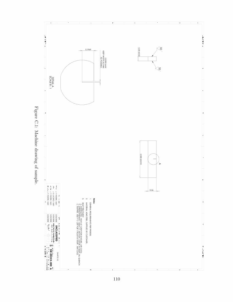
Figu

reC

.1:M

achin

edraw

ing

ofsam

ple.

110

0

$%

$

%

5

5

127(6

*(1(5$/5(48,5(0(1763(5

0$7(5,$/$)6833/,('%<&86720(5

+($775($70(17

D$11($/,1*+($7$7)+2856$,5&22/

E675(1*7+(1,1*)))25+285$77(03)25&('$,5&22/

)))25+285$77(03)25&('$,5&22/

)))25+285$77(03$,5:$50

F7(03(5)))25+2856$77(03$,5&22/

($ % & ' )

,1&,'(17%5$&.(78

'$7(

*

(1*/,6+$//',0(16,216,1,1&+(6

7ROHUDQFHVXQOHVVLQGLFDWHG

6$1',$1$7,21$//$%25$725,(6

7,7/(

$6:;;;

'5$:,1*180%(5

25,*,162/,':25.6

&$*(&

6&$/(

'$7(

6+((72)

,668(

7+,5'$1*/(

352-(&7,21

&855(17,668($33529$/6

'5$:1

&+(&.('

'(6,*1('

$33529('

-7)267(5

-(/8&(52

-7)267(5

-7)267(5

81&/$66,),('

81&/$66,),('

81&/$66,),('

% )& *('$ +

81&/$66,),('

81&/$66,),('

'6,=(

Fig

ure

C.2

:M

achin

edra

win

gof

inci

den

ttu

pbra

cket

.

111

0

$%

$%

5

5

127(6

*(1(5$/5(48,5(0(1763(5

0

$7(5,$/$

)6833/,('%<&86720(5

+

($775

($70(17

D$11($/,1*+

($7$7)+2856$,5&22/

E675(1*7+(1,1*)

))25+285$77(

03)25&('$,5&22/

)

))25+285$77(

03)25&('$,5&22/

)

))25+285$77(

03$

,5:$50

F7(

03(5)

))25+2856$77(

03$,5&22/

( $%&')

75$160,77(

5%5$&.(78

'$7(

*

(1*/,6+$//'

,0(16,216,1,1&+(6

7ROHUDQFHV

XQOHVVLQ

GLFDWHG

6$1',$1$7,21$//$%25$725,(6

7,7/(

$6:;;;

'5$:,1*180%(5

25,*,16

2/,':25.6

&$*(&

6&$/(

'$7(

6+((72)

,668(

7+,5'$1*/(

352-(&7,2

1

&855(17,668($33529$/6

'5$:1

&+(&.('

'(6,*1('

$33529('

-7)267(5

-(/8

&(52

-7)267(5

-7)267(5

81&/$66,),('

81&/$66,),('

81&/$66,),('

%) &* ( ' $+

81&/$66,),('

81&/$66,),('

' 6,=(

Figu

reC

.3:M

achin

edraw

ing

oftran

smitter

support

bracket.

112

D Sample Dimensions

113

Table D.1: Sample dimensions in millimeters.

Sample No. W B a1 a2 a3 a

T08 7.553 14.118 7.635 7.656 7.479 7.590T12 7.581 14.436 7.237 7.163 7.334 7.245T27 7.606 14.567 7.317 7.300 7.478 7.365T36 7.649 14.064 7.165 7.528 7.568 7.420

T19 7.726 14.020 6.948 7.195 7.232 7.125T20 7.485 13.940 6.573 6.594 6.506 6.557T21 7.504 14.133 7.266 7.359 7.183 7.269T23 7.627 14.399 7.135 7.255 7.086 7.158T32 7.620 13.984 6.970 7.173 7.176 7.106

114

E Sequenced Images of Crack Initia-tion and Propagation in Beam

115

Dam

age

0

1

(i) t ≈ 0 µs

Dam

age

0

1

(ii) t ≈ 2µs

Dam

age

0

1

(iii) t ≈ 4µs

Dam

age

0

1

(iv) t ≈ 6 µs

Dam

age

0

1

(v) t ≈ 8µs

Dam

age

0

1

(vi) t ≈ 10µs

Dam

age

0

1

(vii) t ≈ 12µs

Dam

age

0

1

(viii) t ≈ 14µsD

am

age

0

1

(ix) t ≈ 16µs

Dam

age

0

1

(x) t ≈ 18µs

Dam

age

0

1

(xi) t ≈ 20µs

Dam

age

0

1

(xii) t ≈ 22µs

Figure E.1: Simulation of test T36.

116

Dam

age

0

1

(xiii) t ≈ 24µs

Dam

age

0

1

(xiv) t ≈ 26µs

Dam

age

0

1

(xv) t ≈ 28µs

Dam

age

0

1

(xvi) t ≈ 30µs

Dam

age

0

1

(xvii) t ≈ 32µs

Dam

age

0

1

(xviii) t ≈ 34µs

Dam

age

0

1

(xix) t ≈ 36µs

Dam

age

0

1

(xx) t ≈ 38µsD

am

age

0

1

(xxi) t ≈ 40µs

Dam

age

0

1

(xxii) t ≈ 42µs

Dam

age

0

1

(xxiii) t ≈ 44µs

Dam

age

0

1

(xxiv) t ≈ 46µs

Figure E.1: Simulation of test T36 (cont.).

117

Dam

age

0

1

(xxv) t ≈ 48µs

Dam

age

0

1

(xxvi) t ≈ 50µs

Dam

age

0

1

(xxvii) t ≈ 52µs

Dam

age

0

1

(xxviii) t ≈ 54µs

Dam

age

0

1

(xxix) t ≈ 56µs

Dam

age

0

1

(xxx) t ≈ 58µs

Dam

age

0

1

(xxxi) t ≈ 60µs

Dam

age

0

1

(xxxii) t ≈ 62µsD

am

age

0

1

(xxxiii) t ≈ 64µs

Dam

age

0

1

(xxxiv) t ≈ 66µs

Dam

age

0

1

(xxxv) t ≈ 68µs

Dam

age

0

1

(xxxvi) t ≈ 70µs


118

Dam

age

0

1

(xxxvii) t ≈ 72µs

Dam

age

0

1

(xxxviii) t ≈ 74µs

Dam

age

0

1

(xxxix) t ≈ 76µs

Dam

age

0

1

(xl) t ≈ 78µs

Dam

age

0

1

(xli) t ≈ 80µs

Dam

age

0

1

(xlii) t ≈ 82µs

Dam

age

0

1

(xliii) t ≈ 84µs

Dam

age

0

1

(xliv) t ≈ 86µs

Dam

age

0

1

(xlv) t ≈ 88µs


119

(i) t ≈ 0 µs

(ii) t ≈ 2µs

(iii) t ≈ 4µs

(iv) t ≈ 6 µs

Figure E.2: Comparison of simulation to experiment.

120

(v) t ≈ 8µs

(vi) t ≈ 10µs

(vii) t ≈ 12µs

(viii) t ≈ 14µs

Figure E.2: Comparison of simulation to experiment (cont.).

121

(ix) t ≈ 16µs

(x) t ≈ 18µs

(xi) t ≈ 20µs

(xii) t ≈ 22µs


122

(xiii) t ≈ 24µs

(xiv) t ≈ 26µs

(xv) t ≈ 28µs

(xvi) t ≈ 30µs


123

(xvii) t ≈ 32µs

(xviii) t ≈ 34µs

(xix) t ≈ 36µs

(xx) t ≈ 38µs


124

(xxi) t ≈ 40µs

(xxii) t ≈ 42µs

(xxiii) t ≈ 44µs

(xxiv) t ≈ 46µs


125

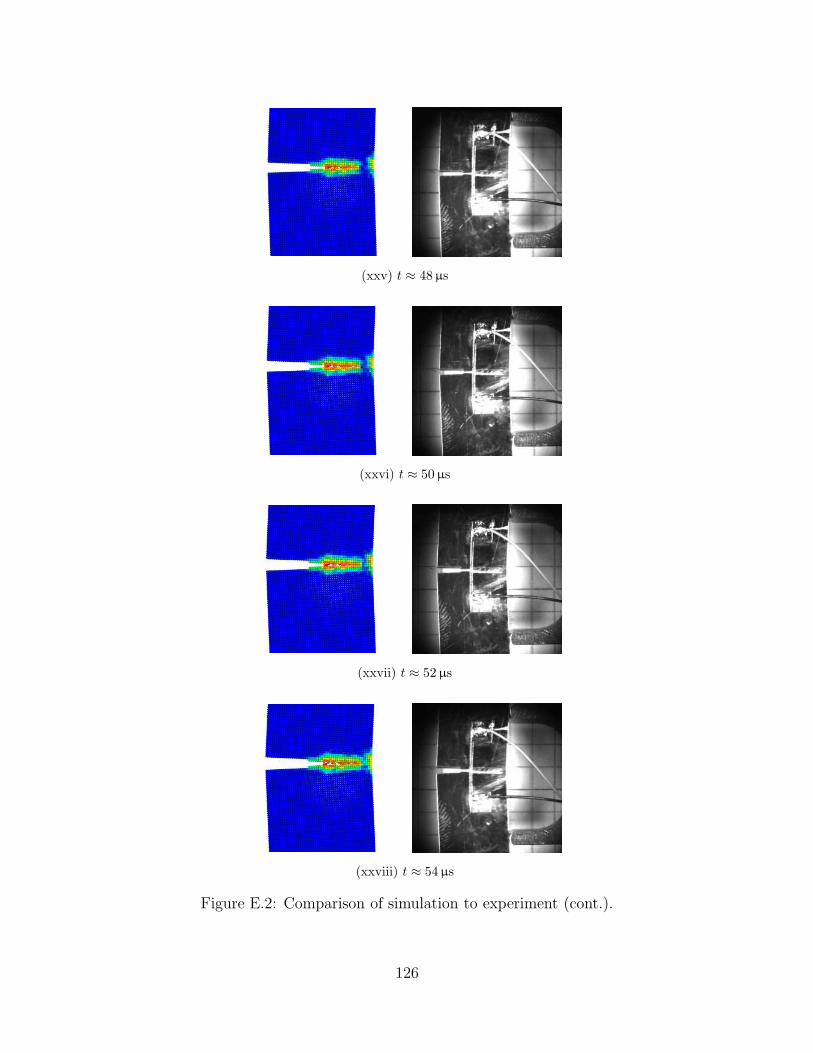
(xxv) t ≈ 48µs

(xxvi) t ≈ 50µs

(xxvii) t ≈ 52µs

(xxviii) t ≈ 54µs


126

(xxix) t ≈ 56µs

(xxx) t ≈ 58µs

(xxxi) t ≈ 60µs

(xxxii) t ≈ 62µs


127

F Additional Derivations of PeridynamicNotions

F.1 Definitions

Before we begin the derivation of the peridynamic equation of motion let us define a fewproperties that will prove useful. All definitions from the body of the dissertation hold unlessredefined here.

F.1.1 Vector-State Point Product

The point product of two states A ∈ Am+p and B ∈ Ap is a state in Am defined by:

(A · B)i1...im〈ξ〉 = Ai1...imj1...jp

〈ξ〉Bj1...jp〈ξ〉 ∀ξ ∈ H (F.1)

and similarly,(B · A)i1...im

〈ξ〉 = Bj1...jp〈ξ〉Aj1...jpi1...im〈ξ〉 ∀ξ ∈ H (F.2)

If the two states are of the same order then A · B = B ·A.

F.1.2 Vector-State Dot Product

The dot product of two states A and B is defined by:

A • B =

∫

H

(A · B) 〈ξ〉 dVξ (F.3)

Note that, once again, if the two states are of the same order then A •B = B • A.

F.1.3 Frechet Derivative

Let Ψ be a function of a state Ψ(·) : Am → Ln, where Ln is the set of all tensors of order n.Suppose there exists a state-valued function denoted ∇Ψ ∈ Am+n such that for any A ∈ Am

129

an any ∆A ∈ Am,

Ψ (A + ∆A) = Ψ (A) + ∇Ψ (A) • ∆A + O (|∆A|) (F.4)

where O (|∆A|) represents higher order terms of ∆A, then Ψ is said to be differentiable and∇Ψ is called the Frechet derivative of Ψ.

F.1.3.1 Example

Let Ψ (A) = 2A •A ∀A ∈ V

Ψ (A + ∆A) = 2 (A + ∆A) • (A + ∆A)

= 2A • A + 4A • ∆A + O (|∆A|)

hence ∇Ψ (A) = 4A.

F.2 Derivation of Peridynamic Equation of Motion

In order to derive the peridynamic equation of motion let us consider a closed, boundedperidynamic body B, similar to that shown in Figure 1.3a, with strain energy density givenby W (Y[x, t]) where Y[x, t] is the deformation state shown in Equation F.5,

Y[x, t]〈x′ − x〉 = (u[x′, t] + x′) − (u[x, t] + x)

= y[x′, t] − y[x, t] (F.5)

for all points x,x′ ∈ B, where u is the displacement and y is the deformation. Let b be theprescribed body force density field. The total potential energy functional for any deformationis then as follows:

Φy =

∫

B

(

W (Y[x, t]〈x′ − x〉) − b[x, t] · y[x, t])

dVx (F.6)

Let ∇W denote the Frechet derivative of W , and define the peridynamic force-vector stateas follows:

T[x, t]〈x′ − x〉 = ∇W (Y[x, t]〈x′ − x〉) (F.7)

By properties of the Frechet derivative, for any variation of the deformation δy, we have thefollowing:

δW (Y[x, t]〈x′ − x〉) = T[x, t]〈x′ − x〉 • δY[x, t]〈x′ − x〉 (F.8)

Substituting Equation F.8 into Equation F.5 and using the definition of a vector-state dotproduct we get the result shown in Equation F.9

δW (Y[x, t]〈x′ − x〉) =

∫

B

T[x, t]〈x′ − x〉 · (δy[x′, t] − δy[x, t]) dVx′ (F.9)

130

Now take the first variation of Φy to get the following:

δΦy =

∫

B

(

δW (Y[x, t]〈x′ − x〉) − b[x, t] · δy[x, t])

dVx (F.10)

Substituting Equation F.9 into Equation F.10 we have:

δΦy =

∫

B

(∫

B

(T[x, t]〈x′ − x〉 · (δy[x′, t] − δy[x, t])) dVx′ − b[x, t] · δy[x, t]

)

dVx (F.11)

a change of variables x′ ↔ x yields:

δΦy =

∫

B

(∫

B

(T[x′, t]〈x − x′〉 − T[x, t]〈x′ − x〉) · δy[x, t]dVx′ − b[x, t] · δy[x, t]

)

dVx

(F.12)or,

δΦy =

∫

B

(∫

B

(T[x′, t]〈x − x′〉 − T[x, t]〈x′ − x〉) dVx′ − b[x, t]

)

· δy[x, t]dVx (F.13)

For a deformation in which Φy is stationary by definition, δΦy = 0, using this and assumingan arbitrary δy we get the peridynamic equilibrium equation shown in Equation F.14.

∫

B

(T[x, t]〈x′ − x〉 − T[x′, t]〈x − x′〉) dVx′ + b[x, t] = 0 (F.14)

Using d’Alembert’s principle, replacing b[x, t] with b[x, t] − ρy[x, t] results in the peri-dynamic equation of motion,

ρy[x, t] =

∫

B

(T[x, t]〈x′ − x〉 −T[x′〈x − x′〉) dVx′ + b[x, t] (F.15)

F.3 Conversion of Stress Tensor to Force-Vector States

Derivation

Let us consider a hyperelastic material (in the sense of classical elasticity theory) with strainenergy density, Ω (F), which is a function of the deformation gradient, F. We wish to equateΩ (F) with peridynamic strain energy density, W (Y[x, t]) presented in Section F.2, i.e.,

W (Y[x, t]) = Ω (F[x, t]) (F.16)

Recall Equation 4.8 from Section 4.2 reproduced here as Equation F.17 which approximatesthe deformation gradient from the deformation state.

F[x, t] =

[∫

H

ω〈ξ〉 (Y〈ξ〉 ⊗ ξ) dVx′

]

K−1 (F.17)

131

We can use Equation F.17 to evaluate the Frechet derivative by considering an incrementalchange in Y,

F (Y + ∆Y) =

∫

H

ω〈ξ〉 (Y i〈ξ〉 + ∆Y i〈ξ〉) ξpK−1pj dVξ

= F (Y) +

∫

H

ω〈ξ〉∆Y i〈ξ〉ξpK−1pj dVξ

= F (Y) +

∫

H

ω〈ξ〉∆Y k〈ξ〉δikξpK−1pj dVξ

= F (Y) +(

δikωK−1pj xp

)

• ∆Y k (from Equation F.3) (F.18)

where, δik is the Kronecker delta having the properties:

δik =

1 i = k

0 otherwise(F.19)

Now using the definition of the Frechet derivative we can, by inspection, see the following:

∇Fijk (Y) = δikωK−1pj xp (F.20)

Now let us compute the incremental change in W due to and incremental change in Ystarting from Equation F.16 we have the following:

∆W =∂Ω

∂Fij∆Fij (F.21)

If we rearrange Equation F.18 slightly we can see the following relationship:

∆Fij = F (∆Y) =(

δikωK−1pj xp

)

• ∆Y k (F.22)

Substituting Equation F.20 into Equation F.22 and that result into Equation F.21 yieldsEquation F.23.

∆W =∂Ω

∂Fij∇Fijk • ∆Y k (F.23)

Recall that the first Piola-Kirchhoff stress, σ, is related to the strain energy density throughthe tensor gradient,

σij (F) =∂Ω

∂Fij

(F) (F.24)

Substitute Equation F.24 into Equation F.23 to get the following:

∆W = σij∇Fijk • ∆Y k (F.25)

=(

σijδikωK−1pj xp

)

• ∆Y k (F.26)

=(

σkjωK−1pj xp

)

• ∆Y k (F.27)

Finally, by comparing Equation F.27 with Equation F.7 and recalling that K is a symmetrictensor we can see by inspection,

T i = σijωK−1jp xp (F.28)

or equivalently,T〈ξ〉 = ω〈ξ〉σ K−1 ξ (F.29)

Which is the same as Equation 4.21.

132

G Hole in a Plate Problem

Before implementing and validating the viscoplasticity model as reported in Chapter 4 apurely elastic model was validated first. The elastic (Hooke’s law) constitutive model shownin Equation G.1,

τij = 3K(

1

3εkkδij

)

+ 2µ

(

εij −1

3εkkδij

)

(G.1)

where, K is the material bulk modulus, µ is the material shear modulus, τ and ε representtensor components of stress and strain, respectively, and δij is the Kronecker delta. Thismodel was implemented into the peridynamic code Emu in a fashion identical to that de-scribed in Chapter 4 for the viscoplastic model (i.e., through the conversion of a stress tensorinto a force-vector state description).

In order to validate our elastic constitutive model we will consider the classic problemof a small hole of radius, a, in an infinite plate, subject to a far field uniaxial tension, Sillustrated in Figure G.1. This problem has an exact solution of the field equations. The

S Sa

rθ

Figure G.1: Illustration of infinite plate with small hole.

133

components of stress in polar coordinates are shown in Equation G.2 through Equation G.4.

τrr[r, θ, S] =S

2

(

1 − a2

r2

)

+S

2

(

3a4

r4− 4a4

r2+ 1

)

cos(2θ) (G.2)

τθθ[r, θ, S] =S

2

(

a2

r2+ 1

)

− S

2

(

3a4

r4+ 1

)

cos(2θ) (G.3)

τrθ[r, θ, S] =S

2

(

3a4

r4− 2a2

r2− 1

)

cos(2θ) (G.4)

Obviously, there is no way to numerically simulate an infinite plate, but we can approachthe solution if we make the plate size many times the diameter of hole. In this case the platewas made to be 10 times, in length and width, the diameter of the hole. The peridynamicmodel does not allow use to apply a far field stress as a boundary condition; therefore, alittle creativity was required in order extract the information needed to make a meaningfulcomparison to the exact solution. A constant velocity was applied to a volume of nodesalong two edges of the plate in opposite directions. The resulting stress in the plate wasthen normalized by the stress recorded in those nodes that the velocity was applied to. Twointeresting comparisons we can make to the exact solution are shown in Figure G.2 andFigure G.3. If we evaluate Equation G.3 at r = a, θ = π/2 with an applied far field stressS = 1 we get the result shown in Equation G.5.

τθθ [a, π/2, 1] = 3 (G.5)

Comparing the result from Equation G.5 with the location of evaluation in Figure G.2 wecan see very good correlation between the peridynamic simulation and the exact solution.We can also evaluate Equation G.4 at r = a, θ = 0, π/2, π, 2π with an applied far fieldstress S = 1, the result is shown in Equation G.6:

τθθ [a, 0, π/2, π, 2π, 1] = 0 (G.6)

Comparing the result from Equation G.6 to Figure G.3 at each of the evaluation locationswe can see that the numerical simulation compares well with the exact solution.

One final comparison was done by looking at the τθθ stress along the line θ = 0, r.The Emu simulations where run at two different node densities labeled course and finein Figure G.4. The course node density represented 20 nodes across the diameter of thehole and the fine node density corresponded to 40 nodes across the diameter of the hole.The simulations were run in order to see if the peridynamic stress measurements converged.Figure G.4 shows no difference in the values of stress between the two simulations. They bothcompare well with the exact solution as well. Small differences between the exact solutionand the simulations are to be expected because the exact solution is for an infinite plate andthe simulations are clearly done on a finite plate. Overall these simulations validated theelastic peridynamic model and gave us the confidence to proceed with the implementationof the viscoplastic model.

134

Norm

alize

dStr

ess

-0.05

3.00

1.00

2.00

Figure G.2: Normalized Cauchy stress, τθθ.

Norm

alize

dStr

ess

-8.00

8.00

-4.00

0.00

4.00

Figure G.3: Normalized Cauchy stress, τrθ.

135

−0.2

0.15

0.5

0.85

1.2

0 0.225 0.45 0.675 0.9

Nor

mal

ized

Str

ess

Distance Along θ = 0, r Axis (m)

τθθ Emu (Course)τθθ Emu (Fine)

τθθ Exact Solution

Figure G.4: Normalized stress as a function of distance along θ = 0, r axis.

136

DISTRIBUTION:

1 MS 1160 Damon Burnett, 05431

1 MS 1160 Doug Dederman, 05431

1 MS 1160 James Dykes, 05431

1 MS 1160 Eric Klamerus, 05431

1 MS 1160 John Ludwigsen, 05431

1 MS 1160 Vincent Luk, 05431

1 MS 1160 Paul Taylor, 05431

1 MS 1160 Stewart Silling, 01435

1 MS 1160 David Littlewood, 01435

1 MS 1160 Michael Parks, 01414

1 MS 1160 Richard Lehoucq, 01414

1 MS 1160 Joseph Bishop, 01525

1 MS 1160 Paul Demmie, 05435

1 MS 1160 Brad Boyce, 01813

1 MS 0899 Technical Library, 9536 (electronic)

137

Dynamic Crack Initiation Toughness: Experiments and ... · Dynamic Crack Initiation Toughness:...

Documents

Transcript of Dynamic Crack Initiation Toughness: Experiments and ... · Dynamic Crack Initiation Toughness:...