Dynamic continuum pedestrian ow model with memory e ect · Dynamic continuum pedestrian ow model...
20
Dynamic continuum pedestrian flow model with memory effect Yinhua Xia * , S.C. Wong † , Chi-Wang Shu ‡ Abstract In this paper, we develop a macroscopic model for pedestrian flow using the dynamic continuum modeling approach. We consider a two-dimensional walking facility that is represented as a continuum within which pedestrians can move freely in any direction. A pedestrian chooses a route based on his or her memory of the shortest path to the desired destination when the facility is empty, and at the same time tries to avoid high densities. In this model, pedestrian flow is governed by a two-dimensional conservation law, and a general speed-flow-density relationship is considered. The model equation is solved numerically using the discontinuous Galerkin method, and a numerical example is employed to demonstrate both the model and the effectiveness of the numerical method. Key Words: Pedestrian flow, dynamic continuum modeling, conservation law, discon- tinuous Galerkin method. PACS number(s): 89.40.-Bb, 02.70Dh, 45.70.Vn 1 Introduction Many models of pedestrian traffic dynamics have been formulated recently [1]. These models can generally be classified into two categories: microscopic models and macroscopic mod- els. The former include the cellular automaton model [2, 3, 4, 5], the social force model * Division of Applied Mathematics, Brown University, Providence, RI 02912, USA. E-mail: [email protected]. † Department of Civil Engineering, The University of Hong Kong, Hong Kong, China. E-mail: [email protected]. ‡ Division of Applied Mathematics, Brown University, Providence, RI 02912, USA. E-mail: [email protected]. 1
Transcript of Dynamic continuum pedestrian ow model with memory e ect · Dynamic continuum pedestrian ow model...
Dynamic continuum pedestrian flow model with
memory effect
Yinhua Xia∗, S.C. Wong†, Chi-Wang Shu‡
Abstract
In this paper, we develop a macroscopic model for pedestrian flow using the dynamic
continuum modeling approach. We consider a two-dimensional walking facility that is
represented as a continuum within which pedestrians can move freely in any direction.
A pedestrian chooses a route based on his or her memory of the shortest path to the
desired destination when the facility is empty, and at the same time tries to avoid high
densities. In this model, pedestrian flow is governed by a two-dimensional conservation
law, and a general speed-flow-density relationship is considered. The model equation is
solved numerically using the discontinuous Galerkin method, and a numerical example
is employed to demonstrate both the model and the effectiveness of the numerical
method.
Key Words: Pedestrian flow, dynamic continuum modeling, conservation law, discon-
tinuous Galerkin method.
PACS number(s): 89.40.-Bb, 02.70Dh, 45.70.Vn
1 Introduction
Many models of pedestrian traffic dynamics have been formulated recently [1]. These models
can generally be classified into two categories: microscopic models and macroscopic mod-
els. The former include the cellular automaton model [2, 3, 4, 5], the social force model
∗Division of Applied Mathematics, Brown University, Providence, RI 02912, USA. E-mail:
[email protected].†Department of Civil Engineering, The University of Hong Kong, Hong Kong, China. E-mail:
[email protected].‡Division of Applied Mathematics, Brown University, Providence, RI 02912, USA. E-mail:
1
[6, 7, 8, 9], and the lattice gas model [10, 11, 12, 13], and are particularly well suited for use
with small crowds. Macroscopic models, in contrast, focus on the overall behavior of pedes-
trian flows, and are more applicable to investigations of extremely large crowds, especially
when examining aspects of motion in which individual differences are less important [14].
The two general types of models − microscopic and macroscopic models − can be seen as
complementing each other.
The continuum approach is widely used in the macroscopic modeling of traffic flow prob-
lems. The continuum modeling of transportation systems for steady-state user equilibrium
problems has been particularly well investigated [15, 16, 17, 18]. A systematic framework
for the dynamic macroscopic modeling of pedestrian flow problems was given in [19], but the
user equilibrium concept was not explicitly considered. To address this issue, Hoogendoorn
and his colleagues developed a predictive user equilibrium model, in which pedestrians were
assumed to have perfect information with which to make their route choice decisions over
time [20, 21, 22]. This modeling approach is useful for representing a more strategic level of
route choice decisions whereby pedestrians accumulate travel information from their daily
experiences or from some other source. However, in certain applications, pedestrians may not
have predictive information when they make a route choice decision [23]. Instead, they may
have to rely on instantaneous information and change their choice in a reactive manner when
walking through a facility (see [24] for the difference between predictive and reactive dynamic
user equilibrium principles). Huang et al. [25] recently revisited the dynamic macroscopic
model of pedestrian flow [19] in the context of the reactive user equilibrium principle. In
the model, pedestrians from a given location choose the path that minimizes the individ-
ual walking costs to their destination based on the instantaneous travel cost information
available to them at the time of making the decision.
In this paper, we also use the dynamic continuum approach to model pedestrian flow
macroscopically. In our model, pedestrian density is governed by a scalar two-dimensional
conservation law. The direction of the flow is determined by the route choice strategy, and the
magnitude of the flow is determined by the relationships among the macroscopic variables of
pedestrian speed, density, and flow. The route choice strategy in our model is different from
those used in the aforementioned models, and is based on the hypothesis that pedestrians seek
to minimize their estimated travel cost based on memory, but temper that behavior to avoid
high densities. The predictive user equilibrium model [20, 21, 22] requires that pedestrians
have perfect information over time for use in choosing their route, whereas the reactive user
equilibrium model [25] requires that they have instantaneous global information about the
entire domain based on which they choose an instantaneous route. The hypothesis on which
2
our model is based, in contrast, posits that pedestrians choose an instantaneous route based
on both the information stored in their memory and local instantaneous information. This
route choice strategy thus falls between the strategies of predictive and reactive route choice.
The main advantages of this model are that it does not require that pedestrians anticipate
changes in the operating conditions over time, especially when they are not familiar with
the likely responses of a crowd, and allows for circumstances in which the quality of the
instantaneous information may be degraded due to adverse environmental conditions such
as bad weather, insufficient lighting, and smoky conditions during escape from a fire.
To solve our model numerically, we adopt the discontinuous Galerkin (DG) method that
was employed in [26] to solve the reactive equilibrium pedestrian model [25]. We do not need
to solve the Eikonal equation at each time step in the numerical procedure, and thus avoid
the most time-consuming aspect of that procedure [26]. The DG method is a type of finite
element method that uses discontinuous, piecewise polynomials as the solution and the test
space. The first DG method was introduced in 1973 by Reed and Hill [27] in their frame-
work for a neutron transport problem that involved a time-independent linear hyperbolic
equation. Cockburn et al. first developed the method for hyperbolic conservation laws in a
series of papers [28, 29, 30, 31] in which they established a framework of solving nonlinear
time-dependent problems more easily. Their framework employs explicit, nonlinearly stable,
high-order Runge-Kutta time discretizations [32] and DG discretization in space with exact
or approximate Riemann solvers as the interface fluxes and total variation bounded (TVB)
nonlinear limiters to derive the non-oscillatory properties of strong shocks. The DG method
is well suited to complex geometries, as it allows them to be applied on unstructured grids.
It can also handle non-conforming elements by allowing the grids to have hanging nodes.
It is highly parallelizable, as the elements are discontinuous and the inter-communications
minimal. The DG method has found wide application in such diverse fields as aeroacoustics,
electro-magnetism, gas dynamics, granular flows, magneto-hydrodynamics, meteorology, the
modeling of shallow water, oceanography, oil recovery simulation, semiconductor device sim-
ulation, the transport of contaminants in porous media, turbomachinery, turbulent flows,
viscoelastic flows, and weather forecasting, among many others. For a detailed description
of this method, its implementation, and applications for conservation laws, we refer interested
readers to [33, 34, 35, 36, 37, 38, 39, 40, 41].
The reminder of the paper is organized as follows. In Section 2, we describe our model of
pedestrian flows and discuss the well-posedness of the linearized equation. In Section 3, we
present the numerical algorithm for the model. A numerical example is given in Section 4
to demonstrate the model and the effectiveness of the numerical method. Finally, we make
3
some concluding remarks in Section 5.
2 Model formulation
2.1 Model equations
We consider a two-dimensional walking facility that is represented as a continuum with a
domain Ω ∈ R2, inflow boundary Γi, outflow boundary Γo, and solid wall boundary Γw
(∂Ω = Γi ∪ Γo ∪ Γw). In domain Ω, we define ρ(x, t) as the pedestrian density and u(x, t)
as the pedestrian walking speed (we consider an isotropic case in which speed is a scalar
quality). Let f(x, t) = (f1(x, t), f2(x, t)) be the vector of the flow flux in the walking
facility. By default, f(x, t) = 0 on Γw. We further define c(x, ρ(x, t)) as the local cost per
unit distance of movement at time t, which depends on the instantaneous pedestrian density
and location x.
Similar to many physical systems, pedestrian flow is governed by a conservation law
ρt(x, t) + ∇ · f(x, t) = 0, ∀x ∈ Ω, (1)
where x = (x, y), ρt(x, t) = ∂ρ(x, t)/∂t and ∇ · f(x, t) = ∂f1(x, t)/∂x + ∂f2(x, t)/∂y.
We need to know the flow flux f(x, t) to establish the model, which comprises the mag-
nitude and direction of this flux.
To determine the magnitude of flux f(x, t), we need to know the relationships among the
macroscopic variables of pedestrian speed, density, and flow. We assume that the pedestrian
speed u(x, t) depends on the pedestrian density
u(x, t) = U(x, ρ(x, t)), (2)
where U(x, ρ) is the function of the pedestrian speed with respect to the density and location
dependence. The flow intensity is then equal to the product of the pedestrian speed and
density, that is,
‖f(x, t)‖ =√
f1(x, t)2 + f2(x, t)2 = u(x, t)ρ(x, t). (3)
To determine the direction of the flow flux, it is necessary to formulate a hypothesis about
the nature of pedestrian flow.
Hypothesis 1 Pedestrians seek to minimize their estimated travel cost based on memory,
but temper this behavior to avoid high densities.
4
We further define φ(x) as the minimum travel cost based on memory from location x ∈ Ω
to destination Γo, at which φ(x) = 0. We thus write
‖∇φ(x)‖ = cm(x), x ∈ Ω,
φ(x) = 0, x ∈ Γo,(4)
where cm(x) is the perceived local cost per unit distance of movement that was built up in
the memory of pedestrians from past experience. This memory effect also reflects the level
of familiarity of the pedestrians with the walking facility, which plays an important role in
the evacuation process in adverse environmental conditions. Equation (4) is the so-called
Eikonal equation.
From the Hypothesis 1, we have
f(x, t)// −∇φ(x) − ω∇c(x, ρ(x, t)) , (5)
where −∇φ represents the memory effect, ∇c represents the effect of avoiding high densities,
and ω is a positive constant that represents the psychological influence. The flow flux
direction is implicitly dependent on ρ(x, t). When ω → ∞, the model reduces to the reactive
user equilibrium model [25], in which the memory effect vanishes. In contrast, when ω → 0,
pedestrians make route choice decisions based solely on their memory, irrespective of the
operating conditions on the walking facility.
In the numerical procedure for the reactive user equilibrium model [25], the Eikonal
equation needs to be solved at each time step. With the route choice strategy employed in
our model, however, we need only solve the Eikonal equation (4) once at the beginning of
the analysis.
2.2 The well-posedness of the linearized equation
There is no general theory for nonlinear differential equations, and no global existence theory
even if we assume that all of the coefficients and data are smooth functions of the variables.
The only general results available are of a local character, and can be phrased in the following
way. Assume that we know the solution ρ for a particular set of data. We then linearize
the nonlinear equations around the known solution ρ. The well-posedness of the linearized
equation is often useful to determine whether the original equations are well posed.
We assume vector n(x, t) = −∇φ(x)−ω∇c(x, ρ(x, t)), which is parallel to the flow flux
f(x, t). Equation (1) can be rewritten as
ρ(x, t)t + ∇ · (f(x, ρ(x, t),∇ρ(x, t))) = 0, (6)
5
where f(x, ρ(x, t),∇ρ(x, t) = u(ρ(x, t))ρ(x, t) n
‖n‖. The change of variables
ρ(x, t) = ρ(x, t) + εv(x, t)
gives the linearized equation
vt + ∇ ·[
∂ρ(f(x, ρ,∇ρ))v + ∂ρx(f(x, ρ,∇ρ))vx + ∂ρy
(f(x, ρ,∇ρ))vy
]
= 0, (7)
which is a second-order partial differential equation. To show that equation (7) is a well-
posed problem, we need to check its ellipticity. For simplicity, we assume that the local cost
function depends only on the pedestrian density, that is, c(ρ(x, t)). Thus, we have
∂ρxn2 = 0, ∂ρy
n1 = 0, ∂ρxn1 = ∂ρy
n2 = −ωc′(ρ),
where n = (n1, n2). By substituting this equation into the linearized equation (7), we obtain
vt + first-order terms + (∂ρxn1)
|f(x, ρ,∇ρ)|
‖n‖3
(
n22vxx − 2n1n2vxy + n2
1vyy
)
= 0, (8)
which is an elliptic partial differential equation for c′(ρ) > 0 and is thus well posed.
The stability requirement that c′(ρ) > 0 is satisfied in most cases. For example, we can
choose the pedestrian speed function and cost function employed in [25, 26], which are given
by
U(ρ) = umax(1 −ρ
ρmax
), and (9)
c(ρ) =1
u(ρ)+ βg(ρ), (10)
where g(ρ) = ρ2 is the discomfort function, ρmax is the jam density, umax is the free-flow
speed, and β is the coefficient that reflects the sensitivity of pedestrians to the comfort level
in their route choice decisions. We now have c′(ρ) > 0 when ρ ∈ (0, ρmax), which satisfies
the well-posed condition of the linearized equation (7).
We find that the effect of avoiding high densities is the source of the ellipticity in this
equation (7), and that this effect prevents the density from outstripping the jam density,
which can be explained as follows. When ρ → ρmax, we have c′(ρ) → +∞ and then n
‖n‖≈
∇ρ
‖∇ρ‖. In the peak domain Ωp ∈ Ω, where ρ → ρmax, ∇ρ · ν ≤ 0, and ν is the outer normal of
domain Ωp, equation (1) can be approximated by
ρ(x, t)t + ∇ ·
(
u(ρ(x, t))ρ(x, t)∇ρ
‖∇ρ‖
)
= 0, x ∈ Ωp. (11)
6
If we multiply equation (11) by the density ρ and integrate it over the domain Ωp, then we
have
d
dt
∫
Ωp
ρ2(x, t)dx ≤ 0,
which verifies that the effect of avoiding high densities prevents the density from outstripping
the jam density. This property is also verified in the numerical test presented in Section 4.
3 Numerical algorithm
Equation (1), which governs the pedestrian flow, is a scalar two-dimensional conservation
law. There has been considerable developments in the algorithms for this type of equation.
In [26], we developed a discontinuous Galerkin (DG) method on triangular meshes to solve
the reactive dynamic user equilibrium model for pedestrian flows. That model required the
Eikonal equation to be solved by the fast sweeping method at each time level. Here, we also
adopt the discontinuous Galerkin method developed in [26] to solve the conservation law,
but need only solve the Eikonal equation (4) at the beginning of the analysis. We therefore
do not address the fast sweeping method on triangular meshes for equation (4) here, and
instead refer interested readers to [26, 42] for details.
We first briefly describe the discontinuous Galerkin method for equation (1). Let Th
denote a tessellation of Ω with shape-regular elements K. Let Γ denote the union of the
boundary faces of elements K ∈ Th, that is, Γ = ∪K∈Th∂K and Γ0 = Γ\∂Ω. We define the
finite element space V kh as
V kh ≡
v ∈ L2(Ω) : v|K ∈ P k(K), ∀K ∈ Th
, (12)
where P k(K) denotes the space of the polynomial in K of the degree at most k. Note that
the functions in V kh are allowed to have discontinuities across the element interfaces.
First, we multiply (1) by the test function vh in V kh , integrate the result over the element
K of triangulation Th, and replace the exact solution ρ with its approximation, ρh ∈ V kh , as
follows.
d
dt
∫
K
ρh(x, t)vh(x)dx +
∫
K
∇ · f(x, t)vh(x)dx = 0, ∀vh ∈ V kh . (13)
Integrating by parts, we formally obtain
d
dt
∫
K
ρh(x, t)vh(x)dx +∑
e∈∂K
∫
e
f(x, t) · ne,Kvh(x)ds
−
∫
K
f(x, t) · ∇vh(x)dx = 0, ∀vh ∈ V kh ,
7
where ne,K is the outward unit normal to edge e. Note that f(x, t)·ne,K has no precise mean-
ing, because ρh is discontinuous at x ∈ e ∈ ∂K. Let ρint(K)h denote the value of ρh evaluated
from inside element K and ρext(K)h the value of ρh evaluated from outside element K (inside
the neighboring element). We replace f(x, t) ·ne,K with he,K(ρint(K)h (x, t), ρ
ext(K)h (x, t), x, t),
which is any consistent two-point monotone Lipschitz flux that is consistent with f · ne,K.
Here, we choose the local Lax-Friedrichs flux:
he,K(a, b, x, t) =1
2[F (a, x, t) · ne,K + F (b, x, t) · ne,K − α(b − a)],
α = maxmin(a,b)≤ρ≤max(a,b)
|U(ρ, x, t)|,
where F (ρ, x, t) = −U(ρ, x, t)ρ(x, t) n
‖n‖. We then replace the integrals according to the
following quadrature rules.
∫
e
f(x, t) · ne,Kvh(x)ds ≈
L∑
l=1
ωlhe,K(ρint(K)h (xel, t), ρ
ext(K)h (xel, t), xel, t)vh(xel)|e|,
∫
K
f(x, t) · ∇vh(x, t)dxdy ≈M
∑
j=1
κjF (ρh(xKj, t), xKj, t) · ∇vh(xKj, t)|K|,
where xel and ωl are the quadrature points and weights on edge e, and xKj and κj are those
in triangle K. Finally, for each element K ∈ Th, we obtain the following semi-discrete weak
formulation.
d
dt
∫
K
ρh(x, t)vh(x)dxdy
+∑
e∈∂K
L∑
l=1
ωlhe,K(ρint(K)h (xel, t), ρ
ext(K)h (xel, t), xel, t))vh(xel)|e|
−
M∑
j=1
κjF (ρh(xKj, t), xKj, t) · ∇vh(xKj, t)|K| = 0, ∀vh ∈ V kh . (14)
The description of the numerical boundary conditions on ∂Ω is given in the next section.
The semi-discrete equation (14) can be rewritten in ordinary differential equation (ODE)
form as
d
dtρh = Lh(ρh), (15)
where operator Lh is the spatial DG discrete approximation of −∇ · f . We then use total
variation diminishing (TVD) Runge-Kutta methods [32, 43] to solve equation (15). Starting
from density ρn at time level tn, to obtain density ρn+1 at time level tn+1 (:= tn + ∆tn), the
8
second-order TVD Runge-Kutta method is given by
ρ(1)h = ρn
h + 4tnLh(ρnh), (16)
ρn+1h =
1
2ρn
h +1
2ρ
(1)h +
1
24tnLh(ρ
(1)h ) (17)
and the third-order TVD Runge-Kutta method by
ρ(1)h = ρn
h + 4tnLh(ρnh), (18)
ρ(2)h =
3
4ρn
h +1
4ρ
(1)h +
1
44tnLh(ρ
(1)h ), (19)
ρn+1h =
1
3ρn
h +2
3ρ
(2)h +
2
34tnLh(ϕ
(2)). (20)
The time step ∆tn = α hUmax
, where h is the minimum of the element diameters in Th and
Umax is the maximum pedestrian walking speed. The constant α is dependent on the degree
of the polynomial in the DG method and on the order of the Runge-Kutta method [37].
4 Numerical tests
Consider a railway platform with a circular obstruction in the middle, as shown in Fig. 1.
Pedestrians enter this platform from the left boundary Γi and leave from the right boundary
Γo. The platform is initially empty (ρ(x, 0)=0), and the boundary conditions on Γi are
f =
(t/12, 0), 0 ≤ t ≤ 60,
(10 − t/12, 0), 60 ≤ t ≤ 120,
(0, 0), t ≥ 120.
There is an outflow boundary condition on Γo, and the solid-wall boundary condition on Γw
is f(x, t) = 0. The pedestrian speed and the cost function are given by equations (9) and
(10), respectively, with umax = 2 and ρmax = 10. In this example, we assume that cm(x) is
the local cost when there are no pedestrians (i.e., ρ = 0). In other words, cm = 1/umax is a
constant.
In practice, we often solve nonlinear problems numerically with no knowledge of whether
the differential equations have any solution. If the numerical solution varies slowly with
respect to the mesh or the approximation space, then the original problem can be viewed
as a perturbation of that numerical solution. In the example employed here, we use the
third-order DG method coupled with the second-order fast sweeping method and the third-
order TVD Runge-Kutta method. As can be seen in Fig. 2, there are 3,417 elements
9
Γw
ΓoΓi
Γw
Obstruction
1 0 0 m
5 0 m
1 0 m
1 0 m
Figure 1: A railway platform with a circular obstruction. The center of the circle is at (50m,
20m) and its area is 400 m2.
in the triangulations of the platform with circular obstruction. We initially use the fast
sweeping method described in [26] to solve the Eikonal equation (4) and to obtain the
memory information φ and ∇φ. We then use the numerical algorithm described in Section
3 to evolve the governing equation (1). We also perform simulations using the first- and
second-order polynomial basis of the DG method, but the numerical results are comparable
to those of the third-order DG method.
X
Y
0 20 40 60 80 1000
10
20
30
40
50
Figure 2: Triangulations of the platform with circular obstruction.
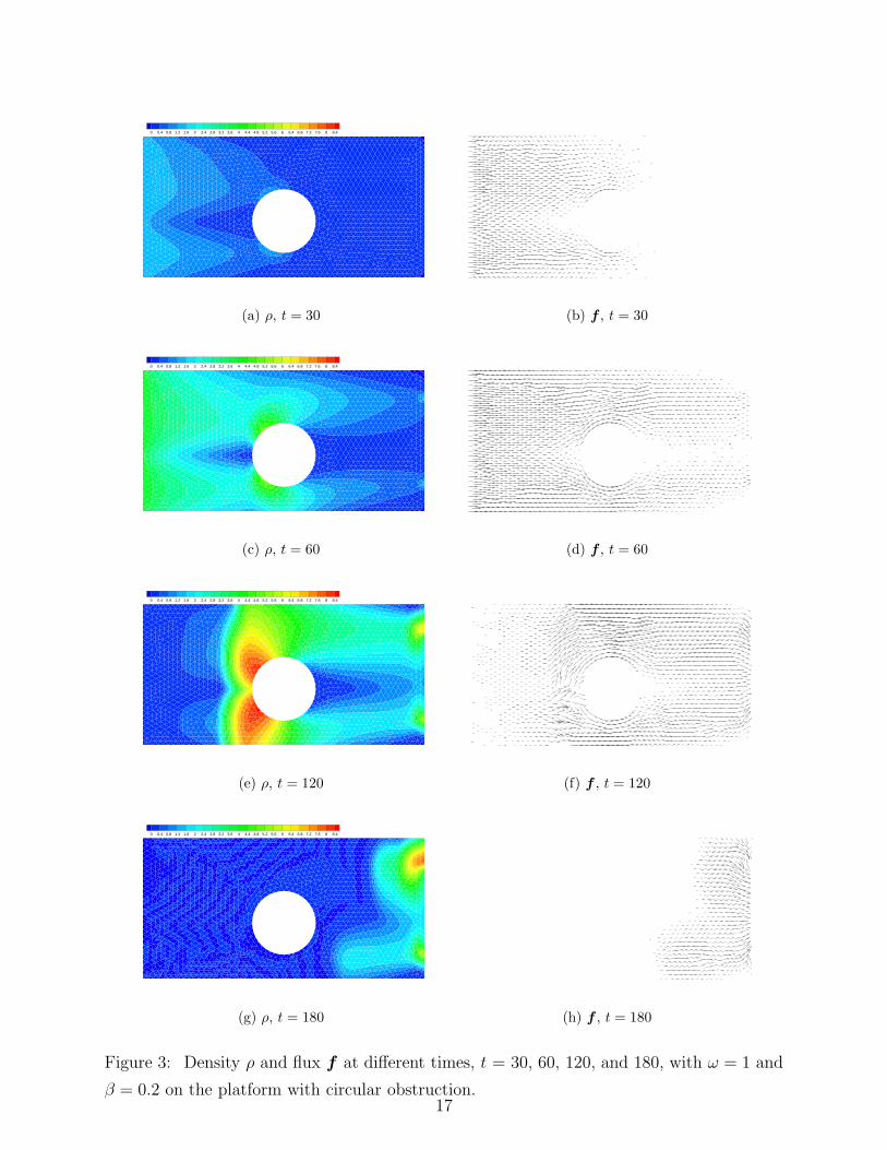
In Fig. 3, we plot the density ρ and flux f with ω = 1, β = 0.2 at times t = 30, 60, 120,
and 180, respectively, to show the movement pattern of pedestrians who walk around the
10
obstruction in the middle of the platform and head toward the exit. The density increases
steadily and reaches its maximum near time t = 120. As the time nears t = 240, the density
returns to zero. Around t = 120 (see Fig. 3 (e)), two shocks can clearly be seen in front of
the obstruction due to the reduction in the width of the corridor. Such shocks are frequently
observed in walking facilities when large crowds of pedestrians queue up to walk through
a bottleneck with reduced capacity. Triangular vacuum regions are also observed in front
of (Fig. 3 (c)) and behind the obstruction (Fig. 3 (e)), which is consistent with the route
choice strategy. These phenomena can also be observed in the reactive equilibrium pedestrian
model [25, 26]. The shocks in the model with memory are stronger than those in the reactive
equilibrium model because of the memory effect whereby pedestrians are attracted to the
optimal route based on their memory despite it being congested. The vacuum regions in the
former model are also smaller than those in the latter for the same reason.
To further illustrate the route choice strategy, in Fig. 4 and Fig. 5 we plot the density ρ
and flux f along x = 30, y = 35, and x = 80 at time t = 120 with ω = 0, 0.5, 1.0, 2.0, 5.0,
and β = 0.2, respectively. In our linearized analysis, the effect of avoiding high densities is the
source of the ellipticity in the linearized equation. When psychological influence parameter
ω increases, both the density and the flux become smooth, which further demonstrates that
the memory effect produces stronger shocks.
In Fig. 6, we give the total travel time∫∫
Ωρ(x, t)dxdt with different ω and β. When
β is fixed, the total travel time is a convex function of ω. When ω increases, the total
travel time first decreases and then increases, which demonstrates the importance of the
memory effect during an evacuation. When the environmental conditions are significantly
degraded, the evacuation process depends solely on the memory of the pedestrians, which
increases the total evacuation time because pedestrians are attracted to the optimal routes
in their memory and fail to avoid crowds. This is particularly problematic for evacuation in
severe environments, such as smoky conditions during escape from a fire or a dark room with
insufficient lighting. However, for a crowd that is unfamiliar with the environment of the
walking facility, in which the memory effect is very low (i.e., with a large ω), the evacuation
time is also increased. Therefore, proper training and education to improve familiarization
with evacuation instructions are essential for pedestrian evacuation. This is particularly
important for inexperienced pedestrians who are unable to identify the quickest route and
tend to reactively switch to less crowded regions during evacuation (i.e., with a large β).
11
5 Conclusion
In this study, we develop a new dynamic continuum model for pedestrian flow in which
the route choice strategy is based on the hypothesis that pedestrians seek to minimize their
perceived travel cost based on memory, but temper this behavior to avoid high densities. The
main advantages of the model are that it does not require that pedestrians anticipate changes
in the operating conditions over time, especially when they are not familiar with the likely
responses of a crowd, and allows for circumstances in which the quality of the instantaneous
information available may be degraded due to adverse environmental conditions such as
bad weather, insufficient lighting, and smoky conditions. We provide an analytical study to
describe the well-posedness of the problem, which demonstrates the existence of a solution
and the mathematical validity of the developed model.
The discontinuous Galerkin method is employed to solve the model. In contrast to that in
[19, 25], the present method does not require the Eikonal equation to be solved numerically
at each time step, which is the most time consuming aspect of the numerical procedure [26].
A numerical test is performed to demonstrate both the model and the effectiveness of the
numerical method. The results demonstrate the important role of the memory effect in the
pedestrian evacuation process. This model will serve as a useful tool in the planning and
design of walking facilities.
In this paper, we consider only a single commodity of pedestrian flow. A multi-commodity
pedestrian model will be developed in future research. The model presented in this paper
can be viewed as falling between the predictive and reactive models. It would be interesting
to construct a systematic framework that explains all of these route choice strategies.
6 Acknowledgments
The work described in this paper was supported by a grant from the Research Grants Council
of the Hong Kong Special Administrative Region of China (Project No. HKU 7183/06E),
and by ARO grant W911NF-08-1-0520 and NSF grant DMS-0809086.
References
[1] D. Helbing, Traffic and related self-driven many-particle systems, Reviews of Modern
Physics 73, 1067-1141 (2001).
12
[2] V.J. Blue and J.L. Adler, Cellular automata microsimulation for modeling bi-directional
pedestrian walkways, Transportation Research Part B 35, 293-312 (2001).
[3] C. Burstedde, K. Klauck, A. Schadschneider and J. Zittartz, Simulation of pedestrian
dynamics using a two-dimensional cellular automaton, Physica A 295, 507-525 (2001).
[4] A. Kirchner and A. Schadschneider, Simulation of evacuation processes using a bionics-
inspired cellular automaton model for pedestrian dynamics, Physica A 312, 260-276
(2002).
[5] W.G. Weng, T. Chen, H.Y. Yuan, W.C. Fan, Cellular automaton simulation of pedes-
trian counter flow with different walk velocities, Physical Review E 74, 036102 (2006).
[6] D. Helbing and P. Molnar, Social force model for pedestrian dynamics, Physical Review
E 51, 4282-4286 (1995).
[7] D. Helbing, I.J. Farkas and T. Vicsek, Simulating dynamical features of escape panic,
Nature 407, 487-490 (2000).
[8] D.R. Parisi and C.O. Dorso, Microscopic dynamics of pedestrian evacuation, Physica A
354, 606-618 (2005).
[9] T.I. Lakoba, D.J. Kaup and N.M. Finkelstein, Modifications of the Helbing-Molnar-
Farkas-Vicsek social force model for pedestrian evolution, Simulation 81, 339-352
(2005).
[10] M. Muramatsu, T. Irie and T. Nagatani, Jamming transition in pedestrian counter flow,
Physica A, 267, 487-498 (1999).
[11] M. Muramatsu and T. Nagatani, Jamming transition in pedestrian traffic at a crossing
with open boundaries, Physica A, 286, 377-390 (2000).
[12] D. Helbing, M. Isobe, T. Nagatani and K. Takimoto K, Lattice gas simulation of ex-
perimentally studied evacuation dynamics, Physical Review E, 67, 067101 (2003).
[13] R.Y. Guo and H.J. Huang, A mobile lattice gas model for simulating pedestrian evac-
uation, Physica A, 387, 580-586 (2008).
[14] G.D. Gaskell and R.J. Benewick, The Crowd in Contemporary Britian, Sage Publica-
tions Ltd, London, 1987.
13
[15] S.C. Wong, Multi-commodity traffic assignment by continuum approximation of network
flow with variable demand, Transportation Research Part B 32, 567-581 (1998).
[16] S.C. Wong, C.K. Lee and C.O. Tong, Finite element solution for the continuum traffic
equilibrium problems, International Journal for Numerical Methods in Engineering 43,
1253-1273 (1998).
[17] H.W. Ho, S.C. Wong and B.P.Y. Loo, Combined distribution and assignment model
for a continuum traffic equilibrium problem with multiple user classes, Transportation
Research Part B 40, 633-650 (2006).
[18] H.W. Ho and S.C. Wong, Housing allocation problem in a continuum transportation
system, Transportmetrica 3, 21-39 (2007).
[19] R.L. Hughes, A continuum theory for the flow of pedestrians, Transportation Research
Part B 36, 507-535 (2002).
[20] S.P. Hoogendoorn, P.H.L. Bovy and W. Daamen, Walking infrastructure design assess-
ment by continuous space dynamic assignment modeling, Journal of Advanced Trans-
portation 38, 69-92 (2003).
[21] S.P. Hoogendoorn and P.H.L. Bovy, Pedestrian route-choice and activity scheduling
theory and models, Transportation Research Part B 38, 169-190 (2004).
[22] S.P. Hoogendoorn and P.H.L. Bovy, Dynamic user-optimal assignment in continuous
time and space, Transportation Research Part B 38, 571-592 (2004).
[23] M. Asano, A. Sumalee, M. Kuwahara and S. Tanaka, Dynamic cell-transmission-based
pedestrian model with multidirectional flows and strategic route choices, Transportation
Research Record 2039, 42-49 (2007).
[24] C.O. Tong and S.C. Wong, A predictive dynamic traffic assignment model in con-
gested capacity-constrained road networks, Transportation Research Part B 34, 625-644
(2000).
[25] L. Huang, S.C. Wong, M. Zhang, C.-W. Shu and W.H.K. Lam, A reactive dynamic user
equilibrium model for pedestrian flows: A continuum modeling approach, Transporta-
tion Research Part B 43, 127-141 (2009).
14
[26] Y. Xia, S.C. Wong, M.P. Zhang, C.-W. Shu and W.H.K. Lam, An efficient discontin-
uous Galerkin method on triangular meshes for a pedestrian flow model, International
Journal for Numerical Methods in Engineering 76, 337-350 (2008).
[27] W.H. Reed and T.R. Hill, Triangular mesh method for the neutron transport equation,
Technical Report LA-UR-73-479, Los Alamos Scientific Laboratory, Los Alamos, NM,
1973.
[28] B. Cockburn and C.-W. Shu, TVB Runge-Kutta local projection discontinuous Galerkin
finite element method for conservation laws II: General framework, Mathematics of
Computation 52, 411-435 (1989).
[29] B. Cockburn, S.-Y. Lin and C.-W. Shu, TVB Runge-Kutta local projection discontinu-
ous Galerkin finite element method for conservation laws III: One dimensional systems,
Journal of Computational Physics 84, 90-113 (1989).
[30] B. Cockburn, S. Hou and C.-W. Shu, The Runge-Kutta local projection discontinuous
Galerkin finite element method for conservation laws IV: The multidimensional case,
Mathematics of Computation 54, 545-581 (1990).
[31] B. Cockburn and C.-W. Shu, The Runge-Kutta discontinuous Galerkin method for
conservation laws V: Multidimensional systems, Journal of Computational Physics 141,
199-224 (1998).
[32] C.-W. Shu and S. Osher, Efficient implementation of essentially non-oscillatory shock-
capturing schemes, Journal of Computational Physics, 77, 439-471 (1988).
[33] K.S. Bey, A. Patra and J.T. Oden, hp-version discontinuous Galerkin methods for hy-
perbolic conservation-laws − a parallel adaptive strategy, International Journal for Nu-
merical Methods in Engineering 38, 3889-3908 (1995).
[34] K.S. Bey and J.T. Oden, hp-version discontinuous Galerkin methods for hyperbolic
conservation laws, Computer Methods in Applied Mechanics and Engineering 133, 259-
286 (1996).
[35] B. Cockburn, Discontinuous Galerkin methods for convection-dominated problems, in
High-Order Methods for Computational Physics, T.J. Barth and H. Deconinck, editors,
Lecture Notes in Computational Science and Engineering, volume 9, Springer, 1999, pp.
69-224.
15
[36] B. Cockburn, G. Karniadakis and C.-W. Shu, The development of discontinuous
Galerkin methods, in Discontinuous Galerkin Methods: Theory, Computation and Ap-
plications, B. Cockburn, G. Karniadakis and C.-W. Shu, editors, Lecture Notes in Com-
putational Science and Engineering, volume 11, Springer, 2000, Part I: Overview, pp.
3-50.
[37] B. Cockburn and C.-W. Shu, Runge-Kutta discontinuous Galerkin methods for
convection-dominated problems, Journal of Scientific Computing 16, 173-261 (2001).
[38] J. Palaniappan, R.B. Haber and R.L. Jerrard, A spacetime discontinuous Galerkin
method for scalar conservation laws, Computer Methods in Applied Mechanics and En-
gineering 193, 3607-3631 (2004).
[39] J.F. Remacle, X.R. Li, M.S. Shephard and J.E. Flaherty, Anisotropic adaptive simula-
tion of transient flows using discontinuous Galerkin methods, International Journal for
Numerical Methods in Engineering 62, 899-923 (2005).
[40] F. Shakib, T.J.R. Hughes and Z. Johan, A new finite-element formulation for com-
putational fluid-dynamics: 10. The compressible Euler and Navier-Stokes equations,
Computer Methods in Applied Mechanics and Engineering 89, 141-219 (1991).
[41] A. Smolianski, O. Shipilova and H. Haario, A fast high-resolution algorithm for linear
convection problems: particle transport method, International Journal for Numerical
Methods in Engineering 60, 655-684 (2007).
[42] J. Qian, Y.-T. Zhang and H.-K. Zhao, Fast sweeping methods for Eikonal equations on
triangular meshes, SIAM Journal of Numerical Analysis 45, 83-107 (2007).
[43] S. Gottlieb and C.-W. Shu, Total variation diminishing Runge-Kutta schemes, Mathe-
matics of Computation 67, 73-85 (1998).
16
0 0.4 0.8 1.2 1.6 2 2.4 2.8 3.2 3.6 4 4.4 4.8 5.2 5.6 6 6.4 6.8 7.2 7.6 8 8.4
(a) ρ, t = 30 (b) f , t = 30
0 0.4 0.8 1.2 1.6 2 2.4 2.8 3.2 3.6 4 4.4 4.8 5.2 5.6 6 6.4 6.8 7.2 7.6 8 8.4
(c) ρ, t = 60 (d) f , t = 60
0 0.4 0.8 1.2 1.6 2 2.4 2.8 3.2 3.6 4 4.4 4.8 5.2 5.6 6 6.4 6.8 7.2 7.6 8 8.4
(e) ρ, t = 120 (f) f , t = 120
0 0.4 0.8 1.2 1.6 2 2.4 2.8 3.2 3.6 4 4.4 4.8 5.2 5.6 6 6.4 6.8 7.2 7.6 8 8.4
(g) ρ, t = 180 (h) f , t = 180
Figure 3: Density ρ and flux f at different times, t = 30, 60, 120, and 180, with ω = 1 and
β = 0.2 on the platform with circular obstruction.17
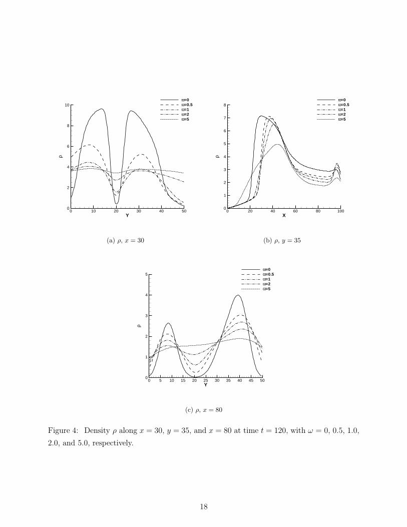
Y
ρ
0 10 20 30 40 500
2
4
6
8
10ω=0ω=0.5ω=1ω=2ω=5
(a) ρ, x = 30
Xρ
0 20 40 60 80 1000
1
2
3
4
5
6
7
8ω=0ω=0.5ω=1ω=2ω=5
(b) ρ, y = 35
Y
ρ
0 5 10 15 20 25 30 35 40 45 500
1
2
3
4
5ω=0ω=0.5ω=1ω=2ω=5
(c) ρ, x = 80
Figure 4: Density ρ along x = 30, y = 35, and x = 80 at time t = 120, with ω = 0, 0.5, 1.0,
2.0, and 5.0, respectively.
18
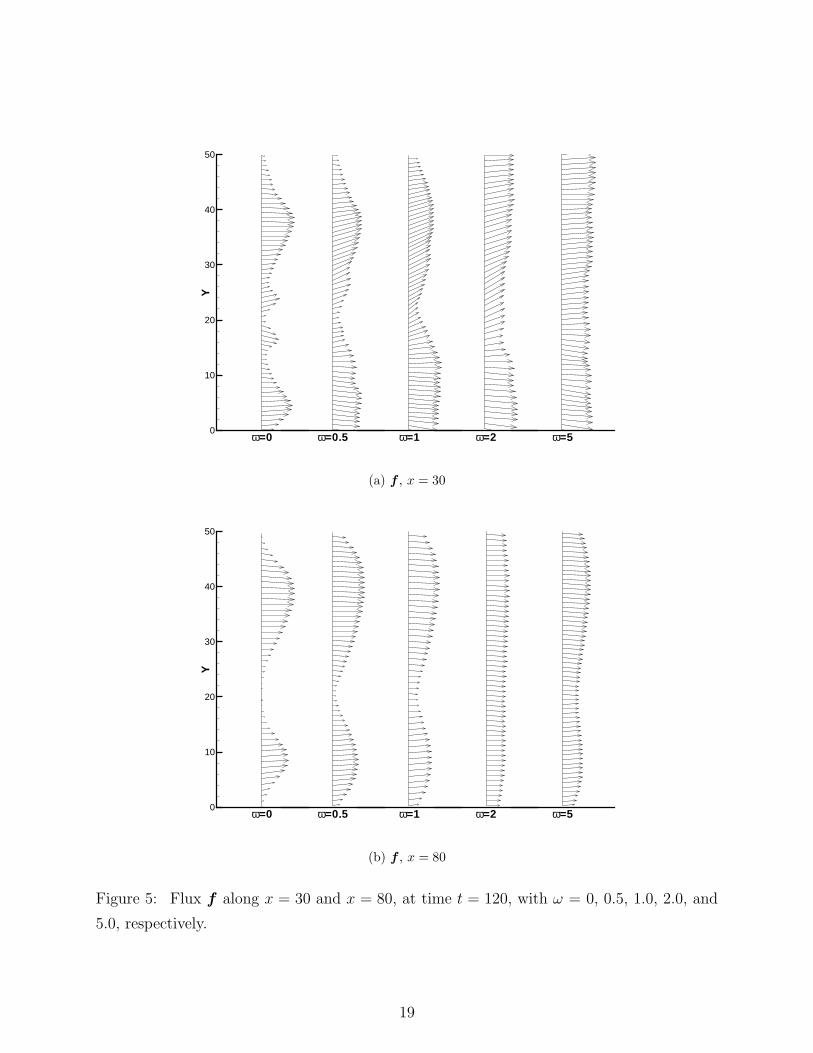
ω=0
Y
0
10
20
30
40
50
ω=2ω=1ω=0.5 ω=5
(a) f , x = 30
ω=0
Y
0
10
20
30
40
50
ω=0.5 ω=1 ω=2 ω=5
(b) f , x = 80
Figure 5: Flux f along x = 30 and x = 80, at time t = 120, with ω = 0, 0.5, 1.0, 2.0, and
5.0, respectively.
19
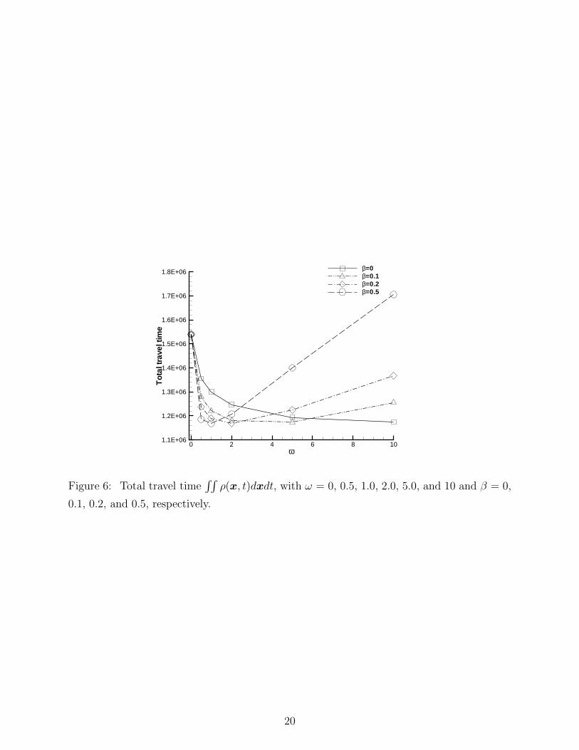
ω
To
talt
rave
ltim
e
0 2 4 6 8 101.1E+06
1.2E+06
1.3E+06
1.4E+06
1.5E+06
1.6E+06
1.7E+06
1.8E+06 β=0β=0.1β=0.2β=0.5
Figure 6: Total travel time∫∫
ρ(x, t)dxdt, with ω = 0, 0.5, 1.0, 2.0, 5.0, and 10 and β = 0,
0.1, 0.2, and 0.5, respectively.
20