Dynamic Competitive Analysisaseshadr/econ714/dca2.pdfDynamic Competitive Analysis Jeremy Greenwood...

Dynamic Competitive Analysis

Jeremy Greenwood

Spring 2001

Contents

1 Dynamic Programming 1

1.1 A Heuristic Approach . . . . . . . . . . . . . . . . . . . . . . . . . . . . 1

1.1.1 Neoclassical Growth Model . . . . . . . . . . . . . . . . . . . . 1

1.1.2 The Envelope Theorem . . . . . . . . . . . . . . . . . . . . . . . 5

1.2 A More Formal Analysis . . . . . . . . . . . . . . . . . . . . . . . . . . 6


1.2.2 Method of Successive Approximation . . . . . . . . . . . . . . . 7

1.2.3 Metric Space . . . . . . . . . . . . . . . . . . . . . . . . . . . . 8

1.2.4 The Contraction Mapping Theorem . . . . . . . . . . . . . . . . 14


1.2.6 Characterizing the Value Function . . . . . . . . . . . . . . . . . 19

1.2.7 Problems . . . . . . . . . . . . . . . . . . . . . . . . . . . . . . 24

2 Business Cycle Analysis 29

ii

CONTENTS – MANUSCRIPT

2.1 Introduction . . . . . . . . . . . . . . . . . . . . . . . . . . . . . . . . . 29

2.1.1 Real Business Cycle Models – Kydland and Prescott (1982) and

Long and Plosser (1983) . . . . . . . . . . . . . . . . . . . . . . 29

2.1.2 Keynesian Investment Multiplier Model . . . . . . . . . . . . . . 30

2.1.3 Current Analysis . . . . . . . . . . . . . . . . . . . . . . . . . . 31

2.2 The Economic Environment . . . . . . . . . . . . . . . . . . . . . . . . 32

2.2.1 The Representative Agent’s Optimization Problem . . . . . . . 34

2.2.2 Impact Effect of Investment Shocks . . . . . . . . . . . . . . . . 35

2.2.3 Dynamic Effects of Investment Shocks . . . . . . . . . . . . . . 38

2.3 Applied General Equilibrium Analysis . . . . . . . . . . . . . . . . . . . 38

2.3.1 Sample Economy and Simulation Technique . . . . . . . . . . . 38

2.3.2 Discrete State Space Dynamic Programming Problem . . . . . . 40

2.3.3 Construction of Markov Chain . . . . . . . . . . . . . . . . . . . 41

2.3.4 Calibration Procedure and Simulation Results . . . . . . . . . . 43

2.3.5 Results . . . . . . . . . . . . . . . . . . . . . . . . . . . . . . . . 45

2.4 Conclusions . . . . . . . . . . . . . . . . . . . . . . . . . . . . . . . . . 47

iii

CONTENTS – MANUSCRIPT

iv

Chapter 1

Dynamic Programming

1.1 A Heuristic Approach

1.1.1 Neoclassical Growth Model

Consider the following optimization problem

max{ct,kt+1}∞t=1

∞Xt=1

βt−1 U(ct)| {z }U :R+→R

subject to

ct + kt+1 = F (kt)| {z }F :R+→R+

.

The above problem can be reformulated as

max{kt+1}∞t=1

∞Xt=1

βt−1U(F (kt)− kt+1).

1

CHAPTER 1 – MANUSCRIPT

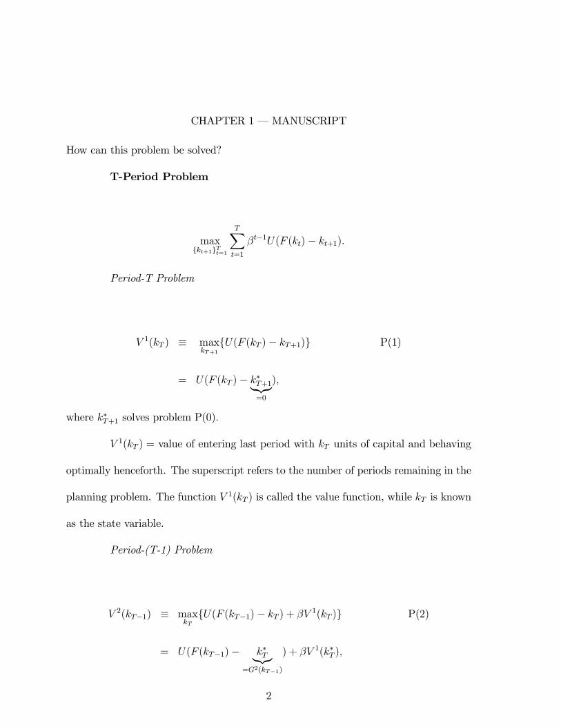
How can this problem be solved?

T-Period Problem

max{kt+1}Tt=1

TXt=1

βt−1U(F (kt)− kt+1).

Period-T Problem

V 1(kT ) ≡ maxkT+1

{U(F (kT )− kT+1)} P(1)

= U(F (kT )− k∗T+1|{z}=0

),

where k∗T+1 solves problem P(0).

V 1(kT ) = value of entering last period with kT units of capital and behaving

optimally henceforth. The superscript refers to the number of periods remaining in the

planning problem. The function V 1(kT ) is called the value function, while kT is known

as the state variable.

Period-(T-1) Problem

V 2(kT−1) ≡ maxkT{U(F (kT−1)− kT ) + βV 1(kT )} P(2)

= U(F (kT−1)− k∗T|{z}=G2(kT−1)

) + βV 1(k∗T ),

2


(a,b) •

• 0

b • • a

Φ

φ

RnE⊂Rn+m

U⊂RnW⊂Rm

Figure 1.1: Implicit Function Theorem

where k∗T = G2(kT−1) solves problem P(2). The function G2 is called the decision rule

or policy function. Here k∗T solves the first-order condition

−U1(F (kT−1)− k∗T ) + βV 11 (k∗T ) = 0. (1.1)

Question: What can be said about the functions G2 and V 2? Note that

first-order condition (1.1) defines an implicit function determining kT as a function of

kT−1. More generally in economics one often comes across equation systems of the form

Φ(x, y) = 0, where x ∈ Rn, y ∈ Rm, and Φ : Rn+m → Rn. Can a function φ be found

that solves for x in terms of y so that x = φ(y)?

Theorem 1 Implicit Function. Let Φ be a Cq mapping from an open set E ⊂ Rn+m

into Rn such that Φ(a, b) = 0 for some point (a, b) ∈ E. Suppose that the Jacobian

determinant |J | = |∂Φ(a,b)∂x

| 6= 0. Then there exits a neighborhood U ⊂ Rn around a and

a neighborhood W ⊂ Rm around b and a unique function φ : W → U such that,

3


1. a = φ(b),

2. φ is class Cqon W ,

3. for all y ∈W , (φ(y), y) ∈ E, and Φ(φ(y), y) = 0.

Now, applying the implicit function theorem to the first-order condition (1.1)

it is apparent that under the standard conditions k∗T = G2(kT−1) will be C1 function

which implies that V 2(kT−1) will be one too.

Period-t Problem

V T+1−t(kt) ≡ maxkt+1

{U(F (kt)− kt+1) + βV T−t−1(kt+1)} P(T+1-t)

= U(F (kt)− k∗t+1) + βV T−t−1(k∗T+1),

where k∗t+1 = GT+1−t(kt) solves problem P(T+1-t).

Observe that dynamic programming has effectively collapsed a single large

problem involving T + 1 − t choice variables into T + 1 − t smaller problems, each

involving one choice variable. To see this, solve out for V T−t(kt+1) in P(T+1-t) to get

V T+1−t(kt) ≡ maxkt+1

{U(F (kt)− kt+1) + βmaxkt+2

{U(F (kt+1)− kt+2) + βV T−t(kt+2)}}

= maxkt+1,kt+2

{U(F (kt)− kt+1) + βU(F (kt+1)− kt+2) + β2V T−t−1(kt+2)}.

Solving out recursively for V T−t(kt+2), V T−t−1(kt+3), ..., yields

4


max{kt+j+1}T−tj=0

T−tXj=0

βjU(F (kt+j)− kt+j+1).

Infinite Horizon Problem

As T →∞ one might expect that

V T+1−t(kt)→ V (kt)

and

GT+1−t(kt)→ G(kt).

This is true but it takes some effort to show it. Thus, the problem for the infinite

horizon will take the form:

V (kt) ≡ maxkt+1

{U(F (kt)− kt+1) + βV (kt+1)} P(∞)

= U(F (kt)− k∗t+1) + βV (k∗t+1)},

where k∗t+1 = G(kt).

1.1.2 The Envelope Theorem

Assumption: V is continuously differentiable.

How is the solution to problem P(∞) characterized? The f.o.c. is

−U1(F (kt)− kt+1) + βV1(kt+1) = 0 (1.2)

5


or

U1(F (kt)− kt+1) = βV1(kt+1). (1.3)

Problem: This equation involves the unknown function V . What should be

done?

Answer : Differentiate both sides of P(∞) with respect to kt to get

V1(kt) = U1(F (kt)− kt+1)F1(kt)− U1(F (kt − kt+1)∂kt+1∂kt

+ V1(kt+1)∂kt+1∂kt

= U1(F (kt)− kt+1)F1(kt) + [−U1(F (kt − kt+1) + V1(kt+1)]∂kt+1∂kt

= U1(F (kt)− kt+1)F1(kt),

since the term in brackets on the second line is zero by the first-order condition (1.2).

Updating this expression from period t to period t+ 1 gives

V1(kt+1) = U1(F (kt+1)− kt+2)F1(kt+1).

This allows equation (1.3) to be rewritten as

U1(F (kt)− kt+1) = βU1(F (kt+1)− kt+2)F1(kt+1).

1.2 A More Formal Analysis


Dynamic Programming Representation

6


V (k) ≡ maxk0{U(F (k)− k0) + βV (k0)} P(1)

The problem at hand is to get answers to the following questions:

1. Will V exist?

2. Is V unique?

3. Is V continuous?

4. Is V continuously differentiable?

5. Is V increasing in k?

6. Is V concave in k?

1.2.2 Method of Successive Approximation

Goal: To approximate the value function V by a sequence of successively better guesses,

denoted by V j at stage j

Procedure:

• Stage 0. Make an initial guess for V . Call it V 0.

• Stage 1. Construct a revised guess for V , denoted by V 1.

V 1(k) ≡ maxk0{U(F (k)− k0) + βV 0(k0)}

7


• Stage n+ 1. Compute V n+1 given V n, as follows

V n+1(k) ≡ maxk0{U(F (k)− k0) + βV n(k0)}. P(2)

This procedure can be represented much more compactly using operator no-

tation.

V n+1 = TV n.

The operator T is shorthand notation for the list of operations, described by P(2) that

are performed on the function V n to transform it into the new one V n+1. Often the

operator T maps some set of functions, say C, into itself. That is, T : C → C. The hope

is that as n gets large it transpires that V n → V , where V = TV .

1.2.3 Metric Space

Definition 2 A metric space is a set S, together with a metric ρ : S × S → R+, such

that for all x, y, z ∈ S (see Figure 2):

1. ρ(x, y) ≥ 0, with ρ(x, y) = 0 if and only if x = y,

2. ρ(x, y) = ρ(y, x),

3. ρ(x, z) ≤ ρ(x, y) + ρ(y, z).

Example 1

8


Vancouver, x

L.A., y

Rochester, z

ρ(y,z)

ρ(x,z)

ρ(x,y)

Figure 1.2: Distances Between Cities

-0.1 0.1 0.3 0.5 0.7 0.9 1.1

t

1.00

1.05

1.10

1.15

1.20

1.25

x(t)

and

y(t)

x(t)=1

y(t)=1+t-t2

ρ(x,y)=0.25

Figure 1.3: Uniform Metric

Space of continuous functions C : [a, b]→ R+. See Figure 3.

ρ(x, y) = maxt∈[a,b]

|x(t)− y(t)|.

Definition 3 A sequence {xn}∞n=0 in S converges to x ∈ S, if for each ε > 0 there

9


exists a Nε such that

ρ(xn, x) < ε, for all n ≥ Nε.

Definition 4 A sequence {xn}∞n=0 in S is a Cauchy sequence if for each ε > 0 there

exists a Nε such that

ρ(xm, xn) < ε, for all m,n ≥ Nε.

Remark 5 A Cauchy sequence in S may not converge to a point in S.

Example 2

Let S = (0, 1], ρ(x, y) = |x − y|, and {xn}∞n=0 = {1/n}∞n=0. Clearly,

xn → 0 /∈ (0, 1]. this sequence satisfies the Cauchy criteria, though,

for

ρ(xn, xm) = | 1m− 1

n| ≤ 1

m+1

n< ε, if m,n >

2

ε.

Definition 6 A metric space (S, ρ) is complete if every Cauchy sequence in S converges

to a point in S.

Theorem 7 Let X ⊆ Rl and C(X) be the set of bounded continuous functions V : X →

R with the uniform metric ρ(V,W ) = maxx∈X

|V −W |. Then C(X) is a complete metric

space.

10


Proof. : Let {V n}n be any Cauchy sequence in C(X). Now, for each x ∈ X the sequence

{V n(x)}n is Cauchy since

|V n(x)− V m(x)| ≤ supy∈X|V n(y)− V m(y)| = ρ(V n, V m).

By the completeness of the reals V n(x)→ V (x), as n→∞. Define the function V by

V (x) for each x ∈ X.

It will now be shown that ρ(V n, V )→ 0 as n→∞. Choose an ε > 0. Now,

|V n(x)− V (x)| ≤ |V n(x)− V m(x)|+ |V m(x)− V (x)|

≤ ρ(V n, V m)| {z }≤ε/2

+ |V m(x)− V (x)|| {z }≤ε/2

.

The first term on the left can be made smaller than ε/2 by the Cauchy criteria; that is,

there exists a Nε such that for all n,m ≥ Nε it transpires that ρ(V n, V m) ≤ ε/2. The

second term can be made smaller than ε/2 by the pointwise convergence of V m to V ;

that is, there exists aMε(x) such that for allm ≥Mε(x) it follows that |V m(x)−V (x)| ≤

ε/2. Observe that while Mε(x) depends on x, Nε does not. Also, note that for any

value of x such aMε(x) will always exist. Therefore, |V n(x)−V (x)| ≤ ε for all n ≥ Nε

independent of the value of x. It follows that ρ(V n, V ) ≤ ε, the desired result.

The last step is to show that V is a continuous function. To do this, pick an

ε > 0. Does there exist a δ ≥ 0 such that |V (x) − V (x0)| ≤ ε whenever ρ(x, x0) ≤ δ?

11


Note that

|V (x)− V (x0)| ≤ |V (x)− V n(x)|| {z }ε/3

+ |V n(x)− V n(x0)|| {z }ε/3

+ |V (x0)− V n(x0)|| {z } .ε/3

The first and third terms can be made arbitrarily small by the uniform convergence of

V n to V . The second term can be made to vanish by the fact that V n is a continuous

function; that is, by picking a δ small enough such that this term is less than ε/3.

Remark 8 Pointwise convergence of a sequence of continuous functions does not imply

that the limiting function is continuous.

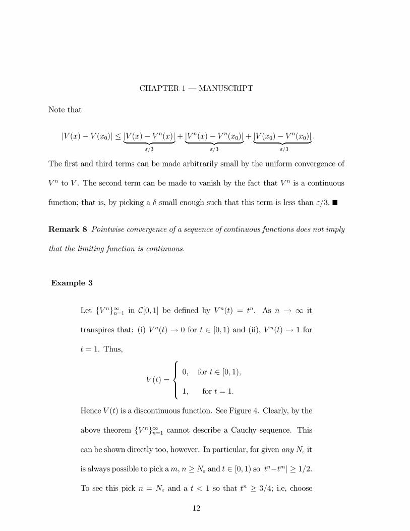
Example 3

Let {V n}∞n=1 in C[0, 1] be defined by V n(t) = tn. As n → ∞ it

transpires that: (i) V n(t) → 0 for t ∈ [0, 1) and (ii), V n(t) → 1 for

t = 1. Thus,

V (t) =

0, for t ∈ [0, 1),

1, for t = 1.

Hence V (t) is a discontinuous function. See Figure 4. Clearly, by the

above theorem {V n}∞n=1 cannot describe a Cauchy sequence. This

can be shown directly too, however. In particular, for given any Nε it

is always possible to pick am, n ≥Nε and t ∈ [0, 1) so |tn−tm| ≥ 1/2.

To see this pick n = Nε and a t < 1 so that tn ≥ 3/4; i.e, choose

12


-0.1 0.1 0.3 0.5 0.7 0.9 1.1

t

0.0

0.2

0.4

0.6

0.8

1.0

tnt

t10t2

t3

Figure 1.4: Pointwise Convergence to a Discontinuous Function

t ≥ (3/4)1/Nε. Next, pick m large enough such that tm < 1/4 or

m ≥ (ln 1/4)/(ln t). The desired results obtains.

Example 4

Consider the space of continuous functions C[−1, 1] with metric

ρ(x, y) =

Z 1

−1|x(t)− y(t)|dt.

Let {V n}∞n=1 in C[−1, 1] be defined by

V n(t) =

0, if − 1 ≤ t ≤ 0,

nt, if 0 < t < 1/n,

1, if 1/n ≤ t ≤ 1.

Show that {V n}∞n=1 is a Cauchy sequence. Deduce that the space of

continuous functions is not complete with this metric.

13


1.2.4 The Contraction Mapping Theorem

Definition 9 Let (S, ρ) be a metric space and T : S → S be function mapping S into

itself. T is a contraction mapping (with modulus β) if for β ∈ (0, 1),

ρ(Tx, Ty) ≤ βρ(x, y), for all x, y ∈ S.

Theorem 10 (Contraction Mapping Theorem or Banach Fixed Point Theorem). If

(S, ρ) is a complete metric space and T : S → S is a contraction mapping with modulus

β, then

1. T has exactly one fixed point V ∈ S such that V = TV,

2. for any V 0 ∈ S, ρ(T nV 0, V ) < βnρ(V 0, V ), n = 0, 1, 2... .

Proof. Define the sequence {V n}∞n=0 by

V n = TV n−1 = TT|{z}T2

V n−2 = T nV 0.

Now, by the contraction property of T

ρ(V 2, V 1) = ρ(TV 1, TV 0) ≤ βρ(V 1, V 0).

Hence,

ρ(V n+1, V n) = ρ(TV n, TV n−1) ≤ βρ(V n, V n−1) ≤ βnρ(V 1, V 0).

14


Therefore for any m > n

ρ(V m, V n) ≤ ρ(V m, V m−1) + ρ(V m−1, V m−2) + ...+ ρ(V n+1, V n)| {z }Triangle of Inequality

≤ (βm−1 + βm−2 + ...+ βn)ρ(V 1, V 0)

≤ βn

1− βρ(V1, V 0).

Therefore {V n}∞n=0 is a Cauchy sequence, since βn

1−β → 0 as n→∞. Since S is complete

V n → V .

To show that V = TV note that for all ε > 0 and V 0 ∈ S

ρ(V, TV ) ≤ ρ(V, T nV 0) + ρ(T nV 0, TV )

≤ ε

2+ε

2,

for large enough n since {V n}∞n=0 is a Cauchy sequence. Therefore, V = TV .

Finally suppose that another function W ∈ S satisfies W = TW . Then,

ρ(V,W ) = ρ(TV, TW ) ≤ βρ(V,W ),

a contradiction unless V = W .

ρ(T nV 0, V ) = ρ(TnV 0, TV ) ≤ βρ(T n−1V 0, V ) ≤ βnρ(V 0, V ).

15


Corollary 11 Let (S, ρ) be a complete metric space and let T : S → S be a contraction

mapping with fixed point V ∈ S. If S 0 is a closed subset of S and T (S 0) ⊆ S 0 then

V ∈ S 0. If in addition T (S0) ⊆ S 00 ⊆ S 0, then V ∈ S 00.

Proof. Choose V 0 ∈ S 0 and note that {T nV 0} is a sequence in S 0 converging to V . Since

S 0 is closed, it follows that V ∈ S0. If T (S0) ⊆ S00, it then follows that V = TV ∈ S00.

Theorem 12 (Blackwell’s Sufficiency Condition) Let X ⊆ Rl and B(X) be the space

of bounded functions V : X → R with the uniform metric. Let T : B(X) → B(X) be

an operator satisfying

1. (Monotonicity) V,W ∈ B(X). If V ≤ W [i.e., V (x) ≤ W (x) for all x] then

TV ≤ TW .

2. (Discounting) There exists some constant β ∈ (0, 1) such that T (V +a) ≤ TV+βa,

for all V ∈ B(X) and a ≥ 0. Then T is a contraction with modulus β.

Proof. For every V,W ∈ B(X), V ≤ W + ρ(V,W ). Thus, (1) and (2) imply

TV ≤ T (W + ρ(V,W ))| {z }Monotonicity

≤ TW + βρ(V,W )| {z }Discounting

.

Thus,

TV − TW ≤ βρ(V,W ).

16


By permuting the functions it is easy to show that

TW − TV ≤ βρ(V,W ).

Consequently,

|TV − TW | ≤ βρ(V,W ),

so that

ρ(TV, TW ) ≤ βρ(V,W ).

Therefore T is a contraction.


Consider the mapping

(TV )(k) = maxk0∈K

{U(F (k)− k0) + βV (k0)}, P(3)

where k, k0 ∈ K = {k1, k2, ..., kn}. Is T a contraction?

1. Monotonicity. Suppose V (k) ≤ W (k) for all k. Need to show that (TV )(k) ≤

(TW )(k).

(TV )(k) = {U(F (k)− k0∗) + βV (k0∗)},

17


where k0∗ maximizes P(3). Now, clearly

(TV )(k) ≤ {U(F (k)− k0∗) + βW (k0∗)}

≤ maxk0∈K

{U(F (k)− k0) + βW (k0)}

= (TW )(k).

2. Discounting.

T (V + a)(k) = maxk0∈K

{U(F (k)− k0) + β[V (k0) + a]}

= maxk0∈K

{U(F (k)− k0) + βV (k0)}+ βa

= (TV )(k) + βa.

1.1 Consider the following dynamic programming problem

V (ki, εr) = maxc,k0j∈K

{U(c) + βnXj=1

πrsV (k0j, εs)},

subject to

c+ i = F (ki),

and

k0j = (1− δ)ki + iεr. (1.4)

18


Let U be a bounded, strictly increasing, strictly concave, continuous function.

Suppose that 0 < β < 1. The bounded positive random variable ε follows a

m-point Markov process. In particular, ε is drawn from the discrete set E ≡

{ε1, ε2,..., εm} according to the probability distribution specified by πrs = Pr{ε0 =

εr|ε = εs}, where 0 ≤ πrs ≤ 1, andPm

j=1 πrs = 1. Furthermore, suppose that

k ∈ K = {k1, k2, ..., kn}.

1. Show that there exists a V that solves the above Bellman equation.

1.2.6 Characterizing the Value Function

What can be said about the function V ?

1. Is V continuous in k?

2. Is V strictly increasing in k?

3. Is V strictly concave in k?

4. Is V differentiable in k?.

Definition 13 A function V : X → R is strictly increasing if x > y implies V (x) >

V (y). A function V : X → R is nondecreasing (or increasing) if x > y implies

V (x) ≥ V (y).

19


Definition 14 A function V : X → R is strictly concave if

V (θx+ (1− θ)y) > θV (x) + (1− θ)V (y),

for all x, y ∈ X such that x 6= y and θ ∈ (0, 1). A function V : X → R is concave if

V (θx+(1− θ)y) ≥ θV (x)+ (1− θ)V (y),for all x, y ∈ X such that x 6= y and θ ∈ (0, 1).

1.1 Show that the space of increasing functions with the uniform metric is complete.

1.1 Show that the space of concave function with the uniform metric is complete.

Assumption: Let U and F be strictly increasing functions.

Assumption: Let U and F be strictly concave functions.

Theorem 15 The function V is both strictly increasing and strictly concave.

Proof. Consider again the mapping given by

(TV )(k) = maxk0{U(F (k)− k0) + βV (k0)}. P(3)

It will be shown that the operator T maps concave functions into strictly concave ones.

It also maps increasing functions into strictly increasing ones. Let V be a concave

function. Take two points k0 6= k1 and let kθ = θk0 + (1− θ)k1. Observe that F (kθ) >

θF (k0) + (1− θ)F (k1), since F is strictly concave. It needs to be shown that

(TV )(kθ) > θ(TV )(k0) + (1− θ)(TV )(k1).

20


To this end, define k0∗0 as the maximizer for (TV )(k0), k0∗1 as the maximizer for (TV )(k1),

and k0θ = θk0∗0 +(1−θ)k0∗1 . Note that k0θ is a feasible choice when k = kθ since k0∗0 ≤ F (k0)

and k0∗1 ≤ F (k1) while θF (k0) + (1− θ)F (k1) < F (kθ). Now,

(TV )(kθ) ≥ U(F (kθ)− k0θ) + βV (k0θ), (k0θ is nonoptimal)

> θ[U(F (k0)− k0∗0 ) + βV (k0∗0 )]

+(1− θ)[U(F (k1)− k0∗1 ) + βV (k0∗1 )], (by strict concavity )

> θ(TV )(k0) + (1− θ)(TV )(k1) (by definition).

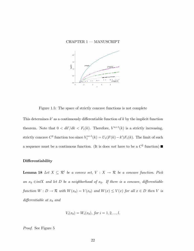
Remark 16 The space of strictly concave is not complete — see figure 4. Hence, to

finish the argument an appeal to the corollary of the contraction mapping theorem can

be made.

Theorem 17 The function V is continuous in k.

Proof. It will be shown that the operator described by P(3) maps strictly increasing,

strictly concave C2 functions into strictly increasing, strictly concave C2 functions.

Suppose that V n is a continuous, strictly increasing, strictly concave C2 function. The

the decision rule for k0 is determined from the first-order condition

U1(F (k)− k0) = βV n1 (k0).

21


0 2 4 6 8

t

0.0

0.5

1.0

1.5

2.0

log(

t)/n

y=log(t)/2

y=log(t)/10

y=log(t)

Figure 1.5: The space of strictly concave functions is not complete

This determines k0 as a continuously differentiable function of k by the implicit function

theorem. Note that 0 < dk0/dk < F1(k). Therefore, V n+1(k) is a strictly increasing,

strictly concave C2 function too since V n+11 (k) = U1(F (k)−k0)F1(k). The limit of such

a sequence must be a continuous function. (It is does not have to be a C2 function)

Differentiability

Lemma 18 Let X ⊆ Rl be a convex set, V : X → R be a concave function. Pick

an x0 ∈intX and let D be a neighborhood of x0. If there is a concave, differentiable

function W : D → R with W (x0) = V (x0) and W (x) ≤ V (x) for all x ∈ D then V is

differentiable at x0 and

Vi(x0) = Wi(x0), for i = 1, 2, ..., l.

Proof. See Figure 5

22


V

W

Figure 1.6: Differentiability of V

.

Theorem 19 (Benveniste and Scheinkman) Suppose that K is a convex set and that

U and F are strictly concave C1 functions. Let V : K → R in line with P(3) and

denote the decision rule associated with this problem by k0 = G(k). Pick k0 ∈intK and

assume that 0 < G(k0) < F (k0). Then V (k) is continuously differentiable at k0 with its

derivative given by

V1 = U1(F (k0)−G(k0))F1(k0).

Proof. Clearly, there exists some neighborhood D of k0 such that 0 < G(k0) < F (k)

for all k ∈ D. Define W on D by

W (k) = U(F (k)−G(k0)) + βV (G(k0)).

23


Now, W is concave and differentiable since U and F are. Furthermore, it follows that

W (k) ≤ maxk0{U(F (k)− k0) + βV (k0)} = V (k),

with this inequality holding strictly at k = k0. The results then follows immediately

from the above lemma.

1.2.7 Problems

1.1 Consider the problem described by

V (k) = maxx1,x2,...,xn

F (x1, x2, ...xn; k).

Let F be a C2 function. Presume that a maximum exists. Show that Vn+1(k) =

Fn+1(x1, x2, ...xn; k).

1.2 (Aiyagari, 1994) Consider the following dynamic programming problem

V (a, zi) = maxc,a0

{U(c) + βnXj=1

πijV (a0, zj)},

subject to

c+ a0 = zi + (1+ r)a,

and

a0 ≥ 0. (1.5)

24


Let U be a bounded, strictly increasing, strictly concave, continuously differen-

tiable function. Suppose that 0 < r < β < 1. The bounded positive random

variable z follows a n-point Markov process. In particular, z is drawn from the

discrete set Z ≡ {z1, z2,..., zn} according to the probability distribution specified

by πij = Pr{z0 = zj|z = zi}, where 0 ≤ πij ≤ 1, andPn

j=1 πij = 1.

1. Is the function V (a, z) continuously differentiable in a, for all a > 0, whenever

a0 > 0?

2. Is the function V (a, z) continuously differentiable in a, for all a > 0, when a0 = 0.

What is the issue here?

1.1 Capacity Choice (Harris, 1987): Here is a problem facing a monopolist. He faces

a demand curve each period given by

q = (1− p),

That is, if the price is p he can sell the quantity q. Production is costless but at

each period in time the monopolist faces a capacity constraint,

q ≤ c,

where c is the upper bound on his production. Capacity can be increased with a

one period time delay according to the cost function

(c0 − c)2,

25


where c0 ≥ c is the level of capacity that the monopolist chooses for next period.

The monopolist faces the time-invariant gross interest rate r.

1. Formulate the monopolist dynamic programming problem.

2. Prove that the solution is given by

V (c) =

α, for c ≥ 1/2,

δ + γc(1− c), for c ≤ 1/2,

where α and δ are some constants and

γ =2(1/r)− 1+p1+ 4(1/r)2

2(1/r),

and that the optimal policy is

c0 = c+

0, for c ≥ 1/2,

(1/r)γ(1/2− c)/(1+ γ/r), for c ≤ 1/2.

Also solve for α and δ.

1.1 The Replacement Problem: Imagine a lot with an age-j building on it. Denote

this amount of capital in this building by k(j). The per period profit from the

lot with an age-j building on it is k(j)α. Time flows continuously and the capital

stock depreciates with age according to the law of motion dk(j)/dj = δk(j). At

any point in time the owner is free to tear down his existing building and replace

it with a new one. The size of a new building is fixed at k. The interest rate is

always r.

26


1. Write out the dynamic programming problem facing the owner.

2. Does a continuous value function solving this problem exist?

3. Is it concave?

4. Is it differentiable?

1.1 Stochastic Goldmining (Bellman, 1957): Consider the problem of an entrepreneur

who owns two goldmines, Anaconda and Bonanza. Ananconda has x units of gold

in its bowls and Bonanza has y units, both measured in dollars. The entrepreneur

has a goldmining machine. The machine has the following properties: If it is used

in Ananconda in a period it will reap the fraction ra of the gold in the mine with

probability pa. With probability 1− pa the machine breaks down, mines no gold,

and can never be used again. Getting another machine is impractical. Likewise,

in any given period the machine can be used in Bonanza. There it may mine the

fraction rb of the gold with probability pb and break down with probability 1−pb.

The entrepreneur’s discount factor is β.

1. Let V (x, y) be the value of the mine. Write out the entrepreneur’s dynamic

programming problem

2. Prove that V is increasing in x and y.

27


3. Derive the locus of x and y combinations that yield the same payoff. What does

this say about how the value function can be written?

28

Chapter 2

Business Cycle Analysis

2.1 Introduction

2.1.1 Real Business Cycle Models – Kydland and Prescott

(1982) and Long and Plosser (1983)

• Cycles are generated via exogenous contemporaneous productivity shocks, λ.

• Dynamic optimizing behavior on the part of agents in the economy implies that

both consumption and investment react positively to supply shocks.

— Output, λF (k,l), increases.

— Consumption smoothing implies both current and future consumption should

rise. Additionally, the marginal product of capital, λF1(k,l), rises. This

29


should stimulate investment too.

• Labor productivity, λF2(k,l), is directly affected. Results in employment and

measures of labor productivity being procyclical.

• Capital accumulation provides a channel of persistence, even if the technology

shocks are white noise. Note investment is reacting to a supply shock.

• Conclusion: Productivity shocks from a neoclassical perspective can generate

the observable co-movements in macroeconomic variables and the persistence of

economic fluctuations.

• Criticism: Do such productivity shocks occur in reality – oil shocks and harvest

failures are two obvious examples but what is another one?

2.1.2 Keynesian Investment Multiplier Model

• “Animal spirits” cause investment fluctuations which generate the business cycle.

— Marginal efficiency of investment shifts exogenously affecting investment

demand and hence output, y = c + i, through the investment multiplier-

accelerator mechanism.

• Quintessential Case: Change in the expected future marginal productivity of

capital which does not affect the current production function. A positive shock

30


in the neoclassical growth model will cause:

— Investment to increase1.

— The real interest to rise to clear the goals market.

— Current consumption to fall and labor effort to rise (and hence leisure to

fall.)

— The marginal product of labor to fall.

2.1.3 Current Analysis

• Adopts the Keynesian view that direct shocks to investment are important for

business fluctuations

• Incorporates them into a neoclassical framework where the rate of capacity uti-

lization is endogenous. Involves Keynes’ (1936) notion of ‘user cost’ in production.

1If investment falls due to a strong income effect, then it is easy to show that consumption will rise

but labor effort will fall.

31


2.2 The Economic Environment

Production Function

y = F (kh, l)

Here h represents the rate of capacity utilization, or the rate at which capital is utilized.

2.1 Let F be a constant-returns-to-scale function. Show that F12 > 0 and F11F22 −

F 212 = 0.

Law of Motion for Capital

k0 = k[1− δ((h)] + i(1+ ε),

which implies

y0 = F ({k[1− δ(h)] + i(1+ ε)}h0, l0) .

Observe that ε is a shock to the marginal efficiency of investment spending. A extra

unit of investment spending today can purchase more units of new capital for tomorrow.

Now, 1/(1+ε) can be thought of as the relative price of new capital in terms of forgone

consumption. That is, it costs 1/(1 + ε) units of consumption to purchase an extra

32


unit of capital. There is a cost of utilizing your capital today in terms of increased

depreciation. Assume that δ1, δ2 > 0.

Technology Shock

ε0 ∼ Φ(ε0|ε).

Tastes

E[∞Xt=0

βtU(ct, lt)],

with

U(c, l) = U(c−G(l)).

Implication:

∂c

∂l

¯̄̄̄U

=U2(c, l)

U1(c, l)= G1(l).

– Intertemporal substitution effect on labor supply is eliminated. Early crit-

ics of real business cycle theory complained that the models required implausible high

elasticities of intertemporal substitution. This utility function implies that the supply

of labor in the current period can be written solely as a function of the current wage.

It is very convenient to use.

Resource Constraint

33


y = c+ i.

2.2.1 The Representative Agent’s Optimization Problem

V (k, ε) = maxc,k0,h,l

[U(c, l) + β

ZQ

V (k0, ε0)dΦ(ε0|ε) P(1)

s.t.

c = F (kh, l)− k0

(1+ ε)+k[1− δ(h)](1+ ε)| {z }

i/(1+ε)

.

The first-order conditions are:

U1(c−G(l))/(1+ ε) = βRQ

V1(k0,ε0)dΦ(ε0|ε)

= βRQ

U1(c0 −G(l0))[F1(k0h0,l0)h0 + (1−δ(h0))

1+ε0 ]dΦ(ε0|ε),

F1(kh, l) =δ1(h)

(1+ ε), (2.1)

F2(kh, l) = G1(l). (2.2)

Equation (2.1) is the efficiency condition regulating capacity utilization. The righthand

side portrays Keynes’ notion of the user cost of capital. Suppose capacity utilization

34


is increased by a unit. This results in old capital depreciating by δ1(h). But a unit of

capital can be replaced at a cost of 1/(1+ ε) in terms of current consumption. Keynes

said (1936, pg. 69-70)

“User cost constitutes the link between the present and the future. For in

deciding the scale of his production an entrepreneur has to exercise a choice

between using up his equipment now or preserving it to be used later on ...

”

2.1 Suppose that Φ satisfies the Feller property: that is, for any continuous function

H(·, ε0) it transpires that the function R H(·, ε0)dΦ(ε0|ε) is continuous too. Doesthe operator defined by P(1) map C2 functions into C2 functions?

2.1 Show that O(k, l, ε) = maxh{F (kh, l) + k[1 − δ(h)]} is concave in k and l. What

does this imply about the value function?

2.2.2 Impact Effect of Investment Shocks

Capacity Utilization and Labor Effort

Consider the impact of a transitory shift in the current technology factor ε. Observe

that (2.1) and (2.2) represent a system of two equations in two unknowns. Using

Crammer’s rule yields

dh

dε> 0,

35


dl

dε> 0.

2.1 Show that dh/dε > 0 and dl/dε > 0.

Interpretation

– An increase in ε reduces the cost of capacity utilization and induces a

higher h.

– Since F12 > 0 labor’s marginal product increases, resulting in a higher level

of employment.

Now,

dw

dε=dF2(kh, l)

dε=dF2(kh/l, 1)

dε> 0,

if and only if

d(kh/l)

dε> 0.

Hence,

dAPLdε

=d[F (kh,l)/l]

dε=d[F (kh/l,1)]

dε= F1(kh/l,1)

dkh/l

dε> 0.

2.1 Show that dw/dε > 0.

36


Capital accumulation

dk0

dε=

−U1(·)[U11(·) + (1+ ε)2β

RQ

V11(·0)dΦ]| {z }Substitution Effect

+ iU11(·)

[U11(·) + (1+ ε)2βRQ

V11(·0)dΦ]| {z }Income Effect

> 0.

Interpretation

Substitution Effect – New capital is more productive, so invest more.

Income Effect – More resources available for capital accumulation and con-

sumption, so invest more.

2.1 It was never established that V is continuously twice differentiable. Let k0 =

K 0(k, ε) represent the decision rule for investment. Is it continuous? Can you

argue by induction that it must be nondecreasing in ε?

Alternative Specification of the Capital Evolution Equation (Capital Augment-

ing Technological Change).

Let

k0 = k[1− δ(h)](1+ ε) + i(1+ ε)

⇒ c = F (kh,l)− k0

1+ ε+ [1− δ(h)]

The efficiency condition governing the use of capital services now becomes

37


F1(kh, l) = δ1(h).

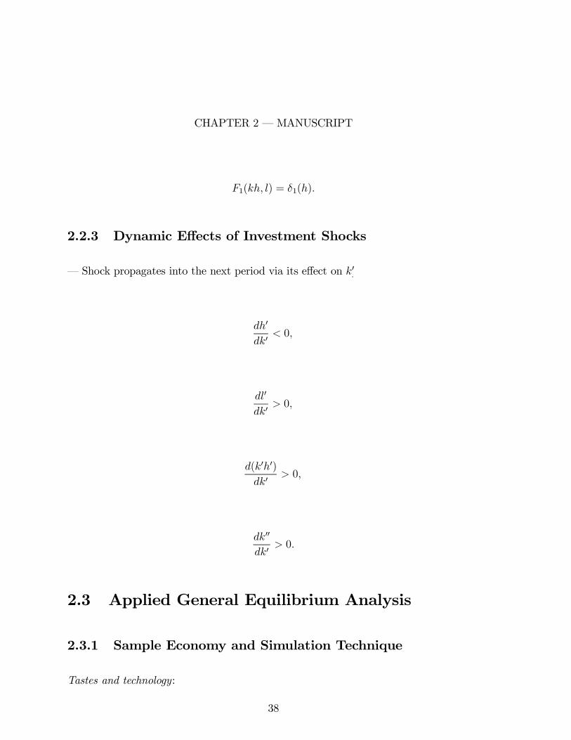
2.2.3 Dynamic Effects of Investment Shocks

– Shock propagates into the next period via its effect on k0.

dh0

dk0< 0,

dl0

dk0> 0,

d(k0h0)dk0

> 0,

dk00

dk0> 0.

2.3 Applied General Equilibrium Analysis

2.3.1 Sample Economy and Simulation Technique

Tastes and technology:

38


U(c, l) =1

1− γ [(c−l1+θ

1+ θ)1−γ] ,

F (kh, l) = A(kh)αl1−α,

δ(h) =1

ωhω.

Technology shock

ε ∈ E = {eξ1 − 1, eξ2 − 1},

with

Pr[ε0 = eξs − 1 | ε = eξr − 1] ≡ πrs for r, s = 1, 2.

Figure 1 illustrates the situation.

The long-run (or unconditional) distribution function for technology shock

Pr[ε = eξs − 1] ≡ φ∗s =πrs

π12 + π21for r, s = 1, 2 and r 6= s.

39


π11π11

π12

π2 2

π22

1

2

1

2π21

Figure 2.1: Two-Point Markov Chain

2.3.2 Discrete State Space Dynamic Programming Problem

Finally, the capital stock in each period is constrained to be an element of the finite

time-invariant set, K, where

K = {k1, ...., kn}.

Representative Agent’s Dynamic Programming Problem

V (ki, ξr) = maxc,k0∈K

{ 1

1− γ (c−∧l1+θ

1+ θ)1−γ + β

2Xs=1

πrsV (k0,ξs)},

subject to

40


c = A(ki,∧h)α

∧l1−α

− k0e−ξr + ki(1−∧hω

ω)e−ξr ,

where

∧h,∧l = argmax[A(ki,

∧h)α

∧l1−α

− ki(1−∧hω

ω)e−ξr −

∧l1+θ

1+ θ].

Observe that V : K×E → R is merely a list of 2n values, one for each (ki, ξr) ∈ K×E

Decision Rule for Capital

k0 = K 0(ki, ξr) ∈ K.

2.3.3 Construction of Markov Chain

Pr[k0 = kj | k = ki, ξ = ξr] =

1, for some j,

0, for the rest.

Trivially, then

nXj=1

Pr[k0 = kj | k = ki, ξ = ξr] = 1 for all (k, ξ) ∈ K× E .

Transition Probabilities

pir,js= Pr[k0 = kj, ξ0 = ξs|k = ki, ξ = ξr] = Pr[k0 = kj | k = ki, ξ = ξr]πrs.

41


P = [pir,js ]| {z }2n×2n

.

– Given some initial probability distribution ρ0|{z}1×2n

over the state.

– Next period’s probability distribution is given by

ρ1 = ρ0P,

or

(ρ111, ..., ρ1n2) = (ρ

011, ..., ρ

0n2)

p11,11 ... p11,n2

......

pn2,11 ... pn2,n2

.Stationary Distribution

ρ∗ = ρ∗P.

2.1 Is (I − P ) invertible? Suppose that the last equation of the system is replaced

with ρ∗n2 = 1−P

i6=n,r 6=2 ρ∗ir. Is there a direct way to compute ρ

∗.

– Computation of Moments

E[y] =2Xr=1

nXi=1

ρ∗irY (ki, ξr),

E[cy] =2Xr=1

nXi=1

ρ∗irC(ki, ξr)Y (ki,ξr),

E[y0y] =2Xs=1

nXj=1

2Xr=1

nXi=1

pir,jsρ∗irY (k

0i, ξ

0s)Y (ki, ξr).

42


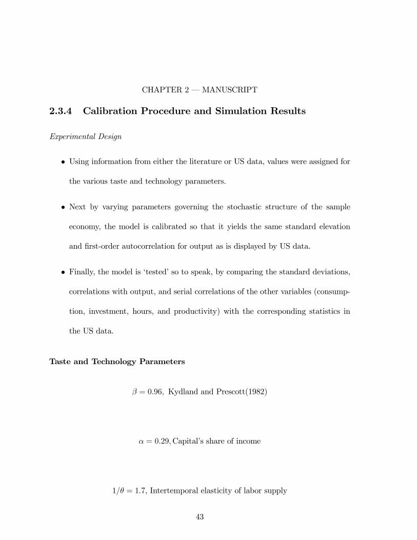
2.3.4 Calibration Procedure and Simulation Results

Experimental Design

• Using information from either the literature or US data, values were assigned for

the various taste and technology parameters.

• Next by varying parameters governing the stochastic structure of the sample

economy, the model is calibrated so that it yields the same standard elevation

and first-order autocorrelation for output as is displayed by US data.

• Finally, the model is ‘tested’ so to speak, by comparing the standard deviations,

correlations with output, and serial correlations of the other variables (consump-

tion, investment, hours, and productivity) with the corresponding statistics in

the US data.

Taste and Technology Parameters

β = 0.96, Kydland and Prescott(1982)

α = 0.29,Capital’s share of income

1/θ = 1.7, Intertemporal elasticity of labor supply

43


– MaCurdy (1981) estimated this to be about .3 for adult males. Heckman and

MaCurdy (1980,1982) found the corresponding value for females to be about 2.2.

γ = 1.0 and 2.0,Coefficient of relative risk aversion

– A controversial parameter. The first estimate is close to what Hansen and Singleton

(1983) found, the second is in accord with what Friend and Blume (1975) discovered.

ω = 1.42, Elasticity of the depreciation function

– This number was picked because it implies a steady-state depreciation rate of 10%.

Stochastic Process Parameters

Let

π11 = π22 ≡ π and ξ1 = −ξ2 = Ξ. (2.3)

Then

σ = Ξ (standard deviation)

λ = 2π − 1 (autocorrelation coefficient)(2.4)

– Picked so as make the model generate the same standard deviation and

first order serial correlation for output as is observed in the data.

44


2.1 Show that (i) φ∗s = πrs/[ π12+π21] and (ii), that given (2.3) the standard deviation

and autocorrelation coefficient are given by (2.4).

2.3.5 Results

Cases: (Shocks Calibrated to Match US Output Fluctuations)

Case 1: γ = 1 σ = 0.047 λ = 0.43

Case 2: γ = 2 σ = 0.051 λ = 0.44

– Size of fluctuations in shocks relative to output seems about the same as

Kydland and Prescott (1982) and Hansen (1985) 5.153.50

= 1.5.

– Required amount of persistence in shock much less than in Kydland and

Prescott (1982) and Hansen (1985).

Stylized Facts

1. (Volatility) Investment much more volatile than output, consumption less. The

model qualitatively mimics this behavior but quantitatively exaggerates it.

2. (Correlations) Hours has the highest correlation with output, but the other vari-

ables particularly consumption come fairly close. The procyclical behavior of

consumption, however, is critically dependent on the value of γ. When γ = 1 the

correlation of consumption with output is only 0.50. For γ = 2, this correlation

45


increases to 0.79 close to the 0.74 value with actual data. Also, increasing γ from

1 to 2 which corresponds to reducing the amount of intertemporal substitution ]

lowers the standard deviation of investment from 14.7% to 11.6%, closer to the

actual data value of 10.5%. Higher values of γ could do even better. Overall, the

best fit for the model corresponds to γ = 2.

3. (Persistence) In the data, consumption and productivity have the highest auto-

correlations, and investment the lowest. In the sample economy consumption also

has the highest autocorrelations productivity the second, and investment the low-

est. the model displays a tendency though to overemphasize, though, the degree

of persistence in investment spending.

U.S. Data Model

Var. S.D. Corr Auto S.D. Corr. Auto

Output 3.5 1.00 .66 3.5 1.00 .66

Cons. 2.5 .74 .72 2.2 .79 .94

Inv. 10.5 .68 .25 11.6 .90 .50

Hours 2.1 .81 .39 2.2 1.00 .66

Prod. 2.2 .82 .77 1.3 1.00 .66

Util. 5.6 0.61 .52

46


Capacity Utilization

So what role does capacity utilization play in the model’s transmission mechanism?

Figure 2 tells the story. Imagine that a positive investment-specific technology shock

hits the economy. The productivity of new capital goods jumps up. Investment should

rise (say from i to i0). But, at the old wage rate, w, this will cause the consumer/worker’s

budget constraint to drop down from wl + rk − i to wl + rk − i0. Provided that

consumption and leisure are normal goods this will cause an increase in work effort but

a fall in consumption. Now, with capacity utilization the wage rate, w, increases to

w0. This happens because: (i) the rate of capacity utilization increases and (ii), capital

services and labor are Edgeworth-Pareto complements in the production function. The

budget line rotates up from wl+ rk− i0 to w0l+ rk− i0, which permits consumption to

rise.

2.4 Conclusions

• Addressed the macroeconomic effects of direct shocks to investment.

• A variable capacity utilization rate may be important for the understanding

of business cycles. The modelling apparatus employed provides a mechanism

through which investment shocks generate a higher utilization rate of the existing

capital stock, and hence higher labor demand. This mechanism stands in contrast

47


Figure 2.2: The Effect of Capacity Utilization on Consumption

to the intertemporal substitution effect which works on labor supply.

48

Bibliography

[1] Greenwood, Jeremy, Hercowitz, Zvi and Gregory W. Huffman. “Investment, Capac-

ity Utilization, and the Real Business Cycle.” American Economic Review, 78, No.

3. (June):402-417.

49

Dynamic Competitive Analysisaseshadr/econ714/dca2.pdfDynamic Competitive Analysis Jeremy Greenwood...

Documents

Transcript of Dynamic Competitive Analysisaseshadr/econ714/dca2.pdfDynamic Competitive Analysis Jeremy Greenwood...