Dynamic Choice under Ambiguity

Marciano Siniscalchi∗

October 28, 2010

Abstract

This paper analyzes dynamic choice for decision makers whose preferences violate Sav-

age’s Sure-Thing principle [40], and therefore give rise to violations of dynamic consistency.

The consistent-planning approach introduced by Strotz [46] provides one way to deal with

dynamic inconsistencies; however, consistent planning is typically interpreted as a solution

concept for a game played by “multiple selves” of the same individual.

The main result of this paper shows that consistent planning under uncertainty is fully

characterized by suitable behavioral assumptions on the individual’s preferences over deci-

sion trees. In particular, knowledge of ex-ante preferences over trees is sufficient to charac-

terize the behavior of a consistent planner. The results thus enable a fully decision-theoretic

analysis of dynamic choice with dynamically inconsistent preferences.

The analysis accommodates arbitrary decision models and updating rules; in particular,

no restriction need be imposed on risk attitudes and sensitivity to ambiguity.

1 Introduction

In a dynamic-choice problem under uncertainty, a decision maker (DM henceforth) acquires

information gradually over time, and takes actions in multiple periods and information scenar-

∗Economics Department, Northwestern University, Evanston, IL 60208; marciano@northwestern.edu. I

have greatly benefited from many extensive conversations with Peter Klibanoff and Nabil al-Najjar. I also thank

the Coeditor, Bart Lipman, and two anonymous referees, as well as Pierpaolo Battigalli, Eddie Dekel, Larry Ep-

stein, Paolo Ghirardato, Alessandro Lizzeri, Fabio Maccheroni, Alessandro Pavan and Larry Samuelson for their

valuable insights, and Simone Galperti for excellent research assistance. All errors are my own.

1

ios. The basic formulation of expected utility (EU) theory instead concerns a “reduced-form,”

atemporal environment, wherein preferences are defined over maps from a state space Ω to a

set of prizes X (“acts”). Thus, in order to analyze dynamic choice problems, it is necessary to

augment the atemporal EU theory with assumptions about the individual’s preferences at dif-

ferent decision points. The standard assumption is of course Bayesian updating: if the individ-

ual’s initial beliefs are characterized by the probability q , her beliefs at any subsequent decision

point h are given by the conditional probability q (·|B ), where the event B represents the infor-

mation available to the individual at h. Together with the assumption that the individual’s risk

preferences do not change, Bayesian updating ensures that the DM’s behavior satisfies a crucial

property, dynamic consistency (DC): the course of action that the individual deems optimal at

a given decision point h, on the basis of the preferences she holds at h, is also optimal when

evaluated from the perspective of any earlier decision point h ′ (and conversely, if h is reached

with positive probability starting from h ′). This implies in particular that backward induction

or dynamic programming can be applied to identify optimal plans of action.

Bayesian updating and the DC property are intimately related to the cornerstone of Savage’s

axiomatization of EU, namely his Postulate P2; Section 2 discusses this tight connection and

provides references. Sensitivity to ambiguity (Ellsberg [7]), or to the common-ratio or common

consequence effects (Allais [2]; Starmer [45]), and other manifestations of non-EU risk attitudes,

typically lead to violations of Savage’s Postulate P2. As a consequence, violations of DC are to

be expected when such preferences are employed to analyze dynamic choice problems; again,

Section 2 elaborates on this point, and provides illustrative examples. These violations of DC,

and ways to address them, are the focus of the present paper.

Whenever a conflict arises among preferences at different decision points, additional as-

sumptions are required to make clear-cut behavioral predictions (Epstein and Schneider [9], p.

7). One approach, introduced by Strotz [46] in the context of deterministic choice with changing

time preferences and tastes, is to assume that the DM adopts the strategy of Consistent Plan-

ning (CP). In Strotz’s own words, at every decision point, a consistent planner chooses “the best

plan among those that [s]he will actually follow” ([46], p. 173).

Formally, CP is a refinement of backward induction that incorporates a specific tie-breaking

rule. Informally, CP reflects the intuitive notion that the DM is sophisticated: that is, she holds

2

correct “beliefs” about her own future choices. The problem with this intuitive notion is that, of

course, “beliefs” about future choices cannot be observed directly; they also cannot be elicited

on the basis of the DM’s initial and/or conditional preferences over acts.

The literature on time-inconsistent preferences circumvents this difficulty by suggesting

that CP is best viewed as a solution concept for a game played by “multiple selves” of the same

individual. Strotz himself ([46, p. 179]) explicitly writes that “[t]he individual over time is an

infinity of individuals”; see also Karni and Safra [28, pp. 392-393]), O’Donoghue and Rabin [36,

p. 106], and Piccione and Rubinstein [37, p. 17]. However, at the very least, this interpretation

represents “a major departure from the standard economics conception of the individual as the

unit of agency” (Gul and Pesendorfer [21, p. 30]). It certainly does not clarify what it means

for an individual decision-maker to adopt the strategy of consistent planning. It reinforces the

perception that a sound, behavioral analysis of multi-period choice requires some form of dy-

namic consistency (Epstein and Schneider [9, p. 2]). Finally, it provides very little guidance as

regards policy analysis.

This paper addresses these issues by providing a fully behavioral analysis of CP in the con-

text of dynamic choice under uncertainty. In the spirit of the menu-choice literature initiated by

Kreps [31], I assume that the individual is characterized by a single, ex-ante preference relation

over dynamic choice problems, modeled as decision trees. I then show that:

• under suitable assumptions, conditional preferences can be derived from ex-ante prefer-

ences over trees, regardless of whether or not preferences over acts satisfy Savage’s postu-

late P2 (cf. Sec. 4.2 and Theorem 2);

• sophistication can be formalized as a behavioral axiom on preferences over trees, regard-

less of whether or not DC holds (cf. Sec. 4.3.2); and

• the proposed sophistication axiom, plus auxiliary assumptions, provides a behavioral ra-

tionale for CP (Theorems 3 and 4), again regardless of whether or not P2 or DC hold.

Three features of the analysis in this paper deserve special emphasis. First, the approach

in this paper is “fully behavioral” in the specific sense that the implications of CP are entirely

reflected in the individual’s ex-ante preferences over trees, which are observable.

3

Second, by providing a formal definition of sophistication that does not involve “multiple

selves,” this paper provides a way to interpret this intuitive notion as a behavioral principle—

but one that applies to preferences over trees, rather than acts. The analysis also indicates that

seemingly minor differences in the way sophistication is formalized can have significant con-

sequences in the context of choice under uncertainty; see Sec. 5.2.

Third, minimal assumptions are required on preferences over acts: the substantive require-

ments considered in this paper are imposed on preferences over trees. In particular, postulate

P2 and hence DC play no role in the analysis. This allows for prior and conditional prefer-

ences that exhibit a broad range of attitude toward risk and ambiguity—a main objective of the

present paper.

The main results in this paper do not restrict attention to any specific model of choice, or

“updating rule.” However, to exemplify the approach taken here, Theorem 5 specializes The-

orem 3 to the case of multiple-priors preferences (Gilboa and Schmeidler, [15]) and prior-by-

prior updating. Furthermore, Sec. 4.4.2 leverages the framework and results in this paper to

address what is often cited as a “paradoxical” implication of CP (e.g. Machina [34], Epstein and

Le Breton [8]): a time-inconsistent, but sophisticated DM may forego freely available informa-

tion, if by doing so she also limits her future options. The analysis in §4.4.2 shows that this

behavior actually has a simple rationalization if preferences over trees, rather than just acts, are

taken into account.

Organization of the paper. Sec. 2 illustrates the key issues by means of examples. Sec. 3

introduces the required notation and terminology. Sec. 4 presents the main results, the special

case of multiple-priors preferences, and the application to value-of-information problems. Sec.

5 discusses the main results. Sec. 6 discusses the important connections with the existing, rich

literature on dynamic choice under ambiguity, as well as work on menu choice, intertemporal

choice with changing tastes, and dynamic choice with non-expected utility preferences.

2 Heuristic treatment

Savage’s P2 and DC. It was asserted above that Bayesian updating and DC are intimately re-

lated to Savage’s postulate P2; this implies that failures of DC are not pathological, but rather

4

the norm, when non-EU preferences are employed to analyze problems of choice under un-

certainty. Savage himself provides an argument along these lines in [40, §2.7]; Ghirardato [13]

formally establishes the equivalence of DC and Bayesian Updating with P2, under suitable an-

cillary assumptions. Proposition 1 in the present paper provides a corresponding, slightly more

general equivalence result in the framework adopted here.1 These results can be illustrated in

simple examples that are also useful to describe the proposed behavioral approach to CP.

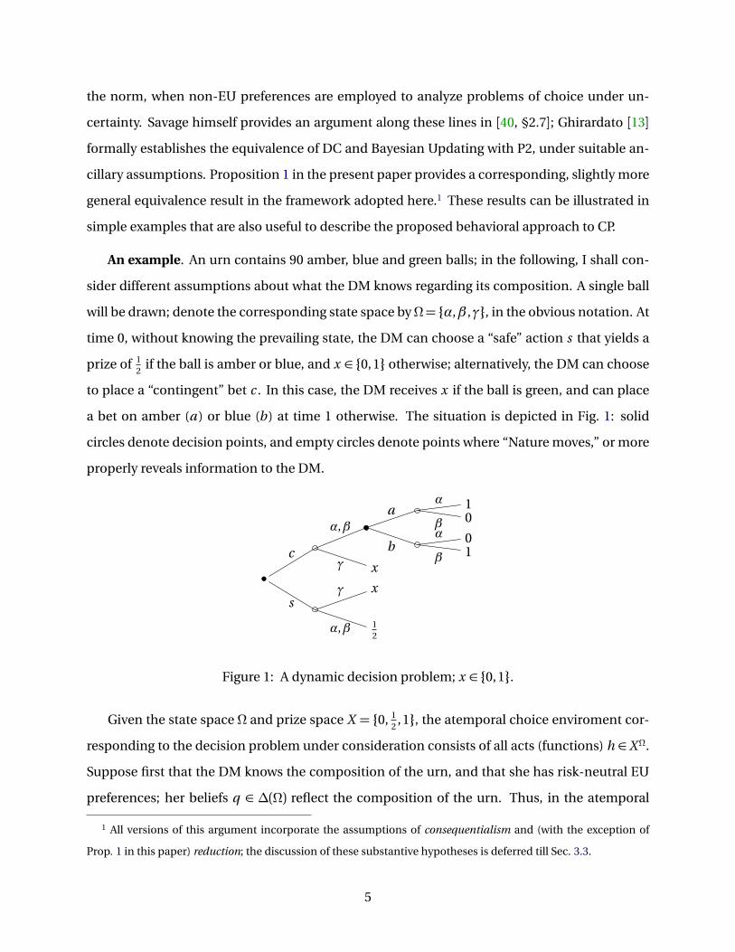
An example. An urn contains 90 amber, blue and green balls; in the following, I shall con-

sider different assumptions about what the DM knows regarding its composition. A single ball

will be drawn; denote the corresponding state space byΩ= α,β ,γ, in the obvious notation. At

time 0, without knowing the prevailing state, the DM can choose a “safe” action s that yields a

prize of 12

if the ball is amber or blue, and x ∈ 0, 1 otherwise; alternatively, the DM can choose

to place a “contingent” bet c . In this case, the DM receives x if the ball is green, and can place

a bet on amber (a ) or blue (b ) at time 1 otherwise. The situation is depicted in Fig. 1: solid

circles denote decision points, and empty circles denote points where “Nature moves,” or more

properly reveals information to the DM.

12

α,β

xγs

xγ1β

0αb

0β

1αa

α,β

c

Figure 1: A dynamic decision problem; x ∈ 0, 1.

Given the state space Ω and prize space X = 0, 12

, 1, the atemporal choice enviroment cor-

responding to the decision problem under consideration consists of all acts (functions) h ∈XΩ.

Suppose first that the DM knows the composition of the urn, and that she has risk-neutral EU

preferences; her beliefs q ∈ ∆(Ω) reflect the composition of the urn. Thus, in the atemporal

1 All versions of this argument incorporate the assumptions of consequentialism and (with the exception of

Prop. 1 in this paper) reduction; the discussion of these substantive hypotheses is deferred till Sec. 3.3.

5

setting, the DM evaluates acts h = (hα, hβ , hγ)∈XΩ according to the functional V (h) = Eq [h].

Now, as described above, augment this basic preference specification by assuming that the

DM updates her beliefs q in the usual way. At the second decision node, she then conditionally

(weakly) prefers a to b if and only if q (α|α,β) ≥ q (β|α,β). This is of course equivalent

to q (α)≥q (β), which is the restriction on ex-ante belief that ensures that, from the point of

view of the initial node, the course of action “c then a ” is weakly preferred to “c then b .” This

is an instance of DC: the ex-ante and conditional rankings of the actions a and b coincide. In

turn, this provides a rationale for the use of backward induction: the plans of action available to

the DM at the first decision node are “c then a ,” “c then b ” and “s ”; but one of the two “c ” plans

can be eliminated by first solving the choice problem at the second node. A simple calculation

then shows that “s ” is never strictly preferred, regardless of the ratio of blue vs. green balls.

Hence, for instance, if q (a )>q (b), then “c then a ” is the unique optimal plan.2

To provide a concrete illustration of the relationship between DC and P2, recall that the

assumptions of ex-ante EU preferences and Bayesian updating delivered two conclusions: (i)

the ranking of a vs. b at the second decision is the same as the ranking of “c then a ” vs. “c

then b ” at the first decision node; furthermore, (ii) the ranking of a vs. b at the second node

is independent of the value of x . Now assume that the modeler does not know that ex-ante

preferences conform to EU, nor that conditional preferences are derived by Bayesian updating;

however, he does know that (i) and (ii) hold. Clearly, the modeler is still able to conclude that

the ranking of “c then a ” and “c then b ” must also be independent of x , so that

(1, 0, 0)¼ (0, 1, 0) ⇔ (1, 0, 1)¼ (0, 1, 1), (1)

where ¼ denotes the DM’s preferences over acts. This is an implication of Savage’s Postulate P2

(cf. [40, p. 23], or Axiom 4.2 in §4.1 below). In other words, as claimed, Eq. (1) is also a necessary

condition for Dynamic Consistency in Fig. 1.

2 As per footnote 1, this argument incorporates the substantive assumptions of Consequentialism and Reduction

(see Sec. 3.3). In the tree of Fig. 1, the relevant aspect of Consequentialism is the fact that that the ranking of a

vs. b at the second decision node is independent of the value of x ; Reduction instead implies that the choice of

c followed by, say, a is evaluated by applying the functional V (·) to the associated mapping from states to prizes,

i.e. (1, 0,x ). I maintain both assumptions in this Introduction; the formal results in the body of the paper allow for

arbitrary departures from Reduction.

6

Ambiguity, DC and CP. I now describe ambiguity-sensitive preferences that violate P2, and

hence yield a failure of DC; see below for an analogous example based on the common-consequence

effect. Assume that, as in the three-color-urn version of the Ellsberg paradox [7], the DM is only

told that the urn contains 30 amber balls. Assume that she initially holds multiple-priors (a.k.a.

“maxmin-expected utility,” or MEU) preferences (Gilboa and Schmeidler [15]), is risk-neutral

for simplicity, and updates her beliefs prior-by-prior (e.g. Jaffray [26], Pires [38]) upon learning

that the ball drawn is not green. Formally, her preferences over acts h ∈RΩ conditional on either

F = Ω or F = α,β, are given by VF (h) =minq∈C Eq [h |F ], where C is the set of all probabilities

q on Ω such that q (α) = 13

. Notice that such conditional preferences are independent of the

value of x , as is the case for Bayesian updates of EU preferences.

Note first that, a priori (i.e. conditional on F = Ω), this DM exhibits the modal preferences

reported by Ellsberg [7]: she prefers a bet on amber to a bet on blue, but she also prefers betting

on blue or green rather than amber or green. Therefore, the DM’s preferences violate Eq. (1),

hence Savage’s postulate P2. Furthermore, conditional on α,β, this DM prefers (1, 0,x ) to

(0, 1,x ) regardless of the value of x , and hence will strictly prefer a to b .

If now x = 1, DC is violated: at the first decision node, the DM strictly prefers the plan “c

followed by b ” to “c followed by a ,” but at the second node she strictly prefers a to b .

To resolve these inconsistencies, suppose that the DM adopts CP. The intuitive assumption

of sophistication implies that, at the first decision node, the DM should correctly anticipate her

future choice of a , regardless of the value of x . This is true despite the fact that, for x = 1, she

really would like to commit to choosing b instead. Hence, when contemplating the choices c

and s at the first decision node, the DM understand that she is really comparing the plan “c

then a ” to “s ”. For x = 0, she will strictly prefer the former; but, for x = 1, she will strictly prefer

the latter. This logic thus delivers unambiguous and coherent behavioral predictions.

A dynamic “common consequence” paradox (cf. Allais [2]). Violations of DC can also arise

when preferences are probabilistically sophisticated but not EU; again, CP provides a way to

deal with them. Suppose that one ball will be drawn from an urn containing 100 balls, num-

bered 1 through 100. Fig. 2 depicts the choice problem and payoffs, where “M ” denotes one

million (dollars), and “1 . . . 11,” “12 . . . , 100” etc. refer to the number on the ball drawn.

The DM’s beliefs are uniform on Ω = 1, . . . , 100 at the initial node, and determined via

7

0.9M

s x12 . . . 100

1Mb

5M2 . . . 11

01a

1 . . . 11

c

Figure 2: A dynamic Allais-type problem; x ∈ 0, 1M .

Bayes’ rule at the second; her preferences are of the rank-dependent EU form (Quiggin [39]),

with quadratic distortion function. If x = 1M , the plan “c followed by b ” is preferred to “c

followed by a ,” whereas the opposite holds if x = 0: this corresponds to the usual violations of

the Independence axiom, and hence of P2. Furthermore, the DM strictly prefers a to b at the

second decision node if x = 1M , so preferences are dynamically inconsistent. Nevertheless, CP

again delivers well-defined behavioral predictions: if x = 1M , the DM will correctly anticipate

choosing a at the second node, and hence, by a simple calculation, opt for s at the initial node.

Karni and Safra [27, 28] illustrate applications of CP with non-EU preferences under risk.

Behavioral analysis of CP. As noted in the Introduction, this paper provides a fully behav-

ioral analysis of CP. To illustrate the key ingredients of the analysis, refer back to the decision

tree in Fig. 1, and adopt a simplified version of the notation to be introduced in Sec. 3 (an anal-

ogous treatment can be provided for the tree in Fig. 2). Denote the original tree in Fig. 1 by f x ;

also denote by cx and sx the subtrees of f x where c or, respectively, s is the only action available

at the initial node. Finally, denote by cax and cbx the subtrees of cx where a or, respectively, b

is the only action available at the second decision node; note that sx , cax and cbx can be inter-

preted as fully specified plans of action. Assume that, at time 0, the DM expresses the following

strict preferences () and indifferences (∼) over decision trees:

ca0 ∼ c0 ∼ f 0 s0 cb0 and cb1 f 1 ∼ s1 ca1 ∼ c1. (2)

The preferences in Eq. (2) exhibit two key features. First, preferences over plans are consistent

with act preferences in the Ellsberg paradox, and more generally with the assumed MEU prefer-

ences at the initial node. Specifically, ca0 s0 cb0 and ca1 ≺ s1 ≺ cb1 correspond to the DM’s

8

ranking of the acts (1, 0,x ), (0, 1,x ) and ( 12

, 12

,x ) for x = 0, 1 provided by the MEU utility index VΩ.

The remaining preference rankings involve non-degenerate trees, and do not merely follow

from the assumption of MEU preferences (even if augmented with prior-by-prior updating);

rather, they reflect the intuition behind sophistication that is the focus of this paper. In particular,

the indifference c1 ∼ ca1 indicates that the DM does not value the option to choose b at time 1,

when a is also available. This is not because she dislikes action b from the perspective of time

0: on the contrary, the ranking cb1 ca1 suggests that she would like to commit to choosing

b at time 1. Therefore, it must be the case that this DM correctly anticipates her future strict

preference for a over b , and evaluates the tree c1 accordingly.

I emphasize that this argument relies crucially upon the rankings of non-degenerate trees—

e.g., c1 ∼ ca1 in Eq. (2). Indeed, this pattern of preferences will constitute the behavioral defini-

tion of Sophistication in §4.3.2. More generally, the proposed approach leverages preferences

over trees to elicit conditional preferences and analyze sophistication and related behavioral

traits, just like the literature on menu choice leverages preferences over menus to investigate

attitudes toward flexibility or commitment, as well as temptation and self-control (see §6).3

The preferences in Eq. (2) indicate how this particular DM resolves the conflict between

her prior and posterior preferences. Furthermore, the rankings f 0 ∼ ca0 and f 1 ∼ s may be

intepreted as the behavioral implications of Sophistication: if x = 0, the DM will choose c and

plan to follow with a , and if x = 1, she will choose s instead—as predicted by CP.

It was just argued that, if the DM is assumed to strictly prefer a to b at the second decision

node, then the prior preferences in Eq. (2) reveal that she is sophisticated. But, reversing one’s

perspective, the following interpretation is equally legitimate: if the DM is assumed to be so-

phisticated, then the prior preferences in Eq. (2) reveal her ranking of a vs. b at the second

decision node. To elaborate, as noted above, the rankings cb1 ca1 ∼ c1 suggest that the DM

expects to choose a rather than b at the second decision node; if the DM is assumed to be so-

phisticated, this expectation must be correct, so she must actually prefer a to b at that node.

In this respect, the DM’s prior preference relation ¼ over trees, partially described in Eq. (2),

3Although I assumed that Reduction holds in this specific example, the notation and formal setup allow the DM

to strictly rank two plans p , p ′ that can be reduced to the same act. This is orthogonal to the issue of sophistication;

imposing Reduction throughout would neither simplify nor hamper the analysis. See §3.3.

9

provides all the information required to analyze behavior in this example.

Details. Certain subtle aspects of CP in the context of choice under uncertainty require fur-

ther analysis, and are fully dealt with in the remainder of this paper. First, eliciting conditional

preferences in general trees requires a more refined approach than the one just described; the

details are provided in Sec. 4.2. Note that only a weak form of sophistication is required.

Second, ties must be handled with care. The Sophistication axiom in Sec. 4.3.2 is purposely

formulated so as to entail no restrictions in case multiple optimal actions exist at a node. In-

stead, a separate axiom captures the tie-breaking assumption that characterizes CP.

Third, this “division of labor” is essential in the setting of choice under uncertainty. Sec.

5.2 shows that, under solvability conditions that are satisfied by virtually all known parametric

models of non-EU preferences, strengthening the Sophistication axiom so as to deal with ties

as well has an undesirable side effect: it imposes a version of P2 on preferences over acts, and

hence, for instance, rules out the modal preferences in the Ellsberg example.

3 Decision Setting

Due to the approach taken in this paper, the notation for decision trees must serve two pur-

poses. First, it must provide a rigorous description of dynamic-choice problem; second, it

must allow a precise, yet relatively straightforward formalization of “tree-surgery” operations—

pruning actions at a given node, replacing actions at a node with different ones, and more gen-

erally “composing” new trees out of old ones. The proposed description of decision trees will

be relatively familiar;4 however, formally describing tree-surgery operations requires a level of

detail that is not needed in other treatments of dynamic choice under uncertainty.

For simplicity, attention is restricted to finite trees associated with a single, fixed sequence

of information partitions; see §5.3 for possible extensions.

4 Epstein [11] and Epstein, Noor and Sandroni [12] adopt a similar notation for decision trees, although they are

not motivated by (and do not define) tree-surgery operations. In the context of risk, the notation in Sec. 3 of Kreps

and Porteus [32] is similar, again except for tree surgery; see Sec. 6 for further details.

10

3.1 Actions, Trees and Histories

Fix a state space Ω, endowed with an algebra Σ, and a connected and separable space X of

outcomes. Information is modeled as a sequence of progressively finer partitionsF0, . . . ,FT of

Ω, for some 0 ≤ T <∞, such that F0 = Ω and Ft ⊂ Σ for all t = 1, . . . , T (sometimes referred

to as a filtration). For every t = 0, . . . , T , the cell of the partitionFt containing the stateω ∈Ω is

denoted byFt (ω); also, a pair (t ,ω), where t ∈ 0, . . . , T andω∈Ω, will be referred to as a node.

Trees and actions can now be defined recursively, as “menus of contingent menus of con-

tingent menus...”. A bit more rigorously, define first a “tree” beginning at the terminal date T

in stateω simply as an outcome x ∈ X . Inductively, define an action available in node (t ,ω) as

a map associating with each stateω′ ∈Ft (ω) a continuation tree beginning at node (t + 1,ω′);

to complete the inductive step, define a tree beginning at node (t ,ω) as a finite collection, or

menus, of actions available at (t ,ω). The details are as follows:

Definition 1 Let FT (ω) = FT =X for allω∈Ω. Inductively, for t = T −1, . . . , 0 andω∈Ω, let

1. A t (ω) be the set of Ft+1-measurable functions a : Ft (ω) → Ft+1 such that, for all ω′ ∈

Ft+1(ω), a (ω′)∈ Ft+1(ω′);

2. Ft (ω) be the collection of non-empty, finite subsets of A t (ω); and

3. Ft =⋃

ω∈Ω Ft (ω).

The elements of A t (ω) and Ft are called actions and trees respectively.

Observe that the mapsω→ A t (ω) andω→ Ft (ω) areFt –measurable.

A tree is interpreted throughout as an exhaustive description of the choices available in a

given decision problem; in particular, if two or more actions are available at a node, the individ-

ual cannot also “randomize” among them. Of course, randomization can be explicitly modeled,

by suitably extending the state space and the description of the tree.

A history describes a possible path connecting two nodes in a tree: specifically, it indicates

the actions taken and events observed along the path. Given the filtration F0, . . . ,FT , the se-

quence of events observed is fully determined by the prevailing state of nature; thus, formally,

a history is identified by the initial time t , the prevailing state ω, and the (possibly empty) se-

quence of actions taken. The details, and some related notation and terminology, are as follows:

11

Definition 2 A history starting at a node (t ,ω) is a tuple h = [t ,ω, a], where either

• a= (a t , . . . , aτ), with t ≤τ≤ T −1, a t ∈ A t (ω) and, for all t = t +1, . . . ,τ, a t ∈ a t−1(ω); or

• a= ; (an empty list).

The cardinality of a is denoted |a|. Furthermore:

1. If h = [t ,ω, a], a= ; and a t ∈ A t (ω), then a∪a t = (a t ); and if a= (a t , . . . , aτ), τ< T −1 and

aτ+1 ∈ aτ(ω), then a∪aτ+1 ≡ (a t , . . . , aτ, aτ+1).

2. A history [t ,ω, a] is terminal iff t + |a|= T , and initial iff a= ;.

3. A history h = [t ′,ω′, a] is consistent with a tree f ∈ Ft (ω) if t ′ = t , ω′ ∈Ft (ω), and either

a = ; or the first action in a is an element of f ; in this case, the continuation tree of f

starting at h is f (h) = f if a= ;, and f (h) = aτ(ω′) if a= (a t , . . . , aτ).

Certain special trees play an important role in the analysis. First, a plan is a tree where a

single action is available at every decision point. Formally, a tree f ∈ Ft is a plan if, for every

history h = [t ,ω, a] consistent with f , | f (h)|= 1. The set of plans in Ft and Ft (ω)will be denoted

by F pt and F p

t (ω) respectively. Second, a constant plan yields the same outcome in every state

of the world. Formally, f xt ,ω ∈ Ft (ω) is the unique plan such that, for every terminal history h

consistent with f xt ,ω, f x

t ,ω(h) = x . If the node (t ,ω) can be understood from the context, the plan

f xt ,ω will be denoted simply by x .

As an example, the tree in Fig. 1, as well as its subtrees, can be formally defined as follows

(recall that a simplified notation was used in the Introduction). Let T = 2,F1 = α,β,γ, and

F2 = α,β,γ. The two choices available at the second decision node in Fig. 1 correspond

to the time-1 actions a ,b ∈ A1(α) = A1(β ) defined by

a (α) = 1, a (β ) = 0 and b (α) = 0, b (β ) = 1. (3)

Next, define the time-0 actions cx , sx , cax , cbx ∈ A0(α) = A0(β ) = A0(γ) by

for ω=α,β , cx (ω) = a ,b, sx (ω) =1

2, cax (ω) = a , cbx (ω) = b; (4)

cx (γ) = sx (γ) = cax (γ) = cbx (γ) = x . (5)

Here, x and 12

denote the constant plans f x1,γ and f

12

1,γ respectively.

12

Now the full tree in Fig. 1 is formally defined as f x ≡ cx , sx ; the subtree beginning with the

choice of c (respectively, s ) is cx (respectively sx ); and the plans corresponding to the choice

of c at the initial node, followed by a (respectively b ) at the second decision node are cax and

cbx . Finally, there are three non-terminal histories consistent with f x : ;, [0,α, cx ] and [0,β , cx ].

3.2 Composite Trees

Fix f ∈ Ft , a history h = [t ,ω, a] consistent with f , and another tree g ∈ Ft+|a|(ω). The composite

tree g h f is, intuitively, a tree that coincides with f everywhere except at history h, where it co-

incides with g . Formalizing this notion is somewhat delicate, so I first provide some heuristics.

Since h = [t ,ω, a] is consistent with f and a = (a t , . . . , aτ), with τ ≥ t , the last element aτ

of the action list a satisfies aτ(ω′) = f (h) for all ω′ ∈ Fτ+1(ω). To capture the idea that f (h)

is replaced with g , one would like to replace aτ in the list a with a new action aτ such that

aτ(ω′) = g at such states, and aτ(ω′) = aτ(ω′) elsewhere. However, recall that, by definition,

aτ−1(ω′) must contain aτ for all ω′ ∈ Fτ(ω); if aτ is replaced with aτ, it is also necessary to

“modify” aτ−1 so that it now contains aτ rather than aτ in such states. These modifications

must be carried out inductively for all actions aτ−1, aτ−2, . . . , a t ; this yields a new, well-defined

action list a= (a t , . . . , aτ). Finally, recall that, by definition, the history h = [t ,ω, a] is consistent

with f precisely when the first action a t in the list a is an element of f (trees are sets of actions).

Then, the tree g h f differs from f precisely in that the action a t is replaced with a t .

Now for the formal details. If a = ;, then let g h f ≡ g . Otherwise, write a = (a t , . . . , aτ),

with τ ≥ t ; let aτ(ω′) = g for all ω′ ∈ Fτ+1(ω), and aτ(ω′) = aτ(ω′) for ω′ ∈ Fτ(ω) \Fτ+1(ω).

Inductively, for t = τ− 1, . . . , t , let a t (ω′) = a t+1 ∪ (a t (ω′) \ a t+1) for all ω′ ∈ Ft+1(ω), and

a t (ω′) = a t (ω′) forω′ ∈Ft (ω) \Ft+1(ω). Finally, let g h f denote the set a t ∪ ( f \ a t ).

As a special case, consider a node (t ,ω) and a plan f ∈ F p0 . Since, by definition, a single ac-

tion is available in f at any node, there is a unique history consistent with f that corresponds to

the node (t ,ω); it is then possible to define a tree that, informally, coincides with f everywhere

except at time t , in case eventFt (ω) occurs. Such tree will be denoted g t ,ω f .

Formally, since f is a t -period plan, there is a unique action list a = (a 0, . . . , a t−1) such that

13

h = [0,ω, a] is consistent with f . Then, for all g ∈ Ft (ω), let g t ,ω f ≡ g h f .5 The notation “g t ,ω f ”

is modeled after “g E f ,” which is often used to indicate composite Savage acts.

3.3 Preferences, Reduction and Consequentialism

Definition 3 A conditional preference system (CPS) is a tuple (¼t ,ω)0≤t<T,ω∈Ω, such that, for

every t andω,¼t ,ω is a binary relation on Ft (ω), and furthermoreω′ ∈Ft (ω) implies¼t ,ω=¼t ,ω′ .

The time-0 preference is also denoted simply by ¼.

Three aspects are worth emphasizing. First, preferences are assumed to be “adapted toF ”:

for each t = 0, . . . , T −1,¼t ,ω is measurable with respect toFt . This reflects the assumption that

¼t ,ω is the DM’s ranking of trees conditional upon observing the eventFt (ω) at time t .

Second, recall that, in the Introduction, preferences over plans were implicitly defined by

first “reducing” plans to acts in the obvious way, and then invoking the DM’s preferences over

acts, represented by the functional V . While this is the “textbook” approach to dynamic choice

with EU preferences, there are compelling reasons to consider alternatives. For instance, the

DM may display a preference for early or late resolution of the uncertainty, as in Kreps and

Porteus [32], Epstein and Zin [10], Segal [41] and, in a fully subjective setting, Klibanoff and

Ozdenoren [30]. To allow for such preference models, reduction is not assumed in the main

results of this paper, Theorems 2 and 3. The proposed approach takes the DM’s preferences

over plans as given, as part of her CPS, regardless of whether or not they are obtained from

underlying preferences over acts by reduction.

Third, the assumption that the only “conditioning information” relevant to the preference

relation ¼t ,ω is the eventFt (ω) implies that our analysis is consequentialist: in particular, two

actions a ,b ∈ A t (ω) are ranked in the same way, in any decision tree where they may be avail-

able. To elaborate, if the actions a and b are available at a history h = [t ,ω, a] consistent with

a tree f , their ranking will of course, depend upon the realized event Ft (ω); however, prior

choices made and alternatives discarded on the path to h, choices the DM would have had to

make at counterfactual histories in f , or events that might have obtained but didn’t, are irrele-

5a is also the unique list such that, for anyω′ ∈Ft (ω), the history h = [0,ω′, a] is consistent with f ; furthermore,

the definition of composite trees implies that g h f = g h ′ f , consistently with the intended interpretation of g t ,ω f .

14

vant. This is a standard property of EU preferences and Bayesian updating, and is preserved in

most applications of non-EU and ambiguity-sensitive preferences. However, some alternative

theoretical approaches to dynamic choice with non-EU preferences or under ambiguity relax

consequentialism to salvage dynamic consistency; this important point is discussed in Sec. 6.

To conclude, recall that a binary relation is a weak order iff it is complete and transitive.

4 Main Results

This section presents the main results of this paper. Theorem 2 in §4.2 shows that sophistication

provides a way to elicit conditional preferences over acts and trees from prior preferences over

trees. §4.3 then takes as primitive a CPS and provides a definition (Def. 5) and characterization

(Theorems 3 and 4) of CP in the context of choice under uncertainty. §4.4.1 considers CP for

MEU preferences and prior-by-prior updating, and §4.4.2 analyzes the value of information

under CP. All proofs are in the Appendix. Further motivation and discussion is provided in §5.

As a preliminary step, §4.1 formalizes the connection between dynamic consistency, Bayesian

updating, and Savage’s Postulate P2 mentioned in the Introduction. This result constitutes a

useful benchmark, and aids in the interpretation of Theorems 2–4.

4.1 Dynamic Consistency, Bayesian updating, and Postulate P2

The main result of this subsection should be considered a “folk theorem”: various versions of it

exist in the literature, beginning with Savage’s own ([40, §2.7]). Its original statement concerns

preferences over acts; I restate it in terms of preferences over plans merely to avoid introducing

new notation.6 Also note that, while the definition of a CPS involves general trees, throughout

this subsection axioms, definitions and results are explicitly restricted to preferences over plans.

For simplicity, assume that every event in the filtration F0, . . . ,FT is not Savage-null: for

every node (t ,ω), it is not the case that p ∼ rt ,ωp for all p ∈ F p0 and r ∈ F p

t . I begin by formalizing

DC, Savage’s Postulate P2, and Savage’s qualitative notion of Bayesian Updating; I follow Savage

[40], §2.7 throughout, to which the reader is referred for interpretation (for DC, see also Epstein

6That is, to further clarify, the resulting additional generality is inessential for my purposes.

15

and Schneider [9]). Note however that Savage’s postulates and definitions pertain to all possible

conditioning events, whereas I restrict attention to the elements of the filtrationF0, . . . ,FT .

Axiom 4.1 (Dynamic Consistency — DC) For all nodes (t ,ω) with t < T , and all actions a ,b ∈

A t (ω) such that a ,b ∈ F pt : if a (ω′)¼t+1,ω′ b (ω′) for allω′ ∈Ft (ω), then a ¼t ,ω b; further-

more, if time-(t +1) preferences are strict for someω∗ ∈Ft (ω), then a t ,ω b.7

Axiom 4.2 (Postulate P2) For all plans p ,q ∈ F p0 , all nodes (t ,ω), and all plans r, s ∈ F p

t (ω),

rt ,ωp ¼ s t ,ωp ⇒ rt ,ωq ¼ s t ,ωq .8

Note that DC relates preferences at different histories; on the other hand, P2 pertains to

prior preferences alone. As asserted in Sec. 2, the MEU preferences specified in Sec. 2, jointly

with the reduction assumption, yield a violation of Axiom 4.2: take r = a , s = b, p = ca0

and q = cb0. This is, of course, the main message conveyed by Ellsberg [7].

Finally, say that the restriction of ¼t ,ω to F pt is derived from ¼ via Bayesian updating (cf.

Savage [40], p. 22) if, for all plans r, s ∈ F pt ,

r ¼t ,ω s ⇔ rt ,ωp ¼ s t ,ωp for some plan p ∈ F0.

For ex-ante EU preferences the above condition indeed characterizes Bayesian updating of the

DM’s prior. The following result is then straightforward:9

Proposition 1 Consider a CPS (¼t ,ω)t ,ω. The following statements are equivalent:

(1) ¼ is a weak order on F p0 , Axiom 4.2 (Postulate P2) holds, and for every node (t ,ω), the

restriction of¼t ,ω to F pt is derived from¼ via Bayesian updating;

(2) every¼t ,ω is a weak order on F pt , and Axiom 4.1 (DC) holds.

This result depends upon the assumption of consequentialism implicit in the framework: ac-

cording to Def. 5, each preference¼t ,ω is defined on (sub)trees with initial eventFt (ω) (cf. §6).

For a version of this result that relaxes consequentialism, see Epstein and Le Breton [8].

7a and b are actions, whereas the singleton sets a and b are trees; on the other hand, a (ω′) and b (ω′) are

trees in Ft+1(ω). Finally, F pt is a set of plans, i.e. special types of trees, and ¼t ,ω and ¼t+1,ω′ are defined over trees.

8A plan is, a fortiori, a t -period plan, so rt ,ωp , etc. are well-defined: cf. §3.2.

9The proof is similar to that of analogous results (e.g. Ghirardato [13]); hence, it is available upon request.

16

Prop. 1 highlights the tension between dynamic consistency and ambiguity that was antici-

pated in the Introduction. However, I now wish to emphasize the implications of this result for

Bayesian updating. If one assumes that prior preferences satisfy P2, then one can define con-

ditional preferences via Bayesian updating, and in this case Prop. 1 implies that DC will hold.

Conversely, if one assumes that DC holds, Prop. 1 implies that Bayesian updating provides a

way to elicit conditional preferences; furthermore, ex-ante preferences necessarily satisfy P2.

4.2 Eliciting Conditional Preferences

Turn now to the main results of the paper, beginning with the elicitation of conditional prefer-

ences. First, we adopt a standard requirement: the conditioning event should “matter.”

Assumption 4.1 (Non-null conditioning events) For every node (t ,ω) and prizes x , y such that

x y , there exists a plan g ∈ F p0 such that x t ,ωg yt ,ωg .

For general preferences over acts or plans, Assumption 4.1 is stronger than the requirement

that every set Ft (ω) not be Savage-null (cf. §4.1); however, the two notions coincide, for in-

stance, for MEU (and of course EU) preferences. Assumption 4.1 is weaker than analogous

conditions in the literature—e.g. the notions of “non-null” event in Ghirardato and Marinacci

[14], which requires that g = y .

4.2.1 Beliefs about Conditional Preferences

I begin by proposing a procedure that elicits the DM’s beliefs about her own future preferences;

the details are in Def. 4. To motivate it, refer to the decision tree in Fig. 1 with x = 1; adopt the

notation in Eqs. (3)–(5). Since cb1 ca1 ∼ c1 ex-ante, it was argued in §2 that a 1,α b

[equivalently, a 1,β b]: if the DM would like to commit to b at the second decision node,

but deems the tree c1 just as good as committing to a , it must be the case that the DM expects

to choose a at the second decision node, if both a and b are available.

However, this argument fails if ca1 ∼ cb1: in this case, the indifference c1 ∼ ca1 is not

sufficiently informative as to the relative conditional ranking of a vs. b . Detecting conditional

indifferences is even more delicate. Thus, a different, but related approach must be adopted:

17

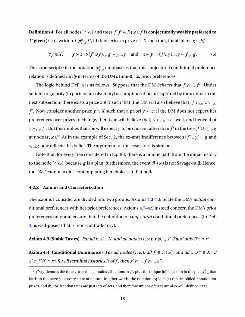
Definition 4 For all nodes (t ,ω) and trees f , f ′ ∈ Ft (ω), f is conjecturally weakly preferred to

f ′ given (t ,ω), written f ¼0t ,ω f ′, iff there exists a prize z ∈X such that, for all plans g ∈ F p

0 ,

∀y ∈X , y z ⇒ ( f ′ ∪ y )t ,ωg ∼ yt ,ωg and z y ⇒ ( f ∪ y )t ,ωg ∼ f t ,ωg . (6)

The superscript 0 in the notation ¼0t ,ω emphasizes that this conjectural conditional preference

relation is defined solely in terms of the DM’s time-0, i.e. prior preferences.

The logic behind Def. 4 is as follows. Suppose that the DM believes that f ¼t ,ω f ′. Under

suitable regularity (in particular, solvability) assumptions that are captured by the axioms in the

next subsection, there exists a prize z ∈ X such that (the DM will also believe that) f ¼t ,ω z ¼t ,ω

f ′. Now consider another prize y ∈ X such that a priori y z ; if the DM does not expect her

preferences over prizes to change, then (she will believe that) y t ,ω z as well, and hence that

y t ,ω f ′. But this implies that she will expect y to be chosen rather than f ′ in the tree ( f ′∪y )t ,ωg

at node (t ,ω).10 As in the example of Sec. 2, the ex-ante indifference between ( f ′ ∪ y )t ,ωg and

yt ,ωg now reflects this belief. The argument for the case z y is similar.

Note that, for every tree considered in Eq. (6), there is a unique path from the initial history

to the node (t ,ω), because g is a plan; furthermore, the eventFt (ω) is not Savage-null. Hence,

the DM “cannot avoid” contemplating her choices at that node.

4.2.2 Axioms and Characterization

The axioms I consider are divided into two groups. Axioms 4.3–4.6 relate the DM’s actual con-

ditional preferences with her prior preferences; Axioms 4.7–4.9 instead concern the DM’s prior

preferences only, and ensure that the definition of conjectural conditional preferences (in Def.

4) is well-posed (that is, non-contradictory).

Axiom 4.3 (Stable Tastes) For all x ,x ′ ∈X , and all nodes (t ,ω): x ¼t ,ω x ′ if and only if x ¼ x ′.

Axiom 4.4 (Conditional Dominance) For all nodes (t ,ω), all f ∈ Ft (ω), and all x ′,x ′′ ∈ X : if

x ′ ¼ f (h)¼ x ′′ for all terminal histories h of f , then x ′ ¼t ,ω f ¼t ,ω x ′′.

10 f ′ ∪ y denotes the time-t tree that contains all actions in f ′, plus the unique initial action in the plan f yt ,ω that

leads to the prize y in every state of nature. In other words, the notation exploits (a) the simplified notation for

prizes, and (b) the fact that trees are just sets of acts, and therefore unions of trees are also well-defined trees.

18

Axiom 4.5 (Conditional Prize-Tree Continuity) For all nodes (t ,ω) and all f ∈ Ft (ω), the sets

x ∈X : x ¼t ,ω f and x ∈X : x ´t ,ω f are closed in X .

Axiom 4.6 (Weak Sophistication) For all nodes (t ,ω), plans g ∈ F p0 , trees f ∈ Ft (ω), and prizes

x ∈X :

x t ,ω f ⇒ ( f ∪x )t ,ωg ∼ x t ,ωg and x ≺t ,ω f ⇒ ( f ∪x )t ,ωg ∼ f t ,ωg .

Axiom 4.3 states that tastes, i.e. preferences over prizes, are unaffected by conditioning.11

Axioms 4.4 and 4.5 are standard, and ensure that conditional certainty equivalents exist (recall

that X is assumed to be a connected and separable topological space).

Axiom 4.6 assumes just enough sophistication to ensure that conjectural and actual condi-

tional preferences coincide: in particular, the logic of sophistication is applied only to compar-

isons between a tree and a constant prize, and then only if the DM has no other choice available

on the path to the node (t ,ω). Preferences at times t > 0 are not required to be sophisticated.

Turn now to the second group of axioms.

Axiom 4.7 (Prize Continuity) For all x ∈ X , the sets x ∈ X : x ¼ x and x ∈ X : x ´ x are

closed in X .

Axiom 4.8 (Dominance) Fix a node (t ,ω), a tree f ∈ Ft (ω), a plan g ∈ F p0 and a prize x ∈X .

(i) If f (h) x for all terminal histories h of f , then ( f ∪x )t ,ωg ∼ f t ,ωg .

(ii) If f (h)≺ x for all terminal histories h of f , then ( f ∪x )t ,ωg ∼ x t ,ωg .

Axiom 4.8 reflects stability of preferences over outcomes. If the individual’s preferences over X

do not change when conditioning onFt (ω), then in (i) she will expect not to choose x at node

(t ,ω), because f yields strictly better outcomes at every terminal history; similarly for (ii). As in

Sec. 2, the indifferences in (i) and (ii) capture the DM’s expectations.

The next axiom is a “beliefs-based” counterpart to Weak Sophistication:

11For the present purposes, it would be sufficient to impose this requirement on a suitably rich subset of prizes.

For instance, if X consists of consumption streams, it would be enough to restrict Axiom 4.3 to constant streams.

19

Axiom 4.9 (Separability) Consider a node (t ,ω), f ∈ Ft (ω), plans g , g ′ ∈ F p0 and x , y ∈X . Then:

(i) ( f ∪ y )t ,ωg 6∼ f t ,ωg and x y imply ( f ∪x )t ,ωg ′ ∼ x t ,ωg ′;

(ii) ( f ∪ y )t ,ωg 6∼ yt ,ωg and x ≺ y imply ( f ∪x )t ,ωg ′ ∼ f t ,ωg ′.

To interpret, consider first the case g = g ′ and fix a prize y . According to the by-now familiar

logic of belief elicitation, ( f ∪ y )t ,ωg 6∼ f t ,ωg indicates that the DM believes that she will not

strictly prefer f to y givenFt (ω)—otherwise indifference would have to obtain. Thus, if x y

and the DM’s preferences over X are stable, she will also expect to strictly prefer x to f given

Ft (ω); again, the elicitation logic yields ( f ∪x )t ,ωg ∼ x t ,ωg . The interpretation of (ii) is similar.

Additionally, Axiom 4.9 implies that these conclusions are independent of the particular

t -period plan under consideration, and hence of what the decision problem looks like if the

event Ft (ω) does not obtain. In this respect, Axiom 4.9 reflects a form of “separability.” More

generally, Axiom 4.9 essentially requires that Eq. (6) in Def. 4 hold for all plans g , or for none.

There is a close analogy with the role of Savage’s Postulate P2: see §4.1 for details.

The main result of this section can now be stated.

Theorem 2 Suppose that Assumption 4.1 holds. Consider the CPS (¼t ,ω), and assume that ¼ is

a weak order on F0. Then the following statements are equivalent.

1. ¼ satisfies Axioms 4.7–4.9; furthermore, for all nodes (t ,ω),¼t ,ω =¼0t ,ω.

2. For every node (t ,ω),¼t ,ω is a weak order, and satisfies Axioms 4.3–4.6.

Theorem 2 and Proposition 1 in §4.1 are structurally similar: Axioms 4.7–4.9 play the role of

Postulate P2 (but add solvability requirements), the definition of conjectural conditional pref-

erences corresponds to Bayesian updating, and Axioms 4.3–4.6 correspond to DC (but again

add solvability requirements). The interpretation is also similar: under Axioms 4.7–4.9, Def. 4

yields well-behaved conditional preferences, and hence can be taken as the definition of con-

ditional preferences; in this case, Axioms 4.3–4.6 will hold. Conversely, if Axioms 4.3–4.6 hold,

the beliefs derived via Def. 4 from prior preferences are actually correct, so that Def. 4 can be

seen as a way to elicit actual conditional preferences. The main differences are that, of course,

Theorem 2 does not rely on P2 or DC, and concerns preferences over non-degenerate trees.

20

4.3 A decision-theoretic analysis of Consistent Planning

4.3.1 Consistent Planning under Uncertainty

As noted in the Introduction, Consistent Planning (CP) is a refinement of backward induction. If

there are unique optimal actions at any point in the tree, the two concepts coincide. Otherwise,

CP complements backward induction with a specific tie-breaking rule: indifferences at a history

h are resolved by considering preferences at the history that immediately precedes h.

To illustrate, consider the tree in Fig. 1 with x = 1, but assume MEU preferences with priors

C = q ∈∆(Ω) : 190≤ q (α)≤ 30

90, 2

90≤ q (β )≤ 15

90. Continue to assume prior-by-prior updating and

reduction, and again adopt the notation in Eqs. (3)–(5). It can then be verified that a ∼1,α b;

however, ca1 cb1, so CP prescribes that the DM will follow c with a . The corresponding

plan ca1 is strictly preferred to s1, so the unique CP “solution” of this tree is the plan ca1.

Algorithmically, CP operates as follows. For each history h = [t ,ω, a] in a tree f , consider

first the set CP0f (h) of actions b ∈ A t+|a|(ω) that, for every realization ω′ ∈ Ft+|a|(ω), prescribe

a continuation action a t+|a|+1,ω′ that has survived prior iterations of the procedure. Intuitively,

such actions b correspond to plans that the DM “will actually follow.” Then, out of these actions,

select the conditionally optimal ones: this completes the induction step and defines the set

CP f (h). Def. 5 is modeled after analogous definitions in Strotz [46] and Gul and Pesendorfer

[20], except that it is phrased in terms of preferences, rather than numerical representations.

Definition 5 (Consistent Planning) Consider a tree f ∈ Ft (ω). For every terminal history h =

[t ,ω, a] consistent with f , let CP f (h) = f (h). Inductively, if h = [t ,ω, a] is consistent with f

and CP f ([t ,ω′, a∪a ]) has been defined for everyω′ ∈Ft+|a|(ω) and a ∈ f (h), let

CP0f (h) =

n

b ∈ A t+|a|(ω) : ∃a ∈ f (h) s.t. ∀ω′ ∈Ft+|a|(ω),

b (ω′) = a+1,ω′ for some a+1,ω′ ∈CP f ([t ,ω′, a∪a ])o

and

CP f (h) =n

b ∈CP0f (h) : ∀a ∈CP0

f (h), b¼t+|a|,ω a o

.

A plan a ∈ Ft (ω) is a consistent-planning solution of f if a ∈CP f ([t ,ω,;]).12

12To help parse notation, a , a+1,ω′ and b in this definition are acts; b (ω′) must therefore be a tree, and in par-

ticular the definition requires that it be the tree a+1,ω′ having a single initial action a+1,ω′ taken from the set

CP f ([t ,ω′, a∪a ]). Finally, braces in b¼t+|a|,ω a are required because ¼t+|a|,ω is defined over trees, not actions.

21

Note that, in order to carry out the CP procedure, it is only necessary to specify the DM’s prefer-

ences over plans. The output of the CP algorithm is also a set of plans.13 Moreover, it is straight-

forward to verify that, if preferences over plans are complete and transitive, then Def. 5 is well-

posed: it always delivers a non-empty set of solutions that the DM deems equally good.

4.3.2 Behavioral Characterization of Consistent Planning

The behavioral analysis of CP takes as input the DM’s CPS (¼t ,ω). The key assumption of Sophis-

tication was introduced in Sec. 2; Axiom 4.6 applies the same principle to a small set of trees,

with unique features. To capture the implications of Sophistication in general trees, it will be

assumed that pruning conditionally dominated actions leaves the DM indifferent. Formally, if g

is a subset of actions available in the tree f at the history h, and every action b ∈ g is strictly pre-

ferred to every action w that lies in f (h) but not in g , then ex-ante the DM must be indifferent

between f and the tree g h f in which the inferior actions have been pruned:

Axiom 4.10 (Sophistication) For all f ∈ Ft , all histories h = [t ,ω, a] consistent with f and such

that a 6= ;, and all g ⊂ f (h): if, for all b ∈ g and w ∈ f (h) \ g , b t+|a|,ω w , then f ∼t ,ω g h f .

Observe that Axiom 4.10 is silent as far as indifferences at node (t + |a|,ω) are concerned. For

instance, if f (h) = a ,b and a ∼t+|a|,ω,b, the axiom does not require that f ∼t ,ω a h f ∼t ,ω

bh f . This allows for the possibility that, ex-ante, the DM have a strict preference for commit-

ment to a or b ; Axiom 4.11 deals with these situations. Axiom 4.10 is also silent if h is the initial

history of f : Axiom 4.12 below encodes the assumptions required in this case. This “division of

labor” is crucial so as to avoid unduly restricting ambiguity attitudes: see §5.2.

The next axiom formalizes the tie-breaking assumption that characterizes CP within the

class of backward-induction solutions: if the DM is indifferent among two or more actions at

a history h, then she can precommit (more precisely, expects to be able to precommit) to any

of them at the history that immediately precedes h. It is important to emphasize that no such

precommitment is possible in case the individual has strict preferences over actions at h: in

such cases, the full force of the Sophistication axiom applies.

13Formally, CP f ([t ,ω,;]) is a set of actions, not plans; however, if a ∈CP f ([t ,ω,;]), then a is a plan.

22

To formalize this assumption, the notion of a next-period commitment version of a tree is

required. Again, refer to the tree f x in Fig. 1; as it turns out, the notation in Eqs. (3)–(5) greatly

simplifies the exposition. Consider a modified version of the tree f x = cx , sx where the action

cx at the initial history ; is replaced with the actions cax and cbx . Recall that, while cx allows a

choice between a and b at the second decision node, cax and cbx enforce a commitment to a

and, respectively, b : cf. Eq. (4). The resulting tree cax , cbx , sx , referred to as the “next-period

commitment version” of f x , is depicted in Fig. 3.

12α,β

xγs

xγ1β

0αbα,βcb

xγ0β

1αaα,β

ca

Figure 3: Next-period commitment version of Fig. 1

To reflect the DM’s ability to precommit in case of future indifferences, it will be assumed

that, if a ∼1,α b, the DM is indifferent ex-ante between f x = cx , sx and its next-period com-

mitment version cax , cbx , sx . Intuitively, if a ∼1,α b, the DM regards the original tree as if it

afforded the same “physical” ability to commit as its next-period commitment version.

In the tree f x , non-trivial future choices must be made only following cx , and only if ω ∈

α,β; this simplifies the construction of its next-period commitment version. For a general

tree, one proceeds as follows. Given a tree f at a node (t ,ω), one fixes an initial action a in the

tree f ; in every state ω′ ∈ Ft (ω), a leads to a continuation tree a (ω′), which by definition is a

set of time-(t + 1) actions (in the intended application of this definition, i.e. Axiom 4.11, such

actions are mutually indifferent, but the following definition does not require this). Out of the

time-(t +1) actions in a (ω′), one picks a distinguished one a+1,ω′ . Finally, one constructs a new

action b available at time t that, for any stateω′ ∈Ft (ω), leads to the time-(t+1) tree containing

the single initial action a+1,ω. Each possible choice of initial action a and subsequent actions

a+1,ω′ leads to a different initial action b in the next-period commitment version of f . Formally:

23

Definition 6 Fix a tree f ∈ Ft (ω). The next-period commitment version of f is the tree

g =n

b ∈ A t (ω) : ∃a ∈ f s.t. ∀ω′ ∈Ft (ω) ∃a+1,ω′ ∈ a (ω′) s.t b (ω′) = a+1,ω′o

.

Now consider a tree f at a node (t ,ω) and a history h consistent with f ; suppose that every

action a ∈ f (h), and every realization of the uncertainty ω′ ∈ Ft (ω), leads to a new history

where the DM is indifferent among all available actions. Then replacing the continuation tree

f (h)with its next-period-commitment version g must leave the DM indifferent at (t ,ω):

Axiom 4.11 (Weak Commitment) For all f ∈ Ft and all histories h = [t ,ω, a] consistent with f :

if, for all a ∈ f (h), all ω′ ∈ Ft+|a|(ω), and all a+1,b+1 ∈ a (ω′), it is the case that a+1 ∼t+|a|+1,ω′

b+1, then f ∼t ,ω g h f , where g is the next-period commitment version of f (h).

Finally, Sophistication allows for the possibility that actions at future histories might be

tempting for future preferences, even though they are unappealing for initial preferences (or

vice versa). The following, standard axiom ensures that, by way of contrast, the availability of

choices at the initial history of f that are deemed inferior given the same initial preference

relation ¼t ,ω is considered neither harmful (as might be the case if the DM were subject to

temptation) nor beneficial (as it would be for a DM who has a preference for flexibility). This

rules out deviations from standard behavior that are not due to differences in information and

perceived ambiguity at distinct points in time:

Axiom 4.12 (Strategic Rationality) For all f , g ∈ Ft (ω) such that f ⊂ g : if, for all b ∈ f and

w ∈ g , b¼t ,ω w , then f ∼t ,ω g .

It is now possible to state the main result of this section. Two related characterizations of

CP will be provided. The first is better suited to the analysis of specific preference models and

updating rules (as in §4.4.1) and applications (as in §4.4.2). The second emphasizes that all

behavioral implications of CP can be identified on the basis of prior preferences alone (as noted

in the Introduction), and also has implications for policy evaluation (cf. Sec. 5.3).

Begin by specifying the DM’s prior and conditional preferences over plans. Next, assume

that this DM employs CP to determine her course of action in any given tree. Then, the DM’s

CPS should indicate indifference between a tree f and any one of its its CP solution(s). The fol-

lowing theorem shows that this is the case precisely when Axioms 4.10–4.12 hold.

24

Theorem 3 Consider a CPS (¼t ,ω)0≤t<T,ω∈Ω such that, for every t = 0, . . . , T and ω ∈ Ω, ¼t ,ω is a

weak order on F pt (ω). The following statements are equivalent.

1. Every¼t ,ω is a weak order on all of Ft (ω); furthermore, Axioms 4.10—4.12 hold.

2. for every node (t ,ω), every tree f ∈ Ft (ω), and every action a ∈CP f ([t ,ω,;]): f ∼t ,ω a .

Suppose instead that the axioms of this section are applied to the CPS (¼0t ,ω)0≤t<T,ω∈Ω de-

rived from the DM’s prior preference ¼ via Def. 4. In this case, Axioms 4.10–4.12 are effectively

assumptions on the DM’s prior preferences; formulating them in terms of the revealed condi-

tional preferences ¼0t ,ω is merely a matter of notational convenience. Leveraging Theorems 2

and 3, one then obtains

Theorem 4 Consider a weak order ¼ on F0 that satisfies Assumption 4.1 and Axioms 4.7–4.9,

and the CPS (¼0t ,ω)0≤t<T,ω∈Ω obtained from¼ via Def. 4. The following statements are equivalent.

1. Axioms 4.10–4.12 hold.

2. For every tree f ∈ F0 and action a ∈CP f ([0,ω,;]): f ∼ a .

4.4 Applications

4.4.1 Consistent Planning for MEU preferences and Prior-by-Prior Updating

To illustrate the results of Sec. 4.3.2, this subsection specializes Theorem 3 to the MEU decision

model and prior-by-prior Bayesian updating, assuming reduction of plans to acts. It is straight-

forward to adapt the analysis to different representations of preferences and different updating

rules (cf. e.g. Gilboa and Schmeidler [16], or Eichberger, Grant and Kelsey [6] and Horie [25]).

Begin by noting that, if f ∈ Ft is a plan, every state ω determines a unique path through f :

formally, for every ω′ ∈ Ft (ω), there is a unique list of actions a such that [t ,ω′, a] is terminal

and consistent with f . Throughout this subsection, for every node (t ,ω) and plan f ∈ Ft (ω),

the notation f (ω) indicates the prize f (h), where h = [t ,ω, a] is the unique terminal history

consistent with f . The required assumption on preferences can now be stated.

25

Assumption 4.2 (MEU) There exists a weak*–closed, convex set C of finitely-additive probabil-

ities on (Ω,Σ) and a continuous function u : X →R such that, for all plans f , g ∈ F0,

f ¼ g ⇔ minq∈C

∫

Ω

u ( f (ω))q (dω)≥minq∈C

∫

Ω

u (g (ω))q (dω).

Moreover, (i) there exist plans f , g ∈ F0 such that f g ; and (ii) for every node (t ,ω) and all

q ∈C , q (Ft (ω))> 0.

Note that the MEU decision rule is often seen as embodying “pessimistic” expectations; by

contrast, Axiom 4.11 in §4.3.2 is “optimistic” about one’s ability to carry out ex-ante preferred

courses of action (provided one does not have opposite strict preferences in the future).14

Part (i) of Assumption 4.2 states that ex-ante preferences over acts are not trivial. Part (ii)

is a strengthening of the assumption that every conditioning eventFt (ω) is not Savage-null; it

ensures that prior-by-prior Bayesian updating is well-defined (cf. Pires [38], Prop. 1 and p. 150).

Assumption 4.2 pertains solely to prior preferences (over plans); Axiom 4.13 below provides

a link with conditional preferences over plans, and in particular will be shown to characterize

prior-by-prior updating. This axiom (see Siniscalchi [42]) recasts the main axiom in Pires [38]

and Jaffray [26] in a form that is more easily compared with Axiom 4.1 (DC) of Sec. 4.1.15

Axiom 4.13 (Constant-act dynamic consistency) For all plans p ∈ F p0 , prizes x ∈ X , and non-

terminal histories h = [0,ω, a] consistent with p :16

p (h)¼|a|,ω x

∧

∀ω′ 6∈ F|a|(ω), p (ω′)¼ x

=⇒ p ¼ x ,

p (h)|a|,ω x

∧

∀ω′ 6∈ F|a|(ω), p (ω′)¼ x

=⇒ p x ; and

p (h)´|a|,ω x

∧

∀ω′ 6∈ F|a|(ω), p (ω′)´ x

=⇒ p ´ x ,

p (h)≺|a|,ω x

∧

∀ω′ 6∈ F|a|(ω), p (ω′)´ x

=⇒ p ≺ x .

Axiom 4.13 differs from Axiom DC in two respects. First, Axiom 4.13 only considers conditional

comparisons between a plan p and a prize x 17, whereas DC has implications whenever two ar-

bitrary plans are compared conditional onF|a|(ω). Second, dominance, rather than conditional

14I thank a referee for this observation.

15For a non-decision-theoretic analysis, see Walley [47].

16Note that the history h reaches node (|a|,ω); hence the notationF|a|(ω), ¼|a|,ω, etc.

17This is why the four cases p (h)¼t ,ω x , p (h)t ,ω x , p (h)´t ,ω x and p (h)≺t ,ω x must all be explicitly considered.

26

preference, is required outside of the conditioning eventF|a|(ω). The motivations for these re-

strictions are discussed in the sources cited above (esp. [38] and [42]).

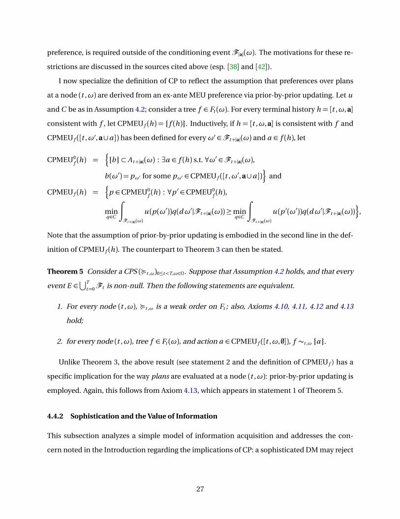
I now specialize the definition of CP to reflect the assumption that preferences over plans

at a node (t ,ω) are derived from an ex-ante MEU preference via prior-by-prior updating. Let u

and C be as in Assumption 4.2; consider a tree f ∈ Ft (ω). For every terminal history h = [t ,ω, a]

consistent with f , let CPMEU f (h) = f (h). Inductively, if h = [t ,ω, a] is consistent with f and

CPMEU f ([t ,ω′, a∪a ]) has been defined for everyω′ ∈Ft+|a|(ω) and a ∈ f (h), let

CPMEU0f (h) =

n

b ⊂ A t+|a|(ω) : ∃a ∈ f (h) s.t. ∀ω′ ∈Ft+|a|(ω),

b (ω′) = pω′ for some pω′ ∈CPMEU f ([t ,ω′, a∪a ])o

and

CPMEU f (h) =n

p ∈CPMEU0f (h) : ∀p ′ ∈CPMEU0

f (h),

minq∈C

∫

Ft+|a|(ω)

u (p (ω′))q (dω′|Ft+|a|(ω))≥minq∈C

∫

Ft+|a|(ω)

u (p ′(ω′))q (dω′|Ft+|a|(ω))o

,

Note that the assumption of prior-by-prior updating is embodied in the second line in the def-

inition of CPMEU f (h). The counterpart to Theorem 3 can then be stated.

Theorem 5 Consider a CPS (¼t ,ω)0≤t<T,ω∈Ω. Suppose that Assumption 4.2 holds, and that every

event E ∈⋃T

t=0Ft is non-null. Then the following statements are equivalent.

1. For every node (t ,ω), ¼t ,ω is a weak order on Ft ; also, Axioms 4.10, 4.11, 4.12 and 4.13

hold;

2. for every node (t ,ω), tree f ∈ Ft (ω), and action a ∈CPMEU f ([t ,ω,;]), f ∼t ,ω a .

Unlike Theorem 3, the above result (see statement 2 and the definition of CPMEU f ) has a

specific implication for the way plans are evaluated at a node (t ,ω): prior-by-prior updating is

employed. Again, this follows from Axiom 4.13, which appears in statement 1 of Theorem 5.

4.4.2 Sophistication and the Value of Information

This subsection analyzes a simple model of information acquisition and addresses the con-

cern noted in the Introduction regarding the implications of CP: a sophisticated DM may reject

27

freely available information. I shall argue that this behavior reflects a basic trade-off between in-

formation acquisition and commitment; this trade-off is difficult to uncover when preferences

over acts only are considered, but becomes transparent in the richer setting of this paper.18

Consider an individual facing a choice between two alternative actions, a and b (the term

“action” is used informally here). Uncertainty is represented by a state space Ω=Ω1×Ω2, where

Ω1 = Ω2 = α,β. The individual receives H dollars if she chooses action a and the second

coordinate of the prevailing state is α, or if she chooses action b and the second coordinate of

the prevailing state is β ; otherwise, she receives L < H dollars. Finally, prior to choosing an

action, the DM can observe the first coordinate of the prevailing state.

The DM has risk-neutral MEU preferences over acts, and evaluates plans by reduction. Her

set of priors is C = λP +(1−λ)Q :λ∈ [0, 1], where P,Q ∈∆(Ω) are defined by

P(α,α) =Q(β ,β ) = 1−2ε, P(α,β ) = P(β ,α) = ε=Q(α,β ) =Q(β ,α), P(β ,β ) =Q(α,α) = 0.

The parameter ε lies in the interval

0, 14

, and should be thought of as being “small”. In other

words, this individual believes that the signal (ω1) is most likely equal to the payoff-relevant

component of the state (ω2), but the relative likelihood ofω2 = α vs. ω2 = β is ambiguous; fur-

thermore, she assigns a (small and unambiguous) probability ε to each state where the signal is

“wrong” (i.e. different from the payoff-relevant component). Finally, assume prior-by-prior up-

dating. Note that the resulting conditional preferences over acts are dynamically inconsistent

(they violate Axiom 4.1 in Sec. 4.1).

The objective is to determine the value of the information conveyed by the signal ω1; this

value turns out to depend upon whether or not the DM has the opportunity to commit to sub-

sequent,ω1–contingent choices (e.g. by writing a binding contract, or delegating choices to an

agent or machine). To adopt the formal framework of Sec. 3, it is useful to consider four plans,

denoted pa a ,pab ,pb a and pbb (the formal definitions are omitted for brevity). For instance, pab

is the plan that prescribes the choice a after seeing ω1 = α and the choice b after observing

ω1 = β ; the DM evaluates it by “reducing” it to the act that yields H if ω ∈ (α,β ), (β ,α) and L

18Footnote 35 in Machina [34] attributes a similar observation, albeit expressed in the language of multiple

selves, to Edi Karni.

28

elsewhere. Under the assumed preferences,

pab pb a pa a ∼ pbb . (7)

If the individual acquires information and can commit, then she effectively faces the tree

f I ,C ≡ pa a ∪pab ∪pb a ∪pbb . Her preferred ex-ante choice is pab , so f I ,C ∼ pab .

If the DM does not acquire information, her feasible choices are the plans pa a and pbb : thus,

she can trivially “commit” to either a or b regardless of the realization ofω1, which she does not

observe. Formally, she faces the tree f NI = pa a ∪pbb . By Eq. (7), CP implies that f NI ∼ pa a ∼ pbb .

The value of the signalω1 under commitment is then the difference between the MEU evalua-

tion of pab and that of pa a , namely (1−3ε)(H − L).

If the individual acquires information but cannot commit, then she faces a tree f I ,NC wherein

the choice of a vs. b is made after observing ω1.19 If the individual is sophisticated (as well as

strategically rational), she will determine her willingness to pay for the information by taking

into account the choices she will actually make after observing ω1: in other words, she will

evaluate the tree f I ,NC according to its CP solution.

Under prior-by-prior updating, one can verify that the DM will strictly prefer b after observ-

ing ω1 = α and a after observing ω1 = β ; therefore, by CP, f I ,NC ∼ pb a . The value of the signal

ω1 is then the difference between the MEU evaluations of pb a and pa a , namely ε(H − L); since

ε∈

0, 14

, this is positive, but smaller than in the commitment case.

To summarize, if the DM can exogenously commit, information is valuable, as usual: the

DM has more options in the tree f I ,C than in the tree f NI (formally, f NI ⊂ f I ,C ) and this is of

course beneficial. Furthermore, and symmetrically, if the DM “exogenously” receives informa-

tion, then commitment is also valuable: it expands the effective choice set from just pb a , the CP

solution of f I ,NC , to f I ,C . Finally, there is a trade-off between information and commitment: the

CP solution pb a of f I ,NC is not a subset or superset of f NI , so one cannot say a priori whether

this sophisticated but dynamically inconsistent DM should acquire information. For the pref-

erences considered here, information is valuable; however, in other settings, the commitment

problem may be so severe that the DM may rationally choose to pay a price so as to avoid in-

19Formally, f I ,NC = c, where the action c satisfies, for instance, c (α) = aα,bα, with aα,bα : ω′ : ω′1 = α →

0, 1, aα(ω′) = 1 ifω′2 =α and aα(ω′) = 0 otherwise, and similarly for bα.

29

formation: for an interesting example, see Eichberger, Grant and Kelsey [6, p. 892]. Similar

patterns of behavior also emerges in related contexts featuring time-inconsistent but sophisti-

cated decision-makers: see e.g. Carrillo and Mariotti [3] and references therein.

5 Discussion of Theorems 2–4

5.1 Counterfactuals and conditional preferences20

Any treatment of dynamic choice involves statements about preferences at potentially counter-

factual decision points. In the tree of Fig. 1, the second node is not reached if the ball drawn

is green; in such case, one cannot directly observe the DM’s preferences at that node. Conse-

quently, substantive assumptions about conditional preferences are required.

This issue arises even with dynamically-consistent preferences (e.g. under EU). As noted

in §4.1, one may employ Bayesian updating to define conditional preferences based on prior

ones, thereby ensuring that DC holds per Proposition 1; however, the preferences thus defined

need not be the DM’s “actual” conditional preferences. As noted in §4.1, one may equivalently

assume that DC holds, and employ Bayesian updating to elicit conditional preferences; how-

ever, the DM’s “actual” conditional preferences may be dynamically inconsistent, in which case

Bayesian updating elicits a spurious object. In other words, the Bayesian updating and DC as-

sumptions may well be incorrect from a descriptive point of view.

Theorem 2 is subject to the same qualifications. Whether one views Def. 4 as a way to define

or elicit conditional preferences, a substantive assumption about conditional preferences must

be made: one either stipulates directly that ¼t ,ω≡¼0t ,ω “by fiat,” or else stipulates that Axioms

4.3–4.6 holds, so beliefs are correct and hence ¼t ,ω≡¼0t ,ω, as Theorem 2 shows. Again, either of

these substantive assumptions may be incorrect from a descriptive standpoint.

On the other hand, Theorem 4 can be “safely” interpreted as a behavioral characterization

of CP in terms of the DM’s prior preferences over trees alone. The conjectural preferences ¼0t ,w

can be interpreted as reflecting the DM’s prior beliefs about her future behavior, and Axioms

4.10–4.12 then ensure that such beliefs “support” or “explain” her ex-ante choices.

20I thank the Coeditor and referees for several observations that guided and motivated this discussion.

30

5.2 An important caveat: Strong Sophistication

Recall that the Sophistication axiom has no implications in the case of indifferences at future

nodes. This is crucial to avoid unduly restricting preferences over plans. If Axiom 4.10 is strength-

ened by replacing strict preferences at future nodes with weak preferences, one obtains

Axiom 5.1 (Strong Sophistication) For all f ∈ Ft , all histories h = [t ,ω, a] with a 6= ; consistent

with f , and all g ⊂ f (h): if, for all b ∈ g and w ∈ f (h) \ g , b¼t+|a|,ω w , then f ∼t ,ω g h f .

Refer to the tree in Fig. 1, with x = 1 and notation as per Eqs. (3)–(5); consider the MEU pref-

erences described in §4.3.1, so in particular a ∼1,α b and ca1 cb1, and the history

h = [1,α, c1], i.e. the second decision point: under Strong Sophistication, a ∼1,α b would

imply that ca1= a hc1 ∼ c1 ∼ bhc1= cb1, which is inconsistent with the preferences

over acts (and plans) specified at the beginning of §4.3.1.

The example points out the key problematic implication of Strong Sophistication: it implies

that, loosely speaking, if the DM is indifferent between two actions at a given history, she must

also be indifferent between them at any earlier history. Furthermore, unlike the Sophistication

axiom adopted here to characterize CP (i.e. Axiom 4.10), Strong Sophistication does impose

restrictions on preferences over acts (or, more generally, plans).

Indeed, it turns out that these restrictions are overly strong for a very broad class of prefer-

ences. Say that preferences admit certainty equivalents if, for every (t ,ω) and p ∈ F pt (ω) there

is x ∈ X with p ∼t ,ω x ; this includes virtually all parametric models of preferences over acts,

assuming reduction. Also say that Ft (ω) is strongly non-null (for ¼) if, for all x , y ∈ X and

p ∈ F pt (ω), x y implies x t ,ωp yt ,ωp .21

Proposition 6 If each ¼t ,ω is a weak order that admits certainty equivalents, each Ft (ω) is

strongly non-null, and Axioms 4.3 and 5.1 hold, then ¼ satisfies Axiom 4.2 (postulate P2), the

restriction of each¼t ,ω to F pt is derived from¼ via Bayesian updating, and Axiom 4.1 (DC) holds.

The basic intuition behind this result is fairly straightforward (although the actual proof takes a

different approach). Given a plan p and a history h consistent with p , if x ∈ X is the certainty

equivalent of p (h) at h, then Strong Sophistication implies that, loosely speaking, x is also the

21For MEU preferences with priors C , this corresponds to minq∈C q (Ft (ω))> 0.

31

“value” that the DM attaches to p (h) at any history immediately preceding h. In other words,

the DM can evaluate the plan p by recursion, as with standard EU preferences. This recursive

structure implies dynamic consistency.

Proposition 6 thus implies that, in particular, Axiom 5.1 can preclude ex-ante Ellsberg pref-

erences in the tree of Fig. 1.22 More broadly, Axiom 5.1 rules out precisely the kind of behavior

that is the focus of the present paper. Axioms 4.10 and 4.11 are formulated so as to avoid this.

5.3 Miscellaneous

Policy evaluation. Welfare analysis is problematic in the presence of dynamic inconsistency.

Refer to the tree in Fig. 1, with x = 1 and preferences as in the Introduction; consider a “policy”

that removes action a . Suppose that an irreversible decision to implement the policy must be

made at time 0; can a definite recommendation be made, despite the noted inconsistency of

the DM’s preferences over acts? If the DM is sophisticated, then at the initial node she strictly

prefers that a be removed, even though she anticipates being unhappy at the second node if

a is indeed deleted. Gul and Pesendorfer [21, p.31] observe that “standard economic models

identify choice with welfare”; from this point of view, the argument just given supports a policy

that removes a (again, assuming an irreversible decision must be made at time 0).

The crux of the argument is that, in view of the results of this paper, there is no ambiguity as

to whose “choice” and “welfare” one is concerned with: there is a single individual, character-

ized by her time-0 preferences over decision trees, who in particular strictly prefers the subtree

with a removed to the tree f 1. By way of contrast, if the decision problem is interpreted as a

game played by multiple selves, it is no longer clear whose choices and welfare one should fo-

cus on; clear-cut policy prescriptions thus necessitate the introduction of an exogenous welfare

criterion—perhaps one that trades off the well-being of the different selves.

Extensions. In the decision framework adopted in this paper, all trees are defined with re-

spect to a fixed filtration F0, . . . ,FT . However, if the DM holds well-defined preferences over

plans conditional upon arbitrary (non-null) events, Theorem 3 suggests that she can also com-

22In Sec. 2, modify the ex-ante MEU preferences so C = q (α) = 13

, q (β)∈ [ε, 23−ε] for some small ε> 0: then

α,β and γ are strongly non-null and Prop. 6 applies. Of course, the analysis in Sec. 2 does not change.

32

pare two trees f and g that are each adapted to a different filtration. This is required, for in-

stance, in order to model a DM who, at time 0, faces a choice between two different informa-

tion structures, of which neither is finer than the other. Intuitively, the DM can apply CP to f

and g separately, and then rank these trees according to her preferences over their respective

CP solutions. By Theorem 3, this is equivalent to the assumption that the axioms in Sec. 4.3.2

apply “filtration-by-filtration”; the straightforward details are omitted.

The previous version of this paper, [43], provides results analogous to those in Sec. 4 for

a more general class of decision trees that allows the agent’s actions at any point in time to

determine the information she can receive at subsequent nodes. It also discusses the extension

to a class of infinite decision trees.

6 Related Literature and Alternative Approaches

Kreps and Porteus [32]. As was noted above, the notation adopted here for decision trees is

closely related to the formalization of a “decision problem” under risk in Sec. 3 of Kreps and

Porteus [32, KP henceforth]. Specifically, a time-t tree in the sense of the present paper is a (fi-

nite) set of state-contingent menus of time-(t +1) trees, whereas in KP, a time-t decision prob-

lem is a (closed) set of lotteries over (contemporaneous payoffs and) time-(t + 1) continuation

problems. The key difference with this paper is that KP propose a model of recursive prefer-

ences, which satisfies dynamic consistency: see their central Axiom 3.1. By way of contrast, the

present paper is concerned precisely with violations of dynamic consistency.

Segal [41]. Again in the setting of risky choice, Segal [41] studies preferences over two-stage

lotteries that do not satisfy the Reduction axiom; he also allows for non-EU risk attitudes. As

Segal states explicitly [41, p. 353], decisions are made only ex-ante in his framework (i.e. before

first-stage lotteries are resolved); therefore, the issue of dynamic (in)consistency simply does

not arise. By way of contrast, the present paper focuses on non-degenerate decision situations

in which choices are made at two or more histories.

Karni and Safra [27, 28]. As noted in Sec. 2, these authors study economic applications of

CP (which they call “behavioral consistency”) to choice under risk with non-EU preferences.

33

These papers employ CP as solution concept of a game played by agents, or selves, of the de-

cision maker; by way of contrast, the present paper is concerned with the decision-theoretic

foundations for CP.

The Menu Choice Literature and Gul and Pesendorfer [20]. The approach in the present

paper is influenced by the menu-choice literature initiated by Kreps [31] and further developed

by Dekel, Lipman and Rustichini [5] and Gul and Pesendorfer [19] in the context of certainty.

The work of Epstein [11] and Epstein, Noor and Sandroni [12], which deals with non-Bayesian

updating for EU preferences but does not allow for broader risk or ambiguity attitudes, and

does not focus on CP, have already been mentioned (cf. footnote 4).

Gul and Pesendorfer [20] axiomatize a version of CP in the setting of dynamic choice under

certainty. Their Theorems 1 and 2 are loosely related to Theorem 2 in §4.2 of this paper; they

axiomatize ex-ante preferences that admit a “weak Strotz representation,” i.e., roughly speak-

ing, a system of conditional preferences that generates it via CP. However, multiple conditional

preference systems can generate the same ex-ante preferences (p. 437); by way of contrast,

Theorems 2 and 4 relate ex-ante preferences to a unique CPS. Gul and Pesendorfer’s Theorem

3 ([20], p. 439) is the closest counterpart to Theorem 3 in this paper: it characterizes CP for a

given time-0 preference on decision problems and a given collection of conditional choice cor-

respondences.23 However, their key axiom IRA corresponds to the Strong Sophistication axiom

discussed in §5.2. As noted in §5.2, this is too strong an assumption for the purposes of this

paper, as it implies a strong form of dynamic consistency.

Hammond [22] and related contributions. Hammond [22] also takes the DM’s behavior in

decision trees as given. He proposes a notion of “consequentialism” that differs significantly

from the one discussed in Sec. 3.3 (cf. [34], p. 1641); call this property “H-consequentialism.”

Hammond’s main result shows that a behavioral rule satisfies H-consequentialism, consequen-

tialism in the sense of Sec. 3.3, and continuity if and only if it is consistent with EU. In other

words, Hammond emphasizes that assumptions about dynamic choice behavior can provide

a foundation for (atemporal) EU preferences over acts. By way of contrast, the assumptions

23In the statement of Theorem 3 in [20], “weak Strotz representation” should actually read “canonical Strotz

representation,” as I have confirmed with the authors (the term “canonical” is formally defined in their paper).

34

on dynamic choice behavior considered in this paper are specifically designed not to restrict

preferences over acts in any way. Rather, Hammond’s result is related to Propositions 1 and 6

(loosely speaking, with H-consequentialism playing the role of FDC or Strong Sophistication).

For two-period decision problems under risk, Gul and Lantto [18] propose weakenings of

H-consequentialism and dynamic consistency, and show that, under reduction of compound

lotteries, the properties they propose are equivalent to the assumption that preferences over

lotteries satisfy Dekel’s betweenness axiom (Dekel [4]). Grant, Kaji and Polak [17] focus on

value-of-information problems; they do not require reduction of two-stage lotteries, and as-

sume suitable versions of DC and strong sophistication (cf. Sec. 5.2). They identify conditions

on ex-ante preferences over two-stage lotteries that are necessary and sufficient for the DM to

prefer more information to less. Thus, like Hammond [22], both papers relate dynamic choice

behavior to properties of ex-ante preferences over lotteries; by way of contrast, the present pa-

per does not impose or derive restrictions on ex-ante preferences over acts or plans.

Recursive preferences under ambiguity. In an influential paper, Epstein and Schneider [9]

characterize the class of MEU preferences over acts that are recursive, and hence dynamically

consistent, in all decision trees consistent with a given filtration. This permits the application

of standard dynamic-programming techniques even in the presence of ambiguity. Maccheroni,

Marinacci and Rustichini [33], and Klibanoff, Marinacci and Mukerji [29] adapt this approach

to different preference models.

Epstein and Schneider’s dynamic consistency requirement corresponds to Axiom 4.1 (DC)

in §4.1; while this assumption does allow for non-trivial manifestations of ambiguity aversion at

each decision node, by Prop. 1 it implies that prior preferences must satisfy Savage’s Postulate

P2 relative to every conditioning event in the filtration under consideration. In particular, as

noted in §4.1, in the tree of Fig. 1, their requirement rules out the modal (ambiguity-averse)

preferences at the initial node. By way of contrast, the approach in this paper does not restrict

preferences over acts.

Non-consequentialist choice. An alternative approach to dynamic choice with non-EU

preferences, advocated in the context of risky choice by Machina [34] and McClennen [35]

35

among others, essentially24 allows conditional preferences at a history h to depend upon the

“context” of the entire decision tree, so as to preserve optimality of the ex-ante optimal plan.

Thus, this approach espouses dynamic consistency, but drops consequentialism. Hanany and

Klibanoff [23, 24] implement this approach for a broad class of ambiguity-averse preferences.

When consequentialism is relaxed in the presence of ambiguity, interpreting the effect of in-

formation on preferences can be problematic. In particular, the same information may appear

to eliminate ambiguity (or perception thereof) in one decision tree, and preserve it in another:

I provide an example in Siniscalchi [44]. This conclusion stands in sharp contrast with the pre-

vailing view of ambiguity as an informational phenomenon.

Al-Najjar and Weinstein [1] discuss further difficulties with violations of consequentialism.

A Appendix

A.1 Proof of Theorem 2 (Eliciting Conditional Preferences)

Remark A.1 Fix a node (t ,ω) and let ≥ be a weak order on Ft (ω) such that (i) for all x , y ∈ X ,

x ≥ y iff x ¼ y ; (ii) if x ∈X satisfies x ¼ f (h) [resp. x ´ f (h)] for all terminal histories h consistent

with f ∈ Ft (ω), then x ≥ f [resp f ≥ x ]; and (iii) the sets U = x ∈ X : x ≥ f and x ∈ X : f ≥ x

are closed in X . Then:

(a) for every f ∈ Ft ,ω, there exists x ∈X such that x ≥ f and f ≥ x (abbreviated x = f );

(b) if f > g , there is x ∈X such that f > x > g .

The proof of this remark is routine, hence omitted.

Turn to Theorem 2. For f , f ′ ∈ Ft (ω) and g ∈ F t0 , write f ¼0

t ,ω|g f ′ to denote that Eq. (6) holds

for g and for a suitable z ∈X . Thus, f ¼0t ,ω f ′ iff f ¼0

t ,ω|g f ′ for all g ∈ F p0 .

Assume that (2) holds, and consider a node (t ,ω). Suppose that f ¼t ,ω f ′ and let z ∈ X

be such that z ∼t ,ω f ′: such a prize exists by Remark A.1. Fix g ∈ F0 arbitrarily: I claim that

f ¼0t ,ω|g f ′, so f ¼0

t ,ω f ′. To see this, suppose first y z , so y t ,ω z by Axiom 4.3; then y t ,ω f ′

by transitivity, and Axiom 4.6 implies that ( f ′ ∪ y )t ,ωg ∼ yt ,ωg . Next, suppose that y ≺ z : again

invoking Axiom 4.3 and transitivity we get y ≺t ,ω f , and Axiom 4.6 implies ( f ∪ y )t ,ωg ∼ f t ,ωg .

24This necessarily brief summary overlooks nuances among different proponents of this approach.

36

This proves the claim. In the opposite direction, consider f , f ′ ∈ Ft (ω) and suppose that f ¼0t ,ω

f ′; let z ∈ X be such that Eq. (6) holds for all g ∈ F p0 . Suppose by contradiction that z t ,ω f ,

so there exist y ′, y ′′ ∈ X such that z t ,ω y ′ t ,ω y ′′ t ,ω f (by Remark A.1). Now Def. 4 implies

( f ∪y ′)t ,ωg ∼ f t ,ωg ∼ ( f ∪y ′′)t ,ωg for all g ∈ F p0 , but Axiom 4.6 and the assumption thatFt (ω) is

not null imply ( f ∪y ′)t ,ωg ∼ y ′t ,ωg y ′′t ,ωg ∼ ( f ∪y ′′)t ,ωg for some such g : contradiction. Hence,

f ¼t ,ω z ; similarly, z ¼t ,ω f ′, and it follows that f ¼t ,ω f ′.

It remains to be shown that¼ satisfies Axioms 4.9 and 4.8 (Axiom 4.7 is immediately implied

by Axioms 4.3 and 4.5). Consider first Axiom 4.9: fix a node (t ,ω), f ∈ Ft ,ω, g , g ′ ∈ F p0 and

x , y ∈ X . For (i), suppose that ( f ∪ y )t ,ωg 6∼ f t ,ωg and x y . By Axiom 4.6, the first relation

implies that f ´t ,ω y , so by transitivity f ≺t ,ω x , and Axiom 4.6 implies that ( f ∪x )t ,ωg ′ ∼ x t ,ωg ′.

The argument for (ii) is similar. Finally, consider Axiom 4.8. If f (h) x for all terminal histories

h consistent with f , then, since f is finite, there is y ∈ X such that y x and f (h) ¼ y for

all terminal h. Now Axiom 4.4 implies f ¼t ,ω y , and hence f t ,ω x ; then Axiom 4.6 implies

( f ∪x )t ,ωg ∼ f t ,ωg , as required. The argument for (ii) is similar.

Now assume that (1) holds. To streamline the exposition, for any node (t ,ω) and f , f ′ ∈ Ft ,ω

call any z ∈X with the properties in Def. 4 for all g ∈ F p0 a cutoff for f ¼0

t ,ω f ′.

Claim 1: For every node (t ,ω), ¼0t ,ω is transitive.

Consider f , f ′, f ′′ ∈ Ft ,ω such that f ¼0t ,ω f ′ and f ′ ¼0

t ,ω f ′′, and let x ,x ′ ∈ X be the respective

cutoffs (which, remember, must apply for all g ∈ F p0 ). Then it must be the case that x ¼ x ′;

otherwise, consider y ′, y ′′ ∈ X such that x ′ y ′ y ′′ x (which exist by Remark A.1): by As-

sumption 4.1, for some g ∈ F p0 , y ′t ,ωg y ′′t ,ωg , and since f ¼0

t ,ω|g f ′ must hold, we conclude

that ( f ′ ∪ y ′)t ,ωg ∼ y ′t ,ωg y ′′t ,ωg ∼ ( f ′ ∪ y ′′)t ,ωg ; but f ′ ¼0t ,ω|g f ′′ must also hold, and it implies

( f ′ ∪ y ′)t ,ωg ∼ f ′t ,ωg ∼ ( f ′ ∪ y ′′)t ,ωg , so a contradiction results.

Now consider y ∈ X and fix an arbitrary g ∈ F p0 . If y x ′, then f ′ ¼0

t ,ω|g f ′′ implies (y ∪

f ′′)t ,ωg ∼ yt ,ωg ; if instead y ≺ x ′, then y ≺ x , and f ¼0t ,ω|g f ′ implies ( f ∪ y )t ,ωg ∼ f t ,ωg . Hence,

x ′ is a cutoff for f ¼0t ,ω f ′′.

Claim 2: Fix a node (t ,ω) and x , y ∈ X . Them x ¼ y iff x ¼0t ,ω y . In particular, x y implies

(x ∪ y )t ,ωg ∼ x t ,ωg for all g ∈ F p0 .

Suppose x ¼ y and fix an arbitrary g ∈ F t0 . For all x ′ y , Axiom 4.8 implies that (x ′∪y )t ,ωg ∼

37

x ′t ,ωg ; similarly, for all x ′ ≺ y , also x ′ ≺ x , and Axiom 4.8 implies (x ∪x ′)t ,ωg ∼ x t ,ωg . Hence, y is

a cutoff for x ¼0t ,ω y .

Conversely, suppose x ¼0t ,ω y and let y ′ be a cutoff. If y ′ ≺ z ≺ y , then for any g ∈ F p

0 , Axiom

4.8 implies (z ∪ y )t ,ωg ∼ yt ,ωg , but Def. 4 requires (z ∪ y )t ,ωg ∼ z t ,ωg : sinceFt (ω) is non-null,

this is a contradiction. Hence, y ′ ¼ y , and similarly x ¼ y ′. By transitivity, x ¼ y .

Claim 3: fix a node (t ,ω), f ∈ Ft ,ω and x ∈ X . Then either f ¼0t ,ω x or x ¼0

t ,ω f (or both). In

particular, if x ,x ′ ∈ X satisfy x ¼ f (h) ¼ x ′ for all terminal histories h consistent with f , then

x ¼0t ,ω f and f ¼0

t ,ω x ′.

Suppose that it is not the case that f ¼0t ,ω x . Then in particular x is not a cutoff; by Claim

2, for all y x , (y ∪ x )t ,ωg ∼ yt ,ωg for all g ∈ F p0 , so there must be y ≺ x and g ∗ ∈ F p

0 such that

( f ∪ y )t ,ωg ∗ 6∼ f t ,ωg ∗. Then Axiom 4.9 implies that, for all y ′ y and all g ∈ F p0 , ( f ∪ y ′)t ,ωg ∼

y ′t ,ωg . On the other hand, for all y ′ ≺ y , also y ′ ≺ x , so Claim 2 implies (x ∪y ′)t ,ωg ∼ x t ,ωg for all

g ∈ F p0 . Hence, y ′ is a cutoff for x ¼0

t ,ω f .

If x ,x ′ are as above, then Axiom 4.8 implies that, for every y ≺ x ′ and g ∈ F p0 , ( f ∪ y )t ,ωg ∼

f t ,ωg , and Claim 2 implies that, for every y x ′ and g ∈ F p0 , (y ∪x ′)t ,ωg ∼ yt ,ωg . Thus, f ¼0

t ,ω x ′,

and the other relation follows similarly.

Claim 4: fix a node (t ,ω) and f ∈ Ft (ω). Then there exists x ∈ X such that x ∼0t ,ω f (i.e.

x ¼0t ,ω f and f ¼0

t ,ω x both hold). Hence, ¼0t ,ω is complete on Ft (ω).

Let L =⋂

x :x¼0t ,ω f y : x ¼ y . Notice that L is an intersection of closed sets by Axiom 4.7, and

hence is closed. Also, the last part of Claim 3 shows that there always exists x ∈ X such that

x ¼0t ,ω f . Since¼0

t ,ω is transitive by Claim 1, if f ¼0t ,ω y , then x ¼0

t ,ω y (and hence x ¼ y ) for every

x ∈ X such that x ¼0t ,ω f : thus, f ¼0

t ,ω y implies y ∈ L. On the other hand, suppose f 6¼0t ,ω y :

then in particular y cannot be a cutoff and, as in the proof of Claim 3, Claim 2 implies that there

must exist x ≺ y and g ∗ ∈ F p0 such that ( f ∪x )t ,ωg ∗ 6∼ f t ,ωg ∗. Then Axiom 4.9 implies that, for all

x ′ x , and g ∈ F p0 , ( f ∪x ′)t ,ωg ∼ x ′t ,ωg ; also, by Claim 2, for all x ′ ≺ x and g , (x ∪x ′)t ,ωg ∼ x t ,ωg .

Thus, x is a cutoff for x ¼0t ,ω f , and since y 6∈ y ′ : x ¼ y ′, y 6∈ L. Thus, L = y : f ¼0

t ,ω y ; as noted

above, this set is non-empty. Similarly, the set U = y : y ¼0t ,ω|g f is non-empty and closed.

By Claim 3, U ∪ L =X , so there exists x ∈U ∩ L, which by definition satisfies x ∼0t ,ω f .

To complete the proof of Theorem 2, note first that ¼0t ,ω is complete and transitive on Ft (ω)

38

by Claims 4 and 1 respectively; by Claim 2, it satisfies Axiom 4.3; by Claim 3, it satisfies Axiom

4.4; by Claim 4 and Axiom 4.7, it satisfies Axiom 4.5.

Finally, we verify that it also satisfies Axiom 4.6. Fix a node (t ,ω), f ∈ Ft (ω), and x ∈ X .

Suppose f 0t ,ω x ; if ( f ∪ x )t ,ωg ∗ 6∼ f t ,ωg ∗ for some g ∗ ∈ F p

0 , then Axiom 4.9 and Claim 2 imply

that, for all g ∈ F p0 , y x implies ( f ∪y )t ,ωg ∼ yt ,ωg and y ≺ x implies (x ∪y )t ,ωg ∼ x t ,ωg . Thus,

by definition x ¼0t ,ω f : contradiction. Similarly, suppose x 0

t ,ω f ; if ( f ∪x )t ,ωg ∗ 6∼ x t ,ωg ∗ for some

g ∗, then for all g ∈ F p0 , y ≺ x implies ( f ∪ y )t ,ωg ∼ f t ,ωg and y x implies (x ∪ y )t ,ωg ∼ x t ,ωg ,

i.e. x is a cutoff for f ¼0t ,ω x : contradiction.

A.2 Proof of Theorems 3 and 4 (Consistent Planning)

Say that history h = [t ,ω, a] precedes history h ′ = [t ′,ω′, a′] iff t = t ′,Ft+|a|(ω) =Ft+|a|(ω′), and

either a = ;, or else a = (a t , . . . , aτ) and a′ = (a t , . . . , aτ, a ′τ+1, . . . , a ′τ+τ′) for some τ′ ≥ 0. In this

case, write h ≤H h ′. The notation h <H h ′ means h ≤H h ′ and not h ′ ≤H h; h =H h ′ instead

means that h ≤H h ′ and h ≤H h ′. Observe that h =H h ′ iff h = [t ,ω, a] and h ′ = [t ,ω′, a] for some

ω′ ∈ Ft+|a|(ω). Finally, if h, h ′ are consistent with f , then h immediately precedes h ′, written

h <∗H h ′, if h <H h ′ and there is no history h ′′ such that h <H h ′′ <H h ′.

Begin with two preliminary remarks. First, the set of actions that CP associates with a given

history h in a tree f only depends upon the continuation tree f (h).

Remark A.2 For every node (t ,ω) with t < T , tree f ∈ Ft (ω), and non-terminal history h =

[t ,ω′, a] consistent with f : CP0f (h) =CP0

f (h)([t + |a|,ω′,;]) and CP f (h) =CP f (h)([t + |a|,ω′,;]).

Proof: Suppose first t +|a|= T−1. Note that, for every a ∈ f (h) andω′′ ∈Ft+|a|(ω′), [t ,ω′′, a∪a ]

is consistent with f and [t + |a|,ω′′,;∪a ] is consistent with f (h); furthermore, f ([t ,ω′′, a∪a ]) =

a (ω′′) =

f (h)

([t+|a|,ω′′,;∪a ]). Therefore, for every a ∈ f (h) andω′′ ∈Ft+|a|(ω′), CP f ([t ,ω′′, a∪

a ]) = a (ω′′) = CP f (h)([t + |a|,ω′′,; ∪ a ]). This immediately implies that CP0f (h) = CP0

f (h)([t +

|a|,ω′,;]), and thus also CP f (h) =CP f (h)([t + |a|,ω′,;]).

The induction step is immediate: if, for every a ∈ f (h) and ω′′ ∈ Ft (ω′), it is the case

that CP f ([t ,ω′′, a ∪ a ]) = CP f (h)([t + |a|,ω′′,; ∪ a ]), then Def. 5 readily implies that CP0f (h) =

CP0f (h)([t + |a|,ω′,;]), and thus also CP f (h) =CP f (h)([t + |a|,ω′,;]).

39

Second, CP solutions are measurable with respect to the partitionsF0, . . . ,FT−1. Hence, only

finitely many histories of any given tree need be considered in order to evaluate it.

Remark A.3 For every node (t ,ω) with t < T , tree f ∈ Ft (ω), and history h consistent with f : if

h ′ =H h, then h ′ is consistent with f , and f (h ′) = f (h). Consequently, CP f (h) =CP f (h ′).

Proof: Since h =H h ′, one can write h = [t ,ω′, a] and h ′ = [t ,ω′′, a], with ω′′ ∈ Ft+|a|(ω′) and

ω′ ∈ Ft (ω). SinceFt+|a|(ω′) ⊂Fτ(ω′) for t = t , . . . , t + |a| − 1, it is the case that ω′′ ∈ Ft (ω′) for

such t ; in particular,ω′′ ∈Ft (ω′) =Ft (ω), so h ′ is consistent with f .

If a = ;, then f (h ′) = f = f (h). Otherwise, let a = (a t , . . . , aτ), with aτ ∈ Aτ(ω′); since

t + |a|= t +(τ− t +1) =τ+1, by assumptionFτ+1(ω′′) =Fτ+1(ω′), and aτ isFτ+1-measurable;

hence, f (h) = aτ(ω′) = aτ(ω′′) = f (h ′). The last implication follows from Remark A.2.

Next, a technical issue must be addressed. Recall from Sec. 3.2 that, if h = [t ,ω, a] is a

history consistent with the tree f , with a = [a t , . . . , aτ], the composite tree g h f is obtained by

iteratively constructing actions a t , . . . , aτ, and replacing the initial action a t in f with a t . One

consequence is that the history h itself is no longer consistent with g h f : rather, in a natural

sense, it corresponds to the history [t ,ω, (a t , . . . , aτ)]. Indeed, any history h ′ = [t ,ω′, a′] consis-

tent with f , with a′ = (a ′t , . . . , a ′τ′) 6= ; and a ′t = a t , is no longer consistent with g h f . Thus, it is

necessary to construct the history corresponding to such h ′ in g h f , and define notation for it.

To this end, continue to denote by (a t , . . . , aτ) the action sequence constructed in the def-

inition of the composite act g h f . Assume first that h ′ is not initial and a ′t = a t . Let σ be the

largest number in t , . . . ,τ such that a ′t = a t and ω′ ∈ Ft (ω) for t = t , . . . ,σ. Then define the

image of h ′ in g h f , denoted h ′|g h f , as [t ,ω′, (a t , . . . , aσ, a ′σ+1, . . . , a ′τ′)]. If instead h ′ is initial, or

a ′t 6= a t , then simply let h ′|g h f = h ′.

While h ′|g h f is formally defined for all histories h ′ consistent with f , it will not be a history

(let alone one consistent with g h f ) in case h strictly precedes h ′ (except for g = a ′τ+1). How-

ever, h ′|g h f is a history consistent with g h f if h does not strictly precede h ′ (the case of interest

in the proof of Theorem 3). The following remark establishes this and other useful facts:

Lemma 7 Let h, h ′ be histories consistent with f ∈ Ft , with h 6<H h ′. Then:

1. h ′|g h f is a history consistent with g h f ;

40

2. if h ′′ is another history consistent with f and such that h 6<H h ′′, then h ′ ≤H h ′′ if and only

if h ′|g h f ≤H h ′′|g h f ;

3. if also h ′ 6=H h, then there is a surjection α : f (h ′)→ (g h f )(h ′|g h f ) such that, if a ′ ∈ f (h ′),

h ′ = [t ,ω′, a′], and h ′|g h f = [t ,ω′, b′], then [t ,ω′′, a′ ∪ a ′]|g h f = [t ,ω′′, b′ ∪ α(a ′)] for all

ω′′ ∈Ft+|a′|(ω′).

4. if neither h ≤H h ′ nor h ′ ≤H h, then (g h f )(h ′|g h f ) = f (h ′).

Proof: Write h = [t ,ω, a] and let notation be as in the construction of h ′|g h f . The assumption

that h 6< h ′ rules out the possibility thatσ= τ<τ′. Also, the first claim is immediate ifσ= τ′ ≤

τ. Thus, assume thatσ<min(τ,τ′). It must be shown that a ′σ+1 ∈ aσ(ω′); there are two cases.

If ω′ 6∈ Fσ+1(ω), then, according to the definition of (a t , . . . , aτ), aσ(ω′) = aσ(ω′), and by

assumption a ′σ+1 ∈ a ′σ(ω′); furthermore, by definition a ′σ = aσ. Thus, a ′σ+1 ∈ aσ(ω′).

If instead ω′ ∈ Fσ+1(ω), then aσ(ω′) = aσ(ω) = aσ+1 ∪ (aσ(ω) \ aσ+1; furthermore, by

definition a ′σ+1 6= aσ+1 and a ′σ = aσ. Because h ′ is a history, a ′σ+1 ∈ a ′σ(ω′) = aσ(ω′) = aσ(ω);

but since a ′σ+1 6= aσ+1, it follows that a ′σ+1 ∈ aσ(ω)\aσ+1, and therefore a ′σ+1 ∈ aσ(ω) = aσ(ω′).

The second claim is immediate if h ′ is initial; otherwise, write h ′ = [t ,ω′, (a ′t , . . . , a ′τ′] and

h ′′ = [t ,ω′′, (a ′′t , . . . , a ′′τ′′], let σ′ be the largest index in t , . . . ,τ such that a t = a ′t and Ft (ω) =

Ft (ω′) for t = t , . . . ,σ, and define σ′′ analogously for h ′′. Since a ′t = a ′′t for t = t , . . . ,τ′, and

Fτ′+1(ω′) =Fτ′+1(ω′′), it must be the case that σ′ ≤σ′′; furthermore, the argument for the first

claim indicates that σ′ ≤ τ′. The second claim then follows immediately if σ′ = τ′; moreover,

ifσ′ <τ′, then we must also haveσ′ =σ′′, because a ′σ′+1 = a ′′σ′+1 andFσ′+1(ω′) =Fσ′+1(ω′′): but

then h ′|g h f = [t ,ω′, (a t , . . . , aσ, a ′σ′+1, . . . , a ′τ′)]≤H [t ,ω′′, (a t , . . . , aσ, a ′σ′+1, . . . , a ′τ′ , a ′′τ′+1, . . . , a ′′τ′′)] =

h ′′|g h f , as required. The converse implication follows by reversing the roles of f and g h f , and

correspondingly those of h ′, h ′′ and h ′|g h f and h ′′|g h f , because f = [ f (h)]h |g h f [g h f ].

For the third claim, again refer to the notation in the construction of h ′|g h f . If h ′ is not

initial and a ′t 6= a t , then h ′|g h f = h ′, and furthermore (g h f )(h ′) = a ′τ′(ω′) = f ′(h ′), so α can be

taken to be the identity map. Next, if h ′ is initial, a surjection α with the required properties

can be obtained by letting α(a ) = a for every a ∈ f (h ′) \ a t , and α(a t ) = a t . Finally, if h ′ is not

initial, letσ be as in the construction of h ′|g h f . As in the proof of the first claim, it cannot be the

case thatσ=τ<τ′, because h 6<h h ′, so eitherσ<min(τ,τ′) orσ=τ′ ≤τ. In the first case, the

41

last action in both h ′ and h ′|g h f is a ′τ′ , so (g h f )(h ′|g h f ) = a ′τ′(ω′) = f ′(h ′) and α can be taken to

be the identity map. In the second case, the last action in h ′|g h f is aτ′ , whereas the last action

in h ′ is a ′τ′ = aτ′ . There are two sub-cases: if ω′ ∈ Fτ′+1(ω), then we must have τ′ < τ because

h 6=H h ′: then (g h f )(h ′|g h f ) = aτ′(ω′) = aτ′+1∪(aτ′(ω′)\aτ′+1), f ′(h ′) = a ′τ′(ω′) = aτ′(ω′), and a

suitable α is given by α(a ) = a for a 6= aτ′+1, and α(aτ′+1) = aτ′+1. If insteadω′ 6∈ Fτ′+1(ω), then

(g h f )(h ′|g h f ) = aτ′(ω′) = aτ′(ω′) = a ′τ′(ω′) = f ′(h ′), and α can again be taken to be the identity.

Finally, let h, h ′ be as in the fourth claim. Since h, h ′ are unranked by ≤H , neither can be

initial, so a′ = [a ′t , . . . , a ′τ′]; also, it also cannot be the case thatω′ ∈Fτ′+1(ω), because otherwise

h ′ ≤H h. Then the proof of the third claim shows that α : f (h ′)→ (g h f )(h ′|g h f ) can be taken to

be the identity map, and the result follows.

For sufficiency, assume (1) in Theorem 3. I will show that, for all (t ,ω) and f ∈ Ft (ω),

f ∼t ,ω CP f ([t ,ω,;]); (8)

to interpret, recall that, for every history h consistent with f , CP f (h) is a set of acts, and hence

can itself be viewed as a tree in Ft (ω). By Axiom 4.12 and the definition of CP f (h), for every

a ∈CP f ([t ,ω,;]), a ∼t ,ω CP f ([t ,ω,;]); transitivity then implies that (ii) in Theorem 3 holds.

Fix a node (t ,ω) and a tree f ∈ Ft (ω). Now construct a sequence f 0, . . . , f N of trees by it-

eratively replacing continuation trees f (h) with the corresponding CP solutions CP f (h). To do

so, two issues must be addressed. First, if Ω is infinite, there are infinitely many histories con-

sistent with f ; however, by Remark A.3, these can be partitioned into equivalence classes, each

element of which yields the same continuation tree and set of CP solutions. Second, as the tree

f is iteratively modified, one must keep track of the image of its histories in the modified trees;

however, the notation developed above and in Lemma 7 makes this relatively straightforward.

To address the first issue, for every τ = t , . . . , T , fix a collection Ωτ ⊂ Ω such that, for every

Eτ ∈Fτ, there is a uniqueω(Eτ) ∈ Ωτ such thatω(Eτ) ∈ Eτ. Then let H 0 be the collection of all

non-terminal histories h = [t ,ω, a] consistent with f and such that ω∈Ωt+|a| (the reason for the

superscript 0 will be clear momentarily). Since f (h) is finite for every history h consistent with

f , and every Ωτ is finite, the set H 0 is also finite.

42

Next, to address the second issue, define a sequence of iteratively modified trees as follows.

First, let f 0 = f . Then, enumerate the elements of H 0 as h0,1, . . . , h0,N in such a way that, for all

n , m ∈ 0, . . . , N , n <m implies h0,n 6<H h0,m : that is, since by construction h0,n 6=H h0,m , either

h0,m strictly precedes h0,n , or the two histories are not ordered by the precedence relation.

The induction step consists of the following two sub-steps. Let n > 0 and assume that the

tree f n−1 has already been defined, along with the collection hn−1,1, . . . , hn−1,N . Then:

• let f n =CP f (h0,n )hn−1,n f n−1;

• for m = 1, . . . , N , let hn ,m = hn−1,m |g hn−1,n f n−1 if hn−1,n 6<H hn−1,m ; else, let hn ,m = hn−1,m .

To elaborate, the tree f n is obtained from f n−1, by replacing the current continuation at the his-

tory hn−1,n , which intuitively corresponds to h0,n , with the set of consistent-planning solutions

of f at h0,n . Then, for each history in f n−1 that does not strictly follow hn−1,n , the image in f n is

constructed (formally, hn−1,m is defined for all m = 1, . . . , N , but the particular assignment cho-

sen is irrelevant if hn−1,n < hn−1,m ). Inductively, this ensures that the structure of actions and

histories in f n reflects that of the corresponding actions and histories in f = f 0:

Lemma 8 For all `= 0, . . . , N :

1. for all n , m ∈ `, . . . , N , h`,n ≤H h`,m iff h0,n ≤H h0,m ;

2. for all n ∈ `+ 1, . . . , N , there is a surjection α`,n : f (h0,n ) → f `(h`,n ) such that, for all

a ∈ f (h0,n ), h0,n = [t ,ωn , a0,n ], h`,n = [t ,ωn , a`,n ] and h0,m = [t ,ωm , a0,n ∪ a ] for some

m ∈ 1, . . . , n imply h`,m = [t ,ωm , a`,n ∪α`,n (a )].

Proof: The first statement is obviously true for ` = 0. Inductively, suppose it holds for some

` < N and consider n , m ≥ `+ 1. By the induction hypothesis, h`,n ≤H h`,m iff h0,n ≤H h0,m ;

furthermore, by construction h0,`+1 6<H h0,n and h0,`+1 6<H h0,m , so again by the induction hy-

pothesis h`,`+1 6<H h`,n and h`,`+1 6<H h`,m . Apply Lemma 7 Part 2 to conclude that h`,n ≤H h`,m

iff h`+1,n ≤H h`+1,m ; the assertion then follows.

The second claim is trivially true for `= 0. Inductively, suppose it holds for some ` <N and

consider n > `+ 1 (if ` = N − 1, there is nothing to show). Since n > `, the induction hypothe-

sis yields a surjection α`,n : f (h0,n )→ f `(h`,n ) with the properties stated in the Lemma. By the

43

choice of ordering on H 0, h0,`+1 6<H h0,n ; thus, by the first claim, h`,`+1 6<H h`,n . Moreover, by as-

sumption n 6= `+1, so also h`,`+1 6=H h`,n . Part 3 of Lemma 7 then yields a surjectionα : f `(h`,n )→

f `+1(h`+1,n ) such that h`,m = [t ,ωm , a`,n ∪ a ] implies h`+1,m = [t ,ωm , a`+1,n ∪ α(a )]. Thus, fix

a ∈ f (h0,n ), h0,n = [t ,ωn , a0,n ], h`,n = [t ,ωn , a`,n ], h`+1,n = [t ,ωn , a`+1,n ] and h0,m = [t ,ωm , a0,n ∪

a ]. Then h`,m = [t ,ωm , a`,n ∪α`,n (a )] and therefore h`+1,m = [t ,ωm , a`+1,n ∪α

α`,n (a )

]. Thus,

α`+1,n =α α`,n has the required properties; furthermore, it is onto, as both α and α`,n are.

Next, there is a unique ω∗ ∈ Ωt ∩Ft (ω), and hence a unique initial history in H 0; since this

history necessarily precedes every other history consistent with f , it must be h0,N . Then, by

construction, hn ,N = h0,N = [t ,ω∗,;] is the only initial history in f n for all n : in particular, this

is true for n =N − 1, so CP f (h0,N )hN−1,N f N−1 = CP f (h0,N ), i.e. f N = CP f ([t ,ω,;]), the r.h.s. of Eq.

(8). Thus, to prove sufficiency, it is enough to show that f n−1 ∼t ,ω f n for all n = 1, . . . , N .

Thus, consider n ∈ 1, . . . , N . By construction, the history hn−1,n is consistent with f n−1 and

intuitively corresponds to h0,n . It will now be shown that, at every history hn−1,m that immedi-

ately follows hn−1,n in f n−1, the continuation tree f n−1(hn−1,m ) is CP f (h0,m ).

Lemma 9 For every m ∈ 1, . . . , n such that h0,n <∗H h0,m , f n−1(hn−1,m ) =CP f (h0,m ).

Proof: It must be the case that m < n . I claim that, for `=m+1, . . . , n−1, and for k = 0, . . . ,`−1,

hk ,` and hk ,m are unordered, and furthermore hk ,k+1 6<H hk ,` for `=m , . . . , n −1.

To see this, consider first k = 0: for `=m +1, . . . , n −1, h0,` 6<H h0,m , because h0,n <∗H h0,m by

assumption. Furthermore, by construction h0,m 6≤H h0,`, so h0,` and h0,m are unordered. Finally,

by construction h0,1 6<H h0,` for `=m , . . . , n −1.

Inductively, assume the claim is true for k −1< `−1. By the inductive hypothesis, hk−1,k 6<H

hk−1,` for ` =m , . . . , n − 1, and hk−1,` and hk−1,m are unordered for ` =m + 1, . . . , n − 1. By Part

2 in Lemma 7, hk ,` and hk ,m are also unordered for ` =m + 1, . . . , n − 1. Moreover, since k < `,

k +1≤ `, so h0,k+1 6<H h0,`; the last part of the claim then follows from Lemma 8.

The claim implies in particular that, for `=m +1, . . . , n −1, h`−1,` and h`−1,m are unordered;

Part 3 of Lemma 7 now implies that f `(h`,m ) = f `−1(h`−1,m ) for such `. Therefore, f n−1(hn−1,m ) =

f m (hm ,m ), and the result follows from the construction of f m .

44

Lemma 10 CP0f (h

0,n ) is the next-period commitment version of f n−1(hn−1,n ).

Proof: Write h0,n = [t ,ωn , a0,n ]. Consider b ∈ CP0f (h

0,n ); by definition, there exists a ∈ f (h0,n )

such that, for everyω′ ∈Ft+|a0,n |(ωn ), b (ω′) = a+1,ω′ for some a+1,ω′ ∈CP f ([t ,ω′, a0,n ∪a ]).

Now, for every ω′ ∈ Ft+|a0,n |(ωn ), let m (ω′) ∈ 1, . . . , n be such that h0,m (ω′) =H [t ,ω′, a0,n ∪

a ]. By Part 2 of Lemma 8, there is a ∈ f n−1(hn−1,n ) such that hn−1,m (ω′) = [t ,ωm (ω′), an−1,n ∪

a ] for all ω′ ∈ Ft+|a0,n |(ωn ) = Ft+|an−1,n |(ωn ). By Lemma 9 and Remark A.3, f n−1(hn−1,m (ω′)) =

CP f (h0,m (ω′)) = CP f ([t ,ω′, a0,n ∪ a ]). Conclude that, for every b ∈ CP0f (h

0,n ), there exists a ∈

f n−1(hn−1,n ) such that, for all ω′ ∈ Ft+|a0,n |(ωn ), there exists a+1,ω ∈ CP f ([t ,ω′, a0,n ∪ a ]) =

CP f (h0,m ) = f n−1(hn−1,m ) = a (ω′) such that b (ω′) = a+1,ω′: that is, b is an element of the next-

period commitment version of f n−1(hn−1,n ).

In the opposite direction, let b be an element of the next-period commitment version of

f n−1,n , so there is a ∈ f n−1(hn−1,n ) such that, for all ω′ ∈ Ft+|an−1,n |(ωn ), there is a+1,ω′ ∈ a (ω′)

such that b (ω′) = a+1,ω′. As above, for every suchω′ let m (ω′)be such that hn−1,m =H [t ,ω′, an−1,n∪

a ]. By measurability, a (ω′) = a (ωm (ω′)), so by Lemma 9, a+1,ω′ ∈ CP f (h0,m (ω′)); furthermore,

by Lemma 8, there is a ∈ f (h0,n ) such that αn−1,n (a ) = a and h0,m (ω′) = [t ,ωm (ω′), a0,n ∪ a ] =H

[t ,ω′, a0,n∪a ]. Hence, for everyω′ ∈Ft+|a0,n |(ωn ), b (ω′) = a+1,ω′ for some a+1,ω′ ∈CP f ([t ,ω′, a0,n∪

a ] =CP f (h0,m ), where the equality follows from Remark A.3: thus, b ∈CP0f (h

0,n ).

The proof of sufficiency can now be completed. By Lemma 10, the set CP0f (h

0,n ), viewed

as a tree, is the next-period commitment version of f n−1(hn−1,n ), so by Axiom 4.11, f n−1 ∼t ,ω

CP0f (h

0,n )hn−1,n f n−1. If now n =N , then hN−1,N is initial, so actually f N−1 ∼t ,ω CP0f (h

0,n ); further-

more, Axiom 4.12 implies that CP0f (h

0,n )∼t ,ω b ∈CP0f (h

0,n ) : ∀a ∈ g ,b¼t ,ω a =C Pf (h0,N ) =

f N . If instead n <N , then Axiom 4.10 implies that CP0f (h

0,n )hn−1,n f n−1 ∼t ,ω C Pf (h0,N )hn−1,n f n−1 =

f n . Thus, in either case, f n−1 ∼t ,ω f n , as required.

For necessity, begin with a preliminary

Lemma 11 Consider a node (t ,ω∗) with t < T , a tree f ∈ Ft (ω∗), and a non-terminal history

h = [t ,ω, a] consistent with f . Then:

1. CP0f (h) =

⋃

a∈ f (h)CP0a ([t + |a|,ω,;]).

45

2. If g ∈ Ft+|a|(ω) is such that CPg ([t +|a|,ω,;]) =CP f (h), then CPg h f ([t ,ω,;]) =CP f ([t ,ω,;]).

Proof: Claim 1 holds because CP0f (h) =CP0

f (h)([t + |a|,ω,;]) by Remark A.2 and Def. 5.

To prove the second claim, it will be shown that, for any history h ′ = [t ,ω′, a′] consistent with

f and such that t + |a′| ∈ t , . . . , t + |a|, CP f (h ′) =CPg h f (h ′|g h f ). The claim is obviously true for

h ′ = h; also, of t + |a′|= t + |a| and h 6= h ′, then neither h ≤H h ′ nor h ′ ≤H h, so Part 4 of Lemma

7 implies that f (h ′) = (g h f )(h ′|g h f ), and Remark A.2 then implies that CP f (h ′) =CPg h f (h ′|g h f ).

Now consider h ′ = [t ,ω′, a′] such that t + |a′| < t + |a|, and assume that the claim has been

proved for all histories that immediately follow h ′. Pick b ∈ CP f (h ′), and let a ∈ f (h ′) be such

that, for allω′′ ∈Ft+|a′|(ω′), b (ω′′) = a+1,ω′′ ⊂CP f ([t ,ω′′, a′∪a ]). Write h ′|g h f = [t ,ω′, b′]. Since

h 6≤H h ′, Lemma 7 yields a surjection α : f (h ′)→ (g h f )(h ′|g h f ) such that, for allω′′ ∈Ft+|a′|(ω′),

[t ,ω′′, a′ ∪ a ]|g h f = [t ,ω′′, b′ ∪ α(a )]. The induction hypothesis implies that, for all such ω′′,

CP f ([t ,ω′′, a′ ∪a ]) =CPg h f ([t ,ω′′, b′ ∪α(a )]). Therefore, b ∈CP0g h f (h

′|g h f ).

Conversely, if b ∈CP0g h f (h

′|g h f ), there is a ∈ (g h f )(h ′|g h f ) such that, for allω′′ ∈Ft+|a′|(ω′),

b (ω′′) = a+1,ω′′ ⊂CPg h f ([t ,ω′′, b′∪a ]). Again by Lemma 7, there is a ∈ f (h ′) such that [t ,ω′′, b′∪

a ] = [t ,ω′′, a′∪a ]|g h f for all suchω′′, and therefore, by the induction hypothesis, CPg h f ([t ,ω′′, b′∪

a ]) =CP f ([t ,ω′′, a′ ∪a ]). Therefore, b ∈CP0f (h

′).

Thus, CP0f (h

′) =CP0g h f (h

′|g h f ), which implies that CP f (h ′) =CPg h f (h ′|g h f ), as required.

Now assume that (2) holds in Theorem 3. Since each ¼t ,ω is complete and transitive on

F pt (ω), and CP f ([t ,ω,;) 6= ; for all f ∈ Ft (ω), ¼t ,ω is also complete and transitive on all of Ft (ω).

Next, the three axioms in (1) will be considered in turn.

Axiom 4.10, Sophistication. Let f ∈ Ft (ω) and fix a history h = [t ,ω′, a] consistent with

f that is neither initial nor terminal, and finally g ⊂ f (h) as in the Axiom. By the first claim

in Lemma 11, CP0g ([t + |a|,ω′,;]) ⊂ CP0

f (h)([t + |a|,ω′,;]). Now fix b CP ∈ CPg ([t + |a|,ω′,;]) and

w CP ∈ CP f (h)([t + |a|,ω′,;]). By the definition of Consistent Planning and Lemma 11, there are

b , w ∈ f (h) such that b ∈ g , b CP ∈CP0b([t + |a|,ω′,;]), and w CP ∈CP0

w ([t + |a|,ω′,;]).

Suppose that w ∈ f (h) \ g : then, by the assumption in the Axiom, b t+|a|,ω′ w , and by

(2) in Theorem 3, b CP t+|a|,ω′ w CP. But since b CP ∈ CP0g ([t + |a|,ω′,;])⊂ CP0

f (h)([t + |a|,ω′,;])

and w CP ∈CP f (h)([t + |a|,ω′,;]), w CP¼t+|a|,ω′ b CP: contradiction.

46

It follows that w ∈ g . That is: for every w CP ∈CP f (h)([t+|a|,ω′,;]), w CP ∈CP0w ([t+|a|,ω′,;])⊂

CP0g ([t +|a|,ω′,;]). Since, furthermore, w CP ¼t+|a|,ω′ a CP for all a CP ∈CP0

f (h)([t +|a|,ω′,;]), hence a

fortiori for all a CP ∈CP0g ([t +|a|,ω′,;]), conclude that w CP ∈CPg ([t +|a|,ω′,;]): that is, CP f (h)([t +

|a|,ω′,;])⊂CPg ([t + |a|,ω′,;]).

Conversely, if b CP ∈ CPg ([t + |a|,ω′,;]), then b CP ∈ CP0f (h)([t + |a|,ω′,;]), and the argument

just given implies that also b CP ∼t+|a|,ω′ w CP for any w CP ∈CP f (h)([t + |a|,ω′,;]): thus, it is also the

case that CPg ([t + |a|,ω′,;])⊂CP f (h)([t + |a|,ω′,;]).

Part 2 of Lemma 11 then implies that CP f ([t ,ω,;]) = CPg h f ([t ,ω,;]), and the definition of

¼t ,ω in (ii) of the Theorem then implies that f ∼t ,ω g h f , as required.

Axiom 4.11, Weak Commitment. Let f ∈ Ft (ω) and fix a history h = [t ,ω′, a] with the prop-

erties indicated in the Axiom. In particular, if a ∈ f (h), ω′′ ∈ Ft+|a|(ω′), and b+1,b ′+1 ∈ a (ω′′) =

f ([t ,ω′′, a∪ a ]), then b+1 ∼t+|a|+1,ω′′ b ′+1; by (ii) in Theorem 3, for all a+1 ∈ CPb+1([t + |a|+

1,ω′′,;]) and a ′+1 ∈CPb ′+1([t + |a|+1,ω′′,;]), a+1 ∼t+|a|+1,ω′′ a ′+1. By Part 1 of Lemma 11,

CPa (ω′′)([t + |a|+1,ω′′,;]) =⋃

b+1∈a (ω′′)

CPb+1([t + |a|+1,ω′′,;]).

Now let g be the next-period commitment version of f (h); I claim that CP0f (h)([t + |a|,ω′,;]) =

CP0g ([t + |a|,ω′,;]): by Part 2 of Lemma 11, this implies that CP f ([t ,ω,;]) = CPg h f ([t ,ω,;]) and

hence, by (ii) of Theorem 3, f ∼t ,ω g h f , as required.

Fix a 0 ∈CP0f (h)([t + |a|,ω′,;]) and let a ∈ f (h) be such that, for everyω′′ ∈Ft+|a|(ω′), a 0(ω′′) =

a+1,ω′′ for some a+1,ω′′ ∈CP f (h)([t+|a|,ω′′,;∪a ]) =CPa (ω′′)([t+|a|+1,ω′′,;]). Then, by the above

argument, a+1,ω′′ ∈CPb+1,ω′′ ([t + |a|+1,ω′′,;]) for some b+1,ω′′ ∈ a (ω′′). Now let b ∈ A t+|a|(ω′) be

such that, for all ω′′ ∈ Ft+|a|(ω′), b (ω′′) = b+1,ω′′; then b ∈ g , and furthermore a 0 satisfies

the following property: for every ω′′ ∈ Ft+|a|(ω′), a 0(ω′′) = a+1,ω′′ for some a+1,ω′′ ∈ CPg ([t +

|a|,ω′′,;∪b ]) =CPb+1,ω′′ ([t + |a|+1,ω′′,;]), where the equality follows from Remark A.2 and the

fact that g ([t + |a|,ω′′,;∪b ]) =b (ω′′) = b+1,ω′′. Therefore, a 0 ∈CP0g ([t + |a|,ω′,;]).

Conversely, suppose a 0 ∈ CP0g ([t + |a|,ω′,;]), so there is b ∈ g such that, for every ω′′ ∈

Ft+|a|(ω′), a 0(ω′′) = a+1,ω′′ for some a+1,ω′′ ∈ CPg ([t + |a|,ω′′,; ∪b ]). But by the definition of

g , there is a ∈ f (h) such that, for all suchω′′, b (ω′′) = b+1,ω′′ for some b+1,ω′′ ∈ a (ω′′). Hence,

CPg ([t + |a|,ω′′; ∪ b ]) = CPb+1,ω′′ ([t + |a|+ 1,ω′′,;]) ⊂ CPa (ω′′)([t + |a|+ 1,ω′′,;]) = CP f (h)([t +

|a|,ω′′,;∪a ]). It follows that a 0 ∈CP f (h)([t + |a|,ω′,;]), as claimed.

47

Axiom 4.12, Strategic Rationality. Let f and g be as in the Axiom. Arguing as for Sophisti-

cation, Lemma 11 implies that CP0g ([t ,ω,;]) ⊂ CP0

f ([t ,ω,;]). Fix b CP ∈ CPg ([t ,ω,;]) and w CP ∈

CP f ([t ,ω,;]). By the definition of Consistent Planning and Lemma 11, there are b , w ∈ f such

that b ∈ g , b CP ∈CP0b([t ,ω,;]), and w CP ∈CP0

w ([t ,ω,;]).

Suppose that w ∈ f \ g : then, by the assumption in the Axiom, b¼t ,ω w , and by the way

¼t ,ω is defined in (ii) of Theorem 3, b CP ¼t ,ω w CP. Since b CP ∈ CP0g ([t ,ω,;]) ⊂ CP0

f ([t ,ω,;])

and w CP ∈ CP f ([t ,ω,;]), w CP¼t ,ω′ b CP: thus, w CP ∼t ,ω b CP. If instead w ∈ g , then w CP ∈

CP0g ([t ,ω,;]), so b CP ¼t ,ω w CP; but since w CP ¼t ,ω b CP as well, again w CP ∼t ,ω b CP.

The definition of ¼t ,ω in (2) of Theorem 3 now implies that f ∼t ,ω g , as required.

A.2.1 Theorem 4

The result follows readily from Theorems 2 and 3, except that, to show that (2) implies (1), we

must show that (2) in the present Theorem implies (2) in Theorem 3. In doing so, since ¼ satis-

fies Axioms 4.7–4.9, Theorem 2 implies that (¼0t ,ω) satisfies Axioms 4.3–4.6 and each relation is a

weak order; we will make use of this fact. Thus, assume that (2) holds, fix a node (t ,ω), f ∈ Ft (ω)

and a ∈CP f ([t ,ω,;]); we apply Def. 4 to show that f ∼0t ,ω a .

As in the proof of Theorem 2, there exists z ∈ X such that z ∼0t ,ω a . Fix g ∈ F p

0 and choose

the unique sequence of t actions a in g such that h = [0,ω, a] is a history of g . Note that, for any

y ∈ X , part 1 of Lemma 11 implies that CP0( f ∪y )t ,ωg (h) = CP0

f ∪y ([t ,ω,;]) = a yt ,ω ∪CP0

f ([t ,ω,;]),

where we explicitly represent y as the plan f yt ,ω = a

yt ,ω ∈ F p

t (ω). Similarly, CP0(a ∪y )t ,ωg (h) =

CP0a ∪y ([t ,ω,;]) = a , a y

t ,ω, because a is a plan. It is also clear that CPy ([t ,ω,;]) =CP fyt ,ω([t ,ω,;]) =

a yt ,ω and CPa ([t ,ω,;]) = a . I shall use these calculations below without explicit notice.

First, we claim that a ¼0t ,ω|g f , using z as cutoff. If y z , so also y 0

t ,ω z by Axiom 4.3,

by transitivity y = a yt ,ω 0

t ,ω a ∼0t ,ω a ′ for every a ′ ∈ CP f ([t ,ω,;]), and hence y 0

t ,ω a ′′

for every a ′′ ∈ CP0f ([t ,ω,;]): therefore, CP( f ∪y )t ,ωg (h) = a

yt ,ω = CP f

yt ,ω([t ,ω,;]). Then, part 2

of Lemma 11 implies that CP( f ∪y )t ,ωg ([0,ω,;]) = CPyt ,ωg ([0,ω,;]), and so by (2) in Theorem 4

also ( f ∪ y )t ,ωg ∼ yt ,ωg . If instead y ≺ z , then a 0t ,ω y ; then CP(a ∪y )([t ,ω,;]) = a =

CPa ([t ,ω,;]), and therefore CP(a ∪y )t ,ωg ([0,ω,;]) = CPa t ,ωg ([0,ω,;]) by part 2 of Lemma 11:

thus, (a ∪ y )t ,ωg ∼ a t ,ωg . This proves the claim.

Next, we claim that f ¼0t ,ω|g a . If y z , then y 0

t ,ω a . Then CPa ∪y ([t ,ω,;]) = a yt ,ω =

48

CPy ([t ,ω,;]), and so (a ∪y )t ,ωg ∼ yt ,ωg by part 2 of Lemma 11 and (2) of Theorem 4. If instead

y ≺ z , then also a 0t ,ω y , and hence a ′ 0

t ,ω y for all a ′ ∈CP f ([t ,ω,;]). Then CP f ∪y ([t ,ω,;]) =

CP f ([t ,ω,;]). Part 2 of Lemma 11 now implies that CP( f ∪y )t ,ωg ([0,ω,;]) =CP f t ,ωg ([0,ω,;]), and so

( f ∪ y )t ,ωg ∼ f t ,ωg . Thus, f ∼0t ,ω|g a for all g ∈ F p

0 , which concludes the proof.

A.3 Other results

Proof of Theorem 5 Recall that all relevant conditional preferences are well-defined. Moreover,

Axiom 4.13 holds iff for all nodes (t ,ω), prizes x ∈X , and plans p ∈ F pt (ω), p ¼t ,ω x if and only if

p t ,ωx ¼ x . The ‘only if’ direction is immediate; for the converse, let p ,x , h be as in the Axiom; by

assumption p ¼t ,ω x implies p t ,ωx ¼ x , and for allω′ 6∈ Ft (ω), p (ω′)¼ x : thus, by monotonicity

of MEU preferences, p ¼ p t ,ωx ¼ x . The other cases are similar.

Now suppose (1) holds. This implies that Axiom A9 in Pires [38]holds, and the results therein

imply that ¼t ,ω is derived from ¼ via prior-by-prior Bayesian updating. Hence, CPMEU and CP

coincide, and (2) follows from Theorem 3. Conversely, assume that (2) holds. Consider a plan

p ∈ F 0t (ω) and a prize x ∈ X such that u (x ) =minq∈C

∫

t ,ωu (p (ω))q (dω|E ); one such prize must

exist because X is connected and u is continuous. Now consider the tree (p ∪x )∈ Ft (ω); clearly,

CPMEU(p∪x )(;) is precisely the set containing p and x ; by (2), we have p ∼t ,ω (p ∪ x ) ∼t ,ω x , i.e.

p ∼t ,ω x . Thus, ¼t ,ω is consistent with MEU and prior-by-prior Bayesian updating of C . This

implies that CPMEU and CP coincide, so Theorem 3 ensures that each preference is complete

and transitive, and that Axioms 4.10, 4.11 and 4.12 hold. Finally, prior-by-prior updating im-

plies that the above restatement of Axiom 4.13 holds.

Proof of Proposition 6: By Axiom 5.1, for all (t ,ω), all r, s ∈ F pt (ω), and all p ∈ F p

0 , r ∼t ,ω s

implies rt ,ωp ∼ (r ∪ s )t ,ωp ∼ s t ,ωp . Thus, by Axiom 4.3, for all x , y ∈ X and p ∈ F p0 , x ∼ y implies

x t ,ωp ∼ yt ,ωp (for x = y , the claim is true by reflexivity), and since Ft (ω) is strongly non-null,

x y implies x t ,ωp yt ,ωp . By assumption, for all r ∈ F pt (ω) there is x ∈ X such that x ∼t ,ω r ,

and so also x t ,ωp ∼ rt ,ωp for all p ∈ F p0 .

Now suppose that, for r, s , p ,q as in Postulate P2, it is the case that rt ,ωp ¼ s t ,ωp . Let x , y ∈X

be such that x ∼t ,ω r and y ∼t ,ω s . If r ≺t ,ω s , then x ≺ y and so rt ,ωp ∼ x t ,ωp ≺ yt ,ωp ∼ s t ,ωp , a

49

contradiction: thus, r ¼t ,ω s . Therefore, x ¼ y , and so also rt ,ωq ∼ x t ,ωq ¼ yt ,ωq ∼ s t ,ωq . Thus,

P2 holds; furthermore, this argument also shows that the restriction of ¼t ,ω to F pt (ω) is derived

from ¼ via Bayesian updating.

References

[1] N.I. Al-Najjar and J. Weinstein. The ambiguity aversion literature: a critical assessment.

Economics and Philosophy, 25(03):249–284, 2009.

[2] Maurice Allais. Le comportement de l’homme rationnel devant le risque: Critique des

postulats et axiomes de l’école américaine. Econometrica, 21:503–546, 1953.

[3] Juan D. Carrillo and T. Mariotti. Strategic ignorance as a self-disciplining device. Review of

Economic Studies, 67(3):529–544, July 2002.

[4] Eddie Dekel. An axiomatic characterization of preferences under uncertainty: Weakening

the independence axiom. Journal of Economic Theory, 40:304–318, 1986.

[5] Eddie Dekel, Barton L. Lipman, and Aldo Rustichini. Representing preferences with a

unique subjective state space. Econometrica, 69(4):891–934, July 2001.

[6] J. Eichberger, S. Grant, and D. Kelsey. Updating Choquet beliefs. Journal of Mathematical

Economics, 43(7-8):888–899, 2007.

[7] Daniel Ellsberg. Risk, ambiguity, and the Savage axioms. Quarterly Journal of Economics,

75:643–669, 1961.

[8] Larry G. Epstein and Michel Le Breton. Dynamically consistent beliefs must be bayesian.

Journal of Economic Theory, 61:1–22, 1993.

[9] Larry G. Epstein and Martin Schneider. Recursive multiple-priors. Journal of Economic

Theory, 113:1–31, 2003.

50

[10] Larry G. Epstein and Stanley E. Zin. Substitution, risk aversion, and the temporal behavior

of consumption and asset returns: A theoretical framework. Econometrica, 57:937–969,

1989.

[11] L.G. Epstein. An Axiomatic Model of Non-Bayesian Updating. Review of Economic Studies,

73(2):413–436, 2006.

[12] L.G. Epstein, J. Noor, and A. Sandroni. Non-Bayesian updating: A theoretical framework.

Theoretical Economics, 3(2):193–229, 2008.

[13] Paolo Ghirardato. Revisiting Savage in a conditional world. Economic Theory, 20:83–92,

March 2002.

[14] Paolo Ghirardato and Massimo Marinacci. Risk, ambiguity, and the separation of utility

and beliefs. Mathematics of Operations Research, 26:864–890, November 2001.

[15] Itzhak Gilboa and David Schmeidler. Maxmin expected utility with a non-unique prior.

Journal of Mathematical Economics, 18:141–153, 1989.

[16] Itzhak Gilboa and David Schmeidler. Updating ambiguous beliefs. Journal of Economic

Theory, 59:33–49, 1993.

[17] S. Grant, A. Kajii, and B. Polak. Preference for information and dynamic consistency. The-

ory and decision, 48(3):263–286, 2000.

[18] F. Gul and O. Lantto. Betweenness satisfying preferences and dynamic choice* 1. Journal

of Economic Theory, 52(1):162–177, 1990.

[19] F. Gul and W. Pesendorfer. Temptation and Self-Control. Econometrica, 69(6):1403–1435,

2001.

[20] F. Gul and W. Pesendorfer. The Revealed Preference Theory of Changing Tastes. Review of

Economic Studies, 72(2):429–448, 2005.

[21] F. Gul and W. Pesendorfer. The case for mindless economics. The foundations of Positive

and normative Economics: A handbook, pages 3–42, 2008.

51

[22] Peter J. Hammond. Consequentialist foundations for expected utility. Theory and Decision,

25:25–78, 1988.

[23] Eran Hanany and Peter Klibanoff. Updating preferences with multiple priors. Theoretical

Economics, 2(3), September 2007.

[24] Eran Hanany and Peter Klibanoff. Updating uncertainty averse preferences. mimeo, Kel-

logg Graduate School, 2007.

[25] M. Horie. Reexamination on Updating Choquet Beliefs. KIER Working Papers, 2007.

[26] Jean-Yves Jaffray. Dynamic decision making with belief functions. In Yaeger et al., editor,

Advances in the Dempster-Shafer Theory of Evidence. Wiley, 1994.

[27] Edi Karni and Zvi Safra. Ascending bid auctions with behaviorally consisitent bidders.

Annals of Operations Research, pages 435–446, 1989.

[28] Edi Karni and Zvi Safra. Behaviorally consistent optimal stopping rules. Journal of Eco-

nomic Theory, 51:391–402, 1990.

[29] Peter Klibanoff, Massimo Marinacci, and Sujoy Mukerji. Recursive smooth ambiguity pref-

erences. Journal of Economic Theory, 144(3):930 – 976, 2009.

[30] Peter Klibanoff and Emre Ozdenoren. Subjective recursive expected utility. mimeo, Kellogg

School of Management, 2004.

[31] David M. Kreps. A representation theorem for “preference for flexibility”. Econometrica,

47(3):565–577, May 1979.

[32] David M. Kreps and Evan L. Porteus. Temporal resolution of uncertainty and dynamic

choice theory. Econometrica, 46:185–200, 1978.

[33] F. Maccheroni, M. Marinacci, and A. Rustichini. Dynamic variational preferences. Journal

of Economic Theory, 128(1):4–44, 2006.

[34] Mark J. Machina. Dynamic consistency and non–expected utility models of choice under

uncertainty. Journal of Economic Literature, 27:1622–1668, 1989.

52

[35] E.F. McClennen. Rationality and Dynamic Choice: Foundational Explorations. Cambridge

University Press, 1990.

[36] T. O’Donoghue and M. Rabin. Doing It Now or Later. The American Economic Review,

89(1):103–124, 1999.

[37] M. Piccione and A. Rubinstein. On the Interpretation of Decision Problems with Imperfect

Recall* 1. Games and Economic Behavior, 20(1):3–24, 1997.

[38] C. P. Pires. A rule for updating ambiguous beliefs. Theory and Decision, 53(2):137–152,

2002.

[39] John Quiggin. A theory of anticipated utility. Journal of Economic Behavior and Organiza-

tion, 3:94–101, 1982.

[40] Leonard J. Savage. The Foundations of Statistics. Wiley, New York, 1954.

[41] Uzi Segal. Two-stage lotteries without the reduction axiom. Econometrica, 58:349–377,

1990.

[42] Marciano Siniscalchi. Bayesian updating for general maxmin expected utility preferences.

Mimeo, Princeton University, September 2001.

[43] Marciano Siniscalchi. Dynamic choice under ambiguity. Technical Report 1430, North-

western University CMS-EMS Discussion Paper, February 2009.

[44] Marciano Siniscalchi. Two out of three ain’t bad: a comment on “The ambiguity aversion

literature: a critical assessment”. Economics and Philosophy, 25(03):335–356, 2009.

[45] C. Starmer. Developments in Non-Expected Utility Theory: The Hunt for a Descriptive

Theory of Choice under Risk. Journal of Economic Literature, 38:332–382, 2000.

[46] R.H. Strotz. Myopia and inconsistency in dynamic utility maximization. Review of Eco-

nomic Studies, 23(3):165–180, 1955-1956.

[47] Peter Walley. Statistical Reasoning with Imprecise Probabilities. Chapman and Hall, Lon-

don and New York, 1991.

53