DYNAMIC CAPITAL STRUCTURE WITH CALLABLE … CAPITAL STRUCTURE WITH CALLABLE DEBT AND DEBT...
40
DYNAMIC CAPITAL STRUCTURE WITH CALLABLE DEBT AND DEBT RENEGOTIATIONS PETER OVE CHRISTENSEN, CHRISTIAN RIIS FLOR, DAVID LANDO, AND KRISTIAN R. MILTERSEN Abstract. We consider a dynamic model of the capital structure of a firm with callable debt that takes into account that equity holders and debt holders have a common interest in restructuring the firm’s capital structure in order to avoid bankruptcy costs. Far away from the bankruptcy threat the equity holders use the call feature of the debt to replace the existing debt in order to increase the tax advantage to debt. When the bankruptcy threat is imminent, the equity holders propose a restructuring of the existing debt in order to avoid bankruptcy. This proposal makes both debt holders and equity holders better off and re-optimize the firm’s capital structure. Both the lower and upper restructuring boundaries are derived endogenously by the equity holders’ incentive compatibility constraints. Our way of renegotiating the debt when the bankruptcy treat is imminent is different from the way the coupons of the debt is renegotiated in the the strategic debt service models of, e.g., Anderson and Sundaresan (1996) and Mella-Barral and Perraudin (1997). In our model the entire debt (principal as well as all future coupon rates) is restructured. It is not just the current coupon payment which is fine tuned. An important part of the debt renegotiation is to derive endogenously the value of debt and equity if the debt restructuring proposal is rejected since this determines the relative bargaining power between the two parties. However, since these values are off the equilibrium path, they have to be derived by an iterative procedure. Our model offers a rational explanation for violations of the absolute priority rule. In equilibrium the debt holders do accept a restructuring proposal from the equity holders which leaves some value to the equity holders even though the debt holders do not get their full principal back. The reason why the debt holders do accept such a proposal is that the alternative if they reject the equity holders’ proposal is not necessarily an immediate liquidation of the firm. In most cases the equity holders would continue to pay the existing coupons until the conditions become even worse before eventually withholding the coupons and de facto forcing the firm into bankruptcy. Since the value of the debt in this alternative situation is lower than the value the debt holders get if they accept the equity holders’ proposal, they are willing to accept the proposal even though the equity holders also get a piece of the pie. We also find that the firm’s objective function is fairly flat over a large area so the capital structure of the firm can vary a lot without any significant costs or losses to the firm’s stake holders. We investigate how firm value, equity value, debt value, par coupon rates, leverage, and yield spreads change in a static comparative analysis. Our results show that optimal leverage is inversely related to both growth options and earnings risk. Date. December 1998. This version: December 13, 2002. 1991 Mathematics Subject Classification. G32, G33, G13. We are grateful for discussions at the Norwegian School of Economics and Business Administration (May 1999 and April 2002), the Nordic Workshop on Corporate Finance at the Copenhagen Business School, Department of Finance (May 1999), the EFA Doctoral Tutorial (August 1999), the University of Vienna, Department of Business Economics (December 1999), the First World Congress of the Bachelier Finance Society (June 2000), the European Finance Association’s annual meeting (August 2000), the Firm and Its Stakeholders: The Evolving Role of Corporate Finance, CEPR Conference (March 2001), the Norwegian School of Management (May 2001), the Midnight Sun Workshop on Stochastic Analysis and Mathematical Finance (June 2001), at the Anderson School at UCLA (March 2002), and The North American Summer Meetings of the The Econometric Society (June 2002) . We are grateful to Peter Bossaerts, Michael Brennan, Bhagwan Chowdhry, Mark Garmaise, Mark Grinblatt, Matthias Kahl, Richard Roll, Eduardo Schwartz, and other seminar participants for valuable comments and suggestions. The first, third, and fourth authors gratefully acknowledge financial support of the Danish Social Science Research Council. In addition, the fourth author gratefully acknowledges financial support of Storebrand. Document typeset in L A T E X. 1
Transcript of DYNAMIC CAPITAL STRUCTURE WITH CALLABLE … CAPITAL STRUCTURE WITH CALLABLE DEBT AND DEBT...

DYNAMIC CAPITAL STRUCTURE WITH CALLABLE DEBT AND DEBTRENEGOTIATIONS
PETER OVE CHRISTENSEN, CHRISTIAN RIIS FLOR, DAVID LANDO, AND KRISTIAN R. MILTERSEN
Abstract. We consider a dynamic model of the capital structure of a firm with callable debt that
takes into account that equity holders and debt holders have a common interest in restructuring the
firm’s capital structure in order to avoid bankruptcy costs. Far away from the bankruptcy threat the
equity holders use the call feature of the debt to replace the existing debt in order to increase the tax
advantage to debt. When the bankruptcy threat is imminent, the equity holders propose a restructuring
of the existing debt in order to avoid bankruptcy. This proposal makes both debt holders and equity
holders better off and re-optimize the firm’s capital structure. Both the lower and upper restructuring
boundaries are derived endogenously by the equity holders’ incentive compatibility constraints. Our way
of renegotiating the debt when the bankruptcy treat is imminent is different from the way the coupons
of the debt is renegotiated in the the strategic debt service models of, e.g., Anderson and Sundaresan
(1996) and Mella-Barral and Perraudin (1997). In our model the entire debt (principal as well as all
future coupon rates) is restructured. It is not just the current coupon payment which is fine tuned.
An important part of the debt renegotiation is to derive endogenously the value of debt and equity if
the debt restructuring proposal is rejected since this determines the relative bargaining power between
the two parties. However, since these values are off the equilibrium path, they have to be derived by an
iterative procedure.
Our model offers a rational explanation for violations of the absolute priority rule. In equilibrium
the debt holders do accept a restructuring proposal from the equity holders which leaves some value to
the equity holders even though the debt holders do not get their full principal back. The reason why the
debt holders do accept such a proposal is that the alternative if they reject the equity holders’ proposal
is not necessarily an immediate liquidation of the firm. In most cases the equity holders would continue
to pay the existing coupons until the conditions become even worse before eventually withholding the
coupons and de facto forcing the firm into bankruptcy. Since the value of the debt in this alternative
situation is lower than the value the debt holders get if they accept the equity holders’ proposal, they
are willing to accept the proposal even though the equity holders also get a piece of the pie.
We also find that the firm’s objective function is fairly flat over a large area so the capital structure
of the firm can vary a lot without any significant costs or losses to the firm’s stake holders.
We investigate how firm value, equity value, debt value, par coupon rates, leverage, and yield spreads
change in a static comparative analysis. Our results show that optimal leverage is inversely related to
both growth options and earnings risk.
Date. December 1998. This version: December 13, 2002.1991 Mathematics Subject Classification. G32, G33, G13.We are grateful for discussions at the Norwegian School of Economics and Business Administration (May 1999 and April
2002), the Nordic Workshop on Corporate Finance at the Copenhagen Business School, Department of Finance (May 1999),
the EFA Doctoral Tutorial (August 1999), the University of Vienna, Department of Business Economics (December 1999),
the First World Congress of the Bachelier Finance Society (June 2000), the European Finance Association’s annual meeting
(August 2000), the Firm and Its Stakeholders: The Evolving Role of Corporate Finance, CEPR Conference (March 2001),
the Norwegian School of Management (May 2001), the Midnight Sun Workshop on Stochastic Analysis and Mathematical
Finance (June 2001), at the Anderson School at UCLA (March 2002), and The North American Summer Meetings of the
The Econometric Society (June 2002) . We are grateful to Peter Bossaerts, Michael Brennan, Bhagwan Chowdhry, Mark
Garmaise, Mark Grinblatt, Matthias Kahl, Richard Roll, Eduardo Schwartz, and other seminar participants for valuable
comments and suggestions. The first, third, and fourth authors gratefully acknowledge financial support of the Danish
Social Science Research Council. In addition, the fourth author gratefully acknowledges financial support of Storebrand.
Document typeset in LATEX.
1
2 PETER OVE CHRISTENSEN, CHRISTIAN RIIS FLOR, DAVID LANDO, AND KRISTIAN R. MILTERSEN
1. Introduction
Most capital structure models ignore the fact that equity holders and debt holders have a commoninterest in restructuring the firm’s capital structure in order to avoid bankruptcy costs when the bank-ruptcy threat becomes imminent. The empirical evidence concerning firms in financial distress show thatmost often debt holders and equity holders come to an agreement of how to restructure the firm’s capitalstructure in such a way that the firm can continue operation either voluntarily before the firm enterschapter 11 or as part of the chapter 11 process (Weiss 1990, Gilson, John, and Lang 1990, Morse andShaw 1988). In this paper we present a model which incorporates this type of debt renegotiations into adynamic capital structure model. Basically, we extend the dynamic capital structure model of Goldstein,Ju, and Leland (2001) to include debt renegotiations at the lower boundary. In our model the capitalstructure of the firm is re-optimized whenever a lower boundary is hit, and the existing debt and equityholders negotiate how to split the firm value between them. Hence, in our model the firm is in fact neverliquidated as opposed to the Goldstein-Ju-Leland model where the firm is liquidated definitively the firsttime the lower boundary is hit. We find that by introducing debt renegotiations the tax advantage todebt is significantly increased and that, in equilibrium, the debt holders rationally accept deviations fromthe absolute priority rule. In addition, we find that the optimal leverage is inversely related to both thethe growth of the firm’s earnings and its risk.
Our model falls in the category of structural credit risk models, where all relevant data of the firm arecommon knowledge to all investors. In this type of model there are no asymmetric information issuesor agency problems. The interior optimal solution for the capital structure comes from counterbalancingtax advantages to debt with debt restructuring costs and costs of financial distress. We work with a verysimple capital structure consisting of equity and a single class of callable perpetual debt.
The model is set up as a dynamic capital structure model with earnings before interest and taxpayments (EBIT) as the only governing state variable. When EBIT hits an upper boundary, the capitalstructure of the firm is re-optimized. This is implemented by calling the current outstanding debt andissuing new debt with higher principal and coupon. When EBIT hits a lower boundary, the capitalstructure of the firm is also re-optimized. This is implemented by canceling all existing debt and equityin the firm and issuing new debt and equity so that the optimal capital structure is reestablished. Theold debt and equity holders negotiate how to split the proceeds from issuing the new debt and equitybetween them. Both the lower and upper boundaries are determined by the equity holders’ incentiveconstraints. Hence, it is common knowledge that the equity holders are the ones who determine whento call the debt and when to renegotiate the debt. Since the call feature of the debt is explicitly statedin the debt contract, the debt holders have no legal right to refuse to get the principal of the debt back(plus possibly a call premium) and forgo all future coupon payments (at the upper boundary). However,during the debt renegotiation phase (at the lower boundary) the debt holders have the right to reject anyrestructuring proposals from the equity holders. If the restructuring proposal from the equity holders isrejected by the debt holders, the equity holders face two alternatives: (i) they can continue to service thedebt by paying the original coupons and possibly make a new restructuring proposal later on or (ii) theycan withhold the coupons, which forces the debt holders to declare the firm bankrupt. Hence, it makesno sense for the equity holders to make a debt restructuring proposal unless they know that it will beaccepted by the debt holders. The delicate issue here is to figure out what the optimal alternative forthe equity holders would be if the debt holders reject the proposal and what the corresponding valuesof debt and equity are. The problem is that these values are off the equilibrium path and, therefore,not derived as part of the solution. We will, however, propose an iterative procedure that can extract

DYNAMIC CAPITAL STRUCTURE WITH CALLABLE DEBT AND DEBT RENEGOTIATIONS 3
these off-the-equilibrium-path debt and equity values.1 The equity holders’ restructuring proposal isconstructed such that both debt and equity holders get the off-the-equilibrium-path values they wouldhave had if the debt holders had rejected the proposal. In addition, the proceeds (excess of the sum of theoff-the-equilibrium-path values of debt and equity) from issuing new debt and equity are split betweenthe existing debt and equity holders with a fraction γ to the equity holders and the rest to the debtholders.2 Obviously, this debt restructuring proposal will never be rejected by the debt holders. Betweenthe points in time when the capital structure of the firm is re-optimized, the capital structure of the firmwill vary as the realized earnings of the firm fluctuate stochastically and thereby change the value of debtand equity. Hence, the firm can change credit rating class both down and up in the time period from onecapital structure re-optimization date to the next re-optimization date. However, the capital structure(i.e., the fraction of debt and equity) that the firm re-optimize to at each re-optimization date (i.e., atthe date when one of the boundaries is hit) is always the same, since the model is stationary. The specificcharacteristics of the firm determine the optimal initial capital structure that the firm always returnsto at each re-optimization date and the boundaries that trigger the dates of when the capital structureis re-optimized. We will see how all the parameters of the firm characteristics influence these decisionvariables.
As it is the case with the other dynamic capital structure models we are aware of (Kane, Marcus, andMcDonald 1985, Fischer, Heinkel, and Zechner 1989a, Goldstein, Ju, and Leland 2001), our model has avery useful scaling property basically saying that if we have solved our model with EBIT initiated at thelevel one, we can just re-scale all the results to get the solution for other initial EBIT values. Wheneverone of the boundaries is hit, the firm’s capital structure is re-optimized. Hence, the scaling property givesthat (besides the scaling factor) everything repeats itself whenever one of the boundaries is hit. Thisfeature of our model makes it tractable to solve the model all though numerical solution methods arenecessary. Especially finding the off-the-equilibrium-path values is somewhat numerically demanding.
We are not the first to consider the problems related to the debt and equity holders’ incentive toavoid paying the bankruptcy costs when the threat of bankruptcy becomes imminent. Anderson andSundaresan (1996) and Mella-Barral and Perraudin (1997) were the first to look at what has later beentermed strategic debt service. In these models the objective is, for each coupon paying date, to findthe following two coupon payment levels: (i) the lowest coupon payment the debt holders would acceptfrom the equity holders and still not declare the firm bankrupt when the equity holders possess all thebargaining power and also (ii) the highest coupon payment the equity holders would accept to pay to thedebt holders instead of not paying any coupon at all and face a bankruptcy call when the debt holdershave all the bargaining power. However, in these types of models the firm’s capital structure is neverre-optimized in a truly dynamic sense. A period of financial distress is likely followed by another periodof financial distress. When firms enter financial distress, the outcome is often an agreement about a totalrestructuring of the capital structure, not just an agreement about reducing the coupon payment of thisperiod (or the next period). We model a game of debt renegotiation where both principal and couponof the existing debt is renegotiated as a consequence of the firm’s financial distress situation in orderto reestablish the firm’s optimal capital structure. This effectively brings the firm out of the financialdistress situation and avoids the threatening bankruptcy costs.
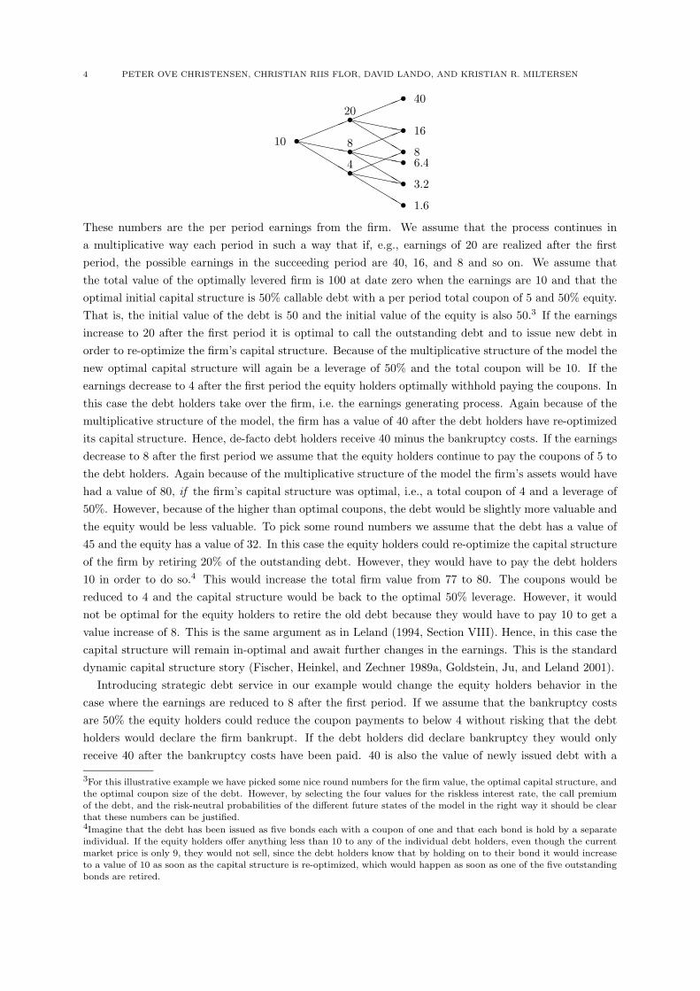
To illustrate this key point of our paper in a discrete setting, consider the following trinomial modelof a firm’s earnings process:
1This iterative procedure gives a solution to the bargaining game which is similar in spirit to the finite number of sequential
offers refinement of the Nash equilibria in the Rubinstein bargaining game (Rubinstein 1982, Rubinstein 1987).2This simple split mimics a reduced form version of the standard Nash bargaining game solution concept.
4 PETER OVE CHRISTENSEN, CHRISTIAN RIIS FLOR, DAVID LANDO, AND KRISTIAN R. MILTERSEN
10 ������
�������
���
�
�
�
20
8
4
�����
�������
��������
�������
���
�����
�������
���
�
�
�
�
�
�
40
16
86.4
3.2
1.6
These numbers are the per period earnings from the firm. We assume that the process continues ina multiplicative way each period in such a way that if, e.g., earnings of 20 are realized after the firstperiod, the possible earnings in the succeeding period are 40, 16, and 8 and so on. We assume thatthe total value of the optimally levered firm is 100 at date zero when the earnings are 10 and that theoptimal initial capital structure is 50% callable debt with a per period total coupon of 5 and 50% equity.That is, the initial value of the debt is 50 and the initial value of the equity is also 50.3 If the earningsincrease to 20 after the first period it is optimal to call the outstanding debt and to issue new debt inorder to re-optimize the firm’s capital structure. Because of the multiplicative structure of the model thenew optimal capital structure will again be a leverage of 50% and the total coupon will be 10. If theearnings decrease to 4 after the first period the equity holders optimally withhold paying the coupons. Inthis case the debt holders take over the firm, i.e. the earnings generating process. Again because of themultiplicative structure of the model, the firm has a value of 40 after the debt holders have re-optimizedits capital structure. Hence, de-facto debt holders receive 40 minus the bankruptcy costs. If the earningsdecrease to 8 after the first period we assume that the equity holders continue to pay the coupons of 5 tothe debt holders. Again because of the multiplicative structure of the model the firm’s assets would havehad a value of 80, if the firm’s capital structure was optimal, i.e., a total coupon of 4 and a leverage of50%. However, because of the higher than optimal coupons, the debt would be slightly more valuable andthe equity would be less valuable. To pick some round numbers we assume that the debt has a value of45 and the equity has a value of 32. In this case the equity holders could re-optimize the capital structureof the firm by retiring 20% of the outstanding debt. However, they would have to pay the debt holders10 in order to do so.4 This would increase the total firm value from 77 to 80. The coupons would bereduced to 4 and the capital structure would be back to the optimal 50% leverage. However, it wouldnot be optimal for the equity holders to retire the old debt because they would have to pay 10 to get avalue increase of 8. This is the same argument as in Leland (1994, Section VIII). Hence, in this case thecapital structure will remain in-optimal and await further changes in the earnings. This is the standarddynamic capital structure story (Fischer, Heinkel, and Zechner 1989a, Goldstein, Ju, and Leland 2001).
Introducing strategic debt service in our example would change the equity holders behavior in thecase where the earnings are reduced to 8 after the first period. If we assume that the bankruptcy costsare 50% the equity holders could reduce the coupon payments to below 4 without risking that the debtholders would declare the firm bankrupt. If the debt holders did declare bankruptcy they would onlyreceive 40 after the bankruptcy costs have been paid. 40 is also the value of newly issued debt with a
3For this illustrative example we have picked some nice round numbers for the firm value, the optimal capital structure, andthe optimal coupon size of the debt. However, by selecting the four values for the riskless interest rate, the call premium
of the debt, and the risk-neutral probabilities of the different future states of the model in the right way it should be clear
that these numbers can be justified.4Imagine that the debt has been issued as five bonds each with a coupon of one and that each bond is hold by a separateindividual. If the equity holders offer anything less than 10 to any of the individual debt holders, even though the currentmarket price is only 9, they would not sell, since the debt holders know that by holding on to their bond it would increaseto a value of 10 as soon as the capital structure is re-optimized, which would happen as soon as one of the five outstandingbonds are retired.
DYNAMIC CAPITAL STRUCTURE WITH CALLABLE DEBT AND DEBT RENEGOTIATIONS 5
coupon of 4 when the earnings is 8. But the debt holder’s original claim is worth more than 40 since itstill has a higher principal and a higher contract coupon. Hence, the debt holders would still be betteroff by not declaring bankruptcy if the equity holders reduced the coupon to 4. This is the strategic debtservice story (Anderson and Sundaresan 1996, Mella-Barral and Perraudin 1997).
Alternatively, the capital structure of the firm could be re-optimized permanently, which we believeis much more common in the real world than period-by-period coupon squeezing. The value of the firmwith a re-optimized capital structure is 80 and hence debt and equity holders do have a common interestin re-optimizing the capital structure. The question, however, is how the debt and equity holders shouldsplit this value. Inspired by the strategic debt service models one could argue that by threatening towithhold the coupons, the equity holders can get away with only paying the debt holders 40 and keepingthe rest of the 80 for themselves. However, since this is a bargaining game the other extreme namelythat the debt holders require all 80 in order not to declare bankruptcy is equally plausible. Hence, anysplit in which the equity holders receive 40γ and the debt holders receive 80 − 40γ, for γ ∈ [0, 1], canbe justified. Had the bankruptcy costs been 40% instead of 50%, the equity holders cannot squeeze thedebt holders down to less than 48. In this case only splits in which the equity holders receive 32γ andthe debt holders receive 80 − 32γ, for γ ∈ [0, 1], are possible.5 The point of our paper is that, if thecapital structure of the firm should be permanently re-optimized, the above arguments are incomplete.The debt holders would realize that the equity holders’ threat of withholding the coupons is non-credible.If the equity holders were faced with the alternative of withholding the coupons or to continue payingthe coupons in full, they would choose to continue paying the coupons since this gives them a value of32 whereas withholding the coupons would give them a value of zero. Hence, if the debt holders and theequity holders cannot come to an agreement of re-optimizing the firms capital structure, the alternativeis not that the the firm goes bankrupt, but rather it is that the equity holders continue to pay the originalcoupons and that the firm survives. That is, the only thing the debt and equity holders need to bargainabout is the gain in total firm value from re-optimizing the capital structure, i.e., the difference betweena firm value of 80 and a firm value of 77. Hence, the possible value splits can be reduced to the onesin which the equity holders receive 32 + 3γ and the debt holders receive 45 + 3(1 − γ), for γ ∈ [0, 1].Note that this is independent of the size of the bankruptcy costs. Hence, the strategic debt serviceargument can both under- and overestimate the fraction of the split that the debt holders must have asa minimum in a capital structure renegotiation game. This looks like a minor extension of the strategicdebt service model but it is complicated by the fact that the value of the firm, if the equity holderscontinue to pay the existing coupons, also includes the value of renegotiating the split of a gain from are-optimization of the capital structure at a different earnings value. This fact has been ignored in ourillustrative example since we just took the firm values of 77 from the model before any renegotiationswere allowed. Our full model do take that into account and at the same time endogenously, consistently,and simultaneously determine the firm value, the optimal capital structure, the optimal coupon size ofthe debt, and the optimal actions of the equity holders including when to propose a debt restructuringand what to propose in a continuous-time continuous-state-space setting.
In the literature there are a lot of other good explanations for why firms choose a specific capitalstructure. There may be many plausible reasons why it is unrealistic to assume a symmetric informationstructure as we have done in our model. The asymmetric information literature is full of explanations
5For this simple example we have ignored the fact that changing the bankruptcy costs would change the initial price of thedebt and therefore the initial optimal capital structure, the optimal coupon size, etc. However, this is only for illustrativepurpose.
6 PETER OVE CHRISTENSEN, CHRISTIAN RIIS FLOR, DAVID LANDO, AND KRISTIAN R. MILTERSEN
different from our explanation. Our explanation basically says that the firm’s capital structure is deter-mined by counterbalancing the tax advantage to debt with costs of debt restructuring or costs of financialdistress whereas the asymmetric information literature includes agency costs and signaling issues. Myersand Majluf (1984) argue that agency costs (cf. also Jensen and Meckling 1976) can lead to the so-calledpecking order theory of different capital structure choices. This theory, however, is a consequence ofgiving the manager of the firm the wrong incentives. If the manager’s incentives can be realigned, bothequity holders and debt holders will ex ante be better off (Dybvig and Zender 1991). In asymmetricinformation models the firm’s capital structure can also be used to credibly signal the value of new in-vestment projects and other variables that the insiders of the firm have better information about thando the outside investors. An example of this type of model is Brennan and Kraus (1987). Going beyondasymmetric information models also behavioral finance models and bounded rationality models can givenew explanations and insight to why firms’ capital structure is determined the way it is. However, wethink that it is important that we fully understand the simplest model of symmetric information wherethe firm’s capital structure is purely driven by the trade off between the tax advantage to debt and thecosts of restructuring the debt and possible bankruptcy costs. Not until we have exhausted the implica-tions of these assumptions should we try to add another layer of complexity to the model in order to seeif this new layer gives a better explanation of the phenomena we observe in practice.
Within the class of symmetric information dynamic capital structure models our model gives a numberof insights of which we will mention some here.
Goldstein, Ju, and Leland (2001) find that their dynamic capital structure model gives much lowerleverage ratios than static capital structure models, ceteris paribus. By adding debt renegotiations tothe model we find that leverage ratios increase relative to the results of Goldstein, Ju, and Leland (2001)approximately back to the level of the static capital structure models such as Leland (1994). Moreover,the introduction of debt renegotiations increases the tax advantage to debt by 50% relative to a dynamiccapital structure model with no debt renegotiation for realistic parameter values.
A very useful insight from Kane, Marcus, and McDonald (1985) and Fischer, Heinkel, and Zechner(1989a) is that by no-arbitrage the unlevered firm value does not exist as a traded security and thereforewe do not have any drift restrictions on this process. Our analysis supports this insight all though wereinterpret the equilibrium argument in the Fischer-Heinkel-Zechner model. Goldstein, Ju, and Leland(2001) are not willing to accept this idea that the unlevered firm value does not exist as a traded security,and use Microsoft, which has a leverage of practically zero, as a counterexample. However, for highgrowth firms like Microsoft our model predicts a capital structure of almost no debt and, hence, for thesetypes of firms the optimally levered firm value and the unlevered firm values are almost the same. So thecounterexample of Goldstein, Ju, and Leland (2001) does not really have any consequence.
Our model gives a simple explanation of the violation of the absolute priority rule for firms in financialdistress, which is a very well documented empirical observation (Weiss 1990, Eberhart, Moore, andRoenfeldt 1990, Betker 1995). Basically, on the equilibrium path it is perfectly rational for the debtholders to accept a restructuring proposal from the equity holders which leaves some value to the equityholders even though the debt holders do not get their full principal back. The reason why the debtholders do accept such a proposal is that the alternative if they reject the equity holders’ proposal is notnecessarily an immediate liquidation of the firm. In most cases the equity holders would continue to paythe existing coupons until the conditions become even worse before eventually withholding the couponsand de facto forcing the firm into bankruptcy. Since the value of the debt in this alternative situation islower than the value the debt holders get if they accept the equity holders’ proposal, they are willing toaccept the proposal even though the equity holders also get a piece of the pie.

DYNAMIC CAPITAL STRUCTURE WITH CALLABLE DEBT AND DEBT RENEGOTIATIONS 7
Finally, our model can be used to question the remarkably small empirically observed bankruptcycosts that are reported in many studies (Warner 1977, Weiss 1990). Suppose the bankruptcy costs areestimated as the proceeds from selling the liquidated firm’s assets or the sum of the prices of the firm’sdebt and equity after recovering from chapter 11 minus the sum of the firm’s debt and equity pricesjust prior to entering chapter 11. In a symmetric information model like ours, the time as well as alldirect and indirects costs of bankruptcy are perfectly anticipated by the investors and therefore alreadyincorporated in the pre chapter 11 prices of the firm’s debt and equity. The post chapter 11 prices stillincorporate all indirect bankruptcy costs such as the loss of skilled employees and the loss of customeras well as supplier confidence, etc. since these costs are borne by the new firm. The direct bankruptcycosts are borne by the old debt and equity holders and are therefore not included in the post chapter 11prices. Hence, this method of estimating the bankruptcy costs only gives an estimate of the true directbankruptcy costs.
The paper is organized as follows. In section 2 we set up the framework of our EBIT based model.We then formulate a benchmark model with no possibilities for debt term renegotiations in section 3.In section 4 we introduce the first simple type of debt renegotiations as an ex ante determined split ofthe firm value. We attempt to improve on this simple type of debt renegotiation in section 5, where wetry to design the debt restructuring proposal in such a way that the debt holders would never reject theoffer. However, this proposal requires knowledge of the values of debt and equity if the debt holders doreject the debt restructuring offer. Unfortunately, these off-the-equilibrium-path values cannot be derivedfrom the usual solution method. In section 6 we present an iterative solution method that is capableof deriving these off-the-equilibrium-path values. In section 7 we make some comparative statics of ourmodel. In section 8 we discuss Fischer, Heinkel, and Zechner (1989a) and Goldstein, Ju, and Leland(2001) in relation to our model. Finally, we conclude in section 9. Appendices A and B contains the finerdetails of our fixed point solution method.
2. Dynamic Capital Structure Models
We model a firm run by equity holders, which has issued a single class of callable perpetual corporatedebt with a fixed instantaneous coupon rate, C. The call feature of debt allows equity holders to betterexploit the tax advantage to debt by increasing the amount of outstanding debt (and thereby the couponpayment rate) when earnings increase. For tractability, the capital structure is limited to a single class ofdebt. That is, we only allow the amount of outstanding debt to be increased by calling all of the existingdebt and issuing new debt.6 Debt is called at a premium and there is a cost of issuing new debt whichis proportional to the principal.
When earnings decrease, equity holders and debt holders have a common interest in restructuring thedebt to avoid bankruptcy costs. A key issue is how to distribute the value of the firm between equityholders and debt holders when this restructuring occurs.
The dynamic adjustment of the capital structure through an infinite series of calls and renegotiationsof debt imply that the firm will, in fact, never go bankrupt. Compared to most of the earlier (static)models in the literature, such as the models by Black and Cox (1976), Leland (1994), and Francois andMorellec (2002) where the debt and equity values are known when the bankruptcy and call boundarieshave been hit, the dynamic adjustment in our model leads to a fixed-point problem when solving forthe initial values of debt and equity. That is, we have no exogenously given boundary conditions. The
6Otherwise, the incentive of the equity holders to sequentially increase the outstanding debt by issuing new debt with thesame seniority and thereby diluting the existing debt will lead to a market break down de facto making it impossible forthe firm to borrow at all.
8 PETER OVE CHRISTENSEN, CHRISTIAN RIIS FLOR, DAVID LANDO, AND KRISTIAN R. MILTERSEN
boundary conditions needed to solve for the initial values of debt and equity depend on the values of debtand equity after the restructuring. But these in turn depend on the optimal capital structure chosen afterthe restructuring. This fixed-point problem has already been studied in Kane, Marcus, and McDonald(1985), Fischer, Heinkel, and Zechner (1989a), and Goldstein, Ju, and Leland (2001), but as we will see,their fixed-point argument does not give the off-the-equilibrium-path values of debt and equity at thelower boundary, which are needed to determine the relative bargaining power between the debt holdersand the equity holders in the renegotiation phase.
The firm is governed by an exogenously given underlying state variable, ξ, which is the firm’s instan-taneous earnings before interest and tax payments (EBIT). The equity holders receive the remainingearnings from the firm after the coupons have been paid to the debt holders and corporate taxes havebeen paid to the tax authorities.7 Following Goldstein, Ju, and Leland (2001), we call ξ the EBIT processand assume that it follows a geometric Brownian motion under the pricing measure Q, i.e.8
(1) dξt = ξtµdt + ξtσdWt,
with a given starting point, ξ0. Here µ and σ are constants parameterizing drift and volatility and W isa standard Brownian motion under the measure, Q. We can think of the origin of the EBIT process, ξ,as the cash flow process generated by a production technology initially owned by an entrepreneur. Theentrepreneur has the option to create a firm (at a certain cost) based on the EBIT process by issuingequity and (callable perpetual) debt.
Moreover, assume that the riskless interest rate, r, in the economy is constant. Since there are taxeson interest income, however, this is not the discount rate used for pricing under the pricing measureQ. Let τi denote the tax rate on interest income in the hands of investors. The discount rate is then(1 − τi)r. This reflects an assumption that not only is interest income taxed at the rate of τi, but thereis also a tax subsidy at the rate of τi associated with interest expenses. Hence, thinking in terms ofdynamic replication of contingent claims, the effective interest rate paid on the money market accountused for borrowing in the replicating portfolio is (1 − τi)r. That is, the price of the replicating portfoliois computed using the after-tax riskless rate. We assume throughout that µ < (1 − τi)r, since otherwisethe cash flows generated from the EBIT process will not have a finite market value.
The market value corresponding to the EBIT process is, at any given date, the total value of theoptimal mix of debt and equity that can be issued based on this EBIT process less the costs of obtainingit (Kane, Marcus, and McDonald 1985). This value will, of course, reflect the advantages and drawbacksof issuing debt including corporate tax savings as well as personal interest and dividend tax payments,and potential bankruptcy costs (Kane, Marcus, and McDonald 1984). This value process is similar to theunlevered firm value process, A, in Fischer, Heinkel, and Zechner (1989a). Note that we do not assumethat any of these two processes (neither the value of the unlevered firm, A, nor the EBIT process, ξ)are price processes of traded securities. Hence, we do not have any no-arbitrage restrictions that giveus the drift of A and ξ under the pricing measure. However, we do assume that there exist a uniquepricing measure denoted Q. That is, we assume that there exists traded securities such that any new
7In general, tax payments can be negative if the coupon rate is higher than the EBIT. In real life this does not lead to a
symmetric tax refund. To mimic this friction the tax refunds will be reduced to a fraction, ε, of the original tax refund inour model.8Since we are working with an infinite time horizon we do not want to use the term ‘equivalent martingale measure’ for Q
because with an infinite time horizon the usual Girsanov measure transformation using the drift does not give an equivalentmeasure. As long as we do not say anything about the EBIT process behavior under the physical measure and how theexistence of Q is related to no arbitrage under the physical measure we are on safe ground. Hence, we just take equation (1)
as a definition.

DYNAMIC CAPITAL STRUCTURE WITH CALLABLE DEBT AND DEBT RENEGOTIATIONS 9
claim that we may want to introduce can be dynamically replicated by already existing traded securitiesand therefore priced.9
In section 8 we will return to how the drift, µ, of the EBIT process under the pricing measure canbe determined implicitly if we have simultaneous observations of the EBIT process, ξ, and some valueprocess of a traded security based on the EBIT process, e.g. the value process of the equity of the firm.
In our model we consider different ways of restructuring the firm’s debt. In each case the conditionsdetermining when the restructuring occurs are determined by the so-called restructuring policy. Therestructuring policy is parameterized by two boundaries, the renegotiation (or bankruptcy) boundary,
¯ξ,
and the call of debt boundary, ξ. That is, when ξ reaches the lower boundary,¯ξ, the debt is renegotiated
(or the firm is declared bankrupt) and when ξ reaches the upper boundary, ξ, the debt is called. Obviously,
¯ξ < ξ0 < ξ. These boundaries will later be derived endogenously by incentive compatibility constraints,but for now they are exogenously given.
The claims on the EBIT process we consider, e.g. debt and equity, will be time-homogeneous claims,in the sense that they do not have a fixed maturity. The payoffs depend only on the current level of ξ
and the level of ξ when the debt and equity was issued. Therefore, we denote the price at any givendate t when the EBIT process is ξt of debt and equity issued at some date s ≤ t when the EBIT processwas ξs, provided that the EBIT process {ξu}u∈[s,t] in the time period [s, t) has stayed inside the interval(¯ξ, ξ)(= (dξs, uξs)) as D(ξt; ξs) and E(ξt; ξs).
In Appendix A we analyze the debt and equity price functions and derive (cf. equation (34) in Appen-dix A) that both debt and equity are positive homogeneous of degree one in (ξt, ξs). That is,
D(λξt;λξs) = λD(ξt; ξs)(2)
and
E(λξt;λξs) = λE(ξt; ξs),(3)
for any ξt ∈ [¯ξ, ξ])(= [dξs, uξs]) and λ ∈ R+.10 Note moreover, that this homogeneity property implies
that the restructuring policy (¯ξ, ξ) for each new issue of debt can be written as (dξs, uξs) for some fixed
constants d and u.Furthermore, for notational simplicity note that the initial values of debt and equity at the date when
the debt is issued can be written as
D(ξs; ξs) = ξsD(1; 1) = Dξs
and
E(ξs; ξs) = ξsE(1; 1) = Eξs,
where D and E are constants determined as D = D(1; 1) and E = E(1; 1). Here we have used the positivehomogeneity property from equations (2) and (3).
Debt is issued at par, i.e. the principal of the debt issued at date s with a coupon rate c∗ξs (cf. Part 1of Conjecture A.1 in Appendix A) is D(ξs; ξs). The debt is callable at a premium, λ, at any given laterdate t ≥ s, i.e. the debt can be called (by the equity holders) at any given date t by paying the debt
9The EBIT process, ξ, and the value process, A, of the unlevered firm are not, in general, in the set of traded securitiesthat can be used to dynamically replicate new (derivative) securities which are functions of the EBIT process.10Note that we have assumed that the EBIT process {ξu}u∈[s,t] in the time period [s, t) has stayed inside the interval
(dξs, uξs). Hence, if ξt ∈ {dξs, uξs}, we know that it is the first time since date s that it hits one of the boundaries. Thus,
we can still use the result from equation (34).
10 PETER OVE CHRISTENSEN, CHRISTIAN RIIS FLOR, DAVID LANDO, AND KRISTIAN R. MILTERSEN
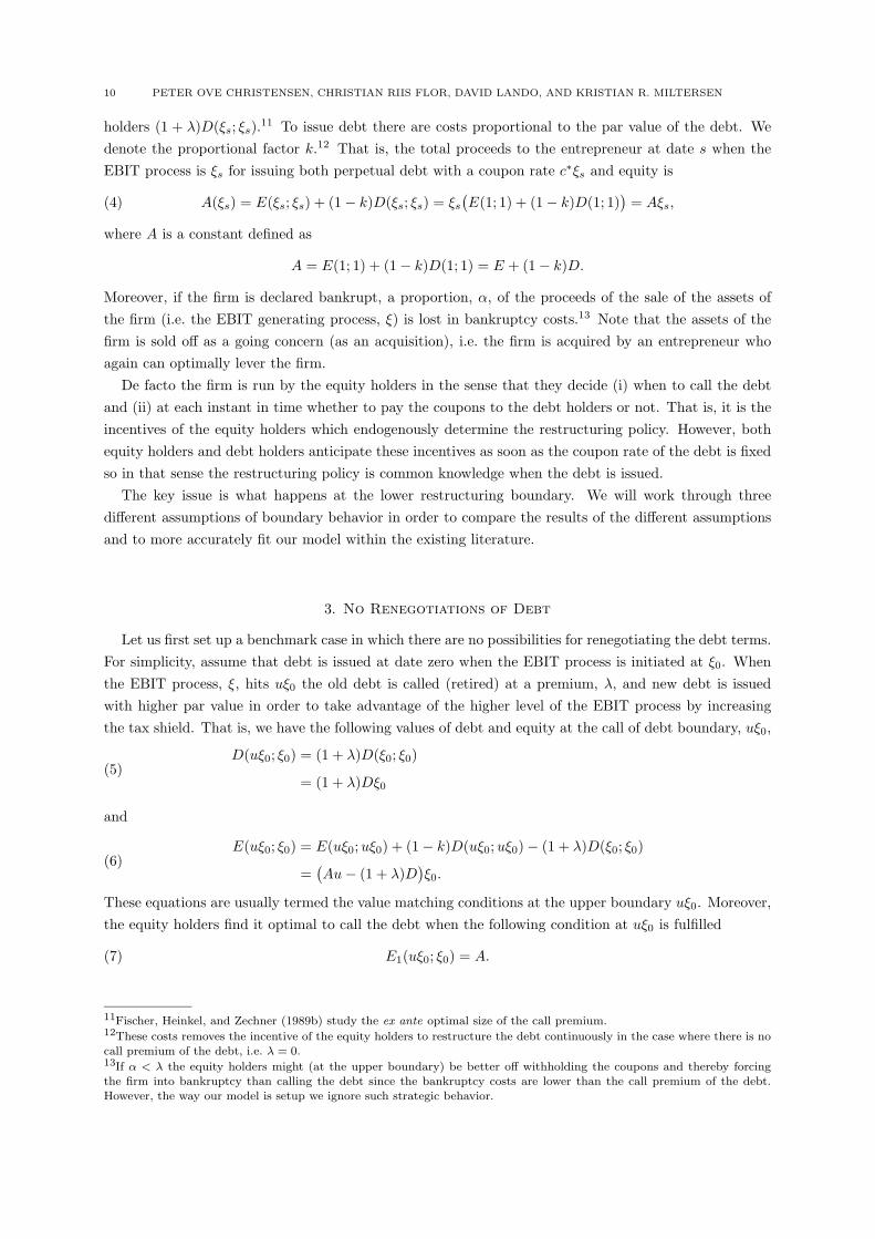
holders (1 + λ)D(ξs; ξs).11 To issue debt there are costs proportional to the par value of the debt. Wedenote the proportional factor k.12 That is, the total proceeds to the entrepreneur at date s when theEBIT process is ξs for issuing both perpetual debt with a coupon rate c∗ξs and equity is
(4) A(ξs) = E(ξs; ξs) + (1 − k)D(ξs; ξs) = ξs
(E(1; 1) + (1 − k)D(1; 1)
)= Aξs,
where A is a constant defined as
A = E(1; 1) + (1 − k)D(1; 1) = E + (1 − k)D.
Moreover, if the firm is declared bankrupt, a proportion, α, of the proceeds of the sale of the assets ofthe firm (i.e. the EBIT generating process, ξ) is lost in bankruptcy costs.13 Note that the assets of thefirm is sold off as a going concern (as an acquisition), i.e. the firm is acquired by an entrepreneur whoagain can optimally lever the firm.
De facto the firm is run by the equity holders in the sense that they decide (i) when to call the debtand (ii) at each instant in time whether to pay the coupons to the debt holders or not. That is, it is theincentives of the equity holders which endogenously determine the restructuring policy. However, bothequity holders and debt holders anticipate these incentives as soon as the coupon rate of the debt is fixedso in that sense the restructuring policy is common knowledge when the debt is issued.
The key issue is what happens at the lower restructuring boundary. We will work through threedifferent assumptions of boundary behavior in order to compare the results of the different assumptionsand to more accurately fit our model within the existing literature.
3. No Renegotiations of Debt
Let us first set up a benchmark case in which there are no possibilities for renegotiating the debt terms.For simplicity, assume that debt is issued at date zero when the EBIT process is initiated at ξ0. Whenthe EBIT process, ξ, hits uξ0 the old debt is called (retired) at a premium, λ, and new debt is issuedwith higher par value in order to take advantage of the higher level of the EBIT process by increasingthe tax shield. That is, we have the following values of debt and equity at the call of debt boundary, uξ0,
D(uξ0; ξ0) = (1 + λ)D(ξ0; ξ0)
= (1 + λ)Dξ0
(5)
and
E(uξ0; ξ0) = E(uξ0;uξ0) + (1 − k)D(uξ0;uξ0) − (1 + λ)D(ξ0; ξ0)
=(Au − (1 + λ)D
)ξ0.
(6)
These equations are usually termed the value matching conditions at the upper boundary uξ0. Moreover,the equity holders find it optimal to call the debt when the following condition at uξ0 is fulfilled
(7) E1(uξ0; ξ0) = A.
11Fischer, Heinkel, and Zechner (1989b) study the ex ante optimal size of the call premium.12These costs removes the incentive of the equity holders to restructure the debt continuously in the case where there is nocall premium of the debt, i.e. λ = 0.13If α < λ the equity holders might (at the upper boundary) be better off withholding the coupons and thereby forcingthe firm into bankruptcy than calling the debt since the bankruptcy costs are lower than the call premium of the debt.However, the way our model is setup we ignore such strategic behavior.
DYNAMIC CAPITAL STRUCTURE WITH CALLABLE DEBT AND DEBT RENEGOTIATIONS 11
Here E1 denotes the partial derivative of the equity price function (ξ, ξ0) �→ E(ξ, ξ0) with respect to thefirst variable, ξ.14 This condition is usually termed the smooth pasting condition at the upper boundaryuξ0.15
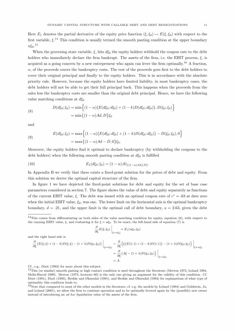
When the governing state variable, ξ, hits dξ0 the equity holders withhold the coupon rate to the debtholders who immediately declare the firm bankrupt. The assets of the firm, i.e. the EBIT process, ξ, isacquired as a going concern by a new entrepreneur who again can lever the firm optimally.16 A fraction,α, of the proceeds covers the bankruptcy costs. The rest of the proceeds goes first to the debt holders tocover their original principal and finally to the equity holders. This is in accordance with the absolutepriority rule. However, because the equity holders have limited liability, in most bankruptcy cases, thedebt holders will not be able to get their full principal back. This happens when the proceeds from thesales less the bankruptcy costs are smaller than the original debt principal. Hence, we have the followingvalue matching conditions at dξ0
D(dξ0; ξ0) = min{
(1 − α)(E(dξ0; dξ0) + (1 − k)D(dξ0; dξ0)
),D(ξ0; ξ0)
}
= min{(1 − α)Ad,D
}ξ0
(8)
and
E(dξ0; ξ0) = max{
(1 − α)(E(dξ0; dξ0) + (1 − k)D(dξ0; dξ0)
) − D(ξ0; ξ0), 0}
= max{(1 − α)Ad − D, 0
}ξ0.
(9)
Moreover, the equity holders find it optimal to declare bankruptcy (by withholding the coupons to thedebt holders) when the following smooth pasting condition at dξ0 is fulfilled
(10) E1(dξ0; ξ0) = (1 − α)A1{(1−α)Ad≥D}.
In Appendix B we verify that there exists a fixed-point solution for the prices of debt and equity. Fromthis solution we derive the optimal capital structure of the firm.
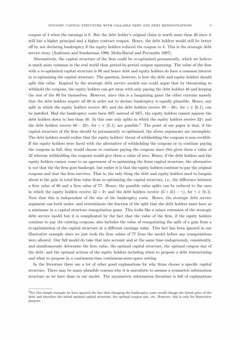
In figure 1 we have depicted the fixed-point solutions for debt and equity for the set of base caseparameters considered in section 7. The figure shows the value of debt and equity separately as functionsof the current EBIT value, ξ. The debt was issued with an optimal coupon rate of c∗ = .63 at date zerowhen the initial EBIT value, ξ0, was one. The lower limit on the horizontal axis is the optimal bankruptcyboundary, d = .21, and the upper limit is the optimal call of debt boundary, u = 2.63, given the debt
14This comes from differentiating on both sides of the value matching condition for equity, equation (6), with respect tothe running EBIT value, ξ, and evaluating it for ξ = uξ0. To be exact, the left-hand side of equation (7) is
∂
∂ξE(ξ; ξ0)
∣∣∣∣ξ=uξ0
= E1(uξ0; ξ0)
and the right hand side is
∂
∂ξ
(E(ξ; ξ) + (1 − k)D(ξ; ξ) − (1 + λ)D(ξ0; ξ0)
) ∣∣∣∣ξ=uξ0
=∂
∂ξ
(ξ(E(1; 1) + (1 − k)D(1; 1)
) − (1 + λ)D(ξ0; ξ0)) ∣∣∣∣
ξ=uξ0
=∂
∂ξ
(Aξ − (1 + λ)D(ξ0; ξ0)
) ∣∣∣∣ξ=uξ0
= A.
Cf., e.g., Dixit (1993) for more about this subject.15This (or similar) smooth pasting or high contact condition is used throughout the literature (Merton 1973, Leland 1994,Mella-Barral 1999). Merton (1973, footnote 60) is the only one giving an argument for the validity of this condition. Cf.Dixit (1991), Dixit (1993), Brekke and Øksendal (1991), and Brekke and Øksendal (1994) for explanations of what type ofoptimality this condition leads to.16Note that compared to most of the other models in the literature, cf. e.g. the models by Leland (1994) and Goldstein, Ju,and Leland (2001), we allow the firm to continue operation and to be optimally levered again by the (possible) new ownerinstead of introducing an ad hoc liquidation value of the assets of the firm.
12 PETER OVE CHRISTENSEN, CHRISTIAN RIIS FLOR, DAVID LANDO, AND KRISTIAN R. MILTERSEN
0.5 1 1.5 2 2.5
10
20
30
40
50
60
ξ
c∗
E(ξ; ξ) + D(ξ; ξ)
E(ξ; 1) + D(ξ; 1)E(ξ; 1)
D(ξ; 1)
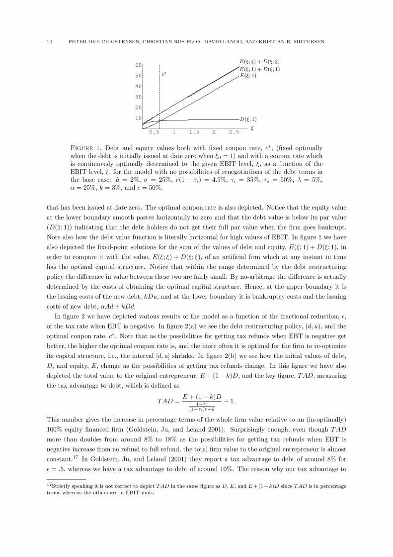
Figure 1. Debt and equity values both with fixed coupon rate, c∗, (fixed optimallywhen the debt is initially issued at date zero when ξ0 = 1) and with a coupon rate whichis continuously optimally determined to the given EBIT level, ξ, as a function of theEBIT level, ξ, for the model with no possibilities of renegotiations of the debt terms inthe base case: µ = 2%, σ = 25%, r(1 − τi) = 4.5%, τi = 35%, τe = 50%, λ = 5%,α = 25%, k = 3%, and ε = 50%.
that has been issued at date zero. The optimal coupon rate is also depicted. Notice that the equity valueat the lower boundary smooth pastes horizontally to zero and that the debt value is below its par value(D(1; 1)) indicating that the debt holders do not get their full par value when the firm goes bankrupt.Note also how the debt value function is literally horizontal for high values of EBIT. In figure 1 we havealso depicted the fixed-point solutions for the sum of the values of debt and equity, E(ξ; 1) + D(ξ; 1), inorder to compare it with the value, E(ξ; ξ) + D(ξ; ξ), of an artificial firm which at any instant in timehas the optimal capital structure. Notice that within the range determined by the debt restructuringpolicy the difference in value between these two are fairly small. By no-arbitrage the difference is actuallydetermined by the costs of obtaining the optimal capital structure. Hence, at the upper boundary it isthe issuing costs of the new debt, kDu, and at the lower boundary it is bankruptcy costs and the issuingcosts of new debt, αAd + kDd.
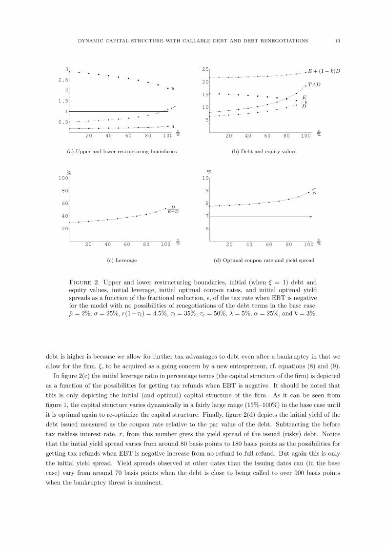
In figure 2 we have depicted various results of the model as a function of the fractional reduction, ε,of the tax rate when EBT is negative. In figure 2(a) we see the debt restructuring policy, (d, u), and theoptimal coupon rate, c∗. Note that as the possibilities for getting tax refunds when EBT is negative getbetter, the higher the optimal coupon rate is, and the more often it is optimal for the firm to re-optimizeits capital structure, i.e., the interval [d, u] shrinks. In figure 2(b) we see how the initial values of debt,D, and equity, E, change as the possibilities of getting tax refunds change. In this figure we have alsodepicted the total value to the original entrepreneur, E + (1− k)D, and the key figure, TAD, measuringthe tax advantage to debt, which is defined as
TAD =E + (1 − k)D
1−τe
(1−τi)r−µ
− 1.
This number gives the increase in percentage terms of the whole firm value relative to an (in-optimally)100% equity financed firm (Goldstein, Ju, and Leland 2001). Surprisingly enough, even though TAD
more than doubles from around 8% to 18% as the possibilities for getting tax refunds when EBT isnegative increase from no refund to full refund, the total firm value to the original entrepreneur is almostconstant.17 In Goldstein, Ju, and Leland (2001) they report a tax advantage to debt of around 8% forε = .5, whereas we have a tax advantage to debt of around 10%. The reason why our tax advantage to
17Strictly speaking it is not correct to depict TAD in the same figure as D, E, and E +(1−k)D since TAD is in percentage
terms whereas the others are in EBIT units.
DYNAMIC CAPITAL STRUCTURE WITH CALLABLE DEBT AND DEBT RENEGOTIATIONS 13
20 40 60 80 100
0.5
1
1.5
2
2.5
3
ε%
u
c∗
d
(a) Upper and lower restructuring boundaries
20 40 60 80 100
5
10
15
20
25
ε%
E + (1 − k)D
TAD
E
D
(b) Debt and equity values
20 40 60 80 100
20
40
60
80
100
ε%
%
DE+D
(c) Leverage
20 40 60 80 100
6
7
8
9
10
ε%
%
c∗D
r
(d) Optimal coupon rate and yield spread
Figure 2. Upper and lower restructuring boundaries, initial (when ξ = 1) debt andequity values, initial leverage, initial optimal coupon rates, and initial optimal yieldspreads as a function of the fractional reduction, ε, of the tax rate when EBT is negativefor the model with no possibilities of renegotiations of the debt terms in the base case:µ = 2%, σ = 25%, r(1−τi) = 4.5%, τi = 35%, τe = 50%, λ = 5%, α = 25%, and k = 3%.
debt is higher is because we allow for further tax advantages to debt even after a bankruptcy in that weallow for the firm, ξ, to be acquired as a going concern by a new entrepreneur, cf. equations (8) and (9).
In figure 2(c) the initial leverage ratio in percentage terms (the capital structure of the firm) is depictedas a function of the possibilities for getting tax refunds when EBT is negative. It should be noted thatthis is only depicting the initial (and optimal) capital structure of the firm. As it can be seen fromfigure 1, the capital structure varies dynamically in a fairly large range (15%–100%) in the base case untilit is optimal again to re-optimize the capital structure. Finally, figure 2(d) depicts the initial yield of thedebt issued measured as the coupon rate relative to the par value of the debt. Subtracting the beforetax riskless interest rate, r, from this number gives the yield spread of the issued (risky) debt. Noticethat the initial yield spread varies from around 80 basis points to 180 basis points as the possibilities forgetting tax refunds when EBT is negative increase from no refund to full refund. But again this is onlythe initial yield spread. Yield spreads observed at other dates than the issuing dates can (in the basecase) vary from around 70 basis points when the debt is close to being called to over 900 basis pointswhen the bankruptcy threat is imminent.
14 PETER OVE CHRISTENSEN, CHRISTIAN RIIS FLOR, DAVID LANDO, AND KRISTIAN R. MILTERSEN
0.5 1 1.5 2 2.5
10
20
30
40
50
ξ
c∗E(ξ; ξ) + D(ξ; ξ)
E(ξ; 1) + D(ξ; 1)
E(ξ; 1)
D(ξ; 1)
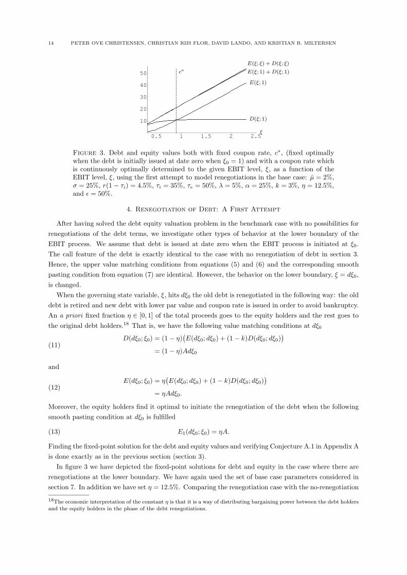
Figure 3. Debt and equity values both with fixed coupon rate, c∗, (fixed optimallywhen the debt is initially issued at date zero when ξ0 = 1) and with a coupon rate whichis continuously optimally determined to the given EBIT level, ξ, as a function of theEBIT level, ξ, using the first attempt to model renegotiations in the base case: µ = 2%,σ = 25%, r(1 − τi) = 4.5%, τi = 35%, τe = 50%, λ = 5%, α = 25%, k = 3%, η = 12.5%,and ε = 50%.
4. Renegotiation of Debt: A First Attempt
After having solved the debt equity valuation problem in the benchmark case with no possibilities forrenegotiations of the debt terms, we investigate other types of behavior at the lower boundary of theEBIT process. We assume that debt is issued at date zero when the EBIT process is initiated at ξ0.The call feature of the debt is exactly identical to the case with no renegotiation of debt in section 3.Hence, the upper value matching conditions from equations (5) and (6) and the corresponding smoothpasting condition from equation (7) are identical. However, the behavior on the lower boundary,
¯ξ = dξ0,
is changed.When the governing state variable, ξ, hits dξ0 the old debt is renegotiated in the following way: the old
debt is retired and new debt with lower par value and coupon rate is issued in order to avoid bankruptcy.An a priori fixed fraction η ∈ [0, 1] of the total proceeds goes to the equity holders and the rest goes tothe original debt holders.18 That is, we have the following value matching conditions at dξ0
D(dξ0; ξ0) = (1 − η)(E(dξ0; dξ0) + (1 − k)D(dξ0; dξ0)
)= (1 − η)Adξ0
(11)
and
E(dξ0; ξ0) = η(E(dξ0; dξ0) + (1 − k)D(dξ0; dξ0)
)= ηAdξ0.
(12)
Moreover, the equity holders find it optimal to initiate the renegotiation of the debt when the followingsmooth pasting condition at dξ0 is fulfilled
(13) E1(dξ0; ξ0) = ηA.
Finding the fixed-point solution for the debt and equity values and verifying Conjecture A.1 in Appendix Ais done exactly as in the previous section (section 3).
In figure 3 we have depicted the fixed-point solutions for debt and equity in the case where there arerenegotiations at the lower boundary. We have again used the set of base case parameters considered insection 7. In addition we have set η = 12.5%. Comparing the renegotiation case with the no-renegotiation
18The economic interpretation of the constant η is that it is a way of distributing bargaining power between the debt holders
and the equity holders in the phase of the debt renegotiations.
DYNAMIC CAPITAL STRUCTURE WITH CALLABLE DEBT AND DEBT RENEGOTIATIONS 15
10 20 30 40
0.5
1
1.5
2
2.5
3
η%
u
c∗
d
(a) Upper and lower restructuring boundaries
10 20 30 40
5
10
15
20
25
η%
E + (1 − k)D
TADE
D
(b) Debt and equity values
10 20 30 40
20
40
60
80
100
η%
%
DE+D
(c) Leverage
10 20 30 40
6
8
10
12
14
η%
%
c∗D
r
(d) Optimal coupon rate and yield spread
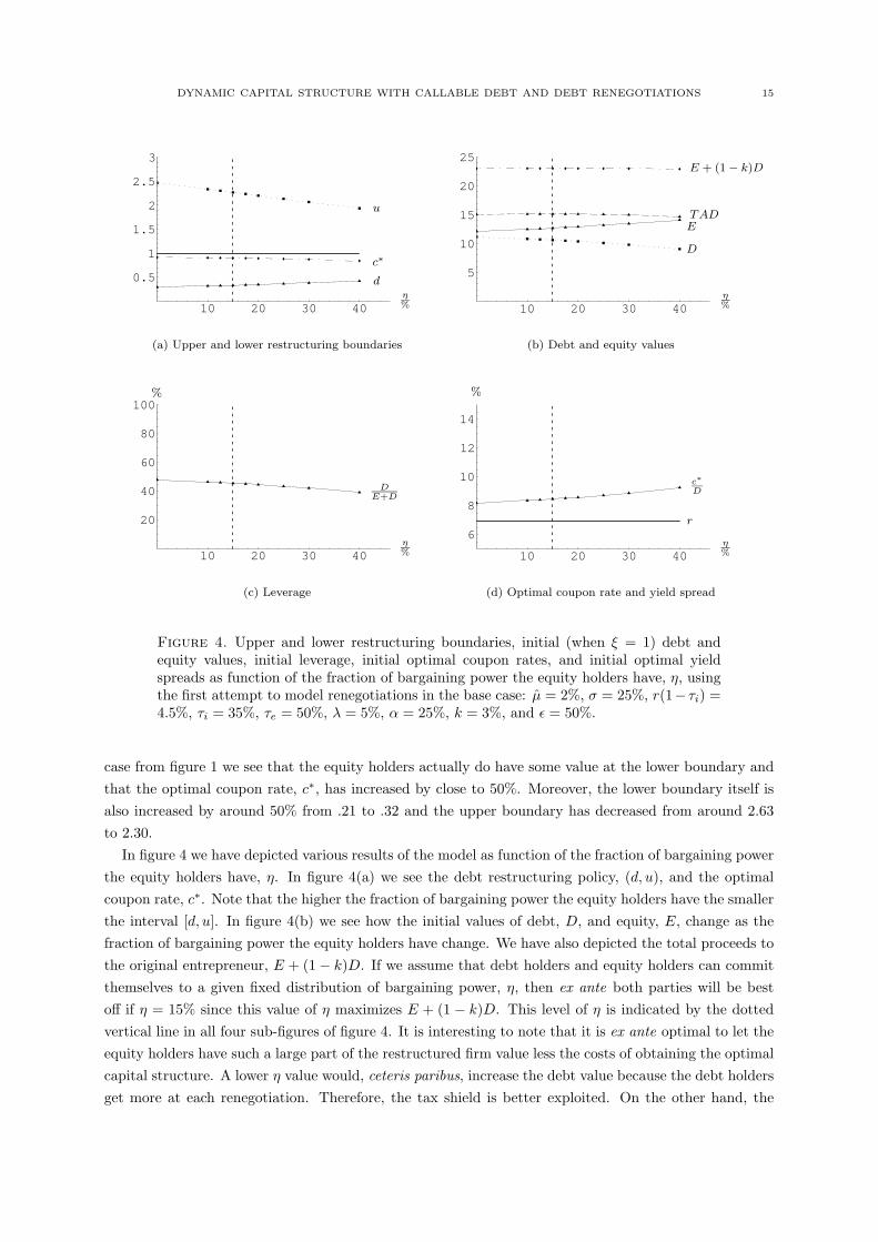
Figure 4. Upper and lower restructuring boundaries, initial (when ξ = 1) debt andequity values, initial leverage, initial optimal coupon rates, and initial optimal yieldspreads as function of the fraction of bargaining power the equity holders have, η, usingthe first attempt to model renegotiations in the base case: µ = 2%, σ = 25%, r(1− τi) =4.5%, τi = 35%, τe = 50%, λ = 5%, α = 25%, k = 3%, and ε = 50%.
case from figure 1 we see that the equity holders actually do have some value at the lower boundary andthat the optimal coupon rate, c∗, has increased by close to 50%. Moreover, the lower boundary itself isalso increased by around 50% from .21 to .32 and the upper boundary has decreased from around 2.63to 2.30.
In figure 4 we have depicted various results of the model as function of the fraction of bargaining powerthe equity holders have, η. In figure 4(a) we see the debt restructuring policy, (d, u), and the optimalcoupon rate, c∗. Note that the higher the fraction of bargaining power the equity holders have the smallerthe interval [d, u]. In figure 4(b) we see how the initial values of debt, D, and equity, E, change as thefraction of bargaining power the equity holders have change. We have also depicted the total proceeds tothe original entrepreneur, E + (1 − k)D. If we assume that debt holders and equity holders can committhemselves to a given fixed distribution of bargaining power, η, then ex ante both parties will be bestoff if η = 15% since this value of η maximizes E + (1 − k)D. This level of η is indicated by the dottedvertical line in all four sub-figures of figure 4. It is interesting to note that it is ex ante optimal to let theequity holders have such a large part of the restructured firm value less the costs of obtaining the optimalcapital structure. A lower η value would, ceteris paribus, increase the debt value because the debt holdersget more at each renegotiation. Therefore, the tax shield is better exploited. On the other hand, the

16 PETER OVE CHRISTENSEN, CHRISTIAN RIIS FLOR, DAVID LANDO, AND KRISTIAN R. MILTERSEN
equity holders get less. Since it is the equity holders who decide when to propose the restructure, a lowerη will postpone a potential restructuring for both low and high EBIT values. This latter effect reducesfirm value because the firm’s capital structure is not re-optimized to exploited the tax shield so often.Hence, the tax shield is exploited less efficiently. These two effects, a static effect demanding a low η anda dynamic effect demanding a high η, counterbalances each other at an η level of .15. In figure 4(c) theinitial leverage ratio in percentage terms is depicted as function of the fraction of bargaining power theequity holders have. As it is seen, the leverage falls as the fraction of bargaining power the equity holdershave increase. Finally figure 4(d) depicts the initial yield of the debt, which have a tendency to increaseas the fraction of bargaining power the equity holders have increase.
The way this renegotiation is setup is quite simple: together the equity holders and the debt holderswill be better off by re-optimizing the capital structure of the firm to the optimal one based on the currentvalue of EBIT. However, there are costs of obtaining this since they have to issue new debt. Still, ifthe current EBIT value is far enough away from the EBIT value at the date when the current capitalstructure was determined the benefits (in form of increased market value of the whole firm) will outweighthe costs of obtaining the optimal capital structure. But this simple renegotiation does not contributemuch to the question of how this gain from the debt restructuring should be split between the originaldebt holders and equity holders. As it is, we just imagine that both equity holders and debt holdershave already put all their old claims on the firm into one pot and forgotten how much each of them havecontributed to the pot. After the re-optimization of the capital structure they start negotiating abouthow to split the pot between them. This is not a very realistic or satisfactory way of thinking of the debtrenegotiation.
We would like to think of the outcome of this debt renegotiation as an agreement between the debtholders and the equity holders made voluntarily in the sense that both parties can reject the renegotiation.As we have set up the model, the initiative to propose the restructuring is with the equity holders sincethe smooth pasting condition is based on the equity value. That is, we can interpret the renegotiationas a one-shot take-it-or-leave-it offer to the debt holders proposed by the equity holders. Since it is theequity holders who time when they make this offer it will of course be beneficial for the equity holders—otherwise they would not have done it. So the equity holders would never like to reject their own debtrestructuring proposal. The question is whether the debt holders would like to accept the proposal ornot. That of course depends on what would happen if they reject the debt restructuring proposal. As afirst attempt we simply assume that the threat of the equity holders is that if the debt holders do notaccept their restructuring proposal, then the equity holders would withhold the coupon rate which againwould trigger an immediate declaration of bankruptcy by the debt holders. If this is a credible threat bythe equity holders, the debt holders would accept the restructuring proposal whenever η ≤ α. (If η > α
the debt holders could get more by declaring the firm bankrupt than by accepting the equity holders’debt restructuring proposal unless the proposal is made for a very high value of ξ.) Hence, as a firstattempt, we assume that η, which reflects the distribution of bargaining power between debt holders andequity holders, is in the interval [0, α].
5. Renegotiation of Debt: A Second Attempt
The problem with our first attempt to model the renegotiation game is that it is not obvious thatthe threat of the equity holders of withholding the coupons if the debt holders reject their restructuringproposal is a credible threat. In fact, it almost never is, because if the debt holders declare the firmbankrupt the equity holders would in most cases get nothing (unless the proposal is made for a fairlyhigh value of ξ so that there would be something left for the equity holders after the bankruptcy costs

DYNAMIC CAPITAL STRUCTURE WITH CALLABLE DEBT AND DEBT RENEGOTIATIONS 17
have been paid and the debt holders have gotten their full principal back). In most cases, it would bebetter for the equity holders to continue paying the original coupon rate (or maybe try to reduce themmarginally as in the strategic debt service models (Anderson and Sundaresan 1996, Mella-Barral andPerraudin 1997))19 and thereby avoiding bankruptcy if their restructuring proposal is rejected by thedebt holders. We would still like to model the renegotiation procedure as if the equity holders make aone-shot take-it-or-leave-it offer to the debt holders. Moreover, the proposal should be made so that it isalways accepted by the debt holders.
We assume that if the debt restructuring proposal is rejected, either the equity holders will continueto pay the existing coupon rate or they will withhold the coupon rate, which leads to an immediatedeclaration of bankruptcy. First let us analyze the situation at the lower boundary, dξ0, which is thepoint where we assume that the equity holders make their restructuring proposal. If the equity holderscontinue to pay the original coupon rate (after a rejection) the equity value is
¯Ec ≡ E(dξ0; ξ0).
On the other hand, if the equity holders withhold the original coupon rate the firm is declared bankruptand the equity value is
¯Eb ≡ max
{(1 − α)Ad − D, 0
}ξ0.
It is the equity holders who determine whether to continue to pay the original coupon rate or to de factodeclare bankruptcy if the restructuring proposal is rejected. Hence, the equity value is the maximum ofthe two alternatives, i.e.
¯Enr ≡ max{
¯Ec,
¯Eb}.
The corresponding value of the debt in case of a rejection of the equity holders’ restructuring proposaldepends on the choice of the equity holders. If the equity holders continue to pay the original couponrate the value of the debt is
¯Dc ≡ D(dξ0; ξ0)
in which case the debt holders are not in a position to force bankruptcy. On the other hand, if theequity holders do not pay the original coupon rate, the debt holders immediately declare bankruptcy.The bankruptcy value of debt is
¯Db ≡ min
{(1 − α)Ad,D
}ξ0.
The choice of whether to declare bankruptcy or to continue to pay the original coupon rate, after thedebt holders have rejected the restructuring proposal, is in the hands of the equity holders. Therefore,the value of the debt is
¯Dnr ≡
¯Dc1{
¯Ec≥
¯Eb} +
¯Db1{
¯Ec<
¯Eb}.
Knowing the value of debt and equity if a debt restructuring offer is rejected, we can compute the gainfrom the debt restructuring as the value of the optimally levered firm less the costs of obtaining theoptimal leverage minus the value the firm would have had if the restructuring proposal was rejected as
(14)¯R = Adξ0 − (
¯Enr +
¯Dnr).
We now assume that this debt restructuring gain,¯R, is distributed between the equity holders and the
debt holders so that the equity holders receives the a priori fixed fraction γ ∈ [0, 1] of this gain and the
19It is not this type of strategic debt service that we pursuit in this model. As already argued in the introduction of thepaper we consider this type of behavior unrealistic as it is not what we observe in practice. Our model is build to capturethe incentives to restructure the entire debt with new principal and new coupon rate so that the equity holders can makea fresh start.
18 PETER OVE CHRISTENSEN, CHRISTIAN RIIS FLOR, DAVID LANDO, AND KRISTIAN R. MILTERSEN
debt holders receive the remaining fraction 1 − γ.20 Hence, the new value matching conditions at thelower boundary, dξ0, are
D(dξ0; ξ0) = (1 − γ)¯R +
¯Dnr(15)
and
E(dξ0; ξ0) = γ¯R +
¯Enr.(16)
The idea behind this new attempt is that it should ensure that both equity holders and debt holders willvoluntarily accept the restructuring proposal since both parties are promised a value which is at least ashigh as the value they would have had if the debt restructuring proposal was rejected. The idea is that if
¯R is non-negative each party get a positive fraction of the gain in addition to their own rejection value.Unfortunately, the equations (15) and (16) does not give a unique distribution of the values of debt andequity in the case where, if the restructuring proposal is rejected, it is optimal to continue paying at theexisting coupon rate. That is, if we assume
¯Ec ≥
¯Eb then
¯Dnr =
¯Dc = D(dξ0; ξ0) and
¯Enr =
¯Ec = E(dξ0; ξ0),
which from equation (14) imply that
¯R = Adξ0 − (
¯Ec +
¯Dc).
But since
¯Ec +
¯Dc = E(dξ0; ξ0) + D(dξ0; ξ0) = Adξ0
at the lower restructuring boundary, we have that
(17)¯R = 0.
However, if¯R = 0 then equations (15) and (16) are vacuous. Hence, we cannot say anything about
how much of Adξ0 to give to the equity holders and how much to give to the debt holders. That is, inthe language of the model in the previous section (section 4), η can be anything in the interval [0, 1].The indeterminacy of the distribution between debt holders and equity holders come from the followingcircularity. Because it is common knowledge when the equity holders make their restructuring proposaland also what they will propose, the debt and equity values at the boundaries just prior to when therestructuring proposal is made are by no-arbitrage determined by how much each party will get afterthe restructuring offer is accepted. But the debt restructuring proposal itself is determined by the valuesof debt and equity if the debt restructuring proposal is not accepted, which in this case is the values ofdebt and equity if we continue with the original coupon rate. These values, however, should include thatthe equity holders will have incentive to make a new debt restructuring proposal in, say, a few seconds.That is, these values must be equal to the values of debt and equity if the debt restructuring proposal isaccepted. This is why we get
¯R = 0. Expressed in another way, our problem is that we are not able to
determine the off-the-equilibrium-path values of debt and equity individually.In the case where
¯Ec <
¯Eb, the model is identical to the model derived in the previous section
(section 4) with η = γα.Hence, our second attempt did not bring us any new aspects to how to endogenously determine the
distribution of Ad between debt holders and equity holders. However, it have highlighted that the problem
20Again the economic interpretation of γ is that it is a way of modeling the distribution of bargaining power between debt
holders and equity holders in the phase of the debt renegotiation.
DYNAMIC CAPITAL STRUCTURE WITH CALLABLE DEBT AND DEBT RENEGOTIATIONS 19
is to determine the off-the-equilibrium-path values of debt and equity individually when ξ0 = 1. That is,E(d; 1) and D(d; 1).
6. Renegotiation of Debt: The Iterative Approach
One way to get the off-the-equilibrium-path values of debt and equity individually is by the followingiterative procedure. Imagine that there are a commonly known finite number, n ∈ N, of options to proposea restructuring of the firm’s debt. Whenever the equity holders make a debt restructuring proposal thisnumber is reduced by one. When there are no more restructuring options left (when n = 0) the onlypossibility at the lower boundary is to declare bankruptcy. This case with no more restructuring optionsleft is exactly our benchmark case, which we have studied extensively in section 3. If we augment ournotation of the value of debt and equity, the incentive compatible restructuring policy parameters, andthe optimal coupon rate parameter with the remaining number of restructuring proposals, we have insection 3 derived the functions D(ξt; ξs, 0) and E(ξt; ξs, 0) giving us the value of debt and equity when thecurrent value of the EBIT process is ξt and the coupon rate of the existing debt is c∗0ξs. In section 3 wehave also derived that the incentive compatible restructuring policy is (d0ξs, u0ξs) and that the optimalcoupon rate to be used at every future restructuring is c∗0 multiplied by the value of the EBIT process atthe date when the new debt is issued.
With this information at hand we have the off-the-equilibrium-path values of debt and equity if thereis one restructuring option left. This is so, because as soon as the equity holders have made the debtrestructuring proposal the last restructuring options is exercised and there are no more options left.Hence, the off-the-equilibrium-path values of debt and equity, i.e., the debt and equity values if thedebt restructuring proposal is rejected are already known from the benchmark case. Thus, we are nowable to derive the value functions of debt and equity, D(·; ·, 1), E(·; ·, 1), the new incentive compatiblerestructuring policy parameters d1 and u1, and the new optimal coupon rate parameter, c∗1. With thisinformation at hand we have the off-the-equilibrium-path values of debt and equity if there are tworestructuring options left.
The idea is to continue this iterative procedure until the debt and equity values, the incentive compat-ible restructuring policy parameters, and the optimal coupon rate parameter converge. In each iterationwe face a problem very similar to the one solved in sections 3 and 4. That is, we have to use ourconjecture-verification argument from appendices A and B in each iteration. To be precise, assume thatwe have the values of debt and equity, D(ξt; ξs, n− 1) and E(ξt; ξs, n− 1), when the current value of theEBIT process is ξt and the coupon rate of the existing debt is c∗n−1ξs and there are n − 1 restructuringoptions left. Our problem is now to find the value functions of debt and equity, D(·; ·, n) and E(·; ·, n),the new incentive compatible restructuring policy parameters, dn and un, and the new optimal couponrate parameter, c∗n, when there are n restructuring options left. To solve that problem we first have tospecify the new value matching and smooth pasting conditions.
The upper value matching and smooth pasting conditions are the same as used in all the previouscases. That is, we have the following value matching conditions for debt and equity at the call of debtboundary, unξ0,
D(unξ0; ξ0, n) = (1 + λ)D(ξ0; ξ0, n)
= (1 + λ)Dnξ0
(18)

20 PETER OVE CHRISTENSEN, CHRISTIAN RIIS FLOR, DAVID LANDO, AND KRISTIAN R. MILTERSEN
and
E(unξ0; ξ0, n) = E(unξ0;unξ0, n) + (1 − k)D(unξ0;unξ0, n) − (1 + λ)D(ξ0; ξ0, n)
=(Anun − (1 + λ)Dn
)ξ0.
(19)
Moreover, the equity holders find it optimal to call the debt when the following smooth pasting conditionat uξ0 is fulfilled
(20) E1(unξ0; ξ0, n) = An.
At the lower boundary we will use the ideas from the model in the previous section (section 5). Thatis, we first have to calculate the gain from restructuring. If the equity holders choose to continue to paythe existing coupon rate (after a rejection) their equity value will be
¯Ec
n ≡ E(dnξ0;c∗n
c∗n−1
ξ0, n − 1) = E(dn;c∗n
c∗n−1
, n − 1)ξ0.
As soon as the equity holders have proposed the restructuring, one renegotiation option is lost. Therefore,in order to calculate the value of continuing with the existing coupon rate we should use the alreadycalculated equity value function for n−1 remaining renegotiation options. Moreover, the existing couponrate is C∗
n = c∗nξ0. So the question is, at which EBIT level, ξ, would it had been optimal (with onlyn − 1 renegotiations options left) to choose the same coupon rate, C∗
n. Since the optimal coupon rateparameter (with only n − 1 renegotiations options left) is c∗n−1 the equity value of continuing with theexisting coupon rate must be calculated as if the debt has been issued when the EBIT value, ξ, was
c∗nc∗n−1
ξ0 because that would have given an optimal coupon rate of21
c∗n−1
c∗nc∗n−1
ξ0 = c∗nξ0 = C∗n.
Similarly, because one of the renegotiation options is lost, the bankruptcy value for the equity holders is
¯Eb
n ≡ max{(1 − α)
(E(dnξ0; dnξ0, n − 1) + (1 − k)D(dnξ0; dnξ0, n − 1)
) − D(ξ0; ξ0, n), 0}
= max{(1 − α)An−1dn − Dn, 0
}ξ0.
Since it is still the equity holders who determine whether to continue to pay the original coupon rate orto de facto declare bankruptcy, if the restructuring proposal is rejected, the equity value is the maximumof the two alternatives, i.e.
¯Enr
n ≡ max{¯Ec
n,¯Eb
n}.The corresponding value of the debt in case of a rejection of the equity holders’ restructuring proposaldepends on the choice of the equity holders. If the equity holders continue to pay the coupon rate thedebt holders have a claim with value
¯Dc
n ≡ D(dnξ0;c∗n
c∗n−1
ξ0, n − 1) = D(dn;c∗n
c∗n−1
, n − 1)ξ0
21This procedure of re-adjusting the initial level of the EBIT, ξ0, in order to get the coupon rate right with one renegotiationoption less left does not necessarily give that the debt will have the same principal with n − 1 renegotiation options left
as was the case with n renegotiation options left even though the coupon rate is right. In fact, the principal will only be
of the right size if D(1; 1, n) = D(1;c∗n
c∗n−1, n − 1). However, this is only a minor inexactitude of our numerical procedure
for two reasons. (i) The principal will only play a role if either (a) the debt is called or (b) if the firm is liquidated andthe acquisition value of the firm net of bankruptcy costs is higher than the principal. When the firm is in financial distressneither (a) nor (b) is the case and therefore the value of the debt is fairly insensitive to the exact size of the principal of
the debt. (ii) When n goes to infinity our numerical calculations show that D(1; 1, n)−D(1;c∗n
c∗n−1, n− 1) converge to zero.
Hence, in the limit the principal will be of the right size, cf. figure 5.
DYNAMIC CAPITAL STRUCTURE WITH CALLABLE DEBT AND DEBT RENEGOTIATIONS 21
in which case the debt holders are not in a position to force bankruptcy. On the other hand, if the equityholders do not pay the coupons, the debt holders declare bankruptcy. The bankruptcy value of debt is
¯Db
n ≡ min{(1 − α)
(E(dnξ0; dnξ0, n − 1) + (1 − k)D(dnξ0; dnξ0, n − 1)
),D(ξ0; ξ0, n)
}= min
{(1 − α)An−1dn,Dn
}ξ0.
Since the choice of whether to declare bankruptcy or to continue to pay the original coupon rate, afterthe debt holders have rejected the restructuring proposal, is in the hands of the equity holders, the valueof the debt is
¯Dnr
n =¯Dc
n1{¯Ec
n≥¯Eb
n} +¯Db
n1{¯Ec
n<¯Eb
n}.
We can now compute the gain from the debt renegotiation as the value of the optimally levered firm lessthe costs of obtaining the optimal leverage minus the value the firm would have had if the restructuringproposal was rejected as
(21)¯Rn = An−1dnξ0 − (
¯Enr
n +¯Dnr
n ).
Again we distribute this gain from the debt restructuring between the equity holders and the debt holdersso that the equity holders receives the a priori fixed fraction γ and the debt holders receive the remainingfraction 1 − γ. Hence, the new value matching conditions at the lower boundary, dnξ0, are
D(dnξ0; ξ0, n) = (1 − γ)¯Rn +
¯Dnr
n(22)
and
E(dnξ0; ξ0, n) = γ¯Rn +
¯Enr
n .(23)
The new smooth pasting condition is obtained by differentiating with respect to ξ and evaluating forξ = dnξ0 on both sides of equation (23), cf. footnote 14,
(24) E1(dξ0; ξ0, n) =∂
∂ξ
(γ¯Rn +
¯Enr
n
) ∣∣∣ξ=dnξ0
.
This gives us the necessary equations to solve for the debt and equity values for n remaining restructuringoptions by the same procedure as outlined in sections 2 and 3. Of course, we have to go throughthe whole procedure of conjecturing and checking the conjecture as outlined in appendices A and B,cf. Conjecture A.1, for each additional renegotiation option added, n. Starting with the values fromsection 3 for zero remaining renegotiations options this inductive procedure should eventually lead toa convergent solution as n goes to infinity, which takes into account the debt holders’ right to rejectany restructuring proposal and continue with the original coupon rate. Numerical experiments showsthat the results stabilize quite quickly (after approximately 10-20 iterations depending on the parametersand the accuracy required). In the base case the convergence can be followed in figure 5. In spirit thissolution procedure is similar to the finite number of sequential offers refinement of the Nash equilibriaused in the Rubinstein bargaining game (Rubinstein 1982, Rubinstein 1987). In a standard Rubinsteinsequential offer bargaining game with no limit on the number of sequential offers any split of the valueis a Nash equilibrium. Put popularly, as long as there is no rule for what will happen, if the playerscannot come to an agreement on a split of the value, they will continue to negotiate forever. If a finalstage is introduced with an exogenously given fixed split of the value (in our case this is liquidation of thefirm) then there is only one Nash equilibrium for any bargaining game with a finite number of sequentialoffers until the final stage is reached.22 Our iterative solution procedure is finding this limiting Nash
22This is one mechanism to formalize what will happen if the players cannot come to an agreement.
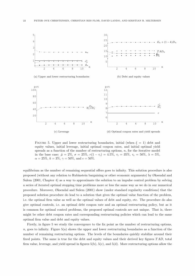
22 PETER OVE CHRISTENSEN, CHRISTIAN RIIS FLOR, DAVID LANDO, AND KRISTIAN R. MILTERSEN
2 4 6 8 10
1
2
3
4
5
n
un
c∗ndn
(a) Upper and lower restructuring boundaries
2 4 6 8 10
5
10
15
20
25
30
n
En + (1 − k)Dn
TADnEnDn
(b) Debt and equity values
2 4 6 8 10
20
40
60
80
100pct
n
DnEn+Dn
(c) Leverage
2 4 6 8 10
6
7
8
9
10
11
12pct
n
c∗nDn
r
(d) Optimal coupon rates and yield spreads
Figure 5. Upper and lower restructuring boundaries, initial (when ξ = 1) debt andequity values, initial leverage, initial optimal coupon rates, and initial optimal yieldspreads as a function of the number of restructuring options, n, for the iterative modelin the base case: µ = 2%, σ = 25%, r(1 − τi) = 4.5%, τi = 35%, τe = 50%, λ = 5%,α = 25%, k = 3%, γ = 50%, and ε = 50%.
equilibrium as the number of remaining sequential offers goes to infinity. This solution procedure is alsoproposed (without any relation to Rubinstein bargaining or other economic arguments) by Øksendal andSulem (2001, Chapter 4) as a way to approximate the solution to an impulse control problem by solvinga series of iterated optimal stopping time problems more or less the same way as we do in our numericalprocedure. Moreover, Øksendal and Sulem (2001) show (under standard regularity conditions) that theproposed solution procedure do lead to a solution that gives the optimal value function of the problem,i.e. the optimal firm value as well as the optimal values of debt and equity, etc. The procedure do alsogive optimal controls, i.e. an optimal debt coupon rate and an optimal restructuring policy, but as itis common for optimal control problems, the proposed optimal controls are not unique. That is, theremight be other debt coupon rates and corresponding restructuring policies which can lead to the sameoptimal firm value and debt and equity values.
Firstly, in figure 5 we study the convergence to the fix point as the number of restructuring options,n, goes to infinity. Figure 5(a) shows the upper and lower restructuring boundaries as a function of thenumber of remaining restructuring options. The levels of the boundaries quickly stabilize around theirfixed points. The same is true for the debt and equity values and their derived key figures TAD, totalfirm value, leverage, and yield spread in figures 5(b), 5(c), and 5(d). More restructuring options allow the
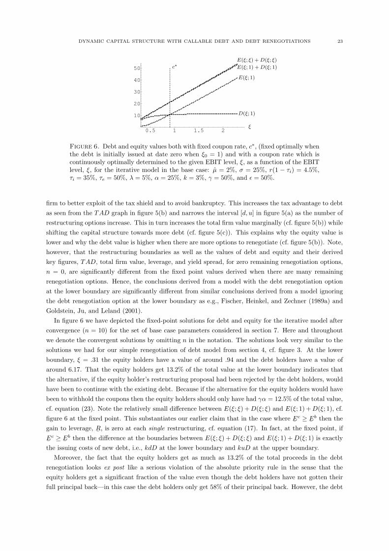
DYNAMIC CAPITAL STRUCTURE WITH CALLABLE DEBT AND DEBT RENEGOTIATIONS 23
0.5 1 1.5 2
10
20
30
40
50
ξ
c∗E(ξ; ξ) + D(ξ; ξ)
E(ξ; 1) + D(ξ; 1)
E(ξ; 1)
D(ξ; 1)
Figure 6. Debt and equity values both with fixed coupon rate, c∗, (fixed optimally whenthe debt is initially issued at date zero when ξ0 = 1) and with a coupon rate which iscontinuously optimally determined to the given EBIT level, ξ, as a function of the EBITlevel, ξ, for the iterative model in the base case: µ = 2%, σ = 25%, r(1 − τi) = 4.5%,τi = 35%, τe = 50%, λ = 5%, α = 25%, k = 3%, γ = 50%, and ε = 50%.
firm to better exploit of the tax shield and to avoid bankruptcy. This increases the tax advantage to debtas seen from the TAD graph in figure 5(b) and narrows the interval [d, u] in figure 5(a) as the number ofrestructuring options increase. This in turn increases the total firm value marginally (cf. figure 5(b)) whileshifting the capital structure towards more debt (cf. figure 5(c)). This explains why the equity value islower and why the debt value is higher when there are more options to renegotiate (cf. figure 5(b)). Note,however, that the restructuring boundaries as well as the values of debt and equity and their derivedkey figures, TAD, total firm value, leverage, and yield spread, for zero remaining renegotiation options,n = 0, are significantly different from the fixed point values derived when there are many remainingrenegotiation options. Hence, the conclusions derived from a model with the debt renegotiation optionat the lower boundary are significantly different from similar conclusions derived from a model ignoringthe debt renegotiation option at the lower boundary as e.g., Fischer, Heinkel, and Zechner (1989a) andGoldstein, Ju, and Leland (2001).
In figure 6 we have depicted the fixed-point solutions for debt and equity for the iterative model afterconvergence (n = 10) for the set of base case parameters considered in section 7. Here and throughoutwe denote the convergent solutions by omitting n in the notation. The solutions look very similar to thesolutions we had for our simple renegotiation of debt model from section 4, cf. figure 3. At the lowerboundary, ξ = .31 the equity holders have a value of around .94 and the debt holders have a value ofaround 6.17. That the equity holders get 13.2% of the total value at the lower boundary indicates thatthe alternative, if the equity holder’s restructuring proposal had been rejected by the debt holders, wouldhave been to continue with the existing debt. Because if the alternative for the equity holders would havebeen to withhold the coupons then the equity holders should only have had γα = 12.5% of the total value,cf. equation (23). Note the relatively small difference between E(ξ; ξ) + D(ξ; ξ) and E(ξ; 1) + D(ξ; 1), cf.figure 6 at the fixed point. This substantiates our earlier claim that in the case where
¯Ec ≥
¯Eb then the
gain to leverage,¯R, is zero at each single restructuring, cf. equation (17). In fact, at the fixed point, if
¯Ec ≥
¯Eb then the difference at the boundaries between E(ξ; ξ) + D(ξ; ξ) and E(ξ; 1) + D(ξ; 1) is exactly
the issuing costs of new debt, i.e., kdD at the lower boundary and kuD at the upper boundary.Moreover, the fact that the equity holders get as much as 13.2% of the total proceeds in the debt
renegotiation looks ex post like a serious violation of the absolute priority rule in the sense that theequity holders get a significant fraction of the value even though the debt holders have not gotten theirfull principal back—in this case the debt holders only get 58% of their principal back. However, the debt
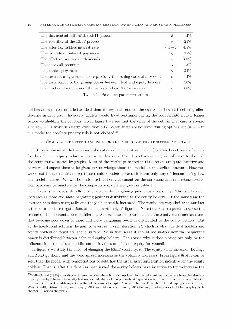
24 PETER OVE CHRISTENSEN, CHRISTIAN RIIS FLOR, DAVID LANDO, AND KRISTIAN R. MILTERSEN
The risk neutral drift of the EBIT process µ 2%The volatility of the EBIT process σ 25%The after-tax riskless interest rate r(1 − τi) 4.5%The tax rate on interest payments τi 35%The effective tax rate on dividends τe 50%The debt call premium λ 5%The bankruptcy costs α 25%The restructuring costs or more precisely the issuing costs of new debt k 3%The distribution of bargaining power between debt and equity holders γ 50%The fractional reduction of the tax rate when EBT is negative ε 50%
Table 1. Base case parameter values.
holders are still getting a better deal than if they had rejected the equity holders’ restructuring offer.Because in that case, the equity holders would have continued paying the coupon rate a little longerbefore withholding the coupons. From figure 1 we see that the value of the debt in that case is around4.85 at ξ = .31 which is clearly lower than 6.17. When there are no restructuring options left (n = 0) inour model the absolute priority rule is not violated.23
7. Comparative statics and Numerical results for the Iterative Approach.
In this section we study the numerical solutions of our iterative model. Since we do not have a formulafor the debt and equity values we can write down and take derivatives of etc., we will have to show allthe comparative statics by graphs. Most of the results presented in this section are quite intuitive andas we would expect them to be given our knowledge about the models in the earlier literature. However,we do not think that this makes these results obsolete because it is our only way of demonstrating howour model behaves. We will be quite brief and only comment on the surprising and interesting results.Our base case parameters for the comparative statics are given in table 1
In figure 7 we study the effect of changing the bargaining power distribution, γ. The equity valueincreases as more and more bargaining power is distributed to the equity holders. At the same time theleverage goes down marginally and the yield spread is increased. The results are very similar to our firstattempt to model renegotiations of debt in section 4, cf. figure 4. Note that η corresponds to γα so thescaling on the horizontal axis is different. At first it seems plausible that the equity value increases andthat leverage goes down as more and more bargaining power is distributed to the equity holders. Butat the fixed-point solution the gain to leverage in each iteration, R, which is what the debt holders andequity holders do negotiate about, is zero. So in that sense it should not matter how the bargainingpower is distributed between debt and equity holders. The reason why it does matter can only be theinfluence from the off-the-equilibrium-path values of debt and equity for n small.
In figure 8 we study the effect of changing the EBIT volatility, σ. The equity value increases, leverageand TAD go down, and the yield spread increases as the volatility increases. From figure 8(b) it can beseen that the model with renegotiations of debt has the usual asset substitution incentive for the equityholders. That is, after the debt has been issued the equity holders have incentive to try to increase the
23Mella-Barral (1999) considers a different model where it is also optimal for the debt holders to deviate from the absolutepriority rule by offering the equity holders a small share of the proceeds at liquidation in order to speed up the liquidationprocess. Both models adds aspects to the whole game of chapter 7 versus chapter 11 in the US bankruptcy code. Cf., e.g.,Weiss (1990), Gilson, John, and Lang (1990), and Morse and Shaw (1988) for empirical studies of US bankruptcy codechapter 11 versus chapter 7.

DYNAMIC CAPITAL STRUCTURE WITH CALLABLE DEBT AND DEBT RENEGOTIATIONS 25
20 40 60 80 100
1
2
3
4
5
γ%
u
c∗
d
(a) Upper and lower restructuring boundaries
20 40 60 80 100
5
10
15
20
25
30
γ%
E + (1 − k)D
TADED
(b) Debt and equity values
20 40 60 80 100
20
40
60
80
100
γ%
%
DE+D
(c) Leverage
20 40 60 80 100
6
7
8
9
10
11
12
γ%
%
c∗D
r
(d) Optimal coupon rate and yield spread
Figure 7. Upper and lower restructuring boundaries, initial (when ξ = 1) debt andequity values, initial leverage, initial optimal coupon rates, and initial optimal yieldspreads as a function of the way the bargaining power is distributed between the debtand equity holders, γ, for the iterative model in the base case: µ = 2%, σ = 25%,r(1 − τi) = 4.5%, τi = 35%, τe = 50%, λ = 5%, α = 25%, k = 3%, and ε = 50%.
volatility of the underlying EBIT process (e.g., by the way they select new projects for the firm andretire old projects) since this activity will increase the value of the equity. However, compared to theusual static model there is a dynamic effect which limits the equity holders incentive to increase thevolatility in the following way: after the debt has been issued the equity holders do take into accountthat this activity of increasing the EBIT volatility at the same time decreases the debt value as well asthe whole firm value in all future debt calls and renegotiations. With the given base case parametersthe advantage for the equity holders to increase the volatility of the EBIT process still remains as theresults show, because this dynamic effect is already capitalized into the current equity price. However,because of this dynamic effect the incentive is limited (but not eliminated) compared to a static capitalstructure model. The reason for this is that increasing the EBIT volatility results (with the given basecase parameters) in a smaller initial total firm value, which is what is important for the equity holdersin all future restructurings.
In figure 9 we study the effect of changing the costs of issuing new debt. The boundaries widens sothat the debt is restructured less frequently when the costs increase. The influence on debt and equityvalues, leverage and yield spreads are fairly small even though TAD decreases from 20% to 10%.

26 PETER OVE CHRISTENSEN, CHRISTIAN RIIS FLOR, DAVID LANDO, AND KRISTIAN R. MILTERSEN
15 20 25 30 35 40
1
2
3
4
5
σ%
u
c∗d
(a) Upper and lower restructuring boundaries
15 20 25 30 35 40
5
10
15
20
25
30
σ%
E + (1 − k)D
TAD
E
D
(b) Debt and equity values
15 20 25 30 35 40
20
40
60
80
100
σ%
%
DE+D
(c) Leverage
15 20 25 30 35 40
6
7
8
9
10
11
12
σ%
%
c∗D
r
(d) Optimal coupon rate and yield spread
Figure 8. Upper and lower restructuring boundaries, initial (when ξ = 1) debt andequity values, initial leverage, initial optimal coupon rates, and initial optimal yieldspreads as a function of the EBIT volatility, σ, for the iterative model in the base case:µ = 2%, r(1 − τi) = 4.5%, τi = 35%, τe = 50%, λ = 5%, α = 25%, k = 3%, γ = 50%,and ε = 50%.
In figure 10 we study the effect of changing the bankruptcy costs factor. Since the firm actually nevergo bankrupt—it is just a far out in the future threat that when all the n renegotiation options havebeen exercised then eventually the firm will go bankrupt—it should have a very limited influence on theequilibrium results. Indeed the results in figure 10 substantiate this claim.
In figure 11 we study the effect of changing the possibilities for tax refunds when EBT is negative,ε. It is not surprising that total firm value increases and that leverage increases as the possibilities fortax refunds increases. However, we were surprised by the magnitude of the change. Note also that bothTAD and the yield spread increases dramatically as the possibilities for tax refunds increases. Especiallyfigure 11(a) tells us that the standard assumption in the literature, cf., e.g., the models of Kane, Marcus,and McDonald (1985), Fischer, Heinkel, and Zechner (1989a), Leland (1994), and Goldstein, Ju, andLeland (2001), of full tax refunds when EBT is negative (the case with ε = 1) is highly unrealistic inthe sense that the optimal initial coupon rate is set so high that the firm will always have negative EBTsince c∗ > ξ. Actually, this is the case as soon as ε is higher than .93. In a model with no renegotiationsthis effect is not nearly as dramatic as can be seen by comparing with figure 2.
Finally, in figure 12 we study the effect of changing the risk neutral drift of the EBIT process, µ.It is not surprising that the total firm value increases as the risk neutral drift approaches the after-tax

DYNAMIC CAPITAL STRUCTURE WITH CALLABLE DEBT AND DEBT RENEGOTIATIONS 27
2 3 4 5 6
1
2
3
4
5
k%
u
c∗d
(a) Upper and lower restructuring boundaries
2 3 4 5 6
5
10
15
20
25
30
k%
E + (1 − k)D
TADE
D
(b) Debt and equity values
2 3 4 5 6
20
40
60
80
100
k%
%
DE+D
(c) Leverage
2 3 4 5 6
6
7
8
9
10
11
12
k%
%
c∗D
r
(d) Optimal coupon rate and yield spread
Figure 9. Upper and lower restructuring boundaries, initial (when ξ = 1) debt andequity values, initial leverage, initial optimal coupon rates, and initial optimal yieldspreads as a function of the costs of restructuring (issuing costs of new debt) factor, k,for the iterative model in the base case: µ = 2%, σ = 25%, r(1 − τi) = 4.5%, τi = 35%,τe = 50%, λ = 5%, α = 25%, γ = 50%, and ε = 50%.
riskless interest rate. This is the usual Microsoft/dot-com stories. These firms have dramatically highprice-earnings ratio. Therefore, for high growth firms a small change in expected earnings has a dramaticeffect on the firm value and therefore also on the equity value. However, notice how the optimal capitalstructure contains less and less debt as the risk neutral drift approaches the after-tax riskless interestrate. This happens because of the limited tax refunds when EBT is negative. If we allow for full taxrefunds when EBT is negative, i.e. ε = 100%, our numerical results show that with µ = 4% and all otherparameters as in the base case then the optimal leverage is around 60% and that the TAD shoots up toabove 75% while the optimal coupon rate exceeds ten times the current earnings. Hence, the reductionof the leverage is purely tax driven: even thought the firm’s EBIT has great potential it is not optimal(because of the limited tax refunds) to take on more debt than such that the current earnings can coverthe coupon rates. Given this observation it is clear that the yield spread go down since the debt value isnot increasing with the firm value as the risk neutral drift approaches the after-tax riskless interest rate.De facto the debt becomes more or less riskless as the leverage decrease. Hence, our model predicts thatfirms with low growth expectations (e.g., utility based firms) will have high optimal leverage and fairlyhigh yield spreads whereas firms with high growth expectations will have very low optimal leverage andalso very low yield spreads.

28 PETER OVE CHRISTENSEN, CHRISTIAN RIIS FLOR, DAVID LANDO, AND KRISTIAN R. MILTERSEN
10 20 30 40 50 60
1
2
3
4
5
α%
u
c∗
d
(a) Upper and lower restructuring boundaries
10 20 30 40 50 60
5
10
15
20
25
30
α%
E + (1 − k)D
TADED
(b) Debt and equity values
10 20 30 40 50 60
20
40
60
80
100
α%
%
DE+D
(c) Leverage
10 20 30 40 50 60
6
7
8
9
10
11
12
α%
%
c∗D
r
(d) Optimal coupon rate and yield spread
Figure 10. Upper and lower restructuring boundaries, initial (when ξ = 1) debt andequity values, initial leverage, initial optimal coupon rates, and initial optimal yieldspreads as a function of the bankruptcy costs factor, α, for the iterative model in thebase case: µ = 2%, σ = 25%, r(1 − τi) = 4.5%, τi = 35%, τe = 50%, λ = 5%, k = 3%,γ = 50%, and ε = 50%.
8. The Risk Neutral Drift of the EBIT Process
In section 2 when we started modeling the EBIT process our starting point was an exogenously givendrift, µ, of the EBIT process under the pricing measure, Q. It is an interesting empirical question howthis drift can be estimated. As we saw in section 7 one of the implications of our model is that theoptimal leverage, the optimal coupon rate, the yield spread, etc. are highly dependent on the value of µ,cf. figure 12. Therefore, figure 12 gives us more or less the answer to the question of how to determine µ:from simultaneous observations of the equity value (right after the debt has been issued) and the valueof the EBIT process a unique value for the risk neutral drift of the EBIT process, µ, can be backed out.That is, for a given µ, we can go through the whole derivation in sections 2–6 of the iterative model tofind the value function of equity, E(·; 1) as function of ξ. Hence, we can define the function, PE(·), whichgives the price earnings ratio (PE ratio) of the firm as function of µ
PE(µ) =E(ξ; ξ)
ξ= E.
This function is well-defined because the equity value is homogeneous of degree one jointly in the twovariables, cf. equation (3). Moreover, figure 12 indicates that PE is an increasing function of µ. Thisimplies that PE has an inverse. Hence, given that we can observe the firm’s initial PE ratio, µ can be

DYNAMIC CAPITAL STRUCTURE WITH CALLABLE DEBT AND DEBT RENEGOTIATIONS 29
20 40 60 80 100
1
2
3
4
5
ε%
uc∗
d
(a) Upper and lower restructuring boundaries
20 40 60 80 100
5
10
15
20
25
30
35
40
ε%
E + (1 − k)D
TAD
E
D
(b) Debt and equity values
20 40 60 80 100
20
40
60
80
100
ε%
%
DE+D
(c) Leverage
20 40 60 80 100
6
7
8
9
10
11
12
ε%
%
c∗D
r
(d) Optimal coupon rate and yield spread
Figure 11. Upper and lower restructuring boundaries, initial (when ξ = 1) debt andequity values, initial leverage, initial optimal coupon rates, and initial optimal yieldspreads as a function of the fractional reduction, ε, of the tax rate when EBT is negativefor the iterative model in the base case: µ = 2%, σ = 25%, r(1 − τi) = 4.5%, τi = 35%,τe = 50%, λ = 5%, α = 25%, k = 3%, and γ = 50%.
determined. This answer to the question of how to determine µ is similar in spirit of how to back outthe (implicit) volatility of the underlying security if one has simultaneous observations of the prices of anoption and the underlying security in a Black-Scholes model, and hence, we term this the implicit riskneutral drift of the EBIT process. This argument, however, requires that the volatility, σ, of the EBITprocess is already known. If both µ and σ are unknown, then we need simultaneous observations of boththe value of the EBIT process, the value of equity, and the value of debt right after the debt has beenissued. (Uniqueness of the solution in this case is yet unsolved.)
Another solution to the problem of how to find µ is to determine it in equilibrium. Apparently, thisis what Fischer, Heinkel, and Zechner (1989a) claim to do. However, we are not able to get to thesame conclusion by following their arguments. Fischer, Heinkel, and Zechner (1989a) start by specifyingexogenously the value process, A, of the unlevered firm including the value of their leverage potentialbut excluding the costs of obtaining the leverage. Moreover, they assume that this value process is ageometric Brownian motion of the form
(25) dAt = Atµdt + AtσdWt

30 PETER OVE CHRISTENSEN, CHRISTIAN RIIS FLOR, DAVID LANDO, AND KRISTIAN R. MILTERSEN
1 2 3 4
1
2
3
4
5
µ%
u
c∗
d
(a) Upper and lower restructuring boundaries
1 2 3 4
20
40
60
80
100
120
µ%
E + (1 − k)D
TAD
E
D
(b) Debt and equity values
1 2 3 4
20
40
60
80
100
µ%
%
DE+D
(c) Leverage
1 2 3 4
6
7
8
9
10
11
12
µ%
%
c∗D
r
(d) Optimal coupon rate and yield spread
Figure 12. Upper and lower restructuring boundaries, initial (when ξ = 1) debt andequity values, initial leverage, initial optimal coupon rates, and initial optimal yieldspreads as a function of the risk neutral drift of the EBIT process, µ, for the iterativemodel in the base case: σ = 25%, r(1 − τi) = 4.5%, τi = 35%, τe = 50%, λ = 5%,α = 25%, k = 3%, γ = 50%, and ε = 50%.
under an exogenously given and unique pricing measure, denoted Q. That is , they assume that thereexists traded securities such that any new claim that we may want to introduce can be dynamicallyreplicated by already existing traded securities and therefore priced.24 This is the same arguments as weused in section 2. With A as the governing state variable, Fischer, Heinkel, and Zechner (1989a) derive,using the same method as we have used in sections 2–3 (with ξ as the governing state variable), thevalue of debt and equity as functions of the current value of the unlevered firm process. Fischer, Heinkel,and Zechner (1989a) does not include renegotiations of the debt in their model, they only work withliquidations at the lower boundary (similar to what Goldstein, Ju, and Leland (2001) do in their modeland what we do in sections 2–3).
Given the dynamics of A as specified in equation (25) and the assumption that A at the same timerepresents the price at which one should be able to acquire the firm before paying the costs of optimallylever the firm, we get the following requirement
(26) At = E(At;At) + (1 − k)D(At;At),
24Note that the value, A, of the unlevered firm is not, in general, one of the traded securities and can therefore not beused in the dynamically replicating argument to price new (derivative) securities which are functions of the value of theunlevered firm.
DYNAMIC CAPITAL STRUCTURE WITH CALLABLE DEBT AND DEBT RENEGOTIATIONS 31
where the notation is adapted from section 2. That is, the value of the unlevered firm must at all timesbe the value of the debt and equity of the (newly) optimally levered firm less the costs of obtaining theoptimal leverage. By homogeneity, equation (26) can be reduced to
(27) 1 = E + (1 − k)D,
which Fischer, Heinkel, and Zechner (1989a) call a no-arbitrage condition on their model. They use thisequation to determine the risk neutral drift, µ, of the unlevered firm value process. In that they claim(and we have no reason to doubt this claim as it will become clear soon) that there is only one µ whichfulfills equation (27).
Comparing the Fischer-Heinkel-Zechner model to the EBIT based model we have developed in sec-tions 2–3 we have also defined the value process A as
At = E(ξt; ξt) + (1 − k)D(ξt; ξt) = κξt.
That is, there exists a constant, κ, such that25
At = κξt.
Hence, if the unlevered firm value process, A, is a geometric Brownian motion so is the EBIT process,ξ, and vice versa. Moreover, the risk neutral drift, µ, (and the volatility, σ) of the unlevered firm valueprocess, A, and the EBIT process, ξ, are the same.
So how is it possible that in the EBIT based model developed in sections 2–3 there are no restrictionson µ whereas in the unlevered firm value based model of Fischer, Heinkel, and Zechner (1989a) µ isuniquely determined? The answer is simple: In the development of the unlevered firm value based model,the after-tax payout rates on debt and equity, cf. table 2 in Appendix A, has to be specified as linearfunctions of (A,C) instead of (ξ, C). That is, in the unlevered firm value based model the payout rate to,say, equity must be specified as δAA+ bAC whereas in the EBIT based model it is specified as δξξ + bξC.δξ and bξ can be found in table 2 in Appendix A. In order to make the two models equivalent, we mustspecify the same payout rate for the unlevered firm value based model as for the EBIT based model.Thus, we must have δAA + bAC = δξξ + bξC, for all C and all A and ξ such that A = κξ. This implythat bA = bξ and
δA = δξ1κ
.
Hence, the ratio, κ, between A and ξ must be specified exogenously before we can specify the payout rateof equity in order to make the unlevered firm value based model equivalent to the EBIT based model.But from the ratio, κ, µ can be backed out implicitly by the same argument as with the PE ratio. Hence,specifying κ exogenously is the same as specifying µ exogenously. This is the reason why there is onlyone µ in the unlevered firm value based model which is consistent, i.e. which fulfills equation (27).
Goldstein, Ju, and Leland (2001) also uses an endogenous drift, µ, which they claim depend on thecoupon rate when the tax advantage to debt is measured. To illustrate how µ can depend on the debtissued consider the following example from Goldstein, Ju, and Leland (2001, p. 495). Suppose that thecurrent level of EBIT is ξ0 = 100 and that the PE ratio is 20. Then the total value of all future earningsis V0 = 100 × 20 = 2000. Furthermore, let the corporate tax rate be τc = .35. Thus the corporate taxpayout rate is τc(ξ − C) = 0.35(100 − C), for a given coupon rate C. Suppose that the firm pays out 35
25Actually, κ = E(1, 1) + (1− k)D(1, 1) = E + (1− k)D. In section 2 we called the constant κ for A, but for this section it
will be too confusing to have both A as a geometric Brownian motion and also a scaling constant.
32 PETER OVE CHRISTENSEN, CHRISTIAN RIIS FLOR, DAVID LANDO, AND KRISTIAN R. MILTERSEN
as a dividend rate to the equity holders. This implies that the total payout from the firm is
total initial payout rate = interest + corporate tax + equity dividend
= C + .35(100 − C) + 35 = 70 + .65C,
thus,
(28) V0
((1 − τi)r − µ
)= ξ0 = 70 + .65C.
Hence, from equation (28) we can back out µ as a function of the coupon rate, C. However, in ouropinion, there is a problem in equation (28). First it is assumed that ξ0 = 100 but in equation (28) onegets ξ0 = 70+ .65C. The missing 30− .65C stems from the assumption that the firm pays the amount 35in dividend to the equity holders. Hence, there is remaining free cash in the firm. The dividend policy isnot irrelevant in Goldstein, Ju, and Leland (2001), as well as in our model, the dividend paid out to theequity holders is residually determined as all of the remaining cash in the firm. Otherwise one needs tospecify how the remaining free cash flow is used (investments or disinvestments in the EBIT generatingprocess) and take that into consideration, as well as how dividends affects the process for EBIT, in theinitial optimization problem.
9. Conclusion
In this paper we have analyzed a dynamic capital structure model which includes debt renegotiationswhen the bankruptcy threat becomes imminent. We have extended the Goldstein-Ju-Leland model intwo ways: (i) instead of liquidating the firm and thereby definitively losing the tax shield, we assumethat the firm is acquired as a going concern by another entrepreneur in case of bankruptcy. Moreover,(ii) we allow for voluntary debt renegotiations. These two extensions both work in the same direction.In our base case example the tax advantage to debt in the Goldstein-Ju-Leland model is around 8% anda leverage is around 35%. (i) extends the tax advantage to debt to 10%, and (ii) extends it further up to15%. At the same time leverage is increased by (i) to 40% and by (ii) further up to around 50%. Thisfigure for leverage is similar to the figure for a static capital structure model with the same parametervalues. The point where the equity holders make their take-it-or-leave-it restructuring offer to the debtholders is determined by standard smooth pasting conditions such that the usual incentive compatibilityconstraints for the equity holders are fulfilled. In the base case example the equity holders get around13% of the firm value, whereas the old debt holders get the rest. In extreme cases (for µ = 4%) theequity holders can get as much as 60% of the value. In both cases the debt holders get less than theirfull principal back. Even though this looks like an ex post violation of the absolute priority rule, thedebt holders are still better off by accepting this restructuring offer from the equity holders than byrejecting it. The reason is that if they reject the offer, the equity holders would continue to pay theexisting coupon rate for some time before eventually withholding the coupons when the earnings of thefirm are even lower. This alternative has a lower value to the debt holders than the value of acceptingthe restructuring proposal right away.
The numerically demanding part of our analysis is to calculate the off-the-equilibrium-path valuesof debt and equity. It turns out that these values are very important in order to understand how theequity holders should optimally time their take-it-or-leave-it restructuring offer. Moreover, these valuesendogenously determine how to split the firm value between the existing debt and equity holders. At thefixed-point solution the exogenously given bargaining power distribution, γ, only plays a minor role in thesense that the gain to restructuring, R, is zero in each iteration. Hence, there is no gain to exogenouslydistribute. The firm value split is fully determined by the endogenously given off-the-equilibrium-path

DYNAMIC CAPITAL STRUCTURE WITH CALLABLE DEBT AND DEBT RENEGOTIATIONS 33
values. To emphasize this point we will go through the following simple example: suppose we assume thatthe firm value split (η) is exogenously given in what we could call a reduced form model (a model of thetype described in section 4). If we set the firm value split in the reduced form model equal to the firm valuesplit our iterative model determined endogenously, we do not get the same lower and upper boundaries asoptimal for the reduced form model as we do for our iterative model.26 The reason is that in the iterativemodel the split is not a fixed number, η. The iterative model takes into account that if the equity holderswant the debt holders to accept their restructuring proposal for another (off-the-equilibrium-path) valueof d, they might very well have to offer them a bigger share of the value.
Our results indicate that empirically we should observe huge variations in leverage between the dateswhen firms realign their capital structure either by renegotiating their debt terms or by issuing newsecurities. Even for fairly small transactions costs as in our examples the earnings of the firm should havechanged by a factor 2.5 before it is optimal for the firm to realign its capital structure. In the mean timebetween realignment dates the fluctuations in earnings result in fluctuations in debt and equity valuesthat makes the leverage vary from around 21% to 87% in our base case example. Moreover, for the samereasons the object function of the firm is very flat over a large area, so even though our model can finda unique optimal capital structure for the firm, it is not that important for the total firm value that thefirm targets it capital structure at that exact level. Furthermore, other issues outside our model even ofsmall magnitude could change the optimum quite a bit because of the fairly flat objective function.
One of the things our model cannot explain is why some firms end up continuing operation after a debtrestructuring while others end up being liquidated. In our model the firm is always more valuable alivethan liquidated and, hence, it is natural that it should never be liquidated. We see two ways that themodel can be extended to include this feature. Either we can introduce an exogenously given probabilitythat the debt and equity holders cannot reach an agreement of how to restructure the firm, or we canintroduce a second state variable measuring the value of the firm’s assets. In this last model the firmcan be liquidated simply because the firm’s assets are more valuable than the present value of the EBITprocess optimally levered. This can, e.g., be the case if the assets can be used for some other purposethan generating the current EBIT. A first attempt in this direction is Flor (2002).
Our model cannot capture strategic debt service of the type where it is simply the current coupon ratewhich is reduced, whereas the capital structure stays fixed as it is modeled in Anderson and Sundaresan(1996) and Mella-Barral and Perraudin (1997). However, it is fairly easy to extend our model to incor-porate both types of debt renegotiations simply by introducing an extra boundary condition above d butbelow one, say s. As long as ξ ∈ (sξ0, uξ0), the debt is serviced with the full coupon rate, c∗ξ0, but whenξ ∈ (dξ0, sξ0] the debt is only serviced according to the strategic debt service models. Finally, when ξ
eventually hits either dξ0 or uξ0, the firm’s capital structure is re-optimized and the game starts all overagain.
Finally, our model does not include investment decisions. The EBIT process is exogenously given. Itis not possible within the model to retain some of the earnings to increase the scale of the EBIT processor to increase the dividend payments by decreasing the scale of the EBIT process. As the model is, allearnings must be paid out to debt holders, equity holders, and the tax authorities.
26For the base case parameters the values are very close but not identical. But for more extreme parameter values thedifferences can be substantial. For example, for µ = 4% the optimal d and u are .30 and 4.28 for the iterative model,whereas for the reduced form model with the same split (60% of the firm value goes to the equity holders) the optimal d
and u are .18 and 3.71.
34 PETER OVE CHRISTENSEN, CHRISTIAN RIIS FLOR, DAVID LANDO, AND KRISTIAN R. MILTERSEN
Appendix A. Fixed Point Solution to the Pricing of Debt and Equity
To set up some notation, we quickly reiterate parts of the standard theory. First, consider a very simpleclaim paying one unit of account when ξ hits the lower boundary,
¯ξ, but only if the lower boundary has
been hit before the upper boundary, ξ. The price, denoted¯P , of this claim as a function of the current
level of EBIT, ξ, can be derived as
¯P (ξ) =
−ξx2ξx1 + ξx1ξx2
Σ, ξ ∈ [
¯ξ, ξ],
where
x1 =( 12σ2 − µ) +
√(µ − 1
2σ2)2 + 2(1 − τi)rσ2
σ2,
x2 =( 12σ2 − µ) −
√(µ − 1
2σ2)2 + 2(1 − τi)rσ2
σ2,
and
Σ = ξx1
¯ξx2 −
¯ξx1 ξx2 .
This follows from the fact that¯P solves the linear ordinary differential equation (ODE)
(29)12σ2ξ2
¯P ′′(ξ) + µξ
¯P ′(ξ) − (1 − τi)r¯
P (ξ) = 0,
with the boundary conditions
¯P (
¯ξ) = 1 and
¯P (ξ) = 0.
Similarly, interchanging the boundary conditions, we find the price of a claim paying one unit of accountwhen ξ hits the upper boundary, ξ, but only if the upper boundary has been hit before the lower boundary,
¯ξ. The price, denoted P , of this claim as a function of the current level of EBIT, ξ, can be derived as
P (ξ) = ¯ξx2ξx1 −
¯ξx1ξx2
Σ, ξ ∈ [
¯ξ, ξ].
We also need a claim that pays a dividend stream at the rate δξs + b at any date s ∈ [t,∞). The date t
value of this claim can easily be derived (either using risk neutral expectations or Gordon’s formula) as
∆ξt + B,
where
∆ =δ
(1 − τi)r − µand B =
b
(1 − τi)r.
With these three claims priced we are able to price all claims of interest in our model. Consider theclaim which pays off a dividend stream at the rate δξt + b at any date, t, until one of the boundarieshas been hit. When it hits one of the boundaries, it pays out a final lump-sum payment. If the lowerboundary,
¯ξ, has been hit first, it pays out
¯F , and if the upper boundary, ξ, has been hit first, it pays
out F . The price, denoted F (·; δ, b,¯ξ,
¯F, ξ, F ), of this claim as a function of the current level of EBIT, ξ,
can easily be derived as
(30) F (ξ; δ, b,¯ξ,
¯F, ξ, F ) = ∆ξ + B + (
¯F − ∆
¯ξ − B)
¯P (ξ) + (F − ∆ξ − B)P (ξ), ξ ∈ [
¯ξ, ξ].
Equation (30) has the following easy interpretation: The date t value of getting the dividend stream atthe rate δξs + b at any date s ∈ [t,∞) is ∆ξt + B. Eventually ξ will hit either
¯ξ or ξ. If, e.g.,
¯ξ has been

DYNAMIC CAPITAL STRUCTURE WITH CALLABLE DEBT AND DEBT RENEGOTIATIONS 35
hit first, the claim pays out¯F and the rest of the dividend stream (with a value of ∆
¯ξ + B) is forgone.
The net present value of this back at date t is (¯F − ∆
¯ξ − B)
¯P (ξt). The same argument applies for the
upper boundary, ξ.Plugging in the definitions of
¯P and P reveals27
F (ξ; δ, b,¯ξ,
¯F, ξ, F ) =
1Σ
((F − ∆ξ − B)
¯ξx2 − (
¯F − ∆
¯ξ − B)ξx2
)ξx1
+1Σ
((¯F − ∆
¯ξ − B)ξx1 − (F − ∆ξ − B)
¯ξx1
)ξx2 + ∆ξ + B, ξ ∈ [
¯ξ, ξ].
(33)
A very useful property of the price function, F , is the following positive homogeneity of degree oneproperty
(34) F (λξ; δ, λb, λ¯ξ, λ
¯F, λξ, λF ) = λF (ξ; δ, b,
¯ξ,
¯F, ξ, F ),
for any ξ ∈ [¯ξ, ξ] and λ ∈ R+. This is very easily checked by directly applying equation (33).28
The economic intuition behind this homogeneity property is quite trivial: if the unit of account waschanged, e.g., from $ to �, on all inputs, then also the value will change accordingly from being measuredin $ to being measured in �. This result heavily relies on the scaling invariant feature of the geometricBrownian motion and that everything except for monetary units is specified in rates.
With this machinery in place we return to the problem of finding the optimal dynamic capital structureof the firm and the values of debt and equity. Basically, debt and equity are claims of the form F justderived. We just have to find δ, b,
¯ξ,
¯F , ξ, and F for both debt and equity.
In order to find the after-tax payout rate, δξ + b, on debt and equity we need to know the tax rules.Coupon payments paid out to the debt holders are expenses for the firm, i.e. they are subtracted from theEBIT (giving earnings before taxes, EBT) before the firm pays corporate tax. Hence, the total tax paidon coupons is the personal interest tax paid by the debt holders. For dividends the firm must first paytax on its EBT before dividends can be paid out to the equity holders. On top of that the equity holderspay dividend tax on dividends paid out. Hence, the after-tax payout rate, δξ + b, on debt is specified as
δξ + b = (1 − τi)C
27Alternatively, equation (33) can be derived by observing that F is the solution to the inhomogeneous ODE (suppressingδ, b,
¯ξ,
¯F , ξ, and F in the notation for F )
(31)1
2σ2ξ2F ′′(ξ) + µξF ′(ξ) − (1 − τi)rF (ξ) + δξ + b = 0,
with the boundary conditions
F (¯ξ) =
¯F and F (ξ) = F.
Recall that the general solution to the ODE (31) is
(32) F (ξ; δ, b,¯ξ,
¯F, ξ, F ) = k1ξx1 + k2ξx2 +
δξ
(1 − τi)r − µ+
b
(1 − τi)r, ξ ∈ [
¯ξ, ξ],
where k1 and k2 are determined by the boundary conditions. Simple manipulations reveal that
k1 =1
Σ
((F − ∆ξ − B)
¯ξx2 − (
¯F − ∆
¯ξ − B)ξx2
)
and
k2 =1
Σ
((¯F − ∆
¯ξ − B)ξx1 − (F − ∆ξ − B)
¯ξx1
).
28That it is true for any ξ ∈ (¯ξ, ξ) follows directly. That it is also true for ξ ∈ {
¯ξ, ξ} must be checked separately. It comes
from the fact that F (¯ξ) =
¯F and F (ξ) = F . The reason why, e.g., F (ξ) = F is because if ξ = ξ then the upper boundary is
hit immediately and therefore (i) there is no waiting time until one of the two boundaries will be hit and (ii) there is zero
probability that the lower boundary will be hit before the upper boundary.
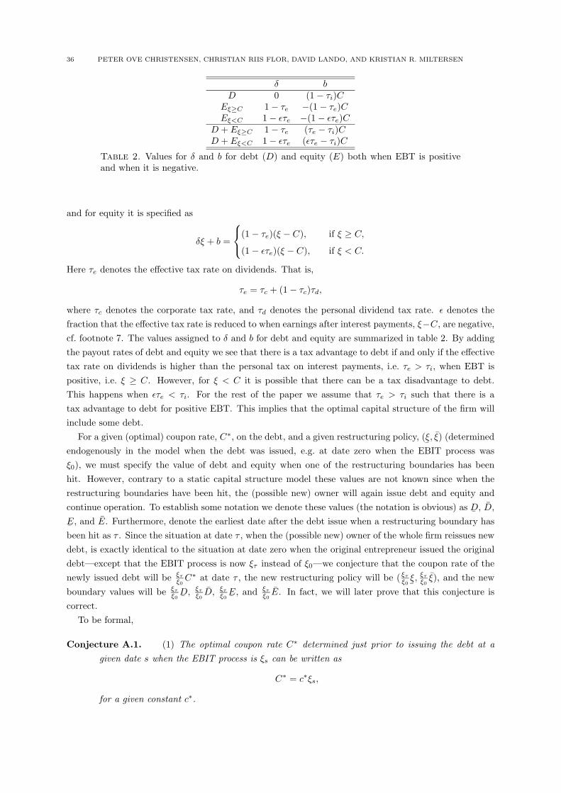
36 PETER OVE CHRISTENSEN, CHRISTIAN RIIS FLOR, DAVID LANDO, AND KRISTIAN R. MILTERSEN
δ bD 0 (1 − τi)C
Eξ≥C 1 − τe −(1 − τe)CEξ<C 1 − ετe −(1 − ετe)C
D + Eξ≥C 1 − τe (τe − τi)CD + Eξ<C 1 − ετe (ετe − τi)C
Table 2. Values for δ and b for debt (D) and equity (E) both when EBT is positiveand when it is negative.
and for equity it is specified as
δξ + b =
(1 − τe)(ξ − C), if ξ ≥ C,
(1 − ετe)(ξ − C), if ξ < C.
Here τe denotes the effective tax rate on dividends. That is,
τe = τc + (1 − τc)τd,
where τc denotes the corporate tax rate, and τd denotes the personal dividend tax rate. ε denotes thefraction that the effective tax rate is reduced to when earnings after interest payments, ξ−C, are negative,cf. footnote 7. The values assigned to δ and b for debt and equity are summarized in table 2. By addingthe payout rates of debt and equity we see that there is a tax advantage to debt if and only if the effectivetax rate on dividends is higher than the personal tax on interest payments, i.e. τe > τi, when EBT ispositive, i.e. ξ ≥ C. However, for ξ < C it is possible that there can be a tax disadvantage to debt.This happens when ετe < τi. For the rest of the paper we assume that τe > τi such that there is atax advantage to debt for positive EBT. This implies that the optimal capital structure of the firm willinclude some debt.
For a given (optimal) coupon rate, C∗, on the debt, and a given restructuring policy, (¯ξ, ξ) (determined
endogenously in the model when the debt was issued, e.g. at date zero when the EBIT process wasξ0), we must specify the value of debt and equity when one of the restructuring boundaries has beenhit. However, contrary to a static capital structure model these values are not known since when therestructuring boundaries have been hit, the (possible new) owner will again issue debt and equity andcontinue operation. To establish some notation we denote these values (the notation is obvious) as
¯D, D,
¯E, and E. Furthermore, denote the earliest date after the debt issue when a restructuring boundary hasbeen hit as τ . Since the situation at date τ , when the (possible new) owner of the whole firm reissues newdebt, is exactly identical to the situation at date zero when the original entrepreneur issued the originaldebt—except that the EBIT process is now ξτ instead of ξ0—we conjecture that the coupon rate of thenewly issued debt will be ξτ
ξ0C∗ at date τ , the new restructuring policy will be ( ξτ
ξ0¯ξ, ξτ
ξ0ξ), and the new
boundary values will be ξτ
ξ0 ¯D, ξτ
ξ0D, ξτ
ξ0 ¯E, and ξτ
ξ0E. In fact, we will later prove that this conjecture is
correct.To be formal,
Conjecture A.1. (1) The optimal coupon rate C∗ determined just prior to issuing the debt at agiven date s when the EBIT process is ξs can be written as
C∗ = c∗ξs,
for a given constant c∗.
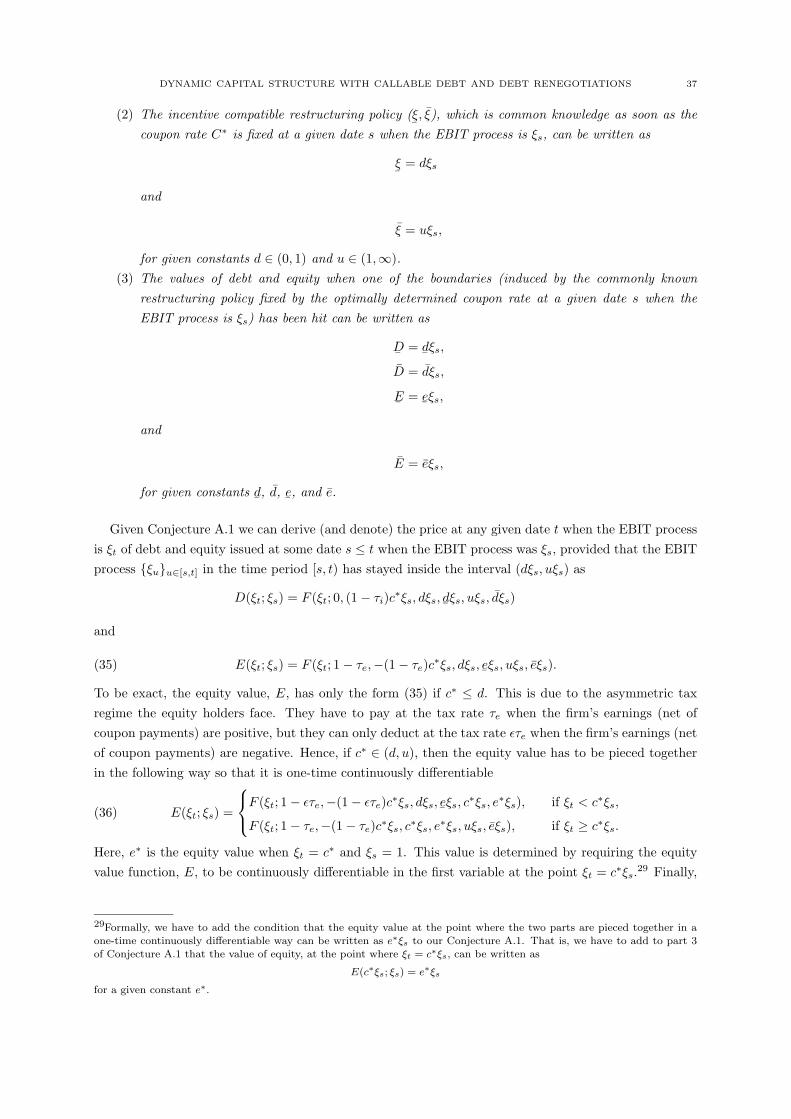
DYNAMIC CAPITAL STRUCTURE WITH CALLABLE DEBT AND DEBT RENEGOTIATIONS 37
(2) The incentive compatible restructuring policy (¯ξ, ξ), which is common knowledge as soon as the
coupon rate C∗ is fixed at a given date s when the EBIT process is ξs, can be written as
¯ξ = dξs
and
ξ = uξs,
for given constants d ∈ (0, 1) and u ∈ (1,∞).(3) The values of debt and equity when one of the boundaries (induced by the commonly known
restructuring policy fixed by the optimally determined coupon rate at a given date s when theEBIT process is ξs) has been hit can be written as
¯D =
¯dξs,
D = dξs,
¯E =
¯eξs,
and
E = eξs,
for given constants¯d, d,
¯e, and e.
Given Conjecture A.1 we can derive (and denote) the price at any given date t when the EBIT processis ξt of debt and equity issued at some date s ≤ t when the EBIT process was ξs, provided that the EBITprocess {ξu}u∈[s,t] in the time period [s, t) has stayed inside the interval (dξs, uξs) as
D(ξt; ξs) = F (ξt; 0, (1 − τi)c∗ξs, dξs,¯dξs, uξs, dξs)
and
E(ξt; ξs) = F (ξt; 1 − τe,−(1 − τe)c∗ξs, dξs,¯eξs, uξs, eξs).(35)
To be exact, the equity value, E, has only the form (35) if c∗ ≤ d. This is due to the asymmetric taxregime the equity holders face. They have to pay at the tax rate τe when the firm’s earnings (net ofcoupon payments) are positive, but they can only deduct at the tax rate ετe when the firm’s earnings (netof coupon payments) are negative. Hence, if c∗ ∈ (d, u), then the equity value has to be pieced togetherin the following way so that it is one-time continuously differentiable
(36) E(ξt; ξs) =
F (ξt; 1 − ετe,−(1 − ετe)c∗ξs, dξs,¯eξs, c
∗ξs, e∗ξs), if ξt < c∗ξs,
F (ξt; 1 − τe,−(1 − τe)c∗ξs, c∗ξs, e
∗ξs, uξs, eξs), if ξt ≥ c∗ξs.
Here, e∗ is the equity value when ξt = c∗ and ξs = 1. This value is determined by requiring the equityvalue function, E, to be continuously differentiable in the first variable at the point ξt = c∗ξs.29 Finally,
29Formally, we have to add the condition that the equity value at the point where the two parts are pieced together in aone-time continuously differentiable way can be written as e∗ξs to our Conjecture A.1. That is, we have to add to part 3of Conjecture A.1 that the value of equity, at the point where ξt = c∗ξs, can be written as
E(c∗ξs; ξs) = e∗ξs
for a given constant e∗.
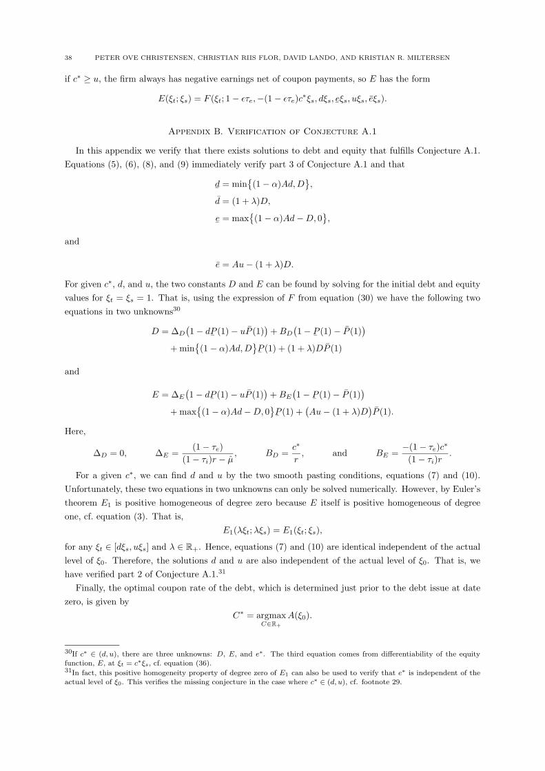
38 PETER OVE CHRISTENSEN, CHRISTIAN RIIS FLOR, DAVID LANDO, AND KRISTIAN R. MILTERSEN
if c∗ ≥ u, the firm always has negative earnings net of coupon payments, so E has the form
E(ξt; ξs) = F (ξt; 1 − ετe,−(1 − ετe)c∗ξs, dξs,¯eξs, uξs, eξs).
Appendix B. Verification of Conjecture A.1
In this appendix we verify that there exists solutions to debt and equity that fulfills Conjecture A.1.Equations (5), (6), (8), and (9) immediately verify part 3 of Conjecture A.1 and that
¯d = min
{(1 − α)Ad,D
},
d = (1 + λ)D,
¯e = max
{(1 − α)Ad − D, 0
},
and
e = Au − (1 + λ)D.
For given c∗, d, and u, the two constants D and E can be found by solving for the initial debt and equityvalues for ξt = ξs = 1. That is, using the expression of F from equation (30) we have the following twoequations in two unknowns30
D = ∆D
(1 − d
¯P (1) − uP (1)
)+ BD
(1 −
¯P (1) − P (1)
)+ min
{(1 − α)Ad,D
}¯P (1) + (1 + λ)DP (1)
and
E = ∆E
(1 − d
¯P (1) − uP (1)
)+ BE
(1 −
¯P (1) − P (1)
)+ max
{(1 − α)Ad − D, 0
}¯P (1) +
(Au − (1 + λ)D
)P (1).
Here,
∆D = 0, ∆E =(1 − τe)
(1 − τi)r − µ, BD =
c∗
r, and BE =
−(1 − τe)c∗
(1 − τi)r.
For a given c∗, we can find d and u by the two smooth pasting conditions, equations (7) and (10).Unfortunately, these two equations in two unknowns can only be solved numerically. However, by Euler’stheorem E1 is positive homogeneous of degree zero because E itself is positive homogeneous of degreeone, cf. equation (3). That is,
E1(λξt;λξs) = E1(ξt; ξs),
for any ξt ∈ [dξs, uξs] and λ ∈ R+. Hence, equations (7) and (10) are identical independent of the actuallevel of ξ0. Therefore, the solutions d and u are also independent of the actual level of ξ0. That is, wehave verified part 2 of Conjecture A.1.31
Finally, the optimal coupon rate of the debt, which is determined just prior to the debt issue at datezero, is given by
C∗ = argmaxC∈R+
A(ξ0).
30If c∗ ∈ (d, u), there are three unknowns: D, E, and e∗. The third equation comes from differentiability of the equityfunction, E, at ξt = c∗ξs, cf. equation (36).31In fact, this positive homogeneity property of degree zero of E1 can also be used to verify that e∗ is independent of the
actual level of ξ0. This verifies the missing conjecture in the case where c∗ ∈ (d, u), cf. footnote 29.

DYNAMIC CAPITAL STRUCTURE WITH CALLABLE DEBT AND DEBT RENEGOTIATIONS 39
That is so because it is the original entrepreneur who determines the coupon rate of the perpetual debtthat he or she would like to issue. Naturally, the entrepreneur sets the coupon rate in order to maximizehis or her own value. Moreover, rewriting C as cξ0 gives exactly the same optimization problem since ξ0
is positive
C∗ = argmaxC∈R+
A(ξ0) = ξ0
(argmax
c∈R+
A(ξ0)ξ0
).
Plugging in the definition of A(ξ0) from equation (4) gives
c∗ = argmaxc∈R+
E(ξ0; ξ0) + (1 − k)D(ξ0; ξ0)ξ0
= argmaxc∈R+
(F (ξ0; 1 − τe,−(1 − τe)cξ0, d(c)ξ0,¯
e(c)ξ0, u(c)ξ0, e(c)ξ0)ξ0
+ (1 − k)F (ξ0; 0, (1 − τi)cξ0, d(c)ξ0,¯
d(c)ξ0, u(c)ξ0, d(c)ξ0)ξ0
)
= argmaxc∈R+
(F (1; 1 − τe,−(1 − τe)c, d(c),
¯e(c), u(c), e(c))
+ (1 − k)F (1; 0, (1 − τi)c, d(c),¯d(c), u(c), d(c))
).
Note that we have emphasized the dependence of d, u,¯d, d,
¯e, and e on the given coupon rate parameter,
c, cf. part 2 and 3 of Conjecture A.1. Finally, notice that the optimal coupon rate parameter, c∗, inthe above optimization is independent of the initial level ξ0 so we have verified the last part (part 1) inConjecture A.1. That is, we have now verified that there exists a fixed-point solution to our debt andequity valuation problem giving us solutions to the value of debt and equity fulfilling Conjecture A.1.Because of our conjecture-verification method of finding the fixed-point solution, we cannot rule out thatthere might be other fixed-point solutions which do not fulfill Conjecture A.1.
References
Anderson, R. W., and S. Sundaresan (1996): “Design and Valuation of Debt Contracts,” The Review of Financial
Studies, 9(1), 37–68.
Betker, B. L. (1995): “Management’s Inventives, Equity’s Bargaining Power, and Deviations from Absolute Priority in
Chapter 11 Bankruptcies,” Journal of Business, 68(2), 161–183.
Black, F., and J. Cox (1976): “Valuing Corporate Securities: Some effects of Bond Indenture Provisions,” The Journal
of Finance, XXXI, 351–367.
Brekke, K. A., and B. Øksendal (1991): “The High Contact Principle as a Sufficiency Condition for Optimal Stopping,”
in Stochastic Models and Option Value, pp. 187–208. Elsevier Science Publishers, B. V., North-Holland, Amsterdam, The
Netherlands.
(1994): “Optimal Switching in an Economic Activity under Uncertainty,” SIAM Journal of Control and Optimiza-
tion, 32(4), 1021–1036.
Brennan, M. J., and A. Kraus (1987): “Efficient Financing under Asymmetric Information,” The Journal of Finance,
XLII(5), 1225–1243.
Dixit, A. K. (1991): “A Simplified Treatment of the Theory of Optimal Regulation of Brownian Motion,” Journal of
Economic Dynamics and Control, 15, 657–673.
(1993): The Art of Smooth Pasting. Harwood Academic Publishers GmbH, Poststrasse 22, 7000 Chur, Switzerland.
Dybvig, P. H., and J. F. Zender (1991): “Capital Structure and Dividend Irrelevance with Asymmetric Information,”
The Review of Financial Studies, 4(1), 201–219.
Eberhart, A. C., W. T. Moore, and R. L. Roenfeldt (1990): “Security Pricing and Deviations from the Absolute
Priority Rule in Bankruptcy Proceedings,” The Journal of Finance, XLV(6), 1457–1469.
Fischer, E. O., R. Heinkel, and J. Zechner (1989a): “Dynamic Capital Structure Choice: Theory and Tests,” The
Journal of Finance, XLIV(1), 19–40.
40 PETER OVE CHRISTENSEN, CHRISTIAN RIIS FLOR, DAVID LANDO, AND KRISTIAN R. MILTERSEN
(1989b): “Dynamic Recapitalization Policies and the Role of Call Premia and Issue Discounts,” Journal of Financial
and Quantitative Analysis, 24, 427–446.
Flor, C. R. (2002): “Capital Structure and Real Assets: Effects of an Implicit Collateral to Debt Holders,” Working
paper, Department of Accounting, Finance, and Law, University of Southern Denmark, Campusvej 55, DK–5230 Odense
M, Denmark.
Francois, P., and E. Morellec (2002): “Capital Structure and Asset Prices: Some Effect of Bankruptcy Procedures,”
Working paper, University of Rochester, Simon School of Business, Rochester, NY 14627, USA, Forthcoming in Journal
of Business.
Gilson, S., K. John, and L. Lang (1990): “Troubled Debt Restructurings: An Empirical Study of Private Renegotiation
of Firms in Default,” Journal of Financial Economics, 27, 315–353.
Goldstein, R., N. Ju, and H. Leland (2001): “An EBIT-Based Model of Dynamic Capital Structure,” Journal of
Business, 74(4), 483–512.
Jensen, M. C., and W. H. Meckling (1976): “Theory of the Firm: Managerial Behavior, Agency Costs and Ownership
Structure,” Journal of Financial Economics, 3, 305–360.
Kane, A., A. J. Marcus, and R. L. McDonald (1984): “How Big is the Tax Advantage to Debt?,” The Journal of
Finance, XXXIX(3), 841–853.
(1985): “Debt policy and the rate of return premium to leverage,” Journal of Financial and Quantitative Analysis,
20(4), 479–499.
Leland, H. E. (1994): “Corporate Debt Value, Bond Covenants, and Optimal Capital Structure,” The Journal of Finance,
XLIX(4), 1213–1252.
Mella-Barral, P. (1999): “The Dynamics of Default and Debt Reorganization,” The Review of Financial Studies, 12(3),
535–578.
Mella-Barral, P., and W. R. N. Perraudin (1997): “Strategic Debt Service,” The Journal of Finance, LII(2), 531–556.
Merton, R. C. (1973): “Theory of Rational Option Pricing,” Bell Journal of Economics and Management Science, 4,
141–183, Reprinted in (Merton 1990, Chapter 8).
(1990): Continuous-Time Finance. Basil Blackwell Inc., Padstow, Great Britain.
Morse, D., and W. Shaw (1988): “Investing in Bankrupt Firms,” The Journal of Finance, XLIII, 1193–1206.
Myers, S. C., and N. S. Majluf (1984): “Corporate Financing and Investment Decisions when Firms have Information
that Investors do not have,” Journal of Financial Economics, 13, 187–221.
Øksendal, B., and A. Sulem (2001): “Introduction to Impulse Control and Applications to Economics,” Working paper,
Department of Mathematics, University of Oslo, Box 1053 Blindern, N–0316 Oslo, Norway.
Rubinstein, A. (1982): “Perfect Equilibrium in a Bargaining Model,” Econometrica, 50, 97–109.
(1987): “A Sequential Strategic Theory of Bargaining,” in Advances in Economic Theory: Fifth World Congress,
pp. 197–224. Cambridge University Press, Cambridge, Great Britain.
Warner, J. (1977): “Bankruptcy Costs: Some Evidence,” The Journal of Finance, XXXII, 337–347.
Weiss, L. A. (1990): “Bankruptcy Resolution: Direct Costs and Violations of Priority of Claims,” Journal of Financial
Economics, 27, 285–314.
Dept. of Accounting, Finance, and Law, School of Business and Economics, Odense University, University
of Southern Denmark, Campusvej 55, DK–5230 Odense M, Denmark
E-mail address: [email protected]
Dept. of Accounting, Finance, and Law, School of Business and Economics, Odense University, University
of Southern Denmark, Campusvej 55, DK–5230 Odense M, Denmark
E-mail address: [email protected]
Department of Operations Research and Statistics, University of Copenhagen, Universitetsparken 5, DK–
2100 København Ø, Denmark
E-mail address: [email protected]
Norwegian School of Economics and Business Administration, Department of Finance and Operations Re-
search, Helleveien 30, N–5045 Bergen, Norway
E-mail address: [email protected]