Dynamic Botanical Filtration System for Indoor Air ...

Syracuse University Syracuse University

SURFACE SURFACE

Mechanical and Aerospace Engineering - Dissertations College of Engineering and Computer Science

12-2011

Dynamic Botanical Filtration System for Indoor Air Purification Dynamic Botanical Filtration System for Indoor Air Purification

Zhiqiang Wang Syracuse University

Follow this and additional works at: https://surface.syr.edu/mae_etd

Part of the Mechanical Engineering Commons

Recommended Citation Recommended Citation Wang, Zhiqiang, "Dynamic Botanical Filtration System for Indoor Air Purification" (2011). Mechanical and Aerospace Engineering - Dissertations. 63. https://surface.syr.edu/mae_etd/63

This Dissertation is brought to you for free and open access by the College of Engineering and Computer Science at SURFACE. It has been accepted for inclusion in Mechanical and Aerospace Engineering - Dissertations by an authorized administrator of SURFACE. For more information, please contact [email protected].

https://surface.syr.edu/

https://surface.syr.edu/mae_etd

https://surface.syr.edu/mae_etd

https://surface.syr.edu/lcsmith

https://surface.syr.edu/mae_etd?utm_source=surface.syr.edu%2Fmae_etd%2F63&utm_medium=PDF&utm_campaign=PDFCoverPages

http://network.bepress.com/hgg/discipline/293?utm_source=surface.syr.edu%2Fmae_etd%2F63&utm_medium=PDF&utm_campaign=PDFCoverPages

https://surface.syr.edu/mae_etd/63?utm_source=surface.syr.edu%2Fmae_etd%2F63&utm_medium=PDF&utm_campaign=PDFCoverPages

mailto:[email protected]

Abstract A dynamic botanical air filtration (DBAF) system was developed, tested and

modeled for indoor air purification. The DBAF system consisted of an

activated-carbon/hydroculture-based root bed for potted-plant, a fan for driving air

through the root bed for purification, and an irrigation system for maintaining proper

moisture content in the root bed. Results from test conducted in a full-scale open

office space indicated that the filtration system had ability to supply clean air

equivalent to 80% of required outdoor air supply for the space. The DBAF was

effective for removing both formaldehyde and toluene at 5 to 32% volumetric water

content of the root bed. It also performed consistently well over the relatively long

testing period of 300 days while running continuously.

In order to improve the understanding of the mechanisms of the DBAF system in

removing the volatile organic compounds, a series of further experiments were

conducted to determine the important factors affecting the removal performance, and

the roles of different transport, storage and removal processes. It was found that

passing the air through the root bed with microbes was essential to obtain meaningful

removal efficiency. Moisture in the root bed also played an important role, both for

maintaining a favorable living condition for microbes and for absorbing water-soluble

compounds such as formaldehyde. The role of the plant was to introduce and maintain

a favorable microbe community that effectively degraded the VOCs that were

adsorbed or absorbed by the root bed. While the moisture in a wet bed had the

scrubber effect for water-soluble compounds such as formaldehyde, presence of the

plant increased the removal efficiency by about a factor of two based on the results

from the reduced-scale root bed experiments.

A mathematical model was also developed for predicting the short and long term

performance of the DBAF with model parameters estimated from the experiments.

The simulation results showed that the model could describe the pressure drop and

airflow relationship well by using the air permeability as a model parameter. The

water source added in the model also lead to the similar bed moisture content and

outlet air RH as that in real test case. The simulation results also showed that the

developed model worked well in analyzing the effect of different parameters. It was

also found that the critical bio-degradation rate constant was 1×10-5 s-1, below which

the DBAF would not be able to sustain the formaldehyde removal performance. The

bio-degradation rate constant of the reduced scale DBAF tested was estimated to be in

the range of 0.8–1.5×10-4 s-1.

Whole building energy simulation results showed that using the DBAF to

substitute 80% of the outdoor air supply without adversely affecting the indoor air

quality could result in 30% saving in heating, 3% in cooling and 0.7% in pump energy

consumption per year at the climate of Syracuse, NY (Zone 5). A higher percentage of

energy savings was found to be achievable for climate zones with a higher annual

heating load (e.g., climate zone 6 and 7).

DYNAMIC BOTANICAL FILTRATION

SYSTEM FOR INDOOR AIR PURIFICATION

By

Zhiqiang Wang

B.S. Tianjin University, 2003

M.S. Tianjin University, 2007

DISSERTATION

Submitted in partial fulfillment of the requirement for the

Degree of Doctor of Philosophy in Mechanical Engineering

in the Graduate School of Syracuse University

December 2011

v

Table of Contents LIST OF FIGURES ............................................................................................................................... IX

LIST OF TABLES ................................................................................................................................ XII

NOMENCLATURE ............................................................................................................................ XIV

ACRONYM ...................................................................................................................................... XVI

ACKNOWLEDGEMENT ................................................................................................................... XVII

CHAPTER 1. INTRODUCTION ...................................................................................................... 1

1.1 BACKGROUND AND PROBLEM DEFINITION ..................................................................................... 1

1.2 OBJECTIVES AND SCOPES ............................................................................................................... 8

1.3 DISSERTATION ORGANIZATION .................................................................................................... 10

CHAPTER 2. LITERATURE REVIEW ............................................................................................. 11

2.1 INTRODUCTION ............................................................................................................................. 11

2.2 METHODS OF IMPROVING INDOOR AIR QUALITY ......................................................................... 12

2.3 BIOFILTER AND INDOOR AIR QUALITY ......................................................................................... 16

2.3.1 Biodegradability of VOC ....................................................................................................... 19

2.3.2 Influence of Low Concentration on Biomass Productivity and Transfer Rates ..................... 22

2.3.3 Impact of Design on Purification Efficiency .......................................................................... 27

2.3.4 Design of Biological Purifiers................................................................................................ 28

2.3.5 Humidification Effect and Biohazards .................................................................................. 30

2.3.6 Summary .............................................................................................................................. 31

2.4 BIOFILTER MODELING .................................................................................................................. 32

2.4.1 Biofilter and Biotrickling Filter Mechanics ........................................................................... 32

2.4.2 Air Flow ................................................................................................................................ 33

2.4.3 Phase Transfer ..................................................................................................................... 34

vi

2.4.4 Diffusion within the Bio-film ................................................................................................ 36

2.4.5 Adsorption on the Solid Phase ............................................................................................. 37

2.4.6 Biomass Growth and Biodegradation .................................................................................. 39

2.4.7 Summary .............................................................................................................................. 40

2.5 MAJOR FINDINGS.......................................................................................................................... 40

CHAPTER 3. PERFORMANCE TESTING, EVALUATION, AND ANALYSIS ....................................... 42

3.1 INTRODUCTION ............................................................................................................................. 42

3.2 METHODS ..................................................................................................................................... 43

3.2.1 Experiments in a Full-scale Environmental Chamber ........................................................... 44

3.2.2 Experiments as Part of an Office HVAC System ................................................................... 48

3.3 RESULTS AND DISCUSSIONS ......................................................................................................... 52

3.3.1 Full-scale Chamber Experiments .......................................................................................... 52

3.3.2 Experiments as Part of an Office HVAC System ................................................................... 60

3.4. MAJOR FINDINGS......................................................................................................................... 70

CHAPTER 4. VOC REMOVAL MECHANISMS AND DETERMINATION OF BIO-DEGRADATION RATE

CONSTANT ............................................................................................................................. 73

4.1 INTRODUCTION ............................................................................................................................. 73

4.2 METHODS ..................................................................................................................................... 74

4.2.1 Formaldehyde Removal by Potted Plant Without Air Passing the Root Bed ........................ 76

4.2.2 Formaldehyde Removal by Microbial Community with Air Flow Passing Through .............. 79

4.2.3 Formaldehyde and Toluene Removal Rate by the DBAF ...................................................... 83

4.3 RESULTS ....................................................................................................................................... 88

4.3.1 Formaldehyde Removal by Potted Plant Without Air Passing the Root Bed ........................ 88

4.3.2 Formaldehyde Removal by Microbial Community with Air Flow Passing through .............. 93

4.3.3 Formaldehyde Removal by Dynamic Botanical Air Filtration System ................................ 100

vii

4.3.4 Toluene Removal by Dynamic Botanical Air Filtration System ........................................... 110

4.4 MAJOR FINDINGS........................................................................................................................ 111

CHAPTER 5. MODEL SIMULATION AND VALIDATION .............................................................. 113

5.1 INTRODUCTION ........................................................................................................................... 113

5.2 MODEL DEVELOPMENT .............................................................................................................. 114

5.2.1 Model Description and Assumptions ................................................................................. 114

5.2.2 Governing Equations .......................................................................................................... 117

5.2.3 Determination of Model Parameters ................................................................................. 123

5.3 MODEL IMPLEMENTATION .......................................................................................................... 124

5.4 SIMULATION RESULTS ................................................................................................................ 124

5.4.1 Model Verification ............................................................................................................. 124

5.4.2 Comparison with Experimental Data and Discussion......................................................... 134

5.5 MAJOR FINDINGS........................................................................................................................ 135

CHAPTER 6. BUILDING ENERGY EFFICIENCY SIMULATION AND ANALYSIS .............................. 137

6.1 INTRODUCTION ........................................................................................................................... 137

6.2 METHODS ................................................................................................................................... 138

6.3 SIMULATION RESULTS ................................................................................................................ 143

6.3.1 Base Case for Syracuse, NY Climate ................................................................................... 143

6.3.2 Cases for Other U.S. Climate .............................................................................................. 146

6.4 CONCLUSIONS ............................................................................................................................ 149

CHAPTER 7. SUMMARY AND CONCLUSIONS .......................................................................... 150

REFERENCES ................................................................................................................................... 155

APPENDIX A. FULL-SCALE CHAMBER PULL-DOWN TEST PROCEDURE ............................................. 166

A.1 TEST FACILITY AND INSTRUMENT ............................................................................................. 166

A.2 TEST PROCEDURE ...................................................................................................................... 167

viii

A.3 CALCULATION OF CADR AND REMOVAL EFFICIENCY .............................................................. 169

APPENDIX B. APPLICATION IN REAL-WORLD CONDITIONS AND TEST PROCEDURE ........................ 173

B.1 SOURCE INTRODUCTION ............................................................................................................ 173

B.2 VOC IDENTIFICATION ................................................................................................................ 173

B.3 FILTER BED SINGLE PASS EFFICIENCY MEASUREMENT ............................................................. 175

B.4 EFFECT OF BED WATER CONTENT TO THE SINGLE PASS EFFICIENCY ........................................ 176

B.5 TEST ROOM CONTAMINANTS CONCENTRATION MONITORING................................................... 178

APPENDIX C. COE BUILDING HUMIDITY LOAD CALCULATION ......................................................... 180

ix

List of Figures Figure 1-1 Main mechanisms of the air purification in this combined technique . 6

Figure 1-2 Overview of objectives and scopes ...................................................... 9

Figure 3-1 Schematic of full-sized dynamic botanical air filtration system: (a)

side view, (b) top view. Moisture content sensor (M.C. sensor). ................ 44

Figure 3-2 Schematic of the environmental chamber test setup: (a) top-view, (b)

side-view. Air handling unit (AHU). ........................................................... 46

Figure 3-3 Integration of botanical filter into an HVAC system and setup for

monitoring. Air handling unit (AHU). Proton Transfer Reaction Mass

Spectrometer (PTR-MS). ............................................................................. 49

Figure 3-4 Normalized formaldehyde concentration at different air flow rate: (a)

250 m3/h airflow rate passing the bed, (b) 600 m3/h airflow rate, (c) 930

m3/h air flow rate. Volumetric water content (VWC) in the filter bed. ....... 53

Figure 3-5 Normalized toluene concentration at different air flow rate: (a) 250

m3/h airflow rate passing the bed, (b) 600 m3/h airflow rate, (c) 930 m3/h air

flow rate. Volumetric water content (VWC) in the filter bed. ..................... 54

Figure 3-6 Test set-up and test chamber concentration vary with time: (a) test

set-up (photo), (b) test results. The red dotted vertical lines represent the

8-hour operation period of the DBAF. ......................................................... 59

Figure 3-7 Effect of DBAF on room air temperature and RH: (a) Temperature,

(b) RH. ......................................................................................................... 61

Figure 3-8 Comparison of room pollutants concentration: (a) Formaldehyde, (b)

Toluene. Outdoor air (OA). Normalized formaldehyde concentration (NFC).

Emission factor (EF). Normalized toluene concentration (NTC). ............... 63

Figure 3-9 Effect of bed water content on removal of pollutants. ....................... 66

x

Figure 3-10 Botanical filter single pass efficiency (SPE) over 300 days. ........... 68

Figure 4-1 Schematic of reduced-sized dynamic botanical air filtration system:

(a) side view, (b) top view. Moisture content sensor (M.C. sensor). ........... 75

Figure 4-2 Schematics of the test set-up for formaldehyde removal by microbial

community with air passing by .................................................................... 80

Figure 4-3 Schematic of the mid-scale chamber system for low concentration

(ppb) test ...................................................................................................... 84

Figure 4-4 Formaldehyde removed by one 8” potted plant ................................. 89

Figure 4-5 Effect of potted plant number on formaldehyde removal .................. 91

Figure 4-6 Effect of light in the chamber on formaldehyde removal .................. 92

Figure 4-7 Test system relative humidity change over time ................................ 94

Figure 4-8 Formaldehyde removal by microbes with single-injection ................ 95

Figure 4-9 Desorption of formaldehyde from sorbent bed with and without

microbes ....................................................................................................... 96

Figure 4-10 Formaldehyde removal by microbes in multi-injection test ............ 97

Figure 4-11 Formaldehyde removal isotherm by wet-bed with and without

microbes ....................................................................................................... 99

Figure 4-12 Sorbent bed moisture retention curve .............................................. 99

Figure 4-13 Chamber formaldehyde equilibrium concentrations at different RHs

.................................................................................................................... 101

Figure 4-14 Long term formaldehyde removal efficiency by DBAF at 90% RH

.................................................................................................................... 102

Figure 4-15 CADR and SPE after one day ........................................................ 104

Figure 4-16 CADR and SPE after one week ..................................................... 104

xi

Figure 4-17 Chamber moniterd RH at different RHs ........................................ 105

Figure 5-1 Schematic of the root bed system and associated transport and storage

processes .................................................................................................... 116

Figure 5-2 Bed average moisture content and outlet air relative humidity ........ 126

Figure 5-3 Vertical distribution of bed moisture content over time .................. 126

Figure 5-4 Effect of partition coefficient ........................................................... 128

Figure 5-5 Effect of gas to solid mass transfer coefficient ................................ 129

Figure 5-6 Effect of gas to liquid coefficient constant without irrigation ......... 131

Figure 5-7 Effect of gas to liquid coefficient constant with irrigation .............. 131

Figure 5-8 Effect of bio-degradation rate constant ............................................ 133

Figure 5-9 Simulation results with all the processes involved .......................... 134

Figure 6-1 Building image for simulation (generated in DesignBuilder) .......... 139

Figure 6-2 First and second floor plan of COE building main tower ................ 140

Figure 6-3 Third, fourth, and fifth floor plan of COE building main tower ...... 140

Figure 6-4 U.S. Climate zones (by county) for the 2004 Supplement to the IECC,

the 2006 IECC, and ASHRAE 90.1-2004 ................................................. 146

Figure A-1 Test facility and instrument ............................................................. 167

Figure A-2 Schematics of the test chamber ....................................................... 169

Figure B-1 Contaminant source introduced into the test room by using

particleboards ............................................................................................. 173

xii

List of Tables Table 2-1 Current and emerging indoor air treatment methods, principle and

limitations ...................................................................................................... 14

Table 2-2 Biodegradability of typical indoor VOC ............................................. 20

Table 3-1 CADR and SPE for formaldehyde and toluene removal ..................... 55

Table 3-2 Average temperature and RH change “∆” in chamber return air from

the initial conditions of 23±0.6 °C and 60±3 % RH .................................... 57

Table 3-3 CADR and SPE of DBAF for VOC emitted from an office furniture

during a 4-day test ........................................................................................ 59

Table 3-4 Average temperature and RH at different periods in a 24-hr-test ....... 61

Table 4-1 Tests conducted to investigate the VOC removal mechanisms of

DBAF ........................................................................................................... 75

Table 4-2 Tests conducted for formaldehyde removal by potted plant without air

passing the root bed at 23±0.6 °C and 50±3 % RH. .................................... 77

Table 4-3 Tests conducted for formaldehyde removal by microbial community

with air flow passing through at 23±0.6 °C and 90±3 % RH ...................... 80

Table 4-4 Tests conducted for formaldehyde removal by DBAF ........................ 84

Table 4-5 Tests conducted for toluene removal by DBAF .................................. 85

Table 4-6 Comparison of calculated and measured adsorbed formaldehyde mass

...................................................................................................................... 99

Table 4-7 Concentration, SPE and CADR at different RHs .............................. 102

Table 4-8 Chamber ventilation and DBAF bed moisture content at different RHs

.................................................................................................................... 105

xiii

Table 4-9 The formaldehyde SPE and CADR of the DBAF at different RHs .. 106

Table 4-10 Comparison of CADR at different series of tests ............................ 107

Table 4-11 Determintation of formaldehyde bio-degradation rate constant ...... 109

Table 4-12 The SPE and CADR of the DBAF in removing toluene at different

RHs ............................................................................................................ 111

Table 5-1 Model key parameters determination ................................................ 123

Table 5-2 The fitted bio-degradation rate constant ............................................ 135

Table 6-1 COE building envelope information (from COE building design

manual) ...................................................................................................... 141

Table 6-2 COE building internal loads (from COE building design manual) ... 142

Table 6-3 Yearly energy and cost saving related to HVAC system .................. 144

Table 6-4 Selected cities for different U.S. climate zones in the simulation ..... 146

Table 6-5 Yearly operation energy and cost saving due to use of DBAF at

different U.S. climate zones ....................................................................... 148

Table B-1 Test room VOC identification (By GC/MS)..................................... 174

Table B-2 Target compounds monitored by PTR-MS (Ion Mass of 21) ........... 175

Table B-3 The schedule for the two-week test .................................................. 179

Table B-4 Air change rate for different operation modes .................................. 179

Table C-1 COE building humidity load calculation .......................................... 180

Table C-2 Determination of note A, B, and C in Talbe C-1 .............................. 181

xiv

Nomenclature Atol - Surface area of the pellets exposed to the bulk air, m2;

cg - Gas phase concentration in the fixed bed, ppm or mg/m3(air);

VOCmairc - Gas phase VOC concentration (mass fraction), kg(VOC)/kg(air);

cp - Gas phase concentration in the pores of sorbent pellet, ppm or

mg/m3(air);

cs - Sorbed phase concentration, ppm or mg/m3 (matrix);

d - Diameter of the spherical sorbent pellet, m;

Dm - Molecular diffusion coefficient, m2/s;

h - Sorbent bed depth, m;

H - Henry’s law constant, m3/m3;

sgmk →, - The VOC mass transfer coefficient between gas and solid, m/s;

lgmk →, - The VOC mass transfer coefficient between gas and liquid, m/s;

aK - Air permeability through the media, s-1;

Kma - VOC partition coefficient between concentration in sorbent material

and in gas (air), corresponding to cm, kg/m3(material)/ (kg/m3(gas))

rp - Mean pore radius, cm;

rs - Radius of the sorbent pellet, m;

T - Temperature, K;

M - Molecular weight of target compound, g/mol;

Q - Air flow rate through the sorbent bed, m3/s;

us - Superfacial velocity or face velocity (=flow rate/ bed cross section

area), m/s;

u - Interstitial velocity of sorbent bed, u= us/εb, m/s;

V bed - Volume of the sorbent fixed bed, m3;

VREV - Representative elementary volume, m3;

εb - Sorbent bed porosity, m3(gas)/m3 (REV);

xv

εp - Sorbent pellet porosity, m3(pore)/m3(sorbent);

σ - Adsorption flux into sorbent pellet, kg/s;

gVOCmlg

,

→σ - Exchange between gas and liquid, kg/(m3s);

gVOCm ,σ - Any source or sink of gas phase VOC components, kg/(m3s);

VOCREVρ - Total VOC mass density per REV, kg/m3 (REV);

gVOCREV

,ρ - Gas phase VOC mass density per REV, kg/m3 (REV);

gVOCgas

,ρ - Intrinsic gas phase VOC mass density in gas, kg/m3 (gas)

pVOCREV

,ρ - Pore VOC mass density per REV, kg/m3REV;

pVOCpor

,ρ - Intrinsic gas phase VOC mass density in the pore, kg/m3pore;

sVOCREV

,ρ - Sorbed phase VOC (in sorbent material) mass density per REV in

chemisorption model, kg/m3REV;

sVOCmat

,ρ - Intrinsic sorbed phase VOC mass density in sorbent material in

chemisorption model, kg/m3material;

ρair - Density of air, kg/m3;

ρm - Density of sorbent material, kg/m3;

ρVOC - Density of liquid VOC, kg/m3;

ν - Kinetic viscosity, m2/s;

xvi

Acronym

Term Definition

ACH - Air change per hour

CADR - Clean air delivery rate

CFM - Cubic feet per minute

DBAF - Dynamic botanical air filtration

EPA - Environmental protection agency

GC/MS - Gas chromatography-mass spectrometry

HVAC - Heating, ventilation, and air conditioning

HPLC - High-performance liquid chromatography

IAQ - Indoor air quality

LPM - Liter per minute

ppb - Part per billion

ppm - Part per million

PTR-MS - Proton transfer reaction - mass spectrometer

RH - Relative humidity

SPE - Single pass efficiency

VOC - Volatile organic compound

VWC - Volumetric water content

xvii

Acknowledgement

This research work was conducted at the Building Energy and Environmental

Systems Laboratory (BEESL), Department of Mechanical and Aerospace Engineering

at Syracuse University. It took about 4 years (2007~2011) to complete the research

works and this dissertation. I would like to thank many people who helped to make it

possible.

First of all and foremost, I would like to sincerely thank my supervisor, Dr.

Jianshun S. Zhang. With his creative ideas, inspirations and enthusiasm, my PhD

experience was productive and exciting. I benefited much from his rigorous

scholarship, energetic and aspiring attitude and kind instruction, which impressed me

so much. I express my greatest gratitude and respect for him.

Secondly, I would like to sincerely thank Dr. Dacheng Ren and his students,

WenHsuan Huang and Geetika. The collaboration with them enriched my knowledge

of microbiology. They provided me a lot of suggestions and help.

My further thanks should be given to my doctoral committee members: Dr. Utpal

Roy, Dr. Thong Quoc Dang, Dr. Jeongmin Ahn, Dr. Suresh Santanam, and Dr. Dacheng

Ren, for their time, helpful comments and insightful questions.

I would like to specially thank my M.S. supervisor, Dr. Junjie Liu from Tianjin

University, China. Without his strong encouragement and support, I would not have

been in United States for further study.

xviii

The members of BEESL group have contributed intensively to both my

professional and personal life in Syracuse. I appreciate the help of Mr. Jim Smith.

Without his help in building the experimental system, I could not have obtained so

many valuable data. I also want to thank Ms. Beverly Guo, who gave me so much

guide and assistance in VOC sampling and measurement. I also want to send my

thanks to other colleagues and friends, who made my study and life in BEESL fruitful

and enjoyable.

The financial supports through sponsored projects from New York State Energy

Research and Development Authority (NYSERDA), Syracuse Center of Excellent

(CoE), and Phytofilter technologies Inc. are also gratefully acknowledged.

Finally, I would like to thank my family. My wife, Jingjing Pei, who is also a

member of BEESL, has helped me so much in the lab. My son, who came between us

during the end of my PhD period, brought me so much more energy and enthusiasm

for life! I also thank my parents and all other family members for their continuous

encouragement and support.

Zhiqiang Wang

Syracuse, August, 2011

1

Chapter 1. Introduction

1.1 Background and Problem Definition

Indoor air quality (IAQ) is a very important issue today because it can

significantly affect people’s health, comfort, satisfaction and productivity. U.S.

Environmental Protection Agency (EPA) studies of human exposure to air pollutants

indicated that indoor air levels of many pollutants may be two to five times – and

occasionally, more than 100 times – higher than outdoor level (U.S. EPA, 2000). In

recent years, comparative risk studies performed by the EPA and science advisory

board (SAB) have consistently ranked indoor air pollution among the top five

environmental risks to public health. The importance of indoor air quality is also due

to the amount of time that people spend indoors. People nowadays in industrialized

countries spend more than 90% of their lifetimes indoors (NRC, 1981). In the United

States, for example, every day an average working person spends 22 hours and 15

minutes indoors and one hour in cars or in other modes of transportation – another

type of indoor environment (Meyer, 1983).

Three strategies for improving indoor air quality are commonly used: pollution

source control, ventilation and air purification. Air purification, as an important part

of integrated control strategies to improve IAQ in an energy-efficient and

cost-effective manner, has received more and more attentions in recent years. In

general, indoor air purification includes removal of particulates, bio-contaminants and

gaseous contaminants. Volatile organic compounds (VOC), which belong to the

2

category of gaseous contaminants, represent a major class of indoor pollutants and

can cause offensive odors, skin and membrane irritations and chronic health problems

including cancer at elevated exposure level.

Presently, there is no single fully satisfactory method for VOC removal from

indoor air due to the difficulties linked to the very low concentration (µg/m3 range),

diversity, and variability at which VOC are typically found in the indoor environment.

Technologies used in current products for removing gaseous pollutants include:

sorption by activated carbon, ultraviolet photocatalytic oxidization or UV-PCO,

plasma ionization, ozone ionization, and bio-trickling filtration. Each of them has its

own limitation. Sorption by activated carbon is a highly effective way to remove

indoor VOC, but at the same time it has the problem of high pressure drop and does

not perform well in removing lighter compound like formaldehyde. Some

commercially available ionization and UV-PCO were found to have little effect in

removing VOC (Chen et al., 2005). Plasma and ionization products emit ozone as a

by-product, which could cause health concerns in rooms with low ventilation rates. In

ozone ionization, residential ozone due to incomplete reaction is also of concern not

only because O3 is a harmful compound by itself, but also because of the harmful

reaction byproducts it can produce. The bio-trickling filtration is usually applied in

removing high concentration pollutants and specified for water soluble compounds,

such as acetone and methanol.

Several studies have demonstrated the potential of biological methods to remove

indoor VOC (Wolverton et al., 1984; Wolverton et al., 1989; Darlington et al., 2000;

3

Darlington et al., 2001; Chen et al., 2005; Orwell et al., 2006; Wood et al., 2006).

Nevertheless, there are very limited data available to understand the intrinsic removal

mechanisms in these systems and there are apparent mismatches between

experimental observations and theoretical results from transfer-based models (S. M.

Zarook et al., 1996; Joseph S. Devinny and J. Ramesh, 2005) on biological air

treatment.

Common indoor plants may provide a valuable weapon in the fight against rising

level of indoor air pollution. Wolverton et al (1984 and 1993) found that many

decorative plants to be surprisingly useful in absorbing potentially harmful gases and

cleaning the air inside modern buildings. However, there are very limited data

demonstrating the effectiveness of botanical air filtration at realistic and full-scale

ventilation conditions and inadequate understanding of the true removal mechanisms

in these systems (Guieysse et al., 2008).

How well do house plants perform when they are used as cleaner for improving

indoor air quality? In the 1990s, a published research indicated that potted plant can

remove 9.2–90% formaldehyde, benzene or xylene in a small-sealed-chamber

(Wolverton et al., 1993). The pollutant reduction by plant seems remarkable at first

glance. Nevertheless, another study clearly explained that the pollutant reduction from

above research was achieved by a high plant loading in chamber (approximately one

plant per 0.5 m3), which is far in excess of what would be reasonable for indoor

environment (Girman et al., 2009). To achieve the results equivalent to those of

chamber studies, 680 plants would be needed for a 340 m3 (1500 ft3) resident house.

4

Therefore, the authors’ conclusion was that indoor plants have little benefit for

removing indoor air VOC in residential and commercial buildings.

Still, because all the studies reviewed by Girman were based on a single potted

plant and most of these studies focused on the pollutant static removal by plant leaves,

it is still too early to make the general statement that indoor plant is not efficient to

remove indoor air VOC. One study has shown that three plants in a real office of

average area 13 m2 (volume 32.5 m3) were more than enough reduce TVOC by up to

over 75% (indoor ambient level, without plants, ranging from 80 to 450 ppb),

maintaining level at below 100 ppb, with or without air-conditioning (Wood et al.,

2006). Studies have shown that VOC could become the potential carbon source for

microbial communities in soil from the rhizosphere of plant (Wolverton et al., 1989;

Fan et al., 1993; Holden et al., 1997; Owen et al., 2007). Moreover, assimilation and

metabolism of formaldehyde by plant leaves appear unlikely to be of value for indoor

air purification due to the low uptake rate (Schmitz et al., 2000). Especially, studies

had demonstrated that it was the microorganisms of the potting mix that were the

primary removal agents, with the plant mainly being responsible for maintaining

root-zone microbial community (Orwell et al., 2004 & 2006). Therefore, if the

polluted air also can be introduced into plant root system and degraded by the

microorganisms there, the removal capacity of the plant would be higher than the

potted plant with leaf effect only.

A dynamic botanical air filtration system based on the principle of absorption by

wet-scrubbers, physical adsorption by activated carbon, and VOC consumption by

5

microbes in the plant’s root system was developed (Figure 1-1). The system applies

mixture of activated carbon and porous shale pebbles as root bed of some special

plants, which will have microbes growing in the root system. The filtration system is

operated with periodical irrigation and airflow passing-through, therefore indoor gas

pollutant, especially VOC will be adsorbed by the activated carbon sorbent, and the

wet root bed will be a scrubber for formaldehyde, which is a water soluble compound.

The adsorbed and/or absorbed organic compound can be degraded by the

microorganisms, which will regenerate the sorbent based root bed. At the same time,

the purified air will be returned to indoor environment to improve indoor air quality.

6

Pebble

ActivatedCarbon

Air space

Water

Root

Microbes

Activated Carbon

Pebble

Water Film

Microbes

Root

Air Space

VOCs

VOCs consumed by microbes

VOCs physical adsorption


VOCs absorbed by wet scrubbing

Purified air

Room air

Water

Pebble

ActivatedCarbon

Air space

Water

Root

Microbes

Activated Carbon

Pebble

Water Film

Microbes

Root

Air Space

VOCs


VOCs physical adsorption


VOCs absorbed by wet scrubbing

Purified air

Room air

Water

Figure 1-1 Main mechanisms of the air purification in this combined technique

In general, the VOC transport, adsorption/absorption and decomposition

mechanism in the whole bio-filtration system may include:

VOC Mass Transfer between Pellets. In fixed-bed adsorption, in addition to

convection by mean airflow, diffusion and mixing of adsorbates in fluid occur as a

result of the adsorbate concentration gradients and the nonuniformity of fluid flow.

This effect gives rise to the dispersion of adsorbates, which takes place along both the

direction of main fluid flow (axial dispersion) and the direction transverse to the main

7

flow direction (radial dispersion).

VOC Interphase Mass Transfer. The transport of adsorbable compounds from

the bulk of the gas phase to the external surface of adsorbent pellets (activated carbon)

constitutes an important step in the overall uptake process.

VOC Absorption by Wet-scrubbing. In the context of air-pollution control,

absorption involves the transfer of a gaseous pollutant from the air into a contacting

liquid, such as water. The liquid serves as a solvent for the pollutant. Water film

formed on the surface of pebbles or activated carbon pellets act as wet scrubbers, on

which water soluble compounds like formaldehyde in the air can be absorbed.

VOC Physical Adsorption by Activated Carbon. Activated carbon is a widely

used adsorbent to remove indoor air VOC. When indoor air passes through the

sorbent bed, these water insoluble compounds like toluene will be physically adsorbed

by activated carbon.

VOC Consumption by Microorganisms. The microbes formed by the root

system of plant may consume the absorbed or adsorbed VOC as a food source. In this

way, the saturated activated carbon might be reactivated, which means more VOC

could be removed and there is no need to replace the activated carbon as long as the

microorganisms remain active.

8

1.2 Objectives and Scopes

The primary goal of the present study was to improve the understanding of VOC

removal mechanisms and factors impacting the performance of dynamic botanical air

filtration system, and model the processes involved in the filter system, including

VOC adsorption, absorption and their biodegradation by microorganisms in the plant

root under realistic conditions. This was attempted through the following specific

objectives:

1. Characterize the air flow, thermal and moisture conditions in the root bed and

their effect on VOC removal efficiency, as well as indoor air temperature and

humidity;

2. Study the influence of water content (WC) of sorbent material on the

adsorption of water soluble/insoluble VOC, such as formaldehyde/toluene;

3. Conduct experimental investigation of the performance of the full-scale filter

in laboratory condition (relatively high concentration level: 1~3 ppm), as well as in

real-world condition (relatively low concentration level: 2~17 ppb);

4. Conduct further experimental investigation of VOC removal mechanisms and

determination of bio-degradation rate by using a small-scale filter;

5. Develop a numerical model to simulate the processes with a combination of

VOC adsorption, absorption and bio-degradation that exist in the filter system, and

improve the filter design;

9

6. Use the model to propose an improved design of a sorbent biofilter system

and predict potential energy benefit for commercial building due to the use of

dynamic botanical air filtration system.

Experimental investigation Modeling and simulation

Parametric study and Performance simulation

Hygrothermal condition:RH, T & WC

VOCs adsorption:WC effect on its capacity

Formaldehyde absorption:WC effect, solubility

VOCs and Formaldehyde bio-degradation: degradation rate

(1)

(2)

(3)

(4)

(5) Sorbent biofilter model,

Input parameters,Validation data

CHAMPS

Experimental investigation and modeling of an integratedsorbent-biofiltration system for air purification

Improved understandingon DBAF

Improved andValidated model

Recommendations onImproved design

(6)

Experimental investigation Modeling and simulation

Parametric study and Performance simulation

Hygrothermal condition:RH, T & WC

VOCs adsorption:WC effect on its capacity

Formaldehyde absorption:WC effect, solubility

VOCs and Formaldehyde bio-degradation: degradation rate

(1)

(2)

(3)

(4)

(5) Sorbent biofilter model,

Input parameters,Validation data

CHAMPS

Experimental investigation and modeling of an integratedsorbent-biofiltration system for air purification

Improved understandingon DBAF

Improved andValidated model

Recommendations onImproved design

(6)

Figure 1-2 Overview of objectives and scopes

10

1.3 Dissertation Organization

The rest of this dissertation is organized as follows: in Chapter 2 the literature

review of currently available methods of improving indoor air quality were first

presented, including the principle and limitation. Later, it was focused on literature

review of biofilter and indoor air quality and biofilter modeling. Major findings of

literature review are summarized and further required research regarding the biofilter

is also identified. Chapter 3 presents the performance testing and evaluation of

dynamic botanical air filtration system at both laboratory relatively high pollutant

concentration level (ppm) and real-world relatively low pollutant concentration level

(ppb). In Chapter 4, results from laboratory experiments are discussed to improve the

understanding of VOC removal mechanisms and determine the bio-degradation rate.

Chapter 5 describes the numerical model development and implementation. Chapter 6

presents results from the energy simulation for a commercial building with the DBAF

integrated under different U.S. climate conditions. Finally, Chapter 7 presents

conclusions and recommendations for future work.

Dynamic botanical air filtration system research involves several disciplines,

including botany, microbiology, chemical engineering as well as mechanical

engineering. This study is primarily from a mechanical engineer’s point of view.We

hope that the techniques, tools, methods and results described here will help identify

research opportunities as well as provide a solid foundation for future work in

botanical air filter experimental investigation and numerical modeling.

11

Chapter 2. Literature Review

2.1 Introduction

As indoor air quality plays a more and more important role in people’s life, the

improvement of indoor air quality becomes one of the critical concerns in buildings. It

is necessary to conduct a literature review to list all the current available methods of

improving indoor air quality, compare the difference of their principle, and find out

the limitation of each method. Moreover, the major objectives of the this study was to

improve the understanding of VOC removal mechanisms of dynamic botanical air

filtration system and model the processes involved in the filter system. It is necessary

to review the research that has been done in terms of biofilter experimental

investigation and modeling. It is also necessary to summarize the achievement and

limitations of studies that have been done and present the further required researches

regarding the botanical air filtration.

The objectives of this chapter were to: 1) review the methods of improving

indoor air quality; 2) review the studies related to bio-filter and indoor air quality; 3)

review the studies of bio-filter modeling.

12

2.2 Methods of Improving Indoor Air Quality

Current solutions to poor indoor air quality include removing the pollutant

sources, increasing ventilation rates, and cleaning the indoor air (US EPA). Although

certain furniture or appliance manufacturers are already phasing out the use of

formaldehyde, removing the pollutant sources is only possible when these are known

and control is technically or economically feasible, which is actually seldom the case.

New substances are constantly detected and classified as hazardous and many sources

can release compounds for years. In addition, there is fear that many air pollutants are

still to be discovered (Otake et al., 2001; Carlsson et al., 2000; Muir and Howard,

2006) and preventive approaches might therefore be needed to ensure indoor air

contaminants are maintained below satisfactory levels at all times. Natural ventilation

is the easiest alternative but it is often not possible because of outdoor weather,

external pollution conditions (Ekberg, 1994; Daisey et al., 1994), or issues of security,

safety in high buildings, climate control and noise, or being not easy for building

internal zone to realize. Periodical air refreshing is often not efficient because many

indoor air pollutants are constantly released. Hence, forced ventilation is still one of

the most common methods used for air treatment (Wargocki et al., 2002). The

improvement of indoor air quality and energy savings are encouraged in the European

Union (EU) and by movements such as the “Green Building” (US Green Building

Council), which means that forced ventilation should be reduced at the same time as

IAQ should be improved. Consequently, there are few alternatives left than purifying

13

the air inside the building.

Existing methods for air purification include combinations of air filtration,

ionization, activated carbon adsorption, ozonation, and photocatalysis (Table 2-1).

These processes can be integrated into the central ventilation system (in duct) or used

in portable air purifiers (or air cleaner) designed for limited spaces. Efficient

strategies for particle removal are now well established and include combinations of

filtration and electrostatic precipitation. The situation is still very different for VOC

removal. For instance, in a study conducted to compare several commercial air

purifiers, Shaugnessy et al. (1994) concluded that, although high efficiency particles

air filters (HEPA filters) and electrostatic precipitators were highly efficient for

particle removal, none of the techniques tested (HEPA filtration, electrostatic

precipitation, ionization, ozonation, activated carbon adsorption) could significantly

remove formaldehyde.

A similar study was recently conducted to compare 15 air cleaners with a

mixture of 16 representative VOC (Chen et al., 2005). The technologies evaluated

included sorption filtration, ultraviolet-photocatalytic oxidation (UVPCO), ozone

oxidation, air ionization and a botanical purifier prototype (where contaminated air

was blown through the rhizosphere of plants and contaminants were in principle

removed by soil microorganisms, the plants or their enzymes through various

mechanisms). The authors concluded that only the botanical system significantly

removed volatile organic compounds, such as formaldehyde, in contrast to the

14

Table 2-1 Current and emerging indoor air treatment methods, principle and limitations

Method Principle Limitation

Current methods

Filtration Air is passed through a fibrous material (often coated with

a viscous substance)

� Not work for gaseous pollutant

� Pressure drop increases as they become saturated.

� Microorganisms can also develop in filters

� Particles reemission might occur.

Electrostatic

precipitator with

ionization

An electric field is generated to trap charged particles � Electrostatic precipitators are often combined with ion

� can generate hazardous charged particles

Adsorption Air pollutants are adsorbed onto porous media, such as

activated carbon or zeolites

� There is a potential risk of pollutant reemission.

� High pressure drop

Ozonation Ozone is generated to oxidize pollutants � Only remove some fumes and certain gaseous pollutants

� Might generate unhealthy ozone and degradation products

� Ozone-based purifiers are not recommended by the American Lung

Association.

Photolysis High energy ultra violet radiation oxidizes air pollutants and

kills pathogens.

� can only remove some fumes and some gaseous pollutants

� might release toxic photoproducts.

� Accidental exposure to UV light is harmful

15

� UV irradiation is energy consuming

Photocatalysis High energy ultra violet radiation is used in combination with

a photocatalyst (TiO2) to generate highly reactive hydroxyl

radicals that can oxidize most pollutants and kill pathogens.

� Suitable for a broad range of organic pollutants.

Emerging methods

Membrane separation Pollutants are passed through a membrane into another fluid

by affinity separation

� This method is normally recommended for highly loaded streams and has not

yet been proven at low VOC levels

� If the separated VOC are not reused, membrane filtration must be completed

with a destruction step.

Enzymatic oxidation Air pollutants are transferred into an aqueous phase where

they are degraded by suitable enzymes

� Little information is however available concerning the efficiency of the

commercial system

� New enzymes must be supplied periodically.

Botanical purification Air is passed though a planted soil or directly on the plants.

The contaminants are then degraded by

microorganisms and/or plants.

� The precise mechanisms being unclear

� Although the efficiency of botanical purification has not been fully proven, a

number of devices have been patented and several commercial products are

available.

Biofilters and

biotrickling filter

Air is passed through a packed bed of a solid support

colonized by attached microorganisms that biodegrade

the VOC

� In one configuration, air was purified through lava rocks covered with a

geotextile cloth supporting mosses (Darlington et al., 2001).

16

adsorption processes that generally only satisfactorily removed the poorly soluble

contaminants.

2.3 Biofilter and Indoor Air Quality

Several studies have demonstrated the potential of biological methods to remove

indoor VOC (Wolverton et al., 1984; Wolverton et al., 1989; Darlington et al., 2000;

Darlington et al., 2001; Chen et al., 2005; Orwell et al., 2006; Wood et al., 2006).

Nevertheless, there is little data available on the biological removal of VOC from

indoor air and the removal mechanisms were rarely studied. In a pioneer study

supported by the NASA, Wolverton and co-authors demonstrated the potential of

plants (and their rhizosphere) to remove indoor VOC in sealed chamber. In their

earliest study (Wolverton et al., 1984), the authors found that several plants could

remove formaldehyde at 19,000–46,000 µg m-3 to levels lower than 2500 µg m-3

(detection limit) in 24 h. Similar studies were conducted with benzene and

trichloroethylene at more relevant concentrations of 325–2190 µg m-3 (Wolverton et

al., 1989). It was then found that the 8 plants tested could remove benzene by 47–90%

in 24 h compared to 5–10% in the control tests, and that the rhizosphere zone was the

most effective area for removal.

Orwell et al. (2004) later investigated the potential of indoor plants for removing

benzene in sealed chamber (0.216m3) and found that microorganisms of the plant

17

rhizosphere were mainly responsible for benzene removal (40–80 mg m-3 d−1). These

results were obtained at high initial benzene concentrations (81,000–163,000 µg m-3)

and benzene removal rate increased linearly with the dose concentration, suggesting

the system might be inefficient under typical indoor air conditions. However, the

same team more recently demonstrated that plants significantly reduced toluene and

xylene at indoor air concentrations of 768–887 µg m−3 (Orwell et al.,2006) and even

the TVOC concentration in office buildings during field testing at real conditions

(Wood et al., 2006). Unfortunately, the divergences in toluene removal reported in the

studies of Chen et al. (2005) and Orwell et al. (2006) cannot be explained, especially

as the prototype used in the earlier study was not fully described. Many parameters

such as the interfacial areas, the moisture content, and the type (hydrophobicity) of

the biomass used can influence pollutant removal in biological purifiers.

Therefore, there is a need for a more coordinated research in the area. Various

botanical purifiers have also been patented (i.e. US5407470, US5277877) but such

devices have not reached a broad market and no data on pollutant removal at relevant

conditions is available. Research on the development of a commercial biological

purifier has been carried out at the University of Guelph, Canada (Darlington et al.,

2000; Air Quality Solution Ltd). In the first configuration, air was purified through

lava rocks covered with a geotextile cloth supporting mosses (Darlington et al., 2001).

This device was operated at relevant influent levels equal to or lower than 300 µg m−3

and displayed a purification efficiency of 30% at the lowest air flow treated. Water

18

was also added to the filter to compensate for water losses through evaporation

(approx. 20 L d−1 in 120 m2 and 640 m3 room). In the second configuration, disclosed

in US patent 6,676,091 from the same author, air is forced directly through a vertical

(or slightly inclined) porous material serving as support for hydroponic plants which

its main purpose is to support the activity of pollutants degrading microorganisms in

the rhizosphere.

From the studies herein presented, it appears that the role of plants in botanical

purifier is often suspected to support a microbial activity that is responsible for

pollutants removal. Direct pollutants accumulation or degradation by plants is

however known to occur during phytoremediation of contaminated soils (Newman

and Reynolds, 2004) and the ability of plant leaves to directly take up and remove

pollutants during air treatment is still debated (Wolverton et al., 1984; Schmitz et al.,

2000; Schäffner et al., 2002). A recent study has suggested that bacteria growing on

plant leaves could also contribute to VOC biodegradation (Sandhu et al., 2007). More

generally, there is growing evidence of the complexity, and importance of interactions

between plants and bacteria (Dudler and Eberl, 2006) and research in this area is

highly important for IAQ. There is a lack of peer-reviewed data available in the

literature and an urgent need to improve our understanding of the fundamental

mechanisms of VOC uptake or release by plants and their microbial hosts

(Kesselmeier and Staudt, 1999). The following discussion will therefore focus on the

more established microbial degradation mechanisms.

19

2.3.1 Biodegradability of VOC

The biological treatment of organic compounds is based upon the capability of

microorganisms to use these molecules as sources of carbon, nutrients and/or energy

or to degrade them cometabolically using unspecific enzymes. The intrinsic

biodegradability of an organic compound depends on many factors such as its

hydrophobicity to the microbial population, the most soluble being generally the most

biodegradable, or its toxicity. Toxicity effects, which sometimes limit the biological

treatment of industrial air, are likely not a problem at the concentrations found in

indoor air (Guieysse et al., 2008) and this will not be discussed further in this review.

Many VOC are rather small molecules that are moderately soluble and in fact,

are biodegradable (Table 2-2) although certain xenobiotic compounds (Guieysse et al.,

2008), such as chlorinated compounds (i.e. tetrachloroethylene), may be recalcitrant.

Given the high number of VOC simultaneous found in indoor air, and the huge

variations in structures and properties, a biological process suitable for indoor air

treatment should rely on diverse, versatile and adaptive microbial communities to

ensure all pollutants are removed. This can be achieved in fixed biofilm based

reactors where high microbial diversity and cell proximity favour cellular exchanges

(Molin and Tolker-Nielsen, 2003; Singh et al., 2006), acclimation (long cell residence

20

Table 2-2 Biodegradability of typical indoor VOC

Substance Biodegradabilitya Henry’s law constants Biological treatment

Hb (atm m3

mol-1)

References Inlet

concentrationc

(mg m-3)

Removal

Efficiency

(%)

Biological

treatmentd

References

Acetaldehyde

(Ethanal; CH3CHO)

3 5.88 10-5

5.88 10-5

7.69 10-5

US EPA (1982)

Zhou and Mopper (1990)

Sander (1999)

18.1 – 180.1e 40 - 80 B Mohd Adly et al. (2001)

Benzene (C6H6) 2 6.25 10-3

5.55 10-3

4.76 10-3

Staudinger and Roberts

(1996)

US EPA (1982)

Sander (1999)

1.6e

0.32 – 1.28e

0.048 – 0.48e

9 – 77

50 to 60

20

B

BF

BF

Ergas et al. (1992)

Wolverton et al. (1989)

Darlingtion (2004)

Formaldehyde

(Methanal; HCHO)

3 3.33 10-7

3.23 10-7

3.13 10-7

Sander (1999)

Zhou and Mopper (1990)


(1996)

0.12 – 0.49e

0.018 – 0.18e

50 to 60

90

BF

BF


Darlingtion (2004)

Naphthalene (C10H8) 1 4.76 10-4 Sander (1999) 0.494e 75 TPPB Macleod and Daugulis

21

4.76 10-4 US EPA (1982) (2003)

Tetrachlorethylene

(Tetrachloroethene;

C2Cl4)

1 2.78 10-2

1.69 10-2

1.56 10-2

US EPA (1982)


(1996)

Sander (1999)

0.678e

0.36 – 4.80e

0 - 8 B

BTr

Ergas et al. (1992)

Torres et al. (1996)

Toluene

(Methylbenzene;

C6H5CH3)

2 6.67 10-3

6.67 10-3

US EPA (1982)


(1996)

1.88e

753.5

0.226 -0.301e

0.057 – 0.57e

14 – 78

50

B

MS

BF

BF

Ergas et al. (1992)

Ergas et al. (1999)

Darlington et al. (2001)

Darlington (2004)

Trichlorethylene

(Trichloroethene;

C2HCl3)

1 9.09 10-3

1.12 10-2

1.00 10-2

Sander (1999)

US EPA (1982)


(1996)

107.44

0.081 – 0.81e

0.054 – 2.149e

0.01 – 0.04e

30

0

50 to 60

0 - 24

MS

BF

BF

BTr

Parvatiyar et al. (1996)

Darlington (2004)


Torre et al. (1996)

Note: a1=low biodegradability, 2=moderate biodegradability, 3=good biodegradability (Shareefdeen and Singh, 2005; Devinny et al., 1999).

b At standard conditions.

c Concentrations close to the average concentration observed in indoor air.

d B = Biofiltration; MS = Membrane Separation; BF = Botanical Filter; TPPB = Two-Phase Partitioning Bioreactor; BTr = Biotrickling Filter.

e In mixture with other compounds

22

time) and synergetic effects at various growth conditions by the establishment of

substrate concentration gradients through the biofilm (Beveridge et al., 1997;

Marshall, 1994). Completing or combining biodegradation with a physicochemical

post-treatment is also possible to ensure the complete removal of all pollutants.

Finally, great variations in total and individual pollutant concentrations leading,

for instance, to long periods of time when a given compound is not found in the

indoor air could lead to permanent or momentary losses in catabolic ability. Such

effects need to be further studied and possibly prevented as discussed below.

2.3.2 Influence of Low Concentration on Biomass Productivity and Transfer

Rates

During the biodegradation process, the concentration of an organic pollutant in

the micro-environment where the microorganisms are found has a profound impact on

microbial activity and ultimately on the pollutant removal rate. At reasonably high

substrate concentrations, the organic pollutant can be metabolized and used to

synthesize more biomass in a process that self-regenerates the biocatalyst. When the

concentration is decreased further, a critical level is reached below which new cells

are no longer produced. It is crucial to compare the low concentrations at which

indoor VOC are typically found with known threshold for microbial growth and

biodegradation.

23

Guieysse et al.(2008) conducted an analysis to compare typical toluene indoor

concentration with known threshold for microbial growth and biodegradation.

Toluene indoor air concentrations of 0.58–17 µg m−3 have been reported in

Californian office buildings (Daisey et al., 1994). Assuming toluene must first transfer

into an aqueous phase before being biodegraded, the maximum aqueous toluene

concentration ( *aqC ) at which microorganisms will be exposed to can be calculated

from the Henry’s law constant (H) coefficient:

i

iaq H

PC =* (2-1)

where Pi is the partial pressure of the target contaminant in the gas phase and Hi is its

constant coefficient of Henry’s law. For toluene (H=6.67 10−3 atm m3 mol−1; Table

2-2), this will result in a *aqC of 2–60 ng L−1 at normal conditions of temperature and

pressure. If toluene is removed by 90%, microorganisms would actually be exposed to

concentrations of 0.2– 6 ng L−1 (at continuous treatment at a steady state). At such

concentration, toluene can be reasonably considered as the limiting substrate if it is

the only carbon source available. By comparison, the threshold growth concentration

of bacteria from drinking-water biofilm has been estimated to about 0.1 µg L−1 (Van

der Kooij et al., 1995) which is in the same range of reported toluene mineralization at

aqueous concentrations of 0.9 µg L−1 with active bacteria (Roch and Alexander,

1997). Hence, from the data currently available, it seems unlikely that indoor air VOC

can support growth.

24

In the same study, from other side, the authors (Guieysse et al., 2008)

represented that the specific cell production rate at typical toluene indoor

concentrations should range from 5×10−5–1.7×10−6 h−1, which are far below the death

cells coefficients for Pseudomonas putida F1 during the degradation of toluene (0.06

h−1; Alagappan and Cowan, 2003). Therefore, in this particular situation, neither

would pollutant supply meet maintenance requirements nor would the specific growth

rate meet the cellular decay rate.

Benoit et al., (2008) also mentioned that indoor air biological treatment will

likely require the development of specific methods to provide and maintain a suitable

catabolic activity. First, due to the complexity and variability of indoor air, an

inoculum that possesses the suitable catabolic ability might be difficult to obtain.

These microorganisms would also likely need to be pre-cultivated at higher VOC

concentration to obtain a significant cell number in a relative short time, which might

impair their ability to take up substrates at trace levels (microorganisms can loose

selective traits when the corresponding selection pressure is released). Second,

maintaining catabolic activity (and not only cell mass or cellular activity) could be

challenging as microorganisms can loose their ability to biodegrade certain substrates

when deprived from them during long periods of time. Finally, even at conditions

when suitable degradation-enzymes are expressed, microbial activity must be capable

to reduce the contaminant at concentration low enough to permit significant mass

transfer. Roch and Alexander (1997) showed toluene mineralization at 0.9 µg L−1 but

25

the pollutant still remained at 79 ng L−1 after 8 days of incubation. Similar findings

were reported by Pahm and Alexander (1993) when studying the biodegradation of

p-nitrophenol at trace concentration although addition of a secondary carbon source

was capable to trigger pollutant removal at concentrations of 1 µg L−1. However, the

feasibility of removing estrogens at 100 ng L−1 to below 2.58 ng L−1 (detection limit)

with pure laccase from T. versicolor was recently demonstrated (Auriol et al., 2007),

showing biological systems should be able to perform at indoor air concentrations.

Clearly, the development of biological methods for indoor air filtration faces

several challenges and requires more research on the microbial mechanisms of

acclimation, survival, substrate recognition, accumulation and uptake at trace

concentration. Low concentrations are common in the environment and certain

microorganisms have developed original survival strategies at such conditions by for

instance accumulating limiting substrate before starting to growth (Singh et al., 2006).

New models to correlate growth with substrate concentration are therefore needed at

trace concentration, as suggested by Butterfield et al. (2002) in a study on

drinking-water biofilm formation at carbon-limited conditions (b2 mg L−1).

The simultaneous presence of many contaminants in indoor air might sustain

microbial growth or, at least, induce pollutant mineralization, as suggested by the

experience of Pahm and Alexander (1993) described above. In addition, certain

microorganisms are able to grow both heterotrophically and autotrophically (Larimer

et al., 2003) or on myriads of different organic compounds (Chain et al., 2006). Such

26

metabolic versatility would give obvious advantages at conditions where numerous

potential carbon and energy sources are simultaneously found at very low

concentrations and would greatly enhance the treatment of indoor air. The question is

therefore not if microbial growth would occur, but if it will cause VOC reduction.

Wood et al. (2006) suggested that a TVOC concentration of 100 ppb was sufficient to

induce a biological response that could reduce the TVOC concentration up to 75%.

Several authors have also challenged the mass transfer and microbial uptake

theories use to predict the effect of substrate concentration in biological purifiers.

Active transfer by enzymatic transformation has for instance been reported and

mechanisms of direct uptake at the air-cell interface have been suggested. For

instance, Miller and Allen (2005) reported that direct pollutant diffusion through the

aqueous layer surrounding the biofilm could not explain the surprisingly high

performances of biological systems treating the highly hydrophobic alpha-pinene.

Likewise, it has been suggested that the aerial mycelia of fungi, which are in direct

contact with the gas phase, might promote the direct uptake of VOC from the gas

phase. This uptake is faster than if a flat biofilm of bacteria directly contacts the gas

phase because of a high gas–mycelium interfacial area of the fungal mat and the

highly hydrophobic nature of the fungal cell wall (Arriaga and Revah, 2005; Kennes

and Veiga, 2004; Van Groenestijn and Kraakman, 2005, Vergara et al., 2006).

27

2.3.3 Impact of Design on Purification Efficiency

It is not only the single pass purification efficiency of the biofiltration device but

the overall purification capacity that is important, explaining why the concept of clean

air delivery rate (CADR, the amount of purified air delivered per unit or time) was

introduced to evaluate and compare the various devices proposed for air removal

(Shaughnessy and Sextro, 2006). Interestingly, at equivalent CADR, purification

devices with high single pass efficiencies should be preferred because of their lower

energy requirement (lower required flow rate).

Models are used to estimate the single pass efficiency of purification devices in

sealed chamber test where pollutant are introduced at a certain amount but where

there is no production (Chen et al., 2005). Thus, Wolverton et al. (1989) reported a

decreased benzene concentration from 765 to 78 µg m−3 in 24 h in a sealed chamber

containing a plant, which resulted in a coefficient which is composed of the pollutant

leakage rate from the system (Q/V) and the pollutant removal in the air purifier

(CADR/V= purifier refreshment capacity). The same author conducted a leak

experiment which calculating the leak contribution to approx. 0.01 h−1. Hence, the

botanical purifier used in this study generated an amount of purified air equivalent to

0.09 room volume per hour (CADR of 0.075 m3 h−1) and would not significantly

improve IAQ at realistic conditions. Low refreshment rates of 0.02–0.3 h−1 were also

achieved by Orwell et al. (2006) in sealed-chambers containing potted plants and

initially supplied with 768–886 µg m−3 of m-xylene or toluene, based on VOC

28

exponential removal rate constants of 0.52–7.44 d−1. Likewise, Chen et al. (2005)

achieved the highest CADR of 8.3 m3 h−1 (refreshment rate of 0.15 h−1) with the

botanical purifier compared to values above 200 m3 h−1 with other portable devices.

Despite this, a significant TVOC removal was recorded when using potted plants

during field testing in office (Wood et al., 2006) and even if such results should be

reproduced at better controlled conditions, they might indicate that our current

evaluation models are inadequate.

2.3.4 Design of Biological Purifiers

Common biological processes for VOC abatement include bio-scrubbers,

biotrickling filter, and bio-filters (Iranpour et al., 2005; Burgess et al., 2001;

Delhoménie and Heitz, 2005; Revah and Morgan- Sagastume, 2005). In

bio-scrubbers, the air is washed with an aqueous phase into which the pollutants

transfer, and the aqueous phase is transferred into a bioreactor where the pollutants

are biodegraded. In Bio-trickling filters, microorganisms are grown on an inert

material (plastics resins, ceramics etc). An aqueous solution containing the nutrients

required for microbial growth is continuously distributed and recirculated at the top of

the reactor and percolates by gravity, thus covering the biofilm with an aqueous layer.

Contaminated air is introduced as co- or counter current and the contaminants diffuse

into the aqueous phase where they are biodegraded. The purpose of the packing

29

material is to facilitate the gas and liquid flows and enhance gas/liquid contact, to

offer a surface for microbial growth, and to resist crushing and compaction. In

biofilters, air is passed through a moist porous material which supports microbial

growth. Water remains within the packing material and is added intermittently to

maintain humidity and microbial viability. The packing material is generally a natural

material (peat, compost, wood shavings, etc,) which is biodegradable and provides

nutrients to the microorganisms although intensive research has been done to use

synthetic materials (Jin et al., 2006).

An additional common limitation to all biological air treatment processes is the

need to transfer contaminants into an aqueous phase prior to their biodegradation,

which is especially problematic in the case of hydrophobic pollutants such as hexane.

The addition of a hydrophobic organic phase into the bioreactors (two liquid phase

partitioning bioreactors) could significantly enhance the transfer of the pollutants to

the microorganisms and thereby, their removal (Muñoz et al., 2007). Other

possibilities include the addition of activated carbon or other adsorbents in

combination with the biological system. Such approaches should be investigated in

the case of indoor air treatment as they could also concentrate the contaminants to

levels suitable for growth.

30

2.3.5 Humidification Effect and Biohazards

Since biological purifiers are typically saturated with water and since indoor air

treatment requires high flows, indoor biological purification might increase the

moisture content in the room or building where it is used. This beneficial effect when

indoor air is too dry (moisture contents of 30–60% are generally recommended for

comfort) could also trigger to the excessive growth of fungi with negative impact on

IAQ (Schleibinger et al., 2004), although these effects are still uncertain (Robbins et

al., 2000; Pasanen, 2001). Darlington et al. (2000) for instance reported that the use of

an indoor biological purifier significantly increased the concentrations of total

suspended spores, although these values were similar to concentrations found in flats

containing house plants, and still remained within healthy levels (100–200 CFU m−3).

In addition, none of the 17 fungal species identified was known to be pathogenic.

Likewise, Ottengraf and Konings (1991) reported that the concentration of microbial

germs (mainly bacteria) in the outlet of full scale industrial biofilters was within the

range of typical indoor air concentration, and only slightly higher than typical outdoor

air concentrations, which was more recently confirmed by Zilli et al. (2005). There is

however too little data available and the potential release of microorganisms from

indoor biological purifiers (especially in the case of faulty equipment or accidents)

should be better studied and prevented if necessary.

31

2.3.6 Summary

A review of the existing research in regards to biological and engineering

constrains reveals numerous problems that must be solved before biologically-based

air purifiers can be properly designed and implemented.

Firstly, our current knowledge on microbial kinetics and the thresholds for

substrate uptake, consumption and gene expression raise serious doubt concerning the

feasibility of microbial degradation of VOC at indoor air concentrations. There is

experimental evidence that VOC can be biologically removed at indoor concentration

even if the precise mechanisms are unknown. This apparent contradiction is perhaps

explained by the fact that our current knowledge was derived from studies conducted

at conditions (single strains with single substrate at high concentration) irrelevant to

the indoor air environment (diverse communities exposed to multiple substrates at

low concentrations and direct pollutant uptake). Clearly, there is a need for

fundamental research at conditions relevant to indoor.

Secondly, the design of biological air purifiers requires the development of new

technologies for highly efficient pollutant transfer (from air to the biological catalyst)

in order to allow high volumetric treatment flows while maintaining high treatment

efficiencies. Current biological purifiers have shown some potential but are all limited

by their low treatment capacity.

Finally, as IAQ is linked to the presence of pollutants other than VOC and as

32

biological methods might always be limited in the cases of poorly soluble or

recalcitrant substances, there is a need to develop combined

physicochemical-biological methods.

2.4 Biofilter Modeling

Many investigators have created mathematical models of biofilters and

biotrickling filters in their efforts to understand and improve reactor performance.

2.4.1 Biofilter and Biotrickling Filter Mechanics

Among modelers there is general agreement on the mechanisms of biofilters and

biotrickling filters (Devinny and Ramesh, 2005). Contaminants are carried into the

biofilter by the air at such rates that the flow is presumed to be laminar, although

dispersion occurs because of the tortuosity of the pores in the porous packing. As the

air passes through the packing, contaminants are transferred from the air to the water

in the biofilm. The contaminants diffuse into the depths of the biofilm, and

microorganisms in the biofilm absorb the contaminants and biodegrade them.

Contaminants may also be adsorbed at the surface of the packing. The great majority

of reactors utilize aerobic respiration, so that oxygen and nutrients must also dissolve

in the water or biofilm and diffuse to the microorganisms.

33

2.4.2 Air Flow

Most biofilter or biotrickling filter models assume that air flow within the reactor

can be adequately modeled as “plug flow”. Under these conditions, the effects of

advection can be modeled in one dimension as:

z

CV

dt

dC air

adv

air

∂

∂−=

(2-2)

where t is time, Cair the concentration of the contaminant in the air, V the interstitial

flow velocity, and z is the axial dimension of the biofilter. Interstitial flow velocity is

higher than approach velocity.

θAV

V = (2-3)

where VA is the approach velocity (face velocity), θ is the bed porosity.

Because there are typically no radial gradients in concentration, radial dispersion

has no effect and is neglected. Axial gradients may be substantial, however, a few

models have considered the possibility of axial dispersion. Hodge and Devinny (1995)

produced such a model that modeled dispersion in the form

2

2

z

CD

dz

dC airf

disp

air

∂

∂=

(2-4)

where Df is the dispersion coefficient. However, both calculations and experiment

indicated that axial dispersion was negligible except for biofilters operating at high

flow rates–with empty bed detention times of a few seconds (Hodge and Devinny,

34

1997). While dispersion occurs as a result of molecular diffusion in biofilters and

biotrickling filters the dominant process is dispersion resulting from the tortuosity of

flow.

2.4.3 Phase Transfer

Transfer of a contaminant from a gas to a stagnant liquid or a biofilm can be

viewed as limited by diffusion resistance within a laminar layer of gas near the

interface and by resistance within the liquid or biofilm. Water within the biofilm is

presumed to be stagnant, so that molecular diffusion is the only transport mechanism.

It has been generally accepted that phase transfer is limited by diffusion in the water

phase: the pores are relatively small, dispersion caused by advection tends to mix the

gas phase, and molecular diffusion constants in water are on the order of 104 times

lower than those in air (concentrations, and therefore concentration gradients, are

generally higher in the biofilm, but usually only by one order of magnitude).

Typically, modelers presume that the concentration at the surface of the biofilm is

determined by Henry’s Law equilibrium with the concentration of contaminant in the

bulk air phase, and that the flux of contaminant into the biofilm is controlled by

diffusion resistance in the biofilm at the surface.

0=

∂

∂=

xx

bfwbf

CDJ (2-5)

35

where Jbf is the flux of contaminant per unit of surface area, Dw is the diffusion

constant in the water film, Cbf the concentration of contaminant in the biofilm, and x is

the coordinate perpendicular to the biofilm surface, which is zero at the air–biofilm

interface. In a biotrickling filter, it is typical that transfer in the flowing water layer is

slower than transport in the air and faster than in the biofilm. The same formulation is

used for transfer from water to the biofilm, and a parallel form is used for transfer

from the air to the water. However, some investigators have observed mass transfer

resistance at the interface. This is most likely to occur where contaminant solubility is

high and biodegradation is rapid. It is less likely in a biofilter treating volatile organic

compounds, but Kim and Deshusses (2003) observed strong external mass transfer

limitation in laboratory and full-scale biotrickling filters treating hydrogen sulfide. In

such cases, models presume that transfer is limited by diffusion resistance in a laminar

layer of gas at the surface, and transfer occurs at a rate determined by the degree to

which the gas–liquid interface of the biofilm is below saturation:

−= − bf

airbfairbf C

H

CkJ (2-6)

where kair–bf is the gas transfer coefficient and H is the Henry’s Law constant for the

contaminant. Li et al.(2003) further approximated the gas transfer coefficient for

spherical packing particles as:

[ ]33.06.0Re1.122

ScR

Dk

p

airbfair +=− (2-7)

36

where Dair is the gas-phase diffusion constant, Rp the particle, Re the Reynolds

number, and Sc is the Schmidt number.

2.4.4 Diffusion within the Bio-film

Diffusion of the contaminant into the biofilm is presumed to follow Fick’s Law:

2

2

x

CD

C bfbf

difft

bf

∂

∂=

∂

∂ (2-8)

where Dw is the molecular diffusion constant of the contaminant in water. While there

is general agreement on this form of the equation, there is less certainty about the

appropriate values for the diffusion constant. Molecular diffusion constants have been

measured in pure water for most compounds, but diffusion within biofilms may be

different. The abundance of cells and exuded polysaccharides reduces the

cross-section of water actually available for diffusion and restricts the contaminant to

diffusion along tortuous pathways. Some investigators have used the empirical

equation developed by Fan et al.(1990) that relates the diffusion coefficient in the

biofilm to the diffusion coefficient measured in water and the total biomass density in

the film (in g/L):

+−=

99.0

92.0

27.019.11

43.01

X

XDD wbf (2-9)

Miller and Allen noted that additional complications are possible. In biofiltration

37

of α-pinene, they showed that biological materials in the biofilm would adsorb the

contaminant, causing an initial delay in transport but not affecting the steady-state

rates of transport. They also found that in biological films, but not in abiotic films,

enzymatic reactions rapidly convert α-pinene to a secondary product that is far more

soluble, greatly increasing the effective solubility and degradation rates over those

predicted for the parent compound.

2.4.5 Adsorption on the Solid Phase

Contaminants that diffuse to the bottom of the biofilm, particularly during the

early stages of treatment when the biofilm is thin, may be adsorbed on the surface of

the packing. Adsorption capacities vary widely with packing material. For biofilters

using activated carbon packing, for example, modeling adsorption is necessary for

accurate description of treatment of waste streams in which the concentration varies

with time. Some modelers have also assumed that the particles are porous and contain

significant amounts of water that can absorb contaminant (Deshusses et al., 1995;

Zarook et al., 1997; Jorio et al., 2003). For biofilters using lava rock, at the other

extreme, adsorption of contaminant is negligible. For all of the packing materials,

biofilm exopolysaccharides and other biofilm compounds may compete for adsorption

sites, reducing adsorption of the contaminant. Finally, adsorption has no effect on

steady-state conditions: the adsorbed material is simply an inactive reservoir that has

38

no influence on treatment efficiency.

Adsorption and desorption have been included in nonsteady-state models, where

it is generally presumed that the mass of material adsorbed per unit surface area at

equilibrium is linearly proportional the concentration of the contaminant in the

biomass at the bottom of the biofilm, Cbfbot.

bfbotadsadseq CKC = (2-10)

where Kads is an empirically determined constant. Ranasinghe et al. (2002) took this

approach but further modeled the adsorption constant as having Arrhenius-type

dependence on temperature:

∆−=

RT

HKK ads exp0 (2-11)

where ∆H is the heat of adsorption, R the gas constant, T the temperature, and K0 is a

constant. Zarook et al. (1997) and Ranasinghe et al. (2002) also considered

non-equilibrium adsorption, assuming the flux from the biofilm to the surface

occurred at a rate proportional to the degree to which it was below equilibrium. Their

formulations were equivalent to:

( )adsadseqadseqads CCkJ −= (2-12)

where Jads is the flux per unit surface area, kads the rate constant, and Cads is the

concentration adsorbed.

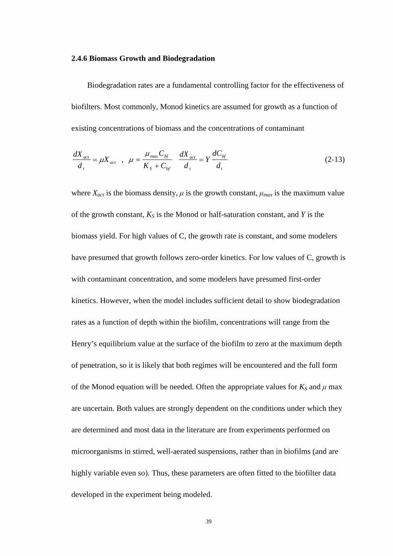
39

2.4.6 Biomass Growth and Biodegradation

Biodegradation rates are a fundamental controlling factor for the effectiveness of

biofilters. Most commonly, Monod kinetics are assumed for growth as a function of

existing concentrations of biomass and the concentrations of contaminant

actt

act Xd

dXµ= ,

bfS

bf

CK

C

+= maxµ

µ t

bf

t

act

d

dCY

d

dX= (2-13)

where Xact is the biomass density, µ is the growth constant, µmax is the maximum value

of the growth constant, KS is the Monod or half-saturation constant, and Y is the

biomass yield. For high values of C, the growth rate is constant, and some modelers

have presumed that growth follows zero-order kinetics. For low values of C, growth is

with contaminant concentration, and some modelers have presumed first-order

kinetics. However, when the model includes sufficient detail to show biodegradation

rates as a function of depth within the biofilm, concentrations will range from the

Henry’s equilibrium value at the surface of the biofilm to zero at the maximum depth

of penetration, so it is likely that both regimes will be encountered and the full form

of the Monod equation will be needed. Often the appropriate values for KS and µ max

are uncertain. Both values are strongly dependent on the conditions under which they

are determined and most data in the literature are from experiments performed on

microorganisms in stirred, well-aerated suspensions, rather than in biofilms (and are

highly variable even so). Thus, these parameters are often fitted to the biofilter data

developed in the experiment being modeled.

40

2.4.7 Summary

Current models for mass transport in the air and within simple biofilms seem

adequate. The major remaining uncertainty is in the determination of appropriate

diffusion constants for various contaminants that reflect conditions in biofilms rather

than water.

Biodegradation rates and biofilm growth models remain somewhat uncertain

because of the lack of knowledge of Monod constants and maximum growth rate

constants for actual conditions in biofilters.

2.5 Major Findings

The major findings of the literature review are:

� The potential of botanical filter to remove indoor VOC has been demonstrated

by researchers, while there are very limited data available to understand the real VOC

removal mechanisms;

� Most of the studies related to botanical air filtration were in terms of the static

effect of the plant to VOC removal, which means there was no air flow passing

through the root bed;

41

� Most of the studies related to botanical air filtration were conducted at

relatively high VOC concentration level (ppm), and therefore, experimental

investigation at low VOC concentration level is needed;

� It has been pointed out that the microbial community plays an important role

in the botanical air filtration system, while the bio-degradation rate of the microbial

community has not been further studied;

� Mathematical model on biofilter or biotrickling filter has been well developed,

while there is no simulation model for botanical air filtration.

Further needed studies are:

� The VOC removal performance of botanical air filtration with air passing

through the root bed is needed to investigated;

� Studies at both relatively high concentration pollutant level (ppm) and low

concentration pollutant level (ppb) are needed;

� Studies are needed to improve the understanding of the VOC removal

mechanisms;

� The bio-degradation rate of botanical air filtration system needs to be

determined;

� A numerical model is needed to simulate the botanical air filtration system and

to help optimizing the design.

42

Chapter 3. Performance Testing, Evaluation, and Analysis

3.1 Introduction

As discussed in the last chapter, previous studies have indicated that the plant’s

root bed has the potential of improving indoor air quality. The microbial communities

may play an important role in degrading VOC. Most previous studies have been focus

on the VOC removal by potted plant without any air passing through the root bed,

which severely limits the chance of contact between VOC and microbial

communities. A dynamic botanical air filtration system (DBAF) prototype based on

the principle of physical adsorption by activated carbon, absorption by water (“wet

scrubber”), and VOC degradation by microorganisms in the plant’s root system was

developed in this study in collaboration with Phytofilter Technologies Inc. In this

system, the polluted indoor air is forced to pass through the plant root bed to improve

the removal performance.

The objectives of this chapter were to: 1) determine the single pass efficiency of

the filter in removing both water soluble and non-soluble VOC and the equivalent

clean air delivery rate (CADR) at a relative high pollutant level (1–3 ppm) in a

full-scale test chamber, as well as at a typical room level (2–17 ppb) in a newly

constructed office room; 2) evaluate the long-term performance in the real-world

environment by monitoring its single pass efficiency for 10 months; 3) investigate the

effect of moisture content in the root bed on the toluene and formaldehyde removal

43

performance, and determine the best moisture content range for removing both water

soluble and insoluble compounds; and 4) investigate the possible effect of the DBAF

may bring to the indoor air temperature and relative humidity (RH).

3.2 Methods

The DBAF system (Figure 3-1) used mixture of activated carbon and porous

shale pebbles as root bed of selected plants (Golden Pothos (Epipremnum aureum))

with microorganisms growing in the root system. The filter bed was 1.8 m in length,

0.6 m in width and 0.2 m in depth. The average diameter of the granular activated

carbon and shale pebbles was 0.005 m, and the mixed ratio is 50/50 by volume. Eight

Golden Pothos were evenly placed in the bed. The filtration system was operated with

periodical irrigation and airflow passing-through. An axial flow fan was installed. The

maximum air flow through the bed was 1014 m3/h. Gas pollutants such as VOC were

adsorbed by the activated carbon sorbent, and the wet root bed also acted as a

scrubber for formaldehyde and other water soluble compounds. The adsorbed and/or

absorbed organic compounds would be degraded by the microbes, regenerating the

sorbent-based root bed. The purified air could be returned to indoor environment

directly or fed to the supply air of an HVAC system to improve indoor air quality.

The DBAF had a controller that automatically sequences the operation of the

irrigation system and fan based on the signal from a moisture content sensor. The

irrigation control sensor was buried in the center of the bed. When the moisture

44

content was below the lower limit, the fan was stopped, and irrigation system

triggered and operated until the moisture content was higher than the higher limit.

Three minutes after the irrigation was stopped, the fan was triggered and operated

until the moisture was below the lower level again. Three Campbell CS616-L water

content reflectometers (M.C. Sensors) were buried inside the bed in sequence for

accurate moisture content measurement in experiments conducted in the real-world

condition ( a newly constructed office building), as shown in Figure 3-1(b).

0.

4m0.2m

a

Fan

Sorbent bed

Goldenpothos

Irrigationline

Sprinkler

1.8

m

0.6m0

.25

m

Irrigationcontrol sensor

M.C.sensor

Fan

Sorbent bed

Goldenpothos

Irrigationline

Sprinkler

1.8

m

0.6m0

.25

m

Irrigationcontrol sensor

M.C.sensor

b

Figure 3-1 Schematic of full-sized dynamic botanical air filtration system: (a) side

view, (b) top view. Moisture content sensor (M.C. sensor).

3.2.1 Experiments in a Full-scale Environmental Chamber

The chamber used had interior dimensions of 4.84 m long x 3.63 m wide x 3.05

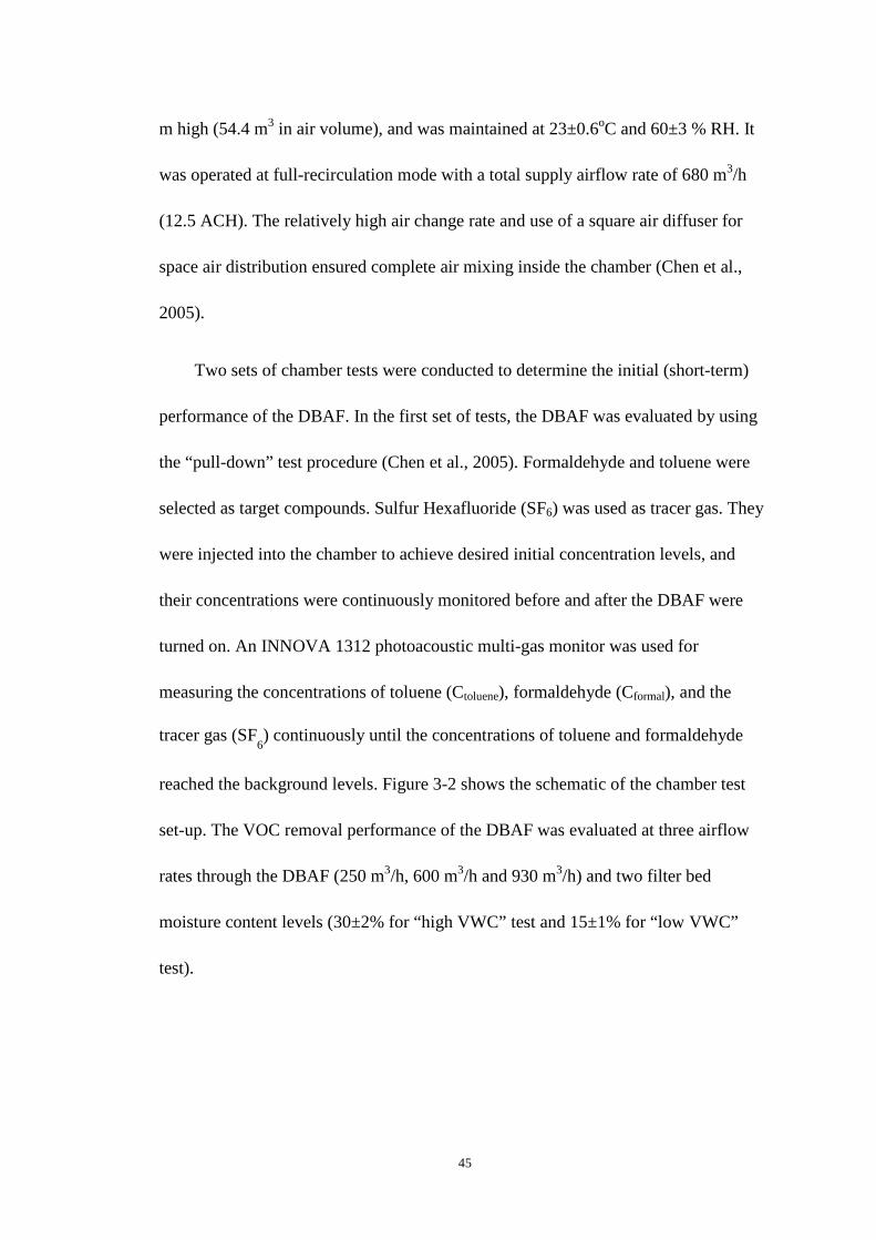
45

m high (54.4 m3 in air volume), and was maintained at 23±0.6oC and 60±3 % RH. It

was operated at full-recirculation mode with a total supply airflow rate of 680 m3/h

(12.5 ACH). The relatively high air change rate and use of a square air diffuser for

space air distribution ensured complete air mixing inside the chamber (Chen et al.,

2005).

Two sets of chamber tests were conducted to determine the initial (short-term)

performance of the DBAF. In the first set of tests, the DBAF was evaluated by using

the “pull-down” test procedure (Chen et al., 2005). Formaldehyde and toluene were

selected as target compounds. Sulfur Hexafluoride (SF6) was used as tracer gas. They

were injected into the chamber to achieve desired initial concentration levels, and

their concentrations were continuously monitored before and after the DBAF were

turned on. An INNOVA 1312 photoacoustic multi-gas monitor was used for

measuring the concentrations of toluene (Ctoluene), formaldehyde (Cformal), and the

tracer gas (SF6) continuously until the concentrations of toluene and formaldehyde

reached the background levels. Figure 3-2 shows the schematic of the chamber test

set-up. The VOC removal performance of the DBAF was evaluated at three airflow

rates through the DBAF (250 m3/h, 600 m3/h and 930 m3/h) and two filter bed

moisture content levels (30±2% for “high VWC” test and 15±1% for “low VWC”

test).

46

Test Chamber

Return Air

Supply Air

AHU

BotanicalFilter

Sampling point

Hot Plate

Diffuser

1 m2.4 m

4.8 m

3.6

m

1.2m 0.

5m

a

Test Chamber

Return Air

Supply Air

AHU

BotanicalFilter

Sampling point

Hot Plate

Diffuser

1 m2.4 m

4.8 m

3.6

m

1.2m 0.

5m

a

Test Chamber

BotanicalFilter

Hot Plate

Diffuser

b

Test Chamber

BotanicalFilter

Hot Plate

Diffuser

b

Figure 3-2 Schematic of the environmental chamber test setup: (a) top-view, (b)

side-view. Air handling unit (AHU).

In the second set of chamber tests, a new working station made of particle board

was placed inside the test chamber to simulate a typical emission source in an office

environment. No clean air was supplied to the chamber and the VOC concentrations

were allowed to increase or decrease depending on the operation of the DBAF. The

test lasted for four days, and the DBAF ran eight hours per day. The air flow rate

passing through the filter bed was ~510 m3/h when the DBAF was turned on. The

same INNOVA gas monitor was used to monitor formaldehyde and TVOC

(quantified as toluene equivalent) concentrations.

Clean air delivery rate (CADR) represents the “effective” clean airflow rate

delivered by the air cleaner (ANSI/AHAM standard: AC-1 2006). The performance

parameter measured directly by the “pull-down” test method was CADR. The analysis

was based on the well-mixed single zone model. Assuming that: 1) the air was well

mixed in chamber (as confirmed by tracer gas testing), and 2) the contaminant

47

removal mechanisms other than air cleaning (e.g. surface adsorption effect and

chamber leakage effect) were could be characterized by a first-order rate constant kn,

the mass conservation of contaminant in the “pull-down” test can be written as (Chen

and Zhang, 2006):

( ) CVkCCADRVkdt

dCV en ⋅−=⋅+−= , (C=C0 at t=0) (3-1)

then

( )VkkCADR ne −= (3-2)

where, V is the testing chamber system volume, m3; kn is the exponential decay

constant of the contaminant concentration without air cleaner operating (empty

chamber effect), h-1; ke is exponential decay constant with air cleaner operating (that

includes both the empty chamber and air cleaner effects), h-1; C0 is the initial

contaminant concentration inside the chamber at t=0, mg/m3; C is the contaminant

concentration inside the chamber at time t, mg/m3.

The decay rate constant of SF6 was 0.031 air change per hour (ACH)

(corresponding to 1.68 m3/h or 1.0 CFM), indicating that chamber leakage rate was

acceptable. When there was no air cleaner in the chamber, the overall decay rate

constant for each individual VOC ranged from 0.031–0.048 ACH (i.e., very close to

that of SF6, indicating minimal surface adsorption effect of the chamber at the

experimental conditions). Therefore the chamber surface adsorption effect was

neglected and only the chamber leakage rate (characterized by SF6 decay rate for each

test) was used to determine kn.

48

The equivalent single pass efficiency (SPE) can be calculated by following

equation (Chen and Zhang, 2006):

dEG

CADR

⋅=η (3-3)

where η is single pass efficiency of the air cleaner, %; G is the air flow rate through

the air cleaner, m3/h; Ed is short-circuiting factor of the air cleaner, ( 1=dE at

well-mixed condition).

3.2.2 Experiments as Part of an Office HVAC System

Following the full-scale chamber tests, the botanical air filtration system was

integrated into the HVAC system of a newly constructed office room in Syracuse,

NY, as shown in Figure 3-3. The total volume of the test room was 265 m3

(approximately 16.4 m long, 5.4 m wide and 3.0 m high). There were 16 work

cubicles in the room. The botanical filter was connected with the supply air duct by

steel pipes with diameter of 0.25 m. An independent fan was installed on the filter

system, which provided an air flow rate of ~815 m3/h. The total amount of supply air

for this room was 2378 m3/h during the tests. Tests were started in the winter

(December 2008 - March 2009). During this test period, the test room was maintained

at 22 oC with a relative humidity of 15%. The effect to the room temperature and RH

was investigated. The effect of filter bed moisture content to the single pass efficiency

was also investigated. The improvement of the indoor air quality by using the

49

botanical filter was evaluated as well. The single pass efficiency of the botanical in

removing formaldehyde and toluene was kept on being monitored until October 2009,

a ten-month-continuous monitoring.

Test RoomReturn Air

Supply Air

AHU

Outdoor AirExhaust Air

Botanicalfilter

PTR-MS

Room air sampling

air samplingbefore filter

air samplingafter filter

Test RoomReturn Air

Supply Air

AHU

Outdoor AirExhaust Air

Botanicalfilter

PTR-MS

Room air sampling

air samplingbefore filter

air samplingafter filter

Figure 3-3 Integration of botanical filter into an HVAC system and setup for

monitoring. Air handling unit (AHU). Proton Transfer Reaction Mass Spectrometer

(PTR-MS).

Preliminary tests revealed that the test room had unusually low pollutant

concentration due to the low emitting materials used. In order to simulate pollutant

level at a more typical office conditions, 48 pieces of unused particleboard were

placed in the test room. The size of each piece was 1.2 m by 0.8 m. After the

particleboards were placed into the test room, an air sample was taken at the return air

duct by using a tenax sorbent tube, and analyzed by gas chromatography-mass

spectrometry (GC/MS). Pentanal, toluene, hexanal, xylene, α-pinene were found to

50

have the highest concentrations. Toluene was selected as the target VOC in current

study since it is commonly used as calibration reference for the total volatile organic

compounds (TVOC) (Hodgson et al., 2000). Meanwhile, another air sample was taken

at the same location by using 2,4-dinitrophenylhydrazine (DNPH) cartridge, and

analyzed by high-performance liquid chromatography (HPLC). Formaldehyde and

acetaldehyde were also detected. Formaldehyde was chosen as the other target

compounds as it is typically identified as a major compound of concern in emission

testing of composite wood materials and office furniture (ANSI/BIFMA standard:

M7.1 2007). A proton transfer reaction mass spectrometer (PTR-MS) was used to

monitor these target compounds in real-time. The detection limits of PTR-MS are

0.06 ppb for toluene and 0.2 ppb for formaldehyde. The sampling inlet of PTR-MS

was connected to the return air duct, as shown in Figure 3-3.

To study the effect of the filter bed on the air temperature and RH, air

temperature and RH sensors were installed in four different locations: air duct right

before entering DBAF, air duct immediately after DBAF, return air duct and supply

air duct of the test room. In the one-day test period, the DBAF was turned on for eight

hours, from 12th hour to 20th hour, and was turned off during the rest of hours of the

day.

To investigate the maximum clean air flow rate that the DBAF could provide,

tests were conducted at four different HVAC system operation modes: 50% outdoor

air (OA) (1138 m3/h), 25% outdoor air, 10% outdoor air, and 5% outdoor air plus the

DBAF (i.e., filter on). The room VOC sampling location was in the return air duct.

51

The 24-hour tests (three-hour-background measurement at 5% OA and the switch to

the test ventilation mode) were conducted. The concentrations at the third hour (start

point of ventilation mode change) were taken as the reference for normalization, 17

ppb for formaldehyde and 2 ppb for toluene, respectively.

To investigate the effect of filter bed moisture content on the toluene and

formaldehyde removal performance, three Campbell CS 616-L water content

reflectometers were used to measure the moisture content in the bed. Average of the

readings from these three sensors was taken as the bed water content. The filter bed

was saturated with water at the beginning of the test, and then the fan was kept on

running until the bed water content decreased to less than 5% in VWC. The filter inlet

and outlet contaminant concentrations were measured periodically, and then the single

pass efficiency was calculated by using the following equation:

in

outin

in

outin

C

CC

GC

CCG −=

−=

)(η (3-4)

where G is the airflow rate through the air cleaner, m3/h; Cin is the contaminant

concentration at the inlet of air cleaner, mg/m3; Cout is the contaminant concentration

at the outlet of air cleaner, mg/m3.

The filter was then kept on running for 10 months. The filter inlet and outlet

contaminant concentrations were measured periodically. The calculated single pass

efficiencies were used to study the long-term performance of the DBAF.

52

3.3 Results and Discussions

3.3.1 Full-scale Chamber Experiments

3.3.1.1 Results from the First Set of Chamber Tests

Pollutant Removal Performance. Figure 3-4 presents the normalized

formaldehyde concentration with three different air flow rates passing the filter bed:

250 m3/h, 600 m3/h and 930 m3/h. Formaldehyde concentration in the chamber at the

time “0 hr” in the tests was 2 mg/m3 (1.64 ppm). The background pollutant

concentration in the chamber was measured for two hours before the test was started,

and all the concentrations measured later were subtracted by the average background

concentration. Then the concentrations were normalized by using the initial

concentration at time t = 0 as reference) to facilitate the comparison. The negative

concentration at the later period of the test means that the concentration achieved was

lower than initial background level. Tracer gas (Sulfur hexafluoride (SF6))

concentration was also presented, and the chamber leakage rate from SF6 calculation

was 0.031 ACH, which corresponded to 1.68 m3/h and was excluded in the final

CADR calculation for the DBAF. The formaldehyde concentration decreased quickly

to the background level after the fan was turned on. With higher airflow rate passing

the sorbent bed, the formaldehyde concentration decreased faster. It means more clean

air was delivered in a fixed time period.

53

-0.2

0.2

0.6

1

1.4

-0.5 0 0.5 1 1.5 2Time (hr)

No

rmal

ized

con

cen

tratio

n

-0.2

0.2

0.6

1.0

1.4

-0.5 0 0.5 1 1.5 2Time (hr)

No

rmal

ized

co

ncen

tratio

n

-0.2

0.2

0.6

1

1.4

-0.5 0 0.5 1 1.5 2Time (hr)

Nor

mal

ized

con

cen

tratio

n

High VWC

Low VWC

SF6

a b

c

Figure 3-4 Normalized formaldehyde concentration at different air flow rate: (a) 250

m3/h airflow rate passing the bed, (b) 600 m3/h airflow rate, (c) 930 m3/h air flow rate.

Volumetric water content (VWC) in the filter bed.

Toluene concentrations were also monitored at the same test conditions, as

shown in Figure 3-5. Toluene concentration at the time “0 hr” in the tests was ~8

mg/m3 (2.16 ppm). Similar trend was observed for the effect of air flow rate, toluene

concentration decreased faster at higher airflow rate test. Results also indicated that

the single pass efficiency (SPE) at higher air flow rate was less than that at lower air

flow rate in general due to smaller residence time, but more clean air can be delivered

during a fixed period of time at higher airflow rate test. That is why formaldehyde or

54

toluene decreased faster at higher airflow rate test.

-0.2

0.2

0.6

1.0

1.4

-0.5 0 0.5 1 1.5 2Time (hr)

Nor

mal

ized

con

cent

ratio

n

-0.2

0.2

0.6

1

1.4

-0.5 0 0.5 1 1.5 2Time (hr)

Nor

mal

ized

con

cent

ratio

n

a b

-0.2

0.2

0.6

1

1.4

-0.5 0 0.5 1 1.5 2Time (hr)

Nor

mal

ized

co

ncen

trat

ion High VWC

SF6

Low VWC

c

Figure 3-5 Normalized toluene concentration at different air flow rate: (a) 250 m3/h

airflow rate passing the bed, (b) 600 m3/h airflow rate, (c) 930 m3/h air flow rate.

Volumetric water content (VWC) in the filter bed.

Table 3-1 lists the CADR and SPE for formaldehyde and toluene in the first set

of chamber tests. Overall, the CADR or SPE was not significantly affected by the test

moisture condition because both high and low VWC conditions in the tests were well

within the range of 5–32% bed water content, which is the range where the botanical

55

filter worked well for both water soluble and insoluble compounds as to be further

discussed later in this paper.

Table 3-1 CADR and SPE for formaldehyde and toluene removal

Air flow

(m3/h)

Pollutant Formaldehyde Toluene

Moisture level

(VWC)

High VWC Low VWC

(30±2%) (15±1%)

High VWC Low VWC

(30±2%) (15±1%)

250±10 CADR (m3/h)

SPE (%)

266.9 253.7

98.7 93.8

247.9 232.4

91.7 85.9

600±15 CADR (m3/h)

SPE (%)

582.4 581.7

94.4 94.3

529.1 436.7

85.8 70.7

930±20 CADR (m3/h)

SPE (%)

698.1 731.8

69.0 73.2

759.7 492.0

77.2 50.1

ASHRAE 62.1-2010 specifies that the requirement of outdoor air for office

buildings is 5 cfm (8.48 m3/h) per person plus 0.06 cfm (1.02 m3/h) per square foot

floor area. ASHRAE 62.1-2010 also specifies a maximum occupant density for office

spaces of five people per 1000 ft2 or per 100 m2. Take this maximum value as

example, the requirement of outdoor air for per 1000 ft2 office building is 85 cfm (144

m3/h). The maximum CADR of the filter for formaldehyde was 731.8 m3/h.

Therefore, the DBAF could serve an office building with 5000 ft2 (465 m2) floor area

56

if formaldehyde is the target pollutant for air cleaning.

Effect of DBAF on the Chamber Air Temperature and RH. The test chamber

air was maintained at 23±0.6oC and 60±3 % RH at the beginning of test, which is

common in a conditioned office space for a hot and humid summer. Table 3-2 lists the

average temperature and relative humidity change in chamber return air with three

different air flow rates passing through the filter bed: 250±10, 600±15 and 930±20

m3/h. For the same air flow rate, tests were also conducted at two different volumetric

water content (VWC) levels in the filter bed: High VWC (30±2%) and Low VWC

(15±1%). The VWC level was measured by the filter bed moisture control sensor. The

sensor was located in the center of the DBAF. Although it does not exactly represent

the average moisture condition of the entire filter bed, the sensor represents relative

levels of VWC in different tests. It can be found that the chamber air was cooled

slightly at high VWC levels. With air flow rate of 250±10 m3/h, temperature

decreased by 0.2–0.5 oC while RH increased by 5.7–13.3%. For air flow rate of

600±15 and 930±20 m3/h, temperature decreased by 0.6–1.1 oC and 0.8–1.0 oC while

RH increased by 11.3–14.5% and 9.4%–13.5%, respectively. In summary, the

chamber air temperature decreased by less than 1 oC and relative humidity increased

by 10% to 15% RH in most tests.

57

Table 3-2 Average temperature and RH change “∆” in chamber return air from the

initial conditions of 23±0.6 °C and 60±3 % RH

Airflow rate

(m3/h)

Bed moisture level

(VWC)

High VWC Low VWC

(30±2%) (15±1%)

Moisture generation

(kg/h)

250±10

Temperature ∆ (oC)

Relative humidity ∆ (% RH)

-0.5 -0.2

13.3 5.7

0.81–1.14

600±15 Temperature ∆ (oC)


-1.1 -0.6

14.5 11.3

1.15–1.37

930±20

Temperature ∆ (oC)


-1.0 -0.8

13.5 9.4

1.23–1.89

Even though introducing humidity through this DBAF is not preferable, the

influence to humidity load of building was analyzed for reference. In this operation

condition, the application of the DBAF will introduce additional humidity that needs

to be removed by the HVAC during summer condition for thermal comfort, but would

improve comfort during winter condition in which humidification is needed. The

prototype DBAF tested produces approximately 0.81–1.89 kg/h of moisture based on

the data in Table 3-2. It should be noted that the DBAF could serve a much larger

building space than the chamber (465 m2 versus 17.6 m2 in floor area) per the outdoor

airflow rate requirement recommended by ASHARE Standard 62.1-2010. The

58

increase of relative humidity due to the operation of DBAF would be much smaller

when it is used for a larger building space that matches its CADR capacity.

3.3.1.2 VOC Removal Performance in the Second Set of Chamber Tests

Figure 3-6(a) shows the test set-up with VOC emissions from an office

workstation system (the second stage of chamber test). Figure 3-6(b) shows the

pollutant concentration in chamber varied with time. It decreased significantly after

the DBAF began to work. Once the filter stopped running, the pollutant concentration

in chamber began to increase due to sustained VOC emissions from the furniture

system. Table 3-3 lists the CADR and SPE calculation for each running period. It was

found that the filter also worked well at low concentration range tested (300 – 400

ppb). The single pass efficiency for formaldehyde was over 90% after the filter had

been continuousely running for four days which might mainly be due to the

absorption of the wet media bed, and meanwhile the SPE for TVOC (quantified as

toluene equivalent) was 38%.

59

0

200

400

600

0 24 48 72 96Elapsed time (hr)

Ch

amb

er C

(pp

b)

Formaldehyde TVOC_as toluene

Filteroff offon on off on off

a b

Figure 3-6 Test set-up and test chamber concentration vary with time: (a) test set-up

(photo), (b) test results. The red dotted vertical lines represent the 8-hour operation

period of the DBAF.

Table 3-3 CADR and SPE of DBAF for VOC emitted from an office furniture during

a 4-day test

VOC Formaldehyde TVOC as toluene equivalent

Time (day) 1st 2nd 3rd 4th 1st 2nd 3rd 4th

Air leakage rate

calculated by SF6 kn

0.031 0.031 0.031 0.031 0.031 0.031 0.031 0.031

Decay rate calculated

after turning on AC ke

16.27 14.83 8.71 8.59 4.86 5.72 3.14 3.63

CADR=V( ke -kn)/60

(m3/h)

510 510 470 465 260 310 169 195

Final single pass 100.0 100.0 92.6 91.3 51.5 60.7 33.1 38.4

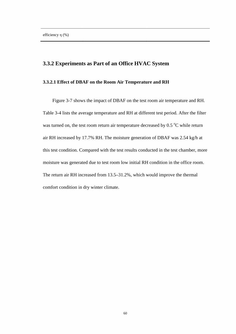
60

efficiency η (%)

3.3.2 Experiments as Part of an Office HVAC System

3.3.2.1 Effect of DBAF on the Room Air Temperature and RH

Figure 3-7 shows the impact of DBAF on the test room air temperature and RH.

Table 3-4 lists the average temperature and RH at different test period. After the filter

was turned on, the test room return air temperature decreased by 0.5 oC while return

air RH increased by 17.7% RH. The moisture generation of DBAF was 2.54 kg/h at

this test condition. Compared with the test results conducted in the test chamber, more

moisture was generated due to test room low initial RH condition in the office room.

The return air RH increased from 13.5–31.2%, which would improve the thermal

comfort condition in dry winter climate.

61

12

15

18

21

24

27

30

6 12 18 24Time (hr)

Air

tem

pera

ture

(C

)

air before DBAFair after DBAFreturn airsupply air

0%

20%

40%

60%

80%

100%

6 12 18 24Time (hr)

Air

rela

tive

hum

idity

air before DBAFair after DBAFreturn airsupply air

a b

Figure 3-7 Effect of DBAF on room air temperature and RH: (a) Temperature, (b)

RH.

Table 3-4 Average temperature and RH at different periods in a 24-hr-test

Air parameter Average Temperature (oC) Average RH (%)

Test Period Ⅰ Ⅱ Ⅲ Ⅰ Ⅱ Ⅲ

6-11hr 12-19hr 20-24hr 6-11hr 12-19hr 20-24hr

Air before filter 23.7 19.7 23.7 12.9 37.6 19.2

Air after filter 26.0 15.8 26.4 20.6 71.0 23.4

Return air 21.4 20.9 21.4 13.5 31.2 20.8

Supply air 19.5 18.6 19.5 16.9 40.5 26.3

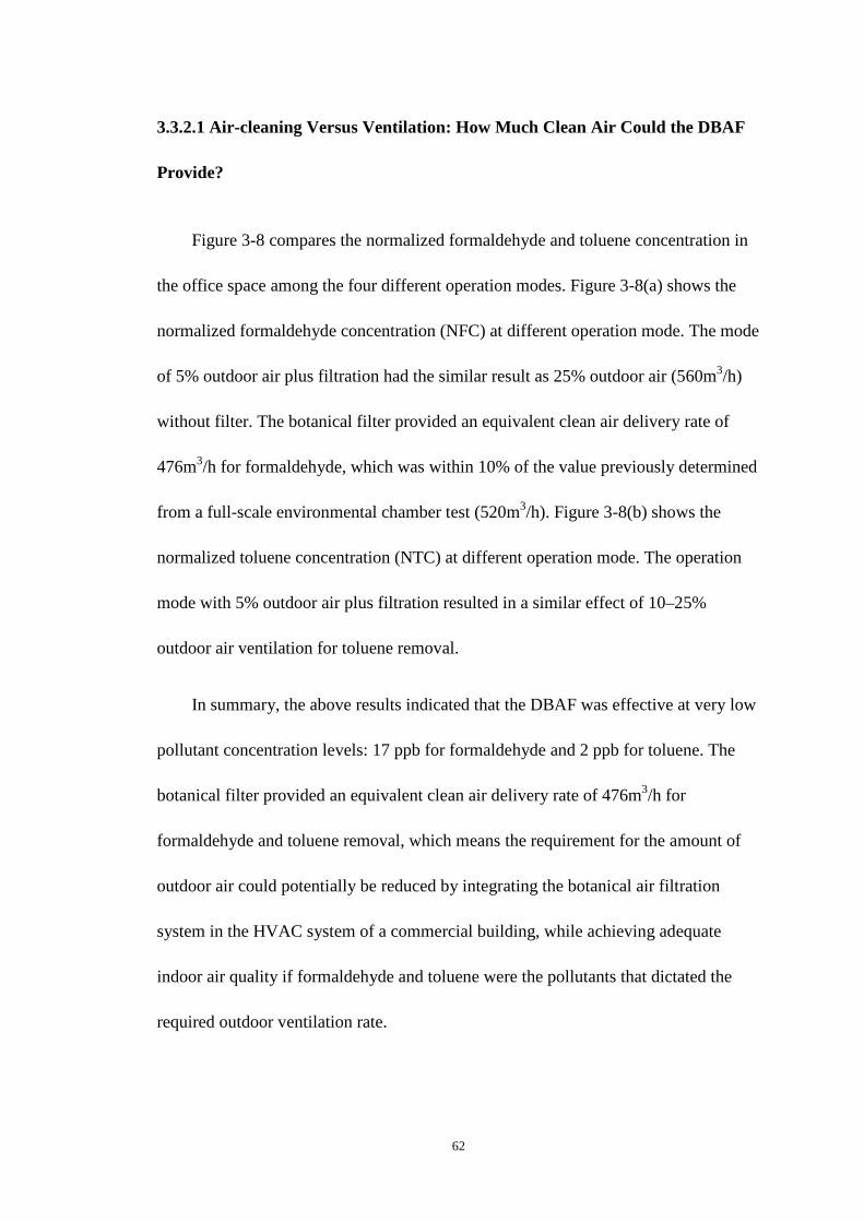
62

3.3.2.1 Air-cleaning Versus Ventilation: How Much Clean Air Could the DBAF

Provide?

Figure 3-8 compares the normalized formaldehyde and toluene concentration in

the office space among the four different operation modes. Figure 3-8(a) shows the

normalized formaldehyde concentration (NFC) at different operation mode. The mode

of 5% outdoor air plus filtration had the similar result as 25% outdoor air (560m3/h)

without filter. The botanical filter provided an equivalent clean air delivery rate of

476m3/h for formaldehyde, which was within 10% of the value previously determined

from a full-scale environmental chamber test (520m3/h). Figure 3-8(b) shows the

normalized toluene concentration (NTC) at different operation mode. The operation

mode with 5% outdoor air plus filtration resulted in a similar effect of 10–25%

outdoor air ventilation for toluene removal.

In summary, the above results indicated that the DBAF was effective at very low

pollutant concentration levels: 17 ppb for formaldehyde and 2 ppb for toluene. The

botanical filter provided an equivalent clean air delivery rate of 476m3/h for

formaldehyde and toluene removal, which means the requirement for the amount of

outdoor air could potentially be reduced by integrating the botanical air filtration

system in the HVAC system of a commercial building, while achieving adequate

indoor air quality if formaldehyde and toluene were the pollutants that dictated the

required outdoor ventilation rate.

63

0.0

0.5

1.0

1.5

0 3 6 9Elapsed time(hr)

Nor

mal

ized

tolu

ene

C

0

0.1

0.2

0.3

0.4

Em

issi

on fa

ctor

(m

g/m

2h)

50%OA_NTC 25%OA_NTC10% OA_NTC 5% OA+ filter_NTC50%OA_EF 25%OA_EF10%OA_EF 5%OA+filter_EF

0.0

0.5

1.0

1.5

0 3 6 9Elapsed time(hr)

Nor

mal

ized

form

alde

hyde

C

0.0

0.2

0.4

0.6

0.8

1.0

Em

issi

on fa

ctor

(m

g/m

2h)

50%OA_NFC 25%OA_NFC10% OA_NFC 5% OA+ filter_NFC25%OA_EF 10%OA_EF5%OA+filter_EF 50%OA_EF

a

b

Figure 3-8 Comparison of room pollutants concentration: (a) Formaldehyde, (b)

Toluene. Outdoor air (OA). Normalized formaldehyde concentration (NFC). Emission

factor (EF). Normalized toluene concentration (NTC).

Figure 3-8 also shows the emission factors at different operating conditions

estimated based on the following mass balance equation for the room space, assuming

64

that the air was well-mixed in the room:

f

dCV AE QC Q C

dtη δ= − − − (3-5)

where, V is the room volume, m3; A is the total surface area of emission source, m2; E

is the emission factor, mg/m2h; Q is the outdoor air ventilation rate, m3/h; C is the

contaminant concentration inside the chamber at time t, mg/m3; Qf is the air flow rate

through the filter, m3/h; η is the single pass efficiency of the filter, which was

determined by measuring the concentrations right before and after the DBAF (η=0

when DBAF was completely bypassed); δ is the room sink effect, mg/h.

For the same outdoor air flow rate and operation mode of the DBAF, the

concentrations of both compounds had a very slow decay rate so that a quasi-steady

state assumption was adopted in estimating the emission factor, E, in Equation (3-5),

i.e., neglecting the transient term on the left hand side of Equation (3-5) and the sink

effect term δ (which was also considered negligible comparing to the other terms in

the equation), we have

( )ηCQQCA

E f+=1

(3-6)

During the field test, the initial emission factors of formaldehyde and toluene were

0.046 mg/m2h and 0.015 mg/m2h respectively at outdoor air ventilation. Figure 3-8

shows that the emission factors increased with outdoor air ventilation or operation of

botanical filter due to a higher concentration gradient between the source and the

room air caused by the reduction of indoor concentration by ventilation or air

cleaning.

65

3.3.2.3 Effect of Bed Water Content

Figure 3-9 shows the effect of bed water content on SPE of the filter. The single

pass efficiency for formaldehyde was maintained at over 70% when the bed water

content was higher than 10%, then it decreased very fast when the water content of

the bed was less than 5%. On the contrary, the SPE for toluene was almost zero when

the bed water content was higher than 40%, then it increased significantly as the bed

water content decreased. The SPE for toluene was maintained at over 40% when the

water content was lower than 30%. The reason for this might be the different water

solubility of these two compounds. Formaldehyde is water soluble, while toluene is

not. The results indicated that 5–32% bed water content is the best range where the

botanical filter worked well for both water soluble and insoluble compounds. The

SPEs were around 70% and 40% for formaldehyde and toluene, respectively in this

range.

66

0%

20%

40%

60%

80%

100%

0 10 20 30

Elapsed time (hr)

Sin

gle

pass

effi

cien

cy

0%

10%

20%

30%

40%

50%

Bed

vol

umet

ric w

ater

con

tent

(m3/

m3)

Formaldehyde

Toluene

Water content

Figure 3-9 Effect of bed water content on removal of pollutants.

Formaldehyde is very weakly adsorbed on activated carbon or any other

untreated adsorbent, because the formaldehyde molecules are small and light so the

Van der Waals force between formaldehyde and activated carbon is very weak (Tseng

et al., 1998). It appears that the “wet film” formed in DBAF worked as an effective

scrubber in removing formaldehyde of the air. Formaldehyde was first absorbed by

the “wet film” formed in the sorbent bed, and then degradated by the microorganisms

living in the “wet film” or the microbial communities in soil from the rhizosphere of

plant.

3.3.2.4 Long-term Performance

Long-term performance evaluation of the DBAF is needed to determine whether

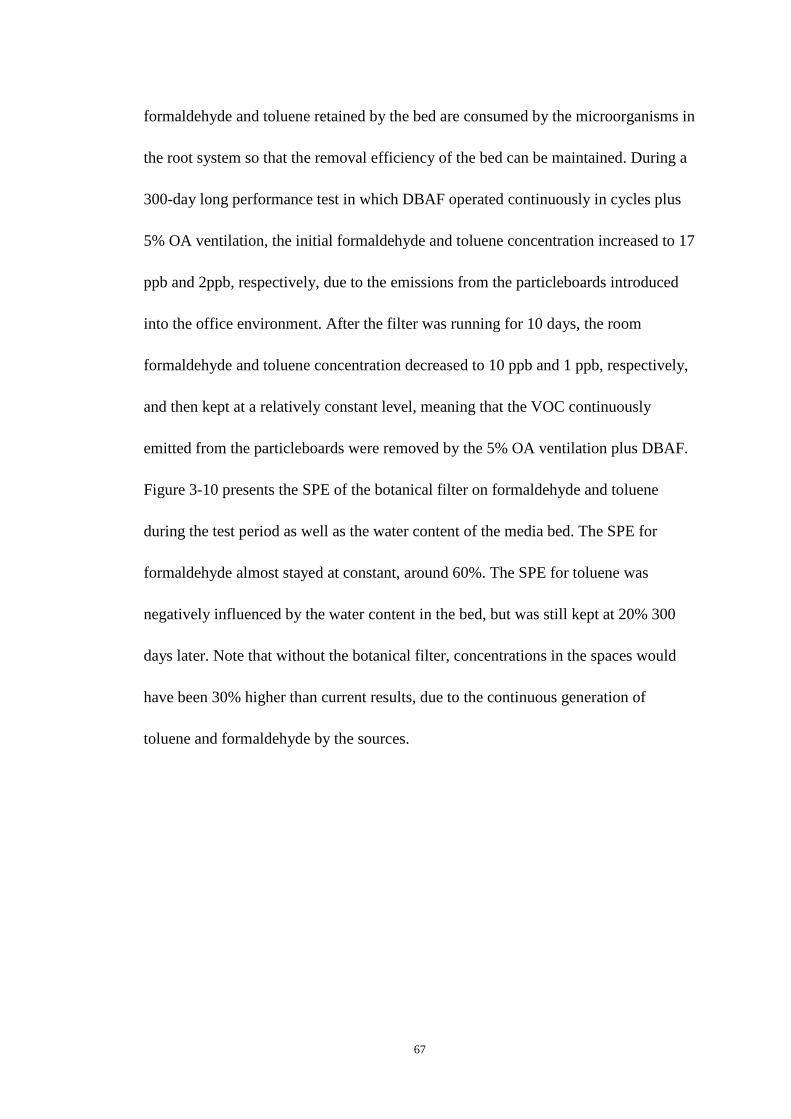
67

formaldehyde and toluene retained by the bed are consumed by the microorganisms in

the root system so that the removal efficiency of the bed can be maintained. During a

300-day long performance test in which DBAF operated continuously in cycles plus

5% OA ventilation, the initial formaldehyde and toluene concentration increased to 17

ppb and 2ppb, respectively, due to the emissions from the particleboards introduced

into the office environment. After the filter was running for 10 days, the room

formaldehyde and toluene concentration decreased to 10 ppb and 1 ppb, respectively,

and then kept at a relatively constant level, meaning that the VOC continuously

emitted from the particleboards were removed by the 5% OA ventilation plus DBAF.

Figure 3-10 presents the SPE of the botanical filter on formaldehyde and toluene

during the test period as well as the water content of the media bed. The SPE for

formaldehyde almost stayed at constant, around 60%. The SPE for toluene was

negatively influenced by the water content in the bed, but was still kept at 20% 300

days later. Note that without the botanical filter, concentrations in the spaces would

have been 30% higher than current results, due to the continuous generation of

toluene and formaldehyde by the sources.

68

0%

20%

40%

60%

80%

100%

0 60 120 180 240 300 360Elapsed time (d)

Sin

gle

pass

effi

cien

cy

0%

10%

20%

30%

40%

50%

wat

er c

onte

nt (

m3/

m3)

formaldehyde

water content

toluene

Figure 3-10 Botanical filter single pass efficiency (SPE) over 300 days.

Seven (7) bacterial species from the botanical filter system using DNA

sequencing were identified, including Arthrobacter aurescens TC1, Arthrobacter

oxydans, Leifsonia xyli subsp. xyli str. CTCB07, Bacillus cereus, A. aurescens,

Pseudomonas putida, and Bacillus spp (Huang et al., 2009). Degradation of

formaldehyde solution by individual species was conducted. According to Henry’s

law, the formaldehyde concentration in the water film around the sorbent particle was

0.001% by weight if the formaldehyde concentration in the air passing through the

sorbent bed was 50 ppb. The initial liquid formaldehyde concentration in the test was

0.001% by weight. It was found that the maximum reduction rate was 86.2% after 24

hours, by A. aurescens TC1 (Huang et al., 2009).

69

Therefore, as long as there are sufficient carbon sources (formaldehyde or VOC)

in the air passing through the bed, the microorganisms living in the sorbent bed will

degrade them. Moreover, the microorganisms that are responsible for the degradation

can quickly reactivate the carbon particle so that it need not be replaced, unlike the

typical carbon filters used for air cleaning which need to be replaced every three-six

months.

There is a concern whether this botanical filter would cause indoor microbial

pollution. A pilot test was conducted to address this issue. Five liters of filter outlet air

was sampled and bubbled through Luria-Bertani (LB) medium (containing 10 g/L

tryptone, 5 g/L yeast extract, and 10 g/L sodium chloride) to observe any possible

microbial growth. No colony was found on the LB agar plates (LB medium

supplemented with 1.5% agar) during incubation for up to 120 h at 30 ºC, which

means there was no microbial pollution in the sampled air. The potential release of

microorganisms from indoor biological purifiers during long-term operation should be

further studied and prevented.

Biofiltration system has been used for many years in the industrial setting as well

as indoor air setting (Darlington et al., 2000). There are some significant differences

between the DBAF and previous biofiltration system. The material used in the

bioscrubber of previous biofiltration system was lava rock, while the bed of DBAF

consisted of porous shale pebble and granular activated carbon. The activated carbon

had a BET surface area of 900–1100 m2/g and 80% of the pore size was less than 10

nanometers, which was highly effective for adsorbing VOC. The plants used in the

70

previous biofiltration system were over hundreds of species of plants typically used in

indoor landscaping, while the plants used in the DBAF were more selective (e.g.

Golden Pothos (Epipremnum aureum)) for ease of maintenance and more root-zone

microbial community. The previous biofiltration system has much lower face velocity

than the current DBAF (0.01 m/s vs. 0.25 m/s), and delivers much less clean air

airflow rate per unit surface area (360 m3/h by a 10 m2 bioscrubber compared to 970

m3/h by a 1.08 m2 DBAF root bed with an acceptable pressure drop of 73 Pa). As a

result, the DBAF system developed in this study would be easier to be adopted for

indoor air cleaning either as part of an HVAC system or operated as a standalone unit

to provide the required clean airflow rate.

3.4. Major Findings

The potential usage of plant’s root bed for removing indoor VOC has been

demonstrated. Although potted plants alone are not efficient in real-world condition,

the dynamic botanical air filtration system (DBAF) developed in this study is very

promising based on the laboratory evaluation and real-field demonstration.

The full-scale chamber experimental results indicated that the DBAF had high

initial removal efficiency for formaldehyde and toluene even without plants in the

bed. With the plants, the filter system had even higher initial removal efficiency (90%

for formaldehyde in the first four days, and over 33% for toluene). However, it was

not clear if the microbes played any role in such a short term test period. The

71

long-term performance test results indicated that the DBAF was effective over a test

period of 300 days, and the same level of single pass removal efficiency was

maintained at the end of the test. This indicated the possible consumption of the VOC

by the microbes. However, further study is needed to investigate the type of microbes

that are responsible for the VOC removal/degradation, and the rate of degradation.

More detailed and carefully controlled laboratory experiments are needed to separate

out the adsorption, absorption and microbe degradation processes involved in the

DBAF root bed to improve the understanding and to develop a simulation model that

can be used to optimize the DBAF deign.

The operation of the DBAF resulted in 1 oC temperature decrease and 9–13%

RH increase in the chamber air. In the office experiments, the operation of DBAF

resulted in 0.5 oC temperature decrease and 17.7% RH increase. The moisture

production rate due to the use of DBAF was in the range of 0.81–1.89 kg/h. Such

moisture generation would improve the thermal comfort condition in winter, while in

summer contribute to little negligible effects on thermal comfort and cooling load

(added 5% more humidity load).

Field experiments in the office space indicated that the use of the DBAF could

reduce the percent of outdoor air supply from 25–5% of total air supply without

adversely affecting the indoor air quality if formaldehyde and toluene are the target

pollutants that dictate the required ventilation rate.

The effect of bed water content on the removal of formaldehyde/toluene was also

72

studied in the field experiments. The single pass removal efficiencies were

approximately 60% for formaldehyde and 20% for toluene when the volumetric water

content was within the range of 5–32% in the root bed. A moisture content that was

higher than 32% resulted in significant increase of single pass efficiency (SPE) for the

water soluble compound (formaldehyde) and reduction of SPE for Toluene.

73

Chapter 4. VOC Removal Mechanisms and Determination of Bio-degradation Rate Constant

4.1 Introduction

In previous chapter, it has been demonstrated that the DBAF performed well in

removing both formaldehyde and toluene at low concentrations (less than 50 ppb),

having consistently ~60% single pass efficiency for formaldehyde and ~20% for

toluene over a 10-month test period, respectively. The test results represent the

whole-filter performance in removing formaldehyde and toluene, but the intrinsic

VOC removal mechanism is still not clear. More experimental research is needed to

understand the underlying VOC removal mechanisms of DBAF. In particular, it is

necessary to clarify the different roles played by the leaves, wet sorbent bed, and

microbial communities.

This chapter presents the methods and results of an experimental study that was

designed to: 1) improve the understanding of the mechanisms of the DBAF system in

removing the volatile organic compounds, including determination of the important

factors affecting the removal performance, and the roles of different transport, storage

and removal processes; 2) determine the VOC biodegradation rate by the microbial

community of the DBAF.

74

4.2 Methods

A reduced-sized dynamic botanical air filtration system was developed for

laboratory evaluation, as shown in Figure 4-1. The filter bed was 0.35 m in length, 0.2

m in width and 0.15 m in depth. The average diameter of the granular activated

carbon and shale pebbles was 0.005 m, and the mixed ratio was 50/50 by volume. The

total weight of the sorbent material was 4900±50 g. Two Golden Pothos

(Epipremnum aureum) were placed in the bed. The filtration system was operated

with periodical irrigation. A tangential flow fan was installed for driving airflow

passing through the bed. The air flow through the bed was 50±3 m3/h, which leads to

a face velocity of ~0.22 m/s. A programmable logic controller was used to

automatically control the operation sequences of the irrigation system and fan in the

DBAF. The irrigation was triggered every two hours and lasted for 5 seconds. The

irrigation water flow rate was 0.4 LPM. The fan was stopped while the irrigation was

on, and was triggered 30 seconds after the irrigation stopped working and operated for

7135 seconds (~2 hours). The water flow rate of the irrigation was measured by a

water flow meter. The actual water flow rate of the irrigation was 0.025 kg/s. One

Campbell CS616-L water content reflectometers (M.C. Sensors) was buried inside the

bed for accurate moisture content measurement.

75

0.4

m0.1

5m

a

Sorbent bed

Goldenpothos

Irrigationline

Sprinkler

0.3

5 m

0.2 m

Tangentialfan

M.C.sensor

b

0.4

m0.1

5m

a

Sorbent bed

Goldenpothos

Irrigationline

Sprinkler

0.3

5 m

0.2 m

Tangentialfan

M.C.sensor

b

Figure 4-1 Schematic of reduced-sized dynamic botanical air filtration system: (a)

side view, (b) top view. Moisture content sensor (M.C. sensor).

To achieve the objecties described above, the experiments in this chapter were

designed into three parts, as shown in Table 4-1. The test methods and test purpose

were also listed in Table 4-1. The detailed test conditions and procedures were

discussed in the following sections.

Table 4-1 Tests conducted to investigate the VOC removal mechanisms of DBAF

Test Group Test methods Test purpose

A. Formaldehyde removal by potted

plant without air passing through

the root bed

Middle-scale chamber,

No ventilation,

Pull-down test

The leaf effect and soil static effect

B. Formaldehyde removal by

microbial community with air flow

passing through

Small-scale chamber,

No ventilation,

Pull-down test

The microbial community effect

76

C. Formaldehyde and toluene

removal by DBAF

Middle-scale chamber,

With ventilation,

Constant source

VOC removal mechanisms of the

DBAF and determination of

bio-degradation rate constant

4.2.1 Formaldehyde Removal by Potted Plant Without Air Passing

the Root Bed

Tests were conducted to investigate the formaldehyde removal by the potted

plants without any air flow passing the root bed. Eight-inch potted Golden Pothos

(Epipremnum aureum) were selected (the same kind of plant used as before). The

tests were conducted in a 5.1 m3 chamber with interior dimensions of 1.83 m long x

1.68 m wide x 1.68 m high. The chamber was located in a conditioned laboratory,

where the temperature and relative humidity were maintained at 23±0.6°C and

50±3 %, respectively. There was no ventilation for the chamber in this test. The

chamber served as a sealed space. A six-inch propeller axial fan was placed in the

middle of the chamber to mix the chamber air in an acceptable manner (equivalent air

change rate of 20 ACH). Para-formaldehyde powder was heated by a hot plate

(250 °C heating temperature set point) to serve as an instant formaldehyde source.

Sulfur Hexafluoride (SF6) was used as a trace gas. Formaldehyde and SF6

concentration were monitored by an INNOVA 1312 photoacoustic multi-gas monitor

in real-time.

Four tests (as shown in Table 4-2) were conducted at standard test conditions:

23±0.6 °C and 50±3% RH. The initial formaldehyde concentration was 20±0.5 ppm.

77

The major purpose of the series of tests was to investigate the formaldehyde removal

by potted plant without any air flow passing through the bed. The pot numbers effect

and light effect were also studied. The detailed CADR calculation was described in

section A.3.

Table 4-2 Tests conducted for formaldehyde removal by potted plant without air

passing the root bed at 23±0.6 °C and 50±3 % RH.

Test No. Test conditions Formaldehyde

concentration

Test purpose

(ppm)

A1 Empty chamber 20±0.5

(Initial

concentration,

instant source)

Background test

A2 Leaf effect only V.S.

total potted plant effect

Study the leaf effect V.S. total effect

A3 One potted plant V.S.

two potted plants

Study the potted numbers effect

A4 With light (a 60-wattz lamp) V.S.

Without light

Study the light effect

The tests were conducted with following steps:

1. Empty chamber test. Test was conducted to check the air tightness of the

chamber and the formaldehyde sink effect in empty chamber. 5 ml SF6 was

injected into the chamber. 125 mg para-formaldehyde powder was injected

into the chamber by heating on the hot plate. The SF6 and formaldehyde

concentration were monitored for 48 hours. The SF6 concentration change

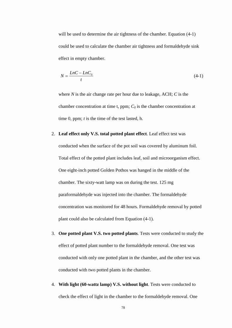
78

will be used to determine the air tightness of the chamber. Equation (4-1)

could be used to calculate the chamber air tightness and formaldehyde sink

effect in empty chamber.

t

LnCLnCN 0−= (4-1)

where N is the air change rate per hour due to leakage, ACH; C is the

chamber concentration at time t, ppm; C0 is the chamber concentration at

time 0, ppm; t is the time of the test lasted, h.

2. Leaf effect only V.S. total potted plant effect. Leaf effect test was

conducted when the surface of the pot soil was covered by aluminum foil.

Total effect of the potted plant includes leaf, soil and microorganism effect.

One eight-inch potted Golden Pothos was hanged in the middle of the

chamber. The sixty-watt lamp was on during the test. 125 mg

paraformaldehyde was injected into the chamber. The formaldehyde

concentration was monitored for 48 hours. Formaldehyde removal by potted

plant could also be calculated from Equation (4-1).

3. One potted plant V.S. two potted plants. Tests were conducted to study the

effect of potted plant number to the formaldehyde removal. One test was

conducted with only one potted plant in the chamber, and the other test was

conducted with two potted plants in the chamber.

4. With light (60-wattz lamp) V.S. without light . Tests were conducted to

check the effect of light in the chamber to the formaldehyde removal. One

79

test was conducted without any light in the chamber, and the other test was

conducted with a sixty-watt lamp placed in the chamber. All the other test

set-ups were the same.

4.2.2 Formaldehyde Removal by Microbial Community with Air

Flow Passing Through

Figure 4-2 shows the schematic of the formaldehyde removal test by microbial

community with air flow passing through. The entire test system was located in a

conditioned chamber, where the ambient conditions were maintained at 23±0.6°C and

50±3 %, respectively. The test system consisted of a 50-liter stainless steel chamber

(for better air mix), an air recirculation pump (with airflow rate of 2 LPM), two

manually controlled three-way valves, and connection tubes. Formaldehyde

concentration was monitored by an INNOVA 1312 photo-acoustic multi-gas monitor.

With valve #1 and #2, the system can be switched between test loop and bypass loop.

The test system was switched to the bypass loop during the period of formaldehyde

injection. After the formaldehyde concentration approached to steady state, the test

system was switched to the test loop.

80

F

Gas monitor

VOC injection RH sensor

Test loopSorbent bed

Ambient conditions:23 °C and 50% RH

Mixing chamber(50L)

Recirculationloop

BypassAir pump

Valve 2 Valve 1

Figure 4-2 Schematics of the test set-up for formaldehyde removal by microbial

community with air passing by

Table 4-3 lists the tests that were conducted for formaldehyde removal by

microbial community with air flow passing by. The test temperature and RH were

23±0.6 °C and 90±3 %, respectively. The initial formaldehyde concentration was

7.5±0.1 ppm. The main purpose of this series of tests was to study the microbial

community effect to formaldehyde removal.

Table 4-3 Tests conducted for formaldehyde removal by microbial community with

air flow passing through at 23±0.6 °C and 90±3 % RH

Test Test conditions Microbes Formaldehyde Test purpose

81

initial

number

concentration

(CFU/mL) (ppm)

B1.

Single-injection

w/o microbes

Wet bed only,

single formaldehyde injection

0 7.5±0.1 The wet bed effect only

B2.

Single-injection

w microbes

Wet bed with microbes,

single formaldedhyde

injection

6.78 × 1010 The microbial community effect

with single formaldehyde

injection

B3.

Multi-injection w

microbes

Wet bed with microbes,

multiple formaldedhyde

injections

2.12 × 109 The microbial community effect

with multiple formaldehyde

injections


1. Test preparation. Two samples of sorbent material were prepared. The

average diameter of the granular activated carbon and shale pebbles was

0.005 m, and the mixed ratio is 50/50 by volume. The diameter of the test

cylinder was half inch. The thickness of the sorbent material was five (5)

inches.The test system was pre-conditioned by 90% RH air for 24 hours. The

air pump was turned on and the pre-conditioned air was re-circulated in the

test system. Formaldehyde was injected to the system through the VOC

injection port in Figure 4-2. The equilibrium formaldehyde concentration in

the system was maintained at ~7.5 ppm.

2. Single-injection without microbes. The first sample of sorbent material was

first saturated with Luria-Bertani (LB) medium (containing 10 g/L tryptone,

82

5 g/L yeast extract, and 10 g/L sodium chloride), and then placed into the test

loop. After the formaldehyde concentration in the system approached to

steady state, the re-circulated air was forced to pass through the test bed. The

formaldehyde was monitored for 24 hours. After the baseline case test was

done, the test system was flushed by lab clean air for 24 hours.

3. Single-injection with microbes. Firstly, the second sample of sorbent

material was saturated with Luria-Bertani (LB) medium (containing 10 g/L

tryptone, 5 g/L yeast extract, and 10 g/L sodium chloride) and Arthrobacter

aurescens TC1 1(CFU number: 6.78 × 1010 CFU/mL), and then installed into

the test loop. Secondly, after the test system was pre-conditioned with 90%

RH air and the same formaldehyde concentration in the system was

approached again, the re-circulated air was forced to pass through the test

bed. The formaldehyde in the system was monitored for 24 hours. After the

proposed case test was finished, the test system was flushed by lab clean air

for 24 hours.

4. Multi-injection with mircobes. The test procedure was conducted in the

same way as the single-injection test. While formaldehyde was injected into

1 Seven (7) bacterial species from the DBAF using DNA sequencing were identified, including Arthrobacter

aurescens TC1, Arthrobacter oxydans, Leifsonia xyli subsp. xyli str. CTCB07, Bacillus cereus, A. aurescens,

Pseudomonas putida, and Bacillus spp. It is found that Arthrobacter aurescens TC1 has the best formaldehyde

removal capacity, which is 86% reduction rate in a 24-hour-test period. Therefore, Arthrobacter aurescens TC1

was selected to conduct the formaldehyde removal.

83

the test system in every 6 hours. There were totally four (4) injections in the

multi-injection test.

4.2.3 Formaldehyde and Toluene Removal Rate by the DBAF

Figure 4-3 shows the schematic of the set-up for low concentration test (ppb

level). The tests were conducted in the same environmental chamber (5.12 m3). The

RH in the chamber will be varied from 55−90% per the requirement of different tests.

A six-inch propeller axial fan was placed in the middle of the chamber to have the

chamber air well mixed (equivalent air change rate of 20 ACH). The chamber was

ventilated by lab clean air. Sulfur Hexafluoride (SF6) was used as a trace gas for air

change rate measurement. Formaldehyde and toluene were continuously generated

into the chamber by Dynacalibrator (Model 450) to serve as a constant source and

monitored by proton transfer reaction mass spectrometer (PTR-MS). The DBAF was

located in the middle of the chamber. A sixty-watt lamp was placed in the chamber to

serve as light source for the plants.

84

Formaldehyde/toluene injection

Lab clean air

PTR-MSSampling tube

Exhaust

Ambient conditions:23ºC and 50%RH Test chamber

(5.12 m3)

Connection to analyzer

Mixing fan

With or without DBAF

Figure 4-3 Schematic of the mid-scale chamber system for low concentration (ppb)

test

Table 4-4 lists the tests that were conducted for formaldehyde removal by DBAF.

The test conditions and test purpose were described in the table. There were two sets

of tests. One set of tests were test C1−4. These tests were to compare the dry bed

effect, wet bed effect, and the whole filter effect. The other set of tests were test C4−6.

These tests were to study the whole filter effect at different RHs.

Table 4-4 Tests conducted for formaldehyde removal by DBAF

Test

No.

Test media

RH

Initial bed

water content

Formaldehyde

concentration

Test purpose

(%) (m3/m3) (ppb)

C1 Empty chamber 50±3 N/A 275±5 Reference test

85

C2 Dry bed, no plant 50±3 0.027 275±5 Effect of dry sorbent

C3 Wet bed, no plant 92±3 0.137 275±5 Effect of moisture of wet bed

C4 DBAF 92±3 0.137 275±5 Effect of RH on DBAF



Table 4-5 lists the tests that were conducted for toluene removal by DBAF. The

test temperature was maintained at 23±0.6°C. The test RH decreased from 92−55%.

The main purpose of this set of tests was to study the whole filter effect at different

RHs.

Table 4-5 Tests conducted for toluene removal by DBAF

Test

No.

Test Note RH Initial bed

water content

Toluene

concentration

Test purpose

(%) (m3/m3) (ppb)

C7 Empty chamber 92±3 0.137 162±5 Background check

C8 DBAF 92±3 0.137 162±5 The whole filter effect

C9 DBAF 75±3 0.078 162±5 The whole filter effect at different RH

C10 DBAF 55±3 0.034 162±5 The whole filter effect at different RH


1. Empty chamber test. Test was conducted to check the formaldehyde natural

decay in empty chamber. 5 ml SF6 was injected into the chamber.

Formaldehyde and toluene were generated into test chamber as well.

86

2. Test with the dry sorbent only in the chamber. Test was conducted in the

chamber with five inches dry sorbent bed only. The air flow rate passing the

bed was the same as the DBAF. Formaldehyde and toluene were

continuously generated into the chamber. Once the formaldehyde and toluene

concentration reached the quasi steady-state, the filter with dry sorbent only

was turned on.

3. Test with the wet sorbent only in the chamber. Test was conducted in the

chamber with five inches wet sorbent bed only. The air flow rate passing the

bed was the same as the DBAF. The sorbent bed has an initial water content

of 0.137 (g/g). Irrigation was triggered for 5 seconds in every 2 hours. The

test chamber RH for this test was 90±3%. Formaldehyde and toluene were

continuously generated into the chamber. Once the formaldehyde and toluene

concentration reached the quasi steady-state, the filter with wet sorbent only

was turned on.

4. Test with DBAF (wet sorbent bed with two Golden Pothos (Epipremnum

aureum)). Tests were conducted in the chamber with DBAF. Two Golden

Pothos (Epipremnum aureum) were placed in the filter bed. The plant density

was 28 plant/(m2 bed). Formaldehyde and toluene were continuously

generated into the chamber. Once the formaldehyde and toluene

concentration reached the quasi steady-state, the DBAF was turned on.

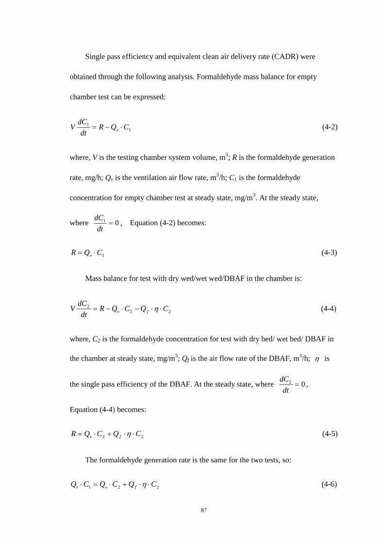
87

Single pass efficiency and equivalent clean air delivery rate (CADR) were

obtained through the following analysis. Formaldehyde mass balance for empty

chamber test can be expressed:

11 CQR

dt

dCV v ⋅−= (4-2)

where, V is the testing chamber system volume, m3; R is the formaldehyde generation

rate, mg/h; Qv is the ventilation air flow rate, m3/h; C1 is the formaldehyde

concentration for empty chamber test at steady state, mg/m3. At the steady state,

where 01 =dt

dC, Equation (4-2) becomes:

1CQR v ⋅= (4-3)

Mass balance for test with dry wed/wet wed/DBAF in the chamber is:

222 CQCQR

dt

dCV fv ⋅⋅−⋅−= η (4-4)

where, C2 is the formaldehyde concentration for test with dry bed/ wet bed/ DBAF in

the chamber at steady state, mg/m3; Qf is the air flow rate of the DBAF, m3/h; η is

the single pass efficiency of the DBAF. At the steady state, where 02 =dt

dC,

Equation (4-4) becomes:

22 CQCQR fv ⋅⋅+⋅= η (4-5)

The formaldehyde generation rate is the same for the two tests, so:

221 CQCQCQ fvv ⋅⋅+⋅=⋅ η (4-6)

88

Therefore, the single pass efficiency of the DBAF can be derived as follows:

f

v

Q

Q

C

C⋅

−= 1

2

1η (4-7)

The equivalent clean air delivery rate (CADR) can be obtained as follows:

η⋅= fQCADR (4-8)

4.3 Results

4.3.1 Formaldehyde Removal by Potted Plant Without Air Passing

the Root Bed

Effect of Leaf. Figure 4-4 shows the formaldehyde removal by potted plant

without any air passing through the root bed. Normalized concentrations (i.e.

concentration divided by the initial concentration at time t = 0) were used to

determine the air tightness of the test chamber. Brown cross points are the normalized

concentration of the trace gas (SF6). The decay rate SF6 shows that the air leakage of

the chamber was 0.002 ACH (air change per hour), which indicates that air tightness

of chamber was acceptable for the test. The chamber formaldehyde concentration was

up to 20 ppm at the beginning of the test. Normalized concentrations (i.e.

concentration divided by the initial concentration at time t = 0) were used to facilitate

the comparison. Dark blue points show the formaldehyde concentration decay over

time for the empty chamber test. Pink triangle points show the formaldehyde

89

concentration decay for the leaf effect only (The top surface of the pot was covered by

aluminum foil to void contact between air and soil). Red square points show the total

effect of the potted plant, including leaf effect and soil effect. Equation (3-1) and (3-2)

can be used to calculation the clean air delivery rate. Equivalent clean air delivery

rates (CADR) of leaf effect test and total effect by the plant were 0.086 and 0.161

m3/h, respectively. It indicates that the formaldehyde removal capacity via static

effect of potted plant is limited. Large amount of potted plant would be required to

maintain acceptable pollutant concentration for a typical indoor space.

0.0

0.2

0.4

0.6

0.8

1.0

1.2

0 12 24 36 48

Time (hr)

No

rmal

ized

co

nce

ntr

atio

n

F_empty_chamber F_leaf_effect F_total_effect SF6

Figure 4-4 Formaldehyde removed by one 8” potted plant

90

Further analysis could be conducted to reflect the limited effect of formaldehyde

removal by potted plant without air passing through the bed. ASHRAE 62.1-2010

specifies that the requirement of outdoor air for office buildings is 5 cfm (8.48 m3/h)

per person plus 0.06 cfm (1.02 m3/h) per square foot floor area. ASHRAE 62.1-2010

also specifies a maximum occupant density for office spaces of five people per 1000

ft2 or per 100 m2. Take this maximum value as example, the requirement of outdoor

air for per 1000 ft2 office building is 85 cfm (144 m3/h). Since one eight-inch potted

Golden Pothos (Epipremnum aureum) could only provide 0.161 m3/h equivalent clean

air delivery rate, 894 potted Golden Pothos will be needed per 100 m2 office building

to follow ASHRAE standard, which is unpractical.

Effect of Potted Plant Numbers. Figure 4-5 shows the effect of the potted plant

numbers on formaldehyde removal. The formaldehyde concentration with two potted

plants placed in the chamber decayed faster than that with one potted plant. The

equivalent clean air delivery rates (CADR) of total effect potted plant can also be

calculated according to the concentration decay in Figure 4-5. It was found that the

equivalent CADR by one potted plant and two potted plants were 0.161 and 0.256

m3/h, respectively. It reflects that the increment of the number of potted plants would

provide more equivalent CADR. Still, it can not significantly improve the removal

efficiency by increasing the number of plants only but without air passing through the

bed.

91

0.0

0.2

0.4

0.6

0.8

1.0

1.2

0 12 24 36 48

Time (hr)

No

rmal

ized

co

nce

ntr

atio

nF_empty_chamber F_1_plant F_2_plants SF6

Figure 4-5 Effect of potted plant number on formaldehyde removal

Effect of Light. Figure 4-6 shows the effect of light in the chamber on

formaldehyde removal. Without light in the chamber, the equivalent CADR for one

potted plant decreased from 0.161−0.144 m3/h in a 24-hour test period, while there

was slightly different after 24 hours. It indicates that the light had little effect after the

leaves were saturated on absorbing formaldehyde. The equivalent CADR for two

potted plants decreased from 0.256−0.207 m3/h, according to Equation (3-1). The

presence of light can improve the performnance on removing formaldehyde if the

leaves have not been saturated.

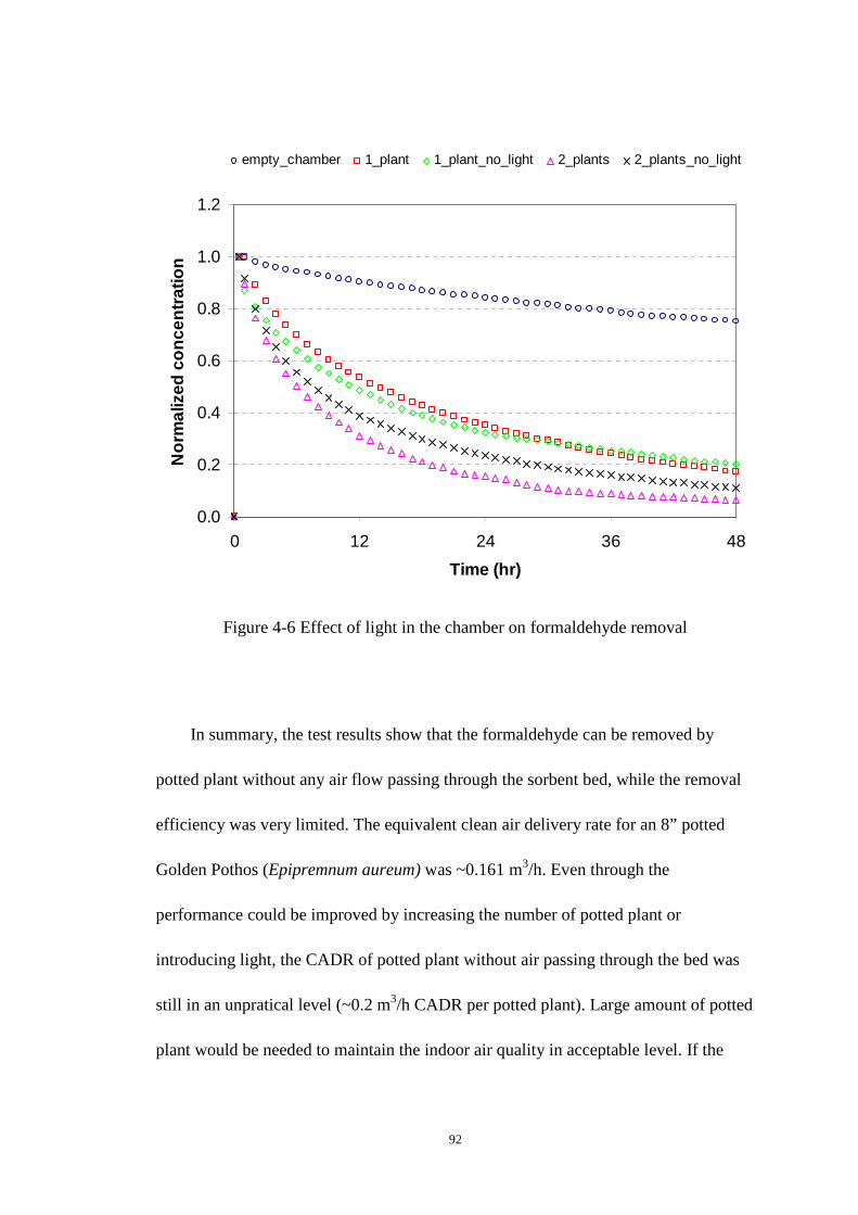
92

0.0

0.2

0.4

0.6

0.8

1.0

1.2

0 12 24 36 48

Time (hr)

No

rmal

ized

co

nce

ntr

atio

nempty_chamber 1_plant 1_plant_no_light 2_plants 2_plants_no_light

Figure 4-6 Effect of light in the chamber on formaldehyde removal

In summary, the test results show that the formaldehyde can be removed by

potted plant without any air flow passing through the sorbent bed, while the removal

efficiency was very limited. The equivalent clean air delivery rate for an 8” potted

Golden Pothos (Epipremnum aureum) was ~0.161 m3/h. Even through the

performance could be improved by increasing the number of potted plant or

introducing light, the CADR of potted plant without air passing through the bed was

still in an unpratical level (~0.2 m3/h CADR per potted plant). Large amount of potted

plant would be needed to maintain the indoor air quality in acceptable level. If the

93

cross-section of the bed was taken into account, then the CADR for potted plant

without air passing through the bed would become 5.1 m3/h per square meter bed.

4.3.2 Formaldehyde Removal by Microbial Community with Air

Flow Passing through

It is necessary to keep the sorbent bed in a humid condition to avoid the

unexpected death of microbes. Figure 4-7 shows the air RH in the recirculation loop

during the test. The test system (Figure 4-2) was first pre-conditioned with 90% RH

clean air for 4 hours. After the test system RH condition became steady, the test

system was switched to recirculation loop. It can be seen that the test system air RH

increased after the switch occured. This is due to the test bed was initially containing

certain amount of liquid solution. It can also be seen that air RH in the recirculation

loop was kept at 95% in a 24-hour test period.

94

0%

20%

40%

60%

80%

100%

0 6 12 18 24 30

Time (hr)

RH

pre-condition with 90% RH air

Test starting point

Figure 4-7 Test system relative humidity change over time

Figure 4-8 shows the normalize formaldehyde concentration in the system in a

single-injection test. The steady formaldehyde concentration in the test system before

switching to the test loop was ~7.5 ppm (9.2 mg/m3). The formaldehyde concentration

in the system decreased to 1.6 mg/m3 with wet bed only in one hour after the switch.

The system concentration was decreased to 0.6 mg/m3 with web bed plus microbes in

one hour after the switch. The equivalent clean air delivery rates were ~0.083 m3/h for

wet bed only and ~0.126 m3/h for wet bed with microbes. If the cross-section of the

bed was taken into account, then the CADR for microbial community with air passing

by would become 5.1 m3/h per square meter bed.

95

The formaldehyde removal rate can be calculated by multiplying the

concentration difference between initial equilibrium concentration and final

equilibrium concentration in the end and volume of the test system. The initial

concentration was 7.5 ppm. The final concentration for wet bed and wet bed with

microbes were 1.27 ppm and 0.52 ppm, respectively. By considering the test system

volume of 0.05 m3, the removal rate by wet bed only was 0.38 mg/h. The removal rate

by wet bed plus microbes was 0.43 mg/h. Therefore, the removal rate by microbes

only would be 0.05 mg/h. The initial bed microbial density was 6.78×1010 CFU/mL.

The removel rate by microbe would be 7.3×10-12 mg/h per CFU/mL.

0.0

0.2

0.4

0.6

0.8

1.0

1.2

0 1 2 3 4Time (hr)

No

rmal

ized

co

nce

ntr

atio

n

wet-bed only wet-bed with microbes

Figure 4-8 Formaldehyde removal by microbes with single-injection

96

After the single-injection test, the tested formaldehyde loaded sorbent bed was

flushed with clean air. The downstream concentration of the sorbent bed was

monitored. Figure 4-9 shows the formaldehyde concentration at the bed downstream.

Desorption was observed by the presence of the concentration increase (peak) which

is due to the formaldehyde adsorption capacity of the sorbent. The formaldehyde peak

concentration of sorbent bed with microbes was significant lower and smaller than

that without microbes. This indicates that part of the formaldehyde was degraded by

the microbes. The un-degraded adsorbed formaldehyde was desorbed as indicated by

the lower peak when there was clear air passing through the bed.

0.00

0.05

0.10

0.15

0.20

0.25

0.30

0.35

0 3 6 9 12

Time (hr)

Fo

rmal

deh

yde

con

cen

trat

ion

(pp

m) wet_bed_degas

wet bed/microbes_degas

switch to test bed

Figure 4-9 Desorption of formaldehyde from sorbent bed with and without microbes

97

Figure 4-10 shows the normalize formaldehyde concentration in the system vary

with time in a multi-injection test. Red diamond points were for the test with

wet-sorbent only. Blue square points were for the test with wet-sorbent together with

microbes. The difference between these two curves after the system was switched to

test loop in each cycle was due to the formaldehyde bio-degradation by microbes.

0.0

0.2

0.4

0.6

0.8

1.0

1.2

0 6 12 18 24Time (hr)

No

rmal

ized

co

nce

ntr

atio

n

wet-bed only wet-bed with microbes

1stinjection

2ndinjection

3rdinjection

4thinjection

Figure 4-10 Formaldehyde removal by microbes in multi-injection test

The adsorbed formaldehyde mass at steady status of each cycle could be

obtained by multiplying the system volume with concentration difference between

98

initial and equilibrium concentration (as shown in Figure 4-11). These were the

measured absorbed mass (as shown in Table 4-6). The maximum absorbed mass

could also be calculated according to Henry’s Law (Smith and Harvey, 2007):

ckp H ⋅= (4-9)

where p is the partial pressure of the solute in the gas above the solution, c is the

concentration of the solute and kH is a constant with the dimensions of pressure

divided by concentration. The constant, known as the Henry's law constant, depends

on the solute, the solvent and the temperature.The Henry’s law constant of

formaldehyde is 3.27E-07 atm·m3/mol.

The bed water content could be obtained from the moisture retention curve (as

shown in Figure 4-12). The calculated absorbed masses were also shown in Table 4-6.

The measured absorbed mass generally agreed with the calculated absorbed mass.

This indicates that the wet-bed had approached its formaldehyde absorption capacity;

therefore the concentration reached a quasi-steady at the end of eachcycle. A

quasi-steady state was also reached with wet-bed with microbes at the end of each

cycle. The reason may be that microbes adsorbed the formaldehyde first and it took

time to degrade. If degration process is fast enough, the concentration is expected to

continuously decrease. It is also noted that there was a concentration difference

between wet-bed only and wet-bed with microbes at the quasi-steady state. This was

due to the degradation of absorbed formaldedhye by the microbial community

99

y = 0.2243x

R2 = 0.7366y = 0.4805x

R2 = 0.8632

0.0

0.2

0.4

0.6

0.8

1.0

1.2

1.4

1.6

1.8

0.0 1.0 2.0 3.0 4.0 5.0 6.0 7.0

equilibrium concentration (mg/m3)

mas

s ad

sorb

ed (m

g)

wet-bed only wet-bed with microbesLinear (wet-bed only) Linear (wet-bed with microbes)

Figure 4-11 Formaldehyde removal isotherm by wet-bed with and without microbes

y = 0.170x2.651

R2 = 0.974

0.000

0.050

0.100

0.150

0.200

0% 20% 40% 60% 80% 100%

Relative humidity

Moi

stur

e co

nten

t (g/

g)

Measured data Power (Measured data)

Figure 4-12 Sorbent bed moisture retention curve

Table 4-6 Comparison of calculated and measured adsorbed formaldehyde mass

Equilibrium

concentration

Sorbent bed

weight

Water content Henry's law

constant for

Calculated

absorbed mass

Measured

absorbed mass

100

formaldehyde

mg/m3 g g atm·m3/mol mg mg

1.46 30.95

4.24±0.21

3.27E-07

0.455±0.023 0.383

2.25 0.700±0.035 0.720

3.93 1.223±0.061 0.991

5.91 1.842±0.092 1.157

In summary, the microbial communities were found to have significant effect on

removing formaldehyde. With the best species from the plant root evenly distributed

in a wet sorbent bed, the CADR became ~1050 m3/h per square meter bed.

4.3.3 Formaldehyde Removal by Dynamic Botanical Air Filtration

System

Dry Bed V.S. Wet Bed V.S. DBAF. As descirbed in section 4.2.3, empty

chamber test was first conducted without the DBAF in the test chamber. Dry bed test,

wet bed test and test with DBAF were then conducted. Since the equilibrium

concentration for each test was stable, there was no need to monitor the concentration

continuously but check for some time dayly. The chamber concentration was

continuously monitored by PTR-MS for two hours daily. The average of the two hour

test data was used as the concentration of that test day. The chamber equilibrium

concentrations for different tests were shown in Figure 4-13. It can be seen the

chamber equilibrium concentration become relative stable and slightly different in a

101

one-week test period. Figure 4-14 shows the results of DBAF test for long term. The

chamber concentration decreases slightly at the beginning of the test and then kept in

a constant level after that.

1

10

100

1000

0 1 2 3 4 5 6 7 8

Time (day)

Con

cent

ratio

n (p

pb)

Empty chamber test Dry bed testWet bed test DBAF test

Figure 4-13 Chamber formaldehyde equilibrium concentrations at different RHs

102

1.0

10.0

100.0

1000.0

0 7 14 21 28 35 42

Time (day)

Fo

rma

ldeh

yde

C (

pp

b)

Before the filter wasturned on

Figure 4-14 Long term formaldehyde removal efficiency by DBAF at 90% RH

Table 4-7 lists single pass efficiency and clean air delivery rate for different tests.

After one day, the SPE of dry bed and wet bed were 3% and 17%, respectively. The

corresponding CADR were 1.5 and 8.5 m3/h, respectively. The SPE of DBAF was

32.7% and the CADR was 16.35 m3/h. After one week, the SPE of dry bed and wet

bed were 2.6 % and 16.1%. The CADR of the dry bed and wet bed were 1.3 and 8.1

m3/h, respectively. The SPE of DBAF was 39.5% and the CADR was 19.75 m3/h.

Table 4-7 Concentration, SPE and CADR at different RHs

Test period Empty

chamber

Dry bed

@ 50±3%RH

Wet bed

@90±2%RH

DBAF

@90±2%RH

103

Concentration

(ppb)

1 day

1 week

1 month

278.5

275.3

273.7

123.3

121.0

/

34.0

35.3

/

18.7

15.5

15.0

Single pass

efficiency

(%)

1 day

1 week

1 month

N/A

N/A

N/A

3

2.6

/

17

16.1

/

32.7

39.5

40.7

CADR

(m3/h)

1 day

1 week

1 month

N/A

N/A

N/A

1.5

1.3

/

8.5

8.1

/

16.35

19.75

20.35

Note: “N/A” means “not applicable”; “/” means “didn’t do”

Figure 4-15 & 4-16 show the CADR and SPE in a bar chart, the CADR due to

leaf effect was only ~1% of the total CADR of DBAF. The CADR due to wet sorbent

was ~52% of the total CADR. The wet sorbent bed effect includes formaldehyde

absorption in water film and adsorption in dry sorbent bed, which was a combined

effect. The difference between DBAF and wet sorbent bed test was due to the

existence of plant. It also can be seen that the CADR of DBAF increased to 19.75

m3/h one week later, which indicates that the plant microbial community continuously

performed well on removing formaldehyde.

104

0.0

5.0

10.0

15.0

20.0

25.0

30.0

35.0

CADR (m3/h) 16.4 8.5 1.5 0.2

SPE (%) 32.7 17.0 3.0 0.0

DBAFWet sorbent

bedDry sorbent

bedleaf

Figure 4-15 CADR and SPE after one day

0.0

5.0

10.0

15.0

20.0

25.0

30.0

35.0

40.0

CADR (m3/h) 19.8 8.1 1.3 0.2

SPE (%) 39.5 16.1 2.6 0.0

DBAFWet sorbent

bedDry sorbent

bedleaf

Figure 4-16 CADR and SPE after one week

105

DBAF at Different RHs. The tests were conducted at three different RH levels:

92%, 75%, and 55%. The different RH level was achieved by adjusting the ventilation.

Figure 4-17 shows the chamber RH for different tests. There was slight fluctuation of

the RH due to the irrigation, with standard deviation of < 2%. The bed moisture

contents for each RH level according to the moisture rention curve were as listed in

Table 4-8.

0

20

40

60

80

100

0 12 24 36 48

Time (hr)

Ch

amb

er R

H (%

)

90% RH test

75% RH test

55% RH test

Figure 4-17 Chamber moniterd RH at different RHs

Table 4-8 Chamber ventilation and DBAF bed moisture content at different RHs

Chamber RH

%

Ventilation air flow

m3/h

Bed moisture content

m3/m3

92±1

75±2

55±3

1.18

5.48

7.02

0.137

0.078

0.034

106

The formaldehyde removal tests at 75% RH and 55% RH were also conducted.

Table 4-9 lists the SPE and CADR of the DBAF in removing formaldehyde at

different RHs. After one day, the SPE of DBAF decreased from 32.7–19.9% as RH

reduced from 90–55%. The corresponding CADR decreased from 16.35–9.95 m3/h.

After two days, the SPE of DBAF reduced from 33.5–20.5%. The CADR reduced

from 16.75–10.25 m3/h accordingly.

The single pass efficiency and clean air delivery rate decreased as the RH

decreases. Since formaldehyde is a water soluble compound, water vapor in the

DBAF bed plays a positive role in removing formaldehyde. As the RH level decreases

from 90–55% RH, less water film is available for absorbing formaldehyde. Therefore,

the SPE and CADR will decrease. It is consistent with the test results in the

real-condition test.

Table 4-9 The formaldehyde SPE and CADR of the DBAF at different RHs

Test period DBAF

@90%RH

DBAF

@75%RH

DBAF

@55%RH

Single pass

efficiency (%)

1 day

2 days

32.7

33.5

24.5

24.7

19.9

20.5

CADR

(m3/h)

1 day

2 days

16.35

16.75

12.25

12.36

9.95

10.25

107

Equivalent clean air deliver rate is a useful parameter to evaluate the

performance of gas filter. Table 4-10 lists the comparison of equivalent clean air

delivery rate for different series of tests. It shows that the CADR was only ~5.1 m3/h

per square meter bed without air flow passing through the bed. The test of microbial

community with air flow passing by provides equivalent CADR of ~1050 m3/h per

square meter bed. While this test was for best species from the plant root system, and

the initial microbial density was 9.78E+10 CFU/ml, which was higher than the

normal microbial density of 1.0E+06–1.0E+08 CFU/ml. The whole effect of DBAF

has a CADR of ~233 m3/h per square meter bed.

Table 4-10 Comparison of CADR at different series of tests

Test set Potted plant without

air flow passing

through the bed

Microbial community

with air flow passing

through

whole effect of DBAF

Test temperature (°C) 23±0.6 23±0.6 23±0.6

Test RH (%) 50±3 90±3 90±3

Test air velocity passing by (m/s) 0 0.25 0.25

Filter bed cross section area (m2) 3.14E-02 1.26E-04 7E-02

Filter bed thickness (m) 0.15 0.15 0.15

Concentration (ppb) 20000 7500 15

CADR (m3/h)/(m2bed) 5.1 1050 233

108

Biodegradation Rate Constant Determination. Two processes happened in

series for the formaldehyde biodegradation. The first one is the gas phase

formaldehyde absorption by the water film, which is followed Henry’s Law. The

second one is the liquid phase formaldehyde degradation by microbial community,

which is followed the first-order kinetics. It should be noted that these two processes

are combined with each other. The concentration in the liquid phase and

biodegradation rate constant are the two unknown parameters. The biodegradation

rate constant can not be directly obtained from experimental data. It has to be fitted

from the comparison between the simulation result and experimental data.

Nevertheless, the biodegradation rate constant still can be calculated based on the

following analysis, which could be used as a reference value.

Biodegradation rate constant calculation can be calculated as follows: the VOC

mass balance in the chamber can be expressed as Equation (4-10).

22 CQCQRdt

dCV totalCADRv ⋅−⋅−= − (4-10)

where, V is the testing chamber system volume, m3; R is the formaldehyde generation

rate, mg/h; Qv is the clean air flow rate, m3/h; C2 is the formaldehyde concentration

with DBAF in the test chamber, mg/m3; totalCADRQ − is the total clean air delivery rate

of the DBAF, m3/h.

The total clean air delivery rate of the DBAF can be further separated into three

parts: leaf effect, wet sorbent effect, and microbial community effect.

109

microbesCADRsorbentwetCADRleafCADRtotalCADR QQQQ −−−− ++= _ (4-11)

where leafCADRQ − is the clean air delivery rate due to leaf effect, m3/h; sorbentwetCADRQ _−

is the clean air delivery rate due to wet sorbent effect (including dry bed effect and

water effect), m3/h; microbesCADRQ − is the clean air delivery rate due to microbial

community effect, m3/h. The CADR of the total DBAF, leaf effect and wet sorbent

effect can be calculated from experimental data, and then the CADR due to microbial

community can be obtained by Equation (4-11).

The clean air delivery rate due to the microbial community effect could be used

to calculate the biodegradation rate constant:

liqbedliqgasmicrobesCADR VCkCQ θ⋅⋅⋅=⋅− (4-12)

where gasC is the equilibrium gas phase formaldehyde concentration in the chamber,

mg/m3; k is the biodegradation rate constant, 1/s; liqC is the equilibrium liquid phase

formaldehyde concentration in the filter bed, mg/m3; bedV is the volume of the filter

bed, m3; liqθ is the volumetric water content in the filter bed, m3/m3.

The biodegradation rate constant can be obtained:

liqbed

microbesCADR

V

HQk

θ⋅⋅

= − (4-13)

where H is the Henry’s law constant, dimensionless.

Table 4-11 Determintation of formaldehyde bio-degradation rate constant

CADR due to Henry’s law Bed Bed Bio-degradation

110

microbes effect

m3/h

constant(unit)

volume

(m3)

water content

(m3/m3)

rate constant

(1/s)

7.60 1.33E-05 0.011 0.13 2.06E-05

4.3.4 Toluene Removal by Dynamic Botanical Air Filtration System

Toluene removal by DBAF at different RHs were also conducted. Table 4-12

lists the SPE and CADR of the DBAF in removing toluene at different RHs. After one

day, the SPE of DBAF increased from 10.1–37.3% as RH decreased from 90–55%

RH. The corresponding CADR increased from 5.05–18.65 m3/h. After two days, the

SPE and CADR of DBAF were staying in the same level as that of one-day test.

The single pass efficiency and clean air delivery rate increased as the RH

decreases. Since toluene is a water insoluble compound, water vapor in the DBAF bed

plays a negative role in removing toluene. As the RH level decreased from 90–55%

RH, more adsorption sites were available for adsorbing toluene. Therefore, the SPE

and CADR would increase. It was consistent with the test results in the real-condition

test.

The toluene biodegradation by microbial community can not be clearly

determined through this series of test. It could be analyzed that the toluene

biodegradation rate in the liquid phase will be very small since toluene is highly water

insoluble. Still, there is a possible that the bio-degradation would occur when the

microbial community expose to the adsorbed toluene directly. The tests conducted in

this chapter are hard to determine the bio-degradation rate of toluene.

111

Table 4-12 The SPE and CADR of the DBAF in removing toluene at different RHs

Test period DBAF

@90%RH

DBAF

@75%RH

DBAF

@55%RH

Single pass efficiency

(%)

1 day

2 days

10.1

10.9

27.5

29

37.3

34.8

CADR

(m3/h)

1 day

2 days

5.05

5.45

13.75

14.5

18.65

17.4

4.4 Major Findings

In order to improve the understanding of the mechanisms of the DBAF system in

removing the volatile organic compounds, a series of further experiments were


the roles of different transport, storage and removal processes were also investigated.

In general, it was found that passing the air through the root bed with microbes was

essential to obtain meaningful removal efficiency. Moisture in the root bed also

played an important role, both for maintaining a favorable living condition for

microbes and for absorbing water-soluble compounds such as formaldehyde. The role

of the plant was to introduce and maintain a favorable microbe community that

effectively degraded the VOCs that were adsorbed or absorbed by the root bed. While

the moisture in a wet bed had the scrubber effect for water-soluble compounds such as

formaldehyde, presence of the plant increased the removal efficiency by about a

factor of two based on the results from the reduced-scale root bed experiments.

112

Moreover, for the same cross-section area of 0.35 m long and 0.2 m wide, the

dry bed with airflow had an equivalent CADR of ~1.5 m3/h. The wet bed with airflow

had an equivalent CADR of ~8.5 m3/h. The DBAF had an equivalent CADR of ~16.4

m3/h. The difference of wet bed with airflow and DBAF was due to the existence of

plant. It was found that wet bed and microbial community are the two major factors to

affect the formaldehyde removal. It was hard to find out which one was the dominant

one in short-time test (one day), while the result shows that microbial community

would become dominant gradually as time went on.

The biodegradation rate constant for formaldehyde was also determined, which

was 2.06E-05 s-1 at 92%RH and 15 ppb formaldehyde level. It should be noted that

this rate constant was only for comparison. Because the transfer of formaldehyde

from gas phase into liquid film and formaldehyde degradation by microbial

community occured in series but not in parallel. They can not be exactly seperated

from the experimental result, while it can be used as a reference for the model initial

input.

113

Chapter 5. Model Simulation and Validation

5.1 Introduction

As noted in Chapter 2 Literature Review, “Biological purifier” is used to

describe any device that includes a biological component (botanical or microbial) for

VOC removal. “Bio-filter” or “Bio-trickling filter” is used to describe the devices that

use a packed bed of a solid support colonized by attached microorganisms that

biodegrade the VOC in the air passing through. “Botanical purifier” or DBAF is used

to specifically describe the devices that use plants and their associated

microorganisms. Many investigators have created mathematical models of bio-filters

and bio-trickling filters in their efforts to understand and improve reactor performance

(Hodge and Devinny, 1997; Devinny and Ramesh, 2005), while this study represents

a first attempt to model the operation of DBAF using a numerical simulation model.

The CHAMPS-BES (Nicolai, 2009) was further developed to account for the

effects of the microbes on the degradation of both water-soluble and non-soluble

VOCs. The improved numerical model was then used to simulate the operation of a

botanical air filtration system that used a mixture of activated carbon and porous shale

pebbles as root bed of selected plants (such as Golden Pothos(Epipremnum aureum)).

The filtration system was operated with periodical irrigation and HVAC return

airflow passing-through the root bed. VOC including aldehydes were either adsorbed

by the activated carbon sorbent or absorbed by water films in the wet root bed (which

114

acts as a wet scrubber for water soluble compounds such as formaldehyde). The

adsorbed and/or absorbed organic compound could be degraded by the microorganism

in the root bed, which would regenerate the sorbent in the root bed. The purified air

returned to indoor environment to improve indoor air quality. These transport and

removal mechanisms were discussed in Chapter 4. The laboratory and real-world

environment tests discussed in Chapter 3 also demonstrated that the DBAF system

had a single-pass removal efficiency of 60% for formaldehyde and 20% for toluene,

and the removal efficiency for both compounds did not decrease significantly over

300-day continuous operation.

In this chapter, we present: 1) a mechanistic numerical model that can be used to

optimize the design and operation of the system as well as improve the understanding

of the pollutant transport and degradation processes involved; and 2) comparisons

between the model simulation results and experimental data, and a method to estimate

the bio-degradation rate constant required for the simulation.

5.2 Model Development

5.2.1 Model Description and Assumptions

As air passes through the filter, the processes involved in the VOC transport,

adsorption/absorption and decomposition mechanism in the whole bio-filtration

system include (Figure 5-1):

115

1. VOC advection by airflow. The transport of gas phase VOC by air flow

through the filter bed;

2. VOC gas phase diffusion through bed void. The VOC diffusion through

bed void occurs;

3. VOC convective mass transfer to sorbent-air interface to be adsorbed by

the sorbent. This is the mass transfer-adsorption process of adsorbable compounds

from the bulk of the gas phase to the external surface of adsorbent pellets (activated

carbon). Each sorbent pellet is assumed to be homogeneous and the VOC internal

diffusion in the micro-pores is not described in detail in the current model;

4. VOC convective mass transfer to liquid-air interface to be absorbed by

the liquid (water). This is the absorption process describing transport of gaseous

pollutant from the air into contacting liquid, such as water film at the surface of

sorbent/pebble. The liquid serves as a solvent for the pollutant. Water film formed in

the surface of pebbles or activated carbon will become the wet scrubbers, where water

soluble compounds such as formaldehyde in the indoor air can be absorbed on it;

5. VOC physical adsorption by activated carbon. After pollutant molecules

transport from gas phase to solid phase by convective mass transfer at the surface of

solid, instant equilibrium between gas phase and solid phase is assumed, which is

described by a constant partition coefficient;

6. VOC absorption by liquid film. Henry’s law constant is the parameter to

describe the instant equilibrium between gas phase and liquid phase;

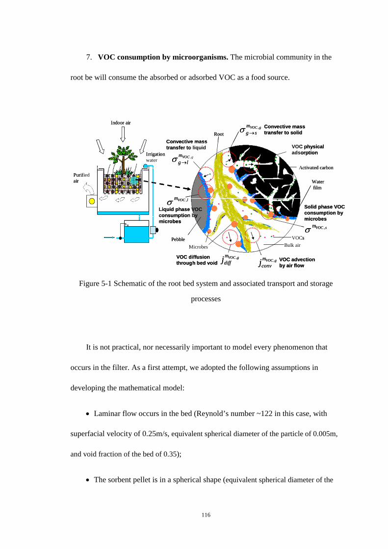
116

7. VOC consumption by microorganisms. The microbial community in the

root be will consume the absorbed or adsorbed VOC as a food source.

Indoor air

Purifiedair

Irrigationwater

Pebble

Activated carbon

Bulk air

VOCs

Microbes

Root

Waterfilm

gVOCmsg

,

→σ

gVOCmlg

,

→σ

gVOCm

convj ,

sVOCm ,σ

lVOCm ,σ

gVOCmdiffj , VOC advection

by air flow

VOC diffusion through bed void

Convective mass transfer to solid

Convective mass transfer to liquid

Solid phase VOC consumption by microbes

Liquid phase VOC consumption by microbes

VOC physical adsorption

Indoor air

Purifiedair

Irrigationwater

Pebble

Activated carbon

Bulk air

VOCs

Microbes

Root

Waterfilm

gVOCmsg

,

→σ

gVOCmlg

,

→σ

gVOCm

convj ,

sVOCm ,σ

lVOCm ,σ

gVOCmdiffj , VOC advection

by air flow

VOC diffusion through bed void

Convective mass transfer to solid

Convective mass transfer to liquid

Solid phase VOC consumption by microbes

Liquid phase VOC consumption by microbes

VOC physical adsorption

Figure 5-1 Schematic of the root bed system and associated transport and storage

processes

It is not practical, nor necessarily important to model every phenomenon that

occurs in the filter. As a first attempt, we adopted the following assumptions in

developing the mathematical model:

• Laminar flow occurs in the bed (Reynold’s number ~122 in this case, with

superfacial velocity of 0.25m/s, equivalent spherical diameter of the particle of 0.005m,

and void fraction of the bed of 0.35);

• The sorbent pellet is in a spherical shape (equivalent spherical diameter of the

117

particle of 0.005m);

• Filter-material composition is homogeneous (e.g., porosity, density);

• Advection and diffusion of the adsorbate in the water film (liquid phase) are

negligible;

• The partition coefficient is constant for a given temperature regardless the

change in concentration;

• Consumption rate of the VOC by microorganisms follows first-order kinetics.

5.2.2 Governing Equations

VOC in the filter bed are divided into three components: gas phase, adsorbed in

solid and absorbed in liquid.

5.2.2.1 VOC Mass Balance in Gas

Transport of gas phase VOC can happen via convection with air, through

diffusion, exchange between gas and solid, and exchange between gas and liquid. It

can be expressed:

( ) gVOCgVOCgVOCgVOCgVOC

gVOCmm

lgm

sgmdiff

mconv

m

jjxt

,,,,,

,

σσσρ

+−−+∂∂

−=∂

∂→→ (5-1)

where gVOCm ,ρ is the VOC density in gas, kg/m3; gVOCmconvj , is VOC mass flux due to

convection, kg/(m2s); gVOCmdiffj , is VOC mass flux due to diffusion, kg/(m2s); the

exchange between gas and solid is denoted bygVOCmsg

,

→σ , kg/(m3s); the exchange between

118

gas and liquid is denoted by gVOCmlg

,

→σ , kg/(m3s), whereas the arrow indicates positive

transfer direction. The term gVOCm ,σ can be used to describe any source or sink of gas

phase VOC components, such as a constant emission source. This term is zero in the

current botanical filtration model.

The VOC transport by convection happens through the bulk air movement. It can

be expressed as:

gVOCgVOC mmair

mconv jcj =, (5-2)

where VOCmairc is the gas phase VOC concentration (mass fraction), kg(VOC)/kg(air); gmj

is air mass flux density from the airflow calculation, kg(air)/(m2s), determined by:

x

pKj a

amg

∂∂

−= (5-3)

For the sorbent bed filter, the air flux can be determined by the air permeability

of the bed and pressure drop across the filter as follows:

x

pKj a

mg

∆∆

−= (5-4)

where aK is air permeability through the media, s; ap is air pressure, which equals to

the sum of partial pressures of dry air and water vapor, Pa; P∆ is the pressure

difference across the entire root bed, Pa; x is the coordinate in the bed flow direction,

m; x∆ is thickness of the bed, m.

The diffusion flux of gas phase VOC in the bed void is calculated by:

x

p

TR

Dj gVOC

VOC

matVOCmdiff

gVOC

∂

∂−= ,,, (5-5)

119

where matVOCD , is the VOC diffusion coefficient in the root-bed material system

(considered as a porous medium), it is calculated by the VOC diffusion coefficient in

air, airVOCD , (given in m2/s), and diffusion resistance factor, vocµ (dimensionless,

which takes into account the tortuosity of bed-void); VOCR is the gas constant for

VOC, JK-1mol-1; T is the temperature, K; gVOCp , is the VOC partial pressure, Pa; x is

the coordinate in the bed flow direction, m.

VOC

airVOCmatVOC

DD

µ,

, = (5-6)

Adsorption Flux: VOC Transfer from Gas to Solid-air Interface. When there

is a concentration gradient between the gas phase concentration in the bulk air and at

the surface of sorbent (gas phase at surface boundary layer, which is assumed to be in

instantaneous equilibrium with the adsorbed VOC at the surface with a partition

coefficient, Kma), there will be an exchange flux into the direction of the lower

concentration.

The mass transfer equation from gas phase to solid phase can now be given:

( )

−

−=−

−= →→

→ma

mmgas

REV

tolsgmmgas

mgas

REV

tolsgmmsg KV

wAk

V

wAk sVOC

gVOCsVOCgVOCgVOC

,

,,,,)1()1( ,, ρρρρσ (5-7)

where sgmk →, is the VOC mass transfer coefficient between gas and solid, m/s; tolA

is the total external surface area of the sorbent material that is available for

pollutant/VOC adsorption or absorption, m2; w is the wetness ratio of the surface of

the activated carbon pellet (It is a function of the bed volume water content: the

wetness ratio equal to zero when the bed is absolutely dry and equal to one as the bed

120

is total saturated with water), dimensionless. REVV is the reference element volume,

m3; maK is the partition coefficient of the solid media.

The total surface area for spherical pellet sorbent bed can be calculated by

Equation (5-8):

( ) ( )R

VR

R

VA porREVREVpor

tol

θπ

π

θ −=

−=

134

3

4

12

3

(5-8)

where porθ is the porosity of the sorbent bed, dimensionless; R is the radius of the

sorbent particle/pellet, m.

Absorption Flux: VOC Transfer from Gas to Liquid-air Inter face. For water

soluble pollutant/VOC, such as formaldehyde, when there is a concentration gradient

between the gas phase concentration in the bulk air and the surface of the liquid (gas

phase at the surface boundary layer of liquid, which is also assumed to be in

instantaneous equilibrium with the absorbed VOC at the surface with a Henry’s law

constant H), there will be an exchange flux into the direction of the lower

concentration.

The mass transfer equation from gas phase to liquid phase can be expressed:

( ) ( )lVOCgVOClVOCgVOCgVOC mmgas

REV

tollgmmgas

mgas

REV

tollgmmlg H

V

wAk

V

wAk,,,,, ,, ρρρρσ −=−= →→

→ (5-9)

where lgmk →, is the VOC mass transfer coefficient between gas and liquid, m/s; w is

the wetness ratio, dimensionless; wAtol is the total external surface area of the liquid

film covering the sorbent material or pebble in filter bed, m2; H is Henry’s law

121

constant, m3/m3.

5.2.2.2 VOC Mass Balance in Solid

VOC mass balance in the solid can be expressed:

sVOCgVOC

sVOCmm

sg

m

t,,

,

σσρ

+=∂

∂→ (5-10)

where sVOCm ,ρ is the VOC density in solid, kg/m3; gVOCmsg

,

→σ is the VOC transport from gas

phase by convective mass transfer, kg/(m3s); sVOCm ,σ is considered as the common

source/sink term. The consumption of adsorbed VOC by microbes is such a sink in

the botanical filtration system. Another example is the chemi-sorption process

(negative source term), and it is not available in the botanical air filtration system.

5.2.2.3 VOC Mass Balance in Liquid

VOC mass balance in liquid film can be expressed:

lVOCgVOC

lVOCmm

lg

m

t,,

,

σσρ

+=∂

∂→ (5-11)

where lVOCm ,ρ is the VOC density in liquid, kg/m3; gVOCmlg

,

→σ is the VOC transport from

gas phase by convective mass transfer, kg/(m3s); lVOCm ,σ is considered as the common

source/sink term. An example for such a source/sink term in the botanical filtration

system is the process of pollutant/VOC degradation by microbes in the root system

(negative source term).

122

5.2.2.4 Source/Sink Flux for Solid/Liquid Phase VOC: Microbial

Biodegradation.

The absorbed or adsorbed VOC will be served as carbon source for

microorganisms. As long as there is carbon source in the liquid film or sorbent

surface, the microbes will take them as nutrition, thus the VOC will be degraded.

Basically, there are two main factors that affect the VOC degradation by microbes.

One is the available carbon source, and the other is the number of microbes that will

take charge of the degradation (Devinny and Ramesh, 2005). So the biodegradation

flux can be expressed as:

lVOClVOC mm K ,, ρσ = (5-12)

where K is the total biodegradation rate constant for the microbial species found in

the root bed, s-1; lVOCm ,ρ is the VOC density in liquid or at the solid surface, kg/m3.

Note that for simplification, it is assumed that the microbes live in liquid films and

have access to VOCs within the film and solid surfaces though the detailed nature of

the microbial activities are not known (e.g., It is conceivable that the area and spatial

distribution of the liquid film in the root bed may vary or fluctuate over time giving

opportunity for adsorption of water-soluble compounds at one time when uncovered

by the liquid file and expose to microbes at another when covered by the liquid film).

Note: The biodegradation rate constant is dependent on the number of microbes,

which depends on the density of microbial community and the area of the root bed.

The biodegradation rate constant in this study was obtained from the experimental

123

results. It was the total effect of DBAF. Further research is needed regarding the

effect of number of microbes.

5.2.3 Determination of Model Parameters

Table 5-1 lists the key input parameters of the numerical model. The partition

coefficients were obtained from experimental data. The Henry’s Law constants were

obtained from literature (as discussed in Chapter two). The gas to solid and gas to

liquid mass transfer coefficients were calculated based on the following equation for

Sherwood number (Sh) (Devinny and Ramesh, 2005).

[ ]33.06.0Re1.1222

ScR

DSh

R

Dk

p

air

p

airm +⋅=⋅= (5-13)

where km is the gas to solid or liquid mass transfer coefficient, Dair is the gas-phase

diffusion constant, Rp is the radius of particle, Sh the Sherwood number, Re the

Reynolds number, and Sc is the Schmidt number.

Table 5-1 Model key parameters determination

Parameter Formaldehyde

Toluene

Partition coefficient 2.91E+04 4.04E+06

Henry’s Law constant (Cgas/Cliquid) 1.33E-05 0.28

Gas to solid mass transfer coefficient (m3/s) 0.27 0.27

124

Gas to liquid mass transfer coefficient (m3/s) 0.55 0.55

5.3 Model Implementation

The model was implemented in CHAMPS-BES as follows: (1) VOC mass was

considered existing in gas, solid and liquid phase; (2) VOC adsorption flux,

absorption flux and bio-consumption flux were implemented as sink terms, which

were applied as “Field Conditions”; (3) water source was enabled to simulate the

irrigation of the DBAF.

5.4 Simulation Results

Model verification was first conducted to test whether the developed model

could work. Model validation was then conducted by comparing to the experimental

data, which also resulted in an estimate for the fitted bio-degradation rate.

5.4.1 Model Verification

In the present study, simulations were first conducted to predict the bed air flow

and moisture distribution. The dimension of the filter bed was 1.8 m by 0.6 m by 0.2

m. The activated carbon particle diameter was 4×10-3 m. Filter inlet air was

maintained at 20 °C with relative humidity of 30% RH. Air density is 1.2 kg/m3 at 20

°C. Bed initial average moisture content was 0.1 m3(water)/m

3(bed). The irrigation system

125

ran for 3 minutes every hour to keep the bed volumetric water content level no less

than 0.08 m3(water)/m3(bed).

5.4.1.1 Modeling of Air Flow through the Bed

In current model, the pressure drop between the inlet and outlet of the filter was

an input parameter. It was measured to be 73 Pa with 0.229 m3/s air passing through

the entire bed (cross-section area of 1.08 m2 and thickness of 0.2 m). According to

Equation (5-4), the air permeability can be calculated by airflow rate and pressure

drop across the filter. The calculated air permeability was 0.00069 s, and was assigned

to the material in the bed. Based on above parameter input to the model, the output air

flux passing through the root-bed was 0.254 kg/(m2s), which was the same as the

measured air flow rate considering air density of 1.2 kg/m3 at 20°C and bed

cross-section area of 1.08 m2.

5.4.1.2 Modeling of Moisture Distribution in the Bed

The initial moisture content in the bed was set as 0.1 m3 (water)/m3(bed). A

water source term was assigned in the field condition to simulate the periodical

irrigation. The water source was activated for three minutes every hour. Water was

added into the bed at the rate of 0.09 kg/(m3s), which means 0.09 kg water was added

in per cubic meter bed per second. Figure 5-2 shows the average bed moisture content

and outlet air RH change over time from simulation. It is shown that due to the

126

scheduled irrigation, the average bed moisture content was maintained at 0.08~0.1

m3(water)/m3(bed). Meanwhile, the bed outlet air RH was in the range of 60% to

95%. Previous field tests showed that the measured bed outlet air RH was between

74% and 82%. It is shown in Figure 5-3 that bed moisture content changes over time

by simulation.

0.00

0.05

0.10

0.15

0.20

0.25

0 3 6 9 12 15 18Time (hr)

Be

d m

ois

ture

co

nte

nt (

m3

/m3

)

0%

20%

40%

60%

80%

100%

Re

lativ

e h

um

idit

y

Outlet RH

Bed moisture content

Figure 5-2 Bed average moisture content and outlet air relative humidity

Figure 5-3 Vertical distribution of bed moisture content over time

127

5.4.1.3 Modeling of Breakthrough Profiles

Breakthrough curve simulation was conducted to investigate the effect of the

parameters involved in the filter model to the filter performance. There are two main

factors in the physical adsorption process: one is the partition coefficient, and the

other is the gas-to-solid mass transfer coefficient. Partition coefficient reflects the

capacity of a material on adsorbing VOC. Higher partition coefficient means bigger

capability. Higher gas-to-solid mass transfer coefficient means faster mass transfer

between gas and solid phase.

Effect of Partition Coefficient. In order to investigate the effect of partition

coefficient, the gas-to-solid mass transfer coefficient was fixed at 0.27 m3/s (the

convective mass transfer was 0.05 m/s), which was for current five inches sorbent bed

based on the calculation. The partition coefficient of the sorbent material was set up at

1, 10, 100 and 1000, respectively. Figure 5-4 shows the change of outlet VOC

concentration at above four different partition coefficients. The inlet pollutant

concentration was maintained at 0.1 mg/m3. The outlet concentration reached

equilibrium in less than one minute when the partition coefficient was only one. As

the partition coefficient increased from 1 to 1000, it took longer time to have the

outlet concentration increased to the same value as the inlet. It can be seen that the

model could present the effect of partition coefficient well.

128

Change in Intrinsic VOC density in gas phase over time

Kma=1 Kma=10 Kma=100 Kma=1000

Time [h]10.950.90.850.80.750.70.650.60.550.50.450.40.350.30.250.20.150.10.050

[mg

/m3]

0.12

0.11

0.1

0.09

0.08

0.07

0.06

0.05

0.04

0.03

0.02

0.01

0

Figure 5-4 Effect of partition coefficient

Effect of Gas-to-solid Mass Transfer Constant. When it came to simulate the

effect of gas-to-solid mass transfer constant, the partition coefficient was fixed at

1000, while the gas-to-solid mass transfer constant was set up at 0, 0.1, 1 and 10,

respectively. The simulation result was as shown in Figure 5-5. For the gas-to-solid

mass transfer constant of 0, it means that there was not any mass transfer occurred

between gas phase and solid phase. The red curve in Figure 5-5 was for the mass

transfer constant at 0, which was as expected that the outlet concentration increased to

the same value as the inlet concentration once the simulation started. Meanwhile, as

the mass transfer constant increased, it took less time to have the outlet concentration

129

become to the equilibrium concentration (same as inlet concentration), which

indicated that the mass transfer process would become quicker as the transfer

coefficient increased. The results show that the model presents the effect of

gas-to-solid mass transfer constant well.


Gas2solid_coef: 0 Gas2solid_coef: 1.25 Gas2solid_coef: 2.5Gas2solid_coef:5.67

Time [h]10.950.90.850.80.750.70.650.60.550.50.450.40.350.30.250.20.150.10.050

[mg

/m3]

0.12

0.11

0.1

0.09

0.08

0.07

0.06

0.05

0.04

0.03

0.02

0.01

0

Figure 5-5 Effect of gas to solid mass transfer coefficient

Effect of Gas-to-liquid Mass Transfer Constant. The next step was to simulate

the pollutant absorption by the wet surface of the sorbent particle. For the water

soluble compounds, such as formaldehyde, the main principle of absorption is due to

the presence of moisture (or water vapor). There are also two major impact factors in

the absorption process: one is the Henry’s Law constant, and the other is the

130

gas-to-liquid mass transfer constant. At normal operation condition (20 °C and 1 atm),

the Henry’s law constant is constant. For example, the Henry’s law constant for

formaldehyde is 1.33×10-5 m3/m3 (Benoit et al., 2008). The gas-to-liquid transfer

coefficient represents the mass flux per unit surface area and per unit concentration

difference. A Higher coefficient value means higher rate of mass transfer. Figure 5-6

shows the effect of gas-to-solid mass transfer coefficient to the breakthrough curve. It

can be seen that it took less time to have the outlet concentration to reach the

equilibrium concentration (same as inlet concentration) as the mass transfer

coefficient increased. Figure 5-7 shows the breakthrough curve at different

gas-to-liquid constants with the irrigation on for 3 minutes per hour. The fluctuation

of the outlet concentration was due to the irrigation (water source assigned in the field

condition).

131


G2Lmtc=0 G2Lmtc=0.1 G2Lmtc=1G2Lmtc=10 Bed_liquid_content

Time [h]87.576.565.554.543.532.521.510.50

Intr

insi

c V

OC

den

sity

in g

as p

has

e [m

g/m

3]

0.2

0.18

0.16

0.14

0.12

0.1

0.08

0.06

0.04

0.02

0

Liq

uid

con

tent (V

olu

me fractio

n) [m

3/m3]

0.12

0.11

0.1

0.09

0.08

0.07

0.06

0.05

0.04

0.03

0.02

0.01

0

Figure 5-6 Effect of gas to liquid coefficient constant without irrigation


G2Lmtc=0.1 G2Lmtc=1 G2Lmtc=10Bed_liquid_content

Time [h]242220181614121086420

Intr

insi

c V

OC

den

sity

in g

as p

has

e [m

g/m

3]

0.12

0.11

0.1

0.09

0.08

0.07

0.06

0.05

0.04

0.03

0.02

0.01

0

Liq

uid

con

tent (V

olu

me fractio

n) [m

3/m3]

0.30.280.26

0.240.220.20.180.16

0.140.120.10.080.06

0.040.020

Figure 5-7 Effect of gas to liquid coefficient constant with irrigation

132

Effect of Bio-degradation Rate Constant by Microbes. As it mentioned in the

model assumption, the pollutant bio-degradation follows the first-order kinetics. The

bio-degradation rate constant reflects the pollutant removal due to the

micro-organisms activities. Figure 5-8 shows the outlet concentration reduction when

the bio-degradation rate constant was increased from 1×10-7 s-1 to 5×10-4 s-1. The

outlet concentration was found higher than the inlet concentration. It was due to the

presence of initial moisture content in the bed. Formaldehyde was first absorbed by

the initial moisture content. As test went on, the initial moisture was gradually

evaporated into the air passing through in addition to the amount already existed in

the inlet air. Since the inlet concentration was still maintained at the same level, the

downstream concentration became slight higher than upstream/inlet concentration. It

can be seen that final outlet concentration was close to the inlet concentration when

the rate constant was increased from 1×10-7 s-1 to 1×10-6 s-1. The final outlet

concentration began to become significantly lower than the inlet concentration when

the rate concentration was increased from 1×10-6 s-1 to 1×10-5 s-1. The final outlet

concentration went down to half of inlet concentration when the rate increased

to1×10-4 s-1. Therefore, the critical bio-degradation rate constant is 1×10-5 s-1, which

means the bio-degradation rate of the DBAF has to be maintained above 1×10-5 s-1 to

be effective in removing formaldehyde.

Figure 5-9 shows the breakthrough curve that has all the processes together. The

simulation cases were conducted in this way: (1) adsorption only; (2) absorption with

133

irrigation; (3) adsorption plus absorption with irrigation; (4) adsorption, absorption

and bio-degradation with irrigation. It can be seen that the VOC removal capacity

increased as more processes were added. These simulation results were only used to

see how these removal processes were involved in the DBAF performance.


Bio-degradation_rate=1e-07 Bio-degradation_rate=1e-06Bio-degradation_rate=1e-05 Bio-degradation_rate=1e-04Bio-degradation_rate=5e-04

Time [h]2423222120191817161514131211109876543210

[mg

/m3]

0.12

0.11

0.1

0.09

0.08

0.07

0.06

0.05

0.04

0.03

0.02

0.01

0

Figure 5-8 Effect of bio-degradation rate constant

134


Adsorption_onlyAbsorption_onlyAdsorption_plus_absorptionAdsorption_plus_absorption_plus_bio-degradation (rate:1e-4)

Time [h]2423222120191817161514131211109876543210

Intr

insi

c V

OC

den

sity

in g

as p

has

e [m

g/m

3] 0.12

0.11

0.1

0.09

0.08

0.07

0.06

0.05

0.04

0.03

0.02

0.01

0

Figure 5-9 Simulation results with all the processes involved

5.4.2 Comparison with Experimental Data and Discussion

Experimental data for the reduced-scale filter are available in Chapter 4.

Formaldehyde removal tests at different RHs were conducted. The chamber steady

state concentration was used as the inlet VOC concentration. The filter efficiency was

calculated from measured data. The simulated efficiency varied with the input

bio-degradation rate constant. When the simulated filter efficiency was equal to the

measured filter efficiency, the fitted bio-degradation rate constant was obtained. Table

5-2 lists the fitted bio-degradation rate constants for different RHs. The fitted

bio-degradation rate constants were 0.8×10-4 s-1 for 92% RH test, 1×10-4 s-1 for 75%

RH test, and 1.5×10-4 s-1 for 55% RH test. It can be concluded that the

135

bio-degradation rate constant was in the range of 0.8–1.5×10-4 s-1 for the

reduced-scale DBAF tested in Chapter 4.

Table 5-2 The fitted bio-degradation rate constant

Model Compound Formaldehyde

Input

Inlet RH 92% 75% 55%

Inlet VOC concentration (mg/m3) 0.018 0.085 0.11

Irrigation rate (kg/m3s) 0.01 0.2 0.1

Initial water content (m3/m3) 0.08 0.05 0.025

Henry's law (m3/m3) 1.33E-05

partition coefficient 29084

Output

Bed output RH 93% 77% 56%

Average bed water content (m3/m3) 0.079 0.049 0.026

Bed output concentration(mg/m3) 0.012 0.064 0.088

Simulated removal efficiency 33% 25% 20%

(Measured removal efficiency) 32% 24% 20%

Fitted bio-degradation rate constant

(1/s) 0.8E-04 1.00E-04 1.50E-04

5.5 Major Findings

The modified CHAMPS-BES model is capable of simulating the operation of the

DBAF system, in good agreement with the measured pressure difference, moisture

content, and outlet relative humidity and concentrations. The model also correctly

simulated the impact of mass transfer coefficient, partition coefficient and Henry’s

136

Law constant on the behavior of the breakthrough curve of the DBAF system.

It was also found that the critical bio-degradation rate constant is 1×10-5 s-1 for

formaldehyde which means that the bio-degradation rate of the DBAF has to be

maintained above 1×10-5 s-1 to be effective in removing formaldehyde. The fitted


reduced-sized DBAF tested in Chapter 4.

137

Chapter 6. Building Energy Efficiency Simulation and Analysis

6.1 Introduction

Buildings accounted for 38.9 percent of total U.S. energy consumption in 2005

(Buildings Energy Databook, 2006). Residential buildings accounted for 53.7 percent

of that total, while commercial buildings accounted for the other 46.3 percent. There

is a growing concern about energy consumption in buildings and its likely adverse

impact on the environment. With economic growth, buildings, especially fully air

conditioned offices, will continue to be a major energy end user. Much of this energy

is used to condition the air needed for ventilation to maintain good indoor air quality.

Indoor Air Quality (IAQ) (sometimes also referred to as Indoor Environmental

Quality or IEQ) is one critical component of constructing "green" homes and

buildings. Energy efficiency is another important component of “green building”. In

Chapter 3, the DBAF has been demonstrated to have the potential to improve the

building indoor air quality without lowering the building energy efficiency, even

increasing the building energy efficiency in some cases.

In this chapter, energyPlus was first used to estimate the potential energy saving

for a small commercial building due to the use of the DBAF in Syracuse, NY.

Additional simulations were then conducted at other U.S. climate zones to provide

suggestion of potential DBAF application at different locations in terms of energy

efficiency.

138

6.2 Methods

Based on the performance test results conducted in the office field demonstration

study in Chapter 3, the outdoor air could be reduced from 560–119 m3/h with the

DBAF (filter bed of 1.2 m by 0.8 m) integrated into the HVAC system. To estimate

the potential benefit in building energy saving due to the use of the botanical air filter,

the energy consumption of the building integrated with the DBAF prototype was first

simulated through EnergyPlus over an entire year using representative climate data in

Syracuse, NY for the Syracuse center of excellence (COE) Headquarters building.

Thereafter, the same office building was simulated at different U.S. climate zones.

The COE building is a 5-story office structure (main tower) with an integrated

two (2) story laboratory building. The energy simulation only focused on the 5-story

main tower, where office, conference room and classrooms are located. The 5-story

main tower is approximately 3387 m2. One DBAF (with eight (8) plants and root bed

of 1.2 m long by 0.8 m wide) could serve 465 m2 office floor areas. Eight DBAF

would be needed for the entire COE building. ASHRAE 62.1-2010 specifies that the

requirement of outdoor air for office buildings is 5 cfm (8.48 m3/h) per person plus

0.06 cfm (1.02 m3/h) per square foot floor area. ASHRAE 62.1-2010 also specifies a

maximum occupant density for office spaces of five people per 1000 ft2 or per 100

m2. The total required outdoor air will be 3731 m3/h per ASHRAE standard. The total

required outdoor air can be reduced to 747 m3/h if eight DBAF are installed in the

139

building.

Figure 6-1 shows the COE building images generated in DesighBuilder. The

building east façade consists of 25% window and 75 % frame wall. The west façade

consists of 100% frame wall. The South facade consists of 100% curtain wall. The

North façade consist of 28 % window and 72% frame wall. The Figures 6-2 and 6-3

show the floor plan of the main tower.

Figure 6-1 Building image for simulation (generated in DesignBuilder)

South-view

East-view

North-view West-view

140

Figure 6-2 First and second floor plan of COE building main tower

Figure 6-3 Third, fourth, and fifth floor plan of COE building main tower

Table 6-1 lists the building envelope information. These are the design

parameters for the building and were assigned to the building envelope as simulation

1st floor 2nd floor

3rd floor 4th floor

5th floor

141

input. Table 6-2 lists the COE building internal loads for different room and these are

the maximum load of the COE building. The COE building thermal control strategy

was 74 °F (23.3 °C) for summer zone temperature control and 71 °F (21.6 °C) for

winter zone temperature control. The zone RH is set at 30–60% all year round. No

difference was set between the corridor and the office and conference spaces for the

purpose of this study.

Table 6-1 COE building envelope information (from COE building design manual)

Construction R-value(hr-ft^2-°F/BTU)

/U-value(BTU/hr-ft^2-°F)

Solar Heat Gain Coefficient

(SHGC)

Roof R-30 N/A

Double skin (curtain wall) U=0.25 0.12

Translucent wall panel U=0.10 0.08

Insulated glass units U=0.38 0.38

Framed wall U=0.07 N/A

142

Table 6-2 COE building internal loads (from COE building design manual)

Floor Room

No. Type

Floor

area

Occupancy load Light

load

Equipment

load Occupancy Density

sf people people/sf W/sf W/sf

1

198L circulation 530 5 0.0094 0.7 0.5

199L entry reception 1432 95 0.0663 0.7 0.5

2

201 office suite 770 6 0.0078 1.1 1.5

202 office suite 1000 10 0.0100 1.1 1.5

203 class room 1000 49 0.0490 1.1 1.0

204 conference room 450 30 0.0667 1.1 2.0

208 server room 145 1 0.0069 1 23000BTU/h

other corridor 2200 3 0.0014 0.7 0.0

3

301 conference room 916 40 0.0437 1.1 2.0

302A MGT room 218 2 0.0092 0.8 24000BTU/h

302B MGT room 100 1 0.0100 0.8 15000BTU/h

303 BETA suite 1758 18 0.0102 1.1 1.5

other reception and corridor 1216 12 0.0099 0.7 0.0

4

401 monitor room 809 16 0.0198 1.1 0.5

401B TCR 159 3 0.0189 0.8 0.5

402 mechanic room 2383 47 0.0197 0.8 /

403 office suite 764 7 0.0092 1.1 1.5

404 office suite 1185 10 0.0084 1.1 1.5

5

501 EQS suite 1122 11 0.0098 1.1 1.5

502 TIEQ office 716 7 0.0098 1.1 1.0

503 TIEQ office 723 7 0.0097 1.1 1.0

504 TIEQ 453 5 0.0110 1.1 1.0

508 office suite 1117 11 0.0098 1.1 1.5

After the building geometry and envelope parameters, internal loads, and zone

thermal control were set up in the DesignBuilder, an IDF file was generated and then

opened in the EnergyPlus. The HVAC system of the building was then modeled in

EnergyPlus, which consists of heating/preheat/reheat coils, cooling coils, supply and

143

return fans, pumps, etc. The yearly energy simulation was finally conducted in

EnergyPLus.

To investigate the potential energy saving due to the use of DBAF, conventional

variable air volume system was applied in the COE building HVAC system. Since the

outdoor air could be reduced by 80% by using the DBAF, the baseline case was the

COE building with ventilation of 3731 m3/h and the proposed case was the COE

building with ventilation of 747 m3/h plus the DBAF. Comparison between above two

simulated cases was conducted. In terms of the simulation set-up, the ventilation

schedule was on for 12 hours (7:00 AM-6:00 PM) during weekday and off during

weekend and holidays. The boiler nominal efficiency for heating was assumed 0.8.

The chiller nominal coefficient of performance for cooling was assumed to be 3.2.

The fan total efficiency for ventilation was assumed 0.7(power transferred to the air in

Watts/fan electricity consumption in Watts). The pump motor efficiency for

hot/chilled water was assumed 0.9. The total nominal power of the fans of the DBAFs

was 0.75 kW.

6.3 Simulation Results

6.3.1 Base Case for Syracuse, NY Climate

With the DBAF integrated into the HVAC system, the outdoor air can be

reduced from 3731–747 m3/h. It led to the change in the energy consumption related

to HVAC system. Table 6-3 shows yearly energy and cost saving due to the use of

144

DBAF for an office building located in Syracuse, NY. The yearly heating energy

saving was 80.2 MBtu (23511 kWh). The natural gas unit price was 15 dollars ($) per

MBtu. And then the yearly operation cost saving for heating was 1203 dollars ($). The

yearly energy saving for cooling and pump were 1889 and 127 kWh, respectively.

The corresponding yearly operation cost saving were 283 dollars ($) and 19 dollars

($). It can be seen the proposed case consumed 4 kWh more electricity for fan. If all

the cost savings were put together, the total yearly operation cost saving would be

1505 dollars ($).

Table 6-3 Yearly energy and cost saving related to HVAC system

Natural Gas Electricity

Heating

(MBtu)

Cooling

(kWh)

Pump

(kWh)

Fan

(kWh)

Baseline

Case

Proposed

case

Baseline

case

Proposed

case

Baseline

case

Proposed

case

Baseline

case

Proposed

case

Jan. 79.5 55.2 0 0 59 49 2961 2931

Feb. 53.4 35.4 0 0 39 30 2957 2787

Mar. 26.3 17.9 0 0 19 15 3953 3512

Apr. 10.9 9.3 1571 1676 852 855 3140 3184

May 2.7 2.7 8089 8088 2808 2807 3537 3681

Jun. 0.4 0.4 13214 12745 3328 3309 3784 3922

Jul. 0.1 0.1 15600 14991 3280 3244 3709 3834

Aug. 0.3 0.3 15752 14931 3604 3571 3991 4135

Sep. 2.9 2.9 7328 7175 2470 2464 3211 3342

Oct. 13.1 11.8 1313 1372 867 868 3111 3244

Nov. 23.0 16.6 0 0 14 11 3112 3048

Dec. 51.5 31.5 0 0 37 26 3093 2942

Yearly

total

264.3 184.1 62867 60978 17377 17250 40558 40561

Energy

Saving

80.2 1889 127 -4

Unit price $/MBtu 15 $/kWh 0.15 $/kWh 0.15 $/kWh 0.15

Cost 1203 283 19 -0.6

145

Saving($)

Total cost

Saving($)

1505

Moreover, the energy saving listed in Table 6-3 can be analyzed further in detail.

The energy saving will be 30% if considering the heating part only, while only 3% for

cooling and 0.7% for pump. The energy consumption difference for fan in the two

cases was less than 0.01% and could be ignored.

The heating and cooling energy consumptions were for all the loads of the

occupied floor, not just the ventilation loads. The pump energy consumption was for

the water moving equipment, including hot water pump, chilled water pump, and

condensed water pump. The fan energy consumption was for all the air moving

equipment needed to meet the heating and cooling loads and the ventilation

requirements of the occupied floor.

Note: The above simulation was based on the premise that the requirement of

outdoor air can be reduced from 3731–747 m3/h after the DBAF was integrated in the

building HVAC system. The energy consumption from the fan of DBAF was

considered in the fan energy part. The temperature and RH effect that the DBAF may

bring to the HVAC system were not reflected in the simulation. Furthermore, the

climate zones also play an important role in the potential energy saving from the

application of the DBAF, which will be discussed in the following section.

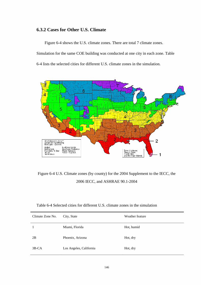
146

6.3.2 Cases for Other U.S. Climate

Figure 6-4 shows the U.S. climate zones. There are total 7 climate zones.

Simulation for the same COE building was conducted at one city in each zone. Table

6-4 lists the selected cities for different U.S. climate zones in the simulation.

Figure 6-4 U.S. Climate zones (by county) for the 2004 Supplement to the IECC, the

2006 IECC, and ASHRAE 90.1-2004

Table 6-4 Selected cities for different U.S. climate zones in the simulation

Climate Zone No. City, State Weather feature

1 Miami, Florida Hot, humid

2B Phoenix, Arizona Hot, dry

3B-CA Los Angeles, California Hot, dry

147

4A Baltimore, Maryland Mild, humid

5A Chicago, Illinois Cold, humid

6A Minneapolis, Minnesota Cold, humid

7 Duluth, Minnesota Very cold

Table 6-5 lists the yearly operation energy and cost saving due to the use of

DBAF at different U.S. climate zones. It can be seen that climate zone 1A has the

highest yearly operation cost saving, which is 3450 dollars ($). The climate zone

3B-CA has the lowest yearly operation cost saving, which is 179 dollars ($). For

climate zone one and two, most of the saving was from cooling and fan while no

significant heating saving was observed. For climate zone three, there is no significant

heating saving and very small cooling and fan saving were found. For climate zone

four, five and six, both heating and cooling saving were observed. It seems that more

heating saving and less cooling saving were found as the climate zone moves further

North. For climate zone seven, the highest heating saving was observed while there

was no cooling saving.

Overall, there is no need to use DBAF for climate zone 3B-CA as long as the

outdoor pollutant level is in an acceptable level. It seems climate zone one could be a

good place to apply the DBAF in terms of cost saving. However, the weather feature

of climate zone one is hot and humid. There is always a need to dehumidify the air in

summer. It has been mentioned that the DBAF would bring additional moisture to air.

Therefore, further analysis regarding the dehumidification issue needs to be

148

conducted for the application in climate zone one. In Chapter 3, it was found that the

moisture generaturion of one DBAF was ~1.89 kg/h. Eight DBAFs were needed for

COE building to maintain acceptable indoor air quality. The total moisture

generaturion would be 15.1 kg/h. The total moisture load for COE building applying

at climate zone one was 334 kg/h (The detailed calculation was described in

Appendix C). Therefore, the moisture load increament due to DBAF was ~5% of the

total building humidity load. This small additional moisture load may not pose a

serious limitation on the DBAF application, but its impact should be analyzed for

specific application cases in Climate Zone 1. Climate zone 2B appears to be a good

place to apply the DBAF due to its hot and dry weather feature.

Table 6-5 Yearly operation energy and cost saving due to use of DBAF at different

U.S. climate zones

Climate

Zone

City, State Natural Gas Electricity Total

Cost

saving

Heating

Cost

saving

Cooling Pump Fan Cost

saving

MBtu $ kWh kWh kWh $ $

1A Miami, FL 0.14 2 16153 684 6150 3448 3450

2B Phoenix, AZ 1.3 20 4477 385 2389 1088 1108

3B-CA Los Angeles, CA 0.2 3 755 33 383 176 179

4A Baltimore, MD 39.7 595 5348 264 -306 795 1390

5A Chicago, IL 76.9 1154 3835 243 180 639 1793

149

6A Minneapolis, MI 121.1 1817 2116 281 -211 328 2145

7 Duluth, MI 161.7 2426 -103 256 -442 -43 2383

6.4 Conclusions

Whole building energy simulation results showed that using the DBAF to

substitute 80% of the outdoor air supply without adversely affecting the IAQ could

save 30% saving in heating, 3% in cooling and 0.7% in pump energy consumption for

yearly operation in Syracuse, NY.

Based on the simulation results for different U.S. climate zones, it was found that

a higher percentage of energy savings was achieved for climate zones where more

heating is required than Syracuse climate (zone five), such as zone six and seven.

Dehumidification issue needs to be considered for climate zone one even though it

has the highest operation cost saving. While it was estimated that the presence of

DBAF only added 5% more load into the whole building humidity load. Climate zone

two might be a good place to apply the DBAF per its hot and dry weather feature.

Climate zone three in California area (Zone 3B-CA) might not be a good place to

apply the DBAF due to little yearly operation cost (~$179).

150

Chapter 7. Summary and Conclusions

The potential usage of plant’s root bed system for removing indoor VOC has

been demonstrated. Although potted plants alone are not efficient in real-world

condition, the studied dynamic botanical air filtration system (DBAF) with polluted

air passing through the plant’s root bed is very promising based on the laboratory

evaluation and real-field demonstration.

1) The full-scale chamber experimental results indicated that the DBAF had high

initial removal efficiency for formaldehyde and toluene even without plants in the

bed. With the plants, the filter system had even higher initial removal efficiency (90%

for formaldehyde in the first four days, and over 33% for toluene). However, it was

not clear if the microbes played any role in such a short term test period. The

long-term performance test results indicated that the DBAF was effective over a test

period of 300 days, and the same level of single pass removal efficiency was

maintained at the end of the test. This indicated the possible consumption of the

VOCs by the microbes as suggested by one study previously (Wolverton et al., 1989).

The operation of the DBAF resulted in 1 oC temperature decrease and 9–13%

RH increase in the chamber air. In the office experiments, the operation of DBAF

resulted in 0.5 oC temperature decrease and 17.7% RH increase. The moisture

production rate due to the use of DBAF was in the range of 0.81–1.89 kg/h. Such

moisture generation would improve the thermal comfort condition in winter, while in

summer contribute to little negligible effects on thermal comfort and cooling load

151

(add 5% more humidity load).

Field experiments in the office space indicated that the use of the DBAF could

reduce the percent of outdoor air supply from 25–5% of total air supply without

adversely affecting the indoor air quality if formaldehyde and toluene are the target

pollutants that dictate the required ventilation rate. In other words, the DBAF was

able to provide 80% of the required outdoor air supply for the field study case.

The effect of bed water content on the removal of formaldehyde/toluene was also

studied in the field experiments. The single pass removal efficiencies were

approximately 60% for formaldehyde and 20% for toluene when the volumetric water

content was within the range of 5–32% in the root bed. A moisture content that was

higher than 32% resulted in significant increase of single pass efficiency (SPE) for the

water soluble compound (formaldehyde) and reduction of SPE for Toluene.

2) In order to improve the understanding of the mechanisms of the DBAF system

in removing the volatile organic compounds, a series of further experiments were


the roles of different transport, storage and removal processes were also investigated.

In general, it was found that passing the air through the root bed with microbes was

essential to obtain meaningful removal efficiency. Moisture in the root bed also

played an important role, both for maintaining a favorable living condition for

microbes and for absorbing water-soluble compounds such as formaldehyde. The role

of the plant was to introduce and maintain a favorable microbe community that

152

effectively degraded the VOCs that were adsorbed or absorbed by the root bed. While

the moisture in a wet bed had the scrubber effect for water-soluble compounds such as

formaldehyde, presence of the plant increased the removal efficiency by about a

factor of two based on the results from the reduced-scale root bed experiments.

Moreover, for the same cross-section area of 0.35 m long and 0.2 m wide, the

dry bed with airflow had an equivalent CADR of 1.5 m3/h. The wet bed with airflow

had an equivalent CADR of 8.5 m3/h. The DBAF had an equivalent CADR of 16.4

m3/h. The difference of wet bed with airflow and DBAF was due to the existence of

plant. It was found that wet bed and microbial community are the two major factors to

affect the formaldehyde removal. It was hard to find out which one was the dominant

one in short-time test (one day), while the result shows that microbial community

would become dominant gradually as time went on.

The biodegradation rate constant for formaldehyde was also determined, which

was 2.06E-05 s-1 at 92% RH and 15 ppb formaldehyde level. It should be noted that

this rate constant was only for comparison. Because the transfer of formaldehyde

from gas phase into liquid film and formaldehyde degradation by microbial

community occured in series but not in parallel. They can not be exactly seperated

from the experimental result, while it can be used as a reference for the model initial

inpu

3) The CHAMPS-BES model was revised and used to model the operation of the

DBAF. Model verification results showed that the model could describe the pressure

153

drop and airflow relationship well by using the air permeability as a model parameter.

The water source added in the model also lead to the similar bed moisture content and

outlet air RH as that in real test case. For the VOC breakthrough curve simulation, the

partition coefficient effect, effect of gas to solid and gas to liquid mass transfer

coefficient were also investigated. The simulation results show the developed model

work well in testing the effect of different parameters. It was also found that the

critical bio-degradation rate constant is 1×10-5 s-1, which means the bio-degradation

rate of the DBAF has to be maintained above 1×10-5 s-1 to be effective in removing

formaldehyde.

In the model validation part, the fitted bio-degradation rate constant was obtained

by comparing the simulation results with experimental data. The fitted


reduced-scale DBAF tested.

4) Whole building energy simulation results showed that using the DBAF to

substitute 80% of the outdoor air supply without adversely affecting the IAQ could

save 30% saving in heating, 3% in cooling and 0.7% in fan energy consumption for

yearly operation in Syracuse, NY.

Based on the simulation results for different U.S. climate zones, it was found that

a higher percentage of energy savings was achieved for climate zones where more

heating is required than Syracuse climate (zone five), such as zone six and seven.

Dehumidification issue needs to be considered for climate zone one even though it

154

has the highest operation cost saving. While it was estimated that the presence of

DBAF only added 5% more load into the whole building humidity load. Climate zone

two might be a good place to apply the DBAF per its hot and dry weather feature.

Climate zone three in California area (Zone 3B-CA) might not be a good place to

apply the DBAF due to little yearly operation cost (~$179).

155

References

Alagappan G, Cowan R. Substrate inhibition kinetics for toluene and benzene

degrading pure cultures and a method for collection and analysis of respirometric

data for strongly inhibited cultures. Biotechnol. Bioeng. 2003; 83: 798–810.

ANSI/AHAM AC-1 2006. Method for Measuring the Performance of Portable

Household Electrical Room Air Cleaner; 2006.

ANSI/BIFMA M7.1 2007. Standard Method For Testing VOC Emissions From

Office Furniture Systems, Components And Seating; 2007.

ANSI/ASHRAE Standard 62.1-2010. Ventilation and acceptable indoor air quality.

Atlanta: American Society of Heating, Refrigerating, and Air-Conditioning

Engineers, Inc.; 2010.

Arriaga S, Revah S. Improving hexane removal by enhancing fungal development in a

microbial consortium biofilter. Biotechnol. Bioeng. 2005; 90: 107–15.

Auriol M, Filali-Meknassi Y, Tyagi RD, Adams CD. Laccase-catalyzed conversion of

natural and synthetic hormones from a municipal waster. Water Res. 2007; 41:

3281–8.

Beveridge TJ, Makin SA, Kadurugamuwa JL, Li Z. Interaction between biofilms and

the environment. FEMS Microbiol. Rev. 1997; 20: 291–303.

Burgess JE, Parsons SA, Stuetz RM. Developments in odour control and waste gas

treatment biotechnology: a review. Biotechnol. Adv. 2001; 19: 35–63.

156

Butterfield PW, Camper AK, Ellis BD, Jones WL. Chlorination of model drinking

water biofilm: implications for growth and organic carbon removal. Water Res.

2002; 36: 4391–405.

Carlsson H, Nilsson U, Ostman C. Video display units: an emission source of the

contact allergenic flame retardant triphenyl phosphate in the indoor environment.

Environ. Sci. Technol. 2000; 34: 3885–9.

Chain P, Denef V, Konstantinidis K, Vergez L, Agullo L. Burkholderia xenovorans

LB400 harbors a multi-replicon, 9.73-Mbp genome shaped for versatility. PNAS

2006; 103: 15280–7.

Chen W, Zhang J, Zhang Z. Performance of air cleaners for removing multiple

volatile organic compounds in indoor air. ASHRAE Trans. 2005; 111: 1101–14.

Chen W, Gao Z, Zhang J. Reduced Energy Use Through Reduced Indoor

Contamination In Residential Buildings. Final report for National Center for

Energy Management and Building Technologies: NCEMBT-20061101.

Daisey J, Hodgon A, Fisk W, Mendell M, Ten Brinke J. Volatile organic compounds

in twelve Californian office buildings: classes, concentrations and sources. Atmos.

Environ. 1994; 28: 3557–62.

Darlington A, Chan M, Malloch D, Pilger C, Dixon MA. The biofiltration of indoor

air: implications for air quality. Indoor Air 2000; 10: 39–46.

Darlington A, Dat J, Dixon M. The biofiltration of indoor air: air flux and temperature

influences the removal of toluene, ethylbenzene, and xylene. Environ. Sci.

Technol. 2001; 35: 240–6.

157

Delhoménie MC, Heitz M. Biofiltration of air: a review. Crit. Rev. Biotechnol. 2005;

25: 53–72.

Deshusses MA, Hamer B, Dunn IJ. Behavior of biofilters for waste air biotreatment.

1. Dynamic model development. Environ. Sci. Technol. 1995; 29: 1048–1058.

Devinny JS, Deshusses MA, Webster TS. Biofiltration for air pollution control. Boca

Raton: Lewis Publishers; 1999.

Devinny JS, Ramesh J. A phenomenological review of biofilter models. Chem. Eng.

J. 2005; 113: 187–196.

Dudler R, Eberl L. Interactions between bacteria and eukaryotes via small molecules.

Curr. Opin. Biotech. 2006; 17:268–73.

Ekberg LA. Volatile organic compounds in office buildings. Atmos. Environ.

1994;28: 3571–5.

Ergas SJ, Schroeger ED, Chang DP. Biodegradation technology for volatile organic

compound removal from airstream. Final report. Contract No. A032-127.

California Environmental Protection Agency, Air Resources Board, Research

Division; 1992. May.

Ergas SJ, Shumway L, FitchMW, Neemann JJ. Membrane process for biological

treatment of contaminated gas streams. Biotechnol. Bioeng. 1999; 63: 431–41.

Fan LS, Leyva-Ramos R, Wisecarver KD, Zehner BJ. Diffusion of phenol through a

biofilm grown activated carbon particles in a draft-tube three-phase fluidized bed

bioreactors. Biotechnol. Bioeng. 1990; 35: 279–286.

158

Fan S, Scow KM. Biodegradation of Trichloroethylene and Toluene By Indigeous

Microbial Populations in Soil. Appl. Environ. Microbiol. 1993; 59(6): 1911-1918.

Girman J, Philips T, and Levin H. Critical Reviews: How well do house plants

perform as indoor air cleaners? Proceedings of Healthy building 2009: paper 667.

Guieysse B, Hort C, Platel V, Munoz R, Ondarts M, Revah S. Biological treatment of

indoor air for VOC removal: Potential and challenges. Biotechnol. Adv. 2008; 26:

398–410.

Hodge DS, Devinny JS. Modeling removal of air contaminants by biofiltration, J.

Environ. Eng. 1995; 121 (1): 21–32.

Hodge DS, Devinny JS. Determination of biofilter model constants using

mini-columns, J. Environ. Eng. 1997; 123 (6): 577–585.

Hodgson AT, Rudd AF, and Chandra S. Volatile organic compound concentrations

and emission rates in new manufactured and site-built houses, Indoor Air 2000;

10: 178-192.

Holden PA, Firestone MK. Soil microorganisms in soil cleanup: how can improve our

understanding? J. Environ. Qual. 1997; 26: 32-40.

Iranpour R, Cox HJ, Deshusses MA, Schroeder ED. Literature review of air pollution

control biofilters and biotrickling filters for odor and volatile compound removal.

Environ. Prog. 2005; 24: 254–67.

Jin Y, Veiga MC, Kennes C. Development of a novel monolith-bioreactor for the

treatment of VOC-polluted air. Environ. Technol. 2006; 27: 1271–7.

159

Jorio H, Payre B, Heitz M. Modeling of gas-phase biofilter performance. J. Chem.

Technol. Biotechnol. 2003; 78: 834–846.

Kennes C, Veiga MC. Fungal biocatalysts in the biofiltration of VOC-polluted air. J.

Biotechnol. 2004; 113: 305–19.

Kesselmeier J, Staudt M. Biogenic volatile organic compounds (VOC): an overview

on emission, physiology and ecology. J. Atmos. Chem. 1999; 33: 23–88.

Kim S, Deshusses MA. Development and experimental validation of a conceptual

model for biotrickling filtration of H2S. Environ. Prog. 2003; 22 (2): 119–128.

Larimer FW, Chain P, Hauser L, Lamerdin J, Malfatti S, Do L. Complete genome

sequence of the metabolically versatile photosynthetic bacterium

Rhodopseudomonas palustris. Nat. Biotechnol. 2003; 22: 55–61.

Li H, Mihelcic JR, Crittenden JC, Anderson KA. Field measurements and modeling

of two-stage biofilter that treats odorous sulfur air emissions, J. Environ. Eng.

2003; 129 (8): 684–692.

Marshall KC. Microbial adhesion in biotechnological processes. Curr. Opin.

Biotechnol. 1994; 5: 296–301.

Meyer, B., Indoor Air Quality, Addison-Wesley, Reading, MA, 1983.

Miller M, Allen D. Modelling transport and degradation of hydrophobic pollutants in

biofilms in biofilters. Proceedings of the USC-TRG Conference on Biofiltration

for Air Pollution Control, Los Angeles, CA, October, 2004.

160

Molin S, Tolker-Nielsen T. Gene transfer occurs with enhanced efficiency in biofilms

and induces enhanced stabilisation of the biofilm structure. Curr. Opin.

Biotechnol. 2003; 14: 255–61.

Muñoz R, Villaverde S, Guieysse B, Revah S. Two phase partitioning bioreactors for

the treatment of volatile organic compounds. Biotechnol. Adv. 2007; 25: 410–22.

Muir DG, Howard PH. Are there other persistent organic pollutants? Environ. Sci.

Technol. 2006; 40: 7157–66.

Newman LA, Reynolds CM. Phytodegradation of organic compounds. Curr. Opin.

Biotechnol. 2004; 15: 225–30.

Nicolai A. Modeling and numerical simulation of salt transport and phase transitions

in unsaturated porous building materials. Ph.D. thesis, 2009.

NRC, Committee on Indoor Air Pollutants: Indoor Pollutants, National Research

Council, National Academy Press, Washington, DC, 1981.

Otake T, Yoshinaga J, Yanagisawa Y. Analysis of organic esters of plasticizer in

indoor air by GC-MS and GC-FPD. Environ. Sci. Technol. 2001; 35: 3099–102.

Orwell RL,Wood RL, Tarran WJ, Torpy F, Burchett MD. Removal of benzene by the

indoor plant/substrate microcosm and implications for air quality. Water Air Soil

Pollut. 2004; 157: 193–207.

Ottengraf SP, Konings JG. Emission of microorganisms from biofilters. Bioprocess

Eng. 1991; 7: 89–96.

161

Orwell RL, Wood RA, Burchett MA, Tarran J, Torpy F. The potted-plant microcosm

substantially reduces indoor air VOC pollution: II. Laboratory study. Water Air

Soil Pollut. 2006; 177: 59–80.

Owen SM, Clark S, Pompe M, Semple KT. Biogenic volatile organic compounds as

potential carbon source for microbial communities in soil from the rhizosphere of

populus tremula. FEMS microbial. Lett. 2007; 268: 34-39.

Pahm MA, Alexander M. Selecting inocula for the biodegradation of organic

compounds at low concentration. Microb. Ecol. 1993; 25: 275–86.

Parvatiyar MG, Govind R, Bishop DF. Treatment of trichloroethylene (TCE) in a

membrane biofilter. Biotechnol. Bioeng. 1996; 50: 57–64.

Ranasinghe MA, Jordan PJ, Gostomski PA. Modelling the mass and energy balance

in a compost biofilter. Proceedings of the A&WMA 95th Annual Meeting and

Exhibition, Baltimore, MD, June 18–24, 2002.

Revah S, Morgan-Sagastume JM. Methods for odor and VOC control. In:

Shareefdeen Z, Singh A, editors. Biotechnology for odour and air pollution.

Heidelberg: Springer- Verlag; 2005. p. 29–64.

Robbins CA, Swenson LJ, Nealley ML, Gots RE, Kelman BJ. Health effects

ofmycotoxins in indoor air: a critical review. Appl. Occup. Environ. Hyg. 2000;

15: 773–84.

Roch F, Alexander M. Inability of bacteria to degrade low concentrations of toluene

in water. Environ. Toxicol. Chem. 1997; 16: 1377–83.

162

Sander R. Compilation of Henry's law constants for inorganic and organic species of

potential importance in environmental chemistry; 1999. http://www.mpch-mainz.

mpg.de/~sander/res/henry.html.

Sandhu A, Halverson LJ, Beattie GA. Bacterial degradation of airborne phenol in the

phyllosphere. Environ. Microbiol. 2007; 9: 383–92.

Schäffner A, Messner B, Langebartels C, Sandermann H. Genes and enzymes for

inplanta phytoremediation of air, water and soil. Acta Biotechnol. 2002; 22:

141–52.

Schleibinger H, Keller R, Rüden H. Indoor air pollution by microorganisms and their

metabolites. In: Pluschke P, editor. The handbook of environmental chemistry,

vol. 4. Berlin Heidelberg: Springer -Verlag; 2004. p. 149–77. Part F.

Schmitz H, Hilger U, Weinder M. Assimilation and metabolism of formaldehyde by

leaves appear unlikely to be of value for indoor air purification. New Phytol.

2000; 147: 307–15.

Shareefdeen Z, Singh A. Biotechnology for odor and air pollution control.

Heidelberg: Springer-Verlag; 2005.

Shaughnessy RJ, Levetin E, Blocker J, Sublette K. Effectiveness of portable indoor

air cleaners: sensory testing results. Indoor Air 1994; 4: 179–88.

Shaughnessy R, Sextro R. What is an effective portable air cleaning device? A

review. J. Occup. Environ. Hyg. 2006; 3: 169–81.

Singh R, Debarati PD, Jain RK. Biofilms: implications in bioremediation. Trends

Microbiol. 2006; 14: 389–97.

163

Zarook SM. Development experimental validation and dynamic analysis of a general

transient biofilter model, chemical engineering science 1997; 52(5): 759-773.

Smith F, Harvey A. Avoid Common Pitfalls When Using Henry's Law. Chemical

Engineering Progress. September 2007.

Staudinger J, Roberts PV. A critical review of Henry's law constants for

environmental applications. Crit. Rev. Environ. Sci. Technol. 1996; 26: 205–97.

Torres EM, Basrai SS, Kogan V. Evaluation of two biotechnologies controlling

POTWair emissions. Proceedings of 1996 USG-TRG Conference on Biofiltration.

Los Angeles, CA: University of Southern California; 1996. p. 182–97.

Tseng C, Hsieh C, Chen S. The Removal of Indoor Formaldehyde by Various Air

Cleaners. Paper 457. Proceedings of the air & waste management association’s

98th annual conference. Minneapolis, Minnesota.

U.S. EPA. Air and steam stripping of toxic pollutants. Tech. Rep. EPA-68-03-002.

Cincinnati, OH, USA: Industrial Environmental Research Laboratory; 1982.

U.S. EPA. Why Is the Environment Indoors Important to Us? Indoor Environment

Division, U.S. Environmental Protection Agency, Washington, DC, 2000.

U.S.EPA. Indoor Air Quality. http://www.epa.gov/iaq/is-imprv.html, last accessed

November 30, 2008.

U.S. Green Building Council. www.usgbc.org, last accessed January 30, 2009.

Van D, Vrouwenvelder HS, Veenendaal HR. Kinetic aspects of biofilm formation on

surfaces exposed to drinking water.Water Sci. Technol. 1995; 32: 61–5.

164

Van Groenestijn JW, Kraakman NR. Recent developments in biological waste gas

purification in Europe. Chem. Eng. J. 2005; 113: 85–91.

Vergara A, Haaren B, Revah S. Phase partition of gaseous hexane and surface

hydrophobicity of Fusarium solani when grown in liquid and solid media with

hexanol and hexane. Biotechnol. Lett. 2006; 28: 2011–7.

Wargocki P, Sundell J, Bischof W, Brundrett G, Fanger PO, et al. Ventilation and

health in non-industrial indoor environments: report from a European

Multidisciplinary Scientific Consensus Meeting (EUROVEN). Indoor Air 2002;

12: 113–28.

Wolverton BC, McDonald RC, Watkins EA. Foliage plants for removing indoor air

pollutants from energy-efficient homes. Econ. Bot. 1984; 38: 224–8.

Wolverto BC, Johnson A, Bounds K. Interior landscape plants for indoor air pollution

abatement, National Aeronautics and Space Administration, 1989. p.1–22.

Wolverton BC, Wolverton JD. Plant and soil microorganisms: Removal of

formaldehyde, xylene and ammonia from the indoor environment. J. Miss. Acad.

Sci. 1993; 11-15.

Wood RA, Burchett MA, Alquezar R, Orwell RL, Tarran J, Torpy F. The potted-plant

microcosm substantially reduces indoor air VOC pollution: 1. Office field-study.

Water Air Soil Pollut. 2006; 175: 163–80.

Zarook SM, Shaikh AA, Ansar Z. Development, experimental validation and dynamic

analysis of a general transient biofilter model. Chem. Eng. Sci. 1997; 52 (5):

759–773.

165

Zhou X, Mopper K. Apparent partition coefficients of 15 carbonyl compounds

between air and seawater and between air and freshwater: implications for

air-exchange. Environ. Sci. Technol. 1990; 24: 1864–9.

Zilli M, Camogli G, Nicolella C. Detachment and emission of airborne bacteria in

gasphase biofilm reactors. Biotechnol. Bioeng. 2005; 91: 707–14.

166

Appendix A. Full-scale Chamber Pull-down test procedure

A.1 Test Facility and Instrument

The pilot/formal tests for characterizing the performance of the media filter in

terms of VOC removal were carried out in a full-scale stainless steel environmental

chamber depicted in Figure A-1(a). The chamber has a dimension of 16 ft long x 12 ft

wide x 10 ft high (4.84 m long x 3.63 m wide x 3.05 m high) and an interior volume

of 1920 ft3 (54.4 m3).

INNOVA 1312 Photoacoustic Multi-gas Monitor was used for online

measurements of the concentration of toluene equivalent (TVOCtoluene), the

concentration of formaldehyde (Cformal), and the concentration of tracer gas (SF6), as

shown in Figure A-1(b). The monitor was based on the photoacoustic infrared

detection method. For TVOCtoluene, the sensitivity and response factor of the

instrument for different compounds were different, so the readings from the gas

monitor were only used as semi-quantitative measures to monitor the change of

TVOC concentrations over time and how they differed for different operation

conditions for the pilot tests.

167

(a) IEQ chamber (b) INNOVA 1312 gas monitor

Figure A-1 Test facility and instrument

A.2 Test Procedure

• Put the filter bed system into the chamber (as shown in Figure A-2)

• Flushed the chamber overnight then set the return air at 800 CFM to make the air

in the chamber in well-mixed. The chamber was running At full-recirculation

mode

• Injected SF6 to check the air tightness of the chamber system. The concentration

was monitored continuously during the entire test period

• Set up 1312 photoacoustic multi-gas monitor to continuously monitor TVOC,

formaldehyde and tracer gas concentration

• Preparation of tested VOC. Weighed calculated amount of liquid toluene (target

300mg which equals to approximately 5mg/m3 initial chamber concentration) to a

glass bottle with septum; weighed calculated amount of paraformaldehyde (target

168

120mg which equals to approximately 2mg/m3 initial chamber concentration) to a

glass bottle with septum. The uncertainty related with injection amount would be

determined from the accuracy and resolution of syringe

• Injection of tested VOC. Quickly opened the chamber door and brought the two

glass bottles (one for formaldehyde and one for liquid toluene) into the chamber.

Poured the solid paraformaldehyde into one petri dish and the liquid toluene into

the other petri dish on the hot plate, left the bottle (on hot plate to facilitate the

evaporation of VOC residuals inside the bottle) and the cap inside the chamber.

Then quickly stepped out of the chamber and closed the chamber door. The

whole process was taken approximately 1 to 2 minutes

• Turned on the power of hot plate from chamber control panel. Recorded the time

• Turned off the power of hot plate after 1 h. The injection period for VOC was 1 h

• Turned on the fan power of the filter bed system to start the air filtration system.

Recorded the time as the test started point

• The test period lasted about 4 hours (The time depended on when the contaminant

concentration decreased to the background level)

• Flushed the chamber once the test was done

• Downloaded test data and analyzed test results.

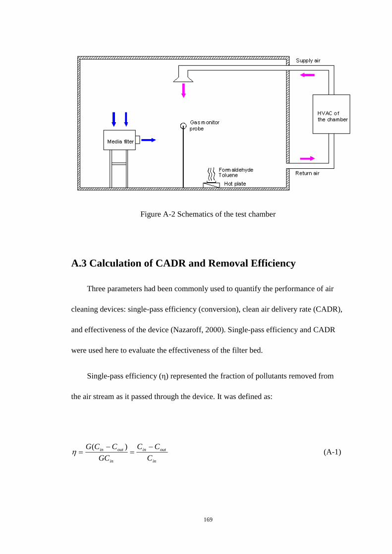
169

Figure A-2 Schematics of the test chamber

A.3 Calculation of CADR and Removal Efficiency

Three parameters had been commonly used to quantify the performance of air

cleaning devices: single-pass efficiency (conversion), clean air delivery rate (CADR),

and effectiveness of the device (Nazaroff, 2000). Single-pass efficiency and CADR

were used here to evaluate the effectiveness of the filter bed.

Single-pass efficiency (η) represented the fraction of pollutants removed from

the air stream as it passed through the device. It was defined as:

in

outin

in

outin

C

CC

GC

CCG −=

−=

)(η (A-1)

170

Where,

Cin

= contaminant concentration at the inlet of air cleaner, mg/m3 for VOC and

number of particles/cm3 for particulates.

Cout

= contaminant concentration at the outlet of air cleaner, mg/m3 for VOC and

number of particles /cm3 for particulates.

G = airflow rate through the air cleaner, CFM or m3/h.

CADR represents the “effective” clean airflow rate delivered by the air cleaner.

It is defined as:

dEGCADR ⋅⋅=η (A-2)

Where, Ed = short-circuiting factor of the air cleaner, Ed=Cin/C, where C is average

concentration in the test chamber (Ed = 1 At well-mixed condition).

CADR was calculated from the test results. The analysis was based on the

well-mixed single zone model. Assuming that the air was well mixed in chamber and

the contaminant removal mechanisms other than air cleaning (e.g. surface deposition

effect and chamber leakage effect) were the same with and without air cleaner

operating and can be characterized by a first-order rate constant kn, the mass

conservation of contaminant can be written as:

171

CCADRVkdt

dCV n ⋅+−= )( , (C=C0 at t=0) (A-3a)

Or

CkCV

CADRk

dt

dCen ⋅−=⋅+−= )( (A-3b)

Where,

V - volume of the testing chamber system, ft3 or m

3,

kn – contaminant concentration decay rate without air cleaner operating (chamber

effects), min-1

or h-1

,

ke – total contaminant concentration decay rate with air cleaner operating, min

-1 or h

-1,

C0 – Initial contaminant concentration inside the chamber, mg/m

3 for VOC and

number of particles/cm3 for particulates.

If CADR did not change during the test period, an analytical solution could be

obtained from Equation (A-3) as:

tkt

V

CADRk

en

eCeCC −+−⋅=⋅= 0

)(

0 (A-4)

CADR was then determined by linear regression of ln (C/C0) vs. t from the measured

concentration decay curve:

)( ne kkVCADR −= (A-5)

After the CADR was calculated, together with measured the airflow rate through the

air cleaner, the removal efficiency could then be calculated by dividing the CADR by

the airflow rate through the air cleaner. This calculated removal efficiency was the

172

same as the single-pass efficiency defined in Equation (A-1) since the air in the

chamber was well-mixed.

The step-by-step data analysis procedure for VOC was summarized as follows:

1. Calculated kn based on the measured tracer gas concentration decay or

contaminant concentration decay before time zero (if the contaminant

decay during the static period did not match the SF6 decay very well);

2. Calculated ke by linear regression of ln (C/C

0) vs. t from measured

concentration decay curve after turning on the air cleaner (dynamic

period);

3. Calculated CADR according to Equation (A-5);

4. Determined the removal efficiency by dividing the calculated CADR value

by the measured airflow rate through the air cleaner.

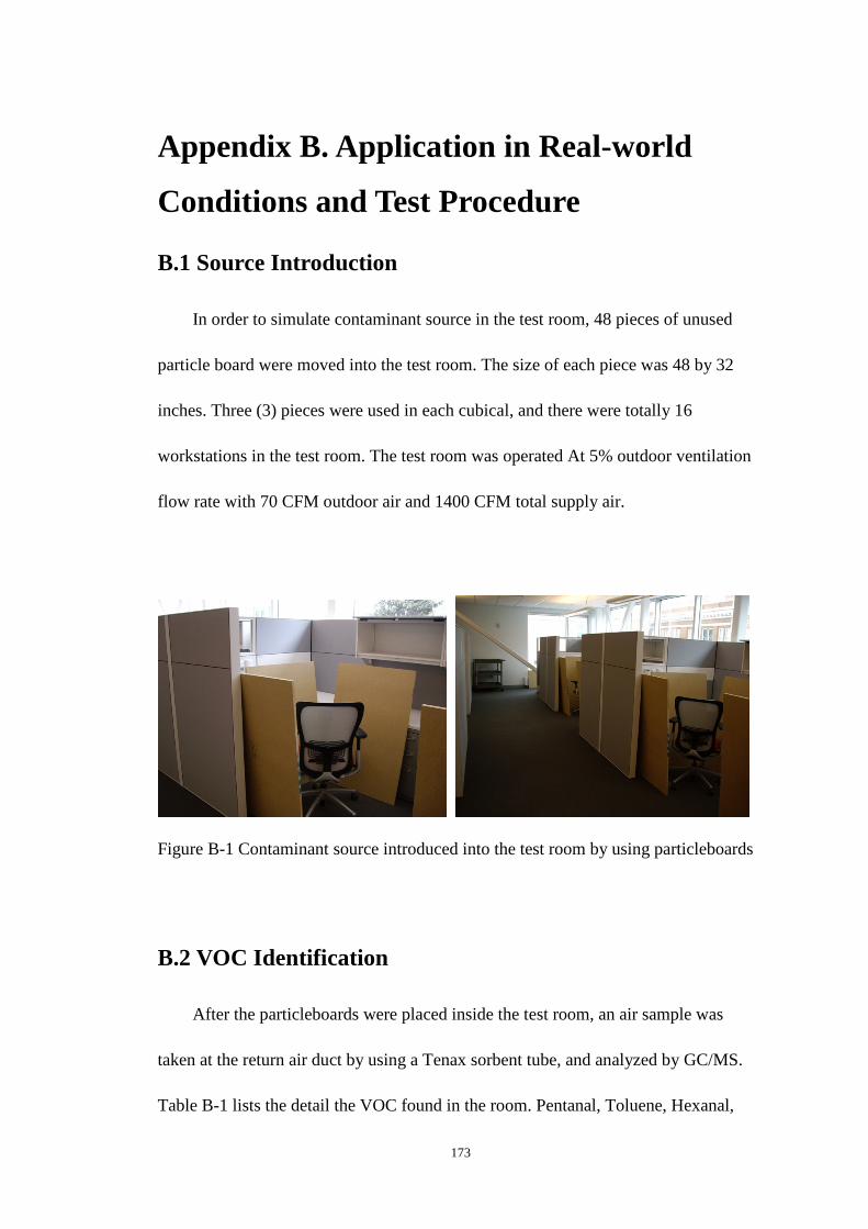
173

Appendix B. Application in Real-world

Conditions and Test Procedure

B.1 Source Introduction

In order to simulate contaminant source in the test room, 48 pieces of unused

particle board were moved into the test room. The size of each piece was 48 by 32

inches. Three (3) pieces were used in each cubical, and there were totally 16

workstations in the test room. The test room was operated At 5% outdoor ventilation

flow rate with 70 CFM outdoor air and 1400 CFM total supply air.

Figure B-1 Contaminant source introduced into the test room by using particleboards

B.2 VOC Identification

After the particleboards were placed inside the test room, an air sample was

taken at the return air duct by using a Tenax sorbent tube, and analyzed by GC/MS.

Table B-1 lists the detail the VOC found in the room. Pentanal, Toluene, Hexanal,

174

Xylene, Alpha-Pinene, (1s)-(b)-Pinene were selected as the target VOC in the room.

In addition, formaldehyde and acetaldehyde were also chosen as target compounds as

they are typically identified as major compounds of concern in emission testing of

composite wood materials.

Table B-1 Test room VOC identification (By GC/MS)

RT Response area

Est.Conc.

(ug/m3)

VOC Name M.W. Formula CAS# Note

2.664 169,827,440 8.37 OXIRANE, TRIMETHYL- 86 C5H10O 5076-19-7

5.059 86,847,696 4.28 MERCAPTAMINE 77 C2H7NS 60-23-1

6.337 118,900,960 5.86 PENTANAL(Valeralde.) 86 C5H10O 110-62-3

7.897 147,092,128 7.25 TOLUENE 92 C7H8 108-88-3

room

bkgd

8.626 186,059,488 9.17 CYCLOTRISILOXANE, HEXAMETHYL- 222 C6H18O3Si3 541-05-9

tube

bkgd

9.562 1,077,273,088 53.08 HEXANAL 100 C6H12O 66-25-1

11.344 68,134,416 3.36 BENZENEETHANOL, .ALPHA.,.BETA.-DIMETHYL- 150 C10H14O 52089-32-4

13.019 597,559,104 29.45 .ALPHA.-PINENE 136 C10H16 80-56-8

13.714 50,035,800 2.47 CAMPHENE 136 C10H16 79-92-5

14.348 51,328,636 2.53 CYCLOTETRASILOXANE, OCTAMETHYL- 296 C8H24O4Si4 556-67-2

14.76 448,029,344 22.08 (1s)-(b)-pinene 136 C10H16 18172-67-3

15.968 61,673,916 3.04 Benzaldehyde

16.441 134,613,712 6.63 d-limonene

16.592 88,311,400 4.35 Octanal 128 C8H16O 124-13-0

17.88 56,756,684 2.80 Undecane

room

bkgd

18.897 108,563,536 5.35 P-TRIMETHYLSILYLOXYPHENYL-BIS(TRIMETHYLS 370 C17H34O3Si3 1000079-08-1

19.249 79,402,592 3.91 Nonanal 142 C9H18O 124-19-6

175

21.382 95,913,080 4.73 PENTADECANAL- 226 C15H30O 2765-11-9

21.518 240,076,816 11.83 2-PROPENOIC ACID, 6-METHYLHEPTYL ESTER 184 C11H20O2 54774-91-3

Table B-2 lists the target compounds that were continuously monitored by PTR-MS.

It also shows the solubility of these compounds in water, which would help to

understand the filter bed performance in removing water soluble vs. non-soluble

compounds.

Table B-2 Target compounds monitored by PTR-MS (Ion Mass of 21)

VOC Name M.W. Formula CAS# Solubility in water

Formaldehyde 31 CH2O 50-00-0 Soluble

Acetaldehyde 45 C2H4O 75-07-0 Soluble

Pentanal (Valeralde.) 86 C5H10O 110-62-3 Very slightly soluble

Toluene 92 C7H8 108-88-3 Insoluble

Hexanal 100 C6H12O 66-25-1 Insoluble

Xylene 106 C8H10 1330-20-7 Insoluble

Alpha-Pinene 136 C10H16 80-56-8 Insoluble

B.3 Filter Bed Single Pass Efficiency Measurement

The filter bed single pass efficiency (SPE) would help to understand the change

of the test room contaminants concentration after the filter system was turned on. The

single pass efficiency was measured as follows:

176

• The contaminants concentration of the filter upstream was measured for a

number of five minute intervalsand the average of these five minutes data was

taken as data 1;

• The sample system was switched to downstream. The contaminant

concentration of the filter downstream was measured for five minute intervals

and the average of these five minutes data was taken as data 2, and it was used

as the downstream concentration;

• The monitor was switched back to measure the upstream concentration for the

next five minutes and the average of these five minutes data was taken as data

3;

• The average of data 1 and data 3 was used as the upstream concentration;

• The filter single pass efficiency could be obtained as one minus downstream

concentration divided by upstream concentration.

B.4 Effect of Bed Water Content to the Single Pass

Efficiency

� The media bed was irrigated with water until it became saturated, which can be

realized in this way: an automatic irrigation system was setup to achieve this. A

moisture control sensor was used to continuously monitor the moisture content

(M.C.) in the filter bed and it was set-up at the saturation level (50%). The

177

irrigation was kept on running until the signal light of the moisture sensor was

off, which means the media bed was saturated already

� The fan was kept running at its maximum flow rate(480cfm) until inlet air RH

was close to the outlet RH: the moisture control sensor was set-up at its minimum

level to avoid the fan stopping running during the test period, which means get

the media bed dry gradually

� In the first half hour, PTR-MS was used to measure the contaminants

concentration of upstream for five minutes, and the average was taken as data 1,

and then it was switched to downstream for another 5-minute measurement and

the average was taken as data 2, after that it was switched back to upstream for

another fiveminute measurement, and the average was taken as data 3. The

average of data 1 and data 3 was used as the upstream value, and data 2 was used

as the downstream value. The single pass efficiency was obtained: one minus

downstream value divided by upstream value

� After that, the test period was extended to 10 minutes for each side, then it took

30 minutes to get one single pass efficiency

� The procedure of measuring single pass efficiency was repeated every 30 minutes

until the bed water content was lower than 5%, and then the filter bed single pass

efficiency at different moisture level could be obtained.

178

B.5 Test Room Contaminants Concentration Monitoring

� On the first day, PTR-MS started to monitor the room concentration, and the

first-two-hour test result was taken as room background, and a GC/MC sample

was also taken at the same time

� After two hours, the particleboards were moved in, then four hours later, a

GC/MS sample was taken to identify the VOCs existing in the room, and hexanal,

pentanal, toluene, xylene, pinene, formaldehyde and acetaldehyde were selected

as target compounds

� In the second day, the room ventilation was adjusted to 5% (70 CFM outdoor air)

at first, then eight hours later, was increased to 50%( 700 CFM outdoor air); 16

hours later, it was switched back to 5%

� Twenty four hours later, the filtration system was turned on and kept running for

eight hours; then was shut off; and then the filter on/off cycle was repeated two

more times

� In the second week, two more tests were done to monitor the room contaminant

concentration change at ventilation of 25% and 10%.

� See Table B-3 for the schedule for the two-week test

179

Table B-3 The schedule for the two-week test

Test period Time (h) Procedure

Week 1

0 Got PTR-MS started

2 Moved particle board in

24 Adjusted outdoor air to 5%

32 Adjusted outdoor air to 50%

45 Adjusted outdoor air back to 5%

72 Turned on the filter

78 Turned off the filter


108 Turned off the filter


132 Truned off the filer

Week 2

0 Got PTR-MS started (with 5% outdoor air)

8 Adjusted ventilation to 25%

24 Adjusted ventilation back to 5%

32 Adjusted ventilation to 10%

48 Adjusted ventilation back to 5%

Table B-4 Air change rate for different operation modes

Room

Volume Supply air Operation mode Air change rate (times/h)

9385 ft3 1400cfm

50% OA 4.5

25% OA 2.2

10% OA 0.9

5% OA 0.4

180

Appendix C. COE Building Humidity Load

Calculation

Table C-1 COE building humidity load calculation

LEAKAGE & INFILTRATION LOAD 273.12 kg/Hr

Formula: LOAD = (C-B) x 0.0012 x A x D x Ex F

A = VOLUME OF CONDITION SPACE (m3) 11854

B = DESIGNED HUMIDITY (g/kg) 12.000

C = SURROUNDING HUMIDITY (g/kg) 20.000

D = VOLUME FACTOR ( Note A) 0.2

E = PRESSURE FACTOR ( Note B) 1

F = CONSTRUCTION FACTOR ( Note C) 1

G= Delta g/kg factor ( calculated ) 12.00 0 HUMAN LOAD 16.58 kg/Hr

Formula: LOAD = G x H x 0.15

G = NUMBER OF PEOPLE 165

H = Work Load Coeff (0.5 Light to 1.6 Heavy) 0.67

MADE UP AIR LOAD 44.7720 kg/Hr

Formula: LOAD = (K- B) x J x 0.0012

J = Air volume in CMH 3731

K = MADE UP AIR HUMIDITY (g/kg) 22.000

DOOR OPENING LOAD 0.00 kg/Hr

Formula: LOAD = (M- B) x 0.0012 x N x P x L x 0.3

L = TOTAL DOOR X-SECTION AREA 0

M = NEXT DOOR AIR HUMIDITY (g/kg) 15

N = EACH OPENING TIME ( seconds ) 30

P = NUMBER OF OPENING /HOUR 2

HYGROSCOPIC MATERIAL LOAD 0.00 kg/Hr

EXPOSED WATER SURFACE LOAD 0.00 kg/Hr

TOTAL HUMIDITY LOAD 334.47 kg/Hr

181

Table C-2 Determination of note A, B, and C in Talbe C-1

Note A ( Volume factor) Note B ( +ve Pressure factor ) Note C ( Construction factor )

<400 CU METER =0.4 + 0 Pa = 1 Wooden wall with cracks = 2 to 3

1000 CU METER = 0.3 + 30 Pa = 0.6 Basement = 1.8 to 2.5

5000 CU METER = 0.25 + 60 Pa = 0.3 4 walls exposed to rain = 1.5 to 2

>10000 CU METER = 0.22 Ground Floor = 1.2 to 1.5

Gypsum walls = 1 to 1.3

Normal good walls = 1

Oil based painted wall = 0.8 to 0.9

Double epoxy painted wall = 0.7 to 0.8

Freezer insulated seal wall =0.6 to 0.8

Tight sealed metal frame = 0.3 to 0.5

182

VITA Name of Author: Zhiqiang Wang

Place of Birth: Kashi, Xinjiang, China

Date of Birth: August 08, 1981

Graduate and undergraduate school attended:

Syracuse University, Syracuse, NY, USA

Tianjin University, Tianjin, China

Degrees Awarded:

M.S. Heating, Ventilating and Air-Conditioning Engineering, 2007, Tianjin

University, China

B.S. Building Environment and Equipment Engineering, 2003, Tianjin

Univeristy, China

Awards and Honors:

Research assistant scholarship at Syracuse University, 2007 - 2011

Professional Experience:

Research Assistant, Syracuse University, Department of Mechanical and

Aerospace Engineering, 2007-2011

Technical Support, Research Center of Commercial Air-Conditioning, LG

Electronics Tianjin Appliances Co., Ltd. Tianjin, China, Feb. 2004 - Aug. 2004

Publications:

Wang Z and Zhang JS. Characterization and performance evaluation of a full-scale

activated carbon-based dynamic botanical air filtration system for improving

indoor air quality. Building and Environment ; 2011, 46(3): 758-768.

183

Huang W, Wang Z, Choudhary G, Guo B, Zhang JS and Ren D. Characterization of

Microbial Species in a Regenerative Bio-filter System for VOC Removal. HVAC

& R journal. Accepted for publication.

Zhang JS, Wang Z, and Ren D. Botanical Air Filtration for Improving IAQ: Myths

and Facts. ASHRAE Journal: 2010, 52(12): 138-140.

Wang Z, Pei J, Zhang JS, and Ren D. 2011. Modeling and Simulation of an Activated

Carbon-based Botanical Air Filtration System for Improving Indoor Air Quality.

To be submitted to Building and Environment.

Wang Z, Zhang JS and Ren D. 2011. Experimental Investigation on the Mechanisms

of Formaldehyde Removal in a Dynamic Botanical Air Filtration System. To be

submitted to Building and Environment.

Huang W, Wang Z, Choudhary G, Guo B, Zhang J, Ren D. Characterization of

Microbial Species in a Regenerative Bio-filter System for VOC Removal.

Proceedings of IAQVEC 2010—the 7th International Conference on Indoor Air

Quality, Ventilation and Energy Conservation in Buildings, August 15-18,

Syracuse, NY, USA. Paper 104-133.

Wang Z, Pei J, Zhang JS, Ren D. Modeling and Simulation of an Activated

Carbon-based Botanical Air Filtration System for Improving Indoor Air Quality.

Proceedings of Clima 2010, Antalya Turkey, May 9-12.

Wang Z, Zhang JS, Mittelmark M, Wolverton BC. Performance evaluation and

demonstration of an activated carbon based botanical air filtration system.

Proceedings of Healthy Building 2009. Paper.564.

184

Liu J, Wang Z, Pei J. Ambient air quality measurement and assessment of a

residential habitation. Journal of Harbin Institute of Technology (New Series).

Vol. 14, 2007: 221-223.

Liu J, Wang Z, Sun J. Analysis of the Penetration Testing of Glass Fibrous Media by

Fractional Particle Size. China Pulp & Paper. Vol. 26, No. 6, 2007: 23-26.

Liu J, Wang Z. Analysis and Design for the Mixing Water System of Fresh Air

Pre-heater. FLUlD MACHlNERY (CHINA). Vol. 35, No. 9, 2007: 65-69.

Liu J, Wang Z. Experimental Analysis and Research on the Filtration Efficiency of

High Efficiency Air Cleaner. FLUlD MACHlNERY (CHINA). Vol. 35, No. 7,

2007: 10-14.

Dynamic Botanical Filtration System for Indoor Air ...

Documents

Transcript of Dynamic Botanical Filtration System for Indoor Air ...