Chemical Engineering Science 67 (2012) 44–56

Contents lists available at ScienceDirect

Chemical Engineering Science

0009-25

doi:10.1

� Corr

E-m

journal homepage: www.elsevier.com/locate/ces

Dynamic bayesian approach to gross error detection and compensation withapplication toward an oil sands process

Ruben Gonzalez a, Biao Huang a,�, Fangwei Xu b, Aris Espejo b

a Department of Chemical and Materials Engineering, University of Alberta, Edmonton, AB, Canada T6G 2G6b Syncrude Canada Ltd., Fort McMurray, Alberta, Canada

a r t i c l e i n f o

Article history:

Received 28 February 2011

Received in revised form

9 July 2011

Accepted 14 July 2011Available online 5 August 2011

Keywords:

Dynamic Bayesian networks

Bayesian diagnosis

Gross error detection

Augmented state estimation

Kalman filter

Dynamic data reconciliation

09/$ - see front matter & 2011 Elsevier Ltd. A

016/j.ces.2011.07.025

esponding author. Tel: þ1 780 492 9016; fax

ail address: biao.huang@ualberta.ca (B. Huan

a b s t r a c t

This paper is concerned with developing an online algorithm for detecting and estimating systematic

errors (gross errors) in mass and energy balances from measurement data. This method has its

application in diagnosing problems in an oil sands process. Conventional techniques for detecting gross

errors presently exist for offline application. The proposed online method entitled Dynamic Bayesian

Gross Error Detection (DBGED) is a dynamic Bayesian analogue of traditional gross error detection, and

can be considered as a type of Switching Kalman Filter. As such, related topics such as Kalman Filtering,

observability and Dynamic Bayesian Inference are discussed. In addition to detecting gross errors, the

DBGED also estimates detected gross error magnitudes in real time (as an augmented state variable) so

that future measurements can be corrected. When the estimate converges to yield satisfactory

prediction errors, gross error estimation is stopped and instruments are corrected with a constant

gross error correction term. DBGED performance is demonstrated through a simulation example and an

example of an industrial application.

& 2011 Elsevier Ltd. All rights reserved.

1. Introduction

1.1. Motivation

Data reconciliation and gross error detection are methodsintended to deal with instrument measurements that are incon-sistent with mass and energy balances. Such inconsistencies arecaused by two types of errors: (1) random error caused by whitenoise and (2) gross error or systematic error caused by processabnormalities such as instrument bias, process leaks, or signifi-cant heat and material loss.

While the theoretical development of this method has ageneral application, in this paper, the application is tailoredtoward a process within the Alberta Oil Sands industry. Morethan two-trillion barrels of oil are locked inside Alberta’s oil sandsdeposits—more than Saudi Arabia’s total proven conventional oilreserves, albeit more challenging to extract. At present, over one-million barrels of oil are produced daily from the oil sands inAlberta, contributing to almost 50% of current Canadian oilproduction. By 2015, Alberta’s bitumen production is forecast tomake up 75% of Canadian crude production. Oil sands growth is

ll rights reserved.

: þ1 780 492 2881.

g).

expected to move Canada from its position as the world’s eighthlargest crude oil producer to the fourth largest by 2015.

The specific application of this work is geared toward thesolids handling facility, where instrument bias is of primaryconcern due to the difficult conditions at which oil sand weight-ometers operate. Instrument bias detection and quantification isrequired to obtain reliable information about feed flow rate of theoil sand operation.

1.2. Review of previous work

Data reconciliation and gross error detection techniques haveevolved since the 1960s with Reilly and Parbani (1963), Mah andTamhane (1982), and Tong and Crowe (1995) making variouscontributions. Data reconciliation was first formulated as aweighted least squares solution to the problem of mass andenergy balances with redundant instrumentation. A review ofthese techniques can be found in Crowe et al. (1983). Leastsquares data reconciliation provides adequate results if incon-sistencies are caused by Gaussian random error. However, ifsystematic error is present, then corrupted instruments couldsmear the data reconciliation results. Gross error detection wasintroduced as a method to improve data reconciliation as itdetected systematic inconsistencies of mass and energy balancecalculations, so as to remove the effect of smearing where

R. Gonzalez et al. / Chemical Engineering Science 67 (2012) 44–56 45

corruption in one measurement corrupts the reference stateestimate (Ozyurt and Pike, 2004).

The proposed dynamic method employs the use of a Kalmanfilter to perform data reconciliation. While the objective ofKalman filtering is similar to data reconciliation, historically, theKalman filter has had limited application toward the chemicalprocessing industry due to the difficulties in developing reliablemodels and tuning stochastic parameters. This made Kalmanfiltering much less applicable to process industries than datareconciliation (Brosilow and Joseph, 2002; Bai et al., 2005). Due tothese difficulties, Bai et al. (2005) developed the similar yetsimpler Dynamic Data Reconciliation (DDR) algorithm. As thename would suggest, it is a dynamic version of the steady statedata reconciliation that is commonly used.

DDR has been proposed as an alternative toward the Kalman filterand has been shown to be better suited for autocorrelated instrumentnoise, the Kalman filter is used in this work for dynamic datareconciliation. The key reason for using the Kalman filter is thewell-understood concept of model observability/delectability, whichcan be used to assess whether too many gross error terms are beingsimultaneously estimated. Furthermore, recent developments of

Fig. 1. Approaches for gross error detection: (a) traditional m

switching Kalman filters such as those in Murphy (1998) haveincreased the reliability of Kalman filtering techniques when appliedto industrial process models. In addition to switching models,Bayesian machine learning techniques in Murphy (2001) havefacilitated the estimation of such stochastic parameters in Kalmanfilters. These contributions have increased the applicability of Kalmanfilters in the use of data reconciliation since they have addressed twoof the issues mentioned in Bai et al. (2005).

1.3. Overview of algorithm

The objective of this work is to develop a dynamic version ofgross error detection that is consistent with Bayesian statistics sothat gross error problems can be detected online and in real time.The benefit of such a method would be better monitoring ofinstrument performance and energy loss. To do this, the proposedmethod entitled Dynamic Bayesian Gross Error Detection(DBGED) replaces each traditional step with its dynamic Bayesianequivalent. Traditional methods can be broken down into foursteps as illustrated in Fig. 1(a). DBGED however, replaces each

ethod and (b) dynamic bayesian gross error detection.

R. Gonzalez et al. / Chemical Engineering Science 67 (2012) 44–5646

traditional step with a Bayesian analog, and updates results inreal time.

Fig. 1(b) displays each step of the DBGED algorithm along withits major equations, explained later on in this paper. Step (1) usesKalman filtering as a dynamic analogue of data reconciliation, theequation in this block is Eq. (14), which is used to update the stateestimate. Step (2) calculates residual error using the first equationshown in this block, which is also shown in Eq. (17); residualerrors are standardized using the second equation Eq. (31). Step(3) filters data with an exponentially weighted low-pass filtergiven by Eq. (36); K from this block is the Kalman gain, which canbe obtained by substituting the model parameters from Eq. (32)into the well-known Kalman Filter equations. Step (4) usesfiltered residuals in order to perform Dynamic Bayesian Diagno-sis; the equation in this block combines Eqs. (44) and (45) intoone single expression.

DBGED has one major difference from the traditional methodin that its application is meant to be online. As such, data from thepast is used to detect gross errors, and correct them so that thesecorrections can be used to reconcile future data. Flagging instru-ments as corrupted with unknown gross errors means thatseparate gross error terms are introduced into the state fordynamic estimation. When the estimates converge, these addi-tional gross error terms are removed and used as a constantcorrection factor for future data. Thus, instrument redundancycan be restored if estimates converge.

1.4. Notation conventions

Subscripted curved brackets are used to denote functionnotation that applies to dynamic variables. Traditional notationfor a time series used subscripts such as wt ,wt�1, . . . ,wt�n for aseries of white noise in a process; however, this work deals withprocesses with multiple variables. Thus a time series for whitenoise in process X at time t would be denoted in this paper aswXðtÞ,wXðt�1Þ, . . . ,wXðt�nÞ and white process noise for Y at time t

would be denoted as wYðtÞ,wYðt�1Þ, . . . ,wYðt�nÞ.Such curved bracket notation is convenient as we deal with a

second dynamic variable a which denotes corrupted instruments(instruments which are corrupted change with time). For exam-ple, labeling an instrument as corrupt has an effect on theestimate uncertainty, denoted by the matrix PXðtÞ. PXðtÞ pertainsto process X and depends on t, but if it is modified by assigninginstruments to the corrupted set [a] it is denoted as PXða,tÞ. a,usually affects the size of the corresponding matrices. Commonmatrices that are modified by a include state and measurementcovariance matrices RYðaÞ and QXða,tÞ, respectively.

Assuming that instrument set a is corrupted not only affectsthe size of a matrix, but often introduces artificial scaling toreduce corruption of state estimates. However, at times, it isdesirable to have the matrix size depend on a but to removeartificial scaling to represent more realistic covariance values.When this occurs, a is used in place of a as in the example of PXða ,tÞ

where the artificial scaling from PXða,tÞ is removed.Subscripted square brackets are used to denote certain indices

of a matrix, thus PX½i,j�ða ,tÞ would refer to the ith row and jthcolumn of PXða ,tÞ. If the operator ‘:’ is used inside these squarebrackets, it denotes all elements pertaining to the correspondingdimension, similar to the notation used in MATLAB. For example,if instruments 3 and 4 were corrupted then a¼ ½3,4�. So if IY is anidentity matrix with the same length as Y, then IY ½:,a� would meanthat we would keep all rows of IY (since ‘:’ is in the row entry), butwould only keep the third and fourth columns (since a¼ ½3,4� is inthe column entry).

Finally, at certain points in this paper, it is desirable to onlyretain diagonal elements of a matrix. The operator Dii returns a

diagonal matrix containing the diagonal elements of the corre-sponding matrix:

DiiðAÞ ¼

A½1,1� 0 � � � 0

0 A½2,2� � � � 0

^ ^ & ^

0 0 � � � A½n,n�

0BBBB@

1CCCCA

In MABLAB, Dii(A) can be generated using the command‘diag(diag(A))’.

2. State estimation

State estimation falls under Step (1) of the proposed method(DBGED), summarized in Fig. 1(b) in the introduction.

2.1. Dynamic model with no gross errors

Traditional data reconciliation seeks to identify a hiddensteady-state that minimizes the residual error of the data, whereresidual errors are weighted in terms of instrument precision. Theearliest methods assumed steady-state and did not considerEq. (1), where XðtÞ is a set of mass-balance variables; however,more advanced methods such as those employed by Tong andCrowe (1995) assumed pseudo steady-state where XðtÞ is affectedby cross-correlated white-noise. The dynamic analogue combinesEq. (1) with equation Eq. (2) to obtain a state-space model asshown below:

Xðtþ1Þ ¼ AXðtÞ þwXðtÞ ð1Þ

YðtÞ ¼ CXðtÞ þvYðtÞ ð2Þ

where XðtÞ is the state at time t and YðtÞ is a set of correspondingmeasurements. A and C are the state transition and observationmatrices, respectively, and wXðtÞ and vYðtÞ are the process andinstrument noise terms, respectively. The distributions of noiseterms are assumed as follows:

wXðtÞ �Nð0,QXÞ ð3Þ

vYðtÞ �Nð0,RY Þ ð4Þ

where QX is the process noise covariance and RY is the instrumentnoise covariance; RY is diagonal but QX is not necessarily diagonalif process noise wXðtÞ is cross-correlated. QX and RY can beestimated by Bayesian learning using the BNT toolbox forMATLAB (Murphy, 2001) or from traditional identification meth-ods. In order to obtain a model based on mass and energybalances, X must be a minimal set of process variables thatcomplete the balance.

2.1.1. Random walk models

Traditional data reconciliation makes no prior assumptionsabout the mean of the hidden states X and does not considerdisturbances or inputs, simply the internal consistency of thedata. The dynamic equivalent to doing this is to assign a random-walk model to that state. The random-walk model serves anumber of purposes. Firstly, it reduces the restrictiveness ofassuming stationary disturbances. This is because random-walkacts as an integrator, which allows the disturbances to drift withtime allowing the filter to track measured responses fromsustained inputs and disturbances, even when these inputs arenot known. However, dynamics in the tracking may be somewhatinaccurate resulting in temporary inaccuracies during highlytransitional operation. Nevertheless, reconciliation during highlytransitional operation is a very difficult procedure requiringextensive knowledge of process parameters that are highly

R. Gonzalez et al. / Chemical Engineering Science 67 (2012) 44–56 47

susceptible to change; attempting reconciliation and gross errordetection under such conditions is usually not recommended.

2.1.2. Non-random walk models

If inputs and disturbances are known and measured, a ran-dom-walk model for the process states is not necessary, but thenthe model becomes susceptible to faults like valve wear and badmeasurements of input variables. It is possible to expand DBGEDto detect problems with respect to input variables as well asmeasured variables, but such techniques are beyond the scopethis project. In the same way that the random-walk model can beremoved if inputs are known, if process variables have a knownproportionality, it is often helpful to assign proportionalitiesbetween states which also essentially removes the random-walkcharacteristic from that state. This can be done by makingcorrelated states a function of a source state. As an example, letx1 be the source state and x2 be a proportional state:

x1ðtþ1Þ ¼ x1ðtÞ þwX1ðtÞ ð5Þ

x2ðtþ1Þ ¼ k2

mx1

mx2

!x1ðtÞ þð1�k2Þx2ðtÞ þwX2ðtÞ ð6Þ

where mx1=mx2

is the assigned proportionality between x1 and x2

(in practice, this proportionality is often achieved as a conse-quence of control systems). k2 is an indicator proportionality:k2 ¼ 1 which refers to perfect proportionality k2 ¼ 0 denotes noprior belief in proportionality. In this example, Eq. (5) is a randomwalk model, while Eq. (6) will maintain some proportionalitywith the state in Eq. (5) as long as k2a0. Nevertheless, this modelbecomes invalid if the proportions are not maintained for somereason; in any case, removing random-walk characteristics shouldbe approached with caution.

2.1.3. Multiple random-walk models

In practice, industrial processes experience multiple types ofdrift; when operating at steady-state, drifts can be quite small,represented by a small value of QX. However, when the process isswitching between operating points, the transitional regionresults in much larger and sustained changes. In such a case,using the same small value of QX will result in sluggish statetracking and prolonged periods of biased predictions, which couldaffect gross error detection performance. The state model can beenhanced by increasing QX for random walk states during periodsof significant transition, especially if prediction errors becomesystematic. Increasing QX during highly transitional regions willmake the algorithm less sensitive to gross errors. This is advanta-geous since gross error detection during highly transitionaloperating periods is not recommendable; one might even wantto halt gross error detection completely at such conditions.

2.2. Dynamic model with gross errors

Many instrument readings are often contaminated by grosserrors (either from instrumentation or the process itself) thatoccur during operation. In this method, gross error terms areeither denoted as stationary (s) or actively changing (a). If a grosserror stabilizes to a reasonably constant value, it can be used tocorrect future instrument measurements. DBGED is designed todetect inconsistencies, and if these consistencies are stable andreliable, DBGED incorporates these errors into corrected stateestimates.

At this point one should introduce the gross error indicator a

which contains a vector of active gross error indices while s

contains a vector of stationary gross error indices. As an example,if there are seven instruments with instruments Y2 and Y5 having

an active gross error with the rest being latent, then a¼ ½2,5� ands¼ ½1,3,4,6,7�. The distinction is important because static grosserrors bs are used as correction constants for instrument readingsYðtÞ and active gross errors ba are treated as additional states. Themodel for b is the random walk model shown below:

bðtÞ ¼ Ibðt�1Þ þwbðtÞ ð7Þ

where

wbðtÞ �Nð0,QbÞ ð8Þ

This random walk model can be added to Eq. (1) resulting in theaugmented state space equation

Xðtþ1Þ

baðtþ1Þ

" #¼

A 0

0 Iba

" #XðtÞ

baðtÞ

" #þ

wXðtÞ

wbðtÞ

" #

YðtÞ�bs ¼ ½C IY ½:,a��XðtÞ

baðtÞ

" #þvYðtÞ ð9Þ

which can be rewritten in shorthand as

Xða,tþ1Þ ¼ AðaÞXða,tÞ þwXða,tÞ

YcðtÞ ¼ CðaÞXða,tÞ þvYðtÞ ð10Þ

where YcðtÞ are instrument observations that have been correctedby latent gross error estimates bs.

It is even more crucial to use a random-walk model for Eq. (7)than it is for the process states. This is because a random-walkmodel assumes that the independent and identically distributed(IID) random variables (wbðtÞ) are integrated (or added). As long asthe mean and variance of the IID sequence wbðtÞ are finite,regardless of their distributions, adding them results in anasymptotic Gaussian distribution according to the central-limittheorem. This property allows the random-walk model to con-verge to gross error disturbances, even it it is highly unlikely thatthey came from wbðtÞ �Nð0,QbÞ.

By more practical reasoning, the random-walk model allowsthe gross error changes to be described as a cumulative series ofindependent Gaussian random variables. In theory, the propaga-tion of a random walk variable will allow the variable to end upanywhere, thus in practice, the random-walk model will allow theestimate to converge to any solution dictated by the evidence. Ifgiven enough time, the gross error estimates will track any grosserror change as long as the real gross error changes are notcontinuously and significantly fluctuating. Not only does this typeof model allow for tracking step changes in gross errors, it canalso track deterministic drift in a stepwise manner, provided thatthe drift is not occurring too quickly. Intuitively, the precision oftracking gross errors comes at a cost of the speed at whichtracking is performed.

One concern is that if a gross error is present, the estimatesX ða,tÞ given by the Kalman filter will be contaminated by grosserrors. One can reduce such contamination by multiplying theappropriate elements of RY by a penalization factor Kerr, but onlywhen the gross error is detected. Instruments with large entries ofRY are given less weight; therefore if Kerr ¼ 100 it essentiallyreduces the influence of corrupted instruments by a factor of 1

100:

RYðaÞ ¼ ðKerr�1ÞMðaÞRYþRY ð11Þ

where Ma is a matrix of zeros except on the main diagonalelements that correspond to active gross errors a.

Using penalized variances modifies the Kalman gain K toobtain KðaÞ to reduce the effect of corrupted instruments. If certainelements of RYðaÞ are penalized, then the same elements of theaugmented state covariance QbðaÞ must also be penalized. This letsthe filter use corrupted instruments to normally estimate theaugmented state baðtÞ without unduely affecting XðtÞ estimates. By

R. Gonzalez et al. / Chemical Engineering Science 67 (2012) 44–5648

taking the set a into account, the Kalman Filter equations can beexpressed as

SðtÞ ¼ CðaÞ½AðaÞPXða,tÞATðaÞ þQXðaÞ�C

TðaÞ þRYðaÞ ð12Þ

KðaÞ ¼ ½AðaÞPXða,tÞATðaÞ þQXðaÞ�C

TðaÞS�1ðtÞ ð13Þ

X ða,tÞ ¼ AðaÞX ða,t�1Þ þKðaÞ½YcðtÞ�CðaÞAðaÞX ða,t�1Þ� ð14Þ

PXða,tÞ ¼ ½I�KðaÞCðaÞ�½AðaÞPXða,t�1ÞATðaÞ þQXðaÞ� ð15Þ

This Kalman filter is applied to Eq. (10) with the appropriatepenalization to all corrupted instruments.

2.3. Observability

Augmented gross error states are added when residual errortests indicate that active gross errors are present, but whenestimates converge, they can be declared static, where they areremoved from the state and used as constant correction factors. Itis important that these augmented gross error states only bedeclared active when necessary; including too many active grosserror into the model will cause it to become unobservable. This isthe motivation behind to treating converged gross error estimatesas constant correction factors wherever possible. Observabilitycan be evaluated by applying an observability criterion; referencein Chen (1999) contains a number of different observabilitycriteria, and the most convenient form for this application isshown in Eq. (16). The linear system is observable if

O¼

AðaÞ�lIXðaÞ 0

0 IY�lIY

CðaÞ IY

264

375 ð16Þ

has full column rank for every eigenvalue l, where O is anobservability matrix and where IX and IY are identity matriceswith the same diagonal length as Xða,tÞ and YðtÞ, respectively.DBGED is able to simultaneously detect any combination ofinstrument gross errors a for which the model is observable. Ifthe augmented state space model is unobservable, there is notenough uncorrupted instrumentation to guarantee the accurateconvergence of both the process and gross error states. However,this is a problem that also affects the traditional method.

3. Standardized residual error

Standardizing the residual error falls under Step (2) of DBGEDshown in Fig. 1(b) in the introduction.

3.1. Residual error

For detecting gross errors, conventional methods rely onresidual errors between instrument readings and their expectedvalue given the estimated hidden state. Calculating and standar-dizing the residual error is the objective for Step (2) of DBGED.The residual error Dr is calculated according to

DrðtÞ ¼ YðtÞ�bs�½C IY ½:,a��X ðtÞ

baðtÞ

24

35

DrðtÞ ¼ YcðtÞ�CðaÞX ða,tÞ ð17Þ

The second line is simply shorthand for the first line as accordingto Eq. (10) where YcðtÞ ¼ YðtÞ�bs is the vector of corrected instru-ment readings, corrected by stationary estimates of gross errors.After the appropriate covariance matrix has been calculated, theresidual error can be standardized and tested.

3.2. Calculating the residual covariance matrix

When performing statistical tests, data is standardized accord-ing to the covariance matrix given by the null hypothesis: ‘‘Noactive gross errors’’. The residual error covariance matrix can beobtained by analyzing the Kalman filter. First, we start with thegeneral residual error expression

DrðtÞ ¼ YðtÞ�CX ðtÞ

which may or may not include augmented states and correctionfactors. In general,

YðtÞ ¼ CXðtÞ þvYðtÞ ð18Þ

XðtÞ ¼ AXðt�1Þ þwXðtÞ ð19Þ

Xðt�1Þ ¼ X ðt�1Þ�dXðt�1Þ ð20Þ

where wXðtÞ is process noise with covariance QX, vYðtÞ is instrumentnoise with covariance RY (using original RY assumes null hypoth-esis), and dXðt�1Þ is the previous estimation error with covariancePXða,t�1Þ, (Kalman filter state estimate uncertainty). These threenoise components on the right hand side of Eqs. (18)–(20) areindependent.

Keeping independence in mind, when expressing Eq. (17) interms of noise components by canceling out XðtÞ, we are left withtwo dependent noise components:

DrðtÞ ¼ vYðtÞ�CdXðtÞ ð21Þ

In order to break down dXðtÞ into its independent noise compo-nents, we analyze the Kalman filter and apply Eqs. (18)–(20)where appropriate. From the Kalman filter, the current stateestimate is calculated as follows:

X ðtÞ ¼ AX ðt�1Þ þK½YðtÞ�CAX ðt�1Þ�

where K is the Kalman gain. Using in Eq. (18) and (20) we expandYðtÞ and X ðt�1Þ into their components.

X ðtÞ ¼ AðXðt�1Þ þdXðt�1ÞÞþK ðCXðtÞ þvXðtÞÞ�CAðXðt�1Þ þdXðt�1ÞÞ� �

Eq. (20) can be used to expand X ðtÞ on the left hand side to XðtÞ anddXðtÞ, while Eq. (19) can be used to expand all XðtÞ terms asXðt�1Þ þwXðtÞ. By expanding and collecting terms, the expressionreduces to

AXðt�1Þ þwXðtÞ þdXðtÞ ¼ AXðt�1Þ þKvYðtÞ þKCwXðtÞ þðI�KCÞAdXðt�1Þ

When solving for dXðtÞ, the terms AXðt�1Þ cancel out so that dXðtÞ isexpressed purely as a set of independent noise components:

dXðtÞ ¼ KvYðtÞ þðI�KCÞðAdXðt�1Þ�wXðtÞÞ ð22Þ

Now that dXðtÞ is broken down into independent components, wecan make the substitution for dXðtÞ in Eq. (21) and collect terms:

DrðtÞ ¼ ½I�CK�vYðtÞ þC½I�KC�½wXðtÞ�AdXðt�1Þ� ð23Þ

The covariance matrix of DrðtÞ, SrðtÞ can then be calculated asfollows:

SrðtÞ ¼ KRRY KTR þKQ ½APXðt�1ÞA

TþQX �KTQ

KR ¼ I�CK

KQ ¼ C½I�KC� ð24Þ

The objective of calculating SrðtÞ is to determine residual errorcovariance under normal conditions. However, in order to beconsistent with the normal conditions assumption, we need tomodify these matrices PXða,t�1Þ and QXðaÞ. PXða,t�1Þ can be made

R. Gonzalez et al. / Chemical Engineering Science 67 (2012) 44–56 49

consistent with normal operation assumptions by removing theartificial scaling of Kerr from gross error states in order to yield thetrue uncertainty PXða ,t�1Þ. PXða ,t�1Þ is calculated as follows:

PXða ,t�1Þ ¼IX 0

0 K�1err Iba

!PXða,t�1Þ

IX 0

0 K�1err Iba

!ð25Þ

Furthermore, we must take into account that if normal conditionsare applied, gross errors would be static and the gross errorelements of QXðaÞ would be zero. We denote the state covarianceat normal conditions with gross error states as QXðaÞ which can becalculated as follows:

QXðaÞ ¼IX 0

0 ð0ÞIba

!QXðaÞ

IX 0

0 ð0ÞIba

!ð26Þ

From these results, QXðaÞ and PXða ,t�1Þ are used to calculate SrðtÞ:

SrðtÞ ¼ KRRYðaÞKTR þKQ ½AðaÞPXða ,t�1ÞA

TðaÞ þQXðaÞ�K

TQ

KR ¼ I�CðaÞKðaÞ

KQ ¼ CðaÞ½I�KðaÞCðaÞ� ð27Þ

where matrices AðaÞ, CðaÞ, and KðaÞ include augmented states, andthe Kalman gain KðaÞ penalizes instruments. Thus, SrðtÞ is thecovariance matrix of the residual error between data and theKalman filter given normal conditions and penalization activityfrom KðaÞ.

4. Standardizing the residual error

The objective of standardization is to obtain a statistic z thathas a mean of zero and a variance of 1. Since DrðtÞ has a mean ofzero, one simply has to use the covariance matrix to standardizethe residual error. One common method to perform standardiza-tion is to use the variances, found in the diagonal elements ofSrðtÞ; standardized z statistics can be obtained by dividing by thesquare-root of the variances

zðtÞ �Dr½i�ðtÞffiffiffiffiffiffiffiffiffiffiffiffiffiffiSr½i,i�ðtÞ

p ð28Þ

where Dr½i�ðtÞ is the ith element of DrðtÞ while Sr½i,i�ðtÞ is the ithdiagonal element of SrðtÞ. The problem with this approximation isthat it does not take correlation into account, thus the vector ofstandardized residuals zðtÞ will be correlated if SrðtÞ is non-diagonal. This is the reason why gross errors cause smearing.A better method can be derived by borrowing concepts from Tongand Crowe (1995).

Tong and Crowe (1995) used the method of Principal Compo-

nents to convert a multivariate hypothesis test into a simplifiedunivariate one. This is done by calculating a set of uncorrelatedstandardized statistics ZPC which are the principal components.These principal components are considered independent andcontain merits of multiple correlated variables.

ZPC ¼L�1=2Sr

E0SrDr

ZPC �Nð0,L�1=2Sr

E0SrSrESr

L�1=2SrÞ �Nð0,IÞ ð29Þ

where LSris a diagonal matrix of eigenvalues while ESr

is amatrix of vertical eigenvectors; E0Sr

is the transpose of ESras well

as its inverse. ZPC has covariance I so that it can be tested againstthe standard normal or Student-t distribution. Tong and Crowe(1995) reduces dimensionality by considering only the principalcomponents that fail the test. After testing, E0Sr

can be used todetermine which instruments contributed most to the failedprinciple component test. Instruments with largest scores in E0Sr

are deemed most suspect to gross error.

The PC testing procedure has been shown to be effective inreducing the total false positive rate. In DBGED, false positives arecontrolled using Bayes’ theorem; thus, the dimensionality of ZPC

does not need to be reduced. Instead, the entire set of principalcomponents is used to obtain a vector of uncorrelated standar-dized residuals Z.

Z ¼ ESrL�1=2

SrE0Sr

Dr ¼S�1=2r Dr

Z �Nð0,½S�1=2r �Sr ½S�1=2

r �0Þ �Nð0,IÞ ð30Þ

This method can be applied to DrðtÞ and the covariance matrix SrðtÞ

to obtain uncorrelated values of ZðtÞ as follows:

ZðtÞ ¼S�1=2rðtÞ DrðtÞ ð31Þ

These values of ZðtÞ remove the correlation that is caused by eachcurrent residual error having an effect on reference state estima-tion. However, Kalman filtering is a dynamic estimation methodand previous corrupted state estimates have an effect on currentstates. Because of this, smearing is not completely removed bythis standardization, however, it is significantly reduced.

5. Data collection by filtering residual error

5.1. Filtering residuals for standardized gross errors

Filtering standardized residual error falls under Step (3) ofDBGED. In the traditional method, after the data has be recon-ciled, residual errors are collected by averaging and gross errorsare evaluated by determining the statistical distance from a meanof zero. In DBGED, one uses a dynamic analog, an exponentiallyweighted moving average.

The exponentially weighted moving average technique isjustified by considering the random-walk model in Eq. (7). Asmentioned before, the entire set of gross error states cannot beestimated simultaneously with the process state due to observa-bility requirements. This gave rise to sequential approach ofestimating residual errors in Step (2) after the process is esti-mated in Step (1). Traditional methods also use this type ofsequential approach. Since the state is estimated first, residualerrors are considered subsidiary observations of gross errors, asthey are entirely dependent on the parent process state estima-tion. One can construct a subsidiary state model where the hiddenstate is the entire set of gross errors:

ZbðtÞ ¼ Zbðt�1Þ þwzðtÞ

ZðtÞ ¼ ZbðtÞ þvzðtÞ ð32Þ

where wzðtÞ represents disturbances in ZbðtÞ, the standardized grosserror state, while vðzÞ is the random noise in the values of ZðtÞcaused by measurement error. The noise terms wzðtÞ and vzðtÞ aredistributed as follows:

wzðtÞ �Nð0,QZÞ ð33Þ

vzðtÞ �Nð0,RZÞ ð34Þ

RZ ¼ I ð35Þ

where QZ is a diagonal matrix and functions as a tuning para-meter. Because the matrices A¼ I, C¼ I, R¼ I and Q are diagonalmatrices, the model assumes that the states are independent. Bysubstituting these values for A,C,R,Q into Eqs. (14) and (15) one

R. Gonzalez et al. / Chemical Engineering Science 67 (2012) 44–5650

obtains an exponentially weighted moving average filter

ZbðtÞ ¼ Zbðt�1Þ þK½ZðtÞ�Zbðt�1Þ� ð36Þ

PZðtÞ ¼ ½I�K�½PZðt�1Þ þQZ � ð37Þ

where K is the Kalman gain, calculated by making appropriatesubstitutions in Eq. (13). Since the model in Eq. (32) model issubsidiary, the standardized residual error ZbðtÞ bears a relation-ship to the gross error state bðtÞ. This relationship is approximatedas follows:

EðZbðtÞÞ �DiiðSrðtÞÞ�1=2bðtÞ

DiiðSrðtÞÞ ¼

Sr½1,1�ðtÞ 0 � � � 0

0 Sr½2,2�ðtÞ � � � 0

^ ^ & ^

0 0 � � � Sr½n,n�ðtÞ

0BBBB@

1CCCCA ð38Þ

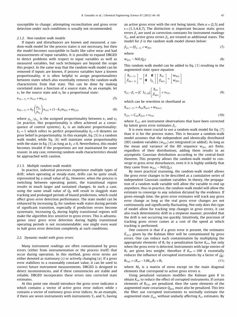
This relationship is only approximate due to the potential effect ofsmearing by previous contaminated state estimates, resulting in afailure to completely remove the correlation from ZbðtÞ. Thisresults in a slight underestimation of ZbðtÞ for larger values, andan overestimation for smaller values. Nevertheless, the relation-ship is fairly precise when all gross errors are detected, asdetected gross errors are appropriately penalized.

Fig. 3. Dynamic bayesian network (DBN).

5.2. Obtaining univariate statistics

The Kalman filter based on Eq. (32) returns the state estimatesZbðtÞ and the posterior covariance matrix PZðtÞ in Eqs. (36) and (37).The final stage of Step (3) is to convert the multivariate statisticsZbðtÞ and PZðtÞ into univariate statistics to be used in Step (4).Because all states have been rendered uncorrelated, obtainingsuch statistics is a trivial procedure:

zðtÞ ¼ Z ½i�ðtÞ ð39Þ

s20ðtÞ ¼ PZ½i,i�ðtÞ ð40Þ

where zðtÞ is the univariate estimate of each standardized residualerror, and s2

0ðtÞ is the variance associated with the estimationuncertainty.

x1 x2

x1 x2

Fig. 2. Reasoning given evidence: (a) predictiv

6. Diagnosing gross error through bayesian inference

Bayesian inference falls under Step (4) of DBGED, summarizedin Fig. 1(b) in the introduction.

6.1. Bayesian methods

Using zðtÞ to infer the probability of a gross error can be donewith the use of Bayes’ theorem:

Pðh9eÞ ¼Pðe9hÞPðhÞ

PðeÞð41Þ

where Pðh9eÞ is the probability of the hypothesis given theevidence, or the posterior probability, P(h) is the prior probabilityof the hypothesis or the prior probability, Pðe9hÞ is the probabilityof the evidence given the hypothesis, or the likelihood, and P(e) isthe total probability of the evidence, which serves as a normal-

ization factor. This method can be particularly useful for diag-nostic reasoning (Korb and Nicholson, 2004; Huang, 2008).

6.2. Dynamic bayesian networks

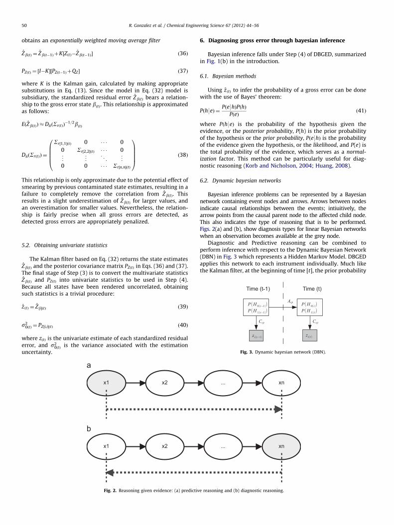
Bayesian inference problems can be represented by a Bayesiannetwork containing event nodes and arrows. Arrows between nodesindicate causal relationships between the events; intiuitively, thearrow points from the causal parent node to the affected child node.This also indicates the type of reasoning that is to be performed.Figs. 2(a) and (b), show diagnosis types for linear Bayesian networkswhen an observation becomes available at the grey node.

Diagnostic and Predictive reasoning can be combined toperform inference with respect to the Dynamic Bayesian Network(DBN) in Fig. 3 which represents a Hidden Markov Model. DBGEDapplies this network to each instrument individually. Much likethe Kalman filter, at the beginning of time [t], the prior probability

... xn

... xn

e reasoning and (b) diagnostic reasoning.

R. Gonzalez et al. / Chemical Engineering Science 67 (2012) 44–56 51

is predicted from the previous estimate at time [t�1]; it isupdated when new evidence becomes available at time [t]. Thisposterior probability is then used to predict the prior for the nextstep. Each arrow is represented by values Acp and Ccp which areactually matrices that contain conditional probabilities that formthe links between each node. It is implied from Fig. 3, that twohypotheses are of the interest. H0: that there are no active(unestimated) gross errors, and H1: that there is an active grosserror. Because there are two hypotheses, the conditional prob-ability matrices Acp and Ccp take the following form:

Acp ¼PðH0ðtþ1Þ9H0ðtÞÞ PðH0ðtþ1Þ9H1ðtÞÞ

PðH1ðtþ1Þ9H0ðtÞÞ PðH1ðtþ1Þ9H1ðtÞÞ

" #ð42Þ

Ccp ¼Pðz iðtÞ9H0Þ 0

0 Pðz iðtÞ9H1Þ

" #ð43Þ

The matrix Acp may be considered as a tuning parameter,which contains our beliefs on how likely it is that the gross errorswill switch between the ‘stationary’ and ‘active’ states. Thismatrix remains constant throughout the algorithm. Conversely,Ccp the matrix of likelihoods, must be updated at each time stepaccording to the estimated value zðtÞ. The proceeding subsectiondiscusses how the likelihoods are obtained.

Fig. 3 indicates that predictive reasoning is performed using Acp

while diagnostic reasoning is performed using Ccp. Predictive reason-ing is performed using the Chain Rule, which takes the form

PðHðtÞ9Hðt�1ÞÞ ¼PðH0ðtÞ9H0ðt�1ÞÞ

PðH1ðtÞ9H1ðt�1ÞÞ

" #¼ AcpPðHðt�1ÞÞ ð44Þ

while updating makes use of Bayes’ Rule, which, in the matrix form is

PðHðtÞ9zðtÞÞ ¼PðH0ðtÞ9zðtÞÞ

PðH1ðtÞ9zðtÞÞ

" #¼

CcpPðHðtÞ9Hðt�1ÞÞPCcpPðHðtÞ9Hðt�1ÞÞ

ð45Þ

Eqs. (44) and (45) are the principle calculations for Step (4), the rest ofthe section is devoted to acquiring the values that make thiscomputation possible.

6.3. Likelihoods of H0 and H1

6.3.1. Model considerations

The Hidden Markov Model in Fig. 3 represents switchingbetween two systems that are represented in Eq. (7), the firstsystem has wbðtÞ ¼ 0, while the other has wbðtÞ �Nð0,Qb½i,i�Þ. Recall

Value of Z

[1] P(z|H0)[2] P(z|H1)

1

2

Fig. 4. Likelihoods of t

that in Eq. (7), Qb½i,i� represents the variance of gross error change.When distinguishing between two hypotheses, the gross errordetection makes a comparison of two Gaussian distributions.

Gaussian distributions are usually adequate to describe thedistributions pertaining to the test statistics. For the first hypoth-esis, residual error deviations from zero are caused by randominstrument error, which is approximately Gaussian for the mostpart. In addition, regardless of the distribution for either hypoth-esis, the residual errors are filtered by taking a weighted average;averaging strengthens Gaussian characteristics of the residuals,which is why Gaussian assumptions are prevalent in similartraditional methods.

6.3.2. Obtaining likelihoods from the distributions

Since this method assumes two different hypotheses, thevariable zðtÞ must come from two different distributions. WhenwbðtÞ ¼ 0, we can assume the standardized residual error estimatezðtÞ is closely distributed around zero, or zðtÞ �Nð0,s0Þ. Note thats0 is obtained from Eq. (40). When wbðtÞ �Nð0,Qb½i,i�Þ, the random-walk model assumes the errors propagate until zðtÞ reaches adistribution with a notably larger variance zðtÞ �Nð0,s1Þ. Specify-ing s1 is addressed laster on.

Once we have values for s0 and s1, we can obtain thelikelihoods PðzðtÞ9H0Þ and PðzðtÞ9H1Þ directly from the distributionas shown in Fig. 4.

As mentioned before, while distributions may not be trulyGaussian, due to modeling properties, Gaussian distributions are atractable approximation. This method still detects gross errors aslong as residuals are far enough from zero to consistently makethe second hypothesis more likely. s0 and s1 are given by tuningparameters; thus they can be arbitrarily set by tuning proceduresto ensure detection of gross errors of a certain size. Because oftuning and flexibility of the random-walk model, the Gaussianapproximation does not significantly hinder performance. Byusing the Gaussian approximations, the likelihood values can beobtained as follows:

Pðz9H0Þ ¼1ffiffiffiffiffiffiffiffiffiffiffiffi

2ps20

q eð�1=2Þz ðtÞ=s20 ð46Þ

Pðz9H1Þ ¼1ffiffiffiffiffiffiffiffiffiffiffiffi

2ps21

q eð�1=2Þz ðtÞ=s21 ð47Þ

s20 is given by the diagonal elements of PZðtÞ as given in Eq. (40).

H0:Distribution Containing noGross Errors

H1:Distribution Given FiniteRandom-Walk Propagation

Z-Axis

Z-Axis

wo distributions.

R. Gonzalez et al. / Chemical Engineering Science 67 (2012) 44–5652

6.3.3. Obtaining distribution parameters

While s20 technically changes with time, it converges to

steady-state rather quickly, and can be considered time-invariant.s2

1 however, can change significantly over time if gross errors aredetected. In order to calculate s2

1 we must first define Sb0, which

is essentially the expected MSE of each instrument due to grosserror after a certain time of operation, for example, one month.Sb0

is essentially a deterioration parameter that can describeanything from random instrument calibration upsets to a finiteperiod of deterministic drift:

b�Nð0,Sb0Þ ð48Þ

The vector of gross error standard deviations in z space isobtained as follows:

~sb0S¼ ½S�1=2

rðtÞ �½S1=2b0�½~1� ð49Þ

By letting sb0S be the appropriate element of ~sb0S, one can obtain

the corresponding value of s1 by independently combining sb0S

and s0:

s1 ¼

ffiffiffiffiffiffiffiffiffiffiffiffiffiffiffiffiffiffiffis2b0Sþs2

0

qð50Þ

One should notice that because S�1=2rðtÞ changes significantly

whenever a gross error is detected, s1 is also highly time-varying.In theory, s1 should be re-calculated for every time step. Inpractice, while it is safer to update s1 every time step, if s0 ismuch smaller than s1, re-calculating s1 does not significantlyimprove performance.

7. Tuning steps (1) and (3)

7.1. Specifying the cutoff Z-value

From Fig. 4, the two distributions for H0 and H1 intersect eachother at a certain value of 7z. At this point, the likelihood of H0

and H1 are identical for that particular instrument; this value of z

is called the cutoff Z-value zc. Gross errors that are large enoughto consistently yield values of zðtÞ4zc are reliably detectable. Onecan specify zc by first specifying bc , the cutoff gross error, the set ofminimum allowable gross error magnitudes that can be accep-tably ignored. The vector of cutoff z-values Zc is obtained bystandardizing bc to z-space:

Zc ¼ ½S�1=2rð1Þ �bc ð51Þ

where Srð1Þ is the steady-state value of SrðtÞ when no gross errorsare detected. This desired value for zc can be obtained bymanipulating s0 and s1. Recall that s0 is a function of the tuningparameter QZ from Eq. (33) while s1 is a function of both QZ andSb0

from Eq. (48).The easiest method to solve this tuning problem is to pick a

reasonable value for Sb0and manipulate QZ so that the desired

values for Zc are obtained. In practice, S1=2b0

is a diagonal matrix ofgross error standard deviations, thus a reasonable value for S1=2

b0

would be a typical gross error magnitude for that instrument.Once Sb0

is specified QZ in Step (3) can then be tuned to match aspecified value of Zc.

7.2. Tuning step (3)

Desired values of s20 and s2

1 can be obtained by substituting zc

into the probability density functions Eqs. (46) and (47) andequating them to each other:

1ffiffiffiffiffiffiffiffiffiffiffiffi2ps2

0

q eð�1=2Þz c=s20 ¼

1ffiffiffiffiffiffiffiffiffiffiffiffi2ps2

1

q eð�1=2Þz c=s21 ð52Þ

By substituting Eq. (50) for s1 and simplifying, the nonlinearequation is reduced to

0¼ logð2ps20Þ�logð2pðs2

b0Sþs2

0ÞÞþzc1

s20

�1

ðs2b0Sþs2

0Þ

!ð53Þ

Since s2b0S

is specified by the choice of Sb0, one can solve for s2

0

using a nonlinear equation solving routine. The solution toEq. (53) specifies the desired diagonal elements of PZð1Þ which isthe steady-state value of PZðtÞ in Step (3). Now we must solve forthe matrix QZ that yields the desired matrix PZð1Þ.

In general, the posterior covariance of the Kalman filter PðtÞ isrelated to the prior covariance Pðt�1Þ according to Eq. (54).

PðtÞ ¼ ðI�ðAPðt�1ÞATþQ ÞCT ðCðAPðt�1ÞA

TþQ ÞCTþRÞ�1CÞ

�ðAPðt�1ÞATþQ Þ ð54Þ

where A is the state transition matrix, C is the observation matrix,Q is the process noise covariance and R is the observation noisecovariance. By observing the Kalman filter from Step (3), one cansee that C¼ I, A¼ I and R¼ I. At steady-state, PðtÞ ¼ Pðt�1Þ ¼ PZð1Þ. Inorder to simplify the algebra, diagonal elements of PZð1Þ can besolved component-wise. Let pzð1Þ ¼ s0, qz, and rz represent thesquare-root of any given diagonal component of PZð1Þ, QZ, and RZ,respectively:

p2zð1Þ ¼ 1�

pzð1Þ2þq2z

p2zð1Þþq2

z þ1

!ðp2

zð1Þþq2z Þ ð55Þ

Solving for q2z yields

q2z ¼

p4zð1Þ

1�p2zð1Þ

¼s4

0

1�s20

ð56Þ

Note that each diagonal element of PZð1Þ hence s0 must be lessthan 1; this is because the observation variances in RZ are allequal to 1. PZð1Þ must be less than both RZ and QZ, becausecombining information from ZðTÞ and ZbðtÞ increases confidence inthe posterior estimate. If solving Eq. (53) results in s041 then Zc

is to lenient (or too large) to be consistent with the filter based onEq. (32). This is not a major issue, it simply means that grosserrors smaller than Zc will be reliably detected, even if QZ is set toa very large value. The specification of QZ can be done as a matrixoperation:

QZ ¼ ðI�PZð1ÞÞ�1P2

Zð1Þ ð57Þ

7.3. Tuning step (1), time-invariant QZ

QZ is the state covariance for the subsidiary gross errorrandom-walk model Eq. (32). Thus, QZ is intrinsically related toQb in the parent random-walk model Eq. (7). Recall the relation-ship between bðtÞ and ZbðtÞ in Eq. (38); their model covariances QZ

and Qb can be likewise related:

E½EðZbðtÞÞ� ¼ E½DiiðSrðtÞÞ�1=2bðtÞ� ¼~0

QZ ¼ E½EðZbðtÞÞEðZbðtÞÞ0�

Qb ¼ E½bðtÞb0ðtÞ�

QZ �DiiðSrðtÞÞ�1Qb ð58Þ

For the purposes of tuning, steady-state residual error variance isassumed, thus Srð1Þ is used. When taking into account penaliza-tion of corrupted instruments, the analogous value of Qb can be

R. Gonzalez et al. / Chemical Engineering Science 67 (2012) 44–56 53

obtained from QZ as follows:

Qb ¼ kerrDiiðSrð1ÞÞQZ ð59Þ

7.4. Tuning step (1), time-variant QZ

The random walk model assumes that gross error change is agradual process with constant variance; this assumption workswell for drifting reference points. Even if a deterministic drift isnot random walk, such a drift is not an unlikely realization ofrandom walk. However, large sudden changes in gross errors aremuch less likely to be caused by random walk. While large andsudden gross errors are not difficult to detect, using time-invariant values of Qb and QZ can result in prohibitively longcorrection times if the sudden gross error change is sufficientlylarge. In order to make the correction time more consistent for allgross errors, Qb and QZ can be converted to time-varying para-meters, which allows better performance in the event of a suddengross error change.

One way to take into account unusual behavior is to allow thevariance parameter change. Even when gross error changes arenon-Gaussian, the model for Z ðtÞ tracks the random variable bðtÞ sothat if the gross error remains constant after its sudden change,Z ðtÞ has the following property:

E½ZbðtÞ� �DiiðSrðtÞÞ�1=2bðtÞ

When applying this property to variances

E½ZbðtÞZ0bðtÞ� �DiiðSrðtÞÞ

�1ðE½bðtÞb

0ðtÞ�ÞþE½ðZbðtÞ�ZbðtÞÞðZ ðtÞ�ZbðtÞÞ

0�

E½ZbðtÞZ0bðtÞ� �DiiðSrðtÞÞ

�1QbþPZðtÞ

By substituting Eq. (58) for Qb

QZ � E½ZbðtÞZ0bðtÞ��PZðtÞ ð60Þ

Qb �DiiðSrðtÞÞ½E½ZbðtÞZ0bðtÞ��PZðtÞ� ð61Þ

In the event that a significant gross error change has occurred,E½Z ðtÞZ 0ðtÞ� will be much larger than PZðtÞ, and we can say that theadjusted value for QZ is defined as follows:

QZadjðtÞ ¼DiiðZ ðtÞZ0ðtÞ�PZðtÞÞ ð62Þ

Fig. 5. Solids handling an

which uses the value of the random matrix Z ðtÞZ 0ðtÞ to estimate itsexpected value. Nevertheless, using a random variable as anestimate for its expected value can be risky and can result innegative values for QZ. The adjusted value is multiplied by a gainmatrix Kp:

Q ZadjðtÞ ¼ ðKpÞDiiðZ ðtÞZ0ðtÞÞ ð63Þ

where Kp is a diagonal matrix of gains of less than or equal to 1 soas to be conservative toward estimates in the presence of noise.PZðtÞ is considered negligible, and is moved from this relationshipto prevent Kp from being negative when calculated as follows:

QZadjðtÞ ¼ KpDiiðZcZ0cÞ

Kp ¼QZ ½DiiðZcZ0cÞ��1 ð64Þ

Recall Zc is the cutoff value specified earlier in this tuning section.Using Zc as a reference to define Kp ensures that detectionperformance is not altered. One can use this adjusted matrixQZadjðtÞ to specify the matrices QZ and Qb when the adjusted valuesexceed the original ones. In practice, more benefit is obtained byscaling Qb than by scaling QZ. If one wishes to scale both matrices,it is often better to scale Qb by a gain larger than Kp and to scale QZ

by a gain smaller than Kp. This allows adequate time for grosserror estimates to converge before the decreasing values of zðtÞsuggest that the gross error estimate has been corrected. In thesimulated system to follow, the following adjustment was used:

QZðtÞ ¼max½QZ ,ð0:2ÞQZadjðtÞ� ð65Þ

QbðtÞ ¼DiiðSrð1ÞÞmax½QZ ,ð10ÞQZadjðtÞ� ð66Þ

Once properly tuned, the gross error magnitude as much less ofan effect on the time for estimation convergence.

8. Simulation of oil sands solids handling

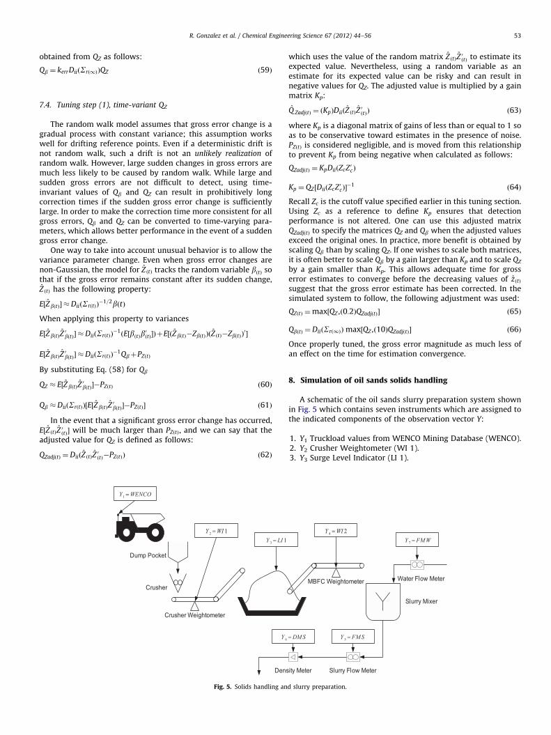
A schematic of the oil sands slurry preparation system shownin Fig. 5 which contains seven instruments which are assigned tothe indicated components of the observation vector Y:

1.

d sl

Y1 Truckload values from WENCO Mining Database (WENCO).

2. Y2 Crusher Weightometer (WI 1). 3. Y3 Surge Level Indicator (LI 1).

urry preparation.

R. Gonzalez et al. / Chemical Engineering Science 67 (2012) 44–5654

4.

TabVar

S

x1

x2

x3

y

y

y

y

y

y

y

Y4 Mix Box Feed Conveyor (MBFC) Weightometer (WI 2).

5. Y5 Slurry Flow Meter (FM S). 6. Y6 Slurry Density Meter (DM S). 7. Y7 Water Flow Meter (FM W).

From the flow chart in Fig. 5, WENCO data is available in a database which records the mass of each truckload and the time atwhich it is dumped into the dump hopper. WI 1 is a weightometeron the crusher conveyor belt which feeds into the surge pile. LI1 gives a reading on the relative level of the surge pile (from 0% to100% which was converted to metric tonnes). WI 2 is a weight-ometer for the mix-box feed conveyor (MBFC), which transportsoil sand from the surge pile to the slurry mix box. In this mix box,slurry is prepared by adding controlled amounts of water to theoil sand. FM W measures the volumetric flow rate of water, andsince the density of water is known, conversion to mass flow istrivial. The volumetric effluent slurry flow is measured by FM S,with the density measured by DM S so that a mass flow rate canbe calculated.

This system is the first stage of the oil sands process, a processbecoming an increasingly important contributor to global energysupply. The components of the hidden states X in this model are:

1.

X1 Oil sand flow through WI 2. 2. X2 Change in surge level. 3. X3 Water flow through FM W.

Here, X1 is of particular interest as this flow dictates the bitumenfeed to the oil sands process. X1 can be directly measured throughY4 however, due to its operating conditions and location in theprocess, Y4 is the instrument that is most frequently biased.

In order to validate that the DBGED algorithm can detect andcorrect sudden gross errors, a simulation was performed.A hypothetical operating point was considered for this systemwith means and variances as shown in Table 1.

A simulation of the system was performed by sequentialgeneration of Gaussian random variables n and applying theparameters in Table 1 to the model, resulting in Eq. (67)–(69);this generated values of ideal process measurements:

wX ¼

300 0 0

150 40 0

0 0 120

0B@

1CA

n1

n2

n3

0B@

1CA ð67Þ

x1ðtþ1Þ

x2ðtþ1Þ

x3ðtþ1Þ

0B@

1CA¼ ð0:7ÞI

x1ðtÞ

x2ðtÞ

x3ðtÞ

0B@

1CAþð0:3Þ

1000

500

0

0B@

1CAþwX ð68Þ

le 1iable definitions.

ymbol Mean S.D. Meaning

1000 300 Real oil sand flow

500 155.2 Real water flow

0 120 Real Hopper level change

1 0 200 WENCO database value

2 0 90 First weightometer readings

3 0 130 Hopper level readings

4 0 80 Second weightometer readings

5 0 60 Slurry flow meter readings

6 0 0.2 Density meter readings

7 0 50 Water flow meter readings

y1ðtÞ

y2ðtÞ

y3ðtÞ

y4ðtÞ

y5ðtÞ

y6ðtÞ

y7ðtÞ

0BBBBBBBBBBB@

1CCCCCCCCCCCA¼

x1ðtÞ þx3ðtÞ

x2ðtÞ þx3ðtÞ

x3ðtÞ

x1ðtÞx1ðtÞ

2:1 þx2ðtÞ

1:02:1x1ðtÞ þ1:0x2ðtÞ

x1ðtÞ þ x2ðtÞ

1:0�1x2

0BBBBBBBBBBBBB@

1CCCCCCCCCCCCCAþ

200n4

90n5

130n6

80n7

60n8

0:2n9

50n10

0BBBBBBBBBBBBB@

1CCCCCCCCCCCCCA

ð69Þ

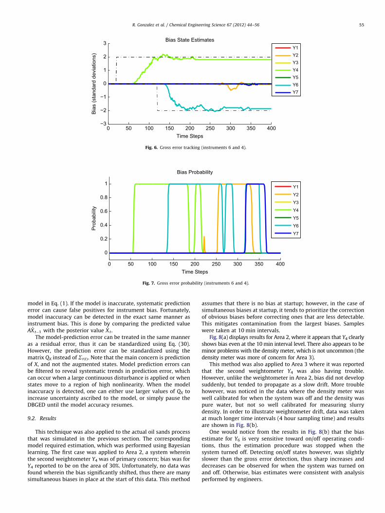
After this, a constant bias with a magnitude of þ2 standarddeviations was added to instrument Y4 (the second weight-ometer) at 20 time steps, and a bias with a magnitude of �2standard deviations was added to instrument Y6 (the densitymeter) at 120 time steps. These bias change patters were chosenas they were very unlikely to be produced by gradual Gaussianrandom-walk which the models assume. The gross error detectionfilter was tuned so that zc¼0.15 for all elements, with the priorgross error variance being equal to the instrument variance.

The discrete-valued Bayesian network was tuned according toEq. (42) with PðBðtþ1Þ ¼ T9BðtÞ ¼ FÞ ¼ 10�3 and PðBðtþ1Þ ¼ F9BðtÞ ¼ TÞ

¼ 10�3, which corresponds to a switching probability of 10�3. Thisvalue was small enough to adequately reduce the occurrence of falsepositives. Since no prior assumptions were made about the possiblemagnitudes of the gross errors, adjustable values were used for QZ

and Qb with adjustments made according to Eqs. (65) and (66). Thesimulation results are shown in Figs. 6 and 7.

In general, the algorithm performed quite well despite using asimulation that was designed to test its limits (namely, extremelynon-Gaussian gross error changes). There was some trouble whenrandom errors in Y2 and Y7 tripped the correction alarm; this wasmost likely due to imperfect estimates of errors in Y4 and Y6 causingmild corruption in the state estimates. However, false alarms in Y2

and Y7 occurred at a time when most gross errors were accounted for.Because the reference state was uncorrupted (due to penalization andcorrection), estimates re-converged to their original value. This is whyfast detection and correction are important to ensure as little ascorruption as possible; as long as state estimates are not significantlycorrupted, instruments will re-converge to their proper values duringa false alarm. Problems can still occur however, if gross errors areintroduced to the system in an unobservable manner; this simplymeans that there are too many active bias states to ensure anuncorrupted state estimate.

False alarm rates can also be reduced by using low switchingprobabilities as was used in this simulation (a switching prob-ability of 10�3). Low switching probabilities also result in adelayed response, as is apparent in Fig. 6; this is because it takesa considerable amount of time to obtain enough evidence of biasto overcome the prior beliefs against switching. Delayed switch-ing is a consequence of caution against false alarms. However, onemust take caution not to set switching probabilities too low sincedelayed detection also means that the state estimate is corruptedfor a longer period of time. This would result in decreasedresiliency against corruption. From Fig. 6, one can observe thatdetection occurs within approximately 30 time steps. Further-more, no instruments were incorrectly identified shortly after themajor corruption occurred. This indicates that these tuningparameters allowed the algorithm to be resilient to corruption.

9. Preliminary industrial application

9.1. Safeguards for industrial application

When bringing this method to apply toward industry, one ofthe chief concerns about applying this method is accuracy of the

0 50 100 150 200 250 300 350 400−3

−2

−1

0

1

2

3 Bias State Estimates

Time Steps

Bia

s (s

tand

ard

devi

atio

ns)

Y1Y2Y3Y4Y5Y6Y7

Fig. 6. Gross error tracking (instruments 6 and 4).

0 50 100 150 200 250 300 350 400

0

0.2

0.4

0.6

0.8

1

Bias Probability

Time Steps

Pro

babi

lity

Y1

Y2

Y3

Y4

Y5

Y6

Y7

Fig. 7. Gross error probability (instruments 6 and 4).

R. Gonzalez et al. / Chemical Engineering Science 67 (2012) 44–56 55

model in Eq. (1). If the model is inaccurate, systematic predictionerror can cause false positives for instrument bias. Fortunately,model inaccuracy can be detected in the exact same manner asinstrument bias. This is done by comparing the predicted valueAX t�1 with the posterior value X t .

The model-prediction error can be treated in the same manneras a residual error, thus it can be standardized using Eq. (30).However, the prediction error can be standardized using thematrix QX instead of SrðtÞ. Note that the main concern is predictionof X, and not the augmented states. Model prediction errors canbe filtered to reveal systematic trends in prediction error, whichcan occur when a large continuous disturbance is applied or whenstates move to a region of high nonlinearity. When the modelinaccuracy is detected, one can either use larger values of QX toincrease uncertainty ascribed to the model, or simply pause theDBGED until the model accuracy resumes.

9.2. Results

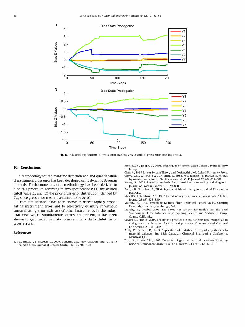
This technique was also applied to the actual oil sands processthat was simulated in the previous section. The correspondingmodel required estimation, which was performed using Bayesianlearning. The first case was applied to Area 2, a system whereinthe second weightometer Y4 was of primary concern; bias was forY4 reported to be on the area of 30%. Unfortunately, no data wasfound wherein the bias significantly shifted, thus there are manysimultaneous biases in place at the start of this data. This method

assumes that there is no bias at startup; however, in the case ofsimultaneous biases at startup, it tends to prioritize the correctionof obvious biases before correcting ones that are less detectable.This mitigates contamination from the largest biases. Sampleswere taken at 10 min intervals.

Fig. 8(a) displays results for Area 2, where it appears that Y4 clearlyshows bias even at the 10 min interval level. There also appears to beminor problems with the density meter, which is not uncommon (thedensity meter was more of concern for Area 3).

This method was also applied to Area 3 where it was reportedthat the second weightometer Y4 was also having trouble.However, unlike the weightometer in Area 2, bias did not developsuddenly, but tended to propagate as a slow drift. More troublehowever, was noticed in the data where the density meter waswell calibrated for when the system was off and the density waspure water, but not so well calibrated for measuring slurrydensity. In order to illustrate weightometer drift, data was takenat much longer time intervals (4 hour sampling time) and resultsare shown in Fig. 8(b).

One would notice from the results in Fig. 8(b) that the biasestimate for Y6 is very sensitive toward on/off operating condi-tions, thus the estimation procedure was stopped when thesystem turned off. Detecting on/off states however, was slightlyslower than the gross error detection, thus sharp increases anddecreases can be observed for when the system was turned onand off. Otherwise, bias estimates were consistent with analysisperformed by engineers.

0 50 100 150 200−2

−1

0

1

2

3

4Bias State Propagation

Time Steps

Bia

s Z

Val

ues

Y1Y2Y3Y4Y5Y6Y7

0 50 100 150 200−2

−1.5

−1

−0.5

0

0.5

1Bias State Propagation

Time Steps

Bia

s Z

Val

ues

Y1Y2Y3Y4Y5Y6Y7

Fig. 8. Industrial application: (a) gross error tracking area 2 and (b) gross error tracking area 3.

R. Gonzalez et al. / Chemical Engineering Science 67 (2012) 44–5656

10. Conclusions

A methodology for the real-time detection and and quantificationof instrument gross error has been developed using dynamic Bayesianmethods. Furthermore, a sound methodology has been derived totune this procedure according to two specifications: (1) the desiredcutoff value Zc, and (2) the prior gross error distribution (defined bySb0 since gross error mean is assumed to be zero).

From simulations it has been shown to detect rapidly propa-gating instrument error and to selectively quantify it withoutcontaminating error estimate of other instruments. In the indus-trial case where simultaneous errors are present, it has beenshown to give higher priority to instruments that exhibit majorgross errors.

References

Bai, S., Thibault, J., McLean, D., 2005. Dynamic data reconciliation: alternative toKalman filter. Journal of Process Control 16 (5), 485–498.

Brosilow, C., Joseph, B., 2002. Techniques of Model-Based Control. Prentice, NewJersey.

Chen, C., 1999. Linear System Theory and Design, third ed. Oxford University Press.Crowe, C.M., Campos, Y.A.G., Hrymak, A., 1983. Reconciliation of process flow rates

by matrix projection 1. The linear case. A.I.Ch.E. Journal 29 (6), 881–888.Huang, B., 2008. Bayesian methods for control loop monitoring and diagnosis.

Journal of Process Control 18, 829–838.Korb, K.B., Nicholson, A., 2004. Bayesian Artificial Intelligence, first ed. Chapman &

Hall/CRC.Mah, R.S.H., Tamhane, A.C., 1982. Detection of gross errors in process data. A.I.Ch.E.

Journal 28 (5), 828–830.Murphy, K., 1998. Switching Kalman filter. Technical Report 98-10, Compaq

Cambridge Res. Lab, Cambridge, MA.Murphy, K., October 2001. The bayes net toolbox for matlab. In: The 33rd

Symposium of the Interface of Computing Science and Statistics. Orange

County California.Ozyurt, D., Pike, R., 2004. Theory and practice of simultaneous data reconciliation

and gross error detection for chemical processes. Computers and ChemicalEngineering 28, 381–402.

Reilly, P., Parbani, R., 1963. Application of statistical theory of adjustments tomaterial balances. In: 13th Canadian Chemical Engineering Conference,Montreal, QC.

Tong, H., Crowe, C.M., 1995. Detection of gross errors in data reconciliation byprincipal component analysis. A.I.Ch.E. Journal 41 (7), 1712–1722.