Dynamic Asset-Liability Management

with Inflation Hedging and Regulatory Constraints

Huamao Wang∗, Jun Yang

Kent Centre for Finance, University of Kent, Canterbury, Kent CT2 7NZ, UK.

Abstract

We examine how inflation risk affects the asset-liability investment allocation problem

of a fund manager who is constrained by regulatory rules. The liability driven investment

framework faces a time-varying investment opportunity set, characterized by a two-factor

affine model of term structure, and is subject to annually-checked Value-at-Risk and maxi-

mum funding constraints required by regulatory authorities. We show that inflation-hedging

is of particular importance for the long-term ALM investor and has an influential impact

on asset allocation by interacting with liability-hedging and intertemporal hedge demands

simultaneously. We also provide justification for the current practice that many managers

tend to act myopically, instead of rebalancing strategically.

Keywords: Inflation risk, Liability risk, Hedging demand, Affine term structure, Risk

premium

JEL: G11, G12, G23

∗Corresponding author. Tel: +44 1227 823593; Fax: +44 1227 827932

Email addresses: h.wang@kent.ac.uk (Huamao Wang), jy79@kent.ac.uk (Jun Yang)

I. Introduction

Inflation hedging has become a concern of critical importance for fund managers. They

consider inflation risk not only as a direct threat with respect to the protection of their

purchasing power, but also, and perhaps more importantly, a threat to fund stability in terms

of arising liabilities. For example, pension plans typically take the promised benefit payments

as pension liabilities and then pay the liability stream by using accumulated investment gains

and pension contributions. While these pension payments will be eroded by inflation over

time. When pension payments are linked (conditional or full indexation) to consumer price

or wage level indexes, an unexpected rise in inflation will result in an increase in pension

liabilities, thereby leading to a deterioration of fund financial level. To this end, the hedging

demand against inflation has received more attention from the fund managers when making

optimal investment decisions.

The focus on inflation hedging is consistent with the heightened focus on liability risk

management that has emerged as a consequence of recent pension crisis. As Figure 1 illus-

trates, a growing number of pension plans in the US are unfortunately materially under-

funded since 2002, reflecting the abnormal increase in liabilities. As a result of these trends,

the funding ratio (i.e. asset to liability ratio) falls below 100%, the “funding floor”, for more

than a decade, with one exception in 2007 when the bullish financial market outperformed

the liability stream. More recently, the Universities Superannuation Scheme (USS) in the

UK reports that its liabilities exceeded assets by £2.9 billion in March 2011 and this deficit

increased sharply to £7.9 billion in June 2013.1 Generally, funding shortfalls are partly

1See employerspensionsforum.co.uk/en/pension-schemes/uss/briefing-on-the-uss--july-2014.

2

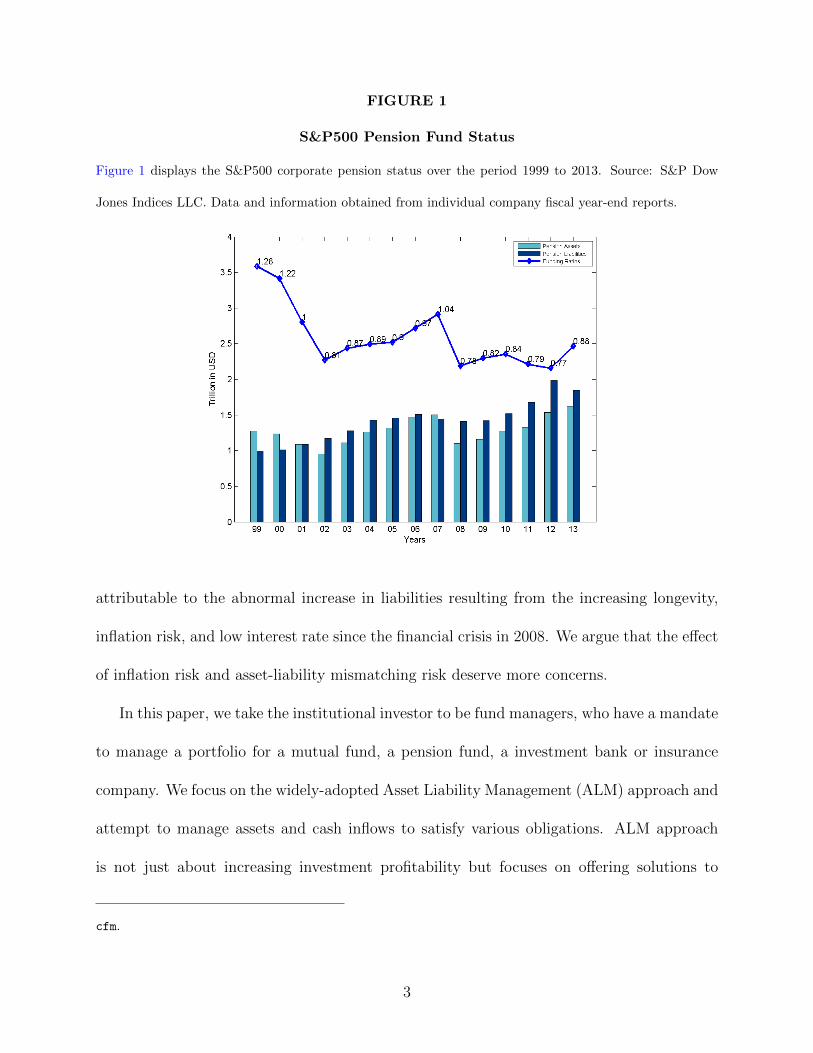
FIGURE 1

S&P500 Pension Fund Status

Figure 1 displays the S&P500 corporate pension status over the period 1999 to 2013. Source: S&P Dow

Jones Indices LLC. Data and information obtained from individual company fiscal year-end reports.

attributable to the abnormal increase in liabilities resulting from the increasing longevity,

inflation risk, and low interest rate since the financial crisis in 2008. We argue that the effect

of inflation risk and asset-liability mismatching risk deserve more concerns.

In this paper, we take the institutional investor to be fund managers, who have a mandate

to manage a portfolio for a mutual fund, a pension fund, a investment bank or insurance

company. We focus on the widely-adopted Asset Liability Management (ALM) approach and

attempt to manage assets and cash inflows to satisfy various obligations. ALM approach

is not just about increasing investment profitability but focuses on offering solutions to

cfm.

3

mitigate or hedge the unexpected changes in risk factors affecting liability values, and most

notably inflation risks. Our goal is to demonstrate how fund managers optimally choose their

portfolio allocation to match liabilities in the future, and as oppose to the nominal economy,

how different their investment strategies are in the real context with the aim of hedging

against inflation risk, and importantly, how regulatory rules affect the manager’s investment

behavior. To the best of our knowledge, we are the first to investigate the inflation effect on

the optimal risk exposure in the presence of risky liabilities and regulatory rules.

To address these questions, we consider a dynamic asset allocation problem in the frame-

work of the ALM. The investment opportunity set is characterized by a two-factor market

model of affine term structure. We account for inflation risk by adopting an inflation-adjusted

yield as the discount rate for calculating the present value of liabilities and correspondingly

the real funding ratio. The real funding ratio is different from the nominal ratio, which uses

a risk-free interest rate or a nominal yield, as it links the liabilities to the price level which

ensures that the purchasing power of future liability payments rises with the price level. To

demonstrate the impact of inflation risk, we examine portfolio weights, hedging demands

and utility losses in the real and nominal economy respectively. Within each economy, we

analyze two distinct investment strategies: a myopic strategy and a dynamic strategy with

optimal rebalancing.

Meanwhile, with the aim of keeping a sustainable funding level, the manager has to

follow two regulatory constraints on the funding ratio required by regulatory authorities.

One constraint requires a number of subsequent and non-overlapping Value-at-Risk (VaR)

checks on an annual basis. Another annually repeated constraint is the maximum funding

constraint imposed by the tax authority, aiming at avoiding the situation where the investor

4

deliberately overfunds to shelter more taxable corporate profits. The complicated problem

of dynamic portfolio optimization in the incomplete market is solved by a state-of-the-art

simulation-based method along with grid search technique (Brandt et al. 2005).

Using this framework, we first examine the impact of inflation on the ALM investment

strategy. We show that inflation hedging is a dominant incentive for a dynamic fund manag-

er with a long-term horizon. Intuitively, an investor who adopts a dynamic strategy tends to

take full advantages of the mean-reverting feature in bond risk premium by investing more

in bonds than the investor with a myopic policy. The extra bond holdings are intertemporal

hedging demands, which indeed exist with a positive sign in our nominal economy. However,

accounting for inflation into the framework alters this. We find that the dynamic investor

reduces his holding for bonds and tilts his portfolio to equities instead, because stock re-

turns are negatively correlated with inflation innovations and more importantly, offer higher

expected returns. To this end, stock turns out to be a good inflation hedge in the ALM

and the inflation-hedging effect is even larger when we exclude predictability in both bond

and stock premia by setting them to be constants. Investors who ignore inflation risk would

suffer significant welfare losses.

Moreover, we also compare portfolio allocations of an asset-liability problem to those

of an asset-only problem. We find that the liability-driven risk induces a large allocation

to bonds, especially for the myopic strategy in the ALM framework. In general, the fund

manager spreads his wealth mainly between stocks and bonds in the presence of liabilities,

whereas the asset-only investor has a well-diversified portfolio with a significant amount of

bonds being replaced by cash. There is an interesting interplay between inflation and liability.

On the one hand, a positive inflation-hedging demand induces a large component in stocks,

5

which provides higher returns and maintain the financial position of funding ratio. This,

in return, partly offsets investor’ concern about liability risk; on the other hand, when the

liability is completely excluded in the optimization problem, then inflation hedging demand

for stocks becomes zero across different funding levels, suggesting that in the asset-only case

inflation is not as important as in the ALM context.

In terms of regulatory effects, we find that both VaR and maximum funding ratio con-

straints reduce the optimal risk exposure. To be specific, when the fund is materially un-

derfunded, it may be optimal to hold the entire portfolio in cash instead, due to the horizon

disparity and the limit of additional cash inflows in our model. When the position is over-

funded, the VaR constraints bind yet with a decreasing effect until the fund has a high

surplus, by then the optimal strategy is less sensitive to the funding levels. With maximum

funding ratio constraints, the ability of exploiting the time variation in the investment op-

portunities has been further limited, thus leading the dynamic strategy almost indifferent

with the myopic strategy.

The contributions of this article are threefold from the perspective of the ALM model,

implementation and insights into practice. To begin with, our paper contributes to the

literature by investigating a theoretical ALM model in the constrained utility maximization

problem, and modelling the real funding ratio in the context of affine term structure. Given

that interest and inflation innovations are two main sources of risk affecting the financial

market and the valuation of liabilities, we consider two common factors (state variables),

i.e. the real interest rate and expected inflation. Their dynamics are characterized by a

vector-valued mean-reverting process, which captures stylized predictability in the expected

inflation rate, bond risk premium and interest rate.

6

To maintain the funding ratio in a healthy financial position, we consider a lower and

an upper bound on funding ratio by repeatedly conducting VaR and maximum funding

constraints on an annal basis. Empirical studies investigating the effect of regulatory re-

quirements on optimal investment allocation are rather limited in both quantity and quality.

These two constraints are separately taken into account by Martellini and Milhau (2012)

and van Binsbergen and Brandt (2014), but none of them has explored the joint effects

simultaneously.

More importantly, our results help to explain the stylized practice that many long-horizon

managers do not strategically rebalance portfolio, but instead prefer to acting myopically.

The reasons can be best summarized as follows: first, inflation hedging is of particular

importance for an ALM investor who has risky liability streams over a long investment

horizon, while it also adds values for the myopic strategy by reducing the probability of

exploiting time-varying bond risk premium; second, both liability immunization and the

time variation in bond market result in a large bond component in the myopic and dynamic

portfolio in turn. In this sense, the difference between the dynamic and myopic investment

strategy is relatively small; third, imposing regulatory constraints further restrict investors

from acting dynamically. Base on these results, we conclude that it is plausible for the

fund manager to take myopically optimal strategy, in which sense the investor can divide

the long-term investment horizon into several relatively shorter terms, e.g. 1-3 years, and

then optimizes the portfolio each time with a terminal wealth (or funding ratio) over a short

horizon.

The rest of our paper is organized as follows. Section II motivates our investigation with a

brief review of related literature. Section III describes the dynamic ALM framework we used

7

for accounting for inflation risk and regulatory rules. Section IV analyzes the joint effects of

inflation, regulatory constraints and time-varying bond premium on optimal portfolio choice

and welfare benefits/losses. Section V concludes. Appendix A summarizes the numerical

method and parameter values.

II. Related Literature

Our study is related to several strands of the literature. Foremost, our research is directly

related to the ALM studies that link obligations with optimal asset-only investment decisions

under regulatory constraints and time-varying expected returns. Our study of inflation-

hedging investment also complements the ALM literature. In this section we summarize the

related literature.

The first ALM application was presented by Merton (1992), who studies a university

managing an endowment fund. Sundaresan and Zapatero (1997) examine the valuation of li-

abilities for a fund and derive the optimal trading strategy with constant parameters. Rudolf

and Ziemba (2004) examine the optimal portfolio of managing the net surplus of assets and

liabilities under time-varying investment opportunities with one state variable. Allowing a

vector-valued diffusion process of state variables, Detemple and Rindisbacher (2008) study

the ALM with intermediate dividends and a funding shortfall at the terminal date. Neverthe-

less, the above papers mainly focus on strategies without considering regulatory constraints.

Conversely, we discuss the ALM with two regulatory rules under the two-factor affine model.

Thus, we can provide new insights by revealing the joint impact of regulations, inflation and

time-varying bond premium.

8

The VaR constraint that we consider has been widely imposed by regulators to control

the risk of extreme losses and protect the interests of beneficiaries. The effects of VaR on

asset allocation without liability are studied first by Basak and Shapiro (2001) who assume

the regulatory horizon coincides with the investment horizon (i.e. static VaR). They find

that a VaR-constrained investor is forced to choose a larger exposure to risky assets than the

unconstrained one in some specific situations. Cuoco et al. (2008) address that such negative

assessment on VaR arises from the static VaR assumption. When VaR is reevaluated at all

time, the allocation to risky assets is always lower. Similar conclusions are obtained by

Yiu (2004) who faces continuously-imposed VaR and uses dynamic programming technique.

Using a pointwise optimization method under a complete market, Shi and Werker (2012)

find that an annually repeated asset-only VaR reduces losses of long-term trading strategies,

but it induces a large opportunity cost by limiting portfolio holdings of risky assets.

In addition to VaR, the maximum funding constraint is usually introduced by the tax

authorities for preventing a deliberate or accidental build-up of excess funds to shelter more

taxable corporate profits (see Pugh 2006). Surprisingly, little literature on ALM has paid

attention to such constraint, except for Martellini and Milhau (2012). This constraint is

required by regulations or customary practices for some funding schemes. For example, the

pension assets should not exceed 105% of the accrued liabilities in the UK. The pension

funding ratio is on average bounded by 130% in the Netherlands. Similar caps are imposed

in Canada and Japan.2

Our paper is closely related to three studies in the recent literature - Hoevenaars et al.

2See also Pugh (2006) for a survey on regulation rules.

9

(2008), Martellini and Milhau (2012) and van Binsbergen and Brandt (2014). These papers

focus on the funding ratio under time-varying investment opportunities. Hoevenaars et al.

(2008) report the hedge qualities and welfare benefits of investing in a menu of seven alterna-

tive assets. They do not explicitly model inflation but infer the inflation hedging qualities of

assets from the correlation between nominal asset returns and inflation. Martellini and Mil-

hau (2012) derive optimal weights in a one-factor complete market setting with the constant

bond risk premium and expected inflation rate. van Binsbergen and Brandt (2014) compare

portfolio weights and certainty equivalents using different discount rates, while they do not

consider inflation effects.

The differences between our paper and the above three are obvious. First, we develop

our ALM model in a two-factor affine term structure framework rather than in the Gaussian

vector autoregression (VAR) model adopted by Hoevenaars et al. (2008) and van Binsbergen

and Brandt (2014). Although both affine and VAR models capture predictability in asset

returns, the VAR model is relatively simple. It does not define the term structure well and

ignores the extra information provided by the no-arbitrage restriction (see, e.g. Sangvinatsos

and Wachter 2005; Piazzesi 2010). Indeed, affine models are advocated by, e.g., Cochrane

and Piazzesi (2005) who point out that affine models exhibit a pricing kernel consistent with

the bond price dynamics and it can predict prices for bonds with different maturities without

breaking no-arbitrage arguments. It is also flexible to the time-series process for yields with

different restrictions.

Second, the incomplete two-factor model characterizes market dynamics more realistically

than the complete one-factor short rate model taken by Martellini and Milhau (2012). The

former captures the time-variation in bond risk premium. It also takes the expected inflation

10

as a second factor in addition to the real interest rate since both the factors affect the

fundamentals in the ALM. It naturally models the dynamics of expected inflation rate as an

affine function of the state variables, whereas the one-factor model and VAR approach fail

in modeling the dynamics of expected inflation.

Third, we discount the liability by using the real bond yield, which complements the case

discussed in van Binsbergen and Brandt (2014). Fourth, the above references do not examine

changes of hedging demands against different funding levels. We fill the gap by comparing

three types of hedging demands under various scenarios. Finally, we consider the maximum

funding constraint along with VaR to ensure that the fund fulfils the requirements by tax

authorities and fund regulators, though these constraints are separately taken into account

by Martellini and Milhau (2012) and van Binsbergen and Brandt (2014) along with other

constraints.

III. Analytical ALM Framework

A. Financial Market

We consider a fund manager with a T -year investment horizon and an asset menu including

a stock index, a 10-year nominal bond and a nominal money market account. The financial

market setting follows Koijen et al. (2010) who specify a two-factor term structure model

based on a general latent three-factor model in Sangvinatsos and Wachter (2005). The two

factors are the real interest rate and expected inflation as in Brennan and Xia (2002) and

Campbell and Viceira (2001). The affine model characterizes the dynamics of time-varying

11

bond risk premium and expected inflation.

The state variables are described by a vector-valued mean-reverting process around zeros,

i.e.,

(1) dXt = −κXtdt+ σXdzt, κ ∈ R2×2, σX ∈ R2×4,

where Xt ≡ (X1t, X2t)> denote the real interest rate and expected inflation respectively and

z ∈ R4×1 is a vector of independent Brownian motions driving uncertainties in the financial

market. Following the above literature, we set σX = [I2×2 02×2], and normalize κ to be

lower triangular.

The instantaneous nominal interest rate, R0t , is affine in the two state variables:

R0t = δ0R + δ>1RXt, δ0R > 0, δ1R ∈ R2×1.(2)

The price of risk Λt is also linear in Xt:

(3) Λt = Λ0 + Λ1Xt, Λ0 ∈ R4×1, Λ1 ∈ R4×2.

Given a process for R0t and Λt, the pricing kernel then follows

(4)dφtφt

= −R0tdt− Λ>t dzt.

Let B(Xt, t, s) denote the nominal price of a bond maturing at s > t. It is assumed to

be an exponential function of time t and of state variables Xt (e.g. Dai and Singleton 2000;

Sangvinatsos and Wachter 2005), i.e.

(5) B(Xt, t, s) = exp{A2(τ)Xt + A1(τ)}, A2(τ) ∈ R1×2, τ = s− t,

12

where A1(τ) and A2(τ) solve a system of ordinary differential equations given by:

A′1(τ) = −A2(τ)σXΛ0 +1

2A2(τ)σXσ

>XA>2 (τ)− δ0R,

A′2(τ) = −A2(τ)[κ+ σXΛ1]− δ>1R.(6)

The resulting bond yield is yτ,t = − 1τ[A2(τ)Xt + A1(τ)]. By applying Ito’s lemma, the

instantaneous bond price is given by

dBt

Bt

= [R0t + σ>BΛt]dt+ σ>Bdzt, σB ∈ R4×1,(7)

where σ>B = A2(τ)σX . Equation (7) shows that the bond risk premium varies with the state

vector Xt. The correlation between the bond risk premium and the state variables depends

on the maturity of the bond via the function A2(τ).

There exists a stock index with the nominal price following the dynamics

(8)dStSt

= (R0t + ηS)dt+ σ>S dzt, σS ∈ R4×1,

where the equity risk premium ηS is a constant. The row vector σ>S is assumed to be linearly

independent of the rows of σX , so that the stock is not spanned by the bond.

The nominal gross return on the single-period cash account, Rft , is given by

(9) Rft = exp(R0

t−1).

We have described the nominal investment opportunity set so far. To address inflation

risk for the fund manager who pays attention to the real funding ratio, it is necessary to

define a stochastic price level Πt,

(10)dΠt

Πt

= πtdt+ σ>Πdzt, σΠ ∈ R4×1.

The instantaneous expected inflation πt is affine in the state variables

(11) πt = δ0π + δ>1πXt, δ0π > 0, δ1π ∈ R2×1.

13

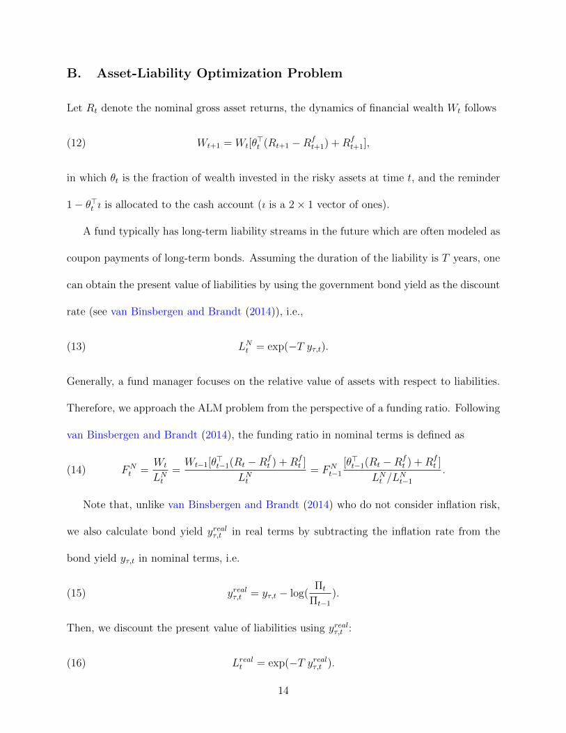
B. Asset-Liability Optimization Problem

Let Rt denote the nominal gross asset returns, the dynamics of financial wealth Wt follows

(12) Wt+1 = Wt[θ>t (Rt+1 −Rf

t+1) +Rft+1],

in which θt is the fraction of wealth invested in the risky assets at time t, and the reminder

1− θ>t ı is allocated to the cash account (ı is a 2× 1 vector of ones).

A fund typically has long-term liability streams in the future which are often modeled as

coupon payments of long-term bonds. Assuming the duration of the liability is T years, one

can obtain the present value of liabilities by using the government bond yield as the discount

rate (see van Binsbergen and Brandt (2014)), i.e.,

(13) LNt = exp(−T yτ,t).

Generally, a fund manager focuses on the relative value of assets with respect to liabilities.

Therefore, we approach the ALM problem from the perspective of a funding ratio. Following

van Binsbergen and Brandt (2014), the funding ratio in nominal terms is defined as

(14) FNt =

Wt

LNt=Wt−1[θ>t−1(Rt −Rf

t ) +Rft ]

LNt= FN

t−1

[θ>t−1(Rt −Rft ) +Rf

t ]

LNt /LNt−1

.

Note that, unlike van Binsbergen and Brandt (2014) who do not consider inflation risk,

we also calculate bond yield yrealτ,t in real terms by subtracting the inflation rate from the

bond yield yτ,t in nominal terms, i.e.

(15) yrealτ,t = yτ,t − log(Πt

Πt−1

).

Then, we discount the present value of liabilities using yrealτ,t :

(16) Lrealt = exp(−T yrealτ,t ).

14

By doing this we link the liabilities to the price level which ensures that the purchasing

power of future liability payments rises with the price level.

The financial wealth and asset returns in real terms are denoted by small letters, i.e.,

(17) wt =Wt

Πt

, rt =RtΠt−1

Πt

, rft =Rft Πt−1

Πt

.

Then, the financial wealth wt in real terms follows:

(18) wt = wt−1[θ>t−1(rt − rft ) + rft ].

As a contribution to the literature, we incorporate inflation risk into the real funding ratio

defined as

Ft =wtLrealt

=wt−1[θ>t−1(rt − rft ) + rft ]

Lrealt

= Ft−1

[θ>t−1(rt − rft ) + rft ]

Lrealt /Lrealt−1

.(19)

Finally, we consider a fund manager who has a power utility function defining over the

funding ratio Ft (resp. FNt ) in real (resp. nominal) terms with constant relative risk-aversion

(CRRA). The manager then solves

(20) J(F,X, t, T ) = maxθt∈Kt

E(F 1−γT

1− γ

),

where Kt is the constraint set described below.

C. Investment Constraints

First, we impose the standard borrowing and short-selling constraints, i.e., θt ≥ 0 and

1 − ı>θt ≥ 0. Second, the fund manager is required to conduct VaR checks repeatedly for

each regulatory horizon, i.e. one year, which is shorter than the 10-year investment horizon.

The manager has to ensure that the probability of a shortfall in funding is not more than the

15

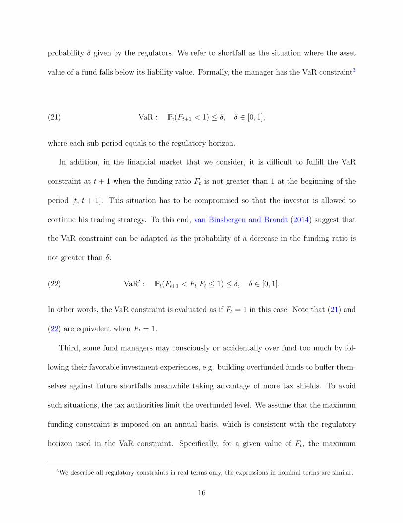
probability δ given by the regulators. We refer to shortfall as the situation where the asset

value of a fund falls below its liability value. Formally, the manager has the VaR constraint3

(21) VaR : Pt(Ft+1 < 1) ≤ δ, δ ∈ [0, 1],

where each sub-period equals to the regulatory horizon.

In addition, in the financial market that we consider, it is difficult to fulfill the VaR

constraint at t + 1 when the funding ratio Ft is not greater than 1 at the beginning of the

period [t, t + 1]. This situation has to be compromised so that the investor is allowed to

continue his trading strategy. To this end, van Binsbergen and Brandt (2014) suggest that

the VaR constraint can be adapted as the probability of a decrease in the funding ratio is

not greater than δ:

(22) VaR′ : Pt(Ft+1 < Ft|Ft ≤ 1) ≤ δ, δ ∈ [0, 1].

In other words, the VaR constraint is evaluated as if Ft = 1 in this case. Note that (21) and

(22) are equivalent when Ft = 1.

Third, some fund managers may consciously or accidentally over fund too much by fol-

lowing their favorable investment experiences, e.g. building overfunded funds to buffer them-

selves against future shortfalls meanwhile taking advantage of more tax shields. To avoid

such situations, the tax authorities limit the overfunded level. We assume that the maximum

funding constraint is imposed on an annual basis, which is consistent with the regulatory

horizon used in the VaR constraint. Specifically, for a given value of Ft, the maximum

3We describe all regulatory constraints in real terms only, the expressions in nominal terms are similar.

16

funding level at the next period t+ 1 should not be greater than a constant k, namely,

(23) maximum funding constraint : Ft+1,t ≤ k,

implying that the maximum funding constraint is dynamically respected at all periods. This

is similar to the case of Martellini and Milhau (2012) when their particular conditions are

satisfied.

The set Kt below summarizes the constraints on the portfolio weights and funding ratio.

(24) Kt = {(θ, F ) : θt ≥ 0, 1− ı>θt ≥ 0,VaR or VaR′, and Ft+1,t ≤ k}.

IV. Strategic Portfolio Choice

This section presents the main insights into ALM by evaluating the joint effects of inflation,

time-varying bond premium, liability, and regulatory constraints on the fund manager’s

portfolio policies and welfare losses. In our analysis, we consider a fund manager who has a

T = 10 years investment horizon with a risk aversion γ = 5, and who can take either myopic

strategy or dynamic strategy. To be specific, for myopically optimal strategies, the investor

solves 10 sequential one-year optimizations and does not use any of the new information,

whereas the dynamic investor strategically optimizes the T -year expected utility function by

using the new information at each rebalancing date.

Moreover, the dynamic asset allocation strategy is driven by three types of hedging

demands. First, the portfolio difference between the dynamic and myopic strategies defines

the intertemporal hedging demand, which hedges against the risks of time-variation in the

17

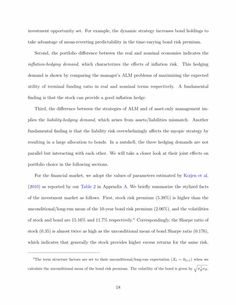
investment opportunity set. For example, the dynamic strategy increases bond holdings to

take advantage of mean-reverting predictability in the time-varying bond risk premium.

Second, the portfolio difference between the real and nominal economies indicates the

inflation-hedging demand, which characterizes the effects of inflation risk. This hedging

demand is shown by comparing the manager’s ALM problems of maximizing the expected

utility of terminal funding ratio in real and nominal terms respectively. A fundamental

finding is that the stock can provide a good inflation hedge.

Third, the difference between the strategies of ALM and of asset-only management im-

plies the liability-hedging demand, which arises from assets/liabilities mismatch. Another

fundamental finding is that the liability risk overwhelmingly affects the myopic strategy by

resulting in a large allocation to bonds. In a nutshell, the three hedging demands are not

parallel but interacting with each other. We will take a closer look at their joint effects on

portfolio choice in the following sections.

For the financial market, we adopt the values of parameters estimated by Koijen et al.

(2010) as reported by our Table 2 in Appendix A. We briefly summarize the stylized facts

of the investment market as follows. First, stock risk premium (5.38%) is higher than the

unconditional/long-run mean of the 10-year bond risk premium (2.06%), and the volatilities

of stock and bond are 15.16% and 11.7% respectively.4 Correspondingly, the Sharpe ratio of

stock (0.35) is almost twice as high as the unconditional mean of bond Sharpe ratio (0.176),

which indicates that generally the stock provides higher excess returns for the same risk.

4The term structure factors are set to their unconditional/long-run expectation (Xt = 02×1) when we

calculate the unconditional mean of the bond risk premium. The volatility of the bond is given by√σ>BσB .

18

Second, both stock and bond returns are negatively correlated with inflation innovations.

Third, the 10-year bond returns are negatively correlated with its risk premium, which is

critical because a long position in the bond can hedge against future changes in investment

environment.

A. Asset Allocation without Regulatory Constraints

In this subsection, we temporarily set aside VaR and maximum funding constraints. The

unconstrained ALM problem has the merits of both simplicity,5 for it excludes regulatory

constraints, and of highlighting the role of various hedging demands. The homothetic CRRA

utility removes the wealth (or funding ratio) effect, we therefore normalize the initial funding

ratio to F0 = 1 and Table 1 reports the optimal portfolio weights.

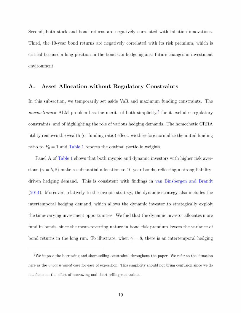
Panel A of Table 1 shows that both myopic and dynamic investors with higher risk aver-

sions (γ = 5, 8) make a substantial allocation to 10-year bonds, reflecting a strong liability-

driven hedging demand. This is consistent with findings in van Binsbergen and Brandt

(2014). Moreover, relatively to the myopic strategy, the dynamic strategy also includes the

intertemporal hedging demand, which allows the dynamic investor to strategically exploit

the time-varying investment opportunities. We find that the dynamic investor allocates more

fund in bonds, since the mean-reverting nature in bond risk premium lowers the variance of

bond returns in the long run. To illustrate, when γ = 8, there is an intertemporal hedging

5We impose the borrowing and short-selling constraints throughout the paper. We refer to the situation

here as the unconstrained case for ease of exposition. This simplicity should not bring confusion since we do

not focus on the effect of borrowing and short-selling constraints.

19

TABLE 1

Optimal Portfolio Weights for the Unconstrained ALM

Panel A (resp. Panel B) gives the portfolio weights and standard deviations (between brackets) at time 0

for a 10-year nominal (resp. real) ALM under the risk aversion γ = 2, 5, 8 respectively, ignoring the VaR

and maximum funding constraints.

Panel A: Nominal ALM

Myopic Dynamic

γ Stocks Cash Bonds Stocks Cash Bonds

2 0.69 (0.039) 0.00 (0.000) 0.31 (0.034) 0.70 (0.046) 0.00 (0.000) 0.30 (0.044)

5 0.28 (0.016) 0.03 (0.037) 0.69 (0.021) 0.27 (0.034) 0.02 (0.025) 0.71 (0.009)

8 0.17 (0.007) 0.02 (0.049) 0.81 (0.041) 0.13 (0.019) 0.00 (0.000) 0.87 (0.013)

Panel B: Real ALM

Myopic Dynamic

γ Stocks Cash Bonds Stocks Cash Bonds

2 0.70 (0.013) 0.00 (0.000) 0.30 (0.013) 0.73 (0.020) 0.00 (0.000) 0.27 (0.020)

5 0.29 (0.006) 0.03 (0.003) 0.68 (0.006) 0.33 (0.002) 0.04 (0.001) 0.63 (0.003)

8 0.18 (0.004) 0.03 (0.003) 0.79 (0.004) 0.20 (0.003) 0.03 (0.002) 0.77 (0.003)

demand of 6%, calculated by taking the difference of the dynamic and myopic allocation

in bonds, implying that in the nominal economy long-term bond offers a positive hedging

demand.

The picture is remarkably different when it is in the real economy as shown in Panel B.

When taking inflation risk into account, the hedging demand for bonds becomes negative,

20

suggesting that inflation hedging dominates the effect induced by the time variation in in-

vestment opportunities. We show that the investor in this case tilts his portfolio towards the

equity and the dynamic strategy always holds more stocks than the myopic. As explained in

Campbell and Shiller (1988), inflation increases future dividends and thus leads to a boost

in stock prices. In our model, both stock and bond returns have negative correlations with

inflation innovations, but the stock’s Sharpe ratio of 0.35 is higher than the unconditional

mean of the bond’s Sharpe ratio (0.176). A negative shock in inflation innovation brings

a higher positive shock in stock return. In other words, the stock investment can hedge

inflation risk more effectively than the bond by offering larger expected returns. Thus, in

comparison with the nominal economy, inflation risk leads to an increase (decrease) in the

stock (bond) portfolio weight in the dynamic strategy. We also note that the difference

of investing myopically between nominal and real economy are rather small. It is because

inflation effect in one-step-ahead efficient static portfolio is relatively less significant, while

it accumulates when investing dynamically at a longer horizon.

In addition, we examine the distribution of the optimal terminal funding ratio FT in real

and nominal terms respectively. Figure 2 displays that the dispersion of the terminal funding

ratio decreases with γ. Indeed, a lower risk aversion implies larger allocation to risky assets

for high expected returns, and thus resulting in a larger probability of generating a higher

terminal funding ratio. For example, when γ = 2, the 97.5% quantile of the real (nominal)

terminal funding ratio given by the dynamic strategy can be exceedingly high, reaching

3.98 (6.29). This feature provides empirical evidence for imposing a right truncation for

the terminal funding ratio distribution, in order to avoid the situation where the investor

deliberately overfunds to shelter more taxable corporate profits. The maximum funding

21

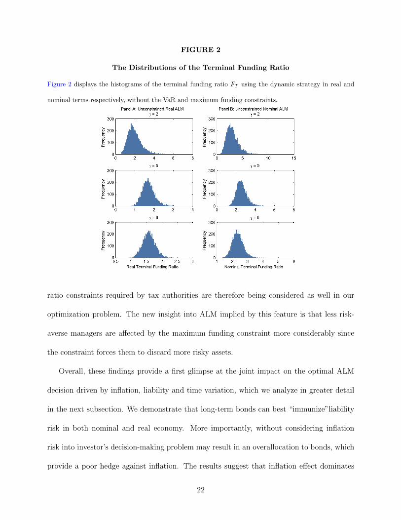
FIGURE 2

The Distributions of the Terminal Funding Ratio

Figure 2 displays the histograms of the terminal funding ratio FT using the dynamic strategy in real and

nominal terms respectively, without the VaR and maximum funding constraints.

ratio constraints required by tax authorities are therefore being considered as well in our

optimization problem. The new insight into ALM implied by this feature is that less risk-

averse managers are affected by the maximum funding constraint more considerably since

the constraint forces them to discard more risky assets.

Overall, these findings provide a first glimpse at the joint impact on the optimal ALM

decision driven by inflation, liability and time variation, which we analyze in greater detail

in the next subsection. We demonstrate that long-term bonds can best “immunize”liability

risk in both nominal and real economy. More importantly, without considering inflation

risk into investor’s decision-making problem may result in an overallocation to bonds, which

provide a poor hedge against inflation. The results suggest that inflation effect dominates

22

the effect of time variation in the investment opportunities. Conversely, inflation risk affects

the unconstrained myopic investor slightly, while later we show that the effect of inflation

could turn to be overwhelming if the regulatory VaR constraint is imposed.

B. Asset Allocation with VaR

B.1. Sensitivity to Funding Levels

To this point, we have illustrated the optimal investment allocation in the absence of regula-

tory constraints. We are now ready to reveal the impact of annually-repeated VaR constraints

under various scenarios. Figure 3 plots the optimal portfolio weights against different initial

funding levels.

Panel A shows the dynamic and myopic investment strategies in the real economy. To

begin with, we focus on the under- or fully-funded case (F0 ≤ 1). A striking feature is that

cash takes the whole portfolio proportion under both investment strategies. Note that, when

the initial funding ratio is not greater than one, the VaR constraint requires the probability

of F1 < F0 being no larger than 0.025. In this case, risky assets are not likely to fulfill

the VaR requirement by increasing the funding ratio within one period. Given that we do

not consider any net additional cash inflows throughout the paper and there is no funding

surplus, the manager has no other choice but has to allocate 100% of his fund into riskless

cash. This is the adverse result in real economy caused by the horizon disparity between the

regulatory horizon (one year) and investment horizon (ten years). The intuition behind this

finding is that a shortfall in the initial funding ratio, especially a severe shortfall, could be

an indicator of an economic downturn in a gloomy market, such as low interest rate and high

23

FIGURE 3

ALM Portfolio Choice with VaR

Figure 3 depicts the optimal portfolio weights and hedging demands versus the funding ratio at time 0 for

a 10-year ALM with the VaR (δ = 0.025) constraint. Panel A (resp. Panel B) summarizes the dynamic and

myopic strategies in the real (resp. nominal) economy under γ = 5.

inflation rate. If there is no net cash inflow to offset the shortfall, the manager probably has

to hold portfolio weights mainly in cash until the financial market recovers. In this sense,

constrained by the borrowing and short-selling limits, the fund manager with lower level of

real funding ratio has to give up potential high returns from risky assets and choose less risk

exposure by holding a large amount of cash for the short-term VaR constraint.

For an over-funded case (F0 > 1), there is a trend of increasing equity allocation in

both the dynamic and myopic strategies, although this pattern has been dampened by VaR

constraints. For instance, the dynamic investor’s stock weight is only 14% (when F0 = 1.04)

in Panel A, whereas the weight reaches up to 33% in the unconstrained ALM in Table 1.

24

Nevertheless, when the fund level increases, the effect of VaR gradually weakens, which

reduces the possibility of being constrained by VaR in the future. This situation is referred

to as the “less binding”VaR constraints by van Binsbergen and Brandt (2014). We find that

the dynamic optimal stock weight is the same as that in the unconstrained setting when the

fund has a large surplus, i.e. F0 is beyond 1.3. To this end, the manager is not restricted

by the regulatory rule and chooses his favourable trading policy as if there was no VaR

constraint.

We complement the literature by investigating hedging demands in real terms across

different initial funding levels. Comparing the dynamic and myopic strategies in Panel A

shows that there is an up to 4% intertemporal hedge demand for stocks. In fact, this positive

intertemporal hedging demand is largely induced by the positive inflation-hedging demand

for the stock as discussed in Section A. By contrast, the dynamic strategy has negative

intertemporal hedging demands for the bond in real terms. It is opposite to the finding in

nominal terms, as discussed in van Binsbergen and Brandt (2014). The negative hedging

demands can be explained by the interplay driven by three types of hedging demands. First,

the inflation-hedging demand raises stock holdings while at the same time reduces the bond

allocation in the dynamic strategy; second, the liability-hedging demand makes the myopic

investor to invest largely in the bond, aiming at hedging against liability risk; third, the effect

of liability risk on the dynamic manager is partly offset by the positive inflation-hedging and

intertemporal hedging demands for the stock. The higher expected returns of stock in the

time-varying investment environment will provide a reliable funding status in the long run

and further reduces the dynamic investor’s concern about liability risk, which then diereses

the bond allocation.

25

Collectively, the negative hedging demand for the bond when F0 > 1 under the real

economy reveals the following new insight into the ALM. Hedging liability risk is crucial for

the myopic investor, while the dynamic investor can partly offset the liability effect by using

positive hedging demands for the stock to dynamically hedge inflation risk, and meanwhile

to exploit the time-varying investment opportunity for higher gains.

Presenting the graphs side by side, our strategy to reveal the inflation effects under VaR-

constrained portfolio choice is to compare the results under the real and nominal economy

presented in Panel A and Panel B of Figure 3. We find that, without introducing inflation,

the stock demand by dynamic investor in Panel B is less than that in the real economy in

Panel A, since there is no incentive to hedge inflation in the nominal setting. Consequently,

liability effect dominates again and the dynamic investor’s intertemporal hedging demands

turn out to be long in the bond and short in the stock. In addition, both the dynamic and

myopic managers allocate a large amount of their wealth between the long-term bond and

stock for relatively high nominal returns. In this way, they maintain a large probability of

being over funded or having an increase in funding to satisfy the VaR requirement. In terms

of the regulatory effect, our investment strategy in the nominal economy is similar to the

finding of van Binsbergen and Brandt (2014) who argue that the dynamic investor has to be

away from his preferred weight in the stock because of VaR constraints.

B.2. Sensitivity to Time Variation

Admittedly, the magnitude of hedging demands in previous case is rather small, generally

less than 5%. We argue that it is due to the time variation in the dynamic strategy and the

liability hedging in the myopic strategy. We are now set the bond risk premium to be its

26

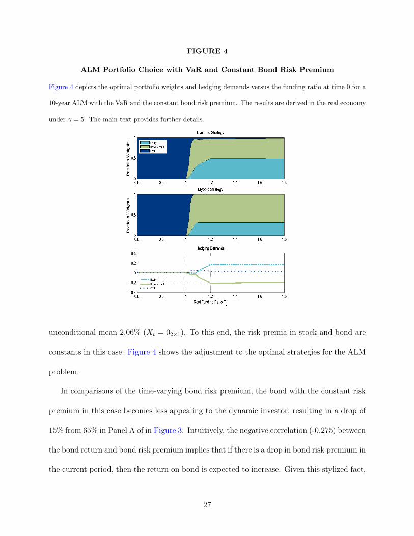
FIGURE 4

ALM Portfolio Choice with VaR and Constant Bond Risk Premium

Figure 4 depicts the optimal portfolio weights and hedging demands versus the funding ratio at time 0 for a

10-year ALM with the VaR and the constant bond risk premium. The results are derived in the real economy

under γ = 5. The main text provides further details.

unconditional mean 2.06% (Xt = 02×1). To this end, the risk premia in stock and bond are

constants in this case. Figure 4 shows the adjustment to the optimal strategies for the ALM

problem.

In comparisons of the time-varying bond risk premium, the bond with the constant risk

premium in this case becomes less appealing to the dynamic investor, resulting in a drop of

15% from 65% in Panel A of in Figure 3. Intuitively, the negative correlation (-0.275) between

the bond return and bond risk premium implies that if there is a drop in bond risk premium in

the current period, then the return on bond is expected to increase. Given this stylized fact,

27

the dynamic investor substantially raises bond holdings to take advantage of the time-varying

bond risk premium as shown in Figure 3 and in the asset-only setting by Sangvinatsos and

Wachter (2005). Nevertheless, the constant bond premium provides the dynamic investor

very limited opportunity to strategically exploit the time variation, and thereby tilting the

portfolio weight to the stock for a higher risk premium (5.38%). As a consequence, this

change produces relatively larger intertemporal hedging demands for bonds and stocks. We

therefore conclude that in the framework of the ALM, time-varying opportunities in long-

term bond market would lead the asset allocation nearly indifference between the dynamic

and myopic trading strategies, indicating that in the presence of liability risk, myopically

optimal strategy might be preferred by the investor.

B.3. Sensitivity to Liability Risk

To see more exactly how liability alters investor’s allocation, our strategy is to compare the

portfolio choice of an ALM investor to that of a traditional asset-only investor. In the latter

case the investor optimizes his utility over the terminal wealth instead of the funding ratio,

and at the same time, his investment behavior is limited by annual VaR constraints with the

“floor”w = 1 and probability δ = 0.025. More specifically,

VaRw : Pt(wt+1 < w) ≤ δ,

VaR′w : Pt(wt+1 < wt|wt ≤ w) ≤ δ.

(25)

Then the asset-only investor’s objective is to maximize the expected utility of terminal wealth

(26) J(w,X, t, T ) = maxθt∈Kw

t

E(w1−γT

1− γ

),

28

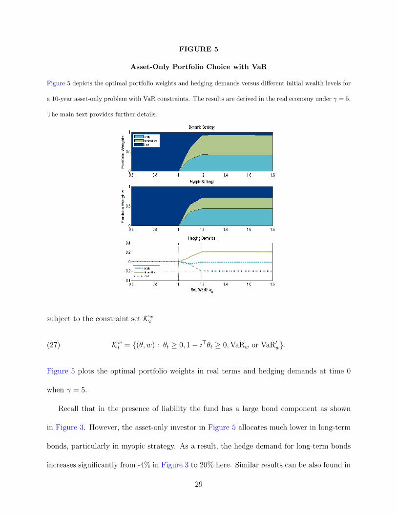
FIGURE 5

Asset-Only Portfolio Choice with VaR

Figure 5 depicts the optimal portfolio weights and hedging demands versus different initial wealth levels for

a 10-year asset-only problem with VaR constraints. The results are derived in the real economy under γ = 5.

The main text provides further details.

subject to the constraint set Kwt

(27) Kwt = {(θ, w) : θt ≥ 0, 1− ı>θt ≥ 0,VaRw or VaR′w}.

Figure 5 plots the optimal portfolio weights in real terms and hedging demands at time 0

when γ = 5.

Recall that in the presence of liability the fund has a large bond component as shown

in Figure 3. However, the asset-only investor in Figure 5 allocates much lower in long-term

bonds, particularly in myopic strategy. As a result, the hedge demand for long-term bonds

increases significantly from -4% in Figure 3 to 20% here. Similar results can be also found in

29

Sangvinatsos and Wachter (2005) who study predictability in bond returns in the asset-only

framework without constraints. They claim that time-varying risk premia generate large

hedging demands for long-term bonds.

Another noticeable feature in Figure 5 is that when the bond allocation decreases, cash

serves as an effective takeover and makes the portfolio well-diversified. Note that cash in

the financial market that we consider provides an average 2% real return, which is roughly

equal to the real bond yield, with much higher liquidity and lower risk. Hence, asset-only

managers, especially those who behave myopically and/or those with shortfalls in wealth,

tilt the optimal portfolio weights to riskless asset, which leads to considerable negative

intertemporal hedging demands for cash in the dynamic strategy.

Interestingly, it is noted that ignoring liability leads the asset-only investor to be less

concerned about inflation risk. Given the fact that stocks serve as a good inflation hedge

with a positive intertemporal demand in Panel A of Figure 3, we find the hedging demand

for stock is nearly zero across different initial wealth, implying that liability might be one of

the main driving force for inflation hedging.

C. Asset Allocation with VaR and Maximum Funding Limits

Up to this point, we have illustrated the impact of VaR on portfolio allocation under various

settings. Next we examine the joint effect of regulatory requirements by introducing the

maximum funding constraint, where the upper-bound level of funding ratio is k = 130%.6

6We consider the upper-bound k = 130% since, as indicated by our results, the VaR constraint will not

bind beyond this level. This bound is also in line with the practice in, e.g., the Netherlands, see Pugh (2006).

30

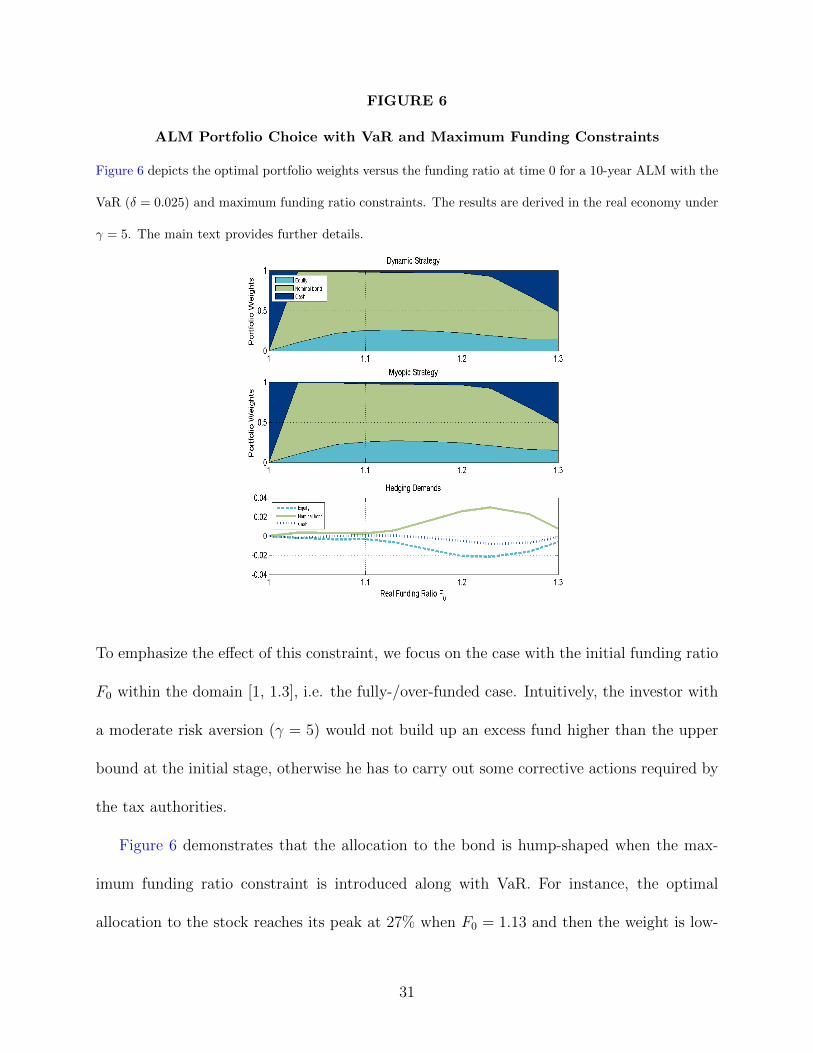
FIGURE 6

ALM Portfolio Choice with VaR and Maximum Funding Constraints

Figure 6 depicts the optimal portfolio weights versus the funding ratio at time 0 for a 10-year ALM with the

VaR (δ = 0.025) and maximum funding ratio constraints. The results are derived in the real economy under

γ = 5. The main text provides further details.

To emphasize the effect of this constraint, we focus on the case with the initial funding ratio

F0 within the domain [1, 1.3], i.e. the fully-/over-funded case. Intuitively, the investor with

a moderate risk aversion (γ = 5) would not build up an excess fund higher than the upper

bound at the initial stage, otherwise he has to carry out some corrective actions required by

the tax authorities.

Figure 6 demonstrates that the allocation to the bond is hump-shaped when the max-

imum funding ratio constraint is introduced along with VaR. For instance, the optimal

allocation to the stock reaches its peak at 27% when F0 = 1.13 and then the weight is low-

31

ered by the manager to about 14% when F0 = 1.3. At the same time, cash holdings go up

dramatically. The hump-shaped allocations are attributed to the weakening effect of VaR

and the strengthening effect of maximum funding constraint when F0 rises. Namely, the

maximum funding constraint is binding gradually to prevent the manager from building up

an exceedingly large surplus. The new insight into the ALM with such constraints is that

the manager should reduce the allocation to risky assets with higher expected returns and

meanwhile increase cash holdings in order to avoid the penalty from tax laws.

The hump-shape (U-shape) hedging demand for the bond (stock) reveals our new insight

into the ALM that the myopic investor reduces the portfolio weight of bond more than

the dynamic investor the under maximum funding constraint. Interestingly, these hedging

demands indicate that under such a constraint, the dynamic and myopic strategy tend to

coincide with each other when the funding level is high. Hence, we conjecture that such

regulatory rules could even entirely remove the gains of dynamic strategy by limiting the

dynamic investor’s ability to exploit time-variation in the investment opportunity set. The

following analysis on the welfare loss of acting myopically confirms our conjecture.

D. Welfare Losses under Real and Nominal Economies

We examine the welfare loss of behaving myopically in the presence of VaR and maximum

funding constraints, and address the effect of inflation on the economic value. We evaluate

such welfare loss of deviating from the dynamic trading strategy by calculating the annualized

certainty equivalent loss (CEL) of the myopic strategy. We denote that, at time 0, the

value function resulting from the optimal policy by J1 and that from the suboptimal by J2.

32

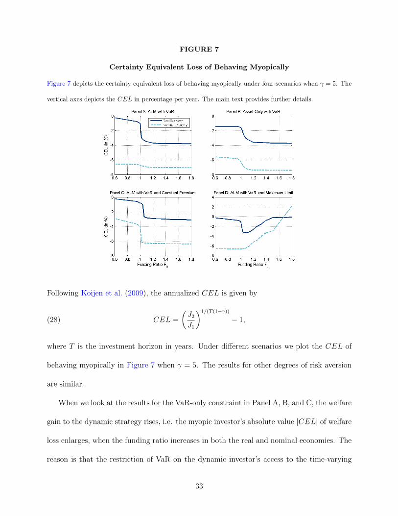
FIGURE 7

Certainty Equivalent Loss of Behaving Myopically

Figure 7 depicts the certainty equivalent loss of behaving myopically under four scenarios when γ = 5. The

vertical axes depicts the CEL in percentage per year. The main text provides further details.

Following Koijen et al. (2009), the annualized CEL is given by

(28) CEL =

(J2

J1

)1/(T (1−γ))

− 1,

where T is the investment horizon in years. Under different scenarios we plot the CEL of

behaving myopically in Figure 7 when γ = 5. The results for other degrees of risk aversion

are similar.

When we look at the results for the VaR-only constraint in Panel A, B, and C, the welfare

gain to the dynamic strategy rises, i.e. the myopic investor’s absolute value |CEL| of welfare

loss enlarges, when the funding ratio increases in both the real and nominal economies. The

reason is that the restriction of VaR on the dynamic investor’s access to the time-varying

33

investment opportunities becomes weaker when the fund ratio goes up. This finding is in

line with van Binsbergen and Brandt (2014) in the nominal economy.

Furthermore, we find the losses of behaving myopically in the real economy are smaller

than those in the nominal economy. For example, the manager in Panel A with the initial

funding ratio F0 = 1 would incur a utility loss of 1% (6.3%) per annum in the real (nominal)

economy, if he gave up exploiting time-variation in the investment opportunity set. The less

welfare loss in the real economy implies our new insight that taking account of inflation risk

into the ALM adds values to the myopic investor.

Put differently, inflation-hedging under the real economy restricts more benefits in the

dynamic strategy. Intuitively, the accumulated effects of inflation risk in the long run could

damage payoffs to the dynamic investor. This result is attributed to our aforementioned fun-

damental finding that inflation risk leads to an increase (decrease) in the dynamic investor’s

intertemporal hedging demand for the stock (bond). Therefore, the dynamic investor cannot

fully exploit time-variation in the bond risk premium because of the raising stock holdings.

In short, the new insight is that the manager loses more benefits of dynamic strategy when

he encounters inflation risk.

More importantly, when the maximum funding constraint is imposed along with the

VaR constraint, the myopic investor experiences U-shaped welfare losses in both the real

and nominal economies, as shown in Panel D. Surprisingly, the myopic strategy could even

provide more benefits than the dynamic strategy, i.e. the welfare loss turns to a positive profit

CEL > 0, when the initial funding ratio is highly over funded more than 1.7. It indicates

that a relatively tight upper-bound limit would lead the manager to behave myopically and

to be less efficient with respect to changes in the opportunities set. Our insight provides

34

an argument for justifying some current practices of using a myopic allocation policy and

ignoring time-varying opportunities in the presence of strict regulatory rules.

V. Conclusion

Inflation risk and regulatory rules feature dominantly in an asset-liability management prob-

lem, but they have been largely ignored in the financial literature. In this paper, we analyze

the optimal risk exposure for an ALM optimization problem in the presence of interactive

hedging demands driven by inflation, liability and the time variation in the investment op-

portunity set. The fund manager chooses the optimal portfolio allocation with respect to

the annually repeated VaR and maximum funding constraints in a two-factor affine model

of term structure.

Our study provides the fund manager with new insights into the ALM problem. First,

long-term bonds can best immunize liability risk in both nominal and real economy. More

importantly, without considering inflation risk into investor’s decision-making problem may

result in an overallocation to bonds, which provide a poor hedge against inflation. The

results suggest that inflation effect dominates the effect of time variation in the investment

opportunities. Second, the regulatory constraints remarkably reduce the welfare of dynamic

strategy, especially under inflation risk. Furthermore, under the strict maximum funding

constraint, the profit of dynamic strategy even completely vanishes and the myopic strategy

of asset allocation is favored.

Given the novelty of our analysis, we believe there are several promising directions for

future research. While we assume that the lower and upper thresholds of constraints are

35

given exogenously by the regulators, it would be valuable to investigate an equilibrium

that allows the risk-taking manager to exploit time variations in the market as much as

possible, and meanwhile, maintains the funding ratio in a desirable range. It would also be of

interest to consider a setting where managers are specialists, each of whom manages one asset

class, instead of well-balanced managers who manage all assets. Moreover, these specialists

compete each other. In practice, managers tend to allocate assets based on the performance

of peer colleagues, because of career concerns, reputations or their annual bonuses. Analyzing

how different such managerial agency behavior is would be worthwhile.

36

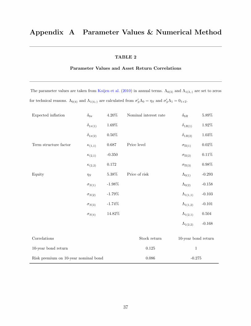
Appendix A Parameter Values & Numerical Method

TABLE 2

Parameter Values and Asset Return Correlations

The parameter values are taken from Koijen et al. (2010) in annual terms. Λ0(3) and Λ1(3,:) are set to zeros

for technical reasons. Λ0(4) and Λ1(4,:) are calculated from σ′SΛ0 = ηS and σ′SΛ1 = 01×2.

Expected inflation δ0π 4.20% Nominal interest rate δ0R 5.89%

δ1π(1) 1.69% δ1R(1) 1.92%

δ1π(2) 0.50% δ1R(2) 1.03%

Term structure factor κ(1,1) 0.687 Price level σΠ(1) 0.02%

κ(2,1) -0.350 σΠ(2) 0.11%

κ(2,2) 0.172 σΠ(3) 0.98%

Equity ηS 5.38% Price of risk Λ0(1) -0.293

σS(1) -1.98% Λ0(2) -0.158

σS(2) -1.79% Λ1(1,1) -0.103

σS(3) -1.74% Λ1(1,2) -0.101

σS(4) 14.82% Λ1(2,1) 0.504

Λ1(2,2) -0.168

Correlations Stock return 10-year bond return

10-year bond return 0.125 1

Risk premium on 10-year nominal bond 0.086 -0.275

37

Numerical Method To solve the complicated and path-dependent dynamic portfolio opti-

mization problem with constraints, we use the simulation-based method proposed by Brandt

et al. (2005). The main idea of their method is to approximate the conditional expectations

by regressing the variables of interest on a polynomial basis of state variables. The regres-

sion coefficients are estimated by cross-sectional regressions across simulated paths of asset

returns and state variables.7

To begin with, we construct a grid of the funding ratio indicated by Ft(j), j = 1, . . . ,M ,

since the optimal portfolio weights depend on the given values of funding ratio. We also

discretize the constrained space [0, 1] × [0, 1] for portfolio weights θt,s(i)-grid, where i =

1, . . . , L, and risky assets s = 1, 2. We then choose the optimal portfolio weights in each

period and along each path by searching over this θt,s(i)-grid. The grid-search is robust and

avoids several convergence issues that could occur when iterating to a solution based on the

first-order conditions (van Binsbergen and Brandt 2007). We simulate N = 5, 000 paths

of asset returns and state variables with T years, and repeat this optimization process 10

times. Raising the number of paths and simulations does not improve the accuracy of our

results at a reported level. We solve the dynamic optimization problem backward recursively

and rebalance the portfolio at an annual basis. The following description is similar to van

Binsbergen and Brandt (2014).

•Time T-1: The investment problem at time T − 1 can be summarized as

(A.1) maxθT−1∈KT−1

ET−1

(F 1−γT

1− γ|FT−1 = FT−1(j)

).

7This approach is inspired by the simulation method for pricing American options in Longstaff and

Schwartz (2001).

38

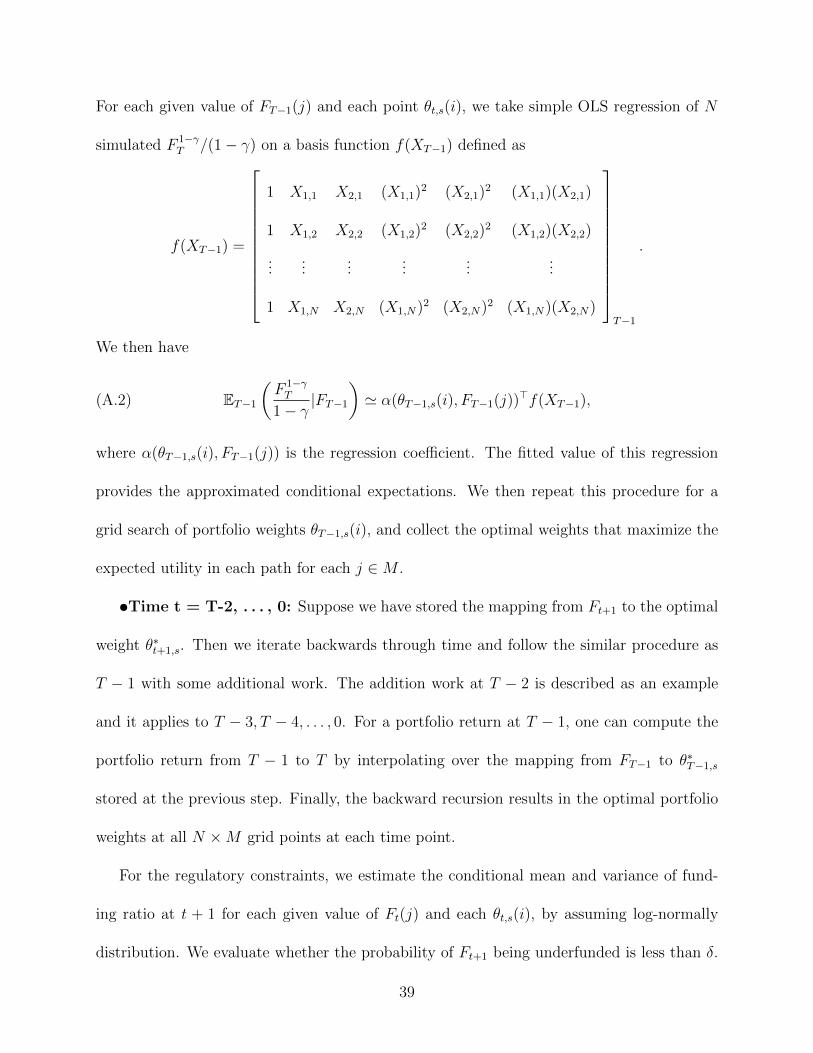
For each given value of FT−1(j) and each point θt,s(i), we take simple OLS regression of N

simulated F 1−γT /(1− γ) on a basis function f(XT−1) defined as

f(XT−1) =

1 X1,1 X2,1 (X1,1)2 (X2,1)2 (X1,1)(X2,1)

1 X1,2 X2,2 (X1,2)2 (X2,2)2 (X1,2)(X2,2)

......

......

......

1 X1,N X2,N (X1,N)2 (X2,N)2 (X1,N)(X2,N)

T−1

.

We then have

(A.2) ET−1

(F 1−γT

1− γ|FT−1

)' α(θT−1,s(i), FT−1(j))>f(XT−1),

where α(θT−1,s(i), FT−1(j)) is the regression coefficient. The fitted value of this regression

provides the approximated conditional expectations. We then repeat this procedure for a

grid search of portfolio weights θT−1,s(i), and collect the optimal weights that maximize the

expected utility in each path for each j ∈M .

•Time t = T-2, . . . , 0: Suppose we have stored the mapping from Ft+1 to the optimal

weight θ∗t+1,s. Then we iterate backwards through time and follow the similar procedure as

T − 1 with some additional work. The addition work at T − 2 is described as an example

and it applies to T − 3, T − 4, . . . , 0. For a portfolio return at T − 1, one can compute the

portfolio return from T − 1 to T by interpolating over the mapping from FT−1 to θ∗T−1,s

stored at the previous step. Finally, the backward recursion results in the optimal portfolio

weights at all N ×M grid points at each time point.

For the regulatory constraints, we estimate the conditional mean and variance of fund-

ing ratio at t + 1 for each given value of Ft(j) and each θt,s(i), by assuming log-normally

distribution. We evaluate whether the probability of Ft+1 being underfunded is less than δ.

39

Those portfolio weights that do not satisfy this VaR requirement (or the maximum funding

constraint) will be excluded from the investor’s choice set.

References

Basak, S., and A. Shapiro: “Value-at-Risk-Based Risk Management: Optimal Policies and

Asset Prices.” Review of Financial Studies, 14 (2001), 371–405.

Brandt, M. W.; A. Goyal; P. Santa-Clara; and J. R. Stroud: “A Simulation Approach to

Dynamic Portfolio Choice with an Application to Learning about Return Predictability.”

Review of Financial Studies, 18 (2005), 831–873.

Brennan, M. J., and Y. Xia: “Dynamic Asset Allocation under Inflation.” Journal of Fi-

nance, 57 (2002), 1201–1238.

Campbell, J. Y., and R. J. Shiller: “Stock Prices, Earnings, and Expected Dividends.”

Journal of Finance, 43 (1988), 661–676.

Campbell, J. Y., and L. M. Viceira: “Who Should Buy Long-Term Bonds?” American

Economic Review, 91 (2001), 99–127.

Cochrane, J. H., and M. Piazzesi: “Bond Risk Premia.” American economic review, 95

(2005), 138–160.

Cuoco, D.; H. He; and S. Isaenko: “Optimal Dynamic Trading Strategies with Risk Limits.”

Operations Research, 56 (2008), 358–368.

40

Dai, Q., and K. J. Singleton: “Specification Analysis of Affine Term Structure Models.”

Journal of Finance, 55 (2000), 1943–1978.

Detemple, J., and M. Rindisbacher: “Dynamic Asset Liability Management with Tolerance

for Limited Shortfalls.” Insurance: Mathematics and Economics, 43 (2008), 281–294.

Duffee, G. R.: “Term Premia and Interest Rate Forecasts in Affine Models.” Journal of

Finance, 57 (2002), 405–443.

Hoevenaars, R. P.; R. D. Molenaar; P. C. Schotman; and T. B. Steenkamp: “Strategic Asset

Allocation with Liabilities: Beyond Stocks and Bonds.” Journal of Economic Dynamics

and Control, 32 (2008), 2939–2970.

Koijen, R. S. J.; T. E. Nijman; and B. J. M. Werker: “When Can Life Cycle Investors Benefit

from Time-Varying Bond Risk Premia?” Review of Financial Studies, 23 (2010), 741–780.

Koijen, R. S. J.; J. C. Rodrıguez; and A. Sbuelz: “Momentum and Mean Reversion in

Strategic Asset Allocation.” Management Science, 55 (2009), 1199–1213.

Longstaff, F., and E. Schwartz: “Valuing American Options by Simulation: A Simple Least-

Squares Approach.” Review of Financial Studies, 14 (2001), 113–147.

Lynch, A. W., and S. Tan: “Multiple Risky Assets, Transaction Costs, and Return Pre-

dictability: Allocation Rules and Implications for U.S. Investors.” Journal of Financial

and Quantitative Analysis, 45 (2010), 1015–1053.

Martellini, L., and V. Milhau: “Dynamic Allocation Decisions in the Presence of Funding

Ratio Constraints.” Journal of Pension Economics and Finance, 11 (2012), 549–580.

41

Merton, R. C.: Continuous-Time Finance. Cambridge, B. Blackwell (1992).

Munk, C.; C. Sørensen; and T. Nygaard Vinther: “Dynamic Asset Allocation under Mean-

Reverting Returns, Stochastic Interest Rates, and Inflation Uncertainty: Are Popular Rec-

ommendations Consistent with Rational Behavior?” International Review of Economics

& Finance, 13 (2004), 141–166.

Piazzesi, M.: “Affine Term Structure Models.” In Handbook of financial econometrics, Vol.

1, Y. Aıt-Sahalia and L. P. Hansen, eds. Amsterdam, Elsevier (2010).

Pugh, C.: “Funding Rules and Actuarial Methods.” OECD Working Papers on Insurance

and Private Pensions, No. 1 (2006).

Rudolf, M., and W. T. Ziemba: “Intertemporal Surplus Management.” Journal of Economic

Dynamics and Control, 28 (2004), 975–990.

Sangvinatsos, A., and J. A. Wachter: “Does the Failure of the Expectations Hypothesis

Matter for Long-Term Investors?” Journal of Finance, 60 (2005), 179–230.

Shi, Z., and B. J. M. Werker: “Short-Horizon Regulation for Long-Term Investors.” Journal

of Banking & Finance, 36 (2012), 3227–3238.

Sundaresan, S., and F. Zapatero: “Valuation, Optimal Asset Allocation and Retirement

Incentives of Pension Plans.” Review of Financial Studies, 10 (1997), 631–660.

van Binsbergen, J. H., and M. W. Brandt: “Solving Dynamic Portfolio Choice Problems by

Recursing on Optimized Portfolio Weights or on the Value Function?” Computational

Economics, 29 (2007), 355–367.

42

van Binsbergen, J. H., and M. W. Brandt: “Optimal Asset Allocation in Asset Liability

Management.” National Bureau of Economic Research Working Paper (2014).

Yiu, K. F. C.: “Optimal Portfolios under a Value-At-Risk Constraint.” Journal of Economic

Dynamics and Control, 28 (2004), 1317–1334.

43