Calhoun: The NPS Institutional Archive

Theses and Dissertations Thesis Collection

1990-06

Dynamic analysis of the Low Power Atmospheric

Compensation Experiment (LACE) spacecraft

Walters, Wesley F.

Monterey, California. Naval Postgraduate School

http://hdl.handle.net/10945/44296

This document was downloaded on January 15, 2015 at 10:59:33

Author(s) Walters, Wesley F.

Title Dynamic analysis of the Low Power Atmospheric Compensation Experiment (LACE)spacecraft

Publisher Monterey, California. Naval Postgraduate School

Issue Date 1990-06

URL http://hdl.handle.net/10945/44296

AD-A241 361

NAVAL POSIGNADUATE SCHOOL()KMoterey, California

DTICELECTE

T-11

THESIS

DYNAMIC ANALYSIS O- FE Ive. LO O-RATMO0S?=ERIC COMPENSA-TON

E.XPERIMEiZT (LACE) SPACECRAFT

by

Wesley F. Walters

Thesis Advisor: Ramesh Kolar

Approved for public release; Distribution is unlimnited

91-13031AI'!~iIHI~H~~l ~REPRODUCED BY

U.S. DEPARTMENT OF COMMERCENAM ONAL TECHNICAL

INFORMATION SERVICESPRINGFIELD, VA 22161

DISCLAIMEi NOTICE

THIS DOCUMENT IS BEST

QUALITY AVAILABLE. THE COPY

FURNISHED TO DTIC CONTAINED

A SIGNIFICANT NUMBER OF

PAGES WHICH DO NOT

REPRODUCE LEGIBLY.

UN C AIS S 17 D

REPORT DOCUMENTATION PAGE Qvrv35 07W.OIU

2a1 EU* 7 R3 O SSPXY 0 ~A~ir-aes~l 3~~$5~10M~

Zb D-LSI4131C-7ARDV5S"DX DISTRIBUTION IS UNI.IMITED

1: PRO~1.C4OGA " ATI ]REPOR.T 1 ifE3 R5S WAMO= OaT0cG tc-V ZAT- REPORT f~tc3'!P S

68 wwVE OF P~tFO;=%G 00AGrVAiZT-i 16b O;FgliC! a SYF &:i KAOf tTOF ' O'047-6-ZAi'.

naval Postgraduate School Naval Postgraduate School

6L~ ADDRESS tcas') Swa. anci ZupCoclel 7b, A0DRESS t~ 5.j~e. aid ZlPCOde)

MontreyCA 9943-000Monterey, CA 93943-5000

Se. ADDRESS(Ciy, State, aidZIPCode) 10 SOURCE 0; PUI.3T.G .UTJOORSPROGRAMT P00CT TASK AOr.(r U*MT,ELEMENT 1-0 NO0 Z. CCESSIOJ 1'O

I, TITLE Ebcaod SeCitntty oall-ficar-on)DYNAMIC ANALYSIS OF THE LOW POWER ATMOSPHERIC COMPENSA.TON EXPERIMENT(LACE) SPACECRAFT

12 PE L F.TOR

13a TYPE OT REPORT 13 TiME COVEREDM DATE OF REPORT tYea,Muoth Day) ~5 PAGE CO.9aMaster's Thesis eOol ____ To___ JUNE 1990 218

16 SUPPEtVEF!.AR' I.0'A O% The wues expressed in this thesis are those or the author and do not reflect theofficial polic% or position of the Department of Defense or the US. Gosernnient

17 COSA- CODES 18i SUIJECT TERVS (Continue oan revrse if necessary and 4entidy by block num,,ber)

FIEO GRO'jP SUB GROUP DYNAMIC ANALYSIS, THERMOELASTIC EFFECTS

CHAOTIC VIBRATIONS19 ASTRAT (ontiue o reeret necessailry and identify b lc ubr

The Lc,. Poscr Atmophieric Compensawin Expriment (L[ACE) spacecraft -as launched for XRL in February 1990The LtLE flighi d~nAomsAesperunen, %,il prostdeou-orbit systems Identificatleon ofia tACE spacecraft The experimnent is designedIitaore 150ndM II~cq.UCIILI. Oilig m1 and msillation amplitudes of the LACE, spacecraft The purpose of tis stud) Is taidesClopafinitte iten It model 0thle LCE spacrafl and conduct ad)nIsamics anailsis 10 determnine natural fecqucncsand mode shapes Four

COlhriUaioO 01 he spAecraft are anal)med Ibis dala %all be compared %sibh actual orbital data and %III prosIde an OPPOrIuIIIII forImprosenil in Int accuracy ol computer umuflaos of flexible structures and multi-body dy~namics Thte.moelasiic efferis due tosllfl-rrniai ra iing artcadorssej to tbeck Ibe magniiuaeof deiormalionsibhat ra) causea problem lot siibiij, otof-urbia identificationThe fina ph-s ci this stuoy As to conduct a parameletec analysts of the spacecraftlbom It, inslesigaic thet presnce of chaoic vibrationfut combinations of excittion amplitude and frequency

20 ISTRiUTONAVALAB4ITY OF ABSTRACT 21 ABSTRACT StCUROTV CLASS F CATIONr.- SSFIn11., ID 0 aAV'F AS R- 0 ' 'S I unclassified

22a NI TRSR & ODA 22h TELEPHO NE(f1nrlodeA~eP)Code)j22c WF"iC 5yCriIQ

NFRjSO'S:~EDvIu1 (408) 6624 1 AA/KJDDOFormr 1473, JUN 86 Ptracous afablons anpobsolete Sf( QTY CLASS f.CAT O?. OF Tm S DAV

S/N 0102-LF-014-6603 UNCLASSIFIED

1. I

Approved for public release; distribution is unlimied.

DYNUAIC ANAPLYSIS OF =.E LO OERAMSPEI

COMPENSATION EXPERIM1ENT (LACE) SPACE-CRAFT-

by

Wesley F7. WaltersMajor, United States Army

B.S., United States Military Academy, 1977

Submitted in Dart--al fulfillment

of the recuirements for the degree of

AERONAUTICAL AND ASTRONAUTICAL ENGINEER

and

MASTER OF SCIENCE INASTRONAUTICAL ENGINEERING

from the

NAVAL POSTGRADUATE SCHOOL

June 1990

Author: Wesley F. Walters

Approved by: _

Ramesh Kolar, Thesis Advisor

Brij rawal, Second Reader

_ERobert -ood, Cha* anDPrme , &t ics Ast nautics

and Graduate Studies

ABSTRACT

The Low Power Atmospheric Compensation ExpEriment (LACE)

spacecraft was launched for NRL in February 1990. The LACE

flight dynamics experiment will provide on-orbit systems

identification of the LACE spacecraft. The experiment is

designed to measure modal frequencies, damping ratios, and

oscillation amplitudes of the LACE spacecraft. The purpose of

this study is to develop a finite elerdent model of the LACE

spacecraft and conduct a dynamics analysis to determine

natural frequencies and mode shapes. Four configurations of

the spacecraft are analyzed. This data will be compared with

actual orbital data and will provide an opportunity for

improvements in the accuracy of computer simulations of

flexible structures and multi-body dynamics. Thermoelastic

effects due to differential heating are addressed to check the

magnitude of deformations that may cause a problem for

stability or on-orbit identification. The final phase of this

study is to conduct a parametric analysis of the spacecraft

boom to investigate the presence of chaotic vibration for

combinations of excitation amplitude and frequency.

Aooession For

-TIS GRA&iDTIC TAB 0

|Unannouncod 0justification

ByDistributton/

AvailabilitY Codos.k WF.atnd/or

Dist Sp )ial

TABLE OF CONTENTS

I. INTRODUCTION. ..................... 1

A. PURPOSE. ..................... 1

D. OVERVIEW/BACKGROUND .. ............. 2

1. Spacecraft Description. ......... 2

2. Experimental Hardware .. ......... 2

3. Acquisition Sequence. .......... 4

4. Orbital Parameters. ........... 5

C. MOTIVATION .................... 5

D. THESIS OUTLINE .................. 6

I.THEORETICAL FORMULATION

A. FINITE ELEMENT METHOD .. ............ 8

1. Rod Elements. ................ 9

2. Beam Elements. .............. 11

3. Plate Bending Theory. ........... 13

B. FREE VIBRATION OF MULTI-DEGREE-OF-FREEDOM

SYSTEMS ...................... 18

C. NUMERICAL EVALUATION OF MODES AND

FREQUENCIES OF MDOF SYSTEMS. ........... 0

III. LACE FINITE ELEMENT MODEL. ............. 25

A. GIFTS CAPABILITIES. .............. 25

B. SIMPLE FINITE ELEMENT MODEL OF LACE. ...... 26

C. COMPLEX FINITE ELEMENT MODEL OF LACE ...... 27

1. Main Spacecraft Body. ........... 27

2. Spacecraft Trusses .. ........... 33

IV. RESULTS OF DYNAMIC ANALYSIS . ........... 38

V. THERMOELASTIC EFFECTS ................ 56

VI. M4ULTI-BODY DYNAMICS. ................ 61

A. COMPONENT MODE SYNTHESIS ............ 61

1. Normal Modes .. .............. 64

2. Constraint Modes .. ............ 65

3. Attachment Modes .. ............ 65

4. Rigid Body Modes .. ............ 66

5. Inertia-Relief Modes. ........... 67

6. Coupling of Components. .......... 67

B. DYNAMICS OF FLEXIBLE BODIES IN TREE TOPOLOGY . 69

1. Overview of Multibody Systems ....... 69

2. Multibody Computer Program - TREETOPS .. 69

a. Body Types. ............. 70

b. Hinges.................70

C. Sensors and Actuators. ........ 71

d. Orbit Environment. .......... 72

VII. CHAOTIC VIBRATIONS ................... 74

A. HOW TO IDENTIFY CHAOTIC VIBRATIONS ....... 74

1. Nonlinear System Elements ......... 75

2. Random Inputs. .............. 75

3. Observation of Time History ........ 76

4. Fourier Spectrum. ............. 76

5. Phase Plane History ............ 76

6. Pseudo-Phase-Space Method ......... 78

7. Poincard Section .. ............ 79

B. QUANTITATIVE TESTS FOR CHAOS. ......... ?9

V

1. Lyapunov Exponent ............ 80

2. Fractal Dimension ..... ............ .82

C. LACE SPACECRAFT BOOM AS A NONLINEAR SYSTEM . . 83

D. CHAOTIC VIBRATION ANALYSIS .... .......... .88

VIII. CONCLUSIONS AND SCOPE FOR FURTHER RESEARCH . . . 115

A. CONCLUSIONS ...... ................. ... 115

B. SCOPE FOR FUTURE RESEARCH ... .......... . 116

APPENDIX A ......... ...................... .. 118

APPENDIX B ......... ...................... .. 120

A. PRIMARY STRUCTURE .... .............. ... 120

1. Determine Stiffness of Honeycomb Panel . 121

2. Determine Equivalent Aluminum

Plate Thickness .... ............ . 121

3. Determine Honeycomb Panel Mass ..... ... 121

4. Determine Equivalent Density ........ . 121

B. SECONDARY STRUCTURE .... ............. ... 122

1. Fixed and Deployable Solar

Array Substrate .... ............ . 122

a. Determine Equivalent

Aluminum Thickness .. ........ . 122

b. Determine Honeycomb Panel Mass 122

c. Determine Equivalent Density 122

2. Deployable Sensor Panels .. ........ . 122

a. Determine Equivalent Aluminum

Thickness .... ............. ... 123

b. Determine Honeycomb Mass ...... .. 123

c. Determine Equivalent Density . . . 123

I a a a a i ii I I i

APPENDIX D . . . . . . . . . . . . . . . . . . . . . . 136

APPENDIX E............................156

APPENDIX F............................159

APPENDIX G..............................164

APPENDIX H..............................177

A. MAXIMUM TEMPERATURE FOR DIAGONALS .......... 177

B. MINIMUM TEMPERATURE FOR THE DIAGONAL . . .. 179

APPENDIX I................................180

APPENDIX J..............................186

LIST OF REFERENCES......................205

BIBLIOGRAPHY.............................208

INITIAL DISTRIBUTION LIST.........................209

ACKNOWLEDGEMENTS

I would like to thank Ram Nagulpally, CASA Gifts, Inc.,

Al Frazier, ABLE-AEC Engineering, and Mike Fisher, NRL, for

their technical support and advice. I would like to

especially thank my advisor, Professor Ramesh Kolar, for his

direction, guidance and help in completing this project. He

has helped me to develop an interest in the field of chaotic

vibrations and non-linear systems.

I would also like to thank Ann Warner for her hard work

and dedication in formatting and typing this document.

Finally, I would like to thank my wife, Suzanne, for her

support and understanding during these three years in

Monterey.

Viii

4

I. INTRODUCTION

A. PURPOSE

This study is concerned with the modeling and analysis of

the Low Power Atmospheric Compensation Experiment (LACE)

spacecraft. One of the missions of the LACE spacecraft is to

conduct and obtain flight data for on-orbit system

identification. The flight dynamics experiment is designed to

measure modal frequencies, damping ratios, oscillaticn

amplitude of the LACE spacecraft and vibration intensity

generated oy boom deployments and retractions. This experiment

will provide an opportunity for improvements in the accuracy

of computer simulations of large flexible space structures and

multi-body dynamics.

It will also provide a mechanism for evaluating influence

of magnetic torques, gravity gradient torques and atmospheric

drag on the LACE-type structures.

The purpose of this study is to develop a finite element

model of the LACE spacecraft using the finite element pcogram

Graphical Interactive Element Total System (GIFTS). Dynamic

analysis is performed on the model to determine the natural

frequencies and mode shapes. Thermoelastic effects due to

differential heating are addressed to check if the magnitude

of deformations could cause a problem for stability or system

i I II P " l d I I I 1

identification. Finally, a parametric analysis is conducted on

a model of the spacecraft boom to investigate the possibility

of chaotic vibrations that may be induced during the mission.

B. OVERVIEW/BACKGROUND

1. Spacecraft Description

NRL-developed LACE was successfully launched on February

14, 1990, from Cape Canaveral on a DELTA II launch vehicle.

The spacecraft incorporates three deployable/retractable booms

of maximum length 150 feet. The 2,800 lb. LACE spacecraft is

stabilized by a 150 ft. zenith directed gravity gradient boom

mounted on top of the spacecraft, a momentum wheel with axis

along the pitch axis and a magnetic damper at the tip of the

gravity gradient boom. The retroreflector boom is mounted

forward and deployed along the velocity vector, while the

balance boom is mounted and pointed aft. Figure 1 shows the

basic configuration of the spacecraft.

2. Experimental Hardware

The flight dynamics experiment hardware consists of

three germanium corner cubes mounted on the lead boom, on the

bottom of the bus and on the aft balance boom to serve as

targets for the 10.6 micron Firepond laser radar at MIT

Lincoln Laboratory, Lexington, Massachusetts. The Firepond

laser has a 4 millisecond square wave pulse at a frequency of

62.5 Hz and pulse energy of 3.2 joules. The Firepond laser

radar will illuminate the cubes to measure the relative motion

2

Fiu e.LACE Saerf ofgrto

r , |

- wN

Figure 1. LACE Spacecraft Configuration

of the boom with respect to the main body. Reflections from

the corner cubes wil l give differential Doppler information on

the magnitude of the displacement rates due to boom flexure.

(Ref. 1]

The Ultra-Violet Plume Instrument (UVPI) will be used

to measure the absolute bus rotation rate. It has the

capability of resolving angular velocities of 5 * 10.3

radian/sec. (Ref. 2]

Figure 2 depicts the LACE flight dynamics experiment.

3

Figure 2. LACE Flight Dynamics Experiment

3. Acquisition Sequence

The recommended acquisition sequence for the LACE

spacecraft calls for four different boom deployments.

Initially, the gravity gradient will be extended to 75 feet.

After the spacecraft has stabilized, the boom will be deployed

to 150 feet and the momentum wheel will be spun up. Then the

leading (retroreflector) and tracking (balance) booms will be

extended to 119.5 feet. The final configuration will have the

retroreflector boom and gravity gradient boom extended to 150

feet and the trailing balance boom extended to 75 feet.

4

4. Orbital Parameters

Table I lists the orbital narazeters for LACE.

Table i. LACE ORBITAL PARAMETERS

itAltiude 1 541 ;_MPeriod 195.47 miI .cination I 43.087 degreesEccentricity .00108

Semi-major Axis I 6919.351 km

C. YOTIVATION

During the past five years, system identification of

flexible space structures has emerged as an important problem.

Many proposed space missions will involve large space

structures that are very flexible, contain thousands of

structural elements and have special mission requirements,

such as pointing accuracies. Some of these structures include

space defense platforms, solar power stations and manned

laboratories, such as the -oace station. These structures may

require some type of active control to carry out ongoing

maneuvers, suppress and control vibration and achieve accurate

and reliable pointing. An obstacle to meeting some of these

objectives can be attributed to the inability to analytically

model the structural dynamics of these highly flexible

structures with a high degree of confidence or precision.

Typically, such information is also required in the design of

vibration suppression and control systems.

5

The inability to model dynamics of large flexible

structures is caused by four Zactors:

1. Because of launch costs, large space structures areconstructed out of very light com-posites and cannotsupport their weight in gravity. This preventsground-based nesting.

2. New composite =aterials will result in modelinguncertainty of the aterial properties.

3. Co-mlications arise from the cobination of very highflexibility and large thermal grauients.

4. On-orbit structure will be exposed to harsh spaceenvironments which include particle radiation, solareffects, gravitational anomalies, extremetemperatures and near vacuum. The structure mayundergo physical parameter changes. (Ref. 3]

General purpose structural modeling and multi-body dynamics

computer programs such as GIFTS and TREETOPS, respectively,

can be used to define and investigate complex space

structures. However, there is no assurance that optimum

structural models can be generated with these programs. It is

envisioned that the on-orbit data received from LACE can be

used to improve these computer models.

D. THESIS OUTLINE

This study contains eight chapters. The second chapter

provides a discussion of the theoretical basis adopted by

GIFTS to develop a finite element model and provide dynamic

analysis. Chapter III describes the development of the simple

beam model and complex finite element model of the LACE

spacecraft. Chapter IV provides the natural frequencies and

6

mode shapes of the spacecraft. in Chanter V a thermoelastic

analysis is conducted on the LACE spacecraft boom to determine

the effects of differential heating. Chapter VI discusses

multi-body dynamics and describes a multi-body program called

TREETOPS. Chapter VII gives a description and a method to

identify chaotic vibrations. A parametric analysis of the LACE

spacecraft boom modeled as a single degree of freedom system

is provided to determine if chaotic vibrations may be induced.

The model uses experimental data for stiffness, mass and

damping and examines the beh,,vior for possible chaos in the

system. Chapter ViiI contains conclusions and scope for future

research.

7

II. THEORETICAL FORMULATION

A. FINITE ELEMENT METHOD

The finite element method is a numerical procedure to

compute the response of complex structures. The basic unit of

this analysis, the discrete finite element, is a geometrically

simolified reoresentation of a small part of the physical

structure. The finite element method views the complete

complex structure as an assembly of a finite number of these

finite discrete elements (beams, rods, plates, etc.), each of

whose properties and deformation responses are simple as

compared to the complete structure. The division of the

discrete elements is natural, in general, and follows the way

the actual structure is built (truss members, frames, etc.).

The elements interconnect at nodes where the elements meet and

move in unison only after compatibility requirements are met.

This assures that adjacent elements will not overlap or

saparate.

Each node has six degrees of freedom with three deflections

and three rotations. Based on how the elements are connected

at the rods, the computed properties of the individual

elements are determined and assembled to obtain the

equivalent, but more complex properties of the entire

assembled model. The structural model created can then be used

8

to nredict the behavior of the real structure. in this study,

the structural model will be used to determine the structure's

natural frequencies and mode shapes. The finite element types

used to model the LA.CE spacecraft include rod, beam and

plate/shell elements. These elements will be discussed further

in accordance with the theory adopted used by GIFTS.

1. Rod Elements

Rod elements are pin-jointed truss members that are

capable of carrying axial forces only. Figure 3 shows a

typical rod element.

XA. E. L 2

Figure 3. Rod Elements

The element is located in tne (x-y-z) coordinate system, which

is also known as the reference or global coordinate system.

Ccordinates along the element are the local or element

coordinate system (1--).

The following derivations can be found in more detail

in Allen and Haisler (Ref. 4: section 7.2]. The element

stiffness matrix, derived from the principle of virtual work,

in local coordinate system, is defined by the equation

9

(1)

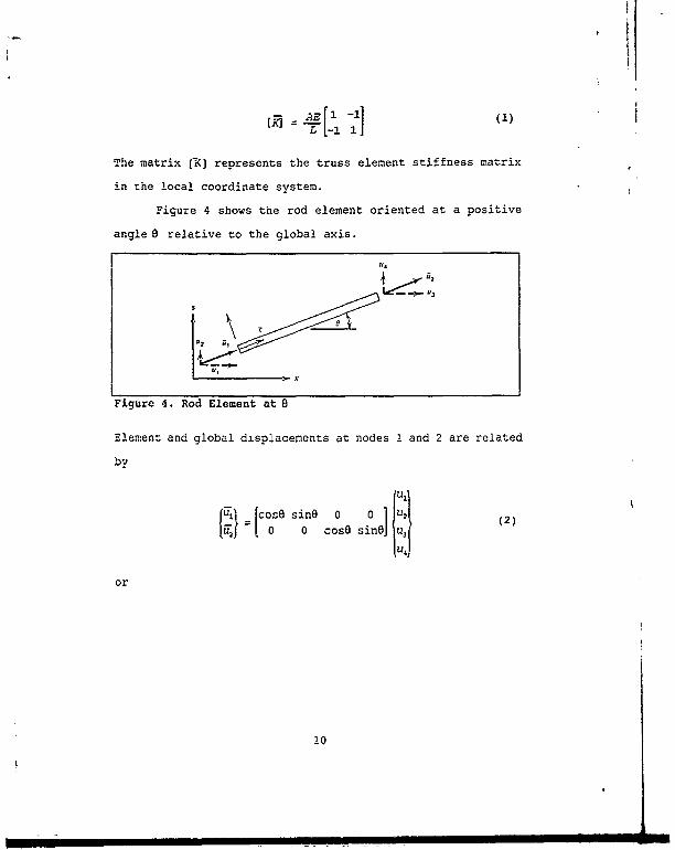
The matrix [9] represents the truss element stiffness matrix

in the local coordinate system.

Figure 4 shows the rod element oriented at a positive

angle 8 relative to the global axis.

114

Figure 4. Rod Element at 8

Element and global displacements at nodes 1 and 2 are related

by

1U = sin 0 U (2)

UJ 10 0 cosO sinG I

or

10

(U = [T] {u) (3)

where

[ r= osO sin8 0 0SO (4),0 cosO in

Using the strain energy equation and the matrix product

transpose rule, the following relations are derived:

- _. [u] ([) {u) (5)2

where

(I=2 T (T (6)

Therefore, using equations (1) and (6), (K] is transformed to

the global coordinate system to obtain

c2 CS - -C S

K= AE CS S' -CS -S1 (7)L l-c^ -CS C

2 csj

-CS -S2 CS SJ

where c = cos 0 and s = sin .

2. Beam Elements

Beam elements are characterized as members that are

capable of resisting bending. The beam element will carry

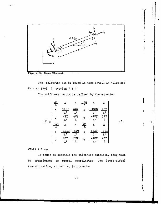
axial forces, shear forces and bending moments. Figure 5

depicts a typical planar beam finite element.

11

-A. El- 7f )

- L

Figure 5. Beam Element

The following can be found in more detail in Allen and

Haisler (Ref. 4: section 7.3.]

The stiffness matrix is defined by the equation

EA -EA 0 0L L

o 12EI 6E1 0 -122I 6E1LV L L 3 L

0 6E 4E1 0 -6EI 2M1L L L2 L (8)

-. A o E o oL L

0 -12EI -6R1 0 1221 -6EXV2 La V2 L2

o 6El 2El 0 -6S1 4EXL2 L L2 L

where I =I

In order to assemble the stiffness matrices, they must

be transformed to global coordinates. The local-global

transformation, Fs before, is given by

12

c sO 000-S C 0 0 0 00 0 1000 (9)0 00 C SO00 0 0 -s C 00 0 0 0 0 1.

where c = cos d and s = sin 0.

The remainder of the finite element formulation is

similar to the previous section on rod elements. The stiffness

matrix in global coordinates is constructed using equations

(6), (8) and (9).

3. Plate Bending Theory

A flat plate, like a beam, supports transverse loads and

offers resistance to bending. Figure 6 shows stresses that act

on a homogeneous linearly elastic plate.

Figure 6. Plate Stresses

The normal stresses a and a vary linearly with Z and

contribute to bending moments M, and M..

13

The normal stress o is negligible when compared with

a,, a, and -Y. The transverse shear stresses -r and -,, vary

quadratically with z. Plate bending in this analysis refers to

external loads perpendicular to the xy plane and applied

moments. (Ref. 5]

The stresses shown in Figure 6 result in the following

equations (Ref. 5] for bending moments M and transverse shears

Q.

r/ C/2 c2C /M= fo/ °zdz iy = i/ °zdz f T = 2/z 7 zdz (lOa)

QX = f. ! Zxdz Q, = f/2c,,d z (lOb)

Stresses a, and a are greatest at the surface z=±t/2,

while , is maximum at the midsurface. Transverse shear

stresses rZ\, ,, are small compared to o\, o and r,, and are

not considered in the classical Kirchhoff plate theory.

In what follows, Kirchhoff's plate theory (Ref. 5] is

briefly reviewed, which forms the basis for the GIFTS

formulation.

As transverse loads are applied to the plate, the points

on the midsurface move only in the z direction. Under loads,

normals to the midsurface are assumed to remain normal before

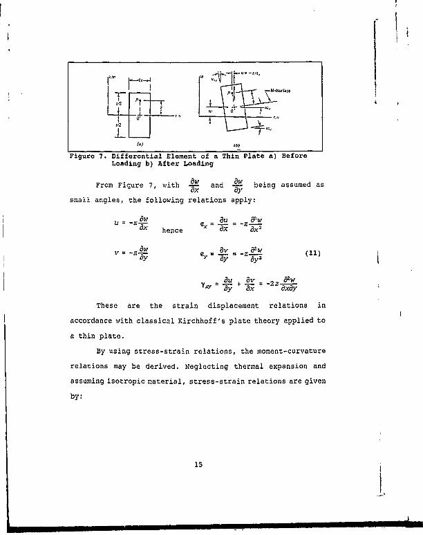
and after deformation. Figure 7 shows a differential element

of a thin plate before and after loading. As shown, the line

OP is perpendicular to the midsurface before and after loading.

14

II z +AftPt -

(ab)

Figure 7. Differential Element of a Thin Plate a) BeforeLoading b) After Loading

From Figure 7, with - and - being assumed asax 8ysmall angles, the following relations apply:

U ! u F W

ax hence -x "x 2

Zaw 8V 7w ii=- ( v (11)

ay ay 6y2

au +v 2z W2w

Yj FY; ax axay

These are the strain displacement relations in

accordance with classical Kirchhoff's plate theory applied to

a thin plate.

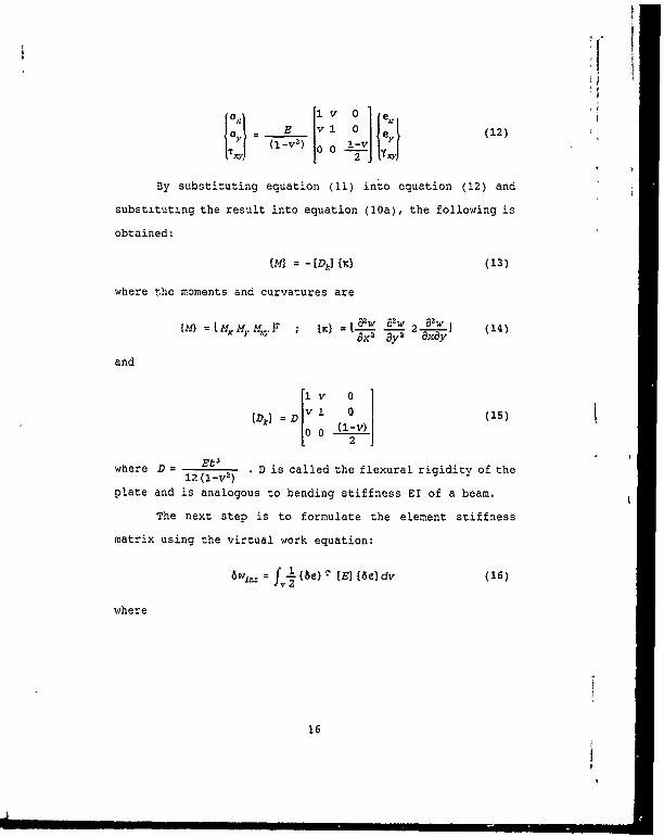
By using stress-strain relations, the moment-curvature

relations may be derived. Neglecting thermal expansion and

assuming isotropic material, stress-strain relations are given

by:

15

I,

lvlI E 1.

(12)

(I-V2) 0 0

By substituting equation (i1) into equation (12) and

substituting the result into equation (10a), the following is

obtained:

{M) = -[Dt] () (13)

where the moments and curvatures are

( M ) M) H, ; { -- 8w a 2 w ( 1 4 )3x2 aY axay

and

V1 0 (15)Dk] = D 0 0 ((-v)

where D - . D is called the flexural rigidity of the12 (1-0 2 )

plate and is analogous to bending stiffness EI of a beam.

The next step is to formulate the element stiffness

matrix using the virtual work equation:

1 e) (6} -E6e) d, (16)

where

16

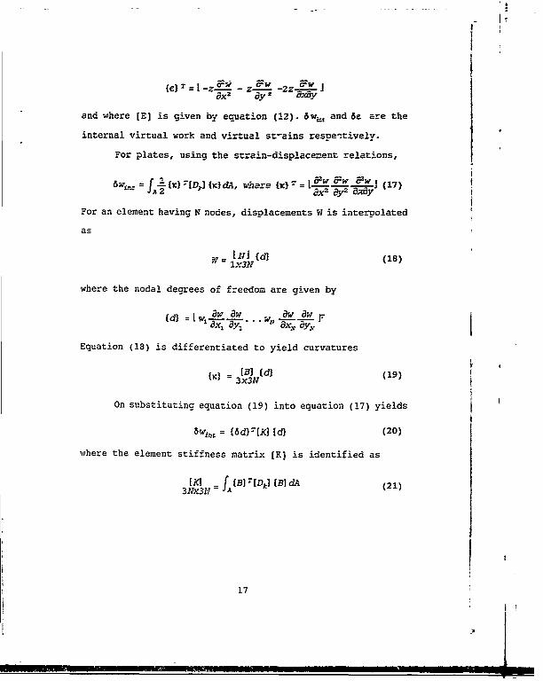
{e =I z.~± -z- -2z ?-!!.T72 ayz ,Xcy

and where [E] is given by equation (12). 6wi., and Se are the

internal virtual work and virtual st-ains resue :tively.

For plates, using the straim-disolacement relations,

W =fA ,[Djl WdA, where {r -w -w ~ (17)

-or an element having N nodes, displacements W is interpolated

as

Ix3I.1

where the nodal degrees of freedom are given by

-d w 8w w waw 'w

Equation (18) is differentiated to yield curvatures

[B] (d) (19)

On substituting equation (19) into equation (17) yields

5w, = {6d)r-[KJ {d}) (20)

where the element stiffness matrix (K] is identified as

XIV fA [B) -- D,)1 (B] dA (1

17

B. FREE VIBRATION OF MnIDGE-O-REO SYSTEMS

Craig j Reff. 61] provides a good overvi ew of mutidegro-

freedom (I-OF) systems.

The equation of motion f or a free undamped MDOF systen can

be written as

[nil (0) - ({u){) (22)

where [in) and [K] are (NxN) matrices and {u(t)) is a 1NxI

vector of generalized displacement coordinates. The solution

of the differential equation gives harmonic motion given by

U =U uCos (W"-) (23)

Substituting equation (23) into (22) yields the eigenvalue

problemi

(UK) 0w2[(M) U = 0 (24)

For non-trivial solution,

Ix~10 (25)

Equation 25 is recognized as the characteristic equation for

the free vibration response, The resulting polynomial in w2

yields the roots cr the eigenvalues which correspond to the

natural frequencies of the system.

18

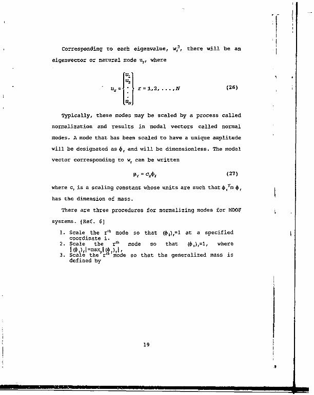
Corresponding to each eigenvalue, w,, there will be an

eigenvecor or natural mode u., where

U =1 r = 1,2 _..N (26)

Typically, these modes may be scaled by a process called

normalization and results in modal vectors called normal

modes. A mode that has been scaled to have a unique amplitude

will be designated as 4, and will be dimensionless. The modal

vector corresponding to w. can be written

P = cA4, (27)

where c, is a scaling constant whose units are such that 4mtr

has the dimension of mass.

There are three procedures for normalizing modes for MDOF

systems. [Ref. 6)

1. Scale the r ' h mode so that ( )r=l at a specifiedcoordinate i.

2. Scale the r'h mode so that (,),=i, whereI ( ,), I=maxl),3. Scale the r'" mode so that the generalized mass is

defined by

19

M.,~r* (28)

The generalized stiffr. for the r" mode is

= kA, (29)

By expressing equation (24) for the r'h mode and oremultiDling

by , the generalized stiffness-mass relations are obtained

as

K..= w-m1 (30)

C. NUMERICAL EVALUATION OF MODES AND FREQUENCIES OF MDOF

SYSTEMS

This section discusses the procedure used by GIFTS to

obtain numerical solution to large eigenproblems. The LACE

spacecraft in its fully deployed state was modeled by over

16,000 degrees of freedom. The dynamic analysis of this

structure involves determining the natural frequencies and the

corresponding natural modes by solving the equation

(K-Wi) 4 =0 (31)

Vector iteration methods are simple and elegant for obtaining

eigenpairs. The specific method used by GIFTS is the subspace

iteration method. The subspace iteration solution is very

effective in the calculation of the lowest eigenvalue and

corresponding eigenvectors of systems with large bandwidth and

which are too large for the high-speed storage of the

computer. (Ref. 7]

20

4

Bathe (Ref. 8] establishes three steps for the subspace

iteration method.

1. Establish q starting iteration vectors, q>p, where pis the number of eigenvalues and vectors to becalculated.

2. Use simultaneous inverse iteration on the q vectorsand Ritz analysis to extract the best eigenvalue andeigenvector approximations from the q iterationvectors.

3. After convergence, the Sturm sequence check is usedto verify that the required eigenvalues andcorresponding eigenvectors have been calculated.

The objective of the subspace iteration method is to solve

for the lowest p eigenvalues and eigenvectors satisfying

K+= 4A (32)

whereA=diagonal (A ) and=- 1, .... p]. The eigenvectors must

also satisfy the orthogonality conditions

V4K - A; 04 = I (33)

Detailed derivatione of the subspace iteration method are

shown in Bathe (Ref. 8]. TIq subspace iteration algorithm

shown below finds an orthogonal basis of vectors in EL+I

subspace.

= (34)

for L=1,2,..., and with iterations from EL to EL+I. Next,

projections of the operators K and M onto KL+I are computed:

21

K~ Z7J.±KXL.1 (35)

Ml Z -£ -(36)

By solving for the eigensystem of-projected bperators

~Kf~~~l& ~L.L4 (37)

where Q is an orthogonal matrix, Lxprove ipproximation tor

the eigenvectorg is found :by-

It may be coted that A L+l--> A azd XL+1 -- ) as L--)0.

The first step of the subspace iteration is to generate the

starting iteration vector6 in 31. The following aigorithm is

used to select the starting iteration vector. The first column

in MX1 is the diagonal of M. The other columns are unit

vectors with entries +1 at coordinates with the smallest k,/m,

ratio.

The subipace iteration method requires a measure to compute

convergence. Assuming that in (L-1) and L iterations,

eigenvalue approximations 1,E(L) and 1,(L+I), i=l, ...p, have been

calculated. The measure for convergence, then, is

I -1 _ )(L) IA ) - Scol ; 1 . .. p.9)

where tol may be 10'2s, when eigenvalues shall be accurate to

2S digits.

22

" ... ...... :I II " qll llL I -I. Ni I

Since equations (32) and (33) can be satisfied by any j

eigenpairs, there must be a way to verify the calculations.

Once the convergence is satisfied in equation (39), with s

being at least equal to 3, a check may be performed to make

sure that the smallest eigenvalues and corresponding

eigenvectors have been calculated. The Sturm sequence property

is used to provide this check. This property is derived from

the following analysis. (Ref. 8 By using the Gauss

elimination solution, the stiffness matrix can be factorized

as

K= LDLr (40)

where L is a lower unit triangular matrix and D is the

diagonal matrix.

Let K-pM be factorized into LDLT. In the decomposition of

K-pM, the number of negative elements in D is equal to the

number of eigenvalues smaller than p . Because of this

property, by assuming a shift V and checking whether p is

smaller or larger than the required eigenvalue, successive

iterations can reduce the interval in which the eigenvalue

must be. A summary of subspace iteration solution is shown in

Table II.

23

Table 11. SUMMARY OF SUBSPACE ITERATION 4

..,+

++

++ ++

-zE '.~.', ,

• I + 4.+ ,+.. . ,

E E

o0 0

24

I I III II I I I I I II . I II I I I I I I I II .. . .

III. LACE FINITE ELEMENT MODEL

A. GIFTS CAPABILITIES

GIFTS has several capabilities which facilitate the

modeling of large complex structures. Some of these

capabilities include:

1. automatic model generation

2. model editing, display and information

3. automatic load and boundary conditions

4. vibrational mode extraction

5. substructuring

6. thermal stress analysis

Element types that can be used include:

1. rods and beams

2. plates/shells

3. solid elements and axisymmetric elements [Ref. 9]

The elements can be selected from a library of options. The

materials can be created by the user or from a library of

defined materials. GIFTS also allows users to define

anisotropic materials.

Static and dynamic analysis can be performed on the model.

The dynamic analysis provides free vibrations and mode shapes.

These vibrational mode shapes can be displayed on the screen.

For structures that undergo thermal loading, deflections and

25

stresses can be calculated by computing thermal (pseudo-

forces) forces to simulate the thermal effects.

GIFTS also has the capability for substructuring and multi-

level substructuring. Large models may be divided into

substructures. Certain areas of a substructure may be modeled

as a second level substructure to allow economic modeling and

reduce computational costs.

B. SIMPLE FINITE ELEMENT MODEL OF LACE

Initially, the LACE spacecraft is modeled as a point mass

with three attached beam members. The three dimensional

triangular trusses are modeled as solid circular beams. To

ensure that this beam had the same bending characteristics,

the following bending stiffness relations was used from ASC-

Able Engineering (Ref. 10).

flexural rigidity (EI) = 1.51! ER4e2 (41)

where

e = maximum bending strain of longerons when completelycoiled (e = d/2R = F/E)

F = coiling stress of longeronsd = longeron diameterE = Young's modulus of longeron materialR = boom radius

with

e = .015R = 5.0 inchesE = 8.0 x 106 psi

This results in El = 5.3 x 106 lbs-in2.

26

From this relation, I is seen to be .663 which results in

a solid circular beam with a radius of .9583 inches. The beam

is with 10 elements for a 150 foot truss and 5 elements for a

75 ft. truss. This model is used in GIFTS with the appropriate

tip masses to determine the natural frequencies and mode

shapes. The results will be shown and discussed in the next

chapter. A listing of the file to generate the model is given

in Appendix A.

C. COMPLEX FINITE ELEMENT MODEL OF LACE

1. Main Spacecraft Body

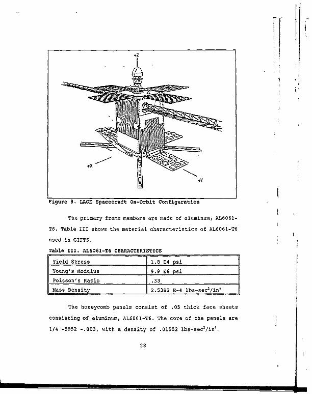
The on-orbit configuration of the LACE spacecraft is

shown in Figure 8. From the figure, it can be seen that the

LACE spacecraft consists of structural panels, solar panels,

sensor panels, truss elements and various beam types.

The primary structure of LACE consists of a frame type

structure consisting of channel section stringers, tee-section

stringers, z-section doublers, and angle-section members. The

primary structure also consists of honeycomb panels. Figures

9a and 9b show the basic configuration of the primary

structure.

The secondary structure of the LACE spacecraft consists

of the fixed and deployable solar array substrate, deployable

sensor panels and deployable sensor arms. Figure 10 shows the

LACE spacecraft secondary structure.

27

+Z

+x I

+Y

Figure 8. LACE Spacecraft On-Orbit Configuration

The primary frame members are made of aluminum, AL6061-

T6. Table III shows the material characteristics of AL6061-T6

used in GIFTS.

Table III. AL6061-T6 CHARACTERISTICS

Yield Stress 1.8 E4 psi

Young's Modulus 9.9 E6 psi

Poisson's Ratio .33

Mass Density 2.5382 E-4 lbs-sec2/in4

The honeycomb panels consist of .05 thick face sheets

consisting of aluminum, AL6061-T6. The core of the panels are

1/4 -5052 -.003, with a density of .01552 lbs-sec2 /in4.

28

ANGLE SECTION +z'SINGER . SPACE END

CORNER FITTING

C+X FIXEDSOLAR ARRAY

SOLAR ARRAY

CAEN-SECSCONTNSRNRING GE

A CX 'rRFIBOOM.-_ : MY ,. DECK

+XF

CHANNEL SECTION LNEO

STRINGER LOE

CORNER FF-NG

Figure 9a. LACE Spacecraft Primary Structure

Figures Ila and lib show the primary and secondary

honeycomb panel structure and dimensions.

The primary panels are one inch thick with a .9 inch

core. The solar array panels are .5 inches thick with a .4

inch core and the deployable sensor panels are .75 inches

thick with a core of .65. The deployable sensor arms are

channel beams with .125 inch thick aluminum, AL6061-T6.

The honeycomb panels are modeled as aluminum panels,

AL6061-T6, with appropriate conversions to account for

29

+Z.

SPACE END

STA. 96.00--- C+Y

STA. 68.375-...Q 1 II-B+X

STA. 41.75-:. B+Y

RIBOOM DC:A+X -

* A-Y A-X

STA. 0.00----. > A+Y

"'"SENSOR PLATE ASSEMBLY

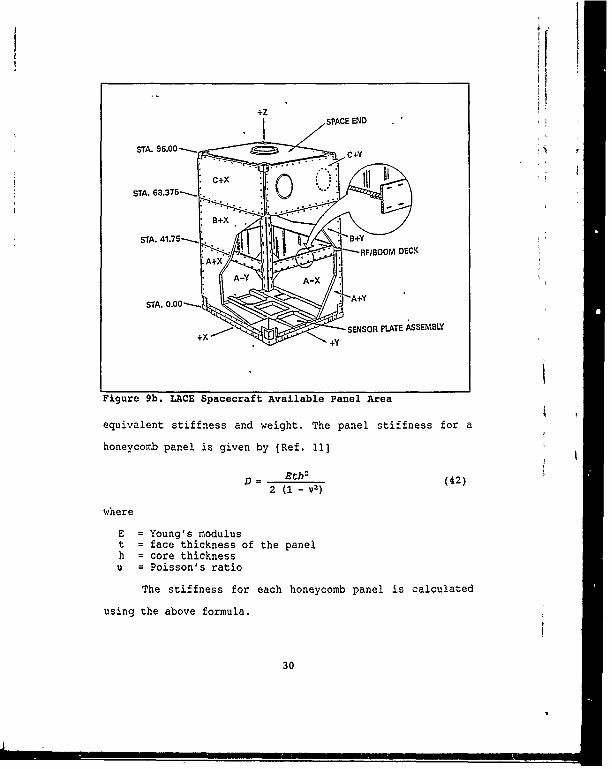
Figure 9b. LACE Spacecraft Available Panel Area

equivalent stiffness and weight. The panel stiffness for a

honeycomb panel is given by (Ref. 11]

D - Eth2 (42)

2 (1 - v2)

where

E = Young's modulust = face thickness of the panelh = core thicknessu = Poisson's ratio

The stiffness for each honeycomb panel is calculated

using the above formula.

30

4zi

DEPLOYABLESENSOR

ARIA 0. 00 0 DMABLE

SM SOR+X/ / ".r-

A + Y FIED -.

SOLAR ARRAY t .y

Figure 10. LACE Spacecraft Secondary Structure

Using the stiffness, an equivalent thickness is

calculated, using the flexural rigidity formula for isotropic

materials.

31

!

FACE SH=-- rMOo EL THIoCKAL. W 1 -76

_/

tooME

j _ ___ ___ _ _ ___ ___ ___HYSOL ..- 9

103 102 604 CORESER5 SERES SMS %-5052-.003

Figure 11a. Primary Panel

FACE SHE-ET.050 I. THICK

AL 6061-T67 s0 11',---4 .... ADHESIVE

I I .1HYSOL-Ff,.I-96

~' 102 103 FACE SHEET-SERIES SERIES .050 11. THICK

AL 6061-T6

L--- ADHESIVE.500 n. _ _YSOL"F"96

V 102 103 %/.5052-.003SERIES SERIES

Figure 11b. Secondary Panels

D - E 0 (43)12 (l-v 2 )

The mass of the honeycomb panels is computed and used

with the new thickness to determine volume and density. These

calculations are presented in Appendix B. Table IV summarizes

32 If

the new parameters used to =odel the honeyconb bafiels as ,

aluminum panels with appropriate stiffness and mass.

Table IV. THICKNESS AND DENSITY PARMETERS

Thickness (in) Density (lbs-sec2/in4)

Primary Panels I .624 5.364 x 1 0.S

Solar Panels I .3634 8.1915 x 10 .5

Sensor Panels .502 6.22 x 10-'

The finite elements model of the main body of the LACE

spacecraft is shown in Figuro 12. The associated file to

generate the model is given in Appendix C.

The LACE spacecraft has several sensors and components.

Even though the spacecraft is essentially a rigid body, the

mass of the components was modeled as accurately as possible

according to the mesh size of the grids. Appendix D contains

the component placements and mass distributions.

2. Spacecraft Trusses

The automatic deployable lattice booms are manufactured

by AEC-Able Engineering Company, Inc. They are designed for

applications that require high dimensional stability and high

ratio of bending stiffness to weight. Figure 13 shows the

principal parts of the continuous longeron boom and the

retraction geometry. The longerons are continuous along the

length and are connected to the batten frames with pivot

fittings. Six diagonals provide shearing strength and

stiffnesses. When the boom is twisted, tension increases on

three of the diagonals, causing batten members to buckle and

33

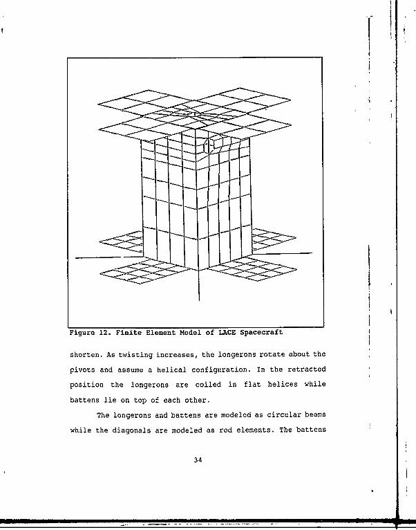
Figure 12. Finite Element Model of LACE Spacecraft

shorten. As twisting increases, the longerons rotate about the

pivots and assume a helical configuration. In the retracted

position the longerons are coiled in flat helices while

battens lie on top of each other.

The longerons and battens are modeled as circular beams

while the diagonals are modeled as rod elements. The battens

34

cONI, ON

-'/

Figure 13. Continuous Longeron Boom

are oval-shaped and attached to the longeron by pivot joints,

but for simplification the battens are modeled as circular and

the joints are not modeled. Listed in Table V are the

dimensions and properties of the truss. When fully retracted

the triangular batten frames lie within a 10 inch diameter

circle.

Figure 14 shows a cross-sectional view of the truss and

its dimensions.

35

... .... ....... .... ./ ... ...II i -"

ill

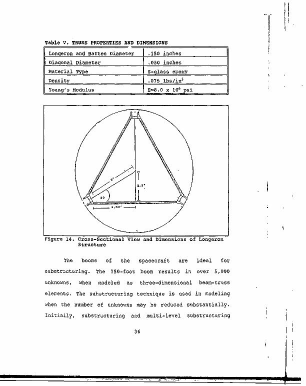
Table V. TRUSS PROPERTIES AND DIMENSIONS I

Longeron and Batten Diameter .150 inches

Diagonal Diameter .050 inches

Material Type S-glass epoxy

Density .075 lbs/in3

Young's Modulus E=8.0 x 106 psi

Figure 14. Cross-Sectional View and Dimensions of LongeronStructure

The booms of the spacecraft are ideal for

substructuring. The 150-foot boom results in over 5,000

unknowns, when modeled as three-dimensional beam-truss

elements. The suhstructuring technique is used in modeling

when the number of unknowns may be reduced substantially.

Initially, substructuring and multi-level substructuring

36

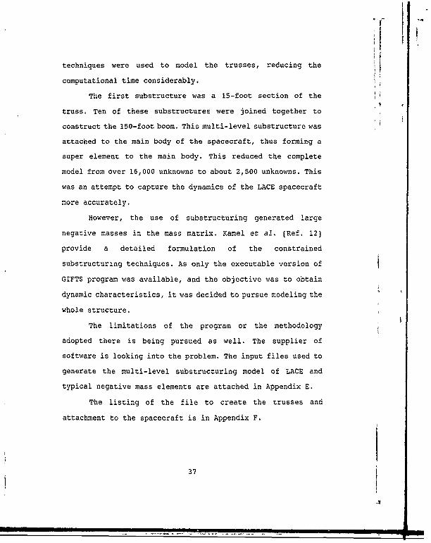
techniques were used to model the trusses, reducing the

computational time considerably.

The first substructure was a 15-foot section of the

truss. Ten of these substructures were joined together to

construct the 150-foot boom. This multi-level substructure was

attached to the main body of the spacecraft, thus forming a

super element to the main body. This reduced the complete

model from over 16,000 unknowns to about 2,500 unknowns. This

was an attempt to capture the dynamics of the LACE spacecraft

more accurately.

However, the use of substructuring generated large

negative masses in the mass matrix. Kamel et al. (Ref. 12]

provide a detailed formulation of the constrained

substructuring techniques. As only the executable version of

GIFTS program was available, and the objective was to obtain

dynamic characteristics, it was decided to pursue modeling the

whole structure.

The limitations of the program or the methodology

adopted there is being pursued as well. The supplier of

software is looking into the problem. The input files used to

generate the multi-level substructuring model of LACE and

typical negative mass elements are attached in Appendix E.

The listing of the file to create the trusses and

attachment to the spacecraft is in Appendix F.

37

IV. RESULTS OF DYNAMIC ANALYSIS

For linear behavior, resonance occurs when the frequency

of excitation equals the natural frequency. In order to avoid

the ill-effects of large amplitude vibration at resonance, the

natural frequency must be known and compared with potential

excitation frequencies. The gravity gradient pitch vibration

frequency is 2.3 x 10'4 Hz and is widely separated from the

lowest modes of the finite element models.

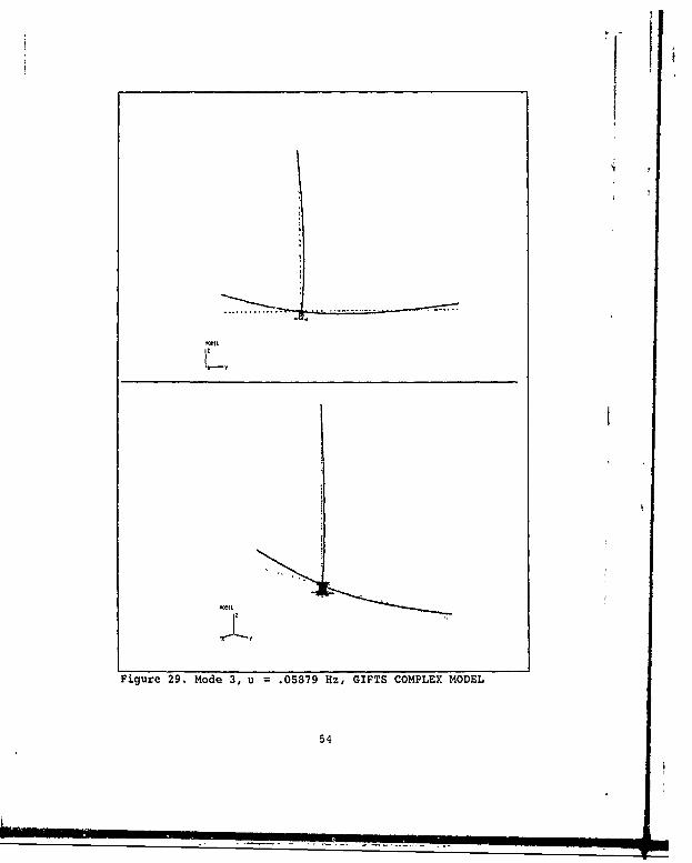
Table V presents computed values for the first four modes

of three different models of the LACE spacecraft.

Table V NATURAL FREQUENCIES OF THREE LACE MODELS

Mode GIFTS NASTRAN (Ref 1] GIFTSBeam Model (Hz) Beam Model (Hz) Complex Model (Hz)

1 .01930 .01935 .0216

2 .04825 .04729 .0516

3 .05454 .0536 .0588

4 .1738 .1106 .1253

Initially, the NASTRAN beam model was developed by Naval

Research Laboratories (NRL). The present beam model was

developed as described in the previous chapter. The first

three modes agree within 2%, however the present fourth mode

appears to be an anomaly. The GIFTS complex model is

consistently 10% higher than the NASTRAN model. The NASTRAN

model appears to yield fairly good data in the lower modes.

38

This discrepancy may be attributed to the modeling

uncertainties and approximation of the geometric and stiffness

distributions. The detailed modeling of NASTRAN was not

available. It may be noted that there is no excitation

frequencies at those computed frequencies. Further, complex

modeling is recommended when higher modes and frequencies are

required. The simple model may not capture these higher modes

and even skip some modes. The higher modes assume importance,

especially, for very flexible structures and in the design of

control systems for vibration control and suppression. Figures

15 to 20 show the mode shapes and frequencies for the NASTRAN

model while Figures 21 to 26 show the data for the GIFTS beam

model. Figures 27 to 30 show the GIFTS complex model of the

spacecraft. Appendix F contains the frequency and mode shapes

of the LACE spacecraft in three configurations as it deploys

to its final state.

39

z 'z

Figure 15. Mode 1, u =.01935 Hz, NASTRAN BEAM1 MODEL

40

lx

z

Figure 16. Mode 2, u =.04729 Hz, NASTRAN BEAM MODEL

41

yl

z x

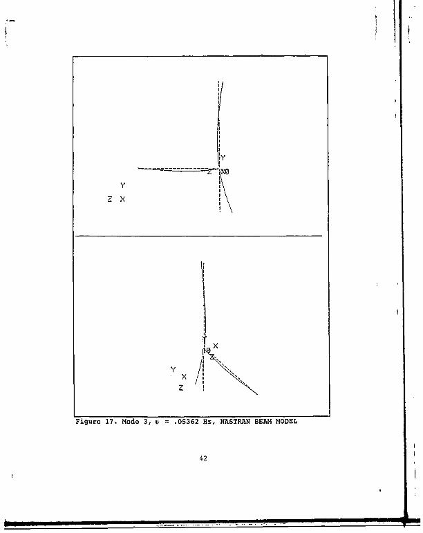
Figure 17. Mode 3, u =.05362 Hz, NASTRAN BEAMd MODEL

42

- x

XD

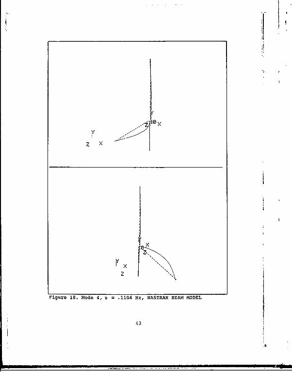
Figure 18. Mode 4, u =.1104 Hz, NASTRAN BEAM MODEL

43

z z

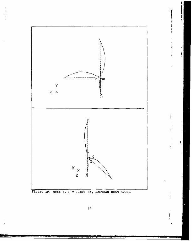
Figure 19. Mode 5, U =.1808 Hz, NASTRAN BEAM MODEL

44

"o

z X

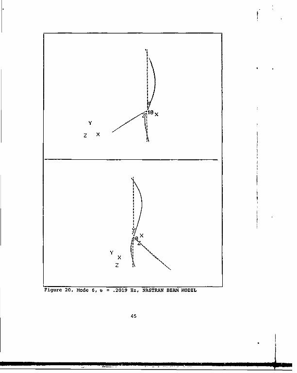
Fiur 20 oe6$ 21 zNSNBA OE

45

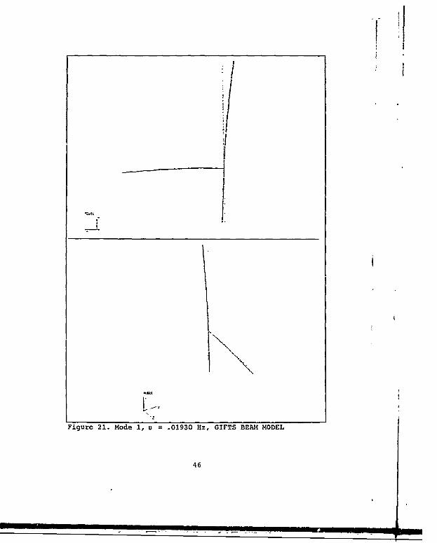
Figure___21. _Mode __1,_u __.01930 __Hz, _GIFTS __BEAM__MODEL

46

Figur 22.Mode , u 04825Hz,(IFSBAMOE

- 47

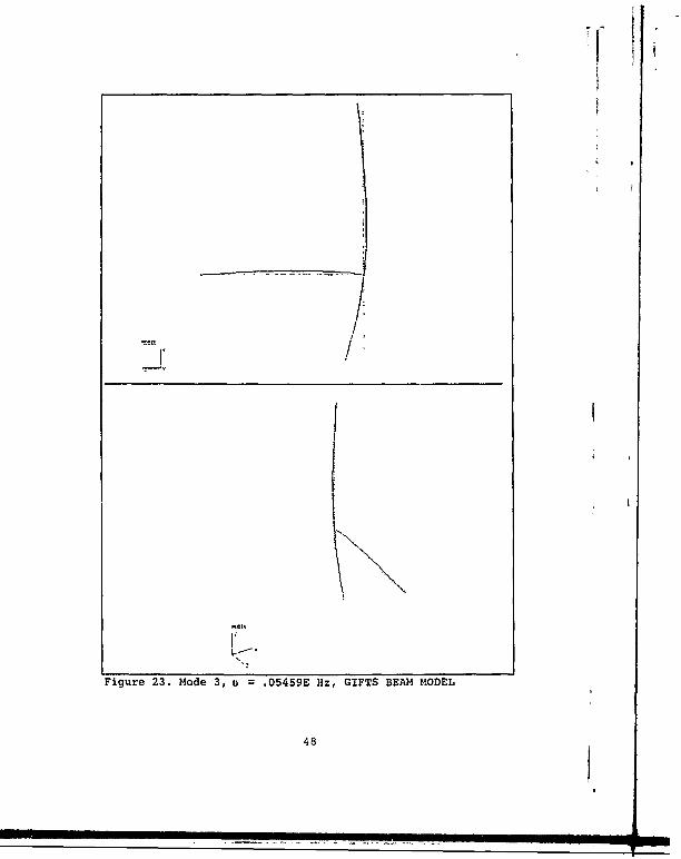
Figure 23. Mode 3, u =.05459E Hz, GIFTS BEAM MODEL

48

Figure 24. Mode 4, u =.1738 Hz, GIFTS BEAM MODEL

49

Figure 25. Mode 5, u =.2142E Hz, GIFTS BEAM MODEL

50

Ii

K

II

Figure 26. Mode 6, u .2349 Hz, GIFTS BEAM MODEL

51

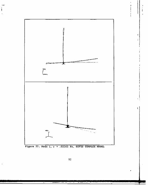
Figure 27. Mode 1, u =.02163 Hz, GIFTS COMPLEX MODEL

52

Figure 28. Mode 2, u =.05165 Hz, GIFTS COMPLEX MODEL

53

.77.

Figure 29. Mode 3, u .05879 Hz, GIFTS COMPLEX MODEL

54

Figure 30. Mode 4, u .1253 Hz, GIFTS COMPLEX MODEL

55

V. THERMOELASTIC EFFECTS

A change in temperature along a bar will change its

dimensions. When an isotropic bar is heated uniformly and is

free to expand, the sides will increase in length. The

material undergoes a uniform thermal strain e, given by:

= (AT) (44)

where a is the coefficient of thermal expansion ai~d AT is an

increase in temperature. The length of the bar will increase

by an amount

8,= a (AT) L

where L is the length of the bar.

The ABLE booms (Ref. 10] used on LACE are designed so that

they undergo minimum thermal bending or twisting in the solar

radiation environment. Pretwist is used to prevent thermal

twisting or thermal bending that would occur if one longeron

is shadowed by another.

This chapter presents analysis for deformations that could

result in a worst case scenario. Two possible scenarios

considered are when the boom may bend due to unequal heating

of the diagonals and unequal heating of the longerons. Unequal

heating of the diagonals is more likely to occur than unequal

heating of longerons. (Ref. 133. The following analysis

56

considers only the unequal heating of the diagonals and

assumes no shadowing effects.

Sources of heat include spacecraft components, solar flux,

albedo flux and thermal radiation of the earth. The solar flux

is defined as the flux existing at a distance of one

astronomical unit (AU) from the sun. Albedo flux is the

fraction of total incident solar radiation on the earth which

is reflected into space as a result of scattering in the

atmosphere and reflection from the clouds and earth surfaces.

Thermal radiation from the earth is the portion of incident

solar radiation absorbed by earth and its atmosphere and re-

emitted as thermal radiation according to Stefan-Boltzman law

(Ref. 11]. For the computation of LACE thermal deformations,

the following data is used (Ref. 13):

Solar flux: 442 Btu/sq ft hr

Thermal Earth Radiation: 70 Btu/sq ft hr

Albedo flux: 160 Btu/sq ft hr

c/ = .8

where e is the emissivity and a is the absorptivity.

The worst case of unequal diagonal heating occurs when the

sun rays are parallel with one set of diagonals and almost

perpendicular to the other set. The set of diagonals

perpendicular to the sun will receive maximum solar flux. The

parallel set will receive no solar flux, but will receive

earth's albedo and thermal radiation flux. A simple approach

is taken where the hottest and coldest temperatures of the

57

sMown

diagonals are calculated. This results in a maximum

temperature of 192'F and a minimum of -5F, Following the

discussion in Ref. 12, calculations are carried out and

presented in Appendix G.

It is assumed that the battens and longerons receive equal

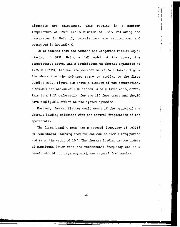
heating of 800F. Using a 3-D model of the truss, the

temperatures above, and a coefficient of thermal expansion of

1.75 x 10"6/OR, the maximum deflection is calculated. Figure

31a shows that the deformed shape is similar to the first

bending mode. Figure 31b shows a closeup of the deformation.

A maximum deflection of 1.88 inches is calculated using GIFTS.

This is a 1.2% deformation for the 150 foot truss and should

have negligible effect on the system dynamics.

However, thermal flutter could occur if the period of the

thermal loading coincides with the natural frequencies of the

spacecraft.

The first bending mode has a natural frequency of .02163

Hz. The thermal loading from the sun occurs over a long period

and is on the order of 10,4 . The thermal loading is two orders

of magnitude lower than the fundamental frequency and as a

result should not interact with any natural frequencies.

58

Figure 31a. Thermal elastic effects resemble 1st bending modeshape.

59

Figure 31b. Close-up view of thermoelastic effects

60

VI. MULTI-BODY DYNAMICS

A. COMPONENT MODE SYNTHESIS

in the previous chapter, finite element techniques were

used to formulate a model of the LACE spacecraft for use in

structural dynamics analysis. This section discusses a class

of reduction methods known as component mode synthesis, or

substructure coupling for dynamic analysis. These methods are

useful for analysis of large structural dynamics problems.

The basic idea of component mode synthesis is to treat the

complex structure as an assemblage of substructures. Each

substructure is analyzed independently and then their dynamic

characteristics (mode shapes and natural frequencies) are

synthesized to analyze the complete structure. There are many

variations of the method of component mode synthesis and

extensive iitera-ure is available (Ref. 14, 15, 16, 17].

Hurty (Ref. 14] developed a procedure for analysis of

structural systems using a displacement method which used

three types of generalized coordinates, namely: 1) rigid body

coordinates, 2) constraint coordinates, and 3) normal mode

coordinates. Hurty used Rayleigh-Ritz approach in his

formulation. The Craig-Bampton method [Ref. 15] is similar to

the treatment due to Hurty, except that it simplifies the

treatment of rigid-body modes of substructures by eliminating

61

I.the separation of boundary forces into statically determinate

and statically indeterminate reactions [Ref. 15]. MacNeal

[Ref. 16] introduced residual flexibility modes to retain the

static contribution of a higher frequency truncated modes.

Rubin [Ref. 17] developed a new method which adds residual

inertial and dissipative results to the method introduced by

MacNeal [Ref. 17].

This section will present the basics of component mode

synthesis.

Craig [Ref. 18] provides a good overview of component mode

synthesis methods. His notation and examples will be used

extensively in this discussion.

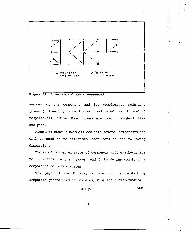
A substructure is generally connected to one or more

adjacent components and is composed of interior degrees of

freedom and boundary degrees of freedom. Figure 32 illustrates

a substructure connected to other components and shows

boundary and interior coordinates.

The equation of motion for a component is given by

Mk t C2 + KX = f (45)

where M is the mass matrix, C is the damping matrix and K is

the stiffness matrix.

The total set of physical coordinates of the component is

defined as P, while interior and boundary points will be

defined as I and B respectively. Boundary coordinates are

further subdivided into statically determinate (rigid body)

62

loundnry o Interiorcoordinate coordinate

Figure 32. Unrestrained truss component

support of the component and its complement, redundant

(excess) boundary coordinates designated as R and E

respectively. These designations are used throughout this

analysis.

Figure 33 shows a beam divided into several components and

will be used to to illustrate mode sets in the following

discussion.

The two fundamental steps of component mode synthesis are

to: 1) define component modes, and 2) to define coupling of

components to form a system.

The physical coordinates, x, can be represented by

component generalized coordinates, P by the transformation

X = *P (46)

63

i

I I

Figure 33. Beam model divided into components

where * consists of component modes of specified type [Ref.

14]. These include:

normal modes of free vibration

attachment modes

constraint modes

rigid body modes

inertia relief modes

These modes are defined as follows. [Ref. 17)

1. Normal Modes

Normal modes are classified as fixed interface normal

modes, free-interface normal modes or hybr:id-interface normal

modes depending on how the interface coordinates are

restrained when the component normal modes are obtained using

64

(K -97,2M) ,P =O0 (47)

The modes are normalized with respect to the mass matrix m.

m,, = I) * K,, A, : diag(Wp)2

where 4,, is component normal modes. The notation 4 will be

used for normal modes, while * will be used for assumed modes.

2. Constraint Modes

A constraint mode is defined by statically imposing a

unit displacement on one coordinate of a C set of physical

coordinates. Let C=E and define a constraint mode by placing

a unit displacement on one coordinate of the C set and zero

displacement on the remaining C set. The matrix of constraint

nodes, *, is defined by the equation:

[Ke, KC K. c1 Re (48)

KK1 K1 o lRre

This equation may be simplified to yield

= = (49)

3. Attachment Modes

Attachment mode is defined by applying a unit force of

the coordinates of an A set (Ref. 15]. In this case,

attachment modes will be defined for A = E. The matrix of

attachment modes t, is shown by the equation

65

K31 K33.Kjr ~~=II~rK., K.. K.~~i 8 JR (50)[K 1 K,. 110 !R,,

Using the first two rows of equation (50) , may be

represented by

I*ia [1]

= =g.1] (51)

where g = K*V is the flexibility matrix.

4. Rigid Body Modes

The boundary conditions are depicted in Figure 45, where

the R set will restrain the component from rigid body motion

and the E set contains redundant boundary conditions. By

defining the' rigid body modes relative to the R set, the

equation is given by

iiI I e K

K I K. K.r] (52)

which simplifies to

1K11 Kle [1irI r ~z (53)11 K.1 1LI*.]j =K.rJ

The *, matrix is given by

66

[tl t , r= = g [eir (54)

5. Inertia-Relief Modes

This method defines attachment modes for a component

with rigid body freedoms. This method was presented by Rubin

(Ref. 16] and MacNeal (Ref. 17]. By letting D'Alembert force

vectors associated with rigid-body modes be applied statically

to a component which is fully constrained on the boundary, 1 m

can be defined as follows.

[ 11 Ka K 1 11 ir 0

K., K. K., = . , H., ,., + kn (55)K' K,. Kr,] [, ;. M,, L, rr

*1-1 IK (Moli° 1 = Miir = Mi0 0a (56)

6. Coupling of Components

This section describes generalized substructure coupling

as applied to free vibration analysis. [Ref. 18]

Assuming two components a and 0 having a common boundary

interface, compatibility of interface displacement requires

X0 1 (57)

The interface forces are related by

67

f", 41'= 0(58)

By representing the physical coordinates x, by

generalized coordinates p, the following equations are derived

%a = *tp4 , XP = Opp (59)

where *4 and * contain assumed static and dynamic modes.

The constraint equations can be written in generalized

form to form a single constraint equation

CP = O (60)

where

(61)

Let P be rearranged and partitioned into dependent PD and

independent, PI, coordinates. Then,

ICDDCD] 0= O (62)

where Cad is nonsingular square matrix and equation

-PP1 [ -rCz~ C IlPr=S (63)

defines S and g, where

S= L-Cil CIIrj (64)Ix'

The p and x corresponding to P are given by

68

Ili 0 ;] I, 0 x (65)

The coupled system of equations for an undamped system

is given by

Mg + Kg = 0 (66)

where

M SILLS , K = S xS (67)

B. DYNAMICS OF FLEXIBLE BODIES IN TREE TOPOLOGY

1. Overview of Multibody Systems

Spacecraft and large spacecraft structures are typical

multibody systems. Large strides have been made in the last 20

years in the efficient formulation and solution of multibody

systems. Particular interest in multibody dynamics has risen

in spacecraft dynamics. Initially, space vehicles were

idealized as rigid bodies or elastic beams. In the mid-1980s

equations of motion were published ior a point-connected set

of interconnected rigid bodies in a topological tree. A model

containing rigid bodies and elastic appendages was eveloped in

the 1970s. The next major step was the incorporation of body

flexibility in the topological tree model. (Ref. 19]

2. Multibody Computer Program - TREETOPS

TREETOPS is a computer program developed to deal with

multibody structures in an open-tree topology. It is a time

69

history simulation of a complex multibody flexible structure

with active control elements. Some of the features include: 1)

any or all bodies can be rigid or deformable, 2) hinges can

have zero to six degrees of freedom, 3) the dimension of the

problem equals the number of degrees of freedom, 4) individual

body deformation can be described by any set of modal vectors,

5) an interactive program, and 6) extensive control simulation

capability. [Ref. 18]

The computer simulation consists of three parts:

defining a tree topology of flexible structures, define a

controller and a set of sensors and actuators.

The structure of the TREETOPS model consists of bodies

and hinges with sensors and actuators included for interfacing

with the control system. Figure 34 shows a typical structure.

a. Body Types

The program simulates a set of bodies in a tree

topology. Each body is defined independently. Sensors,

actuators and hinges are connected to specific points called

node points. Each body may be defined as rigid or flexible.

Each body is to be defined with an ID number, mass

properties, center of mass and all its pertinent node points.

(Ref. 20]

b. Hinges

Hinges interconnect two adjacent bodies. One body

is called the inboard body and the other is called the

outboard bocy. The inboard body is the one on the side closest

70

BODT 3 BODY 2

HINGR 3 / HINGE 2

BODY I

INERTIAL REFERENCEFRAM

Figure 34. Structure composed of bodies and hinges

to the inertial reference frame. Figure 35 shows a hinge

representation.

The functions of the TREETOP hinges are to

[Ref.20]:

1. define topology of thq structure

2. define kinematic variables of the multibody system

3. define relative orientation between adjacent bodies.

c. Sensors and Actuators

A set of 16 sensors have been builz into the

simulation. They include rate gyros, resolvers,

71

1NDOAAL D BODY OUTBO k BODY

Cb

Figure 35. General representation of jth hinge

accelerometers, position and velocity sensors, tachometer, sun

and star sensors, etc. The actuators serve as a way to apply

force and torqup inputs. Inputs may be control or disturbance

inputs. Disturbance inputs can be applied with function

generators to the actuators. Actuator types include reaction

jets, hydraulic cylinder, moment actuator and torque motor.

d. Orbit Environment

TREETOPS has the capability to model the orbit

environment of a spacecraft to include gravity gradient and

aerodynamic drag. A magnetic field model is included which

produces a force through interaction with magnetic actuators.

In computing the atmospheric drag, TREETOPS uses atmospheric

72

d3rzity co-z aued from tbe XC3IA 1970 atospheric =ode!. 1:-he

smacecr; -It orbi- is determined b-i enterino the six orbital

parameters.-

73

VII. CHAOTIC VIBRATIONS

A. HOW TO IDEUNTIFY CHAOTIC VIBRATIONS

Chaos is defined as a cotion that is sensitive to initial

conditions [Ref. 21]. Chaos can occur only in nonlinear

systems, but all nonlinear systems do not exhibit chaos. Chaos

can be observed in many physical systems. A partial list is

shown:

-. Vibrations of buckled elastic structures

2. Mechanical systems with play

3. Large, three-dimensional vibrations of structures

4. Aereoelastic problems

5. Systems with sliding friction

6. Feedback control devices

In order to identify chaotic motions, several procedures

are suggested [Ref. 21]. such as

1. Identify nonlinear elements in the system

2. Check for sources of random input in the system

3. Observe time history of the measured signal

4. Observe phase plane history

5. Examine Fourier spectrum of the signal

6. Determine Poincar6 map of the signal

7. Vary system parameters

74

Quantitative characteristics of chaotic vibrations and the

diagnostic tools used are su=marized as follows:

1. Sensitivity to changes in initial conditions(Lyapunov exponent and fractal basin boundaries)

2. Broad band spectrum of Fourier transform, when motionis generated by a single frequency

3. Fractal properties of the motion in phase space whichindicate a strange attractor (Poincare maps, fractaldimension)

4. Increasing complexity of regular motions asexperimental parameters are changed

5. Transient or intermittent chaotic motions;nonoeriodic bursts of irreaular motion or initiallyrandom-like motion that settles into regular motion.

1. Nonlinear System Elements

A linear system does not exhibit chaotic vibrations.

Typical nonlinear effects from mechanical systems include

nonlinear stiffness, material nonlinearity, nonlinear damping,

free-play, and nonlinear boundary conditions. Nonlinear

elastic effects can be due to large deformation. A good

example of material nonlinearity is the stress-strain

relations of materials modeling rubber or elastomers.

2. Random Inputs

There are no assumed random inputs in chaotic

vibrations. Applied forces and excitations are assumed to be

deterministic. By definition, chaotic vibrations arise from

deterministic physical systems. A large output signal to input

noise ratio is required if nonperiodic response is to be

attributed to a deterministic system behavior. (Ref. 21]

75

3. Observation of Time History

The first indication of chaos may be indicated in the

time history. The motion observed shows no visible pattern or

periodicity and may be chaotic or random.

This method is not conclusive, since motion could have

a long-period behavior that is not detected or quasiperiodic

motion where two or more periodic signals are present.

4. Fourier Spectrum

The presence of a broad band Fourier spectrum in the

output is another clue that may be used to suspect chaotic

vibrations. A precursor to chaos is the presence of wo/n

subharmonics. However, multiharmonic outputs do not always

imply chaotic vibrations as hidden degrees of freedom may be

present.

5. Phase Plane History

in the phase plane, complete information about a

dynamical system is represented by a point. At the next point

in time when the system dynamics change, the point is

displaced.

This moving point gives the history of the dynamical

system. The coordinates chosen for the study of dynamics,

typically, are the amplitude and velocity of motion. Figure 36

shows the phase plane of a simple pendulum. The circle on the

phase plane represents the motion over one cycle and is called

the trajectory. It should be noted that a periodic motion is

a closed orbit in the phase plane and is called a limit cycle.

76

velocity is zero as tile [)en.

dulurnstaffs itSvs~itg Pou-sition isa negatile llinlier.

the distance to tile leit offile center.

. Thle ts~onutinhers specify

asingle point in tv~o-di.

Velricit' i% l ts he ix

position a,~ e throughzero

Winch)~ dctrne again toZero, slid then becomesne'gative to represent left.

iVa'd

nmotion

Figure 36. Phase plane of a pendulum [Ref. 211

Chaotic motions have orbits that never close or repeat. As a

result, the trajectory of the orbits will tend to fill up the

phase plane.

77

6. Pseudo-Phase-Space Method

This method is used when only one variable is available,

as in typical flight tests where measurements are from a

strain-gage or accelerometer. In order to do the 2-D phase

plot from strain-gage measurements, the signal must be

differentiated. In the case of accelerometer data, the signal

has to be integrated twice.

However, by integrating or differentiating, the signal

is filtered (Ref. 22]. Differentiating the signal will amplify

high frequencies and attentuate low frequencies. integration

will have an opposite effect. As a result, phase plane plots

obtained from experimental data will be inaccurate. This

resulted in the development of the pseudo-phase-space method

or embedding space method. For a one degree system with a

measurement x(t), the signal is plotted against itself but

delayed or advanced by a fixed time constant: [x(t), x(t+T)].

This plot yields properties similar to the classical phase

plane. The closed trajectory in the classical phase plot will

be closed in the pseudo-phase method and chaotic motion appear

chaotic in both phase planes.

When the state variables are greater than three

(position, velocity, time), higher dimension pseudo-phase-

space may be constructed using multiple time delays, i.e.,

(x(t), x(t+T), x(t+2T)).

The advantage of the pseudo-phase plane method is that

a single observable variable can be used to construct the

78

pseudo phase picture and portray the system dynamics without

distorting the response through integration or

differentiation.

7. Poincar6 Section

The Poincar6 section can be constructed by placing a

two-dimensional surface in a three-dimensional phase space and

noting where the points of the trajectory penetrate this

surface. This slice will reveal the internal structure of this

location.

If the Poincar6 section does not consist of a finite set

of points or a closed orbit, the motion may be chaotic. For

some lightly damped systems, the Poincar6 section of chaotic

motion appears as a set of unorganized points. This motion is

called stochastic and is shown in Figure 37a. In damped

systems, the Poincar6 section appears more organized with

parallel lines as shown in Figures 37b and 37c. The Poincar6

sections can be enlarged to observe further structure (Figure

38). After several enlargements, if the structured sets

continue to exist, the motion is defined as a strange

attractor. This embedding of structure within the structure

indicates fractal nature of the behavior, which is a strong

indicator of chaotic motions.

B. QUANTITATIVE TESTS FOR CHAOS

The previous section summarized qualitative methods that

require experience to evaluate chaotic systems. There are some

79

I I F

Figure 37. Poincar6 maps chaotic motion

quantitative measures to study chaotic motions. Two well-known

methods are the Lyapunov exponent and fractal dimension (Refs.

22, 25]. Tl'ese methods are described below. The Lyapunov

exponent will not be used in this analysis and will be

discussed summarily.

1. Lyapunov Exponent

The Lyapunov exponent measures how sensitive the system

is to changes in initial conditions. It measures the

exponential attraction or separation, of two adjacent

80

Figure 38. Poincar6 map of chaotic vibration

tra3ectories in phase space with different initial conditions.

It is defined as

d(t) =d2L (68)

or

L=lo2 (t) (69)

where d is the initial distance between two trajectories.

d(t) is the distance at a later time.

L is the Lyapunov exponent.

81

A positive exponent implies d(t), the later distance

will be larger than the initial distance and indicates chaotic

dynamics.

2. Fractal Dimension

The fractal dimension is another quantitative test for

chaos and gives a lower bound on the number of essential

variables needed to model the dynamics of the system. Non-

integer values for a fractal dimension indicates presence of

a strange attractor. (Refs. 22,25]

There are six ways to classify fractal dimensions. The

dimension that will be discussed in this analysis is the

correlation fractal dimension.

The correlation fractal dimension is defined as

C(r) = r (70)

where: C(r) is the probability of the attractor within a

circle, sphere or hypersphere of radius r, and d is the

fractal dimension.

By taking the natural logarithm of both sides of

equation (70) and solving for d, following equation results:

d = lim I iC- ))

The procedure adapted in Sarigul-Klijn (Ref. 22] is

described below:

1. Start with a point on the attractor and calculate thenumber of points inside a circle of radius r.

82

2. Calculate probability C(r) by dividing this number ofpoints by total number of points in the attractor.

3. Repeat this for several points along the attractor.

4. Compute C(r) for several values of r.

S. The slope of log (C(r)) versus log (r) gives d, thecorrelation fractal dimension.

To obtain the correlation dimension of the attractor of

a given system, the procedure must be applied in the pseudo

phase space for several embedded dimensions. The asymptotic

value of the correlation dimension is the fractal dimension of

the attractor and is given by

C(r) = lim -L -Ix 1-xjl) (72)

where: H(s) = 1 if s>O and H(s) 0 if s<0.

Ix, - xJI is the Euclidean distance between the points.

N is total number of points.

If the fractal dimension is approximately equal to the

phase space used for the calculation, the attractor lies in a

higher dimensional phase space. If the fractal dimension is

non-integer and is independent of the dimension of phase

space, the signal is characterized as chaotic. (Ref. 22]

C. LACE SPACECRAFT BOOM AS A NONLINEAR SYSTEM

The booms for the L.E ;- -cecraft have a constant EI

distribution [Ref. !O] and the response would appear to be

linear. However, at each bal, battens are joined to the

83

longerons by joints. Freeplay introduced at the joints tend to

introduce nonlinearities. In this section, the spacecraft boom

elone is modeled and a parametric study to simulate the

in.fluence of nonlinearities introduced by the freeplay at the

joints on the system response is presented. The resulting

behavior of the motion is studied using the methods of chaos

(Ref. 21].

The LACE spacecraft boom is modeled as a nonlinear single-

degree oi freedom system. The equation of motion for such a

system is described by

meu+f(u, ), t) = ACoswt (73)

where f(uu,t) contains nonlinear damping and stiffness terms.

The stiffness of the boom is modeled as

fE = A, u3 + B, U2 +C, U + d,

and the damping as

f = A 2+ BA+ C2

For the present analysis, the damping is assumed to be linear

and contains only the linear term corresponding to equivalent

viscous damping. The nonlinear stiffness contribution due to

the joints is modeled by the cubic term, Au3. The linear term

representing the boom stiffness distribution is determined

from the experimental stiffness properties of the beam using

the relation

84

F= 12EI (74)

The coefficient for the cubic term is treated as a parameter

and as part of the parametric study, is varied as a function

of the linear term as follows

A = C. + nC (75)

where n varies from ±.l to ±.5. The equation of motion reduces

to Duffing's equation in the following form:

mni + B20 + A10 + C~u = Aocoswt (76)

The response of this nonlinear system to a forcing function is

determined by approximating the derivatives as shown in the

equation of motion. A solution based on step-by-step

integration is used to generate the time response. A FORTRAN

program was developed based on the "linear acceleration

method" and is presented in Appendix I. The recursion formulas

used for the numerical integration is derived in the following

analysis.

In the linear acceleration method adopted here, the

acceleration is approximated for a given step by the following

relation:

+ (77)

Integration of equation (77) yields

85

I I+(Ad'z) -2 (78)di ~~ ~ = + f t 2

and

. 2 1 + + + (79)2 At 6

By using incremental quantities, Ap,, Au,, Ala,, and A-u,, the

computational algorithm is set up. Equation (79) may be solved

for u, and equations (78) and (79) are be combined to give Au,

as follows:

AI = u - L) - 3t11 (80)At, 1 AtL I

= 1 3Au,- -- O (81)

Since equation (73) is satisfied at both t, and t.+,, it may be

written as

MA + C1Adt + kjAu1 = AP i (82)

Combining equations (80), (81), and (82) yields the

incremental equation of motion

KjAui = Apl (83)

where

86

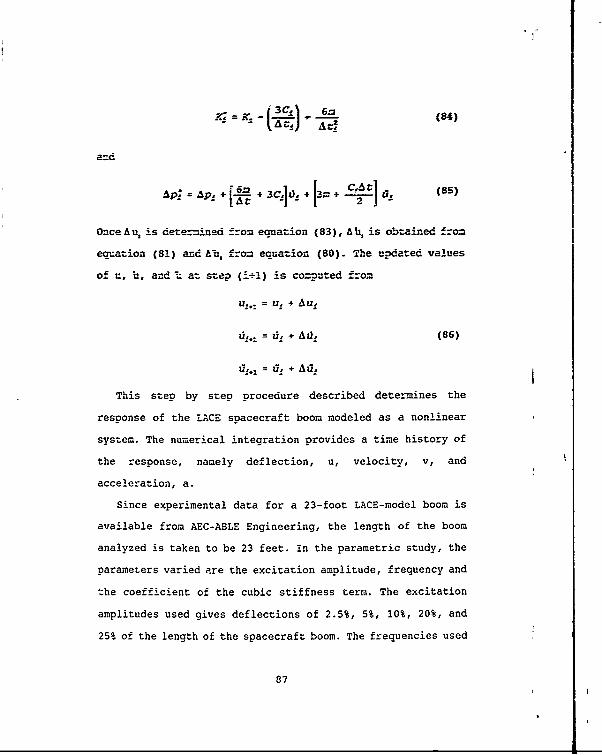
S3C,) 6m

(84)

and

Ap=A, 6D 3IM .4I~~j0 (85)

Once A u, is determined f-om equation (83), Ah, is obtained from

equation (81) and Ab, fro= equation (80). The undated values

of u, b, and l a: step (i-1) is commuted from

u,. = u, + Aug

'I. = d. + Au, (86)

z,. = Z1.+ All,

This step by step procedure described determines the

response of the LACE soacecraft boom modeled as a nonlinear

system. The numerical integration provides a time history of

the response, namely deflection, u, velocity, v, and

acceleration, a.

Since experimental data for a 23-foot LACE-model boom is

available from AEC-ABLE Engineering, the length of the boom

analyzed is taken to be 23 feet. In the parametric study, the

parameters varied are the excitation amplitude, frequency and

the coefficient of the cubic stiffness term. The excitation

amplitudes used gives deflections of 2.5%, 5%, 10%, 20%, and

25% of the length of the spacecraft boom. The frequencies used

87

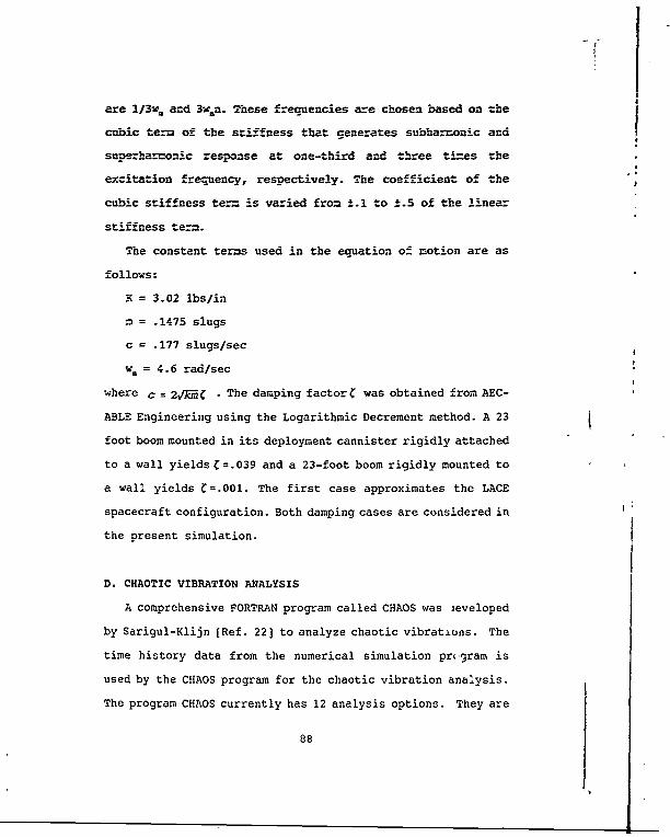
are 1/3w. and 3w.n. These frequencies are chosen based on the

cubic term of the stiffness that generates subharr.onic and

superharmonic response at one-third and three times the

excitation frequency, respectively. The coefficient of the

cubic stiffness term is varied from ±.l to ±.5 of the linear

stiffness term.

The constant terms used in the equation of notion are as

follows:

K = 3.02 lbs/in

m = .1475 slugs

c = .177 slugs/sec

w. = 4.6 rad/sec

where c = 2v(h . The damping factorC was obtained from AEC-

ABLE Engineering using the Logarithmic Decrement method. A 23

foot boom mounted in its deployment cannister rigidly attached

to a wall yields C=.039 and a 23-foot boom rigidly mounted to

a wall yields C=.001. The first case approximates the LACE

spacecraft configuration. Both damping cases are considered in

the present simulation.

D. CHAOTIC VIBRATION ANALYSIS

A comprehensive FORTRAN program called CHAOS was leveloped

by Sarigul-Klijn (Ref. 22] to analyze chaotic vibrations. The

time history data from the numerical simulation prngram is

used by the CHAOS program for the chaotic vibration analysis.

The program CHAOS currently has 12 analysis options. They are

88

1. Plot the t-e history

2. ?lot onto toroidal phase space

3. Take Poincar6 section of toroidal phase space

4. ?lot onto 2-D phase space

5. Plot onto 2-D Van der Pol plane

6. Plot onto 3-D phase space

7. Take Poincar6 section of 3-D phase space

8. 3-D Poincard section of a 4-D hyperspace

9. Compute fourier power spectrum

10. Compute statistics

11. Compute Lyapunov exponent

12. Compute fractal correlation d;mension

As discussed earlier, the stiffness term is modeled as a

combination of linear and cubic terms. The coefficient of the

cubic term is varied as a percentage of the linear term from

10% to 50%, and is seen to yield no significant changes in the

response. Therefore, an average value of 30% is used in all

subsequent numerical simulation.

In order to focus the present study within the scope of

this research, the study is divided into four specific groups.

Each group is identified by excitation frequency and damping.

In each group, the excitation amplitudes are 20.8 ibs, 41.7

lbs, 83.4 ibs, 166.7 lbs, and 208.4 lbs respectively. This

yields a deflection of 2.5%, 5%, 10%, 20%, and 25% of the

length of the beam, respectively. Table VI contains the group

identification.

89

Table VI GROUP IDENTIFICATION

GROUP _ __ C_ _ _

A 1.53 .77

B 13.8 .177

C 1.53 .0454

D 13.8 .0454

The initial analysis consists of studying four qualitative

indicators of chaos. They are time history, fourier power

spectrum, pseudo-phase plane and Poincare section

respectively. Then, quantitative measures of the motion are

computed.

Ficures 39-43 and 44-48 present the qualitative indicators

for cases A and B respectively. The time history is initially

transient and then becomes periodic in both cases. The fourier

power spectrum indicates a broad-band frequency spectrum, with

the number of spikes increasing with an increase in amplitude.

The pseudo-phase plane plot indicates that the motion settles

to a single limit cycle for case A and a double limit cycle

for case B. The Poincar6 section is very sparse and indicates

a periodic system. The periodic time history also indicates a

non-chaotic response.

Figures 49-53 and 54-58 present the qualitative indicators

of chaos for groups C and D. In all cases, the time history is

seen to be non-periodic and the Fourier power spectrum is

observed to be broad-band. In both cases, there appears to be

two limit cycles in the pseudo-phase plot. The Poincard

90

sections appear core dense than the previous groups and has

the appearance of a strange attractor. These systems appear to

be chaotic.

To ascertain the quantitative nature of the response, the

fractal correlation dimension is computed for each group and

is shown in Table VII. Figures 59 and 60 show the fractal

dimension for increasing phase space dimension for two cases

of daping with F=20.8 and 0=1.53 respectively. The plots

for the other cases are given in Appendix J.

A non-integer fractal dimension is indicative of the

presence of chaos in a system [Refs. 22,23,24,25]. This is

consistent with the qualitative indicators of groups C and D.

The inconsistency with groups A and B indicate that the

fractal dimension by itself does not confirm the strangeness

of the strange attractor as believed in the reported

literature and must be used in conjunction with other

indicators of chaos. Additional results pertaining to this

parametric study are reported elsewhere (Ref. 26].

91

IV I

a. Time History b. Fourier Power Spectrum

c. Pseudo Phase Plane d. Poincar6 Section

Figure 39. Qualitative indicators Of Chaos.F=20.8 lbs, 0=1.53 Hz, C=.177.

92

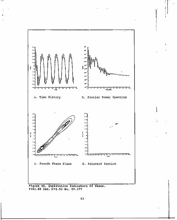
a. Time History b. Fourier Power Spectrum

F=416 b,015 Hz C .

.93

Figur e Qitaidtorysb Fre Cho. petu

F=41.68 lbs, 0)=1.53 Hz, C=.177

93

a. Time History b. Fourier Power Spectrum

c, Pseudo Phase Plane d. poincar6 section

Figure 41. Qualitative Indicators Of Chaos.

F=83.352 lbs, 0=1.53 Hz, C=.177

94

Ii

a. Time History b. Fourier Power Spectrum

I i

c. Pseudo Phase Plane d. Poincard Section

Figure 42. Qualitative Indicators Of Chaos.

F=166.7 ibs, 0=1.53 Hz, C=.177

95

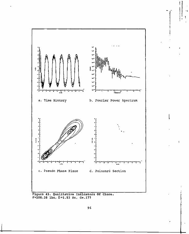
a. Time History b. Fourier Power Spectrum.3 .3.i:rr

c. Pseudo Phase Plane d. Poincar6 Section

Figure 43. Qualitative Indicators Of Chaos.F=208.38 lbs, 0=1.53 Hz, C=.177

96

a. Time History b. Fourier Power Spectrum

c. Pseudo Phase Plane d. Poincard Section

Figure 44. Qualitative Indicators Of Chaos.F=20.8 ibs, 0=13.8 Hz, C=.177

97

a. Time History b. Fourier Power Spectrum

c. Pseudo Phase Plane d. Poincar6 Section

Figure 45. Qualitative Indicators Of Chaos.F=41.68 ibs, 0=13.8 Hz, C=.177

98

a. Time uistory b. Fourier Power Spectrum

c. Pseudo Phase Plane d. Poincar6 Section

Figure 46. Qualitative Indicators of Chaos.

F=83.352 lbs, 0=13.8 Hz, C=.177

99

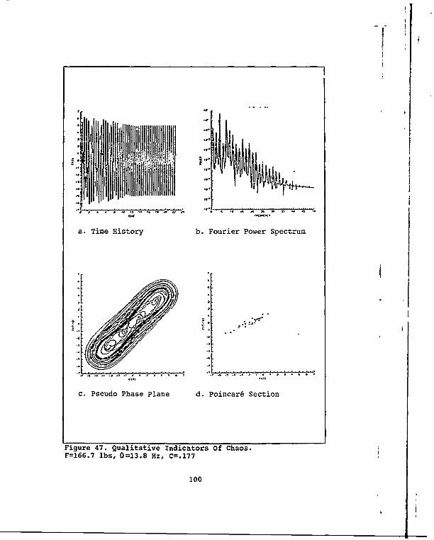
a. im Hitry~I b.Fure Pwr oct

A lh~~iJl

. Ped hs ln .Picr eto

Figure 47. QualitativeIdicaosOfCasF=6. lbs 0= 13. z C=.177

111111 1 0

a. Time History b. Fourier Power Spectrum

c. Pseudo Phase Plane d. Poincard Section

Figure 48. Qualitative Indicators Of Chaos.F=208.38 lbs, 0=13.8 Hz, C=.177

101

fi I '

a. Time History b. Fourier Power Spectrum

... .. ... .. ..

.44

a.~~~~ ~ ~ Tim Hitr .FuirPwrSetu

a.i Tme 0Qaist b.dica o ir PChowe. et

F=4168 ls, =1.5 li, C .05

103)~

a. Time History b. Fourier Power Spectrum

c. Pseudo Phase Plane d. Poincar6 Section

Figure 51. Qualitative Indicators of Chaos.F=83.352 lbs, 0=1.53 Hz, C=.0454

104

Ri

a. Time History b. Fou,.er Power Spectrum

c. Pseudo Phase Plane d. Poincar4 Section

Figure 52. Qualitative Indicators Of Chaos.F=166.7 ibs, 0=1.53 Hz, C=.0454

105

-3

a. Time History b. Fourier Power Spectrum

c. Pseudo Phase Plane d. Poincard Section

Figure 53. Qualitative Indicators Of Chaos.F=208.38 lbs, 0=1.53 Hz, C=.0454

106

30107

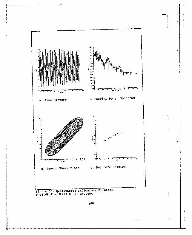
a. Time History b. Fourier Pow~er Spectrum

c. Pseudo Phase Plane d. Poincar6 section

Figure 5.Qualitative Indicators Of Chaos.

F=41.68 ibs, 0=13.8 Hz, C=.0454

108

a. Time History b. Fourier Power Spectrum

c. Pseudo Phase Plane d. Poincar6 Section

Figure 56. Qualitative Indicators Of Chaos.F=83.352 ibs, 0=13.8 Hz, C=.0454

109

a. Time History b. Fourier Power Spectrum

c. Pseudo Phase Plane d. Poincare Section

Figure 57. Qualitative Indicators of Chaos.F=166.7 lbs, 0=13.8 Hz, C=.0454

110

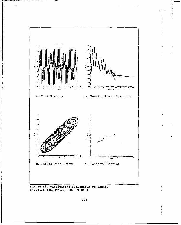
a. Time History b. Fourier Power Spectrum

c. Pseudo Phase Plane d. Poincar6 Section

Figure 58. Qualitative Indicators Of Chaos.F=208.38 lbs, 0=13.8 Hz, C=.0454

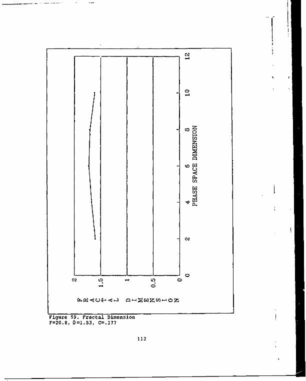
'4

0

CO

C-)

00

rX 4" ' 4 0

Figure 59. Fractal DimensionF=20.8,1)=1.53, C=.177

112

T-

0

414

U - 0-

Figure 60. Fractal Dimension.F=20.8, 0=1.53, c=.0454

113

Table VII. FRACTATL DIMENSION

I C IM--"N.TL

a) 20.8 1.53 1 .!77 i 1.7

.41.7 1 1.53 I .177 1.6

83.4 I 1.53 I .177 I 1.7166.7 1 1.53 .177 1 1.7

208.4 I 1.153 I . 7 1.7

b) 20.8 13.8 I .177 1.2

41.7 13.8 .177 1.2

83.4 I 13.8 1 .177 1.3

266.7 13.8 I .177 1.6208.4 13.8 .177 1.4

C) 20.8 I 1.53 .0454 I 2.05

41.7 I 1.53 .0454 2.4

83.4 1.53 .0454 2.05

166.7 1.53 .0454 I 2.1

201.4 1.53 .0454 2.6

d) 20.8 13.8 .0454 2.1

41.7 13.8 .0454 2.4

13.4 13.8 .0454 1.95

166.7 13.8 .0454 2.1

208.4 13.8 .0454

114

VIII. CONCLUSIONS AND SCOPE FOR FURTHER RESEARCH

A. CONCLUSIONS

A detailed finie-element =ode! of the LACE soacecraft has

been developed using the finite element program GIFTS. A

dynamic analysis was performed on the model to determine the

natural frequencies and mode shapes. This model will provide

a basis for comparison when actual orbital test data is

available.

Thermoelastic effects of the LACE spacecraft boom were

±nvestigated for a worst case temperature scenario. The

results indicated that the deflections induced would have

negligible effect on the systems dynamics and would not affect

the on-orbit systems identification or induced thermal

flutter.

A preliminary study was conducted on a 23-foot section of

the LACE soacecraft boom to investigate the possibility of

chaotic vibrations occuring by varying the excitation

amplitude and frequency. The system was modeled as a single-

degree-of-freedom system with arbitrary nonlinear stiffness,

and nonlinear damping excited by a sinusoidal function. A

numerical integration program was developed to determine the

system response using various excitation amplitudes and

frequencies. Four qualitative methods, time history, fourier

115

power spectrum, pseudo-plane, and Poincar6 section methods

were used to evaluate chaotic vibrations. In addition,

quantitative analysis 3.ncluded computation of correlation

fractal dimension. It was evidenced that a combination of all

appoaches was needed to determine the nature of vibrations.

Chaotic vibrations were present -for the low-damped system

while periodic response was indicated for highly damped

systems.

A non-integer correlation fractal dimension, which is

believed to be a cuantitative indication of chaos in a system,

was evidenced for both periodic and non-periodic responses of

the system. This important result, which is further being

confirmed from analysis of flight test data (Ref. 21] shows

that the fractal dimension by itself is not enough to

characterize the attractors found in nonlinear dynamical

systems. Modeling the "looseness" of joints for triangular

space trusses by Moon & Li [Ref. 27], who report interesting

chaotic behavior, was brought to the attention of the author

during the write-up of this report, which reveal the

importance of understanding the nonlinear dynamic behavior of

large flexible structures.

B. SCOPE FOR FUTURE RESEARCH

Future research may be beneficial in two main areas.

The first is the development of a multi-body dynamics model

of the LACE spacecraft. A structural model using GIFTS has

116

ralready been developed. The results generated may be used to

model the flexibility effects, while other effects introduced

due to on-orbit, such as gravity gradients effects,

atmospheric drag, etc., may be evaluated. These models may be

used as baselines for comparison when the orbital test data

from LACE becomes available. This comparison will provide an

opportunity for improvements and adequacy of these computer

models.

The availability of the orbital test data will provide

information needed to conduct a more detailed study of chaotic

vibrations on the fully deployed LACE spacecraft boom and

assess the sensitivity of the highly flexible boom structure

to accidental or intentional excitation. Assessing the exact

nature of the response of large flexible space structures is

important for missious that require accurate pointing

accuracies and in nuppression and control of vibrations.

117

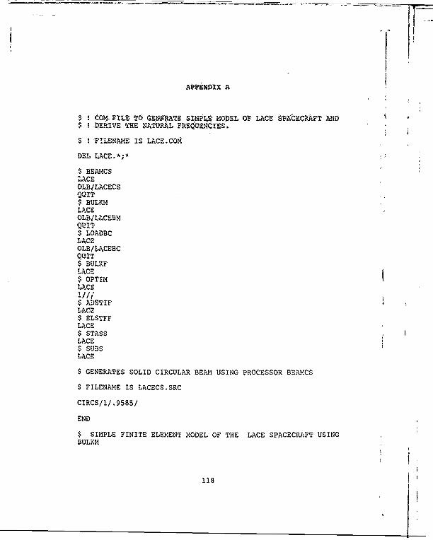
APPENDIX A

$ S OM. FILE TEO GENERATE sINPIg, MODEL OF LACE §?A:CBCRAFT AND

$ ! DERIVE THlE VAfURAL FREQUERCIES.

$ ! -FILENAM4E IS LACE.COM

DEL LACE.*;'

$ BEAMCSLACEOLSILACECSQUIT$ BULKI4LACEOLB/LU.CEBmQUIT$ LOADBCLACEOLBI"~CEBCQUIT$ BULRFLACE$ OPTIMLACEi1/t$ ADSTIFLACE$ ELSTFFLACE$ STASSLACE$ SUBSLACE

$ GENERATES SOLID CIRCULAR BEAM USING PROCESSOR BEAMCS

$ FILENAME IS LACECS.SRC

CIRCS/l/.9585/

END

$ SIMPLE FINITE ELEMENT MODEL OF THE LACE SPACECRAFT USING

BULKM

118

$ FILENAM4E IS LACEBM.SRC

$ ESTABLISH THE KEYPOINTS OF THE MODEL

KPOINT/1/O,0,O/2/O,1800,O/3/O,.-900,0/KPOINT/4/O,0, 1800/5/50,0,0/

$ DEFINE MATERIAL PROPERTIES

ELMAT,4/1/3.E3,6.E6, .29, .000014752/

$DEFINE BEAM CHARACTERISTICS

L-rTYBEAM21,1

S GENERATE THE BEAMS

SLIN;E,1O0/112/1,2,31/5/113/1,3,16/5/114/1,4,31/5/

END

$ GENERATES POINT MASSES FOR THE SPACECRAFT

$ FILENAME IS LACEBC.SRC

MASS/MASSP//6.4078E/2/.0906/3/.0906/4/ .517/

END

119

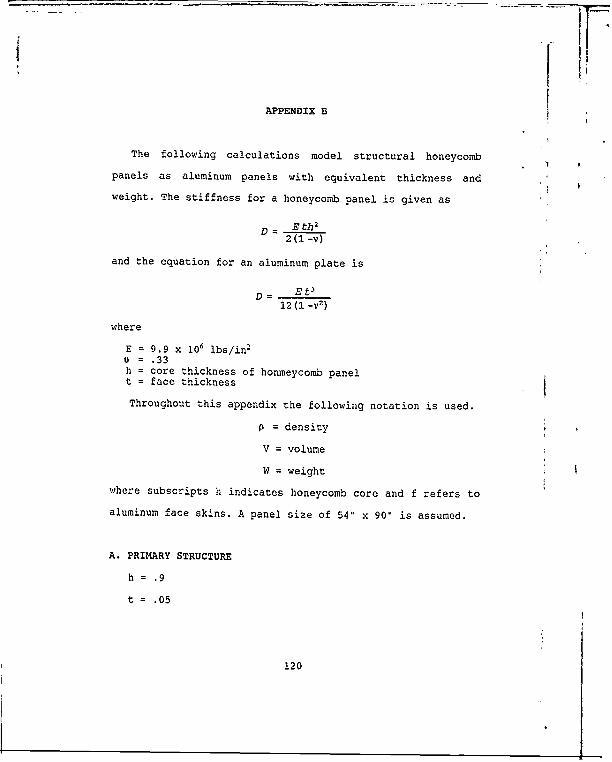
APPENDIX B

The following calculations model structural honeycomb

panels as aluminum panels with equivalent thickness and

weight. The stiffness for a honeycomb panel is given as

D = E th 2

2 (1-v)

and the equation for an aluminum plate is

D - Et12 (1 -v 2 )

where

E = 9.9 x 106 lbs/in2

u = .33h = core thickness of honmeycomb panelt = face thickness o

Throughout this appendix the following notation is used.

p = density

V = volume

W = weight

where subscripts h indicates honeycomb core and f refers to

aluminum face skins. A panel size of 54" x 90" is assumed.

A. PRIMARY STRUCTURE

h= .9

t = .05

120

I

1. Determine Stiffness of Honeycomb Panel

D = (.gX1_09 ) (. 05) (.9)= 2.25xlOs lbs.Iin2(1-.33)2

2. Determine Equivalent Aluminum Plate Thicknessu

D- Et . 2 .250X105 = (9.9x10 6 ) t312(1-v

3 ) 2(1- .332)

c = .624 in

3. Determine Honeycomb Panel Mass

Ph* = 6 lbs/ft 3 = 3.47 x 10 .1 lbs/in3

Pf*= 9.81 x 10" 2 lbs/in3

Vh = .9 x 54 x 96 = 4665.6 in3

V= .1 x 54 x 96 = 518.4 in3

Wh = 4665.6 x 3.47 x i0-3 = 16.2 lbs

Wf*= 518.4 x 9.81 x 10.2 = 50.8 lbs

,asterik items remain constant throughout the

calculations

Total weight = 67 lbs

Total ass 67 lbs = .1734 (lbs-sec3)/in (GIFTS units)

386.4 in/sect

4. Determine Equivalent Density

Volume of aluminum panel = .624x54x96 = 3234.8 in 3'

Equivalent density - .1735(lbs-8ec)/In * 5.364x10o5 (lbs-sec2)/in'

3234.8 in3

121

B. SECONDARY STRUCTURE

1. Fixed and Deployable Solar Array Substrate

h =.4

t =.05

D=(9*9XIO-) (05) (42 = 4 .44XI0'lbs-in2(1-.33 2)

a. Determine Equivalent Aluminum Thickness

t = .3634 in

b. Determine Honeycomb Panel Mass

Vh =.4 x 54 x 96 = 2073.6 in 3

N= 2073.6 xc 3.47 x 10, = -7.195 lbs

Total weight = 58 lbs

Total mass = 58/386.4 = .15 lbs-sec2/il

c. Determine Equivalent Density

Volumne of aluminum panel = 1884 in~

Bquival e2 densi tY Is8 = 7 . 9 6 x10-5 2bs-sec2/Jn'

2. Deployable Sensor Panels

h= .65

t = .05

D= (9. 9x101,) (. 05) (. 65) 2 1. 17 3 x105 bs-in2(1-.332)

122

a. Determine Equivalent Aluminum Thickness

1.173x105

= 99x01) t3

1l2 l.332)

t = .502 in

b. Determine Honeycomb Mass

V= .65 x 54 x 96 = 3369.6 i;n3

W= 3369.6 x 3.47 X10 = 11.7 lbs

Total weight = 62.5 lbs

Total mass = .1617 lbs-sec2 /in

c. Determine Equivalent Density

volume of aluminum panel = .502 x 54 x 96 -2602.4 in3

Equivalent densit~y .1617 =6.22 x 10-5 (lbs-sec2) /Ifl

123

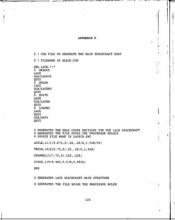
APPENDIX C

$ COM FILE TO GENERATE THE MAIN SPACECRAFT BODY

$ FILENAME IS XLACE.COM

DEL LACE.*;*$ BEAMCSLACEOLB/LACECSQUIT$ BULKMLACEOLE/LACEEMQUIT$ EDITMLACEOLB/LACEMQUIT$ LOADBCLACEMASSOLD/MASSQUIT

$ GENERATES THE BEAM CROSS SECTIONS FOR THE LACE SPACECRAFT$ GENERATES THE FILE USING THE PROCESSOR BEAMCS$ SOURCE FILE NAME IS LACECS.SRC

ANGLE,11/1/2.875,3/.25, .25/0,1.938/90/

TBEAM,1O/2/2.75,3/.25, .25/0,1.938/

CHANNEL/3/7.75,3/.125, .125/

CIRCH, 1/9/5.605,5.5/O.5.5525/

END

$ GENERATES LACE SPACECRAFT MAIN STRUCTURE

$ GENERATES THE FILE USING THE PROCESSOR BULKM

124

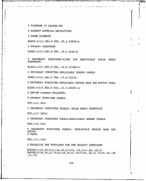
$ FILENAME IS LACEBM.SRC$ ELEMENT MATERIAL DEFINITIONS

$ FRAME ELEMENTS

ELMAT,4/l1.8E4,9.9E6,.33,2.5382E-4/

$ PRIMARY STRUCTURE

ELMAT,4/2/1.8E4,9.9E6,.33,5.364E-5I

$ SECONDARY STRUCTURE-FIXED AND DEPLOYABLE SOLAR ARRAYSUBSTRATE

ELMAT,4/3/1.8E4,9.9E6,.33,8.1915E-5/

$ SECONDARY STRUCTURE-DEPLOYABLE SENSOR PANELS

ELMAT,4/4/1.8E4,9.9E6,.33,6.22E-5/

$ SECONDARY STRUCTURE-DEPLOYABLE SENSOR ARM~S AND BOTTOM PANEL

ELMAT,4/5/1.8E4,9.9E6,.33,2.5382E-4/

$ DEFINE ELEMENT THICKNESS

$ PRIMARY STRUCTURE PANELS

ETH, 1/4/.624/

$ SECONDARY STRUCTURE PANELS- SOLAR ARRAY SUBSTRATE

ETH,3/51.3634/

$ SECONDARY STRUCTURE PANELS-DEPLOYABLE SENSOR PANELS

ETH, 1/6/.502/

$ SECONDARY STRUCTURE PANELS- DEPLOYABLE SENSOR ARMS ANDBOTTOM$ PANEL

ETH, 1/7/.125/

$ ESTABLISH THE KEYPOINTS FOR THE PRIMARY STRUCTURE

KPOINT//26,26,O2/-26,26,0/3/26,-26,0/4/-.26,-26,0/KPOINT/5/26,26,41.75/6/-26,26,41.75/7/26,-.26,41.75/8/.26,.26,41.75/

125

KPOINT/9/26,26,68.375/10/-26,26,68.375/11/26,-26,68.375/I(POINT/ 12/-26,-26,68.375/13/26,26,96/KPOINT/14/-26,26, 96/15/26,-26,96/16/-26,-26,96/

$ ESTABLISH KEYPOINTS FOR THE CIRCULAR ARCS

$ SIDE C+Yf

KPOINT/17/13,26, 68.375/18/13,26,76.5/19/13,26,87.5/20/13,26,96/KPOINT/21/18.5,26,82/22/7.5,26,82/

$ SIDE C-Y

KPOINT/23/-13,-26,68.375/24/-13,-26,76.5/25/-13,-26,87.5/KPOINT/26/-13,-26,96/27/-7 .5, -26, 82/28/-18 .5,-26,82/

$ SIDE +Z

KPOINT/29/26,O, 96/30/5 .5,0,96/31/-S .5,0, 96/32/-26,0, 96/KPOINT/33/0,-5.5,96/34/0,5.5,96/

$ GENERATE VERTICAL ANGLE BEAM MEMBERS FOR C-SECTION PANELS

LETY/BEAM2/1,1/

SLINE,10/L913/9,13,6/10/L1014/10,14,6/9/Ll2l6/12,16,6/10/

SLINE, 10/Llll5/11, 15,6/9/

$ GENERATE VERTICAL ANGLE BEAM MEMBERS FOR B-SECTION PANELS

SLIME, 10/L59/5,9,3/6/L610/6, 10, 3/5/L812/8, 12,3/7/L711/7, 11,3/5/

$ GENERATE VERTICAL ANGLE BEAM MEMBERS FOR A-SECTION PANELS

SLINE,10/Ll5/1,5,3/2/L26/2,6,3/l/L48/4,8,3/3/L37/3,7,3/l/

$ GENERATE HORIZONTAL ANGLE BEAMS FOR TOP AND BOTTOM MEMBERS

$ BOTTOM MEMBERS

SLINE/L12/1,2,6/L34/3,4,6/Ll3/1,3,5/L24/2,4,5/

$ TOP MEMBERS

SLINE/L,1320/13,20, 2/L1420/14,20,5/Ll432/14, 32, 3/L1632/16,32, 3/SLINE/L1626/16,26, 2/L1526/15,26,5/L1329/13,29,3/L1529/15,29,3/

$ GEN~kATE HORIZONTAL T-SECTION BEAM MEMBERS

126

$ B-SECTITOv PAVE-LS

LETY_/BEALM2/1, 2/SLINEz,101L56/5,6,6/7/L78/7,8,6/5/L57/5,7,5/6/L68/6,8,5/5/

$C-SECTION PA-nEL:SSLINE, 10/L917/9, 17,2/13/L1017 /1-0, 17,5/14/L1-012/10, 12,.5/9/SLINE2,10/L1223/12,23,2/10/L1123111,23,519/L9119,11,5101

$ GENERATE LINE%--S ASSOCIATED, WI77h CI.RCUILA7R ARCS

SLINEZ/L1718/17,18,2/L1920/19,20,2/L2324/23,24,2/L2526/25,26,2/SLINE/L2930/29, 30, 2/L3132/31, 32,2/

$ GENERATE CIRCULAR A1RCS

S C-'7Y SIDE PANEL

CARC/C1819/ 18, 22, 19, 4/C1.8/19, 21, 18, 4/

$C-Y SIDE PANEL!

CARC/C819/18,22, 19,4/C1918/19,21,18,4/

$C-Y SIDE PANEL

CARC/C2425/24, 28, 25, 4/C2524/25, 27, 24, 4/

$TOP PANEL +Z

CARC/C3031/30, 33,31,4/C3130/31,34,30,4/

$ GENERATE COMPLINES

COMPLINE7/L1314/L1320,Ll420/L1416/L432,L632/.1315/L1329,LI529/COMPLINE/L1516/L1526, L1626/L1720/L1718,C1819 ,L1920/COMPLINE/L2017/L1920,C1918, L17l8/L2326/L2324,C2425,L2526/COMPLINE/L2326/L2324, C2425 ,L2526/L2623/L2526 ,C2524 ,L2324/COMPLINE/L910/L917,L1017/L1112/Lll23,Ll223/COMPLINE/L2932/L2930,C3031,L3132/L3229/L3132,C3130,L2930/

$ GENERATE GRID ELEMENTS

GETY/QB4/2 ,4/

$ A-PANELS

GRID4/A+Y/L12, L56 ,Ll5, L26/A-X/L24, L68, L26, L48/

GRIO4/A-Y/L34,L79,L48,L37/A+X/L13,L57,L15,L37/

127

G-RID4/B+Y-/L56,L910,L59,L610/B-X/L68, L1012,L61O,L812/,"

GRID4/C-YL-/L1223,L2326,L1626,L1216/C-YR/L11-23,Ll115,L1526,L-2623/GRI-D4/C-X/L-913,L1315,L1115,L911/C-X/L1014,L1-416 ,L1216,L1-012/

$ GENERATE TOP PANEL

CRID4/ZL/L1529,L1516,L1632,L2932/ZR/L1329 ,L3229,L1432,L1314/

$ GENERAT-E RF PANELI

GRI-D4/R:F/L56,L68,L78,L57/

$ GENERASE BOTT-O.M PANEL

GE7TY/Q34/5, 7/GRID4/BOI'TO'/L12 ,L24 ,L34, L13/

$ GENERATE KEYPOINTS FOR SENSOR PANELS AND SENSOR ARMS

KPOTNT/35/19 ,26, 0/36/19, 75.25,0/37/-19,26, 0/38/-19 ,75.25,0/KPO~iNT/39/-26,19,O/40/-75.25,19,O/41/-26,-19,O/42/-75.25,-19lo/KPOINT/43/-19,-26,0/44/-19,-75.25,0/45/19,-26,O/46/19,-75.25

KPOINT/47/26,-19,0/48/75.25,-19,Oj'49/26,19,O/50/75.25, 19,0/KPOINT/51/79.03,79.03,0/52/-79.03,79.03,0/53/-79.03,-79.03,0/KPOINT/54/79.03,-79.03,0/

$ GENERATE LINES FOR SENSOR PANELS

SLIN/L3536/35,36,5/L3738/37,38,5/L3537/35,37,4/L3638/36,38,4/SLIN/L4344/43,44,5/L4546/45,46,5/L4345/43,45,4/L4446/44,46,4/SLINEz/L4748/47,48,5/L4950/49,50,5/L4749/47,49,4/L4850/48,50,4/

$ GENERATE GRID ELEMENTS

GETY/QB4/4, 6/

GRID4/+Y/L3536,L3738,L3537,L3638/-X/L3940,L4142,L3941,L4042/GRID4/-Y/L4344,L4546,L4345,L4446/+X/L4748,L4950,L4749,L4850/

$ GENERATE CHANNEL BEAM ELEMENTS FOR SENSOR ARMS

128

SLINE;,10/L151/1,51-,6/52/L252/2,52,6/51/L453/4,53,6/54/SLINE, 1O/L354/3,54, 6/53/

SGE'ER;E RE7POINTS FOR SOLAR PANEL FOLDOUTS

EP=OINT/55/24,26,96/56/24, 68.5, 96/57/-24,26,96/58/-24,68.5,96/KPOIN/59/-26,24,96/60/-68.5, 24,96/61/-26, -24,96/62/-68.5, -24,9C/KPOINT/63/-24,-26,96/64/-24,-68.5,96/65/24,-26,96/66/24, -68.5,95/KPOINT/67/26,-24,96/68/68.5,-24,96/69/26,24,96/70/68.5,24,96/

$ GENERATE LINES FOR SOL.AR PANEL FOLDOUTS

SLINE-/L5556/55,56,3/L5758/57,58,3/L5557/55,57,3/L5658/56,58,3/SLIN/L596/59,60,3/L6162/6l,62,3/L5961/59,61,3/L6062/6O,62,3/SLINEm/L6364/63,64,3/L6566/65,66,3/L6365/63,65,3/L6466/64,66,3/SLINE:-/L6768/67,68,3/L6970/69,70,3/L6769/67,69,3/L6870/68,70,3/

$ GENERATE GRID ELEMENTS

GPETY/QB4/3, 5/

GRID4/D'Y/L5556,L5758,L5557,L5658/D-X/L5960,L6162,L5961,L6062/GRID4/D-Y/L6364,L6566,L6365,L6466/D+X/L6768,L6970,L6769,L6870/

$ GENEPRATE KEYPOINTS FOR SOLAR FIXED PANELS

$ A+Y PANELS

KPOINT/71/-26,26,20/72/-26,26,46/73/-14,26,46/74/-14,26, 60/KPOINT/75/14,26, 60/76/14,26,46/77/26,26,46/78/26,26,20/

$ A-Y

KPOINT/79/26,-26,20/80/26,-26,46/81/14,-26,46/82/14,-26, 60/KPOINT/83/-14,-26, 60/84/-14,-26, 46/85/-26,-26,46/86/-26, -26,20/

$ c+X

KPOINT/87/26,26,30/88/26,26,45/89/26,14,45/90/26,14,56.01/KPOINT/91/26,26,56.01/92/26,26,88.5/93/26,-26,88.5/94/26,-26,56.01/KPOINT/95/26,-14,56.01/96/26,-14, 45/97/26,-26,45/98/26,-26,30/

$ c-X

KPOINT/99/-26,26,30/100/-26,26,45/101/-26,14,45/102/-26,14,5

6.01/

129

KPOINT13/-26,26,56.1/104/-26,26,88.5/105/-26,-26,88.5/KPOINT/106/-26,-26,56.O1/107/-26,-14,56. O1/108/-26,-14,45/KPOINT/109/-26, -26, 45/110/-26,-26, 30/

END

$ EDIT THE MODEL-GENERATE VERTICAL ANGLE BEAM ELEMENTS

$ GENERATES THE FILE USING THE PROCESSOR EDITM

$ FILE NAME IS LACEM.SRC

PTRtM/l/PTRTH/1

$ GENERATE TOP ANGLE MEMBERS

BEA2/13,55,29/20,55,29/20,57,32/14,57,32/BEA2/14,59,20/32,59,31/32, 61,31/16, 61,26/BEAM2/16, 63,32/26,63, 32/26, 65,32/15, 65,29/BEAM42/15, 67,26/29, 67,26/29, 69:30/13, 69,20/

$ GENERATE BOTTOM ANGLE MEMBERS

BEA21,35,3/35,37,3/2,37,4/BEAM2 /2 ,39, 1/39, 41, 1/4, 41, 3/BEAM2/4,43,2/43,452/3,45,1/BEAM,2/3,47,4/47,49,4/1,49,2/BEAM2/419,422,1/411,414,1/135,139,1/138,142,1/

$GENERATE HOLLOW CIRCULAR BEAM CROSS SECTION FOR CYLINDRICAL$CANNISTERS

PTRTH/9 /

BEAM2/19,364,9/25,352,9/31,405,9/

END

$ GENERATES POINT AND GRID MASSES FOR THE LACE SPACECRAFT

$ GENERATES THE FILE USING THE PROCESSOR LOADBC

$ SOURCE FILE NAME IS MASS.SRC

$ GENERATE MASS DISTRIBUTIONS FOR A-PANELS

$MASS LOADING FOR A-Y PANEL

130

MASSP/8/6.31E-3/166/1 .54E-2 /165/1 .65E-2/?-IASSP/164/1.65E-2/163/1. 19E--2/7/2.87E-3/MASSP/133/9 .76E-3/325/2.48E-/2/ 25-_MASSP/323/2.2SE-2/322/1. 65E-2/13417.4E-3/MASSP/4/6.31E-3/142/1.23E-2/141/8.BBE-3/MASSP/140/8.88E--3/139/7.4E-3/3/7 .4E-3/

$ IMASS LOADING FOR A+Y PANEL

MASSP/5/2.87E-3/159/1.37E-2/160/2.03E-2/MASSP/161/1.61E-2/162/9.47E-3/6/2.87E-3/MASSP/131/5.27E-3/315/1. 61E-2/316/2. 69E-2/MASSP/317/2.93E-2/318/1. 61E-2/132/2. 87E-3/MASSP/l/5 .27E-3/135/5.27E-3/136/9 .47E-3/MASSP/137/l.61E-2/138/9.47E-3/2/2.87E-3/

$ MASS LOADING FOR A-X PANEL

MASSP/6/7 .OIE-3/170/1.86E-2/171/3.07E-2/MASSP/172/2. 36E-2/8/7.97E-3/MASSP/132/2.55E-2/319/5.57E-2/320/7 .22E-2/MASSP/321/4.66E-2/133/7.97E-3/MASSP/2/2.2E-2/146/4.05E-2/147/4.48E-2/IAASSP/148/2.64E-2/4/3.44E-3/

$ MASS LOADING FOR A+X PANEL

MASSP/7/3.44E-3/169/1.88E-2/168/2.3E-2/MASSP/167/7.66E-3/5/3 .44E-3/MASSP/134/1.32E-2/328/4 .7E-2/MASSP/327/6.OE-2/326/3 .89E-2/131/1.62E-2/MASSP/3/l .32E-2/14S/3. 16E-2/144/4.03E-2/MASSP/143/3.46E-2/l/1.62E-2/

$ GENERATES MASS DISTRIBUTIONS FOR B-PANELS

$ MASS LOADING FOR B+Y PANEL

MASSP/5/8 .4E-3/127/B.4E-3/329/8 .4E-3/159/B.4E-3/MASSP/160/1.92E-3/330/1.92E-3/161/3.4E-2/MASSP/331/3.4E-2/162/1.59E-2/332/1 .59E-2/

$ MASS LOADING FOR B-X PANEL

MASSP/170/7 .47E-.3/171/7 .47E-3/172/7.47E-3/MASSP/333/7 47E-3/335/7.47E-3/MASSP/334/8.9E-3/177/2. 16E-3/

$ MASS LOADING FOR B+X PANEL

131

MASSP/11 /4. 27E-3/184/8.83E.-3/183/9.81E-3/IMASSP/182/l 7E-2/9/1.24E-2/1-30/4.27E-3/M.ASSP/342/l .3'!E-2/3411 89E--2/340/3 .48E-2/MASSP/127/2 .57E-2/7/6. 91E-4/169/5.23E-3/MASSP/168/9. 81E-3/167/1 .79E-2/5/1. 39E-2/

$ GENERATES MASS DISTRIBUTIONS FOR C-PANELS

$ MASS LOADING FOR C+Y PANEL

MASSP/344/3.96E-3/345/3 .96E-3/347/3 .96E-3/MASSP/348/3 .96E-3/174/3. 96E-3/175/3.96E-3/

$ MASS LOADING FOR C-Y PANEL

MASSP/181/4 .84E-3/357/4.84E-3/360/9 .68E-3/1MASSP/363/4.84E-3/366/4 .84E-3/MASSP/180/4. 84E-3/356/4.84E-3/359/9.68E-3/MASSP/362/4 84E-3/365/4.84E-3/

$ MASS LOADING FOR C-X PANEL

MASSP/379/8.67E-3/380/8. 67E-3/383/8. 67E-3/MASSP/384/8 .67E-3/387/8. 67E-3/388/8.67E-3/

$ MASS LOADING FOR C+X PANEL

MASSP/158/3.35E-3/378/3.35E-3/368/3.08E-3/MASSP/369/3.08E-3/372/3.08E-3/373/3.08E-3/MASSP/371/3.81E-3/

$ GENERATES MASS DISTRIBUTIONS FOR THE TOP PANEL

MASSP/16/5 .29E-3/153/4 .21E-3/32/3 .56E-3/MASSP/152/9.7E-4/14/2.06E-3/15/2.06E-3/MASSP/158/9 .7E-4/29/9 .7E-4/157/9.7E-4/MASSP/13/2 .06E-3/26/5.71E-3/156/3.77E-3/MASSP/155/3.77E-3/154/2 .47E-3/149/2 .47E-3/MIASSP/150/3.44E-3/151/3.44E-3/20/2 .47E-3/MASSP/394/4.21E-3/393/2.26E-3/392/2.26E-3/MASSP/391/9 .7E-4/30/9 .7E-4/193/9 .7E-4/MASSP/194/9.7E-4/31/9.7E-4/195/9.7E-4/MASSPI196/9.7E-4/398/9 .7E-4/397/1.94E-3/MASSP/396/1.94E-3/395/9.7E-4/

$ GENERATE MASS DISTRIBUTIONS FOR THE RF PANEL

MASSP/8/2.16E-3/172/2. 16E-3/171/2 .52E-3/MASSP/170/2 .16E-3/6/2.16E-3/166/5. 49E-3/MASSP/410/1 .29E-2/406/8.34E-3/402/2. 16E-3/

132

MASSP/162/2. 16E-3/165/6. OE-3 /409/1.1BE-2/1ASSP/405/l. 66E-2/401/1.07E-2/161/1.07E-2/MASSP/164/6.OE-3/408/9 BBE-3/404/2.32E-2/MASSP/400/1.93E-2/160/1.93E-2/163/5. 49E-3/MASSP/407/9.37E-3/403/1.46E-2/399/1.07E-2/MASSP/159/1.07E-2/7/2.56E-3/169/6.03E-3/MASSP/168/6.32E-3/167/2. 16E-3/5/2. 16E-3/

$ GENERATES MASS DISTRIBUTION ON THE BOTTOM PANEL

MASSP/4/5.85E-3/148/9.65E-3/147/1.06E-2/MASSP/146/8.36E-3/2/5.85E-3/142/3.19E-2/MASSP/422/3.77E-2/418/1.73E-2/414/2.23E-2/MASSP/138/1.28E-2/141/2. 83E-2/421/5.5E-2/M4ASSP/417/6. O7E-2/413/4.34E-2/137/1. 15E-2/MASSP/140/2.57E-2/420/5.8E-2/416/6.21E-2/MASSP/412/3.39E-2/136/5. 91E-3/139/2.94E-2/MASSP/419/3.78E-2/415/1.9E-2/411/1.56E-2/MASSP/135/7. 14E-3/3/5.85E-3/14S/7.14E-3/MASSP/144/8. 62E-3/143/1.lE-2/1/5.85E-3/

$ GENERATES MASS DISTRIBUTIONS ON THE SENSOR PANELS AND SENSORARM~S

$ GENERATE MASS LOADINGS FOR THE SENSOR ARMAS

MASSP/l/8. 16E-3/283/7 89E-3/284/1. 12E-2/MASSP/285/7.89E-3/286/8. 16E-3/51/7.89E-3/MASSP/2/8.16E-3/287/7 .89E-3/288/1. 12E-2/MASSP/289/7 89E-3/290/8. 16E-3/52/7.89E-3/M4ASSP/3/8. 16E-3/295/7.89E-3/296/l. 12E-2/MASSP/297/7.89E-3/298/8. 16E-3/54/7.89E-3/MASSP/4/8. 16E-3/291/7.89E-3/292/1.12E-2/MASSP/293/7.89E-3/294/8. 16E-3/53/7.89E-3/

$ GENERATE MASS LOADINGS FOR THE SENSOR PANELS

$ GEIERATE MASS LOADINGS FOR +Y PANEL

MASSP/37/7 .83E-3/246/6 .47E-3/247/5 .56E-3/MASSP/248/5. 63E-3/38/6.02E-3/MASSP/250/4. 66E-3/426/1.22E-2/MASSP/427/1.22E-2/428/7.18E-3/252/4.66E-3/MASSP/249/4.66E-3/423/1.22E-2/424/1.22E-2/MASSP/425/7 18E-3/251/4.66E-3/MASSP/35/6.02E-3/243/6.47E-3/MAkSSP/244/5.56E-3/245/5.63E-3/36/6.02E-3/

$ GENERATE MASS LOADINGS FOR -X PANEL

133

MASSP/41/3.49E-3/256/4.66E-3/257/3.49E-3/MASSP/258/4. 14E-3/42/5.43E-3/MASSP/260/l. 87E-2/431/1.93E-2/MASSP/432/6. 66E-3/433/6.28E-3/262/4 .08E-3/MASSP/259/1.87E-2/429/2.11E-2/430/6. 66E-3/MASSP/431/6 .28E-3/261/4.08E-3/39/5 .3E-3/25312.85E-3/MASSP/253/2.85E-3/254/3.49E-3/255/4.14E-3/40/5.43E-3/

$ GENERATE MASS LOADINGS FOR -Y PANEL

MASSP/44/6.3E-3/265/5 .91E-3/264/5.85E-3(MASSP/263/6.75E-3/43/8.I1E-3/271/4.94E-3/MASSP/437/7.47E-3/436/l 25E-2/435/1.25E-2/MASSP/269/4.94E-3/272/4.94E-3/440/7.47E-3/MASSP/439/1.25E-2/438/1 .25E-2/270/4.94E-3/MASSP/46/6.3E-3/268/5.91E-3/267/5.85E-3/MASSP/266/8.57E-3/45/6.3E-.3/

$ GENERA'IE MASS LOADINGS FOR +X PANEL

MASSP/48/5.14E-3/275/4.79E-3/274/3.45E-3/MASSP/273/2.55E-3/47/4.79E-3/281/3.78E-3/MASSP/443/5.98E-3/442/8. 18E-3/441/S.78E-3/MASSP/279/4.79E-3/282/3.78E-3/446/5.07E-3/MASSP/445/8.18E-3/444/3.71E-3/280/3.78E-3/MASSP/50/5. 14E-3/278/4.79E-3/277/3.84E-3/MASSP/276/2 .48E-3/49/3.78E-3/

$ GENERATES GRID MASS FOR SOLAR PANELS

$ SURFACE MOUNT SOLAR PANELS

,MASSG/A+Y/1.531815E-,.531815E-5,.531815E-5,1.531815E-5/MASSG/A-Y/1.531815E-5,1.531815E-5,1.531815E-5,1.531815E-5/MASSG/B+Y/2 .402E-5,2.402E-5,2 .402E-5,2.402E-5/MASSG/B-Y/2 .402E.-5,2 .402E-5, 2.402E-5,2 .402E-5/MASSG/A+X/1.196E-5,1.196E-S,1.196E-5,1.196E-5/

MASSG/B+X/1 .87E55-,1.8755-5,1.875-5,1.87E-5/MASSG/B-X/1 .8755E-5, 1. 8755E-5, 1. 8755E-5, 1. 87555-5/MASSG/C+X/1 .875-5, 1.876E-5, 1.875-5,1.8075-5/MASSG/C-X/1.8076E-5,1.8076E-5,1.8076E-5,1.8076E-5/

$ DEPLOYED SOLAR PANELS

MASSG/D+X/6. 343E-6, 6.343E-6, 6.343E-6, 6.3435-6/MASSG/D-X/6.343E-6,6.343E-6,6.343E-6,6.343E-6/MASSG/D+Y/6.343E-6,6.343E-6,6.343E-6,6.343E-6/MASSG/D-Y/6. 343E-6, 6.3435-6, 6.343E-6, 6.3435-6/

$ DETERMINES MISCELLANEOUS UNACCOUNTED MASS

134

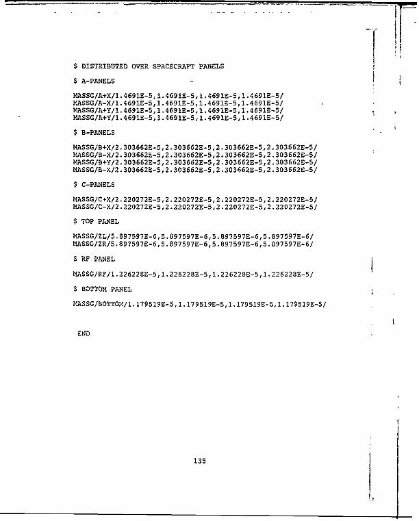
$ DISTRIBUTED OVER SPACECRAFT PANELS

$ A-PANELS

MASSG/A+X/1.4691E-5,1.4691E-5,1.4691E-5,1.4691E-5/MASSG/A-X/1. 469 1E-S,1. 469 1E-5, 1. 469 1E-5,1. 469 1E-5/MASSG/A+Y/1.4691E-5,1.4691E-5,1.4691E-5,1.4691E-5/MASSG/A+Y/1.4691E-5, 1.4691E-5, 1.4691E-5, 1.4691E-5/

$ B-PANELS

MASSG/B+X/2.303662E-5,2.303662E-5,2.303662E-5,2.303662E-5/MIASSG/B-X/2.303662E-5,2.303662E-5,2.303662E-5,2.303662E-5/MASSG/B+Y/2.303662E-5,2.3O36t52E-5,2.303662E-5,2.303662E-5/MASSGIB-X/2.303662E-5,2.303662E-5,2.303662E-5,2.303662E-5/

$ C-PANELS

MASSG/C+X/2.220272E-5,2.220272E-5,2.220272E-5,2.220272E-5/MASSG/C-X/2.220272E-5,2.220272E-5,2.220272E-5,2.220272E-5/

$ TOP PANEL

MASSGIZLI5.897597E-6,51.897597E-6,5.897597E-6,5.897597E-6/MASSG/ZR/5.897597E-6,5.897597E-6,5.897597E-6,5 .897597E-6/

$ RF PANEL

MASSG/RF/1. 22 6228E-5, 1. 226228E-5, 1. 226228E-5, 1.22 622 8E-5/

$ BOTTOM PANEL

MASSG/BOTTOM/1.179519E-S,1.179519E-S,1.179519E-S,1.179519E-5/

END

135

APPENDIX D -

A PANEL (A-X)

-H 0 -

F-4 0~

'-43

- - .

E-4

.491 8.

0.

* - 4- 40136

A PANEL (A+X)

z00.,4

-r 1 -" , :4.) ,*,'0.N.

C., C) N

0

137

II..I

A PANEL (A-Y)

>1

z

±1~' .0. ;r

EI-

".4

4. 0 0 '

1-4 .138

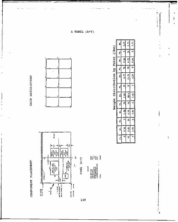
A PANEL (A+Y)

o *,.4

0

o 00 -

cNN

C

- ,-,'- ,-

_____ ____- N

139*N N

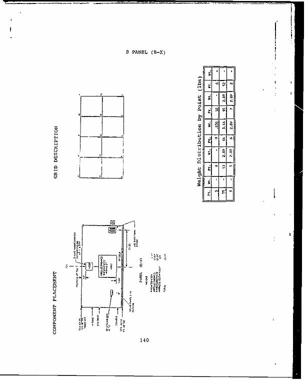
B PANEL (B-X)

HIM

w

(4.00

,- 10

H * -0'*

I

lei0.

140

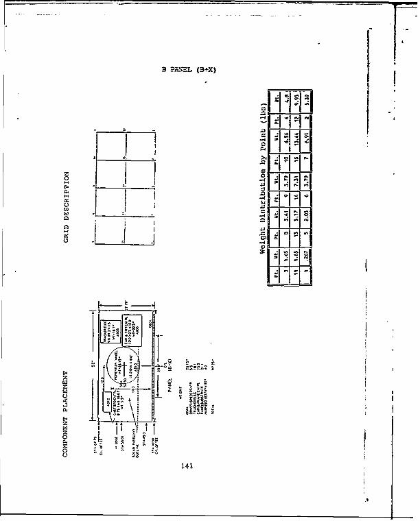
1.B P~EL (B~X)

?~ ~Ii~I-.~

- ~I ,~i,,i d~ I 1.-I

1 1 -4 ~vLI i ~*;~

hi.1:. ~0 -4 ~'.0 1 1--I-

____________ .9~ IC., ________

0

~~

I -I Z

F71 ~

I 4

E~* - II ~-Ii-* -"az 2

.ai~

L <

i

C-Z 5£

' £I I~ r1 ~

~ ;~ ~'o --. -C-,

141

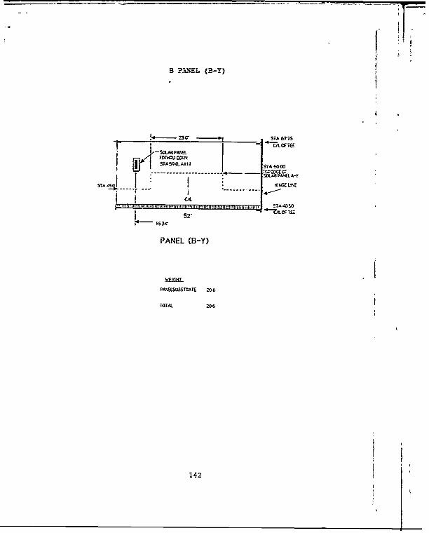
3 ?: EL (B-Y)

14 - " STA 67 .5

FOT~cr.-g -**..i L N -Lr5TA5.Al OA-00

CJL- L I *J-

52' 'C& CF TEE

'63C

PANEL (B-Y)

PlA,%aST%-iATE 206

*OTM. 206

142

3 PMEL (B+Y)

00

I It

4 .) P V

0 .I .i 2

0 I .. l .0F4

1-4 0 - .-7

- :1 . 143

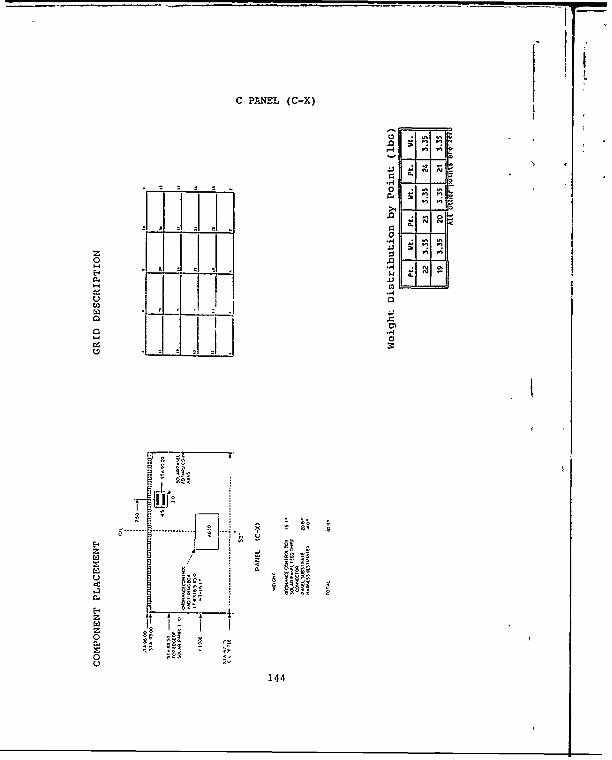
C PPUEL (C-X)

Ito

zi J

.. .. . .. .... ..

t-.4 -I N O

- 144

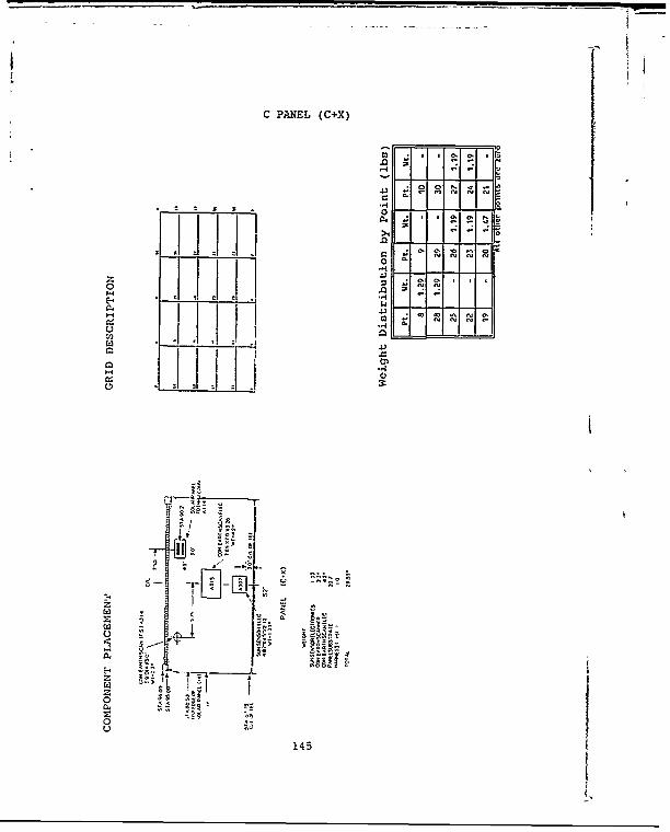
-~ t IC PANEL (C+X)

S 5 0.0.

4 0 0 *'. .~ .-

".4- - - 0

5 0. 0. N0 - .-

.0.1 0. N N N N

o".4

z Ii0 N N5.. .00

* S C C . .5*4 - -II $43.3I-I 400 ~I N 0.- I N N N -

ii ".4Si

o .00'-4 .5-I

0o 00 -

I.I ~ -II~ ""3

* ~.. ~7 .b

~ -*1..S- -

~ : ~\ ~

o ~A~A

"~ ~0~ ~:E- 2 $

I IoE ~

o -~ 145

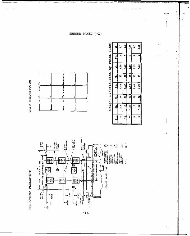
SENSOR PANMEL (-X)

-4-

E'-

00

1

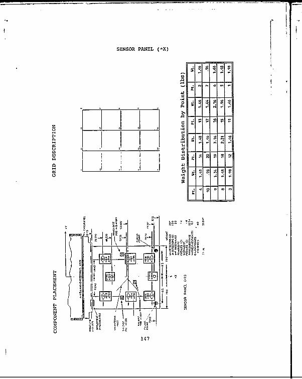
SENSOR PMEL ( X)

- 1___Ig~ _____ - :2'

0 - _ _ _ _ _JAG=_

_______ ______________ _______

1H . . 0 . ~

Mii

~~9 . 1 47 ~ . i c - c

FSENSOR PANEL (-Y)

,' ,* -t t . A%I n . '.. *- --

+___zz 0 4" "" +. .0 0 ,

"< i - N N

- ' ,' 0" -A'

_A,'-- A , ++ + ., .- , -

- -+ -

Il.I3I - i

148

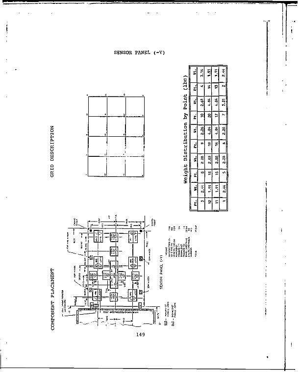
SENSOR PANEL (-Y) II

II .

-4 . 4..i,

O- >1•*1 , N N

Z .,-I

, '1 4' 4;' 4

,4 4, ,I 4

* - : -J 4. .3 4' 4

" L ... ....."T",...

____

-,149

SENSOR ARMS

01,

0 0

E.

.2: .,-o

E4.

z00

ZF 4.)

04

EC)

z -F0

150

II

RF DECK

------ I-

[II

1 4 3 1 a3 2

O ii: • 00NOO 6

P W

(2 151

o I O ' O ' 0 3 0 '

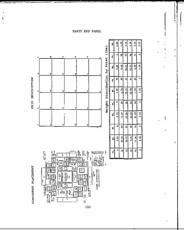
EARTH END PANEL

o . i04 0' -' ,0" N

S-7-1 0

i,0 02p0 0

152N

,0 ' .02', ',

00152*

f-PANEL C (C+Y)

.0 ; . .

I 4 ± °-"- z "-

-I' '-

o -*

~Li~ L3

z 4' K,,

PANEL C (C-Y)

F4 N 4

.".

0.

154. L

SACE E!4D PA!~L

__________________ ii _____ ____

- -\ Z~ 2 -i ~'I jj\~'/

-I I*IJ~~I~I*II \:~z I .. ~

C.. / I I[LILLI- X1 I ** 4,

-______________ -~ ~ ~I~I 'I 'I4 i\ -' II II I P

0 .0.01.01.01.04 z1..I -, ~ fl~ flifi

0 I I____ Cl :1_- ___ ~ 1

~:ii'~I 1- .0

-~ / I i-I..ILilr.0* 44

II(44 .0 .oj .0 C

* .1.

14" 4- III____ I

rVIiI 44 '!~I 1z I ~ a -

I L

III'o 4 't I'ii 45*5~ I ~

z I __o II ~

* -.---- I~~~;

155

APPENDIX E

COY.IL TO GENER=TE 150' T1RUSS AS A SUBSTRUCTURE TO BEATTCHE TO T-E AIV BODT-' OF TESPACE-CRAFT--

S BEAmcsTRUSi5o0L3/TA-RUSCSQuI.T$ BUL~mTRuS 150OLBIT-Ris1oBmQUIT -S LOADECTRUSisoOLBITRUSBCOLB/T.RSMAS15QUT$ BULKFTRUSiSO

//IlS DEF-CSTRUSiSo61,2, 3, 4,5, 6OLB/TRUSDEFQUITS ADSTIFrTRUS 150$ STASSTRUS 15$ DECO-1TRUS 150S REDCSTRUS 150

FILENAME IS TRUSCS.SRC

GENERATES CROSS SECTION 'TYPE AND DIMENSION OF BEAM ELEMENTS

CIRCS/B/.075/END

BULKM FILE THAT GENERATES 150' TRUSS

FILENAME IS TRUS!5OBM.SRC

156

ELMAT, 4/6/6. 0E4, 8.OE6,.29, 1. 9409947-4/KPOINT/lIO,0,4.763/2/0,8.25,o/3/0,o,-4.763/4/1800,0,4.763/00'LO.NT/5/1800,8.25,0/6/1800,0,-4.763/7/90,0,50/

LETYIBEAPM2/6,8S/SLINiE,10/L14/1,4,301/7/L36/3,6,301/7/L25/2,5,301/8'L12/1,2,3/7/SLI-NE-,1O/L23/2,3,3/7/L13/1,3,3/7/L45/4,5,3/7/L56/5,6,3/7/

SLINE,10/L46/4, 6,3/7/ 'EIHFILE TO ADD BATTE-NS AND DIAGONALS TO THE 150' TRUSS

FILENAME IS TRS15OEM.SRC

PTRTH;/8/PTRTiM/6/

$ VERTICAL MEMBERS

BEAM T-2/9,307,7, i,49/157f455,7/158,307,7,149/306,455,7/

$BOTTOM MEMBERS

BEAM-12/9, 158,7, 149/157,306,7/

$ DIAGONAL MEMBERS

ETH, 1/9/.001963/

ROD2/9,159,148/156,306,'10,158,148,'157,305/9,308,148/156,455/

ROD2/10,307, 148/157,454/158,308, 148/305,455/159, 307, 148/306,454 /

ROD2/1,307/2,9/3,9/1, 158/3,307/2,158/4,455/5,157/5,306/6,455/

ROD2/6, 157/4,306/

GENERATES POINT MASSES FOR THE 150' TRUSS

FILENAME IS TRSMlAS15.SRC

MASSP/1/2 .71E-5/2/2 .71E-5/3/2 .71E-5/MASSP/4/2 .71E-5/5/2.71E-5/6/2.71E-5/MASSP/9,307,299/2.71E-5,2.71E-5/308, 606,299/2 .71E-5,2.71E-5/MASSP/607,905,299/2.71E-5,2.71E-5;'END

157

POI14T MASS X MASS Y MASS Z440 1.234E-02 1.234E-02 1.234E-02441 0,650E-03 0.650E-03 0.650E-03442 1.305E-02 1.305E-02 1.305E-02443 1.085E-02 1.065E-02 1.095E-02444 8.560E-03 0.580E-03 8.580E-03445 1.305E-02 -1.907E+00 1.305E-02446 9.940E-03 4.594E-02 9.940E-03447 1.042E-02 1.842E-02 -1.583E-03448 1.842E-02 1.842E-02 1.842E-02449 -6.583E-03 1.842E-02 1.842E-02450 1.842E-02 1.842E-02 1.842E-02

158

APPENDIX F

$ !COM FILE TO GENERATE AND CONNECT SPACECRAFT TRUSSES

S IFILENAME IS TRUSS.COM

DEL TRUSS.*;*

$ BEAMCSLACEOLB/TRUSCSQUIT$BULKMLACEOLB/TRUSSBMQUIT$ EDITMLACEOLE /TRUS SEMQUIT$ LOADBCLACEOLB/TRUSMASSQUIT

$ GENERATES THE FILE FOR THE THREE TRUSSES OF THE LACE$ SPACECRAFT USING THE PROCESSOR BULKM$ BULKM FILE TO GENERATE 150 FOOT TRUSS IN +Y DIRECTION$ ELEMENT MATERIAL

ELMAT,4/6/6.0E4,8.0E6, .29, 1.94099E-4/

KPOINT/451/8.237,26,79.25/452/8.237,1826,79.25/KPOINT/453/13,26,87.5/454/13, 1826,87.5/KPOINT/455/17 .763,26,79.25/456/17.763, 1826, 79.25/KPOINT/457/67 .763,926,79.25/

LETY/BEAM2/6, 8/

SLINE, 10/LTR12/451,452,301/457/LTR34/453,454,301/457/SLINE, 10/LTR56/455,456, 301/457/LTR13/451,453, 3/457/SLINE, 10/LTR35/453,455,i/457/LTR15/451, 455,3/457/SLIME, 10/LTR24/452,454,3/457/LTR46/454,456,3/457/SLIME, 10/LTR26/452,456,3/457/

$ FILE TO GENERATE 150 FOOT TRUSS IN +Z DIRECTION

159

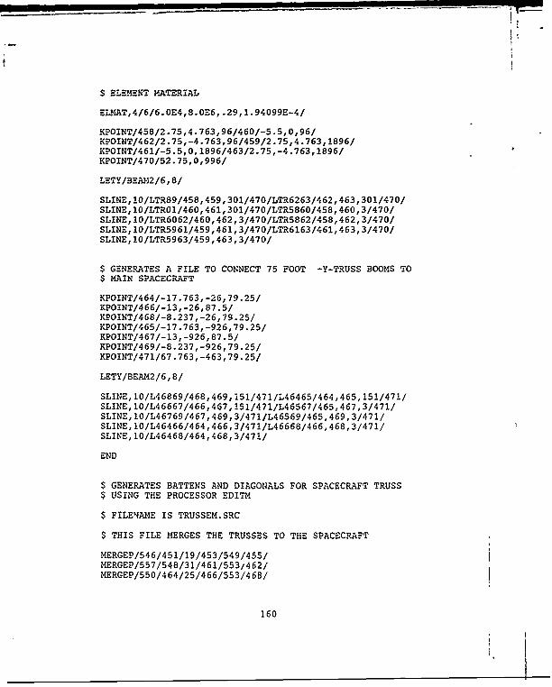
S ELEMENT MATERIAL

ELMT,4/6/6. 0E4,8. 0E6, .29,1. 94099E-4/

KPOINT/458/2.75,4.763,96/460/-5.5,O,96/KPOINT/462/2.75,-4.763,96/459/2.75,4.763,1896/KPOINT/461/-5.5,O,1896/463/2.75,-4.763,1896/KPOINT/470/52 .75,0,996/

LE-TY/BEANU-2/6, 8/

SLIME, 10/LT-R89/458, 459, 301/470/LTR;6263/462, 463,301/470/SLINE, 10/LTR01/460,461, 301/470/LTiR5860/458,460,3/470/SLINE, 10/LTR6062/460,462,3/470/LTR5862/458,462,3/470/SLIME, 10/LTR5961/459,461,3/470/LTR6163/461, 463,3/470/SLIME, 10/LTR5963/459 ,463, 3/470/

$ GENERATES A FILE TO CONNECT 75 FOOT -Y-TRUSS BOOMS TO$ M4AIN SPACECRAFT

KPOINT/464/-17 .763,-26, 79.25/KPOINT/466/-13,-26,87.5/KPOINT/468/-8 .237,-26, 79.25/KPOINT/465/-17.763,-926,79 .25/KPOINT/467/-13,-926,87.5/KPOINT/469/-8.237, -926,79.25/KPOINT/471/67 .763, -463,79.25/

LETY/BEAIM2/6, 8/

SLINE, l0/L46869/468,469, 151/471/L46465/464,465,151/471/SLIME, 10/L46667/466,467,151/471/L46567/465,467,3/471/SLIME, 101L467691467,469,3/471/L46569/465,469,3/471/SLINE, 1O/L46466/464,466, 3/471/L46668/466, 468, 3/471/SLINE, 10/L46468/464,468,3/471/

END

$ GENERATES BATTENS AND DIAGONALS FOR SPACECRAFT TRUSS$ USING THE PROCESSOR EDITH

S FILENAM4E IS TRUSSEM.SRC

$ THIS FILE MERGES THE TRUSSES TO THE SPACECRAFT

MERGEP/546/451/19/453/549/455/MERGEP/557/548/31/461/553/462/MERGEP/550/464/25/466/553/468/

160

$ GENERATES VERTICAL,BOTT"-OM,DIAGONAl- MEMBERS FOR 150 FT TRUSS$ IN THE +Y DIRECTION

PTRTH/8PT;ZM/6

$ VERTICAL/BOTTOM MEMBERS

BEAI12/974, 1273,457,299/1272,1571,457/BEAM2/675,974,457,299/973, 1272,457/BEAM2/675, 1273,457,299/973, 1571,457

$ GENERATES BATTENS AND DIAGONALS FOR SPACECRAFT TRUSS$ USING THE PROCESSOR EDITM

$ FILENAYE IS TRUSSEM.SRC

$ THIS FILE MERGES THE TRUSSES TO THE SPACECRAFT

MERGEP/546/451/19/453/549/455/MERGEP/557/548/31/461/553/462/MERGE-P/550/464/25/466/553/468/

$ GENERATES VERTICAL, BOTTOM, DIAGONAL MEMBERS FOR 150 FT TRUSS$ IN THE +Y DIRECTION

PTRTH/8PTRIM/6

$ VERTICAL/BOTTOM MEMBERS

BEAMd2/974, 1273,457,299/1272,1571,457/BEAM2/675,974,457,299/973,1272,457/BEA2/675,1273,457,299/973, 1571,457

$ DIAGONAL MEMBERS

ETH, 1/10/. 0019 63/

PTRTH/10/

ROD2/455,675/451,1273/455,974/453,1273/453, 675/451,974/ROD2/975,1273,298/1272,1570/974,1274,298/1271,1571/ROD2/675,975,298/972,1272/676,974,298/973,1271/ROD2/675,1274,298/972,1S71/676,1273,298/973,1570/ROD2/456,973/452,1571/456,1272/454,1571/452,1272/454,973/

$ GENERATES VERTICAL, BOTTOM, DIAGONAL MEMBERS FOR 150 FT TRUSS$ IN THE +Z DIRECTION

PTRTH/8

161

PTRZM/ 6

S VERTICAL/BOTTOM MEMBERS

BEAM?2/1578, 1877, 464,299/1876,2175,464/BEA}.2/1578,2176,464,299/1876,2474, 464/BEA}M2/1877, 2176,464,299/2175,2474,464

$ DIAGONAL MEMBERS

EH, 1/10/.001963/

PTRTH/10/

ROD2/463, 1876/459,2175/461, 1876/459,2474/461,2175/463,2474/ROD2/1877,2177,298/2174,2474/1878,2176,298/2175,2473/RZOD2/1579, 1877,298/1876,2174/1578, 1878,298/1875,2175/ROD2/1579,2176,298/1876,2473/1578,2177,298/1875,2474/ROD2/462,2176/462, 1578/460, 1877/460, 1578/458,2176/458,1877/

$ GENERATES VERTICAL,BOTTOM,DIAGONAL MEMBERS FOR 75 FT TRUSS$ IN THE -Y DIRECTIONPTRTH/8

PTRM/6

$ VERTICAL/BOTTOM MEMBERS

BEAM2/2630,2779,470, 149/2778,2927,470/BEAM2/2481, 2779, 470, 149/2629,2927,470/BEAM2/2481,2630,470, 149/2629,2778,470/

$ DIAGONAL MEMBERS

ETH, 1/10/. 001963/

PTRTH/10/

ROD2/464, 2779/466,2630/464,2481/468,2630/468,2779/466,2481/ROD2/2630,2780,148/2777,2927/2631,2779,148/2778,2926/ROD2/2482,2630,148/2629,2777/2481,2631,148/2628,2778/ROD2/2481,2780, 148/2628,2927/2482,2779,148/2629,2926/ROD2/465,2927/467,2778/465,2629/469,2778/469, 2927/467,2629/

END

$ GENERATES MASS FOR THE COMPLETE TRUSS MODEL

$ GENERATES MASS FOR THE 150 FOOT TRUSS IN +Y DIRECTION

162

MASP/518.84E-545/8886E5/43/.846-5

MASSP/454/8 .8846E-5/452/8.8846E-5/456/8 .8846E-5/

MAASSP/1273,1571,299/8.8846E-5,8.8846E-5/IASSP/675, 973,299/8.8846E-5,8.8846E-5/!4ASSP/974, 1272, 299/8.8846E-5, 8. 884 6E-5/

$ GENERATES MASS FOR THE 150 FOOT TRUSS IN +Z DIRECTION

MASSP/464/8. 8846E-5/465/8 .8846E-5/466/8 .8846E-5/MASSP/467/8 .8846E-5/468/8. 8846E-5/469/8 .8846E-5/MASSP/2779, 2927,149/8. 8846E-5, 8.8846E-5/MASSP/2630, 2778, 149/8.8846E-5, 8.8846E-5/MASSP/2481,2629, 149/8.8846E-5,8.8846E-5/

$ GENERATES MASS FOR THE 75 FOOT TRUSS IN -Y DIRECTION

MASSP/458/8 .8846E-5/459/8 .8846E-5/460/8 .8846E-5/MASSP/461/8 .8846E-5/462/8 .8846E-5/463/8 .8846E-5/MASSP/1578, 1876,299/8.8846E-5,8 .8846E-5/MASSP/1877,2175,299/8.8846E-5,8.8846E-5/MASSP/2176,2474,299/8.8846E-5,8.8846E-5/

$ GENERATES TIPMASS FOR EACH TRUSS

MASSP/459/1 .72533E-1/461/1 .72533E-1/463/1 .72533E-1/MASSP/452/3.0193E-2/454/3 .0193E-2/456/3.0193E-2/

MASSP/465/3.0193E-2/467/3.0193E-2/469/3.0193E-2/

END

163

-

APPENDIX G

Before the LACE spacecraft was in its fully deployed state,

it underwent three different configurations. Figures Gi to G4

show the natural frequencies and mode shapes of the LACE

spacecraft in its initial configuration with the gravity

gradient extended to 75 feet. Figures G5 to G8 show LACE with

the gravity gradient extended to 150 feet. Figures G9 to G12

show the LACE spacecraft in its final configuration before

full deployment with the lead and trail booms extended to

119.5 feet.

164

Figure Gi. Mode 1, u .01365 H~z, GIFTS COMPLEX MODEL

165

Figure -2--e2 u .17 zGFSCMPE OE

1647

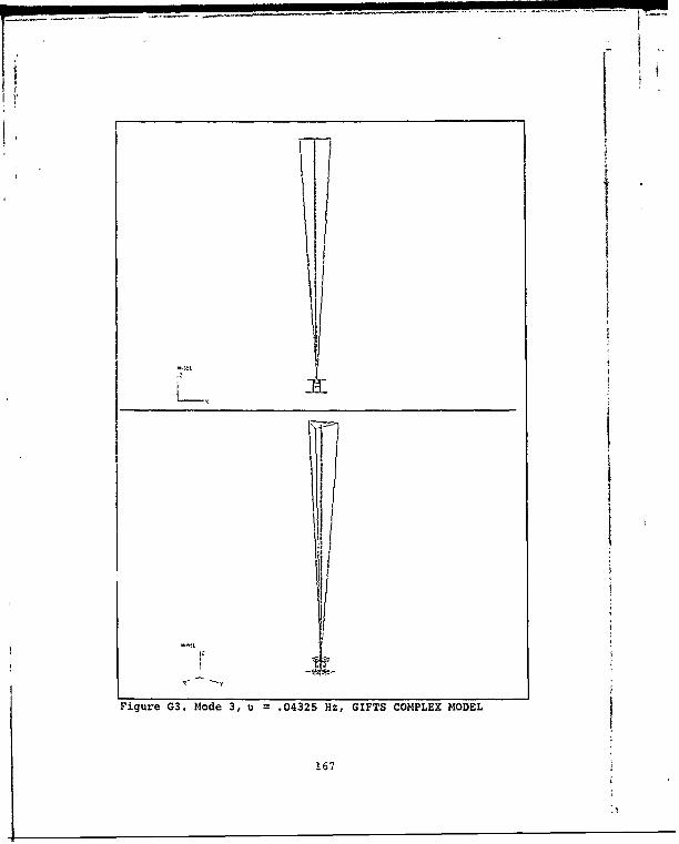
Figure G3. Mode 3, u =.04325 Hz, GIFTS COMPLEX MODEL

167

Figure G4. Mode 4, ui .04579 Hz, GIFTS COMPLEX MODEL

168

F I

4I

31:1

~1-I

-t I

Ii*1

Figure G5. Mode 1, u = .01217 Hz, GIFTS COMPLEX MODEL

169

r*1

I:1

I

~1-II

II;I:

~41~

Figure GS. Mode 2, u = .01226 Hz, GIFTS COMPLEX MODEL

170

/-

I:i

Figure G7. Mode 3, u =.03535 Hz, GIFTS COMPLEX MODEL

171

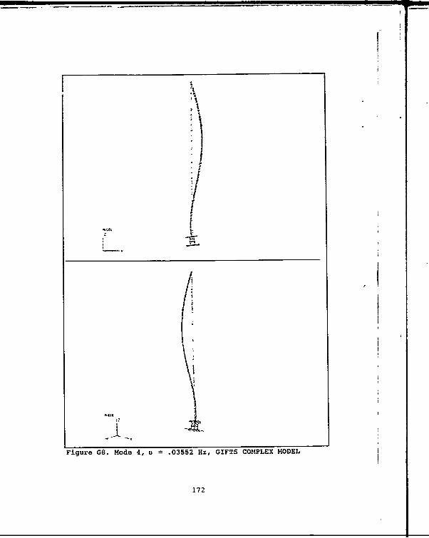
I* 4

4I.

IIi

A

/1 '1I:

FIgure GB. Mode 4, u = .03552 Hz, GIFTS COMPLEX MODEL

172

Figure G9. Mode 1, u =.02322 Hz, GIFTS COMPLEX MODEL

173

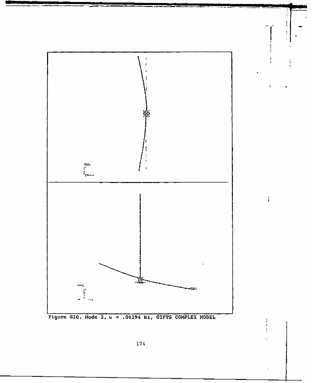
Figure GIO. Mode 2, u .04294 Hz, GIFTS COMPLEX MODEL

174

t I~

Fizgure Gil. Mode 3, u =.04302 Hz, GIFTS COMPLEX MODEL

175

1

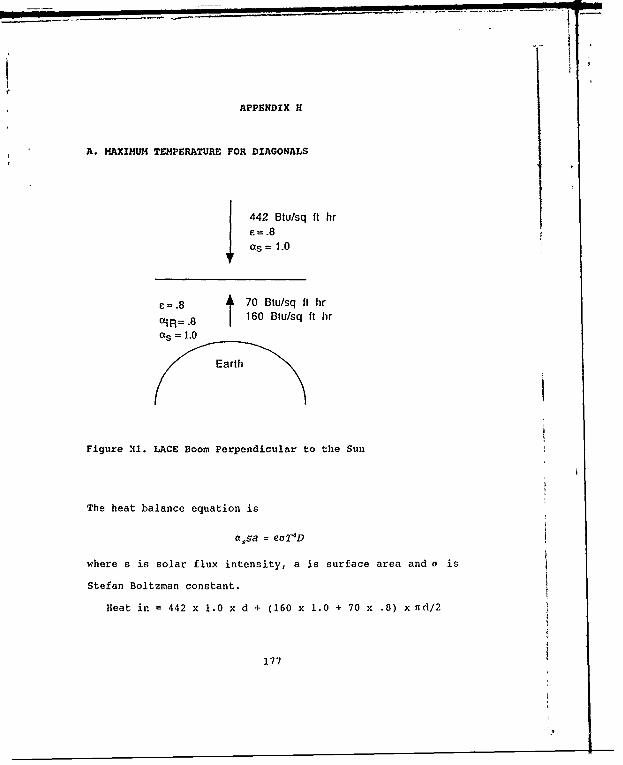
APPENDIX H

A. MAXIMUM TEMPERATURE FOR DIAGONALS

C=.8 fth

E=.8 470 Btu/sq ft hraiR= .8 160 Btu/sq ft hras = 1.0

Earth

Figure 21. LACE Doom Perpendicular to the Sun

The heat balance equation is

a,5 a = eoT4D

where s is solar flux intensity, a is surface area and a is

Stefan loltzman constant.

Heat in' 442 x 1.0 x d + (160 x 1.0 + 70 x .8) x nd/2

177

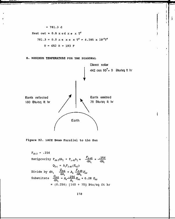
781. 3 d: :=430 0THeat out = 0. 8 x n d x a x T4

B. MINIMUM TEMPERATURE FOR THE DIAGONAL

Di rect solar

~442cos 900 = 0 Btu/sq ft hr

Earth reflected Earth emitted160 Btu/sq ft hr 70 Btulsq it hr

/:tEarth

Figure H2. LACE Beam Parallel to the Sun

Fd1I2 = .256

Reciprocity F d1- 2dA, = F,.dlA, FdI=.256

Q11= AjFj-dj(Eb1)

Divide by dA1 Q- A 2 ld bI dA 2

Substitute A2 .26 2 0. b

(0.256) (160 + 70] Btu/sq ft hr

178

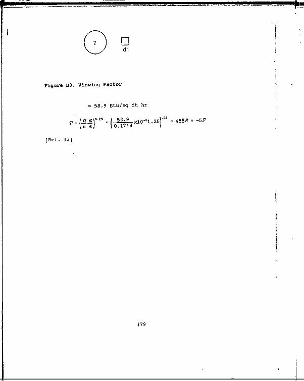
20 dl

Figure H13. Viewing Factor

=58.9 BtU/sq ft hr

-(~;xio-81.25) =455R=-SF

[Ref. 13]

179

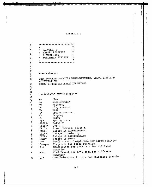
APPENDIX I

C ************************

C * WALTERS, W *

C * THESIS RESEARCH *

C * 6 JUNE 1990 *

C * NONLINEAR SYSTEMS *C * *C ************************CCCC ***PURPOSE***CC THIS PROGRAM COMPUTES DISPLACEMENTS, VELOCITIES,AND

ACCELERATIONC USING LINEAR ACCELERATION METHODCCCC ***VARIABLE DEFINITIONS***CC T= TimeC A= AccelerationC V= VelocityC U= DisplacementC M= MassC K= Spring constantC C= DampingC P= ForceC FS= Spring forceC KSTAR= Delta K*C PSTAR= Delta P*C DELT= Time interval, delta tC DELU= Change in displacementC DELV= Change in velocityC DELA= Change in accelerationC DELP= Change in forceC A0= Coefficient of amplitude for force function

C Omega= Frequency for force functionC Al= Coefficient for X**3 term for stiffness

functionC B1= Coefficient for X**2 term for stiffness

functionC C1= Coefficient for X term for stiffness function

180

C D1= coefficient for constant term for stiffnessfunction

C A2= Coefficient for X**2 term for damping functionC B2= Coefficient for X term for damping functionC C2= Coefficient for constant term for damping

functionC FRAC= Fraction of linear stiffness term used for

coeff. of cubic termCC ***VARIABLE DECLARATIONS***

Real*16 T,A,V,U,M,K,C,FS,KSTAR,PSTAR,DELT,DELU,DELV,

*DELA,DELP,AO,Omega,A1,B1,Cl,D1,A2,B2,C2,FpAC,MASS,P(5000)C DIMENSION P(5000)

Integer I,NC

CHARACTER*7 DUMMYCHARACTER NAME-8, FN*8

C ***INITIAL DATA***C

T=0 .0N=0

CC ***MAIN PROGRAM4***

C ==CREATE A FILE FOR CHAOTIC COMPUTAIONSOPEN (UNIT=l, FILE='ACC.INP', STATUS='OLD')

WRITE (6,*) 'INPUT THE FILE NAME'READ (5,'(A)') NAMEFN = NAMEOPEN (UNIT = 12, FILE = FN, STATUS ='NEW')

WRITE(6,*) 'DO YOU WANT INTERACTIVE INPUT FILE,0=YES, 1=NO'READ(5,*) IYESIF (IYES.GT.0) GO TO 500

CPRINT *~'ENTER INITIAL CONDITIONS'PRINT *,'INITIAL DISPLACEMENT '

READ *,U

PRINT *'INITIAL VELOCITY =

READ *VPrint *,'F(X)=AG*COS(Omega*T)'

Print *,'Enter value for AO'Read *,AO

Print *,'Enter value for omega'Read *,Omega

Print *, K(X)=Al*X**3+B1*X**2+C!*X+DllPrint *~'Enter value for Al'

181

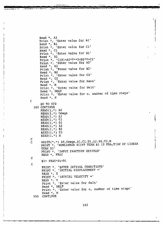
Read *, AlPrint *, 'Enter value for Bi'Read *, B1Print *, 'Enter value for Cl'Read * C1Print *, 'Enter value for Dl'Read * DIPrint *, 'C(X)=A2*V**2+B2*V+C2'Print , 'Enter value for A2'Read *, A2Print , 'Enter value for B2'Read *, B2Print *, 'Enter value for C2'Read *, C2Print *, 'Enter value for mass'Read *, MPrint *, 'Enter value for delt'Read *, DELTPrint *, 'Enter value for n, number of time steps'

Read * NC

GO TO 550500 CONTINUE

RFAD(l,*) AOREAD(1,*) OmegaREAD(I,*) AlREAD(I,*) C1READ(l,*) DREAD(l,*) A2READ(l,*) B2READ(l,*) C2READ(l,*) M

CC WRITE(*,*) A0,Omega,A1,Cl,Dl,A2,B2,C2,M

PRINT *, 'NONLINEAR STIFF TERM BI IS FRACTION OF LINEAR

TERM Dl'PRINT *, 'INPUT FRACTION DESIRED'READ *, FRAC

CB= FRAC*DI+DI

CPRINT * 'ENTER INITIAL CONDITIONS'PRINT * 'INITIAL DISPLACEMENT ='

READ *, UPRINT * 'INITIAL VELOCITY ='

READ * VPrint *, 'Enter value for delt'Read * DELTPrint *, 'Enter value for n, number of time steps'

Read *, N550 CONTINUE

182

Do 20 7-=!,NCall 7Force(P0,Orega,S-,I,?)Call Da~n(A2,B2,C2,V,C)

Call

C

C

C Solve for FSTA-RC

KSTAzR=--.( (3*C)IDz-=-).j(6*14)IDELT~**2)CC Solve for PSTARC

PSTRDE-LP+( ((6*1)IDELiT)+(3*C) )*V+( 13*M,)..C*(DELTT/2) )*A

C Solve for DE-TLUC

DELU=PSTAR/KSTA.R

C Solve for DELVC

DELTV= (3/DE-LT-)*DELU ( 3-V) -A*(DELI2)C Solve for DELA

CDELA= (6/DELT**2) *DE-U-.( (6/DELT) *V) - ( 3A)

CC Write outDut filecC ** OUTPUT TO THE CHAOTIC FILE

WRITE(ll,6000) DUMMY,T,U,V,A6000 FOR1MAT(A7,F6.3,E11.4,4El2.4)

C Update U,V,T for next iterationC

tJ=U+DELUV=V+DELVT=T+DELT

20 ContinueC

Write(*, *)T,U,VCLOSE(UNIT-1)CLOSE(UNIT=11)StopEnd

C

C

183

IC

CSubroutine Force(AO,Ozega,T, I,?)

CC Assigns a value to force based on tireC Input argu=ennC AO-Coeffc;enz,o-ega-frecuency,T-Tize, I-CounterC Output arguentC P-ForceC

Real*16 AO,Onega,T,Pinteger IDIMENSION P(5000)

CCC Define resultsC

P()=AO*COS(Omega*T)C Write(*,*)!,P(I)

ReturnEnd

CC

Subroutine Damp(A2,B2,C2,V,C)CC Assigns a value for dampingC input argumentC A2,B2,C2 - Coefficients of damping functionC U-DisplacementC Output argumentC C-DampingC

Real*16 A2,B2,C2,V,CC Define resultsC

C=A2*V**2+B2*V+C2ReturnEnd

CC*****************************************************, A **

CSubroutine FSPRING(Al,BI,CI,D1,U,I,K,FS)

CC Calculates the value for FSCC Input arguments

184

CC U-DisplacezentsC Al,Bl,C!,Dl- Coefficients for stiffness functionC I-counterCC Output argurentsCC FS-Force of springC

Real*16 Al,Bl,Cl,Dl,U,FS,Kinteger I

CC Define resultsC

K=A!*U**3+3*U**2+C1*U+DlFS=K*UReturnEnd

C

C

CSubroutine DFORCE(T,DELP,I,P)

CC Defines the value for the change in forceCC Input argumentC T-Time,P-ForceC Output argumentC DELP-Change in force

Real*16 T,DELP,F,P(5000)INTEGER I

C DIMENSION P(5000)CC

IF (I.EQ.1) ThenDELP =0

ELSEDELP=P(I)-P(I-1)

EndifReturnEnd

C*********************************************** **** *******

185

-I

APPENDIX J

186

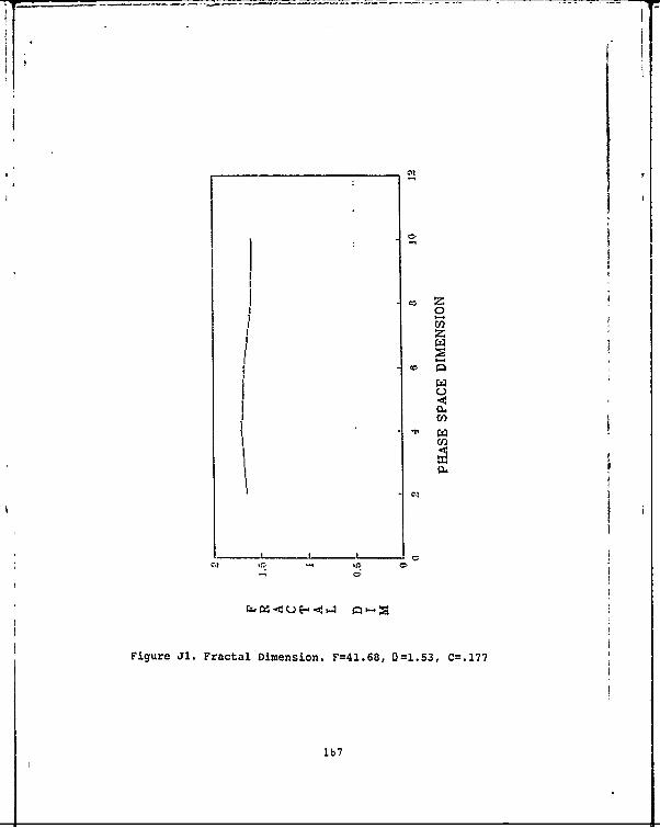
~-z

Ck) IL IL

U E- -. -A iz

Figure J1. Fractal Dimension. F=41.68, 0=1.53, C=.177

lb7

00

z

1881

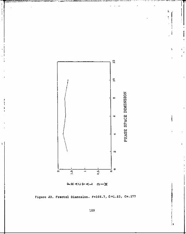
I j

z

cca

Figure J3. Fractal Dimension. F=166.7,01.53, C=.177

189

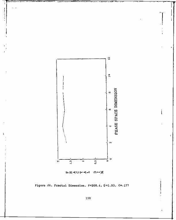
1902

z

T-~ ~ ~ ~ ~ W -- 40 -- 1 4

i912

0

2

C, k

Figure J6. Fractal Dimension. F=41.68, ()13.8, C=.177

192

II

04

~Clk

9 I

c

Figure J7. Fractal Dimension. F=83.35, 0=13.8, C=.177

193

14

CL

1942

cz

rZ4Z - 40 - -' 0

Figure~ ~ ~ ~ ~ J9 -ca ieso.F=0.,01.,C.7

195,

00

Fiur JO.Frctl imnio. 4168 ~.5, .05

196o

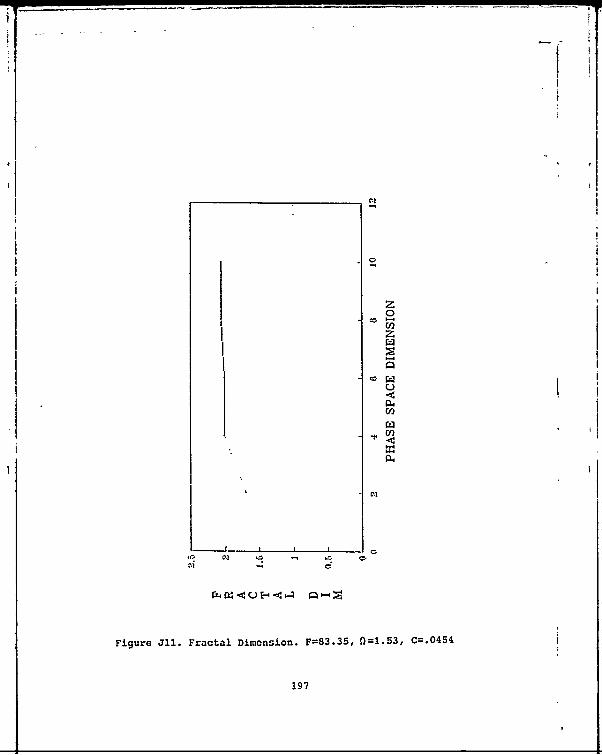
U)

1971

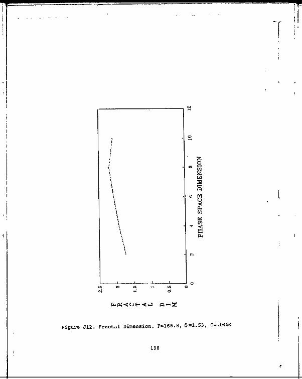
pM ___ __f___ ___ __

rz, -. 4U E -. 4 M --

Figue J2. racal Dmenion F066.8 0=.53 C=045

1981

cn.

1992

z

CL4

Figure J14. Fractal Dimension. F=20.8, 0=13.8, C=.0454

200

- 0

C-)

0\ *C. -.4

Figure J15. Fractal Dimension. F=41.68,()=13.8, c=.0454

201

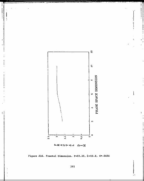
iiN

z

CAC

202

U -i

203

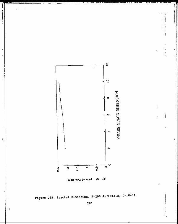
0

z

204

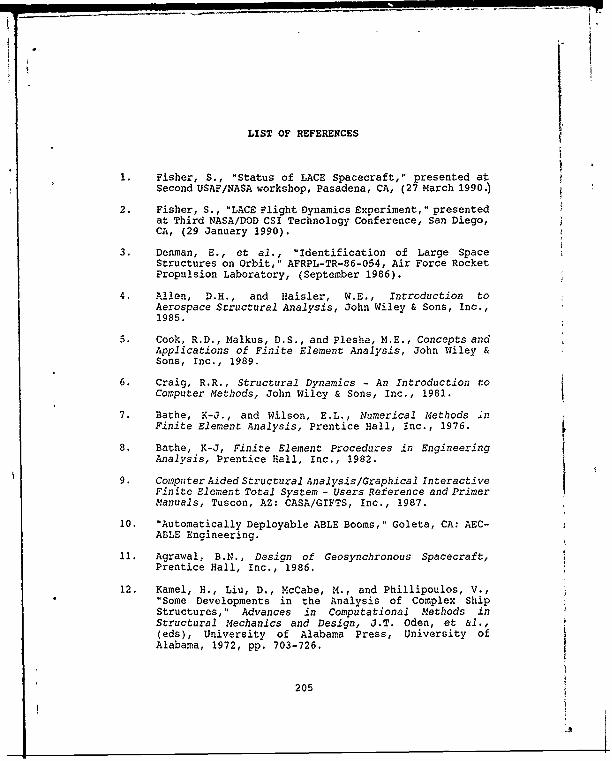
LIST OF REFERENCES

1. Fisher, S., "Status of LACE Spacecraft," presented atSecond USAF/NASA workshop, Pasadena, CA, (27 March 1990.)

2. Fisher, S., "LACE Flight Dynamics Experiment," presentedat Third NASA/DOD CSI Technology Conference, San Diego,CA, (29 January 1990).

3. Denman, E., et al., "Identification of Large SpaceStructures on Orbit," AFRPL-TR-86-054, Air Force RocketPropulsion Laboratory, (September 1986).

4. Allen, D.H., and Haisler, W.E., Introduction toAerospace Structural Analysis, John Wiley & Sons, Inc.,1985.

5. Cook, R.D., Malkus, D.S., and Plesha, M.E., Concepts andApplications of Finite Element Analysis, John Wiley &Sons, Inc., 1989.

6. Craig, R.R., Structural Dynamics - An Introduction toComputer Methods, John Wiley & Sons, Inc., 1981.

7. Bathe, K-J., and Wilson, E.L., Numerical Methods inFinite Element Analysis, Prentice Hall, Inc., 1976.

8. Bathe, K-J, Finite Element Procedures in EngineeringAnalysis, Prentice Hall, Inc., 1982.

9. Computer Aided Structural Analysis/Graphical InteractiveFinite Element Total System - Users Reference and PrimerManuals, Tuscon, AZ: CASA/GIFTS, Inc., 1987.

10. "Automatically Deployable ABLE Booms," Goleta, CA: AEC-ABLE Engineering.

11. Agrawal, B.N., Design of Geosynchronous Spacecraft,Prentice Hall, Inc., 1986.

12. Kamel, H., Liu, D., McCabe, M., and Phillipoulos, V.,"Some Developments in the Analysis of Complex ShipStructures," Advances in Computational Methods inStructural Mechanics and Design, J.T. Oden, et al.,(eds), University of Alabama Press, University ofAlabama, 1972, pp. 703-726.

205

13. Ikeda, P.J., Brogren, E.W., "LACE Thermal Deformation,"Information paper presented to NRL, (I November 1989).

14. Hurty, W.C., "Dynamic Analysis of Structural SystemsUsing Component Modes," AIAA Journal, vol. 3, no. 4,(1965), 678-684.

15. Craig, R.R., and Bampton, M.C.C., "Coupling ofSubstructures for Dynamic Analysis," AIAA Journal, vol.6, no. 7, (1968), 1313-1319.

16. Rubin, S., "Improved Component-Mode Representation forStructural Dynamics Analysis," AIAA Journal, vol. 13,no. 8, (1975), 995-1006.

17. MacNeal, R.H., "A Hybrid Method of Component ModeSynthesis," Computers and Structures, vol 1, (1971),581-601.

18. Martina, D.R., and Miller, K.A., "Combined Experimental,Analytical Modeling of Dynamic Structural Systems," TheAmerican Society of Mechanical Engineer, (1985), 1-18.

19. Singh, R.P., VanderVoort, R.J., and Likins, P.W.,"Dynamics of Flexible Bodies in TREE Topology - AComputer Oriented Approach," Journal of Guidance,Control and Dynamics, vol. 8, no. 5, (Sept.-Oct. 1985),584-589.I

20. "TREETOPS User Manual," Dynacs Engineering Co., Inc.,Clearwater, FL.

21. Moon, F.C., Chaotic Vibrations, John Wiley & Sons, Inc.,1987.

22. Sarigul-Klijn, M.M., "Application of Chaos Methods toHelicopter Vibration Reduction Using Higher HarmonicControl,", Doctoral Dissertation, Naval PostgraduateSchool, Monterey, CA, (March 1990).

23. Thompson, M.T., and Steward,H.B., Nonlinear Dynamics andCHAOS, John Wiley & Sons, Inc., 1986

24. Guckenheimer, J., and Holmes, P., NonlinearOscillations, Dynamical Systems and Bifurcations ofVector Fields, Springer-Verlag, 1983

25. Grassberger, P., and Proccucia,I., "Characterization ofStrange Attractors," Physics Review Letters, No. 50,(1983), 364-379.

206

26. Walters, Wesley F., AE4900 Report, "Parametric Study ofChaotic Vibrations in the LACE Spacecraft Boom," (1990)

27. Moon, F.C., and Li, G.X., "Experimental Study of ChaoticVibrations in a Pin-Jointed Space Truss Structure,' AZAAJournal, vol. 28, no. 5, (1990)

207

-I

BIBLIOGRAPHY

Gere, J.M. and Timoshenko, S.P., Mechanics of Materials, PWS

Publishers, 1984.

Hurty, W.C. and Rubinstein, M.F., Dynamics of Structures,Prentice-Hall, 1964.

Koffman, E.B., and Friedman, F.L., Problem Solving andStructural Programming in Fortran 77, Addison-WesleyPublishing Company, Inc., 1987.

Levy, S., and Wilkinson, J.P., The Component Element Method inDynamics, McGraw-Hill Book Co., 1976.

Meirovitch, L., Elements of Vibration Analysis, McGraw-HillBook Co., 1975.

Segerlind, L.J., Applied Finite Element Analysis, John Wiley& Sons, Inc., 1976.

Thomson, W.T., Theory of Vibration with Applications,Prentice-Hall, 1988.

208

INITIAL DISTRIBUTION LIST

1. Defense Technical Inform-ation Center 2Cameron StationAlexandria, Virginia 22304-6145

2. Superintendent 2Attn: Library, Code 1424Naval Postgraduate SchoolMonterey, California 93943-5000

3. Department Chairman, Code AADepartment of Aeronautics and AstronauticsNaval Postgraduate SchoolMonterey, California 93943-5000

4. Department of Aeronautics and Astronautics 20Attn: Professor Ramesh Kolar, Code AA/KjNaval Postgraduate SchoolMonterey, California 93943-5000

5. Department of Aeronautics and AstronauticsAttn: Professor Brij Agrawal, Code AA/AgNaval Postgraduate SchoolMonterey, California 93943-5000

6. Space Systems Academic GroupAttn: Professor Rudolph Panholzer, Code SPNaval Postgraduate SchoolMonterey, California 93943-5000

7. Major Wesley F. Walters 2293 Skinner Dr.Redstone Arsenal, AL 35808

8. Naval Research Laboratory 2Attn: Dr. Shalom Fisher, Code 8240.1Washington, D.C., 20375

209