Dynamic 3D axisymmetric problems in continuously non ...

International Journal of Solids and Structures 45 (2008) 4523–4542

CORE Metadata, citation and similar papers at core.ac.uk

Provided by Elsevier - Publisher Connector

Contents lists available at ScienceDirect

International Journal of Solids and Structures

journal homepage: www.elsevier .com/locate / i jsols t r

Dynamic 3D axisymmetric problems in continuouslynon-homogeneous piezoelectric solids

Jan Sladek a,*, Vladimir Sladek a, Peter Solek b, Andres Saez c

a Institute of Construction and Architecture, Slovak Academy of Sciences, Dubravska cesta 9, 84503 Bratislava, Slovakiab Department of Mechanics, Slovak Technical University, Bratislava, Slovakiac Department of Continuum Mechanics, Escuela Superior de Ingenieros, University of Sevilla, Camino de los Descubrimientos S/N, E-41092 Sevilla, Spain

a r t i c l e i n f o a b s t r a c t

Article history:Received 17 September 2007Received in revised form 19 March 2008Available online 4 April 2008

Keywords:Transient problemsThermal loadAnisotropic functionally graded materialsTime-difference formLaplace transformStehfest algorithmMeshless approximation

0020-7683/$ - see front matter � 2008 Elsevier Ltddoi:10.1016/j.ijsolstr.2008.03.027

* Corresponding author. Tel.: +421 2 54788662; fE-mail address: [email protected] (J. Sladek).

The meshless local Petrov-Galerkin (MLPG) method is used to analyze transient dynamicproblems in 3D axisymmetric piezoelectric solids with continuously inhomogeneousmaterial properties. Both mechanical and thermal loads are considered here. A 3D axi-symmetric body is created by rotation of a cross section around an axis of symmetry.Axial symmetry of geometry and boundary conditions reduces the original 3D boundaryvalue problem into a 2D problem. The cross section is covered by small circularsub-domains surrounding nodes randomly spread over the analyzed domain. A unit stepfunction is chosen as test function, in order to derive local integral equations on theboundaries of the chosen sub-domains, called local boundary integral equations (LBIE).These integral formulations are either based on the Laplace transform technique or thetime-difference approach. The local integral equations are non-singular and take a verysimple form, despite of inhomogeneous and anisotropic material behaviour across theanalyzed structure. Spatial variation of all physical fields (or of their Laplace transforms)at discrete time instants are approximated on the local boundary and in the interior of thesub-domain by means of the moving least-squares (MLS) method. The Stehfest algorithmis applied for the numerical Laplace inversion, in order to retrieve the time-dependentsolutions.

� 2008 Elsevier Ltd. All rights reserved.

1. Introduction

The coupling between electric and mechanical behaviour in piezoelectric materials has recently found wide rangeengineering applications in smart structures and devices. These materials are extensively utilized as transducers, sensorsand actuators in many engineering fields. The continuous change in the microstructure of functionally graded materials(FGMs) distinguish them from the laminated composite materials, which have a mismatch of mechanical propertiesacross an interface due to two discrete material bonded together. As a result, the constituents of the laminated compos-ites are prone to debonding. In FGMs this problem is avoided or reduced by gradually varying the volume fraction of theconstituents. A review on various aspects of FGMs can be found in the monograph of Suresh and Mortensen (1998) andthe review chapter by Paulino et al. (2003). The demand for piezoelectric materials with high strength, high toughness,low thermal expansion coefficient and low dielectric constant encourages the study of functionally graded piezoelectricmaterials (FGPMs) (Zhu et al., 1995, 1999; Ueda, 2003; Han et al., 2006). These materials are frequently used in struc-tures under a thermal load.

. All rights reserved.

ax: +421 2 54773548.

https://core.ac.uk/display/82619597?utm_source=pdf&utm_medium=banner&utm_campaign=pdf-decoration-v1

mailto:[email protected]

http://www.sciencedirect.com/science/journal/00207683

http://www.elsevier.com/locate/ijsolstr

4524 J. Sladek et al. / International Journal of Solids and Structures 45 (2008) 4523–4542

The solution of the boundary value problems for continuously non-homogeneous piezoelectric solids requires advancednumerical methods due to the high mathematical complexity. Besides this complication, the electric and mechanical fieldsare coupled each other in piezoelectricity. Therefore, sophisticated and advanced computational methods like the finite ele-ment method (FEM) (Gruebner et al., 2003; Govorukha and Kamlah, 2004; Enderlein et al., 2005, Kuna, 1998, 2006) and theboundary element method (BEM) (Pan, 1999; Ding and Liang, 1999; Rajapakse and Xu, 2001; Davi and Milazzo, 2001; Grosset al., 2005, 2007; Garcia-Sanchez et al., 2005, 2007; Saez et al., 2006; Sheng and Sze, 2006) have been applied to generalboundary value problems in piezoelectric solids. In spite of the great success of the FEM and BEM as effective numerical toolsfor the solution of boundary value problems in piezoelectric solids, there is still a growing interest in the development of newadvanced numerical methods. In recent years, meshless formulations are becoming popular due to their high adaptabilityand low costs to prepare input and output data in numerical analysis. A variety of meshless methods has been proposedso far and some of them also applied to piezoelectric problems (Ohs and Aluru, 2001; Liu et al., 2002; Sladek et al.,2006a, 2007a). They can be derived either from a weak-form formulation on the global domain or on a set of local sub-domains.

Due to the high mathematical complexity of the initial-boundary value problems, 3D analyses are occurring very seldom.For homogeneous piezoelectric materials the axisymmetric free and forced vibrations of piezoceramic hollow spheres havebeen studied in (Loza and Shulga, 1984, 1990). Analytical solution for stationary and transient dynamic load of a non-homo-geneous spherically isotropic piezoelectric hollow sphere is given by Chen et al. (2002) and Ding et al. (2003), respectively.The laminate model with radial dependence of physical fields is transformed to 1D problem.

For composite materials the thermal effects play important role due to different material properties of composite com-ponents leading to high thermal stresses. If a temperature load is considered on a piezoelectric solid it is needed take intoaccount a coupling of thermo-electro-mechanical fields. The theory of thermo-piezoelectricity was first time proposed byMindlin (1961). The physical laws for thermo-piezoelectric materials have been explored by Nowacki (1978). Dunn(1993) studied micromechanics models for effective thermal expansion and pyroelectric coefficients of piezoelectric com-posites. Ashida et al. (1994) introduced a technique for three-dimensional axisymmetric problems of piezothermoelasticity.Shang et al. (1996) proposed a method for three-dimensional axisymmetric problems of transversally isotropic thermo-pie-zoelectric materials by means of potential functions and Fourier–Hankel transformations. Ootao and Tanigawa (2007) haverecently presented analytical solution for one-dimensional transient piezothermoelasticity involving a functionally gradedthermo-piezoelectric hollow sphere with a radial variation. Fracture and damage behaviours of a cracked piezoelectric solidunder coupled thermal, mechanical and electrical loads have been studied by Yu and Qin (1996a,b) and Qin and Mai (1997).Nice review on fracture of thermo-piezoelectric materials is given in book (Qin, 2001). Boundary value problems for coupledfields are complex. Analytical methods can be applied only to simple problems of thermo-piezoelectricity (Tsamasphyrosand Song, 2005; Shang et al., 2003a,b). However, the analysis and the design process of engineering smart structures withintegrated piezoelectric actuators or sensors require powerful calculation tools. Up to now the finite element methods(FEM) provides an effective technique (Tzou and Ye, 1994; Gornandt and Gabbert, 2002; Shang et al., 2002; Kuna, 2006).Rao and Sunar (1993) investigated the piezothermoelectric problem of intelligent structures with distributed piezoelectricsensors and actuators and concluded that the inclusion of the thermal effects may help improve the performance character-istics of the system. As far as the authors are aware, very limited works can be found in the literature for the active control offunctionally graded material (FGM) structures using piezoelectric materials. Liew et al. (2001) presented the finite elementformulation based on the first-order shear deformation theory for static and dynamic piezothermoelastic analysis and activecontrol of FGM plates subjected to a thermal load. The first attempt to solve induced non-homogeneity problem in thermo-piezoelectricity for an infinite and semi-space was given by Aouadi (2006).

In this paper, the meshless local Petrov-Galerkin (MLPG) method (Atluri et al., 2003, 2006; Sladek et al., 2004) is ap-plied to transient dynamic problems in 3D axisymmetric piezoelectric solids with continuously non-homogeneous mate-rial properties. Both mechanical and thermal loads are considered here. A 3D axisymmetric body is created by therotation of the cross section around the axis of symmetry. Axial symmetry of the geometry and boundary conditions re-duces the original 3D boundary value problem to a 2D problem. Therefore, it is sufficient to analyze only the cross sec-tion, which is covered by small circular sub-domains surrounding nodes randomly spread over the analyzed domain. Aunit step function is chosen as the test function to derive local integral equations on boundaries of the chosen sub-do-mains. There are two ways of eliminating the time variable in the differential equation. The first of them consists of elim-ination of the time derivative by using Laplace transformations. In the second approach, the finite-differenceinterpolation for the time variation of temperature and displacement fields is used, in order to convert the linear para-bolic and hyperbolic differential equations into linear elliptic differential equations. For 3D axisymmetric problem thelocal boundary integral equations (LBIE) have a boundary-domain integral form. The local integral equations are non-sin-gular and take a very simple form. Spatial variation of the Laplace transforms or the time-discrete temperature, displace-ment and the electric potential on the sub-domain are approximated by means of the moving least-squares (MLS)method (Belytschko et al., 1996; Atluri, 2004). After performing the spatial integrations, a system of linear algebraicequations for the unknown nodal values is obtained. The essential boundary conditions on the global boundary are sat-isfied by the collocation of the MLS approximation expressions for prescribed quantities at the boundary nodal points.Several quasi-static boundary value problems are solved for various values of the Laplace transform parameter. The Steh-fest (1970) numerical inversion method is applied to obtain the time-dependent solutions. The accuracy and the effi-ciency of the proposed MLPG method are verified by several numerical examples.

J. Sladek et al. / International Journal of Solids and Structures 45 (2008) 4523–4542 4525

2. Local integral equations

The governing equations for 3D thermo-piezoelectricity in continuously non-homogeneous solids are given by the equa-tion of motion for displacements, the first Maxwell equation for the vector of electric displacements and heat conductionequation (Mindlin, 1974)

rij;jðx; sÞ þ Xiðx; sÞ ¼ qðxÞ€uiðx; sÞ; ð1ÞDj;jðx; sÞ � Rðx; sÞ ¼ 0; ð2ÞkijðxÞh;jðx; sÞ� �

;i � qðxÞcðxÞ _hðx; sÞ þ Sðx; sÞ ¼ 0; ð3Þ

where rij, ui, Xi, Di, R, h, S, and s are the stress tensor components, displacements, density of body force vector, electric dis-placements, volume density of free charges, temperature difference, density of heat sources, and time variable, respectively.Also, q, kij and c are the mass density, thermal conductivity tensor and specific heat, respectively. The dots over a quantityindicate the time derivatives. A static problem can be considered formally as a special case of the dynamic one, by omittingthe acceleration üi(x, s) in the equations of motion (1) and the time derivative term in Eq. (3). Therefore, both cases are ana-lyzed in this paper simultaneously.

The uncoupled thermoelasticity is considered here. It means that a heat generation by the mechanical field is neglected.Recently, we have considered the heat generation by mechanical field in the coupled thermoelasticity (Sladek et al., 2006b).For most materials the inverse thermoelastic and pyroelectric effects are very weak, i.e., the heat generation by mechanicaland electrical fields can be neglected. Then, the constitutive relations representing the partially-coupling of the mechanical,electrical and thermal fields are given by

rijðx; sÞ ¼ cijklðxÞeklðx; sÞ � ekijðxÞEkðx; sÞ � cijðxÞhðx; sÞ; ð4ÞDjðx; sÞ ¼ ejklðxÞeklðx; sÞ þ hjkðxÞEkðx; sÞ þ pjðxÞhðx; sÞ; ð5Þ

where cijkl(x), ejkl(x), hjk(x) and pj(x) are the elastic, piezoelectric, dielectric and pyroelectric material tensors in a continu-ously non-homogeneous piezoelectric medium, respectively. The stress-temperature modulus cij(x) can be expressedthrough the stiffness coefficients and the coefficients of linear thermal expansion akl

cij ¼ cijklakl: ð6Þ

The strain tensor eij and the electric field vector Ej are related to the displacements ui and the electric potential w, respec-tively, by

eij ¼12

ui;j þ uj;i� �

; ð7Þ

Ej ¼ �w;j: ð8Þ

The following essential and natural boundary conditions are assumed for the mechanical field

uiðx; sÞ ¼ ~uiðx; sÞ; on Cu;

tiðx; sÞ ¼ rijnj ¼ ~tiðx; sÞ; on Ct;

for the electrical field

wðx; sÞ ¼ ~wðxÞ; on Cp;

niDiðx; sÞ ¼ ~QðxÞ; on Cq;

and for thermal field

hðx; sÞ ¼ ~hðx; sÞ on Ca;

qðx; sÞ ¼ kijðxÞh;jðx; sÞniðxÞ ¼ ~qðx; sÞ on Cb;

where Cu is the part of the global boundary with prescribed displacements, and on Ct, Cp, Cq, Ca, and Cb the traction vector,the electric potential, the surface charge density, temperature and the heat flux are prescribed, respectively.

Initial conditions for the mechanical and thermal quantities have to be prescribed

uiðx; sÞjs¼0 ¼ uiðx;0Þ and _uiðx; sÞjs¼0 ¼ _uiðx;0Þhðx; sÞjs¼0 ¼ hðx; 0Þ in X:

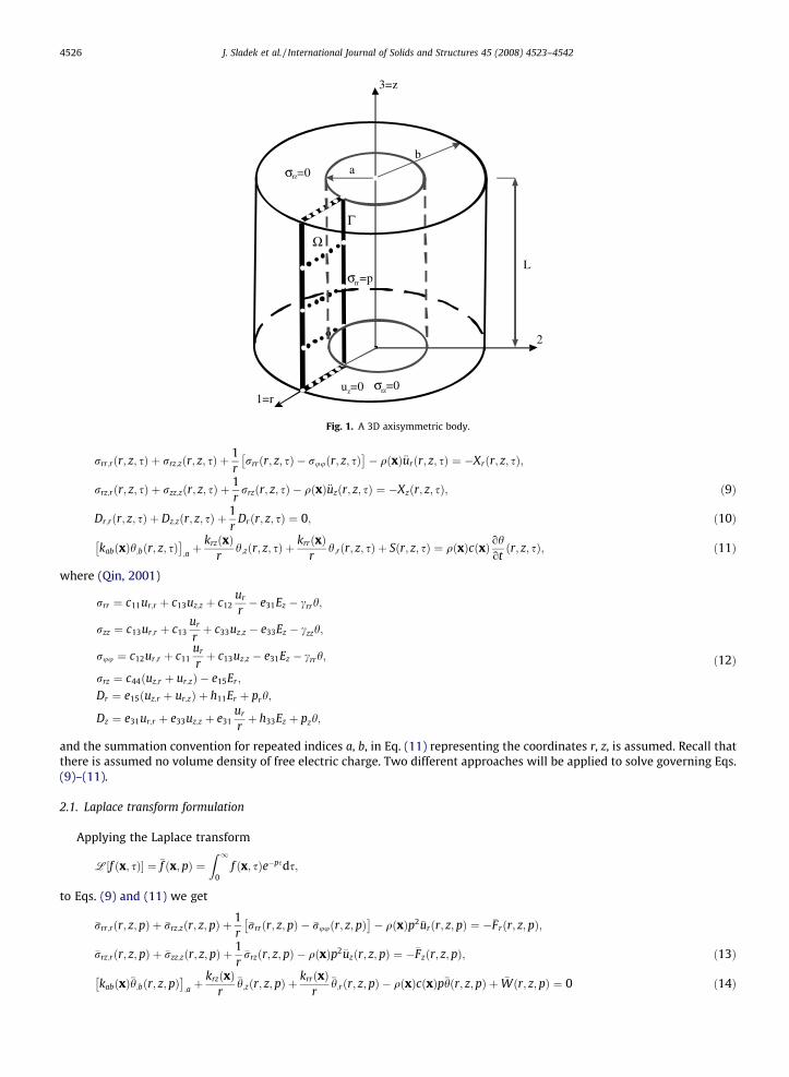
For an axisymmetric problem in transversally isotropic thermo-piezoelectric materials, it is convenient to use cylindricalcoordinates x � (r, u, z) (Fig. 1). The angular component of the displacements vanishes and all physical fields as well as mate-rial coefficients are independent on the angular coordinate u. The axis of symmetry is identical with z-coordinate. In such acase the equilibrium equations have the following form

1=r

2

L

b

3=z

Γ

a

Ω

u =0zσrz=0

σrr=p

σrz=0

Fig. 1. A 3D axisymmetric body.


rrr;rðr; z; sÞ þ rrz;zðr; z; sÞ þ1r

rrrðr; z; sÞ � ruuðr; z; sÞ� �

� qðxÞ€urðr; z; sÞ ¼ �Xrðr; z; sÞ;

rrz;rðr; z; sÞ þ rzz;zðr; z; sÞ þ1r

rrzðr; z; sÞ � qðxÞ€uzðr; z; sÞ ¼ �Xzðr; z; sÞ; ð9Þ

Dr;rðr; z; sÞ þ Dz;zðr; z; sÞ þ1r

Drðr; z; sÞ ¼ 0; ð10Þ

kabðxÞh;bðr; z; sÞ� �

;a þkrzðxÞ

rh;zðr; z; sÞ þ

krrðxÞr

h;rðr; z; sÞ þ Sðr; z; sÞ ¼ qðxÞcðxÞ ohotðr; z; sÞ; ð11Þ

where (Qin, 2001)

rrr ¼ c11ur;r þ c13uz;z þ c12ur

r� e31Ez � crrh;

rzz ¼ c13ur;r þ c13ur

rþ c33uz;z � e33Ez � czzh;

ruu ¼ c12ur;r þ c11ur

rþ c13uz;z � e31Ez � crrh;

rrz ¼ c44 uz;r þ ur;zð Þ � e15Er ;

Dr ¼ e15 uz;r þ ur;zð Þ þ h11Er þ prh;

Dz ¼ e31ur;r þ e33uz;z þ e31ur

rþ h33Ez þ pzh;

ð12Þ

and the summation convention for repeated indices a, b, in Eq. (11) representing the coordinates r, z, is assumed. Recall thatthere is assumed no volume density of free electric charge. Two different approaches will be applied to solve governing Eqs.(9)–(11).

2.1. Laplace transform formulation

Applying the Laplace transform

L f ðx; sÞ½ � ¼ �f ðx; pÞ ¼Z 1

0f ðx; sÞe�psds;

to Eqs. (9) and (11) we get

�rrr;rðr; z; pÞ þ �rrz;zðr; z; pÞ þ1r

�rrrðr; z; pÞ � �ruuðr; z; pÞ� �

� qðxÞp2�urðr; z; pÞ ¼ ��Frðr; z; pÞ;

�rrz;rðr; z; pÞ þ �rzz;zðr; z; pÞ þ1r

�rrzðr; z; pÞ � qðxÞp2�uzðr; z; pÞ ¼ ��Fzðr; z; pÞ; ð13Þ

kabðxÞ�h;bðr; z; pÞ� �

;a þkrzðxÞ

r�h;zðr; z; pÞ þ

krrðxÞr

�h;rðr; z; pÞ � qðxÞcðxÞp�hðr; z; pÞ þ �Wðr; z; pÞ ¼ 0 ð14Þ


where

Fiðx; pÞ ¼ Xiðx; pÞ þ puiðx;0Þ þ _uiðx;0Þ; for i ¼ ðr; zÞWðx; pÞ ¼ Sðx; pÞ þ hðx;0Þ

are the re-defined body forces and heat source, respectively, in the Laplace-transformed domain with the initial-boundaryconditions for the displacements ui(x,0), velocities _uiðx;0Þ and temperature h(x,0). Recall that Eq. (10) remains unchangedby the Laplace transformation, i.e.,

Dr;rðr; z; pÞ þ Dz;zðr; z; pÞ þ1r

Drðr; z; pÞ ¼ 0:

Instead of writing the global weak form for the above governing equation, the MLPG methods construct the weak form overlocal sub-domains such as Xs, which is a small region taken for each node inside the global domain (Atluri, 2004). The localsub-domains overlap each other, and cover the whole global domain X(Fig. 2). The local sub-domains could be of any geo-metric shape and size. In the current paper, the local sub-domains are taken to be of circular shape. The local weak forms ofthe governing Eqs. (13), (10) and (14) can be written as
Z
Xs

�rrr;r þ �rrz;zð Þu�dXþZ

Xs

1r

�rrr � �ruu

� �u�dX�

ZXs

qðxÞp2�urðr; z; pÞu�dX ¼ �Z

Xs

�Frðr; z; pÞu�dX;

ZXs

�rzr;r þ �rzz;zð Þv�dXþZ

Xs

1r

�rrzðr; z; pÞv�dX�Z

Xs

qðxÞp2�uzðr; z; pÞu�v�dX ¼ �Z

Xs

Fzðr; z; pÞv�dX;

ZXs

Dr;r þ Dz;z� �

m�dXþZ

Xs

1r

�Drðr; z; pÞm�dX ¼ 0; ð15Þ

ZXc

kabðxÞ�h;bðr; z; pÞ� �

;a þkrzðxÞ

r�h;zðr; z; pÞ þ

krrðxÞr

�h;rðr; z; pÞ�

� qðxÞcðxÞp�hðr; z; pÞ þWðr; z; pÞ�h�ðxÞdX ¼ 0; ð16Þ

where u*(x), v*(x), m*(x) and h*(x) are test functions.In the MLPG method the test and trial function are not necessarily from the same functional spaces. Applying the Gauss

divergence theorem to the first domain integrals of Eqs. (15) and (16) and selecting Heaviside unit step functions as testfunctions u*(x), v* (x) and m*(x) in each sub-domain, one can recast equations into the following form
Z
oXs

�rrbðr; z; pÞnbdCþZ

Xs

1r

�rrr � �ruu

� �dX�

ZXs

qðxÞp2�urðr; z; pÞdX ¼ �Z

Xs

�Frðr; z; pÞdX;

ZoXs

�rzbðr; z; pÞnbdCþZ

Xs

1r

�rrzðr; z; pÞdX�Z

Xs

qðxÞp2�uzðr; z; pÞdX ¼ �Z

Xs

�Fzðr; z; pÞdX;

ZoXs

�Dbðr; z; pÞnbdCþZ

Xs

1r

�Drðr; z; pÞdX ¼ 0; ð17Þ

ZoXs

�qðr; z; pÞdC�Z

Xs

qðxÞcðxÞp�hðr; z; pÞdXþZ

Xs

krzðxÞr

�h;zðr; z; pÞ þkrrðxÞ

r�h;rðr; z; pÞ

� �dX

¼ �Z

Xs

�Wðr; z; pÞdX; ð18Þ

subdomain =Ω Ωs si '

∂Ωs

∂ Ω ∪Γs s si i i=L

∂Ωs =i ∂ Li

sΩ s=

Ωs''

Lis

Γsθ i or Γsq

i

ri

node xi

support of node xi

local boundary '

x

Ωx

Fig. 2. Local boundaries for weak formulations and the support area for MLS approximation of the trial functions.


where the subscript b in Eq. (17) is considered as a summation index with b = r, z and

�qðr; z; pÞ ¼ kabðxÞ�h;bðr; z; pÞnaðxÞ:

In contrast to the test functions, the trial functions are chosen as the moving least-squares (MLS) approximations for field un-knowns over a number of nodes randomly spread within the domain of influence, as described in more details in Section 3.

2.2. Time-difference formulation

The local weak form can be directly applied to governing Eqs. (9)–(11). If the same test function and the same procedureare applied as in the previous paragraph, one can obtain the set of integro-differential equations
Z
oXs

rrbðr; z; sÞnbdCþZ

Xs

1r

rrr � ruu

� �dX�

ZXs

qðxÞ€urðr; z; sÞdX ¼ �Z

Xs

Xrðr; z; sÞdX;Z

oXs

rzbðr; z; sÞnbdCþZ

Xs

1r

rrzðr; z; sÞdX�Z

Xs

qðxÞ€uzðr; z; sÞdX ¼ �Z

Xs

Xzðr; z; sÞdX;Z

oXs

Dbðr; z; sÞnbdCþZ

Xs

1r

Drðr; z; sÞdX ¼ 0; ð19ÞZ

oXs

qðr; z; sÞdC�Z

Xs

qðxÞcðxÞ _hðr; z; sÞdXþZ

Xs

krzðxÞr

h;zðr; z; sÞ þkrrðxÞ

rh;rðr; z; sÞ

� �dX ¼ �

ZXs

Sðr; z; sÞdX: ð20Þ

The Houbolt finite-difference scheme (Houbolt, 1950) is applied to approximate the acceleration

€uðr; z; skþ1Þ ¼2uðkþ1Þðr; zÞ � 5uðkÞðr; zÞ þ 4uðk�1Þðr; zÞ � uðk�2Þðr; zÞ

Ds2 ; ð21Þ

and a linear interpolation for time variation of the temperature field (Curran et al., 1980)

_hðr; z; skþ1Þ ¼1Ds

hðkþ1Þðr; zÞ � hðkÞðr; zÞh i

; ð22Þ

where Ds is the time step. Here, h(k)(r, z) denotes the value of the temperature at a point (r, z) and the time instant sk = kDs.The value of the time step has to be appropriately selected with respect to material parameters (propagation velocities) andtime dependence of the boundary conditions.

Substituting approximation formulae (21) and (22) into the local integro-differential Eqs. (19) and (20) at the time instantsk+1 = (k + 1)Ds, one obtains the local integral equations for (k = 0, 1, 2, . . . ,N)
Z
oXs

rðkþ1Þrb ðr; zÞnbdCþ

ZXs

1r

rðkþ1Þrr ðr; zÞ � rðkþ1Þ

uu ðr; zÞh i

dX� 1Ds2

ZXs

qðxÞ2uðkþ1Þr ðr; zÞdX

¼ 1Ds2

ZXs

qðxÞ �5uðkÞr ðr; zÞ þ 4uðk�1Þr ðr; zÞ � uðk�2Þ

r ðr; zÞ� �

dX�Z

Xs

Xðkþ1Þr ðr; zÞdX;Z

oXs

rðkþ1Þzb ðr; zÞnbdCþ

ZXs

1r

rðkþ1Þrz ðr; zÞdX� 1

Ds2

ZXs

qðxÞ2uðkþ1Þz ðr; zÞdX

¼ 1Ds2

ZXs

qðxÞ �5uðkÞz ðr; zÞ þ 4uðk�1Þz ðr; zÞ � uðk�2Þ

z ðr; zÞ� �

dX�Z

Xs

Xðkþ1Þz ðr; zÞdX;Z

oXs

Dðkþ1Þb ðr; zÞnbdCþ

ZXs

1r

Dðkþ1Þr ðr; zÞdX ¼ 0; ð23Þ

ZoXs

qðkþ1Þðr; zÞdC� 1Ds

ZXs

qðxÞcðxÞhðkþ1Þðr; zÞdXþZ

Xs

krzðxÞr

hðkþ1Þ;z ðr; zÞ þ krrðxÞ

rhðkþ1Þ;r ðr; zÞ

� �dX

¼ � 1Ds

ZXs

qðxÞcðxÞhðkÞðr; zÞdX�Z

Xs

Sðkþ1Þðr; zÞdX; ð24Þ

where qðkþ1ÞðxÞ ¼ kabðxÞhðkþ1Þ;b ðr; zÞnaðxÞ.

For the first time step, i.e., k = 0, the values uð�2Þb ðxÞ, uð�1Þ

b ðxÞ, uð0Þb ðxÞ and h(0)(x) are given by initial conditions for displace-ments and the temperature, respectively. Applying a spatial approximation for the field unknowns, the local integralEqs. (23) and (24) are transformed into the system of algebraic equation for unknown quantities at nodes, as described inSection 3. The system of algebraic equations is solved by step by step technique with respect to the time stepping.

Recently authors have analyzed 2D problems of piezothermoelasticity with a dependence of material parameters on atemperature distribution (Sladek et al., 2007b). Replacing material parameters by a temperature-dependent function inconstitutive Eqs. (4) and (5), nonlinear expressions are received. If the time step is sufficiently small the material parameterscan be considered as values corresponding to previous k-th time step

rðkþ1Þij ðxÞ ¼ cijklðhðkÞÞeðkþ1Þ

kl ðxÞ � ekijðhðkÞÞEðkþ1Þk ðxÞ � cijðhðkÞÞhðkþ1ÞðxÞ; ð25Þ

Dðkþ1Þj ðxÞ ¼ ejklðhðkÞÞeðkþ1Þ

kl ðxÞ þ hjkðhðkÞÞEðkþ1Þk ðxÞ þ pjðhðkÞÞhðkþ1ÞðxÞ: ð26Þ

In the Laplace transform technique an iterative approach has to be applied. Therefore, the time-difference technique is moreconvenient for problems with temperature-dependent material parameters (induced non-homogeneity).


3. Numerical solution

In general, a meshless method uses a local interpolation to represent the trial function with the values (or the fictitiousvalues) of the unknown variable at some randomly located nodes. The moving least-squares (MLS) approximation (Lancasterand Salkauskas, 1986; Nayroles et al., 1992; Belytschko et al., 1996) used in the present analysis may be considered as one ofsuch schemes. Let us consider a sub-domain Xx of the problem domain X, in the neighbourhood of a point x, for definition ofthe MLS approximation of the trial function around x (Fig. 2). To approximate the distribution of the Laplace transform ofphysical fields �fðx; pÞ (displacements, electrical potential, temperature) in Xx over a number of randomly located nodes{xa}, a = 1, 2, . . . ,n, the MLS approximate �fhðx; pÞ is defined by

�fhðx; pÞ ¼ pTðxÞaðx; pÞ; 8x 2 Xx ð27Þ

where pT(x) = [p1(x), p2(x), . . . ,pm(x)] is a complete monomial basis of order m; and a(x, p) is a vector containing the coeffi-cients aj(x, p), j = 1, 2, . . . ,m which are functions of the space coordinates x = [x1, x2, x3]T and the Laplace transform parameterp. For example, for a 2D problem

pTðxÞ ¼ 1; x1; x2½ �; for linear basis m ¼ 3 ð28aÞ

pTðxÞ ¼ 1; x1; x2; ðx1Þ2; x1x2; ðx2Þ2h i

; for quadratic basis m ¼ 6 ð28bÞ

Similarly to Eq. (27) one can write approximation of f(k)(x) in the time-difference formulation. The coefficient vector a(x, p) isdetermined by minimizing a weighted discrete L2-norm defined as

JðxÞ ¼Xn

a¼1

waðxÞ pTðxaÞaðx; pÞ � faðpÞh i2

; ð29Þ

where wa(x) is the weight function associated with the node a with wa(x) > 0. Recall that n is the number of nodes in Xx forwhich the weight function wa(x) > 0 and faðpÞ are the fictitious nodal values, but not the nodal values of the unknown trialfunction �fhðx; pÞ in general. The stationarity of J in Eq. (29) with respect to a(x, p)

oJ=oa ¼ 0

leads to the following linear relation between a(x, p) and fðpÞ

AðxÞaðx; pÞ � BðxÞfðpÞ ¼ 0; ð30Þ

where

AðxÞ ¼Xn

a¼1

waðxÞpðxaÞpTðxaÞ;

BðxÞ ¼ w1ðxÞpðx1Þ;w2ðxÞpðx2Þ; . . . ;wnðxÞpðxnÞ� �

:

ð31Þ

The MLS approximation is well defined only when the matrix A in Eq. (30) is non-singular. A necessary condition to satisfythis requirement is that at least m weight functions are non-zero (i.e., n P m) for each sample point x 2 X and that the nodesin Xx are not arranged in a special pattern such as on a straight line.

The solution of Eq. (30) for a(x, p) and a subsequent substitution into Eq. (27) lead to the following relations

�uhðx; pÞ ¼ UTðxÞ � uðpÞ ¼Xn

a¼1

/aðxÞuaðpÞ;

�whðx; pÞ ¼Xn

a¼1

/aðxÞwaðpÞ;

�hhðx; pÞ ¼Xn

a¼1

/aðxÞhaðpÞ;

ð32Þ

where

UTðxÞ ¼ pTðxÞA�1ðxÞBðxÞ: ð33Þ

In Eq. (32), /a(x) is usually referred to as the shape function of the MLS approximation corresponding to the nodal point xa.From Eqs. (31) and (33), it can be seen that /a(x) = 0 when wa(x) = 0. In practical applications, wa(x) is often chosen such thatit is non-zero over the support of the nodal point xi. The support of the nodal point xa is usually taken to be a circle of theradius ra centred at xa (see Fig. 2). The radius ra is an important parameter of the MLS approximation because it determinesthe range of the interaction (coupling) between the degrees of freedom defined at considered nodes.

A fourth-order spline-type weight function is applied in the present work

waðxÞ ¼ 1� 6 da

ra

� 2þ 8 da

ra

� 3� 3 da

ra

� 40 6 da

6 ra

0 da P ra

8<: ; ð34Þ


where da = kx � xak and ra is the radius of the circular support domain. With Eq. (34), the C1-continuity of the weight functionis ensured over the entire domain for approximation of primary fields (displacements, electrical potential, temperature),therefore the continuity condition of the secondary fields (traction, electrical displacement, heat flux) is satisfied. The sizeof the support ra should be large enough to cover a sufficient number of nodes in the domain of definition to ensure the reg-ularity of the matrix A. The value of n is determined by number of nodes lying in the support domain with radius ra.

The partial derivatives of the MLS shape functions are obtained as (Atluri, 2004)

/a;k ¼

Xm

j¼1

pj;kðA

�1BÞja þ pjðA�1B;k þ A�1;k BÞja

h i; ð35Þ

�
wherein A�1
;k ¼ A�1

;krepresents the derivative of the inverse of A with respect to xk, which is given by

A�1;k ¼ �A�1A;kA�1

:

The directional derivatives of �fðx; pÞare approximated in terms of the same nodal values as

o�fh

oxkðx; pÞ ¼

Xn

a¼1

faðpÞ/a;kðxÞ: ð36Þ

Substituting the approximations given by Eq. (32) into the local integral Eq. (18), we obtain a system of linear algebraic equa-tions for the fictitious unknown parameters haðpÞ

Xn

a¼1

haðpÞZ

oXs

kbcðxÞnbðxÞ/a;cðxÞdC�

Xn

a¼1

haðpÞZ

Xs

qðxÞcðxÞp/aðxÞdXþXn

a¼1

haðpÞZ

Xs

krzðxÞr

/a;zðxÞ þ

krrðxÞr

/a;rðxÞ

� �dX

¼ �Z

Xs

Wðx; pÞdX; ð37Þ

and subsequently the system of algebraic equations for the fictitious unknown parameters uar ; u

az ; w

an o

is obtained from thesystem of integral equations given by Eq. (17) as

Xn

a¼1

uar ðpÞ

ZoXs

c11ðxÞnrðxÞ/a;rðxÞ þ

c12ðxÞr

nrðxÞ/aðxÞ þ c44ðxÞnzðxÞ/a;zðxÞ

� �dC

þZ

Xs

1r

c11ðxÞ � c12ðxÞð Þ /a;rðxÞ �

1r

/aðxÞ� �

� qðxÞp2/aðxÞ� �

dX

þXn

a¼1

uazðpÞ

ZoXs

c13ðxÞnrðxÞ/a;zðxÞ þ c44ðxÞnzðxÞ/a

;rðxÞ�

dC

þXn

a¼1

waðpÞZ

oXs

e31ðxÞnrðxÞ/a;zðxÞ þ e15ðxÞnzðxÞ/a

;rðxÞ�

dC

¼Xn

a¼1

haðpÞZ

oXs

crrðxÞnrðxÞ/aðxÞdC�Z

Xs

�Frðr; z; pÞdX; ð38Þ

Xn

a¼1

uaz ðpÞ

ZoXs

c33ðxÞnzðxÞ/a;zðxÞ þ c44ðxÞnrðxÞ/a

;rðxÞh i

dCþZ

Xs

c44ðxÞr

/a;rðxÞ � qðxÞp2/aðxÞ

� �dX

þXn

a¼1

uar ðpÞ

ZoXs

c44ðxÞnrðxÞ/a;zðxÞ þ c13ðxÞnzðxÞ /a

;rðxÞ þ1r/aðxÞ

� �� dCþ

ZXs

c44ðxÞr

/a;zðxÞdX

þXn

a¼1

waðpÞZ

oXs

e15ðxÞnrðxÞ/a;rðxÞ þ e33ðxÞnzðxÞ/a

;zðxÞ�

dCþZ

Xs

1r

e15ðxÞ/a;rðxÞdX

¼Xn

a¼1

haðpÞZ

oXs

czzðxÞnzðxÞ/aðxÞdC�Z

Xs

�Fzðr; z; pÞdX; ð39Þ

Xn

a¼1

uar ðpÞ

ZoXs

e15ðxÞnrðxÞ/a;zðxÞ þ e31ðxÞnzðxÞ /a

;rðxÞ þ1r

/aðxÞ� ��

dCþZ

Xs

1r

e15ðxÞ/a;zdX

þXn

a¼1

uazðpÞ

ZoXs

e15ðxÞnrðxÞ/a;rðxÞ þ e33ðxÞnzðxÞ/a

;zðxÞh i

dCþZ

Xs

1r

e15ðxÞ/a;rðxÞdX

�Xn

a¼1

waðpÞZ

oXs

h11ðxÞnrðxÞ/a;rðxÞ þ h33ðxÞnzðxÞ/a

;zðxÞ�

dCþZ

Xs

1r

h11ðxÞ/a;rðxÞdX

¼ �Xn

a¼1

haðpÞZ

oXs

prðxÞnrðxÞ þ pzðxÞnzðxÞð Þ/aðxÞdCþZ

Xs

1r

prðxÞ/aðxÞdX

: ð40Þ


Eqs. (37)–(40) are considered on the sub-domains Xs around each interior node xs and at boundary nodes with prescribednatural boundary conditions (Ct, Cq and Cb). On the parts of the global boundary Cu with prescribed displacements, Cp withprescribed potentials and Ca with prescribed temperature the collocation Eq. (32) are applied.

The time-dependent values of the transformed quantities in the previous consideration can be obtained by an inversetransformation. There are many inversion methods available for the inverse Laplace transformation. As the inverse Laplacetransformation is an ill-posed problem, small truncation errors can be greatly magnified in the inversion process and hencelead to poor numerical results. In the present analysis, the sophisticated Stehfest’s algorithm (Stehfest, 1970) for the numer-ical inversion is used. If �f ðpÞis the Laplace transform of f(t), an approximate value fa of f(t) for a specific time t is given by

faðtÞ ¼ln 2

t

XN

i¼1

vi�f

ln 2t

i� �

; ð41Þ

where

vi ¼ ð�1ÞN=2þiXminði;N=2Þ

k¼ ðiþ1Þ=2½ �

kN=2ð2kÞ!ðN=2� kÞ!k!ðk� 1Þ!ði� kÞ!ð2k� iÞ! : ð42Þ

In numerical analyses we have used N = 10 for single precision arithmetic. It means that for each time t it is needed to solve Nboundary value problems for the corresponding Laplace parameters p = i ln2/t, with i = 1, 2, . . . ,N. If M denotes the number ofthe time instants in which we are interested to know f(t), the number of the Laplace transform solutions �f ðpjÞ is then M � N.

It is noteworthy that most of the alternative methods for the numerical inversion of the Laplace transform (Davies andMartin, 1979) require the use of complex valued Laplace transform parameter, and as a result, the application of complexarithmetic may lead to additional storage requirement and an increase in computing time.

4. Numerical examples

4.1. Hollow sphere

A hollow sphere with continuously non-homogeneous spherically symmetric and radially dependent piezoelectric mate-rial coefficients exhibits transversally isotropic properties. The sphere is radially polarized and either the static or impactloads are considered as spherically symmetric too. The temperature field is assumed to be uniformly distributed. The innera = 0.4m and outer radii b = 1m are considered, respectively. The analytical solution is given by Chen et al. (2002) and Dinget al. (2003) and it is used as a benchmark to test the accuracy of the present method. The boundary conditions with pre-scribed pressures and vanishing electrical displacements on both surfaces correspond to pressured sphere embedded intonon-conductive media (the open-circuit electric condition). A half of the hollow sphere can be created by the rotation ofthe cross section given in Fig. 3 around the z-axis. Note that the radial and axial directions are fixed as shown in Fig. 3 accord-ing to the definition in the cylindrical coordinate system. The unit basis vectors of the spherical coordinate systemfer0 ; eu; exg are related to those of the cylindrical coordinate system {er, eu, ez} as

er0 ¼ er cos xþ ez sin x; ex ¼ �er sin xþ ez cos x:

Thus, the radial directions in two considered coordinate systems are not identical in general.For the numerical calculations, 176 nodes with a regular distribution in the radial and azimuthal directions in the section

with u = 0 are employed. An exponential variation of the elastic, piezoelectric and dielectric coefficients on the radial dis-tance r0 ¼ ffip ðx2

1 þ x23Þ is assumed by

cijðxÞ ¼ c0ij exp cðr0 � aÞ;

eijðxÞ ¼ e0ij exp cðr0 � aÞ;

hijðxÞ ¼ h0ij exp cðr0 � aÞ;

ð43Þ

where the values on the inner radius r0= a are taken under the given temperature as

c011 ¼ 13:9� 1010 N m�2; c0

13 ¼ 7:43� 1010 N m�2 ; c012 ¼ 7:78� 1010 N m�2;

c033 ¼ 11:5� 1010 N m�2; c0

44 ¼ 2:56� 1010 N m�2;

e044 ¼ 12:7 C m�2; e0

31 ¼ �5:2 C m�2; e033 ¼ 15:1 C m�2;

h011 ¼ 6:46� 10�9 CðV mÞ�1

; h033 ¼ 5:62� 10�9 CðV mÞ�1

; q ¼ const ¼ 7500 kg=m3:

It should be noted that proposed computational method works for all continuously non-homogeneous materials. In deriva-tion of local integral equations no limitation is made with respect to spatial variation of material properties. The exponentialvariation in numerical example is selected only for comparative purposes since for such kind of non-homogeneity numericalresults are available. The mass density in this example is considered to be uniform, however, a general spatial variation canbe considered. No restriction is put on the variation of mass density in proposed local integral equations. A static uniformpressure load p0 = 1 Nm�2 is considered on the inner radius r0 = a, in the first step. Variation of the radial displacements

1 11

2

36

49

a

x1

z=x3 p p H(t)= 0

p 0=

u =02

b

D =0i

D =0i

u =01

D =0i

D =0i

ω

Fig. 3. Analyzed domain for a hollow sphere.


ur = u1(x1, x3 = 0), radial and hoop stresses [rrr = r11(x1, x3 = 0),ruu(x1, x3 = 0)] with the radial coordinate r = x1 are presented inFigs. 4–6. Owing to the spherical symmetry the presented results correspond to the following spherical components: ur0(r0, u,x) = ur(x1, u = 0, x3 = 0), rr0r0(r0, u, x) = rrr(x1, u = 0, x3 = 0), ruu(r0, u, x) = ruu(x1, u = 0, x3 = 0).

The results for radial stresses are compared also with the analytical solution (Chen et al., 2002) for constant material coef-ficients. One can observe that functionally graded material properties have a stronger influence on radial displacement val-ues than on the radial stresses. With increasing gradation of elastic parameters the radial displacements are reduced.However, the influence of the material gradation on the hoop stresses is different on the inner and outer radii. On the outerradius the hoop stresses are enhanced with increasing material gradation while on the inner radius they are reduced.

Next, a uniform electrical load on the outer radius Dr = 1 Cm�2 and traction-free surfaces are considered. Variation of theradial displacements, hoop stresses, the electrical potential and the electrical displacement with the radial coordinate arepresented in Figs. 7–10.

The impact pressure load with a uniform distribution on the inner radius is considered too. Vanishing electrical potentialsare considered on both spherical surfaces (the closed-circuit electric condition). The numerical results for radial displace-ments and hoop stresses are presented in Figs. 11 and 12. Both quantities are normalized by corresponding static ones,ustat

r ðaÞ ¼ 0:465� 10�11 m and rstatuu ðaÞ ¼ 1:71 N m�2, respectively. The Laplace transform approach was applied in the numer-

ical analysis. The mass density is considered to be uniform even for functionally graded material.

0

0.1

0.2

0.3

0.4

0.5

0.6

0.4 0.5 0.6 0.7 0.8 0.9 1

r/b

u r *

c33

0

homogeneous

gamma =1

=2

Fig. 4. Variation of radial displacements with the radial coordinate.

0

0.1

0.2

0.3

0.4

0.5

0.6

0.7

0.8

0.9

1

0.4 0.5 0.6 0.7 0.8 0.9 1

r/b

- σrr

homog.:analyt.MLPG

gamma=1=2

Fig. 5. Variation of radial stresses with the radial coordinate.

0

0.2

0.4

0.6

0.8

1

1.2

1.4

1.6

1.8

0.4 0.5 0.6 0.7 0.8 0.9 1

r/b

σ ϕϕ

homogeneous

gamma =1

=2

Fig. 6. Variation of hoop stresses with the radial coordinate.

0

0.1

0.2

0.3

0.4

0.5

0.6

0.7

0.4 0.5 0.6 0.7 0.8 0.9 1

r/b

-ur *

e33

0

homogeneous

gamma =2

Fig. 7. Variation of radial displacements with the radial coordinate in the hollow sphere under a static electrical displacement on the outer radius.


-0.8

-0.7

-0.6

-0.5

-0.4

-0.3

-0.2

-0.1

0

0.1

0.2

0.4 0.5 0.6 0.7 0.8 0.9

r/b

e 330

σ ϕϕ

/c33

0

homogeneous

gamma =2

1

Fig. 8. Variation of hoop stresses with the radial coordinate in the hollow sphere under a static electrical displacement on the outer radius.

0

0.1

0.2

0.3

0.4

0.5

0.6

0.7

0.8

0.4 0.5 0.6 0.7 0.8 0.9 1

r/b

−ψ ∗

h 330

homogeneous

gamma =2

Fig. 9. Variation of the electrical potential with the radial coordinate in the hollow sphere under a static electrical displacement on the outer radius.

0

1

2

3

4

5

6

7

0.4 0.5 0.6 0.7 0.8 0.9 1

r/b

Dr

homogeneous

gamma =2

Fig. 10. Variation of electrical displacements with the radial coordinate in the hollow sphere under a static electrical displacement on the outer radius.


-0.2

0.2

0.6

1

1.4

1.8

0 2 3

(c330/ρ)1/2τ/b

u r/u

rstat

(a)

homogeneous

gamma = 2

4 5 61

Fig. 11. Time variation of radial displacements in the hollow sphere under an impact pressure load on the inner radius.

-0.5

0

0.5

1

1.5

2

2.5

0 2 4

(c330/ρ)1/2τ/b

σ ϕϕ(a

)/σ ϕ

ϕstat(a

)

homog.: analytic MLPG gamma = 2

531

Fig. 12. Time variation of hoop stresses in the hollow sphere under an impact pressure load on the inner radius.


The time evolution of the hoop stresses on the inner radius r0= a is compared also with the analytical results given by Ding

et al. (2003) in case of homogeneous medium. One can observe a good agreement of analytical and MLPG results for a homo-geneous piezoelectric sphere.

For the gradual increase of mechanical material properties with radial coordinate and a uniform mass density, the wavepropagation velocity is increasing with r. Therefore, the peak value of the radial displacements and hoop stresses are reachedin an earlier time instant in FGPM hollow sphere than in a homogeneous one. The maximum quantities are reduced for theFGPM sphere.

4.2. Hollow cylinder

In the next example, we consider an infinitely long functionally graded thick-walled hollow cylinder with the radiia = 0.08 m and b = 0.16 m as depicted in Fig. 1. Since the boundary conditions along the cylinder are considered to be uniforma finite part of the cylinder in the numerical analysis is selected with length L = 0.08 m. On the external surface of the hollowcylinder the temperature, T = 1 deg, is prescribed with studying either a stationary problem or a transient problem with theHeaviside time-step thermal loading at time instant t = 0. The inner surface is kept at zero temperature. We have consideredtransversally isotropic and homogeneous piezoelectric material with coefficients:


c11 ¼ 13:9� 1010 N m�2; c13 ¼ 7:43� 1010 N m�2 ; c12 ¼ 7:78� 1010 N m�2; c33 ¼ 11:5� 1010 N m�2;

c44 ¼ 2:56� 1010 N m�2; e15 ¼ 12:7 C m�2; e31 ¼ �5:2 C m�2; e33 ¼ 15:1 C m�2;

h11 ¼ 6:46� 10�9 CðV mÞ�1; h33 ¼ 5:62� 10�9 CðV mÞ�1

; q ¼ 7500 kg=m3:

k11 ¼ k22 ¼ 50 W=K m; k33 ¼ 75 W=K m; a11 ¼ a22 ¼ 0:88� 10�5 K�1; a33 ¼ 0:5� 10�5 K�1;

p1 ¼ 0; p3 ¼ �5:4831� 10�6 C=K m2; c ¼ 300 W s kg�1 K�1:

The node distribution consists of 421 (21 � 21) nodes uniformly distributed in the rectangular domain (r, z) 2 [a, b] � [0, L] inthe section u = 0 with 21 nodes in the radial as well as axial direction.

The analytical solution is available for an isotropic and homogeneous elastic hollow cylinder under a thermal shock on theexternal surface (Carslaw and Jaeger, 1959; Timoshenko and Goodier, 1951). The temperature, the radial displacement andthe hoop stresses for this problem are given as

hðr; sÞ ¼ Tln r=að Þln b=að Þ � p

X1n¼1

TJ2

0ðaanÞU0ðranÞJ2

0ðaanÞ � J20ðbanÞ

expð�ja2nsÞ; ð44Þ

urðr; sÞ ¼ð1þ mÞað1� mÞ

1r

Z r

ahðx; sÞxdxþ C1r þ C2

r; ð45Þ

ruu ¼aE

1� m1r2

Z r

ahðx; sÞxdx� aE

1� mhðr; sÞ þ E

1� mC1

1� 2mþ C2

r2

� �; ð46Þ

where

U0ðranÞ ¼ J0ðranÞY0ðanbÞ � J0ðanbÞY0ðranÞ;

and an are the roots of the following transcendental equation

J0ðrÞY0ðrb=aÞ � J0ðrb=aÞY0ðrÞ ¼ 0;

with J0(r) and Y0(r) being the Bessel functions of the first and the second kind and zeroth-order. The constants C1 and C2inEqs. (45) and (46) are defined as

C1 ¼ð1� 2mÞað1þ mÞ

1� m1

b2 � a2

Z b

ahðr; sÞrdr;

C2 ¼að1þ mÞ

1� ma2

b2 � a2

Z b

ahðr; sÞrdr:

To test the accuracy of numerical computations we have considered this thermoelastic problem with Young‘s modulusE = 7.1 � 1010N m�2, Poisson ratio m = 0.387, thermal expansion coefficient a = 0.88 � 10�5 K�1 and diffusivity coefficientj ¼ k11

qc ¼ 2:22� 10�5m2=s. The relative numerical errors for the radial displacements and hoop stresses at both cylinder sur-faces were less than 0.05% and 0.36%, respectively. The accuracy for the temperature results was better.

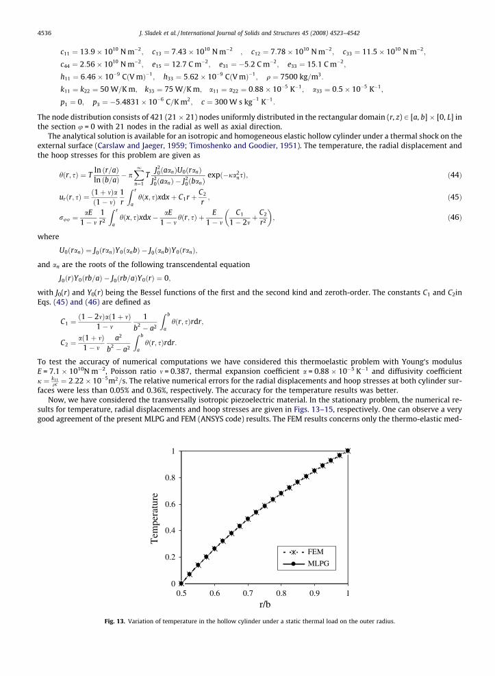
Now, we have considered the transversally isotropic piezoelectric material. In the stationary problem, the numerical re-sults for temperature, radial displacements and hoop stresses are given in Figs. 13–15, respectively. One can observe a verygood agreement of the present MLPG and FEM (ANSYS code) results. The FEM results concerns only the thermo-elastic med-

0

0.2

0.4

0.6

0.8

1

0.5 0.6 0.7 0.8 0.9 1

r/b

Tem

pera

ture

FEM

MLPG

Fig. 13. Variation of temperature in the hollow cylinder under a static thermal load on the outer radius.

0.4

0.5

0.6

0.7

0.8

0.9

1

1.1

0.5 0.6 0.7 0.8 0.9 1

r/b

Rad

ial d

ispl

acem

ent x

10e

-6

FEM

MLPG: elastic piezoelectric

Fig. 14. Variation of the radial displacement in the hollow cylinder under a static thermal load on the outer radius.

-0.5

-0.3

-0.1

0.1

0.3

0.5

0.7

0.5 0.6 0.7 0.8 0.9 1r/b

Hoo

p st

ress

x 1

0e+

6

FEM

MLPG: elastic

piezoelectric

Fig. 15. Variation of hoop stresses on the inner radius of the hollow cylinder under a static thermal load on the outer radius.


ium with vanishing piezoelectric coefficients eij = 0. In the FEM analysis we have used 25,600 quadratic (8-node) elements(plane223).

Vanishing electric displacement boundary conditions are considered on both surfaces of the hollow cylinder and also onboth cut surfaces. The radial displacements are slightly reduced for considered piezoelectric material. The hoop stresses arealmost the same in both the considered materials.

In the transient problem, when the prescribed temperature on the outer surface of the hollow cylinder has a Heavisidetime variation, the temperature evolution at the mid radius is presented in Fig. 16. Recall that the temperature field isnot influenced by the electric properties of the medium in the considered modelling. The shown numerical results are com-pared with those obtained by the FEM (ANSYS) and the comparison with the exact solution has been discussed earlier. Unfor-tunately, no numerical results obtained by the BEM are available for authors. A similar temporal variation for axial and hoopstresses has been obtained too.

4.3. A penny-shaped crack in a finite cylinder

A penny-shaped crack in a finite cylinder as depicted in Fig. 17 is analyzed in the third example. The following geometry isconsidered: crack radius a = 0.5, cylinder radius w = 1.25, and cylinder length L = 3.

-0.1

0

0.1

0.2

0.3

0.4

0.5

0.6

0.7

0 0.1 0.2 0.3 0.4 0.5 0.6

τk11/ρca2

θ/T

FEM

MLPG

Fig. 16. Time variation of the temperature at the mid radius of the hollow cylinder under a thermal shock on the outer radius.

2a

2w

12

3

A BC

DE

Fig. 17. A penny-shaped crack in a finite piezoelectric cylinder.

0

0.1

0.2

0.3

0.4

0.5

0.6

0.7

0.8

0.9

0 0.2 0.4 0.6 0.8 1r /a

u 3 (

10-5

m),

ψ(1

03 V)

u: MLPG FEM

psi: MLPG FEM

Fig. 18. Variations of the crack-opening displacement and the potential with the normalized coordinate r/a.



On the external surface a uniform temperature T = 1 deg is applied, while the temperature T = 0 deg is kept on the crack sur-face. From the symmetry of the problem, the heat flux is vanishing on the section B–C. Vanishing electrical displacements areconsidered on the crack surfaces and on the external surfaces of the finite cylinder. For the case of homogeneous medium, thematerial coefficients are the same as in the previous numerical example. A regular node distribution with 930 (31 � 30) nodes isused for the MLS approximation of the displacements and the electric potential in the analyzed domain ABCDE (see Fig. 17).

Fig. 18 shows a comparison of the numerical results for a cracked homogeneous cylinder by the MLPG method and theFEM in the case of stationary thermal load. One can observe a very good agreement between results by both techniques. Thenormalized stress intensity factor is,

u 3 (

10-5

m)

Fi

fI ¼ KstatI =a33c33T

ffiffiffiffiffiffipap

¼ 0:386:

Now, we have considered also an exponential variation of the elastic, piezoelectric, dielectric and thermal expansion coef-ficients in radial direction is assumed, i.e.,

cijðrÞ ¼ c0ij expðcrÞ;

eijðrÞ ¼ e0ij expðcrÞ;

hijðrÞ ¼ h0ij expðcrÞ;

aijðrÞ ¼ a0ij expðdrÞ:

0

0.05

0.1

0.15

0.2

0.25

0.3

0 0.2 0.4 0.6 0.8 1

homogeneous

FGPM

0

0.1

0.2

0.3

0.4

0.5

0.6

0.7

0.8

0.9

0 0.2 0.4 0.6 0.8 1

r /ar /a

ψ (

103 V

)

homogeneous

FGPM

Fig. 19. Comparison of crack quantities obtained for homogeneous and FGPM material (a) displacement and (b) electrical potential.

0

0.2

0.4

0.6

0.8

1

1.2

1.4

0 0.2 0.4 0.6 0.8 1

τk11/ρcw2

KI/K

Istat

(hom

og)

homogeneous

FGPM

g. 20. Time variation of the stress intensity factor for a penny-shaped crack in a finite cylinder under a thermal shock on external surfaces.


The material coefficients of the functionally graded piezoelectric material (FGPM) at the axis of symmetry r = 0 (denoted bysuperscript 0) are the same as in the homogeneous case. For the gradation exponents, we have used the values c = 2 andd = � 1 in the numerical analysis. It corresponds to the case with growing ceramic fraction in the functionally graded piezo-electric material with increasing the radial coordinate. A ceramic material has higher elastic coefficients and lower thermalexpansion coefficients than a metallic material. The numerical results for the crack-opening displacements and the electricpotential are given in Fig. 19a and b, respectively. The crack-opening displacements are significantly reduced with respect tothe homogeneous material. It is due to higher elastic coefficients and lower thermal expansion in the FGPM than in thehomogeneous material. The electrical potential on the crack surface is reduced too. The ratio of the stress intensity factorsis equal to fI ¼ Kstat

I ðFGPMÞ=KstatI ðhomÞ ¼ 0:704.

Finally, we have considered also a thermal shock with Heaviside time variation of the prescribed temperature on theexternal surfaces of the finite cracked cylinder. Both homogeneous and functionally graded material properties are consid-ered here.

Only a small enhancement of the stress intensity factor for a homogeneous cracked cylinder is observed in Fig. 20. Lowtemperature at relatively short time instants in the crack tip region causes the increasing thermal stresses according Duh-amel–Neumann constitutive law. Therefore, at short time instants the overcoming of the static SIF is observed. In function-ally graded material the overshoot of the static SIF is significantly higher. Despite the lower static value of the SIF in FGPMcracked cylinder as compared with the homogeneous case, the pick value is about 30% higher than the SIF in the homoge-neous cylinder. Therefore, the investigation of transient thermal problems for FGPM is more important than for homoge-neous materials.

5. Conclusions

A meshless local Petrov-Galerkin method (MLPG) is presented for 3D axisymmetric problems in continuously non-homo-geneous and linear piezoelectric solids under a mechanical and thermal load. The transient dynamic governing equations areconsidered here. Two computational approaches based on the Laplace-transform and the time-difference technique are pre-sented. The analyzed domain is divided into small overlapping circular sub-domains. A unit step function is used as the testfunctions in the local weak form of the governing partial differential equations. The derived local boundary-domain integralequations are non-singular. The moving least-squares (MLS) scheme is adopted for the approximation of the physical fieldquantities. The proposed method is a truly meshless method, which requires neither domain elements nor background cellsin either the interpolation or the integration.

The present method provides an alternative numerical tool to many existing computational methods like the FEM or theBEM. The main advantage of the present method is its simplicity. Contrary to the conventional BEM, the present method re-quires no fundamental solutions and all integrands in the present formulation are regular. Thus, no special numerical tech-niques are required to evaluate the integrals. It should be noted here that the fundamental solutions are not available forpiezoelectric solids with continuously varying material properties in general cases. The present formulation possesses thegenerality of the FEM. Therefore, the method is promising for numerical analysis of multi-field problems like piezoelectricor thermoelastic problems, which cannot be solved efficiently by the conventional BEM.

Acknowledgements

The authors acknowledge the support by the Slovak Science and Technology Assistance Agency registered under numbersAPVV-51-021205, APVT-20-035404 and the Slovak Grant Agency VEGA-2/6109/6.

References

Ashida, F., Tauchert, T.R., Noda, N., 1994. Potential function method for piezothermoelastic problems of solids of crystal class 6 mm in cylindricalcoordinates. Journal of Thermal Stresses 17, 361–375.

Aouadi, M., 2006. Generalized thermo-piezoelectric problems with temperature-dependent properties. International Journal of Solids and Structures 43,6347–6358.

Atluri, S.N., 2004. The Meshless Method, (MLPG) for Domain & BIE Discretizations. Tech Science Press.Atluri, S.N., Han, Z.D., Shen, S., 2003. Meshless local Petrov-Galerkin (MLPG) approaches for solving the weakly-singular traction & displacement boundary

integral equations. CMES: Computer Modeling in Engineering & Sciences 4, 507–516.Atluri, S.N., Liu, H.T., Han, Z.D., 2006. Meshless local Petrov-Galerkin (MLPG) mixed finite difference method for solid mechanics. CMES: Computer Modeling

in Engineering & Sciences 15, 1–16.Belytschko, T., Krogauz, Y., Organ, D., Fleming, M., Krysl, P., 1996. Meshless methods; an overview and recent developments. Computer Methods in Applied

Mechanics and Engineering 139, 3–47.Carslaw, H.S., Jaeger, J.C., 1959. Conduction of Heat in Solids. Clarendon, Oxford.Chen, W.Q., Lu, Y., Ye, R., Cai, J.B., 2002. 3D electroelastic fields in a functionally graded piezoceramic hollow sphere under mechanical and electric loadings.

Archives of Applied Mechanics 72, 39–51.Curran, D.A., Cross, M., Lewis, B.A., 1980. Solution of parabolic differential equations by the boundary element method using discretization in time. Applied

Mathematical Modelling 4, 398–400.Davi, G., Milazzo, A., 2001. Multidomain boundary integral formulation for piezoelectric materials fracture mechanics. International Journal of Solids and

Structures 38, 2557–2574.Davies, B., Martin, B., 1979. Numerical inversion of the Laplace transform: a survey and comparison of methods. Journal of Computational Physics 33, 1–32.


Ding, H., Liang, J., 1999. The fundamental solutions for transversally isotropic piezoelectricity and boundary element method. Computers & Structures 71,447–455.

Ding, H.J., Wang, H.M., Chen, W.Q., 2003. Analytical solution for the electroelastic dynamics of a nonhomogeneous spherically isotropic piezoelectric hollowsphere. Archives of Applied Mechanics 73, 49–62.

Dunn, M.L., 1993. Micromechanics of coupled electroelastic composites: effective thermal expansion and pyroelectric coefficients. Journal of AppliedPhysics 73, 5131–5140.

Enderlein, M., Ricoeur, A., Kuna, M., 2005. Finite element techniques for dynamic crack analysis in piezoelectrics. International Journal of Fracture 134, 191–208.

Garcia-Sanchez, F., Saez, A., Dominguez, J., 2005. Anisotropic and piezoelectric materials fracture analysis by BEM. Computers & Structures 83, 804–820.Garcia-Sanchez, F., Zhang, Ch., Sladek, J., Sladek, V., 2007. 2-D transient dynamic crack analysis in piezoelectric solids by BEM. Computational Materials

Science 39, 179–186.Gornandt, A., Gabbert, U., 2002. Finite element analysis of thermopiezoelectric smart structures. Acta Mechanica 154, 129–140.Govorukha, V., Kamlah, M., 2004. Asymptotic fields in the finite element analysis of electrically permeable interfacial cracks in piezoelectric bimaterials.

Archives Applied Mechanics 74, 92–101.Gruebner, O., Kamlah, M., Munz, D., 2003. Finite element analysis of cracks in piezoelectric materials taking into account the permittivity of the crack

medium. Engineering Fracture Mechanics 70, 1399–1413.Gross, D., Rangelov, T., Dineva, P., 2005. 2D wave scattering by a crack in a piezoelectric plane using traction BIEM. SID: Structural Integrity & Durability 1,

35–47.Gross, D., Dineva, P., Rangelov, T., 2007. BIEM solution for piezoelectric cracked finite solids under time-harmonic loading. Engineering Analysis with

Boundary Elements 31, 152–162.Han, F., Pan, E., Roy, A.K., Yue, Z.Q., 2006. Responses of piezoelectric, transversally isotropic, functionally graded and multilayered half spaces to uniform

circular surface loading. CMES: Computer Modeling in Engineering & Sciences 14, 15–30.Houbolt, J.C., 1950. A recurrence matrix solution for the dynamic response of elastic aircraft. Journal of Aeronautical Science 17, 540–550.Kuna, M., 1998. Finite element analyses of crack problems in piezoelectric structures. Computational Materials Science 13, 67–80.Kuna, M., 2006. FEM-techniques for thermo-electro-mechanical crack analyses in smart structures. In: Wei, Yang (Ed.), IUTAM Symposium on Mechanics

and Reliability of Actuating Materials. Springer, Beijing, pp. 131–143.Lancaster, P., Salkauskas, K., 1986. Curves and Surface Fitting: An Introduction. Academic Press, London.Liew, K.M., He, X.Q., Ng, T.Y., Sivashanker, S., 2001. Active control of FGM plates subjected to a temperature gradient: modelling via finite element method

based on FSDT. International Journal for Numerical Methods in Engineering 52, 1253–1271.Liu, G.R., Dai, K.Y., Lim, K.M., Gu, Y.T., 2002. A point interpolation mesh free method for static and frequency analysis of two-dimensional piezoelectric

structures. Computational Mechanics 29, 510–519.Loza, I.A., Shulga, N.A., 1984. Axisymmetric vibrations of a hollow piezoceramic sphere with radial polarization. Soviet Applied Mechanics 20, 113–117.Loza, I.A., Shulga, N.A., 1990. Forced axisymmetric vibrations of a hollow piezoceramic sphere with an electrical method of excitation. Soviet Applied

Mechanics 26, 818–822.Mindlin, R.D., 1961. On the equations of motion of piezoelectric crystals, problems of continuum. In: Muskelishvili, N.I. (Ed.), Mechanics 70th Birthday

Volume. SIAM, Philadelpia, pp. 282–290.Mindlin, R.D., 1974. Equations of high frequency vibrations of thermopiezoelasticity problems. International Journal of Solids and Structures 10, 625–637.Nowacki, W., 1978. Some general theorems of thermo-piezoelectricity. Journal of Thermal Stresses 1, 171–182.Nayroles, B., Touzot, G., Villon, P., 1992. Generalizing the finite element method. Computational Mechanics 10, 307–318.Ohs, R.R., Aluru, N.R., 2001. Meshless analysis of piezoelectric devices. Computational Mechanics 27, 23–36.Ootao, Y., Tanigawa, Y., 2007. Transient piezothermoelastic analysis for a functionally graded thermopiezoelectric hollow sphere. Composite Structures 81,

540–549.Pan, E., 1999. A BEM analysis of fracture mechanics in 2D anisotropic piezoelectric solids. Engineering Analysis with Boundary Elements 23, 67–76.Paulino, G.H., Jin, Z.H., Dodds, R.H., 2003. Failure of functionally graded materials. In: Karihaloo, B., Knauss, W.G. (Eds.), Comprehensive Structural Integrity,

vol. 2. Elsevier Science, pp. 607–644.Qin, Q.H., 2001. Fracture Mechanics of Piezoelectric Materials. WIT Press, Southampton.Qin, Q.H., Mai, Y.M., 1997. Crack growth prediction of an inclined crack in a half-plane thermopiezoelectric solid. Theoretical and Applied Fracture

Mechanics 26, 185–191.Rajapakse, R.K.N.D., Xu, X.L., 2001. Boundary element modeling of cracks in piezoelectric solids. Engineering Analysis with Boundary Elements 25, 771–781.Rao, S.S., Sunar, M., 1993. Analysis of distributed thermopiezoelectric sensors and actuators in advanced intelligent structures. AIAA Journal 31, 1280–1286.Saez, A., Garcia-Sanchez, F., Dominguez, J., 2006. Hypersingular BEM for dynamic fracture in 2-D piezoelectric solids. Computer Methods in Applied

Mechanics and Engineering 196, 235–246.Shang, F., Wang, Z., Li, Z., 1996. Thermal stress analysis of a three-dimensional crack in a thermopiezoelectric solid. Engineering Fracture Mechanics 55,

737–750.Shang, F., Kuna, M., Scherzer, M., 2002. Analytical solutions for two penny-shaped crack problems in thermo-piezoelectric materials and their finite element

comparisons. International Journal of Fracture 117, 113–128.Shang, F., Kuna, M., Kitamura, T., 2003a. Theoretical investigation of an elliptical crack in thermopiezoelectric material. Part I: Analytical development.

Theoretical Applied Fracture Mechanics 40, 237–246.Shang, F., Kitamura, T., Kuna, M., 2003b. Theoretical investigation of an elliptical crack in thermopiezoelectric material. Part II: Crack propagation.

Theoretical Applied Fracture Mechanics 40, 247–253.Sheng, N., Sze, K.Y., 2006. Multi-region Trefftz boundary element method for fracture analysis in plane piezoelectricity. Computational Mechanics 37, 381–

393.Sladek, J., Sladek, V., Atluri, S.N., 2004. Meshless local Petrov-Galerkin method in anisotropic elasticity. CMES: Computer Modeling in Engineering & Sciences

6, 477–489.Sladek, J., Sladek, V., Zhang, Ch., Garcia-Sanchez, F., Wunsche, M., 2006a. Meshless Local Petrov-Galerkin Method for Plane Piezoelectricity. CMC: Computers,

Materials & Continua 4, 109–118.Sladek, J., Sladek, V., Zhang, Ch., Tan, C.L., 2006b. Meshless local Petrov-Galerkin Method for linear coupled thermoelastic analysis. CMES: Computer

Modeling in Engineering & Sciences 16, 57–68.Sladek, J., Sladek, V., Zhang, Ch., Solek, P., Starek, L., 2007a. Fracture analyses in continuously nonhomogeneous piezoelectric solids by the MLPG. CMES:

Computer Modeling in Engineering & Sciences 19, 247–262.Sladek, J., Sladek, V., Zhang, Ch., Solek, P., 2007b. Application of the MLPG to thermo-piezoelectricity. CMES: Computer Modeling in Engineering & Sciences

22, 217–233.Stehfest, H., 1970. Algorithm 368: numerical inversion of Laplace transform. Communication of the Association for Computing Machinery 13, 47–49.Suresh, S., Mortensen, A., 1998. Fundamentals of Functionally Graded Materials. Institute of Materials, London.Timoshenko, S.P., Goodier, J.N., 1951. Theory of Elasticity. McGraw-Hill, New York.Tsamasphyros, G., Song, Z.F., 2005. Analysis of a crack in a finite thermopiezoelectric plate under heat flux. International Journal of Fracture 136, 143–166.Tzou, H.S., Ye, R., 1994. Piezothermoelasticity and precision control of piezoelectric systems: theory and finite element analysis. Journal of Vibration and

Acoustics 116, 489–495.


Ueda, S., 2003. Crack in functionally graded piezoelectric strip bonded to elastic surface layers under electromechanical loading. Theoretical AppliedFracture Mechanics 40, 225–236.

Yu, S.W., Qin, Q.H., 1996a. Damage analysis of thermopiezoelectric properties: Part I – Crack tip singularities. Theoretical Applied Fracture Mechanics 25,263–277.

Yu, S.W., Qin, Q.H., 1996b. Damage analysis of thermopiezoelectric properties: Part II – Effective crack model. Theoretical Applied Fracture Mechanics 25,279–288.

Zhu, X., Wang, Z., Meng, A., 1995. A functionally gradient piezoelectric actuator prepared by metallurgical process in PMN-PZ-PT system. Journal of MaterialScience Letter 14, 516–518.

Zhu, X., Zhu, J., Zhou, S., Li, Q., Liu, Z., 1999. Microstructures of the monomorph piezoelectric ceramic actuators with functionally gradient. Sensors ActuatorsA 74, 198–202.

Dynamic 3D axisymmetric problems in continuously non ...

Documents

Transcript of Dynamic 3D axisymmetric problems in continuously non ...